Bab - Harvard Universitysjg/papers/back2.pdfBab y Got Bac k? An Analysis of F ron t-F acing Represen tations Orien table Surfaces Jonathan Kelner Christopher Mihelic h Ma y 27, 2001

Baby Got Back?

An Analysis of Front-Facing Representations of Orientable Surfaces

Jonathan Kelner

Christopher Mihelich

May 27, 2001

1 Introduction

When manipulating a surface in computer graphics, one frequently begins by triangulating it with

one-sided triangles; he then often restricts his attention to the triangles whose front sides can be

seen from a given vantage point. As such, many algorithms only concern themselves with \front-

facing" subsets of the original surface. However, to date relatively little analysis has been performed

of the topological and geometric properties of these front-facing surfaces. That is the task that we

take up in this paper.

There are two settings in which one can examine the topology of front-facing surfaces. First,

one can investigate the properties of front-facing surfaces as abstract topological spaces. This

turns out to be easy, and it admits a very simple and complete description. Alternatively, one can

consider front-facing surfaces as objects embedded in R3 and examine their properties with respect

to smooth deformations. This is considerably more subtle and complex, and the e�ect of requiring

a surface to be front-facing in this context is a good deal less transparent. Nonetheless, it is still

possible to carry out a complete analysis of front-facing surfaces in this setting, and we provide it

in the sequel.

Our analysis requires some ideas from topology that lie outside the standard corpus of computer

graphics literature. Both in order to keep our paper self-contained, and because we believe they may

be fruitfully applied to other questions in computer graphics, we begin in section 2.2 by providing

a brief treatment of these topological prerequisites.

In section 3 we provide a rigorous de�nition of front-facing surfaces, and we then show that the

abstract topological spaces that can be realized as front-facing surfaces are precisely the oriented

surfaces with boundary. These are fully enumerated and described in section 2.2, so this will provide

a complete understanding of the topological properties of (unembedded) front-facing surfaces.

In section 4, we shall de�ne the spine of a front-facing surface, which will be our main tool

for understanding front-facing surfaces embedded in R3 . We shall then use this to put equivalence

classes of embedded front-facing surfaces up to smooth deformation into a one-to-one correspon-

dence with certain one-dimensional objects. These one-dimensional objects will then illuminate the

essential structure of an embedded front-facing surface.

In section 5, we shall derive as a corollary to the construction in the previous section the

statement that any embedded orientable surface with boundary can be deformed to be front-

facing. This will thus show the requirement that a surface be front-facing to be a very weak one.

It will simultaneously allow the analysis in the preceding section to apply to all orientable surfaces

with boundary.

1

In section 6, we shall consider the boundary of a front-facing surface and in particular show

how to use just the boundary of a front-facing surface to compute the genus of the surface, which

cannot be done without the front-facing presentation. This will be done using the concept of

winding numbers.

Finally, in section 7, we shall deviate slightly from front-facing surfaces and use the topological

tools discussed earlier in the paper to give an algorithm to \cut" a surface with boundary so that

it becomes topologically a disk. The algorithm that we provide is linear in the number of triangles

in the surface, and it uses the minimal number of cuts.

2 Utilitarian Introduction to Topology

In computer graphics, the usual concept of shape is laden with geometrical speci�cs: positions,

lengths, and so forth. It is often of interest, however, to consider a somewhat more exible notion

of shape than the strict notion of congruence (or the stricter notion of coincidence) in R3 . The

geometrical di�erence between two spheres of radii one inch and one yard respectively is certainly

signi�cant if you are rendering one in a video game or trying to carry one up a hill, but both have

\the same shape" in some sense: we call them both spheres, after all. What exactly does \sphere"

mean to us? In fact, our intuitive notion of a sphere is fairly broad, encompassing objects that,

strictly speaking, are not spheres at all. We would say that the surface of a golf ball is a sphere,

despite its many indentations. To human intuition the golf ball \looks like a sphere" except for its

surface detail; but that phrase is not an analytically precise notion.

The mathematical discipline of topology, often characterized as the study of abstract shape,

de�nes with analytical precision a variety of properties that make concrete and exact the intuitive

notion that two objects do or do not \look alike" and provides powerful tools for analyzing shape

in this fairly amorphous setting. In this section we introduce certain fundamental concepts and

theorems of topology of which we shall have frequent use later.

2.1 Notions of equivalence

Topologists have several ideas of what it means for two shapes to be equivalent, each of which is

preferable to its alternatives in appropriate settings. We introduce three of these notions here.

Homeomorphism. The most stringent notion of equivalence used in topology is that of home-

omorphism. Intuitively, two shapes are homeomorphic if you can transform one into the other by

stretching, squishing, dilating, or otherwise pulling parts of the shape around as if it were com-

posed of uncommonly exible putty. You are not allowed to tear the shape, to smash regions out

of existence, or to paste points or regions together.

Of course, a mathematician cannot work with such hand-waving. A precise de�nition is the

following:

De�nition 2.1 Let A � Rm

and B � Rnbe subsets of Euclidean spaces of some dimensions. A

function f : A! B is called a homeomorphism if

1. f is one-to-one and onto;

2. f is continuous; and

3. the inverse function f�1 is continuous.

Sets A and B for which such an f exists are called homeomorphic or topologically equivalent.

2

Condition 1 means that no points were created or destroyed by the transformation, and condition 2

means that the transformation did not tear A. Condition 3 is needed to prevent the transformation

from joining disconnected regions of A, as the following example shows. Let A � R1 be the union

of the half-open intervals [0; 1) and [2; 3), and let B � R1 be the interval [0; 2). De�ne f : A! B

by the rule

f(t) =

�t; if 0 � t < 1;

t� 1; if 2 � t < 3.

Then f is a continuous bijection and so satis�es conditions 1 and 2, but the spaces A and B do

not look alike|the former has more \pieces" (topologists call them connected components) than

the latter. In fact f is not a homeomorphism because it violates condition 3: the inverse function

f�1 : B ! A, namely

f�1(s) =

�s; if 0 � t < 1;

s+ 1; if 1 � t < 2,

is not continuous at s = 1.

Returning to the sphere example, we can see now that the de�nition of homeomorphism declares

all of the examples of \spheres" above to be topologically equivalent. Consider the spheres of radii

one inch and one yard, both centered at the origin of R3 . The continuous function

(x; y; z) 7! (36x; 36y; 36z)

of multiplication by 36 maps the small sphere onto the large one in a one-to-one fashion, and its

obvious inverse

(x; y; z) 7! ( 136x; 1

36y; 1

36z)

is continuous. Consequently the two spheres are homeomorphic. We can prove that any two spheres

in R3 , of any radii, centered at the origin are homeomorphic by replacing 36 in the above argument

by the ratio of the two radii. If we replace the dilation by a more general a�ne transformation, we

can prove any two spheres, concentric or not, to be homeomorphic.

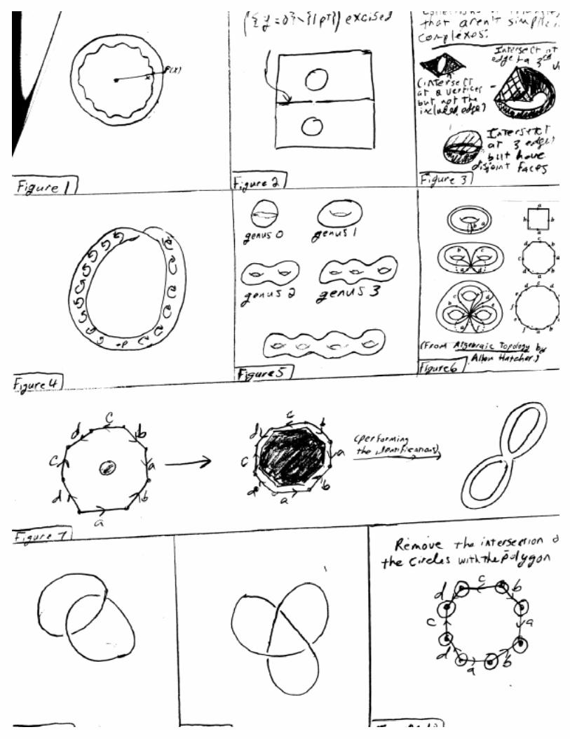
The surface G of the golf ball requires a more complicated construction. We draw a sphere

S surrounding and concentric with the golf ball; call the common center C. A homeomorphism

f : G ! S may be de�ned by radial projection: for each x 2 G let f(x) be the point at which

the ray from C through x intersects S (see Figure 1). This is a continuous bijection, and f�1 is

continuous. To be entirely proper, we should describe precisely the shape of a golf ball and prove

the asserted properties of f and f�1 in detail; the required formulae, however, would be messy and

unenlightening, and in fact topologists routinely omit such veri�cations, so we will do the same.

Homotopy equivalence. For two spaces A and B to be homeomorphic, there must be a pair of

continuous functions f : A! B and g : B ! A such that the compositions g � f and f � g are the

identities on A and B respectively (that is, we have g = f�1). The less strict notion of homotopy

equivalence of A and B requires instead that functions f and g exist such that g � f and f � g may

be continuously deformed to the identities on A and B respectively (this time f and g need not be

inverse functions, but in this setting we call them homotopy inverses). In general, a homotopy or

continuous deformation between two maps h0; h1 : X ! Y is a continuous map h : X � [0; 1]! Y

such that h(�; 0) = h0 and h(�; 1) = h1; if such an h exists, we say that h0 and h1 are homotopic,

and h is a homotopy between them. Usually we write the parameter in [0; 1] as a subscript, so that

h(x; t) appears as ht(x).

An important special case of homotopy equivalence is obtained from a deformation retraction

of a space X onto a subset A � X, which is de�ned to be a homotopy h : X � I ! X such that

3

h0 is the identity on X, but the image of h1 lies entirely in A, and moreover each slice ht �xes

every point in A. Conceptually, such a homotopy is just a means of compressing X onto A without

moving A at all. We claim that the �nal map h1 : X ! A is a homotopy equivalence of X with A,

which we shall prove by showing that the inclusion i : A ! X is a homotopy inverse for h1. On

one hand, the composition h1 � i is exactly the identity on A because h1 �xes every point of A. On

the other hand, the composition i � h1 is just h1, which is homotopic to the identity on X via h.

Obviously any homeomorphism is a homotopy equivalence. A simple example of a homotopy

equivalence that is not a homeomorphism is obtained by taking X to be the interval [�1; 1] and A to

be the point 0 and de�ning a deformation retraction h of X onto A by the formula ht(x) = (1� t)x.

Then h1, the zero map, is a homotopy equivalence, so [�1; 1] is homotopy-equivalent to a point;

but the interval and the point are clearly not homeomorphic because there is no bijective function

between them, much less a bijection continuous in both directions. The same formula for h can be

used to show that any convex set in a Euclidean space is homotopy-equivalent to a point. Spaces

that are homotopic to a point in this fashion are called contractible.

Isotopy. Sometimes the strict notion of homeomorphism is not strict enough. Homeomorphism

is a relationship between abstract topological spaces; even if the topological spaces we care about

happen to be subsets of, say, a Euclidean space, the notion of homeomorphism completely ignores

the manner in which the spaces are embedded in the Euclidean space. The bene�ts of the abstract

treatment have been discussed already. In certain cases, however, the loss of information is unde-

sirable. For instance, consider the two pairs of circles in R3 depicted below (the general term for

a �nite collection of disjoint circles in R3 is link). As abstract topological spaces, the two links

are homeomorphic|each is a disjoint union of two circles. But as objects in three-dimensional

space, the two links do not deserve to be considered equivalent. No amount of pushing, pulling,

and stretching in R3 will unlink the circles in the second picture. Thus, although the pairs of circles

can be transformed into each other abstractly, the transformation cannot be performed by �ddling

around in the ambient space R3 .

The notion of isotopy is a variant of homeomorphism that preserves information about the

embedding. Formally, two spaces A and B, contained in a larger space C, are called isotopic in C

if there is a homotopy h : A� [0; 1]! C so that

1. the slice h0 is the inclusion A! C;

2. the slice h1 is a homeomorphism of A onto B; and

3. each intermediate slice ht is a homeomorphism of A onto its image.

Condition 3 is what gives the concept of isotopy its greater strictness; it means essentially that you

may not squeeze all or part of A down to a point and then rematerialize it elsewhere. For instance,

in Figure 2, which shows the Euclidean plane with all but one point of the line y = 0 excised, the

two circles are homeomorphic, and there is a homotopy satisfying conditions 1 and 2 above, but the

circles are not isotopic: you can't �t one circle through the narrow hole without smashing points

together.

2.2 Piecewise-linear objects

Arbitrary spaces and arbitrary continuous maps can be fairly di�cult to analyze, so it is convenient

to introduce a restricted class of spaces and maps with more tractable behavior. The basic building

block for one of these restricted spaces is the n-dimensional simplex (for n � 0), which is the convex

4

hull of n + 1 points in general position in Rn . For n = 0, 1, 2, and 3, an n-simplex is a point, a

line segment, a triangle, or a tetrahedron respectively. The faces of a simplex are the convex hulls

of all proper subsets of its vertex set. In the case of a 3-simplex (tetrahedron), the faces are the

vertices and edges as well as the ordinary (two-dimensional) faces.

We now de�ne a simplicial complex to be a �nite union of simplices such that any two simplices

in the complex intersect in the empty set or a single simplex. The intersection condition rules

out anomalous intersections such as those in Figure 3, which would complicate many arguments

unnecessarily. The dimension of a simplicial complex is the largest dimension of a simplex appearing

in it. The case of a 2-dimensional complex is a concept very familiar in computer graphics: it is

merely a triangular mesh (often irregular and not a manifold, however). We shall generally restrict

our attention to simplicial complexes hereafter. We shall also generally consider only piecewise

linear maps, namely, maps for which the domain space can be partitioned into several regions so

that the restriction of the map to each region is an a�ne function. As an example, a piecewise-

linear embedding of the circle in the Euclidean plane must have a polygonal rather than a smooth

image.

For �nite simplicial complexes K we can de�ne the Euler characteristic �(K), a numerical

invariant of profound importance. If K has n0 vertices, n1 edges, n2 two-dimensional faces, and so

forth, the Euler characteristic is de�ned by the formula

�(K) = n0 � n1 + n2 � n3 + � � �

(because K is �nite we have nj = 0 for large j, whence the sum breaks o� after �nitely many

terms). If K is a 1-dimensional complex, a graph with vertex set V and edge set E, say, then we

have �(K) = jV j � jEj. For a surface with faces F we have �(K) = jV j � jEj + jF j, which is the

case of the formula that we shall most often need.

It can be proven that �(K) is a topological invariant, i.e., that if K and K 0 are homeomorphic

complexes, then �(K) = �(K 0). Thus � does not depend on the choice of a simplicial-complex

structure on a space. More generally, if K and K 0 are merely homotopy-equivalent complexes, we

still have necessarily that �(K) = �(K 0). We leave the proof of these facts to any reputable text

on algebraic topology.

2.3 The Topology of Orientable Surfaces

Since they are our primary object of study, we brie y review the topology of orientable surfaces.

For a more complete treatment, see [1].

For the sake of this paper, a surface will be taken to be a compact 2-manifold, possibly with

boundary. If a surface has no boundary, we say it is a closed surface.

An orientation of a surface at a point is a choice of which direction is \clockwise" at that

point. An orientation of an entire surface is a choice of an orientation at every point so that the

orientations of nearby points agree. If there exists an orientation of a surface, we say that the

surface is orientable.

Not all surfaces are orientable|sometimes there is no consistent way to choose an orientation

at every point. The simplest example of such a surface is the M�obius strip. Figure 4 shows why

the M�obius strip isn't orientable. Once you choose an orientation at a point, the local consistency

condition forces the orientation at all nearby points. You can thus \push" your orientation around

your surface to de�ne what it must be everywhere. However, if you push it all the way around the

M�obius strip, you get the opposite orientation at your original point of the one you started with,

which shows you cannot consistently orient the surface.

5

If a surface is embedded in R3 , we note that an orientation is the same as a continuous choice

of a unit outward normal vector at each point. To see this, notice that there are two choices for the

outward normal direction at a point. Given a choice of outward normal, one can use the right-hand

rule to choose an orientation. Similarly, one can select an outward normal vector given a choice of

orientation.

There is a very simple classi�cation of closed orientable surfaces up to homeomorphism.1 We

de�ne the genus-0 surface to be the sphere, the genus-1 surface to be the torus, and the genus-g

surface to be the \torus with g holes," as shown in Figure 5. Now, the following theorem fully

classi�es closed orientable surfaces up to homeomorphism:

Theorem 2.2 Every closed orientable surface is homeomorphic to the genus-g surface for some

g � 0.

Proof: This is a well-known classical result. For the proof, see [1]. �

A surface is thus completely determined up to homeomorphism by its genus. For this reason,

it will greatly facilitate our analysis to have a representation of a genus-g surface that is easier to

work with. To this end, we construct a genus-g surface as follows. Start with a polygon with 4g

edges, and label the edges as shown in Figure 6. Now, identify edges with the same letter. That is,

if two edges have the same letter, we can pair o� points on one edge with points on the other (using

the direction of the arrows to determine which end of one edge matches up with which end of the

other). Now, attach the surface to itself along these edges, treating each point on one edge as if it is

touching the corresponding point on the other edge. It is not di�cult to see, as shown in the �gure,

that these edge identi�cations yield the desired shapes. (Again, for the precise formulation of this

construction, see [1].) By explicitly triangulating these polygons, we easily derive as a corollary

that the Euler characteristic of a genus-g surface is 2� 2g.

We can now use the classi�cation of closed oriented surfaces to classify oriented surfaces with

boundary. The boundary of a compact 2-manifold with boundary is a compact 1-manifold without

boundary. All such manifolds are disjoint unions of circles. We can now attach a disk along its

boundary to each boundary circle of our surface. The result cannot have any boundary, and it is

easy to see that the orientation of our original surface extends to the attached disks, so we now

have a closed orientable surface with boundary. Applying Theorem 2.2, to this, we obtain:

Theorem 2.3 Every orientable surface with boundary is homeomorphic to the genus-g surface with

some collection of disjoint disks removed from it. Such surfaces are thus classi�ed by their genus

(which is de�ned to be the genus of the corresponding closed surface) and their number of boundary

components.

We can extend our 4g-gon representation of closed orientable surfaces to orientable surfaces with

boundary by simply cutting little holes out of the interior of the polygon. As shown in Figure 7,

this deformation-retracts onto a collection of circles attached at a point. The number of circles

equals twice the genus plus the number of boundary components minus one. (Note that our surface

must have nonempty boundary for us to perform this deformation retraction. There is no such

deformation retraction for closed surfaces.)

Since Euler characteristic is unchanged by deformation retraction, we can compute it for all

orientable surfaces with boundary by simply computing it for collections of circles attached at a

point. Explicitly performing this computation and combining it with the above result for closed

surfaces yields:

1We shall restrict our attention to orientable surfaces. Classi�cation results similar to the ones provided exist for

nonorientable surfaces as well, but they are not needed and are therefore omitted.

6

Theorem 2.4 An orientable surface S of genus g with n boundary components has �(S) = 2 �

2g � n.

2.4 Knots and Links

Many of the arguments later in this paper draw their motivation from the theory of knots and

links. Furthermore, our discussion of the boundary relies upon this theory explicitly. As such, we

provide a very rudimentary introduction to knots and links. For a more complete introduction, see

[3] for a very readable treatment, or [2] for a more advanced one.

De�nition 2.5 A knot in R3 is the image of a piecewise-linear embedding of the circle S1into R

3.

A link is a union of nonintersecting knots. Two knots or links are considered isomorphic if they

are the images of isotopic maps.

We note that the knots that compose a link can be linked to one another so that you cannot pull

them apart, as shown in Figure 8.

Intuitively, we can think of a knot as a piece of string in R3 with its ends glued together. Two

knots are isomorphic if you can take one and pull the string (without cutting it or making it pass

through itself) so that you get the other.

We can obtain a two-dimensional representation of a knot or link by projecting it into a plane

and recording which strand passes on top at each crossing. (See Figure 9.) In order for this to

be a good representation, we want our knot to be in general position: the projection should be

injective at all but �nitely many points, at each of which exactly two strands of the knot cross

transversely. It is easy to see that any knot is isotopic to one that is in general position with

respect to projection onto a given plane. (This depends essentially on the piecewise linearity of

the embedding; the corresponding assertion for general topological embeddings of circles into R3 is

false.)

The problem of classifying knots up to isotopy is a very hard one. Indeed, there is at present

no polynomial-time algorithm to determine if two knots are isomorphic. In fact, there isn't even a

polynomial algorithm to check if a knot is isomorphic to a simple, unknotted loop. Both problems

have been shown to be decidable, however, using a tool from the theory of 3-manifolds called normal

surface theory.

It is natural to ask which knots or links can be the boundary of an orientable surface. Perhaps

surprisingly, the answer is that all of them can. Given a link L, a surface S with boundary L can

be explicitly constructed using an algorithm known as Seifert's algorithm. A detailed explanation

of this algorithm is provided in [2].

3 De�nition and Classi�cation up to Homeomorphism

We now de�ne our primary objects of study:

De�nition 3.1 Let X be a connected orientable surface (as an abstract topological space), and let

f : X ! R3be a piecewise-linear embedding. We say that the pair (X; f) is a front-facing surface

if we can choose an orientation on the image of f so that its outward normal vector has positive

z-coordinate at all points.

We shall occasionally abuse terminology and call a surface S in R3 front-facing if there exists a pair

(X; f) such that S = Im(f).

7

By the intermediate value theorem, we equivalently could mandate that the outward normal of

the image of f have nonzero z-coordinate at all points. We also note that we lose no generality

by requiring X to be orientable; had we not done so, the remainder of the de�nition would have

forced it. More precisely:

Theorem 3.2 If X is a surface (not necessarily orientable), and f is a piecewise-linear embedding,

(X; f) is front-facing if and only if there is no point on the image of f at which a unit normal vector

has z-coordinate equal to zero. In this case, we say that f realizes X as a front-facing surface.

Proof: If (X; f) is a front-facing surface, clearly no unit-normal vector ever has z-coordinate equal

to zero. For the converse, choose the unit normal vector with positive z-coordinate at each point

of the image of f . This is a continuous choice of a normal vector, so the image of f (and thus X)

is orientable by the remarks about orientability in Section 2.2, and one of the two orientations has

this collection of normal vectors as its set of outward normals. �

It is now natural to ask which orientable surfaces can be embedded in R3 as front-facing surfaces.

We answer this question with the following theorem, which fully classi�es front-facing surfaces up

to homeomorphism:

Theorem 3.3 Given an orientable surface X, there exists f such that (X; f) is front-facing if and

only if X has nonempty boundary.

Proof: We �rst show that an front-facing surface has nonempty boundary. To see this, let S =

Im(f), and consider the projection of S onto the xy-plane. Since the z-coordinate of a normal

vector at a point is nonzero, the projection map will have nonzero Jacobian, so it will be a local

homeomorphism. Since the projection of S will have nonempty boundary, this implies that S does

as well.

For the converse, it su�ces to prove that any surface X with one boundary component (i.e., a

genus-g surface minus a single disk) can be realized as a front-facing surface. We can then realize

surfaces with more boundary components by removing disks from X and restricting f to the result.

Let Xg be a genus-g surface minus a disk. To construct this, we start with the representation

of Sg as a 4g-gon. All of the vertices of the polygon are collapsed to a point when you identify the

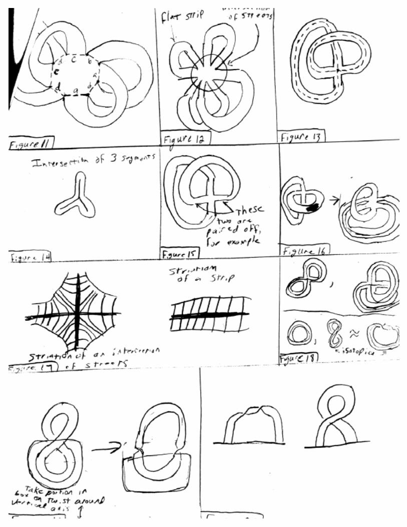
sides. We construct Xg by removing a neighborhood of this point, as shown in Figure 10. We can

now create a surface homeomorphic to this one by starting with a 4g-gon and using strips to attach

pairs of identi�ed sides, as shown in Figure 11. This surface is front-facing, which completes the

proof. �

4 Classi�cation up to Isotopy

The classi�cation of front-facing surfaces up to isotopy is considerably more complex than the

classi�cation up to homeomorphism. Accordingly, our classi�cation puts isotopy classes of front-

facing surfaces into correspondence with relatively complicated objects. However, these objects

render the structure of a front-facing surface much more transparent, which greatly aids in our

understanding of its properties. Throughout this section, we shall work in the smooth category.

All of the results hold in the piecewise-linear category as well, and the proofs carry over with only

minor technical modi�cations.

The intuition behind our classi�cation is that front-facing surfaces look like at strips almost

everywhere. There are �nitely many places, however, where they instead look like an intersection

of a collection of streets, as shown in Figure 12. Looking at these pictures, we see that most of

8

the information about the isotopy class of a surface is embodied by the isotopy class of a one-

dimensional \spine" that lies inside of it, as shown in Figure 13. It will turn out, however, that

isotopy of front-facing surfaces is slightly more restrictive than isotopy of spines. We will thus

need to supplement our spine with some extra information in order to specify a unique front-facing

surface up to isotopy.

We recall that a front-facing surface is a topological space X along with an embedding of X into

R3 . We begin by constructing particularly nice representations of our abstract topological spaces.

We shall then endow them with an additional structure called a striation.

To this end, we de�ne an n-street intersection to be a small neighborhood of an intersection of

n segments in the plane, as shown in Figure 14. Now take a 2k-street intersection, and pair o� the

streets by connecting them with strips, as shown in Figure 15. We claim that there exists a space

of this type homeomorphic to any orientable surface with boundary.

To see this, note that the front-facing surfaces with one boundary that we constructed in the

last section are of precisely this form. Furthermore, given a surface of this form, we can create

a new surface of this form with one more boundary component by poking a hole out of one of

the connecting segments, and stretching this hole so that the result is an intersection of two more

streets, as shown in Figure 16.

Now, away from the street intersections, our surfaces consist of a center line with an interval

attached perpendicularly to each point. At the street intersections, we can also decompose our

surface as a central spine with a bunch of intervals coming out of it, although the structure is

slightly more complicated. For concreteness, we let our intervals be from -1 to 1 with 0 lying on

the spine. Both cases are shown in Figure 17. We can thus endow each of our model spaces with

the structure of a central spine and an interval passing through each point on the spine. Every

point on our surface can be described uniquely by specifying a point on the spine and a number in

the interval [�1; 1]. We call this structure a striation of our surface. We can use the map f to put

this same structure on the image of our surface in R3 . We also note that the spines of our surfaces

are all collections of circles attached at a single point.

The next statement that we would like to make is that we can classify front-facing surfaces up to

isotopy by the isotopy classes of their spines. Unfortunately, this isn't quite the case. For example,

the two pairs of surfaces shown in Figure 18 each have isotopic spines but are not isotopic. These

show the two types of problems that can occur:

1. We can rearrange the ordering of the edges around the center point by isotoping the spine,

but we cannot do this by isotoping a surface.

2. Two surfaces can have the same spine but can have di�erent numbers of \twists" in some of

their circles.

However, if we don't allow the isotopy to modify a small neighborhood of the point where all of

the circles meet, and we keep track of how many twists are in each circle, we shall show that no

problems can occur. With this in mind, we de�ne the objects that we shall use to classify our

front-facing surfaces:

De�nition 4.1 Let f be an embedding of a collection of circles attached at a point into R3, along

with an even integer assigned to each circle. If f maps a small neighborhood of the point at which

the circles attach to a collection of segments in the xy-plane that is centered at 0, and has the

segments separated by equal angles, we say f is a generalized knot. Two generalized knots are

isomorphic if one can be isotoped into the other while holding a small region of the center point

rigid, in such a way that the even integers assigned to the circles match up in the obvious fashion.

9

The basic idea is that you can use the striations on a front-facing surface to \thin" it out so

that it looks like a bunch of strips attached at a street intersection. These objects will then be

classi�ed by their center lines and the number of twists in each of the strips.

Theorem 4.2 Isotopy classes of front-facing surfaces are in one-to-one correspondence with iso-

morphism classes of generalized knots.

Proof: Let S = (X; f) be a striated front-facing surface. The striation on X allows us to de�ne

the spine of S to be the spine of X along with the restriction of f to this spine. We say that

S is rigidi�ed if the spine of S is a generalized knot. It is not di�cult to show that any surface

is isotopic to a rigidi�ed one, and if two rigidi�ed surfaces are isotopic, they are isotopic through

rigidi�ed surfaces. We thus have that classes of rigidi�ed surfaces up to isotopy through rigidi�ed

surfaces are in one-to-one correspondence with isotopy classes of surfaces.

We start to de�ne a map � from the set of rigidi�ed front-facing surfaces to the set of generalized

knots by taking the spine of a surface. It remains to de�ne the number of twists in each circle. We

do this by detaching the portion of our surface that corresponds to the circle (under the striation)

from the rest of the surface, thereby giving us something that is topologically an annulus. We

de�ne the number of twists for the circle to be the linking number of one boundary component of

this annulus with its center line. (This is a standard de�nition. It is not di�cult to see that this

coincides with one's intuitive notion of the number of twists in an annulus embedded in R3 . An

important point is that it is invariant under isotopy.) This number will be even because our surface

is orientable. We note that � is clearly well-de�ned as a map from isotopy classes of rigidi�ed

front-facing surfaces to isomorphism classes of knots.

In the opposite direction, we de�ne a \thickening" map from the set of generalized knots to

the set of rigidi�ed front-facing surfaces as follows. We isotope our generalized knot K so that its

projection into the xy-plane has only transverse intersections. By compactness, there is some � so

that we can replace K with an �-neighborhood of K, and no new intersections occur. (That is,

if we drew the projection of K with a marker of thickness 2�, it would still look as if in general

position.) We now de�ne a striated surface S in R3 by letting the generalized knot be the spine,

and making the interval through a point on the spine be a horizontal segment of length 2� centered

on the spine. Now take the portion of S corresponding to each circle of the generalized knot, cut

it, twist it so that its twisting number is as speci�ed, and reattach it. We will show in the next

section that this sort of object can be isotoped so as to be front-facing.

It is not immediately obvious that is well-de�ned. We have to check that isomorphic gener-

alized knots yield isotopic front-facing surfaces. To this end, let K and K 0 be isomorphic knots,

and let S and S0 be their respective thickenings. We can isotope S0 so that its spine coincides

with the spine of S. Small neighborhoods of the central points of S and S0 can be taken to match

up precisely. Now consider the portions S and S0 corresponding to a speci�c circle in the spines,

intersected with the complements of the small neighborhoods of the central points. Each of these

is a strip. Their center lines match up, they have the same width, and their ends coincide. All such

objects containing the same number of twists can be isotoped into one another while holding the

ends and spines �xed. This thus shows that is well-de�ned.

It now remains to show that � � = Id, and � � = Id. The former is completely trivial: if

you take a generalized knot K and thicken it, the spine of the resulting striated surface is K again

by construction. For the latter composition, let S be a rigidi�ed front-facing surface. Compressing

along the striation allows us to isotope S into a new surface S0 that coincides with � �S at the

intersection of streets, and such that all of the strips attached to this intersection of streets are

of the same uniform width. The spines of the strips in in S' coincide with those in � �, and

10

corresponding strips have the same number of twists. By the comment in the last paragraph, S0 is

therefore isotopic to � �, as desired. �

5 Generality of Front-Facing Surfaces

One might expect the constraint that a surface be front-facing to place stringent restrictions on the

isotopy class of the surface. But in fact front-facing surfaces are not really simpler than general

surfaces, for it can be shown that every orientable surface in R3 with boundary is isotopic to a

front-facing surface in R3 . Here we indicate brie y the proof of this somewhat surprising fact.

We begin with the observation that an annulus with two twists and a front-facing �gure eight,

shown in Figure 19, are isotopic. The same is true if we cut a small chunk out of both shapes

and constrain the ends not to move; so the doubly-twisted strip and the more complicated but

front-facing strip in Figure 20 are isotopic through maps �xing the ends of the strips. By induction

we can use an isotopy to eliminate any even number of twists in a strip, at the cost of making the

shape of its projected image more complicated, and this isotopy can be performed using only space

very near the strip, so as not to collide with any other objects in space.

Suppose we are given a strip, possibly twisted in a very complicated manner, whose ends are

constrained not to move. The strip is probably not presented in a front-facing manner, but we can

atten it out, starting at one end of the strip, so that it is mostly front-facing, with any twists in

the strip accumulating at the other end of the strip. If the number of twists turns out to be even,

we can use the �gure-eight trick to eliminate them, obtaining a front-facing presentation of the

strip. (If the number of twists is odd, we can eliminate all but one, but we shall not need this.)

Now a general orientable surface in R3 is isotopic to an embedded image of one of our abstract

model spaces constructed by piecing several ribbons together at one complex intersection, and we

may rotate the image so that the intersection is front-facing. Using the preceding argument, we

can atten out each ribbon to face entirely forward except for a possible aggregation of several

twists at one point in the ribbon. The number of twists in such an aggregation is necessarily even:

if it were odd, then traversing the ribbon once would reverse a local orientation, contradicting the

assumption that our surface is orientable. We can therefore use the �gure-eight trick to make each

ribbon entirely front-facing, resulting in a front-facing representative of the isotopy class of the

surface, as desired.

6 Winding Numbers

Any front-facing surface is homeomorphic to one of the abstract models considered in section 3.

If, however, we are given a concrete front-facing surface, it may not be obvious to which of the

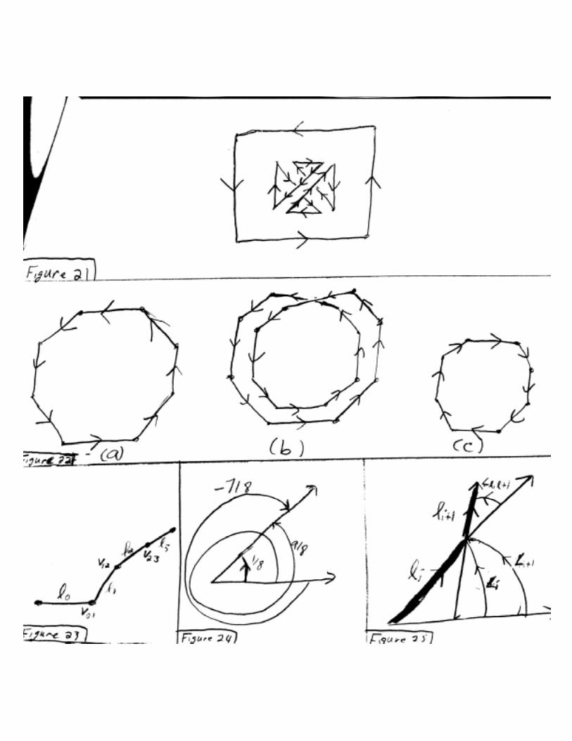
abstract models the surface is homeomorphic. For example, it is not immediately apparent that

the surface shown below in Figure 21 is a torus with two open disks removed. In this section we

shall show how the topological identity of a front-facing surface can be deduced from simple and

mechanical computations involving the boundary of the surface.

6.1 De�nition of the winding number

To state the main theorem of this section, we shall need a precise de�nition of the winding number

of an oriented closed curve, which is informally the net number of counterclockwise rotations made

in a traversal of the curve. For instance, we should like to say that the circle in Figure 22a winds

once, while the double circle in Figure 22b winds twice. Note that the orientation of the curve

11

matters: the circle in Figure 22c looks like that in Figure 22a except that it is traversed in the

opposite direction, but we say that it winds �1 times.

Fortunately, it is easy to give a precise de�nition of this notion because we are dealing with

piecewise-linear curves, which are merely �nite chains of line segments. Given a piecewise-linear

curve , we may divide into a series of linearly parametrized line segments `0, : : :, `N . For

each 0 � i � N the segment `i ends where `i+1 begins (we interpret indices modulo N + 1, so

that `N+1 means `0), and we can de�ne the relative angle \(`i; `i+1) to be the counterclockwise

angle between the two segments at the intersection point, measured as a fraction of a complete

rotation (for instance, a 90� turn in the counterclockwise direction gives a relative angle of 14). This

number may be positive, negative, or zero. For instance, the curve shown in Figure 23 turns in the

counterclockwise direction at v01 but in the clockwise direction at v12, while at v23 it does not turn

at all. We have

\(`0; `1) = +16; \(`1; `2) = � 1

12; \(`2; `3) = 0:

We must assume that the path never turns around at a point, as the curve f(t) given by

f(t) =

�(t; 0; 0); if 0 � t � 1;

(1� t; 0; 0); if 1 � t � 2,

does at t = 1, for it is not clear whether the relative angle at the vertex is +12or �1

2. We will

not de�ne the winding number for such a curve. For curves that do not misbehave in this way,

however, we can de�ne the winding number w( ) as the sum of the relative angles at vertices,

namely

w( ) =X

0�i�N

\(`i; `i+1): (1)

It is now easily veri�ed that the curves in Figure 22 have the winding numbers claimed previously;

for instance, the circle in Figure 22a has eight vertices, each with relative angle 18.

6.2 Elementary properties of the winding number

In each of the examples in Figure 22, the winding number is an integer; but the de�nition (1),

which involves a sum of fairly arbitrary real numbers, gives no indication that this should be true

in general. But in fact w( ) is an integer for any closed piecewise-linear curve . Our �rst object

in this section will be to prove this fact. We decompose as a circular chain of segments `i as

in the previous section, and we continue to measure directed angles in units of counterclockwise

rotations.

For any directed segment `, we de�ne an absolute angle \` of ` to be a counterclockwise angle

from east to the direction of the segment. We say \a" and not \the" because the angle is not

unique; there is a smallest nonnegative absolute angle, but we could obtain a larger angle, or a

negative angle, by introducing extra complete rotations in one direction or the other, as shown

in Figure 24. Nevertheless, the possibility of adding or subtracting complete rotations is the only

ambiguity in the de�nition of the absolute angle in the sense that any two absolute angles of ` di�er

by an integer.

Considering now the segments `i of , �x one choice of the absolute angle \`0. Then the

ambiguity in the absolute angles \`i for 1 � i � N can be eliminated by requiring that the

di�erences \`i � \`i�1 should equal the relative angles \(`i�1; `i) for 1 � i � N (it is easily seen

that this stipulation leads to valid absolute angles).

12

Considering now the segments `i of , �x one choice of the absolute angle of `0, denoted \0.

Now if \i is an absolute angle of `i, it is easy to see that

\i+1 := \i + \(`i; `i+1) (2)

is an absolute angle of `i+1 (see Figure 25). There were many ways to choose \0, but once one

is �xed, we obtain unambiguous absolute angles \i for all i � 0 by inductive application of (2).

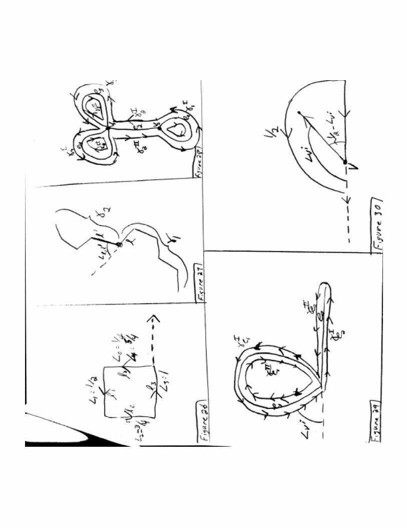
Figure 26 shows an example of the calculation of the \i starting from the choice \0 =14.

In particular we obtain an absolute angle \N+1. This is an absolute angle for `N+1 = `0,

possibly di�erent from the absolute angle \0 (as it is in Figure 26). We do know, however, that

the di�erence \N+1 � \0 of the absolute angles is an integer. But using (2) we see that

\N+1 � \0 =X

0�i�N

(\i+1 � \i) =X

0�i�N

\(`i; `i+1) = w( );

whence the winding number w( ) is an integer, as claimed.

This result is comforting, and it also leads to the important fact that the winding number w( )

is invariant under piecewise-linear homotopy of . For it is intuitive and can be proven (though

we omit the unsightly details) that the winding number is continuous in the time variable of such

a homotopy. But a continuous function on [0; 1] that takes integer values must be constant, and so

w( ) is the same after the homotopy as before.

We have de�ned the winding number for closed curves only, but it is useful to have an analogous

notion for arbitrary curves. A piecewise-linear curve , not necessarily closed, is still representable

as a sequence of segments `i for 0 � i � N . De�ne the internal winding number ~w( ) by the rule

~w( ) =X

0�i<N

\(`i; `i+1): (3)

This is like the de�nition (1) of the ordinary winding number, except that (3) lacks the �nal term

\(`N ; `N+1) appearing in (1)|that last term makes less sense for arbitrary curves because `Nneed not end at the beginning of `0. Unlike the winding number of a closed curve, the internal

winding number of a curve is typically not an integer. Note that the internal winding number

does not specialize to the ordinary winding number if the curve happens to be closed; in fact, it is

immediate from the de�nitions that for a closed curve , we have the relation

w( ) = ~w( ) + \(`N ; `0):

Similarly, if a (not necessarily closed) curve can be represented as a curve 1 followed by another

curve 2 as in Figure 27, the internal winding number ~w( ) is the sum of the internal winding

numbers of 1 and 2, plus the rotation angle between the end of 1 and the beginning of 2. We

shall use these relations to great e�ect in the next subsection.

It is useful to introduce the notion of a chain in order to treat multiple curves at once without

cluttering the analysis. A chain is a �nite formal sumP

ici i, where the ci are integers and the

i are piecewise-linear curves. This is essentially a convenient notation for a collection of several

curves, with multiplicities and orientations recorded. The chain 1 + 2 represents the pair 1 and

2; the chain 4 represents four copies of ; and � represents the curve traversed in the opposite

direction. IfP

ici i is a chain with i closed curves, we can de�ne its winding number by the rule

w

�Xi

ci i

�=Xi

ciw( i);

13

and similarly we can de�ne the internal winding number of any chain.

An important special case of a chain (indeed, the reason why we care about chains here) is the

boundary @S of a front-facing surface S. This boundary is a disjoint union of sets Si homeomorphic

to circles. We can make each Si into a closed path i merely by specifying the direction in which

the circle is to be traversed, which we do as follows. At every point of @S there is a normal vector

z pointing out of the projection plane, as well as an outward normal n to S lying in the plane.

The cross product z�n is then tangent to @S in the plane. Let the direction of this vector be the

direction of motion at that point on @S. It is easily seen that this gives a consistent orientation to

each Si, and we realize the boundary @S as the chainP

i i.

6.3 Relation to Euler characteristic

We shall apply the theory of winding numbers developed above to the boundary of a front-facing

surface, which has the structure of a chain of closed curves as noted above. Speci�cally, we shall

prove that for any front-facing surface S, the winding number w(@S) of its boundary equals the

Euler characteristic �(S) of the surface. Orientable surfaces are classi�ed up to homeomorphism by

their Euler characteristics and the number of their boundary components; the latter measurement

is easily taken, so the stated theorem enables the homeomorphism class of a front-facing surface to

be determined exactly.

We begin by appealing to the homeomorphism classi�cation of front-facing surfaces to represent

S as a thickening of a �nite graph G with vertex set V and edge set E, say, as shown (in a concrete

example) in Figure 28. The boundary @S can be decomposed as the union (not disjoint) of a pair

Ie ; II

e of paths for each edge e 2 E, as shown. Now S admits a piecewise-linear deformation

retraction onto G that deforms Ie and II

e onto e for each e. The deformation retraction is a

homotopy equivalence, so �(G) = �(S); moreover, the homotopy does not change w(@S) by the

homotopy-invariance of the winding number. Thus it su�ces to prove that w(@S) = �(G) =

jV j � jEj.

Now w(@S) equals the sum of the internal winding numbers of the ��plus the rotation angles

at the junctions of adjacent paths ��. These junctions occur only at the vertices of G, and at each

v 2 V there is a number of such junctions equal to twice the indegree deg+ v of the vertex. (Here

we de�ne the indegree to be one-half the number of self-loops at v plus the number of edges of G

other than self-loops that end at v.) We denote these rotation angles by \iv (1 � i � 2 deg+ v) as

in Figure 29. With this notation, we are to prove thatXe2E

( ~w( Ie) + ~w( II

e)) +

Xv2V

X1�i�deg+ v

\i

v= jV j � jEj: (4)

We note �rst that for each e the paths Ie and IIe both traverse e once, but in opposite directions.

Therefore ~w( Ie ) = � ~w( IIe ), and the sum over e in (4) vanishes. To deal with the vertex terms,

note that for v 2 V the quantities 12+\iv are the nonnegative angles bounded by cyclically adjacent

segments at v (see Figure 30), whence we must haveXi

(12+ \i

v) = 1;

or Xi

\i

v = 1�Xi

12= 1� deg+ v:

Therefore we have

w(@S) =Xv2V

(1� deg+ v) = jV j �Xv2V

deg+ v = jV j � jEj = �(S);

14

which was to be demonstrated.

As an example, consider the front-facing surface shown before in Figure 21. There are two

boundary components, of which the outer loop winds once counterclockwise, while the inner winds

�3 times counterclockwise. Hence the winding number of the boundary is �2, and the Euler

characteristic is also �2. Filling in the two holes yields a closed surface of Euler characteristic 0,

which is a torus, so the mystery surface is a torus with two open disks deleted.

7 Cutting Surfaces into Disks

In this section, we present an algorithm for \cutting" a (not necessarily front-facing) surface so

that it becomes topologically a disk. This is useful in several contexts, as many other algorithms

in graphics can be applied more easily to disks than to more topologically complicated objects.

Before we can present the algorithm, however, we must make explicit the notion of a cut. To do

this, we shall �rst need to set forth a small piece of machinery called the combinatorial closure.

Recall that if � is a simplex in some simplicial complex X, all of the faces of � are simplices in

X as well. We de�ne a pseudosimplicial complex to be an object that satis�es all of the conditions

of the de�nition of a simplicial complex except for this one.

Let C be a pseudosimplicial complex, and let �k be a k-simplex in C. We can de�ne the set

of missing `-faces of �k to be the set of `-dimensional simplices in the boundary of �k that are

not in C. Now, we can �ll in a missing `-face of �k by attaching an `-dimensional simplex to �k

and endowing it with the minimal consistent set of adjacency data. If we �ll in every missing face

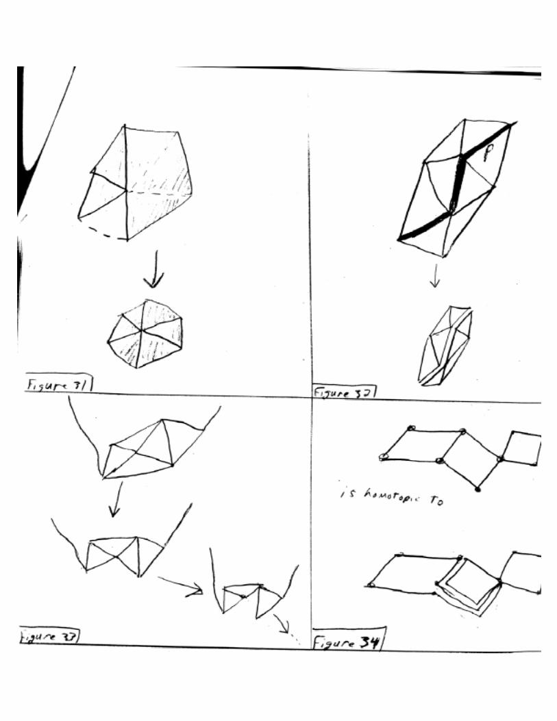
of every simplex in C, the result is a simplicial complex �C, which we shall call the combinatorial

closure of C. This process is shown in Figure 31.

Now let X be a triangulated surface, and let P be a subset of the 1-skeleton of X comprising

the edges e1; : : : ; en. Let C be the pseudosimplicial complex that results from removing e1; : : : ; enfrom X, and let Y = �C. We say that Y is the result of cutting X along P . An example of this is

shown in Figure 32.

Our goal is to cut a surface along a sequence of simple curves that are either closed or have

endpoints lying in the boundary, so that the resulting object is topologically a disk. We would like

to do this while making as few cuts as possible. For technical reasons, we shall allow ourselves to

slightly re�ne our triangularization when necessary.

We note that cutting along a simple closed curve doesn't change the number of faces, and it

changes the number of vertices and edges by the same amount; it therefore doesn't a�ect Euler

characteristic. Cutting along a simple curve with its endpoints in the boundary, however, creates

one more vertex than it creates edges, so it increases Euler characteristic by one. A surface of

genus g with n boundary components has Euler characteristic 2 � 2g � n, and a disk has Euler

characteristic one. Since no cut can decrease Euler characteristic by more than one, we thus must

make at least 2g +n� 1 cuts. If our surface is initially closed, our �rst cut must be along a simple

closed curve, so we must make at least 2g cuts. The algorithms presented below will achieve these

lower bounds.

We �rst consider a surface S with n > 0 boundary components. We can decrease the number

of boundary components by one by cutting along a path that connects a pair of disjoint boundary

components. We do this n�1 times, so that we are left with a surface with one boundary component.

This reduces the problem to the case where n = 1. We note that these paths can be found e�ciently,

for example, by constructing and using a depth-�rst tree of the 1-skeleton whose root is a vertex

on the boundary. The total running time to construct this tree and use it to construct all of the

above paths is linear in the number of simplices in our triangulation.

15

Let T be the closed surface that results from attaching a disk D along the boundary of S. We

recall from Section 2.2 that if we puncture T , it will deformation-retract onto a collection of circles

attached to one another at a point. The intersection of these circles with S yields a collection of

segments that are in some sense the essential ones in S. Cutting along these will yield a disk. The

mathematically inclined reader may �nd a more precise explanation of this in the remark at the

end of this section.

We now describe an algorithm for computing these circles in T . We start by removing some

triangle from T in order to puncture it. This creates a surface with boundary. Now choose some

triangle � that shares an edge with the boundary. Remove the intersection of � with the boundary,

and then remove the 2-simplex �. (See Figure 33.) We note that this is a deformation retraction.

If we now repeat this process until there are no triangles left, what remains is a graph. Possibly

re�ning our simplicial structure if necessary, we may arrange that this graph is homotopic to a

collection of circles that only intersect at a single point in D, as shown in Figure 34. Taking the

intersection of these circles with S yields a collection of segments s1; : : : ; s2g, each of which has its

endpoints on @D. These segments are the \essential" segments for which we were searching. We

now cut along these segments to obtain a new surface Z.

Theorem 7.1 Z is topologically a disk.

We note that this theorem establishes the correctness of our algorithm. Our algorithm achieves our

lower bound on the number of cuts, and it runs in time that is linear in the number of simplices in

S.

Proof of Theorem 7.1: It su�ces to show that Z is connected and has Euler characteristic one.

Since each cut increases Euler characteristic by one, and we made �(S)� 1 cuts, we know that Z

has Euler characteristic one, so we just need to show it to be connected. This follows rather easily

using homology theory from the fact that our cuts form a collection of \essential" curves that is

minimal in an appropriate sense. We make this slightly more precise in the remark at the end of

this section. �

Now suppose S is a closed surface. We puncture it and compute the graph onto which it

deformation-retracts, as above. We then cut along one simple closed curve in this graph. It is not

hard to see that this results in a connected surface R of genus g�1 with one boundary component,

to which we can now apply the above algorithm. We note that the graph onto which S deformation-

retracts can be directly used in the application of our cutting algorithm to R, so this algorithm

has almost exactly the same running time as the algorithm for cutting a surface with nonempty

boundary.

Remark for the mathematically inclined: The \essential" curves discussed in this section are

nontrivial elements of H1(S; @S). Since T �= S=@S, the excision theorem tells us that the push-

forward along the quotient map is an isomorphism from H1(S; @S) to H1(T ). When you puncture

T , it deformation-retracts onto a wedge sum of circles that form a basis for its �rst homology.

The algorithm computes these circles, and then it �nds a collection of elements of H1(S; @S) that

map to them under the push-forward isomorphism. The proof that the result of cutting S along

s1; : : : ; s2g is connected uses just that the si form a basis of simple disjoint curves for H1(S; @S). If

such a collection separated the surface into two components, one could show that the boundary of

one of the components would represent a nontrivial sum of the the si in H1(S; @S), which would

contradict that the si form a basis.

16

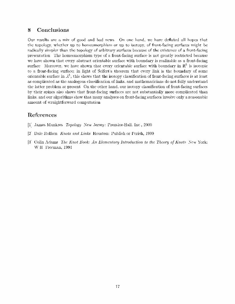
8 Conclusions

Our results are a mix of good and bad news. On one hand, we have de ated all hopes that

the topology, whether up to homeomorphism or up to isotopy, of front-facing surfaces might be

radically simpler than the topology of arbitrary surfaces because of the existence of a front-facing

presentation. The homeomorphism type of a front-facing surface is not greatly restricted because

we have shown that every abstract orientable surface with boundary is realizable as a front-facing

surface. Moreover, we have shown that every orientable surface with boundary in R3 is isotopic

to a front-facing surface; in light of Seifert's theorem that every link is the boundary of some

orientable surface in R3 , this shows that the isotopy classi�cation of front-facing surfaces is at least

as complicated as the analogous classi�cation of links, and mathematicians do not fully understand

the latter problem at present. On the other hand, our isotopy classi�cation of front-facing surfaces

by their spines also shows that front-facing surfaces are not substantially more complicated than

links, and our algorithms show that many analyses on front-facing surfaces involve only a reasonable

amount of straightforward computation.

References

[1] James Munkres. Topology. New Jersey: Prentice-Hall, Inc., 2000.

[2] Dale Rolfsen. Knots and Links. Houston: Publish or Perish, 1990.

[3] Colin Adams. The Knot Book: An Elementary Introduction to the Theory of Knots. New York:

W.H. Freeman, 1994.

17