B5.2: Applied Partial Differential Equations MT 2021 Contents 1 Introduction 2 2 First order quasilinear equations 8 2.1 Definitions ...................................... 8 2.2 Characteristics ................................... 8 2.3 Geometric definition ................................ 8 2.4 Cauchy data ..................................... 12 2.5 Domain of definition ................................ 14 3 Weak solutions and shocks for first order PDEs 19 3.1 Solutions with discontinuous first derivatives .................. 19 3.2 Weak solutions ................................... 20 3.3 Shocks ........................................ 23 3.4 Nonuniqueness of weak solutions ......................... 25 4 First order nonlinear equations 29 4.1 Charpit’s equations ................................. 29 4.2 Boundary data ................................... 30 4.3 Proof that Charpit’s method works ........................ 31 4.4 Discontinuities ................................... 33 4.5 Geometrical optics ................................. 33 5 First order systems 36 5.1 Introduction ..................................... 36 5.2 Cauchy data ..................................... 36 5.3 Characteristics ................................... 38 5.4 Integration along characteristics .......................... 40 5.5 Weak solutions ................................... 44 6 Second order semi-linear equations 50 6.1 Introduction ..................................... 50 6.2 Cauchy data ..................................... 50 6.3 Characteristics ................................... 51 6.4 Canonical forms .................................. 52 1

Welcome message from author
This document is posted to help you gain knowledge. Please leave a comment to let me know what you think about it! Share it to your friends and learn new things together.
Transcript
B5.2: Applied Partial Differential Equations
MT 2021
Contents
1 Introduction 2
2 First order quasilinear equations 82.1 Definitions . . . . . . . . . . . . . . . . . . . . . . . . . . . . . . . . . . . . . . 82.2 Characteristics . . . . . . . . . . . . . . . . . . . . . . . . . . . . . . . . . . . 82.3 Geometric definition . . . . . . . . . . . . . . . . . . . . . . . . . . . . . . . . 82.4 Cauchy data . . . . . . . . . . . . . . . . . . . . . . . . . . . . . . . . . . . . . 122.5 Domain of definition . . . . . . . . . . . . . . . . . . . . . . . . . . . . . . . . 14
3 Weak solutions and shocks for first order PDEs 193.1 Solutions with discontinuous first derivatives . . . . . . . . . . . . . . . . . . 193.2 Weak solutions . . . . . . . . . . . . . . . . . . . . . . . . . . . . . . . . . . . 203.3 Shocks . . . . . . . . . . . . . . . . . . . . . . . . . . . . . . . . . . . . . . . . 233.4 Nonuniqueness of weak solutions . . . . . . . . . . . . . . . . . . . . . . . . . 25
4 First order nonlinear equations 294.1 Charpit’s equations . . . . . . . . . . . . . . . . . . . . . . . . . . . . . . . . . 294.2 Boundary data . . . . . . . . . . . . . . . . . . . . . . . . . . . . . . . . . . . 304.3 Proof that Charpit’s method works . . . . . . . . . . . . . . . . . . . . . . . . 314.4 Discontinuities . . . . . . . . . . . . . . . . . . . . . . . . . . . . . . . . . . . 334.5 Geometrical optics . . . . . . . . . . . . . . . . . . . . . . . . . . . . . . . . . 33
5 First order systems 365.1 Introduction . . . . . . . . . . . . . . . . . . . . . . . . . . . . . . . . . . . . . 365.2 Cauchy data . . . . . . . . . . . . . . . . . . . . . . . . . . . . . . . . . . . . . 365.3 Characteristics . . . . . . . . . . . . . . . . . . . . . . . . . . . . . . . . . . . 385.4 Integration along characteristics . . . . . . . . . . . . . . . . . . . . . . . . . . 405.5 Weak solutions . . . . . . . . . . . . . . . . . . . . . . . . . . . . . . . . . . . 44
6 Second order semi-linear equations 506.1 Introduction . . . . . . . . . . . . . . . . . . . . . . . . . . . . . . . . . . . . . 506.2 Cauchy data . . . . . . . . . . . . . . . . . . . . . . . . . . . . . . . . . . . . . 506.3 Characteristics . . . . . . . . . . . . . . . . . . . . . . . . . . . . . . . . . . . 516.4 Canonical forms . . . . . . . . . . . . . . . . . . . . . . . . . . . . . . . . . . 52
1
B5.2 Applied Partial Differential Equations 2
7 Semi-linear hyperbolic equations 557.1 Non-Cauchy data . . . . . . . . . . . . . . . . . . . . . . . . . . . . . . . . . . 557.2 Weak solutions . . . . . . . . . . . . . . . . . . . . . . . . . . . . . . . . . . . 557.3 Riemann’s method . . . . . . . . . . . . . . . . . . . . . . . . . . . . . . . . . 55
8 Semi-linear elliptic equations 598.1 Well-posed boundary data . . . . . . . . . . . . . . . . . . . . . . . . . . . . . 598.2 Uniqueness theorems for Poisson’s equation . . . . . . . . . . . . . . . . . . . 598.3 Maximum principle . . . . . . . . . . . . . . . . . . . . . . . . . . . . . . . . . 608.4 Green’s functions . . . . . . . . . . . . . . . . . . . . . . . . . . . . . . . . . . 618.5 Complex variable methods . . . . . . . . . . . . . . . . . . . . . . . . . . . . . 64
9 Semi-linear parabolic equations 689.1 General properties . . . . . . . . . . . . . . . . . . . . . . . . . . . . . . . . . 689.2 Well posed boundary data . . . . . . . . . . . . . . . . . . . . . . . . . . . . . 689.3 Uniqueness theorem . . . . . . . . . . . . . . . . . . . . . . . . . . . . . . . . 699.4 Maximum value theorem . . . . . . . . . . . . . . . . . . . . . . . . . . . . . . 699.5 Green’s functions . . . . . . . . . . . . . . . . . . . . . . . . . . . . . . . . . . 709.6 Similarity solutions . . . . . . . . . . . . . . . . . . . . . . . . . . . . . . . . . 73
1 Introduction
These notes should be used to support the lectures for B5.2: Applied Partial DifferentialEquations. First, however, we pause to review some basic concepts relating to partial differ-ential equations and to remember some basic methods for solving ODEs and PDEs. Someworked examples are also included to refresh your memory.
What is a PDE?
A partial differential equation (PDE) is an equation for some quantity u (the dependentvariable) which depends on two (or more) independent variables and involves partial deriva-tives of u with respect to at least some of these independent variables. In this course, welimit attention to just two independent variables, so u = u(x, y), and at most two derivatives.Then our PDE can be written in general terms as follows:
F (x, y, u, ux, uy, uxx, uxy, uyy) = 0.
Notes
1. In applications, x, y often represent spatial variables and a solution may be required insome region Ω. In this case, there will be some conditions to be satisfied on the domainboundary ∂Ω; these are called boundary conditions (BCs).
2. In applications, one of the independent variables may represent time, t say. Then therewill be initial conditions (ICs) to be satisfied (i.e., u may be specified everywhere inΩ at t = 0).
B5.2 Applied Partial Differential Equations 3
3. In applications, systems of partial differential equations (PDEs) can arise involv-ing the dependent variables u1, u2, . . . , um, m ≥ 1 with some (at least) of the PDEsinvolving more than one dependent variable.
4. It is common to use subscripts as shorthand for partial derivatives, i.e.
ux ≡∂u
∂x, uxy ≡
∂2u
∂y∂x, (1)
5. We will assume that u is sufficiently smooth for all the required partial derivatives toexist and to be independent of the order in which the derivatives are performed, i.e.
∂2u
∂y∂x≡ ∂2u
∂x∂y, uxy ≡ uyx. (2)
Definitions
• The order of the PDE is the order of the highest (partial) differential coefficient in theequation.
As with ODEs, it is important to be able to distinguish between linear and nonlinear equa-tions:
• A linear equation is one in which the equation and any BCs or ICs do not include anyproduct of the dependent variables or their derivatives; an equation that is not linear isnonlinear.
∂u
∂t+ c
∂u
∂x= 0 first order linear PDE (the simplest wave equation),
∂2u
∂x2+∂2u
∂y2= Φ(x, y) second order linear PDE (Poisson’s equation).
• A nonlinear equation is semilinear if the coefficients of the highest derivative arefunctions of the independent variables only.
(x+ α)∂u
∂x+ xy
∂u
∂y= u3,
x∂2u
∂x2+ y(x+ y)
∂2u
∂y2+ u
∂u
∂x+ u2∂u
∂y= u4.
• A nonlinear PDE is quasilinear if it is linear in the derivatives of order m, withcoefficients depending only on its independent variables, x, y say, and partial derivativesof order < m.[
1 +
(∂u
∂y
)2]∂2u
∂x2− 2
∂u
∂x
∂u
∂y
∂2u
∂x∂y+
[1 +
(∂u
∂x
)2]∂2u
∂y2= 0.
• Principle of superposition. A linear equation has the useful property that if u1 andu2 both satisfy the equation then so does αu1 + βu2 for any α, β ∈ R. This is oftenused to construct solutions to linear equations (for example to satisfy BCs and ICs, cfFourier series methods). This is NOT true for nonlinear equations.
B5.2 Applied Partial Differential Equations 4
Examples
Wave Equations Waves on a string, sound waves, waves on stretched membranes, electro-magnetic waves, etc
∂2u
∂x2=
1
c2
∂2u
∂t2,
or, more generally,1
c2
∂2u
∂t2= ∇2u
where c is a constant, the wave speed.
Diffusion or Heat Conduction Equations
∂u
∂t= κ
∂2u
∂x2,
or, more generally,∂u
∂t= κ∇2u,
or even∂u
∂t= ∇ · (κ∇u)
where κ is typically a constant (diffusion coefficient or thermal conductivity).
• Both the wave equation and the diffusion equation are linear equations that involvetime t as an independent variable. They require initial and boundary conditions fortheir solution.
• A physical interpretation of a function of two variables might, for example, relate tothe temperature in a metal bar and how this changes over time. Imagine that one endof a a metal bar is placed next to a heat source. In order to describe the response toheating the bar, we need to know: (a) the temperature at a given position, and (b) thetemperature at a given time. In other words, the temperature T in the bar should beviewed as a function of two real variables, position x and time t, say. From this, wecan draw a better understanding of the meaning of a derivative of a function of twovariables. For example, we can describe Tt as ”the rate of change of temperature overtime at a fixed position of x”.
Laplace’s Equation Another example of a second order linear equation is Laplace’s equa-tion:
∂2u
∂x2+∂2u
∂y2= 0. (3)
or more generally∇2u = 0.
This equation usually describes steady processes and is solved subject to BCs.
B5.2 Applied Partial Differential Equations 5
Other Common Second Order Linear PDEs
• Poisson’s equation is simply Laplace’s equation (homogeneous) with a known sourceterm (e.g. electric potential in the presence of a charge density):
∇2u = Φ.
• The Helmholtz equation may be regarded as a stationary wave equation:
∇2u+ k2u = 0.
• The Schrodinger equation is the fundamental equation of physics for describing quan-tum mechanical dynamics. The Schrodinger wave equation is a PDE that describes howthe wavefunction of a physical system evolves over time:
−∇2u+ V u = i∂u
∂t.
Nonlinear PDEs
• An example of a nonlinear equation is Fisher’s equation for the propagation of reaction-diffusion waves:
∂u
∂t=∂2u
∂x2+ u(1− u) 2nd order PDE.
• The following PDE describes nonlinear wave propagation
∂u
∂t+ (u+ c)
∂u
∂x= 0 1st order PDE.
This is an example of a Conservation equation
ut + F (u)x = s,
where F (u) is known as a flux function for some density u(x, t) and s is a source term.
• An example of a quasilinear equation is
x2u∂u
∂x+ (y + u)
∂u
∂y= u3.
• The following PDE is semilinear
y∂u
∂x+ (x3 + y)
∂u
∂y= u3.
B5.2 Applied Partial Differential Equations 6
Systems of PDEs
• Maxwell equations constitute a system of linear PDEs:
∇ ·E =ρ
ε, ∇×B = µj +
1
c2
∂E
∂t,
∇ ·B = 0, ∇×E = −∂B∂t
.
In empty space (free of charges and currents), this system can be rearranged to give theequations of propagation of the electromagnetic field
∂2E
∂t2= c2∇2E,
∂2B
∂t2= c2∇2B.
• Incompressible magnetohydrodynamics (MHD) equations combine Navier-Stokesequation (including the Lorenz force), the induction equation and the solenoidal con-straints:
∂U
∂t+ U · ∇U = −∇Π + B · ∇B + ν∇2U + F ,
∂B
∂t= ∇× (U ×B) + η∇2B,
∇ ·U = 0, ∇ ·B = 0.
• Both of the above systems involve partial derivatives in space and time and, therefore,require ICs and BCs for their solution
When can a PDE be solved?
Having defined a PDE, the general idea is to solve for the function u(x, y). However, a PDEdoes not in general determine u uniquely by itself — boundary conditions are also required.A PDE supplemented by appropriate boundary conditions is often referred to as a system ora problem. For example, a simple problem involving Laplace’s equation is
∂2u
∂x2+∂2u
∂y2= 0 y > 0
u = f(x) y = 0
u→ 0 y →∞.
. (4)
We would like to determine a unique solution to the above problem. We have the PDEand boundary conditions, but is this sufficient information to achieve our aim? Maybe theseparticular boundary condition will lead to no solutions or multiple solutions, or maybe thesolutions will be extremely sensitive to small changes in the boundary conditions. It is ofpointless to attempt to solve a problem for which no solution exists, that many solutionsexist or to find unusual sensitivity of the solution to the boundary conditions.
Faced with a problem like (4), the most important question to ask is: is it well posed?To be well posed, a problem must have the following three properties:
1. a solution u(x, y) exists;
B5.2 Applied Partial Differential Equations 7
2. the solution is unique;
3. the solution depends continuously on the boundary data.
The first of these is obvious: there is no point in trying to find a solution that does not exist.If a problem is physically motivated, and u represents a physical quantity, then we wouldexpect u to have a unique well-defined value at each point. If it does not, it suggests that aboundary condition or other constraint is missing from the problem.
To illustrate the final condition, suppose we vary the function f(x) in (4) by a smallamount and ask whether the corresponding variation in the solution is similarly small. If itis not, then the solution of the problem is practically impossible, since any numerical errorsin f(x), however small, lead to large errors in the solution.
Suggested textbooks
J Ockendon, S Howison, A Lacey & A Movchan, 1999 Applied Partial DifferentialEquations. Oxford.
R. Courant & D. Hilbert, 1989 Methods of Mathematical Physics Volume II. Wiley.
B5.2 Applied Partial Differential Equations 8
2 First order quasilinear equations
2.1 Definitions
In this section we consider partial differential equations (PDEs) of the following form
a(x, y, u)∂u
∂x+ b(x, y, u)
∂u
∂y= c(x, y, u). (5)
Here x and y are independent variables, a, b and c are given smooth (i.e. continuouslydifferentiable) functions, and u(x, y) is a scalar function for which we would like to solve.Equation (5) is known as a first-order quasilinear partial differential equation: first-ordersince there are no second or higher derivatives and quasilinear because it is linear in itshighest derivatives (there are no nonlinear terms like (∂u/∂x)2). Equations of this type arisein many areas of mathematical modelling, including fluid mechanics and traffic flow. Theyalso provide a relatively straightforward introduction to some important concepts, such asCauchy data, characteristics and weak solutions, that will be applied to more complicatedequations later in the course.
Two special cases of (5) are worth mentioning. First, if a and b are independent of u, then(5) becomes the semilinear equation
a(x, y)∂u
∂x+ b(x, y)
∂u
∂y= c(x, y, u). (6)
If it also happens that c is a linear function of u, then we have
a(x, y)∂u
∂x+ b(x, y)
∂u
∂y= α(x, y)u+ β(x, y), (7)
which is a linear equation. It is generally the case that linear equations are significantlybetter-behaved and easier to solve than nonlinear ones.
Equations like (5) often describe the evolution of a quantity u (representing e.g. trafficdensity or fluid velocity) in space and time. In such cases, to emphasise the fact that oneindependent variable represents time, we will use x and t as independent variables instead ofx and y, writing (5) as
a(x, t, u)∂u
∂t+ b(x, t, u)
∂u
∂x= c(x, t, u). (8)
2.2 Characteristics
2.3 Geometric definition
We can think of the solution u(x, y) we are seeking as defining a surface z = u(x, y) inthree-dimensional space. The normal to this surface is in the direction
n ∝∇(u(x, y)− z
)=
∂u
∂x∂u
∂y
−1
(9)
B5.2 Applied Partial Differential Equations 9
a,b,c) T(Characteristics
Characteristic
Initialcurve
projections
z = u
y
s
x
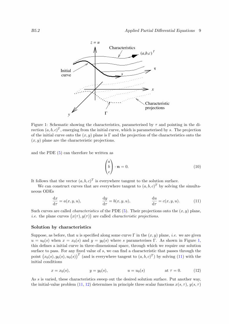
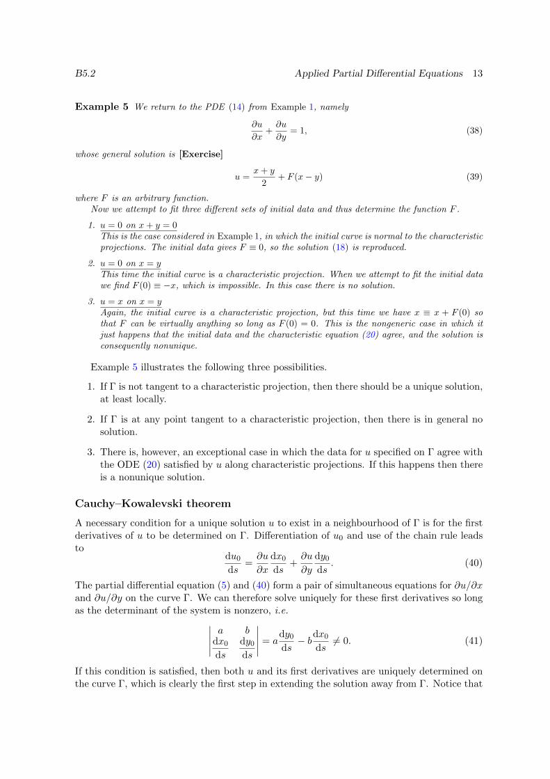
Figure 1: Schematic showing the characteristics, parameterised by τ and pointing in the di-rection (a, b, c)T , emerging from the initial curve, which is parameterised by s. The projectionof the initial curve onto the (x, y) plane is Γ and the projection of the characteristics onto the(x, y) plane are the characteristic projections.
and the PDE (5) can therefore be written asabc
· n = 0. (10)
It follows that the vector (a, b, c)T is everywhere tangent to the solution surface.We can construct curves that are everywhere tangent to (a, b, c)T by solving the simulta-
neous ODEs
dx
dτ= a(x, y, u),
dy
dτ= b(x, y, u),
du
dτ= c(x, y, u). (11)
Such curves are called characteristics of the PDE (5). Their projections onto the (x, y) plane,i.e. the plane curves
(x(τ), y(τ)
)are called characteristic projections.
Solution by characteristics
Suppose, as before, that u is specified along some curve Γ in the (x, y) plane, i.e. we are givenu = u0(s) when x = x0(s) and y = y0(s) where s parameterises Γ. As shown in Figure 1,this defines a initial curve in three-dimensional space, through which we require our solutionsurface to pass. For any fixed value of s, we can find a characteristic that passes through the
point(x0(s), y0(s), u0(s)
)T(and is everywhere tangent to (a, b, c)T ) by solving (11) with the
initial conditions
x = x0(s), y = y0(s), u = u0(s) at τ = 0. (12)
As s is varied, these characteristics sweep out the desired solution surface. Put another way,the initial-value problem (11, 12) determines in principle three scalar functions x(s, τ), y(s, τ)
B5.2 Applied Partial Differential Equations 10
and u(s, τ), and the vector
r =
x(s, τ)y(s, τ)u(s, τ)
(13)
defines the solution surface, parametrised by s and τ .The theory that exists for ODEs may be applied directly to the system (11). For example,
Picard’s theorem tells us that there is a unique solution to (11) satisfying the initial conditions(12) provided the right-hand side (a, b, c)T is bounded and satisfies a Lipschitz condition inu. However, we can easily construct examples for which these conditions fail and the solutioneither blows up or becomes nonunique at some distance from the initial curve.
Equation (13) is called the parametric form of the solution. It may be possible to eliminates and τ from (13) to obtain the solution surface in the implicit form G(x, y, u) = 0. Finally,if this implicit equation can be solved for u, then we obtain the solution in the explicit formu = u(x, y). Explicit solutions are the most convenient, but are often impossible to obtain interms of elementary functions.
Example 1 Consider the PDE∂u
∂x+∂u
∂y= 1, (14)
subject to the boundary data u = 0 when x+ y = 0. The characteristics satisfy
dx
dτ=
dy
dτ=
du
dτ= 1, (15)
and the boundary data lead to the initial conditions
x = s, y = −s, u = 0 at τ = 0. (16)
Hence we find the parametric solution
x = s+ τ, y = −s+ τ, u = τ, (17)
and it is straightforward in this case to eliminate s and τ to obtain the explicit solution
u =x+ y
2. (18)
In Example 1, the PDE (14) is semilinear. In such cases, the characteristic projectionssatisfy the ODEs
dx
dτ= a(x, y),
dy
dτ= b(x, y), (19)
which are independent of the solution u. The standard theory of phase planes may be appliedto the ODEs (19); for example, there is in general a unique characteristic projection througheach point in the (x, y) plane except at critical points where a and b are both zero. Once(19) have been solved to find the characteristic projections in the (x, y) plane, we find that usatisfies the decoupled ODE
du
dτ= c(x(τ), y(τ), u
)(20)
along each characteristic projection.For general quasilinear equations, the characteristic projections depend on the solution;
the three ODEs (11) are coupled and must be solved simultaneously.
B5.2 Applied Partial Differential Equations 11
Example 2 Solve the PDE∂u
∂t+ u
∂u
∂x= 1, (21)
for u(x, t) in t > 0, subject to the initial condition u = x on t = 0.The characteristics are given by
dt
dτ= 1,
dx
dτ= u,
du
dτ= 1, (22)
and the initial data may be parametrised by
t = 0, x = s, u = s at τ = 0. (23)
Solving for t first, we see that t ≡ τ and thus we may replace τ by t henceforth. The initial-valueproblem for u has the solution
u = s+ t, (24)
so that the problem for x becomes
dx
dt= s+ t, x = s when t = 0, (25)
whose solution isx = s+ st+ 1
2 t2. (26)
Now we can solve (26) for s and substitute it into (24) to obtain the solution in explicit form:
u =x+ t+ 1
2 t2
1 + t. (27)
Alternative method of solution
The characteristic equations (11) may be rearranged to give
dx
a(x, y, u)=
dy
b(x, y, u)=
du
c(x, y, u). (28)
Suppose we can spot two linearly independent first integrals of these ODEs, of the formf(x, y, u) = const and g(x, y, u) = const. Then the general solution of the PDE (5) may bewritten in the implicit form
f(x, y, u) = F(g(x, y, u)
), (29)
where F is an arbitrary function.
Example 3 Return to the problem considered in Example 2. The characteristic equations may bewritten as
dt
1=
dx
u=
du
1(30)
and then rearranged to two ODEs:
du
dt= 1,
dx
dt= u. (31)
These may be integrated to give
u = t+ C1, x = 12 t
2 + C1t+ C2, (32)
B5.2 Applied Partial Differential Equations 12
where C1 and C2 are constants. Our two first integrals are, therefore, C1 = f(x, t, u) = u − t andC2 = g(x, t, u) = x− 1
2 t2−C1t = x− 1
2 t2− (u− t)t. The general solution is found by setting f = F (g),
which leads tou = t+ F
(x+ 1
2 t2 − ut
), (33)
where F is an arbitrary function. It may readily be verified that any u(x, t) satisfying the implicitequation (33) is a solution of (21).
The function F is found by fitting the initial data: u = x when t = 0 leads to F (x) ≡ x, that isu = t+ x+ 1
2 t2 − ut, which reproduces the solution (27).
This procedure works because the equation f(x, y, u) = const defines a one-parameterfamily of surfaces, as does g(x, y, u) = const, and characteristics are lines of intersection be-tween one member from each of these two families. Now, any surface defined by an equationof the form f = F (g) has the property that f is constant whenever g is constant. It followsthat such a surface is composed of a family of characteristics, as indicated in Figure 1, and isthus a solution surface for the PDE (5).
Example 4 For the PDE
yu∂u
∂x− xu∂u
∂y= x− y, (34)
the characteristic equations
dx
dτ= yu,
dy
dτ= −xu, du
dτ= x− y, (35)
may be rearranged to give [Exercise]
d
dτ
(x2 + y2
)=
d
dτ
(u2 + 2x+ 2y
)= 0. (36)
It follows that the general solution is
u2 = −2x− 2y + F (x2 + y2), (37)
where F is an arbitrary function.
2.4 Cauchy data
Geometric interpretation
The term Cauchy data refers to the boundary data that, when applied to a PDE, in principledetermine the solution, at least locally. For the first-order quasilinear PDE (5), Cauchy datais the prescription of u on some curve Γ in the (x, y) plane, that is we set u = u0(s) whenx = x0(s) and y = y0(s) where s parametrises Γ. The combination of the PDE (5) andCauchy data is called the Cauchy problem. For the moment we assume that x0, y0 and u0 aresmooth functions of s (although there are interesting cases where this is not true, e.g. whereΓ has corners) and that there are no values of s for which x′0(s) = y′0(s) = 0 (this ensuresthat s is a sensible parameter for Γ).
We have seen that the method of characteristics, outlined in section 2.2, usually allows asolution surface to be constructed in a neighbourhood of Γ. However, the procedure fails ifit happens that the initial curve Γ is at any point tangent to (a, b)T . If this occurs, then thecharacteristic projection, instead of propagating away from the initial curve, points along it.Thus the data u0(s) given on Γ will not in general agree with the ODE (20) satisfied by u inthe direction (a, b).
B5.2 Applied Partial Differential Equations 13
Example 5 We return to the PDE (14) from Example 1, namely
∂u
∂x+∂u
∂y= 1, (38)
whose general solution is [Exercise]
u =x+ y
2+ F (x− y) (39)
where F is an arbitrary function.Now we attempt to fit three different sets of initial data and thus determine the function F .
1. u = 0 on x+ y = 0This is the case considered in Example 1, in which the initial curve is normal to the characteristicprojections. The initial data gives F ≡ 0, so the solution (18) is reproduced.
2. u = 0 on x = yThis time the initial curve is a characteristic projection. When we attempt to fit the initial datawe find F (0) ≡ −x, which is impossible. In this case there is no solution.
3. u = x on x = yAgain, the initial curve is a characteristic projection, but this time we have x ≡ x + F (0) sothat F can be virtually anything so long as F (0) = 0. This is the nongeneric case in which itjust happens that the initial data and the characteristic equation (20) agree, and the solution isconsequently nonunique.
Example 5 illustrates the following three possibilities.
1. If Γ is not tangent to a characteristic projection, then there should be a unique solution,at least locally.
2. If Γ is at any point tangent to a characteristic projection, then there is in general nosolution.
3. There is, however, an exceptional case in which the data for u specified on Γ agree withthe ODE (20) satisfied by u along characteristic projections. If this happens then thereis a nonunique solution.
Cauchy–Kowalevski theorem
A necessary condition for a unique solution u to exist in a neighbourhood of Γ is for the firstderivatives of u to be determined on Γ. Differentiation of u0 and use of the chain rule leadsto
du0
ds=∂u
∂x
dx0
ds+∂u
∂y
dy0
ds. (40)
The partial differential equation (5) and (40) form a pair of simultaneous equations for ∂u/∂xand ∂u/∂y on the curve Γ. We can therefore solve uniquely for these first derivatives so longas the determinant of the system is nonzero, i.e.∣∣∣∣∣ a b
dx0
ds
dy0
ds
∣∣∣∣∣ = ady0
ds− bdx0
ds6= 0. (41)
If this condition is satisfied, then both u and its first derivatives are uniquely determined onthe curve Γ, which is clearly the first step in extending the solution away from Γ. Notice that
B5.2 Applied Partial Differential Equations 14
the criterion (41) is equivalent to requiring Γ not to be tangent to a characteristic projection,as argued above via geometrical reasoning.
When the determinant in (41) is zero, there is either no solution for ∂u/∂x and ∂u/∂yor an infinite number of solutions (this is an instance of the Fredholm Alternative). Byeliminating between (5) and (40) we find that
1
a
dx0
ds=
1
b
dy0
ds6= 1
c
du0
ds⇒ no solution, (42a)
1
a
dx0
ds=
1
b
dy0
ds=
1
c
du0
ds⇒ many solutions. (42b)
The latter equality is the exceptional case, seen in Example 1, in which the variation of u alongΓ just happens to agree with the differential equation (20) satisfied along the characteristicprojection.
The process outlined above can be continued to obtain higher derivatives of u. If ∂u/∂xis known, for example, then further differentiation with respect to s gives
d
ds
(∂u
∂x
)=∂2u
∂x2
dx0
ds+
∂2u
∂x∂y
dy0
ds, (43)
while differentiation of (5) with respect to x yields
a∂2u
∂x2+ b
∂2u
∂x∂y+∂a
∂x
∂u
∂x+∂b
∂x
∂u
∂y+∂a
∂u
(∂u
∂x
)2
+∂b
∂u
∂u
∂x
∂u
∂y=∂c
∂x+∂c
∂u
∂u
∂x. (44)
Now we have a pair of simultaneous equations for ∂2u/∂x2 and ∂2u/∂x∂y. The condition forthis system to have a unique solution is identical to (41).
So long as a, b and c are analytic, so that this differentiation may be continued indefinitely,we can continue this argument to show that the condition (41) allows the derivatives of u toall orders to be defined uniquely at Γ. Thus a Taylor series for u(x, y) may be constructedabout the initial data curve Γ, and it can be shown that this series has a nonzero radiusof convergence. This is the starting point for the proof of the Cauchy–Kowalevski theorem,which states that (5) has a unique analytic solution in some neighbourhood of Γ, provided a,b and c are analytic and satisfy the condition (41).
2.5 Domain of definition
Bounded initial curve
In Example 2, we are given u = x along the whole x-axis. In general, however, the initialdata may only be given on a finite or semi-infinite initial curve Γ. In such cases, the solutionis only defined in the region penetrated by characteristic projections that intersect Γ. Thisregion, which is bounded by the characteristic projections that pass through the end pointsof Γ, is called the domain of definition.
Example 6 Solve the partial differential equation
∂u
∂t+ xu
∂u
∂x= u (45)
for u(x, t) in t > 0, subject to the initial condition u = x when t = 0, 0 < x < 1.
B5.2 Applied Partial Differential Equations 15
0.0 0.5 1.0 1.5 2.00.0
0.2
0.4
0.6
0.8
1.0
......
......
.......
......
......
.......
......
......
....
......
......
.......
......
......
.......
......
......
........
.......
.......
.......
......
.......
......
......
........
.......
.......
.......
......
......
.......
......
.......
......
......
........
.......
.......
.......
......
......
.......
......
.......
......
......
........
.......
.......
..
.......
.......
........
......
......
.......
......
......
.......
......
......
........
.......
........
......
......
.......
......
......
.......
......
......
........
.......
........
......
......
.......
......
......
........
.......
........
......
......
.......
......
......
.......
......
......
........
.......
........
......
......
.......
......
......
.......
......
......
........
.......
......
.......
.......
........
......
......
.......
......
......
.......
......
......
........
.......
........
......
......
.......
......
......
.......
......
......
........
.......
........
.......
.......
........
.......
........
.......
.......
........
.......
........
.......
.......
........
.......
.......
........
.......
........
.......
.......
........
.......
........
.......
.......
......................
.......
.......
........
......
......
........
.......
........
.......
.......
........
.......
.......
.......
......
........
.......
.......
........
.......
........
.......
.......
........
.......
.......
.................................................................................................................................................................................................
.......
.......
........
.......
.......
........
.......
........
.......
.......
........
.......
........
............................................................................................................................................................................................................................................................................................................
.............................................................................................................................................................................................................................................................................................................................................................................................................................................
..........................................................................................................................................................................................................................................................................................................................................................................................................................................
................................................................................................................................................................................................................................................................................................................................................................................
..........................................................................................................................................................................................................................................................................................................................
qqqqqqqqqqqqqqqqqqqqqqqqqqqqqqqqqqqqqqqqqqqqqqqqqqqqqqqqqqqqqqqqqqqqqqqqqqqqqqqqqqqqqqqqqqqqqqqqqqqqqqqqqqqqqqqqqqqqqqqqqqqqqq
qqqqqqqqqqqqqqqqqqqqqqqqqqqqqqqqqqqqqqqqqqqqqqqqqqqqqqqqqqqqqqqqqqqqqqqqqqqqqqqqqqqqqqqqqqqqqqqqqqqqqqqqqqqqqqqqqqqqqqqqqqqqqqqqqqqqqqqqqqqqqqqqqq
t
x
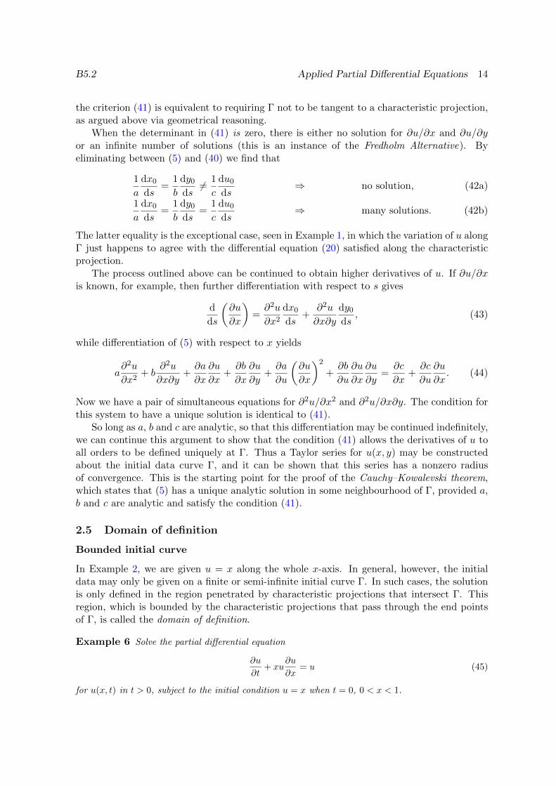
Figure 2: The characteristic projections given by equation (47).
The characteristics are given by
dt
dτ= 1,
dx
dτ= xu,
du
dτ= u, (46)
and the initial data may be parameterised by t = 0, x = s, u = s, 0 < s < 1. The solution inparametric form is
x = s exp(s(et − 1)
), u = set, 0 < s < 1, (47)
and the characteristic projections are shown in Figure 2. The domain of definition is the region0 < x < exp (et − 1).
Note that s may be eliminated from (47) to obtain the solution in the implicit form
x = u exp(u− t− ue−t
), (48)
but there is no explicit formula for u(x, t) in terms of elementary functions.
Blow-up
The domain in which the solution is defined may be further restricted if the solution developsa singularity, such that the PDE (5) ceases to make sense. For example, u may blow up afinite distance from the initial curve Γ. The method of characteristics reduces the partialdifferential equation (5) to the system (11) of ordinary differential equations. Since nonlinearODEs may certainly give rise to solutions that blow up, the same is true of nonlinear PDEs,even those that are semilinear.
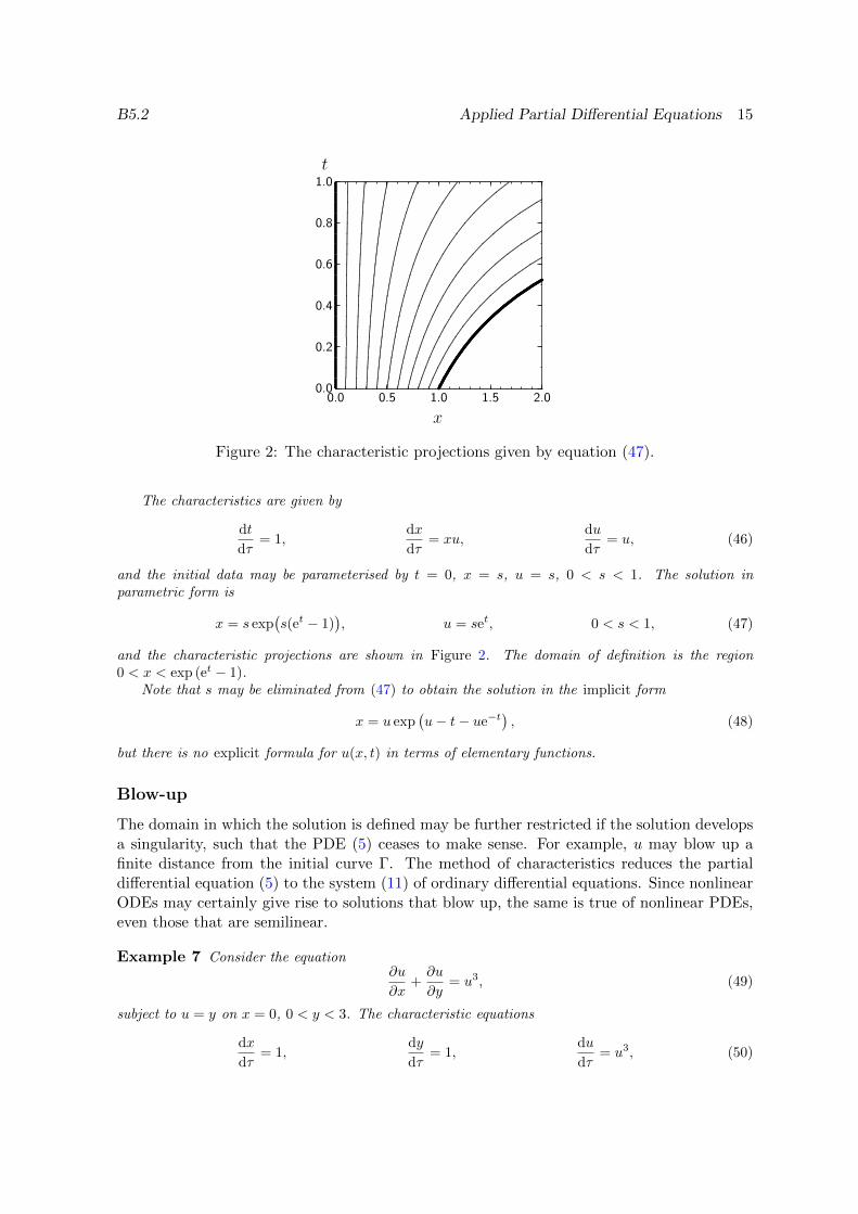
Example 7 Consider the equation∂u
∂x+∂u
∂y= u3, (49)
subject to u = y on x = 0, 0 < y < 3. The characteristic equations
dx
dτ= 1,
dy
dτ= 1,
du
dτ= u3, (50)
B5.2 Applied Partial Differential Equations 16
-1.0 -0.5 0.0 0.5 1.0................................................
-1
0
1
2
3
. . . . . . . . . . . . . . . . . . . . . . . . . . . . . . . . . . . . . . . . . . . . . . . .
............................
.............................
.............................
............................
.............................
.............................
............................
.............................
.............................
..............................
............................
.............................
.............................
..............................
......
..............................
.............................
..............................
.............................
.............................
...............................
.............................
.............
................................................................................................................................................
..........................................................................................................................................
Domain ofdefinition
x
y
Figure 3: Domain of definition for Example 7.
and initial data x = 0, y = s, u = s on τ = 0, 0 < s < 3, have the solution
x = τ, y = s+ τ, u =s√
1− 2s2τ, 0 < s < 3. (51)
We may solve explicitly for u to obtain
u =y − x√
1− 2x(y − x)2. (52)
This blows up on the line s = 1/√
2τ , i.e. on the line
y = x+1√2x. (53)
The domain of definition, bounded by this curve and the characteristic projections y = x and y = x+3,is illustrated in Figure 3.
Nonuniqueness
The domain in which the solution is properly defined may also be limited by u ceasing to bea unique function of x and y. Provided the coefficients a, b and c are well-behaved and udoes not blow up, the method of characteristics outlined in section 2.2 always allows us todetermine in principle the solution in parametric form:
(x(s, τ), y(s, τ), u(s, τ)
). Then u
may in principle be found as a function of x and y so long as there is a unique transformationfrom (s, τ) to (x, y). By the Inverse Function Theorem, a sufficient condition is that theJacobian of the transformation be finite and nonzero:
J =
∣∣∣∣∣∣∣∣∂x
∂τ
∂x
∂s
∂y
∂τ
∂y
∂s
∣∣∣∣∣∣∣∣ = a∂y
∂s− b∂x
∂s6= 0, ∞. (54)
Note that this reproduces the condition (41) for u to be determined in the neighbourhood ofΓ.
B5.2 Applied Partial Differential Equations 17
0.0 0.5 1.0 1.5 2.00.0
0.5
1.0
1.5
2.0
ppppppppppppppppppppppppppppppppppppppppppppppppppppppppppppppppppppppppppppppppppppppppppppppppppppp
..............................................................................................................................
..............................................................................................................................
.............................................................................................................
................................................................
................................................................
................................................................
................................................................
................................................................
...............................................
............................................
............................................
............................................
............................................
............................................
............................................
............................................
............................................
.......................
..................................
..................................
..................................
..................................
..................................
..................................
..................................
..................................
..................................
..................................
..................................
.............
............................
............................
............................
............................
............................
............................
............................
............................
............................
............................
............................
............................
............................
............................
..........
...................................................................................................................................................................................................................................................................................................................................................................................................................................
.......................................................................................................................................................................................................................................................................................................................................................................................................................................................
............................................................................................................................................................................................................................................................................................................................................................................................................................................................................
....................................................................................................................................................................................................................................................................................................................................................................................................................................................................................................
qqqqqqqqqqqqqqqqqqqqqqqqqqqqqqqqqqqqqqqqqqqqqqqqqqqqqqqqqqqqqqqqqqqqqqqqqqqqqqqqqqqqqqqqqqqqqqqqqqqqqqqqqqqqqqqqqqqqqqqqqqqqqqqqqqqqqqqqqqqqqqqq
qqqqqqqqqqqqqqqqqqqqqqqqqqqqqqqqqqqqqqqqqqqqqqqqqqqqqqqqqqqqqqqqqqqqqqqqqqqqqqqqqqqqqqqqqqqqqqqqqqqqqqqqqqqqqqqqqqqqqqqqqqqqqqqqqqqqqqqqqqqqqqqq
qqqqqqqqqqqqqqqqqqqqqqqqqqqqqqqqqqqqqqqqqqqqqqqqqqqqqqqqqqqqqqqqqqqqqqqqqqqqqqqqqqqqqqqqqqqqqqqqqqqqqqqqqqqqqqqqqqqqqqqqqqqqqqqqqqqqqqqqqqqqqqqq
qqqqqqqqqqqqqqqqqqqqqqqqqqqqqqqqqqqqqqqqqqqqqqqqqqqqqqqqqqqqqqqqqqqqqqqqqqqq
......................................
....................................................................
Γ
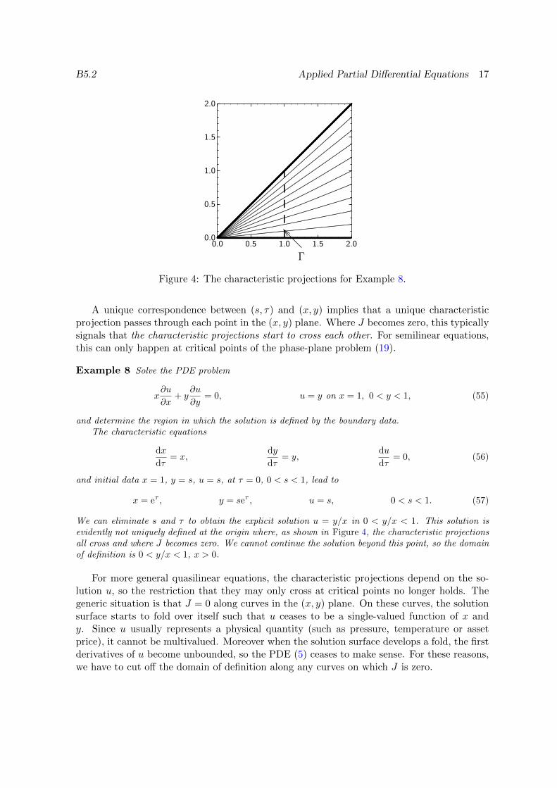
Figure 4: The characteristic projections for Example 8.
A unique correspondence between (s, τ) and (x, y) implies that a unique characteristicprojection passes through each point in the (x, y) plane. Where J becomes zero, this typicallysignals that the characteristic projections start to cross each other. For semilinear equations,this can only happen at critical points of the phase-plane problem (19).
Example 8 Solve the PDE problem
x∂u
∂x+ y
∂u
∂y= 0, u = y on x = 1, 0 < y < 1, (55)
and determine the region in which the solution is defined by the boundary data.The characteristic equations
dx
dτ= x,
dy
dτ= y,
du
dτ= 0, (56)
and initial data x = 1, y = s, u = s, at τ = 0, 0 < s < 1, lead to
x = eτ , y = seτ , u = s, 0 < s < 1. (57)
We can eliminate s and τ to obtain the explicit solution u = y/x in 0 < y/x < 1. This solution isevidently not uniquely defined at the origin where, as shown in Figure 4, the characteristic projectionsall cross and where J becomes zero. We cannot continue the solution beyond this point, so the domainof definition is 0 < y/x < 1, x > 0.
For more general quasilinear equations, the characteristic projections depend on the so-lution u, so the restriction that they may only cross at critical points no longer holds. Thegeneric situation is that J = 0 along curves in the (x, y) plane. On these curves, the solutionsurface starts to fold over itself such that u ceases to be a single-valued function of x andy. Since u usually represents a physical quantity (such as pressure, temperature or assetprice), it cannot be multivalued. Moreover when the solution surface develops a fold, the firstderivatives of u become unbounded, so the PDE (5) ceases to make sense. For these reasons,we have to cut off the domain of definition along any curves on which J is zero.
B5.2 Applied Partial Differential Equations 18
0 01 12 23 34 45 56 60 0
1 1
2 2
3 3
4 4
5 5
Domain ofdefinition
J = 0
(a) (b)t t
x x
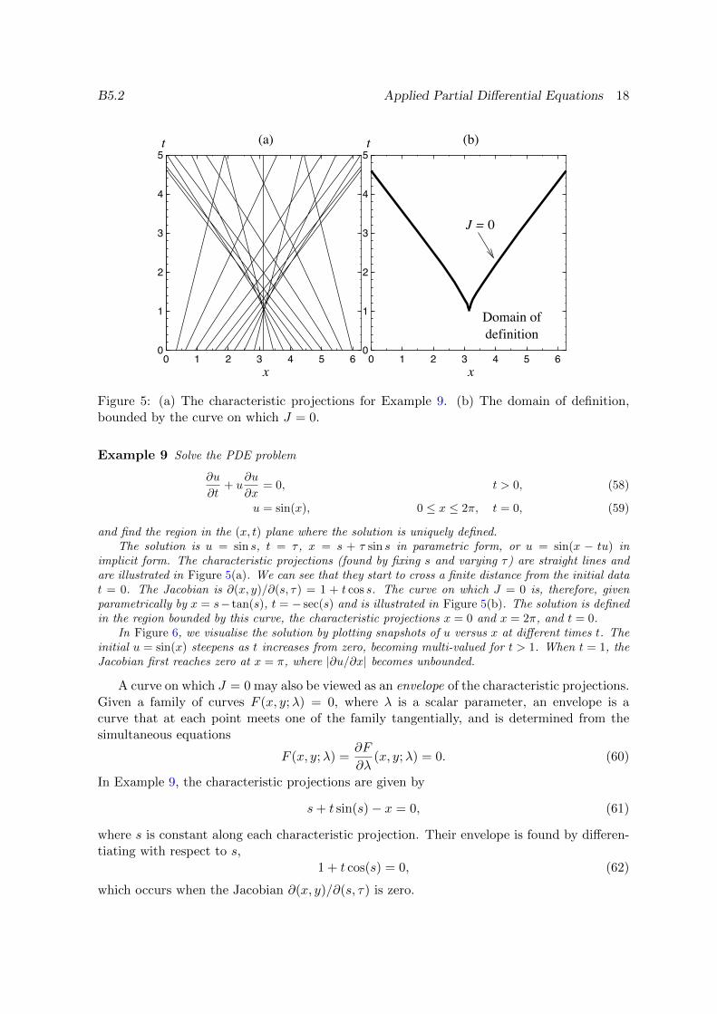
Figure 5: (a) The characteristic projections for Example 9. (b) The domain of definition,bounded by the curve on which J = 0.
Example 9 Solve the PDE problem
∂u
∂t+ u
∂u
∂x= 0, t > 0, (58)
u = sin(x), 0 ≤ x ≤ 2π, t = 0, (59)
and find the region in the (x, t) plane where the solution is uniquely defined.The solution is u = sin s, t = τ , x = s + τ sin s in parametric form, or u = sin(x − tu) in
implicit form. The characteristic projections (found by fixing s and varying τ) are straight lines andare illustrated in Figure 5(a). We can see that they start to cross a finite distance from the initial datat = 0. The Jacobian is ∂(x, y)/∂(s, τ) = 1 + t cos s. The curve on which J = 0 is, therefore, givenparametrically by x = s− tan(s), t = − sec(s) and is illustrated in Figure 5(b). The solution is definedin the region bounded by this curve, the characteristic projections x = 0 and x = 2π, and t = 0.
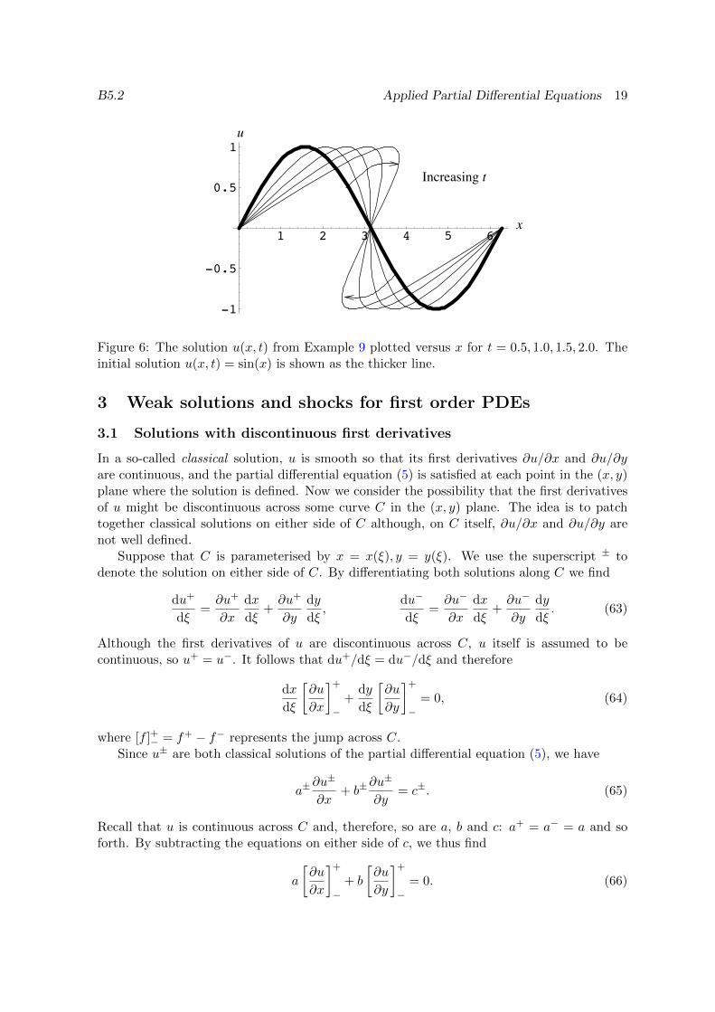
In Figure 6, we visualise the solution by plotting snapshots of u versus x at different times t. Theinitial u = sin(x) steepens as t increases from zero, becoming multi-valued for t > 1. When t = 1, theJacobian first reaches zero at x = π, where |∂u/∂x| becomes unbounded.
A curve on which J = 0 may also be viewed as an envelope of the characteristic projections.Given a family of curves F (x, y;λ) = 0, where λ is a scalar parameter, an envelope is acurve that at each point meets one of the family tangentially, and is determined from thesimultaneous equations
F (x, y;λ) =∂F
∂λ(x, y;λ) = 0. (60)
In Example 9, the characteristic projections are given by
s+ t sin(s)− x = 0, (61)
where s is constant along each characteristic projection. Their envelope is found by differen-tiating with respect to s,
1 + t cos(s) = 0, (62)
which occurs when the Jacobian ∂(x, y)/∂(s, τ) is zero.
B5.2 Applied Partial Differential Equations 19
1 2 3 4 5 6
-1
-0.5
0.5
1
Increasing t
u
x
Figure 6: The solution u(x, t) from Example 9 plotted versus x for t = 0.5, 1.0, 1.5, 2.0. Theinitial solution u(x, t) = sin(x) is shown as the thicker line.
3 Weak solutions and shocks for first order PDEs
3.1 Solutions with discontinuous first derivatives
In a so-called classical solution, u is smooth so that its first derivatives ∂u/∂x and ∂u/∂yare continuous, and the partial differential equation (5) is satisfied at each point in the (x, y)plane where the solution is defined. Now we consider the possibility that the first derivativesof u might be discontinuous across some curve C in the (x, y) plane. The idea is to patchtogether classical solutions on either side of C although, on C itself, ∂u/∂x and ∂u/∂y arenot well defined.
Suppose that C is parameterised by x = x(ξ), y = y(ξ). We use the superscript ± todenote the solution on either side of C. By differentiating both solutions along C we find
du+
dξ=∂u+
∂x
dx
dξ+∂u+
∂y
dy
dξ,
du−
dξ=∂u−
∂x
dx
dξ+∂u−
∂y
dy
dξ. (63)
Although the first derivatives of u are discontinuous across C, u itself is assumed to becontinuous, so u+ = u−. It follows that du+/dξ = du−/dξ and therefore
dx
dξ
[∂u
∂x
]+
−+
dy
dξ
[∂u
∂y
]+
−= 0, (64)
where [f ]+− = f+ − f− represents the jump across C.Since u± are both classical solutions of the partial differential equation (5), we have
a±∂u±
∂x+ b±
∂u±
∂y= c±. (65)
Recall that u is continuous across C and, therefore, so are a, b and c: a+ = a− = a and soforth. By subtracting the equations on either side of c, we thus find
a
[∂u
∂x
]+
−+ b
[∂u
∂y
]+
−= 0. (66)
B5.2 Applied Partial Differential Equations 20
In (64) and (66), we have a homogeneous linear system for [∂u/∂x]+− and [∂u/∂y]+−, whichmust therefore be zero unless the determinant of the system is zero. In other words, the firstderivatives must be continuous unless
bdx
dξ− ady
dξ= 0. (67)
This is identical to the equation for a characteristic projection. Thus, the first derivatives ofu may only be discontinuous across a characteristic projection. Indeed, this may be used asan alternative definition of what a characteristic projection is: it is a curve across which thefirst derivatives of u may be discontinuous.
Example 10 Consider the partial differential equation
∂u
∂x+∂u
∂y= 1, (68)
subject to the boundary condition
u(x, 0) =
0 x < 0,
x x ≥ 0.(69)
The characteristic equationsdx = dy = du (70)
give the general solutionu = x+ f(x− y). (71)
The boundary condition gives
f(s) =
−s s < 0,
0 s ≥ 0,(72)
and the solution is therefore
u =
y x < y,
x x ≥ y.(73)
Notice that the first derivatives of u are discontinuous across the characteristic y = x that passesthrough the origin, but u itself is continuous.
3.2 Weak solutions
In the previous section we showed that classical solutions may be patched together in such away that the first derivatives of u are discontinuous across a characteristic projection. Nowwe attempt to do the same for solutions in which u itself has a jump across some curvein the (x, y) plane. Selecting a unique solution is inherently more problematic when u isdiscontinuous, as the following example illustrates.
Example 11 Consider the partial differential equation
∂u
∂x+∂u
∂y= 0, (74)
subject to
u(0, y) =
0 y < 0,
1 y ≥ 0.(75)
B5.2 Applied Partial Differential Equations 21
pppppppppppppppppppppppppppppppppppppppppppppppppppppppppppppppppppppppppppp
pppppppppppppppppppppppppppppppppppppppppppppppppppppppppppppppppppppppppppp
pppppppppppppppppppppppppppppppppppppppppppppppppppppppppppppppppppppppppppp
pppppppppppppppppppppppppppppppppppppppppppppppppppppppppppppppppppppppppppp
............................................................................................................................................................................................................................................
.......
.......
........................
................................................................................................................................................................................................
.......
.......
........................
...............................................................................................................................................................
.......
.......
........................
.................................................................................................................................................
.......
.......
........................
...................................
......................................
..............................................................................................................................................................................
........
.........................................................................................................................
.............................................................................................................
....................
..... ................................................................................................................................................................................
..... ....................................................................................................................................
...............................................................................................................................................................................................................................
......................................
..........................................................................................................................................................................................................................................................................................................
.......
.......
........................
..................................................................................................................................................................................................................................................................................................................................................
.......
.......
........................
..........................................................................................................................................................................................................................................................................................................................................................................
.......
.......
........................
...................................................................................................................................................
.............................................
........................................................................................
.............................................
....................................
...............................
................................
...................................
..................................
...........................................
.....................................................
......................................................................
.......................
....................................
................................
.................................
.................................
................................
.................................
...............................................................................................
pppppppppppppppppppppppppppppppppppppppppppppppppppppppppppppppppppppppppppppppppppppppppppppppppppppppppppppppppppppppppppppppppppppppppppppppppppppppppppppppppppppppppppppppppppppppppppppppppppppppppppppppppppppppppppppppppppppppppppppppppppppppppppppppppppppppppppppppppppppppppppppppppppppppppppppppppppppppppppppppppppppppppppppppppppppppppppppppppppppppppppppppppppppppppppppppppppppppppppppppppppppppppppppppppp
ppppppppppppppppppppppppppppppppppppppppppppppppppppppppppppppppppppppppppppppppppppppppppppppppppppppppppppppppppppppppppppppppppppppppppppppppppppppppppppppppppppppppppppppppppppppppppppppppppppppppppppppppppppppppppppppppppppppppppppppppppppppppppppppppppppppppppppppppppppppppppppppppppppppppppppppppppppppppppppppppppppppppppppppppppppppppppppppppppppppppppppppppppppppppppppppppppppppppppppppppppppppppppppppppps0
(b)
x
y
x
Γ
(a)y
s0
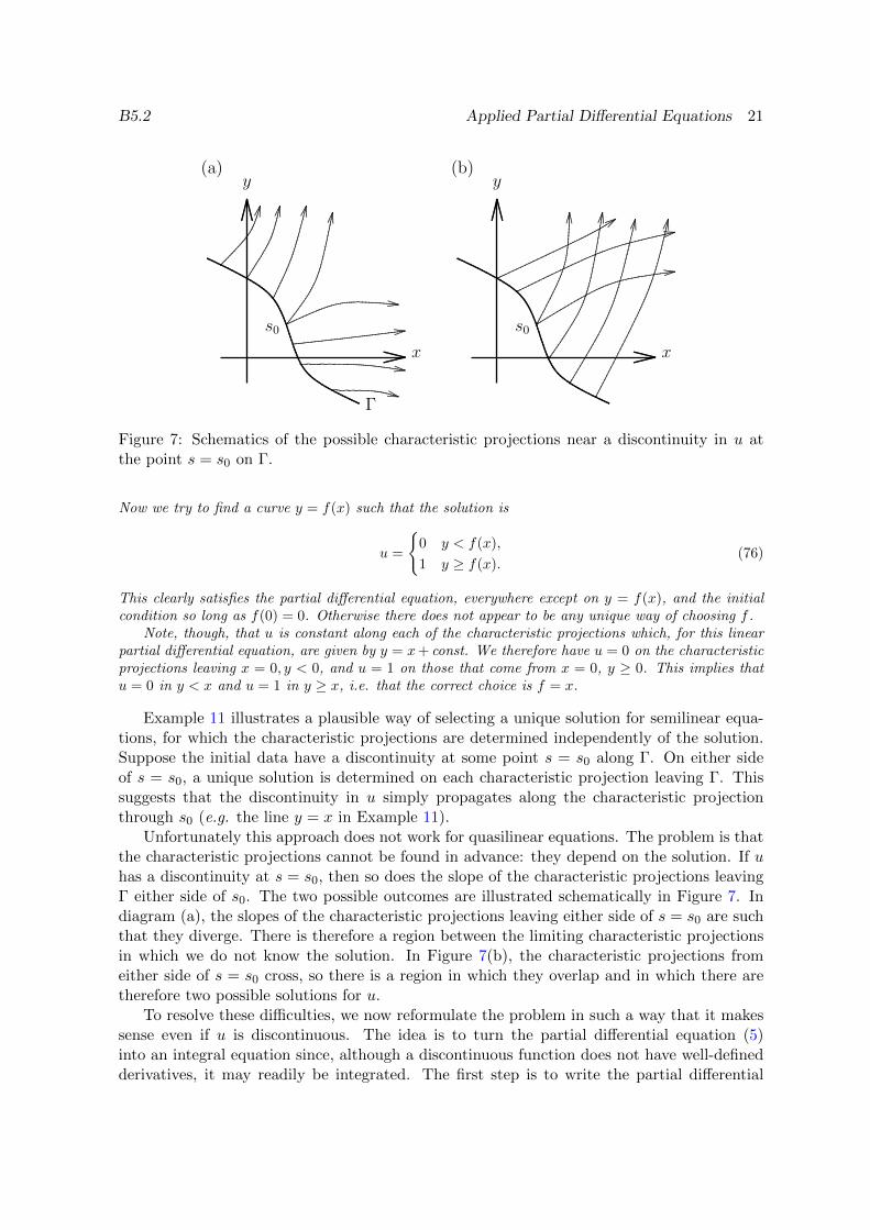
Figure 7: Schematics of the possible characteristic projections near a discontinuity in u atthe point s = s0 on Γ.
Now we try to find a curve y = f(x) such that the solution is
u =
0 y < f(x),
1 y ≥ f(x).(76)
This clearly satisfies the partial differential equation, everywhere except on y = f(x), and the initialcondition so long as f(0) = 0. Otherwise there does not appear to be any unique way of choosing f .
Note, though, that u is constant along each of the characteristic projections which, for this linearpartial differential equation, are given by y = x+ const. We therefore have u = 0 on the characteristicprojections leaving x = 0, y < 0, and u = 1 on those that come from x = 0, y ≥ 0. This implies thatu = 0 in y < x and u = 1 in y ≥ x, i.e. that the correct choice is f = x.
Example 11 illustrates a plausible way of selecting a unique solution for semilinear equa-tions, for which the characteristic projections are determined independently of the solution.Suppose the initial data have a discontinuity at some point s = s0 along Γ. On either sideof s = s0, a unique solution is determined on each characteristic projection leaving Γ. Thissuggests that the discontinuity in u simply propagates along the characteristic projectionthrough s0 (e.g. the line y = x in Example 11).
Unfortunately this approach does not work for quasilinear equations. The problem is thatthe characteristic projections cannot be found in advance: they depend on the solution. If uhas a discontinuity at s = s0, then so does the slope of the characteristic projections leavingΓ either side of s0. The two possible outcomes are illustrated schematically in Figure 7. Indiagram (a), the slopes of the characteristic projections leaving either side of s = s0 are suchthat they diverge. There is therefore a region between the limiting characteristic projectionsin which we do not know the solution. In Figure 7(b), the characteristic projections fromeither side of s = s0 cross, so there is a region in which they overlap and in which there aretherefore two possible solutions for u.
To resolve these difficulties, we now reformulate the problem in such a way that it makessense even if u is discontinuous. The idea is to turn the partial differential equation (5)into an integral equation since, although a discontinuous function does not have well-definedderivatives, it may readily be integrated. The first step is to write the partial differential
B5.2 Applied Partial Differential Equations 22
......................................
......................................
...............................................
......................
ppppppppppppppppppppppppppppppppppppppppppppppppppppppppppppppppppppppppppppppppppppppppppppppppppppppppppppppppppppppppppppppppppppppppppppppppppppppppppppppppppppppppppppppppppppppppppppppppppppppppppppppppppppppppppppppppppppppppppppppppppppppppppppppppppppppppppppppppppppppppppppppppppppppppppppppppppppppppppppppppppppppppppppppppppppppppp
..................................................................................................... ...........................................................................................................................................................................................................................................................................................................................................................................................................................................................................................................
D
y
x
Γ
γ
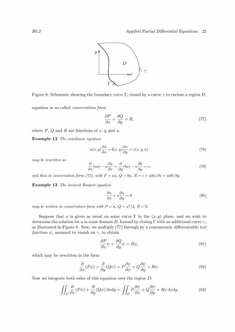
Figure 8: Schematic showing the boundary curve Γ, closed by a curve γ to enclose a region D.
equation in so-called conservation form
∂P
∂x+∂Q
∂y= R, (77)
where P , Q and R are functions of x, y and u.
Example 12 The semilinear equation
a(x, y)∂u
∂x+ b(x, y)
∂u
∂y= c(x, y, u) (78)
may be rewritten as∂
∂x(au)− u∂a
∂x+
∂
∂y(bu)− u ∂b
∂y= c, (79)
and thus in conservation form (77), with P = au, Q = bu, R = c+ u∂a/∂x+ u∂b/∂y.
Example 13 The inviscid Burgers equation
∂u
∂x+ u
∂u
∂y= 0 (80)
may be written in conservation form with P = u, Q = u2/2, R = 0.
Suppose that u is given as usual on some curve Γ in the (x, y) plane, and we wish todetermine the solution for u in some domainD, formed by closing Γ with an additional curve γ,as illustrated in Figure 8. Now, we multiply (77) through by a continuously differentiable testfunction ψ, assumed to vanish on γ, to obtain
∂P
∂xψ +
∂Q
∂yψ = Rψ, (81)
which may be rewritten in the form
∂
∂x(Pψ) +
∂
∂y(Qψ) = P
∂ψ
∂x+Q
∂ψ
∂y+Rψ. (82)
Now we integrate both sides of this equation over the region D:∫∫D
∂
∂x(Pψ) +
∂
∂y(Qψ) dxdy =
∫∫DP∂ψ
∂x+Q
∂ψ
∂y+Rψ dxdy. (83)
B5.2 Applied Partial Differential Equations 23
........................................
.........................
............................................
......................
...............................................
ppppppppppppppppppppppppppppppppppppppppppppppppppppppppppppppppppppppppppppppppppppppppppppppppppppppppppppppppppppppppppppppppppppppppppppppppppppppppppppppppppppppppppppppppppppppppppppppppppppppppppppppppppppppppppppppppppppppppppppppppppppppppppppppppppppppppppppppppppppppppppppppppppppppppppppppppppppppppppppppppppppppppppppppppppppppppp
..................................................................................................... ...........................................................................................................................................................................................................................................................................................................................................................................................................................................................................................................
ppppppppppppppppppppppppppppppppppppp ppppp ppppppppppppppppppppppppppppppppppppppppppppppppppppppppppppppppppppppppppppppppppppppppppppppppppppppppppppppppppppppppppppppppppppppppppp ppppppppppppppppppppppC..........................................................................................................................................................................................................
.................................................. .................................................................
.................................................
.........................................
D1
D2
C1
C2
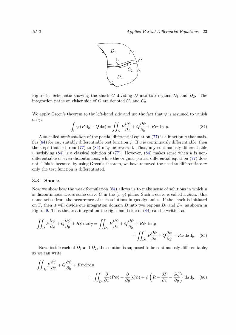
Figure 9: Schematic showing the shock C dividing D into two regions D1 and D2. Theintegration paths on either side of C are denoted C1 and C2.
We apply Green’s theorem to the left-hand side and use the fact that ψ is assumed to vanishon γ: ∫
Γψ (P dy −Qdx) =
∫∫DP∂ψ
∂x+Q
∂ψ
∂y+Rψ dxdy. (84)
A so-called weak solution of the partial differential equation (77) is a function u that satis-fies (84) for any suitably differentiable test function ψ. If u is continuously differentiable, thenthe steps that led from (77) to (84) may be reversed. Thus, any continuously differentiableu satisfying (84) is a classical solution of (77). However, (84) makes sense when u is non-differentiable or even discontinuous, while the original partial differential equation (77) doesnot. This is because, by using Green’s theorem, we have removed the need to differentiate u:only the test function is differentiated.
3.3 Shocks
Now we show how the weak formulation (84) allows us to make sense of solutions in which uis discontinuous across some curve C in the (x, y) plane. Such a curve is called a shock ; thisname arises from the occurrence of such solutions in gas dynamics. If the shock is initiatedon Γ, then it will divide our integration domain D into two regions D1 and D2, as shown inFigure 9. Thus the area integral on the right-hand side of (84) can be written as∫∫
DP∂ψ
∂x+Q
∂ψ
∂y+Rψ dxdy =
∫∫D1
P∂ψ
∂x+Q
∂ψ
∂y+Rψ dxdy
+
∫∫D2
P∂ψ
∂x+Q
∂ψ
∂y+Rψ dxdy. (85)
Now, inside each of D1 and D2, the solution is supposed to be continuously differentiable,so we can write∫∫
Di
P∂ψ
∂x+Q
∂ψ
∂y+Rψ dxdy
=
∫∫Di
∂
∂x(Pψ) +
∂
∂y(Qψ) + ψ
(R− ∂P
∂x− ∂Q
∂y
)dxdy, (86)
B5.2 Applied Partial Differential Equations 24
where i = 1 or 2. The term in brackets is identically zero, because of (77), and Green’stheorem may be applied to the remainder to give∫∫
Di
P∂ψ
∂x+Q
∂ψ
∂y+Rψ dxdy =
∮∂Di
ψ(P dy −Qdx). (87)
As indicated in Figure 9, the integration curves ∂D1 and ∂D2 comprise sections of Γ and γjoined to curves C1 and C2 adjacent to the shock on either side. When the two integrals aresummed, the result is∮
∂D1+∂D2
ψ(P dy −Qdx) =
∮Γ+C1−C2
ψ(P dy −Qdx), (88)
since ψ is zero on γ. Notice the difference in sign because C1 and C2 are traversed in differentdirections. The right-hand side of (84) may therefore be written in the form∫∫
DP∂ψ
∂x+Q
∂ψ
∂y+Rψ dxdy =
∮Γ+C1−C2
ψ(P dy −Qdx). (89)
The integral along Γ cancels with the left-hand side of (84), and we are left with∫C1
ψ(P dy −Qdx)−∫C2
ψ(P dy −Qdx) = 0, (90)
or ∫Cψ([P ]+− dy − [Q]+− dx) = 0, (91)
where [F ]+− denotes the jump in F across the shock C.Since this relation must hold for any (suitably smooth) test function ψ, the term in
brackets must be identically zero and we therefore obtain
dy
dx=
[Q]+−[P ]+−
. (92)
This so-called Rankine–Hugoniot condition determines the slope of the shock in terms of thediscontinuities in P and Q across it.
For semilinear equations, as shown in Example 12, we have P = a(x, y)u, Q = b(x, y)u so(92) reduces to
dy
dx=b[u]+−a[u]+−
=b
a. (93)
This is identical to the slope of characteristic projections so, for semilinear equations, solutionsmay only be discontinuous across characteristic projections. Thus the solution obtained inExample 11 is a valid weak solution. For general quasilinear equations, shocks are differentfrom characteristic projections.
Example 14 Find a weak solution of the problem
∂u
∂t+ u
∂u
∂x= 0, t > 0, (94)
u =
1 x < 0
0 x ≥ 0t = 0. (95)
B5.2 Applied Partial Differential Equations 25
-1.0 -0.5 0.0 0.5 1.00.0
0.5
1.0
1.5
2.0
u = 0u = 1
t
x
Shock
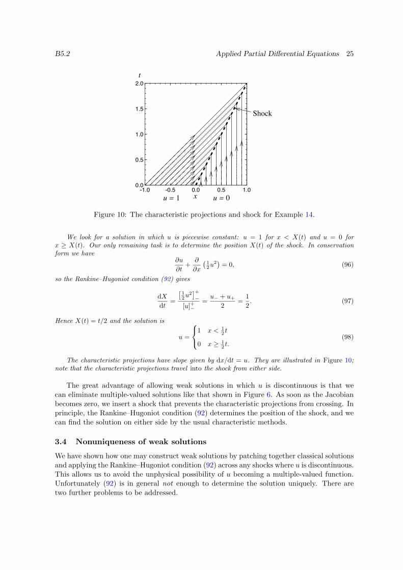
Figure 10: The characteristic projections and shock for Example 14.
We look for a solution in which u is piecewise constant: u = 1 for x < X(t) and u = 0 forx ≥ X(t). Our only remaining task is to determine the position X(t) of the shock. In conservationform we have
∂u
∂t+
∂
∂x
(12u
2)
= 0, (96)
so the Rankine–Hugoniot condition (92) gives
dX
dt=
[12u
2]+−
[u]+−=u− + u+
2=
1
2. (97)
Hence X(t) = t/2 and the solution is
u =
1 x < 12 t
0 x ≥ 12 t.
(98)
The characteristic projections have slope given by dx/dt = u. They are illustrated in Figure 10;note that the characteristic projections travel into the shock from either side.
The great advantage of allowing weak solutions in which u is discontinuous is that wecan eliminate multiple-valued solutions like that shown in Figure 6. As soon as the Jacobianbecomes zero, we insert a shock that prevents the characteristic projections from crossing. Inprinciple, the Rankine–Hugoniot condition (92) determines the position of the shock, and wecan find the solution on either side by the usual characteristic methods.
3.4 Nonuniqueness of weak solutions
We have shown how one may construct weak solutions by patching together classical solutionsand applying the Rankine–Hugoniot condition (92) across any shocks where u is discontinuous.This allows us to avoid the unphysical possibility of u becoming a multiple-valued function.Unfortunately (92) is in general not enough to determine the solution uniquely. There aretwo further problems to be addressed.
B5.2 Applied Partial Differential Equations 26
Problem 1
The Rankine–Hugoniot condition (92) depends on the functions P and Q that appear in theconservation form (77). However, there may be many different ways of expressing the samePDE in conservation form, and a different conservation form leads to a different Rankine–Hugoniot condition.
Example 15 The PDE∂u
∂x+ u
∂u
∂y= 0 (99)
may be written in many different conservation forms, including
∂u
∂x+
∂
∂y
(12u
2)
= 0 or∂
∂x
(12u
2)
+∂
∂y
(13u
3)
= 0. (100)
These lead to the two different Rankine–Hugoniot conditions
dy
dx=
[12u
2]+−
[u]+−=u+ + u−
2or
dy
dx=
[13u
3]+−[
12u
2]+−
=2(u2+ + u+u− + u2−
)3 (u+ + u−)
, (101)
respectively.
Solution
The key is to make sure that the functions P and Q in the conservation law correspond toreal physical quantities (e.g. mass, momentum, energy, etc.). Then the Rankine–Hugoniotcondition (92) ensures that these are conserved across shocks.
Example 16 Consider the following model for traffic flow. Let u(x, t) be the density of cars on astretch of road, where x is distance along the road and t is time. Suppose that the speed v of each caris related to the local density by v = (1− u). Then the flux of cars is given by uv = u(1− u) and theequation representing conservation of cars is
∂u
∂t+
∂
∂x
(u(1− u)
)= 0. (102)
The Rankine–Hugoniot condition associated with this conservation law is
dx
dt=
[u(1− u)
]+−
[u]+−, (103)
which may be rearranged to give [u
(dx
dt− (1− u)
)]+−
= 0. (104)
This equation ensures that the rate at which cars enter a shock from one side equals the rate at whichthey exit the other.
If (102) is rewritten as∂
∂t
(12u
2)
+∂
∂x
(12u
2 − 23u
3)
= 0, (105)
then the corresponding Rankine–Hugoniot condition has no physical interpretation, and the net flux ofcars would not be preserved across a shock.
B5.2 Applied Partial Differential Equations 27
Problem 2
The strategy described above selects a particular weak formulation (i.e. a particular choiceof P and Q) from the many that may be available. The second problem is that this weakformulation may still admit many solutions.
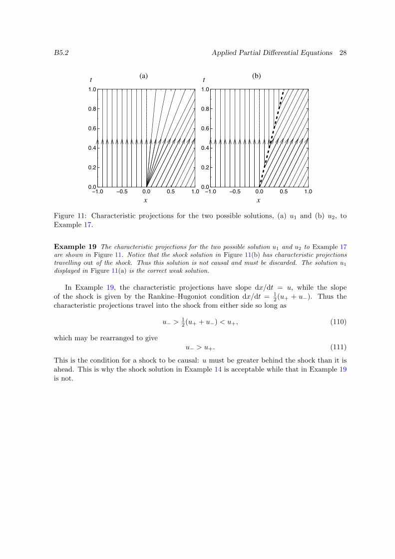
Example 17 The problem
∂u
∂t+ u
∂u
∂x= 0, u(x, 0) =
0 x < 0
1 x ≥ 0(106)
has (at least) two possible weak solutions, namely
u1 =
0 x < 0
x/t 0 ≤ x ≤ t1 x > t
and u2 =
0 x < t/2
1 x ≥ t/2.(107)
It is readily verified that 0, x/t and 1 all satisfy the PDE, and the discontinuities in the first derivativesof u1 occur across characteristic projections, so u1 is a valid solution. Similarly, u2 clearly satisfiesthe PDE on either side of the shock at x = t/2, and the Rankine–Hugoniot condition dx/dt = 1
2 issatisfied, so u2 is also a valid weak solution.
There are several ways around the problem illustrated in Example 17, including the fol-lowing.
1. EntropyHere we pose a function of u that must increase across a shock.
2. ViscosityThis involves introducing a higher derivative to regularise the equation (i.e. smoothout the shock).
Example 18 As shown in Example 17, the equation
∂u
∂t+ u
∂u
∂x= 0 (108)
may have multiple weak solutions. However, the Burgers Equation
∂u
∂t+ u
∂u
∂x= ε
∂2u
∂x2(109)
has a unique solution, given suitable initial and boundary data, for any positive value of ε. So a uniqueweak solution of (108) may be selected by solving (109) and then letting ε→ 0.
3. CausalityThis means ensuring that information travels into the shock, not out of it.
It may be shown that each of these approaches results in the same unique weak solutionbeing selected. We only use the third option, which does not require us to bring any morephysics into the problem, apart from a recognition that one variable (t) represents time.Information travels along characteristic projections, starting from the initial data, in thedirection of increasing t. A shock solution is causal only if this information travels into theshock from either side (as in Figures 10 and ??). By disallowing shocks that do not satisfythis condition, we narrow down the possible weak solutions to just one.
B5.2 Applied Partial Differential Equations 28
1.01.0 0.50.5 0.00.0 0.50.5 1.01.00.00.0
0.20.2
0.40.4
0.60.6
0.80.8
1.01.0
x x
t t(a) (b)
Figure 11: Characteristic projections for the two possible solutions, (a) u1 and (b) u2, toExample 17.
Example 19 The characteristic projections for the two possible solution u1 and u2 to Example 17are shown in Figure 11. Notice that the shock solution in Figure 11(b) has characteristic projectionstravelling out of the shock. Thus this solution is not causal and must be discarded. The solution u1displayed in Figure 11(a) is the correct weak solution.
In Example 19, the characteristic projections have slope dx/dt = u, while the slopeof the shock is given by the Rankine–Hugoniot condition dx/dt = 1
2(u+ + u−). Thus thecharacteristic projections travel into the shock from either side so long as
u− >12(u+ + u−) < u+, (110)
which may be rearranged to giveu− > u+. (111)
This is the condition for a shock to be causal: u must be greater behind the shock than it isahead. This is why the shock solution in Example 14 is acceptable while that in Example 19is not.
B5.2 Applied Partial Differential Equations 29
4 First order nonlinear equations
In this chapter we introduce a method that will enable us to solve fully nonlinear first orderPDEs by solving an associated system of ODEs (Charpit’s equations).
We consider general first-order nonlinear scalar PDEs, i.e. not (necessarily) quasi-linear.The general form of such an equation is
F (p, q, u, x, y) = 0, (112)
where we use∂u
∂x= p,
∂u
∂y= q (113)
as shorthand, so that∂p
∂y=∂q
∂x. (114)
The case of quasilinear equations corresponds to F being a linear function of p and q, i.e.
F (p, q, u, x, y, ) = a(x, y, u)p+ b(x, y, u)q − c(x, y, u). (115)
4.1 Charpit’s equations
If we differentiate (112) with respect to x and y, we obtain
∂F
∂p
∂p
∂x+∂F
∂q
∂q
∂x= −∂F
∂x− p∂F
∂u, (116a)
∂F
∂p
∂p
∂y+∂F
∂q
∂q
∂y= −∂F
∂y− q∂F
∂u, (116b)
or, using (114),
∂F
∂p
∂p
∂x+∂F
∂q
∂p
∂y= −∂F
∂x− p∂F
∂u, (117a)
∂F
∂p
∂q
∂x+∂F
∂q
∂q
∂y= −∂F
∂y− q∂F
∂u. (117b)
So, if we define characteristics or rays as curves(x(τ), y(τ)
)satisfying
dx
dτ=∂F
∂p,
dy
dτ=∂F
∂q(118)
then, along these curves,
dp
dτ= −∂F
∂x− p∂F
∂u,
dq
dτ= −∂F
∂y− q∂F
∂u. (119)
We therefore have a system of four ODEs for x, y, p and q satisfied along the rays. Recall,though, that in general F depends on u also, so to close the system we also need an ODE foru along the rays, namely
du
dτ=∂u
∂x
dx
dτ+∂u
∂y
dy
dτ= p
∂F
∂p+ q
∂F
∂q. (120)
B5.2 Applied Partial Differential Equations 30
In summary, we have the following system of ODEs for x, y, p, q and u, known as Charpit’sequations:
dx
dτ=∂F
∂p, (121a)
dy
dτ=∂F
∂q, (121b)
dp
dτ= −∂F
∂x− p∂F
∂u, (121c)
dq
dτ= −∂F
∂y− q∂F
∂u, (121d)
du
dτ= p
∂F
∂p+ q
∂F
∂q. (121e)
It is easily verified that these reduce to the usual characteristic equations
dx
dτ= a,
dy
dτ= b,
du
dτ= c, (122)
for quasi-linear equations where F takes the form (115).
4.2 Boundary data
As for quasilinear scalar equations, Cauchy data specifies u along some curve Γ in the(x, y)-plane:
x = x0(s), y = y0(s), u = u0(s), (123)
for s in some (possibly infinite) interval. We also require initial conditions for p and q, sayp = p0(s), q = q0(s), which are obtained by differentiating u0 with respect to s and using thePDE (112):
du0
ds= p0
dx0
ds+ q0
dy0
ds, F (p0, q0, u0, x0, y0) = 0. (124)
By the implicit function theorem, the two equations (124) may be solved uniquely (in principle,if not explicitly) for p0 and q0 provided the condition
dx0
ds
∂F
∂q0− dy0
ds
∂F
∂p06= 0 (125)
is satisfied. This is the same as insisting that Γ not be parallel to a ray.Charpit’s method consists of solving the ODEs (121) for (p, q, u, x, y), with (123) and
(124) as initial data at τ = 0. This gives (p, q, u, x, y) all as functions of s and τ and, inprinciple, allows us to reconstruct the solution surface u = u(x, y).
Example 20 Sugar on a spoonConsider sugar piled up on a spoon such that its height is given by u(x, y). At criticality, just beforethe sugar would start to slide off the spoon, the angle between the normal to the surface and the vertical(0, 0, 1) is a prescribed constant, γ, the angle of friction. That is,(
∂u
∂x
)2
+
(∂u
∂y
)2
+ 1 = sec2 γ (126)
B5.2 Applied Partial Differential Equations 31
After rearranging and normalising, this can be written as the Eikonal equation(∂u
∂x
)2
+
(∂u
∂y
)2
= 1, (127)
which is of the form (112) withF (p, q) = 1
2
(p2 + q2 − 1
). (128)
Charpit’s equations for this particular F are
dx
dτ= p,
dy
dτ= q,
dp
dτ= 0,
dq
dτ= 0,
du
dτ= p2 + q2 = 1. (129)
Notice that p and q are constant along rays and, hence, given by their boundary values:
p = p0(s), q = q0(s). (130)
The remaining ODEs are then readily integrated to give
x = x0(s) + p0(s)τ, y = y0(s) + q0(s)τ, u = u0(s) + τ. (131)
Notice that the slope of a ray is given by q0(s)/p0(s) which is constant along each ray. Thus the raysare straight lines, along which u increases linearly with τ .
At the edge of the spoon, the height is zero, so u0(s) = 0. Then we have the system
dx0ds
p0 +dy0ds
q0 = 0, p20 + q20 = 1 (132)
for p0 and q0, whose solution is
p0 =∓y′0√
(x′0)2 + (y′0)2, q0 =
±x′0√(x′0)2 + (y′0)2
, (133)
where ′ is used as shorthand for d/ds. The vector (p0, q0) is the unit normal to the boundary Γ. Hencethe rays are straight lines perpendicular to Γ and u(x, y) is simply the distance of the point (x, y)from Γ.
Notice that there are two possible solutions corresponding to the ± in (133). The correct solutionis chosen by ensuring that the rays propagate into the region of interest, not out of it. So, in (133),we have to choose (p0, q0) to be the inward pointing normal. Otherwise the solution corresponds to thesandpile outside a spoon-shaped hole in a table.
4.3 Proof that Charpit’s method works
If we differentiate F along a ray, we find that
dF
dτ=∂F
∂p
dp
dτ+∂F
∂q
dq
dτ+∂F
∂u
du
dτ+∂F
∂x
dx
dτ+∂F
∂y
dy
dτ= 0. (134)
Since the boundary condition (124) sets F to zero on the initial curve Γ, it must thereforebe zero everywhere along the rays passing through Γ. Hence p, q and u satisfy the equationF (p, q, u, x, y) = 0 everywhere in the domain of definition where there are rays emanatingfrom Γ.
This is not quite sufficient to prove that u is a solution of the original nonlinear PDE. Westill have to show that the functions p and q that result from solving Charpit’s equations areequal to ∂u/∂x and ∂u/∂y respectively. To do this, we first prove that φ ≡ 0, where
φ =∂u
∂s− p∂x
∂s− q∂y
∂s. (135)
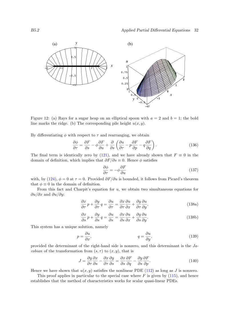
B5.2 Applied Partial Differential Equations 32
-2
-1
0
1
2
-1-0.5
00.5
10
0.25
0.5
0.75
1
-1
0
1
2
0
x
u
y
-2 -1 1 2
-1
-0.5
0.5
1
y
x
(a) (b)
Figure 12: (a) Rays for a sugar heap on an elliptical spoon with a = 2 and b = 1; the boldline marks the ridge. (b) The corresponding pile height u(x, y).
By differentiating φ with respect to τ and rearranging, we obtain
∂φ
∂τ=∂F
∂s− φ∂F
∂u+
∂
∂s
(∂u
∂τ− p∂F
∂p− q∂F
∂q
). (136)
The final term is identically zero by (121), and we have already shown that F ≡ 0 in thedomain of definition, which implies that ∂F/∂s ≡ 0. Hence φ satisfies
∂φ
∂τ= −φ∂F
∂u(137)
with, by (124), φ = 0 at τ = 0. Provided ∂F/∂u is bounded, it follows from Picard’s theoremthat φ ≡ 0 in the domain of definition.
From this fact and Charpit’s equation for u, we obtain two simultaneous equations for∂u/∂x and ∂u/∂y:
∂x
∂τp+
∂y
∂τq =
∂u
∂τ=∂x
∂τ
∂u
∂x+∂y
∂τ
∂u
∂y, (138a)
∂x
∂sp+
∂y
∂sq =
∂u
∂s=∂x
∂s
∂u
∂x+∂y
∂s
∂u
∂y. (138b)
This system has a unique solution, namely
p =∂u
∂x, q =
∂u
∂y, (139)
provided the determinant of the right-hand side is nonzero, and this determinant is the Ja-cobian of the transformation from (s, τ) to (x, y), that is
J =∂y
∂τ
∂x
∂s− ∂x
∂τ
∂y
∂s=∂x
∂s
∂F
∂q− ∂y
∂s
∂F
∂p. (140)
Hence we have shown that u(x, y) satisfies the nonlinear PDE (112) as long as J is nonzero.This proof applies in particular to the special case where F is given by (115), and hence
establishes that the method of characteristics works for scalar quasi-linear PDEs.
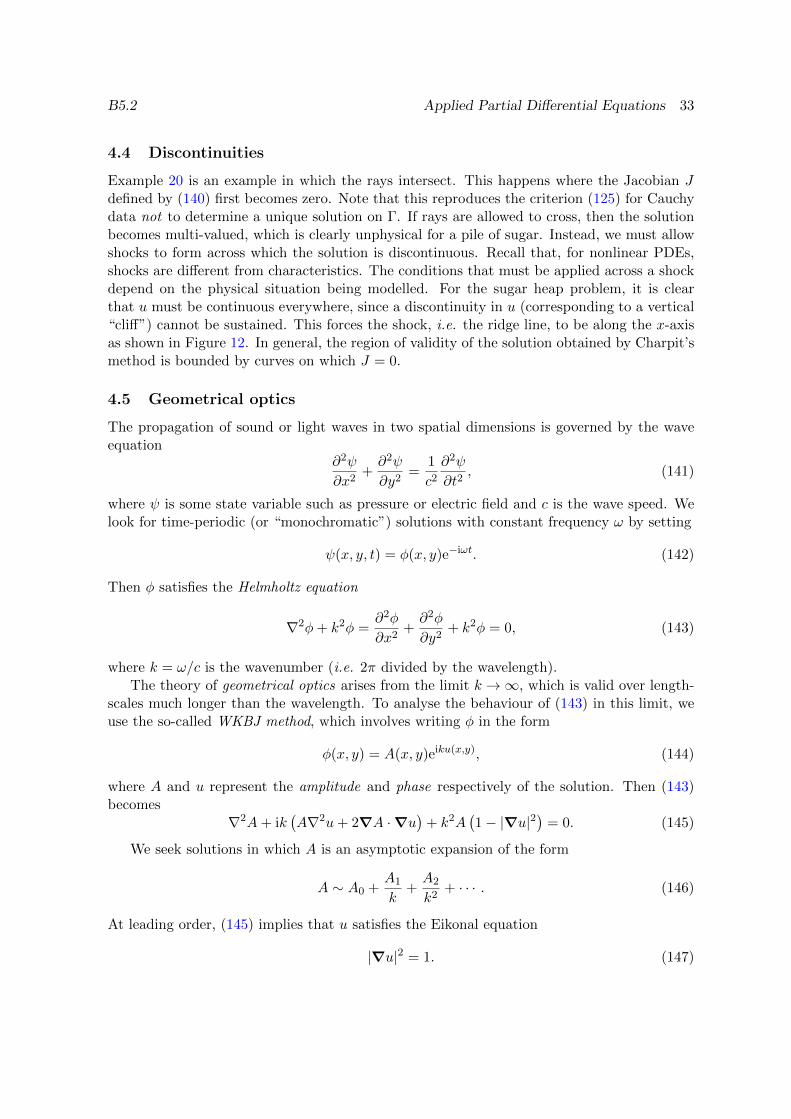
B5.2 Applied Partial Differential Equations 33
4.4 Discontinuities
Example 20 is an example in which the rays intersect. This happens where the Jacobian Jdefined by (140) first becomes zero. Note that this reproduces the criterion (125) for Cauchydata not to determine a unique solution on Γ. If rays are allowed to cross, then the solutionbecomes multi-valued, which is clearly unphysical for a pile of sugar. Instead, we must allowshocks to form across which the solution is discontinuous. Recall that, for nonlinear PDEs,shocks are different from characteristics. The conditions that must be applied across a shockdepend on the physical situation being modelled. For the sugar heap problem, it is clearthat u must be continuous everywhere, since a discontinuity in u (corresponding to a vertical“cliff”) cannot be sustained. This forces the shock, i.e. the ridge line, to be along the x-axisas shown in Figure 12. In general, the region of validity of the solution obtained by Charpit’smethod is bounded by curves on which J = 0.
4.5 Geometrical optics
The propagation of sound or light waves in two spatial dimensions is governed by the waveequation
∂2ψ
∂x2+∂2ψ
∂y2=
1
c2
∂2ψ
∂t2, (141)
where ψ is some state variable such as pressure or electric field and c is the wave speed. Welook for time-periodic (or “monochromatic”) solutions with constant frequency ω by setting
ψ(x, y, t) = φ(x, y)e−iωt. (142)
Then φ satisfies the Helmholtz equation
∇2φ+ k2φ =∂2φ
∂x2+∂2φ
∂y2+ k2φ = 0, (143)
where k = ω/c is the wavenumber (i.e. 2π divided by the wavelength).The theory of geometrical optics arises from the limit k →∞, which is valid over length-
scales much longer than the wavelength. To analyse the behaviour of (143) in this limit, weuse the so-called WKBJ method, which involves writing φ in the form
φ(x, y) = A(x, y)eiku(x,y), (144)
where A and u represent the amplitude and phase respectively of the solution. Then (143)becomes
∇2A+ ik(A∇2u+ 2∇A ·∇u
)+ k2A
(1− |∇u|2
)= 0. (145)
We seek solutions in which A is an asymptotic expansion of the form
A ∼ A0 +A1
k+A2
k2+ · · · . (146)
At leading order, (145) implies that u satisfies the Eikonal equation
|∇u|2 = 1. (147)
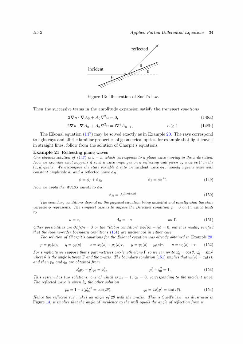
B5.2 Applied Partial Differential Equations 34
incident
reflected
Figure 13: Illustration of Snell’s law.
Then the successive terms in the amplitude expansion satisfy the transport equations
2∇u ·∇A0 +A0∇2u = 0, (148a)
2∇u ·∇An +An∇2u = i∇2An−1, n ≥ 1. (148b)
The Eikonal equation (147) may be solved exactly as in Example 20. The rays correspondto light rays and all the familiar properties of geometrical optics, for example that light travelsin straight lines, follow from the solution of Charpit’s equations.
Example 21 Reflecting plane wavesOne obvious solution of (147) is u = x, which corresponds to a plane wave moving in the x-direction.Now we examine what happens if such a wave impinges on a reflecting wall given by a curve Γ in the(x, y)-plane. We decompose the state variable φ into an incident wave φI , namely a plane wave withconstant amplitude a, and a reflected wave φR:
φ = φI + φR, φI = aeikx. (149)
Now we apply the WKBJ ansatz to φR:
φR = Aeiku(x,y). (150)
The boundary conditions depend on the physical situation being modelled and exactly what the statevariable φ represents. The simplest case is to impose the Dirichlet condition φ = 0 on Γ, which leadsto
u = x, A0 = −a on Γ. (151)
Other possibilities are ∂φ/∂n = 0 or the “Robin condition” ∂φ/∂n + λφ = 0, but it is readily verifiedthat the leading-order boundary conditions (151) are unchanged in either case.
The solution of Charpit’s equations for the Eikonal equation was already obtained in Example 20:
p = p0(s), q = q0(s), x = x0(s) + p0(s)τ, y = y0(s) + q0(s)τ, u = u0(s) + τ. (152)
For simplicity we suppose that s parametrises arc-length along Γ so we can write x′0 = cos θ, y′0 = sin θwhere θ is the angle between Γ and the x-axis. The boundary condition (151) implies that u0(s) = x0(s),and then p0 and q0 are obtained from
x′0p0 + y′0q0 = x′0, p20 + q20 = 1. (153)
This system has two solutions, one of which is p0 = 1, q0 = 0, corresponding to the incident wave.The reflected wave is given by the other solution
p0 = 1− 2(y′0)2 = cos(2θ), q0 = 2x′0y′0 = sin(2θ). (154)
Hence the reflected ray makes an angle of 2θ with the x-axis. This is Snell’s law: as illustrated inFigure 13, it implies that the angle of incidence to the wall equals the angle of reflection from it.
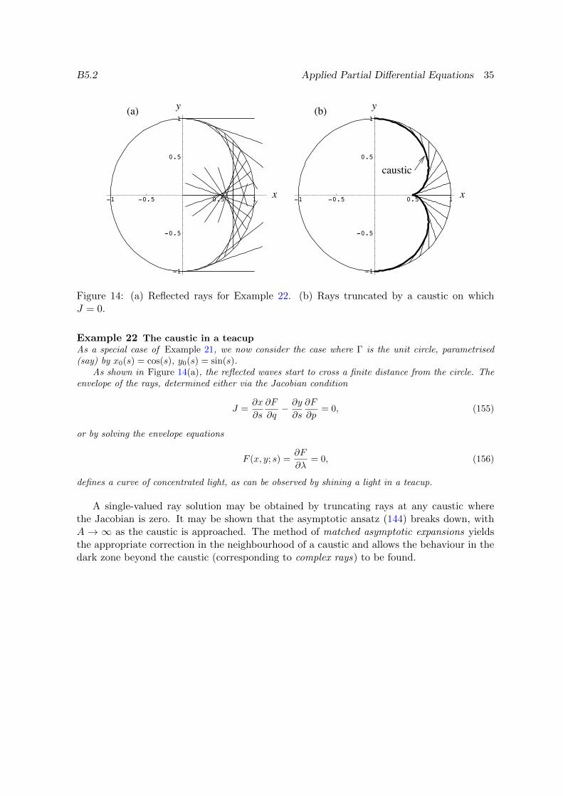
B5.2 Applied Partial Differential Equations 35
-1 -0.5 0.5 1
-1
-0.5
0.5
1
-1 -0.5 0.5 1
-1
-0.5
0.5
1
y y
x x
caustic
(a) (b)
Figure 14: (a) Reflected rays for Example 22. (b) Rays truncated by a caustic on whichJ = 0.
Example 22 The caustic in a teacupAs a special case of Example 21, we now consider the case where Γ is the unit circle, parametrised(say) by x0(s) = cos(s), y0(s) = sin(s).
As shown in Figure 14(a), the reflected waves start to cross a finite distance from the circle. Theenvelope of the rays, determined either via the Jacobian condition
J =∂x
∂s
∂F
∂q− ∂y
∂s
∂F
∂p= 0, (155)
or by solving the envelope equations
F (x, y; s) =∂F
∂λ= 0, (156)
defines a curve of concentrated light, as can be observed by shining a light in a teacup.
A single-valued ray solution may be obtained by truncating rays at any caustic wherethe Jacobian is zero. It may be shown that the asymptotic ansatz (144) breaks down, withA → ∞ as the caustic is approached. The method of matched asymptotic expansions yieldsthe appropriate correction in the neighbourhood of a caustic and allows the behaviour in thedark zone beyond the caustic (corresponding to complex rays) to be found.
B5.2 Applied Partial Differential Equations 36
5 First order systems
5.1 Introduction
In this chapter we consider first-order systems of PDEs of the form
A(x, y,u)∂u
∂x+ B(x, y,u)
∂u
∂y= c(x, y,u), (157)
where now the unknown u is an n-dimensional vector function of x and y, c is also ann-dimensional vector, A and B are n × n matrices. Again, we only consider quasilinearequations, so that (157) is linear in the first derivatives of u. Equations of the form (157)arise frequently in physical problems (e.g. gas dynamics), in which it is often the case thatone of the independent variables represents time, so we will also write (157) in the form
A(x, t,u)∂u
∂t+ B(x, t,u)
∂u
∂x= c(x, t,u). (158)
The other motivation for studying (157) is that many higher-order scalar equations may bewritten in this form.
Example 23 The shallow-water equations describe the flow of a thin layer of liquid over a flatsurface under gravity. If x measures horizontal distance and t is time, then the dimensionless heighth(x, t) and velocity u(x, t) satisfy
∂h
∂t+ u
∂h
∂x+ h
∂u
∂x= 0,
∂u
∂t+ u
∂u
∂x+∂h
∂x= 0, (159)
which may be written in the form (158), with
u =
(hu
), A =
(1 00 1
), B =
(u h1 u
), c =
(00
). (160)
Example 24 Laplace’s equation∂2φ
∂x2+∂2φ
∂y2= 0 (161)
may be written as a first-order system by setting u = ∂φ/∂x, v = −∂φ/∂y. Then u and v satisfy theCauchy–Riemann equations
∂u
∂x− ∂v
∂y= 0,
∂u
∂y+∂v
∂x= 0, (162)
which are in the form of (157), with
u =
(uv
), A =
(1 00 1
), B =
(0 −11 0
), c =
(00
). (163)
(Once u and v are known, φ is found by solving either ∂φ/∂x = u or ∂φ/∂y = −v.)
5.2 Cauchy data
Definition
For the PDE system (157), Cauchy data is to specify u on a curve Γ in the (x, y) plane, i.e.
x = x0(s), y = y0(s), u = u0(s), s1 ≤ s ≤ s2, (164)
B5.2 Applied Partial Differential Equations 37
and the PDE (157) together with the data (164) is known as the Cauchy problem. As for thescalar case, we now ask whether the Cauchy problem determines the first derivatives of u.
Differentiating (164) with respect to s, we find
du0
ds=
dx0
ds
∂u
∂x+
dy0
ds
∂u
∂y. (165)
Now we consider (157) and (165) as a (2n) × (2n) matrix system for the (2n)-dimensionalvector (∂u/∂x, ∂u/∂y)T : (
A Bx′0I y′0I
)(∂u/∂x∂u/∂y
)=
(cu′0
), (166)
where ′ is shorthand for d/ds and I is the n × n identity matrix. The system (166) may besolved uniquely for the first derivatives of u provided the determinant of the matrix on theleft-hand side is nonzero, and this determinant may be rearranged to give
det(x′0B − y′0A
)6= 0. (167)
This is the condition on the initial data for the the first derivatives of u to be locally deter-mined. It clearly reduces to the condition found for scalar equations when n = 1.
Cauchy–Kowalevski theorem
Now we state a generalisation of the theorem previously introduced for scalar PDEs. Forsimplicity we suppose that a coordinate transformation is used to shift the boundary Γ ontothe y-axis, where we specify u:
u = u0(y) on x = 0, y1 ≤ y ≤ y2. (168)
Clearly, so long as u0 is differentiable, we can calculate ∂u/∂y directly:
∂u
∂y=
du0
dyon x = 0, y1 ≤ y ≤ y2. (169)
We can then use the PDE (157) to solve for ∂u/∂x,
∂u
∂x= A−1c−A−1B
∂u
∂y= f
(x, y,u,
∂u
∂y
), say, (170)
so long as A is invertible. Thus the PDE may be written in the form (170) provided |A| 6= 0,which is the same as condition (167), with x0 = 0, y0 = s.
Now suppose that u0(y) is analytic at a point y0 ∈ (y1, y2) and that f is analytic in allits arguments at the point (
0, y0,u0(y0),du0
dy(y0)
).
Then the Cauchy-Kowalevski theorem says that the Cauchy problem (168, 170) has a uniqueanalytic solution u(x, y) in a neighbourhood of (0, y0).
The proof of this theorem works by constructing a Taylor expansion for u and showingit has a finite radius of convergence. It may readily be extended to the case of a generalanalytic initial curve Γ if the condition (167) is satisfied. However, the result is entirely local:the radius of convergence may be extremely small, meaning that u may become singular ornonunique a short distance from the initial data. Moreover, the hypotheses of the theoremare rather restrictive: it says nothing about existence or uniqueness of solutions when theinitial data (say) are nonanalytic.
B5.2 Applied Partial Differential Equations 38
5.3 Characteristics
Definition
There is not a straightforward geometric interpretation of the PDE system (157) as there isin the scalar case. At the very least we have to imagine n solution surfaces — one for eachcomponent of u. There is also no obvious generalisation of the characteristic ODEs. Recall,though, that for scalar PDEs, characteristics are curves on which Cauchy data does not allowthe the first derivatives of u to be determined uniquely, and this definition does generalise ton dimensions.
Consider a curve in the (x, y) plane, parameterised by τ , and suppose that u is known onthis curve. Then, according to (167), the first derivatives of u may be found locally unless
det
(dx
dτB − dy
dτA
)= 0. (171)
A curve (x(τ), y(τ)) satisfying (171) is called a characteristic projection. Since there is nogeneralisation of the concept of characteristic introduced previously for scalar PDEs, it isusual to drop the word “projection” and refer to these plane curves simply as characteristics.
As for scalar PDEs, an alternative definition is that characteristics are curves across whichthe first derivatives of u may be discontinuous. Suppose u is continuous across a curve C inthe (x, y) plane, but its first derivatives take different limiting values (denoted by + and −)on either side of C. If C is parametrised by x = x(ξ), y = y(ξ). Then, by differentiating ualong either side of C, we obtain
du
dξ=∂u+
∂x
dx
dξ+∂u+
∂y
dy
dξ=∂u−
∂x
dx
dξ+∂u−
∂y
dy
dξ(172)
and by subtracting these two equations we find
dx
dξ
[∂u
∂x
]+
−+
dy
dξ
[∂u
∂y
]+
−= 0. (173)
Similarly, because u satisfies the PDE (157) on either side of C, we have
A
[∂u
∂x
]+
−+ B
[∂u
∂y
]+
−= 0. (174)
The homogeneous system (173, 174) implies that the jumps in ∂u/∂x and ∂u/∂y must bezero unless the determinant of the system is zero, which implies that
det
(dx
dξB − dy
dξA
)= 0, (175)
i.e. that C is a characteristic.
Classification
The slopes of the characteristics satisfy the eigenvalue problem
dy
dx= λ where det (B − λA) = 0. (176)
Thus λ satisfies an nth-order polynomial equation, whose roots may be complex in general.A 2× 2 system may be classified as follows, depending on the eigenvalues λ.
B5.2 Applied Partial Differential Equations 39
• If there are two distinct real eigenvalues, then the system is said to be hyperbolic.
• If there is one repeated real eigenvalue, then the system is parabolic.
• If the eigenvalues are complex, then the system is called elliptic.
Example 25 Consider the quasilinear second-order PDE
a∂2φ
∂x2+ 2b
∂2φ
∂x∂y+ c
∂2φ
∂y2= f, (177)
where a, b and f are in general functions of x, y, φ, ∂φ/∂x and ∂φ/∂y. We can write (177) as thefirst-order system(
a b0 −1
)∂u
∂x+
(b c1 0
)∂u
∂y=
(f0
), where u =
(∂φ/∂x∂φ/∂y
). (178)
If a, b, c and f are independent of φ, then we can ignore the uncoupled equation ∂φ/∂x = u, and thecharacteristic slopes satisfy ∣∣∣∣b− λa c− λb
1 λ
∣∣∣∣ = 0
⇒ aλ2 − 2bλ+ c = 0. (179)
The system is thus hyperbolic if b2 > ac, parabolic if b2 = ac, elliptic if b2 < ac.
In dimensions higher than two, there are clearly many possible combinations of real,complex, distinct and repeated roots of the polynomial equation (176), and there is no suchsimple classification. However, we still define an equation as hyperbolic if (176) has ndistinct real roots λ. Since the matrices A and B depend on x, y and, in general, also on thesolution u, the type of the equation (i.e., hyperbolic, elliptic, parabolic or some hybrid) mayalso vary with position.
Now, according to the Cauchy–Kowalevski theorem, provided all our coefficients and initialdata are analytic and the condition (167) is satisfied, there is a unique solution for u in aneighbourhood of Γ. Nevertheless, unless the PDE is hyperbolic, the Cauchy problem is ingeneral ill posed. This may manifest itself in several ways. For example, the unique localsolution may blow up arbitrarily close to Γ or may be pathalogically sensitive to the initialdata.
Example 26 For the Cauchy–Riemann equations, the characteristic slopes satisfy∣∣∣∣−λ −11 −λ
∣∣∣∣ = 0 ⇒ λ = ±i, (180)
so the system is elliptic.Suppose we try to solve (162) in y > 0 subject to the Cauchy data
u = u0(x) = 0, v = v0(x) =εδ2
x2 + δ2on y = 0, (181)
B5.2 Applied Partial Differential Equations 40
where ε and δ are positive constants. Notice that the initial data are analytic and bounded: v0(x) is inthe range (0, ε] for all x. It may be shown1 that the solution of this problem is
u =2εδ2xy
[x2 + (y − δ)2] [x2 + (y + δ)2], v =
εδ2[x2 − y2 + δ2
][x2 + (y − δ)2] [x2 + (y + δ)2]
. (182)
Thus, however small ε is, both u and v blow up at the point (0, δ): by choosing δ small, we can makethe solution break down arbitrarily close to the initial curve y = 0.
For the remainder of this chapter we restrict our attention to hyperbolic systems, for whichthe Cauchy problem is generally well posed, and for which characteristic methods analogousto those used for scalar equations can be applied. So, at each point in the (x, y) plane, weassume that (171) defines n distinct real eigenvalues λ. Thus, by solving dy/dx = λ for eachof these n characteristic slopes, we can obtain in principle n families of characteristics for ann-dimensional hyperbolic system.
5.4 Integration along characteristics
Reduction to an ODE
Suppose λ is a real eigenvalue of (176); recall that λ is in general a function of x, y and u,since A and B are. Now the matrix (B−λA) is singular, so there exists a left eigenvector lT ,such that
lT (B − λA) = 0T , that is lTB = λlTA. (183)
Multiplying the PDE (157) on the left by lT , we obtain
lTA∂u
∂x+ lTB
∂u
∂y= lTc
⇒ lTA
(∂u
∂x+ λ
∂u
∂y
)= lTc. (184)
Along characteristics, whose slope is dy/dx = λ, we have
lTAdu
dx= lTc. (185)
This is the equivalent of the ODE satisfied by u along characteristics in the scalar case. Thereis one ODE of the form (185) satisfied along each of the n families of characteristics.
Riemann invariants
Since (185) is a single differential equation for the n components of u, it is usually notintegrable. However, there are special cases in which the ODE (185) may be rearranged totake the form
d
dx
[R(x, y,u)
]= 0. (186)
1the Cauchy–Riemann equations imply that u + iv is a function of z = x + iy; here, u and v are the realand imaginary parts of the complex function
f(z) =εδ2i
z2 + δ2.
B5.2 Applied Partial Differential Equations 41
If so, the function R is conserved along the characteristics satisfying dy/dx = λ, and is calleda Riemann invariant.
Example 27 Consider the system
∂u
∂x− ∂v
∂y= 0,
∂u
∂y− ∂v
∂x= 0, (187)
which may be written in the form (157) with
u =
(uv
), A =
(1 00 −1
), B =
(0 −11 0
), c =
(00
). (188)
The characteristic slopes satisfy∣∣∣∣−λ −11 λ
∣∣∣∣ = 0 ⇒ λ = ±1, (189)
so the system is hyperbolic. Now we have to solve
lT (B − λA) = lT(∓1 −11 ±1
)= 0T , (190)
and a suitable left eigenvector is lT = (1, ±1). When we multiply the system(1 00 −1
)∂
∂x
(uv
)+
(0 −11 0
)∂
∂y
(uv
)=
(00
)(191)
on the left by lT , we obtain
(1 ∓1
) ∂
∂x
(uv
)+(±1 −1
) ∂∂y
(uv
)= 0. (192)
Using the fact that dy/dx = λ = ±1, this may be rearranged to give
d
dx(u∓ v) = 0, (193)
so the Riemann invariants u∓ v are conserved along the characteristics dy/dx = ±1.In this simple case, the Riemann invariants may be used to write down the general solution. Since
u+v is constant when y+x is constant, we must have u+v = f(y+x) for some function f . Similarly,u− v must take the form g(y − x), so the general solution is
u = 12f(y + x) + 1
2g(y − x), v = 12f(y + x)− 1
2g(y − x), (194)
where f and g are two arbitrary functions. Note that, if we cross-differentiate to eliminate v, we findthat u satisfies the wave equation
∂2u
∂x2− ∂u
∂y2= 0. (195)
For linear hyperbolic PDEs with c = 0, as in Example 27, we can always find a com-plete set of n Riemann invariants. Furthermore, for linear PDEs, the characteristics maybe found independently of the solution. We thus obtain a system of n algebraic equationsfor the components of u in terms of arbitrary functions that are constant along each familyof characteristics. This suggests a plausible method for solving hyperbolic systems numeri-cally. If A, B and c are approximated as being locally constant near Γ, then the resulting
B5.2 Applied Partial Differential Equations 42
autonomous linear system has a complete set of Riemann invariants. Thus the solution u asmall distance from Γ may be found by solving the resulting system of algebraic equations.By repeating this process, the solution may be continued further still from the initial data.This proposed procedure suggests that the Cauchy problem should usually be well posed forhyperbolic systems.
The following two examples show that, when c is nonzero, even linear PDEs have noRiemann invariants in general.
Example 28 The system
∂u
∂x− ∂v
∂y= u+ v,
∂u
∂y− ∂v
∂x= 0 (196)
may be written as (1 00 −1
)∂u
∂x+
(0 −11 0
)∂u
∂y=
(u+ v
0
),
where u = (u, v)T . As in Example 27, the characteristic directions are dy/dx = λ = ±1 and thecorresponding left eigenvectors are lT = (1,±1). Now, the ODEs satisfied along the characteristics are
d
dx(u∓ v) = u+ v on
dy
dx= ±1, (197)
only one of which is integrable:
d
dx(u+ v) = u+ v ⇒ e−x(u+ v) = const on
dy
dx= −1. (198)
Nevertheless, we can use this single Riemann invariant to find the general solution in this case.Since e−x(u+ v) is constant when (y + x) is constant, we may write
u+ v = exf(y + x), (199)
where f is an arbitrary function. Along the other family of characteristics we have (y − x) = const = k,say, so
d
dx(u− v) = u+ v = exf(y + x) = exf(k + 2x) on y − x = k. (200)
This may be integrated with respect to x to give
u− v = 12e(x−y)/2
∫ y+x
0
es/2f(s) ds+ g(y − x), (201)
where g is a second arbitrary function. The general solution is, therefore,
u =1
2exf(y + x) +
1
2g(y − x) +
1
4e(x−y)/2
∫ y+x
0
es/2f(s) ds, (202a)
v =1
2exf(y + x)− 1
2g(y − x)− 1
4e(x−y)/2
∫ y+x
0
es/2f(s) ds. (202b)
Example 29 The system
∂u
∂x− ∂v
∂y= u,
∂u
∂y− ∂v
∂x= 0 (203)
has characteristic equations
d
dx(u∓ v) = u on
dy
dx= ±1, (204)
which cannot be integrated. There are no Riemann invariants and no way to find the general solutionexplicitly.
B5.2 Applied Partial Differential Equations 43
The situation is even worse for fully nonlinear systems, where the characteristics dependon the solution u. Even when such systems have a complete set of n Riemann invariants,since we do not know in advance the curves along which each is conserved, we cannot ingeneral find an explicit solution.
Example 30 The shallow-water equations (159) have characteristic slopes given by
det (B − λA) =
∣∣∣∣u− λ h1 u− λ
∣∣∣∣ = (u− λ)2 − h = 0
⇒ dx
dt= λ = u±
√h, (205)
and the corresponding left eigenvectors are (1, ±√h). The characteristic ODEs are
dh
dt±√h
du
dt= 0 on
dx
dt= u±
√h
⇒ d
dt
(u± 2
√h)
= 0 ondx
dt= u±
√h, (206)
so the Riemann invariants u± 2√h are preserved along the characteristics dx/dt = u±
√h. Although
the system has two Riemann invariants, we cannot infer the general solution.
Regions of influence
Recall that, for scalar PDEs, where Cauchy data are only given on a finite initial curve Γ, thesolution is only determined in the so-called domain of definition, penetrated by characteristicsemanating from Γ. In n dimensions, the domain of definition is the region penetrated by alln families of characteristics originating at Γ. Where there are at least one but fewer than nfamilies of characteristics, the solution is influenced but not fully determined by the Cauchydata on Γ. The region swept out by all the characteristics intersecting Γ is therefore calledthe region of influence.
Example 31 We return to the system considered in Example 27, which has the general solution
u = 12f(y + x) + 1
2g(y − x), v = 12f(y + x)− 1
2g(y − x). (207)
If we are given the Cauchy data u = u0(x), v = v0(x) on y = 0, 0 < x < 1, then we can determine thetwo arbitrary functions f and g:
f(s) = u0(s) + v0(s), 0 < s < 1, (208a)
g(s) = u0(−s)− v0(−s), − 1 < s < 0. (208b)
The solution for u is, therefore,
u = 12
u0(y + x) + v0(y + x) + u0(x− y)− v0(x− y)
, (209)
and a similar expression for v may readily be found.In (209), the first two terms correspond to the function f and are defined in 0 < y + x < 1,
while the final two terms, corresponding to g, are defined in 0 < x − y < 1. The region of influenceis the union of these two domains, where either f or g is defined. The domain of definition is theintersection, where both f and g are defined, that is, 0 < y < max(x, 1− x). They are both illustratedin Figure 15.
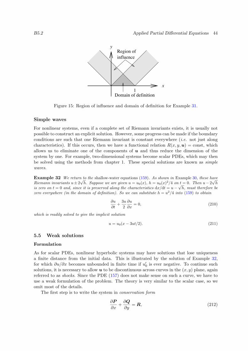
B5.2 Applied Partial Differential Equations 44
influence
y
x1
Domain of definition
Region of
Figure 15: Region of influence and domain of definition for Example 31.
Simple waves
For nonlinear systems, even if a complete set of Riemann invariants exists, it is usually notpossible to construct an explicit solution. However, some progress can be made if the boundaryconditions are such that one Riemann invariant is constant everywhere (i.e. not just alongcharacteristics). If this occurs, then we have a functional relation R(x, y,u) = const, whichallows us to eliminate one of the components of u and thus reduce the dimension of thesystem by one. For example, two-dimensional systems become scalar PDEs, which may thenbe solved using the methods from chapter 1. These special solutions are known as simplewaves.
Example 32 We return to the shallow-water equations (159). As shown in Example 30, these haveRiemann invariants u± 2
√h. Suppose we are given u = u0(x), h = u0(x)2/4 on t = 0. Then u− 2
√h
is zero on t = 0 and, since it is preserved along the characteristics dx/dt = u−√h, must therefore be
zero everywhere (in the domain of definition). So we can substitute h = u2/4 into (159) to obtain
∂u
∂t+
3u
2
∂u
∂x= 0, (210)
which is readily solved to give the implicit solution
u = u0(x− 3ut/2). (211)
5.5 Weak solutions
Formulation
As for scalar PDEs, nonlinear hyperbolic systems may have solutions that lose uniquenessa finite distance from the initial data. This is illustrated by the solution of Example 32,for which ∂u/∂x becomes unbounded in finite time if u′0 is ever negative. To continue suchsolutions, it is necessary to allow u to be discontinuous across curves in the (x, y) plane, againreferred to as shocks. Since the PDE (157) does not make sense on such a curve, we have touse a weak formulation of the problem. The theory is very similar to the scalar case, so weomit most of the details.
The first step is to write the system in conservation form
∂P
∂x+∂Q
∂y= R, (212)
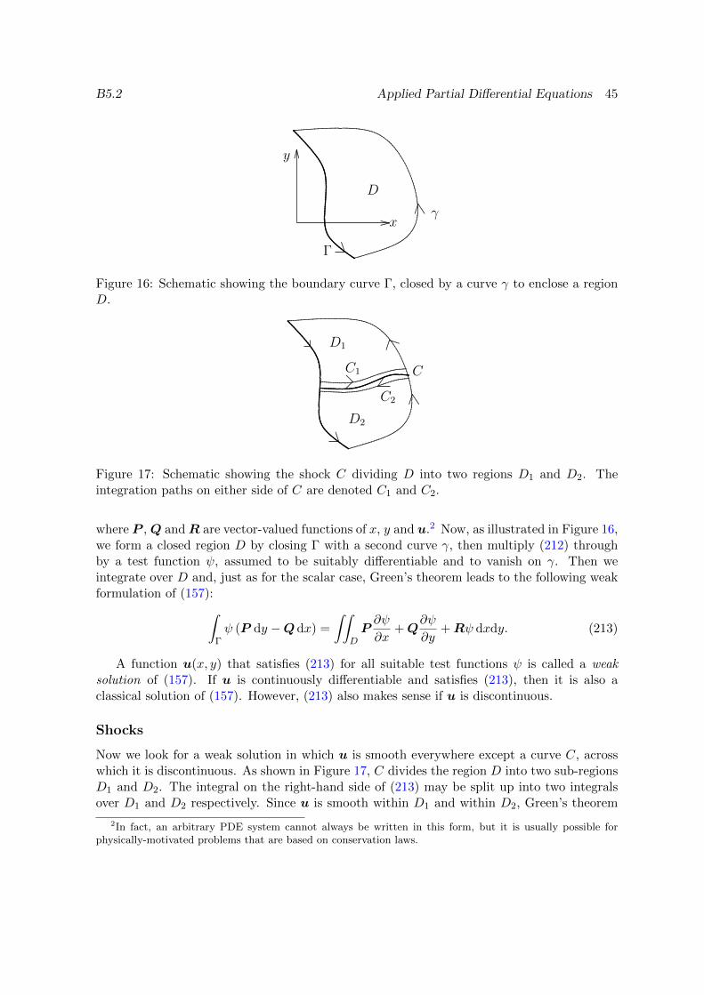
B5.2 Applied Partial Differential Equations 45
......................................
......................................
...............................................
......................
ppppppppppppppppppppppppppppppppppppppppppppppppppppppppppppppppppppppppppppppppppppppppppppppppppppppppppppppppppppppppppppppppppppppppppppppppppppppppppppppppppppppppppppppppppppppppppppppppppppppppppppppppppppppppppppppppppppppppppppppppppppppppppppppppppppppppppppppppppppppppppppppppppppppppppppppppppppppppppppppppppppppppppppppppppppppppp
..................................................................................................... ...........................................................................................................................................................................................................................................................................................................................................................................................................................................................................................................
D
y
x
Γ
γ
Figure 16: Schematic showing the boundary curve Γ, closed by a curve γ to enclose a regionD.
........................................
.........................
............................................
......................
...............................................
ppppppppppppppppppppppppppppppppppppppppppppppppppppppppppppppppppppppppppppppppppppppppppppppppppppppppppppppppppppppppppppppppppppppppppppppppppppppppppppppppppppppppppppppppppppppppppppppppppppppppppppppppppppppppppppppppppppppppppppppppppppppppppppppppppppppppppppppppppppppppppppppppppppppppppppppppppppppppppppppppppppppppppppppppppppppppp
..................................................................................................... ...........................................................................................................................................................................................................................................................................................................................................................................................................................................................................................................
ppppppppppppppppppppppppppppppppppppp ppppp ppppppppppppppppppppppppppppppppppppppppppppppppppppppppppppppppppppppppppppppppppppppppppppppppppppppppppppppppppppppppppppppppppppppppppp ppppppppppppppppppppppC..........................................................................................................................................................................................................
.................................................. .................................................................
.................................................
.........................................
D1
D2
C1
C2
Figure 17: Schematic showing the shock C dividing D into two regions D1 and D2. Theintegration paths on either side of C are denoted C1 and C2.
where P , Q and R are vector-valued functions of x, y and u.2 Now, as illustrated in Figure 16,we form a closed region D by closing Γ with a second curve γ, then multiply (212) throughby a test function ψ, assumed to be suitably differentiable and to vanish on γ. Then weintegrate over D and, just as for the scalar case, Green’s theorem leads to the following weakformulation of (157):∫
Γψ (P dy −Q dx) =
∫∫DP∂ψ
∂x+ Q
∂ψ
∂y+ Rψ dxdy. (213)
A function u(x, y) that satisfies (213) for all suitable test functions ψ is called a weaksolution of (157). If u is continuously differentiable and satisfies (213), then it is also aclassical solution of (157). However, (213) also makes sense if u is discontinuous.
Shocks
Now we look for a weak solution in which u is smooth everywhere except a curve C, acrosswhich it is discontinuous. As shown in Figure 17, C divides the region D into two sub-regionsD1 and D2. The integral on the right-hand side of (213) may be split up into two integralsover D1 and D2 respectively. Since u is smooth within D1 and within D2, Green’s theorem
2In fact, an arbitrary PDE system cannot always be written in this form, but it is usually possible forphysically-motivated problems that are based on conservation laws.
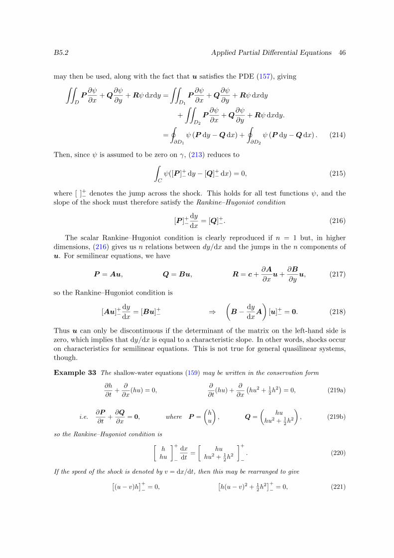
B5.2 Applied Partial Differential Equations 46
may then be used, along with the fact that u satisfies the PDE (157), giving∫∫DP∂ψ
∂x+ Q
∂ψ
∂y+ Rψ dxdy =
∫∫D1
P∂ψ
∂x+ Q
∂ψ
∂y+ Rψ dxdy
+
∫∫D2
P∂ψ
∂x+ Q
∂ψ
∂y+ Rψ dxdy.
=
∮∂D1
ψ (P dy −Qdx) +
∮∂D2
ψ (P dy −Q dx) . (214)
Then, since ψ is assumed to be zero on γ, (213) reduces to∫Cψ([P ]+− dy − [Q]+− dx) = 0, (215)
where [ ]+− denotes the jump across the shock. This holds for all test functions ψ, and theslope of the shock must therefore satisfy the Rankine–Hugoniot condition
[P ]+−dy
dx= [Q]+−. (216)
The scalar Rankine–Hugoniot condition is clearly reproduced if n = 1 but, in higherdimensions, (216) gives us n relations between dy/dx and the jumps in the n components ofu. For semilinear equations, we have
P = Au, Q = Bu, R = c +∂A
∂xu +
∂B
∂yu, (217)
so the Rankine–Hugoniot condition is
[Au]+−dy
dx= [Bu]+− ⇒
(B − dy
dxA
)[u]+− = 0. (218)
Thus u can only be discontinuous if the determinant of the matrix on the left-hand side iszero, which implies that dy/dx is equal to a characteristic slope. In other words, shocks occuron characteristics for semilinear equations. This is not true for general quasilinear systems,though.
Example 33 The shallow-water equations (159) may be written in the conservation form
∂h
∂t+
∂
∂x(hu) = 0,
∂
∂t(hu) +
∂
∂x
(hu2 + 1
2h2)
= 0, (219a)
i.e.∂P
∂t+∂Q
∂x= 0, where P =
(hu
), Q =
(hu
hu2 + 12h
2
), (219b)
so the Rankine–Hugoniot condition is[hhu
]+−
dx
dt=
[hu
hu2 + 12h
2
]+−. (220)
If the speed of the shock is denoted by v = dx/dt, then this may be rearranged to give[(u− v)h
]+− = 0,
[h(u− v)2 + 1
2h2]+− = 0, (221)
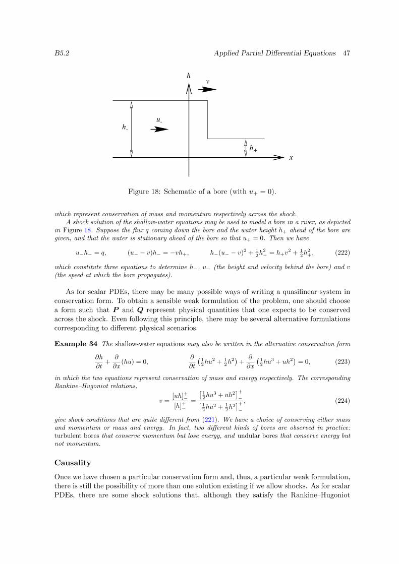
B5.2 Applied Partial Differential Equations 47
h+
h-u-
h
x
v
Figure 18: Schematic of a bore (with u+ = 0).
which represent conservation of mass and momentum respectively across the shock.A shock solution of the shallow-water equations may be used to model a bore in a river, as depicted
in Figure 18. Suppose the flux q coming down the bore and the water height h+ ahead of the bore aregiven, and that the water is stationary ahead of the bore so that u+ = 0. Then we have
u−h− = q, (u− − v)h− = −vh+, h−(u− − v)2 + 12h
2− = h+v
2 + 12h
2+, (222)
which constitute three equations to determine h−, u− (the height and velocity behind the bore) and v(the speed at which the bore propagates).
As for scalar PDEs, there may be many possible ways of writing a quasilinear system inconservation form. To obtain a sensible weak formulation of the problem, one should choosea form such that P and Q represent physical quantities that one expects to be conservedacross the shock. Even following this principle, there may be several alternative formulationscorresponding to different physical scenarios.
Example 34 The shallow-water equations may also be written in the alternative conservation form
∂h
∂t+
∂
∂x(hu) = 0,
∂
∂t
(12hu
2 + 12h
2)
+∂
∂x
(12hu
3 + uh2)
= 0, (223)
in which the two equations represent conservation of mass and energy respectively. The correspondingRankine–Hugoniot relations,
v =[uh]+−[h]+−
=
[12hu
3 + uh2]+−[
12hu
2 + 12h
2]+−
, (224)
give shock conditions that are quite different from (221). We have a choice of conserving either massand momentum or mass and energy. In fact, two different kinds of bores are observed in practice:turbulent bores that conserve momentum but lose energy, and undular bores that conserve energy butnot momentum.
Causality
Once we have chosen a particular conservation form and, thus, a particular weak formulation,there is still the possibility of more than one solution existing if we allow shocks. As for scalarPDEs, there are some shock solutions that, although they satisfy the Rankine–Hugoniot
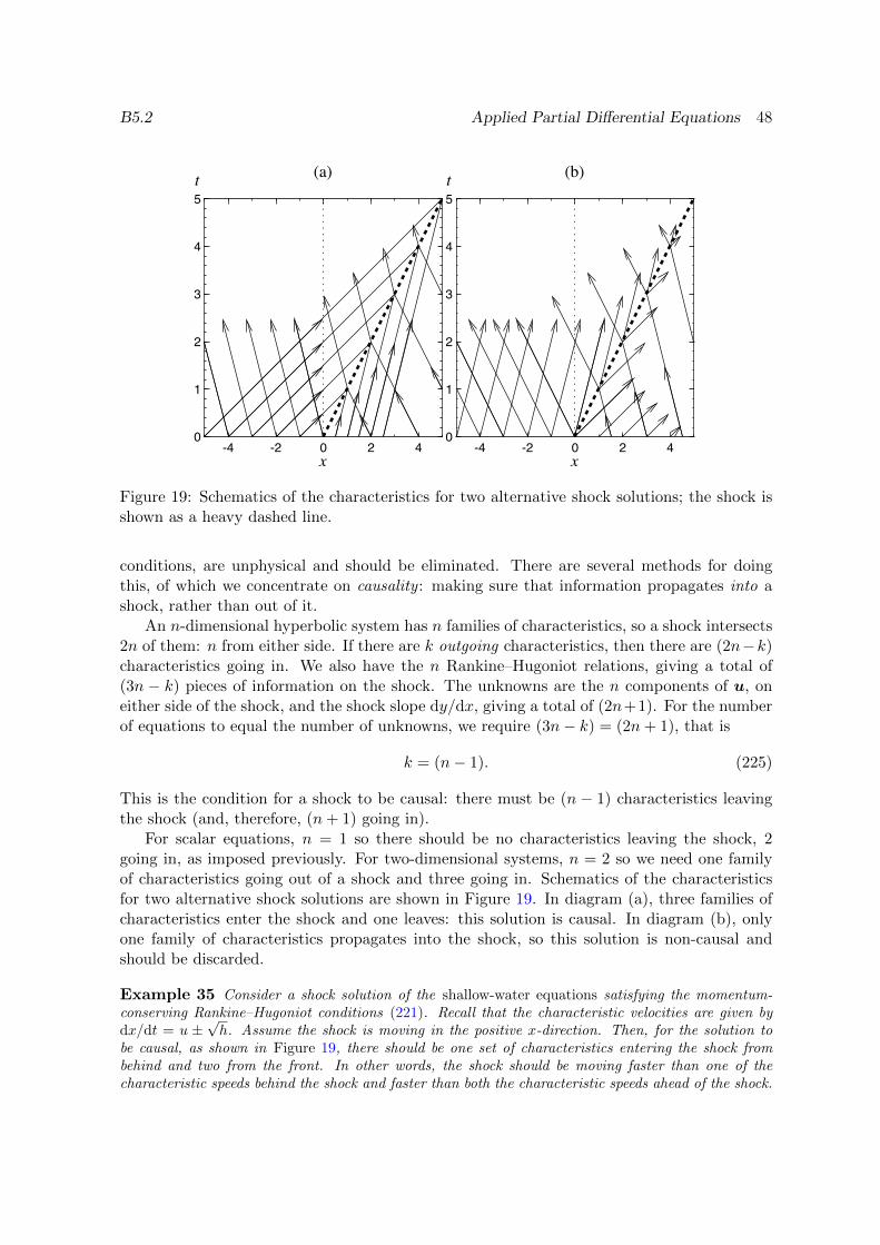
B5.2 Applied Partial Differential Equations 48
-4 -4-2 -20 02 24 40 0
1 1
2 2
3 3
4 4
5 5t t(a) (b)
x x
Figure 19: Schematics of the characteristics for two alternative shock solutions; the shock isshown as a heavy dashed line.
conditions, are unphysical and should be eliminated. There are several methods for doingthis, of which we concentrate on causality : making sure that information propagates into ashock, rather than out of it.
An n-dimensional hyperbolic system has n families of characteristics, so a shock intersects2n of them: n from either side. If there are k outgoing characteristics, then there are (2n−k)characteristics going in. We also have the n Rankine–Hugoniot relations, giving a total of(3n − k) pieces of information on the shock. The unknowns are the n components of u, oneither side of the shock, and the shock slope dy/dx, giving a total of (2n+1). For the numberof equations to equal the number of unknowns, we require (3n− k) = (2n+ 1), that is
k = (n− 1). (225)
This is the condition for a shock to be causal: there must be (n − 1) characteristics leavingthe shock (and, therefore, (n+ 1) going in).
For scalar equations, n = 1 so there should be no characteristics leaving the shock, 2going in, as imposed previously. For two-dimensional systems, n = 2 so we need one familyof characteristics going out of a shock and three going in. Schematics of the characteristicsfor two alternative shock solutions are shown in Figure 19. In diagram (a), three families ofcharacteristics enter the shock and one leaves: this solution is causal. In diagram (b), onlyone family of characteristics propagates into the shock, so this solution is non-causal andshould be discarded.
Example 35 Consider a shock solution of the shallow-water equations satisfying the momentum-conserving Rankine–Hugoniot conditions (221). Recall that the characteristic velocities are given bydx/dt = u ±
√h. Assume the shock is moving in the positive x-direction. Then, for the solution to
be causal, as shown in Figure 19, there should be one set of characteristics entering the shock frombehind and two from the front. In other words, the shock should be moving faster than one of thecharacteristic speeds behind the shock and faster than both the characteristic speeds ahead of the shock.
B5.2 Applied Partial Differential Equations 49
Thus we obtain the following four inequalities
u− +√h− > v, u− −
√h− < v, u+ +
√h+ < v, u+ −
√h+ < v, (226)
where, as before, v is the speed of the shock. From these it follows that
(u− − v)2 < h− and (u+ − v)2 > h+, (227)
and the Rankine–Hugoniot condition (221) then leads to the condition
h+ < h−. (228)
Thus the height behind a bore must be greater than that ahead; otherwise the bore is not causal andthe discontinuity cannot be maintained. That all the inequalities in (226) follow from (228), may beverified from the identities
(u+ − v)2 =h−(h+ + h−)
2h+, (u− − v)2 =
h+(h+ + h−)
2h−, (229)
which follow from (221).
B5.2 Applied Partial Differential Equations 50
6 Second order semi-linear equations
6.1 Introduction
Now we consider second-order scalar equations of the form
a(x, y)∂2u
∂x2+ 2b(x, y)
∂2u
∂x∂y+ c(x, y)
∂2u
∂y2= f
(x, y, u,
∂u
∂x,∂u
∂y
). (230)
This is called a semilinear equation because the coefficients a, b and c are independent ofu and its derivatives. Note that a second-order scalar equation like (230) may always betransformed into a first-order system by setting p = ∂u/∂x, q = ∂u/∂y. Where one of theindependent variables is clearly supposed to represent time, we will also write (230) in theform
a(x, t)∂2u
∂t2+ 2b(x, t)
∂2u
∂x∂t+ c(x, t)
∂2u
∂x2= f
(x, t, u,
∂u
∂x,∂u
∂t
). (231)
We will concentrate on three canonical examples of particular importance, namely thewave equation
∂2u
∂t2− ∂2u
∂x2= 0, (232a)
the heat equation∂u
∂t− ∂2u
∂x2= 0, (232b)
and Laplace’s equation∂2u
∂x2+∂2u
∂y2= 0. (232c)
6.2 Cauchy data
Cauchy data for the general second-order quiasi-linear PDE (230) is to specify u and itsnormal derivative on some curve Γ in the (x, y) plane, i.e.
x = x0(s), y = y0(s), u = u0(s),∂u
∂n= v0(s), (233)
where s parametrises Γ. This is equivalent to specifying u and both its first derivatives on Γ,since
du0
ds=∂u
∂x
dx0
ds+∂u
∂y
dy0
ds(234)
and
v0(s) =∂u
∂n=
(∂u
∂x
dy0
ds− ∂u
∂y
dx0
ds
)(dx0
ds
)2
+
(dy0
ds
)2−1/2
(235)
may be solved simultaneously for ∂u/∂x and ∂u/∂y. We may therefore replace (233) with
x = x0(s), y = y0(s), u = u0(s),∂u
∂x= p0(s),
∂u
∂y= q0(s). (236)
B5.2 Applied Partial Differential Equations 51
A necessary condition for the solution u(x, y) to be uniquely defined in a neighbourhoodof Γ is for the second derivatives of u to be determined on Γ. Now, if we differentiate theinitial data along Γ and use the chain rule, we obtain
dp0
ds=
dx0
ds
∂2u
∂x2+
dy0
ds
∂2u
∂x∂y,
dq0
ds=
dx0
ds
∂2u
∂x∂y+
dy0
ds
∂2u
∂y2. (237)
Along with the PDE (230), this gives us a system of three equations for the three secondpartial derivatives of u, and the determinant of this system is∣∣∣∣∣∣∣∣∣
a 2b cdx0
ds
dy0
ds0
0dx0
ds
dy0
ds
∣∣∣∣∣∣∣∣∣ = a
(dy0
ds
)2
− 2bdx0
ds
dy0
ds+ c
(dx0
ds
)2
. (238)
A necessary condition for the Cauchy data (236) to determine u locally is, therefore,
a
(dy0
ds
)2
− 2bdx0
ds
dy0
ds+ c
(dx0
ds
)2
6= 0. (239)
6.3 Characteristics
Definition
As for first-order equations, we define characteristics to be curves in the (x, y) plane on whichCauchy data do not determine a unique solution. If such a curve is parametrised by x = x(τ),y = y(τ) then, from (239), we have
a
(dy
dτ
)2
− 2bdx
dτ
dy
dτ+ c
(dx
dτ
)2
= 0, (240)
so the slopes of the characteristics satisfy
dy
dx= λ where aλ2 − 2bλ+ c = 0 (241)
Characteristics may also be defined as curves across which the second derivatives of u maybe discontinuous, with lower derivatives continuous. It is left as an exercise to show that thisalternative definition leads to the same equation (241) for the characteristic slopes.
Classification
The PDE (230) is classified according to the number of distinct real characteristics it possesses,and this is determined by the sign of the discriminant b2 − ac.
1. b2 > ac implies that there are two distinct real characteristics and the PDE is hyperbolic.
2. b2 < ac implies that there are two complex conjugate characteristics and the PDE iselliptic.
3. b2 = ac implies that there is one repeated real characteristics and the PDE is parabolic.
B5.2 Applied Partial Differential Equations 52
Since a, b and c are functions of x and y, the PDE may change type (i.e. hyperbolic,parabolic or elliptic) from one region to another. However, the type of a PDE at any givenposition is invariant under coordinate transformations.
Example 36 Suppose we transform to new coordinates (X,Y ), which are given as functions of xand y. Then the PDE (230) is transformed to
A∂2u
∂X2+ 2B
∂2u
∂X∂Y+ C
∂2u
∂Y 2= F, (242)
where
A = a
(∂X
∂x
)2
+ 2b∂X
∂x
∂X
∂y+ c
(∂X
∂y
)2
, (243a)
B = a∂X
∂x
∂Y
∂x+ b
(∂X
∂x
∂Y
∂y+∂X
∂y
∂Y
∂x
)+ c
∂X
∂y
∂Y
∂y, (243b)
C = a
(∂Y
∂x
)2
+ 2b∂Y
∂x
∂Y
∂y+ c
(∂Y
∂y
)2
. (243c)
It follows that
B2 −AC =(b2 − ac
)(∂X∂x
∂Y
∂y− ∂X
∂y
∂Y
∂x
)2
, (244)
so that the sign of the discriminant is invariant.
6.4 Canonical forms
Hyperbolic equations
For hyperbolic PDEs, the quadratic equation (241) has two real distinct roots, say λ1(x, y)and λ2(x, y). Now suppose the differential equations dy/dx = λi have first integrals given by
dy
dx= λ1(x, y) ⇒ ξ(x, y) = const, (245a)
dy
dx= λ2(x, y) ⇒ η(x, y) = const. (245b)
Now we change variables from (x, y) to (ξ, η), using the chain rules
∂u
∂x=∂ξ
∂x
∂u
∂ξ+∂η
∂x
∂u
∂η(246)
and so forth. The PDE (230) is clearly transformed to an equation with an analogous form,that is,
α(ξ, η)∂2u
∂ξ2+ β(ξ, η)
∂2u
∂ξ∂η+ γ(ξ, η)
∂2u
∂η2= φ
(ξ, η, u,
∂u
∂ξ,∂u
∂η
). (247)
We know that the characteristics are given by ξ = const and η = const, so the roots of thequadratic form
α
(dη
dτ
)2
− 2βdη
dτ
dξ
dτ+ γ
(dξ
dτ
)2
= 0 (248)
B5.2 Applied Partial Differential Equations 53
must be dξ/dτ = 0 and dη/dτ = 0. It follows that α = γ = 0, so that (247) takes the form
∂2u
∂ξ∂η= φ
(ξ, η, u,
∂u
∂ξ,∂u
∂η
). (249)
This is the so-called canonical form for second-order hyperbolic PDEs.
Example 37 For the PDE∂2u
∂x2− ∂2u
∂y2= f(x, y), (250)
the characteristics are given by(dy
dx
)2
− 1 = 0 ⇒ y ± x = const. (251)
So we set ξ = x− y, η = x+ y and, by changing variables, obtain
∂2u
∂ξ∂η=
1
4f
(ξ + η
2,η − ξ
2
)= φ(ξ, η), say. (252)
This may now be integrated directly to give the so-called D’Alembert solution
u =
∫∫φ(ξ, η) dξdη + h1(ξ) + h2(η). (253)
Elliptic equations
For elliptic equations, the roots of the characteristic equation (241) are complex conjugates,say
dy
dx= λR(x, y)± iλI(x, y). (254)
Suppose that the integrals of these ODEs can be written in the form
ξ(x, y)± iη(x, y) = const, (255)
for some functions ξ and η. Then we use ξ and η as new variables. Again, the transformedequation must be of the form (247) but, this time, the roots of
α
(dη
dτ
)2
− 2βdη
dτ
dξ
dτ+ γ
(dξ
dτ
)2
= 0 (256)
are dξ/dτ ± idη/dτ = 0, which implies that β = 0, γ = α. The canonical form for ellipticPDEs is, therefore,
∂2u
∂ξ2+∂2u
∂η2= φ
(ξ, η, u,
∂u
∂ξ,∂u
∂η
). (257)
Example 38 For the PDE
y2∂2u
∂x2+ 2xy
∂2u
∂x∂y+ 2x2
∂2u
∂y2= 0, (258)
the characteristics satisfy
dy
dx= (1± i)
x
y⇒ (1± i)x2 − y2 = const. (259)
If we choose ξ = x2, η = x2 − y2, then the equation transforms to
∂2u
∂ξ2+∂2u
∂η2= − 1
2ξ
∂u
∂ξ+
(ξ + η
2ξ(ξ − η)
)∂u
∂η. (260)
B5.2 Applied Partial Differential Equations 54
Parabolic equations
For parabolic PDEs, there is one repeated characteristic slope
dy
dx=b
a, (261)
which we suppose has the solution η(x, y) = const. Then any convenient linearly independentfunction ξ(x, y) may be chosen, and the PDE (230) transforms to the canonical form
∂2u
∂ξ2= φ
(ξ, η, u,
∂u
∂ξ,∂u
∂η
). (262)
B5.2 Applied Partial Differential Equations 55
7 Semi-linear hyperbolic equations
7.1 Non-Cauchy data
As stated in Section 5, Cauchy data for second-order equations specifies both u and its normalderivative on a plane curve Γ. In general, however, there may be boundaries on which it isappropriate to prescribe just one BC or even none.
Example 39 Consider a string of length L and density (i.e. mass per unit length) ρ, stretched to atension T between the points x = 0 and x = L. It may be shown that small transverse displacementsu(x, t) satisfy the wave equation
∂2u
∂t2= c2
∂2u
∂x2, (263)
where t is time and c2 = T/ρ. Suppose we wish to determine u(x, t) in the region 0 ≤ x ≤ L,0 ≤ t ≤ T . To do so, we need to specify the initial displacement u(x, 0) = u0(x) and the initial velocity∂u/∂t(x, 0) = v0(x); these correspond to Cauchy data on the initial curve t = 0, 0 ≤ x ≤ L. On theboundary curves x = 0 and x = L, we give just one boundary condition, namely that the displacementis zero: u(0, t) = u(L, t) = 0. Finally, on the boundary t = T we give no boundary conditions at all.
Example 39 illustrates that, in general, the number of BCs needed on any boundary isequal to the number of characteristic families travelling out of that boundary. Where twosets of characteristics travel out, a boundary is called space-like, and two conditions must begiven. On a time-like boundary, with one characteristic family travelling in and one travellingout, just one condition must be given. Finally, no conditions may be given on a boundarywhere all the characteristics travel in.
7.2 Weak solutions
Weak solutions may be defined in a manner analogous to that used to define first-orderPDEs. Notice that, unlike quasilinear equations, the semilinear equations considered here donot spontaneously form shocks. Consequently a discontinuous solution will only arise if dis-continuous initial data are specified. Furthermore, for semilinear equations, all discontinuitiespropagate along characteristics.
7.3 Riemann’s method
Riemann’s method is a way of solving linear hyperbolic equations that are stated in (i.e. havebeen transformed into) canonical form
L[u] =∂2u
∂x∂y+ a(x, y)
∂u
∂x+ b(x, y)
∂u
∂y+ c(x, y)u = f(x, y). (264)
Suppose Cauchy data are given on a curve Γ in the (x, y) plane, so that u, ∂u/∂x and ∂u/∂yare all known on Γ. The condition (239) for these data to determine the solution locallytranslates into the restriction that Γ must be nowehere parallel to either the x- or y-axis.
We define the adjoint of the differential operator L in (264) by
L?[v] =∂2v
∂x∂y− ∂
∂x(av)− ∂
∂y(bv) + cv. (265)
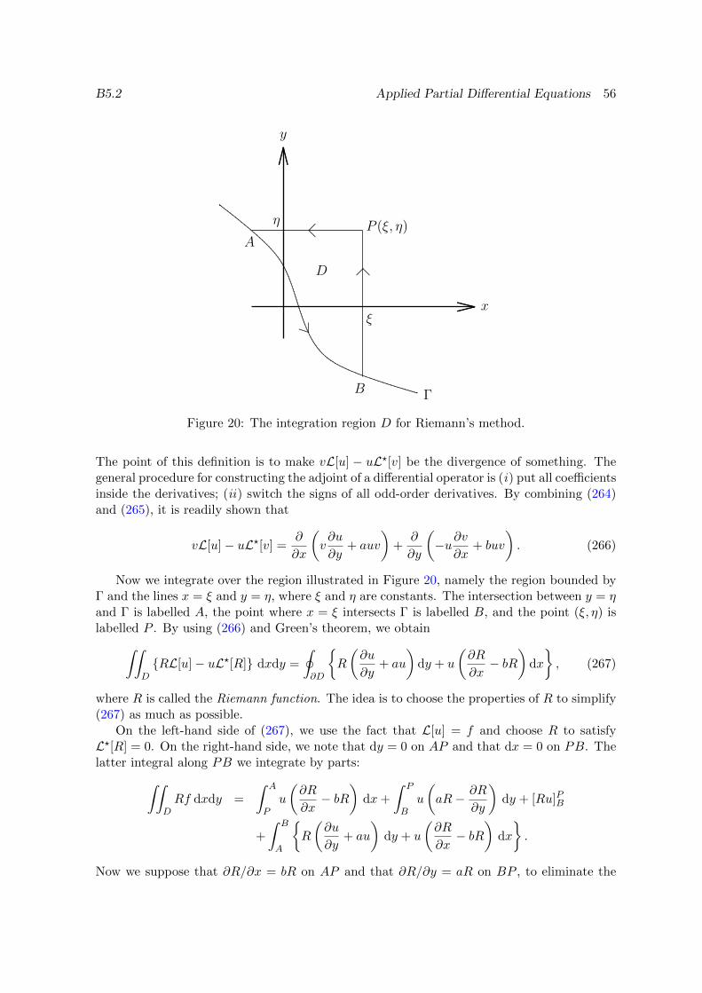
B5.2 Applied Partial Differential Equations 56
pppppppppppppppppppppppppppppppppppppppppppppppppppppppppppppppppppppppppppp
pppppppppppppppppppppppppppppppppppppppppppppppppppppppppppppppppppppppppppp
........................................
........................................
......................
................................................................................................................................................................................................................................................................................................................................................................................................................................................................................................................................................................................................................................................................................................... Γ
ξ
B
A
η P (ξ, η)
x
y
D
Figure 20: The integration region D for Riemann’s method.
The point of this definition is to make vL[u] − uL?[v] be the divergence of something. Thegeneral procedure for constructing the adjoint of a differential operator is (i) put all coefficientsinside the derivatives; (ii) switch the signs of all odd-order derivatives. By combining (264)and (265), it is readily shown that
vL[u]− uL?[v] =∂
∂x
(v∂u
∂y+ auv
)+
∂
∂y
(−u∂v
∂x+ buv
). (266)
Now we integrate over the region illustrated in Figure 20, namely the region bounded byΓ and the lines x = ξ and y = η, where ξ and η are constants. The intersection between y = ηand Γ is labelled A, the point where x = ξ intersects Γ is labelled B, and the point (ξ, η) islabelled P . By using (266) and Green’s theorem, we obtain∫∫
DRL[u]− uL?[R] dxdy =
∮∂D
R
(∂u
∂y+ au
)dy + u
(∂R
∂x− bR
)dx
, (267)
where R is called the Riemann function. The idea is to choose the properties of R to simplify(267) as much as possible.
On the left-hand side of (267), we use the fact that L[u] = f and choose R to satisfyL?[R] = 0. On the right-hand side, we note that dy = 0 on AP and that dx = 0 on PB. Thelatter integral along PB we integrate by parts:∫∫
DRf dxdy =
∫ A
Pu
(∂R
∂x− bR
)dx+
∫ P
Bu
(aR− ∂R
∂y
)dy + [Ru]PB
+
∫ B
A
R
(∂u
∂y+ au
)dy + u
(∂R
∂x− bR
)dx
.
Now we suppose that ∂R/∂x = bR on AP and that ∂R/∂y = aR on BP , to eliminate the
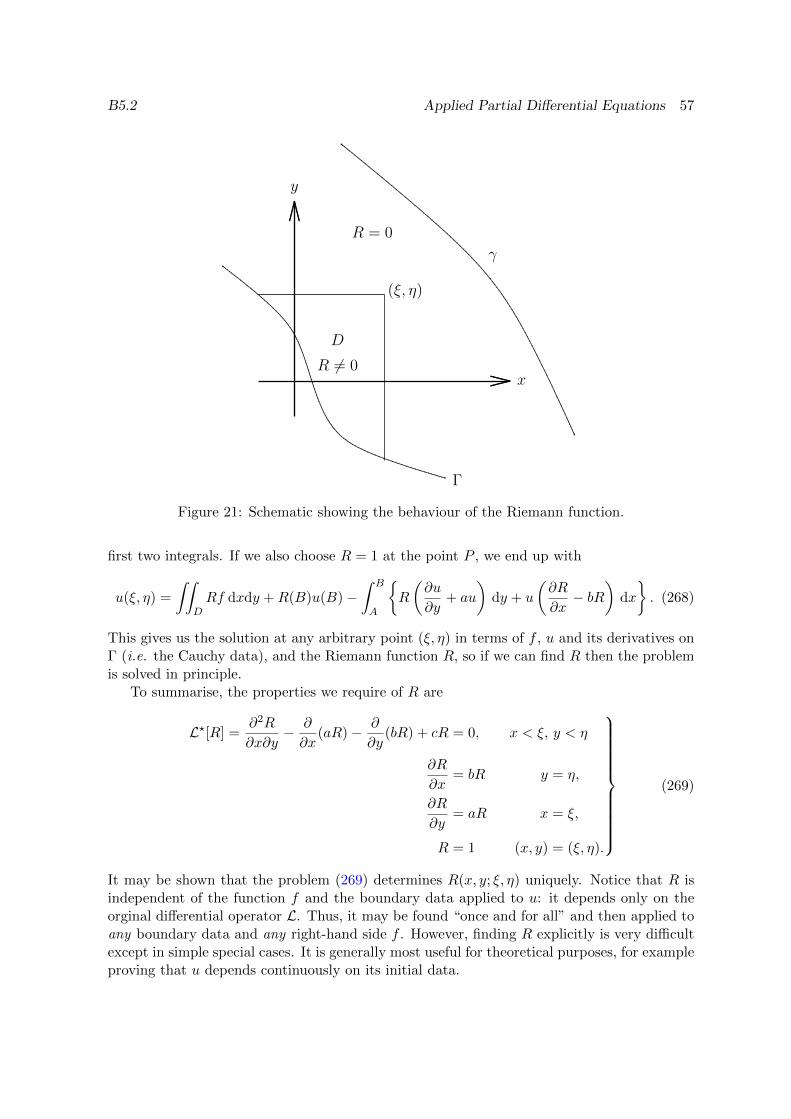
B5.2 Applied Partial Differential Equations 57
pppppppppppppppppppppppppppppppppppppppppppppppppppppppppppppppppppppppppppp
pppppppppppppppppppppppppppppppppppppppppppppppppppppppppppppppppppppppppppp...................................................................................................................................................................................................................................................................................................................................................................................................................................................................................................................................................................................................................................................................................................
..................................................................................................................................................................................................................................................................................................................................................................................................................................................................................................................................................................................................................................................................................................................................................................................................
Γ
(ξ, η)
x
y
γ
D
R = 0
R 6= 0
Figure 21: Schematic showing the behaviour of the Riemann function.
first two integrals. If we also choose R = 1 at the point P , we end up with
u(ξ, η) =
∫∫DRf dxdy +R(B)u(B)−
∫ B
A
R
(∂u
∂y+ au
)dy + u
(∂R
∂x− bR
)dx
. (268)
This gives us the solution at any arbitrary point (ξ, η) in terms of f , u and its derivatives onΓ (i.e. the Cauchy data), and the Riemann function R, so if we can find R then the problemis solved in principle.
To summarise, the properties we require of R are
L?[R] =∂2R
∂x∂y− ∂
∂x(aR)− ∂
∂y(bR) + cR = 0, x < ξ, y < η
∂R
∂x= bR y = η,
∂R
∂y= aR x = ξ,
R = 1 (x, y) = (ξ, η).
(269)
It may be shown that the problem (269) determines R(x, y; ξ, η) uniquely. Notice that R isindependent of the function f and the boundary data applied to u: it depends only on theorginal differential operator L. Thus, it may be found “once and for all” and then applied toany boundary data and any right-hand side f . However, finding R explicitly is very difficultexcept in simple special cases. It is generally most useful for theoretical purposes, for exampleproving that u depends continuously on its initial data.
B5.2 Applied Partial Differential Equations 58
Finally, we note an alternative definition of R in terms of generalised functions. Supposewe form a domain S, in which the solution is to be found, between Γ and a second curve γ.Now we solve the problem
L?[R] = δ(x− ξ)δ(y − η) in S,
R =∂R
∂n= 0 on γ,
(270)
for R backwards, starting from γ, where δ is the Dirac delta function. As illustrated inFigure 21, since R and its first derivatives are zero on γ, R is identically zero outside theregion D considered previously. Across the lines x = ξ and y = η, discontinuities in Rbalance the singularity on the right-hand side of (270); in particular,
R ∼ H(ξ − x) H(η − y) as (x, y)→ (ξ, η), (271)
where H is the Heaviside function. It is readily verified that (270) implies that R satisfies theproperties listed in (269).
Example 40 The inhomogeneous wave equation in canonical form is
L[u] =∂2u
∂x∂y= f(x, y). (272)
Here, the problem satisfied by R is
L?[R] =∂2R
∂x∂y= 0, x < ξ, y < η
∂R
∂x= 0 y = η,
∂R
∂y= 0 x = ξ,
R = 1 (x, y) = (ξ, η).
(273)
Notice that R is constant and, therefore, equal to 1 on x = ξ and on y = η. It follows that the Riemannfunction is simply given by R ≡ 1 in x < ξ, y < η (or R = H(ξ − x) H(η − y)). Thus the solution is
u =
∫∫D
f dxdy + u(B)−∫ B
A
∂u
∂ydy, (274)
which is equivalent to the D’Alembert solution found in Example 37.
B5.2 Applied Partial Differential Equations 59
8 Semi-linear elliptic equations
8.1 Well-posed boundary data
The canonical form for second-order elliptic PDEs is
∂2u
∂x2+∂2u
∂y2= f
(x, y, u,
∂u
∂x,∂u
∂y
). (275)
The operator on the left-hand side is referred to as the Laplacian, for which the symbols ∇2uor 4u are often used as shorthand.
Recall the Cauchy–Kowalevski theorem, which states that a unique solution to (275) existsin a neighbourhood of an initial curve Γ if u, ∂u/∂x and ∂u/∂y are specified analytic functionson Γ and satisfy the condition (239). However, the Cauchy problem is ill posed for ellipticequations. This manifests itself in several ways, including the following.
• Small changes in the initial data may lead to arbitrarily large changes in the solution.This makes it impossible to compute meaningful solutions numerically.
• Although a unique solution exists in a neighbourhood of Γ, that neighbourhood may bearbitrarily small, in that a singularity may form arbitrarily close to Γ.
It transpires that appropriate boundary data for (275) is to give just one boundary con-dition on u everywhere on a closed curve. We show below that this does indeed give a uniquesolution for Poisson’s equation, a special case of (275). This should be constrasted withthe situation for hyperbolic equations where, as illustrated in Figure ??, either 0, 1 or 2boundary conditions are given at each point on a closed curve, depending on the number ofinward-travelling characteristics.
8.2 Uniqueness theorems for Poisson’s equation
Poisson’s equation is a special case of (275), in which the right-hand side f depends only onx and y. Consider the so-called Dirichlet problem, namely Poisson’s equation for u(x, y) insome domain D, with u given on the boundary of D:
∇2u =∂2u
∂x2+∂2u
∂y2= f(x, y) (x, y) ∈ D,
u = g(x, y) (x, y) ∈ ∂D.
(276)
We will now show that, if a solution of (276) exists, then it is unique.Suppose there exist that two solutions u1 and u2 of (276). If φ = u1 − u2, then φ satisfies
the homogeneous Dirichlet problem
∇2φ = 0 (x, y) ∈ D,φ = 0 (x, y) ∈ ∂D.
(277)
Now consider the Dirichlet integral∫∫D∇ · (φ∇φ) dxdy =
∫∫D
∂
∂x
(φ∂φ
∂x
)+
∂
∂y
(φ∂φ
∂y
)dxdy. (278)
B5.2 Applied Partial Differential Equations 60
This may be written in two ways (i) by expanding out the derivatives on the left-hand side,(ii) by using Green’s theorem:∫∫
D
φ∇2φ+ |∇φ|2
dxdy =
∮∂D
φ∂φ
∂nds, (279)
where n and s refer to the outward-pointing normal and arclength respectively on ∂D. Nowwe simplify by using the properties (277) of φ:∫∫
D|∇φ|2 dxdy = 0. (280)
Since the integrand is non-negative (and assumed to be continuous), it must be identicallyzero in D. It follows that φ is constant in D where, since φ = 0 on ∂D, that constant mustbe zero. Hence u1 ≡ u2, so the solution to (276), if it exists, is unique.
Next consider the Neumann problem, in which the normal derivative of u, rather than uitself, is specified on ∂D:
∇2u = f(x, y) (x, y) ∈ D,∂u
∂n= g(x, y) (x, y) ∈ ∂D.
(281)
By Green’s theorem,∫∫D∇2udxdy =
∮∂D
∂u
∂nds ⇒
∫∫Df dxdy =
∮g ds. (282)
This is the solvability condition for (281); if (282) is not satisfied, then (281) has no solution.Now suppose that (281) is satisfied and let u1 and u2 be two solutions of (281). Then
φ = u1 − u2 satisfies the homogeneous Neumann problem
∇2φ = 0 (x, y) ∈ D,∂φ
∂n= 0 (x, y) ∈ ∂D,
(283)
and it is straightforward to show (using the same approach as for the Dirichlet problem) thatφ must therefore be constant. Thus, if the solvability condition (282) is satisfied, then thesolution to (281), if it exists, is unique up to the addition of an arbitrary constant.
This behaviour of the solutions of the Neumann problem is an instance of the Fredholmalternative. The homogeneous problem (283) has the nontrivial solution φ = const. Thusthere is no solution to the inhomogeneous version (281) unless an orthogonality condition(282) is satisfied. If so, then the solution to (281) is nonunique since an arbitrary multiple ofthe homogeneous solution may be added.
8.3 Maximum principle
Suppose u satisfies Poisson’s equation in a bounded domain D,
∇2u = f(x, y) in D, (284)
where f ≥ 0 in D.3 Then u attains its maximum value on ∂D.
3Actually, the theorem also holds if f depends on u and its derivatives, provided it is non-negative in D.
B5.2 Applied Partial Differential Equations 61
This was proven in the Part A DE’s course. I include the proof here for completeness,but it is non-examinable.
The proof proceeds in two parts. First suppose that f is strictly positive in D. If u hasan interior maximum at some point (x0, y0) inside D, then the following conditions must besatisfied at (x0, y0):
∂u
∂x=∂u
∂y= 0,
(∂2u
∂x2
)(∂2u
∂y2
)≥(∂2u
∂x∂y
)2∂2u
∂x2,∂2u
∂y2≤ 0. (285)
But, if f is strictly positive, (284) implies that it is impossible for both ∂2u/∂x2 and ∂2u/∂y2
to be ≤ 0. Hence u cannot have an interior maximum within D, so it must attain its maximumvalue on ∂D.
This completes the proof for the case where f > 0 in D. Now suppose that we only havef ≥ 0 in D, and consider the function
v(x, y) = u(x, y) +ε
4
(x2 + y2
), (286)
where ε is a positive constant. Then
∇2v = f + ε > 0 in D (287)
so, using the result just proved, v attains its maximum value on ∂D. Now, if the maximumvalue of u on ∂D is M and the maximum value of (x2 + y2) on ∂D is R2, then the maximumvalue of v on ∂D (and thus throughout D) is M + (ε/4)R2. In other words, the inequality
u+ε
4
(x2 + y2
)= v ≤M +
ε
4R2 (288)
holds for all (x, y) ∈ D. Letting ε→ 0, we see that u ≤M throughout D, i.e. that u attainsits maximum value on ∂D.
It clearly follows (by using the above result with u replaced by −u) that, if f ≤ 0 in D,then u attains its minimum value on ∂D. In the case f = 0, u therefore attains both itsmaximum and minimum values on ∂V . This is an important property of Laplace’s equation∇2u = 0: in any closed region D, u is bounded between its maximum and minimum valueson ∂D. It may also be used to prove uniqueness of solutions of Poisson’s equation. In thehomogeneous Dirichlet problem (277), φ must take its maximum and minimum values on ∂D.But φ = 0 on ∂D and must, therefore, be identically zero.
8.4 Green’s functions
Green’s functions play the same role for linear elliptic PDEs that Riemann functions play forhyperbolic PDEs. Consider the Dirichlet problem
∇2u = f(x, y) (x, y) ∈ D,u = g(x, y) (x, y) ∈ ∂D.
(289)
Notice that the Laplacian is a self-adjoint operator, so we consider the integral∫∫S
u∇2G−G∇2u
dxdy =
∫∫S∇ · u∇G−G∇u dxdy
=
∮∂S
(u∂G
∂n−G∂u
∂n
)ds, (290)
B5.2 Applied Partial Differential Equations 62
where n and s refer to the outward-pointing normal and arclength on ∂D, and G is theGreen’s function. If we choose G to satisfy
∇2G = δ(x− ξ)δ(y − η) in D,
G = 0 on ∂D,
(291)
where δ is the Dirac delta-function, then we have
u(ξ, η) =
∫∫DGf dxdy +
∮∂D
g∂G
∂nds. (292)
If the Green’s function G can be found from (291), then (292) gives the solution at any point(ξ, η) ∈ D in terms of G and the given functions f and g.
Now we have to find a function G whose Laplacian is equal to a delta function. ThusG should satisfy ∇2G = 0 when (x, y) 6= (ξ, η) and should have some sort of singularity as(x, y)→ (ξ, η), and it turns out that the correct singularity is
G ∼ 1
2πlog∣∣(x, y)− (ξ, η)
∣∣+O(1) as (x, y)→ (ξ, η). (293)
It is readily verified that log∣∣(x, y)− (ξ, η)
∣∣ satisfies Laplace’s equation for all (x, y) 6= (ξ, η).Hence ∫∫
Dφ∇2Gdxdy =
∫∫Sε
φ∇2Gdxdy, (294)
where Sε is a disc of radius ε centred at (ξ, η) and φ(x, y) is any suitably differentiable testfunction. Recalling that ∇2G is a distribution, we evaluate the right-hand side as∫∫
Sε
φ∇2Gdxdy =
∫∫Sε
G∇2φ dxdy +
∮∂Sε
(φ∂G
∂n−G∂φ
∂n
)ds. (295)
Now introducing local polar coordinates x = ξ + r cos θ, y = η + r sin θ, letting ε → 0 andusing the asymptotic behaviour (293), we find that∫∫
Sε
φ∇2Gdxdy ∼∫ 2π
0
∫ ε
0
1
2πlog(r)∇2φ r drdθ
+
∫ 2π
0
1
2πrφ(ξ, η)r drdθ −
∫ 2π
0
1
2πlog(ε)
∂φ
∂rε dθ. (296)
The first and third integrals on the right-hand side vanish as ε→ 0, so we are left with∫∫Sε
φ∇2Gdxdy → φ(ξ, η) as ε→ 0, (297)
and hence (294) reduces to ∫∫Dφ∇2G dxdy ≡ φ(ξ, η). (298)
Thus ∇2G is indeed equal to a delta function.
B5.2 Applied Partial Differential Equations 63
An alternative statement of (291) is, therefore,
∇2G = 0 in D\(ξ, η),
G = 0 on ∂D,
G ∼ 1
2πlog∣∣(x, y)− (ξ, η)
∣∣ as (x, y)→ (ξ, η).
(299)
The trick to obtaining G is thus to find a function that satisfies Laplace’s equation inside Dand is equal to −1/(2π) log
∣∣(x, y)− (ξ, η)∣∣ on ∂D.
Example 41 Green’s function for a half-planeFor the problem
∇2u = f(x, y) y > 0,
u = g(x) y = 0,
u→ 0 y →∞ ,
(300)
the Green’s function satisfies
∇2G = 0 y > 0, (x, y) 6= (ξ, η),
G = 0 y = 0,
G ∼ 1
2πlog∣∣(x, y)− (ξ, η)
∣∣, (x, y)→ (ξ, η).
(301)
This problem is readily solved using the method of images. Consider an image singularity at thepoint (ξ,−η), that is the function 1/(2π) log
∣∣(x, y)− (ξ,−η)∣∣. This function clearly satisfies Laplace’s
equation away from the singularity (which is outside the half-plane in which G is to be defined). It isalso equal to 1/(2π) log
∣∣(x, y)− (ξ, η)∣∣ on the line y = 0. Hence the Green’s function for this problem
is
G(x, y; ξ, η) =1
2πlog∣∣(x, y)− (ξ, η)
∣∣− 1
2πlog∣∣(x, y)− (ξ,−η)
∣∣=
1
4πlog
((x− ξ)2 + (y − η)2
(x− ξ)2 + (y + η)2
). (302)
Example 42 Green’s function for a circleFor a Dirichlet problem on a circular disc of radius a, the Green’s function satisfies
∇2G = 0 x2 + y2 < a2, (x, y) 6= (ξ, η),
G = 0 x2 + y2 = a2,
G ∼ 1
2πlog∣∣(x, y)− (ξ, η)
∣∣, (x, y)→ (ξ, η).
(303)
The point (ξ, η) inside the disc has a corresponding image point (ξ′, η′) outside the disc, defined by(ξ′
η′
)=
a2
ξ2 + η2
(ξη
). (304)
This image point has the property that, for any point (x, y) on the circle x2 + y2 = a2, the ratio∣∣(x, y)− (ξ, η)∣∣∣∣(x, y)− (ξ′, η′)∣∣
is constant, and equal to∣∣(ξ, η)
∣∣/a. The Green’s function is therefore given by
G(x, y; ξ, η) =1
2πlog∣∣(x, y)− (ξ, η)
∣∣− 1
2πlog
(∣∣(x, y)− (ξ′, η′)∣∣ ∣∣(ξ, η)
∣∣a
)
=1
4πlog
( ((x− ξ2) + (y − η)2
)a2
(x2 + y2)(ξ2 + η2)− 2a2xξ − 2a2yη + a4
). (305)
B5.2 Applied Partial Differential Equations 64
Notice that, unlike the Riemann function for hyperbolic PDEs, the Green’s function isdependent on the shape of the region D. Unless D is a simple shape, it is usually difficultto find G explicitly. One useful approach is to use conformal mapping to transform D into asimple domain such as a disc — see below
It is also possible to define a Green’s function for Neumann problems, but this is moredifficult since the solvability condition (282) must be enforced. This may be achieved bydefining G to satisfy
∇2G = δ(x− ξ)δ(y − η)− C in D,
∂G
∂n= 0 on ∂D,
(306)
where C is chosen to satisfy the solvability condition. Integration of (306) over D leads tothe condition C = 1/A, where A is the area of D. Then, by an argument analogous to thatused for the Dirichlet problem, we obtain the solution as
u(ξ, η) = u+
∫∫DGf dxdy −
∮∂D
gGds. (307)
Here, u is the average value of u,
u =1
A
∫∫Dudxdy, (308)
which remains indeterminate (recall that the solution of the Neumann problem is only deter-mined up to the addition of an arbitrary constant).
8.5 Complex variable methods
There is a close connection between Laplace’s equation and functions of a complex variablez = x+ iy. If we transform variables from (x, y) to (z, z), where
z = x+ iy, z = x− iy, (309)
then we find∂2u
∂x2+∂2u
∂y2= 4
∂2u
∂z∂z= 0, (310)
and it follows that the general solution is
u = h1(z) + h2(z), (311)
for some arbitrary functions h1 and h2. If we require u to be a real-valued function of x andy, then we must have h2 = h1, so the general real-valued solution of Laplace’s equation is
u = <[f(z)
](312)
(where f = 2h1). Solutions of Laplace’s equation may sometimes by found by spotting afunction f(z) whose real part is equal to a given function on a given curve.
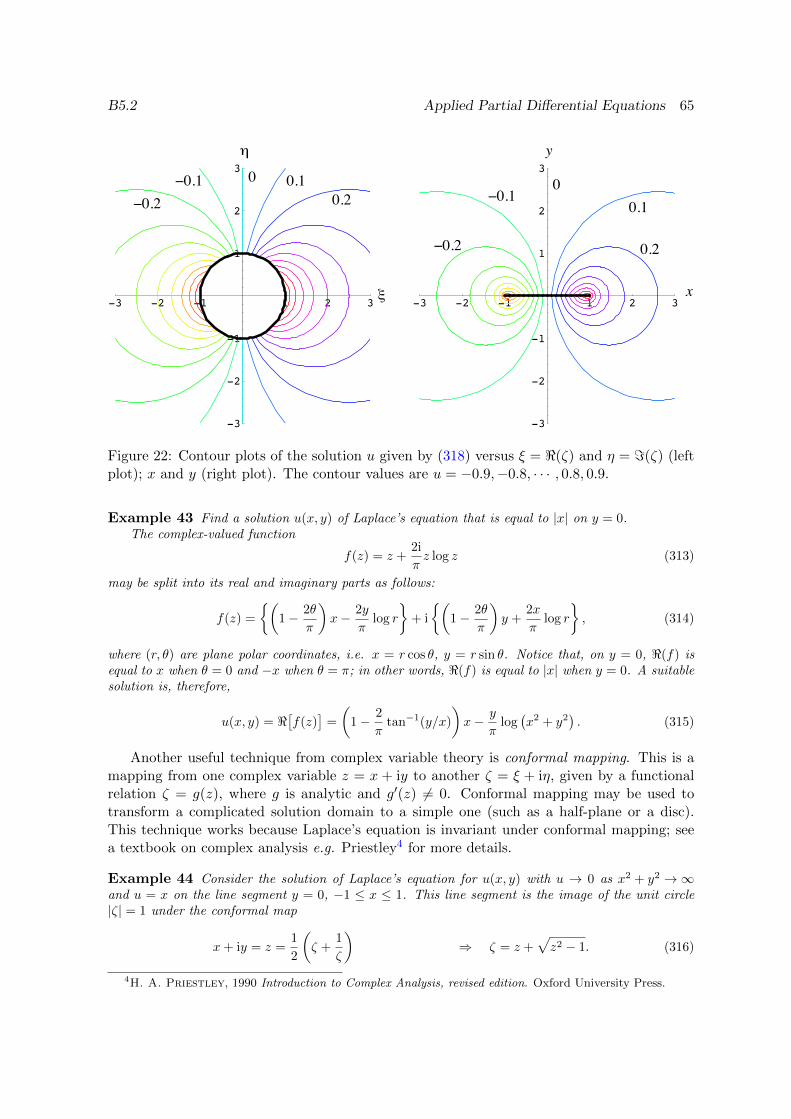
B5.2 Applied Partial Differential Equations 65
-3 -2 -1 1 2 3
-3
-2
-1
1
2
3
-3 -2 -1 1 2 3
-3
-2
-1
1
2
3
x
y
0.1
0.2
0.1
0.2
0.20.1 0 0.1
0.20
Figure 22: Contour plots of the solution u given by (318) versus ξ = <(ζ) and η = =(ζ) (leftplot); x and y (right plot). The contour values are u = −0.9,−0.8, · · · , 0.8, 0.9.
Example 43 Find a solution u(x, y) of Laplace’s equation that is equal to |x| on y = 0.The complex-valued function
f(z) = z +2i
πz log z (313)
may be split into its real and imaginary parts as follows:
f(z) =
(1− 2θ
π
)x− 2y
πlog r
+ i
(1− 2θ
π
)y +
2x
πlog r
, (314)
where (r, θ) are plane polar coordinates, i.e. x = r cos θ, y = r sin θ. Notice that, on y = 0, <(f) isequal to x when θ = 0 and −x when θ = π; in other words, <(f) is equal to |x| when y = 0. A suitablesolution is, therefore,
u(x, y) = <[f(z)
]=
(1− 2
πtan−1(y/x)
)x− y
πlog(x2 + y2
). (315)
Another useful technique from complex variable theory is conformal mapping. This is amapping from one complex variable z = x + iy to another ζ = ξ + iη, given by a functionalrelation ζ = g(z), where g is analytic and g′(z) 6= 0. Conformal mapping may be used totransform a complicated solution domain to a simple one (such as a half-plane or a disc).This technique works because Laplace’s equation is invariant under conformal mapping; seea textbook on complex analysis e.g. Priestley4 for more details.
Example 44 Consider the solution of Laplace’s equation for u(x, y) with u → 0 as x2 + y2 →∞and u = x on the line segment y = 0, −1 ≤ x ≤ 1. This line segment is the image of the unit circle|ζ| = 1 under the conformal map
x+ iy = z =1
2
(ζ +
1
ζ
)⇒ ζ = z +
√z2 − 1. (316)
4H. A. Priestley, 1990 Introduction to Complex Analysis, revised edition. Oxford University Press.
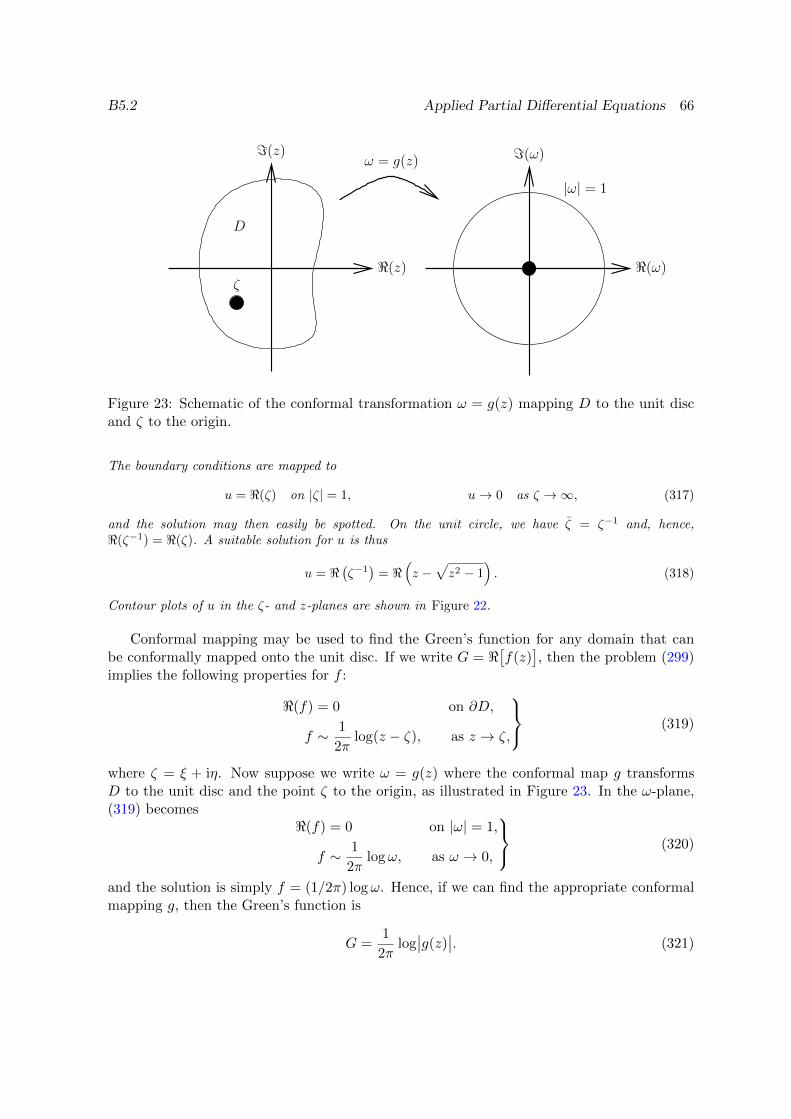
B5.2 Applied Partial Differential Equations 66
|ω| = 1
ω = g(z)
<(z) <(ω)ζ
=(ω)=(z)
D
Figure 23: Schematic of the conformal transformation ω = g(z) mapping D to the unit discand ζ to the origin.
The boundary conditions are mapped to
u = <(ζ) on |ζ| = 1, u→ 0 as ζ →∞, (317)
and the solution may then easily be spotted. On the unit circle, we have ζ = ζ−1 and, hence,<(ζ−1) = <(ζ). A suitable solution for u is thus
u = <(ζ−1
)= <
(z −
√z2 − 1
). (318)
Contour plots of u in the ζ- and z-planes are shown in Figure 22.
Conformal mapping may be used to find the Green’s function for any domain that canbe conformally mapped onto the unit disc. If we write G = <
[f(z)
], then the problem (299)
implies the following properties for f :
<(f) = 0 on ∂D,
f ∼ 1
2πlog(z − ζ), as z → ζ,
(319)
where ζ = ξ + iη. Now suppose we write ω = g(z) where the conformal map g transformsD to the unit disc and the point ζ to the origin, as illustrated in Figure 23. In the ω-plane,(319) becomes
<(f) = 0 on |ω| = 1,
f ∼ 1
2πlogω, as ω → 0,
(320)
and the solution is simply f = (1/2π) logω. Hence, if we can find the appropriate conformalmapping g, then the Green’s function is
G =1
2πlog∣∣g(z)
∣∣. (321)
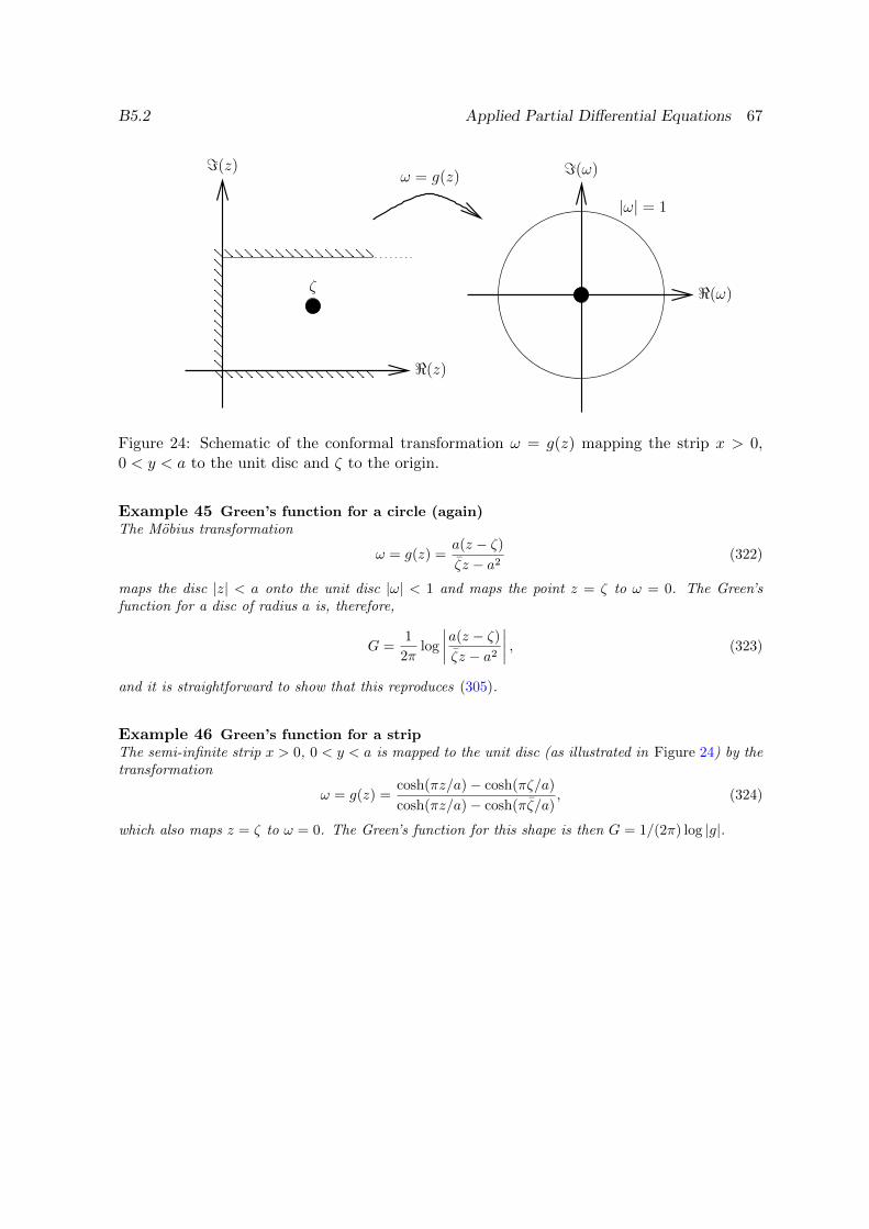
B5.2 Applied Partial Differential Equations 67
|ω| = 1
ω = g(z)
<(ω)
=(ω)
ζ
<(z)
=(z)
Figure 24: Schematic of the conformal transformation ω = g(z) mapping the strip x > 0,0 < y < a to the unit disc and ζ to the origin.
Example 45 Green’s function for a circle (again)The Mobius transformation
ω = g(z) =a(z − ζ)
ζz − a2(322)
maps the disc |z| < a onto the unit disc |ω| < 1 and maps the point z = ζ to ω = 0. The Green’sfunction for a disc of radius a is, therefore,
G =1
2πlog
∣∣∣∣a(z − ζ)
ζz − a2
∣∣∣∣ , (323)
and it is straightforward to show that this reproduces (305).
Example 46 Green’s function for a stripThe semi-infinite strip x > 0, 0 < y < a is mapped to the unit disc (as illustrated in Figure 24) by thetransformation
ω = g(z) =cosh(πz/a)− cosh(πζ/a)
cosh(πz/a)− cosh(πζ/a), (324)
which also maps z = ζ to ω = 0. The Green’s function for this shape is then G = 1/(2π) log |g|.
B5.2 Applied Partial Differential Equations 68
9 Semi-linear parabolic equations
9.1 General properties
In parabolic PDEs one independent variable usually represents time, and we use x and tas independent variables instead of x and y. The canonical form for second-order parabolicequations is
∂2u
∂x2= F
(x, t, u,
∂u
∂x,∂u
∂t
)(325)
and specific examples include the heat equation, or diffusion equation
∂u
∂t=∂2u
∂x2, (326a)
the reaction-diffusion equation∂u
∂t=∂2u
∂x2+ f(x, t, u), (326b)
and the reaction-convection-diffusion equation
∂u
∂t+ q(x, t, u)
∂u
∂x=∂2u
∂x2+ f(x, t, u). (326c)
Another example is the Black–Scholes equation in mathematical finance. All these equationshave the repeated characteristic t = const. They also have the general property that any initialsingularities in u at t = 0 are instantaneously smoothed out when t is positive. Conversely,backward diffusion equations such as
∂u
∂t= −∂
2u
∂x2(326d)
are ill posed, with smooth initial data giving rise to finite-time singularities in general.
9.2 Well posed boundary data
Typical boundary data for a diffusion equation are:
• An initial condition for u at t = 0
• One boundary condition on each of two curves C1 and C2 in the (x, t)-plane that arenowhere parallel to the x-axis.
Example 47 The heat equation∂u
∂t=∂2u
∂x2(327)
is a simple model for the temperature u(x, t) in a uniform bar of conductive material, where x isposition and t is time. Suppose the bar is of length L, its initial temperature is u0(x) and its ends arekept at zero temperature. Then the boundary and initial conditions are
u = u0(x) t = 0, (328a)
u = 0 x = 0, (328b)
u = 0 x = L. (328c)
If, instead of being held at constant temperature, an end is insulated, then the Dirichlet boundarycondition u = 0 is replaced by the Neumann boundary condition ∂u/∂x = 0. Also, the boundaryconditions at x = 0 and x = L may in general be given on moving boundaries, say x = x1(t) andx = x2(t).
B5.2 Applied Partial Differential Equations 69
9.3 Uniqueness theorem
We will now show that the problem
∂u
∂t=∂2u
∂x2+ f(x, t) t > 0, x1(t) < x < x2(t),
u = u0(x) t = 0, x1(t) < x < x2(t),
u = g1(t) t > 0, x = x1(t),
u = g2(t) t > 0, x = x2(t),
(329)
has at most one solution. Suppose there are two solutions u1 and u2; then φ = u1−u2 satisfiesthe homogeneous problem
∂φ
∂t=∂2φ
∂x2t > 0, x1(t) < x < x2(t),
φ = 0 t = 0, x1(t) < x < x2(t),
φ = 0 t > 0, x = x1(t),
φ = 0 t > 0, x = x2(t).
(330)
Now, Leibnitz’ rule gives
d
dt
∫ x2(t)
x1(t)φ2 dx =
∫ x2(t)
x1(t)2φ∂φ
∂tdx+
dx2
dtφ2(x2, t)−
dx1
dtφ2(x1, t)
=
∫ x2(t)
x1(t)2φ∂2φ
∂x2dx =
[2φ∂φ
∂x
]x2x1
−∫ x2(t)
x1(t)2
(∂φ
∂x
)2
dx
= −∫ x2(t)
x1(t)2
(∂φ
∂x
)2
dx ≤ 0. (331)
So the integral ∫ x2(t)
x1(t)φ2 dx
is clearly non-negative, is zero when t = 0 and is a non-increasing function of t. From this wecan conclude that it must be identically zero and, hence, that φ ≡ 0.
9.4 Maximum value theorem
Suppose u satisfies the inhomogeneous heat equation
∂u
∂t=∂2u
∂x2+ f(x, t) (332)
in a region D bounded by the lines t = 0, t = τ and two non-intersecting smooth curves C1
and C2 that are nowhere parallel to the x-axis. Suppose also that f ≤ 0 in D. Then u takesits maximum value either on t = 0 or on one of the curves C1 or C2.
This was proven in Part A DEs. The proof included here is non-examinable.The proof is similar to that for Poisson’s equation. We start by supposing that f is strictly
negative in D. At an internal maximum inside D, u must satisfy
∂u
∂x=∂u
∂t= 0,
∂2u
∂x2≤ 0,
∂2u
∂t2≤ 0. (333)
B5.2 Applied Partial Differential Equations 70
On the other hand, if u has a maximum at a point on t = τ , then it must satisfy
∂u
∂x= 0,
∂u
∂t≥ 0,
∂2u
∂x2≤ 0 (334)
there. With f assumed to be negative, both of these lead to contradictions, and it followsthat u must take its maximum value somewhere on ∂D but not on t = τ .
Now, if the inequality is not strict, i.e. f ≤ 0, then define
v(x, t) = u(x, t) +ε
2x2, (335)
where ε is a positive constant. Then v satisfies
∂v
∂t=∂2v
∂x2+ f(x, t)− ε < 0 (336)
so that v takes its maximum value on either t = 0, C1 or C2. Thus, if the maximum value ofu over these three portions of ∂D is M , and the maximum value of |x| on C1 and C2 is L,then
u ≤ v ≤ ε
2L2 +M. (337)
Now we let ε→ 0 and conclude that u ≤M , i.e. u takes its maximum value on C1 ∪ C2 ∪ t = 0.If f ≥ 0 in D, then a similar argument shows that u attains its minimum value on either
C1, C2 or t = 0. Thus, for the homogeneous equation in which f ≡ 0, u attains both itsmaximum and its minimum values on C1 ∪ C2 ∪ t = 0. This property may be used in auniqueness proof just as for Poisson’s equation.
9.5 Green’s functions
Consider the problem
L[u] =∂u
∂t− ∂2u
∂x2= f(x, t) t > 0, x1(t) < x < x2(t),
u = u0(x) t = 0, x1(t) < x < x2(t),
u = g1(t) t > 0, x = x1(t),
u = g2(t) t > 0, x = x2(t).
(338)
If the adjoint differential operator is defined by
L?[G] = −∂G∂t− ∂2G
∂x2, (339)
then Green’s theorem leads to∫∫D
GL[u]− uL?[G]
dxdt =
∫∫D
∂
∂t(Gu) +
∂
∂x
(u∂G
∂x−G∂u
∂x
)dxdt
=
∮∂D
(u∂G
∂x−G∂u
∂x
)dt−Gudx
, (340)
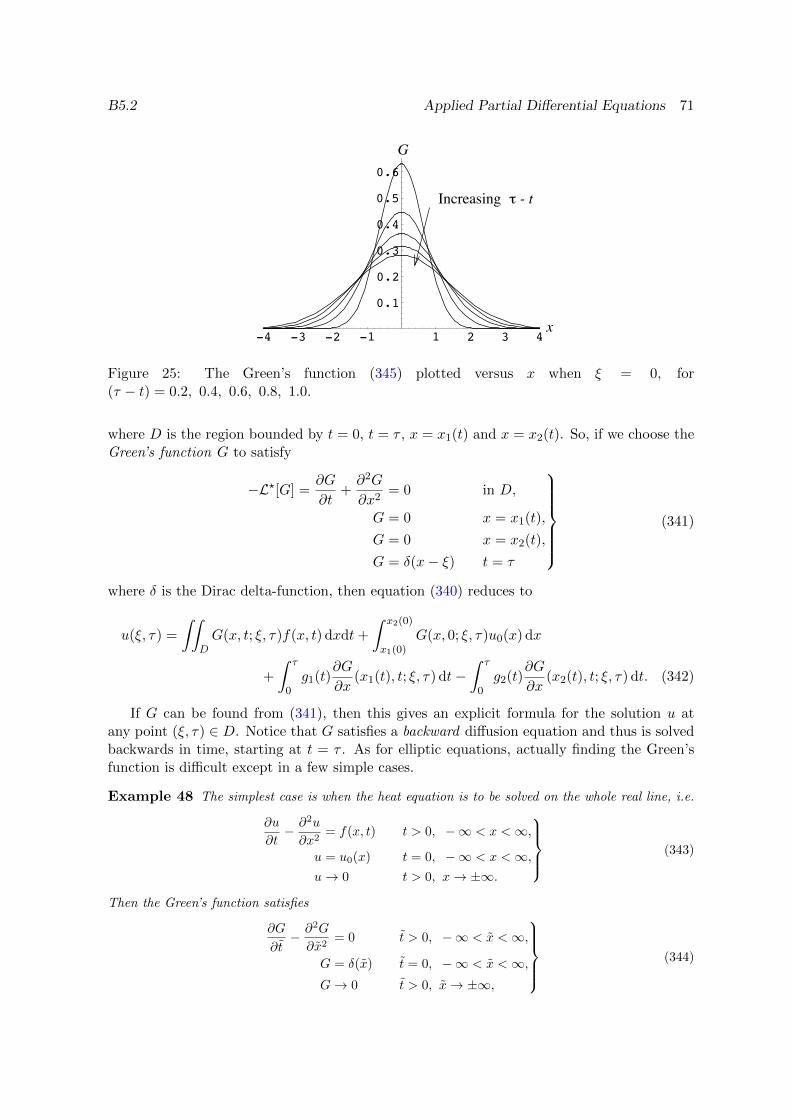
B5.2 Applied Partial Differential Equations 71
-4 -3 -2 -1 1 2 3 4
0.1
0.2
0.3
0.4
0.5
0.6
- tIncreasing
G
x
Figure 25: The Green’s function (345) plotted versus x when ξ = 0, for(τ − t) = 0.2, 0.4, 0.6, 0.8, 1.0.
where D is the region bounded by t = 0, t = τ , x = x1(t) and x = x2(t). So, if we choose theGreen’s function G to satisfy
−L?[G] =∂G
∂t+∂2G
∂x2= 0 in D,
G = 0 x = x1(t),
G = 0 x = x2(t),
G = δ(x− ξ) t = τ
(341)
where δ is the Dirac delta-function, then equation (340) reduces to
u(ξ, τ) =
∫∫DG(x, t; ξ, τ)f(x, t) dxdt+
∫ x2(0)
x1(0)G(x, 0; ξ, τ)u0(x) dx
+
∫ τ
0g1(t)
∂G
∂x(x1(t), t; ξ, τ) dt−
∫ τ
0g2(t)
∂G
∂x(x2(t), t; ξ, τ) dt. (342)
If G can be found from (341), then this gives an explicit formula for the solution u atany point (ξ, τ) ∈ D. Notice that G satisfies a backward diffusion equation and thus is solvedbackwards in time, starting at t = τ . As for elliptic equations, actually finding the Green’sfunction is difficult except in a few simple cases.
Example 48 The simplest case is when the heat equation is to be solved on the whole real line, i.e.
∂u
∂t− ∂2u
∂x2= f(x, t) t > 0, −∞ < x <∞,
u = u0(x) t = 0, −∞ < x <∞,u→ 0 t > 0, x→ ±∞.
(343)
Then the Green’s function satisfies
∂G
∂t− ∂2G
∂x2= 0 t > 0, −∞ < x <∞,
G = δ(x) t = 0, −∞ < x <∞,G→ 0 t > 0, x→ ±∞,
(344)
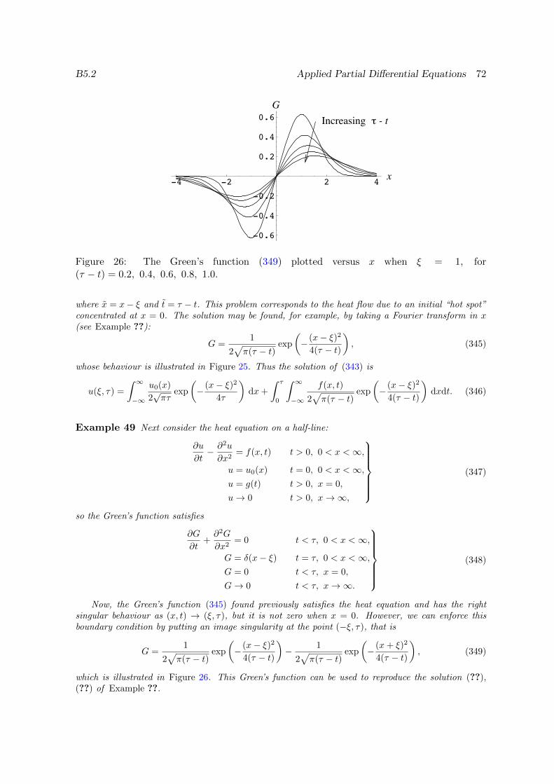
B5.2 Applied Partial Differential Equations 72
-4 -2 2 4
-0.6
-0.4
-0.2
0.2
0.4
0.6 - tIncreasing
x
G
Figure 26: The Green’s function (349) plotted versus x when ξ = 1, for(τ − t) = 0.2, 0.4, 0.6, 0.8, 1.0.
where x = x− ξ and t = τ − t. This problem corresponds to the heat flow due to an initial “hot spot”concentrated at x = 0. The solution may be found, for example, by taking a Fourier transform in x(see Example ??):
G =1
2√π(τ − t)
exp
(− (x− ξ)2
4(τ − t)
), (345)
whose behaviour is illustrated in Figure 25. Thus the solution of (343) is
u(ξ, τ) =
∫ ∞−∞
u0(x)
2√πτ
exp
(− (x− ξ)2
4τ
)dx+
∫ τ
0
∫ ∞−∞
f(x, t)
2√π(τ − t)
exp
(− (x− ξ)2
4(τ − t)
)dxdt. (346)
Example 49 Next consider the heat equation on a half-line:
∂u
∂t− ∂2u
∂x2= f(x, t) t > 0, 0 < x <∞,
u = u0(x) t = 0, 0 < x <∞,u = g(t) t > 0, x = 0,
u→ 0 t > 0, x→∞,
(347)
so the Green’s function satisfies
∂G
∂t+∂2G
∂x2= 0 t < τ, 0 < x <∞,
G = δ(x− ξ) t = τ, 0 < x <∞,G = 0 t < τ, x = 0,
G→ 0 t < τ, x→∞.
(348)
Now, the Green’s function (345) found previously satisfies the heat equation and has the rightsingular behaviour as (x, t) → (ξ, τ), but it is not zero when x = 0. However, we can enforce thisboundary condition by putting an image singularity at the point (−ξ, τ), that is
G =1
2√π(τ − t)
exp
(− (x− ξ)2
4(τ − t)
)− 1
2√π(τ − t)
exp
(− (x+ ξ)2
4(τ − t)
), (349)
which is illustrated in Figure 26. This Green’s function can be used to reproduce the solution (??),(??) of Example ??.
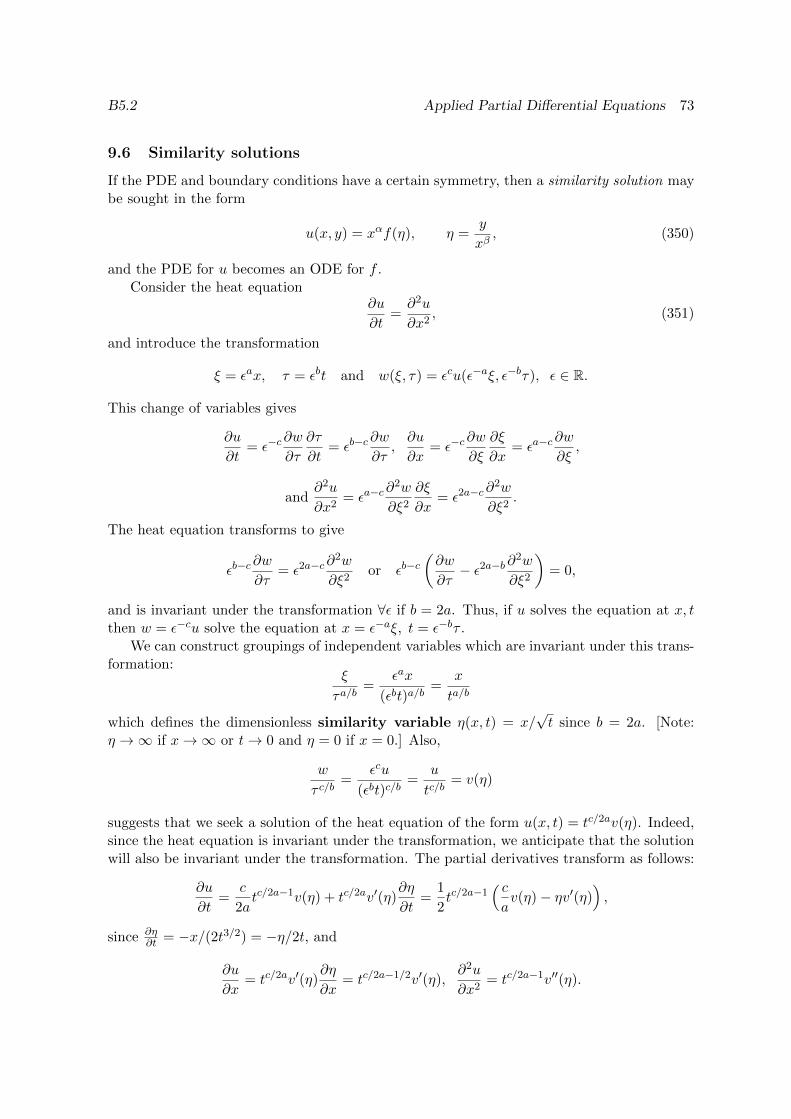
B5.2 Applied Partial Differential Equations 73
9.6 Similarity solutions
If the PDE and boundary conditions have a certain symmetry, then a similarity solution maybe sought in the form
u(x, y) = xαf(η), η =y
xβ, (350)
and the PDE for u becomes an ODE for f .Consider the heat equation
∂u
∂t=∂2u
∂x2, (351)
and introduce the transformation
ξ = εax, τ = εbt and w(ξ, τ) = εcu(ε−aξ, ε−bτ), ε ∈ R.
This change of variables gives
∂u
∂t= ε−c
∂w
∂τ
∂τ
∂t= εb−c
∂w
∂τ,∂u
∂x= ε−c
∂w
∂ξ
∂ξ
∂x= εa−c
∂w
∂ξ,
and∂2u
∂x2= εa−c
∂2w
∂ξ2
∂ξ
∂x= ε2a−c
∂2w
∂ξ2.
The heat equation transforms to give
εb−c∂w
∂τ= ε2a−c
∂2w
∂ξ2or εb−c
(∂w
∂τ− ε2a−b∂
2w
∂ξ2
)= 0,
and is invariant under the transformation ∀ε if b = 2a. Thus, if u solves the equation at x, tthen w = ε−cu solve the equation at x = ε−aξ, t = ε−bτ .
We can construct groupings of independent variables which are invariant under this trans-formation:
ξ
τa/b=
εax
(εbt)a/b=
x
ta/b
which defines the dimensionless similarity variable η(x, t) = x/√t since b = 2a. [Note:
η →∞ if x→∞ or t→ 0 and η = 0 if x = 0.] Also,
w
τ c/b=
εcu
(εbt)c/b=
u
tc/b= v(η)
suggests that we seek a solution of the heat equation of the form u(x, t) = tc/2av(η). Indeed,since the heat equation is invariant under the transformation, we anticipate that the solutionwill also be invariant under the transformation. The partial derivatives transform as follows:
∂u
∂t=
c
2atc/2a−1v(η) + tc/2av′(η)
∂η
∂t=
1
2tc/2a−1
( cav(η)− ηv′(η)
),
since ∂η∂t = −x/(2t3/2) = −η/2t, and
∂u
∂x= tc/2av′(η)
∂η
∂x= tc/2a−1/2v′(η),
∂2u
∂x2= tc/2a−1v′′(η).
B5.2 Applied Partial Differential Equations 74
Then the heat equation reduces to an ODE
tγ/2−1(2v′′(η) + ηv′(η)− γv(η)) = 0, (352)
with γ = c/a such that u(x, t) = tγ/2v(η) and η = x/√t. We conclude that we may be able
to solve the heat equation using (352) if we can write the boundary and initial conditions foru(x, t) as conditions on v and η.
Example 50 Consider the heat equation
∂u
∂t=∂2u
∂x2,
subject to u(x, 0) = u(∞, t) = 0, u(0, t) = tm for some constant m.We seek a solution of the form
u = tmf(η), η =x√t, (353)
for some function f . If this form of u is substituted into the heat equation, f is found to satisfy
d2f
dη2+η
2
df
dη−mf = 0, (354)
with the boundary conditions f(0) = 1, f → 0 as η → ∞. The simplest case is m = 0, when thesolution is
f(η) =2√π
∫ ∞η/2
e−s2
ds = erfc(η/2), (355)
the complementary error function.
Example 51 Consider the problem
ut = uxx, on 0 < x <∞, t > 0,
with u(x, 0) = 0 for 0 < x <∞,∂u
∂x= −q at x = 0, t > 0,
and u→ 0 as x→∞, ∀t > 0.
As above, we seek solutions of the form
u(x, t) = tmf(η), η =x√t,
for some function f . By substituting this form of u in the heat equation we deduce that f satisfies
d2f
dη2+η
2
df
dη−mf = 0. (356)
Now∂u
∂x= tm−1/2f ′(η) ⇒ ∂u
∂x
∣∣∣∣x=0
= tm−1/2f ′(0) = −q.
Since q does not depend on t, we require m = 1/2 so that u(x, t) =√tf(η) where f solves
d2f
dη2+η
2
df
dη− 1
2f = 0, with f ′(0) = −q and f → 0 .as η →∞.
B5.2 Applied Partial Differential Equations 75
Since f = η solves the ODE, we seek a solution of the form f(η) = ηg(η) where
g′′
g′= − (2 + η2/2)
η= −2
η− η
2.
Integrate with respect to η to get
g′ =k ∗ e−η2/4
η2⇒ g(η) = k0 + k1
∫ η e−θ2/4
θ2dθ.
⇒ g(η) = κ0 + κ1
(e−η
2/4
η+
∫ η
0
e−θ2/4dθ
)and f(η) = κ0η + κ1
(e−η
2/2 + η
∫ η
0
e−θ2/4dθ
).
The constants of integration κ0 and κ1 are determined from the initial conditions.
f ′ = ηf ′ + g ⇒ f ′(0) = −q = g(0) = κ0.
Also,
f(η) ∼ η(κ0 + κ1
∫ ∞0
e−θ2/4dθ
)= 0 ⇒ κ1 = −κ0
√π,
since∫∞0e−θ
2/4dθ = 2∫∞0e−r
2
dr = π. The solution of the equation becomes (eventually)
f(η) = ...
u(x, t) = 2q
√t
π
(e−x
2/4t − x√t
∫ ∞x/2√t
er2
dr
).
Example 52 For the telegraph equation
L[u] =∂2u
∂x∂y+ u = f(x, y), (357)
the Riemann function satisfies
L?[u] =∂2R
∂x∂y+R = 0 x < ξ, y < η, (358)
with, as in Example 40, R = 1 on x = ξ and on y = η. Alternatively, if x = ξ − x, y = η − y, then
∂2R
∂x∂y+R = 0, x > 0, y > 0,
R = 1 x = 0,
R = 1 y = 0.
(359)
Notice that this problem is invariant if the two independent variables x and y are swapped. It followsthat a similarity solution of (359) exists in the form
R = F (s), where s = 2√xy, (360)
and F satisfies
d2F
ds2+
1
s
dF
ds+ F = 0, s > 0, (361)
with F (0) = 1. The solution is the Bessel function F = J0(s),5 so the Riemann function for thetelegraph equation is
R =
J0
(2√
(ξ − x)(η − y))
x < ξ, y < η,
0 otherwise.(362)
5the other linearly independent solution to this second-order ODE is Y0(s), which is singular as s→ 0
Related Documents


