B4-3

 242

Numerical simulation of cavity flow induced noise

by LES and FW-H acoustic analogy 

 Nan Zhang*, Hong-cui Shen, Hui-zhi Yao 

China Ship Scientific Research Center, Wuxi, China *

E-mail: [email protected]

ABSTRACT: The predictions of cavity flow and flow-inducednoise are two important and complex issues in fluid-acoustic

coupling field. Numerical studies for these issues are performedin the paper by large eddy simulation (LES) and FW-Hacoustic analogy. Firstly, the wall pressure fluctuations of plate,

foil, shutter hole are computed and compared withexperimental results. The robustness of large eddy simulationin unsteady flow calculation is analyzed. Secondly, the

calculation of a 2-D cavity flow are accomplished. The power spectrum of pressure fluctuations is compared with measureddata and the vorticity distribution is analyzed. Finally, the flow

induced noises of two 3D cavities are predicted. The computedresults are compared with experimental data of Large

Circulation Channel in CSSRC. It shows that the numerical prediction method in the paper is credible.

KEY WORDS: cavity flow; flow induced noise; wall pressurefluctuations; Large eddy simulation; FW-H equation

1 INTRODUCTION

The cavity flow belongs to a basic class of flows with

self-sustaining oscillations. In industrial practice, thecavity-type oscillation is undesirable from the

 perspective of inducement of structure vibration andfatigue, generation of noise and drastic increase indrag on the body.

Many computational studies focus on the computationof the cavity flow field with little attention given tothe acoustic field surrounding the cavity. Exceptions

do exist, including several studies aimed at computingthe acoustics from low and subsonic Mach number flows past cavities. The cavity flow simulations that

focus on the near field are equally important to thedevelopment of a noise prediction capability for cavity

flows; for, if the near-field flow is not simulated properly, one cannot hope to predict the acoustic fieldaccurately. In this sense, advances in computational

fluid dynamic (CFD) modeling go hand-in-hand with

advancing computational aeroacoustic (CAA)methods.

It was shown that a greater understanding of the flow

field and acoustic field generated by grazing flow pasta cavity has been gained over the past ten years. Inaddition, CFD is becoming a more reliable prediction

tool for this flow field. Many CFD analyses rely onDES or LES to correctly simulate the shear layer in

turbulent flow conditions and predict the flow inducednoise accurately

[1-5]. As more confidence is gained in

the use of CFD as a methodology for the prediction of 

such complicated flow-acoustic coupling phenomenon,more researchers are using this method to study the

effect of control devices and cavity/body interactions.

Flow induced noise is a serious problem in manyengineering applications. It can cause humandiscomfort and influence quiet operations of vehicles.

In ship applications, the sound generated by marine propellers, hydrofoils, and even transitional andturbulent boundary layers can induce ambient

concerns and decrease the work efficiency of sailors.There were lots of discoveries and researches about

flow induced noise in aeroacoustics. However, inhydroacoustics, it is short of an intensive investigationfor the problem.

In the paper, the cavity flow and flow induced noiseare studied by the large eddy simulation (LES) withdynamic Smagorinsky subgrid model and FW-H

acoustic analogy with Kirchhoff integral. We aim atestablishing a suitable numerical method to predict the

flow induced noise of cavity in water.

  243

2 COMPUTATIONAL METHOD 

2.1 Large eddy simulation (LES)

The basic assumptions of LES are that: (1) transport islargely governed by large-scale unsteady flow and

these structures can be computationally resolved; (2)small-scale flow features can be undertaken by usingappropriate subgrid scale turbulence models. In LES,

the motion is separated into small and large eddies,this separation is achieved by means of a low-pass

filter. The filter function, )',( x xG , implied here is

then:

1/ , '( , ')

0, 'otherwise

V x V G x x

 x

∈⎧= ⎨⎩

(1)

Filtering the Navier-Stokes equations, one obtains

0)( =∂

∂+

∂

∂i

i

u xt 

 ρ  ρ 

(2)

 j

ij

i j

ij

 j

 ji

 j

i x x

 p

 x xuu

 xu

t  ∂

∂−

∂

∂−

∂

∂

∂

∂=

∂

∂+

∂

∂ τ σ  μ  ρ  ρ  )()()(  

(3)

where jiσ  is the stress tensor due to molecular 

viscosity and ijτ  is the subgrid-scale stress.

In the paper, we adopt four subgrid-scale stressmodels:• Smagorinsky Model (SL)

• Dynamic Smagorinsky Model (DSL)

• Wall-Adapting Local Eddy-Viscosity Model (WALE)• Dynamic Kinetic Energy Model (KET) 

2.2 FW-H acoustic analogy 

Ffowcs Williams and Hawkings utilized thegeneralized function theory to obtain the classicequation that has become associated with their names.

The FW-H equation can be written as the followinginhomogeneous wave equation:

[ ] [ ] [ ])()()()(

),('),('1

2

0

2

2

2

2

 f  H T  x x

 f  L x

 f U t 

t  x pt 

t  x p

c

ij

 ji

i

i

n∂∂

∂+

∂

∂−

∂

∂=

∇−∂

∂

δ δ  ρ 

(4)where

[ ] )/()/(1 00 ρ  ρ  ρ  ρ  iii uvU  +−= (5)

)(ˆnni jiji vuunP L −+= ρ  (6)

[ ]ijij jiij c p puuT  τ δ  ρ  ρ  ρ  −−−−+= )()( 0

2

00(7)

ijT  is Lighthill stress tensor, )( f δ  is Dirac delta

function, H is Heaviside function, u is fluid velocity, v

is body surface velocity, c is velocity of sound, n is a

normal vector that points into the fluid.

The far field solution of FW-H equation can be

written as the following:

0

20

( )4 ' ( , ) d

(1 )

n nT 

 f r  ret 

U U  p x t S

r M 

 ρ π 

=

⎡ ⎤+= ⎢ ⎥

−⎣ ⎦∫

2

0 0

2 30

( ( ))d

(1 )

n r r 

 f r  ret 

U rM c M M  S

r M 

 ρ =

⎡ ⎤+ −+ ⎢ ⎥

−⎣ ⎦∫

(8)

2 2 20 00

14 ' ( , ) d d

(1 ) (1 )r r M 

 L f f 

r r ret ret  

 L L L p x t S S

c r M r M  π 

= =

⎡ ⎤ ⎡ ⎤−= +⎢ ⎥ ⎢ ⎥

− −⎣ ⎦ ⎣ ⎦∫ ∫

2

0

2 300

1 ( ( ))d

(1 )

r r r 

 f r  ret 

 L rM c M M S

c r M =

⎡ ⎤+ −+ ⎢ ⎥

−⎣ ⎦∫

(9)

1 2 3

2 2 304 ' ( , ) dQ

 f 

K K K  p x t V 

c r cr r  π 

>

⎡ ⎤= + +⎢ ⎥

⎣ ⎦∫

(10)

We can computed the far field solution on a Kirchhoff 

control surface to avoid the volume integral.

2.3 Numerical method

The differential equations are discretized by finitevolume method. Bounded central difference scheme isapplied. The velocity-pressure coupling is based on

PISO algorithm and algebraic multigrid method isemployed to accelerate the solution convergence. The

time step is 1×10-5

s and y+≈1.

3 RESULTS AND DISCUSSION

3.1 Wall pressure fluctuations

 3.1.1 Plate & foil  

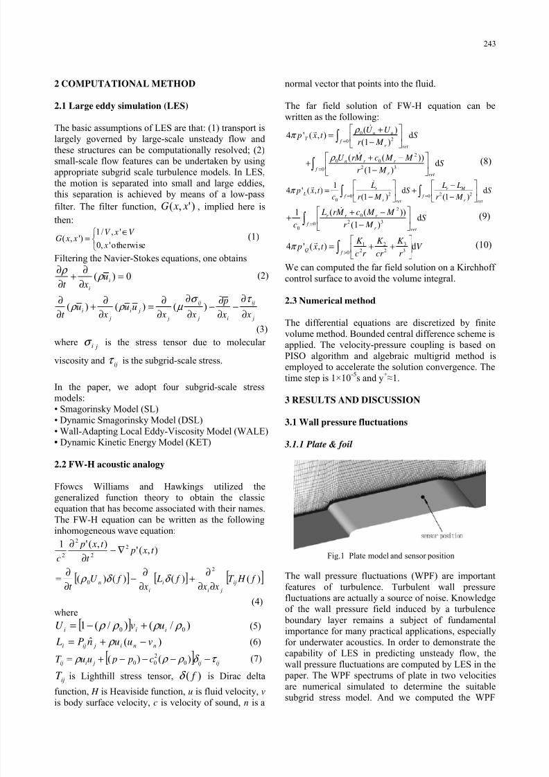
Fig.1 Plate model and sensor position

The wall pressure fluctuations (WPF) are important

features of turbulence. Turbulent wall pressurefluctuations are actually a source of noise. Knowledgeof the wall pressure field induced by a turbulence

 boundary layer remains a subject of fundamentalimportance for many practical applications, especially

for underwater acoustics. In order to demonstrate thecapability of LES in predicting unsteady flow, the

wall pressure fluctuations are computed by LES in the paper. The WPF spectrums of plate in two velocities

are numerical simulated to determine the suitablesubgrid stress model. And we computed the WPF

 244

spectrum of foil by the suitable model. Fig.1 shows

the plate model and sensor position. The plate has anoverall length L of 1.1m and breadth of 0.39m.

Experimental investigations including boundary layer and wall pressure fluctuations have been made inanechoic wind tunnel of CSSRC at velocity 18m/s.

The computational domain is discretized using 1.35million hexahedral cells. Measured and predictedWPF spectrums are shown in Figures 2~5. The

reference pressure in air is Prefair =2×10-5

Pa.

Fig.2 Comparison of measured and computed WPF spectrum(SL model)

Fig.3 Comparison of measured and computed WPF spectrum(DSL model)

Fig.4 Comparison of measured and computed WPF spectrum

(WALE model)

Fig.5 Comparison of measured and computed WPF spectrum(KET model)

These computations are used to investigate the performances of the four subgrid models in predicting

the unsteady characteristics of turbulent flow. We canfind that the differences of the computed results withdifferent subgrid models are very clear. It shows that

the computed WPF magnitude and spectrum shapewith DSL model is better than that with other models.Generally, the DSL model predicts WPF more

accurate than other models.

So we used the DSL model to compute the WPFspectrum of a foil in three velocities (12m/s, 18m/s,

32m/s) . The geometry of foil and sensor position areshown in Fig. 6. The foil has an overall length L of 

1.1m and breadth of 0.39m. Experiments have beencarried out in anechoic wind tunnel of CSSRC. Thecomputational domain is discretized using 1.56

million hexahedral cells. Fig.7-10 show the computedresults including flow and WPF spectrum.

Fig.6 Foil model and sensor position

Fig.7 Computed flow field 

245

 Fig.8 Comparison of measured and computed WPF spectrum

(V=12m/s) 

Fig.9 Comparison of measured and computed WPF spectrum(V=18m/s) 

Fig.10 Comparison of measured and computed WPF spectrum(V=32m/s) 

The predicted overall shape and the magnitude of the

WPF spectrum is fairly good compared with

experiment data. In the frequency scope of 100Hz to10KHz, the predicted accuracy is 1.5dB to 5.5dB at32m/s, 1.2dB to 8.4dB at 18m/s, 1.1dB to 13.3dB at

12m/s. It shows that the computed results agree better with measured data in high velocity than that in low

velocity. And the computed results agree better withmeasured data in low frequency than that in highfrequency. The characteristics of the unsteady flow

with obvious pressure gradient are better captured byLES approach.

 3.1.2 Shutter-hole

We have investigated the wall pressure fluctuations of 

shutter hole in water to identify the source of noise innear field. Experiments including flow field and wall

 pressure fluctuations have been made in the Large

Circulation Channel of CSSRC, which are suitable for validation of numerical results. Figure 11 give theshutter hole model and sensor position. The shutter 

hole is arranged on a axisymmetric body.Measurements were carried out at velocity V =5m/s.

Predicted and Measured WPF spectrums are shown inFigures 12. The reference pressure in water is

Prefwater =1× 10-6

Pa. The computational domain is

discretized using 4.19 million hexahedral cells.

Fig.11 Shutter hole model and sensor position 

Fig.12 Comparison of measured and computed WPF spectrum

In the frequency scope of 100Hz to 10kHz, the predicted accuracy is 1.6dB to 6.0dB. The predictedWPF spectrum is fairly good compared with

experiment data. The flow around shutter hole is very

complex, so the capability of LES is validated. 

3.2 Flow induced noise

 3.2.1 2-D cavity

Unsteady flow past a cavity may create both

 broadband and tonal noise. The formation and

 behavior of a shear layer and its subsequentinteraction with the fluid in the cavity drives the noise

 production. Lafon[6]

studied cavity flow noise of a 2D

cavity. Fig. 13 shows the geometry of the model.

 246

Experiments were carried out in a wind tunnel at the

Institut AeroTechnique, Saint-Cyr-l’Ecole. Flowvelocity is 62.8m/s. M =0.183.

Fig.13 2-D cavity model and sensor position

Comparisons of measured and computed SPLspectrum are shown in Figure 14(a)~(b).

Fig.14 Comparisons of measured and computed SPL spectrum 

Predicted overall shape and magnitude of the SPL

spectrum is well compared with experiment data. Thetwo oscillations modes are reflected accurately. The

computational accuracy of frequency and magnitudeare in 7% to 10% in comparison with measurement.

Computed vorticity distributions of different stages

are shown in Figure 15. The cavity flow ischaracterized by violent ejections of vortices from the

cavity with length scales comparable with the cavitydimensions rather than the thickness of the boundary

layer. The ejected vortex admits the free stream fluidto enter the cavity impinging on the downstream face

of the cavity and triggers another vortex at the cavityleading edge. The vortex grows in the cavity until itcompletely fills the cavity and again gets ejected and

triggers the next vortex shedding. The rapid changes

in the flow past the cavity and its adjacent walls arethe primary sources to generate sound.

Fig.15 Vorticity distributions at different stages

 3.2.2 3-D cavity

We have studied the various flow induced noise of 

five 3-D cavities which were arranged in a submerged body. Experiments have been carried out in the Large

Circulation Channel of CSSRC at velocity V=5m/s.Figure 16 presents the geometries of two models.

Figure 17 give the computed flow fields.

Fig.16 3-D cavity models

Fig.17 Computed flow field

247

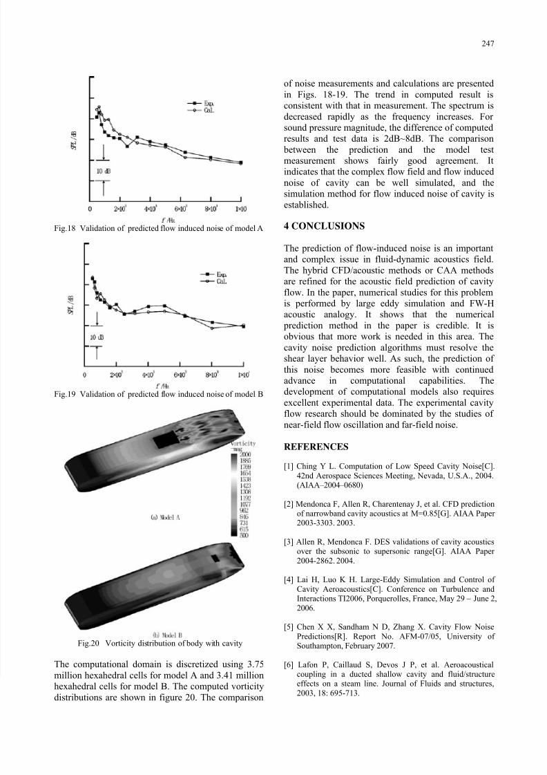
 Fig.18 Validation of predicted flow induced noise of model A

Fig.19 Validation of predicted flow induced noise of model B

Fig.20 Vorticity distribution of body with cavity

The computational domain is discretized using 3.75

million hexahedral cells for model A and 3.41 millionhexahedral cells for model B. The computed vorticity

distributions are shown in figure 20. The comparison

of noise measurements and calculations are presented

in Figs. 18-19. The trend in computed result isconsistent with that in measurement. The spectrum is

decreased rapidly as the frequency increases. For sound pressure magnitude, the difference of computedresults and test data is 2dB~8dB. The comparison

 between the prediction and the model testmeasurement shows fairly good agreement. Itindicates that the complex flow field and flow induced

noise of cavity can be well simulated, and thesimulation method for flow induced noise of cavity is

established.

4 CONCLUSIONS

The prediction of flow-induced noise is an importantand complex issue in fluid-dynamic acoustics field.

The hybrid CFD/acoustic methods or CAA methodsare refined for the acoustic field prediction of cavity

flow. In the paper, numerical studies for this problemis performed by large eddy simulation and FW-Hacoustic analogy. It shows that the numerical

 prediction method in the paper is credible. It isobvious that more work is needed in this area. The

cavity noise prediction algorithms must resolve theshear layer behavior well. As such, the prediction of 

this noise becomes more feasible with continuedadvance in computational capabilities. Thedevelopment of computational models also requires

excellent experimental data. The experimental cavityflow research should be dominated by the studies of 

near-field flow oscillation and far-field noise.

REFERENCES

[1] Ching Y L. Computation of Low Speed Cavity Noise[C].

42nd Aerospace Sciences Meeting, Nevada, U.S.A., 2004.(AIAA–2004–0680)

[2] Mendonca F, Allen R, Charentenay J, et al. CFD predictionof narrowband cavity acoustics at M=0.85[G]. AIAA Paper 2003-3303. 2003.

[3] Allen R, Mendonca F. DES validations of cavity acousticsover the subsonic to supersonic range[G]. AIAA Paper 

2004-2862. 2004.

[4] Lai H, Luo K H. Large-Eddy Simulation and Control of 

Cavity Aeroacoustics[C]. Conference on Turbulence andInteractions TI2006, Porquerolles, France, May 29 – June 2,

2006.

[5] Chen X X, Sandham N D, Zhang X. Cavity Flow Noise

Predictions[R]. Report No. AFM-07/05, University of Southampton, February 2007.

[6] Lafon P, Caillaud S, Devos J P, et al. Aeroacousticalcoupling in a ducted shallow cavity and fluid/structureeffects on a steam line. Journal of Fluids and structures,

2003, 18: 695-713.