B-spline approximation for the baseline hazard function

Enuimnrnetrics; 1991; !2(3): 323-339

B-Spline Approximation for the Baseline Hazard Function

James Angelos’, Carl M.-S. Lee2 and Karan P. Singh3

ABSTRACT

Etezadi-Amoli and Ciampi (Biometrics 1987) introduced a method to approximate the baseline hazard and to estimate the regression coefficients for covariates simultaneously for the extended hazard regression (EHR) model using a quadratic spline approach. In this paper, an estimate of the baseline hazard function by B-spline approximation using a minimax criterion is proposed. The nonlinear problem is approximated by a linear programming problem with only linear constraints. The nice features of this approach are: (i) the minimax criterion provides a robust approximation to the hazard function, and (ii) the linearized problem is numerically simple and fast.

KEY WORDS: Extended hazard regression; minimax criterion; linear pro- gramming; censored survival data.

1. INTRODUCTION

The spline approximation technique has been a very useful tool in the analysis of survival data. The mth order splines are usually defined as piece- wise polynomials of degree m - 1 whose functional values and first m - 2 derivatives agree at the points where they join. Considerable work has been done lately on the smooth estimation of the baseline hazard function in the

Department of Mathematics, Central Michigan University, Mt. Pleasant, MI 48859, U.S.A.

23Department of Biostatietics and Biomathematics, The University of Alabama at Birmingham, UAB Station, Birmingham, Alabama 35294, U.S.A.

1180-4009/9l/030323-17gO8.50 @John Wiley & Sons, Ltd.

Received 11 August 1991 Revised 11 September 1991

324 J . ANGELOS, C. M.-S. LEE A N D K . P. S I N G H

proportional hazard model proposed by Cox (1972). The spline approach is among those nonparametric smoothing techniques that are frequently used (Klotz 1982; Klotz and Yu 1986; Whittemore and Keller 1986; Anderson and Senthilselven 1980; Bloxom 1985, Jarjoura 1988; Etezadi-Amoli and Ciampi 1987). Linear and quadratic splines are used in most of these articles. There is little literature available on the use of cubic splines for hazard estima- tion, although i t has been extensively investigated in the generalized cross- validated approach for the smooth estimation of general regression models and density estimation (e.g., see Wahba 1985, Speckman 1985, Silverman 1982, Li 1985, etc.) Jarjoura (1988) applied the cross-validated likelihood method and used the cubic spline to approximate the hazard function.

Another important smoothing technique is the well known kernel func- tion approach. Similar to the cross-validation method, this approach is well developed for density estimation and general regression models. However, it has not been used frequently for the problems involving censored observa- tions and small samples, which is common in survival data. This is mainly due to the limitations of the assumptions of no censoring and large sam- ples. Tanner and Wong (1984) proposed some kernel function estimates for censored data by the use of a penalized likelihood in combination with cross-validation.

Very recently, Etezadi-Amoli and Ciampi (1987) developed an extended hazard regression (EHR) model that includes proportional hazard (PH) and accelerated failure time (AFT) models as its special cases (also see Ciampi and Etezadi-Amoli 1985). Their model can be expressed as follows:

where h l ( z ) and g(z) are positive functions that are equal to 1 at zero, ho(t) denotes the baseline hazard function, and a and p are vectors of regression parameters. When p = 0, the EHR model reduced to the PH model, and to the AFT model if a = p. They introduced a method to approximate the baseline hazard and estimate the regression coefficients for covariates simultaneously for the EHR model using a quadratic spline approach. In particular, the free knot approach is considered. However, as discussed in Smith (1979), the quadratic spline approach may not be computationally efficient. A more efficient approach can be derived by using the B-spline basis. Klotz (1982) derived a closed-form linear estimate using fixed knots and the B-spline basis to approximate survival data and showed that his linear spline estimate is consistent under some assumptions; later Klotz and Yu (1986) used simulation studies to investigate further this linear spline estimate and concluded that this estimate performs well for small samples.

The main purpose of this paper is to propose a method to solve a rather complicated general spline estimate with free knots to approximate the base- line hazard function, and consequently to approximate the survival function.

BASELINE HAZARD FUNCTION 325

The idea behind our approach is to linearize the problem and to use a lin- ear programming technique. The nice features of this approach are: (i) the minimax criterion provides a robust approximation to the hazard function, and (ii) the linearized problem is numerically simple and fast.

2. B-SPLINES AND METHOD OF ESTIMATION

Let rn, k be positive integers. Let

$-,,,+I 5 * . * - < 20 = a < X1 < X 2 < < xk < 6) = xk+1 . Then we define the mth order (i.e., (rn - 1)th degree) polynomial B-spline as follows:

(2.1) (-1) Bi(T) = ( - q m ( x t + m - x,)[x,, * * 9 x ,+m I(t - X I +

a S t 5 6 ,

where [x,, . . . ,z,+,,,](t - x)+ (m-l) denotes the mth order divided difference of the function

-m+ 15 i 5 k

0 ; t < x

; t 3 x ( t - X ) y ) = [ (2.2)

( t - x)(m-1)

where a is the smallest observation and 6 is the largest observation (i.e., survival time).

< xk will be treated as free parameters. Let C' = (c-,,,+l, ~ - ~ + 2 , , . . , Ck) be a vector in Rm+k of coefficients and X' = (z1,52,. . . ,zk) a vector in Rk of knots satisfying a < x1 < 5 2 < -

Suppose ( t ( ; ) , 6( i ) , q;), i = 1,2,. . . ,n ) is a sample with t ( ; ) observed survival times and

In this article, the knots x1 < x2 <

< xk < 6. Also, set u = [c,xj.

1 ; t ( ; ) survival observed time

{ 0 ; otherwise S(i) =

and t(;) and 6( i ) correspond to the ith covariate vectors q;). Here, we assume random censoring. The log likelihood function can be written as follows:

The object of our estimation procedure is to find a vector U for V(t; U) w ho[g(P.Z)t] such that the function

k

V ( t ; U ) = c c$j(t;X) (2-4) j=m+l

326 J . ANCELOS, C. M.-S. LEE AND K. P. SINCH

maximizes the log likelihood function (2.3). Here we have employed the notation B j ( t ; X ) to emphasize that the knots are free parameters. Now, we describe the maximization procedure.

Let F ( U ) = -1. Then we wish to solve the following constrained opti- mization problem:

(I) Minimize 20 subject to:

(11) F ( U ) L 'w

(12) 6 5 c I hmax x l 2 a - 6

where 6 > 0 is small. The constraint (12) will keep our estimate positive for the hazard func-

tion since the B-splines are positive functions. This of course is a sufficient condition for V ( t ; U ) to be positive, but is not necessary. The h,,, is an upper estimate for the hazard function. The constraints (13) are simply here to prevent the knots from coalescing.

In order to solve this, we employ successive linear programming (SLP) to the following problem:

(II) Given an initial guess UO = (c(-,+~)~, . . . , cM,x10,. . . , z ~ ) , Minimize w subject to:

(111) F(Uo)+ < Vu,F , (112) 6 5 c I L a x

U - Ucj >5 w

x l l a - 6

(113) X $ + I - 28 >_ 6 ; i = 1,2, . . . , k - 1 X k s b - 6

(114) I c i - c i o l s ~ , ; i = - m + l , ..., b 1 z , - x j o l < q j ; j = 1 , 2 ,..., b .

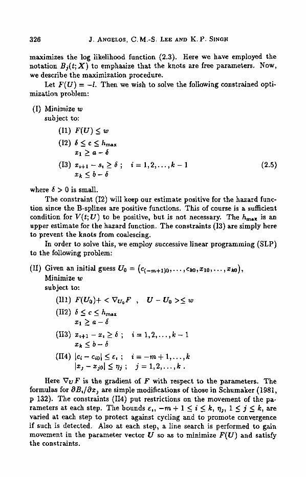
Here VuF is the gradient of F with respect to the parameters. The formulas for dB, /dx , are simple modifications of those in Schumaker (1981, p 132). The constraints (IX4) put restrictions on the movement of the pa- rameters at each step. The bounds E , , -m + l 5 i < b, ql, l < j s b, are varied at each step to protect against cycling and to promote convergence if such is detected. Also at each step, a line search is performed to gain movement in the parameter vector U so as to minimize F(U) and satisfy the constraints.

BASELINE HAZARD FUNCTION 327

3. SOME NUMERICAL ILLUSTRATIONS

Some artificial data sets on hazard functions of the Weibull model were generated. All computations were performed on the CDC Cyber 172 at Central Michigan University, which has approximately 13 digits of accuracy in single precision. The sample sizes for each form of the hazard functions were 30 and 300, respectively.

A collection of subroutines developed by Professor Edwin H. Kaufman, Jr. at Central Michigan University, was used to perform SLP. The program stops when the changes in the parameters are small or a certain number of iterations has failed to improve F(U) . The code is written to handle splines of any order greater than one equal to 2 and knots of any multiplicity.

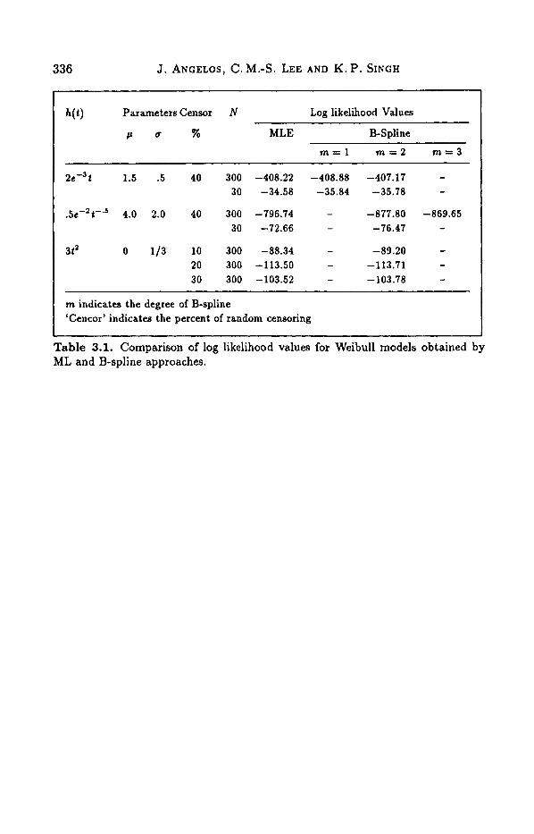
Results are shown in Figures 3.1 3.8 and Tables 3.1 to 3.3. Table 3.1 gives some comparisons of the log likelihood values between MLE and splines for various shapes of Weibull hazard functions. The parameters p and u in the table are scale parameters defined in the generalized log-gamma distri- bution with parameters defined in the generalized log-gamma distribution with parameters p, u and k = 1. A detailed description can be found in Lawless (1980). As shown in this table, splines seem to fit very well for in- creasing hazard functions. However, for decreasing hazard functions, MLE seems more preferable. In general, it seems that using the basis B-spline is very comparable to the classical maximum likelihood approach. Also, it is noticed that if we have a polynomial hazard of a certain degree, then, a spline estimate of that same degree recovers i t quite well given that the amount of censoring is as high as 40 percent.

We close this section with a rationale for our choice of using the B-spline basis. First, we chose the B-spline basis so as to obtain an optimization problem with linear constraints. Second, and most important, is the com- putational efficiency of the B-spline basis. This is brought out strikingly by the fact that dV( t ;U) /dz , , 1 5 j 5 k, are splines, but with a double knot at z3 instead of a simple knot (see, e.g., Schumaker 1981, p 132).

ACKNOWLEDGEMENT

The authors are grateful to Professor Edwin H. Kaufman, Jr. of Central Michigan University for providing us with the subroutines used in this paper.

328 J. ANGELOS, c. M.-S. LEE AND K. P. SINGH

1.oooO

0.80000

o.doooo

0.4OOOO

0.20000

0 OOOa 0.0000 2.0000 4.oooo 6.oooo 10.000

l.Ooo0

0.80000

0 60000

0.40000

0 ~ 2 0 0 0 0

o.ooO0 0.0000 2.0000 4. WOO 8.oooO 10.000

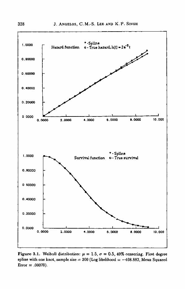
Figure 3.1. Weibull distribution: p = 1.5, u = 0.5, 40% censoring. First degree spline with one knot, sample size = 300 (Log likelihood = -408.882, Mean Squared Error = .00070).

BASELINE HAZARD FUNCTION 329

1 . o m

0.80000

0.60OOO

0.40000

0.20000

0 0000 O.oo00 2.oooo 4.oooo 6.0000 8.oooo 10.000

1 0000

0 Boo00

0 6oooO

0.4OOoO

u .2UUW

o m

- Spline o - True svvivd Survival function

I 1 1 1

0.0000 2 .oooo 40000 6.oooO 8.oooo 10.000

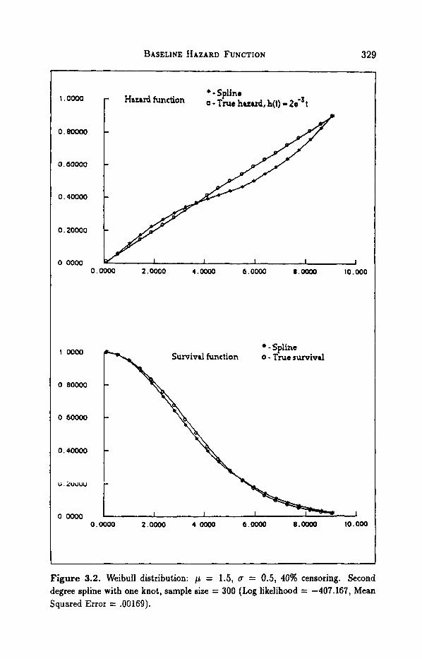
Figure 3.2. WeibuII distribution: p = 1.5, u = 0.5, 40% censoring. Second degree spline with one knot, sample size = 300 (Log likelihood = -407.167, Mean Squared Error = .00169).

330 J . ANGELOS, C.M.-S. LEE AND K. P. SINGH

0 70000

0 56000

0.42000

0 28000

0 14000

0 0000 0 0000 I 4000 2.0000 4.2000 5 . m 7 0000

1 .0000

0 00000

0 60000

0 40000

0 .ZOO00

0 0000

- Spline Survival function 0 - True survival

c

I I I I I 0 0000 1 4000 2.8000 4.2000 5.6000 7. 0000

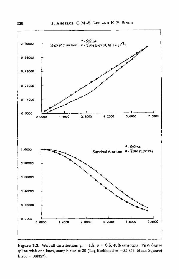
Figure 3.3. Weibull distribution: p = 1.5, u = 0.5, 40% censoring. First degree spline with one knot, sample size = 30 (Log likelihood = -35.844, Mean Squared Error = -00327).

BASELINE HAZARD FUNCTION 331

0.70000

0 56000

0 42000

0 20000

0 14000

0 0000 0 0000 1 4000 2.0000 4.2000 5doOo 7.0000

1 1000

0 88000

0 66000

0 44000

0 22000

0 0000 1 I I I 1 0 o m 1.4000 2.0000 4.2000 5 . m 7 0000

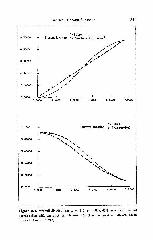
Figure 3.4. Weibull distribution: p = 1.5, u = 0.5, 40% censoring. Second degree spline with one knot, sample size = 30 (Log likelihood = -35.786, Mean Squared Error = .00247).

332 J . ANGELOS, C.M.-S. LEE AND K . P. SINGH

0. soooo

0.40600

0 30000

0.20000

0 10000

0 OOOO

1.1000

0 88000

0. b6000

0.44000

0.22000

0.0000

30 000 150.20 270 40 390 60 510 eo 631.00

r ' - 5 line Survival function o - f rue survival

1 I I I I I 0.0000 1.4000 2. 8000 4.2000 5.6000 7.0000

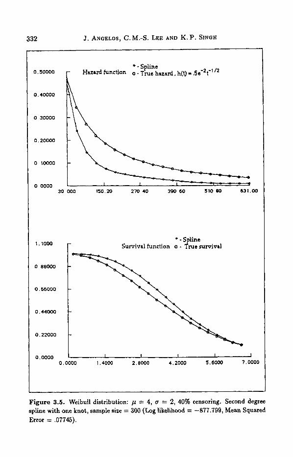
Figure 3.5. Weibull distribution: p = 4, u = 2, 40% censoring. Second degree spline with one knot, sample size = 300 (Log likelihood = -877.799, Mean Squared Error = .07745).

BASELINE HAZARD FUNCTION 333

- Spline -2 -112 Hazard function 0 - True hazald, h(t) = 5 e t

0.030000

0.024000

0 018000

0 012000

0 0060000

0 0000 30.000 150 * 20 270.40 390.60 510.80 63 I .OO

0. sooao

0 40000

0 30000

0.20000

0. too00 - I - - . 0 Woo

30 000 150.20 270 40 390.60 510.80 631.00

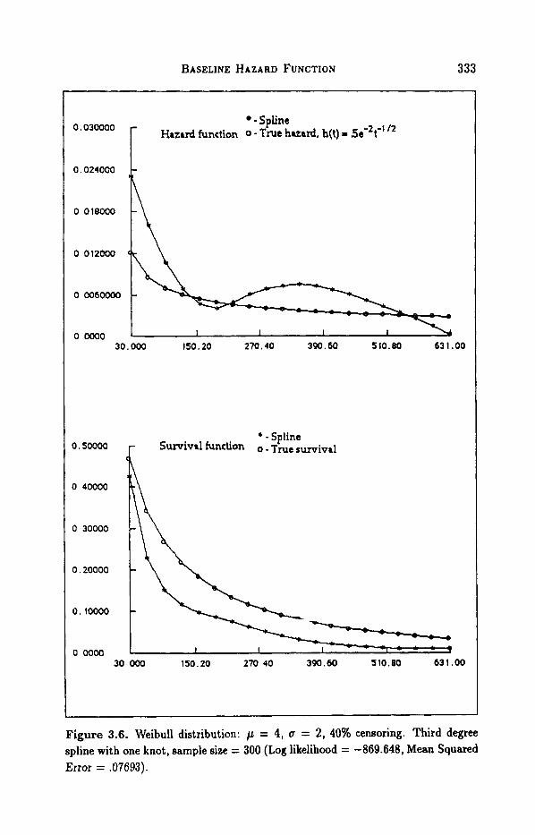
Figure 3.6. Weibull distribution: p = 4, u = 2, 40% censoring. Third degree spline with one knot, sample size = 300 (Log likelihood = -869.648, Mean Squared Error = .07693).

334 3 . ANGELOS, c. M.-S. LEE A N D K. P. S I N G H

0.16000

+ - Spline 0.20000 Hazard function 0 - True hazard, h(t) - 5e'2 t-' '2

-

0 040000

0 0000 10.000 28 000 46.000 b4 000 82.000 100.00

1 0000

0 80000

0 60000

0 40000

0 20000

0 0000 L I I I I

10 000 28.000 46 000 64.000 82.000 100 00

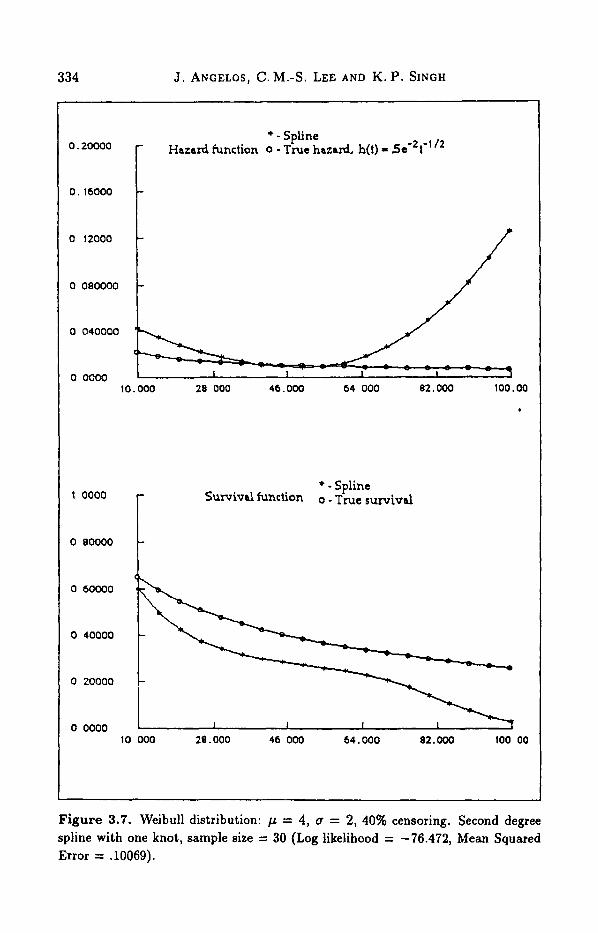
Figure 3.7. Weibull distribution: p = 4, Q = 2, 40% censoring. Second degree spline with one knot, sample size = 30 (Log likelihood = -76.472, Mean Squared Error = .10069).

BASELINE HAZARD FUNCTION 335

6.3800

4 7600

3 1400

1 5200

8.OOOO

-

-

-

-

-0 I0000 -0

1 lo00

0 88000

0 66000

0 44000

0 22000

0.0000

'-s line Hazard )unction 0 - f N e hazard, h(t)=3t2

I - I I I I loo00 0.26000 0.62000 0 98000 I .3400 1 7 m

'-s line Hazard )unction 0 - f N e hazard, h(t)=3t2

I - I I I I loo00 0.26000 0.62000 0 98000 I .3400 1 7 m

-0.10000 0.28000 0 66000 I 0400 1 .42W 1 8000

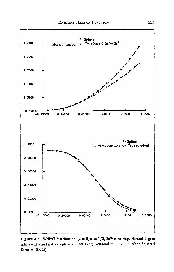
Figure 3.8. Weibull distribution: p = 0, u = 1/3, 20% censoring. Second degree spline with one knot, sample size = 300 (Log likelihood = -113.710, Mean Squared Error = .00298).

336 J. ANGELOS, C . M . 4 . LEE AND K.P. SINGH

h ( t ) Parameters Censor N Log likelihood Values

p a % MLE B-Spline

m = l m = 2 m = 3 ~ ~~~ ~ ~~ ~

2e-3t 1.5 .5 40 300 -408.22 -408.88 -407.17 - 30 -34.58 -35.84 -35.78 -

. 5 ~ - ~ t - . ’ 4.0 2.0 40 300 -796.74 - -877.80 -869.65 30 -72.66 - -76.47 -

3t2 0 113 10 300 -88.34 - -89.20 - 20 300 -113.50 - -113.71 - 30 300 -103.52 - -103.78 -

m indicates the degree of B-spline ‘Cencor’ indicates the percent of random censoring

Table 3.1. Comparison of log likelihood values for Weibull models obtained by ML and B-spline approaches.

BASELINE HAZARD FUNCTION 337

.oooooo

.083350

.166700

.250050

.333400

.416750

.500100

.583450

.666800

.750150

.833500

.916850 1.000200 1.083550 1.166900 1.250250 1.333600 1.416950 1.500300 1.583650 1.667000

.oooooo

.020842

.083367

.187575

.333467

.521042 ,750301 1.021243 1.333868 1.688177 2.084169 2.521844 3.00 1 203 3.522245 4.084971 4.689380 5.335472 6.023248 6.752707 7.523849 8.336667

.oooooo

.020842

.083367

.187575

.333467

.521042

.750300 1.021242 1.333867 1.688175 2.084 167 2.521842 3.001200 3.522242 4.084967 4.689375 5.335467 6.023242 6.752700 7.523842 8.336667

1 .oooooo .999421 .995378 .984487 .963619 .930176 .882431 .819866 .743435 .655650 .560430 .462681 .367658 .280221 .204146 .14 1664 .093313 .058141 .034149 .018841 .009731

1 .oooooo .999421 .995378 .984487 .963619 .930176 .882431 .819866 .743435 .655650 .560430 .462681 .367659 .280221 .204146 .141664 .093313 .058141 .034149 .OM841 .009731

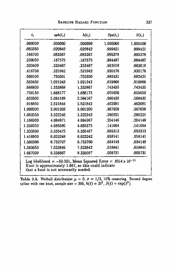
Log likelihood = -89.201, Mean Squared Error = .8314 x lo-" Knot is approximately 1.667, so this could indicate that a knot is not necessarily needed.

Table 3.2. Weibull distribution p = 0, u = 1/3, 10% censoring. Second degree spline with one knot, sample size = 300, h( t ) = 3t2, S(t ) = exp(t3).

338 J . ANGELOS, C. M A . LEE AND K. P. SINGH

.oooooo

.077350

.154700

.232050

.309400

.386750 ,464100 .541450 .618800 .696150 .773500 .850850 .928200 1.005550 1.082900 1.160250 1.237600 1.314950 1.392300 1.469650 1.547000

.oooooo

.017949

.071796

.161542

.287185

.448727

.646 167

.879505

.148741 1.453876 1.794909 2.171839 2.584668 3.033395 3.510821 4.038544 4.594966 5.187286 5.815504 6.479620 7.179627

.oooooo

.017949

.071796

.161542

.287185

.448727

.646166

.879504 1.148740 1.453874 1.794907 2.171837 2.584666 3.033392 3.510817 4.038540 4.594961 5.187281 5.8 15498 6.4796 13 7.179627

1.000000 .999537 .996305 .987582 .970816 .943793 .go4872 .853222 .789033 .713643 .629527 ,540117 .449465 .36 177 1 .280863 .209736 .150232 . 1 0293 3 .067274 .04 1825 ,024667

1.000000 .999537 .996305 .987582 .970816 .943793 .go4872 .853222 .789033 .713644 .629527 .540117 .449466 .361771 .280863 .209736 .150232 .lo2934 .06 72 75 .041825 .024667

Log likelihood = -103.78, Mean Squared Error = .591 x Knot is approximately 1.547, so this could indicate that a knot is not necessarily needed.

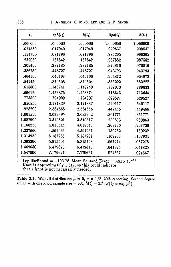
Table 3.3. Weibull distribution p = 0, u = 1/3, 30% censoring. Second degree spline with one knot, sample size = 300, h( t ) = 3t2, s(t) = exp(t3).

BASELINE HAZARD FUNCTION 339

REFERENCES

Anderson, J.A. and A. Senthilselvan (1980), "Smooth estimates for the hazard function".

Bloxom, B. (1985), "A constrained spline estimator of hazard function". Psychometricka

Ciampi, A. and J. Etezadi-Amoli (1985), "A general model for testing the proportional hazards and the accelerated failure time hypotheses in the analysis of censored survival data with covariates". Communicationa in Statistics, Series A 14(3), 651-667.

Cox, D.R. (1972)' "Regression models and like tables with discussion". Journal of the Royal Statistical Society, Series B 34, 187-208.

deBoor, C. (1978). A Proctical Guide to Splines. New York: Spring-Verlag. Etezadi-Amoli, J. and Ciampi, A. (1987), "Extended hazard regression for censored sur-

vival data with covariates: A spline approximation for the baseline hazard function". Biometrics 43, 181-192.

Jarjoura, D. (1988), "Smoothing hazard rates with cubic splines". Communications in Statistics (to appear).

Klotz, J. (1982), "Spline smooth estimates of survival". IMS, Monograph Series. Klotz J . and R.-Y. Yu (1986), "Small sample relative performance of the spline smooth

survival estimator". Communicationa in Statistics, Series B 15, 815-818. Lawless, J.F. (1980), "Inference in the generalized gamma and log-gamma distributions".

Technometrics 22(3), 409-419. Li, K.-C. (1985), "From Stein's unbiased risk estimates to the method of generalized cross-

validation". Annals of Statutics 13(4), 1352-1377. Rice, J. and M. Rosenblatt (1983)' "Smoothing splines: Regression, derivatives and decon-

volution". Annals of Statistics 11, 141-156. Schumaker L.L. (1981). Spline Functions: Basic Theory. New York: John-Wiley k Sons. Silverman, B. (1982), "On the estimation of a probability density function by the maximum

penalized likelihood method". Annals of Stotutics 10(3), 795-810. Smith, P.L. (1979), "Splines as a useful and convenient statistical tool". The American

Statistician 33(2), 57-62. Speckman, P. (1985), "Spline smoothing and optimal rates of convergence in nonparametric

regression models". Annals of Statistics 13, 972-983. Tanner, M.A. and H.-W. Wong (1984), "Data-based nonparametric estimation of the haz-

ard function with applications to model diagnostics and exploratory analysis". Journal of the Americnn Statistical Association 79, 445460.

Wahba, G. (1985), "A comparison of GCV and GML for choosing the smoothing parameter in the generalized spline smoothing problem". Annals of Statutics 13(4) , 1378-1402.

Whitternore, A.S. and J.B. Keller (1986), "Survival estimation using splines". Biometrics

Journal of the Royal Statistical Society, Series B 42(3), 322-327.

SO, 301-321.

42, 495-506.