b' s rns Integrating arbitrage pricing theory and artificial neural

~, . -:~ . ..

ELSEVIER Decision Support Systems 18 (1996) 301- 316

sa0" b' s rns

Integrating arbitrage pricing theory and artificial neural networks to support portfolio management

Shin-Yuan Hung, Ting-Peng Liang *, Victor Wei-ehi Liu Department of Information Management, National Sun Yat-sen University, Kaohsiung, Taiwan 80424, Taiwan ROC

Received 2 November 1994; revised 10 July 1995; accepted 12 November 1995

A b s t r a c t

The paper presents an innovative approach that integrates the arbitrage pricing theory (APT) and artificial neural networks (ANN) to support portfolio management. The integrated approach takes advantage of the synergy between APT and ANN in extracting risk factors, predicting the trend of individual risk factor, generating candidate portfolios, and choosing the optimal portfolio. It uses quadratic programming for identifying surrogate portfolios in APT and ANN to predict factor returns. Empirical results indicate that the integrated method beats the benchmark and outperforms the traditional method that uses the ARIMA model.

Keywords: Arbitrage pricing theory; Artificial neural networks; Portfolio management; Decision support systems; System integration; Unified programming

1. I n t r o d u c t i o n

Portfolio management is a major issue in investment. Its goal is to choose a set of risk assets to form a portfolio that can maximize the return under a given risk or minimize the risk for obtaining a given return. Due to the complexity in portfolio management, institutional investors often need decision support systems (DSS) to facilitate their decision making. A critical factor for developing a successful DSS for portfolio management is its stock selection model.

* Corresponding author. E-mail: [email protected].

A good model allows good stocks to be selected to reach a higher performance.

The most popular model in portfolio management in recent years is the arbitrage pricing theory (APT) developed by Stephen Ross in 1976 [28-31]. Theo- retically, the APT model can price risk assets of a portfolio efficiently from a few risk factors. It identi- fies three to five risk factors [2,27] from a number of possible candidates, and then selects securities based on their relative risks and returns compared to the market. In practice, however, heuristics are usually required to overcome bottlenecks in determining a proper set of stocks when APT is used alone. For instance, in the Roll and Ross investment review process (as shown in Fig. 1) [28], investors have to know the probability of success in meeting the speci-

0167-9236/96/$15.00 Copyright © 1996 Elsevier Science B.V. All fights reserved. PII S0167-9236(96)0003 I-0

302 S.-Y. Hung et a l . / Decision Support Systems 18 (1996) 301-316

fled target before they set up the desired performance level relative to the benchmark (i.e., the market index that they want to "beat") . Further- more, once the target level of performance is set, they need heuristics to determine the levels of risk exposure with each factor and the weight of each risk asset in the portfolio to reach the goal. In general, these heuristics are hard to acquire and are considered highly sensitive in most investment firms.

Recently, much research has focused on using artificial intelligence (AI) techniques to predict stock prices. One technique of particular interests is the a r t i f i c i a l n e u r a l n e t w o r k s ( A N N ) [11,12,14,16,23,34,36,40,41]. Cybento has proven that if correct interconnection weights can be found, an ANN with a sufficient number of neurons in the

hidden layer can be used to approximate any multi- dimensional function to any specified degree of ac- curacy [7]. However, practical limitations exist when we use the ANN alone to support portfolio management. A major one is that it requires heavy computa- tional efforts because the number of securities to be analyzed is usually very large. For instance, if we want to formulate an ANN model to analyze 100 stocks with each having data for 100 periods, we may need 10,000 neurons at certain ANN layers, which is computationally prohibitive.

Given the facts that using ANN models alone to analyze portfolio performance would be too compli- cated and the APT model can reduce the number of the risk factors, it seems to be beneficial to integrate these two approaches. The solution of the integrated

I 1. Add recent observations to our historical data base of individual securities in various markets.

I 2. Create master portfolios, each of which mimics the up and down ]

movements of a single risk factor. I

3. For each stock, determine risk coefficients from regression I against the master portfolios. I

each type of risk over the next month.

5. Calculate the target exposures that tailors the client' s portfolio to pre-specified guidelines

6. Select individual securities that have low total volatility, high alpha or intrinsic value, and the aggregate

targeted pattern of risk exposures.

I 7. Reoptimizethe portfolio monthly. I

Fig. 1. The Roll and Ross investment review process.

S.- Y. Hung et al. / Decision Support Systems 18 (1996) 301-316 303

approach requires to adopt both artificial intelligent and optimization paradigms in a unified manner [ 18]. Toward this end, this paper studies two issues: (1) how ANN can be integrated with APT to support portfolio analysis, and (2) how well the integrated method performs.

In this research, a novel approach for integrating APT and ANN is developed. The approach suggests using quadratic programming to obtain the maximum explained variance of risk factors to risk assets returns for asset pricing in APT. Once risk assets have been priced, ANN can be applied to predict the effects of risk factors on assets prices. Investment alternatives can then be generated, and the optimal (most efficien0 investment portfolio can be determined based on the prediction and the investor's preference. Through the unification of AI and optimization methods, the complex portfolio management can be solved.

To evaluate the integrated approach, empirical studies are conducted. We examine the number of risk factors determining assets pricing in the Taiwan stock market, and compare with the benchmark the performances of (1) integrating APT with the ANN model (IANN model) and (2) integrating APT with the ARIMA model (IARIMA model). The Taiwan Stock Exchange Weighted Price Index (TSEWPI) of the Taiwan stock market was chosen as the benchmark.

This research is an application and implementa- tion of unifying mathematical programming and AI techniques. Its contribution is threefold. First, the integration of APT and ANN successfully eliminates the limitations of using APT or ANN models alone in portfolio management. Second, the integrated approach shows capabilities to effectively automate the portfolio management process. Finally, our findings also show a successful integration of optimization and AI techniques. This can provide insights into further integration of mathematical optimization models and AI techniques.

The remainder of the paper is organized as follows. First, the concepts of APT and ANN are discussed. This is followed by a description of our integrated approach that combines APT with the ANN model. Finally, empirical studies evaluating the performance of the integrated method and their findings are discussed.

2. Research background

2.1. Arbitrage pricing theory

It is a common believe that if you want to obtain a higher return in the financial market, you must bear higher risks. This simple concept raises at least two questions: (1) what do we mean by "r i sk" , and (2) how can it be measured? The capital asset pricing model (CAPM) [33] was an early approach to include risks in portfolio analysis. According to CAPM, the risks of a security are measured by its beta coefficient. The beta coefficient of a security is defined as the sensitivity of the security's return compared to the return of the "market" . In theory, the market is the portfolio composed of all securities and assets available for investment. For example, when a security whose return variation is larger than that of the market, then its beta is greater than one. Its beta would be less than one, otherwise.

Since the CAPM uses a single factor to capture security risks, it is considered inadequate in many situations. To offset this problem, the APT model that refines CAPM to include multiple risk factors was developed later. The major assumption of the APT model is that the investment risks can be broken down into systematic and idiosyncratic risks [28]. Systematic risks are market-oriented and perva- sively influence virtually all security prices (e.g., interest rates or the business cycle). They are intro- duced by the limited number of risk factors we consider for constructing the portfolio. Idiosyncratic risks involve unexpected events peculiar to a single security or a limited number of securities (e.g., the loss of a key contract or a change in government policy toward a specific industry). They can be eliminated in large well diversified portfolios.

Basically, APT is a multiple-index model that uses a few influential risk (common) factors to determine asset prices. Ross was the first to show that a multiple index model would always lead to a unique relative pricing model [31]. The return calculation equation for each security is shown in Eq. (1). In equilibrium conditions, the relative price of each security can be described by the Eq. (2) [10].

k

Ri=ai+ E flit, RL +ei, (1) L=I

304 S.-Y. Hung et aL / Decision Support Systems 18 (1996) 301-316

where:

R~ = the return on risk asset i; a i = the unique expected return associated

with risk asset i; fill = the sensitivity of risk asset i to index

L, for L = 1 . . . k ; R L --- the return on index L; e i -- a random variable with a mean of zero

and a variance of o-2 e i •

k

Ri= Re + E biLAL, (2) L = I

where:

R F =

biL -~

the average return on risk asset i; the risk-free return; the estimated sensitivity of risk asset i to index L; the price of risk L.

A number of empirical studies have examined the validity of the APT model [2-6,8,9,20,24,27,39]. For instance, Roll and Ross [27] gathered the daily returns on 1,260 stocks listed on the New York and American Stock Exchanges between July 3, 1962 and December 31, 1972 (a total of 2,619 trading days). These data were then grouped into 42 groups, with each having 30 stocks. They used these data to evaluate APT and concluded that there were three to five risk factors that determined asset pricing. In Taiwan, Wu and Lin [39] studied the explanation power of asset pricing models using the trading data at the Taiwan Stock Exchange. The results indicated that APT was indeed more powerful than the traditional CAPM model.

2.2. Applying APT to support portfolio management

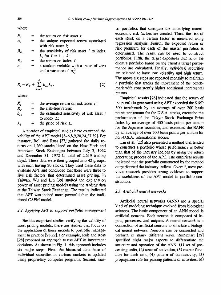
Besides empirical studies verifying the validity of asset pricing models, there are studies that focus on the application of these models to portfolio management in practice [28,22]. For example, Roll and Ross [28] proposed an approach to use APT in investment decisions. As shown in Fig. 1, this approach includes six major steps. First, the historical data base of individual securities in various markets is updated using proprietary computer programs. Second, mas-

ter portfolios that surrogate the underlying macro- economic risk factors are created. Third, the risk of each stock on a certain factor is measured using regression analysis. Fourth, the expected return or risk premium for each of the master portfolios is determined. The result can be used to construct portfolios. Fifth, the target exposures that tailor the client's portfolio based on the client's target performance are calculated. Finally, individual securities are selected to have low volatility and high return. The above six steps are repeated monthly to maintain a portfolio that tracks the movement of the benchmark with consistently higher additional incremental returns.

Empirical results [28] indicated that the return of the portfolio generated using APT exceeded the S &P 500 benchmark by an average of over 200 basis points per annum for the U.S.A. stocks, exceeded the performance of the Tokyo Stock Exchange Price Index by an average of 400 basis points per annum for the Japanese securities, and exceeded the EAFE by an average of over 500 basis points per annum for non-U.S.A, international stocks.

Lin et al. [22] also presented a method that tended to construct a portfolio whose performance is better than that of the industry indices by using the return generating process of the APT. The empirical results indicated that the portfolio constructed by the method outperformed the industry indices. Overall, most previous research provides strong evidence to support the usefulness of the APT model in portfolio construction.

2.3. Artificial neural networks

Artificial neural networks (ANN) are a special kind of modeling technique evolved from biological sciences. The basic component of an ANN model is artificial neurons. Each neuron is composed of inputs, processes, and outputs. A neural network is a connection of artificial neurons to simulate a biological neural network. Neurons can be connected and perform in many different ways. Rumelhart [32] specified eight major aspects to differentiate the structure and operation of the ANN: (1) set of processing units, (2) state of activation, (3) output function for each unit, (4) pattern of connectivity, (5) propagation rule for passing patterns of activities, (6)

S.-Y, Hung et al . / Decision Support Systems 18 (1996) 301-316 305

activation rule for combining inputs affecting a unit with its present state to produce an output, (7) learning rule whereby interconnections can be modified on the basis of experience, and (8) environment within which the learning system must operate.

Since neurons can be connected differently, there are many types of ANN models (called "paradigms"). In general, we categorize these models according to their learning behavior. For example, we may categorize them into supervised or unsupervised learning based on the availability of the outcome class. Supervised learning learns from input data whose classes are known, whereas unsupervised learning groups data without known classes into clusters based on their similarity. In ANN, Percep- tron and back-propagation network (BPN) are supervised learning models, whereas adaptive resonance theory (ART) and bi-directional associative memory (BAM) are unsupervised learning models. Among different models, BPN is the most popular and has the highest success rate.

A BPN model is composed of several layers (generally, more than two layers) of neurons. Each layer contains a predetermined number of neurons. Every neuron in a layer connects to all neurons in

Input Hidden Output Layer Layer Layer

Wjk

Xi ~ 09

Fig. 2. A 4--5-4 back-propagation neural network structure.

the adjacent layers. For example, a 4--5-4 BPN contains four neurons in the input layer, five neurons in the hidden layer, and four neurons in the output layer. Its architecture is shown in Fig. 2. The neurons at the input layer receive messages from the external environment, and those at the output layer send messages to the environment. One or more hidden layers are set between the input and output layers. The existence of the hidden layer enables the ANN to model complex causal structures through interactions among the neurons.

A major step in building ANN models is to learn the connection weights through training. The process of training a BPN includes the following steps: (1) set the connection weights of a BPN model ran- domly, (2) select a training case from the training set and send its input vector to the input layer of the BPN, (3) calculate the output of the BPN, (4) calculate the error between the output of the model and the actual value, (5) adjust the connection weights based on the learning rule to remove the error, (6) repeat steps 2 to 6 until the sum of errors is below the specified tolerance level. A detailed description of the BPN algorithm can be found in [15].

ANN have advantages over traditional classification methods such as discriminant analysis. For instance, ANN can provide a proper solution for complex classification or prediction problems by the internal associative and adaptive abilities of the network. Moreover, ANN is fault-tolerant. ANN have disadvantages too. First, its learning process is very time-consuming. It could easily take hours of compu- tation on a computer before a stable model can be built. Second, it is hard to explain how it solves the problem. The causal relationships are hidden in the network connections. Finally, the determination of an optimum network structure has remained as an art that must rely on trial and error. This adds more uncertainty into the model building process. Overall, it is a useful technique worth serious studies.

2.4. Applying ANN to support inoestment decisions

ANN has been used widely in financial analysis [ 2 5 , 2 6 , 3 5 ] and i n v e s t m e n t p r e d i c t i o n [11,12,14,16,23,34,36,40,41]. For example, Tani- gawa and Kamijo [36] proposed a stock price pattern matching system using a Dynamic Programming


Neural Network (DNN). DNN is based on the integration of the neural network and Dynamic Program- ming matching method (DP-matching). The stock price patterns classified by DNN were evaluated by three chartists (human experts). It became clear that high correlation was found between the classification by DNN and the evaluation by chartists. The proposed DNN system was able to match patterns judged by the chartists as similar.

Kimoto et al. [ 16] proposed an ANN to determine the timing to buy or sell the TOPIX index. They trained and tested the ANN using the weekly data from January 1987 to September 1989. The result indicated that the ANN model performed better than the benchmark. If we set the TOPIX index of Jan- uary 1987 as 1.00, the straight-forward buy-and-hold strategy would result in a performance of 1.67 by September 1989, whereas the performance of the ANN model would be 1.98.

Jang et al. [12] proposed a structure-level adaptive back-propagation learning algorithm that could auto- matically synthesize the structure of a neural network to fit the desired problem. The results indicated that, for the testing period between 1990 and 1991, the annual rates of return from trading decisions suggested by the proposed system were higher than those of the buy-and-hold strategy.

Although ANN have been used to predict stock prices, limitations exist when they are used for portfolio analysis. The major one is that the complexity of the network model increases dramatically as the number of stocks to be analyzed increases. This may make the model building extremely expensive and sometimes impossible.

3. Integrating arbitrage pricing theory with artificial neural networks

Given that both APT and ANN have their strengths and weaknesses, it is natural to seek an integration. Integration of mathematical optimization and artificial intelligence methods has been applied in several occasions [17-19,21]. For example, Liang et al. [21] developed an approach that integrates semi-Markov decision models and ANN for production scheduling. Empirical evidence indicated that the integrated method outperformed the individual method.

Lee and Song [17] proposed a method that integrates linear programming (LP) models and rule- based systems for the crude oil purchase scheduling. The LP model covers the monthly crude oil purchase plan, while the rule-based system covers the daily crude oil delivery schedule. The Post-Model Analy- sis (PMA) approach is necessary because the monthly optimal purchase plan must be adjusted during im- plementation to accommodate the dynamic situation of suppliers and tankers.

Lee et al. [19] proposed a K-FOLIO system, which integrates the Markowitz risk-return optimization model with the expert knowledge of specialists and managers, to support investment management. Empirical results indicated that the cumulated K- FOLIO returns from January to December 1987 were greater than the average market yield and the returns of the unenhanced Markowitz model in Korean Stock Exchange.

An integration of APT and ANN has certain advantages. The APT method has strong theoretical background but needs heuristics in practical applications. The ANN method is capable of providing reliable heuristic models when prediction of certain factors is necessary in constructing portfolios.

The integrated approach in our research includes three major components: APT, ANN, and a portfolio constructor. We need to use the APT model to price the risk assets available for building a portfolio. Once the prices are determined, we need to use the ANN model to predict the trend of each risk factor in the future. Finally, we use the portfolio constructor to generate investment alternatives and select the optimal (most efficient) portfolio from the candidates based on the investor's preference. Fig. 3 shows the process of the integrated approach. Individual mod- ules are described in detail in the following.

3.1. Using APT to price risk assets

The first module of the integrated approach is to determine the prices of risk assets. Its primary pur- pose is to determine the factors having effects on the fluctuation of security returns and their effects on the return of individual securities. Using APT could identify these factors and price all the risk assets available for building a portfolio. It includes four major steps (Steps 1 to 4 in Fig. 3).

S.- Y. Hung et al. / Decision Support Systems 18 (1996) 301-316 307

Using APT to price risk assets

Determination of

Surrogate Portfolio

by Quadratic

Programming (GINO)

4 Asset Pricing

by Regression Analysis (SAS)

3 Calculation of Risk Premium.¢

(l'xcel)

Using ANN Using portfolio constructor to predict the movements and selection mechanism to

I of each risk factor "--] [ - ' - generate suggested portfolio

Return Prediction

Generation of

r Candidate PortfolioJ

9 Setting Objectives

ANN Model

I Construction

6 ANN

Learning (NeuroShcll)

© Fig. 3. The process of the integrated approach.

/o_/ Portfolio

Step 1. Factor analysis. The first step is to decide what kinds of risk assets

are available for consideration in building a portfolio and what will be the benchmark. After the selection is done, factor analysis is used to determine factors effecting the fluctuation of security returns. The factor analysis includes two sub-steps: (1) The prin- ciple factor analysis is applied to determine the proper number of risk factors having effects on the fluctuation of security returns. A factor is selected if its eigenvalue is greater than one [13]. (2) After the number of risk factors is determined, the maximum- likelihood factor analysis is applied to extract the factor structures (including the factor loading matri- ces and a residual matrix). Statistical packages such as: SAS, SPSS, etc. are useful in this step.

Step 2. Surrogate portfolios of risk factors. After the factor analysis, we use the result to

define the basis portfolios (also known as "master portfolios '') and the orthogonal portfolio. A basis portfolio is a collection of securities that can be used as a surrogate measure of a risk factor. An orthogo-

nal portfolio is created to measure the risk-free return. In order to minimize the effect of idiosyncratic risk and maximize the effect of systematic risk, we adopt the minimum idiosyncratic risk procedure in- vented by Lehmman and Modest [20]. Quadratic programming is used to determine the weights of each basis portfolio and the orthogonal portfolio from the factor structures. The weights determined by quadratic programming maximize the explained variance of risk factors to risk assets returns. Tools such as: GINO and LINDO are used at this step. The result of this step often extracts three to five basis portfolios from numerous securities. In our research, three basis portfolios in the former nine periods and four basis portfolios in the latter three periods are identified from 51 stocks.

Step 3. Calculation of risk premiums. In this step, we calculate all the extra returns (also

known as "the risk premiums") of various factors. After the orthogonal portfolio and the basis portfolios have been created, the extra return of each basis portfolio (A L in Eq. (2)) can be calculated. Similarly,

308 S.-Y. Hung et a l . / Decision Support Systems 18 (1996)301-316

the extra returns of the spec!fied benchmark and each of the risk assets (Ri - Re in Eq. (2)) can be calculated.

Step 4. Asset pricing. Finally, we need to determine the sensitivity of

individual asset's risk premium to the changes in certain risk factors. Since there are multiple risk factors surrogated by basis portfolios, each asset has an array of beta coefficients. The process of finding the beta coefficients of an asset is called asset pricing, which can be done by using multiple regression analysis. For the specified benchmark and each risk asset, the beta coefficients are determined from the regression against the risk premiums of each risk factors.

3.2. Using ANN to predict the future trend of each risk factor

Once all risk assets available for portfolio construction have been priced, we use ANN to predict the future trend of each risk factor for building the portfolio. This module includes three major steps (Steps 5, 6, and 7 in Fig. 3).

neural networks. First, the training data sets are used to train the BPNs. This step is very time-consuming. Then, the resulting models are evaluated using the testing data sets. If the test results are not good enough, they have to be retrained. NeuroShell [38] was the software we used in this research.

Step 7. Return prediction. After all the ANN models have been trained, we

use the predictive data sets to forecast the risk-free return and the returns of each risk factor in the succeeding weeks. For each risk asset and the benchmark, its beta coefficients (obtained in Step 4), the predicted risk-free return and the predicted returns of each risk factor are then combined to calculate the predictive returns of the asset. For example, a risk asset has been found to be effected by three risk factors, and its beta coefficients to those factors are 0.1, 0.2, and 0.3 respectively. The predicted risk-free return (for the first week) is 0.5. The predictive returns of each risk factor (for the first week) are 0.6, 0.7, and 0.8, respectively. Given these, the predicted return of the risk asset (for the first week) can be calculated as 0.5 + 0.1" (0.6 - 0.5) + 0.2 * (0.7 - 0.5) + 0.3* (0.8 - 0.5) = 0.64.

Step 5. ANN model definition. In order to use ANN to predict the future trend of

a risk factor (basis portfolio) or the risk-free return (orthogonal portfolio), we have to define proper model structures. If four risk factors are identified for those stocks, then we need to define five ANN models, one for each risk factors and one for the risk-free return. For each model, an analysis period is an input node and a predictive period is an output node. The hidden nodes are determined by heuristics. For example, if we use four weekly returns to predict the following four weekly returns, then the ANN model will have four input and output nodes, respectively. The number of output nodes is determined by the number of predicted weekly risk premiums for the risk factor we need. The optimal numbers of input and hidden nodes are obtained by trial-and-error.

Step 6. Learning. After the structure of the BPNs has been deter-

mined and data are available, we begin to train the

3.3. Using porlfolio constructor and selection mechanism to generate the suggested por(folio

Once the model for predicting future returns of the risk assets has been constructed, we can build portfolios based on the predicted returns and risks of the risk assets. In our research, we use a simulation- based approach that first generates a number of candidate portfolios and then chooses the optimal among the candidates. It includes three major steps (Steps 8, 9, and 10 in Fig. 3).

Step 8. Generation of candidate portfolios. Given the predictive return and risk of each risk

asset, we can construct portfolios by combining different assets. In this step, we use simulation to generate a number of candidate portfolios and calculate their returns and risks. The process of generating a candidate portfolio includes two sub-steps: (1) a set of asset weights (Wil ,Wi2 . . . . . Win) are generated ran- domly to simulate a possible portfolio. An asset weight is the proportion of the risk asset in a portfo-

S.-Y. Hung et aL / Decision Support Systems 18 (1996) 301-316 309

lio. The sum of the asset weights must be equal to one; (2) the predictive return and risk of the portfolio (R-7,tr~) are estimated using the predicted return of the risk assets. Each portfolio generated in this step is a candidate (wn,w~2 . . . . . w~,; R-7,tr~) for selection later.

Step 9. Setting goals. Once enough candidate portfolios are generated,

we can choose the optimal among them to meet our investment goals. In general, our investment goals include predetermined return and risk levels that are considered satisfactory. Although the goals may be set up arbitrarily, a better way is to use the expected performance of the benchmark.

In this step, we first estimate the future return and risk (variance) of the benchmark. Then, the investor uses the estimated performance of the benchmark to determine the proper levels of return and risk. For example, a user may set up goals such as a return being 0.2 above the benchmark return and the volatility being 0.2 less than the standard deviation of the weekly return.

Step 10. Portfolio selection. In the last step, the optimal portfolio is chosen

among the candidates based on the investor's goals. The selection mechanism uses the return and risk of a candidate portfolio to compute its performance score. The formula for calculating the scores for candidates is listed in Appendix A. The optimal portfolio is chosen according to the performance score of the candidate portfolio.

4. Empirical evaluation

Although the integrated method seems to be promising, empirical studies are necessary to evaluate its value. In this section, we present the empirical findings from applying the integrated method to the stocks traded in the Taiwan Stock Exchange. Two major issues were examined in the study. First, whether the por(folios constructed by the integrated method perform better than the benchmark. The benchmark chosen was the TSEWPI, the weighted stock price index published by the Taiwan Stock

Table 1 Hypotheses for the empirical study

Hi:/x(Rp/A jv~ v - R p r s e w e I) = 0 H~ :/z(RPlanlM a --RPTsEwP t) = 0 H3o :/z(RPtA~/N --Rpt~etM ~) = 0 H 04 :/z[E(Rpt ANN ) -- E(RPrse wet )] = 0 H~ : l~[E(RPtAtCtMa)-E(RPrsewet) ] = 0 H~:/z[E(RplA,v, v ) - F_(RptantMA)] = 0 H~: p.[SIXRpt ANN ) - SD(RPrs~w et)] = 0 H i :/z[SD(Rp/a gt~, a ) - SD(RPrsewet)] = 0 H09 :/.~[SD(RPla,v,v) - SD(Rp,a,~/MA)] = 0

Notations: Rp: means the return of the portfolio; E(Rp): means the expected value of Rp; SD(Rp): means the standard deviation of Rp.

Exchange. The integrated method must beat the benchmark to be useful.

The second issue studied was whether the ANN module plays a major role in the integrated method. We chose another method that integrates the traditional ARIMA model [1,37] for time series analysis with APT as a basis for comparison. In other words, the ANN model in Step 6 of the integrated method presented in the previous section was replaced by the ARIMA model. The rest procedures were the same. The original method that integrates APT and ANN is called the IANN approach, whereas the one that integrates APT and ARIMA is called the IARIMA approach. If ANN plays a significant role, we would expect that the former performs better than the latter.

The performance of a portfolio is often measured by its average return and the variance of its return. Most investors desire a higher average return and lower variance. In the study, we chose three key performance indices: weekly return, monthly return, and the standard deviation of the weekly return. Nine null hypotheses for testing, as listed in Table l, are formed. In the Table, Rp stands for the weekly return of a portfolio, E(Rp) stands for the average of the weekly return by four weeks of a portfolio. SD(Rp) stands for the standard deviation of the weekly return in a month. The italic subscripts stand for the portfolio construction method. Therefore, RPtAN N stands for the weekly return of the portfolio constructed by the IANN method.

310 S.- Y. Hung et aL / Decision Support Systems 18 (1996) 301-316

Table 2 The training and evaluation periods

Window Training period Evaluation period

l 1 1 / 2 5 / 9 0 - 1 1 / 2 1 / 9 2 11/28/92-12/19/92 2 12/23/90-12/19/92 12 /26 /92 -01 /16 /93 3 01/20/91-01/16/93 0 1 / 2 3 / 9 3 - 0 2 / 1 3 / 9 3 4 0 2 / 1 7 / 9 1 - 0 2 / 1 3 / 9 3 0 2 / 2 0 / 9 3 - 0 3 / 1 3 / 9 3 5 0 3 / 1 7 / 9 1 - 0 3 / 1 3 / 9 3 0 3 / 2 0 / 9 3 - 0 4 / 1 0 / 9 3 6 0 4 / 1 4 / 9 1 - 0 4 / 1 0 / 9 3 0 4 / 1 7 / 9 3 - 0 5 / 0 8 / 9 3 7 0 5 / 1 2 / 9 1 - 0 5 / 0 8 / 9 3 0 5 / 1 5 / 9 3 - 0 6 / 0 5 / 9 3 8 0 6 / 0 9 / 9 1 - 0 6 / 0 5 / 9 3 0 6 / 1 2 / 9 3 - 0 7 / 0 3 / 9 3 9 0 7 / 0 7 / 9 1 - 0 7 / 0 3 / 9 3 0 7 / 1 0 / 9 3 - 0 7 / 3 1 / 9 3 10 0 8 / 0 4 / 9 1 - 0 7 / 3 1 / 9 3 0 8 / 0 7 / 9 3 - 0 8 / 2 8 / 9 3 11 0 9 / 0 1 / 9 1 - 0 8 / 2 8 / 9 3 0 9 / 0 4 / 9 3 - 0 9 / 2 5 / 9 3 12 0 9 / 2 9 / 9 1 - 0 9 / 2 5 / 9 3 10 /02 /93 -10 /23 /93

Table 3 The results of the factor analysis

Window Identified % of number of explained factors variance

1 3 73.94% 2 3 72.95% 3 3 71.32% 4 3 70.95% 5 3 69.62% 6 3 69.05% 7 3 69.35% 8 3 69.27% 9 3 69.17% 10 4 70.50% l I 4 68.65% 12 4 68.57%

4,1. Data selection Note: A factor was selected if its eigenvalue was greater than one.

The data used for the empirical study were the return of the stocks listed on the Taiwanese Stock Exchange. Fifty-one stocks were selected among the more than 300 traded stocks. The name of the com- panies are listed in Appendix B. The criteria for selection include the following: 1, The stock must be actively traded. 2. The company had never had any major business

crisis. 3. The stock must have been traded for more than

three years by the beginning of the sample period. 4. The sample must cover every industry listed on

the exchange. The time period chosen for research was from

November 25, 1990 to October 23, 1993. The daily return of each stock during the period was obtained

from the econometrics programming system (EPS) database maintained by the Ministry of Education.

4.2. Por(folio construction and evaluation

After data selection, the whole time period was divided into 12 sets of training and evaluation periods, as shown in Table 2. Each set was an experi- mental window that included 103 weeks of data for training and four weeks of data for evaluation. Port- folios were constructed using the training data. Their performance were then evaluated using the evaluation data in the following four weeks. In other words, the investment strategy was to use two years' data to build a portfolio and hold the portfolio for the following four weeks before making changes. The

~Ta/wan EPS data base

-I~ ~ - - I t . - constructor I / / IANN + Selection j---I~/ portfolio m~h.n~,. ] /

. [ A P T j-~ ARIMA ~ ~Se~--l~7:i:: I 7 porffoho / - - . • Perfol evalt I

Fig. 4. The process of the empirical study.

S.-Y. Hung et al . / Decision Support Systems 18 (1996) 301-316 311

T a b l e 4

Per fo rmances o f IANN, IARIMA, and TSEWP1

W i n d o w R p R p R p E(Rp) E(Rp) E(Rp) SD(Rp) SD(Rp) SD(Rp)

IANN IARIMA TSEWPI IANN IARIMA TSEWPI IANN IARIMA TSEWPI

1 1.14763 - 2 . 5 3 5 1 9 - 0 . 6 9 0 .02904 - 0 . 1 2 0 7 7 - 0 . 3 5 7 5 2 .847399 2 .109173 1.472127

2 .83716 - 0 . 0 0 0 2 4 1.13

- 0 .00083 2 .58677 0 .39

- 3 .8678 - 0 .53442 - 2 .26

2 - 3 .14597 - 4 .44424 - 5.52 - 0 .46953 - 1.95593 - 2 .0275 3.14811 3.630031 3 .810699

0 .78375 - 1 .50322 - 2 .28

- 2 .91904 - 4 . 8 7 9 1 2 - 3 . 6 4

3 .40315 3 .00287 3.33

3 2 .15706 2 .3856 1.73 2 .719778 3 .024635 3 .5975 3 .241825 4 .561217 4 .214605

- 0 .85834 - 0 .5943 - 1.35

7 .00779 9 .61702 8.03

2 .5726 0 .69022 5.98

4 8.32671 6 .40028 4.97 3 .750413 3 .97834 3.5625 5.856301 5 .375198 6 .891876

5.41121 4 .40336 8.11

6 .09709 8 .74272 7.73

- 4 .83336 - 3 .633 - 6 .56

5 7 .39059 3 .27437 3.62 3 .07694 1.963683 1.7025 7 .512785 6 .48066 5 .802025

4 .57874 2 .0493 0 .72

8 .27949 9 .11718 8.16

- 7 , 9 4 1 0 6 - 6 . 5 8 6 1 2 - 5 . 6 9

6 - 7 . 8 3 0 0 4 - 4 . 9 4 6 4 5 - 4 . 4 2 0 .55999 2 .183615 - 0 . 0 5 7 5 5 .882015 5 .142435 3 .622636

2 .26519 4 .55688 1.59

5 .92113 2 .15888 - 1.34

1.88368 6 .96515 3 .94

7 0 .90926 4 .1923 - 2 . 4 1 0 .789898 - 0 . 3 5 0 6 2 - 1.6575 3.079681 4 .217338 3 .304304

- 3 .46007 - 5 .66295 - 5.92

1.8945 1.48371 0

3 .8159 - 1.41555 1.7

8 - 2 . 3 9 1 4 1 - 2 . 7 9 9 0 1 - 3 . 3 7 - 1 . 7 4 6 8 6 - 2 . 6 5 4 5 1 - 2 . 6 6 5 2.196361 1.324963 2 .555132

- 2 .14899 - 2 .63767 - 2 .52

1.3598 - 0 .97246 0 .69

- 3 .80684 - 4 .2089 - 5.46

9 5 .31882 6 .67742 4 .14 1.092418 0 .988207 0.33 3 .683057 5 .899683 3 .931878 - 3 .54375 - 3 .70537 - 4.15

2.08921 5 .46665 3.07

0 .50539 - 4 .48587 - 1.74

I 0 2 .88936 0 .22467 1.67 0 .755673 - 0.37031 - 0 .1825 3 .190654 3 .582 2 .553878

3 .9722 4 .38446 2 .36

- 2 .73483 - 2 .264 - 2 .46

- 1.10404 - 3 . 8 2 6 3 6 - 2 . 3

11 - 7 .73562 - 6 .08531 - 1.82 0 .264435 - 1.18447 - 0 .3075 5 .744527 4 .437982 1.912405

1.14462 - 1.32663 0 .48

5 .93113 4 .67864 2.03

1.71761 - 2 . 0 0 4 5 7 - 1.92

12 0 .55258 - 0 .32221 - 1.74 1.497963 2 .166475 1.425 0 .72593 1.662023 2 .293244

2 .24654 2 .87147 1.99

1 .82814 3 .11129 3 .74

1.36459 3 .00535 1.71

A v e r a g e 1 . 0 2 6 6 8 0 . 6 3 9 0 2 9 0 . 2 8 0 2 0 8

Notat ions: Rp: weekly r e m m o f the portfolio; E(Rp): the mon th ly average return o f the portfolio; SD(Rp): the s tandard deviat ion o f the weekly returns in a month o f the portfolio.

312 S.-Y. Hung et a l . / Decision Support Systems 18 (1996) 301-316

return of the portfolio at each of the four evaluation weeks was calculated.

The portfolio construction process follows the procedures specified in Fig. 4. We first applied factor analysis to identify key risk factors. Daily return data were used in this step. The result indicated that three or four factors were identified in different data sets (as shown in Table 3). This is consistent with the findings by Roll and Ross [27], Brown and Weinstein [2], and Fogler [9].

Then, multiple regression analysis was used to price the assets. ANN and ARIMA methods were used to build risk models for return prediction. One hundred and three weekly return data were used at this step to shorten the model building time at a slight cost of precision. Two models (IANN and IARIMA each) were built. Through a trial-and-error process, we found that a 4 - 5 - 4 BPN was the most suitable for our data. The weekly return data were grouped into 96 training sets. Each set includes four weekly returns as the input and four weekly returns as the output. ANN models were built from the training data.

Finally, a set of candidate portfolios were built based on the predicted return and risk of each stock. The optimal was chosen among the candidates and its performances in the following four weeks were observed for evaluation. The performance of the TSEWPI was also calculated.

4.3. Results

Table 4 shows the results of the study. The left three columns show the weekly retum of IANN,

IARIMA, and TSEWPI (the benchmark). The middle three columns show the average monthly return of the portfolios constructed from the above three methods. The right three columns show the standard deviation of the returns. It is obvious that IANN portfolios produced the highest average monthly retum among the three. The performance rank is IANN > IARIMA > TSEWPI.

The paired t-test was used to test the hypotheses in Table 2. The result is shown in Table 5. In the Table, only two relations are statistically significant. They are [Rpza~N-RPrsewel] ( p < 0 . 0 5 ) and [E(RptAN n ) - E(RPrsEwet)] (p < 0.01). In other words, both the weekly return and monthly average return of the portfolios constructed by IANN are significantly higher than the benchmark. Since the standard deviations of the return between IANN and TSEWPI are not significantly different, we can con- clude that IANN builds better portfolios.

Regarding the difference between IANN and IARIMA, the results in Tables 4 and 5 indicate that, though IANN performed better, their difference in performance is not significant. The performance of the IARIMA portfolios was not significantly better than the benchmark either.

Overall, the empirical study has shown that the IANN performs significantly better than the benchmark. A further comparison between IANN and IARIMA allows us to assume that both the ANN model and APT have contributions to the superior performance of IANN. Unfortunately, our data does not allow us to quantify the contribution of each element.

Table 5 Results of the paired t-lest

No. Variable Mean Std. Dev. P-value

1 RPIA N# -- Rprsewel 0.7464715 2.3250799 0.0310 a 2 RP/A RtUA -- RPrsewel 0.3588208 2.1768369 0.2592 3 Rpta~t, v - RplaRtM A 0.3876506 2.4329529 0.2753 4 E(Rpz,4 NN) -- E(RPrs~w et) 0.7464715 0.8308131 0.0099 b 5 E(RptA RIM A) -- E(RPrsEwe t) 0.3588208 0.8313988 0.1630 6 F-.(RPtA N~v) - E(RptARtM A) 0.3876511 0.9722737 0.1946 7 SD(Rpt,~ N~) -- SD(Rprsewet ) 0.3953197 1.6037874 0.4114 8 SD(RptA RtM a) -- SD(RPTs~wp t) 0.5048245 1.2293494 0.1826 9 SD(Rp/A lvN ) -- SD(RptA RtM A) - 0.1095048 1.1249790 0.7423

a is significant at 0.05 level. b is significant at 0.01 level.

S.-Y. Hung et a l . / Decision Support Systems 18 (1996) 301-316 313

5. Conclusions

Portfolio analysis is a key area in investment. In this paper, we have presented an integrated approach that combines APT with ANN to provide a better support. The integrated approach can effectively alle- viate the shortcomings of using APT or ANN alone. Empirical results indicate that this integrated approach beats the benchmark, and outperforms other integrated approaches such as integrating APT with ARIMA.

This study is one of the first to investigate the integration of portfolio management theories and ANN. The findings in this research are helpful to further research in the application and implementa- tion of unified programming. Naturally, limitations exist when we generalize the results. Many interesting areas for further research can also be identified. First, the portfolio generated by the integrated approach may not always be the most efficient. At present, the method focused on generating a portfolio whose performance is better than the specified benchmark. Unless the alternative generator provides the selector with a set of portfolios on the efficient frontier, there is no guarantee that the suggested portfolio will be efficient. Therefore, an interesting research issue is how to modify the approach to ensure the generation of efficient portfolios. One possible approach is to use an optimization technique such as the quadratic programming method again to replace the simulation-based approach.

Second, the empirical study only evaluates the stock portfolio. To extend this research, we may include different types of risk assets, such as bonds, future contracts, and foreign stocks in our analysis. It would be interesting to see whether the integrated method can perform as well in handling different types of assets.

Third, the empirical research studied 12 periods. This may be short for a complete evaluation. There- fore, the empirical findings from our research may be representative of the short-term performance of the integrated approach. When longer time intervals are available in the future, we would like to examine its long-term performance and time dependencies.

Forth, the empirical data were collected from the Taiwan stock market in this research, we may further extend it to other markets such as the U.S.A., Japan, and Hongkong market in the future.

Finally, one drawback of ANN is that it is unable to provide good explanation of its decisions. There- fore, the integrated approach may be used to com- bine with the rule-based approach to build expert systems for portfolio management. This may allow the reasoning to be explained by the knowledge base. It is useful for giving investors more confidence in the suggestions from the system.

Appendix A

The formula for calculating the score of each candidate: 1. Use the extra return (ER) to be the Y-axis, and the

risk (standard deviation, SD) to be the X-axis. The investor's preference (SD, ER) is the original point.

2. Divide all candidates into four quadrants using their predicted returns and risks. The predicted extra return of a candidate is the ERhat, and the predicted risk of a candidate is the SDhat. For each candidate: (1) if SDhat > SD and ERhat ER, then it belongs to the f i r s t quadrant (mod- erate quadrant); (2) if SDhat < SD and ERhat > ER, then it belongs to the s e c o n d quadrant (excel- lent quadrant); (3) if SDhat < SD and ERhat < ER, then it belongs to the t h i r d quadrant (mod- erate quadrant); (4) if SDhat > SD and ERhat < ER, then it belongs to the f o r t h quadrant (bad quadrant).

3. Assign score to each candidate based on the following equation:

candidates in the f i r s t quadrant:

s c o r e = - d i s t a n c e ( S D - S D h a t , E R - E R h a t ) ,

(A.l) candidates in the s e c o n d quadrant:

s c o r e = d i s t a n c e ( S D - S D h a t , E R - E R h a t ) ,

(A.2)

candidates in the t h i r d quadrant:

s c o r e = - d i s t a n c e ( S D - S D h a t , E R - E R h a t ) ,

(A.3)

candidates in the f o r t h quadrant:

s c o r e = - d i s t a n c e ( S D - S D h a t , E R - E R h a t )

- I0, (A.4)

where distance (X ,Y)= (X^2 + Y^2)^(I/2).


Appendix B

The 51 stocks selected are (listed by industry):

CEMENT: Taiwan Cement Asia Cement China Rebar

FOOD: Wei Chuan Food President Enterprise

Great Wall Enterprise Charoen Pokthand Enterprise

PLASTICS: Formosa Plastic Taita Chemical

China General Plastics Corp. Asia Polymer

TEXTILES: Far East Textile Carnival Textile Formosa Chemical & Fibre

Hualon-Teijran Pao Shiang Ind.

Chung Shing Textile Taroko Textile

ELECTRICAL MACHINERY: Tatung Shihlin Elec. & Eng.

ELECTRICAL APPLIANCES, WIRE AND CABLE:

Taiwan Fluorescent Sampo Kolin

CHEMICALS: China Chemical Formosan Union Chemical

Namchow Chemical Lee Chang Yung Chemical Ind.

GLASS: Taiwan Glass

PULP AND PAPER: Shihlin Paper Long Chen Paper

Chung Hwa Pulp Ban Yu Paper

IRON AND STEEL: China Steel U-Lead Ind.

RUBBER: Tay Feng Tire China Synthetic Rubber

AUTOMOBILE: Yue Loong Motor

S.-Y. Hung et a l . / Decision Support Systems 18 (1996) 301-316 315

ELECTRONICS: Rectron Ltd.

CONSTRUCTION: Kuochan Devel. & Const.

SHIPPING: Evergreen Marine

TOURIST: Ambassador Hotel

BANKING AND INSURANCE: Chang Hwa Bank First Bank The Medium Business Bank of Hsin Chu

DEPARTMENT STORE: Far East Dept.

United Micro Electronics

Pacific Const.

China Development I.C.B.C. The Medium Business Bank of Taiwan

References

[1] G.E.P. Box and G.M. Jenkin, Time Series Analysis - Fore- casting and Control (Holden-Day, San Francisco, 1976).

[2] S.J. Brown and M.1. Weinstein, A New Approach to Testing Asset Pricing Models: The Bilinear Paradigm, Journal of Finance 3 (June 1983) 711-743.

[3] S.K. Chang, C.H. Leo and C.W. Chang, The Pricing of Futures Contracts and Arbitrage Pricing Theory, Journal of Financial Research 13 (Winter 1990) 297-306.

[4] N.F. Chert, R. Roll and S.A. Ross, Economics Forces and the Stock Market, Journal of Business 59 (July 1986) 383-403.

[5] N.F. Chert, Some Empirical Tests of the Theory of Arbitrage Pricing, Journal of Finance 38, No. 5 (Dec. 1983) 1393-1414.

[6] S.J. Chen and B.D. Jordan, Some empirical tests in the arbitrage pricing theory: Macrovariables vs. derived factors, Journal of Banking and Finance 17 (Feb. 1993) 65-89.

[7] G. Cybento, Approximation by Superposition of a Sigmoidal Function, Mathematics of Control, Signals, and Systems (Springer-Verlag, New York Inc., 1989).

[8] P. Dhrymes, I. Friend and B. Gultekin, A Critical Reexami- nation of the Empirical Evidence of the Arbitrage Pricing Theory, Journal of Finance 39, No. 2 (June 1984) 323-346.

[9] H.R. Fogler, Common Sense on CAPM, AFT and Correlated Residuals, Journal of Portfolio Management (Summer 1982) 20-28.

[10] M.J. Gruber, Arbitrage Pricing Theory and Portfolio Man- agement, The Second International Conference on Asian- Pacific Financial Markets (Sep. 1991).

[11] G.S. Jang, F. Lai and T.M. Parng, Intelligent Stock Trading Decision Support System Using Dual Adaptive-Structure

Neural Networks, Journal of Information Science and Engi- neering 9 (1993) 271-297.

[12] G.S. Jang, F. Lai, B.W. Jiang and T.M. Parng, Intelligent Stock Trading System with Price Trend Prediction and Re- versal Recognition Using Dual-Module Neural Networks, Journal of Applied Intelligent 3 (1993) 225-248.

[13] H. Kaiser, The Vafimax Criterion for Analytic Rotation in Factor Analysis, Psychometrika 23 (1958) 187-200.

[14] K. Kamijo and T. Tanigawa, Stock Price Pattern Recogni- tion: A Recurrent Neural Network Approach, Proceedings of the International Joint Conference on Neural Networks 1990 ! (1990) 215-221.

[15] T. Khanna, Foundations of Neural Networks (Addison-Wes- ley Publishing Company, 1989).

[16] T. Kimoto, K. Asakawa, M. Yoda and M. Takeoka, Stock Market Prediction System with Modular Neural Networks, Proceedings of the International Joint Conference on Neural Networks 1990 1 (1990) 1-6.

[17] J.K. Lee and Y.U. Song, Unification of Linear Programming with a Rule-Based System by the Post-Model Analysis Ap- proach, Management Science 41, No. 5 (1995) 835-847.

[18] J.K. Lee, Integration and Competition of AI with Quantita- tive Methods for Decision Support, Expert Systems with Applications 1, No. 4 (Mar. 1990) 1-16.

[19] J.K. Lee, R.R. Trippi, S.C. Chu and H.S. Kim, K-FOLIO: Integrating the Markowitz Model with a Knowledge-Based System, The Journal of Portfolio Management (Fall 1990) 89-93.

[20] B.N. Lehmann and D.M. Modest, The Empirical Foundations of the Arbitrage Pricing Theory, Journal of Financial Eco- nomics 21 (1988) 213-254.

316 S.-Y. Hung et aL /Decision Support Systems 18 (1996)301-316

[21] T.P. Liang, H. Moskowitz and Y. Yih, Integrating Neural Networks and Semi-Markov Process for Automated Knowl- edge Acquisition: An Application to Real-Time Scheduling, Decision Sciences 23, No. 6 (Nov./Dec. 1992) 1297-1314.

[22] C.Y. Lin, V.W.C. Liu and LF. Chu, A Research of Examin- ing the Macroeconomics Factors and Constructing the Opti- mal Portfolio for the Taiwan Stock Market - Using the Arbitrage Pricing Theory Approach, NSC Report 81-0301-H- 110-501, Taiwan (Sep. 1992).

[23] I. Matsuba, Application of Neural Sequential Associator to Long-Term Stock Price Prediction, Proceedings of the Inter- national Joint Conference on Neural Networks 1991 II (Nov. 1991) 1196-1201.

[24] C.B. McGowan, Jr. and K. Tandon, A Test for the Cross- Sectional Robustness of the Arbitrage Pricing Model Using Foreign Exchange Rates, Decision Sciences 20 (1989) 142- 148.

[25] S. Piramuthu, M.J. Shaw and J.A. Gentry, A Classification Approach Using Multi-Layered Neural Networks, Decision Support Systems 11 (1994) 509-525.

[26] D.L. Reilly et al., Risk Assessment of Mortgage Applications with a Neural-Network System: An Update as the Test Portfolio Ages, Proceedings of the International Joint Confer- ence on Neural Networks 1990 Wash. II (1990) 479-482.

[27] R. Roll and S.A. Ross, An Empirical Investigation of the Arbitrage Pricing Theory, Journal of Finance 35, No. 5 (1980) 1073-1103.

[28] R. Roll and S.A. Ross, APT - Balancing Risk and Return (The Roll and Ross Asset Management Corporation, 1991).

[29] R. Roll and S.A. Ross, Regulation, the Capital Asset Pricing Model, and the Arbitrage Pricing Theory, Public Utilities Fortnightly (May 26, 1983) 22-28.

[30] R. Roll and S.A. Ross, The Arbitrage Pricing Theory Ap- proach to Strategic Portfolio Planning, Financial Analysts Journal (May/June 1984) 14--26.

[31] S.A. Ross, The Arbitrage Theory of Capital Asset Pricing, Journal of Economic Theory 13 (Dec. 1976) 341-360.

[32] D.E. Rumelhart, J.L. McClelland and the PDP Research Group, Parallel Distributed Processing Explorations in the Microstrueture of Cognition, Vol. 1: Foundations (The MIT Press, 1986).

[33] W.F. Sharp, Capital Asset Prices: A Theory of Market Equilibrium under Conditions of Risk, The Journal of Fi- nance 19, No. 3 (Sep. 1964) 425-442.

[34] S. Srirengan and C.K. Looi, On Using Backpropagation for Prediction: An Empirical Study, Proceedings of the Interna- tional Joint Conference on Neural Networks 1991 II (1991) 1284--1290.

[35] A.J. Surkan and X. Ying, Bond Rating Formulas Derived through Simplifying a Trained Neural Network, Proceedings of the International Joint Conference on Neural Networks 1991 II (1991) 1566-1570.

[36] T. Tanigawa and K. Kamijo, Stock Price Pattern Matching System: Dynamic Programming Neural Network Approach, Proceedings of the International Joint Conference on Neural Networks 1992 II (1992) 465-471.

[37] W. Vandaele, Applied Time Series and Box-Jenkins Models (The Academic Press, 1983).

[38] Ward Systems Group, Inc., NeuroShell: Neural Network Shell Program (245 W. Patrick St., Frederick, MD 21701, Feb. 1990).

[39] C.S. Wu and J.Y. Lin, The Influence of Factors Affecting Price Change on the Explanation Power of Asset Pricing Models: An Empirical Evidence on the Listed Stocks in Taiwan Securities Exchange, Journal of Management Science 7, No. 2 (Dec. 1990) 155-180.

[40] C.C. Yang, S.C.T. Chou, F. Lai and G.S. Jang, Optimization of Neural Stock Market Prediction Systems Using Parallel Distributed Genetic Algorithm, Neural Network World Oune 1993) 883-894.

[41] Y. Yoon and G. S~vale, Predicting Stock Price Performance: A Neural Network Approach, Proceedings of the 24th An- nual Hawaii International Conference on Systems Sciences 4 (1991) 156-162.

Shin.Yuan Hung is a doctoral student in the MIS program at the National Sun Yat-sen University (Taiwan, ROC). He received his Masters degree in MIS from the same University and his Bachelors degree in Statistics from the National Chung Hsing University (Taiwan, ROC). In addition to financial support systems, his current research interests include ex- ecutive information systems and group decision support systems.

Ting-Peng Liang is Professor in Infor- mation Systems and Dean of the Col- lege of Management at the National Sun Yat-sen University. Prior to the current position, he had been Director of the Institute of Information Management at the same university and on the faculties of the Purdue University and the Uni- versity of Illinois at Urbana-Champaign. He has served on the editorial boards of eight professional journals and the program committees of many International

conferences. His papers have appeared in journals such as Man- agement Science, Operations Research, Decision Support Sys- tems, MIS Quarterly, Journal of MIS, IEEE Computer, among others.

Victor Wei-Chi Liu has recently been appointed president of the national Sun Yat-Sen University. Prior to that ap- pointment, he was the president of the Central Investment Holding Company in Taiwan. He received his Ph.D. degree from the Kellogg Graduate School of Management, Northwestern University. He is also a part-time professor at the National Sun Yat-sen University. His research interests include corporate finance, portfolio management and agency theory.

b' s rns Integrating arbitrage pricing theory and artificial neural

Documents