b-Completion of pseudo-Hermitian manifolds

b-Completion of pseudo-Hermitian manifolds

This article has been downloaded from IOPscience. Please scroll down to see the full text article.

2012 Class. Quantum Grav. 29 095007

(http://iopscience.iop.org/0264-9381/29/9/095007)

Download details:

IP Address: 193.204.19.67

The article was downloaded on 29/05/2012 at 13:48

Please note that terms and conditions apply.

View the table of contents for this issue, or go to the journal homepage for more

Home Search Collections Journals About Contact us My IOPscience

IOP PUBLISHING CLASSICAL AND QUANTUM GRAVITY

Class. Quantum Grav. 29 (2012) 095007 (27pp) doi:10.1088/0264-9381/29/9/095007

b-Completion of pseudo-Hermitian manifolds

Elisabetta Barletta1, Sorin Dragomir1, Howard Jacobowitz2

and Marc Soret3

1 Dipartimento di Matematica e Informatica, Universita degli Studi della Basilicata,Viale dell’Ateneo Lucano 10, Campus Macchia Romana, 85100 Potenza, Italy2 Department of Mathematical Sciences, Rutgers University—Camden, Armitage Hall,311 N. 5th Street, Camden, NJ 08102, USA3 Laboratoire de Mathematiques et Physique Theorique, Universite Francois Rabelais, Tours,France

E-mail: [email protected], [email protected], [email protected] [email protected]

Received 19 November 2011, in final form 11 March 2012Published 11 April 2012Online at stacks.iop.org/CQG/29/095007

AbstractWe study the interrelation among pseudo-Hermitian and Lorentzian geometryas prompted by the existence of the Fefferman metric. Specifically for anynondegenerate Cauchy–Riemann manifold M we build its b-boundary M. Thisarises as a S1 quotient of the b-boundary of the (total space of the canonicalcircle bundle over M endowed with the) Fefferman metric. Points of M areshown to be endpoints of b-incomplete curves. A class of inextensible integralcurves of the Reeb vector on a pseudo-Einstein manifold is shown to have anendpoint on the b-boundary provided that the horizontal gradient of the pseudo-Hermitian scalar curvature satisfies an appropriate boundedness condition.

Dedicated to the memory of Stere Ianus4

PACS number: 04.20.Dw

1. Introduction

This paper is part of a larger programme aiming to the study of the relationship amongspacetime physics and Cauchy–Riemann (CR) geometry. A spacetime is a connected C∞

Hausdorff manifold M of dimension m � 2 which has a countable basis and is equipped with aLorentzian metric F of signature (−+· · ·+) and a time orientation. The metric F is not positivedefinite yet it furnishes a distinction of tangent vectors into types (timelike, null, spacelike)leading to a natural causality theory on M (cf [4], pp 21–32). A CR structure is a bundle

4 Romanian mathematician (deceased in 2010). S Ianus had a life-long interest in general relativity theory (froma differential geometric viewpoint—starting with his PhD thesis [27] written under Ghe. Vranceanu (deceased in1979)) and CR geometry. Among his many contributions, S Ianus authored the excellent monograph [28].

0264-9381/12/095007+27$33.00 © 2012 IOP Publishing Ltd Printed in the UK & the USA 1

Class. Quantum Grav. 29 (2012) 095007 E Barletta et al

theoretic recast of the tangential Cauchy–Riemann equations, i.e. given an orientable connected(2n + 1)-dimensional C∞ manifold M a CR structure (of CR dimension n) is a complexsubbundle T1,0(M) ⊂ T (M)⊗C, of a complex rank n, such that (i) T1,0(M) ∩ T1,0(M) = (0)and (ii) if Z,W ∈ C∞(T1,0(M)) then [Z,W ] ∈ C∞(T1,0(M)) (cf [17], p 3). The tangentialCauchy–Riemann operator is the first order differential operator ∂b : C1(M)→ C(T0,1(M)∗)given by

(∂b f

)Z = Z( f ) and a C1 solution to ∂b f = 0 is a CR function. CR manifolds

(i.e. manifolds endowed with CR structures) appear mainly as real hypersurfaces in complexmanifolds although nonembeddable examples exist. The embedding problem is then to look foran immersion of the given CR manifold (M,T1,0(M)) into a complex manifold V such that theCR structure be induced by the complex structure of V , i.e. T1,0(M) = [T (M)⊗ C]∩T 1,0(V )(where T 1,0(V ) is the holomorphic tangent bundle over V ). If M is embedded in V then anyholomorphic function on V defined in a neighborhood of M restricts to a CR function on M andthe CR extension problem is to decide whether the restriction morphism O(V )→ CR1(M) issurjective. The embedding and CR extension problems are related, both have local and globalaspects, and both are physically meaningful (cf [42] and [54]). The geometric approach tothe study of tangential Cauchy–Riemann equations is through the use of pseudo-Hermitianstructures (as introduced by Webster [53]). As a mere consequence of orientability theconormal bundle H(M)⊥x = {ω ∈ T ∗x (M) : Ker(ω) ⊃ H(M)x}, x ∈ M, is an oriented real linebundle (over a connected manifold); hence, H(M)⊥ ≈ M ×R (a bundle isomorphism). Here,H(M) = Re{T1,0(M)⊕T0,1(M)} is the Levi distribution. Hence, globally defined nowhere zerosections θ ∈ C∞(H(M)⊥) exist and a synthetic object (M, T1,0(M), θ ) is a pseudo-Hermitianmanifold. The terminology (cf [53]) is motivated by the formal similarity to Hermitiangeometry, i.e. under the assumption of nondegeneracy on any pseudo-Hermitian manifoldone may build (cf [53, 52]) a unique linear connection ∇ (the Tanaka–Webster connection)resembling Chern’s connection of a Hermitian manifold (cf e.g. [55]). The relationship tosemi-Riemannian geometry is due the presence of a semi-Riemannian metric Fθ on the totalbundle of the canonical circle bundle S1 → C(M) → M which transforms conformallyunder a change of θ and which may be explicitly computed in terms of pseudo-Hermitianinvariants (such as the connection 1-forms of ∇ and their derivatives, the pseudo-Hermitianscalar curvature, etc). Also Fθ is a Lorentz metric when M is strictly pseudoconvex and theLorentzian manifold (C(M),Fθ ) admits a natural time orientation so that C(M) is a spacetime.As it turns out, analysis and geometry problems onC(M) and M are related, e.g. the CR Yamabeproblem (find u ∈ C∞(M) such that the Tanaka–Webster connection of euθ has a constantpseudo-Hermitian scalar curvature, cf [17]) is precisely the Yamabe problem for the Feffermanmetric Fθ .

The scope of this paper is to exploit Schmidt’s construction (cf [46]) of a b-boundaryfor the space-time (C(M),Fθ ) in order to build a b-completion M and b-boundary M of thegiven CR manifold M. The completion M is built in section 4 and theorem 1 lists its maintopological properties. It should be emphasized that the construction of the b-boundary andb-completion depend on a fixed contact form θ and the resulting objects M and M are notCR invariants. In section 5, we take up the problem of differential geometric conditions (interms of pseuo-Hermitian invariants) on a smooth curve in M implying that its endpoint lieson the b-boundary M (cf theorem 3). The main ingredient is an acceleration condition in [14],the Dodson–Sulley–Williamson lemma, of which a rigorous statement and precise proof aregiven in the appendix to this paper.

The constructions in section 4 are actually sufficiently general to carry over easily fromthe case of a strictly pseudoconvex CR manifold to that of a nondegenerate CR manifold ofarbitrary signature (r, s). To preserve a solid bond to physics of spacetimes, we only detail theconstructions (of b-completions and b-boundaries) for strictly pseudoconvex CR manifolds

2

Class. Quantum Grav. 29 (2012) 095007 E Barletta et al

M (whose total space of the canonical circle bundle is a spacetime; see section 3 below) yeta brief application is given when M = P(T0) \ I is Penrose’s twistor CR manifold (a five-dimensional nondegenerate CR manifold of signature (+−), cf [42]) separating right-handedand left-handed spinning photons.

The problem of building a CR analog ∂CRM to the conformal boundary ∂cM of a givenspacetime (cf Schmidt [48]) may be solved along the lines in section 4 and the solutionwill be presented in a further paper. Since the restricted conformal class of the Feffermanmetric is a CR invariant, ∂CRM would be a new CR invariant. A direct construction of ∂CRM(avoiding the use of the Fefferman metric) is feasible (as suggested by the reviewer) by a Cartangeometry approach (this problem will be addressed elsewhere). Aside from the attempts due toBosshard [8] and Johnson [30] (partially confined to toy two-dimensional models), no explicitcalculations of b-boundaries of spacetimes seem to be available in the present day literature.As well as in the classical theory (as built in [46–48]), there is a lack of explicit computabilityof the b-boundary of a CR manifold yet emerging new approaches and techniques (cf Amoresand Gutierrez [1], Friedrich [21], Gutierrez [25], Stahl [49]) are rather promising and (asopposed to more pessimistic expectations, cf Sachs [45], p 220) b-boundary techniques mayplay a strong role in general relativity.

2. A brief review of CR geometry

2.1. CR structures, Levi form, Webster metric

Let (M,T1,0(M)) be a nondegenerate CR manifold of CR dimension n. Then, every pseudo-Hermitian structure θ on M is a contact form, i.e. θ ∧ (dθ )n is a volume form. Oncenondegeneracy is assumed, the Reeb vector is the unique globally defined everywhere nonzerotangent vector field T ∈ X(M), transverse to the Levi distribution, determined by θ (T ) = 1and T � dθ = 0. The Levi form is

Lθ (Z,W ) = −i(dθ )(Z,W ), Z,W ∈ T1,0(M).

Let J : H(M) → H(M) be the complex structure along the Levi distribution, i.e.J(Z+ Z) = i(Z− Z) for any Z ∈ T1,0(M). It is customary to consider also the real Levi form,i.e.

Gθ (X,Y ) = (dθ )(X, JY ), X,Y ∈ H(M).

Then, Gθ is bilinear, symmetric and compatible with J (as a mere consequence of theintegrability conditions imposed on T1,0(M)) and the C-linear extension of Gθ to H(M)⊗ C

coincides with Lθ on T1,0(M) ⊗ T0,1(M). When M is nondegenerate (an assumption we willmaintain for the remainder of this paper), there exist nonnegative integers r, s ∈ Z+ (withr + s = n) such that Lθ,x has a (constant) signature (r, s) at any point x ∈ M. Under atransformation of contact form θ = λ θ (where λ : M → R \ {0} is a C∞ function) theLevi form changes as L

θ= λLθ (hence the analogy among CR and conformal geometry). In

particular, the pair (r, s) is a CR invariant (referred to as the signature of the CR manifold M).The real Levi form Gθ has signature (2r, 2s). As T (M) = H(M)⊕RT, the real Levi form Gθadmits a natural contraction gθ given by

gθ (X,Y ) = Gθ (X,Y ), gθ (X,T ) = 0, gθ (T,T ) = 1

for any X,Y ∈ H(M). Then, gθ (the Webster metric of (M, θ )) is a semi-Riemannian metric ofsignature (2r + 1, 2s). When M is strictly pseudoconvex (i.e. Lθ is positive definite for someθ ) (M,H(M),Gθ ) is a sub-Riemannian manifold (in the sense of [51]) and gθ is a Riemannianmetric on M. In particular, M admits two natural distance functions d, dH : M×M→ [0,+∞)

3

Class. Quantum Grav. 29 (2012) 095007 E Barletta et al

where d is associated with the Webster metric (cf e.g. [33], vol I, pp 157–8) while dH is theCarnot–Caratheodory metric associated with the sub-Riemannian structure (H(M),Gθ ). TheCarnot–Charatheodory distance among two points is measured by employing curves tangentto H(M) only; hence, d(x, y) � dH (x, y) for any x, y ∈ M (thus justifying the use of the termcontraction in the description of the Webster metric).

2.2. Horizontal gradients, Tanaka–Webster connection

The horizontal gradient of a function u ∈ C1(M) is given by ∇Hu = �H∇u where �H :T (M)→ H(M) is the projection relative to the direct sum decomposition T (M) = H(M)⊕RTand gθ (∇u,X ) = X (u) for any X ∈ X(M). The Tanaka–Webster connection is the uniquelinear connection ∇ on (M, θ ) satisfying (i) H(M) is ∇-parallel, (ii) ∇gθ = 0 and ∇J = 0,(iii) the torsion tensor field T∇ is pure, i.e.

T∇ (Z,W ) = 0, T∇ (Z,W ) = 2iLθ (Z,W )T

for any Z,W ∈ T1,0(M) and τ ◦ J + J ◦ τ = 0. The same symbol J denotes the extension ofJ : H(M)→ H(M) to an endomorphism of the tangent bundle by requiring that JT = 0. Alsoτ (X ) = T∇ (T,X ) for any X ∈ X(M) (τ is the pseudo-Hermitian torsion of∇). The divergenceoperator div : X(M) → C∞(M) is meant with respect to the volume form �θ = θ ∧ (dθ )n,i.e. LX�θ = div(X )�θ for any X ∈ X(M) where L denotes the Lie derivative. The sub-Laplacian is the formally self-adjoint, second order, degenerate elliptic operator b given bybu = −div

(∇Hu)

for any u ∈ C2(M). For further use, we set A(X,Y ) = gθ (X, τY ) for anyX,Y ∈ X(M). By a result of Webster, [53], A is symmetric.

Example 1 (Siegel–Fefferman domains). For each δ � 0, let ρδ(z, w) = Im(w) − |z|2 −δ Re(w) |z|4. We consider the family of domains �δ = {(z, w) ∈ C

2 : ρδ(z, w) > 0} so that�0 is the Siegel domain while �1 was introduced in [19] (cf also [9], p 164). Each boundary∂�δ is a CR manifold, of CR dimension 1, with the CR structure

T1,0(∂�δ) = [T (∂�δ)⊗ C] ∩ T 1,0(C2)

induced by the complex structure of C2. A (global) frame of T1,0(∂�δ) is Z = ∂/∂z −

2 z Fδ ∂/∂w where Fδ (z, w) = [1+ δ|z|2(w + w)][δ|z|4 + i]−1; hence, the Levi form is

g11 = ∂∂ρδ (Z,Z) =1

2+ δ

2|z|8 − 1

δ2|z|8 + 1[1+ δ|z|2(w + w)].

Let Lδ = {(z, w) ∈ ∂�δ : g11 = 0} (the null locus of the Levi form) so that L0 = ∅ andLδ ≈ C \ S1

(δ−1/4

)for any δ > 0. Here, S1(r) ⊂ C is the circle of radius r and center the

origin. Indeed let δ ⊂ C be the line of equation v = u + δ−1/2. Then, Lδ consists of all(z, u+ iv) ∈ ∂�δ \ [S1(δ−1/4)× δ] such that

u = 1

2δ|z|2[

1

2ϕδ(|z|)− 1

], v = |z|

2

2

[1

2ϕδ(|z|)+ 1

],

and ϕδ(r) = (δ2r8 + 1)/(δ2r8 − 1) for any r ∈ [0,+∞) \ {δ−1/4}. Next Mδ = ∂�δ \ Lδ isa strictly pseudoconvex CR manifold with two connected components M±δ on which the Leviform Lθδ is respectively positive and negative definite (here θδ = i

2 (∂ − ∂)ρδ).Let R∇ be the curvature tensor field of the Tanaka–Webster connection of (M, θ ) and let

us set

Ric(X,Y ) = trace{Z ∈ T (M) �→ R∇ (Z,Y )X}.If {Tα : 1 � α � n} is a local frame of T1,0(M) then Rαβ = Ric(Tα,Tβ ) is the pseudo-Hermitian Ricci tensor. We also set gαβ = Lθ (Tα , Tβ ) (the local coefficients of the Levi form)

4

Class. Quantum Grav. 29 (2012) 095007 E Barletta et al

and [gαβ] = [gαβ ]−1. The pseudo-Hermitian scalar curvature is ρ = gαβRαβ . A nondegeneratepseudo-Hermitian manifold (M, θ ) is (globally) pseudo-Einstein if Rαβ = (ρ/n) gαβ . Thesphere S2n+1 (carrying the standard contact form, cf e.g. [17], p 60) is pseudo-Einstein.

Example 2 (Grauert tubes). Let (V, g) be a compact connected Cω Riemannian manifold andT ∗ εV = {ξ ∈ T ∗(V ) : g∗(ξ , ξ )1/2 < ε}. There is ε0 > 0 such that T ∗ ε0V admits a canonicalcomplex structure and Mε = ∂ T ∗ εV is a strictly pseudoconvex CR manifold for every0 < ε � ε0 (cf [23]). Let φ(v) = |v|2g be the squared g-length function and θε = ι∗ε

(−Im ∂φ)

where ιε is the inclusion. If V is a harmonic manifold (in the sense of [6]), then each (Mε , θε )

is pseudo-Einstein (cf [50], p 394).

Let M ⊂ C2 be a nondegenerate real hypersurface. A curve γ in M is a chain

if for each point p ∈ γ there is an open set U ⊂ M and a local biholomorphism� : � ⊂ C

2 → �(�) ⊂ C2 defined on an open set � ⊃ U such that p ∈ U and

�(U ) = {(z, u+ iv) ∈ �(�) : v = |z|2 +∑

k, j�2

Fk j(u)zjzk},

for some functions Fk j(u) such that F32(u) = 0 and �(γ ∩U ) lies on the u-axis (cf e.g. [29],p 85). The family of chains is a CR invariant. Chains on ∂�0 = {(z, u+ iv) ∈ C

2 : v = |z|2}are the intersections of ∂�0 with complex lines (cf theorem 2 in [29], p 85). By a result ofFefferman [19], there is an infinite family of chains on M−1 (the connected component of∂�1 \ L1 containing the origin) which is spiral to the origin and the origin is the only spiralpoint on M−1 (cf also theorem 4.15 in [9], p 164).

3. Fefferman spacetimes

3.1. Canonical bundle, Fefferman metric

Let (M,T1,0(M)) be a CR manifold of CR dimension n. A complex-valued differential p-form ω on M is a (p, 0)-form if T0,1(M) �ω = 0. Let �p,0(M) → M be the relevant bundlei.e. C∞ sections in �p,0(M) are the (p, 0)-forms. Let R

+ = (0,+∞) be the multiplicativepositive reals and C(M) = [�n+1,0(M)\ (0)]/R+. Then, C(M) is the total space of a principalS1-bundle π : C(M) → M (the canonical circle bundle, cf e.g. [17], p 119). From nowon, we assume that M is nondegenerate of signature (r, s). For each contact form θ on M,there is a semi-Riemannian metric Fθ on C(M) (the Fefferman metric of (M, θ )) of signature(2r + 1, 2s+ 1) expressed by

Fθ = π∗Gθ + 2(π∗θ )� σ, (1)

where σ ∈ C∞(T ∗(C(M))) is a connection 1-form in S1 → C(M) → M determined by thecontact form θ (cf (2.31) in [17], p 129, and (2.8) in [24], p 857). Also Gθ is the extensionof Gθ to T (M) obtained by requiring that Gθ (T,X ) = 0 for any X ∈ X(M). Throughoutwe adopt the notations and conventions in [37]. However, a review of the approach in [37](or [17], pp 122–31) shows that strict pseudoconvexity of M as required in [37] may berelaxed to nondegeneracy. The connection form σ may be explicitly computed in terms ofpseudo-Hermitian invariants (cf [37])

σ = 1

n+ 2

{dγ + π∗

(iωα

α − i

2gαβ dgαβ −

ρ

4(n+ 1)θ

)}. (2)

Here, γ : π−1(U ) → R is a local fiber coordinate on C(M), i.e. given a local frame{Tα : 1 � α � n} of T1,0(M) defined on the open set U ⊂ M, let {θα : 1 � α � n} bethe corresponding adapted coframe; if c = [ω] ∈ π−1(U ) (brackets indicate classes mod S1)

5

Class. Quantum Grav. 29 (2012) 095007 E Barletta et al

then ω = λ (θ ∧ θ1 ∧ · · · ∧ θn)x for some λ ∈ C \ {0} and γ (c) = arg(λ/|λ|) wherearg : S1 → [0, 2π).

Let us set M = C(M) for simplicity. Let S ∈ X(M) be the tangent to the S1 action, i.e.locally S = [(n+2)/2] ∂/∂γ . Then, Fθ (S, S) = 0, i.e. S is null (or lightlike). By a result in [24],LSFθ = 0 (S is a Killing vector field). Also RicFθ (S, S) = n/2 and S �WFθ = S �CFθ = 0 whereRicFθ , WFθ and CFθ are, respectively, the Ricci, Weyl and Cotton tensor fields of (M,Fθ ). Viceversa (again by a result in [24]) any semi-Riemannian metric F of signature (2r+1, 2s+1) ona manifold M may be realized locally as the Fefferman metric associated with some contactform on the (locally defined) quotient M =M/S provided that F admits a null Killing vectorfield S such that RicF (S, S) > 0 and S �WF = S �CF = 0 (cf theorem 3.1 in [24], p 860). Anobstruction to the global statement may be pinned down as a cohomology class in H1(M, S1)

(when M is the total space of a principal S1-bundle over a (2n+ 1)-dimensional manifold M,cf theorem 4.1 in [24], p 872). By a result in [37], none of the Fefferman metrics

Fe f θ = e f◦πFθ , f ∈ C∞(M), (3)

is Einstein; yet (by a result in [39]) if θ is pseudo-Einstein and transversally symmetric then Fθis locally conformal to an Einstein metric (however the conformal factor depends on the localfiber coordinate). Equality (3) holds by theorem 2.3 in [17], p 128. In particular, the restrictedconformal class [Fθ ] = {e f◦πFθ : f ∈ C∞(M)} is a CR invariant.

3.2. Causality theory

Let M be strictly pseudoconvex, i.e. the Levi form Gθ is positive definite (s = 0) for some θ .Let T↑ ∈ X(M) be the horizontal lift of the Reeb vector with respect to σ , i.e. T↑c ∈ Ker(σ )cand (dcπ)T↑c = Tπ(c) for any c ∈ M. The tangent vector field T↑ − S is timelike; hence,the Lorentzian manifold (M,Fθ ) is time-oriented. Therefore, M is a spacetime, referred tohereafter as the Fefferman spacetime. As to causality theory on the spacetime (M, Fθ , T↑−S)one adopts the conventions in [4]. Given c, c′ ∈ M, we write c � c′ (respectively c � c′)if there is a smooth future-directed timelike curve (respectively, if either c = c′ or there is afuture-directed nonspacelike curve) from c to c′. The chronological future/past (respectivelycausal future/past) of c ∈M is denoted by I±(c) (respectively J±(c)) and

I+(c) = {c′ ∈M : c� c′}, I−(c) = {c′ ∈M : c ∈ I+(c′)},J+(c) = {c′ ∈M : c � c′}, J−(c) = {c′ ∈M : c ∈ J+(c′)}.

The subsets I±(c) ⊂ M are known to be open (while J±(c) are neither open nor closed, ingeneral). The spacetime M is chronological (respectively causal) if c �∈ I+(c) (respectivelyif c �∈ J+(c)) for any c ∈ M. If M is compact (e.g. M = S2n+1 ⊂ C

n+1), then M is neithercausal nor chronological. Indeed if this the case, then M is compact; hence (by proposition2.6 in [4], p 23), M contains a closed timelike curve.

Let α : [a, b]→M be a curve in M. A point c ∈M is the endpoint of α corresponding5

to t = b if limt→b− α(t) = c. If α : [a, b] → M is a future (respectively past) directednonspacelike curve with endpoint c corresponding to t = b, then the point c is a future(respectively past) endpoint of α. A nonspacelike curve in M is future (respectively past)inextensible if it has no future (respectively past) endpoint. Given a spacetime N a Cauchysurface is a subset � ⊂ N such that every inextensible nonspacelike curve intersects �exactly once. Moreover, N is globally hyperbolic if the intersection of causal future and pastof arbitrary points is a compact set. The Alexandrov topology on M is the topology AM

5 The question whether the definition should be formulated with an interval of the form [a, b] or [a, b) is of courseimmaterial (the existence of limt→b− α(t) depends on the topology of Mwhether α(b) is defined or not).

6

Class. Quantum Grav. 29 (2012) 095007 E Barletta et al

generated by the basis of open sets {I+(c) ∩ I−(c′) : c, c′ ∈M}. The Alexandrov topology onM is the topology AM consisting of all sets U ⊂ M such that π−1(U ) ∈ AM.

Proposition 1.

(i) The Fefferman spacetime M admits closed null curves and hence M is not causal. Afortiori M cannot be distinguishing, strongly causal, stably causal, causally continuous,causally simple or globally hyperbolic. In particular, M admits no Cauchy surface.

(ii) The chronological and causal future/past maps c ∈ M �→ I±(c) ⊂ M and c ∈ M �→J±(c) ⊂M are constant on the fibers of π : M→ M.

(iii) The Alexandrov topology AM does not agree with the topology of M as a manifold. TheAlexandrov topology AM is strictly contained in the quotient topology.

Proof.

(i) Let c ∈ M with π(c) = x ∈ M. Then, α : [0, 1] → M, α(t) = e2π it c, 0 � t � 1, is asmooth closed null curve in M; hence, M is not causal. Actually α is contained in the fiberπ−1(x); hence, it is a (closed) null geodesic of M. The listed features of M imply oneanother (in reversed order, cf e.g. [4], p 32) and all imply causality. Inexistence of Cauchysurfaces in M then follows by the classical characterization of global hyperbolicity in[26], pp 211–2.

(ii) Let c, c′ ∈ π−1(x) and c′′ ∈ I+(c). The circle action is transitive along the fibers;hence, c′ = eiϕc for some (unique) ϕ ∈ [0, 2π). Let β : [0, 1] → M be givenby β(t) = eitϕc for any 0 � t � 1. Let 0 < t0 < 1 and (U, xA) a localcoordinate system on M such that (t0 − δ, t0 + δ) ⊂ [0, 1] and β(t) ∈ π−1(U ) forall |t − t0| < δ and some δ > 0. We may assume that U also carries an adaptedcoframe {θα : 1 � α � n}. If c = [λ (θ ∧ θ1 ∧ · · · ∧ θn)x], then xA(β(t)) = xA(x) andγ (β(t)) = arg(λ/|λ|)+tϕ+2πN(t) for some continuous function N : (t0−δ, t0+δ)→ Z

so that for δ > 0 sufficiently small N is constant. Thus, β(t0) = ϕ (∂/∂γ )β(t0); hence, βis nonspacelike (actually null). Also

Fθ,β(t0 )((T↑ − S)β(t0 ), β(t0)) =

ϕ

n+ 2> 0,

i.e. β is past directed and then c′ � c. Together with c � c′′, this implies (cf [4],p 22) c′ � c′′ and then c′′ ∈ I+(c′) thus yielding I+(c) ⊂ I+(c′). The roles of c, c′ areinterchangeable so the opposite inclusion also holds. Let c′′ ∈ I−(c) so that c′′ � c. Yet(by the proof of the statement on the chronological future map) c � c′ hence c′′ � c′, i.e.c′′ ∈ I−(c′). Finally the causal future/past maps J± are constant on the fibers of π due tothe transitivity of �.

(iii) Since M is not strongly causal, its topology as a manifold contains strictly the Alexandrovtopology. �

3.3. Global differential geometry on (M,Fθ )

We will need the following lemma (cf [2]) relating the Levi-Civita connection D of (M,Fθ )to the Tanaka–Webster connection ∇ of (M, θ ).

Lemma 1. For any X,Y ∈ H(M)

DX↑Y↑ = (∇XY )↑ − (dθ )(X,Y )T↑ − (A(X,Y )+ (dσ )(X↑,Y↑))S, (4)

DX↑T↑ = (τX + φX )↑, (5)

7

Class. Quantum Grav. 29 (2012) 095007 E Barletta et al

DT↑X↑ = (∇T X + φX )↑ + 2(dσ )(X↑,T↑)S, (6)

DX↑S = DSX↑ = (JX )↑, (7)

DT↑T↑ = V↑, DSS = 0, DST↑ = DT↑S = 0, (8)

where φ : H(M)→ H(M) is given by Gθ (φX,Y ) = (dσ )(X↑,Y↑) and V ∈ H(M) is givenby Gθ (V,Y ) = 2(dσ )(T↑,Y↑).

Exterior differentiation of (2) leads to

(n+ 2)dσ = π∗{

idωαα − i

2dgαβ ∧ dgαβ −

1

4(n+ 1)d(ρθ )

}.

Using the identities dgαβ = gαγ ωβγ + ωαγ gγ β (a consequence of ∇gθ = 0) and dgαβ =

−gγ βgαρdgργ (a consequence of gαβgβγ = δαγ ), one derives

dgαβ ∧ dgαβ = ωαβ ∧ ωαβ + ωαβ ∧ ωαβ = 0.

Also (cf e.g. [17])

dωαα = Rλμθ

λ ∧ θμ + (W ααλθ

λ −W ααμθ

μ) ∧ θ,

where Rλμ is the pseudo-Hermitian Ricci curvature and W ααλ (respectively W α

αμ) are certaincontractions of covariant derivatives of Aα

β. Consequently

(n+ 2)Gθ (φX,Y ) = i(Rαβθα ∧ θβ )(X,Y )− ρ

4(n+ 1)(dθ )(X,Y )

for any X,Y ∈ H(M) or

φαβ = i

2(n+ 2)

(Rαβ − ρ

2(n+ 1)gαβ

), φαβ = 0. (9)

Similarly

(n+ 2)Gθ (V,Y ) = i(W ααμθ

μ −W ααλθ

λ)(Y )− 1

2(n+ 1)Y (ρ)

for any Y ∈ H(M) or

V α = 1

n+ 2

(iW γ

γ βgβα − 1

2(n+ 1)ρα

). (10)

Let M ⊂ C2 be a nondegenerate real hypersurface and θ a contact form on M. Each chain of

M is the projection via π : C(M) → M of some null geodesic of a metric in the restrictedconformal class [Fθ ] (cf [10]). However, not all null geodesics of [Fθ ] project on chains. Forexample, a fiber of π is easily seen to be a null geodesic and its projection on M is a point. Anull chain is the projection on M of a nonvertical null geodesic which is orthogonal to S. By aresult of Koch every null geodesic projects either to a point, or to a null chain, or to a chain ofM (cf proposition 3.2 in [34], p 250). If M is strictly pseudoconvex, then all nonvertical nullgeodesics project to the chains of M.

8

Class. Quantum Grav. 29 (2012) 095007 E Barletta et al

4. Bundle completion of CR manifolds

4.1. The Schmidt metric

Let M be a strictly pseudoconvex CR manifold, of CR dimension n, and let θ be a contact formon M such that Gθ is positive definite. Let Fθ be the Fefferman metric on M = C(M) and let Dbe the Levi-Civita connection of (M,Fθ ). Let �L : L(M)→M be the principal GL(m,R)-bundle of linear frames tangent to M where m = 2n+ 2. A tangent vector w ∈ Tu(L(M)) isD-horizontal if there is a C1 curve γ : (−δ, δ) → L(M) such that γ (0) = u and γ (0) = wand if γ (t) = (α(t), {Xj,α(t) : 1 � j � m}) then (DαXj)α(t) = 0 for any |t| < δ. Let�u ⊂ Tu(L(M)) be the subspace of all D-horizontal tangent vectors. Then,

Tu(L(M)) = �u ⊕ Ker(du�L), (duRa)�u = �ua (11)

for any u ∈ L(M) and a ∈ GL(m,R), i.e. � is a connection-distribution on L(M). Forany left-invariant vector field A ∈ gl(m,R), let A∗ ∈ X(L(M)) be the correspondingfundamental vector field, i.e. A∗u = (deLu)Ae where e = [

δij

]1�i, j�m ∈ GL(m,R). Also

the map Lu : GL(m,R) → L(M) is given by Lu(a) = ua for any a ∈ GL(m,R). Let{Ei

j : 1 � i, j � m} be the canonical basis of gl(m,R) ≈ Rm2

. If vu : Tu(L(M))→ Ker(du�L)

is the projection associated with the decomposition (11), then let ωij ∈ C∞(T ∗(L(M))) be the

differential 1-forms determined by(ωi

j

)u(X )

(E j

i

)∗u = vu(X ), X ∈ Tu(L(M)), u ∈ L(M).

Then, ω = ωij ⊗ E j

i ∈ C∞(T ∗(L(M))⊗ gl(m,R)) is the connection 1-form of (M,Fθ ). Let�O : O(M) → M be the principal O(1,m − 1)-bundle of Fθ -orthonormal frames tangentto M, where O(1,m − 1) ⊂ GL(m,R) is the Lorentz group. Then, DFθ = 0 implies that�u ⊂ Tu(O(M)) for any u ∈ O(M) and j∗ω ∈ C∞(T ∗(O(M)) ⊗ o(1,m − 1)), i.e. ω isactually o(1,m− 1)-valued, where j : O(M)→ L(M) is the inclusion. In classical language(cf e.g. [33], vol I, p 83), ω is reducible to a connection form on O(M).

Let B(ei) ∈ X(O(M)) be the standard horizontal lift associated with ei where {ei : 1 �i � m} is the canonical linear basis in R

m. That is, B(ei)u ∈ Tu(O(M)) and (du�O)B(ei)u = Xi

for any u = (c, {Xj : 1 � j � m}) ∈ O(M)with c = �O(u) ∈M. Then, {B(ei) : 1 � i � m}is a (global) frame of � (thought of as a connection in O(1,m− 1)→ O(M)→M). Next let{Eα : 1 � α � } ⊂ o(1,m− 1) be an arbitrary linear basis in the Lie algebra of the Lorentzgroup ( = m(m − 1)/2) so that (Eα )

∗ is a (global) frame of Ker(d�O). Given u ∈ O(M)

and X,Y ∈ Tu(O(M)) we set

γu(X,Y ) =m+ ∑A=1

XAY A, (12)

where X = XiB(ei)u + Xm+α (Eα )∗u and Y = Y jB(e j)u + Y m+β (Eβ

)∗u. We essentially follow

the conventions in [30], p 898 (itself based on the presentation in [26]). The originalconstruction in [46] was to consider the canonical 1-form η ∈ C∞(T ∗(L(M)) ⊗ R

m) givenby ηu = u−1 ◦ (du�L) for any u ∈ L(M) and set

gu(X,Y ) = ωu(X ) · ωu(Y )+ ηu(X ) · ηu(Y ) (13)

for any X,Y ∈ Tu(L(M)) and any u ∈ L(M); cf (3.1) in [46], p 274 (or [13], p 421). Thedot products in (13) are respectively the Euclidean inner products in R

m2and R

m. The verydefinitions yield6 j∗g= γ .

6 This does not follow, as the reader should be aware, from a special choice of basis but rather from the fact that theidentification with R

m2, and therefore the (first) dot product in (13), is relative to the chosen basis.

9

Class. Quantum Grav. 29 (2012) 095007 E Barletta et al

4.2. The distance function

As M is oriented so is M; hence, L(M) has two connected components. Let L+(M) be oneof the connected components (an element u ∈ L+(M) is a positively oriented linear frame)so that �L+ = �L|L+(M) : L+(M) → M) is a GL+(m)-principal bundle (here GL+(m) isthe connected component of the identity in GL(m,R)). The approach in [46] was to considerthe distance function dg : L+(M)→ [0,+∞) associated with the Riemannian metric g andtake the Cauchy completion L+(M) of the (generally incomplete) metric space (L+(M), dg).Then, L+(M) is a complete metric space with the metric dg given by

dg(u, v) = limν→∞ dg(uν, vν )

where {uν}ν�1 and {vν}ν�1 are Cauchy sequences in (L+(M), d) representing u, v ∈ L+(M).Also the action of GL+(m) on L+(M) extends to an action of GL+(m) as a topologicalgroup on L+(M). The quotient L+(M)/GL+(m) is then the b-completion of M (cf [46],pp 274–5). However, the work in [21] shows that any G-structure on M (in the sense of[12]) to which ω reduces, with G ⊂ GL(m,R) a closed subgroup, leads (by followingessentially Schmidt’s construction [46]) to the same completion (up to a homeomorphism).In particular, let O+(1,m − 1) be the component of the identity in O(1,m − 1) andO+(M) a component of O(M) so that �O+ : O+(M) → M is a principal O+(1,m − 1)-bundle. Let dγ : O+(M) × O+(M) → [0,+∞) be the distance function associated withthe Riemannian metric γ and O+(M) the Cauchy completion of (O+(M), dγ ). Then,M = O+(M)/O+(1,m− 1) is (homeomorphic to) the b-completion of M. For our purposesin this paper (as to building a b-completion and b-boundary for a CR manifold), we need

Lemma 2. There is a natural free action of O+(1,m − 1) × S1 on O+(M) such thatp = π ◦�O+ : O+(M)→ M is a principal bundle. Let S be the tangent to the S1-action onM. Then,

Ker(du p) = Ker(du�O+ )⊕ RS↑u , u ∈ O+(M), (14)

where S↑ ∈ X(O+(M)) is the �-horizontal lift of S. Also if we set βu = (du�O+ : �u →Tc(M))−1 and

�(σ )u = βu Ker(σc), u ∈ O+(M), c = �O+ (u) ∈M, (15)

then

Tu(O+(M)) = �(σ )u ⊕ Ker(du p), (duRk)�(σ )u = �(σ )Rk(u) (16)

for any u ∈ O+(M) and k ∈ O+(1,m− 1)× S1, i.e. �(σ ) is a connection in O+(M)p→ M.

For each (a, ζ ) ∈ O+(1,m − 1) × S1, the right translation R(a,ζ ) : O+(M) → O+(M) isuniformly continuous with respect to dγ .

Proof. We set G = O+(1,m − 1) × S1 for simplicity. For each ζ ∈ S1, the right translationRζ : M→M induces a diffeomorphism Rζ : L(M)→ L(M) given by

Rζ (u) = (Rζ (c), {(dcRζ )Xj : 1 � j � m})for any linear frame u = (c, {Xj : 1 � j � m}) ∈ L(M). Continuity and S1 ⊂ Isom(M,Fθ )(cf [37]) then imply Rζ

[O+(M)

] = O+(M). So O+(M) admits a natural S1-action. As willbe seen shortly, the two actions commute, i.e.

Ra ◦ Rζ = Rζ ◦ Ra, a ∈ O+(1,m− 1), ζ ∈ S1.

The product group G acts on O+(M) by u · (a, ζ ) = Ra(Rζ (u)). To check (14), note first that

Ker(du�O+ ) ∩ RS↑u ⊂ Ker(du�O+ ) ∩ �u = (0);10

Class. Quantum Grav. 29 (2012) 095007 E Barletta et al

hence, the sum Ker(du�O+ ) + RS↑u is direct. Moreover, if X ∈ Ker(du p), then (du�O+ )X ∈Ker(dcπ), i.e. (du�O+ )X = λSc for some λ ∈ R. Let us set Y = X − λS↑u ∈ Tu(O+(M)).Then, (du�O+ )Y = 0; hence, Ker(du�O+ )⊕RS↑u ⊂ Ker(du p) and (14) follows by comparingdimensions.

Let X ∈ �(σ )u ∩ Ker(du p) so that X = βuY for some Y ∈ Ker(σc) and Ker(dcπ) �(du�O+ )X = (du�O+ )βuY = Y ; hence, Y ∈ Ker(σc) ∩ Ker(dcπ) = (0). So the sum�(σ )u + Ker(du p) is direct and again a mere inspection of dimensions leads to the firstformula in (16). To check the second formula, let k = (a, ζ ) ∈ G. As � is O+(1,m − 1)-invariant, (duRa) ◦ βu = βua. Also �O+ ◦ Rζ = Rζ ◦�O+ , chain rule and the S1-invariance of� (as established later in this proof) yield βRζ (u)

◦ (dcRζ ) = (duRζ ) ◦ βu. Thus,

(duRk)�(σ )u = (duaRζ )(duRa)βuKer(σc)

= (duaRζ )βuaKer(σc) = βRζ (ua)(dcRζ )Ker(σc)

= βRζ (ua)Ker(σRζ (c)) = �(σ )uk.

If c = [ω] ∈ M for some ω ∈ �n+1,0(M)x \ {0}, then Rζ (c) = [ζ ω]. Let (u j) ≡(xA , γ ) : π−1(U ) → R be the local coordinate system on M induced by (U, xA) (a localcoordinate system on M). Here, um = γ and the range of indices is i, j, . . . ∈ {1, . . . ,m} andA,B, . . . ∈ {1, . . . , 2n+ 1}. If Rj = u j ◦ Rζ , then

RA(c) = uA(c), Rm(c) = arg (ζλ/|λ|) , c = [ω] ∈ π−1(U ).

Thus, Rm = γ +arg(ζ )+2Nπ for some continuous function N : π−1(U )→ Z. Consequently∂Rj/∂uk = δ j

k on a sufficiently small neighborhood of each point c ∈ π−1(U ). In particular,Fi j ◦ Rζ = Fi j there so that �i

jk ◦ Rζ = �ijk (here �i

jk are the Christoffel symbols of Fθ ). Itfollows that

∂

∂u j− (�i

jk ◦�L)

Xk

∂

∂Xi

, 1 � j � m, (17)

are S1-invariant (on a neighborhood of each point in L(M)). Here, (u j , Xij) are the naturally

induced local coordinates on L(M) and (17) is a local frame of � defined on the open set�−1

L (U ). Therefore,

(duRζ )�u = �Rζ (u), u ∈ L(M) , ζ ∈ S1. (18)

For each ξ ∈ Rm, let B(ξ ) ∈ X(L(M)) be the standard horizontal vector field associated with

ξ . We will need

R∗ζ η = η , (duRζ )A∗u = A∗

Rζ (u)(19)

for any ζ ∈ S1, u ∈ L(M) and A ∈ gl(m,R) (cf e.g. [12], p 16). As a consequence of (18), thetangent vector (duRζ )B(ξ )u − B(ξ )Rζ (u) is horizontal. On the other hand (by the first relationin (19)), the same vector is also vertical; hence,

(duRζ )B(ξ )u = B(ξ )Rζ (u) , ξ ∈ Rm. (20)

Note that{ωi

j , ηj : 1 � i, j � m

}and

{(Ei

j

)∗, B(e j) : 1 � i, j � m

}are dual. Hence, (by (20)

and the second relation in (19)) R∗zωij = ωi

j and R∗ζ ηj = η j. In particular, S1 ⊂ Isom(L(M), g)

and then S1 ⊂ Isom(O(M), γ ). Combining this with a result of Johnson (cf lemma 1.2 in[30], p 898) it follows that for any compact subset K ⊂ O+(1,m − 1), there are constantsα > 0 and β > 0 such that

αdγ (u, v) � dγ (R(a,ζ )(u),R(a,ζ )(v)) � βdγ (u, v)

for any u, v ∈ O+(M) and any (a, ζ ) ∈ K × S1. In particular, R(a,ζ ) is uniformly continuous.�

11

Class. Quantum Grav. 29 (2012) 095007 E Barletta et al

4.3. b-Completion, b-boundary

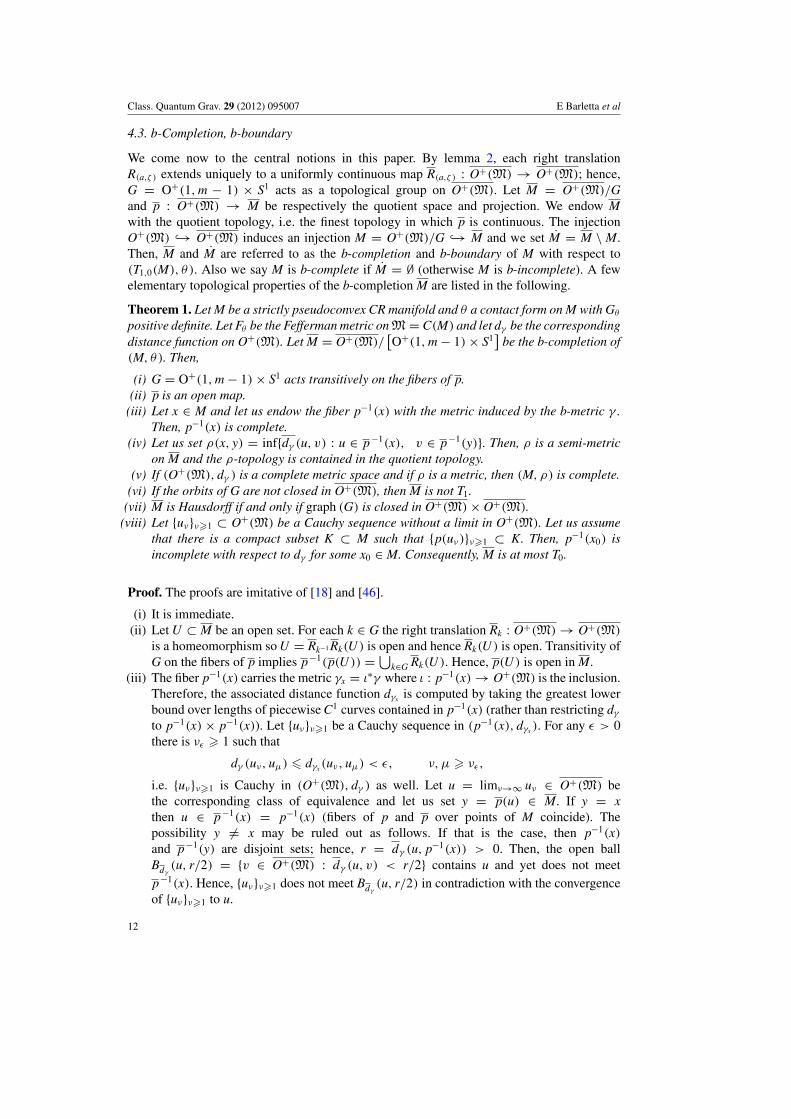
We come now to the central notions in this paper. By lemma 2, each right translationR(a,ζ ) extends uniquely to a uniformly continuous map R(a,ζ ) : O+(M) → O+(M); hence,G = O+(1,m − 1) × S1 acts as a topological group on O+(M). Let M = O+(M)/Gand p : O+(M) → M be respectively the quotient space and projection. We endow Mwith the quotient topology, i.e. the finest topology in which p is continuous. The injectionO+(M) ↪→ O+(M) induces an injection M = O+(M)/G ↪→ M and we set M = M \ M.Then, M and M are referred to as the b-completion and b-boundary of M with respect to(T1,0(M), θ ). Also we say M is b-complete if M = ∅ (otherwise M is b-incomplete). A fewelementary topological properties of the b-completion M are listed in the following.

Theorem 1. Let M be a strictly pseudoconvex CR manifold and θ a contact form on M with Gθpositive definite. Let Fθ be the Fefferman metric on M = C(M) and let dγ be the correspondingdistance function on O+(M). Let M = O+(M)/

[O+(1,m− 1)× S1

]be the b-completion of

(M, θ ). Then,

(i) G = O+(1,m− 1)× S1 acts transitively on the fibers of p.(ii) p is an open map.

(iii) Let x ∈ M and let us endow the fiber p−1(x) with the metric induced by the b-metric γ .Then, p−1(x) is complete.

(iv) Let us set ρ(x, y) = inf{dγ (u, v) : u ∈ p−1(x), v ∈ p−1(y)}. Then, ρ is a semi-metricon M and the ρ-topology is contained in the quotient topology.

(v) If (O+(M), dγ ) is a complete metric space and if ρ is a metric, then (M, ρ) is complete.(vi) If the orbits of G are not closed in O+(M), then M is not T1.

(vii) M is Hausdorff if and only if graph (G) is closed in O+(M)× O+(M).(viii) Let {uν}ν�1 ⊂ O+(M) be a Cauchy sequence without a limit in O+(M). Let us assume

that there is a compact subset K ⊂ M such that {p(uν )}ν�1 ⊂ K. Then, p−1(x0) isincomplete with respect to dγ for some x0 ∈ M. Consequently, M is at most T0.

Proof. The proofs are imitative of [18] and [46].

(i) It is immediate.(ii) Let U ⊂ M be an open set. For each k ∈ G the right translation Rk : O+(M)→ O+(M)

is a homeomorphism so U = Rk−1 Rk(U ) is open and hence Rk(U ) is open. Transitivity ofG on the fibers of p implies p−1(p(U )) =⋃

k∈G Rk(U ). Hence, p(U ) is open in M.(iii) The fiber p−1(x) carries the metric γx = ι∗γ where ι : p−1(x)→ O+(M) is the inclusion.

Therefore, the associated distance function dγx is computed by taking the greatest lowerbound over lengths of piecewise C1 curves contained in p−1(x) (rather than restricting dγto p−1(x) × p−1(x)). Let {uν}ν�1 be a Cauchy sequence in (p−1(x), dγx ). For any ε > 0there is νε � 1 such that

dγ (uν, uμ) � dγx (uν, uμ) < ε, ν, μ � νε,i.e. {uν}ν�1 is Cauchy in (O+(M), dγ ) as well. Let u = limν→∞ uν ∈ O+(M) bethe corresponding class of equivalence and let us set y = p(u) ∈ M. If y = xthen u ∈ p−1(x) = p−1(x) (fibers of p and p over points of M coincide). Thepossibility y �= x may be ruled out as follows. If that is the case, then p−1(x)and p−1(y) are disjoint sets; hence, r = dγ (u, p−1(x)) > 0. Then, the open ballBdγ(u, r/2) = {v ∈ O+(M) : dγ (u, v) < r/2} contains u and yet does not meet

p−1(x). Hence, {uν}ν�1 does not meet Bdγ(u, r/2) in contradiction with the convergence

of {uν}ν�1 to u.

12

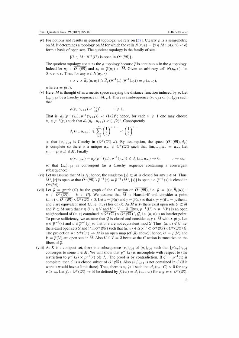
Class. Quantum Grav. 29 (2012) 095007 E Barletta et al

(iv) For notions and results in general topology, we rely on [57]. Clearly ρ is a semi-metricon M. It determines a topology on M for which the cells N(x, ε) = {y ∈ M : ρ(x, y) < ε}form a basis of open sets. The quotient topology is the family of sets

{U ⊂ M : p−1(U ) is open in O+(M)}.The quotient topology contains the ρ-topology because p is continuous in the ρ-topology.Indeed let u0 ∈ O+(M) and x0 = p(u0) ∈ M. Given an arbitrary cell N(x0, ε), let0 < r < ε. Then, for any u ∈ N(u0, r)

ε > r > dγ (u, u0) � dγ (p−1(x), p−1(x0)) = ρ(x, x0),

where x = p(c).(v) Here, M is thought of as a metric space carrying the distance function induced by ρ. Let{xμ}μ�1 be a Cauchy sequence in (M, ρ). There is a subsequence {yν}ν�1 of {xμ}μ�1 suchthat

ρ(yν, yν+1) <(

12

)ν, ν � 1.

That is, dγ (p−1(yν ), p−1(yν+1)) < (1/2)ν ; hence, for each ν � 1 one may chooseuν ∈ p−1(yν ) such that dγ (uν , uν+1) < (1/2)ν . Consequently

dγ (uν, uν+μ) �μ∑

i=1

(1

2

)ν+i−1

<

(1

2

)ν−1

so that {uν}ν�1 is Cauchy in (O+(M), d). By assumption, the space (O+(M), dγ )is complete so there is a unique u∞ ∈ O+(M) such that limν→∞ uν = u∞. Lety∞ = p(u∞) ∈ M. Finally

ρ(yν, y∞) = dγ (p−1(yν ), p−1(y∞)) � dγ (uν, u∞)→ 0, ν →∞,

so that {xμ}μ�1 is convergent (as a Cauchy sequence containing a convergentsubsequence).

(vi) Let us assume that M is T1; hence, the singleton {x} ⊂ M is closed for any x ∈ M. Thus,M \ {x} is open so that O+(M) \ p−1(x) = p−1

(M \ {x}) is open, i.e. p−1(x) is closed in

O+(M).(vii) Let G = graph (G) be the graph of the G-action on O+(M), i.e. G = {(u,Rk(u)) :

u ∈ O+(M), k ∈ G}. We assume that M is Hausdorff and consider a point(u, v) ∈ O+(M)×O+(M) \ G. Let x = p(u) and y = p(v) so that x �= y (if x = y, then uand v are equivalent mod G, i.e. (x, y) lies on G). As M is T2 there exist open sets U ⊂ Mand V ⊂ M such that x ∈ U , y ∈ V and U ∩V = ∅. Thus, p−1(U )× p−1(V ) is an openneighborhood of (u, v) contained in O+(M)×O+(M) \ G, i.e. (u, v) is an interior point.To prove sufficiency, we assume that G is closed and consider x, y ∈ M with x �= y. Letu ∈ p−1(x) and v ∈ p−1(y) so that u, v are not equivalent mod G. Thus, (u, v) �∈ G, i.e.there exist open setsU andV in O+(M) such that (u, v) ∈ U×V ⊂ O+(M)×O+(M)\G.The projection p : O+(M) → M is an open map (cf (ii) above); hence, U = p(U ) andV = p(V ) are open sets in M. Also U ∩ V = ∅ because the G-action is transitive on thefibers of p.

(viii) As K is a compact set, there is a subsequence {vν}ν�1 of {uν}ν�1 such that {p(vν )}ν�1

converges to some x ∈ M. We will show that p−1(x) is incomplete with respect to (therestriction to p−1(x) × p−1(x) of) dγ . The proof is by contradiction. If C = p−1(x) iscomplete, then C is a closed subset of O+(M). Also {uν}ν�1 is not contained in C (if itwere it would have a limit there). Thus, there is ν0 � 1 such that dγ (vν , C) > 0 for anyν � ν0. Let fν : O+(M)→ R be defined by fν (w) = dγ (vν , w) for any w ∈ O+(M).

13

Class. Quantum Grav. 29 (2012) 095007 E Barletta et al

Then, fν is continuous and C closed so that infw∈C fν (w) is realized in C, i.e. for eachν � ν0 there is wν ∈ C such that dγ (vν , wν ) = dγ (vν , C). Note that p(vν )→ x impliesdγ (vν , C)→ 0 as ν →∞. Then, on one hand {wν}ν�1 is Cauchy for

dγ (wν,wμ) � dγ (wν, vν )+ dγ (vν, vμ)+ dγ (vμ,wμ) < ε

for any ν, μ � νε , and on the other hand dγ (vν , wν ) → 0 means that {vν}ν�1

and {wν}ν�1 are equivalent Cauchy sequences so they must represent the same pointlimν→∞wn = limν→∞ vν ∈ O+(M) \ O+(M) which implies that C is not complete. Toprove the second statement in (viii), we will pin down, under the given assumptions, twoelements x, y ∈ M with x �= y such that all open neighborhoods of y contain x as well. Bythe first statement in (viii) there is x ∈ M such that p−1(x) is incomplete with respect to thefull metric d. Therefore, p−1(x) contains at least a Cauchy sequence {wν}ν�1 without limitthere. Letw = limν→∞wν ∈ O+(M)\O+(M). Then,w lies on the topological boundaryof p−1(x) (as a subset of O+(M)); hence, any open neighborhoodU ofw intersects p−1(x).Let y = p(w) ∈ M. Finally, if V ⊂ M is an arbitrary open neighborhood of y then p−1(V )is an open neighborhood of w; hence, p−1(V ) ∩ p−1(x) �= ∅ and hence x ∈ V . �A comment is in order on perhaps a bit subtle difference between statements (iii) and (viii)

in theorem 1: γx is the first fundamental form of p−1(x) as a submanifold of (O+(M), γ ).The distance function dγx (associated with the Riemannian metric γx) and the restriction of dγto p−1(x) × p−1(x) do not coincide7 in general (completeness in (iii) and (viii) is relative todistinct distance functions).

An almost verbatim repetition of the arguments in the proofs of lemma 2 and theorem 1leads to

Corollary 1. The S1 action on M extends to a unique uniformly continuous topological S1

action on M leaving M invariant. Then, M = M/S1 and M = M/S1. Let π : M→ M andπ : M → M be the canonical projections. Then, the fibers of π over b-boundary points arecontained in the b-boundary M and S1 acts transitively on the fibers of π . The projection π isan open map. If the orbits of S1 are not closed in M, then M is not T1. M is Hausdorff if andonly if graph(S1) is closed in M×M.

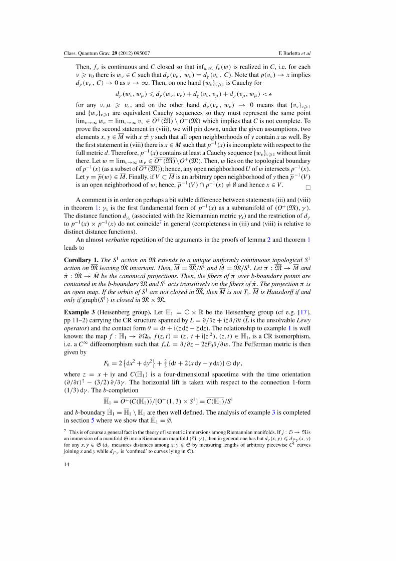
Example 3 (Heisenberg group). Let H1 = C × R be the Heisenberg group (cf e.g. [17],pp 11–2) carrying the CR structure spanned by L = ∂/∂z+ iz ∂/∂t (L is the unsolvable Lewyoperator) and the contact form θ = dt + i(z dz− z dz). The relationship to example 1 is wellknown: the map f : H1 → ∂�0, f (z, t) = (z , t + i|z|2), (z, t) ∈ H1, is a CR isomorphism,i.e. a C∞ diffeomorphism such that f∗L = ∂/∂z − 2zF0∂/∂w. The Fefferman metric is thengiven by

Fθ = 2{dx2 + dy2

}+ 23 {dt + 2(x dy− y dx)} � dγ ,

where z = x + iy and C(H1) is a four-dimensional spacetime with the time orientation(∂/∂t)↑ − (3/2) ∂/∂γ . The horizontal lift is taken with respect to the connection 1-form(1/3) dγ . The b-completion

H1 = O+(C(H1))/[O+(1, 3)× S1] = C(H1)/S

1

and b-boundary H1 = H1 \H1 are then well defined. The analysis of example 3 is completedin section 5 where we show that H1 = ∅.7 This is of course a general fact in the theory of isometric immersions among Riemannian manifolds. If j : S→Nisan immersion of a manifold S into a Riemannian manifold (N, γ ), then in general one has but dγ (x, y) � d j∗γ (x, y)for any x, y ∈ S (dγ measures distances among x, y ∈ S by measuring lengths of arbitrary piecewise C1 curvesjoining x and y while d j∗γ is ‘confined’ to curves lying in S).

14

Class. Quantum Grav. 29 (2012) 095007 E Barletta et al

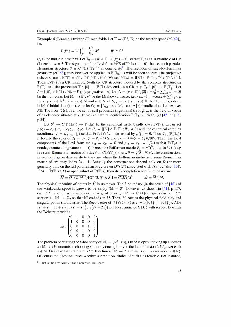
Example 4 (Penrose’s twistor CR manifold). Let T = (C4, �) be the twistor space (cf [42]),i.e.

�(W ) =W

(0 I2

I2 0

)Wt, W ∈ C

4

(I2 is the unit 2×2 matrix). Let T0 = {W ∈ T : �(W ) = 0} so that T0 is a CR manifold of CRdimension n = 3. The signature of the Levi form ∂∂� of T0 is (+− 0); hence, each pseudo-Hermitian structure θ ∈ C∞(H(T0)

⊥) is degenerate8. The methods of pseudo-Hermitiangeometry (cf [53]) may however be applied to P(T0) as will be seen shortly. The projectivetwistor space is P(T) = (T \ {0}) /(C \ {0}). We set P(T0) = {[W ] ∈ P(T) : W ∈ T0 \ {0}}.Then, P(T0) is a CR manifold (with the CR structure induced by the complex structure onP(T)) and the projection T \ {0} → P(T) descends to a CR map T0 \ {0} → P(T0). LetI = {[W ] ∈ P(T) : W0 =W1} (a projective line). Let� = {v ∈ R

4 \{0} : −v20+

∑2i=1 v

2i = 0}

be the null cone. Let M = (R4, η) be the Minkowski space, i.e. η(x, y) = −x0y0 +∑3

i=1 xiyi

for any x, y ∈ R4. Given x ∈ M and v ∈ � let Nx,v = {x + tv : t ∈ R} be the null geodesic

in M of initial data (x, v). Also let �0 ={Nx,v : x ∈M, v ∈ �}

(a bundle of null cones overM). The fiber (�0)x, i.e. the set of null geodesics (light rays) through x, is the field of visionof an observer situated at x. There is a natural identification P(T0) \ I ≈ �0 (cf [42] or [17],p 24).

Let S1 → C(P(T0)) → P(T0) be the canonical circle bundle over P(T0). Let us setρ(ζ ) = ζ2 + ζ 2 + ζ1ζ 3 + ζ 1ζ3. Let U0 = {[W ] ∈ P(T) : W0 �= 0} with the canonical complexcoordinates ζ = (ζ1, ζ2, ζ3) so that P(T0) ∩U0 is described by ρ(ζ ) = 0. Thus, T1,0(P(T0))

is locally the span of T1 = ∂/∂ζ1 − ζ 3 ∂/∂ζ2 and T2 = ∂/∂ζ3 − ζ 1 ∂/∂ζ2. Then, the localcomponents of the Levi form are g11 = g22 = 0 and g12 = g21 = 1/2 (so that P(T0) isnondegenerate of signature (+−)); hence, the Fefferman metric Fθ = π∗Gθ + 1

2 (π∗θ )� dγ

is a semi-Riemannian metric of index 3 on C(P(T0)) (here, θ = i2 (∂−∂)ρ). The constructions

in section 3 generalize easily to the case where the Fefferman metric is a semi-Riemannianmetric of arbitrary index 2s + 1. Actually the constructions depend only on D (or moregenerally only on the full parallelism structure on O+(M) associated with �(σ ), cf also [15]).If M = P(T0) \ I (an open subset of P(T0)), then its b-completion and b-boundary are

M = O+(C(M))/[O+(3, 3)× S1] = C(M)/S1, M = M \M.

The physical meaning of points in M is unknown. The b-boundary (in the sense of [46]) ofthe Minkowski space is known to be empty (M = ∅). However, as shown in [41], p 337,each C∞ function with values in the Argand plane z : M → C ∪ {∞} gives rise to a C∞

section s : M → �0 so that M embeds in M. Then, M carries the physical field s∗gθ andsingular points should arise. The Reeb vector of (M ∩U0, θ ) is T = i

(∂/∂ζ2 − ∂/∂ζ 2

). Also

{T1 + T 1 , T2 + T 2 , i(T1 − T 1

), i

(T2 − T 2

)} is a local frame of H(M) with respect to whichthe Webster metric is

gθ :

⎛⎜⎜⎜⎜⎝

0 1 0 0 01 0 0 0 00 0 0 1 00 0 1 0 00 0 0 0 1

⎞⎟⎟⎟⎟⎠ .

The problem of relating the b-boundary of Ms = (R4, s∗gθ ) to M is open. Picking up a sections : M→ �0 amounts to choosing smoothly one light ray in the field of vision (�0)x over eachx ∈M. One may then start with a C∞ function v : M→ � and set s(x) = {x+ t v(x) : t ∈ R}.Of course the question arises whether a canonical choice of such v is feasible. For instance,

8 That is, the Levi form Lθ has a nontrivial null space.

15

Class. Quantum Grav. 29 (2012) 095007 E Barletta et al

as v : M → � may be thought of as a vector field (of null vectors) tangent to M, one mayrequest that v be an extremal of some classical action (such as the total bending or biegung, cfe.g. [56], in one of its known Lorentzian generalizations, cf e.g. [22] or [16]); Cf also [5]. Letus consider a C∞ function λ : M→ R \ {1} and s : M→ P(T0) \ {I} given by

s(x) =[(1, λ(x)) ,

1

i√

2(1, λ(x)) φ(x)

], x ∈M. (21)

Then, �(s(x)) = 0 and s(x) ∈ I ⇐⇒ λ(x) = 1, i.e. s(x) is well defined. Note thatz = 1 + iλ : M → C is the function required by the approach in [41]. The study of thegeometry of the second fundamental form of (21) is open. A knowledge of that is likely tolead to a useful relationship among Ms and P(T0) \ I.

5. b-Incomplete curves

5.1. Bundle length, b-incomplete curves

Let I ⊂ R be a bounded interval such that 0 ∈ I. According to [46] (slightly reformulated withO+ replacing L+), a curve c : I →M is said to have finite bundle length if there is u ∈ O+(M)

such that the �-horizontal lift c∗ : I → O+(M) issuing at u has finite length with respect tothe b-metric γ , i.e.

L(c∗) =∫

I

∥∥c∗(t)−1c(t)∥∥ dt <∞.

Here, ‖ξ‖ is the Euclidean norm of ξ ∈ Rm; cf also [13], p 437. A curve c : [0, 1) → M

is b-incomplete if it has finite bundle length and admits no continuous extension to a map[0, 1] → M (i.e. c is inextensible). The relevance of this class of curves consists in the factthat the b-boundary M = M \M consists precisely of the end points in M of b-incompletecurves in M.

Similar considerations as to the b-boundary M require the connection �(σ ) in G →O+(M)

p→ M (cf lemma 2). We adopt the following definition. A curve α : I → M hasfinite b-length if there is u ∈ O+(M) such that the �(σ )-horizontal lift α↑ : I → O+(M)

issuing at α↑(0) = u has finite length with respect to the b-metric γ . Also α : [0, 1) → Mis b-incomplete if it has a finite bundle length and admits no continuous extension to a map[0, 1]→ M.

Theorem 2. For any b-incomplete curve α : [0, 1)→ M its end point limt→1− α(t) exists in Mand lies on the b-boundary M. Conversely, any point on M is an endpoint of some b-incompletecurve.

Proof. As α has a finite bundle length, there is u ∈ O+(M) such that the horizontallift α↑ : [0, 1) → O+(M) with α↑(0) = u has finite length with respect to γ . Letc = �O+ ◦ α↑ : [0, 1)→M. As

α↑(t) ∈ �(σ )α↑(t) = βα↑(t)Ker(σc(t)) ⊂ �α↑(t), 0 � t < 1, (22)

one has

γα↑(t)(α↑(t), α↑(t)) = ‖ηα↑(t)

(α↑(t)

) ‖2 = ‖α↑(t)−1c(t)‖2

and L(α↑) <∞ yields

limν→∞

∫ tν

0‖α↑(t)−1c(t)‖ dt = L0

16

Class. Quantum Grav. 29 (2012) 095007 E Barletta et al

for some L0 ∈ R and any sequence {tν}ν�1 ⊂ [0, 1) such that limν→∞ tν = 1. In particular,for any ε > 0 there is νε � 1 such that

dγ (α↑(tν ), α↑(tν+μ)) �

∣∣∣∣∫ tν+μ

tν

∥∥α↑(t)−1c(t)∥∥ dt

∣∣∣∣ < εfor any ν � νε and any μ � 1, i.e. {α↑(tν )}ν�1 is a Cauchy sequence in (O+(M), dγ ).Let u0 ∈ O+(M) be its equivalence class, so that limν→∞ α↑(tν ) = u0 in O+(M). Letx0 = p(u0) ∈ M. By the continuity of p, one has limν→∞ α(tν ) = x0 in M. As α is b-incomplete, it must be that x0 ∈ M\M. Vice versa, let x ∈ M and let c ∈ M such that π(c) = x.By a result in [46], there is a b-incomplete curve ρ : [0, 1)→M such that limt→1−1 ρ(t) = c,i.e. its �-horizontal lift ρ∗ : [0, 1) → O+(M) issuing at some u ∈ �−1

O+ (γ (0)) has finitelength with respect to γ . On the other hand, if α = π ◦ ρ and α↑ : [0, 1) → O+(M) is the�(σ )-horizontal lift of α issuing at u, then (again by (22), i.e. α↑ is �(σ )-horizontal, and hence�-horizontal) α↑ = ρ∗ (as two �-horizontal curves’ issuing at the same point). �

5.2. Inextensible Fefferman spacetimes

A spacetime (N, F ) is an extension of the Fefferman spacetime if M is an open set in N

and ι∗F = Fθ where ι : M → N is the inclusion. Also (M,Fθ ) is inextensible if it has noextension. A strictly pseudoconvex pseudo-Hermitian manifold (M, T1,0(M), θ ) is Feffermaninextensible if the spacetime (M, Fθ , T↑ − S) is inextensible. A CR manifold (N,T1,0(N))is an extension of (M,T1,0(M)) if M ⊂ N is an open subset and the inclusion ι : M → N isa CR map. Then, (M,T1,0(M)) is referred to as inextensible if it has no extension. If N is anextension of M and is a contact form on N, then (C(N),F ) is an extension of (C(M),Fθ )where θ = ι∗ . By proposition 3 below, (C(∂�0),Fθ0 ) is inextensible.

5.3. Inextensible Reeb flow

Let c : [0, s∗) → M be an inextensible smooth timelike curve parametrized by arc length(proper time). By a result in [14] if s∗ < ∞, then c has an endpoint on the b-boundary M

provided that (A.1) is satisfied. A precise statement and proof are given in the appendix. Asan application (of the Dodson–Sulley–Williams lemma), we demonstrate a class of smoothcurves in M having an endpoint on M.

Theorem 3. Let (M, θ ) be a strictly pseudoconvex pseudo-Hermitian manifold and T itsReeb vector. Then, any inextensible integral curve α : [a, b) → M of T has an endpointon the b-boundary M provided that (i) α admits a lift γ : [a, b) → M satisfyingγ (t) = f (t)

(T↑ − S

)γ (t) (a � t < b) for some C∞ function f : [a, b) → R \ {0, 1}

such that φ(t) = ∫ ta f (τ ) dτ is bounded and (ii)∫ s∗

0exp

(∫ t

0‖V‖β(s) ds

)dt <∞, (23)

where s∗ = limt→b− φ(t) and β(s) = α(φ−1(s)) while V ∈ C∞(H(M)) is given by (10). Inparticular, when (M, θ ) is pseudo-Einstein, the same conclusion holds if (ii) is replaced by∫ s∗

0exp

(∫ t

0‖∇Hρ‖β(s) ds

)dt <∞, (24)

where ρ is the pseudo-Hermitian scalar curvature of θ . Also if M = S2n+1 (endowed with thecanonical contact form), then (ii) is equivalent to s∗ <∞.

17

Class. Quantum Grav. 29 (2012) 095007 E Barletta et al

Proof. Let c(s) = γ (φ−1(s)) for any 0 � s < s∗ so that c : [0, s∗) → M is an inextensibletimelike curve, parametrized by arc length, with s∗ finite. Then (by lemma 1)

(Dγ γ )γ (t) = f ′(s)(T↑ − S)γ (t) + f (t)2V↑γ (t),

(Dcc)c(φ(t)) = f (t)−2[(Dγ γ )γ (t) − f ′(t) f (t)−1γ (t)];hence, ‖Dcc‖c(φ(t)) = ‖V‖α(t) for any a � t < b and lemma 4 yields c(s∗−) ∈ M and hence(by corollary 1) β(s∗−) ∈ M.

Moreover, if (M, θ ) is pseudo-Einstein, then (cf [17], p 298) W ααμ = (i/2n) ρμ and hence

(by (10))

‖V‖2 = 2gαβVαV β = Cnραρ

α,

where 2Cn = (2n+ 1)2/[n(n+ 1)(n+ 2)]2 (so that (23) and (24) are equivalent). When M isthe odd-dimensional sphere (carrying the standard contact form) the pseudo-Hermitian scalarcurvature is constant. �

Example 5 (Example 2 continued). Let (V, g) be a harmonic Riemannian manifold andMε = ∂ T ∗εV with the contact form θε . Let Tε be the Reeb vector of (Mε, θε ) andα : [a, b) → Mε an inextensible integral curve of Tε admitting a lift γ : [a, b) → C(Mε )

as in theorem 3 and satisfying (24). Then, α has an endpoint on Mε . Given a C∞ functionf : [a, b) → R \ {0, 1}, the ODE system γ (t) = f (t)

(T↑ − S

)γ (t) admits solutions by

standard existence theorems in ODE theory and their projections on Mε are integral curves ofTε . On the other hand, integral curves of Tε are chains (cf [50], p 393) (and therefore projectionsof null geodesics), thus exhibiting chains which are simultaneously projections of timelikecurves in C(Mε ).

5.4. b-Boundary versus topological boundary

By a result in [47] for any open set U ⊂ M with compact closure one has ∂U ⊂ U . Thefollowing CR analog is also true.

Proposition 2. Let U ⊂ M be an open subset of a strictly pseudoconvex pseudo-Hermitianmanifold (M, θ ) such that its closure Uc is compact in M. Then, the topological boundary ∂Uis contained in the b-boundary U.

Proof. Let x ∈ ∂U = Uc \U◦ so that x �∈ U by the openness of U . In particular, there is a curveα : [0, 1) → U with endpoint x. Let u0 ∈ p−1(α(0)) and let α↑ : [0, 1) → O+(M) be theunique �(σ )-horizontal lift of α issuing at u0. Then, α↑ has an endpoint u1 = limt→1− α

↑(t) ∈p−1(x) ⊂ O+(π−1(U )) because Uc is compact and p is an open map. Consequently there isan integer n0 � 1 such that α↑ lies in the ball Bdγ

(u1 , 1/n0) ⊂ O+(π−1(U )). Let us join u1 tosome point on α↑ by a minimizing geodesic ρ of finite length. Then, π ◦ ρ is a b-incompletecurve in U with the endpoint x; hence, x ∈ U . �

A natural question in [47] is whether (or under which assumptions) ∂U = U . By a resultin [47], if U ⊂M is an open subset such that (i) U c is compact and (ii) U c contains no trapped9

null geodesic, then ∂U = U . The CR analog to this situation would be to consider an opensubset U ⊂ M such that (i) Uc is compact and (ii) Uc contains no trapped chain. The result in[47] does not readily apply to U = π−1(U ). Indeed U c is compact (because S1 is compact)yet U c = π−1(Uc); hence, U c is a saturated10 set imprisoning all fibers of π over points in Uc

(which are null-geodesics of Fθ ).9 In the sense of [47], p 51.10 A union of leaves of the vertical foliation (tangent to S).

18

Class. Quantum Grav. 29 (2012) 095007 E Barletta et al

5.5. b-Boundary points and horizontal curves

The following result is a CR analog to theorem 4.2 in [46], p 276. The proof however mimicsthat in [13], pp 461–2.

Theorem 4. Let x ∈ M be the point determined by the Cauchy sequence {vν}ν�1 ⊂ O+(M),

i.e. x = orbG(v) where v = limν→∞ vν ∈ O+(M). There is a Cauchy sequence {uν}ν�1 lyingon a �(σ )-horizontal curve in O+(M) and determining the same b-boundary point x.

Proof. There is a curve γ : [0, 1) → O+(M) such that γ (tν ) = vν for some tν ∈ [0, 1)and any ν � 1. There is no x ∈ M such that γ (t) ∈ p−1(x) for all 0 � t < 1. Indeedif it were γ ⊂ p−1(x0) for some x0 ∈ M, then {vν}ν�1 would have a limit there (by(iii) in theorem 1, the fiber p−1(x) is complete) instead of O+(M) \ O+(M). Let us setα = p ◦ γ : [0, 1) → M (an inextensible curve). Let α↑ : [0, 1) → O+(M) be theunique �(σ )-horizontal lift of α issuing at α↑(0) = v1 and let us consider the sequenceα↑(tν ) ∈ O+(M) projecting on xν = p(vν ) ∈ M. As G = O+(1,m− 1)× S1 acts transitivelyon fibers for each ν � 1, there is aν ∈ G such that Raν (α

↑(tν )) = vν (actually a1 = e). Letv∞ = limν→∞ vν ∈ O+(M) \ O+(M). Also (as O+(M) is complete) the curve α↑ has anendpoint u∞ = limt→1− α

↑(t) ∈ O+(M) \ O+(M) such that p(u∞) = p(v∞) = x ∈ M. Letthen a∞ ∈ G such that Ra∞ (u∞) = v∞.

By a result of Schmidt [48], O+(1,m − 1) is closed in GL+(m,R) and then G is closedin GL+(m,R) × S1 and hence (by the continuity of the action) limν→∞ aν = a∞ in G. Letα∗ : [0, 1) → O+(M) be the unique �(σ )-horizontal lift of α issuing at α∗(0) = Ra∞ (v1)

and let us consider the sequence uν = α∗(tν ) ∈ O+(M).By the general theory of connections in principal bundles (cf e.g. [33], vol I) right

translations by elements of the structure group map horizontal curves into horizontal curves;hence, Ra∞ ◦ α↑ is a horizontal curve issuing at the same point as α∗ and then α∗ = Ra∞ ◦ α↑.In particular, uν = Ra∞ (α

↑(tν )) for any ν � 1.As in the proof of lemma 2, there is a constant β(a∞) > 0 such that

dγ (Ra∞ (u),Ra∞ (v)) � β(a∞)dγ (u, v), u, v ∈ O+(M).

Also (again by the continuity of the action of G on O+(M)), one has

limν→∞Ra−1

νvν = Ra−1∞ v∞;

hence,

dγ (uν, uμ) = dγ (Ra∞α↑(tν ),Ra∞α

↑(tμ))� β(a∞)dγ (α↑(tν ), α↑(tμ)) = β(a∞)dγ (Ra−1

ν(vν ),Ra−1

μ(vμ))

implying that {uν}ν�1 is a Cauchy sequence with the same limit v∞ ∈ O+(M) \ O+(M) as{vν}ν�1. �

Example 6 (Example 3 continued). The Fefferman metric of (H1, θ0) is given by (with respectto the (global) coordinates (xα ) ≡ (x, y, t, γ ) on C(H1))

[Fαβ

]0�α,β�3 =

⎛⎜⎜⎝

2 0 0 −ay0 2 0 ax0 0 0 a/2−ay ax a/2 0

⎞⎟⎟⎠ , (25)

19

Class. Quantum Grav. 29 (2012) 095007 E Barletta et al

where a = 2/3. If FαβFβγ = δγα , then

[Fαβ

]0�α,β�3 =

⎛⎜⎜⎝

1/2 0 y 00 1/2 −x 0y −x 2|z|2 30 0 3 0

⎞⎟⎟⎠ (26)

where z = x + iy. As a consequence of (25), the only nonvanishing Christoffel symbols|αβ, γ | = 1

2 (Fαγ |β + Fβγ |α − Fαβ|γ ) are

|03, 1| = |30, 1| = a, |13, 0| = |31, 0| = −a.

Consequently, the nonzero Christoffel symbols∣∣ αβγ

∣∣ = Fαλ|βγ , λ| are

∣∣∣∣ 013

∣∣∣∣ =∣∣∣∣ 031

∣∣∣∣ = −a/2,

∣∣∣∣ 213

∣∣∣∣ =∣∣∣∣ 231

∣∣∣∣ = −ay,

∣∣∣∣ 103

∣∣∣∣ =∣∣∣∣ 130

∣∣∣∣ = a/2,

∣∣∣∣ 203

∣∣∣∣ =∣∣∣∣ 230

∣∣∣∣ = −ax,

so that the equations of geodesics of (C(H1),Fθ0 )

d2Cα

ds2+

∣∣∣∣ αβγ∣∣∣∣ dCβ

ds

dCγ

ds= 0

read

d2z

ds2+ iap

dz

ds= 0, (27)

d2t

ds2− ap

d|z|2ds= 0, γ (s) = ps+ q, p, q ∈ R. (28)

We obtain

Proposition 3. (i) The geodesics of (C(H1),Fθ0 ) are either

z(s) = λ exp(−i aps)+ μ

iap, λ, μ ∈ C, (29)

t(s) =( + ap|λ|2 + |μ|

2

ap

)s+ m− 1

ap[λμ e−iaps + λμ eiaps], ,m ∈ R, (30)

γ (s) = ps+ q, p, q ∈ R, (31)

provided that p �= 0, or

z(s) = λs+ μ, t(s) = s+ m, γ (s) = q, λ, μ ∈ C, ,m, q ∈ R, (32)

when p = 0. (ii) Fθ0 is geodesically complete. (iii) Each geodesic (32) is σ -horizontal. (iv) Let 0 = −ap|λ|2 − (1/ap)|μ|2 (p �= 0). The geodesics (29)–(31) are spacelike when > 0,timelike when < 0, or null when = 0. If = 0, then (29)–(31) project on a familyof closed chains in ∂�0 ≈ H1. (v) (32) is a family of geodesics intersecting each fiber ofπ : C(H1) → H1 once. Each geodesic in the family is either spacelike (λ �= 0) or null(λ = 0).

20

Class. Quantum Grav. 29 (2012) 095007 E Barletta et al

Proof. (29)–(30) are the general solution to (27)–(28). In particular, (C(∂�0),Fθ0 ) isinextensible. The statement (iii) follows from σ = (a/2) dγ . For each geodesic C(t) ∈ C(H1),

one has FαβCαCβ = 2|z|2 + 2ap Im(zz)+ ap t; hence,

Fαβ (C(s))Cα(s)Cβ (s) = a2 p2|λ|2 + |μ|2 + ap , s ∈ R, (33)

yielding statement (iv). �

Theorem 5. The b-boundary of (H1 , θ0) is empty (H1 = ∅).A verbatim repetition of the arguments in the proof of lemma 2 describes �(σ ) as

a connection in GL+(4) × S1 → L+(C(H1)) → H1 (reducible to O+(1, 3) × S1 →O+(C(H1))→ H1). Let α : [0, 1)→ H1 be a smooth inextensible curve and α↑ : [0, 1)→L+(C(H1)) its �(σ )-horizontal lift issuing at α↑(0) = u. Let βα↑(s) : Tc(s)(C(H1))→ �α↑(s)be the �-horizontal lift where c = �L+ ◦ α↑. We set X∗ = βX for each X ∈ X(C(H1)). Then,

α↑(s) = dαλ

ds

(∂

∂xλ

)α↑(s)+ dαλμ

ds

(∂

∂Xλμ

)α↑(s)

= dαλ

ds

(∂

∂xλ

)∗α↑(s)+

{dαλμds+ dαν

ds

∣∣∣∣ λνσ∣∣∣∣ (c(s))ασμ(s)

}(∂

∂Xλμ

)α↑(s)

,

where αλ = xλ ◦ α↑ and αλμ = Xλμ ◦ α↑. Moreover, �(σ ) ⊂ � yields

dαλμds+ dαν

ds

(∣∣∣∣ λνσ∣∣∣∣ ◦ c

)ασμ = 0. (34)

In particular,

�(σ )α↑(s) � α↑(s) =2∑

j=0

dα j

ds(s)

(∂

∂x j

)↑α↑(s)+ dγ

ds(s)

(∂

∂γ

)∗α↑(s)

and Ker(σ ) is the span of {∂/∂x, ∂/∂y, ∂/∂t}; hence, dγ /ds = 0. Thus, γ (s) = m withm ∈ R and (34) reads

d

ds

(α0μ + iα1

μ

) = a

2i

dz

dsα3μ ,

dα2μ

ds= a

2

d|z|2ds

α3μ ,

dα3μ

ds= 0. (35)

The general solution to (35) is

α0μ(s) = pμ + a

2tμy(s), α1

μ(s) = qμ − a

2tμx(s),

α2μ(s) = rμ + a

2tμ|z(s)|2, α3

μ(s) = tμ, pμ, qμ, rμ, tμ ∈ R.

Together with theorem 2, this gives

Lemma 3. The b-boundary H1 consists of the endpoints of all inextensible curvesα = (x, y, t) :[0, 1)→ H1 of finite Euclidean length, i.e.

∫ 10 [x2 + y2 + t2]1/2 ds is convergent.

Proof. There is a constant degenerate matrix α0 ∈ R16 such that

[αλμ(s)

] = a

2

⎛⎜⎜⎝

t0y(s) t1y(s) t2y(s) t3y(s)−t0x(s) −t1x(s) −t2x(s) −t3x(s)t0|z(s)|2 t1|z(s)|2 t2|z(s)|2 t3|z(s)|2(2/a)t0 (2/a)t1 (2/a)t2 (2/a)t3

⎞⎟⎟⎠+ α0.

21

Class. Quantum Grav. 29 (2012) 095007 E Barletta et al

We may assume that the connected component L+(C(H1)) is chosen such that for eachc0 ∈ π−1(α(0)), one has

u0 = (c0, {(∂/∂xμ)c0: 0 � μ � 4}) ∈ L+(C(H1)).

We wish to describe curves α : [0, 1) → H1 having finite b-length. Let α↑ : [0, 1) →L+(C(H1)) be the �(σ )-horizontal lift of α issuing at u0. Then, Xλμ(u0) = δλμ and α↑(0) = u0

yield

α0 =

⎛⎜⎜⎝

1 0 0 −(a/2)y0

0 1 0 (a/2)x0

0 0 1 −(a/2)|z0|20 0 0 0

⎞⎟⎟⎠ , tμ = δ3

μ,

where x0 = x(0), y0 = y(0) and z0 = x0 + iy0. Therefore,

[αλμ

] =⎛⎜⎜⎝

1 0 0 (a/2)(y− y0)

0 1 0 −(a/2)(x− x0)

0 0 1 (a/2)[|z|2 − |z0|2]0 0 0 1

⎞⎟⎟⎠

so that

[βλμ

] ≡ [αλμ

]−1 =

⎛⎜⎜⎝

1 0 0 −(a/2)(y− y0)

0 1 0 (a/2)(x− x0)

0 0 1 −(a/2)[|z|2 − |z0|2]0 0 0 1

⎞⎟⎟⎠ .

Finally βλμ(s)eλ = α↑(s)−1 (∂/∂xμ)c(s) yields∫ 1

0‖α↑(s)−1c(s)‖ds =

∫ 1

0[x(s)2 + y(s)2 + t(s)2]

12 ds.

Lemma 3 is proved. Then, theorem 5 follows from lemma 3 and the fact that curvesα : [0, 1) → H1 of finite Euclidean length are actually continuously extendible at s = 1.For a given sequence {sν}ν�1 ⊂ [0, 1) such that sν → 1 as ν →∞

d0(α(sν ), α(sμ)) �∣∣∣∣∫ sμ

sν

(x2 + y2 + t2)1/2 ds

∣∣∣∣(where d0 is the Euclidean distance on R

3) and hence {α(sν )}ν�1 is Cauchy in (R3, d0) andthen convergent. �

6. Comments and open problems

Several other CR and pseudo-Hermitian analogs to Schmidt’s construction (of a b-completionand b-boundary) have been suggested by the reviewers. For every nondegenerate CR manifold,on which a contact form θ has been fixed, the Tanaka–Webster connection ∇ of (M, θ ) givesrise to a connection-distribution �∇ in the principal bundle Gl(2n + 2,R) → L(M) → M.As ∇gθ = 0, the connection �∇ is reducible to the bundle of gθ -orthonormal framesO(2r + 1, 2s) → O(M, gθ ) → M. Only a linear connection on M is needed (cf e.g. [15])to build a bundle completion, so both principal bundles L(M) and O(M, gθ ) are suitable forrepeating the construction in [46]. For instance, let ω∇ ∈ C∞(T ∗(L(M))⊗ gl(2n+ 1,R)) be

22

Class. Quantum Grav. 29 (2012) 095007 E Barletta et al

the connection 1-form corresponding to �∇ and let us set

g∇u (X,Y ) = ω∇u (X ) · ω∇u (Y )+ ηM,u(X ) · ηM,u(Y )

for any X,Y ∈ Tu(L(M)) and u ∈ L(M). Here, ηM ∈ C∞(T ∗(L(M))⊗R2n+1) is the canonical

1-form and dots indicate Euclidean inner products in R(2n+1)2 and R

2n+1. Then, g∇ is aRiemannian metric on L(M) and one may consider the Cauchy completion L+(M) of themetric space (L+(M), d∇ ) where d∇ is the distance function associated with g∇ . ComparingL+(M) and L+(M) is an open problem. For instance, let s : M → M be a global section.Such s exists when M is a real hypersurface in C

n+1 (for then M ≈ M × S1 (cf e.g. [38])and one may set s(x) = (x, 1) for any x ∈ M). Then, the map f : L(M) → L(M) given byf (u) = (s(x), {v↑i , Ss(x) : 1 � i � 2n+ 1}) for any u = (x, {vi : 1 � i � 2n+ 1}) ∈ L(M)and any x ∈ M, is an immersion and one ought to compute the (0, 2)-tensor field f ∗g− g∇ .Here, v↑i ∈ Ker(σs(x)) and (ds(x)π )v

↑i = vi. As emphasized above, both L+(M) and L+(M)

depend upon the choice of θ . The behavior of the completions (and corresponding boundaries)with respect to a transformation θ = ±eu θ (with u ∈ C∞(M)) of the contact form is unknown.

The Carnot–Caratheodory metric dH may fail to be complete, in general, yet completenessof dH is relevant in a number of geometric problems (cf [51] and [3]). The lack of completenesson dH prompts the use of the Cauchy completion M of the metric space (M, dH ). By analogyto the work of Nomizu and Ozeki [40] (that for any Riemannian metric there is a conformaltransformation such that the resulting metric is complete) one may ask whether u ∈ C∞(M)exists such that any of d on L+(M), d∇ on L+(M) or dH on M (built in terms of θ above) becomplete.

Another approach to completions and boundaries, as mentioned in section 1, may rely onthe canonical Cartan geometry of the given nondegenerate CR manifold, which is also relatedto the conformal structure determined by the Fefferman metric Fθ Cap and Gover [11]; cf alsoFrances [20].

Example 1 (used in this paper only for δ = 0) is meant to suggest possible applicationsof our constructions (of ∂�δ and corresponding boundary) and (by including Fefferman’sexample δ = 1) that chains may play a fundamental role in understanding the nature ofboundary points. The same comment applies to examples 2 and 5 (on boundaries of Grauerttubes) due to the work by Stenzel [50] (relating chains to integral curves of Reeb vector fields).

Recent discussion (cf Kempf [32], Kopf [35, 36], Prain [43]) of the possibly discretenature of spacetime (eventually springing from considerations within quantum field theory)relies on the use of spectra of naturally defined differential operators (e.g. the Dirac operatorassociated with a fermionic Weyl spinor field [36]). Comments based on the analogy to spectralgeometry on compact Riemannian manifolds (cf e.g. [32]) remain rather speculative vis-a-visto the non-compactness of spacetime and the hyperbolic (rather than elliptic) nature of theLaplace–Beltrami operator of the given Lorentzian metric. Non-compactness of M = C(M)and non-ellipticity of � (the wave operator, i.e. the Laplace–Beltrami operator of Fθ ) are,very much the same, an obstacle toward a discrete description of (M,Fθ ); yet � is relatedto the sub-Laplacian b (by a result of Lee [37], the pushforward of � is precisely b, i.e.π∗� = b) which again is not elliptic, yet is at least subelliptic (with a loss of 1

2 derivative) andhence hypoelliptic (a feature enjoyed by elliptic operators and highly exploited in subelliptictheory, cf e.g. [7]). Again the information that b has a discrete spectrum is available onlyon compact strictly pseudoconvex CR manifolds (when M is also compact and thus (by ourdiscussion in section 3) it is neither causal nor chronological). Coming to a possible samplingtheory of spacetimes (cf [32], p 8), in order to build a theory anchored into Riemanniangeometry, one may attempt to apply Kanai’s discrete approach (cf [31]) to the Riemannian

23

Class. Quantum Grav. 29 (2012) 095007 E Barletta et al

manifold (O+(M), γ ). Lack of completeness is again relevant to employing rough isometries(as in [31]) and may prompt the use of b-completions and b-boundaries.

Acknowledgments

During the elaboration of this paper Sorin Dragomir visited Universite Francois Rabelais(Tours, France, June 2011) while Howard Jacobowitz and Marc Soret were respectivelyvisiting professors of Universita degli Studi della Basilicata (Potenza, Italy, May 2011) andIstituto Nazionale di Alta Matematica (Potenza, Italy, July 2011). They gratefully acknowledgesupport from the receiving institutions. The authors are grateful to the reviewers for correctionswhich improved the manuscript.

Appendix. The Dodson–Sulley–Williams lemma

The work by Dodson et al [14] gives a sufficient condition that an inextensible timelike curvehas an endpoint on the b-boundary. This is a variant of a result by Schmidt [46] in the presenceof an assumption of the type ‘boundedness of acceleration’ inspired by the work of Rosso [44].Also [14] adjusts some imprecisions in [44]; yet the proof applies only under the additionalcondition that the x0-component of the velocity in Minkowski space is almost everywherenon-unit. We restate the result in [14] (referred to throughout this paper as the Dodson–Sulley–Williams lemma) as it applies to the pseudo-Hermitian context and give a proof for the sake ofcompleteness.

Lemma 4 ([15], p 193). Let (M,T1,0(M), θ ) be a strictly pseudoconvex pseudo-Hermitianmanifold and c : [0, s∗)→M an inextensible timelike curve parametrized by arc length. Letu(s) = (c(s), {Xj,c(s) : 1 � j � m}) ∈ O+(M) be a parallel frame and let c(s) = ξ j(s)Xj,c(s)

be the components of the tangent vector c. Then, Dcc is either spacelike or null. If (i) the set{s ∈ [0, s∗) : ξ 1(s) = 1} has Lebesgue measure zero, (ii) s∗ <∞ and (iii)∫ s∗

0exp

(∫ t

0‖Dcc‖ ds

)dt <∞, (A.1)

then c has an endpoint on M.

The frame u(t) has been chosen such that (DcXj)c(s) = 0, i.e. u(s) ∈ �u(s) for any0 � s � s∗. It gives a linear isometry among Tc(s)(M) and the Minkowski space M (i.e.R

m with the quadratic form −(x0)2 +∑m−1a=1 (x

a)2). If ξ (s) = (ξ 1(s), . . . , ξm(s)) are thecomponents of c(s), then

L(c↑) =∫ s∗

0‖c↑(s)−1c(s)‖ ds =

∫ s∗

0‖ξ (s)‖ ds,

where ‖ξ‖ is the Euclidean norm of ξ ∈ Rm. Let us set ξ ′ = (ξ 2, . . . , ξm) so that ξ = (ξ 1, ξ ′).

Then,

1 = −Fθ (c, c) = −ε jδ jkξjξ k = (ξ 1)2 − ‖ξ ′‖2,

where ‖ξ ′‖ is the Euclidean norm in Rm−1. This is exploited in two ways, i.e. first it yields

|ξ 1(s)| � 1 and hence

φ(s) =∫ s

0ξ 1(σ ) dσ

24

Class. Quantum Grav. 29 (2012) 095007 E Barletta et al

is a new parameter (for φ = ξ 1 so that φ has a constant sign) and second it yields 2 |ξ 1|2 > ‖ξ‖2

so that one may conduct the following estimates:∫ s∗

0|ξ 1| ds � L(c↑) =

∫ s∗

0‖ξ‖ ds �

∫ s∗

0(2(ξ 1)2)1/2 ds =

√2

∫ s∗

0|ξ 1| ds

and hence L(c↑) < ∞ if and only if∫ s∗

0 |ξ 1| ds < ∞. Combining that with a result in [46],one has c(s∗−) = lims→(s∗ )− c(s) ∈ M if and only if φ is bounded. We claim that

φ2 �(φ2 − 1

)Fθ (Dcc , Dcc). (A.2)

In particular, for each value of the parameter (Dcc)c(s) is either spacelike or null11. To prove(A.2), let Ec(s) be the span of {Xa,c(s) : 2 � a � m} and let Pc(s) : Tc(s)(M) → Ec(s) be theprojection. As (DcX1)c(s) = 0,

Dcc = Dc [Pc− Fθ (c,X1)X1] = DcPc− d

ds{Fθ (c,X1)}X1

or

Dcc = DcPc+ φ X1 . (A.3)

Next, DFθ = 0 and again DcX1 = 0 yieldd

ds{Fθ (Pc,X1)} = Fθ (DcPc,X1)

and hence (as X1 is orthogonal to E)

Fθ (DcPc , X1) = 0, (A.4)

i.e. DcPc ∈ E. Then, (A.3)–(A.4) imply

Fθ (Dcc , Dcc) = ‖DcPc‖2 − φ2 . (A.5)

The norm notation on the right-hand side of (A.5) is justified by the fact that Fθ is positivedefinite on E (one should however postpone writing ‖Dcc‖2 until the end of the proof of (A.2)).Also the Cauchy–Schwartz inequality holds for the restriction of Fθ to E and hence

Fθ to |Fθ (DcPc,Pc)| � ‖DcPc‖ ‖Pc‖ = [Fθ (Dcc,Dcc)+ φ2

]1/2 ‖Pc‖ (by (A.5))

or

Fθ (DcPc , Pc)2 �[Fθ (Dcc , Dcc)+ φ2] ‖Pc‖2. (A.6)

On the other hand,

−1 = Fθ (c, c) = ‖Pc‖2 − Fθ (c,X1)2

or

‖Pc‖2 = −1+ φ2. (A.7)

Also (again due to DFθ = 0)

2Fθ (DcPc,Pc) = d

ds{‖Pc‖2},

i.e. (by (A.7))

Fθ (DcPc , Pc) = φφ. (A.8)

Finally one may substitute from (A.8) into (A.6)

(φφ)2 � [Fθ (Dc,Dcc)+ φ2](φ2 − 1)

11 When Dcc is the null assumption (iii) is equivalent to (ii) (and a slight modification of the proof yields Dodson–Sulley–Williams lemma).

25

Class. Quantum Grav. 29 (2012) 095007 E Barletta et al

yielding (A.2). At this point one may complete the proof of lemma 4 as follows:

φ(s∗)φ(0)

= 1

φ(0)

∫ s∗

0ξ 1(t)dt =

∫ s∗

0

φ(t)

φ(0)dt

=∫ s∗

0exp

(log

φ(t)

φ(0)

)dt �

∫ s∗

0exp

∣∣∣∣logφ(t)

φ(0)

∣∣∣∣ dt

=∫ s∗

0exp

∣∣∣∣∫ t

0

φ(s)

φ(s)ds

∣∣∣∣ dt �∫ s∗

0exp

(∫ t

0

∣∣∣∣ φ(s)φ(s)

∣∣∣∣ ds

)dt

�∫ s∗

0exp

(∫ t

0

∣∣φ(s)∣∣(φ(s)2 − 1

)1/2 ds

)dt � (by (A.2))

�∫ s∗

0exp

(∫ t

0‖Dcc‖ds

)dt;

hence (under the assumptions of lemma 4), φ(s∗) is bounded so that c(s∗−) ∈ M.

References

[1] Amores A M and Gutierrez M 2001 Construction of examples of b-completion Nonlinear Anal. 47 2959–70[2] Barletta E, Dragomir S and Urakawa H 2006 Yang–Mills fields on CR manifolds J. Math. Phys. 47 1–41[3] Barletta E and Dragomir S 2006 Jacobi fields of the Tanaka–Webster connection on Sasakian manifolds Kodai

Math. J. 29 406–54[4] Beem J K and Ehrlich P E 1981 Global Lorentzian Geometry (New York: Dekker)[5] Bejan C L and Duggal K L 2005 Global lightlike manifolds and harmonicity Kodai Math. J. 28 131–45[6] Besse A L 1978 Einstein Manifolds (Ergebnisse der Mathematik und ihrer Grenzgebiete) 3 Folge, Bd. 10 (Berlin:

Springer)[7] Bonfiglioli A, Lanconelli E and Uguzzoni F 2007 Stratified Lie Groups and Potential Theory for their Sub-

Laplacians (Springer Monographs in Mathematics) (Berlin: Springer)[8] Bosshard B 1976 On the b-boundary of the closed Friedman-model Commun. Math. Phys. 46 263–8[9] Burns D and Shnider S 1977 Real hypersurfaces in complex manifolds Proc. Symp. Pure Math. 30 141–67

[10] Burns D, Diederich K and Shnider S 1977 Distinguished curves in pseudoconvex boundaries Duke Math.J. 43 407–31

[11] Cap A and Gover A R 2008 CR-Tractors and the Fefferman space Indiana Univ. Math. J. 57 2519–70[12] Crampin M 1967 Pseudo-Riemannian and related structures PhD Thesis King’s College, London[13] Dodson C T J 1978 Space-time edge geometry Int. J. Theor. Phys. 17 389–504[14] Dodson C T J, Sulley L J and Williams P M 1981 An acceleration condition for b-incomplete timelike curves

Math. Proc. Camb. Phil. Soc. 90 191–3[15] Dodson C T J and Sulley L J 1980 On bundle completion of parallelizable manifolds Math. Proc. Camb. Phil.

Soc. 87 523–5[16] Dragomir S and Soret M 2011 Harmonic vector fields on compact Lorentz surfaces Ricerche Mat.

doi:10.1007/s11587-011-0113-1[17] Dragomir S and Tomassini G 2006 Differential Geometry and Analysis on CR Manifolds (Progress in

Mathematics vol 246) (Boston, MA: Birkhauser)[18] Eells J 1974 Fibre Bundles (Global Analysis and its Applications vol 1) (Vienna: IAEA) pp 53–82[19] Fefferman C 1976 Monge–Ampere equations, the Bergman kernel, and geometry of pseudoconvex domains

Ann. Math. 103 395–416Fefferman C 1976 Monge–Ampere equations, the Bergman kernel, and geometry of pseudoconvex domains

Ann. Math. 104 393–4[20] Frances C 2008 Rigidity at the boundary for conformal structures and other Cartan geometries arXiv:0806.1008[21] Friedrich H 1974 Construction and properties of space-time b-boundaries Gen. Rel. Grav. 5 681–97[22] Gil-Medrano O and Hurtado A 2004 Spacelike energy of timelike unit vector fields on a Lorentzian manifold

J. Geom. Phys. 51 82–100[23] Guillemin V and Stenzel M 1991 Grauert tubes and the homogeneous Monge–Ampere equation J. Diff. Geom.

34 561–70[24] Graham C R 1987 On Sparling’s characterization of Fefferman metrics Am. J. Math. 109 853–74

26

Class. Quantum Grav. 29 (2012) 095007 E Barletta et al

[25] Gutierrez M 2009 Equivalence of Cauchy singular boundary and b-boundary in O(3)-reducible space-times J.Geom. Phys. 59 1196–8

[26] Hawking S W and Ellis G F R 1973 The Large-Scale Structure of Space Time (Cambridge: Cambridge UniversityPress)

[27] Ianus S 1963 Immersion of the Reissner–Weyl metric Com. Acad. R. P. Romane 13 857–62Ianus S 1964 On the embedding of Reissner–Weyl space-time V4 into pseudoeuclidean space E6 Stud. Cerc.

Mat. 16 771–6[28] Ianus S 1983 Geometrie Diferentiala cu Aplicatiiın Teoria Relativitatii Editura Academiei Republicii Socialiste

Romania, Bucuresti[29] Jacobowitz H 1990 An Introduction to CR Structures (Mathematical Surveys and Monographs vol 32)

(Providence, RI: American Mathematical Society)[30] Johnson R A 1977 The bundle boundary in some special cases J. Math. Phys. 18 898–902[31] Kanai M 1985 Rough isometries and combinatorial approximations of geometries of non-compact Riemannian

manifolds J. Math. Soc. Japan 37 391–413[32] Kempf A 2010 Spacetime could be simultaneously continuous and discrete, in the same way that information

can be N. J. Phys. 12 115001[33] Kobayashi S and Nomizu K 1963 Foundations of Differential Geometry vol 1 (New York: Interscience)

Kobayashi S and Nomizu K 1969 Foundations of Differential Geometry vol 2 (New York: Interscience)[34] Koch L K 1993 Chains, null-chains, and CR geometry Trans. Am. Math. Soc. 338 245–61[35] Kopf T 2000 Spectral geometry of spacetime arXiv:hep-th/0005260v1[36] Kopf T 1996 Spectral geometry and causality arXiv:gr-qc/960950v1[37] Lee J M 1986 The Fefferman metric and pseudohermitian invariants Trans. Am. Math. Soc. 296 411–29[38] Lee J M 1988 Pseudo-Einstein structures on CR manifolds Am. J. Math. 110 157–78[39] Leitner F 2007 On transversally symmetric pseudo-einstein and Fefferman–Einstein spaces Math. Z. 256 443–59[40] Nomizu K and Ozeki H 1961 The existence of complete Riemannian metrics Proc. Am. Math. Soc. 12 889–91[41] Nurowski P 1996 Optical geometries and related structures J. Geom. Phys. 18 335–48[42] Penrose R 1983 Physical space-time and nonrealizable CR structures Bull. Am. Math. Soc., N.S. 8 427–48[43] Prain A 2006 Spectral geometry and physics, unpublished essay http://people.sissa.it/∼aprain/Site/essays_files/

AMATH%20875%20final%20project.pdf[44] Rosso F 1976 On the boundedness of the 4-acceleration norm for timelike curves in general relativity Rend.

Accad. Sci. Fis. Mat. Univ. Napoli 43 362–71Rosso F 1978 A comparison between Geroch and Schmidt space-time incompleteness Rend. Accad. Sci. Fis.

Mat. Univ. Napoli 11 141–9[45] Sachs R K 1973 Spacetime b-boundaries Commun. Math. Phys. 33 215–20[46] Schmidt B G 1971 A new definition of singular points in general relativity Gen. Rel. Grav. 1 269–80[47] Schmidt B G 1973 The local b-completeness of space-times Commun. Math. Phys. 29 49–54[48] Schmidt B G 1974 A new definition of conformal and projective infinity of space-times Commun. Math.

Phys. 36 73–90[49] Stahl F 1999 Degeneracy of the b-boundary in general relativity Commun. Math. Phys. 208 331–53[50] Stenzel M B 2002 Orbits of the geodesic flow and chains on the boundary of a Grauert tube Math.

Ann. 322 383–99[51] Strichartz R S 1986 Sub-Riemannian geometry J. Diff. Geom. 24 221–63[52] Tanaka N 1975 A Differential Geometric Study on Strongly Pseudo-Convex Manifolds (Kyoto: Kinokuniya

Book Store Co., Ltd.)[53] Webster S M 1978 Pseudohermitian structures on a real hypersurface J. Diff. Geom. 13 25–41[54] Wells R O Jr 1979 Complex manifolds and mathematical physics Bull. Am. Math. Soc. 1 296–336[55] Wells R O Jr 1980 Differential Analysis on Complex Manifolds (New York: Springer)[56] Wiegmink G 1995 Total bending of vector fields on Riemannian manifolds Math. Ann. 303 325–44[57] Wilansky A 1983 Topology for Analysis (Malabar, FL: Krieger)

27