Azimuthal Resistivity Sounding with the Symmetric ... · PDF fileInternational Journal of Scientific and Research Publications, Volume 5, Issue 5, May 2015 1 ISSN 2250 ... Azimuthal

International Journal of Scientific and Research Publications, Volume 5, Issue 5, May 2015 1 ISSN 2250-3153

www.ijsrp.org

Azimuthal Resistivity Sounding with the Symmetric

Schlumberger and the Alpha Wenner Arrays to study

subsurface electrical anisotropy variation with depth

Van-Dycke Sarpong Asare*, Emmanuel Gyasi*, Bismark Fofie Okyere*

* Department of Physics, Kwame Nkrumah University of Science and Technology, Kumasi

Abstract- Azimuthal apparent-resistivity measurements have been conducted using two very common resistivity electrode

configurations for the purpose of determining the extent to which each of the electrode arrays could elicit anisotropy information from

the subsurface. Apparent resistivity sounding were conducted along four different azimuths about a common center to provide

resistivity variation with azimuth. The apparent resistivities are plotted as function of azimuth in radial coordinates to produce

polygons of anisotropy for each depth of investigation. On the polar diagrams, anisotropy manifests as variation from near circular to

elliptic shapes with ellipses with high eccentricity depicting high anisotropy. With this metaphor, the strike of the anisotropy causative

subsurface feature is represented by the major axis of the ellipse. The coefficient of anisotropy was found within the range of 1.030 to

1.308 and 1.125 to 1.588 respectively for the Wenner and Schlumberger arrays indicating the Schlumberger array was more receptive

to anisotropy conditions. The predominant electrical anisotropy direction is the NW – SE. Anisotropic variation with depth was also

investigated for both electrodes arrays and a linear model was obtained. Statistical analysis at a 0.05 confidence interval was

performed on the gradients to determine whether they were significant. Coefficient of anisotropy variation with depth was found to be

insignificant for both configurations, more especially the Wenner. Thus for both arrays, expanding the electrode spacing did not

significantly reveal any significant change in the anisotropy.

Index Terms- Fractures, orientation, subsurface, anisotropy, Azimuthal Sounding

I. INTRODUCTION

Rotational resistivity sounding surveys are occasionally embarked upon to measure subsurface electrical anisotropy. In the

geophysical lexicon, a rock is said to be electrically anisotropic if the value of a vector measurement of its resistivity varies with

direction (Taylor and Flemming, 1988), (Sheriff, 2013). Subsurface anisotropy contains prints of subsurface fracturing, layering, faults

and joint systems, grain boundary cracking among others. Besides, the presence of lateral heterogeneities can produce significant

pseudo-anisotropy effect. Anisotropy is therefore jointly influenced by these factors. Fractures are important in engineering,

geotechnical, hydrogeological and environmental practice because they provide pathways for fluid flow. Many economically

significant petroleum, geothermal, and water supply reservoirs form in fractured rocks. Fracture systems control the dispersion of

chemical contaminants into and through the subsurface. They also affect the stability of engineered structures and excavations (NAP,

1996). Fracture and fracture networks are mapped by determining their orientation, density, aperture and sometimes the fracture-

filling material under the in-situ temperature and pressure conditions.

Considering the causes of electrical anisotropy such as those outlined above, the concept has very important implications in geo-

electrical resistivity survey, data inversion and interpretation. If the subsurface under investigation is anisotropic and the anisotropy is

ignored, convenient assumptions fail and actual geological depths and geologic structures are wrongly imaged and interpreted. It has

also been shown that the inversion of geoelectrical sounding data from an anisotropic underground structure with an isotropic model

can strongly distort the image of the resistivity distribution of the Earth (Changchun, 2000), (Matias 2002, Mathias and Habberjam,

1986) are few examples of papers which have dealt with the subject of the effects of anisotropy on surface resistivity measurements.

In this present paper effort is made to broadly investigate fracture anisotropy using two of the most common electrode arrays; the

alpha Wenner and the symmetric Schlumberger arrays. Specifically the paper tries to establish the effectiveness of the alpha Wenner

and symmetric Schlumberger resistivity sounding in the determination of electrical resistivity anisotropy. It also aimed at

quantitatively determining the anisotropy coefficient from both spreads and also to compare their results.

Azimuthal resistivity and its measurement

International Journal of Scientific and Research Publications, Volume 5, Issue 5, May 2015 2

ISSN 2250-3153

www.ijsrp.org

When conducting electrical resistivity surveys with a collinear set of electrodes as described above, most of the current paths sample

the subsurface below the survey line. We can take advantage of this specific subsurface sampling by varying the azimuth of resistivity

surveys in an effort to measure directional variations of electrical properties. This technique can be sensitive to variations in a

subsurface that has preferentially aligned fractures. Line azimuths that are perpendicular to water-filled fractures for example should

exhibit higher resistivities, affording mapping of the direction of subsurface fracturing. Again, acoording to Boadi et al, the presence

of aligned vertical features and vertical to subvertical thin beds cause anisotropic behavior in rocks and observed changes in apparent

resistivity with azimuth are typically interpreted to indicate fracture anisotropy.

The sensitivity of apparent resistivity to anisotropy parameters for the traditional and special type of arrays have been studied in

(Semenov, 1975, Bolshakov et al., 1997, 1998b). Watson and Barker (2005) showed how, in the same way, lateral changes in

resistivity, which also produce pseudo-anisotropy effects in conventional surveys, can be identified using the offset Wenner technique.

There are other methods of anisotropy parameters determination. Some of these are based on measuring the second derivatives of the

electric potential from a point current source (Mousatov, et. al., 2000). This technology consists in the tensor measurements of the

electric field using specially distributed groups of transmitting and receiving electrodes (tensor array).

Theoretical considerations

The simplest form of anisotropy is the one for which the resistivity is measured respectively along and perpendicular to the bedding

plane. Rocks, predominantly shale, schist, limestones and slates, have definite anisotropic character with respect to these bedding

planes (Telford et al, 1990). Resistivity is assumed to be uniform in the horizontal direction with a value h , and in the vertical

direction has a constant value of v . Recognizing the electrical anisotropy, the equipotential surface due a point current source is an

ellipsoid symmetrical about the z axis;

21

222

2zyx

IV h

1

Where the coefficient of anisotropy

21

h

v

, (Telford et al, 1990). Considering a point a distance

1r from a current source, the

potential at that point will be

12 r

IV h

2

Introducing

21

h

v

into this equation, we have

1

21

2 r

IV hv

3

The latter equation explains that the potential is equivalent to that of an isotropic medium but of equivalent resistivity 21

hv .

In practice, the apparent resistivities are plotted as function of azimuth in radial coordinates to produce polygons of anisotropy for

each depth of investigation.

Two characteristics of this polygon namely its orientation and the anisotropy parameter, are the elements which respectively describe

and quantify the anisotropy. The first is the orientation of the best-fitting ellipse, which is given by the strike azimuth of the major axis

of the ellipse. The second consists of parameters to quantify the anisotropy (Busby, 2000). The length of the major axis of the ellipse

is numerically equivalent to the transverse resistance MAXt while the length of the minor axis is numerically equivalent to the

longitudinal resistivity MINl . The coefficient of anisotropy, λ is the root of the ratio ρt /ρi (Habberjam 1975).


ISSN 2250-3153

www.ijsrp.org

0o

045o

180o

225o

090o 270

o

135o

315o

MIN

MAX

4

The major axis of the ellipse, which can fit any of such anisotropic polygons, gives the strike direction of the fracture.

II. METHOD

The azimuthal resistivity measurements were conducted with the Terrameter SAS 4000 C by ABEM. Both Schlumberger and Wenner

soundings were conducted along four azimuthal profiles (Fig. 1) to define the variation of apparent resistivity with orientation. The

radial vertical electrical sounding involves surface measurements of VES data along four different azimuths, namely 0o – 180

o, 045

o –

225o, 090

o – 270

o and 135

o – 315

o for both array configurations. These respectively correspond to N-S, NE-SW, E-W and NW-SE

geographical azimuths. For each Schlumberger profile, the current electrode spacing (2L) was expanded from 6.0 m in steps of 4 m till

the whole profile is covered. The distance between the potential electrodes was fixed at 2.0 m. For the Wenner sounding, the inter-

electrode separation, a, was expanded from 2 m in steps of 2 m to cover the whole length of the profile.

Fig. 1 Orientation of Azimuthal profiles

III. RESULTS AND DISCUSSIONS

Presentation of Results

In this study, the data and results are organized and presented in three graphical forms: Log-log Resistivity soundings curves,

Polygons of anisotropy and anisotropy-depth scatter plots.

Apparent Resistivity Sounding Curves

From the field results apparent resistivity values were calculated along each profile and plotted against current electrode spacing a (or

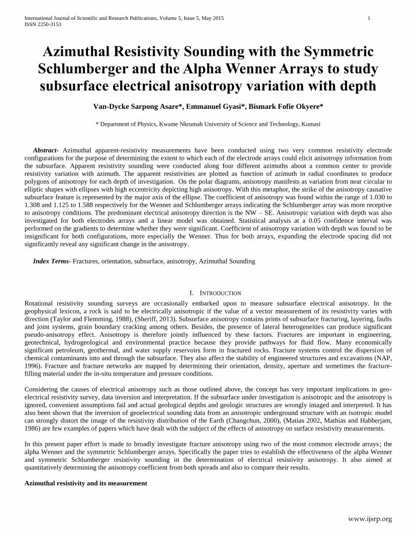
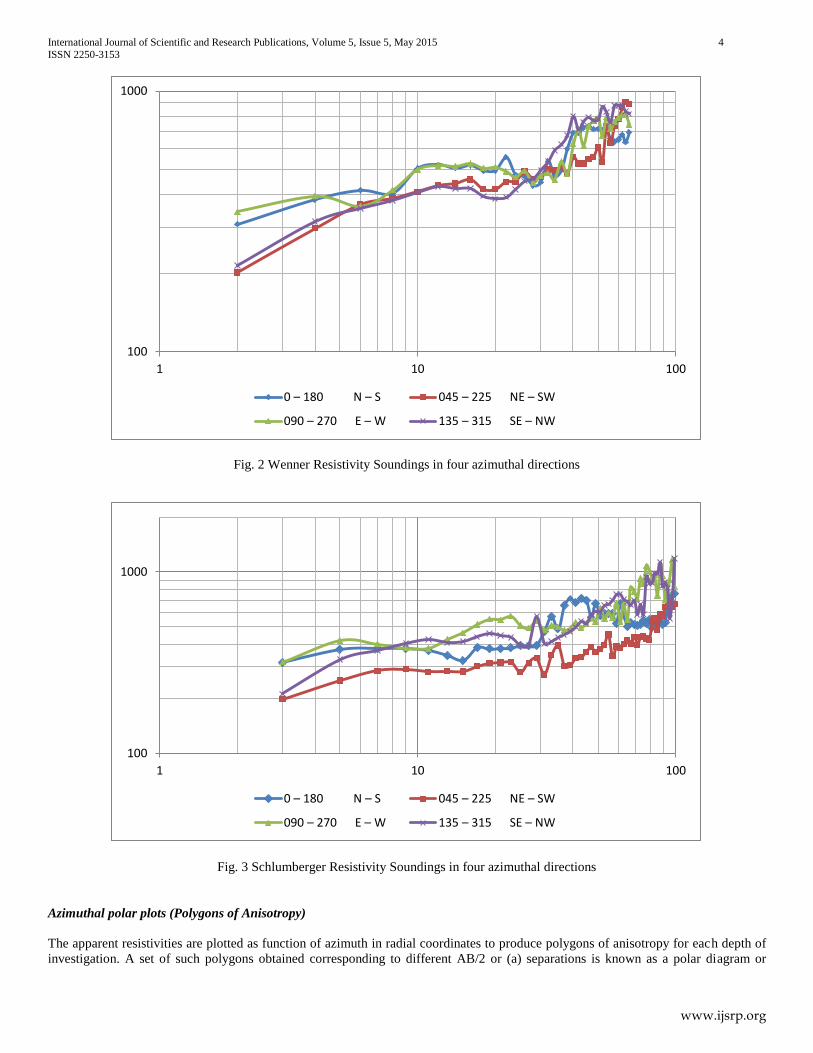
AB/2), on log-log graphs. The sounding curves for the Wenner array in various azimuths are presented on one graph (Fig. 2) and those

for the Schlumberger array are also presented on a separate graph (Fig. 3).

N


ISSN 2250-3153

www.ijsrp.org

Fig. 2 Wenner Resistivity Soundings in four azimuthal directions

Fig. 3 Schlumberger Resistivity Soundings in four azimuthal directions

Azimuthal polar plots (Polygons of Anisotropy)

The apparent resistivities are plotted as function of azimuth in radial coordinates to produce polygons of anisotropy for each depth of

investigation. A set of such polygons obtained corresponding to different AB/2 or (a) separations is known as a polar diagram or

100

1000

1 10 100

0 – 180 N – S 045 – 225 NE – SW

090 – 270 E – W 135 – 315 SE – NW

100

1000

1 10 100

0 – 180 N – S 045 – 225 NE – SW

090 – 270 E – W 135 – 315 SE – NW


ISSN 2250-3153

www.ijsrp.org

anisotropy polygon. The square root of the ratio of the lengths of the major and minor axes of the best-fit ellipse is taken as a measure

of anisotropy (Fig. 3), (Mota et al., 2004). The coefficient is determined by using equation (4)

MIN

MAX

Where ρmax is the apparent resistivity measured along the ellipse major axis; ρmin apparent resistivity measured along the ellipse minor

axis.

Fig. 4 A pattern of polygon of anisotropy showing how the anisotropy coefficient and the strike direction are determined

The major axis of the ellipse, which can fit any of such anisotropic polygons, gives the strike direction of the fracture. So in the

example shown in Fig. 4, the strike direction is NW-SE etc.

a = 2 m a = 4 m a = 6 m a = 8 m a = 10 m a = 12 m

a = 14 m a = 16 m a = 18 m a = 20 m a = 22 m a = 24 m

ρMA

X ρMIN

Major Axis

N

Lines of equal resistivity

(Ohm.m) Data point at indicated

azimuth


ISSN 2250-3153

www.ijsrp.org

a = 26 m a = 28 m a = 30 m a = 32 m a = 34 m a = 36 m

a = 38 m a = 40 m a = 42 m a = 44 m a = 46 m a = 48 m

a = 50 m a = 52 m a = 54 m a = 56 m a = 58 m a = 60 m

a = 62 m a = 64 m a = 66 m

1 – 5 0o – 180

o N – S 2 – 6 045

o – 225

o NE – SW

3 – 7 090o – 270

o E – W 4 – 8 135

o – 315

o SE – NW

Fig. 5 The pattern of Azimuthal apparent resistivity in Ohm-m plotted at different depths with the Wenner Array

L = 3 m L = 5 m L = 7 m L = 9 m L = 11 m L = 13 m


ISSN 2250-3153

www.ijsrp.org

L = 15 m L = 17 m L = 19 m L = 21 m L = 23 m L = 25 m

L = 27 m L = 29 m L = 31 m L = 33 m L = 35 m L = 37 m

L = 39 m L = 41 m L = 43 m L = 45 m L = 47 m L = 49 m

L = 51 m L = 53 m L = 55 m L = 57 m L = 59 m L = 61 m


ISSN 2250-3153

www.ijsrp.org

L = 63 m L = 65 m L = 67 m L = 69 m L = 71 m L = 73 m

L = 75 m L = 77 m L = 79 m L = 81 m L = 83 m L = 85 m

L = 87 m L = 89 m L = 91 m L = 93 m L = 95 m L = 97 m

L = 99 m L = 101 m

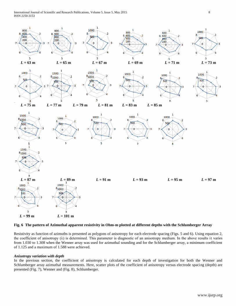
Fig. 6 The pattern of Azimuthal apparent resistivity in Ohm-m plotted at different depths with the Schlumberger Array

Resistivity as function of azimuths is presented as polygons of anisotropy for each electrode spacing (Figs. 5 and 6). Using equation 2,

the coefficient of anisotropy (λ) is determined. This parameter is diagnostic of an anisotropy medium. In the above results i t varies

from 1.030 to 1.308 when the Wenner array was used for azimuthal sounding and for the Schlumberger array, a minimum coefficient

of 1.125 and a maximum of 1.588 were achieved.

Anisotropy variation with depth

In the previous section, the coefficient of anisotropy is calculated for each depth of investigation for both the Wenner and

Schlumberger array azimuthal measurements. Here, scatter plots of the coefficient of anisotropy versus electrode spacing (depth) are

presented (Fig. 7), Wenner and (Fig. 8), Schlumberger.


ISSN 2250-3153

www.ijsrp.org

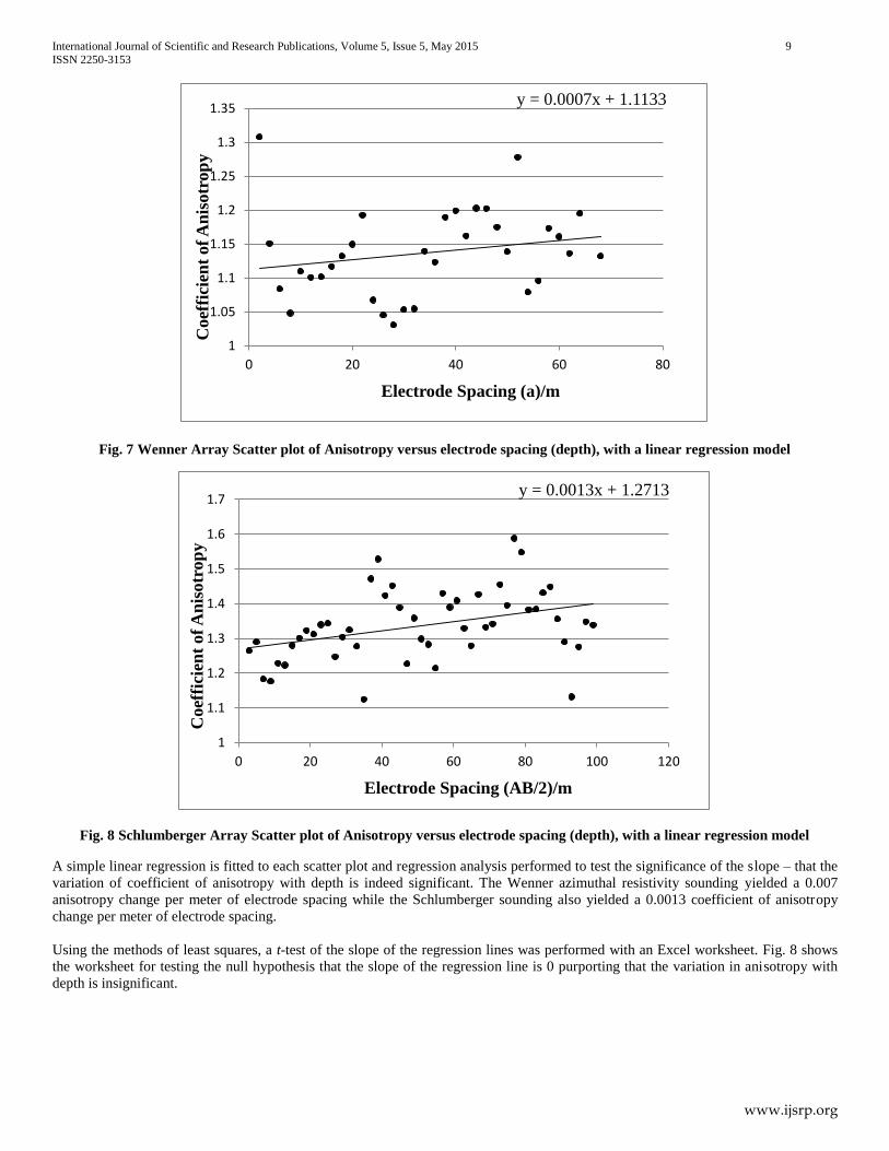
Fig. 7 Wenner Array Scatter plot of Anisotropy versus electrode spacing (depth), with a linear regression model

Fig. 8 Schlumberger Array Scatter plot of Anisotropy versus electrode spacing (depth), with a linear regression model

A simple linear regression is fitted to each scatter plot and regression analysis performed to test the significance of the slope – that the

variation of coefficient of anisotropy with depth is indeed significant. The Wenner azimuthal resistivity sounding yielded a 0.007

anisotropy change per meter of electrode spacing while the Schlumberger sounding also yielded a 0.0013 coefficient of anisotropy

change per meter of electrode spacing.

Using the methods of least squares, a t-test of the slope of the regression lines was performed with an Excel worksheet. Fig. 8 shows

the worksheet for testing the null hypothesis that the slope of the regression line is 0 purporting that the variation in anisotropy with

depth is insignificant.

y = 0.0007x + 1.1133

1

1.05

1.1

1.15

1.2

1.25

1.3

1.35

0 20 40 60 80

Co

effi

cien

t o

f A

nis

otr

op

y

Electrode Spacing (a)/m

y = 0.0013x + 1.2713

1

1.1

1.2

1.3

1.4

1.5

1.6

1.7

0 20 40 60 80 100 120

Coef

fici

ent

of

An

isotr

op

y

Electrode Spacing (AB/2)/m


ISSN 2250-3153

www.ijsrp.org

Wenner Array

Schlumberger Array

n 33

n 49

r 0.213046

r 0.364272

Sx 19.33908

Sx 28.57738

Sy 0.064472

Sy 0.100193

b 0.00071

b 0.001277

Sy-x 0.064

Sy-x 0.094296

Sb 0.000585

Sb 0.000476

t 1.214063

t 2.681565

Df 31

Df 47

p-value 0.233892

p-value 0.010078

Alpha 0.05

Alpha 0.05

t-crit 2.039513

t-crit 2.011741

sig no

Sig Yes

confidence Interval

confidence Interval

Lower -0.00048

Lower 0.000319

Upper -0.00048

Upper 0.002235

Fig. 9 A t-test of the slopes of the regression lines for data in Figs. 7 and 8

The inspection of the azimuthal sounding curves in Figs. 2 and 3, gives the first indication of limited anisotropy

of the subsurface layers beneath the sounding point. This is demonstrated by the near congruity and trending of

the sounding curves.

At each electrode space, the coefficients of anisotropy are calculated for the various azimuths. The results are

presented as polygons of anisotropy shown in Figs. 5 and 6. Where these polygons become more elliptic in

shapes, the higher the anisotropy of the subsurface. In such instances, the major axis identifies the strike

direction of the subsurface feature that giving rise to the anisotropy effect.

It can be observed, again in Figs. 5 and 6, that most of the polygons of anisotropy that assumed elliptic

geometry strike in the NW – SE direction. The Schlumberger configuration was more sensitive to anisotropy

than the Wenner configuration.

The Wenner azimuthal resistivity sounding yielded a 0.007 anisotropy change per meter of electrode spacing

while the Schlumberger sounding also yielded a 0.0013 coefficient of anisotropy change per meter of electrode

spacing.

Depth variation in coefficient of anisotropy was studied with both arrays (Figs. 7 and 8). The coefficient of

anisotropy change per meter of electrode spacing of 0.007 and 0.0013 obtained for the Wenner and

Schlumberger arrays respectively were subject to a student t–test at a significance level of 0.05 to ascertain their

significance Fig. 9. For the Wenner array, the null hypothesis is sustained and therefore it can be concluded that

the population slope is zero and insignificant - anisotropy did not exhibit any significant variation with depth.

The hypothesis test performed on the 0.0013 regression slope obtained when the Schlumberger array azimuthal

resistivity sounding was done indicated, on the basis of the 0.05 level of significance that the slope is

significant. However, the reported confidence interval does not suggest we have very strong evidence the

regression relation is significant.


ISSN 2250-3153

www.ijsrp.org

IV. CONCLUSION

Electrical anisotropy resulting from subsurface features which cause current to have preferential flow direction

is manifested when a configuration of electrodes is rotated about a fixed point. Using two of the most common

conventional collinear electrode arrays, and without any a priori specific site information, this paper has

attempted to establish the effectiveness of alpha Wenner and symmetric Schlumberger resistivity soundings in

the determination of electrical resistivity anisotropy. It also aimed at quantitatively determining the anisotropy

coefficient from both spreads and also to compare their results.

The direction of electrical anisotropy is predominantly in the NW – SE. The Schlumberger array was found to

be more sensitive to electrical anisotropy than the alpha Wenner. The coefficient of anisotropy obtained from

the survey varies from 1.030 to 1.308 when the Wenner array was used and 1.125 to 1.588 for Schlumberger

configuration.

Coefficient of anisotropy variation with depth was found to be insignificant for both configurations, more

especially the Wenner. Thus for both arrays, expanding the electrode spacing did not significantly reveal any

significant change in the anisotropy.

REFERENCES

[1] Boadu, F. K. Determining subsurface fracture characteristics from azimuthal resistivity surveys: A case study at Nsawam, Ghana. GEOPHYSICS (2005), 70(5):B35

[2] Bolshakov, D.K., Modin, I.N., Pervago, E.V., Shevnin, V.A. Separation of anisotropy and inhomogeneity influence by the spectral analysis of azimuthal

resistivity diagrams. Proceedings of 3rd EEGS-ES Meeting. Aarhus, Denmark (1997). P.147-150.

[3] Bolshakov, D.K., Modin, I.N., Pervago, E.V., Shevnin, V.A. Modeling and interpretation of azimuthal resistivity sounding over two-layered model with

arbitrary - oriented anisotropy in each layer. Proceedings of 60th EAGE Conference, Leipzig (1998). P110.

[4] Bolshakov, D.K., Modin, I.N., Pervago, E.V., Shevnin, V.A. New step in anisotropy studies: arrow-type array. Proceedings of 4th EEGS-ES Meeting, Barselona,

(1998), p. 857-860.

[5] Busby, J.P. The effectiveness of azimuthal apparent-resistivity measurements as a method for determining fracture strike orientations. Geophysical

Prospecting, (2000), 48, 677-695.

[6] Changchun, Yin. Geoelectrical inversion for a one-dimensional anisotropic model and inherent non-uniqueness Geophys. J. Int. 140 (2000), 11, 23

[7] Habberjam, G.M. Apparent resistivity anisotropy and strike measurement. Geophs. Prosp. (1975), 23(1): 211-215.

[8] Mallik, S. B., Bhattacharya, D. C., & Nag, S. K. Behaviour of fractures in hard rocks-A study by surface geology and radial VES method. Geoexploration, (1983),

21(3), 181-189

[9] Mota, R. S., F. A. Monteiro, A. Mateus, F.O. Marques, A. Conclaves, J. Figueiras and H. Amaral. Granite fracturing and incipient pollution beneath a recent landfill

facility as detected by geoelectrical surveys. J. Appl. Geophys. (2004), 57(1): 11-22.

[10] Mousatov, A., Pervago, E., Shevnin, V. New approach to resistivity anisotropic measurements. Proceedings of SEG 70th Annual Meeting, Calgary, Alberta,

Canada (2000), NSG-P1.5, 4 pp.

[11] Mousatov, A., Pervago, E., Shevnin, V. Anisotropy determination in heterogeneous media by tensor measurements of the electric field. Proceedings of SEG 72th

Annual Meeting, Salt Lake City (2004). 4 pp.

[12] National Academy of Sciences. Rock Fractures and Fluid Flow: Contemporary Understanding and Applications. NATIONAL ACADEMY PRESS, Washington,

D.C.( 1996).

[13] Pervago, E., Mousatov, A., Shevnin, V. Joint influence of resistivity anisotropy and inhomogeneity on example of a single dipping interface between isotropic overburden and anisotropic basement. Proceedings of the SAGEEP of conference. Denver (2001). ERP_7, 10 p.

[14] Semenov, A.S. Rock anisotropy and electrical fields peculiarities in anisotropic media. Vestnik of Leningrad University. Ser. Geol. and geography (1975) N 24, p.40-47, (In Russian).

[15] Taylor, R.W. and A.H. Fleming. Characterizing jointed systems by azimuth al resistivity surveys. Groundwater, (1988), 26(4): 464-474.

[16] Telford, W.M., Geldard, L.P. and Sheriff, R.E. Applied Geophysics. 2nd Edition (1990). Pp 531, 532.

[17] Watson, K.A. and Barker, R.D. Modelling azimuthal resistivity sounding over a laterally changing resistivity subsurface. Near Surface Geophysics (2005) 3, 3-11.


ISSN 2250-3153

www.ijsrp.org

[18] Watson, K. and Barker, R., 1998. Discriminating between true and pseudo-anisotropic ground using azimuthal resistivity soundings. Proceedings of the 4th EEGS European Section Meeting, Barcelona, Spain (1998), pp. 849-852.

[19] Sheriff, E. R., 2013. Encyclopedic Dictionary of Applied Geophysics. Fourth Edition.

AUTHORS

First Author – Van-Dycke Sarpong Asare, MSc, Department of Physics, Kwame Nkrumah University of Science and Technology,

Kumasi. [email protected]

Second Author – Emmanuel Gyasi, BSc, Kwame Nkrumah University of Science and Technology, Kumasi

Third Author – Bismark Fofie Okyere, BSc, Kwame Nkrumah University of Science and Technology, Kumasi

Correspondence Author – Van-Dycke Sarpong Asare, MSc, Department of Physics, Kwame Nkrumah University of Science and

Technology, Kumasi. [email protected]/ [email protected] (233-244-895283)

mailto:[email protected]/%[email protected]

Azimuthal Resistivity Sounding with the Symmetric ... · PDF fileInternational Journal of Scientific and Research Publications, Volume 5, Issue 5, May 2015 1 ISSN 2250 ... Azimuthal

Documents