1 Step by step 1. EAM MODEL..........................................................................................................................2 2. FRAME MODE L...................................................................................................................19 3. PLATE MODEL................................................................................................ ....................48 4. MEMBRANE MODEL..........................................................................................................75 4.1. Prep roc essin g with sur face elements ................................................................................75 4.2. Prep roce ssin g with domains............................................................................................ 84 5. SHELL MODEL................................................................................................ ....................99

Welcome message from author
This document is posted to help you gain knowledge. Please leave a comment to let me know what you think about it! Share it to your friends and learn new things together.
Transcript

8/3/2019 AxisVMStepByStep
http://slidepdf.com/reader/full/axisvmstepbystep 1/125
1
Step by step
1. EAM MODEL..........................................................................................................................2
2. FRAME MODEL...................................................................................................................19
3. PLATE MODEL................................................................................................ ....................48
4. MEMBRANE MODEL..........................................................................................................75
4.1. Preprocessing with surface elements................................................................................754.2. Preprocessing with domains............................................................................................84
5. SHELL MODEL................................................................................................ ....................99

8/3/2019 AxisVMStepByStep
http://slidepdf.com/reader/full/axisvmstepbystep 2/125
2
1. EAM MODEL
Start Start AxisVM by double-clicking the AxisVM icon in the
AxisVM folder, found on the Desktop, or in the Start, Programs
Menu.
New Create a new model with the New Icon. In the dialogue windowthat pops up, replace the Model Filename with “Beam”.
Select the Design Code. Click OK to close the dialog window.
Objective The objective of the analysis is to determine the internal forces,
longitudinal reinforcement and vertical stirrups in the three way
supported, reinforced concrete beams illustrated below. The
loads on the beams will be presented subsequently.
The analysis will be done according to the Eurocode. The cross-
section of the beam is will be a 400mm x 600mm rectangle. The
left beam is 12m in length and the right beam is 10m.
Coordinate
System
In the lower left corner of the graphics area is the global
coordinate system symbol. The positive direction is marked bythe corresponding capital letter (X, Y, Z). The default coordinate
system of a new model is the X-Z coordinate system. It is
important to note that unless changed the gravity acts along the –
Z direction.
In a new model, the global coordinate default location of the
cursor is the bottom left corner of the graphic area, and is set toX=0, Y=0, Z=0.
You can change to the relative coordinate values by pressing the
‘d’ labeled button on the left of the Coordinate Window. ( Hint :
In the right column of the coordinate window you can specify

8/3/2019 AxisVMStepByStep
http://slidepdf.com/reader/full/axisvmstepbystep 3/125
3
points in cylindrical or spherical coordinate systems). The origin
of the relative coordinate system is marked by a thick blue X.
Geometry The first step is to create the geometry of structure.
Select the Geometry tab to bring up the Geometry Toolbar.
Line Hold down the left mouse button while the cursor is on Line
Tool Icon brings up the Line Icons Selection Menu:
Polygon Lets click on the Polygon icon, which is the second from left to
specify the axis of the two beams. When the Polygon is chosen,
the Relative coordinate system automatically changes to thelocal system (‘d’ prefix)
The polygon coordinates can be drawn with the mouse, or by
typing in their numerical values. Set the first point ( node) of the
line by typing in these entries:
X=0
Y=0Z=0
Finish specifying the first line point by pressing Enter. The first
node of the beam model is now also the global coordinates originpoint.
Relative
Coordinate
System
To enter the next two nodes for our beam model type in the
following sequence:
X=12
Y=0
Z=0, Enter
X=10
Y=0Z=0, Enter
Press ESC twice to exit from polygon drawing function.
Zoom To bring up the Zoom Icon Bar, move the mouse on the ZoomIcon in the left side of the desktop window. It contains six icons.
Lets choose the third icon (Zoom to fit) from the Zoom Icon Bar,
or press Ctrl-W, which has the same effect. An alternative wayof zooming is to press the + or – keys on your numerical keypad.

8/3/2019 AxisVMStepByStep
http://slidepdf.com/reader/full/axisvmstepbystep 4/125
4
The following picture appears:
Geometry
Check
Click the Geometry Check Icon on the top of the desktop, to
check for geometric ambiguities. The program will ask for the
maximum tolerance (distance) for merging points.
After the geometry check a summary of actions appears.
Elements The next step is to specify the finite elements. Click on the
Elements tab to bring up the Finite Elements Toolbar.
Line Elements Press the Line Elements Icon,
then on the appearing selection icon bar use the asterisk (All)
command, then click OK. The Line Elements dialog window
appears. Select Define or Modify if you are correcting an earlier
parameter.

8/3/2019 AxisVMStepByStep
http://slidepdf.com/reader/full/axisvmstepbystep 5/125
5
Material
Library Import
Press the Material Library Import icon to select the material.
In the dialog window that appears select Concrete C25/30 in the
Materials column, then click OK.

8/3/2019 AxisVMStepByStep
http://slidepdf.com/reader/full/axisvmstepbystep 6/125
6
New Cross
Section
Click on the New Cross Section Icon (the rightmost in the
sections line) to create a new cross-section.
Rectangle Define a rectangular cross section by clicking on the
Rectangular Icon.
Modify the offered height (h) to 600 [mm]. Click the Place
Button to select the new cross-section. You should see
something similar with the following picture.

8/3/2019 AxisVMStepByStep
http://slidepdf.com/reader/full/axisvmstepbystep 7/125
7
Finish the cross-section definition by clicking on the Ok
button.
Enter a name for the newly created cross-section. Type in
400x600, and then press OK.
Leaving the Local x Reference on Auto, the orientation of the
local x axis of the beam will be along the x axis of the element,and the local z axis will be in a vertical plane passing through the
x axis.
Perspective Lets check the structure in space! Click the Perspective Icon in
the left side of the application. You can pan or rotate the
structure using the mouse.

8/3/2019 AxisVMStepByStep
http://slidepdf.com/reader/full/axisvmstepbystep 8/125
8
By closing the floating window the last view remains on the
screen.
Display
Options
The local systems, the node numbering and other useful
graphical symbols can be switched on/off by clicking the
Display Options Icon in the left side of the application. (Hint: thesame dialog window can be displayed by selecting the Display
Options item after a right click in the Graphics Area). Checkthe Beam box in the Symbols/Local Systems panel, then select
the Labels tab to check the Cross-Section Name box.
Exit from the dialog window with OK. The local system of the
beams and the name of the cross-sections will be displayed.
Move the cursor on the axis of the beam to bring up an info labelshowing relevant information about the beam.
Because the Elements tab is selected, the tag number, length,material name, cross-section name, self-weight and local
reference of the beam is displayed:
Finally switch from perspective view to Z-X plane.
Zoom to Fit In order to have a good overview, use the Zoom To Fit command.
Nodal Support Click the Nodal Support Icon and select the middle support. Adialog window appears, where you can set the translational
and/or rotational stiffness of the node. Select the global

8/3/2019 AxisVMStepByStep
http://slidepdf.com/reader/full/axisvmstepbystep 9/125
9
direction, and specify the stiffness values.
The first three entries are for the translational stiffness, measured
in [kN/m]. The default value is 1e+10 [kN/m], meaning a full
restriction of the translation, while the value 0 [kN/m] would
mean a free translation.
The next three entries are for the rotational stiffness, measured in
[kN/rad]. The default value of 1e+10 [kN/rad] means a fullyrestricted rotation, while the value 0 [kN/rad] means a free
rotation. Set all rotational stiffness to zero, and restrict thetranslation along X and Z direction. Use the settings in the
following box:
Finish the support definition with OK Select the two exterior supports and make them horizontally free
(X, Y axis) supports in a similar way:
On the screen, restricted translations are shown as yellowstripes, restricted rotations as orange stripes to their rotational
axis.

8/3/2019 AxisVMStepByStep
http://slidepdf.com/reader/full/axisvmstepbystep 10/125
10
Nodal DOF Click the Nodal DOF (Degrees of Freedom) Icon, and select
all nodes with the All command. In the Nodal Degrees of
Freedom dialog window select ‘Frame in Plane X-Z’ from the
predefined settings. After closing this window with OK, all the
nodes will change their color to blue.
This setting selects the nodes of the beams only in translation in
plane X-Z with the rotation around the Y-axis.
Loads The next step is to apply the loads.
Click the Loads tab.
Load Cases It is useful to separate the loads into load cases. Click the Load
Cases Icon to create the load cases. The following dialog
window appears.

8/3/2019 AxisVMStepByStep
http://slidepdf.com/reader/full/axisvmstepbystep 11/125
11
In the left tree view you can see the first load case, created
automatically by the program. Its name is ST1. Click on the
ST1 to change the name of the load case, and overwrite it with
SELF-WEIGHT. Click OK to return to the graphics area. The
active load case will be SELF-WEIGHT. You can see it on the
Info Window.
Display
Options
In the Display Options window select the cross-section name
under the Labels tab, and the cross-section shape and localsystem under the Symbols tab, leaving the rest of the default
settings.
Self Weight Click the Self-Weight Icon, and select all elements with the
All command. When the selection is finished by pressing Ok,
two blue dotted lines will show near the beams axis that their
dead load is placed on them (It will act by default along the –Z
direction, with the gravitational acceleration taken as g=9.81m/s2).
Load
Cases/Groups
Click the Load Cases Icon again, and create three more load
cases by clicking repeatedly the Static Button in the New Case
panel. Name them VARIABLE1, VARIABLE2 and SUPPORT
DISPLACEMENT. Make VARIABLE1 the active load case
by clicking on it, and press OK.

8/3/2019 AxisVMStepByStep
http://slidepdf.com/reader/full/axisvmstepbystep 12/125
12
Line Load Click the Line Load Icon and select the left beam. After
finishing the selection with Ok the following dialog window
appears:
As the load intensity type -17.5 in the pz1, pz2 edit boxes, then
press Ok.
Load
Cases/Groups
Click on the downward pointing triangle on the right of the
Load Cases Icon and the following menu will pop up.
It shows all load cases, a black dot marking the active one. Click
on VARIABLE2 to make it the active load case.
Apply on both beams a -17.5 kN/m uniform linear load acting
in Z direction in the same way as before.
Forced Support
Displacement
Finally select the SUPPORT DISPLACEMENT load case.
Click the Forced Support Displacement Icon, select the
middle support and press Ok. This brings up the following
dialog window.
8/3/2019 AxisVMStepByStep
http://slidepdf.com/reader/full/axisvmstepbystep 13/125
13
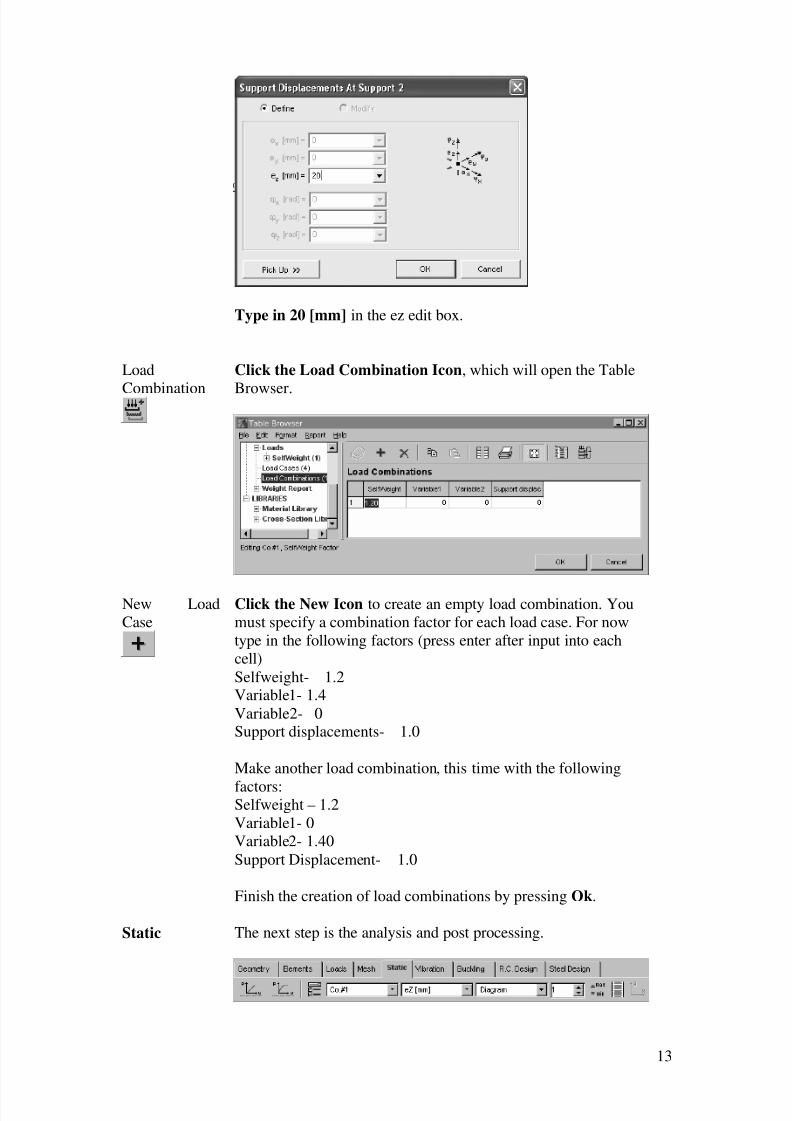
Type in 20 [mm] in the ez edit box.
Load
Combination
Click the Load Combination Icon, which will open the Table
Browser.
New Load
Case
Click the New Icon to create an empty load combination. You
must specify a combination factor for each load case. For now
type in the following factors (press enter after input into each
cell)
Selfweight- 1.2Variable1- 1.4
Variable2- 0Support displacements- 1.0
Make another load combination, this time with the following
factors:Selfweight – 1.2
Variable1- 0
Variable2- 1.40
Support Displacement- 1.0
Finish the creation of load combinations by pressing Ok.
Static The next step is the analysis and post processing.

8/3/2019 AxisVMStepByStep
http://slidepdf.com/reader/full/axisvmstepbystep 14/125
14
Linear
Analysis
Click the Static tab, then the Linear Icon to start the analysis.
If the application prompts for saving, save the model on a localhard disk. After saving, the analysis will start.
Analysis
Click the Details button to view the details of calculation.
Static When the analysis has finished, press Ok. By default the
postprocessor will start with the ez displacement of the first load
case, which is now SELF-WEIGHT. The display mode will be
iso surfaces. You will see the displacements from the dead loadin global Z direction.
Result DisplayParameters
Click the Result Display Parameters Icon and set theparameters according to the picture below.
In the Case Selector combo box select the SELF-WEIGHT load case. If you leave the Undeformed radio button checked in
the Display Shape panel, then the various results will be drawn
on the undeformed shape of the structure. In the Component
combo box select ez from displacements. Set the Display Mode
to diagram. In the Write Values To Panel check Nodes andLines. Close the dialog window with Ok. You should see the
following picture:

8/3/2019 AxisVMStepByStep
http://slidepdf.com/reader/full/axisvmstepbystep 15/125
15
Check the displacement diagrams of various load cases whether
they comply with the expected result. To do this, click on the
combo box next to the Result Display Parameters Icon, and
select desired load case. This time select the first loadcombination (Co. #1).
Min, Max
Value
Click on the Min-Max Value Icon to obtain the location and
value of the maximum and minimum displacements. The
following dialog window appears:
Select the eZ displacement component, and press OK. The
location and value of the negative maximum displacement pops
up in a window. Pressing OK closes it, and the positive
maximum displacement window pops up. Press OK to close it
too.
The various internal force and stress results can be selected
through the second combo box. First view the My bending
moment in the first and second load case (Co#1, Co#2), which is
accessible by clicking on the Beam Internal Forces.

8/3/2019 AxisVMStepByStep
http://slidepdf.com/reader/full/axisvmstepbystep 16/125
16
R.C. Design Click the R.C. Design tab to find out the area of longitudinalreinforcement and vertical stirrups.
Beam
ReinforcementDesign
Click the Beam Reinforcement Design Icon, then select all
beams with the All command (the asterisk), then press Ok. Thefollowing window appears.
8/3/2019 AxisVMStepByStep
http://slidepdf.com/reader/full/axisvmstepbystep 17/125
17
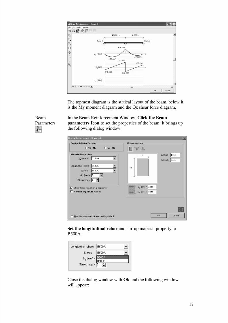
The topmost diagram is the statical layout of the beam, below itis the My moment diagram and the Qz shear force diagram.
Beam
Parameters
In the Beam Reinforcement Window, Click the Beam
parameters Icon to set the properties of the beam. It brings up
the following dialog window:
Set the longitudinal rebar and stirrup material property to
B500A.
Close the dialog window with Ok and the following window
will appear:

8/3/2019 AxisVMStepByStep
http://slidepdf.com/reader/full/axisvmstepbystep 18/125
18
Note that alongside the original My moment diagram (thin line),
the diagram shifted according to code (thick line) is also present.Below the My moment diagram is the As diagram, below the Qz
diagram is the s diagram.
‘As’ is the area of the necessary longitudinal reinforcement of
the beam, while ‘s’ is the required maximal distance of the
stirrups. The longitudinal reinforcement in tension is shown in
blue, the compressed in red. The area 342 mm2 on the ‘As’
diagram is the minimum area of the tensioned longitudinal
reinforcement, while the value 228 mm on the ‘s’ diagram is themaximum stirrup distance.
Click Ok to close this reinforcement window.
8/3/2019 AxisVMStepByStep
http://slidepdf.com/reader/full/axisvmstepbystep 19/125
19
2. FRAME MODEL
Start Start AxisVM by double-clicking the AxisVM icon in the
AxisVM folder, found on the Desktop, or in the Start, ProgramsMenu.
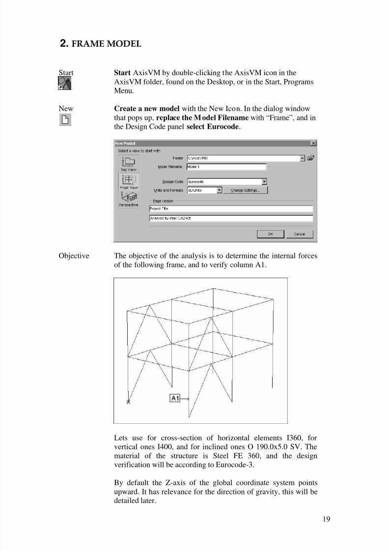
New Create a new model with the New Icon. In the dialog window
that pops up, replace the Model Filename with “Frame”, and in
the Design Code panel select Eurocode.
Objective The objective of the analysis is to determine the internal forces
of the following frame, and to verify column A1.
Lets use for cross-section of horizontal elements I360, for
vertical ones I400, and for inclined ones O 190.0x5.0 SV. The
material of the structure is Steel FE 360, and the design
verification will be according to Eurocode-3.
By default the Z-axis of the global coordinate system pointsupward. It has relevance for the direction of gravity, this will bedetailed later.

8/3/2019 AxisVMStepByStep
http://slidepdf.com/reader/full/axisvmstepbystep 20/125
20
Coordinate
System
In the lower left corner of the graphics area is the global
coordinate system symbol. The positive direction is marked by
the corresponding capital letter (X, Y, Z). The default coordinate
system of a new model is the X-Z coordinate system. It is
important to note that unless changed the gravity acts along the –
Z direction.
In a new model, the global coordinate default location of the
cursor is the bottom left corner of the graphic area, and is set to
X=0, Y=0, Z=0.
You can change to the relative coordinate values by pressing the
‘d’ labeled button on the left of the Coordinate Window. (Hint:
In the right column of the coordinate window you can specify
points in cylindrical or spherical coordinate systems). The origin
of the relative coordinate system is marked by a thick blue X.
The first step is to create the geometry of the structure.
Geometry Click the Geometry tab, below the menu bar. The Geometry
Toolbar appears below the tabs. The geometry of the structurewill be created with the Line Tool.
Line Hold down the left mouse button while the cursor is on the
Line Tool Icon will bring up the following Line Type icon bar:
Polygon Lets click on the Polygon icon, which is the second from left.When the Polygon is chosen, the Relative coordinate system
automatically changes to the local system (‘d’ prefix)
The polygon coordinates for the frame model can be drawn withthe mouse, or by typing in their numerical values.
Set the first point (node) of the line by typing in these entries:
X=0
Y=0
Z=0
Finish specifying the first line point by pressing Enter. The firstnode of the frame model is now also the global coordinatesorigin point.

8/3/2019 AxisVMStepByStep
http://slidepdf.com/reader/full/axisvmstepbystep 21/125
21
To enter the first line (node) of the frame model, enter the
following values:
X=0
Y=0
Z=3.5, Enter
To define the second line of the frame model, enter thefollowing values:
X=6
Y=0
Z=0, Enter
To define the third line of the frame model, enter the following
values:
X=0
Y=0
Z=-3.5, Enter (Note: Negative value)
Exit from the Polygon command by pressing Esc twice.
The following picture is obtained:
Translate Copy the structure vertically upward with the Translate Icon.
For this click the Translate Icon, select the horizontal line and
finish the selection with Enter. In the Translate dialog window
select Spread by Distance, in the ‘d [m]=’ edit box type 3.5,and in the Nodes To Connect panel select All.

8/3/2019 AxisVMStepByStep
http://slidepdf.com/reader/full/axisvmstepbystep 22/125
22
Close the dialog window with Ok, then click on an arbitrary
place in the graphics area and draw upward a vertical line,
which is longer than 3.5 m.

8/3/2019 AxisVMStepByStep
http://slidepdf.com/reader/full/axisvmstepbystep 23/125
23
The following picture is obtained:
Coordinate
SystemSwitch to Z-Y plane.You should see this picture:

8/3/2019 AxisVMStepByStep
http://slidepdf.com/reader/full/axisvmstepbystep 24/125
24
Translate Select the Translate Icon so you can Copy this part of the
model geometry structure. In the Selection Icon bar use the All
command (the asterisk). The selected elements color will
change:
Finishing the selection with Ok, in the dialog window select the
Consecutive method, then in the Nodes to Connect panel select
the Double Selected option.
Close this dialog window with Ok. Now you must select the
nodes to connect. Use a selection window according to the
picture below on the left. The picture on the right shows the
result of your selection:
8/3/2019 AxisVMStepByStep
http://slidepdf.com/reader/full/axisvmstepbystep 25/125
25
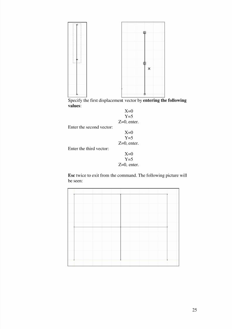
Specify the first displacement vector by entering the following
values:
X=0
Y=5Z=0, enter.
Enter the second vector:
X=0
Y=5Z=0, enter.
Enter the third vector:
X=0
Y=5
Z=0, enter.
Esc twice to exit from the command. The following picture will
be seen:

8/3/2019 AxisVMStepByStep
http://slidepdf.com/reader/full/axisvmstepbystep 26/125
26
Coordinate
System
Switch to perspective View. The colums should be on the
vertical Z-axis. Use the pan function as needed to bring the
model to this perspective.
When you close the dialog bar this settings will remain active.
Polygon Click the Polygon Icon. Draw a segment from the bottom of
A1 column to the middle of the beam in Y direction:

8/3/2019 AxisVMStepByStep
http://slidepdf.com/reader/full/axisvmstepbystep 27/125
27
Continue with a segment to the bottom of the middle column:
Press Esc twice to exit from the command.
Translate Click the Translate Icon, select the two inclined bars then
finish the selection with Ok. In the dialog window select the
Consecutive method, and set the Nodes to Connect to None.
After closing the dialog window with Ok, click on the bottomnode of the A1 column, then on the middle node of the A1
column. This will copy the two inclined bars to the upper story.Copy the bars on the other side of the structure as well. To exit
from translate press Esc. The following picture appears:
Geometry
Check
Check the geometry of the structure with the Geometry Check
Icon, which is toward the end of Geometry Toolbar:

8/3/2019 AxisVMStepByStep
http://slidepdf.com/reader/full/axisvmstepbystep 28/125

8/3/2019 AxisVMStepByStep
http://slidepdf.com/reader/full/axisvmstepbystep 29/125
29
Finish the selection with Ok, and the following dialog window
appears:
MaterialLibraryImport
Click the Browse Material Library Icon in the row labeledMaterial. The following dialog window appears:
Select Steel Fe360 as the active material.
Cross-Section
Library Import
Click Cross-Section Library Import Icon. The following
dialog window appears :
Select from the Cross-Section Tables I Hungarian Beams, then
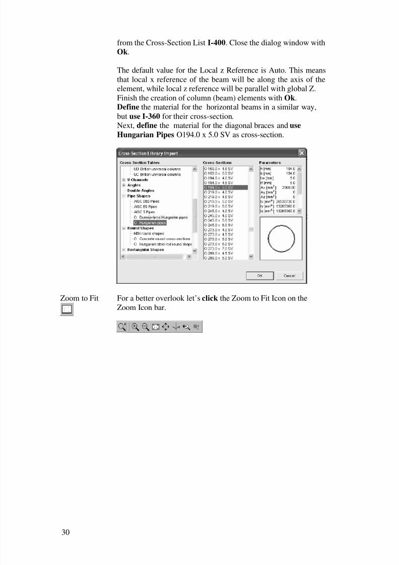
8/3/2019 AxisVMStepByStep
http://slidepdf.com/reader/full/axisvmstepbystep 30/125
30
from the Cross-Section List I-400. Close the dialog window with
Ok.
The default value for the Local z Reference is Auto. This means
that local x reference of the beam will be along the axis of the
element, while local z reference will be parallel with global Z.
Finish the creation of column (beam) elements with Ok.Define the material for the horizontal beams in a similar way,
but use I-360 for their cross-section.
Next, define the material for the diagonal braces and use
Hungarian Pipes O194.0 x 5.0 SV as cross-section.
Zoom to Fit For a better overlook let’s click the Zoom to Fit Icon on theZoom Icon bar.
8/3/2019 AxisVMStepByStep
http://slidepdf.com/reader/full/axisvmstepbystep 31/125
31
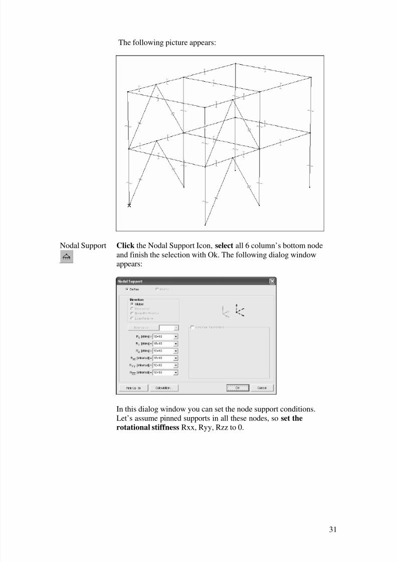
The following picture appears:
Nodal Support Click the Nodal Support Icon, select all 6 column’s bottom node
and finish the selection with Ok. The following dialog windowappears:
In this dialog window you can set the node support conditions.
Let’s assume pinned supports in all these nodes, so set the
rotational stiffness Rxx, Ryy, Rzz to 0.

8/3/2019 AxisVMStepByStep
http://slidepdf.com/reader/full/axisvmstepbystep 32/125
32
Finish the creation of nodal supports with Ok, and the support
symbols will appear.
Loads The next step is to apply the loads. Click the Loads tab.
Load Cases &
Load Groups
It is useful to separate the loads into load cases. Click the Load
Cases & Load Groups Icon to create the load cases. The
following dialog window appears:

8/3/2019 AxisVMStepByStep
http://slidepdf.com/reader/full/axisvmstepbystep 33/125
33
Click on the ST1 (the first static load case) in the upper left
corner, and rename it to VARIABLE1. Close the dialog window
with Ok, and VARIABLE1 will be the current load case. You
can see in the Info Window the name of the current load case:
Line Load Let’s apply loads on the horizontal beams. Apply on the lower
beams 50 kN/m, on the upper beams 25 kN/m. For this click theLine Load Icon, then select the upper beams with a selection
window.

8/3/2019 AxisVMStepByStep
http://slidepdf.com/reader/full/axisvmstepbystep 34/125
34
Finish the selection with Ok, and the following dialog window
appears:
Type -25 in the pz1, pz2 edit boxes, then close the dialog
window with Ok. The following picture appears:
Display
Options
Click the Display Options Icon in the Icons Menu. The
following dialog window appears:Select the Labels tab, then check the Load Value box:

8/3/2019 AxisVMStepByStep
http://slidepdf.com/reader/full/axisvmstepbystep 35/125
35
Close the dialog window with Ok, and the load values will
appear in the graphics area.
8/3/2019 AxisVMStepByStep
http://slidepdf.com/reader/full/axisvmstepbystep 36/125
36
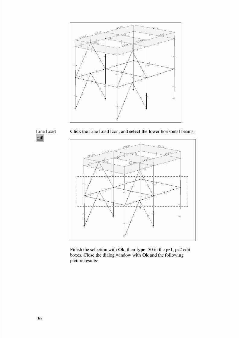
Line Load Click the Line Load Icon, and select the lower horizontal beams:
Finish the selection with Ok, then type -50 in the pz1, pz2 editboxes. Close the dialog window with Ok and the following
picture results:

8/3/2019 AxisVMStepByStep
http://slidepdf.com/reader/full/axisvmstepbystep 37/125
37
Load Cases &
Load Groups
Click the Load Cases & Load Groups Icon.
New Load
Case Static
In the New Case panel click the Static Icon and name the load
case WIND. Close the dialog window with OK. All previous
loads ’disappeared’, and the current load case’s name in the Info
Window is WIND.
CoordinateSystem
Switch to Y-X plane (top view). The following picture appears:
8/3/2019 AxisVMStepByStep
http://slidepdf.com/reader/full/axisvmstepbystep 38/125
38
Line Load Click the Line Load Icon, and define on the upper left columns
a load of intensity 6 kN/m in x direction. From the top view
select the upper left node with a selection windows (thus
selecting everything inside the selection window, including the
two columns). Finish the selection with Ok, then type a load
intensity value of 6 in px1, px2 edit boxes and close the dialog
window. Repeat the above step for the bottom left node.Repeat the above step for the middle left column, except type a
load intensity value of 12.
Coordinate
System
Switch to Perspective View. The following picture appears:
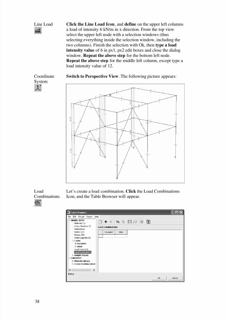
LoadCombinations
Let’s create a load combination. Click the Load CombinationsIcon, and the Table Browser will appear.

8/3/2019 AxisVMStepByStep
http://slidepdf.com/reader/full/axisvmstepbystep 39/125
39
New Row Use the New Row Icon to add a new load combination. You
have to specify a factor for each load case in a load combination.
Let’s assume the following factors. Type in these factors in
their columns:
VARIABLE1 1.2, Enter
WIND 1.2, Enter
Accept the new load combination(s) by closing the Table
Browser with Ok.
Now the preprocessing part of the example is finished.
Display
Options
Click the Display Options Icon, and uncheck the Node, Cross-
Section Shape, Load boxes in the Symbols tab, andthe Load
Value box in the Labels tab.
Static The next step is the analysis and post processing. Click the
Static tab. Here you can start the analysis and visualize the
results.
Linear Static
Analysis
Click on the Linear Static Analysis Icon.
A Model Save Dialog will appear if you haven’t already
assigned a name for the model. Accept save and a Save dialog
window appears, where you can specify the model filename andpath.
During the analysis the following window appears:
Details If you click the details button to view details of computation,
the topmost label shows the current computation step, the upper
bar shows its progress. The lower bar shows the global progress
of computation. The estimated memory requirement shows the
estimated virtual memory demand. If the virtual memory of the
computer is set to a lower value, an error message will appear.
When the computation has finished, the two progress bars willdisappear. Close the window with Ok.

8/3/2019 AxisVMStepByStep
http://slidepdf.com/reader/full/axisvmstepbystep 40/125
40
Static By default the postprocessor will start with the ez displacement
of the first load case, which is now VARIABLE1. The display
mode will be iso surface. Change to isoline display. You will
see the displacements from the VARIABLE1 load case in global
Z direction. To view the results from the load combination select
Co. #1 in the Case Selector combo box.
Switch from Isoline to Diagram by Clicking the Result Display
Parameters Icon and select Diagram in the Display Mode menubox:
Coordinate
System
Switch to Z-X plane. The following picture appears.
Parts Click the Parts Icon on the left Icons Menu. The following
dialog window appears.

8/3/2019 AxisVMStepByStep
http://slidepdf.com/reader/full/axisvmstepbystep 41/125
41
Click the New Button, which brings up a window where you
can specify the name of the part.
Type in 1 and close this window with Ok.
You have to select the entities which will make up the partnamed 1. Select the right columns with a selection window
according to the following picture.
Finish the selection with Ok. The dialog window will reappear
as in the picture below.

8/3/2019 AxisVMStepByStep
http://slidepdf.com/reader/full/axisvmstepbystep 42/125
42
Close the dialog window with Ok, and part 1 will be accepted.
Coordinate
System
Switch to Z-Y plane.
Result Display
Parameters
Click the Result Display Parameters Icon, and check Nodes
and Lines in the Write Values to box.
Click OK to close the dialog window, and the following picture
appears.

8/3/2019 AxisVMStepByStep
http://slidepdf.com/reader/full/axisvmstepbystep 43/125
43
Min/Max
Values
Click the Minimum and Maximum Values Icon to find out the
location of maximum displacement. The following dialog box
will appear:
Here you can select one displacement component. Leave it on ez
and click Ok. First the location and value of the negativeminimum displacement appears.
Click Ok, and the location and value of positive maximum
displacement will appear.
Select from the Result Component combo box Nx from the
8/3/2019 AxisVMStepByStep
http://slidepdf.com/reader/full/axisvmstepbystep 44/125
44
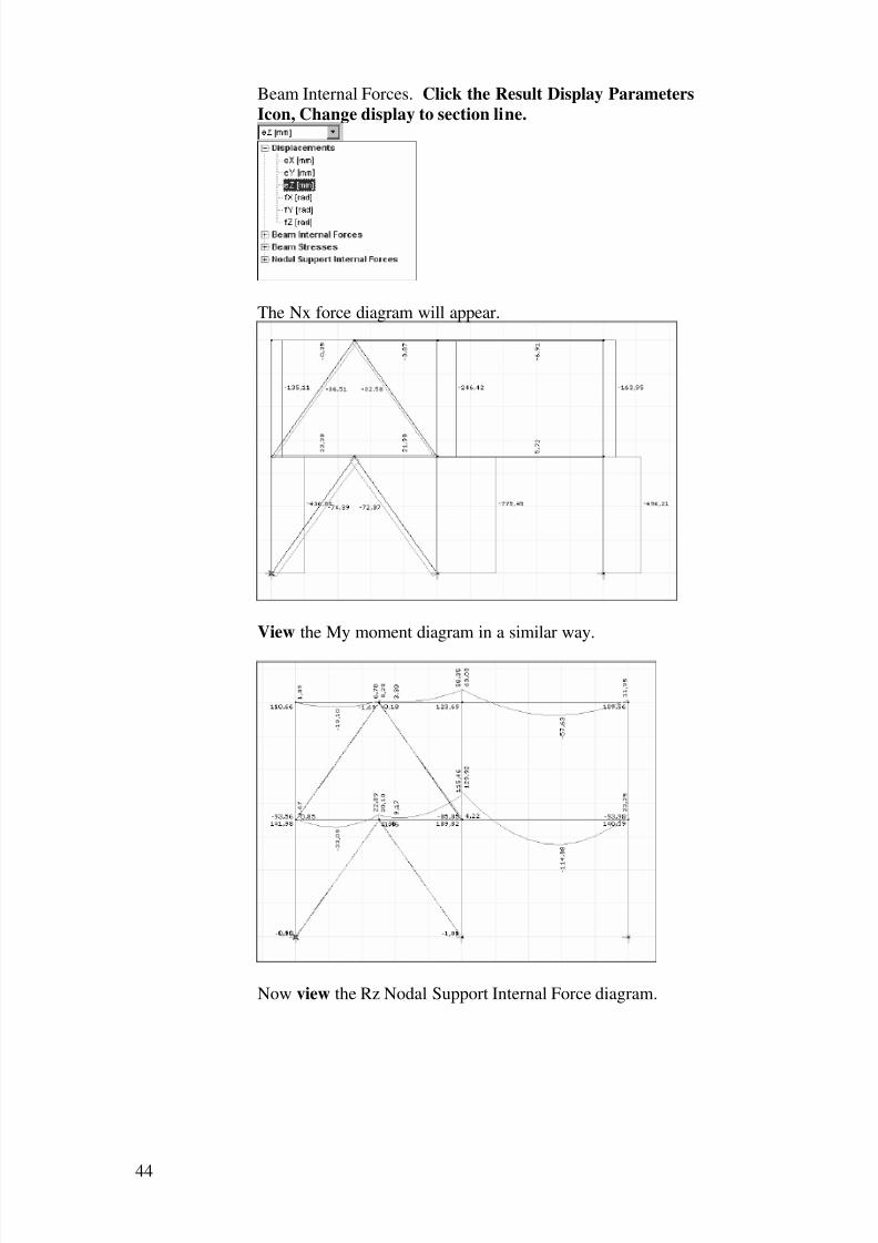
Beam Internal Forces. Click the Result Display Parameters
Icon, Change display to section line.
The Nx force diagram will appear.
View the My moment diagram in a similar way.
Now view the Rz Nodal Support Internal Force diagram.

8/3/2019 AxisVMStepByStep
http://slidepdf.com/reader/full/axisvmstepbystep 45/125
45
Steel Design Click the Steel Design tab to start the checking of column A1.
Design
Parameters
Click the Design Parameters Icon, then select column A1 and
finish the selection with Ok. The following dialog window
appears:
Overwrite Kyy with 1.25, and then close the dialog window
with Ok.
Axial Force-
Bending-Shear
Let’s view the N-M-V diagram.

8/3/2019 AxisVMStepByStep
http://slidepdf.com/reader/full/axisvmstepbystep 46/125
46
The following picture appears:
Buckling Now view the N-M-Flx Buckling diagram:
8/3/2019 AxisVMStepByStep
http://slidepdf.com/reader/full/axisvmstepbystep 47/125
47
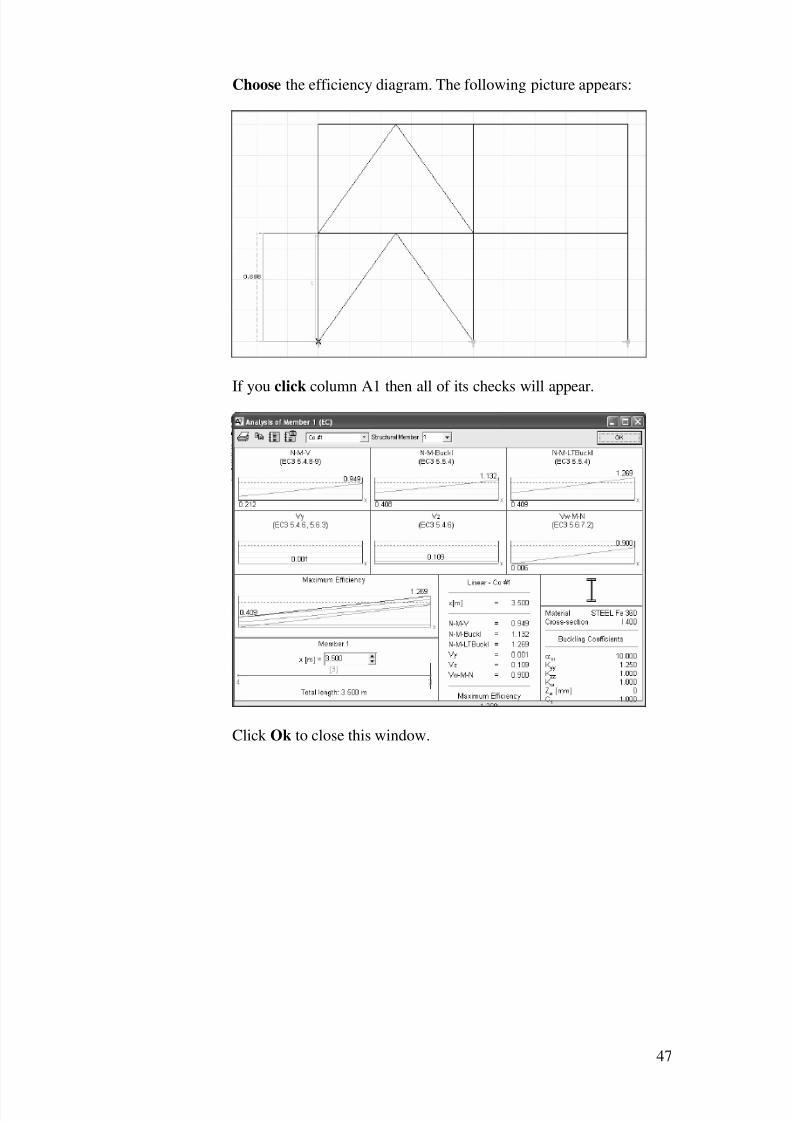
Choose the efficiency diagram. The following picture appears:
If you click column A1 then all of its checks will appear.
Click Ok to close this window.

8/3/2019 AxisVMStepByStep
http://slidepdf.com/reader/full/axisvmstepbystep 48/125
48
3. PLATE MODEL
Start Start AxisVM by double-clicking the AxisVM icon in the
AxisVM folder, found on the Desktop, or in the Start, Programs
Menu.
New Create a new model with the New Icon. In the dialog window
that pops up, replace the Model Filename with “Frame”, and inthe Design Code panel select Eurocode.
Objective The objective of the analysis is to determine the maximum
deflection, bending moments and required reinforcement of the
following plate.
Lets suppose the plate thickness is 20 cm, the concrete is of
C20/25, and the reinforcement is computed according to
Eurocode-2.
The first step is to create the geometry of structure.
CoordinateSystem
In the lower left corner of the graphics area is the globalcoordinate system symbol. The positive direction is marked by
the corresponding capital letter (X, Y, Z). The default coordinate
system of a new model is the X-Z coordinate system. It isimportant to note that unless changed the gravity acts along the –
Z direction.

8/3/2019 AxisVMStepByStep
http://slidepdf.com/reader/full/axisvmstepbystep 49/125
49
In a new model, the global coordinate default location of the
cursor is the bottom left corner of the graphic area, and is set to
X=0, Y=0, Z=0.
The location of the cursor is defined as a relative coordinate.
You can change to the relative coordinate values by pressing the
‘d’ labeled button on the left of the Coordinate Window. (Hint:In the right column of the coordinate window you can specify
points in cylindrical or spherical coordinate systems). The origin
of the relative coordinate system is marked by a thick blue X.
Geometry If not already selected, activate the Geometry tab. Under it
appears the Geometry Toolbar.
View Click the Y-X view from the View Icon Bar.
Line Create the geometry of plate using the Rectangle command.
Holding down the left mouse button on the Line Icon canaccess it.
Note: When the a line type is chosen, the Relative coordinatesystem automatically changes to the local system (‘d’ prefix)
Rectangle The corners of the rectangle can be specified graphically or by
entering the coordinates. Lets enter them with coordinates:
Set the first corner (node) of the rectangle by typing in theseentries:
X=0
Y=0
Z=0
Finish specifying the first corner point by pressing Enter. The
first node of the plate model is now also the global coordinates
origin point.
Relative
Coordinates
Lets specify the relative coordinates of the next corner. Type in
the following sequence of keys:
X=8.4Y=6.8
Z=0
8/3/2019 AxisVMStepByStep
http://slidepdf.com/reader/full/axisvmstepbystep 50/125
50
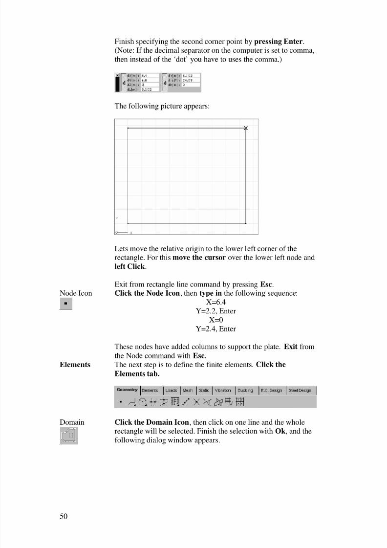
Finish specifying the second corner point by pressing Enter.
(Note: If the decimal separator on the computer is set to comma,
then instead of the ‘dot’ you have to uses the comma.)
The following picture appears:
Lets move the relative origin to the lower left corner of therectangle. For this move the cursor over the lower left node and
left Click.
Exit from rectangle line command by pressing Esc. Node Icon Click the Node Icon, then type in the following sequence:
X=6.4
Y=2.2, Enter
X=0
Y=2.4, Enter
These nodes have added columns to support the plate. Exit from
the Node command with Esc.
Elements The next step is to define the finite elements. Click the
Elements tab.
Domain Click the Domain Icon, then click on one line and the whole
rectangle will be selected. Finish the selection with Ok, and the
following dialog window appears.

8/3/2019 AxisVMStepByStep
http://slidepdf.com/reader/full/axisvmstepbystep 51/125
51
Material
Library Import
Click the Material Library Import Icon in the row of
Material, and the following dialog window appears:
Choose C20/25 from Materials List Box, using the scroll bar if necessary. Close the Material Library Import dialog window
with Ok.
Thickness Type in the thickness combo box the value 200 [mm], then close
the dialog window with Ok. The following picture appears:
Note the red line on the inner contour of the domain
This is the symbol of a (plate) domain. If you move the mouse
on this contour, the properties of the domain will appear in a hint
window.

8/3/2019 AxisVMStepByStep
http://slidepdf.com/reader/full/axisvmstepbystep 52/125
52
Zoom to Fit For a better view let’s click the Zoom to Fit Icon on the Zoom
Icon bar.
Domain
Meshing
Click the Domain Meshing Icon. Use the select All command
(the asterisk) and finish the selection with OK. The following
dialog window appears:
Type in the Average Mesh Element Size edit box the value 0.66
[m], then press Ok. An automatic mesh generation will start. Its
progress is showed in the following window.
When the mesh generation finishes, the following picture
appears:

8/3/2019 AxisVMStepByStep
http://slidepdf.com/reader/full/axisvmstepbystep 53/125
53
The surface element symbol is a solid red square in the center of
the element. If you move the cursor over it, the properties of the
element appear in an info window.
Refinement Let's refine the mesh around the two nodal supports. Depress
the left mouse button over the Refinement Icon, and click the
Refinement by BiSection Icon that appears.
Uniform
Refinement
Select the surface elements around the nodal supports with a
selection box, according to the picture below:
Finish the selection with Ok and accept the offered MaximumSide Length. The result of the refinement is shown in the
following picture:
DisplayOptions Let's view the local coordinate system of the surface elements.Click the Display Options Icon in the Icons Menu (left side).

8/3/2019 AxisVMStepByStep
http://slidepdf.com/reader/full/axisvmstepbystep 54/125
54
Activate the Symbols tab, then on the Local System Panelcheck the Surface box.
Close the dialog window with Ok.
A red line shows the local -x direction, a yellow line the local -ydirection and a green line the local -z direction:
DisplayOptions
Select Display Options Icon to switch off the Surface box onthe Local System panel.

8/3/2019 AxisVMStepByStep
http://slidepdf.com/reader/full/axisvmstepbystep 55/125
55
Nodal Support Let's specify the supports of the structure. Click on the Nodal
Support command then select the two nodes in the center of the
columns and finish the selection with Ok. The Nodal Support
Window appears.
Calculations Click the Calculations button. The following dialog window
appears:
In this dialog window you can specify the support stiffness for
the column type support.
New Cross
Section
Click the New Cross Section Icon. The following dialog
window appears:

8/3/2019 AxisVMStepByStep
http://slidepdf.com/reader/full/axisvmstepbystep 56/125
56
Rectangle
Shape
Click the Rectangular Shape Icon. The following dialog
window appears:
Type 300 [mm] in the upper two edit boxes, as the dimensionsof cross section, and click Place. Click in the Cross Section
Editor Drawing Area to place the rectangle. The location where
the rectangle is placed is unimportant.

8/3/2019 AxisVMStepByStep
http://slidepdf.com/reader/full/axisvmstepbystep 57/125
57
A following picture appears:
Close the Cross Section Editor with Ok. A dialog window asks
for the name of the new cross-section.
Type in 300x300, then close the dialog window with Ok. The
Global Node Support Calculation dialog window’s stiffnessvalues will take into account this cross-section's properties.
Accepting the remaining settings click Ok. The stiffness values
displayed in the Global Node Support Calculation dialog
window will be copied in the Nodal Support dialog window.
Close the dialog window with Ok, and the two supports are
created.

8/3/2019 AxisVMStepByStep
http://slidepdf.com/reader/full/axisvmstepbystep 58/125
58
The following picture appears:
Line Support Let's create the line supports on the contour of the domain. Click
the Line Support Icon, and select the four contour lines of thedomain. They represent walls on the edges of the plate.
Finish the selection with Ok, and the following dialog window
appears.
Calculation Click the Calculation button. Here you can calculate the line
support stiffness due to a wall support. Type in the thickness of
wall edit box 300 [mm]. You can see that the height of the wallis 3.0m, and the wall stiffness is also shwon in this dialog box.

8/3/2019 AxisVMStepByStep
http://slidepdf.com/reader/full/axisvmstepbystep 59/125
59
Depress both the upper and lower End Release Icons. Close
with Ok the dialog windows.
Nodal DOF Click the Nodal DOF Icon. Select all nodes with the Allcommand (the asterisk), then finish the selection with Ok. In the
Nodal Degrees Of Freedom dialog box select Plate in X-Y fromthe list.
Accepting this will constrain the degree of freedom to vertical
displacements and rotations about axes in the plane of the plate.

8/3/2019 AxisVMStepByStep
http://slidepdf.com/reader/full/axisvmstepbystep 60/125
60
Loads The next step is to apply the loads. Click the Loads tab.
Load Cases &
Load Groups
It is useful to group the loads into load cases. To manage the
load cases click the Load Cases & Load Groups Icon. Thefollowing dialog window appears:
ST1 in the upper left corner of the window is the first load case
(created by default). Click it and rename it to Self-Weight.Closing the dialog window it will be the active load case. It can
be seen on the Info Window:
Self Weight Click the Self Weight Icon, and select all elements with the All
command. Finish the selection with Ok, and the self-weight load
will be applied to all elements. This can be seen by the red
dashed lines on the contour of elements.

8/3/2019 AxisVMStepByStep
http://slidepdf.com/reader/full/axisvmstepbystep 61/125
61
New Load
Case
Click the Load Cases & Load Groups Icon again, and create a
new load case with the Static Icon. Name it Permanent Load.
This load case contains the dead loads on the plate. Let's assume
it is 2.5 kN/m2 distributed load.
DistributedSurface Load
Click the Distributed Surface Load Icon and select allelements with the All command. Finish the selection and type in
the -pz input box the value -2.5 kN/m2. The negative value
means a load acting in opposite direction to the local z-axis of
the surface element. This is a load on the surfaces of the plate.
New Load
Case
Create a new load case and name it Live Load. It will contain
the variable loads. Click the Distributed Surface Load Icon
and select all elements with the All command. Finish theselection and type in
-pz=-1.5 kN/m2.
Load
Combinations
Now, that all loads have been applied to the structure, the load
combinations can be created. There will be only one load
combination, containing all load cases. Click the Load
Combinations Icon. The following dialog window appears:

8/3/2019 AxisVMStepByStep
http://slidepdf.com/reader/full/axisvmstepbystep 62/125
62
New Row Create a new load combination by using the New Row
command. You can apply load factors to load cases by using a
load combination. In this example the factors of the Eurocode2
will be used:
Self Weight 1.35
Dead Load 1.35Variable 1.50
Type in these values in their columns. You can move to the next
column by pressing Enter. When finished press Ok, and the new
load combination is created.
Now all the model data is available for the analysis.
Static The next step is the analysis and postprocessing. Click the
Static tab. Here you can start the static analysis and visualize
the results.
Linear Static
Analysis
Click the Linear Static Analysis Icon. If till this point the
model wasn't saved, the program will ask to save. Accept Save,
and a Save dialog window appears, where you can specify the
model file name and path.
The analysis process will start.
During the analysis the following window appears:
If you click the details button, the topmost bar shows the
progress of the current computation step. The bar below it showsthe global analysis progress. The estimated memory requirement
is the amount of virtual memory that must be available. If the
size of the operating systems virtual memory is limited to a
lower value, an error message will appear, showing the required
virtual memory. When the analysis has finished, the progress
bars will disappear.
Static Closing the Linear Analysis window with Ok the postprocessorwill start by default with the first load case (Self-Weight in this
case), the result component is ez displacement and the display
mode is isosurface 2D. This shows the vertical displacementsfrom the first load case.

8/3/2019 AxisVMStepByStep
http://slidepdf.com/reader/full/axisvmstepbystep 63/125
63
Click the Case Selector combo box, and select Co.#1 to view the
results from the load combination.
The Color Legend Window shows that the displacements are
negative, because they are in an opposite direction with the local
z-axis of the elements. This is the top view of a surface load.
Display
Options
Click the Display Options Icon on the Icons Menu in the left
side. Under the Symbols tab, in the Graphics Symbols Panelswitch off the Load and Surface Center options.
Min/Max
Values
Let’s find the maximal displacements. Click the Min, Max
Values Icon. The following dialog window appears:
Here you can select the displacement component extremities.
Accept ez, and a window pops up, showing the location and
value of maximum negative displacement
Click Ok, and another window pops up, showing the location
and value of maximum positive displacement.

8/3/2019 AxisVMStepByStep
http://slidepdf.com/reader/full/axisvmstepbystep 64/125
64
Color Legend The Color Legend Window shows the color ranges. You can
change the number of colors by dragging the handle beside thelevel number edit box or entering a new value.
Let’s find the ranges with a displacement larger than 10 mm.
Click on the values in the Color Legend Window. In the Color
Legend Setup dialog window check Auto Interpolate, thenclick on the bottom value in the left column, and replace -11.4
with -10.

8/3/2019 AxisVMStepByStep
http://slidepdf.com/reader/full/axisvmstepbystep 65/125
65
Close the dialog window with OK, and the new ranges will be
applied.
The ranges with a displacement larger than 10 mm are shown by
the inclined hatching.
Display Mode Let's view the displacement in isoline display mode too. Clickthe Display Mode combo box (the one which is displaying
Isosurface 2D), and select Isoline from the list.

8/3/2019 AxisVMStepByStep
http://slidepdf.com/reader/full/axisvmstepbystep 66/125
66
The following picture appears:
Perspective
View
Let's view the results in perspective. Click the Perspective
View Icon from the View Icon Bar.
Accept the perspective display values in the dialog window by
closing it with Close Icon.
Result DisplayParameters Click the Result Display Parameters Icon to view thedeformed shape. In the Display Shape Panel select Deformed.
When the dialog window is closed the deformed shape of the
structure is shown.
Rendered Click the Rendered Icon in the Display Mode Icon Bar, and the
deformed shape of the structure will be rendered.

8/3/2019 AxisVMStepByStep
http://slidepdf.com/reader/full/axisvmstepbystep 67/125
67
Click the Wireframe Icon and return to the Isoline display
mode.
Let's switch to X-Y Plane.
After studying the deformed shape let’s look at the internalforces. Click the Result Component combo box (the one which
displays ez), and the following list appears:
Open the Surface Internal Forces by clicking on it, then select
mx. The isoline display of the mx internal moments appears on
the screen. This is the moment that is taken by the reinforcementin the -x direction. The my, mxy internal moments and the qxz,
qyz shear forces can be viewed in a similar way.
Open in the Result Component combo box the Nodal SupportInternal Forces, and select Rz. This way you will be able to see
the compressive force acting on the columns.

8/3/2019 AxisVMStepByStep
http://slidepdf.com/reader/full/axisvmstepbystep 68/125
68
Result Display
Parameters
For this click the Result Display Parameters Icon.
The following dialog window appears:
In the Write Values To Panel check the Nodes box, and
uncheck the Min, Max. only. Close the dialog window with Ok and the value of the axial forces in the columns appears near the
nodes.
The reactions from the line supports can be viewed in a similar
way. In Result Display Parameters check only Lines in the
Write Values to Panel. Select Line Support Internal Forces
and value Rz.

8/3/2019 AxisVMStepByStep
http://slidepdf.com/reader/full/axisvmstepbystep 69/125
69
R.C. Design Let's switch to R.C. Design tab.
Here the reinforcement areas from the internal forces can be
obtained.
Reinforcement
Parameters
Click the Reinforcement Parameters Icon, and select all
surface elements with the All command. Finish the selection
with Ok, and the following dialog windows appear:
The characteristics of the concrete are already known from thecreation of domain. Select B500B for the type of the
reinforcement:

8/3/2019 AxisVMStepByStep
http://slidepdf.com/reader/full/axisvmstepbystep 70/125
70
Type in 1.5 for the depth of concrete cover in -x direction, and
2.5 for the -y direction.
When the dialog window is closed, the axb diagram appears,
which is the isosurface diagram of the bottom steel area in -xdirection. In the Result Component combo box you can select
the top or bottom -x or -y direction of the steel reinforcement.
By changing the number of levels and the top and bottom values
in the Color Legend Window, it is easy to see variations in the
required reinforcement needed.
In this case let's study the reinforcement at the top in -x
direction. Switch to –axt in the Result Component combo box.
Min/MaxValues
Find the maximal amount of steel reinforcement using the Min,Max. Values command. Clicking on its icon the following
dialog window appears:
Continue with Ok, and a dialog window appears with the
location and area of maximum reinforcement.
Let's use as minimal reinforcement (0.3%) fi12/18, whose area is
628 mm2/m, and for actual reinforcement fi12/9, whose area is
1257 mm2/m.

8/3/2019 AxisVMStepByStep
http://slidepdf.com/reader/full/axisvmstepbystep 71/125
71
It can be seen that the area for actual reinforcement is greater
than the maximum area of calculated reinforcement, so it can be
applied over the whole plate.
To separate reinforcement regions set the number of levels to 3
in the Color Legend Window.
Activate the Color Legend Setup by clicking on a value, thentype 1257 in the top row, 628 under it and 0 in the last row.
The regions that require the minimum or maximum
reinforcement are displayed.
It can be seen that in the middle region of the plate no top
reinforcement in -x direction is required from calculation, near

8/3/2019 AxisVMStepByStep
http://slidepdf.com/reader/full/axisvmstepbystep 72/125
72
the edges the minimal reinforcement is enough and in the area
around the columns, the maximum reinforcement is required.
To view the reinforcement needed in the area around the
columns Click the Static tab. In Result Component combo box
select Surface Internal Forces and click on -mxy. Set the
display to Isosurface. .
Section Lines Click the Section Lines Icon on the Left Icon Bar.
Click the New Section Plane button, and name the sectionplane Column1 in the dialog window that appears:
Accept the name and specify the section plane on the drawing.
Select one of the column support nodes, then the other column
support node.

8/3/2019 AxisVMStepByStep
http://slidepdf.com/reader/full/axisvmstepbystep 73/125
73
The following dialog window returns:
Accept it with Ok. The display should be set to the Section
Line.
CoordinateSystem Switch to Z-Y plane, Select Surface Internal Forces –m1 andthe moment diagram section across the columns is obtained.
Let's switch off the display of section. Click the Section Lines
Icon uncheck the box before Column1 and close the dialog
window with Ok.
8/3/2019 AxisVMStepByStep
http://slidepdf.com/reader/full/axisvmstepbystep 74/125
74
Result Display
Parameters
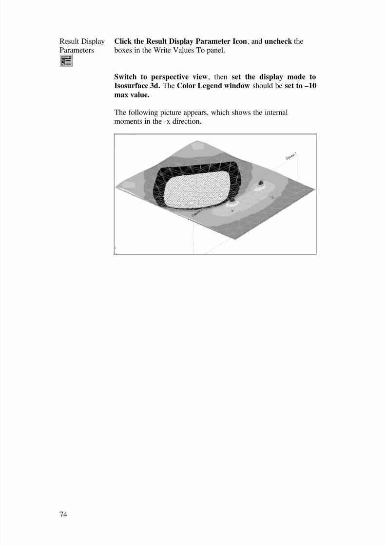
Click the Result Display Parameter Icon, and uncheck the
boxes in the Write Values To panel.
Switch to perspective view, then set the display mode to
Isosurface 3d. The Color Legend window should be set to –10
max value.
The following picture appears, which shows the internal
moments in the -x direction.

8/3/2019 AxisVMStepByStep
http://slidepdf.com/reader/full/axisvmstepbystep 75/125
75
4. MEMBRANE MODEL
4.1. Preprocessing with surface elements
Start Start AxisVM by double-clicking the AxisVM icon in the
AxisVM folder, found on the Desktop, or in the Start, ProgramsMenu.
New Create a new model with the New Icon. In the dialog window
that pops up, replace the Model Filename with “Membrane 1”.Select the Design Code. Click Ok.
Objective The objective of the analysis is to determine the internal forces
and reinforcements of the following wall structure.
Assume the wall thickness is 200 mm, the concrete is of C20/25,
and the reinforcement is B500A computed according to
Eurocode-2.
The first step is to create the geometry of structure.
Coordinate
System
In the lower left corner of the graphics area is, in blue color, the
coordinate system beginning point marked with a blue X. The
coordinate system view can be changed from the Icons Menuwith the Views Icon. Move the cursor over that icon and the
following icon bar is displayed:

8/3/2019 AxisVMStepByStep
http://slidepdf.com/reader/full/axisvmstepbystep 76/125
76
The vertical upward direction is taken as the positive Z direction.
It has relevance for the direction of gravitational force.If the view is not already in Z-X plane, switch to it.
Geometry If not already selected, activate the Geometry tab, under which
the Geometry Toolbar is displayed.
Quad/Triangle
Division
The geometry of the wall is created with the Quad/Triangle
Division Icon. Hold down the left mouse button to display the
sub-menu. Click on the first Icon on the left and the following
dialog window is displayed:
To create the upper part enter N1=20, N2=8.
Close the dialog window with Ok. Now you have to specify the
corners of the Quad. They can be specified graphically or by
entering the coordinates. Lets enter them with coordinates :To enter the first corner, Type in the following sequence of
keys:
X=0 Y=0 Z=3, Enter
Specify the relative coordinates of the next corners in a similar
way. Type in the following sequence of keys :
X=12 Y=0 Z=0, Enter
X=0 Y=0 Z=3, Enter
X=-12 Y=0 Z=0, Enter

8/3/2019 AxisVMStepByStep
http://slidepdf.com/reader/full/axisvmstepbystep 77/125
77
Exit from drawing quads by pressing Esc.
The following Drawing is displayed:
Quad/Triangle
Division
The pillars are created in a similar way. Click the
Quad/Triangle Divison Icon. Enter the following values:N1=3, N2=6
Close the dialog window with Ok. Now you have to specify thecorners of the Quad.
Type in the following sequence of keys :
X=0 Y=0 Z=-6, Enter
X=1 Y=0 Z=0, EnterX=0.8 Y=0 Z=3, Enter
X=-1.8 Y=0 Z=0, Enter
Exit from drawing quads by pressing Esc.
The following drawing is displayed:
Mirror Create the other pillar by mirroring the first one with respect to
the center of structure (X=6). Click the Mirror Icon.
The Selection Icon Bar is displayed:

8/3/2019 AxisVMStepByStep
http://slidepdf.com/reader/full/axisvmstepbystep 78/125
78
Select with a selection window all nodes of the pillar.
The selected elements will be highlighted.
Finish the selection with Ok and the following dialog window
will be displayed:
Set Mirror: Copy, Nodes to connect: None, Copy: All. Now
you have to specify the mirror plane. First select the middle
point of the bottom line of the upper part, then select any point
vertically above it.

8/3/2019 AxisVMStepByStep
http://slidepdf.com/reader/full/axisvmstepbystep 79/125
79
The following drawing is displayed:
The geometry of the wall has been successfully created.
Zoom Let's zoom to the structure. Move the cursor over the ZoomIcon on the Icons Menu. The Zoom Icon Bar pops up.
Fit in Window Click the Fit In Window Icon.
Geometry
Check
In the top icon bar, Click the Geometry Check Icon to check
for possible duplicate entries. In the dialog window displayed thetolerance for merging the nodes can be specified. If the distance
between two nodes is less than the value you enter they
respective nodes will be merged. Enter .001.

8/3/2019 AxisVMStepByStep
http://slidepdf.com/reader/full/axisvmstepbystep 80/125
80
Click OK and a check summary is displayed when completed.
Elements The next step is to create the finite elements. Activate the
Elements tab.
Surface
Elements
Click the Surface Elements Icon. After selecting All elements
the following dialog window is displayed:
Set the type of the element to Membrane(plane stress).
MaterialLibrary Import
Click the Material Library Import Icon. The following dialogwindow is displayed:
Select C25/30 from the Materials list, then accept it with Ok.
Thickness Enter(type) in the Thickness edit box 200 [mm], then close the
dialog window with Ok.

8/3/2019 AxisVMStepByStep
http://slidepdf.com/reader/full/axisvmstepbystep 81/125
81
The surface elements have been created.
Display
Options
To view the local coordinate system of the surface elements
click on the Display Options Icon on the Icons Menu in the left
side. The following dialog window is displayed:
Check the Surface box in the Local Systems panel.
Accept the change with Ok.
If the Mesh, Node, Surface Center is switched on among the
Graphics Symbols, it is visible that the program uses 9-node
membrane elements. These 9 nodes are the corners, middpoints
and center point of surface element. If you move the cursor on
the surface center symbol (a filled square), a hint window is
displayed with the property of the surface element: its tag,material, thickness, mass and references, as shown in the next
drawing:

8/3/2019 AxisVMStepByStep
http://slidepdf.com/reader/full/axisvmstepbystep 82/125
82
The red line shows the x axis of the local coordinate system, the
yellow one the y axis and the green one the z axis.
Line Support To create the supports click on the Line Support Icon andselect the bottom lines of the pillars with a selection box.
Finish the selection with Ok. The following dialog window isdisplayed:

8/3/2019 AxisVMStepByStep
http://slidepdf.com/reader/full/axisvmstepbystep 83/125
83
To create a pinned support use the following settings:
Nodal DOF Click the Nodal DOF Icon, select all nodes with the All
command and accept the selection. In the dialog window scrollto Membrane in Plane X-Z and apply it.

8/3/2019 AxisVMStepByStep
http://slidepdf.com/reader/full/axisvmstepbystep 84/125
84
4.2. Preprocessing with domains
Start Start AxisVM by double-clicking the AxisVM icon in the
AxisVM folder, found on the Deskto, or in the Start, Programs
Menu.
New Create a new model with the New Icon. In the dialog window
that pops up, replace the Model Filename with “Membrane-2”.
Objective The objective of the analysis is to determine the internal forces
and reinforcements of the following wall structure:
Assume that the wall thickness is 200 mm, the concrete is of
C25/30, and the reinforcement is B500A, computed according toEurocode-2.
The first step is to create the geometry of structure.
Coordinate
System
In the lower left corner of the graphics area is the global
coordinate system symbol. The positive direction is marked by
the corresponding capital letter (X, Y, Z). The default coordinate
system of a new model is the X-Z coordinate system. It is
important to note that unless changed the gravity acts along the –Z direction.
8/3/2019 AxisVMStepByStep
http://slidepdf.com/reader/full/axisvmstepbystep 85/125
85
In a new model, the global coordinate default location of the
cursor is the bottom left corner of the graphic area, and is preset
to X=0, Y=0, Z=0.
The location of the cursor is defined as a relative coordinate.
You can change to the relative coordinate values by pressing the
‘d’ labeled button on the left of the Coordinate Window. (Hint:In the right column of the coordinate window you can specify
points in cylindrical or spherical coordinate systems). The origin
of the relative coordinate system is marked by a thick blue X.
Geometry If not already selected, activate the Geometry tab. The
Geometry Toolbar is displayed:
Line Press down the left mouse button while the mouse is on the Line
Icon. (Note: Icons default display is to the last icon selection)
The following icon sub-menu is displayed:
Note: When the a line type is chosen, the Relative coordinate
system automatically changes to the local system (‘d’ prefix)
Polygon Select the Polygon icon, which is the second from left. When
the Polygon is chosen, the Relative coordinate system
automatically changes to the local system (‘d’ prefix)
The polygon coordinates for the frame model can be drawn withthe mouse, or by typing in their numerical values.
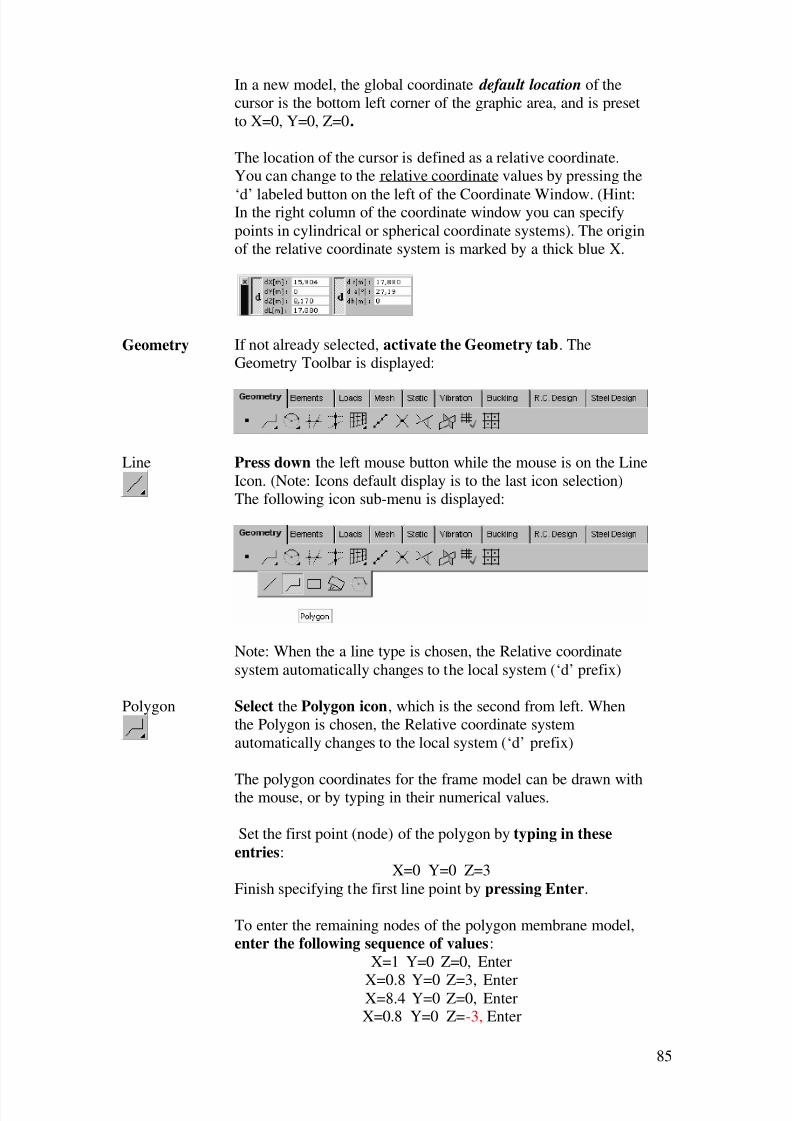
Set the first point (node) of the polygon by typing in these
entries:X=0 Y=0 Z=3
Finish specifying the first line point by pressing Enter.
To enter the remaining nodes of the polygon membrane model,
enter the following sequence of values:
X=1 Y=0 Z=0, Enter
X=0.8 Y=0 Z=3, EnterX=8.4 Y=0 Z=0, EnterX=0.8 Y=0 Z=-3, Enter
8/3/2019 AxisVMStepByStep
http://slidepdf.com/reader/full/axisvmstepbystep 86/125
86
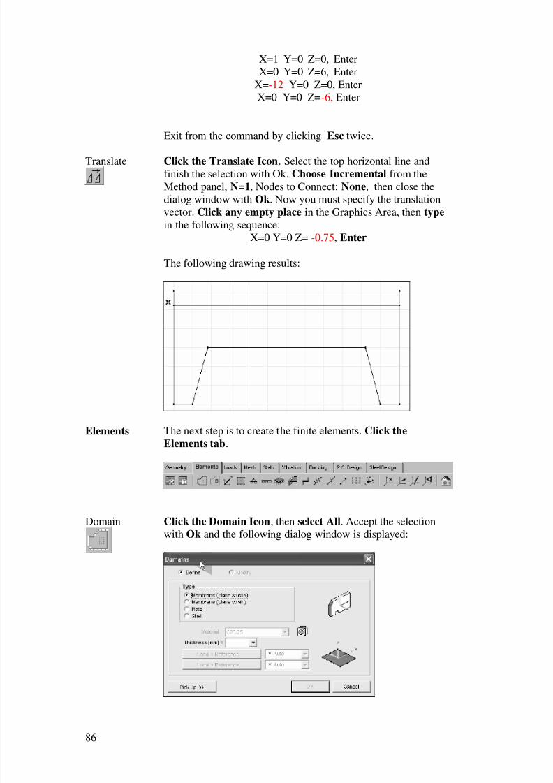
X=1 Y=0 Z=0, Enter
X=0 Y=0 Z=6, Enter
X=-12 Y=0 Z=0, Enter
X=0 Y=0 Z=-6, Enter
Exit from the command by clicking Esc twice.
Translate Click the Translate Icon. Select the top horizontal line and
finish the selection with Ok. Choose Incremental from the
Method panel, N=1, Nodes to Connect: None, then close the
dialog window with Ok. Now you must specify the translation
vector. Click any empty place in the Graphics Area, then type
in the following sequence:
X=0 Y=0 Z= -0.75, Enter
The following drawing results:
Elements The next step is to create the finite elements. Click the
Elements tab.
Domain Click the Domain Icon, then select All. Accept the selection
with Ok and the following dialog window is displayed:

8/3/2019 AxisVMStepByStep
http://slidepdf.com/reader/full/axisvmstepbystep 87/125
87
Set the type of the element to Membrane (plane stress).
Material
Library Import
Click the Material Library Import Icon and the following
dialog window is displayed:
Select C25/30 from the materials list, and close the dialogwindow with Ok.
Thickness Enter(Type in) 200 [mm] as the thickness of wall
,
then close the dialog window with Ok.
8/3/2019 AxisVMStepByStep
http://slidepdf.com/reader/full/axisvmstepbystep 88/125
88
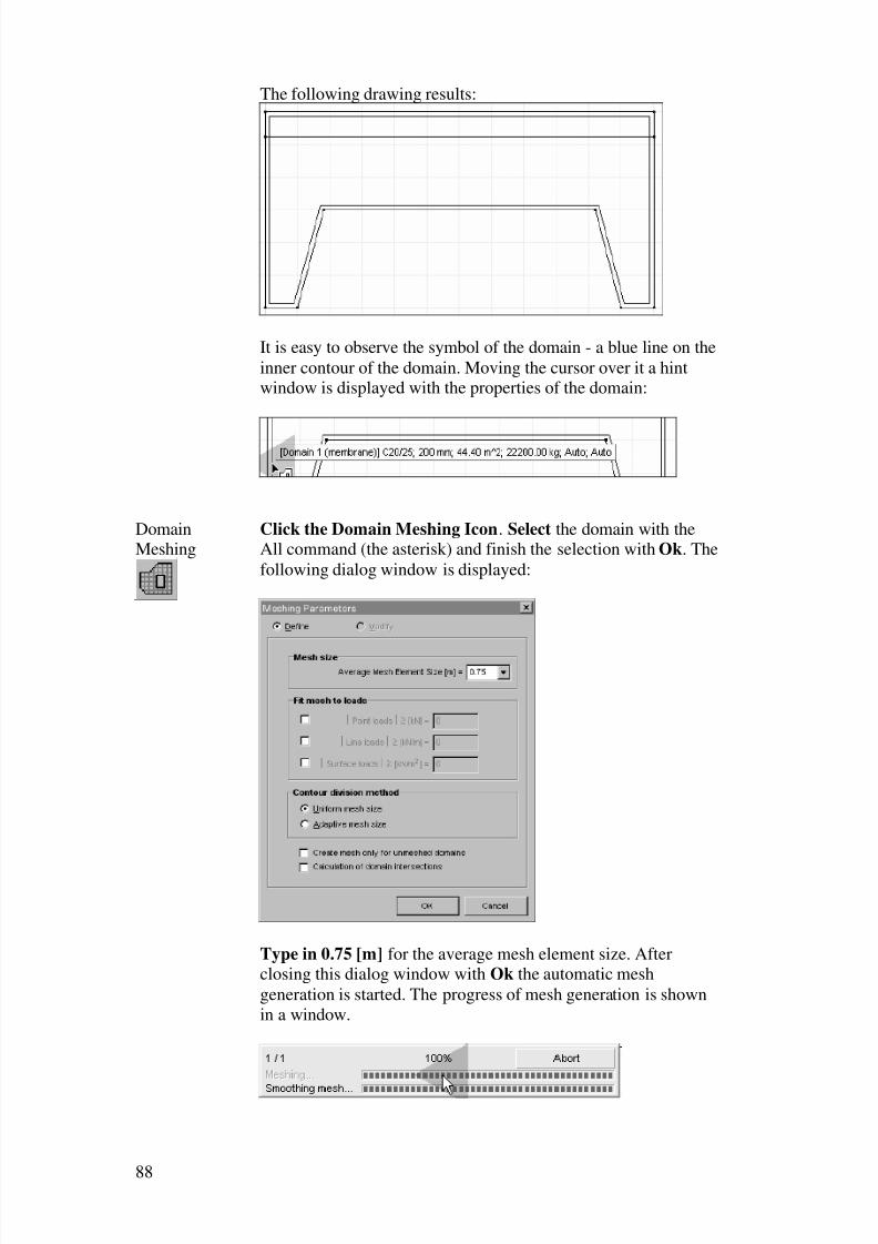
The following drawing results:
It is easy to observe the symbol of the domain - a blue line on the
inner contour of the domain. Moving the cursor over it a hintwindow is displayed with the properties of the domain:
DomainMeshing
Click the Domain Meshing Icon. Select the domain with theAll command (the asterisk) and finish the selection with Ok. The
following dialog window is displayed:
Type in 0.75 [m] for the average mesh element size. Afterclosing this dialog window with Ok the automatic mesh
generation is started. The progress of mesh generation is shown
in a window.
8/3/2019 AxisVMStepByStep
http://slidepdf.com/reader/full/axisvmstepbystep 89/125
89
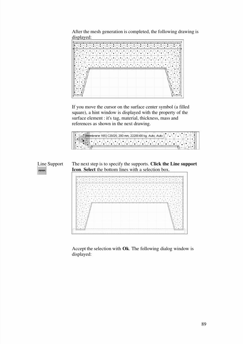
After the mesh generation is completed, the following drawing is
displayed:
If you move the cursor on the surface center symbol (a filled
square), a hint window is displayed with the property of the
surface element : it's tag, material, thickness, mass andreferences as shown in the next drawing.
Line Support The next step is to specify the supports. Click the Line support
Icon. Select the bottom lines with a selection box.
Accept the selection with Ok. The following dialog window is
displayed:

8/3/2019 AxisVMStepByStep
http://slidepdf.com/reader/full/axisvmstepbystep 90/125
90
To create pinned support set the dialog window as shown
below:
Close the dialog window with Ok, and the following drawing is
displayed:
Nodal DOF The next (optional) step is to set the nodal degrees of freedom.
Click the Nodal DOF Icon. Select all nodes with the All
command, finish the selection with Ok, and in the dialogwindow select Membrane in plane X-Z.

8/3/2019 AxisVMStepByStep
http://slidepdf.com/reader/full/axisvmstepbystep 91/125
91
The finite elements have now been created.
The next step is to apply the loads.
Load Click the Loads tab.
Surface EdgeLoad
Assume a 50kN/m vertical distributed load. Click on the
Surface Edge Load Icon, then select the line you have created
with the translate command (the second black line from top):
Finish the selection with Ok, and enter(type) in: py 50 [kn/m]:

8/3/2019 AxisVMStepByStep
http://slidepdf.com/reader/full/axisvmstepbystep 92/125
92
Press Ok and the load is applied.
The following drawing is displayed:
Static The next step is the analysis and postprocessing. Click the
Static tab.
Linear Static
Analysis
Click the Linear Static Analysis Icon. The model will be saved
with it's current name (which is Membrane 2 in this case).
A Model Save Dialog will appear if you haven’t already
assigned a name for the model. Accept save and a Save dialog
window appears, where you can specify the model filename and
path.
Calculation During the calculation the following window is visible:

8/3/2019 AxisVMStepByStep
http://slidepdf.com/reader/full/axisvmstepbystep 93/125
93
Click the Details button to view the details of calculation:
The topmost label shows the current computation step, and the
bar below it shows its progress. The second bar shows the global
progress of computation. The estimated memory requirement
shows the estimated virtual memory needed. If the virtual
memory of the computer is set to a lower value than the needed
value, an error message is displayed. When the computation has
finished, the progress bars will disappear.
Postprocessor Close the window with Ok. By default the postprocessor will
start with the ez displacement, the display mode will be isoline.You will see the vertical displacements.
Display
Options
For a clearer view, switch off the display of Loads. Click the
Display Options Icon, and uncheck the Load box.
Fit in Window Click on the Fit in Window Icon.
The following drawing results:
Click the Result Component combo box (the one showing
ez[mm] and select nx from Surface Internal Forces.

8/3/2019 AxisVMStepByStep
http://slidepdf.com/reader/full/axisvmstepbystep 94/125
94
Min/Max
Value
To find the location of maximum internal force. Click the Min,
Max Value Icon. The following dialog window is displayed:
Here you can select the component you are interested in. Accept
nx by clicking Ok. A dialog window will show the value andlocation of the negative maximum.
Click Ok and another window is displayed showing the locationand value of positive maximum.

8/3/2019 AxisVMStepByStep
http://slidepdf.com/reader/full/axisvmstepbystep 95/125
95
The color regions are delimited by the values in the Color
Legend Window. You can change the number of colors by
dragging the handle beside the level number edit box or entering
a new value.
Color Legend
Setup Window
To find the ranges with a normal force larger than -100 kN/m,
Click on the values in the Color Legend Window. In the Color
Legend Setup dialog window check Auto Interpolate, then
click on the bottom value in the left column, and replace –
331.62 with -100.
Close the dialog window with OK, and the new ranges will be
applied.
The following drawing results:

8/3/2019 AxisVMStepByStep
http://slidepdf.com/reader/full/axisvmstepbystep 96/125
96
The regions with a normal force greater then -100 are hatched.
Isoline View the internal forces in Isoline display mode. Click the
Display Mode combo box (the one which displays Isosurface
2D) and select Isoline from the list.
The isoline drawing is shown below:
View the internal forces of the supports. Select rz from Line
Support Internal Forces in the Result Component combo box.
Result Display
Parameters
Click the Result Display Parameters Icon, and the following
dialog window is displayed. Check the Lines box in the Write
Values To panel and set the Display Mode to Diagram

8/3/2019 AxisVMStepByStep
http://slidepdf.com/reader/full/axisvmstepbystep 97/125
97
Close the dialog window with Ok and the values of support
forces is displayed on the screen:
R.C. Design The next step is to calculate the reinforcement. Click the R.C.Design tab:
Click on the Reinforcement Parameters Icon, and select all
surface elements with the All command. Complete the selection
with OK, and the following dialog window is displayed:

8/3/2019 AxisVMStepByStep
http://slidepdf.com/reader/full/axisvmstepbystep 98/125
98
Close the dialog window with OK and the axb diagram is
displayed:
The area of reinforcement in the x direction is the sum of the axt
and axb values.

8/3/2019 AxisVMStepByStep
http://slidepdf.com/reader/full/axisvmstepbystep 99/125
99
5. SHELL MODEL
Start To run the program click AxisVM 8 icon in the AxisVM folder
on the Desktop.
New Create a new model by clicking the New icon or File / New from
the menu. Enter ‘Reservoir’ into the Model Filename field and
into the first line of the Page Header. Select Front View from
the left toolbar and select Eurocode as Design Code.:
Job definition Determine the specific forces and the amount of reinforcement
for the following reservoir filled with water.
Thickness of the walls and the baseplate is 250 mm, ribs on theupper edge are 30x60s. The structure is made of C25/30 concrete
and B500B rebars. Use Eurocode 2.
Settings Use Settings / Options / Grid & Cursor… to open the following
dialog:

8/3/2019 AxisVMStepByStep
http://slidepdf.com/reader/full/axisvmstepbystep 100/125
100
Replace each value under Cursor Step by 0.2
to ensure that the mouse cursor moves in 0.2 m steps so you
avoid geometric imperfections while drawing the model.
Now you create the geometry using enhanced editing functions.
Geometry Click the Geometry tab under the menu getting to the geometry
toolbar:
Polygon The third icon from the left is Polygon. Click the mouse left button on it to draw a
polygon.
First we draw the reservoir wall in X-Z
plane.
Choose the global origin as the origin of
the polygon. It is on the bottom left at the
intersection of a horizontal and a vertical
brown line representing the global X and Zaxes. The blue x shows the current origin
of the editing coordinate-system.
Relativecoordinate-
To enter further polygon vertices choose the relative coordinate-
system (relative to the blue x). Turn on relative coordinates by

8/3/2019 AxisVMStepByStep
http://slidepdf.com/reader/full/axisvmstepbystep 101/125
101
system clicking the d button. If this button is down the relative
coordinates are displayed and coordinates have a d prefix.
If this button is up global coordinates are displayed.
Move the mouse cursor to the following locations and click once
to enter each vertex: 11.0 right and 0.2 down, down 0.4, right
1.0, up 3.6, left 12.0, down 3.0 (or by keyboard: x 11 z –0,2
[Enter] z –0.4 [Enter] x 1 [Enter] z 3.6 [Enter] x –12 [Enter] z –3
[Enter]).
Double-click at the last vertex to quit the drawing function. Now
you have this:
Translation Use the Translation icon on the Icon bar on the left to create the
geometry of the reservoir in space.
The Selection palette appears:
Select all lines by pressing the Gray* on the keyboard or the
fourth icon on the toolbar. Selected elements turn purple. Click
the OK button to accept the selection and you get to the
Translate dialog.
Select the Incremental method, N=1, and All nodes to connect .
Click OK to close the dialog.

8/3/2019 AxisVMStepByStep
http://slidepdf.com/reader/full/axisvmstepbystep 102/125
102
Change view Select the icon on the left from the toolbar and the X-Y plane or
press [Ctrl+2]
Now specify the translation vector. Its base point can be
anywhere and set its endpoint using relative coordinates to get to
this point:
Change view Select the icon on the left from the toolbarand click the Perspective view (or press
Ctrl+4):
The perspective palette appears:
The cursor changes to show that you can drag and rotate the model toset a new perspective. Rotate it to get to the following settings or enterthese H, V, P values:
Close the palette by clicking any of the two small x button.
Fit in window To see the entire structure click the Zoom icon on the left toolbar
and choose Fit in window:
Numbering Move the cursor to the bottom right corner anf find the
Numbering icon among the speed buttons!

8/3/2019 AxisVMStepByStep
http://slidepdf.com/reader/full/axisvmstepbystep 103/125
103
Here you can turn numbering on or off. Turn on the
check box before Node and node numbers appear
immediately.
Translation(move)
To shape up the grip slope move the line between Node 3 and 4
down by 0.2 m. Drag a selection rectangle around Node 3 and 4:
All elements within the rectangle will be selected (Node 3, Node
4 and the line between them).
Move the cursor onto the selected line and start dragging it. Now
you have to specify the translation vector.
Select the Special constraints icon fromthe Icon bar on the left and choose the
second icon from the flyout toolbar.
Click the vertical line
between Node 4 and 5. Nowyou have applied a parallel
constraint: the translation
vector will be parallel to the
vertical line. Move the line
between Node 3 and 4 down.To specify the exact distance
type Z to get to the dZ
coordiante edit field and type
–0.2 [Enter].
Geometry Check To check the model geo-
metry use the Geometry
Check.
Here you can set the tole-
rance. If two nodes are
closer than this distancethey will automatically
be joined.
After clicking OK acheck report will appear:
Elements Clicking the Elements tab you can specify the element types,material properties, cross-sections and references determining

8/3/2019 AxisVMStepByStep
http://slidepdf.com/reader/full/axisvmstepbystep 104/125
104
local systems of the elements.
Reference point The local system of finite elements can be set by references. In
this example a reference point is used to define the orientation of
the local Z direction on the plane normal and a reference plane todefine the in-plane X and Y axes.
Click the reference point icon then click the midside point of the
line between Node 5 and 11. To locate the midside point move
the cursor along the line and check if the cursor shape changes
from ’/’ to ’ ½’.
Numbering Move the cursor over the Numbering button on the
speed button toolbar. Turn on the Reference check box. Now an „R1” label appears beside the
reference symbol.
Reference plane To set the local system of domains create a
reference plane. Click the icon on the Elements toolbar. You need three points to
define the plane. Click Node 6, click
anywhere on the line between Node 1 and
2 then click Node 1.
You get this:
Domains Define a domain to create structural surface elements. Click the
Domain icon. The Selection palette appears. Click on the
following lines to select domain contours:
6 – 6; 6 – 1;→ Rectangle 6 – 1 – 7 – 12 is automatically
selected1 – 7; 7 – 8; 8 – 2; 2 – 1
11 – 10; 10 – 4; → Rectangle 11 – 10 – 4 – 5 is automatically
selectedClick OK on the Selection palette. You get to the Domains
dialog.
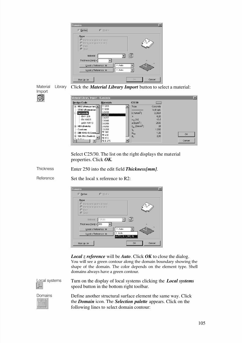
8/3/2019 AxisVMStepByStep
http://slidepdf.com/reader/full/axisvmstepbystep 105/125
105
Material LibraryImport
Click the Material Library Import button to select a material:
Select C25/30. The list on the right displays the materialproperties. Click OK.
Thickness Enter 250 into the edit field Thickness[mm] .
Reference Set the local x reference to R2:
Local z reference will be Auto. Click OK to close the dialog.You will see a green contour along the domain boundary showing theshape of the domain. The color depends on the element type. Shelldomains always have a green contour.
Local systems Turn on the display of local systems clicking the Local systems
speed button in the bottom right toolbar.
Domains Define another structural surface element the same way. Click
the Domain icon. The Selection palette appears. Click on thefollowing lines to select domain contour:

8/3/2019 AxisVMStepByStep
http://slidepdf.com/reader/full/axisvmstepbystep 106/125
106
8 – 9; 9 – 3;→ Polygon 8 – 9 – 3 – 2 is automatically selected.
Click OK on the Selection palette. You get to the Domains
dialog.Choose Shell as element type, 250 mm as Thickness, R2 as
Local x reference, R1 as Local z reference and click OK.
DomainsDefine the remaining structural surface elements the same way.Click the Domain icon. The Selection palette appears. Click on
the following lines to select domain contours:
11 – 10; 10 – 9; → Polygon 11 – 10 – 9 – 8 – 7 – 12 is
automatically selected.
9 – 10; 10 – 4; 4 – 3; → Rectangle 9 – 10 – 4 – 3 is
automatically selected.
5 – 4; 4 – 3; 3 – 2; 2 – 1; → Polygon 5 – 4 – 3 – 2 – 1 isautomatically selected.
Click OK on the Selection palette. You get to the Domains
dialog.Define a shell domain with a thickness of 250 mm but this timewith Auto references and click OK.
You get the following:
Speed buttons Turn off Numbering / Node and Local systems using speed
buttons.
Line elements To define ribs on the upper edges click Line elements on the
Elements toolbar. The Selection palette appears. Press the
[Shift] key and click on the 4 edges. Click OK on the Selection palette. You get to the Line elements dialog.

8/3/2019 AxisVMStepByStep
http://slidepdf.com/reader/full/axisvmstepbystep 107/125
107
Cross-section
Editor
A borda keresztmetszetének megadásához aktiváljuk a Szelvény
felirat mellett jobbra elhelyezked• Szelvényszerkeszt• funkciót!
A következ• ablak jelenik meg:
Rectangularshape
To define a 30 x 60
rectangular shape
click the
Rectangular shapeicon on the toolbar.
Type 300 into the b[mm] edit field
and 600 into
h[mm] then click
the Place button.
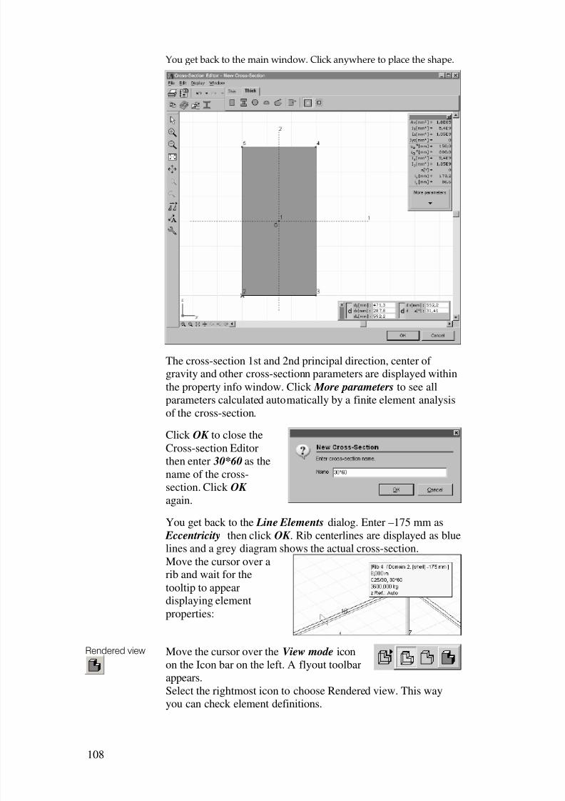
8/3/2019 AxisVMStepByStep
http://slidepdf.com/reader/full/axisvmstepbystep 108/125
108
You get back to the main window. Click anywhere to place the shape.
The cross-section 1st and 2nd principal direction, center of gravity and other cross-sectionn parameters are displayed within
the property info window. Click More parameters to see all
parameters calculated automatically by a finite element analysis
of the cross-section.
Click OK to close the
Cross-section Editor
then enter 30*60 as the
name of the cross-
section. Click OK
again.
You get back to the Line Elements dialog. Enter –175 mm as
Eccentricity then click OK . Rib centerlines are displayed as blue
lines and a grey diagram shows the actual cross-section.
Move the cursor over arib and wait for the
tooltip to appeardisplaying element
properties:
Rendered view Move the cursor over the View mode icon
on the Icon bar on the left. A flyout toolbar
appears.
Select the rightmost icon to choose Rendered view. This way
you can check element definitions.

8/3/2019 AxisVMStepByStep
http://slidepdf.com/reader/full/axisvmstepbystep 109/125
109
Rotate view Click the Rotate view icon on the Zoom
toolbar at the bottom left corner of the
main window.
Drag the model to rotate it. A special
Rotation toolbar appears. You can
control the way view rotation works by
selecting from the options.
Press the [Esc] key or close the Rotation toolbar by clicking the
x button to quit view rotation.
View undo Select View undo from the Zoom toolbar.
Fit in view Click this icon to make the drawing fill the window.
Wireframe Select Wireframe from the view mode flyout toolbar.
Surface support To define supports for the structure click the Surface support
icon on the Elements toolbar. The Selection palette appears.
Click the two non-vertical domains. Click OK on the Selection
toolbar. You get to the support definition dialog. Set R x and R y
to 1E3 and click OK .

8/3/2019 AxisVMStepByStep
http://slidepdf.com/reader/full/axisvmstepbystep 110/125
110
You get this:
Loads To define loads click the Loads tab.
Load cases andload groups
To define load cases and load groups click Load cases and load
groups icon on the Loads toolbar. You get to this dialog:
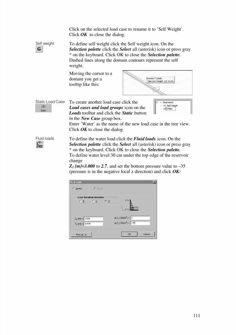
8/3/2019 AxisVMStepByStep
http://slidepdf.com/reader/full/axisvmstepbystep 111/125
111
Click on the selected load case to rename it to ’Self Weight’.
Click OK to close the dialog.
Self weight To define self weight click the Self weight icon. On theSelection palette click the Select all (asterisk) icon or press gray
* on the keyboard. Click OK to close the Selection palette.
Dashed lines along the domain contours represent the self weight.
Moving the cursor to a
domain you get a
tooltip like this:
Static Load Case To create another load case click the
Load cases and load groups icon on the
Loads toolbar and click the Static button
in the New Case group box.Enter ’Water’ as the name of the new load case in the tree view.
Click OK to close the dialog.
Fluid loads To define the water load click the Fluid loads icon. On the
Selection palette click the Select all (asterisk) icon or press gray
* on the keyboard. Click OK to close the Selection palette.
To define water level 30 cm under the top edge of the reservoir
change
Z1 [m]=3.000 to 2.7 , and set the bottom pressure value to –35(pressure is in the negative local z direction) and click OK:
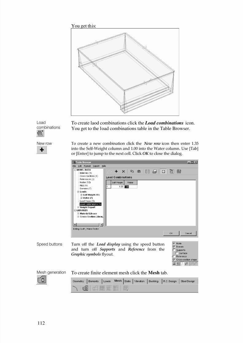
8/3/2019 AxisVMStepByStep
http://slidepdf.com/reader/full/axisvmstepbystep 112/125
112
You get this:
Loadcombinations
To create laod combinations click the Load combinations icon.
You get to the load combinations table in the Table Browser.
New row To create a new combination click the New row icon then enter 1.35into the Self-Weight column and 1.00 into the Water column. Use [Tab]or [Enter] to jump to the next cell. Click OK to close the dialog.
Speed buttons Turn off the Load display using the speed buttonand turn off Supports and Reference from theGraphic symbols flyout.
Mesh generation To create finite element mesh click the Mesh tab.

8/3/2019 AxisVMStepByStep
http://slidepdf.com/reader/full/axisvmstepbystep 113/125
113
Click the Domain
meshing icon. On the
Selection palette click
the Select all (asterisk)
icon or press gray * on
the keyboard. Click OK
to close the Selection palette.
Use Uniform mesh size
and set Average Mesh
Element Size to 0.600 m
and click OK to close the
dialog.
You get a visual
feedback on the meshingprocess. Aftercompleting you get the
following:
Green points at the center of surface elements is the symbol of
shell centerpoints. Moving the mouse over a centerpoint you get
a tooltip information on the element and the domain.

8/3/2019 AxisVMStepByStep
http://slidepdf.com/reader/full/axisvmstepbystep 114/125
114
Now we entered all properties necessary to analyse the model.Static To run the analysis and display the results click the Static tab.
Linear analysis Click Linear static analysis to run the linear analysis.
You get to the dialog which gives you a feedback on the process
of the analysis. Click Details to know more about it.
You can see the actual steps of the calculation. The first bar
shows the actual progress of the current step while the secondone displays the overall progress of the analysis.
The Estimated Memory Requirement shows the necessary
amount of memory to run the analysis. If this value is higher
than the available physical memory AxisVM uses the hard disk
to swap memory blocks during the calculation. If the system of equations fits into the physical memory the calculation is
considerably faster.At the end of the analysis you see the following

8/3/2019 AxisVMStepByStep
http://slidepdf.com/reader/full/axisvmstepbystep 115/125
115
Click OK to close the dialog. You get to the Static tab,displaying the Self Weight load case and eZ (i.e. vertical
displacements due to the self weight).
Numbering Click the Numbering speed button and turn on
Write Values to Surfaces and Min./Max. only.
To see the result for the Water load case click
the dropdown button of the combo box
displaying Self Weight and select Water.
You can change the result component the similar way.
Parts To hide the front wall of the reservoir create a part. Click the
Parts icon on the Icon bar on the left. You get to the Parts
dialog.
Define a part containing everything but the front wall.
Click New and specify the name as WithoutFront.
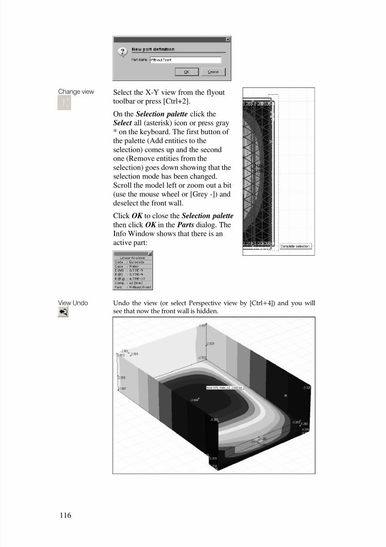
8/3/2019 AxisVMStepByStep
http://slidepdf.com/reader/full/axisvmstepbystep 116/125
116
Change viewSelect the X-Y view from the flyouttoolbar or press [Ctrl+2].
On the Selection palette click the
Select all (asterisk) icon or press gray
* on the keyboard. The first button of
the palette (Add entities to the
selection) comes up and the secondone (Remove entities from the
selection) goes down showing that the
selection mode has been changed.
Scroll the model left or zoom out a bit
(use the mouse wheel or [Grey -]) anddeselect the front wall.
Click OK to close the Selection palette
then click OK in the Parts dialog. The
Info Window shows that there is an
active part:
View Undo Undo the view (or select Perspective view by [Ctrl+4]) and you willsee that now the front wall is hidden.
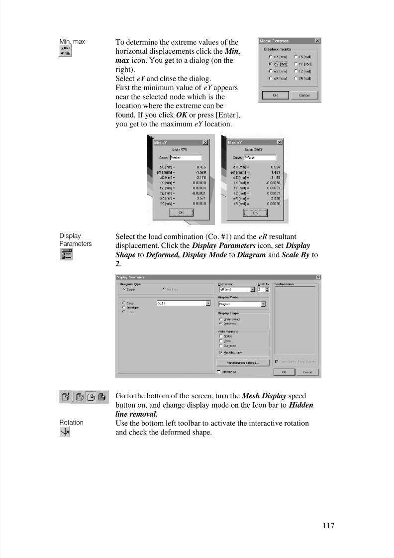
8/3/2019 AxisVMStepByStep
http://slidepdf.com/reader/full/axisvmstepbystep 117/125
117
Min, max To determine the extreme values of the
horizontal displacements click the Min,
max icon. You get to a dialog (on the
right).
Select eY and close the dialog.
First the minimum value of eY appears
near the selected node which is thelocation where the extreme can be
found. If you click OK or press [Enter],
you get to the maximum eY location.
DisplayParameters
Select the load combination (Co. #1) and the eR resultantdisplacement. Click the Display Parameters icon, set Display
Shape to Deformed, Display Mode to Diagram and Scale By to
2.
Go to the bottom of the screen, turn the Mesh Display speed
button on, and change display mode on the Icon bar to Hidden
line removal.Rotation Use the bottom left toolbar to activate the interactive rotation
and check the deformed shape.
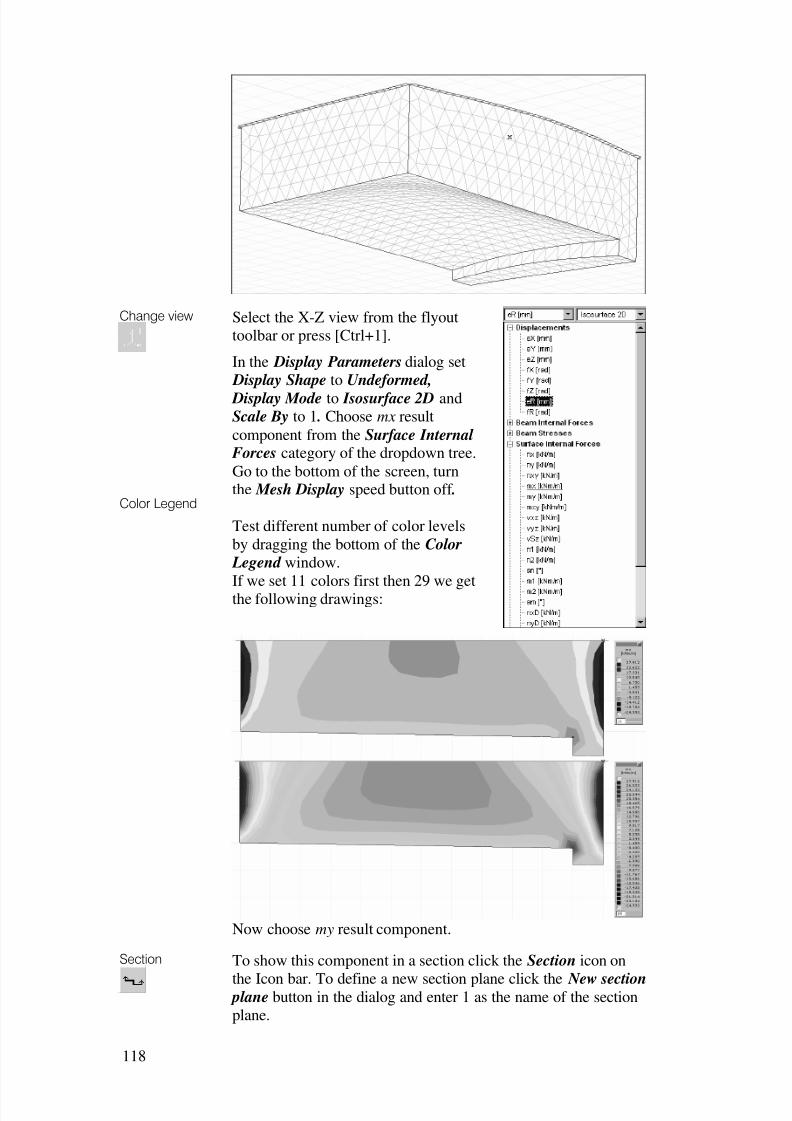
8/3/2019 AxisVMStepByStep
http://slidepdf.com/reader/full/axisvmstepbystep 118/125
118
Change view
Color Legend
Select the X-Z view from the flyout
toolbar or press [Ctrl+1].
In the Display Parameters dialog set
Display Shape to Undeformed,
Display Mode to Isosurface 2D andScale By to 1 . Choose mx result
component from the Surface Internal Forces category of the dropdown tree.
Go to the bottom of the screen, turnthe Mesh Display speed button off .
Test different number of color levels
by dragging the bottom of the Color
Legend window.
If we set 11 colors first then 29 we get
the following drawings:
Now choose my result component.
Section To show this component in a section click the Section icon on
the Icon bar. To define a new section plane click the New section plane button in the dialog and enter 1 as the name of the section
plane.

8/3/2019 AxisVMStepByStep
http://slidepdf.com/reader/full/axisvmstepbystep 119/125
119
A section plane can be defined by two points in side, front of topview. Being in front view click the rib at 6.000 m and enter the
second point somewhere under the first on a vertical line (e.g.typing z –3 [Enter]).
You get back to the Section Lines dialog. Click OK.
Change view
Numbering
Select the Y-Z side view from the flyout toolbar or press
[Ctrl+3].
Click Numbering speed button and turn on Write Values to
Lines.
You get the following diagram:

8/3/2019 AxisVMStepByStep
http://slidepdf.com/reader/full/axisvmstepbystep 120/125
120
Speed buttons Turn off Sections clicking its speed button at the bottom.
Change view Select the perspective view from the flyout toolbar or press
[Ctrl+4].
Choose Rz from Surface Support Internal Forces and set Isoline
display style with 22 levels. Turn on Write Values To Surfaces.
R. C. Design To determine the required amount of reinforcement click the R.
C. Design tab
Vasalásiparaméterek
To define surface reinforcement parameters click the
Reinforcement parameters icon. On the Selection palette click the Select all (asterisk) icon or press gray * on the keyboard.
Click OK to close the Selection palette. In the Surface Re-
inforcement Para-
meters dialog set
Concrete to B500Band change xtop and
xbottom to 45 mm.
Click OK to close
the dialog.
Gyorspaletta Turn off Write Values To Line and Surface by clicking the Numbering
speed button. We get this for axb (required amount of reinforcement inlocal x direction at the bottom of the elements (top and bottom aredefined by the local z coordinate)

8/3/2019 AxisVMStepByStep
http://slidepdf.com/reader/full/axisvmstepbystep 121/125
121
Also check components in other directions and positions: axt, ayb, ayt.
ReinforcedBeam Design
To determine the required amount of reinforcement in concretebeams click the Beam Reinforcement Calculation icon. The
Selection palette appears. Click one of the ribs on the longer
walls and click OK on the palette. You get a warning message:
Close the dialog and you get to the Beam Reinforcementwindow displaying the structural model of the beam, the bending
moment, shear force and torsional force distribution.

8/3/2019 AxisVMStepByStep
http://slidepdf.com/reader/full/axisvmstepbystep 122/125
122
BeamParameters
Click Beam Parameters to specify the design properties. Click the iconof the rectangular cross-section and click OK.
You get the required amount of reinforcement and stirrup
distance.

8/3/2019 AxisVMStepByStep
http://slidepdf.com/reader/full/axisvmstepbystep 123/125
123

8/3/2019 AxisVMStepByStep
http://slidepdf.com/reader/full/axisvmstepbystep 124/125
124
Notes

8/3/2019 AxisVMStepByStep
http://slidepdf.com/reader/full/axisvmstepbystep 125/125
Notes