AVERTISSEMENT Ce document est le fruit d’un long travail approuvé par le jury de soutenance et mis à disposition de l’ensemble de la communauté universitaire élargie. Il est soumis à la propriété intellectuelle de l’auteur : ceci implique une obligation de citation et de référencement lors de l’utilisation de ce document. D’autre part, toute contrefaçon, plagiat, reproduction illicite de ce travail expose à des poursuites pénales. Contact : [email protected] LIENS Code la Propriété Intellectuelle – Articles L. 122-4 et L. 335-1 à L. 335-10 Loi n°92-597 du 1 er juillet 1992, publiée au Journal Officiel du 2 juillet 1992 http://www.cfcopies.com/V2/leg/leg-droi.php http://www.culture.gouv.fr/culture/infos-pratiques/droits/protection.htm

Welcome message from author
This document is posted to help you gain knowledge. Please leave a comment to let me know what you think about it! Share it to your friends and learn new things together.
Transcript

AVERTISSEMENT Ce document est le fruit d’un long travail approuvé par le jury de soutenance et mis à disposition de l’ensemble de la communauté universitaire élargie. Il est soumis à la propriété intellectuelle de l’auteur : ceci implique une obligation de citation et de référencement lors de l’utilisation de ce document. D’autre part, toute contrefaçon, plagiat, reproduction illicite de ce travail expose à des poursuites pénales. Contact : [email protected]
LIENS Code la Propriété Intellectuelle – Articles L. 122-4 et L. 335-1 à L. 335-10 Loi n°92-597 du 1er juillet 1992, publiée au Journal Officiel du 2 juillet 1992 http://www.cfcopies.com/V2/leg/leg-droi.php http://www.culture.gouv.fr/culture/infos-pratiques/droits/protection.htm
00309
THÈSE
En vue de l'obtention du
DOCTORAT DE L'UNIVERSITÉ DE TOULOUSE
Délivré par
Université de Toulouse 1 Capitole (UT1 Capitole)
Présentée et soutenue par
M. Minh Thai TRUONG Le: 02/2015
Titre:
To Develop a Database Management Tool for Multi-Agent Simulation Platform
Ecole doctorale :
Mathématiques, Informatique et Télécommunications de Toulouse (MITT)
Discipline ou spécialité:
Informatique Unité de recherché : CNRS IRIT UMR 5505
Directeurs de Thèse :
Christophe SIBERTIN-BLANC Frédéric AMBLARD Benoit GAUDOU
Rapporteurs :
François PINET
Julie DUGDALE
Autre(s) membre(s) du Jury :
Salima HASSAS

i
Abstract
Recently, there has been a shift from modeling driven approach to data driven approach in
Agent Based Modeling and Simulation (ABMS). This trend towards the use of data-driven
approaches in simulation aims at using more and more data available from the observation
systems into simulation models (Edmonds and Moss, 2005; Hassan, 2009). In a data driven
approach, the empirical data collected from the target system are used not only for the
design of the simulation models but also in initialization, calibration and evaluation of the
output of the simulation platform such as e.g., the water resource management and
assessment system of the French Adour-Garonne Basin (Gaudou et al., 2013) and the
invasion of Brown Plant Hopper on the rice fields of Mekong River Delta region in
Vietnam (Nguyen et al., 2012d).
That raises the question how to manage empirical data and simulation data in such agent-
based simulation platform. The basic observation we can make is that currently, if the
design and simulation of models have benefited from advances in computer science
through the popularized use of simulation platforms like Netlogo (Wilensky, 1999) or
GAMA (Taillandier et al., 2012), this is not yet the case for the management of data, which
are still often managed in an ad hoc manner. Data management in ABM is one of
limitations of agent-based simulation platforms. Put it other words, such a database
management is also an important issue in agent-based simulation systems.
In this thesis, I first propose a logical framework for data management in multi-agent based
simulation platforms. The proposed framework is based on the combination of Business
Intelligence solution and a multi-agent based platform called CFBM (Combination
Framework of Business intelligence and Multi-agent based platform), and it serves several
purposes: (1) model and execute multi-agent simulations, (2) manage input and output
data of simulations, (3) integrate data from different sources; and (4) analyze high volume
of data. Secondly, I fulfill the need for data management in ABM by the implementation of
CFBM in the GAMA platform. This implementation of CFBM in GAMA also
demonstrates a software architecture to combine Data Warehouse (DWH) and Online
Analytical Processing (OLAP) technologies into a multi-agent based simulation system.
Finally, I evaluate the CFBM for data management in the GAMA platform via the
development of a Brown Plant Hopper Surveillance Models (BSMs), where CFBM is used
ii
not only to manage and integrate the whole empirical data collected from the target system
and the data produced by the simulation model, but also to calibrate and validate the
models.
The successful development of the CFBM consists not only in remedying the limitation of
agent-based modeling and simulation with regard to data management but also in dealing
with the development of complex simulation systems with large amount of input and
output data supporting a data driven approach.
Key words:
Agent Based Model, Agent Based Modeling and Simulation, Business Intelligence, Brown
Plant Hopper, Calibration, Data Warehouse, GAMA, Multi-Agent Based Simulation,
Multi-Agent System, OLAP, Validation.
iii
Résumé
Depuis peu, la Modélisation et Simulation par Agents (ABMs) est passée d'une approche
dirigée par les modèles à une approche dirigée par les données (Data Driven Approach,
DDA). Cette ten00308dance vers l’utilisation des données dans la simulation vise à
appliquer les données collectées par les systèmes d’observation à la simulation (Edmonds
and Moss, 2005; Hassan, 2009). Dans la DDA, les données empiriques collectées sur les
systèmes cibles sont utilisées non seulement pour la simulation des modèles mais aussi
pour l’initialisation, la calibration et l’évaluation des résultats issus des modèles de
simulation, par exemple, le système d’estimation et de gestion des ressources hydrauliques
du bassin Adour-Garonne Français (Gaudou et al., 2013) et l’invasion des rizières du delta
du Mékong au Vietnam par les cicadelles brunes (Nguyen et al., 2012d).
Cette évolution pose la question du « comment gérer les données empiriques et celles
simulées dans de tels systèmes ». Le constat que l’on peut faire est que, si la conception et
la simulation actuelles des modèles ont bénéficiées des avancées informatiques à travers
l’utilisation des plateformes populaires telles que Netlogo (Wilensky, 1999) ou GAMA
(Taillandier et al., 2012), ce n'est pas encore le cas de la gestion des données, qui sont
encore très souvent gérées de manière ad-hoc. Cette gestion des données dans des Modèles
Basés Agents (ABM) est une des limitations actuelles des plateformes de simulation multi-
agents (SMA). Autrement dit, un tel outil de gestion des données est actuellement requis
dans la construction des systèmes de simulation par agents et la gestion des bases de
données correspondantes est aussi un problème important de ces systèmes.
Dans cette thèse, je propose tout d’abord une structure logique pour la gestion des données
dans des plateformes de SMA. La structure proposée qui intègre des solutions de
l’Informatique Décisionnelle et des plateformes multi-agents s’appelle CFBM
(Combination Framework of Business intelligence and Multi-agent based platform), elle a
plusieurs objectifs : (1) modéliser et exécuter des SMAs, (2) gérer les données en entrée et
en sortie des simulations, (3) intégrer les données de différentes sources, et (4) analyser les
données à grande échelle. Ensuite, le besoin de la gestion des données dansles simulations
agents est satisfait par une implémentation de CFBM dans la plateforme GAMA. Cette
implémentation présente aussi une architecture logicielle pour combiner entrepôts de

iv
données et technologies du traitement analytique en ligne (OLAP) dans les systèmes
SMAs. Enfin, CFBM est évaluée pour la gestion de données dans la plateforme GAMA à
travers le développement de modèles de surveillance des cicadelles brunes (BSMs), où
CFBM est utilisé non seulement pour gérer et intégrer les données empiriques collectées
depuis le système cible et les résultats de simulation du modèle simulé, mais aussi calibrer
et valider ce modèle.
L'intérêt de CFBM réside non seulement dans l'amélioration des faiblesses des plateformes
de simulation et de modélisation par agents concernant la gestion des données mais permet
également de développer des systèmes de simulation complexes portant sur de nombreuses
données en entrée et en sortie en utilisant l’approche dirigée par les données.
Mots clés:
Modèle par agents, Modélisation et Simulation par agents, Business Intelligence, Cicadelle
brune, Calibration, Data Warehouse, GAMA, Simulation multi-agents, systèmes multi-
agents, OLAP, Validation

v

vi

vii
DEDICATION
This dissertation is dedicated to my father, TRUONG Tan Loc, and to my
mother, NGUYEN Thi To, who always had confidence in me and offered
me encouragement and support in all my endeavors
It is also dedicated to my darling wife, TRUONG Thu Quyen, my lovely
children TRUONG Minh Anh Mai and TRUONG Minh Kien Quoc for
their care, love, understanding, and patience


ix
Preface and Acknowledgements
The research study reported in this thesis has been performed in the Systèmes Multi-
Agents Coopératifs (SMAC) team, at the IRIT Laboratory (Institut de Recherche en
Informatique de Toulouse) - UMR 5505, Université Toulouse 1 Capitole, France. The
work has been carried out in the period from April 2011 to December 2014 under the
supervision of Professor Christophe SIBERTIN-BLANC, Associate Professor Frédéric
AMBLARD and Associate Professor Benoit GAUDOU.
To achieve these results, besides my own effort, would be impossible without the
assistance, very kind support as well as the encouragement of many people. I would like to
thank all of them for their contribution to my work.
I wish to express my deep gratitude to my supervisors, Professor Christophe
SIBERTIN-BLANC, Associate Professor Frédéric AMBLARD and Associate Professor
Benoit GAUDOU for their guidance, patience, motivation, enthusiasm, encouragement and
support during my graduate study. Their creative thinking, knowledge and expertise were
the “power supply” and “feedback” of my conducted research.
I would like to express my appreciation to the members of the thesis defense
committee, Associate Professor François PINET from IRSTEA (Institut national de
Recherche en Sciences et Technologies pour l'Environnement et l'Agriculture), Associate
Professor Julie DUGDALE from Laboratoire d'Informatique de Grenoble - UMR 5217 and
Proffessor Salima HASSAS from LIRIS (Laboratoire d'InfoRmatique en Image et
Systèmes d'information) - UMR 5205, Université Claude Bernard Lyon 1 for their interest
in my research work and the time and effort devoted to this thesis.
My sincere thanks go to Professor Alexis DROGOUL and Associate Professor
HUYNH Xuan Hiep who nominated me for this research, help and encourage me during
the years in-between.
I would like to thank Associate Professor TRAN Cao De and Lecturer VO Huynh
Tram who help and encourage me during the time I studied in France.
I would like to thank all of my colleagues, especially TRUONG Xuan Viet, DANG
Quoc Viet, DIEP Anh Nguyet, HUYNH Quang Nghi, whose sharing, support and
encouragement have helped me to accomplish the study at my full capacity.
Toulouse, / / 2015
TRUONG Minh Thai


Table of contents
TRUONG Minh Thai xi
Table of contents
Abstract ......................................................................................................................... i
Résumé ....................................................................................................................... iii
DEDICATION ................................................................................................................... vii
Preface and Acknowledgements ........................................................................................ ix
Table of contents ................................................................................................................. xi
List of abbreviations .......................................................................................................... xx
List of Tables ................................................................................................................... xxiv
List of Figures .................................................................................................................. xxvi
Chapter 1 INTRODUCTION ............................................................................................. 1
1.1 Context of the Thesis ............................................................................................... 2
1.2 Research Questions and Approach .......................................................................... 3
1.2.1 Problem formulation of the thesis ............................................................. 3
1.2.2 Approach and achievements ...................................................................... 4
1.3 Organization of the Document ................................................................................ 5
Chapter 2 STATE OF THE ART ....................................................................................... 9
2.1 Introduction ........................................................................................................... 11
2.2 An Overview of Multi-Agent Based Simulation ................................................... 12
Table of contents
xii TRUONG Minh Thai
2.2.1 Computer simulation ............................................................................... 12
2.2.1.1 What is a model? ....................................................................... 12
2.2.1.2 What is simulation? ................................................................... 12
2.2.2 Agent based modeling ............................................................................. 15
2.2.2.1 What is an agent? ....................................................................... 15
2.2.2.2 Multi-agent systems ................................................................... 17
2.2.2.3 Modeling Approaches ............................................................... 18
2.2.2.4 Agent-based platforms ............................................................... 18
2.2.2.5 Verification, validation and Calibration of agent-based
simulation models .................................................................................... 19
2.2.2.6 Scale in Agent-based modeling ................................................. 21
2.2.2.7 Key challenges of ABM ............................................................ 22
2.3 Data in Agent-Based Modeling ............................................................................. 24
2.3.1 Moving from modeling driven approach to data driven approach .......... 24
2.3.2 Data management in ABM ...................................................................... 25
2.3.3 The limitation of agent-based platforms in data management................. 26
2.4 An Overview of Business Intelligence Solutions .................................................. 27
2.4.1 What is Business Intelligence? ................................................................ 27
2.4.2 Decision support systems ........................................................................ 28
2.4.3 An Introduction to Data Warehousing ..................................................... 28
2.4.3.1 Data Warehouse ......................................................................... 29
2.4.3.2 Basic components of data warehouse ........................................ 30
Table of contents
TRUONG Minh Thai xiii
2.4.3.3 Multidimensional database ........................................................ 31
2.4.3.4 Multidimensional model ........................................................... 32
2.4.3.5 Granularity of data in data warehouse ....................................... 34
2.4.3.6 Query language for Multidimensional database ........................ 34
2.4.3.7 On-Line Analytical Processing ................................................. 35
2.4.3.8 Data mart ................................................................................... 36
2.5 Using DWH for Simulation ................................................................................... 37
2.6 Conclusion ............................................................................................................. 42
Chapter 3 A SOLUTION TO MANAGE AND ANALYZE AGENT-BASED
MODELS DATA ................................................................................................................ 45
3.1 Introduction ........................................................................................................... 47
3.2 A Logical Framework to Manage and Analyze Data for Agent-based Models .... 48
3.2.1 Computer simulation system ................................................................... 48
3.2.2 Combination Framework of Business Intelligence Solution and Multi-
agent Platform ........................................................................................................ 49
3.2.2.1 Simulation system ..................................................................... 51
3.2.2.2 Data warehouse system ............................................................. 52
3.2.2.3 Decision support system ............................................................ 52
3.3 Implementation of CFBM with the GAMA Platform ........................................... 53
3.3.1 Introduction to GAMA ............................................................................ 53
3.3.2 Software Architecture of CFBM in GAMA ............................................ 56
3.3.2.1 Presentation tier ......................................................................... 57
3.3.2.2 Logic tier ................................................................................... 58
Table of contents
xiv TRUONG Minh Thai
3.3.2.3 Data tier ..................................................................................... 59
3.3.3 Database Features in GAMA ................................................................... 59
3.3.3.1 Access Relational data ............................................................... 60
3.3.3.2 Retrieve Multidimensional database via OLAP ........................ 62
3.4 Discussion .............................................................................................................. 65
3.4.1 Advantages of CFBM .............................................................................. 65
3.4.2 Limitations of CFBM .............................................................................. 67
3.5 Conclusion ............................................................................................................. 67
Chapter 4 APPLYING THE CFBM TO A PEST SURVEILLANCE MODEL .......... 69
4.1 Introduction ............................................................................................................ 71
4.2 Brown Plant Hopper Surveillance Models (BSMs) ............................................... 72
4.2.1 Introduction and purpose ......................................................................... 72
4.2.2 Entities, state variables and scale............................................................. 75
4.2.3 Process overview and scheduling ............................................................ 77
4.2.4 Design concepts ....................................................................................... 77
4.2.5 Initialization ............................................................................................. 78
4.2.6 Input and output ....................................................................................... 79
4.2.7 Sub models .............................................................................................. 80
4.2.7.1 The SIMULATION MODEL .................................................... 82
a) BPHs Prediction model ............................................................. 82
b) Surveillance Network Model (SNM) ........................................ 84
4.2.7.2 The ANALYSIS MODEL ......................................................... 85

Table of contents
TRUONG Minh Thai xv
4.3 CFBM Application ................................................................................................ 87
4.3.1 Data management for the models ............................................................ 87
4.3.1.1 Empirical data specification ...................................................... 87
4.3.1.2 Simulation data specification .................................................... 89
4.3.1.3 Data warehouse specification .................................................... 89
4.3.2 Data retrieval ........................................................................................... 91
4.3.2.1 More flexibility in building agent-based model ........................ 91
4.3.2.2 Data integration and aggregation .............................................. 94
4.4 Experimental Design ............................................................................................. 97
4.4.1 Three Scenarios of the Environment ....................................................... 97
4.4.2 Validation with RMSE ............................................................................ 97
4.5 Conclusion ........................................................................................................... 101
Chapter 5 CFBM APPLICATION TO THE CALIBRATION AND VALIDATION
OF AN AGENT-BASED SIMULATION MODEL ...................................................... 103
5.1 Introduction ......................................................................................................... 105
5.2 Calibration approach ............................................................................................ 105
5.2.1 Calibration of an Agent-Based Model ................................................... 106
5.2.2 Measure of the similarity between two datasets .................................... 109
5.2.2.1 Similarity coefficient using RMSE ......................................... 109
5.2.2.2 Similarity coefficient using the Jaccard Index ........................ 110
5.3 Calibration of the BPHs Prediction model .......................................................... 113
5.3.1 BPHs Prediction model and data management ..................................... 113
Table of contents
xvi TRUONG Minh Thai
5.3.2 Parameters for Calibration ..................................................................... 114
5.3.3 The measurement indicators and the Fitness condition ......................... 115
5.3.4 Implementation of the calibration model ............................................... 115
5.3.5 Calibration Experiment .......................................................................... 125
5.3.5.1 Simulation Outputs and Empirical data ................................... 125
5.3.5.2 To Measure the similarity Coefficient between the simulated
data and empirical data .......................................................................... 126
5.3.5.3 Results of the calibration experiments .................................... 128
5.4 Validation of the Accepted Scenario ................................................................... 133
5.4.1 Implementation of the validation model ................................................ 133
5.4.2 Validation experiment ........................................................................... 135
5.4.2.1 Simulation and validation data ................................................ 135
5.4.2.2 Results of the validation experiment ....................................... 135
5.5 Discussion ............................................................................................................ 137
5.5.1 Application of CFBM for calibration and validation ............................ 137
5.5.2 The Jaccard index with aggregation ...................................................... 138
5.6 Conclusion ........................................................................................................... 140
Chapter 6 CONCLUSION .............................................................................................. 141
6.1 Contributions of the thesis ................................................................................... 142
6.1.1 Achievements of the thesis .................................................................... 142
6.1.2 Benefits and drawbacks of CFBM to deal with data-driven approach in
ABM ............................................................................................................... 143
6.2 Perspectives ......................................................................................................... 144
Table of contents
TRUONG Minh Thai xvii
6.2.1 To integrate web service features into a multi-agent based simulation
platform ............................................................................................................... 144
6.2.2 To integrate data mining technologies to a multi-agent based simulation
platform. .............................................................................................................. 145
Publications .................................................................................................................... 147
Bibliography .................................................................................................................... 149
Appendix A Database Features in GAMA 1.6.1 ......................................................... 161
A.1 Description ........................................................................................................... 163
A.2 Supported DBMS ................................................................................................ 164
A.3 Introduction ......................................................................................................... 165
A.4 SQLSKILL .......................................................................................................... 167
A.4.1 Define a species that uses the SQLSKILL skill .................................... 167
A.4.2 Map of connection parameters .............................................................. 167
A.4.3 Test the connection to a database .......................................................... 169
A.4.4 Select data from database ...................................................................... 170
A.4.5 Insert data into a database ...................................................................... 171
A.4.6 Execution update commands ................................................................. 172
A.5 AgentDB .............................................................................................................. 173
A.5.1 Define a species that inherits from AgentDB ........................................ 174
A.5.2 Connect to database ............................................................................... 174
A.5.3 Check that an agent is connected to a database ..................................... 174
A.5.4 Close the current connection ................................................................. 175
This action ............................................................................................. 175
Table of contents
xviii TRUONG Minh Thai
A.5.5 Get connection parameters .................................................................... 175
A.5.6 Set connection parameters ..................................................................... 176
A.5.7 Retrieve data from a database ................................................................ 176
A.6 MDXSKILL ......................................................................................................... 177
A.6.1 Define a species that uses the MDXSKILL skill ................................... 177
A.6.2 Map of connection parameters............................................................... 178
A.6.3 Test a connection to OLAP database ..................................................... 179
A.6.4 Select data from OLAP database ........................................................... 180
A.7 Working with Spatial Databases .......................................................................... 181
A.7.1 Create a spatial database ........................................................................ 182
A.7.2 Write geometry data of a species to a GIS table .................................... 183
A.7.3 Read geometry data from a database ..................................................... 184
A.8 Using Database Features to Define the Simulation Environment and Create
Agents .......................................................................................................................... 185
A.8.1 Define the boundary of the environment from a database ..................... 185
A.8.2 Create agents from the result of a select action ..................................... 187
A.8.3 Save Geometry data into database ......................................................... 187
Appendix B Entities Data Description ......................................................................... 189
B.1 Empirical Data Description ................................................................................. 190
B.2 Simulation Data Description ................................................................................ 195
B.3 Data Warehouse Description ............................................................................... 197
Appendix C Calibration and Validation Results ........................................................ 201

Table of contents
TRUONG Minh Thai xix
C.1 Parameters and Scenario for Calibration ............................................................. 202
C.1.1 Parameters for calibration of BPHs Prediction model .......................... 202
C.1.2 Scenarios for calibration of BPHs Prediction model ............................. 203
C.2 Similarity Coefficient values of the Simulation .................................................. 205
List of abbreviations
TRUONG Minh Thai xx
List of abbreviations
A
ABM Agent Based Modeling
ABMS Agent-Based Modeling and Simulation
API Application Programming Interface
B
BI Business Intelligence
BDW Business Data Warehouse
BPH(s) Brown Plant Hopper(s).
BSMs Brown Plant Hopper Surveillance Models
C
CFBM Combination Framework of Business intelligence and Multi-agent
based platform
CDSN Correlation & Disk graph-based Surveillance Network
CSV Comma Separated Values
D
DW Data Warehouse
DWH Data Warehouse
DSS Decision Support System
DBMS Database Management System
E
List of abbreviations
TRUONG Minh Thai xxi
ETL Extraction-Transformation-Loading
G
GA Genetic Algorithm
GAMA Generic Agent-based Modeling Architecture
GAML GAma Modeling Language
GIS Geographic Information System
GUI Graphical User Interface
H
HOLAP Hybrid On-Line Analytical Processing
J
JDBC Java DataBase Connectivity
K
KDD Knowledge Discovery in Databases
KIDS Keep It Descriptive, Stupid
KISS Keep It Simple, Stupid
L
LPA Larvae-Pupae-Adult
M
MAS Multi-Agent System
MABS Multi-Agent Based Simulation
MDX MultiDimensional eXpressions
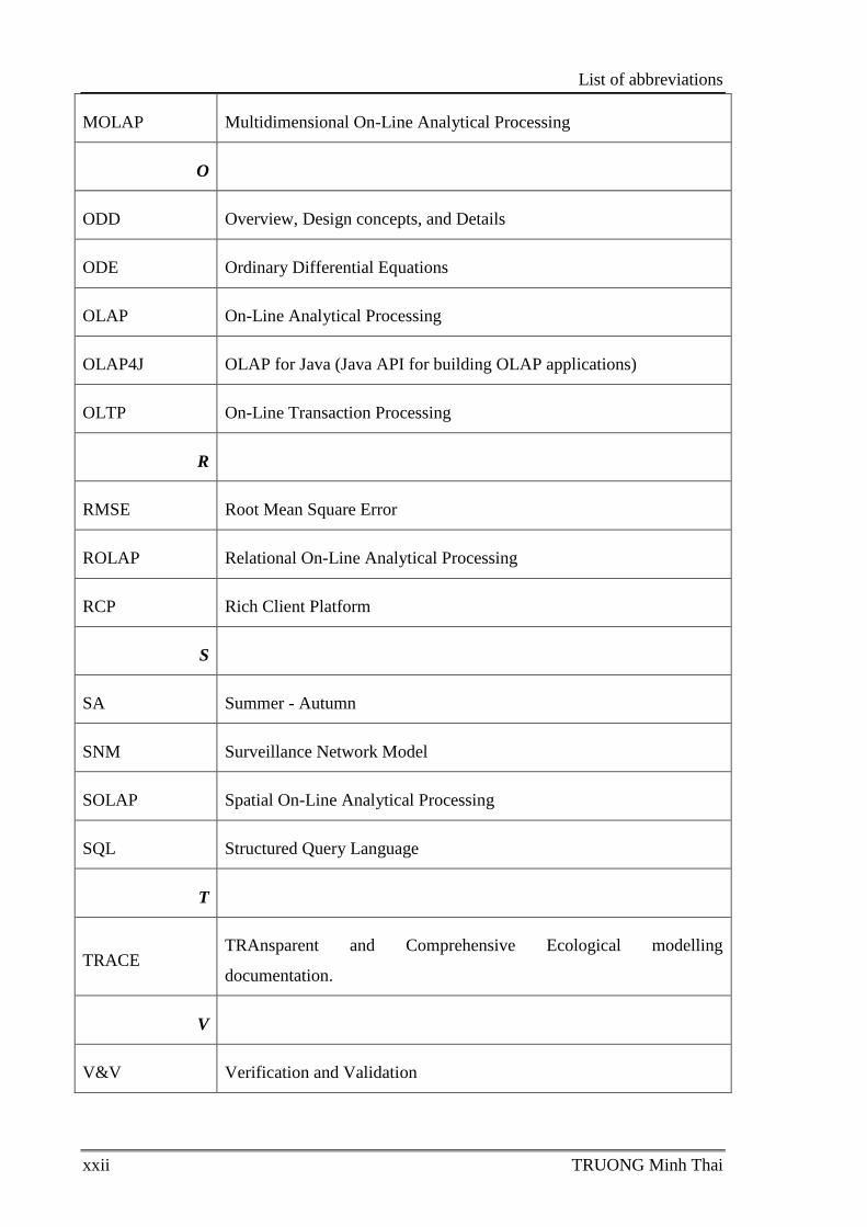
List of abbreviations
xxii TRUONG Minh Thai
MOLAP Multidimensional On-Line Analytical Processing
O
ODD Overview, Design concepts, and Details
ODE Ordinary Differential Equations
OLAP On-Line Analytical Processing
OLAP4J OLAP for Java (Java API for building OLAP applications)
OLTP On-Line Transaction Processing
R
RMSE Root Mean Square Error
ROLAP Relational On-Line Analytical Processing
RCP Rich Client Platform
S
SA Summer - Autumn
SNM Surveillance Network Model
SOLAP Spatial On-Line Analytical Processing
SQL Structured Query Language
T
TRACE TRAnsparent and Comprehensive Ecological modelling
documentation.
V
V&V Verification and Validation

List of abbreviations
TRUONG Minh Thai xxiii
X
XML eXtensible Markup Language
XMLA XML for Analysis
W
WS Winter - Spring
.
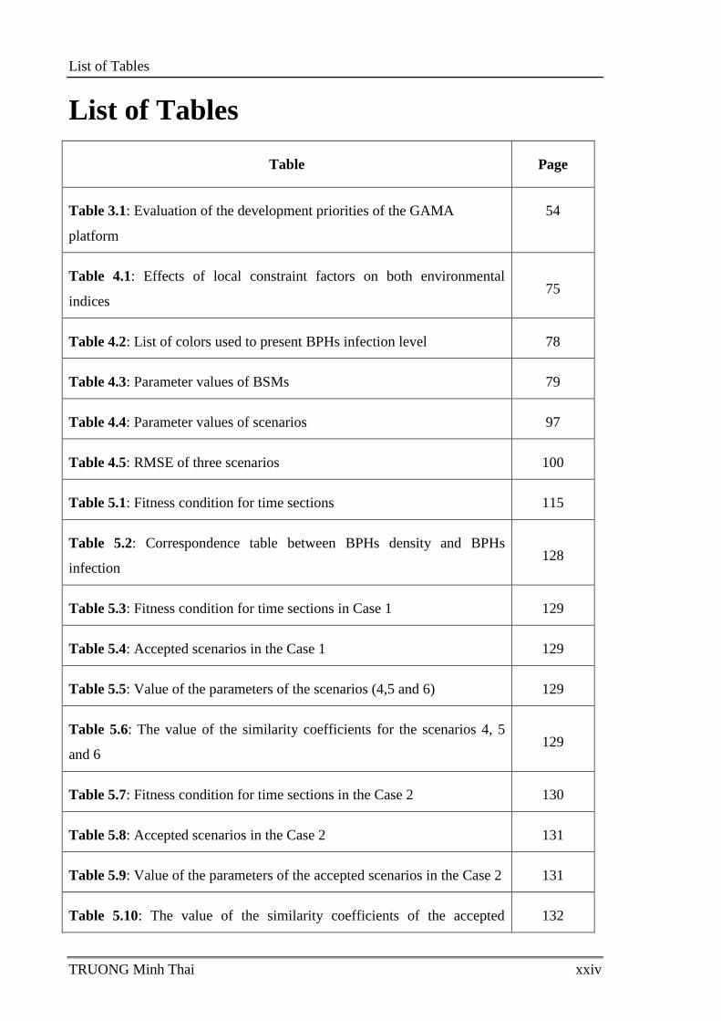
List of Tables
TRUONG Minh Thai xxiv
List of Tables
Table Page
Table 3.1: Evaluation of the development priorities of the GAMA
platform
54
Table 4.1: Effects of local constraint factors on both environmental
indices 75
Table 4.2: List of colors used to present BPHs infection level 78
Table 4.3: Parameter values of BSMs 79
Table 4.4: Parameter values of scenarios 97
Table 4.5: RMSE of three scenarios 100
Table 5.1: Fitness condition for time sections 115
Table 5.2: Correspondence table between BPHs density and BPHs
infection 128
Table 5.3: Fitness condition for time sections in Case 1 129
Table 5.4: Accepted scenarios in the Case 1 129
Table 5.5: Value of the parameters of the scenarios (4,5 and 6) 129
Table 5.6: The value of the similarity coefficients for the scenarios 4, 5
and 6 129
Table 5.7: Fitness condition for time sections in the Case 2 130
Table 5.8: Accepted scenarios in the Case 2 131
Table 5.9: Value of the parameters of the accepted scenarios in the Case 2 131
Table 5.10: The value of the similarity coefficients of the accepted 132
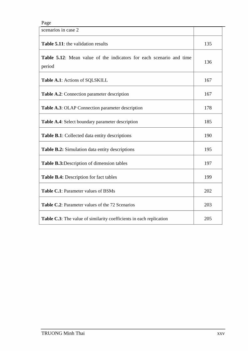
Page
TRUONG Minh Thai xxv
scenarios in case 2
Table 5.11: the validation results 135
Table 5.12: Mean value of the indicators for each scenario and time
period 136
Table A.1: Actions of SQLSKILL 167
Table A.2: Connection parameter description 167
Table A.3: OLAP Connection parameter description 178
Table A.4: Select boundary parameter description 185
Table B.1: Collected data entity descriptions 190
Table B.2: Simulation data entity descriptions 195
Table B.3:Description of dimension tables 197
Table B.4: Description for fact tables 199
Table C.1: Parameter values of BSMs 202
Table C.2: Parameter values of the 72 Scenarios 203
Table C.3: The value of similarity coefficients in each replication 205
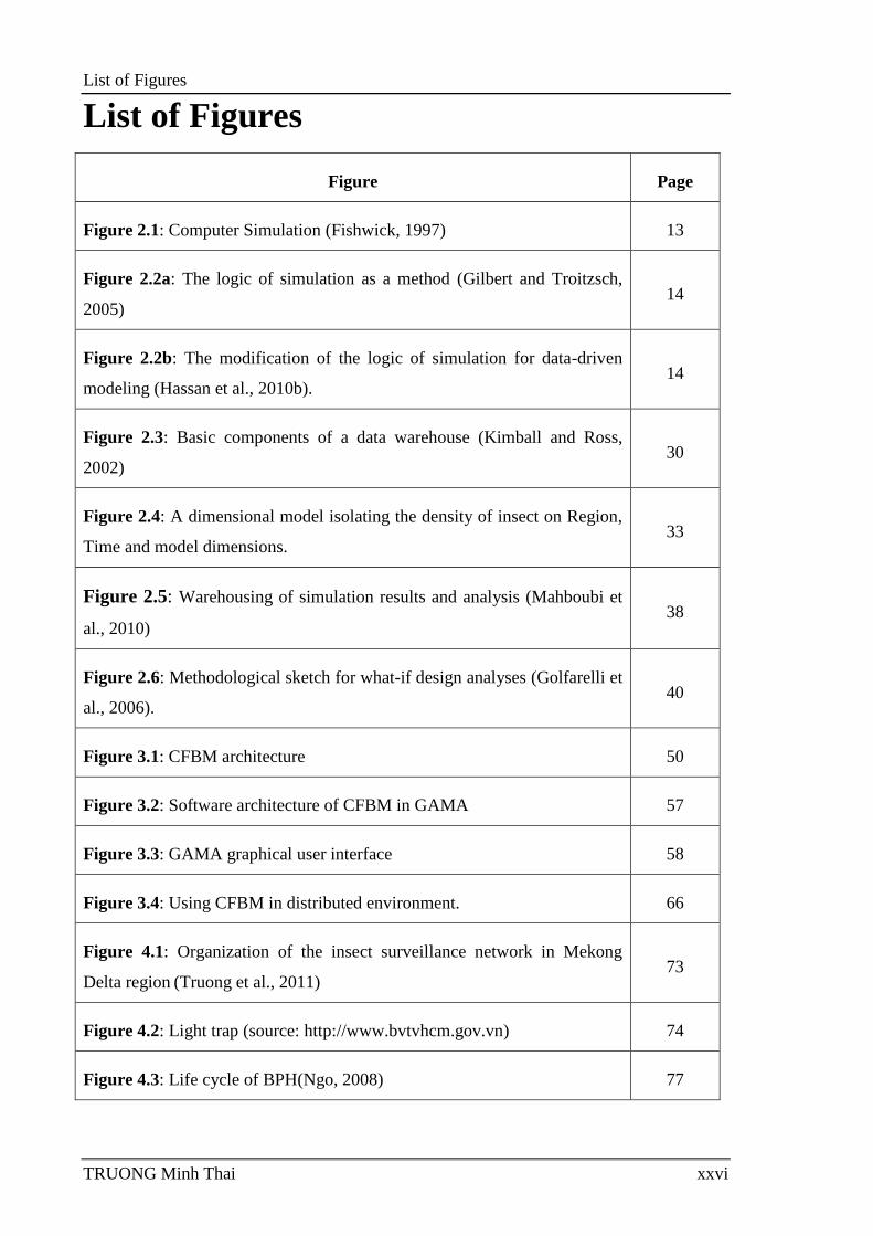
List of Figures
TRUONG Minh Thai xxvi
List of Figures
Figure Page
Figure 2.1: Computer Simulation (Fishwick, 1997) 13
Figure 2.2a: The logic of simulation as a method (Gilbert and Troitzsch,
2005) 14
Figure 2.2b: The modification of the logic of simulation for data-driven
modeling (Hassan et al., 2010b). 14
Figure 2.3: Basic components of a data warehouse (Kimball and Ross,
2002) 30
Figure 2.4: A dimensional model isolating the density of insect on Region,
Time and model dimensions. 33
Figure 2.5: Warehousing of simulation results and analysis (Mahboubi et
al., 2010) 38
Figure 2.6: Methodological sketch for what-if design analyses (Golfarelli et
al., 2006). 40
Figure 3.1: CFBM architecture 50
Figure 3.2: Software architecture of CFBM in GAMA 57
Figure 3.3: GAMA graphical user interface 58
Figure 3.4: Using CFBM in distributed environment. 66
Figure 4.1: Organization of the insect surveillance network in Mekong
Delta region (Truong et al., 2011) 73
Figure 4.2: Light trap (source: http://www.bvtvhcm.gov.vn) 74
Figure 4.3: Life cycle of BPH(Ngo, 2008) 77
List of Figures
TRUONG Minh Thai xxvii
Figure 4.4: Architecture of BSMs. 81
Figure 4.5: BPHs prediction model. 82
Figure 4.6: Brown plant hopper migration model (Truong, 2014) 83
Figure 4.7: Variable V of length T=32 days maximal life duration of BPHs 84
Figure 4.8: Simulation model. 85
Figure 4.9: Analysis flowchart 86
Figure 4.10: Entity relationship diagram of empirical data 88
Figure 4.11:Entity relationship diagram of simulation data 89
Figure 4.12: Star Schema diagram for simulated data for small town. 90
Figure 4.13: Star Schema diagram for light trap data. 91
Figure 4.14: Empirical data as of Jan 01, 2010. 98
Figure 4.15: Simulation data from Jan 01, 2010 produced by the Growth
model 99
Figure 4.16: Simulation data from Jan 01, 2010 produced by the BPHs
Prediction model 100
Figure 5.1: Workflow for the calibration of a model 106
Figure 5.2: Variable V of length T=32 days maximal life duration of BPHs 114
Figure 5.3: Empirical data for calibration and validation 125


INTRODUCTION
TRUONG Minh Thai 1
Chapter 1 INTRODUCTION
Table of content
1.1 Context of the Thesis ............................................................................................... 2
1.2 Research Questions and Approach .......................................................................... 3
1.2.1 Problem formulation of the thesis ............................................................. 3
1.2.2 Approach and achievements ...................................................................... 4
1.3 Organization of the Document ................................................................................ 5
2 Context of the Thesis
INTRODUCTION
1.1 Context of the Thesis
Today, the agent-based simulation approach is increasingly used to develop simulation
systems in quite different fields such as: (1) in natural resources management – e.g., an
agent-based simulation system consisting of a set of management processes (i.e. water,
land, money, and labour forces) built to simulate catchment water management in the north
of Thailand (Becu et al., 2003) or the agent-based modeling used to develop a water
resource management and assessment system which combines spatiotemporal models of
ecological indicators such as rainfall and temperature, water flow and plant growth
(Gaudou et al., 2013); (2) in biology - a model for the study of epidemiology or evacuation
of injured persons (Amouroux et al., 2008; Dunham, 2005; Rao et al., 2009; Stroud et al.,
2007), or the study of the invasion of rice pest (Nguyen et al., 2011; Phan et al., 2010;
Truong et al., 2011); (3) in economics - customer flow management (Julka et al., 2002),
stock market and strategic simulation (Chen and Yeh, 2001), simulated market network
(Galtier et al., 2012), or operational management of risks and organizational design
(Giannakis and Louis, 2011); and (4) in sociology - a multi-agent system to discover how
social actors could behave within an organization (Sibertin-Blanc et al., 2013) or an agent-
based simulation model to explore rules for rural credit management (Barnaud et al.,
2008).
In the building such systems, we are not only concerned with modeling driven approach ‒
that is how to model and combine coupled models from different scientific fields - but also
with data driven approach ‒ that is how to use empirical data collected from the target
system in modeling, simulation and analysis (Edmonds and Moss, 2005; Hassan et al.,
2010a, 2010b, 2008). The main idea behind such simulation systems is to combine and
couple information available from various data sources and knowledge from scientific
fields (like water management, climate sciences, sociology, economics and epidemiology).
Such information mainly takes the form of empirical data gathered from the target system
and these data can be used in processes such as design, initialization, calibration and
validation of models (cf. Chapter 4 and 5). That raises the question about how to manage
empirical data and simulated data in agent-based simulation systems as mentioned above.
Research Questions and Approach 3
INTRODUCTION
Indeed, the current challenge of ABM is data management (Section 2.3.2) because of the
weakness of agent-based platforms in data management addressed in Section 2.3.3. The
basic observation we can make is that currently, if the design and simulation of models has
benefited from advances in computer science through the popularized use of simulation
platforms like Netlogo (Wilensky, 1999) and GAMA (Taillandier et al., 2012), it is not yet
the case for the management of data, which are still managed in an ad hoc manner, despite
the advances in the management of huge datasets (data warehousing for instance). Such a
statement is rather pessimistic if we consider recent tendencies toward the use of data-
driven approaches in simulation aiming at using more and more data available from the
field into simulated models (Edmonds and Moss, 2005; Hassan, 2009).
Therefore there is definitely a need for a robust data management solution of huge datasets
in agent based simulation systems: data management tools are currently needed in agent-
based simulation systems and database management is an important technology for agent-
based simulation systems.
1.2 Research Questions and Approach
1.2.1 Problem formulation of the thesis
In my research, the first question I tackle is “What general architecture could serve the
following purposes: model and execute multi-agents simulations, manage the input and
output data of simulations, integrate data from different sources and enable to analyze
high volume of data?” To solve this problem, I examined several research studies and
solutions, related to simulation, management and analysis of big data. I argue that BI
(Business Intelligence) solutions are a good way to handle and analyze big datasets.
Because a BI solution contains a data warehouse, integrated data tools (ETL, Extract-
Transform-Load tools) and Online Analytical Processing tools (OLAP tools), it is well
adapted to manage, integrate, analyze and present huge amounts of data (Mahboubi et al.,
2010; Vasilakis and El-Darzi, 2004). My answer to the first question is the logical
framework proposed in Section 3.2 of Chapter 3.
The second problem that needs to be solved in my research is "How to introduce DWH
and OLAP technologies into a multi-agent based simulation system having to face huge
amount of data?" The solution I propose in this thesis is the improvement of agent-based
4 Research Questions and Approach
INTRODUCTION
platforms by adding new features, such as deep interactions with data warehouse systems
as presented in Section 3.3 of Chapter 3.
1.2.2 Approach and achievements
In this thesis I propose a solution to handle the input and output of agent-based simulation
models. The solution combines two aspects. The first deals with the status of the data, as a
suitable solution should be able to manage empirical data gathered from the studied
phenomenon or system as well as simulated data produced by simulations considered as in
silico experiments on the same system. The second aspect concerns the use of a Business
Intelligence (BI) solution envisaged as a system of data warehouse and analysis tools. A
data warehouse includes a collection of data that supports decision-making processes
(Inmon, 2005). Analysis tools may be data mining, statistical analysis, prediction analysis
and so on. The services of a BI solution will help us to manage huge amount of historical
data and make several analysis on such data.
I planned to organize my research as follows:
First, I studied the current state of the art on the two aspects (multi-agent simulation
platform and business intelligence solutions) and researched related works on the
management and analysis of input/output data of simulation models. The contribution of
this first step is the state the art of my research. It is the background knowledge for the next
steps.
Secondly, I proposed a conceptual framework that can help us to manage the input and
output of both the simulation models and analysis models; to aggregate the empirical data
and simulated data, which can be used for calibration and validation. The result of the
second step is an article concerning the global architecture of our combined framework of
multi-agent simulation platform and BI solution.
Third, I implemented the logical framework on the GAMA platform and I also gave a use
case that applies the framework in building the Brown Plant Hopper (BPH) Prediction
model. The contribution of this step is an article to present the concrete implementation of
the logical framework (step 2) on GAMA platform and an application of the framework.
Organization of the Document 5
INTRODUCTION
Fourth, I applied the framework to the calibration and validation of a simulation model to
demonstrate the benefits of the proposed framework. The result of this step is an article
about the application of the proposed framework to calibrate and validate an agent-based
simulation model.
1.3 Organization of the Document
The thesis is organized into the following six chapters:
Chapter 1: INTRODUCTION
This chapter presents the problematic of data management in agent-based simulation and
the approach, which has been adopted to solve the research question. In addition, this
chapter also presents the important notations and links between the chapters of the thesis as
a theoretical framework for the reader.
Chapter 2: STATE OF THE ART
Chapter 2 is released as the background of my research with two key parts. First, I present
an overview of multi-agent based simulation (MABS) and then I address the reasons why
we need data management in agent-based modeling (ABM) and the current limitation on
data management in ABM. Specially, some challenges related to data management in
ABM such as replication and experiment, aggregation, calibration and validation are also
mentioned in this part as problems that will be solved in this thesis. Second, I present the
background of business intelligence (BI) solutions and the state of the art linking BI and
simulation.
Chapter 3: A SOLUTION TO MANAGE AND ANALYZE AGENT-BASED MODELS
DATA
Chapter 3 presents a solution for solving the two research questions mentioned in the
Section 1.2.1. First, a logical framework to manage and analyze data in ABM is proposed
with four major components: (1) a model design tool; (2) a model execution tool; (3) an
execution analysis tool; and (4) a database tool. This framework is the Combination
Framework of Business intelligence and Multi-agent based platform called CFBM. CFBM
is proposed to answer the first question in my thesis: “What is the general architecture that
can serve the following purposes: model and execute multi-agent simulation, manage the
6 Organization of the Document
INTRODUCTION
input and output data of simulations, integrate data from different sources and analyze
high volume of data?” Second, I present the architecture of the implementation of CFBM
in GAMA and also introduce some database features of CFBM in GAMA. This part is my
answer for the second research question: How to introduce DWH and OLAP technologies
into a multi-agent based simulation system having to face huge amount of data?”
Specially, some advantages and limitations of CFBM are also discussed in this chapter.
Chapter 4: APPLYING THE CFBM TO A PEST SURVEILLANCE MODEL
The Chapter 4 demonstrates an application of CFBM to manage the input and output data
of Brown Plant Hopper Surveillance Models (BSMs). In this chapter, I illustrate a solution
to manage not only the empirical data (which are used as the input data and evaluation
data) collected from the target system (Insect surveillance network in Mekong Delta
region) (Truong, 2014) and simulation data produced by BSMs runs but also the
integration data of the empirical data and simulation data. The benefits of CFBM in
building agent-based simulation models and in the integration and aggregation data are
also presented in this chapter. Specially, this chapter is not only a demonstration of the
management of the input and output data of multi-agent based simulation model but also a
presentation of a way to solve the challenges in replication and experiment of the
simulation model and aggregation of analysis model.
Chapter 5: CFBM APPLICATION TO THE CALIBRATION AND VALIDATION OF
AN AGENT-BASED SIMULATION MODEL
Chapter 5 releases another application of CFBM in building multi-agent based simulation
systems. CFBM is applied to the calibration and validation of an agent-based simulation
model. In this chapter, I first present an automatic approach with eight steps for calibrating
an agent-based model. The approach helps modelers to test their models more
systematically in a given parameter space, to evaluate (validate) the outputs of each
simulation and to manage all the data in an automatic manner. Then I demonstrate the use
of the proposed approach to calibrate and validate the Brown Plant Hopper Prediction
model. Particularly, a specific measure, Jaccard index for ordered data sets is also
proposed for evaluating the output of a simulation model. Chapter 5 shows how to solve
calibration and validation challenges in ABM.

Organization of the Document 7
INTRODUCTION
Chapter 6: CONCLUSION
Chapter 6 is a summary of the most important contribution of this research. I first
synthesize the achievements of the thesis and publications related to this thesis. Then I
discuss the results and perspective of the thesis.
From this thesis, the readers can get not only an approach to develop a data management
framework in ABM (Chapter 3) but also how to apply the CFBM in GAMA to implement
a multi-agent based simulation system (Chapter 4 and 5), depending on the purpose of the
reader.

8 Organization of the Document
INTRODUCTION
STATE OF THE ART
TRUONG Minh Thai 9
Chapter 2 STATE OF THE ART
Table of Content
2.1 Introduction ........................................................................................................... 11
2.2 An Overview of Multi-Agent Based Simulation ................................................... 12
2.2.1 Computer simulation ............................................................................... 12
2.2.1.1 What is a model? ....................................................................... 12
2.2.1.2 What is simulation? ................................................................... 12
2.2.2 Agent based modeling ............................................................................. 15
2.2.2.1 What is an agent? ...................................................................... 15
2.2.2.2 Multi-agent systems .................................................................. 17
2.2.2.3 Modeling Approaches ............................................................... 18
2.2.2.4 Agent-based platforms .............................................................. 18
2.2.2.5 Verification, validation and Calibration of agent-based
simulation models .................................................................................... 19
2.2.2.6 Scale in Agent-based modeling ................................................. 21
2.2.2.7 Key challenges of ABM ............................................................ 22
2.3 Data in Agent-Based Modeling ............................................................................. 24
2.3.1 Moving from modeling driven approach to data driven approach .......... 24
2.3.2 Data management in ABM ...................................................................... 25
2.3.3 The limitation of agent-based platforms in data management ................ 26
STATE OF THE ART
10 TRUONG Minh Thai
2.4 An Overview of Business Intelligence Solutions .................................................. 27
2.4.1 What is Business Intelligence? ................................................................ 27
2.4.2 Decision support systems ........................................................................ 28
2.4.3 An Introduction to Data Warehousing ..................................................... 28
2.4.3.1 Data Warehouse ......................................................................... 29
2.4.3.2 Basic components of data warehouse ........................................ 30
2.4.3.3 Multidimensional database ........................................................ 31
2.4.3.4 Multidimensional model ............................................................ 32
2.4.3.5 Granularity of data in data warehouse ....................................... 34
2.4.3.6 Query language for Multidimensional database ........................ 34
2.4.3.7 On-Line Analytical Processing .................................................. 35
2.4.3.8 Data mart ................................................................................... 36
2.5 Using DWH for Simulation ................................................................................... 37
2.6 Conclusion ............................................................................................................. 42
Introduction 11
STATE OF THE ART
2.1 Introduction
Integrated socio-environmental modeling in general and the multi-agent based simulation
approach applied to socio-environmental systems in particular have increasingly been used
as decision-support systems in order to design, evaluate and plan public policies linked to
the management of natural resources (Bousquet et al., 2005; Janssen, 2002; Laniak et al.,
2013) or the study of epidemiology or evacuation plans of sick persons (Amouroux et al.,
2008; Dunham, 2005; Rao et al., 2009; Stroud et al., 2007). The main idea behind such
approaches is to combine and couple information available from various data sources and
knowledge from scientific fields (like water management, climate sciences, sociology,
economics and epidemiology). Such information mainly takes the form of empirical data
gathered from the field and of models regarding some aspects of the studied phenomenon
(for instance the behavior of actors from the systems) (Gaudou et al., 2013). For instance,
in the JEAI-DREAM project1, in order to study and assess Brown Plant Hoppers (BPHs)
invasions and their effects on rice fields in the Mekong Delta region (Vietnam), we must
develop and integrate several models (e.g. BPHs growth, rice growth or BPHs migration
models) (Nguyen et al., 2011; Truong et al., 2011). We must also integrate data from
different data sources and analyze the integrated data at different scales (Nguyen et al.,
2012a). Such integrated simulation systems involve high volume of data and we are not
only concerned with modeling ‒ that is how to model and combine coupled models from
different scientific fields - but also with data driven approach (Hassan et al., 2010a, 2008)
‒ that is how to handle big data from different data sources and perform analyses on the
integrated data from these sources as well as integrating big data in model.
In the following sections, I first present the background of multi-agent based simulation
(MABS) in Section 2.2. Then I focus particularly on the way MABS approaches make use
of data either external data (inputs) or generated data (outputs) and the reasons why we
need to manage data in Section 2.3. In Section 2.4, I present the background of business
intelligence (BI) solution and the state of the art of works that link BI and simulation in
Section 2.5.
1 http://www.vietnam.ird.fr/les-activites/renforcement-des-capacites/jeunes-equipes-aird/jeai-dream-umi-209-
ummisco-2011-2013
12 An Overview of Multi-Agent Based Simulation
STATE OF THE ART
2.2 An Overview of Multi-Agent Based Simulation
In this section, I present some basic concepts of simulation and agent-based modeling
approach. I also listed the key challenges of ABM and will address some of them such as
managing output data of replications and scaling in agent-based model by using data
warehouse technologies, which will be mentioned in the Section 4.3 of Chapter 4; and
calibration and validation approach for agent-based model will be demonstrated in Chapter
5.
2.2.1 Computer simulation
2.2.1.1 What is a model?
According to (Minsky, 1965), "To an observer B, an object A* is a model of an object A to
the extent that B can use A* to answer questions that interest him about A". Thus it can be
understood that "a model is a purposeful representation of real system" (Starfield et al.,
1990) cited in (Railsback and Grimm, 2009) and it is used to express or simulate how the
real (target) system works (Abdou et al., 2012; Gilbert, 2008). A model can be known as a
filter conditioned by our knowledge and question, which is the result of the activity of
modeling (Ramat, 2007). In the same line of thought, (Grimm and Railsback, 2005a)
mentioned that "modeling attempts to capture the essence of the system well enough to
address specific questions about the system".
Furthermore, "a model is intended to represent or simulate some real, existing
phenomenon, and this is called the target of the model" (Gilbert, 2008). Real systems or
phenomena are often too complex or develop too slowly to be analyzed using experiments
while we want to understand how they work, explain patterns that we have observed, and
predict a system behavior in response to some changes. Hence the model is built and used
to simulate the system in order to solve problems or answer questions about the system. In
addition, the model can be used for several additional purposes such as studying
phenomena, making prediction, testing scenarios or making artifacts to support decision
making (Gilbert, 2008).
2.2.1.2 What is simulation?
"Simulation means driving a model of a system with suitable inputs and observing the
corresponding outputs" (Bratley et al., 1983) cited by (Axelrod, 1997a). A simulation can
be an effective tool for discovering surprising consequences of simple assumptions
An Overview of Multi-Agent Based Simulation 13
STATE OF THE ART
(Axelrod, 1997a). A simulation can be used as an imitation of a system. For instance, the
weather forecast is a simulation of the weather system (Robinson, 2004).
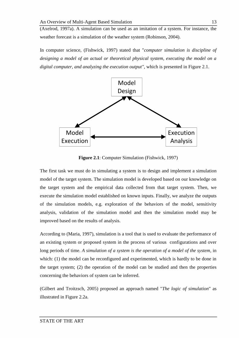
In computer science, (Fishwick, 1997) stated that "computer simulation is discipline of
designing a model of an actual or theoretical physical system, executing the model on a
digital computer, and analyzing the execution output", which is presented in Figure 2.1.
Model Design
Model Execution
Execution Analysis
Figure 2.1: Computer Simulation (Fishwick, 1997)
The first task we must do in simulating a system is to design and implement a simulation
model of the target system. The simulation model is developed based on our knowledge on
the target system and the empirical data collected from that target system. Then, we
execute the simulation model established on known inputs. Finally, we analyze the outputs
of the simulation models, e.g. exploration of the behaviors of the model, sensitivity
analysis, validation of the simulation model and then the simulation model may be
improved based on the results of analysis.
According to (Maria, 1997), simulation is a tool that is used to evaluate the performance of
an existing system or proposed system in the process of various configurations and over
long periods of time. A simulation of a system is the operation of a model of the system, in
which: (1) the model can be reconfigured and experimented, which is hardly to be done in
the target system; (2) the operation of the model can be studied and then the properties
concerning the behaviors of system can be inferred.
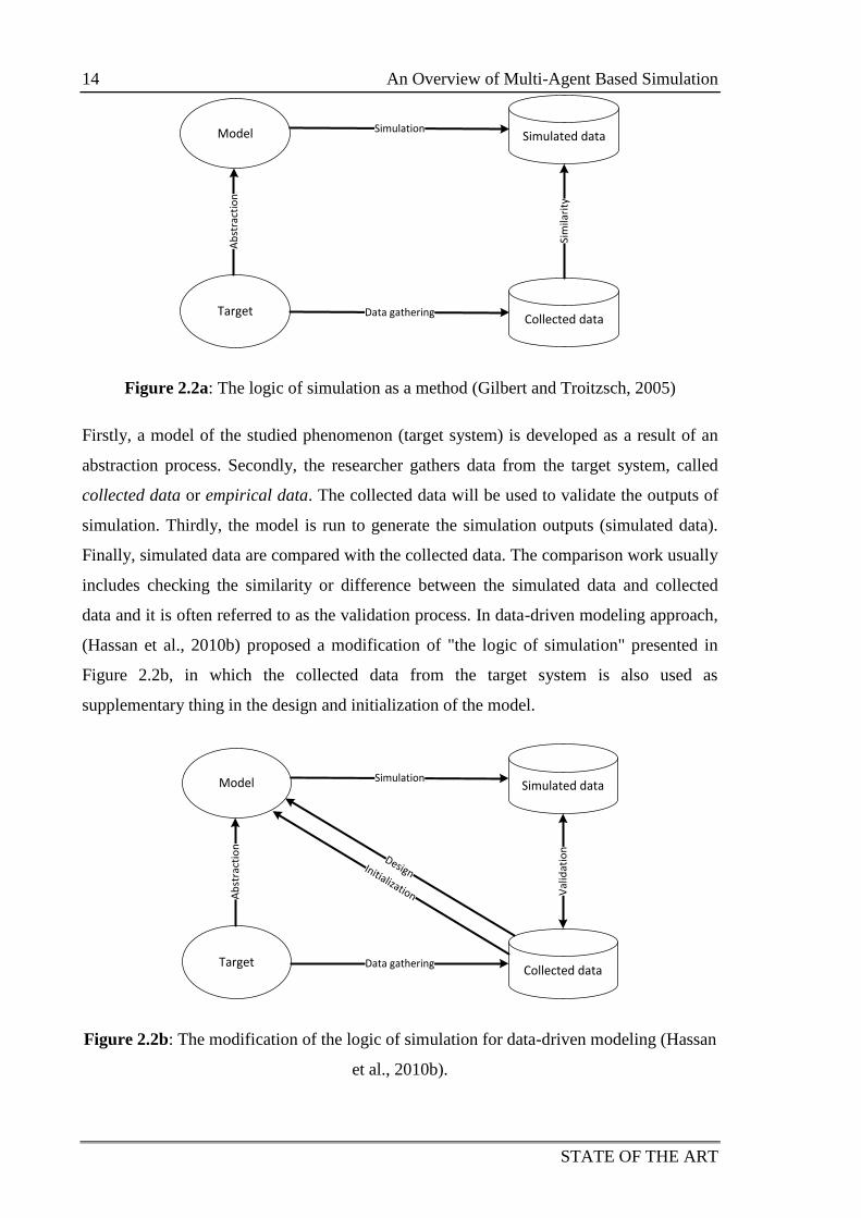
(Gilbert and Troitzsch, 2005) proposed an approach named "The logic of simulation" as
illustrated in Figure 2.2a.
14 An Overview of Multi-Agent Based Simulation
STATE OF THE ART
Target
Model Simulated data
Collected data
Simulation
Data gathering
Ab
stra
ctio
n
Sim
ilari
ty
Figure 2.2a: The logic of simulation as a method (Gilbert and Troitzsch, 2005)
Firstly, a model of the studied phenomenon (target system) is developed as a result of an
abstraction process. Secondly, the researcher gathers data from the target system, called
collected data or empirical data. The collected data will be used to validate the outputs of
simulation. Thirdly, the model is run to generate the simulation outputs (simulated data).
Finally, simulated data are compared with the collected data. The comparison work usually
includes checking the similarity or difference between the simulated data and collected
data and it is often referred to as the validation process. In data-driven modeling approach,
(Hassan et al., 2010b) proposed a modification of "the logic of simulation" presented in
Figure 2.2b, in which the collected data from the target system is also used as
supplementary thing in the design and initialization of the model.
Target
Model Simulated data
Collected data
Simulation
Data gathering
Ab
stra
ctio
n
Val
idat
ion
DesignInitialization
Figure 2.2b: The modification of the logic of simulation for data-driven modeling (Hassan
et al., 2010b).
An Overview of Multi-Agent Based Simulation 15
STATE OF THE ART
The Computer simulation definition in (Fishwick, 1997) and "the logic of simulation"
methodology in (Gilbert and Troitzsch, 2005; Hassan et al., 2010b) are the base portfolio
for designing a logical framework to manage, integrate and analyze data in an agent-based
simulation platform, which I propose in Chapter 3.
2.2.2 Agent based modeling
“Agent-based modeling is a computational method that enables a researcher to create,
analyze, and experiment with models composed of agents that interact within an
environment” (Gilbert, 2008). An agent-based model or multi-agent based model is a
particular kind of model, which is the result of modeling activity. It contains agents that
interact with one another within an environment (Abdou et al., 2012).
ABM is a powerful modeling technology that has been applied in numerous fields such as
physical, biological, social and management sciences (Macal and North, 2010). In biology,
agent based modeling is used to model cellular systems (Alber et al., 2003), to model
ecological systems by using individual-based modeling approach (Grimm and Railsback,
2005b), invasion of rice pest (Nguyen et al., 2011; Phan et al., 2010; Truong et al., 2011).
In economics, ABM has been applied to study several domains (Bonabeau, 2002): (1)
Flows: traffic and customer flow management (Julka et al., 2002); (2) Markets: stock
market and strategic simulation (Chen and Yeh, 2001) or simulated market network
(Galtier et al., 2012); (3): Organization: operational management of risks and
organizational design (Giannakis and Louis, 2011); (4) Diffusion: Diffusion of innovation
and adoption dynamics (Laciana and Oteiza-Aguirre, 2014). In the computational social
science, various phenomena have been examined using agent-based models (Gilbert and
Troitzsch, 2005; Macy and Willer, 2002) cited in (Macal and North, 2010). The Sociology
of Organized Action theory (Crozier and Friedberg, 1977) was used to discover how the
social actors build the organization (Sibertin-Blanc et al., 2013). Agent-based simulation
was used to explore rules for rural credit management (Barnaud et al., 2008).
2.2.2.1 What is an agent?
In computer science, an agent is a software or hardware entity that is situated in an
environment (virtual or real environment). An agent is able to perceive the environment
and other agents, and capable of performing autonomous actions in this environment in
order to meet its design objectives (Ferber, 2007; Wooldridge, 2002). For more detail,
(Ferber, 2007) expressed the following rules to model an agent:
16 An Overview of Multi-Agent Based Simulation
STATE OF THE ART
Agent is able to act in an environment;
Agent has only a partial representation of this environment;
Agent can communicate with other agents;
Agent owns its resources;
Agent can reproduce itself;
Agent has an autonomous behavior.
Agent is driven by a set of tendencies (individual objectives, goals, drives, or
satisfaction/survival function).
Agent-based modeling is a modeling technique that involves agents (Bonabeau, 2002;
Gilbert, 2008; Macal and North, 2010), in which the agents are computer programs or
distinct parts of a program that are used to represent social actors. Agents are programmed
to react to their situated computational environment, which is a model of a real
environment where the social actors operate (Gilbert, 2008). According to (Abdou et al.,
2012), agents have four major characteristics:
Perception: Agents can perceive their environment, including other agents in
their vicinity.
Performance: Agents have a set of behaviors, which enable them to perform
acts such as moving, communicating with other agents, and interacting within
an environment.
Memory: Agents have a memory to record their previous states and actions.
Policy: Agents have a set of rules, heuristics or strategies that can determine,
given their present situation and their history, what they should do next.
In essence, (Ferber, 2007) gave a definition of an agent and the rule to model agents and
(Abdou et al., 2012) classified the seven rules in (Ferber, 2007) into four characteristics for
implementation. For instance, agents with the above characteristics can be implemented in
different ways and architectures such as object-oriented programming, production rule
system or learning process depending on the purpose of simulation (Abdou et al., 2012).
In addition, Agents can be representation of any type of autonomous entities (Crooks and
Heppenstall, 2012). For example, agents can be used to represent an area (town, district, or
city), insect (Brown Plant Hopper), people (farmer), rice plant, weather or light trap in
studying the invasion of Brown Plan Hoppers using agent-based model (Nguyen et al.,
2011; Phan et al., 2010; Truong et al., 2011).
An Overview of Multi-Agent Based Simulation 17
STATE OF THE ART
2.2.2.2 Multi-agent systems
A Multi-Agent System (MAS) is defined as a set of interacting agents in a common
environment in order to achieve a common, coherent task (Gleizes et al., 2011). A MAS is
a system that contains an environment, objects, agents, relationships between all entities, a
set of operations that can be performed by the entities and operators with the task to
represent the application of the operations and changes of the universe in time, due to these
operations (Ferber, 1999) cited in (Bousquet and Page, 2004). According to (Ferber, 2007),
multi-agent systems use the whole set of concepts and techniques allowing heterogeneous
software (or hardware) entities, named agents to cooperate according to complex modes of
interaction and a multi-agent system is based on three major concepts: (1) autonomous
activity of the agents (pro-active), (2) the sociability of the agents and (3) interaction that is
what connects (1) and (2).
There are some similarities between ABM and MAS, i.e. both of them are composed of
agents and their environment. Although ABM and MAS have also been used to simulate
various kind of systems, e.g. socio-economic systems or biological systems (Bandini et al.,
2009) they feature some differences in their concepts. ABM is an approach that is used to
design and implement a model of the system composed agents, which interact within an
environment. The product of the agent-based modeling processes are agent based models
(ABMs), which involve three classical elements: (1) a set of agent with their attributes and
behaviors; (2) a set of agent relationships and methods of interaction; (3) the environment
of agents (Macal and North, 2010). However, MAS field is a broader discipline - It has
closely a relationship with other disciplines e.g. (distributed) artificial intelligence,
philosophy, ecology, software engineering and social sciences (Weiss, 1999; Wooldridge,
2002). MAS methodologies usually deal with solving issues related to the formalization of
different stages, the technical implementation and software engineering principles (Hassan,
2009) that can be applied to build distributed, concurrent, artificial intelligence systems,
etc . For instance, MAS has a wide range of applications such as workflow and business
process management, distributed sensing, information retrieval and management,
electronic commerce, human-computer interfaces, virtual environment, social simulation
(Wooldridge, 2002) ecosystem management (Bousquet and Page, 2004), etc. In MAS, the
problem-solving process is simplified by dividing the necessary knowledge into sub-units
then associating an intelligent independent agent to each subunit and coordinating the
activity of the agents (Bousquet and Page, 2004).
18 An Overview of Multi-Agent Based Simulation
STATE OF THE ART
2.2.2.3 Modeling Approaches
In this section, I present two common approaches in agent-based modeling and simulation.
One paradigm is based on the simplicity of abstract models and the other one is based on
the complexity of descriptive models that are closer target systems.
KISS (Keep It Simple, Stupid) approach
Based on the point of view "the goal of ABM is to enrich modelers understanding of
fundamental processes that may appear in a variety of applications" and "it does not aim
to provide an accurate presentation of a particular empirical applications", KISS
approach was proposed for modeling the phenomena. The principle of KISS is keeping the
assumptions underlying the agent-based model simple while phenomena being examined
may be complicated (Axelrod, 1997a, 1997b). KISS is a modeling driven approach and it
is useful for researchers who look for theoretical models that are abstract enough to explain
examined assumptions.
KIDS (Keep It Descriptive, Stupid)
On the contrary of KISS, KIDS approach was proposed in (Edmonds and Moss, 2005)
based on the point of view in modeling "one starts with a descriptive model (which may be
quite complex) and then only simplifies it where this turns out to be justified. In the KIDS
paradigm, modelers firstly try to build agent-based models that should be closer to the
target phenomenon as much as possible although the results of modeling may be complex
models. Then modelers will remove "things deemed not essential for the models" step by
step (Hassan et al., 2010a). KIDS is a kind of data driven modeling - it uses not only
abstract theoretical assumptions but also data obtained by empirical data or elicitation as
foundations for modeling descriptive models (Edmonds and Moss, 2005; Hassan, 2009).
2.2.2.4 Agent-based platforms
A platform (or software platform) is defined as programming languages or environments
used to convert the model into executable code and then run it (Grimm and Railsback,
2005c). An agent-based platform is constructed on the framework and library paradigms,
in which a framework is a set of standard concepts for designing and describing ABMs
along with a library of software implementing the framework and providing simulation
tools (Railsback et al., 2006). For instance, we can list some of the well-known agent-
An Overview of Multi-Agent Based Simulation 19
STATE OF THE ART
based platforms such as GAMA (Taillandier et al., 2012), MASON (Luke et al., 2005),
Netlogo (Wilensky, 1999), Repast (North et al., 2013) and Swarm (Minar et al., 1996).
2.2.2.5 Verification, validation and Calibration of agent-based simulation
models
Verification of models deals with building a model right while validation of models deals
with building the right model (Balci, 1994).
According to (Pace, 2004), verification involves two aspects for answering the question
"Did I build the thing right": (1) design (specification verification) - it is to assure that all
specifications and nothing else are included in the model or simulation design; and (2):
implementation (implementation verification) - it is to assure that all specifications and
nothing else are included in the model or simulation as built and no errors in the
implementation.
Validation is divided into aspects, which are used to answer the question "Did I build the
right thing". The two aspects are: (1) conceptual validation (conceptual model validation) -
it is to assess the conceptual model based on system theories, which are abstracted from the
target system and system data; and (2) results validation (operational validation) - it is a
process to compare the results of the implemented model (computerized model) with
appropriate collected data to ensure that the model can support intended purposes.
According to (Sargent, 2011), the verification and validation of models are divided into
four processes: (1) conceptual model validation is a process to determine that the theories
and assumptions in conceptual model are correct and that the conceptual model represents
the target system according to the purpose of a particular study; (2) computerized model
verification is a process to assure that the computerized model (the computer programming
and implementation of the conceptual model) is correct; (3) operational validation is a
process to determine that the output of the computerized model has sufficient accuracy for
the model’s intended purpose over the domain of the model’s intended applicability; and
(4) data validity is a process to guarantee that the data necessary for model building, model
evaluation and testing, and conducting the model experiments to solve the problem are
adequate and correct.
(Amblard et al., 2007) distinguished validation of multi-agent simulations into two stages:
internal validation and external validation. Internal validation is used to check the
20 An Overview of Multi-Agent Based Simulation
STATE OF THE ART
conformity between specifications and the implemented model. In the software
engineering field, it is usually called verification and corresponds to the process that is
used to compare the conceptual model to the computerized model. Hence, internal
validation corresponds to building the model right. On the other hand, external validation
is used to check the similarities between the model and the real phenomenon. It is also
named validation process in software engineering, so external validation corresponds to
building the right model.
Calibration of agent-based simulation models
According (Donigian, 2002) citing (ASTM, 1984), the calibration process is known as the
tuning of a model with known input and output information. It is used to adjust or estimate
factors for data, which are not available. In calibration, the validation process is used as the
comparison of the model results with numerical data independently derived from
experiments or observations of the environment. The purpose of calibration is to ensure
that "the calibrated model properly assesses all the variables and conditions which can
affect model results".
To calibrate a simulation model, modelers used several different methods: (Donigian,
2002) used the "weight of evidence" approach to compare the outputs of simulation with
observed value from the target system and then interpreted the result of simulation against
the level of agreement or accuracy (i.e. very good, good, and fair) based on the result of the
comparisons; (Lardy et al., 2014) used Pareto-optimal solution to find the suitable value of
parameters and then evaluated the model based on the Pareto-optimal front; (Ngo and See,
2012; Rogers and Tessin, 2004; Said et al., 2002) used genetic algorithm (GA) to optimize
the value of the parameters, in which the parameters of the model play the role of
chromosomes, the range of data is the genotype and the results of the model calibration
are the phenotype. In general, these researchers validate simulation outputs with empirical
data and check fitness conditions by statistic methods such as Root Mean Squared Error
(RMSE) (Ngo and See, 2012; Willmott et al., 1985). In such works, we need a software
environment, which helps us to run models with different inputs in several times and
analyze the outputs. For example, OpenMOLE2 (Open Model Experiment) is one
2 http://www.openmole.org/
An Overview of Multi-Agent Based Simulation 21
STATE OF THE ART
workflow software, which is useful for model execution and model analysis such as model
replication, calibration, validation and sensitivity analysis.
In my research, I address only the external validation and the calibration. In the following,
I use the word "validation" for external validation; and "calibration" for the fine-tuning of
the output of simulation model by a change in the values of parameters, in which similarity
coefficient or difference coefficient are used as the fitness indicators. In the Chapter 5, I
propose a validation method using a similarity index and I also suggest an automatic
approach to calibrate and validate an agent-based simulation model that is an application of
CFBM (Combination Framework of Business intelligence solution and Multi-agent
platform) presented in Chapter 3.
2.2.2.6 Scale in Agent-based modeling
In this thesis, I used key terms related to the concept of scale as mentioned in (Gibson et
al., 2000): (1) "Scale refers to the spatial, temporal, quantitative, or analytical dimensions
used by scientists to measure and study objects and processes"; (2) "Levels are the unit of
analysis that are located at the same position on a scale" e.g. levels refer regions (micro,
meso and macro) on spatial scale or time (short, medium and long duration) on a temporal
scale; (3) "A hierarchy is a conceptually or linked system for grouping phenomena along
an analytical scale". For instance, (Nguyen et al., 2012b) defined the hierarchies that
includes the links between the regions (Commune → District → Province) on spatial scale
or time (Week → Month → Crop → Year) on temporal scale; (4) "Resolution (grain) is
the precision used in measurement" - the resolution is used to observe quantity depends on
the magnitude of a dimension used in measuring a phenomenon. For example, the
resolution of a day was used to divide the time of the observation of the number of pests on
the rice fields (Nguyen et al., 2012d). According to (Wu et al., 2006), scaling is a set of the
operations to transfer the information between scales and there are two kinds of scaling: (1)
upscaling which is translating information from finer scales to broader scale and (2)
downscaling which is translating information form broader scales to finer scales.
In agent-based modeling, scaling on multi-dimensions (spatial, temporal, etc) is usually
applied, e.g. to manage the groundwater pollution (Schmidt et al., 2011) by building a
framework integrating small scale models (micro-scale model) and large scale models
(macro-scale model). In that framework, upscaling aggregates data from micro-scale
models to macro-scale models. Conversely, downscaling disaggregates data from macro-
22 An Overview of Multi-Agent Based Simulation
STATE OF THE ART
scale models to micro-scale models to aggregate and assess information (Nguyen et al.,
2012b) and to make decision (Nguyen et al., 2012a). The authors build a multi-agent based
model with several kinds of decision maker agents for collecting data, aggregating and
making decision based on Plant Protection Department levels in Mekong Delta region of
Vietnam: (1) CdecisonMaker (agent decision maker at commune level), collects data from
sample rice fields and send weekly reports to agent DdecisionMaker; (2) DdecisionMaker
(agent decision maker in district level) aggregates received information from
CdecisionMaker and sends reports to PdecisionMaker; (3) PdecisionMaker (agent decision
maker in province level) make upscaling on information, which were received from
DdecisionMaker and produces reports based on time scale levels (week → month → crop
→ year). Although scaling has been widely used in agent-based modeling, it is still one of
the challenges of ABM mentioned in the next section.
2.2.2.7 Key challenges of ABM
Even though ABM is a powerful simulation modeling technology and is becoming an
important modeling paradigm in social science, there still remains key challenges among
them, taken from (Crooks et al., 2008):
Replication and experiment. Because we need more confidence in a model, we
opt for several instances confirming the successful application of the model.
That is the reason why researchers need to replicate the model in independent
situations. For example, OpenABM3 is a node in the CoMSES (Computational
Modeling for SocioEcological Science) network, where modelers share their
models and discuss their works so that the models can be replicated on different
dimensions such as time, hardware, languages, toolkits, algorithms and
authorship (Wilensky and Rand, 2007). However, the troubles with replication
are that it is difficult to handle all variables that pertain to a particular situation
and as a consequence, it is almost impossible to ensure that the applications of a
model are compared in independent situations, thus making replication is rarely
done in social science (Crooks et al., 2008). Solutions for solving these
problems are mentioned in (Mahboubi et al., 2010; Vasilakis and El-Darzi,
2004) by using data warehouse technologies and a concrete implementation of
3 http://www.openabm.org/
An Overview of Multi-Agent Based Simulation 23
STATE OF THE ART
data warehouse solution will be demonstrated in Chapter 4 by applying CFBM
represented in Chapter 3.
Verification, Calibration, and Validation. These are three of the major
processes in validation for agent-based simulations (Klügl, 2008). The validity
of a model can be confirmed by using various statistical methods to compare
the output of the model with observation data from the target system and this is
a matter of argument (Crooks et al., 2008). In some cases, the modelers can face
data problems in validation and calibration of the models. For instance,
complex agent-based models are usually executed with several parameters and
generate a huge amount of data, which do not have exactly the same structure
than observation data from the real system and can be measured and validated
in various conditions. In such case, calibration and validation are used to
determine which inputs and outputs are appropriate regarding the observation
data (Ngo and See, 2012; Rogers and Tessin, 2004; Said et al., 2002).
Therefore, how to calibrate and validate agent-based model dealing with
integrated systems with a high volume of input/output data? In chapter 5, we
will demonstrate an approach to handle input/output data of simulations model
and observation data from target systems as an automatic process of calibration
and validation of agent-based model.
Agent representation, Aggregation and Dynamics. In general, there are two key
problems in increasing the scale of an agent-based system: (1) Computational
resources limit the simulation time and/or data storage capacity and (2) Agent
model analysis may become more difficult (Parry, 2009). Specially, agent based
modeling in spatial systems still reveals three limitations: (1) Agent
representation - what the constituents of agent are for the aggregation of objects
at any spatial scale and across different times, (2) The Scale of Agent - Too
difficult to specify the rules for defining agents for aggregations from lower
level unit, (3) The sheer number of agent - the complexity of the computation
usually rises as the square of the number of agents (Crooks and Heppenstall,
2012). There were some research studies to solve the limitations of agent
presentation and the scale of agent in (Taillandier et al., 2012; Vo et al., 2012)
but limitations of simulation time/data store capacity and building scaling
model on large size of data are still not solved. The solution aiming at solving
aggregation issues will be mentioned in Section 4.3.
24 Data in Agent-Based Modeling
STATE OF THE ART
Operational Modeling. Although the agent-based platforms provide several
tools for modeling, presenting and analyzing that can help modelers reduce the
burden in building simulation system (Castle and Crooks, 2006; Crooks, 2007;
Taillandier et al., 2012), an agent-based platform is always limited in its
applicability. For instance, each agent-based platform limits the number and
representation of agents. In addition, the provided tools for building models in
agent-based platform have usually been developed based on generic libraries
with not in well-organized packages, lack of the complete documentation and as
a consequence, it is difficult to find what tools a modeler needs for some
particular tasks in modeling (Railsback et al., 2006).
In Section 2.2, the basic concepts and some of the key challenges of ABM are addressed.
For the next section, I will present some issues of data in ABM.
2.3 Data in Agent-Based Modeling
2.3.1 Moving from modeling driven approach to data driven approach
"The world is increasingly complex, and the systems that need to be analyzed are
becoming more complex" (North and Macal, 2007).
There is a shift from the high abstraction and simplification of agent-based models
produced by the KISS (Keep It Simple Stupid - cf. Section 2.2.2.3) approach to
descriptive models produced by the KIDS (Keep It Descriptive) approach (Edmonds and
Moss, 2005; Hassan, 2009; Hassan et al., 2010a). In agent-based modeling and simulation,
empirical data have been usually used as one of the foundations of abstraction,
initialization and validation for finding the balance between simplification and realistic
behaviors (Hassan, 2009; Hassan et al., 2010b). For instance, (Gaudou et al., 2013; Nguyen
et al., 2012c) used the data collected from the target system such as ecological data (e.g.
rainfall, temperature changes, and plant growth) and socio- economic data (e.g. farmer
decision-making process, demography and land use) in order to design, simulate and
evaluate the decision support systems for planning public policies regarding the
management of natural resource or Rice Pest Management in appropriate. There are still
remaining reasons for KISS to be not an appropriate approach in such cases. Among them
are four taken from (Terano, 2008): (1) the simulation models should produce results,
which correspond with real world phenomena; (2) the phenomena are difficult to explain
Data in Agent-Based Modeling 25
STATE OF THE ART
by existing theories but they can be reproduced in limited manner; (3) the simulation
models should generate satisfactory results. The simulation models are usually run with
multiple parameters hence we can tune parameter values (calibration of model) for
producing desired simulation results; and (4) the results of simulation must be rigorously
validated so the results produced by the models should not be difficult for validation. In
KISS paradigm, the models have been usually made in high abstraction and simplicity. The
complexity is in the outputs of simulation (Axelrod, 1997a), which make it complicated
validating the models outputs with empirical data (Hassan, 2009). On the contrary, KIDS
models have used all the data collected from target systems such as time series data, point
measurements, statistics etc, which can be used as a source for checking the anecdotal
evidence and serve as a basis for checking the reliability of models (Edmonds and Moss,
2005). Therefore, the trend of moving from modeling driven approach (KISS) to data
driven approach (KIDS) is an adaptive solution for the requirements of using more and
more data in agent-based modeling and simulation, in which modelers must build complex
models, which need to produce data corresponding to the collected data from the target
system.
2.3.2 Data management in ABM
In simulation research, modelers' concerns include three aspects: (1) Programming of a
simulation model with three goals, namely validity, usability and extendibility; (2)
Analyzing the results; (3) Sharing the results via publication (Axelrod, 1997a).
During the implementation of a simulation model, (Axelrod, 1997a) takes into account the
interpretation of outputs of the simulation model and the understanding of how the
simulation model works. Because several versions of a simulation model may be created in
the modeling process, the data management problem for researchers is how to manage the
input and output data of different versions. Another issue on analyzing outputs is how to
compare the outputs of different versions to determine what might account for differences.
They are the key challenges in the modeling of agent-based simulation.
We can cite several agent-based models intended to study real phenomena (Gaudou et al.,
2013; Nguyen et al., 2011; Truong et al., 2011), which use data collected from real-world
(target systems) as an input of models and also to validate the models. These models are
instances of the approach "the logic of simulation" described in (Gilbert and Troitzsch,
2005; Hassan et al., 2010b), in which data-driven agent-based approach is used in building
26 Data in Agent-Based Modeling
STATE OF THE ART
a simulation system. As we presented in Section 2.2.1.2, the data collected from the target
system supplies the information for designing the model and it is also used as the input
data and validation data of the model. Although the data collected are very important in the
data-driven agent-based simulation approach, they induce the issues such as:
A high volume of detailed data can be requested on micro level and the issue is
how to handle this huge amount of data.
How to integrate data and avoid the inconsistencies where the data are retrieved
from various data sources.
Furthermore, empirical data (also called collected data, which are collected from target
system - cf. Section 2.2.1.2) are usually collected in space and time and the collected data
can be used for several versions of the model. We need to run models in series of
simulation (replications) and also compare the result of the replications.
More generally, if we apply the computer simulation defined in (Fishwick, 1997) into "the
logic of simulation" in (Gilbert and Troitzsch, 2005; Hassan et al., 2010b) (cf. Section
2.2.1.2) then to manage collected data and simulation data rises as a challenge in
computer simulation in general and multi-agent based simulation in particular or we can
say that data management is needed in computer simulation and it is also an important
discipline in computer simulation.
In order to adapt "the logic of simulation" proposed in (Gilbert and Troitzsch, 2005;
Hassan et al., 2010b), I present the weakness of computer simulation platforms with
respect to data management and then propose Business Intelligence (Section 2.4) as a
solution to supplement the necessary features for ABM in managing, integrating and
analyzing data in Section 3.2 of Chapter 3.
2.3.3 The limitation of agent-based platforms in data management
The basic features of a general computer simulation platform or specifically, of a multi-
agent-based simulation platform are the capability to write models, run simulations of
these models and handle results for analysis and/or validation (Drogoul et al., 2003;
Fishwick, 1997). Most simulation platforms (Netlogo, Repast, and GAMA) strongly
support these features, but they do not offer database functions or, when they do, they
support database functions with inflexibility in use. For instance, Netlogo has an external
package (Netlogo-sql) that supports the execution of SQL statements but “There is no
An Overview of Business Intelligence Solutions 27
STATE OF THE ART
"deep" support for the Netlogo paradigm”4. Repast is a toolbox for agent-based modeling
in Java which has numerous libraries to connect the simulator to useful technologies
(statistical analysis, GIS, SQL, etc.)5. But for using them, users need to have very good
java programming skills. GAMA6 pays a great attention to the modeling of the
environment and the use of GIS data but it only supports access to GIS data on shape files
and has no supporting features to query GIS data in database. This is not an appropriate
tool for users when they need to access only a subset of data.
These platforms support good tools for modeling driven approach but they still need
additional features for data driven approach.
To solve the lack of database management tools in multi-agent based platform and the
challenges of integration of data and analysis of the high volume of integrated data, we
propose a logical architecture framework in Section 3.2 of Chapter 3, in which we use
business intelligence solution mentioned in Section 2.4 as a solution to: (1) manage the
input/output of simulation model and data collected from target system, (2) integrate
simulated data and collected data and (3) analyze integrated data. Furthermore, a concrete
implementation of our framework in GAMA platform is also presented in Section 3.3 of
Chapter 3.
2.4 An Overview of Business Intelligence Solutions
2.4.1 What is Business Intelligence?
According to (Golfarelli et al., 2004), Business Intelligence (BI) has been developed since
the early 90's for analyzing the historical data of companies to better understand the
situation of the business and improve the decision-making process. BI can be defined as
the process of turning data into information and then into knowledge.
According to (Gangadharan and Swami, 2004), BI provides in-depth analysis of detailed
business data, using database and application technologies as well as analysis tools. It
technically includes knowledge management, enterprise resource planning, decision
support systems and data mining. (Rainardi, 2008) defined BI as a collection of activities
4 https://code.google.com/p/netlogo-sql/
5 http://repast.sourceforge.net/docs/RepastJavaGettingStarted.pdf
6 GAMA version 1.5 or earlier version.
28 An Overview of Business Intelligence Solutions
STATE OF THE ART
(gathering, managing, analyzing and understanding data) performing various types of
analysis on the data gathered from the company or from others sources in order to
understand business situations and to help making strategic and tactical decisions to
improve the business performances.
BI is a term enclosing several technologies such as Extraction-Transformation-Loading
(ETL), Data Warehouse (DW/DWH), database query and report, (multidimensional) On-
line Analytical Processing (OLAP), data analysis, data mining and visualization
(Gangadharan and Swami, 2004; Ranjan, 2009). Generally, BI encompasses all the
capabilities required to turn data into Intelligence (Rud, 2009).
A Business Intelligence solution is known as a system of data warehouse and analysis
tools, where the data warehouse collection of data supports decision-making processes
(Inmon, 2005).
2.4.2 Decision support systems
A Decision Support System (DSS) is a set of expandable, interactive information tools
designed to process and analyze data to support managers in decision making (Golffarelli
and Rizzi, 2009). According to (Shim et al., 2002), decision support systems are computer
technology solutions intended to support complex decision making and problem solving.
Data warehouse, On-Line Analytical Processing (OLAP), data mining and web-based DSS
are four powerful tools that can be merged for building DSSs. Commonly, data warehouse
is used to manage data back-ends and OLAP is a category of software technology used to
conduct and access data in data warehouse. Data mining is a set of artificial intelligence
and statistical technologies for data analysis and web-based DSS encompasses a set of
technology associated with World Wide Web services used to deploy DSS.
2.4.3 An Introduction to Data Warehousing
Data warehousing is a collection of decision support technologies, aimed at enabling the
knowledge worker (executive, manager, or analytics) to make better and quicker decisions.
Data warehousing and on-line analytical processing are essential elements of decision
support systems (Chaudhuri and Dayal, 1997). More generally, data warehousing
associates methods, techniques, and tools to support knowledge workers in conducting data
An Overview of Business Intelligence Solutions 29
STATE OF THE ART
analyses that help performing decision-making processes and improving information
resources (Golffarelli and Rizzi, 2009).
Frequently, the software vendors prefer to use the term business intelligence than data
warehousing, as they focus on what a data warehouse can do for a business (Rainardi,
2008).
2.4.3.1 Data Warehouse
(Devlin and Murphy, 1988) referred to the term "Business Data Warehouse" (BDW) as the
single logical storehouse of all information used to report on the business which is based
on relational concepts. We can understand data warehouse as the query-abled source of
data in the enterprise (Kimball et al., 1998). In more details, (Kimball and Caserta, 2004)
defined data warehouse as a system that extracts, cleans, conforms, and delivers source
data into a dimensional data store and then supports and implements querying and analysis
for the purpose of decision making. According to (Golffarelli and Rizzi, 2009; Inmon,
2005), a data warehouse is a collection of data that supports the decision-making
processes. It provides the following features:
It is subject-oriented. Data warehouse hinges enterprise-specific concepts such
as customers, products, sales and orders.
It is integrated and consistent. A data warehouse integrates data, which are
extracted, transformed and loaded from various data sources. It provides a
unified view of all data.
It shows data evolution over time and it is not volatile. Data warehouse is
regularly completed with operational data and keeps on growing. Data in data
warehouse are loaded in snapshots and static format. If the data change then a
new snapshot record is written and recorded with its time stamps. Hence the
historical record of data is kept in the data warehouse. That is detailed in (Bȩbel
et al., 2004; Blaschka et al., 1999; Kimball and Ross, 2002; Wrembel and
Bębel, 2007) who show us how to manage the evolution of a data warehouse.
In practice, a data warehouse can be viewed as a system that retrieves and consolidates
data periodically from the source systems into a dimensional or normalized data store. The
consolidated data is queried for business intelligence or other analytical activities
(Golffarelli and Rizzi, 2009; Kimball and Ross, 2002; Rainardi, 2008).
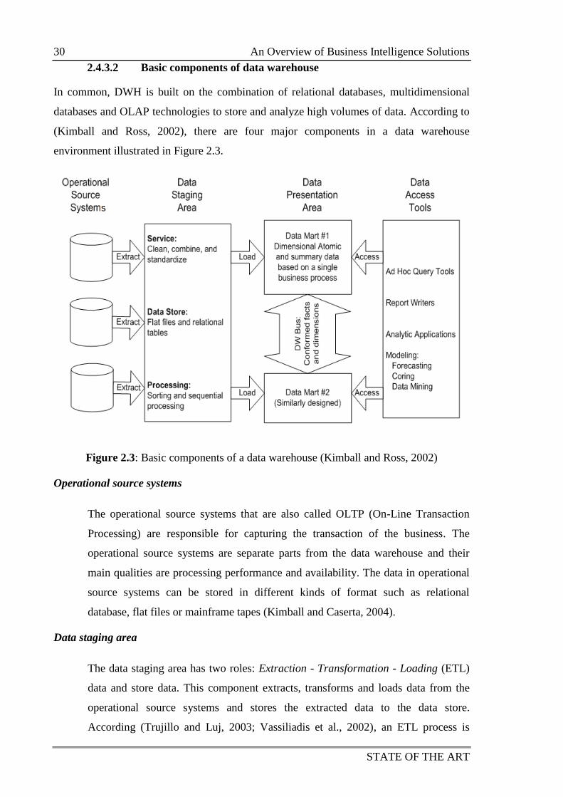
30 An Overview of Business Intelligence Solutions
STATE OF THE ART
2.4.3.2 Basic components of data warehouse
In common, DWH is built on the combination of relational databases, multidimensional
databases and OLAP technologies to store and analyze high volumes of data. According to
(Kimball and Ross, 2002), there are four major components in a data warehouse
environment illustrated in Figure 2.3.
Figure 2.3: Basic components of a data warehouse (Kimball and Ross, 2002)
Operational source systems
The operational source systems that are also called OLTP (On-Line Transaction
Processing) are responsible for capturing the transaction of the business. The
operational source systems are separate parts from the data warehouse and their
main qualities are processing performance and availability. The data in operational
source systems can be stored in different kinds of format such as relational
database, flat files or mainframe tapes (Kimball and Caserta, 2004).
Data staging area
The data staging area has two roles: Extraction - Transformation - Loading (ETL)
data and store data. This component extracts, transforms and loads data from the
operational source systems and stores the extracted data to the data store.
According (Trujillo and Luj, 2003; Vassiliadis et al., 2002), an ETL process is
An Overview of Business Intelligence Solutions 31
STATE OF THE ART
usually done in three main steps: (1) the first step of getting data into data
warehouse is Extraction that reads the needed data from source systems and copies
them into staging area; (2) the second step is Transformation, which involves
several tasks such as cleansing data, combining data from multiple sources, de-
duplicating data and assigning warehouse key; and (3) the third step is Load, which
loads the transformed data into the data warehouse presentation area. (Kimball and
Caserta, 2004) clearly presents the techniques for designing and developing this
part.
Data presentation area
The data presentation area is responsible for organizing, storing and making data
available for presentation. Typically, the data presentation area is managed by a
series of integrated data marts (cf. Section 2.4.3.8) and a data mart is understood as
a wedge of the overall presentation area pie. The data in the data presentation area
are presented, stored, and accessed in dimensional schemas and the data marts are
commonly built on dimension and fact tables (cf. Section 2.4.3.3).
Data access tools
The data access tools or OLAP Analysis Tools (cf. section 2.4.3.7) are used to
query data from the data presentation area and perform analyses on queried data. A
data access tool can be an ad hoc query tool, a report writer, an analytic application
or modeling application. These tools usually support report systems, decision
support systems or forecast systems. In addition, there are some tools such as
modeling tool or forecasting tools which may upload their results back into
operational source systems or the staging/presentation areas of the data warehouse.
2.4.3.3 Multidimensional database
A multidimensional database is based on two main elements: dimension and Fact table (F-
table) where: (1) Dimensions are syntactical categories that allow modelers to specify the
ways to look at the information and are organized in a hierarchy of levels, corresponding to
data domains at different granularity levels; (2) Fact-tables are functions from symbolic
coordinates to measures that are used to present factual data (Cabibbo and Torlone, 1998a).
Multidimensional databases are interpreted in the same manner and they are managed by
OLAP Servers (Kimball et al., 1998).
32 An Overview of Business Intelligence Solutions
STATE OF THE ART
Today, multidimensional databases are implemented among the three OLAP approaches
(ROLAP, MOLAP or HOLAP) and contain two kinds of tables (fact table and dimension
tables):
Fact table:
A fact table is the primary table in a dimensional model where the numerical
performance measurements of the business are stored. Fact table have at least one
measure and two or more foreign keys that connect to the dimension tables' primary
key (Kimball and Ross, 2002).
Dimension tables:
Dimension tables are necessary companions to a fact table. The dimension tables
contain a primary key, which serves as the basis for referential integrity with any
given fact table to which it is joined and at least one attribute to descript the
business (Kimball and Ross, 2002).
For example, SMALLTOWDATA_FACTS fact table in Figure 2.4 of the next section
has one measure to represent the average number of insects produced by simulation
models (Simulate_value) and four foreign keys to connect four dimension tables
(MODELS_DIM, INSECTS_DIM, TIME_DIM and REGIONS_DIM). REGION_DIM
dimension table has one primary key (ID_REGIONS) to identify an area and four
textual attributes that represent region, province, district and small town name of the
area. The relationship between SMALLTOWDATA_FACTS fact table and
REGION_DIM dimension table is specified by ID_REGIONS key.
2.4.3.4 Multidimensional model
Multidimensional models are used to present the structure of data in multidimensional
database. According to (Kimball et al., 1998), a dimensional model is composed of one
fact table with a combination of foreign keys called multipart key and a set of dimension
tables, each of which has a single part primary key that corresponds exactly to one of the
components of the multipart key in the fact table. This structure of dimensional model is
called star-join or star schema.
For example, Figure 2.4 shows the star-schema of a dimension model, which is built in the
Section 4.2.4.3 of Chapter 4.
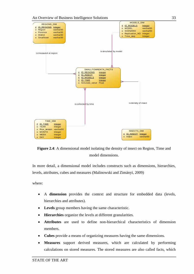
An Overview of Business Intelligence Solutions 33
STATE OF THE ART
Figure 2.4: A dimensional model isolating the density of insect on Region, Time and
model dimensions.
In more detail, a dimensional model includes constructs such as dimensions, hierarchies,
levels, attributes, cubes and measures (Malinowski and Zimányi, 2009)
where:
A dimension provides the context and structure for embedded data (levels,
hierarchies and attributes).
Levels group members having the same characteristic.
Hierarchies organize the levels at different granularities.
Attributes are used to define non-hierarchical characteristics of dimension
members.
Cubes provide a means of organizing measures having the same dimensions.
Measures support derived measures, which are calculated by performing
calculations on stored measures. The stored measures are also called facts, which
is simulated by model
is density of insectis collected by time
is measured at region
SMALLTOWNDATA_FACTS
#
#
#
#
o
ID_REGIONS
ID_INSECT
ID_MODELS
ID_TIME
Simulate_value
Integer
Integer
Integer
Integer
Float
MODELS_DIM
#
o
o
o
o
ID_MODELS
MODEL
SCENARIO
Replication_NO
Time_step
...
Integer
varchar50
varchar50
Integer
Integer
INSECTS_DIM
#
o
ID_INSECT
Insect
Integer
varchar50
TIME_DIM
#
o
o
o
o
o
ID_TIME
YEAR
Rice_season
MONTH
WEEK
DAY
...
Integer
Integer
varchar50
Integer
Integer
Integer
REGIONS_DIM
#
o
o
o
o
ID_REGIONS
Region
Province
District
Smalltown
Integer
varchar30
varchar30
varchar30
varchar30
34 An Overview of Business Intelligence Solutions
STATE OF THE ART
are used to populate each fact table row and determined by answering the question,
“What are we measuring?” (Kimball and Ross, 2002).
The conceptual dimensional model is usually represented via graphic representation
(Golfarelli et al., 1998) or graphical notation (Malinowski and Zimány, 2004).
In my thesis, I use star-schema as the final step to represent physical structure of data
for implementing data warehouse.
2.4.3.5 Granularity of data in data warehouse
"Granularity refers to the level of detail or summarization of the units of data in the data
warehouse". If the granularity of data is in lower level then data are presented in more
detail and conversely (Inmon, 2005).
Granularity is the major issue in the design of a data warehouse that is related to the detail
of data in data warehouse. If we have more detailed of measure (a lower granularity level)
in fact-table then rollup (cf. Section 2.4.3.7) is easy. Conversely, if we choose less detailed
measurement (a higher granularity level) in fact-table, it means that data are presented in
aggregated form that is not comfortable for drill-down (cf. Section 2.4.3.7). However if we
need more detailed data then we will get a higher volume of data. So in the design of
dimensional models, we must decide what level of data details should be made available in
the dimensional model (Kimball and Ross, 2002), according to the granularity of data
obtained from business transactions and the data analysis requirements.
2.4.3.6 Query language for Multidimensional database
As relational databases, multidimensional databases (OLAP databases) also need a special
query language which is a calculus for fact tables and supports multidimensional data
analysis (Cabibbo and Torlone, 1998b). There are several proposals of multidimensional
query languages, e.g. (1) (Libkin et al., 1996) designed a Nested Relational Calculus for
Array (NRCA) and defined a query language for multidimensional arrays called Array
Query Language (AQL); (2) (Cabibbo and Torlone, 1998b) proposed a calculus for fact
tables in a multidimensional database, which supports scalar functions and aggregate
functions; (3) Multidimensional Expressions (MDX) is a syntax that supports the
An Overview of Business Intelligence Solutions 35
STATE OF THE ART
definition and manipulation of multidimensional objects and data7. MDX was introduced
in 1997 by Microsoft8 and now it is widely used in industrial environments such as
Mondrian OLAP Server9, Oracle OLAP
10, SQL Server Analysis Services
11 and OLAP4J
(an open Java API for OLAP)12
.
2.4.3.7 On-Line Analytical Processing
The term OLAP (On-Line Analytical Processing) was mentioned as a "multidimensional
data analysis" technology which provides features to consolidate, view and analyze data
according to multiple dimensions at any given point in time (Codd et al., 1993). OLAP is a
category of software technology that enables analysts, managers and executives to gain
insight into data through fast, consistent, interactive access to a wide variety of possible
views of information that has been transformed from raw data to reflect the real
dimensionality of the enterprise as understood by the user13
and OLAP may be the main
way to exploit information in a data warehouse. OLAP is a tool to decision support, which
aims to extract knowledge from data warehouse (Abelló and Romero, 2009): it provides
multidimensional, summarized view of business data and it is used for reporting,
analyzing, modeling and planning for optimizing the business (Ranjan, 2009).
Today, OLAP can be implemented in three major approaches (Golffarelli and Rizzi, 2009):
ROLAP: Relational OLAP is an implementation of OLAP based on relational
database management systems (Chaudhuri and Dayal, 1997). ROLAP architecture
is a multidimensional interface to relational data, in which data are organized in star
or snowflake schema. A star scheme consists of one fact table in the center and
several dimension tables around (Vassiliadis and Sellis, 1999).
MOLAP: Multidimensional OLAP is an implementation of OLAP based on
multidimensional database management systems (Chaudhuri and Dayal, 1997).
MOLAP architecture provides direct multidimensional view of data, in which data
7 Introduction to MDX at address: http://technet.microsoft.com/en-us/library/aa216773(v=sql.80).aspx
8 http://en.wikipedia.org/wiki/MultiDimensional_eXpressions
9 http://community.pentaho.com/projects/mondrian/
10 http://www.oracle.com/technetwork/database/options/olap/index.html
11 http://technet.microsoft.com/en-us/library/ms175609(v=sql.90).aspx
12 http://www.olap4j.org/
13 A definition of OLAP Council at address: http://www.olapcouncil.org/research/glossaryly.htm.
36 An Overview of Business Intelligence Solutions
STATE OF THE ART
are stored in n-dimensional arrays. Each dimension of the array represents the
respective dimension of the cube (Vassiliadis and Sellis, 1999).
HOLAP: Hybrid OLAP is an implementation of OLAP using both technologies
(ROLAP and MOLAP) (Chaudhuri et al., 2001). In HOLAP Architecture, data are
split and stored in a MOLAP and a ROLAP in various methods: (1) Detailed data
are stored in ROLAP and pre-computed aggregated data are stored in MOLAP; (2)
Recent data are stored in MOLAP and older data are stored in ROLAP (Chaudhuri
et al., 2001).
According to (Chaudhuri and Dayal, 1997), there are four major OLAP operations: (1)
Rollup (increasing the level of aggregation along one or more dimensions); (2) Drill-down
(decreasing the level of aggregation or increasing details on one or more dimensions); (3)
Slide (selection along one dimension) and Dice (projection along several dimensions) and
(4): Pivot (re-orienting the multidimensional view of data).
OLAP technology provides two types of applications: back-end applications (OLAP
Servers) and front-end applications (OLAP Analysis Tools).
OLAP Servers are applications that support operations such as filtering,
aggregating, pivoting, rollup, drill-down on the multidimensional view of data and
they are implemented by using an OLAP storage engine (ROLAP, MOLAP or
HOLAP) (Chaudhuri et al., 2011).
OLAP Analysis Tools are applications that can: (1) define analytical equations
across multiple data dimensions, possibly involving complex calculations, to
represent numerous and speculative enterprise model scenarios; (2) summarize data
sets, aggregating and disaggregating over the various dimensions; and (3) evaluate
and view the outcomes of the analysis (Cabibbo and Torlone, 1998b). An OLAP
analysis tool uses multidimensional query language (cf. Section 2.4.3.6) to query
data from an OLAP Server.
2.4.3.8 Data mart
According (Kimball et al., 1998), data mart is a logical subset of a complete data
warehouse (data warehouse is made up of the union of all its data marts), which is usually
deployed on the basis of special requirements and is organized around a single business
process. Each data mart must be presented by a dimensional model and within a single data
warehouse. (Golffarelli and Rizzi, 2009) defined data mart as a subset or an aggregation of
Using DWH for Simulation 37
STATE OF THE ART
data stored in a primary data warehouse. It includes a set of information pieces related to a
specific business area, corporative department, or category of users.
2.5 Using DWH for Simulation
Data warehouse and OLAP tools are used to integrate data from different data sources and
explore the integrated data for calibration or validation.
(Madeira et al., 2003) proposed an approach to analyze and compare a large
amount of output data from different experiments or similar experiments across
different systems. They gathered data from raw data source (text file or spreadsheet
format) into a multidimensional database and use OLAP tools to analyze or
compare them. They also applied it to share results of experiments on the World
Wide Web.
(Vasilakis and El-Darzi, 2004) are concerned with the combination between output
data analysis and OLAP technologies. Particularly, the authors suggested a general
dimensional schema to store the output of simulation models in cases where the
system includes several models which are run on many replications with many
scenarios.
In order to identify factors that influence the experiment results, (Sosnowski et al.,
2007) proposed a data warehouse for collecting and analyzing simulation results.
Although this is only an application of OLAP technologies to a special problem of
system dependability evaluation using fault injections into running programs, the
experiment of the research demonstrates that dimensional tables can store several
hundreds of thousand records of simulation results. The multidimensional database
of the simulation results can be used to analyze, mine and elaborate reports by
using standard OLAP tools.
(Mahboubi et al., 2010) used a multidimensional model to develop a data
warehouse for coupling complex simulation models such as biological or
meteorological ones. These models are usually coupled models and generate huge
amount of output data. Specially, the authors proposed an approach for integrating
and analyzing simulation results by using data warehousing technologies. The
approach involves four steps illustrated in Figure 2.5.
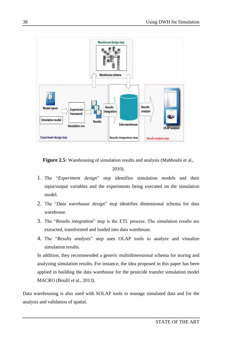
38 Using DWH for Simulation
STATE OF THE ART
Results integration step
Figure 2.5: Warehousing of simulation results and analysis (Mahboubi et al.,
2010).
1. The “Experiment design” step identifies simulation models and their
input/output variables and the experiments being executed on the simulation
model.
2. The “Data warehouse design” step identifies dimensional schema for data
warehouse.
3. The “Results integration” step is the ETL process. The simulation results are
extracted, transformed and loaded into data warehouse.
4. The “Results analysis” step uses OLAP tools to analyze and visualize
simulation results.
In addition, they recommended a generic multidimensional schema for storing and
analyzing simulation results. For instance, the idea proposed in this paper has been
applied in building the data warehouse for the pesticide transfer simulation model
MACRO (Boulil et al., 2013).
Data warehousing is also used with SOLAP tools to manage simulated data and for the
analysis and validation of spatial.
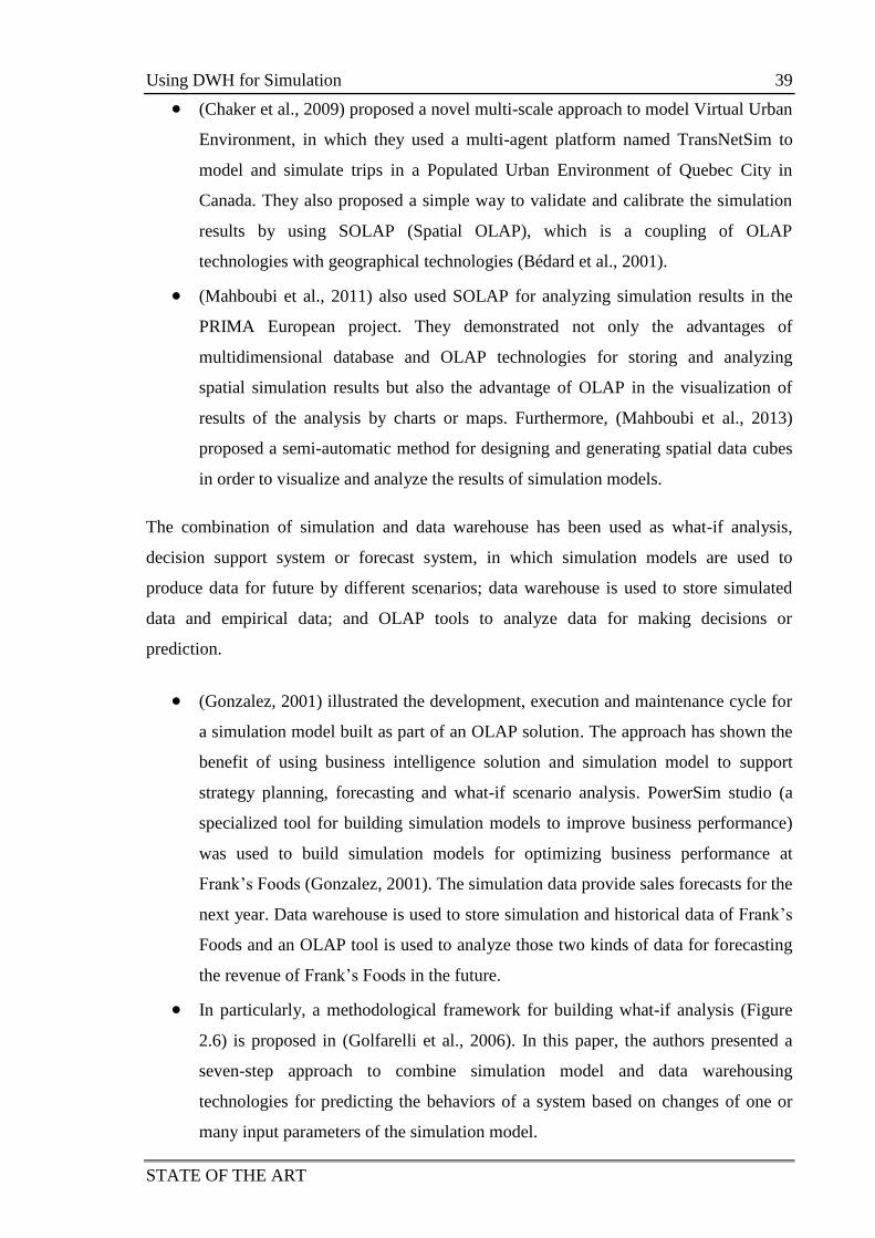
Using DWH for Simulation 39
STATE OF THE ART
(Chaker et al., 2009) proposed a novel multi-scale approach to model Virtual Urban
Environment, in which they used a multi-agent platform named TransNetSim to
model and simulate trips in a Populated Urban Environment of Quebec City in
Canada. They also proposed a simple way to validate and calibrate the simulation
results by using SOLAP (Spatial OLAP), which is a coupling of OLAP
technologies with geographical technologies (Bédard et al., 2001).
(Mahboubi et al., 2011) also used SOLAP for analyzing simulation results in the
PRIMA European project. They demonstrated not only the advantages of
multidimensional database and OLAP technologies for storing and analyzing
spatial simulation results but also the advantage of OLAP in the visualization of
results of the analysis by charts or maps. Furthermore, (Mahboubi et al., 2013)
proposed a semi-automatic method for designing and generating spatial data cubes
in order to visualize and analyze the results of simulation models.
The combination of simulation and data warehouse has been used as what-if analysis,
decision support system or forecast system, in which simulation models are used to
produce data for future by different scenarios; data warehouse is used to store simulated
data and empirical data; and OLAP tools to analyze data for making decisions or
prediction.
(Gonzalez, 2001) illustrated the development, execution and maintenance cycle for
a simulation model built as part of an OLAP solution. The approach has shown the
benefit of using business intelligence solution and simulation model to support
strategy planning, forecasting and what-if scenario analysis. PowerSim studio (a
specialized tool for building simulation models to improve business performance)
was used to build simulation models for optimizing business performance at
Frank’s Foods (Gonzalez, 2001). The simulation data provide sales forecasts for the
next year. Data warehouse is used to store simulation and historical data of Frank’s
Foods and an OLAP tool is used to analyze those two kinds of data for forecasting
the revenue of Frank’s Foods in the future.
In particularly, a methodological framework for building what-if analysis (Figure
2.6) is proposed in (Golfarelli et al., 2006). In this paper, the authors presented a
seven-step approach to combine simulation model and data warehousing
technologies for predicting the behaviors of a system based on changes of one or
many input parameters of the simulation model.
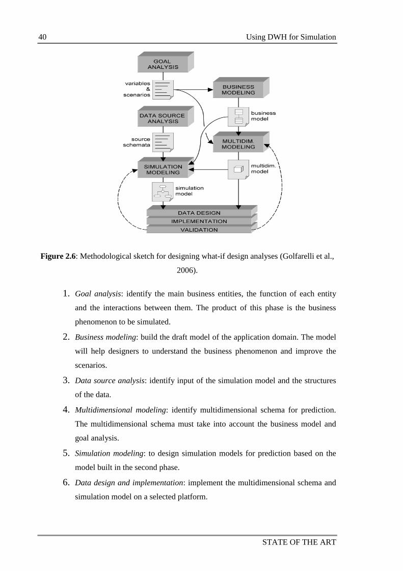
40 Using DWH for Simulation
STATE OF THE ART
Figure 2.6: Methodological sketch for designing what-if design analyses (Golfarelli et al.,
2006).
1. Goal analysis: identify the main business entities, the function of each entity
and the interactions between them. The product of this phase is the business
phenomenon to be simulated.
2. Business modeling: build the draft model of the application domain. The model
will help designers to understand the business phenomenon and improve the
scenarios.
3. Data source analysis: identify input of the simulation model and the structures
of the data.
4. Multidimensional modeling: identify multidimensional schema for prediction.
The multidimensional schema must take into account the business model and
goal analysis.
5. Simulation modeling: to design simulation models for prediction based on the
model built in the second phase.
6. Data design and implementation: implement the multidimensional schema and
simulation model on a selected platform.
Using DWH for Simulation 41
STATE OF THE ART
7. Validation: analyze and compare results of simulation model with real life data
(historical data).
The approach was applied in a selling products forecasting system for Orogel S.p.A
Company, Italia (Golfarelli and Rizzi, 2009).
In other studies, researchers used simulation models, multidimensional database
and OLAP tools to build decision support system or forecast system. Although
these studies only solve specific problems such as analyzing the patients' length of
stay in hospital and bed occupancy for the care of elderly patients - a healthcare
system (Vasilakis et al., 2008) or logistic systems (Ehmke et al., 2011), they
proposed approaches to collect and analyze observation data from the target
system, simulation results or the integration of both by using data warehouse and
OLAP technologies. Furthermore, these studies also show the advantages of the
data warehousing approach in handling, analyzing the outputs of simulation and
supporting decision making.
These research studies demonstrated the power of data warehouse and OLAP technologies
in integrating simulation results and analyzing the integrated data; the usefulness of the
combination of simulation and data warehousing technologies for building what-if system
or decision support system.
The researchers showed that applying DWH in building simulation systems that produce a
high volume of data is as well solution to solving issues: (1) how to manage and integrate
a high volume of data from different data sources (empirical data and simulation data);
(2): how to compare simulated results, which are produced from different experiment,
different parameter values and different versions of such models; and (3): how to
aggregate simulated result on different scales. Data granularity (cf. Section 2.4.3.5) is
another issue that was not mentioned in the articles examined while it is a very important
concern in designing a data warehouse "What level of data detail should be made available
in the dimensional model?"(Kimball and Ross, 2002) and in building a simulation model
"What level of model detail should be made available in modeling?" which I will present in
Chapter 4.
However, there is a challenge in deploying such systems in agent-based simulation
environments because there is no generic framework for the deployment and
implementation of database management tools in the existing agent-based platforms.
42 Conclusion
STATE OF THE ART
Indeed, it raises particular issues such as (1): what is the framework for applying DWH
technologies to agent-based simulation?; (2) how to store simulated data, which are
produced by agents into DWH?; and (3) how to used OLAP in agent-based model?.
Answers for those questions are presented in Chapter 3.
2.6 Conclusion
In Section 2.2 I presented an overview of agent-based simulation and the wide application
domain of agent-based simulation. I also summarized the challenges of agent-based
modeling, focusing on particular issues e.g. replication and experiments in simulation,
calibration and validation of agent-based model and aggregation of simulation data, which
stress the weakness of data management in agent-based modeling and simulation tools.
Furthermore, Section 2.3 is a presentation of the needed for a data driven approach in
agent-based modeling, the reasons why data must be managed and the limitation of agent-
based platform in data management. The main observation we made is that currently, the
design and simulation of models have greatly benefited from advances in computer science
through the popularized use of simulation platforms such as Netlogo (Wilensky, 1999),
Repast (Collier, 2003) or GAMA (Taillandier et al., 2012). This is not yet the case for the
management of data, which is still performed in an ad hoc manner, despite the advances in
the management of huge datasets (data warehousing solutions for instance).
Section 2.4 is an overview of the business intelligence solution. In this section, I presented
the basic terms and technologies of data warehousing, which is a powerful solution for
managing, integrating and analyzing high volumes of data. In Section 2.5, I demonstrated
the strength of data warehousing for integrating and analyzing simulation results and its
advantages for building what-if systems, forecasting systems or decision support systems.
Yet some challenges still exist in using such systems within agent-based modeling
approaches because there is no agent-based platform providing appropriate data
management facilities and integrating OLAP technologies for the implementation of what-
if, forecasting system or decision support systems. This state of affairs is rather damaging
if we consider recent tendencies towards the use of data-driven approaches in simulation
aimed at injecting more and more data into simulated models.
In brief, I mentioned two major issues in this chapter:

Conclusion 43
STATE OF THE ART
What general architecture could serve the following purposes: model and execute
multi-agents simulations, manage input and output data of simulations, integrate
data from different sources and enable to analyze high volume of data?
How to introduce DWH and OLAP technologies into a multi-agent based
simulation system having to face huge amount of data?
The solution to these issues will be presented in the next chapter.

44 Conclusion
STATE OF THE ART
A SOLUTION TO MANAGE AND ANALYZE AGENT-BASED MODELS DATA
TRUONG Minh Thai 45
Chapter 3 A SOLUTION TO MANAGE AND
ANALYZE AGENT-BASED MODELS
DATA
Table of contents
3.1 Introduction ........................................................................................................... 47
3.2 A Logical Framework to Manage and Analyze Data for Agent-based Models .... 48
3.2.1 Computer simulation system ................................................................... 48
3.2.2 Combination Framework of Business Intelligence Solution and Multi-
agent Platform ........................................................................................................ 49
3.2.2.1 Simulation system ..................................................................... 51
3.2.2.2 Data warehouse system ............................................................. 52
3.2.2.3 Decision support system ............................................................ 52
3.3 Implementation of CFBM with the GAMA Platform ........................................... 53
3.3.1 Introduction to GAMA ............................................................................ 53
3.3.2 Software Architecture of CFBM in GAMA ............................................ 56
3.3.2.1 Presentation tier ......................................................................... 57
3.3.2.2 Logic tier ................................................................................... 58
3.3.2.3 Data tier ..................................................................................... 59
3.3.3 Database Features in GAMA................................................................... 59
3.3.3.1 Access Relational data .............................................................. 60
A SOLUTION TO MANAGE AND ANALYZE AGENT-BASED MODELS DATA
46 TRUONG Minh Thai
3.3.3.2 Retrieve Multidimensional database via OLAP ........................ 62
3.4 Discussion .............................................................................................................. 65
3.4.1 Advantages of CFBM .............................................................................. 65
3.4.2 Limitations of CFBM .............................................................................. 67
3.5 Conclusion ............................................................................................................. 67
Introduction 47
A SOLUTION TO MANAGE AND ANALYZE AGENT-BASED MODELS DATA
3.1 Introduction
In this chapter, I present a solution addressing the requirements concerning data
management and analysis in agent-based application, which are mentioned in chapter 2.
First, we are dealing with the question "What general architecture could serve the
following purposes: to model and execute multi-agents simulations, manage input and
output data of simulations, integrate data from different sources and enable to analyze
high volume of data?" Before than proposing a solution, we studied several articles and
solutions related to simulation, management and analysis of big data. In several other
domains, BI solutions are a good way to handle and analyze big data. In particular, for the
development of decision support systems or prediction systems based on simulation
approaches, data warehouse (DW), online analytical processing (OLAP) technologies and
simulation would represent a good solution. Data warehouse and analysis tools as a BI
solution can help users to manage a large amount of simulation data and make several data
analyses that support the decision-making processes (Inmon, 2005; Kimball and Ross,
2002). As I presented in Section 2.5 of Chapter 2, the combination of simulation tools and
data warehousing technologies is a promising solution to store and analyze simulation
results. The Section 2.5 demonstrates the practical possibility and the usefulness of the
combination of simulation, data warehouse and OLAP technologies. These studies also
show the need of a general framework that has, as far as we are aware, not yet been
proposed in the literature.
The second question addressed is "How to introduce DWH and OLAP technologies into a
multi-agent based simulation system having to face huge amount of data?" The solution I
propose in this thesis is the improvement of agent-based platforms by adding new features,
such as intensive interactions with data warehouse systems as presented in Section 3.3.
In the following sections, I first define a computer simulation system, in which, I propose
four major components to construct a software simulation system integrating data
management. In Section 3.2, I design the logical architecture of a framework combining BI
solution and multi-agent platform based on our definition of computer simulation system.
That is my proposal to address the first question. The solution proposed to the second
question is presented in Section 3.3, which details an implementation of the logical
48 A Logical Framework to Manage and Analyze Data for Agent-based Models
A SOLUTION TO MANAGE AND ANALYZE AGENT-BASED MODELS DATA
framework in the GAMA multi-agent based simulation platform. Discussion on advantages
and disadvantages of our framework concludes this chapter.
3.2 A Logical Framework to Manage and Analyze Data for
Agent-based Models
3.2.1 Computer simulation system
In Section 2.2.1.2, I presented computer simulation as defined by Fishwick (1997), the
logic of simulation methodology proposed by Gilbert and Troitzsch (2005) and its
improvement for data-driven approach proposed by Hassan, Pavón, et al. (2010).
Computer simulation (Fishwick, 1997) deals with the processes of abstraction (design of a
model of an actual or theoretical physical system), simulation (execution of the model on a
computer), and similarity/validation (analysis of the execution output). Moreover, we
introduce one more process that concerns data management to fully support the logic of
simulation for data-driven approaches for two main reasons: (1) in a data-driven
perspective there is a need for data management (collected data from target system as well
as simulated data); (2) the need to take into account data in design, initialization and
validation. The lack of attention to data is one of the key pitfalls of agent-based modeling
as mentioned in Section 2.3. For dealing with data-driven approaches in agent-based
modeling, we define a computer simulation system based on Fishwick’s definition and
integrating "the logic of simulation" approach from (Gilbert and Troitzsch, 2005; Hassan et
al., 2010b) as below:
A data-compliant computer simulation system is a computation system with four
components and the intercommunications between them:
Model design tool: a software environment that supports a modeling language,
notations and user interface for modeling an actual or theoretical physical system.
Model execution tool: a software environment that can run models.
Execution analysis tool: a software environment that supports statistical analysis
features for the analysis of output data of models.
Database management tool: a software environment that supports appropriate
database and database management features for all components in the system.
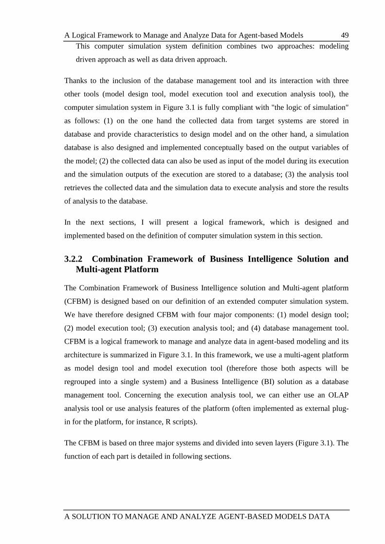
A Logical Framework to Manage and Analyze Data for Agent-based Models 49
A SOLUTION TO MANAGE AND ANALYZE AGENT-BASED MODELS DATA
This computer simulation system definition combines two approaches: modeling
driven approach as well as data driven approach.
Thanks to the inclusion of the database management tool and its interaction with three
other tools (model design tool, model execution tool and execution analysis tool), the
computer simulation system in Figure 3.1 is fully compliant with "the logic of simulation"
as follows: (1) on the one hand the collected data from target systems are stored in
database and provide characteristics to design model and on the other hand, a simulation
database is also designed and implemented conceptually based on the output variables of
the model; (2) the collected data can also be used as input of the model during its execution
and the simulation outputs of the execution are stored to a database; (3) the analysis tool
retrieves the collected data and the simulation data to execute analysis and store the results
of analysis to the database.
In the next sections, I will present a logical framework, which is designed and
implemented based on the definition of computer simulation system in this section.
3.2.2 Combination Framework of Business Intelligence Solution and
Multi-agent Platform
The Combination Framework of Business Intelligence solution and Multi-agent platform
(CFBM) is designed based on our definition of an extended computer simulation system.
We have therefore designed CFBM with four major components: (1) model design tool;
(2) model execution tool; (3) execution analysis tool; and (4) database management tool.
CFBM is a logical framework to manage and analyze data in agent-based modeling and its
architecture is summarized in Figure 3.1. In this framework, we use a multi-agent platform
as model design tool and model execution tool (therefore those both aspects will be
regrouped into a single system) and a Business Intelligence (BI) solution as a database
management tool. Concerning the execution analysis tool, we can either use an OLAP
analysis tool or use analysis features of the platform (often implemented as external plug-
in for the platform, for instance, R scripts).
The CFBM is based on three major systems and divided into seven layers (Figure 3.1). The
function of each part is detailed in following sections.
50 A Logical Framework to Manage and Analyze Data for Agent-based Models
A SOLUTION TO MANAGE AND ANALYZE AGENT-BASED MODELS DATA
Sim
ula
tion s
yst
em
Simulation
database
Empirical
database
Multi-agent simulation models
SQL-agent
Simulation interface
Dat
a w
areh
ouse
syst
em
Data mart
ETL
Data warehouse
Data mart Data mart
Dec
isio
n s
upport
syst
em
Multi-agent analysis models
SQL-agent MDX-agent
OLAP analysis tools
Analysis interface
Sim
ula
tion
layer
Dat
a so
urc
e
layer
Dat
a st
agin
g
layer
Dat
a w
areh
ouse
layer
Anal
ysi
s
layer
Vie
w
layer
Vie
w
layer
RetrieveRetriev
e/Update
Cal
l a
model
Extract
Retriev
e
Load
Load
Retrieve
Retriev
e/
Update
Extract
Figure 3.1: CFBM architecture
A Logical Framework to Manage and Analyze Data for Agent-based Models 51
A SOLUTION TO MANAGE AND ANALYZE AGENT-BASED MODELS DATA
Note:
- DW : Data Warehouse
- SQL : Structured Query Language
- OLAP : OnLine Analysis Processing
- ETL : Extract – Transform – Load
- MDX : Multi Dimensional eXpressions
- SQL-agent : Agent supporting SQL features to query data.
- MDX-agent: Agent supporting MDX features to query data.
- : Data flow.
- : Intercommunication
3.2.2.1 Simulation system
The simulation system includes at the same time the model design (that we won’t detail at
this stage) and the model execution parts. It executes simulations and handles their
input/output data. From a data management point of view, it plays the role of an OnLine
Transaction Processing (OLTP) or of an operational source system. It is considered as an
outside part of the data warehouse (Kimball and Ross, 2002).
Three layers with five components compose the simulation system. The simulation
interface is a user environment that helps the modeler to design and implement his
models, execute simulations and visualize some observations selected (through the design
of the graphical interface) from the simulation. Multi-agent simulation models are used
to simulate phenomena that the modeler aims at studying. The SQL-agent plays the role of
the database management tool and can access a relational database. They can be considered
as intermediary in between the simulation system and the data management part. It is a
particular kind of agents that supports Structured Query Language (SQL) functions to
retrieve simulation inputs from the database containing empirical data (Empirical database)
as well as parameter values and scenarios (Simulation database). SQL-agent is able to store
output simulation data. SQL-agent are also able to transform data (in particular the data
type) from simulation model to relational database, and conversely. Empirical database and
Simulation database are relational databases. Empirical database is used to store
empirical data gathered from the target system that are needed for the simulation and
analysis phases. Simulation database is used to manage the simulation models, simulation
scenarios and output results of the simulation models. These two data sources (Empirical
52 A Logical Framework to Manage and Analyze Data for Agent-based Models
A SOLUTION TO MANAGE AND ANALYZE AGENT-BASED MODELS DATA
as well as Simulation databases) will be used to feed the second part of the framework,
namely the Data warehouse system.
3.2.2.2 Data warehouse system
The data warehouse system is crucial in our approach as it enables to integrate data from
different sources (simulation data as well as empirical data from the target systems). It is
also used as data store to provide data to the decision support systems. The data warehouse
system is divided into three parts. The ETL (Extract-Transform-Load) is a set of processes
with three responsibilities: it extracts all kind of data (empirical data and simulation data)
from the simulation system; then, ETL transforms the extracted data into an appropriate
data format; finally, it loads the transferred data into the data warehouse. The data
warehouse is a relational database used to store historical data loaded from simulation
systems and from other sources (empirical sources for instance) by the ETL. The data
mart is a subset of data stored in the data warehouse used as a data source for the concrete
analysis requirement. We can create several data marts depending on the analysis
requirements. The data mart is a multidimensional database, which is designed based on
multidimensional approach. Therefore, the structure of the data mart is presented using star
join, fact tables and dimension tables to present. Thanks to its multidimensional structure,
data marts are particularly useful to help users to improve the performance of analytic
processes.
3.2.2.3 Decision support system
In CFBM, the decision support system component is a software environment supporting
analysis, visualization of results and decision-making. In our design, we propose to use
either existing OLAP analysis tools or a multi-agent platform equipped with analysis
features or a combination of both. The decision support system of CFBM is composed of
four parts. The analysis interface is a graphical user interface used to handle analysis
models and visualize results. The multi-agent analysis models are a set of tools dedicated
to the analysis of multi-agent simulations, they are created based on analysis requirements
and handled via the analysis interface. One of the key features of our framework is the fact
that the architecture should be independent from the simulation. However, given that we
are using the same platform for model design/implementation, model execution and part of
the analysis, multi-agent analysis tools and multi-agent simulation models are implemented
using the same modeling language, hence it facilitates the communication among the
different components.. The MDX-agent is a special kind of agents, which supports
Implementation of CFBM with the GAMA Platform 53
A SOLUTION TO MANAGE AND ANALYZE AGENT-BASED MODELS DATA
MultiDimensional eXpressions (MDX) functions to query data from a multidimensional
database. The MDX-agent serves as a bridge in between multi-agent analysis models and
data marts. It is used to retrieve data from the data marts into the data warehouse system.
The OLAP analysis tools could be any analysis software that supports OLAP operators.
The multi-agent analysis tools may need several kind of retrievals such as: (1) to retrieve
detailed data from relational databases (simulation database or empirical database) for
analyses for instance for comparison in-between models or in-between a model output and
gathered empirical data; (2) to retrieve pre-aggregated data from multidimensional
databases (data marts) for multi-scale analysis. Hence in the decision support system, we
designed two kinds of database access agent: on the one hand SQL-agent uses structured
query language to retrieve data from relational database and on the other hand MDX-agent
uses multidimensional expressions to query data from multidimensional database.
Therefore, the multi-agent analysis tools can also use SQL-agents (same SQL-agents as in
the simulation system) or MDX agents to appropriately access data.
The key points of the CFBM architecture are that it contains and adapts the four features of
a computer simulation system (model design, model execution, execution analysis, and
database management). The data warehouse manages the related data. The analysis models
and simulation models can interact with each other. Using the CFBM architecture, we can
build a simulation system not only suitable from a conceptual modeling approach but also
from a data driven approach. Furthermore, the CFBM brings certain benefits for building
simulation system with complex requirements such as integrating and analyzing high
volume of data thanks to the data warehouse features. All these functions are integrated
into the same multi-agent platform, GAMA.
3.3 Implementation of CFBM with the GAMA Platform
3.3.1 Introduction to GAMA
GAMA stands for Generic Agent-based Modeling Architecture. It is an open source
modeling and development environment for building agent-based simulations. GAMA is
developed since 2007 by the UMMISCO research team with several partners in France and
Vietnam [Refs]14
. The current version of GAMA (GAMA 1.6.1) supports:
14
https://code.google.com/p/gama-platform/
54 Implementation of CFBM with the GAMA Platform
A SOLUTION TO MANAGE AND ANALYZE AGENT-BASED MODELS DATA
Building large-scale models written in the GAML (GAma Modeling Language)
agent-oriented language, with an optional graphical modeling tool to support rapid
design and prototyping.
Instantiating agents from GIS data, databases or files and executing large-scale
simulations (up to millions of agents).
Coupling in between discrete models or continuous topological layers,
multiple levels of agency and multiple paradigms (mathematical equations, control
architectures, and finite state machines).
Defining different experiments on models, with their own inputs and outputs, and
exploring their parameters space for calibration and validation.
Designing rich user interfaces that support elaborate inspections on agents, user-
controlled actions and panels, and multiple multi-layer 2D/3D displays and aspects.
Before than to choose GAMA to implement our framework, we evaluated the platform on
several dimensions and in particular the possibility to integrate the new features as well as
the possibility to improve incrementally the implemented framework in the future. In order
to assess the GAMA platform, we chose the development priority criteria highlighted in
(Railsback et al., 2006) presented in details in Table 3.1.
Table 3.1: Evaluation of the development priorities of the GAMA platform
Development priority Observation
Fulfill the most critical,
immediate need
GAMA has development guide document, user guide
documents with several model examples.
Continue developing and
maintaining — how to
document and template
models
Since 2007 until now, GAMA has been continuously
updated every year, usually twice a year. In addition, it
provides templates to help create projects and models.
Integrate the software
library with an IDE such as
Eclipse
GAMA is open source software and comes as an Eclipse
RCP (Rich Client Platform) project. Furthermore, the
GAMA user interface is also based on Eclipse platform.
Revive the “framework” GAMA is a high-level modeling environment, and has its
Implementation of CFBM with the GAMA Platform 55
A SOLUTION TO MANAGE AND ANALYZE AGENT-BASED MODELS DATA
part of the platform.
Establish the software
library as one part of an
overall process leading
modelers through the model
design, analysis, and
publication cycle. The
platform provide an ABM
modeling language
(Railsback et al., 2006)
own modeling language called GAML. It is an object-
oriented programming language for modeling agents and
environment.
Make sure the framework
accommodate complex,
multilevel models
GAMA provides a concept called Nested Species
allowing modelers to design hierarchies of agents where
micro-agents belong to a macro-agent enabling multilevel
models.
Provide powerful tools for
generating statistical outputs
Although the tools for managing, integrating and
analyzing the output of simulation were not so strong,
they have been improved by the time. For instance,
GAMA provides the possibility to couple agent-based
models with R benefiting from the statistical features of
the R platform.
Provide powerful tools for
setting up and executing
simulation experiments
GAMA provides two types of experiments:
- GUI: experiments with a graphical user interface,
which displays its input parameters and outputs.
- batch: allow to set up a series of simulations. It looks
like the model analysis feature of OpenMOLE15
to
help modelers in experimental design, model
replication, calibration and so on.
Look for ways to improve
the trade-off between ease
Developers of GAMA are very concerned with the
flexibility of the platform. They developed a high level
15
http://www.openmole.org/
56 Implementation of CFBM with the GAMA Platform
A SOLUTION TO MANAGE AND ANALYZE AGENT-BASED MODELS DATA
of use and generality of
platform
modeling language and graphical tools to represent
agents and environments as well as tools to observe
agents’ status.
Research technologies for
testing, analyzing, and
understanding ABMs
The technologies for testing, analyzing and
understanding ABMs have been taken into account in
GAMA. For instance, GAMA supports code verification
techniques. Furthermore, debugging, validation,
calibration and analysis features are being developed.
From the observation, GAMA adequately supports the development of new features. As
GAMA is built on several Eclipse Java projects, implementation of an additional feature
can take the form of a plug-in project in the Eclipse environment. Developers can therefore
develop their own features for GAMA by implementing new skills, statements, species
(agents) or operations16
. GAMA is also well documented, providing guide for developers
as well as models library. We also have to notice that GAMA has been already updated
twice a year giving us the opportunity to improve the CFBM framework.
We have to notice however that even if the choice of GAMA was partially guided by
cooperation reasons in between IRIT and UMMISCO, Netlogo and Repast platforms,
which are the most commonly used agent-based simulation platforms are also relevant to
implement the CFBM. For instance, Netlogo allows users to write new commands and
report in Java by adding extensions17
while Repast18
is an open source platform written in
Java to which we can also add new package features.
3.3.2 Software Architecture of CFBM in GAMA
The CFBM has been implemented in GAMA within a three-tier architecture as depicted on
Figure 3.2, in which GAMA plays two roles: (1) simulation system; and (2) decision
support system. The roles of the tiers in Figure 3.2 are presented as follows:
16
https://code.google.com/p/gama-platform/wiki/CreationPlugins15
17 http://ccl.northwestern.edu/netlogo/docs/
18 http://repast.sourceforge.net/
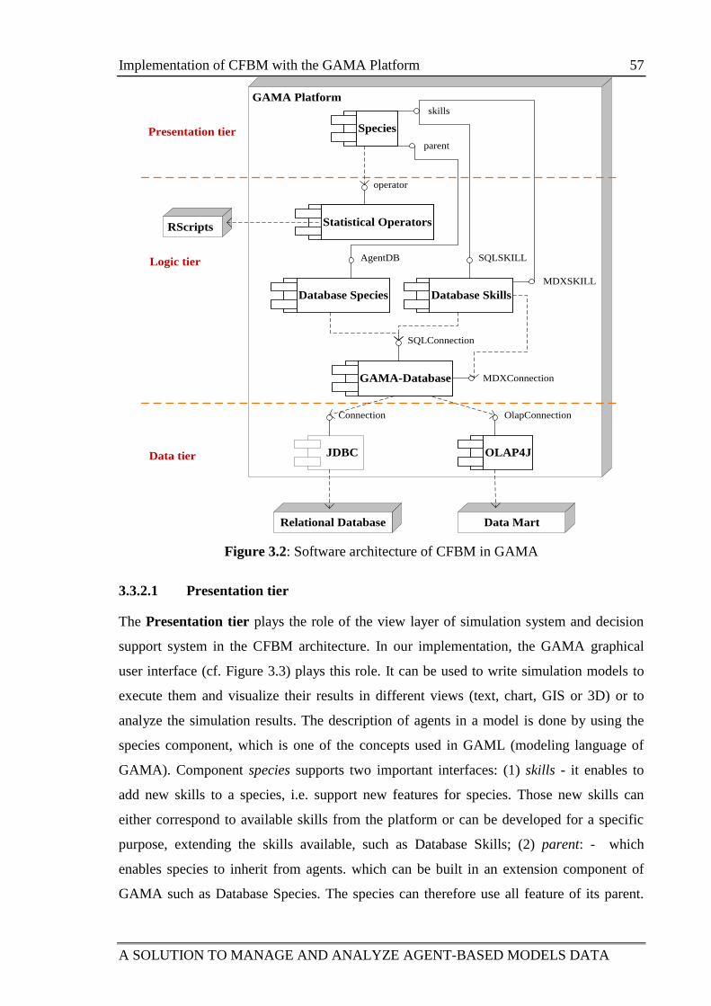
Implementation of CFBM with the GAMA Platform 57
A SOLUTION TO MANAGE AND ANALYZE AGENT-BASED MODELS DATA
GAMA Platform
Species
Statistical OperatorsRScripts
Database Species Database Skills
operator
parent
skills
AgentDB SQLSKILL
MDXSKILL
OLAP4J
Data Mart
Logic tier
Presentation tier
Data tier
GAMA-Database
SQLConnection
MDXConnection
Relational Database
JDBC
Connection OlapConnection
Figure 3.2: Software architecture of CFBM in GAMA
3.3.2.1 Presentation tier
The Presentation tier plays the role of the view layer of simulation system and decision
support system in the CFBM architecture. In our implementation, the GAMA graphical
user interface (cf. Figure 3.3) plays this role. It can be used to write simulation models to
execute them and visualize their results in different views (text, chart, GIS or 3D) or to
analyze the simulation results. The description of agents in a model is done by using the
species component, which is one of the concepts used in GAML (modeling language of
GAMA). Component species supports two important interfaces: (1) skills - it enables to
add new skills to a species, i.e. support new features for species. Those new skills can
either correspond to available skills from the platform or can be developed for a specific
purpose, extending the skills available, such as Database Skills; (2) parent: - which
enables species to inherit from agents. which can be built in an extension component of
GAMA such as Database Species. The species can therefore use all feature of its parent.
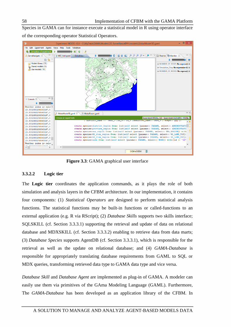
58 Implementation of CFBM with the GAMA Platform
A SOLUTION TO MANAGE AND ANALYZE AGENT-BASED MODELS DATA
Species in GAMA can for instance execute a statistical model in R using operator interface
of the corresponding operator Statistical Operators.
Figure 3.3: GAMA graphical user interface
3.3.2.2 Logic tier
The Logic tier coordinates the application commands, as it plays the role of both
simulation and analysis layers in the CFBM architecture. In our implementation, it contains
four components: (1) Statistical Operators are designed to perform statistical analysis
functions. The statistical functions may be built-in functions or called-functions to an
external application (e.g. R via RScript); (2) Database Skills supports two skills interface;
SQLSKILL (cf. Section 3.3.3.1) supporting the retrieval and update of data on relational
database and MDXSKILL (cf. Section 3.3.3.2) enabling to retrieve data from data marts;
(3) Database Species supports AgentDB (cf. Section 3.3.3.1), which is responsible for the
retrieval as well as the update on relational database; and (4) GAMA-Database is
responsible for appropriately translating database requirements from GAML to SQL or
MDX queries, transforming retrieved data type to GAMA data type and vice versa.
Database Skill and Database Agent are implemented as plug-in of GAMA. A modeler can
easily use them via primitives of the GAma Modeling Language (GAML). Furthermore,
The GAMA-Database has been developed as an application library of the CFBM. In
Implementation of CFBM with the GAMA Platform 59
A SOLUTION TO MANAGE AND ANALYZE AGENT-BASED MODELS DATA
addition, we can add several database functions in the same way we did with the SQL-
agent and MDX-agent based on this application library.
In addition, the logic tier also plays the role of data staging layer of data warehouse
system; therefore, ETL processes can be done by using file features and SQLSKILL or
AgentDB in GAMA or we can use the other ETL tools outside GAMA to perform ETL
processes. In practice, we used file features and SQL-agent in GAMA to transform data
from shape files19
or .csv (Comma Separated Values) text files to relational databases or to
transform data between relational databases such as SQLite, PostgreSQL, MySQL or
MSSQL.
3.3.2.3 Data tier
The Data tier plays two roles in the framework: data source layer and data warehouse
layer. The main functions of this tier are to store and retrieve data from a database or a file
system using JDBC and OLAP4J. JDBC is a Java API enabling to connect to and querying
data from relational databases. OLAP4J20
is a quite similar Java API enabling to connect to
and query data from a multidimensional database. As developed beforehand, Relational
database corresponds to several database like Empirical database, Simulation database or
Data warehouse (cf. Section 3.2.2) and Data mart enables to support the analysis and
decision support system (cf. Section 3.2.2.3).
3.3.3 Database Features in GAMA
Thanks to added database features of GAMA, we can create agents and define the
environment of the simulation by using data selected from database, store simulation
results into relational databases or query data from multidimensional database. Database
features are implemented in the irit.gaml.extensions.database GAMA plug-in with the
following features:
1. Agents can execute SQL queries (create, insert, select, update, drop, delete) to
various kinds of DBMS.
19
http://www.esri.com/library/whitepapers/pdfs/shapefile.pdf
20 http://www.olap4j.org/
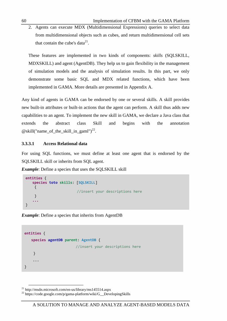
60 Implementation of CFBM with the GAMA Platform
A SOLUTION TO MANAGE AND ANALYZE AGENT-BASED MODELS DATA
2. Agents can execute MDX (Multidimensional Expressions) queries to select data
from multidimensional objects such as cubes, and return multidimensional cell sets
that contain the cube's data21
.
These features are implemented in two kinds of components: skills (SQLSKILL,
MDXSKILL) and agent (AgentDB). They help us to gain flexibility in the management
of simulation models and the analysis of simulation results. In this part, we only
demonstrate some basic SQL and MDX related functions, which have been
implemented in GAMA. More details are presented in Appendix A.
Any kind of agents in GAMA can be endorsed by one or several skills. A skill provides
new built-in attributes or built-in actions that the agent can perform. A skill thus adds new
capabilities to an agent. To implement the new skill in GAMA, we declare a Java class that
extends the abstract class Skill and begins with the annotation
@skill("name_of_the_skill_in_gaml")22
.
3.3.3.1 Access Relational data
For using SQL functions, we must define at least one agent that is endorsed by the
SQLSKILL skill or inherits from SQL agent.
Example: Define a species that uses the SQLSKILL skill
Example: Define a species that inherits from AgentDB
21
http://msdn.microsoft.com/en-us/library/ms145514.aspx 22
https://code.google.com/p/gama-platform/wiki/G__DevelopingSkills
entities {
species agentDB parent: AgentDB {
//insert your descriptions here
}
...
}
...
}
entities { species toto skills: [SQLSKILL] { //insert your descriptions here } ... }
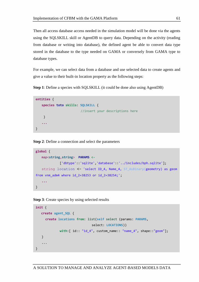
Implementation of CFBM with the GAMA Platform 61
A SOLUTION TO MANAGE AND ANALYZE AGENT-BASED MODELS DATA
Then all access database access needed in the simulation model will be done via the agents
using the SQLSKILL skill or AgentDB to query data. Depending on the activity (reading
from database or writing into database), the defined agent be able to convert data type
stored in the database to the type needed on GAMA or conversely from GAMA type to
database types.
For example, we can select data from a database and use selected data to create agents and
give a value to their built-in location property as the following steps:
Step 1: Define a species with SQLSKILL (it could be done also using AgentDB)
Step 2: Define a connection and select the parameters
Step 3: Create species by using selected results
init {
create agent_SQL {
create locations from: list(self select (params: PARAMS,
select: LOCATIONS))
with:[ id:: "id_4", custom_name:: "name_4", shape::"geom"];
}
...
}
global {
map<string,string> PARAMS <-
['dbtype'::'sqlite','database'::'../includes/bph.sqlite'];
string location <- 'select ID_4, Name_4, ST_AsBinary(geometry) as geom
from vnm_adm4 where id_2=38253 or id_2=38254;';
...
}
entities {
species toto skills: SQLSKILL {
//insert your descriptions here
}
...
}
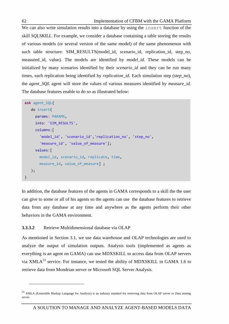
62 Implementation of CFBM with the GAMA Platform
A SOLUTION TO MANAGE AND ANALYZE AGENT-BASED MODELS DATA
We can also write simulation results into a database by using the insert function of the
skill SQLSKILL. For example, we consider a database containing a table storing the results
of various models (or several version of the same model) of the same phenomenon with
such table structure: SIM_RESULTS(model_id, scenario_id, replication_id, step_no,
measured_id, value). The models are identified by model_id. These models can be
initialized by many scenarios identified by their scenario_id and they can be run many
times, each replication being identified by replication_id. Each simulation step (step_no),
the agent_SQL agent will store the values of various measures identified by measure_id.
The database features enable to do so as illustrated below:
In addition, the database features of the agents in GAMA corresponds to a skill the the user
can give to some or all of his agents so the agents can use the database features to retrieve
data from any database at any time and anywhere as the agents perform their other
behaviors in the GAMA environment.
3.3.3.2 Retrieve Multidimensional database via OLAP
As mentioned in Section 3.1, we use data warehouse and OLAP technologies are used to
analyze the output of simulation outputs. Analysis tools (implemented as agents as
everything is an agent on GAMA) can use MDXSKILL to access data from OLAP servers
via XMLA23
service. For instance, we tested the ability of MDXSKILL in GAMA 1.6 to
retrieve data from Mondrian server or Microsoft SQL Server Analysis.
23 XMLA (Extensible Markup Language for Analysis) is an industry standard for retrieving data from OLAP server or Data mining
server.
ask agent_SQL{
do insert(
params: PARAMS,
into: 'SIM_RESULTS',
columns:[
'model_id', 'scenario_id','replication_no', 'step_no',
'measure_id', 'value_of_measure'];
values:[
model_id, scenario_id, replicate, time,
measure_id, value_of_measure] ;
);
}
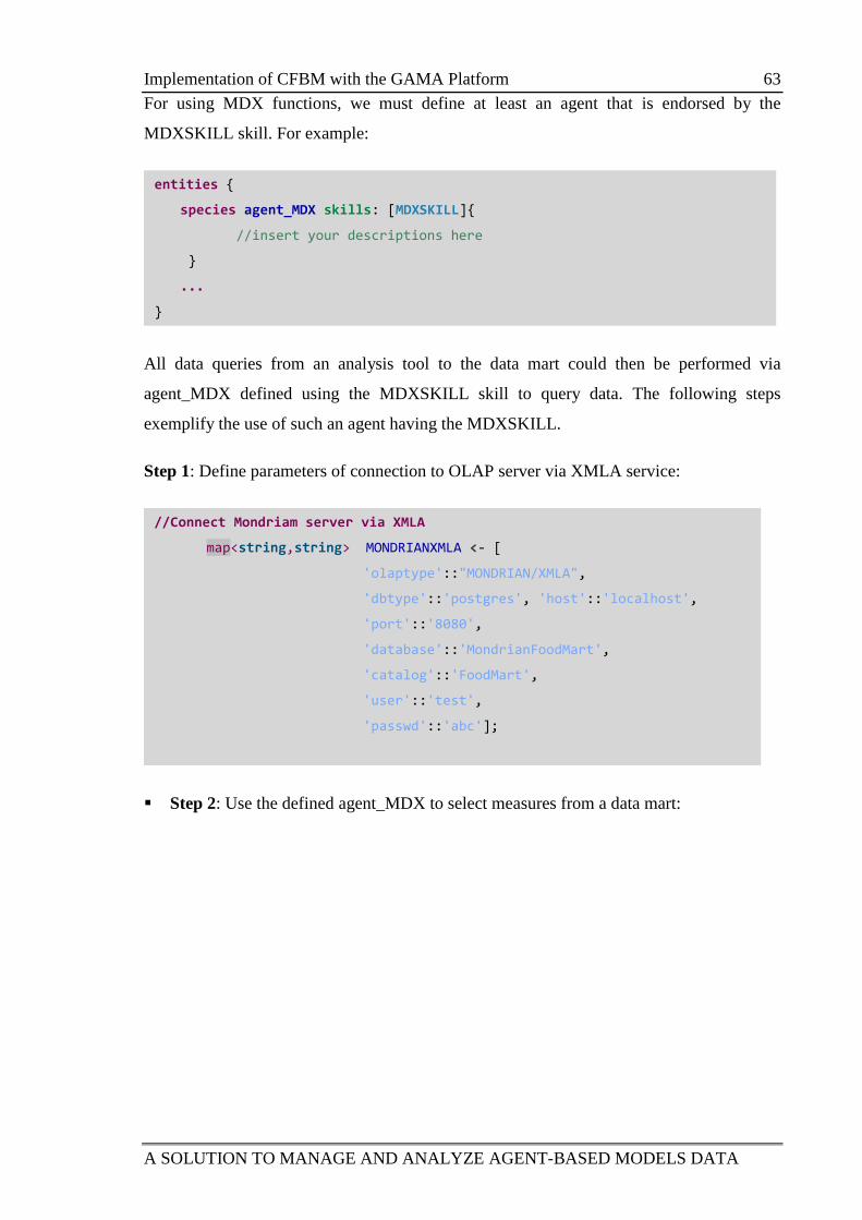
Implementation of CFBM with the GAMA Platform 63
A SOLUTION TO MANAGE AND ANALYZE AGENT-BASED MODELS DATA
For using MDX functions, we must define at least an agent that is endorsed by the
MDXSKILL skill. For example:
All data queries from an analysis tool to the data mart could then be performed via
agent_MDX defined using the MDXSKILL skill to query data. The following steps
exemplify the use of such an agent having the MDXSKILL.
Step 1: Define parameters of connection to OLAP server via XMLA service:
Step 2: Use the defined agent_MDX to select measures from a data mart:
//Connect Mondriam server via XMLA
map<string,string> MONDRIANXMLA <- [
'olaptype'::"MONDRIAN/XMLA",
'dbtype'::'postgres', 'host'::'localhost',
'port'::'8080',
'database'::'MondrianFoodMart',
'catalog'::'FoodMart',
'user'::'test',
'passwd'::'abc'];
entities {
species agent_MDX skills: [MDXSKILL]{
//insert your descriptions here
}
...
}
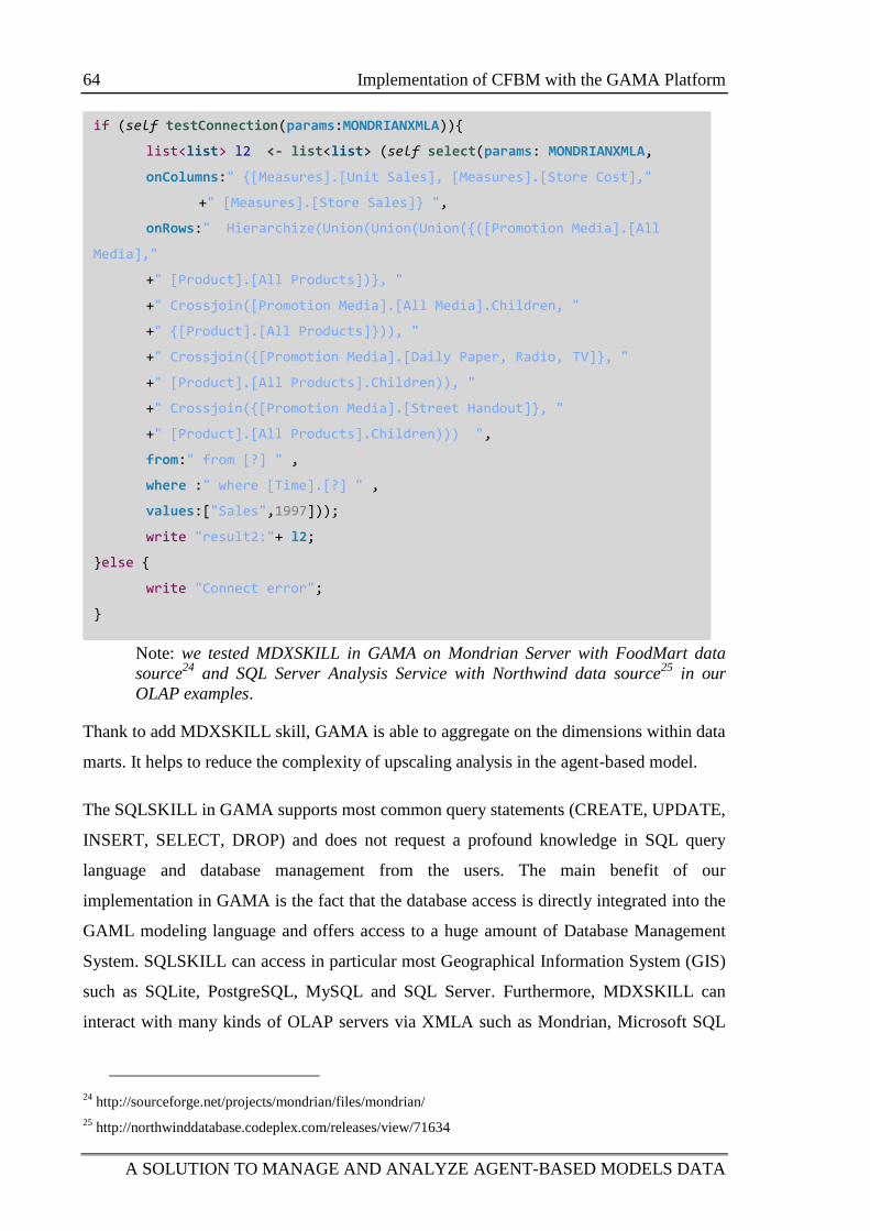
64 Implementation of CFBM with the GAMA Platform
A SOLUTION TO MANAGE AND ANALYZE AGENT-BASED MODELS DATA
Note: we tested MDXSKILL in GAMA on Mondrian Server with FoodMart data
source24
and SQL Server Analysis Service with Northwind data source25
in our
OLAP examples.
Thank to add MDXSKILL skill, GAMA is able to aggregate on the dimensions within data
marts. It helps to reduce the complexity of upscaling analysis in the agent-based model.
The SQLSKILL in GAMA supports most common query statements (CREATE, UPDATE,
INSERT, SELECT, DROP) and does not request a profound knowledge in SQL query
language and database management from the users. The main benefit of our
implementation in GAMA is the fact that the database access is directly integrated into the
GAML modeling language and offers access to a huge amount of Database Management
System. SQLSKILL can access in particular most Geographical Information System (GIS)
such as SQLite, PostgreSQL, MySQL and SQL Server. Furthermore, MDXSKILL can
interact with many kinds of OLAP servers via XMLA such as Mondrian, Microsoft SQL
24
http://sourceforge.net/projects/mondrian/files/mondrian/
25 http://northwinddatabase.codeplex.com/releases/view/71634
if (self testConnection(params:MONDRIANXMLA)){
list<list> l2 <- list<list> (self select(params: MONDRIANXMLA,
onColumns:" {[Measures].[Unit Sales], [Measures].[Store Cost],"
+" [Measures].[Store Sales]} ",
onRows:" Hierarchize(Union(Union(Union({([Promotion Media].[All
Media],"
+" [Product].[All Products])}, "
+" Crossjoin([Promotion Media].[All Media].Children, "
+" {[Product].[All Products]})), "
+" Crossjoin({[Promotion Media].[Daily Paper, Radio, TV]}, "
+" [Product].[All Products].Children)), "
+" Crossjoin({[Promotion Media].[Street Handout]}, "
+" [Product].[All Products].Children))) ",
from:" from [?] " ,
where :" where [Time].[?] " ,
values:["Sales",1997]));
write "result2:"+ l2;
}else {
write "Connect error";
}
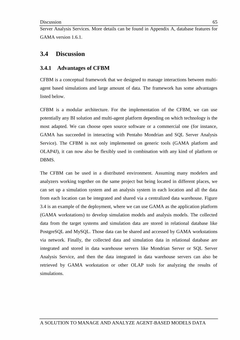
Discussion 65
A SOLUTION TO MANAGE AND ANALYZE AGENT-BASED MODELS DATA
Server Analysis Services. More details can be found in Appendix A, database features for
GAMA version 1.6.1.
3.4 Discussion
3.4.1 Advantages of CFBM
CFBM is a conceptual framework that we designed to manage interactions between multi-
agent based simulations and large amount of data. The framework has some advantages
listed below.
CFBM is a modular architecture. For the implementation of the CFBM, we can use
potentially any BI solution and multi-agent platform depending on which technology is the
most adapted. We can choose open source software or a commercial one (for instance,
GAMA has succeeded in interacting with Pentaho Mondrian and SQL Server Analysis
Service). The CFBM is not only implemented on generic tools (GAMA platform and
OLAP4J), it can now also be flexibly used in combination with any kind of platform or
DBMS.
The CFBM can be used in a distributed environment. Assuming many modelers and
analyzers working together on the same project but being located in different places, we
can set up a simulation system and an analysis system in each location and all the data
from each location can be integrated and shared via a centralized data warehouse. Figure
3.4 is an example of the deployment, where we can use GAMA as the application platform
(GAMA workstations) to develop simulation models and analysis models. The collected
data from the target systems and simulation data are stored in relational database like
PostgreSQL and MySQL. Those data can be shared and accessed by GAMA workstations
via network. Finally, the collected data and simulation data in relational database are
integrated and stored in data warehouse servers like Mondrian Server or SQL Server
Analysis Service, and then the data integrated in data warehouse servers can also be
retrieved by GAMA workstation or other OLAP tools for analyzing the results of
simulations.
66 Discussion
A SOLUTION TO MANAGE AND ANALYZE AGENT-BASED MODELS DATA
DWH Server (Mondrian, SQL Server Analysis Service)
Database Servers (MySQL,Postgress,Sqlite,MSSQL)
GAMA WorkstationGAMA Workstation
Figure 3.4: Using CFBM in distributed environment.
The CFBM allows the handling of a complex simulation system. In particular, we can
build several simulation models to simulate the same phenomenon, conduct important
number of simulations on each of them and compare the simulation results of each model
(e.g. to determine which one is better for which parameters value domain). In this case, it is
very difficult for modelers to manage, analyze or compare output data of simulations if the
modelers do not have an appropriate tool. With the help of SQL agents and relational
database systems in the simulation system part of CFBM, the modelers can create a
database to manage and store simulation models, scenarios and outputs of simulation
models easily. In addition, ETL will load all the outputs of a simulation and appropriate
empirical data into the data warehouse. Subsequently, it also allows the modelers to deal
with several analyses to compare simulation results of a simulation in different scenarios as
well as to validate simulation models with empirical data. In our case study (cf. Chapter 4),
we can fully manage the I/O simulation data of models. Selecting and comparing output
data between different replications or between simulation data and empirical data can be
done in an easier and shorter way than using spreadsheet tools or files (cf. Chapter 4 and
5).
Conclusion 67
A SOLUTION TO MANAGE AND ANALYZE AGENT-BASED MODELS DATA
3.4.2 Limitations of CFBM
Although the CFBM has many advantages, it still has some drawbacks such as:
It is quite complex to implement CFBM because it corresponds to a coupled system
of different applications: multi-agent platform, BI solution and analysis tools. The
integration of all these software components and expertise is an important work that
should not be neglected. However similar complexity is actually present when
working on similar architectures and making integration of important software
components and it is a necessary work to handle data efficiently.
The CFBM is not suitable for building a simple simulation system such as one or
two models working with a small amount of data. The reason is that we need to
implement database management system and data warehouse system, which may
take more time and workforce than other approaches such as using flat files to
manage input/output of simulation. However, if we still want to try the CFBM in
such cases in GAMA, then we can use it with SQLite, a simple relational database
management.
3.5 Conclusion
In this chapter, I proposed a conceptual framework, which is adapted to multi-agent
simulations using and/or generating high volume of data. It supports experts not only in
modeling a phenomenon and executing the models via a multi-agent platform, but enables
also to manage the inputs and outputs of models, as well as aggregating and analyzing
output data of models via data warehouse and OLAP analysis tools.
The key features of CFBM are that it supplies four components: (1) model design, (2)
model execution, (3) execution analysis and (4) database management. These components
are coupled and combined in a uniformed simulation system. The most important point of
CFBM is the powerful integration of data warehouse, OLAP analysis tools and a multi-
agent based platform that can be useful to develop complex simulation systems with large
amounts of input/output data. These systems can be a what-if simulation system, a
prediction/forecast system or a decision support system.
More importantly, the CFBM has certain advantages: (1) CFBM is a modular architecture.
As for the implementation of the CFBM, we can use any BI solution and multi-agent

68 Conclusion
A SOLUTION TO MANAGE AND ANALYZE AGENT-BASED MODELS DATA
platform depending on which technology is the most preferred; (2) CFBM is a logic
architecture dealing with data-driven approach and it fully supports model design tools,
model execution tools, database tools and execution analysis tools; (3) CFBM can be
deployed in distributed environment; and (4) in practice, we recognize that the CFBM
allows the handling of a complex simulation system, which I will present in Chapter 4.
From a conceptual framework, the CFBM is realized by a concrete implementation of the
framework in GAMA. By means of demonstrable implementation in GAMA, it has
succeeded in: (1) designing agent-based model; (2) executing agent-based model, (3)
managing collected data from target system and simulation data; and (4) analyzing the
simulation data. Those applications of CFBM in GAMA are presented in Chapter 4 and 5.
APPLYING THE CFBM TO A PEST SURVEILLANCE MODEL
TRUONG Minh Thai 69
Chapter 4 APPLYING THE CFBM TO A PEST
SURVEILLANCE MODEL
Table of contents
4.1 Introduction ........................................................................................................... 71
4.2 Brown Plant Hopper Surveillance Models (BSMs) .............................................. 72
4.2.1 Introduction and purpose ......................................................................... 72
4.2.2 Entities, state variables and scale ............................................................ 75
4.2.3 Process overview and scheduling ............................................................ 77
4.2.4 Design concepts ....................................................................................... 77
4.2.5 Initialization ............................................................................................. 78
4.2.6 Input and output ....................................................................................... 79
4.2.7 Sub models .............................................................................................. 80
4.2.7.1 The SIMULATION MODEL .................................................... 82
a) BPHs Prediction model ............................................................. 82
b) Surveillance Network Model (SNM) ........................................ 84
4.2.7.2 The ANALYSIS MODEL ......................................................... 85
4.3 CFBM Application ................................................................................................ 87
4.3.1 Data management for the models ............................................................ 87
4.3.1.1 Empirical data specification ...................................................... 87
APPLYING THE CFBM TO A PEST SURVEILLANCE MODEL
70 TRUONG Minh Thai
4.3.1.2 Simulation data specification .................................................... 89
4.3.1.3 Data warehouse specification .................................................... 89
4.3.2 Data retrieval ........................................................................................... 91
4.3.2.1 More flexibility in building agent-based model ........................ 91
4.3.2.2 Data integration and aggregation ............................................... 94
4.4 Experimental Design .............................................................................................. 97
4.4.1 Three Scenarios of the Environment ....................................................... 97
4.4.2 Validation with RMSE ............................................................................ 97
4.5 Conclusion ........................................................................................................... 101
Introduction 71
APPLYING THE CFBM TO A PEST SURVEILLANCE MODEL
4.1 Introduction
This Chapter demonstrates an application of CFBM to manage input and output data of
pest surveillance models called Brown plant hopper Surveillance Models (BSMs). The
BSMs was built to predict the invasion of Brown Plant Hoppers (BPHs) on the rice fields
based on the data collected from the network light traps network in the Mekong Delta
River in Vietnam. The models are part of the research project JEAI-DREAM project26
and
their methodology and implementations were presented in (Truong, 2014).
I first present the motivation to implement CFBM for building BSMs in Section 4.1.
Secondly, I describe the Brown plant hopper Surveillance Models (BSMs) using the ODD
(Overview, Design concepts, and Details) protocol (Grimm et al., 2010, 2006) in Section
4.2. The design concepts of BSMs are also presented in this section, as well as the use of
the CFBM to build the architecture of BSMs. Third, the applications of CFBM is presented
in Section 4.3 on several aspects: the management of the empirical data (used as input data
of models) and of the results of the simulation model are presented in Section 4.3.1; the
flexibility of database features of the CFBM in building agent-based models is presented in
Section 4.3.2, and some experiments of the system are presented in Section 4.4.
Why do we apply CFBM?
Before applying CFBM, the BSMs work as stand-alone models and require many
operations at least for the following tasks: data preparation, data analysis, data aggregation,
etc. With CFBM, we significantly improve the system thanks to the integration of these
operations into a uniform framework making the application more flexible and portable.
The advantages of CFBM concerning each one of these tasks are described below:
Data preparation:
Concerning the model of the Pest surveillance network in Mekong Delta region, the
input data are divided into four main groups:
- insect sampling data (daily sampling data of about 10 insect species on more
than 300 light-traps in the Mekong Delta region of Vietnam),
26 http://www.vietnam.ird.fr/les-activites/renforcement-des-capacites/jeunes-equipes-aird/jeai-dream-umi-
209-ummisco-2011-2013
72 Brown Plant Hopper Surveillance Models (BSMs)
APPLYING THE CFBM TO A PEST SURVEILLANCE MODEL
- administrative regions (province, district, and small town scales),
- land uses (seasonal crops of multiple tree species of the region),
- meteorological data (wind, temperature, humidity, etc).
If we imagine the implementation of the model without using CFBM, even with only
one insect species in three provinces (as the scenarios in Section 4.4.1), we need to
manually filter the data and store them in different files used as input of the model.
With CFBM, using a relational database (Section 4.3.1) these tasks are just replaced by
queries to a relational database (Section 4.3.2). This flexibility allows the modelers to
easily change the temporal or spatial scales of the scenarios. In other words, CFBM
supports the selection and updating of the appropriate data at every scale. Furthermore,
the input and output data can also be distributed and portable.
Data analysis & processing:
Beside built-in operators of GAMA, the model can use many libraries of operators
from either the RDBMS (with the storage procedures) or the RScript services (with
data mining operators). For instance, in a similar simulation process we can apply the
Kriging estimate by adding the Gaussian noises using RScript to estimate number of
BPHs at the cells level of the cellular automaton or applying Root Mean Square Error
(RMSE) and Jaccard Index to validate the results of simulation (cf. Chapter 5).
Data aggregation:
Almost all agent-based models are stochastic. Therefore, the research question is often
answered by an aggregation of multiple simulation results i.e. replications. With
CFBM, the status of each simulation can be archived in the database, and then easily
aggregated after executing a batch of simulations.
4.2 Brown Plant Hopper Surveillance Models (BSMs)
4.2.1 Introduction and purpose
Brown Plant Hoppers (BPHs) are known as one the most harmful rice pest in rice-growing
areas of Asia. BPHs damage rice fields by sucking plant sap of the rice but also by the
transmission of viruses cause disease like the yellowing syndrome on rice (Cabauatan et
al., 2009) and resulting in a reduction of crop vigor, plant height, productive tillers,
quantity and quality of grains (Fujita et al., 2009). BPHs have destroyed rice fields in
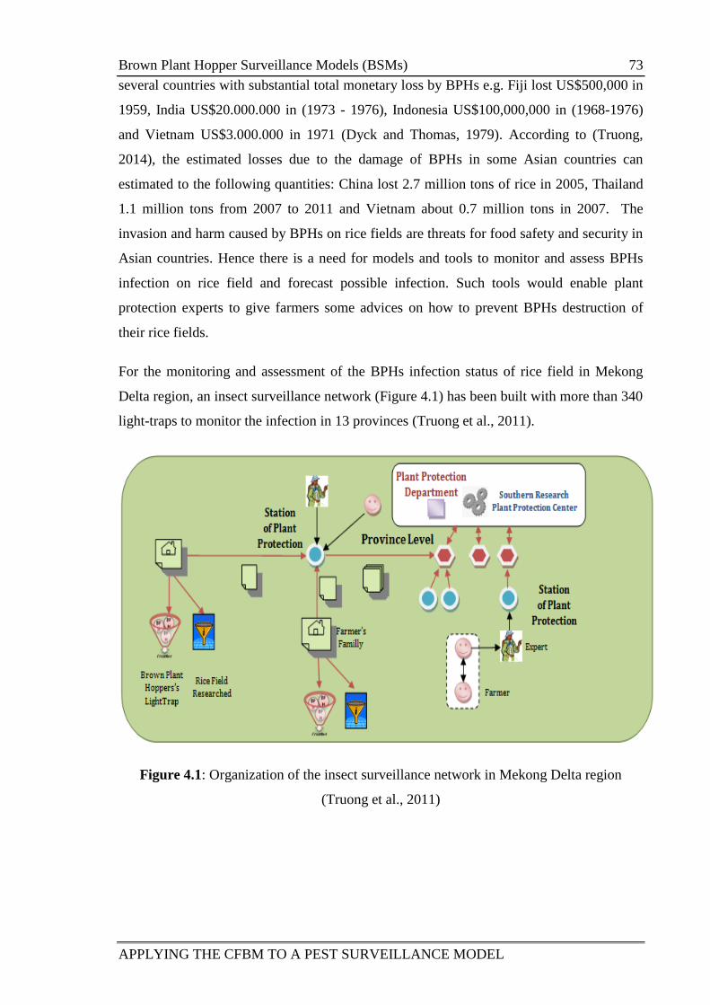
Brown Plant Hopper Surveillance Models (BSMs) 73
APPLYING THE CFBM TO A PEST SURVEILLANCE MODEL
several countries with substantial total monetary loss by BPHs e.g. Fiji lost US$500,000 in
1959, India US$20.000.000 in (1973 - 1976), Indonesia US$100,000,000 in (1968-1976)
and Vietnam US$3.000.000 in 1971 (Dyck and Thomas, 1979). According to (Truong,
2014), the estimated losses due to the damage of BPHs in some Asian countries can
estimated to the following quantities: China lost 2.7 million tons of rice in 2005, Thailand
1.1 million tons from 2007 to 2011 and Vietnam about 0.7 million tons in 2007. The
invasion and harm caused by BPHs on rice fields are threats for food safety and security in
Asian countries. Hence there is a need for models and tools to monitor and assess BPHs
infection on rice field and forecast possible infection. Such tools would enable plant
protection experts to give farmers some advices on how to prevent BPHs destruction of
their rice fields.
For the monitoring and assessment of the BPHs infection status of rice field in Mekong
Delta region, an insect surveillance network (Figure 4.1) has been built with more than 340
light-traps to monitor the infection in 13 provinces (Truong et al., 2011).
Figure 4.1: Organization of the insect surveillance network in Mekong Delta region
(Truong et al., 2011)

74 Brown Plant Hopper Surveillance Models (BSMs)
APPLYING THE CFBM TO A PEST SURVEILLANCE MODEL
The light trap (Figure 4.2) is a tool used to monitor the quantity of pest on rice fields per
day. It catches pest at night using a light attracting mature pest27
. Every day, the number of
BPHs and other pests are collected by farmer of the commune (small town). Those data are
sent to the station of plant protection in districts and provinces. The collected data from
light traps by farmers have been used to predict the BPHs infection status of rice fields by
experts at the station of plant protection and plant protection department. However the
prediction time is currently only of one week.
Figure 4.2: Light trap (source: http://www.bvtvhcm.gov.vn)
The purpose of the research conducted in the DREAM project is to develop a multi-agent
based simulation system that can predict the growth and break-out of BPHs on the rice
fields of the Mekong Delta region based on the historical quantity (or density) of adult
BPHs collected from light traps by the insect surveillance network. This simulation system
is called BSMs and introduced in Section 4.1.
The BSMs will help plant protection experts to predict the density of BPHs in the next 1, 2,
3 or 4 weeks. The BSMs will be used by plant protection experts at station of plant
protection at the districts level and at plant protection department at the provinces.
Furthermore, the outputs of BSMs are also used as the input of the Evaluation &
Optimization model t aiming at evaluating and optimizing the light trap network (Truong,
2014).
27
http://www.bvtvhcm.gov.vn/technology.php?id=66 - website of Plant Protection Department of Ho Chi
Minh City
Brown Plant Hopper Surveillance Models (BSMs) 75
APPLYING THE CFBM TO A PEST SURVEILLANCE MODEL
4.2.2 Entities, state variables and scale
Entities and variable in BSMs
The environmental of migration of BPHs are presented by the following entities: (1)
Smalltown_area, District_area, Province_area, Regional_area correspond to the
administrative areas, each one is described by the attributes (id, name, shape, id of higher
level of administrative); (2) land used area in Summer-Autumn (SA_Rice_Area) and
Winter-Spring (WS_Rice_Area) are the two entities representing the rice-cultivated area
during the Summer-Autumn and Winter-Spring seasons with attributes (id, land used type,
and shape); and (3) Sea_area is the entity presenting sea area in the studied region with
attributes (id, description, and shape).
The meteorological conditions of the migration are presented by: (1) Wind_information -
that represents the general information about the wind (mean, min and max of wind speed,
wind direction) used for the whole study region for a year; and (2) Meteo_stations -
represents the information about the temperature and humidity in the studied region.
More specifically, the environment in BSMs is represented as a grid of cells where the
Cellular_agent entity (cf. the BPHs Prediction model in Section 4.2.7.1) represents a cells
with attributes (id, name, attractiveness index, obstruction index and BPHs density vector).
The BPHs density vector is the number of adult BPHs located in the cell or caught at a
light trap. It is used to store the simulated the number of BPHs at each step of the
simulation. The attractiveness and obstruction indexes are two standardized environmental
indices. The attractiveness index reflects the existence of ideal conditions for the growth of
BPHs. If the Cellular_agent is located in the sea, river or resident area then attractiveness
index is 0 otherwise it will be calculated based on the meteorological conditions (humidity,
temperature) as well as the rice transplantation regions ( by seasonal crops such as Winter-
Spring and Summer-Autumn) (Truong et al., 2013) presented in Table 4.1. On the other
hand, the obstruction index is an opposite indicator of the attractiveness. The higher the
attractiveness index of a cell, the more BPHs migrating to the cell. Contrarily, the higher
the obstruction index, the less BPHs migrating to this cell.
Table 4.1: Effects of local constraint factors on both environmental indices.
No Name of factors Obstruction index
(OI)
Attractiveness index
(AI)
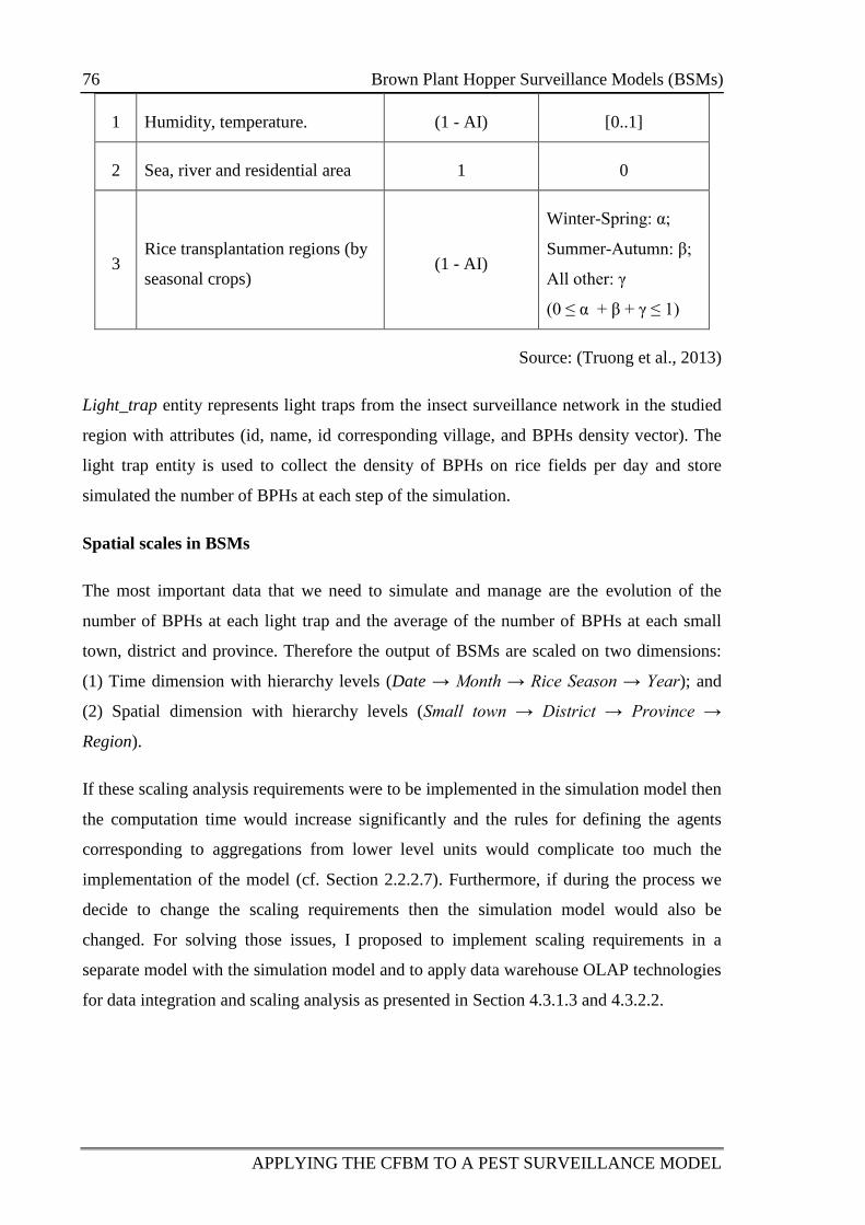
76 Brown Plant Hopper Surveillance Models (BSMs)
APPLYING THE CFBM TO A PEST SURVEILLANCE MODEL
1 Humidity, temperature. (1 - AI) [0..1]
2 Sea, river and residential area 1 0
3 Rice transplantation regions (by
seasonal crops) (1 - AI)
Winter-Spring: α;
Summer-Autumn: β;
All other: γ
(0 ≤ α + β + γ ≤ 1)
Source: (Truong et al., 2013)
Light_trap entity represents light traps from the insect surveillance network in the studied
region with attributes (id, name, id corresponding village, and BPHs density vector). The
light trap entity is used to collect the density of BPHs on rice fields per day and store
simulated the number of BPHs at each step of the simulation.
Spatial scales in BSMs
The most important data that we need to simulate and manage are the evolution of the
number of BPHs at each light trap and the average of the number of BPHs at each small
town, district and province. Therefore the output of BSMs are scaled on two dimensions:
(1) Time dimension with hierarchy levels (Date → Month → Rice Season → Year); and
(2) Spatial dimension with hierarchy levels (Small town → District → Province →
Region).
If these scaling analysis requirements were to be implemented in the simulation model then
the computation time would increase significantly and the rules for defining the agents
corresponding to aggregations from lower level units would complicate too much the
implementation of the model (cf. Section 2.2.2.7). Furthermore, if during the process we
decide to change the scaling requirements then the simulation model would also be
changed. For solving those issues, I proposed to implement scaling requirements in a
separate model with the simulation model and to apply data warehouse OLAP technologies
for data integration and scaling analysis as presented in Section 4.3.1.3 and 4.3.2.2.
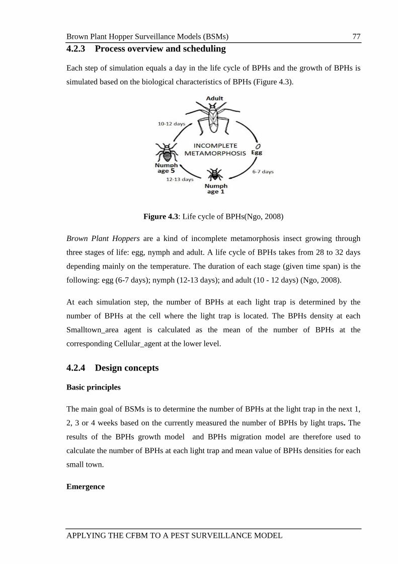
Brown Plant Hopper Surveillance Models (BSMs) 77
APPLYING THE CFBM TO A PEST SURVEILLANCE MODEL
4.2.3 Process overview and scheduling
Each step of simulation equals a day in the life cycle of BPHs and the growth of BPHs is
simulated based on the biological characteristics of BPHs (Figure 4.3).
Figure 4.3: Life cycle of BPHs(Ngo, 2008)
Brown Plant Hoppers are a kind of incomplete metamorphosis insect growing through
three stages of life: egg, nymph and adult. A life cycle of BPHs takes from 28 to 32 days
depending mainly on the temperature. The duration of each stage (given time span) is the
following: egg (6-7 days); nymph (12-13 days); and adult (10 - 12 days) (Ngo, 2008).
At each simulation step, the number of BPHs at each light trap is determined by the
number of BPHs at the cell where the light trap is located. The BPHs density at each
Smalltown_area agent is calculated as the mean of the number of BPHs at the
corresponding Cellular_agent at the lower level.
4.2.4 Design concepts
Basic principles
The main goal of BSMs is to determine the number of BPHs at the light trap in the next 1,
2, 3 or 4 weeks based on the currently measured the number of BPHs by light traps. The
results of the BPHs growth model and BPHs migration model are therefore used to
calculate the number of BPHs at each light trap and mean value of BPHs densities for each
small town.
Emergence
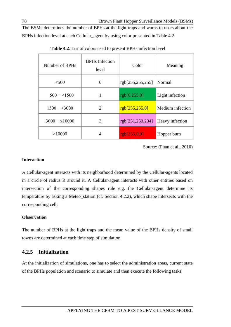
78 Brown Plant Hopper Surveillance Models (BSMs)
APPLYING THE CFBM TO A PEST SURVEILLANCE MODEL
The BSMs determines the number of BPHs at the light traps and warns to users about the
BPHs infection level at each Cellular_agent by using color presented in Table 4.2
Table 4.2: List of colors used to present BPHs infection level
Number of BPHs BPHs Infection
level Color Meaning
<500 0 rgb[255,255,255] Normal
500 − <1500 1 rgb[0,255,0] Light infection
1500 − <3000 2 rgb[255,255,0] Medium infection
3000 − ≤10000 3 rgb[251,253,234] Heavy infection
>10000 4 rgb[255,0,0] Hopper burn
Source: (Phan et al., 2010)
Interaction
A Cellular-agent interacts with its neighborhood determined by the Cellular-agents located
in a circle of radius R around it. A Cellular-agent interacts with other entities based on
intersection of the corresponding shapes rule e.g. the Cellular-agent determine its
temperature by asking a Meteo_station (cf. Section 4.2.2), which shape intersects with the
corresponding cell.
Observation
The number of BPHs at the light traps and the mean value of the BPHs density of small
towns are determined at each time step of simulation.
4.2.5 Initialization
At the initialization of simulations, one has to select the administration areas, current state
of the BPHs population and scenario to simulate and then execute the following tasks:
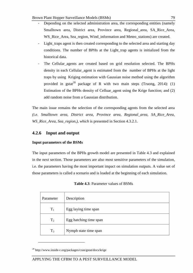
Brown Plant Hopper Surveillance Models (BSMs) 79
APPLYING THE CFBM TO A PEST SURVEILLANCE MODEL
- Depending on the selected administration area, the corresponding entities (namely
Smalltown area, District area, Province area, Regional_area, SA_Rice_Area,
WS_Rice_Area, Sea_region, Wind_information and Meteo_stations) are created.
- Light_traps agent is then created corresponding to the selected area and starting day
conditions. The number of BPHs at the Light_trap agents is initialized from the
historical data.
- The Cellular_agents are created based on grid resolution selected. The BPHs
density in each Cellular_agent is estimated from the number of BPHs at the light
traps by using Kriging estimation with Gaussian noise method using the algorithm
provided in gstat28
package of R with two main steps (Truong, 2014): (1)
Estimation of the BPHs density of Celluar_agent using the Krige function; and (2)
add random noise from a Gaussian distribution.
The main issue remains the selection of the corresponding agents from the selected area
(i.e. Smalltown area, District area, Province area, Regional_area, SA_Rice_Area,
WS_Rice_Area, Sea_region,), which is presented in Section 4.3.2.1.
4.2.6 Input and output
Input parameters of the BSMs
The input parameters of the BPHs growth model are presented in Table 4.3 and explained
in the next section. Those parameters are also most sensitive parameters of the simulation,
i.e. the parameters having the most important impact on simulation outputs. A value set of
those parameters is called a scenario and is loaded at the beginning of each simulation.
Table 4.3: Parameter values of BSMs
Parameter Description
T1 Egg laying time span
T2 Egg hatching time span
T3 Nymph state time span
28 http://www.inside-r.org/packages/cran/gstat/docs/krige
80 Brown Plant Hopper Surveillance Models (BSMs)
APPLYING THE CFBM TO A PEST SURVEILLANCE MODEL
T4 Adult time span
ren Rate for the transition from egg to nymph
rna Rate for the transition from nymph to adult
rb Rate of eggs laid by an adult
m Mortality rate
The empirical data collected from the target system such as administrative regions
(province, district, and small town scales), land uses (seasonal crops of multiple tree
species of the region), meteorological data (wind, temperature, humidity, etc) and the
number of BPHs at 300 light traps are used as input data of the BSMs.
The Output of BSMs
The outputs of BSMs are two observation variables of the model: the number of BPHs at
each light trap and the mean value of the BPHs densities for each small town. These two
outputs are stored with other information such as model, scenario, replication id and time
steps of the generated output data. The data structure used to manage the input and output
data of the BSMs will be presented in Section 4.3.1.
4.2.7 Sub models
The logic of simulation for data-driven modeling approach (Gilbert and Troitzsch, 2005) is
used to develop BSMs. The empirical data collected from the Insect Surveillance Network
in Mekong Delta region are used to different aims: (1) Conceptually to design the model;
(2) as input data to make the simulate; (3) as validation data to evaluate the model output
as presented in Section 2.2.1.2.
The GAMA platform was chosen as modeling environment to develop BSMs thus GAML
(the modeling language of GAMA) was used to formalize the BSMs.
Specifically, the architecture of BSMs (Figure 4.4) is designed and implemented by
applying the CFBM in GAMA. The input and output data of the BSMs are managed by the
database features of the CFBM in GAMA presented in Section 4.3.
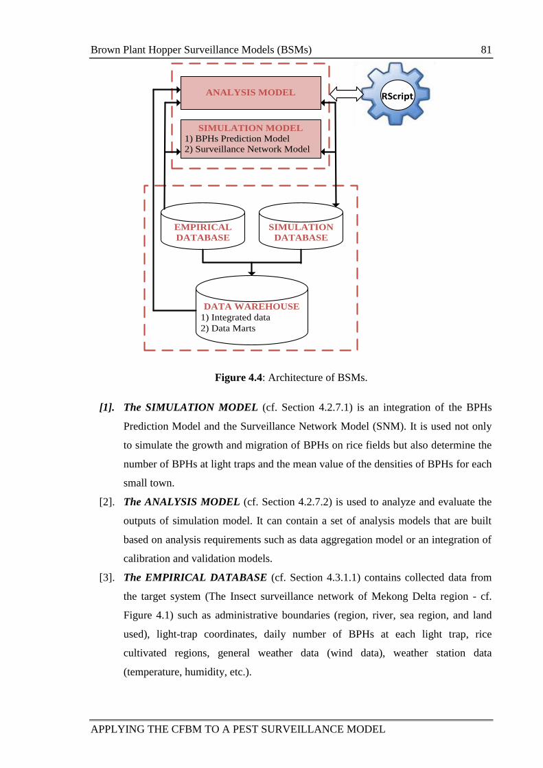
Brown Plant Hopper Surveillance Models (BSMs) 81
APPLYING THE CFBM TO A PEST SURVEILLANCE MODEL
DATA WAREHOUSE
1) Integrated data
2) Data Marts
SIMULATION
DATABASE
EMPIRICAL
DATABASE
SIMULATION MODEL
1) BPHs Prediction Model
2) Surveillance Network Model
ANALYSIS MODEL
RScript
Figure 4.4: Architecture of BSMs.
[1]. The SIMULATION MODEL (cf. Section 4.2.7.1) is an integration of the BPHs
Prediction Model and the Surveillance Network Model (SNM). It is used not only
to simulate the growth and migration of BPHs on rice fields but also determine the
number of BPHs at light traps and the mean value of the densities of BPHs for each
small town.
[2]. The ANALYSIS MODEL (cf. Section 4.2.7.2) is used to analyze and evaluate the
outputs of simulation model. It can contain a set of analysis models that are built
based on analysis requirements such as data aggregation model or an integration of
calibration and validation models.
[3]. The EMPIRICAL DATABASE (cf. Section 4.3.1.1) contains collected data from
the target system (The Insect surveillance network of Mekong Delta region - cf.
Figure 4.1) such as administrative boundaries (region, river, sea region, and land
used), light-trap coordinates, daily number of BPHs at each light trap, rice
cultivated regions, general weather data (wind data), weather station data
(temperature, humidity, etc.).
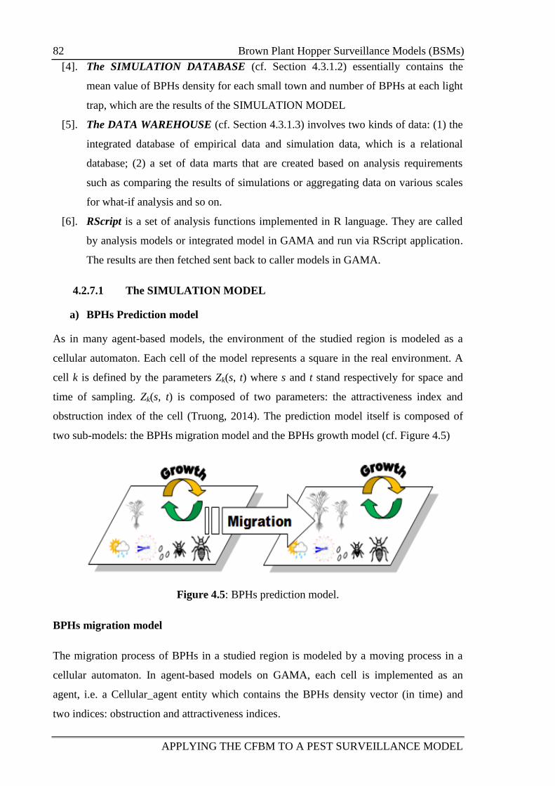
82 Brown Plant Hopper Surveillance Models (BSMs)
APPLYING THE CFBM TO A PEST SURVEILLANCE MODEL
[4]. The SIMULATION DATABASE (cf. Section 4.3.1.2) essentially contains the
mean value of BPHs density for each small town and number of BPHs at each light
trap, which are the results of the SIMULATION MODEL
[5]. The DATA WAREHOUSE (cf. Section 4.3.1.3) involves two kinds of data: (1) the
integrated database of empirical data and simulation data, which is a relational
database; (2) a set of data marts that are created based on analysis requirements
such as comparing the results of simulations or aggregating data on various scales
for what-if analysis and so on.
[6]. RScript is a set of analysis functions implemented in R language. They are called
by analysis models or integrated model in GAMA and run via RScript application.
The results are then fetched sent back to caller models in GAMA.
4.2.7.1 The SIMULATION MODEL
a) BPHs Prediction model
As in many agent-based models, the environment of the studied region is modeled as a
cellular automaton. Each cell of the model represents a square in the real environment. A
cell k is defined by the parameters Zk(s, t) where s and t stand respectively for space and
time of sampling. Zk(s, t) is composed of two parameters: the attractiveness index and
obstruction index of the cell (Truong, 2014). The prediction model itself is composed of
two sub-models: the BPHs migration model and the BPHs growth model (cf. Figure 4.5)
Figure 4.5: BPHs prediction model.
BPHs migration model
The migration process of BPHs in a studied region is modeled by a moving process in a
cellular automaton. In agent-based models on GAMA, each cell is implemented as an
agent, i.e. a Cellular_agent entity which contains the BPHs density vector (in time) and
two indices: obstruction and attractiveness indices.
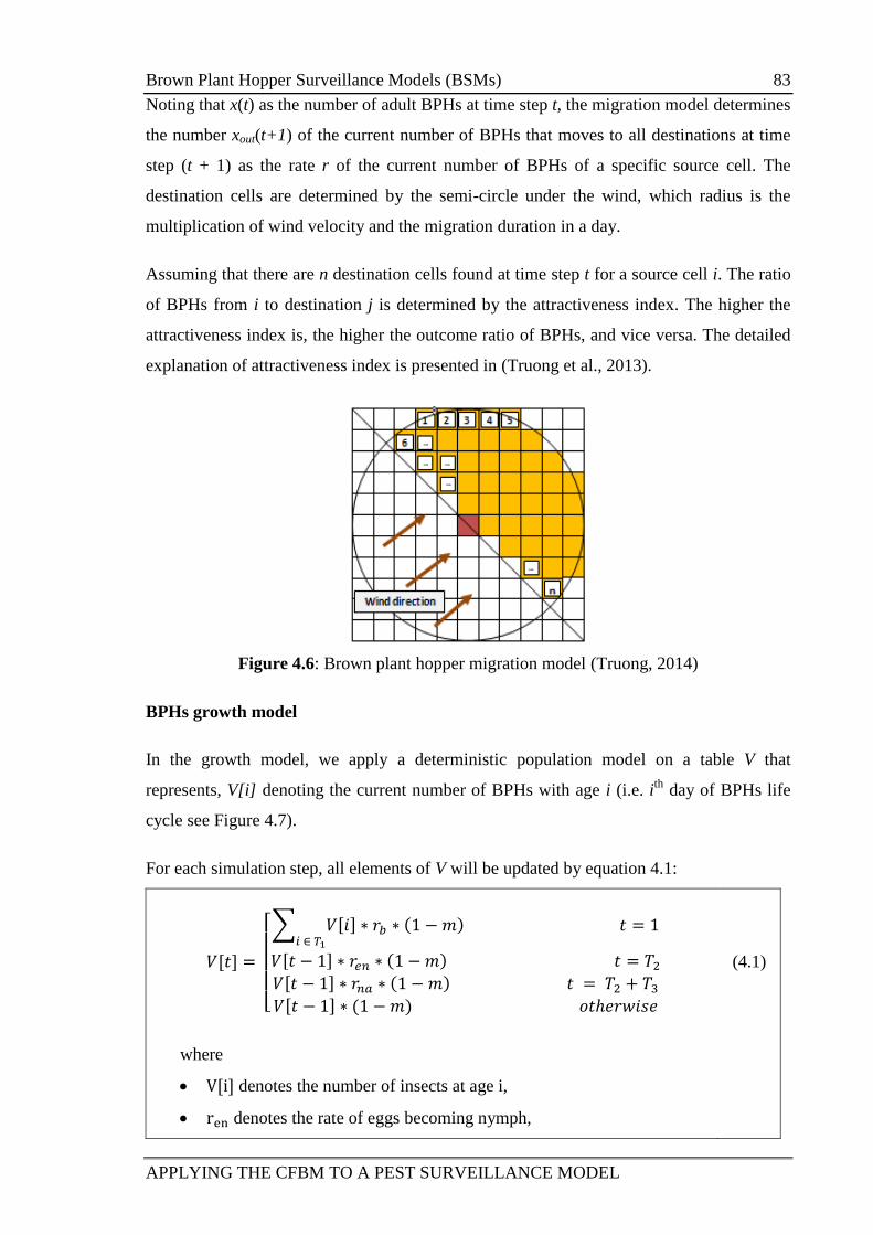
Brown Plant Hopper Surveillance Models (BSMs) 83
APPLYING THE CFBM TO A PEST SURVEILLANCE MODEL
Noting that x(t) as the number of adult BPHs at time step t, the migration model determines
the number xout(t+1) of the current number of BPHs that moves to all destinations at time
step (t + 1) as the rate r of the current number of BPHs of a specific source cell. The
destination cells are determined by the semi-circle under the wind, which radius is the
multiplication of wind velocity and the migration duration in a day.
Assuming that there are n destination cells found at time step t for a source cell i. The ratio
of BPHs from i to destination j is determined by the attractiveness index. The higher the
attractiveness index is, the higher the outcome ratio of BPHs, and vice versa. The detailed
explanation of attractiveness index is presented in (Truong et al., 2013).
Figure 4.6: Brown plant hopper migration model (Truong, 2014)
BPHs growth model
In the growth model, we apply a deterministic population model on a table V that
represents, V[i] denoting the current number of BPHs with age i (i.e. ith
day of BPHs life
cycle see Figure 4.7).
For each simulation step, all elements of V will be updated by equation 4.1:
(4.1)
where
denotes the number of insects at age i,
denotes the rate of eggs becoming nymph,
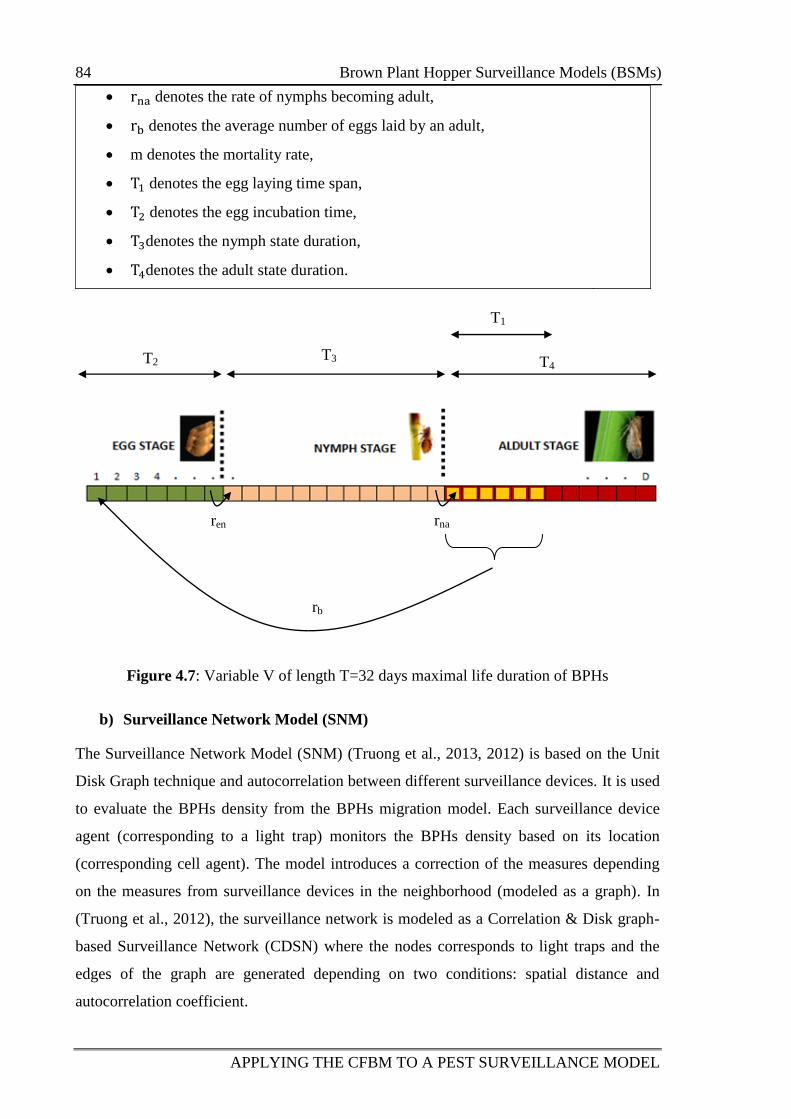
84 Brown Plant Hopper Surveillance Models (BSMs)
APPLYING THE CFBM TO A PEST SURVEILLANCE MODEL
denotes the rate of nymphs becoming adult,
denotes the average number of eggs laid by an adult,
m denotes the mortality rate,
denotes the egg laying time span,
denotes the egg incubation time,
denotes the nymph state duration,
denotes the adult state duration.
Figure 4.7: Variable V of length T=32 days maximal life duration of BPHs
b) Surveillance Network Model (SNM)
The Surveillance Network Model (SNM) (Truong et al., 2013, 2012) is based on the Unit
Disk Graph technique and autocorrelation between different surveillance devices. It is used
to evaluate the BPHs density from the BPHs migration model. Each surveillance device
agent (corresponding to a light trap) monitors the BPHs density based on its location
(corresponding cell agent). The model introduces a correction of the measures depending
on the measures from surveillance devices in the neighborhood (modeled as a graph). In
(Truong et al., 2012), the surveillance network is modeled as a Correlation & Disk graph-
based Surveillance Network (CDSN) where the nodes corresponds to light traps and the
edges of the graph are generated depending on two conditions: spatial distance and
autocorrelation coefficient.
T2 T3
T1
T4
ren rna
rb
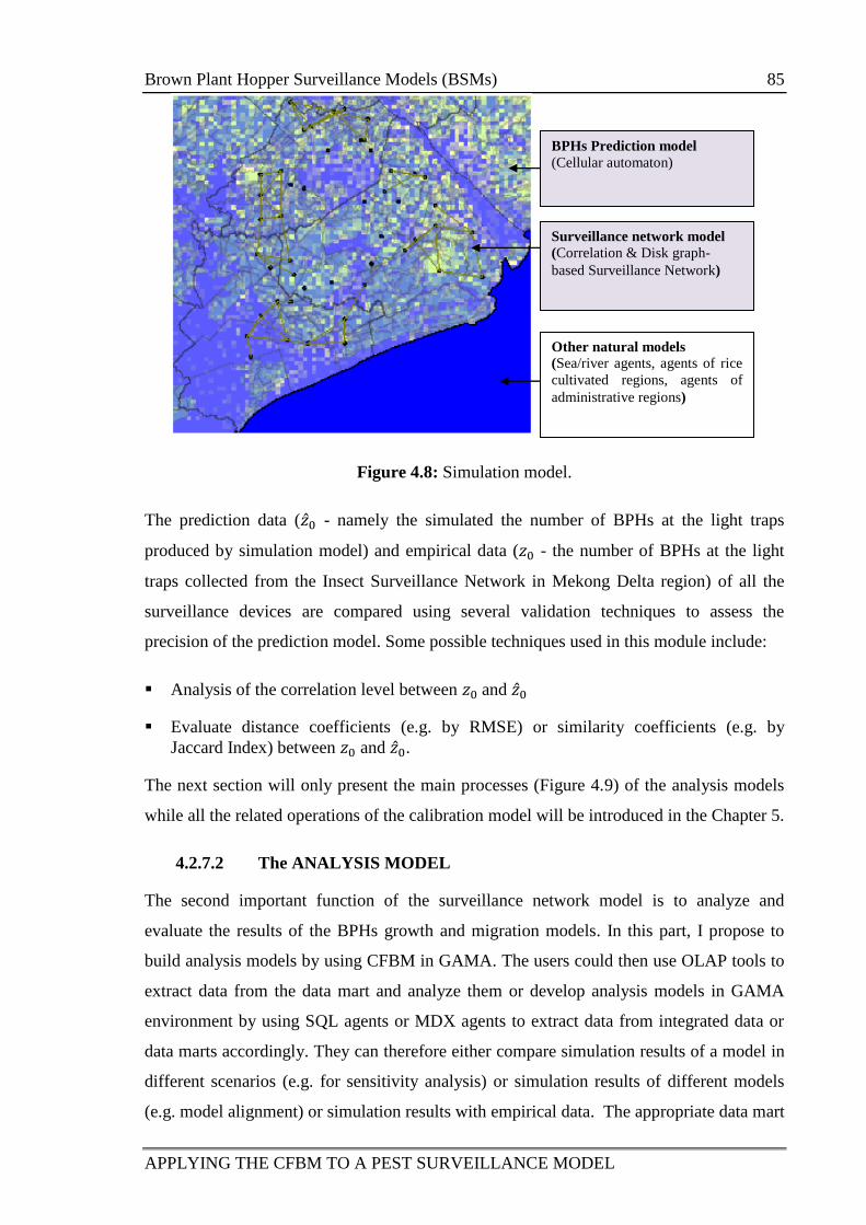
Brown Plant Hopper Surveillance Models (BSMs) 85
APPLYING THE CFBM TO A PEST SURVEILLANCE MODEL
Figure 4.8: Simulation model.
The prediction data ( - namely the simulated the number of BPHs at the light traps
produced by simulation model) and empirical data ( - the number of BPHs at the light
traps collected from the Insect Surveillance Network in Mekong Delta region) of all the
surveillance devices are compared using several validation techniques to assess the
precision of the prediction model. Some possible techniques used in this module include:
Analysis of the correlation level between and
Evaluate distance coefficients (e.g. by RMSE) or similarity coefficients (e.g. by
Jaccard Index) between and .
The next section will only present the main processes (Figure 4.9) of the analysis models
while all the related operations of the calibration model will be introduced in the Chapter 5.
4.2.7.2 The ANALYSIS MODEL
The second important function of the surveillance network model is to analyze and
evaluate the results of the BPHs growth and migration models. In this part, I propose to
build analysis models by using CFBM in GAMA. The users could then use OLAP tools to
extract data from the data mart and analyze them or develop analysis models in GAMA
environment by using SQL agents or MDX agents to extract data from integrated data or
data marts accordingly. They can therefore either compare simulation results of a model in
different scenarios (e.g. for sensitivity analysis) or simulation results of different models
(e.g. model alignment) or simulation results with empirical data. The appropriate data mart
BPHs Prediction model
(Cellular automaton)
Surveillance network model
(Correlation & Disk graph-
based Surveillance Network)
Other natural models
(Sea/river agents, agents of rice
cultivated regions, agents of
administrative regions)
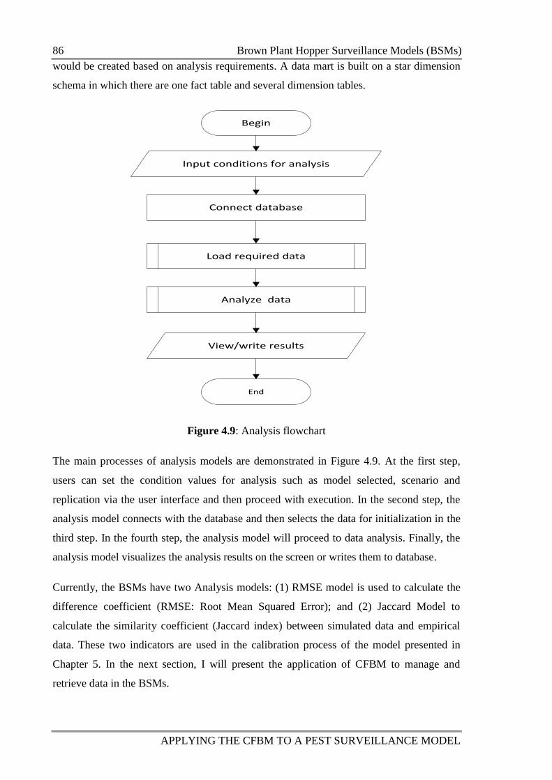
86 Brown Plant Hopper Surveillance Models (BSMs)
APPLYING THE CFBM TO A PEST SURVEILLANCE MODEL
would be created based on analysis requirements. A data mart is built on a star dimension
schema in which there are one fact table and several dimension tables.
Begin
Input conditions for analysis
Analyze data
View/write results
End
Load required data
Connect database
Figure 4.9: Analysis flowchart
The main processes of analysis models are demonstrated in Figure 4.9. At the first step,
users can set the condition values for analysis such as model selected, scenario and
replication via the user interface and then proceed with execution. In the second step, the
analysis model connects with the database and then selects the data for initialization in the
third step. In the fourth step, the analysis model will proceed to data analysis. Finally, the
analysis model visualizes the analysis results on the screen or writes them to database.
Currently, the BSMs have two Analysis models: (1) RMSE model is used to calculate the
difference coefficient (RMSE: Root Mean Squared Error); and (2) Jaccard Model to
calculate the similarity coefficient (Jaccard index) between simulated data and empirical
data. These two indicators are used in the calibration process of the model presented in
Chapter 5. In the next section, I will present the application of CFBM to manage and
retrieve data in the BSMs.
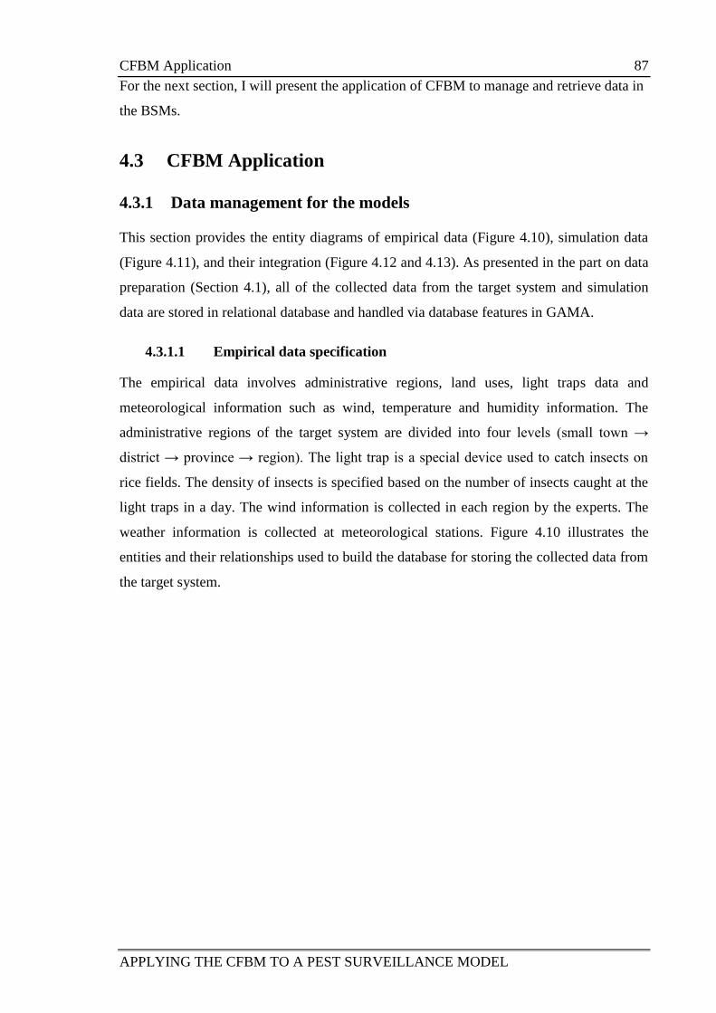
CFBM Application 87
APPLYING THE CFBM TO A PEST SURVEILLANCE MODEL
For the next section, I will present the application of CFBM to manage and retrieve data in
the BSMs.
4.3 CFBM Application
4.3.1 Data management for the models
This section provides the entity diagrams of empirical data (Figure 4.10), simulation data
(Figure 4.11), and their integration (Figure 4.12 and 4.13). As presented in the part on data
preparation (Section 4.1), all of the collected data from the target system and simulation
data are stored in relational database and handled via database features in GAMA.
4.3.1.1 Empirical data specification
The empirical data involves administrative regions, land uses, light traps data and
meteorological information such as wind, temperature and humidity information. The
administrative regions of the target system are divided into four levels (small town →
district → province → region). The light trap is a special device used to catch insects on
rice fields. The density of insects is specified based on the number of insects caught at the
light traps in a day. The wind information is collected in each region by the experts. The
weather information is collected at meteorological stations. Figure 4.10 illustrates the
entities and their relationships used to build the database for storing the collected data from
the target system.
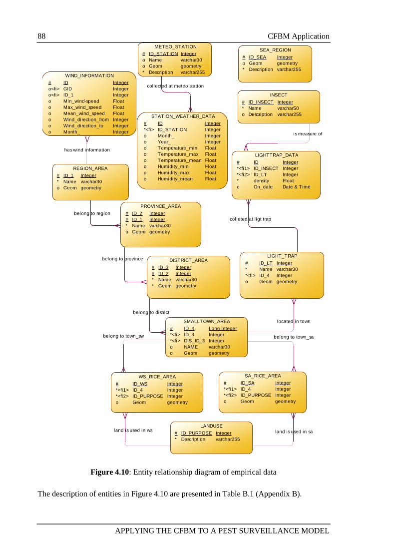
88 CFBM Application
APPLYING THE CFBM TO A PEST SURVEILLANCE MODEL
Figure 4.10: Entity relationship diagram of empirical data
The description of entities in Figure 4.10 are presented in Table B.1 (Appendix B).
belong to region
belong to province
belong to district
belong to town_sw belong to town_sa
land is used in ws land is used in sa
located in town
is measure of
colleted at l igt trap
collected at meteo station
has wind information
PROVINCE_AREA
#
#
*
o
ID_2
ID_1
Name
Geom
Integer
Integer
varchar30
geometry
DISTRICT_AREA
#
#
*
*
ID_3
ID_2
Name
Geom
Integer
Integer
varchar30
geometry
SMALLTOWN_AREA
#
*<fi>
*<fi>
o
o
ID_4
ID_3
DIS_ID_3
NAME
Geom
...
Long integer
Integer
Integer
varchar30
geometry
SA_RICE_AREA
#
*<fi1>
*<fi2>
o
ID_SA
ID_4
ID_PURPOSE
Geom
Integer
Integer
Integer
geometry
WS_RICE_AREA
#
*<fi1>
*<fi2>
o
ID_WS
ID_4
ID_PURPOSE
Geom
Integer
Integer
Integer
geometry
LANDUSE
#
*
ID_PURPOSE
Description
Integer
varchar255
SEA_REGION
#
o
*
ID_SEA
Geom
Description
Integer
geometry
varchar255
LIGHT_TRAP
#
*
*<fi>
o
ID_LT
Name
ID_4
Geom
Integer
varchar30
Integer
geometry
LIGHTTRAP_DATA
#
*<fi1>
*<fi2>
*
o
ID
ID_INSECT
ID_LT
density
On_date
Integer
Integer
Integer
Float
Date & Time
INSECT
#
*
o
ID_INSECT
Name
Description
Integer
varchar50
varchar255STATION_WEATHER_DATA
#
*<fi>
o
o
o
o
o
o
o
o
ID
ID_STATION
Month_
Year_
Temperature_min
Temperature_max
Temperature_mean
Humidity_min
Humidity_max
Humidity_mean
Integer
Integer
Integer
Integer
Float
Float
Float
Float
Float
Float
METEO_STATION
#
o
o
*
ID_STATION
Name
Geom
Description
...
Integer
varchar30
geometry
varchar255
REGION_AREA
#
*
o
ID_1
Name
Geom
Integer
varchar30
geometry
WIND_INFORMATION
#
o<fi>
o<fi>
o
o
o
o
o
o
ID
GID
ID_1
Min_wind-speed
Max_wind_speed
Mean_wind_speed
Wind_direction_from
Wind_direction_to
Month_
...
Integer
Integer
Integer
Float
Float
Float
Integer
Integer
Integer
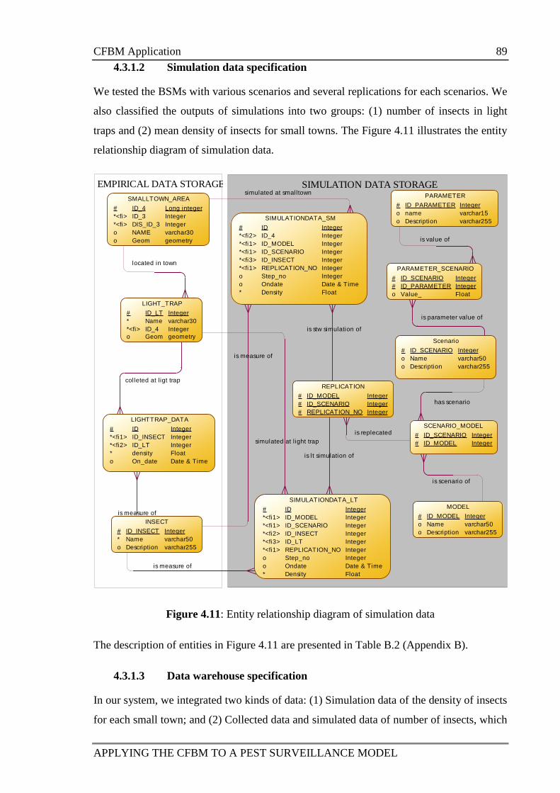
CFBM Application 89
APPLYING THE CFBM TO A PEST SURVEILLANCE MODEL
4.3.1.2 Simulation data specification
We tested the BSMs with various scenarios and several replications for each scenarios. We
also classified the outputs of simulations into two groups: (1) number of insects in light
traps and (2) mean density of insects for small towns. The Figure 4.11 illustrates the entity
relationship diagram of simulation data.
Figure 4.11: Entity relationship diagram of simulation data
The description of entities in Figure 4.11 are presented in Table B.2 (Appendix B).
4.3.1.3 Data warehouse specification
In our system, we integrated two kinds of data: (1) Simulation data of the density of insects
for each small town; and (2) Collected data and simulated data of number of insects, which
SIMULATION DATA STORAGE
is lt simulation of
has scenario
is scenario of
is replecated
is stw simulation of
EMPIRICAL DATA STORAGE
is measure of
simulated at l ight trap
colleted at l igt trap
is measure of
located in town
simulated at smalltown
is measure of
is parameter value of
is value of
SIMULATIONDATA_SM
#
*<fi2>
*<fi1>
*<fi1>
*<fi3>
*<fi1>
o
o
*
ID
ID_4
ID_MODEL
ID_SCENARIO
ID_INSECT
REPLICATION_NO
Step_no
Ondate
Density
Integer
Integer
Integer
Integer
Integer
Integer
Integer
Date & Time
Float
SMALLTOWN_AREA
#
*<fi>
*<fi>
o
o
ID_4
ID_3
DIS_ID_3
NAME
Geom
...
Long integer
Integer
Integer
varchar30
geometry
LIGHTTRAP_DATA
#
*<fi1>
*<fi2>
*
o
ID
ID_INSECT
ID_LT
density
On_date
Integer
Integer
Integer
Float
Date & Time
INSECT
#
*
o
ID_INSECT
Name
Description
...
Integer
varchar50
varchar255
LIGHT_TRAP
#
*
*<fi>
o
ID_LT
Name
ID_4
Geom
...
Integer
varchar30
Integer
geometry
SIMULATIONDATA_LT
#
*<fi1>
*<fi1>
*<fi2>
*<fi3>
*<fi1>
o
o
*
ID
ID_MODEL
ID_SCENARIO
ID_INSECT
ID_LT
REPLICATION_NO
Step_no
Ondate
Density...
Integer
Integer
Integer
Integer
Integer
Integer
Integer
Date & Time
Float
MODEL
#
o
o
ID_MODEL
Name
Description
...
Integer
varchar50
varchar255
Scenario
#
o
o
ID_SCENARIO
Name
Description
Integer
varchar50
varchar255
PARAMETER_SCENARIO
#
#
o
ID_SCENARIO
ID_PARAMETER
Value_
...
Integer
Integer
Float
PARAMETER
#
o
o
ID_PARAMETER
name
Description
...
Integer
varchar15
varchar255
SCENARIO_MODEL
#
#
ID_SCENARIO
ID_MODEL
Integer
Integer
REPLICATION
#
#
#
ID_MODEL
ID_SCENARIO
REPLICATION_NO
...
Integer
Integer
Integer
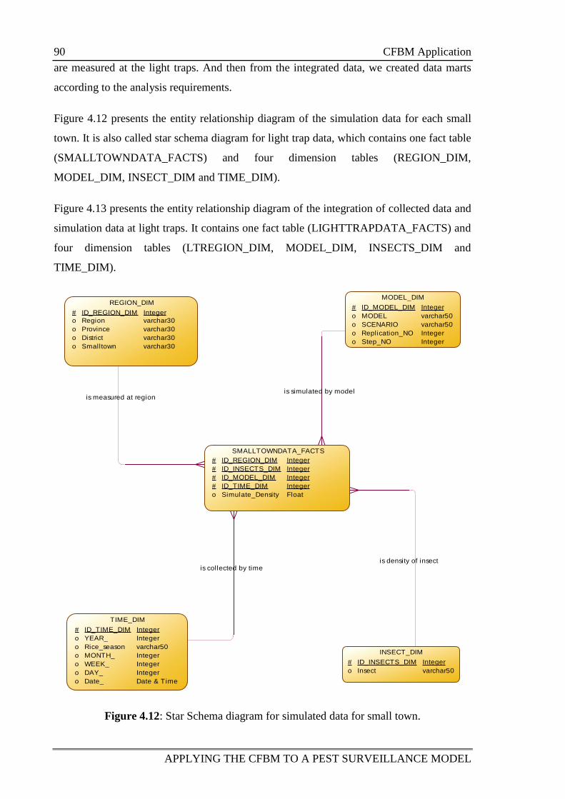
90 CFBM Application
APPLYING THE CFBM TO A PEST SURVEILLANCE MODEL
are measured at the light traps. And then from the integrated data, we created data marts
according to the analysis requirements.
Figure 4.12 presents the entity relationship diagram of the simulation data for each small
town. It is also called star schema diagram for light trap data, which contains one fact table
(SMALLTOWNDATA_FACTS) and four dimension tables (REGION_DIM,
MODEL_DIM, INSECT_DIM and TIME_DIM).
Figure 4.13 presents the entity relationship diagram of the integration of collected data and
simulation data at light traps. It contains one fact table (LIGHTTRAPDATA_FACTS) and
four dimension tables (LTREGION_DIM, MODEL_DIM, INSECTS_DIM and
TIME_DIM).
Figure 4.12: Star Schema diagram for simulated data for small town.
is simulated by model
is density of insectis collected by time
is measured at region
SMALLTOWNDATA_FACTS
#
#
#
#
o
ID_REGION_DIM
ID_INSECTS_DIM
ID_MODEL_DIM
ID_TIME_DIM
Simulate_Density
Integer
Integer
Integer
Integer
Float
MODEL_DIM
#
o
o
o
o
ID_MODEL_DIM
MODEL
SCENARIO
Replication_NO
Step_NO
...
Integer
varchar50
varchar50
Integer
Integer
INSECT_DIM
#
o
ID_INSECTS_DIM
Insect
Integer
varchar50
TIME_DIM
#
o
o
o
o
o
o
ID_TIME_DIM
YEAR_
Rice_season
MONTH_
WEEK_
DAY_
Date_
Integer
Integer
varchar50
Integer
Integer
Integer
Date & Time
REGION_DIM
#
o
o
o
o
ID_REGION_DIM
Region
Province
District
Smalltown
Integer
varchar30
varchar30
varchar30
varchar30
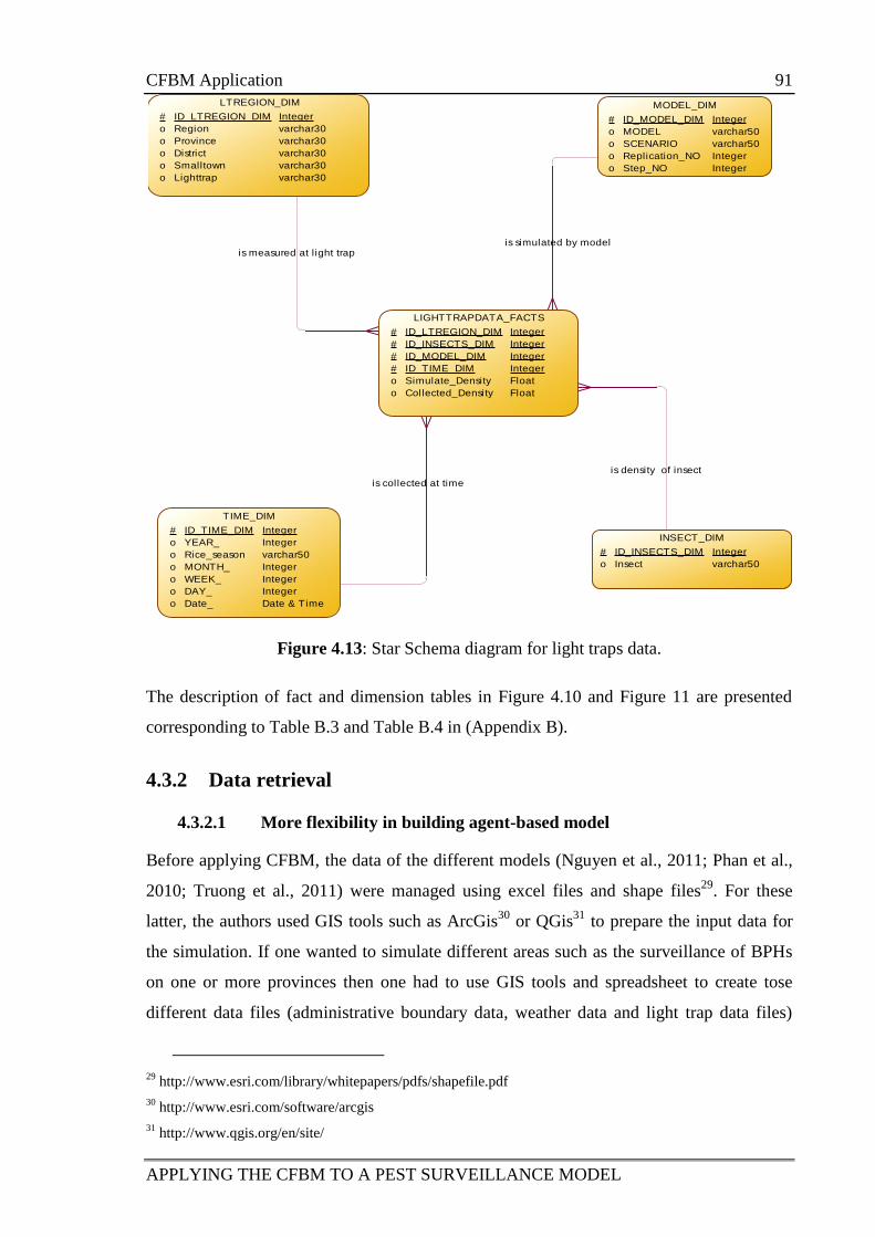
CFBM Application 91
APPLYING THE CFBM TO A PEST SURVEILLANCE MODEL
Figure 4.13: Star Schema diagram for light traps data.
The description of fact and dimension tables in Figure 4.10 and Figure 11 are presented
corresponding to Table B.3 and Table B.4 in (Appendix B).
4.3.2 Data retrieval
4.3.2.1 More flexibility in building agent-based model
Before applying CFBM, the data of the different models (Nguyen et al., 2011; Phan et al.,
2010; Truong et al., 2011) were managed using excel files and shape files29
. For these
latter, the authors used GIS tools such as ArcGis30
or QGis31
to prepare the input data for
the simulation. If one wanted to simulate different areas such as the surveillance of BPHs
on one or more provinces then one had to use GIS tools and spreadsheet to create tose
different data files (administrative boundary data, weather data and light trap data files)
29
http://www.esri.com/library/whitepapers/pdfs/shapefile.pdf
30 http://www.esri.com/software/arcgis
31 http://www.qgis.org/en/site/
is measured at l ight trapis simulated by model
is density of insect
is collected at time
LIGHTTRAPDATA_FACTS
#
#
#
#
o
o
ID_LTREGION_DIM
ID_INSECTS_DIM
ID_MODEL_DIM
ID_TIME_DIM
Simulate_Density
Collected_Density
Integer
Integer
Integer
Integer
Float
Float
LTREGION_DIM
#
o
o
o
o
o
ID_LTREGION_DIM
Region
Province
District
Smalltown
Lighttrap
Integer
varchar30
varchar30
varchar30
varchar30
varchar30
MODEL_DIM
#
o
o
o
o
ID_MODEL_DIM
MODEL
SCENARIO
Replication_NO
Step_NO
...
Integer
varchar50
varchar50
Integer
Integer
INSECT_DIM
#
o
ID_INSECTS_DIM
Insect
Integer
varchar50
TIME_DIM
#
o
o
o
o
o
o
ID_TIME_DIM
YEAR_
Rice_season
MONTH_
WEEK_
DAY_
Date_
Integer
Integer
varchar50
Integer
Integer
Integer
Date & Time
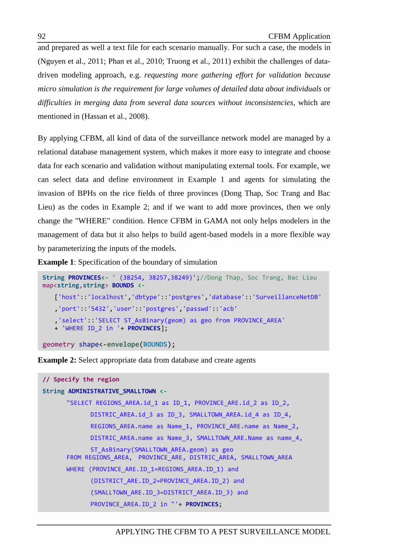
92 CFBM Application
APPLYING THE CFBM TO A PEST SURVEILLANCE MODEL
and prepared as well a text file for each scenario manually. For such a case, the models in
(Nguyen et al., 2011; Phan et al., 2010; Truong et al., 2011) exhibit the challenges of data-
driven modeling approach, e.g. requesting more gathering effort for validation because
micro simulation is the requirement for large volumes of detailed data about individuals or
difficulties in merging data from several data sources without inconsistencies, which are
mentioned in (Hassan et al., 2008).
By applying CFBM, all kind of data of the surveillance network model are managed by a
relational database management system, which makes it more easy to integrate and choose
data for each scenario and validation without manipulating external tools. For example, we
can select data and define environment in Example 1 and agents for simulating the
invasion of BPHs on the rice fields of three provinces (Dong Thap, Soc Trang and Bac
Lieu) as the codes in Example 2; and if we want to add more provinces, then we only
change the "WHERE" condition. Hence CFBM in GAMA not only helps modelers in the
management of data but it also helps to build agent-based models in a more flexible way
by parameterizing the inputs of the models.
Example 1: Specification of the boundary of simulation
Example 2: Select appropriate data from database and create agents
// Specify the region
String ADMINISTRATIVE_SMALLTOWN <-
"SELECT REGIONS_AREA.id_1 as ID_1, PROVINCE_ARE.id_2 as ID_2,
DISTRIC_AREA.id_3 as ID_3, SMALLTOWN_AREA.id_4 as ID_4,
REGIONS_AREA.name as Name_1, PROVINCE_ARE.name as Name_2,
DISTRIC_AREA.name as Name_3, SMALLTOWN_ARE.Name as name_4,
ST_AsBinary(SMALLTOWN_AREA.geom) as geo FROM REGIONS_AREA, PROVINCE_ARE, DISTRIC_AREA, SMALLTOWN_AREA
WHERE (PROVINCE_ARE.ID_1=REGIONS_AREA.ID_1) and
(DISTRICT_ARE.ID_2=PROVINCE_AREA.ID_2) and
(SMALLTOWN_ARE.ID_3=DISTRICT_AREA.ID_3) and
PROVINCE_AREA.ID_2 in "'+ PROVINCES;
String PROVINCES<- ' (38254, 38257,38249)';//Dong Thap, Soc Trang, Bac Lieu map<string,string> BOUNDS <-
['host'::'localhost','dbtype'::'postgres','database'::'SurveillanceNetDB'
,'port'::'5432','user'::'postgres','passwd'::'acb'
,'select'::'SELECT ST_AsBinary(geom) as geo from PROVINCE_AREA' + 'WHERE ID_2 in '+ PROVINCES];
geometry shape<-envelope(BOUNDS);
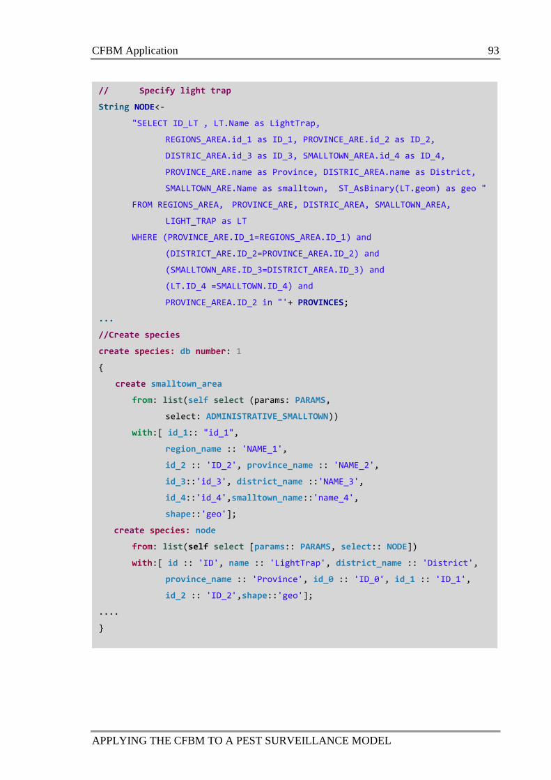
CFBM Application 93
APPLYING THE CFBM TO A PEST SURVEILLANCE MODEL
// Specify light trap
String NODE<-
"SELECT ID_LT , LT.Name as LightTrap,
REGIONS_AREA.id_1 as ID_1, PROVINCE_ARE.id_2 as ID_2,
DISTRIC_AREA.id_3 as ID_3, SMALLTOWN_AREA.id_4 as ID_4,
PROVINCE_ARE.name as Province, DISTRIC_AREA.name as District,
SMALLTOWN_ARE.Name as smalltown, ST_AsBinary(LT.geom) as geo "
FROM REGIONS_AREA, PROVINCE_ARE, DISTRIC_AREA, SMALLTOWN_AREA,
LIGHT_TRAP as LT
WHERE (PROVINCE_ARE.ID_1=REGIONS_AREA.ID_1) and
(DISTRICT_ARE.ID_2=PROVINCE_AREA.ID_2) and
(SMALLTOWN_ARE.ID_3=DISTRICT_AREA.ID_3) and
(LT.ID_4 =SMALLTOWN.ID_4) and
PROVINCE_AREA.ID_2 in "'+ PROVINCES;
...
//Create species
create species: db number: 1
{
create smalltown_area
from: list(self select (params: PARAMS,
select: ADMINISTRATIVE_SMALLTOWN))
with:[ id_1:: "id_1",
region_name :: 'NAME_1',
id_2 :: 'ID_2', province_name :: 'NAME_2',
id_3::'id_3', district_name ::'NAME_3',
id_4::'id_4',smalltown_name::'name_4',
shape::'geo'];
create species: node
from: list(self select [params:: PARAMS, select:: NODE])
with:[ id :: 'ID', name :: 'LightTrap', district_name :: 'District',
province_name :: 'Province', id_0 :: 'ID_0', id_1 :: 'ID_1',
id_2 :: 'ID_2',shape::'geo'];
....
}
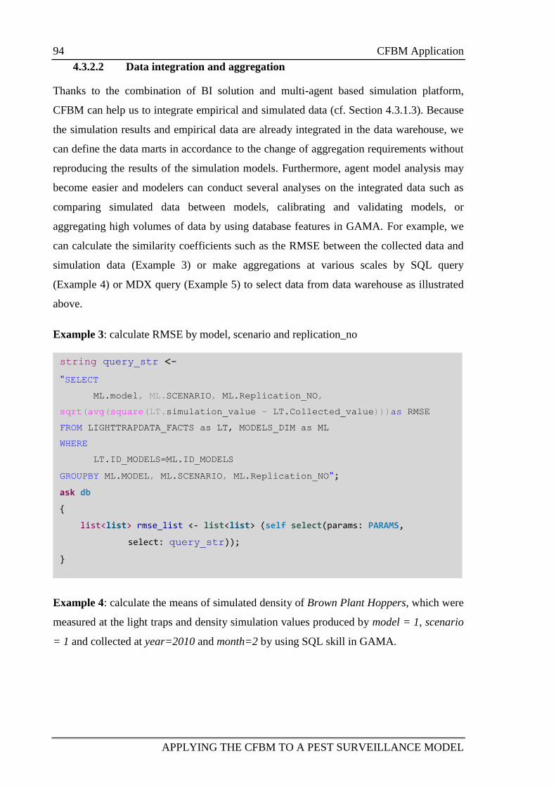
94 CFBM Application
APPLYING THE CFBM TO A PEST SURVEILLANCE MODEL
4.3.2.2 Data integration and aggregation
Thanks to the combination of BI solution and multi-agent based simulation platform,
CFBM can help us to integrate empirical and simulated data (cf. Section 4.3.1.3). Because
the simulation results and empirical data are already integrated in the data warehouse, we
can define the data marts in accordance to the change of aggregation requirements without
reproducing the results of the simulation models. Furthermore, agent model analysis may
become easier and modelers can conduct several analyses on the integrated data such as
comparing simulated data between models, calibrating and validating models, or
aggregating high volumes of data by using database features in GAMA. For example, we
can calculate the similarity coefficients such as the RMSE between the collected data and
simulation data (Example 3) or make aggregations at various scales by SQL query
(Example 4) or MDX query (Example 5) to select data from data warehouse as illustrated
above.
Example 3: calculate RMSE by model, scenario and replication_no
Example 4: calculate the means of simulated density of Brown Plant Hoppers, which were
measured at the light traps and density simulation values produced by model = 1, scenario
= 1 and collected at year=2010 and month=2 by using SQL skill in GAMA.
string query_str <-
"SELECT
ML.model, ML.SCENARIO, ML.Replication_NO,
sqrt(avg(square(LT.simulation_value - LT.Collected_value)))as RMSE
FROM LIGHTTRAPDATA_FACTS as LT, MODELS_DIM as ML
WHERE
LT.ID_MODELS=ML.ID_MODELS
GROUPBY ML.MODEL, ML.SCENARIO, ML.Replication_NO";
ask db
{
list<list> rmse_list <- list<list> (self select(params: PARAMS,
select: query_str));
}
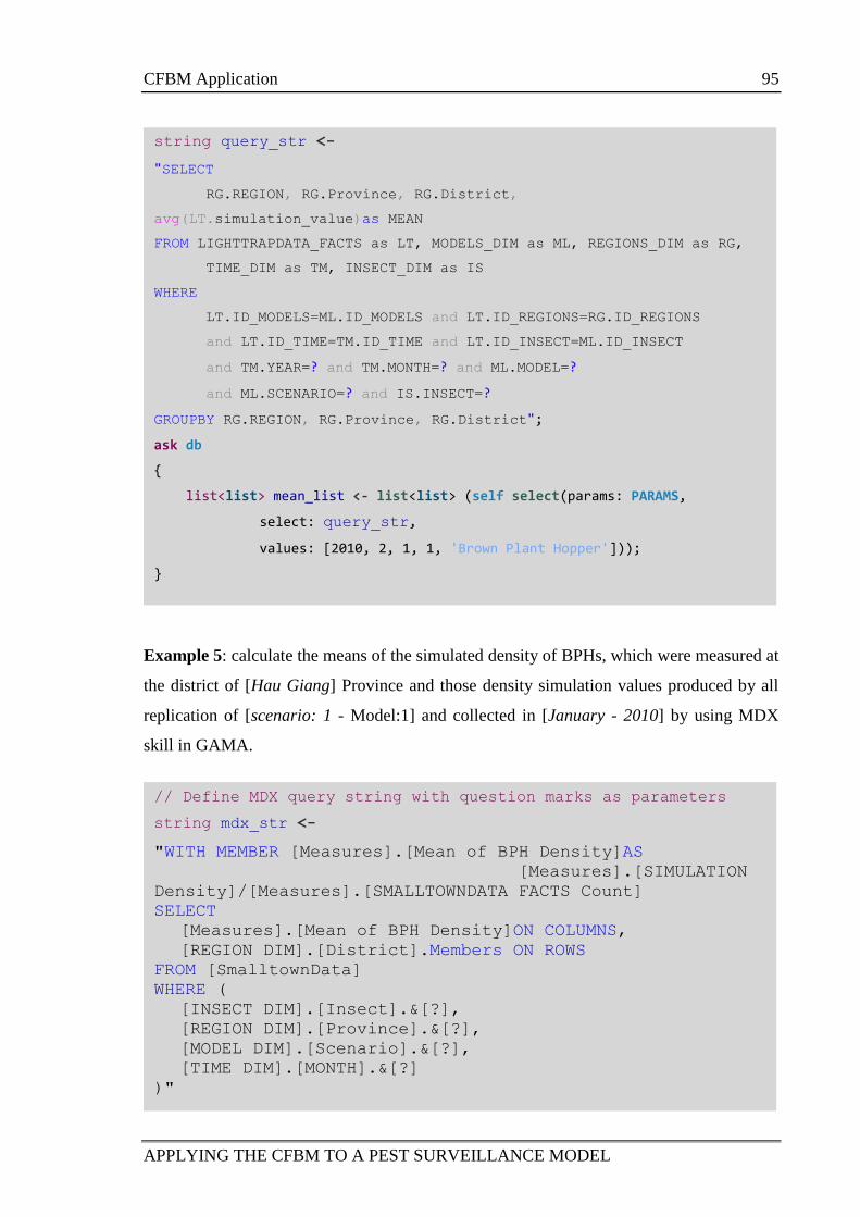
CFBM Application 95
APPLYING THE CFBM TO A PEST SURVEILLANCE MODEL
Example 5: calculate the means of the simulated density of BPHs, which were measured at
the district of [Hau Giang] Province and those density simulation values produced by all
replication of [scenario: 1 - Model:1] and collected in [January - 2010] by using MDX
skill in GAMA.
// Define MDX query string with question marks as parameters
string mdx_str <-
"WITH MEMBER [Measures].[Mean of BPH Density]AS
[Measures].[SIMULATION
Density]/[Measures].[SMALLTOWNDATA FACTS Count]
SELECT
[Measures].[Mean of BPH Density]ON COLUMNS,
[REGION DIM].[District].Members ON ROWS
FROM [SmalltownData]
WHERE (
[INSECT DIM].[Insect].&[?],
[REGION DIM].[Province].&[?],
[MODEL DIM].[Scenario].&[?],
[TIME DIM].[MONTH].&[?]
)"
string query_str <-
"SELECT
RG.REGION, RG.Province, RG.District,
avg(LT.simulation_value)as MEAN
FROM LIGHTTRAPDATA_FACTS as LT, MODELS_DIM as ML, REGIONS_DIM as RG,
TIME_DIM as TM, INSECT_DIM as IS
WHERE
LT.ID_MODELS=ML.ID_MODELS and LT.ID_REGIONS=RG.ID_REGIONS
and LT.ID_TIME=TM.ID_TIME and LT.ID_INSECT=ML.ID_INSECT
and TM.YEAR=? and TM.MONTH=? and ML.MODEL=?
and ML.SCENARIO=? and IS.INSECT=?
GROUPBY RG.REGION, RG.Province, RG.District";
ask db
{
list<list> mean_list <- list<list> (self select(params: PARAMS,
select: query_str,
values: [2010, 2, 1, 1, 'Brown Plant Hopper']));
}
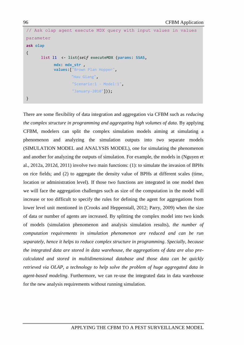
96 CFBM Application
APPLYING THE CFBM TO A PEST SURVEILLANCE MODEL
There are some flexibility of data integration and aggregation via CFBM such as reducing
the complex structure in programming and aggregating high volumes of data. By applying
CFBM, modelers can split the complex simulation models aiming at simulating a
phenomenon and analyzing the simulation outputs into two separate models
(SIMULATION MODEL and ANALYSIS MODEL), one for simulating the phenomenon
and another for analyzing the outputs of simulation. For example, the models in (Nguyen et
al., 2012a, 2012d, 2011) involve two main functions: (1): to simulate the invasion of BPHs
on rice fields; and (2) to aggregate the density value of BPHs at different scales (time,
location or administration level). If those two functions are integrated in one model then
we will face the aggregation challenges such as size of the computation in the model will
increase or too difficult to specify the rules for defining the agent for aggregations from
lower level unit mentioned in (Crooks and Heppenstall, 2012; Parry, 2009) when the size
of data or number of agents are increased. By splitting the complex model into two kinds
of models (simulation phenomenon and analysis simulation results), the number of
computation requirements in simulation phenomenon are reduced and can be run
separately, hence it helps to reduce complex structure in programming. Specially, because
the integrated data are stored in data warehouse, the aggregations of data are also pre-
calculated and stored in multidimensional database and those data can be quickly
retrieved via OLAP, a technology to help solve the problem of huge aggregated data in
agent-based modeling. Furthermore, we can re-use the integrated data in data warehouse
for the new analysis requirements without running simulation.
// Ask olap agent execute MDX query with input values in values
parameter
ask olap
{ list l1 <- list(self executeMDX (params: SSAS,
mdx: mdx_str , values:["Brown Plan Hopper",
"Hau Giang",
"Scenario:1 - Model:1",
"January-2010"]));
}
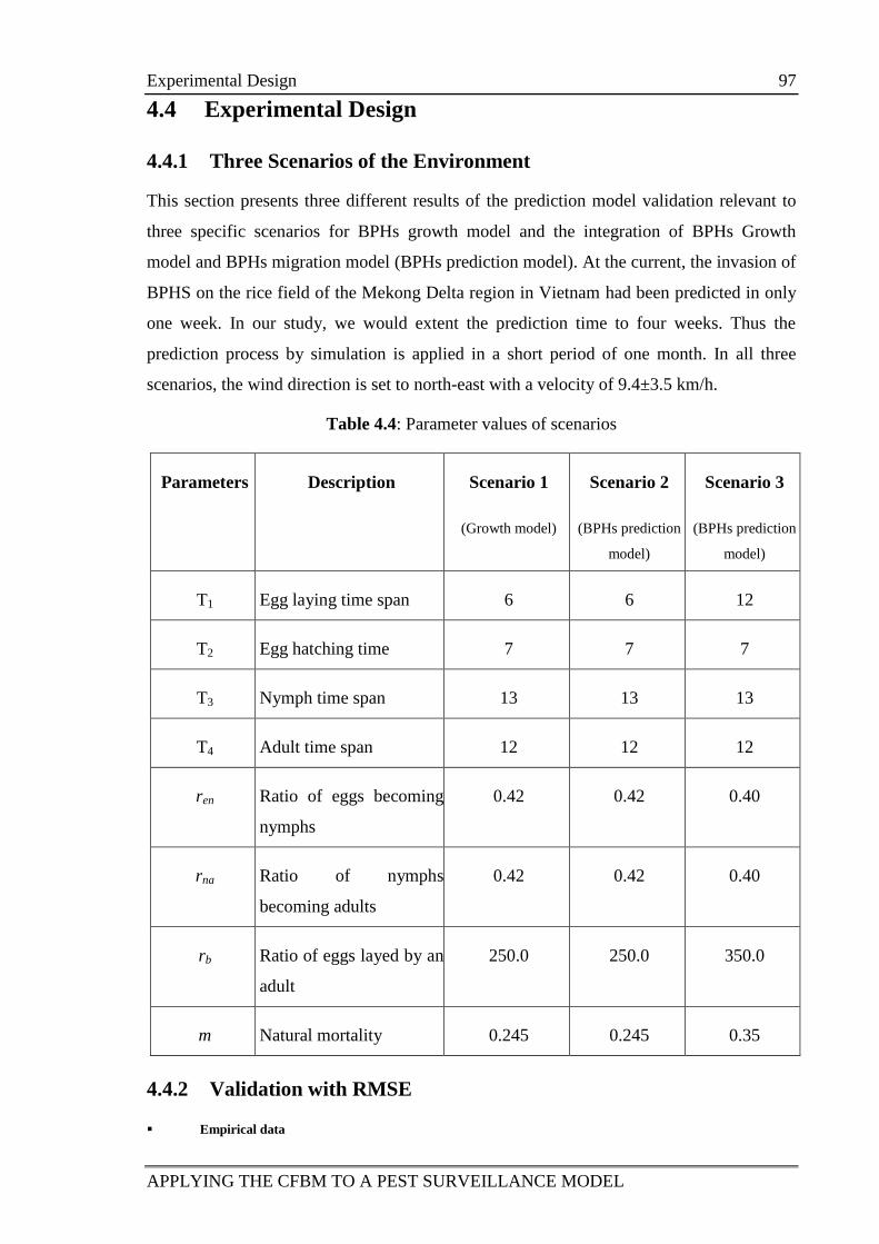
Experimental Design 97
APPLYING THE CFBM TO A PEST SURVEILLANCE MODEL
4.4 Experimental Design
4.4.1 Three Scenarios of the Environment
This section presents three different results of the prediction model validation relevant to
three specific scenarios for BPHs growth model and the integration of BPHs Growth
model and BPHs migration model (BPHs prediction model). At the current, the invasion of
BPHS on the rice field of the Mekong Delta region in Vietnam had been predicted in only
one week. In our study, we would extent the prediction time to four weeks. Thus the
prediction process by simulation is applied in a short period of one month. In all three
scenarios, the wind direction is set to north-east with a velocity of 9.4±3.5 km/h.
Table 4.4: Parameter values of scenarios
Parameters Description Scenario 1
(Growth model)
Scenario 2
(BPHs prediction
model)
Scenario 3
(BPHs prediction
model)
T1 Egg laying time span 6 6 12
T2 Egg hatching time 7 7 7
T3 Nymph time span 13 13 13
T4 Adult time span 12 12 12
ren Ratio of eggs becoming
nymphs
0.42 0.42 0.40
rna Ratio of nymphs
becoming adults
0.42 0.42 0.40
rb Ratio of eggs layed by an
adult
250.0 250.0 350.0
m Natural mortality 0.245 0.245 0.35
4.4.2 Validation with RMSE
Empirical data
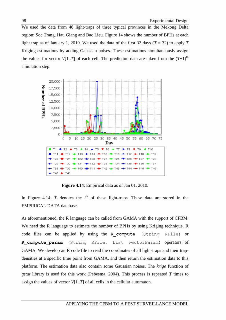
98 Experimental Design
APPLYING THE CFBM TO A PEST SURVEILLANCE MODEL
We used the data from 48 light-traps of three typical provinces in the Mekong Delta
region: Soc Trang, Hau Giang and Bac Lieu. Figure 14 shows the number of BPHs at each
light trap as of January 1, 2010. We used the data of the first 32 days (T = 32) to apply T
Kriging estimations by adding Gaussian noises. These estimations simultaneously assign
the values for vector V[1..T] of each cell. The prediction data are taken from the (T+1)th
simulation step.
Figure 4.14: Empirical data as of Jan 01, 2010.
In Figure 4.14, Ti denotes the ith
of these light-traps. These data are stored in the
EMPIRICAL DATA database.
As aforementioned, the R language can be called from GAMA with the support of CFBM.
We need the R language to estimate the number of BPHs by using Kriging technique. R
code files can be applied by using the R_compute (String RFile) or
R_compute_param (String RFile, List vectorParam) operators of
GAMA. We develop an R code file to read the coordinates of all light-traps and their trap-
densities at a specific time point from GAMA, and then return the estimation data to this
platform. The estimation data also contain some Gaussian noises. The krige function of
gstat library is used for this work (Pebesma, 2004). This process is repeated T times to
assign the values of vector V[1..T] of all cells in the cellular automaton.
Day
Nu
mb
er of B
PH
s
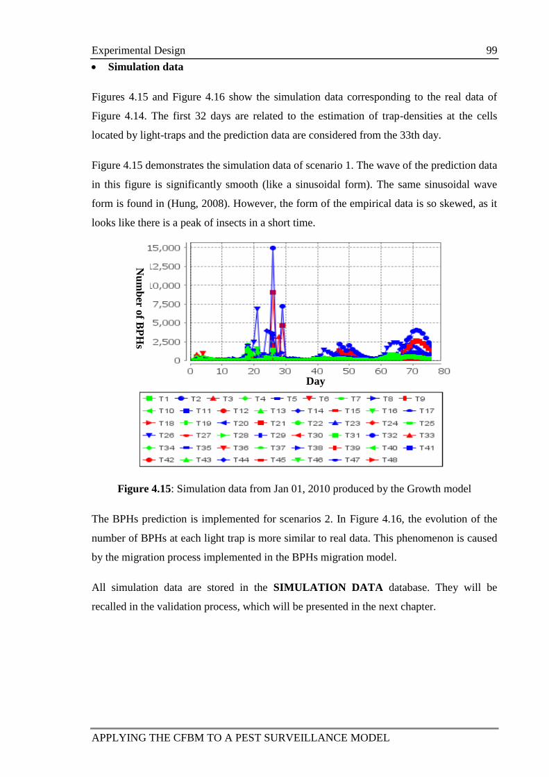
Experimental Design 99
APPLYING THE CFBM TO A PEST SURVEILLANCE MODEL
Simulation data
Figures 4.15 and Figure 4.16 show the simulation data corresponding to the real data of
Figure 4.14. The first 32 days are related to the estimation of trap-densities at the cells
located by light-traps and the prediction data are considered from the 33th day.
Figure 4.15 demonstrates the simulation data of scenario 1. The wave of the prediction data
in this figure is significantly smooth (like a sinusoidal form). The same sinusoidal wave
form is found in (Hung, 2008). However, the form of the empirical data is so skewed, as it
looks like there is a peak of insects in a short time.
Figure 4.15: Simulation data from Jan 01, 2010 produced by the Growth model
The BPHs prediction is implemented for scenarios 2. In Figure 4.16, the evolution of the
number of BPHs at each light trap is more similar to real data. This phenomenon is caused
by the migration process implemented in the BPHs migration model.
All simulation data are stored in the SIMULATION DATA database. They will be
recalled in the validation process, which will be presented in the next chapter.
Day
Nu
mb
er of B
PH
s
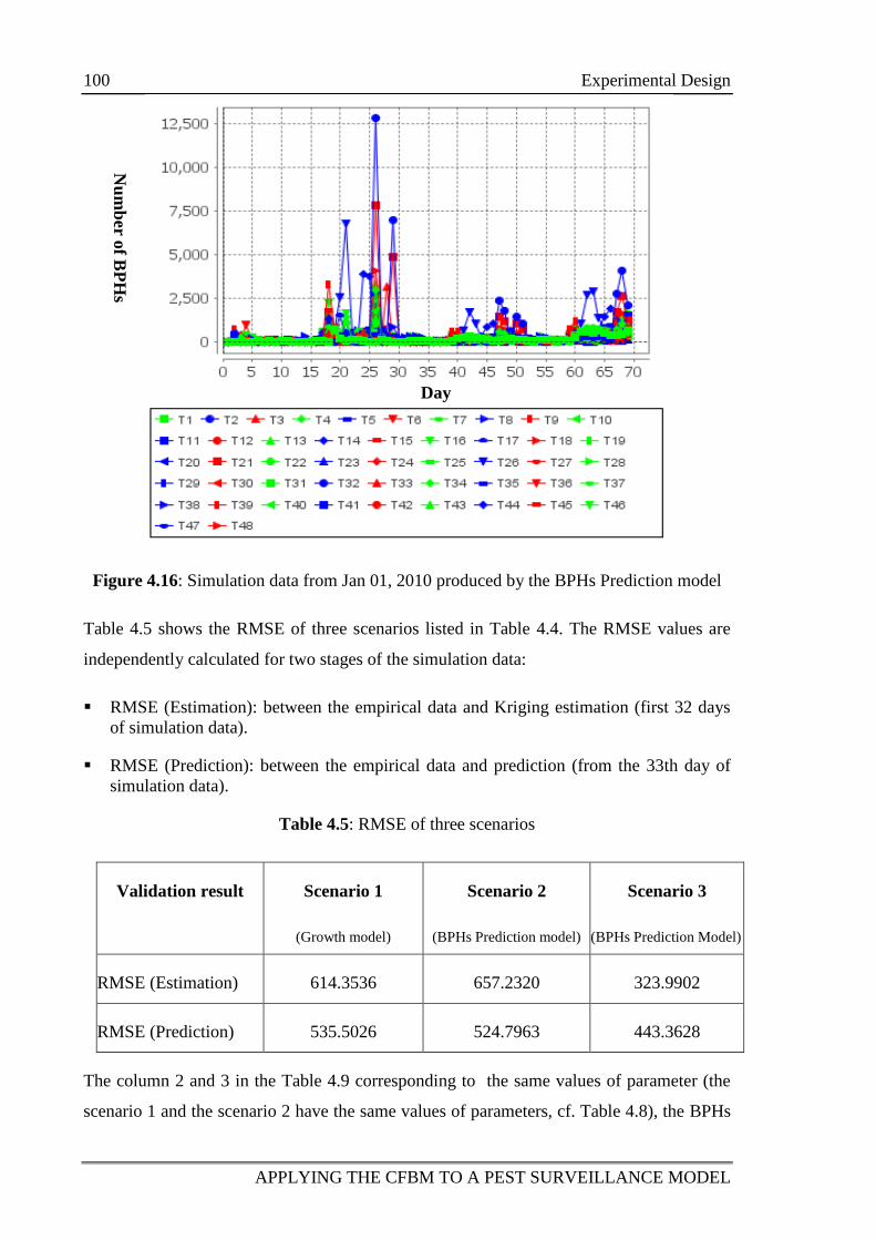
100 Experimental Design
APPLYING THE CFBM TO A PEST SURVEILLANCE MODEL
Figure 4.16: Simulation data from Jan 01, 2010 produced by the BPHs Prediction model
Table 4.5 shows the RMSE of three scenarios listed in Table 4.4. The RMSE values are
independently calculated for two stages of the simulation data:
RMSE (Estimation): between the empirical data and Kriging estimation (first 32 days
of simulation data).
RMSE (Prediction): between the empirical data and prediction (from the 33th day of
simulation data).
Table 4.5: RMSE of three scenarios
Validation result Scenario 1
(Growth model)
Scenario 2
(BPHs Prediction model)
Scenario 3
(BPHs Prediction Model)
RMSE (Estimation) 614.3536 657.2320 323.9902
RMSE (Prediction) 535.5026 524.7963 443.3628
The column 2 and 3 in the Table 4.9 corresponding to the same values of parameter (the
scenario 1 and the scenario 2 have the same values of parameters, cf. Table 4.8), the BPHs
Nu
mb
er of B
PH
s
Day
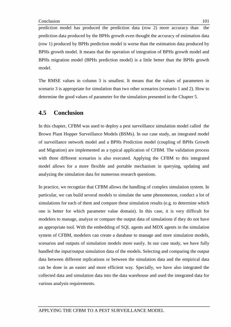
Conclusion 101
APPLYING THE CFBM TO A PEST SURVEILLANCE MODEL
prediction model has produced the prediction data (row 2) more accuracy than the
prediction data produced by the BPHs growth even thought the accuracy of estimation data
(row 1) produced by BPHs prediction model is worse than the estimation data produced by
BPHs growth model. It means that the operation of integration of BPHs growth model and
BPHs migration model (BPHs prediction model) is a little better than the BPHs growth
model.
The RMSE values in column 3 is smallest. It means that the values of parameters in
scenario 3 is appropriate for simulation than two other scenarios (scenario 1 and 2). How to
determine the good values of parameter for the simulation presented in the Chapter 5.
4.5 Conclusion
In this chapter, CFBM was used to deploy a pest surveillance simulation model called the
Brown Plant Hopper Surveillance Models (BSMs). In our case study, an integrated model
of surveillance network model and a BPHs Prediction model (coupling of BPHs Growth
and Migration) are implemented as a typical application of CFBM. The validation process
with three different scenarios is also executed. Applying the CFBM to this integrated
model allows for a more flexible and portable mechanism in querying, updating and
analyzing the simulation data for numerous research questions.
In practice, we recognize that CFBM allows the handling of complex simulation system. In
particular, we can build several models to simulate the same phenomenon, conduct a lot of
simulations for each of them and compare these simulation results (e.g. to determine which
one is better for which parameter value domain). In this case, it is very difficult for
modelers to manage, analyze or compare the output data of simulations if they do not have
an appropriate tool. With the embedding of SQL agents and MDX agents in the simulation
system of CFBM, modelers can create a database to manage and store simulation models,
scenarios and outputs of simulation models more easily. In our case study, we have fully
handled the input/output simulation data of the models. Selecting and comparing the output
data between different replications or between the simulation data and the empirical data
can be done in an easier and more efficient way. Specially, we have also integrated the
collected data and simulation data into the data warehouse and used the integrated data for
various analysis requirements.

CFBM APPLICATION TO THE CALIBRATION AND VALIDATION OF AN AGENT-
BASED SIMULATION MODEL
102 TRUONG Minh Thai
CFBM APPLICATION TO THE CALIBRATION AND VALIDATION OF AN AGENT-
BASED SIMULATION MODEL
TRUONG Minh Thai 103
Chapter 5 CFBM APPLICATION TO THE
CALIBRATION AND VALIDATION OF
AN AGENT-BASED SIMULATION
MODEL
Table of contents
5.1 Introduction ......................................................................................................... 105
5.2 Calibration approach ............................................................................................ 105
5.2.1 Calibration of an Agent-Based Model ................................................... 106
5.2.2 Measure of the similarity between two datasets .................................... 109
5.2.2.1 Similarity coefficient using RMSE ......................................... 109
5.2.2.2 Similarity coefficient using the Jaccard Index ........................ 110
5.3 Calibration of the BPHs Prediction model .......................................................... 113
5.3.1 BPHs Prediction model and data management ..................................... 113
5.3.2 Parameters for Calibration ..................................................................... 114
5.3.3 The measurement indicators and the Fitness condition ......................... 115
5.3.4 Implementation of the calibration model .............................................. 115
5.3.5 Calibration Experiment ......................................................................... 125
5.3.5.1 Simulation Outputs and Empirical data .................................. 125
5.3.5.2 To Measure the similarity Coefficient between the simulated
data and empirical data .......................................................................... 126
CFBM APPLICATION TO THE CALIBRATION AND VALIDATION OF AN AGENT-
BASED SIMULATION MODEL
104 TRUONG Minh Thai
5.3.5.3 Results of the calibration experiments .................................... 128
5.4 Validation of the Accepted Scenario ................................................................... 133
5.4.1 Implementation of the validation model ................................................ 133
5.4.2 Validation experiment ........................................................................... 135
5.4.2.1 Simulation and validation data ................................................ 135
5.4.2.2 Results of the validation experiment ....................................... 135
5.5 Discussion ............................................................................................................ 137
5.5.1 Application of CFBM for calibration and validation ............................ 137
5.5.2 The Jaccard index with aggregation ...................................................... 138
5.6 Conclusion ........................................................................................................... 140
Calibration approach 105
CFBM APPLICATION TO THE CALIBRATION AND VALIDATION OF AN AGENT-
BASED SIMULATION MODEL
5.1 Introduction
Calibration and validation (cf. Section 2.2.2.5) are two of the main challenges for Agent-
Based Modeling and Simulation (ABMS) approaches when the model has to deal with
integrated systems involving high volumes of input/output data (cf. Section 2.2.2.7 and
2.3.2). In this chapter, I propose a calibration approach for agent-based models, using the
Combination Framework of Business intelligence solution and Multi-agent platform
(CFBM, cf. Chapter 3), and in particular taking advantages from its integrated
management of the input data (empirical datasets) and output data of simulations (cf.
Chapter 4). The calibration of the Brown Plant Hopper Prediction model (cf. Section
4.2.7.1) is presented and used throughout the chapter as case study to illustrate the way
CFBM manages data used and generated during the life-cycle of a simulation in particular
during the calibration step. The originality of my approach is that the tools used to analyze
the simulation is also a model, written in the same language, allowing a better integration
of the two models.
In the following sections, I first present the proposed calibration approach for integrated
agent-based simulation models in Section 5.2.1 and suggest two specific measures: the
RMSE (Root Mean Square Error) and the Jaccard index for ordered data sets, which have
been used to evaluate the accuracy of the simulation outputs in Section 5.2.2. In Section
5.3, I apply the approach on the BPHs integrated simulation model illustrating how to
calibrate the model using the CFBM in the GAMA simulation platform. In Section 5.4, I
present the validation of the results of calibration. The scenarios accepted in Section 5.3
will be validated on another data set, using the 2 measures introduced previously (namely
the RMSE and the Jaccard index). Discussion and perspectives conclude this chapter.
5.2 Calibration approach
In this section, I propose an approach to calibrate an agent-based simulation model. The
approach is an application of CFBM. My framework is particularly useful when we work
with integrated simulation systems, where we need to control several models with high
volume of input/output data of simulation or observation data from real system and
analysis results. In this part, I detail the practical use of CFBM for calibration and
validation purposes.
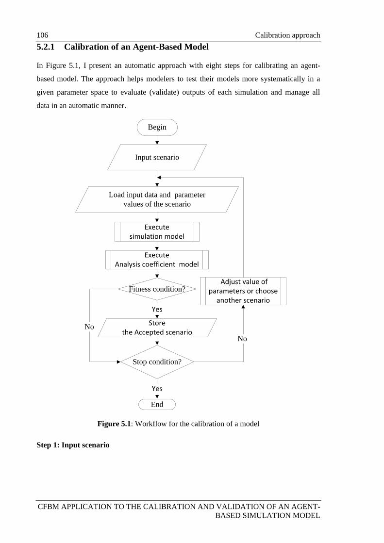
106 Calibration approach
CFBM APPLICATION TO THE CALIBRATION AND VALIDATION OF AN AGENT-
BASED SIMULATION MODEL
5.2.1 Calibration of an Agent-Based Model
In Figure 5.1, I present an automatic approach with eight steps for calibrating an agent-
based model. The approach helps modelers to test their models more systematically in a
given parameter space to evaluate (validate) outputs of each simulation and manage all
data in an automatic manner.
Begin
Load input data and parameter
values of the scenario
Fitness condition?
End
Stop condition?
No
No
Store the Accepted scenario
Yes
Execute simulation model
Execute Analysis coefficient model
Yes
Adjust value of parameters or choose
another scenario
Input scenario
Figure 5.1: Workflow for the calibration of a model
Step 1: Input scenario
Calibration approach 107
CFBM APPLICATION TO THE CALIBRATION AND VALIDATION OF AN AGENT-
BASED SIMULATION MODEL
First, the user chooses the initial simulation scenario. Each scenario is stored in the
database and contains a set of simulation parameters with their value, as identified in the
Section 4.3.1.2.
Step 2: Load input data and parameter values of the scenario
Given the tuple (model, scenario) and the input dataset, the system retrieves the input data
and the related parameters value from database. This step assures that the correct input data
and values of parameters value are loaded in the simulation model.
Step 3: Execute the simulation model
The simulation model is executed with the loaded scenario as input. In this process, the
outputs of the simulation are stored into a database. As the simulation can be executed
many times (replications) with the same scenario, the tuple (model, scenario, replication,
step, output) are stored into the database (cf. SIMULATIONDATA_LT or
SIMULATIONDATA_SM in Section 4.3.1.2), to ensure that the system can handle results
in each step of the simulation
Step 4: Execute analysis coefficient model to compute similarity coefficients
The analysis coefficient model is used to analyze the distance between simulation outputs
and observations from the real system: the step 4 computes the similarity coefficients
between the output data produced by the step 3 and the observation data. A lot of different
similarity coefficients can be used to this purpose depending on the modeler’s goal. In the
sequel I chose to implement the two following functions: (1) the RMSE function to
calculate the root mean square error between two data sets and (2) the JACCARD function
to compute the Jaccard index between two data sets (Cf. Section 5.3.4).
In this step, the analysis coefficient model loads the observation data set (the reference
dataset) and the corresponding simulation output data set corresponding to the tuple
(model, scenario, replicate, step, output) and makes comparison between them. The result
of the analysis coefficient model is also stored into the database with the tuple (model,
scenario, replication, coefficient, value of coefficient).
Step 5: Check fitness condition
The fitness condition is defined by the modeler, depending on the similarity coefficient he
wants to use to validate the simulation outputs. In this chapter, I propose to use RMSE and
Jaccard index (Section 5.2.2) as two similarity indicators of the fitness condition.

108 Calibration approach
CFBM APPLICATION TO THE CALIBRATION AND VALIDATION OF AN AGENT-
BASED SIMULATION MODEL
The result of the analysis coefficient model (Step 4) is compared with fitness value that is
the value of the similarity coefficient defined by the modeler. For example, in my
implementation in Section 5.3.4, the fitness value of Jaccard index is identified from 0.70
to 0.98 depended on which time section of the simulation. There are two cases:
If the fitness condition fulfilled then the system goes to Step 5. This means that
the parameter values are accepted. In this case, the scenario is called an accepted
scenario.
Otherwise the system goes to Step 6. This means that the simulation inputs and
the parameters values are acceptable not accepted.
Step 6: Store the accepted scenario
As the result of the analysis coefficient model of each replication has been stored in the
tuple (model, scenario, replication, coefficient, value of coefficient) in Step 4. Hence, this
step only stores the accepted value of the parameters in the tuple (model, scenario,
replication, coefficient, values of fitness). Note that, we do not need to store the accepted
parameters value in this step because we can identify them from the scenario based on
relationship between the scenario and parameter entities presented in Section 4.3.1.2.
Step 7: Check stop condition
All this calibration process is performed until there are no more scenarios available in the
database. This step checks thus whether the process should end, i.e. whether there is
another scenario instance in the database. Hence, there are two cases:
If the Stop condition is fulfilled, then the process is over: this means that there
is no other scenario instance in the database.
Otherwise, then the system goes to the Step 8: this means that there are other
scenario instances in the database.
Step 8: Adjust the value of parameters or choose another scenario
There are two choices for implementation in this step: (1) adjust the values of the
parameters. It aims at improving the model outputs by altering the parameters values
thanks to a method chosen by the modeler such as "Weight Evidence" (Donigian, 2002) or
"Genetic Algorithm" (Ngo and See, 2012). The result of this process is the creation of a
new scenario for the simulation model, which will be used in the next loop, and it's (i.e. the
Calibration approach 109
CFBM APPLICATION TO THE CALIBRATION AND VALIDATION OF AN AGENT-
BASED SIMULATION MODEL
values of the parameters) storage in the database; or (2) choose another scenario if the
scenario had already been defined by the modeler. The system then goes back to Step 2.
In implementation of the calibration of the BPHs Prediction model (cf. Section 5.3.4), I
defined a set of scenario for calibration then the system will choose a scenario from the
defined scenario set.
This section has illustrated the interest of applying CFBM to calibration of models. It can
indeed handle all data processed by both the simulation model and analysis coefficient
model and then do the calibration. With the eight-step approach, the calibration model can
execute the simulation model with all adjusted values of the parameters, manage the whole
input/output data dealt within the processes, and analyze the similarity between simulation
outputs and observation data. It helps us to specify appropriate values of parameters
automatically.
5.2.2 Measure of the similarity between two datasets
In this section, I introduce two methods to measure the similarity between to data sets that
are the RMSE (Root Mean Square Error) (Hyndman and Koehler, 2006) and Jaccard index
(Jaccard, 1908). These two similarity coefficients are used to measure the similarity
between the simulation results and the empirical data collected from the reference system.
In the sequel, I assume that I want to measure the similarity between the two following
ordered datasets:
X = {x1, x2, … , xn}
Y = {y1, y2, … , yn}
An ordered dataset denotes a dataset where values are temporally ordered.
5.2.2.1 Similarity coefficient using RMSE
Several methods have been proposed to measure the similarity between two datasets as
mentioned in (Ngo and See, 2012; Wolda, 1981). Root Mean Squared Error (RMSE)
(Chatfield, 1992; Taylor, 1992) is usually used to estimate the difference (or error)
between datasets in forecast systems. In particular, it can be used to compare several output
datasets from different models, different output datasets from the same model or simulated
data produced by the model and collected dataset from reference.
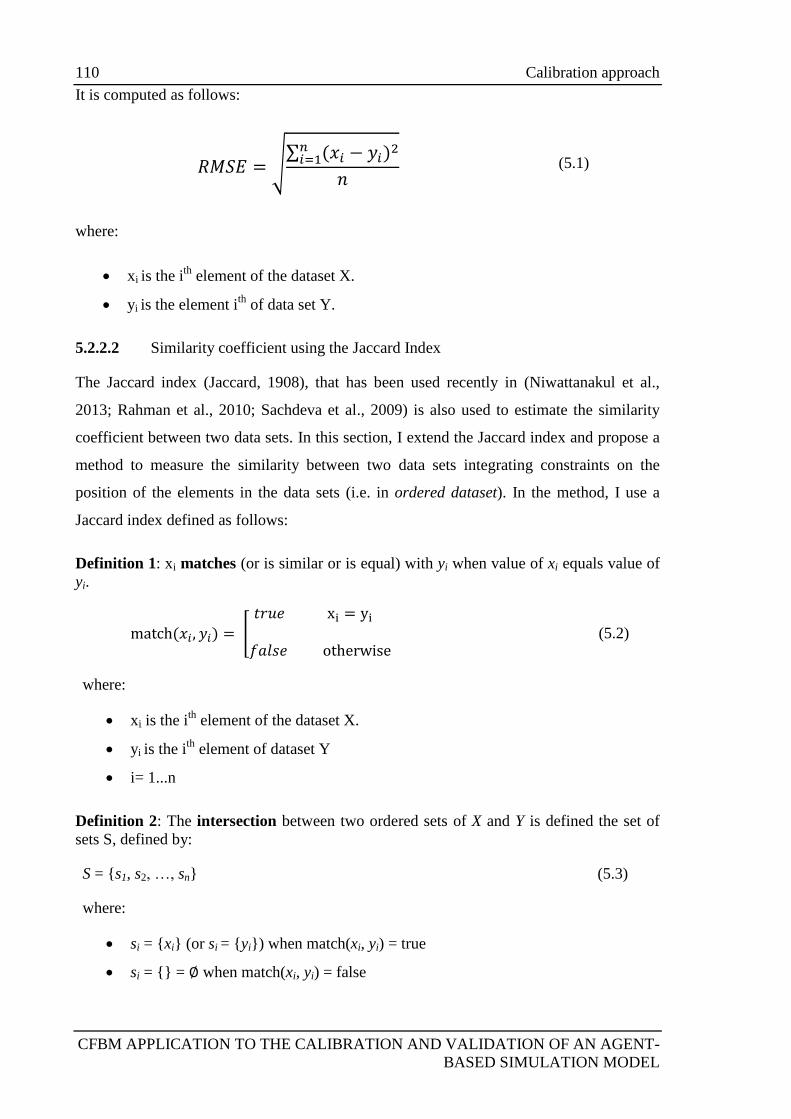
110 Calibration approach
CFBM APPLICATION TO THE CALIBRATION AND VALIDATION OF AN AGENT-
BASED SIMULATION MODEL
It is computed as follows:
(5.1)
where:
xi is the ith
element of the dataset X.
yi is the element ith
of data set Y.
5.2.2.2 Similarity coefficient using the Jaccard Index
The Jaccard index (Jaccard, 1908), that has been used recently in (Niwattanakul et al.,
2013; Rahman et al., 2010; Sachdeva et al., 2009) is also used to estimate the similarity
coefficient between two data sets. In this section, I extend the Jaccard index and propose a
method to measure the similarity between two data sets integrating constraints on the
position of the elements in the data sets (i.e. in ordered dataset). In the method, I use a
Jaccard index defined as follows:
Definition 1: xi matches (or is similar or is equal) with yi when value of xi equals value of
yi.
(5.2)
where:
xi is the ith
element of the dataset X.
yi is the ith
element of dataset Y
i= 1...n
Definition 2: The intersection between two ordered sets of X and Y is defined the set of
sets S, defined by:
S = {s1, s2, …, sn} (5.3)
where:
si = {xi} (or si = {yi}) when match(xi, yi) = true
si = {} = ∅ when match(xi, yi) = false
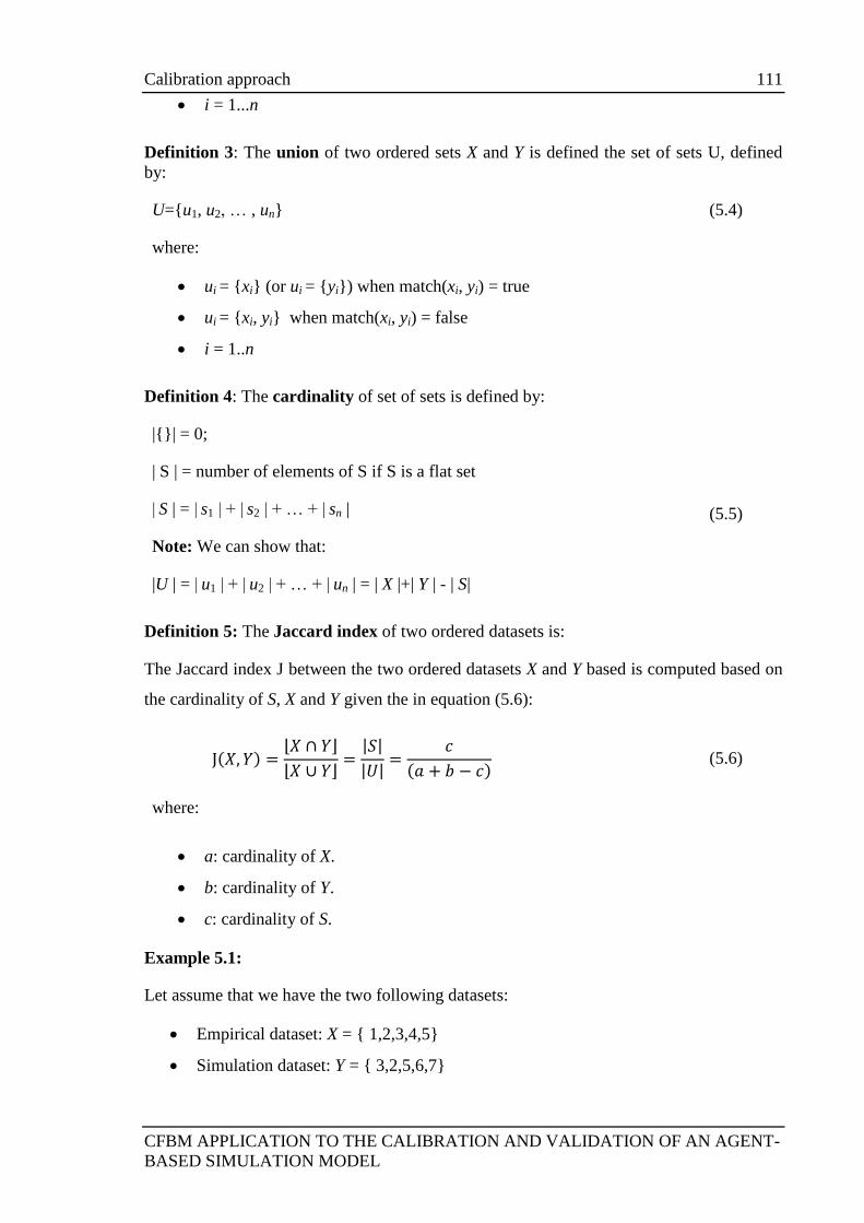
Calibration approach 111
CFBM APPLICATION TO THE CALIBRATION AND VALIDATION OF AN AGENT-
BASED SIMULATION MODEL
i = 1...n
Definition 3: The union of two ordered sets X and Y is defined the set of sets U, defined
by:
U={u1, u2, … , un} (5.4)
where:
ui = {xi} (or ui = {yi}) when match(xi, yi) = true
ui = {xi, yi} when match(xi, yi) = false
i = 1..n
Definition 4: The cardinality of set of sets is defined by:
|{}| = 0;
| S | = number of elements of S if S is a flat set
| S | = | s1 | + | s2 | + … + | sn |
Note: We can show that:
|U | = | u1 | + | u2 | + … + | un | = | X |+| Y | - | S|
(5.5)
Definition 5: The Jaccard index of two ordered datasets is:
The Jaccard index J between the two ordered datasets X and Y based is computed based on
the cardinality of S, X and Y given the in equation (5.6):
(5.6)
where:
a: cardinality of X.
b: cardinality of Y.
c: cardinality of S.
Example 5.1:
Let assume that we have the two following datasets:
Empirical dataset: X = { 1,2,3,4,5}
Simulation dataset: Y = { 3,2,5,6,7}
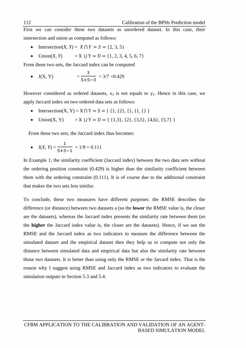
112 Calibration of the BPHs Prediction model
CFBM APPLICATION TO THE CALIBRATION AND VALIDATION OF AN AGENT-
BASED SIMULATION MODEL
First we can consider these two datasets as unordered dataset. In this case, their
intersection and union as computed as follows:
Intersection(X, Y) = {2, 3, 5}
Union(X, Y) = {1, 2, 3, 4, 5, 6, 7}
From these two sets, the Jaccard index can be computed
J(X, Y) =
= 3/7 =0.429
However considered as ordered datasets, x3 is not equals to y1. Hence in this case, we
apply Jaccard index on two ordered data sets as follows:
Intersection(X, Y) = { {}, {2}, {}, {}, {} }
Union(X, Y) = { {1,3}, {2}, {3,5}, {4,6}, {5,7} }
From these two sets, the Jaccard index thus becomes:
J(X, Y) =
= 1/9 = 0.111
In Example 1, the similarity coefficient (Jaccard index) between the two data sets without
the ordering position constraint (0.429) is higher than the similarity coefficient between
them with the ordering constraint (0.111). It is of course due to the additional constraint
that makes the two sets less similar.
To conclude, these two measures have different purposes: the RMSE describes the
difference (or distance) between two datasets a (so the lower the RMSE value is, the closer
are the datasets), whereas the Jaccard index presents the similarity rate between them (so
the higher the Jaccard index value is, the closer are the datasets). Hence, if we use the
RMSE and the Jaccard index as two indicators to measure the difference between the
simulated dataset and the empirical dataset then they help us to compute not only the
distance between simulated data and empirical data but also the similarity rate between
those two datasets. It is better than using only the RMSE or the Jarcard index. That is the
reason why I suggest using RMSE and Jaccard index as two indicators to evaluate the
simulation outputs in Section 5.3 and 5.4.
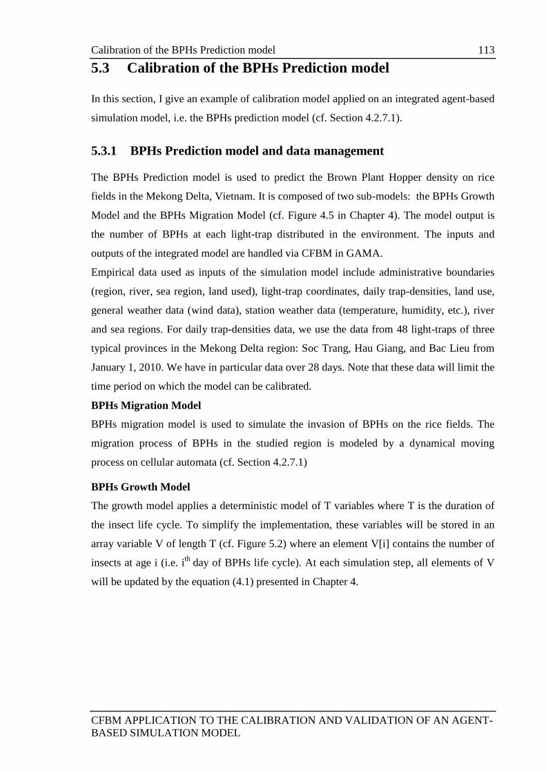
Calibration of the BPHs Prediction model 113
CFBM APPLICATION TO THE CALIBRATION AND VALIDATION OF AN AGENT-
BASED SIMULATION MODEL
5.3 Calibration of the BPHs Prediction model
In this section, I give an example of calibration model applied on an integrated agent-based
simulation model, i.e. the BPHs prediction model (cf. Section 4.2.7.1).
5.3.1 BPHs Prediction model and data management
The BPHs Prediction model is used to predict the Brown Plant Hopper density on rice
fields in the Mekong Delta, Vietnam. It is composed of two sub-models: the BPHs Growth
Model and the BPHs Migration Model (cf. Figure 4.5 in Chapter 4). The model output is
the number of BPHs at each light-trap distributed in the environment. The inputs and
outputs of the integrated model are handled via CFBM in GAMA.
Empirical data used as inputs of the simulation model include administrative boundaries
(region, river, sea region, land used), light-trap coordinates, daily trap-densities, land use,
general weather data (wind data), station weather data (temperature, humidity, etc.), river
and sea regions. For daily trap-densities data, we use the data from 48 light-traps of three
typical provinces in the Mekong Delta region: Soc Trang, Hau Giang, and Bac Lieu from
January 1, 2010. We have in particular data over 28 days. Note that these data will limit the
time period on which the model can be calibrated.
BPHs Migration Model
BPHs migration model is used to simulate the invasion of BPHs on the rice fields. The
migration process of BPHs in the studied region is modeled by a dynamical moving
process on cellular automata (cf. Section 4.2.7.1)
BPHs Growth Model
The growth model applies a deterministic model of T variables where T is the duration of
the insect life cycle. To simplify the implementation, these variables will be stored in an
array variable V of length T (cf. Figure 5.2) where an element V[i] contains the number of
insects at age i (i.e. ith
day of BPHs life cycle). At each simulation step, all elements of V
will be updated by the equation (4.1) presented in Chapter 4.
114 Calibration of the BPHs Prediction model
CFBM APPLICATION TO THE CALIBRATION AND VALIDATION OF AN AGENT-
BASED SIMULATION MODEL
Figure 5.2: Variable V of length T=32 days maximal life duration of BPHs
The parameters of this model and their possible values for calibration are presented in the
next section. They have been identified based on the description of the BPHs life cycle in
(Ngo, 2008) presented in Section 4.2.3 of Chapter 4.
5.3.2 Parameters for Calibration
Equation (4.1) (presented in Chapter 4) show that the BPHs Prediction model has 8
parameters (T1, T2, T3, T4, ren, rna, m). However, the value of T1 (egg laying time span), ren
(the rate of eggs becoming nymph), rna (the rate of nymphs becoming adult) and rb (the
average number of eggs laid by an adult) are constants and their value are: T1=7 days,
ren=0.4, rna=0.4 and rb=360 eggs (Ngo, 2008).
As a consequence, only 4 parameters will be used for the calibration. Those four
parameters are T2 (the egg incubation time) with two possible values i.e. 6 or 7 days, T3
(the nymph state duration) with two values: 12 or 13 days, T4 (the adult state duration)
between 10 days and 12 days and m (the mortality rate) ranges from 0.15 to 0.40.
To summarize, the full parameter space to explore during the calibration is limited to (cf.
Table C.1, Appendix C):
T2: [6, 7]
T3: [12, 13]
T4: [10, 11, 12]
m=[0.15, 0.20, 0.25, 0.30, 0.35, 0.40]
T2 T3
T1
T4
ren rna
rb
Calibration of the BPHs Prediction model 115
CFBM APPLICATION TO THE CALIBRATION AND VALIDATION OF AN AGENT-
BASED SIMULATION MODEL
So the exhaustive exploration of the parameter spaces provides 72 scenarios that
are presented in Table C.2 (Appendix C).
5.3.3 The measurement indicators and the Fitness condition
As presented above, we use two measures (RMSE and Jaccard index) as indicators for
the calibration. The number of BPHs on the rice fields, (that is the main output of the
prediction model) will not be evaluated at each simulation step (representing a day) but on
a seven days period. As we have data over 28 days, we will evaluate the BPHs on the 4
periods: from day 0 (initial day) to 6 (1st week), from day 7 to 13 (2
nd week), from day 14
to 20 (3rd
week) and from day 21 to 27 (4th
week). Hence for each scenario, we compute
the two indicators between the simulation results and empirical data in each of the four
time sections. If we call distance_1, distance_2, distance_3, distance_4 the four defined
fitness condition values of the RMSE and similarity_1, similarity_2, similarity_3,
similarity_4 the four defined fitness condition values of the Jaccard index in each time
period 1st week, 2
nd week, 3
rd week, 4
th week, we can thus define the fitness condition for
the calibration as an expression "and" of conditions in table 5.1.
Table 5.1: Fitness condition for time sections
Coefficient 1st week 2
nd week 3
rd week 4
th week
RMSE <=distance_1 <=distance_2 <=distance_3 <=distance_4
Jaccard index >=similarity_1 >=similarity_2 >=similarity_3 >=similarity_4
5.3.4 Implementation of the calibration model
The calibration model is implemented using Batch experiment32
of GAMA and uses
CFBM to manage the input and output of the BPHs Prediction model and calibration
model. In the sequel I describe the way the calibration model is implemented.
Step 1: Description of the parameters containing the scenario identification and replication
number index
32
https://code.google.com/p/gama-platform/wiki/G__BatchExperiments
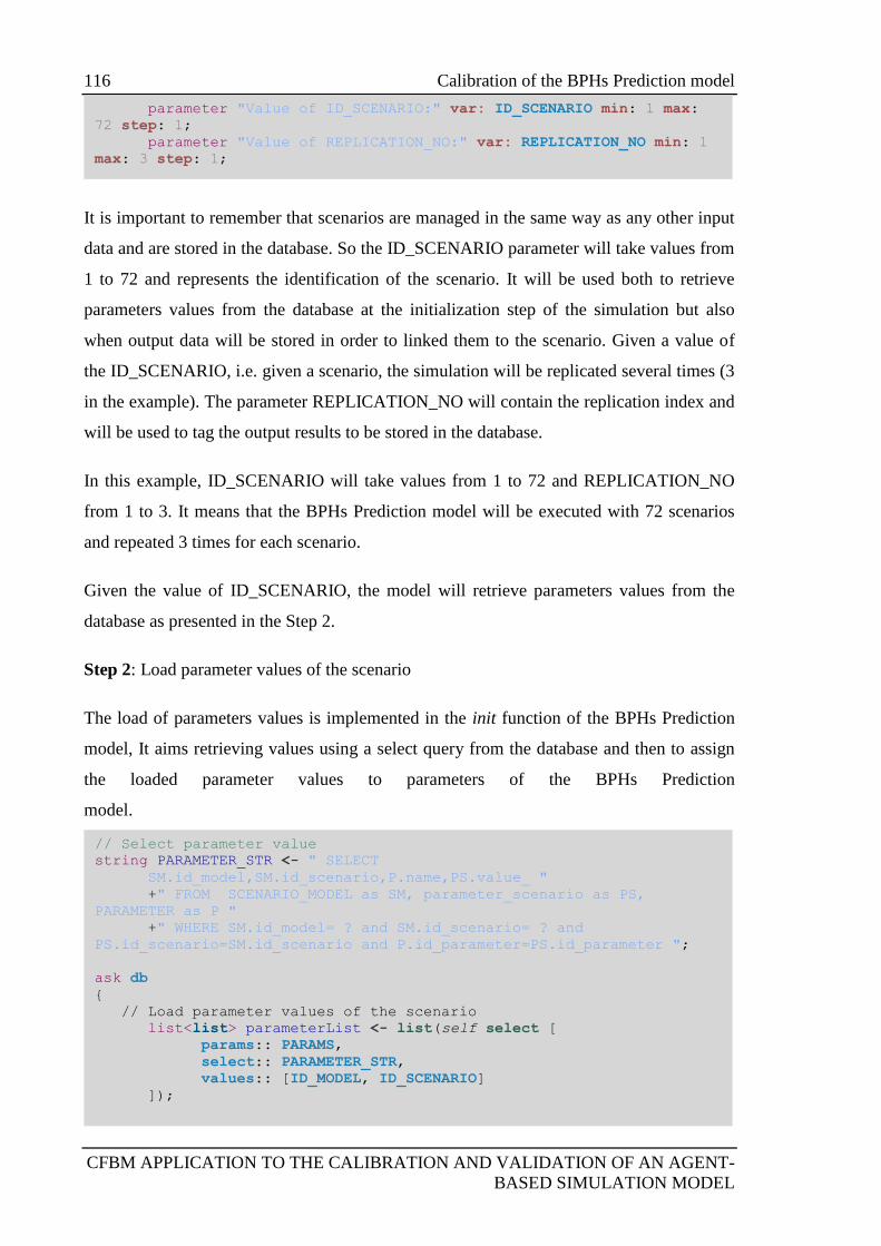
116 Calibration of the BPHs Prediction model
CFBM APPLICATION TO THE CALIBRATION AND VALIDATION OF AN AGENT-
BASED SIMULATION MODEL
It is important to remember that scenarios are managed in the same way as any other input
data and are stored in the database. So the ID_SCENARIO parameter will take values from
1 to 72 and represents the identification of the scenario. It will be used both to retrieve
parameters values from the database at the initialization step of the simulation but also
when output data will be stored in order to linked them to the scenario. Given a value of
the ID_SCENARIO, i.e. given a scenario, the simulation will be replicated several times (3
in the example). The parameter REPLICATION_NO will contain the replication index and
will be used to tag the output results to be stored in the database.
In this example, ID_SCENARIO will take values from 1 to 72 and REPLICATION_NO
from 1 to 3. It means that the BPHs Prediction model will be executed with 72 scenarios
and repeated 3 times for each scenario.
Given the value of ID_SCENARIO, the model will retrieve parameters values from the
database as presented in the Step 2.
Step 2: Load parameter values of the scenario
The load of parameters values is implemented in the init function of the BPHs Prediction
model, It aims retrieving values using a select query from the database and then to assign
the loaded parameter values to parameters of the BPHs Prediction
model.
// Select parameter value
string PARAMETER_STR <- " SELECT
SM.id_model,SM.id_scenario,P.name,PS.value_ "
+" FROM SCENARIO_MODEL as SM, parameter_scenario as PS,
PARAMETER as P "
+" WHERE SM.id_model= ? and SM.id_scenario= ? and
PS.id_scenario=SM.id_scenario and P.id_parameter=PS.id_parameter ";
ask db
{
// Load parameter values of the scenario
list<list> parameterList <- list(self select [
params:: PARAMS,
select:: PARAMETER_STR,
values:: [ID_MODEL, ID_SCENARIO]
]);
parameter "Value of ID_SCENARIO:" var: ID_SCENARIO min: 1 max:
72 step: 1;
parameter "Value of REPLICATION_NO:" var: REPLICATION_NO min: 1
max: 3 step: 1;
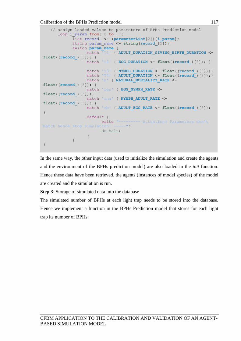
Calibration of the BPHs Prediction model 117
CFBM APPLICATION TO THE CALIBRATION AND VALIDATION OF AN AGENT-
BASED SIMULATION MODEL
In the same way, the other input data (used to initialize the simulation and create the agents
and the environment of the BPHs prediction model) are also loaded in the init function.
Hence these data have been retrieved, the agents (instances of model species) of the model
are created and the simulation is run.
Step 3: Storage of simulated data into the database
The simulated number of BPHs at each light trap needs to be stored into the database.
Hence we implement a function in the BPHs Prediction model that stores for each light
trap its number of BPHs:
// assign loaded values to parameters of BPHs Prediction model
loop i_param from: 0 to: 7{
list record_ <- (parameterList[2])[i_param];
string param_name <- string(record_[2]);
switch param_name {
match 'T1' { ADULT_DURATION_GIVING_BIRTH_DURATION <-
float((record_)[3]); }
match 'T2' { EGG_DURATION <- float((record_)[3]); }
match 'T3' { NYMPH_DURATION <- float((record_)[3]);}
match 'T4' { ADULT_DURATION <- float((record_)[3]);}
match 'm' { NATURAL_MORTALITY_RATE <-
float((record_)[3]); }
match 'ren' { EGG_NYMPH_RATE <-
float((record_)[3]);}
match 'rna' { NYMPH_ADULT_RATE <-
float((record_)[3]); }
match 'rb' { ADULT_EGG_RATE <- float((record_)[3]);
}
default {
write "--------- Attention: Parameters don't
match hence stop simulation! -----";
do halt;
}
}
}
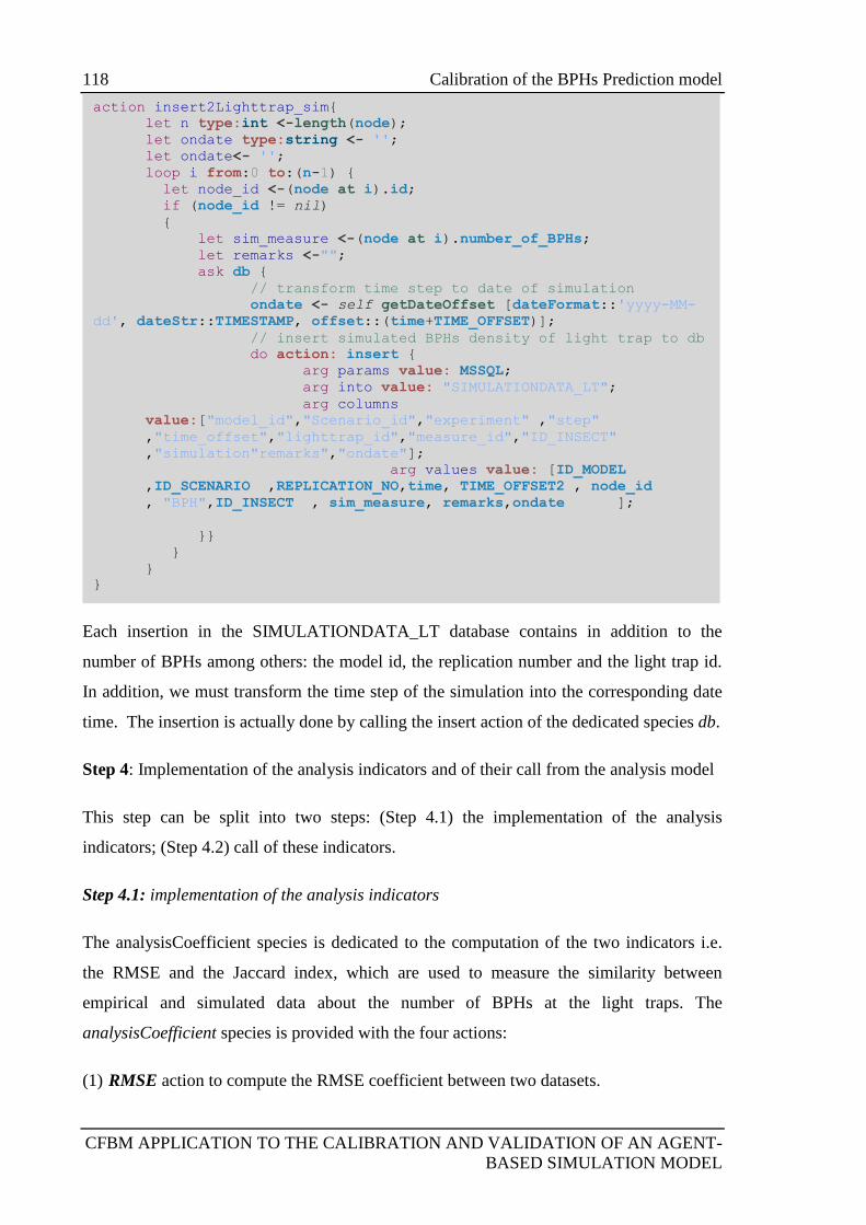
118 Calibration of the BPHs Prediction model
CFBM APPLICATION TO THE CALIBRATION AND VALIDATION OF AN AGENT-
BASED SIMULATION MODEL
Each insertion in the SIMULATIONDATA_LT database contains in addition to the
number of BPHs among others: the model id, the replication number and the light trap id.
In addition, we must transform the time step of the simulation into the corresponding date
time. The insertion is actually done by calling the insert action of the dedicated species db.
Step 4: Implementation of the analysis indicators and of their call from the analysis model
This step can be split into two steps: (Step 4.1) the implementation of the analysis
indicators; (Step 4.2) call of these indicators.
Step 4.1: implementation of the analysis indicators
The analysisCoefficient species is dedicated to the computation of the two indicators i.e.
the RMSE and the Jaccard index, which are used to measure the similarity between
empirical and simulated data about the number of BPHs at the light traps. The
analysisCoefficient species is provided with the four actions:
(1) RMSE action to compute the RMSE coefficient between two datasets.
action insert2Lighttrap_sim{
let n type:int <-length(node);
let ondate type:string <- '';
let ondate<- '';
loop i from:0 to:(n-1) {
let node_id <-(node at i).id;
if (node_id != nil)
{
let sim_measure <-(node at i).number_of_BPHs;
let remarks <-"";
ask db {
// transform time step to date of simulation
ondate <- self getDateOffset [dateFormat::'yyyy-MM-
dd', dateStr::TIMESTAMP, offset::(time+TIME_OFFSET)];
// insert simulated BPHs density of light trap to db
do action: insert {
arg params value: MSSQL;
arg into value: "SIMULATIONDATA_LT";
arg columns
value:["model_id","Scenario_id","experiment" ,"step"
,"time_offset","lighttrap_id","measure_id","ID_INSECT"
,"simulation"remarks","ondate"];
arg values value: [ID_MODEL
,ID_SCENARIO ,REPLICATION_NO,time, TIME_OFFSET2 , node_id
, "BPH",ID_INSECT , sim_measure, remarks,ondate ];
}}
}
}
}
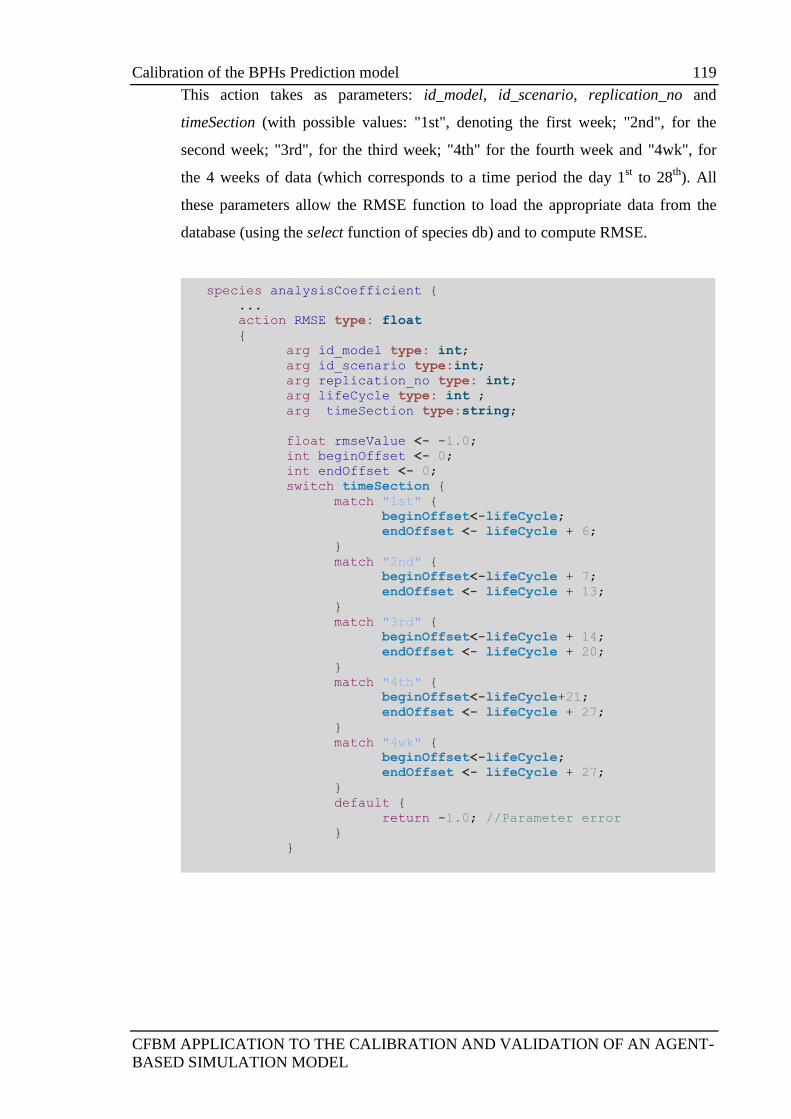
Calibration of the BPHs Prediction model 119
CFBM APPLICATION TO THE CALIBRATION AND VALIDATION OF AN AGENT-
BASED SIMULATION MODEL
This action takes as parameters: id_model, id_scenario, replication_no and
timeSection (with possible values: "1st", denoting the first week; "2nd", for the
second week; "3rd", for the third week; "4th" for the fourth week and "4wk", for
the 4 weeks of data (which corresponds to a time period the day 1st to 28
th). All
these parameters allow the RMSE function to load the appropriate data from the
database (using the select function of species db) and to compute RMSE.
species analysisCoefficient {
...
action RMSE type: float
{
arg id_model type: int;
arg id_scenario type:int;
arg replication_no type: int;
arg lifeCycle type: int ;
arg timeSection type:string;
float rmseValue <- -1.0;
int beginOffset <- 0;
int endOffset <- 0;
switch timeSection {
match "1st" {
beginOffset<-lifeCycle;
endOffset <- lifeCycle + 6;
}
match "2nd" {
beginOffset<-lifeCycle + 7;
endOffset <- lifeCycle + 13;
}
match "3rd" {
beginOffset<-lifeCycle + 14;
endOffset <- lifeCycle + 20;
}
match "4th" {
beginOffset<-lifeCycle+21;
endOffset <- lifeCycle + 27;
}
match "4wk" {
beginOffset<-lifeCycle;
endOffset <- lifeCycle + 27;
}
default {
return -1.0; //Parameter error
}
}
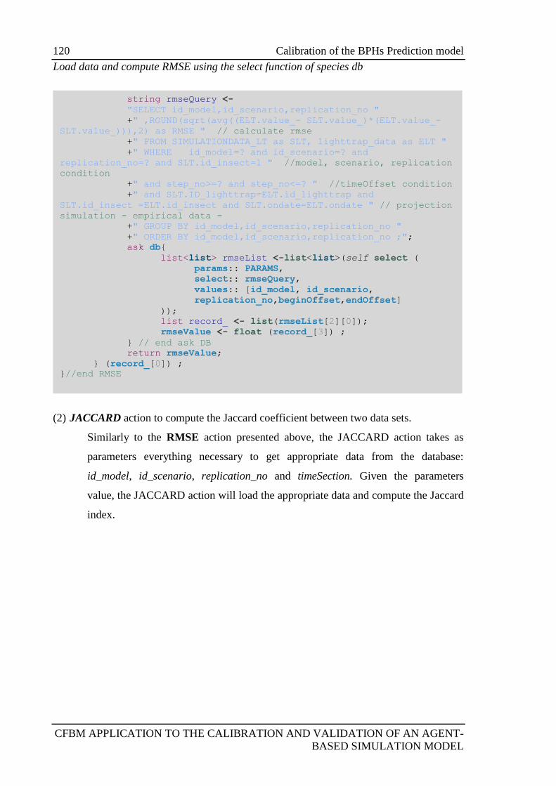
120 Calibration of the BPHs Prediction model
CFBM APPLICATION TO THE CALIBRATION AND VALIDATION OF AN AGENT-
BASED SIMULATION MODEL
Load data and compute RMSE using the select function of species db
(2) JACCARD action to compute the Jaccard coefficient between two data sets.
Similarly to the RMSE action presented above, the JACCARD action takes as
parameters everything necessary to get appropriate data from the database:
id_model, id_scenario, replication_no and timeSection. Given the parameters
value, the JACCARD action will load the appropriate data and compute the Jaccard
index.
string rmseQuery <-
"SELECT id_model,id_scenario,replication_no "
+" ,ROUND(sqrt(avg((ELT.value_- SLT.value_)*(ELT.value_-
SLT.value_))),2) as RMSE " // calculate rmse
+" FROM SIMULATIONDATA_LT as SLT, lighttrap_data as ELT "
+" WHERE id_model=? and id_scenario=? and
replication_no=? and SLT.id_insect=1 " //model, scenario, replication
condition
+" and step_no>=? and step_no<=? " //timeOffset condition
+" and SLT.ID_lighttrap=ELT.id_lighttrap and
SLT.id_insect =ELT.id_insect and SLT.ondate=ELT.ondate " // projection
simulation - empirical data -
+" GROUP BY id_model,id_scenario,replication_no "
+" ORDER BY id_model,id_scenario,replication_no ;";
ask db{
list<list> rmseList <-list<list>(self select (
params:: PARAMS,
select:: rmseQuery,
values:: [id_model, id_scenario,
replication_no,beginOffset,endOffset]
));
list record_ <- list(rmseList[2][0]);
rmseValue <- float (record_[3]) ;
} // end ask DB
return rmseValue;
} (record_[0]) ;
}//end RMSE
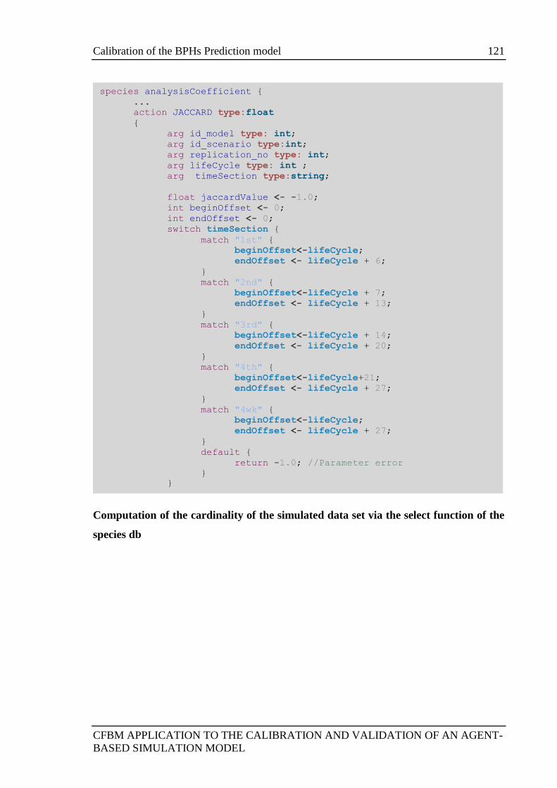
Calibration of the BPHs Prediction model 121
CFBM APPLICATION TO THE CALIBRATION AND VALIDATION OF AN AGENT-
BASED SIMULATION MODEL
Computation of the cardinality of the simulated data set via the select function of the
species db
species analysisCoefficient {
...
action JACCARD type:float
{
arg id_model type: int;
arg id_scenario type:int;
arg replication_no type: int;
arg lifeCycle type: int ;
arg timeSection type:string;
float jaccardValue <- -1.0;
int beginOffset <- 0;
int endOffset <- 0;
switch timeSection {
match "1st" {
beginOffset<-lifeCycle;
endOffset <- lifeCycle + 6;
}
match "2nd" {
beginOffset<-lifeCycle + 7;
endOffset <- lifeCycle + 13;
}
match "3rd" {
beginOffset<-lifeCycle + 14;
endOffset <- lifeCycle + 20;
}
match "4th" {
beginOffset<-lifeCycle+21;
endOffset <- lifeCycle + 27;
}
match "4wk" {
beginOffset<-lifeCycle;
endOffset <- lifeCycle + 27;
}
default {
return -1.0; //Parameter error
}
}
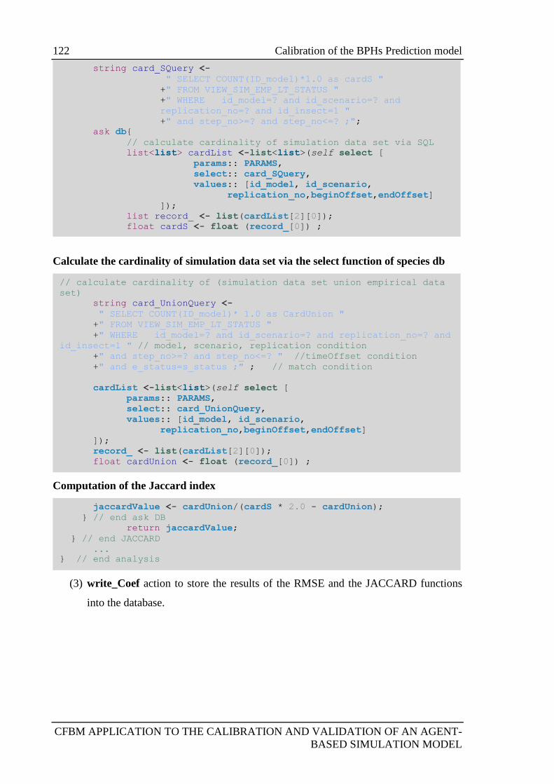
122 Calibration of the BPHs Prediction model
CFBM APPLICATION TO THE CALIBRATION AND VALIDATION OF AN AGENT-
BASED SIMULATION MODEL
Calculate the cardinality of simulation data set via the select function of species db
Computation of the Jaccard index
(3) write_Coef action to store the results of the RMSE and the JACCARD functions
into the database.
jaccardValue <- cardUnion/(cardS * 2.0 - cardUnion);
} // end ask DB
return jaccardValue;
} // end JACCARD
...
} // end analysis
// calculate cardinality of (simulation data set union empirical data
set)
string card_UnionQuery <-
" SELECT COUNT(ID_model)* 1.0 as CardUnion "
+" FROM VIEW_SIM_EMP_LT_STATUS "
+" WHERE id_model=? and id_scenario=? and replication_no=? and
id_insect=1 " // model, scenario, replication condition
+" and step_no>=? and step_no<=? " //timeOffset condition
+" and e_status=s_status ;" ; // match condition
cardList <-list<list>(self select [
params:: PARAMS,
select:: card_UnionQuery,
values:: [id_model, id_scenario,
replication_no,beginOffset,endOffset]
]);
record_ <- list(cardList[2][0]);
float cardUnion <- float (record_[0]) ;
string card_SQuery <-
" SELECT COUNT(ID_model)*1.0 as cardS "
+" FROM VIEW_SIM_EMP_LT_STATUS "
+" WHERE id_model=? and id_scenario=? and
replication_no=? and id_insect=1 "
+" and step_no>=? and step_no<=? ;";
ask db{
// calculate cardinality of simulation data set via SQL
list<list> cardList <-list<list>(self select [
params:: PARAMS,
select:: card_SQuery,
values:: [id_model, id_scenario,
replication_no,beginOffset,endOffset]
]);
list record_ <- list(cardList[2][0]);
float cardS <- float (record_[0]) ;
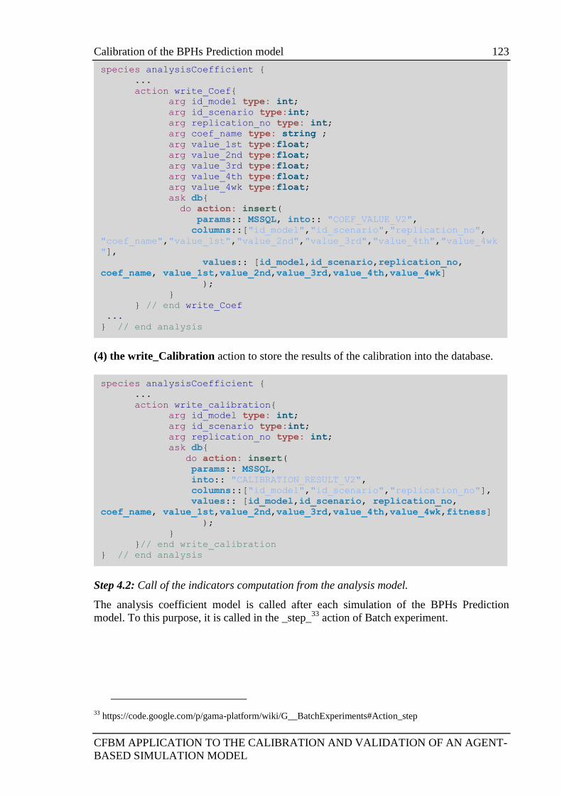
Calibration of the BPHs Prediction model 123
CFBM APPLICATION TO THE CALIBRATION AND VALIDATION OF AN AGENT-
BASED SIMULATION MODEL
(4) the write_Calibration action to store the results of the calibration into the database.
Step 4.2: Call of the indicators computation from the analysis model.
The analysis coefficient model is called after each simulation of the BPHs Prediction
model. To this purpose, it is called in the _step_33
action of Batch experiment.
33
https://code.google.com/p/gama-platform/wiki/G__BatchExperiments#Action_step
species analysisCoefficient {
...
action write_calibration{
arg id_model type: int;
arg id_scenario type:int;
arg replication_no type: int;
ask db{
do action: insert(
params:: MSSQL,
into:: "CALIBRATION_RESULT_V2",
columns::["id_model","id_scenario","replication_no"],
values:: [id_model,id_scenario, replication_no,
coef_name, value_1st,value_2nd,value_3rd,value_4th,value_4wk,fitness]
);
}
}// end write_calibration
} // end analysis
species analysisCoefficient {
...
action write_Coef{
arg id_model type: int;
arg id_scenario type:int;
arg replication_no type: int;
arg coef_name type: string ;
arg value_1st type:float;
arg value_2nd type:float;
arg value_3rd type:float;
arg value_4th type:float;
arg value_4wk type:float;
ask db{
do action: insert(
params:: MSSQL, into:: "COEF_VALUE_V2",
columns::["id_model","id_scenario","replication_no",
"coef_name","value_1st","value_2nd","value_3rd","value_4th","value_4wk
"],
values:: [id_model,id_scenario,replication_no,
coef_name, value_1st,value_2nd,value_3rd,value_4th,value_4wk]
);
}
} // end write_Coef
...
} // end analysis
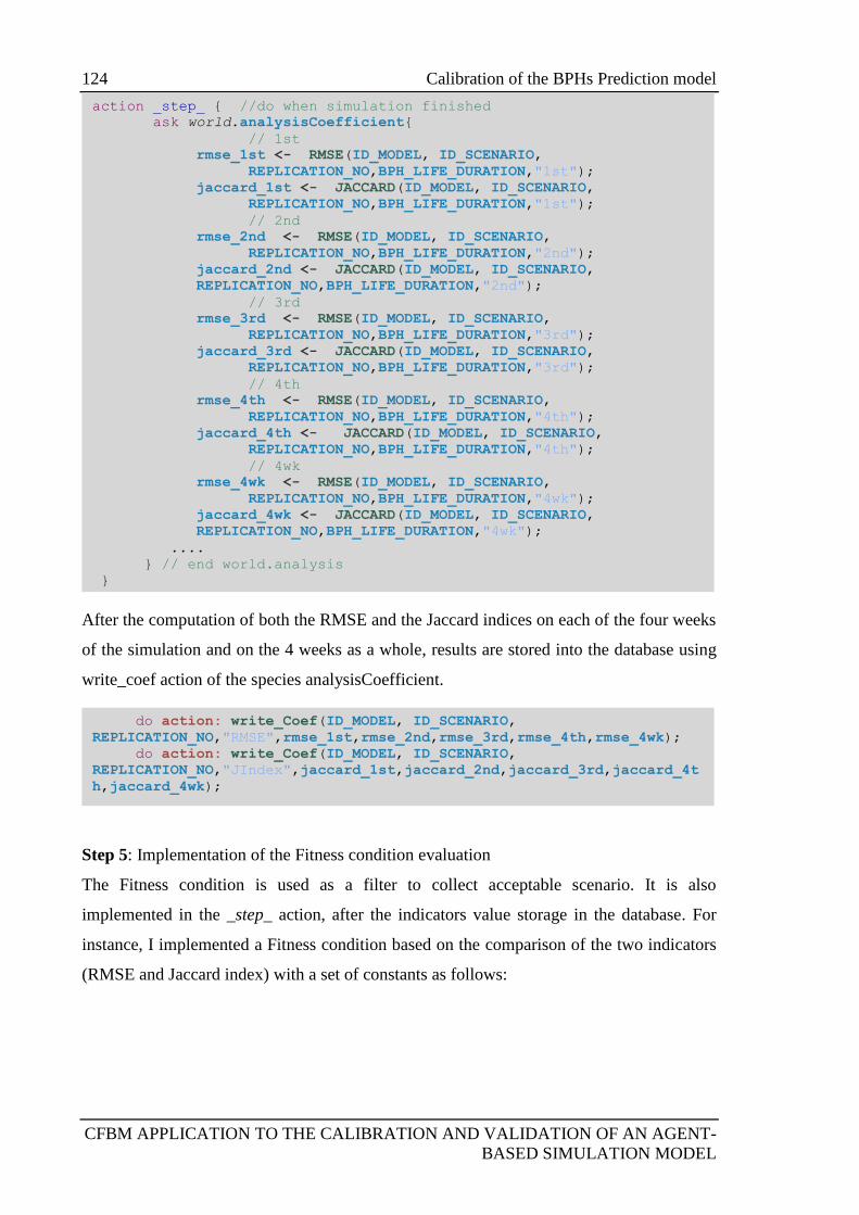
124 Calibration of the BPHs Prediction model
CFBM APPLICATION TO THE CALIBRATION AND VALIDATION OF AN AGENT-
BASED SIMULATION MODEL
After the computation of both the RMSE and the Jaccard indices on each of the four weeks
of the simulation and on the 4 weeks as a whole, results are stored into the database using
write_coef action of the species analysisCoefficient.
Step 5: Implementation of the Fitness condition evaluation
The Fitness condition is used as a filter to collect acceptable scenario. It is also
implemented in the _step_ action, after the indicators value storage in the database. For
instance, I implemented a Fitness condition based on the comparison of the two indicators
(RMSE and Jaccard index) with a set of constants as follows:
do action: write_Coef(ID_MODEL, ID_SCENARIO,
REPLICATION_NO,"RMSE",rmse_1st,rmse_2nd,rmse_3rd,rmse_4th,rmse_4wk);
do action: write_Coef(ID_MODEL, ID_SCENARIO,
REPLICATION_NO,"JIndex",jaccard_1st,jaccard_2nd,jaccard_3rd,jaccard_4t
h,jaccard_4wk);
action _step_ { //do when simulation finished
ask world.analysisCoefficient{
// 1st
rmse_1st <- RMSE(ID_MODEL, ID_SCENARIO,
REPLICATION_NO,BPH_LIFE_DURATION,"1st");
jaccard_1st <- JACCARD(ID_MODEL, ID_SCENARIO,
REPLICATION_NO,BPH_LIFE_DURATION,"1st");
// 2nd
rmse_2nd <- RMSE(ID_MODEL, ID_SCENARIO,
REPLICATION_NO,BPH_LIFE_DURATION,"2nd");
jaccard_2nd <- JACCARD(ID_MODEL, ID_SCENARIO,
REPLICATION_NO,BPH_LIFE_DURATION,"2nd");
// 3rd
rmse_3rd <- RMSE(ID_MODEL, ID_SCENARIO,
REPLICATION_NO,BPH_LIFE_DURATION,"3rd");
jaccard_3rd <- JACCARD(ID_MODEL, ID_SCENARIO,
REPLICATION_NO,BPH_LIFE_DURATION,"3rd");
// 4th
rmse_4th <- RMSE(ID_MODEL, ID_SCENARIO,
REPLICATION_NO,BPH_LIFE_DURATION,"4th");
jaccard_4th <- JACCARD(ID_MODEL, ID_SCENARIO,
REPLICATION_NO,BPH_LIFE_DURATION,"4th");
// 4wk
rmse_4wk <- RMSE(ID_MODEL, ID_SCENARIO,
REPLICATION_NO,BPH_LIFE_DURATION,"4wk");
jaccard_4wk <- JACCARD(ID_MODEL, ID_SCENARIO,
REPLICATION_NO,BPH_LIFE_DURATION,"4wk");
....
} // end world.analysis
}
}
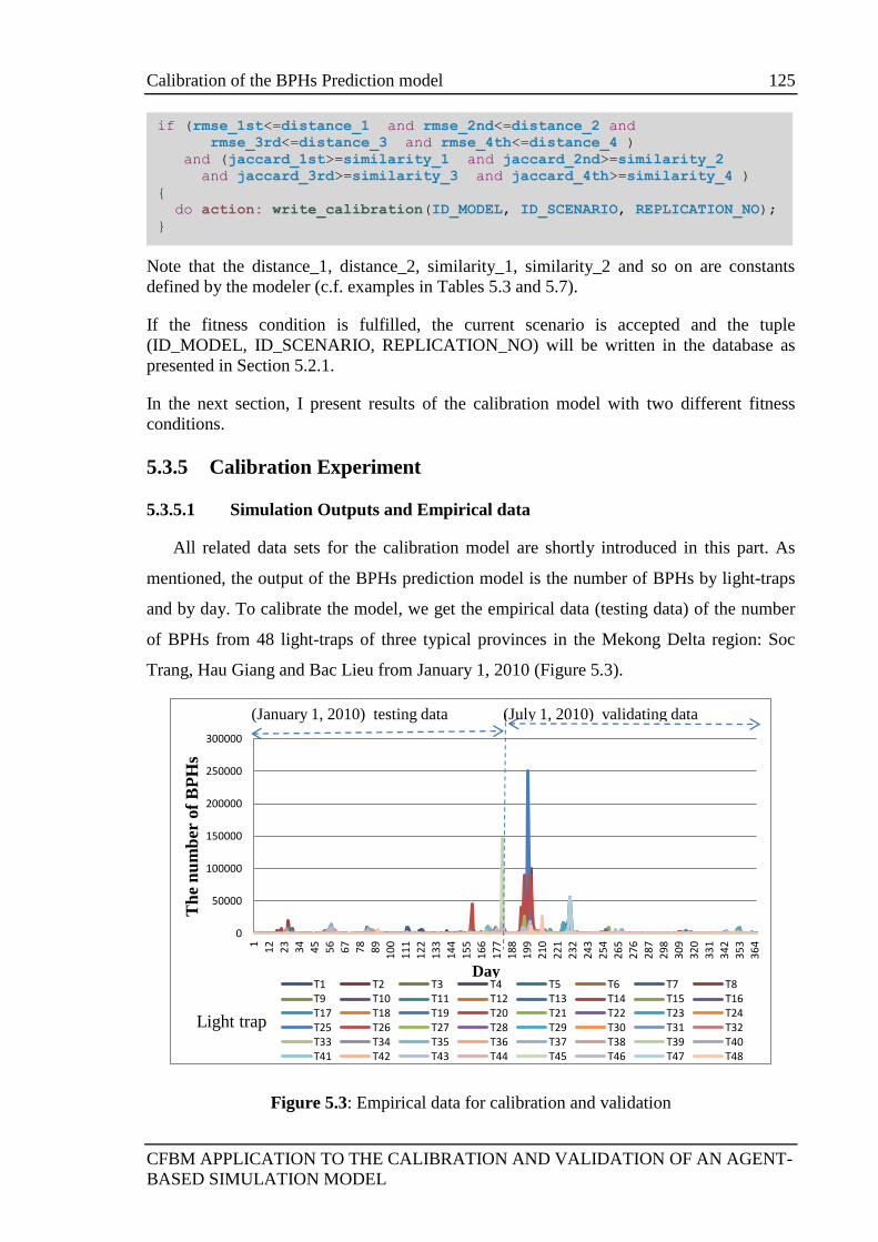
Calibration of the BPHs Prediction model 125
CFBM APPLICATION TO THE CALIBRATION AND VALIDATION OF AN AGENT-
BASED SIMULATION MODEL
Note that the distance_1, distance_2, similarity_1, similarity_2 and so on are constants
defined by the modeler (c.f. examples in Tables 5.3 and 5.7).
If the fitness condition is fulfilled, the current scenario is accepted and the tuple
(ID_MODEL, ID_SCENARIO, REPLICATION_NO) will be written in the database as
presented in Section 5.2.1.
In the next section, I present results of the calibration model with two different fitness
conditions.
5.3.5 Calibration Experiment
5.3.5.1 Simulation Outputs and Empirical data
All related data sets for the calibration model are shortly introduced in this part. As
mentioned, the output of the BPHs prediction model is the number of BPHs by light-traps
and by day. To calibrate the model, we get the empirical data (testing data) of the number
of BPHs from 48 light-traps of three typical provinces in the Mekong Delta region: Soc
Trang, Hau Giang and Bac Lieu from January 1, 2010 (Figure 5.3).
Figure 5.3: Empirical data for calibration and validation
0
50000
100000
150000
200000
250000
300000
1
12
23
34
45
56
67
78
89
10
0
11
1
12
2
13
3
14
4
15
5
16
6
17
7
18
8
19
9
21
0
22
1
23
2
24
3
25
4
26
5
27
6
28
7
29
8
30
9
32
0
33
1
34
2
35
3
36
4
Th
e n
um
ber
of
BP
Hs
T1 T2 T3 T4 T5 T6 T7 T8 T9 T10 T11 T12 T13 T14 T15 T16 T17 T18 T19 T20 T21 T22 T23 T24 T25 T26 T27 T28 T29 T30 T31 T32 T33 T34 T35 T36 T37 T38 T39 T40 T41 T42 T43 T44 T45 T46 T47 T48
Day
Light trap
(January 1, 2010) testing data (July 1, 2010) validating data
if (rmse_1st<=distance_1 and rmse_2nd<=distance_2 and
rmse_3rd<=distance_3 and rmse_4th<=distance_4 )
and (jaccard_1st>=similarity_1 and jaccard_2nd>=similarity_2
and jaccard_3rd>=similarity_3 and jaccard_4th>=similarity_4 )
{
do action: write_calibration(ID_MODEL, ID_SCENARIO, REPLICATION_NO);
}
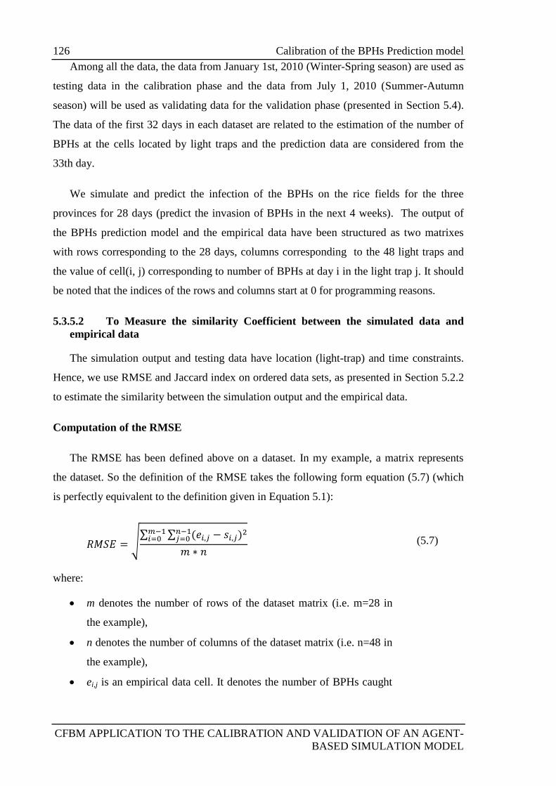
126 Calibration of the BPHs Prediction model
CFBM APPLICATION TO THE CALIBRATION AND VALIDATION OF AN AGENT-
BASED SIMULATION MODEL
Among all the data, the data from January 1st, 2010 (Winter-Spring season) are used as
testing data in the calibration phase and the data from July 1, 2010 (Summer-Autumn
season) will be used as validating data for the validation phase (presented in Section 5.4).
The data of the first 32 days in each dataset are related to the estimation of the number of
BPHs at the cells located by light traps and the prediction data are considered from the
33th day.
We simulate and predict the infection of the BPHs on the rice fields for the three
provinces for 28 days (predict the invasion of BPHs in the next 4 weeks). The output of
the BPHs prediction model and the empirical data have been structured as two matrixes
with rows corresponding to the 28 days, columns corresponding to the 48 light traps and
the value of cell(i, j) corresponding to number of BPHs at day i in the light trap j. It should
be noted that the indices of the rows and columns start at 0 for programming reasons.
5.3.5.2 To Measure the similarity Coefficient between the simulated data and
empirical data
The simulation output and testing data have location (light-trap) and time constraints.
Hence, we use RMSE and Jaccard index on ordered data sets, as presented in Section 5.2.2
to estimate the similarity between the simulation output and the empirical data.
Computation of the RMSE
The RMSE has been defined above on a dataset. In my example, a matrix represents
the dataset. So the definition of the RMSE takes the following form equation (5.7) (which
is perfectly equivalent to the definition given in Equation 5.1):
(5.7)
where:
m denotes the number of rows of the dataset matrix (i.e. m=28 in
the example),
n denotes the number of columns of the dataset matrix (i.e. n=48 in
the example),
ei,j is an empirical data cell. It denotes the number of BPHs caught
Calibration of the BPHs Prediction model 127
CFBM APPLICATION TO THE CALIBRATION AND VALIDATION OF AN AGENT-
BASED SIMULATION MODEL
in day i at light-trap j (the number of BPHs at light trap j in day i).
si,j is the simulation output. It denotes the number of BPHs obtained
in step i (day i) at light-trap j (simulated the number of BPHs at
light trap j in day i).
The RMSE results for each of the three replications of the 72 scenarios are presented in
Table C.3 in Appendix C.
Computation of the Jaccard index
I also compute the Jaccard index (using its definition presented in Equation (5.6) between
the simulation output and empirical data.
(5.6)
where:
a: cardinality of X.
b: cardinality of Y.
c: cardinality of S.
If we calculate the Jaccard index based on the number of BPHs then the values of the
Jaccard indices of all scenarios fall in the range from [0.0, 0.05], which is very low. It
becomes thus hard to consider a scenario with such a result as an acceptable scenario in the
calibration process. This problem can be explained by the fact that the numbers of BPHs
caught at each light-trap has a wide range of values, from zero to ten thousand. Hence, to
exactly simulate the number of BPHs at each light-trap over time is impossible or the
Jaccard index of two ordered data sets is not suitable to measure the similarity coefficient
between two matrixes of values where the domain of the elements is large. For example, if
we simulate 9000 BPHs in a light trap, but the empirical data give 9001 BPHs (over a
maximum of 10000 BPHs observed in light traps), we could recognize intuitively that the
simulation gives pretty good results, whereas the Jaccard index does not consider these two
values similar at all. We also need to remind that empirical data are observed by human
beings so their precision is not perfect.
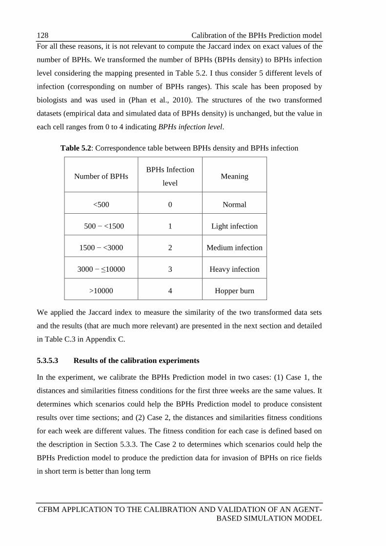
128 Calibration of the BPHs Prediction model
CFBM APPLICATION TO THE CALIBRATION AND VALIDATION OF AN AGENT-
BASED SIMULATION MODEL
For all these reasons, it is not relevant to compute the Jaccard index on exact values of the
number of BPHs. We transformed the number of BPHs (BPHs density) to BPHs infection
level considering the mapping presented in Table 5.2. I thus consider 5 different levels of
infection (corresponding on number of BPHs ranges). This scale has been proposed by
biologists and was used in (Phan et al., 2010). The structures of the two transformed
datasets (empirical data and simulated data of BPHs density) is unchanged, but the value in
each cell ranges from 0 to 4 indicating BPHs infection level.
Table 5.2: Correspondence table between BPHs density and BPHs infection
Number of BPHs BPHs Infection
level Meaning
<500 0 Normal
500 − <1500 1 Light infection
1500 − <3000 2 Medium infection
3000 − ≤10000 3 Heavy infection
>10000 4 Hopper burn
We applied the Jaccard index to measure the similarity of the two transformed data sets
and the results (that are much more relevant) are presented in the next section and detailed
in Table C.3 in Appendix C.
5.3.5.3 Results of the calibration experiments
In the experiment, we calibrate the BPHs Prediction model in two cases: (1) Case 1, the
distances and similarities fitness conditions for the first three weeks are the same values. It
determines which scenarios could help the BPHs Prediction model to produce consistent
results over time sections; and (2) Case 2, the distances and similarities fitness conditions
for each week are different values. The fitness condition for each case is defined based on
the description in Section 5.3.3. The Case 2 to determines which scenarios could help the
BPHs Prediction model to produce the prediction data for invasion of BPHs on rice fields
in short term is better than long term
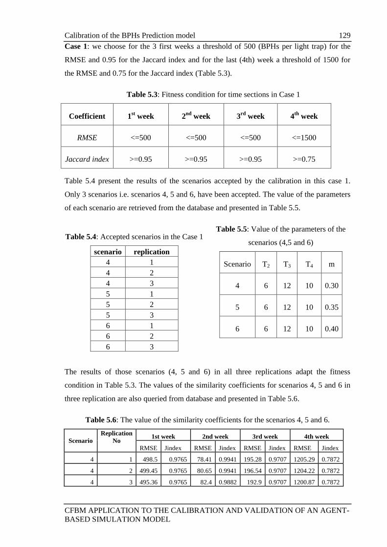
Calibration of the BPHs Prediction model 129
CFBM APPLICATION TO THE CALIBRATION AND VALIDATION OF AN AGENT-
BASED SIMULATION MODEL
Case 1: we choose for the 3 first weeks a threshold of 500 (BPHs per light trap) for the
RMSE and 0.95 for the Jaccard index and for the last (4th) week a threshold of 1500 for
the RMSE and 0.75 for the Jaccard index (Table 5.3).
Table 5.3: Fitness condition for time sections in Case 1
Coefficient 1st week 2
nd week 3
rd week 4
th week
RMSE <=500 <=500 <=500 <=1500
Jaccard index >=0.95 >=0.95 >=0.95 >=0.75
Table 5.4 present the results of the scenarios accepted by the calibration in this case 1.
Only 3 scenarios i.e. scenarios 4, 5 and 6, have been accepted. The value of the parameters
of each scenario are retrieved from the database and presented in Table 5.5.
Table 5.4: Accepted scenarios in the Case 1
scenario replication
4 1
4 2
4 3
5 1
5 2
5 3
6 1
6 2
6 3
Table 5.5: Value of the parameters of the
scenarios (4,5 and 6)
Scenario T2 T3 T4 m
4 6 12 10 0.30
5 6 12 10 0.35
6 6 12 10 0.40
The results of those scenarios (4, 5 and 6) in all three replications adapt the fitness
condition in Table 5.3. The values of the similarity coefficients for scenarios 4, 5 and 6 in
three replication are also queried from database and presented in Table 5.6.
Table 5.6: The value of the similarity coefficients for the scenarios 4, 5 and 6.
Scenario
Replication
No
1st week 2nd week 3rd week 4th week
RMSE Jindex RMSE Jindex RMSE Jindex RMSE Jindex
4 1 498.5 0.9765 78.41 0.9941 195.28 0.9707 1205.29 0.7872
4 2 499.45 0.9765 80.65 0.9941 196.54 0.9707 1204.22 0.7872
4 3 495.36 0.9765 82.4 0.9882 192.9 0.9707 1200.87 0.7872
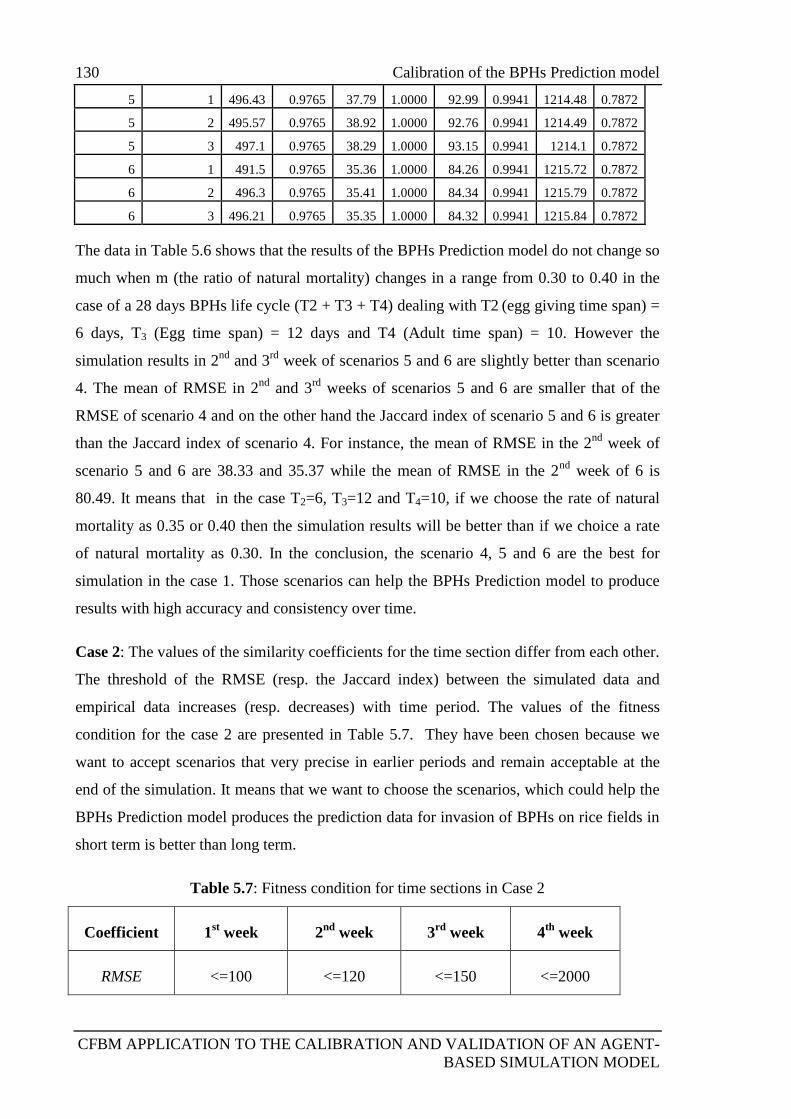
130 Calibration of the BPHs Prediction model
CFBM APPLICATION TO THE CALIBRATION AND VALIDATION OF AN AGENT-
BASED SIMULATION MODEL
5 1 496.43 0.9765 37.79 1.0000 92.99 0.9941 1214.48 0.7872
5 2 495.57 0.9765 38.92 1.0000 92.76 0.9941 1214.49 0.7872
5 3 497.1 0.9765 38.29 1.0000 93.15 0.9941 1214.1 0.7872
6 1 491.5 0.9765 35.36 1.0000 84.26 0.9941 1215.72 0.7872
6 2 496.3 0.9765 35.41 1.0000 84.34 0.9941 1215.79 0.7872
6 3 496.21 0.9765 35.35 1.0000 84.32 0.9941 1215.84 0.7872
The data in Table 5.6 shows that the results of the BPHs Prediction model do not change so
much when m (the ratio of natural mortality) changes in a range from 0.30 to 0.40 in the
case of a 28 days BPHs life cycle (T2 + T3 + T4) dealing with T2 (egg giving time span) =
6 days, T3 (Egg time span) = 12 days and T4 (Adult time span) = 10. However the
simulation results in 2nd
and 3rd
week of scenarios 5 and 6 are slightly better than scenario
4. The mean of RMSE in 2nd
and 3rd
weeks of scenarios 5 and 6 are smaller that of the
RMSE of scenario 4 and on the other hand the Jaccard index of scenario 5 and 6 is greater
than the Jaccard index of scenario 4. For instance, the mean of RMSE in the 2nd
week of
scenario 5 and 6 are 38.33 and 35.37 while the mean of RMSE in the 2nd
week of 6 is
80.49. It means that in the case T2=6, T3=12 and T4=10, if we choose the rate of natural
mortality as 0.35 or 0.40 then the simulation results will be better than if we choice a rate
of natural mortality as 0.30. In the conclusion, the scenario 4, 5 and 6 are the best for
simulation in the case 1. Those scenarios can help the BPHs Prediction model to produce
results with high accuracy and consistency over time.
Case 2: The values of the similarity coefficients for the time section differ from each other.
The threshold of the RMSE (resp. the Jaccard index) between the simulated data and
empirical data increases (resp. decreases) with time period. The values of the fitness
condition for the case 2 are presented in Table 5.7. They have been chosen because we
want to accept scenarios that very precise in earlier periods and remain acceptable at the
end of the simulation. It means that we want to choose the scenarios, which could help the
BPHs Prediction model produces the prediction data for invasion of BPHs on rice fields in
short term is better than long term.
Table 5.7: Fitness condition for time sections in Case 2
Coefficient 1st week 2
nd week 3
rd week 4
th week
RMSE <=100 <=120 <=150 <=2000
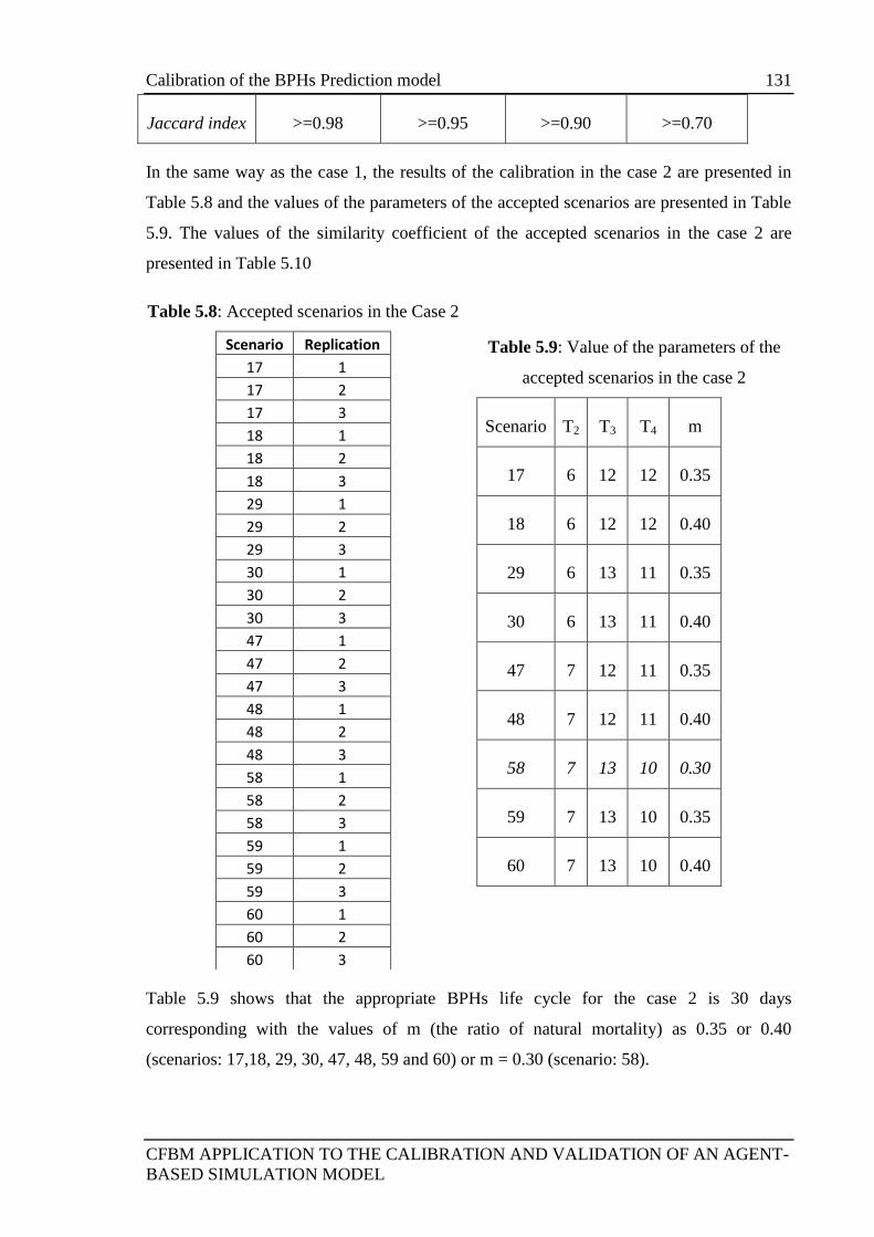
Calibration of the BPHs Prediction model 131
CFBM APPLICATION TO THE CALIBRATION AND VALIDATION OF AN AGENT-
BASED SIMULATION MODEL
Jaccard index >=0.98 >=0.95 >=0.90 >=0.70
In the same way as the case 1, the results of the calibration in the case 2 are presented in
Table 5.8 and the values of the parameters of the accepted scenarios are presented in Table
5.9. The values of the similarity coefficient of the accepted scenarios in the case 2 are
presented in Table 5.10
Table 5.8: Accepted scenarios in the Case 2
Scenario Replication
17 1
17 2
17 3
18 1
18 2
18 3
29 1
29 2
29 3
30 1
30 2
30 3
47 1
47 2
47 3
48 1
48 2
48 3
58 1
58 2
58 3
59 1
59 2
59 3
60 1
60 2
60 3
Table 5.9: Value of the parameters of the
accepted scenarios in the case 2
Scenario T2 T3 T4 m
17 6 12 12 0.35
18 6 12 12 0.40
29 6 13 11 0.35
30 6 13 11 0.40
47 7 12 11 0.35
48 7 12 11 0.40
58 7 13 10 0.30
59 7 13 10 0.35
60 7 13 10 0.40
Table 5.9 shows that the appropriate BPHs life cycle for the case 2 is 30 days
corresponding with the values of m (the ratio of natural mortality) as 0.35 or 0.40
(scenarios: 17,18, 29, 30, 47, 48, 59 and 60) or m = 0.30 (scenario: 58).
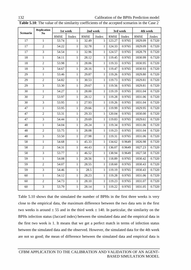
132 Calibration of the BPHs Prediction model
CFBM APPLICATION TO THE CALIBRATION AND VALIDATION OF AN AGENT-
BASED SIMULATION MODEL
Table 5.10: The value of the similarity coefficients of the accepted scenarios in the Case 2
Scenario
Replication
No
1st week 2nd week 3rd week 4th week
RMSE Jindex RMSE Jindex RMSE Jindex RMSE Jindex
17 1 53.74 1 32.49 1 123.27 0.9765 1829.09 0.7320
17 2 54.22 1 32.78 1 124.33 0.9765 1829.09 0.7320
17 3 54.54 1 32.96 1 124.57 0.9765 1828.79 0.7320
18 1 54.11 1 28.12 1 119.45 0.9765 1830.99 0.7320
18 2 53.98 1 28.06 1 119.33 0.9765 1830.95 0.7320
18 3 54.67 1 28.16 1 119.47 0.9765 1830.93 0.7320
29 1 53.46 1 29.87 1 119.26 0.9765 1829.80 0.7320
29 2 54.82 1 30.53 1 119.73 0.9765 1829.81 0.7320
29 3 53.30 1 29.67 1 119.56 0.9765 1829.81 0.7320
30 1 54.27 1 28.00 1 119.19 0.9765 1831.04 0.7320
30 2 53.97 1 28.12 1 119.28 0.9765 1831.06 0.7320
30 3 53.95 1 27.93 1 119.26 0.9765 1831.04 0.7320
47 1 53.95 1 29.66 1 119.99 0.9765 1829.95 0.7320
47 2 53.31 1 29.33 1 120.04 0.9765 1830.00 0.7320
47 3 54.44 1 29.69 1 119.83 0.9765 1829.61 0.7320
48 1 54.04 1 28.24 1 119.34 0.9765 1831.06 0.7320
48 2 53.75 1 28.08 1 119.23 0.9765 1831.04 0.7320
48 3 53.50 1 27.98 1 119.31 0.9765 1831.06 0.7320
58 1 54.68 1 45.33 1 134.62 0.9649 1826.98 0.7320
58 2 54.31 1 44.43 1 136.07 0.9649 1827.23 0.7320
58 3 53.77 1 46.52 1 138.94 0.9649 1827.58 0.7320
59 1 54.08 1 28.56 1 118.89 0.9765 1830.42 0.7320
59 2 54.07 1 28.55 1 118.60 0.9765 1830.43 0.7320
59 3 54.46 1 28.5 1 119.19 0.9765 1830.43 0.7320
60 1 54.12 1 28.23 1 119.28 0.9765 1831.06 0.7320
60 2 54.73 1 28.10 1 119.23 0.9765 1831.07 0.7320
60 3 53.79 1 28.14 1 119.22 0.9765 1831.05 0.7320
Table 5.10 shows that the simulated the number of BPHs in the first three weeks is very
close to the empirical data, the maximum difference between the two data sets in the first
two weeks is around ± 55 and in the third week ± 140. In particular, the similarity on the
BPHs infection status (Jaccard index) between the simulated data and the empirical data in
the first two week is 1. It means that we get a perfect match in terms of infection status
between the simulated data and the observed. However, the simulated data for the 4th week
are not so good; the mean of difference between the simulated data and empirical data is
Validation of the Accepted Scenario 133
CFBM APPLICATION TO THE CALIBRATION AND VALIDATION OF AN AGENT-
BASED SIMULATION MODEL
around 1830.1. In addition, the mean value of Jaccard index in 4th week of all simulation
in Table 5.10 is 0.732. Hence we can say that if we choose the parameter values as in
Table 5.9, the BPHs Prediction model will produce the prediction data for the short term is
more accuracy than the prediction data for long term.
Thus if we want to predict the invasion of BPHs in the short term then we can choose the
scenarios presented in Table 5.9, otherwise we can choose the scenarios presented in Table
5.5.
5.4 Validation of the Accepted Scenario
5.4.1 Implementation of the validation model
Indicators used to evaluate the simulation results
In the validation of the model, I also use the two similarity coefficients introduced above
(Jaccard index and RMSE) to measure the similarity between the outputs of the BPHs
Prediction model and empirical data (equations (5.6) and (5.7) detail how the indicators are
computed).
Implementation of the validation model
The validation model reuses the analysisCoefficient species defined for the calibration
model to compute the similarity coefficients of the simulation results and store the analysis
results in the database. The validation model algorithm is very similar to calibration model
one but does not include steps checking the fitness condition and storing the accepted
scenario (steps 5 and 6 in Section 5.2.1). It is indeed limited to the execution of only one
scenario and to its evaluation. The validation model is implemented by using CFBM in
GAMA platform as follows:
Step 1: Definition of the batch experiment with two main parameters: the scenario
identifier (used to identify the scenario and to retrieve the parameters values from the
database) and the current replication number as follows:
experiment 'VALIDATION_MODEL' type: batch repeat: 1 keep_seed: true
until: ( time >= 2 ) {
parameter "Value of ID_SCENARIO:" var: ID_SCENARIO
among:[4,5,6,17,18,29,30,47,48,58,59,60];
parameter "Value of REPLICATION_NO:" var: REPLICATION_NO min: 1
max: 3 step: 1;
134 Validation of the Accepted Scenario
CFBM APPLICATION TO THE CALIBRATION AND VALIDATION OF AN AGENT-
BASED SIMULATION MODEL
In this step, I only specify which scenarios need to be validated. Hence the parameter
ID_SCENARIO declares which scenario GAMA will use to execute the BPHs Prediction
model (ID_SCENARIO taking its value in [4,5,6,17,18,29,30,47,48,58,59,60] which are
the results of the calibration model presented in Section 5.3.5). Each scenario is then
replicated 3 times.
Step 2: Computation of the indicator on the simulation results
Once the simulation of the BPHs Prediction model has been executed, an agent of the
analysisCoefficient species is called to compute indicators.
The indicator values, computed in this step, will then be stored in the database..
Step 3: Storage of the indicator values in the database
do action: write_Coef(ID_MODEL, ID_SCENARIO,
REPLICATION_NO,"RMSE",rmse_1st,rmse_2nd,rmse_3rd,rmse_4th,rmse_4wk);
do action: write_Coef(ID_MODEL, ID_SCENARIO,
REPLICATION_NO,"JIndex",jaccard_1st,jaccard_2nd,jaccard_3rd,jaccard_4t
h,jaccard_4wk);
action _step_ { //do when simulation finished
ask world.analysisCoefficient{
// 1st
rmse_1st <- RMSE(ID_MODEL, ID_SCENARIO,
REPLICATION_NO,BPH_LIFE_DURATION,"1st");
jaccard_1st <- JACCARD(ID_MODEL, ID_SCENARIO,
REPLICATION_NO,BPH_LIFE_DURATION,"1st");
// 2nd
rmse_2nd <- RMSE(ID_MODEL, ID_SCENARIO,
REPLICATION_NO,BPH_LIFE_DURATION,"2nd");
jaccard_2nd <- JACCARD(ID_MODEL, ID_SCENARIO,
REPLICATION_NO,BPH_LIFE_DURATION,"2nd");
// 3rd
rmse_3rd <- RMSE(ID_MODEL, ID_SCENARIO,
REPLICATION_NO,BPH_LIFE_DURATION,"3rd");
jaccard_3rd <- JACCARD(ID_MODEL, ID_SCENARIO,
REPLICATION_NO,BPH_LIFE_DURATION,"3rd");
// 4th
rmse_4th <- RMSE(ID_MODEL, ID_SCENARIO,
REPLICATION_NO,BPH_LIFE_DURATION,"4th");
jaccard_4th <- JACCARD(ID_MODEL, ID_SCENARIO,
REPLICATION_NO,BPH_LIFE_DURATION,"4th");
// 4wk
rmse_4wk <- RMSE(ID_MODEL, ID_SCENARIO,
REPLICATION_NO,BPH_LIFE_DURATION,"4wk");
jaccard_4wk <- JACCARD(ID_MODEL, ID_SCENARIO,
REPLICATION_NO,BPH_LIFE_DURATION,"4wk");
....
} // end world.analysis
}
}
Validation of the Accepted Scenario 135
CFBM APPLICATION TO THE CALIBRATION AND VALIDATION OF AN AGENT-
BASED SIMULATION MODEL
5.4.2 Validation experiment
5.4.2.1 Simulation and validation data
The validation data are the number of BPHs from 48 light-traps of three typical
provinces in the Mekong Delta region: Soc Trang, Hau Giang and Bac Lieu from July 1,
2010 (See Figure 5.3 in Section 5.3.5.1). The simulation and validation data are also
structured as a matrix with two dimensions, where the horizontal direction presents the
light traps (48 light traps) and the vertical direction presents the number of days (28 days).
The value of cell(i, j) corresponding to the number of BPHs at day i in light trap j.
5.4.2.2 Results of the validation experiment
Table 5.11 presents the values of the indicators index for each time period (1st week, 2
nd
week , 3rd
week and 4th
week) for each scenario and Table 5.12 aggregates indicators for
each scenario and time period by computing their mean value over replications.
Table 5.11: the validation results
scenario replication
no
1st week 2nd week 3rd week 4th week
RMSE Jindex RMSE Jindex RMSE Jindex RMSE Jindex
4 1 1855.98 0.7056 1956.61 0.4328 5497.49 0.4328 2553.02 0.5962
4 2 1855.32 0.7056 2027.82 0.4088 5498.06 0.4177 2554.11 0.6038
4 3 1855.24 0.7013 1977.72 0.4207 5497.47 0.4390 2552.73 0.6038
5 1 1845.24 0.7231 513.71 0.8719 5516.53 0.6077 2525.13 0.6311
5 2 1844.10 0.7231 546.27 0.8512 5521.32 0.6077 2526.21 0.6271
5 3 1845.67 0.7231 500.47 0.8615 5516.43 0.6077 2524.61 0.6311
6 1 1844.95 0.7320 480.53 0.9535 6917.88 0.6038 2530.73 0.6311
6 2 1845.84 0.7320 158.72 0.9535 5522.87 0.6115 2529.13 0.6311
6 3 1844.77 0.7320 145.45 0.9535 5522.90 0.6115 2529.06 0.6311
17 1 1057.49 0.5273 1685.79 0.8311 5809.80 0.5342 539.56 0.7099
17 2 1059.97 0.5413 1685.77 0.8462 5810.44 0.5342 539.14 0.7099
17 3 1051.57 0.5238 1681.04 0.8411 5810.51 0.5342 539.35 0.7099
18 1 1043.73 0.5664 1621.62 0.9255 5827.25 0.5342 559.69 0.7231
18 2 1030.04 0.5628 1620.46 0.9255 5826.55 0.5342 559.69 0.7231
18 3 1045.62 0.5738 1623.40 0.9255 5829.07 0.5342 559.79 0.7231
29 1 1017.22 0.5273 37389.95 0.8930 9793.94 0.5342 996.53 0.7231
29 2 1066.10 0.5448 1640.75 0.8771 5822.26 0.5342 542.58 0.7231
29 3 1026.89 0.5413 1642.43 0.8824 5822.87 0.5342 544.15 0.7231
30 1 1024.21 0.5738 1619.37 0.9310 5830.47 0.5342 560.64 0.7231
30 2 1042.50 0.5628 1619.73 0.9310 5830.53 0.5342 560.53 0.7231
30 3 1046.50 0.5628 1619.20 0.9310 5830.32 0.5342 560.66 0.7231
47 1 1044.45 0.5592 1642.27 0.8930 5821.76 0.5342 541.90 0.7231
136 Validation of the Accepted Scenario
CFBM APPLICATION TO THE CALIBRATION AND VALIDATION OF AN AGENT-
BASED SIMULATION MODEL
47 2 1040.39 0.5520 1641.23 0.8824 5823.11 0.5342 540.10 0.7231
47 3 1062.25 0.5413 1641.45 0.8876 5822.59 0.5342 541.87 0.7231
48 1 1044.71 0.5701 1626.89 0.9310 5830.94 0.5342 560.63 0.7231
48 2 1048.59 0.5592 1623.32 0.9200 5830.39 0.5342 560.56 0.7231
48 3 1040.59 0.5484 1619.55 0.9310 5830.47 0.5342 560.56 0.7231
58 1 1023.78 0.5484 1858.78 0.6311 5803.96 0.5101 495.63 0.7187
58 2 1060.89 0.5135 1861.46 0.6350 5803.38 0.5101 494.39 0.7187
58 3 1044.07 0.5378 1852.13 0.6232 5802.47 0.5101 496.01 0.7143
59 1 1061.66 0.5556 1623.00 0.8930 5826.30 0.5308 545.72 0.7231
59 2 1062.88 0.5592 1622.71 0.9037 5826.58 0.5308 545.22 0.7231
59 3 1037.79 0.5342 1623.12 0.9037 5823.71 0.5308 546.10 0.7231
60 1 1025.98 0.5924 1619.25 0.9422 5831.43 0.5342 561.42 0.7231
60 2 1022.16 0.5628 1618.67 0.9366 5831.33 0.5342 561.34 0.7231
60 3 1058.39 0.5628 1618.48 0.9422 5831.32 0.5342 561.30 0.7231
Table 5.12: Mean value of the indicators for each scenario and time period
Scenario
1st week 2nd week 3rd week 4th week
RMSE Jindex RMSE Jindex RMSE Jindex RMSE Jindex
4 1855.51 0.70 1987.38 0.42 5497.67 0.43 2553.29 0.60
5 1845.00 0.72 520.15 0.86 5518.09 0.61 2525.32 0.63
6 1845.19 0.73 261.57 0.95 5987.88 0.61 2529.64 0.63
17 1056.34 0.53 1684.20 0.84 5810.25 0.53 539.35 0.71
18 1039.80 0.57 1621.83 0.93 5827.62 0.53 559.72 0.72
29 1036.74 0.54 13557.71 0.88 7146.36 0.53 694.42 0.72
30 1037.74 0.57 1619.43 0.93 5830.44 0.53 560.61 0.72
47 1049.03 0.55 1641.65 0.89 5822.49 0.53 541.29 0.72
48 1044.63 0.56 1623.25 0.93 5830.60 0.53 560.58 0.72
58 1042.91 0.53 1857.46 0.63 5803.27 0.51 495.34 0.72
59 1054.11 0.55 1622.94 0.90 5825.53 0.53 545.68 0.72
60 1035.51 0.57 1618.80 0.94 5831.36 0.53 561.35 0.72
The data in Table 5.11 and 5.12 show that the results of the simulation model are not really
stable on different input data sets. If we compare the indicator values in Table 5.6 and 5.10
(computed related to a dataset beginning on January 1st, 2010 (Winter - Spring rice crop))
with the indicator values in Table 5.11 (computed related to a dataset beginning on July
1st, 2010 (Summer - Autumn rice crop)), we can observe a huge loss of similarity in the
results simulations provide in the validation time period. For example, the values of the
Jaccard index in the first three weeks with the first input data set (January 1, 2010) are
always greater than 0.97 while almost all the values of the Jaccard index in the first three
weeks with the validation input dataset (July 1, 2010) are less than 0.75 except some
values in 2nd
week.
Discussion 137
CFBM APPLICATION TO THE CALIBRATION AND VALIDATION OF AN AGENT-
BASED SIMULATION MODEL
In my opinion, the instable nature of the simulation results of the BPHs prediction model
may come from the two following reasons: (1) there is a difference between the actual land
use and land use stored in the database, which is managed by the Agriculture department of
the provinces (such impression is usual in Vietnamese databases); and (2) the input data
(the number of BPHs at the light traps) may not sufficient in terms of number of light
traps. There are indeed only 48 light traps in 3 provinces and their locations are irrational
to collect the BPHs. This is a problem studied in (Truong, 2014; Truong et al., 2013), in
which the authors proposed an approach to optimize the light trap network in Mekong
Delta regions. In addition, the calibration and validation are not performed in the same
rice crop season thus can also be a factor for the instable nature of the simulation results.
Although the BPHs prediction must be tested on bigger empirical data sets and the model
must also to be improved before being used as an actual Decision Support System, this
chapter has presented and illustrated the way my framework can be used to manage the
inputs and the outputs of a simulation model (BPHs Prediction model) and an analysis
model (AnalysisCoefficient model). Specially, this chapter has presented an approach to
calibrate and validate a simulation model in an automatic manner where the two coupling
models (i.e. the simulation model and the model of analysis simulation) are coupling by
sharing their data via a database managed by my CFBM framework.
5.5 Discussion
5.5.1 Application of CFBM for calibration and validation
There have been many studies, which proposed frameworks aiming at building accurate
simulation models (Law, 2009), paradigm for verification and validation of simulation
model (Sargent, 2011) in general or agent-based simulation models (Klügl, 2008) in
particular. Although those frameworks demonstrate processes to help us archive simulation
model with the accuracy of the simulation output, we still need a concrete approach to
solve those two challenges of agent-based models (as expressed in the introduction). By
applying CFBM, we have developed a calibration approach for agent-based models that is
not only capable of handling the inputs/outputs of agent-based simulation models but also
calibrating and validating the agent-based simulation in an automatic manner.
138 Discussion
CFBM APPLICATION TO THE CALIBRATION AND VALIDATION OF AN AGENT-
BASED SIMULATION MODEL
In Section 5.2.1, I did not demonstrate the concrete adjustment function to adjust the
parameters of the simulation model (the adjustment function which could be a kind of
"weight of evidence" (Donigian, 2002) or genetic algorithm (Ngo and See, 2012) because
of two reasons: we only propose a general calibration approach and we let the modeler free
to use adjustment function (s)he chooses. Furthermore, our approach only concerns the
management of the input/output data of the simulation and validation models and the
automation of the calibration process (in particular for models dealing with a huge amount
of data). For instance, we have successfully applied our approach on calibration and
validation of the BPHs prediction model which requires several data sources such as
administrative boundaries (region, river, sea region, land used), light-trap coordinates,
daily trap-densities, rice cultivated regions, general weather data (wind data), station
weather data (temperature, humidity, etc.), river and sea regions of three provinces of
Mekong Delta region of Vietnam as explained in Section 4.3 of Chapter 4.
Thanks to implement the simulation model and the calibration in the same platform, that
helps modelers to test their models more systematically in a given parameter space and
manage the input and output data of the models in an automatic manner. Thus our
approach has helped to reduce time and labor effort.
5.5.2 The Jaccard index with aggregation
In this part, I propose to apply Jaccard index on the aggregation data of the ordered data
sets.
Assume that we have two modality matrixes and the domain of the elements in S and E are
[0 .. k-1], having k values:
(5.8)
The aggregation on the columns on S (or E) has a matrix:
Discussion 139
CFBM APPLICATION TO THE CALIBRATION AND VALIDATION OF AN AGENT-
BASED SIMULATION MODEL
(5.9)
where:
C denotes aggregation matrix on the columns of matrix S (or E).
ci,j is the number of elements in row i in S (or E) having value j.
The aggregation on the rows on S (or E) has a matrix:
(5.10)
where:
R denotes aggregation matrix on the rows of matrix S (or E).
ri,j is the number of elements at columns j in S (or E) having the
value i.
Then we can use the Jaccard index on ordered data sets (equation 5.6) to calculate the
similarity coefficient of the aggregation matrices (equation 5.9, 5.10) of S and E.
For instance, in the case of BPHs prediction model, the BPHs infection status of the light
traps in two data sets (simulation data and empirical data) have been structured as two
matrixes with the rows corresponding to 28 days, columns corresponding to 48 light traps
and the value of cell(i, j) corresponding to BPHs infection at day i of the light trap j. The
simulation data and empirical data have the format as matrix in equation 5.8 with k=[0..4]
(There are 5 BPHs infection status - cf. Table 5.2), m=[0..27] and n=[0..47].
If we want to measure the Jaccard index between BPHs infection statuses on each day of
the whole light traps then we can aggregate on the light trap dimension and get the results
with the format in equation 5.11. On the other hand, if we want to determine the Jaccard
index between BPHs infection statuses of the light traps in the whole of day then we can
aggregate on day dimension then and get the results with the format in equation 5.12.
(5.11)
140 Conclusion
CFBM APPLICATION TO THE CALIBRATION AND VALIDATION OF AN AGENT-
BASED SIMULATION MODEL
Equation 5.11 means that day i has ci,j light traps with BPHs infection status j.
(5.12)
Equation 5.12 means that light trap j has ri,j day with BPHs infection status i.
5.6 Conclusion
In this chapter, we propose an automated calibration approach by applying CFBM to help
modelers to solve the limitations of ABMs concerning the calibration and validation of
agent-based models with high volume of data: BI solution is used to manage the high
volume of input/output data of the simulation models and an analysis model have been
proposed to validate the accuracy of the simulation outputs on large size of input with
varying parameters. We also recommend a specific measure of the similarity coefficient of
two data sets with the constraints on the position of elements, which is called "Jaccard
index on ordered data sets". In our opinion, this measure can be used not only as to
validate the BPHs prediction model but it is also a good measure to validate the outputs of
other models with constraints on location and time.
CONCLUSION
TRUONG Minh Thai 141
Chapter 6 CONCLUSION
Table of contents
6.1 Contributions of the thesis ................................................................................... 142
6.1.1 Achievements of the thesis .................................................................... 142
6.1.2 Benefits and drawbacks of CFBM to deal with data-driven approach in
ABM ............................................................................................................... 143
6.2 Perspectives ......................................................................................................... 144
6.2.1 To integrate web service features into a multi-agent based simulation
platform ............................................................................................................... 144
6.2.2 To integrate data mining technologies to a multi-agent based simulation
platform. .............................................................................................................. 145
142 Contributions of the thesis
CONCLUSION
6.1 Contributions of the thesis
6.1.1 Achievements of the thesis
The first achievement of my research is the design of a logical framework dealing with
data-adapted computer simulations (Section 3.2 of Chapter 3, Publications 1 and 2),
including four major tools: (1) a model design tool: a software environment that supports a
modeling language and a user interface, and this is generic enough to model any kind of
system; (2) a model execution tool: a software environment that can run models; (3) an
execution analysis tool: a software environment that supports statistical analysis features
for the analysis of the simulation output; and (4) a database tool: a software environment
that supports appropriate database management features for all components in the system.
The most important point of the proposed framework is the powerful integration of a data
warehouse, OLAP analysis tools and a multi-agent based platform. As a consequence, the
framework is named CFBM (Combination Framework of Business intelligence solution
and Multi-agent simulation platform). CFBM is useful to develop complex simulation
systems with large amount of input/output data such as a what-if simulation system, a
prediction/forecast system or a decision support system.
The second achievement is the successfully implementation of the CFBM into the multi-
agent simulation platform GAMA (Section 3.3 and Publication 3) in particular by
integrating database features dealing in GAML (GAma Modeling Language). Thanks to
the added database features to GAMA, we can: (1) manage the input and output data of the
simulation models; (2) create agents and define the environment of the simulation by using
data selected from a database; (3) integrate simulation and empirical data, make
aggregation on the integrated data and so on.
These two achievements also answer to the two main questions of my thesis: (1)
What general architecture could serve the following purposes: model and execute
multi-agents simulations, manage input and output data of simulations, integrate
data from different sources and enable to analyze high volume of data?; and (2)
How to introduce DWH and OLAP technologies into a multi-agent based
simulation system having to face huge amount of data?.
Contributions of the thesis 143
CONCLUSION
In this thesis, I also proposed an approach to measure the similarity coefficient between
two ordered data sets (Section 5.2.2 of Chapter 5 and Publication 4), which has been
successfully applied to evaluate the results of the BPHs Prediction model (Section 5.3, 5.4
of Chapter 5 and Publication 4).
Specially, the CFBM has been successfully applied to develop Brown Plant Hopper
Surveillance Models where the CFBM is used: (1) to manage the empirical data collected
from the reference system, the simulation model output, the analysis results of analysis
models (Chapter 4 and Publication 3), and (2) to implement an automatic approach to
calibrate and validate an agent-based simulation model (Chapter 5 and Publication 4).
6.1.2 Benefits and drawbacks of CFBM to deal with data-driven
approach in ABM
In the conclusion, we argue that CFBM (integrated in GAMA) is a framework supporting
the trend of the shift from modeling-driven approach to data-driven approach mentioned in
Section 2.3.1.
There are two major benefits of CFBM as mentioned in the Section 3.4.1: (1) CFBM is a
modular architecture, so we can use any BI solution and multi-agent platform to instantiate
it depending the most adapted technology for a particular implementation of CFBM. For
instance, we choose open source or proprietary BI solution (for instance, GAMA has
succeeded in interacting with Pentaho Mondrian and SQL Server Analysis Service); (2)
CFBM can be used in a distributed environment, where we share the simulation results
with other modelers or conduct the integration and analysis of different simulation results
of other modelers.
Particularly, CFBM is a framework dealing with "the logic of simulation" (Hassan et al.,
2010b), a data-driven modeling approach in ABM. CFBM as instantiated GAMA allows
the modelers: (1) to collect data from the target system and manage the collected data
(empirical data); (2) to use empirical data in modeling processes (the abstraction process
from the target); (3) to use empirical data as the input of simulation models; (4) to execute
simulation models and manage the output results of the simulations; and (5) to compare
simulation outputs with the empirical data. Instances of processes in building multi-agent
simulation models are demonstrated in the application of CFBM to the development of the
Brown Plant Hopper Surveillance Models (BSMs) in Chapter 4 and to the calibration and
validation of the BPHs Prediction model in Chapter 5.
144 Perspectives
CONCLUSION
Although the CFBM has many advantages, it still has some drawback such as: (1) the
implementation of CFBM is a time-consuming task that requires skills in both BI solution
and agent-based modeling and simulation; and (2) the use of CFBM is not suitable to
deploy a simple simulation system, which processes on a small data set because in this
particular case the cost to develop models taking into account all features (which requires
skills in ABM, DW and OLAP technologies) of the CFBM framework could be higher
than the benefits modelers can get from it.
To deal with the first drawback, an open-source version of CFBM has been implemented,
documented and is distributed. In addition, I design and implement it in a modular way in
order that users needing to use a particular component instead of the one provided have
only the dedicated part to implement. About the second drawback, simple models can be
implemented using only a part of the CFBM, i.e. the GAMA platform, using simple built-
in data management features of GAMA without particular difficulties. In addition, I argue
that modelers dealing with large-scale models involving a huge amount of data will need
(and gain benefits) in getting about efficient data management and analysis using dedicated
tools such as the ones involved in the CFBM. I argue that the CFBM framework allows
going one step further in the use of efficient data management tools for agent-based
modelers in an quite easy way.
6.2 Perspectives
CFBM is the both data warehousing and agent-based simulation technologies, which opens
perspectives in the two following directions.
6.2.1 To integrate web service features into a multi-agent based
simulation platform
In the near future, we will focus on extending the flexibility of CFBM on data retrieval.
We will not only continue to improve and develop the database features already existing to
retrieve data from relational (e.g. transaction-sql and calling stored procedures) or
dimensional database (e.g. OLAP Pivot table) servers but we will also to develop the new
features that help agents pertaining to simulation models to retrieve data from website via
various types of web services: in fact, we will integrate various features of Web 2.0 into
CFBM.
Perspectives 145
CONCLUSION
There are several online data sources that provide open data that can be used in simulations
such as websites provide map or traffic data of a city (some of them can be found under the
different formats of OpenGIS standard). These data can be used as the input data,
calibration data or validation data of the simulations such as traffic simulation (Barceló,
2010) or urban simulation (Waddell and Ulfarsson, 2004). This will allow the modeler to
get in a transparent way open data from database as data.gov34
, Google map35
or to
retrieve GeoServer36
.
The integration of web service features does not only provide a fast and efficient way to
use real-world data into multi-agent based simulation models but also an asynchronous
mechanism to publish the simulation data in distributed simulation environment.
Beyond the purely technical improvement of the CFBM implementation into the GAMA
platform, the aim is to rethink to way modelers do simulation involving data in an
environment where a continuous flow of new data are produced and made available via
networks.
6.2.2 To integrate data mining technologies to a multi-agent based
simulation platform.
Due to the huge amount of data that a simulation can produce, modelers could get huge
benefits in integrating data mining tools into agent-based platforms to analyze the
simulation results (Remondino and Correndo, 2006, 2005). According to (Baqueiro et al.,
2009), data mining and agent-based modeling and simulation can be integrated in both
directions: (1) applying data mining to ABMS, in which data mining is used to compare
the simulation results between different experiments of the same model or independent
models representing the same phenomena; and (2) applying ABMS to data mining, in
which simulation models are used to produce data and simulation data can be used as
quasi-real data when there is a lack of real data for a domain-specific data mining task.
The application of data mining technologies in agent-based modeling applications are
mentioned in (Macal and North, 2010) e.g. supervised learning, unsupervised learning, and
34 www.data.gov
35 maps.google.com
36 geoserver.org
146 Perspectives
CONCLUSION
reinforcement learning. In addition, data mining technologies such as association mining,
outlier analysis, evolution analysis, clustering and etc. are also proposed for prediction
analysis of the results of simulations (Morbitzer et al., 2003).
In the integration of data mining technologies into multi agent based simulation platforms,
CFBM will be improved to support not only database features to manage simulation data,
validation data and training data but also data mining features: (1) to evaluate results of
simulations; (2) to make prediction based on simulation results; and (3) to train agents
based on specified training data.
Given the more and more extensive use and production of data in agent-based simulation,
the use of data-mining technologies will become more and more necessary. But we argue
that is first necessary to able to deal efficiently with data before using such tools. CFBM
thus appears to us as a first necessary step but also an ideal frame to extend to link agent-
based simulation and data-mining tools. In addition, the strong integration of CFBM and
the modeling and simulation platform in my implementation opens new way to deeply
integrate data-mining tools and agent-based simulation: data-mining tools can be used not
only on results but also during the simulation. For example, we will thus be able to
integrate agents into the simulation with a behavior driven by data-mining computation.
Those are clearer evidences to the technical and methodological benefits of future
integrations of web services and data mining technologies into a multi-agent based
simulation platform via the extension of the CFBM framework.
Publications 147
TRUONG Minh Thai
Publications
Four articles related to my PhD work have been accepted to national and international
conferences. They mainly describe the results of step 2,3 and 4 mentioned in Section 1.2.2
of Chapter 1.
[1]. Truong, T. M., Truong, X.V, Amblard, F., Drogoul, A., Gaudou, B., Huynh, H.
X.,Le, M.N., & Sibertin-Blanc, C., (2013). A Framework for Combining Business
Intelligence & Agent-based Simulation. In Computing and Communication
Technologies, Research, Innovation, and Vision for the Future (RIVF), 2013
IEEE RIVF International Conference, (Poster).
[2]. Truong, M. T., Amblard, F., & Gaudou, B., (2013). Combination Framework of
BI solution & Multi-agent platform (CFBM) for multi-agent based simulation
with a huge amount of data. Deuxième édition Atelier à la Décision à tous lé
Etages (AIDE @ ECG 2013), pp. 35–42.
[3]. Truong, T. M., Truong, X.V, Amblard, F., Drogoul, A., Gaudou, B., Huynh, H.
X.,Le, M.N., & Sibertin-Blanc, C., (2013). An Implementation of Framework of
Business Intelligence for Agent-based Simulation. The 4th International
Symposium on Information and Communication Technology (SoICT 2013), 2013
ACM 978-1-4503-2454-0, pp. 35-44.
[4]. Truong, T. M., Amblard, F., Gaudou, B. & Sibertin-Blanc, C. (2014). To
Calibrate & Validate an Agent-Based Simulation Model - An Application of the
Combination Framework of BI solution & Multi-agent platform. The 6th
International Conference on Agents and Artificial Intelligence (ICAART 2014).
SCITEPRESS 2014, ICAART (2) 2014, pp. 172-183.

148 Publications
TRUONG Minh Thai
Bibliography 149
TRUONG Minh Thai
Bibliography
Abdou, M., Hamill, L., Gilbert, N., 2012. Agent-Based Models of Geographical Systems.
In: Heppenstall, A.J., Crooks, A.T., See, L.M., Batty, M. (Eds.), Agent-Based Models
of Geographical Systems. Springer Netherlands, Dordrecht, pp. 141–165.
Abelló, A., Romero, O., 2009. On-Line Analytical Processing. In: Encyclopedia of
Database Systems. Springer US, pp. 1949–1954.
Alber, M.S., Kiskowski, M.A., Glazier, J.A., Jiang, Y.I., 2003. On cellular automaton
approaches to modeling biological cells. In: Mathematical Systems Theory in
Biology, Communications, Computation, and Finance. Springer New York, pp. 1–39.
Amblard, F., Bommel, P., Rouchier, J., 2007. Assessment and Validation of Multi-agent
Models. In: Phan, D., Amblard, F. (Eds.), Agent-Based Modelling and Simulation in
The Social and Human Sciences. The Bardwell Press, Oxford, pp. 93–114.
Amouroux, E., Desvaux, S., Drogoul, A., 2008. Towards virtual epidemiology: an agent-
based approach to the modeling of H5N1 propagation and persistence in North-
Vietnam. Intell. agents multi-agent Syst. 5357, 26–33.
ASTM, 1984. Standard Practice for Evaluating Environmental Fate Models of Chemicals.
American Society of Testing Materials. Philadelphia.
Axelrod, R., 1997a. Advancing the Art of Simulation in the Social Sciences. In: Simulating
Social Phenomena. Springer Berlin Heidelberg, pp. 21–40.
Axelrod, R., 1997b. The Complexity of Cooperation: Agent-Based Models of Competition
and Collaboration. Princeton University Press.
Balci, O., 1994. Validation, Verification, and Testing Techniques Throughout the Life
Cycle of a Simulation Study. Ann. Oper. Res. 53, 121–173.
Bandini, S., Manzoni, S., Vizzari, G., 2009. Agent Based Modeling and Simulation: An
Informatics Perspective. J. Artif. Soc. Soc. Simul. 12.
Baqueiro, O., Wang, Y.J., Mcburney, P., Coenen, F., 2009. Integrating Data Mining and
Agent Based Modeling and Simulation. In: Advances in Data Mining. Applications
and Theoretical Aspects. Springer Berlin Heidelberg, pp. 220–231.
Barceló, J. (Ed.), 2010. Fundamentals of Traffic Simulation, International Series in
Operations Research & Management Science. Springer New York, New York, NY.
Barnaud, C., Bousquet, F., Trebuil, G., 2008. Multi-agent simulations to explore rules for
rural credit in a highland farming community of Northern Thailand. Ecol. Econ. 66,
615–627.
Bȩbel, B., Eder, J., Koncilia, C., Morzy, T., Wrembel, R., 2004. Creation and management
of versions in multiversion data warehouse. In: The 2004 ACM Symposium on
Applied Computing. ACM, pp. 717–723.
150 Bibliography
TRUONG Minh Thai
Becu, N., Perez, P., Walker, A., Barreteau, O., Page, C.L., 2003. Agent based simulation of
a small catchment water management in northern Thailand. Ecol. Modell. 170, 319–
331.
Bédard, Y., Merrett, T., Han, J., 2001. Fundamentals of spatial data warehousing for
geographic knowledge discovery. Geogr. data Min. Knowl. Discov. 2, 53–77.
Blaschka, M., Sapia, C., Höfling, G., 1999. On schema evolution in multidimensional
databases. In: DataWarehousing and Knowledge Discovery. Springer Berlin
Heidelberg, pp. 153–164.
Bonabeau, E., 2002. Agent-based modeling: methods and techniques for simulating human
systems. Natl. Acad. Sci. United States Am. 99, 7280–7287.
Boulil, K., Pinet, F., Bimonte, S., Carluer, N., Lauvernet, C., Cheviron, B., Miralles, A.,
Chane, J.-P., 2013. Guaranteeing the Quality of Multidimensional Analysis in Data
Warehouses of Simulation Results: Application to Pesticide Transfer Data Produced
by the MACRO Model. Ecol. Inform. 16, 41–52.
Bousquet, F., Page, C. Le, 2004. Multi-agent simulations and ecosystem management: a
review. Ecol. Modell. 176, 313–332.
Bousquet, F., Trébuil, G., Hardy, B. (Eds.), 2005. Companion Modeling and Multi-agent
Systems for Integrated Natural Resource Management in Asia. International Rice
Research Institute.
Bratley, P., Fox, B., Schrage, L., 1983. A guide to simulation. Springer Verlag, New York,
NY.
Cabauatan, P.Q., Cabunagan, R.C., Choi, I., 2009. Rice viruses transmitted by the brown
planthopper Nilaparvata lugens Stål. Planthoppers New Threat. to Sustain. Intensive
Rice Prod. Syst. Asia 357–368.
Cabibbo, L., Torlone, R., 1998a. A logical approach to multidimensional databases. In:
Advances in Database Technology-EDBT’98. Springer Berlin Heidelberg, pp. 183–
197.
Cabibbo, L., Torlone, R., 1998b. Querying multidimensional databases. In: Database
Programming Languages. Springer Berlin Heidelberg, pp. 319–335.
Castle, C.J., Crooks, A.T., 2006. Principles and concepts of agent-based modelling for
developing geospatial simulations.
Chaker, W., Proulx, M., Moulin, B., Bédard, Y., 2009. Modélisation, Simulation et
Analyse d’Environnements Urbains Peuplés : Approche multi-agent pour l’étude des
déplacements multimodaux. Rev. Int. Géomatique 19, 413–441.
Chatfield, C., 1992. A commentary on error measures. Int. J. Forecast. 101–102.
Chaudhuri, S., Dayal, U., 1997. An Overview of Data Warehousing and OLAP
Technology. ACM Sigmod Rec. 26, 65–77.
Bibliography 151
TRUONG Minh Thai
Chaudhuri, S., Dayal, U., Ganti, V., 2001. Database technology for decision support
systems. Computer (Long. Beach. Calif). 34, 48–55.
Chaudhuri, S., Dayal, U., Narasayya, V., 2011. An overview of business intelligence
technology. Commun. ACM 54, 88–98.
Chen, S., Yeh, C., 2001. Evolving traders and the business school with genetic
programming : A new architecture of the agent-based artificial stock market. J. Econ.
Dyn. Control 25, 363–393.
Codd, E., Codd, S., Salley, C., 1993. Providing OLAP (on-line analytical processing) to
user-analysts: An IT mandate. Codd Date 32.
Collier, N., 2003. Repast: An extensible framework for agent simulation. Univ. Chicago’s
Soc. Sci. Res. 36.
Crooks, A., Castle, C., Batty, M., 2008. Key challenges in agent-based modelling for geo-
spatial simulation. Comput. Environ. Urban Syst. 32, 417–430.
Crooks, A.T., 2007. The Repast Simulation/Modelling System for Geospatial Simulation.
Crooks, A.T., Heppenstall, A.J., 2012. Introduction to Agent-Based Modeling. In:
Heppenstall, A.J., Crooks, A.T., See, L.M., Batty, M. (Eds.), Agent-Based Models of
Geographical Systems. Springer Netherlands, Dordrecht, pp. 85–105.
Crozier, M., Friedberg, E., 1977. L’acteur et le système. Les contraintes de l’action
collective. Paris. Seuil.
Devlin, B., Murphy, P., 1988. An architecture for a business and information system. IBM
Syst. J. 27.
Donigian, A.S., 2002. Watershed model calibration and validation: The HSPF experience.
In: Water Environment Federation, National TMDL Science and Policy 2002. Water
Environment Federation, pp. 44–73.
Drogoul, A., Vanbergue, D., Meurisse, T., 2003. Multi-agent based simulation: Where are
the agents? In: Multi-Agent-Based Simulation II. Springer, pp. 1–15.
Dunham, J., 2005. An agent-based spatially explicit epidemiological model in MASON. J.
Artif. Soc. Soc. Simul. 9.
Dyck, V.A., Thomas, B., 1979. The brown planthopper problem. In: Brown Planthopper:
Threat to Rice Production in Asia. International Rice Research Institute.
Edmonds, B., Moss, S., 2005. From KISS to KIDS – an “ anti-simplistic ” modelling
approach. Multi-Agent Multi-Agent-Based Simul. 3415, 130–144.
Ehmke, J.F., Großhans, D., Mattfeld, D.C., Smith, L.D., 2011. Interactive analysis of
discrete-event logistics systems with support of a data warehouse. Comput. Ind. 62,
578–586.
152 Bibliography
TRUONG Minh Thai
Ferber, J., 1999. Multi-Agent System: An Introduction to Distributed Artificial
Intelligence. Addison-Wesley.
Ferber, J., 2007. Multi-agent Concepts and Methdologies. In: Phan, D., Amblard, F. (Eds.),
Agent-Based Modelling and Simulation in the Social and Human Sciences. The
Bardwell Press, Oxford, pp. 7–33.
Fishwick, P.A., 1997. Computer simulation: growth through extension. Trans. Soc.
Comput. Simul. 14, 13–24.
Fujita, D., Khin, K., Myint, M., Matsumura, M., Yasui, H., 2009. The genetics of host-
plant resistance to rice planthopper and leafhopper 389–400.
Galtier, F., Bousquet, F., Antona, M., Bommel, P., 2012. Markets as communication
systems. J. Evol. Econ. 22, 161–201.
Gangadharan, G., Swami, S., 2004. Business intelligence systems: design and
implementation strategies. In: 26th International Conference on Information
Technology Interfaces. IEEE, pp. 139–144.
Gaudou, B., Sibertin-Blanc, C., Therond, O., Amblard, F., Arcangeli, J.-P., Balestrat, M.,
Charron-Moirez, M.-H., Gondet, E., Hong, Y., Louail, T., Mayor, E., Panzoli, D.,
Sauvage, S., Sanchez-Perez, J.-M., Taillandier, P., Nguyen, V.B., Vavasseur, M.,
Mazzega, P., 2013. The maelia multi-agent platform for integrated assessment of low-
water management issues. In: MABS, Multi-Agent-Based Simulation XIV-
International Workshop.
Giannakis, M., Louis, M., 2011. A multi-agent based framework for supply chain risk
management. J. Purch. Supply Manag. 17, 23–31.
Gibson, C.C., Ostrom, E., Ahn, T.K., 2000. The concept of scale and the human
dimensions of global change: a survey. Ecol. Econ. 32, 217–239.
Gilbert, N., 2008. Agent-based models. In: Gilbert, N. (Ed.), Agent-Based Models. SAGE,
pp. 1–20.
Gilbert, N., Troitzsch, K.G., 2005. Simulation for the Social Scientist, 2nd ed. Open
University Press.
Gleizes, M.-P., Camps, V., Karageorgos, A., Serugendo, G.D.M., 2011. Agents and Multi-
Agent Systems. In: Serugendo, G.D.M., Gleizes, M.-P., Karageorgos, A. (Eds.), Seft-
Organising Software From Natural to Artificial Adaption. Springer, pp. 105–119.
Golfarelli, M., Maio, D., Rizzi, S., 1998. the Dimensional Fact Model: a Conceptual Model
for Data Warehouses. Int. J. Coop. Inf. Syst. 07, 215–247.
Golfarelli, M., Rizzi, S., 2009. What-if simulation modeling in business intelligence. Int. J.
Data Warehous. Min. 5, 24–43.
Bibliography 153
TRUONG Minh Thai
Golfarelli, M., Rizzi, S., Cella, I., 2004. Beyond data warehousing: what’s next in business
intelligence? In: 7th ACM International Workshop on Data Warehousing and OLAP.
ACM, pp. 1–6.
Golfarelli, M., Rizzi, S., Proli, A., 2006. Designing what-if analysis: towards a
methodology. In: The 9th ACM International Workshop on Data Warehousing and
OLAP. ACM, pp. 51–58.
Golffarelli, M., Rizzi, S., 2009. Introduction to Data Warehousing. In: Data Warehouse
Design: Modern Principles and Methodologies. Mc Graw Hill, pp. 1–42.
Gonzalez, F., 2001. Integrating Dynamic Simulations With An OLAP System. In: 19th
International Conference of the System Dynamics Society. The System Dynamic
Society, New York, USA.
Grimm, V., Berger, U., Bastiansen, F., Eliassen, S., Ginot, V., Giske, J., Goss-Custard, J.,
Grand, T., Heinz, S.K., Huse, G., Huth, A., Jepsen, J.U., Jørgensen, C., Mooij, W.M.,
Müller, B., Pe’er, G., Piou, C., Railsback, S.F., Robbins, A.M., Robbins, M.M.,
Rossmanith, E., Rüger, N., Strand, E., Souissi, S., Stillman, R. a., Vabø, R., Visser,
U., DeAngelis, D.L., 2006. A standard protocol for describing individual-based and
agent-based models. Ecol. Modell. 198, 115–126.
Grimm, V., Berger, U., DeAngelis, D.L., Polhill, J.G., Giske, J., Railsback, S.F., 2010. The
ODD protocol: A review and first update. Ecol. Modell. 221, 2760–2768.
Grimm, V., Railsback, S.F., 2005a. Introduction. In: Individual-Based Modeling and
Ecology. Princeton university press, pp. 3–21.
Grimm, V., Railsback, S.F., 2005b. Individual-Based Modeling and Ecology. Princeton
University Press.
Grimm, V., Railsback, S.F., 2005c. Software for Individual-based Models. In: Individual-
Based Modeling and Ecology. Priceton University Press, pp. 270–311.
Hassan, S., 2009. Towards a Data-driven Approach for Agent-Based Modelling :
Simulating Spanish. Universidad Complutense de Madrid.
Hassan, S., Antunes, L., Pavon, J., 2010a. Mentat: a data-driven agent-based simulation of
social values evolution. In: Multi-Agent-Based Simulation X. Springer Berlin
Heidelberg, pp. 135–146.
Hassan, S., Pavón, J., Antunes, L., Gilbert, N., 2010b. Injecting Data into Agent-Based
Simulation. In: Simulating Interacting Agents and Social Phenomena. Springer Japan,
pp. 177–191.
Hassan, S., Pavon, J., Gilbert, N., 2008. Injecting Data into Simulation : Can Agent-Based
Modelling Learn from Microsimulation ? In: The World Congress of Social
Simulation 2008. Washington, D.C.
Hung, N.N., 2008. Principles and Applications in Mathematical model for Biological.
Studies, Agriculture and Environment. Agriculture Publishing House, Vietnam.
154 Bibliography
TRUONG Minh Thai
Hyndman, R.J., Koehler, A.B., 2006. Another Look at Measures of Forecast Accuracy. Int.
J. Forecast. 22, 679–688.
Inmon, W.H., 2005. Building the Data Warehouse, Fourth Edi. ed. Wiley Publishing, Inc.
Jaccard, P., 1908. Nouvelles recherches sur la distribution florale. Bull Soc. Vaud. Sci. Nat
223–270.
Janssen, M.A., 2002. Complexity and Ecosystem Management: The Theory and Practice of
Multi-agent Systems. Edward Elgar Publishing.
Julka, N., Srini, R., Karimi, I., 2002. Agent-based supply chain management - 1 :
framework. Comput. Chem. Eng. 26, 1755–1769.
Kimball, R., Caserta, J., 2004. The data warehouse toolkit: Practical Techniques for
Extracting, Cleaning, Conforming, and Delivering Data. Wiley Publishing, Inc.
Kimball, R., Reeves, L., Ross, M., Thornthwaite, W., 1998. The data warehouse lifecycle
toolkit: expert methods for designing, developing, and deploying data warehouses.
John Wiley & Sons.
Kimball, R., Ross, M., 2002. Data warehouse Toolkit: The complete guide to Dimentional
Modeling, 2nd ed. John Wiley & Sons, Inc.
Klügl, F., 2008. A validation methodology for agent-based simulations. In: Proceedings of
the 2008 ACM Symposium on Applied Computing. pp. 39–43.
Laciana, C.E., Oteiza-Aguirre, N., 2014. An agent based multi-optional model for the
diffusion of innovations. Phys. A Stat. Mech. its Appl. 394, 254–265.
Laniak, G.F., Rizzoli, A.E., Voinov, A., 2013. Thematic Issue on the Future of Integrated
Modeling Science and Technology. Environ. Model. Softw. 39, 1–2.
Lardy, R., Mazzega, P., Sibertin-blanc, C., Auda, Y., Sanchez-Perez, J.-M., Sauvage, S.,
Therond, O., 2014. Calibration of simulation platforms including highly interweaved
processes: the MAELIA multi-agent platform. In: Daniel P. Ames, Quinn, N.W.T.,
Rizzoli, A.E. (Eds.), I7th Intl. Congress on Env. Modelling and Software. San Diego,
CA, USA.
Law, A.M., 2009. How to build valid and credible simulation models. In: Simulation
Conference (WSC), Proceedings of the 2009 Winter. IEEE, pp. 24–33.
Libkin, L., Machlin, R., Wong, L., 1996. A query language for multidimensional arrays:
design, implementation, and optimization techniques. ACM SIGMOD Rec. 25, 228–
239.
Luke, S., Cioffi-revilla, C., Panait, L., Sullivan, K., Balan, G., 2005. MASON : A Multi-
Agent Simulation Environment. Simul. 81 7, 517–527.
Macal, C.M., North, M.J., 2010. Tutorial on agent-based modelling and simulation. J.
Simul. 4, 151–162.
Bibliography 155
TRUONG Minh Thai
Macy, M.W., Willer, R., 2002. From Factors to Actors: Computational Sociology and
Agent-Based Modeling. Annu. Rev. Sociol. 28, 143–166.
Madeira, H., Costa, J.P., Vieira, M., 2003. The OLAP and data warehousing approaches
for analysis and sharing of results from dependability evaluation experiments. In:
International Conference on Dependable Systems and Networks. pp. 86–99.
Mahboubi, H., Bimonte, S., Deffuant, G., 2011. Analyzing demographic and economic
simulation model results: a semi-automatic spatial OLAP approach. Comput. Sci. Its
Appl. 6782, 17–31.
Mahboubi, H., Bimonte, S., Deffuant, G., Chanet, J.-P., Pinet, F., 2013. Semi-Automatic
Design of Spatial Data Cubes from Simulation Model Results. Int. J. Data Warehous.
Min. 9, 70–95.
Mahboubi, H., Faure, T., Bimonte, S., Deffuant, G., Chanet, J.-P., Pinet, F., 2010. A
Multidimensional Model for Data Warehouses of Simulation Results. Int. J. Agric.
Environ. Inf. Syst. 1, 1–19.
Malinowski, E., Zimány, E., 2004. OLAP hierarchies: A conceptual perspective. In:
Advanced Information Systems Engineering. Springer Berlin Heidelberg, pp. 477–
491.
Malinowski, E., Zimányi, E., 2009. Advanced Data Warehouse Design. Springer.
Maria, A., 1997. Introduction to modeling and simulation. In: The 29th Conference on
Winter Simulation. IEEE Computer Society, pp. 7–13.
Minar, N., Burkhart, R., Langton, C., Askenazi, M., 1996. The Swarm Simulation System :
A Toolkit for Building Multi-agent Simulations. Santa Fe: Santa Fe Institute.
Minsky, M., 1965. Matter, mind and models. Massachusetts Institude of Technology.
Morbitzer, C., Strachan, P., Simpson, C., 2003. Application of data mining techniques for
building simulation performance prediction analysis. In: The 8th International
Building Performance Simulation Association Conference. International Building
Performance Simulation Association, pp. 911–918.
Ngo, N.H., 2008. Principles and Applications in Mathematical model for Biological
Studies, Agriculture and Environment. Vietnam: Agriculture Publishing House.
Ngo, T.A., See, L., 2012. Calibration and Validation of Agent-Based Models of Land
Cover Change. In: Heppenstall, A.J., Crooks, A.T., See, L.M., Batty, M. (Eds.),
Agent-Based Models of Geographical Systems. Springer Netherlands, pp. 181–197.
Nguyen, V.G.N., Drogoul, A., Huynh, H.X., 2012a. Toward an Agent-based Multi-scale
Recommendation System for Brown Plant Hopper Control. In: European Modelling
Symposium on Mathematical Modelling and Computer Simulation. IEEE, pp. 9–14.
Nguyen, V.G.N., Drogoul, A., Huynh, H.X., 2012b. Upscaling and Assessing Information
of Agriculture Indicators in Agent-Based Assessment Model from Field to Region
156 Bibliography
TRUONG Minh Thai
Scale. In: Fourth International Conference on Knowledge and Systems Engineering
(KSE). IEEE, Chicago, pp. 136–142.
Nguyen, V.G.N., Drogoul, A., Huynh, H.X., 2012c. Dynamic Evaluating Rice Pest Risk
State of Decision Maker Agents in Rice Pest Management Model. In: Computer
Modeling and Simulation (EMS), 2012 Sixth UKSim/AMSS European Symposium.
IEEE, pp. 39–47.
Nguyen, V.G.N., Huynh, H.X., Drogoul, A., 2012d. Assessing rice area infested by brown
plant hopper using agent-based and dynamically upscaling approach. In: Intelligent
Information and Database Systems. Springer Berlin Heidelberg, pp. 43–52.
Nguyen, V.G.N., Huynh, H.X., Vo, T.T., Drogoul, A., 2011. On weather affecting to
brown plant hopper invasion using an agent-based model. In: International
Conference on Management of Emergent Digital EcoSystems. ACM, pp. 150–157.
Niwattanakul, S., Singthongchai, J., Naenudorn, E., Wanapu, S., 2013. Using of Jaccard
Coefficient for Keywords Similarity. In: International MultiConference of Engineers
and Computer Scientists. pp. 380–384.
North, M., Macal, C., 2007. Managing Business Complexity: Discovering Strategic
Solutions with Agent-Based Modeling and Simulation. Oxford University Press, New
York, NY.
North, M.J., Collier, N.T., Ozik, J., Tatara, E.R., Macal, C.M., Bragen, M., Sydelko, P.,
2013. Complex Adaptive Systems Modeling with Repast Simphony. Complex Adapt.
Syst. Model. 1, 1–26.
Pace, D.K., 2004. Modeling and simulation verification and validation challenges. Johns
Hopkins APL Tech. Dig. 163–172.
Parry, H., 2009. Agent based modeling, large scale simulations. Encycl. Complex. Syst.
Sci. 76–87.
Pebesma, E., 2004. Multivariable geostatistics in S: the gstat package. Comput. Geosci. 30,
683–691.
Phan, C.H., Huynh, H.X., Drogoul, A., 2010. An agent-based approach to the simulation of
Brown Plant Hopper (BPH) invasions in the Mekong Delta. In: Computing and
Communication Technologies, Research, Innovation, and Vision for the Future
(RIVF), 2010 IEEE RIVF International Conference. IEEE, pp. 1–6.
Rahman, M., Hassan, M.R., Buyya, R., 2010. Jaccard Index based availability prediction in
enterprise grids. Procedia Comput. Sci. 1, 2707–2716.
Railsback, S.F., Grimm, V., 2009. Models , Agent-based Models, and the Modeling Cycle.
In: A Course in Individual-Based and Agent-Based Modeling. Princeton University
Press, pp. 1–17.
Railsback, S.F., Lytinen, S.L., Jackson, S.K., 2006. Agent-based Simulation Platforms:
Review and Development Recommendations. Simulation 82, 609–623.
Bibliography 157
TRUONG Minh Thai
Rainardi, V., 2008. Introduction to Data Warehousing. In: Building a Data Warehouse
With Examples in SQL Server. Apress, pp. 1–27.
Ramat, E., 2007. Introduction to Discrete Event Modelling and Simulation. In: Phan, D.,
Amblard, F. (Eds.), Agent-Based Modelling and Simulation in Social and Human
Science. The Bardwell Press, Oxford.
Ranjan, J., 2009. Business intelligence: concepts, components, techniques and benefits. J.
Theor. Appl. Inf. Technol. 9, 60–70.
Rao, D.M., Chernyakhovsky, A., Rao, V., 2009. Modeling and analysis of global
epidemiology of avian influenza. Environ. Model. Softw. 24, 124–134.
Remondino, M., Correndo, G., 2005. Data mining applied to agent based simulation. In:
19th European Conference on Modelling and Simulation. Riga, Latvia.
Remondino, M., Correndo, G., 2006. Mabs validation through repeated execution and data
mining analisys. Int. J. Simul. Syst. 7, 10–21.
Robinson, S., 2004. Simulation: The Practice of Model Development and Use, Journal of
Field Ornithology. Jhon Wiley & Sons.
Rogers, A., Tessin, P. von, 2004. Multi-objective calibration for agent-based models. In:
5th Workshop on Agent-Based Simulation. Lisbon, Portugal.
Rud, O.P., 2009. Business intelligence success factors: Tools for aligning your business in
the global economy. John Wiley & Sons.
Sachdeva, V., Freimuth, D., Mueller, C., 2009. Evaluating the jaccard-tanimoto index on
multi-core architectures. In: Computational Science–ICCS 2009. Springer Berlin
Heidelberg, pp. 944–953.
Said, L. Ben, Bouron, T., Drogoul, A., 2002. Agent-based interaction analysis of consumer
behavior. In: The First International Joint Conference on Autonomous Agents and
Multiagent Systems: Part 1. ACM. pp. 184–190.
Sargent, R., 2011. Verification and validation of simulation models. In: Conference on
Winter Simulation. IEEE, pp. 183–198.
Schmidt, S.I., Picioreanu, C., Craenen, B., Mackay, R., Kreft, J.-U., Theodoropoulos, G.,
2011. A Multi-scale Agent-Based Distributed Simulation Framework for
Groundwater Pollution Management. In: 2011 IEEE/ACM 15th International
Symposium on Distributed Simulation and Real Time Applications. IEEE, pp. 18–27.
Shim, J., Warkentin, M., Courtney, J., Power, D.J., Sharda, R., Carlsson, C., 2002. Past,
present, and future of decision support technology. Decis. Support 931, 1–16.
Sibertin-Blanc, C., Roggero, P., Adreit, F., Baldet, B., Chapron, P., El-Gemayel, J.,
Mailliard, M., Sandri, S., 2013. SocLab: A Framework for the Modeling , Simulation
and Analysis of Power in Social Organizations. J. Artif. Soc. Soc. Simul. 16.
158 Bibliography
TRUONG Minh Thai
Sosnowski, J., Zygulski, P., Gawkowski, P., 2007. Developing Data Warehouse for
Simulation Experiments. In: Lecture Notes in Computer Science. Springer, pp. 543–
552.
Starfield, A.M., Smith, K., Bleloch, A.L., 1990. How to model it: problem solving for the
computer age. McGraw-Hill, Inc.
Stroud, P., Valle, S. Del, Sydoriak, S., Riese, J., Mniszewski, S., 2007. Spatial dynamics of
pandemic influenza in a massive artificial society. Artif. Soc. Soc. Simul. 10.
Taillandier, P., Vo, D.A., Amouroux, E., Drogoul, A., 2012. GAMA: a simulation platform
that integrates geographical information data, agent-based modeling and multi-scale
control. In: Principles and Practice of Multi-Agent Systems. Springer, pp. 242–258.
Taylor, S.J., 1992. Comparing forecasts in finance. Int. J. Forecast. 8, 102–103.
Terano, T., 2008. Beyond the KISS Principle for Agent-Based Social Simulation. J. Socio-
informatics 1, 175–187.
Trujillo, J., Luj, S., 2003. A UML Based Approach for Modeling ETL Processes in Data
Warehouses. Concept. Model. 2003 307–320.
Truong, V.X., 2014. Optimization by simulation of an environmental surveillance network
- application to the fight against rice pests in the mekong delta (vietnam). Université
Pierre & Marie Curie-Paris 6.
Truong, V.X., Drogoul, A., Huynh, H.X., Le, M.N., 2011. Modeling the brown plant
hoppers surveillance network using agent-based model - application for the Mekong
Delta region. In: Proceedings of the Second Symposium on Information and
Communication Technology. ACM, pp. 127–136.
Truong, V.X., Huynh, H.X., Le, M.N., Drogoul, A., 2012. Modeling a Surveillance
Network Based on Unit Disk Graph Technique--Application for Monitoring the
Invasion of Insects in Mekong Delta Region. In: PRIMA 2012: Principles and
Practice of Multi-Agent Systems. Springer, pp. 228–242.
Truong, V.X., Huynh, H.X., Le, M.N., Drogoul, A., 2013. Optimizing an Environmental
Surveillance Network with Gaussian Process Entropy− An optimization approach by
agent-based simulation. In: The Sixth International KES Conference on Agents and
Multi-Agent Systems – Technologies and Applications (KES AMSTA 2013). IOS
Press, pp. 102–111.
Vasilakis, C., El-Darzi, E., 2004. A data warehouse environment for storing and analyzing
simulation output data . Simul. Conf.
Vasilakis, C., El-Darzi, E., Chountas, P., 2008. A decision support system for measuring
and modelling the multi-phase nature of patient flow in hospitals. In: Intelligent
Techniques and Tools for Novel System Architectures. Springer, pp. 201–217.
Vassiliadis, P., Sellis, T., 1999. A survey of logical models for OLAP databases. ACM
SIGMOD Rec. 28, 64–69.
Bibliography 159
TRUONG Minh Thai
Vassiliadis, P., Simitsis, A., Skiadopoulos, S., 2002. Conceptual modeling for ETL
processes. In: 5th ACM International Workshop on Data Warehousing and OLAP.
ACM, pp. 14–21.
Vo, D., Drogoul, A., Zucker, J., 2012. An operational meta-model for handling multiple
scales in agent-based simulations. Comput. Commun. Technol. Res. Innov. Vis.
Futur. (RIVF), 2012 IEEE RIVF Int. Conf. on. IEEE 1–6.
Waddell, P., Ulfarsson, G., 2004. Introduction to Urban Simulation: Design and
Development of Operational 1–35.
Weiss, G., 1999. Multiagent systems: a modern approach to distributed artificial
intelligence. The MIT Press Cambridge, MA, USA.
Wilensky, U., 1999. Netlogo, Technical report. In: Netlogo, Technical Report. , Center for
Connected Learning and Computer-Based Modeling, Northwestern University,
Evanston, IL.
Wilensky, U., Rand, W., 2007. Making models match: Replicating an agent-based model.
J. Artif. Soc. Soc. Simul. 10, 2.
Willmott, C.J., Ackleson, S.G., Davis, R.E., Feddema, J.J., Klink, K.M., Legates, D.R.,
O’Donnell, J., Rowe, C.M., 1985. Statistics for the evaluation and comparison of
models. J. Geophys. Res. 90, 8995–9005.
Wolda, H., 1981. Similarity indices, sample size and diversity. Oecologia 150, 296–302.
Wooldridge, M., 2002. An Introduction to MultiAgent Systems, Computer. John Wiley &
Sons.
Wrembel, R., Bębel, B., 2007. Metadata management in a multiversion data warehouse. J.
data Semant. VIII. Springer Berlin Heidelberg. 118–157.
Wu, J., Jones, K.B., Li, H., 2006. Concepts of Scale and Scaling. In: Wu, J., Jones, B., Li,
H., Loucks, O. (Eds.), Scaling and Uncertainty Analysis in Ecology. Springer
Netherlands, pp. 3–15.

160 Bibliography
160 TRUONG Minh Thai
Database Features in GAMA 1.6.1
TRUONG Minh Thai 161
Appendix A
Database Features in GAMA 1.6.1
A.1 Description ........................................................................................................... 163
A.2 Supported DBMS ................................................................................................ 164
A.3 Introduction ......................................................................................................... 165
A.4 SQLSKILL .......................................................................................................... 167
A.4.1 Define a species that uses the SQLSKILL skill .................................... 167
A.4.2 Map of connection parameters .............................................................. 167
A.4.3 Test the connection to a database .......................................................... 169
A.4.4 Select data from database ...................................................................... 170
A.4.5 Insert data into a database ...................................................................... 171
A.4.6 Execution update commands ................................................................. 172
A.5 AgentDB .............................................................................................................. 173
A.5.1 Define a species that inherits from AgentDB ........................................ 174
A.5.2 Connect to database ............................................................................... 174
A.5.3 Check that an agent is connected to a database ..................................... 174
A.5.4 Close the current connection ................................................................. 175
A.5.5 Get connection parameters .................................................................... 175
A.5.6 Set connection parameters ..................................................................... 176
Database Features in GAMA 1.6.1
162 TRUONG Minh Thai
A.5.7 Retrieve data from a database ................................................................ 176
A.6 MDXSKILL ......................................................................................................... 177
A.6.1 Define a species that uses the MDXSKILL skill ................................... 177
A.6.2 Map of connection parameters............................................................... 178
A.6.3 Test a connection to OLAP database ..................................................... 179
A.6.4 Select data from OLAP database ........................................................... 180
A.7 Working with Spatial Databases .......................................................................... 181
A.7.1 Create a spatial database ........................................................................ 182
A.7.2 Write geometry data of a species to a GIS table .................................... 183
A.7.3 Read geometry data from a database ..................................................... 184
A.8 Using Database Features to Define the Simulation Environment and Create
Agents .......................................................................................................................... 185
A.8.1 Define the boundary of the environment from a database ..................... 185
A.8.2 Create agents from the result of a select action ..................................... 187
A.8.3 Save Geometry data into database ......................................................... 187
163 Description
Database Features in GAMA 1.6.1
A.1 Description
Database features version 1.0 for GAMA 1.6.1
Plug-in: irit.gaml.extensions.database
Authors:
TRUONG Minh Thai [email protected]
Frederic AMBLARD [email protected]
Benoit GAUDOU [email protected]
Christophe SIBERTIN-BLANC [email protected]
Publish-date: 22-05-2014
164 Supported DBMS
Database Features in GAMA 1.6.1
A.2 Supported DBMS
The following DBMSs are currently supported:
SQLite
MySQL Server
PostgreSQL Server
SQL Server
Mondrian OLAP Server
SQL Server Analysis Services
Note that, other DBMSs require a dedicated server to work while SQLite only needs a file
to be accessed.
All the actions can be used independently from the chosen DBMS. Only the connection
parameters are DBMS-dependent.
Introduction 165
Database Features in GAMA 1.6.1
A.3 Introduction
Database features of GAMA provide a set of actions on DataBase Management Systems
(DBMS) and Multi-Dimensional Databases for agents in GAMA. Database features are
implemented in the irit.gaml.extensions.database plug-in and allow agents to:
1. Execute SQL queries (create, insert, select, update, drop, delete) to various kinds of
DBMS,
2. execute MDX (Multidimensional Expressions) queries to select multidimensional
objects, such as cubes, and return multi-dimensional cell sets that contain the cube
data37
.
These features are implemented in two kinds of component: skills38
(SQLSKILL,
MDXSKILL) and species39
(AgentDB)
SQLSKILL and AgentDB provide almost the same features (a same set of actions on
DBMS) but with some slight differences:
- An agent of species AgentDB will maintain a unique connection to the database
during the whole simulation. The connection is thus initialized when the agent is
created.
- In contrast, an agent of a species with the SQLSKILL skill will open a connection
each time he wants to execute a query. This means that each action will be
composed of three running steps:
o Connection to a database.
o Execution of a SQL statement.
o Closure of the database connection.
An agent with the SQLSKILL spends lot of time to create/close the connection each
time it needs to send a query, but it saves database connections (DBMS often limit the
37 http://msdn.microsoft.com/en-us/library/ms145514.aspx
38 A skill provides new built-in attributes or built-in actions that the agent can perform. A skill thus adds new capabilities
to an agent
39 A species is an archetype of agents and specifies their properties. Any species can be nested in another species (called
its macro-species), in which case the populations of its instances will imperatively be hosted by an instance of this macro-
species. A species can also inherit its properties from another species (called its parent species), creating a relationship
similar to specialization in object-oriented design
166 Introduction
Database Features in GAMA 1.6.1
number of simultaneous connections). In contrast, an AgentDB agent only needs to
establish one database connection and it can be used for all its actions. Because it does
not need to create and close database connection for each action; therefore, actions
of AgentDB agents are executed faster than those of SQLSKILL ones but we must
maintain a connection for each agent.
- An agent of a species inheriting from AgentDB species (cf. Section A.5) on using the
SQLSKILL (cf. Section A.4) can only query data from relational database for creating
species, defining environment or analyzing or storing simulation results into RDBMS.
On the other hand, an agent of a species using the MDXSKILL (cf. Section A.6)
supports the OLAP technology to query data from data marts (multidimensional
database).
- The database features help us to have more flexibility in management of simulation
models and analysis of simulation results.
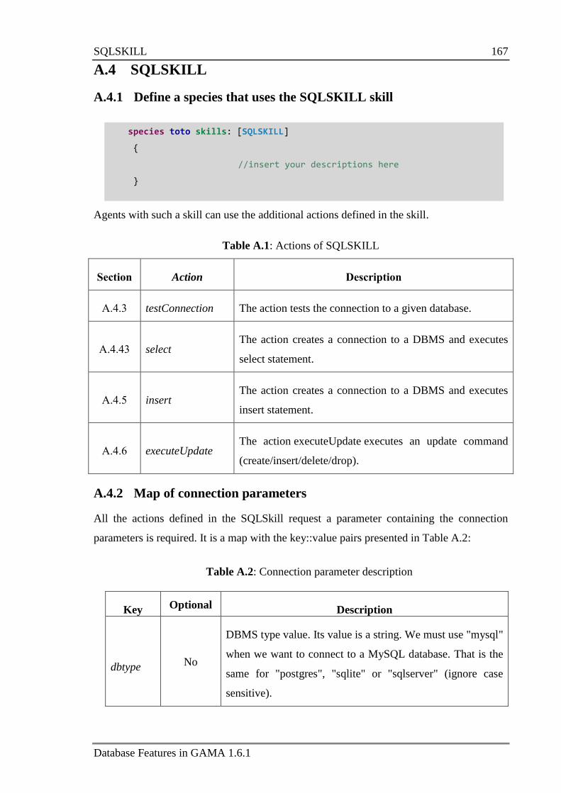
SQLSKILL 167
Database Features in GAMA 1.6.1
A.4 SQLSKILL
A.4.1 Define a species that uses the SQLSKILL skill
Agents with such a skill can use the additional actions defined in the skill.
Table A.1: Actions of SQLSKILL
Section Action Description
A.4.3 testConnection The action tests the connection to a given database.
A.4.43 select The action creates a connection to a DBMS and executes
select statement.
A.4.5 insert The action creates a connection to a DBMS and executes
insert statement.
A.4.6 executeUpdate The action executeUpdate executes an update command
(create/insert/delete/drop).
A.4.2 Map of connection parameters
All the actions defined in the SQLSkill request a parameter containing the connection
parameters is required. It is a map with the key::value pairs presented in Table A.2:
Table A.2: Connection parameter description
Key Optional Description
dbtype No
DBMS type value. Its value is a string. We must use "mysql"
when we want to connect to a MySQL database. That is the
same for "postgres", "sqlite" or "sqlserver" (ignore case
sensitive).
species toto skills: [SQLSKILL]
{
//insert your descriptions here
}
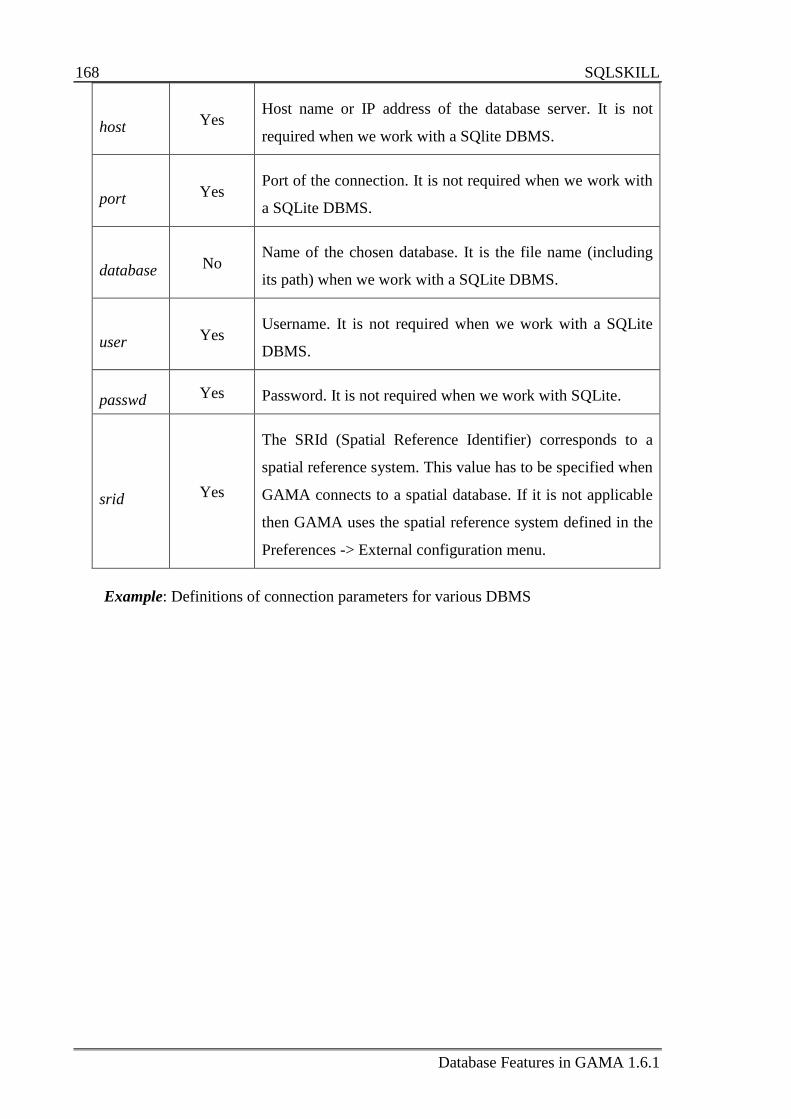
168 SQLSKILL
Database Features in GAMA 1.6.1
host Yes Host name or IP address of the database server. It is not
required when we work with a SQlite DBMS.
port Yes Port of the connection. It is not required when we work with
a SQLite DBMS.
database No Name of the chosen database. It is the file name (including
its path) when we work with a SQLite DBMS.
user Yes Username. It is not required when we work with a SQLite
DBMS.
passwd Yes Password. It is not required when we work with SQLite.
srid Yes
The SRId (Spatial Reference Identifier) corresponds to a
spatial reference system. This value has to be specified when
GAMA connects to a spatial database. If it is not applicable
then GAMA uses the spatial reference system defined in the
Preferences -> External configuration menu.
Example: Definitions of connection parameters for various DBMS
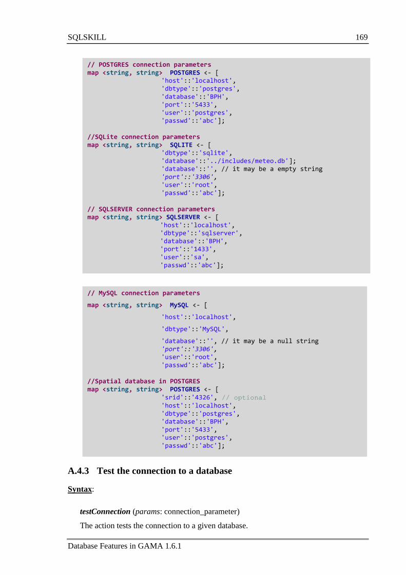
SQLSKILL 169
Database Features in GAMA 1.6.1
A.4.3 Test the connection to a database
Syntax:
testConnection (params: connection_parameter)
The action tests the connection to a given database.
// MySQL connection parameters
map <string, string> MySQL <- [
'host'::'localhost',
'dbtype'::'MySQL',
'database'::'', // it may be a null string 'port'::'3306', 'user'::'root', 'passwd'::'abc'];
//Spatial database in POSTGRES map <string, string> POSTGRES <- [
'srid'::'4326', // optional 'host'::'localhost', 'dbtype'::'postgres', 'database'::'BPH', 'port'::'5433', 'user'::'postgres', 'passwd'::'abc'];
// POSTGRES connection parameters map <string, string> POSTGRES <- [
'host'::'localhost', 'dbtype'::'postgres', 'database'::'BPH', 'port'::'5433', 'user'::'postgres', 'passwd'::'abc'];
//SQLite connection parameters map <string, string> SQLITE <- [
'dbtype'::'sqlite', 'database'::'../includes/meteo.db']; 'database'::'', // it may be a empty string 'port'::'3306', 'user'::'root', 'passwd'::'abc'];
// SQLSERVER connection parameters map <string, string> SQLSERVER <- [
'host'::'localhost', 'dbtype'::'sqlserver', 'database'::'BPH', 'port'::'1433', 'user'::'sa', 'passwd'::'abc'];
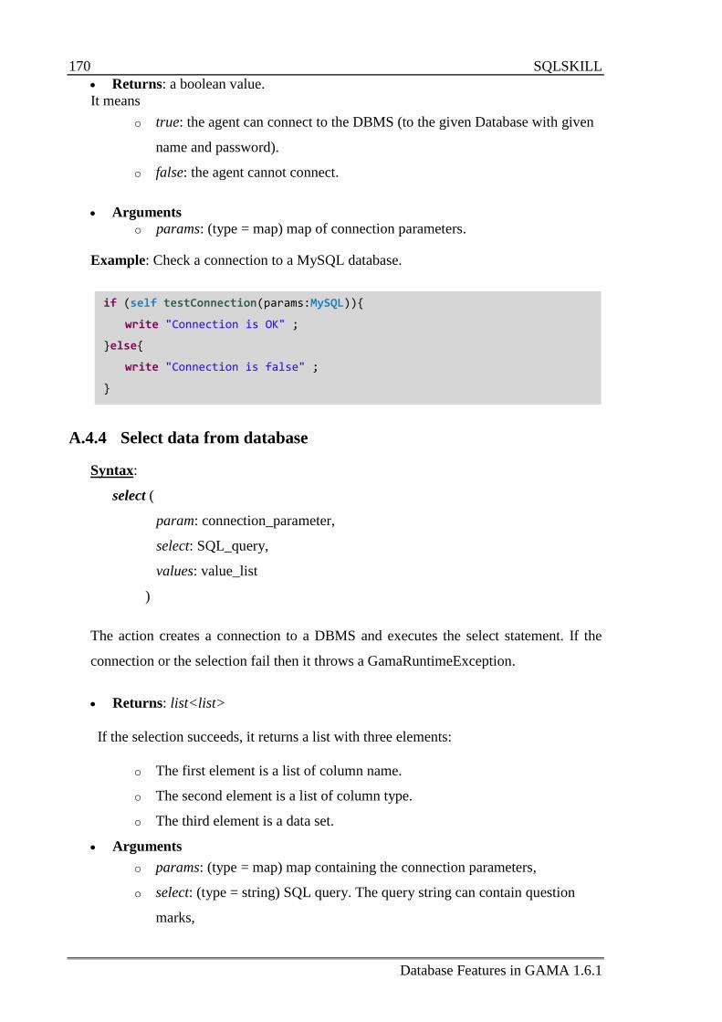
170 SQLSKILL
Database Features in GAMA 1.6.1
Returns: a boolean value.
It means
o true: the agent can connect to the DBMS (to the given Database with given
name and password).
o false: the agent cannot connect.
Arguments
o params: (type = map) map of connection parameters.
Example: Check a connection to a MySQL database.
A.4.4 Select data from database
Syntax:
select (
param: connection_parameter,
select: SQL_query,
values: value_list
)
The action creates a connection to a DBMS and executes the select statement. If the
connection or the selection fail then it throws a GamaRuntimeException.
Returns: list<list>
If the selection succeeds, it returns a list with three elements:
o The first element is a list of column name.
o The second element is a list of column type.
o The third element is a data set.
Arguments
o params: (type = map) map containing the connection parameters,
o select: (type = string) SQL query. The query string can contain question
marks,
if (self testConnection(params:MySQL)){
write "Connection is OK" ;
}else{
write "Connection is false" ;
}
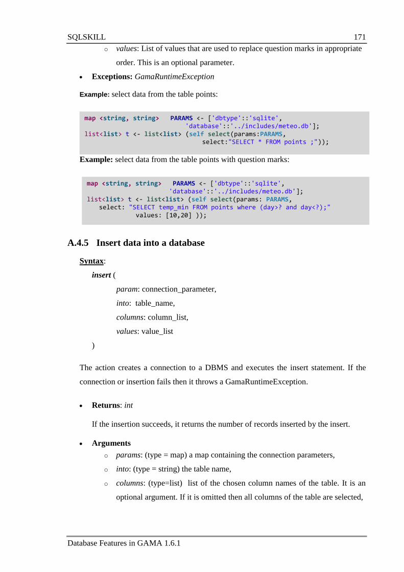
SQLSKILL 171
Database Features in GAMA 1.6.1
o values: List of values that are used to replace question marks in appropriate
order. This is an optional parameter.
Exceptions: GamaRuntimeException
Example: select data from the table points:
Example: select data from the table points with question marks:
A.4.5 Insert data into a database
Syntax:
insert (
param: connection_parameter,
into: table_name,
columns: column_list,
values: value_list
)
The action creates a connection to a DBMS and executes the insert statement. If the
connection or insertion fails then it throws a GamaRuntimeException.
Returns: int
If the insertion succeeds, it returns the number of records inserted by the insert.
Arguments
o params: (type = map) a map containing the connection parameters,
o into: (type = string) the table name,
o columns: (type=list) list of the chosen column names of the table. It is an
optional argument. If it is omitted then all columns of the table are selected,
map <string, string> PARAMS <- ['dbtype'::'sqlite', 'database'::'../includes/meteo.db'];
list<list> t <- list<list> (self select(params: PARAMS, select: "SELECT temp_min FROM points where (day>? and day<?);"
values: [10,20] ));
map <string, string> PARAMS <- ['dbtype'::'sqlite', 'database'::'../includes/meteo.db']; list<list> t <- list<list> (self select(params:PARAMS, select:"SELECT * FROM points ;"));
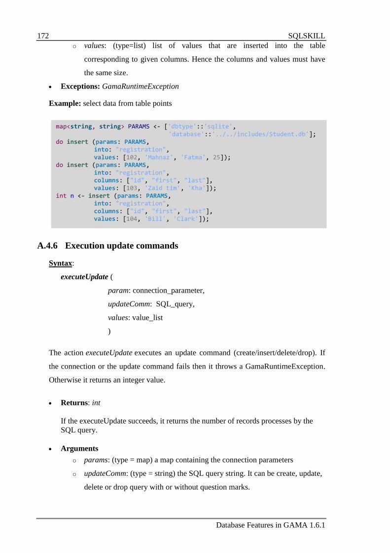
172 SQLSKILL
Database Features in GAMA 1.6.1
o values: (type=list) list of values that are inserted into the table
corresponding to given columns. Hence the columns and values must have
the same size.
Exceptions: GamaRuntimeException
Example: select data from table points
A.4.6 Execution update commands
Syntax:
executeUpdate (
param: connection_parameter,
updateComm: SQL_query,
values: value_list
)
The action executeUpdate executes an update command (create/insert/delete/drop). If
the connection or the update command fails then it throws a GamaRuntimeException.
Otherwise it returns an integer value.
Returns: int
If the executeUpdate succeeds, it returns the number of records processes by the
SQL query.
Arguments
o params: (type = map) a map containing the connection parameters
o updateComm: (type = string) the SQL query string. It can be create, update,
delete or drop query with or without question marks.
map<string, string> PARAMS <- ['dbtype'::'sqlite', 'database'::'../../includes/Student.db'];
do insert (params: PARAMS, into: "registration",
values: [102, 'Mahnaz', 'Fatma', 25]); do insert (params: PARAMS,
into: "registration", columns: ["id", "first", "last"], values: [103, 'Zaid tim', 'Kha']);
int n <- insert (params: PARAMS, into: "registration", columns: ["id", "first", "last"], values: [104, 'Bill', 'Clark']);
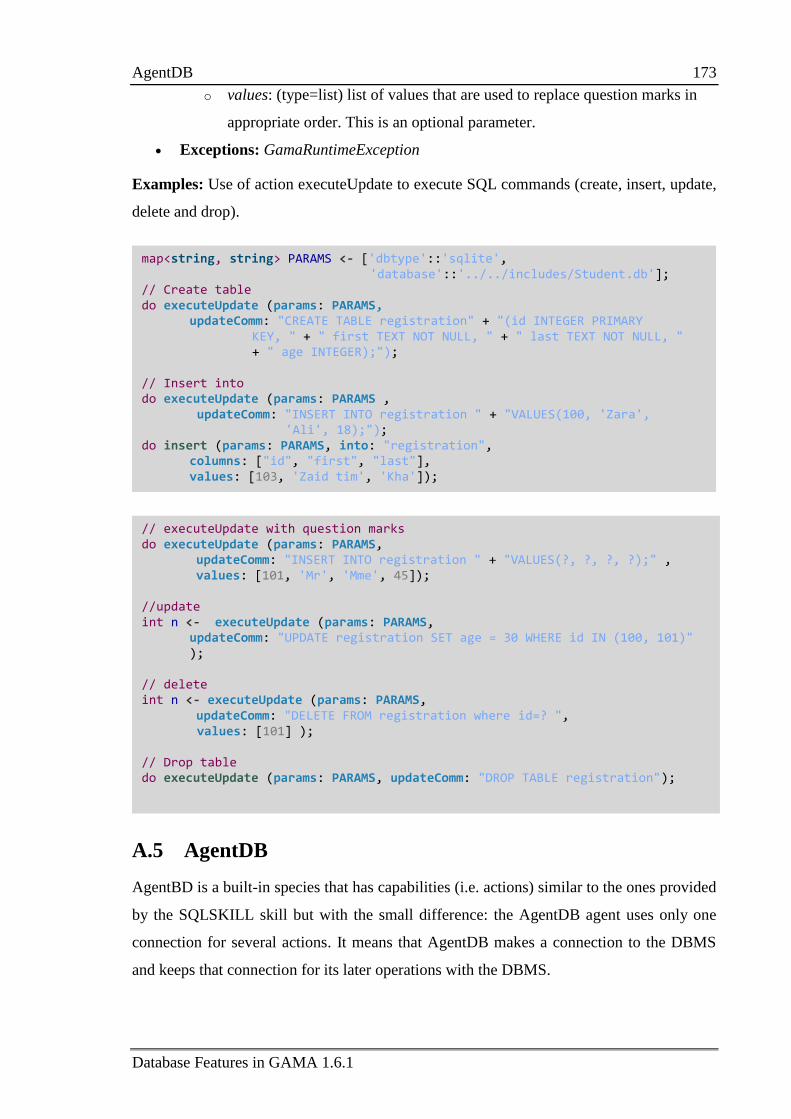
AgentDB 173
Database Features in GAMA 1.6.1
o values: (type=list) list of values that are used to replace question marks in
appropriate order. This is an optional parameter.
Exceptions: GamaRuntimeException
Examples: Use of action executeUpdate to execute SQL commands (create, insert, update,
delete and drop).
A.5 AgentDB
AgentBD is a built-in species that has capabilities (i.e. actions) similar to the ones provided
by the SQLSKILL skill but with the small difference: the AgentDB agent uses only one
connection for several actions. It means that AgentDB makes a connection to the DBMS
and keeps that connection for its later operations with the DBMS.
// executeUpdate with question marks do executeUpdate (params: PARAMS,
updateComm: "INSERT INTO registration " + "VALUES(?, ?, ?, ?);" , values: [101, 'Mr', 'Mme', 45]);
//update int n <- executeUpdate (params: PARAMS,
updateComm: "UPDATE registration SET age = 30 WHERE id IN (100, 101)" );
// delete int n <- executeUpdate (params: PARAMS,
updateComm: "DELETE FROM registration where id=? ", values: [101] );
// Drop table do executeUpdate (params: PARAMS, updateComm: "DROP TABLE registration");
map<string, string> PARAMS <- ['dbtype'::'sqlite', 'database'::'../../includes/Student.db'];
// Create table do executeUpdate (params: PARAMS,
updateComm: "CREATE TABLE registration" + "(id INTEGER PRIMARY KEY, " + " first TEXT NOT NULL, " + " last TEXT NOT NULL, " + " age INTEGER);");
// Insert into do executeUpdate (params: PARAMS ,
updateComm: "INSERT INTO registration " + "VALUES(100, 'Zara', 'Ali', 18);"); do insert (params: PARAMS, into: "registration",
columns: ["id", "first", "last"], values: [103, 'Zaid tim', 'Kha']);
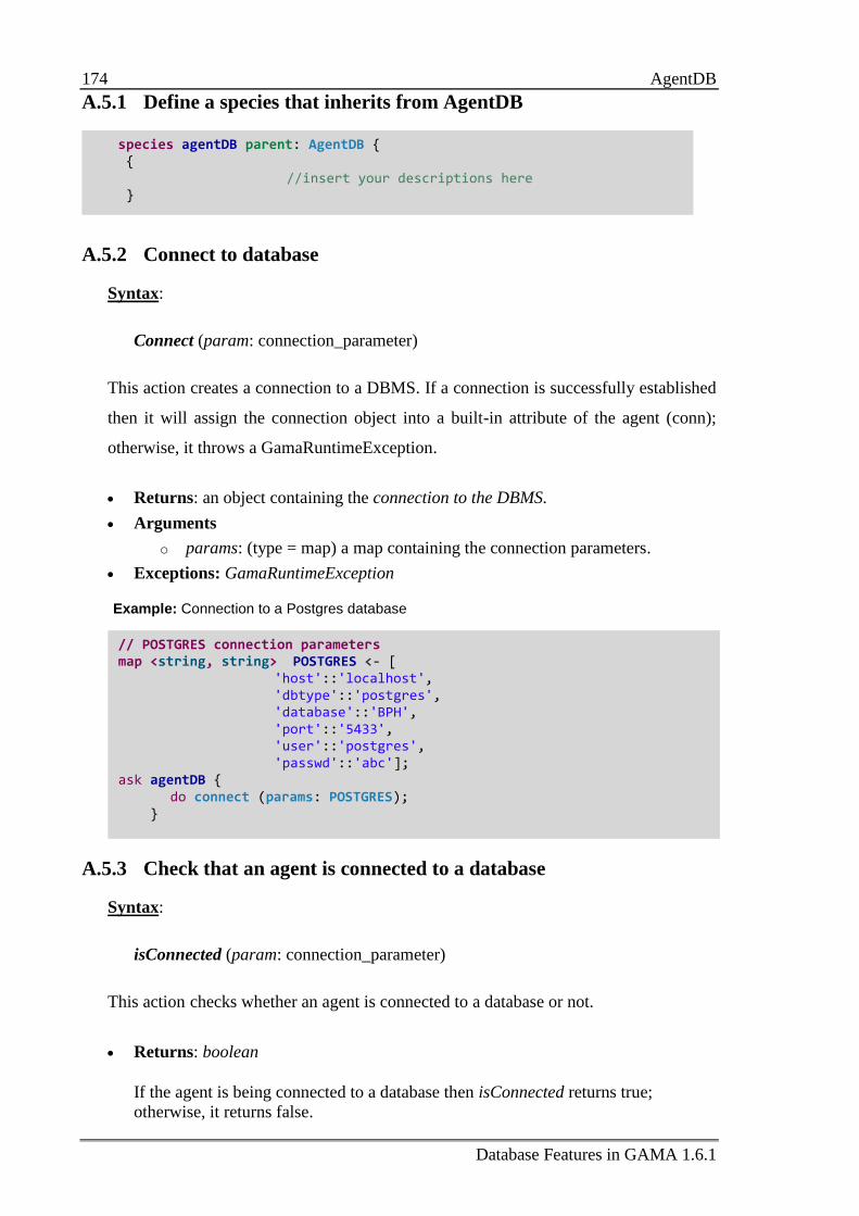
174 AgentDB
Database Features in GAMA 1.6.1
A.5.1 Define a species that inherits from AgentDB
A.5.2 Connect to database
Syntax:
Connect (param: connection_parameter)
This action creates a connection to a DBMS. If a connection is successfully established
then it will assign the connection object into a built-in attribute of the agent (conn);
otherwise, it throws a GamaRuntimeException.
Returns: an object containing the connection to the DBMS.
Arguments
o params: (type = map) a map containing the connection parameters.
Exceptions: GamaRuntimeException
Example: Connection to a Postgres database
A.5.3 Check that an agent is connected to a database
Syntax:
isConnected (param: connection_parameter)
This action checks whether an agent is connected to a database or not.
Returns: boolean
If the agent is being connected to a database then isConnected returns true;
otherwise, it returns false.
species agentDB parent: AgentDB { { //insert your descriptions here }
...
}
// POSTGRES connection parameters map <string, string> POSTGRES <- [
'host'::'localhost', 'dbtype'::'postgres', 'database'::'BPH', 'port'::'5433', 'user'::'postgres', 'passwd'::'abc'];
ask agentDB { do connect (params: POSTGRES);
}
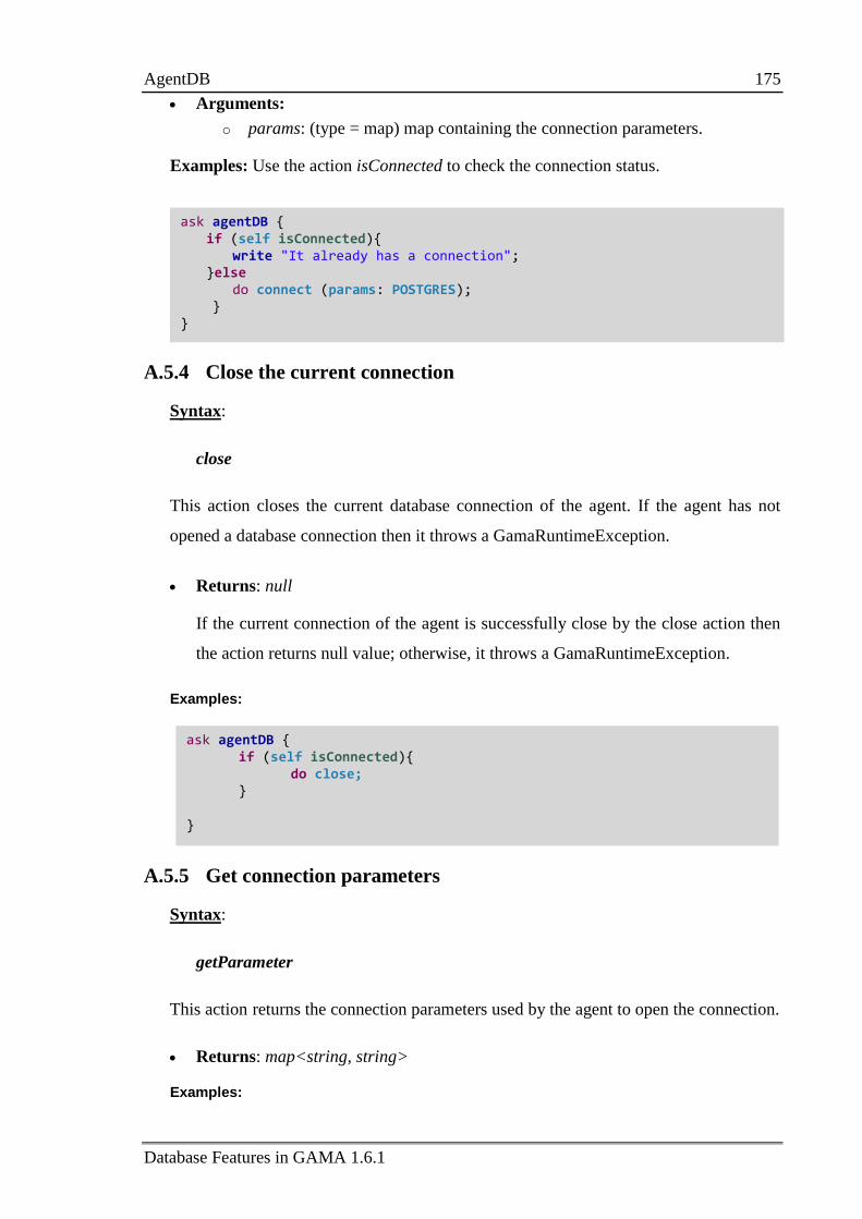
AgentDB 175
Database Features in GAMA 1.6.1
Arguments:
o params: (type = map) map containing the connection parameters.
Examples: Use the action isConnected to check the connection status.
A.5.4 Close the current connection
Syntax:
close
This action closes the current database connection of the agent. If the agent has not
opened a database connection then it throws a GamaRuntimeException.
Returns: null
If the current connection of the agent is successfully close by the close action then
the action returns null value; otherwise, it throws a GamaRuntimeException.
Examples:
A.5.5 Get connection parameters
Syntax:
getParameter
This action returns the connection parameters used by the agent to open the connection.
Returns: map<string, string>
Examples:
ask agentDB { if (self isConnected){
write "It already has a connection"; }else
do connect (params: POSTGRES); } }
ask agentDB { if (self isConnected){
do close; }
}
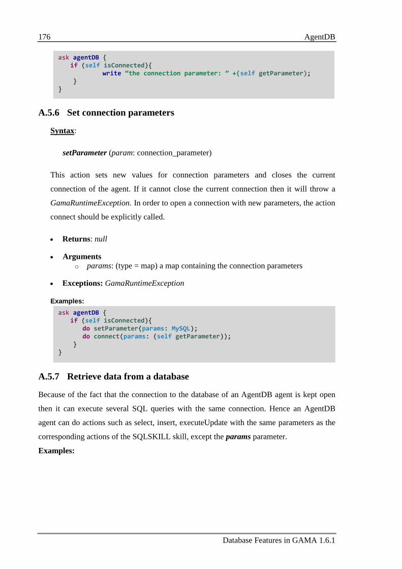
176 AgentDB
Database Features in GAMA 1.6.1
A.5.6 Set connection parameters
Syntax:
setParameter (param: connection_parameter)
This action sets new values for connection parameters and closes the current
connection of the agent. If it cannot close the current connection then it will throw a
GamaRuntimeException. In order to open a connection with new parameters, the action
connect should be explicitly called.
Returns: null
Arguments o params: (type = map) a map containing the connection parameters
Exceptions: GamaRuntimeException
Examples:
A.5.7 Retrieve data from a database
Because of the fact that the connection to the database of an AgentDB agent is kept open
then it can execute several SQL queries with the same connection. Hence an AgentDB
agent can do actions such as select, insert, executeUpdate with the same parameters as the
corresponding actions of the SQLSKILL skill, except the params parameter.
Examples:
ask agentDB { if (self isConnected){ write “the connection parameter: ” +(self getParameter); } }
ask agentDB { if (self isConnected){
do setParameter(params: MySQL); do connect(params: (self getParameter));
} }
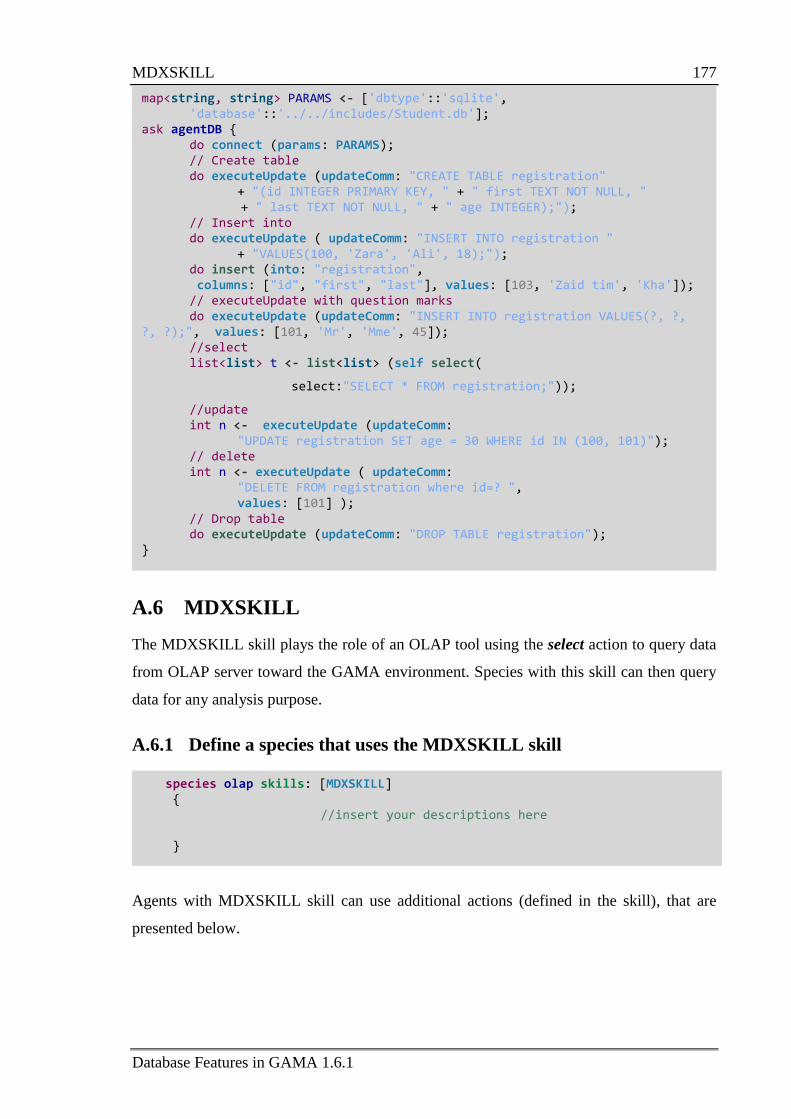
MDXSKILL 177
Database Features in GAMA 1.6.1
A.6 MDXSKILL
The MDXSKILL skill plays the role of an OLAP tool using the select action to query data
from OLAP server toward the GAMA environment. Species with this skill can then query
data for any analysis purpose.
A.6.1 Define a species that uses the MDXSKILL skill
Agents with MDXSKILL skill can use additional actions (defined in the skill), that are
presented below.
species olap skills: [MDXSKILL] { //insert your descriptions here
}
map<string, string> PARAMS <- ['dbtype'::'sqlite', 'database'::'../../includes/Student.db']; ask agentDB {
do connect (params: PARAMS); // Create table do executeUpdate (updateComm: "CREATE TABLE registration" + "(id INTEGER PRIMARY KEY, " + " first TEXT NOT NULL, " + " last TEXT NOT NULL, " + " age INTEGER);");
// Insert into do executeUpdate ( updateComm: "INSERT INTO registration "
+ "VALUES(100, 'Zara', 'Ali', 18);"); do insert (into: "registration",
columns: ["id", "first", "last"], values: [103, 'Zaid tim', 'Kha']); // executeUpdate with question marks do executeUpdate (updateComm: "INSERT INTO registration VALUES(?, ?, ?, ?);", values: [101, 'Mr', 'Mme', 45]); //select
list<list> t <- list<list> (self select(
select:"SELECT * FROM registration;"));
//update int n <- executeUpdate (updateComm: "UPDATE registration SET age = 30 WHERE id IN (100, 101)"); // delete int n <- executeUpdate ( updateComm: "DELETE FROM registration where id=? ",
values: [101] ); // Drop table do executeUpdate (updateComm: "DROP TABLE registration"); }
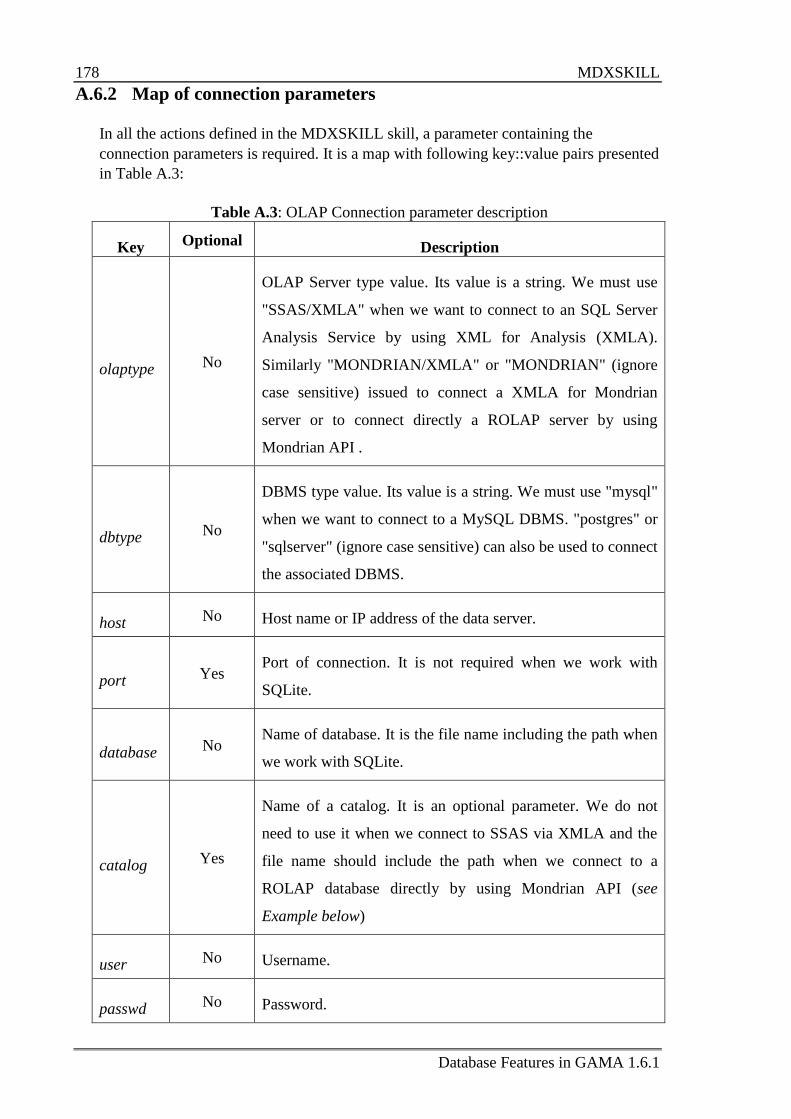
178 MDXSKILL
Database Features in GAMA 1.6.1
A.6.2 Map of connection parameters
In all the actions defined in the MDXSKILL skill, a parameter containing the
connection parameters is required. It is a map with following key::value pairs presented
in Table A.3:
Table A.3: OLAP Connection parameter description
Key Optional Description
olaptype No
OLAP Server type value. Its value is a string. We must use
"SSAS/XMLA" when we want to connect to an SQL Server
Analysis Service by using XML for Analysis (XMLA).
Similarly "MONDRIAN/XMLA" or "MONDRIAN" (ignore
case sensitive) issued to connect a XMLA for Mondrian
server or to connect directly a ROLAP server by using
Mondrian API .
dbtype No
DBMS type value. Its value is a string. We must use "mysql"
when we want to connect to a MySQL DBMS. "postgres" or
"sqlserver" (ignore case sensitive) can also be used to connect
the associated DBMS.
host No Host name or IP address of the data server.
port Yes Port of connection. It is not required when we work with
SQLite.
database No Name of database. It is the file name including the path when
we work with SQLite.
catalog Yes
Name of a catalog. It is an optional parameter. We do not
need to use it when we connect to SSAS via XMLA and the
file name should include the path when we connect to a
ROLAP database directly by using Mondrian API (see
Example below)
user No Username.
passwd No Password.
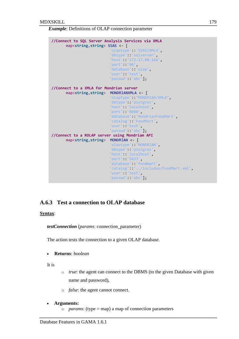
MDXSKILL 179
Database Features in GAMA 1.6.1
Example: Definitions of OLAP connection parameter
A.6.3 Test a connection to OLAP database
Syntax:
testConnection (params: connection_parameter)
The action tests the connection to a given OLAP database.
Returns: boolean
It is
o true: the agent can connect to the DBMS (to the given Database with given
name and password),
o false: the agent cannot connect.
Arguments:
o params: (type = map) a map of connection parameters
//Connect to SQL Server Analysis Services via XMLA map<string,string> SSAS <- [ 'olaptype'::'SSAS/XMLA', 'dbtype'::'sqlserver', 'host'::'172.17.88.166', 'port'::'80', 'database'::'olap', 'user'::'test', 'passwd'::'abc']; //Connect to a XMLA for Mondrian server map<string,string> MONDRIANXMLA <- [ 'olaptype'::"MONDRIAN/XMLA", 'dbtype'::'postgres', 'host'::'localhost', 'port'::'8080', 'database'::'MondrianFoodMart', 'catalog'::'FoodMart', 'user'::'test', 'passwd'::'abc']; //Connect to a ROLAP server using Mondriam API map<string,string> MONDRIAN <- [ 'olaptype'::'MONDRIAN', 'dbtype'::'postgres', 'host'::'localhost', 'port'::'5433', 'database'::'foodmart', 'catalog'::'../includes/FoodMart.xml', 'user'::'test',
'passwd'::'abc'];
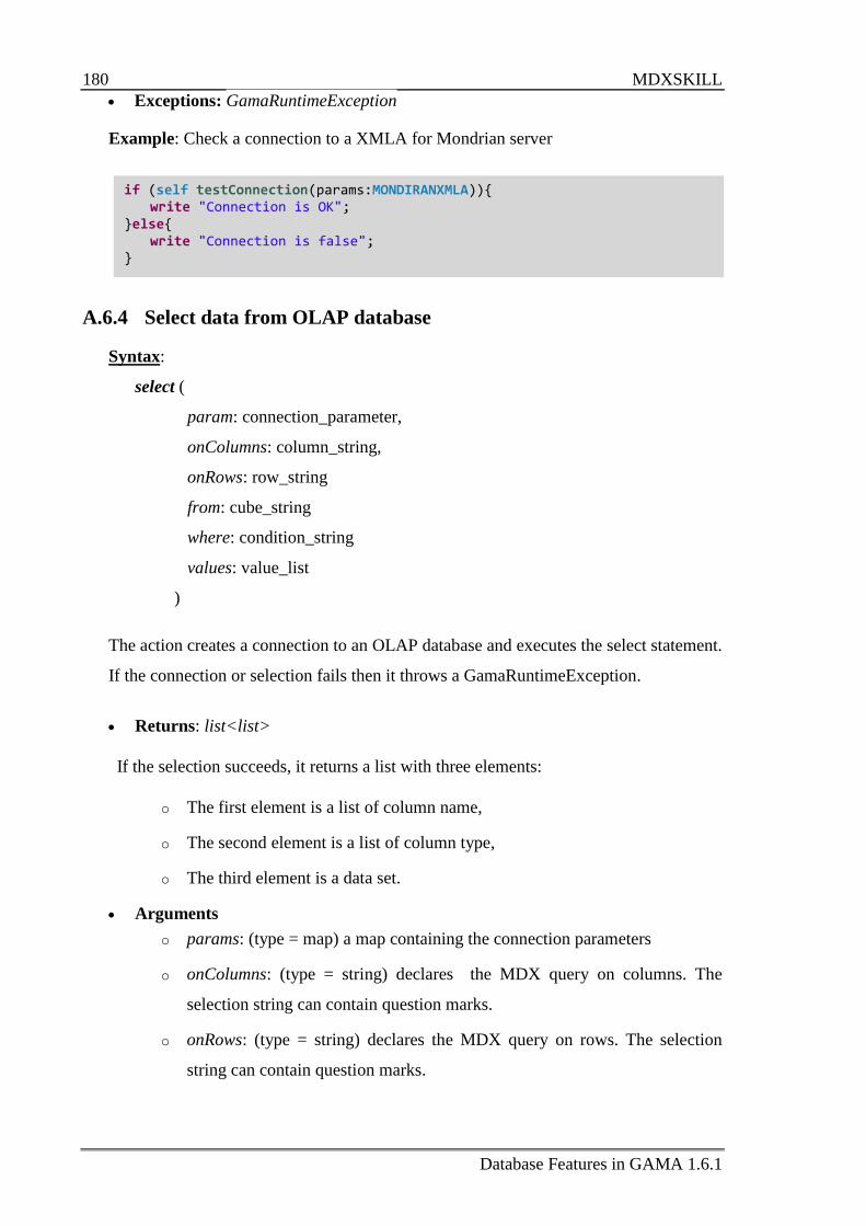
180 MDXSKILL
Database Features in GAMA 1.6.1
Exceptions: GamaRuntimeException
Example: Check a connection to a XMLA for Mondrian server
A.6.4 Select data from OLAP database
Syntax:
select (
param: connection_parameter,
onColumns: column_string,
onRows: row_string
from: cube_string
where: condition_string
values: value_list
)
The action creates a connection to an OLAP database and executes the select statement.
If the connection or selection fails then it throws a GamaRuntimeException.
Returns: list<list>
If the selection succeeds, it returns a list with three elements:
o The first element is a list of column name,
o The second element is a list of column type,
o The third element is a data set.
Arguments
o params: (type = map) a map containing the connection parameters
o onColumns: (type = string) declares the MDX query on columns. The
selection string can contain question marks.
o onRows: (type = string) declares the MDX query on rows. The selection
string can contain question marks.
if (self testConnection(params:MONDIRANXMLA)){ write "Connection is OK"; }else{ write "Connection is false"; }
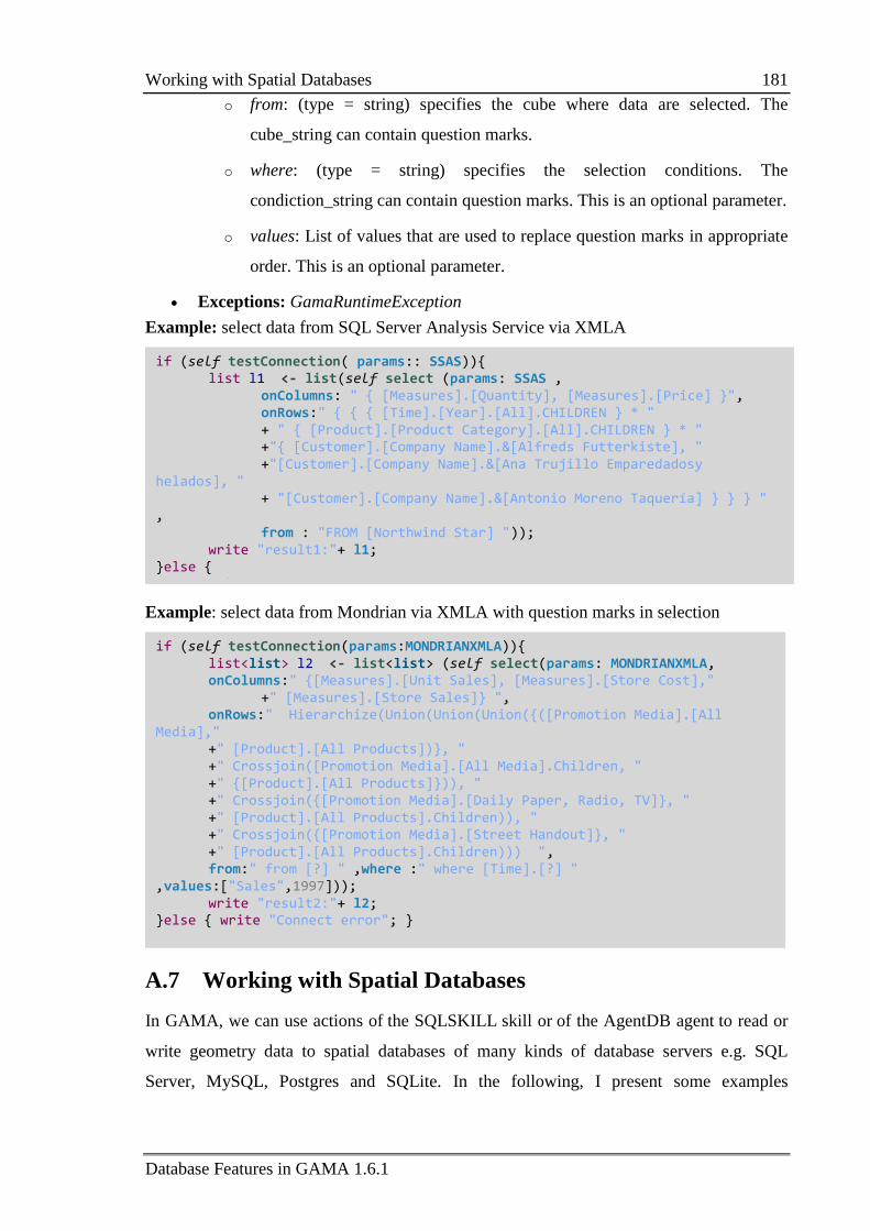
Working with Spatial Databases 181
Database Features in GAMA 1.6.1
o from: (type = string) specifies the cube where data are selected. The
cube_string can contain question marks.
o where: (type = string) specifies the selection conditions. The
condiction_string can contain question marks. This is an optional parameter.
o values: List of values that are used to replace question marks in appropriate
order. This is an optional parameter.
Exceptions: GamaRuntimeException
Example: select data from SQL Server Analysis Service via XMLA
Example: select data from Mondrian via XMLA with question marks in selection
A.7 Working with Spatial Databases
In GAMA, we can use actions of the SQLSKILL skill or of the AgentDB agent to read or
write geometry data to spatial databases of many kinds of database servers e.g. SQL
Server, MySQL, Postgres and SQLite. In the following, I present some examples
if (self testConnection(params:MONDRIANXMLA)){ list<list> l2 <- list<list> (self select(params: MONDRIANXMLA, onColumns:" {[Measures].[Unit Sales], [Measures].[Store Cost]," +" [Measures].[Store Sales]} ", onRows:" Hierarchize(Union(Union(Union({([Promotion Media].[All Media]," +" [Product].[All Products])}, " +" Crossjoin([Promotion Media].[All Media].Children, " +" {[Product].[All Products]})), " +" Crossjoin({[Promotion Media].[Daily Paper, Radio, TV]}, " +" [Product].[All Products].Children)), " +" Crossjoin({[Promotion Media].[Street Handout]}, " +" [Product].[All Products].Children))) ", from:" from [?] " ,where :" where [Time].[?] " ,values:["Sales",1997])); write "result2:"+ l2; }else { write "Connect error"; }
if (self testConnection( params:: SSAS)){ list l1 <- list(self select (params: SSAS , onColumns: " { [Measures].[Quantity], [Measures].[Price] }", onRows:" { { { [Time].[Year].[All].CHILDREN } * " + " { [Product].[Product Category].[All].CHILDREN } * " +"{ [Customer].[Company Name].&[Alfreds Futterkiste], " +"[Customer].[Company Name].&[Ana Trujillo Emparedadosy helados], " + "[Customer].[Company Name].&[Antonio Moreno Taquería] } } } " , from : "FROM [Northwind Star] ")); write "result1:"+ l1; }else { write "Connect error"; }
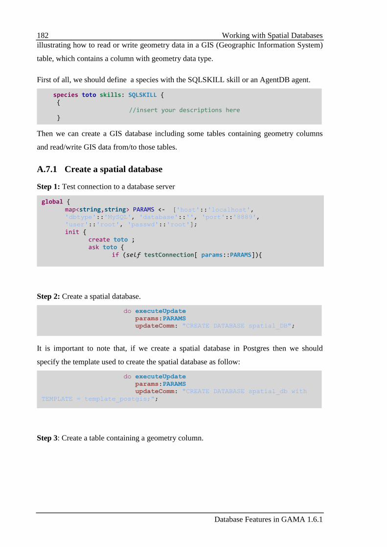
182 Working with Spatial Databases
Database Features in GAMA 1.6.1
illustrating how to read or write geometry data in a GIS (Geographic Information System)
table, which contains a column with geometry data type.
First of all, we should define a species with the SQLSKILL skill or an AgentDB agent.
Then we can create a GIS database including some tables containing geometry columns
and read/write GIS data from/to those tables.
A.7.1 Create a spatial database
Step 1: Test connection to a database server
Step 2: Create a spatial database.
It is important to note that, if we create a spatial database in Postgres then we should
specify the template used to create the spatial database as follow:
Step 3: Create a table containing a geometry column.
do executeUpdate
params:PARAMS
updateComm: "CREATE DATABASE spatial_db with
TEMPLATE = template_postgis;";
do executeUpdate
params:PARAMS
updateComm: "CREATE DATABASE spatial_DB";
global { map<string,string> PARAMS <- ['host'::'localhost', 'dbtype'::'MySQL', 'database'::'', 'port'::'8889',
'user'::'root', 'passwd'::'root']; init { create toto ; ask toto { if (self testConnection[ params::PARAMS]){
species toto skills: SQLSKILL { { //insert your descriptions here }
...
}
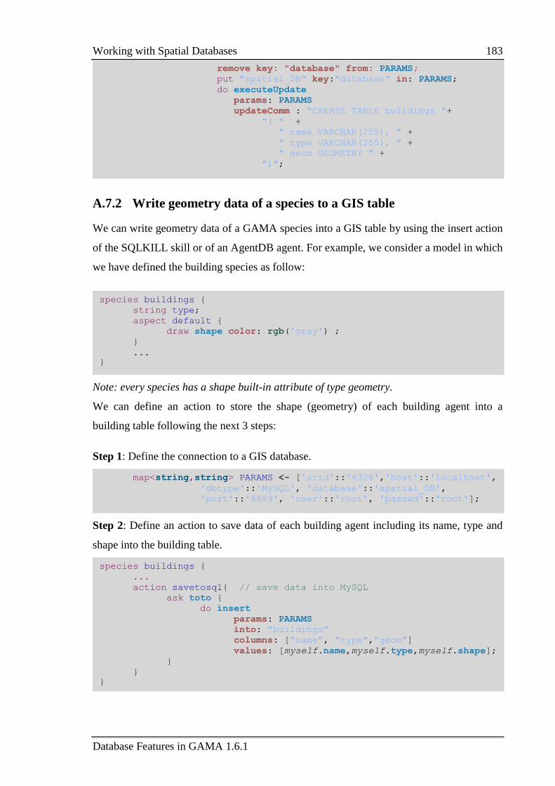
Working with Spatial Databases 183
Database Features in GAMA 1.6.1
A.7.2 Write geometry data of a species to a GIS table
We can write geometry data of a GAMA species into a GIS table by using the insert action
of the SQLKILL skill or of an AgentDB agent. For example, we consider a model in which
we have defined the building species as follow:
Note: every species has a shape built-in attribute of type geometry.
We can define an action to store the shape (geometry) of each building agent into a
building table following the next 3 steps:
Step 1: Define the connection to a GIS database.
Step 2: Define an action to save data of each building agent including its name, type and
shape into the building table.
species buildings {
...
action savetosql{ // save data into MySQL
ask toto {
do insert
params: PARAMS
into: "buildings"
columns: ["name", "type","geom"]
values: [myself.name,myself.type,myself.shape];
}
}
}
map<string,string> PARAMS <- ['srid'::'4326','host'::'localhost',
'dbtype'::'MySQL', 'database'::'spatial_DB',
'port'::'8889', 'user'::'root', 'passwd'::'root'];
species buildings {
string type;
aspect default {
draw shape color: rgb('gray') ;
}
...
}
remove key: "database" from: PARAMS;
put "spatial_DB" key:"database" in: PARAMS;
do executeUpdate
params: PARAMS
updateComm : "CREATE TABLE buildings "+
"( " +
" name VARCHAR(255), " +
" type VARCHAR(255), " +
" geom GEOMETRY " +
")";
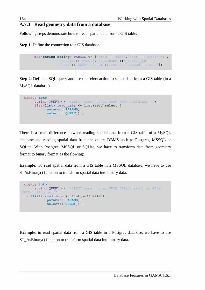
184 Working with Spatial Databases
Database Features in GAMA 1.6.1
A.7.3 Read geometry data from a database
Following steps demonstrate how to read spatial data from a GIS table.
Step 1: Define the connection to a GIS database.
Step 2: Define a SQL query and use the select action to select data from a GIS table (in a
MySQL database).
There is a small difference between reading spatial data from a GIS table of a MySQL
database and reading spatial data from the others DBMS such as Postgres, MSSQL or
SQLite. With Postgres, MSSQL or SQLite, we have to transform data from geometry
format to binary format as the flowing:
Example: To read spatial data from a GIS table in a MSSQL database, we have to use
STAsBinary() function to transform spatial data into binary data.
Example: to read spatial data from a GIS table in a Postgres database, we have to use
ST_AsBinary() function to transform spatial data into binary data.
create toto {
string QUERY <- "SELECT name, type, GEOM.STAsBinary() as GEOM
FROM buildings ;";
list<list> read_data <- list(self select [
params:: PARAMS,
select:: QUERY]) ;
}
create toto {
string QUERY <- "SELECT name, type, geom FROM buildings ;";
list<list> read_data <- list(self select [
params:: PARAMS,
select:: QUERY]) ;
}
map<string,string> PARAMS <- ['srid'::'4326','host'::'localhost',
'dbtype'::'MySQL', 'database'::'spatial_DB',
'port'::'8889', 'user'::'root', 'passwd'::'root'];
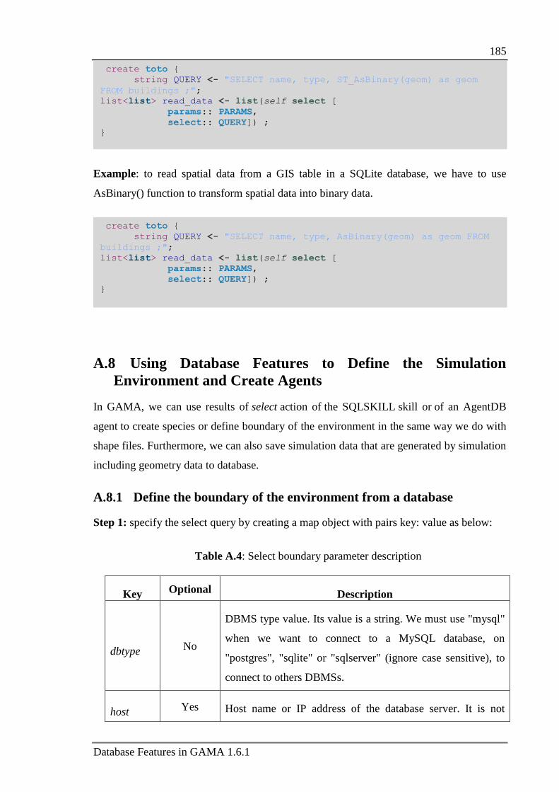
185
Database Features in GAMA 1.6.1
Example: to read spatial data from a GIS table in a SQLite database, we have to use
AsBinary() function to transform spatial data into binary data.
A.8 Using Database Features to Define the Simulation
Environment and Create Agents
In GAMA, we can use results of select action of the SQLSKILL skill or of an AgentDB
agent to create species or define boundary of the environment in the same way we do with
shape files. Furthermore, we can also save simulation data that are generated by simulation
including geometry data to database.
A.8.1 Define the boundary of the environment from a database
Step 1: specify the select query by creating a map object with pairs key: value as below:
Table A.4: Select boundary parameter description
Key Optional Description
dbtype No
DBMS type value. Its value is a string. We must use "mysql"
when we want to connect to a MySQL database, on
"postgres", "sqlite" or "sqlserver" (ignore case sensitive), to
connect to others DBMSs.
host Yes Host name or IP address of the database server. It is not
create toto {
string QUERY <- "SELECT name, type, AsBinary(geom) as geom FROM
buildings ;";
list<list> read_data <- list(self select [
params:: PARAMS,
select:: QUERY]) ;
}
create toto {
string QUERY <- "SELECT name, type, ST_AsBinary(geom) as geom
FROM buildings ;";
list<list> read_data <- list(self select [
params:: PARAMS,
select:: QUERY]) ;
}
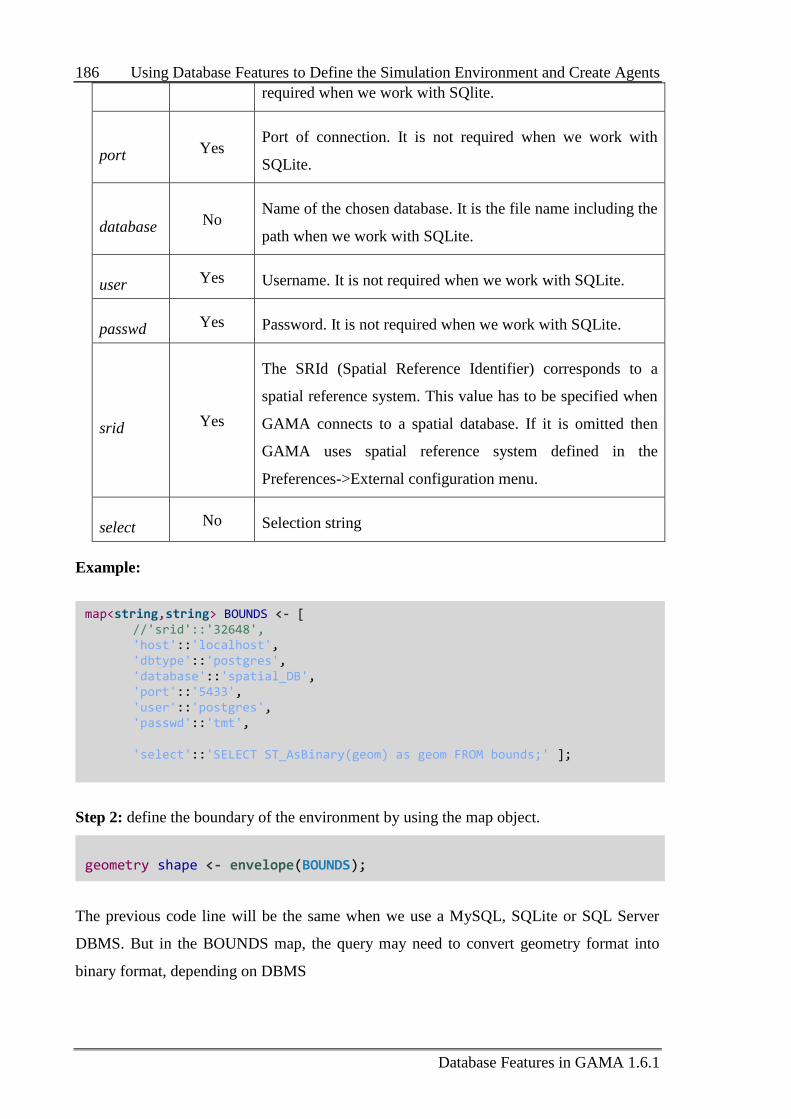
186 Using Database Features to Define the Simulation Environment and Create Agents
Database Features in GAMA 1.6.1
required when we work with SQlite.
port Yes Port of connection. It is not required when we work with
SQLite.
database No Name of the chosen database. It is the file name including the
path when we work with SQLite.
user Yes Username. It is not required when we work with SQLite.
passwd Yes Password. It is not required when we work with SQLite.
srid Yes
The SRId (Spatial Reference Identifier) corresponds to a
spatial reference system. This value has to be specified when
GAMA connects to a spatial database. If it is omitted then
GAMA uses spatial reference system defined in the
Preferences->External configuration menu.
select No Selection string
Example:
Step 2: define the boundary of the environment by using the map object.
The previous code line will be the same when we use a MySQL, SQLite or SQL Server
DBMS. But in the BOUNDS map, the query may need to convert geometry format into
binary format, depending on DBMS
geometry shape <- envelope(BOUNDS);
map<string,string> BOUNDS <- [ //'srid'::'32648', 'host'::'localhost', 'dbtype'::'postgres', 'database'::'spatial_DB', 'port'::'5433', 'user'::'postgres', 'passwd'::'tmt',
'select'::'SELECT ST_AsBinary(geom) as geom FROM bounds;' ];
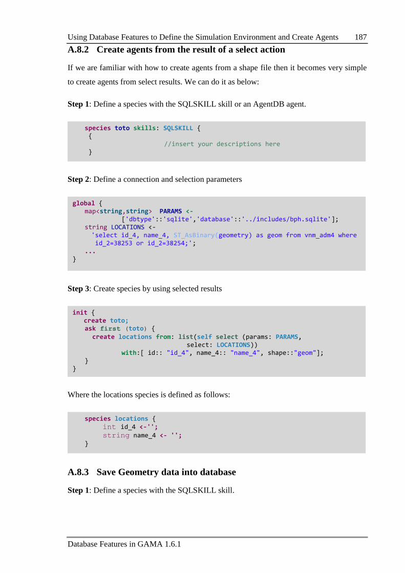
Using Database Features to Define the Simulation Environment and Create Agents 187
Database Features in GAMA 1.6.1
A.8.2 Create agents from the result of a select action
If we are familiar with how to create agents from a shape file then it becomes very simple
to create agents from select results. We can do it as below:
Step 1: Define a species with the SQLSKILL skill or an AgentDB agent.
Step 2: Define a connection and selection parameters
Step 3: Create species by using selected results
Where the locations species is defined as follows:
A.8.3 Save Geometry data into database
Step 1: Define a species with the SQLSKILL skill.
species locations { int id_4 <-'';
string name_4 <- ''; }
init { create toto; ask first (toto) { create locations from: list(self select (params: PARAMS, select: LOCATIONS))
with:[ id:: "id_4", name_4:: "name_4", shape::"geom"]; } }
global { map<string,string> PARAMS <-
['dbtype'::'sqlite','database'::'../includes/bph.sqlite']; string LOCATIONS <- 'select id_4, name_4, ST_AsBinary(geometry) as geom from vnm_adm4 where id_2=38253 or id_2=38254;'; ... }
species toto skills: SQLSKILL { { //insert your descriptions here }
...
}
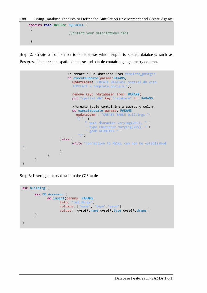
188 Using Database Features to Define the Simulation Environment and Create Agents
Database Features in GAMA 1.6.1
Step 2: Create a connection to a database which supports spatial databases such as
Postgres. Then create a spatial database and a table containing a geometry column.
Step 3: Insert geometry data into the GIS table
ask building {
ask DB_Accessor { do insert(params: PARAMS,
into: "buildings", columns: ["name", "type","geom"], values: [myself.name,myself.type,myself.shape]; }
}
// create a GIS database from template_postgis do executeUpdate(params:PARAMS,
updateComm: "CREATE DATABASE spatial_db with TEMPLATE = template_postgis;");
remove key: "database" from: PARAMS; put "spatial_db" key:"database" in: PARAMS; //create table containing a geometry column
do executeUpdate params: PARAMS updateComm : "CREATE TABLE buildings "+ "( " +
" name character varying(255), " + " type character varying(255), " + " geom GEOMETRY " + ")";
}else { write "Connection to MySQL can not be established "; } } } }
species toto skills: SQLSKILL { { //insert your descriptions here }
Entities Data Description
Entities Data Description
Appendix B
Entities Data Description
B.1 Empirical Data Description ................................................................................. 190
B.2 Simulation Data Description ............................................................................... 195
B.3 Data Warehouse Description ............................................................................... 197
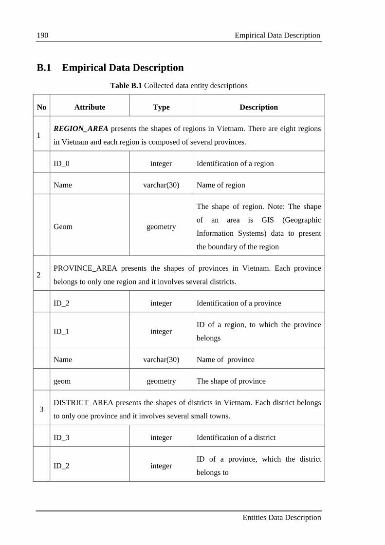
190 Empirical Data Description
Entities Data Description
B.1 Empirical Data Description
Table B.1 Collected data entity descriptions
No Attribute Type Description
1 REGION_AREA presents the shapes of regions in Vietnam. There are eight regions
in Vietnam and each region is composed of several provinces.
ID_0 integer Identification of a region
Name varchar(30) Name of region
Geom geometry
The shape of region. Note: The shape
of an area is GIS (Geographic
Information Systems) data to present
the boundary of the region
2 PROVINCE_AREA presents the shapes of provinces in Vietnam. Each province
belongs to only one region and it involves several districts.
ID_2 integer Identification of a province
ID_1 integer ID of a region, to which the province
belongs
Name varchar(30) Name of province
geom geometry The shape of province
3 DISTRICT_AREA presents the shapes of districts in Vietnam. Each district belongs
to only one province and it involves several small towns.
ID_3 integer Identification of a district
ID_2 integer ID of a province, which the district
belongs to
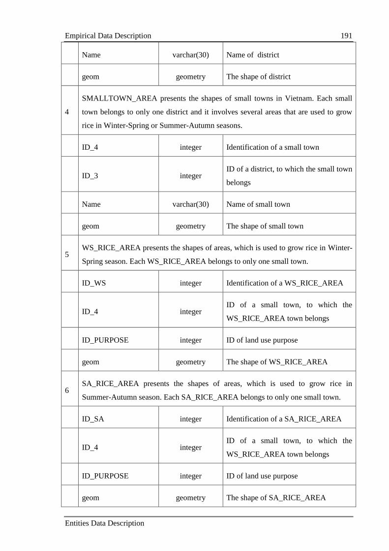
Empirical Data Description 191
Entities Data Description
Name varchar(30) Name of district
geom geometry The shape of district
4
SMALLTOWN_AREA presents the shapes of small towns in Vietnam. Each small
town belongs to only one district and it involves several areas that are used to grow
rice in Winter-Spring or Summer-Autumn seasons.
ID_4 integer Identification of a small town
ID_3 integer ID of a district, to which the small town
belongs
Name varchar(30) Name of small town
geom geometry The shape of small town
5 WS_RICE_AREA presents the shapes of areas, which is used to grow rice in Winter-
Spring season. Each WS_RICE_AREA belongs to only one small town.
ID_WS integer Identification of a WS_RICE_AREA
ID_4 integer ID of a small town, to which the
WS_RICE_AREA town belongs
ID_PURPOSE integer ID of land use purpose
geom geometry The shape of WS_RICE_AREA
6 SA_RICE_AREA presents the shapes of areas, which is used to grow rice in
Summer-Autumn season. Each SA_RICE_AREA belongs to only one small town.
ID_SA integer Identification of a SA_RICE_AREA
ID_4 integer ID of a small town, to which the
WS_RICE_AREA town belongs
ID_PURPOSE integer ID of land use purpose
geom geometry The shape of SA_RICE_AREA
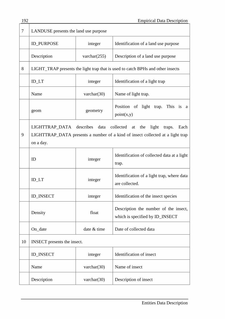
192 Empirical Data Description
Entities Data Description
7 LANDUSE presents the land use purpose
ID_PURPOSE integer Identification of a land use purpose
Description varchar(255) Description of a land use purpose
8 LIGHT_TRAP presents the light trap that is used to catch BPHs and other insects
ID_LT integer Identification of a light trap
Name varchar(30) Name of light trap.
geom geometry Position of light trap. This is a
point(x,y)
9
LIGHTTRAP_DATA describes data collected at the light traps. Each
LIGHTTRAP_DATA presents a number of a kind of insect collected at a light trap
on a day.
ID integer Identification of collected data at a light
trap.
ID_LT integer Identification of a light trap, where data
are collected.
ID_INSECT integer Identification of the insect species
Density float Description the number of the insect,
which is specified by ID_INSECT
On_date date & time Date of collected data
10 INSECT presents the insect.
ID_INSECT integer Identification of insect
Name varchar(30) Name of insect
Description varchar(30) Description of insect
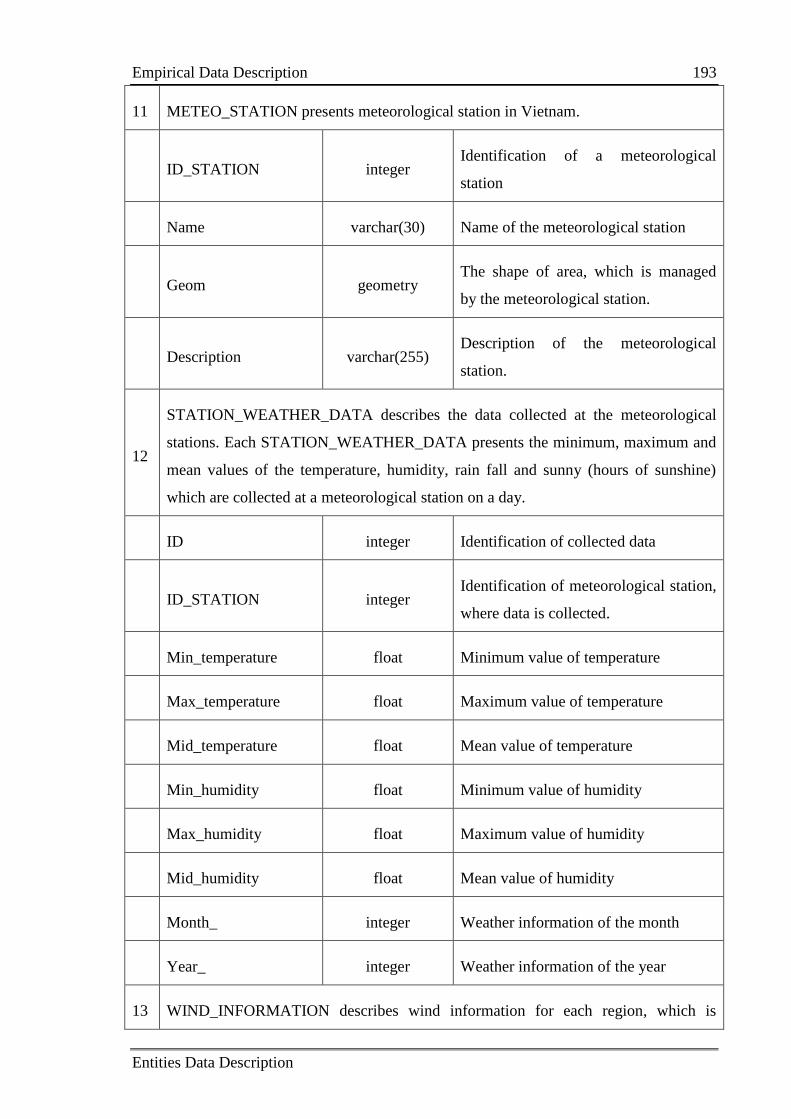
Empirical Data Description 193
Entities Data Description
11 METEO_STATION presents meteorological station in Vietnam.
ID_STATION integer Identification of a meteorological
station
Name varchar(30) Name of the meteorological station
Geom geometry The shape of area, which is managed
by the meteorological station.
Description varchar(255) Description of the meteorological
station.
12
STATION_WEATHER_DATA describes the data collected at the meteorological
stations. Each STATION_WEATHER_DATA presents the minimum, maximum and
mean values of the temperature, humidity, rain fall and sunny (hours of sunshine)
which are collected at a meteorological station on a day.
ID integer Identification of collected data
ID_STATION integer Identification of meteorological station,
where data is collected.
Min_temperature float Minimum value of temperature
Max_temperature float Maximum value of temperature
Mid_temperature float Mean value of temperature
Min_humidity float Minimum value of humidity
Max_humidity float Maximum value of humidity
Mid_humidity float Mean value of humidity
Month_ integer Weather information of the month
Year_ integer Weather information of the year
13 WIND_INFORMATION describes wind information for each region, which is
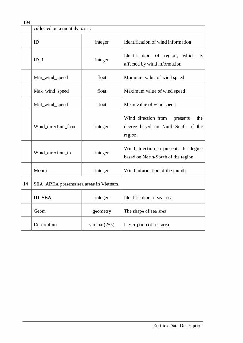
194
Entities Data Description
collected on a monthly basis.
ID integer Identification of wind information
ID_1 integer Identification of region, which is
affected by wind information
Min_wind_speed float Minimum value of wind speed
Max_wind_speed float Maximum value of wind speed
Mid_wind_speed float Mean value of wind speed
Wind_direction_from integer
Wind_direction_from presents the
degree based on North-South of the
region.
Wind_direction_to integer Wind_direction_to presents the degree
based on North-South of the region.
Month integer Wind information of the month
14 SEA_AREA presents sea areas in Vietnam.
ID_SEA integer Identification of sea area
Geom geometry The shape of sea area
Description varchar(255) Description of sea area
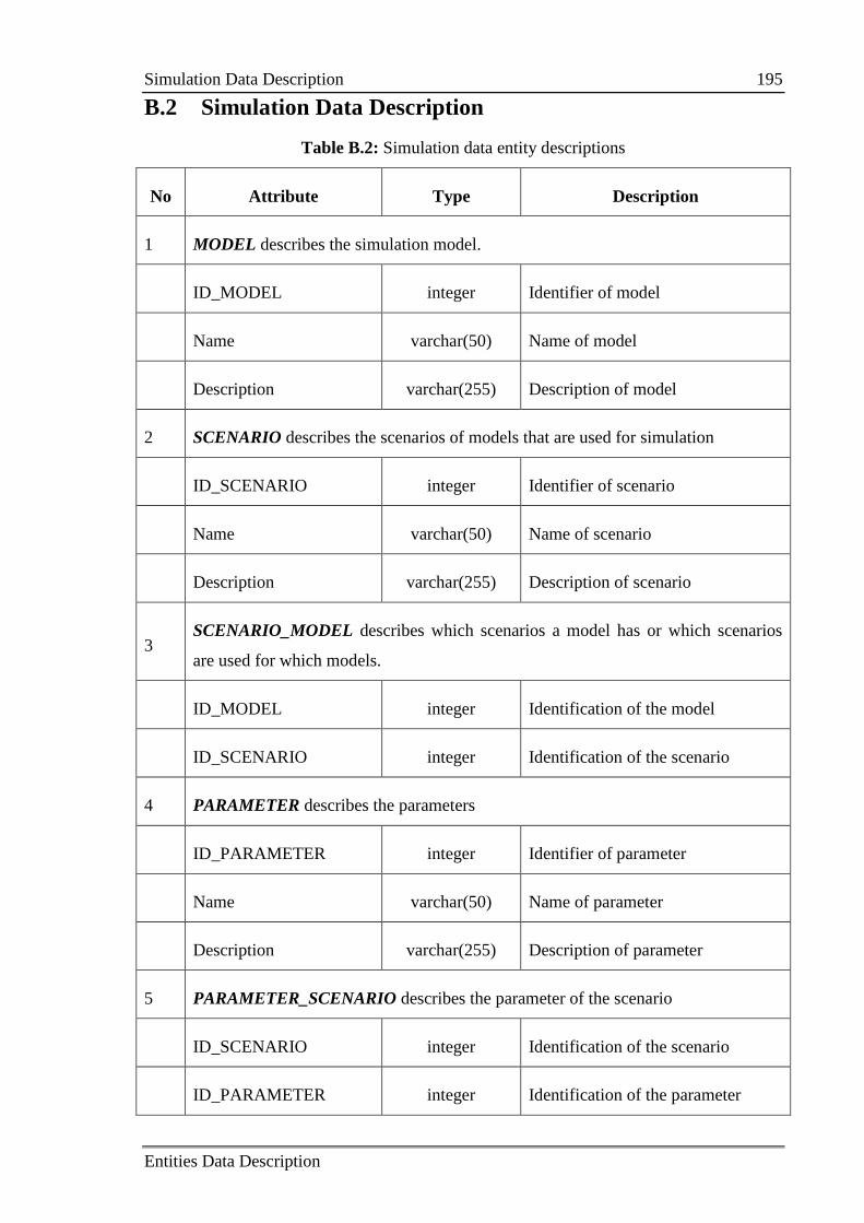
Simulation Data Description 195
Entities Data Description
B.2 Simulation Data Description
Table B.2: Simulation data entity descriptions
No Attribute Type Description
1 MODEL describes the simulation model.
ID_MODEL integer Identifier of model
Name varchar(50) Name of model
Description varchar(255) Description of model
2 SCENARIO describes the scenarios of models that are used for simulation
ID_SCENARIO integer Identifier of scenario
Name varchar(50) Name of scenario
Description varchar(255) Description of scenario
3 SCENARIO_MODEL describes which scenarios a model has or which scenarios
are used for which models.
ID_MODEL integer Identification of the model
ID_SCENARIO integer Identification of the scenario
4 PARAMETER describes the parameters
ID_PARAMETER integer Identifier of parameter
Name varchar(50) Name of parameter
Description varchar(255) Description of parameter
5 PARAMETER_SCENARIO describes the parameter of the scenario
ID_SCENARIO integer Identification of the scenario
ID_PARAMETER integer Identification of the parameter
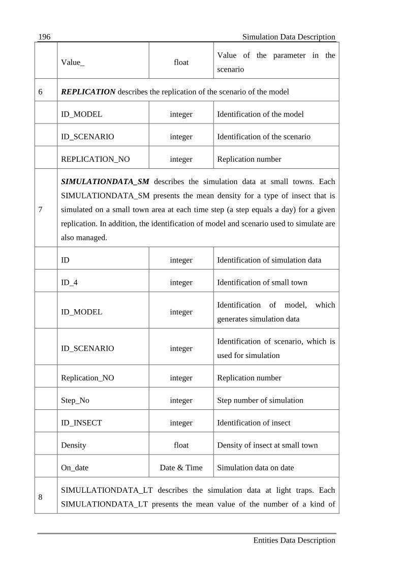
196 Simulation Data Description
Entities Data Description
Value_ float Value of the parameter in the
scenario
6 REPLICATION describes the replication of the scenario of the model
ID_MODEL integer Identification of the model
ID_SCENARIO integer Identification of the scenario
REPLICATION_NO integer Replication number
7
SIMULATIONDATA_SM describes the simulation data at small towns. Each
SIMULATIONDATA_SM presents the mean density for a type of insect that is
simulated on a small town area at each time step (a step equals a day) for a given
replication. In addition, the identification of model and scenario used to simulate are
also managed.
ID integer Identification of simulation data
ID_4 integer Identification of small town
ID_MODEL integer Identification of model, which
generates simulation data
ID_SCENARIO integer Identification of scenario, which is
used for simulation
Replication_NO integer Replication number
Step_No integer Step number of simulation
ID_INSECT integer Identification of insect
Density float Density of insect at small town
On_date Date & Time Simulation data on date
8 SIMULLATIONDATA_LT describes the simulation data at light traps. Each
SIMULATIONDATA_LT presents the mean value of the number of a kind of
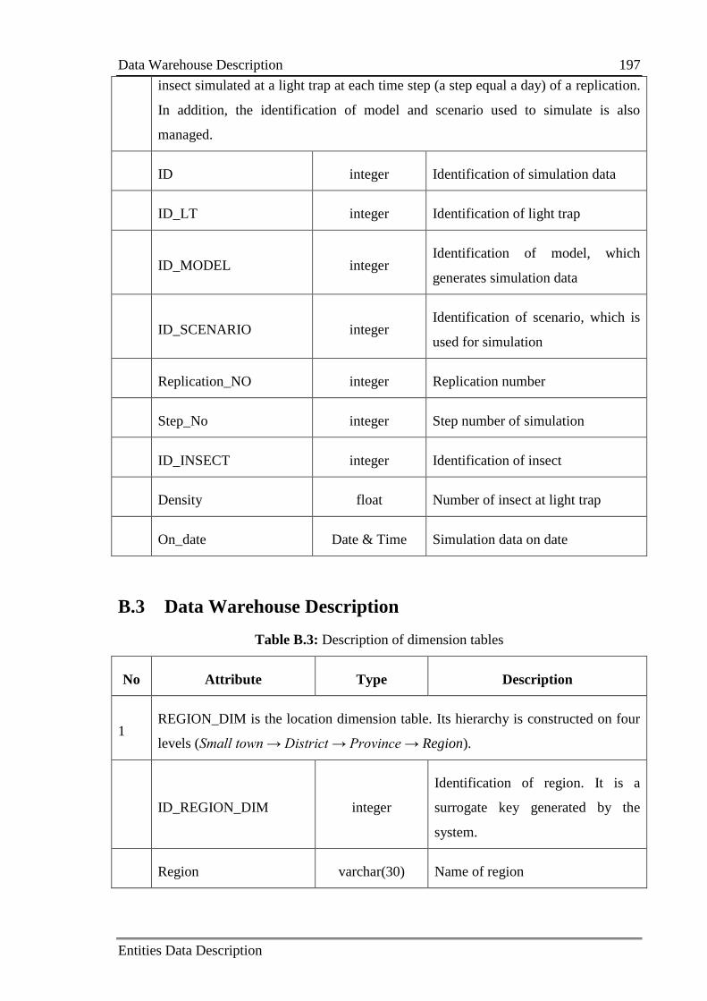
Data Warehouse Description 197
Entities Data Description
insect simulated at a light trap at each time step (a step equal a day) of a replication.
In addition, the identification of model and scenario used to simulate is also
managed.
ID integer Identification of simulation data
ID_LT integer Identification of light trap
ID_MODEL integer Identification of model, which
generates simulation data
ID_SCENARIO integer Identification of scenario, which is
used for simulation
Replication_NO integer Replication number
Step_No integer Step number of simulation
ID_INSECT integer Identification of insect
Density float Number of insect at light trap
On_date Date & Time Simulation data on date
B.3 Data Warehouse Description
Table B.3: Description of dimension tables
No Attribute Type Description
1 REGION_DIM is the location dimension table. Its hierarchy is constructed on four
levels (Small town → District → Province → Region).
ID_REGION_DIM integer
Identification of region. It is a
surrogate key generated by the
system.
Region varchar(30) Name of region
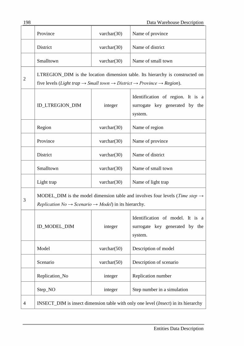
198 Data Warehouse Description
Entities Data Description
Province varchar(30) Name of province
District varchar(30) Name of district
Smalltown varchar(30) Name of small town
2 LTREGION_DIM is the location dimension table. Its hierarchy is constructed on
five levels (Light trap → Small town → District → Province → Region).
ID_LTREGION_DIM integer
Identification of region. It is a
surrogate key generated by the
system.
Region varchar(30) Name of region
Province varchar(30) Name of province
District varchar(30) Name of district
Smalltown varchar(30) Name of small town
Light trap varchar(30) Name of light trap
3 MODEL_DIM is the model dimension table and involves four levels (Time step →
Replication No → Scenario → Model) in its hierarchy.
ID_MODEL_DIM integer
Identification of model. It is a
surrogate key generated by the
system.
Model varchar(50) Description of model
Scenario varchar(50) Description of scenario
Replication_No integer Replication number
Step_NO integer Step number in a simulation
4 INSECT_DIM is insect dimension table with only one level (Insect) in its hierarchy
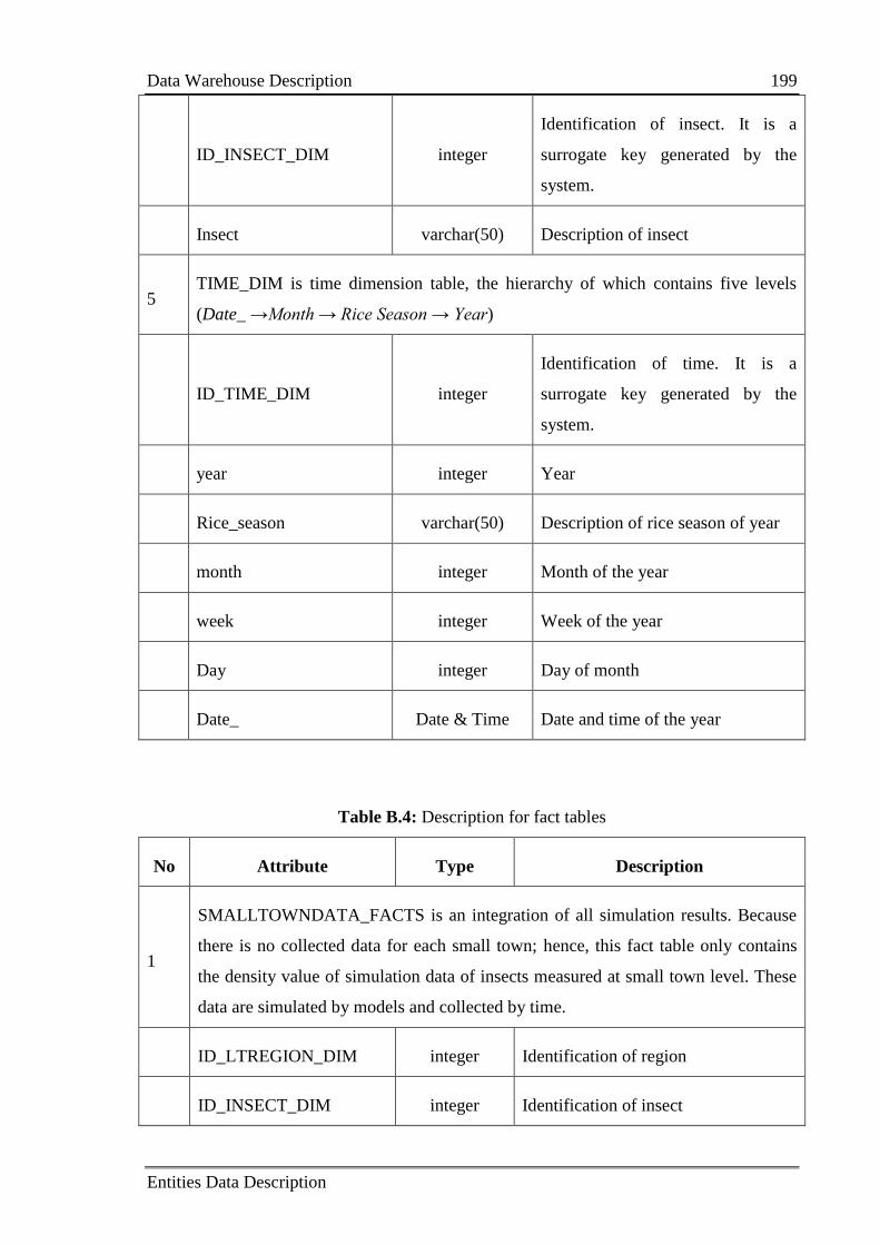
Data Warehouse Description 199
Entities Data Description
ID_INSECT_DIM integer
Identification of insect. It is a
surrogate key generated by the
system.
Insect varchar(50) Description of insect
5 TIME_DIM is time dimension table, the hierarchy of which contains five levels
(Date_ →Month → Rice Season → Year)
ID_TIME_DIM integer
Identification of time. It is a
surrogate key generated by the
system.
year integer Year
Rice_season varchar(50) Description of rice season of year
month integer Month of the year
week integer Week of the year
Day integer Day of month
Date_ Date & Time Date and time of the year
Table B.4: Description for fact tables
No Attribute Type Description
1
SMALLTOWNDATA_FACTS is an integration of all simulation results. Because
there is no collected data for each small town; hence, this fact table only contains
the density value of simulation data of insects measured at small town level. These
data are simulated by models and collected by time.
ID_LTREGION_DIM integer Identification of region
ID_INSECT_DIM integer Identification of insect
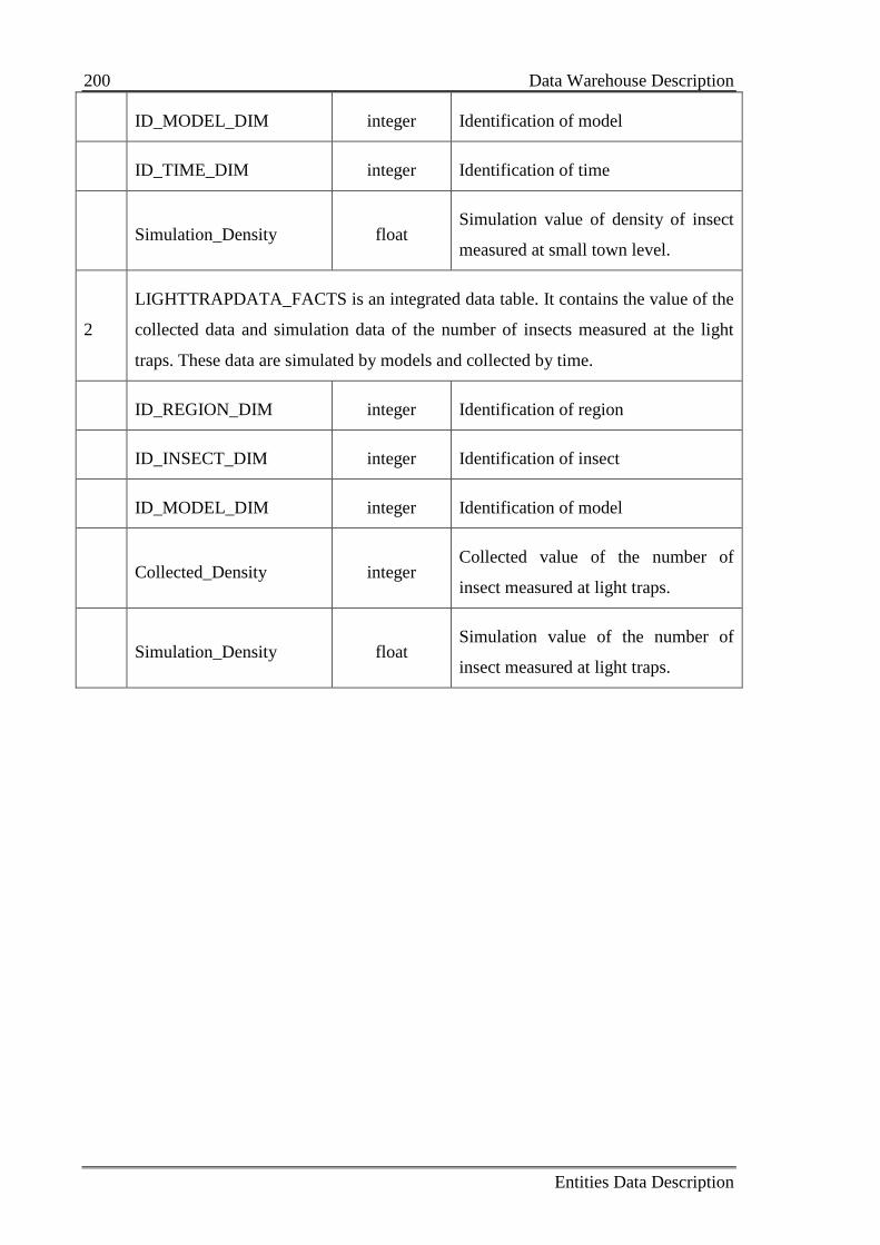
200 Data Warehouse Description
Entities Data Description
ID_MODEL_DIM integer Identification of model
ID_TIME_DIM integer Identification of time
Simulation_Density float Simulation value of density of insect
measured at small town level.
2
LIGHTTRAPDATA_FACTS is an integrated data table. It contains the value of the
collected data and simulation data of the number of insects measured at the light
traps. These data are simulated by models and collected by time.
ID_REGION_DIM integer Identification of region
ID_INSECT_DIM integer Identification of insect
ID_MODEL_DIM integer Identification of model
Collected_Density integer Collected value of the number of
insect measured at light traps.
Simulation_Density float Simulation value of the number of
insect measured at light traps.

Calibration and Validation Results
TRUONG Minh Thai 201
Appendix C
Calibration and Validation Results
C.1 Parameters and Scenario for Calibration ............................................................. 202
C.1.1 Parameters for calibration of BPHs Prediction model .......................... 202
C.1.2 Scenarios for calibration of BPHs Prediction model ............................. 203
C.2 Similarity Coefficient values of the Simulation .................................................. 205
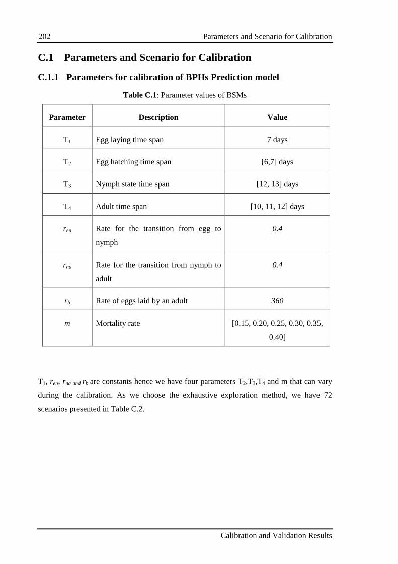
202 Parameters and Scenario for Calibration
Calibration and Validation Results
C.1 Parameters and Scenario for Calibration
C.1.1 Parameters for calibration of BPHs Prediction model
Table C.1: Parameter values of BSMs
Parameter Description Value
T1 Egg laying time span 7 days
T2 Egg hatching time span [6,7] days
T3 Nymph state time span [12, 13] days
T4 Adult time span [10, 11, 12] days
ren Rate for the transition from egg to
nymph
0.4
rna Rate for the transition from nymph to
adult
0.4
rb Rate of eggs laid by an adult 360
m Mortality rate [0.15, 0.20, 0.25, 0.30, 0.35,
0.40]
T1, ren, rna and rb are constants hence we have four parameters T2,T3,T4 and m that can vary
during the calibration. As we choose the exhaustive exploration method, we have 72
scenarios presented in Table C.2.
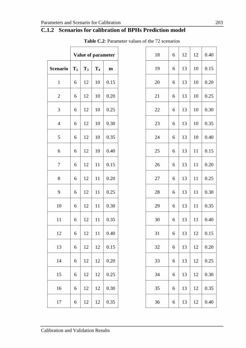
Parameters and Scenario for Calibration 203
Calibration and Validation Results
C.1.2 Scenarios for calibration of BPHs Prediction model
Table C.2: Parameter values of the 72 scenarios
Value of parameter
Scenario T2 T3 T4 m
1 6 12 10 0.15
2 6 12 10 0.20
3 6 12 10 0.25
4 6 12 10 0.30
5 6 12 10 0.35
6 6 12 10 0.40
7 6 12 11 0.15
8 6 12 11 0.20
9 6 12 11 0.25
10 6 12 11 0.30
11 6 12 11 0.35
12 6 12 11 0.40
13 6 12 12 0.15
14 6 12 12 0.20
15 6 12 12 0.25
16 6 12 12 0.30
17 6 12 12 0.35
18 6 12 12 0.40
19 6 13 10 0.15
20 6 13 10 0.20
21 6 13 10 0.25
22 6 13 10 0.30
23 6 13 10 0.35
24 6 13 10 0.40
25 6 13 11 0.15
26 6 13 11 0.20
27 6 13 11 0.25
28 6 13 11 0.30
29 6 13 11 0.35
30 6 13 11 0.40
31 6 13 12 0.15
32 6 13 12 0.20
33 6 13 12 0.25
34 6 13 12 0.30
35 6 13 12 0.35
36 6 13 12 0.40
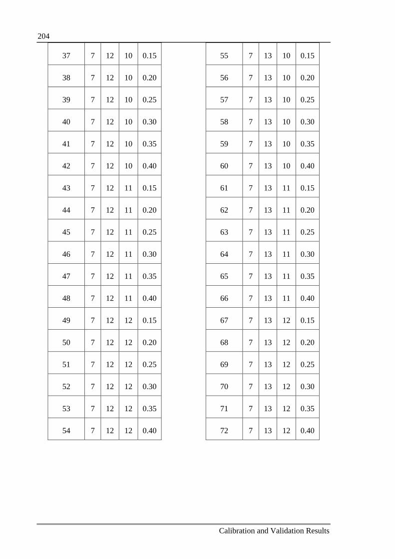
204
Calibration and Validation Results
37 7 12 10 0.15
38 7 12 10 0.20
39 7 12 10 0.25
40 7 12 10 0.30
41 7 12 10 0.35
42 7 12 10 0.40
43 7 12 11 0.15
44 7 12 11 0.20
45 7 12 11 0.25
46 7 12 11 0.30
47 7 12 11 0.35
48 7 12 11 0.40
49 7 12 12 0.15
50 7 12 12 0.20
51 7 12 12 0.25
52 7 12 12 0.30
53 7 12 12 0.35
54 7 12 12 0.40
55 7 13 10 0.15
56 7 13 10 0.20
57 7 13 10 0.25
58 7 13 10 0.30
59 7 13 10 0.35
60 7 13 10 0.40
61 7 13 11 0.15
62 7 13 11 0.20
63 7 13 11 0.25
64 7 13 11 0.30
65 7 13 11 0.35
66 7 13 11 0.40
67 7 13 12 0.15
68 7 13 12 0.20
69 7 13 12 0.25
70 7 13 12 0.30
71 7 13 12 0.35
72 7 13 12 0.40
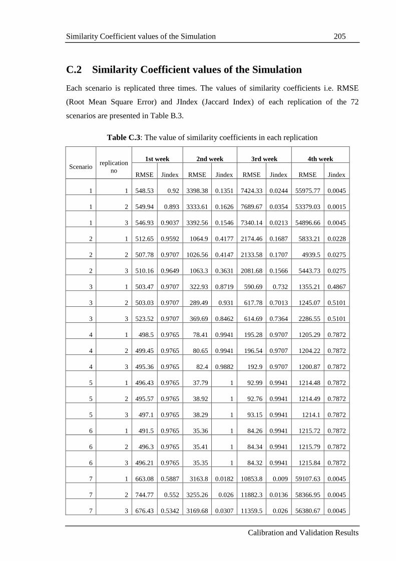
Similarity Coefficient values of the Simulation 205
Calibration and Validation Results
C.2 Similarity Coefficient values of the Simulation
Each scenario is replicated three times. The values of similarity coefficients i.e. RMSE
(Root Mean Square Error) and JIndex (Jaccard Index) of each replication of the 72
scenarios are presented in Table B.3.
Table C.3: The value of similarity coefficients in each replication
Scenario replication
no
1st week 2nd week 3rd week 4th week
RMSE Jindex RMSE Jindex RMSE Jindex RMSE Jindex
1 1 548.53 0.92 3398.38 0.1351 7424.33 0.0244 55975.77 0.0045
1 2 549.94 0.893 3333.61 0.1626 7689.67 0.0354 53379.03 0.0015
1 3 546.93 0.9037 3392.56 0.1546 7340.14 0.0213 54896.66 0.0045
2 1 512.65 0.9592 1064.9 0.4177 2174.46 0.1687 5833.21 0.0228
2 2 507.78 0.9707 1026.56 0.4147 2133.58 0.1707 4939.5 0.0275
2 3 510.16 0.9649 1063.3 0.3631 2081.68 0.1566 5443.73 0.0275
3 1 503.47 0.9707 322.93 0.8719 590.69 0.732 1355.21 0.4867
3 2 503.03 0.9707 289.49 0.931 617.78 0.7013 1245.07 0.5101
3 3 523.52 0.9707 369.69 0.8462 614.69 0.7364 2286.55 0.5101
4 1 498.5 0.9765 78.41 0.9941 195.28 0.9707 1205.29 0.7872
4 2 499.45 0.9765 80.65 0.9941 196.54 0.9707 1204.22 0.7872
4 3 495.36 0.9765 82.4 0.9882 192.9 0.9707 1200.87 0.7872
5 1 496.43 0.9765 37.79 1 92.99 0.9941 1214.48 0.7872
5 2 495.57 0.9765 38.92 1 92.76 0.9941 1214.49 0.7872
5 3 497.1 0.9765 38.29 1 93.15 0.9941 1214.1 0.7872
6 1 491.5 0.9765 35.36 1 84.26 0.9941 1215.72 0.7872
6 2 496.3 0.9765 35.41 1 84.34 0.9941 1215.79 0.7872
6 3 496.21 0.9765 35.35 1 84.32 0.9941 1215.84 0.7872
7 1 663.08 0.5887 3163.8 0.0182 10853.8 0.009 59107.63 0.0045
7 2 744.77 0.552 3255.26 0.026 11882.3 0.0136 58366.95 0.0045
7 3 676.43 0.5342 3169.68 0.0307 11359.5 0.026 56380.67 0.0045
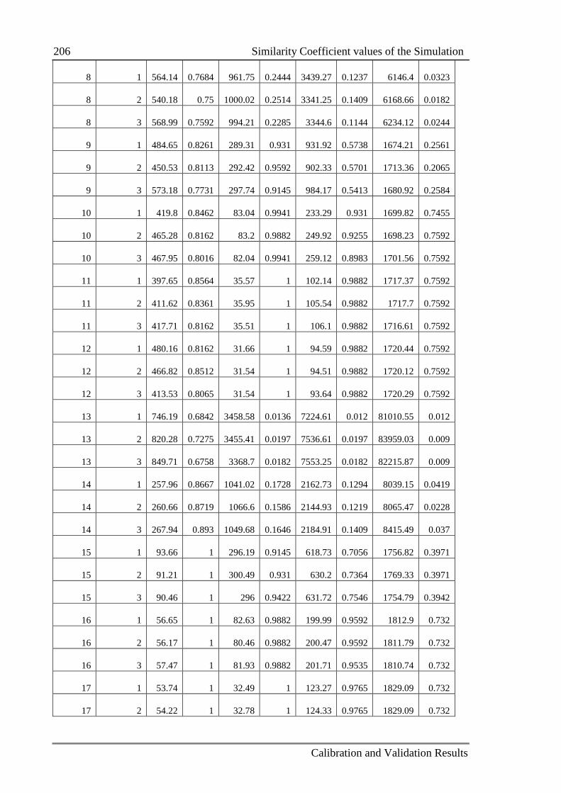
206 Similarity Coefficient values of the Simulation
Calibration and Validation Results
8 1 564.14 0.7684 961.75 0.2444 3439.27 0.1237 6146.4 0.0323
8 2 540.18 0.75 1000.02 0.2514 3341.25 0.1409 6168.66 0.0182
8 3 568.99 0.7592 994.21 0.2285 3344.6 0.1144 6234.12 0.0244
9 1 484.65 0.8261 289.31 0.931 931.92 0.5738 1674.21 0.2561
9 2 450.53 0.8113 292.42 0.9592 902.33 0.5701 1713.36 0.2065
9 3 573.18 0.7731 297.74 0.9145 984.17 0.5413 1680.92 0.2584
10 1 419.8 0.8462 83.04 0.9941 233.29 0.931 1699.82 0.7455
10 2 465.28 0.8162 83.2 0.9882 249.92 0.9255 1698.23 0.7592
10 3 467.95 0.8016 82.04 0.9941 259.12 0.8983 1701.56 0.7592
11 1 397.65 0.8564 35.57 1 102.14 0.9882 1717.37 0.7592
11 2 411.62 0.8361 35.95 1 105.54 0.9882 1717.7 0.7592
11 3 417.71 0.8162 35.51 1 106.1 0.9882 1716.61 0.7592
12 1 480.16 0.8162 31.66 1 94.59 0.9882 1720.44 0.7592
12 2 466.82 0.8512 31.54 1 94.51 0.9882 1720.12 0.7592
12 3 413.53 0.8065 31.54 1 93.64 0.9882 1720.29 0.7592
13 1 746.19 0.6842 3458.58 0.0136 7224.61 0.012 81010.55 0.012
13 2 820.28 0.7275 3455.41 0.0197 7536.61 0.0197 83959.03 0.009
13 3 849.71 0.6758 3368.7 0.0182 7553.25 0.0182 82215.87 0.009
14 1 257.96 0.8667 1041.02 0.1728 2162.73 0.1294 8039.15 0.0419
14 2 260.66 0.8719 1066.6 0.1586 2144.93 0.1219 8065.47 0.0228
14 3 267.94 0.893 1049.68 0.1646 2184.91 0.1409 8415.49 0.037
15 1 93.66 1 296.19 0.9145 618.73 0.7056 1756.82 0.3971
15 2 91.21 1 300.49 0.931 630.2 0.7364 1769.33 0.3971
15 3 90.46 1 296 0.9422 631.72 0.7546 1754.79 0.3942
16 1 56.65 1 82.63 0.9882 199.99 0.9592 1812.9 0.732
16 2 56.17 1 80.46 0.9882 200.47 0.9592 1811.79 0.732
16 3 57.47 1 81.93 0.9882 201.71 0.9535 1810.74 0.732
17 1 53.74 1 32.49 1 123.27 0.9765 1829.09 0.732
17 2 54.22 1 32.78 1 124.33 0.9765 1829.09 0.732
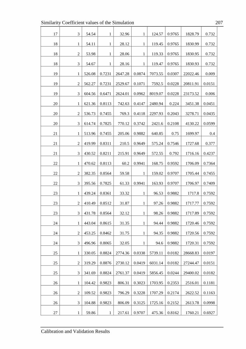
Similarity Coefficient values of the Simulation 207
Calibration and Validation Results
17 3 54.54 1 32.96 1 124.57 0.9765 1828.79 0.732
18 1 54.11 1 28.12 1 119.45 0.9765 1830.99 0.732
18 2 53.98 1 28.06 1 119.33 0.9765 1830.95 0.732
18 3 54.67 1 28.16 1 119.47 0.9765 1830.93 0.732
19 1 526.08 0.7231 2647.28 0.0874 7073.55 0.0307 22022.46 0.009
19 2 562.27 0.7231 2529.67 0.1071 7592.5 0.0228 20811.91 0.0151
19 3 604.56 0.6471 2624.01 0.0962 8019.07 0.0228 23173.52 0.006
20 1 621.36 0.8113 742.63 0.4147 2480.94 0.224 3451.38 0.0451
20 2 536.73 0.7455 769.3 0.4118 2297.93 0.2043 3278.71 0.0435
20 3 614.74 0.7825 770.12 0.3742 2421.6 0.2108 4130.22 0.0599
21 1 513.96 0.7455 205.06 0.9882 640.85 0.75 1699.97 0.4
21 2 419.99 0.8311 210.5 0.9649 575.24 0.7546 1727.68 0.377
21 3 430.52 0.8211 215.91 0.9649 572.55 0.792 1716.16 0.4237
22 1 470.62 0.8113 60.2 0.9941 168.75 0.9592 1706.09 0.7364
22 2 382.35 0.8564 59.58 1 159.02 0.9707 1705.44 0.7455
22 3 395.56 0.7825 61.33 0.9941 163.93 0.9707 1706.97 0.7409
23 1 439.24 0.8361 33.32 1 96.53 0.9882 1717.8 0.7592
23 2 410.49 0.8512 31.87 1 97.26 0.9882 1717.77 0.7592
23 3 431.78 0.8564 32.12 1 98.26 0.9882 1717.89 0.7592
24 1 443.04 0.8615 31.35 1 94.44 0.9882 1720.46 0.7592
24 2 453.25 0.8462 31.75 1 94.35 0.9882 1720.56 0.7592
24 3 496.96 0.8065 32.05 1 94.6 0.9882 1720.31 0.7592
25 1 330.05 0.8824 2774.36 0.0338 5739.11 0.0182 28668.83 0.0197
25 2 319.29 0.8876 2730.12 0.0419 6031.14 0.0182 27244.47 0.0151
25 3 341.69 0.8824 2761.37 0.0419 5856.45 0.0244 29400.02 0.0182
26 1 104.42 0.9823 806.31 0.3023 1703.95 0.2353 2516.01 0.1181
26 2 109.52 0.9823 796.29 0.3228 1707.29 0.2174 2622.52 0.1163
26 3 104.88 0.9823 806.09 0.3125 1725.16 0.2152 2613.78 0.0998
27 1 59.86 1 217.61 0.9707 475.36 0.8162 1760.21 0.6927
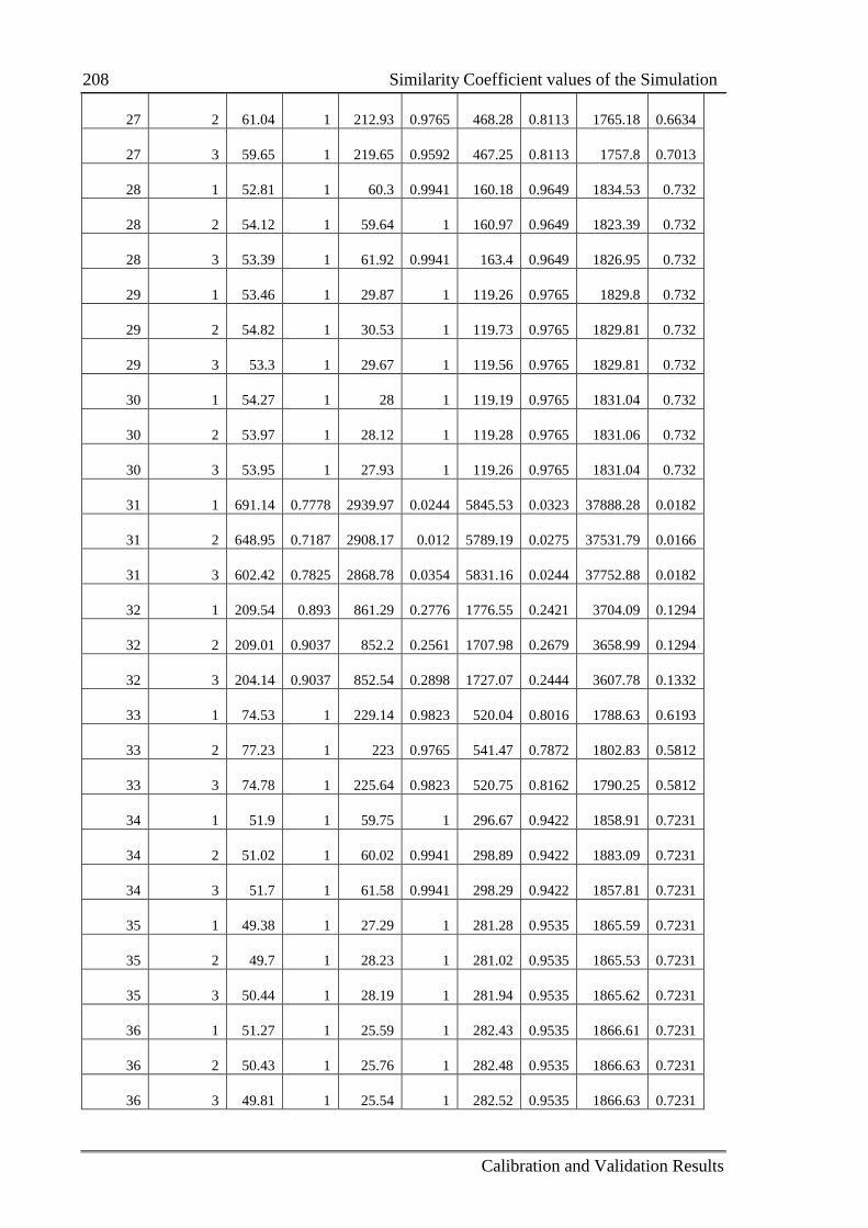
208 Similarity Coefficient values of the Simulation
Calibration and Validation Results
27 2 61.04 1 212.93 0.9765 468.28 0.8113 1765.18 0.6634
27 3 59.65 1 219.65 0.9592 467.25 0.8113 1757.8 0.7013
28 1 52.81 1 60.3 0.9941 160.18 0.9649 1834.53 0.732
28 2 54.12 1 59.64 1 160.97 0.9649 1823.39 0.732
28 3 53.39 1 61.92 0.9941 163.4 0.9649 1826.95 0.732
29 1 53.46 1 29.87 1 119.26 0.9765 1829.8 0.732
29 2 54.82 1 30.53 1 119.73 0.9765 1829.81 0.732
29 3 53.3 1 29.67 1 119.56 0.9765 1829.81 0.732
30 1 54.27 1 28 1 119.19 0.9765 1831.04 0.732
30 2 53.97 1 28.12 1 119.28 0.9765 1831.06 0.732
30 3 53.95 1 27.93 1 119.26 0.9765 1831.04 0.732
31 1 691.14 0.7778 2939.97 0.0244 5845.53 0.0323 37888.28 0.0182
31 2 648.95 0.7187 2908.17 0.012 5789.19 0.0275 37531.79 0.0166
31 3 602.42 0.7825 2868.78 0.0354 5831.16 0.0244 37752.88 0.0182
32 1 209.54 0.893 861.29 0.2776 1776.55 0.2421 3704.09 0.1294
32 2 209.01 0.9037 852.2 0.2561 1707.98 0.2679 3658.99 0.1294
32 3 204.14 0.9037 852.54 0.2898 1727.07 0.2444 3607.78 0.1332
33 1 74.53 1 229.14 0.9823 520.04 0.8016 1788.63 0.6193
33 2 77.23 1 223 0.9765 541.47 0.7872 1802.83 0.5812
33 3 74.78 1 225.64 0.9823 520.75 0.8162 1790.25 0.5812
34 1 51.9 1 59.75 1 296.67 0.9422 1858.91 0.7231
34 2 51.02 1 60.02 0.9941 298.89 0.9422 1883.09 0.7231
34 3 51.7 1 61.58 0.9941 298.29 0.9422 1857.81 0.7231
35 1 49.38 1 27.29 1 281.28 0.9535 1865.59 0.7231
35 2 49.7 1 28.23 1 281.02 0.9535 1865.53 0.7231
35 3 50.44 1 28.19 1 281.94 0.9535 1865.62 0.7231
36 1 51.27 1 25.59 1 282.43 0.9535 1866.61 0.7231
36 2 50.43 1 25.76 1 282.48 0.9535 1866.63 0.7231
36 3 49.81 1 25.54 1 282.52 0.9535 1866.63 0.7231
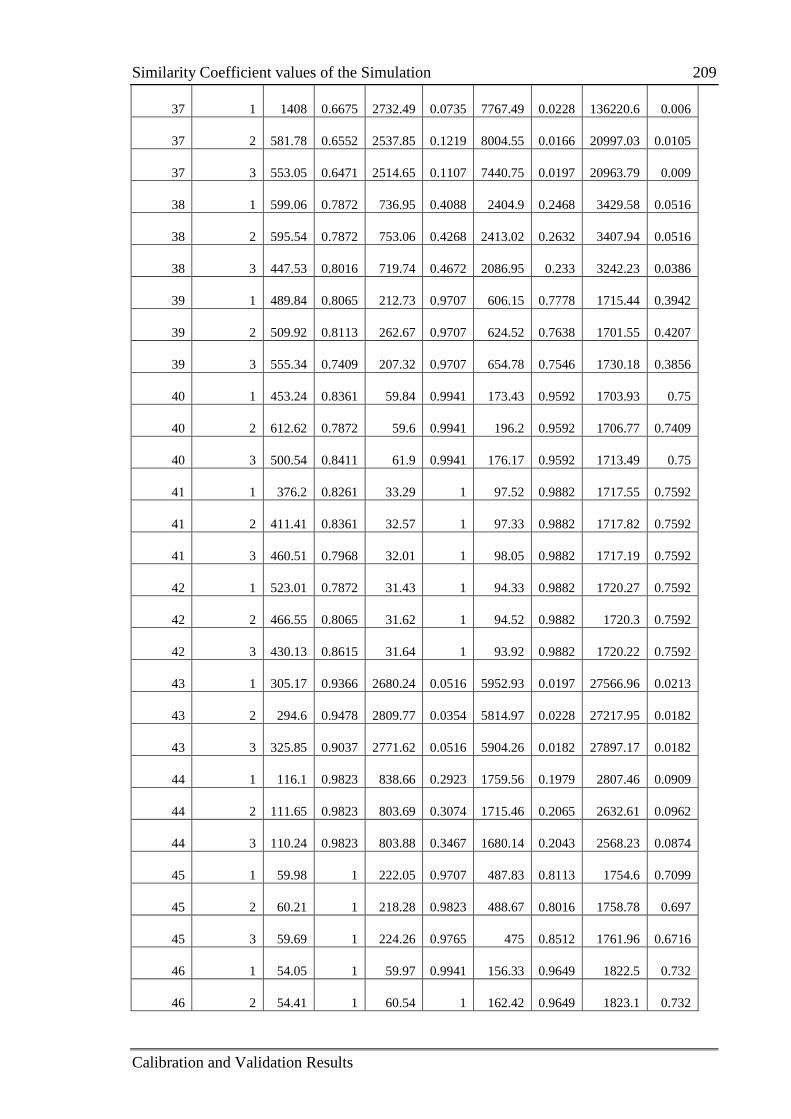
Similarity Coefficient values of the Simulation 209
Calibration and Validation Results
37 1 1408 0.6675 2732.49 0.0735 7767.49 0.0228 136220.6 0.006
37 2 581.78 0.6552 2537.85 0.1219 8004.55 0.0166 20997.03 0.0105
37 3 553.05 0.6471 2514.65 0.1107 7440.75 0.0197 20963.79 0.009
38 1 599.06 0.7872 736.95 0.4088 2404.9 0.2468 3429.58 0.0516
38 2 595.54 0.7872 753.06 0.4268 2413.02 0.2632 3407.94 0.0516
38 3 447.53 0.8016 719.74 0.4672 2086.95 0.233 3242.23 0.0386
39 1 489.84 0.8065 212.73 0.9707 606.15 0.7778 1715.44 0.3942
39 2 509.92 0.8113 262.67 0.9707 624.52 0.7638 1701.55 0.4207
39 3 555.34 0.7409 207.32 0.9707 654.78 0.7546 1730.18 0.3856
40 1 453.24 0.8361 59.84 0.9941 173.43 0.9592 1703.93 0.75
40 2 612.62 0.7872 59.6 0.9941 196.2 0.9592 1706.77 0.7409
40 3 500.54 0.8411 61.9 0.9941 176.17 0.9592 1713.49 0.75
41 1 376.2 0.8261 33.29 1 97.52 0.9882 1717.55 0.7592
41 2 411.41 0.8361 32.57 1 97.33 0.9882 1717.82 0.7592
41 3 460.51 0.7968 32.01 1 98.05 0.9882 1717.19 0.7592
42 1 523.01 0.7872 31.43 1 94.33 0.9882 1720.27 0.7592
42 2 466.55 0.8065 31.62 1 94.52 0.9882 1720.3 0.7592
42 3 430.13 0.8615 31.64 1 93.92 0.9882 1720.22 0.7592
43 1 305.17 0.9366 2680.24 0.0516 5952.93 0.0197 27566.96 0.0213
43 2 294.6 0.9478 2809.77 0.0354 5814.97 0.0228 27217.95 0.0182
43 3 325.85 0.9037 2771.62 0.0516 5904.26 0.0182 27897.17 0.0182
44 1 116.1 0.9823 838.66 0.2923 1759.56 0.1979 2807.46 0.0909
44 2 111.65 0.9823 803.69 0.3074 1715.46 0.2065 2632.61 0.0962
44 3 110.24 0.9823 803.88 0.3467 1680.14 0.2043 2568.23 0.0874
45 1 59.98 1 222.05 0.9707 487.83 0.8113 1754.6 0.7099
45 2 60.21 1 218.28 0.9823 488.67 0.8016 1758.78 0.697
45 3 59.69 1 224.26 0.9765 475 0.8512 1761.96 0.6716
46 1 54.05 1 59.97 0.9941 156.33 0.9649 1822.5 0.732
46 2 54.41 1 60.54 1 162.42 0.9649 1823.1 0.732
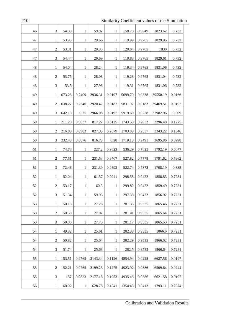
210 Similarity Coefficient values of the Simulation
Calibration and Validation Results
46 3 54.33 1 59.92 1 158.73 0.9649 1823.62 0.732
47 1 53.95 1 29.66 1 119.99 0.9765 1829.95 0.732
47 2 53.31 1 29.33 1 120.04 0.9765 1830 0.732
47 3 54.44 1 29.69 1 119.83 0.9765 1829.61 0.732
48 1 54.04 1 28.24 1 119.34 0.9765 1831.06 0.732
48 2 53.75 1 28.08 1 119.23 0.9765 1831.04 0.732
48 3 53.5 1 27.98 1 119.31 0.9765 1831.06 0.732
49 1 673.28 0.7409 2936.31 0.0197 5699.79 0.0338 39550.19 0.0166
49 2 638.27 0.7546 2920.42 0.0182 5831.97 0.0182 39469.51 0.0197
49 3 642.15 0.75 2966.08 0.0197 5919.69 0.0228 37982.96 0.009
50 1 211.28 0.9037 817.27 0.3125 1743.53 0.2632 3296.48 0.1275
50 2 216.88 0.8983 827.33 0.2679 1703.09 0.2537 3343.22 0.1546
50 3 232.43 0.8876 816.73 0.28 1719.13 0.2491 3695.86 0.0998
51 1 74.78 1 227.2 0.9823 536.29 0.7825 1792.19 0.6077
51 2 77.51 1 231.53 0.9707 527.82 0.7778 1791.62 0.5962
51 3 72.46 1 231.39 0.9592 522.74 0.7872 1798.19 0.635
52 1 52.04 1 61.57 0.9941 298.58 0.9422 1858.83 0.7231
52 2 53.17 1 60.3 1 299.82 0.9422 1859.49 0.7231
52 3 51.34 1 59.93 1 297.38 0.9422 1856.92 0.7231
53 1 50.13 1 27.25 1 281.36 0.9535 1865.46 0.7231
53 2 50.53 1 27.07 1 281.41 0.9535 1865.64 0.7231
53 3 50.06 1 27.75 1 281.17 0.9535 1865.53 0.7231
54 1 49.82 1 25.61 1 282.38 0.9535 1866.6 0.7231
54 2 50.82 1 25.64 1 282.29 0.9535 1866.62 0.7231
54 3 51.74 1 25.68 1 282.5 0.9535 1866.64 0.7231
55 1 153.51 0.9765 2143.34 0.1126 4854.94 0.0228 6627.56 0.0197
55 2 152.21 0.9765 2199.23 0.1275 4923.92 0.0386 6509.64 0.0244
55 3 157 0.9823 2177.15 0.1053 4935.46 0.0386 6621.58 0.0197
56 1 68.02 1 628.78 0.4641 1354.45 0.3413 1793.11 0.2874
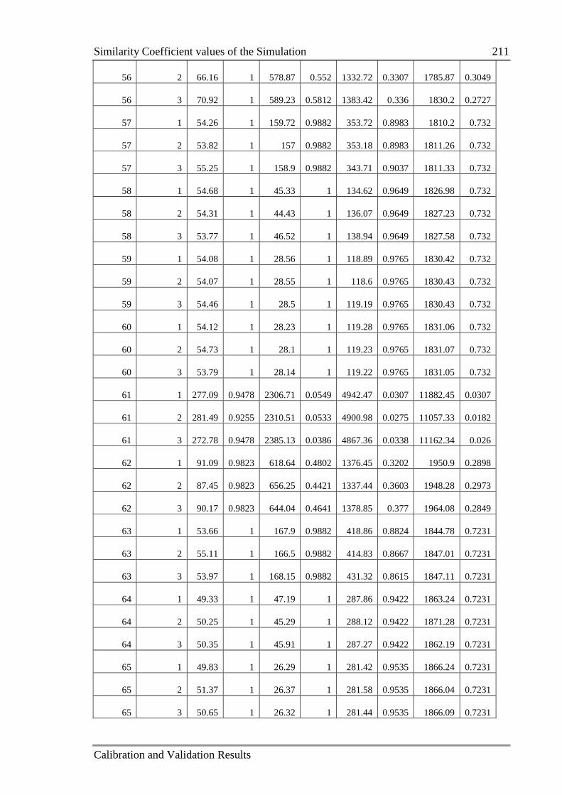
Similarity Coefficient values of the Simulation 211
Calibration and Validation Results
56 2 66.16 1 578.87 0.552 1332.72 0.3307 1785.87 0.3049
56 3 70.92 1 589.23 0.5812 1383.42 0.336 1830.2 0.2727
57 1 54.26 1 159.72 0.9882 353.72 0.8983 1810.2 0.732
57 2 53.82 1 157 0.9882 353.18 0.8983 1811.26 0.732
57 3 55.25 1 158.9 0.9882 343.71 0.9037 1811.33 0.732
58 1 54.68 1 45.33 1 134.62 0.9649 1826.98 0.732
58 2 54.31 1 44.43 1 136.07 0.9649 1827.23 0.732
58 3 53.77 1 46.52 1 138.94 0.9649 1827.58 0.732
59 1 54.08 1 28.56 1 118.89 0.9765 1830.42 0.732
59 2 54.07 1 28.55 1 118.6 0.9765 1830.43 0.732
59 3 54.46 1 28.5 1 119.19 0.9765 1830.43 0.732
60 1 54.12 1 28.23 1 119.28 0.9765 1831.06 0.732
60 2 54.73 1 28.1 1 119.23 0.9765 1831.07 0.732
60 3 53.79 1 28.14 1 119.22 0.9765 1831.05 0.732
61 1 277.09 0.9478 2306.71 0.0549 4942.47 0.0307 11882.45 0.0307
61 2 281.49 0.9255 2310.51 0.0533 4900.98 0.0275 11057.33 0.0182
61 3 272.78 0.9478 2385.13 0.0386 4867.36 0.0338 11162.34 0.026
62 1 91.09 0.9823 618.64 0.4802 1376.45 0.3202 1950.9 0.2898
62 2 87.45 0.9823 656.25 0.4421 1337.44 0.3603 1948.28 0.2973
62 3 90.17 0.9823 644.04 0.4641 1378.85 0.377 1964.08 0.2849
63 1 53.66 1 167.9 0.9882 418.86 0.8824 1844.78 0.7231
63 2 55.11 1 166.5 0.9882 414.83 0.8667 1847.01 0.7231
63 3 53.97 1 168.15 0.9882 431.32 0.8615 1847.11 0.7231
64 1 49.33 1 47.19 1 287.86 0.9422 1863.24 0.7231
64 2 50.25 1 45.29 1 288.12 0.9422 1871.28 0.7231
64 3 50.35 1 45.91 1 287.27 0.9422 1862.19 0.7231
65 1 49.83 1 26.29 1 281.42 0.9535 1866.24 0.7231
65 2 51.37 1 26.37 1 281.58 0.9535 1866.04 0.7231
65 3 50.65 1 26.32 1 281.44 0.9535 1866.09 0.7231
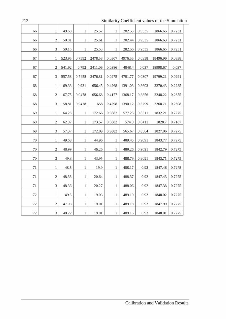
212 Similarity Coefficient values of the Simulation
Calibration and Validation Results
66 1 49.68 1 25.57 1 282.55 0.9535 1866.65 0.7231
66 2 50.01 1 25.61 1 282.44 0.9535 1866.63 0.7231
66 3 50.15 1 25.53 1 282.56 0.9535 1866.65 0.7231
67 1 523.95 0.7592 2478.58 0.0307 4976.55 0.0338 18496.96 0.0338
67 2 541.92 0.792 2411.06 0.0386 4848.4 0.037 18998.67 0.037
67 3 557.53 0.7455 2476.81 0.0275 4781.77 0.0307 19799.21 0.0291
68 1 169.33 0.931 656.45 0.4268 1391.03 0.3603 2270.43 0.2285
68 2 167.75 0.9478 656.68 0.4177 1368.17 0.3856 2248.22 0.2655
68 3 158.81 0.9478 658 0.4298 1390.12 0.3799 2268.71 0.2608
69 1 64.25 1 172.66 0.9882 577.25 0.8311 1832.21 0.7275
69 2 62.97 1 173.57 0.9882 574.9 0.8411 1828.7 0.7187
69 3 57.37 1 172.09 0.9882 565.67 0.8564 1827.06 0.7275
70 1 49.63 1 44.96 1 489.45 0.9091 1843.77 0.7275
70 2 48.99 1 46.26 1 489.26 0.9091 1842.79 0.7275
70 3 49.8 1 43.95 1 488.79 0.9091 1843.71 0.7275
71 1 48.5 1 19.9 1 488.17 0.92 1847.46 0.7275
71 2 48.33 1 20.64 1 488.37 0.92 1847.43 0.7275
71 3 48.36 1 20.27 1 488.06 0.92 1847.38 0.7275
72 1 49.5 1 19.03 1 489.19 0.92 1848.02 0.7275
72 2 47.93 1 19.01 1 489.18 0.92 1847.99 0.7275
72 3 48.22 1 19.01 1 489.16 0.92 1848.01 0.7275
Related Documents