Autonomous terrain-following for unmanned air vehicles

Mechatronics 21 (2011) 844–860

Contents lists available at ScienceDirect

Mechatronics

journal homepage: www.elsevier .com/ locate /mechatronics

Autonomous terrain-following for unmanned air vehicles

Raza Samar ⇑, Abdur RehmanCentre for Control & Instrumentation, Engineering & Scientific Commission, Islamabad, Pakistan

a r t i c l e i n f o

Article history:Available online 25 October 2010

Keywords:Terrain-followingDecision making and autonomyAltitude controlMission planningGuidance and control of UAVsTrajectory tracking and path followingrobust control applicationsEectromechanical actuators

0957-4158/$ - see front matter � 2010 Elsevier Ltd. Adoi:10.1016/j.mechatronics.2010.09.010

⇑ Corresponding author.E-mail addresses: [email protected], raza@m

a b s t r a c t

This paper presents an integrated guidance and control design scheme for an unmanned air vehicle(UAV), and its flight test results. The paper focuses on the longitudinal control and guidance aspects, withparticular emphasis on the terrain-following problem. An introduction to the mission, and the terrain-fol-lowing problem is given first. Waypoints for climb and descent are defined. Computation of the referencetrajectory in the vertical plane is discussed, including a terrain-following (TF) algorithm for real-time cal-culation of climb/descent points and altitudes. The algorithm is particularly suited for online computa-tion and is therefore useful for autonomous flight. The algorithm computes the height at which thevehicle should fly so that a specified clearance from the underlying terrain is always maintained, whileensuring that the vehicle’s rate of climb and rate of descent constraints are not violated. The output ofthe terrain-following algorithm is used to construct a smooth reference trajectory for the vehicle to track.The design of a robust controller for altitude tracking and stability augmentation of the vehicle is thenpresented. The controller uses elevators for pitch control in the inner loop, while the reference pitch com-mands are generated by the outer altitude control loop. The controller tracks the reference trajectorycomputed by the terrain-following algorithm. The design of an electromechanical actuator for actuatingthe control surfaces of the vehicle during flight is also discussed. The entire guidance and control schemeis implemented on an actual experimental vehicle and flight test results are presented and discussed.

� 2010 Elsevier Ltd. All rights reserved.

1. Introduction

The notion of unmanned vehicles capable of autonomous flightis fast becoming a reality, with the level of autonomy continuouslyon the increase. The availability of high performance embeddedcomputing platforms combined with the development of sophisti-cated algorithms has transformed the realm of unmanned vehicleswithin a span of a few years. In this paper we present an integratedapproach to the design of a practical and autonomous terrain-fol-lowing guidance and control system for an experimental aircraft,and discuss its in-flight performance.

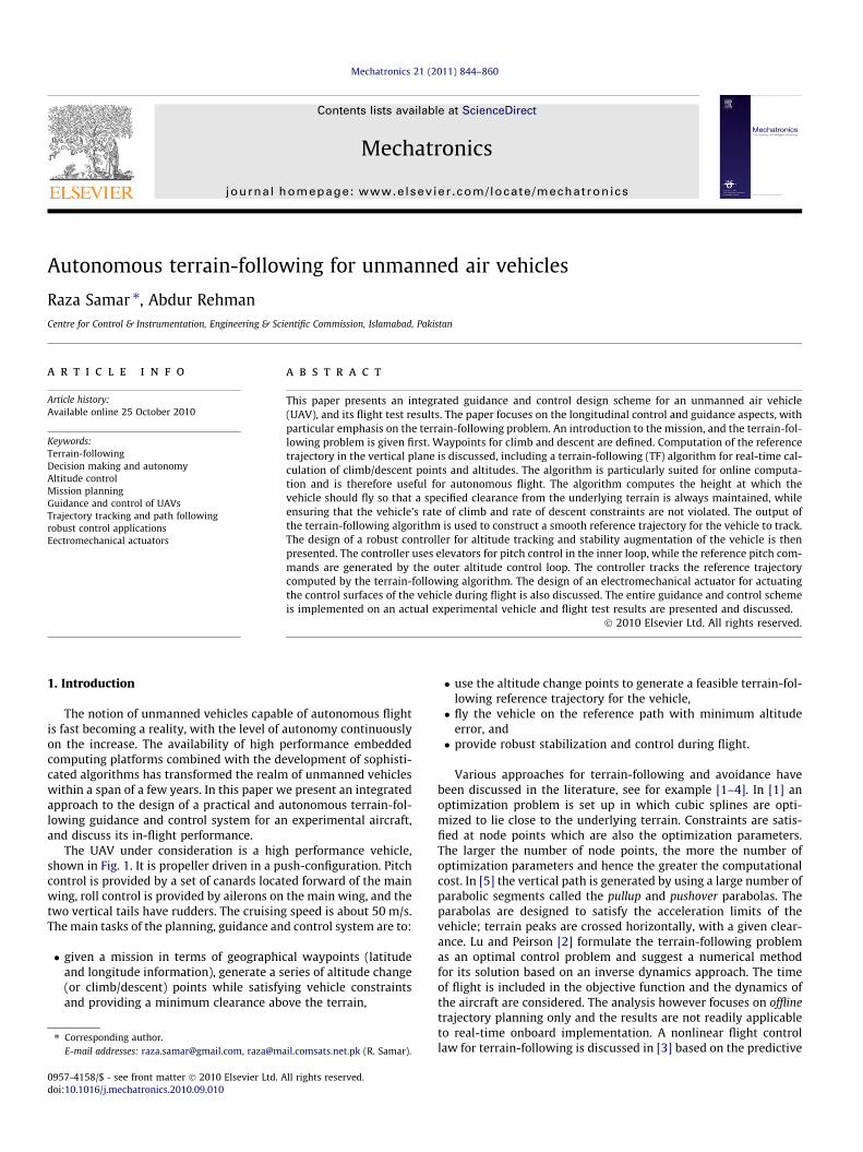
The UAV under consideration is a high performance vehicle,shown in Fig. 1. It is propeller driven in a push-configuration. Pitchcontrol is provided by a set of canards located forward of the mainwing, roll control is provided by ailerons on the main wing, and thetwo vertical tails have rudders. The cruising speed is about 50 m/s.The main tasks of the planning, guidance and control system are to:

� given a mission in terms of geographical waypoints (latitudeand longitude information), generate a series of altitude change(or climb/descent) points while satisfying vehicle constraintsand providing a minimum clearance above the terrain,

ll rights reserved.

ail.comsats.net.pk (R. Samar).

� use the altitude change points to generate a feasible terrain-fol-lowing reference trajectory for the vehicle,� fly the vehicle on the reference path with minimum altitude

error, and� provide robust stabilization and control during flight.

Various approaches for terrain-following and avoidance havebeen discussed in the literature, see for example [1–4]. In [1] anoptimization problem is set up in which cubic splines are opti-mized to lie close to the underlying terrain. Constraints are satis-fied at node points which are also the optimization parameters.The larger the number of node points, the more the number ofoptimization parameters and hence the greater the computationalcost. In [5] the vertical path is generated by using a large number ofparabolic segments called the pullup and pushover parabolas. Theparabolas are designed to satisfy the acceleration limits of thevehicle; terrain peaks are crossed horizontally, with a given clear-ance. Lu and Peirson [2] formulate the terrain-following problemas an optimal control problem and suggest a numerical methodfor its solution based on an inverse dynamics approach. The timeof flight is included in the objective function and the dynamics ofthe aircraft are considered. The analysis however focuses on offlinetrajectory planning only and the results are not readily applicableto real-time onboard implementation. A nonlinear flight controllaw for terrain-following is discussed in [3] based on the predictive

http://dx.doi.org/10.1016/j.mechatronics.2010.09.010

mailto:[email protected]

mailto:[email protected]

http://dx.doi.org/10.1016/j.mechatronics.2010.09.010

http://www.sciencedirect.com/science/journal/09574158

http://www.elsevier.com/locate/mechatronics

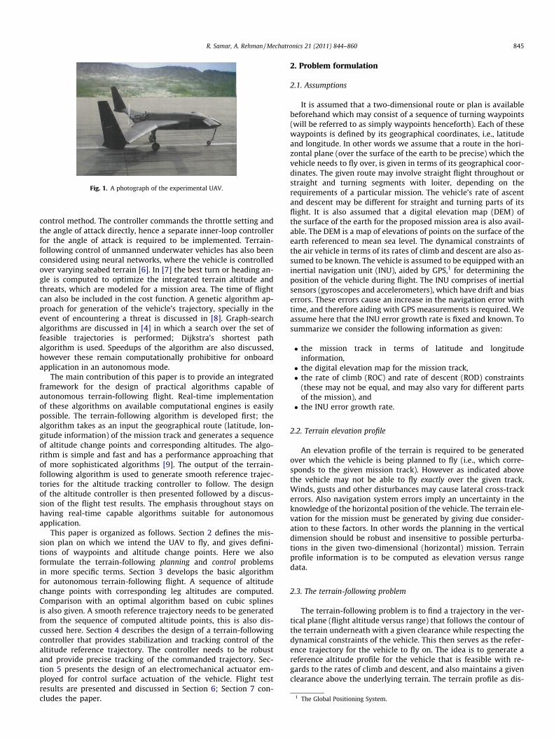
Fig. 1. A photograph of the experimental UAV.

1 The Global Positioning System.

R. Samar, A. Rehman / Mechatronics 21 (2011) 844–860 845

control method. The controller commands the throttle setting andthe angle of attack directly, hence a separate inner-loop controllerfor the angle of attack is required to be implemented. Terrain-following control of unmanned underwater vehicles has also beenconsidered using neural networks, where the vehicle is controlledover varying seabed terrain [6]. In [7] the best turn or heading an-gle is computed to optimize the integrated terrain altitude andthreats, which are modeled for a mission area. The time of flightcan also be included in the cost function. A genetic algorithm ap-proach for generation of the vehicle’s trajectory, specially in theevent of encountering a threat is discussed in [8]. Graph-searchalgorithms are discussed in [4] in which a search over the set offeasible trajectories is performed; Dijkstra’s shortest pathalgorithm is used. Speedups of the algorithm are also discussed,however these remain computationally prohibitive for onboardapplication in an autonomous mode.

The main contribution of this paper is to provide an integratedframework for the design of practical algorithms capable ofautonomous terrain-following flight. Real-time implementationof these algorithms on available computational engines is easilypossible. The terrain-following algorithm is developed first; thealgorithm takes as an input the geographical route (latitude, lon-gitude information) of the mission track and generates a sequenceof altitude change points and corresponding altitudes. The algo-rithm is simple and fast and has a performance approaching thatof more sophisticated algorithms [9]. The output of the terrain-following algorithm is used to generate smooth reference trajec-tories for the altitude tracking controller to follow. The designof the altitude controller is then presented followed by a discus-sion of the flight test results. The emphasis throughout stays onhaving real-time capable algorithms suitable for autonomousapplication.

This paper is organized as follows. Section 2 defines the mis-sion plan on which we intend the UAV to fly, and gives defini-tions of waypoints and altitude change points. Here we alsoformulate the terrain-following planning and control problemsin more specific terms. Section 3 develops the basic algorithmfor autonomous terrain-following flight. A sequence of altitudechange points with corresponding leg altitudes are computed.Comparison with an optimal algorithm based on cubic splinesis also given. A smooth reference trajectory needs to be generatedfrom the sequence of computed altitude points, this is also dis-cussed here. Section 4 describes the design of a terrain-followingcontroller that provides stabilization and tracking control of thealtitude reference trajectory. The controller needs to be robustand provide precise tracking of the commanded trajectory. Sec-tion 5 presents the design of an electromechanical actuator em-ployed for control surface actuation of the vehicle. Flight testresults are presented and discussed in Section 6; Section 7 con-cludes the paper.

2. Problem formulation

2.1. Assumptions

It is assumed that a two-dimensional route or plan is availablebeforehand which may consist of a sequence of turning waypoints(will be referred to as simply waypoints henceforth). Each of thesewaypoints is defined by its geographical coordinates, i.e., latitudeand longitude. In other words we assume that a route in the hori-zontal plane (over the surface of the earth to be precise) which thevehicle needs to fly over, is given in terms of its geographical coor-dinates. The given route may involve straight flight throughout orstraight and turning segments with loiter, depending on therequirements of a particular mission. The vehicle’s rate of ascentand descent may be different for straight and turning parts of itsflight. It is also assumed that a digital elevation map (DEM) ofthe surface of the earth for the proposed mission area is also avail-able. The DEM is a map of elevations of points on the surface of theearth referenced to mean sea level. The dynamical constraints ofthe air vehicle in terms of its rates of climb and descent are also as-sumed to be known. The vehicle is assumed to be equipped with aninertial navigation unit (INU), aided by GPS,1 for determining theposition of the vehicle during flight. The INU comprises of inertialsensors (gyroscopes and accelerometers), which have drift and biaserrors. These errors cause an increase in the navigation error withtime, and therefore aiding with GPS measurements is required. Weassume here that the INU error growth rate is fixed and known. Tosummarize we consider the following information as given:

� the mission track in terms of latitude and longitudeinformation,� the digital elevation map for the mission track,� the rate of climb (ROC) and rate of descent (ROD) constraints

(these may not be equal, and may also vary for different partsof the mission), and� the INU error growth rate.

2.2. Terrain elevation profile

An elevation profile of the terrain is required to be generatedover which the vehicle is being planned to fly (i.e., which corre-sponds to the given mission track). However as indicated abovethe vehicle may not be able to fly exactly over the given track.Winds, gusts and other disturbances may cause lateral cross-trackerrors. Also navigation system errors imply an uncertainty in theknowledge of the horizontal position of the vehicle. The terrain ele-vation for the mission must be generated by giving due consider-ation to these factors. In other words the planning in the verticaldimension should be robust and insensitive to possible perturba-tions in the given two-dimensional (horizontal) mission. Terrainprofile information is to be computed as elevation versus rangedata.

2.3. The terrain-following problem

The terrain-following problem is to find a trajectory in the ver-tical plane (flight altitude versus range) that follows the contour ofthe terrain underneath with a given clearance while respecting thedynamical constraints of the vehicle. This then serves as the refer-ence trajectory for the vehicle to fly on. The idea is to generate areference altitude profile for the vehicle that is feasible with re-gards to the rates of climb and descent, and also maintains a givenclearance above the underlying terrain. The terrain profile as dis-

846 R. Samar, A. Rehman / Mechatronics 21 (2011) 844–860

cussed in Section 2.2 above along with the climb and descent rateconstraints serve as inputs to this problem.

Different performance measures can be used to define the opti-mality of the solution to the terrain-following problem. Here wetake the total error squared over the entire range as the perfor-mance measure:

J ¼Z RF

0e2dR; ð1Þ

where RF is the final range value (the total distance to be traveled).The error e is defined as: e = h � T � Cmin, where T is terrain eleva-tion, Cmin is minimum ground clearance and h is the height to becomputed (on which we would like the vehicle to fly). The errortherefore represents the closeness of the computed altitude h tothe underlying terrain. We define the slope s, the curvature k andthe kink p to be first, second and third derivatives respectively, ofh with respect to range R. Assuming the speed of the UAV to beapproximately constant, the rate of climb (or descent) can beexpressed as: s ¼ dh

dR or equivalently: s ¼ dh=dtV . The curvature k is ex-

pressed as: k ¼ dsdR ¼

d2h=dt2

V2 . The kink p is defined as: p ¼ dkdR or as:

p ¼ d3h=dt3

V3 . The objective function (1) is to be minimized subject tothe following constraints:

0 6 e; ð2Þsmin 6 s 6 smax; ð3Þkmin 6 k 6 kmax; ð4Þpmin 6 p 6 pmax; ð5Þ

where the subscripts ‘min’ and ‘max’ refer to minimum and maxi-mum allowed values for these variables. The curvature and the kinkdefined as above in the range domain are analogous to ‘normalacceleration’ and ‘jerk’ in the time domain. Trajectories that donot comply with system dynamics and constraints can placeimpractical demands on the tracking controller, and therefore mustbe avoided.

The terrain-following problem is therefore to compute thebest height h, and at the same time satisfy the above constraints.The solution to this problem must be capable of online (autono-mous) implementation. Furthermore if the lateral mission plangets changed for some reason, it must be possible to generatenew vertical trajectories quickly and autonomously onboardthe vehicle.

2.4. The tracking problem

The terrain-following algorithm takes into consideration thedynamical constraints of the vehicle, and thus provides the track-ing controllers with feasible reference trajectories. Once a refer-ence altitude profile for the vehicle is available, the next step isto make the vehicle fly on the prescribed trajectory. The trackingproblem is to design an altitude control system that uses the con-trol surfaces of the air vehicle (elevators) to control the altitude asclose as possible to the reference value. This altitude tracking mustbe achieved in the presence of disturbances such as winds andgusts, and across the flight envelope of the vehicle. The controllertherefore must exhibit good robustness properties. Furthermorethe control system should also provide stability augmentation dur-ing various flight maneuvers.

Fig. 2. INU corridor for terrain elevation profile generation.

3. Terrain-following algorithms

We shall discuss two terrain-following algorithms here, theStair algorithm and the Optimal Spline algorithm. But first we dis-cuss generation of terrain elevation data for the mission track.

3.1. Terrain elevation profile generation

If the two-dimensional (horizontal plane) mission track is avail-able, an elevation profile of the terrain underneath can be gener-ated easily using the digital elevation map. However as indicatedin Section 2.2 above, there is always a possibility of deviation(cross-track errors) of the vehicle from the proposed path. Thiscould be due to imperfect lateral track control of the vehicle, dis-turbances such as winds or gusts, and uncertainty or errors inthe knowledge of the position of the vehicle. The positional (navi-gation) errors come about because of the inertial navigation unit(INU) onboard the vehicle. GPS aiding prevents the errors fromgrowing too large but in times of GPS outage, the inertial systemerrors tend to diverge. Low cost INUs usually employed in UAVshave low accuracy inertial sensors and the rate of error growthwith time is therefore high. Uncertainty in the knowledge of theposition of the air vehicle thus generally increases with time. Thisis shown in Fig. 2 where the corridor of uncertainty centeredaround the nominal path of the vehicle is shown to increase withtime (and distance traveled). Each circle indicates the uncertaintyin the position of the vehicle at that range (or distance). The radiiare continuously increasing since the error in the navigation solu-tion grows with time (and range), and therefore the uncertainty inposition also grows.

Terrain profile is data containing terrain elevation versus rangeinformation. This information is used by the terrain-followingalgorithms. However due to the growing position uncertainty ofthe vehicle as indicated in Fig. 2, we need to find a robust elevationprofile so that no peaks in the probable region of presence of thevehicle are missed out. Therefore for a given range, one should pickthe highest value in the region so that chances of ground collisionare ruled out. This is done as follows:

� The entire route is divided into a number of small segments andarcs. For straight part of the route, a length of say 100 m can beused. For turns a resolution of 100/Rt radians (equivalent to100 m) can be used, Rt being the turn radius of the vehicle.� At the end point of each segment (or arc), a circle is drawn with

radius equal to the navigation error (INU error) expected whiletraveling up to that point.� A maximum of all elevations (for all points inside the circle) is

computed and this value is assigned to the centre of the circle.� The maximum elevations are stored as elevation data versus

range.

Thus terrain elevation data is obtained which is based on worstcase elevation values.


3.2. Stair algorithm

It is a simple and computationally fast algorithm, ideally suitedfor online application. It automatically decides altitude changepoints and corresponding heights. The algorithm works on thegiven terrain elevation data and generates a set of altitude changepoints as a function of distance from the initial or start point. Theinputs to the algorithm are:

� terrain elevation versus range data,� minimum ground clearance,� rate of ascent and descent of the vehicle (may be fixed or

varying),� length of a section or patch (user-defined parameter, discussed

below), and� minimum separation between a descent and a subsequent

climb (user-defined parameter, discussed below).

The entire route is divided into sections, and the algorithmworks out section heights according to the constraints imposed.The algorithm consists of the following steps:

Step 1: Divide the entire route into sections (or patches) ofequal length DR (say 5 km); note that the sections weconsider here are not the same as the segments weconsidered when generating the elevation profile inSection 3.1 above. Using terrain elevation data, com-pute the maximum elevation of all points in a section;we call this hmax

i for the ith section. Set the section alti-tude as:

2

4

6

8

10

12

Alti

tude

(m)

Fig. 3.

00

00

00

00

00

00

00

Section

hi ¼ hmaxi þ Cmin; ð6Þ

where hi is the section height and Cmin is the minimumclearance. Collect all section heights h0,h1, . . . ,hn andfind their differences as:

dhi ¼ hiþ1 � hi: ð7Þ

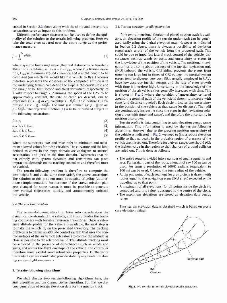
A positive dhi indicates the start of a climb, a negativedhi indicates a descent (Fig. 3).

Step 2: For the ascent case (positive dhi), select the first pointof the next patch (section) as a node; for descent (neg-ative dhi) select the end point of the current patch asthe node. These nodes are the ascent end and descentstart points, indicated by dark dots in Fig. 3.

50 100 150Ground distance (km)

heights and node points versus range for a sample terrain profile.

Step 3: For ascent, join the node (start point of next section)with the current section by a line with a slope equalto the rate of climb of the vehicle. Find the point ofintersection of this line with the current patch, if itdoes not intersect the current patch, look for intersec-tion with previous sections. This point is the ascentstart or climb start point. Collect all ascent start pointsand embed them in the node point list in order. Notethat if the ascent start point does not lie on the cur-rent patch but on some previous patch, then all inter-mediate patches and nodes will be deleted. All ascentstart points become node points.

Step 4: For descent, find the intersection point of a line pass-ing through the descent node point with the nextpatch/section. This line should have a slope equal tothe rate of descent of the vehicle. If there is no inter-section with the next adjacent section, go to the nextsection and so on. The intersection point is the des-cent stop point, all intermediate sections (and nodes)where an intersection cannot be found will beremoved. Collect all descent stop points and embedthem in the vector of node points. In this way thenode list is updated with deletion of some nodepoints, and with appropriate ascent start and descentstop points, as a function of distance from the startpoint.

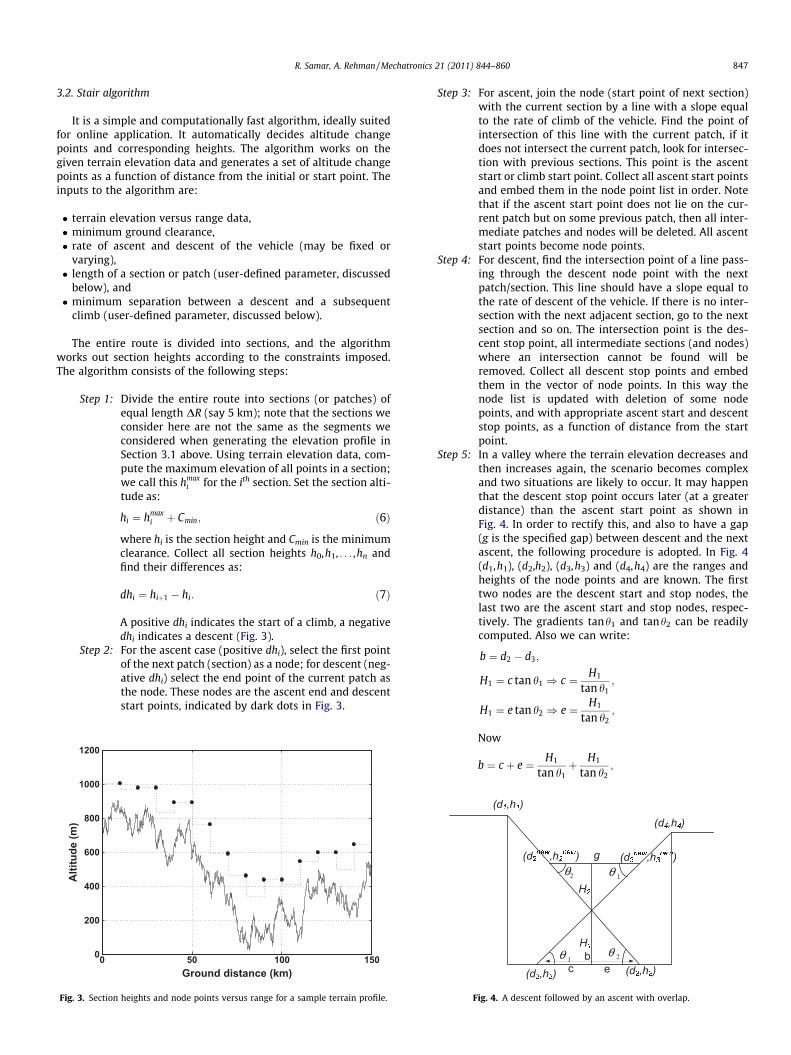
Step 5: In a valley where the terrain elevation decreases andthen increases again, the scenario becomes complexand two situations are likely to occur. It may happenthat the descent stop point occurs later (at a greaterdistance) than the ascent start point as shown inFig. 4. In order to rectify this, and also to have a gap(g is the specified gap) between descent and the nextascent, the following procedure is adopted. In Fig. 4(d1,h1), (d2,h2), (d3,h3) and (d4,h4) are the ranges andheights of the node points and are known. The firsttwo nodes are the descent start and stop nodes, thelast two are the ascent start and stop nodes, respec-tively. The gradients tanh1 and tanh2 can be readilycomputed. Also we can write:

F

b ¼ d2 � d3;

H1 ¼ c tan h1 ) c ¼ H1

tan h1;

H1 ¼ e tan h2 ) e ¼ H1

tan h2;

Now

b ¼ c þ e ¼ H1

tan h1þ H1

tan h2;

(d ,h ) g

H

H

(d ,h )

(d ,h )(d ,h )

(d ,h )

1θ 2θ

1θ2θ(d ,h )

bc e

ig. 4. A descent followed by an ascent with overlap.

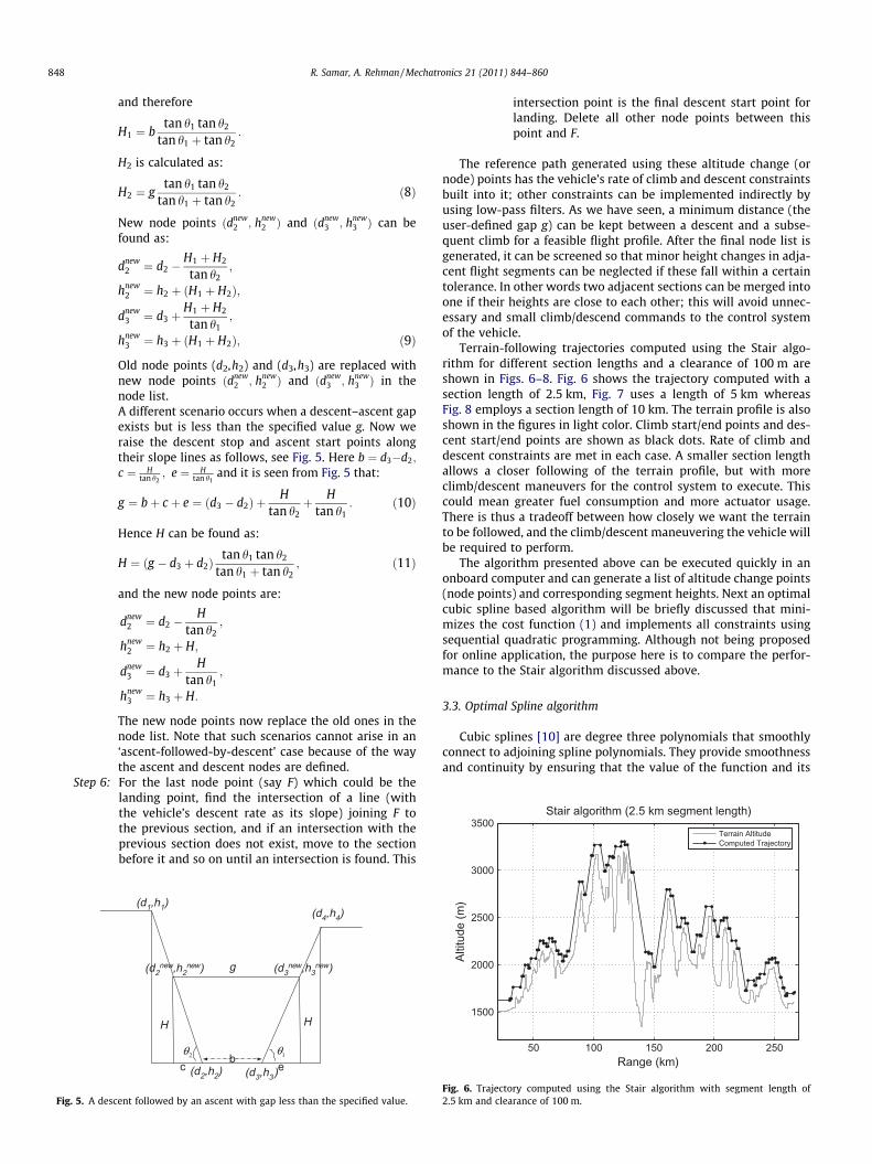
Fig. 5. A desc


and therefore

H1 ¼ btan h1 tan h2

tan h1 þ tan h2:

H2 is calculated as:

H2 ¼ gtan h1 tan h2

tan h1 þ tan h2: ð8Þ

New node points ðdnew2 ; hnew

2 Þ and ðdnew3 ; hnew

3 Þ can befound as:

dnew2 ¼ d2 �

H1 þ H2

tan h2;

hnew2 ¼ h2 þ ðH1 þ H2Þ;

dnew3 ¼ d3 þ

H1 þ H2

tan h1;

hnew3 ¼ h3 þ ðH1 þ H2Þ; ð9Þ

Old node points (d2,h2) and (d3,h3) are replaced withnew node points ðdnew

2 ; hnew2 Þ and ðdnew

3 ; hnew3 Þ in the

node list.A different scenario occurs when a descent–ascent gapexists but is less than the specified value g. Now weraise the descent stop and ascent start points alongtheir slope lines as follows, see Fig. 5. Here b ¼ d3�d2;

c ¼ Htan h2

; e ¼ Htan h1

and it is seen from Fig. 5 that:

g ¼ bþ c þ e ¼ ðd3 � d2Þ þH

tan h2þ H

tan h1: ð10Þ

Hence H can be found as:

H ¼ ðg � d3 þ d2Þtan h1 tan h2

tan h1 þ tan h2; ð11Þ

and the new node points are:

dnew2 ¼ d2 �

Htan h2

;

hnew2 ¼ h2 þ H;

dnew3 ¼ d3 þ

Htan h1

;

hnew3 ¼ h3 þ H:

The new node points now replace the old ones in thenode list. Note that such scenarios cannot arise in an‘ascent-followed-by-descent’ case because of the waythe ascent and descent nodes are defined.

3500Stair algorithm (2.5 km segment length)

Terrain AltitudeComputed Trajectory

Step 6: For the last node point (say F) which could be thelanding point, find the intersection of a line (withthe vehicle’s descent rate as its slope) joining F tothe previous section, and if an intersection with theprevious section does not exist, move to the sectionbefore it and so on until an intersection is found. This

(d2new,h2

new) g

H H

(d1,h1)

(d2,h2) (d3,h3)

(d4,h4)

2θ

(d3new,h3

new)

1θb

c e

ent followed by an ascent with gap less than the specified value.

intersection point is the final descent start point forlanding. Delete all other node points between thispoint and F.

The reference path generated using these altitude change (ornode) points has the vehicle’s rate of climb and descent constraintsbuilt into it; other constraints can be implemented indirectly byusing low-pass filters. As we have seen, a minimum distance (theuser-defined gap g) can be kept between a descent and a subse-quent climb for a feasible flight profile. After the final node list isgenerated, it can be screened so that minor height changes in adja-cent flight segments can be neglected if these fall within a certaintolerance. In other words two adjacent sections can be merged intoone if their heights are close to each other; this will avoid unnec-essary and small climb/descend commands to the control systemof the vehicle.

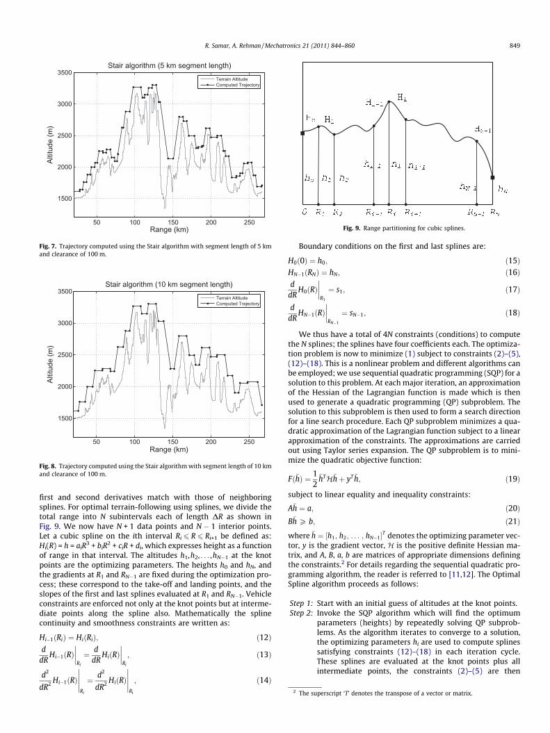
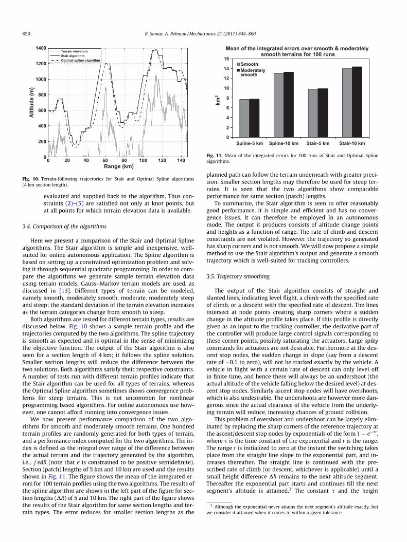
Terrain-following trajectories computed using the Stair algo-rithm for different section lengths and a clearance of 100 m areshown in Figs. 6–8. Fig. 6 shows the trajectory computed with asection length of 2.5 km, Fig. 7 uses a length of 5 km whereasFig. 8 employs a section length of 10 km. The terrain profile is alsoshown in the figures in light color. Climb start/end points and des-cent start/end points are shown as black dots. Rate of climb anddescent constraints are met in each case. A smaller section lengthallows a closer following of the terrain profile, but with moreclimb/descent maneuvers for the control system to execute. Thiscould mean greater fuel consumption and more actuator usage.There is thus a tradeoff between how closely we want the terrainto be followed, and the climb/descent maneuvering the vehicle willbe required to perform.

The algorithm presented above can be executed quickly in anonboard computer and can generate a list of altitude change points(node points) and corresponding segment heights. Next an optimalcubic spline based algorithm will be briefly discussed that mini-mizes the cost function (1) and implements all constraints usingsequential quadratic programming. Although not being proposedfor online application, the purpose here is to compare the perfor-mance to the Stair algorithm discussed above.

3.3. Optimal Spline algorithm

Cubic splines [10] are degree three polynomials that smoothlyconnect to adjoining spline polynomials. They provide smoothnessand continuity by ensuring that the value of the function and its

50 100 150 200 250

1500

2000

2500

3000

Range (km)

Altit

ude

(m)

Fig. 6. Trajectory computed using the Stair algorithm with segment length of2.5 km and clearance of 100 m.

50 100 150 200 250

1500

2000

2500

3000

3500

Range (km)

Altit

ude

(m)

Stair algorithm (5 km segment length)


Fig. 7. Trajectory computed using the Stair algorithm with segment length of 5 kmand clearance of 100 m.

50 100 150 200 250

1500

2000

2500

3000

3500

Range (km)

Altit

ude

(m)

Stair algorithm (10 km segment length)


Fig. 8. Trajectory computed using the Stair algorithm with segment length of 10 kmand clearance of 100 m.

Fig. 9. Range partitioning for cubic splines.

2 The superscript ‘T’ denotes the transpose of a vector or matrix.


first and second derivatives match with those of neighboringsplines. For optimal terrain-following using splines, we divide thetotal range into N subintervals each of length DR as shown inFig. 9. We now have N + 1 data points and N � 1 interior points.Let a cubic spline on the ith interval Ri 6 R 6 Ri+1 be defined as:Hi(R) = h = aiR

3 + biR2 + ciR + di, which expresses height as a function

of range in that interval. The altitudes h1,h2, . . . ,hN�1 at the knotpoints are the optimizing parameters. The heights h0 and hN, andthe gradients at R1 and RN�1 are fixed during the optimization pro-cess; these correspond to the take-off and landing points, and theslopes of the first and last splines evaluated at R1 and RN�1. Vehicleconstraints are enforced not only at the knot points but at interme-diate points along the spline also. Mathematically the splinecontinuity and smoothness constraints are written as:

Hi�1ðRiÞ ¼ HiðRiÞ; ð12Þd

dRHi�1ðRÞ

��Ri

¼ ddR

HiðRÞ��

Ri

; ð13Þ

d2

dR2 Hi�1ðRÞ��Ri

¼ d2

dR2 HiðRÞ��

Ri

; ð14Þ

Boundary conditions on the first and last splines are:

H0ð0Þ ¼ h0; ð15ÞHN�1ðRNÞ ¼ hN ; ð16Þd

dRH0ðRÞ

��R1

¼ s1; ð17Þ

ddR

HN�1ðRÞ��RN�1

¼ sN�1; ð18Þ

We thus have a total of 4N constraints (conditions) to computethe N splines; the splines have four coefficients each. The optimiza-tion problem is now to minimize (1) subject to constraints (2)–(5),(12)–(18). This is a nonlinear problem and different algorithms canbe employed; we use sequential quadratic programming (SQP) for asolution to this problem. At each major iteration, an approximationof the Hessian of the Lagrangian function is made which is thenused to generate a quadratic programming (QP) subproblem. Thesolution to this subproblem is then used to form a search directionfor a line search procedure. Each QP subproblem minimizes a qua-dratic approximation of the Lagrangian function subject to a linearapproximation of the constraints. The approximations are carriedout using Taylor series expansion. The QP subproblem is to mini-mize the quadratic objective function:

Fð�hÞ ¼ 12

�hTH�hþ yT �h; ð19Þ

subject to linear equality and inequality constraints:

A�h ¼ a; ð20ÞB�h P b; ð21Þ

where �h ¼ ½h1; h2; . . . ; hN�1�T denotes the optimizing parameter vec-tor, y is the gradient vector, H is the positive definite Hessian ma-trix, and A, B, a, b are matrices of appropriate dimensions definingthe constraints.2 For details regarding the sequential quadratic pro-gramming algorithm, the reader is referred to [11,12]. The OptimalSpline algorithm proceeds as follows:

Step 1: Start with an initial guess of altitudes at the knot points.Step 2: Invoke the SQP algorithm which will find the optimum

parameters (heights) by repeatedly solving QP subprob-lems. As the algorithm iterates to converge to a solution,the optimizing parameters hi are used to compute splinessatisfying constraints (12)–(18) in each iteration cycle.These splines are evaluated at the knot points plus allintermediate points, the constraints (2)–(5) are then

0 20 40 60 80 100 120 1400

200

400

600

800

1000

1200

1400

Range (km)

Alti

tude

(m)

Terrain elevationStair algorithmOptimal spline algorithm

Fig. 10. Terrain-following trajectories for Stair and Optimal Spline algorithms(4 km section length).

0

2

4

6

8

10

12

14

16

Spline-5 km Spline-10 km Stair-5 km Stair-10 km

km2

Mean of the integrated errors over smooth & moderately smooth terrains for 100 runs

SmoothModerately smooth

Fig. 11. Mean of the integrated errors for 100 runs of Stair and Optimal Splinealgorithms.

3 Although the exponential never attains the next segment’s altitude exactly, bute consider it attained when it comes to within a given tolerance.


evaluated and supplied back to the algorithm. Thus con-straints (2)–(5) are satisfied not only at knot points, butat all points for which terrain elevation data is available.

3.4. Comparison of the algorithms

Here we present a comparison of the Stair and Optimal Splinealgorithms. The Stair algorithm is simple and inexpensive, well-suited for online autonomous application. The Spline algorithm isbased on setting up a constrained optimization problem and solv-ing it through sequential quadratic programming. In order to com-pare the algorithms we generate sample terrain elevation datausing terrain models. Gauss–Markov terrain models are used, asdiscussed in [13]. Different types of terrain can be modeled,namely smooth, moderately smooth, moderate, moderately steepand steep; the standard deviation of the terrain elevation increasesas the terrain categories change from smooth to steep.

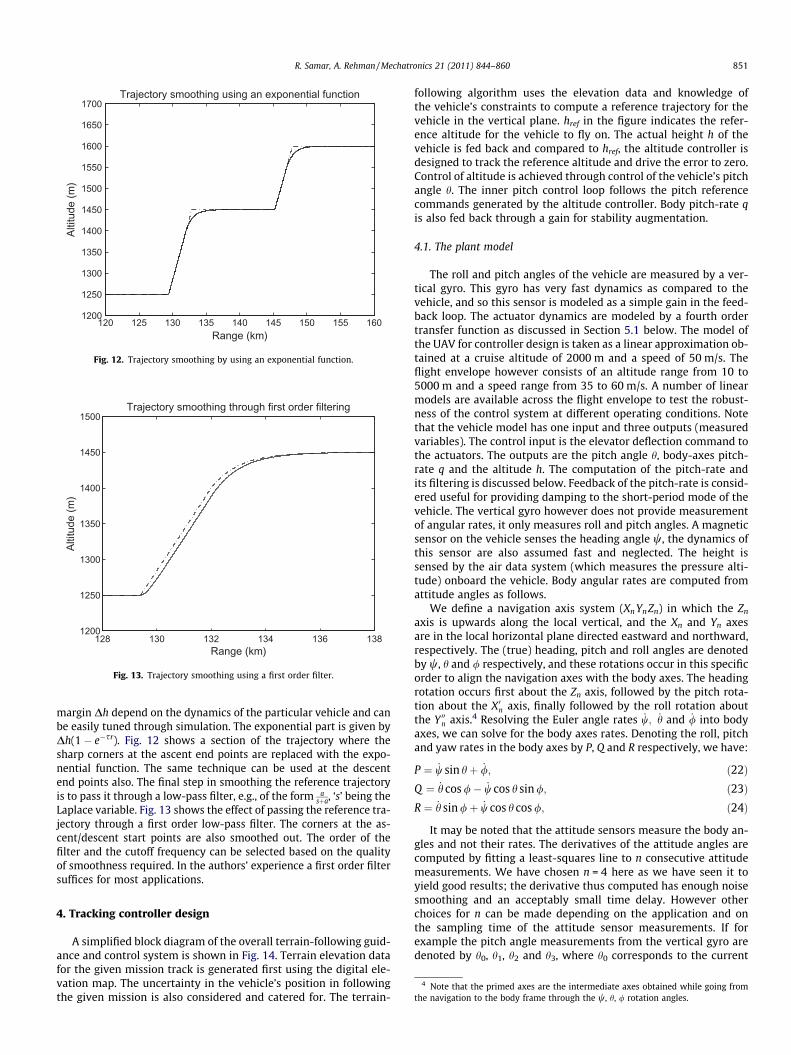
Both algorithms are tested for different terrain types, results arediscussed below. Fig. 10 shows a sample terrain profile and thetrajectories computed by the two algorithms. The spline trajectoryis smooth as expected and is optimal in the sense of minimizingthe objective function. The output of the Stair algorithm is alsoseen for a section length of 4 km; it follows the spline solution.Smaller section lengths will reduce the difference between thetwo solutions. Both algorithms satisfy their respective constraints.A number of tests run with different terrain profiles indicate thatthe Stair algorithm can be used for all types of terrains, whereasthe Optimal Spline algorithm sometimes shows convergence prob-lems for steep terrains. This is not uncommon for nonlinearprogramming based algorithms. For online autonomous use how-ever, one cannot afford running into convergence issues.

We now present performance comparison of the two algo-rithms for smooth and moderately smooth terrains. One hundredterrain profiles are randomly generated for both types of terrain,and a performance index computed for the two algorithms. The in-dex is defined as the integral over range of the difference betweenthe actual terrain and the trajectory generated by the algorithm,i.e.,

RedR (note that e is constrained to be positive semidefinite).

Section (patch) lengths of 5 km and 10 km are used and the resultsshown in Fig. 11. The figure shows the mean of the integrated er-rors for 100 terrain profiles using the two algorithms. The results ofthe spline algorithm are shown in the left part of the figure for sec-tion lengths (DR) of 5 and 10 km. The right part of the figure showsthe results of the Stair algorithm for same section lengths and ter-rain types. The error reduces for smaller section lengths as the

planned path can follow the terrain underneath with greater preci-sion. Smaller section lengths may therefore be used for steep ter-rains. It is seen that the two algorithms show comparableperformance for same section (patch) lengths.

To summarize, the Stair algorithm is seen to offer reasonablygood performance, it is simple and efficient and has no conver-gence issues. It can therefore be employed in an autonomousmode. The output it produces consists of altitude change pointsand heights as a function of range. The rate of climb and descentconstraints are not violated. However the trajectory so generatedhas sharp corners and is not smooth. We will now propose a simplemethod to use the Stair algorithm’s output and generate a smoothtrajectory which is well-suited for tracking controllers.

3.5. Trajectory smoothing

The output of the Stair algorithm consists of straight andslanted lines, indicating level flight, a climb with the specified rateof climb, or a descent with the specified rate of descent. The linesintersect at node points creating sharp corners where a suddenchange in the altitude profile takes place. If this profile is directlygiven as an input to the tracking controller, the derivative part ofthe controller will produce large control signals corresponding tothese corner points, possibly saturating the actuators. Large spikycommands for actuators are not desirable. Furthermore at the des-cent stop nodes, the sudden change in slope (say from a descentrate of �0.1 to zero), will not be tracked exactly by the vehicle. Avehicle in flight with a certain rate of descent can only level offin finite time, and hence there will always be an undershoot (theactual altitude of the vehicle falling below the desired level) at des-cent stop nodes. Similarly ascent stop nodes will have overshoots,which is also undesirable. The undershoots are however more dan-gerous since the actual clearance of the vehicle from the underly-ing terrain will reduce, increasing chances of ground collision.

This problem of overshoot and undershoot can be largely elim-inated by replacing the sharp corners of the reference trajectory atthe ascent/descent stop nodes by exponentials of the form 1 � e�sr,where s is the time constant of the exponential and r is the range.The range r is initialized to zero at the instant the switching takesplace from the straight line slope to the exponential part, and in-creases thereafter. The straight line is continued with the pre-scribed rate of climb (or descent, whichever is applicable) until asmall height difference Dh remains to the next altitude segment.Thereafter the exponential part starts and continues till the nextsegment’s altitude is attained.3 The constant s and the height

w

120 125 130 135 140 145 150 155 1601200

1250

1300

1350

1400

1450

1500

1550

1600

1650

1700

Range (km)

Altit

ude

(m)

Trajectory smoothing using an exponential function

Fig. 12. Trajectory smoothing by using an exponential function.

128 130 132 134 136 1381200

1250

1300

1350

1400

1450

1500

Range (km)

Altit

ude

(m)

Trajectory smoothing through first order filtering

Fig. 13. Trajectory smoothing using a first order filter.


margin Dh depend on the dynamics of the particular vehicle and canbe easily tuned through simulation. The exponential part is given byDh(1 � e�sr). Fig. 12 shows a section of the trajectory where thesharp corners at the ascent end points are replaced with the expo-nential function. The same technique can be used at the descentend points also. The final step in smoothing the reference trajectoryis to pass it through a low-pass filter, e.g., of the form a

sþa, ‘s’ being theLaplace variable. Fig. 13 shows the effect of passing the reference tra-jectory through a first order low-pass filter. The corners at the as-cent/descent start points are also smoothed out. The order of thefilter and the cutoff frequency can be selected based on the qualityof smoothness required. In the authors’ experience a first order filtersuffices for most applications.

4 Note that the primed axes are the intermediate axes obtained while going fromthe navigation to the body frame through the w, h, / rotation angles.

4. Tracking controller design

A simplified block diagram of the overall terrain-following guid-ance and control system is shown in Fig. 14. Terrain elevation datafor the given mission track is generated first using the digital ele-vation map. The uncertainty in the vehicle’s position in followingthe given mission is also considered and catered for. The terrain-

following algorithm uses the elevation data and knowledge ofthe vehicle’s constraints to compute a reference trajectory for thevehicle in the vertical plane. href in the figure indicates the refer-ence altitude for the vehicle to fly on. The actual height h of thevehicle is fed back and compared to href, the altitude controller isdesigned to track the reference altitude and drive the error to zero.Control of altitude is achieved through control of the vehicle’s pitchangle h. The inner pitch control loop follows the pitch referencecommands generated by the altitude controller. Body pitch-rate qis also fed back through a gain for stability augmentation.

4.1. The plant model

The roll and pitch angles of the vehicle are measured by a ver-tical gyro. This gyro has very fast dynamics as compared to thevehicle, and so this sensor is modeled as a simple gain in the feed-back loop. The actuator dynamics are modeled by a fourth ordertransfer function as discussed in Section 5.1 below. The model ofthe UAV for controller design is taken as a linear approximation ob-tained at a cruise altitude of 2000 m and a speed of 50 m/s. Theflight envelope however consists of an altitude range from 10 to5000 m and a speed range from 35 to 60 m/s. A number of linearmodels are available across the flight envelope to test the robust-ness of the control system at different operating conditions. Notethat the vehicle model has one input and three outputs (measuredvariables). The control input is the elevator deflection command tothe actuators. The outputs are the pitch angle h, body-axes pitch-rate q and the altitude h. The computation of the pitch-rate andits filtering is discussed below. Feedback of the pitch-rate is consid-ered useful for providing damping to the short-period mode of thevehicle. The vertical gyro however does not provide measurementof angular rates, it only measures roll and pitch angles. A magneticsensor on the vehicle senses the heading angle w, the dynamics ofthis sensor are also assumed fast and neglected. The height issensed by the air data system (which measures the pressure alti-tude) onboard the vehicle. Body angular rates are computed fromattitude angles as follows.

We define a navigation axis system (Xn Yn Zn) in which the Zn

axis is upwards along the local vertical, and the Xn and Yn axesare in the local horizontal plane directed eastward and northward,respectively. The (true) heading, pitch and roll angles are denotedby w, h and / respectively, and these rotations occur in this specificorder to align the navigation axes with the body axes. The headingrotation occurs first about the Zn axis, followed by the pitch rota-tion about the X0n axis, finally followed by the roll rotation aboutthe Y 00n axis.4 Resolving the Euler angle rates _w; _h and _/ into bodyaxes, we can solve for the body axes rates. Denoting the roll, pitchand yaw rates in the body axes by P, Q and R respectively, we have:

P ¼ _w sin hþ _/; ð22ÞQ ¼ _h cos /� _w cos h sin /; ð23ÞR ¼ _h sin /þ _w cos h cos /; ð24Þ

It may be noted that the attitude sensors measure the body an-gles and not their rates. The derivatives of the attitude angles arecomputed by fitting a least-squares line to n consecutive attitudemeasurements. We have chosen n = 4 here as we have seen it toyield good results; the derivative thus computed has enough noisesmoothing and an acceptably small time delay. However otherchoices for n can be made depending on the application and onthe sampling time of the attitude sensor measurements. If forexample the pitch angle measurements from the vertical gyro aredenoted by h0, h1, h2 and h3, where h0 corresponds to the current

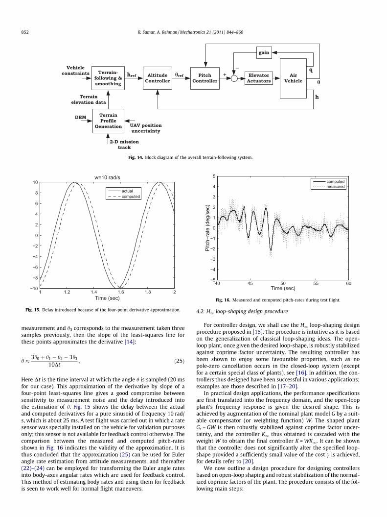
Fig. 14. Block diagram of the overall terrain-following system.

1 1.2 1.4 1.6 1.8 2−10

−8

−6

−4

−2

0

2

4

6

8

10

Time (sec)

w=10 rad/s

actualcomputed

Fig. 15. Delay introduced because of the four-point derivative approximation.

40 45 50 55 60−5

−4

−3

−2

−1

0

1

2

3

4

5

Time (sec)

Pitc

h−ra

te (d

eg/s

ec)

computedmeasured

Fig. 16. Measured and computed pitch-rates during test flight.


measurement and h3 corresponds to the measurement taken threesamples previously, then the slope of the least-squares line forthese points approximates the derivative [14]:

_h � 3h0 þ h1 � h2 � 3h3

10Dt; ð25Þ

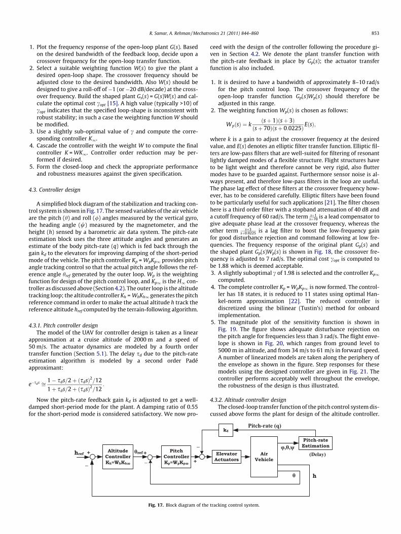
Here Dt is the time interval at which the angle h is sampled (20 msfor our case). This approximation of the derivative by slope of afour-point least-squares line gives a good compromise betweensensitivity to measurement noise and the delay introduced intothe estimation of _h. Fig. 15 shows the delay between the actualand computed derivatives for a pure sinusoid of frequency 10 rad/s, which is about 25 ms. A test flight was carried out in which a ratesensor was specially installed on the vehicle for validation purposesonly; this sensor is not available for feedback control otherwise. Thecomparison between the measured and computed pitch-ratesshown in Fig. 16 indicates the validity of the approximation. It isthus concluded that the approximation (25) can be used for Eulerangle rate estimation from attitude measurements, and thereafter(22)–(24) can be employed for transforming the Euler angle ratesinto body-axes angular rates which are used for feedback control.This method of estimating body rates and using them for feedbackis seen to work well for normal flight maneuvers.

4.2. H1 loop-shaping design procedure

For controller design, we shall use the H1 loop-shaping designprocedure proposed in [15]. The procedure is intuitive as it is basedon the generalization of classical loop-shaping ideas. The open-loop plant, once given the desired loop-shape, is robustly stabilizedagainst coprime factor uncertainty. The resulting controller hasbeen shown to enjoy some favourable properties, such as nopole-zero cancellation occurs in the closed-loop system (exceptfor a certain special class of plants), see [16]. In addition, the con-trollers thus designed have been successful in various applications;examples are those described in [17–20].

In practical design applications, the performance specificationsare first translated into the frequency domain, and the open-loopplant’s frequency response is given the desired shape. This isachieved by augmentation of the nominal plant model G by a suit-able compensator (or weighting function) W. The shaped plantGs = GW is then robustly stabilized against coprime factor uncer-tainty, and the controller K1 thus obtained is cascaded with theweight W to obtain the final controller K = WK1. It can be shownthat the controller does not significantly alter the specified loop-shape provided a sufficiently small value of the cost c is achieved,for details refer to [20].

We now outline a design procedure for designing controllersbased on open-loop shaping and robust stabilization of the normal-ized coprime factors of the plant. The procedure consists of the fol-lowing main steps:


1. Plot the frequency response of the open-loop plant G(s). Basedon the desired bandwidth of the feedback loop, decide upon acrossover frequency for the open-loop transfer function.

2. Select a suitable weighting function W(s) to give the plant adesired open-loop shape. The crossover frequency should beadjusted close to the desired bandwidth. Also W(s) should bedesigned to give a roll-off of�1 (or�20 dB/decade) at the cross-over frequency. Build the shaped plant Gs(s) = G(s)W(s) and cal-culate the optimal cost copt [15]. A high value (typically >10) ofcopt indicates that the specified loop-shape is inconsistent withrobust stability; in such a case the weighting function W shouldbe modified.

3. Use a slightly sub-optimal value of c and compute the corre-sponding controller K1.

4. Cascade the controller with the weight W to compute the finalcontroller K = WK1. Controller order reduction may be per-formed if desired.

5. Form the closed-loop and check the appropriate performanceand robustness measures against the given specification.

4.3. Controller design

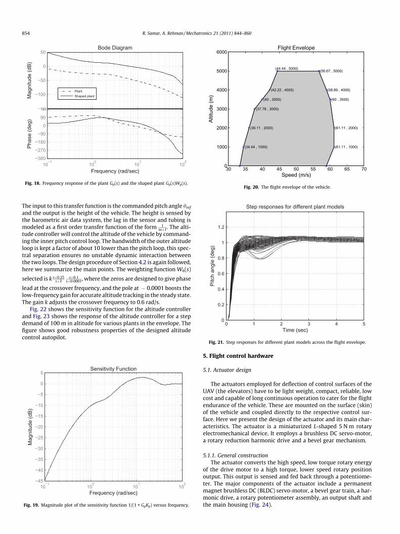
A simplified block diagram of the stabilization and tracking con-trol system is shown in Fig. 17. The sensed variables of the air vehicleare the pitch (h) and roll (/) angles measured by the vertical gyro,the heading angle (w) measured by the magnetometer, and theheight (h) sensed by a barometric air data system. The pitch-rateestimation block uses the three attitude angles and generates anestimate of the body pitch-rate (q) which is fed back through thegain kd to the elevators for improving damping of the short-periodmode of the vehicle. The pitch controller Kp = WpKp1 provides pitchangle tracking control so that the actual pitch angle follows the ref-erence angle href generated by the outer loop. Wp is the weightingfunction for design of the pitch control loop, and Kp1 is the H1 con-troller as discussed above (Section 4.2). The outer loop is the altitudetracking loop; the altitude controller Kh = WhKh1 generates the pitchreference command in order to make the actual altitude h track thereference altitude href computed by the terrain-following algorithm.

4.3.1. Pitch controller designThe model of the UAV for controller design is taken as a linear

approximation at a cruise altitude of 2000 m and a speed of50 m/s. The actuator dynamics are modeled by a fourth ordertransfer function (Section 5.1). The delay sd due to the pitch-rateestimation algorithm is modeled by a second order Padéapproximant:

e�sds ffi 1� sds=2þ ðsdsÞ2=12

1þ sds=2þ ðsdsÞ2=12:

Now the pitch-rate feedback gain kd is adjusted to get a well-damped short-period mode for the plant. A damping ratio of 0.55for the short-period mode is considered satisfactory. We now pro-

Fig. 17. Block diagram of the

ceed with the design of the controller following the procedure gi-ven in Section 4.2. We denote the plant transfer function withthe pitch-rate feedback in place by Gp(s); the actuator transferfunction is also included.

1. It is desired to have a bandwidth of approximately 8–10 rad/sfor the pitch control loop. The crossover frequency of theopen-loop transfer function Gp(s)Wp(s) should therefore beadjusted in this range.

2. The weighting function Wp(s) is chosen as follows:

tracking

WpðsÞ ¼ kðsþ 1Þðsþ 3Þ

ðsþ 70Þðsþ 0:0225Þ EðsÞ;

where k is a gain to adjust the crossover frequency at the desiredvalue, and E(s) denotes an elliptic filter transfer function. Elliptic fil-ters are low-pass filters that are well-suited for filtering of resonantlightly damped modes of a flexible structure. Flight structures haveto be light weight and therefore cannot be very rigid, also fluttermodes have to be guarded against. Furthermore sensor noise is al-ways present, and therefore low-pass filters in the loop are useful.The phase lag effect of these filters at the crossover frequency how-ever, has to be considered carefully. Elliptic filters have been foundto be particularly useful for such applications [21]. The filter chosenhere is a third order filter with a stopband attenuation of 40 dB anda cutoff frequency of 60 rad/s. The term sþ1

sþ70 is a lead compensator togive adequate phase lead at the crossover frequency, whereas theother term sþ3

sþ0:0225 is a lag filter to boost the low-frequency gainfor good disturbance rejection and command following at low fre-quencies. The frequency response of the original plant Gp(s) andthe shaped plant Gp(s)Wp(s) is shown in Fig. 18, the crossover fre-quency is adjusted to 7 rad/s. The optimal cost copt is computed tobe 1.88 which is deemed acceptable.3. A slightly suboptimal c of 1.98 is selected and the controller Kp1

computed.4. The complete controller Kp = WpKp1 is now formed. The control-

ler has 18 states, it is reduced to 11 states using optimal Han-kel-norm approximation [22]. The reduced controller isdiscretized using the bilinear (Tustin’s) method for onboardimplementation.

5. The magnitude plot of the sensitivity function is shown inFig. 19. The figure shows adequate disturbance rejection onthe pitch angle for frequencies less than 3 rad/s. The flight enve-lope is shown in Fig. 20, which ranges from ground level to5000 m in altitude, and from 34 m/s to 61 m/s in forward speed.A number of linearized models are taken along the periphery ofthe envelope as shown in the figure. Step responses for thesemodels using the designed controller are given in Fig. 21. Thecontroller performs acceptably well throughout the envelope,the robustness of the design is thus illustrated.

4.3.2. Altitude controller designThe closed-loop transfer function of the pitch control system dis-

cussed above forms the plant for design of the altitude controller.

control system.

−150

−100

−50

0

50

Mag

nitu

de (d

B)

10−1

100

101

102

−360

−270

−180

−90

0

90

180

Phas

e (d

eg)

Bode Diagram

Frequency (rad/sec)

PlantShaped plant

Fig. 18. Frequency response of the plant Gp(s) and the shaped plant Gp(s)Wp(s).

30 35 40 45 50 55 60 65 700

1000

2000

3000

4000

5000

6000

Speed (m/s)

Altit

ude

(m)

(34.44 , 1000)

(36.11 , 2000)

(37.78 , 3000)

(40 , 3500)

(42.22 , 4000)

(44.44 , 5000) (56.67 , 5000)

(58.89 , 4000)

(60 , 3500)

(61.11 , 2000)

(61.11 , 1000)

Flight Envelope

Fig. 20. The flight envelope of the vehicle.

0 1 2 3 4 50

0.2

0.4

0.6

0.8

1

1.2

Step responses for different plant models

Time (sec)

Pitc

h an

gle

(deg

)


The input to this transfer function is the commanded pitch angle href

and the output is the height of the vehicle. The height is sensed bythe barometric air data system, the lag in the sensor and tubing ismodeled as a first order transfer function of the form 1

asþ1. The alti-tude controller will control the altitude of the vehicle by command-ing the inner pitch control loop. The bandwidth of the outer altitudeloop is kept a factor of about 10 lower than the pitch loop, this spec-tral separation ensures no unstable dynamic interaction betweenthe two loops. The design procedure of Section 4.2 is again followed,here we summarize the main points. The weighting function Wh(s)

selected is k sþ0:25sþ3

sþ0:1sþ0:0001, where the zeros are designed to give phase

lead at the crossover frequency, and the pole at � 0.0001 boosts thelow-frequency gain for accurate altitude tracking in the steady state.The gain k adjusts the crossover frequency to 0.6 rad/s.

Fig. 22 shows the sensitivity function for the altitude controllerand Fig. 23 shows the response of the altitude controller for a stepdemand of 100 m in altitude for various plants in the envelope. Thefigure shows good robustness properties of the designed altitudecontrol autopilot.

100

101

102

10−1

−45

−40

−35

−30

−25

−20

−15

−10

−5

0

5

Mag

nitu

de (d

B)

Sensitivity Function

Frequency (rad/sec)

Fig. 19. Magnitude plot of the sensitivity function 1/(1 + GpKp) versus frequency.

Fig. 21. Step responses for different plant models across the flight envelope.

5. Flight control hardware

5.1. Actuator design

The actuators employed for deflection of control surfaces of theUAV (the elevators) have to be light weight, compact, reliable, lowcost and capable of long continuous operation to cater for the flightendurance of the vehicle. These are mounted on the surface (skin)of the vehicle and coupled directly to the respective control sur-face. Here we present the design of the actuator and its main char-acteristics. The actuator is a miniaturized L-shaped 5 N m rotaryelectromechanical device. It employs a brushless DC servo-motor,a rotary reduction harmonic drive and a bevel gear mechanism.

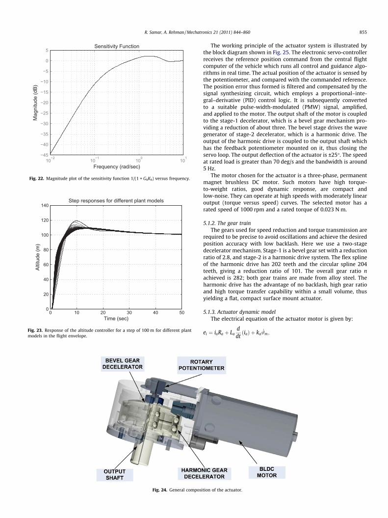
5.1.1. General constructionThe actuator converts the high speed, low torque rotary energy

of the drive motor to a high torque, lower speed rotary positionoutput. This output is sensed and fed back through a potentiome-ter. The major components of the actuator include a permanentmagnet brushless DC (BLDC) servo-motor, a bevel gear train, a har-monic drive, a rotary potentiometer assembly, an output shaft andthe main housing (Fig. 24).

10−2

10−1

100

101

−45

−40

−35

−30

−25

−20

−15

−10

−5

0

5

Mag

nitu

de (d

B)

Sensitivity Function

Frequency (rad/sec)

Fig. 22. Magnitude plot of the sensitivity function 1/(1 + GhKh) versus frequency.

0 10 20 30 40 500

20

40

60

80

100

120

140Step responses for different plant models

Time (sec)

Altit

ude

(m)

Fig. 23. Response of the altitude controller for a step of 100 m for different plantmodels in the flight envelope.

Fig. 24. General composi


The working principle of the actuator system is illustrated bythe block diagram shown in Fig. 25. The electronic servo-controllerreceives the reference position command from the central flightcomputer of the vehicle which runs all control and guidance algo-rithms in real time. The actual position of the actuator is sensed bythe potentiometer, and compared with the commanded reference.The position error thus formed is filtered and compensated by thesignal synthesizing circuit, which employs a proportional–inte-gral–derivative (PID) control logic. It is subsequently convertedto a suitable pulse-width-modulated (PMW) signal, amplified,and applied to the motor. The output shaft of the motor is coupledto the stage-1 decelerator, which is a bevel gear mechanism pro-viding a reduction of about three. The bevel stage drives the wavegenerator of stage-2 decelerator, which is a harmonic drive. Theoutput of the harmonic drive is coupled to the output shaft whichhas the feedback potentiometer mounted on it, thus closing theservo loop. The output deflection of the actuator is ±25�. The speedat rated load is greater than 70 deg/s and the bandwidth is around5 Hz.

The motor chosen for the actuator is a three-phase, permanentmagnet brushless DC motor. Such motors have high torque-to-weight ratios, good dynamic response, are compact andlow-noise. They can operate at high speeds with moderately linearoutput (torque versus speed) curves. The selected motor has arated speed of 1000 rpm and a rated torque of 0.023 N m.

5.1.2. The gear trainThe gears used for speed reduction and torque transmission are

required to be precise to avoid oscillations and achieve the desiredposition accuracy with low backlash. Here we use a two-stagedecelerator mechanism. Stage-1 is a bevel gear set with a reductionratio of 2.8, and stage-2 is a harmonic drive system. The flex splineof the harmonic drive has 202 teeth and the circular spline 204teeth, giving a reduction ratio of 101. The overall gear ratio nachieved is 282; both gear trains are made from alloy steel. Theharmonic drive has the advantage of no backlash, high gear ratioand high torque transfer capability within a small volume, thusyielding a flat, compact surface mount actuator.

5.1.3. Actuator dynamic modelThe electrical equation of the actuator motor is given by:

ei ¼ iaRa þ LaddtðiaÞ þ ka

_#m;

tion of the actuator.

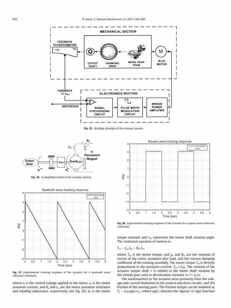
Fig. 25. Working principle of the actuator system.

Fig. 26. A simplified model of the actuator system.

0 0.5 1 1.5 2 2.5 3 3.5 4 4.5 5−3

−2

−1

0

1

2

3

4Sawtooth wave tracking response

Time (sec)

deg

CommandedActual

Fig. 27. Experimental tracking response of the actuator for a sawtooth wavereference command.

0 0.5 1 1.5 2 2.5 3 3.5 4 4.5 5−4

−3

−2

−1

0

1

2

3

4Square wave tracking response

Time (sec)

deg

CommandedActual

Fig. 28. Experimental tracking response of the actuator for a square wave referencecommand.


where ei is the control voltage applied to the motor, ia is the motorarmature current, and Ra and La are the motor armature resistanceand winding inductance, respectively (see Fig. 26). ka is the motor

torque constant and #m represents the motor shaft rotation angle.The rotational equation of motion is:

Tm ¼ Jm€#m þ Bm

_#m;

where Tm is the motor torque, and Jm and Bm are the moment ofinertia of the motor armature plus load, and the viscous dampingcoefficient of the rotating assembly. The motor torque Tm is directlyproportional to the armature current: Tm = kaia. The rotation of theactuator output shaft # is related to the motor shaft rotation bythe overall gear ratio or deceleration constant n:# = #m/n.

The nonlinearities in the actuator arise primarily from the volt-age and current limitation in the control and drive circuits, and thefriction of the moving parts. The friction torque can be modeled asTf ¼ kai0sgnð _#mÞ, where sgn(�) denotes the ‘signum’ or ‘sign’ function

Controller

INUINU Data

Serial Link

Analog Data

Serial Link

Digital Data

Analog D

ata

Onboard Equipment

Telemetry GCS

Servo Amplifier

Power Converter

section

Onboard Data

Handling AnalogDiscrete

Serial

FlightComputer

GPS

Fig. 29. Block diagram of the flight control computer.

0 20 40 60 80 100 120 140 160600

700

800

900

1000

1100

1200

1300

Range (km)

Altit

ude

(m)Altitude tracking: Flight−1

Reference altitudeActual altitude

Fig. 30. Flight-1: commanded and actual altitudes.

5 Random Access Memory.6 Electromagnetic interference.


and i0 is the motor no-load current. Neglecting the nonlinearitieswe can, using the above relations, derive an open-loop transferfunction of the actuator dynamics relating the output shaft angle# to the control voltage ei as:

#

ei¼ ka=nðLasþ RaÞðJms2 þ BmsÞ þ kas2 :

The actuator has a local PID controller (implemented in the sig-nal synthesizing/control circuit) with parameters kp, kI, kD, so thatthe closed-loop actuator transfer function relating the actual actu-ator angular displacement # to the commanded displacement #ref

is:

#

#ref¼ kakDs2 þ kakpsþ kakI

LaJmns4 þ nðJmRa þ LaBmÞs3 þ ðRaBmnþ k2a þ kakDÞs2 þ kakpsþ kakI

:

ð26Þ

where kp, kI and kD are the proportional, integral and derivativegains of the PID controller respectively, used for the actuator servoloop compensation.

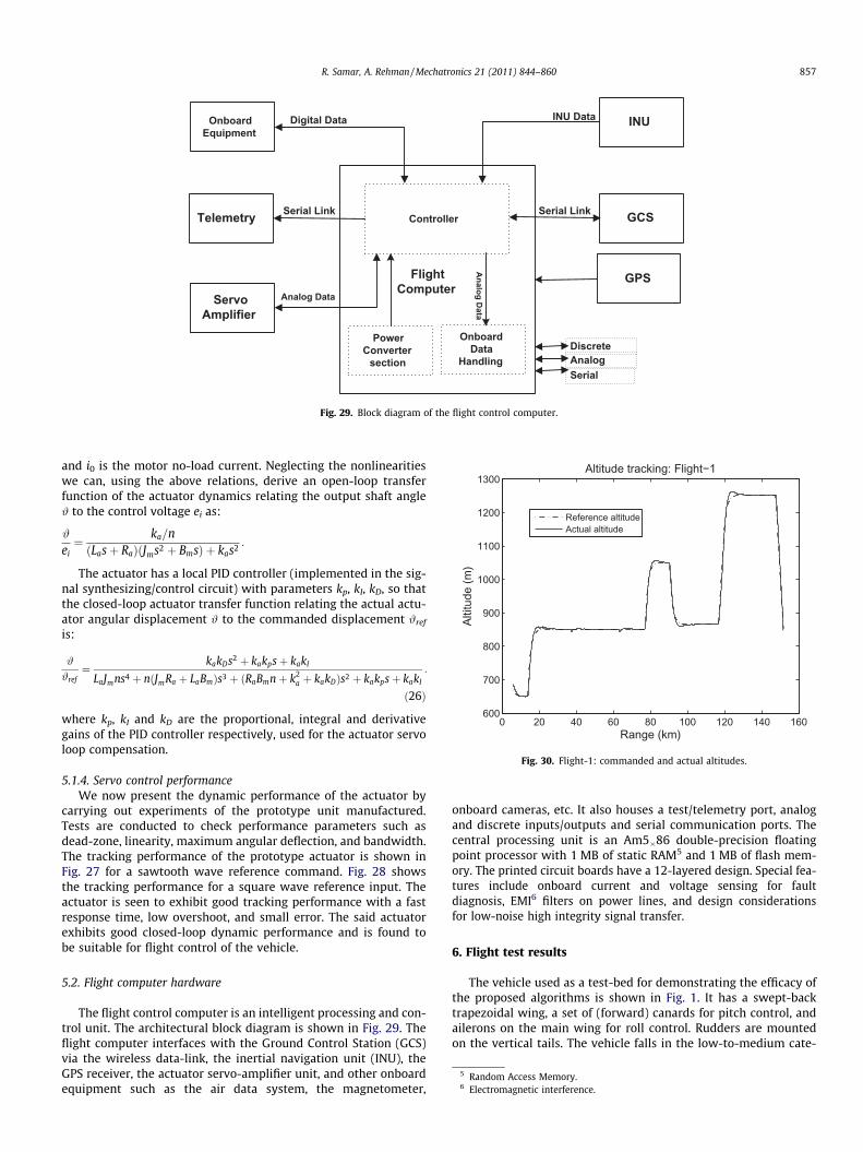
5.1.4. Servo control performanceWe now present the dynamic performance of the actuator by

carrying out experiments of the prototype unit manufactured.Tests are conducted to check performance parameters such asdead-zone, linearity, maximum angular deflection, and bandwidth.The tracking performance of the prototype actuator is shown inFig. 27 for a sawtooth wave reference command. Fig. 28 showsthe tracking performance for a square wave reference input. Theactuator is seen to exhibit good tracking performance with a fastresponse time, low overshoot, and small error. The said actuatorexhibits good closed-loop dynamic performance and is found tobe suitable for flight control of the vehicle.

5.2. Flight computer hardware

The flight control computer is an intelligent processing and con-trol unit. The architectural block diagram is shown in Fig. 29. Theflight computer interfaces with the Ground Control Station (GCS)via the wireless data-link, the inertial navigation unit (INU), theGPS receiver, the actuator servo-amplifier unit, and other onboardequipment such as the air data system, the magnetometer,

onboard cameras, etc. It also houses a test/telemetry port, analogand discrete inputs/outputs and serial communication ports. Thecentral processing unit is an Am5�86 double-precision floatingpoint processor with 1 MB of static RAM5 and 1 MB of flash mem-ory. The printed circuit boards have a 12-layered design. Special fea-tures include onboard current and voltage sensing for faultdiagnosis, EMI6 filters on power lines, and design considerationsfor low-noise high integrity signal transfer.

6. Flight test results

The vehicle used as a test-bed for demonstrating the efficacy ofthe proposed algorithms is shown in Fig. 1. It has a swept-backtrapezoidal wing, a set of (forward) canards for pitch control, andailerons on the main wing for roll control. Rudders are mountedon the vertical tails. The vehicle falls in the low-to-medium cate-

76 77 78 79 80 81 82850

900

950

1000

1050Unfiltered and filtered altitude reference

Altit

ude

(m)

89 90 91 92 93 94 95 96850

900

950

1000

1050

Range (km)

Altit

ude

(m)

UnfilteredFiltered

Fig. 31. Filtered and unfiltered altitude command signals.

100 200 300 400 500 600 700 800 900 1000−5

0

5

10

Pitc

h an

gle

(deg

)

Pitch angle tracking: Flight−1

Reference pitchActual pitch

780 800 820 840 860 8802

3

4

5

6

7

Time (sec)

Pitc

h an

gle

(deg

)

Fig. 32. Flight-1: commanded and actual pitch angles.

100 200 300 400 500 600 700 800 900 1000−2

−1

0

1

2

Pitc

h er

ror (

deg)

Pitch tracking error: Flight−1

100 200 300 400 500 600 700 800 900 1000−3

−2

−1

0

1

2

3

Time (sec)

Pitc

h−ra

te (d

eg/s

)

Body pitch−rate

Fig. 33. Flight-1: pitch angle error and body pitch-rate.

100 200 300 400 500 600 700 800 900 1000

1

2

3

4

deg

Angle of attack: Flight−1

100 200 300 400 500 600 700 800 900 1000−5

0

5Normal acceleration

m/s

ec2

Time (sec)

Fig. 34. Flight-1: angle of attack and normal acceleration.


gory of UAVs in terms of its ceiling and endurance parameters. Theflight envelope covers an altitude range from 10 to 5000 m and aspeed range from 35 to 60 m/s. A piston engine drives the propellerin a push-configuration and provides a maximum power of 100 hp.The wing span is 6.5 m, the aspect ratio is around 7, and the aero-dynamic design provides a maximum lift-to-drag ratio in excess of10. The maximum take-off weight is 450 kg; the vehicle can stayairborne up to 12 h carrying high performance surveillance equip-ment on board.

Several test flights of the air vehicle were conducted over aperiod of one year. These were designed to test different aspectsof the aircraft. Results of two test flights (referred to as flight-1and flight-2 henceforth) are presented below. Figs. 30–34 showthe results of flight-1 and Figs. 35–38 show the results offlight-2. Fig. 30 shows the reference altitude href and the actualvehicle altitude as a function of range. The slight drop in thevehicle altitude at 40 km and 65 km range is due to turn maneu-vers of the vehicle at these instances. As the vehicle banks toturn, the lift vector tilts sideways, reducing the upward compo-

nent, thus causing the altitude to drop. The altitude controllersenses this drop and raises the pitch angle demand href. The in-crease in pitch angle causes the nose of the vehicle to be raised,increasing the angle of attack, and thus generating the extra liftrequired to control the altitude at the desired level. The altitudetracking is seen to be good with the actual altitude closely track-ing the reference altitude.

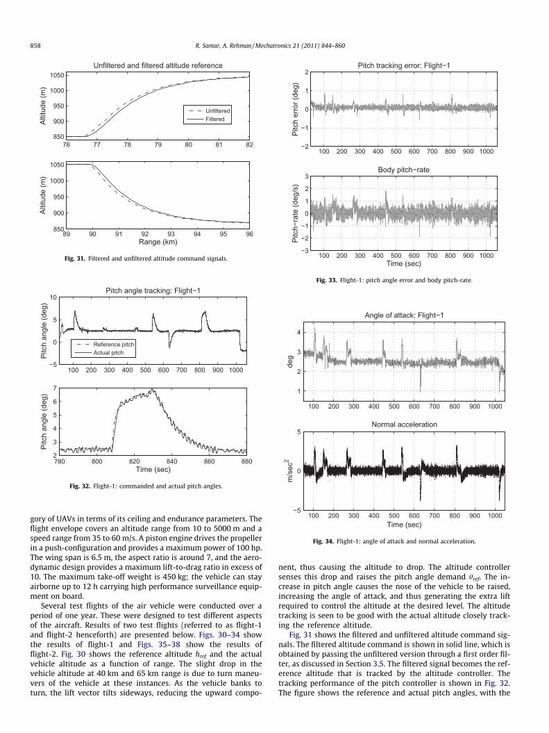
Fig. 31 shows the filtered and unfiltered altitude command sig-nals. The filtered altitude command is shown in solid line, which isobtained by passing the unfiltered version through a first order fil-ter, as discussed in Section 3.5. The filtered signal becomes the ref-erence altitude that is tracked by the altitude controller. Thetracking performance of the pitch controller is shown in Fig. 32.The figure shows the reference and actual pitch angles, with the

0 50 100 150 200 250600

800

1000

1200

1400

1600

1800

2000

2200

Altit

ude

(m)

Altitude tracking: Flight−2

Range (km)

Reference altitudeActual altitude

Fig. 35. Flight-2: commanded and actual altitudes.

200 400 600 800 1000 1200 1400 1600 1800

−2

0

2

4

6

8

Pitc

h an

gle

(deg

)

Pitch angle tracking: Flight−2

Reference pitchActual pitch

1380 1400 1420 1440 1460 1480 1500−2

−1

0

1

2

3

Time (sec)

Pitc

h an

gle

(deg

)

Fig. 36. Flight-2: commanded and actual pitch angles.

200 400 600 800 1000 1200 1400 1600 1800−1.5

−1

−0.5

0

0.5

1

1.5

Pitc

h er

ror (

deg)

Pitch tracking error: Flight−2

Time (sec)

Fig. 37. Flight-2: pitch angle error.

200 400 600 800 1000 1200 1400 1600 18001

2

3

4

5

6

deg

Angle of attack: Flight−2

200 400 600 800 1000 1200 1400 1600 1800−5

0

5Normal acceleration

m/s

ec2

Time (sec)

Fig. 38. Flight-2: angle of attack and normal acceleration.


lower half of the figure showing a zoomed view of the data. Excel-lent command following of the pitch angle is observed. It is seenthat an increase in href causes the altitude controller to generatea larger href, causing the vehicle to climb. Control of altitude isachieved through control of the pitch angle, and good pitch angletracking is seen to give tight altitude control. Fig. 33 shows the er-ror in the pitch angle (i.e., the difference between the reference andactual pitch angles). The error stays within ±1� demonstrating thepitch tracking performance. The body pitch-rate q (Section 4.1) isalso seen in the lower half of the figure. The angle of attack andthe normal acceleration of the vehicle are displayed in Fig. 34.The angle of attack sensor is installed for test purposes only, it isnot available as a standard sensor for feedback control. The corre-lation between the climb/descent maneuvers, the pitch angle, theangle of attack and normal acceleration can be clearly seen fromthe figures. During the climb phase the pitch angle is increasedwhich results in an increase in the angle of attack and the normalacceleration of the vehicle. The larger angle of attack generates thehigher lift required to climb. It may be noted that a separate speed

control system is also in operation throughout, which throttles theengine up and down to maintain the speed of the vehicle at a givenlevel.

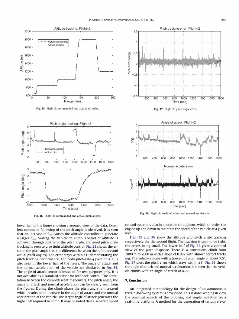
Figs. 35 and 36 show the altitude and pitch angle trackingrespectively, for the second flight. The tracking is seen to be tight,the errors being small. The lower half of Fig. 36 gives a zoomedview of the pitch response. There is a continuous climb from1000 m to 2000 m with a slope of 0.092 with almost perfect track-ing. The vehicle climbs with a (nose-up) pitch angle of about 7.5�.Fig. 37 plots the pitch error which stays within ±1�. Fig. 38 showsthe angle of attack and normal acceleration. It is seen that the vehi-cle climbs with an angle of attack of 4–5�.

7. Conclusion

An integrated methodology for the design of an autonomousterrain-following system is developed. This is done keeping in viewthe practical aspects of the problem, and implementation on areal-time platform. A method for the generation of terrain eleva-


tion data is given which takes into consideration the growing posi-tion uncertainty of the vehicle with range. An algorithm7 for ter-rain-following is next developed which is well-suited for onlinecomputation in autonomous flight. The entire route is broken downinto sections of given length, and the height of each section is com-puted. The climb/descend control effort can be adjusted by varyingthe section lengths. Altitude change points and heights are com-puted that do not violate practical vehicle constraints, while provid-ing the desired terrain clearance. The performance of this algorithmis found to compare favorably to an Optimal Spline algorithm. Thedesign of the tracking control system is next presented. A practicalmethod for pitch-rate estimation is given. Robust pitch angle andaltitude tracking controllers are designed, which maximize robust-ness against system parametric uncertainty. The controllers are seento perform well across the flight envelope of the vehicle. The designof an electromechanical servo actuator is discussed which is used toactuate the control surfaces (elevators) of the vehicle during flight.Finally flight test results are presented and discussed, these demon-strate the overall performance of the terrain-following guidance andcontrol system. Plans are underway to carry out more tests on asmaller vehicle with shorter and possibly more flexible missionrequirements. Although simulation results indicate no limitation ofthe proposed algorithms, however further testing on a range of mis-sion scenarios is planned to generate more experimental data.

References

[1] Funk J. Optimal-path precision terrain-following system. J Aircraft1977;14(2):128–34.

[2] Lu P, Pierson B. Optimal aircraft terrain-following analysis and trajectorygeneration. J Guid Control Dyn 1995;18(3):555–60.

[3] Lu P, Pierson B. Aircraft terrain following based on a nonlinear continuouspredictive control approach. J Guid Control Dyn 1995;18(4):817–23.

[4] Rippel E, Bar-Gill A, Shimkin N. Fast graph-search algorithms for general-aviation flight trajectory generation. J Guid Control Dyn 2005;28(4):801–11.

[5] Asseo S. Terrain following/terrain avoidance path optimization using themethod of steepest descent. In: Proceedings of the IEEE 1988 nationalaerospace and electronics conference (NAECON). Dayton (OH); 1988.

7 The basic algorithm is called the Stair algorithm; this is then augmented with atrajectory smoothing algorithm employing an exponential function and a low-passfilter.

[6] Waldock M, Roberts G, Sutton R. Terrain following control of an unmannedunderwater vehicle using artificial neural networks. In: Proceedings of the IEEcolloquium on control and guidance of remotely operated vehicles. London;1995.

[7] Twigg S, Calise A, Johnson, E. On-line trajectory optimization for autonomousair vehicles. In: Proceedings of the AIAA guidance navigation and controlconference. Austin, Texas; 2003

[8] Pettit R, Homer M. An autonomous threat evasion response algorithm forunmanned air vehicles during low altitude flight. In: Proceedings of the AIAA1st intelligent systems technical conference. Chicago; 2004.

[9] Rehman A, Shahzad A, Kamal W, Samar R. Techniques for terrain following ofautonomous vehicle. In: Proceedings of the 2nd European conference foraerospace sciences (EUCASS). Brussels; 2007.

[10] Hoffman J. Numerical methods for engineers and scientists. 2nd ed. NewYork: Marcel Dekker, Inc.; 2001.

[11] Betts J. Practical methods for optimal control using nonlinear programming.Society for Industrial and Applied Mathematics (SIAM); 2001.

[12] Fletcher R. Practical methods of optimization. John Wiley and Sons; 1987.[13] Kuchar J. Markov model of terrain for evaluation of ground proximity warning

system thresholds. J Guid Control Dyn 2001;24(3):428–35.[14] Mathews J. Numerical methods for mathematics, science, and engineering.

2nd ed. Englewood Cliffs (NJ, USA): Prentice-Hall; 1992.[15] McFarlane D, Glover K. A loop shaping design procedure using H1 synthesis.

IEEE Trans Autom Control 1992;37(6):759–69.[16] Tsai M, Geddes E, Postlethwaite I. Pole-zero cancellations and closed-loop

properties of an H1 mixed sensitivity design problem. Automatica1992;28(3):519–30.

[17] Samar R, Murad G, Postlethwaite I, Gu D-W. A discrete time H1 observer-basedcontroller and its application to a glass tube production process. Eur J Control1996;2:112–25.

[18] Smerlas A, Walker D, Postlethwaite I, Strange M, Howitt J, Gubbells A.Evaluating H1 controllers on the NRC Bell 205 fly-by-wire helicopter. ControlEng Pract 2001;9(1):1–10.

[19] Postlethwaite I, Prempain E, Turkoglu E, Turner M, Ellis K, Gubbells A. Designand flight testing of various H1 controllers for the Bell 205 helicopter. ControlEng Pract 2005;13:383–98.

[20] Skogestad S, Postlethwaite I. Multivariable feedback control analysis anddesign. 2nd ed. West Sussex, England: John Wiley & Sons; 2005.

[21] Samar R. Digital filters for gain stabilization of flexible vehicle dynamics. In:Proceedings of the 17th international federation of automatic control worldcongress. Seoul, South Korea; 2008.

[22] Glover K. All optimal Hankel-norm approximations of linear multivariablesystems and their L1-error bounds. Int J Control 1984;39(6):1115–93.

Autonomous terrain-following for unmanned air vehicles

Documents