Autonomous over-the-horizon navigation using LIDAR data

Auton RobotDOI 10.1007/s10514-012-9309-9

Autonomous over-the-horizon navigation using LIDAR data

Ioannis Rekleitis · Jean-Luc Bedwani · Erick Dupuis ·Tom Lamarche · Pierre Allard

Received: 4 February 2011 / Accepted: 8 September 2012© Her Majesty the Queen in Right of Canada 2012

Abstract In this paper we present the approach for au-tonomous planetary exploration developed at the CanadianSpace Agency. The goal of this work is to enable au-tonomous navigation to remote locations, well beyond thesensing horizon of the rover, with minimal interaction witha human operator. We employ LIDAR range sensors due totheir accuracy, long range and robustness in the harsh light-ing conditions of space. Irregular Triangular Meshes (ITMs)are used for representing the environment, providing an ac-curate, yet compact, spatial representation. In this paper anovel path-planning technique through the ITM is intro-duced, which guides the rover through flat terrain and safelyaway from obstacles. Experiments performed in CSA’s Marsemulation terrain, validating our approach, are also pre-sented.

Keywords Space robotics · Planetary exploration ·Mapping · Path planning

I. Rekleitis (�)School of Computer Science, McGill University, Montreal,QC, Canadae-mail: [email protected]

J.-L. BedwaniInstitut de recherche d’Hydro-Québec (IREQ), Varennes,QC, Canadae-mail: [email protected]

E. Dupuis · T. Lamarche · P. AllardCanadian Space Agency, Saint-Hubert, QC, Canada

E. Dupuise-mail: [email protected]

T. Lamarchee-mail: [email protected]

P. Allarde-mail: [email protected]

1 Introduction

Mobile robotics have enabled scientific breakthroughs inplanetary exploration (Maimone et al. 2006). Recent ac-complishments have demonstrated beyond doubt the neces-sity and feasibility of semi-autonomous rovers for conduct-ing scientific exploration on other planets. Both Mars Ex-ploration Rovers (MERs) “Spirit” and “Opportunity” havethe ability to detect and avoid obstacles, picking a path thattakes them along a safe trajectory. MER’s have traveled upto 300 m/sol. On occasion, the rovers have had to travel tolocations that were at the fringe of the horizon of their sen-sors or even slightly beyond.

The next rover missions to Mars are the “Mars ScienceLaboratory” (MSL) (Hayati et al. 2004; Volpe 2006) andESA’s ExoMars (Vago 2004). Both of these missions haveset target traverse distances on the order of one kilometerper day. Both the MSL and ExoMars rovers are thereforeexpected to drive regularly a significant distance beyond thehorizon of their environment sensors. Earth-based operatorswill therefore not know a-priori the detailed geometry ofthe environment and will thus not be able to select way-points for the rovers throughout their traverses. One of thekey technologies that will be required is the ability to senseand model the 3D environment in which the rover has tonavigate. To address the above mentioned issues, the Cana-dian Space Agency is developing a suite of technologies forlong-range rover navigation. For the purposes of this paper,“long-range” is defined as a traverse that takes the rover be-yond the horizon of the rover’s environment sensors.

The main contribution of this paper is the use of ITMs forconstructing accurate models of the environment and alsofor facilitating the efficient planing of trajectories that areoptimal for a set combination of constraints, such as dis-tance traveled, terrain accessibility, and ruggedness. LIDAR

Auton Robot

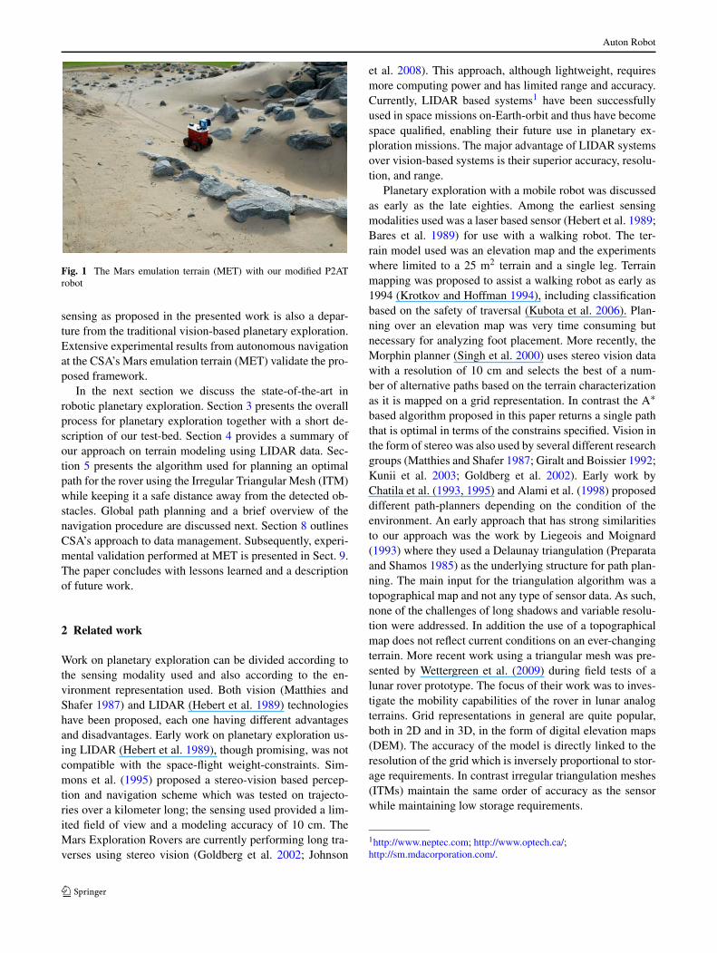
Fig. 1 The Mars emulation terrain (MET) with our modified P2ATrobot

sensing as proposed in the presented work is also a depar-ture from the traditional vision-based planetary exploration.Extensive experimental results from autonomous navigationat the CSA’s Mars emulation terrain (MET) validate the pro-posed framework.

In the next section we discuss the state-of-the-art inrobotic planetary exploration. Section 3 presents the overallprocess for planetary exploration together with a short de-scription of our test-bed. Section 4 provides a summary ofour approach on terrain modeling using LIDAR data. Sec-tion 5 presents the algorithm used for planning an optimalpath for the rover using the Irregular Triangular Mesh (ITM)while keeping it a safe distance away from the detected ob-stacles. Global path planning and a brief overview of thenavigation procedure are discussed next. Section 8 outlinesCSA’s approach to data management. Subsequently, experi-mental validation performed at MET is presented in Sect. 9.The paper concludes with lessons learned and a descriptionof future work.

2 Related work

Work on planetary exploration can be divided according tothe sensing modality used and also according to the en-vironment representation used. Both vision (Matthies andShafer 1987) and LIDAR (Hebert et al. 1989) technologieshave been proposed, each one having different advantagesand disadvantages. Early work on planetary exploration us-ing LIDAR (Hebert et al. 1989), though promising, was notcompatible with the space-flight weight-constraints. Sim-mons et al. (1995) proposed a stereo-vision based percep-tion and navigation scheme which was tested on trajecto-ries over a kilometer long; the sensing used provided a lim-ited field of view and a modeling accuracy of 10 cm. TheMars Exploration Rovers are currently performing long tra-verses using stereo vision (Goldberg et al. 2002; Johnson

et al. 2008). This approach, although lightweight, requiresmore computing power and has limited range and accuracy.Currently, LIDAR based systems1 have been successfullyused in space missions on-Earth-orbit and thus have becomespace qualified, enabling their future use in planetary ex-ploration missions. The major advantage of LIDAR systemsover vision-based systems is their superior accuracy, resolu-tion, and range.

Planetary exploration with a mobile robot was discussedas early as the late eighties. Among the earliest sensingmodalities used was a laser based sensor (Hebert et al. 1989;Bares et al. 1989) for use with a walking robot. The ter-rain model used was an elevation map and the experimentswhere limited to a 25 m2 terrain and a single leg. Terrainmapping was proposed to assist a walking robot as early as1994 (Krotkov and Hoffman 1994), including classificationbased on the safety of traversal (Kubota et al. 2006). Plan-ning over an elevation map was very time consuming butnecessary for analyzing foot placement. More recently, theMorphin planner (Singh et al. 2000) uses stereo vision datawith a resolution of 10 cm and selects the best of a num-ber of alternative paths based on the terrain characterizationas it is mapped on a grid representation. In contrast the A∗based algorithm proposed in this paper returns a single paththat is optimal in terms of the constrains specified. Vision inthe form of stereo was also used by several different researchgroups (Matthies and Shafer 1987; Giralt and Boissier 1992;Kunii et al. 2003; Goldberg et al. 2002). Early work byChatila et al. (1993, 1995) and Alami et al. (1998) proposeddifferent path-planners depending on the condition of theenvironment. An early approach that has strong similaritiesto our approach was the work by Liegeois and Moignard(1993) where they used a Delaunay triangulation (Preparataand Shamos 1985) as the underlying structure for path plan-ning. The main input for the triangulation algorithm was atopographical map and not any type of sensor data. As such,none of the challenges of long shadows and variable resolu-tion were addressed. In addition the use of a topographicalmap does not reflect current conditions on an ever-changingterrain. More recent work using a triangular mesh was pre-sented by Wettergreen et al. (2009) during field tests of alunar rover prototype. The focus of their work was to inves-tigate the mobility capabilities of the rover in lunar analogterrains. Grid representations in general are quite popular,both in 2D and in 3D, in the form of digital elevation maps(DEM). The accuracy of the model is directly linked to theresolution of the grid which is inversely proportional to stor-age requirements. In contrast irregular triangulation meshes(ITMs) maintain the same order of accuracy as the sensorwhile maintaining low storage requirements.

1http://www.neptec.com; http://www.optech.ca/;http://sm.mdacorporation.com/.

Auton Robot

Furthermore, different research groups have proposeda variety of schemes for planetary exploration addressingdifferent problems (Giralt and Boissier 1992). One impor-tant aspect is the control architecture used. JPL for exam-ple introduced two software architectures: CLARAty (Nes-nas et al. 2003) which has focused on module reusabilityand CAMPOUT (Huntsberger et al. 2003) with a focus onmulti-rover applications. Regardless of the sensing modalitysensor data preprocessing, terrain modeling, and path plan-ning (global and local) are major building blocks in mostapproaches, sometimes formulated as behaviors (Gat et al.1994).

More recently, Mora et al. (2008, 2009) proposed a simi-lar functionality to the one proposed in this paper, using dig-ital elevation maps (DEM) for lunar rovers. Global and localDEM’s were proposed, to be constructed from on-orbit im-agery, and from LIDAR scans from the rover. In addition aDijkstra based algorithm was presented taking into accountruggedness, slope, and distance. In this paper we presentan A* based planning algorithm which is much more effi-cient than the Dijkstra based one, because the search is bi-ased towards the goal and no calculations are consumed forcells in irrelevant directions. Further work (Ishigami et al.2011) used the previous approach to calculate and evaluateseveral alternative paths off-line considering different costfunctions.

Currently, the most advanced exploration robots that havebeen deployed for planetary exploration are the Mars Ex-ploration Rovers (MERs) “Spirit” and “Opportunity”. Theserovers have successfully demonstrated concepts such as vi-sual odometry and autonomous path selection from a terrainmodel acquired from sensor data (Biesiadecki et al. 2005).The main sensor suite used for terrain assessment for theMERs has been passive stereo vision (Wright et al. 2005).The models obtained through stereo imagery are used forboth automatic terrain assessment and visual odometry. Pathplanning is based on a variant of D* (Carsten et al. 2008)that facilitates efficient replanning. Due to high computationload visual odometry is rarely used on the MERs; a more ef-ficient algorithm was proposed for the Mars Science Labo-ratory mission that launched on November of 2011 (Johnsonet al. 2008).

In the case of automatic terrain assessment, the raw datain the form of a cloud of 3D points is used to evaluate thetraversability of the terrain immediately in front of the rover,defined as a regular grid of square patches. In the case ofvisual odometry, the model is used to identify and track fea-tures of the terrain to mitigate the effect of slip (Howard andTunstel 2006).

Field trials on a Mars analog site were presented by Bar-foot et al. (2011) comparing different guidance, navigation,and control (GN&C) approaches for a ground ice prospect-ing mission to Mars. The main sensing modality was again

stereo vision, and a teach and repeat path planning strategywas applied.

The problem of autonomous long range navigation isalso very important in terrestrial settings. The DARPA grandchallenge in 2005 resulted in several vehicles traveling 132miles over desert terrain (Montemerlo et al. 2006). The ma-jority of the contestants used a combination of multipleLIDAR, vision, and RADAR sensors. Similar work involvedtraverses on the order to 30 km in the Atacama desert (Wet-tergreen et al. 2005) using vision. More recently the “Leav-ing Flatland” project (Rusu et al. 2009) presented a visionbased scheme for a hexapod walking robot. LIDAR sensorshave also been used successfully for 3D mapping of under-ground mines (Silver et al. 2006). In addition to digital ele-vation maps, semantic labels were attached to the differentareas which facilitated gait selection. Terrestrial navigationhas vast literature which is beyond the scope of this paper;please refer to (Kelly et al. 2006) for a discussion of themany challenges and additional related work.

For our work, we have been using a laser range sensor(LIDAR) as the main sensing modality for many reasons:among others, our mobility platform has very low groundclearance. A LIDAR sensor is capable of providing rangedata to build terrain models with 1–2 cm accuracy. Such ac-curacy would be difficult to attain with most stereo visionsystems over the full range of measurement. Such accuracyis also very important for the scientific return of the missioni.e. identifying rock formations. In addition, LIDAR sensorsreturn accurate geometric information in three dimensionsin the form of a 3D point cloud without requiring additionalprocessing. Finally, since they do not rely on ambient light-ing, we do not have to address the problems arising fromadverse lighting conditions.

3 Overview

The goal of our work is to navigate autonomously from thecurrent position to an operator-specified location which lies

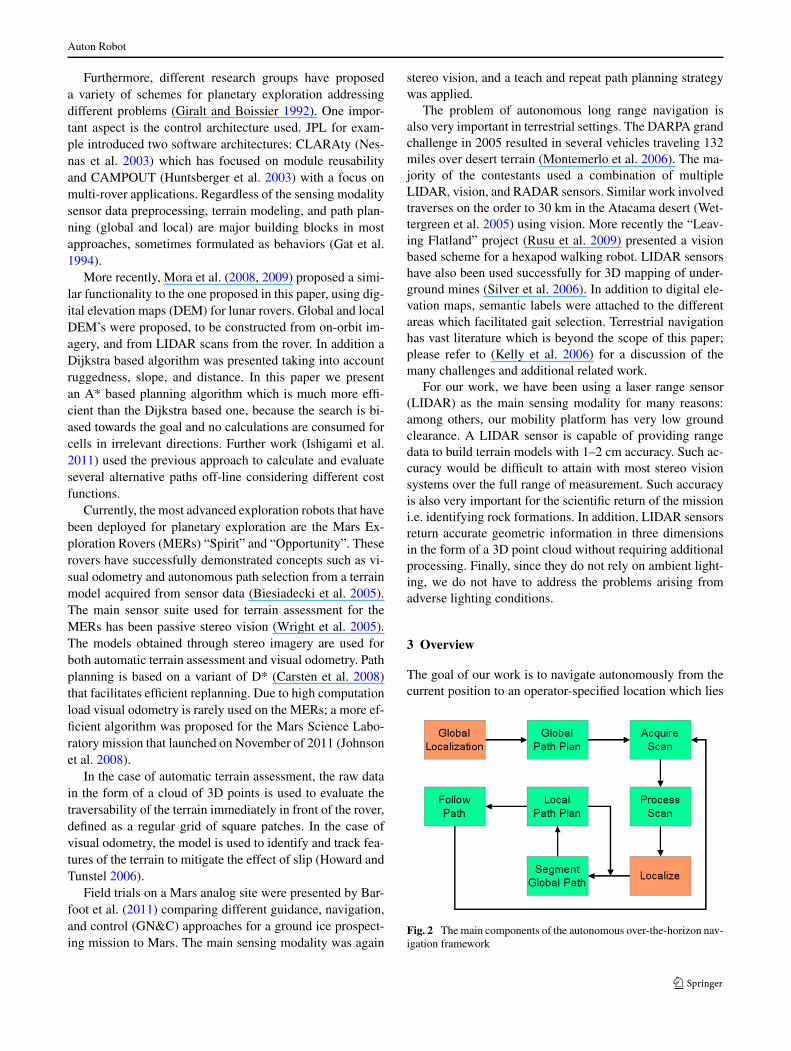
Fig. 2 The main components of the autonomous over-the-horizon nav-igation framework

Auton Robot

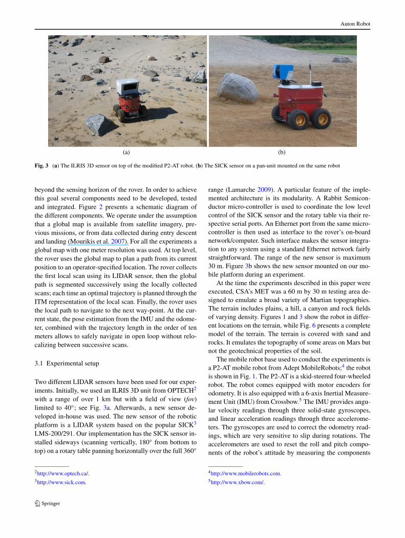
Fig. 3 (a) The ILRIS 3D sensor on top of the modified P2-AT robot. (b) The SICK sensor on a pan-unit mounted on the same robot

beyond the sensing horizon of the rover. In order to achievethis goal several components need to be developed, testedand integrated. Figure 2 presents a schematic diagram ofthe different components. We operate under the assumptionthat a global map is available from satellite imagery, pre-vious missions, or from data collected during entry descentand landing (Mourikis et al. 2007). For all the experiments aglobal map with one meter resolution was used. At top level,the rover uses the global map to plan a path from its currentposition to an operator-specified location. The rover collectsthe first local scan using its LIDAR sensor, then the globalpath is segmented successively using the locally collectedscans; each time an optimal trajectory is planned through theITM representation of the local scan. Finally, the rover usesthe local path to navigate to the next way-point. At the cur-rent state, the pose estimation from the IMU and the odome-ter, combined with the trajectory length in the order of tenmeters allows to safely navigate in open loop without relo-calizing between successive scans.

3.1 Experimental setup

Two different LIDAR sensors have been used for our exper-iments. Initially, we used an ILRIS 3D unit from OPTECH2

with a range of over 1 km but with a field of view (fov)limited to 40◦; see Fig. 3a. Afterwards, a new sensor de-veloped in-house was used. The new sensor of the roboticplatform is a LIDAR system based on the popular SICK3

LMS-200/291. Our implementation has the SICK sensor in-stalled sideways (scanning vertically, 180◦ from bottom totop) on a rotary table panning horizontally over the full 360◦

2http://www.optech.ca/.3http://www.sick.com.

range (Lamarche 2009). A particular feature of the imple-mented architecture is its modularity. A Rabbit Semicon-ductor micro-controller is used to coordinate the low levelcontrol of the SICK sensor and the rotary table via their re-spective serial ports. An Ethernet port from the same micro-controller is then used as interface to the rover’s on-boardnetwork/computer. Such interface makes the sensor integra-tion to any system using a standard Ethernet network fairlystraightforward. The range of the new sensor is maximum30 m. Figure 3b shows the new sensor mounted on our mo-bile platform during an experiment.

At the time the experiments described in this paper wereexecuted, CSA’s MET was a 60 m by 30 m testing area de-signed to emulate a broad variety of Martian topographies.The terrain includes plains, a hill, a canyon and rock fieldsof varying density. Figures 1 and 3 show the robot in differ-ent locations on the terrain, while Fig. 6 presents a completemodel of the terrain. The terrain is covered with sand androcks. It emulates the topography of some areas on Mars butnot the geotechnical properties of the soil.

The mobile robot base used to conduct the experiments isa P2-AT mobile robot from Adept MobileRobots;4 the robotis shown in Fig. 1. The P2-AT is a skid-steered four-wheeledrobot. The robot comes equipped with motor encoders forodometry. It is also equipped with a 6-axis Inertial Measure-ment Unit (IMU) from Crossbow.5 The IMU provides angu-lar velocity readings through three solid-state gyroscopes,and linear acceleration readings through three accelerome-ters. The gyroscopes are used to correct the odometry read-ings, which are very sensitive to slip during rotations. Theaccelerometers are used to reset the roll and pitch compo-nents of the robot’s attitude by measuring the components

4http://www.mobilerobots.com.5http://www.xbow.com/.

Auton Robot

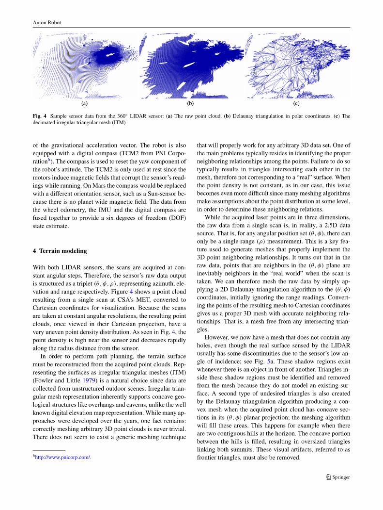
Fig. 4 Sample sensor data from the 360◦ LIDAR sensor: (a) The raw point cloud. (b) Delaunay triangulation in polar coordinates. (c) Thedecimated irregular triangular mesh (ITM)

of the gravitational acceleration vector. The robot is alsoequipped with a digital compass (TCM2 from PNI Corpo-ration6). The compass is used to reset the yaw component ofthe robot’s attitude. The TCM2 is only used at rest since themotors induce magnetic fields that corrupt the sensor’s read-ings while running. On Mars the compass would be replacedwith a different orientation sensor, such as a Sun-sensor be-cause there is no planet wide magnetic field. The data fromthe wheel odometry, the IMU and the digital compass arefused together to provide a six degrees of freedom (DOF)state estimate.

4 Terrain modeling

With both LIDAR sensors, the scans are acquired at con-stant angular steps. Therefore, the sensor’s raw data outputis structured as a triplet (θ,φ,ρ), representing azimuth, ele-vation and range respectively. Figure 4 shows a point cloudresulting from a single scan at CSA’s MET, converted toCartesian coordinates for visualization. Because the scansare taken at constant angular resolutions, the resulting pointclouds, once viewed in their Cartesian projection, have avery uneven point density distribution. As seen in Fig. 4, thepoint density is high near the sensor and decreases rapidlyalong the radius distance from the sensor.

In order to perform path planning, the terrain surfacemust be reconstructed from the acquired point clouds. Rep-resenting the surfaces as irregular triangular meshes (ITM)(Fowler and Little 1979) is a natural choice since data arecollected from unstructured outdoor scenes. Irregular trian-gular mesh representation inherently supports concave geo-logical structures like overhangs and caverns, unlike the wellknown digital elevation map representation. While many ap-proaches were developed over the years, one fact remains:correctly meshing arbitrary 3D point clouds is never trivial.There does not seem to exist a generic meshing technique

6http://www.pnicorp.com/.

that will properly work for any arbitrary 3D data set. One ofthe main problems typically resides in identifying the properneighboring relationships among the points. Failure to do sotypically results in triangles intersecting each other in themesh, therefore not corresponding to a “real” surface. Whenthe point density is not constant, as in our case, this issuebecomes even more difficult since many meshing algorithmsmake assumptions about the point distribution at some level,in order to determine these neighboring relations.

While the acquired laser points are in three dimensions,the raw data from a single scan is, in reality, a 2.5D datasource. That is, for any angular position set (θ,φ), there canonly be a single range (ρ) measurement. This is a key fea-ture used to generate meshes that properly implement the3D point neighboring relationships. It turns out that in theraw data, points that are neighbors in the (θ,φ) plane areinevitably neighbors in the “real world” when the scan istaken. We can therefore mesh the raw data by simply ap-plying a 2D Delaunay triangulation algorithm to the (θ,φ)

coordinates, initially ignoring the range readings. Convert-ing the points of the resulting mesh to Cartesian coordinatesgives us a proper 3D mesh with accurate neighboring rela-tionships. That is, a mesh free from any intersecting trian-gles.

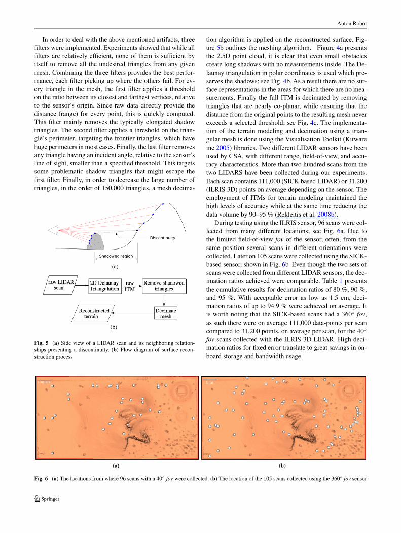
However, we now have a mesh that does not contain anyholes, even though the real surface sensed by the LIDARusually has some discontinuities due to the sensor’s low an-gle of incidence; see Fig. 5a. These shadow regions existwhenever there is an object in front of another. Triangles in-side these shadow regions must be identified and removedfrom the mesh because they do not model an existing sur-face. A second type of undesired triangles is also createdby the Delaunay triangulation algorithm producing a con-vex mesh when the acquired point cloud has concave sec-tions in its (θ,φ) planar projection; the meshing algorithmwill fill these areas. This happens for example when thereare two contiguous hills at the horizon. The concave portionbetween the hills is filled, resulting in oversized triangleslinking both summits. These visual artifacts, referred to asfrontier triangles, must also be removed.

Auton Robot

In order to deal with the above mentioned artifacts, threefilters were implemented. Experiments showed that while allfilters are relatively efficient, none of them is sufficient byitself to remove all the undesired triangles from any givenmesh. Combining the three filters provides the best perfor-mance, each filter picking up where the others fail. For ev-ery triangle in the mesh, the first filter applies a thresholdon the ratio between its closest and farthest vertices, relativeto the sensor’s origin. Since raw data directly provide thedistance (range) for every point, this is quickly computed.This filter mainly removes the typically elongated shadowtriangles. The second filter applies a threshold on the trian-gle’s perimeter, targeting the frontier triangles, which havehuge perimeters in most cases. Finally, the last filter removesany triangle having an incident angle, relative to the sensor’sline of sight, smaller than a specified threshold. This targetssome problematic shadow triangles that might escape thefirst filter. Finally, in order to decrease the large number oftriangles, in the order of 150,000 triangles, a mesh decima-

Fig. 5 (a) Side view of a LIDAR scan and its neighboring relation-ships presenting a discontinuity. (b) Flow diagram of surface recon-struction process

tion algorithm is applied on the reconstructed surface. Fig-ure 5b outlines the meshing algorithm. Figure 4a presentsthe 2.5D point cloud, it is clear that even small obstaclescreate long shadows with no measurements inside. The De-launay triangulation in polar coordinates is used which pre-serves the shadows; see Fig. 4b. As a result there are no sur-face representations in the areas for which there are no mea-surements. Finally the full ITM is decimated by removingtriangles that are nearly co-planar, while ensuring that thedistance from the original points to the resulting mesh neverexceeds a selected threshold; see Fig. 4c. The implementa-tion of the terrain modeling and decimation using a trian-gular mesh is done using the Visualisation Toolkit (Kitwareinc 2005) libraries. Two different LIDAR sensors have beenused by CSA, with different range, field-of-view, and accu-racy characteristics. More than two hundred scans from thetwo LIDARS have been collected during our experiments.Each scan contains 111,000 (SICK based LIDAR) or 31,200(ILRIS 3D) points on average depending on the sensor. Theemployment of ITMs for terrain modeling maintained thehigh levels of accuracy while at the same time reducing thedata volume by 90–95 % (Rekleitis et al. 2008b).

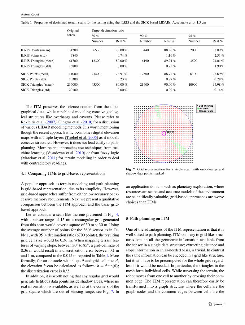
During testing using the ILRIS sensor, 96 scans were col-lected from many different locations; see Fig. 6a. Due tothe limited field-of-view fov of the sensor, often, from thesame position several scans in different orientations werecollected. Later on 105 scans were collected using the SICK-based sensor, shown in Fig. 6b. Even though the two sets ofscans were collected from different LIDAR sensors, the dec-imation ratios achieved were comparable. Table 1 presentsthe cumulative results for decimation ratios of 80 %, 90 %,and 95 %. With acceptable error as low as 1.5 cm, deci-mation ratios of up to 94.9 % were achieved on average. Itis worth noting that the SICK-based scans had a 360◦ fov,as such there were on average 111,000 data-points per scancompared to 31,200 points, on average per scan, for the 40◦fov scans collected with the ILRIS 3D LIDAR. High deci-mation ratios for fixed error translate to great savings in on-board storage and bandwidth usage.

Fig. 6 (a) The locations from where 96 scans with a 40◦ fov were collected. (b) The location of the 105 scans collected using the 360◦ fov sensor

Auton Robot

Table 1 Properties of decimated terrain scans for the testing using the ILRIS and the SICK based LIDARs. Acceptable error 1.5 cm

Originalscans

Target decimation ratio

80 % 90 % 95 %

Number Real % Number Real % Number Real %

ILRIS Points (mean) 31200 6530 79.00 % 3440 88.86 % 2090 93.09 %

ILRIS Points (std) 7840 0.74 % 1.16 % 2.31 %

ILRIS Triangles (mean) 61700 12300 80.00 % 6190 89.91 % 3590 94.01 %

ILRIS Triangles (std) 15800 0.00 % 0.75 % 1.90 %

SICK Points (mean) 111000 23400 78.91 % 12500 88.72 % 6700 93.69 %

SICK Points (std) 10300 0.23 % 0.27 % 0.28 %

SICK Triangles (mean) 216000 43300 80.00 % 21600 90.00 % 10900 94.98 %

SICK Triangles (std) 20100 0.00 % 0.00 % 0.14 %

The ITM preserves the science content from the topo-graphical data, while capable of modeling concave geolog-ical structures like overhangs and caverns. Please refer toRekleitis et al. (2007), Gingras et al. (2010) for a discussionof various LIDAR modeling methods. It is worth mentioningthough the recent approach which combines digital elevationmaps with multiple layers (Triebel et al. 2006) as it modelsconcave structures. However, it does not lead easily to path-planning. More recent approaches use techniques from ma-chine learning (Vasudevan et al. 2010) or from fuzzy logic(Mandow et al. 2011) for terrain modeling in order to dealwith contradictory readings.

4.1 Comparing ITMs to grid-based representations

A popular approach to terrain modeling and path planningis grid-based representation, due to its simplicity. However,grid-based approaches suffer from either low accuracy or ex-cessive memory requirements. Next we present a qualitativecomparison between the ITM approach and the basic grid-based approach.

Let us consider a scan like the one presented in Fig. 4,with a sensor range of 15 m; a rectangular grid generatedfrom this scan would cover a square of 30 m × 30 m. Usingthe average number of points for the 360◦ sensor as in Ta-ble 1, with 95 % decimation ratio (6700 points), the resultinggrid cell size would be 0.36 m. When mapping terrain fea-tures of varying slope, between 30◦ to 85◦, a grid-cell size of0.36 m would result in a discretization error between 0.1 mand 1 m, compared to the 0.015 m reported in Table 1. Moreformally, for an obstacle with slope θ and grid cell size d ,the elevation h can be calculated as follows: h = d tan(θ);the discretization error is h/2.

In addition, it is worth noting that any regular grid wouldgenerate fictitious data points inside shadow areas, where noreal information is available, as well as at the corners of thegrid square which are out of sensing range; see Fig. 7. In

Fig. 7 Grid representation for a single scan, with out-of-range andshadow data points marked

an application domain such as planetary exploration, whereresources are scarce and accurate models of the environmentare scientifically valuable, grid-based approaches are worsechoices than ITMs.

5 Path planning on ITM

One of the advantages of the ITM representation is that it iswell suited to path planning. ITM contrary to grid like struc-tures contain all the geometric information available fromthe sensor in a single data structure; extracting distance andslope information in an as-needed basis, is trivial. In contrastthe same information can be encoded in a grid like structure,but it will have to be precomputed for the whole grid regard-less if it would be needed. In particular, the triangles in themesh form individual cells. While traversing the terrain, therobot moves from one cell to another by crossing their com-mon edge. The ITM representation can therefore easily betransformed into a graph structure where the cells are thegraph nodes and the common edges between cells are the

Auton Robot

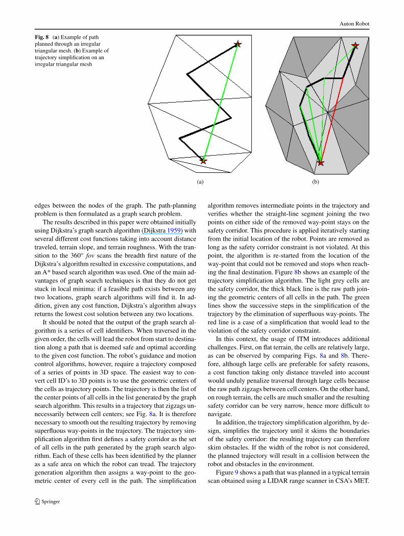
Fig. 8 (a) Example of pathplanned through an irregulartriangular mesh. (b) Example oftrajectory simplification on anirregular triangular mesh

edges between the nodes of the graph. The path-planningproblem is then formulated as a graph search problem.

The results described in this paper were obtained initiallyusing Dijkstra’s graph search algorithm (Dijkstra 1959) withseveral different cost functions taking into account distancetraveled, terrain slope, and terrain roughness. With the tran-sition to the 360◦ fov scans the breadth first nature of theDijkstra’s algorithm resulted in excessive computations, andan A* based search algorithm was used. One of the main ad-vantages of graph search techniques is that they do not getstuck in local minima: if a feasible path exists between anytwo locations, graph search algorithms will find it. In ad-dition, given any cost function, Dijkstra’s algorithm alwaysreturns the lowest cost solution between any two locations.

It should be noted that the output of the graph search al-gorithm is a series of cell identifiers. When traversed in thegiven order, the cells will lead the robot from start to destina-tion along a path that is deemed safe and optimal accordingto the given cost function. The robot’s guidance and motioncontrol algorithms, however, require a trajectory composedof a series of points in 3D space. The easiest way to con-vert cell ID’s to 3D points is to use the geometric centers ofthe cells as trajectory points. The trajectory is then the list ofthe center points of all cells in the list generated by the graphsearch algorithm. This results in a trajectory that zigzags un-necessarily between cell centers; see Fig. 8a. It is thereforenecessary to smooth out the resulting trajectory by removingsuperfluous way-points in the trajectory. The trajectory sim-plification algorithm first defines a safety corridor as the setof all cells in the path generated by the graph search algo-rithm. Each of these cells has been identified by the planneras a safe area on which the robot can tread. The trajectorygeneration algorithm then assigns a way-point to the geo-metric center of every cell in the path. The simplification

algorithm removes intermediate points in the trajectory andverifies whether the straight-line segment joining the twopoints on either side of the removed way-point stays on thesafety corridor. This procedure is applied iteratively startingfrom the initial location of the robot. Points are removed aslong as the safety corridor constraint is not violated. At thispoint, the algorithm is re-started from the location of theway-point that could not be removed and stops when reach-ing the final destination. Figure 8b shows an example of thetrajectory simplification algorithm. The light grey cells arethe safety corridor, the thick black line is the raw path join-ing the geometric centers of all cells in the path. The greenlines show the successive steps in the simplification of thetrajectory by the elimination of superfluous way-points. Thered line is a case of a simplification that would lead to theviolation of the safety corridor constraint.

In this context, the usage of ITM introduces additionalchallenges. First, on flat terrain, the cells are relatively large,as can be observed by comparing Figs. 8a and 8b. There-fore, although large cells are preferable for safety reasons,a cost function taking only distance traveled into accountwould unduly penalize traversal through large cells becausethe raw path zigzags between cell centers. On the other hand,on rough terrain, the cells are much smaller and the resultingsafety corridor can be very narrow, hence more difficult tonavigate.

In addition, the trajectory simplification algorithm, by de-sign, simplifies the trajectory until it skims the boundariesof the safety corridor: the resulting trajectory can thereforeskim obstacles. If the width of the robot is not considered,the planned trajectory will result in a collision between therobot and obstacles in the environment.

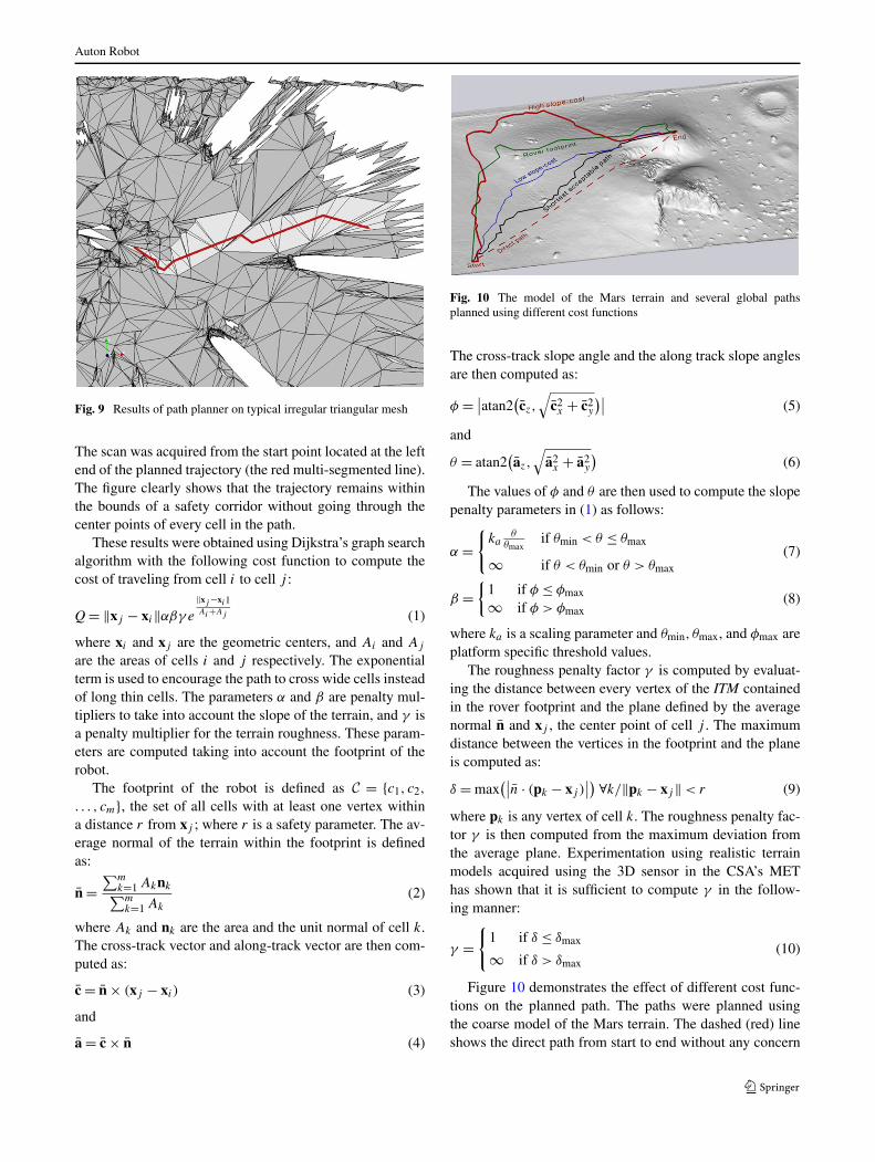
Figure 9 shows a path that was planned in a typical terrainscan obtained using a LIDAR range scanner in CSA’s MET.

Auton Robot

Fig. 9 Results of path planner on typical irregular triangular mesh

The scan was acquired from the start point located at the leftend of the planned trajectory (the red multi-segmented line).The figure clearly shows that the trajectory remains withinthe bounds of a safety corridor without going through thecenter points of every cell in the path.

These results were obtained using Dijkstra’s graph searchalgorithm with the following cost function to compute thecost of traveling from cell i to cell j :

Q = ‖xj − xi‖αβγ e

‖xj −xi‖Ai+Aj (1)

where xi and xj are the geometric centers, and Ai and Aj

are the areas of cells i and j respectively. The exponentialterm is used to encourage the path to cross wide cells insteadof long thin cells. The parameters α and β are penalty mul-tipliers to take into account the slope of the terrain, and γ isa penalty multiplier for the terrain roughness. These param-eters are computed taking into account the footprint of therobot.

The footprint of the robot is defined as C = {c1, c2,

. . . , cm}, the set of all cells with at least one vertex withina distance r from xj ; where r is a safety parameter. The av-erage normal of the terrain within the footprint is definedas:

n =∑m

k=1 Aknk∑m

k=1 Ak

(2)

where Ak and nk are the area and the unit normal of cell k.The cross-track vector and along-track vector are then com-puted as:

c = n × (xj − xi ) (3)

and

a = c × n (4)

Fig. 10 The model of the Mars terrain and several global pathsplanned using different cost functions

The cross-track slope angle and the along track slope anglesare then computed as:

φ = ∣∣atan2

(cz,

√c2x + c2

y

)∣∣ (5)

and

θ = atan2(az,

√a2x + a2

y

)(6)

The values of φ and θ are then used to compute the slopepenalty parameters in (1) as follows:

α ={

kaθ

θmaxif θmin < θ ≤ θmax

∞ if θ < θmin or θ > θmax

(7)

β ={

1 if φ ≤ φmax

∞ if φ > φmax(8)

where ka is a scaling parameter and θmin, θmax, and φmax areplatform specific threshold values.

The roughness penalty factor γ is computed by evaluat-ing the distance between every vertex of the ITM containedin the rover footprint and the plane defined by the averagenormal n and xj , the center point of cell j . The maximumdistance between the vertices in the footprint and the planeis computed as:

δ = max(∣∣n · (pk − xj )

∣∣) ∀k/‖pk − xj‖ < r (9)

where pk is any vertex of cell k. The roughness penalty fac-tor γ is then computed from the maximum deviation fromthe average plane. Experimentation using realistic terrainmodels acquired using the 3D sensor in the CSA’s METhas shown that it is sufficient to compute γ in the follow-ing manner:

γ ={

1 if δ ≤ δmax

∞ if δ > δmax(10)

Figure 10 demonstrates the effect of different cost func-tions on the planned path. The paths were planned usingthe coarse model of the Mars terrain. The dashed (red) lineshows the direct path from start to end without any concern

Auton Robot

about the slope or the roughness of the terrain. For the restof the paths only acceptable triangles were considered, thatis, triangles with an absolute slope of less than 35 degrees.The (green) line labeled “Rover footprint” plans a path tak-ing into account the rover footprint avoiding high-slope ar-eas and showing a slight preference for flatter terrain. Fi-nally, three paths are planned without taking into accountthe rover’s footprint. The shortest acceptable path planned(black line) is close to the direct path while avoiding thecliff due to the infinite cost of high slope triangles. The sec-ond path (blue line) is planned with low slope-cost for ac-ceptable slopes, and the third path (red line) weights flatterrain much higher than distance traveled, thus travelingaround the terrain over the most flat areas. While parame-ters selected by an expert operator have been used in mostrough-terrain navigation approaches, newer research showspromising results using parameters learned by demonstra-tion (Silver et al. 2010). We expect future work to evolvetowards automatic cost function learning.

As mentioned earlier, one of the issues encountered dur-ing our field-testing was due to the fact that the environ-ment sensor has a 360◦ fov and the Dijkstra’s graph searchalgorithm is a breadth-first algorithm: it grows the searchspace from the start location irrespective of the target des-tination. The planner ends up spending much precious timesearching in the direction away from the destination. TheA* graph search algorithm was used in an attempt to reducethe computation time. Experimental results indicate that, us-ing typical terrain models, the computation time can be ac-celerated by a factor of three up to six times on the samecomputer. The path-planner using A* was also tested off-line using the collected scans from the SICK based sensor.Random destination points were selected at five and ten me-ters from the location the scan was originated for all 107scans. The computation time was on average 14 seconds forthe destinations at five meters, and 25 seconds for ten me-ters. The proposed planning method was very efficient, thepaths were computed in seconds using ITMs with severalthousand triangles, and the computed paths were on average25 % longer than a straight line between start and destination(Rekleitis et al. 2008b). As noted earlier, a path was alwaysfound if a feasible path, for a given cost function, existed.For an in-depth discussion of the CSA’s path-planning ap-proach, including the implementation of different cost func-tions, please refer to Rekleitis et al. (2008a).

6 Path-segmentation

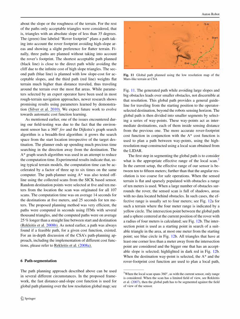
The path planning approach described above can be usedin several different circumstances. In the proposed frame-work, the fast distance-and-slope cost function is used forglobal path planning over the low resolution global map; see

Fig. 11 Global path planned using the low resolution map of theMars-like terrain at CSA

Fig. 11. The generated path while avoiding large slopes andbig obstacles leads over smaller obstacles, not discernible atthat resolution. This global path provides a general guide-line for traveling from the starting position to the operator-selected destination, beyond the robots sensing horizon. Theglobal path is then divided into smaller segments by select-ing a series of way-points. These way-points act as inter-mediate destinations, each of them inside sensing distancefrom the previous one. The more accurate rover-footprintcost function in conjunction with the A* cost function isused to plan a path between way-points, using the high-resolution map constructed using a local scan obtained fromthe LIDAR.

The first step in segmenting the global path is to considerwhat is the appropriate effective range of the local scan.7

In the current setup, the effective range of our sensor is be-tween ten to fifteen meters; further than that the angular res-olution is too coarse for safe operations. When the sensedterrain is flat and sparsely populated with obstacles a rangeof ten meters is used. When a large number of obstacles sur-rounds the rover, the sensed scan is full of shadows, areaswith no data located behind obstacles. In such cases, the ef-fective range is usually set to four meters; see Fig. 12a forsuch a terrain where the four meter range is indicated by ayellow circle. The intersection point between the global pathand a sphere centered at the current position of the rover witha radius of four meters is calculated; see Fig. 12b. The inter-section point is used as a starting point in search of a suit-able triangle in the area, at most one meter from the startingpoint; see blue circle in Fig. 12b. All triangles that have atleast one corner less than a meter away from the intersectionpoint are considered and the bigger one that has an accept-able slope is selected; highlighted in dark red in Fig. 12b.When the destination way-point is selected, the A* and therover-footprint cost function are used to plan a local path,

7When the local scan spans 360◦, as with the current sensor, only rangeis considered. When the scan has a limited field of view, see Rekleitiset al. (2007), then the global path has to be segmented against the fieldof view of the sensor.

Auton Robot

Fig. 12 (a) The global path (green), the local scan, the trajectory upto this point (red), the current position, and the four meter range thelocal path planner would use (yellow circle). (b) The intersection point

between the global path and the four meter range; the local area fromwhere the destination triangle (red) is selected (blue circle). (c) Thelocal path planned (blue)

through the decimated ITM, between the current pose andthe destination way-point; Fig. 12c.

7 Navigation

The algorithm presented in the previous section producesa set of straight-line segments representing the path. Thepiecewise linear path is then interpolated using a Catmull-Rom spline curve,8 with one way-point every half a meter,in order to produce a locally smooth trajectory. The resultingtrajectory is given as input to a low-level motion controllerbased on a discontinuous state feedback control law, initiallyproposed by Astolfi (1999). There were a few improvementsintroduced in order to increase the capabilities of our plat-form. When the IMU detects that the rover is moving uphill,the guidance controller increases the speed in order to gainmomentum. Furthermore, the guidance controller was tunedto reduce the turning in favor of forward motions.

8 Data management

During planetary exploration, an autonomous rover is re-quired to store and handle huge amounts of sensor data, re-sults from scientific experiments and other relevant informa-tion. This information is typically geo-referenced to mapsdescribing the world. As the number of maps increases, sim-ple planning operations become more complex because dif-ferent map combinations can be used to plan the path tothe goal. Data from different sensors, such as LIDAR range

8See http://www.mvps.org/directx/articles/catmull/.

finders, thermal cameras, images from monocular and stereocameras, etc., produce different maps. Moreover, data fromthe same sensor collected at different times and from dif-ferent locations produce maps of varying resolution and fi-delity. Effective management of the different maps is ad-dressed by CSA by the introduction of an Atlas framework.

The implemented Atlas framework supports typical map-ping, localization and planning operations performed by amobile robot. Central to the development is the ability toprovide a generic infrastructure to manage maps from mul-tiple sources. Changes in the map processing algorithms aretransparent to the Atlas implementation. In the same way,using maps from different sensor sources or types becomestransparent to the planning algorithm.

The main features of the Atlas management system arethe capability to dynamically manage a variety of data for-mats, the handling of uncertainty in the spatial relation-ship between the maps, the capability to provide series ofmaps linking two locations in planning operations, and thefunctionality to correlate maps in localization operations(Nsasi Bakambu et al. 2006). Figure 13 presents representa-tive data sets stored in the Atlas used at CSA for the exper-iments leading to the Avatar Explore mission (Martin et al.2008). Figure 13a contains a single infrared image which isused to detect geologically interesting locations for closerinspection by the rover. For this experiment, a heat sourcewas buried in the terrain to provide a clearly identifiable tar-get. A 360◦ LIDAR scan from a single location is displayedin Fig. 13b; such scans are used for safe path-planning bythe rover. Finally, Fig. 13c shows a uniform mesh represen-tation of the testing terrain. This representation is the resultof an off-line integration process that combines several datasets and can be uploaded on the rover by remote operators.

Auton Robot

Fig. 13 Maps from different sensors are stored in the Atlas framework: (a) Image from a thermal camera. (b) A single scan from a 360◦ LIDARsensor. (c) Topographical map of fixed resolution containing information of a larger region

Fig. 14 (a, b) Two LIDAR scans of an area with several obstacles. (c) The Irregular Triangular Mesh resulting from localizing with Kd-ICP andmerging the two scans, eliminating most of the shadows

This data management tool opens new opportunities inthe development of autonomous navigation schemes. For in-stance, maps are never fused by the system, thus permittingregistration of the maps at any time. The system makes itpossible for two given maps to have multiple mutual spa-tial relationships such as an estimation of their relative posefrom the wheel odometry and visual registration. The Atlassystem provides the mechanism to select/merge these mul-tiple estimation relations in order to get the best estimationpossible. The system being modular, it is possible to pro-vide different cost functions in order to obtain more accu-rate use of these multiple relations. Finally, by using rela-tive relations instead of global relations, the Atlas systemautomatically propagates to neighboring maps any improve-ments/changes deriving from the updated relation betweentwo maps. One of the important uses of the Atlas frameworkis to provide all available information of a specific area ofinterest. In particular, in presence of obstacles, most LIDARscans are plagued by long shadows that make path planningchallenging; see Figs. 14a, b. By requesting one or more ad-

ditional data sets from the Atlas for the vicinity of the area ofinterest, the rover is capable of merging the retrieved scansand obtaining a new mesh more suitable for path-planning,see Fig. 14c, where most of the shadows are eliminated. Thesearch query of scans covering a specific point is utilized forretrieving relevant scans.

9 Experimental results

The experiments were run at the CSA’s Mars emulation ter-rain (MET). A large number of experiments were conductedusing the ILRIS 3D LIDAR sensor with limited fov sen-sor. Subsequently, the 360◦ fov sensor enabled us to performseveral experiments validating CSA’s approach to fully au-tonomous over-the-horizon navigation. The first set of testsconducted was for validating the accuracy of the 3D odome-try state estimation algorithm. A large number of closed tra-jectories was executed varying in size and in location. Con-sequently, we were able to quantify the error exhibited in

Auton Robot

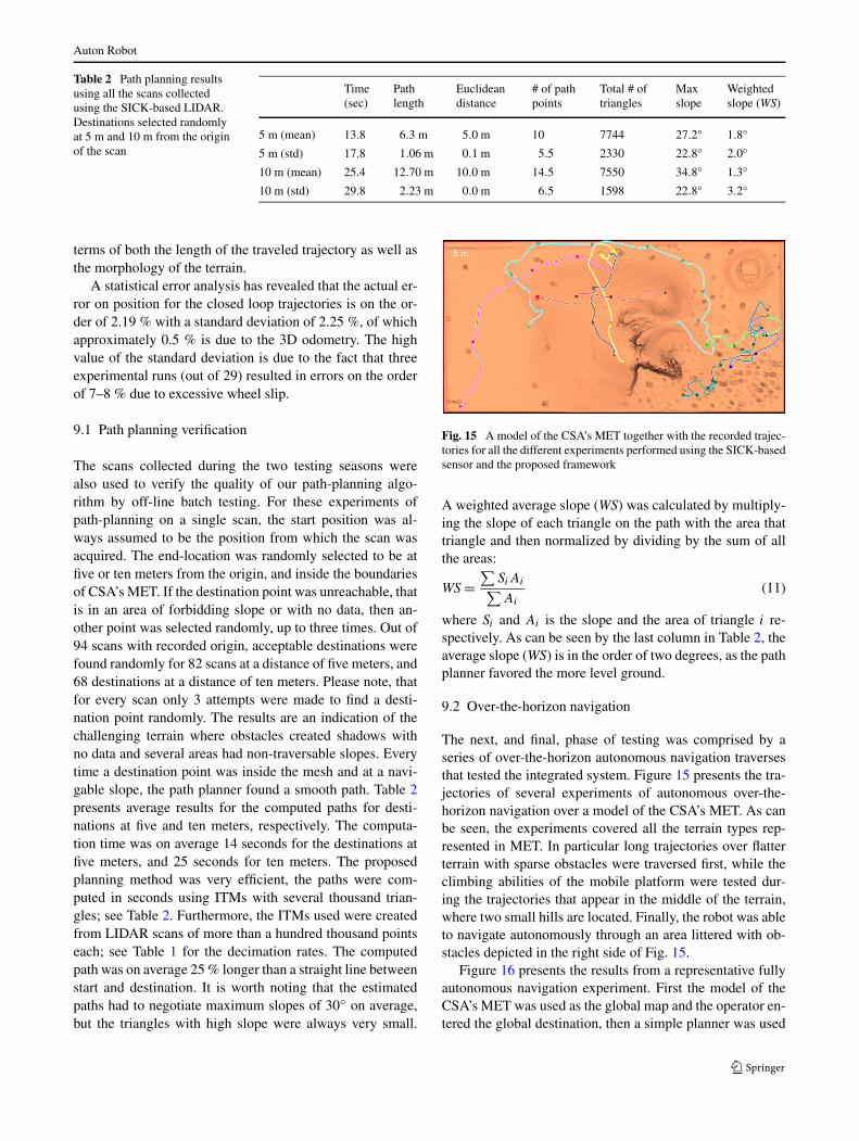
Table 2 Path planning resultsusing all the scans collectedusing the SICK-based LIDAR.Destinations selected randomlyat 5 m and 10 m from the originof the scan

Time(sec)

Pathlength

Euclideandistance

# of pathpoints

Total # oftriangles

Maxslope

Weightedslope (WS)

5 m (mean) 13.8 6.3 m 5.0 m 10 7744 27.2◦ 1.8◦

5 m (std) 17.8 1.06 m 0.1 m 5.5 2330 22.8◦ 2.0◦

10 m (mean) 25.4 12.70 m 10.0 m 14.5 7550 34.8◦ 1.3◦

10 m (std) 29.8 2.23 m 0.0 m 6.5 1598 22.8◦ 3.2◦

terms of both the length of the traveled trajectory as well asthe morphology of the terrain.

A statistical error analysis has revealed that the actual er-ror on position for the closed loop trajectories is on the or-der of 2.19 % with a standard deviation of 2.25 %, of whichapproximately 0.5 % is due to the 3D odometry. The highvalue of the standard deviation is due to the fact that threeexperimental runs (out of 29) resulted in errors on the orderof 7–8 % due to excessive wheel slip.

9.1 Path planning verification

The scans collected during the two testing seasons werealso used to verify the quality of our path-planning algo-rithm by off-line batch testing. For these experiments ofpath-planning on a single scan, the start position was al-ways assumed to be the position from which the scan wasacquired. The end-location was randomly selected to be atfive or ten meters from the origin, and inside the boundariesof CSA’s MET. If the destination point was unreachable, thatis in an area of forbidding slope or with no data, then an-other point was selected randomly, up to three times. Out of94 scans with recorded origin, acceptable destinations werefound randomly for 82 scans at a distance of five meters, and68 destinations at a distance of ten meters. Please note, thatfor every scan only 3 attempts were made to find a desti-nation point randomly. The results are an indication of thechallenging terrain where obstacles created shadows withno data and several areas had non-traversable slopes. Everytime a destination point was inside the mesh and at a navi-gable slope, the path planner found a smooth path. Table 2presents average results for the computed paths for desti-nations at five and ten meters, respectively. The computa-tion time was on average 14 seconds for the destinations atfive meters, and 25 seconds for ten meters. The proposedplanning method was very efficient, the paths were com-puted in seconds using ITMs with several thousand trian-gles; see Table 2. Furthermore, the ITMs used were createdfrom LIDAR scans of more than a hundred thousand pointseach; see Table 1 for the decimation rates. The computedpath was on average 25 % longer than a straight line betweenstart and destination. It is worth noting that the estimatedpaths had to negotiate maximum slopes of 30◦ on average,but the triangles with high slope were always very small.

Fig. 15 A model of the CSA’s MET together with the recorded trajec-tories for all the different experiments performed using the SICK-basedsensor and the proposed framework

A weighted average slope (WS) was calculated by multiply-ing the slope of each triangle on the path with the area thattriangle and then normalized by dividing by the sum of allthe areas:

WS =∑

SiAi∑

Ai

(11)

where Si and Ai is the slope and the area of triangle i re-spectively. As can be seen by the last column in Table 2, theaverage slope (WS) is in the order of two degrees, as the pathplanner favored the more level ground.

9.2 Over-the-horizon navigation

The next, and final, phase of testing was comprised by aseries of over-the-horizon autonomous navigation traversesthat tested the integrated system. Figure 15 presents the tra-jectories of several experiments of autonomous over-the-horizon navigation over a model of the CSA’s MET. As canbe seen, the experiments covered all the terrain types rep-resented in MET. In particular long trajectories over flatterterrain with sparse obstacles were traversed first, while theclimbing abilities of the mobile platform were tested dur-ing the trajectories that appear in the middle of the terrain,where two small hills are located. Finally, the robot was ableto navigate autonomously through an area littered with ob-stacles depicted in the right side of Fig. 15.

Figure 16 presents the results from a representative fullyautonomous navigation experiment. First the model of theCSA’s MET was used as the global map and the operator en-tered the global destination, then a simple planner was used

Auton Robot

Fig. 16 A sequence of consecutive scans together with the trajectoryof the robot. A global model of the Mars emulation terrain (MET) is setas background for reference purposes. (a) The global path is displayed(green line) together with a single scan, (b)–(g) the consecutive scans

can be seen together with the planned path. (h) The global path (green),the traversed path (red) and the odometry (black) are displayed on theCSA’s MET

to calculate the global path. Figure 16h shows all the paths;the global path is presented as a (green) line, and the plannedlocal paths together with the odometric estimates are drawn

as red and black lines respectively. Figure 16a presents thefirst scan and the first local path. The scan was used to de-termine the last point in the global path that resides inside it

Auton Robot

and is accessible from the start position; the selected point isthen designated as the first way-point. It is worth noting thatdue to the shadows, a point in the global path could reside in-side an isolated triangle in which case it would not be reach-able when used as a destination for the local-path-planner.The rover planned and executed a successful traversal andreached the first way point, at which step it took the secondscan; see Fig. 16b. The global path was used again to deter-mine the next local destination, second way point, and thelocal path planner was used to plan the second collision freepath. Finally when the robot reached the second way pointthe final destination from the global path plan was reachableand the robot planned and executed the next trajectories; seeFig. 16c–g.

10 Conclusions and future work

In this paper we presented successful autonomous over-the-horizon navigation experiments in a Mars-like terrain. Theoperator selected a destination way beyond the sensing hori-zon of our rover and then monitored as the robot selectedintermediate destinations, planned a safe path and traversedto the next way-point. The Irregular Triangular Mesh repre-sentation was used which enabled us to have a compact yetaccurate model of the environment. Path planning is con-ducted in the ITM terrain model using the A* graph searchalgorithm using a cost function that takes into account thephysical dimensions of the rover and its limitations to tra-verse rough terrain. A new factor was introduced in the costfunction to handle the conditions of ITM where safe terraincells are typically large in size. Experimental results demon-strating the feasibility of our approach are presented.

Upcoming work includes further research on localizationand scan matching. This will enable the rover to re-localizeby matching features in successive environment scans. Suchan approach has the potential to be computationally less ex-pensive than on-line visual odometry based on stereo cameraviews. Current work includes a re-formulation of the ITMterrain models to render them more amenable to scan match-ing algorithms such as the Iterative Closest Point algorithm(Rusinkiewicz and Levoy 2001).

The realization of autonomous navigation on a Mars-like environment, led to the recent mission Avatar-2. In theAvatar-2 mission (Martin et al. 2008; Dupuis et al. 2010),that completed successfully recently, a Canadian astronauton-orbit in the International Space Station (ISS) communi-cates and sends high level commands to a rover operating atCSA’s MET. The rover collects data from different sensorsand sends them back to ISS. This scenario emulates the situ-ation of a human operator on orbit around Mars, controllinga rover on the Martian surface.

References

Kitware inc. (2005). Visualization toolkits. http://www.vtk.org, Web-site (accessed: September 2005).

Alami, R., Chatila, R., Fleury, S., Ghallab, M., & Ingrand, F. (1998).An architecture for autonomy. The International Journal ofRobotics Research, 17(4), 315–337.

Astolfi, A. (1999). Exponential stabilization of wheeled mobile robotvia discontinuous control. Journal of Dynamic Systems Measure-ment and Control, 121–126.

Bares, J., Hebert, M., Kanade, T., Krotkov, E., Mitchell, T., Simmons,R., & Whittaker, W. (1989). Ambler: an autonomous rover forplanetary exploration. IEEE Computer, 22(6), 18–26.

Barfoot, T., Furgale, P., Stenning, B., Carle, P., Thomson, L., Osinski,G., Daly, M., & Ghafoor, N. (2011). Field testing of a rover guid-ance, navigation, and control architecture to support a ground-iceprospecting mission to Mars. Robotics and Autonomous Systems,59(6), 472–488. doi:10.1016/j.robot.2011.03.004.

Biesiadecki, J., Leger, C., & Maimone, M. (2005). Tradeoffs betweendirected and autonomous on the mars exploration rovers. In Proc.of int. symposium of robotics research, San Francisco.

Carsten, J., Rankin, A., Ferguson, D., & Stentz, A. (2008). Global plan-ning on the mars exploration rovers: software integration and sur-face testing. Journal of Field Robotics, 26(4), 337–357.

Chatila, R., Alami, R., Lacroix, S., Perret, J., & Proust, C. (1993).Planet exploration by robots: from mission planning to au-tonomous navigation. In 1993 international conference on ad-vanced robotics, Tokyo (Japan).

Chatila, R., Lacroix, S., Siméon, T., & Herrb, M. (1995). Planetaryexploration by a mobile robot: mission teleprogramming and au-tonomous navigation. Autonomous Robots Journal, 2(4), 333–344.

Dijkstra, E. W. (1959). A note on two problems in connexion withgraphs. Numerische Mathematik, 1, 269–271.

Dupuis, E., Langlois, P., Bedwani, J. L., Gingras, D., Salerno, A., Al-lard, P., Gemme, S., L’Archevêque, R., & Lamarche, T. (2010).The avatar explore experiments: results and lessons learned. InTenth international symposium on artificial intelligence, roboticsand automation in space (i-SAIRAS), Hokkoido, Japan.

Fowler, R. J., & Little, J. J. (1979). Automatic extraction of irregularnetwork digital terrain models. In SIGGRAPH’79: proc. of the 6thannual conference on computer graphics & interactive techniques(pp. 199–207).

Gat, E., Desai, R., Ivlev, R., Loch, J., & Miller, D. (1994). Behaviorcontrol for robotic exploration of planetary surfaces. IEEE Trans-actions on Robotics and Automation, 10(4), 490–503.

Gingras, D., Lamarche, T., Bedwani, J. L., & Dupuis, E. (2010).Rough terrain reconstruction for rover motion planning. In Sev-enth Canadian conference computer and robot vision, Ottawa,Canada (pp. 191–198).

Giralt, G., & Boissier, L. (1992). The French planetary rover VAP: con-cept and current developments. In Proc. of the 1992 lEEE/RSJ int.conf. on intelligent robots and systems (Vol. 2, pp. 1391–1398).

Goldberg, S., Maimone, M., & Matthies, L. (2002). Stereo vision androver navigation software for planetary exploration. In Proc. ofIEEE aerospace conf. (Vol. 5, pp. 2025–2036).

Hayati, S., Udomkesmalee, G., & Caffrey, R. (2004). Initiating the2002 mars science laboratory (MSL) focused technology pro-gram. In IEEE aerospace conf., Golden, CO, USA.

Hebert, M., et al. (1989). Terrain mapping for a roving planetary ex-plorer. In Proc. of the IEEE int. conf. on robotics and automation(ICRA’89) (Vol. 2, pp. 997–1002).

Howard, A. M. & Tunstel, E. W. (Eds.) (2006). Intelligence for spacerobotics. San Antonio: TSI Press. Chapter: MER surface naviga-tion and mobility.

Auton Robot

Huntsberger, T., Pirjanian, P., Trebi-Ollennu, A., Nayar, H. D., Ag-hazarian, H., Ganino, A., Garrett, M., Joshi, S., & Schenker, P.(2003). Campout: a control architecture for tightly coupled coor-dination of multirobot systems for planetary surface exploration.IEEE Transactions on Systems, Man and Cybernetics. Part A. Sys-tems and Humans, 33(5), 550–559.

Ishigami, G., Nagatani, K., & Yoshida, K. (2011). Path planning andevaluation for planetary rovers based on dynamic mobility index.In IEEE/RSJ international conference on intelligent robots andsystems (pp. 601–606).

Johnson, A., Goldberg, S., Yang, C., & Matthies, L. (2008). Robust andefficient stereo feature tracking for visual odometry. In IEEE int.conf. on robotics and automation (pp. 39–46).

Kelly, A., et al. (2006). Toward reliable off-road autonomous vehiclesoperating in challenging environments. The International Journalof Robotics Research, 25(5–6), 449–483.

Krotkov, E., & Hoffman, R. (1994). Terrain mapping for a walkingplanetary rover. IEEE Trans. on Robotics & Automation, 10(6).

Kubota, T., Ejiri, R., Kunii, Y., & Nakatani, I. (2006). Autonomousbehavior planning scheme for exploration rover. In Second IEEEint. conf. on space mission challenges for information technology(SMC-IT 2006) (p. 7).

Kunii, Y., Tsuji, S., & Watari, M. (2003). Accuracy improvement ofshadow range finder: SRF for 3D surface measurement. In Proc.of IEEE/RSJ int. conf. on intelligent robots and systems (IROS2003) (Vol. 3, pp. 3041–3046).

Lamarche, T. (2009). Conception et prototypage d’un capteur LIDAR3D pour la robotique mobile. Master’s thesis, Ecole Polytech-nique de Montréal.

Liegeois, A., & Moignard, C. (1993). Lecture notes in computer sci-ence: Vol. 708. Geometric reasoning for perception and action(pp. 51–65). Berlin: Springer. Chapter: Optimal motion planningof a mobile robot on a triangulated terrain model.

Maimone, M., Biesiadecki, J., Tunstel, E., Cheng, Y., & Leger, C.(2006). Int. for space robotics (pp. 45–69). San Antonio: TSIPress. Chapter: Surface navigation and mobility intelligence onthe Mars exploration rovers.

Mandow, A., Cantador, T., Garcia-Cerezo, A., Reina, A., Martinez, J.,& Morales, J. (2011). Fuzzy modeling of natural terrain elevationfrom a 3D scanner point cloud. In IEEE 7th international sympo-sium on intelligent signal processing (pp. 1–5).

Martin, E., L’Archevêque, R., Gemme, S., Rekleitis, I., & Dupuis, E.(2008). The avatar project: remote robotic operations conductedfrom the international space station. IEEE Robotics & AutomationMagazine, 14(4), 20–27.

Matthies, L., & Shafer, S. (1987). Error modeling in stereo navigation.IEEE Journal of Robotics and Automation, 3(3), 239–250.

Montemerlo, M., Thrun, S., Dahlkamp, H., Stavens, D., & Strohband,S. (2006). Winning the DARPA grand challenge with an AI robot.In Proc. of the AAAI nat. conf. on artificial intelligence.

Mora, A., Ishigami, G., Nagatani, K., & Yoshida, K. (2008). Sens-ing position planning for lunar exploration rovers. In IEEE inter-national conference on mechatronics and automation (pp. 732–737).

Mora, A., Nagatani, K., Yoshida, K., & Chacin, M. (2009). A path plan-ning system based on 3D occlusion detection for lunar explorationrovers. In Third IEEE international conference on space missionchallenges for information technology.

Mourikis, A., Trawny, N., Roumeliotis, S., Johnson, A., & Matthies,L. (2007). Vision-aided inertial navigation for precise planetarylanding: analysis and experiments. In Proc. robotics: science andsystems conf. (RSS’07), Atlanta, GA.

Nesnas, I., Wright, A., Bajracharya, M., Simmons, R., & Estlin,T. (2003). Claraty and challenges of developing interoperablerobotic software. In Int. conf. on intelligent robots and systems(IROS), Nevada (pp. 2428–2435).

Nsasi Bakambu, J., Gemme, S., & Dupuis, E. (2006). Rover localiza-tion through 3D terrain registration. In IEEE/RSJ internationalconference on intelligent robots and systems, Beijing, China.

Preparata, F. P., & Shamos, M. I. (1985). Computational geometry: anintroduction. New York: Springer.

Rekleitis, I., Bedwani, J. L., Gemme, S., & Dupuis, E. (2007). Terrainmodelling for planetary exploration. In Computer and robot vision(CRV), Montreal, QC, Canada (pp. 243–249).

Rekleitis, I., Bedwani, J. L., Dupuis, E., & Allard, P. (2008a). Pathplanning for planetary exploration. In 5th Canadian conf. on com-puter and robot vision (CRV) (pp. 61–68).

Rekleitis, I., Bedwani, J. L., Gingras, D., & Dupuis, E. (2008b). Ex-perimental results for over-the-horizon planetary exploration us-ing a Lidar sensor. In 11th int. symp. on experimental robotics(ISER’08).

Rusinkiewicz, S., & Levoy, M. (2001). Efficient variants of the ICPalgorithm. In Proc. of the 3rd intl. conf. on 3D digital imagingand modeling (pp. 145–152).

Rusu, R. B., Sundaresan, A., Morisset, B., Hauser, K., Agrawal,M., Latombe, J. C., & Beetz, M. (2009). Leaving flat-land: efficient real-time 3D perception and motion planning.Journal of Field Robotics (Special Issue on 3D Mapping).http://files.rbrusu.com/publications/Rusu09JFR-LFlatland.pdf.

Silver, D., Bagnell, J. A. D., & Stentz, A. T. (2010). Learning fromdemonstration for autonomous navigation in complex unstruc-tured terrain. The International Journal of Robotics Research,29(12), 1565–1592.

Silver, D., Ferguson, D., Morris, A. C., & Thayer, S. (2006). Topolog-ical exploration of subterranean environments. Journal of FieldRobotics, 23(1), 395–415.

Simmons, R., Krotkov, E., Chrisman, L., Cozman, F., Goodwin, R.,Hebert, M., Katragadda, L., Koenig, S., Krishnaswamy, G., Shin-oda, Y., Whittaker, W., & Klarer, P. (1995). Experience with rovernavigation for lunar-like terrains. In Proceedings of IEEE/RSJ in-ternational conference on intelligent robots and systems (Vol. 1,pp. 441–446).

Singh, S., Simmons, R., Smith, T., Stentz, A., Verma, V., Yahja,A., & Schwehr, K. (2000). Recent progress in local and globaltraversability for planetary rovers. In Proceedings of the IEEEinternational conference on robotics and automation (Vol. 2,pp. 1194–1200).

Triebel, R., Pfaff, P., & Burgard, W. (2006). Multi-level surface mapsfor outdoor terrain mapping and loop closing. In Proc. of theIEEE/RSJ int. conf. on intelligent robots and systems (IROS), Bei-jing, China (pp. 2276–2282).

Vago, J. (2004). Overview of exomars mission preparation. In 8th ESAworkshop on advanced space technologies for robotics & automa-tion, Noordwijk, The Netherlands.

Vasudevan, S., Ramos, F., Nettleton, E., & Durrant-Whyte, H. (2010).A mine on its own: fully autonomous, remotely operated mine.IEEE Robotics and Automation Magazine, 63–73.

Volpe, R. (2006). Rover functional autonomy development for the marsmobile science laboratory. In IEEE aerospace conf.

Wettergreen, D., et al. (2005). Second experiments in the robotic inves-tigation of life in the Atacama desert of Chile. In 8th int. symp. onartificial intelligence, robotics and automation in space.

Wettergreen, D., Jonak, D., Kohanbash, D., Moreland, S. J., Spiker, S.,& Teza, J. (2009). Field experiments in mobility and navigationwith a lunar rover prototype. In Field and service robotics.

Wright, J., Trebi-Ollennu, A., Hartman, F., Cooper, B., Maxwell, S.,Yen, J., & Morrison, J. (2005). Terrain modelling for in-situ ac-tivity planning and rehearsal for the mars exploration rovers. InIEEE int. conf. on systems, man and cybernetics (Vol. 2, pp. 1372–1377).

Auton Robot

Ioannis Rekleitis is currently anAdjunct Professor at the School ofComputer Science, McGill Univer-sity. Between 2004 and 2007 he wasa visiting fellow at the CanadianSpace Agency. Between 2002 and2003, he was a Postdoctoral Fel-low at the Carnegie Mellon Univer-sity in the Sensor Based PlanningLab with Professor Howie Choset.His research has focused on mo-bile robotics and in particular inthe area of cooperating intelligentagents with application to multi-robot cooperative localization, map-

ping, exploration and coverage. He has work with underwater, terres-trial, aerial, and space robots. His interests extend to computer visionand sensor networks. Ioannis Rekleitis has published more than fiftyjournal and conference papers. He has an H-Index of 23 (using GoogleScholar). He has served as Program Chair, Associate Editor, and Pro-gram Committee member in several journal and conferences. He isthe Principal Investigator for a five year Natural Sciences and Engi-neering Research Council of Canada (NSERC) discovery grant anda Co-PI on Microsoft Research and NSERC grants. Ioannis Rekleitiswas granted his Ph.D. from the School of Computer Science, McGillUniversity, Montreal, Quebec, Canada in 2002 under the supervisionof Professors Gregory Dudek and Evangelos Milios. Thesis title: “Co-operative Localization and Multi-Robot Exploration”. He finished hisM.Sc. in McGill University in the field of Computer Vision in 1995.He was granted his B.Sc. in 1991 from the Department of Informatics,University of Athens, Greece.

Jean-Luc Bedwani has joined theInstitut de recherche of Hydro-Québec (IREQ) in 2009 as a re-searcher in robotic vision. He isinvolved in the development andintegration of vision systems re-quired to improve the autonomyand capabilities of robots. His cur-rent research interests are in the useof laser line cameras by flexiblerobotic arm for measuring and re-constructing surfaces in 3D. Priorto his position at Hydro-Québec, hefulfilled the role of scientific author-ity in the Avatar Explore experiment

conducted by the Canadian Space Agency. He also worked as a soft-ware engineer to develop a novel digital X-ray system for ImaSightInc. He also worked for Impath Networks where he developed a Video-Over-IP hardware device. Jean-Luc Bedwani holds a B.Sc.A. in com-puter engineering from Université de Sherbrooke and an M.Sc.A. inelectrical engineering from Université de Sherbrooke.

Erick Dupuis has joined the Cana-dian Space Agency in 1992 and iscurrently the manager, of Integra-tion and Planning, at Space Sci-ence & Technology. In his previ-ous role he was the head of therobotics group in the Space Explo-ration Branch. He has been a re-search engineer in robotics, the leadsystems engineer for the SPDMTask Verification Facility and forseveral projects in planetary explo-ration. He was also a member of theJet Propulsion Lab’s Mars ProgramSystems Engineering Team. He is

currently a member of the NASA/ESA Joint Mars Exploration ProgramAnalysis and Review Team. His research interests have concentratedon the remote operation of space robots, starting with ground controlof Canada’s Mobile Servicing System on the International Space Sta-tion. He is now directing R&D on autonomous rover navigation forplanetary exploration missions. Erick Dupuis holds a B.Sc.A. from theUniversity of Ottawa, a Master’s degree from the Massachusetts In-stitute of Technology and a Ph.D. from McGill University. All of hisdegrees are in mechanical engineering with specialization in robotics.

Tom Lamarche has joined theCanadian Space Agency in 2001and is currently a robotics engineerin the Space Exploration branch. Asa research engineer, he has been in-volved in the development, integra-tion, test and demonstration of nu-merous robotic systems and subsys-tems, as well as multiple related testbeds. Covering both robotic manip-ulators and rovers, his research in-terests have concentrated on sens-ing, actuation, motion control, au-tonomous navigation and electron-ics. In the recent years, he has also

been fulfilling the role of technical authority on various technologydevelopment contracts put in place by CSA, including one to developthe JUNO rover platform. Tom Lamarche holds a technical degree inindustrial electronics, a B.Ing. in electrical engineering from École deTechnologie Supérieure and an M.Sc.A. in electrical engineering fromÉcole Polytechnique de Montréal.

Auton Robot

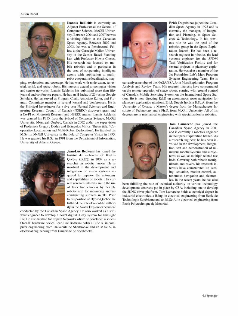
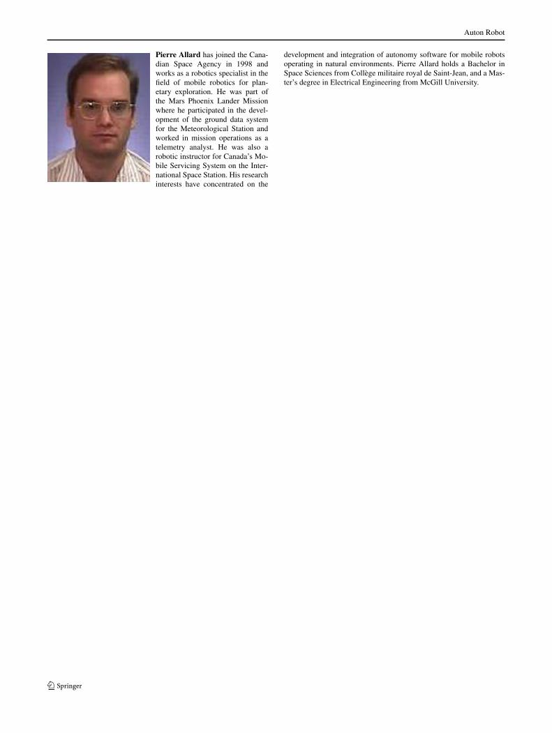
Pierre Allard has joined the Cana-dian Space Agency in 1998 andworks as a robotics specialist in thefield of mobile robotics for plan-etary exploration. He was part ofthe Mars Phoenix Lander Missionwhere he participated in the devel-opment of the ground data systemfor the Meteorological Station andworked in mission operations as atelemetry analyst. He was also arobotic instructor for Canada’s Mo-bile Servicing System on the Inter-national Space Station. His researchinterests have concentrated on the

development and integration of autonomy software for mobile robotsoperating in natural environments. Pierre Allard holds a Bachelor inSpace Sciences from Collège militaire royal de Saint-Jean, and a Mas-ter’s degree in Electrical Engineering from McGill University.