Autonomous Mobile Robots, Chapter 5 © R. Siegwart, I. Nourbakhsh Localization and Map Building • Noise and aliasing; odometric position estimation • To localize or not to localize • Belief representation • Map representation • Probabilistic map-based localization • Other examples of localization system • Autonomous map building 5 "Position" Global Map Perception Motion Control Cognition Real World Environment Localization Path Environment Model Local Map

Welcome message from author
This document is posted to help you gain knowledge. Please leave a comment to let me know what you think about it! Share it to your friends and learn new things together.
Transcript

Autonomous Mobile Robots, Chapter 5
© R. Siegwart, I. Nourbakhsh
Localization and Map Building
• Noise and aliasing; odometric position estimation• To localize or not to localize• Belief representation• Map representation• Probabilistic map-based localization• Other examples of localization system• Autonomous map building
5
"Position" Global Map
Perception Motion Control
Cognition
Real WorldEnvironment
Localization
PathEnvironment ModelLocal Map

Autonomous Mobile Robots, Chapter 5
© R. Siegwart, I. Nourbakhsh
Localization, Where am I?
?
• Odometry, Dead Reckoning
• Localization base on external sensors, beacons or landmarks
• Probabilistic Map Based Localization
5.1
Observation
Mapdata base
Prediction of Position
(e.g. odometry)
Perc
epti
on
Matching
Position Update(Estimation?)
raw sensor data or extracted features
predicted position
position
matchedobservations
YES
Encoder
Per
cep
tion

Autonomous Mobile Robots, Chapter 5
© R. Siegwart, I. Nourbakhsh
Challenges of Localization
• Knowing the absolute position (e.g. GPS) is not sufficient
• Localization in human-scale in relation with environment
• Planing in the Cognition step requires more than only position as input
• Perception and motion plays an important role Sensor noise Sensor aliasing Effector noise Odometric position estimation
5.2

Autonomous Mobile Robots, Chapter 5
© R. Siegwart, I. Nourbakhsh
Sensor Noise
• Sensor noise in mainly influenced by environment e.g. surface, illumination …
• or by the measurement principle itselfe.g. interference between ultrasonic sensors
• Sensor noise drastically reduces the useful information of sensor readings. The solution is: to take multiple reading into account employ temporal and/or multi-sensor fusion
5.2.1

Autonomous Mobile Robots, Chapter 5
© R. Siegwart, I. Nourbakhsh
Sensor Aliasing
• In robots, non-uniqueness of sensors readings is the norm
• Even with multiple sensors, there is a many-to-one mapping from environmental states to robot’s perceptual inputs
• Therefore the amount of information perceived by the sensors is generally insufficient to identify the robot’s position from a single reading Robot’s localization is usually based on a series of readings Sufficient information is recovered by the robot over time
5.2.2

Autonomous Mobile Robots, Chapter 5
© R. Siegwart, I. Nourbakhsh
Effector Noise: Odometry, Dead Reckoning
• Odometry and dead reckoning: Position update is based on proprioceptive sensors Odometry: wheel sensors only Dead reckoning: also heading sensors
• The movement of the robot, sensed with wheel encoders and/or heading sensors is integrated to the position. Pros: Straight forward, easy Cons: Errors are integrated -> unbound
• Using additional heading sensors (e.g. gyroscope) might help to reduce the cumulated errors, but the main problems remain the same.
5.2.3

Autonomous Mobile Robots, Chapter 5
© R. Siegwart, I. Nourbakhsh
Odometry: Error sources
deterministic non-deterministic (systematic) (non-systematic)
deterministic errors can be eliminated by proper calibration of the system. non-deterministic errors have to be described by error models and will always
leading to uncertain position estimate.• Major Error Sources:
Limited resolution during integration (time increments, measurement resolution …)
Misalignment of the wheels (deterministic) Unequal wheel diameter (deterministic) Variation in the contact point of the wheel Unequal floor contact (slipping, not planar …) …
5.2.3

Autonomous Mobile Robots, Chapter 5
© R. Siegwart, I. Nourbakhsh
Odometry: Classification of Integration Errors
• Range error: integrated path length (distance) of the robots movement sum of the wheel movements
• Turn error: similar to range error, but for turns difference of the wheel motions
• Drift error: difference in the error of the wheels leads to an error in the robots angular orientation
Over long periods of time, turn and drift errors
far outweigh range errors! Consider moving forward on a straight line along the x axis. The error
in the y-position introduced by a move of d meters will have a component of dsin, which can be quite large as the angular error grows.
5.2.3

Autonomous Mobile Robots, Chapter 5
© R. Siegwart, I. Nourbakhsh
Odometry: The Differential Drive Robot (1)
y
x
p
y
x
pp
5.2.4

Autonomous Mobile Robots, Chapter 5
© R. Siegwart, I. Nourbakhsh
Odometry: The Differential Drive Robot (2)
• Kinematics
5.2.4

Autonomous Mobile Robots, Chapter 5
© R. Siegwart, I. Nourbakhsh
Odometry: The Differential Drive Robot (3)
• Error model
5.2.4
Autonomous Mobile Robots, Chapter 5
© R. Siegwart, I. Nourbakhsh
Odometry: Growth of Pose uncertainty for Straight Line Movement
• Note: Errors perpendicular to the direction of movement are growing much faster!
5.2.4
Autonomous Mobile Robots, Chapter 5
© R. Siegwart, I. Nourbakhsh
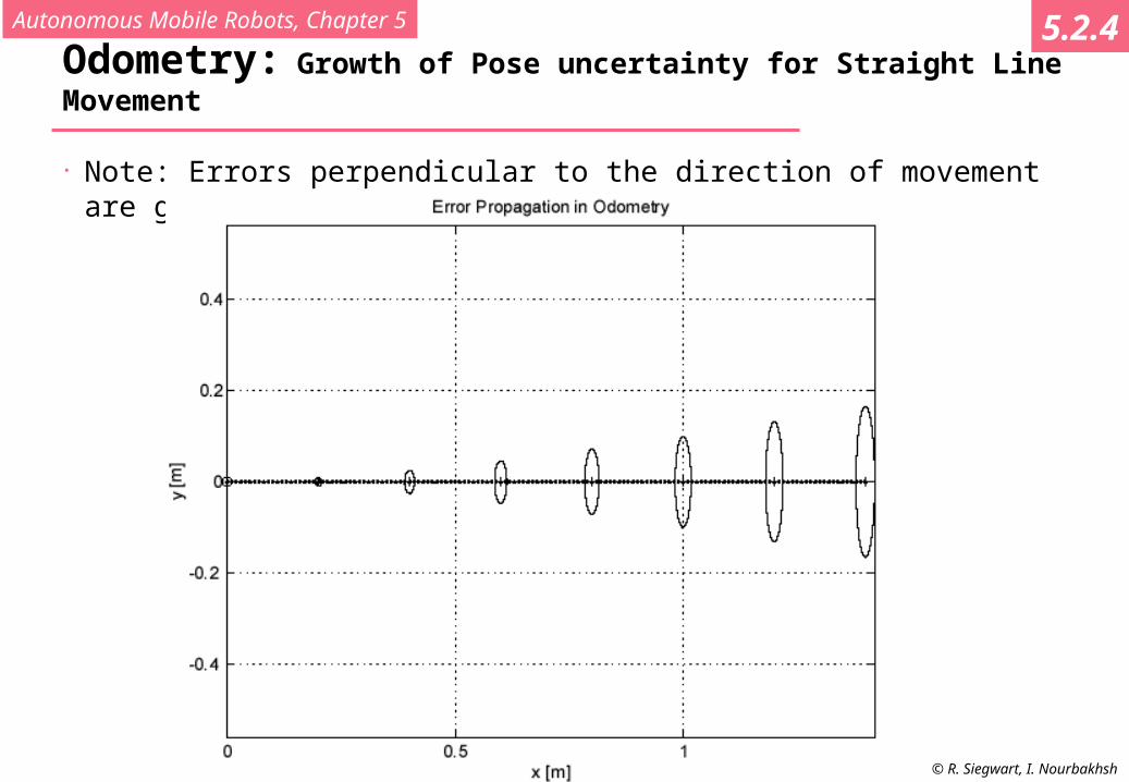
Odometry: Growth of Pose uncertainty for Movement on a Circle
• Note: Errors ellipse in does not remain perpendicular to the direction of movement!
5.2.4

Autonomous Mobile Robots, Chapter 5
© R. Siegwart, I. Nourbakhsh
Odometry: Calibration of Errors I (Borenstein [5])
• The unidirectional square path experiment
• BILD 1 Borenstein
5.2.4
Autonomous Mobile Robots, Chapter 5
© R. Siegwart, I. Nourbakhsh
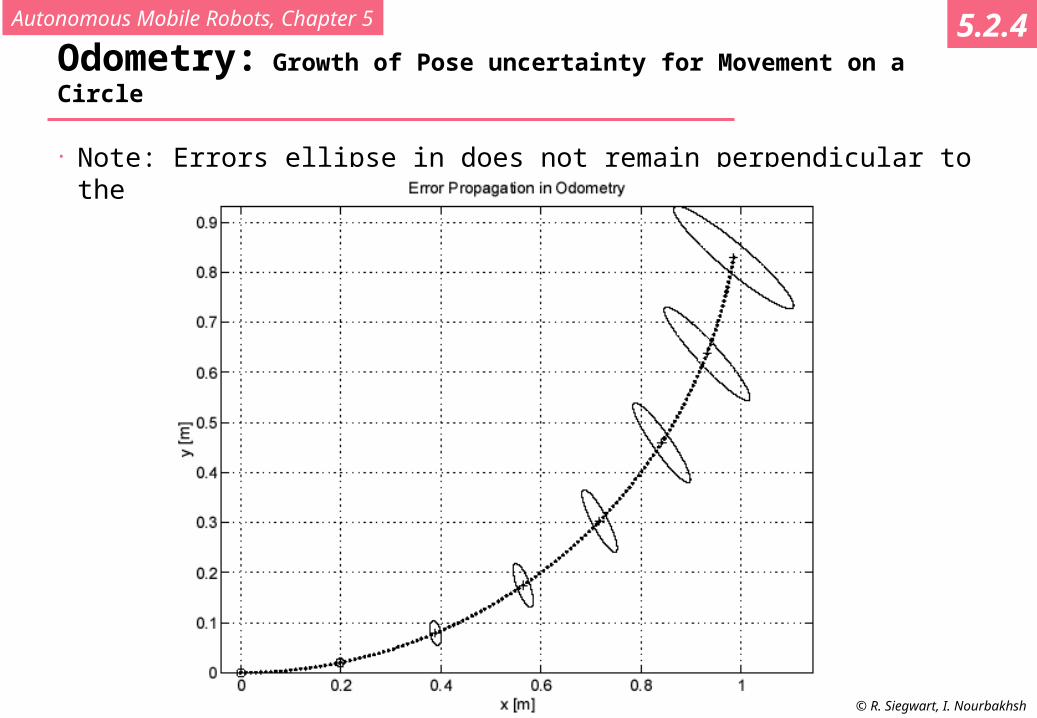
Odometry: Calibration of Errors II (Borenstein [5])
• The bi-directional square path experiment
• BILD 2/3 Borenstein
5.2.4
Autonomous Mobile Robots, Chapter 5
© R. Siegwart, I. Nourbakhsh
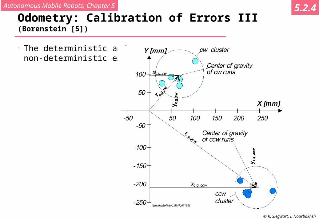
Odometry: Calibration of Errors III (Borenstein [5])
• The deterministic and non-deterministic errors
5.2.4
Autonomous Mobile Robots, Chapter 5
© R. Siegwart, I. Nourbakhsh
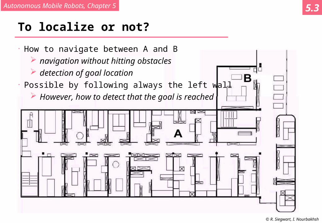
To localize or not?
• How to navigate between A and B navigation without hitting obstacles detection of goal location
• Possible by following always the left wall However, how to detect that the goal is reached
5.3

Autonomous Mobile Robots, Chapter 5
© R. Siegwart, I. Nourbakhsh
Behavior Based Navigation5.3

Autonomous Mobile Robots, Chapter 5
© R. Siegwart, I. Nourbakhsh
Model Based Navigation5.3

Autonomous Mobile Robots, Chapter 5
© R. Siegwart, I. Nourbakhsh
Belief Representation
• a) Continuous mapwith single hypothesis
• b) Continuous mapwith multiple hypothesis
• d) Discretized mapwith probability distribution
• d) Discretized topologicalmap with probabilitydistribution
5.4

Autonomous Mobile Robots, Chapter 5
© R. Siegwart, I. Nourbakhsh
Belief Representation: Characteristics
• Continuous Precision bound by sensor
data Typically single hypothesis
pose estimate Lost when diverging (for
single hypothesis) Compact representation and
typically reasonable in processing power.
• Discrete Precision bound by
resolution of discretisation Typically multiple hypothesis
pose estimate Never lost (when diverges
converges to another cell) Important memory and
processing power needed. (not the case for topological maps)
5.4

Autonomous Mobile Robots, Chapter 5
© R. Siegwart, I. Nourbakhsh
Bayesian Approach: A taxonomy of probabilistic models
More general
More specific
discreteHMMs
continuousHMMs
Markov Loc
semi-cont.HMMs
BayesianFilters
BayesianPrograms
BayesianNetworks
DBNs
KalmanFilters
MCML POMDPs
MDPs
ParticleFilters
MarkovChains
St St-1
St St-1 Ot
St St-1 At
St St-1 Ot At
Courtesy of Julien Diard
S: StateO: ObservationA: Action
5.4

Autonomous Mobile Robots, Chapter 5
© R. Siegwart, I. Nourbakhsh
Single-hypothesis Belief – Continuous Line-Map
5.4.1

Autonomous Mobile Robots, Chapter 5
© R. Siegwart, I. Nourbakhsh
Single-hypothesis Belief – Grid and Topological Map
5.4.1
Autonomous Mobile Robots, Chapter 5
© R. Siegwart, I. Nourbakhsh
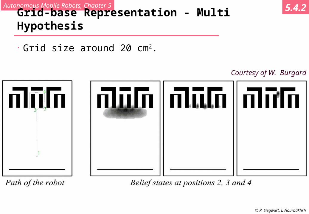
Grid-base Representation - Multi Hypothesis
• Grid size around 20 cm2.
5.4.2
Courtesy of W. Burgard
Autonomous Mobile Robots, Chapter 5
© R. Siegwart, I. Nourbakhsh
Map Representation
1. Map precision vs. application
2. Features precision vs. map precision
3. Precision vs. computational complexity
• Continuous Representation
• Decomposition (Discretization)
5.5

Autonomous Mobile Robots, Chapter 5
© R. Siegwart, I. Nourbakhsh
Representation of the Environment
• Environment Representation Continuos Metric x,y, Discrete Metric metric grid Discrete Topological topological grid
• Environment Modeling Raw sensor data, e.g. laser range data, grayscale images
o large volume of data, low distinctiveness on the level of individual valueso makes use of all acquired information
Low level features, e.g. line other geometric featureso medium volume of data, average distinctivenesso filters out the useful information, still ambiguities
High level features, e.g. doors, a car, the Eiffel towero low volume of data, high distinctivenesso filters out the useful information, few/no ambiguities, not enough information
5.5

Autonomous Mobile Robots, Chapter 5
© R. Siegwart, I. Nourbakhsh
Map Representation: Continuous Line-Based
a) Architecture map
b) Representation with set of infinite lines
5.5.1

Autonomous Mobile Robots, Chapter 5
© R. Siegwart, I. Nourbakhsh
Map Representation: Decomposition (1)
• Exact cell decomposition
5.5.2
Autonomous Mobile Robots, Chapter 5
© R. Siegwart, I. Nourbakhsh
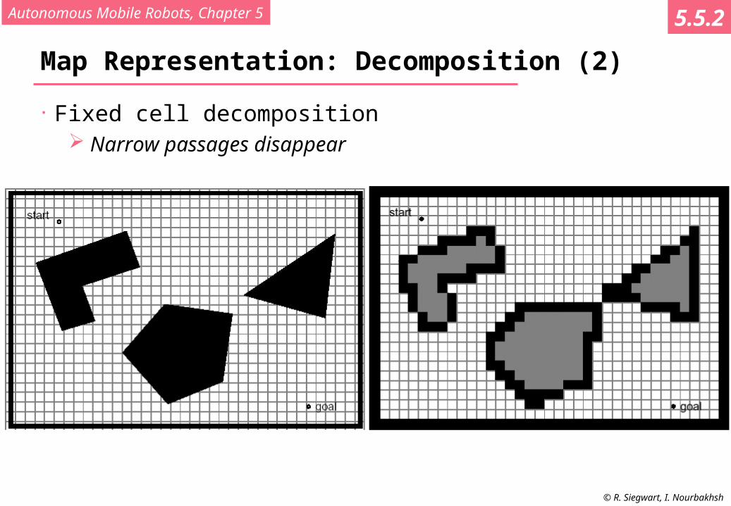
Map Representation: Decomposition (2)
• Fixed cell decomposition Narrow passages disappear
5.5.2

Autonomous Mobile Robots, Chapter 5
© R. Siegwart, I. Nourbakhsh
Map Representation: Decomposition (3)
• Adaptive cell decomposition
5.5.2

Autonomous Mobile Robots, Chapter 5
© R. Siegwart, I. Nourbakhsh
Map Representation: Decomposition (4)
• Fixed cell decomposition – Example with very small cells
5.5.2
Courtesy of S. Thrun

Autonomous Mobile Robots, Chapter 5
© R. Siegwart, I. Nourbakhsh
Map Representation: Decomposition (5)
• Topological Decomposition
5.5.2

Autonomous Mobile Robots, Chapter 5
© R. Siegwart, I. Nourbakhsh
Map Representation: Decomposition (6)
• Topological Decomposition
node
Connectivity(arch)
5.5.2
Autonomous Mobile Robots, Chapter 5
© R. Siegwart, I. Nourbakhsh
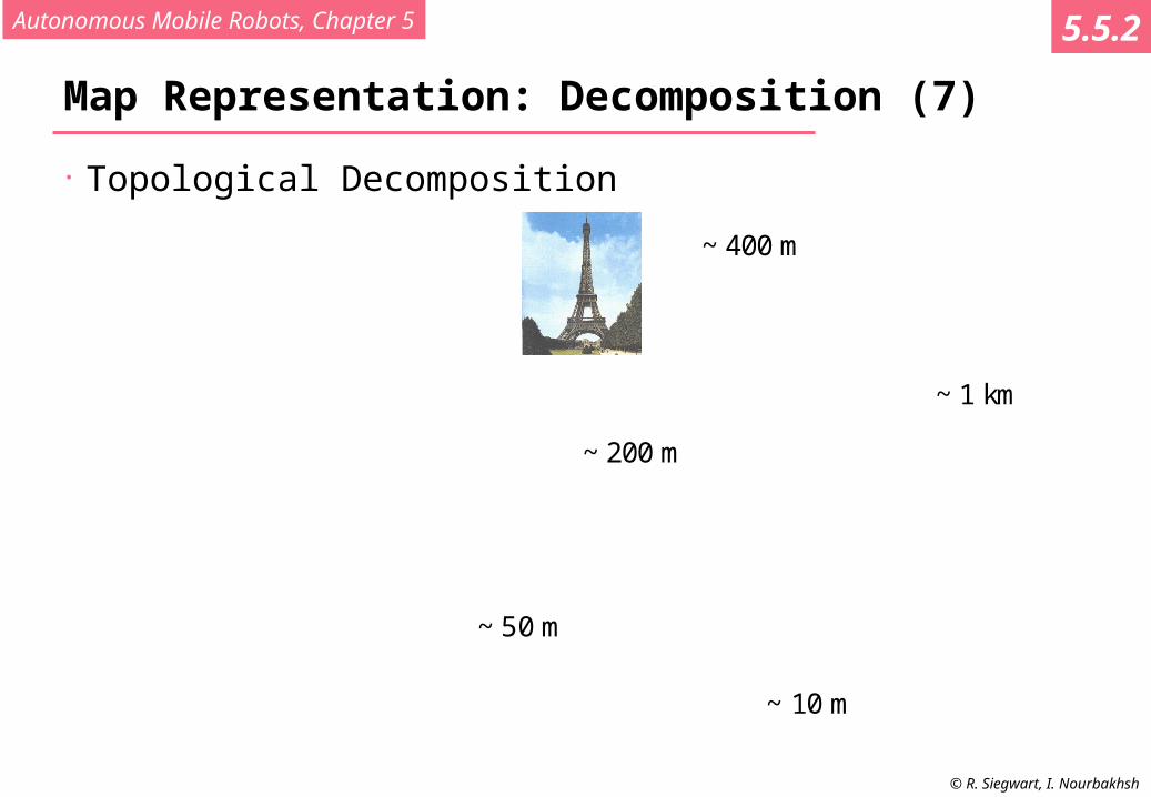
Map Representation: Decomposition (7)
• Topological Decomposition
~ 400 m
~ 1 km
~ 200 m
~ 50 m
~ 10 m
5.5.2
Autonomous Mobile Robots, Chapter 5
© R. Siegwart, I. Nourbakhsh
State-of-the-Art: Current Challenges in Map Representation
• Real world is dynamic
• Perception is still a major challenge Error prone Extraction of useful information difficult
• Traversal of open space
• How to build up topology (boundaries of nodes)
• Sensor fusion
• …
5.5.3

Autonomous Mobile Robots, Chapter 5
© R. Siegwart, I. Nourbakhsh
Probabilistic, Map-Based Localization (1)
• Consider a mobile robot moving in a known environment.
• As it start to move, say from a precisely known location, it might keep track of its location using odometry.
• However, after a certain movement the robot will get very uncertain about its position.
update using an observation of its environment.
• observation lead also to an estimate of the robots position which can than be fused with the odometric estimation to get the best possible update of the robots actual position.
5.6.1
Autonomous Mobile Robots, Chapter 5
© R. Siegwart, I. Nourbakhsh
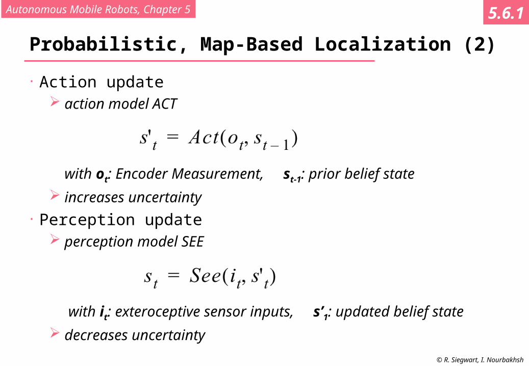
Probabilistic, Map-Based Localization (2)
• Action update action model ACT
with ot: Encoder Measurement, st-1: prior belief state
increases uncertainty• Perception update
perception model SEE
with it: exteroceptive sensor inputs, s’1: updated belief state
decreases uncertainty
5.6.1

Autonomous Mobile Robots, Chapter 5
© R. Siegwart, I. Nourbakhsh
• Improving belief stateby moving
5.6.1
Autonomous Mobile Robots, Chapter 5
© R. Siegwart, I. Nourbakhsh
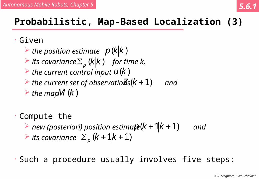
Probabilistic, Map-Based Localization (3)
• Given the position estimate its covariance for time k, the current control input the current set of observations and the map
• Compute the new (posteriori) position estimate and its covariance
• Such a procedure usually involves five steps:
)( kkp)( kkp
)(ku)1( kZ
)(kM
)11( kkp)11( kkp
5.6.1

Autonomous Mobile Robots, Chapter 5
© R. Siegwart, I. Nourbakhsh
The Five Steps for Map-Based Localization
Observationon-board sensors
Mapdata base
Prediction ofMeasurement and Position (odometry)
Per
cept
ion
Matching
Estimation(fusion)
raw sensor data or extracted features
pre
dic
ted
fea
ture
obs
erv
atio
ns
positionestimate
matched predictionsand observations
YES
Encoder
1. Prediction based on previous estimate and odometry
2. Observation with on-board sensors
3. Measurement prediction based on prediction and map
4. Matching of observation and map
5. Estimation -> position update (posteriori position)
5.6.1

Autonomous Mobile Robots, Chapter 5
© R. Siegwart, I. Nourbakhsh
Markov Kalman Filter Localization
• Markov localization localization starting from any
unknown position recovers from ambiguous
situation. However, to update the probability
of all positions within the whole state space at any time requires a discrete representation of the space (grid). The required memory and calculation power can thus become very important if a fine grid is used.
• Kalman filter localization tracks the robot and is inherently
very precise and efficient. However, if the uncertainty of the
robot becomes to large (e.g. collision with an object) the Kalman filter will fail and the position is definitively lost.
5.6.1
Autonomous Mobile Robots, Chapter 5
© R. Siegwart, I. Nourbakhsh
Markov Localization (1)
• Markov localization uses an explicit, discrete representation for the probability of all position in the state space.
• This is usually done by representing the environment by a grid or a topological graph with a finite number of possible states (positions).
• During each update, the probability for each state (element) of the entire space is updated.
5.6.2

Autonomous Mobile Robots, Chapter 5
© R. Siegwart, I. Nourbakhsh
Markov Localization (2): Applying probabilty theory to robot localization
• P(A): Probability that A is true. e.g. p(rt = l): probability that the robot r is at position l at time t
• We wish to compute the probability of each indivitual robot position given actions and sensor measures.
• P(A|B): Conditional probability of A given that we know B. e.g. p(rt = l| it): probability that the robot is at position l given the
sensors input it.
• Product rule:
• Bayes rule:
5.6.2

Autonomous Mobile Robots, Chapter 5
© R. Siegwart, I. Nourbakhsh
Markov Localization (3): Applying probability theory to robot localization
• Bayes rule:
Map from a belief state and a sensor input to a refined belief state (SEE):
p(l): belief state before perceptual update process p(i |l): probability to get measurement i when being at position l
o consult robots map, identify the probability of a certain sensor reading for each possible position in the map
p(i): normalization factor so that sum over all l for L equals 1.
5.6.2

Autonomous Mobile Robots, Chapter 5
© R. Siegwart, I. Nourbakhsh
Markov Localization (4): Applying probability theory to robot localization
• Bayes rule:
Map from a belief state and a action to new belief state (ACT):
Summing over all possible ways in which the robot may have reached l.
• Markov assumption: Update only depends on previous state and its most recent actions and perception.
5.6.2
Autonomous Mobile Robots, Chapter 5
© R. Siegwart, I. Nourbakhsh
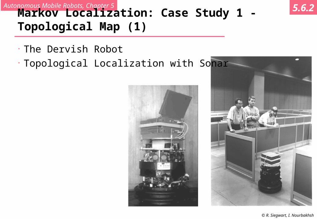
Markov Localization: Case Study 1 - Topological Map (1)
• The Dervish Robot• Topological Localization with Sonar
5.6.2

Autonomous Mobile Robots, Chapter 5
© R. Siegwart, I. Nourbakhsh
Markov Localization: Case Study 1 - Topological Map (2)
• Topological map of office-type environment
5.6.2

Autonomous Mobile Robots, Chapter 5
© R. Siegwart, I. Nourbakhsh
Markov Localization: Case Study 1 - Topological Map (3)
• Update of believe state for position n given the percept-pair i
p(n¦i): new likelihood for being in position n p(n): current believe state p(i¦n): probability of seeing i in n (see table)
• No action update ! However, the robot is moving and therefore we can apply a combination
of action and perception update
t-i is used instead of t-1 because the topological distance between n’ and n can very depending on the specific topological map
5.6.2

Autonomous Mobile Robots, Chapter 5
© R. Siegwart, I. Nourbakhsh
Markov Localization: Case Study 1 - Topological Map (4)
• The calculation
is calculated by multiplying the probability of generating perceptual event i at position n by the probability of having failed to generate perceptual event s at all nodes between n’ and n.
5.6.2

Autonomous Mobile Robots, Chapter 5
© R. Siegwart, I. Nourbakhsh
Markov Localization: Case Study 1 - Topological Map (5)
• Example calculation Assume that the robot has two nonzero belief states
o p(1-2) = 1.0 ; p(2-3) = 0.2 *
at that it is facing east with certainty State 2-3 will progress potentially to 3 and 3-4 to 4. State 3 and 3-4 can be eliminated because the likelihood of detecting an open door
is zero. The likelihood of reaching state 4 is the product of the initial likelihood p(2-3)=
0.2, (a) the likelihood of detecting anything at node 3 and the likelihood of detecting a hallway on the left and a door on the right at node 4 and (b) the likelihood of detecting a hallway on the left and a door on the right at node 4. (for simplicity we assume that the likelihood of detecting nothing at node 3-4 is 1.0)
This leads to:o 0.2 [0.6 0.4 + 0.4 0.05] 0.7 [0.9 0.1] p(4) = 0.003.o Similar calculation for progress from 1-2 p(2) = 0.3.
5.6.2
* Note that the probabilities do not sum up to one. For simplicity normalization was avoided in this example

Autonomous Mobile Robots, Chapter 5
© R. Siegwart, I. Nourbakhsh
Markov Localization: Case Study 2 – Grid Map (1)
• Fine fixed decomposition grid (x, y, ), 15 cm x 15 cm x 1° Action and perception update
• Action update: Sum over previous possible positions
and motion model
Discrete version of eq. 5.22• Perception update:
Given perception i, what is theprobability to be a location l
5.6.2
Courtesy of W. Burgard
Autonomous Mobile Robots, Chapter 5
© R. Siegwart, I. Nourbakhsh
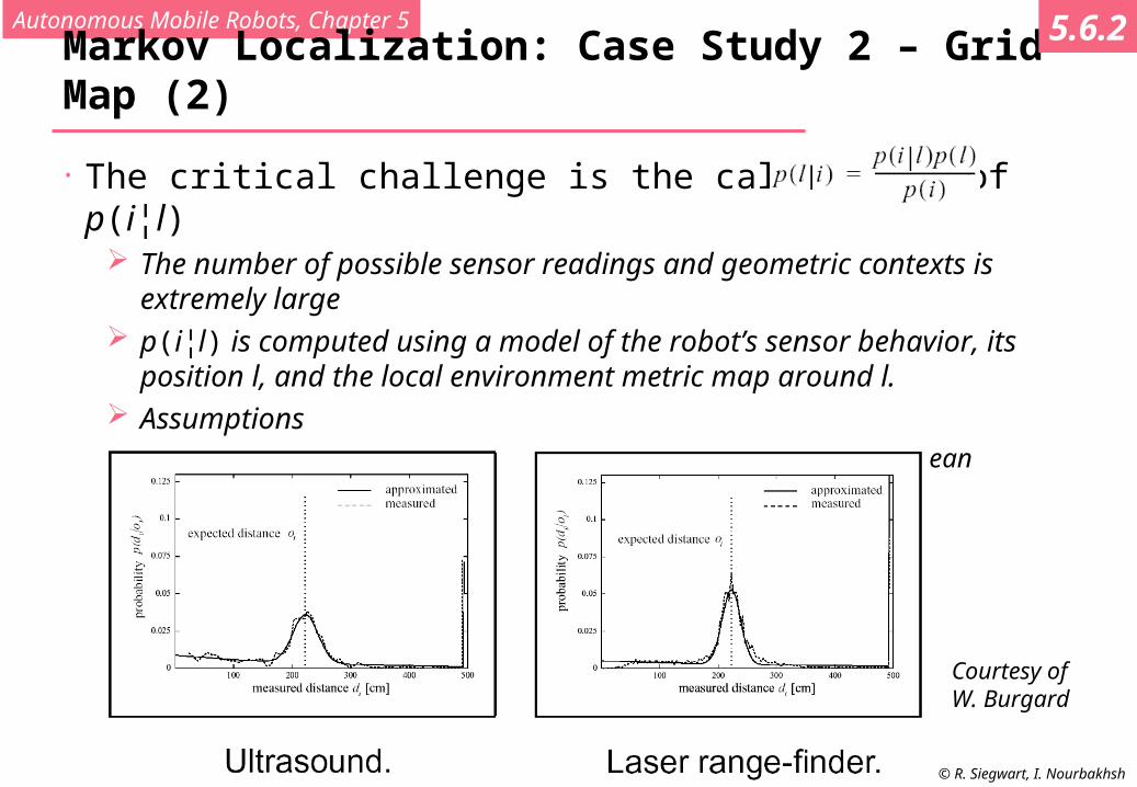
Markov Localization: Case Study 2 – Grid Map (2)
• The critical challenge is the calculation of p(i¦l) The number of possible sensor readings and geometric contexts is extremely large p(i¦l) is computed using a model of the robot’s sensor behavior, its position l, and
the local environment metric map around l. Assumptions
o Measurement error can be described by a distribution with a mean
o Non-zero chance for any measurement
5.6.2
Courtesy of W. Burgard
Autonomous Mobile Robots, Chapter 5
© R. Siegwart, I. Nourbakhsh
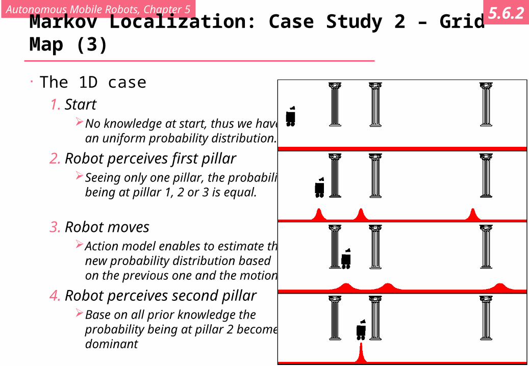
Markov Localization: Case Study 2 – Grid Map (3)
• The 1D case1. Start
No knowledge at start, thus we have an uniform probability distribution.
2. Robot perceives first pillarSeeing only one pillar, the probability
being at pillar 1, 2 or 3 is equal.
3. Robot movesAction model enables to estimate the
new probability distribution based on the previous one and the motion.
4. Robot perceives second pillarBase on all prior knowledge the
probability being at pillar 2 becomesdominant
5.6.2

Autonomous Mobile Robots, Chapter 5
© R. Siegwart, I. Nourbakhsh
Markov Localization: Case Study 2 – Grid Map (4)
• Example 1: Office Building
5.6.2
Position 3
Position 4
Position 5
Courtesy of W. Burgard

Autonomous Mobile Robots, Chapter 5
© R. Siegwart, I. Nourbakhsh
Markov Localization: Case Study 2 – Grid Map (5)
• Example 2: Museum Laser scan 1
5.6.2
Courtesy of W. Burgard
Autonomous Mobile Robots, Chapter 5
© R. Siegwart, I. Nourbakhsh
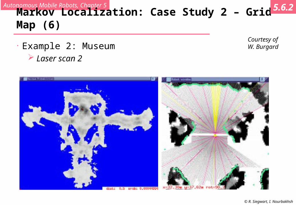
Markov Localization: Case Study 2 – Grid Map (6)
• Example 2: Museum Laser scan 2
5.6.2
Courtesy of W. Burgard

Autonomous Mobile Robots, Chapter 5
© R. Siegwart, I. Nourbakhsh
Markov Localization: Case Study 2 – Grid Map (7)
• Example 2: Museum Laser scan 3
5.6.2
Courtesy of W. Burgard

Autonomous Mobile Robots, Chapter 5
© R. Siegwart, I. Nourbakhsh
Markov Localization: Case Study 2 – Grid Map (8)
• Example 2: Museum Laser scan 13
5.6.2
Courtesy of W. Burgard

Autonomous Mobile Robots, Chapter 5
© R. Siegwart, I. Nourbakhsh
Markov Localization: Case Study 2 – Grid Map (9)
• Example 2: Museum Laser scan 21
5.6.2
Courtesy of W. Burgard

Autonomous Mobile Robots, Chapter 5
© R. Siegwart, I. Nourbakhsh
Markov Localization: Case Study 2 – Grid Map (10)
• Fine fixed decomposition grids result in a huge state space Very important processing power needed Large memory requirement
• Reducing complexity Various approached have been proposed for reducing complexity The main goal is to reduce the number of states that are updated in each
step• Randomized Sampling / Particle Filter
Approximated belief state by representing only a ‘representative’ subset of all states (possible locations)
E.g update only 10% of all possible locations The sampling process is typically weighted, e.g. put more samples
around the local peaks in the probability density function However, you have to ensure some less likely locations are still tracked,
otherwise the robot might get lost
5.6.2
Autonomous Mobile Robots, Chapter 5
© R. Siegwart, I. Nourbakhsh
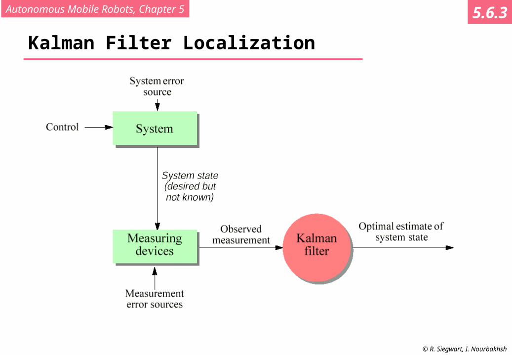
Kalman Filter Localization
5.6.3

Autonomous Mobile Robots, Chapter 5
© R. Siegwart, I. Nourbakhsh
Introduction to Kalman Filter (1)
• Two measurements
• Weighted leas-square
• Finding minimum error
• After some calculation and rearrangements
5.6.3
Autonomous Mobile Robots, Chapter 5
© R. Siegwart, I. Nourbakhsh
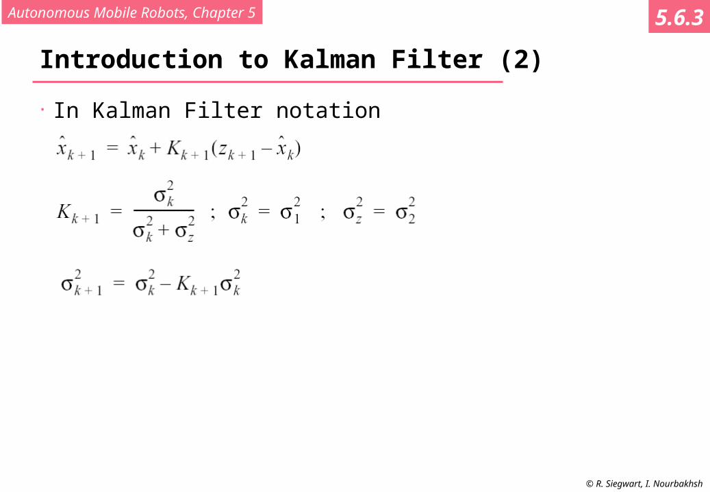
Introduction to Kalman Filter (2)
• In Kalman Filter notation
5.6.3

Autonomous Mobile Robots, Chapter 5
© R. Siegwart, I. Nourbakhsh
Introduction to Kalman Filter (3)
• Dynamic Prediction (robot moving)
u = velocity w = noise
• Motion
• Combining fusion and dynamic prediction
5.6.3
Autonomous Mobile Robots, Chapter 5
© R. Siegwart, I. Nourbakhsh
Kalman Filter for Mobile Robot Localization
Robot Position Prediction
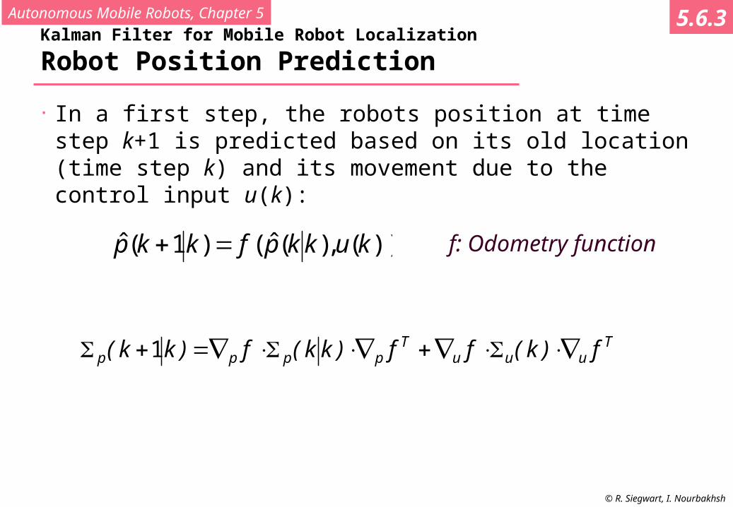
• In a first step, the robots position at time step k+1 is predicted based on its old location (time step k) and its movement due to the control input u(k):
))(,)(ˆ()1(ˆ kukkpfkkp
Tuuu
Tpppp f)k(ff)kk(f)kk( 1
f: Odometry function
5.6.3

Autonomous Mobile Robots, Chapter 5
© R. Siegwart, I. Nourbakhsh
Kalman Filter for Mobile Robot Localization
Robot Position Prediction: Example
b
ssb
ssssb
ssss
k
ky
kx
kukkpkkp
lr
lrlr
lrlr
)2
sin(2
)2
cos(2
)(ˆ)(ˆ
)(ˆ
)()(ˆ)1(ˆ
Tuuu
Tpppp f)k(ff)kk(f)kk( 1
ll
rru sk
skk
0
0)(
OdometryOdometry
5.6.3
Autonomous Mobile Robots, Chapter 5
© R. Siegwart, I. Nourbakhsh
Kalman Filter for Mobile Robot Localization
Observation
• The second step it to obtain the observation Z(k+1) (measurements) from the robot’s sensors at the new location at time k+1
• The observation usually consists of a set n0 of single observations zj(k+1) extracted from the different sensors signals. It can represent raw data scans as well as features like lines, doors or any kind of landmarks.
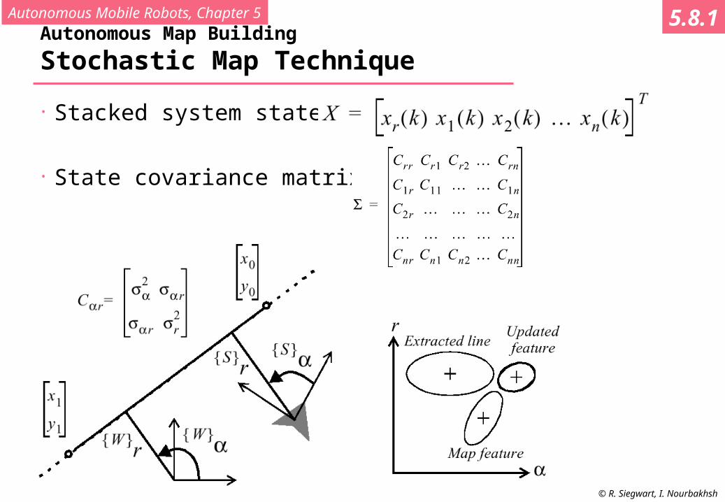
• The parameters of the targets are usually observed in the sensor frame {S}. Therefore the observations have to be transformed to the world frame {W}
or the measurement prediction have to be transformed to the sensor frame {S}. This transformation is specified in the function hi (seen later).
5.6.3

Autonomous Mobile Robots, Chapter 5
© R. Siegwart, I. Nourbakhsh
Kalman Filter for Mobile Robot Localization
Observation: Example
j
r j
line j
Raw Date of Laser Scanner
Extracted Lines Extracted Lines
in Model Space
jrrr
rjR k
)1(,
j
j
R
j rkz )1(
Sensor (robot) frame
5.6.3

Autonomous Mobile Robots, Chapter 5
© R. Siegwart, I. Nourbakhsh
Kalman Filter for Mobile Robot Localization
Measurement Prediction
• In the next step we use the predicted robot position and the map M(k) to generate multiple predicted observations zt.
• They have to be transformed into the sensor frame
• We can now define the measurement prediction as the set containing all ni predicted observations
• The function hi is mainly the coordinate transformation between the world frame and the sensor frame
5.6.3
kkp 1
kkp,zhkz tii 11
ii nikzkZ 111

Autonomous Mobile Robots, Chapter 5
© R. Siegwart, I. Nourbakhsh
Kalman Filter for Mobile Robot Localization
Measurement Prediction: Example
• For prediction, only the walls that are in the field of view of the robot are selected.
• This is done by linking the individuallines to the nodes of the path
5.6.3
Autonomous Mobile Robots, Chapter 5
© R. Siegwart, I. Nourbakhsh
Kalman Filter for Mobile Robot Localization
Measurement Prediction: Example
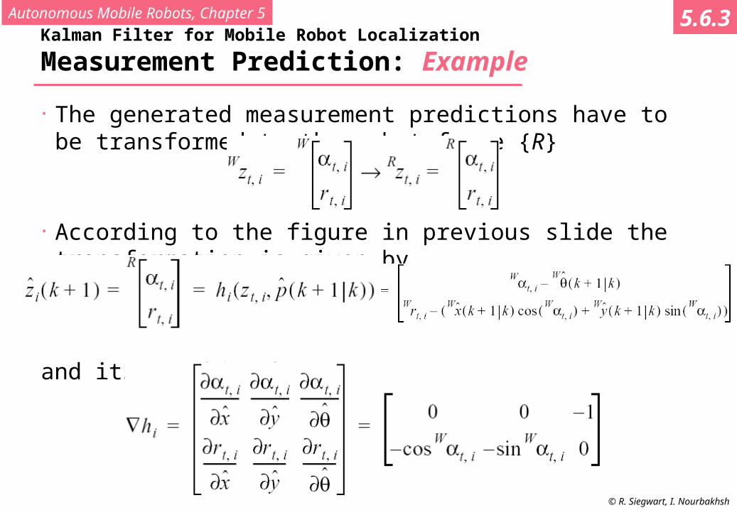
• The generated measurement predictions have to be transformed to the robot frame {R}
• According to the figure in previous slide the transformation is given by
and its Jacobian by
5.6.3

Autonomous Mobile Robots, Chapter 5
© R. Siegwart, I. Nourbakhsh
Kalman Filter for Mobile Robot Localization
Matching
• Assignment from observations zj(k+1) (gained by the sensors) to the targets zt (stored in the map)
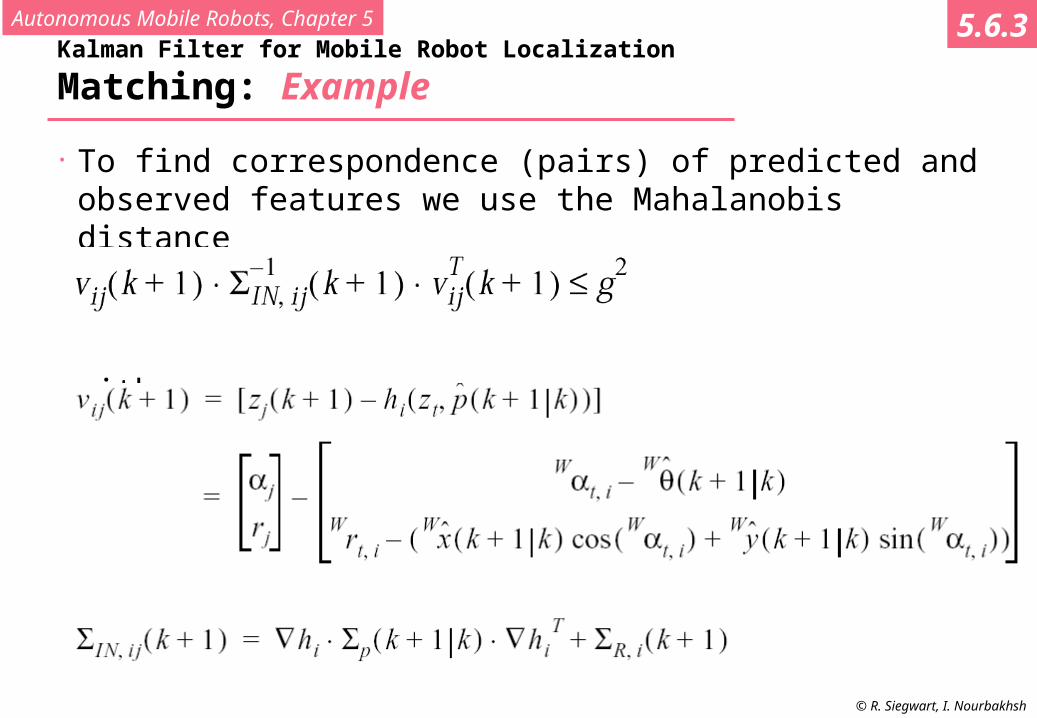
• For each measurement prediction for which an corresponding observation is found we calculate the innovation:
and its innovation covariance found by applying the error propagation law:
• The validity of the correspondence between measurement and prediction can e.g. be evaluated through the Mahalanobis distance:
5.6.3

Autonomous Mobile Robots, Chapter 5
© R. Siegwart, I. Nourbakhsh
Kalman Filter for Mobile Robot Localization
Matching: Example
5.6.3
Autonomous Mobile Robots, Chapter 5
© R. Siegwart, I. Nourbakhsh
Kalman Filter for Mobile Robot Localization
Matching: Example
• To find correspondence (pairs) of predicted and observed features we use the Mahalanobis distance
with
5.6.3
Autonomous Mobile Robots, Chapter 5
© R. Siegwart, I. Nourbakhsh
Kalman Filter for Mobile Robot Localization
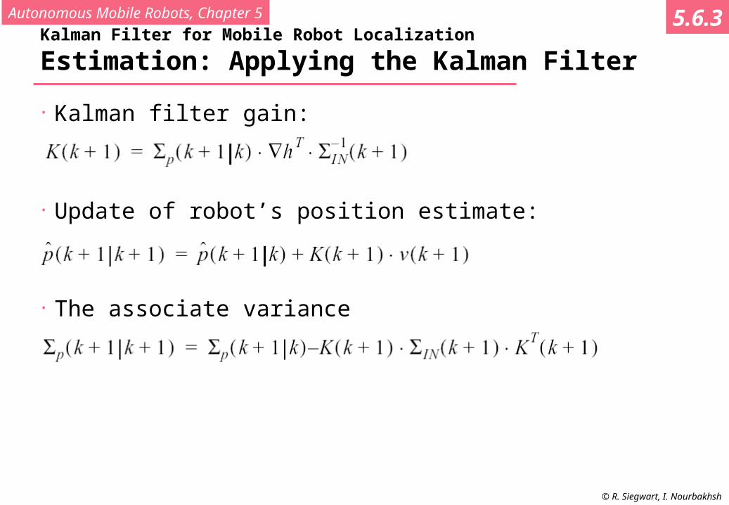
Estimation: Applying the Kalman Filter
• Kalman filter gain:
• Update of robot’s position estimate:
• The associate variance
5.6.3
Autonomous Mobile Robots, Chapter 5
© R. Siegwart, I. Nourbakhsh
Kalman Filter for Mobile Robot Localization
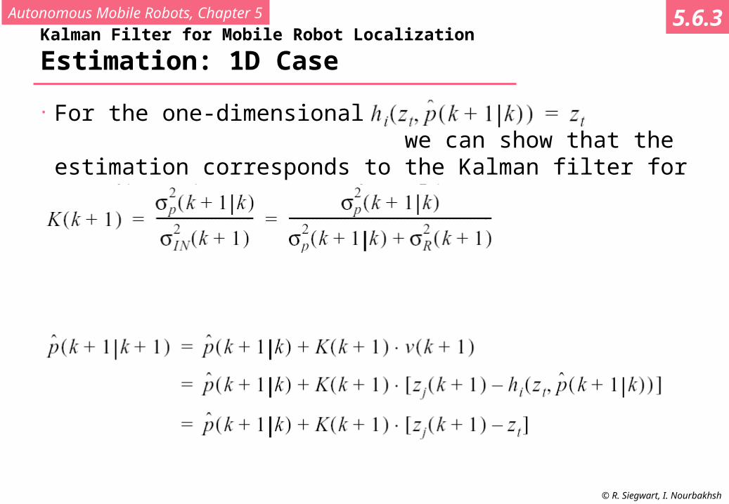
Estimation: 1D Case
• For the one-dimensional case with we can show that the estimation corresponds to the Kalman filter for one-dimension presented earlier.
5.6.3
Autonomous Mobile Robots, Chapter 5
© R. Siegwart, I. Nourbakhsh
Kalman Filter for Mobile Robot Localization
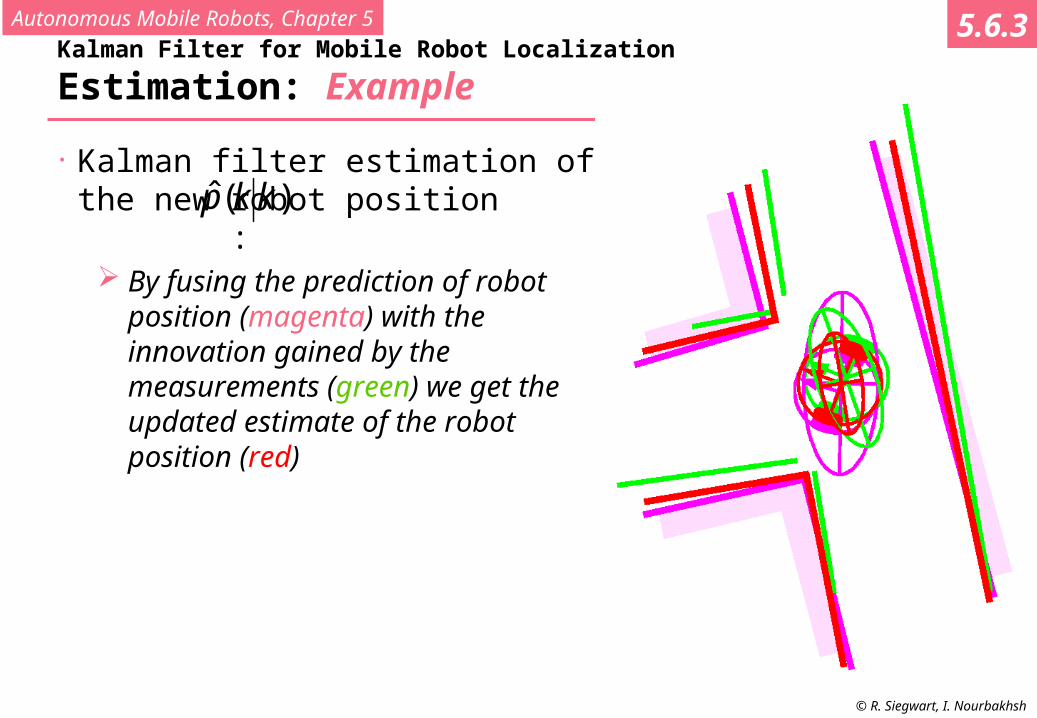
Estimation: Example
• Kalman filter estimation of the new robot position : By fusing the prediction of robot position
(magenta) with the innovation gained by the measurements (green) we get the updated estimate of the robot position (red)
)(ˆ kkp
5.6.3

Autonomous Mobile Robots, Chapter 5
© R. Siegwart, I. Nourbakhsh
Other Localization Methods (not probabilistic)
Localization Baseon Artificial Landmarks
5.7.1

Autonomous Mobile Robots, Chapter 5
© R. Siegwart, I. Nourbakhsh
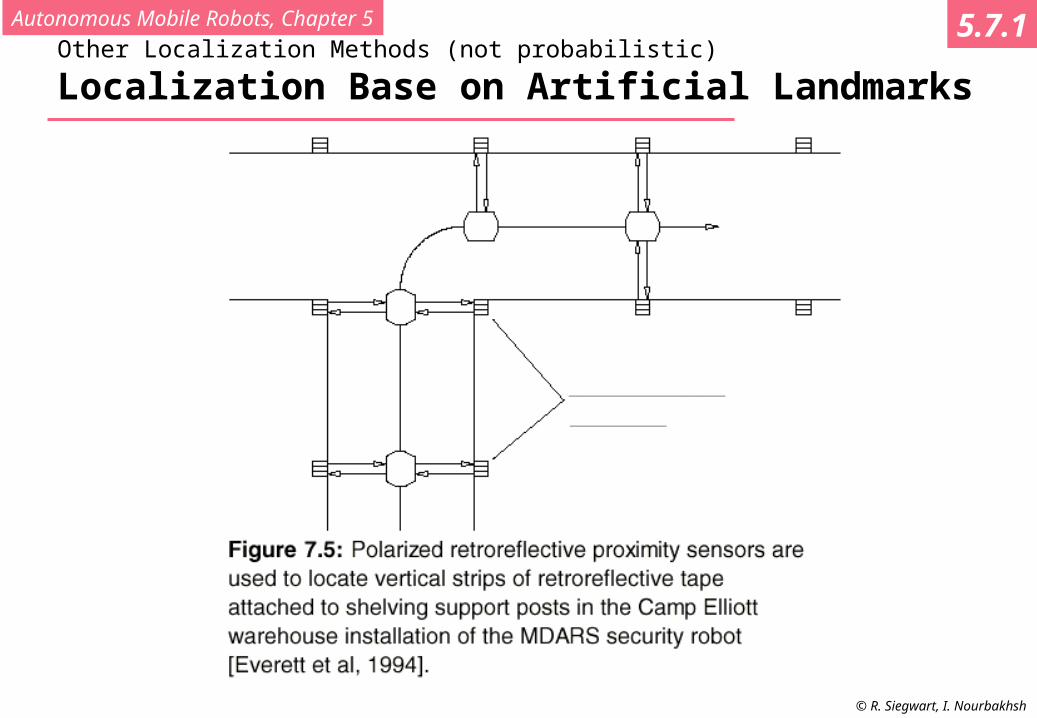
Other Localization Methods (not probabilistic)
Localization Base on Artificial Landmarks
5.7.1
Autonomous Mobile Robots, Chapter 5
© R. Siegwart, I. Nourbakhsh
Other Localization Methods (not probabilistic)
Localization Base on Artificial Landmarks
5.7.1

Autonomous Mobile Robots, Chapter 5
© R. Siegwart, I. Nourbakhsh
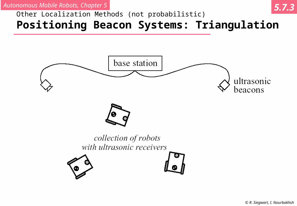
Other Localization Methods (not probabilistic)
Positioning Beacon Systems: Triangulation
5.7.3
Autonomous Mobile Robots, Chapter 5
© R. Siegwart, I. Nourbakhsh
Other Localization Methods (not probabilistic)
Positioning Beacon Systems: Triangulation
5.7.3

Autonomous Mobile Robots, Chapter 5
© R. Siegwart, I. Nourbakhsh
Other Localization Methods (not probabilistic)
Positioning Beacon Systems: Triangulation
5.7.3

Autonomous Mobile Robots, Chapter 5
© R. Siegwart, I. Nourbakhsh
Other Localization Methods (not probabilistic)
Positioning Beacon Systems: Docking
5.7.3

Autonomous Mobile Robots, Chapter 5
© R. Siegwart, I. Nourbakhsh
Other Localization Methods (not probabilistic)
Positioning Beacon Systems: Bar-Code
5.7.3

Autonomous Mobile Robots, Chapter 5
© R. Siegwart, I. Nourbakhsh
Other Localization Methods (not probabilistic)
Positioning Beacon Systems
5.7.3

Autonomous Mobile Robots, Chapter 5
© R. Siegwart, I. Nourbakhsh
Autonomous Map Building
Starting from an arbitrary initial point, a mobile robot should be able to autonomously explore the
environment with its on board sensors, gain knowledge about it,
interpret the scene, build an appropriate map
and localize itself relative to this map.
SLAMThe Simultaneous Localization and Mapping Problem
5.8

Autonomous Mobile Robots, Chapter 5
© R. Siegwart, I. Nourbakhsh
Map Building:
How to Establish a Map
1. By Hand
2. Automatically: Map Building
The robot learns its environment
Motivation:
- by hand: hard and costly
- dynamically changing environment
- different look due to different perception
3. Basic Requirements of a Map: a way to incorporate newly sensed
information into the existing world model
information and procedures for estimating the robot’s position
information to do path planning and other navigation task (e.g. obstacle avoidance)
• Measure of Quality of a map topological correctness
metrical correctness
• But: Most environments are a mixture of predictable and unpredictable features hybrid approach
model-based vs. behaviour-based
12 3.5
predictability
5.8
Autonomous Mobile Robots, Chapter 5
© R. Siegwart, I. Nourbakhsh
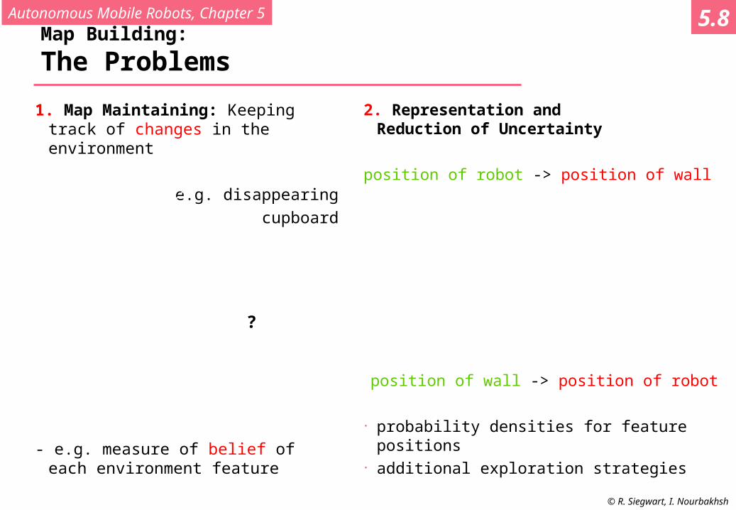
Map Building:
The Problems
1. Map Maintaining: Keeping track of changes in the environment
e.g. disappearing
cupboard
- e.g. measure of belief of each environment feature
2. Representation and Reduction of Uncertainty
position of robot -> position of wall
position of wall -> position of robot
• probability densities for feature positions• additional exploration strategies
?
5.8
Autonomous Mobile Robots, Chapter 5
© R. Siegwart, I. Nourbakhsh
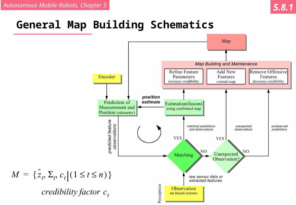
General Map Building Schematics
5.8.1

Autonomous Mobile Robots, Chapter 5
© R. Siegwart, I. Nourbakhsh
Map Representation
• M is a set n of probabilistic feature locations• Each feature is represented by the covariance matrix t and an
associated credibility factor ct
• ct is between 0 and 1 and quantifies the belief in the existence of the feature in the environment
• a and b define the learning and forgetting rate and ns and nu are the number of matched and unobserved predictions up to time k, respectively.
5.8.1
Autonomous Mobile Robots, Chapter 5
© R. Siegwart, I. Nourbakhsh
Autonomous Map Building
Stochastic Map Technique
• Stacked system state vector:
• State covariance matrix:
5.8.1
Autonomous Mobile Robots, Chapter 5
© R. Siegwart, I. Nourbakhsh
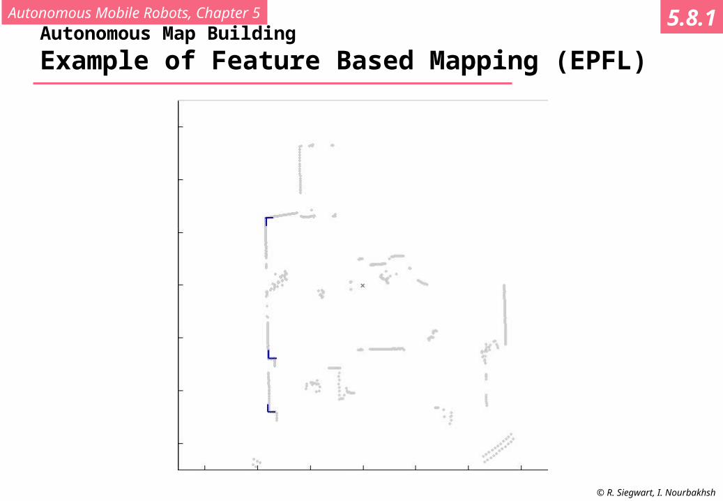
Autonomous Map Building
Example of Feature Based Mapping (EPFL)
5.8.1

Autonomous Mobile Robots, Chapter 5
© R. Siegwart, I. Nourbakhsh
Cyclic Environments
• Small local error accumulate to arbitrary large global errors!• This is usually irrelevant for navigation• However, when closing loops, global error does matter
5.8.2
Courtesy of Sebastian Thrun

Autonomous Mobile Robots, Chapter 5
© R. Siegwart, I. Nourbakhsh
Dynamic Environments
• Dynamical changes require continuous mapping
• If extraction of high-level features would bepossible, the mapping in dynamicenvironments would become significantly more straightforward. e.g. difference between human and wall Environment modeling is a key factor
for robustness?
5.8.2
Autonomous Mobile Robots, Chapter 5
© R. Siegwart, I. Nourbakhsh
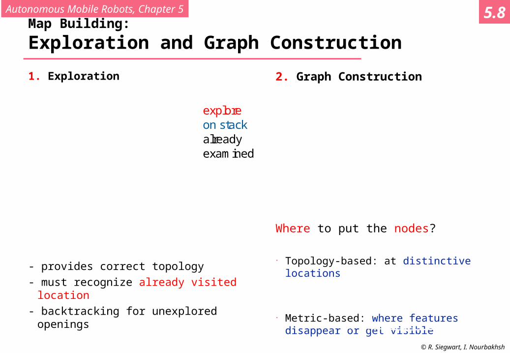
Map Building:
Exploration and Graph Construction
1. Exploration
- provides correct topology
- must recognize already visited location
- backtracking for unexplored openings
2. Graph Construction
Where to put the nodes?
• Topology-based: at distinctive locations
• Metric-based: where features disappear or get visible
exploreon stackalreadyexamined
5.8
Related Documents