Automation, Labor Share, and Productivity: Plant-Level ...

Automation, Labor Share, and Productivity:Plant-Level Evidence from U.S. Manufacturing∗

Emin Dinlersoz†

U.S. Census BureauZoltan Wolf‡

New Light Technologies

May 3, 2019

Abstract

This paper provides plant-level evidence on the relationship betweenautomation, factor usage, and productivity based on the U.S. CensusBureau’s Survey of Manufacturing Technology. More automated plantsexhibit lower production labor share, higher capital share, and higherlabor productivity. They also experience greater long-term labor sharedeclines and production labor productivity growth. Motivated by thesepatterns, a model of production with technology choice is estimated.The estimates indicate that more automated plants have higher totalfactor productivity and place less weight on production labor relative tocapital, resulting in lower share and higher productivity for productionlabor.

JEL Codes: D24, O33, J30, L60Keywords: automation, technology choice, total factor productivity,capital-labor substitution, labor share, CES production function, robots

∗Any opinions and conclusions expressed herein are those of the authors and do notnecessarily represent the views of the U.S. Census Bureau or New Light Technologies. Allremaining errors are our own. All results have been reviewed to ensure that no confidentialinformation is disclosed.†Center for Economic Studies, U.S. Census Bureau, 4600 Silver Hill Road, Suitland, MD

20746. E-mail: [email protected]‡New Light Technologies, 1440 G Street NW, Washington, DC 20005. E-mail:

[email protected]

1 Introduction

The diffusion of automation is believed to be one of the fundamental drivers

of the decline in employment and labor share, and the surge in output and

productivity in U.S. manufacturing over the past decades. As robots increas-

ingly take over the tasks performed by humans, the dependence on labor can

recede further. These aggregate trends notwithstanding, micro evidence on

the connection between automation, labor share, and productivity, has been

scarce. This paper provides additional evidence on this connection using plant-

level measures of automation from the U.S. Census Bureau’s 1991 Survey of

Manufacturing Technology (SMT). The SMT is ideal for studying patterns of

automation-driven capital-labor substitution because it was designed to collect

data from industries where capital better encapsulates advanced technologies

that have the potential to replace labor.1

The stylized facts from the SMT, discussed in Section 2, indicate systematic

relationships between automation and other plant-level outcomes. Specifically,

labor’s share in the value of shipments decreases as the degree of automation

increases, driven by the negative relationship between production labor share

and automation. In addition, more automated plants have a higher capital-

production labor ratio, and a lower fraction of production workers, who are

more productive and receive higher wages. Furthermore, plants with higher

recent investment in automation experience larger declines in production la-

bor share on a 5-to-10-year horizon. These findings are consistent with the

subjective responses of plants in the SMT, which indicate that one of the most

important benefits they receive from automation is reduction in labor costs.

Motivated by the stylized facts, we propose and estimate a model of CES

production where plants choose thier production technology by adjusting the

relative weight of capital and labor in response to relative price developments.

A larger relative weight is interpreted as indication that the plant relies more

1Previous research used general capital measures, indicators of IT investment and use,and robot density as proxies for automation. In its broader definition, automation caninclude robots, machines with a pre-programmed computer software, metal-working lasers,optical inspection devices, automatic-guided vehicles, and many other technologies.

2

heavily on automation in production. This modeling choice is motivated by the

fact that the large observed variation in the degree of automation is positively

correlated with the relative weight. Relative factor prices play a central role

in the model because they determine the relative weight. Modeling the plant’s

automation decision in this manner allows for alternative interpretations about

the nature of automation, since any factor that affects the relative price will

influence the plant’s decision on automation. This approach is different from

standard models of directed technical change, where the relative weight is

typically governed by exogenous factor-augmenting shocks. It is based on the

view that substitution may stem from a variety of factors including, but not

limited to, such exogenous shocks. For instance, relative price variation may

reflect differences in labor market frictions, labor quality and skills, financing

constraints that limit technology adoption, unionization or the threat of it,

the availability of outsourcing or offshoring, all of which may induce a plant

to adjust the relative weight.

As in other models of CES production, the sensitivity of the relative weight

to the relative price is characterized by the elasticity of substitution. This key

technology parameter is estimated in the first step of the empirical analysis

using plant-level information from the SMT. Given an estimate of the elasticity,

the remaining parameters of the production function are determined following

a version of the methodology described in Haltiwanger and Wolf (2018).2

Using factor weights or factor-augmenting shifters in CES production func-

tions has a long tradition in the literature.3 Exogenous factor-augmenting

shocks are typically the primary source of heterogeneity in relative factor pro-

ductivity. An immediate implication is that if there are other forces that

generate heterogeneity in relative factor productivity then this assumption is

arguably too restrictive. For example, if some production units actively in-

vest in more automated capital and/or employ more skilled workers, then the

2The approach uses first-order conditions of profit maximization to determine the elas-ticity of variable factors. Quasi-fixed factor elasticities are estimated controlling for unob-served productivity differences using plant-level variation in advanced technologies invest-ment available from the 1991 SMT.

3For recent examples, see Raval (2017) and Doraszelski and Jaumandreu (2018).

3

relative productivity could reflect differences in automation and labor com-

position. In addition, relative productivity and labor costs can be correlated

in such cases. More generally, the relative weight and productivity of factors

can be correlated with other plant-level outcomes. Although standard models

with exogenous factor weights and productivity are able to generate correla-

tions between these outcomes, the signs of these correlations are not always

consistent with the accumulated evidence.4

Our approach is related to models of task-based automation, which em-

phasize the role of technological improvements in explaining the evolution of

aggregate labor market outcomes.5 These studies posit that the total output

in the economy is a CES aggregate of individual task-level output. In contrast,

the focus in this paper is specifically on the choices made by a production unit

about the extent of automation used in production processes, motivated by

the significant plant-level heterogeneity in the adoption and use of automation

observed in the SMT.

The model of production in this paper is also related to models of endoge-

nous productivity.6 In these models, TFP depends on plant level decisions,

such as R&D and exporting. It is less common to model factor-specific pro-

ductivities or the relative factor weight as functions of plant actions. However,

plant choices such as automation can be aimed at increasing the relative pro-

ductivity of one factor. For instance, investing more in automation can increase

labor productivity.

Earlier work has investigated capital-labor substitution using country and

industry-level information on robots, automation, TFP, and relative input

prices.7 Given the more aggregate nature of these approaches, they are better

4Acemoglu and Restrepo (2018a) demonstrate the shortcomings of standard directedtechnological change models in capturing some hitherto documented effects of automationon labor outcomes. For example, they show that capital-augmenting technical change neverreduces labor demand and increases labor share.

5See Acemoglu and Restrepo (2018a,b) for more details and about evidence that themodel’s implications are consistent with aggregate labor share and wage dynamics.

6See Ericson and Pakes (1995), Doraszelski and Jaumandreu (2018), Aw et al. (2011).7Recent examples based on these variables are Elsby et al. (2013), Karabarbounis and

Newman (2014), Graetz and Michaels (2018),Acemoglu and Restrepo (2017), and Autorand Salomons (2018).

4

suited to account for general equilibrium effects of automation. However, they

are less informative about the connection between automation and production

labor at the micro level. The analysis in this paper is intended to shed light on

this connection by using direct measures of automation-related technologies at

the plant level. The SMT contains information on the investment in, and use

of, 17 such technologies, providing a level of detail unique in this literature.

The results in this paper also contribute to research on the decline in U.S.

labor share.8 Explanations of the decline include the diffusion of labor-saving

technologies and automation brought about by the fall in the relative price of

capital with respect to labor, import intensity and offshoring, the decline in

unionization, or labor reallocation.9 The last one of these has received a lot

of attention with the rise of productive and large firms, and the associated

increase in industry concentration of employment and sales. However, the

microeconomic mechanisms through which these firms emerge have not been

explored in detail. This paper offers additional evidence in this regard, which

suggests that larger and more productive plants tend to be more automated

and have lower production labor share, implying that increasing automation

is one possible explanation behind the rise of such successful production units.

Part of the empirical analysis is related to previous literature that uses

the SMT to analyze the connection between automation and plant-level out-

comes. Most of the existing work relies on extensive measures or simple counts

of technology types.10 A number of papers look at the relationship between

technology presence and plant life-cycle.11. Others explore the wage premia

associated with technology use.12 The SMT has also been used to study the

8In addition to the first two of the studies cited in the previous footnote, Lawrence (2015),Barkai (2016), Autor et al. (2017a,b) are recent examples.

9Autor et al. (2013) highlight the role international trade, while Elsby et al. (2013) con-sider the decline of unionization. Autor et al. (2017a,b) analyze the causes and consequencesof labor reallocation.

10Beede and Young (1996) provide an extensive summary of this literature.11Dunne (1994) explores the relationship between plant age and technology presence,

while Doms et al. (1995) document that capital-intensive plants with advanced technologygrow faster and are less likely to fail.

12Dunne and Schmitz Jr. (1995) find that establishments with more advanced technologiespay the highest wages and employ a higher fraction of non-production workers. Doms et al.

5

connection between labor productivity and technology.13 Our work differs

from these studies in two aspects. First, the analysis is based on intensive

measures, such as the extent of investment in automation, and the degree to

which a plant’s operations depend on automation–instead of basic indicators

of automation presence. In addition, the objective is to estimate a model of

production in a way that accounts for the connection between input prices and

automation, and at the same time controls for unobserved productivity differ-

ences. For the latter purpose, intensive indicators of investment in automation

are more appropriate because they measure these differences more accurately.

2 Data

The main data source is the U.S. Census Bureau’s 1991 version of the SMT,

part of three separate surveys on technology use in manufacturing plants con-

ducted in 1988, 1991, and 1993. It contains a rich set of measures on the

automation-related technologies. Extensive measures on technology presence

are available in the 1988 and 1993 versions, while intensive measures on tech-

nology use and investment are recorded in the 1991 version. The 1991 survey

contains a stratified random sample of about 10,000 observations, representa-

tive of nearly 45,000 plants.

The 1991 SMT has data on 5 broadly defined manufacturing industries14:

Fabricated Metal Products (SIC 34), Industrial Machinery and Equipment

(SIC 35), Electronic and Other Electric Equipment (SIC 36), Transportation

Equipment (SIC 37), and Instruments and Related Products (SIC 38). These

industries were included in the survey because they rely more on automation-

related technologies, which makes them ideal for the purposes of this paper.15

(1997) document that businesses with a greater number of advanced technologies have moreeducated workers, more managers and pay higher wages. They do not find, however, asignificant correlation between skill upgrading and use of advanced technologies.

13SeeMcGuckin et al. (1998).14These industries accounted for about 43% of manufacturing employment in 1991.15The SMT was funded partly by defense agencies. During the developmental phase the

Census Bureau consulted with government agencies, private industry and academic experts.The industries were selected because of the relatively high presence of defense contractors,which also tend to be more advanced in terms of technology. A number of studies in

6

The SMT industries are not substantially different from the rest of man-

ufacturing in terms of average capital and production labor shares, see Table

1(a). Although the non-production labor share is lower and the capital-labor

cost-ratio is higher, these indicators are also comparable to the rest of man-

ufacturing. The fact that the SMT industries do not stand out in terms of

standard measures suggests that these measures may not be informative by

themselves about the underlying extent of automation in an industry.16

2.1 Technology Questions

The SMT contains information on the adoption and use of 17 individual tech-

nologies, see Table 1(b), some of which are directly aimed at automation,

whereas others can facilitate or support automation.17 The current analysis

views all of the technologies as part of the automation in the plant because

they all have the potential to replace production workers.

The 1991 version of the SMT records information about use and invest-

ment, the 1988 and 1993 versions contain information about the presence of

technologies. The 1991 SMT has information only on 4 broad technology

groups, which contain 17 detailed technologies which were the focus of the

1988 and 1991 surveys. While the SMT pertains to an earlier period, many

of the technologies had already diffused to a large extent by the time of the

survey –see Table 1(b). While robots were less common around the time of

the survey, other automation-related technologies were relatively wide-spread.

The similar relative diffusion rates in 1988 and 1993 suggest that the 1991

diffusion rates are likely similar.

engineering economics support this view, see, e.g., Kelley and Watkins (1998). This findingechoes in the SMT: plants that indicate production to military specs have on average highertechnology use and investment.

16Details about the evolution of these industry aggregates can be found in Appendix A.1.The industries exhibit similar trends, and the decline in labor share is consistent with thewell-documented decline for overall manufacturing.

17The former group includes Robots, Automated Storage and Retrieval Systems, Auto-mated Guided Vehicle Systems, and Automated Sensor Based Inspection/Testing Equip-ment, the latter group includes Computer Aided Design/Engineering, Computer AidedManufacturing, Local Area Networks. Exploring which technologies matter most for re-placing labor is important but is beyond the scope of the paper and is left for future work.

7

The key data source for this paper is the 1991 version, because intensive

measures, such as the fraction of automated operations, and the dollar-value

of investment in automation, more accurately capture cross-establishment dif-

ferences in the extent of automation than the simple technology counts. The

technology indicators used in this paper are based on 4 survey questions about

current and planned use of, and investment in, 4 broad technology groups,

see Table 2. Responses are recoded into numerical categories, implying that

the interpretation of exact quantitative differences across categories is diffi-

cult. Nevertheless, these categories capture some of the cross-plant variation

in technology use and investment, which is the key variation used to control

for unobserved productivity differences during production function estimation.

2.2 Technology Index

In the empirical analysis, the degree of automation is measured using infor-

mation about current, as well as planned, investment and use pertaining to

each of the four technology groups, described in Table 1(b).18 In particular,

plant-level responses to the questions in Table 2 are aggregated into a plant-

specific average. The resulting average index is continuous between 0 and 5,

where zero indicates no automation, a positive value represents the average of

the extent to which the plant uses and invests in automation.19

2.3 Input and Output Measures

Plant-level measures of output and inputs were obtained from the 1991 An-

nual Survey of Manufactures (ASM). Since the sampling frame of the ASM is

different from the SMT, some of the records could not be matched. In such

cases, the 1990 ASM and 1992 Census of Manufacturers (CMF) were used

18Incorporating the response to the question on the anticipated cost of future acquisitionsmakes little difference in our results and conlcusions.

19An alternative measure based only on the investment question (2) in Table 1(b) is alsoconsidered. To prevent confusion, whenever both measures are used in the empirical analysis,the main technology index is labeled as “Technology Index I”, whereas the investment-basedone is labeled as “Technology Index II”.

8

to supplement the output and input measures.20 Output is measured as the

deflated value of total value of shipments. Production labor input is measured

by production worker hours, non-production worker input is calculated as the

product of production worker hours and the ratio of non-production wage bill

to production wage bill. Intermediate inputs are calculated as the sum of cost

of parts, contracted work and goods resold. The energy input is composed of

costs of electricity and fuel. Capital stock measures are based on a version of

the Perpetual Inventory Method that generates current capital by summing

the depreciated stock and current investment. The initial capital stock is a

deflated book value that is taken from the ASM-CMF.21

A separate panel of plants is also used to check the robustness of the

elasticity of substitution estimates. This panel is constructed using all ASM

plants from SMT industries, between 1987 and 1996. For the analysis of the

relationship between the degree of automation and the evolution of labor share

and labor productivity, the plants in the 1991 SMT that survive and appear

in the 1997 and 2002 CMF were identified using the U.S. Census Bureau’s

Longitudinal Business Database (LBD). The surviving plants are used to study

the evolution of labor share within the next 5 to 10 years as a function of the

degree of automation in 1991.22

3 Stylized Facts

3.1 Labor Share and Automation

Based on plants’ own assessments in the 1991 SMT, quality improvement and

labor cost reduction are the two most important benefits from automation,

see Figure 1 for more details. In other words, plants recognize the importance

of input prices in automation investment, which is especially relevant for the

purpose of the current analysis. Other benefits include, in decreasing order of

20If an SMT-plant cannot be matched to the 1991 ASM, it is matched to the 1992 CMF.Otherwise, the plant is matched to the 1990 ASM.

21More details on these data can be found in Foster et al. (2017).22Survival bias is also accounted for in this analysis for robustness.

9

importance, the increase in the flexibility of production, lead-time reduction,

and marketing advantage.

In order to get a more accurate picture of input use, Figure 2(a) plots

plants’ labor share in total value of shipments as a function of the technology

index discussed in Section 2.2. Labor share is lower for more automated estab-

lishments: it drops from 29% to 24% as the technology index increases from 0

to 5. The decline is statistically significant for much of the index range, and

is driven by production labor.23 The share of production labor drops nearly

by half moving from the lowest to highest index levels (Figure 2(b)), whereas

non-production labor’s share increases only slightly (Figure 2(c)). More au-

tomated plants also tend to have a lower fraction of their workforce engaged

in production (Figure 2(d)). This fraction drops from 70% to 50% across the

index range. In addition, capital’s share in the value of shipments increases

with the technology index (Figure 3(a)). As a result, the ratio of capital share

to labor share, and the capital-labor ratio also increase with the technology

index (Figures 3(b)-3(c)).24 The technology index is also correlated with other

plant level outcomes. Labor productivity increases with the index, especially

for production labor (Figure 4), a finding robust to alternative ways to mea-

sure labor productivity (Figure A5 in Appendix A.5). Average wage (total

wage bill divided by the number of workers) also increases with the index for

both types of labor (Figure A4).

These relationships are robust to a broad set of controls such as plant

size and age, unionization of production workers, foreign-ownership, military

production, or whether or not a plant exports. Tables 3(a)-3(c) show the es-

timated coefficients of the technology index conditional on these controls.25

23The confidence intervals get larger at the high end of the technology spectrum becausesample size decreases and because of the one-sided nature of the kernel smoothing near theend of the sample.

24The patterns in Figures 2 and 3 continue to hold if plant value added is used insteadof revenues, when industry effects are netted out, or when other plant characteristics arecontrolled for.

25For robustness, these tables also feature the alternative technology index (TechnologyIndex II) that only includes the average investment indicator across the four technologygroups based on survey question 2 in Table 2.

10

The results indicate that, controlling for observables, a 1% increase in technol-

ogy index is associated with a 0.04-0.08% decline in production labor share,

0.12-0.14% increase in production labor productivity, and 0.08-0.09% increase

in average production worker wage across plants. In contrast, the technology

index does not seem to be related to non-production labor share, while av-

erage wage and labor productivity of non-production workers both increase

with the technology index.26 Overall, these results confirm the bivariate rela-

tionships discussed above and are robust when value-added-based measures of

labor share and labor productivity are used.27

3.2 Change in Labor Share and Automation

A full dynamic analysis of the effects of changes in automation is not possible

because the technology index can be constructed in 1991 only.28 However, we

can analyze establishment-level outcomes as a function of the 1991 automa-

tion status, which allows suggestive conclusions about dynamic effects because

many automation-related technologies are likely to remain in place for longer

time periods. To explore the connection between automation and change in

labor share, the following specification is estimated

∆yi = bo + bIIi + bE∆ei + bXXi + εi, (1)

where ∆yi denotes the log difference in the labor share or labor productivity

between 1991 and 1997, or between 1991 and 2002. ∆ei denotes the log differ-

ence in the plant’s total employment over the same horizon, it serves to control

26Non-production worker category includes labor with various education and skill levels.The confounding effect of this unobserved heterogeneity may explain the greater standarderrors for its share.

27Unreported results indicate correlation between some plant characteristics and produc-tion labor share. For example, younger, larger, domestically-owned, and intensely-exportingplants generally have lower production labor share. In addition, younger and larger plantsrely more heavily on automation.

28An additional argument for using the 1991 SMT is that there is significant attritionbetween the 1988 and 1993 surveys, and the technology indicators in these surveys do notreflect investment or usage intensity. Prior research with these two surveys also indicatesome potential recall bias.

11

for growth-related heterogeneity.29 Ii denotes the 1991-value of the technology

index, and Xi contains plant-level controls and industry effects.30 The results

in Tables 4(a) and 4(b) indicate that plants that were more automated in 1991

tend to experience lower production labor share growth and higher produc-

tion labor productivity growth over the next 5 to 10 years. These results,

taken together with those in the previous section, confirm that the correlation

between automation, labor share and labor productivity is statistically and

economically significant.31

4 The Model

This section describes a model of plant-level production that is consistent with

the stylized facts discussed above. A key feature of the model is technology

choice: the plant adjusts the relative weight of capital and production labor

in response to changes in their relative price.

Plant i generates output according to the production function

Qi = θiLβ1niM

β2i E

β3i [α

2/σi Kρ

i + (1− αi)2/σLρpi]γ/ρ, (2)

where θ denotes Hicks-neutral productivity. For simplicity, freely variable

inputs non-production labor (Ln), intermediate inputs (M), and energy (E)

are combined into a Cobb-Douglas (CD) aggregate, with elasticities βj.32 The

focus is on the capital (K) and production labor (Lp), which are aggregated

into a constant-elasticity-of-substitution (CES) composite, Ti = [α2/σi Kρ

i +(1−αi)

2/σLρpi]1/ρ, where σ denotes the elasticity of substitution between Lp and K,

and σ=(1− ρ)−1.

29Growing plants hire more employees and therefore their labor share is expected to rise.30Because ∆yi is observed only for plants surviving till 1997 (or 2002), a Heckman two-step

estimation is also implemented to account for the bias introduced due to this selection.31Controlling for survival bias using a Heckman correction confirms these conclusions:

Tables A2 and A3 in Appendix A.5 show qualitatively similar results. Results are alsostronger when value added is used to measure production labor share and productivity.

32Figure 2(c) indicates no significant correlation between non-production labor share andthe degree of automation, suggesting that the simplification is reasonable.

12

K and Lp are assumed to be quasi-fixed. This assumption is justified by

existing micro evidence that both capital and labor adjustment are subject

to non-linearities – see, e.g., Caballero et al. (1997), Cooper and Haltiwanger

(2006) and Bloom (2009). In addition, a union contract for production workers

exists in nearly 20% of the 1991 SMT plants, which is an indication that

production labor is subject to similar rigidities – see Dinlersoz et al. (2017).

Assuming that Ln is a freely variable input simplifies the analysis and helps

maintain focus on the connection between Lp and K.33

The relative weight of K and Lp in T is determined by αi ∈ (0, 1), which

is referred to as the degree of automation in the plant. As discussed in more

detail in Section 4.1, the first order conditions of cost minimization imply that

in equilibrium the plant adjusts the relative weight αi/(1 − αi) in response

to changes in the relative price of K and Lp, conditional on σ. This is a

deviation from earlier work on CES production because the relative weight is

generally assumed to be exogenously given, and may even be a constant across

establishments, see, e.g. Lawrence (2015) and Raval (2017).

The decision variable αi can be interpreted in a number of ways. A higher

αi in standard models represents a technology that augments the productiv-

ity of K more relative to Lp.34 Alternatively, given the positive relationship

between K and automation in the SMT, a higher αi can also indicate that

the establishment has more automation-related capital. What underlies the

latter interpretation is the plant’s decision on αi in response to a change in

the relative price. Specification (2) can also be interpreted as a reduced-form,

plant-level representation of a task-based production model, analogous to the

approach in Acemoglu and Restrepo (2018a,b).35 Suppose that plant-level

production consists of a set of individual operations indexed on the unit inter-

val [0,1], each of which can be carried out using either capital or production

33It is possible to generalize the analysis using nested CES specifications that allow varyingsubstitutability between both labor inputs and capital, as well as energy and materials.

34To see this, rewrite Ti in (2) as [(AiKi)ρ + (BiLpi)

ρ]γ/ρ and set Ai = α2(1−ρ)/ρi and

Bi = (1− αi)2(1−ρ)/ρ.35However, those models do not pertain to a production unit, and task-level output is

aggregated to the economy-level.

13

labor. The plant chooses αi, the fraction of operations it wants to automate,

and the amount of K or Lp conditional on αi. In this context, a higher αi can

be interpreted as a higher degree of automation.36

It is straightforward to generalize the weights in the composite input Ti by

rewriting it as Ti=[αζ/σi Kρ

i + (1 − αi)ζ/σLρpi]1/ρ, where 0 < ζ is a parameter.

Specification (2) then corresponds to the case of ζ = 2. Although choosing

ζ = 2 restricts the parameter space, the restriction is not inconsistent with the

properties of the SMT, while it delivers analytical convenience and also limits

the number of parameters to estimate.37

Note that in a fully specified model, Hicks-neutrality implies that αi affects

only Ti, so the production function in (2) does not restrict the relationship

between productivity and other plant characteristics. However, if (2) is not

fully specified, θi and other plant characteristics may be correlated.38

4.1 The Plant’s Problem

Throughout this section, plants are assumed to be price takers in input markets

– a standard assumption in the empirical productivity literature. In the first

part, price taking behavior is also assumed for output markets.

4.1.1 Exogenous Output Prices

Plants produce a homogenous good with a fixed price, normalized to one. All

factor prices, denoted by wji, are allowed to vary across plants, as opposed

36Here, no formal equivalence to task-based models is claimed. Although in principle sucha model could be posited at the plant-level, this approach would require additional structureand therefore is left for future work.

37Noting that CD is a special case of (2) with σ = 1, if the true data generating processin the SMT can be described by (2), then we should expect the σ-estimates to be less thanone. We show in Section 5.1 that the value of ζ has implications for the estimated value ofσ, and as we will see in Section 6, ζ = 2 yields elasticity estimates that are consistent withthese expectations, given the properties of the SMT.

38For instance, it may be the case that θi=θ(αi), where αi directly affects Qi in additionto its effect on Ti. Such effects are plausible if adopting labor-saving technologies also resultsin more flexible production, and improves overall coordination and monitoring of productionprocesses, resulting in higher Hicks-neutral productivity.

14

to the typical assumption that they are constant. The assumption of het-

erogenous input prices is justified if, for instance, there are differences across

plants in terms of the quality of their inputs. One example would be the

case in point where plant-level capital stocks differ in the extent to which

they contain automation-related technologies.39 Under these assumptions, the

first-order conditions of cost minimization can be written as40

Ki/Lpi = (wpi/wki)2−σ (3)

αi/(1− αi) = (wpi/wki)1−σ . (4)

These expressions highlight the key mechanism of the model: both the capital-

labor ratio and the relative weight are tied to relative input price variation

and the nature of these relationships is fully determined by σ. It follows from

equations (3) and (4) that Ki/Lpi and αi/(1 − αi) are increasing and convex

in wpi/wki, as long as σ < 1. That is, an increase in the relative price of Lp

induces the plant to substitute K for Lp by increasing αi, and more so for

higher values of αi. Equations (3) and (4) also imply that the capital-labor

ratio can be written as a function of the relative weight:

Ki/Lpi = (αi/(1− αi))2−σ1−σ , (5)

and that this relationship is also convex because 1 < (2−σ)/(1−σ) as long as

σ < 1. Equation (5) formalizes the basic idea that automation increases the

relative weight and the capital-labor ratio.

The implications of equations (3)-(5) are consistent with the observed re-

lationships in the SMT, see the discussion of Figures 3(b)-3(c) in Section 3.

Importantly, the implications are different from alternative models. To be spe-

cific, these relationships are not convex in the case of a standard CES model

with σ < 1, or under Cobb-Douglas production.41

39Input price variation can also be a result of differences across locations, amenities,agglomeration economies, and costs of mobility and adjustment may imply persistent dif-ferences in the price of labor and capital.

40See Appendix A.2 for more details.41In the standard CES model with exogenous relative weight, i.e. [αiK

ρi +(1−αi)Lρpi]γ/ρ,

15

It is useful to describe the properties of shares of input expenditures be-

cause they can be used to develop estimators. By combining equations (3)-(4)

it can be shown that Lpi’s optimal weight in production equals its share in the

cost of Ti:

1− αi = wpiLpi/(wkiKi + wpiLpi). (6)

Using the fact that the revenue share of Ti equals the elasticity, γ, of Qi with

respect to Ti, the revenue shares of Lpi and (Lpi + Lni) can be written as

wpiLpi/Qi = γ(1− αi) (7)

(wpiLpi + wniLni)/Qi = β1 + γ(1− αi). (8)

Equations (6), (7) and (8) indicate that all labor usage indicators are de-

creasing in αi but the revenue shares’ sensitivity to αi depends on γ.42 The

cost share of the jth variable input can be written as csj=βj∑j βj+γ

, and the

share of Ti in total costs is given by csKi+csLpi=γ∑

j βj+γ× ci, where ci =

α2/σi Kρ−1

i +(1−αi)2/σLρ−1pi

α2/σi Kρ

i +(1−αi)2/σLρpi< 1 if σ < 1.43 One difference relative to CD technology

is that imposing constant returns to scale (CRS) is not a sufficient condition

for identification. Even though variable input elasticities are identified by cost

shares under CRS, the share of Ti in total costs underestimates the contribu-

tion of γ to returns-to-scale, irrespective of its value.

If returns-to-scale is unknown, the implications of profit maximization can

be used to recover factor elasticities. The first-order condition from profit

maximization imply that factor elasticities can be written as βj = wjiXji/Qi,

and γ=wkiKi/Qi+wpiLpi/Qi, which show that under exogenous prices and un-

known returns-to-scale, the factor elasticities of both freely variable inputs and

the composite input are identified by revenue shares of input expenditures.44

we have Ki/Lpi = (αi/(1− αi)× wpi/wki)σ, so when σ ∈ (0, 1), Ki/Lpi is concave in bothratios. CD production implies Ki/Lpi = αi/(1 − αi) × wpi/wki, so Ki/Lpi is linear in theratios.

42When γ=1, all three shares decline one-for-one with αi. If γ < 1, the revenue shares’rate of decline is smaller, and the relationship is reversed when γ > 1.

43This statement holds if 1 < Lpi,Ki, which is the case in yearly data on these variables.44See Appendix A.2 for details.

16

4.1.2 Isoelastic Residual Demand

An alternative to fixed output prices is to postulate that the plant’s resid-

ual demand is isoelastic, a commonly used approach in the literature.45 Un-

der this assumption, the inverse residual demand function can be written as

Pi = P (Q/Qi)1−κ ξi with 0 < κ < 1, where P and Q denote aggregate vari-

ables and ξi is an idiosyncratic demand shifter. The results of cost minimiza-

tion are robust to alternative assumptions about demand. The conclusions

of profit maximization are different because under downward sloping demand

conditions marginal revenue products are smaller than marginal products. To

see this, let Ri=PiQi denote plant-level revenues, and write the first order

conditions for the jth variable input and the quasi-fixed inputs as

wjiXji/Ri =κβj (9)

(wkiKi + wpiLpi)/Ri =κγ, (10)

where (10) combines conditions for K and Lp. The implications of (9)-(10) for

the relationship between wpi/wki, Ki/Lpi and αi/(1 − αi) are the same as in

Section 4.1.1 because relative input allocations are not affected by ξi.

An important difference relative to Section 4.1.1 is that the revenue share

of input expenditures now depend on both βj and κ. In principle, informa-

tion on output prices could be used control for output price variation during

estimation, which in turn would allow the identification of factor elasticities.

However, output prices in SMT are recorded as a categorical variable and

preliminary analysis indicates that this variable has no additional explanatory

power conditional on the variables already included in the analysis, potentially

due to the relatively coarse price categories used in the survey.46

45For Recent examples, see De Loecker (2011), Bartelsman et al. (2013), Foster et al.(2016, 2017), and Haltiwanger and Wolf (2018).

46The categorical price variable measures average price for the products of a plant and isavailable in the 1988 and 1993 SMT only. The price information was merged for the set ofplants in the 1991 SMT that are in the union of the 1988 and 1993 SMT plants.

17

5 Estimation

The estimation strategy uses some of the model properties discussed in Section

4. The elasticity of substitution is estimated using a log-linearized version of

(3). The remaining parameters in (2) are estimated conditional on σ, using a

modified version of the method described in Haltiwanger and Wolf (2018).

5.1 Elasticity of Substitution

Log-linearizing equation (3) yields lpi = (σ− 2) lnwpi− (σ− 2) lnwki + ki + εi,

where εi is an iid error. Given data on lpi, ki, and their prices, this equation

can be estimated by running the regression

lpi = δ1 lnwpi + δ2 lnwki + δ3ki + ui. (11)

Since wpi is obtained by dividing production labor costs by production worker

hours, OLS estimates of δ1 are affected by division-bias. This issue is addressed

using geographic variation in wpi as instruments, where the instrument is de-

fined as a county-specific average manufacturing wage indicator, calculated

using plant-level information. This approach is similar to the method used

by Raval (2017). The rental price is also unobserved in both the SMT and

the ASM. The plant-level measure of wki is calculated by combining industry-

specific rental prices and plant-level capital cost measures, which provide wkiKi

and Ki but not wki, implying that δ2 is not identified.47 Under the assump-

tion that the rental price is plant-specific, its effect can be accounted for by a

plant-fixed effect, in which case δ3 is identified in the first-differenced version

of (11). This strategy is justified when plant-level capital prices are persistent,

for instance when they follow a random walk.48

Before moving on to discussing the estimation of factor elasticities, it is

useful to reiterate a point that concerns restricting the parameter space. Con-

47See Foster et al. (2016) for more details on capital measures.48Equation (11) has no explicit dynamic elements in the econometric sense despite the

fact that the plant’s optimal decision on both capital and production labor have dynamicimplications, see Section 4. This is because the main purpose of (11) is to estimate long-runpatterns of capital-labor substitution.

18

ditional on an estimate of δ1, σ̂ is calculate as σ̂=δ̂1+2 because we chose ζ=2

in equation (2). As mentioned in Section 4, this choice is motivated by analyt-

ical convenience and the fact that it supports σ-estimates that are consistent

with the implications of the model and the observed patterns in the SMT. In

particular, the stylized facts suggest that K and Lp are less substitutable than

what a CD specification would imply, and hence one expects σ̂<1. Choosing

ζ=2 allows for this possibility and also helps maintain analytical tractability.

5.2 Factor Elasticities

The estimation strategy for factor elasticities is based on earlier results in the

empirical productivity literature, but also deviates from standard approaches

in order to better make use of the features of the SMT. The 1991 SMT records

categorical responses on how much the plant invested in four technology types

in the previous three years, see question 2 in Table 2. Although the variables

are categorical, they provide direct information on cross-plant differences in

automation investment. The responses are aggregated into a plant-level indi-

cator of technology investment, which is then used as a proxy to control for

unobserved productivity differences during estimation. This proxy is a dis-

tinguishing feature relative to earlier studies because those relied on general

investment to control for unobserved productivity differences.49

In addition to the unique proxy, the estimation strategy deviates from the

standard proxy-based approaches in two other respects. First, it abstracts

from selection because the SMT has limited information on investment his-

tory. Second, it follows the methodology described in Haltiwanger and Wolf

(2018) to non-parametrically estimate the elasticities of freely variable inputs.

Under the assumption of downward-sloping demand, the revenue shares of

variable input expenditures depend only on the corresponding factor elasticity

and the demand parameter, implying that revenue shares can be used to iden-

tify elasticities without projecting revenue variation on proxies, state variables

49The idea of accounting for unobserved productivity differences during estimation byusing firm-level proxies is discussed in Olley and Pakes (1996) and Levinsohn and Petrin(2003).

19

and variable inputs.50 This property is useful because Gandhi et al. (2016)

show that the identification of intermediate input elasticities is problematic

when using intermediate inputs as a proxy. Given estimates of variable input

elasticities, Haltiwanger and Wolf (2018) propose to net out the contribution

of variable input expenditures from revenue variation, and use this net vari-

ation to estimate the remaining coefficients. The main difference relative to

Haltiwanger and Wolf (2018) is how the net variation is used to determine the

remaining coefficients, since their approach considers Cobb-Douglas technol-

ogy. A more detailed description of the estimation strategy can be found in

Appendix A.3.

6 Results

6.1 Estimates of the Elasticity of Substitution

The estimates of σ vary between 0.38 and 0.71 depending on the methods used,

see Table 5(a). These estimates are consistent with what recent work found

using similar data from the U.S. Census Bureau.51 The baseline σ̂, shown

in column 1 of Table 5(a), is determined by a cross-sectional IV. Column 2

contains the results without ki as an explanatory variable. This approach

may be justified if wpi and Lpi are measured with less noise than capital,

which may be the case for ASM.52 If capital is measured with error then

it is a priori unclear whether including ki in (11) is useful. The similarity

of the σ estimates is reassuring and at least suggests that production labor

data alone is informative for substitution patterns. Columns 3 and 4 show

additional robustness checks, where (11) is estimated using ASM data from

SMT industries between 1987 and 1996. Instead of using geographic wage

variation as an instrument, these calculations are based on lagged differences

50See Section 4.1.2 for more details.51For instance, Raval (2017) estimates a plant-level elasticity of substitution between labor

and capital in the range 0.3-0.5, and Oberfield and Raval (2014) report estimates between0.4 and 0.7.

52This survey collects data on book-value capital, which is then converted into marketvalues using data on depreciation and various deflators available at the industry level only.

20

of plant-level wages as instruments in a GMM framework, see Arellano and

Bond (1991). The GMM estimator yields similar σ̂s.

As previously discussed, σ < 1 implies that capital and production labor is

less substitutable than a Cobb-Douglas (CD) specification would imply.53 The

lower estimated substitutability is plausible considering that the plants in the

SMT typically utilize automation, which may give rise to complementarities

between K and Lp. Given σ < 1, the relative weight αi1−αi is increasing and

convex in the relative price.

6.2 Estimates of Factor Elasticities

Table 5(b) shows estimated factor elasticities conditional on the baseline σ̂.

As the column labeled “γ̂” indicates, all reviewed methods yield comparable γ

estimates suggesting that the contribution of the composite input to returns-

to-scale is between 0.17 and 0.25, depending on whether it is determined using

simple plant-level averages of the capital and production labor expenditures in

revenues (row 1) or projection-based methods (rows 2-3). The sum of factor

elasticities is less than one. However, without data on prices and quantities

these point estimates are revenue elasticities implying that they can be consid-

ered as lower bounds for factor elasticities – see Section 4.1.2 for more details.

6.3 Properties of Productivity Estimates

This section investigates the properties of the implied total factor productiv-

ity (TFP) distributions. For robustness, two commonly used CD productivity

measures are evaluated against three CES measures. The first CD measure, de-

noted by CDCRS, is derived under the assumption of constant returns-to-scale.

The second one, labeled as CDNCRS, is calculated under the assumption of non-

constant returns-to-scale. To simplify discussion, we maintain the assumption

of homogenous products, and price taking behavior.54 The CES productivity

indices correspond to the three specifications shown in Table 5(b). The first

of these, denoted by CESFOC, is based on γ̂ obtained as a plant-level average

53In other words, CES isoquants have more curvature than CD isoquants.54Analyzing the role of demand is deferred to future work.

21

of condition (10) under the assumption technology choice. The second CES

measure, labeled as CESEN, is a variant of the first one, in the sense that γ is

estimated using nonlinear least squares. The third one, labeled as CESEX, is

similar to the second one except that αi=1/2 is imposed as a reference point

for a case where αi is an exogenously given constant across plants.

The descriptive statistics, shown in Table 6, suggest that the shape of

the TFP distribution implied by CES specifications is generally different from

those under CD specifications. Although all five distributions have negative

skew indicating that the left tails are longer, there are differences in how dis-

persed and slender they are. CD yields more observations around the mode

and in the tails, indicated by higher kurtosis and lower dispersion. Bivariate

correlations in Table 6(b) echo these differences: while the association among

alternatives derived from the same technology is strong, the correlation be-

tween CD and CES residuals is significantly less than one.

In light of these findings, it is natural to ask whether the TFP distributions

implied by alternative technologies are systematically different. Given that the

SMT collected data from industries where automation is a likely substitute

for labor, the distinction between CD and CES is expected to be relevant.

The p-values of the Kolmogorov-Smirnov (KS) tests in Table 6(c) confirm this

conjecture: the CD and CES measures are significantly different at usual levels

of significance. Interestingly, the assumption of endogenous versus exogenous

technology also matters. In addition, the way elasticities are calculated under

CD also matters. The only pair for which the null of equivalence cannot be

rejected is the one where γ is estimated using different methods.

The KS test is useful to test whether two distributions can be considered

different in the statistical sense. However, it is not informative about possible

sources of the difference. In order to shed some light on the nature of the

differences discussed above, Appendix A.4 provides a detailed decomposition

in which the difference between CDCRS and CESEN is parsed into a term that

is due to differences in the functional form, and additional components that

can be attributed to estimation error. The contribution by the difference in

functional form can be interpreted as an estimate of the specification error in

22

the population if the true data generating process is CESEN. The difference

can be written as

∆i =γ̂

ρ̂ln[α2/σ̂i K ρ̂

i + (1− αi)2/σ̂Lρ̂pi]−(β̂k lnKi + β̂l lnLpi

). (12)

It is a useful metric because it helps understand why the KS test rejects the

null of equivalence. Interpreted as a sample statistic, ∆i accounts for all the

specification error on condition that the estimation error is the same under the

two specifications. Appendix A.4 explores the properties of ∆i in more detail.

It turns out that ∆i is negative for the majority of plants, meaning that the

CDCRS input index in the second term in (12) is systematically higher than

the CESEN input index in the first term of (12). In other words, CDCRS tends

to underestimate productivity if the true underlying productivity is CESEN.

The results also indicate that the extent of this error tends to be higher for

plants with higher capital-production labor ratio and more automation. These

findings imply that accounting for capital-labor substitution patterns in pro-

ductivity estimation is potentially important for correctly measuring TFP.

6.4 Automation, Productivity, and Labor Share

In order to shed light on the relationship between total factor productivity and

automation, Table 7(a) reports the results from regressing the revenue share

of Lp on the estimated TFP (CESEN) and technology index, controlling for

other plant characteristics. The main conclusion is that the revenue share of

Lp is lower in more productive and automated plants and that productivity is

more negatively correlated with Lp share than with technology.55

Table 7(b) repeats the previous analysis using 1 − αi as the dependent

variable, see equation (6). The results indicate that technology is more strongly

associated with this measure.56 Interestingly, 1 − αi is positively associated

55The results are similar if value-added is used instead of total value of shipments indefining labor share.

56Comparing (6) and (7) shows that if γ < 1 then γ(1 − αi) < (1 − αi), and thereforea given change in αi should imply a smaller decline in Lp cost’s share in revenue than incomposite input expenditures.

23

with productivity and negatively associated with plant size, which are the

opposite of the estimated signs in Table 7(a), suggesting that choice of the

labor share measure (revenue- or cost-based) matters for subsequent analyses.

If the model in Section 4 is fully specified, then αi and θi are not correlated.

However, a systematic relationship may emerge between the two measures if

not all factors of production are accounted for during estimation. In other

words, automation may be correlated with productivity in the presence of rele-

vant unobserved heterogeneity. In order to assess the presence of such factors,

the relationship between technology indices, productivity and other observ-

ables is assessed in a regression framework. Table 7(c) contains the estimated

coefficients, which indicate that more productive and larger plants tend to be

also more automated.57 It is important to note that the relationships change

with CDCRS. Table A4 in Appendix A.5 shows the details, here we only point

out that CDCRS is more negatively associated with the share of production

labor in revenue and shows no significant association with the share of pro-

duction labor in composite input expenditures. These findings indicate that

the specification of the production function matters. One implication is that

an incorrectly specified production function can have important consequences

for heterogenous agent models that aim to capture specific relationships re-

garding productivity, automation, and capital-labor substitution.

7 Concluding Remarks

There is a growing body of theoretical and empirical work on the aggregate

effects of automation on employment, labor share, and productivity. However,

micro-evidence on the connection between these variables has been limited,

due mainly to lack of detailed measures on automation. This paper provides

additional evidence on these relationships using plant-level information on au-

57It is a common finding in the productivity literature that the productivity residual iscorrelated with other plant characteristics. It indicates the presence of factors that thissimple model does not account for. For instance, automation may enhance managerialability, inventory management, or coordination in factory floor, which are factors that arenot fully captured by standard measures of input usage.

24

tomation from the U.S. Census Bureau’s 1991 Survey of Manufacturing Tech-

nology (SMT). The stylized facts from the SMT indicate that plants with

greater use of, and investment in, automation have higher capital share and

lower production labor share in revenue. More automated plants have rela-

tively lower fraction of production workers, exhibit higher labor productivity,

and pay higher wages.

Motivated by these facts, a model of plant-level production is proposed and

estimated. A key property of the model is that the plant chooses the relative

weight of capital and labor in a CES composite. The relative weight can be

interpreted as the plant’s choice of the degree of automation. This modeling

choice is a deviation from standard models of biased technical change where

the relative weight of inputs is determined by exogenous factor-augmenting

shocks. Endogenous technology choice reflects the view that substitution be-

tween capital and labor may stem from any shock that alters the relative price

of these inputs. Therefore, the model supports alternative interpretations

about the underlying reasons for capital-labor substitution.

The model’s predictions are consistent with the observed correlations be-

tween the relative weight of inputs and other plant-level outcomes. The es-

timates of the elasticity of substitution are less than one, suggesting comple-

mentarities between capital and labor. This complementarity is plausible con-

sidering that the industries in the SMT are more likely to encapsulate higher

levels of automation. The estimates also imply that the production labor share

is decreasing and the capital-production labor ratio is increasing in the relative

price of production labor. In addition, the estimated total factor productivity

distribution implied by CES production with endogenous technology choice

differs significantly from standard models. The findings also suggest that the

form of the production function matters for the assessment of the relationship

between productivity, labor share, and automation.

Our simple exploration of dynamic relationships indicates that more au-

tomated plants tend to experience larger five- and ten-year declines in labor

share and bigger increases in labor productivity. Given the positive connection

between firm productivity and growth established in previous studies, these

25

findings are consistent with a model where the adoption and use of automa-

tion is behind the success of large and productive firms with low labor shares.

Future work should consider this hypothesis in more detail.

References

Acemoglu, Daron and Pascual Restrepo. Robots and Jobs: Evidence from

US Labor Markets. Working Paper 23285, National Bureau of Economic

Research, 2017.

Acemoglu, Daron and Pascual Restrepo. Modeling Automation. American

Economic Review Papers and Proceedings, 108:48–53, May 2018a.

Acemoglu, Daron and Pascual Restrepo. Artificial Intelligence, Automation,

and Work. Working paper, Federal Trade Commission, 2018b.

Arellano, Manuel and Stephen Bond. Some tests of specification for panel

data: Monte Carlo evidence and an application to employment equations.

Review of Economic Studies, 58(2):277–297, April 1991.

Autor, David and Anna Salomons. Is Automation Labor-Displacing? Pro-

ductivity Growth, Employment, and the Labor Share. Brookings Papers on

Economic Activity, (Spring):1–87, 2018.

Autor, David, David Dorn, Lawrence F. Katz, Christina Patterson, and

John Van Reenen. The Fall of the Labor Share and the Rise of Super-

star Firms. Working Paper 23396, National Bureau of Economic Research,

May 2017a.

Autor, David, David Dorn, Lawrence F. Katz, Christina Patterson, and John

Van Reenen. Concentrating on the Fall of the Labor Share. American

Economic Review, 107(5):180–85, May 2017b.

Autor, David H., David Dorn, and Gordon H. Hanson. The China Syndrome:

Local Labor Market Effects of Import Competition in the United States.

American Economic Review, 103(6):2121–68, October 2013.

26

Aw, Bee Yan, Mark J. Roberts, and Daniel Yi Xu. R&D investment, exporting,

and productivity dynamics. American Economic Review, 101(4):1312–44,

June 2011.

Barkai, Simcha. Declining Labor and Capital Shares. Working paper, Univer-

sity of Chicago, 2016.

Bartelsman, Eric, John Haltiwanger, and Stefano Scarpetta. Cross-Country

Differences in Productivity: The Role of Allocation and Selection. American

Economic Review, 103(1):305–34, February 2013.

Beede, David and Kan H. Young. Patterns of advanced technology adoption

and manufacturing performance: Employment growth, labor productivity,

and employee earnings. 05 1996.

Bloom, Nicholas. The impact of uncertainty shocks. Econometrica, 77(3):

623–685, 2009.

Caballero, Ricardo J., Eduardo M. R. A. Engel, and John C. Haltiwanger.

Aggregate Employment Dynamics: Building from Microeconomic Evidence.

American Economic Review, 87(1):115–37, March 1997.

Cooper, Russell W. and John C. Haltiwanger. On the Nature of Capital

Adjustment Costs. Review of Economic Studies, 73(3):611–633, 2006.

De Loecker, Jan. Product differentiation, multiproduct firms, and estimating

the impact of trade liberalization on productivity. Econometrica, 79(5):

1407–1451, 09 2011.

Dinlersoz, Emin, Jeremy Greenwood, and Henry Hyatt. What Businesses

Attract Unions? Unionization over the Life Cycle of U.S. Establishments.

Industrial and Labor Relations Review, 70(3):733–766, 2017.

Doms, Mark, Timothy Dunne, and Mark J. Roberts. The Role of Technology

Use in the Survival and Growth of Manufacturing Plants. International

Journal of Industrial Organization, 13:523–542, 12 1995.

27

Doms, Mark, Timothy Dunne, and Ken Troske. Workers, Wages, and Tech-

nology. Quarterly Journal of Economics, 112(1):253–290, February 1997.

Doraszelski, Ulrich and Jordi Jaumandreu. Measuring the bias of technological

change. Journal of Political Economy, 126(3):1027–1084, 2018.

Dunne, Timothy. Plant Age and Technology Use in U.S. Manufacturing In-

dustries. RAND Journal of Economics, 25(3):488–499, Autumn 1994.

Dunne, Timothy and James A. Schmitz Jr. Wages, Employment Structure and

Employer Size−Wage Premia: Their Relationship to Advanced-Technology

Usage at US Manufacturing Establishments. Economica, 62:89–107, 02 1995.

Elsby, Michael, Bart Hobijn, and Aysegul Sahin. The Decline of the U.S. Labor

Share. Brookings Papers on Economic Activity, 44(2 (Fall)):1–63, 2013.

Ericson, Richard and Ariel Pakes. Markov-Perfect industry dynamics: A

framework for empirical work. Review of Economic Studies, 62(210):53–82,

1995.

Foster, Lucia, Cheryl Grim, John Haltiwanger, and Zoltan Wolf. Firm-Level

Dispersion in Productivity: Is the Devil in the Details? American Economic

Review, 106(5):95–98, May 2016.

Foster, Lucia, Cheryl Grim, John Haltiwanger, and Zoltan Wolf. Macro and

Micro Dyamics of Productivity: Is the Devil in the Details? Working Paper

23666, National Bureau of Economic Research, August 2017.

Gandhi, Amit, Salvador Navarro, and David Rivers. On the identification of

production functions: How heterogeneous is productivity? Working paper,

2016.

Graetz, Georg and Guy Michaels. Robots at work. The Review of Economics

and Statistics, 100(5):753–768, 2018.

Haltiwanger, John and Zoltan Wolf. Declining Reallocation in the U.S.: Im-

plication for Productivity Growth? Unpublished manuscript, 2018.

28

Karabarbounis, Loukas and Brent Newman. The Global Decline of the Labor

Share. The Quarterly Journal of Economics, 129(1):61–103, 2014.

Kelley, Maryellen R. and Todd A. Watkins. Are defense and non-defense

manufacturing practices all that different? The Defense Industry in the

Post-Cold War Era: Corporate Strategies and Public Policy Perspectives,

1998.

Lawrence, Robert. Recent Declines in Labor’s Share in US Income: A Pre-

liminary Neoclassical Account. Working Paper 21296, National Bureau of

Economic Research, 2015.

Levinsohn, James A. and Amil Petrin. Estimating production functions using

inputs to control for unobservables. The Review of Economic Studies, 70

(2):317–341, April 2003.

McGuckin, Robert, Mary Streitweiser, and Mark Doms. Advanced Technol-

ogy Usage and Productivity Growth. Economics of Innovation and New

Technology, 7(1):1–26, 1998.

Oberfield, Ezra and Devesh Raval. Micro Data and Macro Technology. Work-

ing paper, Federal Trade Commission, 2014.

Olley, Steven G. and Ariel Pakes. The Dynamics of Productivity in the

Telecommunications Equipment Industry. Econometrica, 64(6):1263–1297,

1996.

Raval, Devesh. The Micro Elasticity of Substitution and Non-neutral Tech-

nology. Working paper, Federal Trade Commission, 2017.

29

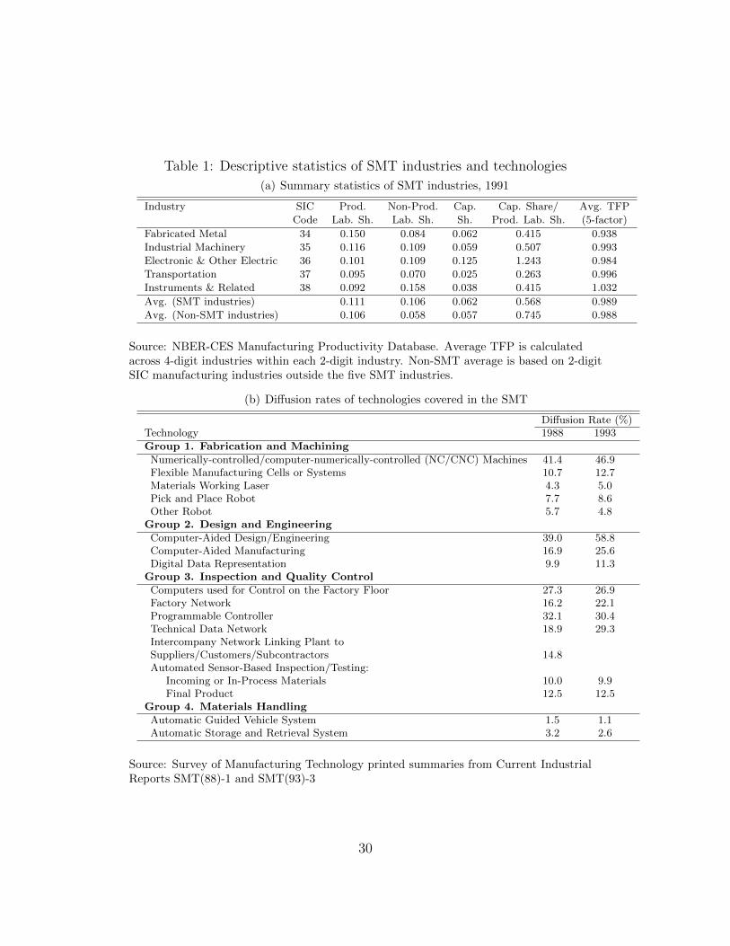
Table 1: Descriptive statistics of SMT industries and technologies

(a) Summary statistics of SMT industries, 1991

Industry SIC Prod. Non-Prod. Cap. Cap. Share/ Avg. TFP

Code Lab. Sh. Lab. Sh. Sh. Prod. Lab. Sh. (5-factor)

Fabricated Metal 34 0.150 0.084 0.062 0.415 0.938

Industrial Machinery 35 0.116 0.109 0.059 0.507 0.993

Electronic & Other Electric 36 0.101 0.109 0.125 1.243 0.984

Transportation 37 0.095 0.070 0.025 0.263 0.996

Instruments & Related 38 0.092 0.158 0.038 0.415 1.032

Avg. (SMT industries) 0.111 0.106 0.062 0.568 0.989

Avg. (Non-SMT industries) 0.106 0.058 0.057 0.745 0.988

Source: NBER-CES Manufacturing Productivity Database. Average TFP is calculatedacross 4-digit industries within each 2-digit industry. Non-SMT average is based on 2-digitSIC manufacturing industries outside the five SMT industries.

(b) Diffusion rates of technologies covered in the SMT

Diffusion Rate (%)Technology 1988 1993

Group 1. Fabrication and Machining

Numerically-controlled/computer-numerically-controlled (NC/CNC) Machines 41.4 46.9Flexible Manufacturing Cells or Systems 10.7 12.7Materials Working Laser 4.3 5.0Pick and Place Robot 7.7 8.6Other Robot 5.7 4.8

Group 2. Design and Engineering

Computer-Aided Design/Engineering 39.0 58.8Computer-Aided Manufacturing 16.9 25.6Digital Data Representation 9.9 11.3

Group 3. Inspection and Quality Control

Computers used for Control on the Factory Floor 27.3 26.9Factory Network 16.2 22.1Programmable Controller 32.1 30.4Technical Data Network 18.9 29.3Intercompany Network Linking Plant toSuppliers/Customers/Subcontractors 14.8Automated Sensor-Based Inspection/Testing:

Incoming or In-Process Materials 10.0 9.9Final Product 12.5 12.5

Group 4. Materials Handling

Automatic Guided Vehicle System 1.5 1.1Automatic Storage and Retrieval System 3.2 2.6

Source: Survey of Manufacturing Technology printed summaries from Current IndustrialReports SMT(88)-1 and SMT(93)-3

30

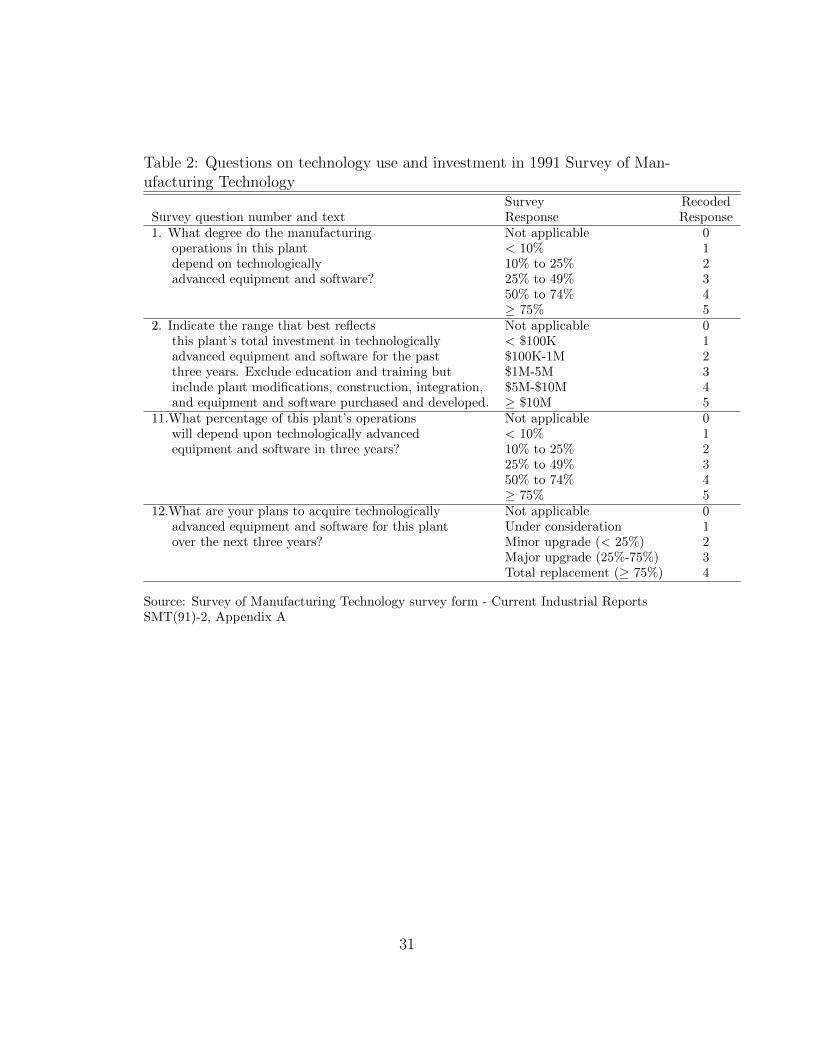
Table 2: Questions on technology use and investment in 1991 Survey of Man-ufacturing Technology

Survey RecodedSurvey question number and text Response Response1. What degree do the manufacturing Not applicable 0

operations in this plant < 10% 1depend on technologically 10% to 25% 2advanced equipment and software? 25% to 49% 3

50% to 74% 4≥ 75% 5

2. Indicate the range that best reflects Not applicable 0this plant’s total investment in technologically < $100K 1advanced equipment and software for the past $100K-1M 2three years. Exclude education and training but $1M-5M 3include plant modifications, construction, integration, $5M-$10M 4and equipment and software purchased and developed. ≥ $10M 5

11.What percentage of this plant’s operations Not applicable 0will depend upon technologically advanced < 10% 1equipment and software in three years? 10% to 25% 2

25% to 49% 350% to 74% 4≥ 75% 5

12.What are your plans to acquire technologically Not applicable 0advanced equipment and software for this plant Under consideration 1over the next three years? Minor upgrade (< 25%) 2

Major upgrade (25%-75%) 3Total replacement (≥ 75%) 4

Source: Survey of Manufacturing Technology survey form - Current Industrial ReportsSMT(91)-2, Appendix A

31

Table 3: Technology and plant outcomes

(a) Labor share and plant characteristics

Labor Share Fraction of WorkersAll Production Non-production in Production

technology index I -0.023∗∗∗ -0.041∗∗∗ 0.026 -0.035∗∗∗

[0.008] [0.016] [0.020] [0.009]R2 0.27 0.28 0.31 0.30technology index II -0.052∗∗∗ -0.083∗∗∗ -0.0064 -0.041∗∗∗

[0.014] [0.019] [0.022] [0.011]R2 0.27 0.28 0.31 0.30N 8100 8100 8100 8100

(b) Labor productivity and plant characteristics

Labor ProductivityAll Production Non-production

technology index I 0.090∗∗∗ 0.120∗∗∗ 0.021[0.018] [0.021] [0.026]

R2 0.26 0.30 0.23technology index II 0.120∗∗∗ 0.142∗∗∗ 0.055

[0.026] [0.029] [0.034]R2 0.26 0.30 0.23N 8100 8100 8100

(c) Salaries and wages per employee and plant characteristics

Average WageAll Production Non-production

technology index I 0.073∗∗∗ 0.084∗∗∗ 0.044∗∗∗

[0.013] [0.012] [0.013]R2 0.22 0.24 0.09technology index II 0.083∗∗∗ 0.086∗∗∗ 0.048∗∗∗

[0.015] [0.014] [0.016]R2 0.22 0.24 0.08N 8100 8100 8100

Notes: All continuous variables in logs. Standard errors –in parentheses– are clustered by4-digit SIC industry. (∗), (∗∗), (∗∗∗) indicate significance at 10, 5, and 1% level,respectively. Technology index I is based on all 4 survey questions in Table 2. Technologyindex II is based only on the investment question (Question 2). All regressions includeother plant characteristics as controls: five plant size (employment) categories (1-20 emp,20-99 emp, 100-499 emp, 500-999 emp, 1000+ emp), four plant age categories (0-5 yrs,5-14 yrs, 15-29 yrs, 30+ yrs), a production worker unionization indicator (1 if the planthas a union contract for production workers), export intensity indicator (1 if more than50% of the plant’s products are exported), an indicator of military production (1 if theplant is engaged in production to military specs), a foreign-ownership indicator (1 if 10%or more of the voting stock or other equity rights are foreign-owned), an indicator ofshipment to defense agencies (1 if the plant ships directly to DOD or Armed Services), anindicator of shipment to primary contractors for defense agencies (1 if shipments are madeto a primary defense contractor), and 4-digit SIC industry fixed effects. N is rounded fordisclosure avoidance.

32

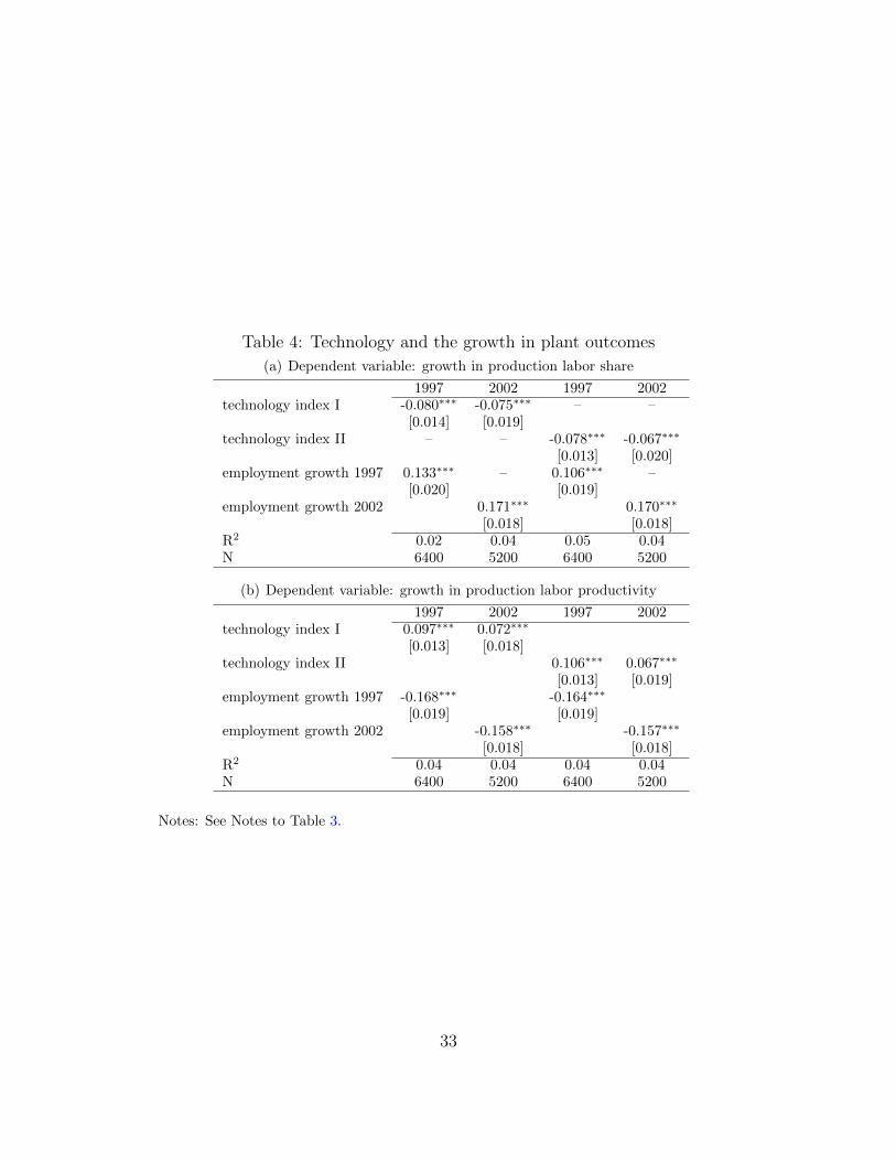
Table 4: Technology and the growth in plant outcomes

(a) Dependent variable: growth in production labor share

1997 2002 1997 2002technology index I -0.080∗∗∗ -0.075∗∗∗ – –

[0.014] [0.019]technology index II – – -0.078∗∗∗ -0.067∗∗∗

[0.013] [0.020]employment growth 1997 0.133∗∗∗ – 0.106∗∗∗ –

[0.020] [0.019]employment growth 2002 0.171∗∗∗ 0.170∗∗∗

[0.018] [0.018]R2 0.02 0.04 0.05 0.04N 6400 5200 6400 5200

(b) Dependent variable: growth in production labor productivity

1997 2002 1997 2002technology index I 0.097∗∗∗ 0.072∗∗∗

[0.013] [0.018]technology index II 0.106∗∗∗ 0.067∗∗∗

[0.013] [0.019]employment growth 1997 -0.168∗∗∗ -0.164∗∗∗

[0.019] [0.019]employment growth 2002 -0.158∗∗∗ -0.157∗∗∗

[0.018] [0.018]R2 0.04 0.04 0.04 0.04N 6400 5200 6400 5200

Notes: See Notes to Table 3.

33

Table 5: Elasticity estimates

(a) Estimates of σ

SMT (IV) ASM (GMMt−2,t−p)full simple p = 7 p = 8

σ̂ 0.63*** 0.71*** 0.60*** 0.38***ρ̂= σ̂−1

σ̂ -0.59 -0.41 -0.67 -1.63N 4400 4400 11500 5500

Notes: IV: cross-section IV with and without capital in the regression. GMMt−2,t−p:GMM using indicated lagged differences as instruments. These regressions are based onthe earliest possible lags available where the Hansen test of overidentifying restrictions donot reject the null of orthogonality. N is rounded for disclosure avoidance.

(b) Production function estimates

N γ̂ β1 β2 β3∑j β̂j + γ̂

FOC4100 0.22 0.12 0.43 0.02 0.77

(0.002) (0.002) (0.003) (0.001) (0.004)Equation (15)

NLS, αi 4000 0.17 0.12 0.43 0.02 0.73(0.075) (0.002) (0.003) (0.001) (0.074)

NLS, αi = 1/2 4000 0.25 0.12 0.43 0.02 0.81(0.047) (0.002) (0.003) (0.001) (0.047)

Notes: Standard errors are bootstrapped. All elasticities are based on output and inputdistributions from which outliers are removed. Variable input elasticities are fixed acrossspecifications. N is rounded for disclosure avoidance.

34

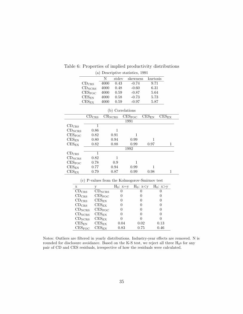
Table 6: Properties of implied productivity distributions

(a) Descriptive statistics, 1991

N stdev skewness kurtosisCDCRS 4000 0.43 -0.74 9.71CDNCRS 4000 0.48 -0.60 6.31CESFOC 4000 0.59 -0.87 5.64CESEN 4000 0.58 -0.73 5.73CESEX 4000 0.59 -0.97 5.87

(b) Correlations

CDCRS CRNCRS CESFOC CESEN CESEX

1991CDCRS 1CDNCRS 0.86 1CESFOC 0.82 0.91 1CESEN 0.80 0.94 0.99 1CESEX 0.82 0.88 0.99 0.97 1

1992CDCRS 1CDNCRS 0.82 1CESFOC 0.78 0.9 1CESEN 0.77 0.94 0.99 1CESEX 0.79 0.87 0.99 0.98 1

(c) P-values from the Kolmogorov-Smirnov test

x y H0: x=y H0: x<y H0: x>yCDCRS CDNCRS 0 0 0CDCRS CESFOC 0 0 0CDCRS CESEN 0 0 0CDCRS CESEX 0 0 0CDNCRS CESFOC 0 0 0CDNCRS CESEN 0 0 0CDNCRS CESEX 0 0 0CESEN CESEX 0.04 0.02 0.13CESFOC CESEN 0.83 0.75 0.46

Notes: Outliers are filtered in yearly distributions. Industry-year effects are removed. N isrounded for disclosure avoidance. Based on the K-S test, we reject all three H0s for anypair of CD and CES residuals, irrespective of how the residuals were calculated.

35

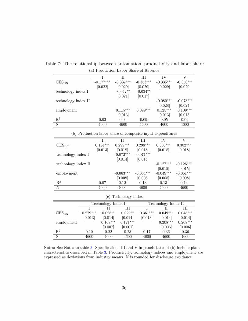
Table 7: The relationship between automation, productivity and labor share

(a) Production Labor Share of Revenue

I II III IV VCESEN -0.177∗∗∗ -0.337∗∗∗ -0.353∗∗∗ -0.335∗∗∗ -0.350∗∗∗

[0.022] [0.029] [0.029] [0.029] [0.029]technology index I -0.042∗∗ -0.034∗∗

[0.021] [0.017]technology index II -0.080∗∗∗ -0.078∗∗∗

[0.028] [0.027]employment 0.115∗∗∗ 0.099∗∗∗ 0.125∗∗∗ 0.109∗∗∗

[0.013] [0.013] [0.013]R2 0.02 0.04 0.09 0.05 0.09N 4600 4600 4600 4600 4600

(b) Production labor share of composite input expenditures

I II III IV VCESEN 0.184∗∗∗ 0.299∗∗∗ 0.298∗∗∗ 0.303∗∗∗ 0.302∗∗∗

[0.013] [0.018] [0.018] [0.018] [0.018]technology index I -0.072∗∗∗ -0.071∗∗∗

[0.014] [0.014]technology index II -0.127∗∗∗ -0.126∗∗∗

[0.015] [0.015]employment -0.063∗∗∗ -0.064∗∗∗ -0.049∗∗∗ -0.051∗∗∗

[0.008] [0.008] [0.008] [0.008]R2 0.07 0.12 0.13 0.13 0.14N 4600 4600 4600 4600 4600

(c) Technology index

Technology Index I Technology Index III II III I II III

CESEN 0.279∗∗∗ 0.028∗∗ 0.029∗∗ 0.361∗∗∗ 0.049∗∗∗ 0.048∗∗∗

[0.013] [0.014] [0.014] [0.013] [0.014] [0.014]employment 0.168∗∗∗ 0.171∗∗∗ 0.208∗∗∗ 0.208∗∗∗

[0.007] [0.007] [0.006] [0.006]R2 0.10 0.22 0.23 0.17 0.36 0.36N 4600 4600 4600 4600 4600 4600

Notes: See Notes to table 3. Specifications III and V in panels (a) and (b) include plantcharacteristics described in Table 3. Productivity, technology indices and employment areexpressed as deviations from industry means. N is rounded for disclosure avoidance.

36

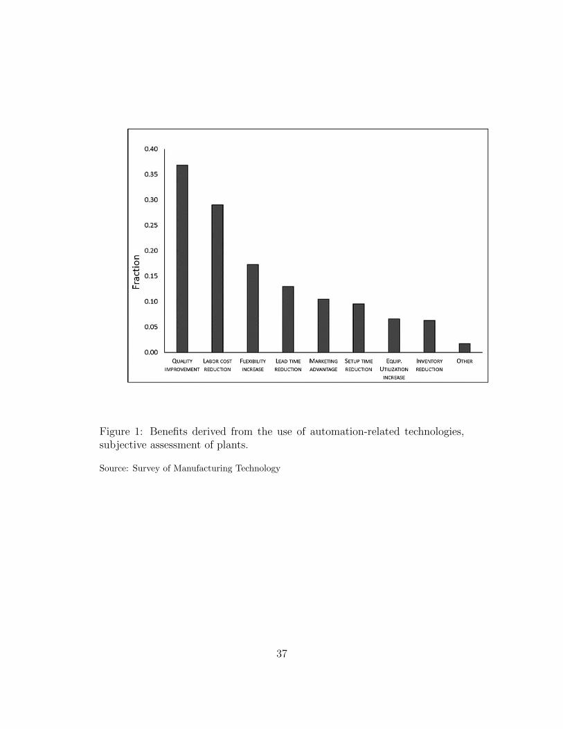
Figure 1: Benefits derived from the use of automation-related technologies,subjective assessment of plants.

Source: Survey of Manufacturing Technology

37

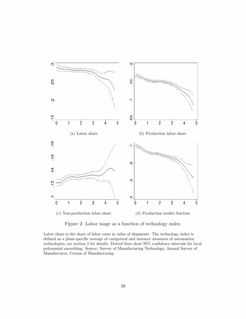
(a) Labor share (b) Production labor share

(c) Non-production labor share (d) Production worker fraction

Figure 2: Labor usage as a function of technology index.

Labor share is the share of labor costs in value of shipments. The technology index isdefined as a plant-specific average of categorical and instance measures of automationtechnologies, see section 2 for details. Dotted lines show 95% confidence intervals for localpolynomial smoothing. Source: Survey of Manufacturing Technology, Annual Survey ofManufactures, Census of Manufacturing

38

(a) Capital share (b) Capital-production labor cost ratio, logs

(c) Capital-production labor ratio, logs

Figure 3: Capital usage as a function of technology index.

Capital share is the share of capital costs in value of shipments. The technology index isdefined as a plant-specific average of categorical and instance measures of automationtechnologies, see section 2 for details. Dotted lines show 95% confidence intervals for localpolynomial smoothing. Source: Survey of Manufacturing Technology, Annual Survey ofManufactures, Census of Manufacturing

39

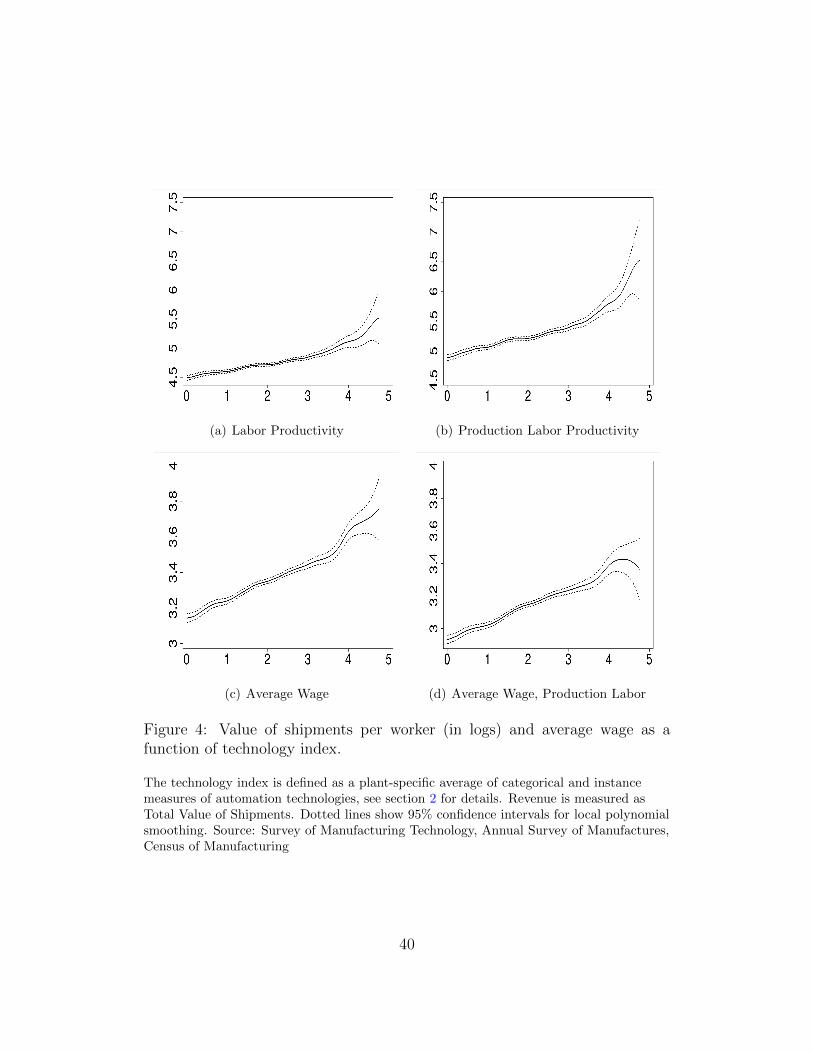
(a) Labor Productivity (b) Production Labor Productivity

(c) Average Wage (d) Average Wage, Production Labor

Figure 4: Value of shipments per worker (in logs) and average wage as afunction of technology index.

The technology index is defined as a plant-specific average of categorical and instancemeasures of automation technologies, see section 2 for details. Revenue is measured asTotal Value of Shipments. Dotted lines show 95% confidence intervals for local polynomialsmoothing. Source: Survey of Manufacturing Technology, Annual Survey of Manufactures,Census of Manufacturing

40

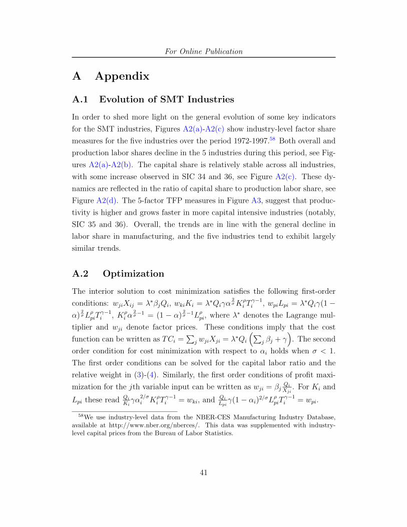
For Online Publication

A Appendix

A.1 Evolution of SMT Industries

In order to shed more light on the general evolution of some key indicators

for the SMT industries, Figures A2(a)-A2(c) show industry-level factor share

measures for the five industries over the period 1972-1997.58 Both overall and

production labor shares decline in the 5 industries during this period, see Fig-

ures A2(a)-A2(b). The capital share is relatively stable across all industries,

with some increase observed in SIC 34 and 36, see Figure A2(c). These dy-

namics are reflected in the ratio of capital share to production labor share, see

Figure A2(d). The 5-factor TFP measures in Figure A3, suggest that produc-

tivity is higher and grows faster in more capital intensive industries (notably,

SIC 35 and 36). Overall, the trends are in line with the general decline in

labor share in manufacturing, and the five industries tend to exhibit largely

similar trends.

A.2 Optimization

The interior solution to cost minimization satisfies the following first-order

conditions: wjiXij = λ∗βjQi, wkiKi = λ∗Qiγα2σKρ

i Tγ−1i , wpiLpi = λ∗Qiγ(1 −

α)2σLρpiT

γ−1i , Kρ

i α2σ−1 = (1 − α)

2σ−1Lρpi, where λ∗ denotes the Lagrange mul-

tiplier and wji denote factor prices. These conditions imply that the cost

function can be written as TCi =∑

j wjiXji = λ∗Qi

(∑j βj + γ

). The second

order condition for cost minimization with respect to αi holds when σ < 1.

The first order conditions can be solved for the capital labor ratio and the

relative weight in (3)-(4). Similarly, the first order conditions of profit maxi-

mization for the jth variable input can be written as wji = βjQiXji

. For Ki and

Lpi these read QiKiγα

2/σi Kρ

i Tγ−1i = wki, and Qi

Lpiγ(1− αi)2/σLρpiT

γ−1i = wpi.

58We use industry-level data from the NBER-CES Manufacturing Industry Database,available at http://www.nber.org/nberces/. This data was supplemented with industry-level capital prices from the Bureau of Labor Statistics.

41

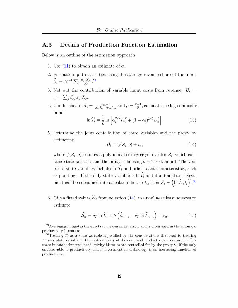
For Online Publication

A.3 Details of Production Function Estimation

Below is an outline of the estimation approach.

1. Use (11) to obtain an estimate of σ.

2. Estimate input elasticities using the average revenue share of the input

β̂j = N−1∑

iwjiXjiRi

.59

3. Net out the contribution of variable input costs from revenue: B̂i =

ri −∑

j β̂j iwjiXji.

4. Conditional on α̂i = wkiKiwkiKi+wpiLpi

and ρ̂ = σ̂−1σ̂

, calculate the log-composite

input

ln T̂i ≡1

ρ̂ln[α2/σ̂i K ρ̂

i + (1− αi)2/σ̂Lρ̂pi]. (13)

5. Determine the joint contribution of state variables and the proxy by

estimatingB̂i = φ(Zi, p) + vi, (14)

where φ(Zi, p) denotes a polynomial of degree p in vector Zi, which con-

tains state variables and the proxy. Choosing p = 2 is standard. The vec-

tor of state variables includes ln T̂i and other plant characteristics, such

as plant age. If the only state variable is ln T̂i and if automation invest-

ment can be subsumed into a scalar indicator ti, then Zi =(

ln T̂i, ti

)′.60

6. Given fitted values φ̂it from equation (14), use nonlinear least squares to

estimate

B̂it = δT ln T̂it + h(φ̂it−1 − δT ln T̂it−1

)+ νit. (15)

59Averaging mitigates the effects of measurement error, and is often used in the empiricalproductivity literature.

60Treating Ti as a state variable is justified by the considerations that lead to treatingKi as a state variable in the vast majority of the empirical productivity literature. Differ-ences in establishments’ productivity histories are controlled for by the proxy ti, if the onlyunobservable is productivity and if investment in technology is an increasing function ofproductivity.

42

For Online Publication

where h is a second-order polynomial in its argument. Under the as-

sumptions of the model, δT in regression (15) identifies γ.

As mentioned earlier, the SMT asks about the plant’s total investment in

technologically advanced equipment and software for the previous three years

for each of the four technology groups. The proxy, ti, is calculated as the

average response of plants over the four technology groups. Together with

ln T̂i, and plant age they determine φ̂i in (14). Under the assumptions of

the model, this value controls for unobserved productivity differences across

plants when estimating δT using data from 1992 in (15). If the plant-level

productivity process is Markovian –a standard assumption in the empirical

productivity literature– then δT is consistently estimated in regression (15).

The standard error of δ̂T is obtained using bootstrap.

A.4 Specification Error

This appendix studies some properties of the specification error when (revenue-

based) TFP is estimated based on a standard Cobb-Douglas (CD) production

function with constant returns to scale

Qi = θiKβi L

1−βpi , (16)

when the underlying data generating process is a CES production function

with decreasing returns to scale (γ < 1) and endogenous technology choice

Qi = θi[α2/σi Kρ

i + (1− αi)2/σLρpi]γ/ρ. (17)

For ease of exposition, the two production functions above abstract from the

variable inputs Ln, M and E used in (2). Including them does not change

the main conclusions regarding the theoretical relationship between specifica-

tion error and technology. In addition, if the sampling error is small, their

contribution to the specification error is negligible.61

61However, including these three inputs matter for the estimated specification error iftheir elasticities are estimated based on different methods for the CES production functionused in the main text and for the CD specification.

43

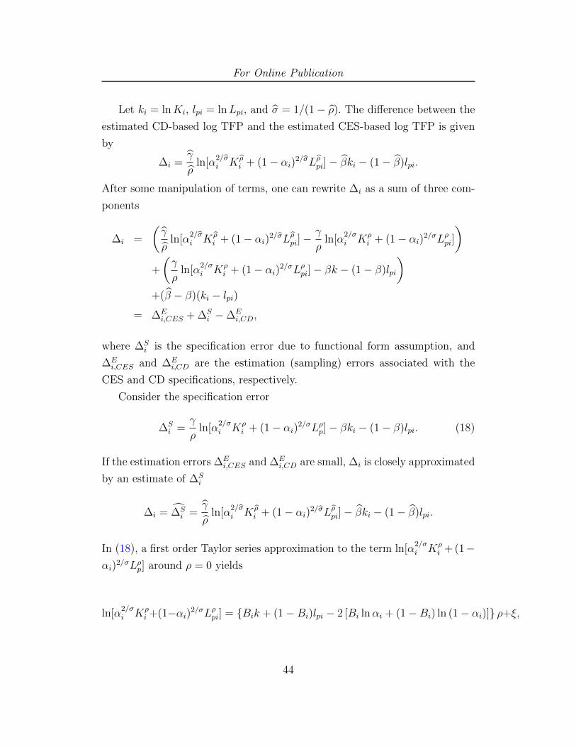
For Online Publication

Let ki = lnKi, lpi = lnLpi, and σ̂ = 1/(1− ρ̂). The difference between the

estimated CD-based log TFP and the estimated CES-based log TFP is given

by

∆i =γ̂

ρ̂ln[α

2/σ̂i K ρ̂

i + (1− αi)2/σ̂Lρ̂pi]− β̂ki − (1− β̂)lpi.

After some manipulation of terms, one can rewrite ∆i as a sum of three com-

ponents

∆i =

(γ̂

ρ̂ln[α

2/σ̂i K ρ̂

i + (1− αi)2/σ̂Lρ̂pi]−γ

ρln[α

2/σi Kρ

i + (1− αi)2/σLρpi])

+

(γ

ρln[α

2/σi Kρ

i + (1− αi)2/σLρpi]− βk − (1− β)lpi

)+(β̂ − β)(ki − lpi)

= ∆Ei,CES + ∆S

i −∆Ei,CD,

where ∆Si is the specification error due to functional form assumption, and

∆Ei,CES and ∆E

i,CD are the estimation (sampling) errors associated with the

CES and CD specifications, respectively.

Consider the specification error

∆Si =

γ

ρln[α

2/σi Kρ

i + (1− αi)2/σLρp]− βki − (1− β)lpi. (18)

If the estimation errors ∆Ei,CES and ∆E

i,CD are small, ∆i is closely approximated

by an estimate of ∆Si

∆i = ∆̂Si =

γ̂

ρ̂ln[α

2/σ̂i K ρ̂

i + (1− αi)2/σ̂Lρ̂pi]− β̂ki − (1− β̂)lpi.

In (18), a first order Taylor series approximation to the term ln[α2/σi Kρ

i + (1−αi)

2/σLρp] around ρ = 0 yields

ln[α2/σi Kρ

i +(1−αi)2/σLρpi] = {Bik + (1−Bi)lpi − 2 [Bi lnαi + (1−Bi) ln (1− αi)]} ρ+ξ,

44

For Online Publication

where

Bi =α2i

α2i + (1− αi)2

, (19)

and ξ is the approximation error. One can thus approximate the specification

error, ∆Si , as follows

∆̃Si = (γBi−β)(ki− lpi)+(γ−1)lpi−2γ [Bi lnαi + (1−Bi) ln (1− αi)] . (20)

The first two terms in the final expression indicate that the magnitude of

the error depends on the capital-production labor ratio and production labor.

To study the contribution of the third term, define

D(αi) = −2 [Bi lnαi + (1−Bi) ln (1− αi)]

The third term is then γD(αi). D(αi) is always positive (since αi ∈ (0, 1)),

and it is a non-monotonic function of αi. It achieves its maximum value of

1.386γ at αi = 0.5, and its minimum value of zero at αi = 0 or αi = 1. The

shape of D(αi) is shown in figure A1.

The term γD(αi) is bounded from above by 1.386γ, and its contribution

to the specification error will be dominated by the first two terms, when γ

is small.62 The rest of the appendix hence assumes away the contribution of

γD(αi).

What is the sign of the specification error, ∆Si ? Consider the approxima-

tion, ∆̃Si , in (20). Because γ < 1, the second term in (20) is negative (for

lpi > 0, or equivalently, Lp > 1). For (ki − lpi) > 0 (i.e. (Ki/Lpi) > 1), the

first term in (20) can be positive or negative, depending on whether γBi − βis positive or negative.63 If the first term is negative, ∆̃S

i is negative for all

plants with at least one production worker and capital-production labor ratio

greater than one.64 In practice, the estimated specification error turns out to

62Note that the estimated value of γ is in the range (0.17, 0.25) based on the samples usedin this paper. These values imply a range of (0, 0.34) for γD(αi).

63Because Bi ∈ (0, 1), one sufficient condition for γBi−β to be negative for all Bi ∈ (0, 1)is γ < β.

64This ratio exceeds one in the samples used in this study.

45

For Online Publication

Figure A1: The shape of D(αi).

be negative for nearly the entire set of plants.

Another question is whether the specification error is exacerbated for plants

with higher degree of automation. Consider the first term in ∆̃Si . Both (γBi−β)

and (ki − lpi) are increasing functions of αi when σ < 1, by the definition of

Bi in (19), and by equations (3) and (4). Now, let F (αi) = γBi − β and

G(αi) = ki − lpi. Note that F ′ > 0 and G′ > 0 given the preceding discussion.

Then, the rate of change of first term with αi is given by F ′G + G′F. When

F > 0, F ′G+G′F > 0. When F < 0, F ′G+G′F can be positive or negative.

As a result, the first term (γBi−β)(ki− lpi) can be an increasing or decreasing

function of αi. The second term in (20), (γ − 1)lpi, can also be increasing

or decreasing in αi, depending on how lpi changes with αi. The model has no

prediction on the direction of this change. For instance, (γ−1)lpi is decreasing

in αi if large plants (large lpi) are also the ones with higher αi.65 The overall

sign of the change in the specification error as αi increases then depends on

65This connection finds support in the SMT sample.

46

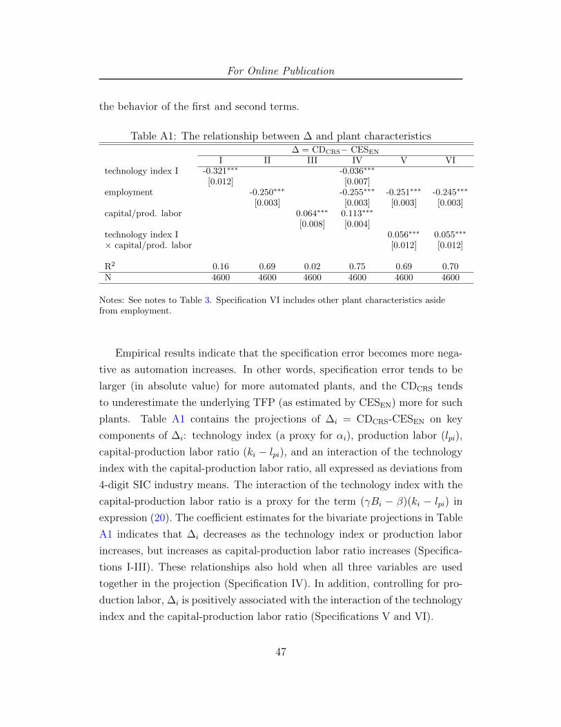
For Online Publication

the behavior of the first and second terms.

Table A1: The relationship between ∆ and plant characteristics∆ = CDCRS− CESEN

I II III IV V VItechnology index I -0.321∗∗∗ -0.036∗∗∗

[0.012] [0.007]employment -0.250∗∗∗ -0.255∗∗∗ -0.251∗∗∗ -0.245∗∗∗

[0.003] [0.003] [0.003] [0.003]capital/prod. labor 0.064∗∗∗ 0.113∗∗∗

[0.008] [0.004]technology index I 0.056∗∗∗ 0.055∗∗∗

× capital/prod. labor [0.012] [0.012]

R2 0.16 0.69 0.02 0.75 0.69 0.70N 4600 4600 4600 4600 4600 4600

Notes: See notes to Table 3. Specification VI includes other plant characteristics asidefrom employment.

Empirical results indicate that the specification error becomes more nega-

tive as automation increases. In other words, specification error tends to be

larger (in absolute value) for more automated plants, and the CDCRS tends

to underestimate the underlying TFP (as estimated by CESEN) more for such

plants. Table A1 contains the projections of ∆i = CDCRS-CESEN on key

components of ∆i: technology index (a proxy for αi), production labor (lpi),

capital-production labor ratio (ki − lpi), and an interaction of the technology

index with the capital-production labor ratio, all expressed as deviations from

4-digit SIC industry means. The interaction of the technology index with the

capital-production labor ratio is a proxy for the term (γBi − β)(ki − lpi) in

expression (20). The coefficient estimates for the bivariate projections in Table

A1 indicates that ∆i decreases as the technology index or production labor

increases, but increases as capital-production labor ratio increases (Specifica-

tions I-III). These relationships also hold when all three variables are used

together in the projection (Specification IV). In addition, controlling for pro-

duction labor, ∆i is positively associated with the interaction of the technology

index and the capital-production labor ratio (Specifications V and VI).

47

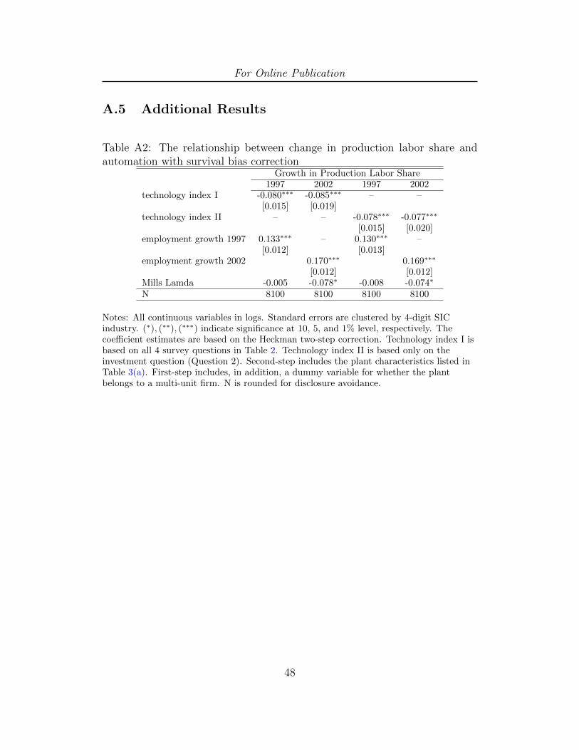
For Online Publication

A.5 Additional Results

Table A2: The relationship between change in production labor share andautomation with survival bias correction

Growth in Production Labor Share1997 2002 1997 2002

technology index I -0.080∗∗∗ -0.085∗∗∗ – –[0.015] [0.019]

technology index II – – -0.078∗∗∗ -0.077∗∗∗

[0.015] [0.020]employment growth 1997 0.133∗∗∗ – 0.130∗∗∗ –

[0.012] [0.013]employment growth 2002 0.170∗∗∗ 0.169∗∗∗

[0.012] [0.012]Mills Lamda -0.005 -0.078∗ -0.008 -0.074∗

N 8100 8100 8100 8100

Notes: All continuous variables in logs. Standard errors are clustered by 4-digit SICindustry. (∗), (∗∗), (∗∗∗) indicate significance at 10, 5, and 1% level, respectively. Thecoefficient estimates are based on the Heckman two-step correction. Technology index I isbased on all 4 survey questions in Table 2. Technology index II is based only on theinvestment question (Question 2). Second-step includes the plant characteristics listed inTable 3(a). First-step includes, in addition, a dummy variable for whether the plantbelongs to a multi-unit firm. N is rounded for disclosure avoidance.

48

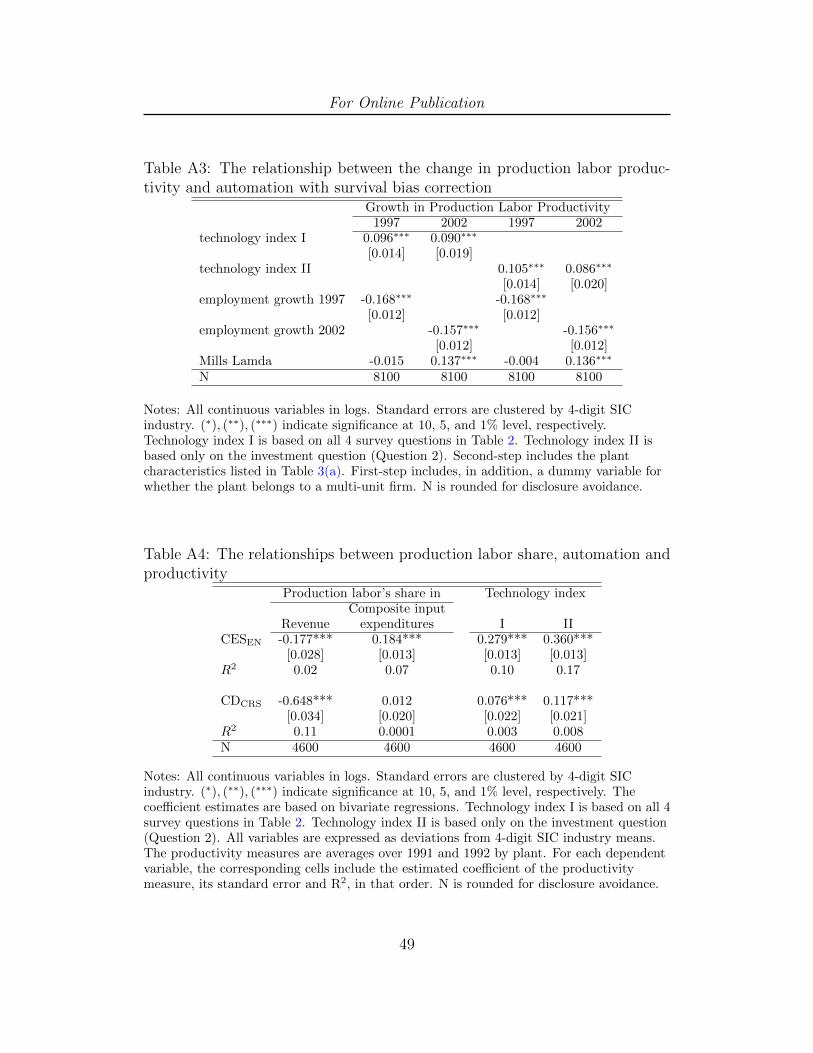
For Online Publication

Table A3: The relationship between the change in production labor produc-tivity and automation with survival bias correction

Growth in Production Labor Productivity1997 2002 1997 2002

technology index I 0.096∗∗∗ 0.090∗∗∗

[0.014] [0.019]technology index II 0.105∗∗∗ 0.086∗∗∗

[0.014] [0.020]employment growth 1997 -0.168∗∗∗ -0.168∗∗∗

[0.012] [0.012]employment growth 2002 -0.157∗∗∗ -0.156∗∗∗

[0.012] [0.012]Mills Lamda -0.015 0.137∗∗∗ -0.004 0.136∗∗∗

N 8100 8100 8100 8100

Notes: All continuous variables in logs. Standard errors are clustered by 4-digit SICindustry. (∗), (∗∗), (∗∗∗) indicate significance at 10, 5, and 1% level, respectively.Technology index I is based on all 4 survey questions in Table 2. Technology index II isbased only on the investment question (Question 2). Second-step includes the plantcharacteristics listed in Table 3(a). First-step includes, in addition, a dummy variable forwhether the plant belongs to a multi-unit firm. N is rounded for disclosure avoidance.

Table A4: The relationships between production labor share, automation andproductivity

Production labor’s share in Technology indexComposite input

Revenue expenditures I IICESEN -0.177*** 0.184*** 0.279*** 0.360***

[0.028] [0.013] [0.013] [0.013]R2 0.02 0.07 0.10 0.17

CDCRS -0.648*** 0.012 0.076*** 0.117***[0.034] [0.020] [0.022] [0.021]

R2 0.11 0.0001 0.003 0.008N 4600 4600 4600 4600

Notes: All continuous variables in logs. Standard errors are clustered by 4-digit SICindustry. (∗), (∗∗), (∗∗∗) indicate significance at 10, 5, and 1% level, respectively. Thecoefficient estimates are based on bivariate regressions. Technology index I is based on all 4survey questions in Table 2. Technology index II is based only on the investment question(Question 2). All variables are expressed as deviations from 4-digit SIC industry means.The productivity measures are averages over 1991 and 1992 by plant. For each dependentvariable, the corresponding cells include the estimated coefficient of the productivitymeasure, its standard error and R2, in that order. N is rounded for disclosure avoidance.

49

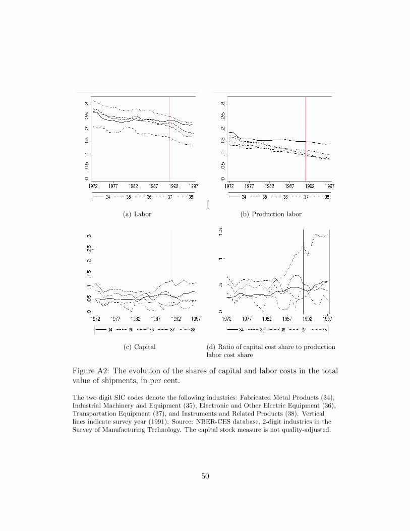
(a) Labor

[(b) Production labor

(c) Capital (d) Ratio of capital cost share to productionlabor cost share

Figure A2: The evolution of the shares of capital and labor costs in the totalvalue of shipments, in per cent.

The two-digit SIC codes denote the following industries: Fabricated Metal Products (34),Industrial Machinery and Equipment (35), Electronic and Other Electric Equipment (36),Transportation Equipment (37), and Instruments and Related Products (38). Verticallines indicate survey year (1991). Source: NBER-CES database, 2-digit industries in theSurvey of Manufacturing Technology. The capital stock measure is not quality-adjusted.

50

Figure A3: Average log-TFP across SIC industries

See notes to Figure A2.

(a) Labor Productivity (b) Average Wage

Figure A4: Non-production labor productivity and average wage (in logs) asa function of technology index.

The technology index is defined as a plant-specific average of categorical and instancemeasures of automation technologies, see section 2 for details. Average wage is measuredas payroll divided by the number of employees. Dotted lines show 95% confidence intervalsof local polynomial smoothing. Source: Survey of Manufacturing Technology

51

(a) Labor (b) Production labor

(c) Non-production labor

Figure A5: Value added per worker (in logs) as a function of technology index

The technology index is defined as a plant-specific average of categorical and instancemeasures of automation technologies, see section 2 for details. Dotted lines show 95%confidence intervals for local polynomial smoothing. Source: Survey of ManufacturingTechnology, Annual Survey of Manufactures, Census of Manufacturing

52