Automatic well-testing model diagnosis and parameter ... well-testing model diagnosis and parameter estimation using artificial neural networks and design ... 2 Department of Industrial

ORIGINAL PAPER - PRODUCTION ENGINEERING

Automatic well-testing model diagnosis and parameter estimationusing artificial neural networks and design of experiments

Rouhollah Ahmadi1 • Jamal Shahrabi2 • Babak Aminshahidy1

Received: 20 July 2016 / Accepted: 24 October 2016 / Published online: 15 November 2016

� The Author(s) 2016. This article is published with open access at Springerlink.com

Abstract The well-testing analysis is performed in two

consecutive steps including identification of underlying

reservoir models and estimation of model-related parame-

ters. The non-uniqueness problem always brings about

confusion in selecting the correct reservoir model using the

conventional interpretation approaches. Many researchers

have recommended artificial intelligence techniques to

automate the well-testing analysis in recent years. The

purpose of this article is to apply an artificial neural net-

work (ANN) methodology to identify the well-testing

interpretation model and estimate the model-related vari-

ables from the pressure derivative plots. Different types of

ANNs including multi-layer perceptrons, probabilistic

neural networks and generalized regression neural net-

works are used in this article. The best structure and

parameters of each neural network is found via grid search

and cross-validation techniques. The experimental design

is also employed to select the most governing variables in

designing well tests of different reservoir models. Seven

real buildup tests are used to validate the proposed

approach. The presented ANN-based approach shows

promising results both in recognizing the reservoir models

and estimating the model-related parameters. The experi-

mental design employed in this study guarantees the

comprehensiveness of the training data sets generated for

learning the proposed ANNs using fewer numbers of

experiments compared to the previous studies.

Keywords Well-testing interpretation � Estimation �Classification � MLP � PNN � GRNN

Introduction

The well-testing provides the required data for the quali-

tative and quantitative characterization of the reservoir.

These data exhibit the real behavior of fluid flow

throughout the reservoir as well as the near-wellbore

region. So the parameters acquired by the well-testing data

analysis are considered as one of the main data sources in

establishing the reservoir management studies.

The interpretation of pressure transient data has two main

objectives: (1) diagnosing the underlying conceptual reser-

voir model, and (2) estimating themodel-related parameters.

The well-testing analysis is an inverse solution to the reser-

voir model identification which is basically performed using

the pressure derivative plots. The non-uniqueness problem,

however, brings about confusion in selecting the correct

reservoir model using the conventional approaches. The use

of expert systems and artificial intelligence (AI) techniques

has therefore been investigated by many authors in recent

years to automate the process of recognizing the conceptual

reservoir models and eliminate the existing problems in

conventional analysis methods. Many approaches investi-

gate the well-testing model identification using the AI

techniques, whereas a few techniques have been developed

to estimate the model-related parameters.

& Jamal Shahrabi

[email protected]; [email protected]

Rouhollah Ahmadi

[email protected]; [email protected]

Babak Aminshahidy

[email protected]; [email protected]

1 Department of Petroleum Engineering, Amirkabir University

of Technology, Tehran Polytechnique, Tehran, Iran

2 Department of Industrial Engineering and Management

Systems, Amirkabir University of Technology, Tehran

Polytechnique, Tehran, Iran

123

J Petrol Explor Prod Technol (2017) 7:759–783

DOI 10.1007/s13202-016-0293-z

As the first attempt in automatic well-testing model

identification using AI techniques, Allain and Horne (1990)

employed syntactic pattern recognition and a rule-based

approach to automatically recognize the conceptual reser-

voir models from the pressure derivative plots. To exhibit a

significant improvement over the previous pattern recog-

nition techniques, the application of ANNs for the auto-

matic well-testing identification was founded by Al-Kaabi

and Lee (1990). They used a back-propagation multi-layer

perceptron (MLP) trained on representative examples of

pressure derivative plots for a wide range of well test

interpretation models in their work. The basic ANN

approach of automatic well-testing diagnosis employed by

Al-Kaabi and Lee (1990), which is the groundwork of

many other studies in this regard, is briefly described in the

following statements:

The pressure derivative curves are firstly sampled for a

limited number of data points and normalized between 0 and

1 (or -1 and 1) using different normalization techniques.

The normalized derivative data points are then used as inputs

to the neural networks. The output layer of ANN consists of

the same number of nodes as the number of conceptual

reservoirmodels considered in the problem. Each node in the

output layer receives a score (activation level) between 0 and

1 representing the probability of occurring the corresponding

reservoir model. The ANN examines the whole pressure

derivative curve at the same time to identify the models

causing the signals presented by the curve. The model cor-

responding to the output node with the largest activation

level is considered as the most probable interpretation

model. Figure 1 illustrates the general application of ANNs

in determining the well-testing interpretation model using

the pressure derivative curves. This figure is a typical

example of the well-testing model diagnosis using ANNs.

Although this figure shows 8 models at the output, the same

ANN approach could be used for classifying any number of

conceptual reservoir models. The improvements and modi-

fications proposed by other researchers are briefly introduced

in the following statements.

Al-Kaabi and Lee (1993) used modular neural networks,

as combination of multiple smaller neural networks, to

identify different model classes. A similar approach was

proposed by Ershaghi et al. (1993) so as to use multiple

neural networks with each network representing a single

conceptual reservoir model due to disadvantages in using a

single comprehensive neural network for covering all

possible reservoir models. Juniardi and Ershaghi (1993)

proposed a hybrid approach to augment the ANN models

from an expert system with other information including

independent field data and tables of frequency of occur-

rence of non-related models.

Kumoluyi et al. (1995) proposed to use higher-order

neural networks (HONNs) instead of conventional MLP

networks in identifying the well-testing interpretation

model regarding both the scale and translation invariance

of the well-testing models with respect to the field data.

Athichanagorn and Horne (1995) presented an ANN

approach combined with the sequential predictive proba-

bility (SPP) method to diagnose the correct reservoir

models from the derivative plots. The SPP technique

determines which candidate models predict the well

response at the best provided that good initial estimates for

the governing parameters of the candidate reservoir models

are utilized. ANN was used to identify the characteristic

components of the pressure derivative curves in terms of

different flow regimes that might appear throughout the

reservoir corresponding to each candidate reservoir model.

Model parameters were then evaluated using the data in the

identified range of the corresponding behavior using the

conventional well-testing analysis techniques.

Sung et al. (1996) suggested the use of Hough transform

(HT), as a unique technique for the extraction of basic

shape and motion analysis in noisy images, combined with

the back-propagation neural network to improve the well-

testing model identification. An ANN approach was later

proposed by Deng et al. (2000) to automate the process of

type curve matching and move the tested curves to their

sample positions. Unlike the previous approaches that used

data point series as input vectors to train ANNs, the binary

vectors of theory curves created by transferring the actual

derivative curves into binary numbers were used as training

samples to train ANN. The well-testing model parameters

are also estimated during the type curve matching process.

Aydinoglu et al. (2002) proposed an ANN approach to

estimate different model parameters for the faulted

Fig. 1 Application of ANN in the well-testing model identification

with the pressure derivative plots as inputs and scores of different

reservoir models as outputs of the network (Vaferi et al. 2011)

760 J Petrol Explor Prod Technol (2017) 7:759–783

123

reservoirs. The network development begins with a simple

architecture and a few input and output features and the

level of complexity of the system are heuristically and

gradually increased as more model parameters tend to be

predicted by the network.

Jeirani and Mohebbi (2006) designed an MLP network

to estimate the initial pressure, permeability and skin factor

of oil reservoirs using the pressure build up test data. In

fact, ANN was iteratively used to compute the bottom-hole

shut-in pressure as a function of the Horner time, during the

steps of estimating the permeability and the skin factor.

Alajmi and Ertekin (2007) utilized an ANN approach to

solve the problem of parameter estimation for double-

porosity reservoir models from the pressure transient data

using a similar procedure as employed by Aydinoglu et al.

(2002). The complexity of ANN is increased step by step

by removing one of the parameters from the input layer at

each stage and adding it to the output layer to be included

as one of the outputs of the network. Kharrat and Razavi

(2008) employed multiple MLP networks of the same

structure to identify multiple reservoir models from the

pressure derivative data. All networks are trained using the

whole set of training data for all the considered models.

Application of ANNs in the well-testing model identifica-

tion was also investigated by Vaferi et al. (2011). They

attempted to use an MLP network with the optimum

architecture to solve the well-testing diagnosis problem.

Regarding the previous studies on the application of

ANNs in automating well-testing analysis, the following

remarks are highlighted:

1. As ANNs provide great abilities in generalizing their

understanding of the pattern recognition space they are

taught to identify, they can identify patterns from

incomplete, noisy and distorted data which is common

to pressure transient data collected during the well

tests.

2. Using ANNs, the needs for elaborate data preparation

as employed in the rule-based approaches (including

smoothing, segmenting, and symbolic transformation)

and the definition of complex rules to identify the

patterns are eliminated. Instead of using rules, an

internal understanding of the pattern recognition space

is automatically inspired in the form of weights that

describe the strength of the connections between the

network processing units.

3. Although some network parameters including the

number of layers or hidden neurons were selected in

a manner to achieve the best performance of classifi-

cation or estimation, no organized and comprehensive

framework was proposed by the previous authors for

selection of the best architectures and parameters of

ANNs.

4. The previous approaches used the analytically or

numerically designed synthetic well-testing models to

train the proposed neural networks. In addition, the

number of training examples was determined using a

predefined range of the governing parameters of the

well-testing interpretation models. The governing

parameters, however, are not selected based on a

statistical criterion. No experimental designs were

used for generating a statistically sufficient training

data set for learning different ANNs.

5. The methods proposed previously for estimating

different well-testing variables require a complex rule

definition; the functional links defined in the input

neurons of ANNs are determined subjectively, not

based on a scientific benchmark.

6. Only two different types of ANNs including MLP and

HONN, combined with other statistical techniques,

were used in the well-testing interpretation in the

previous studies. No attempts were made in applying

other kinds of ANNs for diagnosing the underlying

reservoir models and/or estimating the well-testing

variables.

To alleviate the weaknesses and shortcomings of the

previous studies listed above, this research proposes a more

comprehensive methodology using different types of

ANNs to effectively determine the conceptual reservoir

models and estimate the model-related parameters from the

pressure derivative plots. The best architecture and

parameters of the proposed ANNs will be found using grid

search (GS) and cross-validation (CV) techniques. The

experimental design is also employed prior to training

ANNs to find out the most influential parameters of the

well-testing models and generate a sufficient number of

training examples for training the ANN-based models.

The proposed methodology

Well-testing model identification and parameter estimation

using different types of ANNs during the pressure buildup

tests are the main contributions of this article. Another

contribution reinforced by this article includes the use of

experimental design for selection of the most governing

factors involved in constructing different well-testing

models as well as building a proper training data set used

for learning the classification/estimation models. The pro-

posed procedure is described in the following steps:

1. Experimental Design

J Petrol Explor Prod Technol (2017) 7:759–783 761

123

1.1 The set of all parameters used for building a

well-testing design for each conceptual reservoir

model should be considered. These parameters

may be divided into different categories includ-

ing well parameters, reservoir rock and fluid

properties, reservoir geometry information and

production data before running a pressure

buildup test.

1.2 To determine the most influential variables, a

proper screening design of experiment (DOE) is

performed on the selected uncertain parameters.

DOE proposes the sufficient number of experi-

ments and determines the levels of all factors

during each experiment. The term ‘‘experiment’’

in the application of well-testing interpretation

refers to a well-testing design generated by the

analytical or numerical models. Each experiment

involves a pressure derivative curve plotted for

the corresponding well-testing design that would

be used for further analysis.

1.3 Since the pressure derivative curves are consid-

ered as the time series objects of relatively high

order, they are undertaken by sampling and

dimensionality reduction techniques before pro-

ceeding to the next steps.

1.4 Multiple analysis of variance (MANOVA) is

used to analyze the results of DOE to screen the

most significant well-testing variables from the

initial set of parameters as determined in Step 1.

1.5 A different DOE technique (e.g., fractional

factorial design) is once more utilized to con-

struct a statistically sufficient training data set for

learning the proposed classification/estimation

models using the significant parameters in Step 4.

2. ANN Modeling

2.1 Training data are preprocessed using the appro-

priate techniques including filtering, sampling,

dimensionality reduction and normalization

methods before proceeding to the proposed

models. Different types of ANNs including

MLPs, generalized regression neural networks

(GRNNs) and probabilistic neural networks

(PNNs) are used to identify the well-testing

interpretation model and estimate the model-

related parameters subsequently. The targets

defined in the well-testing analysis are consid-

ered as the only output neuron of the neural

network models. The permeability (K), skin

factor (S), dimensionless wellbore storage (CD),

storativity ratio (x) and inter-porosity flow

coefficient (k) are the well-testing variables that

will be estimated using the proposed ANN-based

model in this article depending on the type of

reservoir model. The structure and parameters of

the proposed neural networks are best identified

via GS and K-fold CV techniques.

3. Model Validation

3.1 Real field buildup tests are finally used to

validate the trained models by comparing the

network outputs with the results of conventional

well-testing analysis.

A simple schematic diagram of the proposed method-

ology is presented in Fig. 2. The proposed approach is not

exclusive to any specific types of reservoir models and

could be applied to oil and gas/gas condensate reservoirs

with a variety of well geometries and reservoir structures,

provided that the model is trained again using the new

training examples of the considered reservoir models.

DOE application

As described in ‘‘The proposed methodology’’ section, the

proposed approach employs the experimental design in two

steps including the screening design (Step 1.4 of ‘‘The

proposed methodology’’ section) and the fractional facto-

rial design (Step 1.5 of ‘‘The proposed methodology’’

section). The flowchart of DOE applications in the well-

testing analysis is illustrated in Fig. 3.

Experimental design

Experimental design is the process of planning a study to

meet the specified objectives. Planning an experiment

properly is very important in order to ensure that the right

type of data and a sufficient sample size and power are

available to answer the research questions of interest as

clearly and efficiently as possible. DOE is a systematic

method to determine the relationship between the factors

affecting a process and its output (Hinkelmann and

Kempthorne 2007; Sundararajan 2015).

There are some outcomes beneficial to our application

when the experimental design is utilized (Antony 2003;

Montgomery 2002):

1. Recognition of input parameters and output results.

762 J Petrol Explor Prod Technol (2017) 7:759–783

123

2. Determination of the effects of input parameters on

output results in a shorter time and lower cost.

3. Determination of the most influential factors.

4. Modeling and finding the relationship among input

parameters and output results.

5. Better understanding of the process and system

performance.

To use the experimental design effectively, the follow-

ing guidelines as displayed in Fig. 4 are recommended

(Jamshidnezhad 2015; Montgomery 2002):

1. Recognition of uncertain parameters There is a variety

of uncertain variables (factors) in building a concep-

tual reservoir model as needed in a well-testing

diagnosis problem. It helps to prepare a list of

uncertain parameters that are to be studied by the

experimental design.

2. Choice of factors ranges and levels In studying

uncertain parameters, the reservoir engineer has to

specify the range over which each factor varies. Wide

range is recommended at the initial investigations (to

screen the most influential factors). After selecting the

most influential factors, the range of factor variations

usually becomes narrower in the subsequent studies. In

addition to the range of factors, the levels at which the

experiments will be conducted must be determined.

Setting two levels for each factor is recommended

when the study objective is just to identify the key

factors in a minimum number of runs (screening).

3. 3 Selection of response variables Selection of response

variables should be done properly so that it provides

useful information about the process. Typically in a

well-testing problem, a number of points sampled on

the pressure derivative plots or a useful transformation

of them may be considered as the response variables.

4. Selection of design method There are several designs

of experiments. In selecting the design, the objective of

the study should be considered. The most appropriate

designs are classical approaches like full factorial

design, fractional factorial design and Plackett–Bur-

man (PB) design (Antony 2003).

In full factorial designs, the experimental runs are per-

formed at all combinations of factor levels. However, as

the number of factors or factor levels in full factorial design

increases, the number of realizations increases exponen-

tially which requires more budget and time. If some higher-

order interactions between primary factors (e.g., third-order

Fig. 2 Schematic diagram of

the proposed model for the well-

testing interpretation and

analysis using ANNs

J Petrol Explor Prod Technol (2017) 7:759–783 763

123

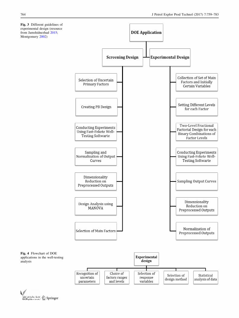
Fig. 3 Different guidelines of

experimental design (resource

from Jamshidnezhad 2015;

Montgomery 2002)

Fig. 4 Flowchart of DOE

applications in the well-testing

analysis

764 J Petrol Explor Prod Technol (2017) 7:759–783

123

and higher) are assumed unimportant, then information on

the main effects (primary factors) and two-order interac-

tions can be obtained by running only a fraction of the full

factorial experiment. This design is the most widely and

commonly used type of design in the industry that is called

fractional factorial design. PB design is one of the most

commonly used of fractional factorial designs, as a stan-

dard two-level screening design (NIST Information Tech-

nology Laboratory 2012) that will be used as the screening

strategy in this article.

5. Statistical analysis of data: In experimental design,

for analyzing the data and obtaining the objective results

and conclusions, statistical methods are employed. Analy-

sis is usually done by a technique called analysis of vari-

ance (ANOVA) in which the differences between

parameter means are analyzed.

ANOVAs evaluate the importance of one or more factors

by comparing the means of response variables at different

factor levels (Montgomery 2002; Nelson 1983). To run an

ANOVA, there must be a continuous response variable and

at least one categorical factor with two or more levels. The

main output from ANOVA study is arranged in a table con-

taining the sources of variation, their degrees of freedom, the

total sum of squares, and the mean squares. The ANOVA

table also includes the F-statistics and p values. These are

employed to determine whether the predictors or factors are

significantly related to the response. If the p value is less than

a predefined alpha (usually a = 0.05), it can be concluded

that at least one factor level mean is different.

When two or more response variables are considered,

MANOVA should be used for analyzing the results.

MANOVA is simply an ANOVA with several dependent

variables (French et al. 2015).

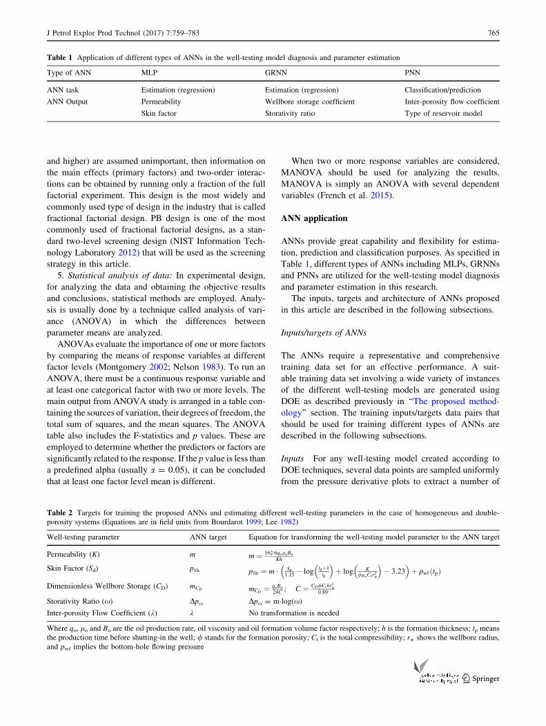
ANN application

ANNs provide great capability and flexibility for estima-

tion, prediction and classification purposes. As specified in

Table 1, different types of ANNs including MLPs, GRNNs

and PNNs are utilized for the well-testing model diagnosis

and parameter estimation in this research.

The inputs, targets and architecture of ANNs proposed

in this article are described in the following subsections.

Inputs/targets of ANNs

The ANNs require a representative and comprehensive

training data set for an effective performance. A suit-

able training data set involving a wide variety of instances

of the different well-testing models are generated using

DOE as described previously in ‘‘The proposed method-

ology’’ section. The training inputs/targets data pairs that

should be used for training different types of ANNs are

described in the following subsections.

Inputs For any well-testing model created according to

DOE techniques, several data points are sampled uniformly

from the pressure derivative plots to extract a number of

Table 1 Application of different types of ANNs in the well-testing model diagnosis and parameter estimation

Type of ANN MLP GRNN PNN

ANN task Estimation (regression) Estimation (regression) Classification/prediction

ANN Output Permeability Wellbore storage coefficient Inter-porosity flow coefficient

Skin factor Storativity ratio Type of reservoir model

Table 2 Targets for training the proposed ANNs and estimating different well-testing parameters in the case of homogeneous and double-

porosity systems (Equations are in field units from Bourdarot 1999; Lee 1982)

Well-testing parameter ANN target Equation for transforming the well-testing model parameter to the ANN target

Permeability (K) m m ¼ 162�6qoloBo

Kh

Skin Factor (Sd) p1h p1h ¼ m � Sd1:15 � log

tpþ1

tp

� �þ log K

/loCtr2w

� �� 3:23

� �þ pwfðtpÞ

Dimensionless Wellbore Storage (CD) mCD mCD¼ qoBo

24C; C ¼ CD/Cthr

2w

0:89

Storativity Ratio (x) Dpx Dpx = m�log(x)Inter-porosity Flow Coefficient (k) k No transformation is needed

Where qo, lo and Bo are the oil production rate, oil viscosity and oil formation volume factor respectively; h is the formation thickness; tp means

the production time before shutting-in the well; / stands for the formation porosity; Ct is the total compressibility; rw shows the wellbore radius,

and pwf implies the bottom-hole flowing pressure

J Petrol Explor Prod Technol (2017) 7:759–783 765

123

data points for further analysis (selecting 30 data points is a

common choice in this regard, as suggested by Al-Kaabi

and Lee, 1990). Pre-processing techniques including

dimensionality reduction and normalization are then

applied on the sampled data. Principal component analysis

(PCA) and singular value decomposition (SVD) are among

the most common techniques of dimensionality reduction

that could be employed for this purpose. The final training

input data sets used for learning the classification/estima-

tion models are created using the normalized data for all

the classes considered.

Targets As previously declared, determination of the

well-testing interpretation models and estimation of the

model-related variables form the pressure derivative plots

using different types of ANNs are the main objects of the

present article. The first part could be regarded as a clas-

sification problem, whereas the second part is an estimation

task.

For the classification purposes where the ANN tries to

predict the correct label of conceptual reservoir models

from the normalized pressure derivative data, the corre-

sponding labels (i.e., reservoir classes) of the input data are

used as the main targets for the trained networks.

To estimate the model parameters, on the other hand, a

variable transformation is initially performed. During

conventional well-testing interpretation, the reservoir

models and their corresponding flow regimes are charac-

terized on the pressure derivative plots. These flow regimes

are described in the form of straight lines of different

slopes or specific shapes on the well-testing diagnosis

plots. The model parameters are then estimated using the

slopes of different straight lines (Lee 1982). Therefore, in

this article, rather than estimating the well-testing model

parameters directly from the pressure derivative plots, the

slopes of lines and some other related variables are con-

sidered as the main targets of the proposed ANN models.

Such useful equations for the case of homogeneous and

double-porosity reservoir models, as they are investigated

later in ‘‘Results and discussions’’ section for testing the

proposed ANN-based approach, are provided in Table 2.

When predicted, the outputs of ANNs must be finally

transformed back to the original well-testing parameters

using the provided equations.

While MLP networks are suggested for estimating the

permeability and skin factor values from the pressure

derivative plots in this article, they are not recommended

for estimating the values of wellbore storage coefficient,

storativity ratio, and inter-porosity flow coefficient and for

classifying the correct reservoir models using the pressure

derivative data, due to relatively large MSE values of the

MLP networks when modeling these parameters for the

reservoir models considered in this article (‘‘Results and

discussions’’ section). Other types of ANNs including

GRNN and PNN are therefore investigated for modeling

the variables the MLP networks are not capable of pre-

dicting. As will be discussed in ‘‘PNNs/GRNNs’’ section,

PNN and GRNN have similar architectures, but there is a

fundamental difference; probabilistic networks perform

classification where the target variable is categorical,

whereas GRNNs perform regression where the target

variable is continuous.

GRNNs are recommended to estimate the values of

wellbore storage coefficient and storativity ratio as they get

continuous values when transformed to their corresponding

variables according to the equations provided in Table 2.

For the inter-porosity flow coefficient, however, no trans-

formation is applied before passing the values to the neural

network model; therefore, owing to the discrete nature of

the values of the inter-porosity flow coefficient (where only

a limited number of values is used for generating the

training examples using the DOE technique), a classifier

rather than a regressor would be used to predict their val-

ues. The PNN classifier is thus employed for predicting the

values of inter-porosity flow coefficient from the pressure

derivative plots. The classification and diagnosis of con-

ceptual reservoir models is also performed using a PNN

classifier.

MLP networks

MLPs are feed-forward ANN models mapping the sets of

input data onto a set of appropriate outputs. An MLP

consists of multiple layers of nodes in a directed graph,

with each layer fully connected to the next one. Except for

the input nodes, each node is a neuron (or processing ele-

ment) with a nonlinear activation function. MLP utilizes a

supervised learning technique called back-propagation for

training the network (Rosenblatt 1961; Rumelhart et al.

1986). MLP is a modification of the standard linear per-

ceptron and can distinguish data that are not linearly sep-

arable (Cybenko 1989).

A two-layer MLP network (including one input layer,

one hidden layer and one output layer) with the optimum

number of hidden neurons is capable of modeling the

complex nonlinear functions (Haykin 1999). Therefore,

two-layer MLP networks are proposed for estimating some

of the well-testing model parameters in this research.

PNNs/GRNNs

A PNN, introduced by Specht (1990), is a feed-forward

neural network, which was derived from the Bayesian

network and a statistical algorithm called Kernel Fisher

discriminant analysis. In a PNN, the operations are orga-

nized into a multilayered feed-forward network with four

766 J Petrol Explor Prod Technol (2017) 7:759–783

123

layers including input layer, pattern layer, summation layer

and output layer. The general architecture of PNNs is

illustrated in Fig. 5.

There are several advantages using PNN instead of MLP

for classification purposes; they are much faster and can be

more accurate than MLP networks; and they are relatively

insensitive to outliers and generate accurate predicted tar-

get probability scores.

GRNN, as proposed by Specht (1991), falls into the cat-

egory of PNNs. Like other PNNs, it needs only a fraction of

the training samples a back-propagation neural network

would need. Using a PNN is especially advantageous due to

its ability to converge to the underlying function of the data

with only few training samples available. The additional

knowledge needed to get the fit in a satisfying way is rela-

tively small and can be done without any additional input by

the user. This makes GRNN a very useful tool to perform

predictions and comparisons of the system performance in

practice. According to Bowden et al. (2005), GRNNs could

be treated as supervised feed-forward ANNs with a fixed

model architecture. The general structure of GRNNs is

similar to that of PNNs as shown in Fig. 5.

The probability density function used in GRNN is the

normal distribution function. Each training sample, Xj, is

used as the mean of a normal distribution (Li et al. 2014):

YðX; rÞ ¼Pn

j¼1 Yj exp � D2j

2r2

� �

Pnj¼1 exp � D2

j

2r2

� � ð1Þ

D2j ¼ ðX � XjÞT � ðX � XjÞ ð2Þ

The distance, Dj, between the training sample Xj and the

point of prediction X, is used as a measure of how well

each training sample can represent the position of predic-

tion, X. Within Eqs. 1 and 2, the standard deviation or the

smoothing parameter, r, is the only unknown parameter

that needs to be obtained through training (calibration). For

a bigger smoothing parameter, the possible representation

of the point of evaluation by the training sample is possible

for a wider range of X.

Fig. 6 General procedure of finding the best ANN parameters using

GS and CV

Fig. 5 General architecture of PNNs and GRNNs (based upon Gibbs

et al. 2006)

J Petrol Explor Prod Technol (2017) 7:759–783 767

123

As shown in Fig. 5, the structure of GRNN consists of

four layers including input, pattern, summation and output

units that are fully connected. According to Specht (1991),

the input units are formed by the elements of the input

vector X, feeding into each of the pattern units in the

second layer. The sum of squared differences between an

input vector X and the observed data Xj, is recorded in the

pattern units as Dj2. It then feeds into a nonlinear (e.g.,

exponential) activation function before passing into the

summation units. The two parts, A and B, in the summation

units correspond to the numerator and denominator in

Eq. 1, respectively. The quotient of parts A and B is the

predicted output by Y(X).

The model architecture of GRNNs is fixed by the fact

that the number of input nodes is determined by the number

of inputs m, the number of pattern nodes depends on the

size of the observed input data n, and the nodes in the

summation units always consist of two parts including a

denominator node and a numerator node.

Design of different types of ANNs

The following steps are considered in selecting the struc-

ture and parameters of the best ANN, as defined by the

minimum generalization error, through application of GS

and CV techniques (as suggested by Ben-Hur and Weston

(2015) in exploring the search space of hyper-parameters

of the radial basis function kernels):

1. A range of values of the network parameters (including

the number of hidden neurons, the network learning

algorithm and the activation functions of different

layers for MLPs, and the smoothing parameter for

PNNs and GRNNs) is considered in learning multiple

ANNs. Different combinations of the network param-

eters are used in an iterative manner through the GS

technique for building the ANN models. Each network

is trained using tenfold CV technique for an improved

estimation of the generalization error of the network.

To eliminate bias of error estimation, CVs are repeated

multiple times and the estimated generalization errors

are averaged over the repetitions. MSE values are

considered as the performance criteria of MLPs and

GRNNs, while the misclassification rate is used to

measure the performance of PNN classifiers. Normal-

ized pressure derivative data points are considered as

inputs to the networks, while the well-testing variables

according to the equations provided in Table 2 are

used as the targets.

2. The network with the minimum generalization error is

selected as the best ANN.

Table 3 The list of all parameters involved in the well-testing design of VH/VDP models

Type of variable Variable Symbol Type of reservoir model

Reservoir rock properties Permeability K VH/VDP

Net pay thickness h VH/VDP

Skin factor Sd VH/VDP

porosity u VH/VDP

Storativity ratio x VDP

Inter-porosity flow coefficient k VDP

Wellbore properties Dimensionless wellbore storage CD VH/VDP

Wellbore radius rw VH/VDP

Reservoir geometry Reservoir extent Xe (Ye) VH/VDP

Reservoir outer boundary Boundary VH/VDP

Production data Production time tp VH/VDP

Production rate qo VH/VDP

Reservoir fluid properties Initial reservoir pressure Pi VH/VDP

Water saturation Sw VH/VDP

Reservoir temperature Tres VH/VDP

API gravity API VH/VDP

Oil formation volumetric factor Bo VH/VDP

Oil viscosity lo VH/VDP

Total compressibility Ct VH/VDP

Oil compressibility Co VH/VDP

Solution gas oil ratio Rs VH/VDP

768 J Petrol Explor Prod Technol (2017) 7:759–783

123

3. The best network is finally trained using all available

training data.

The flowchart of selecting the best ANN parameters is

also illustrated in Fig. 6.

Results and discussions

To simply show the capabilities of the proposed approach in

automating the well-testing analysis, two different concep-

tual reservoir models including vertical well in a homoge-

neous reservoir (VH) and vertical well in a double-porosity

system (VDP) are investigated in this section. These cases

are among the most common reservoir models occurred

worldwide especially in the Iranian oil reservoirs. This

article does not consider the well-testing analysis of more

complex models using the presented approach that could be

the subjects of future studies. Nevertheless, this approach

could be applied to more complex types of reservoir models

including gas/gas condensate reservoir systems, partial

penetration models, and horizontal/deviated wells from the

pressure transient data, provided that the ANN-based model

is reconstructed and re-trained using the new training

examples of the considered reservoir models. To arrive at

the automatic well-testing interpretation and analysis for the

two reservoir models, different steps of the methodology

proposed in ‘‘The proposed methodology’’ section are

tracked in the following.

Screening design (first phase of DOE)

The parameters involved in creating both VH and VDP

models are listed in Table 3. The VDP model involves a

larger number of variables than the VH reservoir model

when creating the well-testing designs. In other words, the

VDP model is more comprehensive in the number of

Fig. 7 Effect of different well-

testing model parameters on

shape of the pressure derivative

plot; a permeability, b skin

factor, c wellbore storage

coefficient, d storativity ratio,

e inter-porosity flow coefficient,

and f outer boundary of

reservoir (from IHS Energy Inc.

2015)

J Petrol Explor Prod Technol (2017) 7:759–783 769

123

variables than the VH reservoir model. Therefore, the

screening design will be directed only for the VDP model

and the analyzed results are then applied to both VDP and

VH models.

Some parameters listed in Table 3 play a clearly strong

role in the well-testing diagnosis by affecting the shape of

the pressure derivative curves. Therefore, these parame-

ters are not included in the experimental design because

of their certain effects. These variables include perme-

ability, skin factor, wellbore storage coefficient, storativity

ratio, inter-porosity flow coefficient and outer boundary of

reservoir. The effect of these parameters on the pressure

derivative plots is well illustrated in Fig. 7 and also

described in the following statements (IHS Energy Inc.

2015):

1. As the permeability changes, the ordinate of the zero-

slope straight line representative of the matrix flow

moves vertically upward or downward (Fig. 7a).

2. Variation of the skin factor causes a noticeable change

in the hump of the near wellbore phenomena (Fig. 7b).

3. A change in the wellbore storage coefficient shifts the

unit-slope straight line at the start of pressure deriva-

tive curve horizontally along the time axis (Fig. 7c).

4. Changing the value of storativity ratio affects the dip

depth of the fracture-matrix period for a double-

porosity system (Fig. 7d).

5. Any changes in the inter-porosity flow coefficient

causes a horizontal shift for the fracture-matrix dip in a

fractured reservoir (Fig. 7e).

6. The type of reservoir outer boundary has a significant

influence on the shape of the pressure derivative curve

when the matrix radial flow has ended (Fig. 7f).

Therefore, among 21 parameters introduced in Table 3

for the VDP model, only 15 variables are considered in the

experimental design. The experimental design in this study

was performed using Minitab 17 software. In the first phase

of DOE, the screening design is performed using PB design

for selecting the most influential factors among 15 nomi-

nated variables.

As PB design is a two-level fractional factorial design,

the list of all variables that should be investigated for the

VDP model along with their binary settings are shown in

Table 4. According to PB design, for the 15-factor well-

testing diagnosis problem considered here, 49 experiments

would be conducted among which 48 trials are performed

at the two levels of each factor and 1 trial is conducted at

their mean levels (Table 5). The rows and columns of

Table 5 indicate the parameter index and the experiment

number, respectively. The values -1, ?1 and 0 correspond

to the low, high and mean levels of each factor,

respectively.

To create the corresponding well-testing models of

pressure buildup tests according to the design table in

Table 5, the Fast Fekete Well-Testing Software is

employed. The models are synthesized analytically rather

than numerically in this article. It should be noted that the

created well-testing models are presumed to be single

phase oil and the reservoir pressure is assumed to be above

the bubble point pressure. The experiments are conducted

according to the factor levels indicated in Table 5. The

values of unaffected variables are kept constant during the

experimentation phase according to Table 6. The outputs

of the conducted experiments are the corresponding pres-

sure derivative curves for the created pressure buildup

Table 4 The list of all variables involved in VDP model and their binary settings for PB design (The numbers in parentheses, where provided,

are the corresponding values in SI units)

Variable Setting of level ?1 Setting of level -1 Field units (SI units)

h 100 (30.48) 1000 (304.79) ft (m)

u 10 30 %

rw 0.2 (0.06) 0.4 (0.12) ft (m)

Xe (Ye) 2000 (609.57) 6000 (1828.71) ft (m)

tp 50 (180,000) 120 (432,000) hr (s)

qo 500 (9.2E-4) 1500 (2.76E-3) STBD (m3/s)

Pi 4000 (2.76E?7) 6000 (4.14E ? 7) psia (Pa)

Swi 0 30 %

Tres 140 (60) 220 (104.44) �F (�C)API 25 40 degree

Bo 1 (1) 1.5 (1.5) RBBL/STB (Rm3/Sm3)

lo 0.5 (5E-4) 50 (0.05) cp (Pa�s)Ct 1e-6 (1.45E-10) 1e-5 (1.45E-9) psi-1 (Pa-1)

Co 1e-6 (1.45E-10) 1e-5 (1.45E-9) psi-1 (Pa-1)

Rs 100 (17.81) 900 (178.11) SCF/STB (Sm3/Sm3)

770 J Petrol Explor Prod Technol (2017) 7:759–783

123

Table 5 PB design table for 15 nominated well-testing parameters for VDP model; each P stands for a specific parameter according to the list of

variables in Table 4

Experiment no. P1 P2 P3 P4 P5 P6 P7 P8 P9 P10 P11 P12 P13 P14 P15

1 1 1 -1 1 -1 1 -1 -1 -1 1 1 -1 1 1 -1

2 1 1 -1 1 -1 1 -1 -1 1 1 1 1 -1 1 1

3 1 -1 1 -1 1 -1 -1 1 1 1 1 -1 1 1 1

4 -1 -1 1 1 -1 1 -1 1 -1 -1 -1 1 1 -1 1

5 -1 -1 -1 -1 1 1 -1 1 -1 1 -1 -1 -1 1 1

6 1 1 1 1 1 -1 -1 -1 -1 1 -1 -1 -1 -1 1

7 -1 -1 1 1 1 -1 1 -1 1 -1 -1 1 1 1 1

8 -1 1 -1 -1 -1 1 1 -1 1 1 -1 -1 1 -1 -1

9 1 1 -1 -1 -1 -1 1 -1 -1 -1 -1 1 1 -1 1

10 1 -1 -1 -1 -1 1 1 -1 1 -1 1 -1 -1 -1 1

11 -1 -1 -1 -1 -1 -1 -1 -1 -1 -1 -1 -1 -1 -1 -1

12 1 1 1 -1 -1 -1 -1 1 -1 -1 -1 -1 1 1 -1

13 -1 1 1 -1 1 1 -1 -1 1 -1 -1 1 1 1 -1

14 -1 1 -1 -1 -1 -1 1 1 -1 1 -1 1 -1 -1 -1

15 -1 1 -1 -1 1 1 1 1 -1 1 1 1 1 1 -1

16 1 1 1 1 -1 1 1 1 1 1 -1 -1 -1 -1 1

17 1 1 1 1 -1 -1 -1 -1 1 -1 -1 -1 -1 1 1

18 1 -1 -1 -1 -1 1 -1 -1 -1 -1 1 1 -1 1 -1

19 -1 1 1 1 -1 1 -1 1 -1 -1 1 1 1 1 -1

20 1 -1 -1 1 -1 -1 1 1 1 -1 1 -1 1 -1 -1

21 -1 -1 1 1 1 1 -1 1 1 1 1 1 -1 -1 -1

22 1 -1 -1 1 1 1 1 -1 1 1 1 1 1 -1 -1

23 -1 -1 -1 1 1 -1 1 -1 1 -1 -1 -1 1 1 -1

24 -1 1 1 -1 1 -1 1 -1 -1 -1 1 1 -1 1 1

25 1 1 -1 1 1 1 1 1 -1 -1 -1 -1 1 -1 -1

26 -1 1 -1 1 -1 -1 1 1 1 1 -1 1 1 1 1

27 1 1 -1 1 1 -1 -1 1 -1 -1 1 1 1 -1 1

28 -1 -1 -1 1 1 -1 1 1 -1 -1 1 -1 -1 1 1

29 1 1 1 -1 1 1 1 1 1 -1 -1 -1 -1 1 -1

30 -1 1 -1 -1 1 1 1 -1 1 -1 1 -1 -1 1 1

31 1 1 -1 -1 1 -1 -1 1 1 1 -1 1 -1 1 -1

32 1 -1 1 1 1 1 1 -1 -1 -1 -1 1 -1 -1 -1

33 -1 1 -1 1 -1 -1 -1 1 1 -1 1 1 -1 -1 1

34 -1 -1 1 1 -1 1 1 -1 -1 1 -1 -1 1 1 1

35 -1 -1 -1 -1 1 -1 -1 -1 -1 1 1 -1 1 -1 1

36 1 -1 -1 -1 1 1 -1 1 1 -1 -1 1 -1 -1 1

37 -1 -1 1 -1 -1 -1 -1 1 1 -1 1 -1 1 -1 -1

38 1 -1 -1 1 1 1 -1 1 -1 1 -1 -1 1 1 1

39 -1 1 1 1 1 1 -1 -1 -1 -1 1 -1 -1 -1 -1

40 -1 1 1 -1 -1 1 -1 -1 1 1 1 -1 1 -1 1

41 -1 -1 -1 1 -1 -1 -1 -1 1 1 -1 1 -1 1 -1

42 0 0 0 0 0 0 0 0 0 0 0 0 0 0 0

43 -1 1 1 1 1 -1 1 1 1 1 1 -1 -1 -1 -1

44 1 1 1 -1 1 -1 1 -1 -1 1 1 1 1 -1 1

45 1 -1 1 1 -1 -1 1 -1 -1 1 1 1 -1 1 -1

46 1 -1 1 -1 1 -1 -1 -1 1 1 -1 1 1 -1 -1

47 1 -1 1 -1 -1 -1 1 1 -1 1 1 -1 -1 1 -1

48 -1 -1 1 -1 -1 1 1 1 -1 1 -1 1 -1 -1 1

49 1 -1 1 -1 -1 1 1 1 1 -1 1 1 1 1 1

J Petrol Explor Prod Technol (2017) 7:759–783 771

123

tests. The buildup tests are supposed to last enough so that

the pressure derivative curves are entirely formed. There-

fore, a long enough shut-in time was assumed for all the

buildup tests.

Subsequent to the experimentation, the resulting pres-

sure derivative curves are uniformly sampled at 30 data

points. The extracted sets of points are then normalized

using the min–max operator in Eq. 3:

Xnew ¼ X �minðXÞmaxðXÞ �minðXÞ ð3Þ

where X and Xnew are the sampled and normalized pressure

derivative values, respectively.

The number of points sampled on the pressure derivative

curves dictates the number of responses for PB design. To

reduce further the number of responses, suitable dimen-

sionality reduction techniques may be used. Singular value

decomposition (SVD) is here employed for its major

capabilities (Ientilucci 2003):

1. Transformation of the correlated variables into a set of

uncorrelated ones to better reflect various relationships

among the original data items.

2. Identifying and ordering the dimensions along which

the data points exhibit the most variation.

3. Finding the best approximation of the original data

using fewer numbers of dimensions.

What makes SVD practical for nonlinear problem

applications is that the variation below a particular

threshold could be simply ignored to massively reduce data

assuring that the main relationships of interest have been

preserved. In the present application, SVD is applied to the

sampled pressure derivative data points. Dimensionality of

the sampled data is then reduced from 30 to 4 dimensions

regarding the cumulative relative variance provided by the

selected dimensions reaching a predefined threshold (here

99.9% of the total variance). The remaining dimensions

provide less than 0.1% of the total variance of data and

hence are ignored during further studies. MANOVA is then

employed on the reduced data to analyze the screening

design.

After performing MANOVA on PB design with reduced

responses of the well-testing diagnosis problem, the p val-

ues for all the well-testing model parameters are shown in

Table 7. As a result, only 7 variables among 15 nominated

variables are considered as significant by comparing their

p values against the chosen value of a (equal to 0.05).

Fractional factorial design (second phase of DOE)

The next steps during the well-testing interpretation and

analysis including the well-testing designs, reservoir model

diagnosis and evaluation of model parameters will be

implemented using 13 variables (7 variables selected after

the screening design plus 6 variables of less uncertainty

discussed in ‘‘Screening design (first phase of DOE)’’

section). The well-testing diagnosis will be performed

through the following steps:

1. The second phase of DOE is directed using a two-level

fractional factorial design; the experiments are con-

ducted using the Fast Fekete Well-Testing Software.

1.1 All 13 variables previously selected are used in

constructing the well-testing designs for the VDP

model, while the storativity ratio and inter-

porosity flow coefficient are excluded from

studying the VH model as they are inherent to

the naturally fractured reservoirs. The fractional

factorial design for the VDP model consists of

129 runs for 13 variables at two levels including

one center point at their mean levels.

To better investigate the relationships among the

model parameters (as the inputs) and the pressure

derivative data points (as the model responses),

the number of experiments could be increased

Table 6 The values of unaffected well-testing variables during the experimentation phase (The numbers in parentheses, where provided, are the

corresponding values in SI units)

Variable K Sd CD x k Reservoir outer boundary

Value 500 (4.95E-13) 0 2000 0.1 1 9 10-5 No flow

Field units (SI units) md (m2) Dimensionless –

Table 7 Results of conducting MANOVA study on PB design with 15 primary factors and reduced responses

Variable Pi tp qo h / Swi Ct rw Xe Tres API lo Bo Co Rs

p value 0.95 0.3 0 0 0 0.98 0 0 0 0.1 0.98 0 0 0.36 0.19

772 J Petrol Explor Prod Technol (2017) 7:759–783

123

and more number of factor levels may be

examined. To consider wider ranges of values

of the well-testing variables common to the

Iranian oil reservoirs, four different levels are

defined for each input variable according to the

values provided in Table 8. The fractional fac-

torial design is then accomplished for any binary

combinations of the factor levels. So the number

of repetitions of two-level DOEs (each contain-

ing 129 experiments) equals4

2

� �¼ 6 when

taking all the factor levels into account. There-

fore, the total number of experiments considered

for the VDP model is equal to 6 9 129 = 774

experiments.

1.2 To conduct a two-level fractional factorial design

for the VH model with 11 parameters, a design

Table 8 Different levels of the well-testing variables for the fractional factorial design (The numbers in parentheses, where provided, are the

corresponding values in SI units)

Variable 1st level 2nd level 3rd level 4th level Field units (SI units)

K 10 (9.87E-15) 100 (9.87E-14) 500 (4.93E-13) 1200 (1.18E-12) md (m2)

h 20 (6.10) 200 (60.96) 1000 (304.79) 1800 (548.61) ft (m)

Sd 5- 0 5 20 Dimensionless

CD 100 1000 5000 10,000 Dimensionless

x 0.001 0.05 0.1 0.3 Dimensionless

k 1 9 10-8 1 9 10-6 1 9 10-5 1 9 10-4 Dimensionless

/ 5 15 20 30 %

Ct 1 9 10-6 (1.45E-10) 5 9 10–6 (7.25E-10) 1 9 10-5 (1.45E-9) 5 9 10–5 (7.25E-9) psi-1 (Pa-1)

rw 0.25 (7.6E-2) 0.3 (9.1E-2) 0.35 (0.11) 0.4 (0.12) ft (m)

Xe 1500 (457.18) 3000 (914.36) 4000 (1219.14) 5000 (1523.93) ft (m)

qo 500 (9.2E-4) 1500 (2.76E-3) 2500 (4.60E-3) 4000 (7.36E-3) STBD (m3/s)

lo 0.5 (5E-4) 5 (5E-3) 15 (0.015) 40 (0.04) cp (Pa�s)Bo 1 1.1 1.2 1.3 RBBL/STB (Rm3/Sm3)

Table 9 The number of training examples used for building different types of ANNs

ANN Target Number of training examples

MLP1 Permeability 1164

MLP2 Skin factor 1164

GRNN1 Wellbore storage Coefficient 1164

GRNN2 Storativity ratio 774

PNN1 Inter-porosity flow coefficient 774

PNN2 Type of reservoir model 1164

Fig. 8 The scree plot of PCA results; the first 8 components comprise

99.9% of the total energy of data

J Petrol Explor Prod Technol (2017) 7:759–783 773

123

table containing 65 experiments is created.

Similarly, when defining four different levels

for the selected factors according to Table 8, a

number of 6 9 65 = 390 experiments are totally

considered for the VH model.

2. At the end of the second phase of DOE, the training

data sets involving a wide variety of well-testing

samples both for VDP and VH reservoir models are

generated. The number of training examples used for

building different types of ANNs is shown in Table 9.

2.1 For any well-testing model created according to

the DOE tables, the pressure derivative plots are

sampled uniformly to extract 30 data points for

further analysis.

2.2 Principal component analysis (PCA) is then

applied on the sampled data for additional

dimensionality reduction. Similar to the proce-

dure for the SVD technique, the appropriate

number of components could be selected using

a predefined threshold, regarding the relative

variance (power) the principal components pro-

vide. Using the scree plot, the relative variance

of the components is plotted against the index

of the components in a descending order.

Regarding the scree plot in Fig. 8, the cumula-

tive variance of the principal components

approaches a threshold of 0.999 using the first

8 components. The other components are disre-

garded due to negligible variances shared by

them on the total power of the data. The number

of inputs to each ANN is therefore 8, equal to

the number of principal components retrieved.

Each ANN has also 1 neuron in its output layer

to predict the requested parameter based on the

equations in Table 2.

2.3 The reduced data are then normalized using the

min–max operator (Eq. 3) to lie between 0 and 1.

The final training data sets used for learning the

classification/estimation models are created using

the normalized data for the VDP and VH classes.

ANN application

The ANN models are now constructed using the training

data sets generated with the help of DOE techniques in

‘‘Fractional factorial design (second phase of DOE)’’ sec-

tion. MLPs, PNNs and GRNNs are employed for the well-

testing model diagnosis and the model-related parameter

estimation. The architectures of the networks are deter-

mined based on the methodologies described in ‘‘design of

different types of ANNs’’ section.

MLP

MLP networks are used to estimate the values of perme-

ability and skin factor from the normalized and reduced

pressure derivative data points. Multiple networks with

different parameters and structures are created and com-

pared in the framework of GS and CV techniques. The

number of hidden neurons, the network learning algorithm

and the activation functions of different layers are varied

based on Table 10. The mean squared error (MSE) is

commonly used as the performance criterion of the neural

networks when they are used for prediction or regression

tasks. So, the MLP network with the minimum general-

ization MSE is selected as the best MLP. The minimum

MSE values of different MLP networks as well as the

corresponding number of hidden neurons are shown in

Table 11. As observed, the minimum error is obtained for

the hyperbolic tangent sigmoid algorithm and the Bayesian

regulation back-propagation function using 17 neurons in

the hidden layer. The best set of network parameters is

employed for building two individual MLP networks for

estimating the transformed values of the permeability and

the skin factor. The regression plots of both training and

test data is represented in Fig. 9a through 9d for the two

MLP networks considered. Figure 10a, b illustrate the plots

of target values versus the MLP outputs of the permeability

and skin factor transformed values, respectively. The circle

markers on the plots indicate the target values, while the

network outputs are shown by the stars. It should be noted

that the permeability and skin factor values are estimated

for both VH and VDP models, covering all 1164 training

data, as indicated on the x-axes of the plots. There are good

consistencies between the targets and the networks outputs

for both parameters, as observed on the plots.

Table 10 Different network parameters used in studying MLP networks

Number of hidden Neurons Learning algorithm Activation function

5 to 22 Levenberg–Marquardt backpropagation Hyperbolic tangent sigmoid

Bayesian regulation backpropagation Log-sigmoid

Scaled conjugate gradient backpropagation Linear

774 J Petrol Explor Prod Technol (2017) 7:759–783

123

PNNs/GRNNs

PNNs are used to predict the underlying reservoir model

and the discrete value of the inter-porosity flow coefficient

(if needed), while GRNNs are employed to estimate the

values of dimensionless wellbore storage and storativity

ratio (if required). Various networks with different

smoothing parameters (from 0.01 to 0.5) are created and

Table 11 Minimum MSE values and optimum number of hidden neurons used for selecting the best MLP networks in order to estimate the

permeability and skin factor

Learning algorithm Activation function Minimum MSE Number of hidden neurons

Hyperbolic tangent sigmoid Levenberg–Marquardt backpropagation 0.00067 10

Scaled conjugate gradient backpropagation 0.0091 22

Bayesian regulation backpropagation 0.00041 17

Log-sigmoid Levenberg–Marquardt backpropagation 0.19529 18

Scaled conjugate gradient backpropagation 0.19589 10

Bayesian regulation backpropagation 0.19589 7

Linear Levenberg–Marquardt Backpropagation 0.0053 22

Scaled conjugate gradient backpropagation 0.0053 5

Bayesian regulation backpropagation 0.0053 7

Fig. 9 The regression plots of

MLP outputs versus targets for

a training data of permeability,

b test data of permeability,

c training data of skin factor and

d test data of skin factor

J Petrol Explor Prod Technol (2017) 7:759–783 775

123

compared through GS and CV techniques. The perfor-

mance of different GRNNs versus the values of smoothing

parameters is plotted and depicted in Fig. 11a, b for esti-

mating the wellbore storage coefficient and the storativity

ratio, respectively. The same plots are demonstrated in

Fig. 11c, d for PNN classifiers used for modeling the inter-

porosity flow coefficient and the well-testing reservoir

model, respectively. The smoothing parameter that yields

the best performance of GRNNs/PNNs (corresponding to

the minimum values of MSE and misclassification rate,

respectively) is selected as the best smoothing parameter

and will be used for further studies (Table 12).

The regression plots of both GRNNs used for estimating

the wellbore storage coefficient and storativity ratio

Fig. 10 Plots of targets versus MLP outputs of a permeability transformed values, and b skin factor transformed values

776 J Petrol Explor Prod Technol (2017) 7:759–783

123

(trained using the best smoothing parameter and all avail-

able training data) are shown for the whole set of training

and test data in Fig. 12a, b, respectively.

In addition, the targets versus the PNN outputs of the

inter-porosity flow coefficient transformed values and the

type of reservoir model are displayed in Fig. 13a, b,

respectively. Figure 14a, b also exhibit the targets versus

the GRNN outputs of the wellbore storage coefficient and

storativity ratio transformed values, respectively. The cir-

cle markers on the plots indicate the target values, while

the network outputs are illustrated by the stars. As the

x-axes of the plots show, the storativity ratio and inter-

porosity flow coefficient values are estimated just for the

VDP model with only 774 training examples, while other

parameters of study are obtained for both VH and VDP

models, covering all 1164 training data. According to the

plots, there is a good agreement between the targets and the

networks outputs for different parameters.

Finding the best structures and parameters of different

MLPs, GRNNs and PNNs, the best performance of each

Table 12 The best values of smoothing parameters used in developing GRNNs and PNNs for modeling different variables

Variable Wellbore storage coefficient Storativity ratio Inter-porosity flow coefficient Well-testing reservoir model

Best smoothing parameter 0.02 0.01 0.01 0.01

Type of ANN GRNN PNN

Fig. 11 The performance plots of GRNNs and PNNs illustrating the

network performance for different smoothing parameters used in

constructing the neural networks, a GRNN for estimating the

wellbore storage coefficient, b GRNN for estimating the storativity

ratio, c PNN for predicting the inter-porosity flow coefficient, and

d PNN for classifying the well-testing reservoir model

J Petrol Explor Prod Technol (2017) 7:759–783 777

123

neural network engaged for the estimation or classification

purposes is illustrated in Table 13.

Validation of trained models

To validate the proposed ANN-based models for the well-

testing interpretation and analysis in this article, several

case studies are tested here. These cases include seven real

field buildup tests including three VDP and four VH

reservoir models under different reservoir rock and fluid

conditions producing at different oil rates.

In each case, the pressure derivative plot is firstly cre-

ated from the pressure transient data. After proper manip-

ulations and required preprocessing including sampling,

dimensionality reduction and normalization (similar to the

works described in ‘‘fractional factorial design (second

phase of DOE)’’ section), the preprocessed derivative data

points are fed as inputs into the neural network models

including MLPs, PNNs and GRNNs. The network outputs

are finally post-processed using the equations in Table 2 to

determine the underlying reservoir model and estimate the

model-related properties.

Some parameters including permeability, skin factor

and wellbore storage coefficient are estimated for all the

cases independent of the type of reservoir model. The

well-testing model is then identified by the PNN clas-

sifier. The storativity ratio and the inter-porosity flow

coefficient would be evaluated if the underlying reser-

voir model is classified as the double-porosity type. The

seven test cases have also been analyzed using the

conventional analysis techniques and the well-testing

model parameters have been estimated in this way. The

validation results using the proposed model for the seven

test cases in comparison with the conventional estima-

tions are summarized in Table 14.

The relative errors of estimations using the proposed

ANN-based model compared to the conventional analysis

results are shown in Table 15.

As shown in Table 14, the proposed approach has cor-

rectly predicted the types of reservoir model for all the

seven test cases. This confirms the presented model as a

reliable (binary) classifier for determining the well-testing

interpretation models using the pressure derivative plots.

The model-related variables have also been estimated by

the proposed model relatively close to the conventional

estimations, since nearly small relative errors are obtained

using the ANN-based model compared to the conventional

analysis techniques, as illustrated in Table 15. This also

indicates the reliability of the proposed approach in esti-

mating the model-related variables from the real pressure

transient test data for the two cases considered in this

article, when the underlying reservoir model has been

properly identified by the presented model. Such an accu-

racy could not be achieved in estimating the well-testing

variables unless the model is trained with a sufficiently

large and comprehensive training data set covering wide

ranges of the most influencing parameters. Dealing with

large numbers of parameters to generate an extensive

training data set in a manageable time and effort (by

conducting a fewer number of experiments) has been

effectively achieved using the DOE technique in this

article.

Fig. 12 The regression plots of GRNN outputs versus targets for the whole set of training and test data for a wellbore storage coefficient, and

b storativity ratio

778 J Petrol Explor Prod Technol (2017) 7:759–783

123

Conclusions

1. A new methodology based on ANNs is proposed in

this article to automate the process of well-testing

interpretation and analysis. The presented approach

enables conceptual reservoir model identification and

estimation of model-related parameters from the

pressure derivative plots using different types of

ANNs.

2. Experimental design is executed to select the most

influential variables affecting the well-testing designs.

The fractional factorial design is also implemented to

Fig. 13 Plots of targets versus PNN outputs of a inter-porosity flow coefficient transformed values, and b type of reservoir model. The numbers

1 and 2 on the y-axis of the plot (b) correspond to the VH and VDP models, respectively

J Petrol Explor Prod Technol (2017) 7:759–783 779

123

generate statistically sufficient number of training

examples for proper learning of the proposed ANNs.

3. The pressure derivative plots are primarily sampled at a

limited number of data points, undergone by dimen-

sionality reduction techniques, and finally normalized

prior to introduction to the neural network models.

4. Two different reservoir models including homoge-

neous and double-porosity systems are investigated in

this article; so the model-related parameters that will

be estimated using the proposed model include

permeability, skin factor and dimensionless wellbore

storage coefficient (for all kinds of reservoir models)

Fig. 14 Plots of targets versus GRNN outputs of a wellbore storage coefficient transformed values, and b storativity ratio transformed values

780 J Petrol Explor Prod Technol (2017) 7:759–783

123

and storativity ratio and inter-porosity flow coefficient

(in the case of double-porosity systems).

5. Two MLP networks are designed in this study to

estimate the permeability and skin factor in their

output neurons. The dimensionless wellbore storage

coefficient and storativity ratio are estimated using two

different GRNNs, while two different PNNs are

employed to predict the value of inter-porosity flow

Table 13 Performance of the proposed neural network models for estimating the well-testing model parameters and identifying the conceptual

reservoir model

Variable Permeability Skin factor Storativity

ratio

Wellbore storage

coefficient

Reservoir

model

Inter-porosity flow

coefficient

Data mining task Estimation Classification

Type of neural network MLP GRNN PNN

Network performance

criterion

MSE Misclassification rate

Network performance value 1.35 9 10-4 2.94 9 10-5 5.33 9 10-5 6.74 9 10-5 0 0

Table 14 Estimation of model-related parameters and the well-testing model diagnosis using the conventional analysis techniques and the

proposed ANN-based approach (The numbers in parentheses, where provided, are the corresponding values in SI units)

Method of analysis Test number Model type K, md (m2) S CD x k

Conventional approach 1 VDP 0.26 (2.57E-16) -3.3 3 0.71 1.0E-08

2 17.25 (1.70E-14) 5.52 101 0.232 1.1E-08

3 131 (1.29E-13) -7.6 22,800 0.58 1.0E-4

4 VH 5.8 (5.72E-15) -5.5 135 – –

5 98.5 (9.76E-14) -6.1 310 – –

6 130 (1.28E-13) 14.05 50 – –

7 455 (4.49E-13) 17.2 58.5 – –

Proposed Approach 1 VDP 0.24 (2.37E-16) -3.09 2.9 0.74 1.0E-08

2 16.62 (1.64E-14) 5.6 96.92 0.226 1.0E-08

3 136.87 (1.35E-13) -7.5 22,448 0.633 1.0E-04

4 VH 5.38 (5.31E-15) -5.98 137.74 – –

5 100.72 (9.94E-14) -6.14 314.78 – –

6 121.05 (1.19E-13) 15.05 48.06 – –

7 422.05 (4.17E-13) 18.4 57 – –

Table 15 Relative errors of estimations (in percentage) using the proposed ANN-based model in comparison with the conventional analysis

results

Test number K S CD x k

1 7.69 6.36 3.33 4.23 0.00

2 3.65 1.45 4.04 2.59 9.09

3 4.48 1.32 1.54 9.14 0.00

4 7.24 8.73 2.03 – –

5 2.25 0.66 1.54 – –

6 6.88 7.12 3.88 – –

7 7.24 6.98 2.56 – –

Average of All tests 5.64 4.66 2.70 5.32 3.03

J Petrol Explor Prod Technol (2017) 7:759–783 781

123

coefficient and classify the well-testing interpretation

model.

6. To involve some other well-testing variables in the

estimation process, the transformed values of the

model-related parameters are used as the targets for

training the neural network models. To estimate the

model-related parameters for a given pressure deriva-

tive plot using the trained neural networks, the network

outputs are converted back to the expected variables

using the proper equations.

7. The validation results using the real field buildup test

data confirm that the proposed models generate

reliable results both in the case of identifying the

correct reservoir models and estimating the model-

related parameters using the pressure derivative plots

compared to the results of conventional well-testing

analysis techniques.

8. Unlike the conventional analysis techniques in which

the well-testing reservoir models are determined from

the visual inspection of the pressure derivative plots,

ANNs are trained with the representative examples to

recognize the underlying reservoir model and esti-

mate the model-related properties. So ANN-based

models are very helpful especially when dealing with

the complex patterns on the pressure derivative

curves. The great advantages of the ANN-based

approach relates to the improvements in the pattern

recognition problem compared to the conventional

techniques.

Future works

1. The well-testing interpretation and analysis model

presented in this article employs only the pressure

derivative plots as inputs to the model. Using the same

approach to identify the conceptual reservoir model

and to estimate the model-related parameters from

other diagnostic plots such as semi-log or linear graphs

is recommended for future works.

2. The current research shows the capabilities of the

proposed ANN-based approach for the well-testing

analysis of the homogeneous and double-porosity

systems. Although the proposed approach is inves-

tigated by these two types of reservoir models in

this article, it is not exclusive to any specific model

and could be applied to any system with any types

of fluid, well geometry and reservoir structure,

provided that the proposed model is re-trained

using the proper examples generated for the set of

those models. Using other conceptual reservoir

models and considering more complex hydrocarbon

systems or fluids like gas condensate reservoirs and

horizontal/deviated wells are, therefore, highly

encouraged.

Open Access This article is distributed under the terms of the

Creative Commons Attribution 4.0 International License (http://

creativecommons.org/licenses/by/4.0/), which permits unrestricted

use, distribution, and reproduction in any medium, provided you give

appropriate credit to the original author(s) and the source, provide a

link to the Creative Commons license, and indicate if changes were

made.

References

Alajmi M, Ertekin T (2007) The development of an artificial neural

network as a pressure transient analysis tool for applications in

double-porosity reservoirs. Paper SPE 108604 presented at the

SPE Asia pacific oil and gas conference and exhibition, Jakarta,

Indonesia

Al-Kaabi AU, Lee WJ (1990) An artificial neural network approach to

identify the well test interpretation model: applications. Paper

SPE 20552 presented at the 65th annual technical conference and

exhibition, New Orleans, LA

Al-Kaabi AU, Lee WJ (1993) Using artificial neural networks to

identify the well test interpretation model. Paper SPE 20332

presented at the SPE petroleum computer conference, Denver

Allain OF, Horne RN (1990) Use of artificial intelligence in well-test

interpretation. JPT 42(3):342–349. doi:10.2118/18160-PA

Antony J (2003) Design of experiments for engineers and scientists.

Butterworth-Heinemann, Oxford

Athichanagorn S, Horne RN (1995) Automatic parameter estimation

from well test data using artificial neural network. Paper SPE

30556 presented at the SPE annual technical conference and

exhibition, Dallas, USA

Aydinoglu G, Bhat M, Ertkin T (2002) Characterization of partially

sealing faults from pressure transient data: an artificial neural

network approach. Paper SPE 78715 presented at the SPE

eastern regional meeting, Lexington, Kentucky, USA

Bourdarot G (1999) Well testing: interpretation methods. Editions

TECHNIP

Bowden GJ, Dandy GC, Maier HR (2005) Input determination for

neural network models in water resources applications: part 1—

background and methodology. J Hydrol 301(1–4):75–92

Cybenko G (1989) Approximation by superpositions of a sigmoidal

function. Math Control Signal 2(4):303–314

Deng Y, Chen Q, Wang J (2000) The artificial neural network method

of well-test interpretation model identification and parameter

estimation. Paper SPE 64652 presented at the SPE international

oil and gas conference and exhibition, Beijing, China

Ershaghi I, Li X, Hassibi M, Shikari Y (1993) A robust neural

network model for pattern recognition of pressure transient test

data. Paper SPE 26427 presented at the SPE annual technical

conference and exhibition, Houston, Texas

Gibbs MS, Morgan N, Maier HR, Dandy GC, Nixon J, Holmes M

(2006) Investigation into the relationship between chlorine decay

and water distribution parameters using data driven methods.

Math Comput Model 44(5):485–498

Haykin S (1999) Neural networks, a comprehensive foundation.

Prentice Hall, Upper Saddle River

Hinkelmann K, Kempthorne O (2007) Design and analysis of

experiments. Introduction to experimental design, vol 1. Wiley,

New York

782 J Petrol Explor Prod Technol (2017) 7:759–783

123

Jamshidnezhad M (2015) Experimental design in petroleum reservoir

studies. Gulf Professional Publishing, Elsevier, Oxford. doi:10.

1016/B978-0-12-803070-7.00001-6

Jeirani Z, Mohebbi A (2006) Estimating the initial pressure,

permeability and skin factor of oil reservoirs using artificial

neural networks. J Petrol Sci Eng 50:11–20

Juniardi IR, Ershaghi I (1993) Complexities of using neural network

in well test analysis of faulted reservoirs. Paper SPE 26106

presented at the western regional meeting, Anchorage, Alaska

Kharrat R, Razavi SM (2008) Determination of reservoir model from

well test data using an artificial neural network. Sci Iran

15(4):487–493

Kumoluyi AO, Daltaban TS, Archer JS (1995) Identification of well-

test models by use of higher-order neural networks. Paper SPE

27558 presented at the SPE european petroleum computer

conference, Aberdeen

Lee WJ (1982) Well testing. Society of petroleum engineers of AIME

Li X, Zecchin AC, Maier HR (2014) Selection of smoothing parameter

estimators for general regression neural networks—applications to

hydrological and water resources modelling. Environ Modell

Softw 59:162–186. doi:10.1016/j.envsoft.2014.05.010

Montgomery DC (2002) Design and analysis of experiments. Wiley,

New york

Nelson PR (1983) A comparison of sample sizes for the analysis of

means and the analysis of variance. J Qual Technol 15:33–39

Rosenblatt FX (1961) Principles of neurodynamics: perceptrons and

the theory of brain mechanisms. Spartan Books, Washington

Rumelhart DE, Geoffrey EH, Williams RJ (1986) Learning internal

representations by error propagation. In: Rumelhart DE,

McClelland JL, PDP research group (eds) Parallel distributed

processing: explorations in the microstructure of cognition.

Foundations, vol 1. MIT Press, Cambridge

Specht DF (1991) A general regression neural network. Neural Netw

IEEE Trans 2(6):568–576

Specht DF (1990) Probabilistic neural networks. Neural Netw

3:109–118. doi:10.1016/0893-6080(90)90049-Q

Sung W, Yoo I, Ra S, Park H (1996) Development of the HT-BP

neural network system for the identification of a well-test

interpretation model. Paper SPE 30974 presented at the SPE

eastern regional meeting, Morgantown

Vaferi B, Eslamloueyan R, Ayatollahi S (2011) Automatic recogni-

tion of oil reservoir models from well testing data by using

multi-layer perceptron networks. J Petrol Sci Eng 77:254–262

Web References

Ben-Hur A, Weston J (2015) A user’s guide to support vector

machines. Technical report. http://pyml.sourceforge.net/doc/

howto.pdf. Accessed 10 Feb 2016

French A, Macedo M, Poulsen J, Waterson T, Yu A (2015)

Multivariate analysis of variance (MANOVA). http://userwww.

sfsu.edu/*efc/classes/biol710/manova/MANOVAnewest.pdf.

Accessed 10 Feb 2016

Ientilucci EJ (2003) using the singular value decomposition. http://

www.cis.rit.edu/*ejipci/research.htm. Accessed 10 Feb 2016

IHS Energy Inc (2015) Well testing and rate transient analysis

consulting. http://cdn.ihs.com/www/images/Fekete-WellTest-

Fundamentals.png. Accessed 10 Feb 2016

NIST Information Technology Laboratory (2012) NIST/SEMATECH

e-handbook of statistical methods. www.itl.nist.gov/div898/

handbook/pri/section3/pri335.htm. Accessed 10 Feb 2016

Sundararajan K (2015) Design of experiments—a primer. http://www.

isixsigma.com/tools-templates/design-of-experiments-doe/design-

experiments-%E2%90%93-primer/. Accessed 10 Feb 2016

J Petrol Explor Prod Technol (2017) 7:759–783 783

123