Automatic Vehicle Counting System for Traffic Monitoring

To link to this article : DOI : 10.1117/1.JEI.25.5.051207 URL : http://dx.doi.org/10.1117/1.JEI.25.5.051207

To cite this version : Crouzil, Alain and Khoudour, Louahdi and Valiere, Paul and Truong Cong, Dung Nghi Automatic Vehicle Counting System for Traffic Monitoring. (2016) Journal of Electronic Imaging, vol. 25 (n° 5). pp. 1-12. ISSN 1017-9909

Open Archive TOULOUSE Archive Ouverte (OATAO) OATAO is an open access repository that collects the work of Toulouse researchers and makes it freely available over the web where possible.

This is an author-deposited version published in : http://oatao.univ-toulouse.fr/ Eprints ID : 16983

Any correspondence concerning this service should be sent to the repository

administrator: [email protected]

brought to you by COREView metadata, citation and similar papers at core.ac.uk

provided by Open Archive Toulouse Archive Ouverte

Automatic vehicle counting system for traffic monitoring

Alain Crouzil,a,* Louahdi Khoudour,b Paul Valiere,c and Dung Nghy Truong Congd

aUniversité Paul Sabatier, Institut de Recherche en Informatique de Toulouse, 118 route de Narbonne, 31062 Toulouse Cedex 9, FrancebCenter for Technical Studies of South West, ZELT Group, 1 avenue du Colonel Roche, 31400 Toulouse, FrancecSopra Steria, 1 Avenue André-Marie Ampère, 31770 Colomiers, FrancedHo Chi Minh City University of Technology, 268 Ly Thuong Kiet Street, 10th District, Ho Chi Minh City, Vietnam

Abstract. The article is dedicated to the presentation of a vision-based system for road vehicle counting andclassification. The system is able to achieve counting with a very good accuracy even in difficult scenarios linkedto occlusions and/or presence of shadows. The principle of the system is to use already installed cameras in roadnetworks without any additional calibration procedure. We propose a robust segmentation algorithm that detectsforeground pixels corresponding to moving vehicles. First, the approach models each pixel of the backgroundwith an adaptive Gaussian distribution. This model is coupled with a motion detection procedure, which allowscorrectly location of moving vehicles in space and time. The nature of trials carried out, including peak periodsand various vehicle types, leads to an increase of occlusions between cars and between cars and trucks. Aspecific method for severe occlusion detection, based on the notion of solidity, has been carried out and tested.Furthermore, the method developed in this work is capable of managing shadows with high resolution. Therelated algorithm has been tested and compared to a classical method. Experimental results based on fourlarge datasets show that our method can count and classify vehicles in real time with a high level of performance(>98%) under different environmental situations, thus performing better than the conventional inductive loopdetectors.

Keywords: computer vision; tracking; traffic image analysis; traffic information systems.

1 Introduction

A considerable number of technologies able to measuretraffic flows are available in the literature. Three of themost established ones are summarized below.

Inductive loops detectors (ILD): The most deployed areinductive loops installed on roads all over the world.1

This kind of sensor presents some limitations linked tothe following factors: electromagnetic fields, vehicles mov-ing very slowly not taken into account (<5 km∕h), vehiclesclose to each other, and very small vehicles. Furthermore, thecost for installation and maintenance is very high.

Infrared detectors (IRDs): There are two main familiesamong the IRDs: passive IR sensors and active ones (emis-sion and reception of a signal). This kind of sensor presentslow accuracy in terms of speed and flow. Furthermore, theactive IRDs do not allow detecting certain vehicles such astwo-wheeled or dark vehicles. They are also very susceptibleto rain.1

Laser sensors: Laser sensors are applied to detectvehicles, to measure the distance between the sensor andthe vehicles, and the speed and shape of the vehicles.This kind of sensor does not allow detecting fast vehicles,is susceptible to rain, and presents difficulty in detectingtwo-wheeled vehicles.1

A vision-based system is chosen here for several reasons:the quality of data is much richer and more complete com-pared to the information coming from radar, ILD, or lasers.Furthermore, the computational power of contemporary com-puters is able to meet the requirements of image processing.

In the literature, a great number of methods dealing withvehicle classification using computer vision can be found. Infact, the tools developed in this area are either industrial sys-tems developed by companies like Citilog in France,2 orFLIR Systems, Inc.,3 or specific algorithms developed byacademic researchers. According to Ref. 4, many commer-cially available vision-based systems rely on simple process-ing algorithms, such as virtual detectors, in a way similar toILD systems, with limited vehicle classification capabilities,in contrast to more sophisticated academic developments.5,6

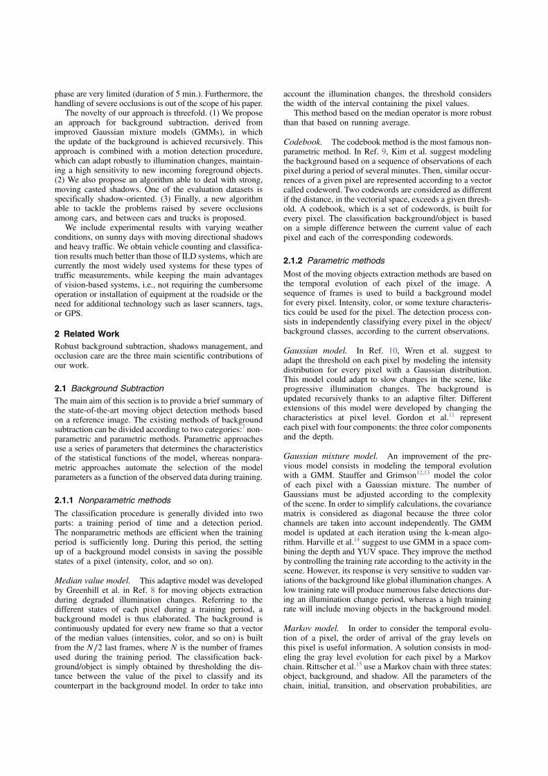
This study presents the description of a vision-based sys-tem to automatically obtain traffic flow data. This systemoperates in real time and can work during challenging scenar-ios in terms of weather conditions, with very low-cost cam-eras, poor illumination, and in the presence of many shadows.In addition, the system is conceived to work on the alreadyexisting cameras installed by the transport operators.Contemporary cameras are used for traffic surveillance ordetection capabilities like incident detections (counterflow,stopped vehicles, and so on). The objective in this work isto directly use the existing cameras without changing existingparameters (orientation, focal lens, height, and so on). From auser-needs analysis carried out with transport operators, thesystem presented here is mainly dedicated to a vehicle count-ing and classification for ring roads (cf. Fig. 1).

Recently, Unzueta et al.7 published a study on the samesubject. The novelty of their approach relies on a multi-cuebackground subtraction procedure in which the segmentationthresholds adapt robustly to illumination changes. Even if theresults are very promising, the datasets used in the evaluation

*Address all correspondence to: Alain Crouzil, E-mail: [email protected]

phase are very limited (duration of 5 min.). Furthermore, thehandling of severe occlusions is out of the scope of his paper.

The novelty of our approach is threefold. (1) We proposean approach for background subtraction, derived fromimproved Gaussian mixture models (GMMs), in whichthe update of the background is achieved recursively. Thisapproach is combined with a motion detection procedure,which can adapt robustly to illumination changes, maintain-ing a high sensitivity to new incoming foreground objects.(2) We also propose an algorithm able to deal with strong,moving casted shadows. One of the evaluation datasets isspecifically shadow-oriented. (3) Finally, a new algorithmable to tackle the problems raised by severe occlusionsamong cars, and between cars and trucks is proposed.

We include experimental results with varying weatherconditions, on sunny days with moving directional shadowsand heavy traffic. We obtain vehicle counting and classifica-tion results much better than those of ILD systems, which arecurrently the most widely used systems for these types oftraffic measurements, while keeping the main advantagesof vision-based systems, i.e., not requiring the cumbersomeoperation or installation of equipment at the roadside or theneed for additional technology such as laser scanners, tags,or GPS.

2 Related Work

Robust background subtraction, shadows management, andocclusion care are the three main scientific contributions ofour work.

2.1 Background Subtraction

The main aim of this section is to provide a brief summary ofthe state-of-the-art moving object detection methods basedon a reference image. The existing methods of backgroundsubtraction can be divided according to two categories:7 non-parametric and parametric methods. Parametric approachesuse a series of parameters that determines the characteristicsof the statistical functions of the model, whereas nonpara-metric approaches automate the selection of the modelparameters as a function of the observed data during training.

2.1.1 Nonparametric methods

The classification procedure is generally divided into twoparts: a training period of time and a detection period.The nonparametric methods are efficient when the trainingperiod is sufficiently long. During this period, the settingup of a background model consists in saving the possiblestates of a pixel (intensity, color, and so on).

Median value model. This adaptive model was developedby Greenhill et al. in Ref. 8 for moving objects extractionduring degraded illumination changes. Referring to thedifferent states of each pixel during a training period, abackground model is thus elaborated. The background iscontinuously updated for every new frame so that a vectorof the median values (intensities, color, and so on) is builtfrom the N∕2 last frames, where N is the number of framesused during the training period. The classification back-ground/object is simply obtained by thresholding the dis-tance between the value of the pixel to classify and itscounterpart in the background model. In order to take into

account the illumination changes, the threshold considersthe width of the interval containing the pixel values.

This method based on the median operator is more robustthan that based on running average.

Codebook. The codebook method is the most famous non-parametric method. In Ref. 9, Kim et al. suggest modelingthe background based on a sequence of observations of eachpixel during a period of several minutes. Then, similar occur-rences of a given pixel are represented according to a vectorcalled codeword. Two codewords are considered as differentif the distance, in the vectorial space, exceeds a given thresh-old. A codebook, which is a set of codewords, is built forevery pixel. The classification background/object is basedon a simple difference between the current value of eachpixel and each of the corresponding codewords.

2.1.2 Parametric methods

Most of the moving objects extraction methods are based onthe temporal evolution of each pixel of the image. Asequence of frames is used to build a background modelfor every pixel. Intensity, color, or some texture characteris-tics could be used for the pixel. The detection process con-sists in independently classifying every pixel in the object/background classes, according to the current observations.

Gaussian model. In Ref. 10, Wren et al. suggest toadapt the threshold on each pixel by modeling the intensitydistribution for every pixel with a Gaussian distribution.This model could adapt to slow changes in the scene, likeprogressive illumination changes. The background isupdated recursively thanks to an adaptive filter. Differentextensions of this model were developed by changing thecharacteristics at pixel level. Gordon et al.11 representeach pixel with four components: the three color componentsand the depth.

Gaussian mixture model. An improvement of the pre-vious model consists in modeling the temporal evolutionwith a GMM. Stauffer and Grimson12,13 model the colorof each pixel with a Gaussian mixture. The number ofGaussians must be adjusted according to the complexityof the scene. In order to simplify calculations, the covariancematrix is considered as diagonal because the three colorchannels are taken into account independently. The GMMmodel is updated at each iteration using the k-mean algo-rithm. Harville et al.14 suggest to use GMM in a space com-bining the depth and YUV space. They improve the methodby controlling the training rate according to the activity in thescene. However, its response is very sensitive to sudden var-iations of the background like global illumination changes. Alow training rate will produce numerous false detections dur-ing an illumination change period, whereas a high trainingrate will include moving objects in the background model.

Markov model. In order to consider the temporal evolu-tion of a pixel, the order of arrival of the gray levels onthis pixel is useful information. A solution consists in mod-eling the gray level evolution for each pixel by a Markovchain. Rittscher et al.15 use a Markov chain with three states:object, background, and shadow. All the parameters of thechain, initial, transition, and observation probabilities, are

estimated off-line on a training sequence. Stenger et al.16 pro-posed an improvement, since after a short training period,the model of the chain and its parameters continues to beupdated. This update, carried out during the detection period,allows us to better deal with the nonstationary states linked,for example, to sudden illumination changes.

2.2 Shadow Removal

In the literature, several shadow detection methods exist,and, hereunder, we briefly mention some of them.

In Ref. 17, Grest et al. determine the shadow zones bystudying the correlation between a reference image and acurrent image from two hypotheses. The first one statesthat a pixel in a shadowed zone is darker than the samepixel in an illuminated zone. The second one starts froma correlation between the texture of a shadowed zone andthe same zone of the reference image. The study of Joshiet al.18 shows correlations between the current image andthe background model using four parameters: intensity,color, edges, and texture.

Avery et al.19 determine the shadow zones with a region-growing method. The starting point is located at the edge ofthe segmented object. Its position is calculated thanks to thesun position obtained from GPS data and time codes of thesequence.

Song et al.20 make the motion detection with Markovchain models and detect shadows by adding different shadowmodels.

Recent methods for both background subtraction andshadow suppression mix multiple cues, such as edges andcolor, to obtain more accurate segmentations. For instance,Huerta et al.21 apply heuristic rules by combining a conicalmodel of brightness and chromaticity in the RGB color spacealong with edge-based background subtraction, obtainingbetter segmentation results than other previous state-of-the-art approaches. They also point out that adding ahigher-level model of vehicles could allow for better results,as these could help with bad segmentation situations. Thisoptimization is seen in Ref. 22, in which the size, position,and orientation of a three-dimensional bounding box of avehicle, which includes shadow simulation from GPSdata, are optimized with respect to the segmented images.Furthermore, it is shown in some examples that this approachcan improve the performance compared to using onlyshadow detection or shadow simulation. Their improvementis most evident when shadow detection or simulation is inac-curate. However, a major drawback for this approach is theinitialization of the box, which can lead to severe failures.

Other shadow detection methods are described in recentsurvey articles.23,24

2.3 Occlusion Management

Except when the camera is located above the road, withperpendicular viewing to the road surface, when vehicles

are close, they partially occlude one another and correctcounting is difficult. The problem becomes harder whenthe occlusion occurs as soon as the vehicles appear in thefield of view. Coifman et al.25 propose tracking vehicle fea-tures and to group them by applying a common motionconstraint. However, this method fails when two vehiclesinvolved in an occlusion have the same motion. For example,if one vehicle is closely following another, the latter partiallyoccludes the former and the two vehicles can move with thesame speed and their trajectory can be quite similar. This sit-uation is usually observed when the traffic is too dense fordrivers to keep large spacings between vehicles and to avoidocclusions, but not enough congested to make them con-stantly change their velocity. Pang et al.5 propose a threefoldmethod: a deformable model is geometrically fitted onto theoccluded vehicles; a contour description model is utilized todescribe the contour segments; a resolvability index isassigned to each occluded vehicle. This method providesvery promising results in terms of counting capabilities.Nonetheless, the method needs the camera to be calibratedand the process is time-consuming.

3 Moving Vehicle Extraction and Counting

3.1 Synopsis

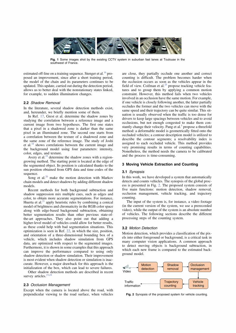
In this work, we have developed a system that automaticallydetects and counts vehicles. The synopsis of the global proc-ess is presented in Fig. 2. The proposed system consists offive main functions: motion detection, shadow removal,occlusion management, vehicle tracking, and trajectorycounting.

The input of the system is, for instance, a video footage(in the current version of the system, we use a prerecordedvideo), while the output of the system is an absolute numberof vehicles. The following sections describe the differentprocessing steps of the counting system.

3.2 Motion Detection

Motion detection, which provides a classification of the pix-els into either foreground or background, is a critical task inmany computer vision applications. A common approachto detect moving objects is background subtraction, inwhich each new frame is compared to the estimated back-ground model.

Motion

detection

Shadow

removal

Occlusion

management

Vehicle

tracking

Trajectory

countingTraffic

information

Video

Fig. 2 Synopsis of the proposed system for vehicle counting.

Fig. 1 Some images shot by the existing CCTV system in suburban fast lanes at Toulouse in thesouthwest of France.

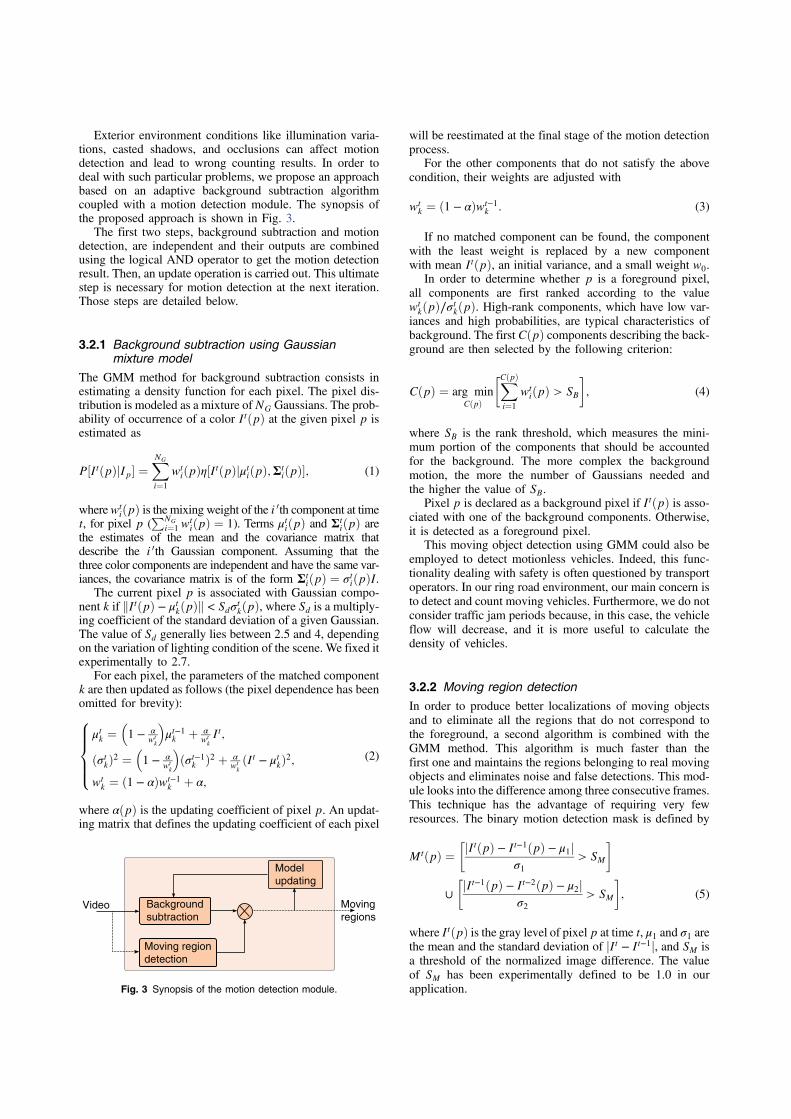
Exterior environment conditions like illumination varia-tions, casted shadows, and occlusions can affect motiondetection and lead to wrong counting results. In order todeal with such particular problems, we propose an approachbased on an adaptive background subtraction algorithmcoupled with a motion detection module. The synopsis ofthe proposed approach is shown in Fig. 3.

The first two steps, background subtraction and motiondetection, are independent and their outputs are combinedusing the logical AND operator to get the motion detectionresult. Then, an update operation is carried out. This ultimatestep is necessary for motion detection at the next iteration.Those steps are detailed below.

3.2.1 Background subtraction using Gaussianmixture model

The GMM method for background subtraction consists inestimating a density function for each pixel. The pixel dis-tribution is modeled as a mixture ofNG Gaussians. The prob-ability of occurrence of a color ItðpÞ at the given pixel p isestimated as

EQ-TARGET;temp:intralink-;e001;63;516P½ItðpÞjIp$ ¼X

NG

i¼1

wtiðpÞη½ItðpÞjμtiðpÞ;Σt

iðpÞ$; (1)

wherewtiðpÞ is the mixing weight of the i 0th component at time

t, for pixel p (PNG

i¼1 wtiðpÞ ¼ 1). Terms μtiðpÞ and Σ

tiðpÞ are

the estimates of the mean and the covariance matrix thatdescribe the i 0th Gaussian component. Assuming that thethree color components are independent and have the same var-iances, the covariance matrix is of the form Σ

tiðpÞ ¼ σ

tiðpÞI.

The current pixel p is associated with Gaussian compo-nent k if kItðpÞ − μ

tkðpÞk < Sdσ

tkðpÞ, where Sd is a multiply-

ing coefficient of the standard deviation of a given Gaussian.The value of Sd generally lies between 2.5 and 4, dependingon the variation of lighting condition of the scene. We fixed itexperimentally to 2.7.

For each pixel, the parameters of the matched componentk are then updated as follows (the pixel dependence has beenomitted for brevity):

EQ-TARGET;temp:intralink-;e002;63;301

8

>

>

>

<

>

>

>

:

μtk ¼&

1 − α

wtk

'

μt−1k þ α

wtk

It;

ðσtkÞ2 ¼&

1 − α

wtk

'

ðσt−1k Þ2 þ α

wtk

ðIt − μtkÞ

2;

wtk ¼ ð1 − αÞwt−1

k þ α;

(2)

where αðpÞ is the updating coefficient of pixel p. An updat-ing matrix that defines the updating coefficient of each pixel

will be reestimated at the final stage of the motion detectionprocess.

For the other components that do not satisfy the abovecondition, their weights are adjusted with

EQ-TARGET;temp:intralink-;e003;326;708wtk ¼ ð1 − αÞwt−1

k : (3)

If no matched component can be found, the componentwith the least weight is replaced by a new componentwith mean ItðpÞ, an initial variance, and a small weight w0.

In order to determine whether p is a foreground pixel,all components are first ranked according to the valuewtkðpÞ∕σtkðpÞ. High-rank components, which have low var-

iances and high probabilities, are typical characteristics ofbackground. The first CðpÞ components describing the back-ground are then selected by the following criterion:

EQ-TARGET;temp:intralink-;e004;326;577CðpÞ ¼ arg minCðpÞ

(

X

CðpÞ

i¼1

wtiðpÞ > SB

)

; (4)

where SB is the rank threshold, which measures the mini-mum portion of the components that should be accountedfor the background. The more complex the backgroundmotion, the more the number of Gaussians needed andthe higher the value of SB.

Pixel p is declared as a background pixel if ItðpÞ is asso-ciated with one of the background components. Otherwise,it is detected as a foreground pixel.

This moving object detection using GMM could also beemployed to detect motionless vehicles. Indeed, this func-tionality dealing with safety is often questioned by transportoperators. In our ring road environment, our main concern isto detect and count moving vehicles. Furthermore, we do notconsider traffic jam periods because, in this case, the vehicleflow will decrease, and it is more useful to calculate thedensity of vehicles.

3.2.2 Moving region detection

In order to produce better localizations of moving objectsand to eliminate all the regions that do not correspond tothe foreground, a second algorithm is combined with theGMM method. This algorithm is much faster than thefirst one and maintains the regions belonging to real movingobjects and eliminates noise and false detections. This mod-ule looks into the difference among three consecutive frames.This technique has the advantage of requiring very fewresources. The binary motion detection mask is defined by

EQ-TARGET;temp:intralink-;e005;326;224MtðpÞ ¼

(

jItðpÞ − It−1ðpÞ − μ1j

σ1

> SM

)

∪

(

jIt−1ðpÞ − It−2ðpÞ − μ2j

σ2

> SM

)

; (5)

where ItðpÞ is the gray level of pixel p at time t, μ1 and σ1 arethe mean and the standard deviation of jIt − It−1j, and SM isa threshold of the normalized image difference. The valueof SM has been experimentally defined to be 1.0 in ourapplication.

Moving

regionsVideo

Model

updating

Background

subtraction

Moving region

detection

Fig. 3 Synopsis of the motion detection module.

3.2.3 Result combination and model updating

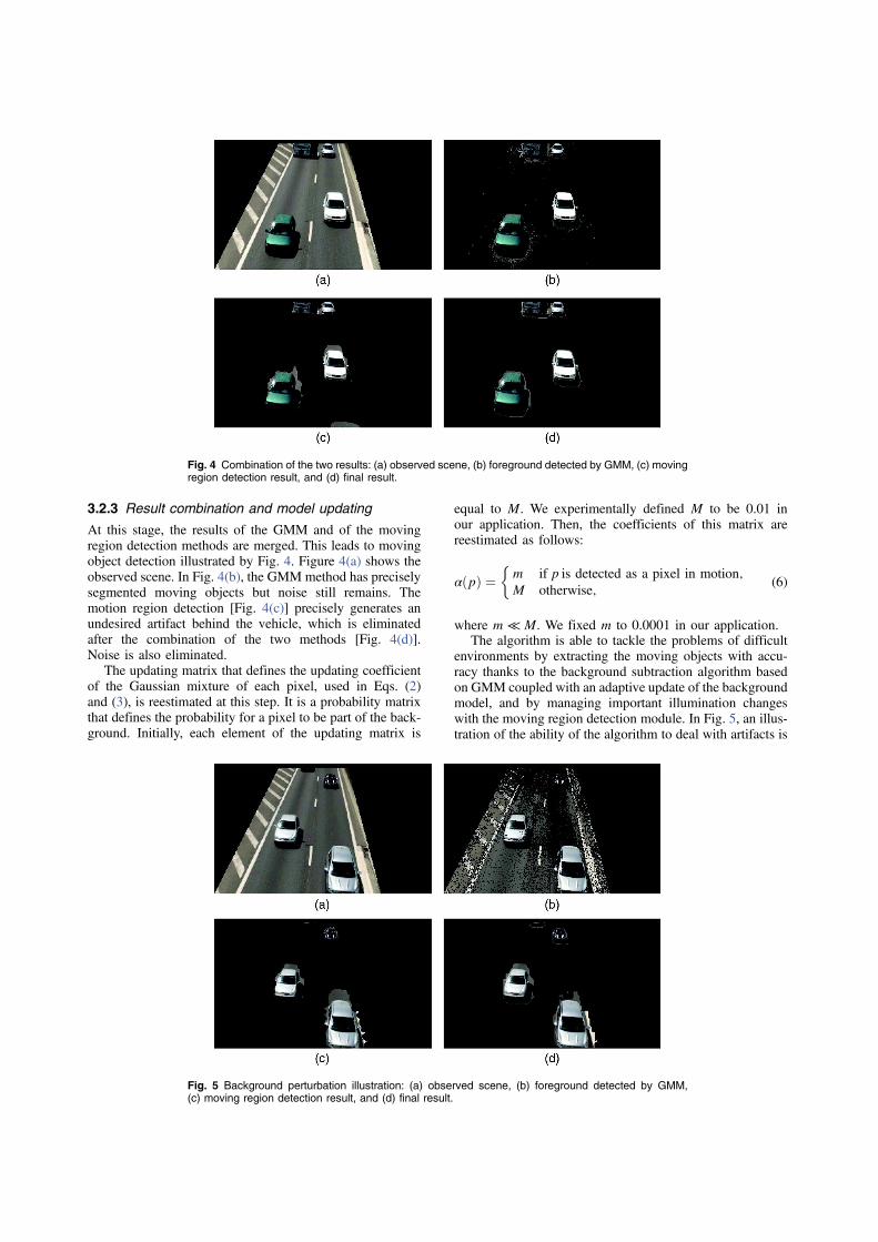
At this stage, the results of the GMM and of the movingregion detection methods are merged. This leads to movingobject detection illustrated by Fig. 4. Figure 4(a) shows theobserved scene. In Fig. 4(b), the GMM method has preciselysegmented moving objects but noise still remains. Themotion region detection [Fig. 4(c)] precisely generates anundesired artifact behind the vehicle, which is eliminatedafter the combination of the two methods [Fig. 4(d)].Noise is also eliminated.

The updating matrix that defines the updating coefficientof the Gaussian mixture of each pixel, used in Eqs. (2)and (3), is reestimated at this step. It is a probability matrixthat defines the probability for a pixel to be part of the back-ground. Initially, each element of the updating matrix is

equal to M. We experimentally defined M to be 0.01 inour application. Then, the coefficients of this matrix arereestimated as follows:

EQ-TARGET;temp:intralink-;e006;326;461αðpÞ ¼

+

m if p is detected as a pixel in motion;

M otherwise;(6)

where m ≪ M. We fixed m to 0.0001 in our application.The algorithm is able to tackle the problems of difficult

environments by extracting the moving objects with accu-racy thanks to the background subtraction algorithm basedon GMM coupled with an adaptive update of the backgroundmodel, and by managing important illumination changeswith the moving region detection module. In Fig. 5, an illus-tration of the ability of the algorithm to deal with artifacts is

Fig. 4 Combination of the two results: (a) observed scene, (b) foreground detected by GMM, (c) movingregion detection result, and (d) final result.

Fig. 5 Background perturbation illustration: (a) observed scene, (b) foreground detected by GMM,(c) moving region detection result, and (d) final result.

provided. Observed scene [Fig. 5(a)] was captured after animportant background perturbation was caused by the pass-ing of a truck a few frames earlier. The detected foreground[Fig. 5(b)] is disturbed, but the moving region detectionmodule [Fig. 5(c)] allows us to achieve a satisfying result[Fig. 5(d)].

3.3 Shadow Elimination

For shadow elimination, the algorithm developed is inspiredfrom Xiao’s approach.26 This latter was modified andadapted to our problem. The authors have noticed that ina scene including vehicles during a period with high illumi-nation changes, these vehicles present strong edges whereasshadows do not present such marked edges. In fact, fromwhere the scene is captured, road seems to be relatively uni-form. In a shadowed region, contrast is reduced and reinfor-ces this characteristic. Edges on the road are located only onmarking. On the contrary, vehicles are very textured and con-tain many edges. Our method aims at correctly removingshadows while preserving the initial edges of the vehicles.As shown in Fig. 6, all steps constituting our method areprocessed in sequence. Starting from results achieved bythe motion detection module, we begin to extract edges.Then, exterior edges are removed. Finally, blobs (regionscorresponding to vehicles in motion) are extracted fromremaining edges. Each step is detailed in the following para-graphs. This method is efficient, whatever the difficultylinked to the shadow.

3.3.1 Edge extraction

Edge detection is a fundamental tool in image processing,which aims at identifying in a digital image pixels

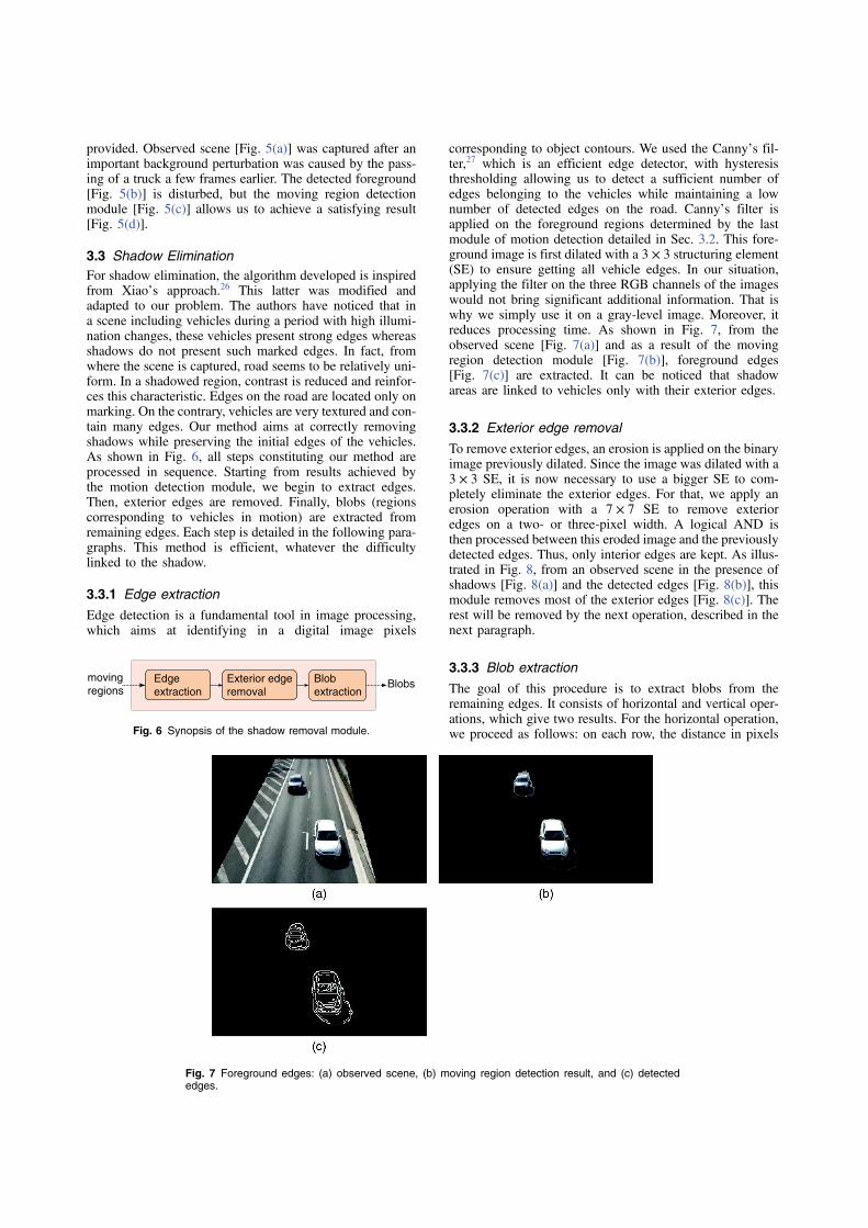
corresponding to object contours. We used the Canny’s fil-ter,27 which is an efficient edge detector, with hysteresisthresholding allowing us to detect a sufficient number ofedges belonging to the vehicles while maintaining a lownumber of detected edges on the road. Canny’s filter isapplied on the foreground regions determined by the lastmodule of motion detection detailed in Sec. 3.2. This fore-ground image is first dilated with a 3 × 3 structuring element(SE) to ensure getting all vehicle edges. In our situation,applying the filter on the three RGB channels of the imageswould not bring significant additional information. That iswhy we simply use it on a gray-level image. Moreover, itreduces processing time. As shown in Fig. 7, from theobserved scene [Fig. 7(a)] and as a result of the movingregion detection module [Fig. 7(b)], foreground edges[Fig. 7(c)] are extracted. It can be noticed that shadowareas are linked to vehicles only with their exterior edges.

3.3.2 Exterior edge removal

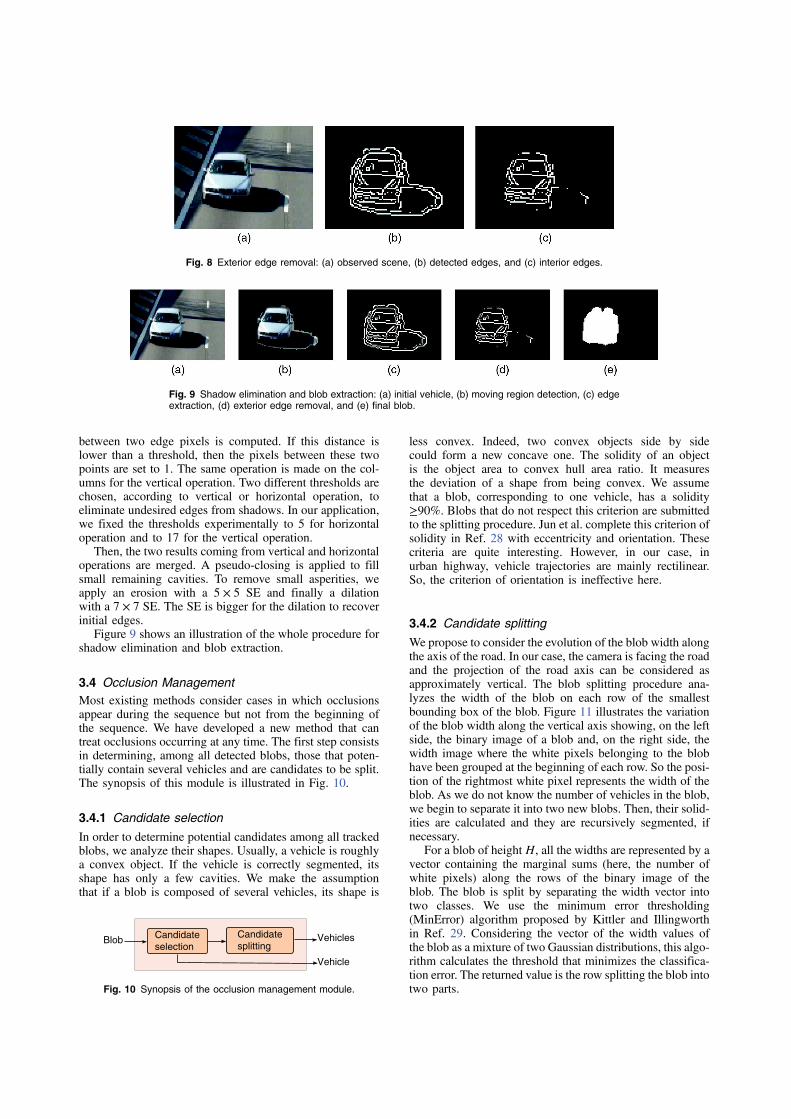
To remove exterior edges, an erosion is applied on the binaryimage previously dilated. Since the image was dilated with a3 × 3 SE, it is now necessary to use a bigger SE to com-pletely eliminate the exterior edges. For that, we apply anerosion operation with a 7 × 7 SE to remove exterioredges on a two- or three-pixel width. A logical AND isthen processed between this eroded image and the previouslydetected edges. Thus, only interior edges are kept. As illus-trated in Fig. 8, from an observed scene in the presence ofshadows [Fig. 8(a)] and the detected edges [Fig. 8(b)], thismodule removes most of the exterior edges [Fig. 8(c)]. Therest will be removed by the next operation, described in thenext paragraph.

3.3.3 Blob extraction

The goal of this procedure is to extract blobs from theremaining edges. It consists of horizontal and vertical oper-ations, which give two results. For the horizontal operation,we proceed as follows: on each row, the distance in pixels

moving

regionsEdge

extraction

Exterior edge

removal

Blob

extractionBlobs

Fig. 6 Synopsis of the shadow removal module.

Fig. 7 Foreground edges: (a) observed scene, (b) moving region detection result, and (c) detectededges.

between two edge pixels is computed. If this distance islower than a threshold, then the pixels between these twopoints are set to 1. The same operation is made on the col-umns for the vertical operation. Two different thresholds arechosen, according to vertical or horizontal operation, toeliminate undesired edges from shadows. In our application,we fixed the thresholds experimentally to 5 for horizontaloperation and to 17 for the vertical operation.

Then, the two results coming from vertical and horizontaloperations are merged. A pseudo-closing is applied to fillsmall remaining cavities. To remove small asperities, weapply an erosion with a 5 × 5 SE and finally a dilationwith a 7 × 7 SE. The SE is bigger for the dilation to recoverinitial edges.

Figure 9 shows an illustration of the whole procedure forshadow elimination and blob extraction.

3.4 Occlusion Management

Most existing methods consider cases in which occlusionsappear during the sequence but not from the beginning ofthe sequence. We have developed a new method that cantreat occlusions occurring at any time. The first step consistsin determining, among all detected blobs, those that poten-tially contain several vehicles and are candidates to be split.The synopsis of this module is illustrated in Fig. 10.

3.4.1 Candidate selection

In order to determine potential candidates among all trackedblobs, we analyze their shapes. Usually, a vehicle is roughlya convex object. If the vehicle is correctly segmented, itsshape has only a few cavities. We make the assumptionthat if a blob is composed of several vehicles, its shape is

less convex. Indeed, two convex objects side by sidecould form a new concave one. The solidity of an objectis the object area to convex hull area ratio. It measuresthe deviation of a shape from being convex. We assumethat a blob, corresponding to one vehicle, has a solidity≥90%. Blobs that do not respect this criterion are submittedto the splitting procedure. Jun et al. complete this criterion ofsolidity in Ref. 28 with eccentricity and orientation. Thesecriteria are quite interesting. However, in our case, inurban highway, vehicle trajectories are mainly rectilinear.So, the criterion of orientation is ineffective here.

3.4.2 Candidate splitting

We propose to consider the evolution of the blob width alongthe axis of the road. In our case, the camera is facing the roadand the projection of the road axis can be considered asapproximately vertical. The blob splitting procedure ana-lyzes the width of the blob on each row of the smallestbounding box of the blob. Figure 11 illustrates the variationof the blob width along the vertical axis showing, on the leftside, the binary image of a blob and, on the right side, thewidth image where the white pixels belonging to the blobhave been grouped at the beginning of each row. So the posi-tion of the rightmost white pixel represents the width of theblob. As we do not know the number of vehicles in the blob,we begin to separate it into two new blobs. Then, their solid-ities are calculated and they are recursively segmented, ifnecessary.

For a blob of height H, all the widths are represented by avector containing the marginal sums (here, the number ofwhite pixels) along the rows of the binary image of theblob. The blob is split by separating the width vector intotwo classes. We use the minimum error thresholding(MinError) algorithm proposed by Kittler and Illingworthin Ref. 29. Considering the vector of the width values ofthe blob as a mixture of two Gaussian distributions, this algo-rithm calculates the threshold that minimizes the classifica-tion error. The returned value is the row splitting the blob intotwo parts.

Fig. 8 Exterior edge removal: (a) observed scene, (b) detected edges, and (c) interior edges.

Fig. 9 Shadow elimination and blob extraction: (a) initial vehicle, (b) moving region detection, (c) edgeextraction, (d) exterior edge removal, and (e) final blob.

BlobCandidate

selection

Candidate

splittingVehicles

Vehicle

Fig. 10 Synopsis of the occlusion management module.

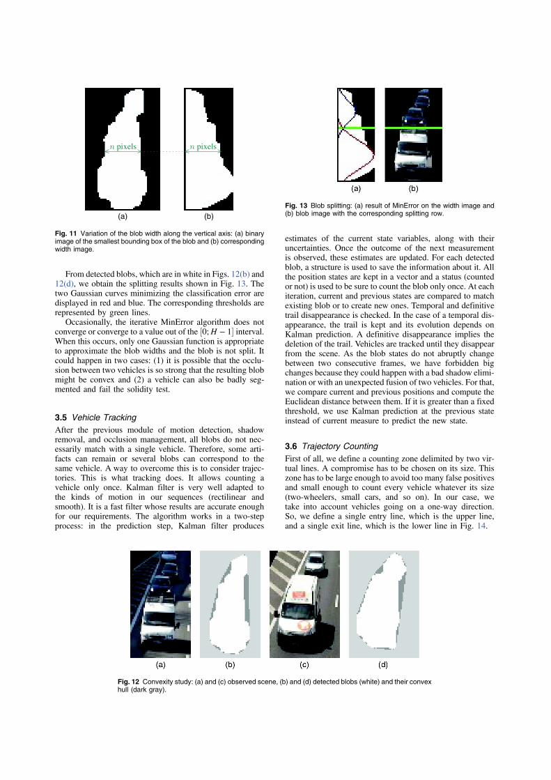
From detected blobs, which are in white in Figs. 12(b) and12(d), we obtain the splitting results shown in Fig. 13. Thetwo Gaussian curves minimizing the classification error aredisplayed in red and blue. The corresponding thresholds arerepresented by green lines.

Occasionally, the iterative MinError algorithm does notconverge or converge to a value out of the ½0;H − 1$ interval.When this occurs, only one Gaussian function is appropriateto approximate the blob widths and the blob is not split. Itcould happen in two cases: (1) it is possible that the occlu-sion between two vehicles is so strong that the resulting blobmight be convex and (2) a vehicle can also be badly seg-mented and fail the solidity test.

3.5 Vehicle Tracking

After the previous module of motion detection, shadowremoval, and occlusion management, all blobs do not nec-essarily match with a single vehicle. Therefore, some arti-facts can remain or several blobs can correspond to thesame vehicle. A way to overcome this is to consider trajec-tories. This is what tracking does. It allows counting avehicle only once. Kalman filter is very well adapted tothe kinds of motion in our sequences (rectilinear andsmooth). It is a fast filter whose results are accurate enoughfor our requirements. The algorithm works in a two-stepprocess: in the prediction step, Kalman filter produces

estimates of the current state variables, along with theiruncertainties. Once the outcome of the next measurementis observed, these estimates are updated. For each detectedblob, a structure is used to save the information about it. Allthe position states are kept in a vector and a status (countedor not) is used to be sure to count the blob only once. At eachiteration, current and previous states are compared to matchexisting blob or to create new ones. Temporal and definitivetrail disappearance is checked. In the case of a temporal dis-appearance, the trail is kept and its evolution depends onKalman prediction. A definitive disappearance implies thedeletion of the trail. Vehicles are tracked until they disappearfrom the scene. As the blob states do not abruptly changebetween two consecutive frames, we have forbidden bigchanges because they could happen with a bad shadow elimi-nation or with an unexpected fusion of two vehicles. For that,we compare current and previous positions and compute theEuclidean distance between them. If it is greater than a fixedthreshold, we use Kalman prediction at the previous stateinstead of current measure to predict the new state.

3.6 Trajectory Counting

First of all, we define a counting zone delimited by two vir-tual lines. A compromise has to be chosen on its size. Thiszone has to be large enough to avoid too many false positivesand small enough to count every vehicle whatever its size(two-wheelers, small cars, and so on). In our case, wetake into account vehicles going on a one-way direction.So, we define a single entry line, which is the upper line,and a single exit line, which is the lower line in Fig. 14.

(a) (b)

pixelspixels

Fig. 11 Variation of the blob width along the vertical axis: (a) binaryimage of the smallest bounding box of the blob and (b) correspondingwidth image.

Fig. 12 Convexity study: (a) and (c) observed scene, (b) and (d) detected blobs (white) and their convexhull (dark gray).

Fig. 13 Blob splitting: (a) result of MinError on the width image and(b) blob image with the corresponding splitting row.

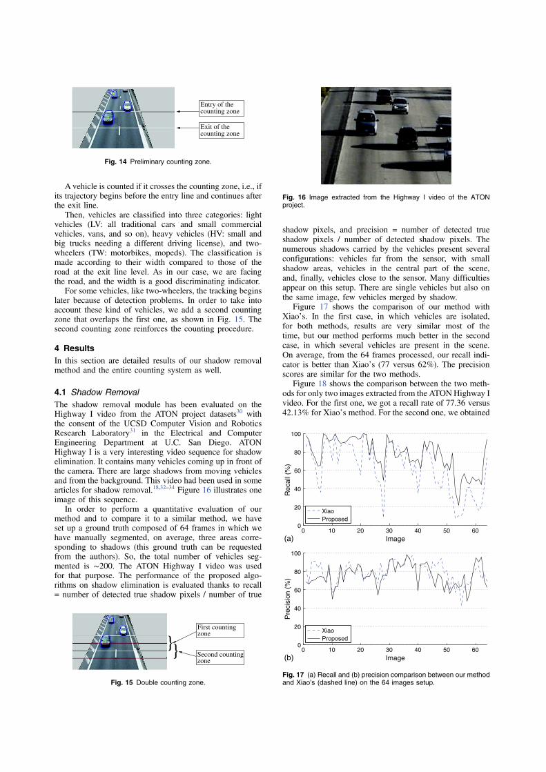
Avehicle is counted if it crosses the counting zone, i.e., ifits trajectory begins before the entry line and continues afterthe exit line.

Then, vehicles are classified into three categories: lightvehicles (LV: all traditional cars and small commercialvehicles, vans, and so on), heavy vehicles (HV: small andbig trucks needing a different driving license), and two-wheelers (TW: motorbikes, mopeds). The classification ismade according to their width compared to those of theroad at the exit line level. As in our case, we are facingthe road, and the width is a good discriminating indicator.

For some vehicles, like two-wheelers, the tracking beginslater because of detection problems. In order to take intoaccount these kind of vehicles, we add a second countingzone that overlaps the first one, as shown in Fig. 15. Thesecond counting zone reinforces the counting procedure.

4 Results

In this section are detailed results of our shadow removalmethod and the entire counting system as well.

4.1 Shadow Removal

The shadow removal module has been evaluated on theHighway I video from the ATON project datasets30 withthe consent of the UCSD Computer Vision and RoboticsResearch Laboratory31 in the Electrical and ComputerEngineering Department at U.C. San Diego. ATONHighway I is a very interesting video sequence for shadowelimination. It contains many vehicles coming up in front ofthe camera. There are large shadows from moving vehiclesand from the background. This video had been used in somearticles for shadow removal.18,32–34 Figure 16 illustrates oneimage of this sequence.

In order to perform a quantitative evaluation of ourmethod and to compare it to a similar method, we haveset up a ground truth composed of 64 frames in which wehave manually segmented, on average, three areas corre-sponding to shadows (this ground truth can be requestedfrom the authors). So, the total number of vehicles seg-mented is ∼200. The ATON Highway I video was usedfor that purpose. The performance of the proposed algo-rithms on shadow elimination is evaluated thanks to recall= number of detected true shadow pixels / number of true

shadow pixels, and precision = number of detected trueshadow pixels / number of detected shadow pixels. Thenumerous shadows carried by the vehicles present severalconfigurations: vehicles far from the sensor, with smallshadow areas, vehicles in the central part of the scene,and, finally, vehicles close to the sensor. Many difficultiesappear on this setup. There are single vehicles but also onthe same image, few vehicles merged by shadow.

Figure 17 shows the comparison of our method withXiao’s. In the first case, in which vehicles are isolated,for both methods, results are very similar most of thetime, but our method performs much better in the secondcase, in which several vehicles are present in the scene.On average, from the 64 frames processed, our recall indi-cator is better than Xiao’s (77 versus 62%). The precisionscores are similar for the two methods.

Figure 18 shows the comparison between the two meth-ods for only two images extracted from the ATONHighway Ivideo. For the first one, we got a recall rate of 77.36 versus42.13% for Xiao’s method. For the second one, we obtained

counting zone

Exit of thecounting zone

Entry of the

Fig. 14 Preliminary counting zone.

Second countingzone

First countingzone

Fig. 15 Double counting zone.

Fig. 16 Image extracted from the Highway I video of the ATONproject.

0 10 20 30 40 50 600

20

40

60

80

100

Image

Recall

(%)

Xiao

Proposed

0 10 20 30 40 50 600

20

40

60

80

100

Image

Pre

cis

ion (

%)

Xiao

Proposed

(a)

(b)

Fig. 17 (a) Recall and (b) precision comparison between our methodand Xiao’s (dashed line) on the 64 images setup.

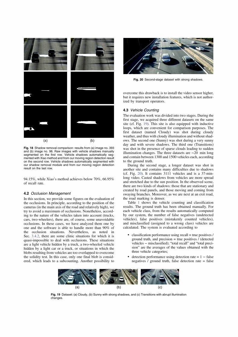
94.15%, while Xiao’s method achieves below 70%, 66.95%of recall rate.

4.2 Occlusion Management

In this section, we provide some figures on the evaluation ofthe occlusions. In principle, according to the position of thecameras (in the main axis of the road and relatively high), wetry to avoid a maximum of occlusions. Nonetheless, accord-ing to the nature of the vehicles taken into account (trucks,cars, two-wheelers), there are, of course, some unavoidableocclusions. In these cases, we have analyzed them one byone and the software is able to handle more than 90% ofthe occlusion situations. Nevertheless, as noted inSec. 3.4.2, there are some clinic situations for which it isquasi-impossible to deal with occlusions. These situationsare a light vehicle hidden by a truck, a two-wheeled vehiclehidden by a light car or a truck, or situations in which theblobs resulting from vehicles are too overlapped to overcomethe solidity test. In this case, only one final blob is consid-ered, which leads to a subcounting. Another possibility to

overcome this drawback is to install the video sensor higher,but it requires new installation features, which is not author-ized by transport operators.

4.3 Vehicle Counting

The evaluation work was divided into two stages. During thefirst stage, we acquired three different datasets on the samesite (cf. Fig. 19). This site is also equipped with inductiveloops, which are convenient for comparison purposes. Thefirst dataset (named Cloudy) was shot during cloudyweather, and thus with cloudy illumination and without shad-ows. The second one (Sunny) was shot during a very sunnyday and with severe shadows. The third one (Transitions)was shot in the presence of sparse clouds leading to suddenillumination changes. The three datasets are ∼20 min longand contain between 1300 and 1500 vehicles each, accordingto the ground truth.

During the second stage, a longer dataset was shot inanother site and contains many difficulties due to shadows(cf. Fig. 20). It contains 3111 vehicles and is a 37-min-long video. Casted shadows from vehicles are more spreadand stretched due to the sun position. In the observed scene,there are two kinds of shadows: those that are stationary andcreated by road panels, and those moving and coming fromswaying branches. Moreover, as we are next at an exit road,the road marking is denser.

Table 1 shows the vehicle counting and classificationresults. The ground truth has been obtained manually. Foreach vehicle class, from the results automatically computedby our system, the number of false negatives (undetectedvehicles), false positives (mistakenly counted vehicles),and misclassified (assigned to a wrong class) vehicles arecalculated. The system is evaluated according to

• classification performance using recall = true positives /ground truth, and precision = true positives / (detectedvehicles − misclassified); “total recall” and “total preci-sion” are the averages of the values obtained with thethree vehicle categories;

• detection performance using detection rate = 1 − falsenegatives / ground truth, false detection rate = false

Fig. 18 Shadow removal comparison: results from (a) image no. 393and (b) image no. 98. Raw images with vehicle shadows manuallysegmented on the first row. Vehicle shadows automatically seg-mented with Xiao method and from our moving region detection resulton the second row. Vehicle shadows automatically segmented withour shadow removal module and from our moving region detectionresult on the last row.

Fig. 19 Dataset: (a) Cloudy, (b) Sunny with strong shadows, and (c) Transitions with abrupt illuminationchanges.

Fig. 20 Second-stage dataset with strong shadows.

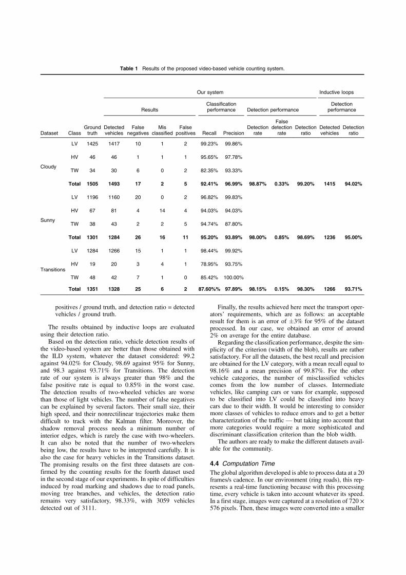
positives / ground truth, and detection ratio = detectedvehicles / ground truth.

The results obtained by inductive loops are evaluatedusing their detection ratio.

Based on the detection ratio, vehicle detection results ofthe video-based system are better than those obtained withthe ILD system, whatever the dataset considered: 99.2against 94.02% for Cloudy, 98.69 against 95% for Sunny,and 98.3 against 93.71% for Transitions. The detectionrate of our system is always greater than 98% and thefalse positive rate is equal to 0.85% in the worst case.The detection results of two-wheeled vehicles are worsethan those of light vehicles. The number of false negativescan be explained by several factors. Their small size, theirhigh speed, and their nonrectilinear trajectories make themdifficult to track with the Kalman filter. Moreover, theshadow removal process needs a minimum number ofinterior edges, which is rarely the case with two-wheelers.It can also be noted that the number of two-wheelersbeing low, the results have to be interpreted carefully. It isalso the case for heavy vehicles in the Transitions dataset.The promising results on the first three datasets are con-firmed by the counting results for the fourth dataset usedin the second stage of our experiments. In spite of difficultiesinduced by road marking and shadows due to road panels,moving tree branches, and vehicles, the detection ratioremains very satisfactory, 98.33%, with 3059 vehiclesdetected out of 3111.

Finally, the results achieved here meet the transport oper-ators’ requirements, which are as follows: an acceptableresult for them is an error of *3% for 95% of the datasetprocessed. In our case, we obtained an error of around2% on average for the entire database.

Regarding the classification performance, despite the sim-plicity of the criterion (width of the blob), results are rathersatisfactory. For all the datasets, the best recall and precisionare obtained for the LV category, with a mean recall equal to98.16% and a mean precision of 99.87%. For the othervehicle categories, the number of misclassified vehiclescomes from the low number of classes. Intermediatevehicles, like camping cars or vans for example, supposedto be classified into LV could be classified into heavycars due to their width. It would be interesting to considermore classes of vehicles to reduce errors and to get a bettercharacterization of the traffic — but taking into account thatmore categories would require a more sophisticated anddiscriminant classification criterion than the blob width.

The authors are ready to make the different datasets avail-able for the community.

4.4 Computation Time

The global algorithm developed is able to process data at a 20frames/s cadence. In our environment (ring roads), this rep-resents a real-time functioning because with this processingtime, every vehicle is taken into account whatever its speed.In a first stage, images were captured at a resolution of 720 ×576 pixels. Then, these images were converted into a smaller

Table 1 Results of the proposed video-based vehicle counting system.

Our system Inductive loops

ResultsClassificationperformance Detection performance

Detectionperformance

Dataset ClassGroundtruth

Detectedvehicles

Falsenegatives

Misclassified

Falsepositives Recall Precision

Detectionrate

Falsedetectionrate

Detectionratio

Detectedvehicles

Detectionratio

Cloudy

LV 1425 1417 10 1 2 99.23% 99.86%

HV 46 46 1 1 1 95.65% 97.78%

TW 34 30 6 0 2 82.35% 93.33%

Total 1505 1493 17 2 5 92.41% 96.99% 98.87% 0.33% 99.20% 1415 94.02%

Sunny

LV 1196 1160 20 0 2 96.82% 99.83%

HV 67 81 4 14 4 94.03% 94.03%

TW 38 43 2 2 5 94.74% 87.80%

Total 1301 1284 26 16 11 95.20% 93.89% 98.00% 0.85% 98.69% 1236 95.00%

Transitions

LV 1284 1266 15 1 1 98.44% 99.92%

HV 19 20 3 4 1 78.95% 93.75%

TW 48 42 7 1 0 85.42% 100.00%

Total 1351 1328 25 6 2 87.60%% 97.89% 98.15% 0.15% 98.30% 1266 93.71%

resolution of 288 × 172 without affecting the countingaccuracy. Of course, the different routines present differentconsumption with respect to the total. One can find belowthe main differences between these routines:

1. Motion detection: 45.48% (including GMM andupdating, 31.07%, and moving region detection,14.41%);

2. Tracking: 37.19%;

3. Shadow removal: 16.01%;

4. Occlusion management: 1.00%;

5. Trajectory counting: 0.31%.

5 Conclusion

In this work, we developed an advanced road vehicle count-ing system. The aim of such a system is to replace or comple-ment in the future the old systems based on ILD. The systemhas been tested with different kinds of illumination changes(cloudy, sunny, transitions between sun and clouds),obtaining results better than those of ILD. The developedalgorithm is able to eliminate several kinds of shadowsdepending on the time of the day. Another particular strengthof the method proposed is its ability to deal with severeocclusions between vehicles. Multicore programming allowsus to achieve real-time performances with only a piece ofsoftware. The perspective of this work is, with the same sen-sor, to continue to calculate traffic indicators like occupationrate or density of vehicles. The two previous indicators couldbe used to calculate more global congestion indicators. Theinfrastructure operators are very interested in having suchstatistics in real time for management purposes.

References

1. “Sensors for intelligent transport systems,” 2014, http://www.transport-intelligent.net/english-sections/technologies-43/captors/??lang=en.

2. “Citilog website,” 2015, http://www.citilog.com.3. “FLIR Systems, Inc.,” 2016, http://www.flir.com/traffic/.4. S. Birchfield, W. Sarasua, and N. Kanhere, “Computer vision traffic sensor

for fixed and pan-tilt-zoom cameras,” Technical Report Highway IDEAProject 140, Transportation Research Board, Washington, DC (2010).

5. C. C. C. Pang, W. W. L. Lam, and N. H. C. Yung, “Amethod for vehiclecount in the presence of multiple-vehicle occlusions in traffic images,”IEEE Trans. Intell. Transp. Syst. 8, 441–459 (2007).

6. M. Haag and H. H. Nagel, “Incremental recognition of traffic situationsfrom video image sequences,” Image Vis. Comput. 18, 137–153 (2000).

7. L. Unzueta et al., “Adaptive multicue background subtraction for robustvehicle counting and classification,” IEEE Trans. Intell. Transp. Syst.13, 527–540 (2012).

8. S. Greenhill, S. Venkatesh, and G. A. W. West, “Adaptive model forforeground extraction in adverse lighting conditions,” Lec. NotesComput. Sci. 3157, 805–811 (2004).

9. K. Kim et al., “Real-time foreground-background segmentation usingcodebook model,” Real-Time Imaging 11, 172–185 (2005).

10. C. R. Wren et al., “Pfinder: real-time tracking of the human body,” IEEETrans. Pattern Anal. Mach. Intell. 19, 780–785 (1997).

11. G. Gordon et al., “Background estimation and removal based on rangeand color,” in IEEE Computer Society Conf. on Computer Vision andPattern Recognition, pp. 459–464 (1999).

12. C. Stauffer and W. E. L. Grimson, “Adaptive background mixturemodels for real-time tracking,” in IEEE Computer Society Conf. onComputer Vision and Pattern Recognition, pp. 2246–2252 (1999).

13. C. Stauffer and W. E. L. Grimson, “Learning patterns of activity usingreal-time tracking,” IEEE Trans. Pattern Anal. Mach. Intell. 22, 747–757 (2000).

14. M. Harville, G. G. Gordon, and J. I. Woodfill, “Foreground segmenta-tion using adaptive mixture models in color and depth,” in Proc. IEEEWorkshop on Detection and Recognition of Events in Video, pp. 3–11(2001).

15. J. Rittscher et al., “A probabilistic background model for tracking,” inProc. ECCV, pp. 336–350 (2000).

16. B. Stenger et al., “Topology free hidden Markov models: application tobackground modeling,” in Proc. of Eighth IEEE Int. Conf. on ComputerVision, pp. 294–301 (2001).

17. D. Grest, J.-M. Frahm, and R. Koch, “A color similarity measure forrobust shadow removal in real time,” in Proc. of the Vision,Modeling and Visualization Conf., pp. 253–260 (2003).

18. A. J. Joshi et al., “Moving shadow detection with low- and mid-levelreasoning,” in Proc. of IEEE Int. Conf. on Robotics and Automation,pp. 4827–4832 (2007).

19. R. Avery et al., “Investigation into shadow removal from traffic images,”Transp. Res. Record: J. Transp. Res. Board 2000, 70–77 (2007).

20. X. F. Song and R. Nevatia, “Detection and tracking of moving vehiclesin crowded scenes,” in IEEE Workshop on Motion and VideoComputing, pp. 4–8 (2007).

21. I. Huerta et al., “Detection and removal of chromatic moving shadowsin surveillance scenarios,” in IEEE 12th Int. Conf. on Computer Vision,pp. 1499–1506 (2009).

22. B. Johansson et al., “Combining shadow detection and simulation forestimation of vehicle size and position,” Pattern Recognit. Lett. 30,751–759 (2009).

23. A. Sanin, C. Sanderson, and B. C. Lowell, “Shadow detection: a surveyand comparative evaluation of recent methods,” Pattern Recognit. 45,1684–1695 (2012).

24. N. Al-Najdawi et al., “A survey of cast shadow detection algorithms,”Pattern Recognit. Lett. 33, 752–764 (2012).

25. B. Coifman et al., “A real-time computer vision system for vehicletracking and tracking surveillance,” Transp. Res. Part C 6, 271–288(1998).

26. L. Z. M. Xiao and C.-Z. Han, “Moving shadow detection andremoval for traffic sequences,” Int. J. Autom. Comput. 4(1), 38–46(2007).

27. J. Canny, “A computational approach to edge detection,” IEEE Trans.Pattern Anal. Mach. Intell. PAMI-8, 679–698 (1986).

28. G. Jun, J. K. Aggarwal, and M. Gokmen, “Tracking and segmentationof highway vehicles in cluttered and crowded scenes,” in Proc. of IEEEWorkshop Applications of Computer Vision, pp. 1–6 (2008).

29. J. Kittler and J. Illingworth, “Minimum error thresholding,” PatternRecognit. 19, 41–47 (1986).

30. “Shadow detection and correction research area of the autonomousagents for on-scene networked incident management (ATON) project.”http://cvrr.ucsd.edu/aton/shadow/

31. “UC San Diego Computer Vision and Robotics Research Laboratory.”http://cvrr.ucsd.edu/.

32. A. Prati et al., “Detecting moving shadows: algorithms and evaluation,”IEEE Trans. Pattern Anal. Mach. Intell. 25, 918–923 (2003).

33. I. Mikic et al., “Moving shadow and object detection in traffic scenes,”in Proc. of 15th Int. Conf. on Pattern Recognition, pp. 321–324(2000).

34. M. M. Trivedi, I. Mikic, and G. T. Kogut, “Distributed video networksfor incident detection and management,” in Proc. of 2000 IEEEIntelligent Transportation Systems, pp. 155–160 (2000).

Alain Crouzil received his PhD degree in computer science from thePaul Sabatier University of Toulouse in 1997. He is currently an asso-ciate professor and a member of the Traitement et Comprehensiond’Images group of Institut de Recherche en Informatique deToulouse. His research interests concern stereo vision, shape fromshading, camera calibration, image segmentation, change detection,and motion analysis.

Louahdi Khoudour received his PhD in computer science from theUniversity of Lille, France, in 1996. He then obtained the leadingresearch degree in 2006 from the University of Paris (Jussieu). Heis currently a researcher in the field of traffic engineering and control.He is head of the ZELT (Experimental Zone and Traffic Laboratory ofToulouse) group at the French Ministry of Ecology and Transport.

Paul Valiere received his MS degree in computer science from theUniversity Paul Sabatier at Toulouse, France, in 2012. He is currentlya software engineer at Sopra Steria company.

Dung Nghy Truong Cong received her BS degree in telecommuni-cations engineering from the Ho Chi Minh City University ofTechnology, Vietnam, in July 2004, her MS degree in signal, image,speech, and telecommunications from the Grenoble Institute ofTechnology (INPG), France, in July 2007, and her PhD in signaland image processing from the Pierre & Marie Curie University.She is currently an associate professor at Ho Chi Minh CityUniversity of Technology, Vietnam. Her research interests span theareas of signal and image processing, computer vision, and patternrecognition.