Dissertation Master in Computer Engineering – Mobile Computing Automatic Transcription of Music using Deep Learning Techniques André Ferreira Gil Leiria, 31 st of March 2019

Welcome message from author
This document is posted to help you gain knowledge. Please leave a comment to let me know what you think about it! Share it to your friends and learn new things together.
Transcript
Dissertation
Master in Computer Engineering – Mobile Computing
Automatic Transcription of Music using Deep Learning Techniques
André Ferreira Gil
Leiria, 31st of March 2019

This page was intetionally left blank
Dissertation
Master in Computer Engineering – Mobile Computing
Automatic Transcription of Music using Deep Learning Techniques
André Ferreira Gil
Dissertation developed under the supervision of Professor Carlos Fernando Almeida Grilo, Professor Gustavo Miguel Jorge Reis and Professor Patrício Rodrigues Domingues, from the School of Technology and Management of the Polytechnic Institute of Leiria.
Leiria, 31st of March 2019

This page was intetionally left blank
III
Acknowledgements
First of all, I would like to thank my supervisors, Prof. Carlos Grilo, Prof. Gustavo Reis and
Prof. Patricio Domingues, for all their advice, support, guidance and patience throughout
this dissertation. Without them this work would have been unfeasible.
Also I would like to thank the Polytechnic Institute of Leiria for giving me the opportunity
to study in an amazing school that is comprised by competent staff who strive daily to
prepare students for the future.
In addition, I am very grateful to my family and friends who have helped directly and/or
indirectly in this work, from financial aid to psychological encouragement.
Lastly but not less important, I would especially like to thank my girlfriend, Maria Angeles,
for all the support and patience during all this journey.
Thank you.

IV
This page was intetionally left blank

V
Previous note
The following publication has resulted from this dissertation: (Gil et al., 2018d)

VI
This page was intetionally left blank
VII
Resumo
A transcrição de música consiste em identificar as notas musicais ao longo duma música.
Esta é uma tarefa árdua que geralmente requer pessoas com muitos anos de treino. Devido à
sua enorme dificuldade, tem havido um grande interesse em automatizar esta tarefa. No
entanto, a transcrição automática de música engloba vários campos de pesquisa, tais como o
processamento sinal, aprendizagem de máquina, teoria musical e cognição e percepção de
pitch e de psicoacústica. Deste modo uma possível solução ao problema torna-se difícil de
encontrar.
Neste trabalho é apresentado uma nova abordagem de transcrição automática de música de
piano usando técnicas de aprendizagem profunda. Tiramos proveito deste tipo de técnicas
para criar vários classificadores, sendo cada um deles responsável por identificar uma única
nota musical. Em teoria, esta técnica de divide to conquer pode permitir melhorar a
capacidade de transcrição de cada classificador.
É de realçar que também são aplicadas duas etapas adicionais denominadas por, pré-
processamento e pós-processamento, com o intuito de aperfeiçoar a eficiência do nosso
sistema. A fase de pré-processamento visa aumentar a qualidade dos dados de entrada antes
de iniciar o processo de classificação, enquanto que a fase de pós-processamento visa em
corrigir erros originados durante a fase de classificação.
Inicialmente, foram realizadas experiências preliminares de modo a otimizar o nosso modelo
final ao longo das três etapas: pré-processamento, classificação e pós-processamento. O
modelo resultante é finalmente comparado com outros dois trabalhos recentes que utilizam
tanto a mesma técnica de inteligência artificial como também o mesmo conjunto de dados
de treino e teste, mas com outro tipo de abordagem. A abordagem utilizada por estes
trabalhos consiste em criar uma única rede neuronal responsável em identificar todas a notas
musicais, em vez de uma rede neuronal por cada nota. No fim, é demonstrado que a nossa
abordagem é capaz de superar os dois outros trabalhos em métricas de frame-based e ao
mesmo tempo, alcançar resultados similares em métricas de onset only, demonstrando assim
a viabilidade da abordagem.
Palavras-chave: Transcrição Automática de Música, processamento de sinal
digital, redes neuronais artificiais, aprendizagem computacional e aprendizagem
profunda.

VIII
This page was intetionally left blank
IX
Abstract
Music transcription is the problem of detecting notes that are being played in a musical piece.
This is a difficult task that only trained people are capable of doing. Due to its difficulty,
there have been a high interest in automate it. However, automatic music transcription
encompasses several fields of research such as, digital signal processing, machine learning,
music theory and cognition, pitch perception and psychoacoustics. All of this, makes
automatic music transcription an hard problem to solve.
In this work we present a novel approach of automatically transcribing piano musical pieces
using deep learning techniques. We take advantage of deep learning techniques to build
several classifiers, each one responsible for detecting only one musical note. In theory, this
division of work would enhance the ability of each classifier to transcribe. Apart from that,
we also apply two additional stages, pre-processing and post-processing, to improve the
efficiency of our system. The pre-processing stage aims at improving the quality of the input
data before the classification/transcription stage, while the post-processing aims at fixing
errors originated during the classification stage.
In the initial steps, preliminary experiments have been performed to fine tune our model, in
both three stages: pre-processing, classification and post-processing. The experimental
setup, using those optimized techniques and parameters, is shown and a comparison is given
with other two state-of-the-art works that apply the same dataset as well as the same deep
learning technique but using a different approach. By different approach we mean that a
single neural network is used to detect all the musical notes rather than one neural network
per each note. Our approach was able to surpass in frame-based metrics these works, while
reaching close results in onset-based metrics, demonstrating the feasability of our approach.
Keywords: Automatic Music Transcription, multi-pitch estimation, digital signal
processing, artificial neural networks, machine learning and deep learning.

X
This page was intetionally left blank
XI
List of acronyms
AI - Artificial intelligence.
AMT - Automatic music transcription.
ANN - Artifical neural network.
CGP - Cartesian genetic programming.
CNN - Convolutional neural network.
CSV - Comma Separated Values.
DFT - Discrete Fourier Transform.
DSP - Digital signal processing.
F0 - Fundamental frequency.
FFT - Fast Fourier Transform.
GA - Genetic algorithm.
HMM - Hidden Markov Model.
Hz - Hertz.
JPEG - Joint Photographic Expercts Group.
KHz - Kilohertz.
MIDI - Musical Instrument Digital Interface.
NMF - Non-negative matrix factorization.
RNN - Recurrent neural network.
STD - Standard deviation.
STFT - Short-Time Fourier Transform.
SVM - Support vector machine.
URL - Uniform Resource Locator.

XII
This page was intetionally left blank
XIII
Table of Contents
1. Introduction .................................................................................... 1
1.1. Motivation ......................................................................................................... 2
1.2. Goals and contributions ..................................................................................... 4
1.3. Dissertation structure ......................................................................................... 4
2. Background ..................................................................................... 5
2.1. General concepts................................................................................................ 5
2.1.1. Sound waves .............................................................................................. 5
2.1.2. Digital audio recording ............................................................................. 6
2.1.3. Types of signal .......................................................................................... 8
2.1.4. Music characteristics ................................................................................. 9
2.2. Digital signal processing ................................................................................. 10
2.2.1. Fourier analysis ....................................................................................... 10
2.2.2. Spectral leakage ...................................................................................... 15
2.2.3. Windowing .............................................................................................. 15
2.2.4. Missing fundamentals ............................................................................. 16
2.2.5. Pitch vs Fundamental frequency ............................................................. 17
2.3. Multi-pitch estimation ..................................................................................... 18
2.3.1. Overlapping partials ................................................................................ 19
2.3.2. Spectral characteristics ............................................................................ 20
2.3.3. Transients ................................................................................................ 21
2.3.4. Reverberation .......................................................................................... 21
2.4. Artificial neural networks ................................................................................ 22
2.4.1. Neuron model .......................................................................................... 22
2.4.2. ANN architecture .................................................................................... 24
2.4.3. Learning method ..................................................................................... 25
2.4.4. Types of activation functions .................................................................. 25
2.4.5. Types of neural networks ........................................................................ 27
2.5. Summary .......................................................................................................... 28
XIV
3. Related work ................................................................................. 29
3.1. General overview ............................................................................................ 29
3.1.1. Iterative estimation.................................................................................. 29
3.1.2. Joint estimation ....................................................................................... 31
3.2. Artificial Neural Networks .............................................................................. 33
3.2.1. How the training data affects music transcription systems ..................... 33
3.2.2. Feature learning and 88 classifiers .......................................................... 35
3.2.3. Comparison of different types of Neural Networks ................................ 35
3.2.4. Exploring the limits of simple architectures ........................................... 36
3.3. Genetic algorithms .......................................................................................... 37
3.3.1. Reducing the search space by using a better initialization method ........ 38
3.3.2. Combining genetic algorithms with an onset detection algorithm ......... 39
3.3.3. Using cartesian genetic programming to evolve several classifiers ....... 39
3.4. Summary ......................................................................................................... 40
4. Proposed model ............................................................................ 41
4.1. Architecture ..................................................................................................... 41
4.2. Pre-processing ................................................................................................. 41
4.3. Classification ................................................................................................... 43
4.4. Post-processing ................................................................................................ 44
4.4.1. Fix notes duration (step 1) ...................................................................... 46
4.4.2. Fix notes duration according to onsets (step 2) ...................................... 49
4.4.3. Fix notes onsets (step 3) .......................................................................... 50
4.5. Summary ......................................................................................................... 54
5. Preliminary experiments ............................................................. 55
5.1. Dataset ............................................................................................................. 55
5.2. Pre-processing ................................................................................................. 56
5.3. Classifiers ........................................................................................................ 60
5.4. Post-processing ................................................................................................ 65
XV
5.5. Summary .......................................................................................................... 66
6. Results ........................................................................................... 67
6.1. Dataset ............................................................................................................. 67
6.2. Metrics ............................................................................................................. 67
6.3. Experimental setup .......................................................................................... 68
6.4. Achieved results and comparison .................................................................... 70
6.4.1. Comparison ............................................................................................. 73
6.5. Impact of the onset algorithm .......................................................................... 74
6.6. Summary .......................................................................................................... 75
7. Conclusion and future work ....................................................... 77
7.1. Future work ..................................................................................................... 77
Bibliography .......................................................................................... 79
Appendix ................................................................................................ 85
A. Metadata .......................................................................................................... 85
B. Default classifiers ............................................................................................ 86
C. ANN models .................................................................................................... 87
D. Transcription examples.................................................................................... 90

XVI
This page was intetionally left blank

XVII
List of figures
Figure 1.1 - The two main tasks of the transcription process ................................................ 1
Figure 1.2 - Common approach for pitch estimation process................................................ 2
Figure 1.3 - Monolithic process for transcribing musical notes ............................................ 3
Figure 1.4 - Multiple classifiers, each one responsible for detecting a specific musical note
............................................................................................................................................... 3
Figure 2.1 - Representation of the oscillations generated by a sound ................................... 6
Figure 2.2 - Comparison of a continuous and a discrete signal ............................................. 6
Figure 2.3 - Low sampling rate problem ............................................................................... 7
Figure 2.4 - An example of a digital sound that follows the Nyquist theorem ..................... 7
Figure 2.5 - Digital signal with a bit depth of 2 .................................................................... 8
Figure 2.6 - Three examples of periodic signals ................................................................... 9
Figure 2.7 - Representation of a quasi-periodic signal. This sound was generated by a virtual
piano software, playing the note E1. ..................................................................................... 9
Figure 2.8 - Low and high frequency representation........................................................... 11
Figure 2.9 - Example of both the Fourier analysis and the Fourier synthesis processes ..... 11
Figure 2.10 - A comparison of the same sound in two different domains .......................... 14
Figure 2.11 - Representation of the spectral leakage event ................................................. 15
Figure 2.12 - An example of missing fundamental resulting at 300 Hz .............................. 16
Figure 2.13 - Representation of a monophonic signal ......................................................... 18
Figure 2.14 - Representation of a polyphonic signal ........................................................... 18
Figure 2.15 - An example of the spectral envelope ............................................................. 20
Figure 2.16 - Representation of a biological neuron ........................................................... 23
Figure 2.17 - Representation of an artificial neuron ............................................................ 23
Figure 2.18 - Representation of an ANN with a single hidden layer .................................. 24
Figure 2.19 - Representation of a multi-layer neural network ............................................ 24
Figure 2.20 - Example of a linear and a non-linear problem ............................................... 26
Figure 2.21 - Representation of several activation functions .............................................. 27
Figure 4.1 - Overall architecture of the proposed model ..................................................... 41
Figure 4.2 - Representation of the main steps during the pre-processing stage .................. 42
Figure 4.3 - Representation of the initial steps of the data transformation step .................. 42
XVIII
Figure 4.4 - Example of positive, negative or silence frames, regarding the musical note D4
............................................................................................................................................. 43
Figure 4.5 - Representation of all the transformations that occurs during the data
transformation step in the pre-processing stage .................................................................. 43
Figure 4.6 - Representation of the main steps that happen during the classification stage . 44
Figure 4.7 - Representation of the structure of a single step in the post-processing stage . 45
Figure 4.8 - Representation of the all three steps that are taken during the post-processing
stage ..................................................................................................................................... 46
Figure 4.9 - Example of how the step 1 from the post-processing stage works .................. 47
Figure 4.10 - Representation of all the sequences given to the post-processing step 1 and its
resultant transcription .......................................................................................................... 48
Figure 4.11 - Representation of the three types of sequences, received by the post-processing
step 2 ................................................................................................................................... 49
Figure 4.12 - Representation of a perfect onset detection and a more likely output from our
onset algorithm .................................................................................................................... 50
Figure 4.13 - Representation of the three possible transformations that could occur in this
post-processing step ............................................................................................................ 51
Figure 4.14 - Illustration of the given input data in an ideal scenario, with all the three types
of possible predictions ......................................................................................................... 52
Figure 4.15 - Representation of the difference on how different predictions, from step 3,
could affect the resultant transcription ................................................................................ 53
Figure 4.16 - Pseudo code of the adapted loss function applied in the step 3 ..................... 54
Figure 5.1 - Example of how the silence classifier works .................................................. 58
Figure 5.2 - Differences between the separation of the musical piece into frames with and
without the overlapping technique ...................................................................................... 59
Figure 5.3 - Representation of the impact on the frequency spectrum when the frequency
mean data transformation is applied .................................................................................... 59
Figure 5.4 - Types of model shapes experimented .............................................................. 61
Figure 6.1 – Representation of the resultant transcription from the classification stage up to
the post-processing step 2 ................................................................................................... 71
Figure 6.2 - Portion of the expected and resultant transcription of the BMW 846 Prelude in
C Major musical piece ......................................................................................................... 72
XIX
List of tables
Table 2.1 - Corresponding frequency of each pitch, from C0 to B8 ................................... 17
Table 5.1 - Data transformations experimented .................................................................. 57
Table 5.2 - Hyperparameters and/or group of hyperparameters tested ............................... 60
Table 5.3 - Optimization techniques experimented ............................................................. 63
Table 5.4 - Overview of the most prominent hyperparameters and optimization techniques
found .................................................................................................................................... 65
Table 5.5 - Post-processing techniques experimented......................................................... 65
Table 6.1 - Sequence order of the pre-processing techniques used ..................................... 68
Table 6.2 - Sequence order of the optimization techniques applied .................................... 69
Table 6.3 - Sequence order of the post-processing techniques applied ............................... 69
Table 6.4 - Hyperparameters applied during both the classification and post-processing stage
............................................................................................................................................. 69
Table 6.5 - Achieved results ................................................................................................ 70
Table 6.6 - Improvements through each post-processing step ............................................ 70
Table 6.7 – Audible version from the resultant transcription of each step and the original
version ................................................................................................................................. 72
Table 6.8 - Comparison with other similar state-of-the-art works ...................................... 73
Table 6.9 - Comparison with other artificial neural network techniques ............................ 73
Table 6.10 - Comparison with the results obtained with the perfect onsets algorithm ....... 74
Table A.0.1 - Metadata fields .............................................................................................. 85
Table B.0.2 - Hyperparameters used on the default classifiers ........................................... 86
Table C.0.3 - Details of the Cone shape model ................................................................... 87
Table C.0.4 - Details of the Diamond shape model............................................................. 88
Table C.0.5 - Details of the Linear shape model ................................................................. 88
Table C.0.6 - Tiny Linear shape model, used in all post-processing units. ......................... 89


This page was intetionally left blank

1
1. Introduction
Music transcription is the process of discovering the musical notes that are present in a
musical piece. This process is usually done by experts by hear and it takes several years of
training until they are able to do it reasonably well.
Automatic music transcription (AMT) consists in the same process done by a machine.
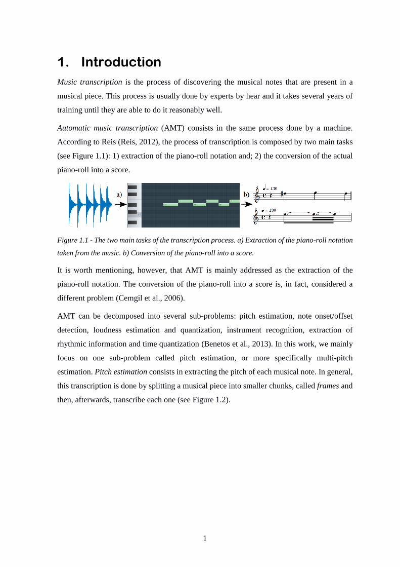
According to Reis (Reis, 2012), the process of transcription is composed by two main tasks
(see Figure 1.1): 1) extraction of the piano-roll notation and; 2) the conversion of the actual
piano-roll into a score.
Figure 1.1 - The two main tasks of the transcription process. a) Extraction of the piano-roll notation
taken from the music. b) Conversion of the piano-roll into a score.
It is worth mentioning, however, that AMT is mainly addressed as the extraction of the
piano-roll notation. The conversion of the piano-roll into a score is, in fact, considered a
different problem (Cemgil et al., 2006).
AMT can be decomposed into several sub-problems: pitch estimation, note onset/offset
detection, loudness estimation and quantization, instrument recognition, extraction of
rhythmic information and time quantization (Benetos et al., 2013). In this work, we mainly
focus on one sub-problem called pitch estimation, or more specifically multi-pitch
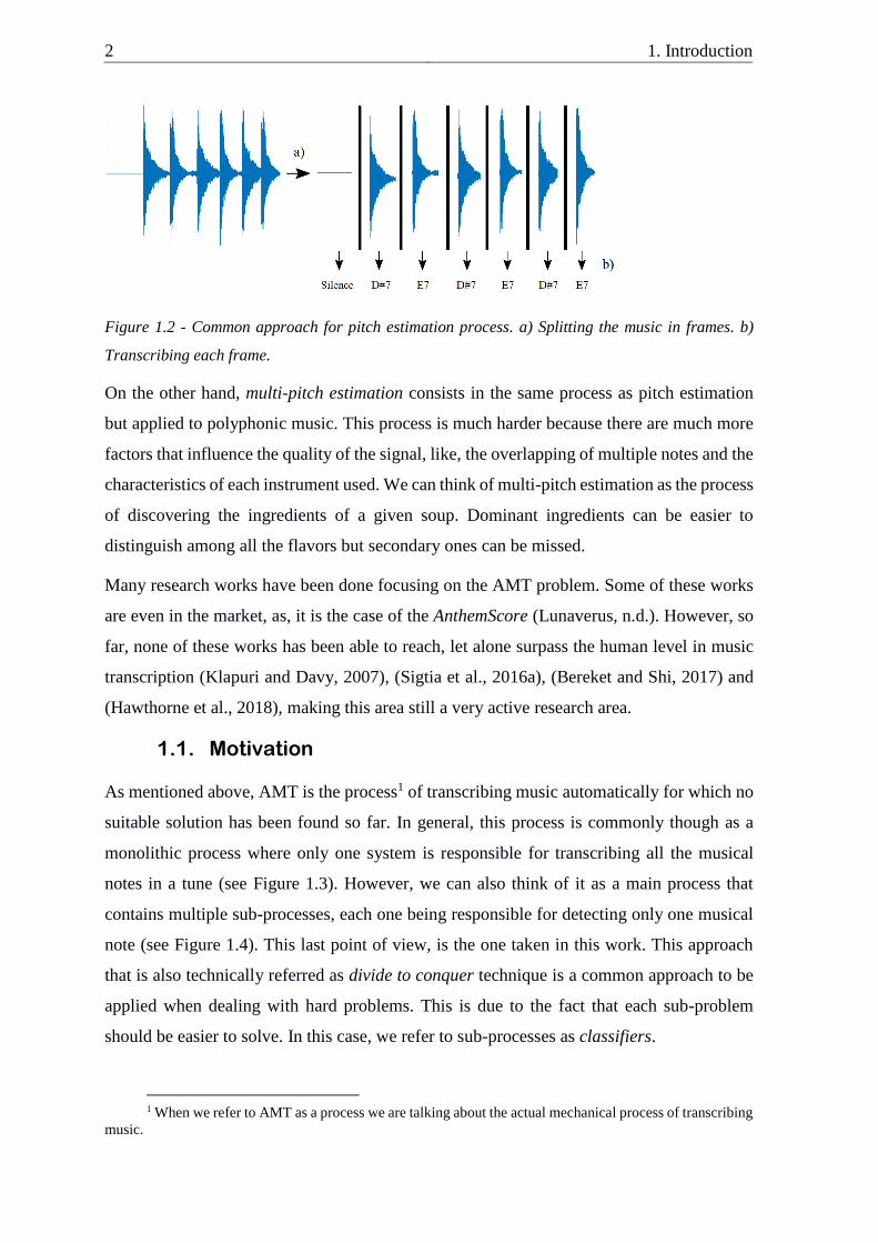
estimation. Pitch estimation consists in extracting the pitch of each musical note. In general,
this transcription is done by splitting a musical piece into smaller chunks, called frames and
then, afterwards, transcribe each one (see Figure 1.2).
2 1. Introduction
Figure 1.2 - Common approach for pitch estimation process. a) Splitting the music in frames. b)
Transcribing each frame.
On the other hand, multi-pitch estimation consists in the same process as pitch estimation
but applied to polyphonic music. This process is much harder because there are much more
factors that influence the quality of the signal, like, the overlapping of multiple notes and the
characteristics of each instrument used. We can think of multi-pitch estimation as the process
of discovering the ingredients of a given soup. Dominant ingredients can be easier to
distinguish among all the flavors but secondary ones can be missed.
Many research works have been done focusing on the AMT problem. Some of these works
are even in the market, as, it is the case of the AnthemScore (Lunaverus, n.d.). However, so
far, none of these works has been able to reach, let alone surpass the human level in music
transcription (Klapuri and Davy, 2007), (Sigtia et al., 2016a), (Bereket and Shi, 2017) and
(Hawthorne et al., 2018), making this area still a very active research area.
1.1. Motivation
As mentioned above, AMT is the process1 of transcribing music automatically for which no
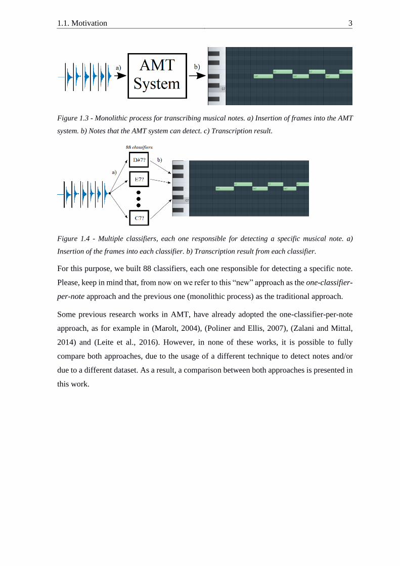
suitable solution has been found so far. In general, this process is commonly though as a
monolithic process where only one system is responsible for transcribing all the musical
notes in a tune (see Figure 1.3). However, we can also think of it as a main process that
contains multiple sub-processes, each one being responsible for detecting only one musical
note (see Figure 1.4). This last point of view, is the one taken in this work. This approach
that is also technically referred as divide to conquer technique is a common approach to be
applied when dealing with hard problems. This is due to the fact that each sub-problem
should be easier to solve. In this case, we refer to sub-processes as classifiers.
1 When we refer to AMT as a process we are talking about the actual mechanical process of transcribing
music.
1.1. Motivation 3
Figure 1.3 - Monolithic process for transcribing musical notes. a) Insertion of frames into the AMT
system. b) Notes that the AMT system can detect. c) Transcription result.
Figure 1.4 - Multiple classifiers, each one responsible for detecting a specific musical note. a)
Insertion of the frames into each classifier. b) Transcription result from each classifier.
For this purpose, we built 88 classifiers, each one responsible for detecting a specific note.
Please, keep in mind that, from now on we refer to this “new” approach as the one-classifier-
per-note approach and the previous one (monolithic process) as the traditional approach.
Some previous research works in AMT, have already adopted the one-classifier-per-note
approach, as for example in (Marolt, 2004), (Poliner and Ellis, 2007), (Zalani and Mittal,
2014) and (Leite et al., 2016). However, in none of these works, it is possible to fully
compare both approaches, due to the usage of a different technique to detect notes and/or
due to a different dataset. As a result, a comparison between both approaches is presented in
this work.
4 1. Introduction
1.2. Goals and contributions
The main goal of this project is to present the one-classifier-per-note approach based on
machine learning techniques. As mentioned above, this approach consists on having n
classifiers, where each one is responsible for transcribing one note, instead of the traditional
approach, of having one classifier responsible for transcribing all the notes. Additionally, it
is also presented some post-processing steps to improve the final results.
The contributions of this project are as follows:
• To update the current state-of-the-art.
• To present a comparison between the one-classifier-per-note approach and the
traditional one.
• To present different types of post-processing steps.
• To collaborate by opening the source code of both scripts for creating the datasets
and also for training the classifiers and the post-processing units.
• To publish a paper in the Portuguese Conference on Pattern Recognition.
1.3. Dissertation structure
The structure of the rest of this document is as follows:
• Chapter 2, Background – This chapter contains the concepts and terminologies
needed to understand this work;
• Chapter 3, Related work – In this chapter a summary of works related to our project
of the AMT field are described;
• Chapter 4, Proposed model – In this chapter our approach for the AMT problem is
presented;
• Chapter 5, Preliminary experiments – In this chapter an overview of the preliminary
experiments accomplished in order to achieve our final model are present;
• Chapter 6, Results – This chapter comprises the results achieved from our model as
well as a comparison with other state-of-the-art works;
• Chapter 7, Conclusion and future work – In this chapter some final thoughts and
conclusions are presented, as well as future work.

5
2. Background
The problem of automatic music transcription is a vast problem that combines different
fields, from sound concepts and music theory to different types of digital processing
methods. As a result, in this chapter we present the terminology and concepts that are
necessary in order to understand the meaning of this work.
This chapter is divided into four main sections: general concepts, digital signal processing,
multi-pitch estimation and aritificial neural networks.
In the general concepts section, an overview of the terminology and basic concepts is given.
In the digital signal processing section, more advanced topics regarding signal processing
are introduced. The multi-pitch estimation section compares single with multi pitch
estimation. It also presents the main problems that can arise with pitch estimation problems.
To finish, in the artificial neural networks section, an explanation about the artificial neural
networks technique and its several variations are presented.
2.1. General concepts
Music is a form of art that is transmitted through sound. Thus, when dealing with music
transcription, concepts regarding sound are also very important in order to achieve a good
transcription.
In this section, basic concepts and terminologies such as what is referred as sound, the
differences between digital and real-world sound, how a digital sound can have good quality,
how a sound can be categorized and the main characteristics of the music, will be addressed.
2.1.1. Sound waves
We refer to sound as vibrations in some medium. Those vibrations, also called cycles, occur
when the air is compressed (high pressure), rarefacted (low pressure) and finally returns to
its original state. In general, human beings are able to hear vibrations from 20 to 20 000
times per second or, more technically, from 20 Hertz (Hz) to 20 Kilohertz (KHz),
approximately. Any sound with a frequency bellow 20Hz is refered to as infrasound and
above 20KHz as ultrasound.
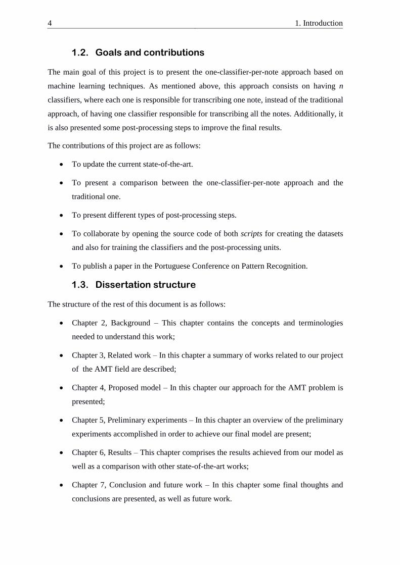
In general, we visualize those vibrations in a digital format as, for example, in an oscillogram
or in a computer program. These are represented as a function of time (see Figure 2.1), where
6 2. Background
time is represented horizontally (x axis) and pressures values (amplitude) are represented
vertically (y axis).
Figure 2.1 - Representation of the oscillations generated by a sound. The picture in the left side
represents a sound generated mathematically and the picture in the right side shows a piano
recording sound.
High levels of pressure (compression stage) are represented in the top part of the y axis, and
low levels of pressure (rarefactor stage) in the bottom part of the y axis.
2.1.2. Digital audio recording
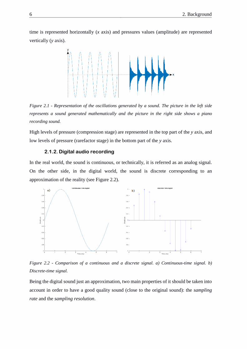
In the real world, the sound is continuous, or technically, it is referred as an analog signal.
On the other side, in the digital world, the sound is discrete corresponding to an
approximation of the reality (see Figure 2.2).
Figure 2.2 - Comparison of a continuous and a discrete signal. a) Continuous-time signal. b)
Discrete-time signal.
Being the digital sound just an approximation, two main properties of it should be taken into
account in order to have a good quality sound (close to the original sound): the sampling
rate and the sampling resolution.
2.1. General concepts 7
Sampling rate
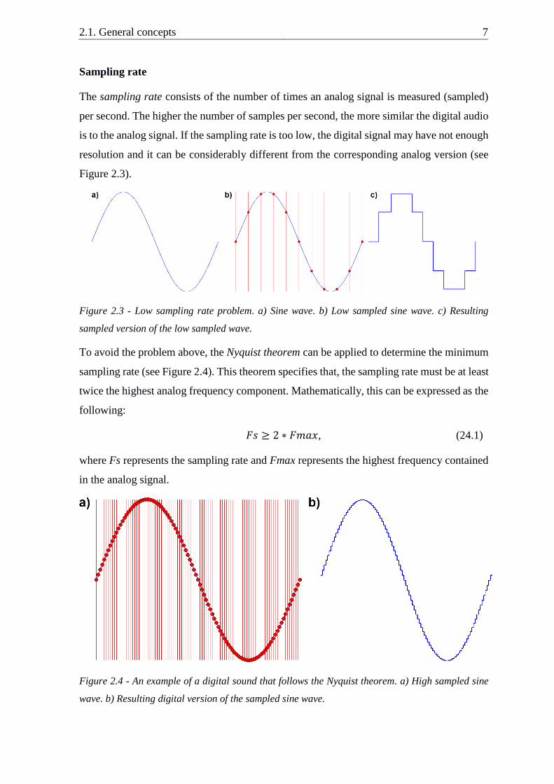
The sampling rate consists of the number of times an analog signal is measured (sampled)
per second. The higher the number of samples per second, the more similar the digital audio
is to the analog signal. If the sampling rate is too low, the digital signal may have not enough
resolution and it can be considerably different from the corresponding analog version (see
Figure 2.3).
Figure 2.3 - Low sampling rate problem. a) Sine wave. b) Low sampled sine wave. c) Resulting
sampled version of the low sampled wave.
To avoid the problem above, the Nyquist theorem can be applied to determine the minimum
sampling rate (see Figure 2.4). This theorem specifies that, the sampling rate must be at least
twice the highest analog frequency component. Mathematically, this can be expressed as the
following:
𝐹𝑠 ≥ 2 ∗ 𝐹𝑚𝑎𝑥, (24.1)
where Fs represents the sampling rate and Fmax represents the highest frequency contained
in the analog signal.
Figure 2.4 - An example of a digital sound that follows the Nyquist theorem. a) High sampled sine
wave. b) Resulting digital version of the sampled sine wave.
8 2. Background
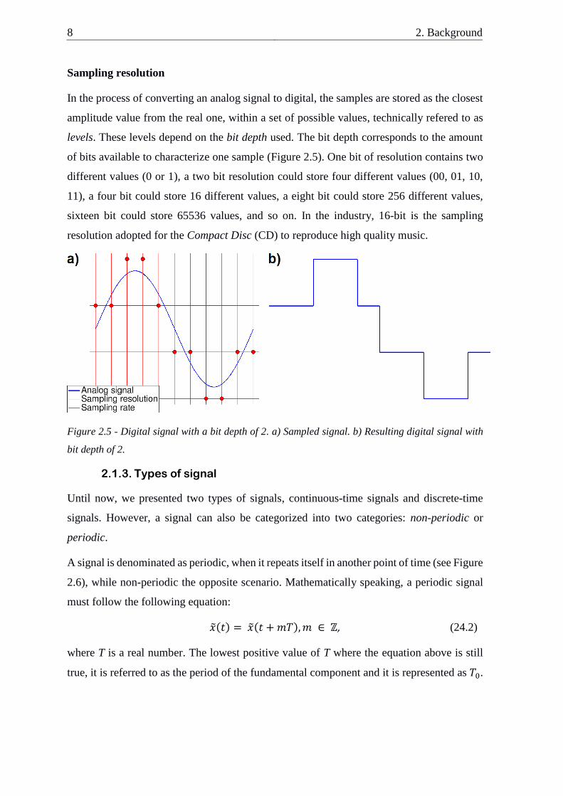
Sampling resolution
In the process of converting an analog signal to digital, the samples are stored as the closest
amplitude value from the real one, within a set of possible values, technically refered to as
levels. These levels depend on the bit depth used. The bit depth corresponds to the amount
of bits available to characterize one sample (Figure 2.5). One bit of resolution contains two
different values (0 or 1), a two bit resolution could store four different values (00, 01, 10,
11), a four bit could store 16 different values, a eight bit could store 256 different values,
sixteen bit could store 65536 values, and so on. In the industry, 16-bit is the sampling
resolution adopted for the Compact Disc (CD) to reproduce high quality music.
Figure 2.5 - Digital signal with a bit depth of 2. a) Sampled signal. b) Resulting digital signal with
bit depth of 2.
2.1.3. Types of signal
Until now, we presented two types of signals, continuous-time signals and discrete-time
signals. However, a signal can also be categorized into two categories: non-periodic or
periodic.
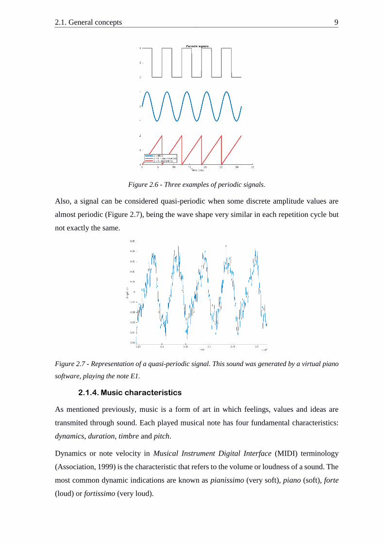
A signal is denominated as periodic, when it repeats itself in another point of time (see Figure
2.6), while non-periodic the opposite scenario. Mathematically speaking, a periodic signal
must follow the following equation:
��(𝑡) = ��(𝑡 + 𝑚𝑇), 𝑚 ∈ ℤ, (24.2)
where T is a real number. The lowest positive value of T where the equation above is still
true, it is referred to as the period of the fundamental component and it is represented as 𝑇0.
2.1. General concepts 9
Figure 2.6 - Three examples of periodic signals.
Also, a signal can be considered quasi-periodic when some discrete amplitude values are
almost periodic (Figure 2.7), being the wave shape very similar in each repetition cycle but
not exactly the same.
Figure 2.7 - Representation of a quasi-periodic signal. This sound was generated by a virtual piano
software, playing the note E1.
2.1.4. Music characteristics
As mentioned previously, music is a form of art in which feelings, values and ideas are
transmited through sound. Each played musical note has four fundamental characteristics:
dynamics, duration, timbre and pitch.
Dynamics or note velocity in Musical Instrument Digital Interface (MIDI) terminology
(Association, 1999) is the characteristic that refers to the volume or loudness of a sound. The
most common dynamic indications are known as pianissimo (very soft), piano (soft), forte
(loud) or fortissimo (very loud).
10 2. Background
Duration is the time interval during which the musical note lasts. The moments in which the
sound starts and ends are designated by onset and offset, respectively.
Timbre represents the type of the sound. It is the shape of the sound wave. This characteristic
is what makes us differentiate a piano sound from a person singing.
Pitch is the tonal height of a sound. It represents how low or high a note sounds and it is
closely related to the frequency: the physical property. In addition to that, it is the
characteristic responsible for distinguishing different notes of the same instrument.
2.2. Digital signal processing
Digital signal processing (DSP), a sub-field of signal processing, consists in the application
of computational methods on digital signals in order to extract features, which are used in
analysis, classification, recognition or transformation problems.
The file format, Joint Photographic Expercts Group (JPEG), is a good example of where
these techniques are applied in order to compress the size of images (Bako, 2004).
Additionally, DSP techniques are commonly applied in order to estimate the velocity or the
distance travelled of an object, by detecting the shift on the frequency signal received from
a radar (Giordano, 2009).
In this work, DSP techniques are also applied in order to reach our goal, that is, transcribe
piano music. Thus, basic terminologies like the frequency unit and more advanced ones such
as how a signal can be decomposed into frequencies and a deeper understanding of some
DSP methods, with a special focus to the set of methods from the family of the Fourier
Transform, are introduced. At the end, problems and possible solutions, if any, regarding
these methods will also be presented.
2.2.1. Fourier analysis
As stated before, sound consists in cycles (back and forth) in a medium. The number of
cycles per unit of time of a sound wave is named as frequency. A sound with a high frequency
contains a large number of cycles and small wavelength (period). On the contrary, a sound
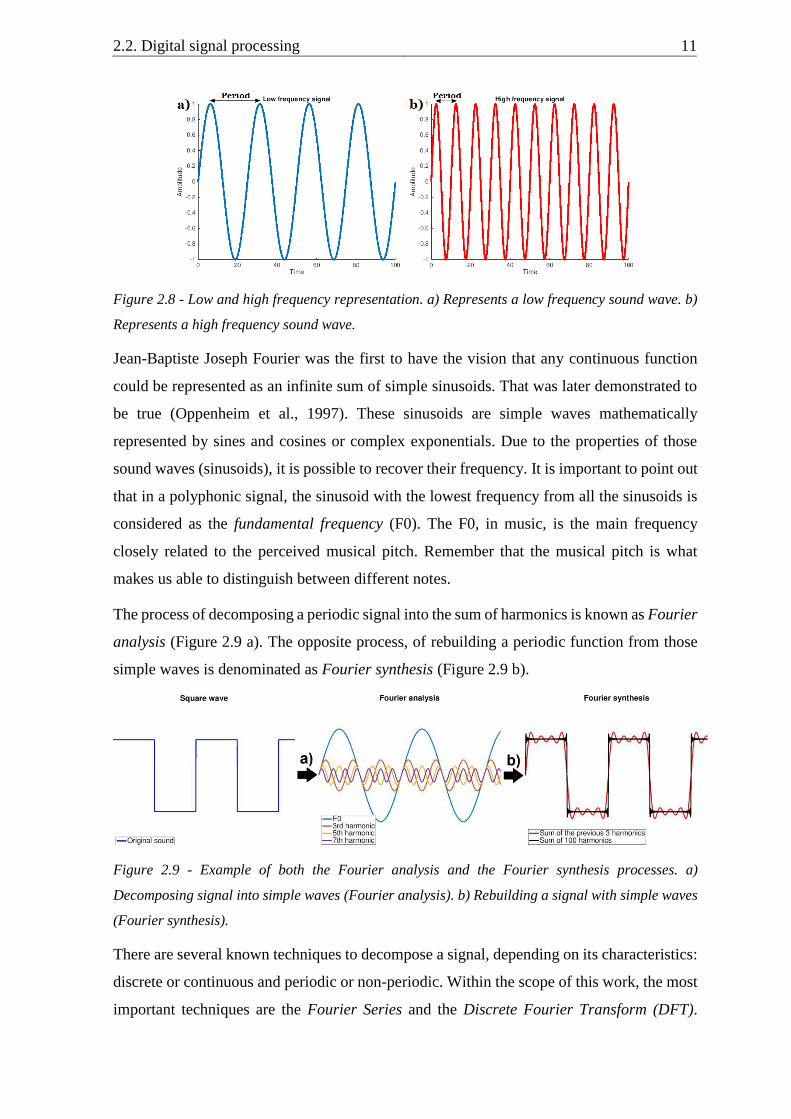
with low frequency has less number of cycles and a larger wavelength (Figure 2.8).
2.2. Digital signal processing 11
Figure 2.8 - Low and high frequency representation. a) Represents a low frequency sound wave. b)
Represents a high frequency sound wave.
Jean-Baptiste Joseph Fourier was the first to have the vision that any continuous function
could be represented as an infinite sum of simple sinusoids. That was later demonstrated to
be true (Oppenheim et al., 1997). These sinusoids are simple waves mathematically
represented by sines and cosines or complex exponentials. Due to the properties of those
sound waves (sinusoids), it is possible to recover their frequency. It is important to point out
that in a polyphonic signal, the sinusoid with the lowest frequency from all the sinusoids is
considered as the fundamental frequency (F0). The F0, in music, is the main frequency
closely related to the perceived musical pitch. Remember that the musical pitch is what
makes us able to distinguish between different notes.
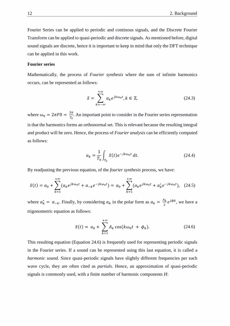
The process of decomposing a periodic signal into the sum of harmonics is known as Fourier
analysis (Figure 2.9 a). The opposite process, of rebuilding a periodic function from those
simple waves is denominated as Fourier synthesis (Figure 2.9 b).
Figure 2.9 - Example of both the Fourier analysis and the Fourier synthesis processes. a)
Decomposing signal into simple waves (Fourier analysis). b) Rebuilding a signal with simple waves
(Fourier synthesis).
There are several known techniques to decompose a signal, depending on its characteristics:
discrete or continuous and periodic or non-periodic. Within the scope of this work, the most
important techniques are the Fourier Series and the Discrete Fourier Transform (DFT).
12 2. Background
Fourier Series can be applied to periodic and continous signals, and the Discrete Fourier
Transform can be applied to quasi-periodic and discrete signals. As mentioned before, digital
sound signals are discrete, hence it is important to keep in mind that only the DFT technique
can be applied in this work.
Fourier series
Mathematically, the process of Fourier synthesis where the sum of infinite harmonics
occurs, can be represented as follows:
�� = ∑ 𝑎𝑘𝑒𝑗𝑘ω0𝑡, 𝑘 ∈
+∞
𝑘=−∞
ℤ, (24.3)
where ω0 = 2𝜋𝐹0 = 2𝜋
𝑇0. An important point to consider in the Fourier series representation
is that the harmonics forms an orthonormal set. This is relevant because the resulting integral
and product will be zero. Hence, the process of Fourier analysis can be efficiently computed
as follows:
𝑎𝑘 =1
𝑇0∫ ��(𝑡)𝑒−𝑗𝑘ω0𝑡
𝑇0
𝑑𝑡. (24.4)
By readjusting the previous equation, of the fourier synthesis process, we have:
��(𝑡) = 𝑎0 + ∑(𝑎𝑘𝑒𝑗𝑘ω0𝑡 + 𝑎−𝑘𝑒−𝑗𝑘ω0𝑡) =
+∞
𝑘=1
𝑎0 + ∑(𝑎𝑘𝑒𝑗𝑘ω0𝑡 + 𝑎𝑘∗ 𝑒−𝑗𝑘ω0𝑡)
+∞
𝑘=1
, (24.5)
where 𝑎𝑘∗ = 𝑎−𝑘. Finally, by considering 𝑎𝑘 in the polar form as 𝑎𝑘 =
𝐴𝑘
2𝑒𝑗𝜙𝑘, we have a
trigonometric equation as follows:
��(𝑡) = 𝑎0 + ∑ 𝐴𝑘 cos(𝑘ω0𝑡 + 𝜙𝑘)
+∞
𝑘=1
. (24.6)
This resulting equation (Equation 24.6) is frequently used for representing periodic signals
in the Fourier series. If a sound can be represented using this last equation, it is called a
harmonic sound. Since quasi-periodic signals have slightly different frequencies per each
wave cycle, they are often cited as partials. Hence, an approximation of quasi-periodic
signals is commonly used, with a finite number of harmonic components H:
2.2. Digital signal processing 13
��(𝑡) ≈ 𝑎0 + ∑ 𝐴𝑘 cos(𝑘ω0𝑡 + 𝜙𝑘) .
𝐻
𝑘=1
(24.7)
Fourier Transform
Fourier transform and all its variations are techniques used to convert signals from the time
domain (time-amplitude) into the frequency domain. These methods are commonly used by
AMT systems because, as mentioned previouslly, pitch is a characteristic from music that
gives us the possibility to distinguish notes from the same instrument and this characteristic
is closely related to the frequency, making these methods highly relevant for the AMT
problem.
The Fourier transform decomposes the signal into a sum of simple waves (fourier analysis)
resulting in the frequencies of the signal. This technique is used for periodic continuous
signals with infinite length as follows:
𝐹𝑇��(𝑓) = ��(𝑓) = ∫ ��(𝑡)𝑒−𝑗2𝜋𝑓𝑡𝑑𝑡.+∞
−∞
(24.8)
Discrete Fourier Transform
As mentioned above, the Fourier Transform technique can only be applied to periodic
continuous signals. However, a digital signal is discrete. Hence, another technique called
Discrete Fourier Transform (DFT) is applied. The DFT can be calculated as follows:
𝐷𝐹𝑇��[𝑘] = ��[𝑘] = ∑ ��[𝑛]
+∞
𝑛=−∞
𝑒−𝑗2𝜋𝑘𝑛, (24.9)
where k is the spectral bin corresponding to each frequency. In Equation 24.9, infinite
discrete signals are targeted. However, infinite signals create computational problems. Thus,
Equation 24.10 is defined to tackle this problem:
𝐷𝐹𝑇��[𝑘] = ��[𝑘] = ∑ ��[𝑛]
𝑁−1
𝑛=0
𝑒−𝑗2𝜋𝑁
𝑘𝑛, 𝑘 = 0, … , 𝑁 − 1, (24.10)
where N represents the length of the waveform (number of samples).
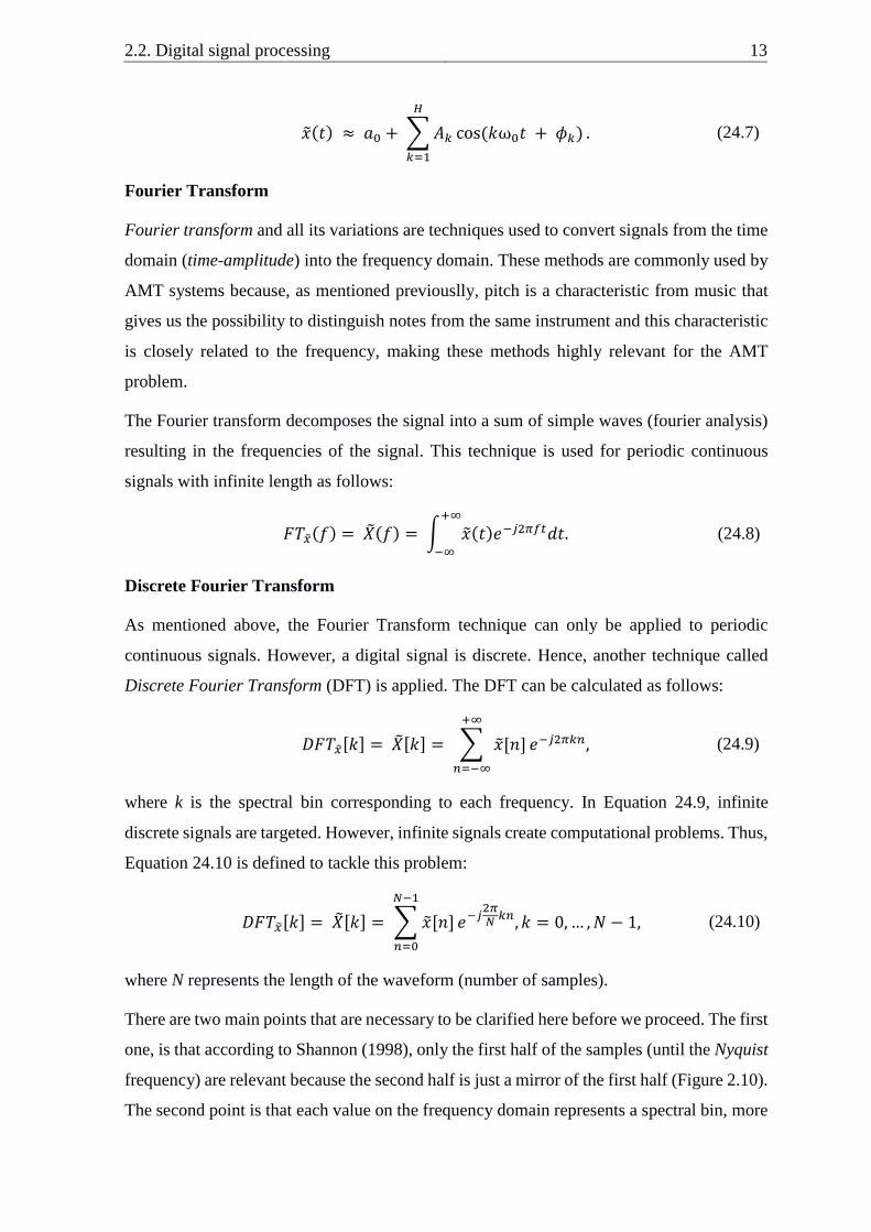
There are two main points that are necessary to be clarified here before we proceed. The first
one, is that according to Shannon (1998), only the first half of the samples (until the Nyquist
frequency) are relevant because the second half is just a mirror of the first half (Figure 2.10).
The second point is that each value on the frequency domain represents a spectral bin, more
14 2. Background
specifically, it represents a range of frequencies and not just one frequency. For example, if
a signal has 4096 samples and its sampling rate is 44100 Hz, each bin is linearly separated
by ∆𝑓 = 𝐹𝑠
𝑁=
44100
4096≅ 10.77𝐻𝑧. Thus, each spectral bin k will contain a range of
frequencies between 𝑓𝑘 = 𝑘 ∗ 10.77𝐻𝑧 ± 10.77𝐻𝑧. As a result, some piano notes
correspond to the same spectral bin, making the process of detecting notes harder.
Figure 2.10 - A comparison of the same sound in two different domains. a) Sound in the time domain.
b) Sound in the frequency domain.
Fast Fourier Transform
DFT is a common technique used for periodic discrete signals. However, this technique can
be computationally expensive for real time applications, such as AMT systems. Thus, in
order to fulfill this necessity, another technique called fast Fourier Transform (FFT) is used.
This is the DSP technique applied in our work.
FFT is a fast algorithm which applies efficiently the DFT in a signal that contains a structured
number of samples such as the power of two. This technique reduces the number of
operations from 𝑂(𝑁2), where N represents the number of samples, to 𝑂(𝑁 ∗ 𝑙𝑜𝑔2 𝑁)
(Cooley et al., 1967).
2.2. Digital signal processing 15
2.2.2. Spectral leakage
The DFT and its variations assume that a signal is periodic. However, if the number of
samples does not match with the whole number of periods, discontinuities will occur, leading
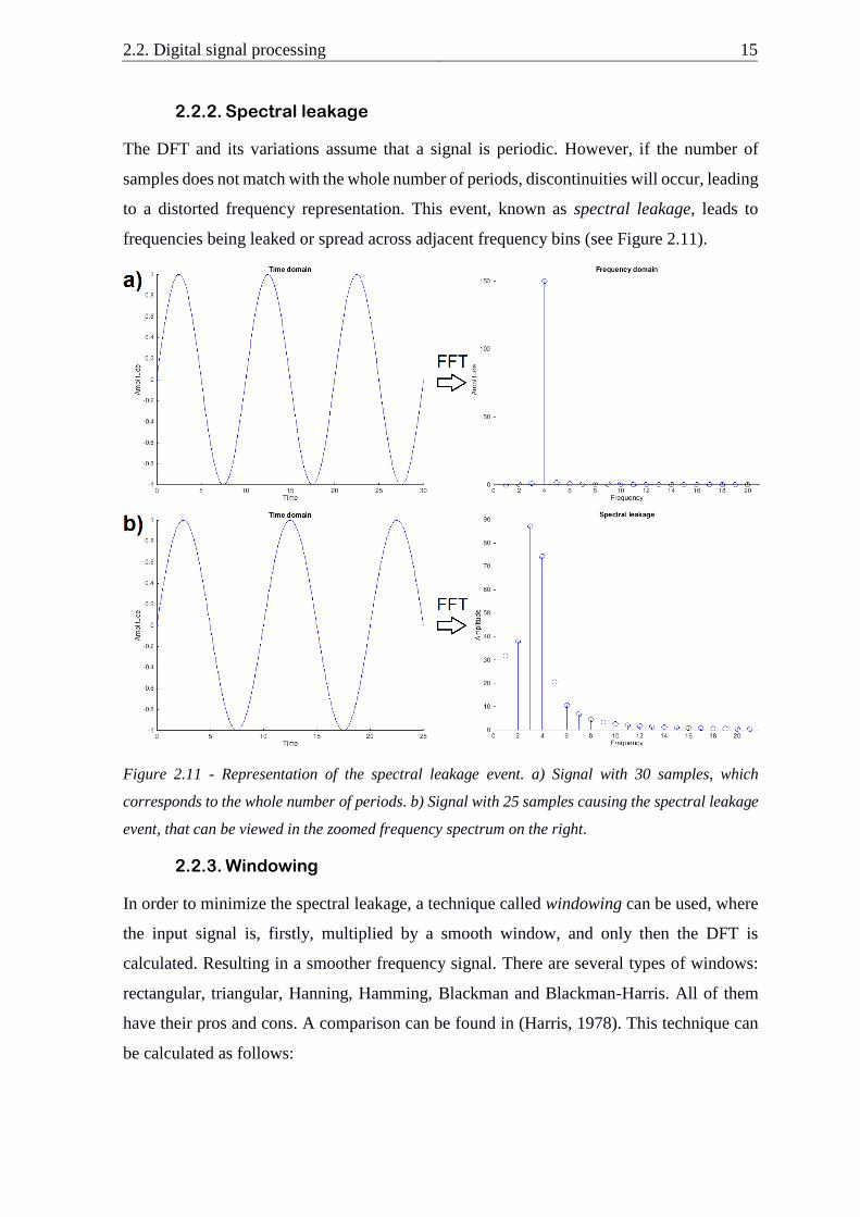
to a distorted frequency representation. This event, known as spectral leakage, leads to
frequencies being leaked or spread across adjacent frequency bins (see Figure 2.11).
Figure 2.11 - Representation of the spectral leakage event. a) Signal with 30 samples, which
corresponds to the whole number of periods. b) Signal with 25 samples causing the spectral leakage
event, that can be viewed in the zoomed frequency spectrum on the right.
2.2.3. Windowing
In order to minimize the spectral leakage, a technique called windowing can be used, where
the input signal is, firstly, multiplied by a smooth window, and only then the DFT is
calculated. Resulting in a smoother frequency signal. There are several types of windows:
rectangular, triangular, Hanning, Hamming, Blackman and Blackman-Harris. All of them
have their pros and cons. A comparison can be found in (Harris, 1978). This technique can
be calculated as follows:
16 2. Background
𝑌𝑘 = ∑ 𝑎𝑛��𝑛𝑊𝑁𝑛𝑘 , 𝑊 = 𝑒−𝑗2𝜋,
𝑁−1
𝑛=0
(24.11)
where 𝑎𝑛 is the the type of window.
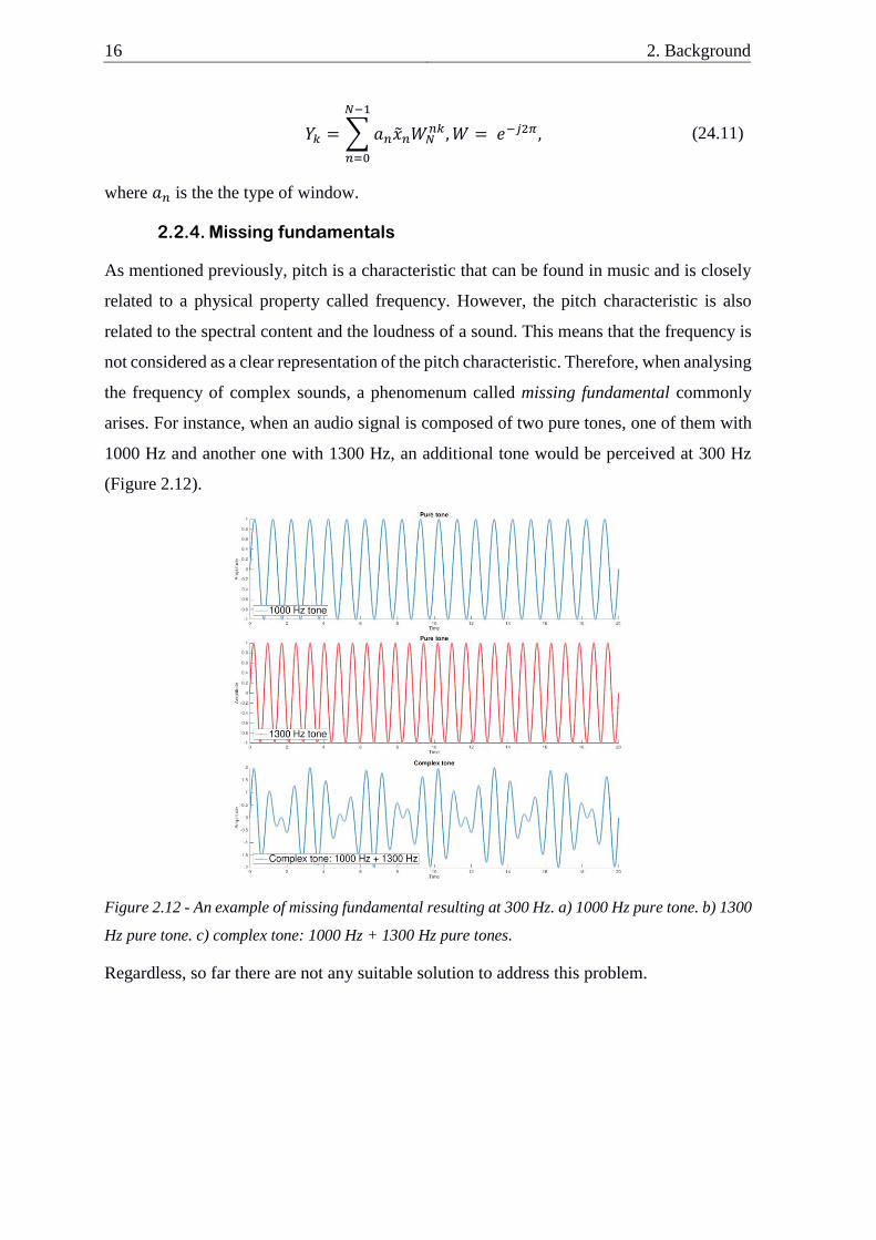
2.2.4. Missing fundamentals
As mentioned previously, pitch is a characteristic that can be found in music and is closely
related to a physical property called frequency. However, the pitch characteristic is also
related to the spectral content and the loudness of a sound. This means that the frequency is
not considered as a clear representation of the pitch characteristic. Therefore, when analysing
the frequency of complex sounds, a phenomenum called missing fundamental commonly
arises. For instance, when an audio signal is composed of two pure tones, one of them with
1000 Hz and another one with 1300 Hz, an additional tone would be perceived at 300 Hz
(Figure 2.12).
Figure 2.12 - An example of missing fundamental resulting at 300 Hz. a) 1000 Hz pure tone. b) 1300
Hz pure tone. c) complex tone: 1000 Hz + 1300 Hz pure tones.
Regardless, so far there are not any suitable solution to address this problem.

2.2. Digital signal processing 17
2.2.5. Pitch vs Fundamental frequency
Regarding the frequency of a given sound, a common error is made:
What is the frequency of the piano MIDI note number 55?
The sentence above is not completely correct because a piano note (like most of the sounds)
do not contain a single frequency, but instead it is composed by several frequencies
(harmonics). A better question would be the following one:
What is the fundamental frequency of the piano MIDI note number 55?
The fundamental frequency (F0), as mentioned previously, is the lowest frequency on an
harmonic series and is the essential one in order to distinguish a pitch in a given signal. For
instance, if a piano note sound has an F0 around 260Hz, our brain should be able to map it
as a C4 pitch (see Table 2.1).
Table 2.1 - Corresponding frequency of each pitch, from C0 to B8.
Note Octave
0 1 2 3 4 5 6 7 8
C 16 33 65 131 262 523 1047 2093 4186
C# 17 35 69 139 278 554 1109 2218 4435
D 18 37 73 147 294 587 1175 2349 4699
D# 20 39 78 156 311 622 1245 2489 4978
E 21 41 82 165 330 659 1319 2637 5274
F 22 44 87 175 349 699 1397 2794 5588
F# 23 46 93 185 370 740 1475 2960 5920
G 25 49 98 196 392 784 1568 3136 6272
G# 26 52 104 208 415 831 1661 3322 6645
A 28 55 110 220 440 880 1760 3520 7040
A# 29 58 117 233 466 932 1865 3729 7459
B 31 62 124 247 494 988 1976 3951 7902
18 2. Background
In the field of AMT two different terms are commonly confused: F0 estimation and pitch
estimation. F0 estimation consists in the extraction of the exact frequency components of a
signal and then match them to the pitches of the notes. The second process, pitch estimation,
consists on determining the pitch from a given signal even without knowing exactly the F0
of the sound. This last process is the one applied in this dissertation.
2.3. Multi-pitch estimation
Multi-pitch estimation algorithms commonly assume that there can be two or more harmonic
sources in the same short-time signal. According to Yeh et al. (2010), a signal can be
expressed as a sum of harmonic signals plus the residual part:
𝑦[𝑛] = ∑ 𝑦𝑚[𝑛] + 𝑧[𝑛]
𝑀
𝑚=1
, 𝑀 > 0 with 𝑦𝑚[𝑛] ≈ 𝑦𝑚[𝑛 + 𝑁𝑚], (24.12)
where n represents the discrete time index, M is the number of harmonic signals, 𝑦𝑚[𝑛] the
quasi-periodic part of the mth source, 𝑁𝑚 the period of the mth source and z[n] the residual
part.
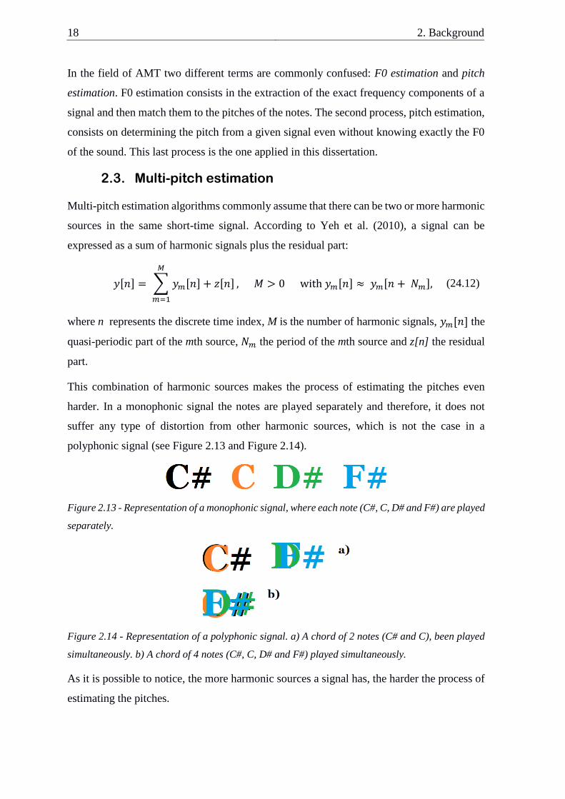
This combination of harmonic sources makes the process of estimating the pitches even
harder. In a monophonic signal the notes are played separately and therefore, it does not
suffer any type of distortion from other harmonic sources, which is not the case in a
polyphonic signal (see Figure 2.13 and Figure 2.14).
Figure 2.13 - Representation of a monophonic signal, where each note (C#, C, D# and F#) are played
separately.
Figure 2.14 - Representation of a polyphonic signal. a) A chord of 2 notes (C# and C), been played
simultaneously. b) A chord of 4 notes (C#, C, D# and F#) played simultaneously.
As it is possible to notice, the more harmonic sources a signal has, the harder the process of
estimating the pitches.
2.3. Multi-pitch estimation 19
In addition to that, other types of problems, can also occur, such as the distortion of a signal
because of its residual components. The residual components are all the components that
cannot be explained by simple waves (sinusoids), as for example the background noise, non-
harmonic partials or spurious components.
In the following sections, several common problems regarding the multi-pitch estimation
problem are presented.
2.3.1. Overlapping partials
As mentioned above, in polyphonic signals, different sources may overlap or interfere with
each other. Those different sources can be considered in harmony if their fundamental
frequencies (𝐹𝑎 and 𝐹𝑏) can be represented as follows:
𝐹𝑎 = 𝑚
𝑛𝐹𝑏 , 𝑛, 𝑚 ∈ ℕ, (24.13)
in which every 𝑛𝑡ℎ partial of the source a overlaps every 𝑚𝑡ℎ partial of source b, as proved
by Klapuri in (Klapuri, 1998). This augments the probability of partial collisions. Another
issue demonstrated in (Yeh, 2008) occurs when the F0 of a note is multiple of another note’s
F0. In this case, the higher note can hide the lower one.
Interference and overlaping of different sources can disturb a signal in several ways, as its
frequencies, amplitudes and phases. For instance, when two sources are superposed, the
resulting sound wave would be a sum of those two sources. On the contrary, when there is a
harmonic overlap, the resulting wave would have two simple harmonic motions with the
same frequency but with different amplitude and phases.
There are several works in which the authors tried to detect those overlaping partials, which
in the case of being successful could help in the process of multi-pitch estimation. In
(Parsons, 1976) the author tried to detect those overlapping components based on three tests:
spectral peak symmetry, distance and well-behaved phase. However, even with only two
different sources, that is actually a very restrictive number of sources, the results were not
good. Later on, several authors (Viste and Evangelista, 2002), (Virtanen, 2003), (Every and
Szymanski, 2004) and (Yeh and Roebel, 2009) tried to address the problem by knowing in
advance how many different sources existed in a given signal but unfortunatelly the results
were poor. Thus, this problem remains a challenge.
20 2. Background
2.3.2. Spectral characteristics
In a musical piece, it is common that several types of instruments are played simultaneously.
This adds even more complexity to the transcription problem.
In the following three sub-sections, different types of instrument characteristics are present,
such as: the spectral envelope, inharmonic partials and spurious components.
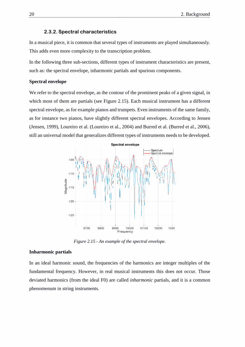
Spectral envelope
We refer to the spectral envelope, as the contour of the prominent peaks of a given signal, in
which most of them are partials (see Figure 2.15). Each musical instrument has a different
spectral envelope, as for example pianos and trumpets. Even instruments of the same family,
as for instance two pianos, have slightly different spectral envelopes. According to Jensen
(Jensen, 1999), Loureiro et al. (Loureiro et al., 2004) and Burred et al. (Burred et al., 2006),
still an universal model that generalizes different types of instruments needs to be developed.
Figure 2.15 - An example of the spectral envelope.
Inharmonic partials
In an ideal harmonic sound, the frequencies of the harmonics are integer multiples of the
fundamental frequency. However, in real musical instruments this does not occur. Those
deviated harmonics (from the ideal F0) are called inharmonic partials, and it is a common
phenomenum in string instruments.
2.3. Multi-pitch estimation 21
Spurious components
Another type of influent characteristic that can be also observed in string instruments is the
one called phantom partials. According to Conklin (Conklin, 1999), these phantom partials,
in string instruments are related to the tension variation on the plucked strings, and are close
to the frequencies of the normal partials. Nevertheless, recent works (Moore et al., 2017)
and (Moore et al., 2018) also suggest that non-string components, like the mechanical parts
or the wooden components of a piano, could also contribute to the appearance of those
phantom partials. These kind of partials are sometimes fairly dominant compared to the
normal partials, which in turn can lead to a bad transcription.
2.3.3. Transients
In music, it is quite common, specially in some types of musical pieces, that the notes are
played roughly, resulting in abrupt variations in the sound signal. According to Rodet and
Jaillet (Rodet and Jaillet, 2001), these fast variations are denominated as transients. The
transients usually refer to note onsets (fast attacks) or to note offsets (fast releases). Due to
those abrupt variations and also that most of the variations have high levels of energy, the
sound signal will contain several spurious components, making the process of estimating the
pitch in those areas very hard. Recent research works tend to consider the transient as a
specific signal component, where it is detected by either a parametric approach (Daudet,
2004) and (Molla and Torrésani, 2004), or a non-parametric approach (Rodet and Jaillet,
2001), (obel, 2003) and (Bello et al., 2005).
2.3.4. Reverberation
When a note is played and then released, the sound produced does not disappear suddenly.
It usually takes time in order to be not earable anymore. This process, the prolongation of a
preceding sound is called reverberation. Thus, a recorded signal can be considered as a
mixture of multiple sounds, which are direct sounds, reflected sounds and reverberated
sounds. According to Yeh et al. (Yeh et al., 2006), Beauchamp et al. (Beauchamp et al.,
1992) and Baskind et al. (2012), depending on the recording environment, a monophonic
sound can also become a polyphonic sound, because the reverberated and reflected sounds
add complexity to the analysis of the recorded signal.
22 2. Background
2.4. Artificial neural networks
Artifical neural networks (ANNs) or simply neural networks are an artificial intelligence
(AI) technique based on biological brains. This technique has been used successfully in
many complex problems, such as: autonomous vehicles (Bojarski et al., 2016), autonomous
farm (Pearlstein et al., 2016), (Luo et al., 2010) and (Stentz et al., 2002), anomaly detection
in internet traffic (Pradhan et al., 2012), cancer detection in medical images (Singh et al.,
2015) and also music transcription (Sigtia et al., 2016a) and (Kelz et al., 2016). This is one
of the reasons whereby we have applied ANNs in this work, because they are good at
tackling difficult problems and, apart from that, it’s a technique already applied in the AMT
problem, and thus, a more closer comparison with other works can be made.
This section is divided into five topics: neuron model, ANN architecture, learning method,
types of activation functions and types of ANNs. Initially, a comparison between the
biological neuron and an artificial neuron is presented. Then, an overview of the main
components of an ANN is introduced. Continuing, an explanation of how the ANNs learn is
presented. To conclude, a deeper explanation regarding activation functions, following by
an introduction of several types of ANNs are presented.
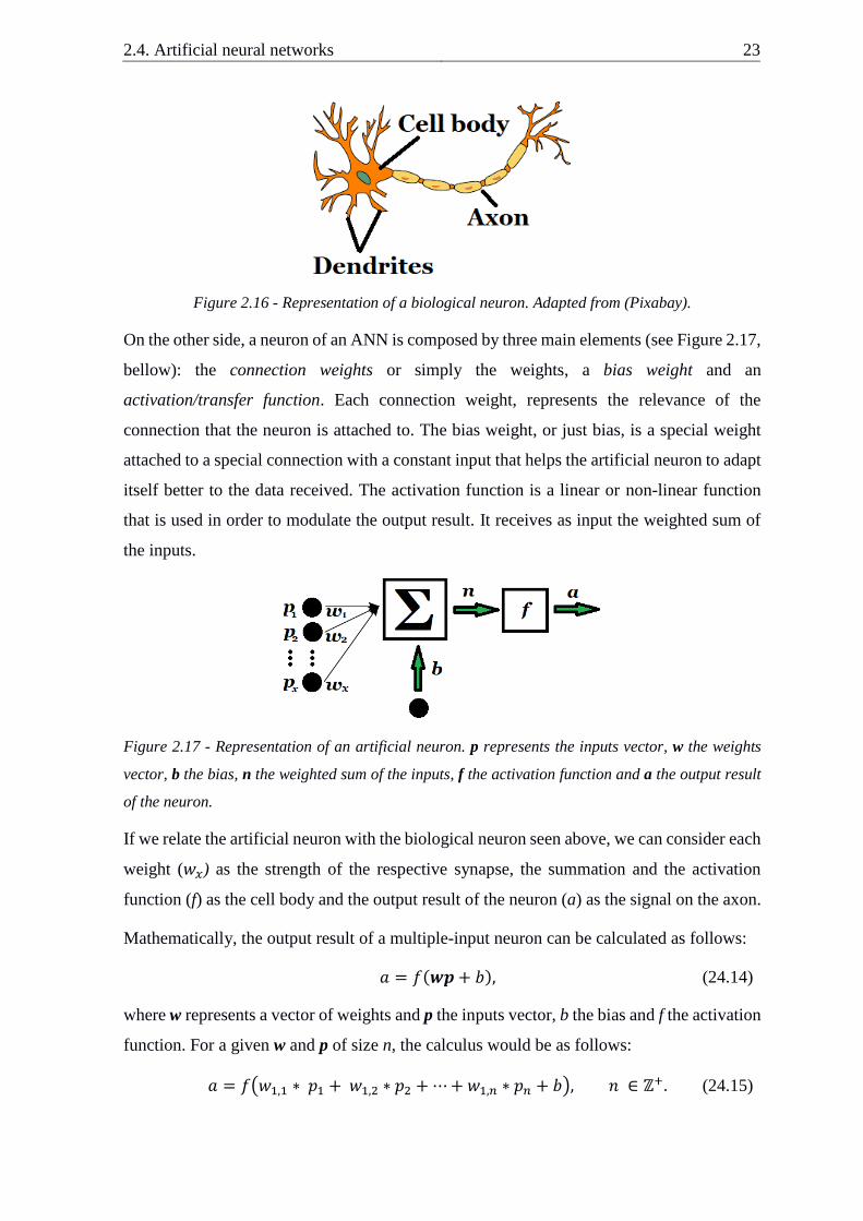
2.4.1. Neuron model
As mentioned above, ANNs were inspired by biological brains. The human brain has roughly
86 ∗ 109 of connected elements, called neurons. Each neuron, is composed by three main
components (see Figure 2.16, bellow): the dentrites, the cell body and the axon. The dentrites
are tree-like connections that receive and transport incoming signals to the cell body. Hence,
the cell body is the component responsible for processing the incoming signals, by summing
and thresholding. However, sometimes, the dentrites also process those informations before
it arrives to the cell body. The last main component, the axon, is in charge of transporting
and transmiting the output signal from the cell to other neurons. The transmition, is done in
the edge of the axon in a zone called synapse. Synapses transform the electrical signal into
a chemical one and, then, send it to the dentrites of other neurons.
2.4. Artificial neural networks 23
Figure 2.16 - Representation of a biological neuron. Adapted from (Pixabay).
On the other side, a neuron of an ANN is composed by three main elements (see Figure 2.17,
bellow): the connection weights or simply the weights, a bias weight and an
activation/transfer function. Each connection weight, represents the relevance of the
connection that the neuron is attached to. The bias weight, or just bias, is a special weight
attached to a special connection with a constant input that helps the artificial neuron to adapt
itself better to the data received. The activation function is a linear or non-linear function
that is used in order to modulate the output result. It receives as input the weighted sum of
the inputs.
Figure 2.17 - Representation of an artificial neuron. p represents the inputs vector, w the weights
vector, b the bias, n the weighted sum of the inputs, f the activation function and a the output result
of the neuron.
If we relate the artificial neuron with the biological neuron seen above, we can consider each
weight (𝑤𝑥) as the strength of the respective synapse, the summation and the activation
function (f) as the cell body and the output result of the neuron (a) as the signal on the axon.
Mathematically, the output result of a multiple-input neuron can be calculated as follows:
𝑎 = 𝑓(𝒘𝒑 + 𝑏), (24.14)
where w represents a vector of weights and p the inputs vector, b the bias and f the activation
function. For a given w and p of size n, the calculus would be as follows:
𝑎 = 𝑓(𝑤1,1 ∗ 𝑝1 + 𝑤1,2 ∗ 𝑝2 + ⋯ + 𝑤1,𝑛 ∗ 𝑝𝑛 + 𝑏), 𝑛 ∈ ℤ+. (24.15)
24 2. Background
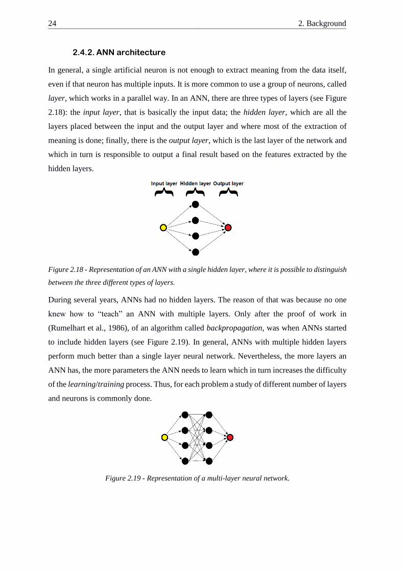
2.4.2. ANN architecture
In general, a single artificial neuron is not enough to extract meaning from the data itself,
even if that neuron has multiple inputs. It is more common to use a group of neurons, called
layer, which works in a parallel way. In an ANN, there are three types of layers (see Figure
2.18): the input layer, that is basically the input data; the hidden layer, which are all the
layers placed between the input and the output layer and where most of the extraction of
meaning is done; finally, there is the output layer, which is the last layer of the network and
which in turn is responsible to output a final result based on the features extracted by the
hidden layers.
Figure 2.18 - Representation of an ANN with a single hidden layer, where it is possible to distinguish
between the three different types of layers.
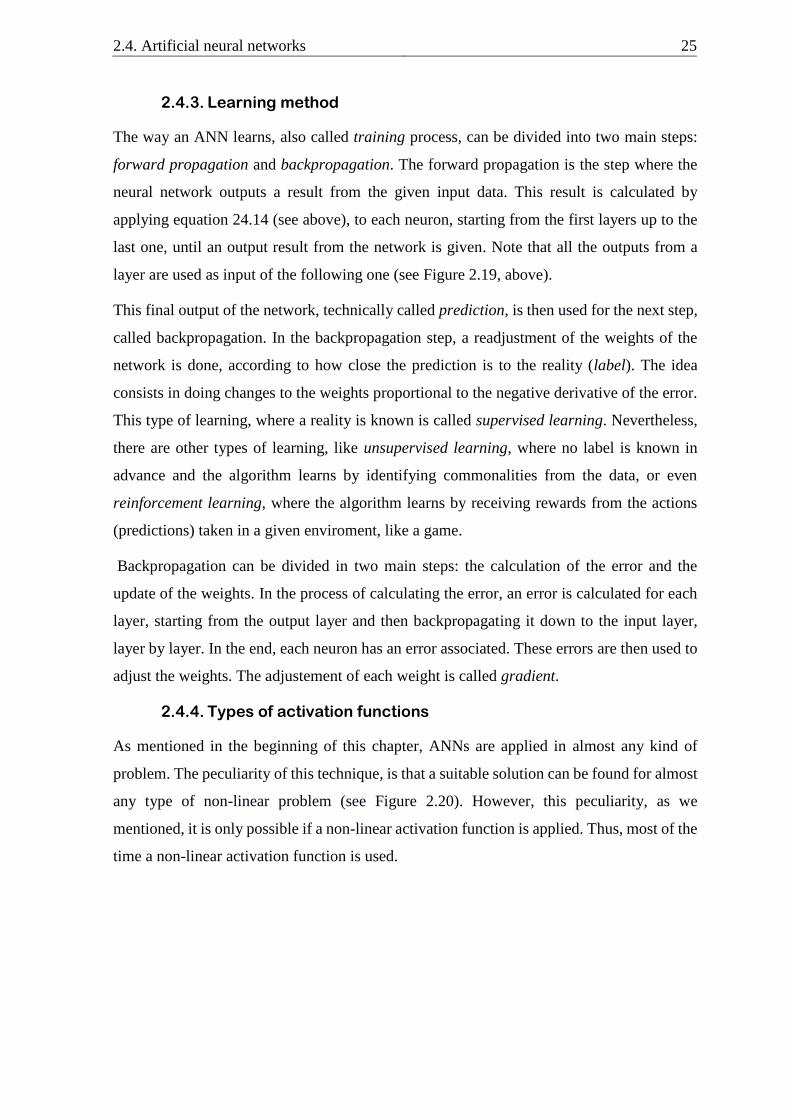
During several years, ANNs had no hidden layers. The reason of that was because no one
knew how to “teach” an ANN with multiple layers. Only after the proof of work in
(Rumelhart et al., 1986), of an algorithm called backpropagation, was when ANNs started
to include hidden layers (see Figure 2.19). In general, ANNs with multiple hidden layers
perform much better than a single layer neural network. Nevertheless, the more layers an
ANN has, the more parameters the ANN needs to learn which in turn increases the difficulty
of the learning/training process. Thus, for each problem a study of different number of layers
and neurons is commonly done.
Figure 2.19 - Representation of a multi-layer neural network.
2.4. Artificial neural networks 25
2.4.3. Learning method
The way an ANN learns, also called training process, can be divided into two main steps:
forward propagation and backpropagation. The forward propagation is the step where the
neural network outputs a result from the given input data. This result is calculated by
applying equation 24.14 (see above), to each neuron, starting from the first layers up to the
last one, until an output result from the network is given. Note that all the outputs from a
layer are used as input of the following one (see Figure 2.19, above).
This final output of the network, technically called prediction, is then used for the next step,
called backpropagation. In the backpropagation step, a readjustment of the weights of the
network is done, according to how close the prediction is to the reality (label). The idea
consists in doing changes to the weights proportional to the negative derivative of the error.
This type of learning, where a reality is known is called supervised learning. Nevertheless,
there are other types of learning, like unsupervised learning, where no label is known in
advance and the algorithm learns by identifying commonalities from the data, or even
reinforcement learning, where the algorithm learns by receiving rewards from the actions
(predictions) taken in a given enviroment, like a game.
Backpropagation can be divided in two main steps: the calculation of the error and the
update of the weights. In the process of calculating the error, an error is calculated for each
layer, starting from the output layer and then backpropagating it down to the input layer,
layer by layer. In the end, each neuron has an error associated. These errors are then used to
adjust the weights. The adjustement of each weight is called gradient.
2.4.4. Types of activation functions
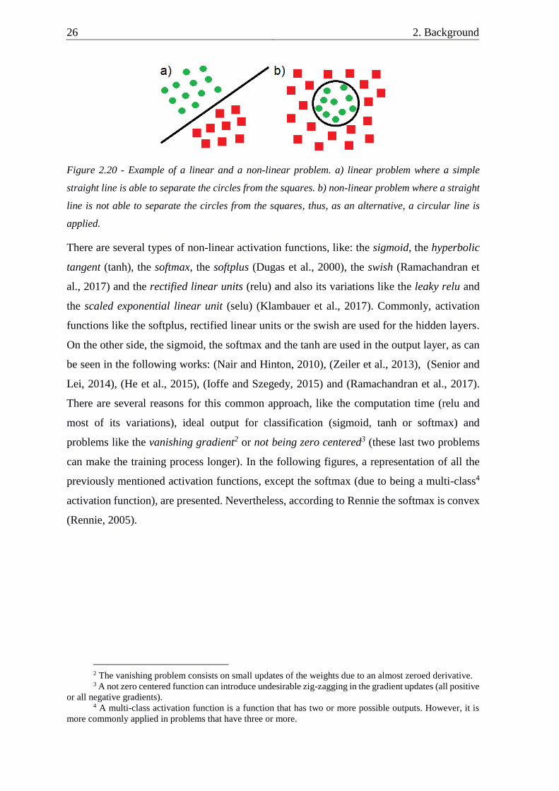
As mentioned in the beginning of this chapter, ANNs are applied in almost any kind of
problem. The peculiarity of this technique, is that a suitable solution can be found for almost
any type of non-linear problem (see Figure 2.20). However, this peculiarity, as we
mentioned, it is only possible if a non-linear activation function is applied. Thus, most of the
time a non-linear activation function is used.
26 2. Background
Figure 2.20 - Example of a linear and a non-linear problem. a) linear problem where a simple
straight line is able to separate the circles from the squares. b) non-linear problem where a straight
line is not able to separate the circles from the squares, thus, as an alternative, a circular line is
applied.
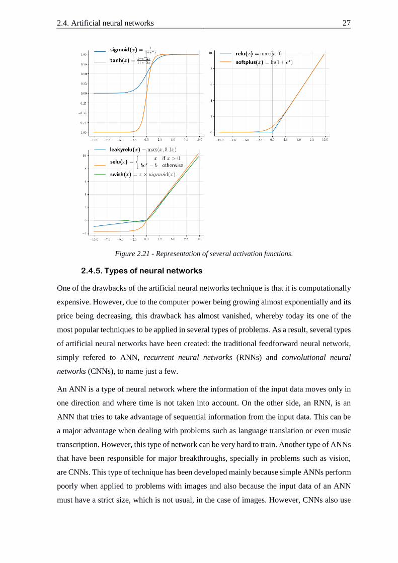
There are several types of non-linear activation functions, like: the sigmoid, the hyperbolic
tangent (tanh), the softmax, the softplus (Dugas et al., 2000), the swish (Ramachandran et
al., 2017) and the rectified linear units (relu) and also its variations like the leaky relu and
the scaled exponential linear unit (selu) (Klambauer et al., 2017). Commonly, activation
functions like the softplus, rectified linear units or the swish are used for the hidden layers.
On the other side, the sigmoid, the softmax and the tanh are used in the output layer, as can
be seen in the following works: (Nair and Hinton, 2010), (Zeiler et al., 2013), (Senior and
Lei, 2014), (He et al., 2015), (Ioffe and Szegedy, 2015) and (Ramachandran et al., 2017).
There are several reasons for this common approach, like the computation time (relu and
most of its variations), ideal output for classification (sigmoid, tanh or softmax) and
problems like the vanishing gradient2 or not being zero centered3 (these last two problems
can make the training process longer). In the following figures, a representation of all the
previously mentioned activation functions, except the softmax (due to being a multi-class4
activation function), are presented. Nevertheless, according to Rennie the softmax is convex
(Rennie, 2005).
2 The vanishing problem consists on small updates of the weights due to an almost zeroed derivative. 3 A not zero centered function can introduce undesirable zig-zagging in the gradient updates (all positive
or all negative gradients). 4 A multi-class activation function is a function that has two or more possible outputs. However, it is
more commonly applied in problems that have three or more.
2.4. Artificial neural networks 27
Figure 2.21 - Representation of several activation functions.
2.4.5. Types of neural networks
One of the drawbacks of the artificial neural networks technique is that it is computationally
expensive. However, due to the computer power being growing almost exponentially and its
price being decreasing, this drawback has almost vanished, whereby today its one of the
most popular techniques to be applied in several types of problems. As a result, several types
of artificial neural networks have been created: the traditional feedforward neural network,
simply refered to ANN, recurrent neural networks (RNNs) and convolutional neural
networks (CNNs), to name just a few.
An ANN is a type of neural network where the information of the input data moves only in
one direction and where time is not taken into account. On the other side, an RNN, is an
ANN that tries to take advantage of sequential information from the input data. This can be
a major advantage when dealing with problems such as language translation or even music
transcription. However, this type of network can be very hard to train. Another type of ANNs
that have been responsible for major breakthroughs, specially in problems such as vision,
are CNNs. This type of technique has been developed mainly because simple ANNs perform
poorly when applied to problems with images and also because the input data of an ANN
must have a strict size, which is not usual, in the case of images. However, CNNs also use
28 2. Background
simple ANNs, but they are only applied after the input data is “parsed/filtered” by
convolutional and (commonly) pooling layers. We can think of both these layers as a way of
extracting the main features of an image. In addition to that, also the pooling layer is
responsible for transforming the input data into a strict size.
2.5. Summary
This chapter presented several important topics of the dissertation. The topics range from
general basics such as sound and music characteristics to more specific concepts such as
deeper analysis of digital signal processing. The chapter also touched on artificial neural
networks.
Remember that, most AMT systems commonly apply methods such as the FFT, referred
above, to a sound signal to be easier in detecting pitches on it. However, these methods have
their own set of problems, namely: missing fundamentals and spectral leakage. Regarding
spectral leakage, a possible solution called windowing could be applied in order to attenuate
the problem. For missing fundamentals, to the best of our knowledge, currently, there is no
known solution. Another important point is that, ANNs are good problem-solvers for almost
any type of complex problem, including automatic music transcription. As a result, we have
applied in this work the FFT and the ANN technique.
In the following chapter, a review of other research works related to single and multi
estimation problems are presented, in order to understand how other authors tackled them.
29
3. Related work
This chapter reviews related works of the AMT field. The review has three main sections:
1) general overview; 2) artificial neural networks and 3) genetic algorithms.
3.1. General overview
The problem of transcribing monophonic music automatically can be considered solved.
However, automatic transcription of polyphonic music is still being researched.
Since the first polyphonic music transcription system (Moorer, 1975), several posterior
related works have been presented. These works have originated the appearance of several
different approaches to the AMT problem. According to Yeh (Yeh, 2008), those approaches
can be classified into two groups: iterative estimation approaches and joint estimation
approaches.
3.1.1. Iterative estimation
An iterative estimation approach consists in finding the most predominant-F0 estimation,
apply the respective cancelation or surpression technique and repeat this process until the
termination condition is met. This approach assumes that per each iteration a dominant
source exists. When this assumption is not met, the iteration process can lead to an
accumulation of errors.
There are two types of cancelation techniques, direct cancellation and cancellation by
spectral models.
Direct cancellation
Direct cancellation applies a single-F0 estimation algorithm to extract the predominant-F0
and then removes all harmonics of the extracted source from the observed input signal. This
technique assumes that the complete removal of the dominant source does not affect the
following estimations. The term “direct” cancellation denotes that the source interaction, as
for example, overlapping partials, are not taken into account.
In (Parsons, 1976) the author applied the Schoroeder’s histogram in order to extract the
predominant-F0s in a two-speaker separation problem. After the first F0 estimation, the
spectral peaks corresponding to its harmonics were excluded before the calculation of the
next histogram. In (Lea, 1992) the author used a method that iteratively extracts the
predominant peak in the summary autocorrelation as an F0 and cancels the estimate in the
30 3. Related work
autocorrelation array. In 1993, in the work (Cheveigné, 1993), the author proposed a time-
domain cancellation model where both iterative and joint approaches were studied. The
iterative cancellation approach was responsible for estimating the predominant F0 by
average magnitude difference function and cancel it by comb filtering. Direct cancellation
was also used on the spectral domain. In (Ortiz-Berenguer et al., 2005), the authors used
spectral patterns trained from previously recorded piano sounds to perform harmonic
matching. The predominant-F0s found were removed iterativelly by means of binary masks
around the matched harmonics in the observed spectrum.
Cancellation by spectral models
In (Klapuri, 2003) the author introduced an algorithm based on harmonicity and spectral
smoothness. In the preprocessing stage a RASTA-like technique (Hermansky and Morgan,
1994) a logarithmic frequency scale is used, to compress the spectral magnitudes and remove
the additive noise. The resulting spectrum is then splitted into multiple frequency bands. F0
weights are calculated on each band by normalizing the sum of their partial amplitudes and
by taking into account the inharmonicity. The predominant weights, from those resulting F0
weights, are then smoothed using an algorithm described in (Klapuri, 2001) and finally
subtracted from the signal spectrum to avoid its corruption after several iterations of direct
cancellation. This way, the overlapping partials still contain energy for the following
sources. This method, which is denominated by bandwise smooth model, uses the moving
average over the amplitudes within one octave band in order to smooth the envelope of an
extracted source. This process is repeated until the maximum weight related to the signal-
to-noise ratio is lower than a certain threshold.
Later on, in (Klapuri, 2005) a perceptually motivated multiple-F0 estimation method is
presented. Initially, subband signals were compressed and an half-wave rectifier was
applied. Harmonic matching is then applied on the summary spectrum. This way, the
predominant F0 is extracted. Then, a 1/k smooth5 is used to smoothen the predominant source
while retaining energy of higher partials for the next iteration. Later on, in (Klapuri, 2006),
the author proposed a spectral model, similar to the previous mentioned 1/k smooth model,
which attempts to generalize a variety of musical instrument sounds.
In (Santoro and Cheng, 2009) the authors presented an algorithm based on Klapuri’s work,
for multiple F0 estimation using the modified discrete cosine transform domain.
5 Partial amplitudes are inversely proportional to the partial index.
3.1. General overview 31
3.1.2. Joint estimation
Nowadays, joint estimation approaches are the most common used approaches for automatic
music transcription systems. According to Benetos et al. (Benetos et al., 2013), those
approaches can be categorized as: feature-based, statistical model-based and spectrogram
factorisation-based.
Feature-based
From all the types of joint approaches, feature-based approaches, are the most currently used
for AMT systems. This can be due to the fact that since the last few years, the field of AI
have grown up significantly.
Regarding AMT, several types of feature-based approaches have been proposed.
In (Yeh, 2008) and (Yeh et al., 2010) the author(s) proposed a frame-based system for
estimating multiple fundamental frequencies (F0s) of polyphonic music signals. This system
is composed of five main tasks: FFT analysis – in this step, each frame is converted to the
time-frequency domain; Noise level estimation – step responsible to detect sinusoids and
noise from the previous analysed data representation; F0 candidate selection – step
responsible for selecting the possible F0s candidates; Jointly F0 evaluation – step
responsible for jointly evaluate the possible combinations from the previously selected F0s;
Polyphony inference – step responsible for estimating the existent notes.
In (Lunaverus, n.d.) the author presents a music transcription system using convolutional
neural networks (CNNs). This system uses what they call Dynamic Q, which, according to
them, is an improved version of the constant-Q transform. Focusing on the AMT problem,
using the constant-Q transform instead of the Short-Time Fourier Transform (STFT) as data
representation should perform better because in the constant-Q transform the frequencies are
spaced with a similar distance to the way that the notes are spaced (in terms of frequency) in
a piano.
In (Bello and Sandler, 2000), the authors proposed a simple polyphonic music transcription
system using a blackboard system with the top-down approach. A blackboard system is
designed to handle complex problems. This technique works as a group of experts trying to
solve a problem in a blackboard in which they only take action when it is related to their area
of expertise. The blackboard system presented contains a hypotheses database, a scheduler
and knowledge sources. One of the knowledge sources is a neural network that is able to
recognize chords in order to adapt the number of notes that the system needs to detect.
32 3. Related work
In (Reis et al., 2008b), the authors proposed an hybrid approach in which it sits between
classical genetic algorithms (GAs) and traditional memetic algorithms. As the authors
explain, genetic algorithms are good for exploring the space but, on the other side, they are
not good enough to refine an already found solution, and that is the reason why they combine
with memetic algorithms.
Statistical model-based
In (Duan et al., 2010), the authors present a multi-F0 estimation system in which a maximum
likelihood approach is used. In this system spectral peaks are detected using a peak detector
described in (Duan et al., 2008). Those peaks are then used to generate F0s candidates. Then,
a greedy search strategy is applied in order to reduce the number of generated F0s candidates.
To finish, an interation process is done in which newly estimated F0s are added, until the
maximum allowed polyphony is reached.
In (Davy et al., 2006) the authors extended the previous work done in (Walmsley et al.,
1998), (Walmsley et al., 1999), (Davy and Godsill, 2002b) and (Davy and Godsill, 2002a)
named in their work, Bayesian harmonic model. Here, the authors assumed the noise as
white, as opposed to one of the previous works, and the inharmonicity parameter took a
multiplicative form. Also a re-design of the Markov Chain Monte Carlo was done. All these
modifications have originated a more robust and efficient (in computational terms) model.
In (Emiya et al., 2010), a multipitch estimator based on the likelihood maximization
principle is presented. This system decomposes the audio signals into a sum of sinusoidal
components and a colored noise. Then, a moving average process is applied to the noise and
the spectral envelope of the partials is modeled by an autoregressive model. The F0 is then
calculated using the Weighted Maximum Likelihood principle. Finally the F0s are jointly
evaluated.
3.2. Artificial Neural Networks 33
Spectrogram factorisation-based
In (Smaragdis and Brown, 2003), the non-negative matrix factorization (NMF) technique
was introduced for the first time in the AMT problem. This technique aims at decomposing
the input signal (into x frequency bins and n frames). Later on, in the work (Cont, 2006),
new rules were added into the NMF update rules as an attempt to improve the performance
of the algorithm. In (Vincent et al., 2010), harmonicity and spectral smoothness constraints
were added in order to reduce octave errors. In (Bertin et al., 2010) a Bayesian framework
for NMF was proposed by the authors. This framework considered each pitch as a model of
Gaussian components in harmonic positions. In (O’Brien and Plumbley, 2017), a refinement
of non-negative matrix decomposition is presented. This model assumed that the
transcription itself was approximately low rank. The idea behind this, as they mention, is
that:“the total number of distinct activation patterns should be relatively small since the
pitch content between adjacent frames shoud be similar”.
3.2. Artificial Neural Networks
In this section several related works that apply ANNs to the AMT field are described. These
works are essential in order to understand the way taken to achieve our final solution.
Additionally, two current state-of-the-art works which are used as a reference, in a following
chapter, to compare our work are also described.
3.2.1. How the training data affects music transcription systems
The goal of the project undertaken by Kelz and Widmer (Kelz and Widmer, 2017) was to
analyze how a dataset used for training a music transcription system, based on ANNs, can
affect their performance. For that purpose, the authors created three different datasets, based
on the MAPS dataset (Emiya, 2008), denominated by FLUID-ISOL, FLUID-COMBI and
MAPS-MUS.
The FLUID-ISOL dataset contains only isolated notes, in the training set, and chords in the
testing set that were created with a synthesizer, using isolated notes and two-note
combinations. The FLUID-COMBI dataset contains chords in the training set, that were
previously created by the authors for the FLUID-ISOL, and isolated notes in the testing set.
The MAPS-MUS dataset, contains pieces of music in both the training set and testing set
(the configuration used is similar to the Configuration 2, described in section 3.2.3).
34 3. Related work
For the experiments, the authors used three different types of ANNs: ConvNet which has the
same architecture as the one used in (Kelz et al., 2016); SmallConvNet, similar to the
ConvNet but smaller; AUNet, based on (Ronneberger et al., 2015).
The experiments carried out were as follows: SmallConvNet with FLUID-ISOL,
SmallConvNet with FLUID-COMBI and ConvNet and AUNet with MAPS-MUS.
In the experiment with SmallConvNet/FLUID-COMBI the results were positive, in sense
that the ANN was able to transcribe most of the piano midi notes with an accuracy higher
than 80% (the accuracy is calculated according to MIREX). On the other side, in
SmallConvNet/FLUID-ISOL, as the authors mention, the ANN could not generalize the
features learnt from the isolated notes in order to be able to identify chords. Most of the
piano midi notes had an accuracy bellow 20%. In the last experiments, the ConvNet/MAPS-
MUS and AUNET/MAPS-MUS, the authors compared their performance in two different
case scenarios: shared notes and unshared notes.
The first scenario, shared notes, contains notes and chords that appear in both the training
set and the testing set. On the second scenario, the unshared notes, the testing set contains
different notes and chords from the training set.
The results on the first scenario, shared notes, were positive. Both ANNs were able to
surpass 60% of accuracy in most piano notes. However in the second scenario, unshared
notes, the accuracy in both ANNs dropped significantly, and most of the notes had an
accuracy bellow 20%, some even got an accuracy of 0%.
Based in these results, the authors concluded that certain neural networks have difficulty to
generalize the leaned features, leading to poor results when it consists in transcribing unseen
notes or chords.
To conclude, the authors suggest that a possible solution could be the use of source
separation to decompose the input signal into its constituent parts but, as they mention,
source separation, is still an ongoing research field. The purpose of this technique is to
decompose a mixture of sounds. An example of that could be when we are in a noisy
environment, as a disco, and we focus on a desirable conversation, ignoring the surrounding
noise.
3.2. Artificial Neural Networks 35
3.2.2. Feature learning and 88 classifiers
In (Zalani and Mittal, 2014), the authors implemented a polyphonic music transcription
system based on deep learning techniques. Their chosen dataset is the MAPS, where they
used six pieces of music of nearly 30 minutes each for the training set and four different
pieces of music of around 15 minutes for the testing set. These authors used the following
two techniques in succession: feature learning, which is like a recursive restricted Boltzmann
machine and 88 support vector machines (SVMs).
The first technique, feature learning, is an unsupervised system that is in charge of extracting
features coming from the music, like temporal dependencies among different notes, whose
purpose is to help the SVMs afterwards.
The second technique, the 88 SVMs, are supervised systems, in which each one is
responsible for transcribing only one note. These SVMs were trained with the STFT coming
from the music and with the data extracted from the feature learning step.
The authors also mention that a smoothing algorithm, called Hidden Markov Model (HMM),
was applied to improve their accuracy results from 52,07% to 63,10%.
3.2.3. Comparison of different types of Neural Networks
In (Sigtia et al., 2016a), the authors have created a supervised neural network model for
polyphonic piano music transcription. As they mention, the architecture of their model is a
combination of an acoustic model and a music language model. This type of architecture is
a common one in another field, called speech recognition. The acoustic model is responsible
for detecting the notes in each frame of the piece of music and the music language model is
the one responsible for making correlations between the output of the previous model over
time.
For the acoustic model, three different neural networks were experimented by the authors:
an artificial neural network, a recurrent neural network and a convolutional neural network
(CNN). All those neural networks were trained using the constant-Q transform.
For the music language model, the authors also experimented three different types of neural
networks: the generative RNN, the Neural Autoregressive Distribution Estimator (NADE)
(Larochelle and Murray, 2011) and the RNN-NADE.
The experiments were done with two different datasets, both of them based on MAPS called
Configuration 1 and Configuration 2.
36 3. Related work
The Configuration 1, dataset is a group of four folds of different pieces of music, each one
with 216 pieces of music in the training set and 54 pieces of music in the testing set (more
information can be found in (Sigtia et al., 2016b)).
The Configuration 2 dataset contains 210 pieces in the training set (180 were used for
training and 30 for evaluation) and 60 pieces in the testing set. This last dataset can be
considered more realistic, as the authors mention, because the pieces of music in the testing
set have been recorded from a different piano.
In order to improve their results, the authors applied three different post processing methods,
a thresholding method, a HMM and a hybrid architecture.
The results obtained using both datasets, Configuration 1 and Configuration 2 show that,
CNNs yields the best performance in all evaluation metrics (f-measure). In Configuration 1
the CNN reached between 73,57%-74,45% in f-measure frame-based and 65,35%-67% in f-
measure onset only (further details regarding the evaluation metrics can be seen in section
6.2) . The ANN, on the other side, reached between 67,54%-68,32% in frame-based and
60,02-63,18%. In Configuration 2, the CNN reached 64,14% in frame-based and 54,89% in
onset only. The DNN reached 59,91% in frame-based and 49,43% in onset only.
3.2.4. Exploring the limits of simple architectures
There are some transcription systems whose architecture is composed by two main parts:
acoustic model and the music language model. An example of this can be found in the work
mentioned above, in section 3.2.3. However, in (Kelz et al., 2016) the authors focus only on
the acoustic model, in order to explore the limitations of simple architectures for music
transcription systems. They compared three different types of ANNs for the acoustic model:
ANN, CNN and a fully convolutional neural network which is called AllConv.
The datasets chosen by the authors are the Configuration 1 and a similar dataset to
Configuration 2, from the work referred above (Section 3.2.3).
In order to get the best possible results, the authors have focused their efforts in two sets of
preliminary experiments, types of representation and hyperparameters6 search and
optimization techniques. In the first set, the one that the authors called types of
representation, they did several experiments in order to determine what should be the best
data representation for training the ANNs. For these experiments, the authors used two
6 Hyperparameters are parameters that need to be predefined before the training phase of the ANNs.
3.3. Genetic algorithms 37
different types of ANNs: a perceptrons network and a shallow net. In addition to that, the
authors experimented four different types of data representation: spectrograms with linearly
spaced bins (S), spectrograms with logarithmically spaced bins (LS), spectrograms with
logarithmically spaced bins and logarithmically scalled magnitude (LM) and constant-Q-
transform. After analyzing the results, they concluded that, for the perceptrons network, the
best type of data representation was the S type and that, for the shallow net, the best was the
LM type.
In the second set of experiments, the authors conducted several experiments in order to
understand which type of hyperparameters or technique have more influence in the results
so that the authors could know where to focus. With the obtained results, the authors
concludes that the most influential hyperparameter is the learning rate. The learning rate is
the parameter that determines how much the weights are updated each iteration.
To finish the study, after studying several preliminary experiments, mentioned above, they
conducted their final setup experiment. The results were positive. In Configuration 1 the
CNN was able to reach a f-measure of 79,33% and the ANN 73,11%. In the second dataset,
Configuration 2, the CNN reached a f-measure of 70,60% and the ANN 65,15%.
As the authors mention, simpler arquitecture approaches, that is to say, those that use only
an acoustic model, are able to reach or surpass more complex arquitectures in frame
transcription, those with an acoustic model and a music language model.
3.3. Genetic algorithms
So far, we have seen multiple works, regarding AMT, using mainly artificial neural
networks. In this section, another type of technique of the AI field is discussed, genetic
algorithms (GAs), which promise positive and efficient results to the AMT problem.
The following research works have applied this technique to this problem, (Reis et al.,
2008a) in which the authors evolved a harmonic structure using genetic algorithms; (Reis et
al., 2012) where the authors used genetic algorithms in combination with an onset detection
algorithm; and (Leite et al., 2016), in which the authors applied for the first time cartesian
genetic programming to the AMT problem.
Genetic algorithms are a different technique from neural networks. This technique is based
on the theory of evolution, consisting in evolving a population of individuals. Each
individual is a potential solution for the problem. The process of evolving a population
38 3. Related work
consists in applying two types of operators, called recombination and mutation, to the
population in order to find the best individual for the problem. The recombination operator
consists in combining characteristics from different individuals. Mutation consist in
randomly changing characteristics from the individuals.
To be able to find the best solution, it is also important to specify two main components: a
fitness function, used to assess the quality of each individual, and a selection method, used
to stochastically select the best individuals.
A description of several works that apply genetic algorithms and as well had a major
influence on our work, are explained in the following topics.
3.3.1. Reducing the search space by using a better initialization
method
GAs can find effective solutions for almost any kind of problem. However, often, a
considerable amount of time is needed to find a good solution, be it because the search space
is extremely vast or because the evaluation step is computationally demanding.
In AMT, the search space is extremely vast, which makes the application of GAs in this
problem very tough. However, if we could be able to “reduce” the search space, of the AMT
problem, that disadvantage would be alleviated. And that was the focus in (Reis et al., 2007).
Of course, reducing the search space is not possible. However, it is possible to give a starting
point closer to the target solution, which in turn reduces the number of generations necessary
to find the target solution.
In order to give a better starting point that could be closer to the target solution, the authors
have initialized the first population of the GAs with the most likely notes in a given song.
Those likely notes were discovered by analyzing the frequencies of a signal. In the end, the
frequencies with the highest picks in the signal are matched each one with the corresponding
note(s), giving as a result the likely notes.
Another relevant point that must be mentioned about this work, is the way of evaluating an
individual. The authors created a synthesizer that was responsible to generate an audio from
each individual. Then, the resulted audios, were compared with the original sound in the
fitness function, whereas the more similar the generated audio were to the original one, the
better the individual was considered.
3.3. Genetic algorithms 39
3.3.2. Combining genetic algorithms with an onset detection
algorithm
In (Reis, 2012), the author has proven that genetic algorithms can reach state-of-the-art
results in the AMT problem, by overcoming all the current obstacles regarding this
technique. In order to overcome those problems, the author has elaborated a transcription
system in which three different steps must be taken into account in order to complete the
process: audio segmentation, transcription step and adjust note duration.
The first step, audio segmentation, consists in a note onset detection algorithm (Martins,
2008), which is fundamental because the detected onsets are used, afterwards, to split the
song in several segments. Those resulting segments of the song, are then used in the
transcription step.
The transcription step is in charge of transcribing each segment of the song. As mentioned
in the work above, an ideal initialization of the population has a positive impact on the
results. Taking that into consideration, the authors used a similar process of initializing the
population with the likely notes in a given song (based on the most relevant frequencies
contained on it).
To finish, in the third step, to adjust note duration, a Hill-Climber algorithm is used. This
algorithm is responsible for transversing all musical notes and, then, the duration of each
note is augmented 50 miliseconds. From all those notes, if some note overlaps another one,
both notes are merged (this process can be repeated if the quality of the individual gets
improved).
3.3.3. Using cartesian genetic programming to evolve several
classifiers
Cartesian genetic programming (CGP) is a recent variation of genetic algorithms proposed
by Julian Miller in (Miller and Thomson, 2000). Generally speaking this technique is a
simple integer representation of a program in the form of directed graph. In non technical
terms, we can describe this as a lookup table.
The genotypes in CGP are just a list of integers where their primitives and their connections
are represented. As for example, for a genotype as follows “3 1 4 -> 6”: 3 represents a
reference to the function that will be applied to the input data; 1 and 4 represents both a
reference to the input data of that function; 6 represents the output result of that function,
which can afterwards be used as input data for other genotypes.
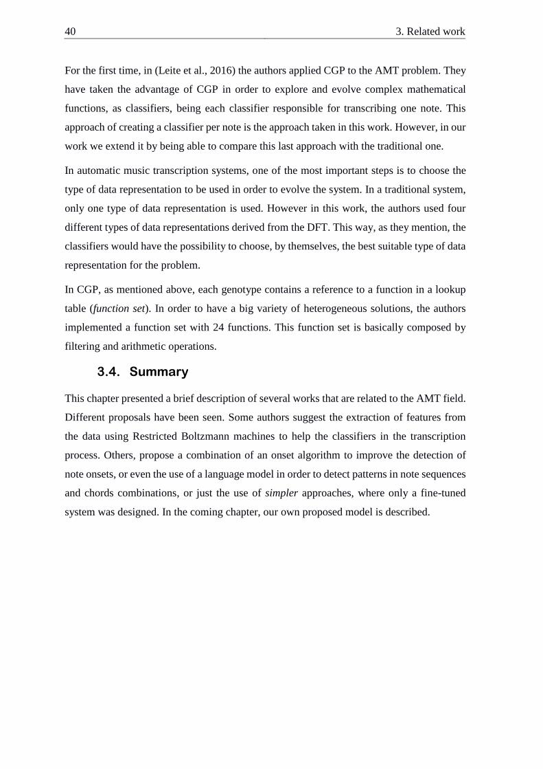
40 3. Related work
For the first time, in (Leite et al., 2016) the authors applied CGP to the AMT problem. They
have taken the advantage of CGP in order to explore and evolve complex mathematical
functions, as classifiers, being each classifier responsible for transcribing one note. This
approach of creating a classifier per note is the approach taken in this work. However, in our
work we extend it by being able to compare this last approach with the traditional one.
In automatic music transcription systems, one of the most important steps is to choose the
type of data representation to be used in order to evolve the system. In a traditional system,
only one type of data representation is used. However in this work, the authors used four
different types of data representations derived from the DFT. This way, as they mention, the
classifiers would have the possibility to choose, by themselves, the best suitable type of data
representation for the problem.
In CGP, as mentioned above, each genotype contains a reference to a function in a lookup
table (function set). In order to have a big variety of heterogeneous solutions, the authors
implemented a function set with 24 functions. This function set is basically composed by
filtering and arithmetic operations.
3.4. Summary
This chapter presented a brief description of several works that are related to the AMT field.
Different proposals have been seen. Some authors suggest the extraction of features from
the data using Restricted Boltzmann machines to help the classifiers in the transcription
process. Others, propose a combination of an onset algorithm to improve the detection of
note onsets, or even the use of a language model in order to detect patterns in note sequences
and chords combinations, or just the use of simpler approaches, where only a fine-tuned
system was designed. In the coming chapter, our own proposed model is described.
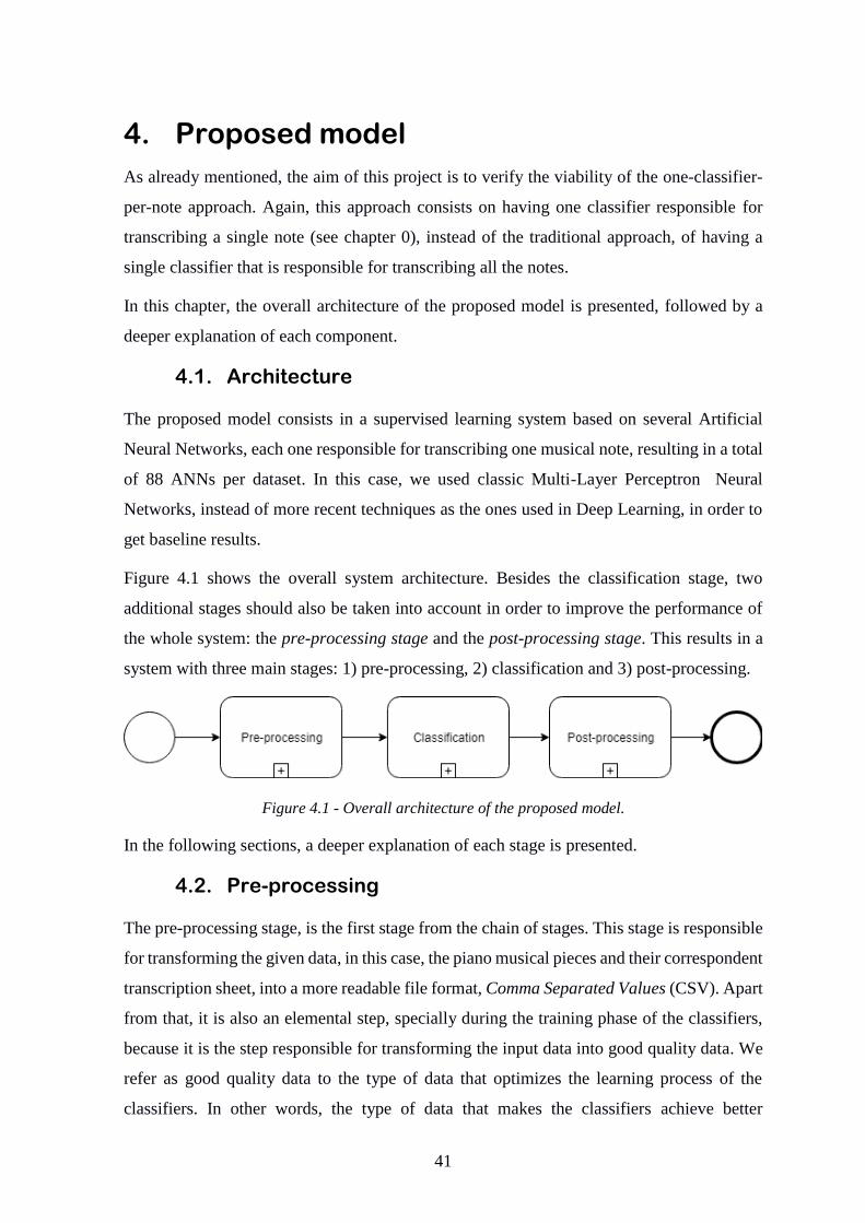
41
4. Proposed model
As already mentioned, the aim of this project is to verify the viability of the one-classifier-
per-note approach. Again, this approach consists on having one classifier responsible for
transcribing a single note (see chapter 0), instead of the traditional approach, of having a
single classifier that is responsible for transcribing all the notes.
In this chapter, the overall architecture of the proposed model is presented, followed by a
deeper explanation of each component.
4.1. Architecture
The proposed model consists in a supervised learning system based on several Artificial
Neural Networks, each one responsible for transcribing one musical note, resulting in a total
of 88 ANNs per dataset. In this case, we used classic Multi-Layer Perceptron Neural
Networks, instead of more recent techniques as the ones used in Deep Learning, in order to
get baseline results.
Figure 4.1 shows the overall system architecture. Besides the classification stage, two
additional stages should also be taken into account in order to improve the performance of
the whole system: the pre-processing stage and the post-processing stage. This results in a
system with three main stages: 1) pre-processing, 2) classification and 3) post-processing.
Figure 4.1 - Overall architecture of the proposed model.
In the following sections, a deeper explanation of each stage is presented.
4.2. Pre-processing
The pre-processing stage, is the first stage from the chain of stages. This stage is responsible
for transforming the given data, in this case, the piano musical pieces and their correspondent
transcription sheet, into a more readable file format, Comma Separated Values (CSV). Apart
from that, it is also an elemental step, specially during the training phase of the classifiers,
because it is the step responsible for transforming the input data into good quality data. We
refer as good quality data to the type of data that optimizes the learning process of the
classifiers. In other words, the type of data that makes the classifiers achieve better
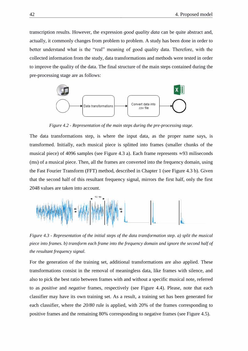
42 4. Proposed model
transcription results. However, the expression good quality data can be quite abstract and,
actually, it commonly changes from problem to problem. A study has been done in order to
better understand what is the “real” meaning of good quality data. Therefore, with the
collected information from the study, data transformations and methods were tested in order
to improve the quality of the data. The final structure of the main steps contained during the
pre-processing stage are as follows:
Figure 4.2 - Representation of the main steps during the pre-processing stage.
The data transformations step, is where the input data, as the proper name says, is
transformed. Initially, each musical piece is splitted into frames (smaller chunks of the
musical piece) of 4096 samples (see Figure 4.3 a). Each frame represents ≈93 miliseconds
(ms) of a musical piece. Then, all the frames are converted into the frequency domain, using
the Fast Fourier Transform (FFT) method, described in Chapter 1 (see Figure 4.3 b). Given
that the second half of this resultant frequency signal, mirrors the first half, only the first
2048 values are taken into account.
Figure 4.3 - Representation of the initial steps of the data transformation step. a) split the musical
piece into frames. b) transform each frame into the frequency domain and ignore the second half of
the resultant frequency signal.
For the generation of the training set, additional transformations are also applied. These
transformations consist in the removal of meaningless data, like frames with silence, and
also to pick the best ratio between frames with and without a specific musical note, referred
to as positive and negative frames, respectively (see Figure 4.4). Please, note that each
classifier may have its own training set. As a result, a training set has been generated for
each classifier, where the 20/80 rule is applied, with 20% of the frames corresponding to
positive frames and the remaining 80% corresponding to negative frames (see Figure 4.5).
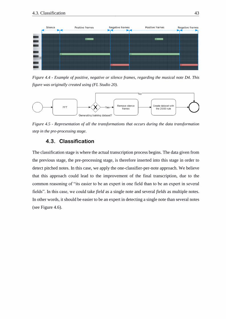
4.3. Classification 43
Figure 4.4 - Example of positive, negative or silence frames, regarding the musical note D4. This
figure was originally created using (FL Studio 20).
Figure 4.5 - Representation of all the transformations that occurs during the data transformation
step in the pre-processing stage.
4.3. Classification
The classification stage is where the actual transcription process begins. The data given from
the previous stage, the pre-processing stage, is therefore inserted into this stage in order to
detect pitched notes. In this case, we apply the one-classifier-per-note approach. We believe
that this approach could lead to the improvement of the final transcription, due to the
common reasoning of “its easier to be an expert in one field than to be an expert in several
fields”. In this case, we could take field as a single note and several fields as multiple notes.
In other words, it should be easier to be an expert in detecting a single note than several notes
(see Figure 4.6).
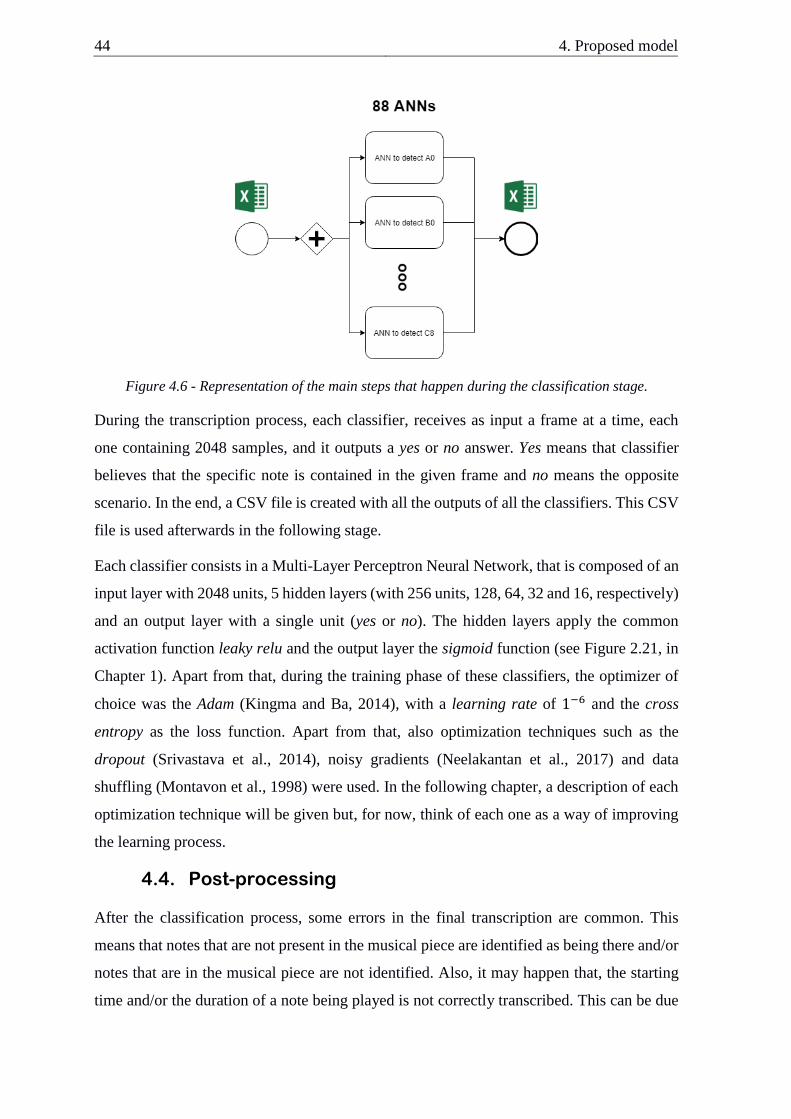
44 4. Proposed model
Figure 4.6 - Representation of the main steps that happen during the classification stage.
During the transcription process, each classifier, receives as input a frame at a time, each
one containing 2048 samples, and it outputs a yes or no answer. Yes means that classifier
believes that the specific note is contained in the given frame and no means the opposite
scenario. In the end, a CSV file is created with all the outputs of all the classifiers. This CSV
file is used afterwards in the following stage.
Each classifier consists in a Multi-Layer Perceptron Neural Network, that is composed of an
input layer with 2048 units, 5 hidden layers (with 256 units, 128, 64, 32 and 16, respectively)
and an output layer with a single unit (yes or no). The hidden layers apply the common
activation function leaky relu and the output layer the sigmoid function (see Figure 2.21, in
Chapter 1). Apart from that, during the training phase of these classifiers, the optimizer of
choice was the Adam (Kingma and Ba, 2014), with a learning rate of 1−6 and the cross
entropy as the loss function. Apart from that, also optimization techniques such as the
dropout (Srivastava et al., 2014), noisy gradients (Neelakantan et al., 2017) and data
shuffling (Montavon et al., 1998) were used. In the following chapter, a description of each
optimization technique will be given but, for now, think of each one as a way of improving
the learning process.
4.4. Post-processing
After the classification process, some errors in the final transcription are common. This
means that notes that are not present in the musical piece are identified as being there and/or
notes that are in the musical piece are not identified. Also, it may happen that, the starting
time and/or the duration of a note being played is not correctly transcribed. This can be due
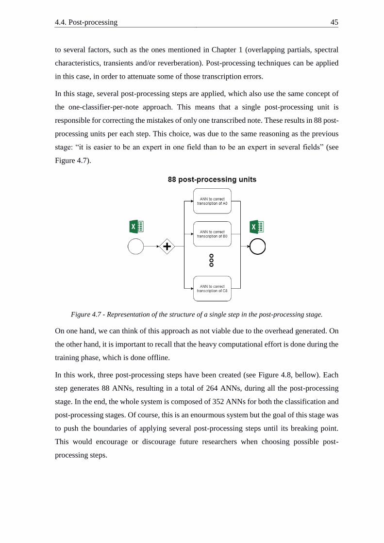
4.4. Post-processing 45
to several factors, such as the ones mentioned in Chapter 1 (overlapping partials, spectral
characteristics, transients and/or reverberation). Post-processing techniques can be applied
in this case, in order to attenuate some of those transcription errors.
In this stage, several post-processing steps are applied, which also use the same concept of
the one-classifier-per-note approach. This means that a single post-processing unit is
responsible for correcting the mistakes of only one transcribed note. These results in 88 post-
processing units per each step. This choice, was due to the same reasoning as the previous
stage: “it is easier to be an expert in one field than to be an expert in several fields” (see
Figure 4.7).
Figure 4.7 - Representation of the structure of a single step in the post-processing stage.
On one hand, we can think of this approach as not viable due to the overhead generated. On
the other hand, it is important to recall that the heavy computational effort is done during the
training phase, which is done offline.
In this work, three post-processing steps have been created (see Figure 4.8, bellow). Each
step generates 88 ANNs, resulting in a total of 264 ANNs, during all the post-processing
stage. In the end, the whole system is composed of 352 ANNs for both the classification and
post-processing stages. Of course, this is an enourmous system but the goal of this stage was
to push the boundaries of applying several post-processing steps until its breaking point.
This would encourage or discourage future researchers when choosing possible post-
processing steps.
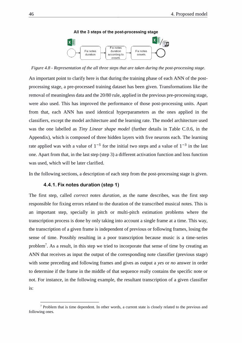
46 4. Proposed model
Figure 4.8 - Representation of the all three steps that are taken during the post-processing stage.
An important point to clarify here is that during the training phase of each ANN of the post-
processing stage, a pre-processed training dataset has been given. Transformations like the
removal of meaningless data and the 20/80 rule, applied in the previous pre-processing stage,
were also used. This has improved the performance of those post-processing units. Apart
from that, each ANN has used identical hyperparameters as the ones applied in the
classifiers, except the model architecture and the learning rate. The model architecture used
was the one labelled as Tiny Linear shape model (further details in Table C.0.6, in the
Appendix), which is composed of three hidden layers with five neurons each. The learning
rate applied was with a value of 1−5 for the initial two steps and a value of 1−3 in the last
one. Apart from that, in the last step (step 3) a different activation function and loss function
was used, which will be later clarified.
In the following sections, a description of each step from the post-processing stage is given.
4.4.1. Fix notes duration (step 1)
The first step, called correct notes duration, as the name describes, was the first step
responsible for fixing errors related to the duration of the transcribed musical notes. This is
an important step, specially in pitch or multi-pitch estimation problems where the
transcription process is done by only taking into account a single frame at a time. This way,
the transcription of a given frame is independent of previous or following frames, losing the
sense of time. Possibly resulting in a poor transcription because music is a time-series
problem7. As a result, in this step we tried to incorporate that sense of time by creating an
ANN that receives as input the output of the corresponding note classifier (previous stage)
with some preceding and following frames and gives as output a yes or no answer in order
to determine if the frame in the middle of that sequence really contains the specific note or
not. For instance, in the following example, the resultant transcription of a given classifier
is:
7 Problem that is time dependent. In other words, a current state is closely related to the previous and
following ones.
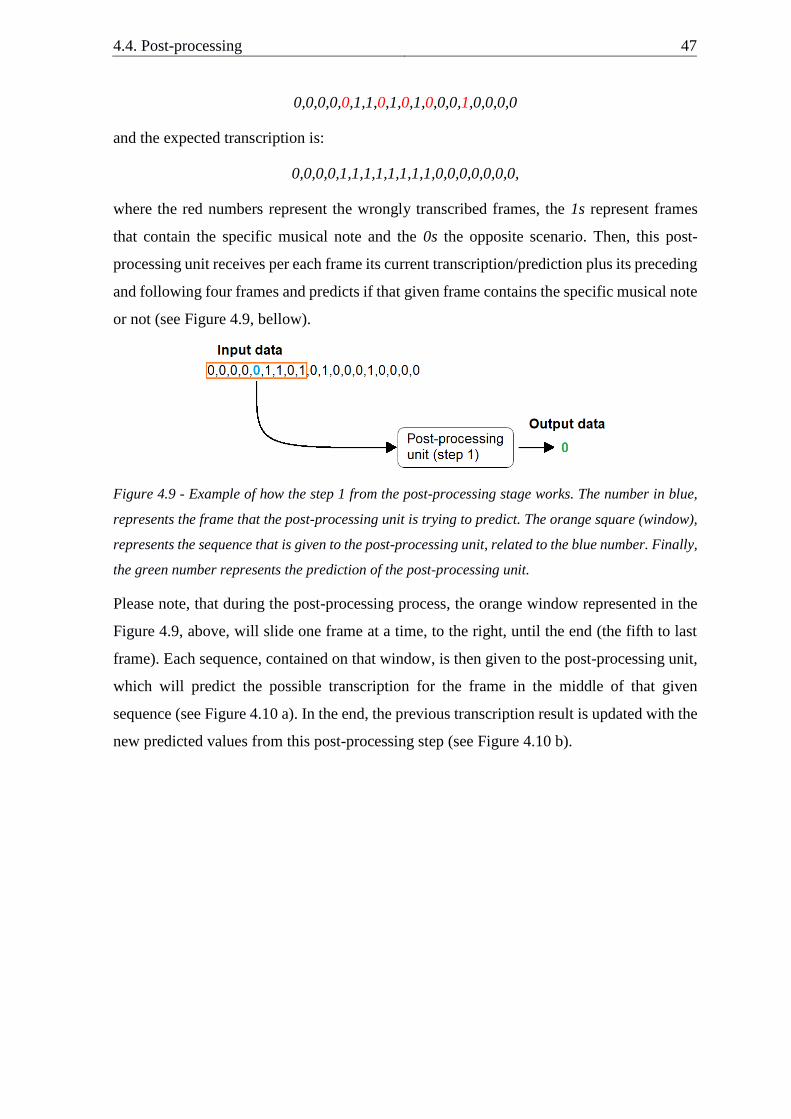
4.4. Post-processing 47
0,0,0,0,0,1,1,0,1,0,1,0,0,0,1,0,0,0,0
and the expected transcription is:
0,0,0,0,1,1,1,1,1,1,1,1,0,0,0,0,0,0,0,
where the red numbers represent the wrongly transcribed frames, the 1s represent frames
that contain the specific musical note and the 0s the opposite scenario. Then, this post-
processing unit receives per each frame its current transcription/prediction plus its preceding
and following four frames and predicts if that given frame contains the specific musical note
or not (see Figure 4.9, bellow).
Figure 4.9 - Example of how the step 1 from the post-processing stage works. The number in blue,
represents the frame that the post-processing unit is trying to predict. The orange square (window),
represents the sequence that is given to the post-processing unit, related to the blue number. Finally,
the green number represents the prediction of the post-processing unit.
Please note, that during the post-processing process, the orange window represented in the
Figure 4.9, above, will slide one frame at a time, to the right, until the end (the fifth to last
frame). Each sequence, contained on that window, is then given to the post-processing unit,
which will predict the possible transcription for the frame in the middle of that given
sequence (see Figure 4.10 a). In the end, the previous transcription result is updated with the
new predicted values from this post-processing step (see Figure 4.10 b).
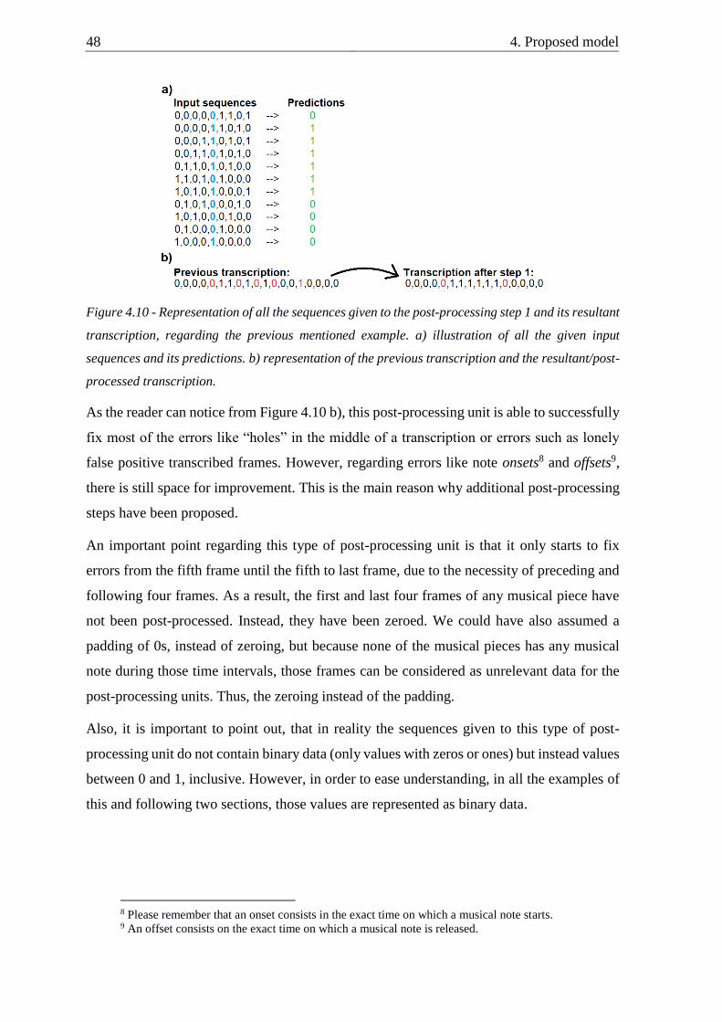
48 4. Proposed model
Figure 4.10 - Representation of all the sequences given to the post-processing step 1 and its resultant
transcription, regarding the previous mentioned example. a) illustration of all the given input
sequences and its predictions. b) representation of the previous transcription and the resultant/post-
processed transcription.
As the reader can notice from Figure 4.10 b), this post-processing unit is able to successfully
fix most of the errors like “holes” in the middle of a transcription or errors such as lonely
false positive transcribed frames. However, regarding errors like note onsets8 and offsets9,
there is still space for improvement. This is the main reason why additional post-processing
steps have been proposed.
An important point regarding this type of post-processing unit is that it only starts to fix
errors from the fifth frame until the fifth to last frame, due to the necessity of preceding and
following four frames. As a result, the first and last four frames of any musical piece have
not been post-processed. Instead, they have been zeroed. We could have also assumed a
padding of 0s, instead of zeroing, but because none of the musical pieces has any musical
note during those time intervals, those frames can be considered as unrelevant data for the
post-processing units. Thus, the zeroing instead of the padding.
Also, it is important to point out, that in reality the sequences given to this type of post-
processing unit do not contain binary data (only values with zeros or ones) but instead values
between 0 and 1, inclusive. However, in order to ease understanding, in all the examples of
this and following two sections, those values are represented as binary data.
8 Please remember that an onset consists in the exact time on which a musical note starts. 9 An offset consists on the exact time on which a musical note is released.

4.4. Post-processing 49
4.4.2. Fix notes duration according to onsets (step 2)
In order to improve the current transcription, regarding problems like note onsets and offsets,
an additional post-processing step has been created. This new step is similar to the previous
one since it receives as input a sequence of transcribed frames from the previous post-
processing step (step 1). However, in this step, two additional sequences are also given as
input. One sequence, with the initial transcription created by the classifiers and a second one,
based on the output of an onset algorithm (Martins, 2008) (see Figure 4.11, bellow).
Figure 4.11 - Representation of the three types of sequences, received by the post-processing step 2.
The idea behind the concept of receiving both sequences of previous transcribed frames of
step 1 and the initial transcription from the classifiers was figured out based on the article
(Zhang et al., 2016). In this article, the authors have proposed a system for creating new
images based on two stages, instead of just one, which was the common approach at that
time. This second stage would receives the original input given to the first stage plus the
predicted outcome from that initial stage. In the end, they were able to improve their results.
In this case, we considered the original input as the first input received from the post-
processing stage, the one created by the classifiers, and the predicted output as the predicted
transcription from the previous post-processing step (step 1).
In addition to that, a sequence of the output of an onset algorithm was also given. This
algorithm has the main goal of detecting musical note onsets contained in a musical piece.
Of course, this algorithm is not 100% accurate, but its performance is good (around ~78%
of f-measure value). However, this algorithm is not able to distinguish between onsets of
different musical notes (see Figure 4.12, for an example).
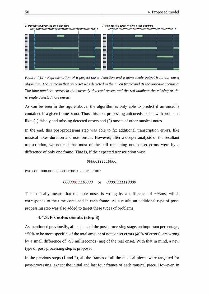
50 4. Proposed model
Figure 4.12 - Representation of a perfect onset detection and a more likely output from our onset
algorithm. The 1s mean that an onset was detected in the given frame and 0s the opposite scenario.
The blue numbers represent the correctly detected onsets and the red numbers the missing or the
wrongly detected note onsets.
As can be seen in the figure above, the algorithm is only able to predict if an onset is
contained in a given frame or not. Thus, this post-processing unit needs to deal with problems
like: (1) falsely and missing detected onsets and (2) onsets of other musical notes.
In the end, this post-processing step was able to fix additional transcription errors, like
musical notes duration and note onsets. However, after a deeper analysis of the resultant
transcription, we noticed that most of the still remaining note onset errors were by a
difference of only one frame. That is, if the expected transcription was:
00000111110000,
two common note onset errors that occur are:
00000011110000 or 00001111110000
This basically means that the note onset is wrong by a difference of ~93ms, which
corresponds to the time contained in each frame. As a result, an additional type of post-
processing step was also added to target these types of problems.
4.4.3. Fix notes onsets (step 3)
As mentioned previouslly, after step 2 of the post-processing stage, an important percentage,
~50% to be more specific, of the total amount of note onset errors (40% of errors), are wrong
by a small difference of ~93 milliseconds (ms) of the real onset. With that in mind, a new
type of post-processing step is proposed.
In the previous steps (1 and 2), all the frames of all the musical pieces were targetted for
post-processing, except the initial and last four frames of each musical piece. However, in
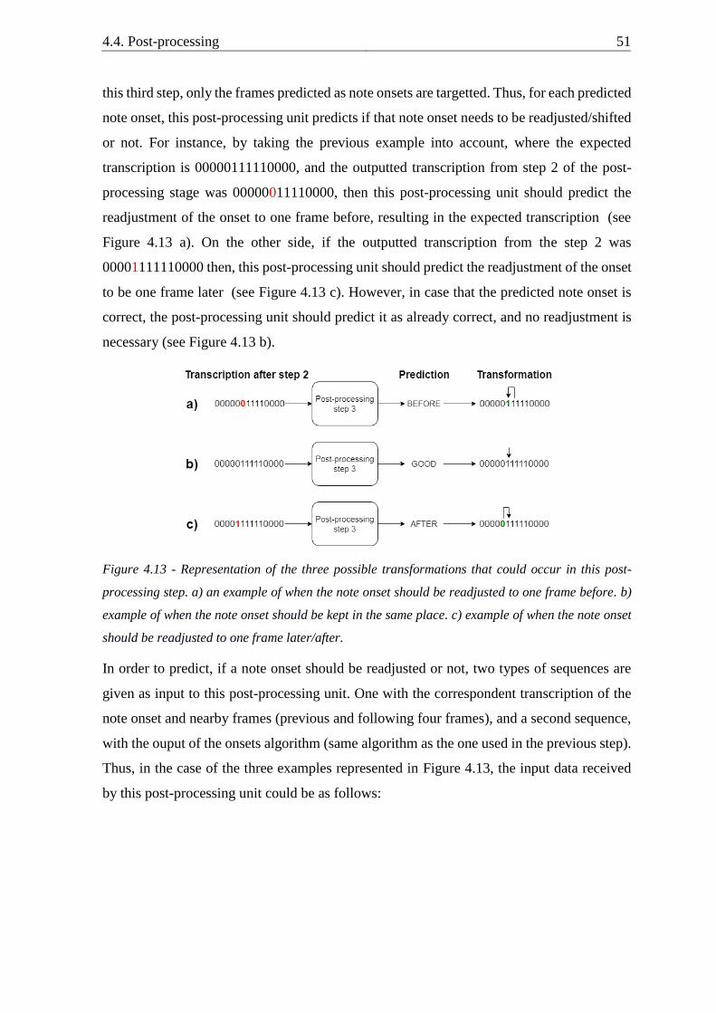
4.4. Post-processing 51
this third step, only the frames predicted as note onsets are targetted. Thus, for each predicted
note onset, this post-processing unit predicts if that note onset needs to be readjusted/shifted
or not. For instance, by taking the previous example into account, where the expected
transcription is 00000111110000, and the outputted transcription from step 2 of the post-
processing stage was 00000011110000, then this post-processing unit should predict the
readjustment of the onset to one frame before, resulting in the expected transcription (see
Figure 4.13 a). On the other side, if the outputted transcription from the step 2 was
00001111110000 then, this post-processing unit should predict the readjustment of the onset
to be one frame later (see Figure 4.13 c). However, in case that the predicted note onset is
correct, the post-processing unit should predict it as already correct, and no readjustment is
necessary (see Figure 4.13 b).
Figure 4.13 - Representation of the three possible transformations that could occur in this post-
processing step. a) an example of when the note onset should be readjusted to one frame before. b)
example of when the note onset should be kept in the same place. c) example of when the note onset
should be readjusted to one frame later/after.
In order to predict, if a note onset should be readjusted or not, two types of sequences are
given as input to this post-processing unit. One with the correspondent transcription of the
note onset and nearby frames (previous and following four frames), and a second sequence,
with the ouput of the onsets algorithm (same algorithm as the one used in the previous step).
Thus, in the case of the three examples represented in Figure 4.13, the input data received
by this post-processing unit could be as follows:
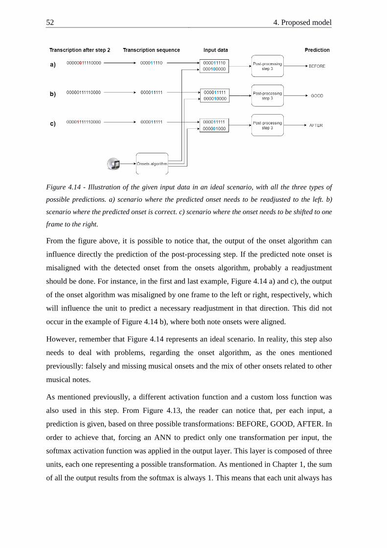
52 4. Proposed model
Figure 4.14 - Illustration of the given input data in an ideal scenario, with all the three types of
possible predictions. a) scenario where the predicted onset needs to be readjusted to the left. b)
scenario where the predicted onset is correct. c) scenario where the onset needs to be shifted to one
frame to the right.
From the figure above, it is possible to notice that, the output of the onset algorithm can
influence directly the prediction of the post-processing step. If the predicted note onset is
misaligned with the detected onset from the onsets algorithm, probably a readjustment
should be done. For instance, in the first and last example, Figure 4.14 a) and c), the output
of the onset algorithm was misaligned by one frame to the left or right, respectively, which
will influence the unit to predict a necessary readjustment in that direction. This did not
occur in the example of Figure 4.14 b), where both note onsets were aligned.
However, remember that Figure 4.14 represents an ideal scenario. In reality, this step also
needs to deal with problems, regarding the onset algorithm, as the ones mentioned
previouslly: falsely and missing musical onsets and the mix of other onsets related to other
musical notes.
As mentioned previouslly, a different activation function and a custom loss function was
also used in this step. From Figure 4.13, the reader can notice that, per each input, a
prediction is given, based on three possible transformations: BEFORE, GOOD, AFTER. In
order to achieve that, forcing an ANN to predict only one transformation per input, the
softmax activation function was applied in the output layer. This layer is composed of three
units, each one representing a possible transformation. As mentioned in Chapter 1, the sum
of all the output results from the softmax is always 1. This means that each unit always has
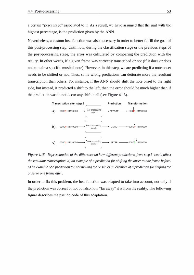
4.4. Post-processing 53
a certain “percentage” associated to it. As a result, we have assumed that the unit with the
highest percentage, is the prediction given by the ANN.
Nevertheless, a custom loss function was also necessary in order to better fulfill the goal of
this post-processing step. Until now, during the classification stage or the previous steps of
the post-processing stage, the error was calculated by comparing the prediction with the
reality. In other words, if a given frame was correctly transcribed or not (if it does or does
not contain a specific musical note). However, in this step, we are predicting if a note onset
needs to be shifted or not. Thus, some wrong predictions can detiorate more the resultant
transcription than others. For instance, if the ANN should shift the note onset to the right
side, but instead, it predicted a shift to the left, then the error should be much higher than if
the prediction was to not occur any shift at all (see Figure 4.15).
Figure 4.15 - Representation of the difference on how different predictions, from step 3, could affect
the resultant transcription. a) an example of a prediction for shifting the onset to one frame before.
b) an example of a prediction for not moving the onset. c) an example of a prediction for shifting the
onset to one frame after.
In order to fix this problem, the loss function was adapted to take into account, not only if
the prediction was correct or not but also how “far away” it is from the reality. The following
figure describes the pseudo code of this adaptation.
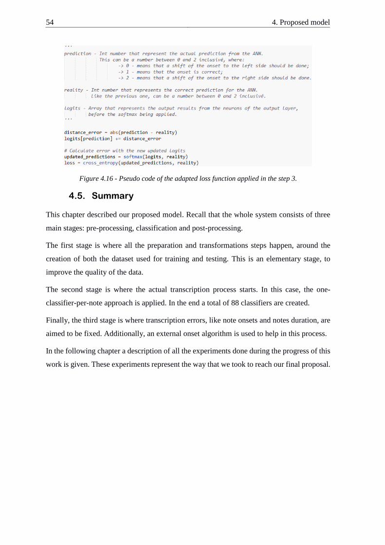
54 4. Proposed model
Figure 4.16 - Pseudo code of the adapted loss function applied in the step 3.
4.5. Summary
This chapter described our proposed model. Recall that the whole system consists of three
main stages: pre-processing, classification and post-processing.
The first stage is where all the preparation and transformations steps happen, around the
creation of both the dataset used for training and testing. This is an elementary stage, to
improve the quality of the data.
The second stage is where the actual transcription process starts. In this case, the one-
classifier-per-note approach is applied. In the end a total of 88 classifiers are created.
Finally, the third stage is where transcription errors, like note onsets and notes duration, are
aimed to be fixed. Additionally, an external onset algorithm is used to help in this process.
In the following chapter a description of all the experiments done during the progress of this
work is given. These experiments represent the way that we took to reach our final proposal.
55
5. Preliminary experiments
To fine tune the parameters for our model, we performed several preliminary experiments.
For those experiments, we resorted to tools such as Matlab (The MathWorks inc, 2018) and
Tensorflow (Google Brain Team, 2018). Matlab was used for the whole pre-processing
stage. Tensorflow, a python framework10 for machine learning, supported the classification
and post-processing stages.
This chapter is split into four sections: dataset, pre-processing, classification and post-
processing. The dataset section describes the dataset used in the preliminary experimens.
The pre-processing section introduces the preliminary experiments performed for data
transformations in order to improve the quality of the data. The classification section focuses
on the search towards the best hyperparameters and optimization techniques. Finally, the
last section presents the experiments regarding the different post-processing techniques and
ways to improve their performance.
5.1. Dataset
Our dataset of choice is the MAPS (Emiya, 2008) dataset, which is widely used in works
related to AMT (Reis, 2012), (Leite et al., 2016), (Kelz et al., 2016) and (Kelz and Widmer,
2017). As mentioned in Chapter 3, MAPS contains piano sounds with isolated notes, chords
and musical pieces. However, in our study, we resorted to musical pieces only. This is
motivated by the fact that current state-of-the-art studies, which we use to compare our own
work, only deal with musical pieces (Sigtia et al., 2016a), (Kelz et al., 2016), (Hawthorne et
al., 2018) and (Li et al., 2018).
When doing preliminary experiments, the ideal approach would be to use the same dataset
as in the final setup experiments. However, due to the long time required per each
experiment, a smaller dataset, referred as 70 musics, has been created and used (further
details can be found in (Gil et al., 2018c) and in (Gil et al., 2018b)). This smaller dataset
significantly reduced the computational time needed per experiment, allowing to perform a
wider range of experiments. Additionally, to further limit computational time demands, we
focused our preliminary experiments on the musical note MIDI number 55. According to
10 A framework is a structure designed for supporting or enclosing an entity in order to simplify the
process of doing/create a given task.
56 5. Preliminary experiments
our preliminary study (described in the following topic), MIDI number 55 is one of the most
frequent musical notes in the dataset, and it is thus a good reference point.
The 70 musics dataset comprises 68 musical pieces in the training set and eight pieces in the
testing set. The musical pieces were carefully selected according to the following links:
(Emiya et al., 2007) and (Reis, n.d.). Note that, there are no repeated musical pieces in both
sets.
For the preliminary experiments of the post-processing stage, we used the second fold of
Configuration 1. This fold is comprised of 216 musical pieces in the training set and 54
pieces in the testing set. The rationale for this option is twofold: i) experiments for the post-
processing stage are much less computationally demanding and ii) this is one of the folds of
the dataset selected for our final setup.
5.2. Pre-processing
When dealing with ANNs, a fundamental point to get good results is to have good quality
data. However, the expression good quality data is quite abstract. Moreover, it depends on
the problem itself. To get a better grasp of the data, an analysis was performed, resorting to
several metrics such as i) the number of frames with each note, ii) number of frames without
each note, iii) number of notes played simultaneously with also the correspondent number
of frames associated with it, among many other fields. The full details are given in the
Appendix, Section A.
Five main observations were revealed from the assessed metadata: (1) The musical note
MIDI number 55 is one of the most frequent musical notes in the dataset and, therefore, it is
a good reference point for our preliminary experiments; (2) Some musical notes, like the
ones ranging from 21 to 29 or 100 to 108, are rarelly or never played during a musical piece,
which can make the detection of those musical notes unfeasible, due to insufficient training
data; (3) some frames of a musical piece, can contain up to 16 or more (played) simultaneous
musical notes substantially hardening the transcription process; (4) all the musical pieces
have frames that only contain silence/noise, which is nonrelevant data for the training phase
of the classifiers and the post-processing units; (5) each musical note has a different balance
of frames with and without that note, a situation that impairs the transcription when the
unbalance is too large.
These five observations allowed us a better understanding of some possible transformations
that could improve the transcription results. Nevertheless, and since tests are the best way of

5.2. Pre-processing 57
knowing whether the quality of the data has been improved or not, several tests were
performed with a default classifier (further details can be found in Appendix, Section A).
The experimented data transformations can be categorized into three types: i) data
representation, when the transformation aims at improving the quality of the data by
transforming the input data into another type of representation; ii) parsing, to improve data
by discarding (nonrelevant) frames; iii) augmenting detection precision, to improve the
temporal resolution, enhancing the precision of note onsets and offsets. An important point
is that the parsing-based transformations were solely applied to the training set, because they
transform the data according to the ideal/expected transcription (labels), something
impossible in a real scenario.
The tested transformations are listed in the table bellow.
Table 5.1 - Data transformations experimented. The transformations in bold represent the ones
incorporated into our model.
Name Type Positive impact?
Frequency signal Data representation Yes
Removal of nonrelevant frames Parsing Yes
Ratio between positive and negative
labels Parsing Yes
Normalization Data representation No
Silence classifier Parsing No
Overlapping Augmenting detection precision Yes
Frequency mean Data representation No
The first three data transformations, represented in the table above are the transformations
proposed in our model (see previous chapter). All these three transformations positively
impacted the results of the transcription system and were therefore incorporated them into
our model. Furthermore, although the overlapping transformation allowed for improved
results, a problem related to the application of the transformation forced us to drop it (we
discuss this later). Next, we briefly review each of the transformation models.
The Frequency signal data transformation converts the input signal into the frequency
domain, using the FFT. The Removal of nonrelevant frames transformation discards
unrelevant frames such as frames with silence. The Ratio between positive and negative
labels aims at balancing the training set with the 20/80 rule, where 20% of the frames have
the specific musical note and the remaining 80% of the frames do not have it. Several
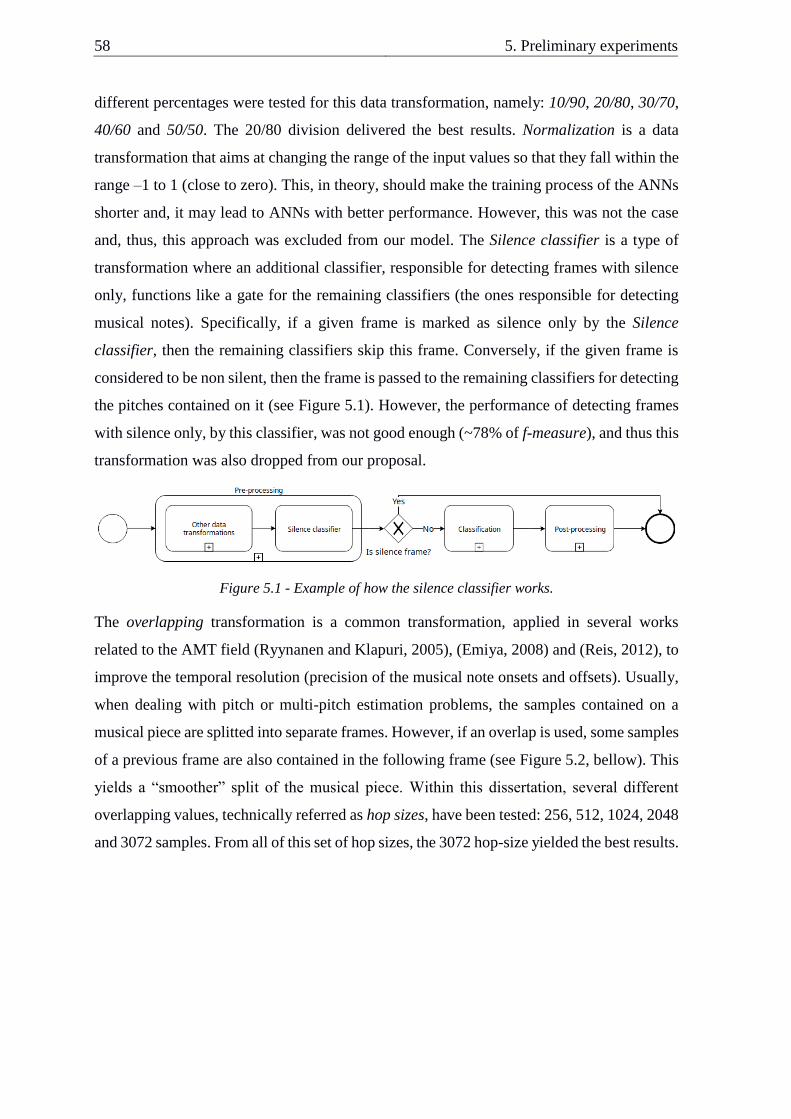
58 5. Preliminary experiments
different percentages were tested for this data transformation, namely: 10/90, 20/80, 30/70,
40/60 and 50/50. The 20/80 division delivered the best results. Normalization is a data
transformation that aims at changing the range of the input values so that they fall within the
range –1 to 1 (close to zero). This, in theory, should make the training process of the ANNs
shorter and, it may lead to ANNs with better performance. However, this was not the case
and, thus, this approach was excluded from our model. The Silence classifier is a type of
transformation where an additional classifier, responsible for detecting frames with silence
only, functions like a gate for the remaining classifiers (the ones responsible for detecting
musical notes). Specifically, if a given frame is marked as silence only by the Silence
classifier, then the remaining classifiers skip this frame. Conversely, if the given frame is
considered to be non silent, then the frame is passed to the remaining classifiers for detecting
the pitches contained on it (see Figure 5.1). However, the performance of detecting frames
with silence only, by this classifier, was not good enough (~78% of f-measure), and thus this
transformation was also dropped from our proposal.
Figure 5.1 - Example of how the silence classifier works.
The overlapping transformation is a common transformation, applied in several works
related to the AMT field (Ryynanen and Klapuri, 2005), (Emiya, 2008) and (Reis, 2012), to
improve the temporal resolution (precision of the musical note onsets and offsets). Usually,
when dealing with pitch or multi-pitch estimation problems, the samples contained on a
musical piece are splitted into separate frames. However, if an overlap is used, some samples
of a previous frame are also contained in the following frame (see Figure 5.2, bellow). This
yields a “smoother” split of the musical piece. Within this dissertation, several different
overlapping values, technically referred as hop sizes, have been tested: 256, 512, 1024, 2048
and 3072 samples. From all of this set of hop sizes, the 3072 hop-size yielded the best results.
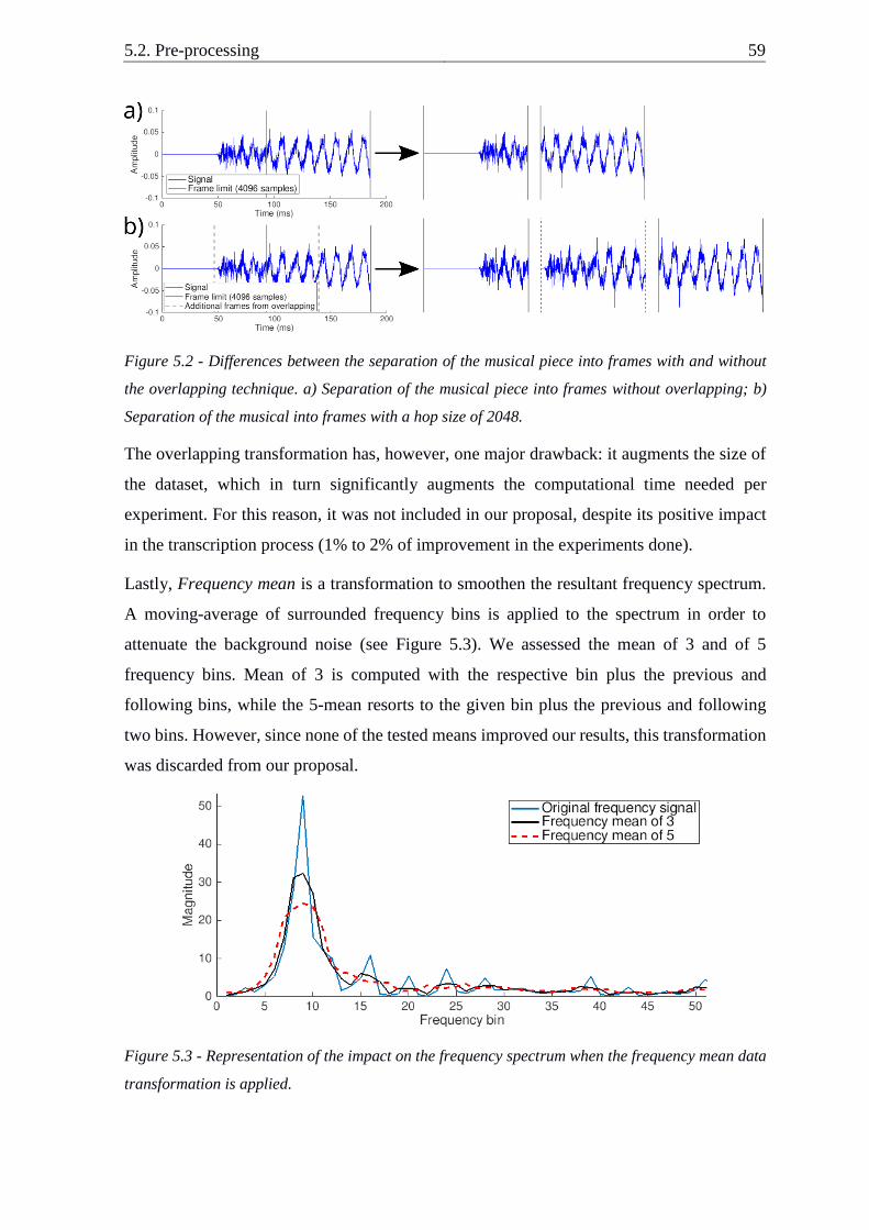
5.2. Pre-processing 59
Figure 5.2 - Differences between the separation of the musical piece into frames with and without
the overlapping technique. a) Separation of the musical piece into frames without overlapping; b)
Separation of the musical into frames with a hop size of 2048.
The overlapping transformation has, however, one major drawback: it augments the size of
the dataset, which in turn significantly augments the computational time needed per
experiment. For this reason, it was not included in our proposal, despite its positive impact
in the transcription process (1% to 2% of improvement in the experiments done).
Lastly, Frequency mean is a transformation to smoothen the resultant frequency spectrum.
A moving-average of surrounded frequency bins is applied to the spectrum in order to
attenuate the background noise (see Figure 5.3). We assessed the mean of 3 and of 5
frequency bins. Mean of 3 is computed with the respective bin plus the previous and
following bins, while the 5-mean resorts to the given bin plus the previous and following
two bins. However, since none of the tested means improved our results, this transformation
was discarded from our proposal.
Figure 5.3 - Representation of the impact on the frequency spectrum when the frequency mean data
transformation is applied.
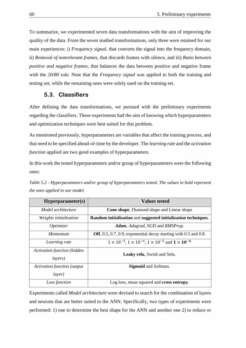
60 5. Preliminary experiments
To summarize, we experimented seven data transformations with the aim of improving the
quality of the data. From the seven studied transformations, only three were retained for our
main experiences: i) Frequency signal, that converts the signal into the frequency domain,
ii) Removal of nonrelevant frames, that discards frames with silence, and iii) Ratio between
positive and negative frames, that balances the data between positive and negative frame
with the 20/80 rule. Note that the Frequency signal was applied to both the training and
testing set, while the remaining ones were solely used on the training set.
5.3. Classifiers
After defining the data transformations, we pursued with the preliminary experiments
regarding the classifiers. These experiments had the aim of knowing which hyperparameters
and optimization techniques were best suited for this problem.
As mentioned previously, hyperparameters are variables that affect the training process, and
that need to be specified ahead-of-time by the developer. The learning rate and the activation
function applied are two good examples of hyperparameters.
In this work the tested hyperparameters and/or group of hyperparameters were the following
ones:
Table 5.2 - Hyperparameters and/or group of hyperparameters tested. The values in bold represent
the ones applied in our model.
Hyperparameter(s) Values tested
Model architecture Cone shape, Diamond shape and Linear shape
Weights initialization Random initialization and suggested initialization techniques.
Optimizer Adam, Adagrad, SGD and RMSProp.
Momentum Off, 0.5, 0.7, 0.9, exponential decay starting with 0.5 and 0.8.
Learning rate 1 × 10⁻³, 1 × 10⁻⁴, 1 × 10⁻⁵ and 𝟏 × 𝟏𝟎−𝟔
Activation function (hidden
layers) Leaky relu, Swish and Selu.
Activation function (output
layer)
Sigmoid and Softmax.
Loss function Log loss, mean squared and cross entropy.
Experiments called Model architecture were devised to search for the combination of layers
and neurons that are better suited to the ANN. Specifically, two types of experiments were
performed: 1) one to determine the best shape for the ANN and another one 2) to reduce or
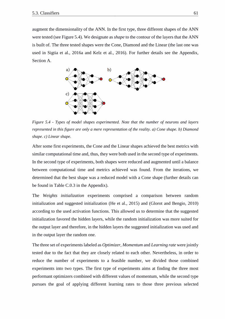
5.3. Classifiers 61
augment the dimensionality of the ANN. In the first type, three different shapes of the ANN
were tested (see Figure 5.4). We designate as shape to the contour of the layers that the ANN
is built of. The three tested shapes were the Cone, Diamond and the Linear (the last one was
used in Sigtia et al., 2016a and Kelz et al., 2016). For further details see the Appendix,
Section A.
Figure 5.4 - Types of model shapes experimented. Note that the number of neurons and layers
represented in this figure are only a mere representation of the reality. a) Cone shape. b) Diamond
shape. c) Linear shape.
After some first experiments, the Cone and the Linear shapes achieved the best metrics with
similar computational time and, thus, they were both used in the second type of experiments.
In the second type of experiments, both shapes were reduced and augmented until a balance
between computational time and metrics achieved was found. From the iterations, we
determined that the best shape was a reduced model with a Cone shape (further details can
be found in Table C.0.3 in the Appendix).
The Weights initialization experiments comprised a comparison between random
initialization and suggested initialization (He et al., 2015) and (Glorot and Bengio, 2010)
according to the used activation functions. This allowed us to determine that the suggested
initialization favored the hidden layers, while the random initialization was more suited for
the output layer and therefore, in the hidden layers the suggested initialization was used and
in the output layer the random one.
The three set of experiments labeled as Optimizer, Momentum and Learning rate were jointly
tested due to the fact that they are closely related to each other. Nevertheless, in order to
reduce the number of experiments to a feasible number, we divided those combined
experiments into two types. The first type of experiments aims at finding the three most
performant optimizers combined with different values of momentum, while the second type
pursues the goal of applying different learning rates to those three previous selected
62 5. Preliminary experiments
optimizers in order to discover the best combination of both. The learning rate is the
hyperparameter that determines the amplitude of the changes when updating the weights.
The momentum is a hyperparameter that works as a ”push” on the process of updating the
weights based on the slope of the error surface derivative. The momentum was also tested
with an exponential decay where for each 20 epochs11 its value was reduced by 20%. In the
end, the best combination was the Adam optimizer with ”no momentum” and a learning rate
of 1 × 10⁻⁶. By ”no momentum” we mean that we did not specify a momentum from the
table above (50, 70 or 90), because the Adam optimizer already applies and adapts by itself
the value of the momentum12. In the set of experiments denominated as Activation functions,
commonly applied functions like the sigmoid and the leaky relu and other, more recent
activation functions such as the softmax, the swish and the selu, were experimented. We
found that a combination of both the leaky relu in the hidden layers and the sigmoid on the
output layer was the most performant. Finally, three different loss functions were tested: log
loss, mean squared and cross entropy. In this case the cross entropy was the most prominent.
After the hyperparameters being established, we focused on the optimization techniques to
apply. These consist on techniques used during the training process to improve the
performance of the ANN. Commonly, these techniques focus on improving at least one of
the following points: i) computation time required for the training process and/or ii) results
achieved.
In this dissertation six different optimization techniques have been experimented (see Table
5.3).
11 An epoch represents a forward and backward pass of all the training examples. 12 Actually, the Adam optimizer does not apply the momentum hyperparameter. Instead, it applies a
closely related concept. However, for the sake of understanding, we refer to it as momentum.
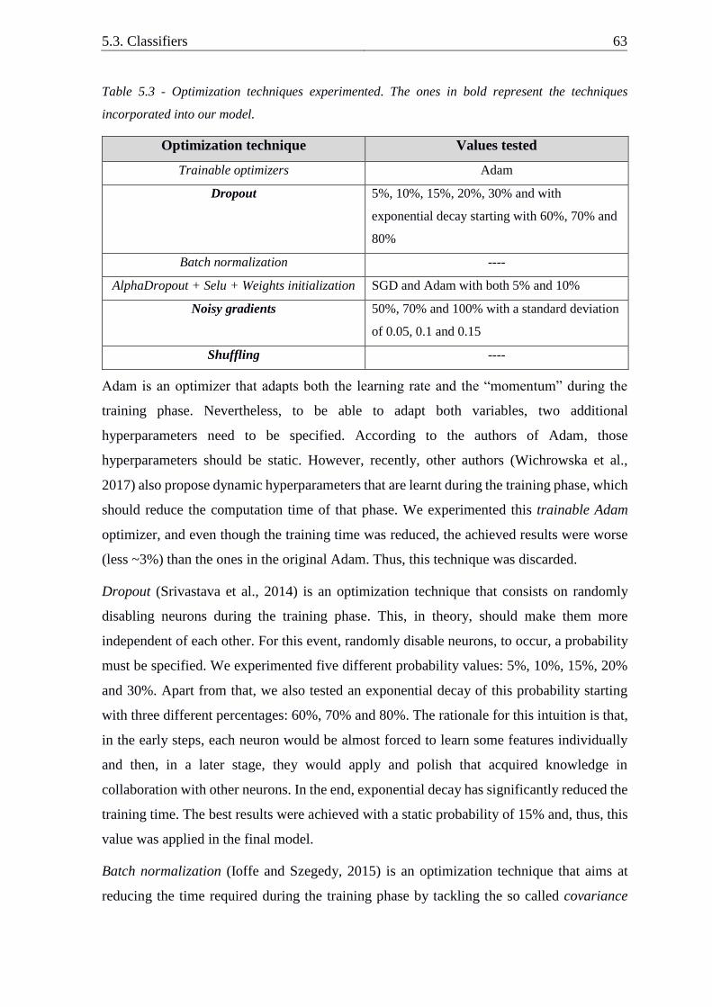
5.3. Classifiers 63
Table 5.3 - Optimization techniques experimented. The ones in bold represent the techniques
incorporated into our model.
Optimization technique Values tested
Trainable optimizers Adam
Dropout 5%, 10%, 15%, 20%, 30% and with
exponential decay starting with 60%, 70% and
80%
Batch normalization ----
AlphaDropout + Selu + Weights initialization SGD and Adam with both 5% and 10%
Noisy gradients 50%, 70% and 100% with a standard deviation
of 0.05, 0.1 and 0.15
Shuffling ----
Adam is an optimizer that adapts both the learning rate and the “momentum” during the
training phase. Nevertheless, to be able to adapt both variables, two additional
hyperparameters need to be specified. According to the authors of Adam, those
hyperparameters should be static. However, recently, other authors (Wichrowska et al.,
2017) also propose dynamic hyperparameters that are learnt during the training phase, which
should reduce the computation time of that phase. We experimented this trainable Adam
optimizer, and even though the training time was reduced, the achieved results were worse
(less ~3%) than the ones in the original Adam. Thus, this technique was discarded.
Dropout (Srivastava et al., 2014) is an optimization technique that consists on randomly
disabling neurons during the training phase. This, in theory, should make them more
independent of each other. For this event, randomly disable neurons, to occur, a probability
must be specified. We experimented five different probability values: 5%, 10%, 15%, 20%
and 30%. Apart from that, we also tested an exponential decay of this probability starting
with three different percentages: 60%, 70% and 80%. The rationale for this intuition is that,
in the early steps, each neuron would be almost forced to learn some features individually
and then, in a later stage, they would apply and polish that acquired knowledge in
collaboration with other neurons. In the end, exponential decay has significantly reduced the
training time. The best results were achieved with a static probability of 15% and, thus, this
value was applied in the final model.
Batch normalization (Ioffe and Szegedy, 2015) is an optimization technique that aims at
reducing the time required during the training phase by tackling the so called covariance
64 5. Preliminary experiments
shift problem. Recall that, in a multi-layer neural network, the update of the weights is done
from the last layer to the first one. According to the authors, when the initial layers are
updated, the following ones should also be readapted according to that change. Otherwise,
the problem of covariance shift will occur. This effect gets even stronger when deeper ANNs
are used. Nevertheless, our proposed model has only five hidden layers and thus it is not
strongly impacted by the covariance shift problem. Furthermore, this technique also implies
additional calculations which in turn augments the computational time of each update of the
weights. As a result, we did not include this technique into our model because, even though
the number of epochs were slighly reduced, the computational time taken for the whole
training process was almost the double.
The AlphaDropout + Selu + Weights initialization (Klambauer et al., 2017) is a recent
optimization technique that also aims at reducing the time needed during the training phase
like the previously mentioned technique, but without additional computationally expensive
calculus. According to the authors, a combination of the AlphaDropout, which consists on a
variation of the dropout technique, with the selu activation function and a suggestive way of
initializing the weights should reduce significantly the training time. Although the authors
only present experiments regarding the SGD optimizer, in this work we tried both the Adam
and the SGD. Additionally, they also mention that a smaller value of dropout occurrence
should be used, around 5% or 10%. Thus, in this work we have tested both the SGD and the
Adam optimizer with 5% and 10%. In the end, we noticed that this technique has
significantly reduced the training time, but at the cost of the achieved results, which were
poorer (less ~5%), and thus it was discarded.
One way of improving the ANNs performance is by forcing them to broaden their search.
Both the noisy gradients (Neelakantan et al., 2017) and the shuffling (Lecun et al., 1998)
optimization techniques do that but in different ways. The noisy gradients technique aims at
randomly adding a gaussian distribution of noise to the gradients of the network. The
shuffling, on the other hand, aims at randomly shuffle the training sequence of the input data.
Both techniques have helped to improve the robustness of our model, leading to better
results, and through this way their implementation. Regarding the noisy gradients technique,
we determined that a probability of 70% with a standard deviation (STD) of 0.05 resulted
in the best achieved results. On the other hand, the shuffle was applied every time that was
possible due to its positive results.
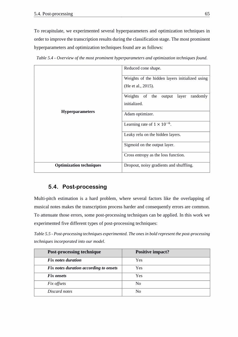
5.4. Post-processing 65
To recapitulate, we experimented several hyperparameters and optimization techniques in
order to improve the transcription results during the classification stage. The most prominent
hyperparameters and optimization techniques found are as follows:
Table 5.4 - Overview of the most prominent hyperparameters and optimization techniques found.
Hyperparameters
Reduced cone shape.
Weights of the hidden layers initialized using
(He et al., 2015).
Weights of the output layer randomly
initialized.
Adam optimizer.
Learning rate of 1 × 10⁻⁶.
Leaky relu on the hidden layers.
Sigmoid on the output layer.
Cross entropy as the loss function.
Optimization techniques Dropout, noisy gradients and shuffling.
5.4. Post-processing
Multi-pitch estimation is a hard problem, where several factors like the overlapping of
musical notes makes the transcription process harder and consequently errors are common.
To attenuate those errors, some post-processing techniques can be applied. In this work we
experimented five different types of post-processing techniques:
Table 5.5 - Post-processing techniques experimented. The ones in bold represent the post-processing
techniques incorporated into our model.
Post-processing technique Positive impact?
Fix notes duration Yes
Fix notes duration according to onsets Yes
Fix onsets Yes
Fix offsets No
Discard notes No
66 5. Preliminary experiments
As described before, the fix notes duration post-processing technique aims to add the sense
of time into the transcription system by receiving as input data a sequence of previously
transcribed frames (from the classifiers) and predicts the possible transcription for the frame
in middle of that sequence. The fix notes duration and notes onsets is a similar post-
processing technique as the previous one, but it also tries to improve the note onsets by also
receiving the output from an onset algorithm (Martins, 2008). Apart from that, it also
receives a sequence of the original transcription from the classifiers. The fix onsets is a
technique that specifically targets improving the note onsets by readjusting a note onset, if
needed, to one previous or posterior frame. It receives as input a sequence of previous
transcribed frames and the output of the onset algorithm. The fix offsets is similar to the fix
onsets but, instead, it targets note offsets. However, this technique only receives as input the
sequence of previously transcribed frames. Finally, the discard notes is a post-processing
technique that aims at discarding wrongly detected musical notes. It does that by receiving
as input, informations such as: i) the number of frames within that musical note, ii) the
sequence of previously transcribed frames, iii) the output of the onset algorithm and iv) the
output of the possible notes algorithm (Reis, 2012), which consists on an algorithm for
detecting notes by considering the most prominent spectral peaks.
In our experiments, only the first three post-processing techniques -- fix notes duration, fix
notes duration according to onsets and fix onsets -- had a positive impact in the results, and
thus were selected to integrate our model.
5.5. Summary
This chapter introduced the preliminary experiments done in order to reach our final model.
For each main stage – pre-processing, classification and post-processing – preliminary
experiments have been accomplished. These experiments were essential to fine tune our
model in order to improve its final transcription.
In the next chapter the results achieved from our fine tuned model are presented.
67
6. Results
This chapter describes the results achieved with our model. Initially, a description of the
dataset and the metrics used for evaluating the model are presented. The configurations
applied on the model are also described. Finally, the achieved results and a comparison with
two other state-of-the-art works, followed by a demonstration of the impact of the onset
algorithm applied is given.
6.1. Dataset
As previously explained, one of the main motivations for this work is to compare both the
one-classifier-per-note approach with the traditional one. For this purpose, we have used the
Configuration 113 dataset based on the MAPS (Emiya, 2008), which is a popular dataset used
in recent AMT works. Recall that this dataset is composed of four folds, each one containing
a different combination of musical pieces, with 216 musical pieces in the training set and 54
pieces in the testing set. This means that, for each fold, a transcription system comprised of
88 ANNs for the classification stage and 88 * 3 (number of steps) = 264 ANNs for the post-
processing stage, must be created.
We consider Configuration 1 to be an appropriate dataset for the purpose of comparing both
approaches, because it is composed of four folds instead of a single one. In the end, the
difference of the results obtained, that is, the mean from all the folds, should highlight the
difference of applying a distinct approach, instead of other complementary factors such as
the use of different hyperparameters. This is due to the fact that fine tuned hyperparameters
for a given fold may not be as optimal when applied to another fold.
6.2. Metrics
Regarding the AMT field, when comparing different approaches, two different types of
metrics are commonly used: frame-based and note-based metrics (Bay et al., 2009). Frame-
based metrics consists on evaluating frame-by-frame the resultant transcription whereas
note-based consists on evaluating each transcribed musical note by considering its pitch,
onset and, depending on the given metric, its offset. In this work, we use both types of
metrics. The note-based metrics are based on MIREX (“MIREX”). We refer as onset only
to the metrics that consider the pitch and the onset with a tolerance of ±50𝑚𝑠 (its assumed
13 More details can be found in (Sigtia et al., 2016b).
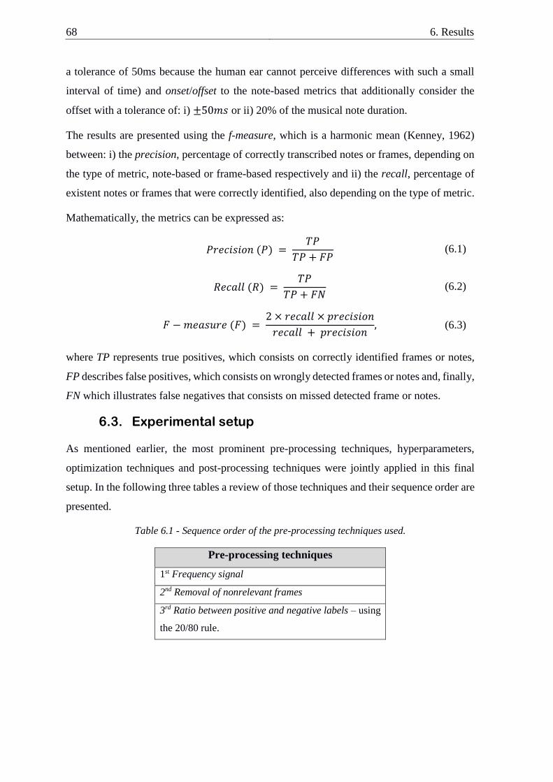
68 6. Results
a tolerance of 50ms because the human ear cannot perceive differences with such a small
interval of time) and onset/offset to the note-based metrics that additionally consider the
offset with a tolerance of: i) ±50𝑚𝑠 or ii) 20% of the musical note duration.
The results are presented using the f-measure, which is a harmonic mean (Kenney, 1962)
between: i) the precision, percentage of correctly transcribed notes or frames, depending on
the type of metric, note-based or frame-based respectively and ii) the recall, percentage of
existent notes or frames that were correctly identified, also depending on the type of metric.
Mathematically, the metrics can be expressed as:
𝑃𝑟𝑒𝑐𝑖𝑠𝑖𝑜𝑛 (𝑃) = 𝑇𝑃
𝑇𝑃 + 𝐹𝑃 (6.1)
𝑅𝑒𝑐𝑎𝑙𝑙 (𝑅) = 𝑇𝑃
𝑇𝑃 + 𝐹𝑁 (6.2)
𝐹 − 𝑚𝑒𝑎𝑠𝑢𝑟𝑒 (𝐹) = 2 × 𝑟𝑒𝑐𝑎𝑙𝑙 × 𝑝𝑟𝑒𝑐𝑖𝑠𝑖𝑜𝑛
𝑟𝑒𝑐𝑎𝑙𝑙 + 𝑝𝑟𝑒𝑐𝑖𝑠𝑖𝑜𝑛, (6.3)
where TP represents true positives, which consists on correctly identified frames or notes,
FP describes false positives, which consists on wrongly detected frames or notes and, finally,
FN which illustrates false negatives that consists on missed detected frame or notes.
6.3. Experimental setup
As mentioned earlier, the most prominent pre-processing techniques, hyperparameters,
optimization techniques and post-processing techniques were jointly applied in this final
setup. In the following three tables a review of those techniques and their sequence order are
presented.
Table 6.1 - Sequence order of the pre-processing techniques used.
Pre-processing techniques
1st Frequency signal
2nd Removal of nonrelevant frames
3rd Ratio between positive and negative labels – using
the 20/80 rule.
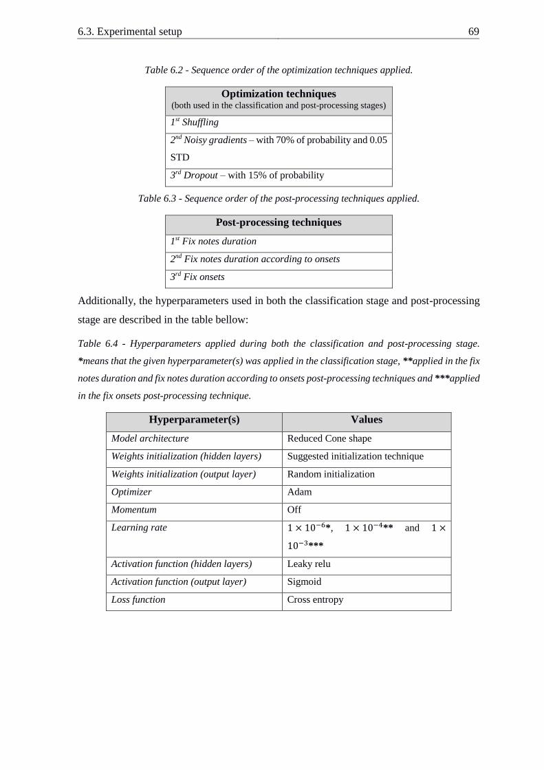
6.3. Experimental setup 69
Table 6.2 - Sequence order of the optimization techniques applied.
Optimization techniques (both used in the classification and post-processing stages)
1st Shuffling
2nd Noisy gradients – with 70% of probability and 0.05
STD
3rd Dropout – with 15% of probability
Table 6.3 - Sequence order of the post-processing techniques applied.
Post-processing techniques
1st Fix notes duration
2nd Fix notes duration according to onsets
3rd Fix onsets
Additionally, the hyperparameters used in both the classification stage and post-processing
stage are described in the table bellow:
Table 6.4 - Hyperparameters applied during both the classification and post-processing stage.
*means that the given hyperparameter(s) was applied in the classification stage, **applied in the fix
notes duration and fix notes duration according to onsets post-processing techniques and ***applied
in the fix onsets post-processing technique.
Hyperparameter(s) Values
Model architecture Reduced Cone shape
Weights initialization (hidden layers) Suggested initialization technique
Weights initialization (output layer) Random initialization
Optimizer Adam
Momentum Off
Learning rate 1 × 10⁻⁶*, 1 × 10⁻⁴** and 1 ×
10−3***
Activation function (hidden layers) Leaky relu
Activation function (output layer) Sigmoid
Loss function Cross entropy
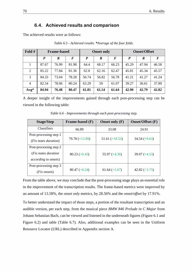
70 6. Results
6.4. Achieved results and comparison
The achieved results were as follows:
Table 6.5 - Achieved results. *Average of the four folds.
Fold # Frame-based Onset only Onset/Offset
P R F P R F P R F
1 87.67 76.99 81.98 64.4 68.17 66.23 45.29 47.94 46.58
2 85.22 77.84 81.36 62.8 62.16 62.47 45.81 45.34 45.57
3 84.33 73.04 78.28 56.74 56.82 56.78 41.21 41.27 41.24
4 82.54 78.06 80.24 63.29 59 61.07 39.27 36.61 37.89
Avg* 84.94 76.48 80.47 61.81 61.54 61.64 42.90 42.79 42.82
A deeper insight of the improvements gained through each post-processing step can be
viewed in the following table:
Table 6.6 - Improvements through each post-processing step.
Stage/Step Frame-based (F) Onset only (F) Onset/Offset (F)
Classifiers 66.89 33.08 24.91
Post-processing step 1
(Fix notes duration) 79.78 (+12.89) 51.61 (+18.53) 34.54 (+9.63)
Post-processing step 2
(Fix notes duration
according to onsets)
80.23 (+0.45) 55.97 (+4.36) 39.07 (+4.53)
Post-processing step 3
(Fix onsets) 80.47 (+0.24) 61.64 (+5.67) 42.82 (+3.75)
From the table above, we may conclude that the post-processing stage plays an essential role
in the improvement of the transcription results. The frame-based metrics were improved by
an amount of 13.58%, the onset only metrics, by 28.56% and the onset/offset by 17.91%.
To better understand the impact of those steps, a portion of the resultant transcription and an
audible version, per each step, from the musical piece BMW 846 Prelude in C Major from
Johann Sebastian Bach, can be viewed and listened in the underneath figures (Figure 6.1 and
Figure 6.2) and table (Table 6.7). Also, additional examples can be seen in the Uniform
Resource Locator (URL) described in Appendix section A.
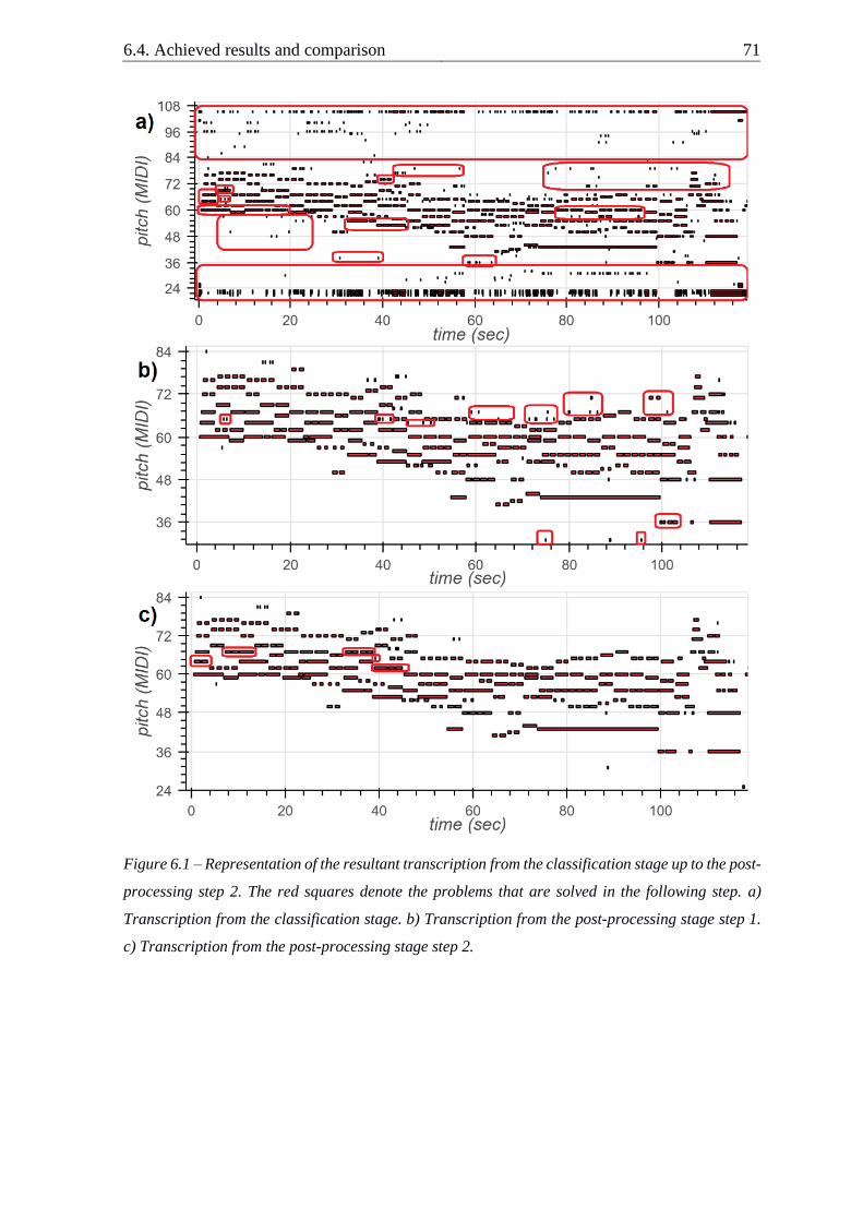
6.4. Achieved results and comparison 71
Figure 6.1 – Representation of the resultant transcription from the classification stage up to the post-
processing step 2. The red squares denote the problems that are solved in the following step. a)
Transcription from the classification stage. b) Transcription from the post-processing stage step 1.
c) Transcription from the post-processing stage step 2.
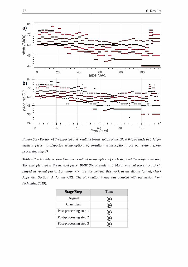
72 6. Results
Figure 6.2 - Portion of the expected and resultant transcription of the BMW 846 Prelude in C Major
musical piece. a) Expected transcription. b) Resultant transcription from our system (post-
processing step 3).
Table 6.7 – Audible version from the resultant transcription of each step and the original version.
The example used is the musical piece, BMW 846 Prelude in C Major musical piece from Bach,
played in virtual piano. For those who are not viewing this work in the digital format, check
Appendix, Section A, for the URL. The play button image was adapted with permission from
(Schmidsi, 2019).
Stage/Step Tune
Original
Classifiers
Post-processing step 1
Post-processing step 2
Post-processing step 3
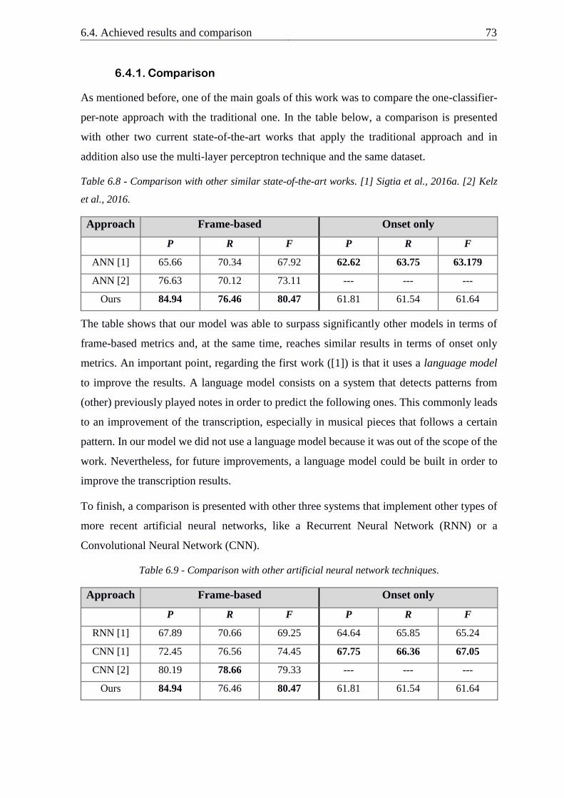
6.4. Achieved results and comparison 73
6.4.1. Comparison
As mentioned before, one of the main goals of this work was to compare the one-classifier-
per-note approach with the traditional one. In the table below, a comparison is presented
with other two current state-of-the-art works that apply the traditional approach and in
addition also use the multi-layer perceptron technique and the same dataset.
Table 6.8 - Comparison with other similar state-of-the-art works. [1] Sigtia et al., 2016a. [2] Kelz
et al., 2016.
Approach Frame-based Onset only
P R F P R F
ANN [1] 65.66 70.34 67.92 62.62 63.75 63.179
ANN [2] 76.63 70.12 73.11 --- --- ---
Ours 84.94 76.46 80.47 61.81 61.54 61.64
The table shows that our model was able to surpass significantly other models in terms of
frame-based metrics and, at the same time, reaches similar results in terms of onset only
metrics. An important point, regarding the first work ([1]) is that it uses a language model
to improve the results. A language model consists on a system that detects patterns from
(other) previously played notes in order to predict the following ones. This commonly leads
to an improvement of the transcription, especially in musical pieces that follows a certain
pattern. In our model we did not use a language model because it was out of the scope of the
work. Nevertheless, for future improvements, a language model could be built in order to
improve the transcription results.
To finish, a comparison is presented with other three systems that implement other types of
more recent artificial neural networks, like a Recurrent Neural Network (RNN) or a
Convolutional Neural Network (CNN).
Table 6.9 - Comparison with other artificial neural network techniques.
Approach Frame-based Onset only
P R F P R F
RNN [1] 67.89 70.66 69.25 64.64 65.85 65.24
CNN [1] 72.45 76.56 74.45 67.75 66.36 67.05
CNN [2] 80.19 78.66 79.33 --- --- ---
Ours 84.94 76.46 80.47 61.81 61.54 61.64
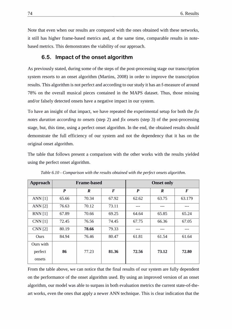
74 6. Results
Note that even when our results are compared with the ones obtained with these networks,
it still has higher frame-based metrics and, at the same time, comparable results in note-
based metrics. This demonstrates the viability of our approach.
6.5. Impact of the onset algorithm
As previously stated, during some of the steps of the post-processing stage our transcription
system resorts to an onset algorithm (Martins, 2008) in order to improve the transcription
results. This algorithm is not perfect and according to our study it has an f-measure of around
78% on the overall musical pieces contained in the MAPS dataset. Thus, those missing
and/or falsely detected onsets have a negative impact in our system.
To have an insight of that impact, we have repeated the experimental setup for both the fix
notes duration according to onsets (step 2) and fix onsets (step 3) of the post-processing
stage, but, this time, using a perfect onset algorithm. In the end, the obtained results should
demonstrate the full efficiency of our system and not the dependency that it has on the
original onset algorithm.
The table that follows present a comparison with the other works with the results yielded
using the perfect onset algorithm.
Table 6.10 - Comparison with the results obtained with the perfect onsets algorithm.
Approach Frame-based Onset only
P R F P R F
ANN [1] 65.66 70.34 67.92 62.62 63.75 63.179
ANN [2] 76.63 70.12 73.11 --- --- ---
RNN [1] 67.89 70.66 69.25 64.64 65.85 65.24
CNN [1] 72.45 76.56 74.45 67.75 66.36 67.05
CNN [2] 80.19 78.66 79.33 --- --- ---
Ours 84.94 76.46 80.47 61.81 61.54 61.64
Ours with
perfect
onsets
86 77.23 81.36 72.56 73.12 72.80
From the table above, we can notice that the final results of our system are fully dependent
on the performance of the onset algorithm used. By using an improved version of an onset
algorithm, our model was able to surpass in both evaluation metrics the current state-of-the-
art works, even the ones that apply a newer ANN technique. This is clear indication that the
6.6. Summary 75
one-classifier-per-note approach is a viable way of addressing the multi-pitch estimation
problem.
6.6. Summary
This chapter described the achieved results from our proposed model. Recall that our
transcription system was able to surpass current state-of-the-art works in frame-based
metrics and at the same time reaches comparable results in note-based metrics. In addition,
we have also abserved that the performance of the applied onset algorithm, directly
influences the final performance of our system. Therefore, if a better onset detection
algorithm could be used, our system could reach or even surpass the current state-of-the-art
works regarding to note-based metrics, while additionally improving on the remaining
metrics.

76
This page was intetionally left blank
77
7. Conclusion and future work
One of the main aims of this work was to check the viability of the one-classifier-per-note
approach using artificial neural networks. To accomplish that, we elaborated an initial study
to find out the current state-of-the-art works, related to the AMT field, which combined
artificial neural networks with the traditional approach. From this, we established that a
classical deep learning technique was preferable in order to have a baseline comparison.
After establishing both the type of ANN technique and the dataset to be used, we pursued
with several preliminary experiments. These, were a fundamental step for our model because
it shaped the way that the transcription is performed. We noticed that both a pre-processing
and post-processing stage should be taken into account, in order to improve the whole
performance of the system. The pre-processing stage would transform the sound signal into
a more appropriate representation, while the post-processing stage would aim at fixing errors
in the original transcription.
In the end, our model was able to surpass current state-of-the-art-works regarding the frame-
based metrics and, at the same time, reaching comparable results in note-based metrics. Even
when we compare with other works that apply newer ANN techniques, our model is still
better in frame-based metrics. This indicates the viability of the one-classifier-per-note
approach.
7.1. Future work
For future work, we would like to propose an improvement of the onset algorithm used. As
demonstrated, if a better onset algorithm is applied our transcription system would perform
better. Thus, a possible solution could be to create an additional ANN to reduce the number
of false positives from the original onset algorithm or, instead, create a from-scratch onset
algorithm using deep learning techniques, like some authors propose (Lacoste and Eck,
2005), (Eyben et al., 2010) and (Schlüter and Böck, 2014). Apart from that, also those onsets
could be filtered by musical note, where not only the onset algorithm will detect if a given
onset occurs but also which musical note corresponds to.
Planning ahead, now that we have baseline results using classical ANNs, a next step would
be to use more sophisticated ones, such as RNNs or CNNs. Also, a different type of data
representation could be tested, such as the constant-Q transform, because the separation of
78 7. Conclusion and future work
the frequency bins using this technique is more closely related to the real separation of the
musical notes than the FFT.
Apart from that, a language model system could also be created, like some authors suggest
(Sigtia et al., 2014) and (Sigtia et al., 2016a). It was out of the scope of this work to create a
language model, but, for future improvements, the incorporation of this additional system
could lead to an improvement on the transcription results.
To conclude, an attention mechanism could also be applied during the classification stage.
This mechanism consists on making the ANN focusing only or mostly on a given part of the
input data. In our case, by using the one-classifier-per-note approach, the ANN responsible
for detecting some specific note should only/mostly focus on the frequency bins related to
the fundamental frequency or its harmonics, which could lead to an improvement in the
results obtained.
79
Bibliography
Association, 1999. Complete MIDI 1.0 detailed specification.
Bako, 2004. JPEG 2000 image compression.
Baskind, Cheveigné, 2003. Pitch-tracking of reverberant sounds, application to spatial
description of sound scenes. Presented at the AES 24th International Conference on
Multichannel Audio.
Bay, Ehmann, Downie, 2009. Evaluation of multiple-f0 estimation and tracking systems.
Presented at the 10th International Society for Music Information Retrieval
Conference, pp. 315–320.
Beauchamp, Maher, Brown, 1992. Detection of musical pitch from recorded solo
performances, 94.
Bello, Daudet, Duxbury, Davies, Sandler, 2005. A tutorial on onset detection in music
signals. IEEE Transactions on speech and audio processing 13(5) 1035–1047.
Bello, Sandler, 2000. Blackboard system and top-down processing for the transcription of
simple polyphonic music. Presented at the Digital Audio Effects, pp. 7–9.
Benetos, Dixon, Giannoulis, Kirchhoff, Klapuri, 2013. Automatic music transcription:
challenges and future directions. Journal of Intelligent Information Systems.
Bereket, Shi, 2017. An AI approach to automatic natural music transcription.
Bertin, Badeau, Vincent, 2010. Enforcing harmonicity and smoothness in bayesian non-
negative matrix factorization applied to polyphonic music transcription. Presented at
the IEEE Transactions on Audio, Speech & Language Processing 18, pp. 538–549.
Bojarski, Testa, Dworakowski, Firner, Flepp, Goyal, Jackel, Monfort, Muller, Zhang,
Zhang, Zhao, Zieba, 2016. End to end learning for self-driving cars.
arXiv:1604.07316.
Burred, Röbel, Rodet, 2006. An accurate timbre model for musical instruments and its
application to classification. Presented at the Workshop on Learning the Semantics
of Audio Signals, pp. 1–1.
Cemgil, Kappen, Barber, 2006. A generative model for music transcription. IEEE
Transactions on Audio, Speech, and Language Processing 14(2) 679–694.
Cheveigné, 1993. Separation of concurrent harmonic sounds: fundamental frequency
estimation. Journal of The Acoustical Society of America.
Conklin, 1999. Generation of partials due to nonlinear mixing in a stringed instrument.
Cont, 2006. Realtime multiple pitch observation using sparse non-negative constraints.
Presented at the International Conference on Music Information Retrieval.
Cooley, Lewis, Welch, 1967. Historical notes on the fast fourier transform. Presented at the
Audio and Electroacoustics, IEEE Transactions on 15, pp. 76–79.
Daudet, 2004. Sparse and structured decompositions of audio signals in overcomplete
spaces. Presented at the International Conference on Digital Audio Effects, pp. 22–
26.
Davy, Godsill, 2002b. Bayesian harmonic models for musical signal analysis. Bayesian
Statistics 7.
Davy, Godsill, 2002a. Bayesian harmonic models for musical pitch estimation and analysis.
Presented at the Proceedings of the IEEE International Conference on Acoust.,
Speech, Signal Processing 2.
Davy, Godsill, Idier, 2006. Bayesian analysis of polyphonic western tonal music. The
Journal of the Acoustical Society of America 2498–2517.
80
Duan, Pardo, Zhang, 2010. Multiple fundamental frequency estimation by modeling spectral
peaks and non-peak regions. Presented at the IEEE Transactions on Audio Speech
and Language Processing 18(8), pp. 2121–2133.
Duan, Zhang, Shi, 2008. Unsupervised single-channel music source separation by average
harmonicstructure modeling. Presented at the Audio, Speech, and Language
Processing, IEEE Transactions on 16, pp. 766–778.
Dugas, Bengio, Bélisle, Nadeau, Garci, 2000. Incorporating second-order functional
knowledge for better option pricing. Presented at the Advances in Neural Information
Processing Systems 13, pp. 472–478.
Emiya, 2008. Transcription automatique de la musique de piano. Telecom ParisTech.
Emiya, Badeau, David, 2010. Multipitch estimation of quasi-harmonic sounds in colored
noise. Presented at the Digital Audio Effects.
Emiya, Badeau, David, 2007. Automatic transcription of piano music - examples [WWW
Document]. Homepage of Valentin EMIYA. URL http://pageperso.lif.univ-
mrs.fr/~valentin.emiya/EUSIPCO08/results.html
Every, Szymanski, 2004. A spectral-filtering approach to music signal separation. Presented
at the Digital Audio Effects, pp. 197–200.
Eyben, Böck, Schuller, Graves, 2010. Universal onset detection with bidirectional long
short-term memory neural networks. Presented at the 11th International Society for
Music Information Retrieval Conference, pp. 589–594.
Gil, Grilo, Reis, Domingues, 2018c. Training set 70 musics.
Gil, Grilo, Reis, Domingues, 2018b. Testing set 70 musics.
Gil, Grilo, Reis, Domingues, 2018a. Metadata files example.
Gil, Reis, Domingues, Grilo, 2018d. Automatic music transcription using a one-classifier-
per-note approach. Presented at the Portuguese Conference on Pattern Recognition.
Giordano, 2009. Cengage learning, in: College Physics: Reasoning and Relationships. pp.
421–424.
Glorot, Bengio, 2010. Understanding the difficulty of training deep feedforward neural
networks. Journal of Machine Learning Research 246–256.
Google Brain Team, 2018. Tensorflow.
Harris, 1978. On the use of windows for harmonic analysis with the discrete fourier
transform. Presented at the IEEE, pp. 51–83.
Hawthorne, Elsen, Song, Roberts, Simon, Raffel, Engel, Oore, Eck, 2018. Onsets and
frames: dual-objective piano transcription. Presented at the 19th International
Society for Music Information Retrieval Conference.
He, Zhang, Ren, Sun, 2015. Delving deep into rectifiers: surpassing human-level
performance on imagenet classification, in: 1502. Presented at the IEEE International
Conference on Computer Vision.
Hermansky, Morgan, 1994. RASTA processing of speech. Presented at the Speech and
Audio Processing, IEEE Transactions on, pp. 578–589.
Ioffe, Szegedy, 2015. Batch normalization: accelerating deep network training by reducing
internal covariate shift. arXiv:1502.03167.
Jensen, 1999. Timbre models of musical sounds. University of Copenhagen.
Kelz, Dorfer, Korzeniowski, ock, Arzt, Widmer, 2016. On the potential of simple framewise
approaches to piano transcription. Presented at the 17th International Society for
MusicInformation Retrieval Conference.
Kelz, Widmer, 2017. An experimental analysis of the entanglement problem in neural-
network-based music transcription systems. arXiv preprint arXiv:1702.00025.
Kenney, 1962. Mathematics of Statistics. Van Nostrand, pp. 57–58.
81
Kingma, Ba, 2014. Adam: a method for stochastic optimization. arXiv preprint arXiv:
1412.6980.
Klambauer, Unterthiner, Mayr, 2017. Self-normalizing neural networks. Advances in Neural
Information Processing Systems.
Klapuri, 2006. Multiple fundamental frequency estimation by summing harmonic
amplitudes. Presented at the 7th International Conference on Music Information
Retrieval, pp. 216–221.
Klapuri, 2005. A perceptually motivated multiple-f0 estimation method. IEEE Workshop on
Applications of Signal Processing to Audio and Acoustics 291–294.
Klapuri, 2003. Multiple fundamental frequency estimation based on harmonicity and
spectral smoothness. Presented at the IEEE Transactions on Speech and Audio
Processing 11(6).
Klapuri, 2001. Multipitch estimation and sound separation by the spectral smoothness
principle. Presented at the Acoustics, Speech, and Signal Processing.
Klapuri, 1998. Number theoretical means of resolving a mixture of several harmonic sounds.
Presented at the European Signal Processing Conference.
Klapuri, Davy, 2007. Signal processing methods for music transcription.
Lacoste, Eck, 2005. Onset detection with artificial neural networks for MIREX 2005.
Larochelle, Murray, 2011. The neural autoregressive distribution estimator. Journal of
Machine Learning Research 29–37.
Lea, 1992. Auditory model of vowel perception. University of Nottingham.
Lecun, Bottou, Orr, Müller, 1998. Efficient backprop, in: Neural Networks: Tricks of the
Trade. Springer.
Leite, Miragaia, Reis, Grilo, Fernandéz, 2016. Cartesian genetic programming applied to
pitch estimation of piano notes. Presented at the IEEE Symposium Series on
Computational Intelligence.
Li, Qu, Wang, Li, Das, Metze, 2018. Music theory inspired policy gradient method for piano
music transcription. Presented at the 32nd Conference on Neural Information
Processing Systems.
Loureiro, Yehia, Paula, 2004. Timbre classification of a single musical instrument. Presented
at the 5th International Conference on Music Information Retrieval.
Lunaverus, n.d. AnthemScore.
Luo, Wei, Zhou, Zhang, Sun, 2010. Prediction of vegetable price based on neural network
and genetic algorithm. Presented at the International Federation for Information
Processing, pp. 672–681.
Marolt, 2004. A connectionist approach to automatic transcription of polyphonic piano
music. IEEE Transactions on Multimedia 6 439–449.
Martins, 2008. A computational framework for sound segregation music signals.
Universidade Católica Portuguesa, Porto.
Miller, Thomson, 2000. Cartesian genetic programming.
MIREX [WWW Document], 2018. . Music information retrieval evaluation exchange. URL
https://www.music-ir.org/mirex/wiki/MIREX_HOME (accessed 3.1.18).
Molla, Torrésani, 2004. Determining local transientness of audio signals. Presented at the
Signal Processing Letters, IEEE 11, pp. 625–628.
Montavon, Orr, Müller, 1998. Neural networks: tricks of the trade. Springer, pp. 9–48.
Moore, Neldner, Rokni, 2018. Are phantom partials produced in piano strings? The Journal
of the Acoustical Society of America 144 1890–1890.
Moore, Rokni, Adkison, Neldner, 2017. The production of phantom partials due to
nonlinearities in the structural components of the piano. The Journal of the
Acoustical Society of America.
82
Moorer, 1975. On the segmentation and analysis of continuous musical sound by digital
computer.
Nair, Hinton, 2010. Rectified linear units improve restricted boltzmann machines. Presented
at the International Conference on Machine Learning, pp. 807–814.
Neelakantan, Vilnis, Le, Sutskever, Kaiser, Kurach, Martens, 2017. Adding gradient noise
improves learning for very deep networks. arXiv preprint arXiv:1511.06807.
obel, 2003. Transient detection and preservation in the phase vocoder.
O’Brien, Plumbley, 2017. Automatic music transcription using low rank non-negative
matrix decomposition. Presented at the 25th European Signal Processing
Conference.
Oppenheim, Willsky, Nawab, 1997. Prentice-Hall signal processing, in: Signals and
Systems. p. 16.
Ortiz-Berenguer, Casajús-Quirós, Torres-Guijarro, 2005. Multiple pianonote identification
using a spectral matching method with derived patterns. Journal of the Audio
Engineering Society 32–43.
Parsons, 1976. Separation of speech from interfering speech by means of harmonic selection.
The Journal of the Acoustical Society of America.
Pearlstein, Kim, Seto, 2016. Convolutional neural network application to plant detection,
based on synthetic imagery. Presented at the IEEE.
Poliner, Ellis, 2007. Improving a generalization for polyphonic piano transcription.
Presented at the Applications of Signal Processing to Audio and Acoustics, pp. 86–
89.
Pradhan, Pradhan, Sahu, 2012. Anomaly detection using different artificial neural network
training functions. International Journal of Engineering Sciences & Emerging
Technologies 29–36.
Ramachandran, Zoph, Le, 2017. Searching for activation functions. arXiv:1710.05941.
Reis, n.d. Automatic transcription of piano music - Benchmark using Onset-only evaluation
metric [WWW Document]. URL
http://ww3.estg.ipleiria.pt/~gustavo.reis/benchmark/onsetOnly.html
Reis, Fonseca, Fernandez, 2007. Genetic algorithm approach to polyphonic music
transcription. Presented at the Intelligent Signal Processing, pp. 1–6.
Reis, Fonseca, Fernandez, Ferreira, 2008a. A genetic algorithm approach with harmonic
structure evolution for polyphonic music transcription. IEEE International
Symposium on Signal Processing and Information Technology 491–496.
Reis, Fonseca, Vega, Ferreira, 2008b. Hybrid genetic algorithm based on gene fragment
competition for polyphonic music transcription, in: Applications of Evolutionary
Computing. Springer, pp. 305–314.
Reis, G., 2012. Una aproximación genética a la transcripción automática de música.
Universidad de Extremadura.
Reis, Vega, Ferreira, 2012. Automatic transcription of polyphonic piano music using genetic
algorithms, adaptive spectral envelope modeling, and dynamic noise level
estimation. IEEE Transactions on Audio Speech and Language Processing 2313–
2328.
Rennie, 2005. Regularized logistic regression is strictly convex.
Rodet, Jaillet, 2001. Detection and modeling of fast attack transients.
Ronneberger, Fischer, Brox, 2015. U-net: convolutional networks for biomedical image
segmentation. Presented at the International Conference on Medical Image
Computing and Computer Assisted Invervention.
Rumelhart, Hinton, Williams, 1986. Learning representations by back-propagating errors.
Nature 533–536.
83
Ryynanen, Klapuri, 2005. Polyphonic music transcription using note event modeling.
Presented at the IEEE Workshop on Applications of Signal Processing to Audio and
Acoustics, pp. 319–322.
Santoro, Cheng, 2009. Multiple F0 estimation in the transform domain. Presented at the 10th
International Society for Music Information Retrieval Conference, pp. 165–170.
Schlüter, Böck, 2014. Improved musical onset detection with convolutional neural networks.
Presented at the IEEE International Conference on Acoustics, Speech and Signal
Processing, pp. 6979–6983.
Schmidsi, 2019. Play button image.
Senior, Lei, 2014. Fine context, low-rank, softplus deep neural networks for mobile speech
recognition. Presented at the IEEE International Conference on Acoustics, Speech
and Signal Processing, pp. 7644–7648.
Shannon, 1998. Communication in the presence of noise. Presented at the Proceedings of
the IEEE 72, pp. 1192–1201.
Sigtia, Benetos, Cherla, Weyde, Gacez, Dixon, 2014. An RNN-based music language model
for improving automatic music transcription. Presented at the 15th International
Society for Music Information Retrieval Conference.
Sigtia, Benetos, Dixon, 2016a. An end-to-end neural network for polyphonic piano music
transcription. IEEE/ACM Transactions on Audio, Speech, and Language Processing
24(5) 927–939.
Sigtia, Benetos, Dixon, 2016b. Pieces of music used in Configuration 1 [WWW Document].
URL http://www.eecs.qmul.ac.uk/~sss31/TASLP/info.html
Singh, Vijay, Singh, 2015. Artificial neural network and cancer detection. Presented at the
National Conference on Advances in Engineering, Technology & Management, pp.
20–24.
Smaragdis, Brown, 2003. Non-negative matrix factorization for polyphonic music
transcription. Presented at the IEEE Workshop on Applications of Signal Processing
to Audio and Acoustics, pp. 177–180.
Srivastava, Hinton, Krizhevsky, Sutskever, Salakhutdinov, 2014. Dropout: a simple way to
prevent neural networks from overfitting. The Journal of Machine Learning Research
1929–1958.
Stentz, Dima, Wellington, Herman, Stager, 2002. A system for semi-autonomous tractor
operations. Autonomous Robots 13(1) 87–104.
The MathWorks inc, 2018. Matlab.
Vincent, Bertin, Badeau, 2010. Adaptive harmonic spectral decomposition for multiple pitch
estimation. IEEE Transactions on Audio, Speech, and Language Processing 18(3).
Virtanen, 2003. Algorithm for the separation of harmonic sounds with time-frequency
smoothness. Presented at the Digital Audio Effects, pp. 35–40.
Viste, Evangelista, 2002. An extension for source separation techniques avoiding beats.
Presented at the Digital Audio Effects, pp. 71–75.
Walmsley, Godsill, Rayner, 1999. Polyphonic pitch tracking using joint bayesian estimation
of multiple frame parameters. Presented at the Applications of Signal Processing to
Audio and Acoustics, pp. 119–122.
Walmsley, Godsill, Rayner, 1998. Multidimensional optimisation of harmonic signals. 9th
European Signal Processing Conference.
Wichrowska, Maheswaranathan, Hoffman, Colmenarejo, Denil, Freitas, Sohl-Dickstein,
2017. Learned optimizers that scale and generalize. arXiv:1703.04813.
Yeh, 2008. Multiple fundamental frequency estimation of polyphonic recordings. Presented
at the Acoustics, Speech, and Signal Processing, pp. 225–228.
84
Yeh, Roebel, 2009. The expected amplitude of overlapping partials of harmonic sounds.
Presented at the IEEE International Conference on Acoustics, Speech, and Signal
Processing, pp. 3169–3172.
Yeh, Roebel, Rodet, 2010. Multiple fundamental frequency estimation and polyphony
inference of polyphonic music signals. Presented at the IEEE Transactions on Audio
Speech and Language Processing 18(6).
Yeh, Roebel, Rodet, 2006. Multiple f0 tracking in solo recordings of monodic instruments,
120th ed.
Zalani, Mittal, 2014. Polyphonic music transcription a deep learning approach.
Zeiler, Ranzato, Monga, Mao, Yang, Le, Nguyen, Senior, Vanhoucke, Dean, Hinton, 2013.
On rectified linear units for speech processing. Presented at the Acoustics, Speech,
and Signal Processing, 1988, pp. 3517–3521.
Zhang, Xu, Li, Zhang, Wang, Xiaogang, Huang, Metaxas, 2016. StackGAN: text to photo-
realistic image synthesis with stacked generative adversarial networks.
arXiv:1612.03242.
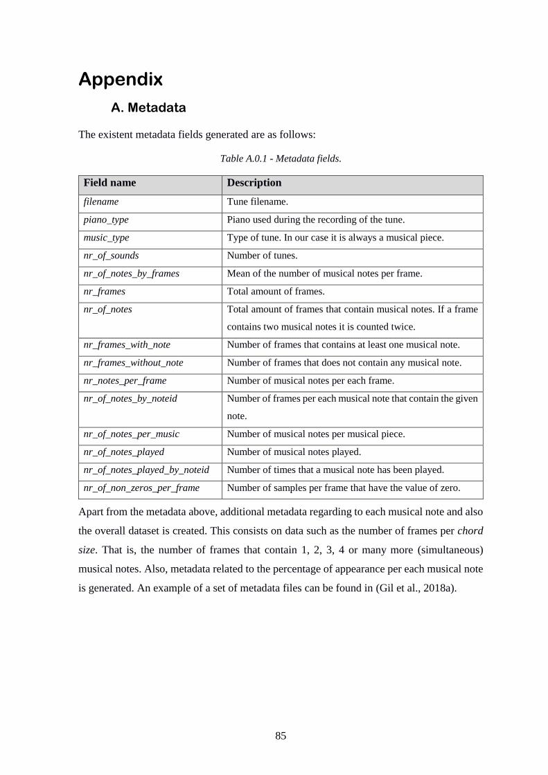
85
Appendix
A. Metadata
The existent metadata fields generated are as follows:
Table A.0.1 - Metadata fields.
Field name Description
filename Tune filename.
piano_type Piano used during the recording of the tune.
music_type Type of tune. In our case it is always a musical piece.
nr_of_sounds Number of tunes.
nr_of_notes_by_frames Mean of the number of musical notes per frame.
nr_frames Total amount of frames.
nr_of_notes Total amount of frames that contain musical notes. If a frame
contains two musical notes it is counted twice.
nr_frames_with_note Number of frames that contains at least one musical note.
nr_frames_without_note Number of frames that does not contain any musical note.
nr_notes_per_frame Number of musical notes per each frame.
nr_of_notes_by_noteid Number of frames per each musical note that contain the given
note.
nr_of_notes_per_music Number of musical notes per musical piece.
nr_of_notes_played Number of musical notes played.
nr_of_notes_played_by_noteid Number of times that a musical note has been played.
nr_of_non_zeros_per_frame Number of samples per frame that have the value of zero.
Apart from the metadata above, additional metadata regarding to each musical note and also
the overall dataset is created. This consists on data such as the number of frames per chord
size. That is, the number of frames that contain 1, 2, 3, 4 or many more (simultaneous)
musical notes. Also, metadata related to the percentage of appearance per each musical note
is generated. An example of a set of metadata files can be found in (Gil et al., 2018a).
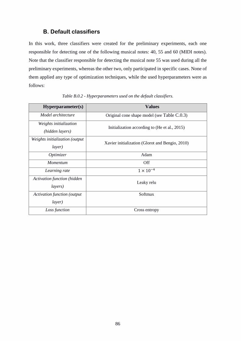
86
B. Default classifiers
In this work, three classifiers were created for the preliminary experiments, each one
responsible for detecting one of the following musical notes: 40, 55 and 60 (MIDI notes).
Note that the classifier responsible for detecting the musical note 55 was used during all the
preliminary experiments, whereas the other two, only participated in specific cases. None of
them applied any type of optimization techniques, while the used hyperparameters were as
follows:
Table B.0.2 - Hyperparameters used on the default classifiers.
Hyperparameter(s) Values
Model architecture Original cone shape model (see Table C.0.3)
Weights initialization
(hidden layers) Initialization according to (He et al., 2015)
Weights initialization (output
layer) Xavier initialization (Glorot and Bengio, 2010)
Optimizer Adam
Momentum Off
Learning rate 1 × 10⁻⁴
Activation function (hidden
layers) Leaky relu
Activation function (output
layer)
Softmax
Loss function Cross entropy
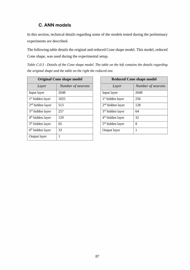
87
C. ANN models
In this section, technical details regarding some of the models tested during the preliminary
experiments are described.
The following table details the original and reduced Cone shape model. This model, reduced
Cone shape, was used during the experimental setup.
Table C.0.3 - Details of the Cone shape model. The table on the left contains the details regarding
the original shape and the table on the right the reduced one.
Original Cone shape model Reduced Cone shape model
Layer Number of neurons Layer Number of neurons
Input layer 2048 Input layer 2048
1st hidden layer 1025 1st hidden layer 256
2nd hidden layer 513 2nd hidden layer 128
3rd hidden layer 257 3rd hidden layer 64
4th hidden layer 129 4th hidden layer 32
5th hidden layer 65 5th hidden layer 8
6th hidden layer 33 Output layer 1
Output layer 1
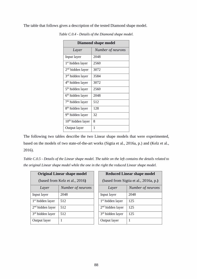
88
The table that follows gives a description of the tested Diamond shape model.
Table C.0.4 - Details of the Diamond shape model.
Diamond shape model
Layer Number of neurons
Input layer 2048
1st hidden layer 2560
2nd hidden layer 3072
3rd hidden layer 3584
4th hidden layer 3072
5th hidden layer 2560
6th hidden layer 2048
7th hidden layer 512
8th hidden layer 128
9th hidden layer 32
10th hidden layer 8
Output layer 1
The following two tables describe the two Linear shape models that were experimented,
based on the models of two state-of-the-art works (Sigtia et al., 2016a, p.) and (Kelz et al.,
2016).
Table C.0.5 - Details of the Linear shape model. The table on the left contains the details related to
the original Linear shape model while the one in the right the reduced Linear shape model.
Original Linear shape model
(based from Kelz et al., 2016)
Reduced Linear shape model
(based from Sigtia et al., 2016a, p.)
Layer Number of neurons Layer Number of neurons
Input layer 2048 Input layer 2048
1st hidden layer 512 1st hidden layer 125
2nd hidden layer 512 2nd hidden layer 125
3rd hidden layer 512 3rd hidden layer 125
Output layer 1 Output layer 1
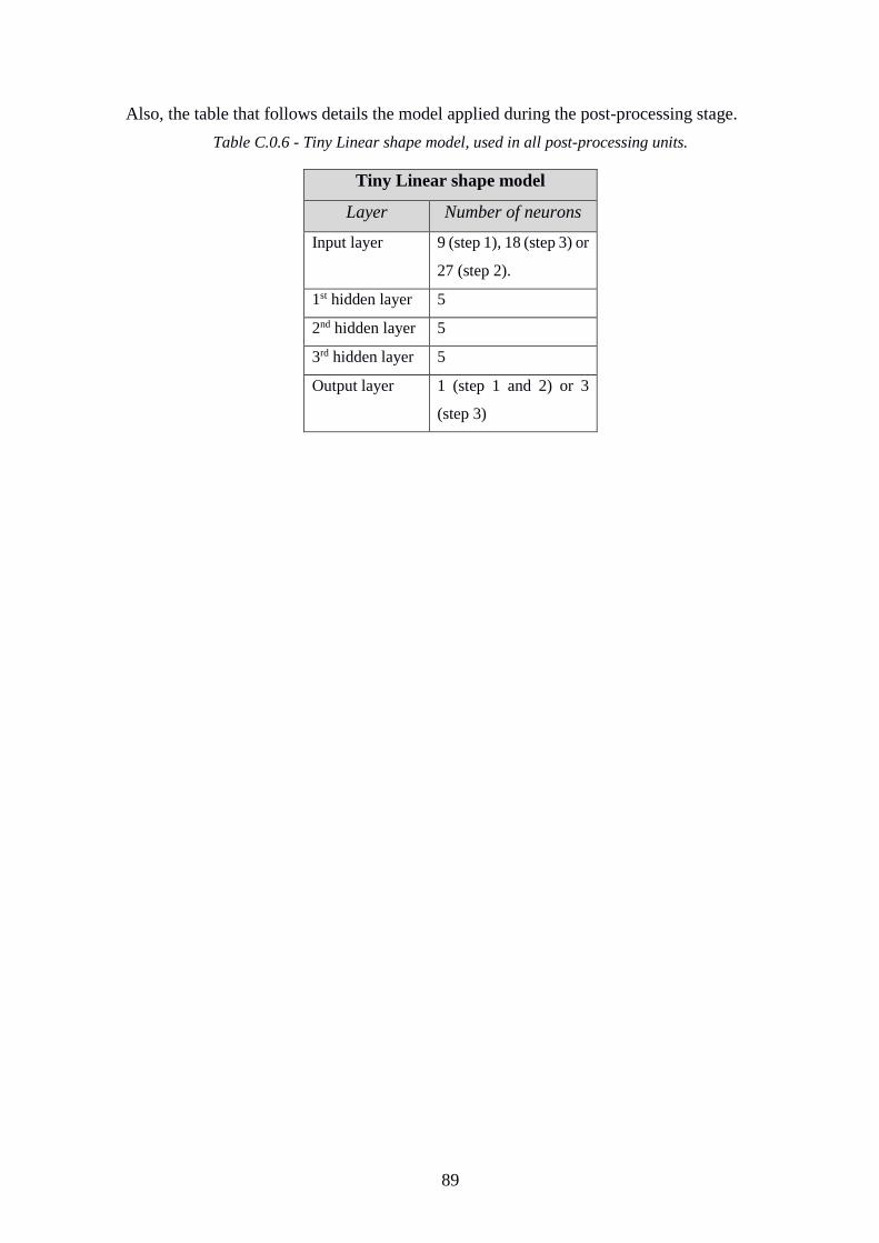
89
Also, the table that follows details the model applied during the post-processing stage.
Table C.0.6 - Tiny Linear shape model, used in all post-processing units.
Tiny Linear shape model
Layer Number of neurons
Input layer 9 (step 1), 18 (step 3) or
27 (step 2).
1st hidden layer 5
2nd hidden layer 5
3rd hidden layer 5
Output layer 1 (step 1 and 2) or 3
(step 3)
90
D. Transcription examples
To have a better insight of the efficiency of our system, several transcription examples can
be found in:
https://bitbucket.org/matapatos/mei-cm_ml_pitchdetection/src/master/transcription_examples/
The URL above has a folder composed by three sub-folders, each one holding piano pieces
from the different testing sets used. These sub-folders are, afterwards, composed by five
folders: originals, labels, classifiers, step_1, step_2 and step_3. The last four folders,
classifiers, step_1, step_2 and step_3, contain the examples of the transcribed pieces
according the given step and/or stage. The originals folder has the original musical pieces
that were used to test our system, and the labels folder contains the expected audible version
according to the labels. The difference between the originals and the labels is that the second
one does not take into account the volume of the note (velocity in MIDI terminology), which
is preferable in our case for comparing the resultant transcription with the expected one.
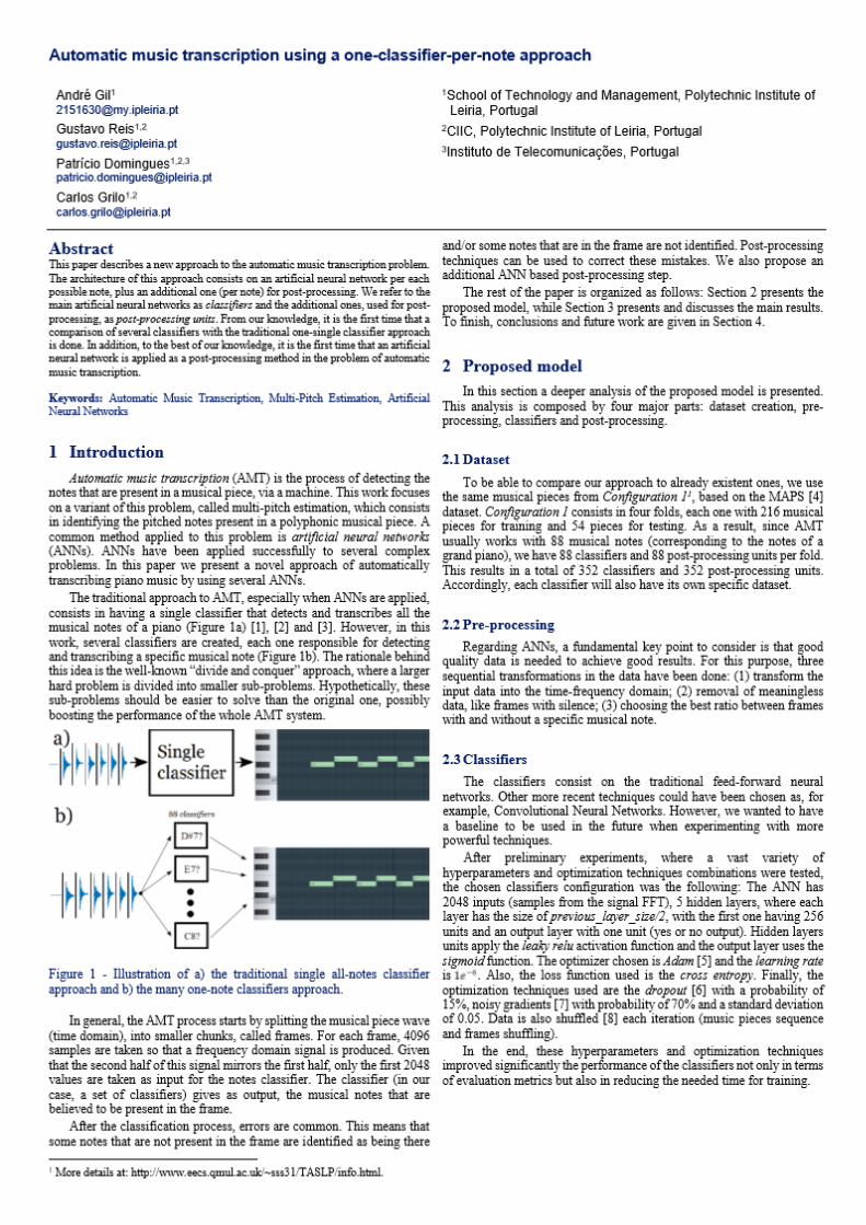
91
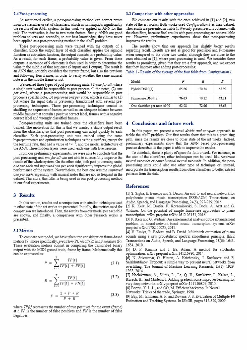
92
Related Documents