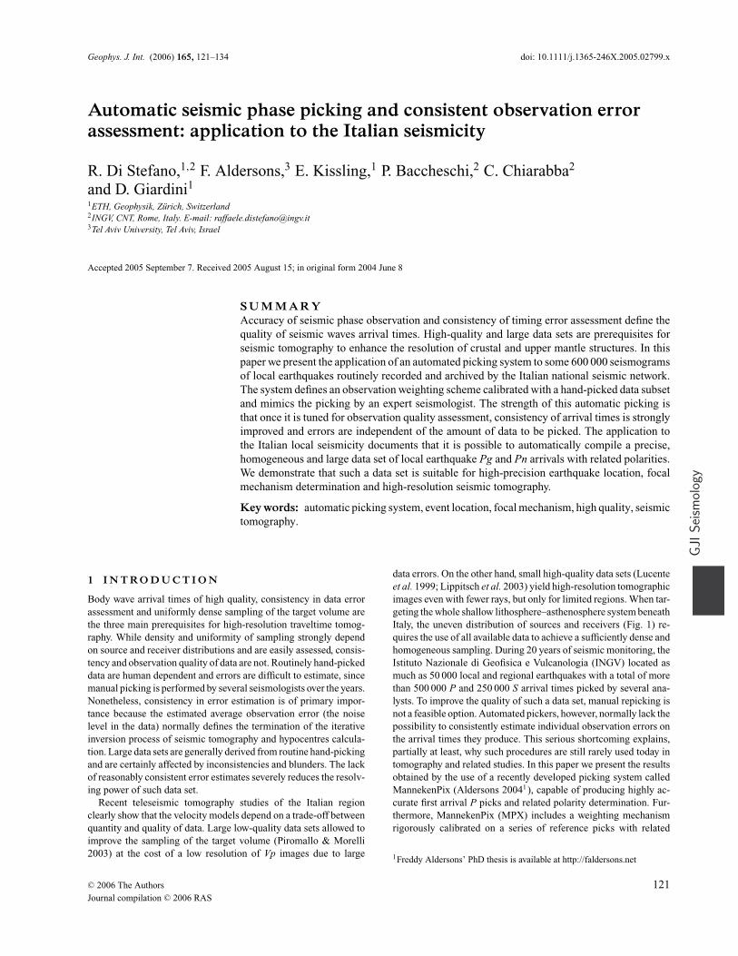
Automatic seismic phase picking and consistent · PDF fileAutomatic seismic phase picking and consistent observation error ... Single-trace picking can be seen as ... Klumpen & Joswig

Geophys. J. Int. (2006) 165, 121–134 doi: 10.1111/j.1365-246X.2005.02799.x

GJI

Sei

smol

ogy

Automatic seismic phase picking and consistent observation errorassessment: application to the Italian seismicity

R. Di Stefano,1,2 F. Aldersons,3 E. Kissling,1 P. Baccheschi,2 C. Chiarabba2

and D. Giardini11ETH, Geophysik, Zurich, Switzerland2INGV, CNT, Rome, Italy. E-mail: [email protected] Aviv University, Tel Aviv, Israel

Accepted 2005 September 7. Received 2005 August 15; in original form 2004 June 8

S U M M A R YAccuracy of seismic phase observation and consistency of timing error assessment define thequality of seismic waves arrival times. High-quality and large data sets are prerequisites forseismic tomography to enhance the resolution of crustal and upper mantle structures. In thispaper we present the application of an automated picking system to some 600 000 seismogramsof local earthquakes routinely recorded and archived by the Italian national seismic network.The system defines an observation weighting scheme calibrated with a hand-picked data subsetand mimics the picking by an expert seismologist. The strength of this automatic picking isthat once it is tuned for observation quality assessment, consistency of arrival times is stronglyimproved and errors are independent of the amount of data to be picked. The application tothe Italian local seismicity documents that it is possible to automatically compile a precise,homogeneous and large data set of local earthquake Pg and Pn arrivals with related polarities.We demonstrate that such a data set is suitable for high-precision earthquake location, focalmechanism determination and high-resolution seismic tomography.

Key words: automatic picking system, event location, focal mechanism, high quality, seismictomography.

1 I N T RO D U C T I O N

Body wave arrival times of high quality, consistency in data errorassessment and uniformly dense sampling of the target volume arethe three main prerequisites for high-resolution traveltime tomog-raphy. While density and uniformity of sampling strongly dependon source and receiver distributions and are easily assessed, consis-tency and observation quality of data are not. Routinely hand-pickeddata are human dependent and errors are difficult to estimate, sincemanual picking is performed by several seismologists over the years.Nonetheless, consistency in error estimation is of primary impor-tance because the estimated average observation error (the noiselevel in the data) normally defines the termination of the iterativeinversion process of seismic tomography and hypocentres calcula-tion. Large data sets are generally derived from routine hand-pickingand are certainly affected by inconsistencies and blunders. The lackof reasonably consistent error estimates severely reduces the resolv-ing power of such data set.

Recent teleseismic tomography studies of the Italian regionclearly show that the velocity models depend on a trade-off betweenquantity and quality of data. Large low-quality data sets allowed toimprove the sampling of the target volume (Piromallo & Morelli2003) at the cost of a low resolution of Vp images due to large

data errors. On the other hand, small high-quality data sets (Lucenteet al. 1999; Lippitsch et al. 2003) yield high-resolution tomographicimages even with fewer rays, but only for limited regions. When tar-geting the whole shallow lithosphere–asthenosphere system beneathItaly, the uneven distribution of sources and receivers (Fig. 1) re-quires the use of all available data to achieve a sufficiently dense andhomogeneous sampling. During 20 years of seismic monitoring, theIstituto Nazionale di Geofisica e Vulcanologia (INGV) located asmuch as 50 000 local and regional earthquakes with a total of morethan 500 000 P and 250 000 S arrival times picked by several ana-lysts. To improve the quality of such a data set, manual repicking isnot a feasible option. Automated pickers, however, normally lack thepossibility to consistently estimate individual observation errors onthe arrival times they produce. This serious shortcoming explains,partially at least, why such procedures are still rarely used today intomography and related studies. In this paper we present the resultsobtained by the use of a recently developed picking system calledMannekenPix (Aldersons 20041 ), capable of producing highly ac-curate first arrival P picks and related polarity determination. Fur-thermore, MannekenPix (MPX) includes a weighting mechanismrigorously calibrated on a series of reference picks with related

1Freddy Aldersons’ PhD thesis is available at http://faldersons.net

C© 2006 The Authors 121Journal compilation C© 2006 RAS

122 R. Di Stefano et al.

Figure 1. (a) Italian seismic stations network between 1988 and 2001: squares denote vertical component seismometers while triangles are three-componentsstations; (b) Italian seismicity recorded at INGV network between 1983 and 2001; dots indicate magnitude lower than 4.0 while squares denote events withM ≥ 4.0. Note the uneven distribution of epicentres.

observation error estimates provided by the user. The quality weight-ing mechanism of MPX can be tuned toward predicting the samepicking uncertainties as those that would be estimated by the user.As such, it acts as a consistent extension of the manual approachand not as a totally independent method possibly in conflict withthe legacy. To calibrate MPX on INGV data, we selected a ref-erence data set (RD) of about 700 waveforms that was picked andquality-weighted by an expert seismologist. We tuned the MPX pro-cedure to mimic the behaviour of the seismologist, by comparingthe results of the manual and the automatic picking (AP) on the RD.Finally, we applied MPX to a large data set of seismograms (seis-micity for the period 1988–2002), testing the performance of theweighted MPX arrival times in standard earthquake location and inlocal earthquake tomography.

2 I N G V S TAT I O N N E T W O R KA N D S E I S M I C I T Y I N I TA LY

The INGV seismic network (Fig. 1a) located over 50 000 local andregional earthquakes between 1983 and 2003. As shown in Fig. 1(b),the seismicity distribution is uneven, clustered along the axis of theAlps and Apennines and in the Calabrian Arc, with some large gapsin the Tyrrhenian and Adriatic regions (Amato et al. 1997). In ad-dition to the abundant crustal seismicity, there are two regions ofsubcrustal earthquakes. One such region is located in the NorthernApennines, where foci reach 90 km depth (Selvaggi & Amato 1992),the other region being in the Calabrian Arc, where a Benioff zone isidentified down to 500 km depth (Giardini & Velona 1991; Selvaggi& Chiarabba 1995). The geometry of the INGV network signifi-

cantly changed between 1980 and today and digital waveforms areonly available since 1988. Only 60 stations were available in 1980but their number is about 160 today. As a consequence, the sam-pling power of the data set has also changed considerably over theyears. During the 1984–2001 period, most stations were equippedwith short-period 1 s seismometers (S13), and signals were sampledat 50 Hz. At INGV, seismograms are picked visually by a team ofanalysts for routine location and magnitude determination. Theseparameters are stored in the waveform-event parameters databaseand represent the INGV seismic bulletin. During periods of intenseseismic activity as in 1997, not all seismograms have been hand-picked and thus some P-wave arrivals are missing.

3 T H E AU T O M AT I C P - P H A S EP I C K I N G S Y S T E M M P X

There are basically two main approaches to automated picking. Afirst way is to pick each seismogram independently from the oth-ers and one event at a time. Single-trace picking can be seen asan extension of the detection process, and some methods work innear-real time. It is also the first way analysts usually work with dur-ing the routine task of picking seismograms. Traditional methodsquantify some attributes of waveforms like amplitude, frequency orpolarization, and apply their detection and picking algorithms onthese attributes or on a smoothed combination of them. Amongthe wide variety of traditional methods for picking first arrivalP-waves of local and regional events, Allen (1978, 1982) designeda STA/LTA (short-term-average long-term-average) algorithm ap-plied on an envelope function sensitive to both amplitude and

C© 2006 The Authors, GJI, 165, 121–134

Journal compilation C© 2006 RAS

Automatic seismic phase picking and consistent observation error assessment 123

frequency of seismograms. Despite its age, Allen’s picking sys-tem is still part of Earthworm (Johnson et al. 1994) and Sac2000(Goldstein et al. 1999). Baer & Kradolfer (1987) derived their pick-ing engine from Allen’s work but they use the square of a modifiedenvelope to generate a characteristic function whose value is testedagainst an adjustable threshold. The Baer–Kradolfer picker is in-tegrated into Pitsa (Scherbaum & Johnson 1992). Autoregressivemethods (Morita & Hamaguchi 1984; Takanami & Kitagawa 1988;Kushnir et al. 1990; GSE/JAPAN/40 1992; Takanami & Kitagawa2003) work also well for picking local events, but they can alsobe used at regional and teleseismic distances (Leonard & Kennett1999; Sleeman & van Eck 1999). The Cusum algorithm (Basseville& Nikiforov 1993) appears to be an attractive alternative to autore-gressive methods at regional distances (Der & Shumway 1999; Deret al. 2000). Klumpen & Joswig (1993) apply pattern recognition onpolarization images for P- and S-onset picking of three-componentlocal data. Non-traditional methods like neural networks can some-times work directly on seismograms (Dai & MacBeth 1995, 1997),avoiding the need to compute attributes or characteristic functions.

A second approach is to work on several seismograms at once,exploiting the similarity of waveforms from nearby events. Thismultitrace approach derives basically from controlled source seis-mic methods (Peraldi & Clement 1972) used to compute static cor-rections for seismic reflection data. In seismology, seismograms aretypically organized in common station gathers (Dodge et al. 1995;Shearer 1997). A good account of the methodology and its histori-cal progress is provided by Aster & Rowe (2000). The single-traceapproach appears today to be more versatile than the multitrace ap-proach in the sense that it is not based on the restrictive criterionof waveforms similarity. A multitrace approach is inherently betteradapted to relatively restricted volume studies like those where clus-ters usually occur. Aster & Rowe (2000) suggest, however, that fur-ther developments in adaptive filtering and event clustering (Roweet al. 2002) might significantly extend the range of data sets that canbenefit from cross-correlation picking techniques.

Because MPX was originally developed to pick local events inthe Dead Sea region (Aldersons 2004), where locally a great varietyof waveforms is observed, it follows the single-trace approach. De-spite the impressive number of picking methods reported, the needfor complementary components has probably not received enoughrecognition in the literature. Examples of such components are high-fidelity filters of seismograms and methods for estimating time un-certainties associated with picked phases. In order to be meaningful,every physical measurement needs an assessment about its own un-certainty. Estimating picking uncertainties is an equally importantfunction of an automated system as determining arrival times. MPXintegrates the robust Baer–Kradolfer (1987) single-trace pickingalgorithm into a three-step automatic procedure (Aldersons 2004)

Figure 2. Calibration procedure setup: spectral density windows (N and N + S), TP theoretical arrival time predicted with IASP91 1-D earth velocity model,and the Safety Gaps set taking into account the prediction error, related to the TP.

consisting of pre-picking (spectral analysis and filtering), picking(and polarity) determination and error assessment.

Spectral analysis and waveform filtering

Filters are sometimes used in seismological analysis to reduce thelevel of noise that can obscure a precise recognition of phase on-sets. In fact, commonly used filters often distort also the signal partwhile attempting to increase the signal-to-noise ratio (SNR). For thisreason and in order to preserve as much as possible the true shapeof onsets when filtering is used, MPX allows to apply an adaptiveWiener filter (Douglas 1997; Aldersons 2004) on the waveforms inthe pre-picking step. Although the distortion by the Wiener filterof MPX is neglectable, we have not filtered the INGV data set be-cause filtering did not significantly improve the picking accuracyor success rate. However, whether the Wiener filter is applied ornot, SNRs derived from spectral densities analysis are always com-puted by the Wiener filter routines in the pre-picking step of MPXas they generate important predictors for the quality weighting en-gine. MPX is designed, in its present release, to enhance the qualityof a catalogue of routinely located earthquakes when event recog-nition has already been performed by standard procedures. Thus,it works on waveforms associated to known, though approximate,earthquake locations. A theoretical arrival time (TP) can, therefore,be calculated and it is used in MPX as a reference to place two timewindows in the noise and in the signal + noise part of the waveform,respectively (Fig. 2). The first window (N) is set before TP and isused to evaluate the noise spectral density while the second win-dow is set after the pick and is used to evaluate the noise and signalspectral density. Spectral densities are calculated using a maximumentropy method (see Aldersons 2004). Since the predicted arrivaltime is used simply to focus MPX in the ‘region’ near the P on-set, the TP can be determined by a simple 1-D ray tracing routineand the hypocentre–receiver distance. TP uncertainties as large as±3 s do not prevent MPX to converge to the real onset determina-tion. Noise and signal + noise windows must be safely separatedby gaps (Safety Gaps, Fig. 2) which width depends on the expecteduncertainty in the TP calculation.

Arrival time picking

After the spectral density analysis, the waveform is used as the inputfor the picking engine (Baer & Kradolfer 1987). In this processingphase the characteristic function CFi of the waveform (see AppendixA for details) is calculated and used by the picking engine to find theonset. The onset is accepted as a pick for a value of CFi larger thena pre-defined Threshold1 for a certain amount of time (TupEvent).Threshold1 is automatically determined by MPX based on the noise

C© 2006 The Authors, GJI, 165, 121–134



window analysis, while TupEvent has a fixed value of 0.5 sec de-rived from the dominant frequencies of P onsets observed at localand regional distances (Appendix A). A typical frequency range forPg and very short distance Pn from local earthquakes is between1.0 Hz and 4 Hz. Polarity of the P-wave onset is also determined bythe picking engine at this stage (Baer & Kradolfer 1987).

Error assessment

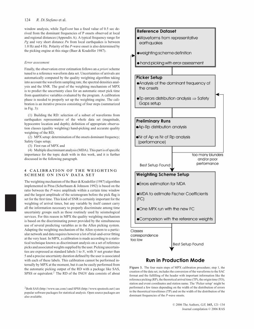
Finally, the observation error estimation follows an a priori schemetuned to a reference waveform data set. Uncertainties of arrivals areautomatically computed by the quality weighting algorithm takinginto account the waveform sampling rate, the spectral densities anal-ysis and the SNR. The goal of the weighting mechanism of MPXis to predict the uncertainty class for an automatic onset pick timefrom quantitative variables evaluated by the program. A calibrationphase is needed to properly set up the weighting engine. The cali-bration is an iterative process consisting of four steps (summarizedin Fig. 3):

(1) Building the RD: selection of a subset of waveforms fromearthquakes representative of the whole data set (magnitude,hypocentre location and depth); definition of appropriate observa-tion classes (quality weighting) hand-picking and accurate qualityweighting of the RD;

(2) MPX setup: determination of the onsets dominant frequency;Safety Gaps setup;

(3) First run of MPX and(4) Multiple discriminant analysis (MDA). This part is of specific

importance for the topic dealt with in this work, and it is furtherdiscussed in the following paragraph.

4 C A L I B R AT I O N O F T H E W E I G H T I N GS C H E M E O N I N G V DATA S E T

The weighting mechanism of the Baer & Kradolfer (1987) algorithmimplemented in Pitsa (Scherbaum & Johnson 1992) is based on theratio between the P-wave amplitude within a certain time windowand the largest amplitude of the seismogram before the pick flag isset for the first time. This kind of SNR is certainly important for theweighting of arrival times, but any variable by itself cannot carryall the information necessary to properly discriminate among timeuncertainty groups such as those routinely used by seismologicalservices. For this reason in MPX the quality weighting mechanismis based on the discriminating power provided by the simultaneoususe of several predicting variables as in the Allen picking system.Adapting the weighting mechanism of the Allen system to a partic-ular network and data requires however a lot of trial-and-error fittingat the very least. In MPX, a calibration is made according to a statis-tical technique known as discriminant analysis on a set of referencepicks and associated weights supplied by the user. Picking uncertain-ties are expressed as standard labels 1 to N , with N not greater than5 and a precise uncertainty duration defined by the user is associatedwith each of these labels. This calibration cannot be performed in-ternally by MPX at the moment, but it can be easily performed fromthe automatic picking output of the RD with a package like SAS,SPSS or equivalent.2 The RD of the INGV data consists of about

2Both SAS (http://www.sas.com/) and SPSS (http://www.spsstools.net/) arepopular software packages for statistical analysis. Open source packages arealso available.

Figure 3. The four main steps of MPX calibration procedure; step 1, thecreation of the data set, includes the conversion of the waveforms to the SACformat and the fulfilling of the header with important information like thereference picking (RP), the theoretical arrival time (TP), the origin time (TO),station and event coordinates and station name. The ‘Picker setup’ might beperformed a few times depending on the width of the distribution of errorsin the theoretical traveltimes (TP) and on the width of the distribution of thedominant frequencies of the P-wave onsets.

C© 2006 The Authors, GJI, 165, 121–134



Figure 4. Reference data set; 12 epicentre locations (stars) and stations(triangles); the distribution of the stations, epicentres, hypocentres and themagnitudes giving a broad range of frequencies for the P onset in Italy areconsidered representative of the whole INGV data set.

700 waveforms from 12 events (Fig. 4) with magnitudes rangingfrom 3 to 5.5, and from shallow crustal depth to 600 km depth inthe southern Tyrrhenian sea.

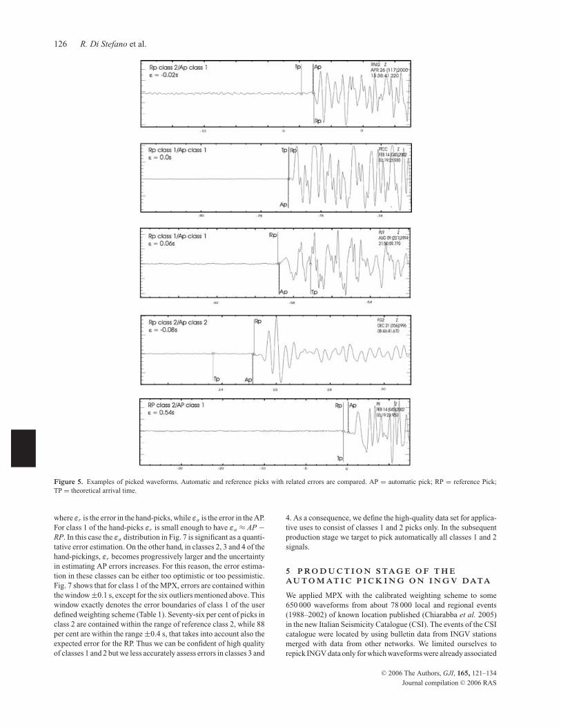
The application of MPX weighting engine on the INGV datademonstrated that enlarging the RD does not improve calibrationresults. More important is in fact to have a data set representativeof the spectrum of frequencies characteristic for the first arrivalsdue to different sources, stations’ locations and regional structureheterogeneities affecting the wave propagation. The waveforms ofthe RD have been accurately picked by hand (Fig. 5) and the er-rors have been estimated based on the weighting scheme shown inTable 1. We defined the error boundaries of each class according tothe typical noise level in the waveforms and the sampling rate. Thecharacteristics of the seismicity and of the stations network in theItalian region introduce the problem of dealing with different kindsof signals for the first onset, whose frequency content changesmainly with the hypocentral distance. Pg, short distance Pn andlong distance Pn are present in the data set together with phasesfrom deep events of the southern Tyrrhenian sea Benioff zone. Inorder to better calibrate MPX we have split the data set into Pg, Pnand deep events and we have run MPX separately on the three partsof the RD. The reference hand-picking (RP) and the AP (Fig. 5)are the key values in the MDA, together with variables (predictors),calculated by MPX for each AP (see Appendix B for details aboutMDA and predictors). The difference between AP and RP is theerror ε associated to the AP. A weight class is then attributed toeach |ε| according to Table 1. A statistical relation between pre-dictors and user-defined weight classes is found through MDA. Re-sulting Fischer’s coefficients for the INGV reference dataset are pro-

vided in Table 2. Fischer’s coefficients (Fischer 1936, 1938) actuallyrepresent the memory of the errors association, allowing MPX tomake a prediction of the target weights on unseen cases (Aldersons2004). Fischer’s coefficients newly derived from the MDA are usedin the MPX input file for the second run. This loop is stopped whenthe correspondence between the reference weights and MPX weightsis maximum and the number of blunders introduced by the AP isminimized.

To assess the quality of the weighting scheme results, we comparethe classes attributed by MPX to those determined by the seismol-ogist for the same seismic signals (Table 3). The number of class 1,2, 3 and rejected RP that fall into MPX class 1, 2, 3 and rejected, arecounted to appraise the number of RP correctly weighted (bold), up-graded (grey cells), or downgraded (white cells) by MPX. A correctpicking quality estimation (class 1 in class 1, class 2 in class 2, . . .)being our goal, the higher are the main diagonal elements in Table 3with as small as possible off-diagonal numbers, the better is the MPXperformance. To establish high-quality data set, however, downgrad-ing of a certain number of best quality picks by MPX (white cells inTable 3) can be endured, while an upgrading of even a few actuallylowest quality RPs (light grey cells) cannot. As well, a few upgradesof medium quality picks (dark grey cells below the main diagonalin Table 3) are still acceptable in common geophysical applications.The calibration output shows that MPX correctly rejects 75 per centof waveforms also rejected by the seismologist. Among the recog-nized arrival times ∼88 per cent of potentially high-quality picks(reference classes 1 and 2) are picked by MPX while ∼12 per centis lost due to MPX misidentification. MPX recognizes also65 per cent of reference classes 3 and 4 as arrival times, rejecting∼35 per cent. Such evidence (Table 3) demonstrates that althoughwe lose 12 per cent of potentially high-quality picks, MPX doesnot introduce mistakenly identified phases into high-quality classesfrom waveforms considered useless by the seismologist. Anotherimportant property is that ∼91 per cent of picks attributed by MPXto classes 1 and 2 correctly belong to reference classes 1 and 2. Fig. 6displays traveltime versus distance values for each MPX weightclass. The fit for MPX values of class 1 is nearly perfect both forshallow and for deep events. Pg and Pn traveltimes of shallow eventscan be represented by:

• Y = 0.1653X + 1.2962 (Pg)• Y = 0.1199X + 7.1858 (Pn)

with a crossover distance of about 130 km corresponding to a flatMoho located at a mean depth of 25 km. High-quality picks arepresent for both Pg and Pn. MPX class 1 results fall into referenceclass 1 error range of ±0.1 s except 5 that actually should have beenattributed to reference class 2 (|ε| ≈ = 0.15 s) and 1 belonging toreference class 3 (|ε| ∼ = 0.25 s). MPX class 2 results also displayan almost linear fit. Errors are larger but mainly contained withinthe error range of class 2, except for about 11 arrival times out of85, that should have been attributed by MPX to reference class 3and 6 that belong to lower classes. Classes 3 and 4 are essentiallydominated by downgraded picks. To better comprehend the reasonfor larger errors in MPX class 2 we must note that an importantfocus must be put on the meaning of the ε, whose distribution isshown in Fig. 7: ε is the difference between the RP and the AP as-suming the hand-pickings and in particular their observation errorsas correct. The formula of ε for the AP can be correctly rewrittenas:

εa = AP − (R P + εr ),

C© 2006 The Authors, GJI, 165, 121–134



Figure 5. Examples of picked waveforms. Automatic and reference picks with related errors are compared. AP = automatic pick; RP = reference Pick;TP = theoretical arrival time.

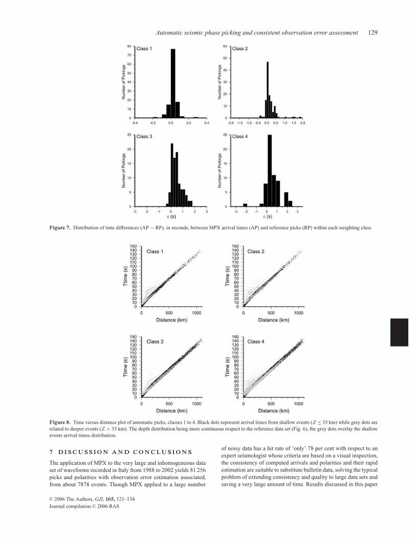
whereεr is the error in the hand-picks, while εa is the error in the AP.For class 1 of the hand-picks εr is small enough to have εa ≈ AP −RP. In this case the εa distribution in Fig. 7 is significant as a quanti-tative error estimation. On the other hand, in classes 2, 3 and 4 of thehand-pickings, εr becomes progressively larger and the uncertaintyin estimating AP errors increases. For this reason, the error estima-tion in these classes can be either too optimistic or too pessimistic.Fig. 7 shows that for class 1 of the MPX, errors are contained withinthe window ±0.1 s, except for the six outliers mentioned above. Thiswindow exactly denotes the error boundaries of class 1 of the userdefined weighting scheme (Table 1). Seventy-six per cent of picks inclass 2 are contained within the range of reference class 2, while 88per cent are within the range ±0.4 s, that takes into account also theexpected error for the RP. Thus we can be confident of high qualityof classes 1 and 2 but we less accurately assess errors in classes 3 and

4. As a consequence, we define the high-quality data set for applica-tive uses to consist of classes 1 and 2 picks only. In the subsequentproduction stage we target to pick automatically all classes 1 and 2signals.

5 P RO D U C T I O N S TA G E O F T H EAU T O M AT I C P I C K I N G O N I N G V DATA

We applied MPX with the calibrated weighting scheme to some650 000 waveforms from about 78 000 local and regional events(1988–2002) of known location published (Chiarabba et al. 2005)in the new Italian Seismicity Catalogue (CSI). The events of the CSIcatalogue were located by using bulletin data from INGV stationsmerged with data from other networks. We limited ourselves torepick INGV data only for which waveforms were already associated

C© 2006 The Authors, GJI, 165, 121–134



Table 1. Weighting scheme applied to the Italian dataset: ε is the uncertaintyattributed to a pick. ε between ±0.10 and ±0.20 means that the uncertaintybar is smaller than 0.4 s and greater than 0.2 s.

ε (s) Class

0.00 ÷ ±0.10 1±0.10 ÷ ±0.20 2±0.20 ÷ ±0.40 3±0.40 ÷ ±0.80 4

. > ±0.80 Rej

Table 2. Fischers linear discriminant coefficients of the Italian dataset (seeAppendix B).

Classes

1 2 3 4

Predictors WfStoN 0.4283 .4228 .4235 .3954GdStoN 0.0217 .0376 .0145 .0126

GdAmpR 0.0321 .0370 .0565 .0386GdSigFR 0.3331 .2948 .2173 .2396

GdDelF −0.0086 −.0117 .1066 .1009ThrCFRat −0.2815 −.4683 −.4522 −.4177PcAboThr −1.2612 −1.1877 −1.3602 −1.0344PcBelThr 0.0593 .0611 .0673 .0625

CFNoiDev 6.8090 6.9343 7.1238 7.1325

to events and easily accessible. MPX recognized 217 435 P-wavearrival times (71 per cent of the 306 334 onsets recognized by theanalysts) from 60 251 out of the 78 000 events. The first result is thatwhile 90 per cent of bulletin readings are unweighted, we are nowable to discriminate higher quality from lower quality picks. 37 929out of the 217 435 P phases (17.44 per cent) fall into class 1 and33 759 phases (15.52 per cent) fall into class 2. These percentagesare slightly lower than for the calibration subset due to the presenceof a larger number of very small magnitude events (noisy signals) inthe full data set, yielding a higher number of weights 3 and 4 phases.Fig. 8 shows the time versus distance plots for the four MPX classesof picks. Due to the higher number and wider geographic distributionof events, a larger variability in depth and a much higher numberof Pg phases with respect to the calibration data set (Fig. 6) areobserved. On the other hand, the slopes and intercepts of the linearregressions of Pg and Pn for the full data set are in good agreementwith the ones obtained for the calibration data set (Fig. 6). This factand the results for classes 1 and 2, confirm the reliability of themethod and the representativeness of the chosen calibration dataset.

6 Q UA L I T Y A S S E S S M E N T O F T H E A PR E S U LT S : 1 - D L O C AT I O N A N D L O C A LE A RT H Q UA K E T O M O G R A P H Y

To assess the quality of the repicking we first compare the 1-D lo-cations obtained with only P phases from INGV stations pickedwith MPX to the data set obtained for the same events with bulletinphases. In order to restrict the analysis to rather well-constrainedevents, we selected 7878 events having more than four P readings,small location errors and an azimuthal gap smaller than 180◦, bothwith bulletin data and with MPX data. MPX recognizes an over-all number of 81 256 P-wave onsets, representing 78 per cent withrespect to the 104 458 INGV bulletin readings related to the sameevents. 15 735 (19,37 per cent) of MPX picks fall into class 1, 14 679(18.06 per cent) fall into class 2, 17 748 (21.84 per cent) fall intoclass 3 and 33 094 (40.73 per cent) fall into class 4, yielding thus

Table 3. Performance table (confusion matrix) showing the correspondancebetween MPX (Ap) and hand picks (Rp) classes.

Ap Classes

1 2 3 4 rej

Rp Classes 1 116 47 22 13 132 5 21 46 38 283 1 11 26 29 304 0 6 9 18 24

rej 0 0 8 37 134

∼38 per cent (30 414) of high-quality arrival times and related polar-ities. The availability of such a high number of high-quality weightedpolarities makes this subset also suitable for well-constrained focalmechanism determinations with a higher confidence than for thebulletin data (Di Stefano et al. 2002). The number of available po-larities in the bulletin are in fact only 30 per cent with respect tothe MPX data set and no error estimation is given. Since a sim-ple 1-D model was used to locate events, long-distance ray pathstravelling in complex structures such as those of the Italian region,may accumulate very large residuals. So the P-wave residuals afterlocation depend also on the lateral seismic velocity heterogeneities.Nevertheless, the comparison of residual distributions for the twodifferent data sets leads to some important conclusions. In Fig. 9,we show distributions of arrival time residuals (events with at least 4phases), the difference in depth and the absolute depth calculationsfor both MPX and bulletin locations. Plot 1 in Fig. 9(a) representsbulletin data, for which the standard deviation σ is 0.91 s whilefor MPX data (plot 3) including low-quality classes 3 and 4, σ is1.27 s. The same calculation performed on high-quality MPX picks(plot 2) gives a much smaller σ of 0.63 s. Despite the fact thatlocation residuals suffer from misfits due to the 1-D model, theseσ values show that most of the large residuals from MPX are dueto classes 3 and 4. These results mark the importance of an ac-curate weighting scheme. On the other hand, due to the lack ofproper weights, poor bulletin picks (CSI) cannot be separated fromgood picks leading to a higher level of noise. In Figs 9(b–d) weshow the effect of the automatic picking and weighting on the loca-tion of events with either MPX or bulletin readings using the samemethod and parameters setup (rms cut, distance weighting, etc.). Itis widely known that hypocentral depth is the most sensitive andless constrained focal parameter. Fig. 9(b) represents the distribu-tion of absolute values of ε z . By comparing these results with thehistograms for MPX depths (Fig. 9c) and bulletin depths (Fig. 9d) weargue that most of the deepening is due to the fact that about 1000events located with bulletin data are badly located at the surfacewhile the same events are correctly located within the upper crustwith MPX. Fig. 9(c) shows clustering of events around 7 km and 14km, in agreement with what is known about the crustal seismicity inthe target region (Selvaggi & Amato 1992; Amato et al. 1997). Wethus verified the improvement on the depth variable when locatingwith MPX weighted picks. The mean of the distribution for MPXdepths is around 10 km, (within the upper crust) while the epicentresfollow the Apennines belt. Subcrustal seismicity is present to theeast of the Northern Apennines. Such locations are consistent withthose obtained using data from temporary local networks.

We have verified the resolution enhancement in local earthquakestomography achievable by using the automatic picks, classes 1 to4, along with a selection of weighted picks from other local and re-gional networks. We selected 8206 events that occurred from 1988to 2002 with at least one MPX pick from the INGV network and weadded P-wave arrival times with high-quality manual weights from

C© 2006 The Authors, GJI, 165, 121–134



Figure 6. Plots for the MPX classes. Crosses represent events below 35 km depth, while circles are events with focal depth above 35 km. Colours are relatedto differences, in absolute value, with respect to hand reference picks.

other networks. The majority of phases consists of MPX picks. Se-lected events have more than 15 phases, azimuthal gap smaller than180◦, 1-D location errors less than 5 km (x, y, z) and 1-D RMS resid-uals less than 0.6s. The total number of P observations is 165,968.Based on the number of picks belonging to each class we estimatean rms ≤ 0.2 s for our high-quality data set, significantly smallerthan the one of bulletin data. In previous studies, Chiarabba andAmato (1996) estimated that more than 45 per cent of the bulletindata (Italian seismicity 1975–1997) have errors higher than 0.2 sand that most of the largest errors are found at stations as distantas 60 km and above and especially on large distance Pn where er-rors reach ±0.8 s. For this reason Chiarabba & Amato (1996), andDi Stefano et al. (1999) excluded long distance (200 km) Pn fromtheir tomographic inversion. Mainly four factors contribute to finalresiduals rms in local source tomography: random data errors, sys-tematic data errors, misfit to the velocity model, and misfit to thehypocentral parameters. Large random and systematic data errorsmust be properly identified and removed from the data set, as thereis no way to separate them from real anomalies and hypocentre lo-cations during the inversion procedure. This is the major source of

errors in seismic tomography and it is in this part that benefits ofusing MPX are greatest, rejecting a large amount of noisy uselessdata and enhancing the effect of good data. Moreover, the use ofMPX allows us to include long- and very long-distance Pn travel-times, previously affected by large errors, thus sampling large scaleand deep structures, without blurring crustal anomalies revealed byhigh-quality Pg phases. Di Stefano et al. (1999) used some 48 000bulletin P-wave arrival times to image the lithosphere beneath Italywith layers at 8, 22 and 38 km depth and a cell size of about 27 kmin latitude and 21 km in longitude. With our data set we performedsensitivity checkerboard tests, decreasing the cell size to 15 km inlatitude and longitude and adding three more layers at mantle depth(54, 66 and 80 km). We observe very high-to-fair resolution forall the layers except at 80 km depth where resolution is high onlybeneath the Calabrian Arc. Fig. 10(a) shows results of a synthetictest at 8 and 22 km depth, where anomalies are 30 km wide. Theresolution is much higher than the one obtained by Di Stefano et al.(1999) especially at 8 km depth (Fig. 10b). The enhanced resolutionof the crust and the low noise level in our automatic picks encouragesfuture tomographic studies.

C© 2006 The Authors, GJI, 165, 121–134



Figure 7. Distribution of time differences (AP − RP), in seconds, between MPX arrival times (AP) and reference picks (RP) within each weighting class.

Figure 8. Time versus distance plot of automatic picks, classes 1 to 4. Black dots represent arrival times from shallow events (Z ≤ 35 km) while grey dots arerelated to deeper events (Z > 35 km). The depth distribution being more continuous respect to the reference data set (Fig. 6), the grey dots overlay the shallowevents arrival times distribution.

7 D I S C U S S I O N A N D C O N C L U S I O N S

The application of MPX to the very large and inhomogeneous dataset of waveforms recorded in Italy from 1988 to 2002 yields 81 256picks and polarities with observation error estimation associated,from about 7878 events. Though MPX applied to a large number

of noisy data has a hit rate of ‘only’ 78 per cent with respect to anexpert seismologist whose criteria are based on a visual inspection,the consistency of computed arrivals and polarities and their rapidestimation are suitable to substitute bulletin data, solving the typicalproblem of extending consistency and quality to large data sets andsaving a very large amount of time. Results discussed in this paper

C© 2006 The Authors, GJI, 165, 121–134



Figure 9. Distribution of residuals and depths after 1-D location. (a) Residuals from phases recorded only by INGV stations. Plot 1: CSI bulletin picks (classes1-4). Plot 2: MPX picks (classes 1-2). Plot 3: MPX picks (classes 1-4). (b) Difference between depths derived from MPX and bulletin depths. Note that mostdepths derived from MPX picks are deeper than bulletin depths. (c) Depths derived from MPX. (d) Bulletin depths. Note how the number of events located atthe surface is reduced with MPX.

suggest that 1-D locations obtained by using the MPX arrival timesare more accurate and that hypocentral depths are better constrainedthan those obtained with INGV bulletin data only. The analysis of1-D location residuals and the time versus distance plots show theeffectiveness of the picking system. By using MPX we were able tostrongly decrease the noise level of data, enhancing the resolutionand the depth range of tomographic studies, demonstrating also thatlower quality observations (classes 3 and 4) when properly weightedare still useful, complementing high-quality data in tomographicapplications.

The successful application of the automatic picking system MPXto the INGV data represents a very significant test for its generalapplicability to other regional data sets. Our next step will be tosignificantly increase the number and consistency of high-qualityphases by repicking waveforms recorded at other local and regionalpermanent networks to build the highest quality and largest data setof P-wave readings and polarities in the Italian region.

A C K N O W L E D G M E N T S

We are grateful to the responsibles of the INGV national networkwho provided us with 20 years of digital recordings used in this study,and to the analysts and responsibles of the INGV-OV and INGV-CT,DipTeris Genova, CRS-OGS, University of Calabria, ENI-AGIP,

Umbria Resil, Marche and Abruzzo regional networks (the last threesponsored by the National Seismic Survey) who provided comple-mentary hand-picked data.

Our work has been strongly improved by the useful suggestions oftwo anonymous referees. A special thank is also due to P. De Gori,F. Bernardi, L. Chiaraluce, M.G. Ciaccio, B. Castello for helpfulcomments and E. Boschi for continuous encouragement.

R E F E R E N C E S

Aldersons, F., 2004. Toward a three-dimensional crustal structure of theDead Sea region from local earthquake tomography, PhD thesis, Tel AvivUniversity, Israel, 120 pages. http://faldersons.net

Allen, R., 1978. Automatic earthquake recognition and timing from singletraces, Bull. seism. Soc. Am., 68, 1521–1532.

Allen, R., 1982. Automatic phase pickers: their present use and futureprospects, Bull. seismol. Soc. Am., 72, S225–S242.

Amato, A., Chiarabba, C. & Selvaggi, G., 1997. Crustal and deep seismicityin Italy (30 years after), Ann. Geofis., XL(5), 981–993.

Aster, R. & Rowe, C., 2000. Automatic phase pick refinement and similarevent association in large seismic datasets, in Advances in Seismic EventLocation, 18, pp. 231–263, eds Thurber, C.H. & Rabinowitz, N., Modernapproaches in geophysics, Kluwer Academic Publishers,Dordrecht, theNetherlands.

Baer, M. & Kradolfer, U., 1987. An Automatic phase picker for local andteleseismic events, Bull. seism. Soc. Am., 77, 1437–1445.

C© 2006 The Authors, GJI, 165, 121–134



Figure 10. Comparison between sensitivity checkerboard tests. (a) Pg and Pn automatic picks from the INGV network merged with high-quality manualpicks from other networks. Grid spacing is 15 km in latitude and longitude. The grey scale from −15 to 15 represents Vp perturbations in percentage. (b) Pgand very short distance Pn bulletin data from Di Stefano et al. (1999). Grid spacing is 0.25◦ in latitude and longitude.

Basseville, M. & Nikiforov, I.V., 1993. Detection of Abrupt Changes: Theoryand Application. Prentice Hall Information and System Science Series,Prentice Hall, Englewood Cliffs, New Jersey.

Chiarabba, C. & Amato, A., 1996. Crustal velocity structure of the Apennines(Italy) from P-wave travel time tomography, Ann. Geofis., 39, 1133–1148.

Chiarabba, C., Jovane, L. & Di Stefano, R., 2005. A new view of Italianseismicity using 20 years of instrumental recordings. Tectonophysics, 395,251–268.

Dai, H. & MacBeth, C., 1995. Automatic picking of seismic arrivals in localearthquake data using an artificial neural network, Geophys. J. Int., 120,758–774.

Dai, H. & MacBeth, C., 1997. The application of back-propagation neu-ral network to automatic picking seismic arrivals from single-componentrecordings, J. geophys. Res., 102, 15 105–15 115.

Der, Z.A. & Shumway, R.H., 1999. Phase onset time estimation at regionaldistances using the CUSUM algorithm, Phys. Earth planet. Inter., 113,227–246.

Der, Z.A., McGarvey, M.W. & Shumway, R.H., 2000. Automatic interpreta-tion of regional short period seismic signals using the CUSUM-SA algo-rithm, Proceedings of the 22nd DoD/DoE Seismic Research Symposium.New Orleans, LA, Louisiana.

Di Stefano, R., Chiarabba, C., Lucente, F. & Amato, A., 1999. Crustaland uppermost mantle structure in Italy from the inversion of P-wavearrival times: geodynamic implications, Geophys. J. Int., 139, 483–498.

Di Stefano, R., Amato, A., Aldersons, F. & Kissling, E., 2002. Automaticre-picking and re-weighting of first arrival times from the Italian Seismic

Network waveforms database, EOS Trans. Am. geophys. Un., 83, S71A–1059, Fall Meet. Suppl.

Dodge, D.A., Beroza, G.C. & Ellsworth, W.L., 1995. Foreshock sequenceof the 1992 Landers, California earthquake and its implications for earth-quake nucleation, J. geophys. Res., 100, 9865–9880.

Douglas, A., 1997. Bandpass filtering to reduce noise on seismograms: isthere a better way? Bull. seism. Soc. Am., 87(4), 770–777.

Fischer, R.A., 1936. The use of multiple measurements in taxonomic prob-lems. Ann. Eugenics, 7, 179–188.

Fischer, R.A., 1938. The statistical utilization of multiple measurements,Ann. Eugenics, 8, 376–386.

GSE/JAPAN/40, 1992. A fully automated method for determining the arrivaltimes of seismic waves and its application to an on-line processing system.Paper tabled in the 34th GSE session in Geneva GSE/RF/62.

Giardini, D. & Velona, M., 1991. The deep seismicity of the Tyrrhenian Sea,Terra Nova, 3, 57–64.

Goldstein, P., Dodge, D. & Firpo, M., 1999. SAC2000: signal processing andanalysis tools for seismologists and engineers, UCRL-JC-135963, Invitedcontribution to the IASPEI International Handbook of Earthquake andEngineering Seismology.

Johnson, S.J. & Anderson, N., 1978. On power estimation in maximumentropy spectrum analysis, Geophysics, 43, 681–690.

Johnson, C.E., Lindh, A.G. & Hirshorn, B., 1994. Robust regional phaseassociation, U.S.G.S. Open File Report 94–621.

Joswig, M. & Schulte-Theis, H., 1993. Master-event correlations of weaklocal earthquakes by dynamic waveform matching, Geophys. J. Int., 113,562–574.

C© 2006 The Authors, GJI, 165, 121–134



Klumpen, E. & Joswig, M., 1993. Automated reevaluation of local earth-quake data by application of generic polarization patterns for P- and S-onsets, Computers & Geosciences, 19(2), 223–231.

Kushnir, A., Lapshin, V., Pinsky, V. & Fyen, J., 1990. Statistically optimalevent detection using small array data, Bull. seism. Soc. Am., 80(6b),1934–1950.

Leonard, M. & Kennett, B.L.N., 1999. Multi-component autoregressive tech-niques for the analysis of seismograms, Phys. Earth planet. Int., 113,247–263.

Lucente, F.P., Chiarabba, C., Cimini G.B., Giardini, D., 1999. Tomographicconstraints on the geodynamic evolution of the Italian region, Geophys.Res. Lett., 104, 20 307–20 327.

Morita, Y. & Hamaguchi, H., 1984. Automatic detection of onset time ofseismic waves and its confidence interval using the autoregressive modelfitting, Zisin, 37, 281–293.

Lippitsch, R., Kissling, E. & Ansorge, J., 2003. Upper mantle structurebeneath the Alpine orogen from high-resolution teleseismic tomography,J. geophys. Res., 108(B8), 2376, doi:10.1029/2002JB002016.

Peraldi, R. & Clement, A., 1972. Digital processing of refraction data studyof first arrivals, Geophys. Prospecting, 20, 529–548.

Piromallo, C. & Morelli, A., 2003. P wave tomography of the mantleunder the Alpine-Mediterranean area J. geophys. Res., 108(B2), 2065,doi:10.1029/2002JB001757.

Rowe, C.A., Aster, R.C., Borchers, B. & Young, C.J., 2002. An automatic,adaptive algorithm for refining phase picks in large seismic data sets, Bull.seism. Soc. Am., 92(5), 1660–1674.

Selvaggi, G. & Amato, A., 1992. Subcrustal earthquakes in the NorthernApennines (Italy); evidence for a still active subduction? Geophys. Res.Lett., 19(21), 2127–2130.

Selvaggi, G. & Chiarabba, C., 1995. Seismicity and P-wave velocity imageof the Southern Tyrrhenian subduction zone, Geophys. J. Int., 121, 818–826.

Shearer, P.M., 1997. Improving local earthquake locations using the L1 normand waveform cross correlation: application to the Whittier Narrows, Cal-ifornia, aftershock sequence, J. geophys. Res., 102, 8269–8283.

Scherbaum, F. & Johnson, J., 1992. Programmable Interactive Toolbox forSeismological Analysis (PITSA). IASPEI Software Library, 5, Seismo-logical Society of America, El Cerrito.

Sleeman, R. & van Eck, T., 1999. Robust automatic P-phase picking: an on-line implementation in the analysis of broadband seismogram recordings.Phys. Earth planet. Int., 113, 265–275.

Takanami, T. & Kitagawa, G., 1988. A new efficient procedure for the esti-mation of onset times of seismic waves, J. phys. Earth, 36, 267–290.

Takanami, T. & Kitagawa, G. (eds), 2003. Methods and Applications of Sig-nal Processing in Seismic Network Operations. Springer, Berlin, LectureNotes in Earth Sciences, 98.

A P P E N D I X A : AU T O M AT I C P I C K I N G

After the application of a Wiener filter in step 1 of MPX, the au-tomatic determination of the first P-wave onset time is done bythe picking algorithm of Baer & Kradolfer (1987). This algorithmdefines first an approximate squared envelope function E2

i of theseismogram xi, given by

E2i = x2

i + x2i

∑ij=1 x2

j∑i

j=1 x2j

, (A1)

where x denotes the time derivative of x. The algorithm uses then acharacteristic function CFi, defined as

C Fi = E4i − E4

i

σ 2(E4

i

) , (A2)

in which E4i is the mean of E4

i from j = 1 to i and σ 2(E4i ) is the

variance of E4i . This characteristic function differs only from the

statistical Z score of E4i by the use of the variance σ 2 as denomina-

tor in (A2) instead of the standard deviation σ used in the Z score. Apick flag is set if CFi increases above a given value Threshold1. Theonset is accepted as a valid pick only if the value of the characteristicfunction stays above Threshold1 for a certain amount of time TU-pEvent. If the characteristic function drops below Threshold1 after ashorter duration than TUpEvent, the pick is rejected and the pick flagis removed. The pick flag is however not removed if the characteris-tic function drops below Threshold1 for an amount of time shorterthan TdownMax. This happens frequently for events with low-to-moderate SNRs. The variance σ 2(E4

i ) is continuously updated toaccount for variations of the noise level, except when CFi exceedsthe given value Threshold2 usually chosen greater than Threshold1.The variance of E4

i is thus frozen when the validity of the onsetis examined, shortly after the pick flag has been set. In MPX, theThreshold1 value of the characteristic function that triggers the pickflag is determined in a fully adaptive and automatic way. For eachseismogram, Threshold1 is first set equal to the highest value of CFi

within the time window corresponding to the noise segment of theWiener filter. If the SNR after the application of the Wiener filter isgreater than 14 dB, the value of Threshold1 is increased accordingto an internal table derived empirically. Regarding the amount oftime TUpEvent required to validate an onset after a pick flag hasbeen set, Baer & Kradolfer (1987) recommend to use at least onefull cycle of the longest signal period expected. In the case of localevents that occurred in the vicinity of the Dead Sea basin, TUpEventhas an optimal value at 0.5 s. A value of 1.0 s could be a sensiblechoice when regional and local events are mixed together in onesingle picking set. The amount of time TdownMax during whichCFi can drop below Threshold1 without clearing the pick flag hasan optimal value in MPX at half the signal period of highest powerdensity as measured by the Wiener filter routine. This value is quiteconsistent with Baer & Kradolfer (1987) who recommend half themean of the two corner periods of their bandpass filter. Threshold2,the threshold value for freezing the variance update of E4

i , is optimalin MPX at a value of 2 × Threshold1. This value is again in perfectagreement with the recommendations of Baer and Kradolfer.

Delay corrections

One known shortcoming (e.g. Sleeman & van Eck 1999) of theBaer–Kradolfer algorithm is that the raw onset time provided is al-ways somewhat late compared to what an analyst would determineas the onset time of a valid phase. For local earthquake data recordedby short-period instruments, this delay can be as small as one samplefor the best seismograms. For most seismograms, the delay is greaterdue to the interference of noise. In order to reduce the delay of theBaer–Kradolfer onset times, all versions of MPX include a primarydelay correction. This correction derives from how the onset is de-termined by the Baer–Kradolfer algorithm. When a pick flag is setand validated, the characteristic function value is generally far abovethe background level observed in the segment of noise immediatelypreceding the onset. The idea for the correction is to move the rawautomatic onset back in time as long as the characteristic functiondecreases significantly toward earlier samples. The delay correctionstops when (CFi − CFi−1) is smaller than 0.01, or when this con-dition cannot be met after moving back the onset by three samples.This process is not perfect since the characteristic function may notdecrease monotonically toward its background level, or because aclear background level may not even exist in the vicinity of the on-set due to the disturbance by strong noise. Nevertheless, this simple

C© 2006 The Authors, GJI, 165, 121–134



correction usually provides good to very acceptable results for localearthquakes recorded by short-period instruments. When regionaland teleseismic data are picked with the original Baer–Kradolfer al-gorithm, raw picking delays can be much longer than a few samples.This behaviour of the algorithm has also been observed by Sleeman& van Eck (1999). It results apparently from the fact that little or nofrequency contrast (x2 terms in A1) between the P wave train and thenoise contributes then to the build-up of the characteristic functionfor these events. At lower frequencies typical of greater epicentraldistances, the characteristic function is slow to reach the pickingthreshold level. The primary correction becomes then insufficient.In order to better correct the delay for regional and teleseismic ar-rivals, a secondary delay correction exists in MPX. This secondarycorrection is applied immediately after the primary correction. Itdoes not appear to interfere adversely with the primary correction,so important for local earthquake data. A simple moving averageSMAi,P of period P is given at the seismogram sample index i by

SM Ai,P =∑P−1

j=0 xi− j

P, i ≥ P. (A3)

The corresponding simple moving standard deviation SMSTDi,P isthen

SM ST Di,P =[∑P−1

j=0 (xi− j − SM Ai,P )2

P

]1/2

, i ≥ P. (A4)

MPX 1.7 uses a number of samples P in (A3) and (A4) correspond-ing to the period of highest noise spectral density as determined bythe Wiener filter routine. The standard deviation band of MPX 1.7is defined as

ST DBi,P = SM Ai,P ± 2 × SM ST Di,P , i ≥ P. (A5)

For a positive onset (increasing amplitude of first motion), theprecise condition is that the delay correction stops at the first sam-ple xi below the higher value of STDBi,P in (A5). This conditionis usually met at an intermediate value between the two STDBi,P

values. For a negative onset, the delay correction stops at the firstsample xi above the lower value of STDBi,P . The secondary correc-tion is however skipped if the seismogram value xi at the onset timecorrected by the primary correction is not out the deviation bandSTDBi,P by more than 0.1 × SMSTDi,P .

A P P E N D I X B : D I S C R I M I N A N TA N A LY S I S

Discriminant analysis is a statistical technique whose general pur-pose is to identify quantitative relationships between two or morecriterion groups and a set of discriminating variables also calledpredictors. It requires the criterion groups to be mutually exclusive,and it assumes the absence of collinearity among discriminatingvariables, the equality of population covariance matrices and mul-tivariate normality for each group. The mathematical objective isto weight and linearly combine the predictors in a way that maxi-mizes the differences between groups while minimizing differenceswithin groups (Fischer 1936, 1938). When more than two groupsare involved, the technique is commonly referred to as multiplediscriminant analysis (MDA). As a descriptive technique, discrim-inant analysis serves to explain how various groups differ, what thedifferences between and among groups are on a specific set of dis-criminating variables and which of these variables best account forthe differences. As a predictive technique, it is used to predict the

unknown group membership of cases based on the actual value ofthe discriminating variables. The problem at hand in the weightingmechanism of MPX is to predict the uncertainty group of AP timesfrom quantitative variables evaluated by the program. In order to beable to perform these predictions, it is however necessary to deriveclassification rules from an initial descriptive discriminant analysison data for which the group membership is known. For a given dataset, this discriminant analysis provides valuable guidelines to theuser regarding both the definition of appropriate uncertainty groupsand the selection of the most relevant predictors. The group member-ship predictions on unseen data are not done in a statistical package.MPX performs this prediction internally by computing Fischer’s lin-ear discriminant functions from the coefficients determined duringthe initial descriptive discriminant analysis.

The discriminating variables of MPX

The lack of discriminating power resulting from the use of only onepredictor can be easily understood. For instance, any SNR derivedfrom a segment of signal and a segment of noise implies alreadythat a limiting choice has been made. Basically, the length of thesegments can be chosen to be long or short compared to the domi-nant period of the signal. If long segments are selected, chances arethat a general characterization of the overall quality of the seismo-grams will be gained. This overall quality might then discriminaterather well between picks located far away from true onsets andthose located closer from true onsets. What is missing, however, inthe prediction process is a localized SNR value derived from veryshort segments. Used in isolation, this localized SNR might reflectthe accuracy of the picked features, but little will be known about thepossibility of gross errors. When the information provided by bothpredictors is combined, some discriminating power is gained be-cause a decision matrix can then be derived with information aboutboth the possibility of gross errors and a very localized quality fac-tor. Similarly, the discriminating power can be further increased byadding appropriate variables in the prediction process. Naturally,defining the most appropriate predictors is not a straightforwardtask. The benefits of using discriminant analysis for this purposeare that trial and error is reduced to a minimum, no decision matrixneeds to be coded explicitly and the best predictors for specific datasets can be easily selected from the pool of standard discriminat-ing variables already gathered. Discriminant analysis is thus usefulboth to define new predictors, and to select the available ones mostappropriate to tackle specific data sets. The pool of standard pre-dictors available so far includes nine variables evaluated internallyby MPX. On specific data sets, the optimal number of predictorsusually ranges from six to eight among the nine available.

Predictor 1 (WfStoN) is a SNR derived from the signal and noisepower spectra determined by the Wiener filter routines. Its value isevaluated at the final automatic onset time and it is given in decibelsby

P1 = 10 log10

∑FN yf =0 PS,S( f )

∑FN yf =0 PN ,N ( f )

, (B1)

where P S,S( f ) and P N ,N ( f ) are the power spectral densities of thesignal and the noise, respectively, and FNy is the Nyquist Frequency.Although the Wiener filter uses short data segments (about 2 s forlocal data), the length of these segments is long compared to oneapparent cycle of the P wave train. Predictor 1 is an overall qualityestimate around the final automatic onset time.

Predictor 2 (GdStoN) is a SNR determined by the delay-correction routines. Its value is evaluated at the final automatic onset

C© 2006 The Authors, GJI, 165, 121–134



time and it is given in decibels by

P2 = 20 log10

∑FN yf =0 AS( f )

∑FN yf =0 AN ( f )

, (B2)

where AS( f ) and AN ( f ) are the magnitude spectra of the signaland the noise, respectively, and FNy is the Nyquist frequency. Thelength of the noise segment is half the length of the Wiener filternoise segment. The signal segment extends from the picked onsetuntil the second zero-crossing after the onset. Its length is about oneapparent cycle of the P wave train. Predictor 2 is a localized measureof quality at the final automatic onset time.

Predictor 3 (GdAmpR) is a SNR determined in the time domainby the delay-correction routines. Its value is evaluated at the finalautomatic onset time and it is given in decibels by

P3 = 20 log10

AmpS

AmpN, (B3)

where AmpS and AmpN are the peak-to-peak maximum amplitude ofthe signal and noise, respectively. The length of the noise segment ishalf the length of the Wiener filter noise segment. The signal segmentextends from the picked onset until the second zero-crossing afterthe onset. Its length is about one apparent cycle of the P wavetrain. Predictor 3 is also a localized measure of quality at the finalautomatic onset time.

Predictor 4 (GdSigFR) is the SNR evaluated at the dominant fre-quency of the signal, as determined by the delay-correction routines.Its value is evaluated at the final automatic onset time and it is givenin decibels by

P4 = 20 log10

AS(FS)

AN (FS), (B4)

where AS(FS) is the value of the magnitude spectrum of the signalat the dominant frequency of the signal f = FS , and AN (FS) is thevalue of the magnitude spectrum of the noise at frequency f = FS .The length of the noise segment is half the length of the Wiener filternoise segment. The signal segment extends from the picked onsetuntil the second zero-crossing after the onset. Its length is about oneapparent cycle of the P wave train. Predictor 4 is also a localizedmeasure of quality at the final automatic onset time.

Predictor 5 (GdDelF) is the difference between the dominantfrequency of the signal and the dominant frequency of the noise, asdetermined by the delay-correction routines. Its value is evaluated

at the final automatic onset time and it is given in hertz’s by

P5 = FS − FN , (B5)

where f = FS is the dominant frequency of the signal and f =FN is the dominant frequency of the noise. The length of the noisesegment is half the length of the Wiener filter noise segment. Thesignal segment extends from the picked onset until the second zero-crossing after the onset. Its length is about one apparent cycle of theP wave train. Predictor 5 is a localized measure of the frequencycontrast between the signal and the noise.

Predictor 6 (ThrCFRat) is the natural logarithm of the ratio be-tween the first maximum of the characteristic function after pickingto the Threshold1 value, as determined by the AP routines. It is givenby

P6 = lnC FMax1

Threshold1. (B6)

Predictor 6 is a localized measure of quality derived from the char-acteristic function.

Predictor 7 (PcAboThr) is the percentage of characteristic func-tion samples above the Threshold1 value before the picked onset,as determined by the AP routines. The data segment has the lengthof the Wiener filter noise segment and stops one sample before thepicked onset. A Predictor 7 value different from zero is often as-sociated with a possible earlier pick time, or with a high level ofpre-arrival noise.

Predictor 8 (PcBelThr) is the percentage of characteristic func-tion samples below the Threshold1 value after the picked onset, asdetermined by the AP routines. The signal data segment length is1/10 the length of the Wiener filter mixed signal-and-noise segmentand starts at the picked onset. A Predictor 8 value different fromzero is often associated with low-to-moderate SNRs.

Predictor 9 (CFNoiDev) is a measure of deviation of the charac-teristic function before the picked onset, as determined by the AProutines. It is given by

P9 = ln

∑Ni=1 |C Fi −C Fmedian|

N

|Threshold1 − CFmedian| , (B7)

where the CFi are the N samples of the characteristic function ina noise segment of length equal to the length of the Wiener filternoise segment, and CFmedian is the median value of CFi over the Nsamples.

C© 2006 The Authors, GJI, 165, 121–134


Automatic seismic phase picking and consistent · PDF fileAutomatic seismic phase picking and consistent observation error ... Single-trace picking can be seen as ... Klumpen & Joswig

Documents