Automatic reconstruction of fault networks from seismicity catalogs: Three-dimensional optimal anisotropic dynamic clustering

JOURNAL OF GEOPHYSICAL RESEARCH, VOL. ???, XXXX, DOI:10.1029/,

Automatic Reconstruction of Fault Networks from SeismicityCatalogs: 3D Optimal Anisotropic Dynamic ClusteringG. Ouillon1, C. Ducorbier2 and D. Sornette3,4

1 Lithophyse, 1 rue de la croix, 06300 Nice, France2 Laboratoire de Physique de la Matiere Condensee, CNRS UMR 6622, Universite de Nice-Sophia Antipolis,Parc Valrose, 06108 Nice, France3 D-MTEC, ETH Zurich, Kreuzplatz 5, CH-8032 Zurich, Switzerland4 Department of Earth and Space Sciences and Institute of Geophysics and Planetary Physics, University ofCalifornia, Los Angeles, California 90095-1567

Abstract. We propose a new pattern recognition method that is able to reconstructthe 3D structure of the active part of a fault network using the spatial location of earth-quakes. The method is a generalization of the so-called dynamic clustering method, thatoriginally partitions a set of datapoints into clusters, using a global minimization cri-terion over the spatial inertia of those clusters. The new method improves on it by tak-ing into account the full spatial inertia tensor of each cluster, in order to partition thedataset into fault-like, anisotropic clusters. Given a catalog of seismic events, the out-put is the optimal set of plane segments that fits the spatial structure of the data. Eachplane segment is fully characterized by its location, size and orientation. The main tun-able parameter is the accuracy of the earthquake localizations, which fixes the resolu-tion, i.e. the residual variance of the fit. The resolution determines the number of faultsegments needed to describe the earthquake catalog, the better the resolution, the finerthe structure of the reconstructed fault segments. The algorithm reconstructs success-fully the fault segments of synthetic earthquake catalogs. Applied to the real catalog con-stituted of a subset of the aftershocks sequence of the 28th June 1992 Landers earth-quake in Southern California, the reconstructed plane segments fully agree with faultsalready known on geological maps, or with blind faults that appear quite obvious on longer-term catalogs. Future improvements of the method are discussed, as well as its poten-tial use in the multi-scale study of the inner structure of fault zones.

1. Introduction

Tectonic deformation encompasses a wide spectrum ofscales, both in spatial and temporal dimensions. Thiscertainly constitutes a fundamental obstacle to thoroughlystudy, from observations alone, the whole set of relevant pro-cesses. It is now clear that seismic events occur on faults,while faults grow by accumulation of slip, by the growth ofdamage in the region of their tips, and by linkage betweenpre-existing faults of various sizes, all three processes occur-ing in large part during earthquakes (see Scholz (2002) fora review of earthquake nucleation and fault growth mech-anisms and Sornette et al. (1990) and Sornette (1991) fora general theoretical set-up). In the last twenty years, alarge amount of knowledge has been obtained on the statis-tical properties and general phenomenology of faults andearthquakes (including the distribution of sizes, of inter-event time distributions, the geometrical correlations, andso on), but a clear physical and mechanical understandingof the links and interactions between and among them is stillmissing. Such knowledge may prove decisive to drasticallyimprove our understanding of seismic risks, especially thetime-dependent risks associated with the future large andpotentially destructive seismic events.

The study of natural fault networks and of earthquakecatalogs is generally conducted in two very different ways,which clearly reveal still distinct scientific cultures. On oneside, brittle tectonics (within which we include seismotec-tonics) and structural geology pays a lot of attention to

Copyright 2008 by the American Geophysical Union.0148-0227/08/$9.00

structures, but dwells quite little on their nonlinear collec-tive dynamics. Thus, brittle tectonics and structural geol-ogy are incapable of any predictive seismological statement,despite an impressive amount of theoretical and laboratory-validated concepts coming from rock physics and rheology(see Scholz (2002), Passchier and Trouw (2005) and Pol-lard and Fletcher (2005)), as well as from observationaltechniques. Brittle tectonics and structural geology mainlyconsider structures as isolated and thus focus on the “one-body” problem, generally solvable through the use of classi-cal physics and/or the use of the mechanics of homogeneousmedia. On the other side, statistical analyses can reveal pat-terns, but rarely provide anything else than purely empiricaldescriptions of the data. Some statistical analyses may evenbe seriously flawed due to their very nature (see for instanceOuillon and Sornette (1996) who reveal a mechanism lead-ing to spurious multifractal analyses of fault patterns). Forinstance, when dealing with earthquakes, most spatial anal-yses deal with epicenters or hypocenters. Since real earth-quakes involve extended oriented structures, statistical anal-yses based on point-wise representation of earthquakes mayled to spurious correlations between events, especially thesmallest ones, which may distord any model of the collec-tive build-up of a large shock by previous smaller events.

Statistical analyses can also be performed using fault net-works, but they are most often restricted to the available2D surface maps. It is then difficult to assess the amountof information that is genuinely representative of 3D activefaulting at depth and, as such, related to seismogenesis, inthe goal of developing better understanding and improvedforecasts. There are several problems when working withnetworks of surface-intersecting faults. First, the samplingof fault data is by far more difficult and time-consuming than

1

arX

iv:p

hysi

cs/0

7030

84v1

[ph

ysic

s.ge

o-ph

] 7

Mar

200

7

X - 2 OUILLON, DUCORBIER AND SORNETTE: 3D DETERMINATION OF FAULT PATTERNS

constructing earthquake catalogs, with the often unavoid-able existence of subjective inputs. Second, one can onlymap small-scale features in small-scale domains (see Ouil-lon et al (1995) and Ouillon et al (1996) for a rather uniquehigh-resolution multi-scale analysis of fracturing and fault-ing of the Arabic plate). The domains chosen for such sam-pling may not be good representative, as their choice mayeither be arbitrary or reflect practical constraints. Third,there can exist some masks (like cities, deserts or vegeta-tion) which make observations impossible in sometimes vastareas. This can seriously bias statistical results (see Ouillonand Sornette (1996)). In any case, if one takes account of allthose shortcomings, spatial analyses are possible at any scale(from millimeters to thousands of kilometers - see Ouillonet al (1995) and Ouillon et al (1996) which showed how toexploit such data with multifractal and anisotropic waveletmethods so as to reconstruct objective fault maps at multi-ple scales), but there is a terrible lack of data in the time do-main. Darrozes et al. (1998) and Gaillot et al. (2002) stud-ied the aftershock sequence of the 1980 M5.1 Arudy earth-quake in the French Pyrenees using anisotropic wavelets.Their method is an extension of the Optimal AnisotropicWavelet Coefficient method (Ouillon et al (1995); Ouillonet al (1996)). This method uses anisotropic filters, whichproperties (size and orientation) can vary from one locationto another within the same dataset. At each spatial loca-tion, the shape of the filter is chosen such that it revealsbest the local anisotropic features, if any (hence the “opti-mal” qualification). In this way, each pixel in the image ischaracterized by a local optimal anisotropy. This method al-lowed one to detect and map linear structures in the Arudysequence, and to quantify their orientation. However, iden-tified faults are still sets of neighbouring pixels, each pixel“ignoring” that it possibly belongs to the same fault as itsneighbours. The images provided by wavelet analysis stillneed to be post-processed in order to compute, for example,the size of the lineaments. The method is also restrictedto 2D datasets. Extension to 3D geometries would be the-oretically straightforward, but the size of images to handleat the scale of a regional catalogue is totally unrealistic, aslarge volumes of space would have to be discretized at scalesmuch lower than the earthquake localization accuracy.

The structure of the present state of a fault pattern in-tegrates its whole history, i.e. reflects the largest possibletime scale, which can be several tens of millions of years. Atvery short time scales, seismology offers pictures of the slippattern over a reconstructed fault surface that occured dur-ing an earthquake. But this kind of inversion is performedonly for the largest shocks. In between, paleo-seismologyallows one to decipher the sliding history along discontinu-ities, but it still focuses on major faults and major seismicevents for obvious reasons of time and space resolution. Infact, there is absolutely no work at all on the mechanicsof faulting within a fault network as a whole derived fromfield observations, at time scales comparable with those ofa seismic catalog. Obtaining such information would cer-tainly constrain significantly our concepts and methods onthe space-time organization of earthquakes and on the po-tential for their forecasts, with the ultimate goal of betterassessment of time-dependent hazard.

Most studies focus on earthquake catalogs. This comesfrom the fact that earthquake catalogs contain in generala large number of events, allowing accurate statistics to becomputed, and that building such a database is reasonablymastered at the technical level. A homogeneous seismo-graphic network can span a very large domain, which allowfor spatial analyses at scales from a few tens of meters tohundreds or thousands of kilometers, at least in 2D. Depthis often omitted in most statistical analyses, as the increasesof pressure and temperature, as well as the finite thicknessof the seismogenic layer, clearly break any possible symme-try along the vertical direction, which one generally does

not know how to deal with when performing statistics (seehowever Bethoux et al (1998) for a genuine 3D wavelet anal-ysis of seismicity in the Alpine arc). Another reason for theuse of seismic catalogs for the analysis of fault networks isthat they also allow for clean analyses in the time domain,at scales varying from few seconds to decades.

Up to now, most of the information available on the struc-ture of fault patterns comes from surface mapping at variousscales. One can however question the reliability of such datasets, as earthquakes catalogs generally include large quan-tities of events which do not seem to be linked to any suchfaults, but rather seem to be associated with active faultsburied at depth which do not cross-cut the surface. It isthus rather clear that comparing 2D map views of the long-term cumulative brittle deformation to the 3D structure ofthe short-term incremental deformation can provide at besta poor insight into, and at worst a biased incorrect modelof, the multi-scale tectonic processes as a whole. A detailedknowledge of the 3D structure of fault networks is needed tobetter understand the mechanics of earthquake interactionand collective behaviour. In the last few years, in paral-lel to the ever increasing capabilities of computers, earth-quake localization algorithms have significantly improved sothat the accuracy for the spatial resolution of earthquakehypocenters dropped down to about 1km, and even to a fewtens of meters within clusters (when using relative locationsthrough cross-correlating waveforms, Shearer et al (2005)).This provides new opportunities to learn about the detailed3D structure of fault patterns at depth using seismicity itselfas a diagnostic.

The basis of our paper is that seismic hazard assessmentfaces two fundamental bottlenecks: (i) catalogs are inher-ently incomplete with respect to the typical recurrence timeof large earthquakes which are many times larger than theduration of the available catalogs; (ii) earthquakes occuron faults, but most of them are still unknown, drasticallylimiting our understanding and our assessment of seismicrisks. The principal issue therefore lies in the associationbetween earthquakes and faults. A recent effort to assignearthquakes and simple fault structures in the San Fran-cisco Bay area showed significant disparities that arose fromthe simplified geometry of fault zones at depth and theamount and direction of systematic biases in the calculationof earthquake hypocenters (Wesson, 2003). The geometryof an active fault zone is often constrained by mapping thesurface trace; dip angle at depth and depth extent are ei-ther constrained by results of controlled source seismology(if available) and the distribution of hypocenter locationsor they are just extrapolated using geometric constraints,if seismologic constraints are not available. For example,one of the most sophisticated fault models available, theCommunity Fault Model (CFM) of the Southern CaliforniaEarthquake Center (SCEC), combines available informationon surface traces, seismicity, seismic reflection profiles, bore-hole data, and other subsurface imaging techniques to pro-vide three-dimensional representations of major strike-slip,blind-thrust, and oblique-reverse faults of southern Califor-nia (Plesch, 2002). Each fault is represented by a triangu-lated surface in a precise geographic reference frame. How-ever, the representation of a fault by a simple surface cannotreflect the fine-detailed structure seen in extinct fault zonesand in drilling experiments of active faults (e.g. Scholz, 2002; Faulkner, 2003). These results suggest that fault zonesactually consist of narrow earthquake-generating cores, pos-sibly accompanied by small subsidiary faults. Our presentcontribution is to propose a general method to identify andlocate active faults in seismically active regions by using ascientifically rigorous approach based on active seismicity.

OUILLON, DUCORBIER AND SORNETTE: 3D DETERMINATION OF FAULT PATTERNS X - 3

Our goal is to gain a better understanding of the link be-tween fault structures and earthquakes.

For this, the present paper presents a new pattern recog-nition method which determines an optimal set of plane seg-ments, hereafter labeled as ‘faults’ that best fit a given setof earthquake hypocenters. In the first part, we provide ashort overview of pattern recognition methods used to de-tect linear or planar features in images, such as the Houghand wavelet transforms. We then present in more detailsthe dynamic clustering method, which provides a partitionof a set of data points into clusters, before detailing ournew method, a generalization of dynamic clustering to thecase of anisotropic structures. We illustrate this new tech-nique through benchmark tests on synthetic datasets, beforeproviding results obtained on a subset of the Landers after-shocks sequence. The final discussion of our results com-pares this new method with other clustering methods, andoutline its potential use in the study of fault-zones struc-tures. We then sketch the next set of improvements for thismethod which will be developed in sequel papers.

2. Line and plane detection in imageanalysis

The detection of linear and planar structures in seismo-tectonics has a long history, but still suffers from a lack ofquantitative methods. From the early years of instrumen-tal seismology, the main instrument to identify faults fromearthquakes has indeed been the eye. It is by visual inspec-tion that tectonic plates boundaries or the Benioff planein subduction zones have been delineated. Visual inspec-tion remains the main approach to identify blind faults atsmaller scales. Very few efforts have been devoted to thedevelopment of automatic digital detections of linear or pla-nar spatial features from earthquake catalogs. We shall thusnow describe two major approaches in image analysis, andoutline their advantages and drawbacks, before turning todynamic clustering.

2.1. The Hough transform

The Hough transform (see Duda and Hart, 1972) is atechnique that is widely used in digital image analysis, withapplications, for example, in the detection and characteriza-tion of edges, or the reconstruction of trajectories in particlephysics experiments. The original Hough transform identi-fies linear features within an image, but it can be extendedto other shapes (like circles or ellipses). We shall anywaypresent it for straight line detection in 2D for the sake ofsimplicity. The basic idea is that, given a set of data points,there is an infinite number of lines that can pass througheach point. The aim of the Hough transform is to determinethe set of lines that get through several points.

Each line can be parameterized using two parameters rand θ in the Hough space. The parameter r is the distancebetween this line and the origin, and θ is the orientation ofthe normal to that line (and is measured from the abscissaaxis). Then, the infinite number of lines passing through agiven point defines a curve r(θ) in the Hough plane. All linespassing through a point located at (x0, y0) obey the equa-tion r(θ) = x0 ·cos(θ)+y0 ·sin(θ). If we now consider severalpoints of our dataset that are located on the same straightline in direct space, their associated r(θ) curves will all crossat the same (r, θ) point in the Hough space. Reciprocally,the corresponding line is then fully identified. Note that sev-eral distinct sets of r(θ) curves can cross in the Hough spaceat different (r, θ) locations, so that as many linear featurescan be extracted at once. This idea can be extended to ar-bitrary 2D structures (such as circles or ellipses) or to 3D

spaces and planar features, provided that one extends thedimension of the Hough space correspondingly. For exam-ple, this dimension is equal to 4 when one wants to detectstraight lines in a 3D real space, so that the method is notused in practice in that case (or rather in a much simplifiedform, provided there is only a very small number of suchlines to detect, see Bhattacharya et al (2000)). The dimen-sion of the Hough space drops to 3 when dealing with planarfeatures.

The main problem of this technique is that it does notprovide directly the spatial extension of the linear or pla-nar features, only their positions in space, as each line (orplane) has an infinite size. A post-processing step must thenbe performed in order to compute the finite extension. An-other drawback is that the Hough transform does not takeaccount of the uncertainties in the localization of the set ofdata points, a crucial parameter in seismology. All in all, itappears that the Hough transform is very efficient only whendealing with few very clean ordered patterns (see howeversome specific strategies that can be defined to deal with realfracture planes (Sarti and Tubaro, 2002). Another majorargument against the use of the Hough transform for faultsegment reconstruction from seismic catalogs is that thereis absolutely no way to include any other information onemay have about seismic events, such as their seismic momenttensors, focal mechanisms or magnitudes.

2.2. The Optimal Anisotropic Wavelet Coefficientmethod

The characterization of anisotropy is a basic task in struc-tural geology, tectonics and seismology. The orientationsof structures stem from mechanical boundary conditions,which we are in general interested to invert. They controlthe future evolution of the system, which we are interestedto predict. Tools for quantifying anisotropy generally mate-rialize in rose diagrams (for 2D fracture maps for instance)or in stereographical projections (when data are sampledin 3D space). The main drawback of these representationsis that they are scale-dependent. For example, as shownin (Ouillon, 1995 ; Ouillon et al, 1995), in the case of en-echelon fractures, small-scale and large-scale features willpossess fundamentally different anisotropy properties. Inthat case, mapping at small scales will not give any clueon the large scale properties of the system. The so-calledOptimal Anisotropic Wavelet Coefficient (OAWC) method,presented in the above publications, was designed to specif-ically address this problem.

For 2D signals, such as fault maps and fracture maps, awavelet is a band-pass filter which is characterized, in realspace, by a width (called resolution), a length and an az-imut. In a nutshell, the OAWC method consists in fixingthe resolution and convolving the wavelet with the map offault traces, varying its length and azimut. For any givenposition, when the result of the convolution (which is thewavelet coefficient) reaches a maximum, one stores the as-sociated azimut of the wavelet and switch to the next spa-tial location. Building a histogram of such optimal azimutsprovides a rose diagram at the considered resolution. Per-forming this process at different resolutions allows one todescribe the evolution of anisotropy with scale from a singleinitial data set. Looking at various maps of fractures andfaults patterns in Saoudi Arabia, Ouillon, 1995 and Ouil-lon et al, 1995 were able to show that anisotropy propertieschange drastically at resolutions that can be related to thethicknesses of the mechanical layers involved in the brittledeformation process (from sandstone beds up to the conti-nental crust).

The OAWC method has been extended to characterizethe anisotropy of mineralization in thin plates, as well as todetect faults or lineaments from earthquakes epicenter maps(Darrozes et al, 1997 ; Darrozes et al, 1998 ; Gaillot et al,

X - 4 OUILLON, DUCORBIER AND SORNETTE: 3D DETERMINATION OF FAULT PATTERNS

1997 ; Gaillot et al, 1999 ; Gregoire et al, 1998). In thissecond class of applications, the issue concerning the finiteaccuracy of event localizations is addressed by consideringa wavelet resolution larger than the spatial uncertainties.However, this method does not provide direct informationabout the size of the structures, and indeed does not ma-nipulate structures as such. Each point in space is char-acterized by anisotropy properties, but the method do notnaturally construct clusters from neighbouring points withsimilar characteristics. Moreover, its extension to 3D sig-nals and their associated 3D patterns would prove unrea-sonably time-consuming (as space has to be discretized ata scale smaller than the chosen resolution) and would sufferfrom edge effects near the top and bottom of the seismo-genic zone. Nothwithstanding its power and flexibility, it isno better that the Hough transform for our present problemof reconstructing a network of fault segments best associatedwith a given seismic catalog.

3. Dynamic clustering3.1. Dynamic clustering in 2D

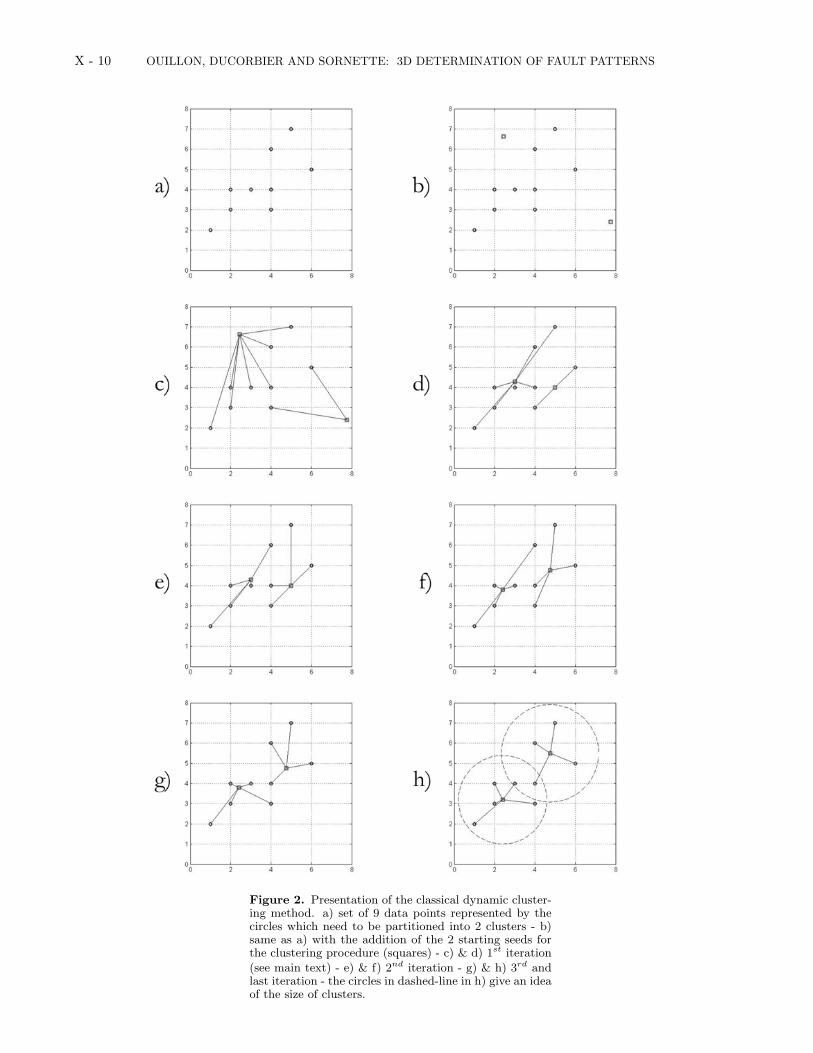
Dynamic clustering (also known as k-means) is a verygeneral image processing technique that allows one to par-tition a set of data points using a simple criterion of inertia.The method is described in many papers or textbooks (seefor example Mac Queen (1967)), so it will suffice for ourpurposes to perform a practical demonstration in 2D - butextension of the method to 3D is straightforward.

We first define a set of N datapoints (xi, yi), with i =1, N . Fig. 2 (stage a) is an example with N = 9. Our goal isto partition this dataset into a given number Nc of clusters,with Nc < N . In the example illustrated in Fig. 2, Nc = 2.The first step consists in throwing 2 more points at randomrepresented with square symbols (stage b)). Note that thoseadded points can be chosen to coincide with points belong-ing to the initial dataset. We now link each circle to theclosest square, and obtain a first partition of the datasetinto 2 clusters (stage c)). The first cluster features 2 dat-apoints, while the second cluster features 7 data points inour example. Each square is now moved to the barycenterof the associated cluster (stage d)), leaving the partition in-tact. As the squares change position, so do the distancesbetween squares and circles. We link once again each cir-cle to the closest square, which updates the partition (stagee)). Clusters now feature respectively 4 and 5 data points.Squares are then moved once again to the barycenters ofthe associated clusters (stage f)). We associate once moreeach circle to the closest square (stage g)), which updatesthe partition to a new one, the squares being moved to thebarycenters of the corresponding clusters. We obtain stage h(the signification of the dashed-line circles will be given be-low). One can then check that any further iteration doesn’tchange the partition anymore (that is, the location of thesquares), so that the method converges to a fixed structure,which is the final partition of the dataset.

For any given partition, we can compute the inertia ofeach cluster ic (featuring Nic points) by:

Iic =1

Nic

Nic∑j=1

D2j (1)

where Dj is the distance between one point belonging to thecluster ic and the barycenter of that cluster. It can then beproven that the final partition we obtain minimizes the sumof inertia over all clusters. However, there can exist severallocal minima for the global inertia in the partition space, sothat one has to run the dynamic clustering procedure sev-eral times, using different initial location of the squares inorder to select the partition which corresponds to the gen-uine global minimum. Stage h shows the final partition we

obtained starting from stage b, with 2 dashed-line circles.Each circle is centered on the barycenter of a cluster, andits radius is taken as twice the square root of the inertia ofthat cluster. The role of those circles is just to illustrate thesize of each cluster, and the way we quantify this size willbecome clearer later. The total variance in stage h is 3.5375(note that coordinates are dimensionless in our example).

We performed this dynamic clustering process using hun-dreds of different initial positions for the squares, and wereable to find two other local variance minima (with corre-sponding partitions illustrated on Fig. 3a and 3b). The finalinertia of the configuration shown in Fig. 3a is 3.1111, whilethe one we computed for Fig. 3b is 3.5833. The partitionwhich minimizes the global inertia is thus the one shown onFig. 3a. Note however that those three minima are not verydifferent from each other, so that all of them appear as veryreasonable partitions. The similarity of the numerical val-ues of the variances suggests that all three partitions wouldbe barely discriminated by a human operator alone, whichone generally refers to as ‘subjectivity’. Note also that thefinal partitions display data points that lay almost half-waybetween two squares, so that adding some noise on the posi-tions of the data points (to simulate earthquake localizationuncertainties) would certainly make a given final partitionswitch to one of the two others, and vice-versa.

3.2. The problem of anisotropy in 3D - Principalcomponent analysis

Dynamic clustering, as described in the previous section,is an iterative procedure which minimizes the sum of vari-ances over a given number of clusters. As presently set up,dynamical clustering suffers from the two following draw-backs:

(i) the user has to choose a priori the number of clustersnecessary to partition our data set; the method to removethis constraint will be addressed in the next section;

(ii) Using a criterion in terms of the minimization of thetotal inertia is certainly not adequate when data points haveto be partitioned into anisotropic clusters, as we plan to doby associating earthquakes with faults. As an alternative,we propose a minimization criterion which takes account ofthe whole inertia tensor of each cluster.

The inertia tensor of a given cluster of points embeddedin a 3D space is equivalent to the covariance matrix of theircoordinates (x, y, z). The covariance matrix C reads :

C =

(σ2x cov(x, y) cov(x, z)

cov(x, y) σ2y cov(y, z)

cov(x, z) cov(y, z) σ2z

)(2)

where the diagonal terms are the variances of the variablesx, y and z, while the off-diagonal terms are the covariancesof the pairs of variables. Diagonalizing the covariance ma-trix provides a set of three eigenvalues and their associatedeigenvectors. The largest eigenvalue λ2

1 provides an infor-mation on the largest dimension of the cluster (thereafterconsidered as its length), and its associated eigenvector ~u1

provides the direction along which the length is striking.The second largest eigenvalue λ2

2 (and its eigenvector ~u2)gives the same kind of information for the width of the clus-ter, while the smallest eigenvalue λ2

3 (and its eigenvector ~u3)gives an information on the thickness of the cluster. If wenow consider that data points cluster around a fault, eigen-values and eigenvectors provide the dimensions and orienta-tions of the fault plane, the third eigenvector being normalto the fault plane.

OUILLON, DUCORBIER AND SORNETTE: 3D DETERMINATION OF FAULT PATTERNS X - 5

The relationship between an eigenvalue and the dimen-sion of the fault along the associated direction depends onthe specific distribution of points on the plane. In the fol-lowing, we shall assume for simplicity that data points aredistributed uniformly over a plane, so that the length of thefault L is λ1

√12, and its width W is λ2

√12. The square

root of the third eigenvalue is the standard deviation of thelocation of events perpendicularly to the fault plane. If thefault plane really represents the fault associated with theearthquakes, the standard deviation of the location of eventsperpendicularly to the fault plane should be of the order ofthe localization uncertainty. Our idea is to partition thedata points by minimizing the sum of all λ2

3 values obtainedfor each cluster, so that the partition will converge to a setof clusters that tend to be as thin as possible in one direc-tion, while being of arbitrary dimension in other directions.This procedure defines a set of fault-like objects in the mostnatural way possible. For each cluster, the knowledge ofthe third eigenvector ~u3 is then sufficient to determinate thestrike and dip of the fault.

4. A new method: the 3D OptimalAnisotropic Dynamic Clustering4.1. Definition of the 3D Optimal AnisotropicDynamic Clustering

The general problem we have to solve is to partition a setof earthquake hypocenters into separate clusters labelled asfaults. The previous section presented the general methodto determine the size of a cluster as well as a new mini-mization criterion for anisotropic dynamic clustering. Weshall now give a brief overview of a new algorithm that wepropose, which also performs the automatic determinationof the number of clusters to be used in the partition. Thislast property is particularly important in order for the faultnetwork to be entirely deduced from the data with no a pri-ori bias. To simplify at this stage of development (this canbe refined in the future), we consider that the localizationuncertainty of earthquakes is uniform in the whole catalogand equal to ∆. The idea is thus that all clusters should becharacterized by λ3 < ∆. If not, part of the variance maybe explained by something else than localization errors, i.e.another fault. The algorithm can be described as follows.

1. We first consider N0 faults with random positions, ori-entations and sizes.

2. For each earthquake in the catalog, we search for theclosest fault and associate the former to the latter. Thisprovides a partition of seismic events in clusters.

3. For each cluster, we compute the position of itsbarycenter as well as its covariance matrix. This matrixis diagonalized, which provides its eigenvectors and eigen-values. From those last parameters, we compute the strike,the dip, the length and the width, i.e. the characteristics ofthe fault which explain best the given cluster. The center ofthe fault is located at the barycenter of the cluster.

4. If we have λ3 < ∆ for all clusters, the computationstops, as the dispersion of events around faults can be fullyexplained by localization errors. If not, we get back to step(2) and loop until we converge to a fixed geometry. Then,if there is at least one cluster for which λ3 > ∆, we get tostep (5).

5. We split the thickest cluster (the one which possessesthe largest λ3 value) by removing the associated fault andreplacing it by at least 2 other faults with random positionswithin that cluster. Obviously the cluster with the largestλ3 is the one which needs most to be fitted using more faults.Note that this step increases the total number of fault N0

used in the partition.

6. We go back to step (2).The computation then stops when there are enough faults

in the system to split the set of earthquake hypocenters inclusters that all obey the condition λ3 < ∆. In addition,we remove from further analysis those clusters which con-tain too few events or the earthquakes which are spatiallyisolated.

4.2. Tests on synthetic datasets

This algorithm has been tested on synthetic sets of events.The synthetic catalog of earthquakes has been constructedas follows. We first choose the number of faults as well astheir characteristics. We then put at random some datapoints on those planes, and add some noise to simulate thelocalization uncertainty characterizing the location of natu-ral events. This set of data points is then used as an inputfor the new algorithm presented in the previous section. Ourgoal is to check if the algorithm is able to find the charac-teristics of the original fault network. As we want to ensurethat no a priori knowledge of the dataset can contaminatethe determination of the clusters, we start the algorithmwith an initial number of faults equal to N0 = 1.

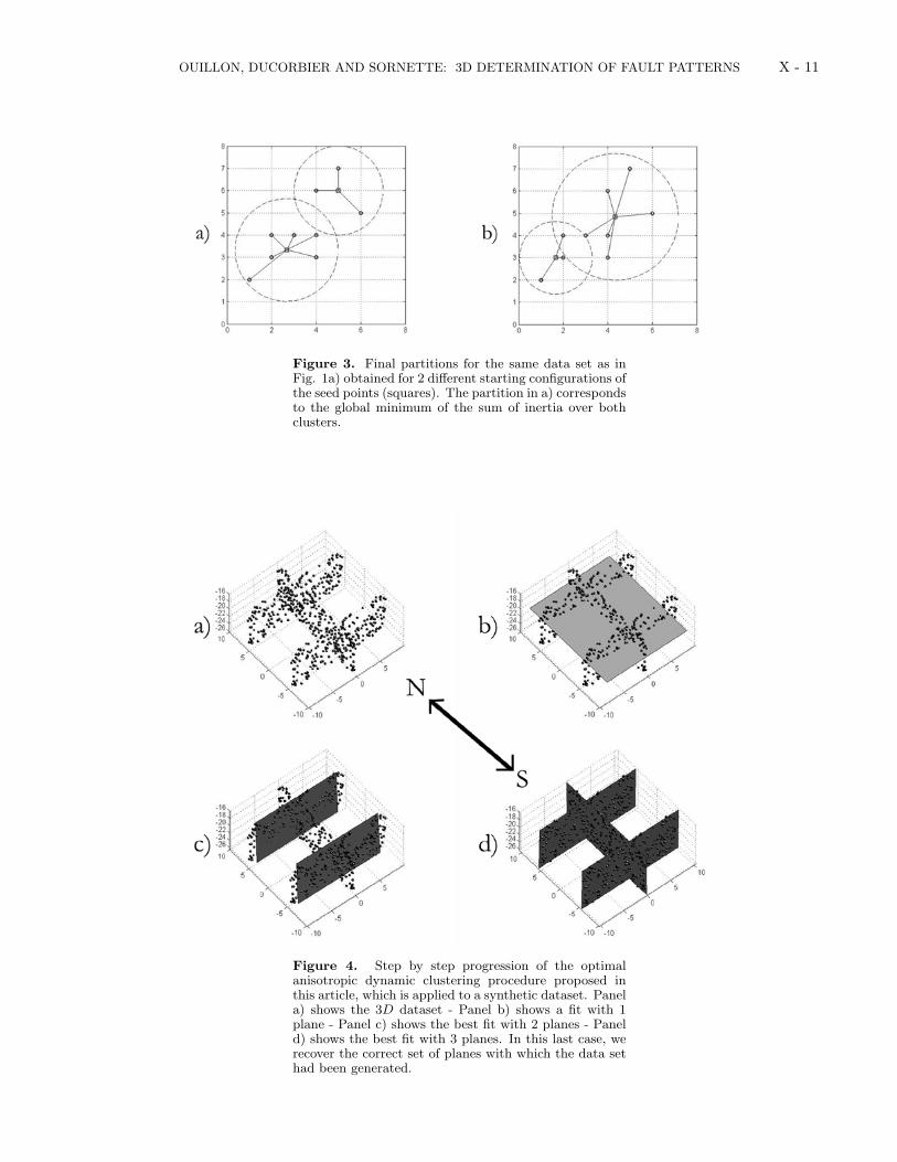
We shall begin by detailing the example shown in Fig. 4a.This dataset has been generated using two parallel planes,each of them being normal to a third one. All planes are ver-tical. Two planes strike N90 (and are located 12km apart)while the third one strikes N0. All planes are 20km long and10km wide. Two hundred earthquakes are located randomlyon each of those three planes while a random white noise inthe interval [−0.01km; +0.01km] is added to each coordinateof every earthquake. We set ∆ = 0.01km and start the 3DOptimal Anisotropic Clustering algorithm on this dataset.As we start with N0 = 1, the algorithm first fits the datasetwith a single plane determined from the covariance matrixof the whole catalog, giving the solution shown in Fig. 4b.Note that the best fitting plane is horizontal, and thus doesnot reflect at all the original geometry. Its length is 19.667km and its width is 16.798 km. For that plane, we findλ3 = 5.038 km > ∆, so that a second plane is introducedin order to decrease λ3. The algorithm then converges tothe fit proposed in Fig. 4c. The plane A strikes N90 anddips S86. Its length is 16.985 km and its width is 9.944 km.Its λ3 value is 2.933 km. The plane B strikes N90 and dipsN87. Its length and width are respectively 16.985 km and10.073 km. Its λ3 value is 3.043 km. The two planes stand11km apart. The cluster associated to plane A being thethickest (and its thickness being larger than ∆), we split itsplane in two, so that there are now three planes available tofit the data. After a few iterations, the algorithm convergesthe structure shown in Fig. 4d. One can check that the spa-tial location of each plane is correct, while the azimuts anddips are determined within an error of less than 0.005 de-grees. The dimensions of the planes are determined within3%. The value λ3 for each plane is slightly lower than ∆.The algorithm has thus found by itself that it needed threeplanes to fit correctly the dataset, the remaining variancebeing explained by the localization errors.

Using synthetic tests developed to demonstrate the powerof the method, we considered several other fault geometries,with varying strikes, dips and dimensions. It is worth notingthat the spatial extent of the reconstructed fault structurewas found with great accuracy in each case. Our synthetictests have been performed with a seismicity uniformly distri-bution on the fault planes. In the future, we plan to performmore in-depth tests with synthetic catalogs on more complexmulti-scale fault networks in the presence of a possible non-uniform complex spatial organization of seismicity, so as tobetter mimic real catalogs. But since, as we shall see in thenext section, the extents of faults inverted form natural data

X - 6 OUILLON, DUCORBIER AND SORNETTE: 3D DETERMINATION OF FAULT PATTERNS

sets seem reasonable as well (see next section), we conjec-ture that our method is robust with respect to the presenceof heterogeneity.

4.3. Application to the Landers aftershocks sequence4.3.1. Implementation

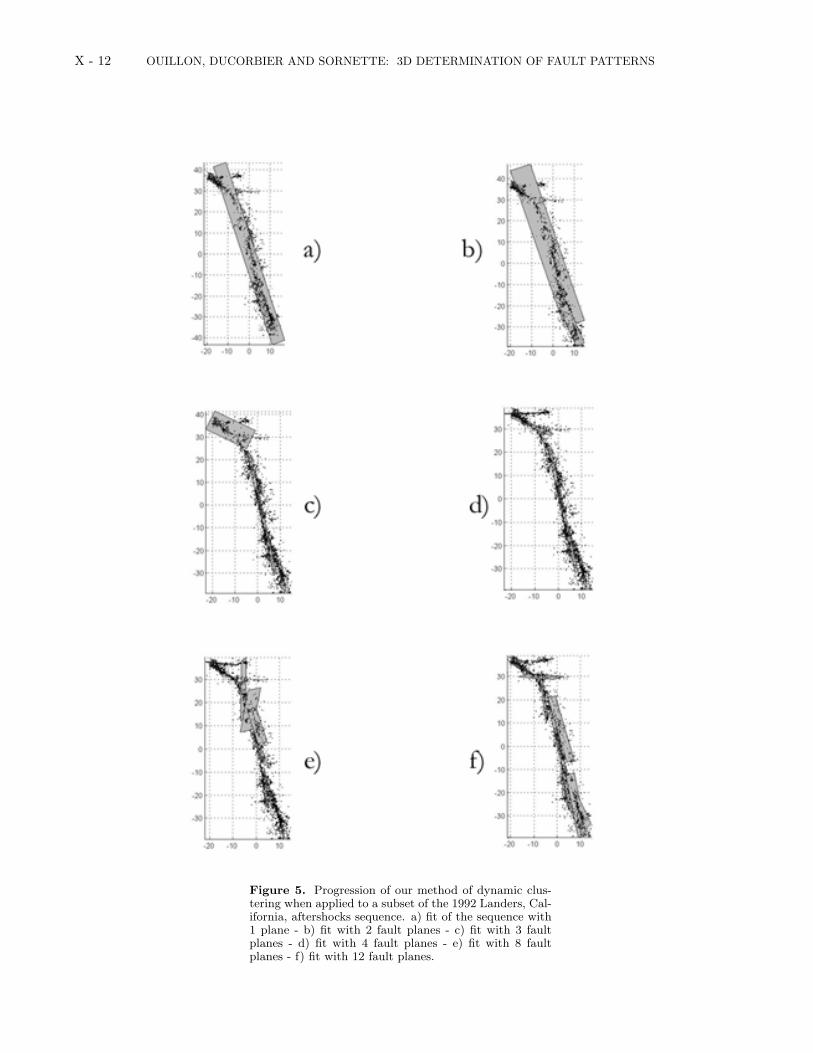
As the method yields correct results on simple syntheticexamples, we are encouraged to apply it to real time se-ries, such as the aftershock sequence of the 1992 Landersearthquake in Southern California. We used the locationsprovided by Shearer et al (2005) and considered only thefirst two weeks of aftershock activity, i.e. a set of 3503events. We used such a limited subset of the full sequencedue to limits set by the required computation time. In thefuture, we plan to parallelize the algorithm in order to beable to deal with much larger catalogs. The relative local-ization uncertainty is reported to be a few tens of metersy Shearer et al (2005), but we set ∆ = 1 km to performa first coarse scale inversion. Our justification for setting∆ = 1 km is twofold. First, the absolute localization errorsare certainly larger than a few tens of meters. Second, usinga value of ∆ smaller than 1 km would imply to use a muchlarger catalog, with many more events to sample correctlysmall-scale features, hence increasing the computation timeprohibitively. We detail hereafter the progression of the al-gorithm as the number of introduced faults increases, as wedid in the previous section for the synthetic case shown inFig. 5a to 5f. As the 3D spatial structure of the sequenceis quite complex, we show only the projection of the resultson the horizontal plane.

Stage a) shows the result of the fit with a single fault,for which we obtain λ3 = 2.9 km. Since this value is largerthan ∆ = 1 km, we introduce a second fault, and obtain thepattern shown in stage b). The second fault is found to in-crease the quality of the fit mainly at the southern end of thesequence, where a large amount of events are located. Thelargest λ3 is still about 2.9 km. We thus introduce a thirdfault, with the optimal three fault structure shown in stagec). The new fault now helps to increase the quality of the fitin the northern end. Notice that this third fault is found tobe horizontal, a signature of the competition between sev-eral strands as observed in the synthetic test presented inFig. 4b. Indeed, one can observe visually that this north-ern region is characterized by at least three branches, whichexplains the optimization with an horizontal northern fault.The value λ3 for this last fault is about 2.5km, leading tothe introduction of a fourth fault, whose optimal structureis shown in stage d). Now, the northern end is fitted moresatisfactorily, and the largest λ3 value drops to 1.8km. Thealgorithm thus continues to introduce new faults, and westep directly to the pattern we obtain with 8 faults which isshown in Fig. 5e. At this stage, the algorithm has dissectedthe central part of the dataset, but still does not providea good fit to the branch at 30km North of the origin. Asthe largest value λ3 is 1.4km, the algorithm still needs morefaults. Fig. 5f shows the optimal fault structure fittingthe data set of aftershock hypocenters with 12 faults. Thenorthern part now appears to be fitted very nicely, while thesouthern part looks quite complex. As the largest value λ3

is now 1.14km, the algorithm needs more faults to fit thedata with the threshold condition ∆ = 1 km. We find thatthe largest value λ3 drops below ∆ = 1 km for 16 faults,for which the computation stops and yields the final patternshown in Fig. 6. When interpreting this figure, it is im-portant to realize that some fault planes are nearly vertical,which make them barely visible in the projection shown inFig. 6.

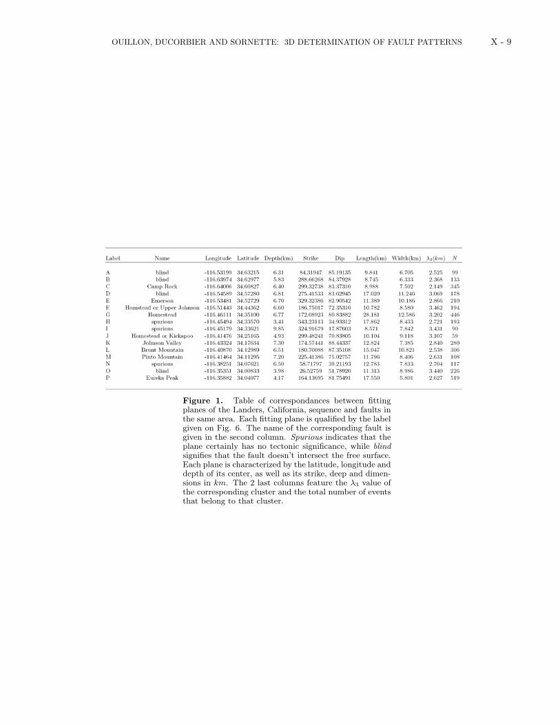
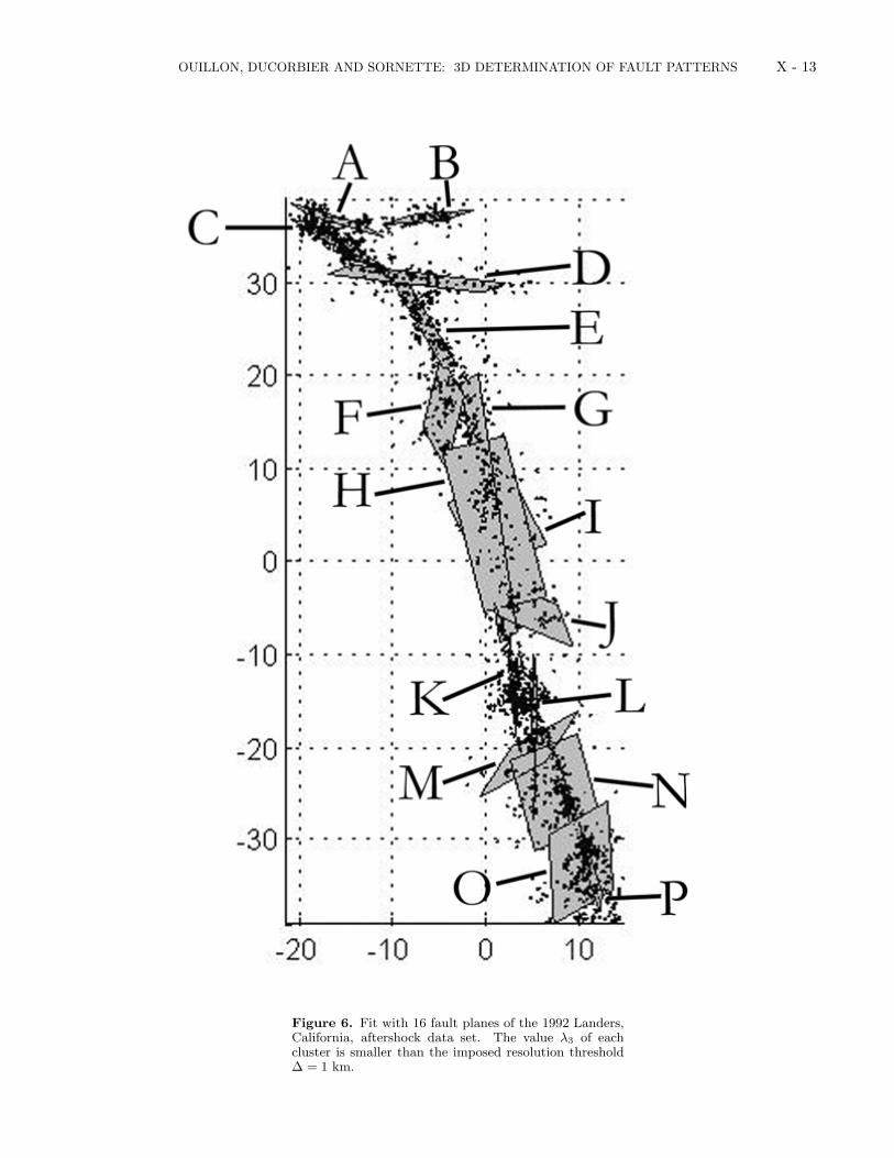
In order to describe the fault network, it is convenient tolabel the 16 faults from A to P , which allows us to dis-cuss this pattern fault by fault. The parameters of the16 fault planes (size and orientation) are given in Table 1.

These fault planes will now be classified into three differentcatagories, namely (i) spurious planes (which have no tec-tonic significance) (ii) previously known planes (that corre-spond to mapped faults) (iii) unknown planes (that may cor-respond to blind faults or to otherwise structures unmappedfor whatever reason).4.3.2. Spurious planes

An inspection of Table 1 reveals that most proposedplanes dip close to the vertical. Three planes, H, I and Nhave rather abnormal dips, which leads us to suspect thatthey are spurious. Indeed, H and I are near normal to theplane G, which is located in a zone with rather diffuse seis-micity in the direction normal to that plane. Introducingplanes H and I is a convenient way to reduce the variancein that zone. It is likely that those planes have no tectonicsignificance, but have been found by the algorithm as theway to satisfy the criterion on λ3 (we shall come back belowto this argument). Plane N also seems to be introduced justto decrease the variance in a zone displaying fault branching.All other 13 fault planes out of the 16 have dips larger than50 degrees, so that we have a priori no reason to removethem.4.3.3. Previously known faults

Because the fault planes have been obtained by fittingseismicity data, none of them cross-cut the free surface. Itis however interesting to compare the planes in Fig. 6 to thefaults mapped at the surface in the Landers area (see Liuet al, 2003), and to underline possible correspondances. Forexample, plane C clearly corresponds to the southern end ofthe Camp Rock fault. Plane E corresponds to the Emersonfault. Plane G is a good candidate for the Homestead Val-ley fault. Note that surface faulting is quite complex anddiffuse in that zone. Continuing to the South, planes K andL seem to match respectively with the Johnson Valley andBrunt Mountain faults, while plane P is the Eureka Peakfault. All those faults are known to have been activatedduring the Landers event. Plane F is located in quite acomplex faulting zone, but its azimuth fits well with boththe Northern end of the Homestead Valley fault or with theUpper Johnson Valley fault. In the former case, plane Gwould then fit with most of the Homestead Valley fault andthe Maume fault. Plane J is also located in a zone of com-plex faulting, and it is difficult to guess if it corresponds tothe Southern end of the Homestead Valley fault, or to theKickapoo fault. Note that it may also feature events fromboth faults.4.3.4. Unknown faults

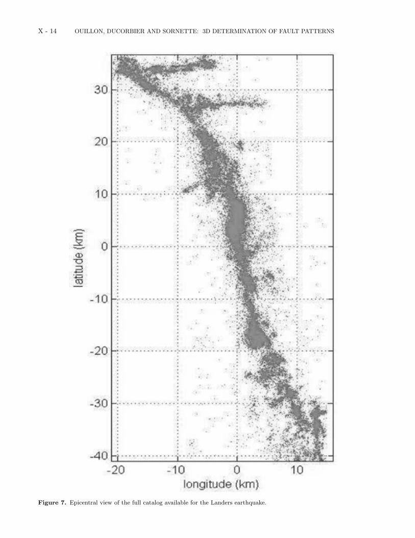
This last set contains planes A, B, D, M and O. PlanesA, B and D obviously fit blind faults, that one can guess,for instance, in Fig. 7 which plots the full set of eventsin Shearer et al (2005)’s catalog in the same area. In theSouthern end, plane M may fit with the Pinto Mountainfault, while O would be a genuine blind fault.

5. Discussion and Conclusion

We have introduced a new powerful method, the 3D Op-timal Anisotropic Dynamic Clustering, that allows us topartition a 3D set of earthquakes hypocenters into distinctanisotropic clusters which can be interpreted as fault planes.The method was first applied to a variety of synthetic datasets, which confirmed its ability to recover correctly withhigh accuracy the existence of present faults. We then ap-plied the 3D Optimal Anisotropic Dynamic Clustering tothe sequence of aftershocks following the 1992 Landers eventin California. In this later case, we were able to recognizethe faults that were already known by surface mapping. Inaddition, the 3D Optimal Anisotropic Dynamic Clusteringmethod allowed us to identify some additional blind faults.

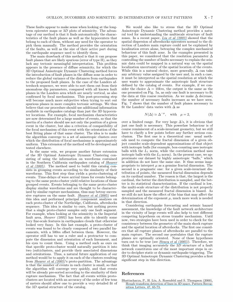
OUILLON, DUCORBIER AND SORNETTE: 3D DETERMINATION OF FAULT PATTERNS X - 7

These faults appear to make sense when looking at the long-term epicenter maps or 3D plots of seismicity. The advan-tage of our method is that it finds automatically the charac-teristics of the fault planes as well as the hypocenters thatbelong to each of them, without any need for the operator topick them manually. The method provides the orientationof the faults, as well as the size of their active part duringthe earthquake sequence used to identify them.

The main drawback of this method is that it can proposefault planes that are likely spurious (error of type II), as theylack any tectonic meaningful interpretation. This problemappears in the presence of diffuse seismicity, for which the3D Optimal Anisotropic Dynamic Clustering method forcesthe introduction of fault planes in the diffuse zone in order toreduce the global variance of the distances from earthquakesto the proposed fault planes. In the case of the Landers af-tershock sequence, we were able to sort them out from theiranomalous dip parameters, compared with all known faultplanes in the Landers area which are nearly vertical, as alsoconfirmed by focal mechanisms. This post-processing stepwill become much more subjective when trying to sort outspurious planes in more complex tectonic settings. We thusbelieve that our procedure should use additional informationavailable in earthquakes catalogs than just the 3D hypocen-ter locations. For example, focal mechanism characteristicsare now determined for a large number of events, so that theinertia of a cluster should use not only the position of a givenevent in the cluster, but also a criterion of compatibility ofthe focal mechanism of this event with the orientation of thebest fitting plane of that same cluster. The idea is to makethe algorithm converge to a set of anisotropic clusters overwhich the distribution of focal mechanisms is approximatelyuniform. This extension of the method will be developed andtested elsewhere.

In the same vein, we propose another future extensionof the 3D Optimal Anisotropic Dynamic Clustering con-sisting of using the information on waveforms containedin the Southern California earthquakes catalog of Sheareret al (2005). The method used to build this catalog con-sists in grouping events according to the similarity of theirwaveforms. This first step thus yields a proto-clustering ofevents. Time-delays of wave arrival times for events belong-ing to the same proto-cluster yield relative locations of thosegrouped events. Events belonging to the same proto-clusterdisplay similar waveforms and are thought to be character-ized by similar rupture mechanisms, thus may betray succes-sive ruptures on the same fault. Shearer et al (2005) usedthis idea and performed principal component analyses oneach proto-cluster of the Northridge, California, aftershockssequence. This idea is similar to ours, but nothing provesthat a single proto-cluster samples only one fault segment.For example, when looking at the seismicity in the Imperialfault area, Shearer (2002) has been able to identify somevery fine-scale features in earthquakes clouds that otherwiselooked very fuzzy. In this last example, a proto-cluster ofevents was found to be clearly composed of two parallel lin-eaments, with a 500m offset between them. However, theoperator still has to use a ruler and a protractor to com-pute the dimension and orientation of each lineament, andhis eyes to count them. Using a method such as ours onthat specific proto-cluster would naturally partition it intotwo (sub)clusters, and provide their associated dimensionsand orientations. Thus, a natural future application of ourmethod would be to apply it on each of the clusters resultingfrom Shearer et al (2005)’s proto-partition. The advantageis that the number of events in each cluster is small, so thatthe algorithm will converge very quickly, and that eventswill be already pre-sorted according to the similarity of theirrupture mechanism. The fact that all events within proto-clusters are located with an accuracy of the order of few tensof meters should allow one to provide a very detailed fit ofthe 3D spatial structure of the catalog.

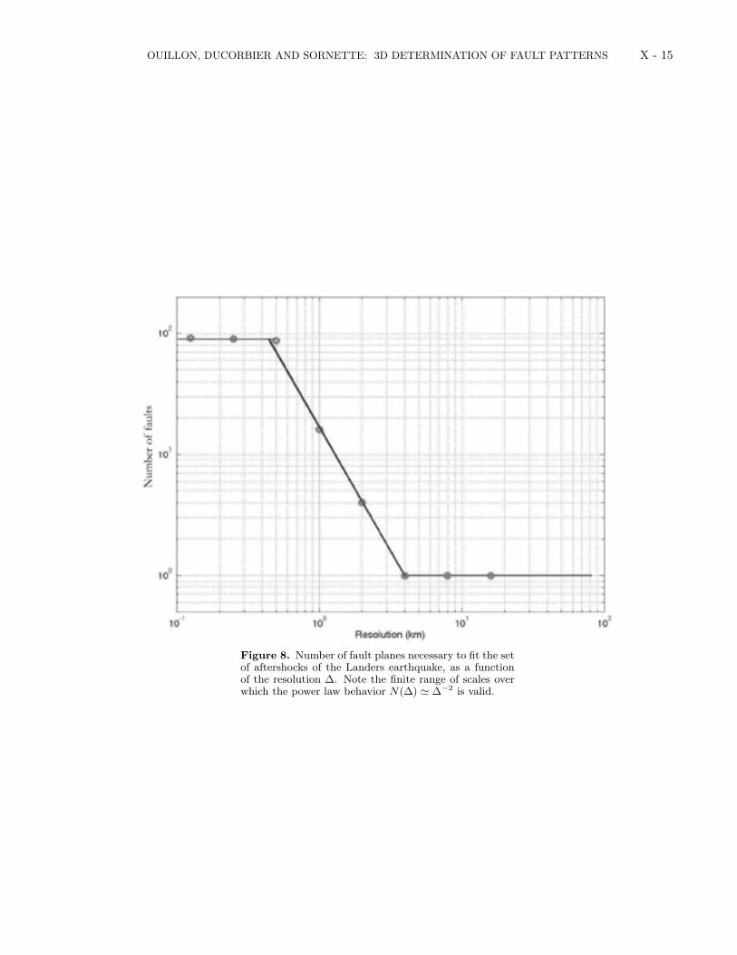
We would also like to stress that the 3D OptimalAnisotropic Dynamic Clustering method provides a natu-ral tool for understanding the multiscale structure of faultzones. In a recent paper, Liu et al (2003) showed that thespatial dispersion of aftershocks epicenters normal to the di-rection of Landers main rupture could not be explained bylocalization errors alone, betraying the complex mechanicalbehaviour of this fault zone. In the examples presented inthis paper, we considered that the resolution parameter ∆controlling the number of faults necessary to explain the seis-mic data could be mapped in a natural way on the spatiallocalization uncertainty of the spatial location of the events.While this is a natural choice, more generally, ∆ can takeany arbitrary value assigned by the user and, in such a case,it must be interpreted as the spatial resolution at which theuser wants to approximate the anisotropic fault structuredefined by the catalog of events. For example, if we con-sider the choice ∆ = 10km, the output is the same as theone presented on Fig. 5a, as only one fault is necessary to fitthe data at this coarse resolution. As we make ∆ decrease,the number of necessary faults increases as we have seen.Fig. 7 shows that the number of fault planes necessary tofit the Landers’ data varies with ∆ as

N(∆) ' ∆−µ, with µ = 2, (3)

over a limited range. For very large ∆’s, it is obvious thatjust one fault is necessary. This powerlaw behaviour is ofcourse reminiscent of a scale-invariant geometry, but we stillhave to clarify a few points before any further serious con-clusion. The first one is a theoretical one: usual meth-ods used to compute the fractal dimension of a given ob-ject consider scale-dependent approximations of that objectwith isotropic balls (for example, box-counting uses isotropicballs with the L1 norm, while the correlation method usesisotropic balls with the L2 norm). In the present case, we ap-proximate our dataset by highly anisotropic “balls,” whichin addition do not have the same size. It thus seems inap-propriate to interpret µ as a genuine fractal dimension. Thesecond is a pragmatic one: for a given scale-invariant dis-tribution of points, the measured fractal dimension dependson its cardinal number. The reason is that, the largest is thecardinal, the better the distribution is sampled, and the bet-ter is its statistical characterization. If the cardinal is low,the multi-scale structure of the distribution is not properlysampled and the measured fractal dimension is biased. Aswe still do not know the effect of the bias that may affect thedetermination of the exponent µ, much more work is neededin that direction.

Considering earthquake forecasting and seismic hazardassessment, the knowledge of the fault network architecturein the vicinity of large events will also help to test differentcompeting hypothesis on stress transfer mechanism. Untilnow, two strategies have been used in order to check for theconsistency between the geometry of the main shock ruptureand the spatial location of aftershocks. The first one consid-ers that all rupture planes of aftershocks are parallel to themain rupture. The second one postulates that the ruptureplanes are optimally oriented. None of those hypothesesturn out to be true (see Steacy et al (2005)). Therefore, wethink that imaging accurately the 3D structure of a faultnetwork constitutes one of the most important steps in or-der to decipher static or dynamic earthquake triggering. The3D Optimal Anisotropic Dynamic Clustering provides a firstsignificant step in this direction.

References

Bhattacharya, P., H. Liu, A. Rosenfeld and S. Thompson (2000),Hough transform detection of lines in 3D space, Pattern Recog-nition Letters, 47, 65-73.

X - 8 OUILLON, DUCORBIER AND SORNETTE: 3D DETERMINATION OF FAULT PATTERNS

Bethoux, N., G. Ouillon and M. Nicolas (1998), The instrumen-tal seismicity of the Western Alps: spatio-temporal patternsanalysed with the wavelet transform, Geophys. J. Int., 135,177-194.

Darrozes, J., P. Gaillot and P. Courjault-Rade (1998), 2D prop-agation of a sequence of aftershocks combining anisotropicwavelet transform and GIS, Phys. Chem. Earth, 23, 303-308.

Duda, R.O. and P.E. Hart (1972), Use of the Hough transforma-tion to detect lines and curves in pictures, Comm. ACM, 15,11-15.

Faulkner, D. R., A.C. Lewis and E.H. Rutter (2003), On the in-ternal structure and mechanics of large strike-slip fault zones:field observations of the Carboneras fault in southeasternSpain, Tectonophysics, 367, 235-251.

Gaillot P., J. Darrozes, M. De Saint Blanquat and G. Ouillon(1997), The normalised optimised anisotropic wavelet coeffi-cient (NOAWC) method: an image processing tool for multi-scale analysis of rock fabric, Geophys. Res. Lett., 24, 14, 1819-1822.

Gaillot, P., J. Darrozes and J.L. Bouchez (1999), Wavelet trans-forms: the future of rock shape fabric analysis?, J. Struct.Geol., 21, 1615-1621.

Gaillot, P., J. Darrozes, P. Courjault-Rade and D. Amorese(2002), Structural analysis of hypocentral distribution ofan earthquake sequence using anisotropic wavelets: methodand application, J. Geophys. Res., 107 (B10), 2218,doi:10.1029/2001JB0000212.

Gregoire, V., J. Darrozes, P. Gaillot, P. Launeau and A.Nedelec (1998), Magnetite grain shape fabric and distributionanisotropy versus rock magnetic fabric: a 3D-case study, J.Struct. Geol., 20, 937-944

Helmstetter, A., G. Ouillon and D. Sornette (2003), Are after-shocks of large Californian earthquakes diffusing?, J. Geophys.Res., 108, 2483, 10.1029/2003JB002503.

Liu, J., K. Sieh and E. Hauksson (2003), A Structural Interpre-tation of the Aftershock ”Cloud” of the 1992Mw7.3 LandersEarthquake, Bull. Seism. Soc. Am. 93, 1333-1344.

Mac Queen, J. (1967), Some methods for classification and anal-ysis of multivariate observations, pp. 281-297 in: L. M. LeCam and J. Neyman [eds.] Proceedings of the fifth Berkeleysymposium on mathematical statistics and probability, Vol. 1.University of California Press, Berkeley. xvii + 666 p.

Ouillon, G. (1995), Application de lanalyse multifractale et dela transformee en ondelettes anisotropes a la caracterisationgeometrique multiechelle des reseaux de failles et de fractures,Documents du BRGM, 246.

Ouillon G. , C. Castaing and D. Sornette (1996), HierarchicalGeometry of Faulting, J. Geophys. Res., 101 (B3), 5477-5487.

Ouillon, G. and D. Sornette (1996), Unbiased Multifractal Anal-ysis of Fault Patterns, Geophys. Res. Lett., 23, 23, 3409-3412.

Passchier, C.W. and R.A.J. Trouw (2005), Microtectonics,Springer Verlag.

Plesch, A. and Shaw, J. H. (2002), SCEC 3D Commu-nity Fault Model for Southern California, Eos Trans.AGU, Fall Meet. Suppl., 83, Abstract S21A-0966.(http://structure.harvard.edu/cfm includes Broderick,Kamerling and Sorlien maps).

Pollard, D. D. and R.C. Fletcher (2005), Fundamentals of Struc-tural Geology, Cambridge University Press.

Sarti, A. and S. Tubaro (2002), Detection and characterization ofplanar fractures using a 3D Hough transform, Signal Process-ing, 82, 1269, doi:10.1016/S0165-1684(02)00249-9.

Scholz, C. (2002), The Mechanics of Earthquakes and Faulting,Cambridge University Press.

Shearer, P.M. (2002), Parallel fault strands at 9-km depth re-solved on the Imperial Fault, Southern California, Geophys.Res. Lett., 29, 1674, doi:10.1029/2002GL015302.

Shearer, P.M., J.L. Hardebeck, L. Astiz and K.B. Richards-Dinger(2003), Analysis of similar event clusters in aftershocks of the1994 Northridge, California, earthquake, J. Geophys. Res., 108(B1), 2035, doi:10.1029/2001JB000685.

Shearer, P., E. Hauksson and G. Lin (2005), Southern californiahypocenter relocation with waveform cross-correlation, part 2:Results using source-specific station terms and cluster analysis,Bulletin of the Seismological Society of America, 95, 904-915.

Sornette, D. (1991) Self-organized criticality in plate tectonics,in the proceedings of the NATO ASI “Spontaneous formationof space-time structures and criticality,” Geilo, Norway 2-12april 1991, edited by T. Riste and D. Sherrington, Dordrecht,Boston, Kluwer Academic Press, volume 349, p.57-106.

Sornette, D., Ph. Davy and A. Sornette (1990) Structuration ofthe lithosphere in plate tectonics as a self-organized criticalphenomenon, J. Geophys. Res. 95, 17353-17361.

Steacy, S., S.S. Nalbant, J. McCloskey, C. Nostro, O. Scotti andD. Baumont (2005), Onto what planes should Coulomb stressperturbations be resolved?, J. Geophys. Res., 110 (B05S15),doi:10.1029/2004JB003356.

Wesson, R. L., W. H. Bakun and D.M. Perkins (2003), Associa-tion of earthquakes and faults in the San Francisco Bay areausing Bayesian inference, Bulletin of the Seismological Societyof America, 93, 1306-1332.

Guy Ouillon, Lithophyse, 1 rue de la croix, 06300 Nice, France(e-mail: [email protected])

Caroline Ducorbier, LPMC, CNRS and University of Nice,06108 Nice, France ()

Didier Sornette, D-MTEC, ETH Zurich, Kreuzplatz 5, CH-8032 Zurich, Switzerland and D-ESS and IGPP, UCLA, Los An-geles, California, USA (e-mail: [email protected])

OUILLON, DUCORBIER AND SORNETTE: 3D DETERMINATION OF FAULT PATTERNS X - 9

Figure 1. Table of correspondances between fittingplanes of the Landers, California, sequence and faults inthe same area. Each fitting plane is qualified by the labelgiven on Fig. 6. The name of the corresponding fault isgiven in the second column. Spurious indicates that theplane certainly has no tectonic significance, while blindsignifies that the fault doesn’t intersect the free surface.Each plane is characterized by the latitude, longitude anddepth of its center, as well as its strike, deep and dimen-sions in km. The 2 last columns feature the λ3 value ofthe corresponding cluster and the total number of eventsthat belong to that cluster.

X - 10 OUILLON, DUCORBIER AND SORNETTE: 3D DETERMINATION OF FAULT PATTERNS

Figure 2. Presentation of the classical dynamic cluster-ing method. a) set of 9 data points represented by thecircles which need to be partitioned into 2 clusters - b)same as a) with the addition of the 2 starting seeds forthe clustering procedure (squares) - c) & d) 1st iteration(see main text) - e) & f) 2nd iteration - g) & h) 3rd andlast iteration - the circles in dashed-line in h) give an ideaof the size of clusters.

OUILLON, DUCORBIER AND SORNETTE: 3D DETERMINATION OF FAULT PATTERNS X - 11

Figure 3. Final partitions for the same data set as inFig. 1a) obtained for 2 different starting configurations ofthe seed points (squares). The partition in a) correspondsto the global minimum of the sum of inertia over bothclusters.

Figure 4. Step by step progression of the optimalanisotropic dynamic clustering procedure proposed inthis article, which is applied to a synthetic dataset. Panela) shows the 3D dataset - Panel b) shows a fit with 1plane - Panel c) shows the best fit with 2 planes - Paneld) shows the best fit with 3 planes. In this last case, werecover the correct set of planes with which the data sethad been generated.

X - 12 OUILLON, DUCORBIER AND SORNETTE: 3D DETERMINATION OF FAULT PATTERNS

Figure 5. Progression of our method of dynamic clus-tering when applied to a subset of the 1992 Landers, Cal-ifornia, aftershocks sequence. a) fit of the sequence with1 plane - b) fit with 2 fault planes - c) fit with 3 faultplanes - d) fit with 4 fault planes - e) fit with 8 faultplanes - f) fit with 12 fault planes.

OUILLON, DUCORBIER AND SORNETTE: 3D DETERMINATION OF FAULT PATTERNS X - 13

Figure 6. Fit with 16 fault planes of the 1992 Landers,California, aftershock data set. The value λ3 of eachcluster is smaller than the imposed resolution threshold∆ = 1 km.

X - 14 OUILLON, DUCORBIER AND SORNETTE: 3D DETERMINATION OF FAULT PATTERNS

Figure 7. Epicentral view of the full catalog available for the Landers earthquake.

OUILLON, DUCORBIER AND SORNETTE: 3D DETERMINATION OF FAULT PATTERNS X - 15

Figure 8. Number of fault planes necessary to fit the setof aftershocks of the Landers earthquake, as a functionof the resolution ∆. Note the finite range of scales overwhich the power law behavior N(∆) ' ∆−2 is valid.