Automatic Parcellation of Longitudinal Cortical Surfaces By Manal H. Alassaf B.Sc. in Computer Science, May 2004, Taif University, Saudi Arabia M.Sc. in Computer Science, May 2010, The George Washington University, USA A Dissertation submitted to The Faculty of The School of Engineering and Applied Science of The George Washington University in partial fulfillment of the requirements for the degree of Doctor of Philosophy May 17, 2015 Dissertation directed by James K. Hahn Professor of Engineering and Applied Science

Welcome message from author
This document is posted to help you gain knowledge. Please leave a comment to let me know what you think about it! Share it to your friends and learn new things together.
Transcript

Automatic Parcellation of Longitudinal Cortical Surfaces
By Manal H. Alassaf
B.Sc. in Computer Science, May 2004, Taif University, Saudi Arabia
M.Sc. in Computer Science, May 2010, The George Washington University, USA
A Dissertation submitted to
The Faculty of
The School of Engineering and Applied Science
of The George Washington University
in partial fulfillment of the requirements
for the degree of Doctor of Philosophy
May 17, 2015
Dissertation directed by
James K. Hahn
Professor of Engineering and Applied Science

All rights reserved
INFORMATION TO ALL USERSThe quality of this reproduction is dependent upon the quality of the copy submitted.
In the unlikely event that the author did not send a complete manuscriptand there are missing pages, these will be noted. Also, if material had to be removed,
a note will indicate the deletion.
Microform Edition © ProQuest LLC.All rights reserved. This work is protected against
unauthorized copying under Title 17, United States Code
ProQuest LLC.789 East Eisenhower Parkway
P.O. Box 1346Ann Arbor, MI 48106 - 1346
UMI 3687479
Published by ProQuest LLC (2015). Copyright in the Dissertation held by the Author.
UMI Number: 3687479

ii
The School of Engineering and Applied Science of The George Washington University
certifies that Manal H. Alassaf has passed the Final Examination for the degree of Doctor
of Philosophy as of March 2nd, 2015. This is the final and approved form of the
dissertation.
Automatic Parcellation of Longitudinal Cortical Surfaces
Manal H. Alassaf
Dissertation Research Committee:
James K. Hahn, Professor of Engineering and Applied Science, Dissertation Director
Abdou S. Youssef, Professor of Engineering and Applied Science, Committee Member
Claire Monteleoni, Assistant Professor of Computer Science, Committee Member
Mohamad Z. Koubeissi, Associate Professor of Neurology, Committee Member

iii
Dedication
بسم هللا الرمحن الرحيم
الكرميني: إىل والديّ ، حفظها هللافائزة بنت عساف العواجي :والديت
حسني بن منصور العساف، رمحه هللا :والدي
To My Parents: Faizah Assaf Alawaji
Hussein Mansour Alassaf, 1945-2008
هذا من فضل هللا

iv
Abstract of Dissertation
Automatic Parcellation of Longitudinal Cortical Surfaces
Preterm birth incidence is a main cause of developing cognitive and neurologic
disorders in childhood especially with children who are born extremely preterm. The
human brain experiences significant functional and morphological changes at early
development before and around birth. Understanding and modeling brain normal growth
and cortical changes in early development are the keys to understanding and tracking
neurologic disorders. The objective of this dissertation is to develop methods for
longitudinally modeling brain development in order to provide researchers with tools for
understanding normal growth patterns and for designing interventions that minimize
potential preterm brain injury. We present a novel algorithm for longitudinally parcellating
the developing brain at different stages of development. The algorithm assigns each cortical
location to a neuroanatomical brain structure during early development. A labeled newborn
brain atlas at 41 weeks gestational age (GA) is used to propagate labels of anatomical
regions of interest to a spatio-temporal atlas, which provides a dynamic model of brain
development at each week between 28-44 GA weeks. First, cortical labels from the volume
of the newborn brain are propagated to an age-matched cortical surface from the spatio-
temporal atlas. Then, labels are propagated across the cortical surfaces of each week of the
spatio-temporal atlas by registering successive cortical surfaces using a new approach and
using an energy optimization function. This procedure incorporates local and global, spatial
and temporal information when assigning the labels. The result is a complete parcellation
of 17 neonatal brain surfaces with similar points per labels distributions across weeks.

v
Table of Contents Dedication ......................................................................................................................... iii
Abstract of Dissertation ................................................................................................... iv
List of Figures .................................................................................................................. vii
List of Tables .................................................................................................................... ix
List of Acronyms ............................................................................................................... x
Chapter 1-Introduction .................................................................................................... 1
1.1. Brain Anatomy ................................................................................................... 2
1.2. Developing Brain Imaging ................................................................................. 3
1.3. Brain Development ............................................................................................. 5
1.4. Motivation ........................................................................................................... 8
1.5. Aim..................................................................................................................... 10
1.6. Dissertation Contributions .............................................................................. 11
1.7. Summary ........................................................................................................... 11
Chapter 2: Background and Related Work ................................................................. 13
2.1. Introduction ....................................................................................................... 13
2.2. Related Work .................................................................................................... 13
2.2.1. Brain Structures and Functions .............................................................. 13
2.2.2. Brain Parcellation ..................................................................................... 17
2.2.3. Brain Atlases.............................................................................................. 22
2.2.4. Developing Brain Atlases ......................................................................... 33
2.3. Background ....................................................................................................... 41
2.3.1. MRI Surface Construction ....................................................................... 41
2.3.2. Image/Surface Registration...................................................................... 42
2.4. Conclusion ......................................................................................................... 53
2.5. Summary ........................................................................................................... 54
Chapter 3: Methods ........................................................................................................ 55
3.1. Introduction ...................................................................................................... 55
3.2. Input and Pipeline ............................................................................................ 56
3.3. Propagating the Labels in the Volume Space ................................................ 57
3.4. Volume-Surface Parcellation .......................................................................... 60
vi
3.5. Surface-Surface Parcellation ........................................................................... 63
Problem Statement ................................................................................................... 64
Mapping Space ......................................................................................................... 65
Parcellation .............................................................................................................. 67
Chapter 4: Results and Evaluation ............................................................................... 74
4.1. Introduction ...................................................................................................... 74
4.2. Experimental Setup .......................................................................................... 74
4.3. Results and Evaluation .................................................................................... 75
4.3.1. Results ........................................................................................................ 75
4.3.2. Evaluation .................................................................................................. 78
4.4. Limitation ........................................................................................................... 90
4.5. Summary ............................................................................................................. 90
Chapter 5: Conclusion and Future Work ..................................................................... 92
5.1. Conclusion ......................................................................................................... 92
5.2. Future Work ..................................................................................................... 93
6. Appendix 1 ............................................................................................................... 94
7. Appendix 2 ............................................................................................................. 122
7.1. Ray Triangle Intersection.............................................................................. 122
7.2. Surface Points Normal Calculations ............................................................. 123
Bibliography .................................................................................................................. 125

vii
List of Figures
Figure 1.1. Brain Anatomy ..…………………………………………………....... 3
Figure 1.2. Timeline of pregnancy by weeks and months of gestational age …….. 6
Figure 1.3. GM and WM intensities of developing brain in contrast to developed
brain .......…………………………………………………………….. 6
Figure 1.4. Axonal Growth ………………….…………………………………... 7
Figure 1.5. Two-dimensional representation of the pallial and subpallial origins
and the GABAergic and glutamatergic radial and tangential migratory
paths in human fetus brain at 19 post-conceptual weeks ....................... 9
Figure 2.1. Old Brain Illustrations ……………………………………………..... 16
Figure 2.2. FreeSurfer Generated Surfaces ….…………………………………... 22
Figure 2.3. Pipeline of probabilistic developing brain atlas construction stages ..... 24
Figure 2.4. Two-year-old brain of UNC infant atlas ……………………………... 25
Figure 2.5. T2 mid-axial slices are presented to demonstrate the variation of
natural brain shape within a population of 12 healthy neonates aging
37–43 GA weeks …………………………………………………...... 26
Figure 2.6. Comparison of different registration types between two neonates
brain T2 MRI scans ...…….………………………………………...... 31
Figure 2.7. Linear Transformation Models …………………………………….... 42
Figure 2.8. Deforming and Pending Cow using FFD ……………………………. 46
Figure 2.9. Non-rigid registration using cover tree pipeline ……………………... 47
Figure 3.1. Pipeline of the proposed method ………………………..…………... 58
Figure 3.2. Propagating the labels in the volume space ………………………….. 59
Figure 3.3. ALBERTs’ 20 labeled brain normalization and fusing to generate one
template ………................................................................................... 60
Figure 3.4. Illustration of the localization of a surface point pi inside a voxel in
the volume between two volume grid points [x1, y1, z1] and [x2, y2,
z2] ….................................................................................................... 61
Figure 3.5. Volume-Surface Parcellation ………...……………………………… 63
Figure 3.6. Surface-Surface Parcellation …………………..…………………...... 67
Figure 3.7. Lateral View of Parcellated Brain and Refinements Results ………… 72
Figure 3.8. Superior and lateral views of the surface mean curvature on selected
GA weeks of the spatio-temporal atlas …………….………………… 73
Figure 4.1. Results of first stage: Propagating the labels in the volume space into
week 41 of spatio-temporal atlas …...................................................... 75
Figure 4.2. 3D results of second stage of volume-surface parcellation ...………… 77
Figure 4.3. Parcellation results using UNC labels map on ten selected GA weeks 80
viii
Figure 4.4. Parcellation results using ALBERT labels map on ten selected GA
weeks ……………………………………………………………....... 81
Figure 4.5. Parcellation results using JHU labels map on ten selected GA weeks 82
Figure 4.6. The UNC Infant 0-1-2 Atlas validation experiment ………................. 84
Figure 4.7. The ALBERT Atlas validation experiment ………...……..……......... 87
Figure 4.8. The number of points per two biomarker growth regions, (Middle
Temporal Gyrus (MTG), and Inferior Temporal Gyrus (ITG)) is
plotted against age at time of scan ………………………………........ 89
Figure 7.1. Translation t maps the ray to the barycentric coordinate (u,v) …......... 123
Figure 7.2. Illustration of surface vertex normal vector calculation using
surrounding facets normal vectors …………………………………... 124

ix
List of Tables
Table 2.1. Neonatal Developing Brain Single time Atlases ………………………. 39
Table 2.2. Developing Brain Spatio-temporal and Longitudinal (4D) Atlases ........ 40
Table 3.1. ALBERT Atlas Subjects Age at Scan …………………………............. 57
Table 4.1. Spatio-temporal atlas information: number of points per surface,
number of triangles per surface, average pairing distance, and
parcellation time starting from week 41 and going in both directions
with and without multithreading ............................................................ 79
Table 4.2. Dice similaity index of propagating labels among neonate, 1, 2 years
old atlas. Left (light gray shaded cells): Starting the propagation from
year 2 towards neonate. Right (dark gray shaded cells): Starting
propagation from neonate towards year 2 ............................................... 84
Table 4.3. ALBERTs atlas information: range of age at scan of 20 neonates brains
and number of scans avaliable in the ALBERTs atlas per each age ….... 86
Table 4.4. ALBERTs leave-one-out experiments setup with labels agreements
accuracy between the test data and the proposed parcellation result
reported in each experiment …………………………………………... 86
Table 6.1. Index of the UNC infant-AAL atlas ROIs’ names and colors ………..... 94
Table 6.2. Index of the ALBERT atlas ROIs’ names and colors ………………...... 97
Table 6.3. Index of the JHU atlas ROIs’ names and colors …………..………….... 99
Table 6.4. Longitudinal Probabilistic Distribution of Points per ROIs using
Symmetric UNC Parcellation Map ……………………………………. 103
Table 6.5. Longitudinal Probabilistic Distribution of Points per ROIs using
Asymmetric UNC Parcellation Map ………………………………….. 105
Table 6.6. Longitudinal Probabilistic Distribution of Points per ROIs using
Symmetric ALBERT Parcellation Map ……………………………….. 109
Table 6.7. Longitudinal Probabilistic Distribution of Points per ROIs using
Asymmetric ALBERT Parcellation Map ………………………........... 111
Table 6.8. Longitudinal Probabilistic Distribution of Points per ROIs using
Symmetric JHU Parcellation Map …………………………………….. 114
Table 6.9. Longitudinal Probabilistic Distribution of Points per ROIs using
Asymmetric JHU Parcellation Map ………………………………….... 117

x
List of Acronyms 2D Two-Dimensional
3D Three-Dimensional
4D Four-Dimensional
AAL Automated Anatomical Labeling
ALBERT A Label-Based Encephalic ROI Template
B-spline Basis spline
CC Cross Correlation
CSF Cerebrospinal Fluid
CT Computed Tomography
DOF Degrees Of Freedom
DW Diffusion-Weighted
EM Expectation Maximization
FFD Free-Form Deformation
fMRI functional MRI
GA Gestational Age
GB Gigabyte
GE Ganglionic Eminence
GHz Gigahertz
GM Gray Matter
HAMMER Hierarchical Attribute Matching Mechanism for Elastic Registration
HCP Human Connectome Project
ICP Iterative Closest Point
xi
IDE Integrated Development Environment
JE Joint Entropy
JHU John Hopkins University
LDDMM Large Deformation Diffeomorphic Metric Mapping
MAP Maximum-a-Posteriori
MI Mutual Information
MNI Montreal Neurology Institute
MoG Mixture of Gaussian
MRF Markov Random Field
MRI Magnetic Resonance Imaging
NIH National Institutes of Health
NMI Normalized Mutual Information
NN Nearest Neighbor
PDF Probability Density Function
PET Positron Emission Tomography
PTB Preterm Birth
RAM Random Access Memory
ROIs Regions Of Interest
S Source
SSD Sum of Square Differences
SVM Support Vector Machines
SVZ Subventricular Zone
T Target

xii
UNC University of North Carolina
U.S. United States
VZ Ventricular Zone
WM White Matter
X Transformation

1
Chapter 1-Introduction
In the United States, one in every eight infants is born prematurely [1]. Premature
birth is ranked second among causes of infant death in the U.S. [2]. Preterm birth (PTB)
refers to the birth of an infant of 37 weeks gestational age (GA) or less. Although
improvements in neonatal intensive care can increase the survival rate of prematurely born
infants, the development of cognitive and neurologic disorders is still common especially
with those who are extremely preterm [3,4]. Special therapies are needed for the
neurodevelopmental care of PTB neonates. But most importantly, understanding normal
growth and development processes of the brain are the keys to understanding and tracking
neurologic disorders [5,6]. The objective of this dissertation is to develop methods for
longitudinal modeling and quantitative measuring of brain structures development, in order
to provide researchers with tools for understanding normal growth patterns and for
designing interventions that minimize potential preterm brain injury.
Invisible to human sensory perception, the brain remains a hidden world filled with
mysteries awaiting scientific discovery. But what is inside the brain that scientists are
interested in knowing about? How can the brain be non-invasively visualized? How can
we track its development and why is it important to understand brain normal growth?
Motivated by these questions, this dissertation contributes to the investigation of the
developing brain. In this chapter, a general description of brain anatomy, its development,
and the terminology used throughout the dissertation are presented. This includes a brief
description of developing brain imaging techniques, and the challenges associated with
these techniques. Finally, motivation, aim, and dissertation contribution conclude this
chapter.

2
1.1. Brain Anatomy
The cerebrum, cerebellum, and brainstem are the main components of human brain
as shown in Figure 1.1(a). Similarly, there are three main tissue classes in the brain: gray
matter (GM) or cerebral cortex, white matter (WM) or subcortex, and cerebrospinal fluid
(CSF). The GM contains cells and the WM contains neuronal axons myelinated sheaths.
The outer layer that covers the cerebrum, or the two cerebral hemispheres, is called the
cerebral cortex and forms the largest part of the human brain. Cerebral cortex has highly
convoluted topography. The grooves, which encompass two-thirds of the cerebral cortex,
are called sulci (s. sulcus) and the folds are called gyri (s. gyrus). Four main lobes in each
hemisphere of the cerebral cortex can be recognized by obvious sulci or gyri landmarks on
the cortex as shown in Figure 1.1(b). Studying the cerebral cortex is important because it
plays a significant role in high-level human functions and activities such as language,
memory, planning, etc., and it is important to understand the relationship between functions
and structures of the human brain (discussed in details in section 2.2.1).
A number of neuroanatomical regions or structures exist in the brain and vary
between neuroanatomical atlases where each atlas divides the brain into a number of
regions based on relative knowledge. To identify brain structures, anatomical expertise
about the geometry and the boundaries between structures is required. In addition, special
radiology expertise related to classes’ intensity distribution and imaging artifacts is
necessary. Sometimes tissue identification is needed prior to identifying brain structures or
regions [7]. The process of identifying brain structures is usually called brain tissue
segmentation, while the process of labeling brain regions is referred to as anatomical
segmentation, or brain parcellation which is described in depth in Chapter 2 (see Figure
1.1(c)).

3
Figure 1.1. Brain Anatomy. a) Lateral view of the main three components of the brain and principal fissures
and lobes of the cerebrum (Source: [8]). b) Illustration of brain tissue anatomy (Source: [9]). c)
Brain parcellation of 24 regions (Source [10]).
1.2. Developing Brain Imaging
Today, advancements in technical and scientific research provide great
opportunities to combine disciplines in science and technology, producing innovative ways
to conduct research and to solve real world problems. The most useful technologies where
engineering science and medical science intermingle are medical imaging modalities. One
example that is widely used to examine the pregnant women and to image the fetus is
Obstetric Ultrasonography. This technique uses an ultrasound probe to transmit ultrasound
waves through the body. These waves, which are not naturally heard by humans, reflect
and echo off the body tissues and are recorded as images. Even though the ultrasound
images are very helpful in visualizing fetus growth and development [11], they do not
provide comprehensive information about brain anatomy.
Magnetic Resonance Imaging (MRI) is a powerful, painless, non-invasive and non-
ionized technique for capturing detailed images that underlay tissue characteristics within
the brain. For the developing brain, it captures the entire brain including the brain soft
tissues, vasculature, and microstructure [12]. MRI uses a magnetic field and radio
frequency to capture these pictures. The magnetic field aligns the nuclear magnetization of

4
hydrogen atoms within body water, while the radio wave pulses alter these alignments
causing nuclear magnetization to produce rotating magnetic fields that are detectable by
the scanner and produced in gray scale images. Interpreting a brain MRI scan means
finding a correspondence between gray scale intensity in each MR image and labeled
anatomical tissues or regions.
MRI is not only used to investigate the anatomy and physiology of the body, but
can also be fused within ultrasound or x-ray computed tomography (CT) images to reveal
additional information about any organ [13]. Moreover, functional MRI (fMRI) captures
activity in any region of the brain by detecting the blood flow to that region [14]. In
addition, Diffusion-Weighted (DW) MRI allows visualization of the brain tissue structure
and organization due to its sensitivity to the diffusion patterns of free water [15-17].
By taking serial scans during and after the gestational time, we can assess the
longitudinal maturity of the brain both in utero and ex utero. However, taking MRI scans
of fetal brain in utero is challenging due to fetus motion artifacts caused by limited
acquisition time [18]. Recent studies have developed approaches to successfully overcome
this problem [19,20]. Another challenge of scanning fetal brain using MR imaging is the
variation of the magnetic field strength that is used to acquire the MR images from one
scanner to another; usually between one and three Tesla. This produces intensity
inhomogeneity such that the brain intensity images produced by different scanners are
dissimilar. This can be problematic for image-based techniques such as registration and
segmentation since these techniques depend heavily on intensity. Another challenge
presented when dealing with these techniques is the partial volume effect where the
resolution (sampling grid of MR signal) of scans differ from one scanner device to another

5
[7]. However, techniques have been developed to correct for the intensity inhomogeneity
and the partial volume effect [21,22]. Despite these challenges, MRI is the most viable
imaging modality to longitudinally capture and track the developing brain in utero as
demonstrated in the parcellation algorithm of this dissertation.
1.3. Brain Development
Brain development starts at the embryonic period; more specifically, at the fifth
week of pregnancy. Figure 1.2 illustrates the timeline of pregnancy by weeks and months
of GA [23]. In the first months of pregnancy and before birth, the brain experiences the
most development and changes in shape, size and structure [24,25]. Most significantly,
changes occur in the size and in the cortical folding of the brain. Growth continues rapidly
until the brain is two to three years old, when the process slows and stabilizes and the
developing brain becomes mature. Using MR images allows for quantitative and
qualitative assessment and measurement of human brain myelination (maturation)
processes and growth patterns [26-30].
Myelination is the process of covering the WM by myelin, lipid bilayer. The fast
myelination starts before birth and is completed within the first two or three years of life,
while the long myelination continues until adulthood [31,32]. Myelin promotes efficient
neural signal transmission along the nerve cells. The appearance of the developing brain in
structural MRI differs significantly from the appearance of the mature adult brain. The
myelinated WM in T1-weighted MRI increases in intensity from hypo intense to hyper
intense relative to GM. In T2-weighted MRI WM decreases from hyper intense to hypo
intense relative to GM [24,33,34]. Thus, the developing brain MR images are characterized
by an inverted contrast of WM and GM as opposed to the developed brain as seen in Figure

6
1.3. The inverted contrast is due to WM axonal growth where myelin sheath forms around
the axon tracts [35,36] (see Figure 1.4) and change occurs in the cell water content as a
result of decreasing both T1 and T2 times in order to avoid fetus motion [36,37]. By the
completion of the myelination process, the brain tissue contrast appears in MR images
similar to the adult brain tissue contrast, while the brain structure, shape, and size are
different [38].
Figure 1.2. Timeline of pregnancy by weeks and months of gestational age (Source: [39]).
Figure 1.3. GM and WM intensities of developing brain in contrast to developed brain (Source: [40]).

7
Figure 1.4. Axonal growth.
Human corticogenesis and brain growth patterns can be predicted using structural
MRI, DW MRI, and histology. Corticogenesis is the process responsible for creating the
cerebral cortex (GM). The cerebral cortex development starts in the embryogenesis period
and continues after birth [36]. Cerebral cortex is a highly convoluted structure composed
of six layers and located on the outer layer of the brain [41], which constitutes the cognitive
and intellectual ability center in humans. The six layers’ neurons are generated in the
ventricular/subventricular zones and subpallial ganglionic eminence [42-45] and then
migrate along glial cell scaffold structures to their final destination structure in the cortical
plate [46-49]. During fetal development, this highly orchestrated cellular migration
towards the cortical plate is characterized by having radial and tangential migrational
trajectories [46,50-52]. Recently, Kolasinski et al. described the migration paths in detail
using structural and DW MRI, and emphasized that the radial patterns originated from the
ventricular/subventricular zone, while the tangentio-radial patterns originated in ganglionic
eminence [52] (see Figure 1.5). As a result, an increase in the cerebral cortex surface area
occurs [53]. At the same time, the total brain tissue volume increases at the ratio of
22ml/week [26]. The radial growth of cerebral cortex in early development is postulated
by lateral spreading of the neuron cells and the increase of the cortical surface area
[51,53,54]. However, local cortical growth and folding which form the sulci and gyri

8
during early developments [24] are more complicated. Several methods are proposed to
mathematically simulate local cortical growth using elasticity and plasticity [55], tension
forces [56], and a reaction-diffusion system [57]. Recently, Budday et al. proposed a
differential growth mechanical model for the developing brain to simulate cortical folding.
In their model, the cortex (GM) grows morphogenetically at a constant rate and the
subcortex (WM) grows in response to overstretch [9]. To date, no defined model that
precisely underlay the mechanism of local brain folding and convoluting in detail during
gestational time has been produced [6,9]. In this dissertation, we rely on the global,
concentric, and radial growth hypothesis to track the local regions of interest (ROIs)
development when parcellating the developing brain longitudinal MRI scans’ surfaces.
1.4. Motivation
Automatic analysis of the developing brain is challenging and needs special
dedicated image analysis algorithms that account for the intensity change over time.
Cerebral cortex poses a special challenge due to its convolution nature that varies from one
person to another. Surface based analysis of such a structure is necessary to account for the
convolution and to capture the buried regions [58]. Establishing a benchmark to assess the
developing brain anatomical ROIs growth of PTB children requires surface-based studies
[59]. Limited studies have attempted to identify typical patterns of growth using surfaces
such as growth trajectories [60] and structural development biomarkers [61]. Other studies
have aimed to identify cortical folding or cortical thickness in the developing brain [62,63]
while others focused on analyzing the intellectual and functional abilities and abnormalities
on the PTB brain [64]. Also, studies have focused on tracking the developmental changes

9
Figure 1.5. Two-dimensional representation of the pallial and subpallial origins and the GABAergic and
glutamatergic radial and tangential migratory paths in human fetus brain at 19 post-conceptual
weeks. Tangential migration can occur within the subventricular/ventricular zone (SVZ/VZ, blue
area) in the pallial SVZ/VZ where glutant neurons originate. However, as the blue arrows show,
radial migration occurs along radial glial fascicles, forming a dominate pattern that is perpendicular
to cortical plate (CP) orientation. In the pallial SVZ/VZ and subpallial ganglionic eminence (green),
human brain GABAergic neurons develop. The green arrows identify the tangential corridors of
radial trajectory of GABAergic neurons in intermediate zone as it moves towards the CP after
presenting its original migration pattern as tangentially oriented to the CP. Revealing a radial
trajectory to the CP, the light green arrows show GABAergic neuronal migration that develops in
the SVZ/VZ as it has been found to present in human and non-human primates. As indicated,
ganglionic eminence (GE), where ganglionic neurons originate, also transfers to thalamus by way
of subcortical paths (Source: [52]).
related to the intensity color change between GM and WM in MR images [65,66]. Until
recently only a few quantitative studies have analyzed the longitudinal regional growth
trajectories [60]. However, there is a lack of surface-based studies compared to volumetric
image-based ones especially at early age of brain development.
Viewed from another perspective, several studies have shifted focus to creating
developing brain probabilistic atlases, which provide a reference of knowledge for
physiological functional disorders and abnormalities research [67-69]. As discussed in

10
Chapter 2, some of the existing neonatal developing brain atlases are constructed with
tissue segmentation without parcellation. If they account for parcellation, it is performed
manually [70-73]. In addition, the parcellation is provided for a single GA week as a single-
subject atlas [71,72] or population-average atlas [70,71,73]. UNC Infant 0-1-2 Atlas is the
first publically available neonate automatically parcellated developing brain atlas [74].
Nevertheless, this neonate parcellated atlas is also single aged, at 41 GA week.
Conclusively, no longitudinal parcellation maps exist for neonatal developing brain at early
GA.
1.5. Aim
Most neuroimaging studies of the developing brain have developed algorithms for
intensities in MR images. Therefore, these studies were performed on the image space.
Few studies have focused on the cortical surfaces of the developing brain within the age
range of birth until adulthood. Neither have these studies included early GA brain
development. This dissertation presents work on surface-based longitudinal (spatio-
temporal) atlas analysis of early brain development starting from 28 week GA to 44 week
GA. The purpose is to provide automated methods for spatio-temporal parcellation with
quantitative measures of brain development. These methods can assist researchers in
understanding normal growth patterns and in designing interventions to reduce preterm
brain injury.

11
1.6. Dissertation Contributions
The dissertation describes methods for modeling the normal growth in prematurely
born infants. More specifically, it identifies methods for tracking the growth of different
cortical anatomical structures’ ROIs at early GA. In addition, it offers an automated
longitudinal parcellation method for the developing brain. The proposed parcellation
algorithm uses preterm brain spatio-temporal brain atlas with tissue-segmentations and
infant brain parcellated atlas to longitudinally parcellate the developing brain at different
stages of development. Chapter 2 sheds light on previous related work and provides
background on techniques employed throughout the dissertation. Chapter 3 proposes a
novel framework for solving the problem of registering and propagating the labels of a
parcellated atlas across longitudinal surfaces with large curvature variation. In Chapter 4,
quantitative results of modeling the regional growth of the developing brain will be
presented, which can offer a useful marker of neurodevelopmental changes. Finally,
Chapter 5 contains conclusions and recommendations for future work directions.
1.7. Summary
In this chapter, knowledge about brain development, its anatomy, and developing
brain imaging modalities are presented. Also, the chapter delineated the motivation for
solving the problem of how to longitudinally parcellate the developing brain. Justifications
of the need for providing a solution is emphasized.

12
"The brain, the masterpiece of creation, is almost unknown to us."
Nicolaus Steno, 1669
Is it known now?

13
Chapter 2: Background and Related Work
Based on:
MH Alassaf, Y Yim, JK Hahn. “Non-rigid Surface Registration using Cover Tree based Clustering and Nearest Neighbor Search”, Proceedings of the 9th International Conference on Computer Vision Theory and Applications. (2014) 579-587.
MH Alassaf, JK Hahn. “Probabilistic Developing Brain Atlases: A Survey”. 2015 (In Submission).
2.1. Introduction
As a biological structure, there is none more complex than the human brain. For
centuries, scientists have worked to discover the relationship between the brain’s structures
and functions. This chapter presents the literature review (section 2.2) of related work in
the relationship between brain structure and functions, constructing digital brain atlases
techniques, and parcellated brain atlases methods. The chapter provides a general overview
of the techniques used throughout the dissertation, such as image registration and brain
parcellation in section 2.3. Also, discussed are the challenges of applying these techniques
to MR images of the developing brain.
2.2. Related Work
2.2.1. Brain Structures and Functions
Historically, brain drawings from the Middle Ages were primarily schematic
rather than anatomical, aiming to determine which brain sections were associated with
brain functions. Ibn al-Haytham (965 – 1040 AD), an Arab scholar known to the west
as Alhazen, was the first to anatomically illustrate the eye and its visual function in his
book “Kitab Al-manazir” [75,76] (The Book of Optics). The brain was shown

14
schematically as in Figure 2.1(a). Islamic scholar Ibn Sīnā (980 – 1037AD), known to
the west as Avicenna, was the first medical philosopher to anatomically divide the brain
into three compartments called “cellula”. In his book “Al-Canon fi Al-Tebb” (The law
of Medicine), he further labeled the cerebral ventricles with five labels based on their
functionality. These consisted of: "sensus communis", "fantasia", "ymaginativa",
"cogitativa seu estimativa", and "memorativa" [77] which correspond with common
sense, fantasy, imagination, reasoning and cognition, and memory, respectively (Figure
2.1(b)). Later, illustrations by Leonardo da Vinci (1452 – 1519AD), an Italian scholar
known for his contributions to both science and art, complimented Avicenna’s
illustrations by further anatomically describing the brain in cross sections [76] as seen
in Figure 2.1(c). However, in the early modern age, Belgian scientist Andreas Vesalius
(1514 – 1564 AD) who was also known as the founder of modern human anatomy,
produced more authentic illustrations of the brain in his book “De Humani Commis
Fabrica” (On the Structure of the Human Body) [78]. An example of the illustrations
can be seen in Figure 2.1(d).
With the discovery of modern age technologies, more comprehensive
descriptions of the whole volume of the brain began to emerge. In 1909 using a
microscope, German neurologist Korbinian Brodmann (1868 – 1918AD),
distinguished 52 distinct regions in the cerebral cortex from their cytoarchitectonic
(histological) features such as cortical thickness, laminae thickness, number and type
of cells, and other features [79] as seen in Figure 2.1(e). Brodmann’s discovery of these
regions has allowed their extensive use in many brain studies to relate function with its
corresponding brain structures. His work was based on German anatomist Franz Joseph

15
Gall’s (1758 – 1828 AD) belief in localization of brain functions to several locations
on the brain cerebral cortex. Using a microscope to divide the brain frontal lobe into
eight zones based on nerve cells shape, volume, and arrangement, Sandies (1914 – 1984
AD) described the distinct function of each division in his cytoarchitectural and
myeloarchitectural studies [68]. In 1957, neuroscientist and professor at John Hopkins
University Vernon Mountcastle (1918 – 2015 AD) discovered the columnar
organization of the neocortex, which form the basis for most recent studies focusing on
the relationship between brain function and structure [67]. In Mountcastle’s description
of neocortex columnar organization, he divided the cerebral cortex into modules each
of which plays the role of functional processing unit that receives input and produces
output.
Today, scientists divide each brain hemisphere into four lobes: the frontal lobe,
temporal lobe, parietal lobe, and occipital lobe with each lobe being associated with
distinct functions [69] (see Figure 1.1(a)). In partial agreement with Avicenna, the
frontal lobe is the center of cognitive activities like planning, predicting, decision
making and long-term memory. The temporal lobe is involved in processing sensory
input such as auditory, visual perception, and languages. The parietal lobe is involved
in sensory information like perception, navigation, spatial orientation, touch and pain,
while the occipital lobe is involved in appropriately transforming vision for parietal
and temporal processing.
Through the evolvement of medical imaging technologies, more sophisticated
studies relating brain structures with functions have emerged using MRI, fMRI, DW
MRI, and PET (Positron Emission Tomography). In particular, these are highly useful

16
Figure 2.1. Old Brain Illustrations. a) The eye and the visual system schematic by Alhazen which forms the
basis of vision and light radiated in straight light theories, dated 1038 AD (Sources: [75,76]). b)
Avicenna’s brain illustration of the three brain parts and five cerebral areas, dated 1347 AD (Source:
[77]). c) Leonardo da Vinci’s illustration of the brain and introduction of the cross sections drawing
to further describe 3D anatomy, dated (1490-1500 AD) (Source: [76]). d) Vesalius’s detailed
illustration of the physical brain, dated 1543 AD (Source: [78]). e) The Brodmann brain numerical
map of 52 discrete regions based on histological differences between regions, dated 1909 AD
(Source: [76]).

17
for cortical morphology caused by brain disease studies such as migraine [80],
schizophrenia [81-83], and Alzheimer [84-87] studies to name a few. Since fMRI gives
information about the functionally activated area in the brain but does not provide
structure information, coupling it with structure information from MRI is important in
order to determine relationships in areas of the cerebral cortex [88]. For example, the
Human Connectome Project (HCP) is a currently active project funded by National
Institutes of Health (NIH) and aims to provide a mapping of the structural and
functional neural connections of the human brain primarily using fMRI and MRI
[89,90].
Human brain cortex can be further neuroanatomically divided into a number of
regions, each of which is described by a label and associated with specific functions.
The process of recognizing structures formations in brain MR images is called
parcellation.
2.2.2. Brain Parcellation
Parcellation is the process of labeling the cortical geometric features and can be
performed on brain MR images or on surfaces constructed from those images. After
parcellation, regional and sub-regional studies can be performed to more deeply
understand human brain functions and activities.
As previously mentioned, the first attempt to parcellate the human brain based
on cytoarchitectonic characteristics was done by Brodmann. Currently, in vivo
parcellation is done on MR images or on surfaces constructed from these images (see

18
section 2.3.1 for surface construction). Hence, high-resolution structural MRI (i.e. 1.5
or 3 Tesla) is preferable because it reveals more structure information and detailed
anatomical landmark. Historically, cortical parcellation was done manually by an
anatomical expert who gave each pixel on each MRI slice a label, either axial, sagittal,
or coronal. “Talairach- Tournoux” is an example of such an atlas [91]. Talairach and
Tournoux labeled post-mortem brain slices of a 60 year old French woman with
anatomical labels based on sulci and gyri and Brodmann cytoarchitectonic areas
estimations. They also introduced the Talairach coordinate system with nine degree of
freedom (DOF) transformation (including 3 for scaling and 6 for rigid transformation),
which maps any brain to the Talairach atlas and localizes the brain regions in functional
imaging studies (see Figure 2.7 for linear transformation models).
Manual parcellation involves knowledge in different disciplines such as: brain
geometry and region landmark, relationship between structure and function,
cytoarchitectonics and myeloarchitectonics, and radiology [92]. Roland and Zilles offer
additional information in their paper which describes in detail the criteria and properties
of parcellating the human brain cerebral cortex [93]. Generally, the process of manual
labeling is time and labor intensive [10,92,94,95]. It consumes several hours (e.g. 12-
14) to parcellate one conventional MRI scan [96]. Further, it could take up to a week
to parcellate one high resolution MRI scan [92]. In addition, intra- and inter- rater
differences compromise manual parcellation validity. Therefore, there is a need to
automate the process, which is not a trivial task. The inter-subject cortical geometric
patterns’ heterogeneity has made automating the parcellation process a challenging
problem especially when the brain is developing. Thus parcellation based on a

19
population-average atlas is preferable since it eliminates the inter-subject variability
(see section 2.3.3).
Automatic parcellation of the brain cortex of MRI relies on the same criterion
used in manual parcellation including cytoarchitectonic characteristics (intensity
values), sulci or gyri landmarks (curvature), and global and local position in the brain.
Two main approaches have been developed to automate any MRI brain parcellation;
one using image/surface registration and the other using image/surface segmentation
[10]. Image/surface registration is based on registering a labeled brain atlas
image/surface to the unlabeled brain and then warping the labels from the atlas into the
unlabeled brain using the deformation field generated from the registration. The
segmentation approach is based on segmenting sulci or gyri on unlabeled brain
image/surface and delineating the sub-regions based on this segmentation. In this
dissertation we focus on developing brain surface parcellation using image and surface
registration-based approaches.
Usually in the registration-based approach, automatic cortical parcellation is
done by registering an unlabeled brain with either a manually labeled single-subject
atlas or a population-average brain atlas, to propagate the labels [10]. For the
registration, landmarks between neuroanatomical regions drive the surface registration
while intensity values drive the image registration of the two brains. This approach has
been used by researchers to parcellate the human brain cortex. Some researchers have
used semi-automatic interactive affine [97,98], or non-rigid [99,100] image registration
to propagate the labels using either single-subject atlas [101] or population-average

20
atlas [102,103]. Still, others have used fully automatic non-rigid surface registration to
propagate the labels with automatic topology correction [88,92].
Image/surface registration plays an important role in driving correct label
propagation. Another more important registration role appears when building a
population-based average atlas, because it is important to align the population correctly
to build the atlas. To register the cortical surfaces of two mature brains, the surface
geometry (i.e. sulci and gyri) defines landmarks between neuroanatomical regions.
Spherical inflation is the most well-known solution for automatically registering the
cortical surfaces of mature brains by minimizing the mean square difference between
surface folding patterns [104]. This technique is implemented in FreeSurfer tool which
provides a successful parcellation of any registered brain into a built-in parcellated
mature brain template [92]. While a marker-less surface parcellation called Spherical
Demons has been proposed, the process still involves spherical inflation [105,106].
In spherical inflation, forces are applied to flatten one hemisphere cortical
surface, unfolding the buried regions such that the whole cortical surface becomes
visible [107] (see Figure 2.2 (a) and (d)). This flattening is followed by mapping to a
specific coordinate system; in this case spherical as shown in Figure 2.2(c). With this
coordinate system, corresponding landmarks between surfaces are located and used to
minimize the mean-squared difference employed by the registration algorithm.
Spherical inflation is used to register cortical surfaces and is also used to construct an
atlas from a population after aligning the surfaces (see Figure 2.2(d)). Even though
spherical inflation succeeds in registering mature cortical surface, it has several
drawbacks. First, the original surface metric properties are not preserved due to the

21
applied force, which introduces an average of 15% distortion onto the surface [107].
Secondly, the process restricts the points on the flattened plane borders and treats them
differently from the internal points, which in the case of spherical the border points are
the ones closest to the polar regions [107]. Lastly, the process as a whole is time
consuming and computationally expensive, especially with high-resolution surfaces
[94].
The parcellation that follows spherical inflation in FreeSurfer is based on an
estimation of probabilistic information with reference to parcellated brain atlases at any
location of the brain [92] (see Figure 2.2(e)). By registering a new cortical surface into
labeled atlases, labels can be propagated based on Markov Random Field (MRF) model
prediction. The used parcellated atlases are for mature brains, which will introduce a
bias if used to parcellate the developing brain. Goualher et al. used another approach
to propagate the labels [108]. They built a graph where the sulci are the nodes and the
neighboring relationships between them form the edges. Labels are learned for each
sulcus using likelihood estimation based on the manually labeled training set [108].
MRI surface based parcellation is better than image based parcellation for the
following reasons:
1. The nature of the cerebral cortex, which consists of convolutions, makes it more
appealing to study as a 3D surface instead of a 3D volume.
2. Sulci and gyri, which are intensively used in defining the landmark between
structures, are best represented in a surface form rather than in intensity domain.

22
Figure 2.2. FreeSurfer generated surfaces where green represents gyri and red represents sulci: a) Pial surface
constructed from one subject brain MRI at the GM-CSF border. b) Inflated cortical surface. c)
Spherical surface. d) Average atlas of a population in the spherical coordinate. e) Single subject
cortical surface after automatic parcellation with 36 ROIs. (Sources: [92,104]).
3. Using cortical 3D surface form, more accurate measurements including curvature,
deepness of sulci, and structure area can be used.
2.2.3. Brain Atlases
A brain atlas is a repository of knowledge that provides a representation of
anatomical structure as reference information in a spatial framework. In addition to
maps of the subject of study, terminology associated with that particular domain along
with coordinate system that describes the study focus are inclusive in that repository.
By having an atlas with properties that provide a reference guide, allied disciplines
have effective and authoritative communication within the field targeting a specific
issue. There are many advantages of digital brain atlases when compared to their
counterpart conventional printed atlases [58]. Primarily, the advantages are that digital
atlas is searchable, extendable, provide precise delineation of anatomy, and can be used
in many population studies for automatic analysis with less human intervention
[30,58,74]. In addition, they can be used as references in brain tissue-segmentation and
parcellation [30,74,109].

23
The early brain atlases were constructed from a single-subject such as the
Brodmann atlas in 1909 [79], Talairach and Tournoux atlas in 1988 [91], and Montreal
Neurology Institute (MNI) digital atlas in 2002 [110]. Recent studies focus on
constructing a digital brain atlas using many subjects in order to best represent the
anatomical variability of the population. Therefore, building a digital brain atlas usually
involves collecting a large number of MRI brain scans. If the brain is developing, the
same number of scans is needed for each time point/age of development. For example,
to construct a developing brain atlas for fetus in utero, we need to scan the brain of n
fetuses at each week of gestation. However, these population-based atlases are harder
to construct than single-subject atlases keeping in mind the inherited differences in the
brain structure and function from one subject to another. If constructed unbiased and
using suitable techniques, the resultant repository provide tremendous amount of
neurobiological information which is the common language of neuroscientific
communication.
A fundamental question in this topic is: what is the best way to construct a
digital brain atlas? Brain atlas has to model an infinite number of brain physical
representations to accurately and probabilistically provide a reference that best
describes the population. The digital brain atlas construction process itself involves
three main steps (see Figure 2.3). The first step involves brain image preprocessing and
cleaning. The second step consists of normalizing all brains images of each age to a
common space using image registration techniques [109]. Finally, it is necessary to
fuse the grouped normalized brain images per age to create a common reference atlas
for that age [109]. If multiple channels or scanning modalities are used in the atlas

24
construction, additional information can be provided such as tissue segmentation maps
or neuroanatomical ROIs maps. The result is one brain atlas per age or group, with
tissue probability maps, and sometimes with label (parcellation) map identifying a
number of neuroanatomical ROIs (see Figure 2.4).
Figure 2.3. Pipeline of probabilistic developing brain atlas construction stages.

25
Figure 2.4. Two-year-old brain of UNC infant atlas [74], from left to right: T1-weighted image, CSF, GM,
WM, and anatomical parcellation map.
Step 1: Preprocessing
MRI is the most useful modality for constructing brain atlases since it offers a
non-invasive window to look into the human brain. Because early age developing brain
T2-weighted MRI image has better tissue contrast than T1-weighted MRI image, most
of the developing brain studies use T2- weighted MRI in contrast to developed brain
studies, which use T1-weighted MRI [111,112]. To construct a brain probabilistic atlas
from n MRI scans, all the non-brain tissues and organs, e.g. skull and eyes, need to be
removed from each scan. Usually, either the Brain Extraction Tool (BET) [113], Brain
Surface Extractor (BSE) [114], or BrainVoyager QX [115] is used for this process. In
addition, the resulting brain images are corrected for field inhomogeneity or intensity
nonuniformity, where N3 or N4 algorithms are generally used for this correction
[21,22]. Sometimes intensity rescaling is necessary to compensate for intensity
differences between scans [116]. To construct probability maps in addition to the atlas,
special kinds of brain segmentations algorithms are needed. Different probability maps
require different segmentations, either tissue segmentation or ROIs segmentation.
Depending on the age of the studied group, this segmentation is done manually, as for
example, the case of fetal brain ROIs segmentation, or by utilizing some developed

26
algorithms and available tools or priors such as FSL [117], SPM [118], or FreeSurfer
[119] like in the case of adult tissue and ROIs segmentations.
After preprocessing the images, the probabilistic brain atlas estimation problem
statement can be clearly defined as follows: given n images taken by a single imaging
modality Ii, i∈ �1,n], and represented as intensity values Ii(x) we need to achieve a
representative image for the n scans, Î, having two goals in mind: 1) Î requiring the
least energy to deform into each image of the population Ii and 2) Î retaining sufficient
information from each image Ii that authorize it to represent the population. The first
goal is met through normalization step, and the second goal is met through the fusing
step.
Figure 2.5: T2 mid-axial slices are presented to demonstrate the variation of natural brain shape within a
population of 12 healthy neonates [72] aging 37–43 GA weeks.
Step 2: Normalization
The aim of the normalization step is to map all the scans into a common space.
Each scan represents one subject at a specific time, and each subject has unique brain
structure as shown in Figure 2.5. In order to build a reference brain atlas from many
scans, these scans need to be aligned in a unified space. Normalizing brain scans of
single imaging modality, e.g. MRI, utilizes registration techniques. For registration,
two important factors need to be specified: 1) the choice of the common space, which
is also referred to as template, target or reference; and 2) the type of spatial
transformation needed, or in other words the DOF level for the required alignment.

27
1) Common Space Selection
Since we have many scans from which an atlas is built, mapping them into a
common space, or template, in the normalization step is important to account for
variability of individual morphology. The template selection is a major topic in medical
imaging studies related to atlas construction. Several brain atlas studies reported
different selections of templates. In the simplest case, the template is chosen as one
subject of the scans as proposed by Evans et al. [120]. However, it is difficult to choose
the subject scan that best represents the population as a template; therefore, choosing
one could introduce a bias. By bias we mean the resulting atlas is generally optimized
so as to be similar to the selected template. Many approaches have been developed to
reduce or overcome this bias. For example, Park et al. [121] used Multi-Dimensional
Scaling (MDS) [122] to select the most similar subject to the population geometrical
mean as the template in order to reduce the bias. However, while choosing the optimal
single subject reduces risk of bias in the final registration, it does not totally overcome
it. Seghers et al. [116] used pairwise registration between all pairs of subjects in the
population, where a single subject image is deformed by averaging all the estimated
deformations between it and its pairs in the population images. However, pairwise
registration is computationally expensive especially with large number n. Avants and
Gee [123], Joshi et al. [124], and Bhatia et al. [125] proposed groupwise registration of
all scans into a hidden mean space simultaneously, which will result in an atlas that is
optimized to be similar to the population-average. Avants et al. [126] employed
diffeomorphisms transformation space to iteratively generate the template by averaging
the minimum shape distance between the images and the initial template.

28
However, a template-free registration approach is proposed by Miller et al.
[127] using entropy based groupwise registration method where they use the sum of
entropies along pixel stacks of the n images as a joint alignment criterion. Building on
this registration approach, Rohlfing et al. [128] constructed a template-free brain atlas
using unbiased non-rigid registration algorithm similar to the one proposed by Balci et
al. [129]. Balci et al. extended Miller’s approach to include B-splines-based free-form
deformations in 3D and stochastic gradient descent-based multi-resolution setting
optimization [129]. Lorenzen et al. [130] utilized Fréchet mean estimation and large
deformations metric mapping to form an unbiased statistical framework for brain atlas
constructing. While, Jia et al. [131] made use of hierarchical groupwise registration
framework where iteratively each subject image is restricted to deform locally with
respect to its neighbors’ images within the learned global image manifold.
2) Spatial Transformation Types
The selected template will play the role of the target in the image registration
process [132]. The aim of image registration is to find the spatial transformation X that
maps points of the source image, also called the float, to the corresponding points of
the target image, also called the reference. Registration is used in correlating
information obtained from same or different imaging modalities, like PET or MRI
scans. In addition, registration is a very valuable tool for tracking time series
information about the development of an organ, or of a disease. In the context of brain
atlas construction, which usually uses single imaging modality (hence MRI), we focus
on intra-modality registration techniques.

29
Generally, MR images are obtained by sampling a 3D intensity volume of
voxels into a discrete grid of points. To register two MR images the source S and the
target T, a transformation � is estimated to align S points into T points; � ∶���, �, ��� → ��� , � , ���. Registration is an iterative process where individual
iteration consists of many stages such as similarity computation, interpolation,
regularization and optimization. A similarity metric is used to pair S and T points by
measuring the intensity similarity or minimizing distance between point pairs after a
single iteration. When registering images, interpolation is needed to obtain intensity
where a transformed S point is located on a non-grid position on T image. The topology
is assumed to be preserved when transforming similar images such as brain images.
Also, transformation is constrained to be smoothed by regularization.
The registration problem can be classified into three broad categories based on
the type of spatial transformation; rigid (also called linear), affine, and non-rigid (also
called non-linear or deformable) registration (see Figures 2.6 and 2.7). The needed
spatial transformation depends on the problem at hand and the nature of the images
being registered. In case we want to register rigid structure of the same subject in two
images, linear alignment is enough. But if we want to register same structure of two
different subjects, affine transformation is needed. Additionally, if we want to register
soft tissue of non-rigid structure that varies across subjects, non-linear transformation
is necessary. These three registration categories are discussed in details in section 2.3.2.
Step 3: Fusing
Now that we have all brain scans normalized into one common space, each
denoted by ��̅, we need to fuse their information to produce one template atlas ��. It

30
should be noted that the variations in brain position in space is taken care of as the
normalization step corrects for differences in location. Furthermore, in case of using
affine and non-rigid registration, a correction is made to accommodate head size or
head shape differences.
Several techniques have been employed to fuse the information of all the
normalized images, such as weighted [133] or uniform averaging [134], voting, patch-
based voting and sparse-based learning. Usually, all normalized images are treated
equally voxel-by-voxel to construct the atlas by averaging the correspondence voxels
[71,132]. To achieve better atlas construction, weighted averaging based on similarity
measure between voxels can be used, as demonstrated in equation (2.1) where wi is the
weight of the ith normalized image ��̅:
����� = ∑ ����̅�������∑ ������ (2.1)
In fact, if an outlier is present in the population used to create the atlas, the level
of representation of the atlas to the population will be reduced [109]. To overcome this
problem, dictionary-based learning can be utilized such that a synthetic image is
learned by looking-up similar patches in a dictionary. Recently, Shi et al. used batch-
based dictionary in group sparsity framework to construct an atlas, where the neighbors
of the voxel in 3D patch of all subjects participate to vote for that voxel value in the
resultant atlas [109]. This method preserves finer anatomical details in the constructed
atlas [109].

31
Figure 2.6: Comparison of different registration types between two neonates brain T2 MRI scans. Top row:
The source brain is rigidly aligned to the target brain (6 DOF) and the difference between the two
scans is extreme due to each neonate having different brain size. Middle row: The source brain is
affinely aligned to the target brain (12 DOF). This alignment corrects for the brain size differences
while preserving the convolution patterns inside the source brain. Bottom row: the source brain is
non-rigidly aligned to the target brain and optimized to look similar to it. The difference between
the target and the deformed source is minimal in the case of non-rigid registration.
In the case of constructing 4D brain atlas, usually referred to as spatio-temporal
or longitudinal atlases, where time is the fourth dimension, special care of the time
parameter is needed. Hence, time plays a significant role in dividing the population into
groups. Each group of images are fused together to construct the targeted group atlas,
which represents one time in the spatio-temporal atlas. Time dependent kernel
regression [135] is used to estimate the weight of each scan in the population-average.
Hence, Gaussian kernel is used to produce the weight w to the kth scan at time t as given
in equation (2.2):

32
����, �� = � √"# $
%�&'%&�()( (2.2)
Accordingly, the average atlas at time t is given by equation (2.3):
�*+��� = ∑ ��*�,*���̅�������∑ ��*�,*����� (2.3)
Davis et al. [136] and Ericsson et al. [137] used time-dependent kernel
regression in order to construct spatio-temporal atlases by which they made the
contribution of the subjects closer to the template time higher than far away subjects.
Similarly, time-dependent kernel regression and Gaussian weighted averaging are
employed to construct the spatio-temporal neonates atlas with constant kernel width
,as in [30,138,139] and with variant width , as in [140].
2.2.3.1. Multi-channel Brain Atlases
Brain tissue segmentation is the process of assigning each pixel in the MR
images, or voxel in the MRI volume, to a tissue class in the brain, either GM, WM, or
cerebrospinal fluid (CSF) based on physiological properties. Parcellation, as defined
previously, is the process of segmenting the brain image into different structures,
referred to as ROIs, based on specified knowledge. Both processes are needed by which
we delineate a structure or tissue on medical imaging data either to visualize it or to
identify it in pathological reports. By adding the tissue and/or structure segmentation
into the brain atlas construction, multi-channel brain atlases are produced.

33
2.2.4. Developing Brain Atlases
Before we report the developing brain atlases available in literature, and
techniques in constructing them, it is important to describe how these developing brain
MRIs are tissue segmented or ROIs labeled.
2.2.4.1. Developing Brain Atlases with Tissue Segmentation
MR images represent intensities where each intensity range falls within a
specific tissue type (GM, WM, CSF), allowing us to segment the tissue. In the case of
developing brain, the intensity change of WM during the myelination process imposes
a challenge for its segmentation. In addition, the differences in the intensities range
from one scanning protocol to another and the large overlapping between tissue
intensities in MR images complicate the process and postulate the need for spatial prior
information to initialize the segmentation process. This spatial prior is built by
collecting manual segmentations done by experts, or automatic segmentation done by
developed algorithms, and fusing them into a common space, for example, using a
probabilistic brain atlas with tissue segmentation maps. Most of the neonatal brain
developing image segmentation used an atlas as prior to guide the segmentation
[36,141-145]. Some studies address this intensity variability using probability density
function (PDF) non-parametric estimation or a mixture of Gaussian (MoG) modeling.
In general, atlas based segmentation algorithms performs two steps. Step one involves
registering the tissue segmented atlas into the brain in query for segmentation. Step two
includes segmenting the query brain using the segmented atlas priors. Some brain
segmentation studies have performed the two steps sequentially [146-148], while other
studies have performed them jointly [149-152].

34
Weisenfeld and Warfield proposed fused classification algorithm to
automatically learn the subject specific tissue class-conditional PDFs [145]. They used
tissue segmented atlas as reference to obtain the prior tissue information, and employed
MRF prior in a neighborhood around each pixel to account for spatial homogeneity
[145]. Further, they differentiated between myelinated WM and unmyelinated WM
classes [145]. Anbeek et al. made use of K-nearest neighbor (k-NN) classification to
segment the neonatal MRI by employing voxel coordinate and voxel intensities as
features for the classifier [153]. Habas et al. [154] constructed a probabilistic fetal
spatio-temporal atlas with tissue maps by utilizing the Expectation Maximization (EM)
classification [155], where the brain scans are manually tissue segmented, and the atlas
tissue segmentation maps are produced by tissue class membership modeling after
normalizing all the scans. Also, Kuklisova-Murgasova et al. [30] built a probabilistic
neonatal spatio-temporal atlas with tissue maps by incorporating the prior information
into the EM algorithm. They extended the method to refine the partial volume
misclassification between tissue boundaries like CSF-GM boundary. Similar to
Kuklisova-Murgasova et al., Serag et al. [112] developed a probabilistic neonatal
spatio-temporal atlas while employing non-rigid registration in the normalization step
instead of affine registration. Serag et al. used Free-Form Deformation (FFD) based
non-rigid pairwise registration in the normalization step with variant kernel regression
in the fusing step. In addition, Serag et al. [112] created a probabilistic fetal spatio-
temporal atlas using the same approach of the neonatal construction albeit having the
prior segmented manually. Schuh et al. [139] also used the prior tissue segmentation
information to construct neonatal spatio-temporal atlas with probabilistic tissue maps

35
similar to Serag et al., differing by using parametric diffeomorphic deformation
registration algorithm and with fixed kernel width. Shi et al. [111] used late time (2
years) tissue segmented brain atlas to segment early time (1 year and neonate) brain
atlases. They segmented the late time brain atlas using fuzzy segmentation algorithm
[142], after which the segmentation is carried into earlier time using a joint registration-
segmentation framework that incorporates EM algorithm [149,150].
On the other hand, some studies segmented the developing brain without using
an atlas as prior information. Song et al. [156] used fuzzy nonlinear Support Vector
Machines (SVM) [157] to learn the intensity-based prior from training data, then
incorporating this prior in the Maximum-a-Posteriori (MAP) within a graph-cut
framework [158] to obtain the segmentation. Xue et al. [159] adopted EM-MRF
scheme for tissue segmentation after reducing the partial volume effect by
incorporating a knowledge-based prior in each iteration of the EM algorithm, resulting
in correction of the boundaries of the CSF-GM and CSF-background. However, a
problem arises in purely intensity-based methods such that they are prone to systematic
misclassifications when the distributions of WM and GM tissue classes overlap.
2.2.4.2. Developing Brain Atlases with Parcellation
In spite of parcellation methodology, and as in the case of brain tissue
segmentation, some parcellation techniques used prior information encoded in an atlas,
while others depend on data-driven information without incorporating an atlas
[160,161]. For developing brains, due to rapid brain development during gestational
time, the use of adult or even pediatric atlases as prior information to parcellate the

36
developing brain is not suitable and will introduce a bias. There is a need for providing
a specialized prior for developing brain parcellation. Historically, parcellating the
developing brain was done manually. Manual parcellation involves knowledge in
different disciplines such as: brain geometry and region landmark, relationship between
structure and function, cytoarchitectonics and myeloarchitectonics, and radiology [92].
Gilmore et al. used anatomy experts to manually parcellate the brain of 74 neonates
into 38 ROIs for the purpose of studying the GM growth and the asymmetry in the
neonatal brain [70]. In this study, the individual parcellation maps are used to compare
individual brains. Oishi et al. manually parcellated an atlas built from 25 neonate into
122 ROIs [71]. Gousias et al. designed a delineation protocol to manually parcellate
the brains of 20 preterm and term neonates into 50 ROIs based on macro-anatomical
landmarks [72]. In this work, all brains were segmented region by region by the same
rater instead of brain by brain. The result includes 20 templates of neonate brains with
their parcellation maps, called a label-based encephalic ROI template (ALBERT). Out
of these 20 parcellation maps, Gousias et al. constructed different atlases based on the
age at scan using pairwise registration and label fusion [73]. The result consists of 40
atlases where each atlas is the result of label fusion of the remaining 19 ALBERTs (20
atlases), 14 ALBERTs in the cases of preterms (15 atlases), or 4 ALBERTs in the cases
of terms (5 atlases). However, these atlases are not internet accessible or available; only
the 20 templates of the individual with manual parcellation maps are internet
accessible.
Manual parcellation is time and labor intensive and can suffer from intra- and
inter- rater differences and disagreements [92]. Therefore, Automated Anatomical

37
Labeling (AAL) is desirable. The first publically available neonate automatically
parcellated atlas was constructed by Shi et al. and called UNC Infant 0-1-2 Atlas [74].
This neonate parcellated atlas is part of infant atlas ranging from neonate to one to two
years old. In this atlas, the adult parcellation map of MNI called Colin27 (average of
27 subjects) with 90 ROIs was warped into each subject of the two year old images
(total is 95 subjects) in order to propagate the labels by using a hierarchical nonlinear
deformable registration algorithm called HAMMER [162]. Then, labels are propagated
from two years to one year old, then to neonate, using the correspondences established
by longitudinal deformation fields. The parcellation maps of all subjects per age are
then fused together using majority voting to generate one parcellation map per age. The
resulting neonate parcellated atlas represents only one age, 41 GA week. Recently,
Alassaf and Hahn [163] proposed a method to carry on this neonate one age parcellation
map prior of Shi et al. into other GA weeks in the spatio-temporal atlas of Serag et al.
Their longitudinal method depends on modeling the shortest path of growth from one
week surface to another as rays. Each ray is originating from the unlabeled surface
week and intersecting the labeled surface week, where the label propagation is based
on optimizing ray-triangle intersection framework, resulting in parcellating spatio-
temporal neonatal atlas of 28-44 GA weeks.
Without using an atlas as prior, Shi et al. proposed a multi-region multi-
reference neonate atlas construction by parcellating the brain population-average atlas
into 76 different ROIs using watershed algorithm [164], then used affinity propagation
[165] to cluster the ROIs. The result is used within a joint registration-segmentation

38
framework to parcellate new query brain, resulting in subject-specific parcellated atlas
[161].
Having described brain atlas construction, segmentation, and parcellation
techniques, the following section will present a literature review on existing developing
brain atlases, their properties, and the employed techniques in constructing each of
them.
2.2.4.3. Developing Brain Atlases Available in Literature
Brain atlases for neonate at one age exist in the literature. Gilmore et al. utilized
FFD based non-rigid registration to construct one probabilistic neonate brain atlas using
74 MRI brain scans of neonate aging between 38.8 to 47.8 GA weeks with manual
parcellation map of 38 ROIs [70]. Weisenfeld and Warfield used affine registration to
construct one probabilistic neonate brain atlas using 15 subjects at 42 GA week with
tissue segmentation maps [145]. Similarly, Oishi et al. used affine registration among
25 neonates ranging in age between 38 and 41 post-conceptional weeks to construct a
probabilistic atlas with manual parcellation into 122 ROIs [71]. For Gousias et al.,
pairwise registration and label fusing were used to construct different atlases out of 20
manually parcellated scans of neonates, 15 subjects aged between 37 and 43
postmenstrual weeks, and 5 subjects aged between 39 and 45 postmenstrual weeks [73].
Their manual parcellation delineated 50 ROIs. Shi et al. used groupwise registration
diffeomorphic non-rigid registration to construct a probabilistic brain atlas out of 73
neonates aging roughly at 41 GA week with tissue segmentation maps [109]. List of
these single time neonatal atlases are presented in Table 2.1.

39
Table 2.1. Neonatal Developing Brain Single time Atlases
Atlas/
Year
# o
f S
ub
jects
Age Range
Probability
map (Tissue
segmentation
) La
bel
Ma
p
(RO
I
Pa
rcel
lati
on
)
Bias? Available online Used Registration
Gilmore et
al., 2007 [70]
74 38.8–47.8 GA weeks
No
Yes
manually to
38 ROIs
- -
Nonlinear (FFD)
using mutual
information (MI)
Weisenfeld
and
Warfield,
2009 [145]
15 42 GA
Yes, GM, CSF, myelin
WM,
unmyelinated WM, and
subcortical
GM
No - - Affine
Oishi et al.
2011 [71] 25
38–41 post-
conceptiona
l weeks(0–4 days)
- Yes
manually to
122 ROIs
-
http://lbam.med.j
hmi.edu/ Or
www.mri.kenned
ykrieger.org
Affine
Gousias et
al. 2012 [72] 20
postmenstrual
15 in 37–43
weeks and 5 in 39–45
weeks
- Yes, to 50
ROIs -
http://biomedic.d
oc.ic.ac.uk/brain-development/inde
x.php?n=Main.N
eonatal3
Manually
Gousias et
al. 2013 [73] 20
postmenstrual
15 in 37–43
weeks and 5 in 39–45
weeks
- Yes to 50
ROIs No -
Pairwise
registration and
label fusion
Shi et al.
2014 [109] 73
postnatal 24±10 (9–
55 days)
(≈41 GA Week)
Yes for GM, WM, CSF
No No -
Groupwise Nonlinear
registration
(Diffeomorphic Demons)
Most recently, population based longitudinal atlases have begun to emerge for
developing brain. Many studies have been conducted to construct longitudinal neonatal
brain atlases. The first attempt to create 4D neonatal atlas was by Kazemi et al. [160],
who used 7 neonates of 39 to 42 GA weeks to construct two templates; one from 39-
40 GA weeks and the other from 41 to 42 GA weeks by performing non-rigid
registration into a template and then averaging the voxels. Habas et al. constructed a
spatio-temporal atlas with tissue maps for fetal brain using tissue probability maps prior
and kernel regression from 20 fetuses with age range of 20.5 to 24.7 weeks GA [166].

40
Kuklisova-Murgasova et al. developed a 4D probabilistic atlas with tissue maps of
neonates that covers the range of 29 to 44 GA weeks by using regression kernel and
affinely registering the subjects into an average space [30]. Serag et al. used pairwise
non-rigid registration and kernel regression to produce a 4D probabilistic multi-channel
atlas out of 204 neonates and 80 fetuses that cover the range of 28 to 44 GA weeks and
23 to 37 GA weeks, respectively. Shi et al. constructed a longitudinal infant atlas at
birth (neonate), one year old, and two years old from 95 infants using groupwise
nonlinear registration with tissue and parcellation maps. Schuh et al. constructed a
neonatal 4D atlas of 118 subjects using pairwise parametric diffeomorphic deformation
and kernel regression with tissue maps. Gholipour et al. constructed a 4D atlas of 40
fetuses using symmetric diffeomorphic deformation and kernel regression [138]. Table
2.2 provides a list of available 4D fetal and neonatal probabilistic atlases.
Table 2.2. Developing Brain Spatio-temporal and Longitudinal (4D) Atlases
Atlas/
Year
# o
f S
ub
jects
Age
Range
Feta
l (F
et.
)
/Neo
na
tal
(Neo
.)
Probability
map (Tissue
segmentation)
La
bel
Ma
p
(RO
I
Pa
rcel
lati
on
)
Bias? Available online Used Registration
Kazemi
et al.
2007
[160]
7
39 – 42
GA
weeks
Neo. No No Yes
http://www.u-
picardie.fr/labo/GRAMFC
Nonlinear (squared
difference
minimization)
Habas et
al. 2009
& 2010
[166]
20
20-24
GA
Weeks
Fet.
Yes, GM, WM,
the germinal matrix and
ventricles
No No -
Nonlinear
(template-free, groupwise), kernel
regression
Kuklisov
a-
Murgaso
va et.al.
2011 [30]
142
29-44
GA weeks
Neo.
Yes for six Structures:
cortex, white
matter, subcortical grey
matter,
brainstem, cerebellum and
cerebro-spinal
fluid
No No www.brain-
development.org
Affine, pairwise,
kernel regression
Serag et
al. 2012
[140]
204
28-44
GA
weeks
Neo. Yes for GM, WM, CSF
No No www.brain-
development.org
Nonlinear (FFD),
pairwise, kernel
regression

41
Serag et
al. 2012
[140]
80
23-37
GA weeks
Fet. Yes for GM,
WM, CSF No No
www.brain-
development.org
Nonlinear (FFD),
pairwise, kernel regression
Shi et al.
2011 [74] 95
Neo- 1-
2- years (38.7 -
46.4 GA
weeks)
Neo. Yes for GM,
WM, CSF
Yes to
90
ROIs (Using
MNI
Colin 27)
No
http://www.med.unc.e
du/bric/ideagroup/free
-softwares/unc-infant-0-1-2-atlases
Nonlinear using
feature-based groupwise
registration
algorithm
Gholipou
r et al.
2014
[138]
40
26 - 35
GA weeks
Fet. - No No
crl.med.harvard.edu/r
esearch/fetal brain
atlas/
Nonlinear
(symmetric
diffeomorphic deformation),
kernel regression
Schuh et
al. 2015
[139]
118
28-44
GA
Weeks
Neo. Yes for GM, WM, CSF
No No -
Nonlinear
(parametric
diffeomorphic deformation),
pairwise, kernel
regression
2.3. Background
2.3.1. MRI Surface Construction
Segmenting the brain tissues (GM, WM, and CSF) in any MRI results in a
mapping of tissue value at each voxel. This mapping allows for constructing a specific
surface for each tissue. Cortical surfaces of the brain can be constructed to visualize the
CSF-GM border or GM-WM border. These surfaces can be generated from the tissue
classified MR images using Marching Cubes algorithm [167]. In general, Marching
Cubes algorithm extracts polygonal or triangular mesh of iso-surface from three
dimensional (3D) scalar volume of voxels. By specifying tissue value, cube is marching
the volume voxels and determining whether or not each voxel belongs to this tissue. If
all cube corners belong to this tissue, the voxel is below the iso-surface. If there is no
match at any of the cube corners, the voxel is above the iso-surface. If there is partial
matching, the surface is passing through the voxel. By interpolating values along the
cube edges, polygons can be constructed and later fused together to generate the final

42
iso-surface that represents this tissue. The cortical surfaces used in this dissertation are
constructed from the GM-WM border (referred to as WM surfaces).
2.3.2. Image/Surface Registration
Registration is introduced in 2.2.3. The aim of image/surface registration is to
find the spatial transformation that maps points of the source image/surface, also called
the float, to the corresponding points of the target image/surface, alscalled the
reference. To register two MR images/surfaces the source S and the target T, a
transformation � is estimated to align S points into T points; � ∶ ���, �, ��� →��� , � , ���.
There are three broad categories of spatial transformation; rigid (also called
linear), affine, and non-rigid (also called non-linear or deformable) registration. These
three categories are explained next. More types of transformation (shown in Figure 2.7)
are occasionally needed for special registrations.
Figure 2.7. Linear Transformation Models (Source: [76]).

43
2.3.2.1. Rigid Transformations
Three-dimensional (3D) rigid transformation has six degree of freedom
(DOF) and can be described by a translation vector d and 3x3 orthogonal rotation
matrix R for any given point � = ��, , ��� as in equation (2.4):
�-�.�/��� = 0� + 2 (2.4)
These transformations preserve the points being transformed and the distance
between them.
2.3.2.2. Affine Transformations
Three-dimensional (3D) affine transformation has twelve DOF considering
the sheering and the scaling beside the translation and the rotation. When the
transformation and the rotation are insufficient to align the source into the target,
3D affine transformation is needed. Affine transformation is described by a
translation vector d and 9 parameters matrix M encoding rotation, scaling and
shearing for any given point � = ��, , ��� as in equation (2.5):
�344�56��� = 7� + 2 (2.5)
These transformations preserve collinearity but do not preserve the distance
between the points being transformed, as the scales could enlarge or minimize it,
and as the shears could shift the points parallel to an axis.

44
2.3.2.3. Non-rigid Transformations
Both rigid and affine transformations provide global transformation effect,
where the same transformation parameters are applied on all points. Non-rigid
transformations increase the DOF locally by providing local effect at each point.
Non-rigid registration is needed when the structure being registered varies inter- or
intra- subject such as soft tissues. Complex differences in objects shapes can be
described by simple space deformations where the objects are treated as fluid [168]
or elastic [169]. The general non-rigid transformation equation (2.6) is composed
from two parts: global transformation, part, usually affine, to align the images, and
local transformation part to deform the images locally:
�5859-�.�/��� = �.:8;3:��� +�<8=3:��� (2.6)
In non-rigid registration, every position in S image/surface is mapped into
a single corresponding position in T image/surface. Three main techniques are
developed for non-rigid image registration: B-spline FFD [170], Demons [171], and
large deformation diffeomorphic metric mapping (LDDMM) [172]. The most
famous non-rigid surface registration algorithm is Iterative Closest Point algorithm
(ICP) [173,174] which has many variants [175-177]. In general, non-rigid
registration method is iterative, combining in each iteration an applied similarity
criteria between S and T and a calculated geometric transformation. Iterations’
transformations can be composed and they have two important characteristics,
which are smoothness, to preserve the contour of the deforming object, and
invertibility, to allow both forward and backward registration (from T to S).
Different similarity metrics are used in non-rigid registration including sum of

45
square differences (SSD) or cross correlation (CC) for intra- or monomodality
registration, joint entropy (JE), mutual information (MI) or normalized mutual
information (NMI) for inter- or multimodality registration. Some can be used for
both monomodality and multimodality like MI and NMI [178]. For more details a
survey can be found in [179,180] for image registration, in [181,182] for surface
registration, and in [183] for similarity metrics. Since the non-rigid image
transformation used in this work is based on FFD, and since the surfaces in this
work are parcellated without deforming them, brief descriptions of FFD and ICP
are necessary.
In FFD, a 3D lattice of uniformly spaced control points is embedded into
the 3D volume of MRI. Manipulating the lattice will then manipulate the contained
3D volume (see Figure 2.8). Each point in each image experiences a displacement
proportional to convolving the control point vectors of the voxel containing it with
a B-spline kernel, which will provide local deformations that are globally
continuous and smooth. The spacing along each dimension δx, δy, δz specifies the
degree of locality for each deformation. By using i, j, k as subscripts to index the
location of a control point within the lattice φi,j,k, the local displacement on any
point � = ��, , ��� is described by a B-spline tensor product over the local control
point as shown in equation (2.7):
�>?@A>��� = ∑ ∑ ∑ B�C�B�D�B���E�F:,GFH,�F5I5JKIHJKI:JK (2.7)

46
where B refers to the cubic B-spline basis functions as in [170], L = M�/O�P Q 1,
S = T/OUV Q 1, W = M�/OXP Q 1, C = �/O� Q M�/O�P , D = /OU Q T/OUV, � = �/OX QM�/OXP.
Figure 2.8. Deforming and Pending Cow using FFD (Source: [184]).
In ICP, the least squared distance between points’ pairs of two surfaces
meshes is minimized to find the best rigid transformation that aligns them together.
The linear solution of Horn [185] finds the rigid transformation such that the energy
function given in equation (2.8) is minimized:
Y = ∑ |[� Q 0�\� Q \=� Q 2|"5�J� (2.8)
where Sc is the centroid of the source mesh. The translation vector d is the offset
between the two meshes centroid while the unit quaternion rotation matrix R is the
eigenvector corresponding to the largest eigenvalue of the cross-covariant matrix
of both meshes after describing all the points with respect to their centroid in each
mesh. Different similarity metrics are used to pair n points of T and S. For non-
rigid alignment, the process is iterative such that various optimizations are
performed in every iteration to pair the points or find the correspondences and use

47
this pairing to find the best local transformation for each point. Different
optimization methods involve different criteria like neighboring point and Jacobean
calculation. Therefore, surface non-rigid registration using ICP algorithm is
computationally expensive and time consuming.
Figure 2.9: Non-rigid registration using cover tree pipeline (Source: [177]).
In our previous work on non-rigid surface registration [177], we proposed
a novel non-rigid registration method that computes the correspondences of two
deformable surfaces using the cover tree [186]. The aim in that work is to find the
correct correspondences without landmark selection and to reduce the
computational complexity. As shown in Figure 2.9, the method consists of four
steps which are initial alignment, construction of the cover tree, piecewise rigid (p-
rigid) ICP registration, and non-rigid ICP registration. In the initial alignment step,
the two input surfaces are initially matched by aligning them and scaling the surface
S according to the maximum ranges of the points on S and T. After initial
alignment, the cover tree is constructed from the points of both surfaces and used
for hierarchical clustering and k-NN in the correspondence computation of the p-
rigid and non-rigid ICP registration, respectively. The points of the two surfaces
are divided into multiple clusters by cutting the cover tree into sub-trees rooted at

48
nodes of a selected level. The hierarchical clustering based on cover tree helps to
establish correspondences of the clusters between two surfaces. For the p-rigid ICP
registration, the method finds the correspondence of each source point p among the
points in the same cluster which comes from T, q, and has the best correspondence
measure given in equation (2.9):
∑ −+⋅+−−−=
++−−=
kkkqp
IsometricNormalDistCorr
qNqLpNpLnnqp
EEEqpE
))(,())(,()1(
)1(),(
2
2βαβα
βαβα (2.9)
The first term EDist is used to find the closest point by calculating the Euclidean
distance between two points. The second term ENormal that indicates the angle
between the normal vectors is calculated by inner product of two normalized
vectors, np and nq. The third term EIsometric is defined to enforce the two
corresponding points that have similar connectivity with the adjacent points Nk.
This is measured by calculating the absolute difference between the length L of the
connecting edges of p and that of the connecting edges of q.
Once the corresponding point sets on the two surfaces have been
determined, each cluster on S is locally transformed to T by minimizing the error
between the two point sets. In the non-rigid ICP registration, the candidate
correspondences of a given point on S are computed by looking for its k-NN in the
cover tree, which are originating from T. A correct correspondence is chosen as the
one that has the best correspondence measure among the k nearest points. After
determining two correspondent point sets from S and T as P and P’, respectively,
the deformation D is applied on P to deform it to P’ by iteratively optimizing the

49
energy function EDR given in equation (2.10) that includes a fitting term, a stiffness
term, and a Jacobian penalty term:
)10.2())(())(())(,())(,(0
i
N
iJacobianiSmoothiiFitiDR pDEpDEpDpEPDPE ∑
=
++′=′ δγω
The first term EFit measures the accuracy of alignment by calculating the
distance between P’ and D(P). The second error term ESmooth regularizes the
deformation by minimizing the sum of differences of the deformation between
adjacent points as shown in equation (2.11):
∑∈
−=)(
)()())((ij pNp
ijiSmooth pDpDpDE (2.11)
The third term EJacobian regularizes the deformation by assigning penalty to
the points with the negative Jacobian determinant. To impose penalty to the points
with negative Jacobian and avoid the folding of the deformation, EJacobian is defined
by equation (2.12):
)))((1log())(( DJDetcpDE iJacobian −= (2.12)
where Det(J) is the determinant of the Jacobian matrix J, and c is the constant that
adjusts the effect of the negative Jacobian term. The constant c is proportional to
the distance between pi and its farthest neighbor. This Jacobian penalty term is
applied only for the points with the negative Jacobian. The derivatives of the
deformation is normalized by the edge length, |N(p) – p| where N(p) is the adjacent
point of p. The Jacobian matrix of the deformation is calculated by equation (2.13):

50
−−
−−
−−
−−
=
∂∂
∂∂
∂∂
∂∂
=
yy
yy
xx
yy
yy
xx
xx
xx
yy
xx
vvN
vTvNT
vvN
vTvNTvvN
vTvNT
vvN
vTvNT
y
T
x
Ty
T
x
T
TJ
)(
)())((
)(
)())((
)(
)())((
)(
)())((
)( (2.13)
To minimize the EDR between two corresponding point sets P and P’, the
Levenberg Marquardt optimization algorithm [187] is applied. γ and δ are the
parameters that adjust the effect of stiffness term and Jacobian term, respectively.
If the stiffness parameter γ is small, the optimization converges quickly to the
closest point based on the fitting term. However, the surface mesh becomes very
irregular and bumpy. As γ is larger, the deformation is smoother but the
optimization becomes slower and the surface may shrink. We set γ to 1. The
parameter δ for Jacobian term is set to 1 if the point has a negative Jacobian.
Otherwise the value is set to 0. The optimization ends when the termination
condition is met. If the reduced error measure after each iteration i, EDRi - EDR
i-1, is
less than 5% of the error measure EDRi, it is considered that the optimization
converges to the optimum. By penalizing the deformation with stiffness term and
Jacobian term, the proposed optimization regularizes the deformation so that the
deformed surface has smooth deformation with less folding. More details can be
found in [177].
Using this method, we analyzed the time complexity of the search to find
the correspondence candidates in both stages p-wise registration and non-rigid
registration. The correspondence computation time of p-rigid registration was

51
reduced from O(n2) to )1
1(
4
4
c
cnO
d
−− and the correspondence computation time of non-
rigid registration was reduced to O(c12 n log n) according to the following claims:
Claim 1: The correspondence computation using clustering reduces the time
complexity of our p-rigid ICP from O(n2) to O(nl) where l is the number of nodes
in the largest cluster.
Claim 2: When applying cover tree-based hierarchical clustering, the number of
nodes l in any cluster is upper bounded by 4
4
1
1
c
c d
−− where c is the expansion constant
of the cover tree and d is the depth of the sub-tree that corresponds to a cluster.
Proof:
Each node in the cover tree has at most c4 children [186]. Assuming the
worst case, when the constructed cover tree is balanced and each node has exactly
c4 children, then cutting the cover tree at level i with k nodes will introduce k
clusters. Each cluster contains one root node of the sub-tree and all its decedent
nodes in all the lower levels from the level i down to the leaves level j. Let d denotes
the depth of the sub-tree, i.e. d = i-j. The number of the nodes in each cluster is
calculated as follows: At level i, d is 0 and each cluster has one node, the root. The
total number of nodes at level i is (c4)0 =1. At the next level i-1, d is 1 and each
cluster has at most c4 nodes which are the children of the root node. The total
number of nodes at level i-1 is (c4)1 = c4. As the level decreases by 1, d increases

52
by 1 and each cluster at each level has at most (c4)d nodes. Therefore, the total
number of the nodes in a cluster is calculated using equation (2.14):
4
44241404
0
4
1
1)(...)()()(
c
cccccc
dd
d
i
i
−−=++++=∑
= (2.14)
Thus, the number of the nodes l in the largest cluster is upper bounded by
4
4
1
1
c
c d
−−
■.
Claim 3: The correspondence computation using cover tree-based hierarchical
clustering reduces the time complexity of our p-rigid ICP from O(n2) to )1
1(
4
4
c
cnO
d
−−
where c is the expansion constant of the cover tree and d is the depth of the sub-
tree that corresponds to a cluster.
Claim 4: The cover tree based NN search reduces the correspondence computation
time for non-rigid ICP from O(n2) to O(c12 n log n).
Proof:
Let S and T have the same number of points, n. The time complexity of the
cover tree based NN search is O(c12 log n) when the tree is constructed from T. As
it takes O(c12 log n) time to find the k-NN for each point on S, the total time
complexity for all points on S is O(c12 n log n) ■.
Even though this method allowed performing a marker-less registration of
two surfaces with less computational time and resulted in accurate deformation, it

53
is well-known that surface non-rigid registration is generally time consuming and
computationally expensive especially with surfaces that have a large number of
points. Therefore, we solve the problem of parcellating the brain surfaces of the
spatio-temporal atlas 28-44 GA weeks without the need to perform non-rigid
registration. In fact, we started tackling the parcellation problem by applying this
non-rigid registration method to deform the surfaces and propagate the labels after
the deformation, but the problem was solved without the need for expensive
computational non-rigid registration, as discussed in Chapter 3.
2.4. Conclusion
The automatic parcellation approaches mentioned in this chapter have been
developed for mature brain and are not currently used to automatically and longitudinally
parcellate neonatal developing brain atlases at early GA weeks. In fact, if the brain
undergoes significant changes in shape, size and structure, as in the case of neonatal brain
during early development [24], it has no reliable folding patterns to drive the registration
in the case of registration-based parcellation or to rely on in the case of segmentation-based
parcellation. Moreover, parcellating it based on a mature brain template introduces a bias
since several studies suggested that developing brain analysis needs to be performed
independent of mature brain due to significant differences in brain tissue properties, image
intensities appearance, and anatomical shapes [30,132,140]. Even though developing brain
parcellated atlases reported in this chapter exist in scientific literature, they provide
parcellation for a single GA week. No longitudinal parcellation for developing brain that
covers early GA weeks exist.

54
In this dissertation we propose a longitudinal parcellation method for developing
brains that is novel, fast, and automatic. The method preserves the surface, without
deforming, distorting, or mapping it into a different coordinate system. Also, the method
does not rely on any landmark or sulcal depth, and requires only moderate time to perform
the parcellation. The parcellation is performed on the brain surface shape three dimensional
(3D) coordinate system as opposed to the spherical 2D coordinate system. Also, the
parcellation is applied to the whole brain surface as opposed to one hemisphere as in the
case of spherical inflation method, and is therefore, suitable to be used with symmetric and
asymmetric brain templates. Moreover, the parcellation is done by longitudinally
propagating a probabilistic estimation of a labeled neonatal brain atlas at one age of
gestation to other gestational weeks using spatial points pairing and temporal points voting
without performing the time consuming deformable surface registration.
2.5. Summary
This chapter covers the related work on brain atlases generation and processing,
available developing brain atlases, and developed brain parcellation algorithms. It also
gives an overview of techniques used throughout the dissertation, such as image/surface
registration and parcellation. Also, discussed are the challenges of applying these
techniques on the developing brain MRI.

55
Chapter 3: Methods
Based on:
MH Alassaf, JK Hahn, “Automatic Parcellation of Longitudinal Cortical Surfaces”, SPIE medical imaging. International Society for Optics and Photonics (2015).
MH Alassaf, JK Hahn. “Longitudinally Parcellating the Human Developing Brain Cortex”. 2015 (In Submission).
3.1. Introduction
Advances in MRI have facilitated studying brain maturation at the physiological,
morphological, and functional levels [24]. Tracking the growth and folds of developing
brain regions is important for early detection of disease such as autism, schizophrenia, and
epilepsy [9]. Parcellation refers to the process of labeling specific neuroanatomically
defined areas using MRI. Originally, cortical parcellation was done manually, a time and
labor intensive process [92,94,95], highlighting the need for automation. Automating
cortical parcellation has been challenging due to inter-subject cortical geometric
heterogeneity, especially in the developing brain as described in Chapter 2.
In this chapter, we present a novel automatic method to parcellate the cortical
surface of the neonatal brain at different stages of development. A labeled newborn brain
atlas at 41 weeks gestational age (GA) is used to propagate labels of anatomical regions of
interest to a spatio-temporal atlas, which provides a dynamic model of brain development
at each week between 28-44 GA weeks. The first step involves propagating labels from the
cortical volume of the newborn brain to an age-matched cortical surface from the spatio-
temporal atlas. Next, we used a novel approach and an energy optimization function to
propagate labels across the cortical surfaces of each week of the spatio-temporal atlas by
registering successive cortical surfaces. In this procedure, local and global, spatial and

56
temporal information are incorporated when assigning the labels. As a result, we were able
to produce a complete parcellation of 17 neonatal brain surfaces with similar points per
labels distributions across weeks.
3.2. Input and Pipeline
In order to label developing cortical structures, we used the three available labeled
neonatal brain atlases; the newborn UNC atlas at week 41 GA [74], the ALBERT atlas
with 20 newborn infants [70], and the JHU atlas [71], along with the neonatal spatio-
temporal brain atlas of weeks 28-44 GA [140] as input. The average age of the ALBERT’s
20 subjects is 41 GA week (see Table 3.1 for more details). UNC Atlas parcellation divides
the cortex into 90 ROIs, ALBERT atlas parcellation divides the brain into 50 ROIs while
JHU atlas divides the brain into 122 ROIs. Details about these ROIs are provided in tables
6.1, 6.2, and 6.3 in Appendix 1.
The proposed method involves three steps (Figure 3.1). Step one involves
propagating the labels from the labeled brain atlas to the corresponding age match of the
spatio-temporal brain atlas, week 41 as in section 3.3. Second, the labels are propagated
from the spatio-temporal atlas volume of week 41 to a constructed WM surface of the same
week using proposed volume-surface parcellation, described in section 3.4. Finally, the
labels are propagated from the spatio-temporal atlas week 41 surface, among surfaces of
the other weeks of the spatio-temporal atlas using the proposed surface-surface parcellation
in section 3.5.

57
3.3. Propagating the Labels in the Volume Space
All UNC, ALBERT, and JHU atlases are provided as 3D volumes of intensities and
labels. They need to be registered into the corresponding week, week 41, of the spatio-
temporal atlas volume in order to transform the labels into that week. Later in stage two,
labels need to be described in surface representation. Stage one of the pipeline is intended
to register the volumes.
A labeled volume of a neonate brain atlas parcellation map of week 41 GA, with C
neuroanatomical regions of interest (ROIs) labels, is registered using FFD [170] to the
corresponding week in the spatio-temporal atlas, week 41. This is done by applying FFD
registration between the intensity volumes of UNC, ALBERTs, and JHU atlases one at a
time as source S, and the intensity volume of week 41 of the spatio-temporal atlas as target
T. Then, resultant transformations are used to deform or warp the labels volumes of UNC,
Table 3.1. ALBERT Atlas Subjects Age at Scan.
ALBERT Gestational Age Age at scan
1 Term 41.43
2 Term 44.43
3 Term 40.71
4 Term 44.86
5 Term 39.43
6 26.71 41
7 30.57 36.85
8 29.57 36.57
9 26.85 39
10 29 39.85
11 29 39.85
12 28 40.14
13 34.57 43.29
14 29.14 39.14
15 26.85 41.85
16 31.57 43.31
17 26.71 39.57
18 26 41.71
19 32 41.85
20 29 41.29
Average: 41.36
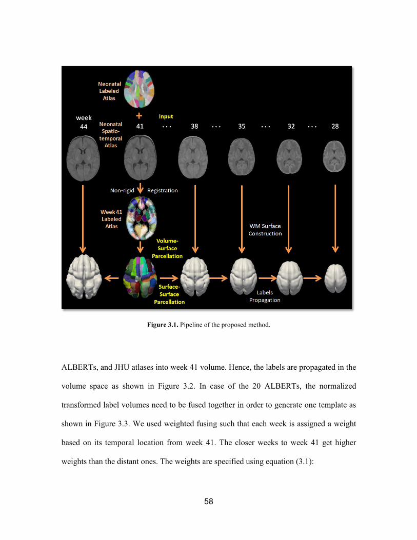
58
Figure 3.1. Pipeline of the proposed method.
ALBERTs, and JHU atlases into week 41 volume. Hence, the labels are propagated in the
volume space as shown in Figure 3.2. In case of the 20 ALBERTs, the normalized
transformed label volumes need to be fused together in order to generate one template as
shown in Figure 3.3. We used weighted fusing such that each week is assigned a weight
based on its temporal location from week 41. The closer weeks to week 41 get higher
weights than the distant ones. The weights are specified using equation (3.1):
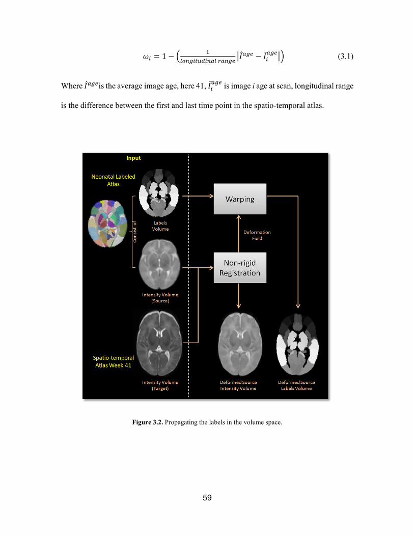
59
]� = 1 Q ^ �:85.�*_/�53:-35.6 `��3.6 Q ��̅3.6`a (3.1)
Where ��3.6is the average image age, here 41, ��̅3.6 is image i age at scan, longitudinal range
is the difference between the first and last time point in the spatio-temporal atlas.
Figure 3.2. Propagating the labels in the volume space.

60
Figure 3.3: ALBERTs’ 20 labeled brain normalization and fusing to generate one template.
3.4. Volume-Surface Parcellation
At this stage, week 41 of the spatio-temporal atlas is automatically delineated by
labels. A WM surface is constructed from this 41 week intensity volume using Marching
Cubes algorithm [167]. To get a smooth surface, the volume is blurred using a Gaussian
kernel with σ = 2 before constructing the surface. The goal of this stage is to find a surface-
based representation of the labels from the volume. We start by embedding the surface
inside the volume of labels by rigid alignment. Then, for each point pi on the surface, the

61
intersection between the surface and the volume determines the label of pi. Each
intersection is located inside a voxel in the volume and the majority of the voxel corners
labels is selected as the pi label. Let b be a set that holds the eight corners’ labels cG , S ∈�1,8e. Labeling pi is based on C-length weights vector: �:, f ∈ �1, ge. This weights vector
defines a scoring function h� →�:. bjcGk and the label associated to point pi is given by
equation (3.2):
flm$f�h�� = lnopl�:�:. bjcGk (3.2)
Furthermore, the eight votes are not uniformly distributed among the eight corners.
Rather, they are determined based on the location inside the voxel where pi is located
following the trilinear interpolation weighting mechanism. Considering a voxel between
two volume grid points [x1, y1, z1] and [x2, y2, z2] as in Figure 3.4:
Figure 3.4: Illustration of the localization of a surface point pi inside a voxel in the volume between two
volume grid points [x1, y1, z1] and [x2, y2, z2], the participation of each voxel corner in the voting
process is weighted by the location of pi.

62
The votes’ participation is specified as follows in equations (3.3-3.13):
Δx = pi.x – x1 (3.3)
Δy = pi.y – y1 (3.4)
Δz = pi.z – z1 (3.5)
f1 = (1-Δx)*(1-Δy)*(1-Δz) (3.6)
f2 = (1-Δx)*Δy*(1-Δz) (3.7)
f3 = (1-Δx)*Δy*Δz (3.8)
f4 = (1-Δx)*(1-Δy)*Δz (3.9)
f5 = Δx*(1-Δy)*(1-Δz) (3.10)
f6 = Δx*Δy*(1-Δz) (3.11)
f7 = Δx*Δy*Δz (3.12)
f8 = Δx*(1-Δy)*Δz (3.13)
If there is no majority, the label of the corner nearest to the intersection point
(denoted as NN) is participating in the voting more than the other corners labels according
to equation (3.14):
cG = q1 Q rrsLt�luv$, LcS = rrww/�x*35=6
y ,z�ℎ$n�Lt$ (3.14)
Consequently, the label of the NN will be selected to be the label of pi. In this way,
jaggies and aliasing artifacts at the boundaries are avoided, ensuring clear boundaries
between regions. If pi intersects the volume in an empty space where no label is defined, a
ray is traced from pi in the direction of its normal vector ni to find an intersection point p

63
within a non-empty voxel. Ray tracing [188] advances a fractional distance d from pi along
its normal vector ni to find new point p as described in equation (3.15):
h�s� = h� + su� (3.15)
This is done iteratively with small d steps until the ray intersects non-empty voxel.
Then, this voxel corners’ labels are similarly used to assign pi a label. Illustration of this
stage using UNC atlas parcellation map is shown in Figure 3.5.
3.5. Surface-Surface Parcellation
The input to this stage is the labeled atlas surface at week 41 of the spatio-temporal
atlas, which plays the role of prior L. The goal is to propagate these labels from the week
41 surface into WM surfaces which are constructed from each week of the spatio-temporal
atlas, weeks 28-44 GA. Each surface is represented in an isotropic triangular mesh t of v
vertices, e edges, and x triangles, and embedded in a 3D Cartesian space.
Figure 3.5. Volume-Surface Parcellation: Labels are propagated from the volume to the surface after
alignment.

64
Problem Statement
Automatically and longitudinally labeling the developing brain cortical gyri and
sulci problem can be phrased within conditional probability framework. In this framework,
for a given observed surface model M, the classification of each point in M depends on its
location with respect to the prior information L. Here, the prior L is incorporated in the
parcellation of M. Considering the large degree of variability in cortical folding patterns of
M, both the priors on L and the conditional probability of observing the surface given the
classification can be conveyed within a mapping space. This allows them to be expressed
as a function of position on the cortical surface; making them non-stationary. Using this
mapping space, the classifiers are distributed and each classifier is responsible for a region
with limited number of classes that occur within it. Therefore, a relationship is established
between the number of classes falling within a region of space and the accuracy of the
mapping system, P(L(pi) = l). Meaning that, P(L(pi) = l) ≠ 0 at each mapped location pi
only for a small number of classes l. In this way, the problem of classifying each surface
point into one of C labels is decomposed into a set of tractable problems of classifying the
points in each region of the surface model into one of only a small number of labels.
A function f(p) needs to be calculated to define the mapping space c�h�:h → �.
This function takes as input a point in the surface p, returning the corresponding location
in the prior coordinates x. The returned coordinates are useful in this context only if they
are spatially and temporally related to the anatomical location of p. This type of mapping
therefore provides the ability to meaningfully relate coordinates temporally. Using the
mapping space, the class statistics will vary as function of location.

65
Mapping Space
During the brain myelination, radial glial cells form the scaffolds where neurons
migrate to their cortical destinations [24,53] and cause an increase in the cerebral cortex
surface area [53] with total brain tissue volume increasing at the ratio of 22 ml/week [26].
Inspired by the neuronal migrational trajectories (described in section 1.3), which are radial
dominant and cortical plate perpendicular [52], and since the cortex globally grows radial
with constant rate assumption in early GA development, we can trace the growth of the
cortex by linearly registering all weeks’ cortical surfaces, identifying the centroid, and
shooting rays from the centroid in all directions. Each ray will intersect all surfaces in
several points on its way out. Considering a small time interval, these intersection points
model the shortest path of growth from one week to its next; hence, a mapping between
them. However, to account for the local cortical surface folding that forms the sulci and
gyri, a local directional mapping between the points is more desirable. We rely on local
pairing between points of consecutive weeks’ surfaces to propagate the labels among pairs
from labeled surface to unlabeled surface. To map the points locally and also to accelerate
the process, we shoot a single ray ri from each point pi of the unlabeled surface t along its
normal vector direction ni towards the labeled surface t±1 rather than shooting all rays from
the centroid. In fact, the ray will intersect the labeled surface at some point inside a triangle
xj on that surface mesh. Therefore, defining the mapping function c�h�:h → �.
Denoting the vertices of xj by vj1, vj2, and vj3, the intersection between a ray
originating at pi having the normalized direction ni with xj will occur when the equality in
equation (3.16) is satisfied:
h�* + su�* =DG�*±� + CjDG"*±� Q DG�*±�k + t�DGI*±� Q DG�*±�� (3.16)

66
We solve in barycentric coordinate for three unknowns: d, u, and s using the linear solution
of [189] (see Appendix 2 for more details). After locating xj, xj vertices’ labels will vote to
label pi and pi will take the label of the majority. If there is no majority among xj vertices’
labels, pi will take the label of the closest vertex to the intersection point Iij.
Additionally, due to the fact that one ray can intersect many triangles, a margin
around the unlabeled surface is defined to insure that only local intersections within the
margin are considered. The benefits of defining a margin are that it will lead to more
efficient pairing and accelerates the process. In fact, when two consecutive GA weeks brain
surfaces are aligned, some regions of the earlier week surface cover or occlude the later
week surface in some locations, and vice versa, as shown in Figure 3.6. This surface
overlaying is primarily due to the fact that brain curvature is deforming [24]. The solution
of this situation is to look for intersections from each side of the surface via the positive
and the negative normal direction as demonstrated in Figure 3.6. In addition, energy
optimization function described in equation (3.17) is used to find the best intersection:
Y�5*6-x6=*jh�*, �G*±�k = Y/�x*jh�*, �G*±�k + Y58-H3:�u�*, �uG*±�� (3.17)
where h�* and u�* represent a point and its normal vector on surface t, respectively. And
�G*±� and �uG*±� represent a triangle and its normal vector on surface t±1, respectively. In
the first term Edist, the process is optimized by looking for the closest intersected triangle
within the described margin, as in equation (3.18):
Y/�x*jh�*, �G*±�k = pLuG sLt�luv$jh�*, ��G*±�k (3.18)

67
Figure 3.6. Surface-Surface Parcellation: Shooting rays from the unlabeled surface points along their normal
vectors and within a margin around the surface toward the labeled surface.
where ��G*±� is the intersection point inside the triangle �G*±� with the ray originating from
h�*. In the second term Enormal, the process is optimized by guaranteeing that the selected
triangle has the most similar normal vector direction to the point normal vector direction.
Therefore, intersections with surface triangles in the opposite direction are avoided, as in
equation (3.19):
Y58-H3:�u�*, �uG*±�� = pLuG �1 Q vzt�u�*, �uG�±��� (3.19)
Parcellation
While parcellating the spatio-temporal atlas starting from week 41 and using this
parcellation as prior then going in both directions, we build a history of the point-triangle
mapping between successive weeks. When we parcellate the surface of t, using prior
labeled surface of t±1, the history information obtained from all weeks t±2, t±3, t±4 …

68
etc., are incorporated in the majority voting process such that all previously labeled
surfaces participate in giving labels to surface t points. The number of points participating
in the voting process is specified by the level of priors available at week t, starting from
week 41 and going in both directions one at a time. We build a tree for each point pi at time
t such that pi will be the root of the tree. In the next tree level, we add 3 nodes, which are
the intersected triangle vertices at time t±1. Each additional level of the tree will have 3depth
nodes, which are the intersected triangles vertices at time t±depth. These nodes are the ones
participating in the voting. Let � be a set that holds the labels of these nodes. The size of
� can be expressed using equation (3.20):
|�| = ∑ 3|�9��|���J* Q 1 (3.20)
Now, given the mapping function f, and the number of votes participating in the voting
process, the probability of assigning class l into current point pi is given by equation (3.21):
h�h� = f� = #84*�H6x=:3xx:8==_-�5�x�X684� (3.21)
After collecting the labels that will participate in the voting process, we can specify
the amount of participation of each label based on its temporal location or tree level such
that the weeks closer to the current week t participate more than distant weeks. Labeling pi
is formulated based on C-length weights vector: �:*, f ∈ �1, ge. This weights vector defines
a relative scoring function based on the longitudinal location � of each point participating
in the voting h� →�:*. ��h�*� such that points in t±1 participate more than points in t±2,
points in t±2 participate more than points in t±3, and so on. To specify this temporal
participation, time dependent kernel regression [135] is used to estimate the weight of votes

69
coming from each time. Hence, Gaussian kernel is used to produce the weight � of the
votes of the kth time point t as given in equation (3.22):
�*��W, �� = 1,√2� $
Q��WQ��2,2 (3.22)
Then, the label associated with point pi is given by equation (3.23):
flm$f�h�*� = lnopl�:�:��jh��k, W ∈ �� + 1, 41eznW ∈ �41, � Q 1e (3.23)
These votes and their weights will specify the level of certainty when assigning a label to
any point. The propagated error will also be quantified based on those votes.
For this Gaussian kernel, the choice of the kernel width , is important, because it
will specify the amount of participation at each level of the tree. We chose , = 1. With
this choice, the previous 4 times are going to directly affect the prediction of the current
label at time t as they will be assigned higher weights than the rest times. According to
Markov Chain theory, each state depends only on the states immediately previous in time.
Hence, the labels are treated as random variables lt such that t indicates the time, the future
is conditionally depends on the past according to the probability given in equation (3.24):
h��* = S|�*±� = L*±�, �*±" = L*±", … , ��� = L��� =h��* = S|�*±� = L*±�, �*±" = L*±", �*±I = L*±I, �*±� = L*±�� (3.24)
Let the discrete values a1, …, at denote the variables of a Markov sequence as in equation
(3.25):
hjf* = l�& `f*±� = l�&±� , f*±" = l�&±( , …, f�� = l���� =hjf* = l�& `f*±� = l�&±� , f*±" = l�&±( , f*±I = l�&±� , f*±� = l�&±�� (3.25)

70
The sequence lt is called a Markov chain [190]. For Markov chain, the starting state does
not affect the long-range predictions.
Additionally, the parcellation is followed by three refinement steps. The first
refinement is to fill the gaps. The second refinement is to correct for the parcellation
depending on the topology of the surface. The third refinement is to merge small patches
with their neighbors as shown in Figure 3.7.
If the ray segment is parallel with the triangles in the defined margin or when u or
s is larger than 1, no intersection can be found. Therefore, small gaps, or few points with
no assigned label could occur in the parcellated surface. Filling the gaps is solved by
adopting a semi-supervised learning approach to propagate the labels between the surface
points [191]. In this approach, labels are propagated through the neighbors iteratively until
convergence. A C-dimensional vector is defined for each unlabeled point pi to hold weights
for each possible candidate region. Only the weights of the neighboring regions of pi (e.g.
regions of the points that share an edge with pi in the triangulated surface mesh) are
considered and updated. Then, the label of the higher weight region will be given to pi.
This is done iteratively until all unlabeled points are labeled.
Since brain cortex topology consists of sulci and gyri, one automatic, numeric way
to capture this topology is by calculating the curvature of the surface. Using the mean
curvature (see Figure 3.8), we locate the set Σ of points with maximum/minimum curvature
on the surface. Referring to some brain sulci and gyri segmentations, some of these points
are located on the boundaries between ROIs. We check to see if these points are surrounded
with more than one ROI in a bounded space. If yes, then we determine whether there is

71
leakage from one ROI to another passing through these points. The leakage is identified by
checking for a connected patch around one side of a line formed by points of Σ, where the
patch size does not exceed a specified threshold. If we find a leak, we correct for it by
pulling the region back to these points, which serve as the boundary between two ROIs,
thereby eliminating the leakage.
Shooting rays along the points’ normal vectors direction could result in cross
intersection due to the fact that the neonatal brain surface curvature is deforming. This
results in small patches near borders that belong to neighboring regions after parcellation.
The described situation is directly related to the change in the normal vectors direction,
especially where the curvature is high among neighboring points. Whenever a small patch
with less than a pre-specified threshold number of points is located, we merge it with the
neighboring region where the largest border is shared.
3.6. Summary
This chapter presented an approach for propagating a number of neuroanatomical
ROIs through 4D atlas of the developing brain. The approach consists of three stages. In
the first stage, non-rigid registration of MR images of intensity volumes is performed to
propagate the labels into the spatio-temporal atlas at one GA week. In the second stage,
intersections between volume, and surface constructed from it are used to propagate the
labels from the volume space into the surface space. In the third stage, ray-triangle
intersections framework between consecutive weeks’ surfaces is described to propagate

72
the labels among the GA weeks of the spatio-temporal atlas. Experimental results of this
approach and evaluation methods are presented in Chapter 4.
Figure 3.7. Lateral view of parcellated brain and refinements results. First row: Before and after refinement
step 1 of filling gaps on left column and right column, respectively. Middle row: Before and after
refinement step 2 of correcting for the topology using mean curvature on left column and right
column, respectively. Bottom row: Before and after refinement step 3 of merging small patches with
neighbors on left column and right column, respectively. Final Refinement Result is shown on the
right of the last row.

73
Figure 3.8. Superior and lateral views of the surface mean curvature on selected GA weeks of the spatio-
temporal atlas. Top: Symmetric results. Bottom: Asymmetric results.

74
Chapter 4: Results and Evaluation
4.1. Introduction
This chapter presents the experimental results of the method discussed in Chapter
3 that demonstrate a three-stage parcellation algorithm for 4D atlas of the developing brain.
Both final results and individual stages’ results are presented in this chapter. Also offered
are evaluation methods and discussion. Since there is no available neonatal parcellated
atlas that covers weeks 28-44 GA to use as ground truth and for comparison purposes, we
designed four experiments to validate the resultant parcellation.
4.2. Experimental Setup
The method described in Chapter 3 has been implemented using C# programming
language. The programming and compilation are performed on Microsoft Visual Studio
2012 IDE. The system used is a DELL Precision T7500 Workstation with Intel Xeon
2.27GHz E5607 processor, 54 GB of usable RAM. The operating system is Windows 7
Professional. Two versions of the code are implemented; one without using parallelism,
and one with using parallelism in parallel threading [192]. Comparison between
performances in term of time is given in Table 4.1.
With regards to the input data, we used the three available datasets on the web for
the labeled neonatal atlases; UNC [74], ALBERT [72], and JHU [71]. For the spatio-
temporal atlas, we used the only online accessible 4D neonatal atlas that is constructed
from the largest number of subjects [140] in order to best represent the population.

75
4.3. Results and Evaluation
4.3.1. Results
We performed the proposed parcellation on the neonatal spatio-temporal atlas
[140] using UNC labeled atlas of C=90 ROIs parcellation map [74], ALBERT labeled
atlas of C=50 ROIs parcellation map (44 are cortical ROIs only) [72], and JHU labeled
atlas of C=122 ROIs parcellation map [71]. Two versions of each parcellation map are
used: one is symmetric and another is asymmetric. In the first stage of propagating the
labels in the volume space, the UNC and JHU neonate atlases are non-rigidly registered
into week 41 of the spatio-temporal atlas and labels are propagated in the volume
domain. For ALBERT atlas, since it consists of 20 parcellated subjects, we need to
normalize their volumes into week 41 of the spatio-temporal brain space, then fuse their
information to build one template. Each subject is non-rigidly registered to week 41 of
the spatio-temporal atlas (which is the average age of ALBERTs as given in Table 3.1)
and labels are propagated in the volume domain. Then, fusing is performed using voxel-
level majority voting to generate one template (as described in section 3.3), which is
used in the stages that follow. Results of the first stage are given in Figure 4.1.
Figure 4.1. Results of first stage: Propagating the labels in the volume space into week 41 of spatio-temporal
atlas. Left: Deformed UNC atlas labels. Middle: Deformed ALBERTs atlases labels after majority
voting. Right: Deformed JHU atlas labels.

76
In the volume-surface parcellation stage, the deformed volume of labels of
UNC, ALBERT, and JHU are used one at a time to transfer labels into the WM surface
of the spatio-temporal atlas at week 41.
For UNC atlas, out of 90 ROIs, three ROIs numbered: 75,76, and 79 in the
parcellation map did not initially appear in the volume-surface parcellation results of
week 41 because they did not intersect with the constructed cortical surface.
Additionally, eight ROIs numbered: 25, 26, 29, 31, 32, 36, 42 and 80 in the parcellation
map have a very small number of points assigned to each. Therefore, these regions fade
away at different weeks during the propagation because they are considered as small
patches and were merged into their neighbors at some longitudinal point in the
refinement step as shown in Table 6.5. The remaining 79 ROIs are presented and
propagated from week 41 in both directions into the spatio-temporal atlas by proposed
surface-surface parcellation.
For ALBERT atlas, 44 cortical ROIs are propagated into the surface after
removing the cerebellum and non-cortical structures, which are ROIs numbered: 17,
18, 19, 44, 45, and 48 in the parcellation map as shown in Table 6.7.
For JHU atlas, 49 ROIs did not initially appear in the volume-surface
parcellation results of week 41 because they did not intersect with the constructed
cortical surface. These ROIs have numbers: [7-16], 21, 23, [25-29], 31, 32, 37, 38, [41-
57], [59-66], 102, 119, and 120 in the parcellation map. Also, twelve ROIs numbered:
3, 4, 5, 20, 24, 30, 58, 85, 87, 115, 116 and 118 in the parcellation map had only a small
number of points assigned to them. Therefore, these regions fade away at different

77
weeks during the propagation because they are considered as small patches and were
merged into their neighbors in the refinement step as shown in Table 6.9.
The results of this stage in 3D form parcellated surfaces at week 41 GA are
embedded in Figure 4.2 and in the supplementary material for interactive illustrations.
Figure 4.2. 3D results of second stage of volume-surface parcellation. Left: Using UNC atlas labels. Middle:
Using ALBERT atlas labels. Right: Using JHU atlas labels. Top: Symmetric. Bottom: Asymmetric.

78
In the last stage of surface-surface parcellation, labels are propagated into all
spatio-temporal atlas weeks. The symmetric and asymmetric results of this stage in
selected GA weeks are shown in Figure 4.3 using UNC atlas parcellation map, Figure
4.4 using ALBERT parcellation map, and Figure 4.5 using JHU parcellation map.
Visual inspection shows consistent propagation of the labels over time. Processing time
is reported in Table 4.1 and depends heavily on the number of points per source surface
and the number of triangles per target surface. Because longitudinal brain development
and cortical changes in two consecutive GA weeks is minimal and subtle [24,26,193],
the ray-triangle intersection process provides rough pairing between the two surfaces
as solid ground to propagate the labels among them. It also describes the growth
trajectories between successive weeks. The average Euclidian distances of the pairing
done by the proposed parcellation across weeks are reported in Table 4.1. The average
ranges from 0.26 to 1.02 mm in the symmetric surfaces, and ranges from 0.26 to 1.03
mm in the asymmetric surfaces. This minimal distance between the consecutive
surfaces strengthen the proposed parcellation method which rely on the pairing between
the consecutive weeks without the need of performing the time-consuming deformable
registration.
4.3.2. Evaluation
To our best knowledge, this is the first parcellated atlas of neonatal developing
brain that covers GA weeks 28 to 44. For this reason, several approaches are necessary
to evaluate the results. We used four evaluation methods on the proposed parcellation.
The first approach incorporates ground truth parcellation to assess the validity of the

79
proposed parcellation method. The second evaluation method includes cross validation
on ALBERT’s 20 subjects to validate the final result. The third evaluation measures
the local growth of individual neuroanatomical regions (labels) over time. The fourth
evaluation focuses on comparing the probabilistic distribution of the labels among
points across successive weeks. Finally, the utility of the parcellation in capturing the
normal growth of perinatal brain individual ROI development is demonstrated in tables
6.4 to 6.9 in Appendix 1.
Table 4.1. Spatio-temporal atlas information: number of points per surface, number of triangles per surface,
average pairing distance, and parcellation time starting from week 41 and going in both directions
with and without multithreading. Sym.: Symmetric, Asym: Asymmetric
Wee
k Number of
points/Surface
Number of
triangles/Surface Average paring
distance (mm)
Time without
multithreading
(min:sec)
Time with
multithreading
(min:sec)
Sym. Asym. Sym. Asym. Sym. Asym. Sym. Asym. Sym. Asym.
28 35,172 34,872 70,348 69,740 0.58 0.55 11:50 12:40 05:55 5:09
29 37,464 36,926 74,932 73,844 0.96 1.00 14:16 14:22 06:46 5:55
30 40,900 40,522 81,796 81,040 0.77 0.82 16:35 17:15 07:38 6:56
31 43,848 43,706 87,692 87,412 0.70 0.70 17:55 19:47 08:33 7:51
32 46,435 46,448 93,048 92,896 1.02 1.08 20:42 18:02 09:51 9:01
33 50,784 51,264 101,788 102,536 0.69 0.70 22:13 26:38 11:01 10:30
34 53,206 53,784 106,420 107,576 0.93 0.98 25:34 30:47 12:13 12:01
35 56,990 59,240 113,976 118,488 0.64 0.66 30:11 26:50 13:52 14:20
36 60,230 64,180 120,452 128,364 0.26 0.26 30:52 40:15 14:43 15:35
37 60,252 64,752 120,496 129,508 0.85 0.82 35:15 45:47 16:51 17:52
38 69,070 73,280 138,148 146,564 1.02 1.03 45:24 58:13 20:29 22:35
39 78,548 82,254 157,104 164,516 0.49 0.43 50:22 63:58 24:07 24:54
40 76,848 80,770 153,700 161,540 0.55 0.49 50:03 63:28 22:37 25:05
41 78,222 82,310 156,440 164,620 - - - - - -
42 86,188 88,924 172,392 177,860 0.86 0.86 59:13 71:53 25:16 27:32
43 85,472 88,694 170,964 177,400 0.41 0.38 60:09 75:27 26:59 29:17
44 88,532 91,070 177,084 182,152 0.31 0.31 63:21 77:10 27:55 30:04

80
Figure 4.3. Parcellation results using UNC labels map on ten selected GA weeks. Top: Symmetric results.
Bottom: Asymmetric results.

81
Figure 4.4. Parcellation results using ALBERT labels map on ten selected GA weeks. Top: Symmetric
results. Bottom: Asymmetric results.

82
Figure 4.5. Parcellation results using JHU labels map on ten selected GA weeks. Top: Symmetric results.
Bottom: Asymmetric results.

83
First Validation: Spatial and Temporal Consistency using Longitudinal Atlas
We used UNC Infant 0-1-2 parcellated brain atlas [74] to evaluate the proposed
longitudinal method. This brain atlas provides full parcellation of the brain at three
temporal ages: newborn, 1 year, and 2 years. As ground truth, a parcellated surface is
constructed from each time point. Then, labels are propagated from one time point to
another; from birth to year 1 and from year 1 to year 2 surfaces and vice versa, using
the proposed parcellation method. The result is compared with ground truth point-by-
point and by using DICE similarity index [194], which is given in equation (4.1) for
any two sets X and Y and measures the overlapping and the agreement of these two sets,
hence X and Y stand for the result and the ground truth:
2|� ∩ �| |�|⁄ + |�| (4.1)
Having a consistency of 70% to 90%, the propagated labels are compared to ground
truth as shown in Table 4.2. This consistency is comparable with the consistency of a
similar experiment reported by UNC Infant 0-1-2 brain atlas authors [74]. In fact, the
consistency is similar on birth vs. 1 year and is better on 1 vs. 2 years of age (90%). As
shown in Figure 4.6, the location of most of the mismatched points is at the borders
between regions; the ambiguous locations where precise parcellation could be missed
even if it is done manually by an expert. We believe that dramatic changes in the brain
shape, geometry, curvature and size between neonates to 1 year then to 2 year old are
key reasons why a higher accuracy was not achieved in our validation experiment.
These changes in the brain are less in magnitude during a week as opposed to a year.
Furthermore, due to significant changes between neonatal and 1-year-old brains, a
larger error is reported after propagating the labels starting from neonate towards 2

84
years old, as indicated in the dark gray shaded cells in Table 4.2. The main reason for
this is the differences in the cortical growth rates during the first two years of age, as
the cortex grows 1.8 times in average during the first year and 1.2 times in average
during the second year [195].
Table 4.2. Dice similaity index of propagating labels among neonate, 1, 2 years old atlas. Left (light gray
shaded cells): Starting the propagation from year 2 towards neonate. Right (dark gray shaded cells):
Starting propagation from neonate towards year 2.
From 2 to 1 From 1 to neo. From neo. to 1 From 1 to 2
DICE score 0.9042 0.8027 0.7297 0.7135
Figure 4.6: The UNC Infant 0-1-2 Atlas validation experiment. Top row: Ground truth parcellation maps.
Second and third rows: Proposed method parcellation maps starting from 0 to 1 then to 2 years and
the color coded agreement between the ground truth and the proposed method parcellation where
error is shown in red. Fourth and fifth rows: Proposed method parcellation maps starting from 2 to
1 then to 0 year old and the color coded agreement between the ground truth and the proposed
method parcellation where error is shown in red.

85
Second Validation: Spatial and Temporal Consistency using Cross validation
The ALBERTs atlas dataset consists of 20 brain MRI scans and their manual
parcellation maps. Each brain scan was taken at specific week of gestation as shown
Table 3.1. According to Table 4.3, several GA weeks have more than one scan.
Therefore, cross validation/leave-one-out/n-folds/jackknife technique can be employed
to validate the proposed method. Using this technique, one scan per age is removed
from the dataset and called testing scan, the remaining scans are used to create a
template by normalizing and fusing them as described in section 3.3, called training
set. The new template is used as an input for the proposed parcellation, and its labels
are propagated in the spatio-temporal atlas starting from week 41 GA and targeting the
testing scan age week. The resultant parcellation of the training set at that age is then
compared with the testing scan. The disagreement between the manual and the
automated parcellation is quantified point-by-point, whereas this disagreement will
report the percentage of error. To further explain how this cross validation was set up,
we leave-one-out of each individual week as ground truth, making the testing data size
equal to 1 and the training data size 20-1 equal to 19. With the available 20 ALBERTs,
we need to perform 5 cross validation experiments where each experiment uses a
different age and a randomly selected scan at that age as the testing data according to
Table 4.4.
As reported in Table 4.4, parcellation results using the proposed method have
83.79% to 87.08% accuracy with the testing data. The accuracy depends heavily on the
randomly selected data for testing. If the leave-one-out scan represents an outlier of the
ALBERTs population, the result will be compromised as shown in Figure 4.7. This

86
compares to the accuracy of a similar experiment reported by FreeSurfer parcellation
[92] for adult brain, which reports an accuracy of 79% to 83%.
Table 4.3. ALBERTs atlas information: range of age at scan of 20 neonates brains and number of scans
avaliable in the ALBERTs atlas per each age.
Age at scan (week) 36 39 40 41 43 44 Total
Number of scans/age 2 6 2 6 2 2 20
Table 4.4. ALBERTs leave-one-out experiments setup with labels agreements accuracy between the test data
and the proposed parcellation result reported in each experiment.
Age at scan (week) 36 39 40 43 44 Training data
size
Testing
data size
Labels
agreement
Number of scans/age 2 6 2 2 2
Experiment 1 1 19 1 85.93890%
Experiment 2 1 19 1 87.08815%
Experiment 3 1 19 1 83.79138%
Experiment 4 1 19 1 84.88628%
Experiment 5 1 19 1 83.82167%
Third validation: Measuring the Normal Growth
We compared the number of points per label to measure the growth of the brain
between weeks. Ultimately, the number of points per region label is expected to
fluctuate from one week to another as the brain grows and cells form. The growth of
the ROIs fluctuate from one week to another due to the brain structure convolution and
sulci and gyri maturation as shown in Appendix 1’s tables 6.4 to 6.9. Figure 4.8 shows
the growth of two regions reported as good cortical growth biomarkers for the used
neonatal spatio-temporal atlas [61] and which is consistent with the growth reported in
clinical studies. These regions are: Middle Temporal Gyrus (MTG), and Inferior
Temporal Gyrus (ITG).

87
Figure 4.7: The ALBERT Atlas validation experiment. Left column: The leave-one-out per GA week test
subject parcellation map as ground truth. Middle column: The parcellation map of proposed method
starting from week 41 GA to the corresponding test subject GA week. Right column: The color-
coded agreement between the test subject and the proposed method parcellation where error is
shown in red.

88
Figure 4.7: Continued

89
Figure 4.8. The number of points per two biomarker growth regions, (Middle temporal gyrus (MTG), and
Inferior temporal gyrus (ITG)) is plotted against age at time of scan.
Fourth Validation: Longitudinal Probabilistic Distribution Consistency
Demonstrating the growth model, the fitting of the propagated labels from a
labeled week to a successive unlabeled week is evaluated. The spatial distribution of
points per labels of each week after parcellation is quantified by statistical probability.
The distribution of the points under each label is maintained with the same probability
in all GA week, even though the numbers of surface points (reported in Table 4.1) vary
significantly between weeks.
The detailed quantitative information about the growth of each ROI is reported
in tables in Appendix 1; including: Tables 6.4 and 6.5 using UNC parcellation map
symmetrically and asymmetrically, Tables 6.6 and 6.7 using ALBERT parcellation

90
map symmetrically and asymmetrically, and Tables 6.8 and 6.9 using JHU parcellation
map symmetrically and asymmetrically.
4.4. Limitation
Spatially, one can consider the isotropic concentric brain growth model encoded in
the proposed ray-triangle intersection framework a limitation. However, the actual
implemented ray-triangle algorithm takes into account the local growth as the rays are shot
locally in the direction of their normal vector and are perpendicular to the cortical plate.
Therefore, it is not fully isometric and concentric. The local ray-triangle intersection
framework is the most relevant model to the growth trajectory, which reflects the behavior
of the neuronal migration while the brain is developing. If a detailed model describing the
brain ROIs growth trajectories at early development were available, we would more
accurately model the brain ROIs growth at early gestational age. Temporally, it is important
to mention that when error appears in time t, it will propagate to all times following it, e.g.
time t±1, t±2, and so on. Currently, to limit this error propagation we incorporated the
history of the previous week’s parcellated surfaces in the voting process as described in
section 3.5. A future project will investigate and address this issue by incorporating the
neighboring points in the voting process. Finally, having no ground truth of all GA weeks
to compare our result with is a validation limitation, especially in weeks 28 to 35 GA.
4.5. Summary
This chapter described the experimental results of the method of parcellating the
developing brain longitudinal cortical surfaces proposed in this dissertation. Two different
datasets are used to parcellate the spatio-temporal atlas. The proposed method has three

91
stages. Individual stages’ results are provided along with final results. Also, several
evaluations of this parcellation method are discussed. In the next chapter we will conclude
the description of this work and propose possible future work.

92
Chapter 5: Conclusion and Future Work
5.1. Conclusion
The marker-less automatic parcellation method described in this dissertation has
been shown to provide a label for each point in the longitudinal cortical surfaces of 17
consecutive GA weeks. Label propagation across neonatal spatio-temporal brain atlas
surfaces is phrased within a customized ray-triangle intersection framework. The accuracy
of label assignment in the proposed method is leveraged out through the use of local and
global, spatial and temporal information. The local information is encoded by modeling
the shortest spatial path of growth throughout the 17 weeks as directional rays. The global
information is merged into the parcellation by incorporating the history of the voting
process in a temporal fashion. The proposed brain parcellation method is applicable when
we cannot rely on the surface curvature alone to locate the landmarks or predict the labels,
and when the growth is radial, as in the case of developing brains. Having the labels
propagated with the same probabilistic distribution into younger GA weeks is appealing,
especially with the lack of parcellated brain atlases in early development, such as at week
28 GA. The aim is to parcellate the developing brain, which can be used as a benchmark
to assess brain structures development of preterm born children in order to discover
functional abnormalities at early age. We ultimately aim to facilitate the acquisition of
detailed morphometric information allowing the investigation of correlations between
morphological characteristics of neonatal brain regions and specific disorders at early GA.

93
5.2. Future Work
The long-term future work includes extending this method to the use of other
labeled neonatal brain atlases and to parcellate different neonatal and fetal brain spatio-
temporal atlases. Also, we intend to perform cortical region analysis, find the gyrification
indices on the developing brain and accelerate the parcellation by making use of GPU
computation. In addition, we intend to investigate more ways to quantify the propagated
error.

94
6. Appendix 1
Table 6.1. Index of the UNC infant-AAL atlas ROIs’ names and colors. Sym.: Symmetric,
Asym.: Asymmetric.
Index Color
(Sym.)
Color
(Asym.) Region Abbreviation
1 Precentral gyrus left PreCG-L
2 Precentral gyrus right PreCG-R
3 Superior frontal gyrus (dorsal) left SFGdor-L
4 Superior frontal gyrus (dorsal) right SFGdor-R
5 Orbitofrontal cortex (superior) left ORBsupb-L
6 Orbitofrontal cortex (superior) right ORBsupb-R
7 Middle frontal gyrus left MFG-L
8 Middle frontal gyrus right MFG-R
9 Orbitofrontal cortex (middle) left ORBmid-L
10 Orbitofrontal cortex (middle) right ORBmid-R
11 Inferior frontal gyrus (opercular) left IFGoperc-L
12 Inferior frontal gyrus (opercular)
right IFGoperc-R
13 Inferior frontal gyrus (triangular) left IFGtriang-L
14 Inferior frontal gyrus (triangular)
right IFGtriang-R
15 Orbitofrontal cortex (inferior) left ORBinf-L
16 Orbitofrontal cortex (inferior) right ORBinf-R
17 Rolandic operculum left ROL-L
18 Rolandic operculum right ROL-R
19 Supplementary motor area left SMA-L
20 Supplementary motor area right SMA-R
21 Olfactory left OLF-L
22 Olfactory right OLF-R
23 Superior frontal gyrus (medial) left SFGmed-L
24 Superior frontal gyrus (medial) right SFGmed-R
25 Orbitofrontal cortex (medial) left ORBmed-L
26 Orbitofrontal cortex (medial) right ORBmed-R
27 Rectus gyrus left REC-L
28 Rectus gyrus right REC-R
29 Insula left INS-L
30 Insula right INS-R
31 Anterior cingulate gyrus left ACG-L
32 Anterior cingulate gyrus right ACG-R
33 Middle cingulate gyrus left MCG-L

95
34 Middle cingulate gyrus right MCG-R
35 Posterior cingulate gyrus left PCG-L
36 Posterior cingulate gyrus right PCG-R
37 Hippocampus left HIP-L
38 Hippocampus right HIP-R
39 ParaHippocampal gyrus left PHG-L
40 ParaHippocampal gyrus right PHG-R
41 Amygdala left AMYG-L
42 Amygdala right AMYG-R
43 Calcarine cortex left CAL-L
44 Calcarine cortex right CAL-R
45 Cuneus left CUN-L
46 Cuneus right CUN-R
47 Lingual gyrus left LING-L
48 Lingual gyrus right LING-R
49 Superior occipital gyrus left SOG-L
50 Superior occipital gyrus right SOG-R
51 Middle occipital gyrus left MOG-L
52 Middle occipital gyrus right MOG-R
53 Inferior occipital gyrus left IOG-L
54 Inferior occipital gyrus right IOG-R
55 Fusiform gyrus left FFG-L
56 Fusiform gyrus right FFG-R
57 Postcentral gyrus left PoCG-L
58 Postcentral gyrus right PoCG-R
59 Superior parietal gyrus left SPG-L
60 Superior parietal gyrus right SPG-R
61 Inferior parietal lobule left IPL-L
62 Inferior parietal lobule right IPL-R
63 Supramarginal gyrus left SMG-L
64 Supramarginal gyrus right SMG-R
65 Angular gyrus left ANG-L
66 Angular gyrus right ANG-R
67 Precuneus left PCUN-L
68 Precuneus right PCUN-R
69 Paracentral lobule left PCL-L
70 Paracentral lobule right PCL-R
71 Caudate left CAU-L
72 Caudate right CAU-R
73 Putamen left PUT-L
74 Putamen right PUT-R

96
75 Pallidum left PAL-L
76 Pallidum right PAL-R
77 Thalamus left THA-L
78 Thalamus right THA-R
79 Heschl gyrus left HES-L
80 Heschl gyrus right HES-R
81 Superior temporal gyrus left STG-L
82 Superior temporal gyrus right STG-R
83 Temporal pole (superior) left TPOsup-L
84 Temporal pole (superior) right TPOsup-R
85 Middle temporal gyrus left MTG-L
86 Middle temporal gyrus right MTG-R
87 Temporal pole (middle) left TPOmid-L
88 Temporal pole (middle) right TPOmid-R
89 Inferior temporal gyrus left ITG-L
90 Inferior temporal gyrus right ITG-R

97
Table 6.2. Index of the ALBERT atlas ROIs’ names and colors. Sym.: Symmetric, Asym.:
Asymmetric.
Index Color
(Sym.)
Color
(Asym.) Region
1 Hippocampus right
2 Hippocampus left
3 Amygdala right
4 Amygdala left
5 Anterior temporal lobe, medial part right
6 Anterior temporal lobe, medial part left
7 Anterior temporal lobe, lateral part right
8 Anterior temporal lobe, lateral part left
9 Gyri parahippocampalis et ambiens anterior part right
10 Gyri parahippocampalis et ambiens anterior part left
11 Superior temporal gyrus, middle part right
12 Superior temporal gyrus, middle part left
13 Medial and inferior temporal gyri anterior part right
14 Medial and inferior temporal gyri anterior part left
15 Lateral occipitotemporal gyrus, gyrus fusiformis anterior
part right
16 Lateral occipitotemporal gyrus, gyrus fusiformis anterior
part left
17 Cerebellum right
18 Cerebellum left
19 Brainstem, spans the midline
20 Insula left
21 Insula right
22 Occipital lobe left
23 Occipital lobe right
24 Gyri parahippocampalis et ambiens posterior part left
25 Gyri parahippocampalis et ambiens posterior part right
26 Lateral occipitotemporal gyrus, gyrus fusiformis posterior
part left
27 Lateral occipitotemporal gyrus, gyrus fusiformis posterior
part right
28 Medial and inferior temporal gyri posterior part left
29 Medial and inferior temporal gyri posterior part right
30 Superior temporal gyrus, posterior part left
31 Superior temporal gyrus, posterior part right
32 Cingulate gyrus, anterior part left
33 Cingulate gyrus, anterior part right
34 Cingulate gyrus, posterior part left

98
35 Cingulate gyrus, posterior part right
36 Frontal lobe left
37 Frontal lobe right
38 Parietal lobe left
39 Parietal lobe right
40 Caudate nucleus left
41 Caudate nucleus right
42 Thalamus left
43 Thalamus right
44 Subthalamic nucleus left
45 Subthalamic nucleus right
46 Lentiform Nucleus left
47 Lentiform Nucleus right
48 Corpus Callosum
49 Lateral Ventricle right
50 Lateral Ventricle left

99
Table 6.3. Index of the JHU atlas ROIs’ names and colors. Sym.: Symmetric, Asym.:
Asymmetric.
Index Color
(Sym.)
Color
(Asym.) Region Location
1 corpus callosum left
2 corpus callosum right
3 anterior limb of internal capsule left
4 anterior limb of internal capsule right
5 posterior limb of internal capsule left
6 posterior limb of internal capsule right
7 retrolenticular part of internal capsule left
8 retrolenticular part of internal capsule right
9 anterior corona radiata left
10 anterior corona radiata right
11 superior corona radiata left
12 superior corona radiata right
13 posterior corona radiata left
14 posterior corona radiata right
15 cingulum cingular part left
16 cingulum cingular part right
17 cingulum hippocampal part left
18 cingulum hippocampal part right
19 fornix left
20 fornix right
21 stria terminalis left
22 stria terminalis right
23 tapetum left
24 tapetum right
25 superior longitudinal fasciculus left
26 superior longitudinal fasciculus right
27 external capsule left
28 external capsule right
29 posterior thalamic radiation left
30 posterior thalamic radiation right
31 sagittal stratum left
32 sagittal stratum right
33 thalamus left
34 Thalamus right
35 Putamen left
36 Putamen right
37 globus pallidus left
38 globus pallidus right
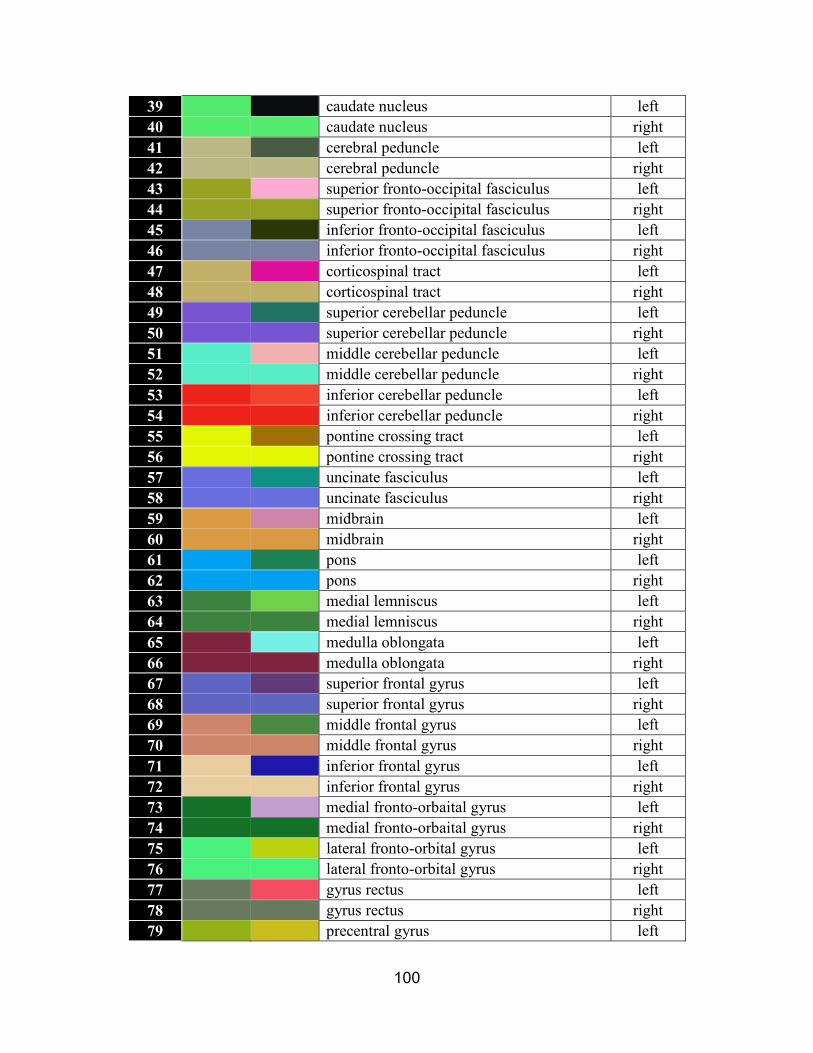
100
39 caudate nucleus left
40 caudate nucleus right
41 cerebral peduncle left
42 cerebral peduncle right
43 superior fronto-occipital fasciculus left
44 superior fronto-occipital fasciculus right
45 inferior fronto-occipital fasciculus left
46 inferior fronto-occipital fasciculus right
47 corticospinal tract left
48 corticospinal tract right
49 superior cerebellar peduncle left
50 superior cerebellar peduncle right
51 middle cerebellar peduncle left
52 middle cerebellar peduncle right
53 inferior cerebellar peduncle left
54 inferior cerebellar peduncle right
55 pontine crossing tract left
56 pontine crossing tract right
57 uncinate fasciculus left
58 uncinate fasciculus right
59 midbrain left
60 midbrain right
61 pons left
62 pons right
63 medial lemniscus left
64 medial lemniscus right
65 medulla oblongata left
66 medulla oblongata right
67 superior frontal gyrus left
68 superior frontal gyrus right
69 middle frontal gyrus left
70 middle frontal gyrus right
71 inferior frontal gyrus left
72 inferior frontal gyrus right
73 medial fronto-orbaital gyrus left
74 medial fronto-orbaital gyrus right
75 lateral fronto-orbital gyrus left
76 lateral fronto-orbital gyrus right
77 gyrus rectus left
78 gyrus rectus right
79 precentral gyrus left

101
80 precentral gyrus right
81 postcentral gyrus left
82 postcentral gyrus right
83 superior parietal gyrus left
84 superior parietal gyrus right
85 precuneus left
86 precuneus right
87 cingular gyrus left
88 cingular gyrus right
89 supramarginal gyrus left
90 supramarginal gyrus right
91 angular gyrus left
92 angular gyrus right
93 superior temporal gyrus left
94 superior temporal gyrus right
95 middle temporal gyrus left
96 middle temporal gyrus right
97 inferior temporal gyrus left
98 inferior temporal gyrus right
99 fusiform gyrus left
100 fusiform gyrus right
101 parahippocampal gyrus left
102 parahippocampal gyrus right
103 entrhinal cortex left
104 entrhinal cortex right
105 superior occipital gyrus left
106 superior occipital gyrus right
107 middle occipital gyrus left
108 middle occipital gyrus right
109 inferior occipital gyrus left
110 inferior occipital gyrus right
111 cuneus left
112 cuneus right
113 lyngual gyrus left
114 lyngual gyrus right
115 amygdala left
116 amygdala right
117 hippocampus left
118 hippocampus right
119 cerebellar hemisphere left
120 cerebellar hemisphere right

102
121 insular cortex left
122 insular cortex right

103
Table 6.4. Longitudinal Probabilistic Distribution of Points per ROIs using Symmetric UNC Parcellation Map with 90 ROIs given as:
Number of points per ROI (Percentage on surface %) Week
/ROI# 28 29 30 31 32 33 34 35 36 37 38 39 40 41 42 43 44
1 & 2 1031(2.9
31%)
1087(2.9
01%)
1190(2.9
1%)
1266(2.8
87%)
1409(3.0
28%)
1570(3.0
85%)
1708(3.2
1%)
1916(3.3
62%)
1978(3.2
84%)
2092(3.4
72%)
2497(3.6
15%)
2721(3.4
64%)
2734(3.5
58%)
2757(3.5
25%)
2963(3.4
38%)
2838(3.3
2%)
2907(3.2
84%)
3 & 4 1073(3.0
51%)
1180(3.1
5%)
1349(3.2
98%)
1527(3.4
82%)
1807(3.8
84%)
2128(4.1
81%)
2290(4.3
04%)
2648(4.6
46%)
2824(4.6
89%)
2881(4.7
82%)
3183(4.6
08%)
3573(4.5
49%)
3467(4.5
12%)
3657(4.6
75%)
4334(5.0
29%)
4173(4.8
82%)
4248(4.7
98%)
5 & 6 547(1.55
5%)
614(1.63
9%)
695(1.69
9%)
772(1.76
1%)
823(1.76
9%)
907(1.78
2%)
984(1.84
9%)
1077(1.8
9%)
1123(1.8
65%)
1073(1.7
81%)
1161(1.6
81%)
1324(1.6
86%)
1293(1.6
83%)
1352(1.7
28%)
1578(1.8
31%)
1540(1.8
02%)
1652(1.8
66%)
7 & 8 2769(7.8
73%)
2909(7.7
65%)
3209(7.8
46%)
3442(7.8
5%)
3627(7.7
96%)
3893(7.6
49%)
4085(7.6
78%)
4351(7.6
35%)
4460(7.4
05%)
4495(7.4
6%)
4715(6.8
26%)
5126(6.5
26%)
5024(6.5
38%)
5073(6.4
85%)
5395(6.2
6%)
5357(6.2
68%)
5547(6.2
66%)
9 &
10
376(1.06
9%)
456(1.21
7%)
561(1.37
2%)
677(1.54
4%)
738(1.58
6%)
831(1.63
3%)
956(1.79
7%)
1151(2.0
2%)
1218(2.0
22%)
1187(1.9
7%)
1307(1.8
92%)
1542(1.9
63%)
1541(2.0
05%)
1587(2.0
29%)
1729(2.0
06%)
1736(2.0
31%)
1778(2.0
08%)
11 &
12
718(2.04
1%)
709(1.89
2%)
724(1.77
%)
715(1.63
1%)
705(1.51
5%)
694(1.36
4%)
668(1.25
5%)
689(1.20
9%)
658(1.09
2%)
674(1.11
9%)
762(1.10
3%)
790(1.00
6%)
816(1.06
2%)
815(1.04
2%)
860(0.99
8%)
900(1.05
3%)
927(1.04
7%)
13 &
14
756(2.14
9%)
826(2.20
5%)
926(2.26
4%)
968(2.20
8%)
1054(2.2
65%)
1135(2.2
3%)
1230(2.3
12%)
1330(2.3
34%)
1437(2.3
86%)
1415(2.3
48%)
1596(2.3
11%)
1775(2.2
6%)
1731(2.2
52%)
1658(2.1
2%)
1686(1.9
56%)
1808(2.1
15%)
1802(2.0
35%)
15 &
16
1632(4.6
4%)
1683(4.4
92%)
1734(4.2
4%)
1751(3.9
93%)
1773(3.8
11%)
1793(3.5
23%)
1834(3.4
47%)
1834(3.2
18%)
1879(3.1
2%)
1819(3.0
19%)
1941(2.8
1%)
2132(2.7
14%)
2118(2.7
56%)
2075(2.6
53%)
2100(2.4
37%)
2228(2.6
07%)
2255(2.5
47%)
17 &
18
522(1.48
4%)
542(1.44
7%)
572(1.39
9%)
586(1.33
6%)
588(1.26
4%)
587(1.15
3%)
590(1.10
9%)
614(1.07
7%)
533(0.88
5%)
557(0.92
4%)
615(0.89
%)
880(1.12
%)
804(1.04
6%)
558(0.71
3%)
948(1.1
%)
991(1.15
9%)
950(1.07
3%)
19 &
20
730(2.07
6%)
769(2.05
3%)
787(1.92
4%)
780(1.77
9%)
816(1.75
4%)
896(1.76
%)
872(1.63
9%)
873(1.53
2%)
1027(1.7
05%)
1077(1.7
87%)
1510(2.1
86%)
1935(2.4
63%)
1891(2.4
61%)
2006(2.5
64%)
2225(2.5
82%)
2296(2.6
86%)
2408(2.7
2%)
21 &
22
427(1.21
4%)
441(1.17
7%)
467(1.14
2%)
467(1.06
5%)
469(1.00
8%)
451(0.88
6%)
440(0.82
7%)
467(0.81
9%)
456(0.75
7%)
407(0.67
5%)
361(0.52
3%)
366(0.46
6%)
338(0.44
%)
338(0.43
2%)
337(0.39
1%)
309(0.36
2%)
302(0.34
1%)
23 &
24
860(2.44
5%)
902(2.40
8%)
954(2.33
3%)
957(2.18
3%)
995(2.13
9%)
971(1.90
8%)
1033(1.9
42%)
1153(2.0
23%)
1151(1.9
11%)
1137(1.8
87%)
1330(1.9
26%)
1754(2.2
33%)
1652(2.1
5%)
1778(2.2
73%)
2107(2.4
45%)
2061(2.4
11%)
2415(2.7
28%)
25 &
26
93(0.264
%)
97(0.259
%)
101(0.24
7%)
106(0.24
2%)
106(0.22
8%)
109(0.21
4%)
115(0.21
6%)
126(0.22
1%)
123(0.20
4%)
126(0.20
9%)
137(0.19
8%)
267(0.34
%)
282(0.36
7%)
309(0.39
5%)
422(0.49
%)
407(0.47
6%)
486(0.54
9%)
27 &
28
222(0.63
1%)
252(0.67
3%)
291(0.71
1%)
301(0.68
6%)
340(0.73
1%)
371(0.72
9%)
360(0.67
7%)
382(0.67
%)
386(0.64
1%)
380(0.63
1%)
380(0.55
%)
424(0.54
%)
393(0.51
1%)
395(0.50
5%)
404(0.46
9%)
403(0.47
1%)
398(0.45
%)
29 &
30 0(0%) 0(0%) 0(0%) 0(0%) 0(0%) 0(0%) 0(0%) 0(0%) 0(0%)
46(0.076
%)
181(0.26
2%)
200(0.25
5%)
197(0.25
6%)
196(0.25
1%)
184(0.21
3%)
174(0.20
4%)
159(0.18
%)
31 &
32 0(0%) 0(0%) 0(0%) 0(0%) 0(0%) 0(0%) 0(0%) 0(0%) 0(0%) 0(0%)
354(0.51
3%)
750(0.95
5%)
739(0.96
2%)
823(1.05
2%)
919(1.06
6%)
909(1.06
4%)
1110(1.2
54%)
33 &
34
164(0.46
6%)
362(0.96
6%)
502(1.22
7%)
523(1.19
3%)
489(1.05
1%)
443(0.87
%)
405(0.76
1%)
220(0.38
6%)
527(0.87
5%)
488(0.81
%)
1130(1.6
36%)
1436(1.8
28%)
1361(1.7
71%)
1323(1.6
91%)
1310(1.5
2%)
1588(1.8
58%)
1684(1.9
02%)
35 &
36
217(0.61
7%)
253(0.67
5%)
260(0.63
6%)
242(0.55
2%)
215(0.46
2%)
190(0.37
3%)
156(0.29
3%)
164(0.28
8%)
169(0.28
1%)
192(0.31
9%)
186(0.26
9%)
166(0.21
1%)
165(0.21
5%)
172(0.22
%)
164(0.19
%)
159(0.18
6%)
150(0.16
9%)
37 &
38
560(1.59
2%)
684(1.82
6%)
727(1.77
8%)
805(1.83
6%)
817(1.75
6%)
946(1.85
9%)
903(1.69
7%)
897(1.57
4%)
957(1.58
9%)
942(1.56
3%)
1074(1.5
55%)
1114(1.4
18%)
1085(1.4
12%)
1164(1.4
88%)
1285(1.4
91%)
1278(1.4
95%)
1308(1.4
77%)
39 &
40
1511(4.2
96%)
1614(4.3
08%)
1635(3.9
98%)
1676(3.8
22%)
1664(3.5
76%)
1640(3.2
22%)
1586(2.9
81%)
1491(2.6
16%)
1460(2.4
24%)
1423(2.3
62%)
1293(1.8
72%)
1244(1.5
84%)
1218(1.5
85%)
1188(1.5
19%)
1050(1.2
18%)
1011(1.1
83%)
992(1.12
%)
41 &
42
292(0.83
%)
317(0.84
6%)
334(0.81
7%)
341(0.77
8%)
405(0.87
%)
438(0.86
1%)
437(0.82
1%)
417(0.73
2%)
407(0.67
6%)
428(0.71
%)
389(0.56
3%)
326(0.41
5%)
346(0.45
%)
306(0.39
1%)
264(0.30
6%)
276(0.32
3%)
276(0.31
2%)
43 &
44
616(1.75
1%)
682(1.82
%)
847(2.07
1%)
994(2.26
7%)
1027(2.2
07%)
1393(2.7
37%)
1402(2.6
35%)
1391(2.4
41%)
1703(2.8
27%)
1640(2.7
22%)
2160(3.1
27%)
2510(3.1
95%)
2479(3.2
26%)
2726(3.4
85%)
3284(3.8
1%)
2975(3.4
81%)
3049(3.4
44%)
45 &
46
509(1.44
7%)
546(1.45
7%)
630(1.54
%)
768(1.75
2%)
861(1.85
1%)
1070(2.1
02%)
1224(2.3
%)
1453(2.5
5%)
1489(2.4
72%)
1467(2.4
35%)
1715(2.4
83%)
1920(2.4
44%)
1943(2.5
28%)
1804(2.3
06%)
1934(2.2
44%)
1921(2.2
48%)
1924(2.1
73%)

104
47 &
48
2119(6.0
25%)
2207(5.8
91%)
2301(5.6
26%)
2411(5.4
99%)
2511(5.3
97%)
2609(5.1
26%)
2714(5.1
01%)
2681(4.7
04%)
2529(4.1
99%)
2532(4.2
02%)
2601(3.7
66%)
2644(3.3
66%)
2406(3.1
31%)
2477(3.1
67%)
2424(2.8
12%)
2203(2.5
77%)
2203(2.4
88%)
49 &
50 0(0%) 0(0%)
150(0.36
7%)
179(0.40
8%)
229(0.49
2%)
292(0.57
4%)
368(0.69
2%)
466(0.81
8%)
512(0.85
%)
489(0.81
2%)
676(0.97
9%)
971(1.23
6%)
769(1.00
1%)
852(1.08
9%)
951(1.10
3%)
814(0.95
2%)
918(1.03
7%)
51 &
52
990(2.81
5%)
1045(2.7
89%)
1060(2.5
92%)
1202(2.7
41%)
1259(2.7
06%)
1504(2.9
55%)
1630(3.0
64%)
1789(3.1
39%)
1865(3.0
96%)
1857(3.0
82%)
2111(3.0
56%)
2340(2.9
79%)
2167(2.8
2%)
2297(2.9
37%)
2356(2.7
34%)
2316(2.7
1%)
2475(2.7
96%)
53 &
54
87(0.247
%)
106(0.28
3%)
152(0.37
2%)
201(0.45
8%)
238(0.51
2%)
335(0.65
8%)
440(0.82
7%)
536(0.94
1%)
577(0.95
8%)
572(0.94
9%)
729(1.05
5%)
976(1.24
3%)
885(1.15
2%)
1040(1.3
3%)
1144(1.3
27%)
1033(1.2
09%)
1044(1.1
79%)
55 &
56
1065(3.0
28%)
1309(3.4
94%)
1490(3.6
43%)
1647(3.7
56%)
1744(3.7
48%)
1967(3.8
65%)
2185(4.1
07%)
2353(4.1
29%)
2497(4.1
46%)
2621(4.3
5%)
2840(4.1
12%)
3321(4.2
28%)
3202(4.1
67%)
3394(4.3
39%)
3315(3.8
46%)
3123(3.6
54%)
3057(3.4
53%)
57 &
58
1413(4.0
17%)
1466(3.9
13%)
1599(3.9
1%)
1699(3.8
75%)
1801(3.8
71%)
1919(3.7
7%)
2036(3.8
27%)
2236(3.9
23%)
2284(3.7
92%)
2324(3.8
57%)
2503(3.6
24%)
2505(3.1
89%)
2514(3.2
71%)
2381(3.0
44%)
2478(2.8
75%)
2495(2.9
19%)
2484(2.8
06%)
59 &
60
288(0.81
9%)
319(0.85
1%)
364(0.89
%)
436(0.99
4%)
545(1.17
1%)
685(1.34
6%)
769(1.44
5%)
997(1.74
9%)
1173(1.9
48%)
1306(2.1
68%)
1641(2.3
76%)
2040(2.5
97%)
1838(2.3
92%)
2101(2.6
86%)
2436(2.8
26%)
2287(2.6
76%)
2388(2.6
97%)
61 &
62
897(2.55
%)
933(2.49
%)
959(2.34
5%)
989(2.25
6%)
1039(2.2
33%)
1077(2.1
16%)
1111(2.0
88%)
1189(2.0
86%)
1196(1.9
86%)
1236(2.0
51%)
1379(1.9
97%)
1536(1.9
55%)
1548(2.0
14%)
1538(1.9
66%)
1765(2.0
48%)
1732(2.0
26%)
1795(2.0
28%)
63 &
64
579(1.64
6%)
640(1.70
8%)
765(1.87
%)
856(1.95
2%)
979(2.10
4%)
1023(2.0
1%)
1140(2.1
43%)
1329(2.3
32%)
1445(2.3
99%)
1465(2.4
31%)
1611(2.3
32%)
1852(2.3
58%)
1953(2.5
41%)
2033(2.5
99%)
2296(2.6
64%)
2545(2.9
78%)
2547(2.8
77%)
65 &
66
870(2.47
4%)
899(2.4
%)
968(2.36
7%)
1107(2.5
25%)
1223(2.6
29%)
1368(2.6
88%)
1443(2.7
12%)
1588(2.7
86%)
1686(2.7
99%)
1651(2.7
4%)
1783(2.5
81%)
1936(2.4
65%)
1909(2.4
84%)
1958(2.5
03%)
2090(2.4
25%)
2063(2.4
14%)
2131(2.4
07%)
67 &
68
1151(3.2
72%)
1187(3.1
68%)
1298(3.1
74%)
1440(3.2
84%)
1525(3.2
78%)
1673(3.2
87%)
1703(3.2
01%)
1696(2.9
76%)
1964(3.2
61%)
2027(3.3
64%)
2722(3.9
41%)
3150(4.0
1%)
3097(4.0
3%)
3200(4.0
91%)
3268(3.7
92%)
3299(3.8
6%)
3369(3.8
05%)
69 &
70
149(0.42
4%)
165(0.44
%)
185(0.45
2%)
214(0.48
8%)
214(0.46
%)
247(0.48
5%)
241(0.45
3%)
242(0.42
5%)
261(0.43
3%)
240(0.39
8%)
271(0.39
2%)
276(0.35
1%)
252(0.32
8%)
261(0.33
4%)
247(0.28
7%)
259(0.30
3%)
280(0.31
6%)
71 &
72
622(1.76
8%)
693(1.85
%)
741(1.81
2%)
807(1.84
%)
794(1.70
7%)
953(1.87
2%)
1124(2.1
13%)
1227(2.1
53%)
1438(2.3
88%)
1351(2.2
42%)
1595(2.3
09%)
1925(2.4
51%)
2094(2.7
25%)
1902(2.4
32%)
2389(2.7
72%)
2235(2.6
15%)
2390(2.7
%)
73 &
74
1012(2.8
77%)
1119(2.9
87%)
1254(3.0
66%)
1364(3.1
11%)
1404(3.0
18%)
1586(3.1
16%)
1650(3.1
01%)
1675(2.9
39%)
1864(3.0
95%)
1800(2.9
87%)
2006(2.9
04%)
2145(2.7
31%)
2193(2.8
54%)
2219(2.8
37%)
2433(2.8
23%)
2546(2.9
79%)
2651(2.9
94%)
75 &
76 0(0%) 0(0%) 0(0%) 0(0%) 0(0%) 0(0%) 0(0%) 0(0%) 0(0%) 0(0%) 0(0%) 0(0%) 0(0%) 0(0%) 0(0%) 0(0%) 0(0%)
77 &
78
718(2.04
1%)
709(1.89
2%)
760(1.85
8%)
826(1.88
4%)
862(1.85
3%)
912(1.79
2%)
924(1.73
7%)
968(1.69
9%)
985(1.63
5%)
968(1.60
7%)
1067(1.5
45%)
1236(1.5
74%)
1187(1.5
45%)
1296(1.6
57%)
1589(1.8
44%)
1385(1.6
2%)
1490(1.6
83%)
79 &
80 0(0%) 0(0%) 0(0%) 0(0%) 0(0%) 0(0%) 0(0%) 0(0%) 0(0%) 0(0%) 0(0%) 0(0%) 0(0%) 0(0%) 0(0%) 0(0%) 0(0%)
81 &
82
1300(3.6
96%)
1331(3.5
53%)
1468(3.5
89%)
1535(3.5
01%)
1577(3.3
9%)
1625(3.1
93%)
1587(2.9
83%)
1756(3.0
81%)
1772(2.9
42%)
1764(2.9
28%)
2819(4.0
81%)
3462(4.4
07%)
3480(4.5
28%)
2804(3.5
85%)
3537(4.1
04%)
3355(3.9
25%)
3636(4.1
07%)
83 &
84
550(1.56
4%)
588(1.57
%)
644(1.57
5%)
723(1.64
9%)
804(1.72
8%)
910(1.78
8%)
995(1.87
%)
1214(2.1
3%)
1458(2.4
21%)
1504(2.4
96%)
1816(2.6
29%)
2150(2.7
37%)
2111(2.7
47%)
2241(2.8
65%)
3207(3.7
21%)
3408(3.9
87%)
3418(3.8
61%)
85 &
86
1223(3.4
77%)
1355(3.6
17%)
1573(3.8
46%)
1765(4.0
25%)
2004(4.3
07%)
2314(4.5
47%)
2552(4.7
96%)
2859(5.0
17%)
3222(5.3
49%)
3271(5.4
29%)
3561(5.1
56%)
3941(5.0
17%)
4114(5.3
53%)
4308(5.5
07%)
4407(5.1
13%)
4308(5.0
4%)
4366(4.9
32%)
87 &
88
199(0.56
6%)
221(0.59
%)
274(0.67
%)
359(0.81
9%)
475(1.02
1%)
592(1.16
3%)
692(1.30
1%)
800(1.40
4%)
942(1.56
4%)
996(1.65
3%)
1109(1.6
06%)
1342(1.7
09%)
1389(1.8
07%)
1451(1.8
55%)
1580(1.8
33%)
1575(1.8
43%)
1601(1.8
08%)
89 &
90
3765(10.
705%)
3685(9.8
36%)
3857(9.4
3%)
3922(8.9
45%)
3989(8.5
74%)
4171(8.1
95%)
4135(7.7
72%)
4260(7.4
75%)
4084(6.7
81%)
3804(6.3
13%)
3690(5.3
42%)
3894(4.9
57%)
3515(4.5
74%)
3783(4.8
36%)
4158(4.8
24%)
4553(5.3
27%)
4951(5.5
92%)

105
Table 6.5. Longitudinal Probabilistic Distribution of Points per ROIs using Asymmetric UNC Parcellation Map with 90 ROIs given as:
Number of points per ROI (Percentage on surface %) Week
/ROI# 28 29 30 31 32 33 34 35 36 37 38 39 40 41 42 43 44
1 504(1.44
5%)
527(1.42
7%)
577(1.42
4%)
617(1.41
2%)
673(1.44
9%)
780(1.52
2%)
821(1.52
6%)
911(1.53
8%)
938(1.46
2%)
967(1.49
3%)
1136(1.5
5%)
1223(1.4
87%)
1229(1.5
22%)
1247(1.5
15%)
1346(1.5
14%)
1400(1.5
78%)
1459(1.6
02%)
2 419(1.20
2%)
440(1.19
2%)
507(1.25
1%)
547(1.25
2%)
605(1.30
3%)
686(1.33
8%)
741(1.37
8%)
845(1.42
6%)
894(1.39
3%)
947(1.46
3%)
1019(1.3
91%)
1142(1.3
88%)
1131(1.4
%)
1167(1.4
18%)
1264(1.4
21%)
1253(1.4
13%)
1293(1.4
2%)
3 461(1.32
2%)
495(1.34
1%)
583(1.43
9%)
666(1.52
4%)
776(1.67
1%)
927(1.80
8%)
980(1.82
2%)
1121(1.8
92%)
1159(1.8
06%)
1170(1.8
07%)
1279(1.7
45%)
1368(1.6
63%)
1347(1.6
68%)
1394(1.6
94%)
1462(1.6
44%)
1462(1.6
48%)
1488(1.6
34%)
4 295(0.84
6%)
329(0.89
1%)
382(0.94
3%)
433(0.99
1%)
492(1.05
9%)
600(1.17
%)
666(1.23
8%)
810(1.36
7%)
922(1.43
7%)
933(1.44
1%)
1130(1.5
42%)
1407(1.7
11%)
1344(1.6
64%)
1434(1.7
42%)
1875(2.1
09%)
1821(2.0
53%)
1840(2.0
2%)
5 257(0.73
7%)
287(0.77
7%)
340(0.83
9%)
323(0.73
9%)
362(0.77
9%)
407(0.79
4%)
441(0.82
%)
483(0.81
5%)
484(0.75
4%)
461(0.71
2%)
498(0.68
%)
576(0.7
%)
561(0.69
5%)
593(0.72
%)
603(0.67
8%)
611(0.68
9%)
622(0.68
3%)
6 193(0.55
3%)
231(0.62
6%)
274(0.67
6%)
332(0.76
%)
376(0.81
%)
393(0.76
7%)
425(0.79
%)
497(0.83
9%)
499(0.77
8%)
472(0.72
9%)
528(0.72
1%)
649(0.78
9%)
601(0.74
4%)
639(0.77
6%)
804(0.90
4%)
745(0.84
%)
836(0.91
8%)
7 1318(3.7
8%)
1375(3.7
24%)
1489(3.6
75%)
1571(3.5
94%)
1637(3.5
24%)
1728(3.3
71%)
1823(3.3
89%)
1910(3.2
24%)
1972(3.0
73%)
1969(3.0
41%)
2069(2.8
23%)
2261(2.7
49%)
2196(2.7
19%)
2196(2.6
68%)
2325(2.6
15%)
2277(2.5
67%)
2354(2.5
85%)
8 1327(3.8
05%)
1382(3.7
43%)
1489(3.6
75%)
1611(3.6
86%)
1703(3.6
66%)
1862(3.6
32%)
1951(3.6
27%)
2093(3.5
33%)
2134(3.3
25%)
2120(3.2
74%)
2182(2.9
78%)
2341(2.8
46%)
2321(2.8
74%)
2326(2.8
26%)
2335(2.6
26%)
2414(2.7
22%)
2387(2.6
21%)
9 153(0.43
9%)
186(0.50
4%)
211(0.52
1%)
240(0.54
9%)
254(0.54
7%)
301(0.58
7%)
334(0.62
1%)
396(0.66
8%)
429(0.66
8%)
423(0.65
3%)
471(0.64
3%)
549(0.66
7%)
553(0.68
5%)
573(0.69
6%)
670(0.75
3%)
669(0.75
4%)
696(0.76
4%)
10 208(0.59
6%)
225(0.60
9%)
281(0.69
3%)
317(0.72
5%)
346(0.74
5%)
416(0.81
1%)
478(0.88
9%)
550(0.92
8%)
593(0.92
4%)
585(0.90
3%)
659(0.89
9%)
796(0.96
8%)
773(0.95
7%)
820(0.99
6%)
925(1.04
%)
949(1.07
%)
971(1.06
6%)
11 187(0.53
6%)
196(0.53
1%)
205(0.50
6%)
199(0.45
5%)
212(0.45
6%)
216(0.42
1%)
200(0.37
2%)
204(0.34
4%)
213(0.33
2%)
214(0.33
%)
230(0.31
4%)
228(0.27
7%)
224(0.27
7%)
221(0.26
8%)
231(0.26
%)
250(0.28
2%)
243(0.26
7%)
12 372(1.06
7%)
370(1.00
2%)
376(0.92
8%)
413(0.94
5%)
413(0.88
9%)
435(0.84
9%)
431(0.80
1%)
448(0.75
6%)
486(0.75
7%)
425(0.65
6%)
430(0.58
7%)
373(0.45
3%)
361(0.44
7%)
367(0.44
6%)
337(0.37
9%)
356(0.40
1%)
354(0.38
9%)
13 495(1.41
9%)
532(1.44
1%)
591(1.45
8%)
617(1.41
2%)
650(1.39
9%)
691(1.34
8%)
724(1.34
6%)
793(1.33
9%)
833(1.29
8%)
794(1.22
6%)
875(1.19
4%)
994(1.20
8%)
1027(1.2
72%)
1007(1.2
23%)
1056(1.1
88%)
1114(1.2
56%)
1119(1.2
29%)
14 407(1.16
7%)
437(1.18
3%)
483(1.19
2%)
490(1.12
1%)
531(1.14
3%)
596(1.16
3%)
621(1.15
5%)
683(1.15
3%)
725(1.13
%)
716(1.10
6%)
743(1.01
4%)
831(1.01
%)
800(0.99
%)
868(1.05
5%)
822(0.92
4%)
859(0.96
8%)
861(0.94
5%)
15 847(2.42
9%)
879(2.38
%)
916(2.26
1%)
938(2.14
6%)
963(2.07
3%)
952(1.85
7%)
1000(1.8
59%)
1034(1.7
45%)
1055(1.6
44%)
1023(1.5
8%)
975(1.33
1%)
1080(1.3
13%)
1065(1.3
19%)
1085(1.3
18%)
1114(1.2
53%)
1169(1.3
18%)
1186(1.3
02%)
16 450(1.29
%)
488(1.32
2%)
532(1.31
3%)
567(1.29
7%)
609(1.31
1%)
658(1.28
4%)
720(1.33
9%)
795(1.34
2%)
844(1.31
5%)
811(1.25
2%)
891(1.21
6%)
1001(1.2
17%)
1020(1.2
63%)
1048(1.2
73%)
1038(1.1
67%)
1078(1.2
15%)
1085(1.1
91%)
17 42(0.12
%)
46(0.125
%)
58(0.143
%)
60(0.137
%)
70(0.151
%)
72(0.14
%)
81(0.151
%)
82(0.138
%)
83(0.129
%)
84(0.13
%)
293(0.4
%)
503(0.61
2%)
532(0.65
9%)
347(0.42
2%)
553(0.62
2%)
370(0.41
7%)
330(0.36
2%)
18 56(0.161
%)
65(0.176
%)
64(0.158
%)
65(0.149
%)
72(0.155
%)
83(0.162
%)
91(0.169
%)
106(0.17
9%)
118(0.18
4%)
105(0.16
2%)
120(0.16
4%)
148(0.18
%)
159(0.19
7%)
178(0.21
6%)
237(0.26
7%)
234(0.26
4%)
222(0.24
4%)
19 431(1.23
6%)
454(1.22
9%)
474(1.17
%)
470(1.07
5%)
524(1.12
8%)
638(1.24
5%)
594(1.10
4%)
670(1.13
1%)
901(1.40
4%)
1034(1.5
97%)
1125(1.5
35%)
1183(1.4
38%)
1184(1.4
66%)
1192(1.4
48%)
1331(1.4
97%)
1251(1.4
1%)
1283(1.4
09%)
20 382(1.09
5%)
385(1.04
3%)
390(0.96
2%)
422(0.96
6%)
442(0.95
2%)
482(0.94
%)
581(1.08
%)
789(1.33
2%)
819(1.27
6%)
858(1.32
5%)
860(1.17
4%)
833(1.01
3%)
820(1.01
5%)
825(1.00
2%)
832(0.93
6%)
859(0.96
8%)
892(0.97
9%)
21 195(0.55
9%)
207(0.56
1%)
208(0.51
3%)
205(0.46
9%)
211(0.45
4%)
211(0.41
2%)
206(0.38
3%)
224(0.37
8%)
212(0.33
%)
215(0.33
2%)
240(0.32
8%)
234(0.28
4%)
221(0.27
4%)
227(0.27
6%)
226(0.25
4%)
221(0.24
9%)
211(0.23
2%)
22 415(1.19
%)
441(1.19
4%)
333(0.82
2%)
324(0.74
1%)
321(0.69
1%)
309(0.60
3%)
307(0.57
1%)
299(0.50
5%)
301(0.46
9%)
314(0.48
5%)
309(0.42
2%)
309(0.37
6%)
310(0.38
4%)
304(0.36
9%)
288(0.32
4%)
285(0.32
1%)
287(0.31
5%)
23 424(1.21
6%)
453(1.22
7%)
491(1.21
2%)
524(1.19
9%)
586(1.26
2%)
665(1.29
7%)
700(1.30
2%)
866(1.46
2%)
933(1.45
4%)
943(1.45
6%)
1402(1.9
13%)
1743(2.1
19%)
1673(2.0
71%)
1669(2.0
28%)
1960(2.2
04%)
1865(2.1
03%)
1915(2.1
03%)

106
24 336(0.96
4%)
346(0.93
7%)
381(0.94
%)
440(1.00
7%)
476(1.02
5%)
526(1.02
6%)
565(1.05
%)
683(1.15
3%)
747(1.16
4%)
741(1.14
4%)
1017(1.3
88%)
1169(1.4
21%)
1155(1.4
3%)
1189(1.4
45%)
1147(1.2
9%)
1116(1.2
58%)
1115(1.2
24%)
25 0(0%) 0(0%) 0(0%) 100(0.22
9%)
96(0.207
%)
114(0.22
2%)
122(0.22
7%)
154(0.26
%)
172(0.26
8%)
165(0.25
5%)
250(0.34
1%)
350(0.42
6%)
348(0.43
1%)
306(0.37
2%)
377(0.42
4%)
435(0.49
%)
449(0.49
3%)
26 0(0%) 0(0%) 0(0%) 0(0%) 0(0%) 51(0.099
%)
65(0.121
%)
92(0.155
%)
100(0.15
6%)
102(0.15
8%)
297(0.40
5%)
421(0.51
2%)
400(0.49
5%)
563(0.68
4%)
606(0.68
1%)
472(0.53
2%)
499(0.54
8%)
27 202(0.57
9%)
235(0.63
6%)
260(0.64
2%)
298(0.68
2%)
318(0.68
5%)
352(0.68
7%)
365(0.67
9%)
414(0.69
9%)
433(0.67
5%)
406(0.62
7%)
440(0.6
%)
491(0.59
7%)
463(0.57
3%)
457(0.55
5%)
609(0.68
5%)
543(0.61
2%)
563(0.61
8%)
28 286(0.82
%)
297(0.80
4%)
324(0.8
%)
292(0.66
8%)
303(0.65
2%)
294(0.57
4%)
301(0.56
%)
311(0.52
5%)
288(0.44
9%)
284(0.43
9%)
274(0.37
4%)
276(0.33
6%)
278(0.34
4%)
293(0.35
6%)
304(0.34
2%)
322(0.36
3%)
313(0.34
4%)
29 0(0%) 0(0%) 0(0%) 0(0%) 0(0%) 0(0%) 0(0%) 0(0%) 0(0%) 41(0.063
%)
174(0.23
7%)
164(0.19
9%)
171(0.21
2%)
163(0.19
8%)
251(0.28
2%)
262(0.29
5%)
252(0.27
7%)
30 260(0.74
6%)
204(0.55
2%)
202(0.49
8%)
211(0.48
3%)
220(0.47
4%)
238(0.46
4%)
235(0.43
7%)
240(0.40
5%)
188(0.29
3%)
195(0.30
1%)
211(0.28
8%)
214(0.26
%)
188(0.23
3%)
218(0.26
5%)
214(0.24
1%)
217(0.24
5%)
210(0.23
1%)
31 0(0%) 0(0%) 0(0%) 0(0%) 0(0%) 0(0%) 0(0%) 0(0%) 273(0.42
5%)
434(0.67
%)
645(0.88
%)
745(0.90
6%)
706(0.87
4%)
677(0.82
3%)
721(0.81
1%)
866(0.97
6%)
970(1.06
5%)
32 0(0%) 0(0%) 0(0%) 0(0%) 0(0%) 0(0%) 0(0%) 0(0%) 193(0.30
1%)
393(0.60
7%)
607(0.82
8%)
674(0.81
9%)
703(0.87
%)
697(0.84
7%)
665(0.74
8%)
722(0.81
4%)
722(0.79
3%)
33 216(0.61
9%)
227(0.61
5%)
330(0.81
4%)
334(0.76
4%)
365(0.78
6%)
317(0.61
8%)
420(0.78
1%)
628(1.06
%)
870(1.35
6%)
847(1.30
8%)
928(1.26
6%)
992(1.20
6%)
976(1.20
8%)
846(1.02
8%)
970(1.09
1%)
986(1.11
2%)
1097(1.2
05%)
34 0(0%) 108(0.29
2%)
121(0.29
9%)
152(0.34
8%)
179(0.38
5%)
218(0.42
5%)
221(0.41
1%)
312(0.52
7%)
790(1.23
1%)
868(1.34
%)
1125(1.5
35%)
1282(1.5
59%)
1320(1.6
34%)
1417(1.7
22%)
1249(1.4
05%)
1273(1.4
35%)
1329(1.4
59%)
35 502(1.44
%)
460(1.24
6%)
511(1.26
1%)
571(1.30
6%)
553(1.19
1%)
511(0.99
7%)
512(0.95
2%)
417(0.70
4%)
448(0.69
8%)
434(0.67
%)
483(0.65
9%)
482(0.58
6%)
457(0.56
6%)
456(0.55
4%)
533(0.59
9%)
522(0.58
9%)
542(0.59
5%)
36 0(0%) 0(0%) 0(0%) 0(0%) 0(0%) 0(0%) 0(0%) 0(0%) 0(0%) 0(0%) 0(0%) 0(0%) 0(0%) 60(0.073
%)
56(0.063
%) 0(0%) 0(0%)
37 0(0%) 55(0.149
%)
153(0.37
8%)
176(0.40
3%)
183(0.39
4%)
222(0.43
3%)
216(0.40
2%)
248(0.41
9%)
269(0.41
9%)
271(0.41
9%)
375(0.51
2%)
457(0.55
6%)
451(0.55
8%)
521(0.63
3%)
574(0.64
5%)
565(0.63
7%)
563(0.61
8%)
38 157(0.45
%)
267(0.72
3%)
316(0.78
%)
354(0.81
%)
434(0.93
4%)
506(0.98
7%)
465(0.86
5%)
507(0.85
6%)
588(0.91
6%)
517(0.79
8%)
564(0.77
%)
498(0.60
5%)
503(0.62
3%)
507(0.61
6%)
541(0.60
8%)
558(0.62
9%)
587(0.64
5%)
39 986(2.82
7%)
982(2.65
9%)
941(2.32
2%)
949(2.17
1%)
976(2.10
1%)
951(1.85
5%)
926(1.72
2%)
886(1.49
6%)
851(1.32
6%)
833(1.28
6%)
734(1.00
2%)
683(0.83
%)
667(0.82
6%)
695(0.84
4%)
595(0.66
9%)
567(0.63
9%)
535(0.58
7%)
40 955(2.73
9%)
974(2.63
8%)
959(2.36
7%)
997(2.28
1%)
997(2.14
6%)
997(1.94
5%)
1041(1.9
36%)
924(1.56
%)
886(1.38
%)
858(1.32
5%)
757(1.03
3%)
697(0.84
7%)
724(0.89
6%)
699(0.84
9%)
615(0.69
2%)
625(0.70
5%)
623(0.68
4%)
41 110(0.31
5%)
132(0.35
7%)
153(0.37
8%)
169(0.38
7%)
186(0.4
%)
206(0.40
2%)
208(0.38
7%)
225(0.38
%)
242(0.37
7%)
247(0.38
1%)
186(0.25
4%)
188(0.22
9%)
189(0.23
4%)
164(0.19
9%)
165(0.18
6%)
170(0.19
2%)
169(0.18
6%)
42 0(0%) 0(0%) 0(0%) 0(0%) 0(0%) 0(0%) 0(0%) 82(0.138
%)
81(0.126
%)
77(0.119
%)
70(0.096
%)
67(0.081
%)
64(0.079
%)
71(0.086
%)
61(0.069
%)
61(0.069
%)
52(0.057
%)
43 96(0.275
%)
111(0.30
1%)
156(0.38
5%)
232(0.53
1%)
247(0.53
2%)
415(0.81
%)
555(1.03
2%)
682(1.15
1%)
908(1.41
5%)
955(1.47
5%)
1309(1.7
86%)
1520(1.8
48%)
1442(1.7
85%)
1479(1.7
97%)
1826(2.0
53%)
1768(1.9
93%)
1874(2.0
58%)
44 99(0.284
%)
105(0.28
4%)
141(0.34
8%)
160(0.36
6%)
233(0.50
2%)
469(0.91
5%)
646(1.20
1%)
759(1.28
1%)
1003(1.5
63%)
940(1.45
2%)
1157(1.5
79%)
1384(1.6
83%)
1411(1.7
47%)
1540(1.8
71%)
1657(1.8
63%)
1673(1.8
86%)
1700(1.8
67%)
45 351(1.00
7%)
357(0.96
7%)
417(1.02
9%)
458(1.04
8%)
490(1.05
5%)
526(1.02
6%)
545(1.01
3%)
633(1.06
9%)
641(0.99
9%)
658(1.01
6%)
918(1.25
3%)
1058(1.2
86%)
1055(1.3
06%)
1014(1.2
32%)
1051(1.1
82%)
1050(1.1
84%)
1059(1.1
63%)
46 523(1.5
%)
572(1.54
9%)
634(1.56
5%)
566(1.29
5%)
637(1.37
1%)
638(1.24
5%)
626(1.16
4%)
661(1.11
6%)
739(1.15
1%)
759(1.17
2%)
828(1.13
%)
888(1.08
%)
903(1.11
8%)
907(1.10
2%)
834(0.93
8%)
861(0.97
1%)
879(0.96
5%)
47 1261(3.6
16%)
1350(3.6
56%)
1390(3.4
3%)
1530(3.5
01%)
1536(3.3
07%)
1714(3.3
43%)
1696(3.1
53%)
1819(3.0
71%)
1790(2.7
89%)
1787(2.7
6%)
1839(2.5
1%)
1891(2.2
99%)
1803(2.2
32%)
1873(2.2
76%)
1792(2.0
15%)
1666(1.8
78%)
1634(1.7
94%)
48 833(2.38
9%)
875(2.37
%)
1019(2.5
15%)
1167(2.6
7%)
1149(2.4
74%)
1261(2.4
6%)
1303(2.4
23%)
1469(2.4
8%)
1489(2.3
2%)
1462(2.2
58%)
1471(2.0
07%)
1481(1.8
01%)
1345(1.6
65%)
1399(1.7
%)
1277(1.4
36%)
1288(1.4
52%)
1290(1.4
16%)

107
49 143(0.41
%)
143(0.38
7%)
168(0.41
5%)
206(0.47
1%)
226(0.48
7%)
299(0.58
3%)
363(0.67
5%)
452(0.76
3%)
500(0.77
9%)
494(0.76
3%)
674(0.92
%)
864(1.05
%)
742(0.91
9%)
783(0.95
1%)
829(0.93
2%)
774(0.87
3%)
839(0.92
1%)
50 77(0.221
%)
79(0.214
%)
98(0.242
%)
126(0.28
8%)
142(0.30
6%)
182(0.35
5%)
218(0.40
5%)
283(0.47
8%)
337(0.52
5%)
325(0.50
2%)
454(0.62
%)
650(0.79
%)
527(0.65
2%)
564(0.68
5%)
666(0.74
9%)
610(0.68
8%)
687(0.75
4%)
51 573(1.64
3%)
624(1.69
%)
719(1.77
4%)
811(1.85
6%)
876(1.88
6%)
1017(1.9
84%)
1096(2.0
38%)
1197(2.0
21%)
1254(1.9
54%)
1246(1.9
24%)
1357(1.8
52%)
1515(1.8
42%)
1428(1.7
68%)
1524(1.8
52%)
1608(1.8
08%)
1521(1.7
15%)
1641(1.8
02%)
52 515(1.47
7%)
537(1.45
4%)
610(1.50
5%)
670(1.53
3%)
715(1.53
9%)
827(1.61
3%)
913(1.69
8%)
1018(1.7
18%)
1056(1.6
45%)
1042(1.6
09%)
1164(1.5
88%)
1372(1.6
68%)
1283(1.5
88%)
1323(1.6
07%)
1391(1.5
64%)
1445(1.6
29%)
1473(1.6
17%)
53 136(0.39
%)
161(0.43
6%)
188(0.46
4%)
202(0.46
2%)
220(0.47
4%)
274(0.53
4%)
286(0.53
2%)
298(0.50
3%)
323(0.50
3%)
326(0.50
3%)
354(0.48
3%)
409(0.49
7%)
374(0.46
3%)
401(0.48
7%)
435(0.48
9%)
429(0.48
4%)
420(0.46
1%)
54 125(0.35
8%)
130(0.35
2%)
154(0.38
%)
188(0.43
%)
205(0.44
1%)
257(0.50
1%)
315(0.58
6%)
377(0.63
6%)
396(0.61
7%)
405(0.62
5%)
486(0.66
3%)
614(0.74
6%)
590(0.73
%)
642(0.78
%)
722(0.81
2%)
704(0.79
4%)
737(0.80
9%)
55 1114(3.1
95%)
1088(2.9
46%)
1078(2.6
6%)
1157(2.6
47%)
1196(2.5
75%)
1300(2.5
36%)
1353(2.5
16%)
1442(2.4
34%)
1437(2.2
39%)
1420(2.1
93%)
1461(1.9
94%)
1608(1.9
55%)
1542(1.9
09%)
1639(1.9
91%)
1609(1.8
09%)
1628(1.8
36%)
1834(2.0
14%)
56 1188(3.4
07%)
1228(3.3
26%)
1308(3.2
28%)
1255(2.8
71%)
1259(2.7
11%)
1397(2.7
25%)
1434(2.6
66%)
1574(2.6
57%)
1559(2.4
29%)
1542(2.3
81%)
1545(2.1
08%)
1688(2.0
52%)
1728(2.1
39%)
1750(2.1
26%)
1762(1.9
81%)
1689(1.9
04%)
1693(1.8
59%)
57 885(2.53
8%)
923(2.5
%)
1006(2.4
83%)
1083(2.4
78%)
1116(2.4
03%)
1121(2.1
87%)
1174(2.1
83%)
1244(2.1
%)
1184(1.8
45%)
1195(1.8
46%)
1284(1.7
52%)
1284(1.5
61%)
1265(1.5
66%)
1183(1.4
37%)
1200(1.3
49%)
1158(1.3
06%)
1168(1.2
83%)
58 704(2.01
9%)
725(1.96
3%)
743(1.83
4%)
765(1.75
%)
775(1.66
9%)
806(1.57
2%)
834(1.55
1%)
923(1.55
8%)
921(1.43
5%)
963(1.48
7%)
1107(1.5
11%)
1187(1.4
43%)
1305(1.6
16%)
1254(1.5
24%)
1230(1.3
83%)
1155(1.3
02%)
1212(1.3
31%)
59 221(0.63
4%)
227(0.61
5%)
254(0.62
7%)
296(0.67
7%)
336(0.72
3%)
388(0.75
7%)
421(0.78
3%)
502(0.84
7%)
562(0.87
6%)
591(0.91
3%)
655(0.89
4%)
770(0.93
6%)
766(0.94
8%)
794(0.96
5%)
885(0.99
5%)
871(0.98
2%)
869(0.95
4%)
60 135(0.38
7%)
152(0.41
2%)
173(0.42
7%)
205(0.46
9%)
224(0.48
2%)
260(0.50
7%)
295(0.54
8%)
377(0.63
6%)
453(0.70
6%)
513(0.79
2%)
682(0.93
1%)
878(1.06
7%)
850(1.05
2%)
1008(1.2
25%)
1141(1.2
83%)
1101(1.2
41%)
1156(1.2
69%)
61 628(1.80
1%)
656(1.77
7%)
686(1.69
3%)
722(1.65
2%)
759(1.63
4%)
803(1.56
6%)
833(1.54
9%)
902(1.52
3%)
937(1.46
%)
938(1.44
9%)
1030(1.4
06%)
1158(1.4
08%)
1197(1.4
82%)
1233(1.4
98%)
1469(1.6
52%)
1478(1.6
66%)
1512(1.6
6%)
62 532(1.52
6%)
533(1.44
3%)
567(1.39
9%)
579(1.32
5%)
592(1.27
5%)
612(1.19
4%)
633(1.17
7%)
672(1.13
4%)
676(1.05
3%)
680(1.05
%)
758(1.03
4%)
814(0.99
%)
859(1.06
4%)
827(1.00
5%)
895(1.00
6%)
871(0.98
2%)
897(0.98
5%)
63 165(0.47
3%)
187(0.50
6%)
224(0.55
3%)
251(0.57
4%)
295(0.63
5%)
295(0.57
5%)
331(0.61
5%)
361(0.60
9%)
397(0.61
9%)
413(0.63
8%)
480(0.65
5%)
533(0.64
8%)
539(0.66
7%)
551(0.66
9%)
583(0.65
6%)
672(0.75
8%)
686(0.75
3%)
64 364(1.04
4%)
386(1.04
5%)
456(1.12
5%)
519(1.18
7%)
573(1.23
4%)
696(1.35
8%)
775(1.44
1%)
843(1.42
3%)
909(1.41
6%)
923(1.42
5%)
997(1.36
1%)
1092(1.3
28%)
1071(1.3
26%)
1056(1.2
83%)
1361(1.5
31%)
1348(1.5
2%)
1383(1.5
19%)
65 224(0.64
2%)
223(0.60
4%)
256(0.63
2%)
291(0.66
6%)
328(0.70
6%)
370(0.72
2%)
400(0.74
4%)
446(0.75
3%)
490(0.76
3%)
502(0.77
5%)
556(0.75
9%)
611(0.74
3%)
565(0.7
%)
603(0.73
3%)
634(0.71
3%)
612(0.69
%)
624(0.68
5%)
66 497(1.42
5%)
507(1.37
3%)
553(1.36
5%)
603(1.38
%)
650(1.39
9%)
721(1.40
6%)
777(1.44
5%)
869(1.46
7%)
943(1.46
9%)
944(1.45
8%)
1032(1.4
08%)
1160(1.4
1%)
1118(1.3
84%)
1132(1.3
75%)
1216(1.3
67%)
1215(1.3
7%)
1237(1.3
58%)
67 554(1.58
9%)
605(1.63
8%)
622(1.53
5%)
703(1.60
8%)
861(1.85
4%)
1068(2.0
83%)
1024(1.9
04%)
1333(2.2
5%)
1669(2.6
%)
1724(2.6
62%)
2006(2.7
37%)
2285(2.7
78%)
2192(2.7
14%)
2355(2.8
61%)
2564(2.8
83%)
2411(2.7
18%)
2372(2.6
05%)
68 643(1.84
4%)
710(1.92
3%)
773(1.90
8%)
873(1.99
7%)
1054(2.2
69%)
895(1.74
6%)
815(1.51
5%)
866(1.46
2%)
953(1.48
5%)
994(1.53
5%)
1181(1.6
12%)
1273(1.5
48%)
1240(1.5
35%)
1344(1.6
33%)
1330(1.4
96%)
1308(1.4
75%)
1314(1.4
43%)
69 268(0.76
9%)
284(0.76
9%)
359(0.88
6%)
377(0.86
3%)
387(0.83
3%)
515(1.00
5%)
437(0.81
3%)
490(0.82
7%)
465(0.72
5%)
507(0.78
3%)
518(0.70
7%)
539(0.65
5%)
478(0.59
2%)
490(0.59
5%)
500(0.56
2%)
459(0.51
8%)
472(0.51
8%)
70 91(0.261
%)
93(0.252
%)
150(0.37
%)
259(0.59
3%)
113(0.24
3%)
263(0.51
3%)
317(0.58
9%)
170(0.28
7%)
165(0.25
7%)
175(0.27
%)
154(0.21
%)
164(0.19
9%)
139(0.17
2%)
130(0.15
8%)
130(0.14
6%)
126(0.14
2%)
134(0.14
7%)
71 201(0.57
6%)
198(0.53
6%)
339(0.83
7%)
378(0.86
5%)
408(0.87
8%)
536(1.04
6%)
592(1.10
1%)
683(1.15
3%)
805(1.25
4%)
760(1.17
4%)
928(1.26
6%)
1171(1.4
24%)
1239(1.5
34%)
1137(1.3
81%)
1508(1.6
96%)
1425(1.6
07%)
1527(1.6
77%)
72 473(1.35
6%)
569(1.54
1%)
631(1.55
7%)
735(1.68
2%)
740(1.59
3%)
862(1.68
1%)
940(1.74
8%)
917(1.54
8%)
1018(1.5
86%)
1017(1.5
71%)
1125(1.5
35%)
1248(1.5
17%)
1339(1.6
58%)
1288(1.5
65%)
1493(1.6
79%)
1376(1.5
51%)
1494(1.6
4%)
73 256(0.73
4%)
353(0.95
6%)
424(1.04
6%)
471(1.07
8%)
467(1.00
5%)
562(1.09
6%)
579(1.07
7%)
609(1.02
8%)
702(1.09
4%)
657(1.01
5%)
771(1.05
2%)
852(1.03
6%)
879(1.08
8%)
895(1.08
7%)
987(1.11
%)
1043(1.1
76%)
1074(1.1
79%)
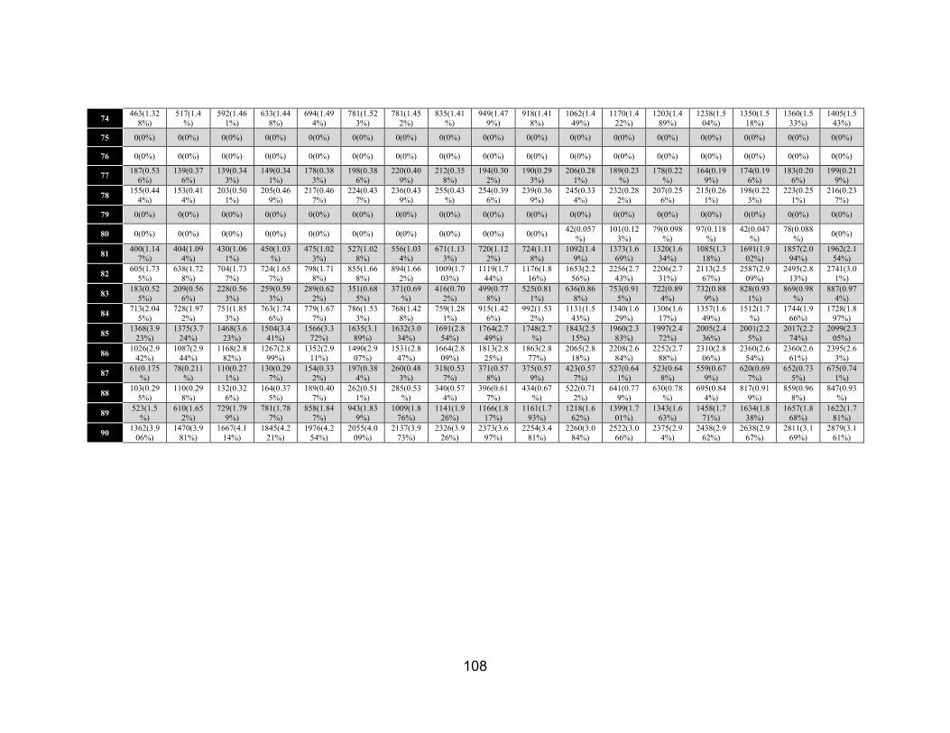
108
74 463(1.32
8%)
517(1.4
%)
592(1.46
1%)
633(1.44
8%)
694(1.49
4%)
781(1.52
3%)
781(1.45
2%)
835(1.41
%)
949(1.47
9%)
918(1.41
8%)
1062(1.4
49%)
1170(1.4
22%)
1203(1.4
89%)
1238(1.5
04%)
1350(1.5
18%)
1360(1.5
33%)
1405(1.5
43%)
75 0(0%) 0(0%) 0(0%) 0(0%) 0(0%) 0(0%) 0(0%) 0(0%) 0(0%) 0(0%) 0(0%) 0(0%) 0(0%) 0(0%) 0(0%) 0(0%) 0(0%)
76 0(0%) 0(0%) 0(0%) 0(0%) 0(0%) 0(0%) 0(0%) 0(0%) 0(0%) 0(0%) 0(0%) 0(0%) 0(0%) 0(0%) 0(0%) 0(0%) 0(0%)
77 187(0.53
6%)
139(0.37
6%)
139(0.34
3%)
149(0.34
1%)
178(0.38
3%)
198(0.38
6%)
220(0.40
9%)
212(0.35
8%)
194(0.30
2%)
190(0.29
3%)
206(0.28
1%)
189(0.23
%)
178(0.22
%)
164(0.19
9%)
174(0.19
6%)
183(0.20
6%)
199(0.21
9%)
78 155(0.44
4%)
153(0.41
4%)
203(0.50
1%)
205(0.46
9%)
217(0.46
7%)
224(0.43
7%)
236(0.43
9%)
255(0.43
%)
254(0.39
6%)
239(0.36
9%)
245(0.33
4%)
232(0.28
2%)
207(0.25
6%)
215(0.26
1%)
198(0.22
3%)
223(0.25
1%)
216(0.23
7%)
79 0(0%) 0(0%) 0(0%) 0(0%) 0(0%) 0(0%) 0(0%) 0(0%) 0(0%) 0(0%) 0(0%) 0(0%) 0(0%) 0(0%) 0(0%) 0(0%) 0(0%)
80 0(0%) 0(0%) 0(0%) 0(0%) 0(0%) 0(0%) 0(0%) 0(0%) 0(0%) 0(0%) 42(0.057
%)
101(0.12
3%)
79(0.098
%)
97(0.118
%)
42(0.047
%)
78(0.088
%) 0(0%)
81 400(1.14
7%)
404(1.09
4%)
430(1.06
1%)
450(1.03
%)
475(1.02
3%)
527(1.02
8%)
556(1.03
4%)
671(1.13
3%)
720(1.12
2%)
724(1.11
8%)
1092(1.4
9%)
1373(1.6
69%)
1320(1.6
34%)
1085(1.3
18%)
1691(1.9
02%)
1857(2.0
94%)
1962(2.1
54%)
82 605(1.73
5%)
638(1.72
8%)
704(1.73
7%)
724(1.65
7%)
798(1.71
8%)
855(1.66
8%)
894(1.66
2%)
1009(1.7
03%)
1119(1.7
44%)
1176(1.8
16%)
1653(2.2
56%)
2256(2.7
43%)
2206(2.7
31%)
2113(2.5
67%)
2587(2.9
09%)
2495(2.8
13%)
2741(3.0
1%)
83 183(0.52
5%)
209(0.56
6%)
228(0.56
3%)
259(0.59
3%)
289(0.62
2%)
351(0.68
5%)
371(0.69
%)
416(0.70
2%)
499(0.77
8%)
525(0.81
1%)
636(0.86
8%)
753(0.91
5%)
722(0.89
4%)
732(0.88
9%)
828(0.93
1%)
869(0.98
%)
887(0.97
4%)
84 713(2.04
5%)
728(1.97
2%)
751(1.85
3%)
763(1.74
6%)
779(1.67
7%)
786(1.53
3%)
768(1.42
8%)
759(1.28
1%)
915(1.42
6%)
992(1.53
2%)
1131(1.5
43%)
1340(1.6
29%)
1306(1.6
17%)
1357(1.6
49%)
1512(1.7
%)
1744(1.9
66%)
1728(1.8
97%)
85 1368(3.9
23%)
1375(3.7
24%)
1468(3.6
23%)
1504(3.4
41%)
1566(3.3
72%)
1635(3.1
89%)
1632(3.0
34%)
1691(2.8
54%)
1764(2.7
49%)
1748(2.7
%)
1843(2.5
15%)
1960(2.3
83%)
1997(2.4
72%)
2005(2.4
36%)
2001(2.2
5%)
2017(2.2
74%)
2099(2.3
05%)
86 1026(2.9
42%)
1087(2.9
44%)
1168(2.8
82%)
1267(2.8
99%)
1352(2.9
11%)
1490(2.9
07%)
1531(2.8
47%)
1664(2.8
09%)
1813(2.8
25%)
1863(2.8
77%)
2065(2.8
18%)
2208(2.6
84%)
2252(2.7
88%)
2310(2.8
06%)
2360(2.6
54%)
2360(2.6
61%)
2395(2.6
3%)
87 61(0.175
%)
78(0.211
%)
110(0.27
1%)
130(0.29
7%)
154(0.33
2%)
197(0.38
4%)
260(0.48
3%)
318(0.53
7%)
371(0.57
8%)
375(0.57
9%)
423(0.57
7%)
527(0.64
1%)
523(0.64
8%)
559(0.67
9%)
620(0.69
7%)
652(0.73
5%)
675(0.74
1%)
88 103(0.29
5%)
110(0.29
8%)
132(0.32
6%)
164(0.37
5%)
189(0.40
7%)
262(0.51
1%)
285(0.53
%)
340(0.57
4%)
396(0.61
7%)
434(0.67
%)
522(0.71
2%)
641(0.77
9%)
630(0.78
%)
695(0.84
4%)
817(0.91
9%)
859(0.96
8%)
847(0.93
%)
89 523(1.5
%)
610(1.65
2%)
729(1.79
9%)
781(1.78
7%)
858(1.84
7%)
943(1.83
9%)
1009(1.8
76%)
1141(1.9
26%)
1166(1.8
17%)
1161(1.7
93%)
1218(1.6
62%)
1399(1.7
01%)
1343(1.6
63%)
1458(1.7
71%)
1634(1.8
38%)
1657(1.8
68%)
1622(1.7
81%)
90 1362(3.9
06%)
1470(3.9
81%)
1667(4.1
14%)
1845(4.2
21%)
1976(4.2
54%)
2055(4.0
09%)
2137(3.9
73%)
2326(3.9
26%)
2373(3.6
97%)
2254(3.4
81%)
2260(3.0
84%)
2522(3.0
66%)
2375(2.9
4%)
2438(2.9
62%)
2638(2.9
67%)
2811(3.1
69%)
2879(3.1
61%)

109
Table 6.6. Longitudinal Probabilistic Distribution of Points per ROIs using Symmetric ALBERT Parcellation Map with 50 ROIs given
as: Number of points per ROI (Percentage on surface %) Week
/ROI# 28 29 30 31 32 33 34 35 36 37 38 39 40 41 42 43 44
1 & 2 159(0.4
52%)
176(0.4
7%)
189(0.46
2%)
150(0.34
2%)
164(0.35
2%)
187(0.36
7%)
189(0.35
5%)
173(0.30
4%)
186(0.30
9%)
199(0.33
%)
216(0.31
3%)
281(0.35
8%)
308(0.40
1%)
379(0.48
5%)
425(0.49
3%)
429(0.50
2%)
485(0.54
8%)
3 & 4 0(0%) 0(0%) 0(0%) 74(0.169
%)
132(0.28
4%)
167(0.32
8%)
176(0.33
1%)
206(0.36
1%)
253(0.42
%)
245(0.40
7%)
268(0.38
8%)
289(0.36
8%)
336(0.43
7%)
325(0.41
5%)
309(0.35
9%)
317(0.37
1%)
278(0.31
4%)
5 & 6 452(1.2
85%)
523(1.3
96%)
591(1.44
5%)
701(1.59
9%)
769(1.65
3%)
900(1.76
8%)
967(1.81
7%)
1197(2.1
%)
1342(2.2
28%)
1367(2.2
69%)
1621(2.3
47%)
1879(2.3
92%)
1851(2.4
09%)
1927(2.4
64%)
2035(2.3
61%)
2091(2.4
46%)
2335(2.6
37%)
7 & 8 486(1.3
82%)
494(1.3
19%)
565(1.38
1%)
615(1.40
3%)
701(1.50
7%)
771(1.51
5%)
901(1.69
3%)
993(1.74
2%)
1148(1.9
06%)
1149(1.9
07%)
1249(1.8
08%)
1441(1.8
35%)
1398(1.8
19%)
1476(1.8
87%)
2384(2.7
66%)
2568(3.0
04%)
2565(2.8
97%)
9 & 10 1993(5.
666%)
2055(5.
485%)
2083(5.0
93%)
2119(4.8
33%)
2131(4.5
8%)
2077(4.0
81%)
2063(3.8
77%)
1994(3.4
99%)
1945(3.2
29%)
1903(3.1
58%)
1721(2.4
92%)
1599(2.0
36%)
1555(2.0
23%)
1509(1.9
29%)
1400(1.6
24%)
1330(1.5
56%)
1321(1.4
92%)
11 &
12
650(1.8
48%)
660(1.7
62%)
736(1.8
%)
822(1.87
5%)
834(1.79
3%)
881(1.73
1%)
928(1.74
4%)
1100(1.9
3%)
1078(1.7
9%)
1093(1.8
14%)
1887(2.7
32%)
2688(3.4
22%)
2804(3.6
49%)
1927(2.4
64%)
2808(3.2
58%)
2665(3.1
18%)
2835(3.2
02%)
13 &
14
1517(4.
313%)
1593(4.
252%)
1800(4.4
01%)
1901(4.3
35%)
2020(4.3
42%)
2262(4.4
44%)
2358(4.4
32%)
2601(4.5
64%)
2683(4.4
55%)
2666(4.4
25%)
2785(4.0
32%)
3127(3.9
81%)
3069(3.9
94%)
3275(4.1
87%)
3616(4.1
95%)
3668(4.2
91%)
3667(4.1
42%)
15 &
16
671(1.9
08%)
758(2.0
23%)
794(1.94
1%)
873(1.99
1%)
931(2.00
1%)
1027(2.0
18%)
1073(2.0
17%)
1089(1.9
11%)
1122(1.8
63%)
1116(1.8
52%)
1177(1.7
04%)
1256(1.5
99%)
1251(1.6
28%)
1297(1.6
58%)
1323(1.5
35%)
1351(1.5
81%)
1336(1.5
09%)
17 &
18 0(0%) 0(0%) 0(0%) 0(0%) 0(0%) 0(0%) 0(0%) 0(0%) 0(0%) 0(0%) 0(0%) 0(0%) 0(0%) 0(0%) 0(0%) 0(0%) 0(0%)
19 &
20
559(1.5
89%)
524(1.3
99%)
528(1.29
1%)
498(1.13
6%)
501(1.07
7%)
473(0.92
9%)
471(0.88
5%)
497(0.87
2%)
583(0.96
8%)
700(1.16
2%)
961(1.39
1%)
1034(1.3
16%)
1026(1.3
35%)
899(1.14
9%)
883(1.02
5%)
908(1.06
2%)
892(1.00
8%)
21 &
22
4826(13
.721%)
5204(13
.891%)
5846(14.
293%)
6586(15.
02%)
6920(14.
873%)
8076(15.
868%)
8783(16.
508%)
9352(16.
41%)
9647(16.
017%)
9631(15.
985%)
10957(1
5.864%)
12606(1
6.049%)
11718(1
5.248%)
12355(1
5.795%)
12827(1
4.883%)
12207(1
4.282%)
12586(1
4.216%)
23 &
24
602(1.7
12%)
606(1.6
18%)
606(1.48
2%)
632(1.44
1%)
630(1.35
4%)
630(1.23
8%)
630(1.18
4%)
634(1.11
2%)
768(1.27
5%)
778(1.29
1%)
876(1.26
8%)
832(1.05
9%)
761(0.99
%)
744(0.95
1%)
798(0.92
6%)
851(0.99
6%)
857(0.96
8%)
25 &
26
817(2.3
23%)
876(2.3
38%)
912(2.23
%)
925(2.11
%)
937(2.01
4%)
1016(1.9
96%)
1033(1.9
42%)
1099(1.9
28%)
1082(1.7
96%)
1127(1.8
7%)
1152(1.6
68%)
1243(1.5
82%)
1212(1.5
77%)
1281(1.6
38%)
1266(1.4
69%)
1242(1.4
53%)
1218(1.3
76%)
27 &
28
2115(6.
013%)
2167(5.
784%)
2312(5.6
53%)
2364(5.3
91%)
2490(5.3
52%)
2694(5.2
93%)
2725(5.1
22%)
2851(5.0
03%)
3035(5.0
39%)
3028(5.0
26%)
3153(4.5
65%)
3436(4.3
74%)
3347(4.3
55%)
3580(4.5
77%)
3625(4.2
06%)
3658(4.2
8%)
3803(4.2
96%)
29 &
30
400(1.1
37%)
398(1.0
62%)
451(1.10
3%)
487(1.11
1%)
567(1.21
9%)
571(1.12
2%)
584(1.09
8%)
680(1.19
3%)
741(1.23
%)
724(1.20
2%)
851(1.23
2%)
905(1.15
2%)
955(1.24
3%)
947(1.21
1%)
956(1.10
9%)
955(1.11
7%)
1031(1.1
65%)
31 &
32 0(0%) 0(0%) 0(0%) 0(0%) 0(0%) 0(0%) 0(0%) 0(0%) 0(0%) 0(0%)
634(0.91
8%)
1014(1.2
91%)
1010(1.3
14%)
984(1.25
8%)
995(1.15
4%)
1073(1.2
55%)
1265(1.4
29%)
33 &
34
154(0.4
38%)
355(0.9
48%)
511(1.24
9%)
537(1.22
5%)
510(1.09
6%)
531(1.04
3%)
476(0.89
5%)
269(0.47
2%)
667(1.10
7%)
602(0.99
9%)
890(1.28
9%)
977(1.24
4%)
910(1.18
4%)
826(1.05
6%)
785(0.91
1%)
853(0.99
8%)
897(1.01
3%)
35 &
36
11561(3
2.87%)
12307(3
2.85%)
13451(3
2.888%)
14175(3
2.328%)
15129(3
2.517%)
16228(3
1.885%)
17076(3
2.094%)
18530(3
2.514%)
19210(3
1.894%)
19230(3
1.916%)
21440(3
1.041%)
24542(3
1.245%)
24043(3
1.286%)
24787(3
1.688%)
27437(3
1.834%)
27493(3
2.166%)
28510(3
2.203%)
37 &
38
6011(17
.09%)
6403(17
.091%)
6873(16.
804%)
7375(16.
819%)
7959(17.
107%)
8559(16.
817%)
8799(16.
538%)
9734(17.
08%)
10269(1
7.05%)
10475(1
7.385%)
12324(1
7.843%)
13737(1
7.489%)
13439(1
7.488%)
13757(1
7.587%)
14960(1
7.357%)
14892(1
7.423%)
15314(1
7.298%)
39 &
40
114(0.3
24%)
117(0.3
12%)
154(0.37
7%)
176(0.40
1%)
182(0.39
1%)
281(0.55
2%)
380(0.71
4%)
359(0.63
%)
457(0.75
9%)
386(0.64
1%)
535(0.77
5%)
725(0.92
3%)
899(1.17
%)
797(1.01
9%)
1130(1.3
11%)
1054(1.2
33%)
1099(1.2
41%)
41 &
42
855(2.4
31%)
897(2.3
94%)
933(2.28
1%)
1010(2.3
03%)
1049(2.2
55%)
1215(2.3
87%)
1260(2.3
68%)
1308(2.2
95%)
1403(2.3
29%)
1351(2.2
42%)
1449(2.0
98%)
1527(1.9
44%)
1508(1.9
62%)
1529(1.9
55%)
1624(1.8
84%)
1634(1.9
12%)
1643(1.8
56%)
43 &
44 0(0%) 0(0%) 0(0%) 0(0%) 0(0%) 0(0%) 0(0%) 0(0%) 0(0%) 0(0%) 0(0%) 0(0%) 0(0%) 0(0%) 0(0%) 0(0%) 0(0%)
45 &
46
710(2.0
19%)
808(2.1
57%)
954(2.33
3%)
1042(2.3
76%)
1093(2.3
49%)
1226(2.4
09%)
1271(2.3
89%)
1293(2.2
69%)
1451(2.4
09%)
1398(2.3
2%)
1613(2.3
35%)
1795(2.2
85%)
1837(2.3
9%)
1872(2.3
93%)
2118(2.4
57%)
2223(2.6
01%)
2336(2.6
39%)

110
47 &
48
155(0.4
41%)
150(0.4
%)
162(0.39
6%)
161(0.36
7%)
145(0.31
2%)
126(0.24
8%)
115(0.21
6%)
117(0.20
5%)
101(0.16
8%)
98(0.163
%)
82(0.119
%)
88(0.112
%)
97(0.126
%)
81(0.104
%)
71(0.082
%)
83(0.097
%)
77(0.087
%)
49 &
50
365(1.0
38%)
393(1.0
49%)
449(1.09
8%)
625(1.42
5%)
641(1.37
8%)
886(1.74
1%)
948(1.78
2%)
914(1.60
4%)
1059(1.7
58%)
986(1.63
6%)
1229(1.7
79%)
1527(1.9
44%)
1514(1.9
7%)
1668(2.1
32%)
2413(2.8
%)
1927(2.2
55%)
2182(2.4
65%)

111
Table 6.7. Longitudinal Probabilistic Distribution of Points per ROIs using Asymmetric ALBERT Parcellation Map with 50 ROIs given
as: Number of points per ROI (Percentage on surface %) Week
\ROI
#
28 29 30 31 32 33 34 35 36 37 38 39 40 41 42 43 44
1 0(0%) 0(0%) 0(0%) 0(0%) 0(0%) 0(0%) 0(0%) 0(0%) 0(0%) 0(0%) 0(0%) 0(0%) 41(0.051
%)
110(0.13
4%)
46(0.052
%) 0(0%) 0(0%)
2 0(0%) 0(0%) 0(0%) 0(0%) 0(0%) 0(0%) 0(0%) 0(0%) 0(0%) 0(0%) 0(0%) 67(0.081
%)
140(0.17
3%)
202(0.24
5%)
236(0.26
5%)
264(0.29
8%)
272(0.29
9%)
3 0(0%) 0(0%) 0(0%) 0(0%) 42(0.09
%)
124(0.2
42%)
130(0.2
42%)
133(0.22
5%)
157(0.24
5%)
164(0.25
3%)
173(0.23
6%)
176(0.21
4%)
179(0.22
2%)
142(0.17
3%)
195(0.21
9%)
235(0.26
5%)
230(0.25
3%)
4 102(0.29
2%)
112(0.3
03%)
130(0.3
21%)
130(0.2
97%)
144(0.3
1%)
186(0.3
63%)
230(0.4
28%)
305(0.51
5%)
318(0.49
5%)
256(0.39
5%)
260(0.35
5%)
256(0.31
1%)
130(0.16
1%)
130(0.15
8%)
191(0.21
5%)
195(0.22
%)
192(0.21
1%)
5 267(0.76
6%)
299(0.8
1%)
345(0.8
51%)
395(0.9
04%)
449(0.9
67%)
511(0.9
97%)
581(1.0
8%)
690(1.16
5%)
764(1.19
%)
779(1.20
3%)
900(1.22
8%)
1045(1.2
7%)
1017(1.2
59%)
1038(1.2
61%)
1049(1.1
8%)
1080(1.2
18%)
1197(1.3
14%)
6 177(0.50
8%)
193(0.5
23%)
212(0.5
23%)
252(0.5
77%)
310(0.6
67%)
365(0.7
12%)
393(0.7
31%)
474(0.8
%)
571(0.89
%)
596(0.92
%)
728(0.99
3%)
855(1.03
9%)
841(1.04
1%)
844(1.02
5%)
923(1.03
8%)
909(1.02
5%)
957(1.05
1%)
7 335(0.96
1%)
351(0.9
51%)
390(0.9
62%)
410(0.9
38%)
431(0.9
28%)
494(0.9
64%)
555(1.0
32%)
610(1.03
%)
676(1.05
3%)
699(1.08
%)
750(1.02
3%)
870(1.05
8%)
836(1.03
5%)
876(1.06
4%)
1239(1.3
93%)
1254(1.4
14%)
1237(1.3
58%)
8 231(0.66
2%)
256(0.6
93%)
293(0.7
23%)
331(0.7
57%)
356(0.7
66%)
419(0.8
17%)
521(0.9
69%)
529(0.89
3%)
618(0.96
3%)
583(0.9
%)
731(0.99
8%)
772(0.93
9%)
752(0.93
1%)
890(1.08
1%)
977(1.09
9%)
1173(1.3
23%)
1144(1.2
56%)
9 1045(2.9
97%)
1094(2.
963%)
1121(2.
766%)
1169(2.
675%)
1181(2.
543%)
1173(2.
288%)
1159(2.
155%)
1114(1.8
8%)
1009(1.5
72%)
989(1.52
7%)
912(1.24
5%)
848(1.03
1%)
840(1.04
%)
774(0.94
%)
817(0.91
9%)
811(0.91
4%)
818(0.89
8%)
10 802(2.3
%)
819(2.2
18%)
777(1.9
17%)
822(1.8
81%)
859(1.8
49%)
900(1.7
56%)
847(1.5
75%)
862(1.45
5%)
835(1.30
1%)
834(1.28
8%)
776(1.05
9%)
685(0.83
3%)
730(0.90
4%)
646(0.78
5%)
588(0.66
1%)
600(0.67
6%)
581(0.63
8%)
11 475(1.36
2%)
474(1.2
84%)
529(1.3
05%)
544(1.2
45%)
571(1.2
29%)
609(1.1
88%)
589(1.0
95%)
647(1.09
2%)
654(1.01
9%)
638(0.98
5%)
685(0.93
5%)
737(0.89
6%)
690(0.85
4%)
708(0.86
%)
703(0.79
1%)
739(0.83
3%)
757(0.83
1%)
12 516(1.48
%)
538(1.4
57%)
570(1.4
07%)
570(1.3
04%)
617(1.3
28%)
630(1.2
29%)
641(1.1
92%)
704(1.18
8%)
698(1.08
8%)
777(1.2
%)
1109(1.5
13%)
1463(1.7
79%)
1428(1.7
68%)
1401(1.7
02%)
1707(1.9
2%)
1522(1.7
16%)
1573(1.7
27%)
13 499(1.43
1%)
555(1.5
03%)
641(1.5
82%)
711(1.6
27%)
793(1.7
07%)
905(1.7
65%)
1000(1.
859%)
1120(1.8
91%)
1167(1.8
18%)
1132(1.7
48%)
1194(1.6
29%)
1365(1.6
59%)
1324(1.6
39%)
1397(1.6
97%)
1651(1.8
57%)
1715(1.9
34%)
1693(1.8
59%)
14 730(2.09
3%)
791(2.1
42%)
893(2.2
04%)
980(2.2
42%)
1048(2.
256%)
1158(2.
259%)
1204(2.
239%)
1373(2.3
18%)
1455(2.2
67%)
1455(2.2
47%)
1543(2.1
06%)
1714(2.0
84%)
1752(2.1
69%)
1826(2.2
18%)
1939(2.1
81%)
1989(2.2
43%)
1993(2.1
88%)
15 411(1.17
9%)
392(1.0
62%)
364(0.8
98%)
393(0.8
99%)
359(0.7
73%)
391(0.7
63%)
345(0.6
41%)
376(0.63
5%)
377(0.58
7%)
370(0.57
1%)
399(0.54
4%)
426(0.51
8%)
448(0.55
5%)
465(0.56
5%)
472(0.53
1%)
470(0.53
%)
462(0.50
7%)
16 796(2.28
3%)
832(2.2
53%)
887(2.1
89%)
869(1.9
88%)
877(1.8
88%)
870(1.6
97%)
883(1.6
42%)
869(1.46
7%)
840(1.30
9%)
756(1.16
8%)
685(0.93
5%)
731(0.88
9%)
647(0.80
1%)
647(0.78
6%)
661(0.74
3%)
652(0.73
5%)
660(0.72
5%)
17 0(0%) 0(0%) 0(0%) 0(0%) 0(0%) 0(0%) 0(0%) 0(0%) 0(0%) 0(0%) 0(0%) 0(0%) 0(0%) 0(0%) 0(0%) 0(0%) 0(0%)
18 0(0%) 0(0%) 0(0%) 0(0%) 0(0%) 0(0%) 0(0%) 0(0%) 0(0%) 0(0%) 0(0%) 0(0%) 0(0%) 0(0%) 0(0%) 0(0%) 0(0%)
19 0(0%) 0(0%) 0(0%) 0(0%) 0(0%) 0(0%) 0(0%) 0(0%) 0(0%) 0(0%) 0(0%) 0(0%) 0(0%) 0(0%) 0(0%) 0(0%) 0(0%)
20 113(0.32
4%)
88(0.23
8%)
215(0.5
31%)
228(0.5
22%)
264(0.5
68%)
287(0.5
6%)
302(0.5
62%)
319(0.53
8%)
380(0.59
2%)
426(0.65
8%)
473(0.64
5%)
657(0.79
9%)
651(0.80
6%)
642(0.78
%)
697(0.78
4%)
799(0.90
1%)
752(0.82
6%)
21 0(0%) 0(0%) 0(0%) 0(0%) 0(0%) 0(0%) 0(0%) 0(0%) 0(0%) 46(0.071
%)
179(0.24
4%)
170(0.20
7%)
173(0.21
4%)
336(0.40
8%)
313(0.35
2%)
326(0.36
8%)
353(0.38
8%)
22 2027(5.8
13%)
2172(5.
882%)
2552(6.
298%)
2762(6.
319%)
3085(6.
642%)
3599(7.
021%)
4017(7.
469%)
4541(7.6
65%)
4949(7.7
11%)
4834(7.4
65%)
5465(7.4
58%)
6327(7.6
92%)
5912(7.3
2%)
6131(7.4
49%)
6173(6.9
42%)
6170(6.9
57%)
6347(6.9
69%)
23 1791(5.1
36%)
1917(5.
191%)
2166(5.
345%)
2473(5.
658%)
2729(5.
875%)
3317(6.
47%)
3590(6.
675%)
4132(6.9
75%)
4392(6.8
43%)
4369(6.7
47%)
5011(6.8
38%)
5748(6.9
88%)
5288(6.5
47%)
5618(6.8
25%)
5723(6.4
36%)
5383(6.0
69%)
5573(6.1
19%)

112
24 311(0.89
2%)
352(0.9
53%)
394(0.9
72%)
423(0.9
68%)
376(0.8
1%)
411(0.8
02%)
418(0.7
77%)
432(0.72
9%)
441(0.68
7%)
374(0.57
8%)
379(0.51
7%)
353(0.42
9%)
381(0.47
2%)
416(0.50
5%)
399(0.44
9%)
425(0.47
9%)
451(0.49
5%)
25 451(1.29
3%)
488(1.3
22%)
455(1.1
23%)
506(1.1
58%)
378(0.8
14%)
377(0.7
35%)
372(0.6
92%)
387(0.65
3%)
412(0.64
2%)
409(0.63
2%)
438(0.59
8%)
414(0.50
3%)
406(0.50
3%)
408(0.49
6%)
427(0.48
%)
398(0.44
9%)
376(0.41
3%)
26 337(0.96
6%)
340(0.9
21%)
354(0.8
74%)
375(0.8
58%)
381(0.8
2%)
425(0.8
29%)
443(0.8
24%)
491(0.82
9%)
495(0.77
1%)
520(0.80
3%)
541(0.73
8%)
606(0.73
7%)
636(0.78
7%)
646(0.78
5%)
636(0.71
5%)
659(0.74
3%)
620(0.68
1%)
27 336(0.96
4%)
379(1.0
26%)
414(1.0
22%)
423(0.9
68%)
433(0.9
32%)
451(0.8
8%)
479(0.8
91%)
487(0.82
2%)
487(0.75
9%)
486(0.75
1%)
496(0.67
7%)
536(0.65
2%)
540(0.66
9%)
579(0.70
3%)
576(0.64
8%)
585(0.66
%)
599(0.65
8%)
28 1163(3.3
35%)
1201(3.
252%)
1317(3.
25%)
1376(3.
148%)
1451(3.
124%)
1534(2.
992%)
1535(2.
854%)
1650(2.7
85%)
1723(2.6
85%)
1722(2.6
59%)
1835(2.5
04%)
1920(2.3
34%)
1941(2.4
03%)
1965(2.3
87%)
1997(2.2
46%)
2048(2.3
09%)
2087(2.2
92%)
29 905(2.59
5%)
917(2.4
83%)
991(2.4
46%)
1021(2.
336%)
1092(2.
351%)
1184(2.
31%)
1218(2.
265%)
1280(2.1
61%)
1348(2.1
%)
1354(2.0
91%)
1383(1.8
87%)
1494(1.8
16%)
1472(1.8
22%)
1565(1.9
01%)
1590(1.7
88%)
1584(1.7
86%)
1603(1.7
6%)
30 129(0.37
%)
136(0.3
68%)
165(0.4
07%)
186(0.4
26%)
214(0.4
61%)
243(0.4
74%)
271(0.5
04%)
326(0.55
%)
336(0.52
4%)
361(0.55
8%)
514(0.70
1%)
618(0.75
1%)
595(0.73
7%)
681(0.82
7%)
747(0.84
%)
715(0.80
6%)
864(0.94
9%)
31 236(0.67
7%)
242(0.6
55%)
265(0.6
54%)
279(0.6
38%)
311(0.6
7%)
324(0.6
32%)
331(0.6
15%)
371(0.62
6%)
409(0.63
7%)
387(0.59
8%)
440(0.6
%)
468(0.56
9%)
490(0.60
7%)
473(0.57
5%)
465(0.52
3%)
454(0.51
2%)
538(0.59
1%)
32 0(0%) 24(0.06
5%)
222(0.5
48%)
136(0.3
11%)
143(0.3
08%)
65(0.12
7%)
143(0.2
66%)
94(0.159
%)
576(0.89
7%)
478(0.73
8%)
611(0.83
4%)
695(0.84
5%)
680(0.84
2%)
690(0.83
8%)
575(0.64
7%)
570(0.64
3%)
567(0.62
3%)
33 0(0%) 0(0%) 0(0%) 0(0%) 0(0%) 0(0%) 0(0%) 0(0%) 250(0.39
%)
199(0.30
7%)
288(0.39
3%)
331(0.40
2%)
358(0.44
3%)
335(0.40
7%)
450(0.50
6%)
483(0.54
5%)
549(0.60
3%)
34 0(0%) 0(0%) 0(0%) 0(0%) 0(0%) 0(0%) 0(0%) 158(0.26
7%)
489(0.76
2%)
565(0.87
3%)
696(0.95
%)
749(0.91
1%)
774(0.95
8%)
735(0.89
3%)
708(0.79
6%)
734(0.82
8%)
770(0.84
6%)
35 0(0%) 0(0%) 0(0%) 0(0%) 0(0%) 0(0%) 0(0%) 0(0%) 116(0.18
1%)
89(0.137
%)
96(0.131
%)
99(0.12
%)
110(0.13
6%)
139(0.16
9%)
141(0.15
9%)
148(0.16
7%)
147(0.16
1%)
36 6096(17.
481%)
6371(17
.253%)
6849(16
.902%)
7308(16
.721%)
7698(16
.573%)
8564(16
.706%)
9066(16
.856%)
10182(1
7.188%)
10807(1
6.839%)
11130(1
7.189%)
12296(1
6.779%)
13773(1
6.744%)
13500(1
6.714%)
13936(1
6.931%)
14869(1
6.721%)
15067(1
6.988%)
15403(1
6.913%)
37 6183(17.
731%)
6552(17
.744%)
7118(17
.566%)
7558(17
.293%)
8117(17
.475%)
8907(17
.375%)
9228(17
.158%)
10442(1
7.627%)
10924(1
7.021%)
11329(1
7.496%)
12785(1
7.447%)
14340(1
7.434%)
14185(1
7.562%)
13872(1
6.853%)
15371(1
7.286%)
15245(1
7.188%)
15604(1
7.134%)
38 2970(8.5
17%)
3134(8.
487%)
3377(8.
334%)
3806(8.
708%)
4051(8.
722%)
4295(8.
378%)
4409(8.
198%)
4705(7.9
42%)
5070(7.9
%)
5175(7.9
92%)
5812(7.9
31%)
6717(8.1
66%)
6666(8.2
53%)
6866(8.3
42%)
7388(8.3
08%)
7359(8.2
97%)
7471(8.2
04%)
39 3020(8.6
6%)
3176(8.
601%)
3464(8.
548%)
3807(8.
71%)
4097(8.
821%)
4509(8.
796%)
4759(8.
848%)
5152(8.6
97%)
5578(8.6
91%)
5773(8.9
16%)
7169(9.7
83%)
7924(9.6
34%)
7738(9.5
8%)
7423(9.0
18%)
8641(9.7
17%)
8640(9.7
41%)
8966(9.8
45%)
40 151(0.43
3%)
152(0.4
12%)
153(0.3
78%)
196(0.4
48%)
201(0.4
33%)
248(0.4
84%)
288(0.5
35%)
268(0.45
2%)
396(0.61
7%)
335(0.51
7%)
393(0.53
6%)
462(0.56
2%)
528(0.65
4%)
539(0.65
5%)
666(0.74
9%)
595(0.67
1%)
665(0.73
%)
41 178(0.51
%)
219(0.5
93%)
226(0.5
58%)
322(0.7
37%)
339(0.7
3%)
394(0.7
69%)
430(0.7
99%)
364(0.61
4%)
394(0.61
4%)
295(0.45
6%)
390(0.53
2%)
496(0.60
3%)
572(0.70
8%)
543(0.66
%)
729(0.82
%)
698(0.78
7%)
739(0.81
1%)
42 443(1.27
%)
488(1.3
22%)
628(1.5
5%)
692(1.5
83%)
739(1.5
91%)
811(1.5
82%)
789(1.4
67%)
845(1.42
6%)
953(1.48
5%)
808(1.24
8%)
598(0.81
6%)
591(0.71
9%)
579(0.71
7%)
611(0.74
2%)
592(0.66
6%)
600(0.67
6%)
585(0.64
2%)
43 519(1.48
8%)
569(1.5
41%)
663(1.6
36%)
792(1.8
12%)
830(1.7
87%)
989(1.9
29%)
930(1.7
29%)
873(1.47
4%)
1002(1.5
61%)
982(1.51
7%)
1115(1.5
22%)
1124(1.3
66%)
1043(1.2
91%)
1035(1.2
57%)
1053(1.1
84%)
1044(1.1
77%)
1032(1.1
33%)
44 0(0%) 0(0%) 0(0%) 0(0%) 0(0%) 0(0%) 0(0%) 0(0%) 0(0%) 0(0%) 0(0%) 0(0%) 0(0%) 0(0%) 0(0%) 0(0%) 0(0%)
45 0(0%) 0(0%) 0(0%) 0(0%) 0(0%) 0(0%) 0(0%) 0(0%) 0(0%) 0(0%) 0(0%) 0(0%) 0(0%) 0(0%) 0(0%) 0(0%) 0(0%)
46 405(1.16
1%)
461(1.2
48%)
419(1.0
34%)
461(1.0
55%)
510(1.0
98%)
583(1.1
37%)
588(1.0
93%)
620(1.04
7%)
716(1.11
6%)
676(1.04
4%)
807(1.10
1%)
923(1.12
2%)
914(1.13
2%)
954(1.15
9%)
1075(1.2
09%)
1145(1.2
91%)
1185(1.3
01%)
47 348(0.99
8%)
406(1.0
99%)
489(1.2
07%)
533(1.2
2%)
534(1.1
5%)
560(1.0
92%)
572(1.0
64%)
598(1.00
9%)
694(1.08
1%)
667(1.03
%)
745(1.01
7%)
811(0.98
6%)
832(1.03
%)
779(0.94
6%)
918(1.03
2%)
965(1.08
8%)
1011(1.1
1%)
48 0(0%) 0(0%) 0(0%) 0(0%) 0(0%) 0(0%) 0(0%) 0(0%) 0(0%) 0(0%) 0(0%) 0(0%) 0(0%) 0(0%) 0(0%) 0(0%) 0(0%)
49 0(0%) 0(0%) 0(0%) 0(0%) 0(0%) 0(0%) 0(0%) 140(0.23
6%)
194(0.30
2%)
228(0.35
2%)
318(0.43
4%)
505(0.61
4%)
548(0.67
8%)
749(0.91
%)
1000(1.1
25%)
783(0.88
3%)
873(0.95
9%)

113
50 374(1.07
2%)
436(1.1
81%)
474(1.1
7%)
467(1.0
69%)
438(0.9
43%)
452(0.8
82%)
528(0.9
82%)
577(0.97
4%)
510(0.79
5%)
707(1.09
2%)
1162(1.5
86%)
1393(1.6
94%)
1463(1.8
11%)
1548(1.8
81%)
1611(1.8
12%)
1464(1.6
51%)
1574(1.7
28%)

114
Table 6.8. Longitudinal Probabilistic Distribution of Points per ROIs using Symmetric JHU Parcellation Map with 122 ROIs given as:
Number of points per ROI (Percentage on surface %) Week\
ROI# 28 29 30 31 32 33 34 35 36 37 38 39 40 41 42 43 44
1 & 2 133(0.37
8%)
140(0.3
74%)
144(0.3
52%)
146(0.3
33%)
146(0.3
14%)
143(0.2
81%)
150(0.2
82%)
159(0.2
79%)
161(0.2
67%)
179(0.2
97%)
240(0.3
47%)
285(0.3
63%)
262(0.3
41%)
330(0.4
22%)
438(0.5
08%)
363(0.42
5%)
408(0.46
1%)
3 & 4 0(0%) 0(0%) 51(0.12
5%)
81(0.18
5%)
80(0.17
2%)
135(0.2
65%)
156(0.2
93%)
147(0.2
58%)
214(0.3
55%)
180(0.2
99%)
258(0.3
74%)
335(0.4
26%)
323(0.4
2%)
329(0.4
21%)
395(0.4
58%)
421(0.49
3%)
517(0.58
4%)
5 & 6 221(0.62
8%)
226(0.6
03%)
258(0.6
31%)
273(0.6
23%)
302(0.6
49%)
319(0.6
27%)
318(0.5
98%)
335(0.5
88%)
343(0.5
69%)
345(0.5
73%)
371(0.5
37%)
397(0.5
05%)
404(0.5
26%)
403(0.5
15%)
414(0.4
8%)
471(0.55
1%)
474(0.53
5%)
7 & 8 0(0%) 0(0%) 0(0%) 0(0%) 0(0%) 0(0%) 0(0%) 0(0%) 0(0%) 0(0%) 0(0%) 0(0%) 0(0%) 0(0%) 0(0%) 0(0%) 0(0%)
9 & 10 0(0%) 0(0%) 0(0%) 0(0%) 0(0%) 0(0%) 0(0%) 0(0%) 0(0%) 0(0%) 0(0%) 0(0%) 0(0%) 0(0%) 0(0%) 0(0%) 0(0%)
11 &
12 0(0%) 0(0%) 0(0%) 0(0%) 0(0%) 0(0%) 0(0%) 0(0%) 0(0%) 0(0%) 0(0%) 0(0%) 0(0%) 0(0%) 0(0%) 0(0%) 0(0%)
13 &
14 0(0%) 0(0%) 0(0%) 0(0%) 0(0%) 0(0%) 0(0%) 0(0%) 0(0%) 0(0%) 0(0%) 0(0%) 0(0%) 0(0%) 0(0%) 0(0%) 0(0%)
15 &
16 0(0%) 0(0%) 0(0%) 0(0%) 0(0%) 0(0%) 0(0%) 0(0%) 0(0%) 0(0%) 0(0%) 0(0%) 0(0%) 0(0%) 0(0%) 0(0%) 0(0%)
17 &
18
763(2.16
9%)
818(2.1
83%)
769(1.8
8%)
789(1.7
99%)
799(1.7
17%)
802(1.5
76%)
719(1.3
51%)
691(1.2
12%)
640(1.0
63%)
630(1.0
46%)
610(0.8
83%)
577(0.7
35%)
541(0.7
04%)
565(0.7
22%)
531(0.6
16%)
507(0.59
3%)
510(0.57
6%)
19 &
20
557(1.58
4%)
572(1.5
27%)
570(1.3
94%)
653(1.4
89%)
667(1.4
34%)
724(1.4
23%)
793(1.4
9%)
831(1.4
58%)
890(1.4
78%)
861(1.4
29%)
837(1.2
12%)
821(1.0
45%)
836(1.0
88%)
815(1.0
42%)
787(0.9
13%)
741(0.86
7%)
765(0.86
4%)
21 &
22 0(0%) 0(0%) 0(0%) 0(0%) 0(0%) 0(0%) 0(0%) 0(0%) 0(0%) 0(0%) 0(0%) 0(0%) 0(0%) 0(0%) 0(0%) 0(0%) 0(0%)
23 &
24 0(0%) 0(0%) 0(0%) 0(0%) 0(0%) 0(0%) 0(0%) 0(0%) 0(0%) 0(0%) 0(0%)
72(0.09
2%)
49(0.06
4%)
107(0.1
37%)
216(0.2
51%)
143(0.16
7%)
190(0.21
5%)
25 &
26 0(0%) 0(0%) 0(0%) 0(0%) 0(0%) 0(0%) 0(0%) 0(0%) 0(0%) 0(0%) 0(0%) 0(0%) 0(0%) 0(0%) 0(0%) 0(0%) 0(0%)
27 &
28 0(0%) 0(0%) 0(0%) 0(0%) 0(0%) 0(0%) 0(0%) 0(0%) 0(0%) 0(0%) 0(0%) 0(0%) 0(0%) 0(0%) 0(0%) 0(0%) 0(0%)
29 &
30 0(0%) 0(0%) 0(0%) 0(0%) 0(0%) 0(0%) 0(0%) 0(0%) 0(0%) 0(0%) 0(0%) 0(0%) 0(0%) 0(0%) 0(0%) 0(0%) 0(0%)
31 &
32 0(0%) 0(0%) 0(0%) 0(0%) 0(0%) 0(0%) 0(0%) 0(0%) 0(0%) 0(0%) 0(0%) 0(0%) 0(0%) 0(0%) 0(0%) 0(0%) 0(0%)
33 &
34
565(1.60
6%)
630(1.6
82%)
684(1.6
72%)
756(1.7
24%)
770(1.6
55%)
921(1.8
1%)
951(1.7
87%)
1024(1.
797%)
1078(1.
79%)
1080(1.
792%)
1247(1.
805%)
1318(1.
678%)
1312(1.
707%)
1306(1.
67%)
1392(1.
615%)
1391(1.6
27%)
1383(1.5
62%)
35 &
36
393(1.11
7%)
454(1.2
12%)
507(1.2
4%)
563(1.2
84%)
603(1.2
96%)
697(1.3
69%)
739(1.3
89%)
799(1.4
02%)
940(1.5
61%)
918(1.5
24%)
1076(1.
558%)
1093(1.
392%)
1122(1.
46%)
1153(1.
474%)
1297(1.
505%)
1360(1.5
91%)
1380(1.5
59%)
37 &
38 0(0%) 0(0%) 0(0%) 0(0%) 0(0%) 0(0%) 0(0%) 0(0%) 0(0%) 0(0%) 0(0%) 0(0%) 0(0%) 0(0%) 0(0%) 0(0%) 0(0%)
39 &
40
329(0.93
5%)
354(0.9
45%)
371(0.9
07%)
423(0.9
65%)
412(0.8
86%)
534(1.0
49%)
650(1.2
22%)
643(1.1
28%)
781(1.2
97%)
690(1.1
45%)
945(1.3
68%)
1349(1.
717%)
1532(1.
994%)
1380(1.
764%)
1980(2.
297%)
1785(2.0
88%)
1916(2.1
64%)
41 &
42 0(0%) 0(0%) 0(0%) 0(0%) 0(0%) 0(0%) 0(0%) 0(0%) 0(0%) 0(0%) 0(0%) 0(0%) 0(0%) 0(0%) 0(0%) 0(0%) 0(0%)
43 &
44 0(0%) 0(0%) 0(0%) 0(0%) 0(0%) 0(0%) 0(0%) 0(0%) 0(0%) 0(0%) 0(0%) 0(0%) 0(0%) 0(0%) 0(0%) 0(0%) 0(0%)
45 &
46
129(0.36
7%)
139(0.3
71%)
164(0.4
01%)
176(0.4
01%)
184(0.3
95%)
155(0.3
05%)
150(0.2
82%)
138(0.2
42%)
139(0.2
31%)
144(0.2
39%)
128(0.1
85%)
124(0.1
58%)
133(0.1
73%)
125(0.1
6%)
118(0.1
37%)
115(0.13
5%)
123(0.13
9%)

115
47 &
48 0(0%) 0(0%) 0(0%) 0(0%) 0(0%) 0(0%) 0(0%) 0(0%) 0(0%) 0(0%) 0(0%) 0(0%) 0(0%) 0(0%) 0(0%) 0(0%) 0(0%)
49 &
50 0(0%) 0(0%) 0(0%) 0(0%) 0(0%) 0(0%) 0(0%) 0(0%) 0(0%) 0(0%) 0(0%) 0(0%) 0(0%) 0(0%) 0(0%) 0(0%) 0(0%)
51 &
52 0(0%) 0(0%) 0(0%) 0(0%) 0(0%) 0(0%) 0(0%) 0(0%) 0(0%) 0(0%) 0(0%) 0(0%) 0(0%) 0(0%) 0(0%) 0(0%) 0(0%)
53 &
54 0(0%) 0(0%) 0(0%) 0(0%) 0(0%) 0(0%) 0(0%) 0(0%) 0(0%) 0(0%) 0(0%) 0(0%) 0(0%) 0(0%) 0(0%) 0(0%) 0(0%)
55 &
56 0(0%) 0(0%) 0(0%) 0(0%) 0(0%) 0(0%) 0(0%) 0(0%) 0(0%) 0(0%) 0(0%) 0(0%) 0(0%) 0(0%) 0(0%) 0(0%) 0(0%)
57 &
58 0(0%) 0(0%) 0(0%) 0(0%) 0(0%) 0(0%) 0(0%) 0(0%) 0(0%) 0(0%) 0(0%) 0(0%) 0(0%) 0(0%) 0(0%) 0(0%) 0(0%)
59 &
60 0(0%) 0(0%) 0(0%) 0(0%) 0(0%) 0(0%) 0(0%) 0(0%) 0(0%) 0(0%) 0(0%) 0(0%) 0(0%) 0(0%) 0(0%) 0(0%) 0(0%)
61 &
62 0(0%) 0(0%) 0(0%) 0(0%) 0(0%) 0(0%) 0(0%) 0(0%) 0(0%) 0(0%) 0(0%) 0(0%) 0(0%) 0(0%) 0(0%) 0(0%) 0(0%)
63 &
64 0(0%) 0(0%) 0(0%) 0(0%) 0(0%) 0(0%) 0(0%) 0(0%) 0(0%) 0(0%) 0(0%) 0(0%) 0(0%) 0(0%) 0(0%) 0(0%) 0(0%)
65 &
66 0(0%) 0(0%) 0(0%) 0(0%) 0(0%) 0(0%) 0(0%) 0(0%) 0(0%) 0(0%) 0(0%) 0(0%) 0(0%) 0(0%) 0(0%) 0(0%) 0(0%)
67 &
68
3022(8.5
92%)
3194(8.
526%)
3437(8.
403%)
3601(8.
212%)
3945(8.
479%)
4229(8.
309%)
4471(8.
403%)
4886(8.
573%)
5070(8.
418%)
5177(8.
592%)
5872(8.
502%)
7142(9.
093%)
6808(8.
859%)
7417(9.
482%)
8506(9.
869%)
8620(10.
085%)
8905(10.
059%)
69 &
70
2870(8.1
6%)
3066(8.
184%)
3451(8.
438%)
3771(8.
6%)
3999(8.
595%)
4376(8.
598%)
4682(8.
8%)
5138(9.
016%)
5340(8.
866%)
5300(8.
796%)
5739(8.
309%)
6295(8.
014%)
6279(8.
171%)
6374(8.
149%)
6757(7.
84%)
6649(7.7
79%)
6853(7.7
41%)
71 &
72
1484(4.2
19%)
1571(4.
193%)
1783(4.
359%)
1834(4.
183%)
1964(4.
221%)
2086(4.
099%)
2233(4.
197%)
2384(4.
183%)
2481(4.
119%)
2406(3.
993%)
2605(3.
772%)
2920(3.
717%)
2929(3.
811%)
2958(3.
782%)
3174(3.
683%)
3440(4.0
25%)
3456(3.9
04%)
73 &
74
602(1.71
2%)
659(1.7
59%)
701(1.7
14%)
755(1.7
22%)
800(1.7
19%)
840(1.6
5%)
912(1.7
14%)
968(1.6
99%)
1014(1.
684%)
975(1.6
18%)
1045(1.
513%)
1185(1.
509%)
1167(1.
519%)
1192(1.
524%)
1359(1.
577%)
1295(1.5
15%)
1343(1.5
17%)
75 &
76
1058(3.0
08%)
1153(3.
078%)
1218(2.
978%)
1290(2.
942%)
1338(2.
876%)
1412(2.
774%)
1431(2.
69%)
1591(2.
792%)
1635(2.
715%)
1612(2.
675%)
1746(2.
528%)
1928(2.
455%)
1823(2.
372%)
1721(2.
2%)
1932(2.
242%)
1927(2.2
55%)
1980(2.2
36%)
77 &
78
956(2.71
8%)
1040(2.
776%)
1143(2.
795%)
1158(2.
641%)
1207(2.
594%)
1261(2.
478%)
1248(2.
346%)
1321(2.
318%)
1291(2.
143%)
1264(2.
098%)
1281(1.
855%)
1430(1.
821%)
1364(1.
775%)
1454(1.
859%)
1555(1.
804%)
1596(1.8
67%)
1752(1.9
79%)
79 &
80
1401(3.9
83%)
1494(3.
988%)
1552(3.
795%)
1612(3.
676%)
1750(3.
761%)
1915(3.
763%)
1980(3.
721%)
2143(3.
76%)
2213(3.
674%)
2318(3.
847%)
2802(4.
057%)
3021(3.
846%)
2953(3.
843%)
2936(3.
753%)
3210(3.
724%)
3070(3.5
92%)
3136(3.5
42%)
81 &
82
1319(3.7
5%)
1373(3.
665%)
1529(3.
738%)
1679(3.
829%)
1813(3.
897%)
1974(3.
878%)
2103(3.
953%)
2295(4.
027%)
2371(3.
937%)
2411(4.
002%)
2643(3.
827%)
2639(3.
36%)
2604(3.
389%)
2551(3.
261%)
2614(3.
033%)
2642(3.0
91%)
2688(3.0
36%)
83 &
84
552(1.56
9%)
590(1.5
75%)
662(1.6
19%)
792(1.8
06%)
902(1.9
39%)
1039(2.
041%)
1126(2.
116%)
1364(2.
393%)
1579(2.
622%)
1726(2.
865%)
2108(3.
052%)
2566(3.
267%)
2376(3.
092%)
2564(3.
278%)
2908(3.
374%)
2733(3.1
98%)
2822(3.1
88%)
85 &
86
989(2.81
2%)
1029(2.
747%)
1049(2.
565%)
1085(2.
474%)
1185(2.
547%)
1243(2.
442%)
1196(2.
248%)
1298(2.
278%)
1284(2.
132%)
1346(2.
234%)
1656(2.
398%)
1976(2.
516%)
2020(2.
629%)
1981(2.
533%)
2132(2.
474%)
2080(2.4
34%)
2173(2.4
54%)
87 &
88
582(1.65
5%)
828(2.2
1%)
1017(2.
487%)
1096(2.
5%)
1030(2.
214%)
1237(2.
43%)
1125(2.
114%)
877(1.5
39%)
1562(2.
593%)
1525(2.
531%)
2762(3.
999%)
3615(4.
602%)
3502(4.
557%)
3410(4.
359%)
3597(4.
173%)
3739(4.3
75%)
4240(4.7
89%)
89 &
90
451(1.28
2%)
487(1.3
%)
592(1.4
47%)
650(1.4
82%)
754(1.6
21%)
809(1.5
9%)
920(1.7
29%)
1113(1.
953%)
1250(2.
075%)
1256(2.
085%)
1408(2.
039%)
1678(2.
136%)
1806(2.
35%)
1919(2.
453%)
2217(2.
572%)
2382(2.7
87%)
2379(2.6
87%)
91 &
92
1617(4.5
97%)
1668(4.
452%)
1769(4.
325%)
1899(4.
331%)
2018(4.
337%)
2164(4.
252%)
2303(4.
328%)
2488(4.
366%)
2574(4.
274%)
2571(4.
267%)
2747(3.
977%)
2968(3.
779%)
2941(3.
827%)
3020(3.
861%)
3282(3.
808%)
3211(3.7
57%)
3315(3.7
44%)
93 &
94
1548(4.4
01%)
1623(4.
332%)
1782(4.
357%)
1953(4.
454%)
2017(4.
335%)
2199(4.
321%)
2240(4.
21%)
2552(4.
478%)
2592(4.
304%)
2639(4.
38%)
3921(5.
677%)
4974(6.
332%)
4956(6.
449%)
4056(5.
185%)
5944(6.
897%)
5945(6.9
55%)
6153(6.9
5%)
95 &
96
968(2.75
2%)
1031(2.
752%)
1221(2.
985%)
1316(3.
001%)
1506(3.
237%)
1674(3.
289%)
1846(3.
47%)
2100(3.
685%)
2511(4.
169%)
2580(4.
282%)
2916(4.
222%)
3440(4.
379%)
3573(4.
649%)
3680(4.
705%)
3999(4.
64%)
4057(4.7
47%)
4077(4.6
05%)

116
97 &
98
3515(9.9
94%)
3496(9.
332%)
3691(9.
024%)
3724(8.
493%)
3806(8.
18%)
4040(7.
938%)
4063(7.
636%)
4259(7.
473%)
4090(6.
791%)
3799(6.
305%)
3710(5.
371%)
3949(5.
027%)
3521(4.
582%)
3866(4.
942%)
4266(4.
95%)
4658(5.4
5%)
5102(5.7
63%)
99 &
100
975(2.77
2%)
1132(3.
022%)
1313(3.
21%)
1495(3.
41%)
1655(3.
557%)
1875(3.
684%)
2078(3.
906%)
2323(4.
076%)
2412(4.
005%)
2543(4.
221%)
2614(3.
785%)
2948(3.
753%)
2983(3.
882%)
3089(3.
949%)
3011(3.
494%)
2875(3.3
64%)
2729(3.0
83%)
101 &
102 0(0%) 0(0%) 0(0%) 0(0%) 0(0%) 0(0%) 0(0%) 0(0%) 0(0%) 0(0%) 0(0%) 0(0%) 0(0%) 0(0%) 0(0%) 0(0%) 0(0%)
103 &
104
565(1.60
6%)
597(1.5
94%)
583(1.4
25%)
605(1.3
8%)
636(1.3
67%)
600(1.1
79%)
603(1.1
33%)
535(0.9
39%)
586(0.9
73%)
607(1.0
07%)
652(0.9
44%)
583(0.7
42%)
577(0.7
51%)
601(0.7
68%)
449(0.5
21%)
420(0.49
1%)
396(0.44
7%)
105 &
106
45(0.128
%)
99(0.26
4%)
135(0.3
3%)
175(0.3
99%)
215(0.4
62%)
272(0.5
34%)
343(0.6
45%)
442(0.7
76%)
493(0.8
19%)
497(0.8
25%)
717(1.0
38%)
992(1.2
63%)
821(1.0
68%)
869(1.1
11%)
916(1.0
63%)
845(0.98
9%)
922(1.04
1%)
107 &
108
1431(4.0
69%)
1513(4.
039%)
1747(4.
271%)
1978(4.
511%)
2162(4.
647%)
2572(5.
053%)
2786(5.
236%)
3071(5.
389%)
3230(5.
363%)
3176(5.
271%)
3672(5.
316%)
4176(5.
316%)
3840(4.
997%)
4080(5.
216%)
4266(4.
95%)
4084(4.7
78%)
4380(4.9
47%)
109 &
110
593(1.68
6%)
687(1.8
34%)
815(1.9
93%)
946(2.1
57%)
1018(2.
188%)
1171(2.
301%)
1280(2.
406%)
1427(2.
504%)
1500(2.
49%)
1542(2.
559%)
1662(2.
406%)
1958(2.
493%)
1884(2.
452%)
2070(2.
646%)
2013(2.
336%)
1897(2.2
19%)
1947(2.1
99%)
111 &
112
927(2.63
6%)
931(2.4
85%)
989(2.4
18%)
1063(2.
424%)
1124(2.
416%)
1286(2.
527%)
1312(2.
466%)
1446(2.
537%)
1566(2.
6%)
1533(2.
544%)
1862(2.
696%)
2049(2.
609%)
2109(2.
744%)
2099(2.
683%)
2215(2.
57%)
2213(2.5
89%)
2207(2.4
93%)
113 &
114
2487(7.0
71%)
2644(7.
057%)
2844(6.
954%)
3001(6.
844%)
3101(6.
665%)
3345(6.
572%)
3625(6.
813%)
3619(6.
35%)
3674(6.
1%)
3657(6.
07%)
4023(5.
825%)
4325(5.
506%)
4088(5.
32%)
4215(5.
389%)
4379(5.
081%)
4112(4.8
11%)
4029(4.5
51%)
115 &
116 0(0%) 0(0%) 0(0%) 0(0%) 0(0%)
46(0.09
%)
50(0.09
4%)
70(0.12
3%)
168(0.2
79%)
173(0.2
87%)
214(0.3
1%)
221(0.2
81%)
230(0.2
99%)
244(0.3
12%)
231(0.2
68%)
226(0.26
4%)
214(0.24
2%)
117 &
118
645(1.83
4%)
677(1.8
07%)
743(1.8
17%)
780(1.7
79%)
831(1.7
86%)
918(1.8
04%)
905(1.7
01%)
912(1.6
%)
896(1.4
88%)
877(1.4
56%)
901(1.3
04%)
952(1.2
12%)
951(1.2
38%)
1019(1.
303%)
1077(1.
25%)
1064(1.2
45%)
1120(1.2
65%)
119 &
120 0(0%) 0(0%) 0(0%) 0(0%) 0(0%) 0(0%) 0(0%) 0(0%) 0(0%) 0(0%) 0(0%) 0(0%) 0(0%) 0(0%) 0(0%) 0(0%) 0(0%)
121 &
122
559(1.58
9%)
560(1.4
95%)
536(1.3
11%)
539(1.2
29%)
522(1.1
22%)
483(0.9
49%)
477(0.8
97%)
421(0.7
39%)
437(0.7
26%)
508(0.8
43%)
596(0.8
63%)
602(0.7
66%)
593(0.7
72%)
493(0.6
3%)
511(0.5
93%)
496(0.58
%)
509(0.57
5%)

117
Table 6.9. Longitudinal Probabilistic Distribution of Points per ROIs using Asymmetric JHU Parcellation Map with 122 ROIs given
as: Number of points per ROI (Percentage on surface %) Week\
ROI# 28 29 30 31 32 33 34 35 36 37 38 39 40 41 42 43 44
1 363(1.04
1%)
432(1.17
%)
466(1.15
%)
583(1.33
4%)
544(1.17
1%)
594(1.15
9%)
431(0.80
1%)
365(0.61
6%)
333(0.51
9%)
333(0.51
4%)
652(0.89
%)
945(1.14
9%)
1050(1.3
%)
1203(1.4
62%)
1507(1.6
95%)
1403(1.5
82%)
1535(1.6
86%)
2 114(0.32
7%)
112(0.30
3%)
101(0.24
9%)
105(0.24
%)
103(0.22
2%)
102(0.19
9%)
95(0.177
%)
101(0.17
%)
96(0.15
%)
104(0.16
1%)
98(0.134
%)
98(0.119
%)
100(0.12
4%)
211(0.25
6%)
219(0.24
6%)
100(0.11
3%)
101(0.11
1%)
3 0(0%) 0(0%) 0(0%) 0(0%) 0(0%) 0(0%) 0(0%) 0(0%) 0(0%) 0(0%) 98(0.134
%)
125(0.15
2%)
131(0.16
2%)
134(0.16
3%)
144(0.16
2%)
144(0.16
2%)
154(0.16
9%)
4 0(0%) 0(0%) 0(0%) 0(0%) 0(0%) 0(0%) 0(0%) 0(0%) 0(0%) 0(0%) 94(0.128
%)
131(0.15
9%)
137(0.17
%)
196(0.23
8%)
218(0.24
5%)
235(0.26
5%)
267(0.29
3%)
5 0(0%) 0(0%) 0(0%) 0(0%) 0(0%) 46(0.09
%)
82(0.152
%)
86(0.145
%)
93(0.145
%)
92(0.142
%)
108(0.14
7%)
119(0.14
5%)
110(0.13
6%)
114(0.13
9%)
116(0.13
%)
115(0.13
%)
120(0.13
2%)
6 222(0.63
7%)
200(0.54
2%)
201(0.49
6%)
221(0.50
6%)
242(0.52
1%)
278(0.54
2%)
263(0.48
9%)
269(0.45
4%)
282(0.43
9%)
246(0.38
%)
244(0.33
3%)
268(0.32
6%)
274(0.33
9%)
268(0.32
6%)
306(0.34
4%)
307(0.34
6%)
317(0.34
8%)
7 0(0%) 0(0%) 0(0%) 0(0%) 0(0%) 0(0%) 0(0%) 0(0%) 0(0%) 0(0%) 0(0%) 0(0%) 0(0%) 0(0%) 0(0%) 0(0%) 0(0%)
8 0(0%) 0(0%) 0(0%) 0(0%) 0(0%) 0(0%) 0(0%) 0(0%) 0(0%) 0(0%) 0(0%) 0(0%) 0(0%) 0(0%) 0(0%) 0(0%) 0(0%)
9 0(0%) 0(0%) 0(0%) 0(0%) 0(0%) 0(0%) 0(0%) 0(0%) 0(0%) 0(0%) 0(0%) 0(0%) 0(0%) 0(0%) 0(0%) 0(0%) 0(0%)
10 0(0%) 0(0%) 0(0%) 0(0%) 0(0%) 0(0%) 0(0%) 0(0%) 0(0%) 0(0%) 0(0%) 0(0%) 0(0%) 0(0%) 0(0%) 0(0%) 0(0%)
11 0(0%) 0(0%) 0(0%) 0(0%) 0(0%) 0(0%) 0(0%) 0(0%) 0(0%) 0(0%) 0(0%) 0(0%) 0(0%) 0(0%) 0(0%) 0(0%) 0(0%)
12 0(0%) 0(0%) 0(0%) 0(0%) 0(0%) 0(0%) 0(0%) 0(0%) 0(0%) 0(0%) 0(0%) 0(0%) 0(0%) 0(0%) 0(0%) 0(0%) 0(0%)
13 0(0%) 0(0%) 0(0%) 0(0%) 0(0%) 0(0%) 0(0%) 0(0%) 0(0%) 0(0%) 0(0%) 0(0%) 0(0%) 0(0%) 0(0%) 0(0%) 0(0%)
14 0(0%) 0(0%) 0(0%) 0(0%) 0(0%) 0(0%) 0(0%) 0(0%) 0(0%) 0(0%) 0(0%) 0(0%) 0(0%) 0(0%) 0(0%) 0(0%) 0(0%)
15 0(0%) 0(0%) 0(0%) 0(0%) 0(0%) 0(0%) 0(0%) 0(0%) 0(0%) 0(0%) 0(0%) 0(0%) 0(0%) 0(0%) 0(0%) 0(0%) 0(0%)
16 0(0%) 0(0%) 0(0%) 0(0%) 0(0%) 0(0%) 0(0%) 0(0%) 0(0%) 0(0%) 0(0%) 0(0%) 0(0%) 0(0%) 0(0%) 0(0%) 0(0%)
17 275(0.78
9%)
262(0.71
%)
240(0.59
2%)
239(0.54
7%)
238(0.51
2%)
254(0.49
5%)
235(0.43
7%)
230(0.38
8%)
214(0.33
3%)
215(0.33
2%)
210(0.28
7%)
209(0.25
4%)
219(0.27
1%)
218(0.26
5%)
181(0.20
4%)
165(0.18
6%)
173(0.19
%)
18 833(2.38
9%)
799(2.16
4%)
805(1.98
7%)
802(1.83
5%)
821(1.76
8%)
749(1.46
1%)
669(1.24
4%)
686(1.15
8%)
508(0.79
2%)
496(0.76
6%)
446(0.60
9%)
396(0.48
1%)
427(0.52
9%)
405(0.49
2%)
379(0.42
6%)
368(0.41
5%)
359(0.39
4%)
19 88(0.252
%)
114(0.30
9%)
180(0.44
4%)
214(0.49
%)
219(0.47
1%)
265(0.51
7%)
295(0.54
8%)
408(0.68
9%)
447(0.69
6%)
441(0.68
1%)
339(0.46
3%)
337(0.41
%)
308(0.38
1%)
319(0.38
8%)
339(0.38
1%)
328(0.37
%)
343(0.37
7%)
20 0(0%) 0(0%) 110(0.27
1%)
116(0.26
5%)
157(0.33
8%)
251(0.49
%)
255(0.47
4%)
267(0.45
1%)
309(0.48
1%)
295(0.45
6%)
344(0.46
9%)
326(0.39
6%)
322(0.39
9%)
268(0.32
6%)
242(0.27
2%)
333(0.37
5%)
347(0.38
1%)
21 0(0%) 0(0%) 0(0%) 0(0%) 0(0%) 0(0%) 0(0%) 0(0%) 0(0%) 0(0%) 0(0%) 0(0%) 0(0%) 0(0%) 0(0%) 0(0%) 0(0%)
22 0(0%) 183(0.49
6%)
268(0.66
1%)
322(0.73
7%)
356(0.76
6%)
393(0.76
7%)
335(0.62
3%)
353(0.59
6%)
431(0.67
2%)
373(0.57
6%)
456(0.62
2%)
548(0.66
6%)
558(0.69
1%)
305(0.37
1%)
349(0.39
2%)
431(0.48
6%)
499(0.54
8%)
23 0(0%) 0(0%) 0(0%) 0(0%) 0(0%) 0(0%) 0(0%) 0(0%) 0(0%) 0(0%) 0(0%) 0(0%) 0(0%) 0(0%) 0(0%) 0(0%) 0(0%)
24 0(0%) 0(0%) 0(0%) 0(0%) 0(0%) 0(0%) 0(0%) 0(0%) 0(0%) 0(0%) 0(0%) 0(0%) 0(0%) 120(0.14
6%)
182(0.20
5%)
43(0.048
%) 0(0%)

118
25 0(0%) 0(0%) 0(0%) 0(0%) 0(0%) 0(0%) 0(0%) 0(0%) 0(0%) 0(0%) 0(0%) 0(0%) 0(0%) 0(0%) 0(0%) 0(0%) 0(0%)
26 0(0%) 0(0%) 0(0%) 0(0%) 0(0%) 0(0%) 0(0%) 0(0%) 0(0%) 0(0%) 0(0%) 0(0%) 0(0%) 0(0%) 0(0%) 0(0%) 0(0%)
27 0(0%) 0(0%) 0(0%) 0(0%) 0(0%) 0(0%) 0(0%) 0(0%) 0(0%) 0(0%) 0(0%) 0(0%) 0(0%) 0(0%) 0(0%) 0(0%) 0(0%)
28 0(0%) 0(0%) 0(0%) 0(0%) 0(0%) 0(0%) 0(0%) 0(0%) 0(0%) 0(0%) 0(0%) 0(0%) 0(0%) 0(0%) 0(0%) 0(0%) 0(0%)
29 0(0%) 0(0%) 0(0%) 0(0%) 0(0%) 0(0%) 0(0%) 0(0%) 0(0%) 0(0%) 0(0%) 0(0%) 0(0%) 0(0%) 0(0%) 0(0%) 0(0%)
30 0(0%) 0(0%) 0(0%) 0(0%) 0(0%) 0(0%) 0(0%) 0(0%) 0(0%) 0(0%) 0(0%) 0(0%) 0(0%) 160(0.19
4%)
202(0.22
7%)
198(0.22
3%)
188(0.20
6%)
31 0(0%) 0(0%) 0(0%) 0(0%) 0(0%) 0(0%) 0(0%) 0(0%) 0(0%) 0(0%) 0(0%) 0(0%) 0(0%) 0(0%) 0(0%) 0(0%) 0(0%)
32 0(0%) 0(0%) 0(0%) 0(0%) 0(0%) 0(0%) 0(0%) 0(0%) 0(0%) 0(0%) 0(0%) 0(0%) 0(0%) 0(0%) 0(0%) 0(0%) 0(0%)
33 627(1.79
8%)
656(1.77
7%)
708(1.74
7%)
763(1.74
6%)
803(1.72
9%)
795(1.55
1%)
796(1.48
%)
809(1.36
6%)
883(1.37
6%)
853(1.31
7%)
920(1.25
5%)
928(1.12
8%)
898(1.11
2%)
920(1.11
8%)
969(1.09
%)
973(1.09
7%)
964(1.05
9%)
34 566(1.62
3%)
553(1.49
8%)
392(0.96
7%)
420(0.96
1%)
417(0.89
8%)
456(0.89
%)
495(0.92
%)
510(0.86
1%)
546(0.85
1%)
558(0.86
2%)
594(0.81
1%)
596(0.72
5%)
520(0.64
4%)
543(0.66
%)
531(0.59
7%)
544(0.61
3%)
516(0.56
7%)
35 285(0.81
7%)
323(0.87
5%)
384(0.94
8%)
409(0.93
6%)
457(0.98
4%)
535(1.04
4%)
496(0.92
2%)
507(0.85
6%)
597(0.93
%)
586(0.90
5%)
546(0.74
5%)
591(0.71
9%)
597(0.73
9%)
588(0.71
4%)
683(0.76
8%)
720(0.81
2%)
729(0.8
%)
36 460(1.31
9%)
471(1.27
6%)
536(1.32
3%)
572(1.30
9%)
637(1.37
1%)
765(1.49
2%)
771(1.43
4%)
886(1.49
6%)
926(1.44
3%)
929(1.43
5%)
911(1.24
3%)
981(1.19
3%)
983(1.21
7%)
1003(1.2
19%)
1070(1.2
03%)
1099(1.2
39%)
1110(1.2
19%)
37 0(0%) 0(0%) 0(0%) 0(0%) 0(0%) 0(0%) 0(0%) 0(0%) 0(0%) 0(0%) 0(0%) 0(0%) 0(0%) 0(0%) 0(0%) 0(0%) 0(0%)
38 0(0%) 0(0%) 0(0%) 0(0%) 0(0%) 0(0%) 0(0%) 0(0%) 0(0%) 0(0%) 0(0%) 0(0%) 0(0%) 0(0%) 0(0%) 0(0%) 0(0%)
39 113(0.32
4%)
125(0.33
9%)
167(0.41
2%)
192(0.43
9%)
201(0.43
3%)
332(0.64
8%)
392(0.72
9%)
386(0.65
2%)
450(0.70
1%)
366(0.56
5%)
422(0.57
6%)
548(0.66
6%)
571(0.70
7%)
581(0.70
6%)
884(0.99
4%)
786(0.88
6%)
857(0.94
1%)
40 92(0.264
%)
105(0.28
4%)
118(0.29
1%)
143(0.32
7%)
144(0.31
%)
192(0.37
5%)
235(0.43
7%)
328(0.55
4%)
383(0.59
7%)
411(0.63
5%)
514(0.70
1%)
602(0.73
2%)
730(0.90
4%)
683(0.83
%)
866(0.97
4%)
734(0.82
8%)
839(0.92
1%)
41 0(0%) 0(0%) 0(0%) 0(0%) 0(0%) 0(0%) 0(0%) 0(0%) 0(0%) 0(0%) 0(0%) 0(0%) 0(0%) 0(0%) 0(0%) 0(0%) 0(0%)
42 0(0%) 0(0%) 0(0%) 0(0%) 0(0%) 0(0%) 0(0%) 0(0%) 0(0%) 0(0%) 0(0%) 0(0%) 0(0%) 0(0%) 0(0%) 0(0%) 0(0%)
43 0(0%) 0(0%) 0(0%) 0(0%) 0(0%) 0(0%) 0(0%) 0(0%) 0(0%) 0(0%) 0(0%) 0(0%) 0(0%) 0(0%) 0(0%) 0(0%) 0(0%)
44 0(0%) 0(0%) 0(0%) 0(0%) 0(0%) 0(0%) 0(0%) 0(0%) 0(0%) 0(0%) 0(0%) 0(0%) 0(0%) 0(0%) 0(0%) 0(0%) 0(0%)
45 0(0%) 0(0%) 0(0%) 0(0%) 0(0%) 0(0%) 0(0%) 0(0%) 0(0%) 0(0%) 0(0%) 0(0%) 0(0%) 0(0%) 0(0%) 0(0%) 0(0%)
46 0(0%) 0(0%) 0(0%) 0(0%) 0(0%) 0(0%) 0(0%) 0(0%) 0(0%) 0(0%) 0(0%) 0(0%) 0(0%) 0(0%) 0(0%) 0(0%) 0(0%)
47 0(0%) 0(0%) 0(0%) 0(0%) 0(0%) 0(0%) 0(0%) 0(0%) 0(0%) 0(0%) 0(0%) 0(0%) 0(0%) 0(0%) 0(0%) 0(0%) 0(0%)
48 0(0%) 0(0%) 0(0%) 0(0%) 0(0%) 0(0%) 0(0%) 0(0%) 0(0%) 0(0%) 0(0%) 0(0%) 0(0%) 0(0%) 0(0%) 0(0%) 0(0%)
49 0(0%) 0(0%) 0(0%) 0(0%) 0(0%) 0(0%) 0(0%) 0(0%) 0(0%) 0(0%) 0(0%) 0(0%) 0(0%) 0(0%) 0(0%) 0(0%) 0(0%)
50 0(0%) 0(0%) 0(0%) 0(0%) 0(0%) 0(0%) 0(0%) 0(0%) 0(0%) 0(0%) 0(0%) 0(0%) 0(0%) 0(0%) 0(0%) 0(0%) 0(0%)
51 0(0%) 0(0%) 0(0%) 0(0%) 0(0%) 0(0%) 0(0%) 0(0%) 0(0%) 0(0%) 0(0%) 0(0%) 0(0%) 0(0%) 0(0%) 0(0%) 0(0%)

119
52 0(0%) 0(0%) 0(0%) 0(0%) 0(0%) 0(0%) 0(0%) 0(0%) 0(0%) 0(0%) 0(0%) 0(0%) 0(0%) 0(0%) 0(0%) 0(0%) 0(0%)
53 0(0%) 0(0%) 0(0%) 0(0%) 0(0%) 0(0%) 0(0%) 0(0%) 0(0%) 0(0%) 0(0%) 0(0%) 0(0%) 0(0%) 0(0%) 0(0%) 0(0%)
54 0(0%) 0(0%) 0(0%) 0(0%) 0(0%) 0(0%) 0(0%) 0(0%) 0(0%) 0(0%) 0(0%) 0(0%) 0(0%) 0(0%) 0(0%) 0(0%) 0(0%)
55 0(0%) 0(0%) 0(0%) 0(0%) 0(0%) 0(0%) 0(0%) 0(0%) 0(0%) 0(0%) 0(0%) 0(0%) 0(0%) 0(0%) 0(0%) 0(0%) 0(0%)
56 0(0%) 0(0%) 0(0%) 0(0%) 0(0%) 0(0%) 0(0%) 0(0%) 0(0%) 0(0%) 0(0%) 0(0%) 0(0%) 0(0%) 0(0%) 0(0%) 0(0%)
57 0(0%) 0(0%) 0(0%) 0(0%) 0(0%) 0(0%) 0(0%) 0(0%) 0(0%) 0(0%) 0(0%) 0(0%) 0(0%) 0(0%) 0(0%) 0(0%) 0(0%)
58 0(0%) 0(0%) 0(0%) 0(0%) 0(0%) 0(0%) 0(0%) 0(0%) 0(0%) 0(0%) 0(0%) 0(0%) 0(0%) 81(0.098
%) 0(0%) 0(0%) 0(0%)
59 0(0%) 0(0%) 0(0%) 0(0%) 0(0%) 0(0%) 0(0%) 0(0%) 0(0%) 0(0%) 0(0%) 0(0%) 0(0%) 0(0%) 0(0%) 0(0%) 0(0%)
60 0(0%) 0(0%) 0(0%) 0(0%) 0(0%) 0(0%) 0(0%) 0(0%) 0(0%) 0(0%) 0(0%) 0(0%) 0(0%) 0(0%) 0(0%) 0(0%) 0(0%)
61 0(0%) 0(0%) 0(0%) 0(0%) 0(0%) 0(0%) 0(0%) 0(0%) 0(0%) 0(0%) 0(0%) 0(0%) 0(0%) 0(0%) 0(0%) 0(0%) 0(0%)
62 0(0%) 0(0%) 0(0%) 0(0%) 0(0%) 0(0%) 0(0%) 0(0%) 0(0%) 0(0%) 0(0%) 0(0%) 0(0%) 0(0%) 0(0%) 0(0%) 0(0%)
63 0(0%) 0(0%) 0(0%) 0(0%) 0(0%) 0(0%) 0(0%) 0(0%) 0(0%) 0(0%) 0(0%) 0(0%) 0(0%) 0(0%) 0(0%) 0(0%) 0(0%)
64 0(0%) 0(0%) 0(0%) 0(0%) 0(0%) 0(0%) 0(0%) 0(0%) 0(0%) 0(0%) 0(0%) 0(0%) 0(0%) 0(0%) 0(0%) 0(0%) 0(0%)
65 0(0%) 0(0%) 0(0%) 0(0%) 0(0%) 0(0%) 0(0%) 0(0%) 0(0%) 0(0%) 0(0%) 0(0%) 0(0%) 0(0%) 0(0%) 0(0%) 0(0%)
66 0(0%) 0(0%) 0(0%) 0(0%) 0(0%) 0(0%) 0(0%) 0(0%) 0(0%) 0(0%) 0(0%) 0(0%) 0(0%) 0(0%) 0(0%) 0(0%) 0(0%)
67 1689(4.8
43%)
1800(4.8
75%)
1956(4.8
27%)
2068(4.7
32%)
2288(4.9
26%)
2646(5.1
62%)
2693(5.0
07%)
3073(5.1
87%)
3258(5.0
76%)
3362(5.1
92%)
4151(5.6
65%)
4637(5.6
37%)
4551(5.6
35%)
4558(5.5
38%)
5098(5.7
33%)
4920(5.5
47%)
5064(5.5
61%)
68 1537(4.4
08%)
1589(4.3
03%)
1707(4.2
13%)
1874(4.2
88%)
2014(4.3
36%)
2254(4.3
97%)
2367(4.4
01%)
2666(4.5
%)
2986(4.6
53%)
3172(4.8
99%)
3754(5.1
23%)
4199(5.1
05%)
4116(5.0
96%)
4310(5.2
36%)
4632(5.2
09%)
4668(5.2
63%)
4702(5.1
63%)
69 1221(3.5
01%)
1291(3.4
96%)
1451(3.5
81%)
1577(3.6
08%)
1693(3.6
45%)
1829(3.5
68%)
1959(3.6
42%)
2143(3.6
17%)
2209(3.4
42%)
2222(3.4
32%)
2362(3.2
23%)
2643(3.2
13%)
2541(3.1
46%)
2605(3.1
65%)
2805(3.1
54%)
2779(3.1
33%)
2881(3.1
64%)
70 1406(4.0
32%)
1498(4.0
57%)
1708(4.2
15%)
1878(4.2
97%)
1998(4.3
02%)
2235(4.3
6%)
2419(4.4
98%)
2702(4.5
61%)
2827(4.4
05%)
2806(4.3
33%)
3026(4.1
29%)
3352(4.0
75%)
3301(4.0
87%)
3396(4.1
26%)
3499(3.9
35%)
3601(4.0
6%)
3598(3.9
51%)
71 819(2.34
9%)
861(2.33
2%)
938(2.31
5%)
969(2.21
7%)
1027(2.2
11%)
1080(2.1
07%)
1138(2.1
16%)
1204(2.0
32%)
1291(2.0
12%)
1233(1.9
04%)
1348(1.8
4%)
1504(1.8
28%)
1580(1.9
56%)
1539(1.8
7%)
1595(1.7
94%)
1680(1.8
94%)
1684(1.8
49%)
72 883(2.53
2%)
944(2.55
6%)
1024(2.5
27%)
1048(2.3
98%)
1100(2.3
68%)
1186(2.3
14%)
1207(2.2
44%)
1288(2.1
74%)
1355(2.1
11%)
1397(2.1
57%)
1417(1.9
34%)
1683(2.0
46%)
1700(2.1
05%)
1720(2.0
9%)
1680(1.8
89%)
1773(1.9
99%)
1762(1.9
35%)
73 435(1.24
7%)
479(1.29
7%)
519(1.28
1%)
572(1.30
9%)
606(1.30
5%)
654(1.27
6%)
708(1.31
6%)
762(1.28
6%)
803(1.25
1%)
775(1.19
7%)
861(1.17
5%)
1018(1.2
38%)
945(1.17
%)
1005(1.2
21%)
1126(1.2
66%)
1127(1.2
71%)
1183(1.2
99%)
74 210(0.60
2%)
248(0.67
2%)
289(0.71
3%)
334(0.76
4%)
367(0.79
%)
436(0.85
%)
475(0.88
3%)
524(0.88
5%)
553(0.86
2%)
529(0.81
7%)
578(0.78
9%)
684(0.83
2%)
664(0.82
2%)
693(0.84
2%)
795(0.89
4%)
785(0.88
5%)
861(0.94
5%)
75 702(2.01
3%)
721(1.95
3%)
751(1.85
3%)
775(1.77
3%)
782(1.68
4%)
765(1.49
2%)
771(1.43
4%)
827(1.39
6%)
826(1.28
7%)
795(1.22
8%)
796(1.08
6%)
907(1.10
3%)
894(1.10
7%)
931(1.13
1%)
937(1.05
4%)
939(1.05
9%)
946(1.03
9%)
76 555(1.59
2%)
546(1.47
9%)
537(1.32
5%)
538(1.23
1%)
537(1.15
6%)
516(1.00
7%)
502(0.93
3%)
480(0.81
%)
519(0.80
9%)
441(0.68
1%)
483(0.65
9%)
579(0.70
4%)
547(0.67
7%)
556(0.67
5%)
644(0.72
4%)
619(0.69
8%)
628(0.69
%)
77 590(1.69
2%)
644(1.74
4%)
696(1.71
8%)
758(1.73
4%)
780(1.67
9%)
755(1.47
3%)
742(1.38
%)
715(1.20
7%)
716(1.11
6%)
713(1.10
1%)
692(0.94
4%)
741(0.90
1%)
741(0.91
7%)
634(0.77
%)
657(0.73
9%)
660(0.74
4%)
683(0.75
%)

120
78 875(2.50
9%)
936(2.53
5%)
994(2.45
3%)
1012(2.3
15%)
1046(2.2
52%)
1040(2.0
29%)
1071(1.9
91%)
1062(1.7
93%)
1045(1.6
28%)
1021(1.5
77%)
1121(1.5
3%)
1260(1.5
32%)
1247(1.5
44%)
1325(1.6
1%)
1440(1.6
19%)
1420(1.6
01%)
1415(1.5
54%)
79 1008(2.8
91%)
1054(2.8
54%)
1250(3.0
85%)
1224(2.8
01%)
1272(2.7
39%)
1521(2.9
67%)
1523(2.8
32%)
1569(2.6
49%)
1535(2.3
92%)
1598(2.4
68%)
1805(2.4
63%)
1904(2.3
15%)
1896(2.3
47%)
1927(2.3
41%)
2229(2.5
07%)
2026(2.2
84%)
1982(2.1
76%)
80 752(2.15
6%)
770(2.08
5%)
785(1.93
7%)
881(2.01
6%)
1002(2.1
57%)
1161(2.2
65%)
1357(2.5
23%)
1323(2.2
33%)
1335(2.0
8%)
1381(2.1
33%)
1524(2.0
8%)
1690(2.0
55%)
1679(2.0
79%)
1588(1.9
29%)
1902(2.1
39%)
1813(2.0
44%)
1913(2.1
01%)
81 607(1.74
1%)
664(1.79
8%)
734(1.81
1%)
824(1.88
5%)
894(1.92
5%)
954(1.86
1%)
1026(1.9
08%)
1142(1.9
28%)
1151(1.7
93%)
1179(1.8
21%)
1458(1.9
9%)
1426(1.7
34%)
1427(1.7
67%)
1405(1.7
07%)
1568(1.7
63%)
1549(1.7
46%)
1552(1.7
04%)
82 571(1.63
7%)
617(1.67
1%)
708(1.74
7%)
932(2.13
2%)
871(1.87
5%)
958(1.86
9%)
1046(1.9
45%)
1022(1.7
25%)
1077(1.6
78%)
1116(1.7
23%)
1182(1.6
13%)
1178(1.4
32%)
1222(1.5
13%)
1244(1.5
11%)
1198(1.3
47%)
1194(1.3
46%)
1218(1.3
37%)
83 387(1.11
%)
404(1.09
4%)
433(1.06
9%)
483(1.10
5%)
555(1.19
5%)
631(1.23
1%)
694(1.29
%)
822(1.38
8%)
907(1.41
3%)
959(1.48
1%)
1155(1.5
76%)
1340(1.6
29%)
1306(1.6
17%)
1305(1.5
85%)
1447(1.6
27%)
1419(1.6
%)
1478(1.6
23%)
84 240(0.68
8%)
251(0.68
%)
313(0.77
2%)
362(0.82
8%)
389(0.83
7%)
441(0.86
%)
495(0.92
%)
569(0.96
%)
656(1.02
2%)
713(1.10
1%)
928(1.26
6%)
1171(1.4
24%)
1087(1.3
46%)
1244(1.5
11%)
1436(1.6
15%)
1354(1.5
27%)
1435(1.5
76%)
85 0(0%) 0(0%) 0(0%) 76(0.174
%)
97(0.209
%)
119(0.23
2%)
138(0.25
7%)
187(0.31
6%)
209(0.32
6%)
231(0.35
7%)
299(0.40
8%)
373(0.45
3%)
351(0.43
5%)
409(0.49
7%)
476(0.53
5%)
451(0.50
8%)
479(0.52
6%)
86 931(2.67
%)
965(2.61
3%)
1061(2.6
18%)
956(2.18
7%)
1080(2.3
25%)
1005(1.9
6%)
951(1.76
8%)
1228(2.0
73%)
1266(1.9
73%)
1281(1.9
78%)
1556(2.1
23%)
1742(2.1
18%)
1640(2.0
3%)
1627(1.9
77%)
1587(1.7
85%)
1543(1.7
4%)
1593(1.7
49%)
87 0(0%) 0(0%) 0(0%) 0(0%) 0(0%) 158(0.30
8%)
300(0.55
8%)
531(0.89
6%)
1071(1.6
69%)
1281(1.9
78%)
1449(1.9
77%)
1623(1.9
73%)
1430(1.7
7%)
1397(1.6
97%)
1441(1.6
2%)
1537(1.7
33%)
1765(1.9
38%)
88 44(0.126
%)
192(0.52
%)
335(0.82
7%)
464(1.06
2%)
422(0.90
9%)
480(0.93
6%)
550(1.02
3%)
849(1.43
3%)
1852(2.8
86%)
2095(3.2
35%)
2545(3.4
73%)
2700(3.2
83%)
2727(3.3
76%)
2629(3.1
94%)
2688(3.0
23%)
2847(3.2
1%)
2875(3.1
57%)
89 299(0.85
7%)
316(0.85
6%)
369(0.91
1%)
413(0.94
5%)
483(1.04
%)
512(0.99
9%)
573(1.06
5%)
671(1.13
3%)
756(1.17
8%)
777(1.2
%)
890(1.21
5%)
1013(1.2
32%)
1070(1.3
25%)
1095(1.3
3%)
1291(1.4
52%)
1384(1.5
6%)
1413(1.5
52%)
90 235(0.67
4%)
258(0.69
9%)
283(0.69
8%)
307(0.70
2%)
347(0.74
7%)
409(0.79
8%)
456(0.84
8%)
547(0.92
3%)
600(0.93
5%)
589(0.91
%)
696(0.95
%)
860(1.04
6%)
931(1.15
3%)
933(1.13
4%)
1133(1.2
74%)
1147(1.2
93%)
1134(1.2
45%)
91 674(1.93
3%)
687(1.86
%)
729(1.79
9%)
778(1.78
%)
802(1.72
7%)
848(1.65
4%)
881(1.63
8%)
936(1.58
%)
943(1.46
9%)
954(1.47
3%)
995(1.35
8%)
1082(1.3
15%)
1017(1.2
59%)
1114(1.3
53%)
1206(1.3
56%)
1126(1.2
7%)
1170(1.2
85%)
92 970(2.78
2%)
963(2.60
8%)
1016(2.5
07%)
1095(2.5
05%)
1157(2.4
91%)
1256(2.4
5%)
1340(2.4
91%)
1453(2.4
53%)
1544(2.4
06%)
1566(2.4
18%)
1684(2.2
98%)
1855(2.2
55%)
1879(2.3
26%)
1864(2.2
65%)
2059(2.3
15%)
2051(2.3
12%)
2125(2.3
33%)
93 545(1.56
3%)
557(1.50
8%)
637(1.57
2%)
664(1.51
9%)
711(1.53
1%)
779(1.52
%)
804(1.49
5%)
930(1.57
%)
986(1.53
6%)
964(1.48
9%)
1346(1.8
37%)
1943(2.3
62%)
1897(2.3
49%)
1470(1.7
86%)
2051(2.3
06%)
2281(2.5
72%)
2408(2.6
44%)
94 769(2.20
5%)
813(2.20
2%)
884(2.18
2%)
918(2.1
%)
996(2.14
4%)
1105(2.1
56%)
1117(2.0
77%)
1214(2.0
49%)
1299(2.0
24%)
1374(2.1
22%)
1999(2.7
28%)
2494(3.0
32%)
2427(3.0
05%)
2559(3.1
09%)
2990(3.3
62%)
3091(3.4
85%)
3245(3.5
63%)
95 881(2.52
6%)
905(2.45
1%)
983(2.42
6%)
1041(2.3
82%)
1105(2.3
79%)
1197(2.3
35%)
1272(2.3
65%)
1368(2.3
09%)
1492(2.3
25%)
1491(2.3
03%)
1608(2.1
94%)
1756(2.1
35%)
1789(2.2
15%)
1850(2.2
48%)
1814(2.0
4%)
1862(2.0
99%)
1896(2.0
82%)
96 587(1.68
3%)
612(1.65
7%)
680(1.67
8%)
753(1.72
3%)
821(1.76
8%)
921(1.79
7%)
932(1.73
3%)
1080(1.8
23%)
1198(1.8
67%)
1297(2.0
03%)
1467(2.0
02%)
1702(2.0
69%)
1746(2.1
62%)
1873(2.2
76%)
1976(2.2
22%)
1994(2.2
48%)
1994(2.1
9%)
97 468(1.34
2%)
527(1.42
7%)
620(1.53
%)
643(1.47
1%)
742(1.59
7%)
805(1.57
%)
912(1.69
6%)
994(1.67
8%)
1050(1.6
36%)
1048(1.6
18%)
1077(1.4
7%)
1212(1.4
73%)
1194(1.4
78%)
1272(1.5
45%)
1424(1.6
01%)
1420(1.6
01%)
1365(1.4
99%)
98 1329(3.8
11%)
1418(3.8
4%)
1595(3.9
36%)
1722(3.9
4%)
1827(3.9
33%)
1920(3.7
45%)
2014(3.7
45%)
2211(3.7
32%)
2305(3.5
91%)
2130(3.2
89%)
2128(2.9
04%)
2304(2.8
01%)
2174(2.6
92%)
2264(2.7
51%)
2523(2.8
37%)
2721(3.0
68%)
2794(3.0
68%)
99 1537(4.4
08%)
1495(4.0
49%)
1529(3.7
73%)
1652(3.7
8%)
1603(3.4
51%)
1783(3.4
78%)
1700(3.1
61%)
1852(3.1
26%)
1851(2.8
84%)
1842(2.8
45%)
1898(2.5
9%)
2113(2.5
69%)
2067(2.5
59%)
2172(2.6
39%)
2212(2.4
88%)
2247(2.5
33%)
2470(2.7
12%)
100 1169(3.3
52%)
1226(3.3
2%)
1316(3.2
48%)
1263(2.8
9%)
1282(2.7
6%)
1403(2.7
37%)
1467(2.7
28%)
1603(2.7
06%)
1532(2.3
87%)
1579(2.4
39%)
1619(2.2
09%)
1763(2.1
43%)
1801(2.2
3%)
1791(2.1
76%)
1799(2.0
23%)
1756(1.9
8%)
1715(1.8
83%)
101 72(0.206
%)
95(0.257
%)
117(0.28
9%)
126(0.28
8%)
137(0.29
5%)
151(0.29
5%)
171(0.31
8%)
184(0.31
1%)
188(0.29
3%)
182(0.28
1%)
189(0.25
8%)
190(0.23
1%)
185(0.22
9%)
193(0.23
4%)
190(0.21
4%)
196(0.22
1%)
177(0.19
4%)
102 0(0%) 0(0%) 0(0%) 0(0%) 0(0%) 0(0%) 0(0%) 0(0%) 0(0%) 0(0%) 0(0%) 0(0%) 0(0%) 0(0%) 0(0%) 0(0%) 0(0%)
103 393(1.12
7%)
435(1.17
8%)
465(1.14
8%)
475(1.08
7%)
517(1.11
3%)
503(0.98
1%)
527(0.98
%)
536(0.90
5%)
543(0.84
6%)
566(0.87
4%)
570(0.77
8%)
542(0.65
9%)
504(0.62
4%)
421(0.51
1%)
374(0.42
1%)
351(0.39
6%)
311(0.34
1%)

121
104 236(0.67
7%)
237(0.64
2%)
212(0.52
3%)
242(0.55
4%)
270(0.58
1%)
289(0.56
4%)
285(0.53
%)
264(0.44
6%)
311(0.48
5%)
310(0.47
9%)
266(0.36
3%)
236(0.28
7%)
252(0.31
2%)
201(0.24
4%)
215(0.24
2%)
237(0.26
7%)
250(0.27
5%)
105 94(0.27
%)
101(0.27
4%)
125(0.30
8%)
152(0.34
8%)
192(0.41
3%)
252(0.49
2%)
304(0.56
5%)
374(0.63
1%)
409(0.63
7%)
392(0.60
5%)
519(0.70
8%)
663(0.80
6%)
562(0.69
6%)
591(0.71
8%)
628(0.70
6%)
610(0.68
8%)
656(0.72
%)
106 0(0%) 49(0.133
%)
68(0.168
%)
86(0.197
%)
99(0.213
%)
129(0.25
2%)
168(0.31
2%)
221(0.37
3%)
264(0.41
1%)
258(0.39
8%)
357(0.48
7%)
487(0.59
2%)
405(0.50
1%)
430(0.52
2%)
478(0.53
8%)
484(0.54
6%)
503(0.55
2%)
107 613(1.75
8%)
652(1.76
6%)
739(1.82
4%)
823(1.88
3%)
884(1.90
3%)
1054(2.0
56%)
1141(2.1
21%)
1260(2.1
27%)
1333(2.0
77%)
1326(2.0
48%)
1513(2.0
65%)
1785(2.1
7%)
1632(2.0
21%)
1800(2.1
87%)
1958(2.2
02%)
1843(2.0
78%)
1980(2.1
74%)
108 758(2.17
4%)
768(2.08
%)
868(2.14
2%)
947(2.16
7%)
1005(2.1
64%)
1174(2.2
9%)
1297(2.4
11%)
1456(2.4
58%)
1534(2.3
9%)
1494(2.3
07%)
1672(2.2
82%)
1992(2.4
22%)
1791(2.2
17%)
1864(2.2
65%)
1971(2.2
16%)
1971(2.2
22%)
2043(2.2
43%)
109 260(0.74
6%)
312(0.84
5%)
385(0.95
%)
442(1.01
1%)
506(1.08
9%)
557(1.08
7%)
621(1.15
5%)
657(1.10
9%)
678(1.05
6%)
691(1.06
7%)
744(1.01
5%)
862(1.04
8%)
772(0.95
6%)
859(1.04
4%)
866(0.97
4%)
817(0.92
1%)
854(0.93
8%)
110 331(0.94
9%)
367(0.99
4%)
439(1.08
3%)
518(1.18
5%)
575(1.23
8%)
655(1.27
8%)
730(1.35
7%)
820(1.38
4%)
841(1.31
%)
841(1.29
9%)
928(1.26
6%)
1063(1.2
92%)
1043(1.2
91%)
1108(1.3
46%)
1127(1.2
67%)
1085(1.2
23%)
1093(1.2
%)
111 341(0.97
8%)
328(0.88
8%)
382(0.94
3%)
405(0.92
7%)
533(1.14
8%)
586(1.14
3%)
609(1.13
2%)
716(1.20
9%)
792(1.23
4%)
792(1.22
3%)
1079(1.4
72%)
1250(1.5
2%)
1323(1.6
38%)
1299(1.5
78%)
1443(1.6
23%)
1366(1.5
4%)
1363(1.4
97%)
112 381(1.09
3%)
411(1.11
3%)
428(1.05
6%) 437(1%)
554(1.19
3%)
614(1.19
8%)
578(1.07
5%)
646(1.09
%)
857(1.33
5%)
840(1.29
7%)
1099(1.5
%)
1236(1.5
03%)
1218(1.5
08%)
1260(1.5
31%)
1102(1.2
39%)
1136(1.2
81%)
1160(1.2
74%)
113 839(2.40
6%)
927(2.51
%)
959(2.36
7%)
1091(2.4
96%)
1101(2.3
7%)
1290(2.5
16%)
1352(2.5
14%)
1605(2.7
09%)
1711(2.6
66%)
1682(2.5
98%)
1822(2.4
86%)
1945(2.3
65%)
1824(2.2
58%)
1814(2.2
04%)
1932(2.1
73%)
1810(2.0
41%)
1760(1.9
33%)
114 948(2.71
9%)
961(2.60
3%)
1101(2.7
17%)
1200(2.7
46%)
1211(2.6
07%)
1342(2.6
18%)
1522(2.8
3%)
1694(2.8
6%)
1876(2.9
23%)
1813(2.8
%)
1899(2.5
91%)
1990(2.4
19%)
1905(2.3
59%)
1950(2.3
69%)
1861(2.0
93%)
1872(2.1
11%)
1878(2.0
62%)
115 0(0%) 0(0%) 0(0%) 0(0%) 0(0%) 0(0%) 0(0%) 0(0%) 0(0%) 0(0%) 110(0.15
%)
110(0.13
4%)
107(0.13
2%)
72(0.087
%)
114(0.12
8%)
119(0.13
4%)
127(0.13
9%)
116 0(0%) 0(0%) 0(0%) 0(0%) 0(0%) 0(0%) 0(0%) 0(0%) 105(0.16
4%)
103(0.15
9%)
129(0.17
6%)
149(0.18
1%)
124(0.15
4%)
70(0.085
%)
66(0.074
%)
69(0.078
%)
66(0.072
%)
117 141(0.40
4%)
161(0.43
6%)
182(0.44
9%)
196(0.44
8%)
198(0.42
6%)
222(0.43
3%)
232(0.43
1%)
225(0.38
%)
226(0.35
2%)
232(0.35
8%)
198(0.27
%)
209(0.25
4%)
227(0.28
1%)
285(0.34
6%)
255(0.28
7%)
255(0.28
8%)
269(0.29
5%)
118 0(0%) 0(0%) 0(0%) 0(0%) 0(0%) 0(0%) 115(0.21
4%)
142(0.24
%)
291(0.45
3%)
248(0.38
3%)
362(0.49
4%)
429(0.52
2%)
421(0.52
1%)
568(0.69
%)
516(0.58
%)
547(0.61
7%)
558(0.61
3%)
119 0(0%) 0(0%) 0(0%) 0(0%) 0(0%) 0(0%) 0(0%) 0(0%) 0(0%) 0(0%) 0(0%) 0(0%) 0(0%) 0(0%) 0(0%) 0(0%) 0(0%)
120 0(0%) 0(0%) 0(0%) 0(0%) 0(0%) 0(0%) 0(0%) 0(0%) 0(0%) 0(0%) 0(0%) 0(0%) 0(0%) 0(0%) 0(0%) 0(0%) 0(0%)
121 342(0.98
1%)
348(0.94
2%)
351(0.86
6%)
404(0.92
4%)
412(0.88
7%)
446(0.87
%)
456(0.84
8%)
465(0.78
5%)
475(0.74
%)
519(0.80
2%)
666(0.90
9%)
664(0.80
7%)
679(0.84
1%)
692(0.84
1%)
814(0.91
5%)
854(0.96
3%)
928(1.01
9%)
122 160(0.45
9%)
188(0.50
9%)
195(0.48
1%)
207(0.47
4%)
219(0.47
1%)
231(0.45
1%)
231(0.42
9%)
237(0.4
%)
245(0.38
2%)
254(0.39
2%)
265(0.36
2%)
253(0.30
8%)
277(0.34
3%)
209(0.25
4%)
269(0.30
3%)
262(0.29
5%)
250(0.27
5%)

122
7. Appendix 2
7.1. Ray Triangle Intersection
In 1997, a benchmark fast linear solution to find the intersection between any ray
and triangle was proposed by [189] where the plane equation is not needed to compute the
intersection. Denoting the three vertices of the triangle by �K, ��, lus�", the barycentric
coordinate �C, D� equation of any point inside the triangle is given in equation (7.1):
��C, D� = �1 Q C Q D��K + C�� + D�" (7.1)
A ray originated at � with direction � intersects the triangle by a displacement � that aligns
the ray origin with a point inside the triangle as given in equation (7.2) (see Figure 7.1):
� + �� = �1 Q C Q D��K + C�� + D�" (7.2)
Rearranging the terms will provide the following linear system of equations in (7.3), a
solution through which the intersection can be found:
�Q�, �� Q �K, �" Q�Ke ��CD� = � Q �K (7.3)
Where both C and D ≥ 0 for the intersection to be within the triangle, and C + D ≤ 1. If
one of C or D = 1, then the ray is parallel with one of the triangle’s edges. And if � < 0,
the triangle is not visible to the ray (e.g. the ray intersects the triangle in the opposite
direction of �).

123
Figure 7.1. Translation t maps the ray to the barycentric coordinate (C, D) (Source: www.scratchapixel.com)
7.2. Surface Points Normal Calculations
For any surface approximated as a polygonal or triangular mesh, the surface
vertices normal vectors are usually computed by averaging the normal vectors of the facets
surrounding these vertices. For example, with reference to Figure 7.2, the normal vector at
vertex V0 will be given by the normalized average of the facets sharing vertex V0 as shown
in equation (7.4):
rK����� = ∑ w����������`∑ w���������� ` (7.4)

124
Figure 7.2. Illustration of surface vertex normal vector calculation using surrounding facets normal vectors.
where each facet normal is computed by the cross product of two of its edges. i.e. r������ =��� Q �K� × ��" Q �K�. Equal weights for the contribution of the facets in the average is
initially suggested by Gouraud [196]. While Thürrner and Wüthrich adjusted the weights
to accounts for the angle of each facet such that facets with the same normal vectors
contribute only once [197], Max suggested taking the area of the facet into account by
assigning larger weights for small facets [198]. Gouraud’s normal calculation using equal
weights is efficient and convenient for shading and rendering, but Max’s method seems
superior, especially with spherical like surfaces.

125
Bibliography
[1] NS Green, K Damus, JL Simpson, J Iams, EA Reece, CJ Hobel, et al. Research agenda
for preterm birth: recommendations from the March of Dimes, Obstet.Gynecol. 193
(2005) 626-635.
[2] WM Callaghan, MF MacDorman, SA Rasmussen, C Qin, EM Lackritz. The
contribution of preterm birth to infant mortality rates in the United States, Pediatrics.
118 (2006) 1566-1573.
[3] N Marlow, D Wolke, MA Bracewell, M Samara. Neurologic and developmental
disability at six years of age after extremely preterm birth, N.Engl.J.Med. 352 (2005)
9-19.
[4] BR Vohr, LL Wright, AM Dusick, L Mele, J Verter, JJ Steichen, et al.
Neurodevelopmental and functional outcomes of extremely low birth weight infants
in the National Institute of Child Health and Human Development Neonatal Research
Network, 1993-1994, Pediatrics. 105 (2000) 1216-1226.
[5] R Pienaar, B Fischl, V Caviness, N Makris, PE Grant. A methodology for analyzing
curvature in the developing brain from preterm to adult, Int J Imaging Syst Technol.
18 (2008) 42-68.
[6] S Budday, P Steinmann, E Kuhl. The role of mechanics during brain development,
J.Mech.Phys.Solids. 72 (2014) 75-92.
[7] N Richard, M Dojat, C Garbay. Automated segmentation of human brain MR images
using a multi-agent approach, Artif.Intell.Med. 30 (2004) 153-176.
[8] H Gray, Anatomy of the human body, Lea & Febiger 1918.
[9] S Budday, C Raybaud, E Kuhl. A mechanical model predicts morphological
abnormalities in the developing human brain, Scientific reports. 4 (2014).
[10] W Li. Automated parcellation on the surface of human cerebral cortex generated from
MR images. Doctoral dissertation, University of Iowa. (2012).
[11] TL Angtuaco. Ultrasound imaging of fetal brain abnormalities: three essential
anatomical levels, Ultrasound Q. 21 (2005) 287-294.
[12] T Paus, D Collins, A Evans, G Leonard, B Pike, A Zijdenbos. Maturation of white
matter in the human brain: a review of magnetic resonance studies, Brain Res.Bull.
54 (2001) 255-266.

126
[13] SJ Counsell, NL Kennea, AH Herlihy, JM Allsop, MC Harrison, FM Cowan, et al. T2
relaxation values in the developing preterm brain, AJNR Am.J.Neuroradiol. 24
(2003) 1654-1660.
[14] JP Boardman, LE Dyet. Recent advances in imaging preterm brain injury, Minerva
Pediatr. 59 (2007) 349-368.
[15] J Kolasinski, CJ Stagg, SA Chance, GC Deluca, MM Esiri, EH Chang, et al. A
combined post-mortem magnetic resonance imaging and quantitative histological
study of multiple sclerosis pathology, Brain. 135 (2012) 2938-2951.
[16] C Beaulieu. The basis of anisotropic water diffusion in the nervous system–a technical
review, NMR Biomed. 15 (2002) 435-455.
[17] KL Miller, CJ Stagg, G Douaud, S Jbabdi, SM Smith, TE Behrens, et al. Diffusion
imaging of whole, post-mortem human brains on a clinical MRI scanner,
Neuroimage. 57 (2011) 167-181.
[18] D Prayer, PC Brugger, U Nemec, RI Milos, C Mitter, G Kasprian, Cerebral
malformations, Fetal MRI, Springer, 2011, pp. 287-308.
[19] F Rousseau, OA Glenn, B Iordanova, C Rodriguez-Carranza, DB Vigneron, JA
Barkovich, et al. Registration-based approach for reconstruction of high-resolution
in utero fetal MR brain images, Acad.Radiol. 13 (2006) 1072-1081.
[20] S Jiang, H Xue, A Glover, M Rutherford, D Rueckert, JV Hajnal. MRI of moving
subjects using multislice snapshot images with volume reconstruction (SVR):
application to fetal, neonatal, and adult brain studies, Medical Imaging, IEEE
Transactions on. 26 (2007) 967-980.
[21] JG Sled, AP Zijdenbos, AC Evans. A nonparametric method for automatic correction
of intensity nonuniformity in MRI data, Medical Imaging, IEEE Transactions on. 17
(1998) 87-97.
[22] NJ Tustison, BB Avants, PA Cook, Y Zheng, A Egan, PA Yushkevich, et al. N4ITK:
improved N3 bias correction, Medical Imaging, IEEE Transactions on. 29 (2010)
1310-1320.
[23] WJ Hamilton, JD Boyd, HW Mossman. Human embryology (prenatal development
of form and function). Human embryology (prenatal development of form and
function). (1945).
[24] MA Rutherford, MRI of the Neonatal Brain, WB Saunders Co 2002.

127
[25] C Limperopoulos, JS Soul, K Gauvreau, PS Huppi, SK Warfield, H Bassan, et al. Late
gestation cerebellar growth is rapid and impeded by premature birth, Pediatrics. 115
(2005) 688-695.
[26] PS Hüppi, S Warfield, R Kikinis, PD Barnes, GP Zientara, FA Jolesz, et al.
Quantitative magnetic resonance imaging of brain development in premature and
mature newborns, Ann.Neurol. 43 (1998) 224-235.
[27] J Ferrie, L Barantin, E Saliba, S Akoka, F Tranquart, D Sirinelli, et al. MR assessment
of the brain maturation during the perinatal period: quantitative T2 MR study in
premature newborns, Magn.Reson.Imaging. 17 (1999) 1275-1288.
[28] SJ Counsell, EF Maalouf, AM Fletcher, P Duggan, M Battin, HJ Lewis, et al. MR
imaging assessment of myelination in the very preterm brain, AJNR
Am.J.Neuroradiol. 23 (2002) 872-881.
[29] C Laule, IM Vavasour, SH Kolind, DK Li, TL Traboulsee, G Moore, et al. Magnetic
resonance imaging of myelin, Neurotherapeutics. 4 (2007) 460-484.
[30] M Kuklisova-Murgasova, P Aljabar, L Srinivasan, SJ Counsell, V Doria, A Serag, et
al. A dynamic 4D probabilistic atlas of the developing brain, Neuroimage. 54 (2011)
2750-2763.
[31] M Knaap, J Valk, C Bakker, M Schooneveld, J Faber, J Willemse, et al. Myelination
as an expression of the functional maturity of the brain, Developmental Medicine &
Child Neurology. 33 (1991) 849-857.
[32] SJ Counsell, MA Rutherford, FM Cowan, AD Edwards. Magnetic resonance imaging
of preterm brain injury, Arch.Dis.Child.Fetal Neonatal Ed. 88 (2003) F269-74.
[33] AJ Barkovich. Concepts of myelin and myelination in neuroradiology, AJNR
Am.J.Neuroradiol. 21 (2000) 1099-1109.
[34] Van der Knaap, Marjo S, J Valk, Magnetic resonance of myelination and myelin
disorders, Springer 2005.
[35] PI Yakovlev, A Lecours. The myelogenetic cycles of regional maturation of the brain,
Regional development of the brain in early life. (1967) 3-70.
[36] M Nishida, N Makris, DN Kennedy, M Vangel, B Fischl, KS Krishnamoorthy, et al.
Detailed semiautomated MRI based morphometry of the neonatal brain: preliminary
results, Neuroimage. 32 (2006) 1041-1049.
[37] J Dobbing, J Sands. Quantitative growth and development of human brain,
Arch.Dis.Child. 48 (1973) 757-767.

128
[38] M Wilke, V Schmithorst, S Holland. Normative pediatric brain data for spatial
normalization and segmentation differs from standard adult data, Magnetic
Resonance in Medicine. 50 (2003) 749-757.
[39] M Häggström. Medical gallery of Mikael Häggström 2014, Wikiversity Journal of
Medicine. 1 (2014).
[40] A Serag. Spatio-temporal modeling and analysis of brain development, Doctoral
dissertation, Imperial College London. (2013).
[41] P Rakic. Evolution of the neocortex: a perspective from developmental biology,
Nature Reviews Neuroscience. 10 (2009) 724-735.
[42] N Ulfig, F Neudorfer, J Bohl. Transient structures of the human fetal brain: subplate,
thalamic reticular complex, ganglionic eminence, Histol.Histopathol. 15 (2000) 771-
790.
[43] JG Parnavelas, P Alifragis, B Nadarajah. The origin and migration of cortical neurons,
Prog.Brain Res. 136 (2002) 73-80.
[44] Z Petanjek, I Kostovic, M Esclapez. Primate-specific origins and migration of cortical
GABAergic neurons, Front.Neuroanat. 3 (2009) 26.
[45] AE Ayoub, S Oh, Y Xie, J Leng, J Cotney, MH Dominguez, et al. Transcriptional
programs in transient embryonic zones of the cerebral cortex defined by high-
resolution mRNA sequencing, Proc.Natl.Acad.Sci.U.S.A. 108 (2011) 14950-14955.
[46] I Bystron, C Blakemore, P Rakic. Development of the human cerebral cortex: Boulder
Committee revisited, Nature Reviews Neuroscience. 9 (2008) 110-122.
[47] O Marín, JL Rubenstein. A long, remarkable journey: tangential migration in the
telencephalon, Nature Reviews Neuroscience. 2 (2001) 780-790.
[48] O Marín, JL Rubenstein. Cell migration in the forebrain, Annu.Rev.Neurosci. 26
(2003) 441-483.
[49] M Sild, ES Ruthazer. Radial glia: progenitor, pathway, and partner, Neuroscientist. 17
(2011) 288-302.
[50] P Rakic. Mode of cell migration to the superficial layers of fetal monkey neocortex,
J.Comp.Neurol. 145 (1972) 61-83.
[51] P Rakic. Specification of cerebral cortical areas, Science. 241 (1988) 170-176.

129
[52] J Kolasinski, E Takahashi, AA Stevens, T Benner, B Fischl, L Zöllei, et al. Radial and
tangential neuronal migration pathways in the human fetal brain: Anatomically
distinct patterns of diffusion MRI coherence, Neuroimage. 79 (2013) 412-422.
[53] PA Habas, JA Scott, A Roosta, V Rajagopalan, K Kim, F Rousseau, et al. Early folding
patterns and asymmetries of the normal human brain detected from in utero MRI,
Cereb.Cortex. 22 (2012) 13-25.
[54] P Rakic, AE Ayoub, JJ Breunig, MH Dominguez. Decision by division: making
cortical maps, Trends Neurosci. 32 (2009) 291-301.
[55] R Toro, Y Burnod. A morphogenetic model for the development of cortical
convolutions, Cereb.Cortex. 15 (2005) 1900-1913.
[56] DC Van Essen. A tension-based theory of morphogenesis and compact wiring in the
central nervous system, NATURE-LONDON-. (1997) 313-318.
[57] J Lefèvre, J Mangin. A reaction-diffusion model of human brain development, PLoS
computational biology. 6 (2010) e1000749.
[58] DC Van Essen, DL Dierker. Surface-based and probabilistic atlases of primate
cerebral cortex, Neuron. 56 (2007) 209-225.
[59] J Hill, D Dierker, J Neil, T Inder, A Knutsen, J Harwell, et al. A surface-based analysis
of hemispheric asymmetries and folding of cerebral cortex in term-born human
infants, J.Neurosci. 30 (2010) 2268-2276.
[60] G Li, L Wang, F Shi, W Lin, D Shen, Constructing 4D Infant Cortical Surface Atlases
Based on Dynamic Developmental Trajectories of the Cortex, Medical Image
Computing and Computer-Assisted Intervention–MICCAI 2014, Springer, 2014, pp.
89-96.
[61] A Serag, IS Gousias, A Makropoulos, P Aljabar, JV Hajnal, JP Boardman, et al.,
Unsupervised learning of shape complexity: application to brain development,
Spatio-temporal Image Analysis for Longitudinal and Time-Series Image Data,
Springer, 2012, pp. 88-99.
[62] J Dubois, M Benders, C Borradori-Tolsa, A Cachia, F Lazeyras, R Ha-Vinh Leuchter,
et al. Primary cortical folding in the human newborn: an early marker of later
functional development, Brain. 131 (2008) 2028-2041.
[63] J Dubois, M Benders, A Cachia, F Lazeyras, R Ha-Vinh Leuchter, SV Sizonenko, et
al. Mapping the early cortical folding process in the preterm newborn brain,
Cereb.Cortex. 18 (2008) 1444-1454.

130
[64] S Horsch, B Hallberg, K Leifsdottir, B Skiöld, Z Nagy, M Mosskin, et al. Brain
abnormalities in extremely low gestational age infants: a Swedish population based
MRI study, Acta Paediatrica. 96 (2007) 979-984.
[65] A Serag, P Aljabar, S Counsell, J Boardman, JV Hajnal, D Rueckert, Tracking
developmental changes in subcortical structures of the preterm brain using multi-
modal MRI, (2011) 349-352.
[66] A Vardhan, M Prastawa, C Vachet, J Piven, G Gerig, Characterizing growth patterns
in longitudinal MRI using image contrast, (2014) 90340D-90340D-8.
[67] VB Mountcastle. Modality and topographic properties of single neurons of cat’s
somatic sensory cortex, J.Neurophysiol. 20 (1957) 408-434.
[68] F Sanides. Structure and function of the human frontal lobe, Neuropsychologia. 2
(1964) 209-219.
[69] SG Waxman, Clinical neuroanatomy, McGraw-Hill Medical New York 2010.
[70] JH Gilmore, W Lin, MW Prastawa, CB Looney, YS Vetsa, RC Knickmeyer, et al.
Regional gray matter growth, sexual dimorphism, and cerebral asymmetry in the
neonatal brain, J.Neurosci. 27 (2007) 1255-1260.
[71] K Oishi, S Mori, PK Donohue, T Ernst, L Anderson, S Buchthal, et al. Multi-contrast
human neonatal brain atlas: application to normal neonate development analysis,
Neuroimage. 56 (2011) 8-20.
[72] IS Gousias, AD Edwards, MA Rutherford, SJ Counsell, JV Hajnal, D Rueckert, et al.
Magnetic resonance imaging of the newborn brain: manual segmentation of labelled
atlases in term-born and preterm infants, Neuroimage. 62 (2012) 1499-1509.
[73] IS Gousias, A Hammers, SJ Counsell, L Srinivasan, MA Rutherford, RA Heckemann,
et al. Magnetic resonance imaging of the newborn brain: automatic segmentation of
brain images into 50 anatomical regions, PloS one. 8 (2013) e59990.
[74] F Shi, P Yap, G Wu, H Jia, JH Gilmore, W Lin, et al. Infant brain atlases from neonates
to 1-and 2-year-olds, PLoS One. 6 (2011) e18746.
[75] Alhazen, AI Al-Haytham, A Sabra, Kitab al-Manazir, National Council for Culture,
Arts and Letters 1983.
[76] AW Toga, JC Mazziotta, Brain mapping: The methods, Academic press 2002.
[77] W Sudhoff. Die Lehre von den Hirnventrikeln in textlicher und graphischer Tradition
des Altertums und Mittelalters, Archiv für Geschichte der Medizin. (1913) 149-205.

131
[78] A Vesalius, De humani corporis fabrica, Norman Publishing 1998.
[79] K Brodmann, Vergleichende Lokalisationslehre der Grosshirnrinde in ihren Prinzipien
dargestellt auf Grund des Zellenbaues, Barth 1909.
[80] MA Rocca, A Ceccarelli, A Falini, B Colombo, P Tortorella, L Bernasconi, et al. Brain
gray matter changes in migraine patients with T2-visible lesions: a 3-T MRI study,
Stroke. 37 (2006) 1765-1770.
[81] K Kleist. Schizophrenic symptoms and cerebral pathology. Journal of Mental Science.
(1960).
[82] NC Andreasen. Negative symptoms in schizophrenia: definition and reliability,
Arch.Gen.Psychiatry. 39 (1982) 784-788.
[83] TE Goldberg, JR Kelsoe, DR Weinberger, NH Pliskin, PD Kirwin, KF Berman.
Performance of schizophrenic patients on putative neuropsychological tests of frontal
lobe function, Int.J.Neurosci. 42 (1988) 51-58.
[84] JP Kesslak, O Nalcioglu, CW Cotman. Quantification of magnetic resonance scans
for hippocampal and parahippocampal atrophy in Alzheimer's disease, Neurology. 41
(1991) 51-54.
[85] CR Jack Jr, RC Petersen, PC O'Brien, EG Tangalos. MR-based hippocampal
volumetry in the diagnosis of Alzheimer's disease, Neurology. 42 (1992) 183-188.
[86] S Lehericy, M Baulac, J Chiras, L Pierot, N Martin, B Pillon, et al.
Amygdalohippocampal MR volume measurements in the early stages of Alzheimer
disease, AJNR Am.J.Neuroradiol. 15 (1994) 929-937.
[87] M Laakso, H Soininen, K Partanen, E Helkala, P Hartikainen, P Vainio, et al. Volumes
of hippocampus, amygdala and frontal lobes in the MRI-based diagnosis of early
Alzheimer's disease: correlation with memory functions, Journal of Neural
Transmission-Parkinson's Disease and Dementia Section. 9 (1995) 73-86.
[88] S Sandor, R Leahy. Surface-based labeling of cortical anatomy using a deformable
atlas, Medical Imaging, IEEE Transactions on. 16 (1997) 41-54.
[89] DC Van Essen, K Ugurbil, E Auerbach, D Barch, T Behrens, R Bucholz, et al. The
Human Connectome Project: a data acquisition perspective, Neuroimage. 62 (2012)
2222-2231.
[90] DC Van Essen, K Ugurbil. The future of the human connectome, Neuroimage. 62
(2012) 1299-1310.

132
[91] J Talairach, P Tournoux, Co-planar stereotaxic atlas of the human brain : 3-
dimensional proportional system : an approach to cerebral imaging, G. Thieme ; New
York : Thieme Medical Publishers, Stuttgart ; New York, 1988.
[92] B Fischl, A van der Kouwe, C Destrieux, E Halgren, F Segonne, DH Salat, et al.
Automatically parcellating the human cerebral cortex, Cereb.Cortex. 14 (2004) 11-
22.
[93] PE Roland, K Zilles. Structural divisions and functional fields in the human cerebral
cortex, Brain Res.Rev. 26 (1998) 87-105.
[94] C Destrieux, B Fischl, A Dale, E Halgren. Automatic parcellation of human cortical
gyri and sulci using standard anatomical nomenclature, Neuroimage. 53 (2010) 1-15.
[95] R Wright, V Kyriakopoulou, C Ledig, M Rutherford, J Hajnal, D Rueckert, et al.
Automatic quantification of normal cortical folding patterns from fetal brain MRI,
Neuroimage. 91 (2014) 21-32.
[96] B Crespo-Facorro, J Kim, NC Andreasen, R Spinks, DS O'Leary, HJ Bockholt, et al.
Cerebral cortex: a topographic segmentation method using magnetic resonance
imaging, Psychiatry Research: Neuroimaging. 100 (2000) 97-126.
[97] A Evans, C Beil, S Marrett, C Thompson, A Hakim. Anatomical-functional correlation
using an adjustable MRI-based region of interest atlas with positron emission
tomography, Journal of Cerebral Blood Flow & Metabolism. 8 (1988) 513-530.
[98] JL Lancaster, MG Woldorff, LM Parsons, M Liotti, CS Freitas, L Rainey, et al.
Automated Talairach atlas labels for functional brain mapping, Hum.Brain Mapp. 10
(2000) 120-131.
[99] T Greitz, C Bohm, S Holte, L Eriksson. A computerized brain atlas: construction,
anatomical content, and some applications. J.Comput.Assist.Tomogr. 15 (1991) 26-
38.
[100] FL Bookstein, Thin-plate splines and the atlas problem for biomedical images,
(1991) 326-342.
[101] DL Collins, CJ Holmes, TM Peters, AC Evans. Automatic 3‐D model‐based
neuroanatomical segmentation, Hum.Brain Mapp. 3 (1995) 190-208.
[102] DL Collins, TM Peters, AC Evans, Automated 3D nonlinear deformation procedure
for determination of gross morphometric variability in human brain, (1994) 180-190.
[103] DL Collins, P Neelin, TM Peters, AC Evans. Automatic 3D intersubject registration
of MR volumetric data in standardized Talairach space, J.Comput.Assist.Tomogr. 18
(1994) 192-205.

133
[104] B Fischl, MI Sereno, RB Tootell, AM Dale. High-resolution intersubject averaging
and a coordinate system for the cortical surface, Hum.Brain Mapp. 8 (1999) 272-284.
[105] BT Yeo, M Sabuncu, T Vercauteren, N Ayache, B Fischl, P Golland, Spherical
demons: Fast surface registration, Medical Image Computing and Computer-Assisted
Intervention–MICCAI 2008, Springer, 2008, pp. 745-753.
[106] BT Yeo, MR Sabuncu, T Vercauteren, N Ayache, B Fischl, P Golland. Spherical
demons: fast diffeomorphic landmark-free surface registration, Medical Imaging,
IEEE Transactions on. 29 (2010) 650-668.
[107] B Fischl, MI Sereno, AM Dale. Cortical surface-based analysis: II: Inflation,
flattening, and a surface-based coordinate system, Neuroimage. 9 (1999) 195-207.
[108] G Le Goualher, E Procyk, DL Collins, R Venugopal, C Barillot, AC Evans.
Automated extraction and variability analysis of sulcal neuroanatomy, Medical
Imaging, IEEE Transactions on. 18 (1999) 206-217.
[109] F Shi, L Wang, G Wu, G Li, JH Gilmore, W Lin, et al. Neonatal atlas construction
using sparse representation, Hum.Brain Mapp. (2014).
[110] N Tzourio-Mazoyer, B Landeau, D Papathanassiou, F Crivello, O Etard, N Delcroix,
et al. Automated anatomical labeling of activations in SPM using a macroscopic
anatomical parcellation of the MNI MRI single-subject brain, Neuroimage. 15 (2002)
273-289.
[111] F Shi, Y Fan, S Tang, JH Gilmore, W Lin, D Shen. Neonatal brain image
segmentation in longitudinal MRI studies, Neuroimage. 49 (2010) 391-400.
[112] A Serag, V Kyriakopoulou, M Rutherford, A Edwards, J Hajnal, P Aljabar, et al. A
multi-channel 4D probabilistic atlas of the developing brain: application to fetuses
and neonates, Annals of the British Machine Vision Association. (2012) 1-14.
[113] SM Smith. Fast robust automated brain extraction, Hum.Brain Mapp. 17 (2002) 143-
155.
[114] DW Shattuck, RM Leahy. Automated graph-based analysis and correction of cortical
volume topology, Medical Imaging, IEEE Transactions on. 20 (2001) 1167-1177.
[115] R Goebel, F Esposito, E Formisano. Analysis of FIAC data with BrainVoyager QX:
from single-subject to cortically aligned group GLM analysis and self-organizing
group ICA, Hum.Brain Mapp. 27 (2006) 392-401.
[116] D Seghers, E D’Agostino, F Maes, D Vandermeulen, P Suetens, Construction of a
brain template from MR images using state-of-the-art registration and segmentation
134
techniques, Medical Image Computing and Computer-Assisted Intervention–
MICCAI 2004, Springer, 2004, pp. 696-703.
[117] Y Zhang, M Brady, S Smith. Segmentation of brain MR images through a hidden
Markov random field model and the expectation-maximization algorithm, Medical
Imaging, IEEE Transactions on. 20 (2001) 45-57.
[118] WD Penny, KJ Friston, JT Ashburner, SJ Kiebel, TE Nichols, Statistical parametric
mapping: the analysis of functional brain images: the analysis of functional brain
images, Academic press 2011.
[119] AM Dale, B Fischl, MI Sereno. Cortical surface-based analysis: I. Segmentation and
surface reconstruction, Neuroimage. 9 (1999) 179-194.
[120] AC Evans, DL Collins, S Mills, E Brown, R Kelly, TM Peters, 3D statistical
neuroanatomical models from 305 MRI volumes, (1993) 1813-1817.
[121] H Park, PH Bland, AO Hero III, CR Meyer, Least biased target selection in
probabilistic atlas construction, Medical Image Computing and Computer-Assisted
Intervention–MICCAI 2005, Springer, 2005, pp. 419-426.
[122] TF Cox, MA Cox, Multidimensional scaling, CRC Press 2000.
[123] B Avants, JC Gee. Geodesic estimation for large deformation anatomical shape
averaging and interpolation, Neuroimage. 23 (2004) S139-S150.
[124] S Joshi, B Davis, M Jomier, G Gerig. Unbiased diffeomorphic atlas construction for
computational anatomy, Neuroimage. 23 (2004) S151-S160.
[125] KK Bhatia, JV Hajnal, BK Puri, AD Edwards, D Rueckert, Consistent groupwise
non-rigid registration for atlas construction, (2004) 908-911.
[126] BB Avants, P Yushkevich, J Pluta, D Minkoff, M Korczykowski, J Detre, et al. The
optimal template effect in hippocampus studies of diseased populations, Neuroimage.
49 (2010) 2457-2466.
[127] EG Miller, NE Matsakis, PA Viola, Learning from one example through shared
densities on transforms, 1 (2000) 464-471.
[128] T Rohlfing, NM Zahr, EV Sullivan, A Pfefferbaum, The SRI24 multichannel brain
atlas: construction and applications, (2008) 691409-691409-12.
[129] SK Balci, P Golland, M Shenton, WM Wells. Free-Form B-spline Deformation
Model for Groupwise Registration, Med.Image Comput.Comput.Assist.Interv. 10
(2007) 23-30.

135
[130] P Lorenzen, BC Davis, S Joshi, Unbiased atlas formation via large deformations
metric mapping, Medical Image Computing and Computer-Assisted Intervention–
MICCAI 2005, Springer, 2005, pp. 411-418.
[131] H Jia, G Wu, Q Wang, D Shen. ABSORB: Atlas building by self-organized
registration and bundling, Neuroimage. 51 (2010) 1057-1070.
[132] V Fonov, AC Evans, K Botteron, CR Almli, RC McKinstry, DL Collins. Unbiased
average age-appropriate atlases for pediatric studies, Neuroimage. 54 (2011) 313-
327.
[133] X Artaechevarria, A Munoz-Barrutia, C Ortiz-de-Solórzano. Combination strategies
in multi-atlas image segmentation: Application to brain MR data, Medical Imaging,
IEEE Transactions on. 28 (2009) 1266-1277.
[134] T Rohlfing, R Brandt, R Menzel, CR Maurer. Evaluation of atlas selection strategies
for atlas-based image segmentation with application to confocal microscopy images
of bee brains, Neuroimage. 21 (2004) 1428-1442.
[135] EA Nadaraya. On estimating regression, Theory of Probability & Its Applications. 9
(1964) 141-142.
[136] BC Davis, PT Fletcher, E Bullitt, S Joshi. Population shape regression from random
design data, International journal of computer vision. 90 (2010) 255-266.
[137] A Ericsson, P Aljabar, D Rueckert, Construction of a patient-specific atlas of the
brain: Application to normal aging, (2008) 480-483.
[138] A Gholipour, C Limperopoulos, S Clancy, C Clouchoux, A Akhondi-Asl, JA Estroff,
et al., Construction of a Deformable Spatiotemporal MRI Atlas of the Fetal Brain:
Evaluation of Similarity Metrics and Deformation Models, Medical Image
Computing and Computer-Assisted Intervention–MICCAI 2014, Springer, 2014, pp.
292-299.
[139] A Schuh, M Murgasova, A Makropoulos, C Ledig, SJ Counsell, JV Hajnal, et al.,
Construction of a 4D Brain Atlas and Growth Model Using Diffeomorphic
Registration, Spatio-temporal Image Analysis for Longitudinal and Time-Series
Image Data, Springer, 2015, pp. 27-37.
[140] A Serag, P Aljabar, G Ball, SJ Counsell, JP Boardman, MA Rutherford, et al.
Construction of a consistent high-definition spatio-temporal atlas of the developing
brain using adaptive kernel regression, Neuroimage. 59 (2012) 2255-2265.
[141] P Bazin, DL Pham. Topology-preserving tissue classification of magnetic resonance
brain images, Medical Imaging, IEEE Transactions on. 26 (2007) 487-496.

136
[142] DL Pham, JL Prince. An adaptive fuzzy C-means algorithm for image segmentation
in the presence of intensity inhomogeneities, Pattern Recog.Lett. 20 (1999) 57-68.
[143] M Prastawa, JH Gilmore, W Lin, G Gerig. Automatic segmentation of MR images
of the developing newborn brain, Med.Image Anal. 9 (2005) 457-466.
[144] SK Warfield, M Kaus, FA Jolesz, R Kikinis. Adaptive, template moderated, spatially
varying statistical classification, Med.Image Anal. 4 (2000) 43-55.
[145] NI Weisenfeld, SK Warfield. Automatic segmentation of newborn brain MRI,
Neuroimage. 47 (2009) 564-572.
[146] CA Cocosco, AP Zijdenbos, AC Evans. A fully automatic and robust brain MRI
tissue classification method, Med.Image Anal. 7 (2003) 513-527.
[147] B Fischl, DH Salat, E Busa, M Albert, M Dieterich, C Haselgrove, et al. Whole brain
segmentation: automated labeling of neuroanatomical structures in the human brain,
Neuron. 33 (2002) 341-355.
[148] K Van Leemput, F Maes, D Vandermeulen, P Suetens. Automated model-based bias
field correction of MR images of the brain, Medical Imaging, IEEE Transactions on.
18 (1999) 885-896.
[149] J Ashburner, KJ Friston. Unified segmentation, Neuroimage. 26 (2005) 839-851.
[150] KM Pohl, J Fisher, WEL Grimson, R Kikinis, WM Wells. A Bayesian model for
joint segmentation and registration, Neuroimage. 31 (2006) 228-239.
[151] F Wang, BC Vemuri, SJ Eisenschenk. Joint registration and segmentation of
neuroanatomic structures from brain MRI, Acad.Radiol. 13 (2006) 1104-1111.
[152] A Yezzi, L Zöllei, T Kapur. A variational framework for integrating segmentation
and registration through active contours, Med.Image Anal. 7 (2003) 171-185.
[153] P Anbeek, KL Vincken, F Groenendaal, A Koeman, MJ Van Osch, J Van der Grond.
Probabilistic brain tissue segmentation in neonatal magnetic resonance imaging,
Pediatr.Res. 63 (2008) 158-163.
[154] PA Habas, K Kim, F Rousseau, OA Glenn, AJ Barkovich, C Studholme, A spatio-
temporal atlas of the human fetal brain with application to tissue segmentation,
Medical Image Computing and Computer-Assisted Intervention–MICCAI 2009,
Springer, 2009, pp. 289-296.
[155] AP Dempster, NM Laird, DB Rubin. Maximum likelihood from incomplete data via
the EM algorithm, Journal of the royal statistical society.Series B (methodological).
(1977) 1-38.

137
[156] Z Song, SP Awate, DJ Licht, JC Gee, Clinical neonatal brain MRI segmentation
using adaptive nonparametric data models and intensity-based Markov priors,
Medical Image Computing and Computer-Assisted Intervention–MICCAI 2007,
Springer, 2007, pp. 883-890.
[157] CJ Burges. A tutorial on support vector machines for pattern recognition, Data
mining and knowledge discovery. 2 (1998) 121-167.
[158] Y Boykov, O Veksler, R Zabih. Fast approximate energy minimization via graph
cuts, Pattern Analysis and Machine Intelligence, IEEE Transactions on. 23 (2001)
1222-1239.
[159] H Xue, L Srinivasan, S Jiang, M Rutherford, AD Edwards, D Rueckert, et al.
Automatic segmentation and reconstruction of the cortex from neonatal MRI,
Neuroimage. 38 (2007) 461-477.
[160] K Kazemi, HA Moghaddam, R Grebe, C Gondry-Jouet, F Wallois. A neonatal atlas
template for spatial normalization of whole-brain magnetic resonance images of
newborns: preliminary results, Neuroimage. 37 (2007) 463-473.
[161] F Shi, P Yap, Y Fan, JH Gilmore, W Lin, D Shen. Construction of multi-region-
multi-reference atlases for neonatal brain MRI segmentation, Neuroimage. 51 (2010)
684-693.
[162] D Shen, C Davatzikos. HAMMER: hierarchical attribute matching mechanism for
elastic registration, Medical Imaging, IEEE Transactions on. 21 (2002) 1421-1439.
[163] MH Alassaf, JK Hahn, Automatic Parcellation of Longitudinal Cortical Surfaces,
SPIE medical imaging. International Society for Optics and Photonics (2015).
[164] L Vincent, P Soille. Watersheds in digital spaces: an efficient algorithm based on
immersion simulations, IEEE Trans.Pattern Anal.Mach.Intell. 13 (1991) 583-598.
[165] BJ Frey, D Dueck. Clustering by passing messages between data points, Science.
315 (2007) 972-976.
[166] PA Habas, K Kim, JM Corbett-Detig, F Rousseau, OA Glenn, AJ Barkovich, et al.
A spatiotemporal atlas of MR intensity, tissue probability and shape of the fetal brain
with application to segmentation, Neuroimage. 53 (2010) 460-470.
[167] WE Lorensen, HE Cline, Marching cubes: A high resolution 3D surface construction
algorithm, 21 (1987) 163-169.
[168] W Crum, C Tanner, D Hawkes. Anisotropic multi-scale fluid registration: evaluation
in magnetic resonance breast imaging, Phys.Med.Biol. 50 (2005) 5153.

138
[169] R Bajcsy, S Kovačič. Multiresolution elastic matching, Computer vision, graphics,
and image processing. 46 (1989) 1-21.
[170] D Rueckert, LI Sonoda, C Hayes, DL Hill, MO Leach, DJ Hawkes. Nonrigid
registration using free-form deformations: application to breast MR images, Medical
Imaging, IEEE Transactions on. 18 (1999) 712-721.
[171] J Thirion. Fast non-rigid matching of 3D medical images, (1995).
[172] MF Beg, MI Miller, A Trouvé, L Younes. Computing large deformation metric
mappings via geodesic flows of diffeomorphisms, International journal of computer
vision. 61 (2005) 139-157.
[173] PJ Besl, ND McKay, Method for registration of 3-D shapes, (1992) 586-606.
[174] Z Zhang. Iterative point matching for registration of free-form curves and surfaces,
International journal of computer vision. 13 (1994) 119-152.
[175] S Rusinkiewicz, M Levoy, Efficient variants of the ICP algorithm, (2001) 145-152.
[176] S Rusinkiewicz, O Hall-Holt, M Levoy, Real-time 3D model acquisition, 21 (2002)
438-446.
[177] MH Alassaf, Y Yim, JK Hahn. Non-rigid Surface Registration using Cover Tree
based Clustering and Nearest Neighbor Search, Proceedings of the 9th International
Conference on Computer Vision Theory and Applications. (2014) 579-587.
[178] JP Pluim, JA Maintz, MA Viergever. Mutual-information-based registration of
medical images: a survey, Medical Imaging, IEEE Transactions on. 22 (2003) 986-
1004.
[179] J Maintz, MA Viergever. A survey of medical image registration, Med.Image Anal.
2 (1998) 1-36.
[180] TS Yoo, Insight into images: principles and practice for segmentation, registration,
and image analysis, AK Peters Ltd 2004.
[181] MA Audette, FP Ferrie, TM Peters. An algorithmic overview of surface registration
techniques for medical imaging, Med.Image Anal. 4 (2000) 201-217.
[182] GK Tam, Z Cheng, Y Lai, FC Langbein, Y Liu, D Marshall, et al. Registration of 3D
point clouds and meshes: A survey from rigid to nonrigid, Visualization and
Computer Graphics, IEEE Transactions on. 19 (2013) 1199-1217.

139
[183] KK Bhatia, J Hajnal, A Hammers, D Rueckert, Similarity metrics for groupwise non-
rigid registration, Medical Image Computing and Computer-Assisted Intervention–
MICCAI 2007, Springer, 2007, pp. 544-552.
[184] G Hirota, R Maheshwari, MC Lin. Fast volume-preserving free-form deformation
using multi-level optimization, Comput.-Aided Des. 32 (2000) 499-512.
[185] BK Horn. Closed-form solution of absolute orientation using unit quaternions, JOSA
A. 4 (1987) 629-642.
[186] A Beygelzimer, S Kakade, J Langford, Cover trees for nearest neighbor, (2006) 97-
104.
[187] DW Marquardt. An algorithm for least-squares estimation of nonlinear parameters,
Journal of the Society for Industrial & Applied Mathematics. 11 (1963) 431-441.
[188] A Appel, Some techniques for shading machine renderings of solids, (1968) 37-45.
[189] T Möller, B Trumbore. Fast, minimum storage ray-triangle intersection, Journal of
graphics tools. 2 (1997) 21-28.
[190] A Papoulis. Probability, random variables, and stochastic processes, 1991, Joseph
Tabrikian (S’89-M’97-SM’98) received the B.Sc., M.Sc., and Ph.D.degrees in
Electrical Engineering from the Tel-Aviv University, Tel-Aviv, Israel, in. 1992
(1986) 1996-1998.
[191] Y Bengio, O Delalleau, N Le Roux. Label propagation and quadratic criterion, Semi-
supervised learning. (2006) 193-216.
[192] S Toub, PC Platform. Patterns of parallel programming, Microsoft Corporation.
(2010).
[193] G Li, D Shen. Consistent sulcal parcellation of longitudinal cortical surfaces,
Neuroimage. 57 (2011) 76-88.
[194] LR Dice. Measures of the amount of ecologic association between species, Ecology.
26 (1945) 297-302.
[195] G Li, J Nie, L Wang, F Shi, W Lin, JH Gilmore, et al. Mapping region-specific
longitudinal cortical surface expansion from birth to 2 years of age, Cereb.Cortex. 23
(2013) 2724-2733.
[196] H Gouraud. Continuous shading of curved surfaces, Computers, IEEE Transactions
on. 100 (1971) 623-629.

140
[197] G Thürrner, CA Wüthrich. Computing vertex normals from polygonal facets, Journal
of Graphics Tools. 3 (1998) 43-46.
[198] N Max. Weights for computing vertex normals from facet normals, Journal of
Graphics Tools. 4 (1999) 1-6.
Related Documents