Automatic Design of Transonic Airfoils to Reduce Reduce the Shock ...

Automatic Design of Transonic Airfoils to ReduceReduce the Shock Induced Pressure Drag

Antony Jameson

Princeton UniversityMAE Report 1881

As presented at the 31st Israel Annual Conferenceon Aviation and Aeronautics

February 21-22, 1990

AUTOMATIC DESIGN OF TRANSONIC AIRFOILS TO

REDUCE THE SHOCK INDUCED PRESSURE DRAG

Antony Jameson

Princeton University

Princeton, New Jersey, USA

Abstract

This paper discusses the use of control theory for op-timum design of aerodynamic configurations. Exam-ples are presented of the application of this msethodto the reduction of shock induced pressure drag onairfoils in two-dimensional transonic flow.

1 Introduction

Prior to 1960, computational methods were hardlyused in aerodynamic analysis. The primary tool forthe development of aerodynamic configurations wasthe wind tunnel. Shapes were tested and modifi-cations selected in the light of pressure and forcemeasurements together with flow visualization tech-niques. Computational methods are now quite widelyaccepted in the aircraft industry. This has beenbrought about by a combination of radical improve-ments in numerical algorithms and continuing ad-vances in both speed and memory of computers.

If a computational method is to be useful in thedesign process, it must be based on a mathematicalmodel which provides an appropriate representationof the significant features of the flow, such as shockwaves, vortices and boundary layers. The methodmust also be robust, not liable to fail when param-eters are varied, and it must be able to treat usefulconfigurations, ultimately the complete aircraft. Fi-nally, reasonable accuracy should be attainable atreasonable cost. Must progress has been made inthese direcionts [1, 2, 3, 4, 5, 6, 7, 8, 9, 10]. In manyapplications where the flow is unseparated, includingdesigns for transonic flow with weak shock waves,useful predictions can be made quite inexpensivelyusing the potential flow equation [1, 2, 3, 4]. Meth-ods are also available for solving the Euler equationsfor two- and three- dimensional configurations up toa complete aircraft [5, 6, 7, 8, 9, 10]. Viscous simula-tions are generally complicated by the need to allowfor turbulance: while the Reynolds averaged equa-tions can be solved by current methods, the results

depend heavily on the choice of turbulence models.Assuming that one has the ability to predict the per-formance of a given design, the equation then arisesof how to modify it to attain significant improve-ments in its performance.

Given the range of well proven methods now avail-able, one can thus distinguish objectives for compu-tational aerodynamics at several levels:

1. Capability to predict the flow past an airplaneor important components in different flight regimessuch as take-off or cruise, and off-design condi-tions such as flutter.

2. Interactive design calculations to allow rapidimprovement of the design.

3. Automatic design optimization.

Substantial progress has been made toward thefirst objective, and in relatively simple cases suchas an airfoil or wing in inviscid flow, calculationscan be performed fast enough that the second ob-jective is within reach. The subtlety and complex-ity of fluid flow is such that it is unlikely that in-teractive trials can lead to a truly optimum design.Eventually, therefore, one should aim to have auto-matic optimization procedures built into the designprocess. This is the third objective. Progress hasbeen inhibited by the extreme computing costs thatmight be incurred, but useful design methods havebeen devised for various simplified cases such as two-dimensional airfoils and cascades, and wings in po-tential flow.

In particular, it has been recognized that the de-signer generally has an idea of the kind of pressuredistribution that will lead to the desired performance.Thus, it is useful to consider the problem of calculat-ing the shape that will lead to a given pressure distri-bution in steady flow. Such a shape does not neces-sarily exist, unless the pressure distribution satisfiescertain constraints, and the problem must thereforebe very carefully formulated: no shape exists, forexample, for which stagnation pressure is attained

1

over the entire surface. The problem of designing atwo-dimensional profile to attain a desired pressuredistribution was first studied by Lighthill, who solvedit for the case of incompressible flow by conformallymapping the profile to a unit circle [11]. The speedover the profile is

q = φθ/h (1)

where φ is the potential for flow past a circle, and h isthe modulus of the mapping function. The solutionfor φ is known for incompressible flow. Let qd bethe desired surface speed. The surface value of h canbe obtained by setting q = qd in Equation 1, andsince the mapping function is analytic, it is uniquelydetermined by the value of h on the boundary. Asolution exists for a given speed q∞ at infinity onlyif

1

2π

∮

qdθ = q∞ (2)

and there are additional contraints on q if the profileis required to be closed.

Lighthill’s method was extended to compressibleflow by McFadden [12]. Starting with a given shapeand a corresponding mapping function h(0), the flowequation can be solved for the potential φ(0), whichnow depends on h(0), A new mapping function h(1),is then determined by setting q = qd in Equation 1,and the process is repeated. In the limiting case ofzero Mach number, the method reduces to Lighthill’smethod, and McFadden gives a proof that the itera-tions will converge for small Mach numbers. He alsoextends the method to treat transonic flow throughintroduction of artificial viscosity to suppress the ap-pearance of shock waves, which would cause the up-dated mapping function to be discontinuous. Thisdifficulty can also be overcome by smoothing thechanges in the mapping function. Such an approachis used in a computer program written by the au-thor at Grumman Aerospace. It allows the recov-ery of smooth profiles that generate flows containingshock waves, and it has been used to design improvedblade sections for propeller [13]. A related methodfor three-dimensional design was devised by Garabe-dian and McFadden [14]. In their scheme the steadypotential flow solution is obtained by solving an ar-tificial time dependent equation, and the surface istreated as a free boundary. This is shifted accordingto an auxiliary time dependent equation in such away that the flow evolves toward the specified pres-sure distribution.

Another way to formulate the problem of design-ing a profile for a given pressure distribution is tointegrate the corresponding surface speed to obtainthe surface potential. The potential flow equation isthen solved with a Dirichlet boundary condition, and

a shape correction is determined from the calculatednormal velocity through the surface. This approachwas first tried by Tranen [15]. Volpe and Melnik haveshown how to allow for the constraints that must besatisfied by the pressure distribution if a solution isto exist [16]. The same idea has been used by Hennefor three-dimensional design calculations [17].

The hodograph approach transformation offers analternative approach to the design of airfoils in tran-sonic flows. Garabedian and Korn achieved a strik-ing success in the design of airfoils to produce shock-free transonic flows by using the method of complexcharacteristics to solve the equation in the hodo-graph plane [18]. Another design procedure has beenproposed by Giles, Drela, and Thompkins [19], whowrite the two-dimensional Euler equations for invis-cid flow in a streamline coordinate system, and usea Newton iteration. An option is then provided totreat the surface coordinates as unknowns while thepressure is fixed.

Finally, there have been studies of the possibilityof meeting desired design objectives by using con-trained optimization [20, 21]. The configuration isspecified by a set of parameters, and any suitablecomputer program for flow analysis is used to evalu-ate the aerodynamic characteristics. The optimiza-tion method then selects values of these parametersthat maximize some criterion of merit, such as thelift-to-drag ratio, subject to other constraints suchas required wing thickness and volume. In princi-ple, this method allows the designer to specify anyreasonable design objectives. The method becomesextremely expensive, however, as the number of pa-rameters is increased, and its successful applicationin practice depends heavily on the choice of a para-metric representation of the configuration.

In a recent paper [22], the author suggested thatthere are benefits in regarding the design problems asa control problem in which the control is the shape ofthe boundary. A variety of alternative formulationsof the design problem can then be treated system-atically by using the mathematical theory for con-trol of systems governed by partial differential equa-tions [23]. Suppose that the boundary is defined bya function f(x), where x is the positive vector. Asin the case of optimization theory applied to the de-sign problem, the desired objective is specified by acost function I, which may for examplle, measurethe deviation from the desired surface pressure dis-tribution, but could also represent other measuredof performance such as lift and drag. The introduc-tion of a cost function has the advantage that if theobjective is unattainable, it is still possible to find aminimum cost function. Now a variation in the con-trol δf leads to a variable δI in the cost. It is shown

2

in the following sections that δI can be expressed tofirst order as an inner product of a gradient functiong with δf :

δI = (g, δf) (3)

Hence g is independent of the particular variation δfin the control, and can be determined by solving anadjoint equation. Now choose

δf = −λg (4)

where λ is a sufficient small positive number. Then,

δI = −λ (g, g) < 0 (5)

assuring a reduction in I. After making such a mod-ification, the gradient can be recalculated and theprocess repeated to follow a path of steepest descentuntil a minimum is reached. In order to avoid violat-ing constraints, such as a minimum acceptable wingthickness, the steps can be taken along the projec-tion of the gradient into the allowable subspace of thecontrol function. In this way one can devise designprocedures which must necessarily converge at leastto a local minimum, and which might be acceleratedby the use of more sophisticated descent methods.While there is a possibility of more than one localminimum, the cost function can be chosen to reducethe likelihood of difficulties caused by such a contin-gency, and in any case the method will lead to animprovement over the inital design. The mathemat-ical development resembles, in many respects, themethod of calculating transonic potential flow pro-posed by Bristeau, Pironneau, Glowinski, Periaux,Perrier and Poirier, who reformulated the solution ofthe flow equations as a least squares problem in con-trol theory [4]. Pironneau has also studied the use ofcontrol theory for optimum shape design of systemsgoverned by elliptic equations [24].

This paper explores the application of control the-ory for the design of transonic airfoils in two-dimensionalflow. The governing equation is taken to be the tran-sonic potential flow equation, and the profile is gener-ated by conformal mapping from a unit circle. Thus,the control is taken to be the modulus of the map-ping function on the boundary. The cost functionis taken to be a blend of a measure of the deviationfrom a desired pressure distribution, and the pressuredrag induced by the appearance of shock waves. Theequations are developed in the next section. Sectino3 outlines the numerical procedures used to solve thecorresponding discrete equations. Section 4 presentssome computational results which demonstrate thecapability of the method to reshape the profile to re-duce the pressure drag in transonic flow by a factorof ten. The success of the method for this modelproblem encourages the belief that it offers a feasible

approach to more complex optimization problems,such as the optimization of the complete wing, orthe inclusion of a viscous flow model for design toreduce both pressure and friction drag.

2 Design for potential flow us-

ing conformal mapping

Consider the case of two-dimensional compressibleinviscid flow. In the absence of shock waves, an ini-tially irrotational flow will remain irrotational, andwe can assume that the velocity vector q is the gra-dient of a potential φ. In the presence of weak shockwaves this remains a fairly good approximation. Letζ, T and S denote vorticity, temperature and en-tropy. Then, according to Crocco’s Theorem, vortic-ity in steady inviscid iso-energetic flow is associatedwith entropy production through the relation

q × ζ + T ▽ S = 0 (6)

Thus, the introduction of a potential is consistentwith the assumption of isentropic flow, and shockwaves are modelled by isentropic jumps. Let p, ρ, cand M be the pressure, density, speed-of-sound andMach number q/c. Then the potential flow equationis

▽ · ρ▽ φ = 0 (7)

where the density is given by

ρ =

{

1 +γ − 1

2M2

∞

(

1 − q2)

}1/(γ−1)

(8)

while

p =ργ

γM2∞

, c2 =γp

ρ(9)

Here M∞ is the Mach number in the free stream,and the units have been chosen so that p and q havethe value unity in the far field. Equation 8 is a con-sequence of the energy equation in the form

c2

γ − 1+q2

2= constant (10)

Suppose that the domain D exterior to the pro-file C in the z-plane is conformally mapped on to

3

the domain exterior to a unit circle in the σ-plane assketched in Figure 1. Let R and θ be polar coordi-nates in the σ-plane, and let r be the inverted radialcoordinate 1/R. Also let h be the modulus of thederivative of the mapping function

h =

∣

∣

∣

∣

dz

dσ

∣

∣

∣

∣

(11)

Now the potential flow equation becomes

∂

∂θ(ρφθ) + r

∂

∂r(rρφr) = 0 in D (12)

where the density is given by Equation 8, and thecircumferential and radial velocity components are

u =rφθ

h, v =

r2φr

h(13)

whileq2 = u2 + v2 (14)

The condition of flow tangency leads to the Neumannboundary condition

v =1

h

∂φ

∂r= 0 on C (15)

In the far field, the potential is given by an asymp-totic estimate, leading to a Dirichlet boundary con-dition at r = 0 [2].

Suppose that it is desired to achieve a specifiedvelocity distribution qd on C. Introduce the costfunction

I =1

2

∫

C

(q − qd)2dθ, (16)

The design problem is now treated as a control prob-lem where the control function is the mapping mod-ulus h, which is to be chosen to minimize I subjectto constrains defined by the flow equations 7-15.

A modification δh to the mapping modulus willresult in variations δφ, δu, δv, and δρ to the poten-tial, velocity components and density. The resultingvariation in the cost will be

δI =

∫

C

(q − qd) δq dθ, (17)

where on C, q = u. Also,

δu = rδφθ

h− u

δh

h, δv = r2

δφr

h− v

δh

h

while according to equations 8 and 14

∂ρ

∂u= −

ρu

c2,

∂ρ

∂v= −

ρv

c2

Hence,

δρ = −ρ

c2(uδu+ vδv)

= ρq2

c2δh

h−ρ

c2r

h(uδφθ + vrδφr) (18)

It follows that δφ satisfies

Lδφ = −∂

∂θ

(

ρM2φθδh

h

)

− r∂

∂r

(

ρM2rφrδh

h

)

where

L ≡∂

∂θ

{

ρ

(

1 −u2

c

)

∂

∂θ−ρuv

c2r∂

∂r

}

+ r∂

∂r

{

ρ

(

1 −v2

c

)

r∂

∂r−ρuv

c2∂

∂θ

}

(19)

Then if ψ is any periodic differentiable function whichvanishes in the far field,

∫

D

ψ

r2Lδφ dS =

∫

D

ρM2▽ φ · ▽ψ

δh

hdS (20)

where dS is the area element rdrdθ, and the righthand side has been integrated by parts.

Now we can augment Equation 17 by subtractingthe contraint 20. The auxiliary function ψ then playsthe role of a Lagrange multiplier. Substituting for δqand integrating the term

∫

C

(q − qd) rδφ

hθ dθ

by parts, we obtain

δI =

∫

C

(q − qd) qδh

hdθ −

∫

C

δθ∂

∂θ

(

q − qdh

)

dθ

−

∫

D

ψ

r2Lδφ dS +

∫

D

ρM2▽ φ · ▽ψ

δh

hdS

Now suppose that ψ satisfies the adjoint equation

Lψ = 0 in D (21)

with the boundary condition

∂ψ

∂r=

1

ρ

∂

∂θ

(

q − qdh

)

on C (22)

Then, integrating by parts,

∫

D

ψ

r2LδSφ dS = −

∫

C

ρψrδφ dθ

and

δI = −

∫

C

(q − qd) qδh

hdθ

+

∫

D

ρM2▽ φ · ▽ψ

δh

hdS (23)

Here the first term represents the direct effect of thechange in the metric, while the area integral repre-sents a correction for the effect of compressibility.

4

Equation 23 can be further simplified to representδI purely as a boundary integral because the map-ping function is fully determined by the value of itsmodulus on the boundary. Set

logdz

dσ= f + iβ

where

f = log

∣

∣

∣

∣

dz

dσ

∣

∣

∣

∣

= log h

and

δf =δh

h

Then f satisfies Laplace’s equation

∆f = 0 in D

and if there is no stretching in the far field, f → 0.Thus,

∆δf = 0 in D

and δf → 0 in the far field.

Introduce another auxiliary function P which sat-isfies

∆P = ρM2▽ φ · ▽ψ in D (24)

andP = 0 on C (25)

Then, the area integral in Equation 23 is

∫

D

∆P δf dS =

∫

C

δf∂P

∂rdθ −

∫

D

∆P δf dS

and finally

δI =

∫

C

gδf dθ (26)

where

g =∂P

∂r− (q − qd) q (27)

This suggests setting

δf = −λg

so that if λ is a sufficient small positive number

δI = −λ

∫

C

g2dθ < 0

Arbitrary variations in δf cannot, however, be ad-mitted. The condition that f → 0 in the far field,and also the requirement that the profile should beclosed, imply constraints which must be satisfied byf on the boundary C. Suppose that log

(

dzdσ

)

is ex-panded as a power series

log

(

dz

dσ

)

=

∞∑

n=0

cnσn

(28)

where only negative powers are retained because oth-erwise dz

dσ would become unbounded for large σ. Thecondition that f → 0 as σ → ∞ implies

c0 = 0

Also, the change in z on integration around circuit ais

∆z =

∫

dz

dσdσ = 2πic1

so the profile will be closed only if

c1 = 0

On C, Equation 28 reduced to

fC + iβC =

∞∑

n=0

(ancos nθ − bnsin nθ)

+i

∞∑

n=0

(bncos nθ − ansin nθ)

Thus an and bn are the Fourier coefficients of fC ,and these contraints reduce to

a0 = 0, a1 = 0, b1 = 0

In order to satisfy these contraints, we can projectg onto the admissible subspace for fC by setting

g̃ = g −A0 −A1cos θ −B1sin θ (29)

where

A0 =1

2π

∫

C

g dθ,

A1 =1

π

∫

C

g cos θ dθ, (30)

B1 =1

π

∫

C

g sin θ dθ,

Then,∫

C

(g − g̃) g̃ dθ = 0

and if we takeδf = λg̃

it follows that to first order

δI = −λ

∫

C

gg̃ dθ = −λ

∫

C

(g̃ + g − g̃) g dθ

= −λ

∫

C

g̃2 dθ < 0

If the flow is subsonic, this procedure should convergetoward the desired speed distribution since the solu-tion will remain smooth, and no unbounded deriva-tives will appear. If, however, the flow is transonic,one must allow for the appearance of shock waves

5

in the trial solutions, even if qd is smooth. Thenq − qd is not differentiable. This difficulty can becircumvented by a more sophisticated choice of thecost function. Consider the choice

I =1

2

∫

C

(

λ1S2 + λ2

(

dS

dθ

)2)

dθ (31)

where λ1 and λ2 are parameters, and the periodicfunction S(θ) satisfies the equation

λ1S − λ2d2S

dθ2= q − qd (32)

Then,

δI =

∫

C

(

λ1SδS + λ2dS

dθ

d

dθδS

)

dθ

=

∫

C

S

(

λ1δS + λ2d2

dθ2δS

)

dθ

=

∫

C

Sδq dθ

Thus, S replaces q−qd in the previous formulas, andif one modifies the boundary condition 22 to

∂ψ

∂r=

1

ρ

∂

∂θ

(

S

h

)

on C (33)

the formula for the gradient becomes

g =∂P

∂r− Sq (34)

instead of Equation 27. Then, one modifies f by astep −λg̃ in the direction of the projected gradientas before.

The final design procedure is thus as follows. Choosean initial profile and corresponding mapping functionf . Then:

1. Solve the flow equations (7-15) for φ, u, v, q, ρ.

2. Solve the ordinary differential equation 32 forS.

3. Solve the adjoint equation (21) for ψ subjectto the boundary condition (33).

4. Solve the auxiliary Poisson equation (24) forP .

5. Evaluate

g =∂P

∂r− Sq

on C, and find its projection g̃ onto the admis-sible subspace of variations according to Equa-tions 29 and 31.

6. Correct the boundary condition mapping func-tion fC by

δf = λg̃

and return to step 1.

3 Numerical Procedures

The practical realization of the design procedure de-pends on the availability of sufficiently fast and accu-rate numerical procedures for the implementation ofthe essential steps, in particular the solution of boththe flow and the adjoint equations. If the numericalprocedures are not accurate enough, the resulting er-rors in the gradient may impair or prevent the con-vergence of the descent procedure. If the proceduresare too slow, the cumulative computing time may be-come excessive. In this case, it was possible to buildthe design procedure around the author’s computerprogram FLO36, which solves the transonic poten-tial flow equation in conservation form in a domainmapped to the unit disk. The solution is obtained bya very rapid multigrid alternating direction method.The original scheme is described in Reference [25].The program has been much improved since it wasoriginally developed, and well converged solutions oftransonic flows on a mesh with 128 cells in the cir-cumferential direction and 32 cells in the radial direc-tion are typically obtained in 5-20 multigrid cycles.The scheme uses artificial dissipative terms to in-troduce upwind biasing which simulates the rotateddifference scheme [2], while preserving the conser-vation form. The alternating direction method is ageneralization of conventional alternating directionmethods, in which the scalar parameters are replacedby upwind difference operators to produce a schemewhich remains stable when the type changes fromslliptic to hyperbolic as the flow becomes locally su-personic [25]. The conformal mapping is generatedby a power series of the form of Equation 28 with anadditional term

(

1 −ǫ

π

)

log

(

1 −1

σ

)

to allow for a wedge angle ǫ at the trailing edge. Thecoefficients are determined by an iterative processwith the aid of fast Fourier transforms [2].

The adjoint equation has a form very similar tothe flow equation. While it is linear in its dependentvariable, it also changes type from elliptic in subsoniczones of the flow to hyperbolic in supersonic zones ofthe flow. Thus, it was possible to adapt exactly thesame algorithm to solve both the adjoint and the flowequations, but with reverse biasing of the differenceoperators in the downwind direction in the adjointequation, corresponding to the reversed direction ofthe zone-of-dependence. The Poisson equation (24)is solved by the Buneman algorithm.

An alternative procedure would be to calculate theexact derivative of the cost function with respect tothe control directly from the discrete equations used

6

to approximate the transonic potential flow equa-tion. This would eliminate discretization errors inthe estimate of the gradient at the expense of morecomplicated formulas with correspondingly increasedcomputing costs, and it was therefore rejected.

4 Results

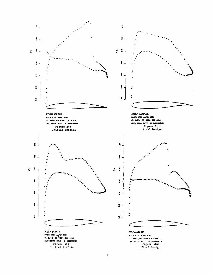
The capatability of the scheme in practice has beenverified by a variety of numerical experiments. First,in order to illustrate the use of the scheme to solvethe inverse problem of designing profiles for a givempressure distribution, Figures 2 and 3 show the re-sults of design calculations in which the targer pres-sure distributions correspond to the Korn and NACA64A410 airfoils. For the Korn design, the initial pro-file was the NACA 64A410, and a shock free de-sign essentially indistinguishable from the Korn air-foil was obtained in 25 iterations. Figure 3 illustratesthe reverse process. Starting from the Korn airfoil,a profile indistinguishable from the NACA 64A410was recovered in 15 iterations.

It is interesting to speculate on the possibility ofdesigning profiles to realize the smooth Korn pres-sure distribution at Mach numbers higher than theKorn design point of Mach 0.75. Figures 4 and 5show the results of attempts to realize such designs atMach numbers of 0.8 and 0.82. Although the resultsshow a smooth pressure distribution on the surface,these flows in fact contain embedded shocks detachedfrom the surface, and these is a corresponding pres-sure drag. At Mach 0.82, a very strong shock waveis located above the reversed camber region towardsthe rear of the top surface. These flows are extremelysensitive to small variations in the geometry, and re-quired 200 to 400 iterations to converge.

These examples show that the attainment of asmooth surface pressure distribution is not sufficientto guarantee low pressure drag, because of the possi-bility that detached shock waves may still appear inthe flow field. To prevent this, one may include thedrag coefficient in the cost function so that Equation31 is replaced by the form

I =1

2

∫

C

(

λ1S2 + λ2

(

dS

dθ

)2)

dθ + βCD

where S is the smoothed deviation from the targetspeed given by Equation 32, and β is a parameterwhich may be varied to alter the trade-off betweendrag reduction and derivation from the desired pres-sure distribution. Representing the drag as

D =

∫

C

(p− p∞) dy

the procedure of Section 2 may be used to determinethe gradient of the augmented cost function by solv-ing the adjoint equation with a correspondingly mod-ified boundary condition. Figure 6 shows the resultof including a drag penalty for the case of the Korntarget pressure distribution at Mach 0.82. In com-parison with Figure 4, it can be seen that the dragcoefficient is reduced from 0.0089 to 0.0010, while thelift coefficient is very slightly reduced from 0.645 to0.630.

The remaining examples illustrates the use of themethod in a pure drag reduction mode. In this case,the target pressure distribution is taken to be theactual pressure distribution of the initial profile pre-dicted by the numerical solution of the flow equa-tion. The addition of a drag penalty now causesthe method to reshape the profile to reduce its drag.The inclusion of the initial pressure distribution asa targer forces the method to generate a profile as alife coefficient close to that of the initial profile, andavoids the pitfall of using the optimization procedureto discover that a flat plate at zero-angle of attachhas zero drag. The program also has an option togenerate solutions at a fixed lift coefficient while al-lowing the angle-of-attack to float. Figure 7 shows aredesign of the RAE 2822 at Mach 0.730 with an ini-tial lift coefficient of 1.05. In this case the design wasessentially frozen after 6 cycles, and the strength ofthe shock wave was reduced at each cycle, with thefinal restul that the drag coefficient was reduced from0.0170 to 0.016.

The question arises whether whether optimizationat one design point might not lead to an improvementin a very narrow band of conditions at the expense ofimpaired off-design performance. The optimizationprocedure is not, however, limited to a single designpoint. If one takes the sum of cost functions forseveral design points, the formulas for the gradientare additive, and the method may be used to seek acompromise design. Figure 8 illustrates the result ofsuch an experiment. The RAE 2822 was again usedas the initial profile, with three design targets, CL1.05 at Mach 0.730, CL 0.95 at Mach 0.740, and CL0.85 at Mach 0.750. These three conditions all pro-duce severe shock waves of roughly equal strength,with initial drag coefficients of 0.0173, 0.0156, and0.0149. The objective is now to reduce the sum ofthe three drag coefficients. After 9 cycles, the coef-ficients are 0.0055, 0.0023, and 0.0006. The sum ofthe drag coefficients is thus reduced from 0.0478 to0.0084. It can also be seen that an almost shock freeresults is obtained at Mach 0.750. The convergenceof the method tends to be more erratic when seekinga compromise design with additive cost functions ofthis kind. If a very low value of drag is attained at

7

one of the design points, this makes a small contri-bution to the gradient, so in the following cycle themodification to reduce the drag at the other designpoints may cause the drag at the first design pointto bounce back up again.

5 Conclusion

If optimization is to have a real impact on design,it will be necessary to treat more complete modelsof the flow, at least including viscous effects in theboundary layer, and to treat three-dimension config-urations. The present study of two-dimensional in-viscid flow provides a useful model, however, to testthe feasibility of using control theory as a design tool.The experience gained with it reinforces the belilefthat control theory offers an effective approach to de-sign. In comparision with more straight forward op-timization methods, the use of the adjoint equationto estimate the gradient greatly reduces computingcosts. A similar formulation can be used for the op-timization of complete three-dimensional wings, us-ing coordinate tranformations to generate the shape,and one may also modify the adjoint equations to al-low for a boundary layer. Intelligent optimizationmethods ought, in due course, to play an increas-ingly important role in the design process, with realpay-offs both in reduced design costs and in increasedefficiency of the final project.

References

[1] Murman, E.M. and Cole, J.D., “Calculation ofPlane Steady Transonic Flows”, AIAA Journal,Vol. 9, 1971, pp. 114-121.

[2] Jameson, A., “Iterative Solution of TransonicFlows Over Airfoils and Wings”, IncludingFlows at Mach 1, Comm. Pure. Appl. Math, Vol.27, 1974, pp. 283-309.

[3] Jameson, A. and Caughey, D.A., “A Fi-nite Volume Method for Transonic PotentialFlow Calculations”, Proc. AIAA 3rd Com-putational Fluid Dynamics Conference, Albu-querque, 1977, pp. 35-54.

[4] Bristeau, M.O., Pironneau, O., Glowinski, R.,Periaux, J., Perrier, P., and Poirier, G., “Onthe Numerical Solution of Nonlinear Problemsin Fluid Dynamics by Least Squares and Fi-nite Element Methods (II). Application to Tran-sonic Flow Simulations”, Proc. 3rd Interna-tional Conference on Finite Elements in Non-linear Mechanics, FENOMECH 84, Stuttgart,

1983, edited by J. St. Doltsinis, North Holland,1985, pp. 363-394.

[5] Jameson, A., Schmidt, W., and Turkel, E.,“Numerical Solution of the Euler Equationsby Finite Volume Methods Using Runge-KuttaTime Stepping Schemes”, AIAA Paper 81-1259,AIAA 14th Fluid Dynamics and Plasma Dy-namics Conference, Palo Alto, 1981.

[6] Ni, Ron Ho, “A multiple Grid Scheme for Solv-ing the Euler Equations”, AIAA Journal, Vol.20, 1982, pp. 1565-1571.

[7] Pulliam, T.H. and Steger, J.L., “Recent Im-provements in Efficiency, Accuracy and Con-vergence for Implicit Approximate Factoriza-tion Algorithms”, AIAA Paper 85-0360, AIAA23rd Aerospace Sciences Meeting, Reno, Jan-uary 1985.

[8] MacCormack, R.W., “Current Status of Numer-ical Solutions of the Navier-Stokes Equations”,AIAA Paper 85-0032, AIAA 23rd AerospaceSciences Meeting, Reno, January 1985.

[9] Jameson, A, Baker, T.J. and Weatherill, N.P.,“Calculation of Inviscid Transonic Flow Overa Complete Aircraft”, AIAA Paper 86-0103,AIAA 24th Aerospace Sciences Meeting, Reno,January 1986.

[10] Jameson, A., “Successess and Challenges inComputational Aerodynamics”, AIAA Paper87-1184-CP, 8th Computational Fluid Dynam-ics Conference, Hawaii, 1987.

[11] Lighthill, M.J., “A New Method of Two Di-mensional Aerodynamic Design”, ARC, RandM 2112, 1945.

[12] McFadden, G.B., “An Artificial ViscosityMethod for the Design of Supercritical Airfoils”,New York University Report COO-3077-158,1979.

[13] Taverna, F., “Advanced Airfoil Design for Gan-eral Aviation Propellers”, AIAA Paper 83-1791,1983.

[14] Garabedian, P. and McFadden, G., “Computa-tional Fluid Dynamics of Airfoils and Wings”,Proc. of Symposium on Transonic, Shock,and Multi-dimensional Flows, Madison, 1981,Meyer, R., ed., Academic Press, New York,1982, pp. 1-16.

[15] Tranen, J.L., “A Rapid Computer Aided Tran-sonic Airfoil Method”, AIAA Paper 74-501,1974.

8

[16] Volpe, G. and Melnik, R.E., “The Design ofTransonic Aerofoils by a Well Posed InverseMethod”, Int. J. Numerical Methods in Engi-neering, Vol. 22, 1986, pp. 341-361.

[17] Henne, P.A., “An Inverse Transonic Wing De-sign Method”, AIAA Paper 80-0330, 1980.

[18] Garabedian, P.R. and Korn, D.G., “Nu-merical Design of Transonic Airfoils”, Proc.SYNSPADE 1970, Hubbard, B., ed., AcademicPress, New York, 1971, pp. 253-271.

[19] Giles, M., Drela, M. and Thompkins, W.T.,“Newton Solution of Direct and Inverse Tran-sonic Euler Equations”, AIAA Paper 85-1530,Proc AIAA 7th Computational Fluid DynamicsConference, Cincinnati, 1985, pp. 394-402.

[20] Hicks, R.M. and Henne, P.A., “Wing Design byNumerical Optimization’, AIAA Paper 79-0080,1979.

[21] Constentino, G.B., and Holst, T.L., “Numeri-cal Optimization Design of Advanced TransonicWing Configurations”, NASA Report, T.M.85950, 1984.

[22] Jameson, Antony, “Aerodynamic Design viaControl Theory”, J. Scientific Computing, Vol.3, 1988, pp. 233-260.

[23] Lion, Jacques Louis, “Optimal Control of Sys-tems Governed by Partial Differential Equa-tions”, translated by S.K. Mitter, Springer Ver-lag, new York, 1971.

[24] Pironneau, Olivier, “Optimal Shape Design forElliptic Sysytems”, Springer Verlag, New York,1984.

[25] Jameson, Antony, “Acceleration of TransonicPotential Flow Calculations on ArtibritaryMeshes by the Multiple Grid Method”, AIAAPaper 79-1458, Fourth AIAA ComputationalFluid Dynamics Conference, Williamsburg, July1979.

9

10

11

12

13