Automatic Camera Calibration for Image Sequences of a Football Match

Automatic Camera Calibration forImage Sequences of a Football Match

Flávio Szenberg1, Paulo Cezar Pinto Carvalho2, Marcelo Gattass1

1TeCGraf - Computer Science Department, PUC-RioRua Marquês de São Vicente, 255, 22453-900, Rio de Janeiro, RJ, Brazil

{szenberg, gattass}@tecgraf.puc-rio.br

2IMPA - Institute of Pure and Applied MathematicsEstrada Dona Castorina, 110, 22460-320, Rio de Janeiro, RJ, Brazil

[email protected]

Abstract

In the broadcast of sports events one can commonly see adds or logos thatare not actually there – instead, they are inserted into the image, with theappropriate perspective representation, by means of specialized computergraphics hardware. Such techniques involve camera calibration and thetracking of objects in the scene. This article introduces an automatic cameracalibration algorithm for a smooth sequence of images of a football (soccer)match taken in the penalty area near one of the goals. The algorithm takesspecial steps for the first scene in the sequence and then uses coherence toefficiently update camera parameters for the remaining images. Thealgorithm is capable of treating in real-time a sequence of images obtainedfrom a TV broadcast, without requiring any specialized hardware.

Keywords: camera calibration, automatic camera calibration, computer vision,tracking, object recognition, image processing.

1 Introduction

In the broadcast of sports events one can commonly see adds or logos that are notactually there – instead, they are inserted into the image, with the appropriateperspective representation, by means of specialized computer graphics hardware.Such techniques involve camera calibration and the tracking of objects in the scene.In the present work, we describe an algorithm that, for a given broadcast image, iscapable of calibrating the camera responsible for visualizing it and of tracking thefield lines in the following scenes in the sequence. With this algorithm, the programsrequire minimal user intervention, thus performing what we call automatic cameracalibration. Furthermore, we seek to develop efficient algorithms that can be used inwidely available PC computers.There are several works on camera calibration, such as [1], [2], [3], and the most

classical one, [4], which introduced the well-known Tsai method for cameracalibration. All methods presented in these works require the user to specifyreference points – that is, points in the image for which one knows the true positionin the real world. In this work, our purpose is to obtain such data automatically.The method for automatically obtaining reference points is based on objectrecognition. Some works related to this method include [5], [6], [7] and [8]. [9]discusses some limitations of model-based recognition.In [10], a camera self-calibration method for video sequences is presented. Somepoints of interest in the images are tracked and, by using the Kruppa equations, thecamera is calibrated. In the present work, we are interested in recognizing andtracking a model, based on the field lines, and only then calibrating the camera.The scenes we are interested in tracking are those of a football (soccer) match,focused on the penalty area near one of the goals. There is where the events of thematch that call more attention take place. In this article we restrict our scope toscene sequences that do not present cuts. That is, the camera’s movement is smoothand the image sequence follows a coherent pattern.The primary objective of our work was to develop an algorithm for a real-timesystem that works with television broadcast images. A major requirement for thealgorithm is its ability to process at least 30 images per second.

2 General View of the Algorithm

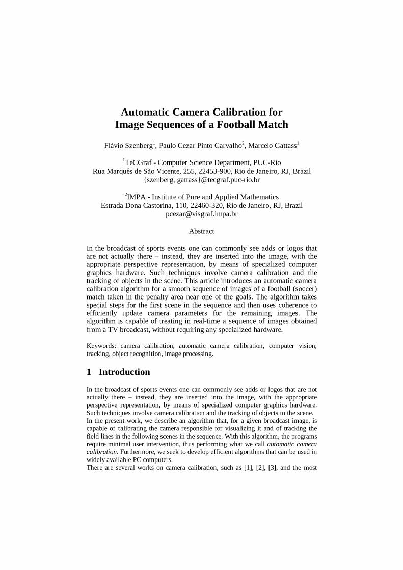
The proposed algorithm is based on a sequence of steps, illustrated in the flowchartshown in Fig. 1. The first four steps are performed only for the first image in thescene. They include a segmentation step that supports the extraction of the field linesand the determination of a preliminary plane projective transformation. For thesubsequent images of the sequence, the algorithm performs an adjustment of thecamera parameters based on the lines obtained in the previous images and on thepreliminary transformation.

Camer a Calibr ationThe camera is calibrated by means of the Tsai method.

Computation of the plane pr ojec tive tr ans for mationA better-fitting geometric transformationis found, based on a

enlarged set of lines.

Filtering to e nhance linesThe Laplacian of Gaussian (LoG) filter is applied to the

image with threshold t0 .

Next i mage inthe se quence

Detec tion of long straight-line segmentsA segmentation step loca tes long straight line segmen ts

candidate to be field lines.

First i mage of the sequence

Line rec ognitionA subset of the line segmen ts is recognized as

representing field lines.

Line re adjustmentThe field lines, either recogn ized or located by th e

transformation, are readjusted based on the LoG filteringresult applied to the image with threshold t1 (t1 < t0).

Computation of the ini tial plane projectivetrans for mation

A geometric transformation that maps fie ld lines to theirrecognized images is found.

Informat ion in pixels

Geometric informat ion

Informat ion in pixels

Camer a Calibr ationThe camera is calibrated by means of the Tsai method.

Computation of the plane pr ojec tive tr ans for mationA better-fitting geometric transformationis found, based on a

enlarged set of lines.

Filtering to e nhance linesThe Laplacian of Gaussian (LoG) filter is applied to the

image with threshold t0 .

Next i mage inthe se quence

Detec tion of long straight-line segmentsA segmentation step loca tes long straight line segmen ts

candidate to be field lines.

First i mage of the sequence

Line rec ognitionA subset of the line segmen ts is recognized as

representing field lines.

Line re adjustmentThe field lines, either recogn ized or located by th e

transformation, are readjusted based on the LoG filteringresult applied to the image with threshold t1 (t1 < t0).

Computation of the ini tial plane projectivetrans for mation

A geometric transformation that maps fie ld lines to theirrecognized images is found.

Informat ion in pixels

Geometric informat ion

Informat ion in pixels

Fig. 1 - Algorithm flowchart.

3 Filtering

This step of the algorithm is responsible for improving the images obtained from the

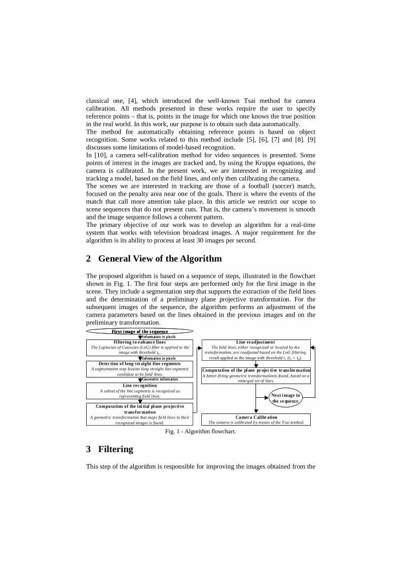
television broadcast. Our primary objective here is to enhance the image to supportthe extraction of straight-line segments corresponding to the markings on the field.To perform this step, we use classical image-processing tools [11]. In the presentarticle, image processing is always done in grayscale. To transform color imagesinto grayscale images, the image luminance is computed.In order to extract pixels from the image that are candidate to lie on a straight-linesegment, we apply the Laplacian filter. Because of noise, problems may arise if thisfilter is directly applied to the image. To minimize them, the Gaussian filter mustfirst be applied to the image. Thus, the image is filtered by a composition of theabove filters, usually called the Laplacian of Gaussian (LoG) filter.The pixels in the image resulting from the LoG filtering with values greater than aspecified threshold (black pixels) are candidate to be on one of the line segments.The remaining pixels (white pixels) are discarded.Figs. 3, 4, and 5 show an example of this filtering step for the image given in Fig. 2.We will use this image to explain all the steps of the proposed algorithm. In thesefigures we can notice the improvement due to applying a Gaussian filter prior to theLaplacian filtering. The lines are much more noticeable in Fig. 5 than in Fig. 4.

Fig. 2 - Original image. Fig. 3 - Image with Gaussian filter.

Fig. 4 - Original image with Laplacian filter. Fig. 5 - Original image with LoG filter.

4 Detecting Long Segments

Once the filtering step has roughly determined the pixels corresponding to the linesegments, the next step consists in locating such segments. In our specific case, weare interested in long straight-line segments.Up to now in the algorithm, we only have pixel information. The pixels that have

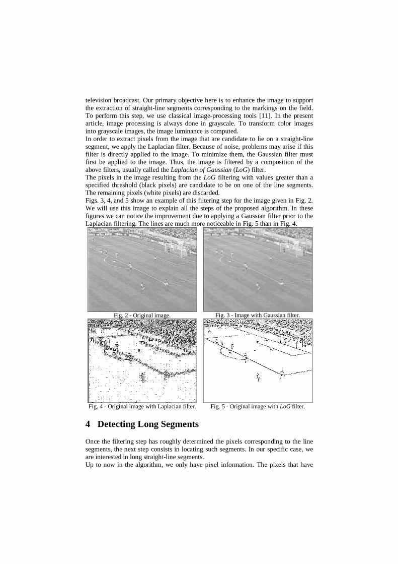
passed through the LoG filtering are black; those that have not are white. Thedesired result, however, must be a geometric structure – more explicitly, parametersthat define the straight-line segments.The procedure proposed for detecting long segments is divided in two steps:1. Eliminating pixels that do not lie on line segments:In this step, the image is divided into cells by a regular grid as shown in Fig. 6. Foreach of these cells, we compute the covariance matrix

where n is the number of black pixels in the cell, xi and yi are the coordinates of eachblack pixel, and x’ and y’ are the corresponding averages. By computing theeigenvalues λ1 and λ2 of this matrix, we can determine to what extent the blackpixels of each cell are positioned as a straight line. If one of such eigenvalues is nullor if the ratio between the largest and the smallest eigenvalue is greater than aspecified value, then the cell is selected and the eigenvector relative to the largesteigenvalue will provide the predominant direction for black pixel orientation.Otherwise, the cell is discarded. The result can be seen in Fig. 7.

Fig. 6 - Image divided into cells. Fig. 7 - Pixels forming straight-line segments.

Fig. 8 - Extraction of straight-line segments.2. Determining line segments:The described cells are traversed in such a way that columns are processed from leftto right and the cells in each column are processed bottom-up. Each cell is given alabel, which is a nonnegative integer. If there is no predominant direction in a cell, itis labeled 0. Otherwise the three neighboring cells to the left and the cell below the

given cell are checked to verify whether they have a predominant direction similarto the one of the current cell. If any of them does, then the current cell receives itslabel; otherwise, a new label is used for the current cell. After this numberingscheme is performed, cells with the same label are grouped and, afterwards, groupsthat correspond to segments that lie on the same line are merged. At the end of theprocess, each group provides a line segment. The result is illustrated in Fig. 8.

5 Recognizing Field Lines

The information we have now is a collection of line segments, some of whichcorrespond to field lines. Our current goal, then, is to recognize, among thosesegments, the ones that are indeed projections of a field line, and to identify thatline.For this purpose we use a model-based recognition method [5]. In our case, themodel is the set of lines of a football field. This method is based on interpretations,that is, it interprets both data sets – the real model and the input data – and checkswhether they are equivalent, according to certain restrictions

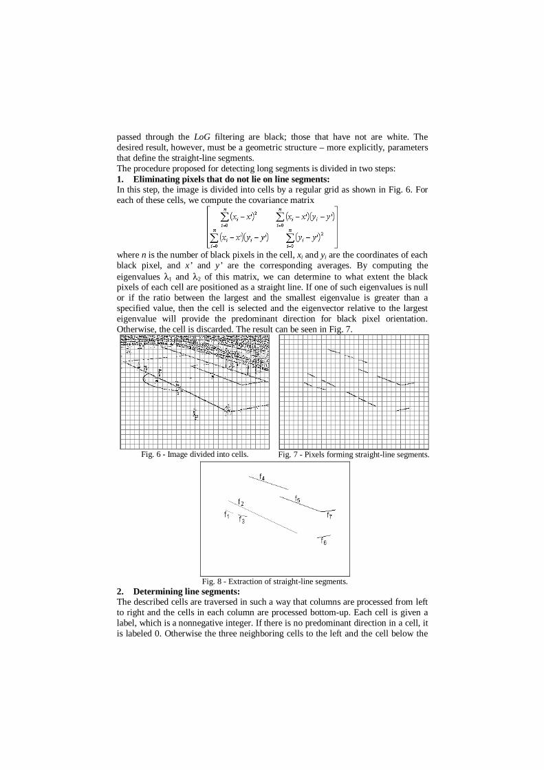
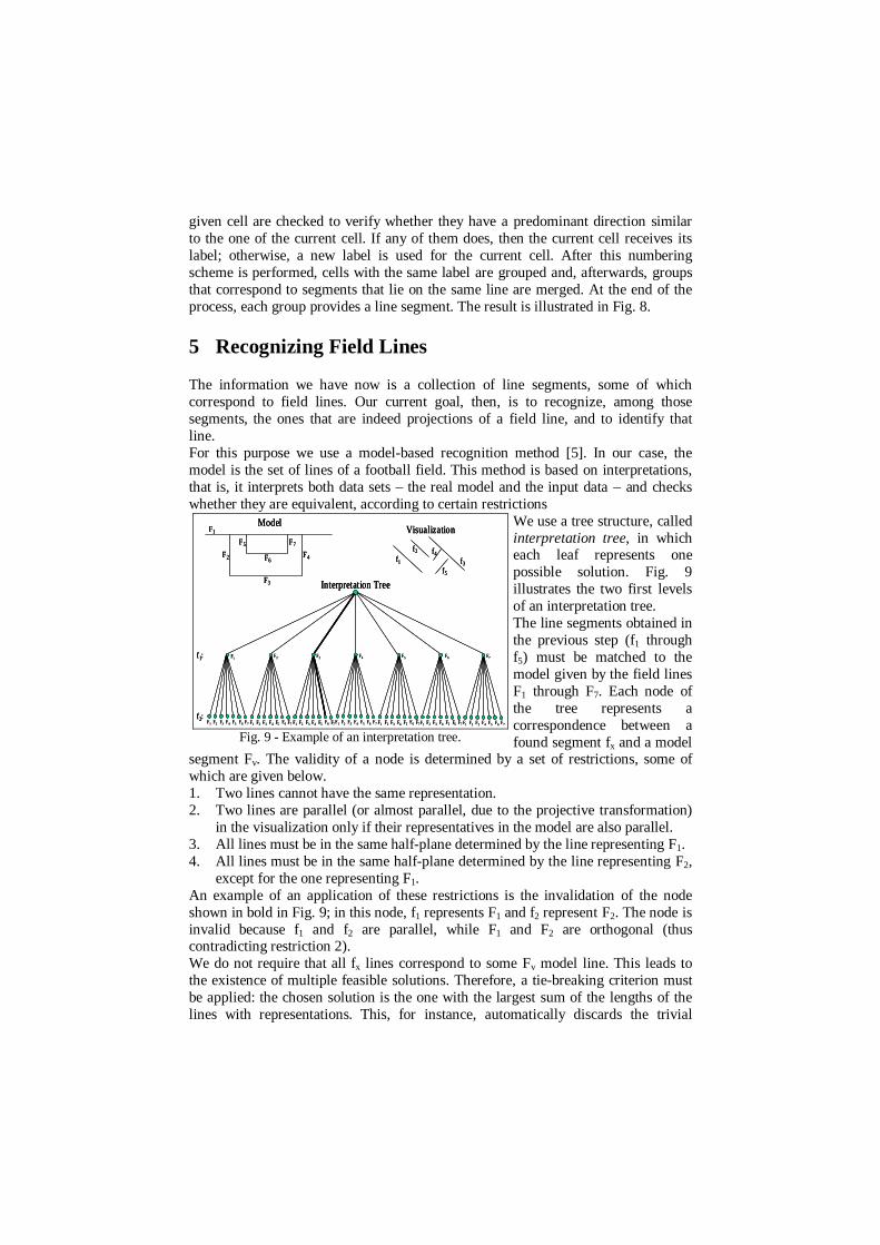
We use a tree structure, calledinterpretation tree, in whicheach leaf represents onepossible solution. Fig. 9illustrates the two first levelsof an interpretation tree.The line segments obtained inthe previous step (f1 throughf5) must be matched to themodel given by the field linesF1 through F7. Each node ofthe tree represents acorrespondence between afound segment fx and a model

segment Fv. The validity of a node is determined by a set of restrictions, some ofwhich are given below.1. Two lines cannot have the same representation.2. Two lines are parallel (or almost parallel, due to the projective transformation)

in the visualization only if their representatives in the model are also parallel.3. All lines must be in the same half-plane determined by the line representing F1.4. All lines must be in the same half-plane determined by the line representing F2,

except for the one representing F1.An example of an application of these restrictions is the invalidation of the nodeshown in bold in Fig. 9; in this node, f1 represents F1 and f2 represent F2. The node isinvalid because f1 and f2 are parallel, while F1 and F2 are orthogonal (thuscontradicting restriction 2).We do not require that all fx lines correspond to some Fv model line. This leads tothe existence of multiple feasible solutions. Therefore, a tie-breaking criterion mustbe applied: the chosen solution is the one with the largest sum of the lengths of thelines with representations. This, for instance, automatically discards the trivial

f1:

f2:

Interpretation Tree

F1 F6F2 F3 F4 F5 F7 F1 F6F2 F3 F4 F5 F7 F1 F6F2 F3 F4 F5 F7 F1 F6F2 F3 F4 F5 F7 F1 F6F2 F3 F4 F5 F7 F1 F6F2 F3 F4 F5 F7F1 F6F2 F3 F4 F5 F7

F1F6F2 F3 F4 F5 F7

F1

F6F2

F3

F4

F5 F7

Model

f1

f2

f3

f4

f5

Visualization

f1:

f2:

Interpretation Tree

F1 F6F2 F3 F4 F5 F7 F1 F6F2 F3 F4 F5 F7 F1 F6F2 F3 F4 F5 F7 F1 F6F2 F3 F4 F5 F7 F1 F6F2 F3 F4 F5 F7 F1 F6F2 F3 F4 F5 F7F1 F6F2 F3 F4 F5 F7

F1F6F2 F3 F4 F5 F7f1:

f2:

Interpretation Tree

F1 F6F2 F3 F4 F5 F7 F1 F6F2 F3 F4 F5 F7 F1 F6F2 F3 F4 F5 F7 F1 F6F2 F3 F4 F5 F7 F1 F6F2 F3 F4 F5 F7 F1 F6F2 F3 F4 F5 F7F1 F6F2 F3 F4 F5 F7

F1F6F2 F3 F4 F5 F7

F1

F6F2

F3

F4

F5 F7

ModelF1

F6F2

F3

F4

F5 F7

Model

f1

f2

f3

f4

f5

Visualization

f1

f2

f3

f4

f5

Visualization

Fig. 9 - Example of an interpretation tree.

solution (where none of the lines has a representation).For the situation in Fig.9 we have: f1 : ∅, f2 : F3, f3 : ∅, f4 : F1, f5 : F6, f6 : F4, f7 : F7,where fx : Fy means that line fx represents line Fy and fx : ∅ indicates that fx

represents none of the model lines.

6 Computing the Planar Projective Transformation

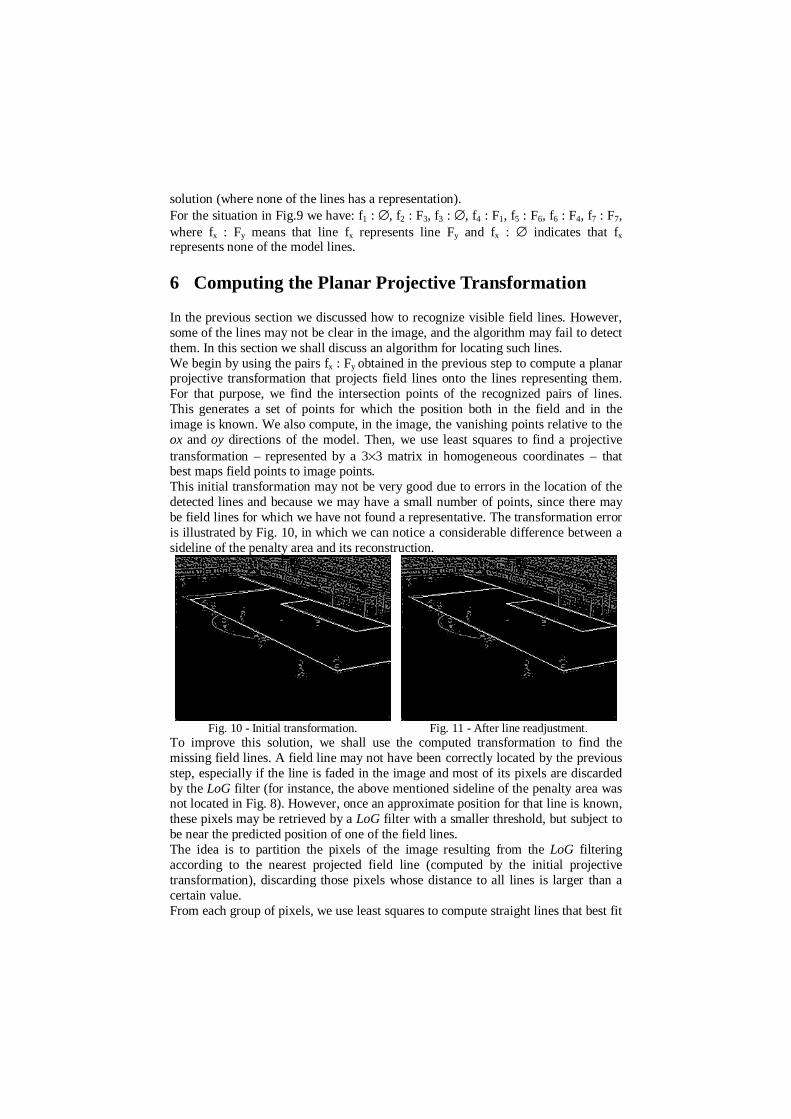
In the previous section we discussed how to recognize visible field lines. However,some of the lines may not be clear in the image, and the algorithm may fail to detectthem. In this section we shall discuss an algorithm for locating such lines.We begin by using the pairs fx : Fy obtained in the previous step to compute a planarprojective transformation that projects field lines onto the lines representing them.For that purpose, we find the intersection points of the recognized pairs of lines.This generates a set of points for which the position both in the field and in theimage is known. We also compute, in the image, the vanishing points relative to theox and oy directions of the model. Then, we use least squares to find a projectivetransformation – represented by a 3×3 matrix in homogeneous coordinates – thatbest maps field points to image points.This initial transformation may not be very good due to errors in the location of thedetected lines and because we may have a small number of points, since there maybe field lines for which we have not found a representative. The transformation erroris illustrated by Fig. 10, in which we can notice a considerable difference between asideline of the penalty area and its reconstruction.

Fig. 10 - Initial transformation. Fig. 11 - After line readjustment.To improve this solution, we shall use the computed transformation to find themissing field lines. A field line may not have been correctly located by the previousstep, especially if the line is faded in the image and most of its pixels are discardedby the LoG filter (for instance, the above mentioned sideline of the penalty area wasnot located in Fig. 8). However, once an approximate position for that line is known,these pixels may be retrieved by a LoG filter with a smaller threshold, but subject tobe near the predicted position of one of the field lines.The idea is to partition the pixels of the image resulting from the LoG filteringaccording to the nearest projected field line (computed by the initial projectivetransformation), discarding those pixels whose distance to all lines is larger than acertain value.From each group of pixels, we use least squares to compute straight lines that best fit

those pixels. Such lines will replace those that originated the groups. We call thisstep of the method line readjustment.With this new set of lines, we compute a new planar projective transformation. Thisnew transformation is expected to have better quality than the previous one, becausethe input points used to obtain the transformation are restricted to small regions inthe vicinity of each line. Therefore, the noise introduced by the effect of otherelements of the image is reduced.With this new set of lines, we compute a new planar projective transformation, inthe same way as done for the initial transformation. The result of this readjustment isillustrated in Fig. 11. These images are in negative to better highlight the extractedfield lines, represented in white. The gray points in the images are the output of theLoG filter, and they are in the image only to provide an idea of the precision of thetransformation. We can notice that the sideline of the penalty area in the upper partof the images is better located in Fig. 11 than in Fig. 10.Some problems may arise in this readjustment due to the players. If there is a largenumber of them over a line – for instance, when there is a wall –, this line may notbe well adjusted.

7 Camera Calibration

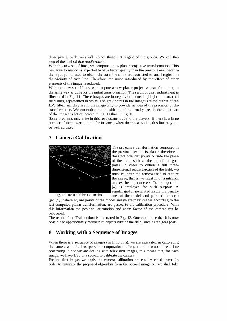
The projective transformation computed inthe previous section is planar, therefore itdoes not consider points outside the planeof the field, such as the top of the goalposts. In order to obtain a full three-dimensional reconstruction of the field, wemust calibrate the camera used to capturethe image, that is, we must find its intrinsicand extrinsic parameters. Tsai’s algorithm[4] is employed for such purpose. Aregular grid is generated inside the penaltyarea of the model, and pairs of the form

(pci, pii), where pci are points of the model and pii are their images according to thelast computed planar transformation, are passed to the calibration procedure. Withthis information the position, orientation and zoom factor of the camera can berecovered.The result of the Tsai method is illustrated in Fig. 12. One can notice that it is nowpossible to appropriately reconstruct objects outside the field, such as the goal posts.

8 Working with a Sequence of Images

When there is a sequence of images (with no cuts), we are interested in calibratingthe camera with the least possible computational effort, in order to obtain real-timeprocessing. Since we are dealing with television images, this means that, for eachimage, we have 1/30 of a second to calibrate the camera.For the first image, we apply the camera calibration process described above. Inorder to optimize the proposed algorithm from the second image on, we shall take

Fig. 12 - Result of the Tsai method.

advantage of the previous image. We can use its final plane projectivetransformation as an initial transformation for the current image, and go directly tothe line readjusting method.

9 Results

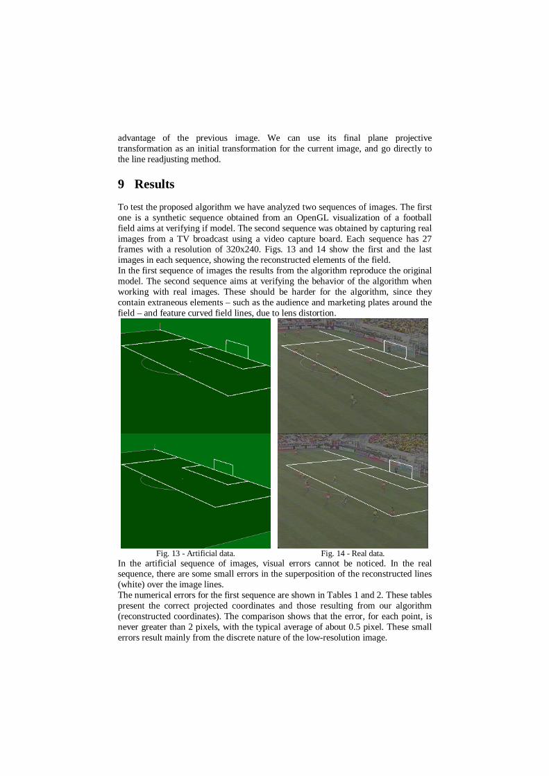
To test the proposed algorithm we have analyzed two sequences of images. The firstone is a synthetic sequence obtained from an OpenGL visualization of a footballfield aims at verifying if model. The second sequence was obtained by capturing realimages from a TV broadcast using a video capture board. Each sequence has 27frames with a resolution of 320x240. Figs. 13 and 14 show the first and the lastimages in each sequence, showing the reconstructed elements of the field.In the first sequence of images the results from the algorithm reproduce the originalmodel. The second sequence aims at verifying the behavior of the algorithm whenworking with real images. These should be harder for the algorithm, since theycontain extraneous elements – such as the audience and marketing plates around thefield – and feature curved field lines, due to lens distortion.

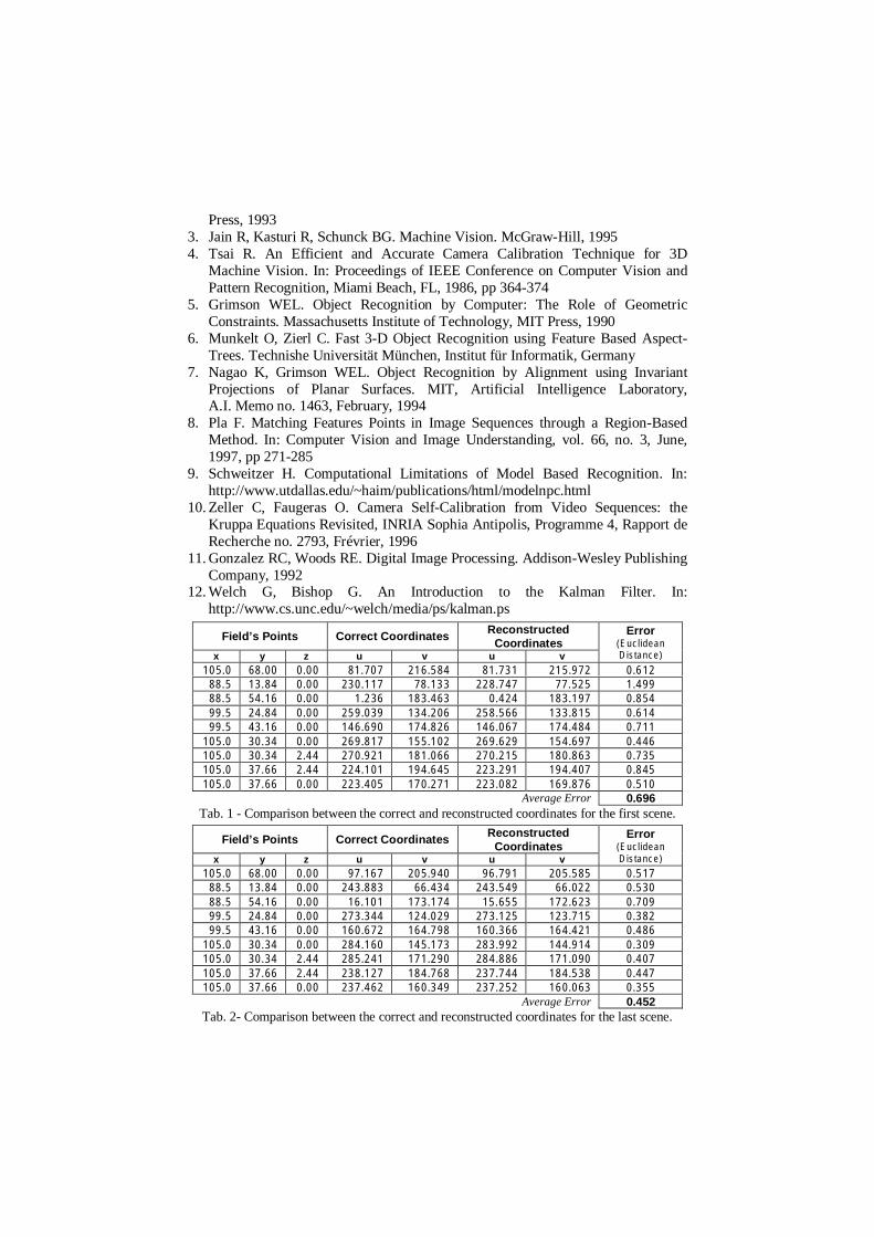
Fig. 13 - Artificial data. Fig. 14 - Real data.In the artificial sequence of images, visual errors cannot be noticed. In the realsequence, there are some small errors in the superposition of the reconstructed lines(white) over the image lines.The numerical errors for the first sequence are shown in Tables 1 and 2. These tablespresent the correct projected coordinates and those resulting from our algorithm(reconstructed coordinates). The comparison shows that the error, for each point, isnever greater than 2 pixels, with the typical average of about 0.5 pixel. These smallerrors result mainly from the discrete nature of the low-resolution image.

The tests were conducted in a Pentium III 600 MHz. The processing time was 380milliseconds for the first sequence and 350 milliseconds for the second one. Thisdifference results from the fact that the algorithm detected 10 line segments in thefirst image of the synthetic sequence and only 7 in the TV sequence, as we can seein Fig. 8 (the side lines and goal posts were not detected in the first TV image). Thisincrease in the number of detected segments influences the processing time of therecognition step, increasing the depth of the interpretation tree. Both processingtimes are well below the time limit for real-time processing. If the desired frame rateis 30 fps, up to 900 milliseconds could be used for processing 27 frames.

10 Conclusions

The algorithm presented here has generated good results even when applied to noisyimages extracted from TV. Our goal to obtain an efficient algorithm that could beused in widely available computers was reached. In the hardware platform where thetests were performed the processing time was well below the time needed for real-time processing. The extra time could be used, for example, to draw ads and logoson the field.

11 Future Works

Although the method presented here is capable of performing camera calibration inreal time for an image sequence, the sequence resulting from the insertion of newelements in the scene suffers from some degree of jittery, due to fluctuations in thecomputed camera position and orientation. We intend to investigate processes forsmoothing the sequence of cameras by applying Kalman filtering [12] or otherrelated techniques.Another interesting work is to develop techniques to track other objects moving onthe field, such as the ball and the players. We also plan to investigate an efficientalgorithm to draw objects on the field behind the players, thus giving the impressionthat the objects drawn are at grass level and the players seem to walk over them.

12 Acknowledgments

This work was developed in TeCGraf/PUC-Rio and Visgraf/IMPA, and waspartially funded by CNPq. TeCGraf is a Laboratory mainly funded byPETROBRAS/CENPES. We are also grateful to Ralph Costa and Dibio Borges fortheir valuable suggestions.

References

1. Carvalho PCP, Szenberg F, Gattass M. Image-based Modeling Using a Two-stepCamera Calibration Method. In: Proceedings of International Symposium onComputer Graphics, Image Processing and Vision, SIBGRAPI’98, Rio deJaneiro, 1998, pp 388-395

2. Faugeras O. Three-Dimensional Computer Vision: a Geometric ViewPoint. MIT

Press, 19933. Jain R, Kasturi R, Schunck BG. Machine Vision. McGraw-Hill, 19954. Tsai R. An Efficient and Accurate Camera Calibration Technique for 3D

Machine Vision. In: Proceedings of IEEE Conference on Computer Vision andPattern Recognition, Miami Beach, FL, 1986, pp 364-374

5. Grimson WEL. Object Recognition by Computer: The Role of GeometricConstraints. Massachusetts Institute of Technology, MIT Press, 1990

6. Munkelt O, Zierl C. Fast 3-D Object Recognition using Feature Based Aspect-Trees. Technishe Universität München, Institut für Informatik, Germany

7. Nagao K, Grimson WEL. Object Recognition by Alignment using InvariantProjections of Planar Surfaces. MIT, Artificial Intelligence Laboratory,A.I. Memo no. 1463, February, 1994

8. Pla F. Matching Features Points in Image Sequences through a Region-BasedMethod. In: Computer Vision and Image Understanding, vol. 66, no. 3, June,1997, pp 271-285

9. Schweitzer H. Computational Limitations of Model Based Recognition. In:http://www.utdallas.edu/~haim/publications/html/modelnpc.html

10. Zeller C, Faugeras O. Camera Self-Calibration from Video Sequences: theKruppa Equations Revisited, INRIA Sophia Antipolis, Programme 4, Rapport deRecherche no. 2793, Frévrier, 1996

11. Gonzalez RC, Woods RE. Digital Image Processing. Addison-Wesley PublishingCompany, 1992

12. Welch G, Bishop G. An Introduction to the Kalman Filter. In:http://www.cs.unc.edu/~welch/media/ps/kalman.ps

Field’s Points Correct Coordinates ReconstructedCoordinates

x y z u v u v

Error(EuclideanDistance)

105.0 68.00 0.00 81.707 216.584 81.731 215.972 0.61288.5 13.84 0.00 230.117 78.133 228.747 77.525 1.49988.5 54.16 0.00 1.236 183.463 0.424 183.197 0.85499.5 24.84 0.00 259.039 134.206 258.566 133.815 0.61499.5 43.16 0.00 146.690 174.826 146.067 174.484 0.711

105.0 30.34 0.00 269.817 155.102 269.629 154.697 0.446105.0 30.34 2.44 270.921 181.066 270.215 180.863 0.735105.0 37.66 2.44 224.101 194.645 223.291 194.407 0.845105.0 37.66 0.00 223.405 170.271 223.082 169.876 0.510

Average Error 0.696Tab. 1 - Comparison between the correct and reconstructed coordinates for the first scene.

Field’s Points Correct Coordinates ReconstructedCoordinates

x y z u v u v

Error(EuclideanDistance)

105.0 68.00 0.00 97.167 205.940 96.791 205.585 0.51788.5 13.84 0.00 243.883 66.434 243.549 66.022 0.53088.5 54.16 0.00 16.101 173.174 15.655 172.623 0.70999.5 24.84 0.00 273.344 124.029 273.125 123.715 0.38299.5 43.16 0.00 160.672 164.798 160.366 164.421 0.486

105.0 30.34 0.00 284.160 145.173 283.992 144.914 0.309105.0 30.34 2.44 285.241 171.290 284.886 171.090 0.407105.0 37.66 2.44 238.127 184.768 237.744 184.538 0.447105.0 37.66 0.00 237.462 160.349 237.252 160.063 0.355

Average Error 0.452Tab. 2- Comparison between the correct and reconstructed coordinates for the last scene.