16 th International LS-DYNA ® Users Conference Automotive June 10-11, 2020 1 Automatic Analysis of Crash Simulations with Dimensionality Reduction Algorithms such as PCA and t-SNE David Kracker 1 , Jochen Garcke 2 , Axel Schumacher 3 , Pit Schwanitz 1 1 Dr. Ing. h.c. F. Porsche AG, Body Engineering CAE Vehicle Safety, 71287 Weissach, Germany, 2 Fraunhofer Center for Machine Learning and Fraunhofer Institute for Scientific Computing (SCAI), Institut für Numerische Simulation, 53115 Sankt Augustin, Germany 3 University of Wuppertal, Faculty for Mechanical Engineering and Safety Engineering, Chair for Optimization of Mechanical Structures, 42119 Wuppertal, Germany Abstract The increasing number of crash simulations and the growing complexity of the models require an efficiently designed evaluation of the simulation results. Nowadays a full vehicle model consists of approximately 10 million shell elements. Each of them contains various evaluation variables that describe the physical behavior of the element. Therefore, the simulation models are very high dimensional. During vehicle development, a large number of models is created that differ in geometry, wall thicknesses and other properties. These model changes lead to different physical behavior during a vehicle crash. This behavior is to be analyzed and evaluated automatically. In this article, potentials of several algorithms for dimensionality reduction are investigated. The linear Principal Component Analysis (PCA) is compared to the non-linear t-distributed stochastic neighbor embedding (t-SNE) algorithm. For those algorithms, it is necessary that the input data always has an identical feature space. Geometrical modifications of the model lead to changes of finite element meshes and therefore to different data representations. Therefore, several 2D and 3D discretization approaches are considered and evaluated (sphere, voxel). In order to assess the quality of the results, a scale-independent quality criterion is used for the discretization and the subsequent dimensionality reduction. The simulations used in this paper are carried out with LS-DYNA ® . The aim of the presented study is to develop an efficient process for the investigation of different data transformation approaches, dimensionality reduction algorithms, and physical evaluation quantities. The resulting evaluation method should represent physically relevant effects in the existing simulations in a low-dimensional space without human interaction and thus support the engineer in the evaluation of the results. 1. Introduction More challenging legal requirements, increasing capability of supercomputers, and more efficient development processes are driving a growth in the number of crash simulations. A manual evaluation of the results is thus reaching its limits and therefore requires an increased automation. This paper investigates to what extent methods of machine learning can support the engineer in evaluating multiple simulations. The focus is on the dimensionality reduction of high-dimensional crash simulation data. The goal is to enable the user to get a quick overview about the different crash behavior of individual components without having to look at each simulation in detail in a post-processor. The data used in this work are taken from a robustness analysis of a front-end vehicle section model [10]. The model collides at 64 km/h with an off-center positioned deformable barrier (ODB) according to the EURO NCAP [11]. The crash has a duration of 120ms, the result files contain the information of 62 states. In 51 simulations, the wall thicknesses of selected components were scattered using the Advanced Latin Hypercube Method. These variations represent the production-related scattering of the wall thicknesses for each component and allow an evaluation of the robustness of the concept. In Figure 1, the two components, which are used exemplarily for the analysis in this work, are highlighted. The Crash Management System plays a major role in the low-speed crash, whereas the longitudinal member is important in high-speed crash scenarios.

Welcome message from author
This document is posted to help you gain knowledge. Please leave a comment to let me know what you think about it! Share it to your friends and learn new things together.
Transcript
16th International LS-DYNA® Users Conference Automotive
June 10-11, 2020 1
Automatic Analysis of Crash Simulations with Dimensionality
Reduction Algorithms such as PCA and t-SNE
David Kracker1, Jochen Garcke2, Axel Schumacher3, Pit Schwanitz1
1Dr. Ing. h.c. F. Porsche AG, Body Engineering CAE Vehicle Safety, 71287 Weissach, Germany,
2 Fraunhofer Center for Machine Learning and Fraunhofer Institute for Scientific Computing (SCAI), Institut für Numerische Simulation, 53115 Sankt Augustin, Germany
3University of Wuppertal, Faculty for Mechanical Engineering and Safety Engineering, Chair for Optimization of Mechanical Structures, 42119 Wuppertal, Germany
Abstract The increasing number of crash simulations and the growing complexity of the models require an efficiently designed evaluation of the simulation results. Nowadays a full vehicle model consists of approximately 10 million shell elements. Each of them contains various evaluation variables that describe the physical behavior of the element. Therefore, the simulation models are very high dimensional. During vehicle development, a large number of models is created that differ in geometry, wall thicknesses and other properties. These model changes lead to different physical behavior during a vehicle crash. This behavior is to be analyzed and evaluated automatically. In this article, potentials of several algorithms for dimensionality reduction are investigated. The linear Principal Component Analysis (PCA) is compared to the non-linear t-distributed stochastic neighbor embedding (t-SNE) algorithm. For those algorithms, it is necessary that the input data always has an identical feature space. Geometrical modifications of the model lead to changes of finite element meshes and therefore to different data representations. Therefore, several 2D and 3D discretization approaches are considered and evaluated (sphere, voxel). In order to assess the quality of the results, a scale-independent quality criterion is used for the discretization and the subsequent dimensionality reduction. The simulations used in this paper are carried out with LS-DYNA®. The aim of the presented study is to develop an efficient process for the investigation of different data transformation approaches, dimensionality reduction algorithms, and physical evaluation quantities. The resulting evaluation method should represent physically relevant effects in the existing simulations in a low-dimensional space without human interaction and thus support the engineer in the evaluation of the results.
1. Introduction
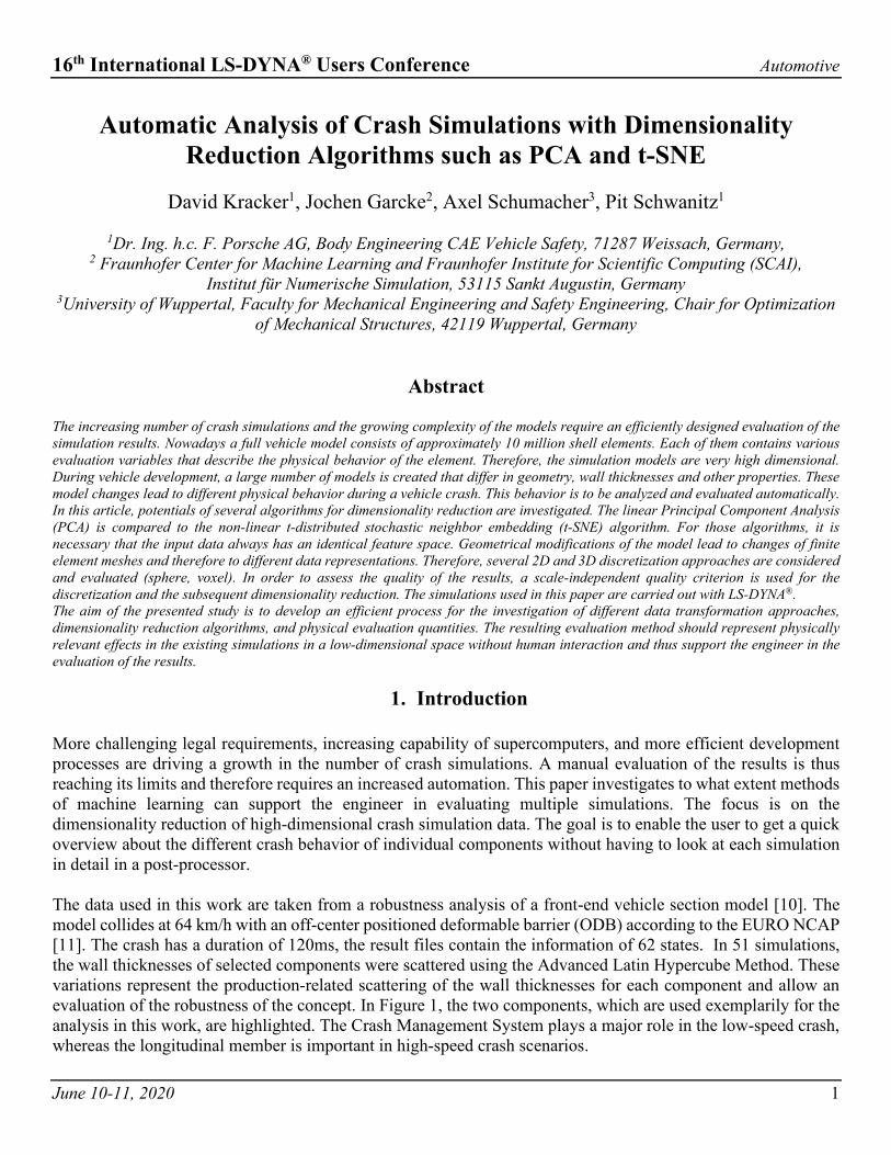
More challenging legal requirements, increasing capability of supercomputers, and more efficient development processes are driving a growth in the number of crash simulations. A manual evaluation of the results is thus reaching its limits and therefore requires an increased automation. This paper investigates to what extent methods of machine learning can support the engineer in evaluating multiple simulations. The focus is on the dimensionality reduction of high-dimensional crash simulation data. The goal is to enable the user to get a quick overview about the different crash behavior of individual components without having to look at each simulation in detail in a post-processor. The data used in this work are taken from a robustness analysis of a front-end vehicle section model [10]. The model collides at 64 km/h with an off-center positioned deformable barrier (ODB) according to the EURO NCAP [11]. The crash has a duration of 120ms, the result files contain the information of 62 states. In 51 simulations, the wall thicknesses of selected components were scattered using the Advanced Latin Hypercube Method. These variations represent the production-related scattering of the wall thicknesses for each component and allow an evaluation of the robustness of the concept. In Figure 1, the two components, which are used exemplarily for the analysis in this work, are highlighted. The Crash Management System plays a major role in the low-speed crash, whereas the longitudinal member is important in high-speed crash scenarios.
16th International LS-DYNA® Users Conference Automotive
June 10-11, 2020 2
Especially the longitudinal member shows an interesting behavior in the 51 simulations and three different deformation modes can be observed. The location where the deformation starts after exceeding a certain force varies in the 51 simulations. In some simulations, the beam starts to fold at the front, in others at the back, and in the remaining ones at the front and back simultaneously. In an automated analysis process, such different behaviors are to be detected by the algorithm and shall be visualized in a clear and understandable manner. The unrobust behavior of the component makes it an excellent candidate for further analysis in this work.
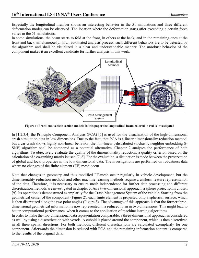
Figure 1: Front-end vehicle section model: In this paper the longitudinal beam colored in red is investigated In [1,2,3,4] the Principle Component Analysis (PCA) [5] is used for the visualization of the high-dimensional crash simulation data in low dimensions. Due to the fact, that PCA is a linear dimensionality reduction method, but a car crash shows highly non-linear behavior, the non-linear t-distributed stochastic neighbor embedding (t-SNE) algorithm shall be compared as a potential alternative. Chapter 2 analyses the performance of both algorithms. To objectively evaluate the quality of the dimensionality reduction, a quality criterion based on the calculation of a co-ranking matrix is used [7, 8]. For the evaluation, a distinction is made between the preservation of global and local properties in the low dimensional data. The investigations are performed on robustness data where no changes of the finite element (FE) mesh occur. Note that changes in geometry and thus modified FE-mesh occur regularly in vehicle development, but the dimensionality reduction methods and other machine learning methods require a uniform feature representation of the data. Therefore, it is necessary to ensure mesh independence for further data processing and different discretization methods are investigated in chapter 3. As a two-dimensional approach, a sphere projection is chosen [9]. Its operation is demonstrated exemplarily for the Crash Management System of the vehicle. Starting from the geometrical center of the component (Figure 2), each finite element is projected onto a spherical surface, which is then discretized along the two polar angles (Figure 3). The advantage of this approach is that the former three-dimensional geometrical information is now represented in a reduced form in two dimensions. This might lead to better computational performance, when it comes to the application of machine learning algorithms. In order to make the two-dimensional data representation comparable, a three-dimensional approach is considered as well by using a discretization with voxels. A cuboid is placed around the component, which is then discretized in all three spatial directions. For both methods, different discretizations are calculated exemplarily for one component. Afterwards the dimension is reduced with PCA and the remaining information content is compared to the results of the original data.
Crash Management System
Longitudinal Member
Crash Management System
16th International LS-DYNA® Users Conference Automotive
June 10-11, 2020 3
Figure 2: Calculation of geometrical center
Figure 3: Projection of the finite elements onto the sphere
Figure 4: Calculation of voxel grid
Figure 5: Projection of the finite elements into voxel grid
2. Results Dimensionality Reduction
The purpose of reducing the dimensionality of the data is to represent the essential properties of a simulation by a reduced number of variables that contain most of the information about the existing data set. Those variables can then be used to visualize the simulation results in two or three-dimensional space and to quickly gain useful insights into similarities and differences of the simulations. There are several ways to reduce the dimension of the data. In this paper, the PCA as well as the t-SNE algorithm are reviewed for their applicability in the analysis of crash simulations. In the first step, the simulation results were extracted from the d3plot files by using an input-reader from LASSO [12]. For data analysis, the plastic strain of each element from the longitudinal member is used as the evaluation quantity. The longitudinal member consists of 2286 elements. Two data representations are investigated in this paper. In the first one, the 62 vectors from the individual states, each of length 2286 (plastic strains of each element), are concatenated and thus result in a single vector of dimension 141,732 per simulation. Consequently, the results of the 51 simulations form a matrix of the dimension 51x141,732, which is used for further calculations. In the following, this approach is called OPioS (One Point is one Simulation). In the second data representation method, the states of each simulation are no longer concatenated to one single vector. Each state contributes to the input matrix with one row, which contains the information of the e elements for that state. This results in an input matrix for the dimensionality reduction of the size 3162x2286. In the following, this approach is called OLioS (One Line is one Simulation).
16th International LS-DYNA® Users Conference Automotive
June 10-11, 2020 4
2.1 Feature Representation Approach OPioS
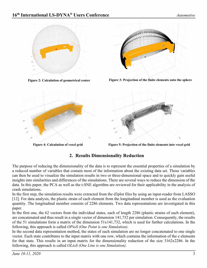
In this chapter, the PCA is examined for the first data representation approach OPioS. PCA is transforming the data in such way, that a smaller number of parameters describes most variance in the data. The components are sorted regarding their included information amount and consequently by their significance. The first components contain most of the information and therefore are used for the dimensionality reduction. Figure 6 shows the results by plotting the first two principal components against each other on the two axes. Three clusters can be identified, which contain the simulations of the three different deformation behaviors already mentioned (folding front, back, both ends). This reduced representation gives the engineer a quick overview of the different deformation behavior of a component over many simulations.
Figure 6: Visualization of the first two principle components from PCA. Dimension of the Input-Matrix: 51x14173
The information content of the principal components can be interpreted via the explained variance. This variable describes how much variance of the whole data is contained in the corresponding principal component. In Figure 6, the curve with the circles shows the course of the explained variance of the first 51 principal components. The curve converges with the 51st principal component against one. Accordingly, 51 principal components describe the entire information content of the present data set. The first two principal components are used for the visualization, since they contain most information about the available data in relation to the other components. The explained variance with two principal components is 0.258. This value gives an indication of the information lost during dimensionality reduction. The maximum value, which can be achieved, is one. In this example, the value is low, which is an indicator of a large loss of information. Nevertheless, the information obtained from the 2D plot (Figure 6) still groups the simulations into the observed three deformation behaviors. Therefore, it is useful for the engineer in order to get a quick overview over a bunch of simulations.
16th International LS-DYNA® Users Conference Automotive
June 10-11, 2020 5
2.2 Feature Representation Approach OLioS
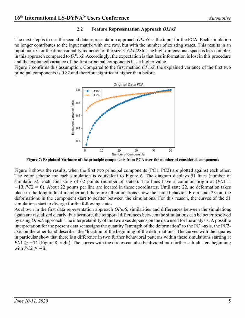
The next step is to use the second data representation approach OLioS as the input for the PCA. Each simulation no longer contributes to the input matrix with one row, but with the number of existing states. This results in an input matrix for the dimensionality reduction of the size 3162x2286. The high-dimensional space is less complex in this approach compared to OPioS. Accordingly, the expectation is that less information is lost in this procedure and the explainedd variance of the first principal components has a higher value. Figure 7 confirms this assumption. Compared to the first method OPioS, the explained variance of the first two principal components is 0.82 and therefore significant higher than before.
Figure 7: Explained Variance of the principle components from PCA over the number of considered components
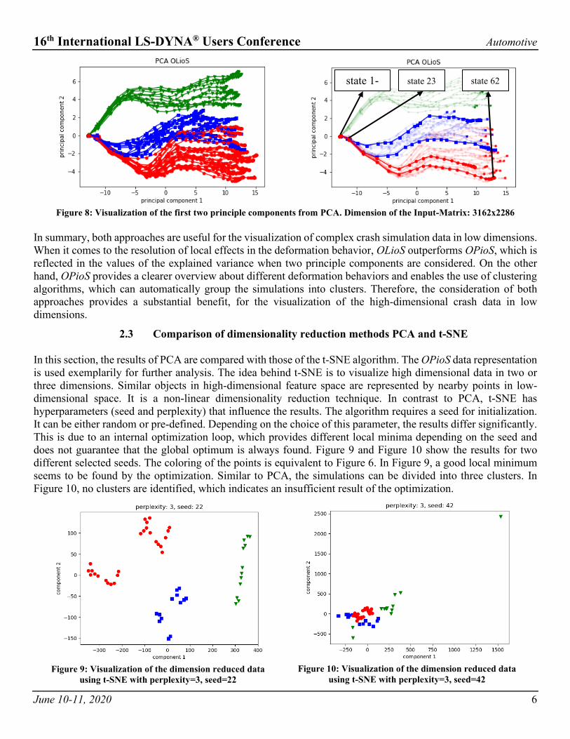
Figure 8 shows the results, when the first two principal components (PC1, PC2) are plotted against each other. The color scheme for each simulation is equivalent to Figure 6. The diagram displays 51 lines (number of simulations), each consisting of 62 points (number of states). The lines have a common origin at (𝑃𝑃𝑃𝑃1 =−13,𝑃𝑃𝑃𝑃2 = 0). About 22 points per line are located in these coordinates. Until state 22, no deformation takes place in the longitudinal member and therefore all simulations show the same behavior. From state 23 on, the deformations in the component start to scatter between the simulations. For this reason, the curves of the 51 simulations start to diverge for the following states. As shown in the first data representation approach OPioS, similarities and differences between the simulations again are visualized clearly. Furthermore, the temporal differences between the simulations can be better resolved by using OLioS approach. The interpretability of the two axes depends on the data used for the analysis. A possible interpretation for the present data set assigns the quantity "strength of the deformation" to the PC1-axis, the PC2-axis on the other hand describes the "location of the beginning of the deformation". The curves with the squares in particular show that there is a difference in two further behavioral patterns within these simulations starting at 𝑃𝑃𝑃𝑃1 ≥ −11 (Figure 8, right). The curves with the circles can also be divided into further sub-clusters beginning with 𝑃𝑃𝑃𝑃2 ≥ −8.
16th International LS-DYNA® Users Conference Automotive
June 10-11, 2020 6
Figure 8: Visualization of the first two principle components from PCA. Dimension of the Input-Matrix: 3162x2286
In summary, both approaches are useful for the visualization of complex crash simulation data in low dimensions. When it comes to the resolution of local effects in the deformation behavior, OLioS outperforms OPioS, which is reflected in the values of the explained variance when two principle components are considered. On the other hand, OPioS provides a clearer overview about different deformation behaviors and enables the use of clustering algorithms, which can automatically group the simulations into clusters. Therefore, the consideration of both approaches provides a substantial benefit, for the visualization of the high-dimensional crash data in low dimensions.
2.3 Comparison of dimensionality reduction methods PCA and t-SNE
In this section, the results of PCA are compared with those of the t-SNE algorithm. The OPioS data representation is used exemplarily for further analysis. The idea behind t-SNE is to visualize high dimensional data in two or three dimensions. Similar objects in high-dimensional feature space are represented by nearby points in low-dimensional space. It is a non-linear dimensionality reduction technique. In contrast to PCA, t-SNE has hyperparameters (seed and perplexity) that influence the results. The algorithm requires a seed for initialization. It can be either random or pre-defined. Depending on the choice of this parameter, the results differ significantly. This is due to an internal optimization loop, which provides different local minima depending on the seed and does not guarantee that the global optimum is always found. Figure 9 and Figure 10 show the results for two different selected seeds. The coloring of the points is equivalent to Figure 6. In Figure 9, a good local minimum seems to be found by the optimization. Similar to PCA, the simulations can be divided into three clusters. In Figure 10, no clusters are identified, which indicates an insufficient result of the optimization.
Figure 9: Visualization of the dimension reduced data
using t-SNE with perplexity=3, seed=22
Figure 10: Visualization of the dimension reduced data
using t-SNE with perplexity=3, seed=42
state 1-
state 23 state 62
16th International LS-DYNA® Users Conference Automotive
June 10-11, 2020 7
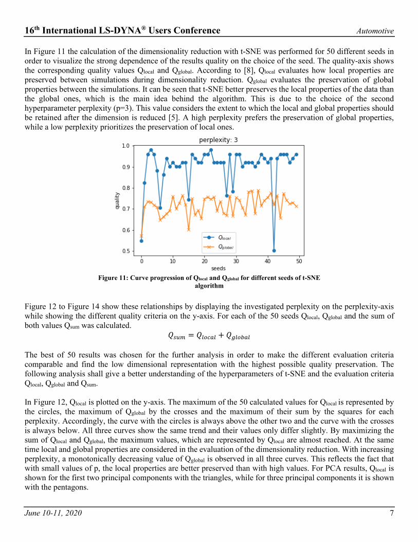
In Figure 11 the calculation of the dimensionality reduction with t-SNE was performed for 50 different seeds in order to visualize the strong dependence of the results quality on the choice of the seed. The quality-axis shows the corresponding quality values Qlocal and Qglobal. According to [8], Qlocal evaluates how local properties are preserved between simulations during dimensionality reduction. Qglobal evaluates the preservation of global properties between the simulations. It can be seen that t-SNE better preserves the local properties of the data than the global ones, which is the main idea behind the algorithm. This is due to the choice of the second hyperparameter perplexity (p=3). This value considers the extent to which the local and global properties should be retained after the dimension is reduced [5]. A high perplexity prefers the preservation of global properties, while a low perplexity prioritizes the preservation of local ones.
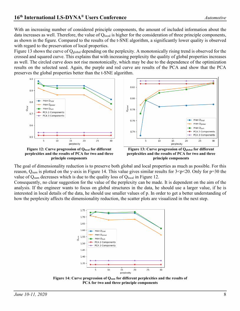
Figure 12 to Figure 14 show these relationships by displaying the investigated perplexity on the perplexity-axis while showing the different quality criteria on the y-axis. For each of the 50 seeds Qlocal, Qglobal and the sum of both values Qsum was calculated.
𝑄𝑄𝑠𝑠𝑠𝑠𝑠𝑠 = 𝑄𝑄𝑙𝑙𝑙𝑙𝑙𝑙𝑙𝑙𝑙𝑙 + 𝑄𝑄𝑔𝑔𝑙𝑙𝑙𝑙𝑔𝑔𝑙𝑙𝑙𝑙 The best of 50 results was chosen for the further analysis in order to make the different evaluation criteria comparable and find the low dimensional representation with the highest possible quality preservation. The following analysis shall give a better understanding of the hyperparameters of t-SNE and the evaluation criteria Qlocal, Qglobal and Qsum. In Figure 12, Qlocal is plotted on the y-axis. The maximum of the 50 calculated values for Qlocal is represented by the circles, the maximum of Qglobal by the crosses and the maximum of their sum by the squares for each perplexity. Accordingly, the curve with the circles is always above the other two and the curve with the crosses is always below. All three curves show the same trend and their values only differ slightly. By maximizing the sum of Qlocal and Qglobal, the maximum values, which are represented by Qlocal are almost reached. At the same time local and global properties are considered in the evaluation of the dimensionality reduction. With increasing perplexity, a monotonically decreasing value of Qglobal is observed in all three curves. This reflects the fact that with small values of p, the local properties are better preserved than with high values. For PCA results, Qlocal is shown for the first two principal components with the triangles, while for three principal components it is shown with the pentagons.
Figure 11: Curve progression of Qlocal and Qglobal for different seeds of t-SNE
algorithm
16th International LS-DYNA® Users Conference Automotive
June 10-11, 2020 8
With an increasing number of considered principle components, the amount of included information about the data increases as well. Therefore, the value of Qlocal is higher for the consideration of three principle components, as shown in the figure. Compared to the results of the t-SNE algorithm, a significantly lower quality is observed with regard to the preservation of local properties. Figure 13 shows the curve of Qglobal depending on the perplexity. A monotonically rising trend is observed for the crossed and squared curve. This explains that with increasing perplexity the quality of global properties increases as well. The circled curve does not rise monotonically, which may be due to the dependence of the optimization results on the selected seed. Again, the purple and red curve are results of the PCA and show that the PCA preserves the global properties better than the t-SNE algorithm.
The goal of dimensionality reduction is to preserve both global and local properties as much as possible. For this reason, Qsum is plotted on the y-axis in Figure 14. This value gives similar results for 3<p<20. Only for p=30 the value of Qsum decreases which is due to the quality loss of Qlocal in Figure 12. Consequently, no clear suggestion for the value of the perplexity can be made. It is dependent on the aim of the analysis. If the engineer wants to focus on global structures in the data, he should use a larger value, if he is interested in local details of the data, he should use smaller values of p. In order to get a better understanding of how the perplexity affects the dimensionality reduction, the scatter plots are visualized in the next step.
Figure 12: Curve progression of Qlocal for different
perplexities and the results of PCA for two and three principle components
Figure 13: Curve progression of Qglobal for different
perplexities and the results of PCA for two and three principle components
Figure 14: Curve progression of Qsum for different perplexities and the results of
PCA for two and three principle components
16th International LS-DYNA® Users Conference Automotive
June 10-11, 2020 9
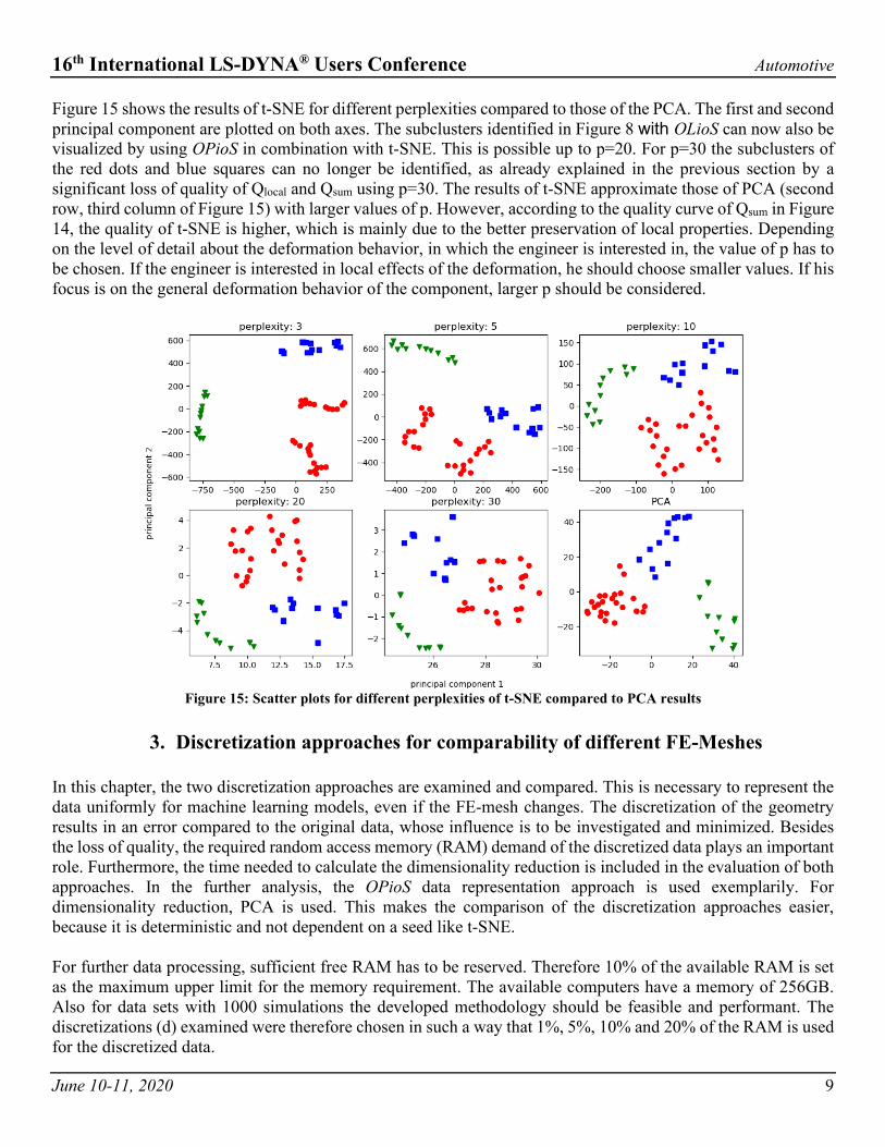
Figure 15 shows the results of t-SNE for different perplexities compared to those of the PCA. The first and second principal component are plotted on both axes. The subclusters identified in Figure 8 with OLioS can now also be visualized by using OPioS in combination with t-SNE. This is possible up to p=20. For p=30 the subclusters of the red dots and blue squares can no longer be identified, as already explained in the previous section by a significant loss of quality of Qlocal and Qsum using p=30. The results of t-SNE approximate those of PCA (second row, third column of Figure 15) with larger values of p. However, according to the quality curve of Qsum in Figure 14, the quality of t-SNE is higher, which is mainly due to the better preservation of local properties. Depending on the level of detail about the deformation behavior, in which the engineer is interested in, the value of p has to be chosen. If the engineer is interested in local effects of the deformation, he should choose smaller values. If his focus is on the general deformation behavior of the component, larger p should be considered.
Figure 15: Scatter plots for different perplexities of t-SNE compared to PCA results
3. Discretization approaches for comparability of different FE-Meshes
In this chapter, the two discretization approaches are examined and compared. This is necessary to represent the data uniformly for machine learning models, even if the FE-mesh changes. The discretization of the geometry results in an error compared to the original data, whose influence is to be investigated and minimized. Besides the loss of quality, the required random access memory (RAM) demand of the discretized data plays an important role. Furthermore, the time needed to calculate the dimensionality reduction is included in the evaluation of both approaches. In the further analysis, the OPioS data representation approach is used exemplarily. For dimensionality reduction, PCA is used. This makes the comparison of the discretization approaches easier, because it is deterministic and not dependent on a seed like t-SNE. For further data processing, sufficient free RAM has to be reserved. Therefore 10% of the available RAM is set as the maximum upper limit for the memory requirement. The available computers have a memory of 256GB. Also for data sets with 1000 simulations the developed methodology should be feasible and performant. The discretizations (d) examined were therefore chosen in such a way that 1%, 5%, 10% and 20% of the RAM is used for the discretized data.
16th International LS-DYNA® Users Conference Automotive
June 10-11, 2020 10
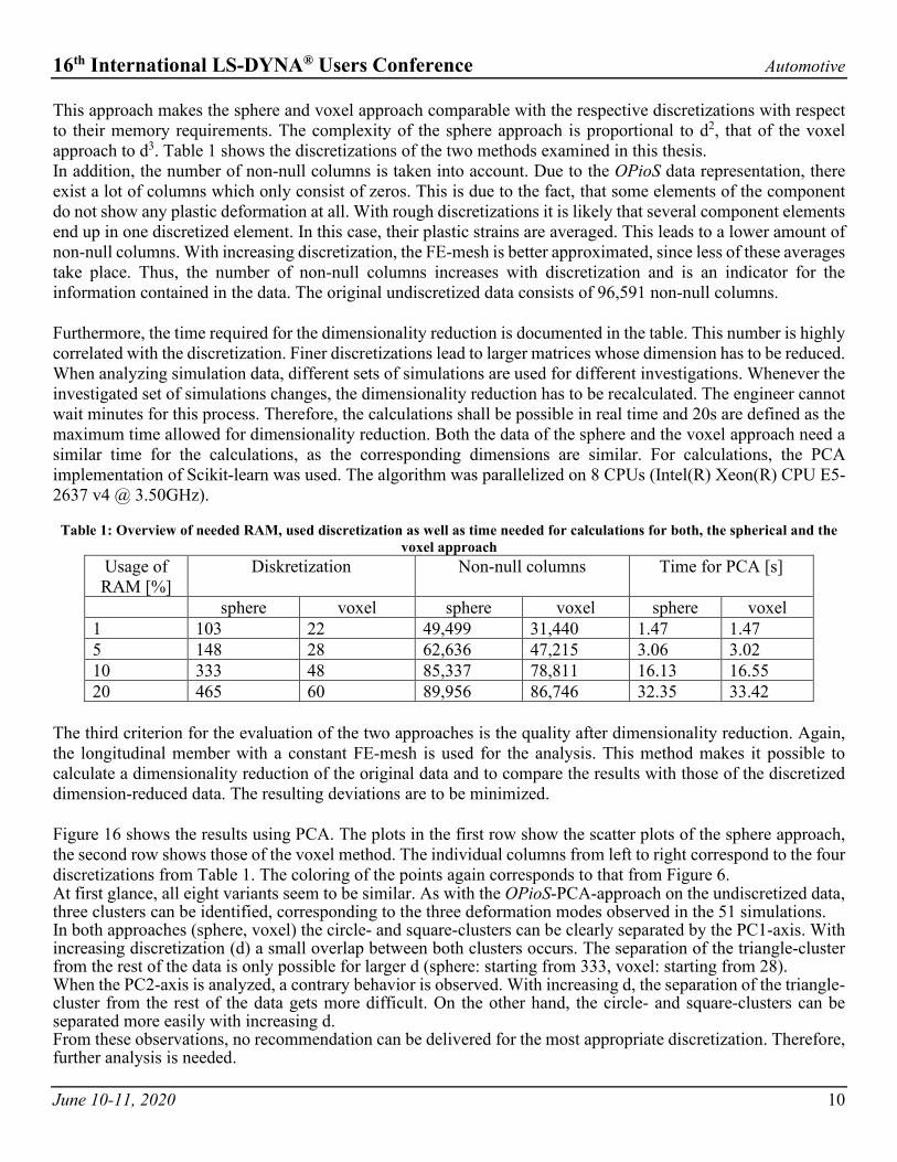
This approach makes the sphere and voxel approach comparable with the respective discretizations with respect to their memory requirements. The complexity of the sphere approach is proportional to d2, that of the voxel approach to d3. Table 1 shows the discretizations of the two methods examined in this thesis. In addition, the number of non-null columns is taken into account. Due to the OPioS data representation, there exist a lot of columns which only consist of zeros. This is due to the fact, that some elements of the component do not show any plastic deformation at all. With rough discretizations it is likely that several component elements end up in one discretized element. In this case, their plastic strains are averaged. This leads to a lower amount of non-null columns. With increasing discretization, the FE-mesh is better approximated, since less of these averages take place. Thus, the number of non-null columns increases with discretization and is an indicator for the information contained in the data. The original undiscretized data consists of 96,591 non-null columns. Furthermore, the time required for the dimensionality reduction is documented in the table. This number is highly correlated with the discretization. Finer discretizations lead to larger matrices whose dimension has to be reduced. When analyzing simulation data, different sets of simulations are used for different investigations. Whenever the investigated set of simulations changes, the dimensionality reduction has to be recalculated. The engineer cannot wait minutes for this process. Therefore, the calculations shall be possible in real time and 20s are defined as the maximum time allowed for dimensionality reduction. Both the data of the sphere and the voxel approach need a similar time for the calculations, as the corresponding dimensions are similar. For calculations, the PCA implementation of Scikit-learn was used. The algorithm was parallelized on 8 CPUs (Intel(R) Xeon(R) CPU E5-2637 v4 @ 3.50GHz).
Table 1: Overview of needed RAM, used discretization as well as time needed for calculations for both, the spherical and the voxel approach
Usage of RAM [%]
Diskretization Non-null columns Time for PCA [s]
sphere voxel sphere voxel sphere voxel 1 103 22 49,499 31,440 1.47 1.47 5 148 28 62,636 47,215 3.06 3.02 10 333 48 85,337 78,811 16.13 16.55 20 465 60 89,956 86,746 32.35 33.42
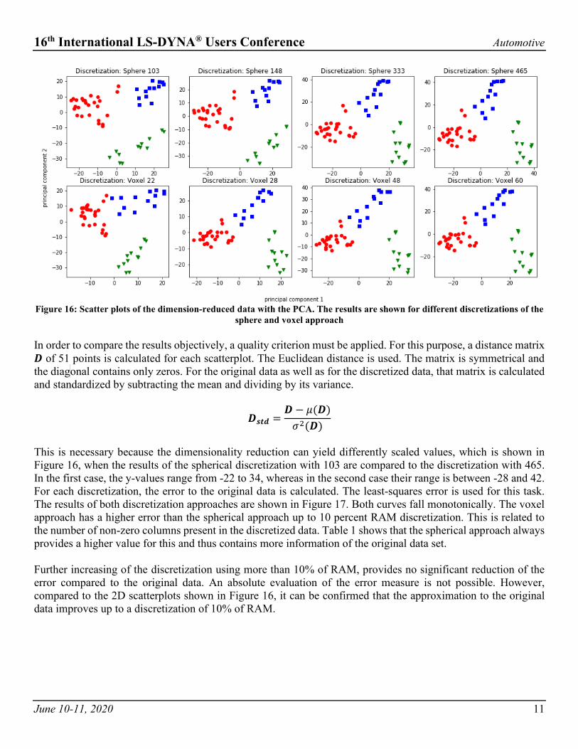
The third criterion for the evaluation of the two approaches is the quality after dimensionality reduction. Again, the longitudinal member with a constant FE-mesh is used for the analysis. This method makes it possible to calculate a dimensionality reduction of the original data and to compare the results with those of the discretized dimension-reduced data. The resulting deviations are to be minimized. Figure 16 shows the results using PCA. The plots in the first row show the scatter plots of the sphere approach, the second row shows those of the voxel method. The individual columns from left to right correspond to the four discretizations from Table 1. The coloring of the points again corresponds to that from Figure 6. At first glance, all eight variants seem to be similar. As with the OPioS-PCA-approach on the undiscretized data, three clusters can be identified, corresponding to the three deformation modes observed in the 51 simulations. In both approaches (sphere, voxel) the circle- and square-clusters can be clearly separated by the PC1-axis. With increasing discretization (d) a small overlap between both clusters occurs. The separation of the triangle-cluster from the rest of the data is only possible for larger d (sphere: starting from 333, voxel: starting from 28). When the PC2-axis is analyzed, a contrary behavior is observed. With increasing d, the separation of the triangle-cluster from the rest of the data gets more difficult. On the other hand, the circle- and square-clusters can be separated more easily with increasing d. From these observations, no recommendation can be delivered for the most appropriate discretization. Therefore, further analysis is needed.
16th International LS-DYNA® Users Conference Automotive
June 10-11, 2020 11
Figure 16: Scatter plots of the dimension-reduced data with the PCA. The results are shown for different discretizations of the
sphere and voxel approach In order to compare the results objectively, a quality criterion must be applied. For this purpose, a distance matrix 𝑫𝑫 of 51 points is calculated for each scatterplot. The Euclidean distance is used. The matrix is symmetrical and the diag onal contains only zeros. For the original data as well as for the discretized data, that matrix is calculated and standardized by subtracting the mean and dividing by its variance.
𝑫𝑫𝒔𝒔𝒔𝒔𝒔𝒔 =𝑫𝑫 − 𝜇𝜇(𝑫𝑫)𝜎𝜎2(𝑫𝑫)
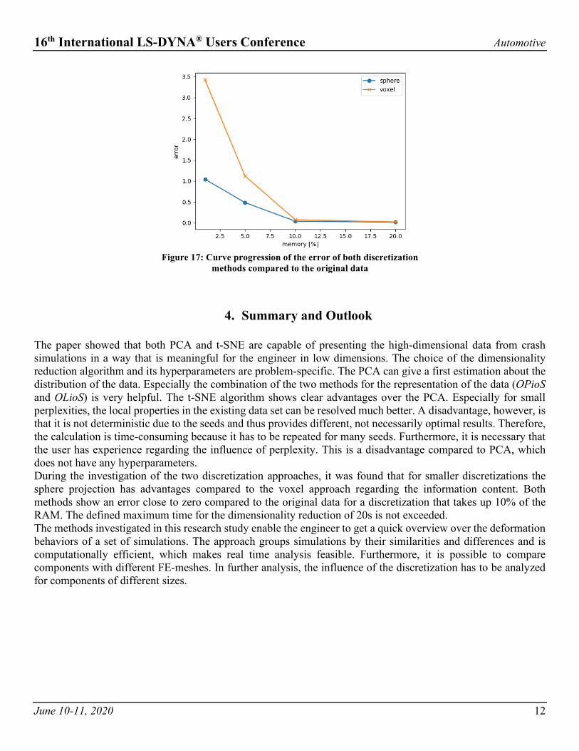
This is necessary because the dimensionality reduction can yield differently scaled values, which is shown in Figure 16, when the results of the spherical discretization with 103 are compared to the discretization with 465. In the first case, the y-values range from -22 to 34, whereas in the second case their range is between -28 and 42. For each discretization, the error to the original data is calculated. The least-squares error is used for this task. The results of both discretization approaches are shown in Figure 17. Both curves fall monotonically. The voxel approach has a higher error than the spherical approach up to 10 percent RAM discretization. This is related to the number of non-zero columns present in the discretized data. Table 1 shows that the spherical approach always provides a higher value for this and thus contains more information of the original data set. Further increasing of the discretization using more than 10% of RAM, provides no significant reduction of the error compared to the original data. An absolute evaluation of the error measure is not possible. However, compared to the 2D scatterplots shown in Figure 16, it can be confirmed that the approximation to the original data improves up to a discretization of 10% of RAM.
16th International LS-DYNA® Users Conference Automotive
June 10-11, 2020 12
4. Summary and Outlook
The paper showed that both PCA and t-SNE are capable of presenting the high-dimensional data from crash simulations in a way that is meaningful for the engineer in low dimensions. The choice of the dimensionality reduction algorithm and its hyperparameters are problem-specific. The PCA can give a first estimation about the distribution of the data. Especially the combination of the two methods for the representation of the data (OPioS and OLioS) is very helpful. The t-SNE algorithm shows clear advantages over the PCA. Especially for small perplexities, the local properties in the existing data set can be resolved much better. A disadvantage, however, is that it is not deterministic due to the seeds and thus provides different, not necessarily optimal results. Therefore, the calculation is time-consuming because it has to be repeated for many seeds. Furthermore, it is necessary that the user has experience regarding the influence of perplexity. This is a disadvantage compared to PCA, which does not have any hyperparameters. During the investigation of the two discretization approaches, it was found that for smaller discretizations the sphere projection has advantages compared to the voxel approach regarding the information content. Both methods show an error close to zero compared to the original data for a discretization that takes up 10% of the RAM. The defined maximum time for the dimensionality reduction of 20s is not exceeded. The methods investigated in this research study enable the engineer to get a quick overview over the deformation behaviors of a set of simulations. The approach groups simulations by their similarities and differences and is computationally efficient, which makes real time analysis feasible. Furthermore, it is possible to compare components with different FE-meshes. In further analysis, the influence of the discretization has to be analyzed for components of different sizes.
Figure 17: Curve progression of the error of both discretization
methods compared to the original data
16th International LS-DYNA® Users Conference Automotive
June 10-11, 2020 13
5. References
[1] Iza-Teran, R., & Garcke, J. (2019). A geometrical method for low-dimensional representations of
simulations. SIAM/ASA Journal on Uncertainty Quantification, 7(2), 472-496. [2] Bohn, B., Garcke, J., Iza-Teran, R., Paprotny, A., Peherstorfer, B., Schepsmeier, U., & Thole, C. A. (2013). Analysis
of car crash simulation data with nonlinear machine learning methods. Procedia Computer Science, 18, 621-630. [3] Teran, R. I. (2014). Enabling the analysis of finite element simulation bundles. International Journal for Uncertainty
Quantification, 4(2). [4] Diez, C., Wieser, C., Harzheim, L., & Schumacher, A. (2016). Automated Generation of Robustness Knowledge for
selected Crash Structures. In Proceedings of 14th LS-DYNA Forum 2016, Bamberg. [5] Wold, S., Esbensen, K., & Geladi, P. (1987). Principal component analysis. Chemometrics and intelligent laboratory
systems, 2(1-3), 37-52. [6] Maaten, L. V. D., & Hinton, G. (2008). Visualizing data using t-SNE. Journal of machine learning research 9
(2008), 2579-2605. [7] Lee, J., & Verleysen, M. (2008). Quality assessment of nonlinear dimensionality reduction based on K-ary
neighborhoods. Proceedings of the Workshop on New Challenges for Feature Selection in Data Mining and Knowledge Discovery at ECML/PKDD 2008, in PMLR 4:21-35
[8] Lee, J. A., & Verleysen, M. (2010). Scale-independent quality criteria for dimensionality reduction. Pattern Recognition Letters, 31(14), 2248-2257.
[9] Spruegel, T., Schröppel, T., & Wartzack, S. (2017). Generic approach to plausibility checks for structural mechanics with deep learning. In: Proceedings of the 21st International Conference on Engineering Design (ICED 17), Vol 1: Resource Sensitive Design, Design Research Applications and Case Studies, Vancouver, Canada, 21-25.08. 2017.
[10] Andricevic, N. (2016). Robustheitsbewertung crashbelasteter Fahrzeugstrukturen (Doctoral dissertation, Albert-Ludwigs-Universität Freiburg).
[11] url: http ://www.euroncap.com/, visited on 13.02.2020 [12] url: https://github.com/lasso-gmbh/lasso-python, visited on 09.03.2020
Related Documents


![NLTE simulations with CRASH code and related issues Fall 2011 Review Igor Sokolov [with Michel Busquet and Marcel Klapisch (ARTEP)]](https://static.cupdf.com/doc/110x72/56649eac5503460f94bb25e2/nlte-simulations-with-crash-code-and-related-issues-fall-2011-review-igor-sokolov.jpg)


