Automated Fish Species Classification using Artificial Neural ...

W&M ScholarWorks W&M ScholarWorks

Dissertations, Theses, and Masters Projects Theses, Dissertations, & Master Projects

2003

Automated Fish Species Classification using Artificial Neural Automated Fish Species Classification using Artificial Neural

Networks and Autonomous Underwater Vehicles Networks and Autonomous Underwater Vehicles

Daniel Foster Doolittle College of William and Mary - Virginia Institute of Marine Science

Follow this and additional works at: https://scholarworks.wm.edu/etd

Part of the Artificial Intelligence and Robotics Commons, Fresh Water Studies Commons,

Oceanography Commons, and the Systems Biology Commons

Recommended Citation Recommended Citation Doolittle, Daniel Foster, "Automated Fish Species Classification using Artificial Neural Networks and Autonomous Underwater Vehicles" (2003). Dissertations, Theses, and Masters Projects. Paper 1539617813. https://dx.doi.org/doi:10.25773/v5-h4xn-2622

This Thesis is brought to you for free and open access by the Theses, Dissertations, & Master Projects at W&M ScholarWorks. It has been accepted for inclusion in Dissertations, Theses, and Masters Projects by an authorized administrator of W&M ScholarWorks. For more information, please contact [email protected].

AUTOMATED FISH SPECIES CLASSIFICATION USING ARTIFICIAL

NEURAL NETWORKS AND AUTONOMOUS UNDERWATER VEHICLES

A Thesis

Presented to

The Faculty of the School of Marine Science

The College of William and Mary in Virginia

In Partial Fulfillment

Of the Requirements for the Degree of

Master of Science

by

Daniel Foster Doolittle

2003

APPROVAL SHEET

This thesis is submitted in partial fulfillment of

The requirements for the degree of

Master of Science

iniel FrDoolittle

Approved, April 2003

Mark R. Patterson, Ph.D. Committee Co-Chair/Co-Advisor

LRoger L. Mann, Ph.D.Committee Co-Chair/Co-Advisor

Herbert M. Austin, Ph.D.

Jesse/E. McNincM, Ph.D.

Zia-ur Rahman, Ph.D. Department of Applied Science College of William and Mary Williamsburg, Virginia

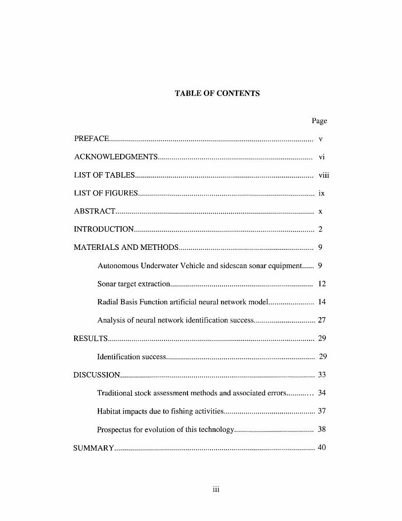
TABLE OF CONTENTS

Page

PREFACE............................................................................................................ v

ACKNOWLEDGMENTS.................................................................................. vi

LIST OF TABLES.............................................................................................. viii

LIST OF FIGURES............................................................................................. ix

ABSTRACT......................................................................................................... x

INTRODUCTION............................................................................................... 2

MATERIALS AND METHODS....................................................................... 9

Autonomous Underwater Vehicle and sidescan sonar equipment 9

Sonar target extraction........................................................................... 12

Radial Basis Function artificial neural network model....................... 14

Analysis of neural network identification success................................ 27

RESULTS............................................................................................................. 29

Identification success............................................................................... 29

DISCUSSION....................................................................................................... 33

Traditional stock assessment methods and associated errors.............. 34

Habitat impacts due to fishing activities................................................ 37

Prospectus for evolution of this technology.......................................... 38

SUMMARY............................................................................................................40

APPENDIX A.........................................................................................................41

APPENDIX B....................................................................................................... 57

APPENDIX C....................................................................................................... 62

APPENDIX D....................................................................................................... 80

APPENDIX E......................................................................................................... 87

LITERATURE CITED.......................................................................................... 94

VITA........................................................................................................................ 104

iv

PREFACE

This thesis manuscript is in review for publication in the American Fisheries Society Symposium Series (number to be determined) entitled Benthic Habitat and the Effects o f Fishing. The body of this thesis therefore follows the style and construction of a journal or book chapter publication. Information important to the thesis, but not suitable for peer review publication due to space constraints and publication costs, have been included in the appendices at the end of the manuscript. The neural network fish classifier software developed during this work is documented in Appendix A. Appendix B is a primer on image processing and describes the steps used during this project to pre- process the sonar data. Image processing algorithms are also presented here. Raw data examples and notes taken from experiences learned in the field are given in Appendix C. This research represents a potential new method to augment traditional fisheries stock assessment. It offers significant advantages over trawl-based population estimation, but is just one method of many. A short introduction to hydroacoustic principals and alternative methods of acoustic species identification and stock assessment are reviewed in Appendix D. While the impetus for this research was to provide a new tool for fisheries management and fisheries research, it cannot be ignored that the remote species classification technology invented here would benefit, among other tasks, homeland defense and harbor security initiatives. Appendix E introduces potential future uses and beneficiaries of this technology.

v

ACKNOWLEDGMENTS

It is difficult to suitably acknowledge the mentorship, support and friendship provided me by my co-advisors Roger Mann and Mark Patterson. Much of this work would be impossible without their patience and belief that funding would eventually occur for my unconventional research topic. It did, and for two years my committee and I have explored the mysteries of neurocomputing, the design and anatomy of autonomous underwater vehicles, the physics of underwater sound and proof that a picture is, through image processing advances, worth a thousand words. It’s notable that these academic adventures occurred at an institution without formal acoustics, underwater engineering, or neural computing departments, yet expertise abounds within the faculty of William and Mary and VIMS. Proving again that interdisciplinary study often yields intellectual products that are more then the sum of their individual components.

This work would not have occurred without my aforementioned committee. Zia ur- Rahman generously tutored me on the basics of digital image processing and the history and practice of neural network design. Jesse McNinch generously gave his time, equipment, funding and acoustical expertise. This was in addition to the friendship and moral support of the entire McNinch family. Herb Austin continually reminded me why I was pursuing this project and that fisheries management is not a lost cause.

I gratefully acknowledge field assistance from Dave Rudders, Kirsten Bassion, Courtney Schuup, Roland Roberson, Joel Hoffman, Eric Brasseur, and Art Trembanis. Live specimens of many fish species were kindly provided for acoustic pen trials by John Olney, Brian Watkins, Jim Goins, and Phil Sadler. Marty Wilcox, Tom Wilcox, and Doug Blaha, of Marine Sonic Technology Ltd. (MSTL), provided technical advice and the loan of sidescan sonar equipment. Don Scott modified MSTL software for our use. Jim Sias, Jim Underwood, Dave Hunt, and Tom Richmond of Sias Patterson Inc., furnished a Fetch-class Autonomous Underwater Vehicle and were a wealth of valuable technical assistance. Mike Meier of the Virginia Marine Resources Commission provided a second Marine Sonic Technology 600 kHz towfish and computer system. Maylon White, Liz Kopecki, and Elizabeth Fichau graciously allowed aquarium access and diving support at the Virginia Marine Science Museum. Wanda Cohen, Harold Burrell, Susan Maples, and Susan Stein provided graphic arts and public relations support.

I owe former Dean of Graduate Studies, Mike Newman a large measure of gratitude for his office’s support during financially lean times. The VIMS Juvenile Trawl Survey, CHESSMAP Trawl Survey, Chris Bonzek, and Pat Geer provided much needed and appreciated workship opportunities over the years.

vi

Jane Lopez, Margaret Fonner, Cindy Forrester, Gail Reardon, Gina Burrell, and Maxine Butler are responsible for keeping so much of this institute functioning smoothly. I thank them all for their unending willingness to assist me with funding, purchasing, travel, and departmental requirements. Susan Rollins, Sharon Miller, and George Pongonis are gratefully acknowledged for their assistance with small vessel operations. Daniel Gouge willingly allowed me to clutter his dive locker and provided hours of enjoyable discussion.

This work would not have been completed without the support, encouragement, and goading of the Bassion and Pertalion families. Kirsten Bassion deserves special mention; I would not be here without her love and confidence.

This research was funded in part by a grant from the National Oceanic and Atmospheric Administration’s (NOAA) Sea Grant Technology Program. Sias Patterson Incorportated, Marine Science Technology, The Virginia Institute of Marine Science and the College of William and Mary provided matching funds to support this research.

LIST OF TABLES

Table Page

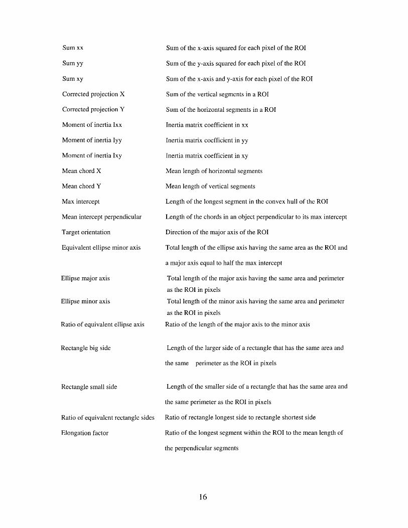
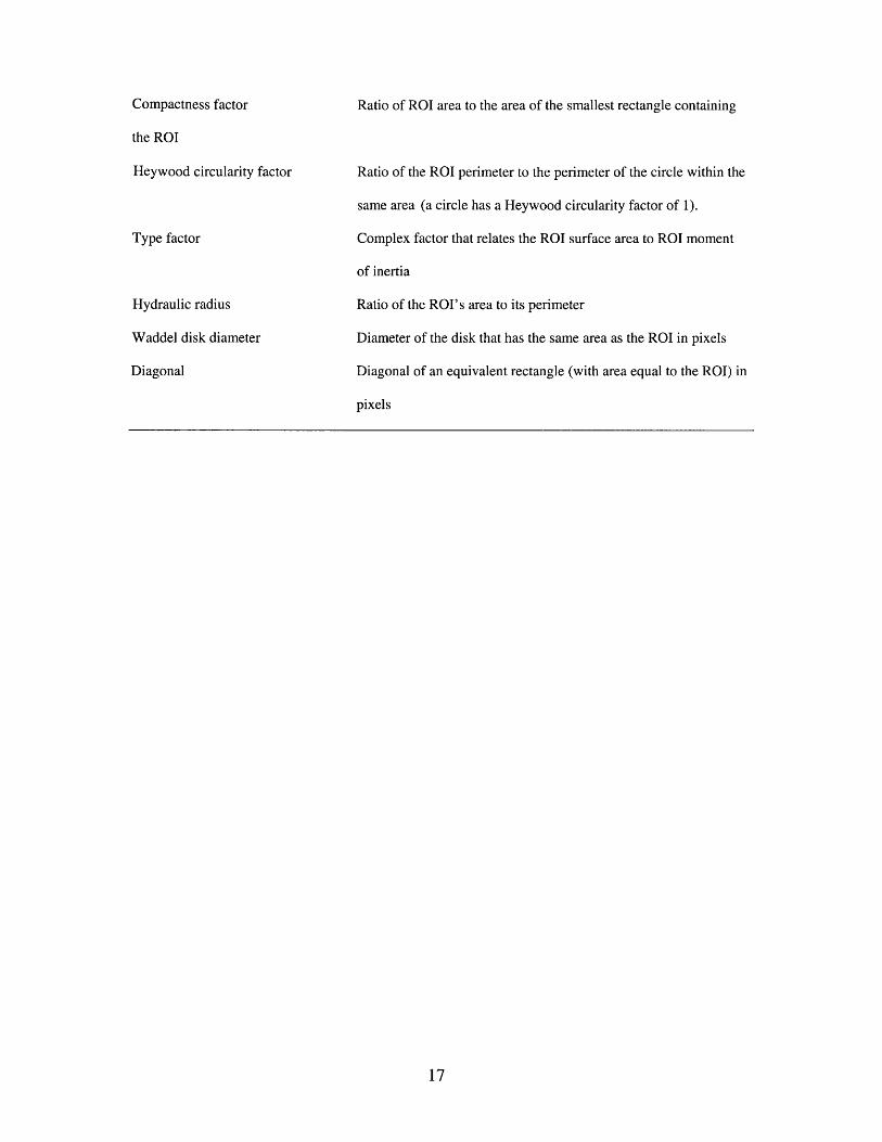
1. Components of the image vector used by the RBF neural net

classifier for species identification.......................................................... 15

2. Results of classification process reported as the percentage of

images correctly classified........................................................................ 31

viii

LIST OF FIGURES

Figure Page

1. Samples of side scan sonar imagery form various frequencies............... 6

2. Sample output of digital sidescan mosaic collected from AUV withassociated navigation and spatial location data......................................... 7

3a. Fetch class AUV in aquarium during collection of ground trutheddata................................................................................................................ 10

3b. Annotated view of AUV detailing sensors and components................... 10

4a. Diagram of monofilament mesh cages used in York River field trials... 11

4b. Image of mesh cage being deployed......................................................... 11

4c. Sample sonar data of fish inside mesh cage.............................................. 11

5. Architecture of a Radial Basis Function artificial neural networkused in this work......................................................................................... 22

6. Schematic diagram of the image classification approach used inthis study..................................................................................................... 23

7. Screen shot of the front panel graphical user interface developedin Lab VIEW and ZDK to process and classify image vector data 24

8. Conceptual flowchart for modification of the weights ofthe RBF neural network........................................................................... 26

9. Conceptual flowchart for the classification process used bythe RBF neural network........................................................................... 28

ABSTRACT

There is a direct link between the quality of fisheries data and the effectiveness of fisheries management. Increasing the quality and quantity of data on which stock assessments and management decisions are based is a critical national issue (National Research Council 2000). I approach this challenge through the creation and demonstration of a novel stock assessment tool. A new method of remote fish species identification and quantification is presented. The technique uses a Radial Basis Function artificial neural network classifier to discriminate and enumerate selected fish species from high-resolution sidescan sonar images. To demonstrate this technology, I have trained the classifier to successfully discriminate sharks (Caracharias taurus) from jacks (Caranx hippos). The classifier achieved a 97 % accuracy level when presented novel images and 100 % accuracy when tested with training images. Additional species can be easily added to the classifier’s library. Data were acquired using a 600 kHz sidescan sonar (Marine Sonic Technology Ltd.) deployed on a Fetch-class Autonomous Underwater Vehicle (AUV) and a conventional towfish. Deployment of the AUV was found to have the following advantages over a towfish: useful images can be gathered by an AUV under rough seas, when the heave in a towfish cable could result in distorted imagery; the AUV was immune to boat electrical noise that produces artifacts in sonar images; and auxiliary sensors (video, CTD, O2, pH) can be used on the AUV to simultaneously characterize the water column and bottom type during surveys. Fish avoidance reactions are also lessened with use of AUVs. Once equipped with analysis tools such as the one presented here, AUVs will provide scientists a new tool to unobtrusively document fish stock behavior and population size, thus yielding data that may help to better tune stock assessment models. I also predict such tools will become valuable in the delineation and characterization of essential fish habitat.

x

AUTOMATED FISH SPECIES CLASSIFICATION USING ARTIFICIAL

NEURAL NETWORKS AND AUTONOMOUS UNDERWATER VEHICLES

INTRODUCTION

Stock assessment is concerned with the prediction of fluctuations, and quantification

of abundance in fish populations. A quantitative understanding of ecological processes is

nearly impossible without accurate estimates of population size or trends (Krebs 1989).

Abundance data also facilitates our understanding of population, community, and

ecosystem dynamics of marine ecosystems (Fogerty and Murawski 1998). Furthermore,

the ability to empirically test ecological hypotheses in the field are constrained by how

accurately population sizes can be determined (Krebs 1989; Gunderson 1993). Fisheries

science practitioners have struggled with generating accurate population estimates for

decades with limited success, as evidenced by the number of stocks listed as overfished

or collapsed altogether (National Research Council 1999). It is important to note that

stock assessment failures are not the only cause for stock collapse or over-fishing. Other

causes include poor enforcement of fishery regulations, mismatches between harvesting

capacity and stock sizes, excessive lags between management changes and fluctuations in

stock sizes, and technological innovations in fish catching operations (Murawski et al.

2000). Although cessation of fishing effort is assumed to allow recovery of depleted fish

populations (Hilborn and Walters 1992), there is evidence that recovery is not guaranteed

even after a period of fifteen years (Hutchings 2000). Timely, accurate stock assessments

are thus vital for effective resource management.

2

The application of new sonar, image processing, and computer technologies that

would allow stock assessment teams and working fishermen to accurately and reliably

discriminate between fish species would be a major step towards solving the problems of

unwanted and wasteful bycatch. Additionally, such technologies would give a more

detailed insight into the composition and size of fish stocks and would likely result in the

reduction of the biases and imprecision that are inherent in trawl surveys, and the

resulting stock assessments (National Research Council 1998).

The development and application of acoustic remote sensing tools have already

produced significant benefits to the marine environment while concurrently assisting

commercial harvesters with reducing their costs. In Nova Scotia, scallop fishermen have

partnered with scientists to create high-resolution multi-beam and sidescan sonar habitat

base maps of the fishing grounds (Molyneaux 2002, Kostylev et al. 1999). These base

maps allow scallop fishermen to target habitats that are likely to produce larger catches,

while reducing the number of hours that their gear is scraping the sea floor. As an

example, one scalloper dredged for 162 hours over 729 nautical miles to harvest a 27,280

pound quota. The next year, armed with habitat base maps, the same scallop vessel

harvested an identical quota in 42 hours and only dredged over 250 nautical miles of

seafloor (Molyneaux 2002).

Although ship-based trawl surveys are arguably the most common method of stock

assessment, reasonable estimates of fish population abundance and distribution can be

found with hydroacoustic techniques (MacLennan and Simmonds 1992) and direct count

methods, such as aerial surveys (McDaniel et al. 2000), SCUBA transects (Ault et al.

1998), camera sleds (Conan and Maynard 1987), and electro-fishing (Kruse et al. 1998).

3

Another survey technique is ichthyoplankton sampling (Phillips and Mason 1986;

Pennington and Berrien 1984), which requires surveying the water column for eggs and

larvae of target species, and then estimating the size of the spawning stock required to

produce the number of larvae or eggs sampled. Gunderson (1993) provides a complete

discussion of these methods of fisheries resource surveys.

Autonomous Underwater Vehicles (AUVs) are currently being developed worldwide

at government, academic, and private research laboratories, with dozens of AUVs already

in operation. Combining AUV technology with high-resolution sidescan sonar should

provide a useful tool for stock assessment and related fisheries questions, including the

delineation of essential fish habitat. This is especially useful in areas that are hard to

sample, such as reef environments or shallow waters. Currently, AUVs are useful tools

for seabed surveys, oceanographic data collection, offshore oil and gas operations, and

military applications (Doolittle 2003, Jones 2002). Data collected from AUVs represent

significant cost savings in terms of reduced personnel hours, 24-hour sampling

capabilities, and reduced surface ship support. Ship-based surveys for offshore pelagic or

demersal fisheries resources can cost anywhere from 10,000 dollars per day for surveys

in northwest Atlantic ocean waters (T. Azarovitz, National Marine Fisheries Service,

Woods Hole, MA. Personal Communication) up to 38,000 dollars per day for Antarctic

fisheries research (Office of Polar Programs, National Science Foundation, personal

communication), excluding salaries of onboard personnel.

Sidescan sonar is an acoustic imaging technology that uses high frequency, ranging

from 100 kHz to 2.4 MHz, focused sound waves to “illuminate” the sea floor and

produce realistic pictures of what lies beneath, and unique to this research, in the water

4

column. As sound waves propagate away from the sidescan transducers, objects in the

path of the beam reflect some of the acoustic energy back to the sonar instrument, and

these signals are then amplified, processed, and passed on to either a display or printer

(Figure 1). The earliest imaging sonar research is credited to the British and Germans

beginning in the 1920s and 1930s, but it suffered from the limitations of analog

technology, namely attenuation of the sonar signal as it traveled along copper wires and

deficiencies with signal display and recording equipment (Fish and Carr 2001). Today,

advances in digital signal processing and increased computational power have largely

overcome these problems. Modern high frequency systems can reliably image objects

that are smaller than 1 cm3 and digital software can “stitch” together sonar records to

make high-resolution, geo-referenced, digital mosaics of the seafloor (Figure 2).

Sidescan sonar proved its capabilities during the 1960s and 1970s as an

indispensable tool to locate wrecks, mines, lost nuclear weapons, and downed submarines

and aircraft. The petroleum industry pioneered the commercial use of sidescan sonar for

pipeline routing and inspection in the 1970s and 1980s as offshore drilling became

popular (Fish and Carr 1990). As the 1990s progressed, sidescan sonars became

available in higher and higher frequencies allowing significant advances in image

resolution. With increased resolving power, sidescan sonar has been used to map and

classify marine fisheries habitats (McRea et al. 1999; Edsall et al. 1993), detect and

enumerate salmon during their upstream migrations (Trevorrow 1998, 2001), investigate

trawl damage to marine habitat (Friedlander et al. 1999), and map relic oyster reefs in

turbid, low visibility environments (DeAlteris 1988).

5

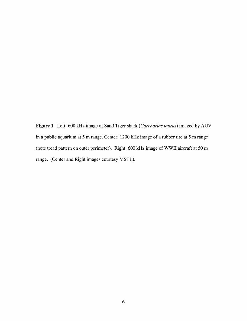
Figure 1. Left: 600 kHz image of Sand Tiger shark (Carcharias taurus) imaged by AUV

in a public aquarium at 5 m range. Center: 1200 kHz image of a rubber tire at 5 m range

(note tread pattern on outer perimeter). Right: 600 kHz image of WWII aircraft at 50 m

range. (Center and Right images courtesy MSTL).

6

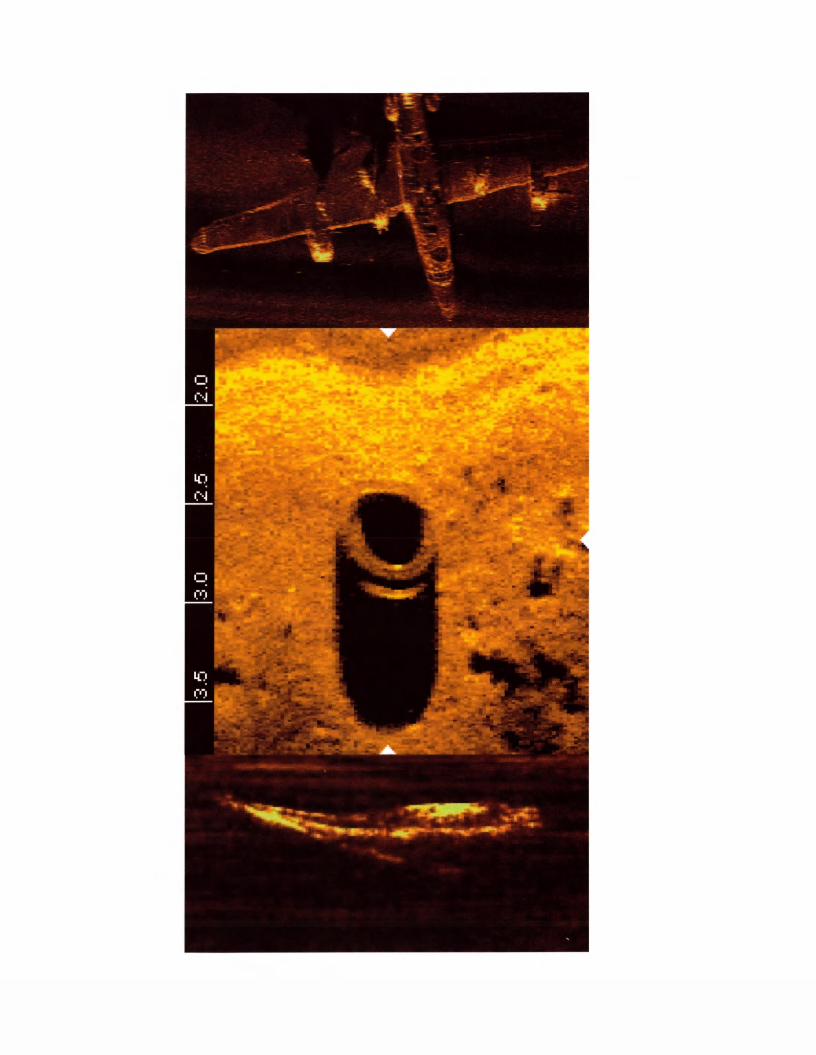
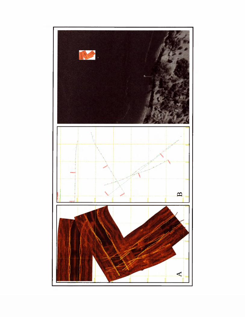
Figure 2. A. Sample output of a digital sidescan mosaic, gathered by an AUV at 2.2 kt

(1.1 m/s) in depth-following mode (2.5 m depth, water column 5.5 m deep). B.

Navigation track lines interpolated by the mosaicking software, Sonar Web Pro

(Chesapeake Technology). C. Geo-reference mosaic shown on aerial photo of the York

River, Virginia (37° 13.61' North, 76° 29.25’ West), where these data were gathered.

7

Given that individual fish (Treverrow 2000) and fish shoals (O’Driscoll and

McClatchie 1998) can be discerned from modern sidescan imagery, we believe that

significant progress can be made using sidescan sonar coupled with novel image

processing algorithms to automatically classify and enumerate individual fish, with the

goal of augmenting traditional stock assessment.

The processing algorithms introduced here include a Radial Basis Function (RBF)

neural network classifier that can recognize individual fish. The goals of the study were

to (1) successfully integrate sidescan sonar into an AUV and use it to image fish in the

wild, in underwater pens, and public aquaria, (2) develop image extraction and

classification algorithms capable of robustly distinguishing two species of fish from one

another to demonstrate proof-of-concept, and (3) identify steps necessary for the

automation and integration of the classifier algorithms into the AUV control software for

future adaptive sampling needs, for example, re-sampling or following a fish school.

MATERIALS AND METHODS

Autonomous Underwater Vehicle and sidescan sonar equipment

A Fetch-class AUV (Sias Patterson, Inc.; Patterson 1998, Patterson and Sias 1998,

1999) equipped with a 600 kHz sidescan sonar (Marine Sonics Technology, Ltd.) was

used to acquire ground-truthed sonar images of fishes from the Virginia Marine Science

Museum (Figure 3) and from test pens (Figure 4) placed in the York River, Virginia, a

sub-estuary of the Chesapeake Bay. In the river, range settings of 5, 10, and 20 m, with a

5 m range delay were used, and in the aquarium, 5 or 10 m with no range delay were

used. A range delay of 5 m combined with a 10 m range setting was used most

frequently in the field, as it provided a good compromise between acoustic resolution and

area surveyed. The focal point of our particular transducer geometry was approximately

10 m (M. Wilcox, Marine Sonic Technology Limited, White Marsh, VA. personal

communication). Fixed gain settings were found to be ineffective for image collection in

dynamic environments. We enabled MSTL Host-Remote commands onboard the AUV

to ensure automatic setting of the time varying gain (TVG) levels using a fuzzy-logic

based algorithm (Scott and Wilcox 1998).

The AUV collected data on natural fish abundance and fish avoidance behavior on

several occasions, surveying a shallow tidal creek (Sarah Creek, York River, VA. 37°

15.29’ N. 76° 28.84’ W. 1- 4 m depth), and the lower York River itself (37° 14.20’ N. 76°

9

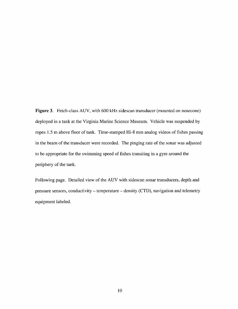
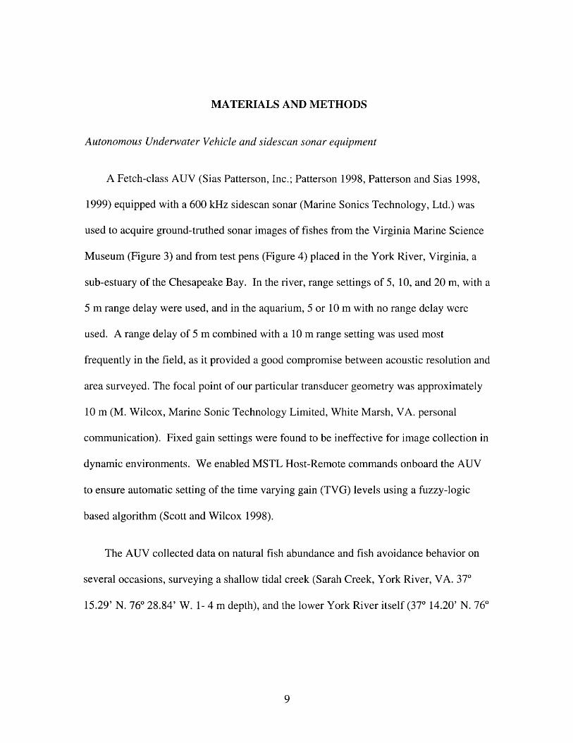
Figure 3. Fetch-class AUV, with 600 kHz sidescan transducer (mounted on nosecone)

deployed in a tank at the Virginia Marine Science Museum. Vehicle was suspended by

ropes 1.5 m above floor of tank. Time-stamped Hi-8 mm analog videos of fishes passing

in the beam of the transducer were recorded. The pinging rate of the sonar was adjusted

to be appropriate for the swimming speed of fishes transiting in a gyre around the

periphery of the tank.

Following page. Detailed view of the AUV with sidescan sonar transducers, depth and

pressure sensors, conductivity - temperature - density (CTD), navigation and telemetry

equipment labeled.

10

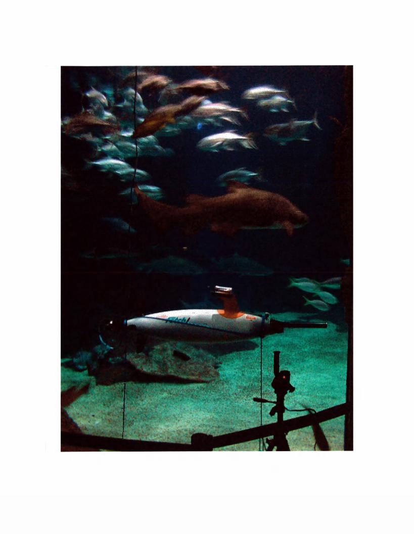
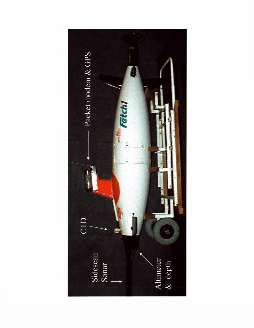
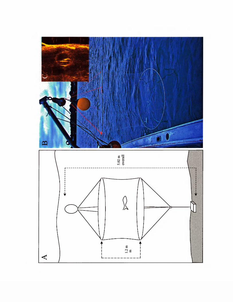
Figure 4. A. Diagram of circular mesh and hoop cage used to confine fishes during

groundtruthing of the sidescan sonar in the York River, Virginia. Cage is 1.2 m (3.9 ft)

high and hoops are 1.53 m (5 ft) in diameter with 2.5 cm (lin) square mesh monofilament

netting stretched around them. A 49.9 kg (110 lb) weight was used to anchor the pen to

the river floor while a 35 cm diameter (14 in) plastic buoy was tethered just below the

river surface. The buoy provided 15 kg (33 lbs) of buoyancy and served to keep the mesh

cage from collapsing in the river current. B. Image of mesh pen being deployed from a

small 7.9 m (26 ft) vessel. C. Sample 600 kHz sidescan sonar image (range 10 m) of net

pen with an encaged 71.2 cm (28 in) striped bass (Morone saxatilis).

11

28.00’ W. 2 - 25 m depth). This latter survey occurred in conjunction with sampling by a

Virginia Institute of Marine Science (VIMS) research vessel conducting a fisheries stock

assessment trawl. Additional sonar images were acquired with a similar 600 kHz towfish

and topside computer system deployed from a VIMS Garvey class, small vessel.

During the sampling in the aquarium, we discovered sources of noise and crosstalk

in the recorded sidescan images that were corrected in later field deployments. These

corrections included isolating and eliminating sources of common-mode noise inside the

AUV (filtering the switching power supplies to eliminate a power supply harmonic at 600

kHz), eliminating a five degree starboard roll in the AUV in order to produce a more

uniform sonar image on both channels, tilting the sonar transducers down five degrees

from the horizontal to reduce cross-talk between the sensors, and installing a barium-

loaded vinyl sheeting underneath each transducer to further eliminate transducer cross­

talk.

Sonar target extraction

Raw sidescan images were exported from the sonar collection software (Seascan

PC, Marine Sonic Technology Ltd.) as Tagged Image File Format (TIFF) files. The

image files were 1024 lines by 500 pixels wide, and a time-stamp marking each ping

return line (corresponding to a horizontal row of pixels) was also saved by using a

customized TIFF field. Lab VIEW 6.1 with IMAQ Vision 6.0 (National Instruments)

was used to develop extraction algorithms that separated regions of interest (ROIs) from

unwanted targets in the remainder of the image. For this project, ROIs are those regions

12

first bottom return, and the air-water interface. The extraction algorithm performed the

following image transformations: rotation, image masking, color plane extraction,

histogram creation, and basic and advanced morphological operations. These steps are

briefly expanded below. Each image was first rotated from the dimensions of 1024 by

500 pixels to 500 by 1024 pixels to return the image to the dimensions under which it

was originally collected. This step was required to maintain the proper aspect ratio of

each sonar target. Next, if the image containing the ROI exceeded a window size of 220

pixels by 220 pixels (as most of the shark images did), an image mask was created

around the ROI, thus isolating it from the background. The red color plane was then

extracted from the red, green, blue (RGB) TIFF image to allow the calculation of a pixel

intensity histogram. Once length, width, area, and mean pixel intensity values were

calculated, a threshold operator was applied, followed by a dilation and/or erosion

operation, in order to remove any spurious pixels from the frame before particle analysis

operators were invoked. Some images required further morphological operators to be

applied. This was warranted when some artifact of the original sonar image, such as the

air - water interface, was corrupting the bounding box surrounding the ROI. When this

occurred, a morphological operator that removes pixels touching the borders of the

bounding box was applied. Particle analysis was then performed on the extracted ROIs,

using algorithms already available in IMAQ Vision.

Metrics extracted by this procedure are listed in Table 1. All data were not collected

at the same range settings. Therefore affine transformations were performed on metrics

when appropriate to provide dimensional similarity in the resulting data sets, to ensure all

13

images used for training and classification by the neural network showed all objects

at the same size.

Radial Basis Function artificial neural network model

Artificial neural networks (ANNs) are computational models that are inspired by

advances in neuroscience and neurobiology. Essentially, a neural network is composed

of many simple processors, called units or nodes, organized into layers that may possess

discreet amounts of local memory. Each of these layers and individual units are

connected to each other and carry various sorts of numerical data. Each unit processes

and passes on, or halts, the data that it receives from other units or layers. From a

biological model, each node or unit is similar to a neuron and the connections between

units are similar to synapses. It is important to note that artificial neural networks take

their design from biological models but do not attempt to replicate real neural

connections. Neural networks were first reported in the early 1940s and have sustained

periods of great popularity in the 1980s (Werbos 1994), and again more recently. Much

of the current popularity is due in part to advances in desktop computing and the

availability of numerous robust ANN models.

We identified the Radial Basis Function (RBF) model as the best candidate for

classification of sidescan sonar imagery. RBF networks offer the advantages of high

levels of noise immunity (Li and Leiss 2001) and a great ability in solving complex, non­

linear problems in the fields of speech and pattern recognition, robotics, real time signal

analysis and other areas dominated by non-linear processes.

14

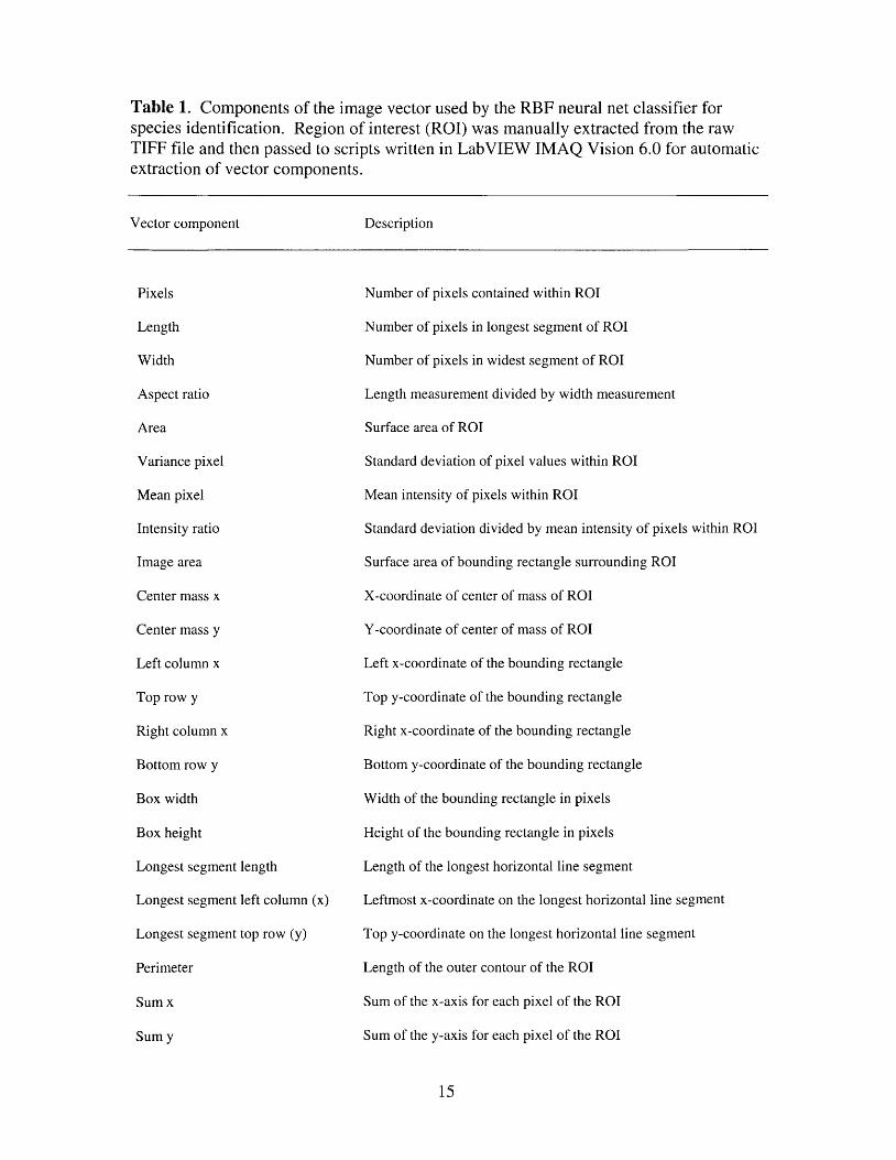
Table 1. Components of the image vector used by the RBF neural net classifier for species identification. Region of interest (ROI) was manually extracted from the raw TIFF file and then passed to scripts written in Lab VIEW IMAQ Vision 6.0 for automatic extraction of vector components.

Vector component Description

Pixels

Length

Width

Aspect ratio

Area

Variance pixel

Mean pixel

Intensity ratio

Image area

Center mass x

Center mass y

Left column x

Top row y

Right column x

Bottom row y

Box width

Box height

Longest segment length

Longest segment left column (x)

Longest segment top row (y)

Perimeter

Sum x

Sum y

Number of pixels contained within ROI

Number of pixels in longest segment of ROI

Number of pixels in widest segment of ROI

Length measurement divided by width measurement

Surface area of ROI

Standard deviation of pixel values within ROI

Mean intensity of pixels within ROI

Standard deviation divided by mean intensity of pixels within ROI

Surface area of bounding rectangle surrounding ROI

X-coordinate of center of mass of ROI

Y-coordinate of center of mass of ROI

Left x-coordinate of the bounding rectangle

Top y-coordinate of the bounding rectangle

Right x-coordinate of the bounding rectangle

Bottom y-coordinate of the bounding rectangle

Width of the bounding rectangle in pixels

Height of the bounding rectangle in pixels

Length of the longest horizontal line segment

Leftmost x-coordinate on the longest horizontal line segment

Top y-coordinate on the longest horizontal line segment

Length of the outer contour of the ROI

Sum of the x-axis for each pixel of the ROI

Sum of the y-axis for each pixel of the ROI

15

Sum xx

Sum yy

Sum xy

Corrected projection X

Corrected projection Y

Moment of inertia Ixx

Moment of inertia Iyy

Moment of inertia Ixy

Mean chord X

Mean chord Y

Max intercept

Mean intercept perpendicular

Target orientation

Equivalent ellipse minor axis

Ellipse major axis

Ellipse minor axis

Ratio of equivalent ellipse axis

Rectangle big side

Rectangle small side

Ratio of equivalent rectangle sides

Elongation factor

Sum of the x-axis squared for each pixel of the ROI

Sum of the y-axis squared for each pixel o f the ROI

Sum of the x-axis and y-axis for each pixel of the ROI

Sum of the vertical segments in a ROI

Sum of the horizontal segments in a ROI

Inertia matrix coefficient in xx

Inertia matrix coefficient in yy

Inertia matrix coefficient in xy

Mean length of horizontal segments

Mean length of vertical segments

Length of the longest segment in the convex hull of the ROI

Length of the chords in an object perpendicular to its max intercept

Direction of the major axis of the ROI

Total length of the ellipse axis having the same area as the ROI and

a major axis equal to half the max intercept

Total length of the major axis having the same area and perimeter

as the ROI in pixels

Total length of the minor axis having the same area and perimeter

as the ROI in pixels

Ratio of the length of the major axis to the minor axis

Length of the larger side of a rectangle that has the same area and

the same perimeter as the ROI in pixels

Length of the smaller side of a rectangle that has the same area and

the same perimeter as the ROI in pixels

Ratio of rectangle longest side to rectangle shortest side

Ratio of the longest segment within the ROI to the mean length of

the perpendicular segments

16

Compactness factor

the ROI

Heywood circularity factor

Type factor

Hydraulic radius

Waddel disk diameter

Diagonal

Ratio of ROI area to the area of the smallest rectangle containing

Ratio of the ROI perimeter to the perimeter of the circle within the

same area (a circle has a Heywood circularity factor of 1).

Complex factor that relates the ROI surface area to ROI moment

of inertia

Ratio of the ROI’s area to its perimeter

Diameter of the disk that has the same area as the ROI in pixels

Diagonal of an equivalent rectangle (with area equal to the ROI) in

pixels

17

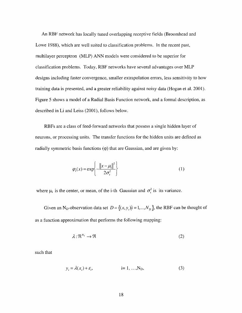
An RBF network has locally tuned overlapping receptive fields (Broomhead and

Lowe 1988), which are well suited to classification problems. In the recent past,

multilayer perceptron (MLP) ANN models were considered to be superior for

classification problems. Today, RBF networks have several advantages over MLP

designs including faster convergence, smaller extrapolation errors, less sensitivity to how

training data is presented, and a greater reliability against noisy data (Hogan et al. 2001).

Figure 5 shows a model of a Radial Basis Function network, and a formal description, as

described in Li and Leiss (2001), follows below.

RBFs are a class of feed-forward networks that possess a single hidden layer of

neurons, or processing units. The transfer functions for the hidden units are defined as

radially symmetric basis functions (cp) that are Gaussian, and are given by:

where pi is the center, or mean, of the i-th Gaussian and of is its variance.

Given an No-observation data set D = {(x,y;)|/ = 1,...,ND}, the RBF can be thought of

as a function approximation that performs the following mapping:

( 1)

(2)

such that

y i = A(xl) + ei, i= 1, ...,No, (3)

18

where X is the regression function, the error term Ej is a zero-mean random variable of

perturbation, Ni is the dimension of the input space, and x; and y;, are the i-th components

of the input and output vectors, respectively.

Each unit in the hidden layer of the RBF forms a localized receptive field in the

input space X that has a centroid located at c, and whose width is determined by the

variance a of the Gaussian equation. This allows a smooth interpolation over the total

input space. Therefore, unit i gives a maximal response for input stimuli close to q. The

hidden layer then performs a nonlinear vector-valued mapping (J) from the input space X

to an Ne-dimensional “hidden” space O {0(x.)|i = 1,...,A D},

Each nonlinear basis function (J)(x) is then defined by some radial basis function (p

<f>(x): <R N‘ (4)

where

(f){x) = [(^(x),...,^ (x) \ i s an Nh dimensional vector.

(5)

where IIJI is the Euclidean norm on 9iw' .

19

Finally, the output layer performs a linear combination of the nonlinear basis

A

function (j)i to generate the function approximation by X :

X (x,D) = Y j wi</>i(x). (6)/=i

The overall scheme of the procedure is shown in Figure 6. We used an

implementation of a RBF model in the LabVIEW-based software package ZDK (General

Vision) to map image vectors to three outputs: jack, shark, or not jack or shark (Figure 7).

The image vector data extracted by the Lab VIEW IMAQ Vision algorithms are stored in

an Excel spreadsheet and imported into the ZDK-based recognition engine. Image vector

components are automatically scaled to 8-bit resolution, to comply with ZDK input

requirements.

Influence fields are important features of the learning process of the ZDK RBF

neural network and are defined here in order to more clearly describe the subsequent

learning and recognition tasks. The Active Influence Field (AIF) of a neuron describes

the area around the stored prototype (or the variance around the Gaussian center in the

RBF model described earlier). The AIF of a neuron is automatically adjusted as new

vectors are introduced during network training. The Maximum Influence Field (MAF)

defines the largest influence field value that can be assigned to one neuron, while the

Minimum Influence Field (MIF) defines the smallest influence field value when a

reduction in the AIF occurs during the learning of a new prototype (Silicon Recognition

2002). When a neuron’s AIF is reduced and limited to this value, the neuron prototype

lies very near the boundary of its category space and is likely to be overlapped by another

20

category space. When this happens, the neuron is considered to be “degenerated” and is

flagged for removal from the network.

21

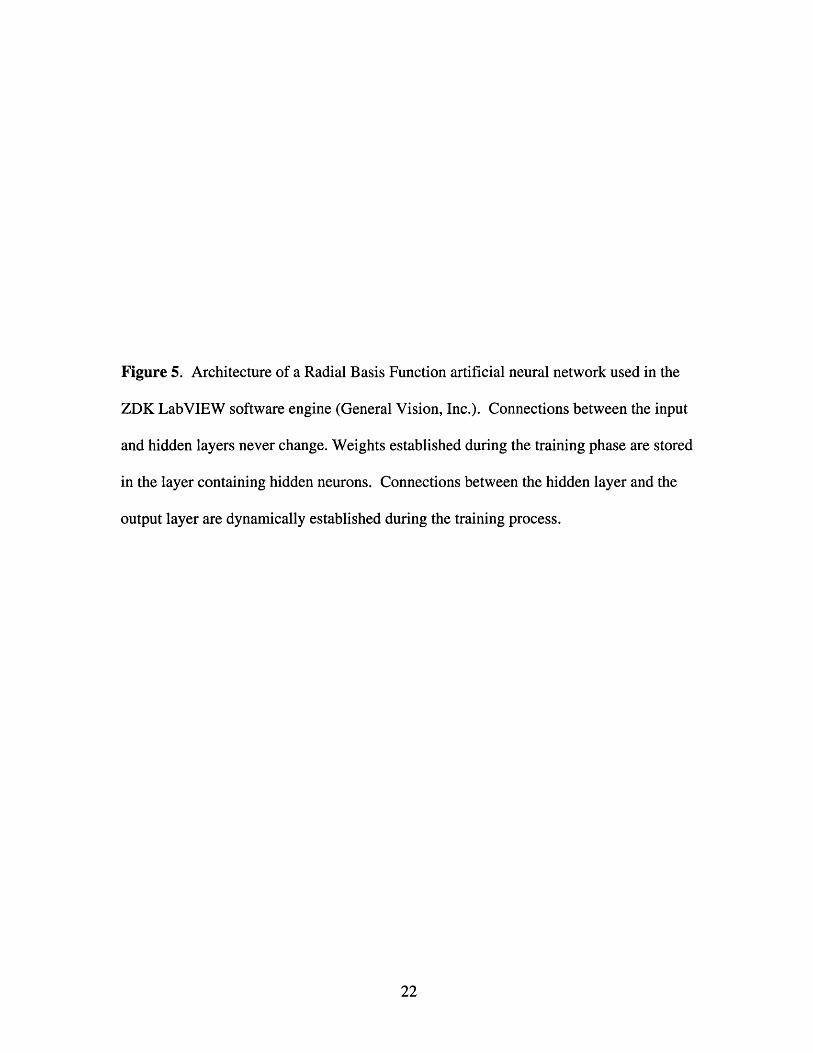
Figure 5. Architecture of a Radial Basis Function artificial neural network used in the

ZDK Lab VIEW software engine (General Vision, Inc.). Connections between the input

and hidden layers never change. Weights established during the training phase are stored

in the layer containing hidden neurons. Connections between the hidden layer and the

output layer are dynamically established during the training process.

22

outputlayer

hiddenneurons ' I*'.: »•,

inputs X,

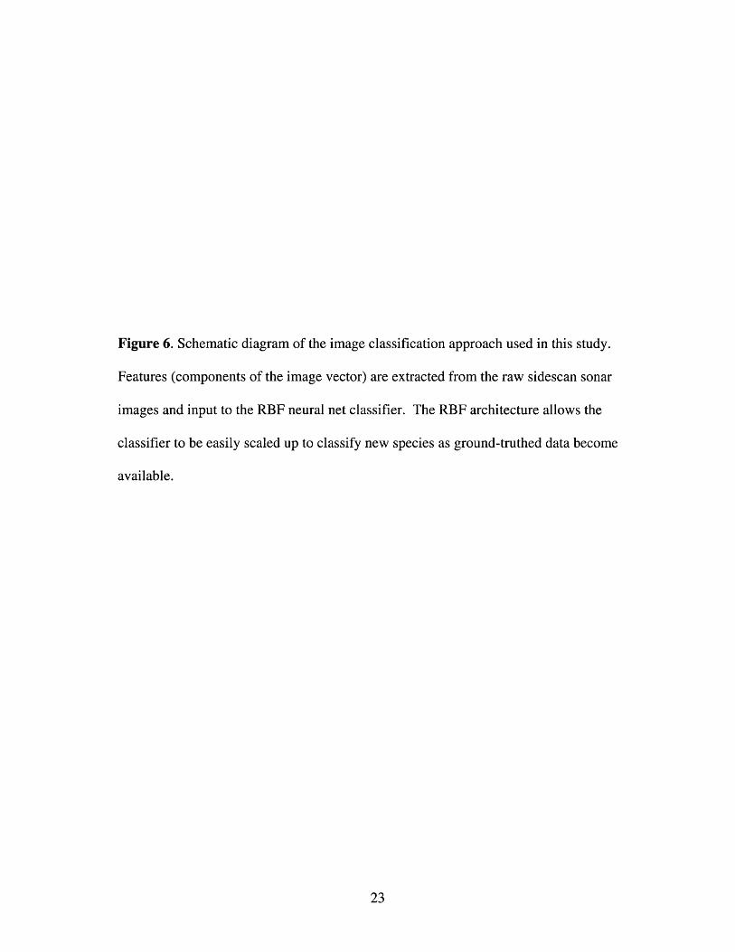
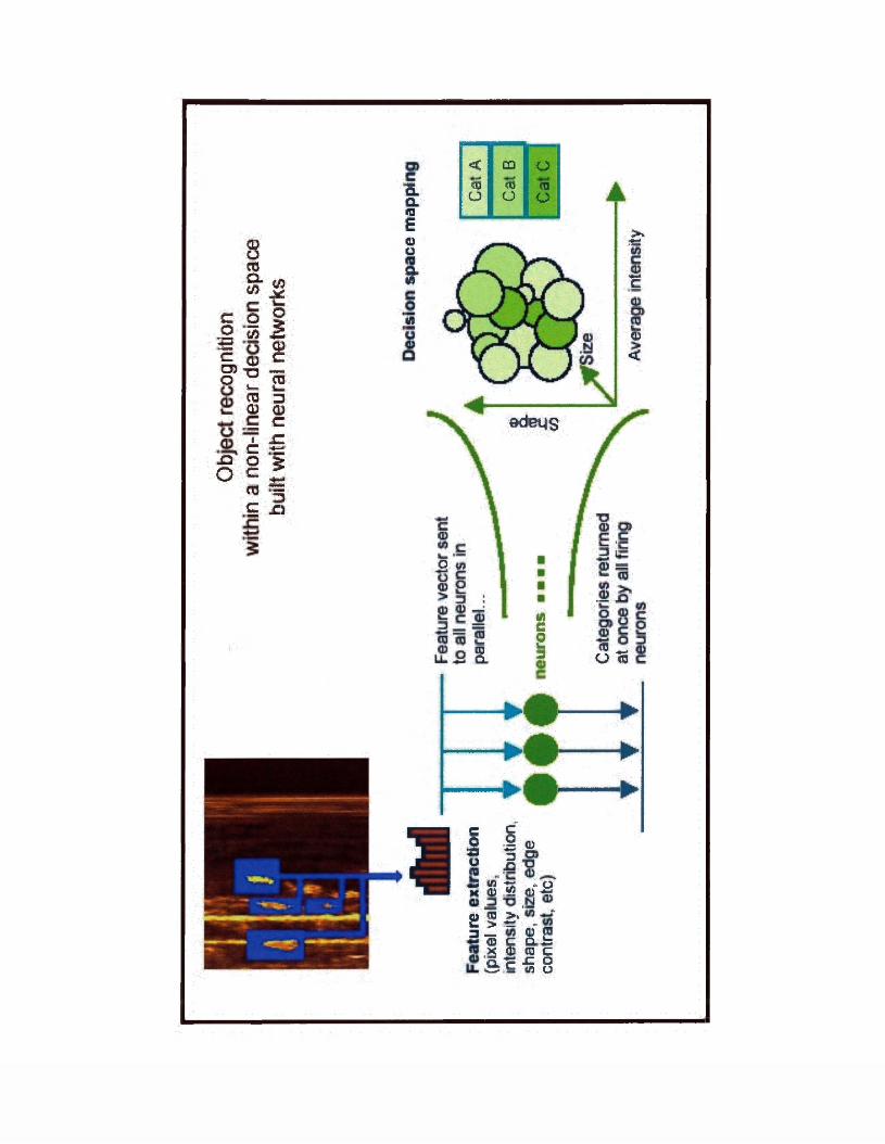
Figure 6. Schematic diagram of the image classification approach used in this study.

Features (components of the image vector) are extracted from the raw sidescan sonar

images and input to the RBF neural net classifier. The RBF architecture allows the

classifier to be easily scaled up to classify new species as ground-truthed data become

available.

23

8JOS-«(A jg

c o 2 .2 S3 J

8

■a.a<o£Vo

8-

< CD o<6 CO CDo a a

OSc ^ _CJ3 Tn *—io ^ «

40

03 _<D CD

iJ2J OO c

os C f j

3CDC

x :4 - J

5■jjjg'5

> irti

I

c3<

q a?

i

edBMS

8I

1

1 I . o 3 ~z £>*3 w -5; * ax <d .52 <u ^5

2 5 £ “3a c &Sx 53 cd c K ? -C OiJs.fe <n U

<D O ^

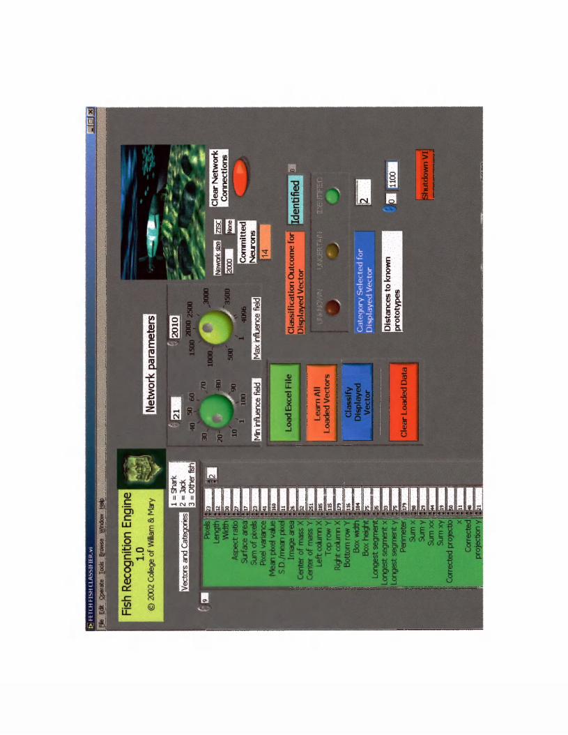
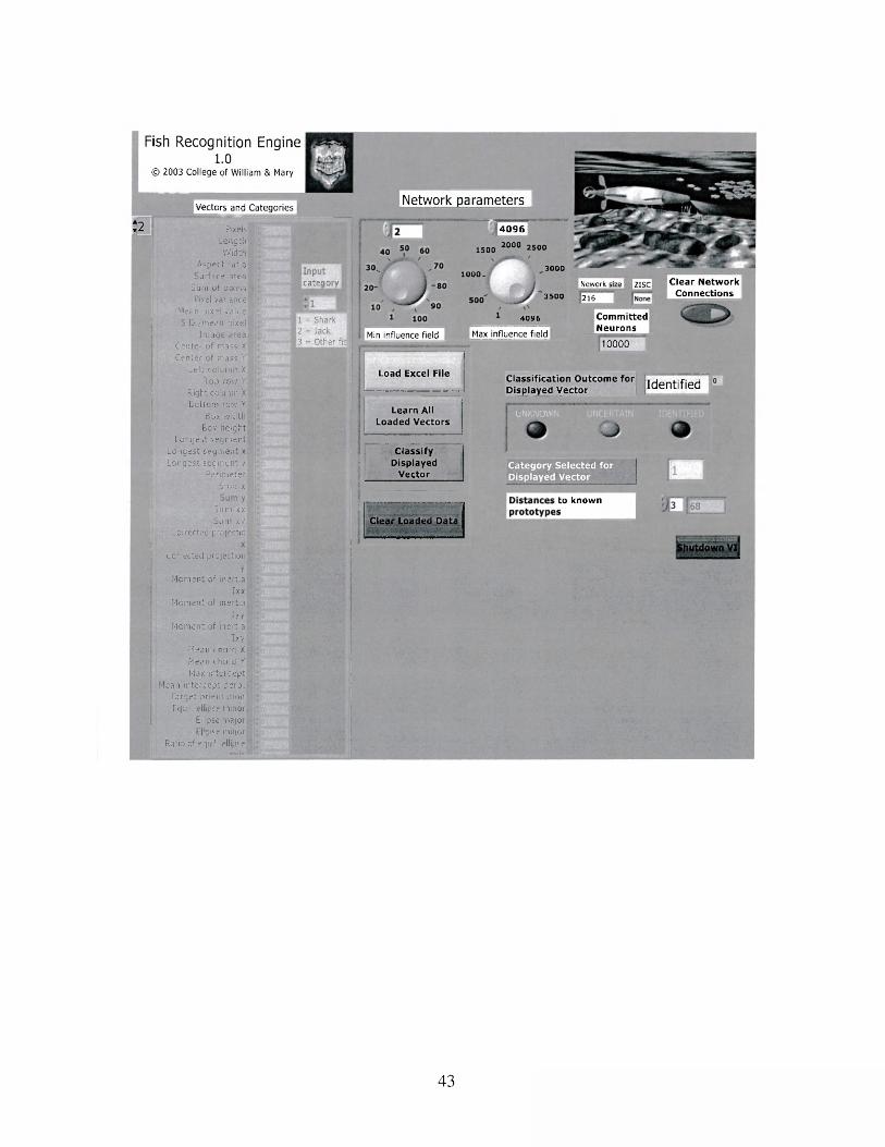
Figure 7. Screen shot of the front panel graphical user interface developed in Lab VIEW

and ZDK to process and classify image vector data. Vectors are imported in from an

comma separated (csv) spreadsheet, and scaled to 8 bits before processing.

24

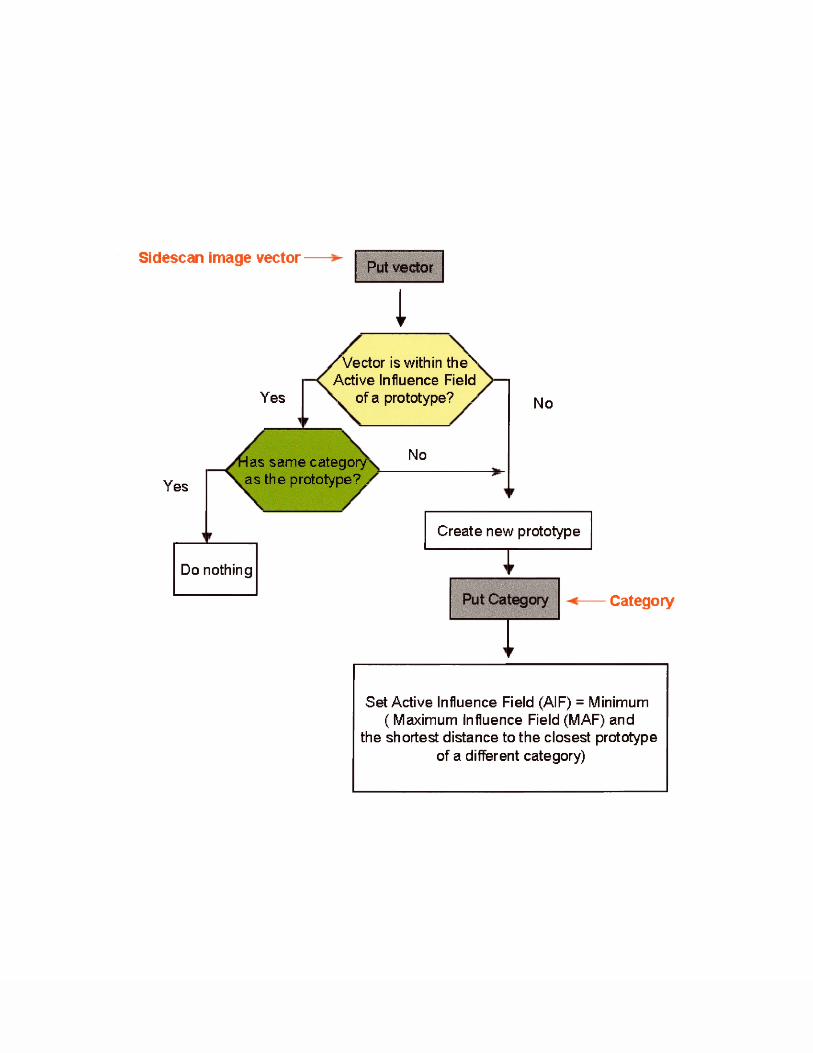
A learning process is required to train the neurons with prototype, or ground-truthed

sidescan sonar images. The learning process can result in the following actions:

(1) if the presented vector is not within the influence field of any

prototypes already stored in the network, then a new neuron is

committed to that vector;

(2) if the input vector falls within the influence field of an already

learned vector, no change is made to the network connections or

influence fields;

(3) if the input vector falls within the wrong influence field, or is

mismatched to its category, then one or more influence fields are

readjusted. Adjustment of the influence field occurs at the MAF or

the MIF. If the MIF is adjusted to a minimum threshold level it is

considered a “degraded” neuron and is subsequently flagged for

removal. This process is graphically illustrated in Figure 8.

Once the network has been trained with prototypes or ground-truthed imagery, it is

ready to perform recognition tasks on previously unseen data. Formally, classification

consists of evaluating whether an N-dimensional input vector lies within the AIF of any

prototype in the network. If the vector is not within any AIF in the network it is

classified as not recognized. If the vector is within an AIF, the input is recognized as

belonging to that AIF’s corresponding category. If the input vector lies within two or

more prototype’s AIF that are assigned to two different categories, then the input is coded

25

Figure 8. Conceptual flowchart for modification of the weights of the RBF ANN by new

prototypes, i.e., new training image vectors. Adapted from General Vision (2001).

26

Sidescan image vectorPut vector

l/V ector is within the^ Active Influence Field S. of a prototype? >Yes No

NoHas sam e category as the prototype?,Yes

Category

Do nothing

Create new prototype

Set Active Influence Field (AIF) = Minimum ( Maximum Influence Field (MAF) and

the shortest distance to the closest prototype of a different category)

as "recognized but not formally identified." The classification process is shown in

Figure 9.

Analysis o f Neural Network Identification Success

The reliability and performance of any neural network model is dependent upon

the selection and available amount of training data, associated weights, and selection of

correct input vectors. Neural network accuracy (percentage of correct classifications)

will be the primary evaluation criteria. If the neural network is unable to satisfactorily

classify the sonar data it is given, then more vectors will need to be learned by the

network and new prototypes (or training examples) will be added to the neural network

model. If additional training input data is not sufficient to yield high percentages of

correct classifications, then the model may be then cleared and rebuilt using the same

input vectors but adjusting the influence fields. If new influence field settings will not

yield satisfactory results, then selection of new input vectors will be required. Evaluation

of each network was accomplished with the cross validation technique known as a Leave

One Out (LOO) method (Hogan et al. 2001). This technique takes N patterns or images

and uses N-l for training and 1 for testing over N iterations.

27

Figure 9. Conceptual flowchart for the classification process used by the RBF ANN,

when presented with new data Adapted from General Vision (2001).

28

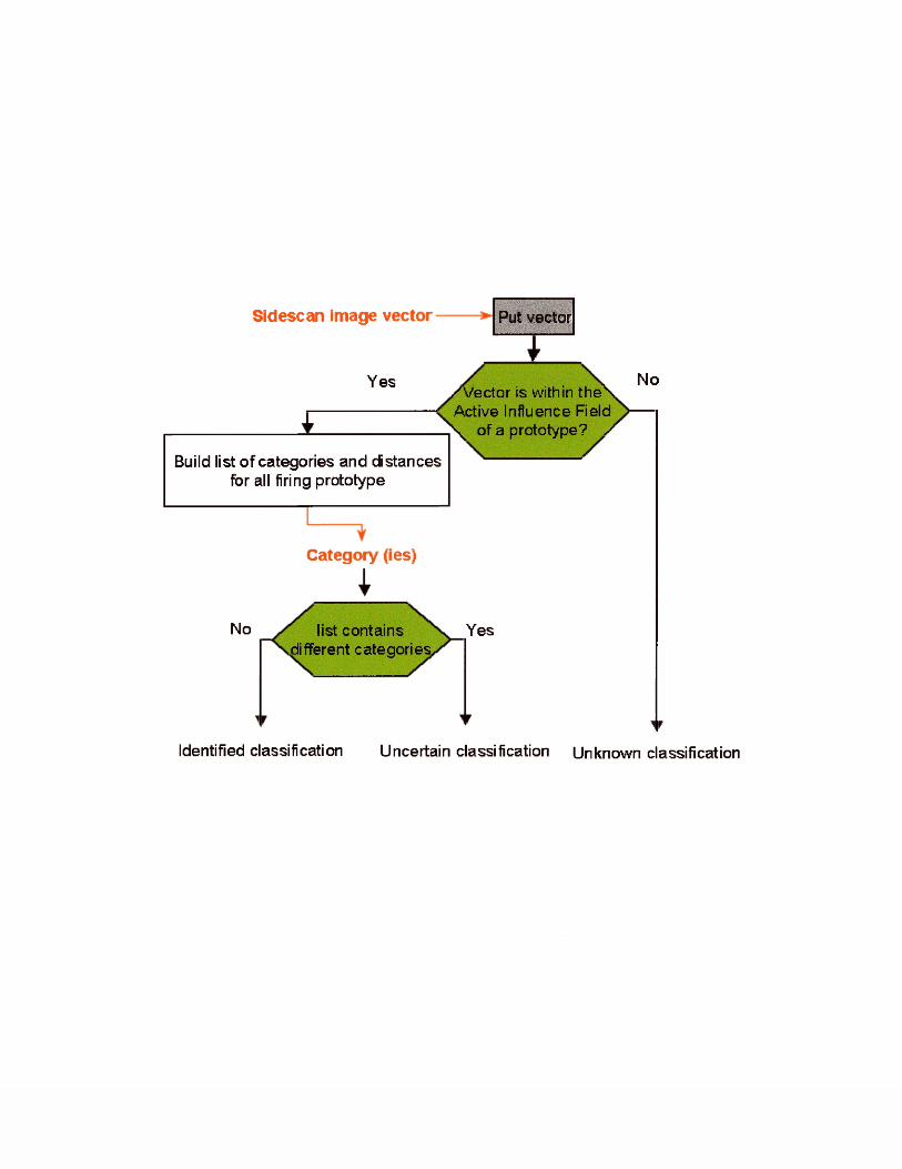
Sidescan image vector Put vector

NoY es/V ector is within t h e \ Active Influence Field \ of a prototype? /

Build list o f categories and distances for all firing prototype

Category (ies)

No list contains different categories,

Yes

Identified classification Uncertain classification Unknown classification

RESULTS

Identification success

Table 2 shows the results of classifying thirty-three novel images. Twelve of these

images were of sand tiger sharks, fourteen of crevalle jack, and seven of fish that were

not sharks or jacks. Non-shark or jack test data included sonar images of barracuda

(■Sphyraena guachancho), spadefish (Chaetodipterus faber), tarpon {Megalops

atlanticus), and cobia (Rachycentron canadum). The overall success of the most

successful network ranged from 90.1 % to 97.0 % with one image being incorrectly

classified and two images classified correctly but with uncertainty. The success of the

classifier on all training images was 100 %. Following Nelson and Illingworth (1991), we

deem our classifier successfully trained because we achieved 100% classification

accuracy on the training images and an acceptably high (90.1 % to 97.0 %) accuracy

level with novel images. The goal is to classify a putative target at some predetermined

successful percentage rate, using the fewest number of classification metrics in the

prototype (training) and test images. In other words, the image vector should contain

enough information to successfully classify the target.

Surveys in the field revealed that the AUV can easily count individual fishes, even in

schools, if the range setting is kept to 10 m or 5 m. When the AUV passed through a

school of fish, turning motions of the school away from the AUV were minimal, even

when the vehicle was within 2 m of the targets. Furthermore, the AUV imaged abundant

29

putative fish targets in the water column in the York River when surveying over 2.5

nautical miles of this habitat in depth-following mode, swimming 3 m deep, while a

simultaneous trawl by a 65' research vessel caught no fish.

30

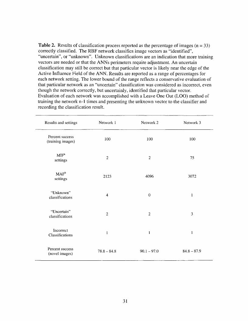
Table 2. Results of classification process reported as the percentage of images (n = 33) correctly classified. The RBF network classifies image vectors as “identified”, “uncertain”, or “unknown”. Unknown classifications are an indication that more training vectors are needed or that the ANNs perimeters require adjustment. An uncertain classification may still be correct but that particular vector is likely near the edge of the Active Influence Field of the ANN. Results are reported as a range of percentages for each network setting. The lower bound of the range reflects a conservative evaluation of that particular network as an “uncertain” classification was considered as incorrect, even though the network correctly, but uncertainly, identified that particular vector.Evaluation of each network was accomplished with a Leave One Out (LOO) method of training the network n-1 times and presenting the unknown vector to the classifier and recording the classification result.

Results and settings Network 1 Network 2 Network 3

Percent success 100 100 100(training images)

MIFasettings 2 2 75

MAFbsettings 2123 4096 3072

“Unknown” A 0 1classifications 4

“Uncertain” Qclassifications Z L 3

Incorrecti l 1

Classifications

Percent success (novel images) 7 8 .8 -8 4 .8 90.1 -9 7 .0 84.8 - 87.9

31

a The Minimum Influence Field (MIF) is the lower limit of the neurons influence field. The greater the

MIF value the more the possibility exists for overlapping categories and will likely result in a more

“uncertain” classifications.

b The Maximum Influence Field (MAF) defines the variance around the center of the neuron. Tuning this

value to the a smaller number is preferred as it will result in more “identified” responses.

32

DISCUSSION

The research described herein combines the scientific fields of fisheries science,

hydroacoustics in the form of sidescan sonar, digital image processing, and artificial

neural network modeling, or more commonly named, neurocomputing. Additionally, it

utilizes a sampling platform that is quickly becoming a major research tool at many

universities and government research laboratories, Autonomous Underwater Vehicles.

This interdisciplinary convergence of several research fields will result in the creation of

tools and methods that may be viewed as a significant development for marine science in

general, and fisheries science in particular, namely automated species identification from

sidescan sonar records.

This research is a departure from traditional hydroacoustic methods in that it

develops an algorithm that uses 2-dimensional (2D) image data, instead of the more

commonly used signal strength data. By using image-processing techniques combined

with artificial neural net classifiers, we leverage the considerable advantages of these

tools and apply them to an element of the side scan sonar record that is traditionally

ignored, the water column. Given advances in imaging science and the computational

ability of modern computers, image-processing techniques that utilize artificial neural

networks for classification are arguably superior (Egmont-Petersen et al. 2002) for

pattern recognition tasks over more traditional acoustic signal processing and

33

classification methodologies such as principal components analysis (PCA) and cluster

analysis (Lane and Stoner 1994).

Within the field of fisheries science, a critical issue is the quality and quantity of data

that stock assessments and management decisions are based upon (National Research

Council 1998). Stock assessments and other scientific information are the foundation for

the rational and sustainable utilization of renewable resources (Hilborn and Walters

1992). Fish population (stock) assessments require data on the biology of the species,

catches, abundance trends, and stock characteristics such as age composition, which are

used to estimate the current status of the stock and its past history. This understanding

aids managers in the selection of fishing quotas to be achieved and thresholds or limits to

be avoided (National Research Council 1998). The increasing numbers of stocks listed as

over-fished, failed rebuilding schemes and schedules, and the number of collapsed or

declining fisheries are poignant reminders that the current models and tools are in need of

improvement.

Errors associated with trawl surveys

Fisheries management decisions are largely influenced by commercial landings data

sets that are calibrated against the results of independent fishery resource surveys. Data

from commercial and research surveys are often found to be biased and imprecise and

therefore of limited utility. However, in many cases, these are the best, or only, data

available. Bias may come from under-reporting of catch by commercial fishers (Castillo

and Mendo 1987; Hearn et al. 1999) or from over-reporting (Watson and Pauly 2001).

Imprecision is often introduced during “expeditionary” research cruises where the

34

distance between samples is typically ten to hundreds of kilometers. As an example,

independent groundfish surveys conducted by the Northeast Fisheries Science Center

typically make only one trawl every 690 km2 (Sissenwine et al. 1983). Variability of fish

populations, especially in coastal ocean and estuarine ecosystems, likely occurs at much

smaller spatial scales then can be adequately resolved by traditional trawl sampling

schemes. Even at small spatial scales, a traditional trawl survey may still be imprecise in

its ability to resolve population density and abundance values for species that utilize

shallow waters for some part of their life history (Rozas and Minello 1997). For

example, the Virginia Institute of Marine Science (VIMS) Juvenile Finfish Survey is

unable to sample in water shallower then 1.2 m due to vessel draft limitations (P. Geer,

Virginia Institute of Marine Science, Gloucester Point, VA. personal communication).

Using National Ocean Survey data, VIMS has assigned the Virginia portion of the

Chesapeake Bay into 0.46 km2 grids in order to calculate the number of possible stations

available to trawl. Of the total grids, 19% (6,056 out of 31,337) are in waters too

shallow for the VIMS vessel to sample. Additional bias may be introduced in tidally

dominated estuarine habitats such as the Chesapeake Bay, due to spatial and temporal

changes in the nekton distribution with each tide (Peterson and Turner 1994).

Abundance indices derived from bottom trawl surveys often have the implicit

assumption that a constant area is swept by the trawl during survey tows (Engas and

Godo 1989). It has been shown that basic changes in trawl geometry can drastically bias

catch results (Byrne et al. 1981; Carrothers 1981; Koeller 1991; Andrew et al. 1991) and

gear performance, thus changing efficiency measurements. Estimates of survey and

commercial gear efficiency have profound impacts on the precision and robustness of

35

fisheries stock assessments. For surveys, gear efficiency estimates provide the means of

converting relative indices of abundance to absolute indices. In commercial fisheries,

estimates of gear efficiency can provide meaningful insights on absolute abundance,

potential impacts of gear on the environment, and the fraction of the resource that can be

economically and sustainably harvested.

Selectivity (and efficiency) of trawls is also sensitive to towing speeds (Dahm et al.

2002) and tow duration (Somerton et al. 2002). Acoustic techniques for stock estimation,

however, are fairly immune to such variability given the fact that the beam geometry and

range data are well known for each acoustic application.

Another source of significant bias results from avoidance behavior by the target

species. Observations of fish avoidance behavior during interactions with fishing gear

have been widely documented (Foster et al. 1981; Carrothers 1981; Rose 1996;

Kennleyside 1997; Morgan et al. 1997). Fish can normally detect the presence of trawl

gear. Each species reacts differently to the fishing gear, thus biasing estimates of species

composition and mortality in favor of those species with less effective avoidance

strategies. Avoidance behavior will generally result in under-estimation of abundance

and over-estimation of mortality rate (DeAlteris and Morse 1997). Studies conducted by

Ona and Godo (1990) documented vessel avoidance behavior from the sea surface to 200

m depth and at distances of 2.0 km for gadoids and other demersal fish species.

Radiated vessel sound may also cause fish to disperse. Misund et al. (1997)

demonstrated that horizontal avoidance close to the vessel might have caused an under­

estimation of the biomass of herring of about 20% during a single survey. Gartz et al.

36

(1999) investigated larval avoidance of zooplankton nets and determined a 10% over­

estimation of mortality rates for striped bass larvae from the Sacramento-San Joaquin

Estuary. In the Chesapeake Bay, and other shallow water systems, vessel avoidance may

be more significant due to propeller wash extending all the way through the water column

to the sediment water interface and mobilizing large clouds of particulates and cavitation

bubbles. Franks (2001) has documented wind-driven mixed-layer turbulence avoidance

behavior in larval fish, and avoidance of bubbles is documented in pelagic schooling

species (Sharpe and Dill 1997). Sonar data collected from AUVs are of superior quality

because of reductions in fish avoidance behavior (Fernandes et al. 2000) due to

significantly lowered underwater-radiated noise signatures (Griffiths et al. 2001).

Habitat impacts due to fishing

An additional benefit of this work is that it may decrease habitat disturbance by

mobile fishing gears during resource surveys and commercial harvesting. Habitat

complexity and structure is a key indicator of the overall health of marine ecosystems.

Mobile fishing gear, such as bottom trawls and scallop dredges, has been shown to

deleteriously impact biological communities by altering the physical and biogeochemical

characteristics of marine substrates (Caddy 1973; Mayer et al. 1991; Watling and Norse

1998; Engle and Kvitek 1998; Auster 1998; Kaiser 1998; Schwinghamer et al. 1998;

Pilskaln et al. 1998). The burial and mixing of sediments, reduction of habitat

complexity, and removal of macrofauna by mobile gears has the potential to affect the

trophic dynamics of the entire biological assemblage from bacteria to apex predators

(Caddy 1993; Collie et al. 1997; Pilskaln et al. 1998; Schwinghamer et al. 1998; Engel

and Kvitek 1998). The severity of the impacts and the time to recovery depend on many

37

factors, including community structure, intensity and duration of the disturbance, and the

physical characteristics of the particular environment affected.

A review of the literature, however, offers no clear consensus as to the extent fishing

gear affects habitat. On one extreme, habitat disturbance by fishing gear has been

described as resembling forest clear cutting (Watling and Norse 1998) while on the other,

Currie and Perry (1999) describe nominal impacts to sandy habitats. Other researchers

cite reductions in habitat complexity and biodiversity as a result of the smoothing of

bedforms and the removal of macrofauna (Thrush et al. 1995; Collie et al. 1997).

Prospectus for future evolution o f this technology

The ZISC (Zero Instruction Set Computing) chip, recently developed by

International Business Machines (IBM) and implemented by General Vision Inc., is a

silicon implementation of the RBF neural network model. This study utilizes a software

emulation environment of the ZISC technology and allows network optimization before

being hard coded to the ZISC chips. Currently, each chip has 78 neurons arranged for

parallel operation and can operate on 64-byte wide vectors. An unlimited number of

these chips can be connected together resulting in the ability to build an infinitely sized

neural network engine. For detailed specifications, see Silicon Recognition (2002). In

the ZISC chip, a neuron is defined as a silicon resource that stores (or remembers) a

“prototype,” along with its category label and its influence field. The dynamic nature of

the learning process is due to each ZISC neuron possessing its own logic to perform

distance calculations and comparisons with the influence field, and being able to adjust

the influence field dynamically as new prototypes are introduced to the network. The

38

neuron “fires” only when it perceives that an input data vector falls within its influence

field.

One of the most exciting elements of the ZISC chip and its implementation of

RBF networks is its unmatched speed in pattern recognition tasks. Nearly 500,000

pattern evaluations per second are possible, allowing real-time pattern classification and

recognition. This will enable future, real-time adaptive sampling protocols to be

implemented in hardware onboard the AUV. For instance, aggregations of a species in a

school can be recognized as the AUV passes by, and the range and bearing computed,

which can, in turn, be used to control the speed and path of the AUV. We anticipate that

fisheries research-class AUVs that can follow individual fishes or schools of fish for

extended periods of time will be developed very soon, providing an unprecedented view

of habitat utilization and mapping of essential fish habitat. In fact, Iwakami et al. (2002)

recently reported the ability of a large AUV to locate, via passive sonar tracking

algorithms, and approach, within 50 m, a humpback whale (Megaptera novaeangliae).

Once remote sensing tools, such as the species identification software proposed here,

are developed, an AUV equipped with sidescan sonar and other acoustic technologies

will be a resilient tool for sampling shallow near shore and coastal ocean environments

for fishery resources. It is anticipated that AUVs will significantly augment more

traditional stock assessment tools, like trawl surveys, in the near future.

39

SUMMARY

Neural network classifiers, using radial basis functions, are a promising tool for

analyzing putative fish targets in sidescan sonar images. In this study, odontaspids (sand

tiger shark) and carangids (crevalle jack) were successfully distinguished from several

fish species unknown to the classifier. These images were gathered in a noise-rich

environment of a public aquarium and not under acoustically “ideal” conditions, thus

illustrating the robustness of the RBF classifier. The sidescan sonar was successfully

deployed from a small AUV, and proved capable of successfully imaging single fish held

in a pen, and enumerating individual fishes in schools in a tidal creek. Fishes in schools

also showed minimal avoidance behavior when the AUV passed through an aggregation,

and on another occasion, the AUV imaged substantial numbers of fishes over a 2 nautical

mile track when a larger research vessel was unable to catch any fishes in its trawl.

Future research endeavors on this topic will accelerate the emergence of AUV technology

as the platform of choice for sidescan stock assessment and habitat assessment tasks

because of its immunity to waves and vessel electrical noise, and its ability to survey

environments difficult to sample using conventional ship-based technology.

40

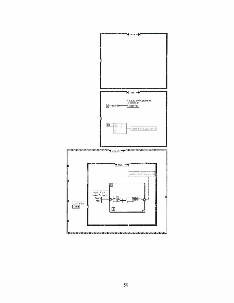
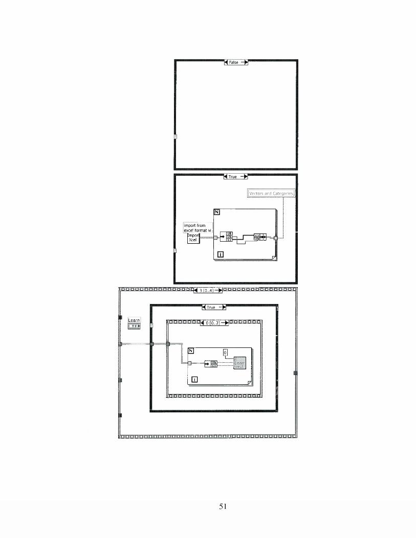
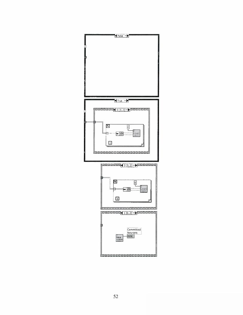
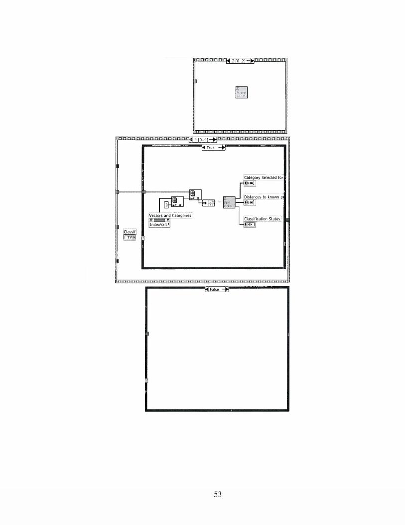
APPENDIX A

Software Documentation

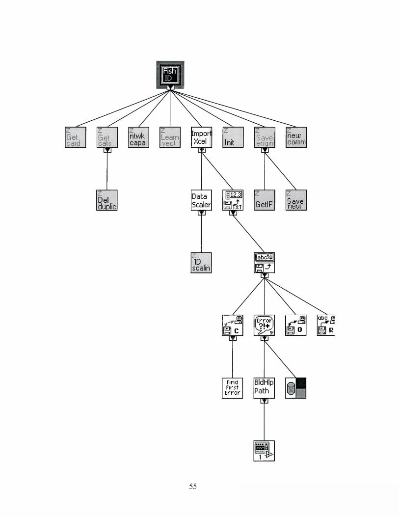
All image processing routines and construction of the ANN classifier was

accomplished within the Lab VIEW 6.1 graphical programming environment. Image

processing scripts were constructed and evaluated with Lab VIEW Vision Builder 6.0.

The ANN classifier was built with ZDK4LV distributed by General Vision Inc.

ZDK4LV consists of a number of sub VI’s (virtual instruments) that are embedded within

the Lab VIEW environment. What follows in this appendix is a graphical documentation

of the software code used to complete this project.

41

AUV Fish Classifier l.O.vi

Fish species classification engine using ZISC and RBF neural network technology

1) clear ZISC if any neurons are committed.

2) Load a file with vectors and their known category.

3) Learn all vectors.

4) Choose one of the vector of the input file and verify that its output category matches the input category when you click the Green button. Distance should be zero.

5) Modify one of the values of the displayed vector and try to recognize again. Distance should report the difference between the new and former vector, category might be off depending on the contents of the engine built in (3).

42

Fish Recognition Engine l.o

© 2003 C ollege o f William & Mary

▼2 Pixels

L e n g th . W id th

A s p e c t ra t io S u r f a c e a r e a

S u m o f p ix e ls

Pixel v a r ia n c e M ean p ixel v a lu e S .D ./m e a n p ix e l .

I m a g e a r e a C e n te r o f m a s s X C e n te r o f m a s s Y

L eft c o lu m n X T o p ro w Y

R ight co lu m n X B o tto m ro w Y

Box w id th Box h e ig h t

L o n g e s t s e g m e n t / L o n g e s t s e g m e n t x L o n g e s t s e g m e n t y ,

P e r im e te r S u m x

C o rre c te d p ro je c tio n '

VM o m e n t o f in e r t ia

IxxM o m e n t o f in e r t ia

iyyM o m e n t o f in e r t ia

Ix y

M ean c h o r d X M ea n c h o r d Y M ax i n t e r c e p t

le a n i n t e r c e p t p e r p . T a r g e t o r ie n t a t i o n Equil. e llipse m in o r.

Ellipse m a jo r Ellipse m in o r

R atio o f equ il, e llip se

Network parametersvec to rs and C ategories

4 0 9 6

1 5 0 0 2 ^ ° ° 2 5 0 0

3 0 0 01 0 0 0 -

Clear Network Connections

c a t e a o Nework size ZISC

3 5 0 0 216

Committed Neurons

4 0 9 61 = S h ark2 = Jack3 = O th e r fi

Min influence field Max influence field10000

Load Excel File C lassification O utcom e for Displayed Vector Identified

Learn All Loaded Vectors

UNKNOW

C lassifyDisplayed

VectorCategory Selected for Displayed Vector

to knownS u m xx !

-S u m xy Clear Loaded Data

C o rre c te d p ro je c tio

43

n n

[TO

[«»>!

ExOi

n o

H D

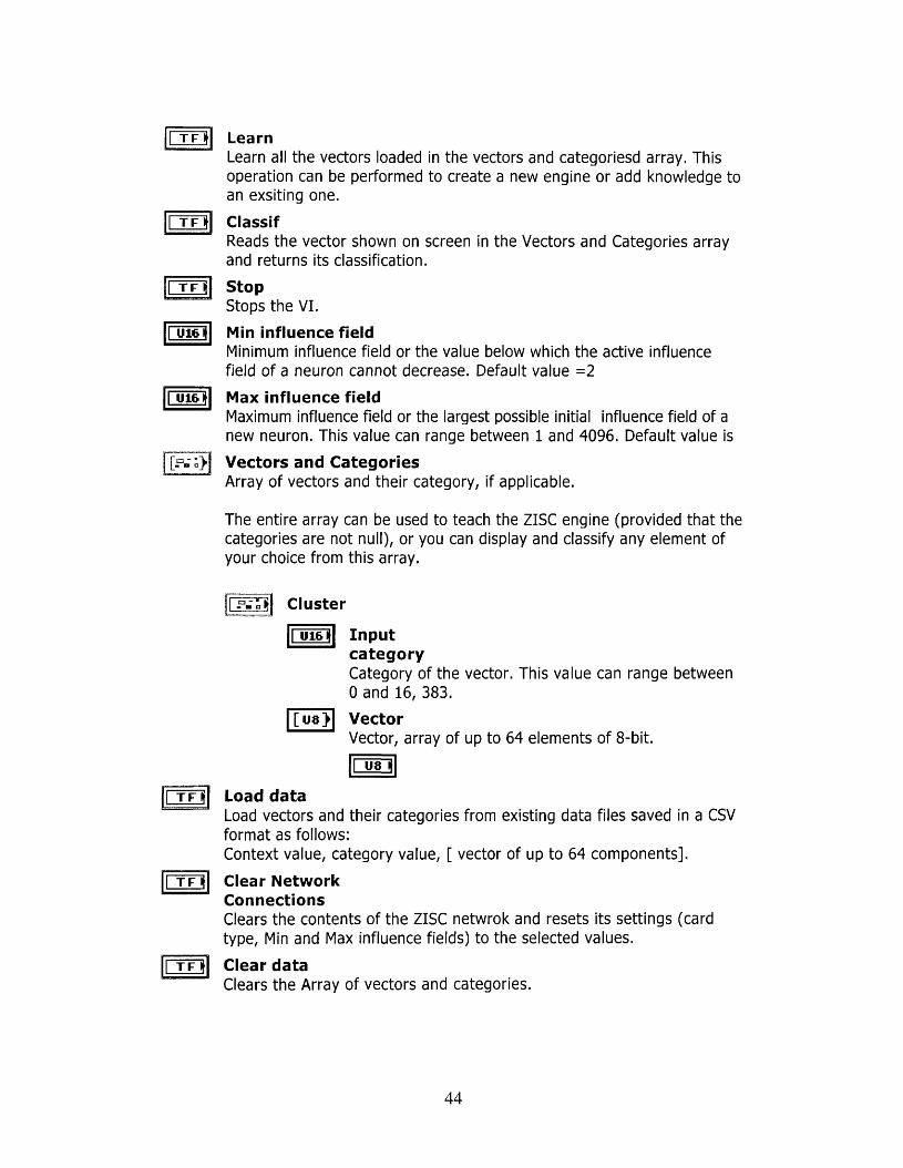
LearnLearn all the vectors loaded in the vectors and categoriesd array. This operation can be performed to create a new engine or add knowledge to an exsiting one.

ClassifReads the vector shown on screen in the Vectors and Categories array and returns its classification.

StopStops the VI.

Min influence fieldMinimum influence field or the value below which the active influence field of a neuron cannot decrease. Default value =2

Max influence fieldMaximum influence field or the largest possible initial influence field of a new neuron. This value can range between 1 and 4096. Default value is

Vectors and CategoriesArray of vectors and their category, if applicable.

The entire array can be used to teach the ZISC engine (provided that the categories are not null), or you can display and classify any element of your choice from this array.

Cluster

I ui6n| InputcategoryCategory of the vector. This value can range between 0 and 16, 383.

[ua>| VectorVector, array of up to 64 elements of 8-bit.

nisiLoad dataLoad vectors and their categories from existing data files saved in a CSV format as follows:Context value, category value, [ vector of up to 64 components].

Clear Network ConnectionsClears the contents of the ZISC netwrok and resets its settings (card type, Min and Max influence fields) to the selected values.

Clear dataClears the Array of vectors and categories.

44

(uie]

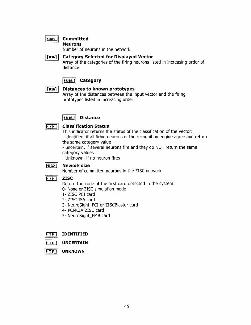
FuaTl CommittedNeuronsNumber of neurons in the network.

Category Selected for Displayed VectorArray of the categories of the firing neurons listed in increasing order of distance.

► u i6 1 Category

Distances to known prototypesArray of the distances between the input vector and the firing prototypes listed in increasing order.

FOrc]

u n

E m

► ui6 i Distance

Classification StatusThis indicator returns the status of the classification of the vector:- identified, if all firing neurons of the recognition engine agree and return the same category value- uncertain, if several neurons fire and they do NOT return the same category values- Unknown, if no neuron fires

Nework sizeNumber of committed neurons in the ZISC network.

ZISCReturn the code of the first card detected in the system:0- None or ZISC simulation mode1- ZISC PCI card2- ZISC ISA card3- NeuroSight_PCI or ZISCBIaster card4- PCMCIA ZISC card5- NeuroSight_EMB card

EIE]E m

E m

IDENTIFIED

UNCERTAIN

UNKNOWN

45

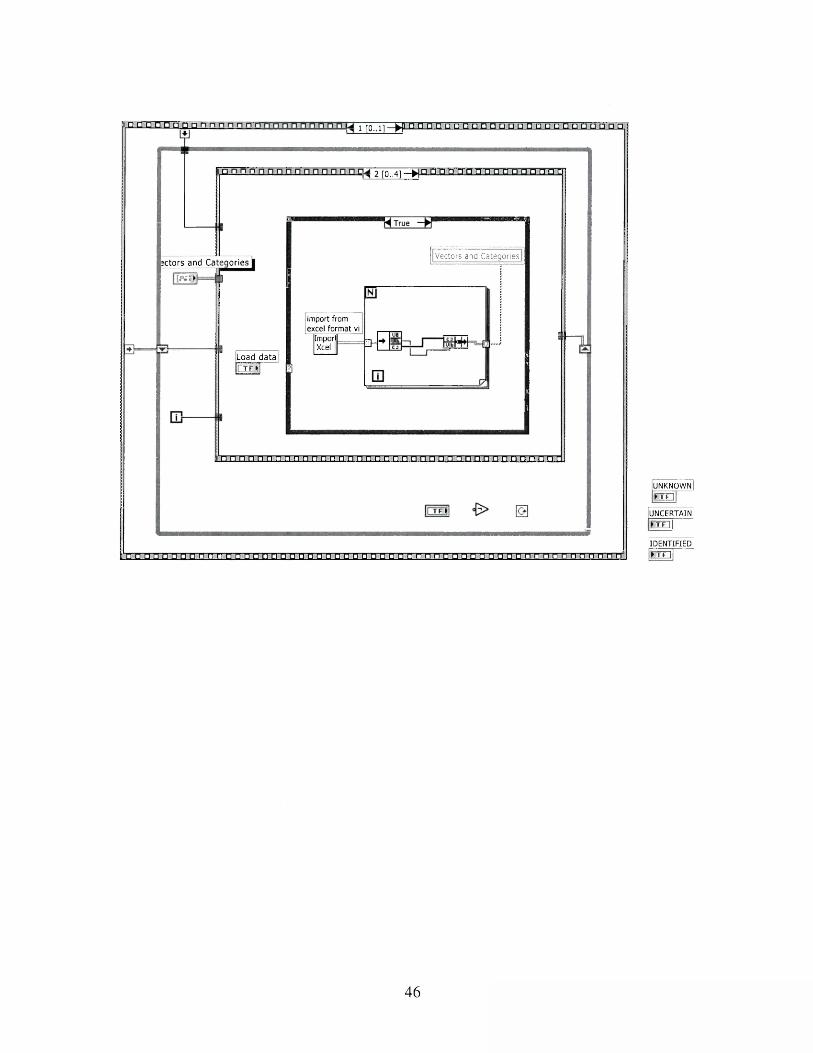
h i d □ □ □ □ □ □ t [0t!]_frfim □ □ □ □ □ □ □ □ □ □ □ □ □ □ □ □ □ □ □ □ □ □

□ [o..4] - > P -P a a D a a a a n a n n dxlx

V e c to rs a n d C a te g o r ie s |actors and C ate g o r ie s

im p o rt from e x c el fo rm a t vi

[m porlXcel

i jfc4 oib-—‘ I C3

Load d ata

Idol

□ □ □ □ □ □ □ □ □ □ □ □ □ □ □ □ □ □ □ □ □ □ □ □ □ □ □ a n mTnrrmTDTra

i d a a d B a d n n r i r i b J D a t l t l d D n n a a D n u D D a a D n n n n n D D a n n a D n n n n n n n n n n n n

UNKNOWNHE

UNCERTAINnn\IDENTIFIED

Em I

46

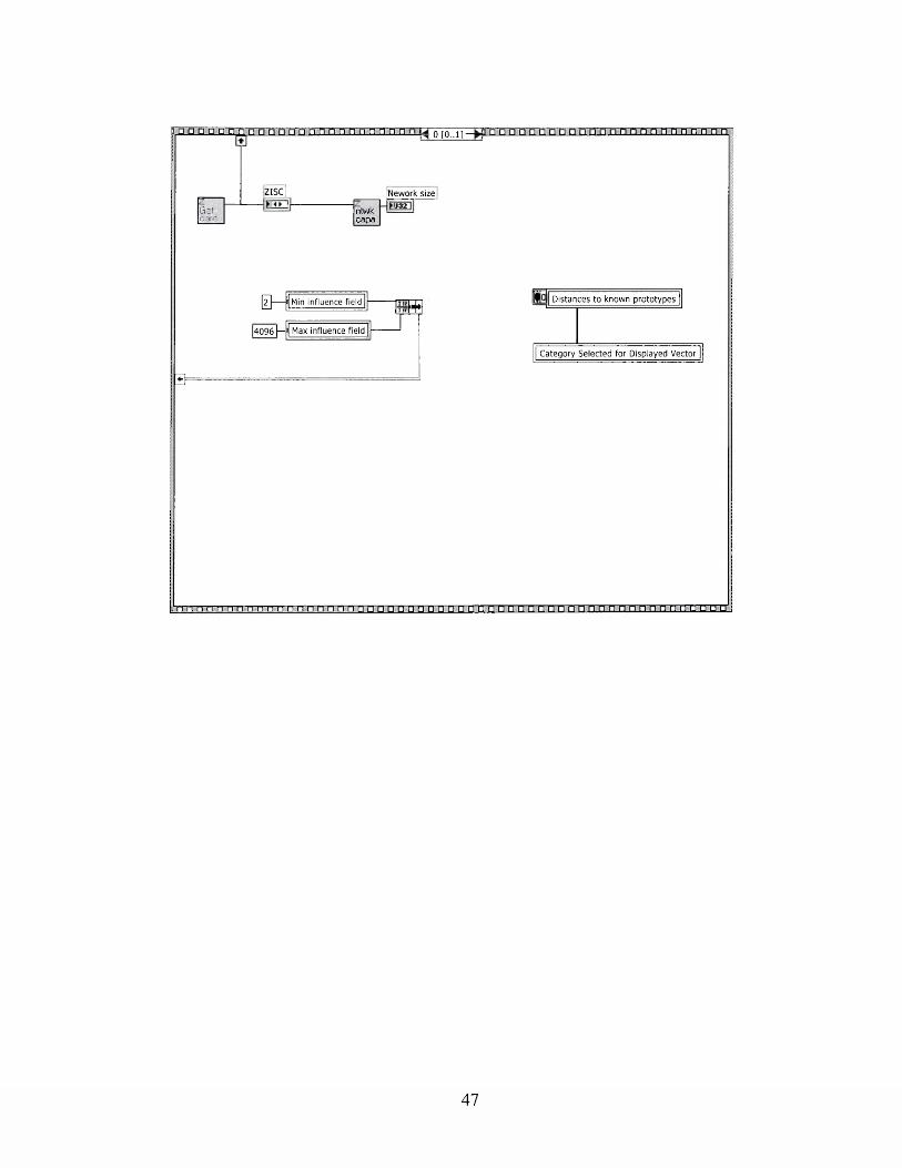
! □ □ □ □ □ a n n n n n n □ □ □ □ □ □ □ □ □ □ □ 0 r0--11 □ □ □ □ □ □ □ □ □ □ □ □ □ □ □ □ □ □ □ □ □ □ □ □

G e tc a rd

ZISC I------------ ntwkJ

capa

iNew ork size

H H Min in fluence field U 1i » h * i

|4 0 9 6 1 — j~Ma x in flu en c e field

0=

| D is ta n c e s to k now n p ro to ty p e s |

| C a te g o ry S e le c te d fo r D isp lay ed V e c to r |

m i-m rm n n n n n n n n~n~n nTm"rmn n n n n n n n n n cm n n n n n n n n n n n n a n n n n n n n m m

47

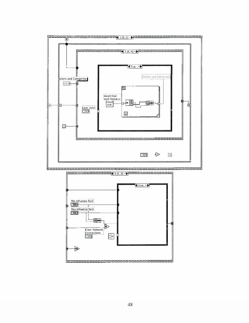
) □ □ □ □ □ p n g □ n n n a c m a n a c i Qn a m x g I —►p □

ira m 2 [o..4] — D D P O P D P P Q Q g j u i a x

r ecto rs and C a t e g o n e ^

f®

m-

Load data

T r '^ T

Vectors and Categories]

im p o rt from [excel fo rm a t vi

Im portXcel □

m

m nn~n n n'm-rrrn n n n n n n n n n n n n n n n n n n n n n n crirnTmT

urrtru □ □ □ □ □ □ □ □ □ □ □ □ □ □ D M n □ □ □ □ □ □ □ □ □■I □ □ □ □ □ □ □ □ □ □ □ □ □ □ □ 0 [Q..4] — □ □ □ □ □ □ □ □ □ □ □ □ □ □ □ ! =

"H F alse - K

|Min influ en ce field I||~uit >]---------- ------

[Max influ en ce field 1

Clear N etw ork C o n n e ctio n s

/□□□□□□□□□□□□□□□□ nmmmin □□□□□□□□□□□ cnmi

48

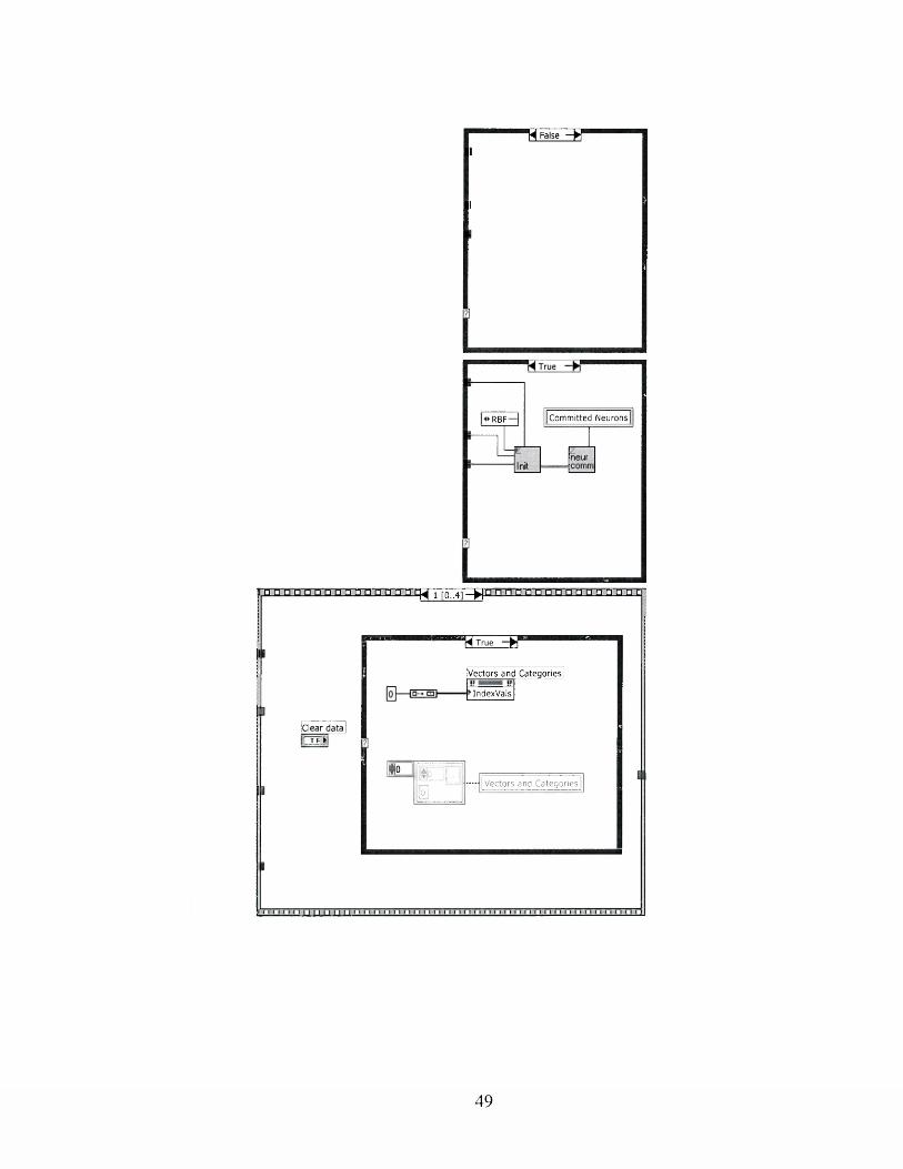
— ^ i s e ^ I

!

RBF— | C o m m itted N e u ro n s

□ n a a n a n a a axmxLaaxn i ro,.41 - » a □ □ a.a.a □ □ □ □ □ ans.

(C lear d a ta

QO

"Hlrue ~>T"

[V ectors a n d C a te g o r ie s

In d e x V als

||o 1 ®o rISf ij 1|Vectors and Categories!

El

49

H False

Vectors and Categories

IndexVals

V e cto rs a n d C a te g o r ie s

□ p□ □ □ □ □ p'n□ □□ fl-anxH 2f0..4i->|PaQPB~B~c

V e c to rs a n d C a te g o r ie s

[ import from i excel format vi

ImporlXcel

(Load data

[ □ n r

□ □ □ □ □ □ □ □ □ □ □ □ □ □ □ □ □ □ □ □ □ crn □ □ □ □ □ □ □ □ □ □ □ □ mrri

50

*HFa|se ~K*

V e c to rs a n d C a te g o r ie s !

import from excel format vi

|tmporl( ~ Xcel

m a n n a □ □ □ □ 3 r0i.41-fr|n □ □ □ □ □ □ □ □ □ n n n n n c

Learn

H True ~>f

o ro,,2i-Ha a □ □

0 | T

□

zLearnvect

i n n H r t n h h U t l r i n r i n n n n n n n r f

51

"H F alse - K *

— — — HnUe -ff

i □ □ n ' a ' c H o r o .,21 - » □ □ □ □ □ □ □

0 I T fs— - E M =

m

Learnvect

□ □ □ □ □ □ □ □ □ □ □ □ □ □ □ □ □ □ □ □

□ □ □ □ □ rxq Q f0 2] -frp □□□□□□

n m n g

C om m ittedN eu rons

c o m m

&*□□□□□□□□□□□□□□ □"□'□•ITTTTT

52

! □□□"□ □ di^ 2 ro..2i- |p d o aq

Saveenqin

a‘p □□□□□□□□□□□□□□□□ m ui,□□□□□□□□□ n□□□□□ 4[ 0 . . 4 ] □□□□□□□□□□□□□□£

■ H I ^

Classif

04 r H ! ' G e tcats

[Category Selected for

W ]|

Distances to known pi jttiife] |

Vectors and Categories

IndexVals*[Classification Status [

H False - W *

53

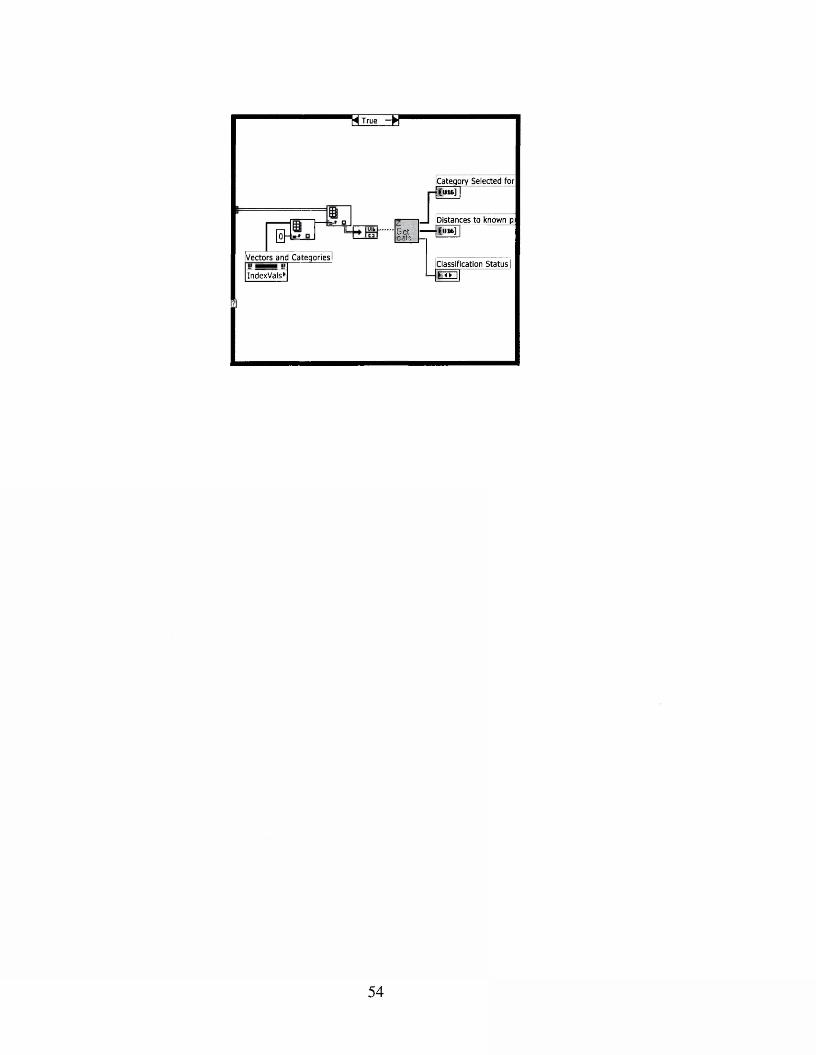
H True - K

Category Selected for Com] I

Vectors and Categories,

04 Get&

rJ_ | [Distance s to I'flra] |

known p

IndexVals*Classification Status |

nn\

54

M M

neurcomrnS ave

enqin 1 1 T

Saveneur

Error?!+,

FindFirstError

55

ntwkcapa

r- _, , _ O d vCenqin

b 0t card

b a I- cats

Learnvect

ImportXcel

neurcomm

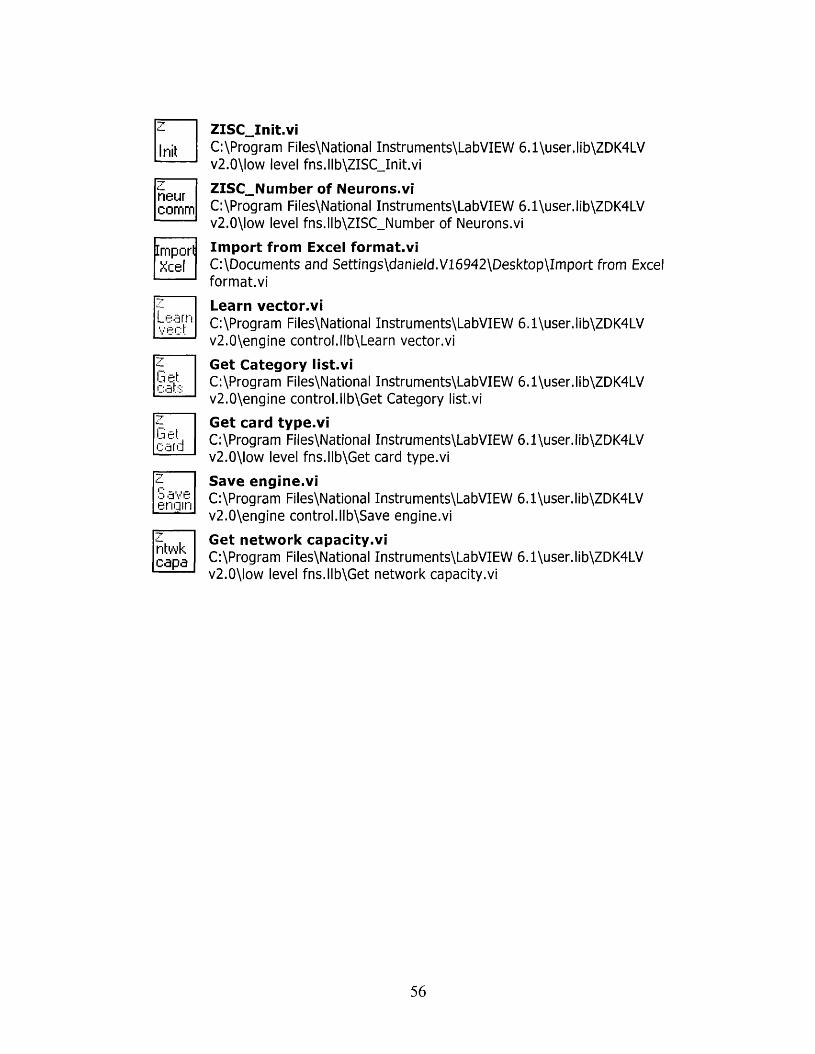
I nitZISC_Init.viC:\Program Files\National Instruments\LabVIEW 6.1\user.lib\ZDK4LV v2.0\low level fns.llb\ZISC_Init.vi

ZISC_Number of Neurons.viC:\Program Files\National Instruments\LabVIEW 6.1\user.lib\ZDK4LV v2.0\low level fns.llb\ZISC_Number of Neurons.vi

Import from Excel format.viC:\Documents and Settings\danield.V16942\Desktop\Import from Excel format.vi

Learn vector.viC:\Program Files\National Instruments\LabVIEW 6.1\user.lib\ZDK4LV v2.0\engine control.llb\Learn vector.vi

Get Category list.viC:\Program Files\National Instruments\LabVIEW 6.1\user.lib\ZDK4LV v2.0\engine control.llb\Get Category list.vi

Get card type.viC:\Program Files\National Instruments\LabVIEW 6.1\user.lib\ZDK4LV v2.0\low level fns.llb\Get card type.vi

Save engine.viC:\Program Files\National Instruments\LabVIEW 6.1\user.lib\ZDK4LV v2.0\engine control.llb\Save engine.vi

Get network capacity.viC:\Program Files\National Instruments\LabVIEW 6.1\user.lib\ZDK4LV v2.0\low level fns.llb\Get network capacity.vi

56

APPENDIX B

Digital image processing o f side scan sonar records

Acoustic images gathered by sidescan sonar can now rival photographs as

frequencies approach 5 MHz. Therefore, it is reasonable that techniques originally

developed for optical image processing and machine vision applications can be applied to

sonar images. Image processing is a large field of research and cannot be adequately

addressed here. The reader is directed to texts such as Jahne (2002), Suel et al., (2000) or

Jain (1989) for descriptions of image processing theory and algorithms.

It is useful to define exactly what a digital image is, for the concepts presented

below build upon the basic principles of how an image is defined. A digital image is

simply a two-dimensional array of values that correspond to some signal intensity; sound

pressure returning to an acoustic transducer and converted to electrical voltages in the

case of sonar and light intensity returning to an optical sensor in digital photography.

Formally, the image is a function of some intensity:

fU y)

where/ represents the brightness or signal intensity at the point, termed pixel, (x, y).

Typically, these pixels are spatially mapped to a two-dimensional, Cartesian coordinate

system where the starting coordinate (0, 0) is the upper left corner of the image.

57

The resolution of an image, the number of planes, and definition are three additional

basic components of a digital image. Image resolution is often expressed as the number

of pixels in each vertical and horizontal column. As an example, the images presented in

Appendix C are composed of columns of pixels that number 220 in the vertical and 220

in the horizontal. One can think of the number of planes within an image as the depth or

level of complexity of information contained within the image. For example, a gray scale

image contains only one plane while a true color image has three (or more) planes of

intensity data, one red, one green, and one blue plane. The bit depth of an image is

defined by the number of bits used to encode each pixel with a value or shade. As an

example, image definition, or bit depth, is given by 2n which states that a pixel may have

n different values. If n is 8 bits, then a pixel may have 256 values. If n is 16 bits, then a

pixel could have 65,536 different shades or values.

It is important to note that image processing is a collection of multiple steps that are

scripted together to yield information contained within an image. Hierarchical processing

schemes are therefore necessary to extract desired information from an image (Jahne,

2002, Egmont-Petersen et al., 2002). This hierarchy begins with image formation,

illumination and digitization. Once a digital version of the image is created, it usually

will require filtering or preprocessing. Operations such as contrast enhancement and

noise removal could occur during this step. Data reduction via feature extraction or

image compression is a common next step in the image processing hierarchy.

Segmentation describes operations that partition an image according to a particular

criterion or data point, such as texture segregation, color matching, object clustering, etc.

Object recognition operations often describe an objects position, orientation, and scale of

58

targets within an image. Operations common during the recognition phase include:

template matching, particle analysis, and edge detection. Many of these tasks are

completed with image transforms, which are mathematical operators that alter the image

on a pixel-by-pixel basis. There exist two classes of image transforms that can be applied,

global and point transforms. A global transform is one that acts equally on each pixel in

the image while a point transform will operate only on each pixel and its immediate

neighbors.

Particle analysis will receive special mention here as the tools common for that

operation are useful to this project. Particle analysis can be characterized as a set of tools

that are used to measure the area, length, coordinates, chords and axes, shape features and

shape equivalence features of a particle, shape or blob in an image (National Instruments,

2001; Suel et al., 2000).

Before particle analysis can take place, the image typically requires thresholding.

Thresholding can turn a n-bit image, in this case an 8 bit gray scale image with pixel

values ranging from 0 to 255, to a binary image with pixel values of 0 or 1. This process

results in an image that is segmented into a background region and a particle region. It

has the benefit of removing objects of interest from the background.

One useful method of changing a pixel’s (or particle’s) overall size and shape is to

use morphological operators. These work on binary images and process each individual

pixel based on the values of the pixels in its immediate neighborhood. Morphological

operators are used when it is desired to smooth edges of particles, expand or reduce the

size of particles or find the boundaries of particles. The dilation operator serves to fill

59

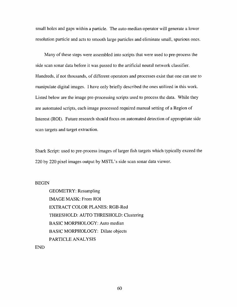
small holes and gaps within a particle. The auto-median operator will generate a lower

resolution particle and acts to smooth large particles and eliminate small, spurious ones.

Many of these steps were assembled into scripts that were used to pre-process the

side scan sonar data before it was passed to the artificial neural network classifier.

Hundreds, if not thousands, of different operators and processes exist that one can use to

manipulate digital images. I have only briefly described the ones utilized in this work.

Listed below are the image pre-processing scripts used to process the data. While they

are automated scripts, each image processed required manual setting of a Region of

Interest (ROI). Future research should focus on automated detection of appropriate side

scan targets and target extraction.

Shark Script: used to pre-process images of larger fish targets which typically exceed the

220 by 220 pixel images output by MSTL’s side scan sonar data viewer.

BEGIN

GEOMETRY: Resampling

IMAGE MASK: From ROI

EXTRACT COLOR PLANES: RGB-Red

THRESHOLD: AUTO THRESHOLD: Clustering

BASIC MORPHOLOGY: Auto median

BASIC MORPHOLOGY: Dilate objects

PARTICLE ANALYSIS

END

60

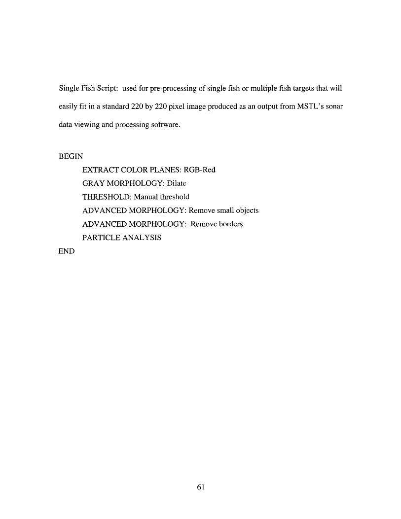
Single Fish Script: used for pre-processing of single fish or multiple fish targets that will

easily fit in a standard 220 by 220 pixel image produced as an output from MSTL’s sonar

data viewing and processing software.

BEGIN

EXTRACT COLOR PLANES: RGB-Red

GRAY MORPHOLOGY: Dilate

THRESHOLD: Manual threshold

ADVANCED MORPHOLOGY: Remove small objects

ADVANCED MORPHOLOGY: Remove borders

PARTICLE ANALYSIS

END

61

APPENDIX C

Side Scan Sonar Practices for Imaging Water Column Biologic Targets:

Notes from the field

The success of this work relies on the quality, and to some extent, the quantity, of

the sidescan data that is gathered and the ability to determine relevant, species-specific

features in the sonograms. The central thesis of this work is that fish species

identification and quantification is possible through image processing techniques and the

use of artificial neural network classifiers and does not rely on more traditional hydro­

acoustic methods mentioned earlier, such as echo counting and echo integration. Sidescan

sonar is mostly immune to the shallow water limitations of most vessel-based, downward

looking sonar methods, especially at the short (~ 10-20 m) ranges that are being used for

this project. Most traditional sonar sampling methods utilize down looking transducers

and therefore suffer from much reduced sampling volumes when used in shallow waters,

such as the Chesapeake Bay and other estuarine and riverine systems.

This is the fundamental reason for utilizing an AUV as our sampling platform

because it is significantly decoupled from the effects of sea state and produces superior

imagery over towed systems. An additional advantage of the AUV is that it can enter

into waters too shallow for a vessel-deployed, towed, sidescan system.

Furthermore, this work is dependent upon the correct selection of species-specific

variables (e.g. morphology of acoustic returns, packing density, linear size and shape,

62

schooling parameters, etc.) that will be used by the neural network program to

discriminate between species.

While these tasks were accomplished, it was not without significant trial and error

and the need for several adjustments to the AUV and the side scan sonar system. This

appendix serves to document our trials and fixes. I hope it serves as a guide to others

who may use these techniques in the future so that they do not suffer the pitfalls we

encountered.

During the collection of ground-truthed sidescan images for initial neural network

training, many lessons were learned in order to optimize data collection of biological

targets. Although the aquarium experiments are preferred for ground truthing of the

sidescan imagery due to water clarity for video-based species verification, it was

discovered that the quality of the images suffer from degradation due to the noisy

environment found within the aquarium. Sources of noise include tank filtration and

circulation pumps and visitors tapping on the viewing glass. Another problem seen in

figure 2a (and all aquarium data gathered at VMSM) is aliasing of fish images, first

bottom returns and air/water interface returns. We believe that this multipathing is due to

the fact that Marine Sonics Sonar control hardware does not provide individual

transducer power on/off options while the control software does allow individual

transducer display and recording. Therefore, The glass wall facing the sidescan

transducer acts as a reflecting surface and generates a delayed signal source that lags the

sound source generated by the transducer facing the interior of the aquarium tank.

Subsequent aquarium deployments required that the transducer facing the tank wall to be

covered with barium loaded vinyl sheeting designed to limit sound signal transmission.

63

This material can be obtained from McMaster-Carr Inc. (http://www.mcmaster.com). We

successfully used the 0.042 inch thick by 54 inch wide, STL=20, Catalog # 54665T22 at

$6.33 per foot. A thicker version is also available at 0.107 inch thick and 54 inch wide,

STL=26, Catalog # 546656T32 at $8.16 per foot.

During the aquarium exercise, we discovered several necessary improvements to

the sidescan sonar and the AUV that will be required for improving field-gathered sonar

imagery. These improvements include: isolation and elimination of sources of suspected

common-mode noise inside the AUV via installation of filter capacitors to eliminate

harmonics at 600 kHz on the DC to DC converters inside and robot and the installation of

ferrite chokes on all power leads, elimination of 3-5 degree of starboard roll in the AUV

in order to produce a more uniform sonar image on both channels, and lastly, to tilt the

individual sonar transducers 2-5 degrees down from horizontal to eliminate cross talk

between the sensors. In addition to adding the barium loaded sheeting behind each side

scan transducer, we have now increased the lateral distance between them by 2.5 inches

by refashioning the transducer mount. These improvements have resulted in greatly

improved sidescan imagery.

Data Examples

Catalogs of raw data examples are presented below. All images are

groundtruthed unless otherwise noted. Data collected for this project include

approximately 12 hours of video data with 878 megabytes (729 individual sonar files) of

concurrent side scan sonar imagery collected from the Virginia Marine Science Museum,

Virginia Beach, Virginia. In addition to the video/sonar data from the aquarium, there is

1.35 gigabytes (1298 individual files) of side scan sonar data that has been ground truthed

64

with the acoustic net pen experiments from the York River, VA. All raw and processed

data is deposited with Dr. Mark Patterson at the Virginia Institute of Marine Science in

Gloucester Point, Virginia.

65

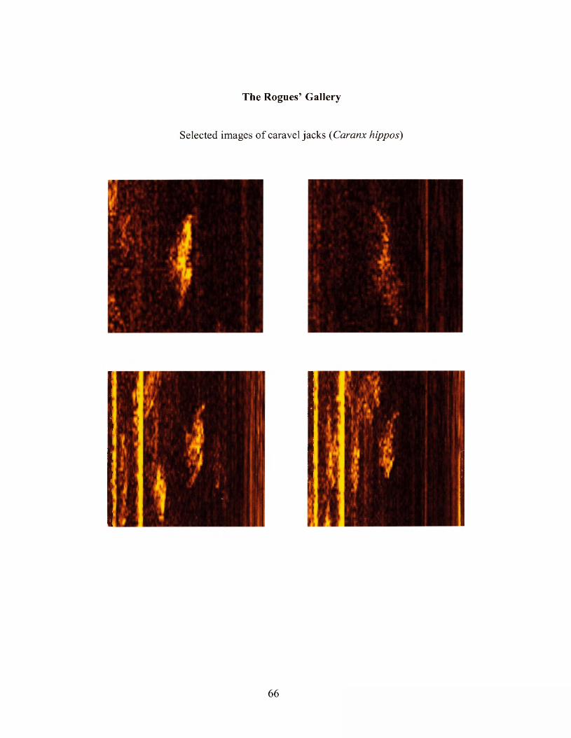
The Rogues’ Gallery

Selected images of caravel jacks (Caranx hippos)

66

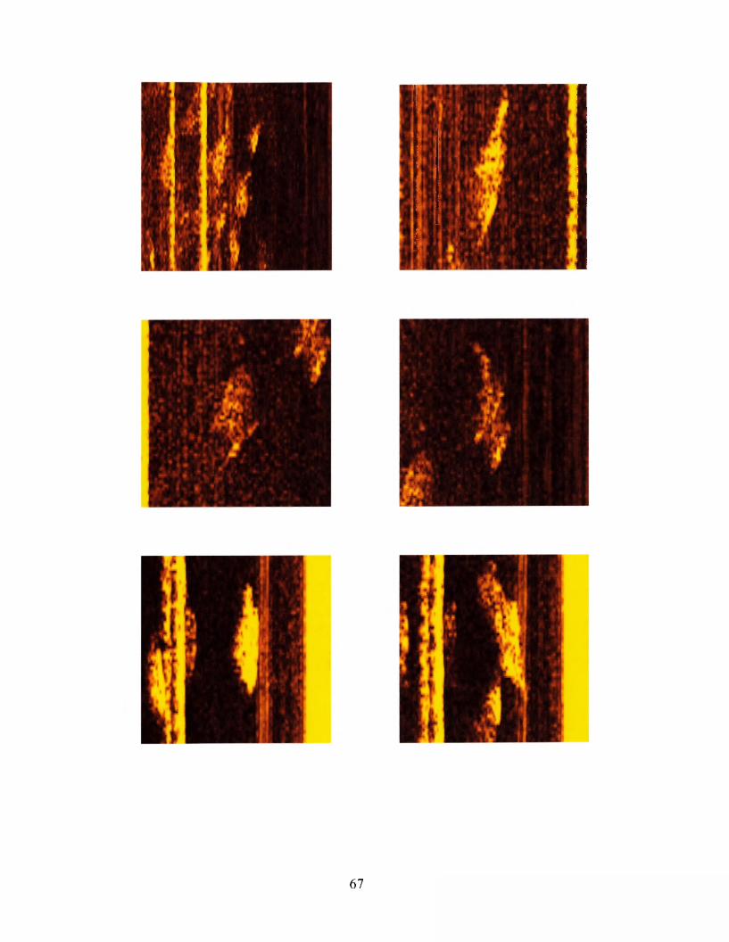
67

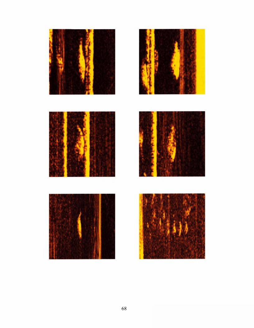
tMM

I

68

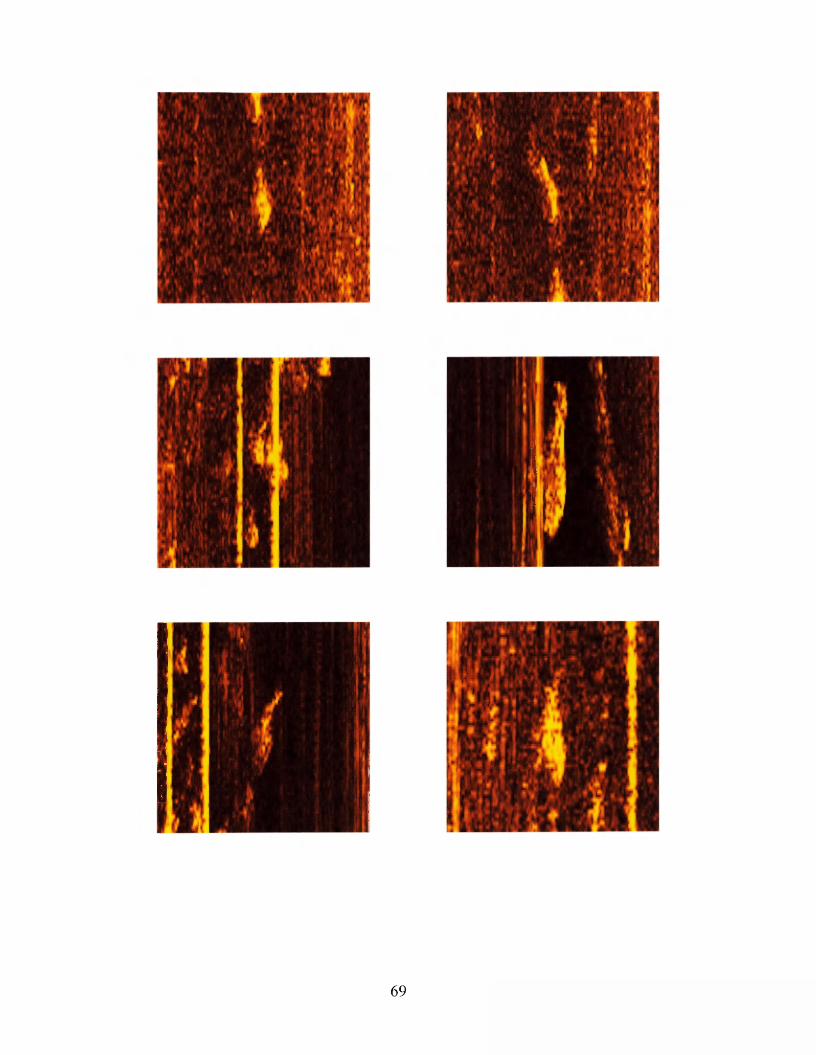
69

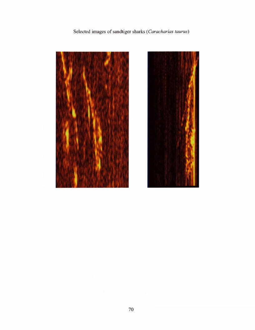
Selected images of sandtiger sharks (Caracharias taurus)

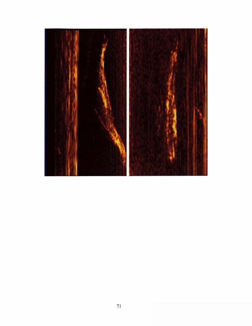
71

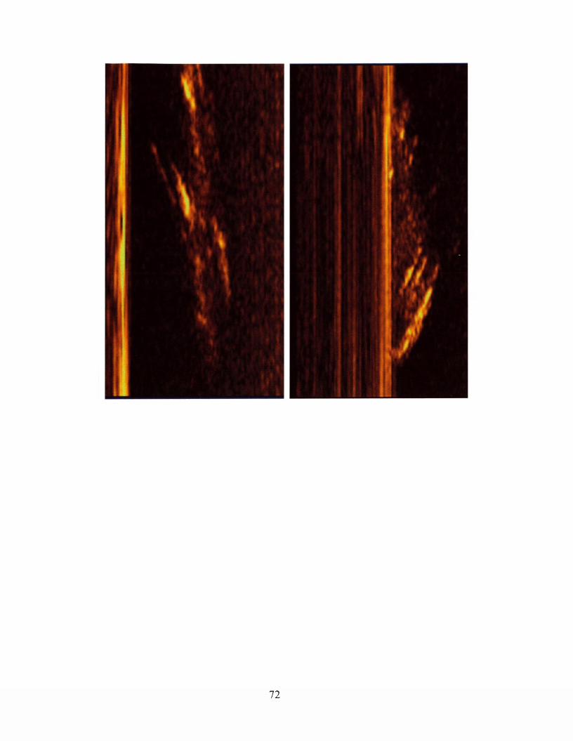
72

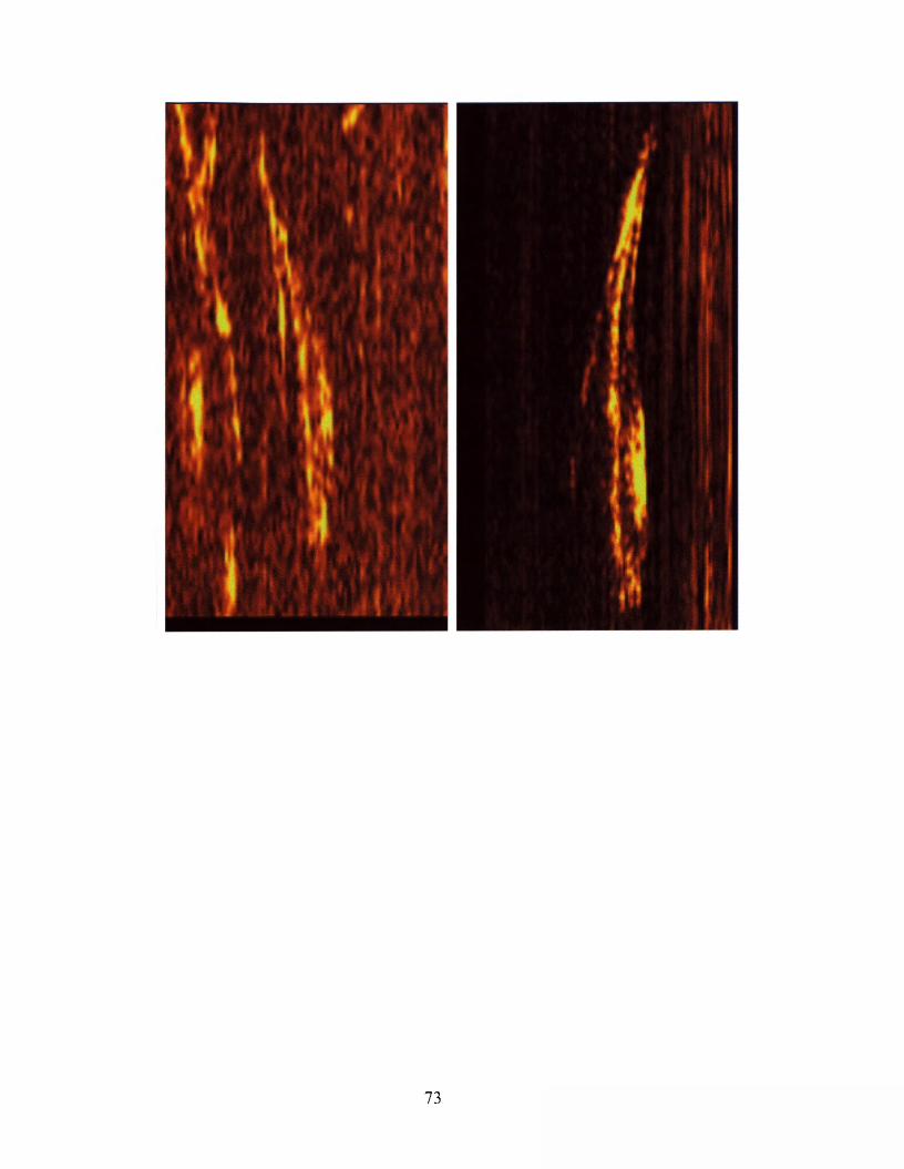
73

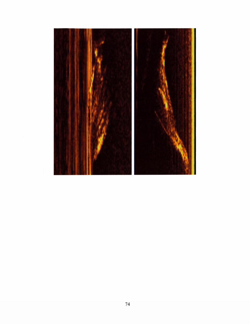
74

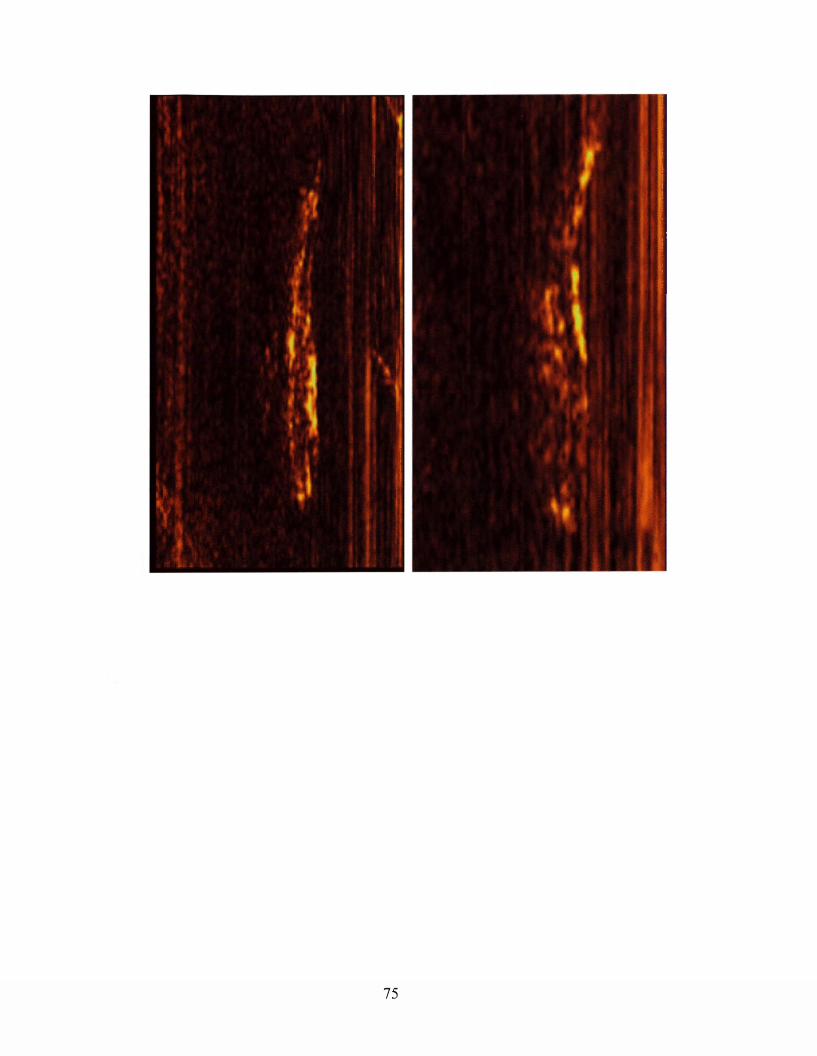
75

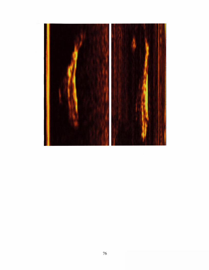
76

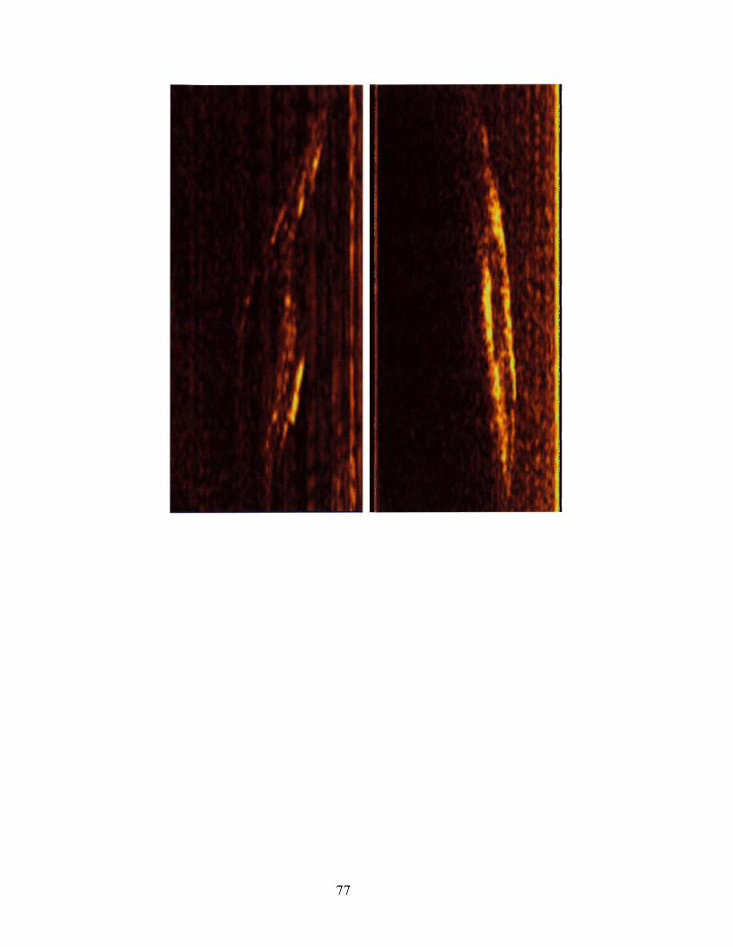
77

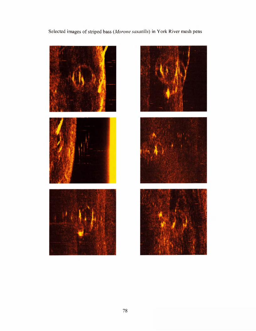
Selected images of striped bass (Morone saxatilis) in York River mesh pens

78

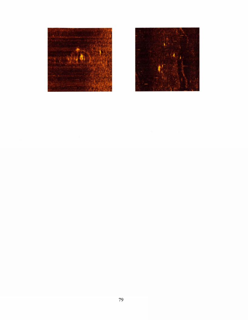
APPENDIX D

Basic Acoustic Theory

This study utilizes a specialized form of acoustic imaging, sidescan sonar, and

offers an alternative to traditional forms of acoustic population estimation methods. It

may, therefore be useful to review the basic principals of underwater acoustics. The term

acoustics, as used here, describes the generation, propagation, reception and

interpretation of sound (pressure) waves traveling through an elastic medium, such as

seawater.

Nearly all forms of acoustics utilize some device to generate sound waves and

listen for returned sound signals. Most often, these devices are electro-mechanical

transducers manufactured from magnetostricitve elements (such as nickel or ferrites),

electrostrictive ceramic material, such as barium titanate, or piezoelectric materials, such

as quartz, Rochelle salt, or lithium sulfate (Albers, 1969). When an electric current is

passed through the transducer, it oscillates at a specific frequency. This oscillation

physically moves the adjacent water particles and therefore establishes outgoing pressure

waves.

Propagation o f sound

Sound (or pressure) waves will propagate through any elastic medium, such as air,

water, steel, etc. Conversely, there is no sound propagation in space or any vacuum.

When an air particle or water molecule is displaced from its original position within a

homogeneous medium, the elastic properties of the surrounding medium push the

80

displaced molecule back into its original location. However, inertial forces will act on

the molecule and when it is pushed beyond its original position and a localized oscillation

is established (Everest, 2001). This concept is core to describing how sound waves travel

through seawater, or any other sound-conducting medium.

Density of the medium affects the speed of propagation. To illustrate, imagine

putting ones ear to a train track. It is possible to hear an oncoming train much earlier

through the rails. Since the steel track is denser, soundwaves propagate more rapidly

through metal then in the less dense air. Sound velocity in air is about 330 m/s, 1500 m/s

in water and about 5000 m/s in steel.

Sonar operating frequency largely determines attenuation loss (absorption) that

occurs as the sound wave propagates through the water column and is a significant

determinant of the distance that the wave can be propagated. The duration of the

transmission pulse and the length of the pulse determine the resolution capability of a

particular sonar system. The shorter the pulse duration and length, the better the

resolution of smaller targets. However, range decreases with pulse duration and length.

See Clay and Medwin (1977) and Gunderson (1993) for detailed explanations of acoustic

absorption and transmission theory.

Reception and interpretation

The single most important parameter in acoustics is the speed of sound. The speed

of sound ( c ) in the sea averages 1500 m/s, yet can fluctuate with changes in temperature,

salinity, and pressure. Equation (D-l) illustrates how c responds to environmental

fluctuations in seawater.

c= 1449.2 + 4.6T - 0.055T2 + 0.00029T3 + (1.34-0.010T)(S-35)+0.016z (D-l)

81

where c = speed (m/s), T = temperature (°C), S = salinity (parts per thousand), and z =

depth (m).

With the ability to accurately measure the speed of sound, and the use of high­

speed digital counters to measure the time between outgoing and reflected sound pulses,

we are able to use acoustics to “illuminate” the ocean. The word illuminate is

appropriate, as sound waves behave very much like light waves. As a sound wave moves

through the ocean, it will typically continue to propagate through the water, interact with

physical boundaries, and/or scatter when it comes into contact with reflecting objects or

surfaces (Clay and Medwin, 1977). It is the study and understanding of these processes

that form the basis for acoustical oceanography and fisheries hydroacoustics. As this

study focuses on a new tool for fisheries science, acoustical oceanography will not be

discussed in detail. Clay and Medwin (1977) give a thorough treatment of acoustical

oceanography and MacLennan and Simmonds (1992) is the seminal text for fisheries

acoustics. What follows is a review of the history and current state of fisheries acoustics.

Fisheries acoustics

The beginnings of what I term “traditional” fisheries acoustics can be traced to

early studies on the acoustical reflecting properties of fish (Rusby et al., 1973) and the

invention in 1965 of an echo integration system and paper chart recorders (Templemann

and May, 1965). By traditional, I mean a down-looking transducer with a symmetrically

spreading, conical beam that seeks to measure the levels of backscatter of acoustic energy

from organisms in the water column. Since the 1960’s, improvements in echo-sounder

and time-varied-gain (TVG) accuracy and precision, the development of multibeam

acoustic systems (Traynor & Ehrenberg, 1979), and the demonstration of the frequency

82

dependence of sound scattering by organisms of different sizes, led to increasing efforts

to interpret acoustic signals quantitatively. In the 1980’s, the advent of high-speed

analog/digital voltage converters, portable computers, and mass data storage devices,

coupled with new generations of signal analysis software, enabled more accurate, precise,

and complex processing and storage of acoustic signals (e.g., Stevens, 1986). These

technological advances allowed the development of analytical tools and numerical

models that could estimate fish size and abundance from acoustic data (Dickie et al.,

1983; Rose and Leggett, 1988). Species determination has been elusive though

(Maclennan and Simmons, 1992).

Classical hydroacoustic stock assessment methods utilize target strengths of

returning signals to classify fish into stock and biomass distinctions. Target strength can

be defined as a logarithmic measure of the proportion of the incident energy which is

reflected or backscattered from the fish or target according to the following formula

TS = 10 log (I2 / Ii) (D-2)

where h is the reflected intensity at lm from the target and I\ is the incident intensity.

For example, if a fish generated a reflected intensity of 0.00041\, then

TS = 10 log (0.0004) (D-3)

= - 34 dB relative to 1 pPa at 1 m

Most acoustic measurements are reported in decibels (dB) in favor of SI units for

pressure and intensity given that the logarithmic dB facilitates the use of numbers that

may be very large or very small, which are commonly found in acoustic applications.

The use of the dB scale allows TS description of acoustic scatters that range in size from

83

small zooplankton (-70 dB) to herring (-40 dB) to large whales, (-10 dB) to a submarine

(30 dB). For underwater acoustics, a common reference intensity (/i) standard for 0 dB is

a i m sphere positioned 1 m from the transducer (Kinsler et al., 2000). For comparison, a

60 mm diameter Cu calibration sphere has a TS of -33.6 dB. These TS signals are then

processed with echo integration or echo counting techniques, or a combination of both, as

described in Forbes and Nakken (1972), Thorne (1983) and MacLennan and Simmonds

(1992).

Target strength integration and counting methods, however, are often stymied by

changes in fish aspect ratio and tilt angle, discontinuities in the density of the water

column, and inability to discriminate heterogeneously mixed groups of fish. The result is

highly variable population estimates (Horne 2000, Gauthier and Rose 2001). A 24 cm

Atlantic herring may give a TS of -38 dB when in a normal swimming mode, but may

present a much smaller TS of say -65 dB (not much larger then zooplankton) if it is

positioned “heads up” or vertically within the acoustic beam. When acoustic surveys are

conducted in shallow water, additional difficulties arise. Vertical, or “down-looking”

sonar can only ensonify small volumes of the water column due to short ranges and

narrow beams of the sonar (Stepnowski and Moszynski, 2000).

Despite the shortcomings of hydroacoustics mentioned above, benefits of

hydroacoustic surveys that are not available from traditional forms of fishery stock

assessment methods include: full water column assessment, continuous track-line

assessment, analysis of fish behavior (which can help limit bias from net or vessel

avoidance), and ultimately a significant cost savings in equipment and personnel. The

shortcomings of most trawl surveys are that they are brief synoptic “snapshots” of fish

84

populations. Trawl nets are usually deployed for short periods of time over large

geographic areas. Additionally, trawls are designed to only sample species from a region

of the water column, typically benthic or pelagic. While trawls cannot be replaced by

hydroacoustic methods due to the need for ground-truthing the acoustic data and

providing other biological data (e.g., sex and sexual maturity, food habits, species

composition, etc.), acoustic data can adeptly augment conventional survey methods.

Other acoustic technologies

Shoal description and school shape analysis techniques were first developed

qualitatively by commercial fishermen to improve catch selectivity. The commercial

fishers developed no formal methods as they relied on observations and catch data to

interpret the signals shown on their echo sounders. Marine scientists eventually

developed quantitative measures of echogram returns (Lu and Lee, 1995; Coetzee, 2000;

Jech and Luo, 2000; LeFeuvre et al., 2000; Lawson et al., 2001). All of these techniques

however, utilize standard, down-looking, lower frequency (12 - 200 kHz) echosounders.

Researchers have now begun to explore alternate acoustic technologies for

estimation of fish stock populations. Misund and Coatzee (2000) have utilized horizontal

beaming, multibeam sonars to investigate school distribution near the sea surface, an area

often lost to down-looking, hull-mounted, transducers due to vessel avoidance reactions

of near surface fish schools. Multibeam techniques have also been used for shallow

water observations (Gerlotto et al., 1998; Gerlotto et al., 2000) and for three-dimensional

visualization of fish schools (Gerlotto et al., 1999). Ehrenberg and Torkelson (2000) are

investigating the application of lower frequency (10 kHz) FM slide chirp techniques to

biomass estimation. Another novel approach to biomass estimation is absorption

85

spectroscopy, or acoustic measurements of absorption loss due to swim bladder

resonance (Diachok, 2000). Demer et al, (2000) reports advances in the use of the

Doppler effect to study fish behavior by measuring changes in a transmitted signal due to

fish movement.

These technologies are still based in the domain of acoustic signal processing

whereas this project is seeking to utilize image processing techniques and neural network

classifiers for the classification of high-resolution sidescan sonar records. This approach

is warranted by the increasing quality of sidescan sonar imagery. With frequencies

approaching 5 MHz and transverse resolutions of <2 mm, these side scan systems are

good analogs of optically formed images.

86

APPENDIX E

Future developments and use ofAUV technology

The following text was recently published in the journal, Underwater Magazine

(Doolittle, 2003). It presents an overview of the current capabilities and future directions

of AUV technology. Figures are omitted as they are all found in the main body of this

thesis.

AUV science: present capabilities and future directions.

Autonomous Underwater Vehicles (AUV) are becoming common tools available

to scientists and other underwater professionals. Traditionally, AUVs have been

developed for science and military applications but are increasingly becoming viable

commercial ventures. Broadly speaking, AUVs are emerging as essential tools for

seabed surveys, oceanographic data collection, offshore oil and gas operations, and

military applications (Jones, 2002). Data collected from AUVs represent significant cost

savings in terms of reduced personnel hours, 24-hour sampling capabilities, and reduced

surface ship support. Given low purchase prices ($147,200 for a Fetch2 class AUV from

Sias Patterson Inc. to c. $300,000 for a REMUS class AUV from Hydroid Inc) and

minimal operational budget requirements, it is not difficult to imagine that AUVs will

significantly augment ship based marine resource surveys in the very near future.

More then 60 vehicle designs are now operational at US and worldwide research

institutions. This number does not include legacy, or one-off vehicles developed by and

87

for the military. This article is not intended to be a complete review of the many

missions AUV’s have performed while in the service of military or research operations

but to outline the scientific uses of this robust technology and give a recent example of

such use. Of particular interest are the small sized AUV’s that are well suited to littoral

and estuarine research and require relatively simple and inexpensive logistical support

infrastructure (such as ships, technicians, etc.).

While there are many one-off vehicles in operation, there are currently only 3 US

commercial vendors of small work-class AUVs. The term work-class denotes the ability

for sustained mission duration (>4 hours), mission-specific, reconfigurable control

software, and reasonable sensor payload capacity. Domestic vendors of small AUVs

include Sias Patterson Inc., Hydroid, and Bluefin Robotics. The small AUV has

significant benefits over the larger AUVs that are currently in service. Benefits include:

simplified tooling and consequently lowered manufacturing costs, less cumbersome and

costly deployment and recovery systems, lowered battery expense and lowered risks to

collisions and deleterious interactions with other users the coastal ocean.

Survey-class AUV’s, such as the C&C Technologies/Kongsberg Simrad Hugin,

Subsea 7’s HS Autosub and the Maridan vehicles, tend to be larger, have greater

endurance and depth capabilities and often greater payload capacity yet suffer from

significant operational and ownership costs and increased logistical requirements. These

vehicles have been extensively reviewed elsewhere and will not be discussed here.

Of equal, or possibly greater, importance is the performance of onboard sensors and

processing capabilities of the AUV. Sensors typically found on most small AUV’s

include: side scan sonar, multibeam swath bathymetry, nutrient video cameras, current-

temperature-depth (CTD) sensors, acoustic Doppler current velocimeters (ADCP) and

numerous other sensor payloads. This article will highlight one recent development in

neural network based, automated species recognition of fish, in addition to other objects,

imaged with side scan sonar.

Sias Patterson Inc. Fetch2

The second generation, Fetch-class AUV from Sias Patterson is the newest and

possibly the most revolutionary of the small work class AUVs currently available. Fetch

2 is a small commercial, multipurpose, networkable AUV using off-the-shelf components

that is programmable by non-experts in robotics. Size and performance specifications

include a length of 1.96 m (77 in), a diameter of 0.29 m (11.5 in) and a weight of 73 kg

(160 lbs). Typical survey speed is 2.5 m/s (5 kt) with top speed reaching 4.5 m/s (9 kt).

Mission duration is >22 hours at survey speed and c. 8 hours at maximum speed. Fetch2

has a maximum rated depth of 150 m (500 ft). A 300 m (1000 ft) model is currently

under construction and will become commercially available later this year. The Fetch2

vehicle incorporates a low-drag, hydrodynamic hull shape and has folding forward dive

planes, aft rudders and communications mast in order to aid launch and recovery. The

non-cruciform control surface configuration also allows for unparalleled maneuverability.

89

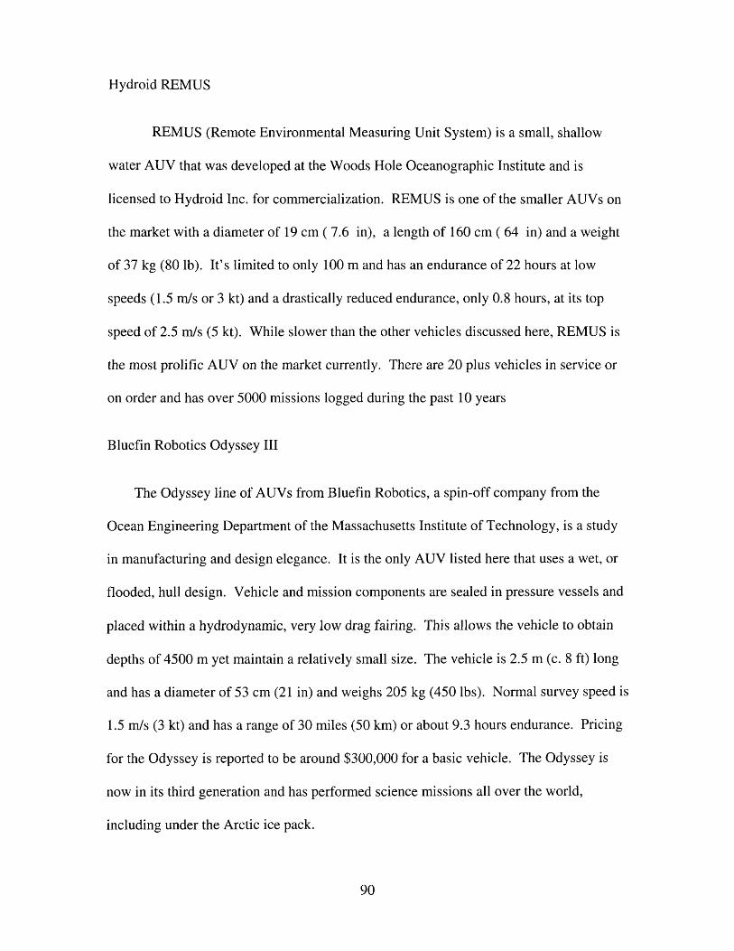
Hydroid REMUS

REMUS (Remote Environmental Measuring Unit System) is a small, shallow

water AUV that was developed at the Woods Hole Oceanographic Institute and is

licensed to Hydroid Inc. for commercialization. REMUS is one of the smaller AUVs on

the market with a diameter of 19 cm ( 7.6 in), a length of 160 cm ( 64 in) and a weight

of 37 kg (80 lb). It’s limited to only 100 m and has an endurance of 22 hours at low

speeds (1.5 m/s or 3 kt) and a drastically reduced endurance, only 0.8 hours, at its top

speed of 2.5 m/s (5 kt). While slower than the other vehicles discussed here, REMUS is

the most prolific AUV on the market currently. There are 20 plus vehicles in service or

on order and has over 5000 missions logged during the past 10 years

Bluefin Robotics Odyssey III

The Odyssey line of AUVs from Bluefin Robotics, a spin-off company from the

Ocean Engineering Department of the Massachusetts Institute of Technology, is a study

in manufacturing and design elegance. It is the only AUV listed here that uses a wet, or

flooded, hull design. Vehicle and mission components are sealed in pressure vessels and

placed within a hydrodynamic, very low drag fairing. This allows the vehicle to obtain

depths of 4500 m yet maintain a relatively small size. The vehicle is 2.5 m (c. 8 ft) long

and has a diameter of 53 cm (21 in) and weighs 205 kg (450 lbs). Normal survey speed is

1.5 m/s (3 kt) and has a range of 30 miles (50 km) or about 9.3 hours endurance. Pricing

for the Odyssey is reported to be around $300,000 for a basic vehicle. The Odyssey is

now in its third generation and has performed science missions all over the world,

including under the Arctic ice pack.

90

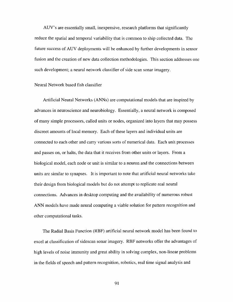
AUV’s are essentially small, inexpensive, research platforms that significantly

reduce the spatial and temporal variability that is common to ship collected data. The

future success of AUV deployments will be enhanced by further developments in sensor

fusion and the creation of new data collection methodologies. This section addresses one

such development; a neural network classifier of side scan sonar imagery.

Neural Network based fish classifier

Artificial Neural Networks (ANNs) are computational models that are inspired by

advances in neuroscience and neurobiology. Essentially, a neural network is composed

of many simple processors, called units or nodes, organized into layers that may possess

discreet amounts of local memory. Each of these layers and individual units are

connected to each other and carry various sorts of numerical data. Each unit processes

and passes on, or halts, the data that it receives from other units or layers. From a

biological model, each node or unit is similar to a neuron and the connections between

units are similar to synapses. It is important to note that artificial neural networks take

their design from biological models but do not attempt to replicate real neural

connections. Advances in desktop computing and the availability of numerous robust

ANN models have made neural computing a viable solution for pattern recognition and

other computational tasks.

The Radial Basis Function (RBF) artificial neural network model has been found to

excel at classification of sidescan sonar imagery. RBF networks offer the advantages of

high levels of noise immunity and great ability in solving complex, non-linear problems

in the fields of speech and pattern recognition, robotics, real time signal analysis and

91

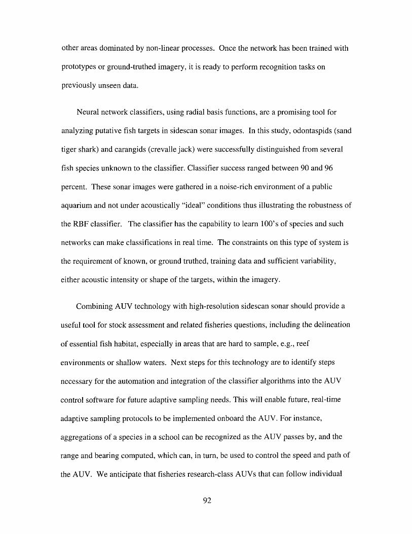
other areas dominated by non-linear processes. Once the network has been trained with

prototypes or ground-truthed imagery, it is ready to perform recognition tasks on

previously unseen data.

Neural network classifiers, using radial basis functions, are a promising tool for

analyzing putative fish targets in sidescan sonar images. In this study, odontaspids (sand

tiger shark) and carangids (crevalle jack) were successfully distinguished from several

fish species unknown to the classifier. Classifier success ranged between 90 and 96

percent. These sonar images were gathered in a noise-rich environment of a public

aquarium and not under acoustically “ideal” conditions thus illustrating the robustness of

the RBF classifier. The classifier has the capability to learn 100’s of species and such

networks can make classifications in real time. The constraints on this type of system is

the requirement of known, or ground truthed, training data and sufficient variability,

either acoustic intensity or shape of the targets, within the imagery.

Combining AUV technology with high-resolution sidescan sonar should provide a

useful tool for stock assessment and related fisheries questions, including the delineation

of essential fish habitat, especially in areas that are hard to sample, e.g., reef

environments or shallow waters. Next steps for this technology are to identify steps

necessary for the automation and integration of the classifier algorithms into the AUV

control software for future adaptive sampling needs. This will enable future, real-time

adaptive sampling protocols to be implemented onboard the AUV. For instance,

aggregations of a species in a school can be recognized as the AUV passes by, and the

range and bearing computed, which can, in turn, be used to control the speed and path of

the AUV. We anticipate that fisheries research-class AUVs that can follow individual

92

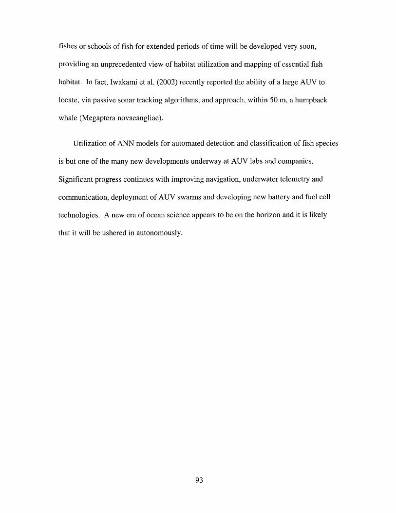
fishes or schools of fish for extended periods of time will be developed very soon,

providing an unprecedented view of habitat utilization and mapping of essential fish

habitat. In fact, Iwakami et al. (2002) recently reported the ability of a large AUV to

locate, via passive sonar tracking algorithms, and approach, within 50 m, a humpback

whale (Megaptera novaeangliae).

Utilization of ANN models for automated detection and classification of fish species

is but one of the many new developments underway at AUV labs and companies.

Significant progress continues with improving navigation, underwater telemetry and

communication, deployment of AUV swarms and developing new battery and fuel cell

technologies. A new era of ocean science appears to be on the horizon and it is likely

that it will be ushered in autonomously.

93

LITERATURE CITED

Albers, V.M. 1969. Underwater Acoustic Instrumentation. Instrument Society of America. Pittsburgh, Pennsylvania.

Andrew, N.L., K.J. Graham, S.J. Kennedy and M.K. Broadhurst. 1991. The effects of trawl configuration on the size and composition of catches using benthic prawn trawls off the coast of New South Wales, Australia. International Council for the Exploration of the Sea Journal of Marine Science 48: 201-209.

Ault, J.S., J.A. Bohnsack, and G.A. Meester. 1998. A retrospective (1979-1996)multispecies addessment of coral reef fish stocks in the Florida Keys. Fisheries Bulletin 96(3):395-414.

Auster, P.J. 1998. A conceptual model of the impacts of fishing gear on the integrity of fish habitats. Conservation Biology 12(6): 1198-1203.

Broomhead, D.S. and D. Lowe. 1988. Multivariable functional interpolation and adaptive networks. Complex Systems 2:321-355.

Byrne, C.J., T.R. Ararovitz, and M.P. Sissenwine. 1981. Factors affecting variability of research vessel trawl surveys. Pages 258-273 in W.G. Doubleday and D. Rivard, editors. Bottom Trawl Surveys. Canadian Special Publication of Fisheries and Aquatic Science 58.

Caddy, J.F. 1973. Underwater observations on tracks of dredges and trawls and someeffects of dredging on a scallop ground. Journal of the Fisheries Research Board of Canada 30(2): 173-180.

Caddy, J.F. 1993. Toward a comparative evaluation of human impacts on fisheryecosystems of enclosed and semi-enclosed seas. Reviews in Fisheries Science l(l):57-95.

Carrothers, P.J.G. 1981. Catch variability due to variations in groundfish otter trawlbehaviour and possibilities to reduce it through instrumented fishing gear studies and improved fishing procedures. Pages 247-257 in W.G. Doubleday and D. Rivard, editors. Bottom Trawl Surveys. Canadian Special Publication of Fisheries and Aquatic Science 58.

Castillo, S. and J. Mendo. 1987. Estimation of unregistered Peruvian anchoveta(Engraulis ringens ) in official catch statistics, 1951 to 1982. Pages 109-116 in D.

94

Pauly and I. Tsukayama, editors. The Peruvian Anchoveta and its up welling ecosystem: three decades of change. International Center for Living Aquatic Resource Management 15, Manila, Philippines.

Clay, C.S. and H. Medwin. 1977. Acoustical Oceanography. John Wiley and Sons. New York, New York.

Coatzee, J. 2000. Use of shoal analysis and patch estimation system (SHAPES) to characterize sardine schools. Aquatic Living Resources 13(1): 1-10.

Collie, J.S., G.A. Escanero, and P.C. Valentine. 1997. Effects of bottom fishing on the benthic megafauna of Georges Bank. Marine Ecology Progress Series 155:159- 72.

Conan, G.Y., and D.R. Maynard. 1987. Estimates of snow crab (Chionecetes opilio)abundance by underwater television: a method for population studies on benthic fisheries resources. Journal of Applied Ichthyology 3(4): 158-165.

Currie, D.R. and G.D. Parry. 1999. Impacts and efficiency of scallop dredging ondifferent soft substrates. Canadian Journal of Fisheries and Aquatic Sciences 56:539-550.

Dahm, E., H.Wienbeck, C.W. West, J.W. Valdemarsen, and F.G. O’Neill. 2002. On the influence of towing speed and gear size on the selective properties of bottom trawls. Fisheries Research 55:103-119.

DeAlteris, J.T. 1988. The application of hydroacoustics to the mapping of subtidal oyster reefs. Journal of Shellfish Research 7(l):41-45.

DeAlteris, J.T. and D.L. Morse, 1997. Fishing gear management. Pages 167-176 in J. Boreman, B.S. Nakashima, J.A.Wilson and R.L.Kendall, editors. Northwest Atlantic Groundfish: Perspectives on a Fishery Collapse American Fisheries Society, Bethesda, Maryland.

Demer, D.A., M. Barange, and A.J. Boyd. 2000. Measurements of three-dimensional fish school velocities with and acoustic Doppler current profiler. Fisheries Research 47:201-214.

Diachok, O. 2000. Absorption spectroscopy: A new approach to estimation of biomass. Fisheries Research 47:231-244.

Dickie, L.M., R.G. Dowd, and P.R. Bourdeau. 1983. An echo counting and loggingsystem (ECOLOG) for demersal fish size distributions and densities. Canadian Journal of Fisheries and Aquatic Science 40(4):487-498.

Doolittle, D.F. 2003. The payoff is in the payload: using AUVs in Scientific Research. Underwater Magazine 15(2):67-69.

95

Edsall, T.A., G.W. Kennedy, and W.H. Horns. 1993. Distribution, abundance, andresting microhabitat of Burbot on Julian’s Reef, southwestern Lake Michigan. Transactions of the American Fisheries Society 122:560-574.

Egmont-Petersen, M., D. de Ridder, and H. Handels. 2002. Image processing with neural networks: a review. Pattern Recognition 35:2279-2301.

Engal, J. and R. Kvitek. 1998. Effects of otter trawling on a bentihic community on Monterey Bay National Marine Sanctuary. Conservation Biology 12(6): 1204- 1214.

Engas, A. and O.R. Godo. 1989. Swept area variation with depth and its influence on abundance indices of groundfish from trawl surveys. Journal of Northwest Atlantic Fisheries Science 9:133-139.

Ehrenberg, J.E. and T.C. Torkelson. 2000. FM slide (chirp) signals: a technique for significantly improving the signal-to-noise performance in hydroacoustic assessment systems. Fisheries Research 47:193-199.

Everest. F.A. 2001. Master handbook of acoustics. McGraw-Hill. New York, New York.

Fernandes, P.G., A.S. Brierley, E.J. Simmonds, N.W. Millard, S.D. McPhail, F.Armstrong, P. Stevenson and M. Squires. 2000. Fish do not avoid survey vessels. Nature 404(6773):35-36.

Fish, J.P. and H.A. Carr. 1990. Sound Underwater Images: a Guide to the Generation and Interpretation of Side Scan Sonar Data. Lower Cape Publishing, Orleans, Massachusetts.

Fish, J.P. and H.A. Carr. 2001. Sound Reflections: Advanced Applications of Side Scan Sonar. Lower Cape Publishing, Orleans, Massachusetts.

Fogarty, M.J. and S.A. Murawski. 1998. Large scale disturbance and the structure of marine systems: fishery impacts on Georges Bank. Ecological Applications 8(Supplement 1):S6-S22.

Forbes, S.T. and O. Nakken. 1972. Manual of methods for fisheries resource survey and appraisal. Part 2. The use of acoustic instruments for fish detection and abundance estimation. Food and Agricultural Organization. Manual of Fisheries Science. Number 5.

Foster, J.J., C.M. Campbell and G.C.W. Sabin. 1981. The fish catching process relevant to trawls. Pages 229-245 in W.G. Doubleday and D. Rivard, editors. Bottom trawl surveys. Canadian Special Publication of Fisheries and Aquatic Science 58.

96

Franks, P.J.S. 2001. Turbulence avoidance: An alternate explanation of turbulence-enhanced ingestion rates in the field. Limnology and Oceanography 46(4):959- 963.

Friedlander, A.M., G.W. Boehlert, M.E. Mason, J.V. Gardner, and P. Dartnell. 1999.Sidescan-sonar mapping of benthic trawl marks on the shelf and slope off Eureka, California. Fishery Bulletin 97(4):786-801.

Gartz, R.G., L.W. Miller, R.W.Fujimura,P.E. Smith. 1999. Measurement of larval striped bass (Morone saxatilis) net avoidance using evasion radius estimation to improve estimates of abundance and mortality. Journal of Plankton Research 21(3):561- 580.

Gauthier, S. and G.A. Rose. 2001. Target strength of encaged Atlantic redfish (Sebastes spp.). International Council for the Exploration of the Sea Journal of Marine Science 58: 562-568.

General Vision. 2001. ZDK4LV: ZISC developer kit for Lab VIEW for pattern and image recognition. General Vision Incorporated, Petaluma, California.

Gerlotto, F., C. Hernandez, and E. Linares. 1998. Experiences with multibeam sonar in shallow tropical waters. Fisheries Research 35:143-147.

Gerlotto, F., M Soria, and P. Freon. 1999. From two dimensions to three: the use ofmultibeam sonar for a new approach in fisheries acoustics. Canadian Journal of Fisheries and Aquatic Science 56:6-12.

Gerlotto, F., S. Georgakarakos, and P.K. Eriksen. 2000. The application of multibeam sonar technology for quantitative estimates of fish density in shallow water acoustic surveys. Aquatic Living Resources 13:385-393.

Griffiths, G., P. Enoch, and N.M. Millard. 2001. On the radiated noise of the Autosub autonomous underwater vehicle. International Council for the Exploration of the Sea Journal of Marine Science 58(6): 1195-1200.

Gunderson, D.R. 1993. Surveys of Fisheries Resources. John Wiley and Sons, New York, New York.

Hearn, W.S., T. Polacheck, K.H. Pollock, and W. Whitelaw. 1999. Estimation of tagreporting rates in age-structured multicomponent fisheries where one component has observers. Canadian Journal of Fisheries and Aquatic Sciences 56(7): 1255- 1265.

Hilbom, R. and C.J. Walters. 1992. Quantitative Fisheries Stock Assessment: Choice, Dynamics and Uncertainty. Chapman and Hall, New York, New York.

97

Hogan, J.M., N. Norris, and J. Diederich. 2001. Classification of facial expressions with domain Gaussian RBF networks. Pages 143-166 in R.J. Howlett and L.C. Jain, editors. Radial Basis Function Networks 2: New Advances in Design. Physica- Verlag, Heidelberg, Germany.

Horne, J.K. 2000. Acoustic approaches to remote species identification: a review. Fisheries Oceanography 9(4):356-371.

Hutchings, J.A. 2000. Collapse and recovery of marine fishes. Nature 406:882-885.

Iwakami, H., T. Ura, K. Asakawa, T. Fujii, Y. Nose, J. Kojima, Y. Shirasaki, T. Asai, S. Uchida, N. Higashi, and T. Fukuchi. 2002. Approaching whales by autonomous underwater vehicle. Marine Technology Society Journal 36:80-85.

Jahne, B. 2002. Digital image processing. 5th ed. Springer. Berlin, Germany.

Jain, A. 1988. Fundamentals of digital image processing. Prentice Hall, Upper Saddle River, New Jersey.

Jech, J.M. and J. Luo. 2000. Digital echo visualization and information system (DEVIS) for processing spatially-explicit fisheries acoustic data. Fisheries Research 47:115-124.

Jones, D. 2002. The AUV marketplace. Underwater Magazine 14(4):75-79.

Kaiser, M.J. 1998. Significance of bottom-fishing disturbance. Conservation Biology 12(6): 1230-1235.

Keenleyside, M.H.A. 1997. Development of research on fish behaviour as part offisheries science in Canada. Canadian Journal of Fisheries and Aquatic Sciences 54(11):2709-2719.

Kinsler, L.E., A.R. Frey, A.B. Coppens, and J.V. Sanders. 2000. Fundamentals of acoustics. John Wiley and Sons, New York, New York.

Koeller, P.A., 1991. Approaches to improving groundfish survey abundance estimates by controlling the variability of survey gear geometry and performance. Journal of Northwest Atlantic Fisheries Science 11:51-58.

Kostylev, V.E., B.J. Todd, G.B.J. Fader, R.C. Courtney, G.D.M. Cameron, and R.A.Pickrill. 1999. Benthic habitat mapping on the Scotian Shelf based on multibeam bathymetry, surficial geology and sea floor photographs. Marine Ecology

Progress Series 219:121-137.

Krebs, C.J. 1989. Ecological Methodology. Harper Collins Publishers, New York, New York.

98

Kruse, C.G., W.A. Hubert, and F.J. Rahel. 1998. Single-pass electrofishing predicts trout abundance in mountain streams with sparse habitat. North American Journal of Fisheries Management 18(4):940-946.

Lane, D.M. and J.P. Stoner. 1994. Automatic interpretation of sonar imagery using qualitative feature matching. Institute of Electrical and Electronics Engineers (IEEE) Journal of Oceanic Engineering 19(3): 391-405.

Lawson, G.L., M. Barange, and P. Freon. 2001. Species identification of pelagic fish schools on the South African continental shelf using acoustic descriptors and ancillary information. International Council for the Exploration of the Sea Journal of Marine Science 57: 275-287.

LeFeuvre, P., G.A. Rose., R. Gosine, R.Hale, w.Pearson, and R.Khan. 2000. Acoustic species identification in the Northwest Atlantic using digital image processing. Fisheries Research 47:137-147.

Li, S.T. and E.L. Leiss. 2001. On noise-immune RBF networks. Pages 95-124 in R.J. Howlett and L.C. Jain, editors. Radial Basis Function Networks 1: Recent Developments in Theory and Applications. Physica-Verlag, Heidelberg,Germany.

Lu, H.J. and K.T. Lee. 1995. Species identification of fish shoals from echograms by an echo-signal image processing system. Fisheries Research 24:99-111.

MacLennan, D.N. and E.J. Simmonds. 1992. Fisheries Acoustics. Chapman and Hall, London, England.

Mayer, L.M., D.F. Schick, R.H. Findlay and D.L. Rice. 1991. Effects of commercialdragging on sedimentary organic matter. Marine Environmental Research 31:249- 261.

McDaniel, C.J., L.B. Crowder, and J.A. Priddy. 2000. Spatial dynamics of sea turtle abundance and shrimping intensity in the U.S. Gulf of Mexico. Conservation Ecology 4(1): 15. [online] URL: http://www.consecol.org/vol4/issl/artl5.

McRea, J.E. Jr., H.G. Greene, V.M. O’Connell, and W.W. Wakefield. 1999. Mapping marine habitats with high resolution sidescan sonar. Oceanologica Acta 22(6):679-686.

Misund, O.A. and J. Coatzee. 2000. Recording fish schools by multi-beam sonar: potential for validating and supplementing echo integration recordings of schooling fish. Fisheries Research 47:149-159.

99

Misund, O.A, J.T. Ovredal,and M.T. Hafsteinsson. 1997. Reactions of herring schools to the sound field of a survey vessel. Aquatic Living Resources 9(1):5-11.

Molyneaux, P. 2002. New technology fosters surigical-strike scalloping. National Fishermen 82(12): 18-19,60-61.

Morgan, M.J., E.M. Deblois and G.A.Rose, 1997. An observation on the reaction of Atlantic cod (Gadus morhua) in a spawning shoal to bottom trawling. Selected Proceedings of the Symposium on the Biology and Ecology of Northwest Atlantic Cod, October 24-28, Saint John’s, Newfoundland, Canada (1994). Canadian Journal of Fisheries and Aquatic Sciences 54 (Supplement 1):217-223.

Murawski. S.A., R. Brown, H-L. Lai, P.J. Rago, and L. Hendrickson. 2000. Large-scale closed areas as a fishery management tool in temperate marine systems: The Georges Bank experience. Bulletin of Marine Science 66(3):775-798.

National Instruments. 2001. IMAQ vision Concepts Manual. National Instruments, Austin, Texas.

National Research Council (NRC). 1998. Improving Fish Stocks Assessments. National Academy Press, Washington, District of Columbia.

National Research Council (NRC). 1999. Sustaining Marine Fisheries. National Academy Press, Washington, District of Columbia.

National Research Council (NRC). 2000. Improving the Collection, Management, and Use of Marine Fisheries Data. National Academy Press, Washington, District of Columbia.

Nelson. M.M. and W.T. Illingworth. 1991. A practical guide to neural nets. Addison- Wesley Publishing Company, Reading, Massachusetts.

O’Driscoll. R.L. and S. McClatchie. 1998. Spatial distribution of planktivorous fish schools in relation to krill abundance and local hydrography off Otago, New Zealand. Deep Sea Research II 45:1295-1325.

Ona, E. and O. R. Godo. 1990. Fish reaction to trawling noise: The significance for trawl sampling. Rapports et Proces-Verbaux des Reunions 189:159-166.

Patterson, M.R. 1998. A finite state machine approach to layered command and control of autonomous underwater vehicles implemented in G, a graphical programming language. Ocean Community Conference 1998 Proceedings, Volume 2, Marine Technology Society Annual Conference, November 16-19, Baltimore, Maryland (1998): 745-751.

100

Patterson, M.R., and J.H. Sias. 1998. Fetch!® commercial autonomous underwater vehicle: a modular, platform-independent architecture using desktop personal computer technology. Ocean Community Conference 1998 Proceedings, Volume 2, Marine Technology Society Annual Conference, November 16-19, 1998, Baltimore, Maryland (1998):891-897.

Patterson, M.R., and J.H. Sias. 1999. Modular Autonomous Underwater Vehicle System. U.S. Patent No. 5,995,882. 8 Claims, 17 Drawing Sheets.

Pennington, M. and P. Berrien. 1984. Measuring the precision of estimates of total egg production based on plankton surveys. Journal of Plankton Research 6(5):869- 879.

Peterson, G.W. and R.E. Turner. 1994. The value of salt marsh edge vs. interior as a habitat for fish and decapod crustaceans in a Louisiana tidal marsh. Estuaries 17:235-262.

Phillips, A.C., and J.C. Mason. 1986. A towed, self-adjusting sled sampler for demersal fish eggs and larvae. Fisheries Research 4(3-4):235-242.

Pilskaln, C.H., J.H. Churchill, and L.M. Mayer. 1998. Resuspension of sediment bybottom trawling in the Gulf of Maine and potential geochemical consequences. Conservation Biology 12(6): 1223-1229.

Rose, C.S. 1996. Behavior of North Pacific groundfish encountering trawls: Applications to reduce bycatch. Pages 235-242, in T. Wray, editor. Proceedings of the Solving Bycatch Workshop, September 25-27, Seattle, Washington (1995). Alaska Sea Grant College Program, Fairbanks, Alaska.

Rose, G. and W. Leggett. 1988. Hydroacoustic signal classification of fish schools by species. Canadian Journal of Fisheries and Aquatic Science 55:597-604.

Rozas, L.P. and T.J. Minello. 1997. Estimating densities of small fishes and decapodcrustaceans in shallow estuarine habitats: a review of sampling design with focus on gear selection. Estuaries 20(1): 199-213.

Rusby, J.S.M., M.L. Somers, J. Revie., B.S. McCartney, and A.R. Stubbs. 1973. An experimental survey of a herring fishery by long-range sonar. Marine Biology 22(3):271-292.

Scott, D.M. and T.E. Wilcox. 1998. Side scan sonar suitable for AUV applications, [online] URL: http://www.marinesonic.com/downloads.

Schwinghamer, P., D.C. Gordon, T.W. Rowell, J. Prena, D.L. McKeown, G. Sonnichsen, and J.Y. Guignes. 1998. Effects of experimental otter trawling on surficial

101

sediment properties of a sandy-bottom ecosystem on the Grand Banks of Newfoundland. Conservation Biology 12(6): 1215-1222.

Seul. M., L. O’Gorman, and M.J. Sammon. 2000. Practical algorithms for image analysis: description, examples, and code. Cambridge University Press. Cambridge, England.

Sharpe, F.A. and L.M. Dill. 1997. The behavior of Pacific herring schools in response to artificial humpback whale bubbles. Canadian Journal of Zoology 75(5):725-730.

Silicon Recognition, 2002. ZISC user manual, [online] URL: http://www.silirec.com/Download/ ZISC_Manual.pdf.

Sissenwine, M.P., T.R. Azarovitz . and J.B. Suomala. 1983. Determining the abundance of fish. Pages 51-101 in A.G. Macdonald and I.G. Priede, editors. Experimental Biology at Sea. Academic Press, London.

Somerton, D.A., R.S. Otto, and S.E. Syrjala. 2002. Can changes in tow duration onbottom trawl surveys lead to changes in CPUE and mean size? Fisheries Research 55:63-70.

Stepnowski, A. And M. Moszynski. 2000. Inverse problem solution techniques as applied to indirect in situ estimation of fish target strength. Journal of the Acoustical Society of America 107(5):2554-2562.

Stevens, C.R. 1986. A hydroacoustic data acquisition system (HYDAS) for the collection of acoustic data from fish stocks. Canadian Technical Report Fisheries and Aquatic Science Number1520.

Templeman, W. and A. May. 1965. Research vessel catches of cod in the Hamilton Inlet Bank area in relation to depth and temperature. ICNAF Special Publication 6:149- 165.

Thome, R.E. 1983. Assessment of population abundance by hydroacoustics. Biological Oceanography 2:254-261.

Thrush. S.F., J.E. Hewitt, V.J. Cummings, and P.K. Dayton. 1995. The impact of habitat disturbance by scallop dredging on marine benthic communities: what can be predicted from the results of experiments? Marine Ecology Progress Series 129:141-150.

Traynor, J. and J. Ehrenberg. 1979. Evaluation of the dual beam acoustic fish targetstrength measurement method. Journal of the Fisheries Research Board of Canada 36:1065-1071.

102

Trevorrow, M.V. 1998. Boundary scattering limitations to fish detection in shallow waters. Fisheries Research 35:127-135.

Trevorrow, M.V. 2000. Detection of migratory herring in a shallow channel using 12- and 100- kHz sidescan sonars. Aquatic Living Resources 13(5):395-401.

Trevorrow, M.V. 2001. An evaluation of a steerable sidescan sonar for surveys of near­surface fish. Fisheries Research 50(3): 221-234.

Watling. L. and E.A. Norse. 1998. Disturbance of the seabed by mobile fishing gear: A comparison to forest clearcutting. Conservation Biology 12(6): 1180-1197.

Watson, R. and D. Pauly. 2001. Systematic distortions in world fisheries catch trends. Nature 414: 534-536.

Werbos, P.J. 1994. The Roots of Backpropagation: From Ordered Derivatives to Neural Networks and Political Forecasting. J. Wiley and Sons, New York, New York.

103

VITA

Daniel Foster Doolittle

Bom in Greensboro, North Carolina on 2 April 1972. Graduated from Marlboro College, Marlboro Vermont in 1995 with a B.A. in Environmental Science. Began working at the National Marine Fisheries Service in Woods Hole, Massachusetts in 1997. Entered the graduate program at the College of William and Mary, School of Marine Science at the Virginia Institute of Marine Science in 1999. Earned a M.S. from the College of William and Mary in 2003.

104