Rheinisch-Westfälische Technische Hochschule Aachen Lehr- und Forschungsgebiet Informatik 2 Programmiersprachen und Verifikation Automated Complexity Analysis of Term Rewrite Systems Lars Noschinski Diplomarbeit im Studiengang Informatik vorgelegt der Fakultät für Mathematik, Informatik und Naturwissenschaften der Rheinisch-Westfälischen Technischen Hochschule Aachen im März 2010 Gutachter: Prof. Dr. Jürgen Giesl Prof. Dr. Peter Rossmanith

Welcome message from author
This document is posted to help you gain knowledge. Please leave a comment to let me know what you think about it! Share it to your friends and learn new things together.
Transcript

Rheinisch-Westfälische Technische Hochschule AachenLehr- und Forschungsgebiet Informatik 2Programmiersprachen und Verifikation
Automated Complexity Analysisof Term Rewrite Systems
Lars Noschinski
Diplomarbeitim Studiengang Informatik
vorgelegt derFakultät für Mathematik, Informatik und Naturwissenschaften der
Rheinisch-Westfälischen Technischen Hochschule Aachen
im März 2010
Gutachter: Prof. Dr. Jürgen GieslProf. Dr. Peter Rossmanith


Danksagungen
Ich bedanke mich ganz herzlich bei Prof. Giesl für seine Unterstützung und die Mög-lichkeit, diese Arbeit im Rahmen des AProVE-Projektes durchzuführen und bei Prof.Rossmanith für seine Bereitschaft diese Arbeit zu bewerten.Mein besonderer Dank gilt Fabian Emmes für die Betreuung und die vielen hilfreichen
und anregenden Diskussionen. Auch bei Carsten Fuhs bedanke ich mich für zahlreichehilfreiche Hinweise. Ich danke auch Carsten Otto, Marc Brockschmidt, Christian vonEssen und den übrigen Mitarbeitern und Diplomanden des Lehrstuhls für eine sehrangenehme, (nicht nur Arbeits-)atmosphäre.Ganz besonders bedanke ich mich bei meiner Freundin und meiner Familie dafür, dass
sie immer für mich da sind und mich tatkräftig unterstützen.
Hiermit versichere ich, dass ich die Arbeit selbständig ver-fasst und keine anderen als die angebenen Quellen und Hilfs-mittel benutzt sowie Zitate kenntlich gemacht habe.
Aachen, den 18. März 2010,
Lars Noschinski


Contents
1. Introduction 7
2. Complexity Dependency Tuples 112.1. Complexity of a TRS . . . . . . . . . . . . . . . . . . . . . . . . . . . . . . 122.2. Dependency Tuples . . . . . . . . . . . . . . . . . . . . . . . . . . . . . . . 142.3. Framework . . . . . . . . . . . . . . . . . . . . . . . . . . . . . . . . . . . 182.4. Usable Rules . . . . . . . . . . . . . . . . . . . . . . . . . . . . . . . . . . 272.5. Reduction Pair processor . . . . . . . . . . . . . . . . . . . . . . . . . . . 29
3. Complexity Dependency Graph 353.1. Simplifying S . . . . . . . . . . . . . . . . . . . . . . . . . . . . . . . . . . 373.2. Graph simplification . . . . . . . . . . . . . . . . . . . . . . . . . . . . . . 383.3. Transformation techniques . . . . . . . . . . . . . . . . . . . . . . . . . . . 473.4. A strategy for applying processors . . . . . . . . . . . . . . . . . . . . . . 55
4. Annotated CDTs 574.1. Annotated Complexity Dependency Tuples . . . . . . . . . . . . . . . . . 584.2. Correspondence Labeling . . . . . . . . . . . . . . . . . . . . . . . . . . . 604.3. Lockstepped Rewriting . . . . . . . . . . . . . . . . . . . . . . . . . . . . . 664.4. Solving annotated CDT problems with polynomial orders . . . . . . . . . 734.5. Narrowing Transformation . . . . . . . . . . . . . . . . . . . . . . . . . . . 78
5. Evaluation 85
6. Conclusion 896.1. Future Work . . . . . . . . . . . . . . . . . . . . . . . . . . . . . . . . . . 90
A. Techniques for plain TRSs 93A.1. Identifying constant runtime complexity . . . . . . . . . . . . . . . . . . . 93A.2. Start term transformation . . . . . . . . . . . . . . . . . . . . . . . . . . . 94
5


1. Introduction
By now, software systems are an ubiquitous part of our lives and we depend on themin many ways. Often, we are not aware of those systems, yet even vitally importantfacilities depend on them: Modern communication systems, banks, traffic control, med-ical systems, the control of a nuclear reactor. For a private computer mainly used forgames and surfing, a failure may only be a mere nuisance, but for other systems, a failurecan even have drastic results: All traffic lights on a crossroad switching to green at thesame time may result in a crash. A financial system not correctly accounting money canhave severe economical consequences. But even for systems not that critical, the costsresulting of faulty software can be very high.So there is a great incentive for knowing that a system performs as intended. With the
ever-growing complexity of such systems, understanding them becomes a difficult task.Testing the systems on known cases is a widely used technique, but fails if cases occurthe testers did not thought of. Also, testing can never guarantee correctness, as everysufficiently big system has an effectively infinite number of configurations or inputs.Another approach are mathematical proofs. For this, one needs a mathematical model
in which this proof is established. It is necessary that the model accurately describes allaspects we are interested in. Yet, it must be concise enough, so a proof can be carriedout. Exactly modeling real world systems is often not possible, so the model will onlybe an approximation. If a model has been found, the requirements can be formulatedin this model. Care must be taken that the specification really models exactly what acorrect system is intended to do.The last step is proving that the system fulfills the specification. Doing this by hand
is error-prone and often not feasible, due to the complexity of the system. Hence, strongautomated analysis is a worthwhile goal. Two well studied characteristics are partialcorrectness and termination. If a program is partially correct, every result computed bythis program is correct. A terminating program is one which produces a result for everyinput. But not only whether a program produces a result is important, but also how longit takes. Hence, the topic of this diploma thesis is to automatically prove upper boundsfor the runtime of a program. All techniques described in this paper were implementedin the automated termination (and now also complexity) prover AProVE [GST06].Real programming languages are often not specified with formal rigor or the sheer
complexity of the language makes a direct analysis hardly manageable. Therefore, onechooses a simpler theoretical system in which analysis is performed and transforms theoriginal program to this system, while preserving the relevant properties.Term Rewriting is a branch of theoretical computer science which combines deductive
proving, programming and elements of logic. It may be used for the analysis of systemsfrom equational logic. In this context, the rules of a term rewrite system can be conceived
7

1. Introduction
as directed equations and the syntactic rewrite relation can be used to automaticallydeduce semantic properties of the corresponding equation system.On the other hand, Term Rewrite Systems (TRS) are a simple, albeit Turing-complete,
programming calculus, which shares a big similarity with functional languages. Pro-grams which make use of pattern matching can often be easily translated. Consider thefollowing Haskell program computing the length of a list:
data Nats = Zero | Succ Nats
length [ ] = Zerolength ( x : y ) = Succ ( length y )
This is essentially the same function as the TRS Rlength (both in terms of resulting termand the number of evaluation steps):
length(Nil)→ Zerolength(Cons(x, y))→ Succ(length(y))
Our mental model is that the two rules of Rlength define a function length, which can becomputed by applying the rules to a term and we call length a defined symbol. The othersymbols in this system are constructor symbols. They cannot be evaluated by themselvesand hence can be conceived as data.These properties and their conceptual simplicity make term rewrite systems a well-
suited tool for the analysis of programs. Recent efforts successfully employ term rewritingtechniques to automatically prove termination for different real-world languages: Haskell[GSST06], Prolog [SGST09] and Java Bytecode [OBEG10].Once one has established that a TRS is terminating, the logical next step is to study
the evaluation complexity: Given a term t, what is the longest sequence of evaluationsteps which can be performed starting with t? As usual, we are interested in the con-nection between the size of the input and the length of the sequence. For DerivationalComplexity, one considers an arbitrary formed input. The analysis of Runtime Com-plexity restricts the start terms to a specific form, the so-called Basic Terms: Only theoutermost symbol may be a defined one, all other symbols in the term must be con-structors. So the runtime complexity of TRS is the complexity of a single function call,while the derivational complexity is the complexity of an arbitrary expression consistingof the functions defined in the TRS.There are at least two view points for this analysis. One possibility is to investi-
gate which complexity bounds are imposed by different termination techniques. Thisleads to characterizations of complexity classes by rewrite techniques [BCMT99b]. Onthe other hand, one can use those techniques to automatically derive upper boundsfor algorithms specified by term rewrite systems. Early work in termination analysisconcentrated on direct termination techniques, proving the termination of a system inone step: Simplification orders like the Lexicographic Path Order [Der87], Knuth BendixOrders [ZHM09; KB70] and orders defined by interpretations like Polynomial Orders[CMTU05] [Lan79]. The complexity bounds derived by such techniques are of a rather
8
theoretical interest: Doubly exponential for polynomial interpretations [HL89], multiplyrecursive for lexicographic path orderings [Wei95]. Recently, a path order guaranteeingpolynomial complexity was presented by Avanzini and Moser [AM08]. Sufficiently re-stricted polynomial interpretations bound the complexity in their degree [BCMT99a],but even unrestricted polynomial interpretations are often too weak when applied di-rectly: The obviously terminating rule f(0, 1, x) → f(x, x, x) cannot be oriented strictlyby any polynomial order.In the termination community, focus has since shifted to transformation techniques
like semantic labeling [Zan95] and dependency pairs [AG00], which improve the powerof classic termination techniques considerably.The original Dependency Pair Method does not preserve polynomial complexities.
Hence Hirokawa and Moser [HM08a] introduced a variant called Weak DependencyPairs (see also [HM08b]) and presented adapted versions of the Reduction Pair andDependency Graph processors. Unfortunately, their techniques require the use of thevery restricted class of Strongly Linear Interpretations (SLI).Hence, in this thesis we present Complexity Dependency Tuples, a new variant of
Dependency Pairs, which preserves an upper bound for runtime complexity of TRSs withan eager evaluation strategy. For confluent systems, the transformed system even has theexactly same runtime complexity. We also developed an extended variant which exactlypreserves upper and lower bounds for all systems. Unlike to the Weak DP approachby Hirokowa and Moser, no SLI are needed. Our approach makes more informationsabout the function call structure explicit; hence our Dependency Graph admits well-known graph transformations like Instantiation, Narrowing and Rewriting [GTSF06].This techniques are embedded in a general framework, which allows easy extensionthrough additional processors.This thesis is organized as follows: In the first chapter, we motivate our work and
recapitulate some basic notions. The second chapter introduces our main contribution:A framework for proving the runtime complexity of TRSs based on our newly-developedComplexity Dependency Tuples (CDT). Also, two elementary techniques (called Proces-sors in our framework) are introduced: The Usable Rules Processor (Section 2.4) removesrules not needed for the further analysis. The Reduction Pair Processor (Section 2.5)can be used iteratively to prove upper bounds for single tuples, hence simplifying theremaining problem. In Chapter 3, we introduce the SCC Split Processor, our equiva-lent to the original Dependency Graph Processor. The other big contribution of thischapter are the graph transformation techniques, which greatly increase the power ofour approach. The chapter on annotated CDTs finally presents an extension of CDTsto achieve an exact transformation of the original system. Finally, we give experimen-tal results, comparing an implementation of our techniques against tools implementingexisting techniques. We conclude with an discussion of topics interesting for furtherinvestigation.
9


2. Complexity Dependency TuplesWe start with a short introduction to term rewriting. For an in-depth treatment of thetopic, see also [Ohl02] or [BN98].
Definition 2.1 (Term). Let Σ be a finite signature of function symbols and V be a(possibly infinite) set of variables. Each function symbol f ∈ Σ has an unique arityarf ∈ N. The set of terms over Σ and V is the minimal set T (Σ,V) such that:
• V ⊆ T (Σ,V) and
• f(t1, . . . , tn) ∈ T (Σ,V) if f ∈ Σ with arity n and t1, . . . , tn ∈ T (Σ,V).
The set of variables occurring in a term t is denoted by V(t). If t = f(t1, . . . , tn), thenf is the root symbol of t, denoted by root(t). The terms t1, . . . , tn are the arguments oft. The size |t| of a term t is the number of function symbols in t, i.e., |x| = 0 for x ∈ Vand |f(t1, . . . , tn)| = 1 +
∑1≤i≤n |tn|.
A Term Rewrite System is a finite set of rules R. A rule is a pair of terms l→ r suchthat the left-hand side (or lhs) l is not a variable and all variables of the right-hand side(or rhs) r occur also in l, i.e., V(r) ⊆ V(l). The latter is called the variable condition. Arule not satisfying the variable condition is called a generalized rule.We understand a TRS as a program and the rules as definitions of functions. Hence
we split the signature in two parts.
Definition 2.2 (Defined Symbols and Constructor Symbols). We call a function symbolf ∈ Σ defined (with regard to a set of rules R) if there is a rule l → r ∈ R such that fis the root symbol of l. The set of defined function symbols is denoted with DR.The remaining symbols are called constructor symbols and their set is denoted by CR.
Often, we need to decompose terms. For this, we need the notion of a position.
Definition 2.3 (Position). A position is a word over N∗. The empty word is denotedby ε. For a term t, the subterm t|π at position π is
t|π :=t if π = ε
ti|π′ if t = f(t1, . . . , tn) and π = i.π′
The set of positions of t is denoted by Pos(t). A position π of a term t is called defined(w.r.t. a TRS R) if the root symbol of t|π is defined.There are two orders on N∗: We write π < τ if τ = πκ for a non-empty κ. We write ≤
for the reflexive closure of <. If neither π ≤ τ nor τ ≤ π, then π and τ are independentor parallel, denoted by π ⊥ τ . The other order is the lexicographic order : π <lex τ if andonly if
11

2. Complexity Dependency Tuples
• π = ε 6= τ or
• π = i.π′, τ = j.τ ′ and i <N j (where <N is the usual order on the naturals) or
• π = i.π′, τ = i.τ ′ and π′ <lex τ′.
For terms s, t and a position π ∈ Pos(t), t[s]π is the term derived from t by replacingthe subterm at position π by s.
Definition 2.4 (Substitution and Matching). A substitution σ is a map V → T (Σ,V).In contrast to the usual definition, we allow σ to have an infinite domain. Substitutionsare extended to terms in the obvious manner, i.e., σ(f(t1, . . . , tn)) = f(σ(t1), . . . , σ(tn)).We usually write tσ instead of σ(t).A term t matches a term p, if t = pσ for some substitution σ. In this case, we say
t is an instance of p. Two terms s and t unify with a substitution σ, if sσ = tσ. Thesubstitution is called the most general unifier or mgu, if for each substitution µ unifyings and t we have µ = στ for some substitution τ .
Now, s rewrites to t with rule l→ r at position π, denoted by s π−→l→r t if s = C[lσ]πand t = C[rσ]π for some substitution π and some context C. In this case, we call lσ aredex (reducible expression). Now, s → t is called a rewrite step. We say a term t isa normal form of s with regard to a TRS R, if s −→∗ t and t contains no R-redex. Asystem is weakly terminating, if each term has a normal form and (strongly) terminatingif there are no infinite reductions. It is confluent, if t1 ←∗ s→∗ t2 implies t1 →∗ u←∗ t2.In particular, in a confluent system each term has at most one normal form.A rewrite step is innermost, denoted by s i−→ t, if all arguments of sσ are in normal
form with regard to R. The definition of innermost termination is analogous to thedefinition above. The transitive closure of a rewrite relation is denoted by a ∗, e.g. −→∗
or i−→∗.A term starting with a defined function symbol may be evaluated and hence our
mental model is that of a function call. On the other hand, a term consisting purely ofconstructors is always static and hence can be conceived as data. This mental modelworks best if the TRS is a non-overlapping constructor system. In a constructor system,the arguments of all left-hand sides are constructor terms. A system is called non-overlapping, if no left-hand sides l1, l2 exist such that l1 unifies with a subterm of l2. Wewill see that the techniques presented here work equally well for the weaker notion of aconfluent system.
2.1. Complexity of a TRSAn obvious way to define the complexity of a TRS is to measure the length of a rewritesequence against the size of an arbitrary start term. This is called the derivationalcomplexity of a Term Rewrite System. However, this measurement does not measurethe complexity of the functions defined by a TRS, but the complexity of all possiblecombinations of those functions.
12

2.1. Complexity of a TRS
Example 2.5. Consider the following simple rewrite system computing the double of anatural number.
double(0)→ 0 (2.1)double(s(x))→ s(s(double(x))) (2.2)
Obviously, doubling a number in unary notation has linear complexity (each s symbolmust be replaced by two s symbols) and it is easy to see that the second rule can onlybe applied n times to a term of the form sn(0) (sn denotes applying s n-times).But the derivational complexity of the above system is in fact exponential: The start
term doublen(s(0)) computes 2n and hence has a exponential derivation length. A similar,but more complex example was given by Cichon and Lescanne [CL92] in an analysis ofTRSs for number theoretic functions.
When analyzing algorithms, one normally considers only the complexity of the algo-rithm applied to data, i.e., applied to something which does not evaluate by itself. Toadapt this mental model to term rewrite systems, we will consider only start terms whereonly the root symbol denotes a function. This notion was introduced by [HM08a].
Definition 2.6 (Derivation length). Let t be a term and a rewrite relation. Then thederivation length of t with regard to is the length of the longest -sequence startingwith t. This is denoted by dl(t,). If the derivation is infinite, we set dl(t,) :=∞.
Arithmetic on N0∪∞ is defined as usual: n+∞ =∞ for all n ∈ N0 and n ·∞ =∞for all n > 0. The product 0 · ∞ is undefined. We have n < ∞ for all n ∈ N0 and∞ ≤∞.
Definition 2.7 (Runtime Complexity). Let T be a set of terms and a rewrite relation.Then
rc(n, T,) := maxdl(t,) | t ∈ T, |t| ≤ n
is the runtime complexity of with regard to the set of start terms T .
For T = T (Σ,V), rc is the derivational complexity function. We get the complexitymeasurement we are interested in, if we choose T to be the set of basic terms.
Definition 2.8 (Basic Terms). A term t is called basic, if the only defined symbol in tis the root symbol. Formally, we define
TB,R := f(t1, . . . , tn) | f ∈ DR and ti ∈ T (CR,V) for all 1 ≤ i ≤ n
as the set of basic terms.
Advanced terms are a slight generalization of basic terms: They allow arbitrary nor-mal forms instead of constructor terms as arguments. Such terms will often occur asintermediate steps.
13

2. Complexity Dependency Tuples
Definition 2.9 (Advanced Terms). A term t is called advanced, if all arguments are innormal form. Formally, we define
TA,R := f(t1 . . . , tn) | f ∈ DR and ti in R-normal form for all 1 ≤ i ≤ n
as the set of advanced terms.
Throughout this thesis, if we talk about runtime complexity without specifying theset of start terms, we refer to the runtime complexity on basic terms. In this case, wewill often write just rc(n,) instead of rc(n, TB,).As can be seen in the preceding explanations, the complexity of a TRS depends on
the choice of the rewrite relation. In many cases, the innermost rewrite relation yieldsexponentially better complexity bounds. This is demonstrated by the following exampledescribing a tree construction.
Example 2.10.
tree(0)→ leaf (2.3)tree(s(x))→ makeNode(tree(x)) (2.4)
makeNode(x)→ node(x, x) (2.5)
Using an innermost strategy, this TRS has a linear runtime complexity, as only fullyevaluated terms are duplicated. But if we are going to always evaluate the makeNoderule first, we need exponentially many steps to reach a normal form.
Most programming languages use a strict evaluation strategy (which corresponds toinnermost rewriting). Even the transformation of Haskell, which uses a lazy evaluationstrategy, to TRSs in AProVE ([GSST06]) uses an innermost strategy. Therefore, we willmostly restrict our work to innermost rewriting.
2.2. Dependency TuplesLet us introduce some notation first. For a function symbol f in the signature Σ, thefresh function symbol f] is the tuple symbol of f. The set of tuple symbols is denotedby Σ]. For examples, we reuse the original notation of [AG00] and denote the tuplesymbols with uppercase letters instead. For a term t = f(t1, . . . , tn) ∈ T (Σ,V), we callt] = f](t1, . . . , tn) the sharped term of t. The set of all those sharped terms is denoted byT ](Σ,V). For the set of basic sharped terms we write T ]B(Σ,V) := t] | t ∈ TB(Σ,V).The Dependency Pair approach is a powerful method for termination analysis. The
idea is to make function calls explicit.
Example 2.11 ([AG00]). So for the system R consisting of the rules
minus(x, 0)→ x (2.6)minus(s(x), s(y))→ minus(x, y) (2.7)
quot(0, s(y))→ 0 (2.8)quot(s(x), s(y))→ s(quot(minus(x, y), s(y))) (2.9)
14
2.2. Dependency Tuples
the set of dependency pairs P is defined as
MINUS(s(x), s(y))→ MINUS(x, y) (2.10)QUOT(s(x), s(y))→ QUOT(minus(x, y)) (2.11)QUOT(s(x), s(y))→ MINUS(x, y). (2.12)
Now, to prove termination of R, one can show that it suffices to prove that no infinitechain of dependency pairs exists. Intuitively, a sequence S of pairs s1 → t1, s2 → t2, . . .is a chain, if there exists a R∪P derivation D such that D starts with an instance of s1and S is the sequence of P-steps at the top position in D.By their modular nature, Dependency Pairs admit a number of transformation tech-
niques like the dependency graph, usable rules, (forward) instantiation, narrowing andmore. In this chapter we will explore how to adapt the Dependency Pair approach andrelated techniques to complexity analysis.Now, one idea to prove the complexity of a system would be counting the P-steps
(instead of just proving there are only finitely many of them). Unfortunately, the stan-dard DP-transformation does not preserve complexity: The maximal length of a chainmay be exponentially smaller than the runtime complexity of the system, as can be seenbelow.
Example 2.12. Consider the following system, which builds a full binary tree of a givendepth:
tree(0)→ leaf (2.13)tree(s(x))→ node(tree(x), tree(x)) (2.14)
Obviously, this system has an exponential (innermost) runtime complexity. But if welook at the corresponding set of dependency pairs
TREE(s(x))→ TREE(x), (2.15)
it is easy to see that each chain can have at most a length linear in the size of the startterm (as the term gets smaller in each iteration).
It is easy to see why this is the case: When we use the pair (2.15), we always consideronly one of the possible function calls of the right-hand side of the rule (2.14). Therefore,in each step we discard half the remaining reductions. For a more in-depth investigationof the complexity of the regular dependency pair method see [MSW08].To prevent the described problem, we need to consider all function calls on the right-
hand side of a rule. For this, we extend the definition of Dependency Pairs to DependencyTuples: Instead of single recursive call, now a list of recursive calls may occur on theright-hand side.
Definition 2.13 (Complexity Dependency Tuple). Let l, r1, . . . , rn ∈ T ](Σ,V). Then
l→ [r1, . . . , rn]
15

2. Complexity Dependency Tuples
is a Complexity Dependency Tuple (CDT). Instead of [r1, . . . , rn] we often write r. If wewant to represent the right-hand side of tuple as a term, we tie the elements of the listtogether by the use of a compound symbol.
Definition 2.14 (Compound symbols). Let Σ be a signature. Let ΣC be a set offunction symbols disjoint to Σ and Σ]. Then the elements of ΣC are called compoundsymbols.
Usually, we are not interested in the exact compound symbol and denote an arbitrarycompound symbol by Com. So instead of l→ [r1, . . . , rn] we write l→ Com(r1, . . . , rn).Compound symbols are not supposed to occur below other kinds of function symbols.They are only intended to tie together sharped terms (or compounds of sharped terms).We call such terms well-formed.
Definition 2.15 (Well-formed terms). A term t is well-formed, if it is a compound ofsharped terms. They are denoted by T ]T (Σ,V), which is the minimal set such that
(1) T ] ⊆ T ]T and
(2) Com(t1, . . . , tn) ∈ T ]T if Com is a compound symbol of arity n and t1, . . . , tn arewell-formed.
It is easy to see that rewriting a well-formed term yields a well-formed term again.Now we can define the CDT transformation. Instead of creating one dependency pairfor each defined subterm of the right-hand side of a rule, we create one dependency tuplewhich covers all dependency pairs.
Definition 2.16 (CDT Transformation). Let R be a set of rules over T (Σ,V). Letl→ r ∈ R be a rule and π1 <lex · · · <lex πn be the defined positions of r. Then
l] → [r|]π1 , . . . , r|]πn ]
is the CDT of l→ r. The set of dependency tuples of R is denoted by DtR.
Example 2.17. For the system given in 2.12, the set of dependency tuples is given by
T(0)→ [] (2.16)T(s(x))→ [(T(x),T(x)]. (2.17)
Note that even for rules without a function call on the right-hand side a dependencytuple is created. Later on, we will see that those may be removed without hurting the(asymptotic) complexity of a system.Nested function calls in a rule are linearized, so we get
MINUS(x, 0)→ [] (2.18)MINUS(s(x), s(y))→ [MINUS(x, y)] (2.19)
QUOT(0, x)→ [] (2.20)QUOT(s(x), s(x))→ [QUOT(minus(x, y)),MINUS(x, y)] (2.21)
for the system in Example 2.11.
16

2.2. Dependency Tuples
Example 2.18. Complexity Dependency tuples do not always exacly model the possiblederivations in the original system. Consider the following TRS
g(x)→ x (2.22)g(x)→ a(f(x)) (2.23)
f(s(x))→ f(g(x)) (2.24)
with the Dependency Tuples
G(x)→ [] (2.25)G(x)→ [F(x)] (2.26)
F(s(x))→ [F(g(x)),G(x)]. (2.27)
This does not exactly model the possible derivations in the original system, because g(x)can be evaluated independent of G(x, y) in the last tuple, for example by using the firstrule for g, but the second tuple (which corresponds to the second rule) for G. We willfurther investigate this in Chapter 4. For now, we just like to point out that this is nota concern for problems which are confluent with an innermost rewrite strategy.
Now that we have extended Dependency Pairs to CDTs, we have to find an equivalentto chains. Let us recall their formal definition. When we talk about chains, we assumeall pairs respective tuples in them are renamed variable disjoint.
Definition 2.19 (Chain, [GTSF06] Def. 3). Let P, R be TRSs. A (possibly infinite)sequence of pairs s1 → t1, s2 → t2, . . . from P is a (P,R)-chain iff there is a substitutionσ with tiσ −→∗R si+1σ for all i. The chain is an innermost (P,R)-chain iff tiσ
i−→∗R si+1σand siσ is in normal form w.r.t. R for all i.
As the right-hand side of a Dependency Tuple is a list of terms instead of a single term,each pair has not a single successor, but (up to) n successors, where n is the number ofterms. Hence, we get no linear sequence, but a (possibly) infinite tree. As a first step,we define a linear chain for dependency tuples. To distinguish these from the chainsdefined above, we will call them tuple chains or short t-chains.
Definition 2.20 (t-Chain). Let Dt be a set of dependency tuples, R a TRS. A (possiblyinfinite) sequence of tuples s1 → [t1,1, . . . , t1,n1 ], s2 → [t2,1, . . . , t2,n2 ], . . . is a (Dt,R)-t-chain iff there is a substitution σ and a (possible infinite) sequence e1, e2, . . . of naturalnumbers, with ti,eiσ −→∗R si+1 for all i. The chain is an innermost (Dt,R)-t-chain iffti,eiσ
i−→∗R si+1 and siσ is in normal form w.r.t. R for all i.We write s→ t 〈i〉 u→ v, if the i-th rhs of s→ t was used for the chain s→ t, u→ v.
This definition actually is equivalent to the classic definition of chains, but moves theselection of the function calls from the transformation of the system into the definitionof the t-chain.
17

2. Complexity Dependency Tuples
Definition 2.21 (Chain Tree). Let Dt be a set of dependency tuples, R a TRS. A(possibly infinite) tree of tuples from Dt is an (innermost) (Dt,R)-chain tree, if thereexists a substitution σ, such that each path is an (innermost) (Dt,R)-t-chain with thissubstitution and for each node s0 → t0 and its successors si → ti with 1 ≤ i ≤ n0 holds:s0 → t0 〈i〉 si → ti.Such a chain tree starts with a term u, if s→ [t1, . . . , tn] is the root node and u = sσ.
A root chain is t-chain starting in the root node of the chain tree.
Example 2.22 ((Dt,R)-chain tree). Let (Dt,R) be the quot-minus system from Ex-amples 2.11 and 2.17. Then for the substitution
x1/s(s(0)), y1/s(0), x2/0, y2/s(0), x3/s(0), y3/0, x4/s(0), y4/0).
the following tree is a maximal (Dt,R)-chain tree.
1: Q(s(x1), s(y1))→ [Q(m(x1, y1), s(y1)),M(x1, y1)]
2: Q(s(x2), s(y2))→ [Q(m(x2, y2), s(y2)),M(x2, y2)] 3: M(s(x3), s(y3))→ [M(x3, y3)]
4: M(x4, y4)→ []
Definition 2.23. Let Dt be a set of Dependency Tuples, S a subset of Dt, R a TRSand t] ∈ T ](Σ,V). Then, by |MCT(t)|S , we denote the maximal number of nodes fromS occurring in an innermost (Dt,R)-chain tree starting with t. Again, the size of aninfinite tree is denoted by ∞.
If we set S = Dt, then |MCT(t)|S is the size of the maximal innermost chain treestarting with t. We will need the set S as, in contrast to termination analysis, we oftenwill not be able to remove tuples completely. Instead we will remove them from S only,to mark that they do not need be explicitely counted anymore.Remark 2.24. The S-size of the biggest chain tree of a term t] ∈ T ](Σ,V) correspondsto the maximal number of S-steps in a i−→Dt∪R-derivation of t].
Proof. If we understand tuples as rules, then tuple symbols may only occur directlybelow compound symbols, so each Dt-step corresponds to a node in a chain-tree.
2.3. FrameworkThe original approach to Dependency Pairs has been formalized in a modular framework.This framework consist of processors which take a dependency pair problem as inputand return zero or more new problems as output. The processors are independent inthe sense that they do not need to care about how the input problem was generated or
18

2.3. Framework
transformed. So integrating new techniques is easily possible; one only needs to checkthe correctness of the new processor, not of the whole framework extended with the newprocessor.In this section we present a similar approach for Complexity Dependency Tuples. For
our analysis, we are mostly interested in the asymptotic complexity of a problem, i.e.,we are not interested in a concrete function f describing the complexity of a system, butrather in the behavior of this function as the size of the start term approaches infinity.Often the Landau notation is used for this: For example, one writes f(n) ∈ O(g(n))if f(n) does not grow substantially faster than g(n) as n approaches infinity. Thisnotation allows to ignore if the growth of two functions differs only by a constant factor.In particular, if f and g are polynomial functions, we have f(n) ∈ O(g(n)) if andonly if the degree of f is at most the degree of g. We choose a related, but slightlydifferent notation for two reasons: First, we want to be able to represent informationsas finite runtime complexity (i.e., the system is terminating) or polynomial complexitywith unknown degree, which are not readily representable in Landau notation. Also, wewant to perform arithmetic on those values.
Definition 2.25 (Asymptotic Domain). Let
D := Poly(0),Poly(1),Poly(2), . . . ,Poly(?),Finite, Infinite
be the domain of asymptotic complexities with order
Poly(0) < Poly(1) < Poly(2) < . . . < Poly(?) < Finite < Infinite
and ≤ the reflexive closure of <.We define the conversion function ι such that for a function f : N→ N we have
ι(f) :=
Poly(k) if f(n) is a polynomial of degree kInfinite if f(n) =∞ for some n ∈ NFinite else
We will use this asymptotic domain to represent the complexity of a CDT problem inour framework. A value of Poly(k) represents a complexity bounded by a polynomialof degree k, a value of Poly(?) a complexity bounded by an arbitrary polynomial.A value of Finite denotes a terminating system and Infinite is used, if a system isnonterminating. This is related to Landau notation in the following sense:
ι(f) = Poly(k) ⇒ f(n) ∈ O(nk)ι(f) ≤ Poly(?) ⇒ f(n) ∈ O(nk) for some k ∈ Nι(f) ≤ Finite ⇒ f(n) ∈ O(nk) for some function gι(f) = Infinite ⇒ none of the above
We define the arithmetic operations on D in a way which is compatible with thisrelation:
19

2. Complexity Dependency Tuples
Definition 2.26 (Arithmetic on D). For x, y ∈ D, the binary operation + is defined asx + y = max(x, y) and the binary operation · as x · y = Poly(k + l), if x = Poly(k)and y = Poly(l), and as x · y = max(x, y) for all other cases. The binary operation is defined by
x y =
Poly(0) if x ≤ yx else.
The definition of is guided by the following intuition: Let f, g be two functionssuch that f grows substantially faster than g, i.e., g(n) ∈ O(f(n)), but f(n) 6∈ O(g(n)).Then f − g grows essentially as fast as f , i.e., f(n) ∈ O(f(n) − g(n)). If on the otherhand f does not grow substantially faster than g, then f − g may not grow at all, sof − g ∈ O(1) is possible (but not necessarily the case). So we have ι(f) ι(g) ≤ ι(f − g)for all functions.Remark 2.27. The operations +, · on D are associative, commutative and distributive.Now we introduce the notion of a CDT problem.
Definition 2.28 (CDT problem). Let R be a TRS, Dt be a set of dependency tuples,S ⊆ Dt. Then (Dt,S,R) is called a CDT problem. The runtime complexity of a CDTproblem is defined as
rc(n, (Dt,S,R)) := max|MCT(t])|S | t ∈ TB(Σ,V), |t| ≤ n.
The asymptotic runtime complexity of a CDT problem is rcD(P ) := ι(rP ) where rP (n) :=rc(n, P ). For a TRS R, the CDT problem (Dt(R),Dt(R),R) is the canonical CDTproblem.
For this definition to be useful, the runtime complexity of (Dt(R),Dt(R),R) shouldbe an upper bound of the runtime complexity of i−→R. This means we have to prove thatthe derivation length of a basic term t w.r.t. to R is bounded by the size of a maximalchain tree of t] w.r.t. to Dt(R) and R. For innermost derivations, all arguments areevaluated to normal forms before the root position is evaluated. We can use this toreduce the analysis of an arbitrary term to the analysis of some advanced terms. Letdlu(t, i−→R) denote the length of the longest i−→R sequence rewriting a term t to the normalform u. Furthermore for t = f(t1, . . . , tk) let
U := (u1, . . . , uk) | ui normal form of ti
the set containing all combinations of normal forms of t1, . . . tn. Then we have
dl(t, i−→R) = max(u1,...,uk)∈U
(dl(f(u1, . . . , uk),
i−→R) +∑
1≤i≤kdlui(t|i,
i−→R)).
This can be approximated by
dl(t, i−→R) ≤ maxu1,...,uk
dl f(u1, . . . , uk) +∑
1≤i≤kdl(t|i,
i−→R).
For confluent systems this is even an equality, as normal forms are unique. We nowintroduce a shorter notation to express the maximum in the above formula.
20

2.3. Framework
Definition 2.29. Let t = f(t1, . . . , tk) be a term R a TRS. For each 1 ≤ i ≤ k let sibe an R-normal form of ti such that dl(f(s1, . . . , sk),
i−→R) is maximal. Then we writet⇓ = f(s1, . . . , sk) and say t is an argument normal form.
It is easy to see that t⇓ is an advanced term if t has a defined root symbol.
Example 2.30. Consider the TRS given in Example 2.18 and the term t = f(g(s(x))).Now there are two different possibilities to reduce the argument of t to a normal form:If we reduce using the first rule, we get t1 = f(s(x). Using the second rule, we gett2 = f(a(f(s(x))). But of these two, only t1 is in argument normal form, as its derivationlength is greather than the derivation length of t2. Note that an argument normal formdoes not need to be unique in general.
Now we can show that our definition of the complexity of CDT problem is indeedsensible, as the complexity of a canonical CDT problem is an upper bound for the com-plexity of the original TRS. We prove this separately for terminating and nonterminatingTerm Rewrite Systems.
Lemma 2.31. Let R be a TRS and Dt,S := Dt(R). Let l be = if R is confluent and< else. If t ∈ TA,R and R is terminating on t, then we have
dl(t, i−→R) l |MCT(t])|S .
Example 2.32. Before giving the proof, we will illustrate how this lemma works. Werecall the chain tree given in Example 2.22.
1: Q(s(x1), s(y1))→ [Q(m(x1, y1), s(y1)),M(x1, y1)]
2: Q(s(x2), s(y2))→ [Q(m(x2, y2), s(y2)),M(x2, y2)] 3: M(s(x3), s(y3))→ [M(x3, y3)]
4: M(x4, y4)→ []
The substitution for x1, y2 was x1/s(s(0)), y1/s(0), so this chain tree starts with the ba-sic term Q(s(s(s(0))), s(s(0))). Now consider the associated term without tuple symbols.The first reduction step is
q(s(s(s(0))), s(s(0))) i−→ s(q(m(s(s(0)), s(0)), s(s(0))))
which corresponds to node (1) of the chain tree. In this term, there are two function calls.Both can be counted separately. Before we can evaluate the q symbol, its argumentshave to be evaluated in normal form:
m(s(s(0)), s(0)) i−→ m(s(0), 0) i−→ 0
21
2. Complexity Dependency Tuples
These reduction steps corresponds to the nodes (3) and (4) in the graph. Till now, wehave 3 reduction steps. Now, when we go from node (1) to node (2) in the graph, theevaluation of m(x1, y1) is hidden in the edge:
q(m(s(s(0)), s(0)), s(s(0))) i−→∗ q(s(0), s(s(0)))
This is correct, because the evaluation of m (in the i−→∗-steps) has already been counted.Now we just have to count the last q-step, which corresponds to node (2):
q(s(0), s(s(0)))→ q(m(0, s(0)), s(s(0)))
So we have four derivation steps and as many nodes in the corresponding chain tree.
Proof. By induction on dl(t, i−→R). Let l → r ∈ R be a rule. Note that t matches l ifand only if t] matches l]. So, if dl(t, i−→R) = 0, then also t] in Dt-normal form and thereis no non-empty (Dt,R)-chain tree starting with t].Otherwise, there exist a rule l → r ∈ R and a substitution σ such that t = lσ
i,ε−→rσ = u and dl(t, i−→R) = 1 + dl(u, i−→R). By Lemma 2.33 below we have
dl(u, i−→R) l∑
π∈DPos(u)dl(u|π⇓,
i−→R)
and dl(u|π⇓,i−→R) < dl(t, i−→R) for all π. As all arguments of lσ are in normal form, we
have dl(u|π,i−→R) = 0 for all π ∈ DPos(u) \ DPos(r). Now, by applying the induction
hypothesis the (in)equality
dl(t, i−→R) = 1 + dl(u, i−→R) l∑
π∈DPos(r)1 + |MCT(u|π⇓])|S
holds.Now we will show that there is a chain tree for t], having Dt(l → r) as root node
and arbitrary non-empty chain trees for the u|π⇓] with π ∈ π1, . . . , πk = DPos(r) assuccessors:
Dt(l→ r)
CT of t′|π1. . . CT of t′|πk
We have Dt(l → r) = l] → [r|]π1 , . . . , r|]πn ] with a substitution σ such that lσ = t.
Hence, r|πiσ = u|πi and r|]πiσi−→∗R u|πi⇓]. Therefore, if T1, . . . , Tk are chain trees for
u|π1⇓], . . . , u|πk⇓], then the tree with root node Dt(l→ r) with successors Ti is a chain
tree of t. Hence
dl(t, i−→R) l |MCT(t])|S = 1 +∑
π∈DPos(r)|MCT(u|π⇓])|S .
22

2.3. Framework
follows.
In the lemma above we used the proposition that the derivation length of a termis bounded by the sum of the derivation lengths of the argument normal forms of itssubterms. That this is valid is show by the following lemma.
Lemma 2.33. Let t be a term and R a TRS. Let l be = if R is confluent and < else.Then dl(t, i−→R) l
∑π∈DPos(t) dl(t|π⇓,
i−→R) holds.
Proof. By induction over |t|. For |t| = 1, this is obvious as t⇓ = t. We even haveequality. Now consider the case |t| > 1 and let the root symbol of t be k-ary. Then,because of the innermost strategy, we have
dl(t, i−→R) l dl(t⇓, i−→R) +∑
1≤i≤kdl(t|i,
i−→R)
The t|i are smaller then t and hence the induction hypothesis can be applied:
dl(t, i−→R) l dl(t⇓, i−→R) +∑
1≤i≤k
∑π∈DPos(t|i)
dl(t|i.π⇓,i−→R)
=∑
π∈DPos(t)dl(t|π⇓,
i−→R)
Hence the proposition is shown.
Lemma 2.34. Let R be a set of tuples with Dt,S := Dt(R). If R is not innermostterminating on TB, then there exists a term t] such that |MCT(t])|S =∞.
Proof. Let t0 ∈ TB be a minimal term admitting an infinite i−→R derivation (i.e., allproper subterms of t0 are i−→R-terminating). Then we have t0
i,>ε−−→∗R s1 = l1σi,ε−→ r1σ
for some rule l → r ∈ R. Again r1σ is non-terminating and therefore has a minimal,non-terminating subterm t1. As the root symbol of t1 is defined, l1σ → t1 correspondsto a right-hand side of the dependency tuple of l1 → r1. Continuing this way, we get aninfinite sequence of dependency tuples.Now, as s1
i−→ r1σ is an innermost step, all arguments of s1 are in normal form andhence are the arguments of s]1. So, if νi is the dependency tuple of l1 → r1, then ν1, ν2, . . .is an infinite (Dt,R)-t-chain.
Corollary 2.35. Let (Dt(R),Dt(R),R) be a CDT problem. If R is terminating on allt ∈ TB, we have ι(r) ≤ rcD((Dt,S,R)) where r(n) := rc(n, i−→R). If R is confluent, weeven have ι(r) = rcD((Dt,S,R)).
CDT problems can be transformed with Processors, which either directly compute thecomplexity of the problem or generate a new set of problems, from which the complexityof the original system can be computed.
23
2. Complexity Dependency Tuples
Before we can introduce this concept formally, we need to elaborate on the semanticsof the set S in a (Dt,S,R) problem. By the definition of the complexity of an CDTproblem, we do not need to consider the complexity of the nodes in Dt \ S to computethe complexity of the problem. For our framework, we now have to decide whetherwe should just ignore the complexity of those nodes or if we assume, that we alreadyknow a complexity bound for them. The latter has the advantage that we can use thisinformation to simplify complexity proofs for a system.
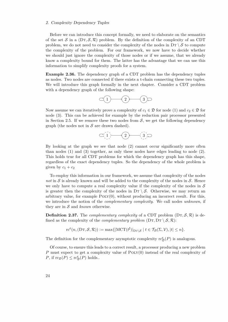
Example 2.36. The dependency graph of a CDT problem has the dependency tuplesas nodes. Two nodes are connected if there exists a t-chain connecting these two tuples.We will introduce this graph formally in the next chapter. Consider a CDT problemwith a dependency graph of the following shape:
1 2 3
Now assume we can iteratively prove a complexity of c1 ∈ D for node (1) and c2 ∈ D fornode (3). This can be achieved for example by the reduction pair processor presentedin Section 2.5. If we remove these two nodes from S, we get the following dependencygraph (the nodes not in S are drawn dashed).
1 2 3
By looking at the graph we see that node (2) cannot occur significantly more oftenthan nodes (1) and (3) together, as only these nodes have edges leading to node (2).This holds true for all CDT problems for which the dependency graph has this shape,regardless of the exact dependency tuples. So the dependency of the whole problem isgiven by c1 + c2
To employ this information in our framework, we assume that complexity of the nodesnot in S is already known and will be added to the complexity of the nodes in S. Hencewe only have to compute a real complexity value if the complexity of the nodes in Sis greater then the complexity of the nodes in Dt \ S. Otherwise, we may return anarbitrary value, for example Poly(0), without producing an incorrect result. For this,we introduce the notion of the complementary complexity. We call nodes unknown, ifthey are in S and known otherwise.
Definition 2.37. The complementary complexity of a CDT problem (Dt,S,R) is de-fined as the complexity of the complementary problem (Dt,Dt \ S,R):
rcc(n, (Dt,S,R)) := max|MCT(t])|Dt\S | t ∈ TB(Σ,V), |t| ≤ n.
The definition for the complementary asymptotic complexity rccD(P ) is analogous.
Of course, to ensure this leads to a correct result, a processor producing a new problemP must expect to get a complexity value of Poly(0) instead of the real complexity ofP , if rcD(P ) ≤ rcc
D(P ) holds..
24
2.3. Framework
Definition 2.38 (Processors). A CDT processor Proc is a function
Proc(P ) = (fup, P1, . . . , Pk)
mapping a CDT problem P = (Dt,S,R) to a complexity fup ∈ D and a set of CDTproblems P1, . . . , Pk. A processor is correct if
rcD(P ) ≤ fup +∑
1≤i≤k(rcD(Pi) rcc
D(Pi)) + rccD(P )
holds.
Let us elaborate on the correctness inequality above a bit more. Proc computes theresult described by
fup +∑
1≤i≤k(rcD(Pi) rcc
D(Pi)).
The difference rcD(Pi) rccD(Pi) encodes the expectation, that a processor solving the
new problem Pi may return a complexity smaller then rcD(Pi) if rcD(Pi) is bounded byrcc
D(Pi). Adding rccD(P ) is the counterpart to this expectation: It allows the processor
to compute a result less or equal to rcD(P ), if rcD(P ) is bounded by rccD(P ). How these
constraints work is illustrated below.
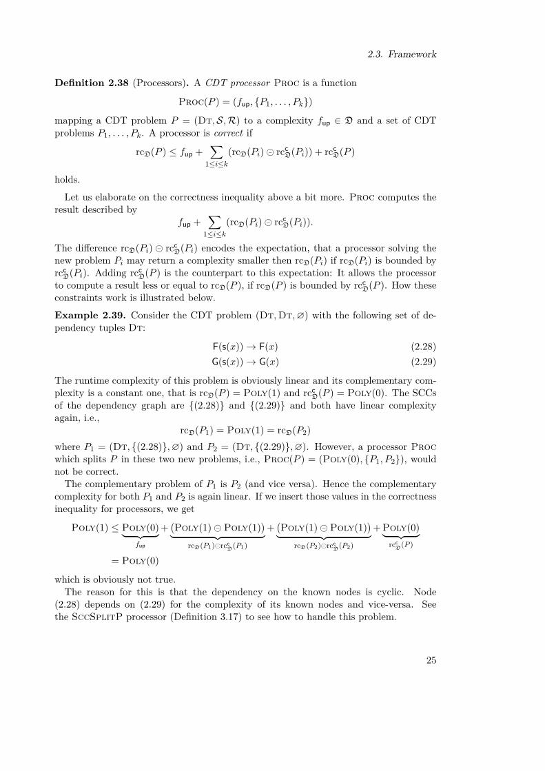
Example 2.39. Consider the CDT problem (Dt,Dt,∅) with the following set of de-pendency tuples Dt:
F(s(x))→ F(x) (2.28)G(s(x))→ G(x) (2.29)
The runtime complexity of this problem is obviously linear and its complementary com-plexity is a constant one, that is rcD(P ) = Poly(1) and rcc
D(P ) = Poly(0). The SCCsof the dependency graph are (2.28) and (2.29) and both have linear complexityagain, i.e.,
rcD(P1) = Poly(1) = rcD(P2)where P1 = (Dt, (2.28),∅) and P2 = (Dt, (2.29),∅). However, a processor Procwhich splits P in these two new problems, i.e., Proc(P ) = (Poly(0), P1, P2), wouldnot be correct.The complementary problem of P1 is P2 (and vice versa). Hence the complementary
complexity for both P1 and P2 is again linear. If we insert those values in the correctnessinequality for processors, we get
Poly(1) ≤ Poly(0)︸ ︷︷ ︸fup
+(Poly(1)Poly(1)
)︸ ︷︷ ︸rcD(P1)rcc
D(P1)
+(Poly(1)Poly(1)
)︸ ︷︷ ︸rcD(P2)rcc
D(P2)
+ Poly(0)︸ ︷︷ ︸rcc
D(P )
= Poly(0)
which is obviously not true.The reason for this is that the dependency on the known nodes is cyclic. Node
(2.28) depends on (2.29) for the complexity of its known nodes and vice-versa. Seethe SccSplitP processor (Definition 3.17) to see how to handle this problem.
25

2. Complexity Dependency Tuples
Example 2.40. The following example illustrates the advantages of our correctnesscondition compared to the simpler (but obviously correct) condition
rcD(P ) ≤ fup +∑
1≤i≤krcD(Pi)
Consider the CDT problem P with the following dependency graph:
1 : F(s(x))→ [F(x),G(a)] 2 : G(x)→ H(x) 3 : H(b)→ G(c)
Now, the runtime complexity of this problem is linear in the length of the input (as eachiteration of tuple 1 calls the second tuple exactly once and one cannot go through thesecond SCC more then once). On the other hand, we know that in a t-chain both 2 and3 occur almost the same number of times. So, if we find out that 3 only occurs once ineach chain tree, we are tempted to return a constant runtime complexity (and no newproblems) for the whole problem.With the simpler condition, this would not be correct as the constraint rcD(P ) <
Poly(0) is not fulfilled. However, using the condition of Definition 2.38 we have tofulfill the constraint
rcD(P ) < Poly(0) + rccD(P )
which is fulfilled, as both the complexity of the first SCC (which equals rccD(P )) and the
complexity of P are linear.
After motivating our definition of a processor, we have to formalize how to combine theresults of the processors to a single, upper bound for the complexity of a CDT problem.For this, we build a proof tree.
Definition 2.41 (Proof Tree). A proof tree is a finite, non-empty tree with nodes(P, fup), where P is a CDT problem such that for each node (P, fup) and its children(P1, fup1), . . . , (Pk, fupk) holds: There exists a correct processor Proc such that
Proc(P ) = (fup, P1, . . . , Pk)
holds. A node of the proof tree is also called proof node.
The complexity is recursively propagated from the leaves to the root.
Definition 2.42 (Result of a proof node). Let T be a proof tree and N a node in T .Then the result of a node (P, fup) is
res(N) := fup + res(N1) + . . .+ res(Nk)
where N1, . . . , Nk are the children of N .
Now we need to show that the result of a proof tree is indeed an upper bound for theproblem in the root node.
26

2.4. Usable Rules
Theorem 2.43 (Correctness of the Proof Tree). Let T be a finite proof tree with rootnode (P, f) and P = (Dt,S,R). Then rcD(P ) ≤ res(P ) + rcc
D(P ). In particular, wehave rcD(P ) ≤ res(P ) for Dt = S.
Proof. We prove the theorem by induction on the depth of T . If the depth is 1, then(P, fup) has no children and
rcD(P ) ≤ fup(n) + rccD(n)P = res(P ) + rcc
D(n)P
holds. Else, (P, fup) has children (P1, fup1), . . . , (Pk, fupk) and we have
rcD(P ) ≤ fup +∑
1≤i≤k(rcD(Pi) rcc
D(Pi)) + rccD(P ).
By the induction hypothesis, rcD(Pi) ≤ res(Pi) + rccD(Pi) holds too, and this implies
rcD(P ) ≤ fup +∑
1≤i≤k(rcD(Pi) rcc
D(Pi)) + rccD(P )
≤ fup +∑
1≤i≤k(res(Pi) rcc
D(Pi)) + rccD(P )
(†)≤ fup +
∑1≤i≤k
res(Pi) + rccD(P )
= res(P ) + rccD(P ).
(†): Note that (x+ y) z = (x z) + (y z) holds true for all values of x, y ∈ D.
To ensure the existence of a finite proof tree, we need a processor which generates nochildren and nevertheless returns a valid result.
Definition 2.44 (Fail processor). The fail processor FailP always returns (Infinite, []).
FailP is obviously correct. When implementing the techniques the described in thisthesis, FailP corresponds to hitting a time or resource limit. Another trivial processoris the emptiness check of S: It converts a trivial problem to a complexity value. It willbe implicitly used after every use of another processor.
Definition 2.45 (S-is-empty processor). Let P = (Dt,S,R) be an CDT problem. Theprocessors SEmptyP returns (Poly(0), []) if S = ∅.
2.4. Usable Rules
For our analysis of a CDT problem (Dt,S,R), the TRS R is only relevant in so far, asthe rules are needed to connect the tuples in a (Dt,R)-t-chain. Quite often, after theinitial transformation (or a transformation like those described in Chapter 3), R willcontain rules, which are not usable in this context.
27
2. Complexity Dependency Tuples
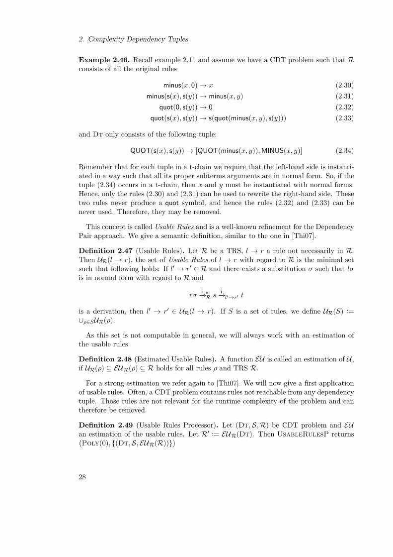
Example 2.46. Recall example 2.11 and assume we have a CDT problem such that Rconsists of all the original rules
minus(x, 0)→ x (2.30)minus(s(x), s(y))→ minus(x, y) (2.31)
quot(0, s(y))→ 0 (2.32)quot(s(x), s(y))→ s(quot(minus(x, y), s(y))) (2.33)
and Dt only consists of the following tuple:
QUOT(s(x), s(y))→ [QUOT(minus(x, y)),MINUS(x, y)] (2.34)
Remember that for each tuple in a t-chain we require that the left-hand side is instanti-ated in a way such that all its proper subterms arguments are in normal form. So, if thetuple (2.34) occurs in a t-chain, then x and y must be instantiated with normal forms.Hence, only the rules (2.30) and (2.31) can be used to rewrite the right-hand side. Thesetwo rules never produce a quot symbol, and hence the rules (2.32) and (2.33) can benever used. Therefore, they may be removed.
This concept is called Usable Rules and is a well-known refinement for the DependencyPair approach. We give a semantic definition, similar to the one in [Thi07].
Definition 2.47 (Usable Rules). Let R be a TRS, l → r a rule not necessarily in R.Then UR(l → r), the set of Usable Rules of l → r with regard to R is the minimal setsuch that following holds: If l′ → r′ ∈ R and there exists a substitution σ such that lσis in normal form with regard to R and
rσi−→∗R s
i−→l′→r′ t
is a derivation, then l′ → r′ ∈ UR(l → r). If S is a set of rules, we define UR(S) :=∪ρ∈SUR(ρ).
As this set is not computable in general, we will always work with an estimation ofthe usable rules
Definition 2.48 (Estimated Usable Rules). A function EU is called an estimation of U ,if UR(ρ) ⊆ EUR(ρ) ⊆ R holds for all rules ρ and TRS R.
For a strong estimation we refer again to [Thi07]. We will now give a first applicationof usable rules. Often, a CDT problem contains rules not reachable from any dependencytuple. Those rules are not relevant for the runtime complexity of the problem and cantherefore be removed.
Definition 2.49 (Usable Rules Processor). Let (Dt,S,R) be CDT problem and EUan estimation of the usable rules. Let R′ := EUR(Dt). Then UsableRulesP returns(Poly(0), (Dt,S, EUR(R))
)
28

2.5. Reduction Pair processor
Example 2.50. For the Example 2.46 given above, the processor UsableRulesP re-turns the CDT problem with the same set Dt and new set of rules R
minus(x, 0)→ x
minus(s(x), s(y))→ minus(x, y)
as none of the quot-rules is usable for the only tuple
QUOT(s(x), s(y))→ [QUOT(minus(x, y)),MINUS(x, y)] (2.35)
in this problem.
The correctness of UsableRulesP follows directly from the following lemma.
Theorem 2.51. Let (Dt,S,R) be CDT problem and EU an estimation of the usablerules. Then
rc(n, (Dt,S,R)) = rc(n,Dt,S, EUR(Dt))
holds for all n ∈ N.
Proof. Let s1 → t1, s2 → t2, . . . be an innermost (Dt,R)-t-chain with substitution σ. Ifa rule l→ r is needed to construct this chain, then there exist i, j ∈ N such that
(ti)jσi−→∗R u
i−→∗l→r vi−→∗R si+σ
holds. As siσ is in normal form with regard to R by the definition of an innermostt-chain, l→ r ∈ UR(si → ti).
2.5. Reduction Pair processorThe use of well-founded orders is one of the classic techniques for proving termination ofa term rewrite system. Popular variants include simplification orders and orders basedon interpretations. Those techniques do not only ensure termination, but also imposean upper bound on the complexity of the systems which can be proved terminating. Asindicated in the preliminaries, most of the well-known orders do not yield polynomialbounds. A path order guaranteeing a polynomial bound on the runtime complexity ispresented in [AM08].Two notable cases of orders based on interpretations are polynomial interpretations
[Lan79; CMTU05] and matrix interpretations. In the general case, polynomial interpre-tations impose a doubly exponential derivational complexity and a complexity of 2O(n)
for linear polynomial interpretations [HL89]. Finally, [BCMT99b] shows that strongmonotonicity and a restriction to the interpretation of constructor symbols guarantee apolynomial runtime complexity. Johannes Waldmann gives a short overview on the up-per bounds induced by matrix interpretations in [Wal09]. In particular, upper triangularmatrices of degree d induce a derivational complexity of O(nd) [PSS97].
29
2. Complexity Dependency Tuples
For Dependency Pairs there exists a reduction pair processor which employs reductionpairs to remove single nodes from the dependency graph. Unfortunately, this is notpossible for complexity analysis. In this section, we define the variant of reduction pairprocessor, which can use orders to remove tuples from the S section. For this matter, weadapt safe reduction pairs and collapsible orders as described in [HM08a]. In addition wedevelop constraints a polynomial interpretation must fulfill to be usable as a reductionpair which establishes an upper polynomial bound.First, we introduce some general notation about orders on terms [Der87; CMTU05].
A term ordering is a tuple (%,) of orderings over T (Σ,V) for some alphabet Σ andvariables V such that % is a quasi-ordering, i.e. transitive and reflexive and is a strictordering, i.e., transitive and irreflexive such that % ⊂ and % ⊂ . Here, denotes the composition of relations.A relation R is well-founded if each sequence t1 R t2 R t3 . . . is finite, stable, if it is
closed under substitution, i.e., t1 R t2 implies t1σ R t2σ for all substitutions and mono-tonic, if it is closed under contexts, i.e f(s1, . . . , sn) R f(s1, . . . , sk−1, tk, sk+1, . . . , sn)follows from sk R tk. An ordering R is compatible with a rewrite system R, if s R tholds for all terms with s→R tA term ordering (%,) is a reduction pair, if is well-founded, % and are stable and% is monotonic. A reduction pair is called safe, if each compound symbol is strictly mono-tonic in all of its arguments, i.e., Com(s1, . . . , sn) Com(s1, . . . , sk−1, tk, sk+1, . . . , sn)if sk tk.We now give a definition of orders, which can be collapsed into the natural numbers.
This definition is similar to the one given in [HM08a].
Definition 2.52 (Collapsible order). An order is G-collapsible on a TRS R, if thereexists a function G : T → N such that s→R t and s t implies G(s) > G(t).
So, for a term t, G(t) is the maximal number of -steps which can be performedstarting with t. Hirokawa and Moser [HM08a] state that most reduction orders arecollapsible.Now we can give the definition of our reduction pair processor.
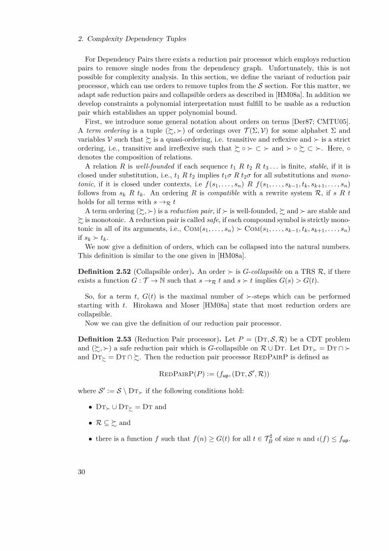
Definition 2.53 (Reduction Pair processor). Let P = (Dt,S,R) be a CDT problemand (%,) a safe reduction pair which is G-collapsible on R∪Dt. Let Dt = Dt ∩ and Dt% = Dt ∩%. Then the reduction pair processor RedPairP is defined as
RedPairP(P ) := (fup, (Dt,S ′,R))
where S ′ := S \Dt if the following conditions hold:
• Dt ∪Dt% = Dt and
• R ⊆ % and
• there is a function f such that f(n) ≥ G(t) for all t ∈ T ]B of size n and ι(f) ≤ fup.
30
2.5. Reduction Pair processor
To automatize this processor, we need a reduction pair, for which the function f canbe easily computed. For the reduction pair based on polynomial interpretations given inTheorem 2.56 this function is given by the interpretation function. A similar result canbe derived for reduction pairs based on matrix interpretations (compare [MSW08] forhow to construct a matrix order to prove the complexity of a TRS directly). Avanziniand Moser [AM09] describe a reduction pair with similar constraints for which ι(f) isbounded by Poly(?). We give an example for the application of the reduction pairprocessor at the end of this section.
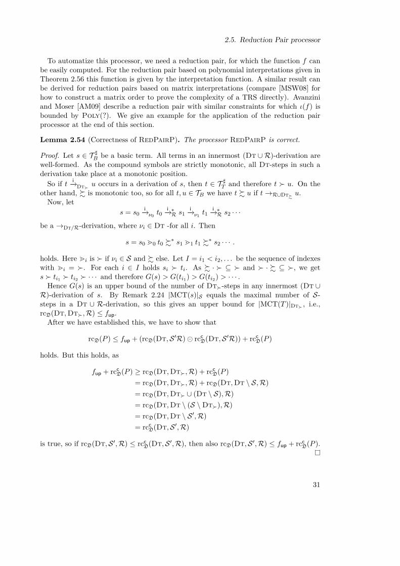
Lemma 2.54 (Correctness of RedPairP). The processor RedPairP is correct.
Proof. Let s ∈ T ]B be a basic term. All terms in an innermost (Dt ∪ R)-derivation arewell-formed. As the compound symbols are strictly monotonic, all Dt-steps in such aderivation take place at a monotonic position.So if t i−→Dt u occurs in a derivation of s, then t ∈ T ]T and therefore t u. On the
other hand, % is monotonic too, so for all t, u ∈ TB we have t % u if t→R∪Dt%u.
Now, lets = s0
i−→ν0 t0i−→∗R s1
i−→ν1 t1i−→∗R s2 · · ·
be a →Dt/R-derivation, where νi ∈ Dt -for all i. Then
s = s0 m0 t0 %∗ s1 m1 t1 %
∗ s2 · · · .
holds. Here mi is if νi ∈ S and % else. Let I = i1 < i2, . . . be the sequence of indexeswith mi = . For each i ∈ I holds si ti. As % · ⊆ and · % ⊆ , we gets ti1 ti2 · · · and therefore G(s) > G(ti1) > G(ti2) > · · · .Hence G(s) is an upper bound of the number of Dt-steps in any innermost (Dt ∪R)-derivation of s. By Remark 2.24 |MCT(s)|S equals the maximal number of S-steps in a Dt ∪ R-derivation, so this gives an upper bound for |MCT(T )|Dt , i.e.,rcD(Dt,Dt,R) ≤ fup.After we have established this, we have to show that
rcD(P ) ≤ fup + (rcD(Dt,S ′R) rccD(Dt,S ′R)) + rcc
D(P )
holds. But this holds, as
fup + rccD(P ) ≥ rcD(Dt,Dt,R) + rcc
D(P )= rcD(Dt,Dt,R) + rcD(Dt,Dt \ S,R)= rcD(Dt,Dt ∪ (Dt \ S),R)= rcD(Dt,Dt \ (S \Dt),R)= rcD(Dt,Dt \ S ′,R)= rcc
D(Dt,S ′,R)
is true, so if rcD(Dt,S ′,R) ≤ rccD(Dt,S ′,R), then also rcD(Dt,S ′,R) ≤ fup + rcc
D(P ).
31

2. Complexity Dependency Tuples
An alternative to the reduction pair processor would be a technique which appliesan order to solve the whole problem at once. But the big benefit of the reduction pairprocessor is that the constraints for the order are much weaker. If we want to prove thecomplexity of a CDT problem with a single order, we have to orient all tuples strictly(and the rules weakly). Using the reduction pair processor it suffices to orient one tuplestrictly. For some problems this is crucial to the success of a proof. We will see anexample for that after we introduce orders based on polynomial interpretations.But there are further advantages to the reduction pair approach. By the modular
nature of this processor, it is possible to use different types of orders to simplify theproblem iteratively. But not only the proof of the complexity of a problem is modular-ized, but also the theory needed to find applicable orders. For orders like polynomialor matrix interpretations it is well-known how to construct the constraints necessary tofulfill the requirements of the reduction pair processor, so their adaption is a simple task.In particular there is an extension of the Reduction Pair processor which employs usablerules w.r.t argument filtering systems [GTSF06]: This extension allows ignoring some ofthe usable rules of a system under certain conditions. If we want to use this techniquefor our complexity analysis, we only have to redo the correctness proof for the reductionpair processor, not for correctness proof for the orders we employ.To implement this processor we must be able to (automatically) find a reduction pair.
Polynomial interpretations are a well-understood and easily automated mechanism forfinding reduction pairs and obviously collapsible. Only few additional constraints arenecessary to use them for proving polynomial runtime complexity. First, we recall theshort definition of an interpretation and the associated ordering.
Definition 2.55 (Interpretation). Let (A,A,%A) be an algebra. Let Σ be a signatureand V a probably infinite set of variables. For each n-ary function symbol f ∈ Σ let [f ]be a n-ary function A × · · · × A → A. [·] is called an A-interpretation. A (variable)assignment is a mapping V → N.We extend [·] to T (Σ,V) by setting
[t]α :=α(x) if t = x ∈ V[f ]α([t1]α, . . . , [tn]α) if t = f(t1, . . . , tn)
So [t] is a function mapping an assignment to A. For terms s, t, we set s t if and onlyif [s]α A [t]α for all assignments α. Analogous, s % t if and only if [s]α %A [t]α.We say a rule l→ r is strictly decreasing, if l r and weakly decreasing, if l % r.
In this section, we are interested primarily in interpretations over the algebra (N, >,≥),where > and ≥ are the usual greater and greater-equal relations on the natural numbers.A simple idea to derive a complexity bound is the following: Let [·] be an interpretation
over N. If s → t implies [s] > [t], i.e. the order associated with [·] is collapsible,then obviously the derivation length of s with regard to → is smaller or equal then[s]. Bonfante, Cichon, Marion, and Touzet [BCMT99b] already outlined the restrictionsneeded for a polynomial order to fulfill this requirement. But for reduction pairs, thoserestrictions can be loosened considerably.
32

2.5. Reduction Pair processor
Theorem 2.56. Let R,P be TRSs over Σ and V. Let [·] be a polynomial interpretationsuch that the associated ordering (%,) is a reduction pair with R ⊆ % and P ⊆ . If foreach n-ary compound symbol Com the interpretation is [Com](x1, . . . , xn) = x1+. . .+xn,the reduction pair is a safe reduction pair.If in addition [c](x1, . . . , xn) = a1x1 + · · · + anxn + b with ai ∈ 0, 1 and b ∈ N for
all n-ary constructor symbols f ∈ CR, then [f ](k) is an upper bound for the number ofP-steps in a derivation of a term with size k and root symbol f .
Proof. The first restriction is obvious. The second restriction ensures that the interpre-tation of a constructor term is at most its size k (multiplied with a factor c independentof k). So we get also
c′ · [f ](m1, . . . ,mn) ≥ [f ](cm1, . . . , cmn) ≥ dl(f(t1, . . . , tn),→Dt/R)
for all defined symbols f and constructor terms t1, . . . , tn such that |ti| ≤ mi.
There are well-established techniques to find reduction pairs with the help of polyno-mial interpretations [GTSF06] [CMTU05] [FGMSTZ07]. Those techniques allow givingarbitrary restrictions to the form of the constructed polynomials, so they can easily beemployed to automate the above theorem.
Example 2.57. Consider the CDT problem (Dt,S,R) described by the following de-pendency graph:
EVENODD(s(x), s(0))→ Com1(EVENODD(x, 0))
EVENODD(x, 0)→ Com2(EVENODD(x, s(0)))
These two tuples cannot be oriented strictly by a polynomial interpretation. The secondrule requires [0] > [s(0)] and hence [s] must be a constant as all coefficients are naturalnumbers. But then [s(x)] > [x] does not hold for all variable assignments, so we need[0] < [s(0)], too.But orienting a single tuple strictly (and the other weakly) is easy. The interpretation
[EVENODD](x, y) = x [s](x) = x+ 1 [0] = 0
orients the first tuple strict and hence it may be removed from S. By applying theKnownnessP processor presented in the next section, we may remove the other tupleto and hence have proved linear complexity for this problem.
33


3. Complexity Dependency Graph
The Dependency Graph is an important part of the original Dependency Pair approach.The idea is to expose which pairs can follow each other in a chain. For dependencytuples, we use essentially the same definition.
Definition 3.1 (Complexity Dependency Graph). For a CDT problem (Dt,S,R), theComplexity Dependency Graph is the directed graph G = (V,E) with nodes V = Dtand two nodes v1 = s1 → t1, v2 = s2 → t2 are connected in G, i.e., (v1, v2) ∈ E iffs1 → t1, s2 → t2 is a t-chain.We say an edge (v1, v2) exists for the rhs i, iff v1 〈i〉 v2 holds.
We say that u is a predecessor (successor) of v, if (u, v) ∈ E ((v, u) ∈ E). A path is asequence of nodes u1, u2, . . . such that ui+1 is a successor of ui for all i > 1. A node vis reachable from u, if there is a (probably non-empty) path from v to u.
Example 3.2. The Complexity Dependency Graph for Example 2.11 is the followinggraph (we shortened the function symbols to one character):
M(x, 0)→ []M(s(x), s(y))→ [M(x, y)]
Q(0, x)→ []Q(s(x), s(y)→ [Q(m(x, y), s(y)),M(x, y)]
In termination analysis, it is sound (and complete) to decompose P into the stronglyconnected components of the graph. Here, we follow the usual convention for dependencypairs and require that an SCC contains at least one edge. This differs from the usualgraph-theoretic definition, where a single, unconnected node is also considered a SCC.
Definition 3.3 (Strongly Connected Component). A subset C of a graph G is stronglyconnected, if for every pair of nodes u, v ∈ C there are a non-empty paths from u to vand from v to u. Such a set is called a strongly connected component (or SCC ), if it isnot a proper subset of another strongly connected set.
Definition 3.4 (Mathematical SCC). A mathematical SCC (MSCC) is an SCC or asingle node not part of any SCC.
Sometimes, we need a more fine grained look on SCCs.
Definition 3.5 (Cycle). A subset C = c1, . . . , cn of a graph G is called a cycle, if theci are pairwise disjoint and c1, c2, . . . , cn, c1 is a path in G.
35

3. Complexity Dependency Graph
Obviously, each cycle is contained in a SCC. Unfortunately, the SCC-decompositionof the Complexity Dependency Graph is not complexity preserving.
Example 3.6. Consider the following system computing powers of two.
double(0)→ 0 (3.1)double(s(x))→ s(s(double(x))) (3.2)
exp(0)→ s(0) (3.3)exp(s(x))→ double(exp(x)) (3.4)
As we have seen in Example 2.5, the derivation length of doublen(x) is exponential in n.Evaluating exp(sn(x)) yields doublen(x), so the system has indeed exponential runtimecomplexity. The CDT-transformation yields the following pairs
DOUBLE(0)→ [] (3.5)DOUBLE(s(x))→ [DOUBLE(x)] (3.6)
EXP(0)→ [] (3.7)EXP(s(x))→ [EXP(x),DOUBLE(exp(x))] (3.8)
and 3.6 and 3.8 are the SCCs of the graph. It is easy to see that the runtimecomplexity of both SCCs is linear. By analyzing each SCC on its own, we ignore thefact that 3.8 calls 3.6 with arguments exponential in the size of the start term.
As one of the main advantages of the Dependency Graph is the ability to decomposethe original problem into smaller ones, we need to find a replacement for the SCC-decomposition. An obviously correct, but much weaker idea is to decompose the graphinto its components.
Definition 3.7 (Component). A component of a graph G is an inclusion-maximal subsetC ⊆ G such that for all pairs of nodes u, v ∈ C there is a path from u to v in theunderlying undirected graph.
Theorem 3.8 (Graph Split). Let (Dt,S,R) be a CDT problem and C1, . . . , Ck thecomponents of the dependency graph. Then we have
min1≤i≤k
rc(n, (Ci,S ∩ Ci,R)) ≤ rc(n, (Dt,S,R)) ≤ max1≤i≤k
rc(n, (Ci,S ∩ Ci,R)).
Proof. By the definition of the dependency graph, a t-chain starting with a node s→ tcan only reach nodes in the same component. Therefore all t-chains in a chain treelie in only one component and therefore for each (Dt,R)-chain tree T there exists an1 ≤ i ≤ k such that T is an (Ci,R)-chain tree.
To compute the Graph-Split, we need the dependency graph. Unfortunately, thisgraph is not computable in general. But for all our needs an approximation containing atleast all the edges of the dependency graph suffices. As our definition of the ComplexityDependency Graph is essentially the same as the definition of the Dependency Graph fortermination, we can easily use well-known graph approximations [AG00; Mid01; GTS05a;Thi07] as described in [Thi07].
36

3.1. Simplifying S
3.1. Simplifying SIn this section we will see how to use the Dt versus S distinction to simplify proofs ofcomplexity. This distinction resembles the notion of relative rewriting [BD86]: We useboth nodes in S and Dt \ S, but count only nodes in S. So we when we remove a tuplefrom S, we call this relative tuple removal.While the techniques presented here do not make the graph by itself simpler, they
reduce the number of pairs which have to be oriented strictly by the reduction pairprocessor. First, we make a simple observation.Remark 3.9 (Relative Graph Split). Let (Dt,S,R) be a CDT problem and S1 ∪ · · · ∪Skbe a partition of S. Then
rc(n, (Dt,S,R)) =∑
1≤i≤krc(n, (Dt,Si,R))
holds for all n ∈ N.This remark allows us to prove upper bounds for each tuple separately: If we we know
the upper bound for some of the tuples, we may remove them from S. As Example 2.39demonstrates, the naive way of turning Remark 3.9 into a processor is incorrect. Wewill see how to use this correctly later.Often, we can derive an upper bound for the occurrences of one node, if we know how
often its predecessors can occur.
Lemma 3.10 (Knownness propagation). Let (Dt,S,R) be a CDT problem with depen-dency graph (Dt, E) and ν ∈ Dt. Let N be the set of incoming nodes of ν, i.e., (ρ, ν) ∈ Efor all ρ ∈ N . Furthermore, let k be the maximal number of right-hand sides of a tuplein N . If |T |N = s for an arbitrary (Dt,S,R)-chain tree T , then |T |ρ ≤ 1 + ks.
Proof. Let T be a (Dt,S,R)-chain tree and v an occurrence of ν in T . Then either vis the root node, or v is successor of a node in N . Each of these nodes has at most kright-hand sides, so |T |ν ≤ 1 + ks follows.
We can use this theorem to reduce the work needed to be done by the reduction pairprocessor.
Definition 3.11 (Knownness propagation processor). Let P = (Dt,S,R) be a CDTproblem. Let ν ∈ Dt be a node in the dependency graph and N be the set of incomingnodes of ν. If N ∩ S = ∅, then the knownness propagation processor KnownnessPreturns
KnownnessP(P ) := (Poly(0), (Dt,S \ ν,R))
Lemma 3.12 (Correctness of KnownnessP). The processor KnownnessP is correct.
Proof. Follows from Lemma 3.10, as rccD(Dt,S \ ν,R) = rcc
D(P ).
Example 3.13. Recall the graph of Example 2.36:
37

3. Complexity Dependency Graph
1 2 3
As none of the incoming nodes of node (2) is in S, the KnownnessP processor returnsthe trivial problem
1 2 3
which can be solved by the SEmptyP processor.
In the next section we will see that some nodes in Dt \ S can even be removedcompletely from the problem. Combining this with the results above, we can finally getsome kind of SCC processor.
3.2. Graph simplificationIn this section we build on the results of the (relative) graph split and try to makecomponents as SCC-like as possible. Of particular interest are those nodes, which canonly occur at the beginning or at the end of a t-chain, i.e., those nodes which have noincoming respective outgoing edge in the dependency graph. We call those nodes leadingrespective trailing (or dangling, if we mean both).We have demonstrated in Example 3.6 that the SCC-split is unsound as we cannot see
anymore that an SCC was reached with arguments considerably bigger then the startterm. This observation suggests that paths not leading to a SCC may be removed safely.
Theorem 3.14 (Removal of trailing nodes). Let (Dt,S,R) be a CDT problem withdependency graph G. Let V ⊆ Dt \ S be a set containing all nodes reachable from V .Then
rc(n, (Dt,S,R)) = rc(n,Dt′,S,R)
holds, where Dt′ := Dt \ V .
Proof. As all nodes reachable from V are contained in V , there can be no node fromDt \ V after a node from V on an innermost (Dt,S,R)-t-chain. Hence, removing allV -nodes from a (Dt,S,R)-chain tree T still yields a valid (Dt′,S,R)-chain tree T ′. AsV and S are disjoint, |T |S = |T ′|S holds.
Example 3.15. Consider the CDT problem given by the following dependency graph.
1: F(s(x), a)→ F(x, a) 2: F(0, x)→ F(s(0), b)
It is not possible to orient tuple (1) strictly and tuple (2) weakly with an polynomialorder. Tuple (1) requires that [s](x) > x for all x ∈ N, while the second tuple requiresthat [0] ≤ [s(0)]. By applying Theorem 3.14, node (2) can be removed and the remainingtuple can easily be oriented strictly.
38

3.2. Graph simplification
Note that the above theorem even allows us to remove whole SCCs, if they are markedas being of known complexity. We have restricted the theorem to known nodes, but wecan use a combination of Remark 3.9, Lemma 3.10 and Lemma 3.21 to delete arbitrarytrailing nodes. Now, we finally are able to find a worthy equivalent to the DependencyGraph Processor which allows splitting a DP problem in its SCCs.
Definition 3.16 (Preceding MSCCs). Let G be a graph, C1 6= C2 two mathematicalSCCs of G. If there is an edge (c1, c2) for some c1 ∈ C1 and c2 ∈ C2, we say C1 precedesC2 and write C1 / C2. We denote by /∗ the transitive and reflexive closure of / and by/+ the transitive closure.By C1
/ :=⋃C/∗C1 C we denote the reachability closure of C1, i.e., the set of all nodes,
from which C1 can be reached.
Definition 3.17 (SCC Split processor). Let P = (Dt,S,R) be a CDT problem andC1, . . . , Ck the SCCs of the dependency graph. For each SCC Ci let Dti := Ci
/. Thenthe SCC Split processor SccSplitP returns
SccSplitP(P ) = (Poly(0), [(Dt1, C1 ∩ S,R), . . . , (Dtk, Ck ∩ S,R)])
Proving the correctness of SccSplitP turns out to be rather technical. We will givethe idea of the proof directly and move the technical details to auxiliary lemmas.
Lemma 3.18 (Correctness of SccSplitP). The processor SccSplitP is correct.
Proof. Let G be the dependency graph of P and C be the set of mathematical SCCs ofG. For a C ∈ C, let PC := (C/, C ∩ S,R). By remark 3.9 we have
rcD(P ) ≤∑C∈C
rcD(PC)
≤∑C∈C
rcD(C/, C/ ∩ S,R)
≤∑C∈CT
rcD(C/, C/ ∩ S,R)
where CT is the set of MSCCs which have no successor (i.e., not C / C ′ for any pair ofC ∈ CT and C ′ ∈ C). In Lemma 3.19 we show that
rcD(C/, C/ ∩ S,R) ≤∑B/∗C
(rcD(PB) rccD(PB)) + rcD(P )
holds for all C ∈ C. Together with the above, this proves
rcD(P ) ≤∑B/∗C
(rcD(PB) rccD(PB)) + rcD(P ).
In addition, Lemma 3.20 tells us that rcD(PC) rccD(PC) = Poly(0) for all C ∈ C which
are only MSCCs but no SCCs. So we finally arrive at
rcD(P ) ≤∑
1≤i≤k(rcD(PCi) rcc
D(PCi)) + rcD(P ),
which proves the correctness of the processor.
39
3. Complexity Dependency Graph
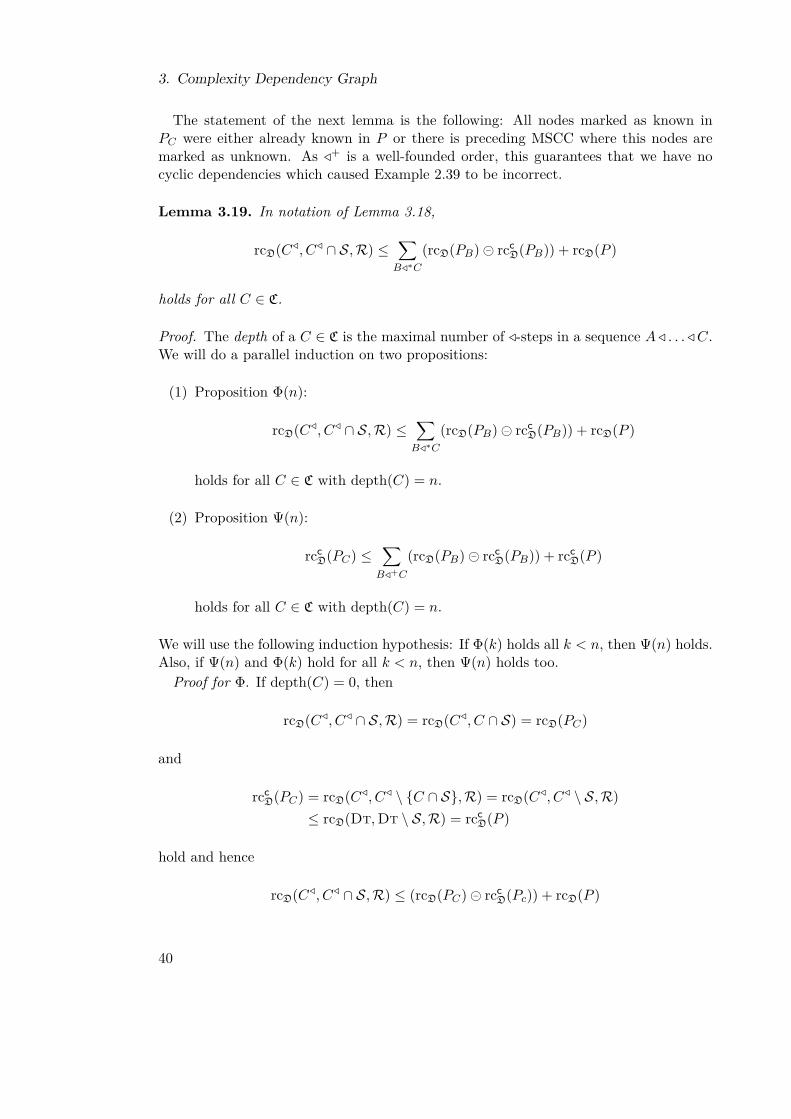
The statement of the next lemma is the following: All nodes marked as known inPC were either already known in P or there is preceding MSCC where this nodes aremarked as unknown. As /+ is a well-founded order, this guarantees that we have nocyclic dependencies which caused Example 2.39 to be incorrect.
Lemma 3.19. In notation of Lemma 3.18,
rcD(C/, C/ ∩ S,R) ≤∑B/∗C
(rcD(PB) rccD(PB)) + rcD(P )
holds for all C ∈ C.
Proof. The depth of a C ∈ C is the maximal number of /-steps in a sequence A/ . . . / C.We will do a parallel induction on two propositions:
(1) Proposition Φ(n):
rcD(C/, C/ ∩ S,R) ≤∑B/∗C
(rcD(PB) rccD(PB)) + rcD(P )
holds for all C ∈ C with depth(C) = n.
(2) Proposition Ψ(n):
rccD(PC) ≤
∑B/+C
(rcD(PB) rccD(PB)) + rcc
D(P )
holds for all C ∈ C with depth(C) = n.
We will use the following induction hypothesis: If Φ(k) holds all k < n, then Ψ(n) holds.Also, if Ψ(n) and Φ(k) hold for all k < n, then Ψ(n) holds too.Proof for Φ. If depth(C) = 0, then
rcD(C/, C/ ∩ S,R) = rcD(C/, C ∩ S) = rcD(PC)
and
rccD(PC) = rcD(C/, C/ \ C ∩ S,R) = rcD(C/, C/ \ S,R)
≤ rcD(Dt,Dt \ S,R) = rccD(P )
hold and hence
rcD(C/, C/ ∩ S,R) ≤ (rcD(PC) rccD(Pc)) + rcD(P )
40
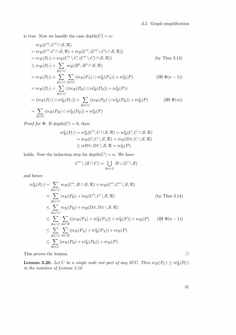
3.2. Graph simplification
is true. Now we handle the case depth(C) = n:
rcD(C/, C/ ∩ S,R)= rcD(C/, C ∩ S,R) + rcD(C/, (C/ \ C) ∩ S,R))= rcD(PC) + rcD(C/ \ C, (C/ \ C) ∩ S,R)) (by Thm 3.14)≤ rcD(PC) +
∑B/+C
rcD(B/, B/ ∩ S,R)
= rcD(PC) +∑B/+C
∑A/∗C
(rcD(PA) rccD(PA)) + rcc
D(P ) (IH Φ(n− 1))
= rcD(PC) +∑B/+C
((rcD(PB) rccD(PB)) + rcc
D(P ))
= (rcD(PC) rccD(PC)) +
∑B/+C
(rcD(PB) rccD(PB)) + rcc
D(P ) (IH Ψ(n))
=∑B/∗C
(rcD(PB) rccD(PB)) + rcc
D(P )
Proof for Ψ. If depth(C) = 0, then
rccD(PC) = rcc
D(C/, C ∩ S,R) = rccD(C,C ∩ S,R)
= rcD(C,C \ S,R) = rcD(Dt, C \ S,R)≤ rcDt,Dt \ S,R = rcc
D(P )
holds. Now the induction step for depth(C) = n. We have
C/ \ (S ∩ C) =⋃
B/+C
B ∪ (C \ S)
and hence
rccD(PC) =
∑B/+C
rcD(C/, B ∩ S,R) + rcD(C/, C/ \ S,R)
=∑B/+C
rcD(PB) + rcD(C/, C \ S,R) (by Thm 3.14)
≤∑B/+C
rcD(PB) + rcD(Dt,Dt \ S,R)
≤∑B/+C
∑A/∗B
((rcD(PA) + rccD(PA)) + rcc
D(P )) + rcD(P ) (IH Φ(n− 1))
≤∑B/+C
∑A/∗B
(rcD(PA) + rccD(PA)) + rcD(P )
≤∑B/∗C
(rcD(PB) + rccD(PB)) + rcD(P ).
This proves the lemma.
Lemma 3.20. Let C be a single node not part of any SCC. Then rcD(PC) ≤ rccD(PC)
in the notation of Lemma 3.18.
41

3. Complexity Dependency Graph
Proof. Follows directly from Lemma 3.21 below.
If we consider nodes not in any SCC, we observe that they do not heavily influence theasymptotic complexity; how often such a node can occur in a chain tree is determinedby the SCCs from which this node is reachable.
Lemma 3.21. Let P = (Dt,S,R) be a CDT problem such that no s ∈ ST occurs inany SCC of the dependency graph. Then there exists constants c1, c2 such that
rc(n, (Dt,S,R)) ≤ c1 + c2 · rcc(n, (Dt,S,R))
holds for all n ∈ N.
Proof. Induction over |S|. If |S| = 0, we have rc(n, (Dt,S,R)) = 0 and hence this caseholds. Else, as no s ∈ S is part of any SCC, there exists a s ∈ S such that S ∩Pred = ∅,where Pred is the set of predecessors of s (i.e., the complexity of all predecessors isknown). Set S ′ := S \ s and let k be the maximal number of right-hand sides in Dt.Then, by using knownness propagation (3.10), we have
rc(n, (Dt, s,R)) ≤ 1 + k · rc(n, (Dt,Pred,R)) ≤ 1 + k · rcc(n, P )
as P ⊆ Dt \ S. Hence
rc(n, P ) ≤ 1 + rc(n, (Dt, s,R)) + rc(n, (Dt,S ′,R))= 1 + rc(n, (Dt, s,R)) + c1 + c2 · rcc(n, (Dt,S ′,R)) (†)= 1 + rc(n, (Dt, s,R)) + c1 + c2 · (rcc(n, P ) + rc(n, (Dt, s,R))) (‡)≤ 1 + c1 + (1 + c2)rc(n, (Dt, s,R)) + c2 · rcc(n, P )≤ 1 + c1 + (1 + c2)(1 + k · rcc(n, P )) + c2 · rcc(n, P )≤ (2 + c1 + c2) + (k + kc2 + c2) · rcc(n, P )≤ c′1 + c′2 · rcc(n, P )
for some constants c′1 and c′2. In the (†)-step, we are applying the induction hypothesis,while in the (‡)-step we use the fact that (Dt \ S) ∪ s = Dt \ S ′.
If we fully remove nodes from the graph, there are often nodes, for which some, butnot all right-hand sides have no successor anymore. Simplifying those does not influencethe complexity of the CDT problem.
Definition 3.22 (Removal of trailing right-hand sides). Let P = (Dt,S,R) be a CDTproblem. Let s → t with t = [t1, . . . , tn] be a node in the dependency graph G suchfor the right-hand sides with indexes I = 1 ≤ i1, . . . , ik ≤ n exists no edge in G. Letu = [tj1 , . . . , tjn−k ] be a tuple where j1 < . . . < jn−k are the indexes not in I. Then theremoving trailing rhs processor RemoveTrailRhsP returns
RemoveTrailRhsP(P ) := (Poly(0), (Dt′,S ′,R))
where Dt′ := Dt[s→ t/s→ u] and S ′ := Dt[s→ t/s→ u].
42

3.2. Graph simplification
Lemma 3.23. The processor RemoveTrailRhsP is correct.
Proof. There is no (Dt,S,R)-t-chain containing s → t 〈i〉 v → w for any i ∈ I andv → w ∈ Dt.
In particular circumstances, we may also remove nodes without an incoming edge.For removing leading nodes, there are two obstacles: On the one hand, they might havemultiple right-hand sides. By removing such a node from a chain tree, we would notonly reduce its size by one, but split it into multiple trees. We will see how to handlethis case later on. A more serious issue arises from the fact, that we are concerned withthe complexity analysis on basic terms only.
Example 3.24. Consider the nonterminating system R:
start(x)→ inf(inf(x))inf(inf(x))→ inf(inf(x))
with the following dependency graph:
(1) START(x)→ INF(inf(x)) (2) INF(inf(x))→ INF(inf(x))
While there are infinite t-chains consisting only of copies of the second node, none ofthese starts with a term t] where t is a basic term. So the runtime complexity of theCDT problem ((2),R) is always 0.
So we may not remove a leading node if one of the obstacles above exist.
Lemma 3.25 (Removal of simple leading nodes). Let (Dt,S,R) be a CDT problemwith dependency graph G = (V,E). Let v = s→ [t] be a node of G with only one right-hand side. If v has no incoming edges and t contains no DR-symbols, then there existconstants k, l such that
rc(n, (Dt,S,R)) ≤ 1 + rc(nk + l, (Dt′,S ′,R))
holds, where Dt′ := D \ v and S ′ := Dt′ ∩ S.
Proof. As v has no incoming edge, v can only occur as the root node in a (Dt,R)-chaintree. Let T be an innermost (Dt,R)-chain tree with substitution σ whose root node iss→ [t] and sσ is basic. We now consider the chain tree T ′ derived from T by removingv. Hence |T |S ≤ |T ′|S + 1.If T ′ is not empty, T has the following form:
s→ [t] s′ → t′
. . .
...
. . .
43
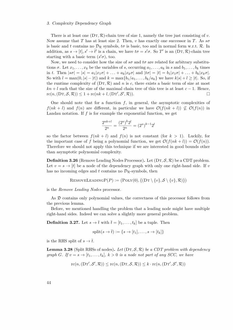
3. Complexity Dependency Graph
There is at least one (Dt,R)-chain tree of size 1, namely the tree just consisting of v.Now assume that T has at least size 2. Then, v has exactly one successor in T . As sσis basic and t contains no DR symbols, tσ is basic, too and in normal form w.r.t. R. Inaddition, as s→ [t], s′ → t′ is a chain, we have tσ = s′σ. So T ′ is an (Dt,R)-chain treestarting with a basic term (s′σ), too.Now, we need to consider how the size of sσ and tσ are related for arbitrary substitu-
tions σ. Let x1, . . . , xk be the variables of s, occurring a1, . . . , ak in s and b1, . . . , bk timesin t. Then |sσ| = |s| = a1|x1σ| + . . . + ak|xkσ| and |tσ| = |t| = b1|x1σ| + . . . + bk|xkσ|.So with l = max(0, |s| − |t|) and k = maxb1/a1, . . . , bk/ak we have k|s|+ l ≥ |t|. So, ifthe runtime complexity of (Dt,R) and n is c, there exists a basic term of size at mostkn+ l such that the size of the maximal chain tree of this tree is at least c− 1. Hence,rc(n, (Dt,S,R)) ≤ 1 + rc(nk + l, (Dt′,S ′,R)).
One should note that for a function f , in general, the asymptotic complexities off(nk + l) and f(n) are different, in particular we have O(f(nk + l)) 6⊆ O(f(n)) inLandau notation. If f is for example the exponential function, we get
2nk+l
2n = (2n)k2l
2n = (2n)k−12l
so the factor between f(nk + l) and f(n) is not constant (for k > 1). Luckily, forthe important case of f being a polynomial function, we get O(f(nk + l)) = O(f(n)).Therefore we should not apply this technique if we are interested in good bounds otherthan asymptotic polynomial complexity.
Definition 3.26 (Remove Leading Nodes Processor). Let (Dt,S,R) be a CDT problem.Let v = s → [t] be a node of the dependency graph with only one right-hand side. If vhas no incoming edges and t contains no DR-symbols, then
RemoveLeadingP(P ) :=(Poly(0), (Dt \ v,S \ v,R)
)is the Remove Leading Nodes processor.
As D contains only polynomial values, the correctness of this processor follows fromthe previous lemma.Before, we mentioned handling the problem that a leading node might have multiple
right-hand sides. Indeed we can solve a slightly more general problem.
Definition 3.27. Let s→ t with t = [t1, . . . , tk] be a tuple. Then
split(s→ t) := s→ [t1], . . . , s→ [tk]
is the RHS split of s→ t.
Lemma 3.28 (Split RHSs of nodes). Let (Dt,S,R) be a CDT problem with dependencygraph G. If v = s→ [t1, . . . , tk], k > 0 is a node not part of any SCC, we have
rc(n, (Dt′,S ′,R)) ≤ rc(n, (Dt,S,R)) ≤ k · rc(n, (Dt′,S ′,R))
44

3.2. Graph simplification
where Dt′ := (Dt \ v) ∪ split(v) and
S ′ :=
(S \ v) ∪ split(v) if v ∈ DtS if v 6∈ Dt.
In the case k = 0, this split would lead to a complete removal of the node. This caseis already handled by Theorem 3.14. As this would make the proof more complicated,we do not include it here.
Proof. Such a node can only occur once in each t-chain. Hence, if we consider all subtreesstarting with v in a chain tree, those subtrees are not overlapping. Therefore, if we reducethe size of each subtree by a factor of l, the size of the whole tree is reduced by at mosta factor of l. This is demonstrated in the graphs below, where the original chain-tree ison the left and the transformed chain-tree is on the right.
u→ v
s→ t
t1ti tk s→ t
t1 ti tk
u→ v
s→ ti
tis→ t1
t1
Each subtree T starting with v has at most k successors, each of them again a subtree.Let us call these trees T1 to Tk. Assume Tl is the largest one (measuring S-nodes) ofthem. Let T ′ be the tree we get if we remove all of T1 to Tk except Tl. Then |T |S ≤ k|T ′|S .Now, if s → [t1, . . . , tn], u → v, . . . is a t-chain, then s → [ti], u → v, . . . is also a
t-chain for some 1 ≤ i ≤ n. So if we replace v by s → [tl] in T ′, the resulting treeis (Dt′,R)-chain tree. Replacing v does not change the size, as v ∈ S if and only ifs→ [tl] ∈ S ′.So for each (Dt,R)-chain tree of size m, we can construct a (Dt′,R)-chain tree
starting with the same term of size m′ such that m < km′. The two graphs in the figureabove visualize this construction.
The above theorem does not only solve the problem of leading nodes having morethen one right-hand side, but leverages also the “defined symbols on the right handside” problem a bit: If only some of the right-hand sides have defined symbols, we arenevertheless able to delete the others.
Definition 3.29 (RhsSplitP). Let P = (Dt,S,R) be a CDT problem. Let V be theset of nodes not part of any SCC and with at least one right-hand side. Let k be themaximal number of right-hand sides of a tuple in V. Then
RhsSplitP(P ) := (fup, (Dt′,S ′,R))
45
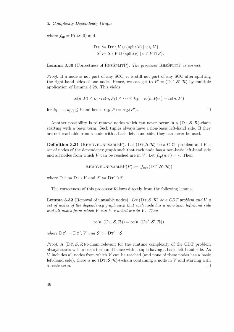
3. Complexity Dependency Graph
where fup = Poly(0) and
Dt′ := Dt \ V ∪ split(v) | v ∈ V S ′ := S \ V ∪ split(v) | v ∈ V ∩ S.
Lemma 3.30 (Correctness of RhsSplitP). The processor RhsSplitP is correct.
Proof. If a node is not part of any SCC, it is still not part of any SCC after splittingthe right-hand sides of one node. Hence, we can get to P ′ = (Dt′,S ′,R) by multipleapplication of Lemma 3.28. This yields
rc(n, P ) ≤ k1 · rc(n, P1) ≤ · · · ≤ k|V | · rc(n, P|V |) = rc(n, P ′)
for k1, . . . , k|V | ≤ k and hence rcD(P ) = rcD(P ′).
Another possibility is to remove nodes which can never occur in a (Dt,S,R)-chainstarting with a basic term. Such tuples always have a non-basic left-hand side. If theyare not reachable from a node with a basic left-hand side, they can never be used.
Definition 3.31 (RemoveUnusableP). Let (Dt,S,R) be a CDT problem and V aset of nodes of the dependency graph such that each node has a non-basic left-hand sideand all nodes from which V can be reached are in V . Let fup(n; r) = r. Then
RemoveUnusableP(P ) := (fup, (Dt′,S ′,R))
where Dt′ := Dt \ V and S ′ := Dt′ ∩ S.
The correctness of this processor follows directly from the following lemma.
Lemma 3.32 (Removal of unusable nodes). Let (Dt,S,R) be a CDT problem and V aset of nodes of the dependency graph such that each node has a non-basic left-hand sideand all nodes from which V can be reached are in V . Then
rc(n, (Dt,S,R)) = rc(n, (Dt′,S ′,R))
where Dt′ := Dt \ V and S ′ := Dt′ ∩ S.
Proof. A (Dt,S,R)-t-chain relevant for the runtime complexity of the CDT problemalways starts with a basic term and hence with a tuple having a basic left-hand side. AsV includes all nodes from which V can be reached (and none of these nodes has a basicleft-hand side), there is no (Dt,S,R)-t-chain containing a node in V and starting witha basic term.
46

3.3. Transformation techniques
3.3. Transformation techniquesTwo nodes are connected in the dependency graph, if there is a chain consisting ofthose two nodes. So this connection criterion is a local one and only considers a singlestep. Often, this is less information than what we need to prove a complexity bound(or termination). One can use transformation techniques to look further than one step:A transformation step replaces one node by zero or more new nodes, which incorporatesome information about the neighbors of the old node. Often this makes finding areduction pair easier or even breaks cycles in the dependency graph. The transformationspresented here are adapted variants of the Dependency Pair transformations describedin Giesl, Thiemann, Schneider-Kamp, and Falke [GTSF06].
Definition 3.33 (Replacing a tuple). Let Dt, N be sets of dependency tuples. Let νbe a tuple. Then Dt[ν/N ] is the set, where ν was replaced by N:
Dt[ν/N ] :=
Dt if ν 6∈ Dt(Dt \ ν) ∪N else
For a CDT problem (Dt,S,R) we also write (Dt,S,R)[ν/N ] for (Dt[ν/N ],S[ν/N ],R).
The idea behind the instantiation techniques is to propagate informations about pos-sible instantiations of variables. For the (backward) instantiation technique one takespreceding nodes u → v into account to instantiate variables of a node s → t. If v con-tains no defined symbols, this is easy: vi and s must unify for some i. But in general, vicontains R-defined symbols which might get rewritten before s can be applied. So, weneed to remove everything from vi which is not kept constant in a chain u → v, s → t.This is done by the Cap function.
Definition 3.34 (Cap). Let R be a set of generalized rules (i.e., rules potentiallyviolating the variable condition). Then t′ := CapR(t) is the term which is derived fromt by replacing each subterm t|π by a fresh variable, if there exists a substitution σ suchthat tσ −→∗R u
π−→R v.For the innermost case, we have t′ := Capi
R(s→ t) as the term, which is derived fromt by replacing each subterm t|π by a fresh variable, if there exists a substitution σ suchthat sσ is in R-normal form and tσ i−→∗R u
i−→ [π]Rv.An estimated cap function ECap is a function which replaces at least all those positions
replaced by the real cap function with fresh variables.
Once again, the definition above is a semantic one. A more general definition (andcomputable estimations) are given by [GTS05a] and [Thi07], Definition 3.7.It is important to note that we only analyze rewriting on a restricted set of start terms.
So we must make sure that transforming the graph still allows all derivations which arerelevant for the complexity of the system, starting with basic terms.
Example 3.35. For illustration, consider the following (incorrect) application of instan-tiation. Let the CDT problem (Dt,S,R) be given by the TRS R := ab→ b and thefollowing dependency graph:
47

3. Complexity Dependency Graph
1: F(x)→ F(a(c)) 2: F(a(c))→ F(a(c))
This system has the infinite t-chain (1), (2), (2), . . . which starts with the basic tupleterm F(x). As a(c) is in normal form, so we instantiate x with a(c). Then tuples (1)and (2) are the same and we are left with the system (2). This system has still aninfinite t-chain (2), (2), . . . , but this does not start with a basic term anymore, so it isterminating with regard to the set of basic terms.To prevent this problem, we always add a new tuple which can be used as a “starter”
for such a sequence:
1: F′(x)→ F(a(c)) 2: F(a(c))→ F(a(c))
Definition 3.36 (Instantiation Processor). Let P = (Dt,S,R) be a CDT problem ands→ t ∈ Dt a dependency tuple. Let ECapi be an estimated Capi function and
N := s′ → t ∪ sµ→ tµ | µ := mgu(ECapiR(u→ vi), s), u→ [v1, . . . , vn] ∈ Dt,
1 ≤ i ≤ n, sµ, uµ normal w.r.t. R
where s′ is derived from s by replacing the root symbol with a fresh tuple symbol. Then
InstP(P ) := (Poly(0), (Dt,S,R)[s→ t/N ])
is the instantiation processor InstP.
Lemma 3.37 (Correctness of InstP). The processor InstP is correct.
Proof. We show that for each (Dt,S,R)-chain tree T there exist a (Dt′,S ′,R)-chaintree T ′ (and vice versa) such that |T |x = |T ′|x for all x ∈ Dt ∩ Dt′ and that|T |s→t = |T ′|N . Then rcD((Dt,S,R)) = rcD((Dt′,S ′,R)) and rcc
D((Dt,S,R)) =rcc
D((Dt′,S ′,R)) and the lemma holds true.Let T ′ be a (Dt′,R)-chain tree with substitution σ. The tuple s′ → t is a leading
node and hence can only occur as the root node of a chain tree. When we replace it bys→ t we still have a valid chain tree that still starts with a basic term. Any occurrenceof some sµ→ tµ can be replaced by a variable renamed instance s′′ → t
′′ of s→ t. Wejust have to extend σ such that s′′σ = sµσ and t′′σ = tµσ.For the other direction, let T be a (Dt,R)-chain tree with substitution σ. We will
show that by replacing every occurrence of s→ t by a tuple from N we get a (Dt′,R)-chain tree T ′ of the same size, starting with a basic term. If the root node is s→ t, wemay replace it by s′ → t, as shown above. Now consider the other nodes.Then we have a sub-chain u → v, s → t with uσ in normal form and viσ
i−→∗R sσfor some i. Then sσ unifies with CapR(u → vi) with an MGU µ. Hence, there is
48

3.3. Transformation techniques
a substitution θ such that sµθ = sσ and tµθ = tσ. By renaming sµ → tµ variabledisjoint to any tuple in T , the substitution σ can be extended such that sµθ = sµσ andtµθ = tµσ. Therefore, we can replace s→ t in T ′ by sµ→ tµ. This does not change thesize as N ∈ S ′ if and only if s→ t ∈ S.
The only difference to the instantiation processor for termination is the additionaldependency tuple s′ → t. This is not necessary for termination analysis, because we areonly interested in the existence of a cycle there. For analysis of start term problems thismatters as were are interested in the existence of cycles which can be reach from a startterm.The instantiation processor employs information from preceding nodes, so an obvious
idea is to do the same thing for succeeding nodes. This complicates matters a bit:Instead of capping the subterms which can be rewritten, we have to cap the terms whichmight have been the result of rewriting. To do this, we reverse the rules. In general, theresulting rules will not satisfy the variable condition, which is why we defined Cap forgeneralized rules earlier.
Definition 3.38 (Forward Instantiation Processor). Let P = (Dt,S,R) be a CDTproblem and s → t ∈ Dt a dependency tuple with t = [t1, . . . , tk]. Let ECap be anestimated Cap function and EU an estimated usable rules function. Let
N := s→ [] ∪ sµ→ tµ |µ := mgu(ti,ECapR′−1(u)), u→ v ∈ Dt,sµ, uµ normal w.r.t. R, 1 ≤ i ≤ k
where R′ := EUR(s→ t). Then
FInstP(P ) := (Poly(0), (Dt,S,R)[s→ t/N ])
is the forward instantiation processor FInstP.
Lemma 3.39 (Correctness of FInstP). The processor FInstP is correct.
Proof. Like for InstPP, we show that for each (Dt,S,R)-chain tree T there exist a(Dt′,S ′,R)-chain tree T ′ such that |T |x = |T ′|x for all x ∈ Dt ∩ Dt′ and that|T |s→t = |T ′|N .The first case follows with the same reasoning as for Lemma 3.37. For the other
direction, let T be an innermost (Dt,R)-chain tree with substitution σ. If there is anoccurrence s′ → t
′ of s → t in T and sσ is an instance of sµ, we can replace s → t bysµ→ tµ and still get a valid innermost (Dt∪N,R)-chain tree: If we extend σ such thatsµσ = s′σ, then tµσ = tµ.Now consider a chain s→ t, u→ v in T . Then tσ i−→∗R uσ and in particular tσ i−→∗R′ uσ.
Hence uσ −→∗R′−1 tσ and therefore ECapR′−1(u) unifies with t with an MGU µ. Assσ → tσ and uσ → vσ are instances of sµ → tµ and uµ → vµ, this means that sµ andtµ are in normal form with regard to R and sµ → tµ ∈ N . So we can replace all suchinner nodes in T with tuples from N .All the changes above do not influence the size of the chain tree. The remaining case
is if s→ t occurs as a leaf node in T . Those can always be replaced by s→ [].
49
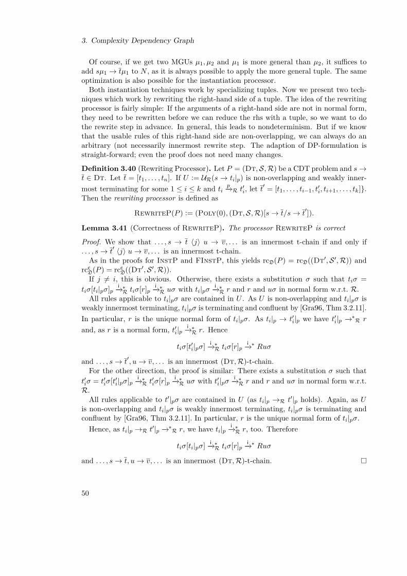
3. Complexity Dependency Graph
Of course, if we get two MGUs µ1, µ2 and µ1 is more general than µ2, it suffices toadd sµ1 → tµ1 to N , as it is always possible to apply the more general tuple. The sameoptimization is also possible for the instantiation processor.Both instantiation techniques work by specializing tuples. Now we present two tech-
niques which work by rewriting the right-hand side of a tuple. The idea of the rewritingprocessor is fairly simple: If the arguments of a right-hand side are not in normal form,they need to be rewritten before we can reduce the rhs with a tuple, so we want to dothe rewrite step in advance. In general, this leads to nondeterminism. But if we knowthat the usable rules of this right-hand side are non-overlapping, we can always do anarbitrary (not necessarily innermost rewrite step. The adaption of DP-formulation isstraight-forward; even the proof does not need many changes.
Definition 3.40 (Rewriting Processor). Let P = (Dt,S,R) be a CDT problem and s→t ∈ Dt. Let t = [t1, . . . , tn]. If U := UR(s → ti|p) is non-overlapping and weakly inner-most terminating for some 1 ≤ i ≤ k and ti
p−→R t′i, let t′ = [t1, . . . , ti−1, t
′i, ti+1, . . . , tk].
Then the rewriting processor is defined as
RewriteP(P ) := (Poly(0), (Dt,S,R)[s→ t/s→ t′]).
Lemma 3.41 (Correctness of RewriteP). The processor RewriteP is correct
Proof. We show that . . . , s → t 〈j〉 u → v, . . . is an innermost t-chain if and only if. . . , s→ t
′ 〈j〉 u→ v, . . . is an innermost t-chain.As in the proofs for InstP and FInstP, this yields rcD(P ) = rcD((Dt′,S ′,R)) and
rccD(P ) = rcc
D((Dt′,S ′,R)).If j 6= i, this is obvious. Otherwise, there exists a substitution σ such that tiσ =
tiσ[ti|pσ]pi−→∗R tiσ[r]p
i−→∗R uσ with ti|pσi−→∗R r and r and uσ in normal form w.r.t. R.
All rules applicable to ti|pσ are contained in U . As U is non-overlapping and ti|pσ isweakly innermost terminating, ti|pσ is terminating and confluent by [Gra96, Thm 3.2.11].In particular, r is the unique normal form of ti|pσ. As ti|p → t′i|p we have t′i|p −→∗R r
and, as r is a normal form, t′i|pi−→∗R r. Hence
tiσ[t′i|pσ] i−→∗R tiσ[r]pi−→∗ Ruσ
and . . . , s→ t′, u→ v, . . . is an innermost (Dt,R)-t-chain.
For the other direction, the proof is similar: There exists a substitution σ such thatt′iσ = t′iσ[t′i|pσ]p
i−→∗R t′iσ[r]pi−→∗R uσ with t′i|pσ
i−→∗R r and r and uσ in normal form w.r.t.R.All rules applicable to t′|pσ are contained in U (as ti|p →R t′|p holds). Again, as U
is non-overlapping and ti|pσ is weakly innermost terminating, ti|pσ is terminating andconfluent by [Gra96, Thm 3.2.11]. In particular, r is the unique normal form of ti|pσ.Hence, as ti|p →R t′|p −→∗R r, we have ti|p
i−→∗R r, too. Therefore
tiσ[ti|pσ] i−→∗R tiσ[r]pi−→∗ Ruσ
and . . . , s→ t, u→ v, . . . is an innermost (Dt,R)-t-chain.
50

3.3. Transformation techniques
The restriction that R is weakly innermost terminating can easily be lifted. Thisrequires an asymmetric definition of the complexity, similar to the asymmetric definitionof (in)finiteness used in [GTSF06]. It will be easy to adapt this for our framework.The rewriting technique is related to the narrowing technique. The basic idea is the
same: If a right-hand side of a tuple s→ t does not unify with any of the successors, atleast one R-step has to occur before a Dt-step can happen. The RewritingP processorhandles the case where it is correct to rewrite an arbitrarily chosen redex. But in manycases, the set of usable rules is not non-overlapping. Also, it might be necessary toinstantiate some variables before an R-reduction can happen. So for each non-variableposition on the right-hand side, the narrowing processor computes all narrowings.
Definition 3.42 (Narrowing of terms and tuples). Let R be a set of rules, t a term andπ ∈ Pos(t). If t|π 6∈ V and tπ unifies with the left-hand side of a (variable-renamed) rulel→ r ∈ R and a mgu µ, then t′ := tµ[rµ]π is a R-narrowing of t. If we want to be moreexact, we will refer to as a π, l→ r-narrowing.If s→ [t1, . . . , tk] ∈ Dt and t′ is an R-narrowing of ta, 1 ≤ a ≤ k with substitution µ,
then sµ→ [t1µ, . . . , ta−1µ, t′, ta+1µ, . . . , tk] is a R-narrowing of s→ t.
Recall the formulation of the narrowing processor for Dependency Pairs described in[GTSF06, Def. 28].
Definition 3.43 (Narrowing for Dependency Pairs, [GTSF06, compare Def. 28]). LetP ′ = P ] s→ t. For (P ′,R) the innermost narrowing processor returns (P ∪ sµ1 →t1, . . . , sµn → tn,R) if t1, . . . , tn are all R-narrowings of t with the mgu’s µ1, . . . , µnsuch that sµi is in normal form. Moreover, for all v → w ∈ P ′ where t unifies with the(variable renamed) left-hand side v by a mgu µ, one of the terms sµ or vµ must not bein normal form.
This can be adapted with no more than technical changes: We have more then oneright-hand side, so we write t instead of t. Now, instead of checking whether t unifieswith a left-hand side, on has to check whether one of the ti of t = [t1, . . . , tn] unifies witha left-hand side.However, having multiple right-hand sides really restricts the applicability: We may
not apply narrowing if one of the right-hand sides unifies with one of the successor nodes.Also, even if we are allowed to apply narrowing, we have to generate the narrowings forall right-hand sides at once. This is particularly bad, as even narrowing for terminationtends to produce many new tuples.We present an improvement of the narrowing technique which allows narrowing the
i-th right-hand side of a tuple s→ t, if we would be able to narrow the pair s→ ti. Thereasoning is the following: Let µ1, . . . , µm be all substitutions of R-narrowings of ti. Ifwe are allowed to narrow ti, then ti does not unify with any variable renamed left-handside in Dt. Now, if we want to rewrite sτ and sτ does not match any sµj , 1 ≤ j ≤ m,then tiτ is normal with regard to R and hence w.r.t. Dt, too. So, we add an additionaltuple s→ v, where v is derived from t by removing ti.Another change is prompted by our proof goal: For narrowing for termination analysis,
we only need to care about infinite chains. On the other hand, for complexity analysis
51

3. Complexity Dependency Graph
we care in particular aboute finite chains respective chain-trees. So, we need to careabout an occurrence of s → t at the end of a t-chain, too: In this case, it is possiblethat none of the narrowings can replace s → t. To make the proof simpler, we add theadditional tuple s → [] (which can always replace s → t at the end of a chain, but willnever belong to any SCC). In practice, this node can always be removed by applying theSccSplitP processor.
Lemma 3.44 (Narrowing). Let (Dt,S,R) be a CDT problem and s → t ∈ Dt suchthat t = [t1, . . . , tk]. Let u1, . . . , um be the narrowings with substitutions µ1, . . . , µm of ata, 1 ≤ a ≤ k such that sµ1, . . . , sµm are in normal form. Let
pj := [t1µj , . . . , ta−1µj , uj , ta+1µj , . . . , tkµj ]
and let M be the set of indexes of the right-hand sides which fulfill the following condi-tions:
• For each i ∈M , the term ti does not unify with any left hand side in Dt and
• for each mgu θ of the narrowings of ti there is a j such that µj is at least as generalas θ (i.e., there exists a σ such that θ = µjσ).
Set M ′ := 1, . . . , k \M and v := [tq1 , . . . , tql ] for q1 < . . . < ql = M ′.If in addition for all 1 ≤ i ≤ m the right hand side taµi does not unify with any
(variable renamed) left-hand side in Dt, then
rc(n, (Dt,S,R)) ≤ rc(n, ((Dt,S,R)[s→ t/N ]))
for all n ∈ N, where
N := s→ [], s→ v, sµ1 → u1, . . . , sµm → um.
Proof. We show that for each t ∈ T ]B and for each innermost (Dt,S,R)-chain tree of tthere exists a (Dt′,S ′,R)-chain tree of t of at least the same size.Consider a (Dt,S,R)-chain tree T and an occurrence of s→ t in T . If this occurrence
has no successor in T , it can be replaced by s → []. Else, it has successors v1 → w1to vp → wj for the right-hand sides with indexes 1 ≤ i1 < . . . < ip < k and there is asubstitution σ such that sσ is in normal form and tijσ
i−→∗R vijσ for all 1 ≤ j ≤ p.
· · · s→ [t]
vi1 → wii
vip → wip
We distinguish three cases:
• i1, . . . , ip ∩M = ∅. Then we can replace s→ t by s→ v.
52
3.3. Transformation techniques
• i1, . . . , ip ∩M 6= ∅ and a ∈ i1, . . . , ip.As ta does not unify with va, also taσ does not unify with vaσ. Hence a l→ r ∈ R-step takes place between them:
taσ = taσ[ta|πσ] = taσ[lρ]πi−→ [π]Rtaσ[rρ]π
i−→∗R vaσ
We may assume l → r is renamed variable disjoint to any tuple in the chain tree.Therefore we can extend σ to act on l → r like ρ, i.e., lρ = lσ. Hence there is asubstitution τ such that µτ = σ, where µ = mgu(ta|p, l).Now, t′a := taµ[rµ]p is a narrowing of t. Again, we may assume that sµ → t′ais variable disjoint to any tuple in the chain tree. Therefore we can extend σ tobehave like τ on the variables of sµ (and t′). Then we have sµσ = sσ and
t′aσ = t′aτ = taµτ [rµτ ]π = taσ[rσ]π = taσ[rρ]πi−→∗R vaσ
Let t′ := [t1µ, . . . , ta−1µ, t′a, ta+1µ, . . . , tk]. Then sµ→ t′, va → wa is still a t-chain.
The same holds for sµ → t′, vijwij for all j with ij 6= a, as t′ijσ = tijσ holds. Ifthis occurrence of s→ t has a predecessor v′ → w′ in T , this is still a predecessorof sµ→ t′, as sµσ = sσ. Hence, we may replace s→ t by sµ→ t′.
• i1, . . . , ip ∩M 6= ∅ and a 6∈ i1, . . . , ip: Let j ∈ i1, . . . , ip ∩M .As tj does not unify with vj , also tjσ does not unify with vjσ. Hence a l→ r ∈ R-step takes place between them:
tjσ = tjσ[tj |πσ] = tjσ[lρ]πi−→ [π]Rtjσ[rρ]π
i−→∗R vjσ
We may assume l → r is renamed variable disjoint to any tuple in the chain tree.Therefore we can extend σ to act on l → r like ρ, i.e., lρ = lσ. Hence there is asubstitution τ such that θτ = σ, where θ = mgu(tj |p, l).There exists a narrowing of ta with substitution µ such that θ = µτ ′ for some τ ′.Let sµ → t′ be the tuple belonging to this narrowing. We may assume that sµ isvariable disjoint to any tuple in the chain tree and hence we can extend σ to actlike τ ′τ on sµ. Then we have
sµσ = sµτ ′τ = sθτ = sσ
and we can replace s→ t by sµ→ t′.
Definition 3.45 (Narrowing Processor). Let P = (Dt,S,R) be a CDT problem andlet s → t and N be defined like in the previous lemma. If s → t and all nodes of thedependency graph reachable from s→ t are in S, then
NarrowingP(P ) := (Poly(0), (Dt[s→ t/N ],S,R))
is the narrowing processor NarrowingP.
53

3. Complexity Dependency Graph
Lemma 3.46 (Correctness of NarrowingP). The processor NarrowingP is correct.
Proof. Follows directly from Lemma 3.44, as rccD(P ) = rcc
D(Dt[s→ t/N ],S,R).
Restricting the narrowing processor to cases where all rules reachable from the nar-rowed tuple are in S is a pretty severe applicability restriction. In particular, a singlesuccessful application of the reduction pair processor on a SCC forbids the use of thenarrowing processor on this SCC later on. This is caused by NarrowingP not beingcomplete (i.e., the transformation may increase the complexity): If this increases thecomplexity of a known node, the known node could hide the complexity of an unknownnode.
Example 3.47. Consider the CDT problem with rules
f(g(a(x)))→ x
g(a(s(x)))→ 0
and the following dependency graph
1: A(s(x))→ [A(f(g(a(x)))),F(x)] 2: F(t(x))→ [F(x)]
This CDT problemhas a linear runtime complexity. Note that there is no loop fromnode (1) to itself, as f(g(a(x))) can never be innermost evaluated to a with root symbols. If we forgot for a moment about the restrictions related to S, we would be allowed toapply narrowing to node (1), yielding the following new dependency graph:
1: A(s(x))→ [A(x),F(x)]
2: A(s(s(x)))→ [A(0),F(s(x))]
3: F(t(x))→ [F(x)]
4: A(s(x))→ []
5: A(s(x))→ [F(x)]
This new system still has a linear runtime complexity. But now node (1) has linearcomplexity, too. As it is not in S, a processor working on the new problem is allowed toreturn Poly(0), which would be incorrect.
Of course, one can always enlarge S before applying the processor, but this is ofdubious value: We have to prove the complexity for those nodes again. So we proposetwo approaches to make the narrowing processor more applicable: A first one would be tofind additional conditions such that this processor is indeed complete. If R is innermostterminating, the conditions of [GTSF06, Def. 28a] will work; but this would requirean additional termination proof. In the cited paper, this is avoided by an asymmetricdefinition of (in)finiteness for Dependency Pair problems. This approach should beadapted to our framework.
54

3.4. A strategy for applying processors
Our second suggestion is more along the lines of “enlarging S”: Instead of splittingDt in the two sets of known nodes (those in S) and unknown nodes (those in Dt \ S),one could use a ternary split:
• unknown nodes: We still need to determine how often those nodes can occur. Thisis equivalent to our current S.
• known nodes: We already know how often those nodes can occur. This is equivalentto our current Dt \ S.
• ignored nodes: We have already proved how often these nodes can occur in the orig-inal system, but we are not allowed to use this information to prove the complexityof other nodes, as it may be different in the current system.
Then the narrowing processor would be correct, if it changed the status of all knownnodes reachable from the narrowed node to counted.
3.4. A strategy for applying processorsUntil now, we have developed a quite a list of processors: In Chapter 2, the proces-sors UsableRulesP an RedPairP were presented. The processors KnownnessP,SccSplitP, RemoveTrailRhsP, RhsSplitP and RemoveUnusableP presented inSection 3.1 and 3.2 always return simpler problems. This is not necessarily the casefor the processors InstP, FInstP, RewriteP, NarrowingP presented in Section 3.3.Often they allow solving CDT problems which cannot be proved with only the othertechniques. But all of them can be applied infinitely on certain problems without sim-plifying the problem, but making it harder to solve.If no start term transformation is performed (compare Chapter A), the first proces-
sors should be RemoveUnusableP and RemoveLeadingP, as they possible removetuples completely from the problem. The RhsSplitP processor potentially increasesthe size of the graph, but the resulting tuples are clearly simpler to solve, so it should beapplied after the RemoveUnusableP processor as long as applicable. The SccSplitPprocessor only should be used afterwards, otherwise the previous processors would haveto be applied to all the new problems. This should be followed by RemoveTrailRhsPas long as applicable, as the split may make additional right-hand sides trailing. As theUsableRulesP processor yields better results for smaller sets of tuples, it is sensibleto apply this processor only afterwards.These initial transformations are guaranteed to make the CDT problem simpler. As
searching for orders is costly compared to the other processors, one should apply theRedPairP processor not until now. A successful application of his processor should bealways followed by as many KnownnessP passes as possible. It may be useful to restrictthe runtime of the reduction pair processor, as this can vary greatly for current searchtechniques. If the reduction pair processor is not successful, one of the transformationprocessors should be tried. As those techniques may simplify cycles in the graph, it isadvantageous, to use the knownness propagation, RemoveUnusableP and SccSplitP
55
3. Complexity Dependency Graph
processors afterwards, followed again by the RedPairP processor. A simple method toprevent infinite applications of the transformation processors is applying them at most aconstant number of times. A much more sophisticated heuristic is described in [GTSF06].
56

4. Annotated CDTs
In Example 2.17 we remarked that the CDT transformation does not exactly model thederivations possible in the original system. The transformed system allows derivationswhich have no equivalent in the original system. This can even lead to an exponentialblowup of the complexity.
Example 4.1. Consider the following TRS, which has a linear runtime complexity.
g(x)→ x (4.1)g(x)→ a(f(x)) (4.2)
f(s(x))→ f(g(x)) (4.3)
This can be easily seen by the following polynomial interpretation (see also 2.56):
[g](x) = x+ 1 [a](x) = x [f](x) = x [s](x) = x+ 2
But the transformed system with the dependency tuples
G(x)→ [] (4.4)G(x)→ [F(x)] (4.5)
F(s(x))→ [F(g(x)),G(x)] (4.6)
admits a exponential runtime complexity, as the following derivation shows:
F(sn+1(x)) i−→ [F (sn(x)), G(sn(x))]i−→ [F (g(sn(x))), G(sn(x))]i−→ [F (sn(x)), G(sn(x))]i−→ [F (sn(x)), [F (sn(x))]]
Only one s-symbol was removed, but the number of F -terms was duplicated.
While the above example is a pathological one (it employs nested recursion [Tai61],which is not often seen in real programs), the asymptotic complexity may increase evenfor more “normal” examples. Also, the transformation grows the size of the right-handside considerably, which is a disadvantage when trying to find polynomial interpretations.
57

4. Annotated CDTs
Example 4.2. Example 2.11 has a linear complexity which cannot be shown by anycombination of CDT techniques and linear polynomial interpretations as described in2.56. This boils down to the inability to find a suitable interpretation for
minus(x, 0)→ x (4.7)minus(s(x), s(y))→ minus(x, y) (4.8)
MINUS(s(x), s(y))→ [MINUS(x, y)] (4.9)QUOT(s(x), s(y))→ [QUOT(minus(x, y), s(y)),MINUS(x, y)] (4.10)
which orients 4.9 strictly and the other rules weakly. Now, if we use the WiDP approachpresented by Hirokawa and Moser [HM08a], we have to replace the tuple 4.10 by
QUOT(s(x), s(y))→ QUOT(minus(x, y), s(y)) (4.11)
and orient all rules strictly. This can be done with a linear interpretation.If we would know that the subterms starting with minus and MINUS in 4.10 have
to be evaluated the same way, we would by allowed to (implicitly) transform our CDTproblem in a WiDP problem for finding an interpretation. We will call such subtermsrelated. Note that without any transformation, the original TRS from Example 2.11cannot even be shown to be terminating with a polynomial interpretation.
Both problems motivate the introduction of Annotated CDT problems. The idea isto keep track which application of a CDT corresponds to which R-rule. For this, weintroduce the notions of correspondence labeled terms and lockstepped rewriting. Thesechanges result in transformation, which exactly models the derivations and runtimecomplexity of the original system.
4.1. Annotated Complexity Dependency TuplesTo keep track which tuples corresponds to which rule, we will need some additionalinformations. First, the rule a tuple is based on. Usually that is the rule which was usedto generate the ACDT during the transformation process. Second, we need to knowwhich defined positions of the base rule actually occur in the tuple. And third, we needto keep track of substitutions applied to the tuple. This is mainly necessary to avoidadding additional rules in the Instantiation and Forward Instantiation transformationprocessors.
Definition 4.3 (Annotated Complexity Dependency Tuple). Let l → r ∈ be a rule, σa substitution and F ⊆ DPos(r). If π1 <lex · · · <lex πn are the elements of F , then
d := lσ] → [rσ|]π1 , . . . , rσ|]πn ]
is a CDT based on l→ r, σ and F and
ACDT(l→ r, σ, F ) := (d, (l→ r, σ, F ))
is the corresponding Annotated Complexity Dependency Tuple. For a rule l → r, thecanonical annotated CDT is defined as ACDT(l→ r, id,DPos(r)).
58

4.1. Annotated Complexity Dependency Tuples
We define some selectors for referring to the elements of an annotated CDT.
Definition 4.4. Let ν := (p→ q, (l→ r, σ, F )) be an annotated CDT. Then selT(ν) :=d is the tuple rule of ν and selB(ν) := l → r the base rule. The base substitution isdenoted by selS(ν) and the set of base positions by selP(ν).
Example 4.5. Consider the rule
f(s(x), y)→ cons(g(x), f(g(x), y)
and assume that the function symbols f and g are defined. Then the canonical annotatedCDT is
F(s(x), y)→ [G(x),F(g(x), y),G(x)]
with annotations
f(s(x), y)→ cons(g(x), f(g(x), y) id 1 <lex 2 <lex 2.1
The set of base positions can be used to reconstruct which right-hand sides are related.The first RHS has position 1, the second 2 and the third 2.1 in the base rule. Thisrelations can also be visualized as a forest (i.e., a set of trees):
1: G(x) 2: F(g(x), y)
2.1: G(x)
We know now that the first right-hand side is independent of the other right-hand sides,but the second and third right-hand side are related (and hence g(x) should be evaluatedthe same way as the (second) G(x).Furthermore, the tuple F(s(0), s(z))→ [G(x)] with annotations
f(s(x), y)→ cons(g(x), f(g(x), y) x/0, y/s(z) 2.1
is an example of a non-canonical annotated CDT for the same base rule.
Definition 4.6 (Related positions). Let ν be an ACDTwith tuple rule p→ [q1, . . . , qn].Let 1 ≤ i, j ≤ n. Two positions i.π and j.τ are related, if κi.π = κj .τ where selP(ν) =κ1 <lex · · · <lex κn.
In the example above, the related positions are 2.1 and 3 as well as 2.1.1 and 3.1.Now we define the annotated variant of CDT problems. For simplicity of the exposition
we omit the set S which was present for ordinary CDT problems. This means that alltuples are always considered to be of unknown complexity. Note that Dt is now a setof annotated tuples.
59

4. Annotated CDTs
Definition 4.7 (Annotated CDT problem). Let R be a TRS, Dt be a set of annotateddependency tuples such that selB(ν) ∈ R for all ν ∈ Dt. Then (Dt,R) is called anannotated CDT problem. It is called canonical, if Dt is the set of canonical ACDTs ofR.For a rule ρ ∈ R, the set ρass of associated rules and tuples contains exactly ρ and all
ν ∈ Dt with ρ = selB(ν). In addition, we write ρ ass= ρ′ if either ρ ∈ R and ρ′ ∈ ρass orρ = ρ′ ∈ Dt.
Note the restriction on R above. Standard CDT problems do not enforce a certainrelationship between R and Dt. But this restriction is needed, as we often will make usefrom the fact that a term s is reducible if s] is reducible. Unfortunately, this preventsusing a usable rules processor.When we rewrite a term with an ACDT, we just handle it like a CDT and ignore the
annotations.
Definition 4.8 (Rewriting for annotated CDT problems). Let ν be an ACDT withselT(ν) = p→ q and let be one of → or i−→. Then s ν t :⇔ s p→q t.
So, like with CDTs, rewriting with an annotated CDT will preserve well-formednessof a term. We close this section with a remark about rewriting in an annotated CDTproblem. If we can rewrite a sharped term, we always can rewrite the unsharped termto. This is due to the fact that the left-hand sides of tuples are always sharped instancesof the left-hand sides of their base rules.Remark 4.9. Let (Dt,R) be an annotated CDT problem and ν ∈ Dt. If s] i−→ν t, thenalso s i−→selB(ν) u for all terms s ∈ T (Σ,V). If ν is canonical, even the inverse holds.
4.2. Correspondence LabelingIn Example 4.1 we have demonstrated that the simple transformation of a term rewritesystem into a CDT problem may cause an exponential blowup of complexity. We willintroduce a method which allows for a complete transformation. The right-hand side ofa CDT has independent terms for each defined position. In an ACDT, one can use thebase positions to see which one are related.Now we want to carry over this information to terms which are rewritten with an
ACDT. To this end, positions of a term are labeled. The idea is that positions getthe same labels if they were created by related positions of an ACDT. This annotationcan be used later on to enforce that those subterms are evaluated the same way, thuspreventing the exponential complexity blowup.
Definition 4.10 (Correspondence labeling function). A correspondence labeling is afunction ϕ : N∗ → N∗ ∪ mapping positions to a label. We call a position π labeledif ϕ(π) 6= , else unlabeled.The initial correspondence labeling, mapping the root position to the empty word and
leaving any other position unlabeled, is denoted by ε.
60

4.2. Correspondence Labeling
Definition 4.11 (Correspondence labeled terms). A term t with a correspondence la-beling ϕ such that ϕ(π) = for all π 6∈ Pos(t) is called a correspondence labeled termor corlab term.We write tϕ|π to denote the corlab term (t|π)ψ where ψ(x) := ϕ(πx).
Example 4.12. Let t = Com(QUOT(minus(x, y), s(y)),MINUS(x, y)) a term with cor-respondence labeling ϕ such that ϕ(1) = 1, ϕ(1.1) = ϕ(2) = 2 and ϕ(π) = else. Inexamples, we write instead
tϕ = Com(QUOT1(minus2(x, y), s(y)),MINUS2(x, y)).
Also, we have tϕ|1.1 = minus2(x, y).
If two positions are related in an ACDT, the subterms at this position are almostequal. The only difference is that one of them may be a sharped term.
Definition 4.13 (Term/Tuple Term Equivalence). Let s, t ∈ T (Σ,V) ∪ T ](Σ,V). Weconsider s and t tuple-equivalent, if s = t or s ∈ T (Σ,V) and s] = t or t ∈ T (Σ,V) ands = t]. This equivalence relation is denoted by ≡T .If sϕ and tψ are correspondence labeled, they are tuple equivalent if and only if s ≡T t
and ϕ = ψ holds.
At the beginning of this section we explained that same labels shall indicate thatthose positions were created by related positions of an ACDT. Hence we must definehow rewriting a corlab term influences the labels. We will first show how to handle thisfor rules and then define the labeling for tuples in terms of the labeling of their baserule. For ordinary rules, we just give each defined position an unique label. For tuplerules, the labeling of the subterm corresponding to the position π in the associated ruleis to be the same as the labeling of the subterm at π in the associated rule.
Definition 4.14 (Correspondence labeling for rules). Let l → r ∈ R and w ∈ N∗. Letπ1 <lex, · · · <lex πn be the defined positions of r. Then we define clR(l→ r, w) as
clR(l→ r, w)(π) :=w.i if π = πi
else.
Example 4.15. Recall the rule from Example 4.5. The positions of a rule are notrelated, so every position will get a different label. Also, we will only label definedpositions, as the others are not relevant for rewriting. To prevent creating duplicates,we prefix the new labels with the old label w at the position of the redex.
fw(s(x), y)→ cons(gw.1(x), fw.2(gw.3(x), y)
The labeling of a tuple should match the labeling of the base rule, so that relatedpositions create the same labels. So for the canonical tuple of the above rule, we willdefine the labeling to be
Fw(s(x), y)→ [(Gw.1(x),Fw.2(gw.3(x), y),Gw.3(x)]
61

4. Annotated CDTs
Please note that w.i ⊥ w.j for distinct i, j ∈ N. So, in derivations D1 and D2 of e.g. gw.1and gw.3, the labels occurring in D1 will be pairwise distinct from the lables occurringin D2.
Definition 4.16 (Correspondence labeling for dependency tuples). Let (Dt,R) be anannotated CDT problem, ν ∈ Dt a tuple with selP(ν) = κ1 <lex . . . <lex κn andselB(ν) = ρ. Let w ∈ N∗. The correspondence labeling of ν is based on the labeling of ρ:
clR(ν, w)(π) :=clR(ρ, w)(πj .τ) if π = j.τ
else.
After defining the correspondence labeling of rules, we can now define a labelingrewrite relation. As we are interested in innermost rewriting, we are only interested inthe labeling of the root symbol of a redex, so we discard the labeling below. Note thatthis definition does not restrict rewriting (in comparison to normal innermost rewriting)but just adds a labeling.
Definition 4.17 (Rewrite relation for corlab terms). Let (Dt,R) be a CDT problemand let s, t be terms. For r ∈ R ∪Dt: sϕ i,π−→r t
ψ iff s i,π−→r t and
ψ(τ) =ϕ(τ) if τ 6≥ πcl(r, ϕ(π))(π′) if τ = ππ′ for some π′
Note that all labelings occurring in the original term below the position of the redexare discarded. This is no problem for innermost rewriting, as those terms are knownto be in normal form. An appropriate labeling for full rewriting would be slightly morecomplicated: One would like to preserve the labels, but if the applied rule is duplicating,one would need to use separate labels on each duplicated subterm.
Example 4.18. Let ρ be the rule from 4.15 and assume g(0) is a normal form. Then
h2(f3(s(g4(0), y))) i−→ρ h2(cons(g3.1(g(0)), f3.2(g3.3(g(0)), y)))
is a rewrite step.If now two positions have the same label, and are rewritten with associated rules, then
the labels of the related positions below these positions will be the same: Consider thefollowing rule and its canonical tuple
gw(x)→ hw.1(hw.2(x)Gw(x)→ [Hw.1(hw.2(x),Hw.2(x)].
Then we have a following derivation:
[(F1(g2(x), y),G2(x)] i−→ [(F1(h2.1(h2.2(x)), y),G2(x)]i−→ [(F1(h2.1(h2.2(x)), y), [H2.1(h2.2(x),H2.2(x)]]
Both the g and G subterms were related in the original term. Rewriting both of them(with associated rules) keeps this property.
62

4.2. Correspondence Labeling
In general, we are not interested in all labelings, but only in such labeled terms whichcould be derived starting from a term tε or t]ε for a t ∈ T (Σ,V). In many cases, wewill expect that we rewrite all positions with the same label essentially “at the sametime”, i.e., if we perform a reduction of a redex labeled w, we will try to reduce all otherredexes with the same label before reducing any other position.
Definition 4.19 (Parallel Rewriting). Let (Dt,R) be an annotated CDT problem andlet s1 ∈ T (Σ,V) ∪ T ](Σ,V) be a term. Let ϕ1 be a correspondence labeling of s. For aρ ∈ R let sϕ1
1i,π1−−→ρass . . .
i,πn−−→ρass sϕn+1n+1 be a derivation such that ϕ1(π1) = · · · = ϕn(πn).
If all terms labeled with ϕ1(π1) in sϕn+1n+1 are in i−→Dt/R-normal form, then it is a parallel
derivation step. Let D = D1D2 . . . be a derivation such that is D1 is a parallel derivationstep. Then D is called a parallel derivation.
The following definition captures the most important properties of such terms.
Definition 4.20 (Correctly corlab terms). Let tϕ be a corlab term. We call tϕ correctlycorlab if and only if all of the following restrictions are fulfilled:
(1) Two positions with the same label are equivalent, i.e: Let π, τ ∈ Pos(t). If ϕ(π) =ϕ(τ) and ϕ(π) 6= , then tϕ|π ≡T tϕ|τ .
(2) Labels of tuple symbols are pairwise distinct, i.e: Let π, τ ∈ Pos(t) such that π 6= τand root(π), root(τ) ∈ Σ]. Then ϕ(π) 6= ϕ(τ).
(3) Smaller labels are in normal form, i.e: Let π, τ ∈ Pos(t) be labeled positions. Ifϕ(π) 6= ϕ(τ) then either ϕ(π) ⊥ ϕ(τ) or ϕ(π) < ϕ(τ) and tϕ|π is in normal formwith regard to Dt ∪R (or vice versa).
(4) All labels below a labeled position are different, i.e: Let π, τ, κ ∈ Pos(t) be labeledpositions with π < τ, κ and τ 6= κ. Then ϕ(τ) 6= ϕ(κ).
The cases 4.20(1) and 4.20(4) just formalize our intuition that positions labeled thesame way should be the same. As with normal CDTs, we only want to count the tuplesteps. Hence there should be always only one for each label. For non-canonical systems,a term t ∈ T (Σ,V) can be reduced if and only iff t] can be reduced, as for each rulel→ r a tuple l] → q exists. For non-canonical systems, this is not guaranteed anymore.So a subterm t] with a label w may remain in the term infinitely, even if other subtermswith the same label can be rewritten. This gives rise to case 4.20(3).We will now see that parallel rewriting preserves the “correctly corlab” property. First
a simple remark, which is immediately obvious from the definitions.Remark 4.21. Let ν be an annotated CDT with selT(ν) = p → q. Consider the rewritestep pϕ π−→ν q
ψ. Then the labels of tuple symbols in qψ are pairwise distinct. If ν is acanonical tuple, then each label in ψ occurs also as a label of a tuple symbol in qψ.
Lemma 4.22. Let (Dt,R) be an annotated CDT problem and let s ∈ T (Σ,V)∪T ](Σ,V)be a term. Let ν ∈ R∪Dt be a rule. If sχ i,ε−→R t
ϕ for some labeling χ, then tϕ is correctlycorlab.
63
4. Annotated CDTs
We may visualize the proposition of this lemma as: The rhs of a rule or tuple iscorrectly corlab. It is not important whether sχ is correctly corlab as all labels belowthe root position are irrelevant.
Proof. Assume that ν ∈ R. All labels in clR(ν, χ(ε)) are pairwise distinct, so 4.20(1)holds. By definition of clR(ν, ·), all labels are pairwise distinct (yields 4.20(2) and4.20(4)). Furthermore, all labels are independent and therefore 4.20(3) holds.Otherwise ν ∈ Dt with selB(ν) = l → r and selT(ν) = l]σ → [r|]π1σ, . . . , r|
]πnσ]. We
have s = u] for some term u and uχ i−→l→r vψ.
4.20(1) Let τ, κ ∈ Pos(t) be distinct positions such that ϕ(τ) = ϕ(κ). Then τ = iτ ′ andκ = jκ′ for some 1 ≤ i, j ≤ n and πiτ
′ = πjκ′. By construction of ν this yields
t|τ ≡T t|κ and ϕ|τ = ϕ|κ.
4.20(2) Remark 4.21.
4.20(3) For all labels a, b in tϕ holds either a = b or a ⊥ b.
4.20(4) Let 1 ≤ i ≤ n. Then tϕ|i ≡T vψ|πi and this property follows as the compoundsymbol is not labeled.
The above lemma considers only a single reduction step at the root position. Toprove that parallel rewriting in general also preserves this property, we first need ageneralization of tuple equivalence: If we rewrite terms s and s] at the root position, theresulting terms t and u are not tuple equivalent anymore.
Example 4.23. Consider the following rule and its canonical ACDT:
qa(s(x), s(y))→ s(qa.1(ma.2(x, y), s(y)))Qa(s(x), s(y))→ [Qa.1(ma.2(x, y), s(y)),Ma.2(x, y)]
If we rewrite the term qε(s(s(0)), s(0)) (and its sharped variant), we get
s(q1(m2(s(0), 0), s(s(0)))) respectively [Q1(m2(s(0), 0), s(0)),M2(s(0), 0)].
Now, these terms are not tuple-equivalent anymore, but the subterms with the samelabels still are (e.g. (m2(s(0), 0) and M2(s(0), 0)). In the above case, both terms stillcontain the same set of labels. If we use the (non-canonical) tuple
Qa(s(x), s(y))→ [Ma.2(x, y)]
instead, subterms with the same label would still have be tuple-equivalent, but not everylabel would have a counterpart in the other term.
These cases are formalized in the next definition.
64

4.2. Correspondence Labeling
Definition 4.24 (corlab equivalent terms). Let sϕ and tψ be terms. Let (Dt,R) be aCDT problem and sϕ′ be derived from sϕ by dropping the labels of subterms in normalform.If imgϕ′ ⊆ imgψ and s|π ≡T t|τ for all positions π ∈ Pos(s), τ ∈ Pos(t) with
ϕ(π) = ψ(τ) 6= , then s and t are (weakly) corlab equivalent with regard to (Dt,R).This property is denoted by sϕ vcl t
ψ. If even imgϕ = imgψ, then sϕ and tψ are stronglycorlab equivalent, denoted by sϕ ≡cl t
ψ.
We need to show that the intuition we gave above for the corlab equivalence fits thedefinition.
Lemma 4.25. Let (Dt,R) be an annotated CDT problem and let sϕ be a labeled termin T (Σ,V). Let ρ ∈ R and let ν ∈ Dt be an associated ACDT. If sϕ i,ε−→ρ t
ψ ands]ϕ
i,ε−→ν uχ, then tψ wcl u
χ.If ν is canonical, then s]ψ i−→ν u
χ is always a derivation and tψ ≡cl uχ holds.
Proof. As we are rewriting at ε, we have
ψ(π) = clR(ρ, χ(ε))(π) for all π ∈ Pos(t)
respectivelyχ(π) = clR(ν, χ(ε))(π) for all π ∈ Pos(u).
As clR(ν, ·) is based on clR(ρ, ·), we have imgχ ⊆ imgψ. Let selP(ν) = τ1 <lex · · · <lexτn be the base positions of ν.We still need to show that t|π ≡T u|κ holds for all π ∈ Pos(t), κ ∈ Pos(u) with
ψ(π) = χ(κ). In this case there exist 1 ≤ i, j ≤ n such that π = τi and κ = jκ′ andτjκ′ = τi by the definition of clR. Hence
u|κ = (u|j)|κ′ ≡T (t|τj )|κ′ = t|τjκ′ = t|τi = t|π
and tψ vcl uχ is proven.
If ν is canonical then s]ψ i−→ν uχ is a derivation by Remark 4.9. In this case τ1, . . . , τn
are all defined positions of the DPos of the right-hand side of ρ and therefore
ψ(i) = clR(T, χ(ε))(i) = clR(R,χ(ε))(τi) = ϕ(τi)
for all 1 ≤ i ≤ n and we derive imgϕ = imgψ, hence tϕ ≡cl uψ.
Lemma 4.26 (Rewriting preserves correct correspondence labeling). Let (Dt,R) be anannotated CDT problem and let sϕ be a correctly corlab term from T (Σ,V) ∪ T ]T (Σ,V).Choose an a ∈ imgϕ. Let Π := π1, . . . , πm be the set of all positions of s such thatϕ(πi) = a and s|πi not in normal form. If sϕ i,π1−−→ρ1 · · ·
i,πm−−→ρm tψ and ρi ∈ ρass for someρ ∈ R, then tψ is correctly corlab.
Proof. First some auxiliary propositions:
65

4. Annotated CDTs
† As sϕ is correctly corlab, s|κ ≡T s|τ for all κ, τ ∈ Π. By Lemma 4.25 we derivetψ|κ vcl t
ψ|τ or tψ|κ vcl tψ|τ .
‡ As any label introduced by i,π−→ is strictly greater than ϕ(π) and there is no labelu > ϕ(π) in imgϕ, we have ψ(τ) 6= ψ(κ) for any pair of τ < π and κ ≥ π.
We check the conditions of definition 4.20:
4.20(1) Let τ, κ ∈ Pos(t) such that ψ(τ) = ψ(κ). For positions “under Π” this conditionis obviously satisfied: If τ ≥ π and κ ≥ π′ for some π, π′ ∈ Π then this property isfulfilled as t|π vcl t|π′ or t|π wcl t|π′ (by †). Else neither τ ≥ π nor κ ≥ π for anyπ ∈ Π (because of ‡).If τ, κ ⊥ π for all π ∈ Π then the positions are unaffected by the reduction, i.e.,tψ|τ = sϕ|τ and tψ|κ = sϕ|κ. Therefore the tuple equivalence property holds, as itheld for those positions in s before.Now assume τ < π and κ < π′ for some π, π′ ∈ Π. By definition, these positionwere equivalent before the rewrite and we have s|τ ≡T s|κ. Hence s|π = s|π′follows. By 4.20(2), either π = π′ or s|π, s|π′ 6∈ Σ]. Therefore t|π = t|π′ . Applying4.20(4) to sϕ now yields t|τ ≡T t|κ and ψ|τ = ψ|κ.The combination τ ⊥ π for all π ∈ Π and κ < π′ for some π′ ∈ Π (or the other wayround) is not possible. In this case we would have a 6∈ imgϕ|τ but a ∈ imgϕ|κwhich is a contradiction to the requirement that sϕ is correctly corlab.
4.20(2) Follows from Lemma 4.21 as there is at most one 1 ≤ i ≤ m such that ρi ∈ Dtbecause s is correctly corlab.
4.20(3) Let Ω := img(cl(ρ, a)). By definition of corlab rewriting, img(ψ|πi) ⊆ Ω for all1 ≤ i ≤ m. All labels in Ω are pairwise independent. Furthermore b > a for allb ∈ Ω. As 4.20(3) holds true in sϕ, we already know that this holds for all labelsbesides a. But if an a is still in tϕ, it is in normal form.
4.20(4) Subterms starting at positions in Π are correctly corlab by Lemma 4.22. Sub-terms starting at positions independent of all elements of Π were correctly corlab insϕ and stay so in tψ. Therefore we only need to consider positions above positionsin Π.If a position τ above a tuple symbol labeled a is labeled, there can be no otherposition with label ϕ(τ) (as only one tuple symbol labeled a exists in sϕ by 4.20(2),but by 4.20(1)all terms labeled ϕ(τ) are equivalent). Therefore, consider Π′ :=Π \ π | root(s|π) ∈ Σ]. We have sϕ|τ = sϕ|τ ′ and hence tψ|τ = tψ|τ ′ for allτ, τ ′ ∈ Π′. So, this property is preserved, too.
4.3. Lockstepped RewritingIn the last section we introduced correspondence labelings and a rewriting relation oncorlab terms. Furthermore, we have seen that we can keep the labeling in a special form if
66
4.3. Lockstepped Rewriting
we do parallel rewrite steps. While this is certainly a helpful conception, it is not neededthat those steps occur in parallel, they may very well be interleaved with other steps. Butwe must take care that we do not use different, not associated rules for rewriting redexeswith the same label. In this section, we formalize this in the lockstepped derivation andshow that this rewrite relation can be used to model the runtime complexity of a TRSprecisely by an annotated CDT problem.Which rule or tuple is to be used to reduce a label, is captured by a history function.
Definition 4.27 (History function). Let (Dt,R) be an annotated CDT problem. Ahistory function is a partial mapping N∗ → R. It associates a label with a rule (andtherefore its associated dependency tuples) used when rewriting a subterm with thislabel.We denote a history function with an uppercase Greek letter, usually Φ or Ψ. Both
the empty history function and the undefined history value are denoted by 4.
This mapping is enforced and extend by lockstepped rewriting: A rewrite step isallowed, if its an innermost corlab step and either honors the history function or isundefined in the history function. In the latter case, the history function will be extendedto remember the choice.
Definition 4.28 (Lockstepped Rewriting). Let P := (Dt,R) be a CDT problem andlet sϕ, tψ be corlab terms. Furthermore let Φ, Ψ be history functions and ν ∈ Dt ∪ R.Then the innermost lockstepped rewrite relation pi−→ is defined as follows:
(sϕ,Φ) pi,π−→r (tψ,Ψ)
if and only if sϕ i,π−→r tψ and one of the following conditions is fulfilled:
(1) The redex is labeled, but the history for this step is undefined, i.e., ϕ(π) ∈ N∗ andΦ(ϕ(π)) = 4. In this case, we define
Ψ(x) =
ν if x = ϕ(π) and ν ∈ RselB(ν) if x = ϕ(π) and ν ∈ DtΦ(x) if x 6= ϕ(π).
(2) The redex is labeled and the reduction honors the history, i.e. ϕ(π) 6= andΦ(ϕ(π)) = r′ and r ∈ r′ass.
If we are not interested in the position or the rule used, those may be omitted. Thesame applies if the concrete history does not matter. In this case we just write sϕ pi−→ tψ.
In chapter 2 we used (Dt,R)-chain trees to measure the complexity of a CDT problem(Dt,S,R). For annotated CDT problems (Dt,R), we will simply use the derivationlength of rewrite sequences. To count only Dt- and not R-steps, we make use of relativerewriting [BD86].
67

4. Annotated CDTs
Definition 4.29 (Relative Rewrite Relation). Let (Dt,R) be an annotated CDT prob-lem. Then
pi,π−→Dt/R:= pi−→∗R pi,π−→Dt pi−→∗Ris the relative rewrite relation of Dt and R. Here, denotes the composition of orders.
In short, a relative Dt/R-rewrite step consists of zero or more R-steps, exactly oneDt-step and zero or more R-steps. In particular, there are only finitely many R-steps ina row. The following theorem suggests the use of this rewrite relation for the definitionof complexity for an annotated CDT problem.
Theorem 4.30. Let R be a terminating rewrite system, P := (Dt,R) its canonicalannotated CDT problem and t ∈ TA,R. Then dl((t]ε,4), pi−→Dt/R) = dl(t, i−→ R).
The proof of this theorem is technically involved. To prove that dl((t]ε,4), pi−→Dt/R)is an upper bound for dl(t, i−→ R), we show that each i−→R-step can be mimicked by aseries of (parallel) lockstepped Dt ∪ R-steps and such a series always contains exactlyone Dt-step.
Lemma 4.31. Let (Dt,R) be an annotated CDT problem. Let uϕ be a correctly corlabterm from T (Σ,V) such that each label occurs at most once. Let vψ be a correctly corlabterm and uϕ wcl v
ψ. If a := ϕ(π) and
uϕi,π−→ρ u
′ϕ′
for some ρ ∈ R, thenvψ = vψ0
0 pi,τ1−−→ρass· · · pi,τn−−→ρass
vψnn
where τ1, . . . , τn all positions in vψ such that ψ(τi) = a and vψ|τi not in pi−→Dt∪R-normalform. Furthermore, u′ϕ′ wcl v
ψnn and both are correctly corlab again.
If (Dt,R) is canonical and uϕ ≡cl vψ, then also u′ϕ′ ≡cl v
ψnn
Proof. Correctly corlab follows from lemma 4.26. By Lemma 4.25, u′ϕ′ |π wcl vψnn |τi for
all 1 ≤ i ≤ n. Assume for some i there exist positions π′ < π and τ ′i < τi such thatϕ(π′) = ψ(τ ′). Then we have uϕ|π′ ≡T vψ|τ ′i and therefore uϕ|π = vψ|τi . As u ∈ T (Σ,V),both uϕ|π and vψ|τi are rewritten with ρ. Hence, u′ϕ′ |π = vψnn |τi and u′ϕ
′ |π′ = vψnn |τ ′i .If there is a position τ in vψ with ψ(τ) = a such that τ 6= τi for all 1 ≤ i ≤ n, then
v|τ = vn|τ is in normal form, hence all labels at and below τ will be dropped for checkingwhether vψnn vcl u
′ϕ′ . By Remark 4.9, this can only happen if root(v|τ ) ∈ Σ]. In thiscase, all symbols above are compound symbols. Those do not occur in u, hence theycannot be labeled (or must be in normal form).As all other positions independent of π respectively τi, 1 ≤ i ≤ n have not changed in
u′ϕ′ respectively vψnn , we have vψnn vcl u
′ϕ′ .Now show that u′ϕ′ ≡cl v
ψnn if (Dt,R) is canonical and uϕ ≡cl v
ψ. In this case, wemight replace all vcl and wcl above by ≡cl.
68

4.3. Lockstepped Rewriting
Now, we will do the induction to tie the steps described in the previous lemma together.As we only count the Dt-steps in the lockstepped derivation, we need to make sure thateach label occuring in u also occurs at a tuple symbol in v. This ensures that thelockstepped sequence described in the previous lemma is a single pi−→Dt/R-step.
Lemma 4.32. Let (Dt,R) be the canonical annotated CDT problem for the terminatingrewrite system R. Let uϕ be a correctly corlab term from T (Σ,V), such that each labeloccurs at most once. Let vψ be a correctly corlab term such that v ∈ T ]T and for eachlabel in imgψ \ there is a position π in v such that root(v|π) is a tuple symbol.Furthermore, let Ψ be a history function such that for each k ∈ imgψ, we have Ψ(k′) = 4for all k′. If all rewritable positions in the terms u and v are labeled and uϕ ≡cl v
ψ, then
dl((vψ,Ψ), pi−→Dt/R) ≥ dl(uϕ, i−→R)
holds.
Proof. We use induction on the derivation length of uϕ. If this is 0, we are done. Else,there is an u′ ∈ T (Σ,V) and a position π such that
uϕi,π−→ρ u
′ϕ′
for some ρ ∈ R.Let τ1, . . . , τn be the set of v-positions such that ψ(τi) = ϕ(π) for all 1 ≤ i ≤ n for all
1 ≤ i ≤ n. As u ≡cl v holds, we have u|π ≡T v|τi . By Remark 4.9, each of those positionscan be rewritten either by ρ (if root(v|τi) ∈ Σ) or some dependency tuple associated withρ (if root(v|τi) ∈ Σ]. In addition, we have Ψ(ψ(τi)) = 4, so we get
(vψ,Ψ) pi,τ1−−→ρass(vψ1
1 ,Ψ1) pi,τ2−−→ρass· · · pi,τn−−→ρass
(v′ψ′ ,Ψ′)
as all τi are independent.Exactly one τi refers to a position with a tuple symbol in v, so exactly one rule from
Dt is used and (vψ,Ψ) pi−→ Dt/R(v′ψ′ ,Ψ′) is a single derivation step.We now need to show that u′ϕ′ and v′ψ′ fulfill the conditions of this lemma, so we can
apply the induction hypothesis. Both terms are correctly corlab by Lemma 4.26 and allrewritable positions are labeled. Rules from R never insert the same label more thanonce and, so each label still occurs at most once in u′.In addition, Ψ(k′) = 4 for all labels k′ in ϕ′, ψ′. Remark 4.21 ensures that there is
a tuple symbol in v′ for each label in ψ′. As both rules and CDTs are T ]T -preserving,v′ ∈ T ]T . Also, ϕ(ψ) do not occur anymore in v′ψ′ , as we have rewritten all positions τifor 1 ≤ i ≤ n.By Lemma 4.31 u′ϕ′ ≡cl v
′ψ′ and both are correctly corlab.
This is the first half of theorem 4.30. Note that the proof of this lemma gives us en evenstronger result: Not only can every i−→R-sequence be mimicked by an pi−→Dt/R-sequence,but also every parallel pi−→Dt/R-sequence by an i−→R-derivation. Unfortunately, this does
69

4. Annotated CDTs
not suffice to prove the other half of theorem 4.30, as not every lockstepped derivation isalso a parallel derivation. We will now see that we can reorder any lockstepped rewritesequence so that subterms with the same label are evaluated in parallel. For canonicalCDT problem problems this allows us to derive anR rewrite sequence of the same length,so we can prove the other direction of Theorem 4.30.
Lemma 4.33. Let (Dt,R) be an annotated CDT problem, t0 ∈ T (Σ ∪ Σ],V). If
(tϕ00 ,Φ0) pi,π1−−→R1
(tϕ11 ,Φ1) pi,π2−−→R2
(tϕ22 ,Φ2)
for some R1, R2 ∈ R ∪Dt and π1 ⊥ π2, then also
(tϕ00 ,Φ0) pi,π2−−→R2
(t′ϕ′1
1 ,Φ′1) pi,π1−−→R1(tϕ2
2 ,Φ2)
Proof. As π1 and π2 are independent, we have t0i,π2−−→ t′1
i,π1−−→ t2 for regular rewriting.At first, we need to check whether the history allows such a swap for lockstepped
rewriting. As rewriting changes the history only for labels with undefined history,
(tϕ00 ,Φ0) pi,π2−−→R2
(t′ϕ′1
1 ,Φ′1)
is a valid derivation. To prove that
(t′ϕ′1
1 ,Φ′1) pi,π1−−→R1(tϕ′2
2 ,Φ2)
is also valid, we consider two cases:
(1) a := ϕ0(π1) = ϕ0(π2): We either have Φ0(a) = 4 or Φ0(a) = R for an R ass= R1.In both cases Φ1(a) = R and therefore R ass= R2. This allows us to chooseΦ′1(a) = R.
(2) ϕ0(π1) 6= ϕ0(π2): We have Φ0(ϕ0(π1)) = Φ1(ϕ′1(π1)).
Now, it is left to show that ϕ′2 = ϕ2. But this is obviously true, as the labels of arewritten subterm only depend on the label and the rule used.
Now we are going to show that each Dt∪R-derivation (starting with a sharped basicterm) can be reordered such that it contains only parallel derivation steps. By copyingthe proof of lemma 4.32 this suffices to show a lower bound.
Definition 4.34. For a derivation
D := sϕ = sϕ00 pi,π1−−→ sϕ1
1 pi,π2−−→ · · ·
define wiD := ϕi−1(ϕi), i.e., wiD is the label of the i-th rewrite step.
Lemma 4.35. Let (Dt,R) be an annotated CDT problem. Let t ∈ T ]T (Σ,V), tψ correctlycorlab and D be a pi−→R∪Dt-rewrite sequence of tψ. Then there exists another pi−→R∪Dt-sequence D′ with at least the same length such that
D′ := tψ = tψ00 pi,τ1−−→ρ1
tψ11 pi,τ2−−→ρ2
· · ·
and the following condition holds:
70

4.3. Lockstepped Rewriting
(1) If wiD′ 6= wi+1D′ , then wiD′ 6= wjD′ for all j > i.
(2) tψ00 pi,τ1−−→ρ1
tψ11 is the beginning of D, too.
(3) If wiD′ 6= wi+1D′ , then t
ψi1 is correctly corlab.
Proof. LetD := sϕ0
0 pi,π1−−→ρ1sϕ1
1 pi,π2−−→ρ2· · ·
and tψ = sϕ00 . Let a := w1
D. At first, we will show the following proposition:
† If wiD = w1D for some 1 ≤ i ≤ n then πj ⊥ πi for all 1 ≤ j < i:
Let wiD = w1D = a and assume that there is a j < i such that πj ≤ πi. As tψ is
correctly corlab, there is no no position τ with a label b < a in tψ such that tψ|τis not normal. Let j be minimal such that j < i and πj < πi. Then tψ|πj is not innormal form and hence not ψ(πj) < a. As the labels generated by reducing a redexlabeled b are strictly greater then b, it follows that wiD 6= a. This is a contradictionto our assumption.Now we show that there is no j < i such that πj > πi. We know that sϕ0
0 iscorrectly corlab. The step sϕ0
0 pi,π1−−→ sϕ11 is an innermost step, hence all arguments
of sϕ00 |π1 are in normal form. As wiD = w1
D, we have sϕ00 |π1 ≡T s
ϕ00 |πi and therefore
also the arguments of sϕ00 |πi are in normal form. So there cannot be a rewrite step
below πi before a rewrite step at or above πi.
We prove this lemma by induction on the length of D. The proposition † and Lemma4.33 allow us to reorder D such that all rewrites of the label a are at the beginning ofthe sequence. Thus we arrive at the sequence
E := tψ00 pi,τ1−−→ρ1
tψ11 pi,τ2−−→ρ2
· · ·
where tψ00 = sϕ0
0 and a k exists such that the first k steps are labeled with a: I.e.,ψ0(τi) = a for 1 ≤ i ≤ k and ψ0(τj) 6= a for all j > k. In particular, we have Ψk = Φ1,as ρ1, . . . , ρk are all associated.Consider the subsequence of D′ starting with tψkk :
E′ := tψkk pi,τk+1−−−→ρk+1tψk+1k+1 pi,τk+2−−−→ρk+2
· · ·
Now assume that there is still a position τ labeled with a left in tψkk . Then there aretwo cases:
(1) tψkk |τ is in normal form. This is allowed for correctly corlab terms.
(2) tψkk |τ is not in normal form. But then there can be no reduction step at a positionabove τ in the rest of the derivation (as it would not be innermost). So changingthis position does not prevent any later rewrite steps.
71

4. Annotated CDTs
Hence we can insert a rewrite step tψkk pi−→ρ′ t′ψ′ in E′
tψkk pi,τ−→ρ′ t′ψ′ pi,τk+1−−−→ρk+1
tk+1[r]ψk+1τ pi,τk+2−−−→ρk+2
tk+2[r]ψk+2τ pi,τk+3−−−→ρk+3
· · ·
where r is the term such that tk[r]τ = t′. Afterwards, set k := k + 1.
Hence, we can assume that tψkk is correctly corlab by 4.26. Now, E′ fulfills the condi-tions of this lemma, so we can apply it again. By iterating this (infinitely, if necessary),we finally arrive at a sequence D′ which has the required form.
The next lemma is the counterpart to Lemma 4.32. Note that it is slightly moregeneral, in allowing generic CDT problems, not just canonical ones.
Lemma 4.36. Let (Dt,R) be a CDT problem for a terminating rewrite system R. Letuϕ be a correctly corlab term from T (Σ,V) such that each label occurs at most once. Letvψ be a correctly corlab term such that v ∈ T ]T . If all rewritable positions in the terms uand v are labeled and uϕ wcl v
ψ, then
dl(vψ, pi−→Dt/R) ≤ dl(uϕ, i−→R).
Proof. We use induction on dl(vψ, pi−→Dt/R) + dl(uϕ, i−→). If the derivation length of vψ is0, we are done. Else, choose a pi−→-derivation D of vψ with maximal length. By Lemma4.35, D can be chosen such that
D := vψ0 pi,τ1−−→ρ1· · · pi,τk−−→ρk
vψkk pi,τk+1−−−→ρk+1· · · pi,τn−−→ρn
v′ψn
where v′ ∈ T ]T (Σ,V) and the following restrictions apply: Let w := w1D. Then there
exists a 1 ≤ k ≤ n, such that wiD = w for all 1 ≤ i ≤ k, but wiD 6= w for all k < i ≤ n.This yields ρ1, . . . , ρk ∈ ρass for some ρ ∈ R. In addition vψkk |τ is in pi−→-normal form forall τ ∈ Pos(v′) with ψk(τ) = w.As uϕ wcl v
ψ, there is a position π ∈ Pos(u) such that ϕ(π) = w. This position isunique, as each label occurs at most once in uϕ. We have uϕ i,π−→R u′ϕ
′ . Rules from Rnever insert the same label more than once. As π is the only labeled position in Pos(uϕ)such that ϕ(π) ⊥ w does not hold, no label occurs more then once in u′.By Lemma 4.31, vψkk vcl u
′ϕ′ and both are correctly corlab. As vψ is correctly corlab,the pi−→Dt/R-length of the first k steps of D is 0 or 1. The length of uϕ → u′ϕ
′ is 1.Therefore we can apply the induction hypothesis.
Now we are able to prove Theorem 4.30.
Proof Theorem 4.30. We show the theorem by proving that dl(t]ε,4, pi−→Dt/R) is an upperbound for dl(t, i−→ R) as well as an lower bound.The upper bound bound can easily be derived from Lemma 4.32: If t is a normal form,
there is nothing left to show. Else, we can use the above lemma to show
dl(t]ε,4, pi−→Dt/R) ≥ dl(tε, i−→ R).
72

4.4. Solving annotated CDT problems with polynomial orders
Similary, the lower bound bound can easily be derived from Lemma 4.36: If t is anormal form, there is nothing left to show. Else, we can use the above lemma to show
dl(t]ε,4, pi−→Dt/R) ≤ dl(tε, i−→ R).
Concluding this section, we have seen that an annotated CDT problem with lock-stepped rewriting accurately models the runtime complexity of the underlying TRS.This comes at the cost of having a more complex tuple variant and a strong relationbetween R and Dt. We finish with the definition of the complexity of an annotatedCDT problem.
4.4. Solving annotated CDT problems with polynomial ordersUntil now, we have not seen any technique for actually solving annotated CDT problems.One possibility is convert the problem to an ordinary CDT problem, but this simplydiscards the additional information in the annotations. We have seen that for canonicalannotated CDT problems holds dl(t, i−→R) = dl(t], pi−→Dt/R). A similar result holds fornon-canonical annotated CDT problems .Remark 4.37. Let (Dt,R) be an arbitrary annotated CDT problem. Then we havedl(t], pi−→Dt/R) ≤ dl(t, i−→R) for all terms t ∈ TA,R(Σ,V).
Sketch. Let Dt′ be the canonical ACDT of R. We show dl(t], pi−→Dt/R) ≤ dl(t], pi−→Dt′/R)holds. For each tuple in ν ∈ Dt, its base rule l → r is contained in R, so the canonicaltuple ν ′ for this base rule is in Dt′. Let π1, . . . , πk be the defined positions of r. Then
selT(ν ′) = l] → [r|]π1 , . . . , r|]πk
]
andselT(ν) = l]σ → [r|]πi1σ, . . . , r|
]πim
σ]
where 1 ≤ i1 < · · · < im ≤ k. So the lhs of ν ′ matches always if ν matches. Rewritingwith ν ′ yields the same, but maybe more, right-hand sides.
So the R part of an annotated CDT problem always contains full information aboutthe complexity of the problem. We can now use this for deciding on a per-tuple basis,if we want to count a function symbol by its tuple symbol (and hence, Dt/R-steps) orby itself (i.e., R-steps). This weakens the restrictions an order must fulfill. Recall theExample 4.2. We remarked that
QUOT(s(x), s(y))→ [QUOT(minus(x, y), s(y)),MINUS(x, y)]
can not be oriented strictly in the setting of the example, but
QUOT(s(x), s(y))→ [QUOT(minus(x, y)]
73

4. Annotated CDTs
can, even if we are required to orient the minus-rules strictly, too. By applying Lemma4.37 we see that this is allowed; but we have to take care that all the strict steps occurringat minus (or below) must be at monotone positions. The following definition capturesall the necessary restrictions.
Definition 4.38. Let (Dt,R) be a CDT problem. For each pair (ν, i) with ν ∈ Dt,1 ≤ i ≤ n and π1 <lex · · · <lex πn the DPos of ν choose whether C(ν, i) = T orC(ν, i) = (j, τ) where πjτ = πi. Let EU be an estimated usable rules function.Let (%,) be a weak reduction pair on T ]T (Σ,V) such that EUR(selT(ν)) ⊂ % for all
ν ∈ Dt and Dt ⊂ and for each tuple ν ∈ Dt with selT(ν) = νl → νr holds
(1) if C(ν, i) = T then root(νr) strictly monotonic in its i-th argument and
(2) if C(ν, i) = (j, τ) then root(νr|κ) monotonic at its k-th argument for all properprefixes κ.k of j.τ . Furthermore EUR(νl → νr|j.τ ) ⊆ and for each rule l → r ∈EUR(νl → νr|jτ ) holds: If π is a defined position in r, then r is monotonic at π.
Remark 4.39. If there is a derivation s i−→ν t with selT(ν) = νl → νr and C(ν, i) = (j, τ)holds then for all derivations t i−→∗R u
i,>j.τ−−−→l→r v holds l → r ∈ EUR(νl → νr|jτ ) by thedefinition of usable rules.We say Υ(t|j.τ ) holds if each such rule l → r ∈ and the following holds: If π is a
defined position in r, then r is monotonic at π.
By Lemma 4.35 we know that all lockstepped derivations can be transformed in theform required by this theorem.
Theorem 4.40. Let (Dt,R) be a CDT problem and D be a parallel lockstepped deriva-tion starting with basic term s such that D = D1D2 . . ., all derivation steps in Di arelabeled with wi and wi 6= wj for all i 6= j. Let (%,) based on an interpretation Ξ be areduction ordering as described in the previous definition, then dl(s, pi−→Dt/R) ≤ [s].
Proof. As (%,) is a weak reduction ordering, we have % for each step in D. If each Di
with a Dt-step contains at least one -step then [s] ≥ dl(s, pi−→Dt/R).We use induction over the prefix D1D2 . . . Dn of D.Induction hypothesis: Let tψ be the first term of Dn. Then tψ is correctly corlab and
for each w ∈ imgψ \ holds one of the following properties:
(1) There is a π ∈ Pos(t) labeled with w such that π is a monotonic position in t andΥ(t|π) holds.
(2) There is a π ∈ Pos(t) labeled with w such that root(t|π) ∈ Σ], π is a monotonicposition in t and t|π is not in normal form.
(3) There exists no π ∈ Pos(t) labeled with w such that t|π is not in normal form androot(tπ) ∈ Σ].
74

4.4. Solving annotated CDT problems with polynomial orders
If this holds for every Di, then in each Di with a Dt-step holds (1) or (3) for wi andtherefore there is at least one -step in such a Di.Note that the first term in each Di is correctly corlab by Lemma 4.26. Also, all terms
are in T ]T , as this property is preserved by rewriting.Induction start, i.e., n = 0. D1 consists of only one derivation step, namely sε pi,ε−→ν t
ψ
for some tψ and ν ∈ Dt. Let νr be the right-hand side of ν and k the arity of thecompound symbol of νr. Consider all labels w in ψ. Note that each w occurs at mostonce in tψ.If ψ(i) 6= w for all 1 ≤ i ≤ k, then case (3) holds. Otherwise, choose 1 ≤ i ≤ k such
that ψ(i) = w. If C(ν, i) = T , then case (2) holds if t|i is not in normal form, else case (3)holds. Now, if C(ν, i) = (j, τ), then by Definition 4.38(2), the position jτ is monotonicand Υ(t|jτ) holds, so case (1) holds. So, as tϕ is the start of D2, the induction startholds.Induction step, i.e., n → n + 1. Let tψ be the first term of Dn and uχ its last term
(and hence the first term of Dn+1). As tψ is correctly corlab, positions with the samelabel are independent. As all rewrite steps in Dn are labeled with wn, this allows us toconsider each wn separately. Consider all labels w in tψ.First, if case (3) holds for a label w in tψ, it also holds in uχ (or w does not occur in
uχ anymore), as no subterms labeled w can be created (as tψ is correctly corlab).Now, assume that (3) does not hold for w. For both (1) and (2) we have to distinguish
between w = wn and w 6= wn.Case w 6= wn. If (2) holds for w, we have a position π such that ψ(π) = w and
root(t|π) ∈ Σ] and t|π not in normal form. Then all symbols above π are compoundsymbols, so π is still a monotone position in u and therefore either (2) or (3) holds forw in uχ.Otherwise, (1) holds for w in tϕ. Let π be the monotonic position labeled w for which
Υ(t|π) holds. We may assume that no rewrite above π occurs in Dn: If a rewrite aboveπ occurs, t|π is in normal form. As π 6∈ Σ] and tψ is correctly corlab, all other subtermslabeled w are also in normal form and therefore (3) already applies for w in tψ.If a rewrite occurs below π, Υ(t|π) still holds.Case w = wn. As tϕ is correctly corlab, there is at most one tuple symbol labeled
with w in tψ. If no such position exists (or it is in normal form), case (3) already holdsfor this w. So we may assume that there is a Dt-step in Dn. Hence there is no suchtuple symbol labeled w in uχ anymore, so (3) holds for w in uχ.Now we still need to consider the symbols w occurring in uχ but not in tψ. Consider
the case “(1) holds for wn in tψ” first. Let π be a position fulfilling the requirements of(1) and labeled with wn. Then by Remark 4.39 π is still a monotone position in uχ andΥ(u|π) holds. By the definition of the correspondence labeling, the labels introducedby a Dt-rule are subset of those introduced by an ordinary rule; so for all symbolsintroduced between tψ and uχ, case (1) holds.Now consider the case that (2) holds for w in tψ. Let π be the position of the tuple
symbol. Only those labels introduced by the rewrite step at π are relevant, because (3)applies to the other labels introduced in Dn. As π is a monotonic position, the induction
75

4. Annotated CDTs
hypothesis follows with the same argumentation as for the induction start.
At the beginning of this chapter, we mentioned two TRS with linear complexity whichcould not be shown by using the CDT techniques presented here. We will now see thatthey are solvable with our new order for annotated CDT problems.
Example 4.41. Consider the TRS from Example 4.41, which has a linear runtimecomplexity. The corresponding annotated CDT problem has the following annotatedtuples:
G(x)→ Com1 g(x)→ x, id,∅G(x)→ Com2(F(x)) g(x)→ a(f(x)), id, 1
F(s(x))→ Com3(F(g(x)),G(x)) f(s(x))→ f(g(x)), id, ε, 1
We use the Com-syntax here, as we need to interpret the compound symbols. Thefollowing interpretation makes Com3 not strongly monotonic in the second argument,hence all usable rules of g(x) must be oriented strictly.
[F](x) = x [G](x) = 1 + x [a](x) = x [Com1] = 0[f](x) = x [g](x) = 1 + x [s](x) = 2 + x [Com2](x) = x
[Com3](x, y) = x
It is easy to verify that this interpretation fulfills the conditions of Theorem 4.40 andhence linear complexity can be proved for this example.
Example 4.42. Our other introductory example was 2.11. This is linear, even if trans-formed into a CDT problem. But none of our CDT techniques is able to prove this.Consider the transformation into an annotated CDT problem:
M(s(x), s(y))→ Com1(M(x, y))m(s(x), s(y))→ m(x, y), id, ε
Q(s(x), s(y))→ Com2(Q(m(x, y), s(y)),M(x, y))q(s(x), s(y))→ q(m(x, y), s(y)), id, ε, 1
We removed tuples with an empty right-hand side as they are trailing (which is validnot only for CDT problems but also for the annotated variant considered here). Theusable rules are
minus(x, 0)→ x
minus(s(x), s(y))→ minus(x, y)
end we find the following linear interpretation fulfilling the conditions of the theorem:
[M ](x, y) = x [Q](x, y) = x [Com1](x) = x
[m](x, y) = 1 + x [s](x) = 2 + x [Com2](x, y) = x
76

4.4. Solving annotated CDT problems with polynomial orders
Similar to the example above Com2 is not monotonous in its second argument, there-fore the usable minus rules have been oriented strictly and occur only at monotonouspositions.
77

4. Annotated CDTs
4.5. Narrowing TransformationLike for normal CDT problems, we can also apply transformation techniques to anno-tated CDT problems. For space reasons, we will only present narrowing here, to illustratethe additional complexity associated with lockstepping. Both instantiation and forwardinstantiation can be defined the same way as for the unannotated case. This is unprob-lematic, as substitution automatically takes care of lockstepping (the variables are thesame in all right-hand sides). Also, the base rule does not change. But for narrowingand rewriting, this is very involved, if we want to retain the annotations: Instead of justdoing one reduction step per narrowing, we need to reduce all related positions of thetuple and the base rule. In most cases, one of the related positions is at a tuple symbol,so we need not only to reduce with rules from R, but also with tuples from Dt. But asthe structure of our tuple rules is fixed to be one compound symbol around some sharpedterms, the right-hand side resulting from the reduction steps needs to be adjusted.
Example 4.43. We will illustrate our techniques with the following example: Let R bethe set
g(x, y)→ f(times(x, double(x))) (4.12)double(0)→ 0 (4.13)
double(s(x))→ s(s(double(x))) (4.14)times(0, y)→ 0 (4.15)
times(s(x), y)→ plus(y, times(x, y)) (4.16)plus(x, y)→ · · · (4.17)
and Dt the set of the following canonical tuples:
G(x, y)→ [F(times(x, double(y))),TIMES(x, double(y)),DOUBLE(y)] (4.18)TIMES(0, y)→ [] (4.19)
TIMES(s(x), y)→ [PLUS(y, times(x, y)),TIMES(x, y)] (4.20)
For space reasons, we will shorten the names of the function symbols to their firstcharacter throughout this chapter.
Example 4.44. The first problem we will solve is the structure of a narrowed right-handside. Consider the rhs of the tuple (4.18):
[F1(t2(x, d3(y))),T2(x, d3(y)),D3(y)]
Now, if apply the substitution x/s(z), we can narrow with (4.16) and its associatedtuple:
[F1(p2.1(d(y), t2.2(z, d(y)))), [P2.1(d(y), t2.2(z, d(y))),T2.2(z, d(y))], D3(y)]
This cannot be a right-hand side of a tuple, as it is a nested list of terms. This can easilysolved by collapsing the inner list:
[F1(p2.1(d(y), t2.2(z, d(y)))), P2.1(d(y), t2.2(z, d(y))),T2.2(z, d(y)), D3(y)]
78

4.5. Narrowing Transformation
This operation changes the arity of the outer compound symbol. But this does not affectpossible derivations, as compound symbols are only static context.
Definition 4.45. Let s be a term. If there exists a position p and a number i, such thatroot(s|q) a compound symbol for all q ≤ pi, then the p, i-collapsing of sϕ is defined as
Collapsep,i(sϕ) := sϕ[Com(sϕ|p.1, . . . , sϕ|p.(i−1),
sϕ|p.i.1, . . . , sϕ|p.i.m,sϕ|p.(i+1), . . . , s
ϕ|p.n)]p
if n is the arity of root(s|p) and m the arity of root(s|p.i). We use the Com notationinstead of [] here, as it clashes with the replace-in-term notation. We write
Collapsep(sϕ) := Collapsep,i1 · · · Collapsep,ik
where the ij are all arguments of s|p such that root(s|p.ij ) is a compound symbol. Thesymbol denotes function composition.
Remark 4.46. Let (R,Dt) be a CDT problem. In the situation above, if (sϕ,Φ) pi−→Dt∪R∗
(tψ,Ψ) is a derivation, then
(Collapsep.i(sϕ),Φ) pi−→Dt∪R∗
(Collapsep.i(tψ),Ψ)
is also a derivation.
Example 4.47. Collapsing does not suffice to create a valid rhs. Consider anothernarrowing of the rhs of tuple (4.18). Using the substitution x/0 and rule (4.15), weget
[F1(0), [],D3(0)] and after collapsing [F1(0),D3(0)]
Remember that we also need to narrow the base rule. This gives us f1(0). So, no subtermcorresponding to D(0) does occur here, and thus we need to filter D(0) from the narrowedrhs. This leaves us (after collapsing) with [F1(0)].The same issue applies to the narrowing from Example 4.44. Here we have d(0) terms
in the narrowed base rule, but they do not correspond to 3D(0), as they occur under arewritten position. So we need to filter it.
Definition 4.48. Let sϕ be a term from T ]T (Σ,V), p ∈ Pos(s) and s|p = Com(t1, . . . , tn).Let Q ⊆ 1, . . . , n. Then we define
filtp,Q(sϕ) := s[Com(ti1 , . . . , tim)]p
where 1 ≤ i1 < · · · < im ≤ n and i1, . . . , im = 1, . . . , n \Q.
Example 4.49. So, Collapse and filt can be used to bring a narrowed right-hand sidein correct shape. The last issue is labeling. Consider the narrowing from Example 4.44again. As explained above D3(y) needs to be filtered and we have
[F1(p2.1(d(y), t2.2(z, d(y)))),P2.1(d(y), t2.2(z, d(y))),T2.2(z, d(y))].
79

4. Annotated CDTs
This labeling differs from the one which is used when we apply the narrowed rule:
G(s(z), y)→ [F1(p2(3d(y), t4(z, d5(y)))),P2(d3(y), t4(z, d5(y))),T4(z, d5(y)), ]
But this will not cause a problem: All tuples with the same base rule share the samelabeling (and only such with the same base rule can be applied to one specific label).
Having solved these introductory problems, we can now define what a narrowing of anannotated CDT is. For the narrowing of a rule, see Definition 3.42. Narrowing a tupleis more involved. To recapitulate, we have to do the following steps:
(1) Apply the same rule (or an associated tuple) to all related positions.
(2) Filter out those tuples which occur below a narrowed position.
(3) Collapse the nested compound symbols.
The easiest way to do this is building the ACDT from scratch from the narrowed baserule.
Definition 4.50 (Narrowing of an annotated CDT). Let (Dt,R) be an annotatedCDT problem and let ρ, ν ∈ Dt be tuples such that selB(ν) = s → t. Furthermore, letl→ r := selS(ρ)(selB(ρ)) and t′ be the π, l→ r-narrowing with substitution µ of tσ.Then the π, ρ-narrowing νnar of ν is defined as follows:
νnar := ACDT(sσµ→ t′, id, F )
whereF := (selP(ν) \ τ ∈ selP(ν) | π < τ) ∪ πτ | τ ∈ selP(ρ)
.
Remark 4.51. Let (R,Dt) be a CDT problem. Let δnar be a π, ρ-narrowing of δ ∈ Rwith ρ ∈ R and sϕ i,ε−→δ u
χ i,π−→ρ tψ a derivation. Then sϕ i,ε−→δnar t
ψ′ is also a derivation.For the next remark we require that all related positions can be rewritten with some
ρass. We will see later that this does not impose a restriction on the cases we areinterested in.Remark 4.52. Let (R,Dt) be CDT problem. Let ν ∈ Dt. Let
Pπ = ip | i ∈ N, p ∈ N∗, πip = π.
where selP(ν) = π1 <lex · · · <lex πk Furthermore, let
sϕi,ε−→ν u
χ i,p1−−→ρ1 tψ11
i,p2−−→ρ2 · · ·i,pn−−→ρn (tψnn ,Ψ)
be a pi−→Dt∪R-derivation such that ρj ∈ ρass for some ρ ∈ Dt, and the pj are all positionsin Pπ. Let Qπ = i ∈ N | πi > π. Then there exists a π, ρ-narrowing νnar of ν such that
sϕi−→νnar u
χ = Collapseε(filtε,Qπ(tψ′n ))
80
4.5. Narrowing Transformation
is also derivation for some labelling ψ′.For the labellings of uχ and uχ
′ = Collapseε(filtε,Qπ(tψnn holds the following: Ifχτ = then χ′τ = and if χτ = χτ ′ then also χ′τ = χ′τ ′. So the labelling of uχ allowsall derivations the labelling of uχ′ allows.
Definition 4.53 (Touched labels). We say that a derivation touches a label w, if a stepsϕ −→ [π]tψ occurs for any labeled terms sϕ, tψ such that ϕ(π) = w.The set of touched labels of a derivation D is denoted by tl(D).
For the narrowing proof, we need a notation for the length of a concrete derivationsequence.
Definition 4.54. Let D := t0 ρ1 · · · ρn tn be a rewrite sequence and one of ourrewrite relations (→, i−→, pi−→, . . . ). Then the S-length of D is defined to be n, the numberof S-steps in D. This is denoted by lenS(D).
Theorem 4.55 (Narrowing). Let (Dt,R) be an annotated CDT problem and ν ∈Dt. Let ν1, . . . , νm be the narrowings with substitutions µ1, . . . , µm of a ν such thatsµ1, . . . , sµm are in normal form. If selT(ν) = p→ q, let
ν0 := (p→ [], (selB(ν), selS(ν),∅)).
Let Dt′ := Dt[ν/ν0, . . . , νm] and R′ := R ∪ selB(ν1), . . . , selB(νm). Then we havedl(t]ε, pi−→Dt/R) ≤ 2 · dl(t]ε, pi−→ Dt′/R′) for all basic terms t] ∈ T ]B(Σ,V).
The definition of narrowing for dependency pairs requires that the right-hand side ofd does not unify with any left-hand side of a pair. We do not need this restriction here,as rewrite the tuple symbol in this case.
Proof. Let D be a pi−→Dt∪R-derivation of t]ε. We apply Lemma 4.56 to replace all ν]-steps.We call the resulting derivation D′ and have
lenDt(D) ≤ 2 · lenDt′(D′).
This proves the theorem.
The following lemma uses the notation of Theorem 4.55.
Lemma 4.56. If D is a pi−→Dt∪R-derivation of a correctly corlab term (sϕ,4), then thereexists a pi−→Dt′∪R′-derivation Dtrans of (sϕ,4), with the following properties:
(1) the first term of D equals the first term of Dtrans and
(2) lenDT (D) ≤ 2 · lenDt′(Dtrans)
81

4. Annotated CDTs
Proof (Sketch). We conduct the proof by induction on the number n of ν]-steps in Dwhose reduct is not in normal form.By Lemma 4.35 we may assume thatD consists of (potentially infinite) homogeneously
labeled subsequenceD = Dw1 , Dw2 , . . .
where the tl(Dwi) = wi and all wi are pairwise distinct. Therefore Dwi does not dependon the history of the earlier derivations.If n = 0, D already fulfills the conditions for Dtrans, so the base case of the induction
is trivial. Else, let i be the smallest number such that Dwi contains a ν-step. If i > 1,then Dw1 , . . . Dwi−1 already have the form required by Dtrans. Hence, we may assumei = 0.By the definition of correctly corlab we know that there is at most one tuple position
labeled w1 in the first term in Dw1 and therefore there is at most one tuple step in eachDw1 . As all positions with the same label are independent, we assume by Lemma 4.33that
Dw1 = sϕ11 pi,p1−−→selB(ν) · · · p
i,pk−1−−−−→selB(ν) sϕkk pi,pk−−→ν s
ϕk+1k+1 = tψ
Assume that there is no Dt-reduction step below pk in Drem = Dw2 , Dw3 , . . . . As allsymbols above pk are compound symbols, there will also never be a derivation at or abovepk in Drem. So we may replace ν by ν0 and hence sϕk+1
k+1 by uχ := tψ[Com]pk . We callthis modified derivation D′w1 . The same replacement must be also be applied to everyterm in the remaining derivation. If there are R-steps below pk, we just drop them. Wedenote the change remaining sequence by D′rem := Dw2 [Com]pk , Dw3 [Com]pk , . . . . Afterthis replacement, lenDt′(D′w1) = lenDt(Dw1) as there are no Dt-steps below pk and D′w1does not contain any ν-step anymore. Furthermore uχ is correctly corlab by Lemma4.26. So we iteratively apply this lemma to D′rem.Otherwise, there is a Dt-reduction step below pk in Drem. By applying Lemma 4.33
first and then Lemma 4.35 to Drem, we may assume that such a step occurs in Dw2 .Therefore, each subterm labeled with w2 is at a position below some pj for 1 ≤ j ≤ k.
There is a ρ ∈ Dt such that all rewrite steps in Dw2 are performed with ρ or selB(ρ).As all pj are independent, we apply Lemma 4.33 to Dw1 , Dw2 to get a derivation D′ =D′1, . . . , D
′k where a νass-step is immediately followed by the ρass-steps below and the
ν-step is the last νass-step:
Dw1 = sϕ11 pi,p1−−→selB(ν) s
′ϕ′11 pi,>p1−−−→selB(ρ) s
ϕ22 pi,p2−−→selB(ν) · · ·
pi,pk−1−−−−→selB(ρ) sϕkk pi,pk−−→ν s
ϕk+1k+1 pi,>pk−−−→∗selB(ρ) · · · p
i,pk.l−−−→ρ= s′ϕ′k+1k+1 = tψ
Here we assumed that we have ρass-steps below every pj . Why we can do this withoutloss of generality is described in the proof of 4.35. So no position labeled with w2 remainsin tψ.The l in the last derivation step above selects a right-hand side of ρ and hence is
associated with a base position of ρ. Let Q ⊆ 1, · · · , r be the set of indexes ofselP(ν) = π1 <lex · · · <lex πr, such that πi > πl for all i ∈ Q. As the arguments
82

4.5. Narrowing Transformation
sk+1|pk.l are in normal form (else the ρ-step would not be innermost), also sk+1|pk.i isin normal form for all i ∈ Q. Therefore, we can filter those positions, without mak-ing the derivation shorter. That is, filtpk,Q(tψ) admits the same derivations as tψ andhence Collapsepk,l(filtpk,Q(tψ)) admits the same derivations. Collapsepk,l(filtpk,Q(tψ)admits the same derivations. So, if we apply this transformation to every term inDrem := Dw3 , Dw4 , · · · – we denote this byD′rem := Collapsepk,l(filtpk,Q(Dw3 , Dw4 , · · · ))– then D′rem is still a valid derivation, of the same Dt-length.By Remarks 4.51 and 4.52, we have
sϕ11 pi,p1−−→selB(δ) · · · p
i,pk−1−−−−→selB(δ) sχkk pi,pk−−→δ u
χ
where u = Collapsepk,l(filtpk,Q(sk+1)) and by relabeling uχ admits the same derivationsas Collapsepk,l(filtpk,Q(sϕk+1
k+1 )).So again, we can apply this lemma iteratively to D′rem.
83

5. Evaluation
Apart from the narrowing processor for annotated CDT problems, all techniques pre-sented here have been implemented in our termination prover AProVE [GST06]. Toefficiently find polynomial orders, we used an encoding to propositional logic as de-scribed in [FGMSTZ07]. To solve these constraints, we employed the state-of-the-artSAT solver MiniSAT1. For approximation of the dependency graph, Cap function andusable rules we used the techniques described in [GTS05a; Thi07]. For the ReductionPair processor, we also used Usable Rules with regard to argument filtering systems.As a test bed we employed the current version of the Termination Problem Database
[Tpd]. This database contains 1381 TRS which are used to test tools analyzing innermostruntime complexity (RCi). In the RCi category of the Termination Competition 2009a subset of 403 examples was chosen, based on a categorization of those examples infamilies of similar examples. These 1381 examples are the same as used in the fulltermination category (i.e. without a restricted rewrite strategy). As such, a significantpart of these examples are not good example problems for RCi: Many of them are trivialif one restricts the analysis to basic start terms. In Appendix A we present two smalltechniques for identifying these systems.We compared our implementation with the two participants of the RCi category in last
year’s Termination Competition2, TCT23 and CaT4. We will refer to this as complexitycompetition. Our implementation was tested on a 4-core machine with Intel Xeon 5140processors at 2.33 GHz and 16 GB RAM. CaT and TCT2 ran on the machine used forthe termination competition. This machine features eight dual-core AMD Opterons at2.6GHz and 64GB RAM. For all tools, a timeout of 60 seconds was used.We employed Theorem A.4 described in Appendix A to find examples with a constant
runtime complexity. We proved termination with a very simple method: We used asimple rewriter, which computes all derivations of start terms (and the system is ter-minating, if and only if the rewriter terminates). This method could prove a constantruntime complexity for 404 problems. In the result tables, we show both the number ofsuccessfully solved examples of the whole example collection (TPDB) and the numberof those examples not having constant runtime complexity (INT).In addition, we used AProVE to check for non-termination in these examples. As
innermost non-termination does not necessarily imply non-termination on basic terms,we checked some of the non-termination certificates by hand and found that at least67 of the remaining examples are also innermost non-terminating on start terms. In
1http://minisat.se2http://termcomp.uibk.ac.at/status/rules.html3http://cl-informatik.uibk.ac.at/software/tct/4http://cl-informatik.uibk.ac.at/software/cat/
85
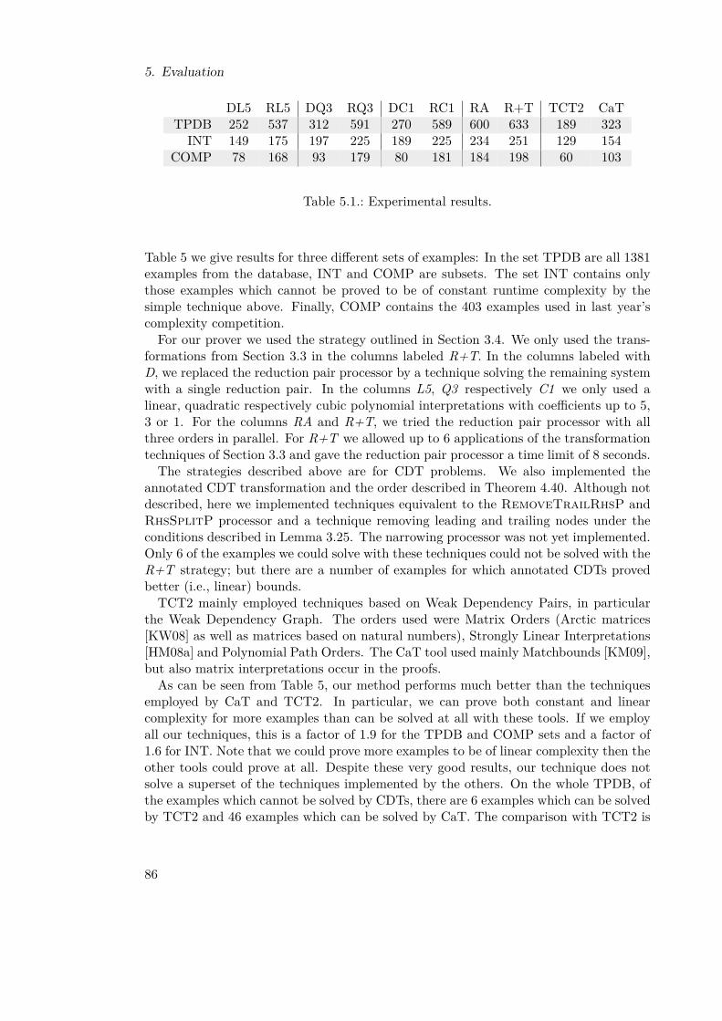
5. Evaluation
DL5 RL5 DQ3 RQ3 DC1 RC1 RA R+T TCT2 CaTTPDB 252 537 312 591 270 589 600 633 189 323
INT 149 175 197 225 189 225 234 251 129 154COMP 78 168 93 179 80 181 184 198 60 103
Table 5.1.: Experimental results.
Table 5 we give results for three different sets of examples: In the set TPDB are all 1381examples from the database, INT and COMP are subsets. The set INT contains onlythose examples which cannot be proved to be of constant runtime complexity by thesimple technique above. Finally, COMP contains the 403 examples used in last year’scomplexity competition.For our prover we used the strategy outlined in Section 3.4. We only used the trans-
formations from Section 3.3 in the columns labeled R+T. In the columns labeled withD, we replaced the reduction pair processor by a technique solving the remaining systemwith a single reduction pair. In the columns L5, Q3 respectively C1 we only used alinear, quadratic respectively cubic polynomial interpretations with coefficients up to 5,3 or 1. For the columns RA and R+T, we tried the reduction pair processor with allthree orders in parallel. For R+T we allowed up to 6 applications of the transformationtechniques of Section 3.3 and gave the reduction pair processor a time limit of 8 seconds.The strategies described above are for CDT problems. We also implemented the
annotated CDT transformation and the order described in Theorem 4.40. Although notdescribed, here we implemented techniques equivalent to the RemoveTrailRhsP andRhsSplitP processor and a technique removing leading and trailing nodes under theconditions described in Lemma 3.25. The narrowing processor was not yet implemented.Only 6 of the examples we could solve with these techniques could not be solved with theR+T strategy; but there are a number of examples for which annotated CDTs provedbetter (i.e., linear) bounds.TCT2 mainly employed techniques based on Weak Dependency Pairs, in particular
the Weak Dependency Graph. The orders used were Matrix Orders (Arctic matrices[KW08] as well as matrices based on natural numbers), Strongly Linear Interpretations[HM08a] and Polynomial Path Orders. The CaT tool used mainly Matchbounds [KM09],but also matrix interpretations occur in the proofs.As can be seen from Table 5, our method performs much better than the techniques
employed by CaT and TCT2. In particular, we can prove both constant and linearcomplexity for more examples than can be solved at all with these tools. If we employall our techniques, this is a factor of 1.9 for the TPDB and COMP sets and a factor of1.6 for INT. Note that we could prove more examples to be of linear complexity then theother tools could prove at all. Despite these very good results, our technique does notsolve a superset of the techniques implemented by the others. On the whole TPDB, ofthe examples which cannot be solved by CDTs, there are 6 examples which can be solvedby TCT2 and 46 examples which can be solved by CaT. The comparison with TCT2 is
86

particularly interesting, as TCT2 implements another variant for Dependency Pairs forcomplexity analysis. So experimental evidence suggests that our method is much morepowerful on many examples.Looking at the whole database, we can solve 45% of all examples. If we restrict
ourselves to the subset of interesting examples, i.e., those which are not trivially provedto be of constant complexity or to be non-terminating, we can still solve 27.5%.
87

6. Conclusion
In this thesis we laid down the foundations of a modular and extensible framework forautomated complexity analysis of term rewrite systems, in the spirit of the venerableDependency Pair approach. All results have been successfully automated in the AProVEtermination tool. Using this implementation, we were able to prove 633 of 1381 examplesrespectively 251 of 977 interesting examples to be of at most cubic runtime complexity.These results are better by a wide margin than the results of the winner of the complexitycategory in the Termination Competition 2009 1.Apart from pure numbers, how does our approach compare to the Weak Dependency
Pair approach presented by Hirokawa and Moser [HM08a; HM08b]? Both WDPs andCDTs build upon the Dependency Pair approach for termination, but different techniqueswhere chosen to guarantee that the upper bound derived for the transformed system isalso an upper bound for the original TRS. Consider the following rule from Example2.11:
quot(s(x), s(y))→ s(quot(minus(x, y), s(y)))
The classic Dependency Pair transformation generates the pairs
QUOT(s(x), s(y))→ QUOT(minus(x, y), s(y))QUOT(s(x), s(y))→ MINUS(x, y), s(y).
Our approach generates the same pairs, but ties them together into one right hand side
QUOT(s(x), s(y))→ [QUOT(minus(x, y), s(y)), MINUS(x, y), s(y)],
while for Weak DPs no explicit pair for the minus function call on the right hand side isgenerated:
QUOT(s(x), s(y))→ QUOT(minus(x, y), s(y))
The advantage compared to our approach is that there is no duplication of functionsymbols. Hence their transformation does not change the complexity of the system andthere is no need for a technique similar to our lockstepping. But this advantage comesat a great cost: For Weak Dependency Pairs it is necessary to orient all rules strictly,as evaluation steps both with rules and with pairs have to be counted. To allow the useof an reduction pair which orients only the pairs P strictly and the rules weakly, therules have to be compatible with a Strongly Linear Interpretation (SLI) and must benon-duplicating. The latter is a very strong restriction.
1http://termcomp.uibk.ac.at/status/rules.html
89
6. Conclusion
In contrast to this, the constraints required by our reduction pair processor are verysimilar to those required by the reduction pair processor for termination: Besides therequirement that one must be able to derive a bound for the number of strict rewritesteps, the only additional restriction is the monotonicity for the compound symbol, whichcan be easily fulfilled for many orders.Also, our Complexity Dependency Graph is very similar to the original Dependency
Graph and contains a node for each function call in the system. Due to this similarity,many of the powerful techniques developed for termination analysis can be easily adaptedto for complexity analysis, as was demonstrated in this thesis. We have seen, that thisis not as easy for the annotated variant, so there is still room for improvement. Incontrast to that, due to the definition of WDPs, the Weak Dependency Graph makesonly the topmost function calls explicit. This prevents techniques like the Rewriting andNarrowing transformations, as those assume that rule steps are only needed to establisha connection between two pair. But for Weak DPs they need to be counted to derive avalid complexity bound. A technique working on the Weak Dependency Graph is PathDetection [HM08b]. Unfortunately, the number of paths which have to be considered forthis technique may be exponential in the number of nodes and can still be quadratic ifthe graph of SCCs is a tree. Still, this technique requires SLIs and non-duplicating rulesto be able to orient some rules weakly.A weakness of both CDTs and WDPs is the missing ability to completely remove tuples
respectively pairs in SCCs. Our SccSplitP processor is a first step in this direction. Insummary one can say that our work greatly enhances the possibilities to automaticallyderive feasible complexity bounds for Term Rewrite Systems.
6.1. Future Work
We presented a modular framework for the analysis of innermost runtime complexity.It will be interesting to see what is needed to extended the approach presented here toother rewrite strategies and other sets of start terms, e.g. to derivational complexity.The annotated CDT transformation is complexity preserving, but the annotation of
the CDTs makes transformation techniques like narrowing considerably more compli-cated. We have yet to see how the rewriting technique can be adapted. So work isneeded to see whether it is possible to make the annotations optional on a per-tuplebasis to restore the modularity of the ordinary CDT approach. As the narrowing forannotated CDTs takes lockstepping into account, it should be considered if it is advanta-geous to start with annotated CDTs and switch to normal CDTs later, if the annotatedmethod cannot prove a complexity bound. Also, finding a more natural representa-tion for lockstepping would be greatly appreciated. A first step towards this would beto define the complexity in terms of t-chains and chain trees as for unannotated CDTproblems. The representation chosen by Hirokawa and Moser [HM08a] for their WeakDependency Pairs avoids this problem, but loses a great amount of flexibility, as onlythe topmost function calls are made explicit.Most transformation theorems presented here do not only yield an upper bound, but
90
6.1. Future Work
also a lower bound on the complexity. It should be an easy task to extend the frameworkto support those bounds, too. This would allow analyzing non-termination of TRSs onbasic terms. Known techniques for analyzing non-termination [Opp08; GTS05b; TGS08]could be easily adapted, as they produce a certificate of the loop found. For analysis ofnon-infinite lower bounds, there are no techniques the author knows of yet.We have chosen to produce only asymptotic complexity results in our framework. For
some use cases, it might be useful to be able to compute concrete bounds. To do this,one would need to propagate the complexity values for known nodes down to the leavesof the proof tree, so they can be used to compute the bounds depending on them. Onthe same matter, we currently compute the result of a processor always by summing upall complexities. It might be useful to allow more flexibility here; this will be requiredfor the technique outlined in the next paragraph.While our framework allows for a great amount of modularity, it still lacks a technique
for analyzing each SCC by itself: We always need to consider all nodes before a SCC,too (albeit in a weakened way). To allow otherwise, one will need to compute boundson the length (of the relevant part) of the output of nodes. Such an analysis can bestrengthened by taking into account sorts, sufficient definedness or the symbols matchedby later nodes.An obvious place for improvement is the addition of additional orders. As we need to
choose the interpretation in a way which establishes an upper bound for the complexity,the need for polynomials with a degree higher then 2 is greater than for terminationanalysis. But with the current state-of-the-art techniques like encoding constraints forthe polynomial in propositional logic [FGMSTZ07], the search for such polynomials isoften not feasible.The search for higher-dimensional matrix orders is faster then for polynomials of the
same degree and can also be used for complexity analysis [PSS97]. It seems that theconstraints on the shape and the values on the diagonal can be lifted for defined functionsymbols when analyzing runtime complexity. Another candidate is the polynomial pathorder presented in [AM08]. For best results, the orders must be adapted to be usableas reduction pairs. Avanzini and Moser [AM09] show how to do this for the polynomialpath order and Weak Dependency Pairs [HM08a], which have a similar notion of safereduction pairs as used in this thesis.It may be advantageous to label nodes by the SCC to which they belong. This would
allow different interpretations for the same function symbol in different SCCs. To thisend, it might be useful to consider that for polynomial orders we may allow a controlledsize increase between SCCs (and probably something similar for other orders).We have adapted the classic transformation techniques [GTSF06], but not yet the
heuristics for their application. Also it should be possible to implement positional nar-rowing [Thi07], a strong refinement of the standard narrowing technique. Even thoughwe already use strong estimations of Cap and usable rules, those techniques can be im-proved as we do analysis only on basic start terms. This can be done by keeping trackof the symbols which can occur in a term. Narrowing and Rewriting require the systemto be weakly innermost terminating (that is, each term can be rewritten to a normalform) to be complete. But of course a complexity proof implies termination, so if we
91

6. Conclusion
are able to successfully complete the proof, then we know that the system is weaklyinnermost terminating (on basic terms) and hence the proof is complete. To use this inthe framework, an asymmetric definition of the complexity like in [GTS05a] is needed.
92

A. Techniques for plain TRSs
The techniques presented in the main part of thesis all work on CDT problems. In thischapter, we present two simple techniques which work on plain Term Rewrite Systemsinstead.
A.1. Identifying constant runtime complexityWith the techniques presented, we can only identify constant runtime complexity if weget a dependency graph without cycles (without ever using the reduction pair processor).But there is another class of term rewrite systems for which a constant complexity canbe easily shown: Systems having only a finite number of (relevant) basic terms.Throughout this section,R designates a finite set of rules over alphabet Σ and variablesV. With we denote either → or i−→, depending on whether we talk about full orinnermost runtime complexity.
Lemma A.1. If T (Σ,V) contains only finitely many basic terms and R is (innermost)terminating on the set of start terms TB, then R has constant (innermost) runtimecomplexity, i.e., rc(n,) ≤ c for some c ∈ N.
Proof. dl(t,) | t ∈ TB(Σ,V) is a finite subset of N and hence has a maximum.
Obviously, if all constructor symbols are constants, the set of basic terms can onlybe finite. Now, the usual assumption is that V is infinite, so any system containinga non-constant function symbol would have infinite many basic terms. But it is easysee that we may restrict us to basic terms with only one distinct variable symbol. Thereason for this is that matching can only detect equality of variables, not inequality.
Lemma A.2. Let s ∈ T (Σ,V) and V ⊂ V be the set of variables in s. Let x ∈ V be avariable and σ a substitution where vσ = x for all v ∈ V . Then dl(s,) ≤ dl(sσ,).
Proof. Let t be a term and π ∈ Pos(t). If s|π matches l (for any l → r ∈ R), then sσ|πmatches l.
In addition, with a similar argument, we may restrict us to constructor symbols occur-ring on the left-hand side of rules in R: A function symbol not occurring on a left-handside can only be matched by variables.
Lemma A.3. Let s ∈ T (Σ,V). Let x ∈ V be a variable and σ be the substitutionreplacing x by t = f(t1, . . . tn) and t a basic term with f not occurring on the left-handside of a rule in R. Then dl(s,) = dl(sσ,).
93

A. Techniques for plain TRSs
So, we arrive at the following simple theorem:
Theorem A.4. Let Cl be the set of of constructor symbols occurring on the left-handside of rules in R. Let
T := f(t1, . . . , tn) | f ∈ DR, ti ∈ T (Cl, x).
If T is finite and R is (innermost) terminating on T , then R has constant (innermost)runtime complexity. T is finite if and only iff all constructor symbols are constants.
While such systems may appear to be not very common, a significant amount of exam-ples in the runtime complexity categories of the current Termination Problem Database[Tpd] belongs to this class of problems: This is due to the fact that those exampleswere constructed for unrestricted start terms instead of basic terms. Of 1381 examples,432 have only finitely many relevant start terms and 343 of these can be proved to beinnermost terminating with a current version of AProVE. It is worth noting that thosesystems are terminating on all inputs, not only on basic terms. These numbers can besignificantly improved if we can teach AProVE to do local termination.
A.2. Start term transformationBy definition, runtime complexity is a start term problem. For the generic problem oflocal termination of TRS, not many results are known. A recent paper by Endrullis,Vrijer, andWaldmann [EVW09] employs partial algebras for a direct termination methodand combine this with semantic labeling to convert a local termination problem into aglobal termination problem. We describe a simple application of Usable Rules (see 2.4)to remove rules not reachable from start terms. Due to the simple structure of startterms, this approach gives good results.Remark A.5. Let R be a set of rules and R′ ⊆ R be a set containing all rules reachablefrom a start term, i.e: ρ ∈ R′ if there exists a basic term s such that s R t ρ v.Then rc(n,R) = rc(n,R′).This allows us to use any over-approximation of usable rules to simplify our initial
TRS. Using the usable rules technique implemented in AProVE, this technique is appli-cable to a set of 723 of the 1381 examples above. If we apply both techniques, we get463 systems with finite set of (relevant) constructor systems. 435 of them are locallyinnermost terminating and can be proved as such by AProVE. So at least 31% of thewhole example set have constant innermost runtime complexity. One should note, thatthis technique is not complete; i.e. if the transformed system is nonterminating, theoriginal system might still be terminating on start terms.
94
Bibliography
[AG00] Thomas Arts and Jürgen Giesl. “Termination of term rewriting usingdependency pairs”. In: Theoretical Computer Science 236.1-2 (2000),pp. 133 –178.
[AM08] Martin Avanzini and Georg Moser. “Complexity Analysis by Rewrit-ing”. In: Proceedings of the 9th International Symposium on Functionaland Logic Programming. Vol. 4989. Lecture Notes in Computer Science.Springer, 2008, pp. 130–146.
[AM09] Martin Avanzini and Georg Moser. “Dependency Pairs and PolynomialPath Orders”. In: Proceedings of the 20th International Conference onRewriting Techniques and Applications. Vol. 5595. Lecture Notes in Com-puter Science. Springer, 2009, pp. 48–62.
[BCMT99a] Guillaume Bonfante, Adam Cichon, Jean-Yves Marion, and HélèneTouzet. “Algorithms With Polynomial Interpretation TerminationProof”. In: Journal of Functional Programming 11 (1999), p. 2001.
[BCMT99b] Guillaume Bonfante, Adam Cichon, Jean-Yves Marion, and HélèneTouzet. “Complexity Classes and Rewrite Systems with Polynomial In-terpretation”. In: Proceedings of the 12th International Workshop onComputer Science Logic. Springer, 1999, pp. 372–384.
[BD86] Leo Bachmair and Nachum Dershowitz. “Commutation, Transformation,and Termination.” In: Proceedings of the 8th International Conferenceon Automated Deduction. Vol. 230. Lecture Notes in Computer Science.Springer, 1986, pp. 5–20.
[BN98] Franz Baader and Tobias Nipkow. Term Rewriting and All That. Cam-bridge University Press, 1998.
[CL92] Adam Cichon and Pierre Lescanne. “Polynomial Interpretations and theComplexity of Algorithms”. In: Proceedings of the 11th InternationalConference on Automated Deduction: Automated Deduction. Springer,1992, pp. 139–147.
[CMTU05] Evelyne Contejean, Claude Marché, Ana Paula Tomás, and Xavier Ur-bain. “Mechanically Proving Termination Using Polynomial Interpreta-tions”. In: Journal of Automated Reasoning 34.4 (2005), pp. 325–363.
[Dbla] Rewriting Techniques and Applications, 19th International Conference,RTA 2008, Hagenberg, Austria, July 15-17, 2008, Proceedings. Vol. 5117.Lecture Notes in Computer Science. Springer, 2008.
95
Bibliography
[Dblb] Rewriting Techniques and Applications, 20th International Conference,RTA 2009, Brasília, Brazil, June 29 - July 1, 2009, Proceedings.Vol. 5595. Lecture Notes in Computer Science. Springer, 2009.
[Der87] Nachum Dershowitz. “Termination of rewriting”. In: Journal of SymbolicComputation 3 (1-2 1987), pp. 69–116.
[EVW09] Jörg Endrullis, Roel C. de Vrijer, and Johannes Waldmann. “LocalTermination”. In: Proceedings of the 20th International Conference onRewriting Techniques and Applications. Vol. 5595. Lecture Notes in Com-puter Science. Springer, 2009, pp. 270–284.
[FGMSTZ07] Carsten Fuhs, Jürgen Giesl, Aart Middeldorp, Peter Schneider-Kamp,René Thiemann, and Harald Zankl. “SAT Solving for Termination Anal-ysis with Polynomial Interpretations”. In: Proceedings of the 6th Inter-national Conference on Theory and Applications of Satisfiability Testing.Vol. 4501. Lecture Notes in Computer Science. Springer, 2007, pp. 340–354.
[Gra96] Bernhard Gramlich. “Termination and Confluence Properties of Struc-tured Rewrite Systems”. Fachbereich Informatik, Universität Kaiser-slautern, Jan. 1996, p. 217.
[GSST06] Jürgen Giesl, Stephan Swiderski, Peter Schneider-Kamp, and René Thie-mann. “Automated Termination Analysis for Haskell: From Term Rewrit-ing to Programming Languages”. In: Proceedings of the 17th Interna-tional Conference on Rewriting Techniques and Applications. Vol. 4098.Lecture Notes in Computer Science. Springer, 2006, pp. 297–312.
[GST06] Jürgen Giesl, Peter Schneider-Kamp, and René Thiemann. “AProVE1.2: Automatic Termination Proofs in the Dependency Pair Framework”.In: Proceedings of the 3rd International Joint Conference on AutomatedReasoning. Vol. 4130. Lecture Notes in Artificial Intelligence. Springer,2006, pp. 281–286.
[GTS05a] Jürgen Giesl, René Thiemann, and Peter Schneider-Kamp. “Proving andDisproving Termination in the Dependency Pair Framework”. In: Deduc-tion and Applications. Vol. 05431. Dagstuhl Seminar Proceedings. Inter-nationales Begegnungs- und Forschungszentrum für Informatik (IBFI),Schloss Dagstuhl, Germany, 2005.
[GTS05b] Jürgen Giesl, René Thiemann, and Peter Schneider-Kamp. “Provingand Disproving Termination of Higher-Order Functions”. In: Proceed-ings of 5th International Workshop on Frontiers of Combining Systems.Springer, 2005, pp. 216–231.
[GTSF06] Jürgen Giesl, René Thiemann, Peter Schneider-Kamp, and StephanFalke. “Mechanizing and Improving Dependency Pairs”. In: Journal ofAutomated Reasoning 37.3 (2006), pp. 155–203.
96

Bibliography
[HL89] Dieter Hofbauer and Clemens Lautemann. “Termination proofs and thelength of derivations”. In: Proceedings of the 3rd international conferenceon Rewriting Techniques and Applications. Springer, 1989, pp. 167–177.
[HM08a] Nao Hirokawa and Georg Moser. “Automated Complexity AnalysisBased on the Dependency Pair Method”. In: Proceedings of the 4th Inter-national Joint Conference on Automated Reasoning. Vol. 5195. LectureNotes in Computer Science. Springer, 2008, pp. 364–379.
[HM08b] Nao Hirokawa and Georg Moser. “Complexity, Graphs, and the Depen-dency Pair Method”. In: Proceedings of the 15th International Confer-ence on Logic for Programming, Artificial Intelligence and Reasoning.Vol. 5330. Lecture Notes in Computer Science. Springer, 2008, pp. 652–666.
[KB70] Donald E. Knuth and Peter B. Bendix. “Simple word problems in uni-versal algebras”. In: Computational Problems in Abstract Algebra. Perg-amon, 1970, pp. 263–267.
[KM09] Martin Korp and Aart Middeldorp. “Match-bounds revisited”. In: Infor-mation and Computation 207.11 (2009), pp. 1259–1283.
[KW08] Adam Koprowski and Johannes Waldmann. “Arctic Termination ...BelowZero”. In: Proceedings of the 19th International Conference on Rewrit-ing Techniques and Applications. Vol. 5117. Lecture Notes in ComputerScience. Springer, 2008, pp. 202–216.
[Lan79] Dallas S. Lankford. On Proving Term Rewriting Systems are Noethe-rian. Memo MTP-3. Revised October 1979. Mathematics Department,Louisiana Tech. University, May 1979.
[Mid01] Aart Middeldorp. “Approximating Dependency Graphs Using Tree Au-tomata Techniques”. In: Proceedings of the First International Joint Con-ference on Automated Reasoning. Springer, 2001, pp. 593–610.
[MSW08] Georg Moser, Andreas Schnabl, and Johannes Waldmann. “ComplexityAnalysis of Term Rewriting Based on Matrix and Context DependentInterpretations”. In: Proceedings of the IARCS Annual Conference onFoundations of Software Technology and Theoretical Computer Science.Vol. 2. LIPIcs. Schloss Dagstuhl - Leibniz-Zentrum fuer Informatik, 2008,pp. 304–315.
[OBEG10] Carsten Otto, Marc Brockschmidt, Christian von Essen, and JürgenGiesl. “Automated Termination Analysis of Java Bytecode by TermRewriting”. In: Proceedings of the 21th International Conference onRewriting Techniques and Applications (to appear). 2010.
[Ohl02] Enno Ohlebusch. Advanced Topics in Term Rewriting. Springer, 2002.[Opp08] Martin Oppelt. “Automatische Erkennung von Ableitungsmustern in
nichtterminierenden Wortersetzungssystemen”. Diplomarbeit. HTWKLeipzig, July 2008.
97
Bibliography
[PSS97] Sven Eric Panitz and Manfred Schmidt-Schauß. “TEA: AutomaticallyProving Termination of Programs in a Non-strict Higher-Order Func-tional Language”. In: Proceedings of the 4th International Symposiumon Static Analysis. Springer, 1997, pp. 345–360.
[SGST09] Peter Schneider-Kamp, Jürgen Giesl, Alexander Serebrenik, and RenéThiemann. “Automated Termination Proofs for Logic Programs by TermRewriting”. In: Transactions of Computational Logic (2009).
[Tai61] William W. Tait. “Nested Recursion”. In: Mathematische Annalen 143(1961), pp. 236–250.
[TGS08] René Thiemann, Jürgen Giesl, and Peter Schneider-Kamp. “DecidingInnermost Loops”. In: Proceedings of the 19th International Conferenceon Rewriting Techniques and Applications. Vol. 5117. Lecture Notes inComputer Science. Springer, 2008, pp. 366–380.
[Thi07] René Thiemann. The DP Framework for Proving Termination of TermRewriting. Tech. rep. AIB-2007-17. RWTH Aachen University, Oct. 2007.
[Tpd] Termination Problem Database 7.0.2. url: http://www.termination-portal.org/wiki/TPDB.
[Wal09] Johannes Waldmann. “Automatic Termination”. In: Proceedings of the20th International Conference on Rewriting Techniques and Applications.Vol. 5595. Lecture Notes in Computer Science. Springer, 2009, pp. 1–16.
[Wei95] Andreas Weiermann. “Termination Proofs for Term Rewriting Systemsby Lexicographic Path Orderings Imply Multiply Recursive DerivationLengths”. In: Theoretical Computer Science 139.1&2 (1995), pp. 355–362.
[Zan95] Hans Zantema. “Termination of Term Rewriting by Semantic Labelling”.In: Fundamenta Informaticae 24.1/2 (1995), pp. 89–105.
[ZHM09] Harald Zankl, Nao Hirokawa, and Aart Middeldorp. “KBO Orientabil-ity”. In: Journal of Automated Reasoning 43.2 (2009), pp. 173–201.
98
Related Documents