Automated color correction for colorimetric applications using barcodes Ismael Benito Altamirano Aquesta tesi doctoral està subjecta a la llicència Reconeixement- NoComercial – CompartirIgual 4.0. Espanya de Creative Commons. Esta tesis doctoral está sujeta a la licencia Reconocimiento - NoComercial – CompartirIgual 4.0. España de Creative Commons. This doctoral thesis is licensed under the Creative Commons Attribution-NonCommercial- ShareAlike 4.0. Spain License.

Welcome message from author
This document is posted to help you gain knowledge. Please leave a comment to let me know what you think about it! Share it to your friends and learn new things together.
Transcript
Automated color correction for colorimetric applications using barcodes
Ismael Benito Altamirano
Aquesta tesi doctoral està subjecta a la llicència Reconeixement- NoComercial – CompartirIgual 4.0. Espanya de Creative Commons. Esta tesis doctoral está sujeta a la licencia Reconocimiento - NoComercial – CompartirIgual 4.0. España de Creative Commons. This doctoral thesis is licensed under the Creative Commons Attribution-NonCommercial-ShareAlike 4.0. Spain License.
I S M A E L B E N I T O - A LTA M I R A N O
A U T O M AT E D C O L O R C O R R E C T I O N
F O R C O L O R I M E T R Y A P P L I C AT I O N S
U S I N G B A R C O D E S
U N I V E R S I TAT D E B A R C E L O N A
P H D I N E N G I N E E R I N G A N D A P P L I E D S C I E N C E S
D I R E C T O R : J O A N D A N I E L P R A D E S

A U T O M AT E D C O L O R C O R R E C T I O N
F O R C O L O R I M E T R Y A P P L I C AT I O N S
U S I N G B A R C O D E S
Programa de doctorat en Enginyeria i Ciències Aplicades
Autor: Ismael Benito-Altamirano
Director: Dr. Joan Daniel Prades
Tutor: Dr. Ángel Diéguez Barrientos

Copyright © 2022 Ismael Benito-Altamirano
published by universitat de barcelona
phd in engineering and applied sciences
director: joan daniel prades
tutor: ángel diéguez
This work is licensed by a Creative Commons license cbea.
First printing, January 2022
Acknowledgements
First, this thesis is dedicated to my family. We are a small family: my parents, my grandparentsand my uncles and aunt. Specially, to my mother, who never has failed to encourage me to followwhat I like to study, also for her constancy in response to my chaos. Also, specially to my father,from whom I got the passion for photography and computer science, knowing this one couldunderstand better this thesis. To my paternal grandparents who are no longer with us. To mymaternal grandmother who always has good advice, recently she said to my mother: "the kid hasstudied enough, since you send it to kindergarten with 3 years, he hasn’t stopped", referring tothis thesis!
To my friends, beginning with Anna, who is my flatmate and my partner; and who hassupported me during these final thesis months. To other friends from the high school, bothneighborhoods I grew up and those friends from the faculty, also. To other colleagues withwhom I have shared the fight for a better university model, and now we share other fights, to mycomrades!
To the Department of Electronics and Biomedical Engineering of Universitat de Barcelona, toall its members. Specially, to Dr. A. Cornet for being a nice host at the department. Specially, toDr. A. Herms, to encourage me to pursue the thesis in this department and to contact Dr. J. D:Prades, director of this thesis. Also, to other colleagues from the MIND research group i from theLaboratory from ’the 0 floor’: to Dr. C. Fàbrega, to Dr. O. Canals, and many others!
To Dr. J. D. Prades himself, for the opportunity by accepting this thesis proposal, and embracethe idea I presented, leading to the creation of ColorSensing. To the ColorSensing team, beginingwith Maria Eugenia Martín, co-funder and CEO of ColorSensing. Without forgetting, all theother teammates: to Josep Maria, to Hanna, to Dani, to Maria, to Ferran and to Miriam (Dr. M.Marchena). But also, to the former teammates: to Peter, to Oriol (Dr. O. Cusola), to Arnau, toCarles, to Pablo, to Gerard, to Hamid and to David. Thank you very much all for this journey.
This thesis has been funded in part by the European Research Council under the H2020
Framework Program ERC Grant Agreements no. 727297 and no. 957527. Also, by the Eurostartsprograma with the Agreement no. 11453. Secondary funding sources have been: AGAUR -PRODUCTE (2016-PROD-00036), BBVA Leonardo, and ICREA Academia programs.

Agraïments
Aquesta tesi va dedicada en primera instància a la meva família. Som una família petita: a mons pares, als
meus avis i als meus tiets. Especialment, a ma mare, perquè mai a fallat en animar-me per perseguir el que
m’agrada estudiar, també per la seva constància davant del meu desordre. Especialment també, al meu pare,
per la seva passió amb la fotografia i la informàtica que des de petit m’ha inculcat, així hom pot entendre
aquesta tesi molt millor. Als meus avis paterns que ja no estan. A la meva àvia materna que sempre té bons
consells, i fa poc li va dir a ma mare: "si el nen ja ha estudiat prou, d’ençà que el vas portar amb tres anys
(al col·legi) no ha parat d’estudiar", referint-se a aquesta tesi!
Als meus amics, començant per l’Anna, que és la meva companya de pis, i la meva parella; que m’ha
recolzat durant aquests darrers mesos a casa mentre redactava la tesi. A tots aquells amics de l’institut, del
barri, de la ’urba’ i de la facultat. També a aquelles companyes amb les quals hem compartit lluites a la
universitat des de l’època d’estudi i ara seguim compartint altres espais polítics, els i les meves camarades.
Al Departament d’Enginyeria Electrònica i Biomèdica de la Universitat de Barcelona, a tots els seus
membres. Especialment, al Dr. A. Cornet per la seva acollida al departament. Al Dr. A. Herms, per
animar-me a fer la tesi al Departament i contactar al Dr. J. D. Prades, director d’aquesta tesi. També, a
altres companyes i companys del MIND, el nostre grup de recerca, i del Laboratori ’de planta 0’: al Dr. C.
Fàbrega, la Dra. O. Casals, i tots els altres!
Al mateix Dr. J. D. Prades, per l’oportunitat acceptant aquesta tesi, i acollir la idea que li vaig presentar
fins al punt d’impulsar la creació de ColorSensing. A tot l’equip de ColorSensing, començant per la Maria
Eugenia Martín, cofundadora i CEO de ColorSensing. Però, per suposat, a la resta de l’equip: al Josep
Maria, a la Hanna, al Dani, a la María, al Ferran i a la Miriam (Dra. M. Marchena). Però també als seus
antics membres amb qui hem coincidit: al Peter, a l’Oriol (Dr. O. Cusola), a l’Arnau, al Carles, al Pablo, al
Gerard, a l’Hamid i al David. Moltes gràcies a tots i totes per fer aquest viatge conjuntament.

Index
Abstract 11
1 Introduction 15
1.1 Objectives . . . . . . . . . . . . . . . . . . . . . . . . . . . . . . . . . . . . . . 19
1.2 Thesis sctructure . . . . . . . . . . . . . . . . . . . . . . . . . . . . . . . . . . 20
2 Background and methods 21
2.1 The image consistency problem . . . . . . . . . . . . . . . . . . . . . . . . . . 21
2.1.1 Color reproduction . . . . . . . . . . . . . . . . . . . . . . . . . . . . . 22
2.1.2 Image consistency . . . . . . . . . . . . . . . . . . . . . . . . . . . . . 23
2.1.3 Color charts . . . . . . . . . . . . . . . . . . . . . . . . . . . . . . . . . 24
2.2 2D Barcodes: the Quick-Response Code . . . . . . . . . . . . . . . . . . . . . 26
2.2.1 Scalability . . . . . . . . . . . . . . . . . . . . . . . . . . . . . . . . . . 28
2.2.2 Data encoding in QR Codes . . . . . . . . . . . . . . . . . . . . . . . . 29
2.2.3 Computer vision features of QR Codes . . . . . . . . . . . . . . . . . 32
2.2.4 Readout of QR Codes . . . . . . . . . . . . . . . . . . . . . . . . . . . 34
2.3 Data representation . . . . . . . . . . . . . . . . . . . . . . . . . . . . . . . . . 37
2.3.1 Color spaces . . . . . . . . . . . . . . . . . . . . . . . . . . . . . . . . . 37
2.3.2 Color transformations . . . . . . . . . . . . . . . . . . . . . . . . . . . 38
2.3.3 Images as bitmaps . . . . . . . . . . . . . . . . . . . . . . . . . . . . . 41
2.4 Computational implementation . . . . . . . . . . . . . . . . . . . . . . . . . . 43
3 QR Codes on challenging surfaces 45
3.1 Proposal . . . . . . . . . . . . . . . . . . . . . . . . . . . . . . . . . . . . . . . 46
3.1.1 Fundamentals of projections . . . . . . . . . . . . . . . . . . . . . . . 47
3.1.2 Proposed transformations . . . . . . . . . . . . . . . . . . . . . . . . . 48
8
3.2 Experimental details . . . . . . . . . . . . . . . . . . . . . . . . . . . . . . . . 52
3.2.1 Datasets . . . . . . . . . . . . . . . . . . . . . . . . . . . . . . . . . . . 52
3.3 Results . . . . . . . . . . . . . . . . . . . . . . . . . . . . . . . . . . . . . . . . 55
3.3.1 Qualitative surface fitting . . . . . . . . . . . . . . . . . . . . . . . . . 55
3.3.2 Quantitative data readability . . . . . . . . . . . . . . . . . . . . . . . 58
3.4 Conclusions . . . . . . . . . . . . . . . . . . . . . . . . . . . . . . . . . . . . . 61
4 Back-compatible Color QR Codes 63
4.1 Proposal . . . . . . . . . . . . . . . . . . . . . . . . . . . . . . . . . . . . . . . 64
4.1.1 Color as a source of noise . . . . . . . . . . . . . . . . . . . . . . . . . 65
4.1.2 Back-compatibility proposal . . . . . . . . . . . . . . . . . . . . . . . 68
4.2 Experimental details . . . . . . . . . . . . . . . . . . . . . . . . . . . . . . . . 73
4.2.1 Color generation and substitution . . . . . . . . . . . . . . . . . . . . 73
4.2.2 Placing colors inside the QR Code . . . . . . . . . . . . . . . . . . . . 75
4.2.3 QR Code versions and digital IDs . . . . . . . . . . . . . . . . . . . . 75
4.2.4 Channels . . . . . . . . . . . . . . . . . . . . . . . . . . . . . . . . . . . 75
4.3 Results . . . . . . . . . . . . . . . . . . . . . . . . . . . . . . . . . . . . . . . . 77
4.3.1 Embedding colors in QRs codes: empty channel . . . . . . . . . . . . 77
4.3.2 Image augmentation channel . . . . . . . . . . . . . . . . . . . . . . . 78
4.3.3 Colorimetry setup as channel . . . . . . . . . . . . . . . . . . . . . . . 79
4.3.4 Readability . . . . . . . . . . . . . . . . . . . . . . . . . . . . . . . . . 81
4.3.5 Example of use case . . . . . . . . . . . . . . . . . . . . . . . . . . . . 85
4.4 Conclusions . . . . . . . . . . . . . . . . . . . . . . . . . . . . . . . . . . . . . 86
5 Image consistency using an improved TPS3D method 89
5.1 Proposal . . . . . . . . . . . . . . . . . . . . . . . . . . . . . . . . . . . . . . . 90
5.1.1 Linear corrections . . . . . . . . . . . . . . . . . . . . . . . . . . . . . 91
5.1.2 Polynomial corrections . . . . . . . . . . . . . . . . . . . . . . . . . . . 93
5.1.3 Thin-plate spline correction . . . . . . . . . . . . . . . . . . . . . . . . 95
5.2 Experimental details . . . . . . . . . . . . . . . . . . . . . . . . . . . . . . . . 98
5.2.1 Dataset and pipeline . . . . . . . . . . . . . . . . . . . . . . . . . . . . 100
5.2.2 Benchmark metrics . . . . . . . . . . . . . . . . . . . . . . . . . . . . . 103
5.3 Results . . . . . . . . . . . . . . . . . . . . . . . . . . . . . . . . . . . . . . . . 105
5.3.1 Detecting failed corrections . . . . . . . . . . . . . . . . . . . . . . . . 105
9
5.3.2 Color correction performance . . . . . . . . . . . . . . . . . . . . . . . 106
5.3.3 Execution time performance . . . . . . . . . . . . . . . . . . . . . . . 109
5.4 Conclusions . . . . . . . . . . . . . . . . . . . . . . . . . . . . . . . . . . . . . 112
6 Application: Colorimetric indicators 115
6.1 Proposal . . . . . . . . . . . . . . . . . . . . . . . . . . . . . . . . . . . . . . . 118
6.1.1 Early prototypes . . . . . . . . . . . . . . . . . . . . . . . . . . . . . . 118
6.1.2 A machine-readable pattern for colorimetric indicators . . . . . . . . 120
6.1.3 A Color QR Code for colorimetric indicators . . . . . . . . . . . . . . 122
6.2 Experimental details . . . . . . . . . . . . . . . . . . . . . . . . . . . . . . . . 124
6.2.1 Sensor fabrication . . . . . . . . . . . . . . . . . . . . . . . . . . . . . 124
6.2.2 Experimental setup . . . . . . . . . . . . . . . . . . . . . . . . . . . . . 125
6.2.3 Expected response model . . . . . . . . . . . . . . . . . . . . . . . . . 128
6.3 Results . . . . . . . . . . . . . . . . . . . . . . . . . . . . . . . . . . . . . . . . 129
6.3.1 The color response . . . . . . . . . . . . . . . . . . . . . . . . . . . . . 129
6.3.2 Model fitting . . . . . . . . . . . . . . . . . . . . . . . . . . . . . . . . 132
6.4 Conclusions . . . . . . . . . . . . . . . . . . . . . . . . . . . . . . . . . . . . . 140
7 Conclusions 143
7.1 Thesis conclusions . . . . . . . . . . . . . . . . . . . . . . . . . . . . . . . . . 143
7.2 Future work . . . . . . . . . . . . . . . . . . . . . . . . . . . . . . . . . . . . . 145
List of Figures 147
List of Tables 160
Bibliography 163

Abstract
Color-based sensor devices often offer qualitative solutions, where amaterial change its color from one color to another, and this is changeis observed by a user who performs a manual reading. These materi-als change their color in response to changes in a certain physical orchemical magnitude. Nowadays, we can find colorimetric indicatorswith several sensing targets, such as: temperature, humidity, environ-mental gases, etc. The common approach to quantize these sensors isto place ad hoc electronic components, e.g. a reader device.
With the rise of smartphone technology, the possibility to auto-matically acquire a digital image of those sensors and then computea quantitative measure is near. By leveraging this measuring processto the smartphones, we avoid the use of ad hoc electronic components,thus reducing colorimetric application cost. However, there existsa challenge on how-to acquire the images of the colorimetric appli-cations and how-to do it consistently, with the disparity of externalfactors affecting the measure, such as ambient light conditions ordifferent camera modules.
In this thesis, we tackle the challenges to digitize and quantizecolorimetric applications, such as colorimetric indicators. We make astatement to use 2D barcodes, well-known computer vision patterns,as the base technology to overcome those challenges. We focus onfour main challenges: (I) to capture barcodes on top of real-worldchallenging surfaces (bottles, food packages, etc.), which are theusual surface where colorimetric indicators are placed; (II) to define anew 2D barcode to embed colorimetric features in a back-compatiblefashion; (III) to achieve image consistency when capturing imageswith smartphones by reviewing existent methods and proposing anew color correction method, based upon thin-plate splines mappings;and (IV) to demonstrate a specific application use case applied toa colorimetric indicator for sensing CO2 in the range of modifiedatmosphere packaging –MAP–, one of the common food-packagingstandards.

Resum
Els dispositius de sensat basats en color, normalment ofereixen solucions
qualitatives, en aquestes solucions un material canvia el seu color a un
altre color, i aquest canvi de color és observat per un usuari que fa una
mesura manual. Aquests materials canvien de color en resposta a un canvi
en una magnitud física o química. Avui en dia, podem trobar indicadors
colorimètrics que amb diferents objectius, per exemple: temperatura, humitat,
gasos ambientals, etc. L’opció més comuna per quantitzar aquests sensors és
l’ús d’electrònica addicional, és a dir, un lector.
Amb l’augment de la tecnologia dels telèfons intel·ligents, la possibilitat
d’automatitzar l’adquisició d’imatges digitals d’aquests sensors i després
computar una mesura quantitativa és a prop. Desplaçant aquest procés de
mesura als telèfons mòbils, evitem l’ús d’aquesta electrònica addicional, i
així, es redueix el cost de l’aplicació colorimètrica. Tanmateix, existeixen
reptes sobre com adquirir les imatges de les aplicacions colorimètriques i de
com fer-ho de forma consistent, a causa de la disparitat de factors externs que
afecten la mesura, com per exemple la llum ambient or les diferents càmeres
utilitzades.
En aquesta tesi, encarem els reptes de digitalitzar i quantitzar aplicacions
colorimètriques, com els indicadors colorimètrics. Fem una proposició per
utilitzar codis de barres en dues dimensions, que són coneguts patrons
de visió per computador, com a base de la nostra tecnologia per superar
aquests reptes. Ens focalitzem en quatre reptes principals: (I) capturar
codis de barres sobre de superfícies del món real (ampolles, safates de menjar,
etc.), que són les superfícies on usualment aquests indicadors colorimètrics
estan situats; (II) definir un nou codi de barres en dues dimensions per
encastar elements colorimètrics de forma retro-compatible; (III) aconseguir
consistència en la captura d’imatges quan es capturen amb telèfons mòbils,
revisant mètodes de correcció de color existents i proposant un nou mètode
basat en transformacions geomètriques que utilitzen splines; i (IV) demostrar
l’ús de la tecnologia en un cas específic aplicat a un indicador colorimètric
per detectar CO2 en el rang per envasos amb atmosfera modificada –MAP–,
un dels estàndards en envasos de menjar.

Chapter 1. Introduction
The rise of the smartphone technology developed in parallel to thepopularization of digital cameras enabled an easier access to photog-raphy devices to the people. Nowadays, modern smartphones haveonboard digital cameras that can feature good color reproduction forimaging uses [1].
Alongside with this phenomenon, there has been a popularizationof color-based solutions to detect biochemistry analytes [2]. Bothphenomena are probable to be linked. As the first one eases thesecond. Scientists who want to pursue research to discover new orimprove existent color-based analytics found themselves with betterand better imaging tools, spending fewer and fewer resources.
Color-based sensing [2] is often preferred over electronic sensing[3] for three reasons: one, the rapid detection of the analytes; two,the high sensitivity; and three, the high selectivity of colormetricsensors. Nevertheless, imaging acquisition on smartphone devicesstill presents some acquisition challenges, and how to overcome thosechallenges is still an open debate [4].
This is why, the ERC-StG BetterSense project (ERC n. 336917)was granted the extension ERC-PoC GasApp project (ERC n.727297).Bettersense was an ERC-funded project which aimed to solve highpower consumption and the poor selectivity of electronic gas sensortechnologies [5]. GasApp was an ERC-funded project that aimed tobring the capability to detect gases to smartphone technology, relyingon color-based sensor technology [6].
The accumulated knowledge from BetterSense was translated intothe GasApp project to create colorimetric indicators to sense targetgases, the GasApp proposal is detailed in Figure 1.1. Later on, theSnapGas project (Eurostars n. 11453) was also granted to carry on thisresearch topic, and apply the new technology to other colorimetricindicators to sense environmental gases [7].
16 automated color correction for colorimetry applications using barcodes
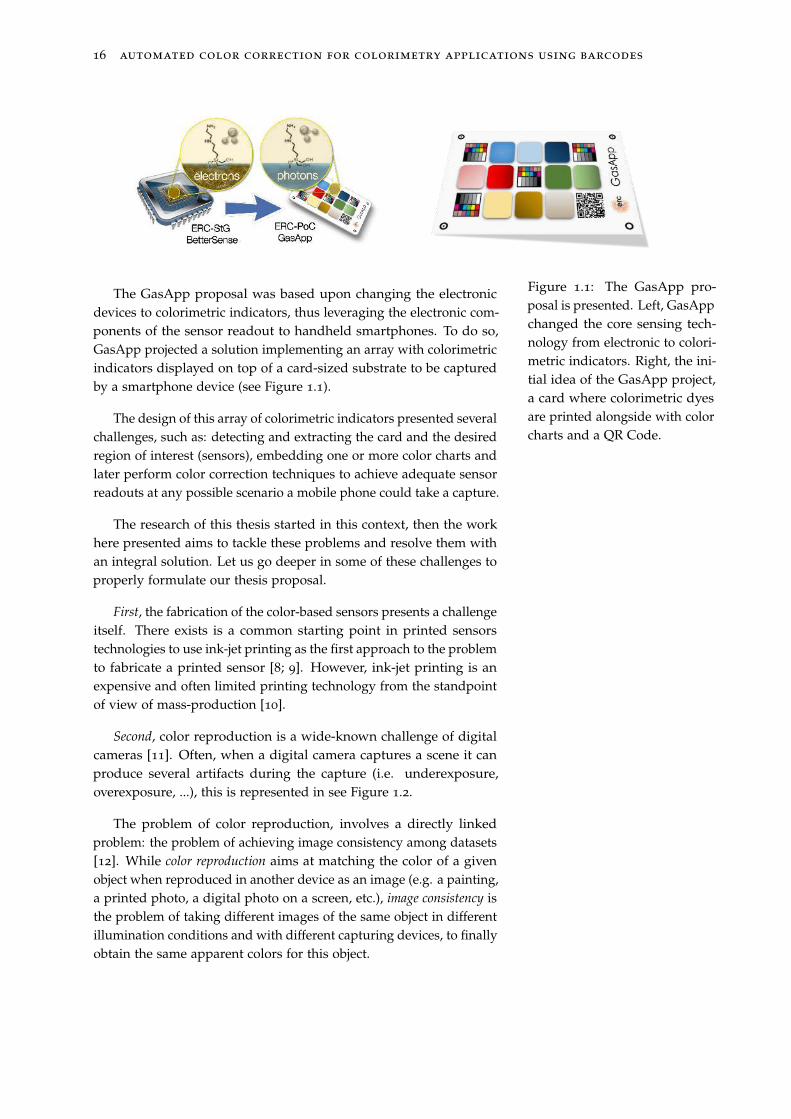
Figure 1.1: The GasApp pro-posal is presented. Left, GasAppchanged the core sensing tech-nology from electronic to colori-metric indicators. Right, the ini-tial idea of the GasApp project,a card where colorimetric dyesare printed alongside with colorcharts and a QR Code.
The GasApp proposal was based upon changing the electronicdevices to colorimetric indicators, thus leveraging the electronic com-ponents of the sensor readout to handheld smartphones. To do so,GasApp projected a solution implementing an array with colorimetricindicators displayed on top of a card-sized substrate to be capturedby a smartphone device (see Figure 1.1).
The design of this array of colorimetric indicators presented severalchallenges, such as: detecting and extracting the card and the desiredregion of interest (sensors), embedding one or more color charts andlater perform color correction techniques to achieve adequate sensorreadouts at any possible scenario a mobile phone could take a capture.
The research of this thesis started in this context, then the workhere presented aims to tackle these problems and resolve them withan integral solution. Let us go deeper in some of these challenges toproperly formulate our thesis proposal.
First, the fabrication of the color-based sensors presents a challengeitself. There exists is a common starting point in printed sensorstechnologies to use ink-jet printing as the first approach to the problemto fabricate a printed sensor [8; 9]. However, ink-jet printing is anexpensive and often limited printing technology from the standpointof view of mass-production [10].
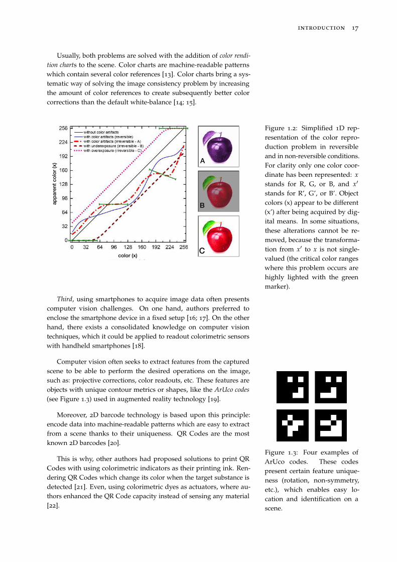
Second, color reproduction is a wide-known challenge of digitalcameras [11]. Often, when a digital camera captures a scene it canproduce several artifacts during the capture (i.e. underexposure,overexposure, ...), this is represented in see Figure 1.2.
The problem of color reproduction, involves a directly linkedproblem: the problem of achieving image consistency among datasets[12]. While color reproduction aims at matching the color of a givenobject when reproduced in another device as an image (e.g. a painting,a printed photo, a digital photo on a screen, etc.), image consistency isthe problem of taking different images of the same object in differentillumination conditions and with different capturing devices, to finallyobtain the same apparent colors for this object.
introduction 17
Usually, both problems are solved with the addition of color rendi-
tion charts to the scene. Color charts are machine-readable patternswhich contain several color references [13]. Color charts bring a sys-tematic way of solving the image consistency problem by increasingthe amount of color references to create subsequently better colorcorrections than the default white-balance [14; 15].
A
C
B
color (x)
ap
pare
nt
co
lor
(x)
Figure 1.2: Simplified 1D rep-resentation of the color repro-duction problem in reversibleand in non-reversible conditions.For clarity only one color coor-dinate has been represented: x
stands for R, G, or B, and x′
stands for R’, G’, or B’. Objectcolors (x) appear to be different(x’) after being acquired by dig-ital means. In some situations,these alterations cannot be re-moved, because the transforma-tion from x′ to x is not single-valued (the critical color rangeswhere this problem occurs arehighly lighted with the greenmarker).
Third, using smartphones to acquire image data often presentscomputer vision challenges. On one hand, authors preferred toenclose the smartphone device in a fixed setup [16; 17]. On the otherhand, there exists a consolidated knowledge on computer visiontechniques, which it could be applied to readout colorimetric sensorswith handheld smartphones [18].
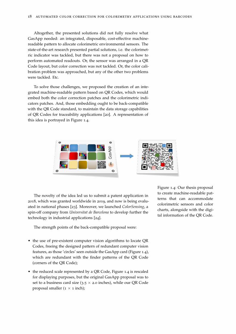
Computer vision often seeks to extract features from the capturedscene to be able to perform the desired operations on the image,such as: projective corrections, color readouts, etc. These features areobjects with unique contour metrics or shapes, like the ArUco codes
(see Figure 1.3) used in augmented reality technology [19].
Moreover, 2D barcode technology is based upon this principle:encode data into machine-readable patterns which are easy to extractfrom a scene thanks to their uniqueness. QR Codes are the mostknown 2D barcodes [20].
Figure 1.3: Four examples ofArUco codes. These codespresent certain feature unique-ness (rotation, non-symmetry,etc.), which enables easy lo-cation and identification on ascene.
This is why, other authors had proposed solutions to print QRCodes with using colorimetric indicators as their printing ink. Ren-dering QR Codes which change its color when the target substance isdetected [21]. Even, using colorimetric dyes as actuators, where au-thors enhanced the QR Code capacity instead of sensing any material[22].
18 automated color correction for colorimetry applications using barcodes
Altogether, the presented solutions did not fully resolve whatGasApp needed: an integrated, disposable, cost-effective machine-readable pattern to allocate colorimetric environmental sensors. Thestate-of-the-art research presented partial solutions, i.e. the colorimet-ric indicator was tackled, but there was not a proposal on how toperform automated readouts. Or, the sensor was arranged in a QRCode layout, but color correction was not tackled. Or, the color cali-bration problem was approached, but any of the other two problemswere tackled. Etc.
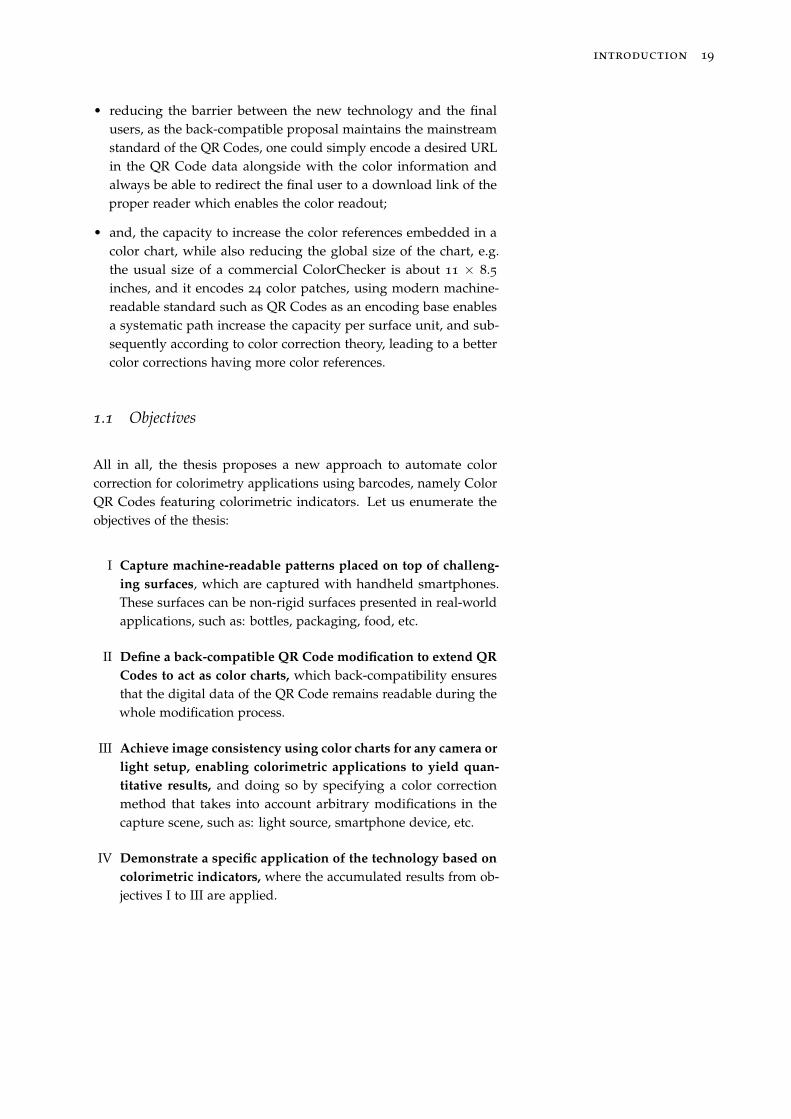
To solve those challenges, we proposed the creation of an inte-grated machine-readable pattern based on QR Codes, which wouldembed both the color correction patches and the colorimetric indi-cators patches. And, those embedding ought to be back-compatiblewith the QR Code standard, to maintain the data storage capabilitiesof QR Codes for traceability applications [20]. A representation ofthis idea is portrayed in Figure 1.4.
Figure 1.4: Our thesis proposalto create machine-readable pat-terns that can accommodatecolorimetric sensors and colorcharts, alongside with the digi-tal information of the QR Code.
The novelty of the idea led us to submit a patent application in2018, which was granted worldwide in 2019, and now is being evalu-ated in national phases [23]. Moreover, we launched ColorSensing, aspin-off company from Universitat de Barcelona to develop further thetechnology in industrial applications [24].
The strength points of the back-compatible proposal were:
• the use of pre-existent computer vision algorithms to locate QRCodes, freeing the designed pattern of redundant computer visionfeatures, as those ’circles’ seen outside the GasApp card (Figure 1.4),which are redundant with the finder patterns of the QR Code(corners of the QR Code);
• the reduced scale represented by a QR Code, Figure 1.4 is rescaledfor displaying purposes, but the original GasApp proposal was toset to a business card size (3.5 × 2.0 inches), while our QR Codeproposal smaller (1 × 1 inch);
introduction 19
• reducing the barrier between the new technology and the finalusers, as the back-compatible proposal maintains the mainstreamstandard of the QR Codes, one could simply encode a desired URLin the QR Code data alongside with the color information andalways be able to redirect the final user to a download link of theproper reader which enables the color readout;
• and, the capacity to increase the color references embedded in acolor chart, while also reducing the global size of the chart, e.g.the usual size of a commercial ColorChecker is about 11 × 8.5inches, and it encodes 24 color patches, using modern machine-readable standard such as QR Codes as an encoding base enablesa systematic path increase the capacity per surface unit, and sub-sequently according to color correction theory, leading to a bettercolor corrections having more color references.
1.1 Objectives
All in all, the thesis proposes a new approach to automate colorcorrection for colorimetry applications using barcodes, namely ColorQR Codes featuring colorimetric indicators. Let us enumerate theobjectives of the thesis:
I Capture machine-readable patterns placed on top of challeng-
ing surfaces, which are captured with handheld smartphones.These surfaces can be non-rigid surfaces presented in real-worldapplications, such as: bottles, packaging, food, etc.
II Define a back-compatible QR Code modification to extend QR
Codes to act as color charts, which back-compatibility ensuresthat the digital data of the QR Code remains readable during thewhole modification process.
III Achieve image consistency using color charts for any camera or
light setup, enabling colorimetric applications to yield quan-
titative results, and doing so by specifying a color correctionmethod that takes into account arbitrary modifications in thecapture scene, such as: light source, smartphone device, etc.
IV Demonstrate a specific application of the technology based on
colorimetric indicators, where the accumulated results from ob-jectives I to III are applied.
20 automated color correction for colorimetry applications using barcodes
1.2 Thesis sctructure
In this thesis, we tackled the above-mentioned objectives. Prior to that,we introduced a chapter to present the backgrounds and methods ap-plied to this thesis. Then, we presented four thematic chapters relatedto each one of the objectives. These chapters were prepared with acoherent structure: a brief introduction, a proposal, an experimentaldetails section, the results presentation and the conclusion discussion.Later, a general conclusion chapter was added to close the thesis. Letus briefly present the content of each thematic chapter.
First, in chapter 3 we reviewed the state-of-the-art method toextract QR Codes from different surfaces. Then, we focused on anovel approach to readout QR Codes on challenging surfaces, such asthose found in food packages, such as cylinders or any non-rigidplastic [25; 26].
Second, in chapter 4 we introduced the main proposal of the the-sis, the back-compatible Color QR Codes [23]. Here, we also introducednot only the machine-readable pattern proposal but also we bench-marked the different possible approaches to embed colors in a QRCode by taking into account its data encoding (which colors are tobe embedded where, etc.) and how it affected the QR Code finalreadability.
Third, in chapter 5 we sought for a unified framework of color cor-rections based upon affine [14], polynomial [27; 28], root-polynomial[28] and thin-plate splines [15] color corrections. Within that frame-work, we presented our new proposal for an improved TPS3D method
to achieve image consistency.
Finally, in chapter 6 we surveyed the different color sensors wherewe already used partial approaches to our solution [29; 30]. Then,we also studied how tho apply our proposal to an actual applica-
tion of a colorimetric indicator that sensed CO2 levels [31] in modifiedatmosphere packaging [32].
Chapter 2. Background and methods
2.1 The image consistency problem
Color reproduction is one of the most studied problems in the audio-visual industry, that is present in our daily lives, long before today’ssmartphones, when color was introduced to the cinema, also withcolor analog cameras and color home TVs [11]. In the past years,reproducing and measuring color has also become an important chal-lenge for other industries such as health care, food manufacturing andenvironmental sensing. Regarding health care, dermatology is oneof the main fields where color measurement is a strategic problem,from measuring skin-tones to avoid dataset bias [33] to medical imageanalysis to retrieve skin lesions [34; 35]. In food manufacturing, coloris used as an indicator to solve quality control and freshness problems[36; 37; 38]. As for environmental sensing [4], colorimetric indicatorsare widely spread to act as humidity [39], temperature [40] and gassensors [41; 42].
In this section, we focus on image consistency, a reduced problemfrom color reproduction. While color reproduction aims at matchingthe color of a given object when reproduced in another device as animage (e.g. a painting, a printed photo, a digital photo on a screen,etc.), image consistency is the problem of taking different images of thesame object in different illumination conditions and with differentcapturing devices, to finally obtain the same apparent colors forthis object. In this problem, the apparent colors of an object do notneed to match its “real” spectral color, they only rather have to besimilar in each instance captured in different scenarios. In otherwords, all instances should match the first or the best capture, andnot the real-life color. Therefore, image consistency is the actualproblem to solve in the before-mentioned applications, in which itis more important to compare acquired images between them, sothat consistent conclusions can be drawn with all instances, thancomparing them to an actual reflectance spectrum.
22 automated color correction for colorimetry applications using barcodes
2.1.1 Color reproduction
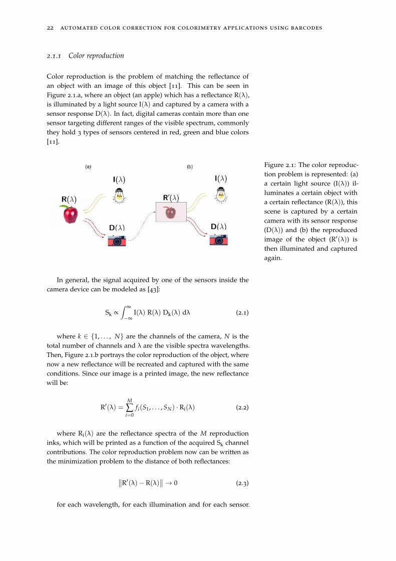
Color reproduction is the problem of matching the reflectance ofan object with an image of this object [11]. This can be seen inFigure 2.1.a, where an object (an apple) which has a reflectance R(λ),is illuminated by a light source I(λ) and captured by a camera with asensor response D(λ). In fact, digital cameras contain more than onesensor targeting different ranges of the visible spectrum, commonlythey hold 3 types of sensors centered in red, green and blue colors[11].
Figure 2.1: The color reproduc-tion problem is represented: (a)a certain light source (I(λ)) il-luminates a certain object witha certain reflectance (R(λ)), thisscene is captured by a certaincamera with its sensor response(D(λ)) and (b) the reproducedimage of the object (R′(λ)) isthen illuminated and capturedagain.
In general, the signal acquired by one of the sensors inside thecamera device can be modeled as [43]:
Sk ∝
∫ ∞
−∞I(λ) R(λ) Dk(λ) dλ (2.1)
where k ∈ {1, . . . , N} are the channels of the camera, N is thetotal number of channels and λ are the visible spectra wavelengths.Then, Figure 2.1.b portrays the color reproduction of the object, wherenow a new reflectance will be recreated and captured with the sameconditions. Since our image is a printed image, the new reflectancewill be:
R′(λ) =M
∑i=0
fi(S1, . . . , SN) · Ri(λ) (2.2)
where Ri(λ) are the reflectance spectra of the M reproductioninks, which will be printed as a function of the acquired Sk channelcontributions. The color reproduction problem now can be written asthe minimization problem to the distance of both reflectances:
∥
∥R′(λ)− R(λ)∥
∥→ 0 (2.3)
for each wavelength, for each illumination and for each sensor.
background and methods 23
The same formulation could be written when displaying images on ascreen by changing R(λ) for I(λ).
Color reproduction is a wide open problem, and with each steptowards its general solution, the goal of achieving image consistencywhen acquiring image datasets is nearer. Since color reproductionsolutions aim at attaining better acquisition devices and better repro-duction systems, the need for solving the image consistency problemwill eventually disappear. But this is not yet the case.
2.1.2 Image consistency
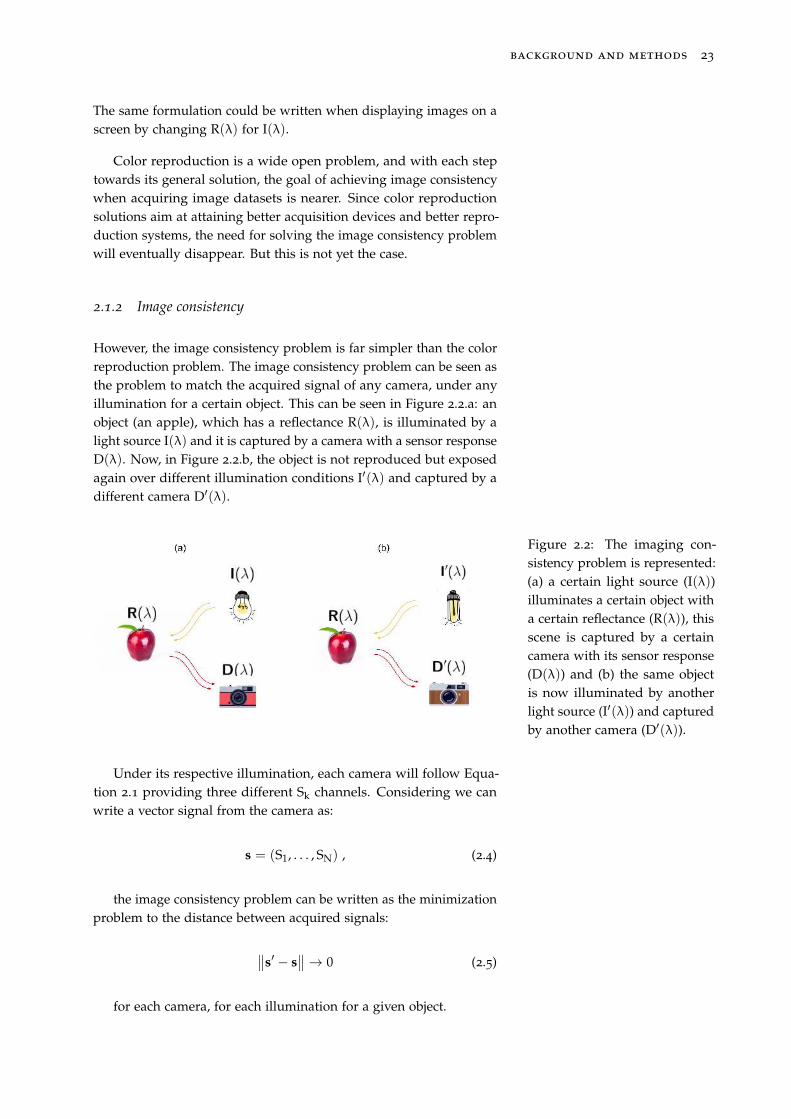
However, the image consistency problem is far simpler than the colorreproduction problem. The image consistency problem can be seen asthe problem to match the acquired signal of any camera, under anyillumination for a certain object. This can be seen in Figure 2.2.a: anobject (an apple), which has a reflectance R(λ), is illuminated by alight source I(λ) and it is captured by a camera with a sensor responseD(λ). Now, in Figure 2.2.b, the object is not reproduced but exposedagain over different illumination conditions I′(λ) and captured by adifferent camera D′(λ).
Figure 2.2: The imaging con-sistency problem is represented:(a) a certain light source (I(λ))illuminates a certain object witha certain reflectance (R(λ)), thisscene is captured by a certaincamera with its sensor response(D(λ)) and (b) the same objectis now illuminated by anotherlight source (I′(λ)) and capturedby another camera (D′(λ)).
Under its respective illumination, each camera will follow Equa-tion 2.1 providing three different Sk channels. Considering we canwrite a vector signal from the camera as:
s = (S1, . . . , SN) , (2.4)
the image consistency problem can be written as the minimizationproblem to the distance between acquired signals:
∥
∥s′ − s∥
∥→ 0 (2.5)
for each camera, for each illumination for a given object.
24 automated color correction for colorimetry applications using barcodes
The image consistency problem is easier to solve, as we havechanged the problem from working with continuous spectral distri-butions (see Equation 2.3) to N-dimensional vector spaces (see Equa-tion 2.5). These spaces are usually called color spaces, and the map-pings between those spaces are usually called color conversions. Defor-mations or corrections inside a given color space are often referred toas color corrections. In this thesis, we will be using RGB images fromdigital cameras. Thus, we will work with device-dependent color spaces.
This means that the mappings will be performed between RGBspaces. Then, we can rewrite the color vector definition for RGBcolors following Equation 2.4 as:
s = (r, g, b), s ∈ R3 , (2.6)
where R3 represents here a generic 3-dimensional RGB space. In
subsection 2.3.1, we detail how color spaces are defined according totheir bit resolution and color channels.
2.1.3 Color charts
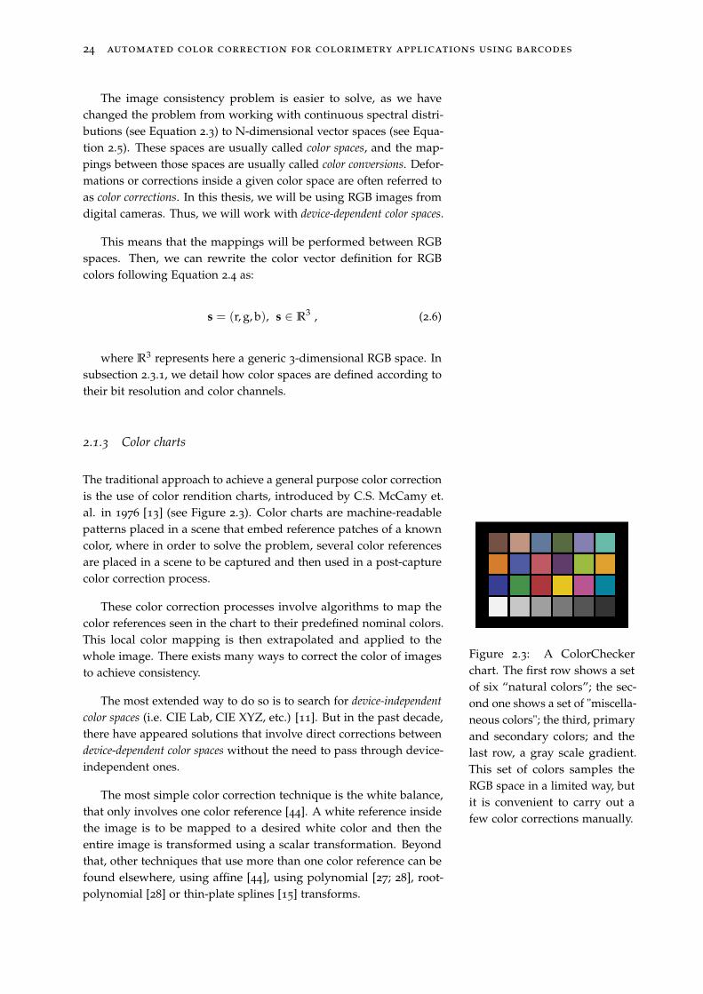
The traditional approach to achieve a general purpose color correctionis the use of color rendition charts, introduced by C.S. McCamy et.al. in 1976 [13] (see Figure 2.3). Color charts are machine-readablepatterns placed in a scene that embed reference patches of a knowncolor, where in order to solve the problem, several color referencesare placed in a scene to be captured and then used in a post-capturecolor correction process.
These color correction processes involve algorithms to map thecolor references seen in the chart to their predefined nominal colors.This local color mapping is then extrapolated and applied to thewhole image. There exists many ways to correct the color of imagesto achieve consistency.
Figure 2.3: A ColorCheckerchart. The first row shows a setof six “natural colors”; the sec-ond one shows a set of "miscella-neous colors"; the third, primaryand secondary colors; and thelast row, a gray scale gradient.This set of colors samples theRGB space in a limited way, butit is convenient to carry out afew color corrections manually.
The most extended way to do so is to search for device-independent
color spaces (i.e. CIE Lab, CIE XYZ, etc.) [11]. But in the past decade,there have appeared solutions that involve direct corrections betweendevice-dependent color spaces without the need to pass through device-independent ones.
The most simple color correction technique is the white balance,that only involves one color reference [44]. A white reference insidethe image is to be mapped to a desired white color and then theentire image is transformed using a scalar transformation. Beyondthat, other techniques that use more than one color reference can befound elsewhere, using affine [44], using polynomial [27; 28], root-polynomial [28] or thin-plate splines [15] transforms.
background and methods 25
It is safe to say that, in most of these post-capture color correctiontechniques, increasing the number and quality of the color refer-ences offers a systematic path towards better color calibration results.This strategy however, comes along with more image area dedicatedto accommodate these additional color references and therefore, acompromise must be found.
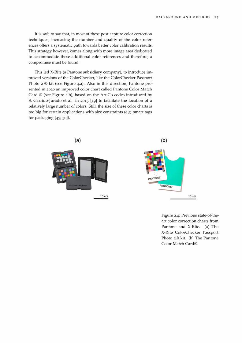
This led X-Rite (a Pantone subsidiary company), to introduce im-proved versions of the ColorChecker, like the ColorChecker PassportPhoto 2 ® kit (see Figure 4.a). Also in this direction, Pantone pre-sented in 2020 an improved color chart called Pantone Color MatchCard ® (see Figure 4.b), based on the AruCo codes introduced byS. Garrido-Jurado et al. in 2015 [19] to facilitate the location of arelatively large number of colors. Still, the size of these color charts istoo big for certain applications with size constraints (e.g. smart tagsfor packaging [45; 30]).
Figure 2.4: Previous state-of-the-art color correction charts fromPantone and X-Rite. (a) TheX-Rite ColorChecker PassportPhoto 2® kit. (b) The PantoneColor Match Card®.
26 automated color correction for colorimetry applications using barcodes
2.2 2D Barcodes: the Quick-Response Code
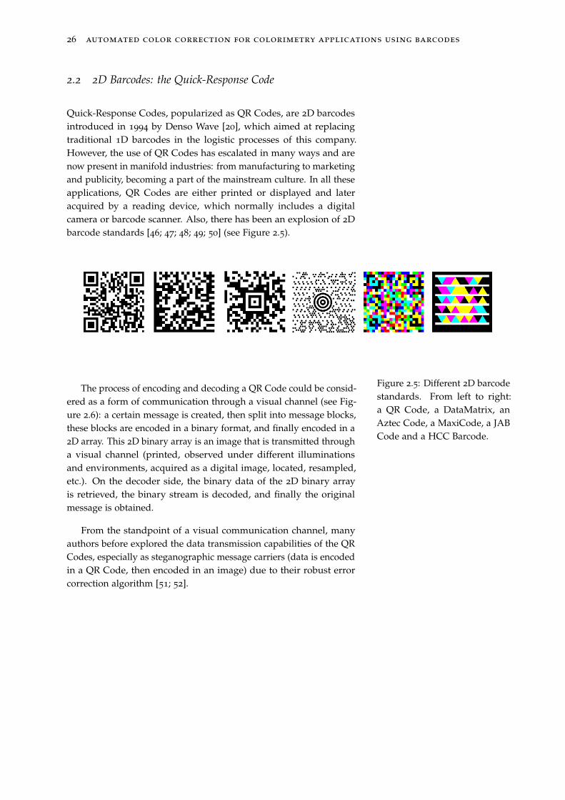
Quick-Response Codes, popularized as QR Codes, are 2D barcodesintroduced in 1994 by Denso Wave [20], which aimed at replacingtraditional 1D barcodes in the logistic processes of this company.However, the use of QR Codes has escalated in many ways and arenow present in manifold industries: from manufacturing to marketingand publicity, becoming a part of the mainstream culture. In all theseapplications, QR Codes are either printed or displayed and lateracquired by a reading device, which normally includes a digitalcamera or barcode scanner. Also, there has been an explosion of 2Dbarcode standards [46; 47; 48; 49; 50] (see Figure 2.5).
Figure 2.5: Different 2D barcodestandards. From left to right:a QR Code, a DataMatrix, anAztec Code, a MaxiCode, a JABCode and a HCC Barcode.
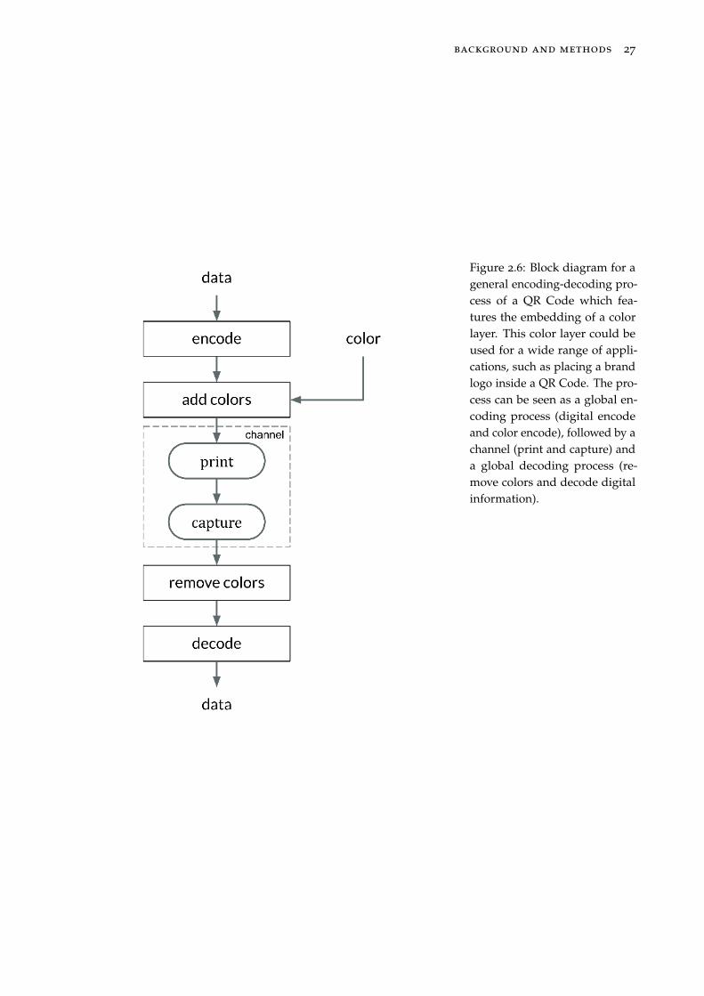
The process of encoding and decoding a QR Code could be consid-ered as a form of communication through a visual channel (see Fig-ure 2.6): a certain message is created, then split into message blocks,these blocks are encoded in a binary format, and finally encoded in a2D array. This 2D binary array is an image that is transmitted througha visual channel (printed, observed under different illuminationsand environments, acquired as a digital image, located, resampled,etc.). On the decoder side, the binary data of the 2D binary arrayis retrieved, the binary stream is decoded, and finally the originalmessage is obtained.
From the standpoint of a visual communication channel, manyauthors before explored the data transmission capabilities of the QRCodes, especially as steganographic message carriers (data is encodedin a QR Code, then encoded in an image) due to their robust errorcorrection algorithm [51; 52].
background and methods 27
Figure 2.6: Block diagram for ageneral encoding-decoding pro-cess of a QR Code which fea-tures the embedding of a colorlayer. This color layer could beused for a wide range of appli-cations, such as placing a brandlogo inside a QR Code. The pro-cess can be seen as a global en-coding process (digital encodeand color encode), followed by achannel (print and capture) anda global decoding process (re-move colors and decode digitalinformation).
28 automated color correction for colorimetry applications using barcodes
2.2.1 Scalability
Many 2D barcode standards allow modulating the amount of dataencoded in the barcode. For example, the QR Code standard imple-ments different barcode versions from version 1 to version 40. Eachversion increases the edges of the QR Code by 4 modules, from thestarting 21 × 21 (v1) modules up to 144 × 144 modules (v40) [20].
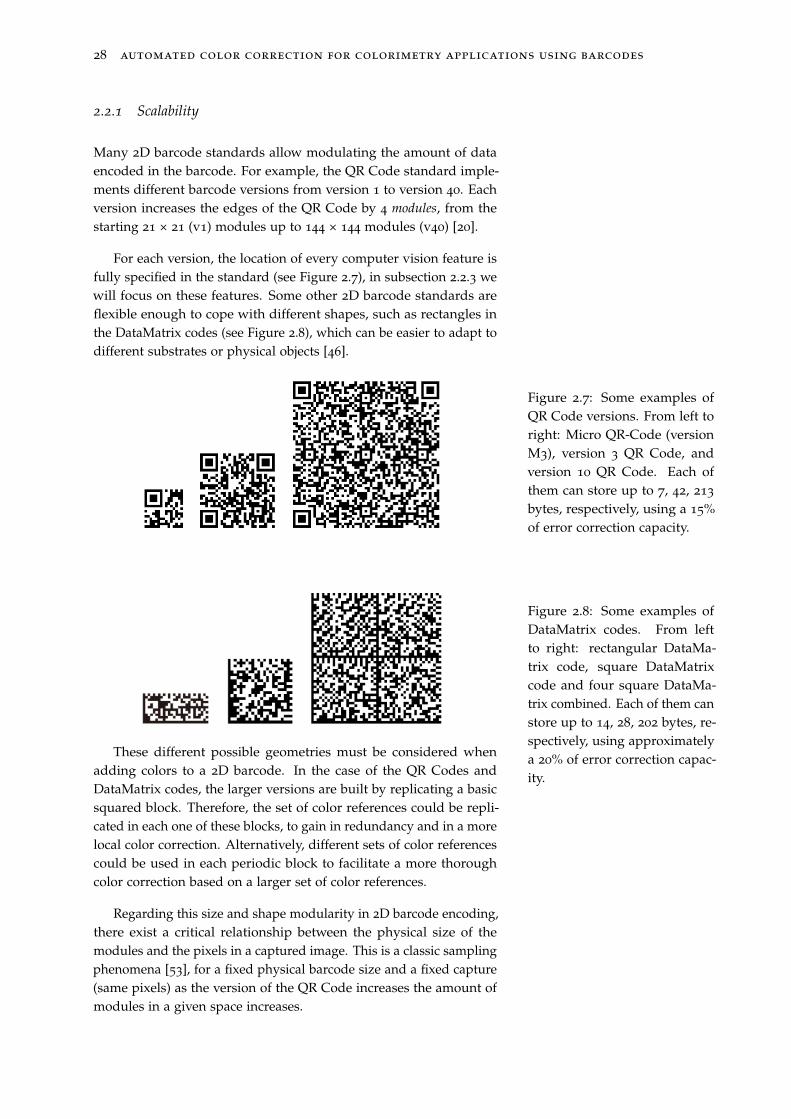
For each version, the location of every computer vision feature isfully specified in the standard (see Figure 2.7), in subsection 2.2.3 wewill focus on these features. Some other 2D barcode standards areflexible enough to cope with different shapes, such as rectangles inthe DataMatrix codes (see Figure 2.8), which can be easier to adapt todifferent substrates or physical objects [46].
Figure 2.7: Some examples ofQR Code versions. From left toright: Micro QR-Code (versionM3), version 3 QR Code, andversion 10 QR Code. Each ofthem can store up to 7, 42, 213
bytes, respectively, using a 15%of error correction capacity.
Figure 2.8: Some examples ofDataMatrix codes. From leftto right: rectangular DataMa-trix code, square DataMatrixcode and four square DataMa-trix combined. Each of them canstore up to 14, 28, 202 bytes, re-spectively, using approximatelya 20% of error correction capac-ity.
These different possible geometries must be considered whenadding colors to a 2D barcode. In the case of the QR Codes andDataMatrix codes, the larger versions are built by replicating a basicsquared block. Therefore, the set of color references could be repli-cated in each one of these blocks, to gain in redundancy and in a morelocal color correction. Alternatively, different sets of color referencescould be used in each periodic block to facilitate a more thoroughcolor correction based on a larger set of color references.
Regarding this size and shape modularity in 2D barcode encoding,there exist a critical relationship between the physical size of themodules and the pixels in a captured image. This is a classic samplingphenomena [53], for a fixed physical barcode size and a fixed capture(same pixels) as the version of the QR Code increases the amount ofmodules in a given space increases.
background and methods 29
Thus, the apparent size of the module in the captured imagedecreases, when this size is near a bunch of pixels we start to seealiasing problems [54]. In turn, this problem leads to a point that QRCodes cannot be fully recognized by the QR-Code decoding algorithm.This is even more important if we substitute these black and whitemodules with colors, where the error in finding the right referencearea may lead to huge errors in the color correction. Therefore,this sampling problem will accompany the implementation of ourproposal taking into account the size of the final QR Code dependingon the application field and the typical resolution of the cameras usedin those applications.
2.2.2 Data encoding in QR Codes
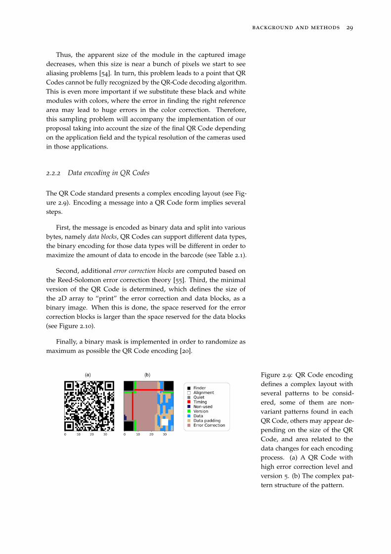
The QR Code standard presents a complex encoding layout (see Fig-ure 2.9). Encoding a message into a QR Code form implies severalsteps.
First, the message is encoded as binary data and split into variousbytes, namely data blocks, QR Codes can support different data types,the binary encoding for those data types will be different in order tomaximize the amount of data to encode in the barcode (see Table 2.1).
Second, additional error correction blocks are computed based onthe Reed-Solomon error correction theory [55]. Third, the minimalversion of the QR Code is determined, which defines the size ofthe 2D array to “print” the error correction and data blocks, as abinary image. When this is done, the space reserved for the errorcorrection blocks is larger than the space reserved for the data blocks(see Figure 2.10).
Finally, a binary mask is implemented in order to randomize asmaximum as possible the QR Code encoding [20].
Figure 2.9: QR Code encodingdefines a complex layout withseveral patterns to be consid-ered, some of them are non-variant patterns found in eachQR Code, others may appear de-pending on the size of the QRCode, and area related to thedata changes for each encodingprocess. (a) A QR Code withhigh error correction level andversion 5. (b) The complex pat-tern structure of the pattern.
30 automated color correction for colorimetry applications using barcodes
ECC level Bits Numeric Alphanumeric Binary Kanji
Version 1
L 152 41 25 17 10
M 128 34 20 14 8
Q 104 27 16 11 7
H 72 17 10 7 4
Version 2
L 272 77 47 32 20
M 224 63 38 26 16
Q 176 48 29 20 12
H 128 34 20 14 8
Version 39
L 22,496 6,743 4,087 2,809 1,729
M 17,728 5,313 3,22 2,213 1,362
Q 12,656 3,791 2,298 1,579 972
H 9,776 2,927 1,774 1,219 750
Version 40
L 23,648 7,089 4,296 2,953 1,817
M 18,672 5,596 3,391 2,331 1,435
Q 13,328 3,993 2,42 1,663 1,024
H 10,208 3,057 1,852 1,273 784
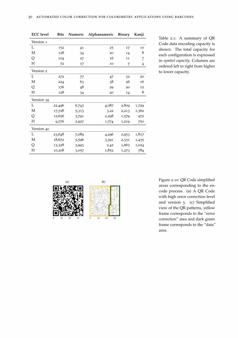
Table 2.1: A summary of QRCode data encoding capacity isshown. The total capacity foreach configuration is expressedin symbol capacity. Columns areordered left to right from higherto lower capacity.
Figure 2.10: QR Code simplifiedareas corresponding to the en-code process. (a) A QR Codewith high error correction leveland version 5. (c) Simplifiedview of the QR patterns, yellowframe corresponds to the “errorcorrection” area and dark greenframe corresponds to the “data”area.
background and methods 31
During the generation of a QR Code, the level of error correctioncan be selected, from high to low capabilities: H (30 %), Q (25%),M (15%) and L (7%). This should be understood as the maximumnumber of error bits that a certain barcode can support (maximumBit Error Ratio, detailed in chapter 4). Notice the error correctioncapability is independent of the version of the QR Code. However,both combined define the maximum data storage capacity of the QRCode, for a fixed version, higher error correction implies a reductionof the data storage capacity of the QR Code.
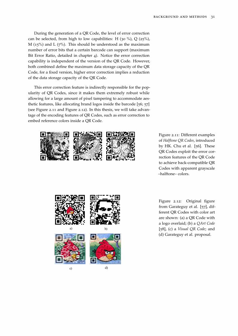
This error correction feature is indirectly responsible for the pop-ularity of QR Codes, since it makes them extremely robust whileallowing for a large amount of pixel tampering to accommodate aes-thetic features, like allocating brand logos inside the barcode [56; 57](see Figure 2.11 and Figure 2.12). In this thesis, we will take advan-tage of the encoding features of QR Codes, such as error correction toembed reference colors inside a QR Code.
Figure 2.11: Different examplesof Halftone QR Codes, introducedby HK. Chu et al. [56]. TheseQR Codes exploit the error cor-rection features of the QR Codeto achieve back-compatible QRCodes with apparent grayscale–halftone– colors.
Figure 2.12: Original figurefrom Garateguy et al. [57], dif-ferent QR Codes with color artare shown: (a) a QR Code witha logo overlaid; (b) a QArt Code
[58], (c) a Visual QR Code; and(d) Garateguy et al. proposal.
32 automated color correction for colorimetry applications using barcodes
2.2.3 Computer vision features of QR Codes
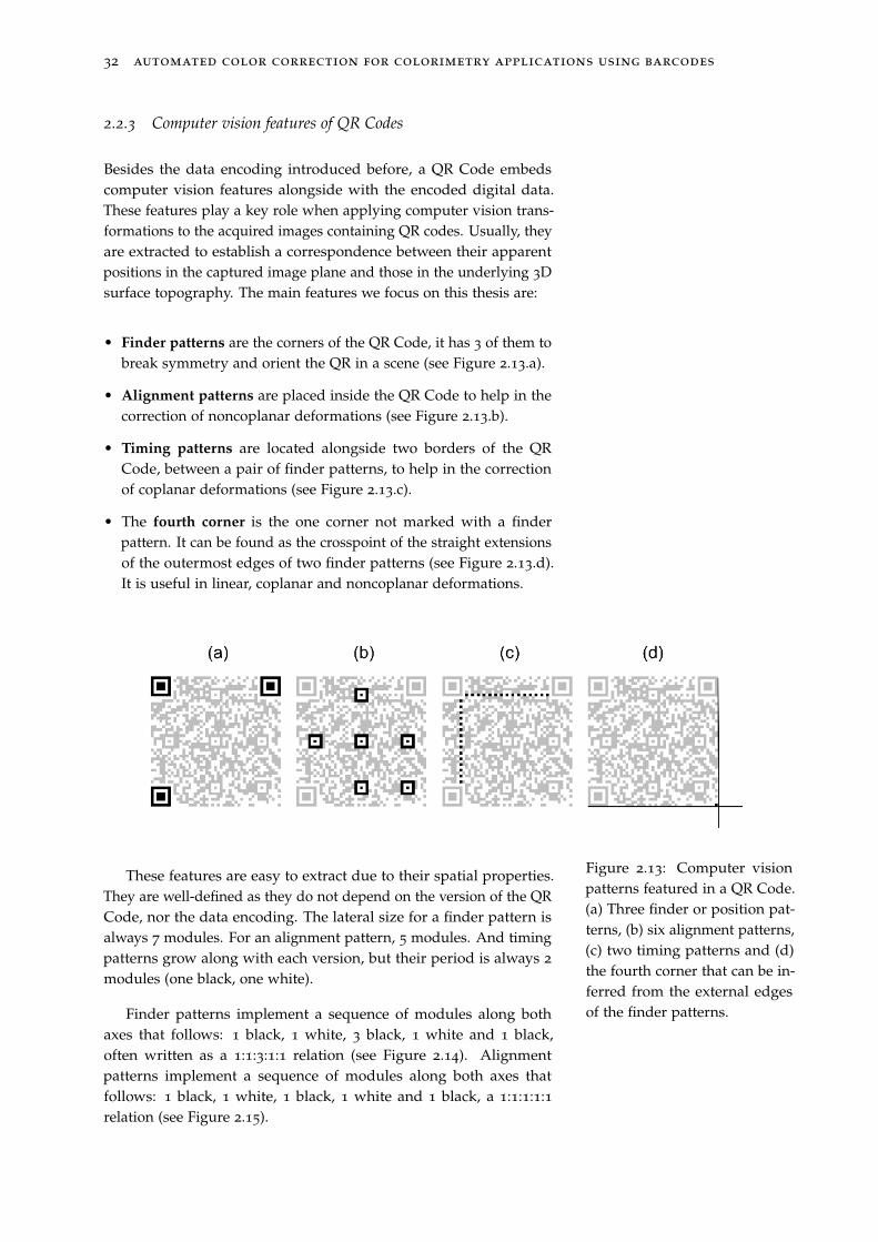
Besides the data encoding introduced before, a QR Code embedscomputer vision features alongside with the encoded digital data.These features play a key role when applying computer vision trans-formations to the acquired images containing QR codes. Usually, theyare extracted to establish a correspondence between their apparentpositions in the captured image plane and those in the underlying 3Dsurface topography. The main features we focus on this thesis are:
• Finder patterns are the corners of the QR Code, it has 3 of them tobreak symmetry and orient the QR in a scene (see Figure 2.13.a).
• Alignment patterns are placed inside the QR Code to help in thecorrection of noncoplanar deformations (see Figure 2.13.b).
• Timing patterns are located alongside two borders of the QRCode, between a pair of finder patterns, to help in the correctionof coplanar deformations (see Figure 2.13.c).
• The fourth corner is the one corner not marked with a finderpattern. It can be found as the crosspoint of the straight extensionsof the outermost edges of two finder patterns (see Figure 2.13.d).It is useful in linear, coplanar and noncoplanar deformations.
Figure 2.13: Computer visionpatterns featured in a QR Code.(a) Three finder or position pat-terns, (b) six alignment patterns,(c) two timing patterns and (d)the fourth corner that can be in-ferred from the external edgesof the finder patterns.
These features are easy to extract due to their spatial properties.They are well-defined as they do not depend on the version of the QRCode, nor the data encoding. The lateral size for a finder pattern isalways 7 modules. For an alignment pattern, 5 modules. And timingpatterns grow along with each version, but their period is always 2
modules (one black, one white).
Finder patterns implement a sequence of modules along bothaxes that follows: 1 black, 1 white, 3 black, 1 white and 1 black,often written as a 1:1:3:1:1 relation (see Figure 2.14). Alignmentpatterns implement a sequence of modules along both axes thatfollows: 1 black, 1 white, 1 black, 1 white and 1 black, a 1:1:1:1:1relation (see Figure 2.15).

background and methods 33
Thus, the relation between white and black pixels provides a pathto use pattern recognition techniques to extract these features, as theserelations are invariant to perspective transformations. Moreover, theselinear relations can be expressed as squared relations, and are stillinvariant under perspective transformations. This is specially usefulwhen using extraction algorithms based upon contour recognition [18;59], for finder patterns the relation becomes 7²:5²:3² (see Figure 2.14);and for alignment patterns, 5²:3²:1² (see Figure 2.15).
Figure 2.14: Finder pattern def-inition in terms of modules.Finder pattern measures always7 × 7 modules. If scannedwith a line barcode scanner the1:1:3:1:1 ratio is maintained nomatter the direction of the scan-ner. If scanned using contour ex-traction the aspect ratio 7²:5²:3²is maintained as well if the QRCode is captured within a pro-jective scene (i.e. a handheldsmartphone).
Figure 2.15: Alignment patterndefinition in terms of modules.Alignment pattern measures al-ways 5 × 5 modules. If scannedwith a line barcode scanner the1:1:1:1:1 ratio is maintained nomatter the direction of the scan-ner. If scanned using contour ex-traction the aspect ratio 5²:3²:1²is maintained as well if the QRCode is captured within a pro-jective scene (i.e. a handheldsmartphone).
34 automated color correction for colorimetry applications using barcodes
2.2.4 Readout of QR Codes
Let us explore a common pipeline towards QR Code readout. First,consider a QR Code captured from a certain point-of-view in a flatsurface which is almost coplanar to the capture device (e.g. a boxin a production line). Note that more complex applications, such asbottles [60], all sorts of food packaging [61], etc., which are key to thisthesis, are tackled down in chapter 3.
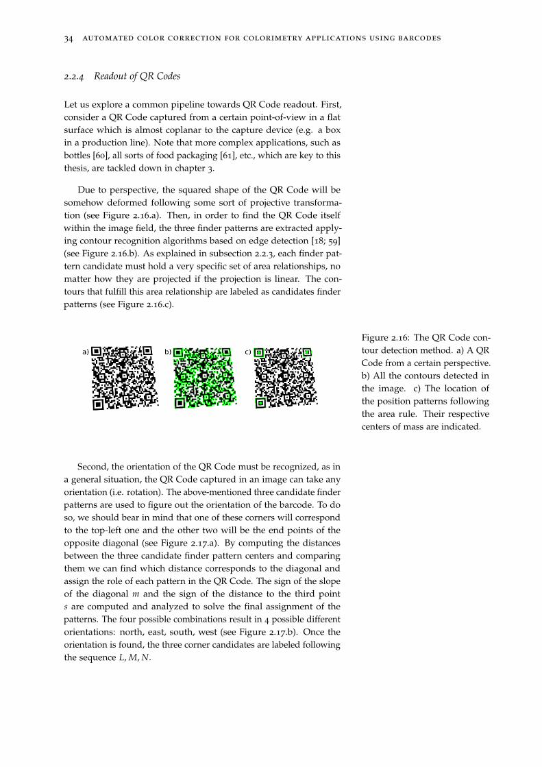
Due to perspective, the squared shape of the QR Code will besomehow deformed following some sort of projective transforma-tion (see Figure 2.16.a). Then, in order to find the QR Code itselfwithin the image field, the three finder patterns are extracted apply-ing contour recognition algorithms based on edge detection [18; 59](see Figure 2.16.b). As explained in subsection 2.2.3, each finder pat-tern candidate must hold a very specific set of area relationships, nomatter how they are projected if the projection is linear. The con-tours that fulfill this area relationship are labeled as candidates finderpatterns (see Figure 2.16.c).
Figure 2.16: The QR Code con-tour detection method. a) A QRCode from a certain perspective.b) All the contours detected inthe image. c) The location ofthe position patterns followingthe area rule. Their respectivecenters of mass are indicated.
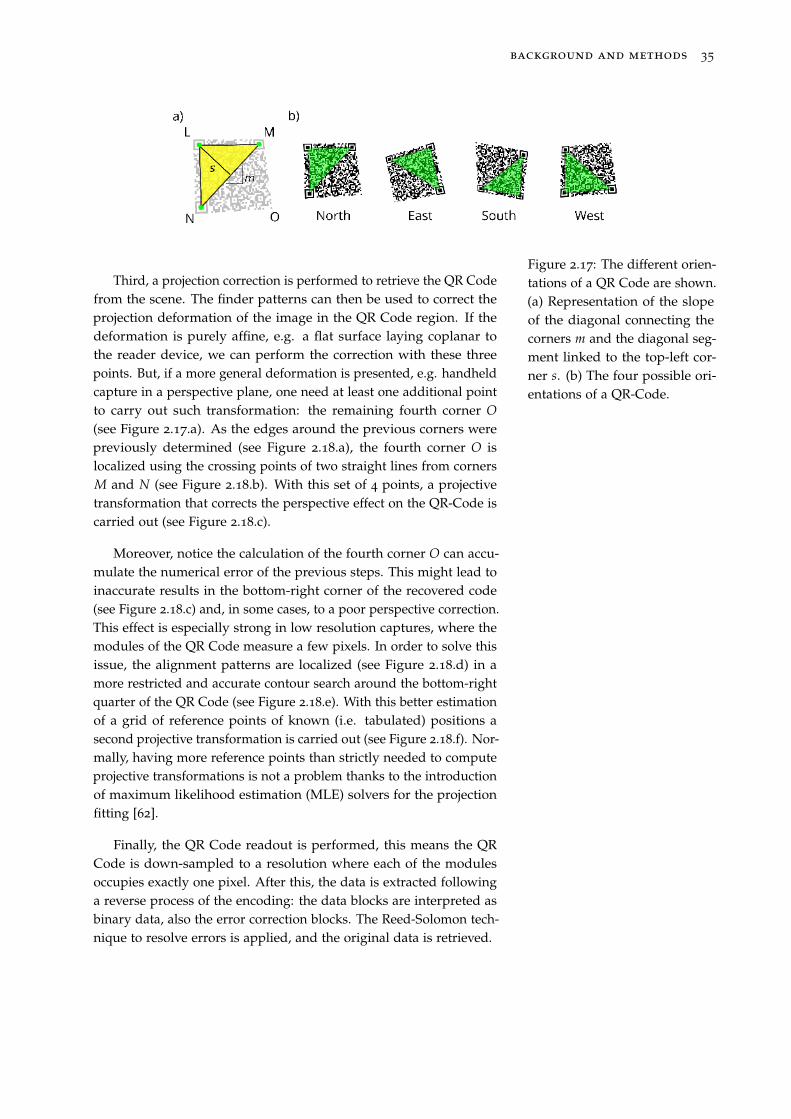
Second, the orientation of the QR Code must be recognized, as ina general situation, the QR Code captured in an image can take anyorientation (i.e. rotation). The above-mentioned three candidate finderpatterns are used to figure out the orientation of the barcode. To doso, we should bear in mind that one of these corners will correspondto the top-left one and the other two will be the end points of theopposite diagonal (see Figure 2.17.a). By computing the distancesbetween the three candidate finder pattern centers and comparingthem we can find which distance corresponds to the diagonal andassign the role of each pattern in the QR Code. The sign of the slopeof the diagonal m and the sign of the distance to the third points are computed and analyzed to solve the final assignment of thepatterns. The four possible combinations result in 4 possible differentorientations: north, east, south, west (see Figure 2.17.b). Once theorientation is found, the three corner candidates are labeled followingthe sequence L, M, N.
background and methods 35
Figure 2.17: The different orien-tations of a QR Code are shown.(a) Representation of the slopeof the diagonal connecting thecorners m and the diagonal seg-ment linked to the top-left cor-ner s. (b) The four possible ori-entations of a QR-Code.
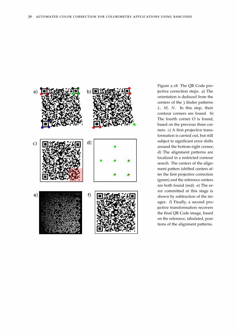
Third, a projection correction is performed to retrieve the QR Codefrom the scene. The finder patterns can then be used to correct theprojection deformation of the image in the QR Code region. If thedeformation is purely affine, e.g. a flat surface laying coplanar tothe reader device, we can perform the correction with these threepoints. But, if a more general deformation is presented, e.g. handheldcapture in a perspective plane, one need at least one additional pointto carry out such transformation: the remaining fourth corner O
(see Figure 2.17.a). As the edges around the previous corners werepreviously determined (see Figure 2.18.a), the fourth corner O islocalized using the crossing points of two straight lines from cornersM and N (see Figure 2.18.b). With this set of 4 points, a projectivetransformation that corrects the perspective effect on the QR-Code iscarried out (see Figure 2.18.c).
Moreover, notice the calculation of the fourth corner O can accu-mulate the numerical error of the previous steps. This might lead toinaccurate results in the bottom-right corner of the recovered code(see Figure 2.18.c) and, in some cases, to a poor perspective correction.This effect is especially strong in low resolution captures, where themodules of the QR Code measure a few pixels. In order to solve thisissue, the alignment patterns are localized (see Figure 2.18.d) in amore restricted and accurate contour search around the bottom-rightquarter of the QR Code (see Figure 2.18.e). With this better estimationof a grid of reference points of known (i.e. tabulated) positions asecond projective transformation is carried out (see Figure 2.18.f). Nor-mally, having more reference points than strictly needed to computeprojective transformations is not a problem thanks to the introductionof maximum likelihood estimation (MLE) solvers for the projectionfitting [62].
Finally, the QR Code readout is performed, this means the QRCode is down-sampled to a resolution where each of the modulesoccupies exactly one pixel. After this, the data is extracted followinga reverse process of the encoding: the data blocks are interpreted asbinary data, also the error correction blocks. The Reed-Solomon tech-nique to resolve errors is applied, and the original data is retrieved.
36 automated color correction for colorimetry applications using barcodes
Figure 2.18: The QR Code pro-jective correction steps. a) Theorientation is deduced from thecenters of the 3 finder patternsL, M, N. In this step, theircontour corners are found. b)The fourth corner O is found,based on the previous three cor-ners. c) A first projective trans-formation is carried out, but stillsubject to significant error shiftsaround the bottom-right corner;d) The alignment patterns arelocalized in a restricted contoursearch. The centers of the align-ment patters (shifted centers af-ter the first projective correction(green) and the reference centersare both found (red). e) The er-ror committed at this stage isshown by subtraction of the im-ages. f) Finally, a second pro-jective transformation recoversthe final QR Code image, basedon the reference, tabulated, posi-tions of the alignment patterns.
background and methods 37
2.3 Data representation
2.3.1 Color spaces
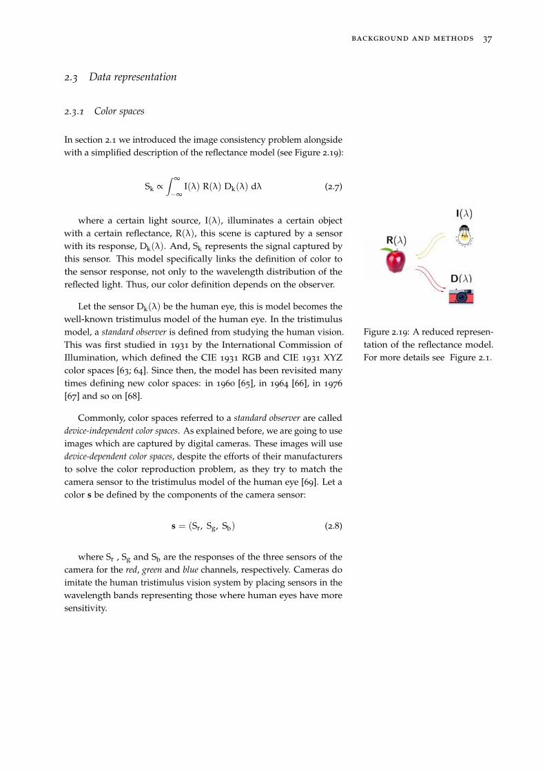
In section 2.1 we introduced the image consistency problem alongsidewith a simplified description of the reflectance model (see Figure 2.19):
Sk ∝
∫ ∞
−∞I(λ) R(λ) Dk(λ) dλ (2.7)
where a certain light source, I(λ), illuminates a certain objectwith a certain reflectance, R(λ), this scene is captured by a sensorwith its response, Dk(λ). And, Sk represents the signal captured bythis sensor. This model specifically links the definition of color tothe sensor response, not only to the wavelength distribution of thereflected light. Thus, our color definition depends on the observer.
Figure 2.19: A reduced represen-tation of the reflectance model.For more details see Figure 2.1.
Let the sensor Dk(λ) be the human eye, this is model becomes thewell-known tristimulus model of the human eye. In the tristimulusmodel, a standard observer is defined from studying the human vision.This was first studied in 1931 by the International Commission ofIllumination, which defined the CIE 1931 RGB and CIE 1931 XYZcolor spaces [63; 64]. Since then, the model has been revisited manytimes defining new color spaces: in 1960 [65], in 1964 [66], in 1976
[67] and so on [68].
Commonly, color spaces referred to a standard observer are calleddevice-independent color spaces. As explained before, we are going to useimages which are captured by digital cameras. These images will usedevice-dependent color spaces, despite the efforts of their manufacturersto solve the color reproduction problem, as they try to match thecamera sensor to the tristimulus model of the human eye [69]. Let acolor s be defined by the components of the camera sensor:
s = (Sr, Sg, Sb) (2.8)
where Sr , Sg and Sb are the responses of the three sensors of thecamera for the red, green and blue channels, respectively. Cameras doimitate the human tristimulus vision system by placing sensors in thewavelength bands representing those where human eyes have moresensitivity.
38 automated color correction for colorimetry applications using barcodes
Note that s is defined as a vector in Equation 2.8. Although, itsdefinition lacks the specification of its vector space:
s = (r, g, b) ∈ R3 (2.9)
where r, g, b is a simplified notation of the channels of the color,and R
3 is a generic RGB color space. As digital cameras store digitalinformation in a finite discrete representation, R
3 should becomeN
3[0,255] for 8-bit images (see Figure 2.20). This discretization process
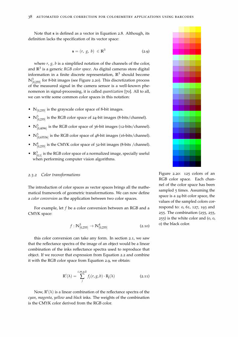
of the measured signal in the camera sensor is a well-known phe-nomenon in signal-processing, it is called quantization [70]. All to all,we can write some common color spaces in this notation:
Figure 2.20: 125 colors of anRGB color space. Each chan-nel of the color space has beensampled 5 times. Assuming thespace is a 24-bit color space, thevalues of the sampled colors cor-respond to: 0, 61, 127, 193 and255. The combination (255, 255,255) is the white color and (0, 0,0) the black color.
• N[0,255] is the grayscale color space of 8-bit images.
• N3[0,255] is the RGB color space of 24-bit images (8-bits/channel).
• N3[0,4096] is the RGB color space of 36-bit images (12-bits/channel).
• N3[0,65536] is the RGB color space of 48-bit images (16-bits/channel).
• N4[0,255] is the CMYK color space of 32-bit images (8-bits /channel).
• R3[0,1] is the RGB color space of a normalized image, specially useful
when performing computer vision algorithms.
2.3.2 Color transformations
The introduction of color spaces as vector spaces brings all the mathe-matical framework of geometric transformations. We can now definea color conversion as the application between two color spaces.
For example, let f be a color conversion between an RGB and aCMYK space:
f : N3[0,255] → N
4[0,255] (2.10)
this color conversion can take any form. In section 2.1, we sawthat the reflectance spectra of the image of an object would be a linearcombination of the inks reflectance spectra used to reproduce thatobject. If we recover that expression from Equation 2.2 and combineit with the RGB color space from Equation 2.9, we obtain:
R′(λ) =c,m,y,k
∑j
f j(r, g, b) · Rj(λ) (2.11)
Now, R′(λ) is a linear combination of the reflectance spectra of thecyan, magenta, yellow and black inks. The weights of the combinationis the CMYK color derived from the RGB color.
background and methods 39
In turn, we can express the CMYK color also as a linear combina-tion of the RGB color channels, fi(r, g, b) is our color correction here,then:
R′(λ) =c,m,y,k
∑j
[
r,g,b
∑k
ajk · k]
· Rj(λ) (2.12)
Note that we have defined fi as a linear transformation betweenthe RGB and the CMYK color spaces, doing so is the most commonway to perform color transformations between color spaces.
This is the foundation of the ICC Profile standard [71]. Profilingis a common technique when reproducing colors. For example, takeFigure 2.20, if the colors are seen displayed on a screen they willshow the RGB space of the LED technology of the screen. However, ifthey have been printed, the actual colors the reader will be looking atwill be the linear combination of CMYK inks representing the RGBspace, following Equation 2.12. ICC profiling is present in each colorprinting process.
Alongside with the described example, here below, we presentsome of the most common color transformations we will use duringthe development of this thesis, that include normalization, desaturation,binarization and colorization transformations.
2.3.2.1 Normalization
Normalization is the process to map a discrete color space with limitedresolution (N[0,255], N
3[0,255], N
3[0,4096], ...) to a color space which is
limited to a certain range of values, normally from 0 to 1 R[0,1], butoffers theoretically infinite resolution 1. All our computation will take 1 The infinite resolution that represents
R is not computationally feasible. How-ever, the computational representationof a R space, a float number, handles ahigher precision than other former spacebefore normalization.
place in such normalized spaces. Formally the normalization processis a mapping that follows:
fnormalize : NK[0, 2n ] → R
K[0,1] (2.13)
where K is the number of channels of the color space (i.e. K = 1 forgrayscale, K = 3 for RGB color spaces, etc.) and n is the bit resolutionof the color space (i.e. 8, 12, 16, etc.).
Note that a normalization mapping might not be that simple thatonly implies a division by a constant. For example, an image can benormalized using an exponential law to compensate camera acquisi-tion issues [72; 73].
40 automated color correction for colorimetry applications using barcodes
2.3.2.2 Desaturation
Desaturation is the process to map a color space to a grayscale repre-sentation of this color space. Thus, formally this mapping will alwaysbe a mapping from a vector field to a scalar field. We will assumethe color space has been previously normalized following a mapping(see Equation 2.13). Then:
fdesaturate : RK[0,1] → R[0,1] (2.14)
where K is still the number of channel the input color space has.There exist several ways to desaturate color spaces, for example, eachCIE standard incorporates different ways to compute their luminancemodel [64].
2.3.2.3 Binarization
Binarization is the process to map a grayscale color space to a bi-nary color space, this means the color space gets reduced only to arepresentation of two values. Formally:
fbinarize : R[0,1] → N[0,1] (2.15)
Normally, these mappings need to define some kind of threshold tosplit the color space representation into two subsets. Thresholds canbe as simple as a constant threshold or more complex [74].
2.3.2.4 Colirization
Colorization is the process to map a grayscale color space to a full-featured color space. We can define a colorization as:
fcolorize : R[0,1] → RK[0,1] (2.16)
where K is now the number of channel the output color space has.This process is more unusual than the previous mappings presentedhere. It is often implemented in those algorithms that pursue imagerestoration [75]. In this work, colorization will be of a special interestin chapter 4.
background and methods 41
2.3.3 Images as bitmaps
A digital image is the result of capturing a scene with an array ofsensors [11], following Equation 2.7. Take a monochromatic imageI, this means we only have one color channel in our color space.This image can be seen as a mapping between a vector field, the 2Dplane of the array of sensors, and a scalar field, the intensity of lightcaptured by each sensor:
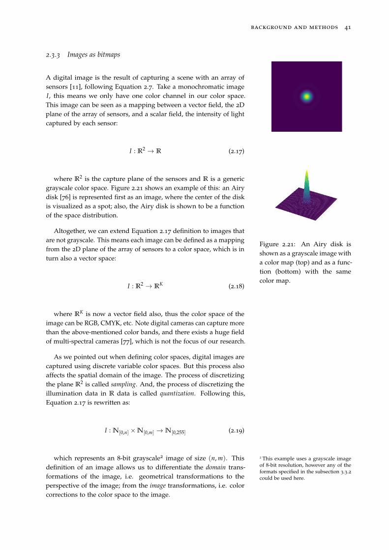
Figure 2.21: An Airy disk isshown as a grayscale image witha color map (top) and as a func-tion (bottom) with the samecolor map.
I : R2 → R (2.17)
where R2 is the capture plane of the sensors and R is a generic
grayscale color space. Figure 2.21 shows an example of this: an Airydisk [76] is represented first as an image, where the center of the diskis visualized as a spot; also, the Airy disk is shown to be a functionof the space distribution.
Altogether, we can extend Equation 2.17 definition to images thatare not grayscale. This means each image can be defined as a mappingfrom the 2D plane of the array of sensors to a color space, which is inturn also a vector space:
I : R2 → R
K (2.18)
where RK is now a vector field also, thus the color space of the
image can be RGB, CMYK, etc. Note digital cameras can capture morethan the above-mentioned color bands, and there exists a huge fieldof multi-spectral cameras [77], which is not the focus of our research.
As we pointed out when defining color spaces, digital images arecaptured using discrete variable color spaces. But this process alsoaffects the spatial domain of the image. The process of discretizingthe plane R
2 is called sampling. And, the process of discretizing theillumination data in R data is called quantization. Following this,Equation 2.17 is rewritten as:
I : N[0,n] ×N[0,m] → N[0,255] (2.19)
which represents an 8-bit grayscale2 image of size (n, m). This 2 This example uses a grayscale imageof 8-bit resolution, however any of theformats specified in the subsection 3.3.2could be used here.
definition of an image allows us to differentiate the domain trans-formations of the image, i.e. geometrical transformations to theperspective of the image; from the image transformations, i.e. colorcorrections to the color space to the image.
42 automated color correction for colorimetry applications using barcodes
In chapter 3, when dealing with the extraction of QR Codes fromchallenging surfaces we used the definition in Equation 2.17 to refer tothe capturing plane of the image and how it relates to the underneathsurface where the QR Code is placed by projective laws.
In chapter 4 we used the definition of Equation 2.19 to detail ourproposal encoding process of colored QR Codes. In this scenario, itis interesting reducing the notation of image definition taking intoaccount images can be seen as matrices. So, Equation 2.19 can berewritten in a compact form as:
I ∈ [0, 255]n×m (2.20)
where I is now a matrix which exist in a matrix space [0, 255]n×m.This vector space contains both the definition of the spatial coordinatesof the image and the color space.
As before, we can use this notation to represent different imageexamples:
• I ∈ [0, 255]n×m, is an 8-bit grayscale image with size (n, m).
• I ∈ [0, 255]n×m×3, is an 8-bit RGB image with size (n, m).
• I ∈ [0, 1]n×m, is a float normalized grayscale image with size (n, m).
• I ∈ {0, 1}n×m, is a binary image with size (n, m).
Finally, we can redefine the color space transformations (fromEquation 2.13 to Equation 2.16) transformations of these image spaces:
• Normalization:
fnormalize : [0, 255]n×m×3 → [0, 1]n×m×3 (2.21)
• Desaturation:
fdesaturate : [0, 1]n×m×3 → [0, 1]n×m (2.22)
• Binarization:
fbinarize : [0, 1]n×m → {0, 1}n×m (2.23)
• Colorization:
fcolorize : [0, 1]n×m → [0, 1]n×m×3 (2.24)
background and methods 43
2.4 Computational implementation
In 1990, Guido van Rosum released the first version of Python, anopen-source, interpreted, high-level, general-purpose, multi-paradigm(procedural, functional, imperative, object-oriented) programminglanguage [78]. Since then, Python has released three major versionsof the language: Python 1 (1990), Python 2 (2000) and Python 3 (2008)[79].
At the time we started to work in the thesis development, Pythonwas one of the popular programming languages both in the academiaand in the industry [80]. As Python is an interpreted language, theactual code of Python is executed by the Python Virtual Machine(PVM), this opens the door to create different PVM written withdifferent compiled languages, the official Python distribution is basedupon a C++ PVM, that is why the mainstream Python distribution iscalled ’CPython’ [81].
CPython allows the user to create bindings to C/C++ libraries, thiswas specially useful for our research. OpenCV is a widely-knowntool-kit for computer vision applications, which is written in C++, butpresents bindings to other languages like Java, MATLAB or Python[82].
Altogether, we decided to use Python as our main programming language.Both achieving rapid script capabilities that Python offers alongsidewith standard libraries from Python and C++. The research startedwith the use of Python 3.6 and ended with the use of Python 3.8, dueto Python development cycle.
Let us detail the stack of standard libraries used during the devel-opment of the thesis:
• Python environment: we started using the Anaconda, an open-source Python distribution that contained pre-compiled packagesready to be used, such as OpenCV [83]. We adopted also pyenv,a tool to install Python distributions and manage virtual environ-ments [84]. Later on, we started to use docker technology, lightvirtual machines to enclose the PVM and our programs [85].
• Scientific and data: we adopted the well-known numpy / scipy /matplotlib stack,
– numpy is a C++ implementation of array representation (MATLAB-like) for Python [86],
– scipy is a compendium of common mathematical operationsfully compatible with NumPy arrays, often SciPy implementsbindings to consolidated calculus frameworks written in C++and Fortran, such as OpenBlas [87],
44 automated color correction for colorimetry applications using barcodes
– matplotlib is a 2D graphics environment we used to representour data [88].
NumPy, SciPy and Matplotlib are the entry point to a huge ecosys-tem of packages which use them as their core. When processingdatasets two main packages were used,
– pandas is an abstraction layer to the previous stack, data isorganized in spreadsheets (like Excel, Origin Lab, etc.) [89],
– xarray is another abstraction layer to the previous stack, withlabeled N-dimensional arrays, xarray can be regarded as theN-dimensional generalization of pandas [90].
• Images manipulation: there is a huge ecosystem regarding imagemanipulation in Python, previous to computer vision, we adoptedsome packages to read and manipulate images,
– pillow is the popular fork from the unmaintained Python Imag-ing Library, we used Pillow specially to manipulate the imagecolor spaces, i.e. profile an image from RGB to be printed inCMYK [91],
– imageio was used as an abstraction layer from Pillow, which usesPillow and other I/O libraries (such as rawpy) to read imagesand convert them directly to NumPy matrices, we standardizedour code to read images using this package instead of usingother solutions (SciPy, Matplotlib, Pillow, OpenCV, ...) [92],
– imgaug was used to enhance image datasets, by tuning ran-domly parameters of the image (illumination, contrast, etc.), thisis a well-known technique to increase dataset when trainingcomputer vision models [93].
• Computer vision: we mainly adopted OpenCV as our main frame-work to perform feature extraction algorithms, affine and per-spective corrections and other operations [59]. Despite this, otherpopular frameworks were used for some applications, such asscikit-learn [94], scikit-image [95], keras [96], etc.
• QR Codes: regarding the encoding of QR Codes we adoptedmainly the package python-qrcode and use it as a base to createour Color QR Codes [97]; regarding the decoding of the QR Codes,there exists different frameworks we worked with,
– zbar is a light C++ barcode scanner, which decodes QR Codesand other 1D and 2D barcodes [98], among the available Pythonbindings to this library we chose the pyzbar library [99],
– zxing is a Java bar code scanner, similar to ZBar, formerly main-tained by Google, and it is the core of most of Android QR Codescanners [100], as this library was not written in Python we didnot use it in a daily basis, but we kept it as secondary QR Codescanner.
Chapter 3. QR Codes on challenging surfaces
In chapter 2 we have introduced the popular QR codes [20], whichhave become part of mainstream culture. With the original applica-tions in mind (e.g. a box in a production line), the QR Codes weredesigned, first, to be placed on top of flat surfaces, second, layingcoplanar to the reader device.
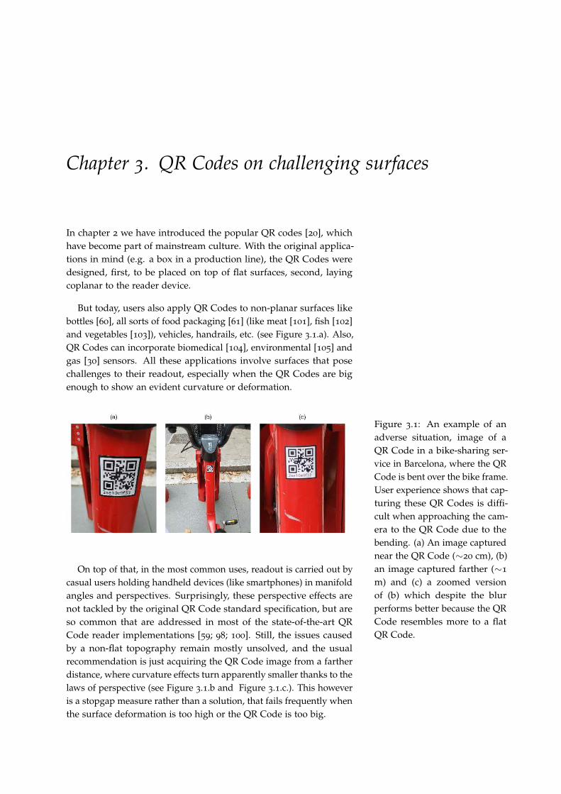
But today, users also apply QR Codes to non-planar surfaces likebottles [60], all sorts of food packaging [61] (like meat [101], fish [102]and vegetables [103]), vehicles, handrails, etc. (see Figure 3.1.a). Also,QR Codes can incorporate biomedical [104], environmental [105] andgas [30] sensors. All these applications involve surfaces that posechallenges to their readout, especially when the QR Codes are bigenough to show an evident curvature or deformation.
Figure 3.1: An example of anadverse situation, image of aQR Code in a bike-sharing ser-vice in Barcelona, where the QRCode is bent over the bike frame.User experience shows that cap-turing these QR Codes is diffi-cult when approaching the cam-era to the QR Code due to thebending. (a) An image capturednear the QR Code (∼20 cm), (b)an image captured farther (∼1
m) and (c) a zoomed versionof (b) which despite the blurperforms better because the QRCode resembles more to a flatQR Code.
On top of that, in the most common uses, readout is carried out bycasual users holding handheld devices (like smartphones) in manifoldangles and perspectives. Surprisingly, these perspective effects arenot tackled by the original QR Code standard specification, but areso common that are addressed in most of the state-of-the-art QRCode reader implementations [59; 98; 100]. Still, the issues causedby a non-flat topography remain mostly unsolved, and the usualrecommendation is just acquiring the QR Code image from a fartherdistance, where curvature effects turn apparently smaller thanks to thelaws of perspective (see Figure 3.1.b and Figure 3.1.c.). This howeveris a stopgap measure rather than a solution, that fails frequently whenthe surface deformation is too high or the QR Code is too big.
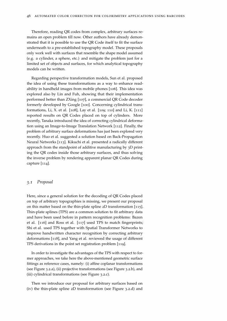
46 automated color correction for colorimetry applications using barcodes
Therefore, reading QR codes from complex, arbitrary surfaces re-mains an open problem till now. Other authors have already demon-strated that it is possible to use the QR Code itself to fit the surfaceunderneath to a pre-established topography model. These proposalsonly work well with surfaces that resemble the shape model assumed(e.g. a cylinder, a sphere, etc.) and mitigate the problem just for alimited set of objects and surfaces, for which analytical topographymodels can be written.
Regarding perspective transformation models, Sun et al. proposedthe idea of using these transformations as a way to enhance read-ability in handheld images from mobile phones [106]. This idea wasexplored also by Lin and Fuh, showing that their implementationperformed better than ZXing [107], a commercial QR Code decoderformerly developed by Google [100]. Concerning cylindrical trans-formations, Li, X. et al. [108], Lay et al. [109; 110] and Li, K. [111]reported results on QR Codes placed on top of cylinders. Morerecently, Tanaka introduced the idea of correcting cylindrical deforma-tion using an Image-to-Image Translation Network [112]. Finally, theproblem of arbitrary surface deformations has just been explored veryrecently. Huo et al. suggested a solution based on Back-PropagationNeural Networks [113]. Kikuchi et al. presented a radically differentapproach from the standpoint of additive manufacturing by 3D print-ing the QR codes inside those arbitrary surfaces, and thus solvingthe inverse problem by rendering apparent planar QR Codes duringcapture [114].
3.1 Proposal
Here, since a general solution for the decoding of QR Codes placedon top of arbitrary topographies is missing, we present our proposalon this matter based on the thin-plate spline 2D transformation [115].Thin-plate splines (TPS) are a common solution to fit arbitrary dataand have been used before in pattern recognition problems: Bazenet al. [116] and Ross et al. [117] used TPS to match fingerprints;Shi et al. used TPS together with Spatial Transformer Networks toimprove handwritten character recognition by correcting arbitrarydeformations [118], and Yang et al. reviewed the usage of differentTPS derivations in the point set registration problem [119].
In order to investigate the advantages of the TPS with respect to for-mer approaches, we take here the above-mentioned geometric surfacefittings as reference cases, namely: (i) affine coplanar transformations(see Figure 3.2.a), (ii) projective transformations (see Figure 3.2.b), and(iii) cylindrical transformations (see Figure 3.2.c).
Then we introduce our proposal for arbitrary surfaces based on(iv) the thin-plate spline 2D transformation (see Figure 3.2.d) and
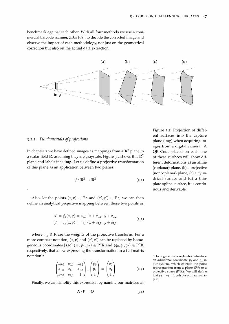
qr codes on challenging surfaces 47
benchmark against each other. With all four methods we use a com-mercial barcode scanner, ZBar [98], to decode the corrected image andobserve the impact of each methodology, not just on the geometricalcorrection but also on the actual data extraction.
Figure 3.2: Projection of differ-ent surfaces into the captureplane (img) when acquiring im-ages from a digital camera. AQR Code placed on each oneof these surfaces will show dif-ferent deformations(a) an affine(coplanar) plane, (b) a projective(noncoplanar) plane, (c) a cylin-drical surface and (d) a thin-plate spline surface, it is contin-uous and derivable.
3.1.1 Fundamentals of projections
In chapter 2 we have defined images as mappings from a R2 plane to
a scalar field R, assuming they are grayscale. Figure 3.2 shows this R2
plane and labels it as img. Let us define a projective transformationof this plane as an application between two planes:
f : R2 → R
2 (3.1)
.
Also, let the points (x, y) ∈ R2 and (x′, y′) ∈ R
2, we can thendefine an analytical projective mapping between those two points as:
x′ = fx(x, y) = a0,0 · x + a0,1 · y + a0,2
y′ = fy(x, y) = a1,0 · x + a1,1 · y + a1,2(3.2)
where ai,j ∈ R are the weights of the projective transform. For amore compact notation, (x, y) and (x′, y′) can be replaced by homo-geneous coordinates [120] (p0, p1, p2) ∈ P2
R and (q0, q1, q2) ∈ P2R,
respectively, that allow expressing the transformation in a full matrixnotation1: 1 Homogeneous coordinates introduce
an additional coordinate p2 and q2 inour system, which extends the pointrepresentation from a plane (R2) to aprojective space (P2
R). We will definethat p2 = q2 = 1 only for our landmarks[120].
a0,0 a0,1 a0,2
a1,0 a1,1 a1,2
a2,0 a2,1 1
·
p0
p1
1
=
q0
q1
1
(3.3)
Finally, we can simplify this expression by naming our matrices as:
A · P = Q (3.4)
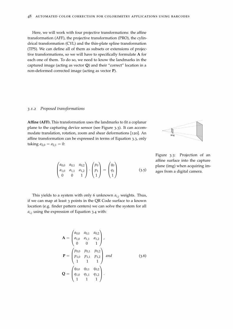
48 automated color correction for colorimetry applications using barcodes
Here, we will work with four projective transformations: the affinetransformation (AFF), the projective transformation (PRO), the cylin-drical transformation (CYL) and the thin-plate spline transformation(TPS). We can define all of them as subsets or extensions of projec-tive transformations, so we will have to specifically formulate A foreach one of them. To do so, we need to know the landmarks in thecaptured image (acting as vector Q) and their “correct” location in anon-deformed corrected image (acting as vector P).
3.1.2 Proposed transformations
Affine (AFF). This transformation uses the landmarks to fit a coplanarplane to the capturing device sensor (see Figure 3.3). It can accom-modate translation, rotation, zoom and shear deformations [120]. Anaffine transformation can be expressed in terms of Equation 3.3, onlytaking a2,0 = a2,1 = 0:
Figure 3.3: Projection of anaffine surface into the captureplane (img) when acquiring im-ages from a digital camera.
a0,0 a0,1 a0,2
a1,0 a1,1 a1,2
0 0 1
·
p0
p1
1
=
q0
q1
1
(3.5)
This yields to a system with only 6 unknown ai,j weights. Thus,if we can map at least 3 points in the QR Code surface to a knownlocation (e.g. finder pattern centers) we can solve the system for allai,j using the expression of Equation 3.4 with:
A =
a0,0 a0,1 a0,2
a1,0 a1,1 a1,2
0 0 1
,
P =
p0,0 p0,1 p0,2
p1,0 p1,1 p1,2
1 1 1
and
Q =
q0,0 q0,1 q0,2
q1,0 q1,1 q1,2
1 1 1
.
(3.6)
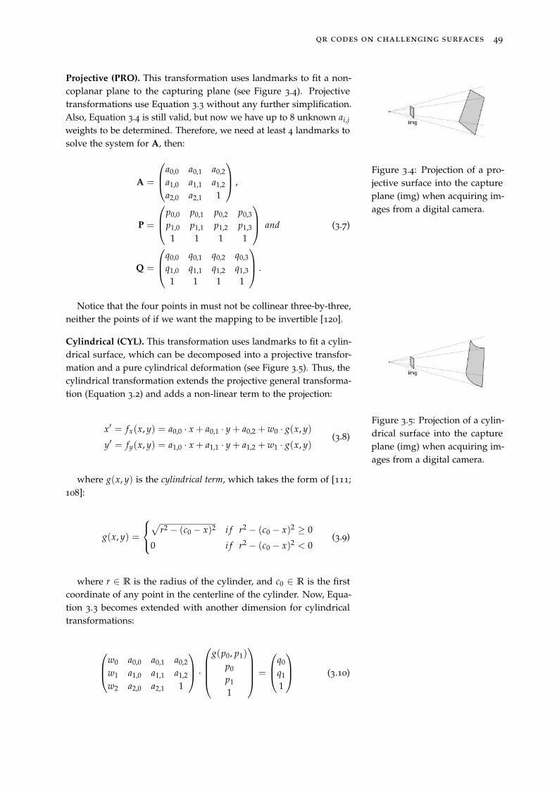
qr codes on challenging surfaces 49
Projective (PRO). This transformation uses landmarks to fit a non-coplanar plane to the capturing plane (see Figure 3.4). Projectivetransformations use Equation 3.3 without any further simplification.Also, Equation 3.4 is still valid, but now we have up to 8 unknown ai,j
weights to be determined. Therefore, we need at least 4 landmarks tosolve the system for A, then:
Figure 3.4: Projection of a pro-jective surface into the captureplane (img) when acquiring im-ages from a digital camera.
A =
a0,0 a0,1 a0,2
a1,0 a1,1 a1,2
a2,0 a2,1 1
,
P =
p0,0 p0,1 p0,2 p0,3
p1,0 p1,1 p1,2 p1,3
1 1 1 1
and
Q =
q0,0 q0,1 q0,2 q0,3
q1,0 q1,1 q1,2 q1,3
1 1 1 1
.
(3.7)
Notice that the four points in must not be collinear three-by-three,neither the points of if we want the mapping to be invertible [120].
Cylindrical (CYL). This transformation uses landmarks to fit a cylin-drical surface, which can be decomposed into a projective transfor-mation and a pure cylindrical deformation (see Figure 3.5). Thus, thecylindrical transformation extends the projective general transforma-tion (Equation 3.2) and adds a non-linear term to the projection:
Figure 3.5: Projection of a cylin-drical surface into the captureplane (img) when acquiring im-ages from a digital camera.
x′ = fx(x, y) = a0,0 · x + a0,1 · y + a0,2 + w0 · g(x, y)
y′ = fy(x, y) = a1,0 · x + a1,1 · y + a1,2 + w1 · g(x, y)(3.8)
where g(x, y) is the cylindrical term, which takes the form of [111;108]:
g(x, y) =
√
r2 − (c0 − x)2 i f r2 − (c0 − x)2 ≥ 0
0 i f r2 − (c0 − x)2< 0
(3.9)
where r ∈ R is the radius of the cylinder, and c0 ∈ R is the firstcoordinate of any point in the centerline of the cylinder. Now, Equa-tion 3.3 becomes extended with another dimension for cylindricaltransformations:
w0 a0,0 a0,1 a0,2
w1 a1,0 a1,1 a1,2
w2 a2,0 a2,1 1
·
g(p0, p1)
p0
p1
1
=
q0
q1
1
(3.10)
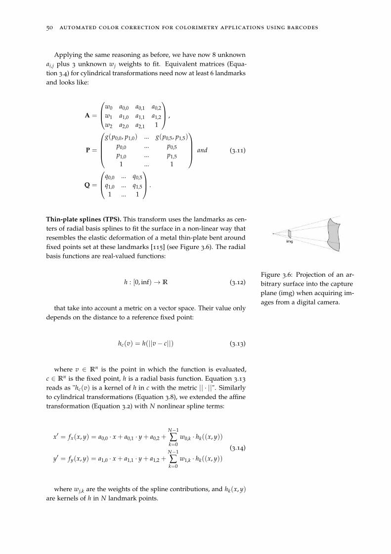
50 automated color correction for colorimetry applications using barcodes
Applying the same reasoning as before, we have now 8 unknownai,j plus 3 unknown wj weights to fit. Equivalent matrices (Equa-tion 3.4) for cylindrical transformations need now at least 6 landmarksand looks like:
A =
w0 a0,0 a0,1 a0,2
w1 a1,0 a1,1 a1,2
w2 a2,0 a2,1 1
,
P =
g(p0,0, p1,0) ... g(p0,5, p1,5)
p0,0 ... p0,5
p1,0 ... p1,5
1 ... 1
and
Q =
q0,0 ... q0,5
q1,0 ... q1,5
1 ... 1
.
(3.11)
Thin-plate splines (TPS). This transform uses the landmarks as cen-ters of radial basis splines to fit the surface in a non-linear way thatresembles the elastic deformation of a metal thin-plate bent aroundfixed points set at these landmarks [115] (see Figure 3.6). The radialbasis functions are real-valued functions:
Figure 3.6: Projection of an ar-bitrary surface into the captureplane (img) when acquiring im-ages from a digital camera.
h : [0, inf)→ R (3.12)
that take into account a metric on a vector space. Their value onlydepends on the distance to a reference fixed point:
hc(v) = h(||v− c||) (3.13)
where v ∈ Rn is the point in which the function is evaluated,
c ∈ Rn is the fixed point, h is a radial basis function. Equation 3.13
reads as "hc(v) is a kernel of h in c with the metric || · ||". Similarlyto cylindrical transformations (Equation 3.8), we extended the affinetransformation (Equation 3.2) with N nonlinear spline terms:
x′ = fx(x, y) = a0,0 · x + a0,1 · y + a0,2 +N−1
∑k=0
w0,k · hk((x, y))
y′ = fy(x, y) = a1,0 · x + a1,1 · y + a1,2 +N−1
∑k=0
w1,k · hk((x, y))
(3.14)
where wj,k are the weights of the spline contributions, and hk(x, y)
are kernels of h in N landmark points.
qr codes on challenging surfaces 51
These radial basis function remains open to multiple definitions.Bookstein [115] found that the second order polynomial radial basisfunction is the proper function to compute splines in R
2 mappings inorder to minimize the bending energy, and mimic the elastic behaviorof a metal thin-plate. Thus, let h be:
h(r) = r2 ln(r) (3.15)
with the corresponding kernels computed using the euclideanmetric:
||(x, y)− (cx, cy)|| =√
(x− cx)2 + (y− cy)2 (3.16)
Finally, in matrix representation, terms from Equation 3.4 areexpanded as follows:
A =
(
w0,0 ... w0,N−1 a0,0 a0,1 a0,2
w1,0 ... w1,N−1 a1,0 a1,1 a1,2
)
,
P =
h0(p0,0, p1,0) ... h0(p0,N−1, p1,N−1)... ...
...hN−1(p0,0, p1,0) ... hN−1(p0,N−1, p1,N−1)
p0,0 ... p0,N−1
p1,0 ... p1,N−1
1 ... 1
and
Q =
(
q0,0 ... q0,N−1
q1,0 ... q1,N
)
.
(3.17)
First, notice that only ai,j affine weights are present, since thisdefinition does not include a perspective transformation. Second, incontrast with previous transformations, this system is unbalanced:we have a total of 2N + 6 weights to compute (2N wj,k spline weightsplus 6 ai,j affine weights) however we only have defined N landmarks.In the previous transformations, we used additional landmarks tosolve the system, but Bookstein imposed an additional condition ofthe spline contributions: the sum of wj,k coefficients to be 0, and alsotheir cross-product with the pi,k landmark coordinates [115]. Suchcondition makes spline contributions tend to 0 at infinity, while affinecontributions prevail. This makes our system of equations solvableand can be expressed as:
(
w0,0 ... w0,N−1
w1,0 ... w1,N−1
)
·
p0,0 ... p0,N−1
p1,0 ... p1,N−1
1 ... 1
T
= 0 (3.18)
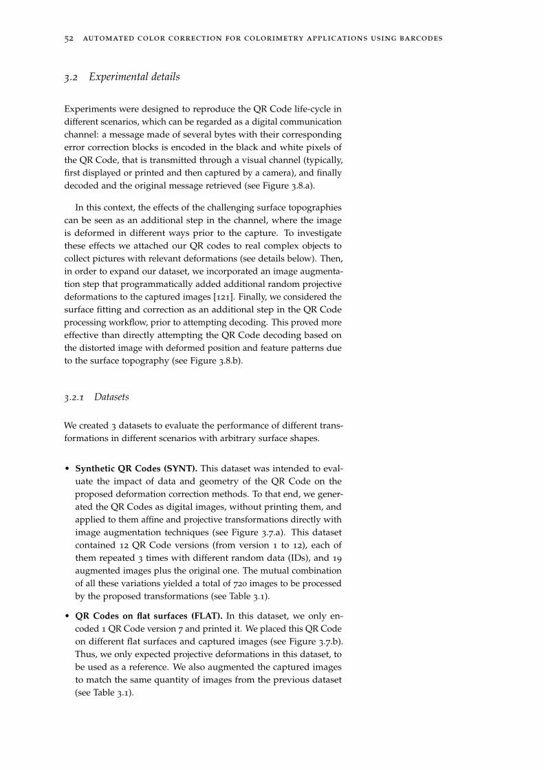
52 automated color correction for colorimetry applications using barcodes
3.2 Experimental details
Experiments were designed to reproduce the QR Code life-cycle indifferent scenarios, which can be regarded as a digital communicationchannel: a message made of several bytes with their correspondingerror correction blocks is encoded in the black and white pixels ofthe QR Code, that is transmitted through a visual channel (typically,first displayed or printed and then captured by a camera), and finallydecoded and the original message retrieved (see Figure 3.8.a).
In this context, the effects of the challenging surface topographiescan be seen as an additional step in the channel, where the imageis deformed in different ways prior to the capture. To investigatethese effects we attached our QR codes to real complex objects tocollect pictures with relevant deformations (see details below). Then,in order to expand our dataset, we incorporated an image augmenta-tion step that programmatically added additional random projectivedeformations to the captured images [121]. Finally, we considered thesurface fitting and correction as an additional step in the QR Codeprocessing workflow, prior to attempting decoding. This proved moreeffective than directly attempting the QR Code decoding based onthe distorted image with deformed position and feature patterns dueto the surface topography (see Figure 3.8.b).
3.2.1 Datasets
We created 3 datasets to evaluate the performance of different trans-formations in different scenarios with arbitrary surface shapes.
• Synthetic QR Codes (SYNT). This dataset was intended to eval-uate the impact of data and geometry of the QR Code on theproposed deformation correction methods. To that end, we gener-ated the QR Codes as digital images, without printing them, andapplied to them affine and projective transformations directly withimage augmentation techniques (see Figure 3.7.a). This datasetcontained 12 QR Code versions (from version 1 to 12), each ofthem repeated 3 times with different random data (IDs), and 19
augmented images plus the original one. The mutual combinationof all these variations yielded a total of 720 images to be processedby the proposed transformations (see Table 3.1).
• QR Codes on flat surfaces (FLAT). In this dataset, we only en-coded 1 QR Code version 7 and printed it. We placed this QR Codeon different flat surfaces and captured images (see Figure 3.7.b).Thus, we only expected projective deformations in this dataset, tobe used as a reference. We also augmented the captured imagesto match the same quantity of images from the previous dataset(see Table 3.1).
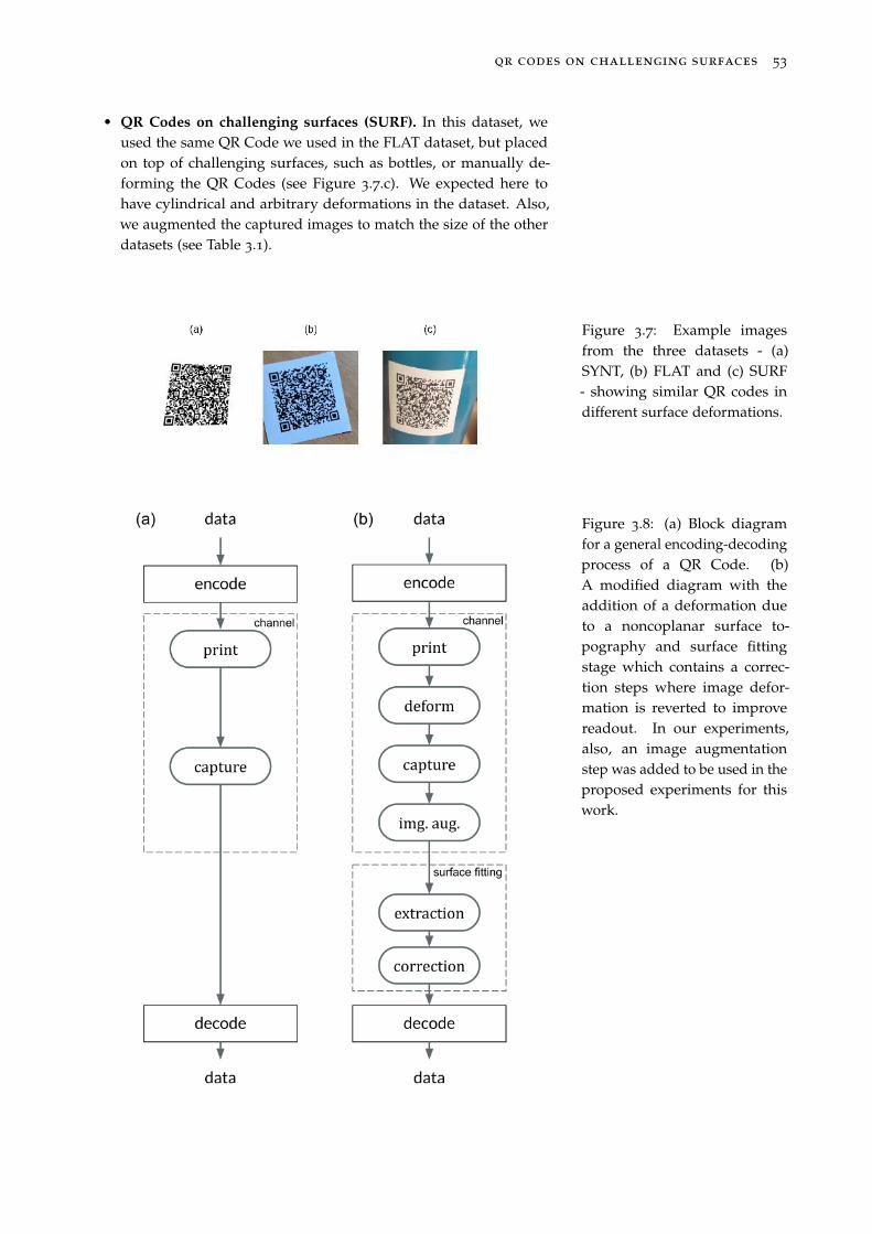
qr codes on challenging surfaces 53
• QR Codes on challenging surfaces (SURF). In this dataset, weused the same QR Code we used in the FLAT dataset, but placedon top of challenging surfaces, such as bottles, or manually de-forming the QR Codes (see Figure 3.7.c). We expected here tohave cylindrical and arbitrary deformations in the dataset. Also,we augmented the captured images to match the size of the otherdatasets (see Table 3.1).
Figure 3.7: Example imagesfrom the three datasets - (a)SYNT, (b) FLAT and (c) SURF- showing similar QR codes indifferent surface deformations.
Figure 3.8: (a) Block diagramfor a general encoding-decodingprocess of a QR Code. (b)A modified diagram with theaddition of a deformation dueto a noncoplanar surface to-pography and surface fittingstage which contains a correc-tion steps where image defor-mation is reverted to improvereadout. In our experiments,also, an image augmentationstep was added to be used in theproposed experiments for thiswork.
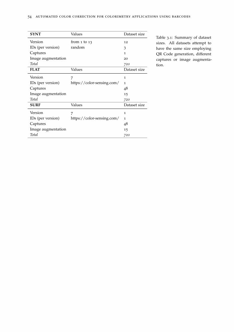
54 automated color correction for colorimetry applications using barcodes
SYNT Values Dataset size
Version from 1 to 13 12
IDs (per version) random 3
Captures 1
Image augmentation 20
Total 720
FLAT Values Dataset size
Version 7 1
IDs (per version) https://color-sensing.com/ 1
Captures 48
Image augmentation 15
Total 720
SURF Values Dataset size
Version 7 1
IDs (per version) https://color-sensing.com/ 1
Captures 48
Image augmentation 15
Total 720
Table 3.1: Summary of datasetsizes. All datasets attempt tohave the same size employingQR Code generation, differentcaptures or image augmenta-tion.
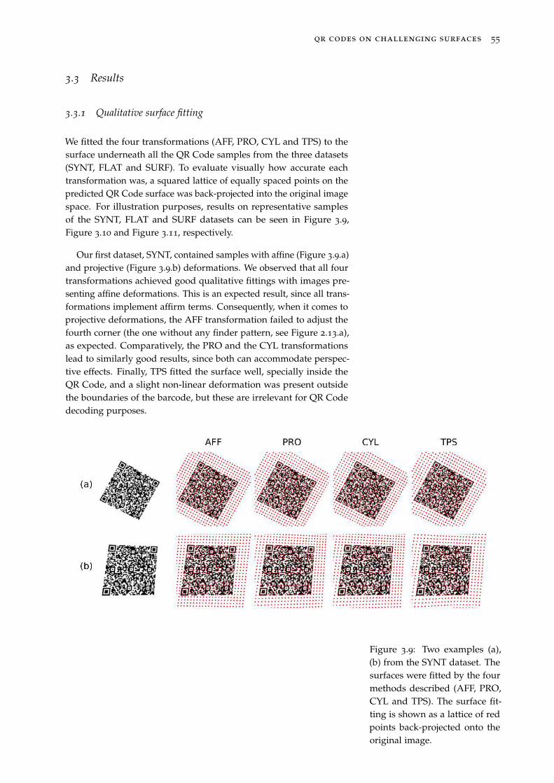
qr codes on challenging surfaces 55
3.3 Results
3.3.1 Qualitative surface fitting
We fitted the four transformations (AFF, PRO, CYL and TPS) to thesurface underneath all the QR Code samples from the three datasets(SYNT, FLAT and SURF). To evaluate visually how accurate eachtransformation was, a squared lattice of equally spaced points on thepredicted QR Code surface was back-projected into the original imagespace. For illustration purposes, results on representative samplesof the SYNT, FLAT and SURF datasets can be seen in Figure 3.9,Figure 3.10 and Figure 3.11, respectively.
Our first dataset, SYNT, contained samples with affine (Figure 3.9.a)and projective (Figure 3.9.b) deformations. We observed that all fourtransformations achieved good qualitative fittings with images pre-senting affine deformations. This is an expected result, since all trans-formations implement affirm terms. Consequently, when it comes toprojective deformations, the AFF transformation failed to adjust thefourth corner (the one without any finder pattern, see Figure 2.13.a),as expected. Comparatively, the PRO and the CYL transformationslead to similarly good results, since both can accommodate perspec-tive effects. Finally, TPS fitted the surface well, specially inside theQR Code, and a slight non-linear deformation was present outsidethe boundaries of the barcode, but these are irrelevant for QR Codedecoding purposes.
Figure 3.9: Two examples (a),(b) from the SYNT dataset. Thesurfaces were fitted by the fourmethods described (AFF, PRO,CYL and TPS). The surface fit-ting is shown as a lattice of redpoints back-projected onto theoriginal image.
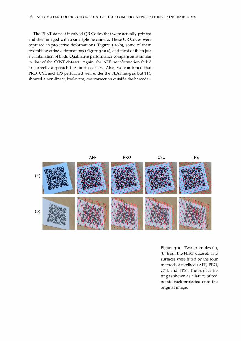
56 automated color correction for colorimetry applications using barcodes
The FLAT dataset involved QR Codes that were actually printedand then imaged with a smartphone camera. These QR Codes werecaptured in projective deformations (Figure 3.10.b), some of themresembling affine deformations (Figure 3.10.a), and most of them justa combination of both. Qualitative performance comparison is similarto that of the SYNT dataset. Again, the AFF transformation failedto correctly approach the fourth corner. Also, we confirmed thatPRO, CYL and TPS performed well under the FLAT images, but TPSshowed a non-linear, irrelevant, overcorrection outside the barcode.
Figure 3.10: Two examples (a),(b) from the FLAT dataset. Thesurfaces were fitted by the fourmethods described (AFF, PRO,CYL and TPS). The surface fit-ting is shown as a lattice of redpoints back-projected onto theoriginal image.
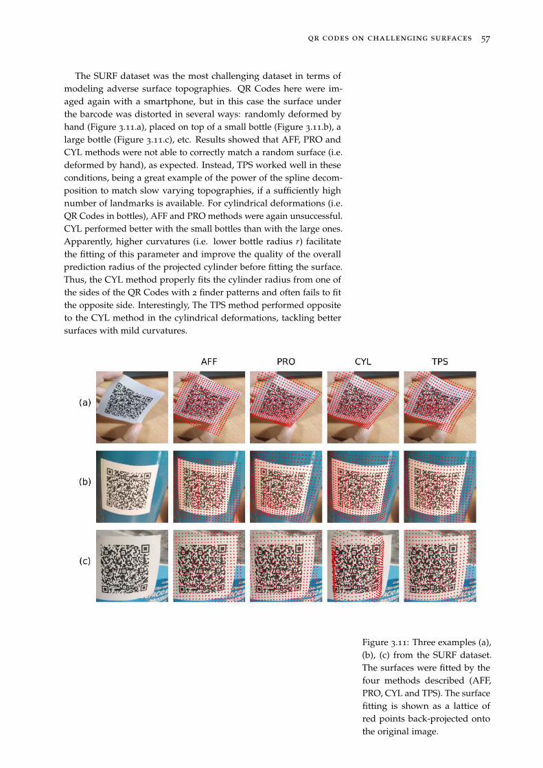
qr codes on challenging surfaces 57
The SURF dataset was the most challenging dataset in terms ofmodeling adverse surface topographies. QR Codes here were im-aged again with a smartphone, but in this case the surface underthe barcode was distorted in several ways: randomly deformed byhand (Figure 3.11.a), placed on top of a small bottle (Figure 3.11.b), alarge bottle (Figure 3.11.c), etc. Results showed that AFF, PRO andCYL methods were not able to correctly match a random surface (i.e.deformed by hand), as expected. Instead, TPS worked well in theseconditions, being a great example of the power of the spline decom-position to match slow varying topographies, if a sufficiently highnumber of landmarks is available. For cylindrical deformations (i.e.QR Codes in bottles), AFF and PRO methods were again unsuccessful.CYL performed better with the small bottles than with the large ones.Apparently, higher curvatures (i.e. lower bottle radius r) facilitatethe fitting of this parameter and improve the quality of the overallprediction radius of the projected cylinder before fitting the surface.Thus, the CYL method properly fits the cylinder radius from one ofthe sides of the QR Codes with 2 finder patterns and often fails to fitthe opposite side. Interestingly, The TPS method performed oppositeto the CYL method in the cylindrical deformations, tackling bettersurfaces with mild curvatures.
Figure 3.11: Three examples (a),(b), (c) from the SURF dataset.The surfaces were fitted by thefour methods described (AFF,PRO, CYL and TPS). The surfacefitting is shown as a lattice ofred points back-projected ontothe original image.
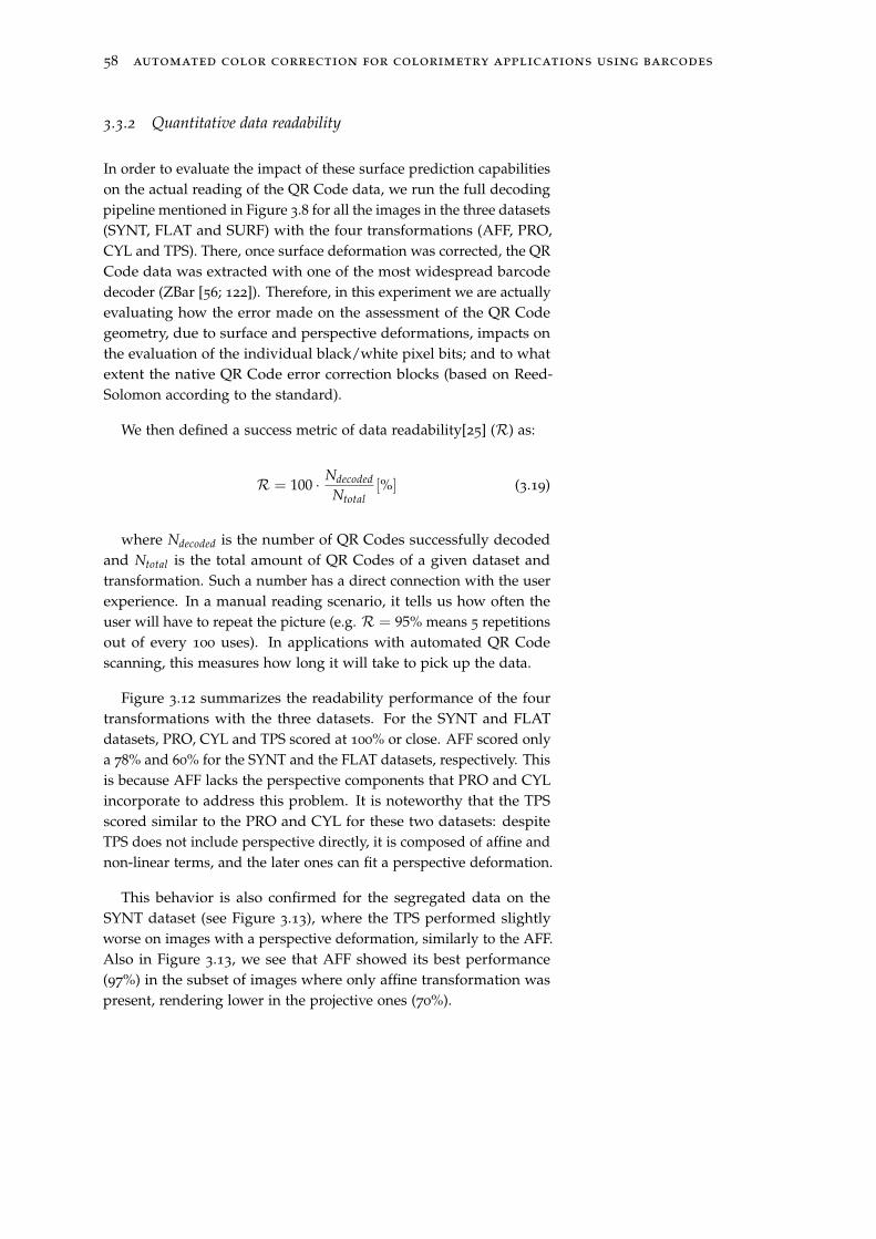
58 automated color correction for colorimetry applications using barcodes
3.3.2 Quantitative data readability
In order to evaluate the impact of these surface prediction capabilitieson the actual reading of the QR Code data, we run the full decodingpipeline mentioned in Figure 3.8 for all the images in the three datasets(SYNT, FLAT and SURF) with the four transformations (AFF, PRO,CYL and TPS). There, once surface deformation was corrected, the QRCode data was extracted with one of the most widespread barcodedecoder (ZBar [56; 122]). Therefore, in this experiment we are actuallyevaluating how the error made on the assessment of the QR Codegeometry, due to surface and perspective deformations, impacts onthe evaluation of the individual black/white pixel bits; and to whatextent the native QR Code error correction blocks (based on Reed-Solomon according to the standard).
We then defined a success metric of data readability[25] (R) as:
R = 100 · Ndecoded
Ntotal[%] (3.19)
where Ndecoded is the number of QR Codes successfully decodedand Ntotal is the total amount of QR Codes of a given dataset andtransformation. Such a number has a direct connection with the userexperience. In a manual reading scenario, it tells us how often theuser will have to repeat the picture (e.g. R = 95% means 5 repetitionsout of every 100 uses). In applications with automated QR Codescanning, this measures how long it will take to pick up the data.
Figure 3.12 summarizes the readability performance of the fourtransformations with the three datasets. For the SYNT and FLATdatasets, PRO, CYL and TPS scored at 100% or close. AFF scored onlya 78% and 60% for the SYNT and the FLAT datasets, respectively. Thisis because AFF lacks the perspective components that PRO and CYLincorporate to address this problem. It is noteworthy that the TPSscored similar to the PRO and CYL for these two datasets: despiteTPS does not include perspective directly, it is composed of affine andnon-linear terms, and the later ones can fit a perspective deformation.
This behavior is also confirmed for the segregated data on theSYNT dataset (see Figure 3.13), where the TPS performed slightlyworse on images with a perspective deformation, similarly to the AFF.Also in Figure 3.13, we see that AFF showed its best performance(97%) in the subset of images where only affine transformation waspresent, rendering lower in the projective ones (70%).
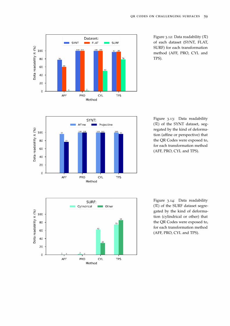
qr codes on challenging surfaces 59
Figure 3.12: Data readability (R)of each dataset (SYNT, FLAT,SURF) for each transformationmethod (AFF, PRO, CYL andTPS).
Figure 3.13: Data readability(R) of the SYNT dataset, seg-regated by the kind of deforma-tion (affine or perspective) thatthe QR Codes were exposed to,for each transformation method(AFF, PRO, CYL and TPS).
Figure 3.14: Data readability(R) of the SURF dataset segre-gated by the kind of deforma-tion (cylindrical or other) thatthe QR Codes were exposed to,for each transformation method(AFF, PRO, CYL and TPS).
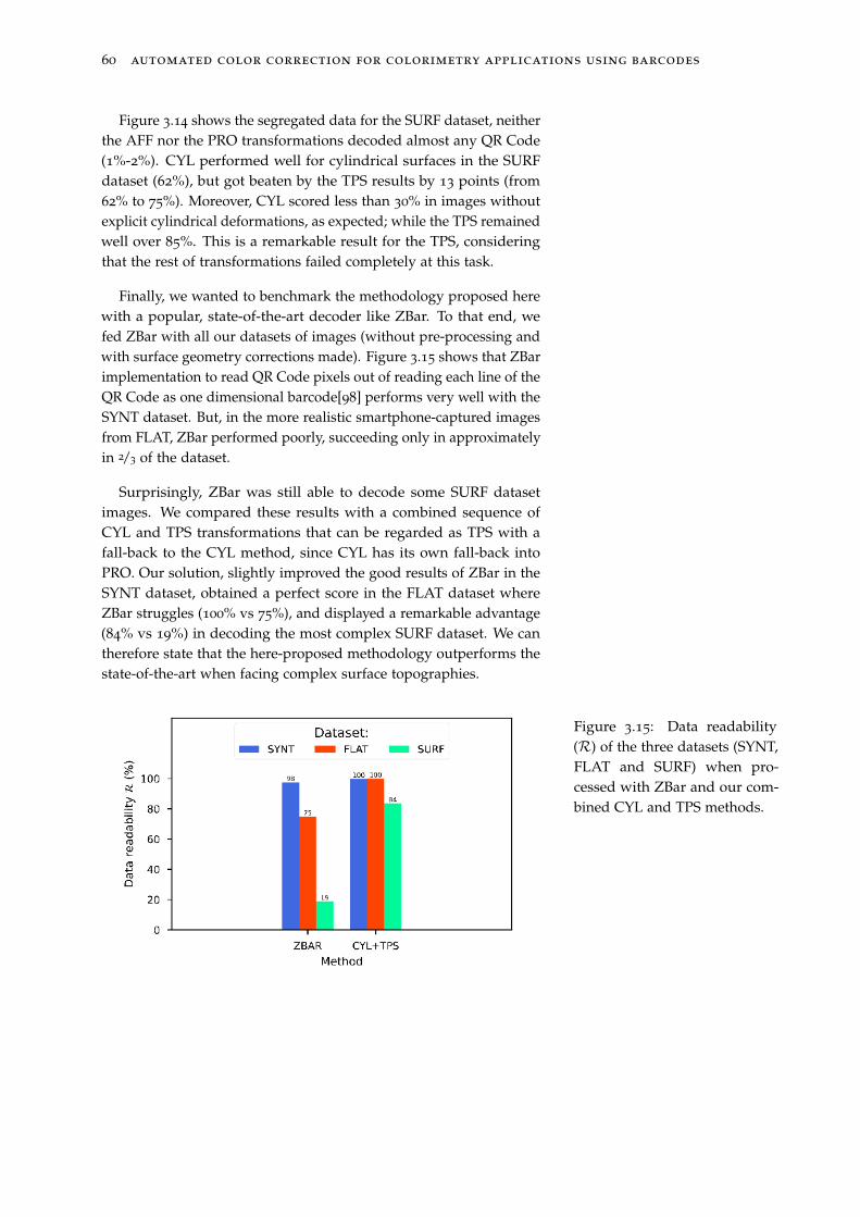
60 automated color correction for colorimetry applications using barcodes
Figure 3.14 shows the segregated data for the SURF dataset, neitherthe AFF nor the PRO transformations decoded almost any QR Code(1%-2%). CYL performed well for cylindrical surfaces in the SURFdataset (62%), but got beaten by the TPS results by 13 points (from62% to 75%). Moreover, CYL scored less than 30% in images withoutexplicit cylindrical deformations, as expected; while the TPS remainedwell over 85%. This is a remarkable result for the TPS, consideringthat the rest of transformations failed completely at this task.
Finally, we wanted to benchmark the methodology proposed herewith a popular, state-of-the-art decoder like ZBar. To that end, wefed ZBar with all our datasets of images (without pre-processing andwith surface geometry corrections made). Figure 3.15 shows that ZBarimplementation to read QR Code pixels out of reading each line of theQR Code as one dimensional barcode[98] performs very well with theSYNT dataset. But, in the more realistic smartphone-captured imagesfrom FLAT, ZBar performed poorly, succeeding only in approximatelyin 2/3 of the dataset.
Surprisingly, ZBar was still able to decode some SURF datasetimages. We compared these results with a combined sequence ofCYL and TPS transformations that can be regarded as TPS with afall-back to the CYL method, since CYL has its own fall-back intoPRO. Our solution, slightly improved the good results of ZBar in theSYNT dataset, obtained a perfect score in the FLAT dataset whereZBar struggles (100% vs 75%), and displayed a remarkable advantage(84% vs 19%) in decoding the most complex SURF dataset. We cantherefore state that the here-proposed methodology outperforms thestate-of-the-art when facing complex surface topographies.
Figure 3.15: Data readability(R) of the three datasets (SYNT,FLAT and SURF) when pro-cessed with ZBar and our com-bined CYL and TPS methods.
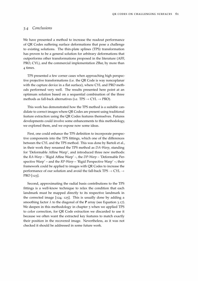
qr codes on challenging surfaces 61
3.4 Conclusions
We have presented a method to increase the readout performanceof QR Codes suffering surface deformations that pose a challengeto existing solutions. The thin-plate splines (TPS) transformationhas proven to be a general solution for arbitrary deformations thatoutperforms other transformations proposed in the literature (AFF,PRO, CYL), and the commercial implementation ZBar, by more than4 times.
TPS presented a few corner cases when approaching high perspec-tive projective transformations (i.e. the QR Code is way noncoplanarwith the capture device in a flat surface), where CYL and PRO meth-ods performed very well. The results presented here point at anoptimum solution based on a sequential combination of the threemethods as fall-back alternatives (i.e. TPS → CYL → PRO).
This work has demonstrated how the TPS method is a suitable can-didate to correct images where QR Codes are present using traditionalfeature extraction using the QR Codes features themselves. Futuresdevelopments could involve some enhancements to this methodology,we explored them, and we expose now some ideas.
First, one could enhance the TPS definition to incorporate perspec-tive components into the TPS fittings, which one of the differencesbetween the CYL and the TPS method. This was done by Bartoli et al.,in their work they renamed the TPS method as DA-Warp, standingfor ’Deformable Affine Warp’, and introduced three new methods:the RA-Warp – ’Rigid Affine Warp’ –, the DP-Warp – ’Deformable Per-spective Warp’ – and the RP-Warp – ’Rigid Perspective Warp’ –; theirframework could be applied to images with QR Codes to increase theperformance of our solution and avoid the fall-back TPS → CYL →
PRO [123].
Second, approximating the radial basis contributions to the TPSfittings is a well-know technique to relax the condition that eachlandmark must be mapped directly to its respective landmark inthe corrected image [124; 125]. This is usually done by adding asmoothing factor λ to the diagonal of the P array (see Equation 3.17).We deepen in this methodology in chapter 5 when we applied TPSto color correction, for QR Code extraction we discarded to use itbecause we often want the extracted key features to match exactlytheir position in the recovered image. Nevertheless, as it was notchecked it should be addressed in some future work.
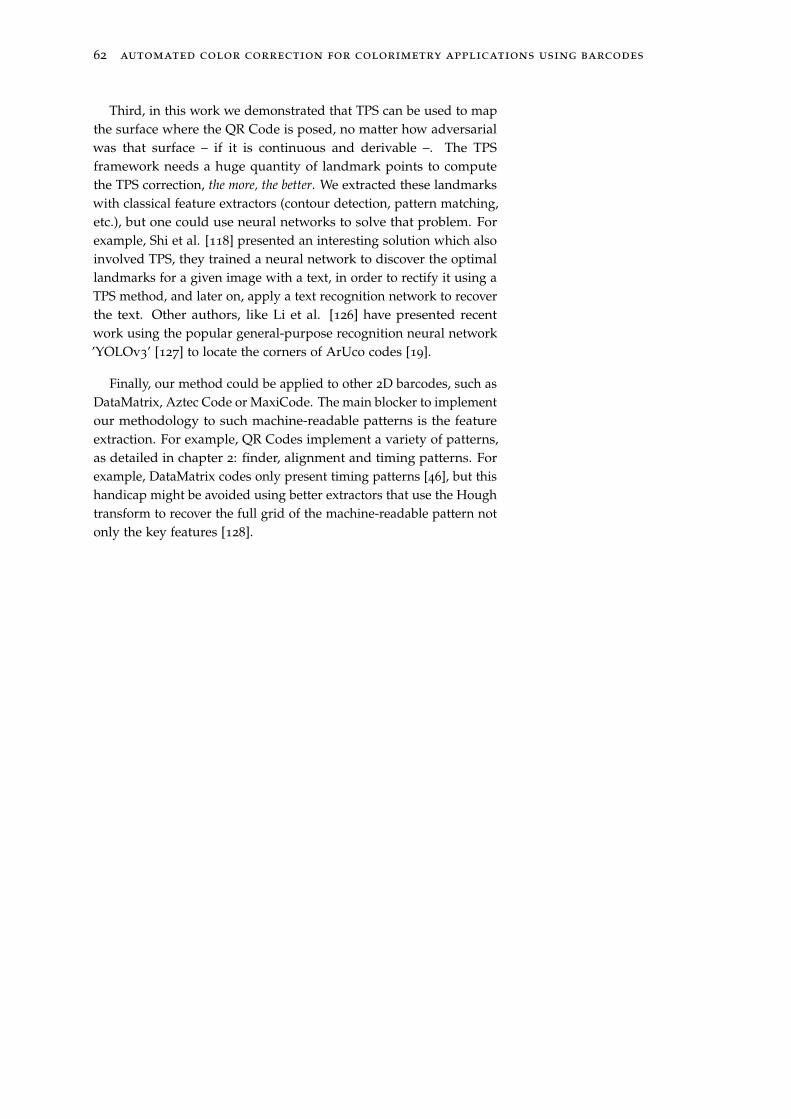
62 automated color correction for colorimetry applications using barcodes
Third, in this work we demonstrated that TPS can be used to mapthe surface where the QR Code is posed, no matter how adversarialwas that surface – if it is continuous and derivable –. The TPSframework needs a huge quantity of landmark points to computethe TPS correction, the more, the better. We extracted these landmarkswith classical feature extractors (contour detection, pattern matching,etc.), but one could use neural networks to solve that problem. Forexample, Shi et al. [118] presented an interesting solution which alsoinvolved TPS, they trained a neural network to discover the optimallandmarks for a given image with a text, in order to rectify it using aTPS method, and later on, apply a text recognition network to recoverthe text. Other authors, like Li et al. [126] have presented recentwork using the popular general-purpose recognition neural network’YOLOv3’ [127] to locate the corners of ArUco codes [19].
Finally, our method could be applied to other 2D barcodes, such asDataMatrix, Aztec Code or MaxiCode. The main blocker to implementour methodology to such machine-readable patterns is the featureextraction. For example, QR Codes implement a variety of patterns,as detailed in chapter 2: finder, alignment and timing patterns. Forexample, DataMatrix codes only present timing patterns [46], but thishandicap might be avoided using better extractors that use the Houghtransform to recover the full grid of the machine-readable pattern notonly the key features [128].
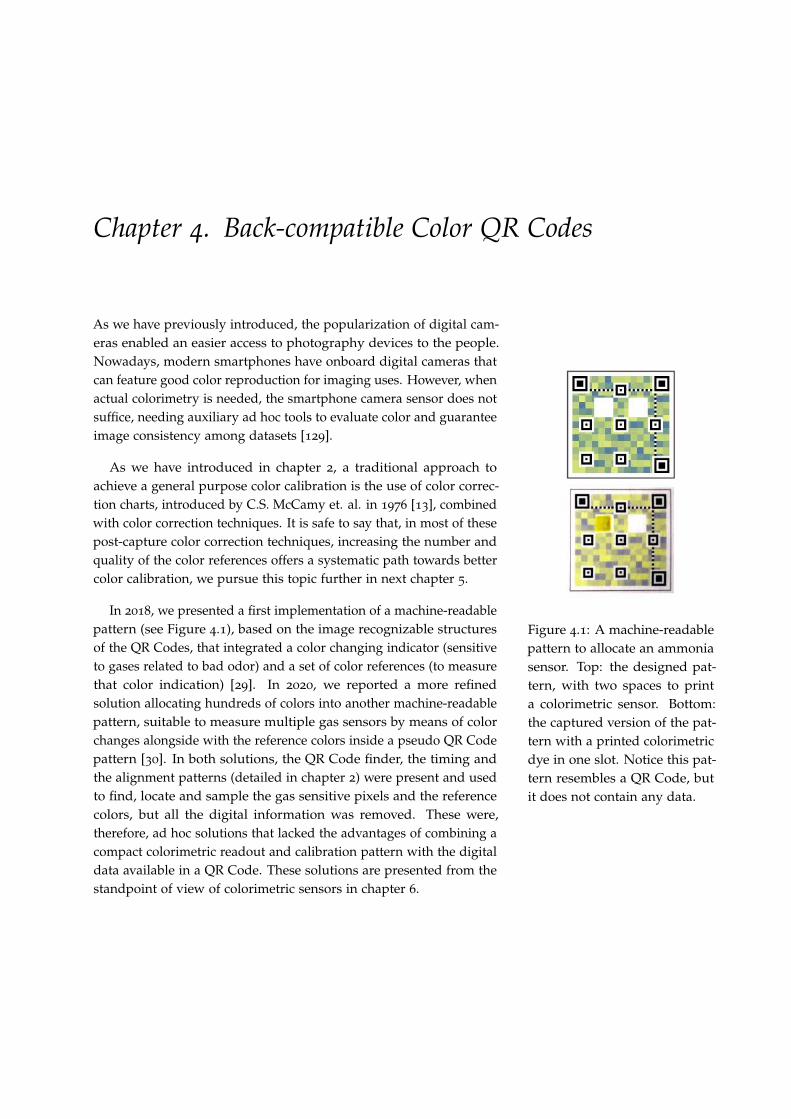
Chapter 4. Back-compatible Color QR Codes
As we have previously introduced, the popularization of digital cam-eras enabled an easier access to photography devices to the people.Nowadays, modern smartphones have onboard digital cameras thatcan feature good color reproduction for imaging uses. However, whenactual colorimetry is needed, the smartphone camera sensor does notsuffice, needing auxiliary ad hoc tools to evaluate color and guaranteeimage consistency among datasets [129].
As we have introduced in chapter 2, a traditional approach toachieve a general purpose color calibration is the use of color correc-tion charts, introduced by C.S. McCamy et. al. in 1976 [13], combinedwith color correction techniques. It is safe to say that, in most of thesepost-capture color correction techniques, increasing the number andquality of the color references offers a systematic path towards bettercolor calibration, we pursue this topic further in next chapter 5.
Figure 4.1: A machine-readablepattern to allocate an ammoniasensor. Top: the designed pat-tern, with two spaces to printa colorimetric sensor. Bottom:the captured version of the pat-tern with a printed colorimetricdye in one slot. Notice this pat-tern resembles a QR Code, butit does not contain any data.
In 2018, we presented a first implementation of a machine-readablepattern (see Figure 4.1), based on the image recognizable structuresof the QR Codes, that integrated a color changing indicator (sensitiveto gases related to bad odor) and a set of color references (to measurethat color indication) [29]. In 2020, we reported a more refinedsolution allocating hundreds of colors into another machine-readablepattern, suitable to measure multiple gas sensors by means of colorchanges alongside with the reference colors inside a pseudo QR Codepattern [30]. In both solutions, the QR Code finder, the timing andthe alignment patterns (detailed in chapter 2) were present and usedto find, locate and sample the gas sensitive pixels and the referencecolors, but all the digital information was removed. These were,therefore, ad hoc solutions that lacked the advantages of combining acompact colorimetric readout and calibration pattern with the digitaldata available in a QR Code. These solutions are presented from thestandpoint of view of colorimetric sensors in chapter 6.
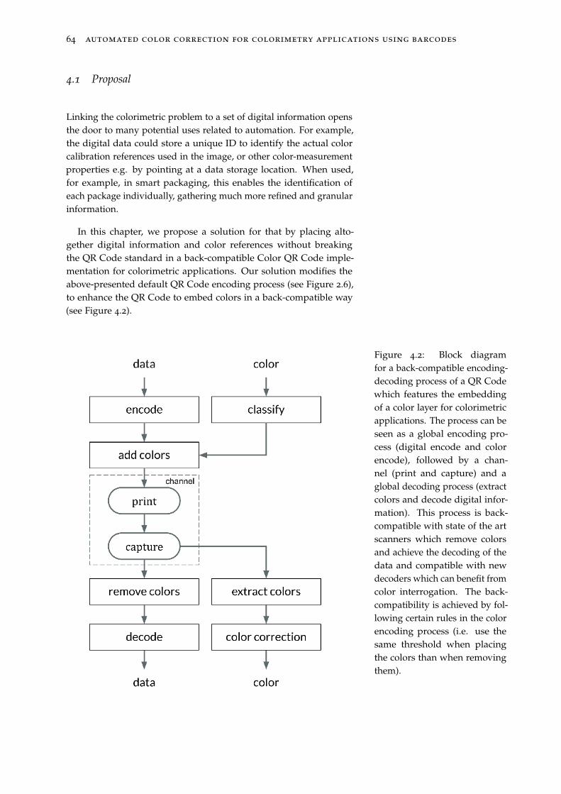
64 automated color correction for colorimetry applications using barcodes
4.1 Proposal
Linking the colorimetric problem to a set of digital information opensthe door to many potential uses related to automation. For example,the digital data could store a unique ID to identify the actual colorcalibration references used in the image, or other color-measurementproperties e.g. by pointing at a data storage location. When used,for example, in smart packaging, this enables the identification ofeach package individually, gathering much more refined and granularinformation.
In this chapter, we propose a solution for that by placing alto-gether digital information and color references without breakingthe QR Code standard in a back-compatible Color QR Code imple-mentation for colorimetric applications. Our solution modifies theabove-presented default QR Code encoding process (see Figure 2.6),to enhance the QR Code to embed colors in a back-compatible way(see Figure 4.2).
Figure 4.2: Block diagramfor a back-compatible encoding-decoding process of a QR Codewhich features the embeddingof a color layer for colorimetricapplications. The process can beseen as a global encoding pro-cess (digital encode and colorencode), followed by a chan-nel (print and capture) and aglobal decoding process (extractcolors and decode digital infor-mation). This process is back-compatible with state of the artscanners which remove colorsand achieve the decoding of thedata and compatible with newdecoders which can benefit fromcolor interrogation. The back-compatibility is achieved by fol-lowing certain rules in the colorencoding process (i.e. use thesame threshold when placingthe colors than when removingthem).
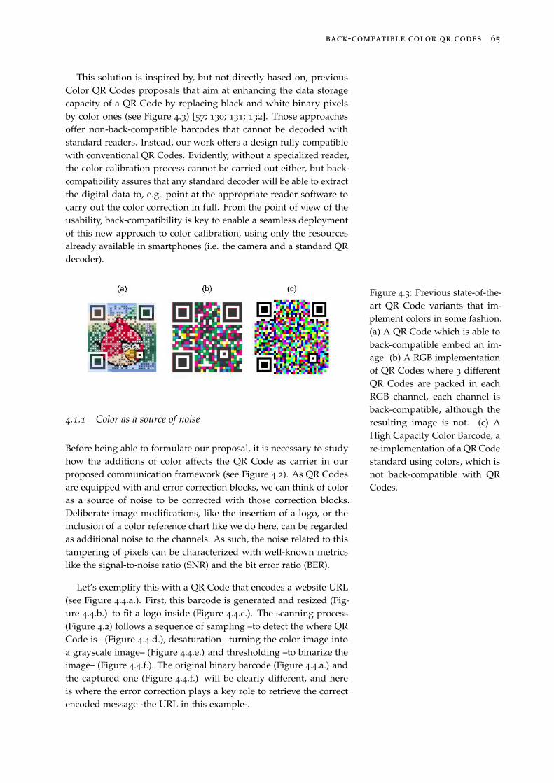
back-compatible color qr codes 65
This solution is inspired by, but not directly based on, previousColor QR Codes proposals that aim at enhancing the data storagecapacity of a QR Code by replacing black and white binary pixelsby color ones (see Figure 4.3) [57; 130; 131; 132]. Those approachesoffer non-back-compatible barcodes that cannot be decoded withstandard readers. Instead, our work offers a design fully compatiblewith conventional QR Codes. Evidently, without a specialized reader,the color calibration process cannot be carried out either, but back-compatibility assures that any standard decoder will be able to extractthe digital data to, e.g. point at the appropriate reader software tocarry out the color correction in full. From the point of view of theusability, back-compatibility is key to enable a seamless deploymentof this new approach to color calibration, using only the resourcesalready available in smartphones (i.e. the camera and a standard QRdecoder).
Figure 4.3: Previous state-of-the-art QR Code variants that im-plement colors in some fashion.(a) A QR Code which is able toback-compatible embed an im-age. (b) A RGB implementationof QR Codes where 3 differentQR Codes are packed in eachRGB channel, each channel isback-compatible, although theresulting image is not. (c) AHigh Capacity Color Barcode, are-implementation of a QR Codestandard using colors, which isnot back-compatible with QRCodes.
4.1.1 Color as a source of noise
Before being able to formulate our proposal, it is necessary to studyhow the additions of color affects the QR Code as carrier in ourproposed communication framework (see Figure 4.2). As QR Codesare equipped with and error correction blocks, we can think of coloras a source of noise to be corrected with those correction blocks.Deliberate image modifications, like the insertion of a logo, or theinclusion of a color reference chart like we do here, can be regardedas additional noise to the channels. As such, the noise related to thistampering of pixels can be characterized with well-known metricslike the signal-to-noise ratio (SNR) and the bit error ratio (BER).
Let’s exemplify this with a QR Code that encodes a website URL(see Figure 4.4.a.). First, this barcode is generated and resized (Fig-ure 4.4.b.) to fit a logo inside (Figure 4.4.c.). The scanning process(Figure 4.2) follows a sequence of sampling –to detect the where QRCode is– (Figure 4.4.d.), desaturation –turning the color image intoa grayscale image– (Figure 4.4.e.) and thresholding –to binarize theimage– (Figure 4.4.f.). The original binary barcode (Figure 4.4.a.) andthe captured one (Figure 4.4.f.) will be clearly different, and hereis where the error correction plays a key role to retrieve the correctencoded message -the URL in this example-.
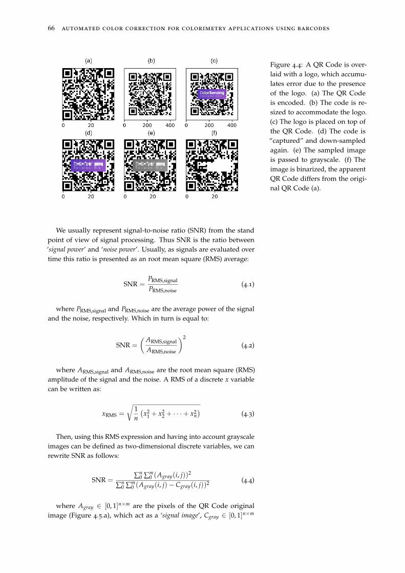
66 automated color correction for colorimetry applications using barcodes
Figure 4.4: A QR Code is over-laid with a logo, which accumu-lates error due to the presenceof the logo. (a) The QR Codeis encoded. (b) The code is re-sized to accommodate the logo.(c) The logo is placed on top ofthe QR Code. (d) The code is“captured” and down-sampledagain. (e) The sampled imageis passed to grayscale. (f) Theimage is binarized, the apparentQR Code differs from the origi-nal QR Code (a).
We usually represent signal-to-noise ratio (SNR) from the standpoint of view of signal processing. Thus SNR is the ratio between‘signal power’ and ‘noise power’. Usually, as signals are evaluated overtime this ratio is presented as an root mean square (RMS) average:
SNR =PRMS,signal
PRMS,noise(4.1)
where PRMS,signal and PRMS,noise are the average power of the signaland the noise, respectively. Which in turn is equal to:
SNR =
(
ARMS,signal
ARMS,noise
)2
(4.2)
where ARMS,signal and ARMS,noise are the root mean square (RMS)amplitude of the signal and the noise. A RMS of a discrete x variablecan be written as:
xRMS =
√
1n
(
x21 + x2
2 + · · ·+ x2n
)
(4.3)
Then, using this RMS expression and having into account grayscaleimages can be defined as two-dimensional discrete variables, we canrewrite SNR as follows:
SNR =∑
n0 ∑
m0 (Agray(i, j))2
∑n0 ∑
m0 (Agray(i, j)− Cgray(i, j))2 (4.4)
where Agray ∈ [0, 1]n×m are the pixels of the QR Code originalimage (Figure 4.5.a), which act as a ‘signal image’, Cgray ∈ [0, 1]n×m
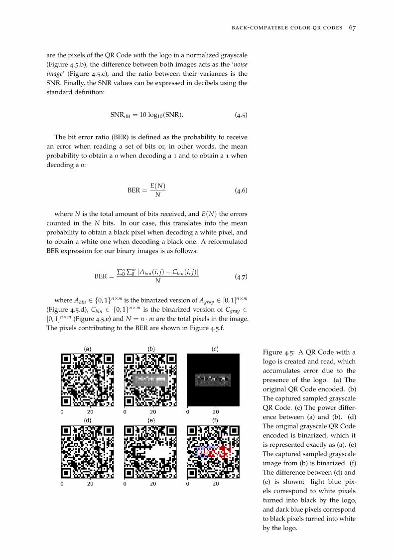
back-compatible color qr codes 67
are the pixels of the QR Code with the logo in a normalized grayscale(Figure 4.5.b), the difference between both images acts as the ‘noise
image’ (Figure 4.5.c), and the ratio between their variances is theSNR. Finally, the SNR values can be expressed in decibels using thestandard definition:
SNRdB = 10 log10(SNR). (4.5)
The bit error ratio (BER) is defined as the probability to receivean error when reading a set of bits or, in other words, the meanprobability to obtain a 0 when decoding a 1 and to obtain a 1 whendecoding a 0:
BER =E(N)
N(4.6)
where N is the total amount of bits received, and E(N) the errorscounted in the N bits. In our case, this translates into the meanprobability to obtain a black pixel when decoding a white pixel, andto obtain a white one when decoding a black one. A reformulatedBER expression for our binary images is as follows:
BER =∑
n0 ∑
m0 |Abin(i, j)− Cbin(i, j)|
N(4.7)
where Abin ∈ {0, 1}n×m is the binarized version of Agray ∈ [0, 1]n×m
(Figure 4.5.d), Cbin ∈ {0, 1}n×m is the binarized version of Cgray ∈[0, 1]n×m (Figure 4.5.e) and N = n ·m are the total pixels in the image.The pixels contributing to the BER are shown in Figure 4.5.f.
Figure 4.5: A QR Code with alogo is created and read, whichaccumulates error due to thepresence of the logo. (a) Theoriginal QR Code encoded. (b)The captured sampled grayscaleQR Code. (c) The power differ-ence between (a) and (b). (d)The original grayscale QR Codeencoded is binarized, which itis represented exactly as (a). (e)The captured sampled grayscaleimage from (b) is binarized. (f)The difference between (d) and(e) is shown: light blue pix-els correspond to white pixelsturned into black by the logo,and dark blue pixels correspondto black pixels turned into whiteby the logo.
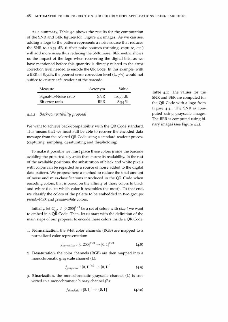
68 automated color correction for colorimetry applications using barcodes
As a summary, Table 4.1 shows the results for the computationof the SNR and BER figures for Figure 4.4 images. As we can see,adding a logo to the pattern represents a noise source that reducesthe SNR to 10.53 dB, further noise sources (printing, capture, etc.)will add more noise thus reducing the SNR more. BER metric showsus the impact of the logo when recovering the digital bits, as wehave mentioned before this quantity is directly related to the errorcorrection level needed to encode the QR Code. In this example, witha BER of 8.54%, the poorest error correction level (L, 7%) would notsuffice to ensure safe readout of the barcode.
Measure Acronym Value
Signal-to-Noise ratio SNR 10.53 dBBit error ratio BER 8.54 %
Table 4.1: The values for theSNR and BER are computed forthe QR Code with a logo fromFigure 4.4. The SNR is com-puted using grayscale images.The BER is computed using bi-nary images (see Figure 4.4).
4.1.2 Back-compatibility proposal
We want to achieve back-compatibility with the QR Code standard.This means that we must still be able to recover the encoded datamessage from the colored QR Code using a standard readout process(capturing, sampling, desaturating and thresholding).
To make it possible we must place these colors inside the barcodeavoiding the protected key areas that ensure its readability. In the restof the available positions, the substitution of black and white pixelswith colors can be regarded as a source of noise added to the digitaldata pattern. We propose here a method to reduce the total amountof noise and miss-classifications introduced in the QR Code whenencoding colors, that is based on the affinity of those colors to blackand white (i.e. to which color it resembles the most). To that end,we classify the colors of the palette to be embedded in two groups:pseudo-black and pseudo-white colors.
Initially, let G′rgb ∈ [0, 255]l×3 be a set of colors with size l we wantto embed in a QR Code. Then, let us start with the definition of themain steps of our proposal to encode these colors inside a QR Code:
1. Normalization, the 8-bit color channels (RGB) are mapped to anormalized color representation:
fnormalize : [0, 255]l×3 → [0, 1]l×3 (4.8)
2. Desaturation, the color channels (RGB) are then mapped into amonochromatic grayscale channel (L):
fgrayscale : [0, 1]l×3 → [0, 1]l (4.9)
3. Binarization, the monochromatic grayscale channel (L) is con-verted to a monochromatic binary channel (B):
fthreshold : [0, 1]l → {0, 1}l (4.10)
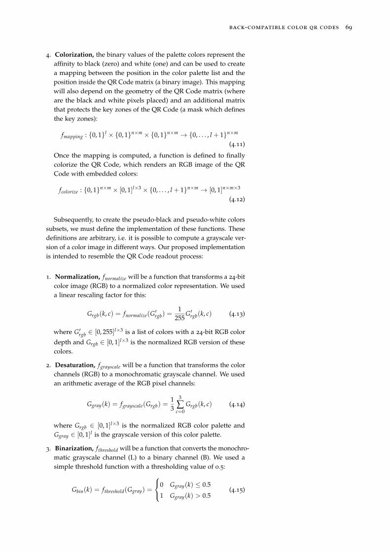
back-compatible color qr codes 69
4. Colorization, the binary values of the palette colors represent theaffinity to black (zero) and white (one) and can be used to createa mapping between the position in the color palette list and theposition inside the QR Code matrix (a binary image). This mappingwill also depend on the geometry of the QR Code matrix (whereare the black and white pixels placed) and an additional matrixthat protects the key zones of the QR Code (a mask which definesthe key zones):
fmapping : {0, 1}l × {0, 1}n×m × {0, 1}n×m → {0, . . . , l + 1}n×m
(4.11)
Once the mapping is computed, a function is defined to finallycolorize the QR Code, which renders an RGB image of the QRCode with embedded colors:
fcolorize : {0, 1}n×m × [0, 1]l×3 × {0, . . . , l + 1}n×m → [0, 1]n×m×3
(4.12)
Subsequently, to create the pseudo-black and pseudo-white colorssubsets, we must define the implementation of these functions. Thesedefinitions are arbitrary, i.e. it is possible to compute a grayscale ver-sion of a color image in different ways. Our proposed implementationis intended to resemble the QR Code readout process:
1. Normalization, fnormalize will be a function that transforms a 24-bitcolor image (RGB) to a normalized color representation. We useda linear rescaling factor for this:
Grgb(k, c) = fnormalize(G′rgb) =
1255
G′rgb(k, c) (4.13)
where G′rgb ∈ [0, 255]l×3 is a list of colors with a 24-bit RGB color
depth and Grgb ∈ [0, 1]l×3 is the normalized RGB version of thesecolors.
2. Desaturation, fgrayscale will be a function that transforms the colorchannels (RGB) to a monochromatic grayscale channel. We usedan arithmetic average of the RGB pixel channels:
Ggray(k) = fgrayscale(Grgb) =13
3
∑c=0
Grgb(k, c) (4.14)
where Grgb ∈ [0, 1]l×3 is the normalized RGB color palette andGgray ∈ [0, 1]l is the grayscale version of this color palette.
3. Binarization, fthreshold will be a function that converts the monochro-matic grayscale channel (L) to a binary channel (B). We used asimple threshold function with a thresholding value of 0.5:
Gbin(k) = fthreshold(Ggray) =
0 Ggray(k) ≤ 0.5
1 Ggray(k) > 0.5(4.15)
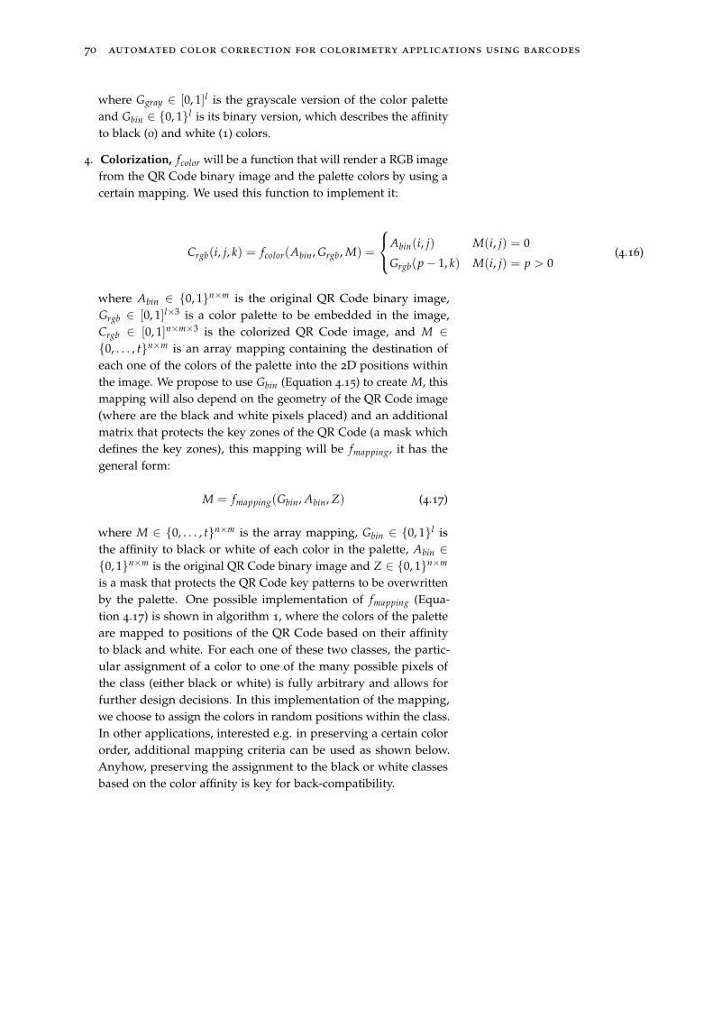
70 automated color correction for colorimetry applications using barcodes
where Ggray ∈ [0, 1]l is the grayscale version of the color paletteand Gbin ∈ {0, 1}l is its binary version, which describes the affinityto black (0) and white (1) colors.
4. Colorization, fcolor will be a function that will render a RGB imagefrom the QR Code binary image and the palette colors by using acertain mapping. We used this function to implement it:
Crgb(i, j, k) = fcolor(Abin, Grgb, M) =
Abin(i, j) M(i, j) = 0
Grgb(p− 1, k) M(i, j) = p > 0(4.16)
where Abin ∈ {0, 1}n×m is the original QR Code binary image,Grgb ∈ [0, 1]l×3 is a color palette to be embedded in the image,Crgb ∈ [0, 1]n×m×3 is the colorized QR Code image, and M ∈{0, . . . , t}n×m is an array mapping containing the destination ofeach one of the colors of the palette into the 2D positions withinthe image. We propose to use Gbin (Equation 4.15) to create M, thismapping will also depend on the geometry of the QR Code image(where are the black and white pixels placed) and an additionalmatrix that protects the key zones of the QR Code (a mask whichdefines the key zones), this mapping will be fmapping, it has thegeneral form:
M = fmapping(Gbin, Abin, Z) (4.17)
where M ∈ {0, . . . , t}n×m is the array mapping, Gbin ∈ {0, 1}l isthe affinity to black or white of each color in the palette, Abin ∈{0, 1}n×m is the original QR Code binary image and Z ∈ {0, 1}n×m
is a mask that protects the QR Code key patterns to be overwrittenby the palette. One possible implementation of fmapping (Equa-tion 4.17) is shown in algorithm 1, where the colors of the paletteare mapped to positions of the QR Code based on their affinityto black and white. For each one of these two classes, the partic-ular assignment of a color to one of the many possible pixels ofthe class (either black or white) is fully arbitrary and allows forfurther design decisions. In this implementation of the mapping,we choose to assign the colors in random positions within the class.In other applications, interested e.g. in preserving a certain colororder, additional mapping criteria can be used as shown below.Anyhow, preserving the assignment to the black or white classesbased on the color affinity is key for back-compatibility.
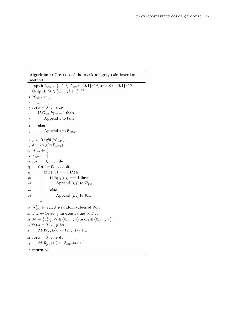
back-compatible color qr codes 71
Algorithm 1: Creation of the mask for grayscale insertionmethod
Input: Gbin ∈ {0, 1}l , Abin ∈ {0, 1}n×m, and Z ∈ {0, 1}n×m
Output: M ∈ {0, . . . , l + 1}n×m
1 Wcolor ← []
2 Bcolor ← []
3 for k = 0, . . . , l do
4 if Gbin(k) == 1 then
5 Append k to Wcolor
6 else
7 Append k to Bcolor
8 p← lenght(Wcolor)
9 q← lenght(Bcolor)
10 Wpos ← []
11 Bpos ← []
12 for i = 0, . . . , n do
13 for j = 0, . . . , m do
14 if Z(i, j) == 1 then
15 if Abin(i, j) == 1 then
16 Append (i, j) to Wpos
17 else
18 Append (i, j) to Bpos
19 W ′pos ← Select p random values of Wpos
20 B′pos ← Select q random values of Bpos
21 M← {0}i,j ∀i ∈ {0, . . . , n} and j ∈ {0, . . . , m}22 for k = 0, . . . , p do
23 M(W ′pos(k))←Wcolor(k) + 1
24 for k = 0, . . . , q do
25 M(B′pos(k))← Bcolor(k) + 1
26 return M
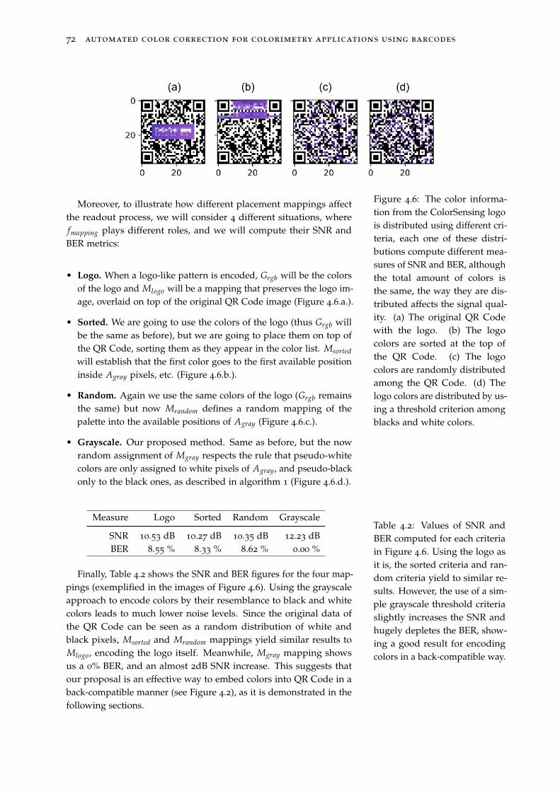
72 automated color correction for colorimetry applications using barcodes
Figure 4.6: The color informa-tion from the ColorSensing logois distributed using different cri-teria, each one of these distri-butions compute different mea-sures of SNR and BER, althoughthe total amount of colors isthe same, the way they are dis-tributed affects the signal qual-ity. (a) The original QR Codewith the logo. (b) The logocolors are sorted at the top ofthe QR Code. (c) The logocolors are randomly distributedamong the QR Code. (d) Thelogo colors are distributed by us-ing a threshold criterion amongblacks and white colors.
Moreover, to illustrate how different placement mappings affectthe readout process, we will consider 4 different situations, wherefmapping plays different roles, and we will compute their SNR andBER metrics:
• Logo. When a logo-like pattern is encoded, Grgb will be the colorsof the logo and Mlogo will be a mapping that preserves the logo im-age, overlaid on top of the original QR Code image (Figure 4.6.a.).
• Sorted. We are going to use the colors of the logo (thus Grgb willbe the same as before), but we are going to place them on top ofthe QR Code, sorting them as they appear in the color list. Msorted
will establish that the first color goes to the first available positioninside Agray pixels, etc. (Figure 4.6.b.).
• Random. Again we use the same colors of the logo (Grgb remainsthe same) but now Mrandom defines a random mapping of thepalette into the available positions of Agray (Figure 4.6.c.).
• Grayscale. Our proposed method. Same as before, but the nowrandom assignment of Mgray respects the rule that pseudo-whitecolors are only assigned to white pixels of Agray, and pseudo-blackonly to the black ones, as described in algorithm 1 (Figure 4.6.d.).
Measure Logo Sorted Random Grayscale
SNR 10.53 dB 10.27 dB 10.35 dB 12.23 dBBER 8.55 % 8.33 % 8.62 % 0.00 %
Table 4.2: Values of SNR andBER computed for each criteriain Figure 4.6. Using the logo asit is, the sorted criteria and ran-dom criteria yield to similar re-sults. However, the use of a sim-ple grayscale threshold criteriaslightly increases the SNR andhugely depletes the BER, show-ing a good result for encodingcolors in a back-compatible way.
Finally, Table 4.2 shows the SNR and BER figures for the four map-pings (exemplified in the images of Figure 4.6). Using the grayscaleapproach to encode colors by their resemblance to black and whitecolors leads to much lower noise levels. Since the original data ofthe QR Code can be seen as a random distribution of white andblack pixels, Msorted and Mrandom mappings yield similar results toMlogo, encoding the logo itself. Meanwhile, Mgray mapping showsus a 0% BER, and an almost 2dB SNR increase. This suggests thatour proposal is an effective way to embed colors into QR Code in aback-compatible manner (see Figure 4.2), as it is demonstrated in thefollowing sections.
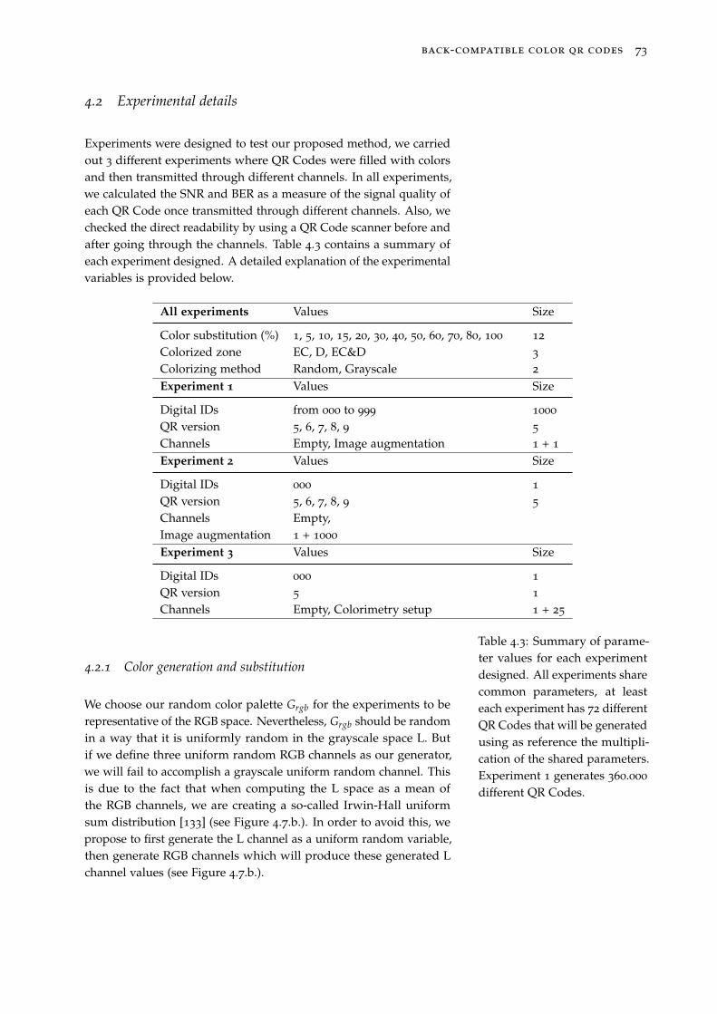
back-compatible color qr codes 73
4.2 Experimental details
Experiments were designed to test our proposed method, we carriedout 3 different experiments where QR Codes were filled with colorsand then transmitted through different channels. In all experiments,we calculated the SNR and BER as a measure of the signal quality ofeach QR Code once transmitted through different channels. Also, wechecked the direct readability by using a QR Code scanner before andafter going through the channels. Table 4.3 contains a summary ofeach experiment designed. A detailed explanation of the experimentalvariables is provided below.
All experiments Values Size
Color substitution (%) 1, 5, 10, 15, 20, 30, 40, 50, 60, 70, 80, 100 12
Colorized zone EC, D, EC&D 3
Colorizing method Random, Grayscale 2
Experiment 1 Values Size
Digital IDs from 000 to 999 1000
QR version 5, 6, 7, 8, 9 5
Channels Empty, Image augmentation 1 + 1
Experiment 2 Values Size
Digital IDs 000 1
QR version 5, 6, 7, 8, 9 5
Channels Empty,Image augmentation 1 + 1000
Experiment 3 Values Size
Digital IDs 000 1
QR version 5 1
Channels Empty, Colorimetry setup 1 + 25
Table 4.3: Summary of parame-ter values for each experimentdesigned. All experiments sharecommon parameters, at leasteach experiment has 72 differentQR Codes that will be generatedusing as reference the multipli-cation of the shared parameters.Experiment 1 generates 360.000
different QR Codes.
4.2.1 Color generation and substitution
We choose our random color palette Grgb for the experiments to berepresentative of the RGB space. Nevertheless, Grgb should be randomin a way that it is uniformly random in the grayscale space L. Butif we define three uniform random RGB channels as our generator,we will fail to accomplish a grayscale uniform random channel. Thisis due to the fact that when computing the L space as a mean ofthe RGB channels, we are creating a so-called Irwin-Hall uniformsum distribution [133] (see Figure 4.7.b.). In order to avoid this, wepropose to first generate the L channel as a uniform random variable,then generate RGB channels which will produce these generated Lchannel values (see Figure 4.7.b.).
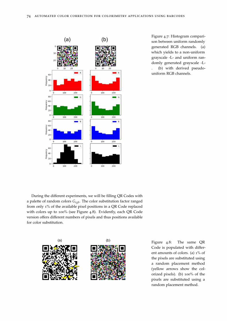
74 automated color correction for colorimetry applications using barcodes
Figure 4.7: Histogram compari-son between uniform randomlygenerated RGB channels. (a)which yields to a non-uniformgrayscale -L- and uniform ran-domly generated grayscale -L-. (b) with derived pseudo-uniform RGB channels.
During the different experiments, we will be filling QR Codes witha palette of random colors Grgb. The color substitution factor rangedfrom only 1% of the available pixel positions in a QR Code replacedwith colors up to 100% (see Figure 4.8). Evidently, each QR Codeversion offers different numbers of pixels and thus positions availablefor color substitution.
Figure 4.8: The same QRCode is populated with differ-ent amounts of colors. (a) 1% ofthe pixels are substituted usinga random placement method(yellow arrows show the col-orized pixels). (b) 100% of thepixels are substituted using arandom placement method.
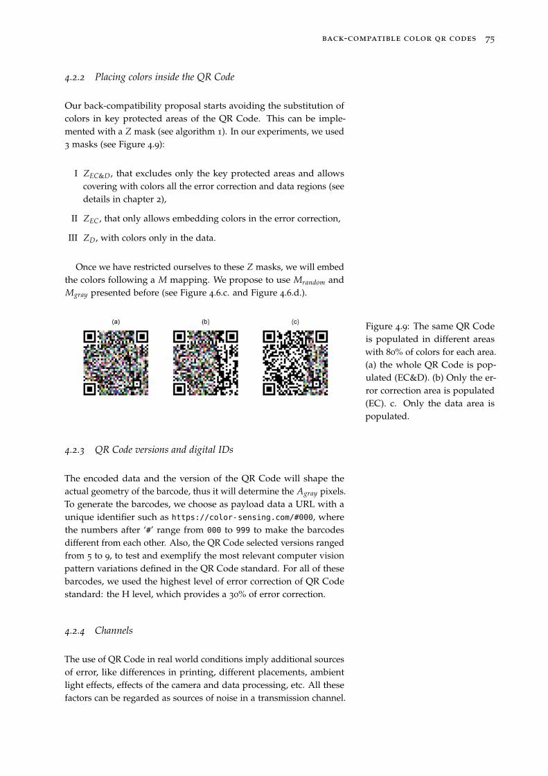
back-compatible color qr codes 75
4.2.2 Placing colors inside the QR Code
Our back-compatibility proposal starts avoiding the substitution ofcolors in key protected areas of the QR Code. This can be imple-mented with a Z mask (see algorithm 1). In our experiments, we used3 masks (see Figure 4.9):
I ZEC&D, that excludes only the key protected areas and allowscovering with colors all the error correction and data regions (seedetails in chapter 2),
II ZEC, that only allows embedding colors in the error correction,
III ZD, with colors only in the data.
Once we have restricted ourselves to these Z masks, we will embedthe colors following a M mapping. We propose to use Mrandom andMgray presented before (see Figure 4.6.c. and Figure 4.6.d.).
Figure 4.9: The same QR Codeis populated in different areaswith 80% of colors for each area.(a) the whole QR Code is pop-ulated (EC&D). (b) Only the er-ror correction area is populated(EC). c. Only the data area ispopulated.
4.2.3 QR Code versions and digital IDs
The encoded data and the version of the QR Code will shape theactual geometry of the barcode, thus it will determine the Agray pixels.To generate the barcodes, we choose as payload data a URL with aunique identifier such as https://color-sensing.com/#000, wherethe numbers after ‘#’ range from 000 to 999 to make the barcodesdifferent from each other. Also, the QR Code selected versions rangedfrom 5 to 9, to test and exemplify the most relevant computer visionpattern variations defined in the QR Code standard. For all of thesebarcodes, we used the highest level of error correction of QR Codestandard: the H level, which provides a 30% of error correction.
4.2.4 Channels
The use of QR Code in real world conditions imply additional sourcesof error, like differences in printing, different placements, ambientlight effects, effects of the camera and data processing, etc. All thesefactors can be regarded as sources of noise in a transmission channel.
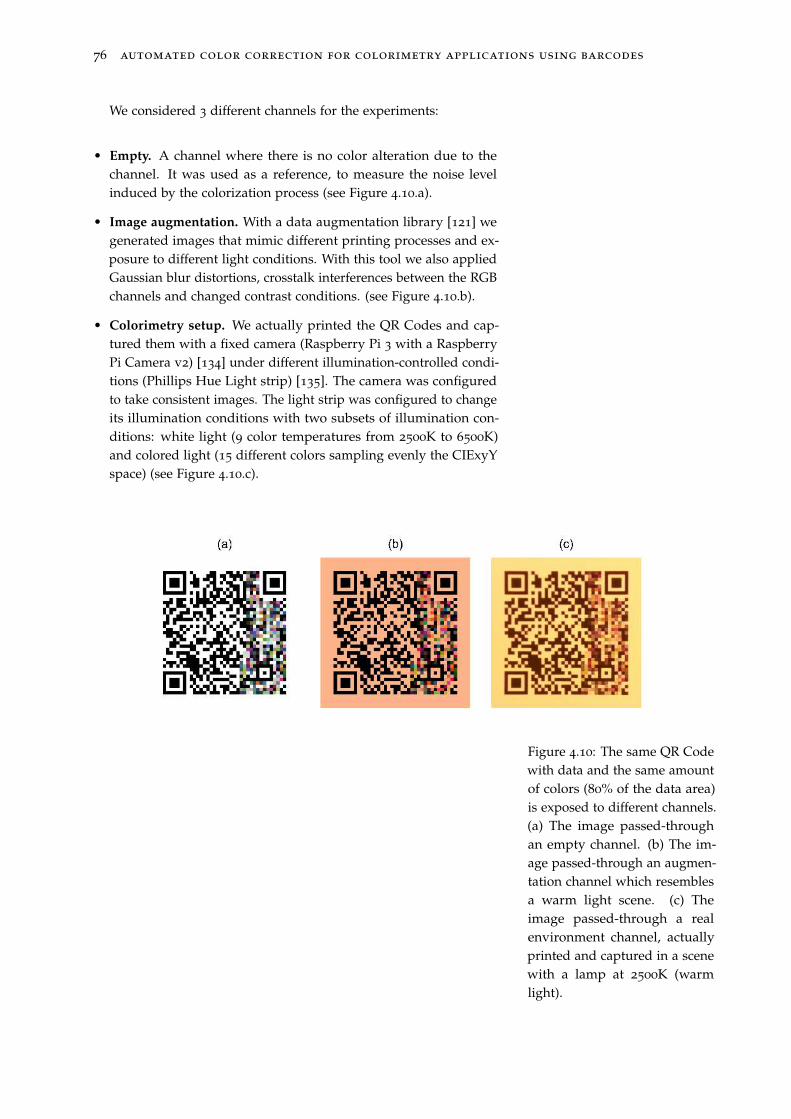
76 automated color correction for colorimetry applications using barcodes
We considered 3 different channels for the experiments:
• Empty. A channel where there is no color alteration due to thechannel. It was used as a reference, to measure the noise levelinduced by the colorization process (see Figure 4.10.a).
• Image augmentation. With a data augmentation library [121] wegenerated images that mimic different printing processes and ex-posure to different light conditions. With this tool we also appliedGaussian blur distortions, crosstalk interferences between the RGBchannels and changed contrast conditions. (see Figure 4.10.b).
• Colorimetry setup. We actually printed the QR Codes and cap-tured them with a fixed camera (Raspberry Pi 3 with a RaspberryPi Camera v2) [134] under different illumination-controlled condi-tions (Phillips Hue Light strip) [135]. The camera was configuredto take consistent images. The light strip was configured to changeits illumination conditions with two subsets of illumination con-ditions: white light (9 color temperatures from 2500K to 6500K)and colored light (15 different colors sampling evenly the CIExyYspace) (see Figure 4.10.c).
Figure 4.10: The same QR Codewith data and the same amountof colors (80% of the data area)is exposed to different channels.(a) The image passed-throughan empty channel. (b) The im-age passed-through an augmen-tation channel which resemblesa warm light scene. (c) Theimage passed-through a realenvironment channel, actuallyprinted and captured in a scenewith a lamp at 2500K (warmlight).
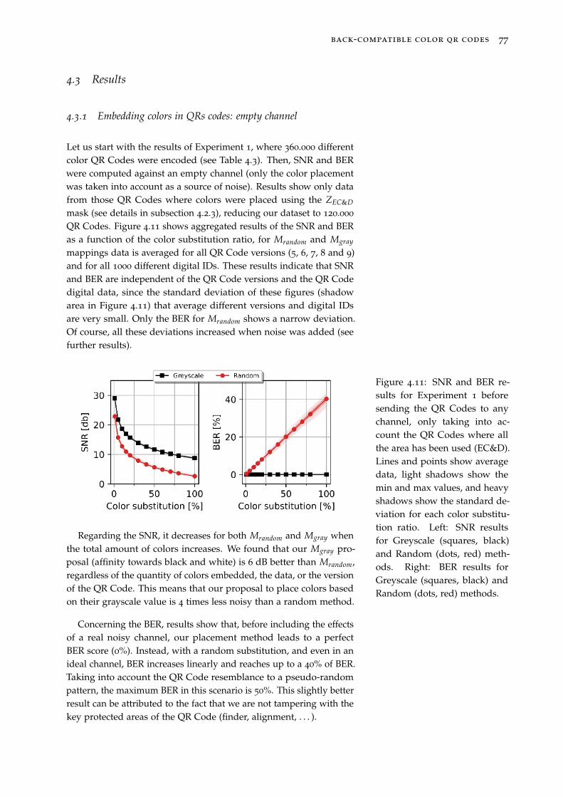
back-compatible color qr codes 77
4.3 Results
4.3.1 Embedding colors in QRs codes: empty channel
Let us start with the results of Experiment 1, where 360.000 differentcolor QR Codes were encoded (see Table 4.3). Then, SNR and BERwere computed against an empty channel (only the color placementwas taken into account as a source of noise). Results show only datafrom those QR Codes where colors were placed using the ZEC&D
mask (see details in subsection 4.2.3), reducing our dataset to 120.000
QR Codes. Figure 4.11 shows aggregated results of the SNR and BERas a function of the color substitution ratio, for Mrandom and Mgray
mappings data is averaged for all QR Code versions (5, 6, 7, 8 and 9)and for all 1000 different digital IDs. These results indicate that SNRand BER are independent of the QR Code versions and the QR Codedigital data, since the standard deviation of these figures (shadowarea in Figure 4.11) that average different versions and digital IDsare very small. Only the BER for Mrandom shows a narrow deviation.Of course, all these deviations increased when noise was added (seefurther results).
Figure 4.11: SNR and BER re-sults for Experiment 1 beforesending the QR Codes to anychannel, only taking into ac-count the QR Codes where allthe area has been used (EC&D).Lines and points show averagedata, light shadows show themin and max values, and heavyshadows show the standard de-viation for each color substitu-tion ratio. Left: SNR resultsfor Greyscale (squares, black)and Random (dots, red) meth-ods. Right: BER results forGreyscale (squares, black) andRandom (dots, red) methods.
Regarding the SNR, it decreases for both Mrandom and Mgray whenthe total amount of colors increases. We found that our Mgray pro-posal (affinity towards black and white) is 6 dB better than Mrandom,regardless of the quantity of colors embedded, the data, or the versionof the QR Code. This means that our proposal to place colors basedon their grayscale value is 4 times less noisy than a random method.
Concerning the BER, results show that, before including the effectsof a real noisy channel, our placement method leads to a perfectBER score (0%). Instead, with a random substitution, and even in anideal channel, BER increases linearly and reaches up to a 40% of BER.Taking into account the QR Code resemblance to a pseudo-randompattern, the maximum BER in this scenario is 50%. This slightly betterresult can be attributed to the fact that we are not tampering with thekey protected areas of the QR Code (finder, alignment, . . . ).
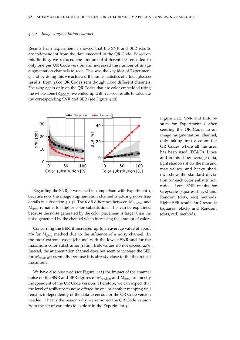
78 automated color correction for colorimetry applications using barcodes
4.3.2 Image augmentation channel
Results from Experiment 1 showed that the SNR and BER resultsare independent from the data encoded in the QR Code. Based onthis finding, we reduced the amount of different IDs encoded toonly one per QR Code version and increased the number of imageaugmentation channels to 1000. This was the key idea of Experiment2, and by doing this we achieved the same statistics of a total 360.000
results, from 3.600 QR Codes sent though 1.000 different channels.Focusing again only on the QR Codes that are color embedded usingthe whole zone (ZEC&D) we ended up with 120.000 results to calculatethe corresponding SNR and BER (see Figure 4.12).
Figure 4.12: SNR and BER re-sults for Experiment 2 aftersending the QR Codes to animage augmentation channel,only taking into account theQR Codes where all the areahas been used (EC&D). Linesand points show average data,light shadows show the min andmax values, and heavy shad-ows show the standard devia-tion for each color substitutionratio. Left: SNR results forGreyscale (squares, black) andRandom (dots, red) methods.Right: BER results for Greyscale(squares, black) and Random(dots, red) methods.
Regarding the SNR, it worsened in comparison with Experiment 1,because now the image augmentation channel is adding noise (seedetails in subsection 4.2.4). The 6 dB difference between Mrandom andMgray remains for higher color substitution. This can be explainedbecause the noise generated by the color placement is larger than thenoise generated by the channel when increasing the amount of colors.
Concerning the BER, it increased up to an average value of about7% for Mgray method due to the influence of a noisy channel. Inthe most extreme cases (channel with the lowest SNR and for themaximum color substitution ratio), BER values do not exceed 20%.Instead, the augmentation channel does not seem to increase the BERfor Mrandom; essentially because it is already close to the theoreticalmaximum.
We have also observed (see Figure 4.13) the impact of the channelnoise on the SNR and BER figures of Mrandom and Mgray are mostlyindependent of the QR Code version. Therefore, we can expect thatthe level of resilience to noise offered by one or another mapping willremain, independently of the data to encode or the QR Code versionneeded. That is the reason why we removed the QR Code versionfrom the set of variables to explore in the Experiment 3.
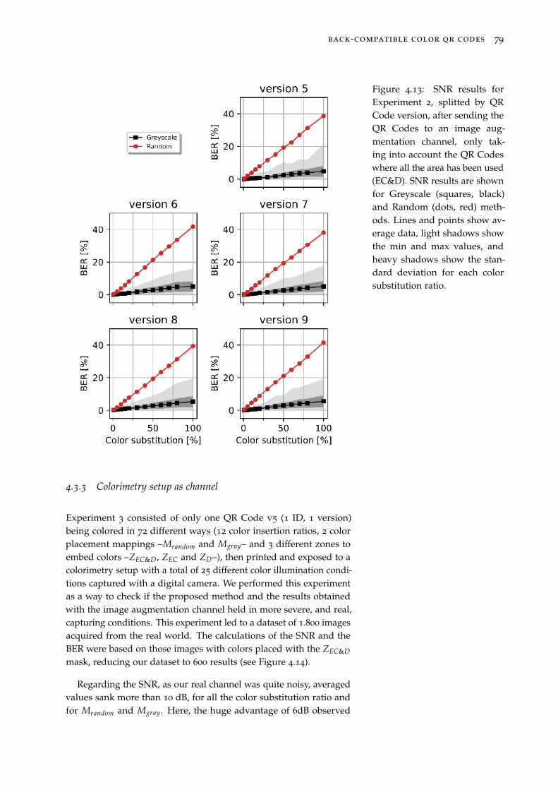
back-compatible color qr codes 79
Figure 4.13: SNR results forExperiment 2, splitted by QRCode version, after sending theQR Codes to an image aug-mentation channel, only tak-ing into account the QR Codeswhere all the area has been used(EC&D). SNR results are shownfor Greyscale (squares, black)and Random (dots, red) meth-ods. Lines and points show av-erage data, light shadows showthe min and max values, andheavy shadows show the stan-dard deviation for each colorsubstitution ratio.
4.3.3 Colorimetry setup as channel
Experiment 3 consisted of only one QR Code v5 (1 ID, 1 version)being colored in 72 different ways (12 color insertion ratios, 2 colorplacement mappings –Mrandom and Mgray– and 3 different zones toembed colors –ZEC&D, ZEC and ZD–), then printed and exposed to acolorimetry setup with a total of 25 different color illumination condi-tions captured with a digital camera. We performed this experimentas a way to check if the proposed method and the results obtainedwith the image augmentation channel held in more severe, and real,capturing conditions. This experiment led to a dataset of 1.800 imagesacquired from the real world. The calculations of the SNR and theBER were based on those images with colors placed with the ZEC&D
mask, reducing our dataset to 600 results (see Figure 4.14).
Regarding the SNR, as our real channel was quite noisy, averagedvalues sank more than 10 dB, for all the color substitution ratio andfor Mrandom and Mgray. Here, the huge advantage of 6dB observed
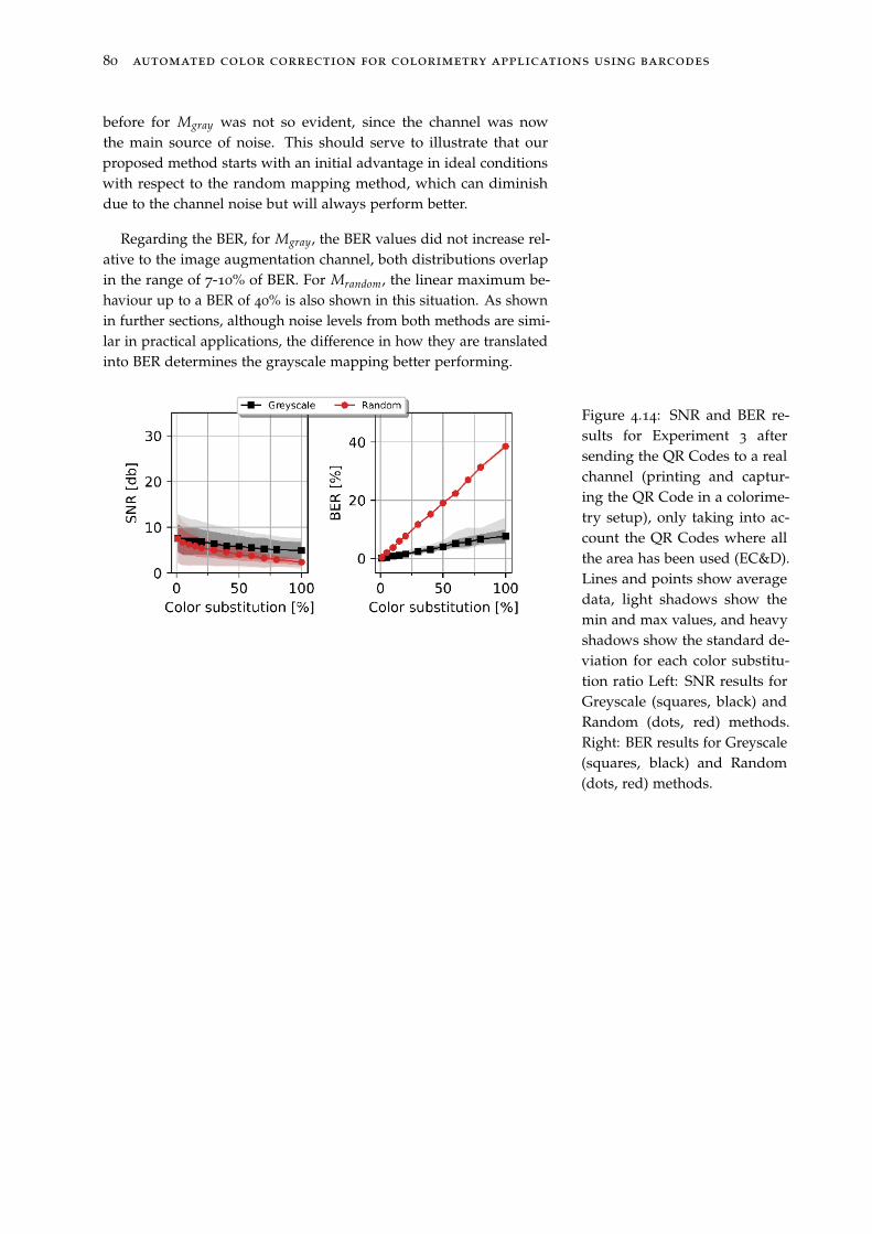
80 automated color correction for colorimetry applications using barcodes
before for Mgray was not so evident, since the channel was nowthe main source of noise. This should serve to illustrate that ourproposed method starts with an initial advantage in ideal conditionswith respect to the random mapping method, which can diminishdue to the channel noise but will always perform better.
Regarding the BER, for Mgray, the BER values did not increase rel-ative to the image augmentation channel, both distributions overlapin the range of 7-10% of BER. For Mrandom, the linear maximum be-haviour up to a BER of 40% is also shown in this situation. As shownin further sections, although noise levels from both methods are simi-lar in practical applications, the difference in how they are translatedinto BER determines the grayscale mapping better performing.
Figure 4.14: SNR and BER re-sults for Experiment 3 aftersending the QR Codes to a realchannel (printing and captur-ing the QR Code in a colorime-try setup), only taking into ac-count the QR Codes where allthe area has been used (EC&D).Lines and points show averagedata, light shadows show themin and max values, and heavyshadows show the standard de-viation for each color substitu-tion ratio Left: SNR results forGreyscale (squares, black) andRandom (dots, red) methods.Right: BER results for Greyscale(squares, black) and Random(dots, red) methods.
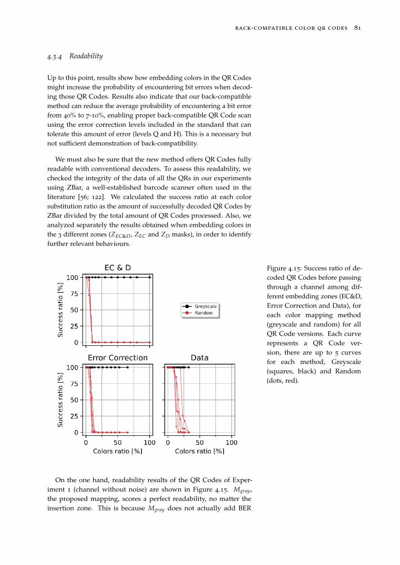
back-compatible color qr codes 81
4.3.4 Readability
Up to this point, results show how embedding colors in the QR Codesmight increase the probability of encountering bit errors when decod-ing those QR Codes. Results also indicate that our back-compatiblemethod can reduce the average probability of encountering a bit errorfrom 40% to 7-10%, enabling proper back-compatible QR Code scanusing the error correction levels included in the standard that cantolerate this amount of error (levels Q and H). This is a necessary butnot sufficient demonstration of back-compatibility.
We must also be sure that the new method offers QR Codes fullyreadable with conventional decoders. To assess this readability, wechecked the integrity of the data of all the QRs in our experimentsusing ZBar, a well-established barcode scanner often used in theliterature [56; 122]. We calculated the success ratio at each colorsubstitution ratio as the amount of successfully decoded QR Codes byZBar divided by the total amount of QR Codes processed. Also, weanalyzed separately the results obtained when embedding colors inthe 3 different zones (ZEC&D, ZEC and ZD masks), in order to identifyfurther relevant behaviours.
Figure 4.15: Success ratio of de-coded QR Codes before passingthrough a channel among dif-ferent embedding zones (EC&D,Error Correction and Data), foreach color mapping method(greyscale and random) for allQR Code versions. Each curverepresents a QR Code ver-sion, there are up to 5 curvesfor each method, Greyscale(squares, black) and Random(dots, red).
On the one hand, readability results of the QR Codes of Exper-iment 1 (channel without noise) are shown in Figure 4.15. Mgray,the proposed mapping, scores a perfect readability, no matter theinsertion zone. This is because Mgray does not actually add BER
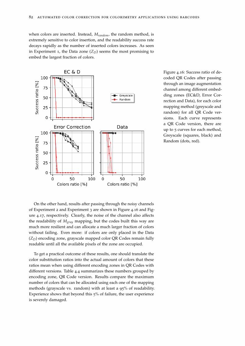
82 automated color correction for colorimetry applications using barcodes
when colors are inserted. Instead, Mrandom, the random method, isextremely sensitive to color insertion, and the readability success ratedecays rapidly as the number of inserted colors increases. As seenin Experiment 1, the Data zone (ZD) seems the most promising toembed the largest fraction of colors.
Figure 4.16: Success ratio of de-coded QR Codes after passingthrough an image augmentationchannel among different embed-ding zones (EC&D, Error Cor-rection and Data), for each colormapping method (greyscale andrandom) for all QR Code ver-sions. Each curve representsa QR Code version, there areup to 5 curves for each method,Greyscale (squares, black) andRandom (dots, red).
On the other hand, results after passing through the noisy channelsof Experiment 2 and Experiment 3 are shown in Figure 4.16 and Fig-ure 4.17, respectively. Clearly, the noise of the channel also affectsthe readability of Mgray mapping, but the codes built this way aremuch more resilient and can allocate a much larger fraction of colorswithout failing. Even more: if colors are only placed in the Data(ZD) encoding zone, grayscale mapped color QR Codes remain fullyreadable until all the available pixels of the zone are occupied.
To get a practical outcome of these results, one should translate thecolor substitution ratios into the actual amount of colors that theseratios mean when using different encoding zones in QR Codes withdifferent versions. Table 4.4 summarizes these numbers grouped byencoding zone, QR Code version. Results compare the maximumnumber of colors that can be allocated using each one of the mappingmethods (grayscale vs. random) with at least a 95% of readability.Experience shows that beyond this 5% of failure, the user experienceis severely damaged.
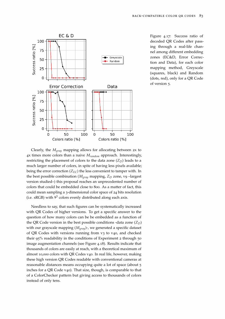
back-compatible color qr codes 83
Figure 4.17: Success ratio ofdecoded QR Codes after pass-ing through a real-life chan-nel among different embeddingzones (EC&D, Error Correc-tion and Data), for each colormapping method, Greyscale(squares, black) and Random(dots, red), only for a QR Codeof version 5.
Clearly, the Mgray mapping allows for allocating between 2x to4x times more colors than a naive Mrandom approach. Interestingly,restricting the placement of colors to the data zone (ZD) leads to amuch larger number of colors, in spite of having less pixels available;being the error correction (ZEC) the less convenient to tamper with. Inthe best possible combination (Mgray mapping, ZD zone, v9 –largestversion studied–) this proposal reaches an unprecedented number ofcolors that could be embedded close to 800. As a matter of fact, thiscould mean sampling a 3-dimensional color space of 24 bits resolution(i.e. sRGB) with 93 colors evenly distributed along each axis.
Needless to say, that such figures can be systematically increasedwith QR Codes of higher versions. To get a specific answer to thequestion of how many colors can be be embedded as a function ofthe QR Code version in the best possible conditions -data zone (ZD)with our grayscale mapping (Mgray)-, we generated a specific datasetof QR Codes with versions running from v3 to v40, and checkedtheir 95% readability in the conditions of Experiment 2 through 50
image augmentation channels (see Figure 4.18). Results indicate thatthousands of colors are easily at reach, with a theoretical maximum ofalmost 10,000 colors with QR Codes v40. In real life, however, makingthese high version QR Codes readable with conventional cameras atreasonable distances means occupying quite a lot of space (about 5
inches for a QR Code v40). That size, though, is comparable to thatof a ColorChecker pattern but giving access to thousands of colorsinstead of only tens.
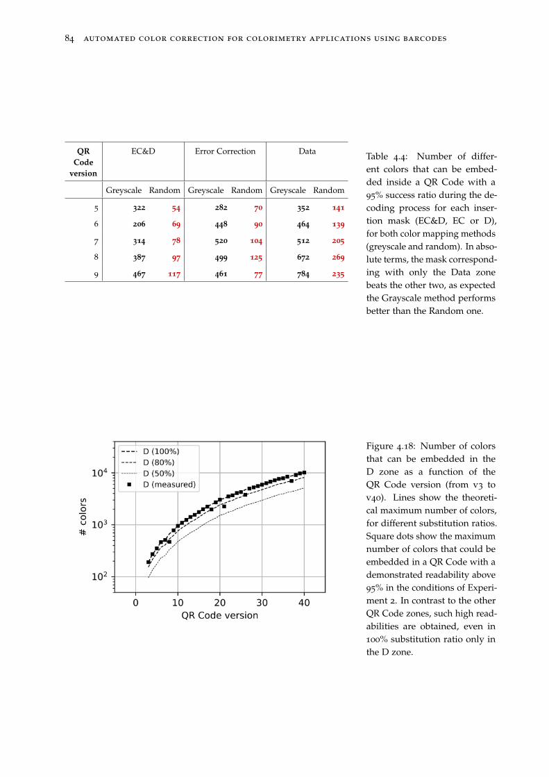
84 automated color correction for colorimetry applications using barcodes
QR
Code
version
EC&D Error Correction Data
Greyscale Random Greyscale Random Greyscale Random
5 322 54 282 70 352 141
6 206 69 448 90 464 139
7 314 78 520 104 512 205
8 387 97 499 125 672 269
9 467 117 461 77 784 235
Table 4.4: Number of differ-ent colors that can be embed-ded inside a QR Code with a95% success ratio during the de-coding process for each inser-tion mask (EC&D, EC or D),for both color mapping methods(greyscale and random). In abso-lute terms, the mask correspond-ing with only the Data zonebeats the other two, as expectedthe Grayscale method performsbetter than the Random one.
Figure 4.18: Number of colorsthat can be embedded in theD zone as a function of theQR Code version (from v3 tov40). Lines show the theoreti-cal maximum number of colors,for different substitution ratios.Square dots show the maximumnumber of colors that could beembedded in a QR Code with ademonstrated readability above95% in the conditions of Experi-ment 2. In contrast to the otherQR Code zones, such high read-abilities are obtained, even in100% substitution ratio only inthe D zone.
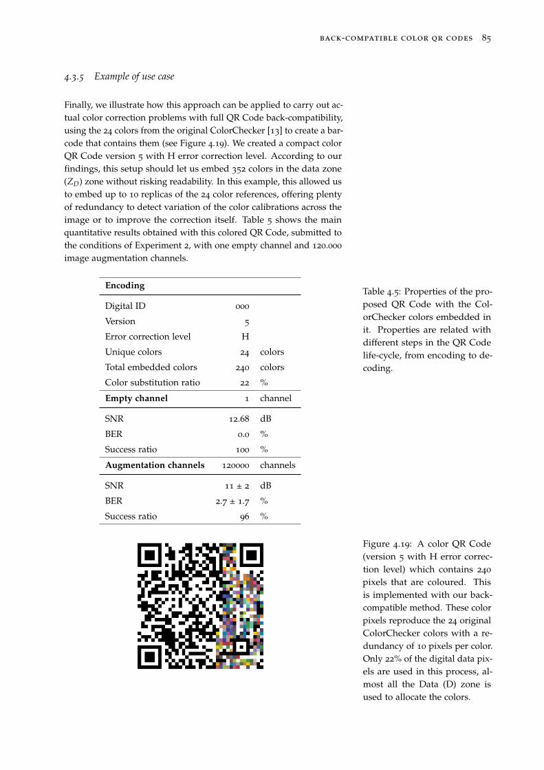
back-compatible color qr codes 85
4.3.5 Example of use case
Finally, we illustrate how this approach can be applied to carry out ac-tual color correction problems with full QR Code back-compatibility,using the 24 colors from the original ColorChecker [13] to create a bar-code that contains them (see Figure 4.19). We created a compact colorQR Code version 5 with H error correction level. According to ourfindings, this setup should let us embed 352 colors in the data zone(ZD) zone without risking readability. In this example, this allowed usto embed up to 10 replicas of the 24 color references, offering plentyof redundancy to detect variation of the color calibrations across theimage or to improve the correction itself. Table 5 shows the mainquantitative results obtained with this colored QR Code, submitted tothe conditions of Experiment 2, with one empty channel and 120.000
image augmentation channels.
Encoding
Digital ID 000
Version 5
Error correction level H
Unique colors 24 colors
Total embedded colors 240 colors
Color substitution ratio 22 %
Empty channel 1 channel
SNR 12.68 dB
BER 0.0 %
Success ratio 100 %
Augmentation channels 120000 channels
SNR 11 ± 2 dB
BER 2.7 ± 1.7 %
Success ratio 96 %
Table 4.5: Properties of the pro-posed QR Code with the Col-orChecker colors embedded init. Properties are related withdifferent steps in the QR Codelife-cycle, from encoding to de-coding.
Figure 4.19: A color QR Code(version 5 with H error correc-tion level) which contains 240
pixels that are coloured. Thisis implemented with our back-compatible method. These colorpixels reproduce the 24 originalColorChecker colors with a re-dundancy of 10 pixels per color.Only 22% of the digital data pix-els are used in this process, al-most all the Data (D) zone isused to allocate the colors.
86 automated color correction for colorimetry applications using barcodes
4.4 Conclusions
We have presented a method to pack a set of colors, useful for colorcalibration, in a QR Code in a fully back-compatible manner, thisis preserving its conventional ability to store digital data. By doingthis, we enhanced the state-of-the-art color charts with two mainfeatures: first, we did leverage the computer vision readout of thecolor references to the QR Code features; and two, de facto we reducedthe size of the color charts to the usual size of a QR Code, one or twoinches.
Also, we have demonstrated that the color capacity of the QRCodes constructed this way (up to a few thousand colors!) is ordersof magnitude higher than that found in the traditional color charts,due to the image density and pattern recognition robustness of theQR Codes.
Moreover, compared to other colored QR Codes, our proposal,based on the grayscale affinity of the colors to white or black, leads tomuch lower signal alteration levels and thus much higher readability,than the found in more naive approaches like, e.g., random assign-ment methods, which represent the aesthetic QR Codes (printing alogo).
This work opens a way to explore further methods to embed colorinformation in conventional 2D barcodes. Tuning how we defined ourcriteria of color embedding upon the affinity of colors to black andwhite would lead to more efficient embedding methods. We exploredsome of these ideas to seek those improved methods, and we exposethem below.
First, the way in which we implemented the grayscale (a meanvalue of the RGB channels) is only one of the ways to compute agrayscale channel, i.e. one could use the luma definition a weightedmean based on the human eye vision:
fgrasycale(r, g, b) = 0.2126 · r + 0.7152 · g + 0.0722 · b .
Or the lightness one:
fgrasycale(r, g, b) =12(max(r, g, b) + min(r, g, b)) .
These grayscale definitions are often part of colorspaces definitions[11], such as CIELab, CIELuv, HSL, etc. All these different grayscalewill generate different color distributions, displacing colors betweenblack and white regions of the QR Code.
back-compatible color qr codes 87
Second, we defined a way to select the area inside the QR Codewhere to embed the colors (see algorithm 1), this could be improvedalso. For example, we could decide to implement fthreshold in a morecomplex fashion. Let us imagine a certain set of colors Grgb to encodein a certain QR Code, one could create more than two sets to definethe black-white affinity, i.e. four sets, namely: blackest colors (0),blackish colors (1), whitish colors (2) and whitest colors (3):
fthreshold(Ggray) =
0 0.00 < Ggray(k) ≤ 0.25
1 0.25 < Ggray(k) ≤ 0.50
2 0.50 < Ggray(k) ≤ 0.75
3 0.75 < Ggray(k) ≤ 1.00
And accommodate algorithm 1 to this new output from fgrayscale
by assigning those colors with higher potential error (1,2) to theDATA zone and those with lower potential error (0,3) to the EC zone.Theoretically, this would outperform our current approach, as in thiswork we demonstrated that DATA zones are more resilient to errorthan EC zones, thus displacing away from EC critical colors wouldlead to a systematic increase of color capacity.
Third, many authors have contributed to create aesthetic QR Codeswhich embed trademarks and images with incredibly detailed results,we wanted to highlight some solutions that might be combined withour technology to embed even further colors or improve the controlover the placement of the colors.
Halftone QR Codes were proposed by Chu et al. [56], they sub-stituted QR Code modules for subsampled modules that containedwhite and black colors. These submodules presented a ditheringpattern that followed the encoded image shape. One could use thedithering idea to embed also colors inside subsampled pixels.
QArt Codes were introduced by Cox [58], the proposal aims to forcethe QR Code encoding to block certain areas of the QR Code to beblack or white no matter what the encoded data is (note this is onlypossible for some kinds of data encoding). One could use this featureto preserve dedicated areas for color embeddings, as a complementto algorithm 1. Note the need for a back-compatible criteria is still-present, the QArt Code only provides us the certainty if a module ofthe original QR Code is black or white, but they must remain black orwhite during the decoding process. This combination of technologieshas a potential impact in reducing the cost of producing the ColorQR Codes. as one could fix the position of the colored modulesbefore encoding the data using our grayscale criteria, then printthe QR Code using cost-effective printing technologies (rotogravure,flexography, etc.) and the black and white pixels using also cost-effective monochromatic printing technologies (laser printing), ratherthan use digital ink-jet printing to print the whole code.
88 automated color correction for colorimetry applications using barcodes
Finally, we have assumed that our back-compatible Color QR Codes
are meant to be for colorimetric measurement, as this is the preambleof our research.
Nevertheless, the above-presented results could be applied to en-code data in the color of the QR Codes in a back-compatible manner.This means, include more digital information in the same space. Otherauthors have presented their approaches to this solution, none of themin a back-compatible way. Les us propose a couple of ideas to achievethese digital back-compatible Color QR Codes, based on other ideas tocolor encode data in QR Codes.
First, Blasinki et al. [130] introduced a way to multiplex 3 QR Codesin one, by encoding a QR Code in each CMY channel of the printedimage. And then, when they recovered the QR Code, they applied acolor interference cancellation algorithm to extract the QR Codes from theRGB captured image, they also discussed how to approach the colorreproduction problem and manipulated further the remaining blackpatterns (finder, alignment and timing) to include color references.
All in all, this rendered non back-compatible Color QR Codes.Now, using our proposed method, one could turn this approach toback-compatibility again by simply do the following: keep the firstQR Code to multiplex as the ’default’ QR Code; then, take another3 additional QR Codes and create a barcode following Blasinki et al.method; in turn, create a "pseudo-white" and "pseudo-black" versionof this color QR Code; and finally, re-encode the default QR Codewith the pseudo-colors in a back-compatible manner. Also, note thisproposal is not restricted by the number of channels an image has,as we are exploiting intermediate values, not only the extreme ones.There should exist a limit yet to discover of how many QR Code canbe multiplexed in this fashion.
Second, other authors like Berchtold et al. – JAB Code –[49] orGrillo et al. – HCCBC –[136] fled from the original QR Code standardto redefine entirely the data encoding process. The main caveat oftheir technological proposals is the lack of back-compatibility, as wehave discussed before. One could combine both technologies to createmore adoptable tecnology. Grillo et al. proposal seems the easiest wayto go, as they kept the factor form of QR Codes. Theoretically, onecould simply multiplex one HCCBC with one QR Code as describedwith the previous method and achieve a digital back-compatible ColorQR Code.
Chapter 5. Image consistency using an improved TPS3D
method
Thin-plates splines (TPS) were introduced by Duchon in 1978 [137],reformulated by Meinguet in 1979 [138]. Later in 1989, TPS werepopularized by Bookestein [115] due to their potential to fit datalinked by an elastic deformation, especially when it comes to shapedeformation.
So far, TPS have been used widely to solve problems like morphingtransformations in 2D spaces. For example, Rohr et al. [139] andCrum et al. [140] used TPS to perform elastic registration of similarfeatures in different images in a dataset. Or, Bazen et al. [116] usedTPS to match fingerprints. Moreover, we have successfully used TPSto improve QR Code extraction in chapter 3.
TPS framework can be applied to color spaces. As explained inchapter 2, color spaces are three-dimensional spaces. TPS formulationcovers this scenario for 3D deformations [137; 138; 115]. In fact, wecan already find works that apply them to color technology. Forexample, Colatoni et al. [141] and Poljicak et al. [142] used TPS tocharacterize screen displays. Also, Sharma et al. [143] interpolatedcolors to be printed in commercial printers using TPS. Moreover,Menesatti et al. [15] proposed a new approach to color correct datasetfor image consistency based upon TPS, and called this method 3D
Thin-Plate Splines (TPS3D).
In this chapter, we focus on the implementation of thin-plate splinecolor corrections, specifically in the use of the TPS3D method toperform color correction in image datasets directly in RGB spaces,while proposing an alternative radial basis function [144] to be used tocompute the TPS, and introducing a smoothing factor to approximatethe solution in order to reduce corner-case errors [145]. All in all,we illustrate here the advantages and limitations of the new TPS3Dmethodology to color correct RGB images.
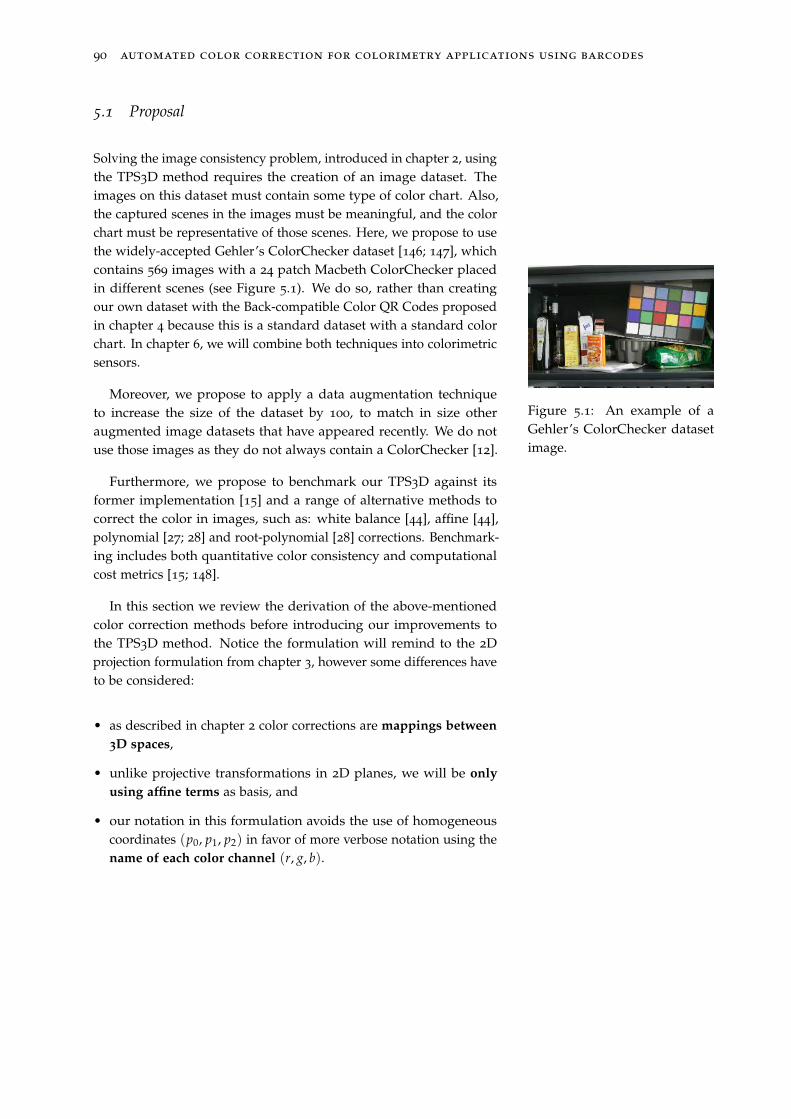
90 automated color correction for colorimetry applications using barcodes
5.1 Proposal
Solving the image consistency problem, introduced in chapter 2, usingthe TPS3D method requires the creation of an image dataset. Theimages on this dataset must contain some type of color chart. Also,the captured scenes in the images must be meaningful, and the colorchart must be representative of those scenes. Here, we propose to usethe widely-accepted Gehler’s ColorChecker dataset [146; 147], whichcontains 569 images with a 24 patch Macbeth ColorChecker placedin different scenes (see Figure 5.1). We do so, rather than creatingour own dataset with the Back-compatible Color QR Codes proposedin chapter 4 because this is a standard dataset with a standard colorchart. In chapter 6, we will combine both techniques into colorimetricsensors.
Figure 5.1: An example of aGehler’s ColorChecker datasetimage.
Moreover, we propose to apply a data augmentation techniqueto increase the size of the dataset by 100, to match in size otheraugmented image datasets that have appeared recently. We do notuse those images as they do not always contain a ColorChecker [12].
Furthermore, we propose to benchmark our TPS3D against itsformer implementation [15] and a range of alternative methods tocorrect the color in images, such as: white balance [44], affine [44],polynomial [27; 28] and root-polynomial [28] corrections. Benchmark-ing includes both quantitative color consistency and computationalcost metrics [15; 148].
In this section we review the derivation of the above-mentionedcolor correction methods before introducing our improvements tothe TPS3D method. Notice the formulation will remind to the 2Dprojection formulation from chapter 3, however some differences haveto be considered:
• as described in chapter 2 color corrections are mappings between
3D spaces,
• unlike projective transformations in 2D planes, we will be only
using affine terms as basis, and
• our notation in this formulation avoids the use of homogeneouscoordinates (p0, p1, p2) in favor of more verbose notation using thename of each color channel (r, g, b).
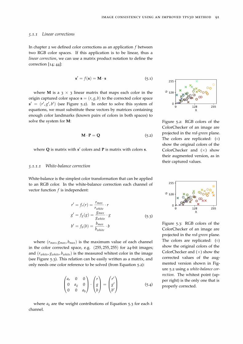
image consistency using an improved tps3d method 91
5.1.1 Linear corrections
In chapter 2 we defined color corrections as an application f betweentwo RGB color spaces. If this application is to be linear, thus alinear correction, we can use a matrix product notation to define thecorrection [14; 44]:
s′ = f (s) = M · s (5.1)
where M is a 3 × 3 linear matrix that maps each color in theorigin captured color space s = (r, g, b) to the corrected color spaces′ = (r′, g′, b′) (see Figure 5.2). In order to solve this system ofequations, we must substitute these vectors by matrices containingenough color landmarks (known pairs of colors in both spaces) tosolve the system for M: Figure 5.2: RGB colors of the
ColorChecker of an image areprojected in the red-green plane.The colors are replicated: (◦)show the original colors of theColorChecker and (×) showtheir augmented version, as intheir captured values.
M · P = Q (5.2)
where Q is matrix with s′ colors and P is matrix with colors s.
5.1.1.1 White-balance correction
White-balance is the simplest color transformation that can be appliedto an RGB color. In the white-balance correction each channel ofvector function f is independent:
r′ = fr(r) =rmax
rwhite· r
g′ = fg(g) =gmax
gwhite· g
b′ = fb(b) =bmax
bwhite· b
(5.3)
Figure 5.3: RGB colors of theColorChecker of an image areprojected in the red-green plane.The colors are replicated: (◦)show the original colors of theColorChecker and (×) show thecorrected values of the aug-mented version shown in Fig-ure 5.2 using a white-balance cor-
rection. The whitest point (up-per right) is the only one that isproperly corrected.
where (rmax, gmax, bmax) is the maximum value of each channelin the color corrected space, e.g. (255, 255, 255) for 24-bit images;and (rwhite, gwhite, bwhite) is the measured whitest color in the image(see Figure 5.3). This relation can be easily written as a matrix, andonly needs one color reference to be solved (from Equation 5.2):
ar 0 00 ag 00 0 ab
·
r
g
b
=
r′
g′
b′
(5.4)
where ak are the weight contributions of Equation 5.3 for each k
channel.
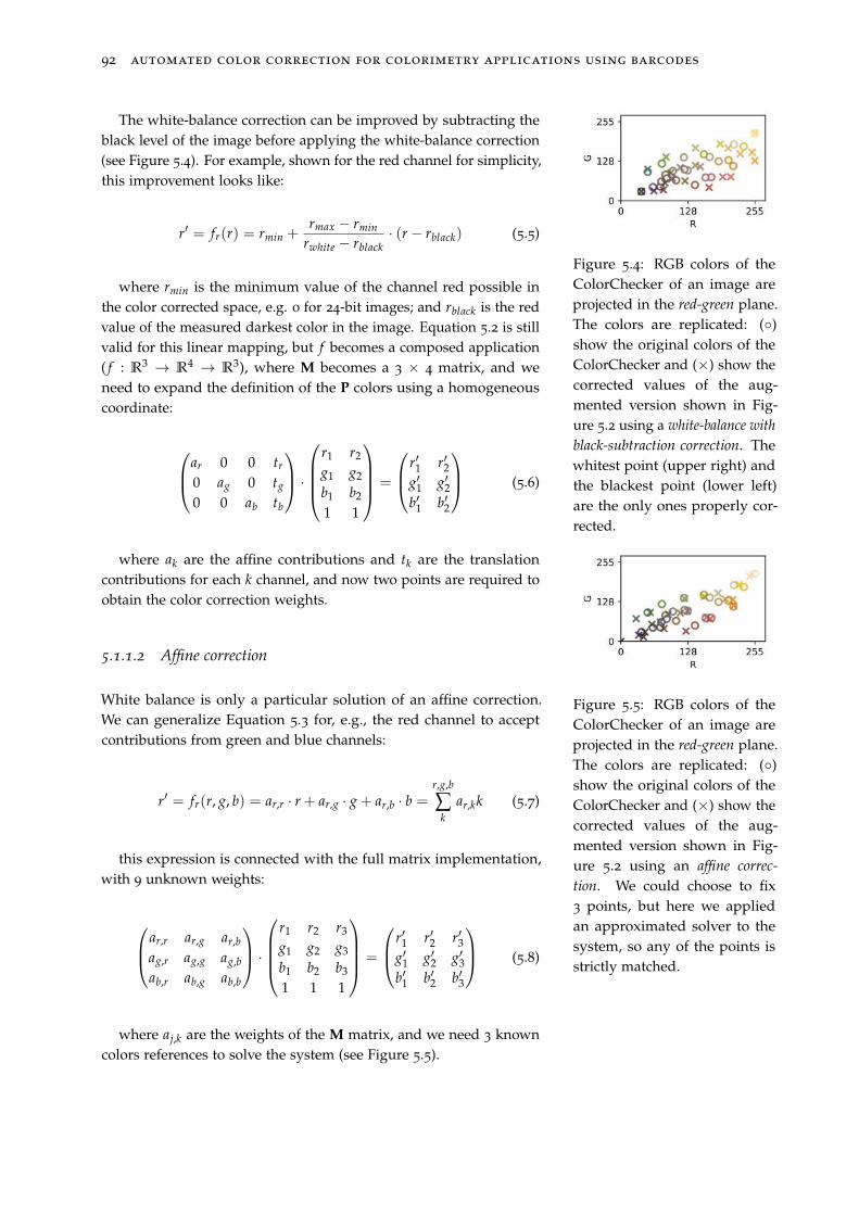
92 automated color correction for colorimetry applications using barcodes
The white-balance correction can be improved by subtracting theblack level of the image before applying the white-balance correction(see Figure 5.4). For example, shown for the red channel for simplicity,this improvement looks like:
r′ = fr(r) = rmin +rmax − rmin
rwhite − rblack· (r− rblack) (5.5)
Figure 5.4: RGB colors of theColorChecker of an image areprojected in the red-green plane.The colors are replicated: (◦)show the original colors of theColorChecker and (×) show thecorrected values of the aug-mented version shown in Fig-ure 5.2 using a white-balance with
black-subtraction correction. Thewhitest point (upper right) andthe blackest point (lower left)are the only ones properly cor-rected.
where rmin is the minimum value of the channel red possible inthe color corrected space, e.g. 0 for 24-bit images; and rblack is the redvalue of the measured darkest color in the image. Equation 5.2 is stillvalid for this linear mapping, but f becomes a composed application( f : R
3 → R4 → R
3), where M becomes a 3 × 4 matrix, and weneed to expand the definition of the P colors using a homogeneouscoordinate:
ar 0 0 tr
0 ag 0 tg
0 0 ab tb
·
r1 r2
g1 g2
b1 b2
1 1
=
r′1 r′2g′1 g′2b′1 b′2
(5.6)
where ak are the affine contributions and tk are the translationcontributions for each k channel, and now two points are required toobtain the color correction weights.
5.1.1.2 Affine correction
White balance is only a particular solution of an affine correction.We can generalize Equation 5.3 for, e.g., the red channel to acceptcontributions from green and blue channels:
Figure 5.5: RGB colors of theColorChecker of an image areprojected in the red-green plane.The colors are replicated: (◦)show the original colors of theColorChecker and (×) show thecorrected values of the aug-mented version shown in Fig-ure 5.2 using an affine correc-
tion. We could choose to fix3 points, but here we appliedan approximated solver to thesystem, so any of the points isstrictly matched.
r′ = fr(r, g, b) = ar,r · r + ar,g · g + ar,b · b =r,g,b
∑k
ar,kk (5.7)
this expression is connected with the full matrix implementation,with 9 unknown weights:
ar,r ar,g ar,b
ag,r ag,g ag,b
ab,r ab,g ab,b
·
r1 r2 r3
g1 g2 g3
b1 b2 b3
1 1 1
=
r′1 r′2 r′3g′1 g′2 g′3b′1 b′2 b′3
(5.8)
where aj,k are the weights of the M matrix, and we need 3 knowncolors references to solve the system (see Figure 5.5).
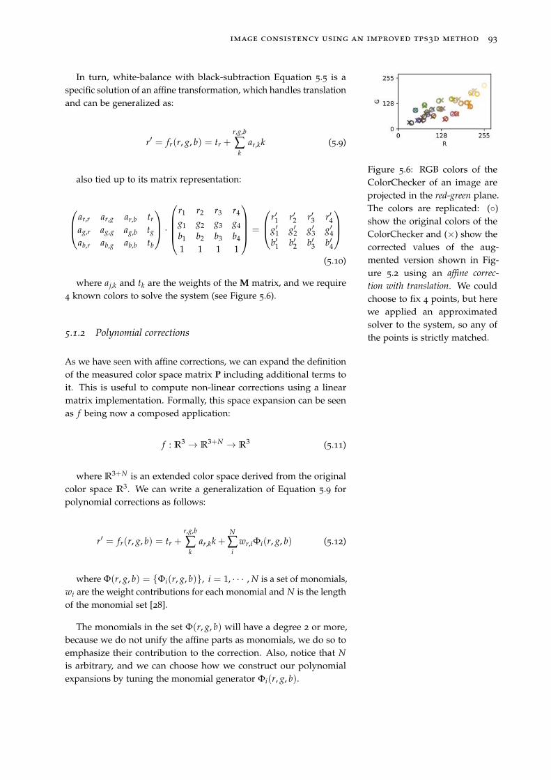
image consistency using an improved tps3d method 93
In turn, white-balance with black-subtraction Equation 5.5 is aspecific solution of an affine transformation, which handles translationand can be generalized as:
Figure 5.6: RGB colors of theColorChecker of an image areprojected in the red-green plane.The colors are replicated: (◦)show the original colors of theColorChecker and (×) show thecorrected values of the aug-mented version shown in Fig-ure 5.2 using an affine correc-
tion with translation. We couldchoose to fix 4 points, but herewe applied an approximatedsolver to the system, so any ofthe points is strictly matched.
r′ = fr(r, g, b) = tr +r,g,b
∑k
ar,kk (5.9)
also tied up to its matrix representation:
ar,r ar,g ar,b tr
ag,r ag,g ag,b tg
ab,r ab,g ab,b tb
·
r1 r2 r3 r4
g1 g2 g3 g4
b1 b2 b3 b4
1 1 1 1
=
r′1 r′2 r′3 r′4g′1 g′2 g′3 g′4b′1 b′2 b′3 b′4
(5.10)
where aj,k and tk are the weights of the M matrix, and we require4 known colors to solve the system (see Figure 5.6).
5.1.2 Polynomial corrections
As we have seen with affine corrections, we can expand the definitionof the measured color space matrix P including additional terms toit. This is useful to compute non-linear corrections using a linearmatrix implementation. Formally, this space expansion can be seenas f being now a composed application:
f : R3 → R
3+N → R3 (5.11)
where R3+N is an extended color space derived from the original
color space R3. We can write a generalization of Equation 5.9 for
polynomial corrections as follows:
r′ = fr(r, g, b) = tr +r,g,b
∑k
ar,kk +N
∑i
wr,iΦi(r, g, b) (5.12)
where Φ(r, g, b) = {Φi(r, g, b)}, i = 1, · · · , N is a set of monomials,wi are the weight contributions for each monomial and N is the lengthof the monomial set [28].
The monomials in the set Φ(r, g, b) will have a degree 2 or more,because we do not unify the affine parts as monomials, we do so toemphasize their contribution to the correction. Also, notice that N
is arbitrary, and we can choose how we construct our polynomialexpansions by tuning the monomial generator Φi(r, g, b).
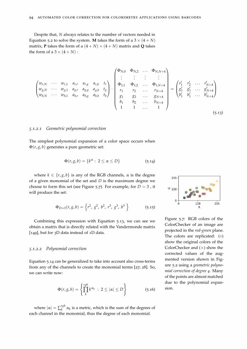
94 automated color correction for colorimetry applications using barcodes
Despite that, N always relates to the number of vectors needed inEquation 5.2 to solve the system. M takes the form of a 3× (4 + N)
matrix, P takes the form of a (4 + N)× (4 + N) matrix and Q takesthe form of a 3× (4 + N) :
wr,N · · · wr,1 ar,r ar,g ar,b tr
wg,N · · · wg,1 ag,r ag,g ag,b tg
wb,N · · · wb,1 ab,r ab,g ab,b tb
·
ΦN,0 ΦN,2 . . . ΦN,N+4...
......
...Φ1,1 Φ1,2 . . . Φ1,N+4
r1 r2 . . . rN+4
g1 g2 . . . gN+4
b1 b2 . . . bN+4
1 1 . . . 1
=
r′1 r′2 . . . r′N+4g′1 g′1 . . . g′N+4b′1 b′1 . . . b′N+4
(5.13)
5.1.2.1 Geometric polynomial correction
The simplest polynomial expansion of a color space occurs whenΦ(r, g, b) generates a pure geometric set:
Φ(r, g, b) = {kα : 2 ≤ α ≤ D} (5.14)
where k ∈ {r, g, b} is any of the RGB channels, α is the degreeof a given monomial of the set and D is the maximum degree wechoose to form this set (see Figure 5.7). For example, for D = 3 , itwill produce the set:
ΦD=3(r, g, b) ={
r2, g2, b2, r3, g3, b3}
(5.15)
Combining this expression with Equation 5.13, we can see weobtain a matrix that is directly related with the Vandermonde matrix[149], but for 3D data instead of 1D data.
Figure 5.7: RGB colors of theColorChecker of an image areprojected in the red-green plane.The colors are replicated: (◦)show the original colors of theColorChecker and (×) show thecorrected values of the aug-mented version shown in Fig-ure 5.2 using a geometric polyno-
mial correction of degree 4. Manyof the points are almost matcheddue to the polynomial expan-sion.
5.1.2.2 Polynomial correction
Equation 5.14 can be generalized to take into account also cross-termsfrom any of the channels to create the monomial terms [27; 28]. So,we can write now:
Φ(r, g, b) =
{
rgb
∏k
kαk : 2 ≤ |α| ≤ D
}
(5.16)
where |α| = ∑rgbk αk is a metric, which is the sum of the degrees of
each channel in the monomial, thus the degree of each monomial.
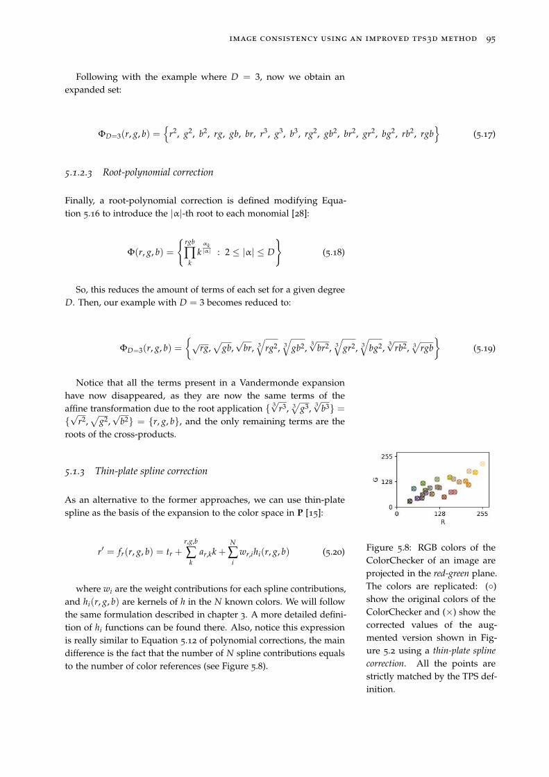
image consistency using an improved tps3d method 95
Following with the example where D = 3, now we obtain anexpanded set:
ΦD=3(r, g, b) ={
r2, g2, b2, rg, gb, br, r3, g3, b3, rg2, gb2, br2, gr2, bg2, rb2, rgb}
(5.17)
5.1.2.3 Root-polynomial correction
Finally, a root-polynomial correction is defined modifying Equa-tion 5.16 to introduce the |α|-th root to each monomial [28]:
Φ(r, g, b) =
{
rgb
∏k
kαk|α| : 2 ≤ |α| ≤ D
}
(5.18)
So, this reduces the amount of terms of each set for a given degreeD. Then, our example with D = 3 becomes reduced to:
ΦD=3(r, g, b) =
{√rg,√
gb,√
br, 3√
rg2, 3√
gb2,3√
br2, 3√
gr2, 3√
bg2,3√
rb2, 3√
rgb
}
(5.19)
Notice that all the terms present in a Vandermonde expansionhave now disappeared, as they are now the same terms of theaffine transformation due to the root application { 3
√r3, 3√
g3, 3√
b3} ={√
r2,√
g2,√
b2} = {r, g, b}, and the only remaining terms are theroots of the cross-products.
5.1.3 Thin-plate spline correction
As an alternative to the former approaches, we can use thin-platespline as the basis of the expansion to the color space in P [15]:
r′ = fr(r, g, b) = tr +r,g,b
∑k
ar,kk +N
∑i
wr,ihi(r, g, b) (5.20) Figure 5.8: RGB colors of theColorChecker of an image areprojected in the red-green plane.The colors are replicated: (◦)show the original colors of theColorChecker and (×) show thecorrected values of the aug-mented version shown in Fig-ure 5.2 using a thin-plate spline
correction. All the points arestrictly matched by the TPS def-inition.
where wi are the weight contributions for each spline contributions,and hi(r, g, b) are kernels of h in the N known colors. We will followthe same formulation described in chapter 3. A more detailed defini-tion of hi functions can be found there. Also, notice this expressionis really similar to Equation 5.12 of polynomial corrections, the maindifference is the fact that the number of N spline contributions equalsto the number of color references (see Figure 5.8).
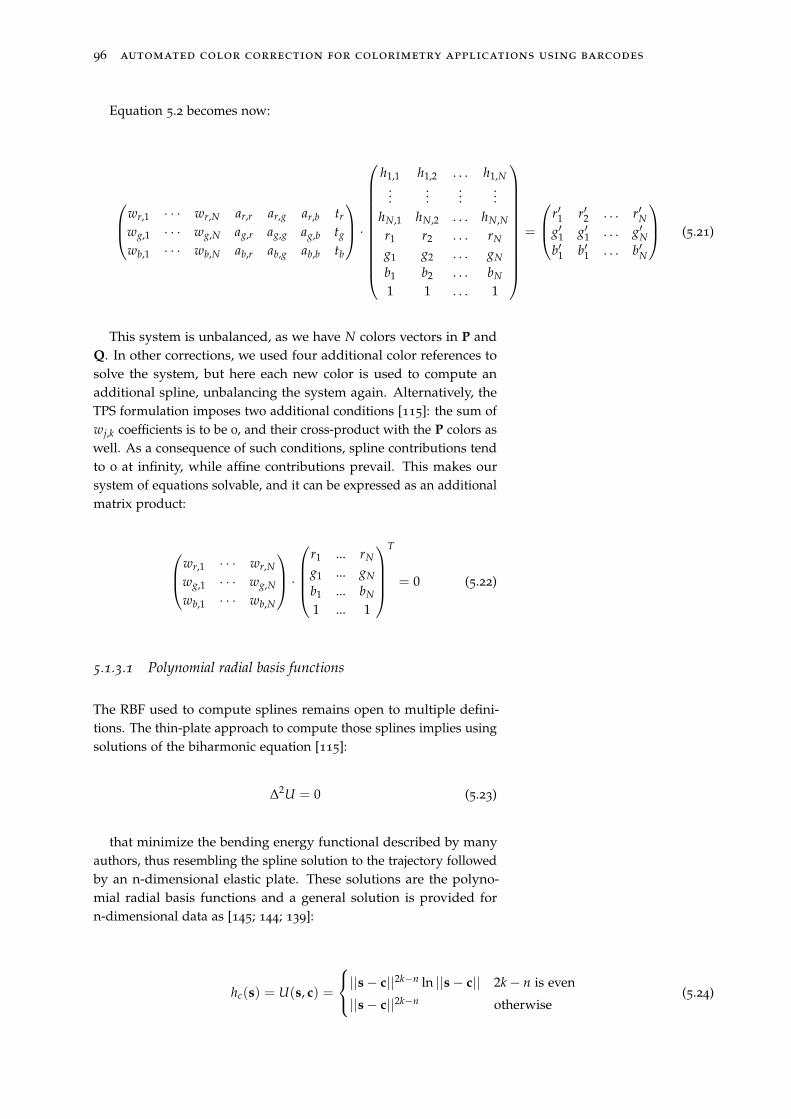
96 automated color correction for colorimetry applications using barcodes
Equation 5.2 becomes now:
wr,1 · · · wr,N ar,r ar,g ar,b tr
wg,1 · · · wg,N ag,r ag,g ag,b tg
wb,1 · · · wb,N ab,r ab,g ab,b tb
·
h1,1 h1,2 . . . h1,N...
......
...hN,1 hN,2 . . . hN,N
r1 r2 . . . rN
g1 g2 . . . gN
b1 b2 . . . bN
1 1 . . . 1
=
r′1 r′2 . . . r′Ng′1 g′1 . . . g′Nb′1 b′1 . . . b′N
(5.21)
This system is unbalanced, as we have N colors vectors in P andQ. In other corrections, we used four additional color references tosolve the system, but here each new color is used to compute anadditional spline, unbalancing the system again. Alternatively, theTPS formulation imposes two additional conditions [115]: the sum ofwj,k coefficients is to be 0, and their cross-product with the P colors aswell. As a consequence of such conditions, spline contributions tendto 0 at infinity, while affine contributions prevail. This makes oursystem of equations solvable, and it can be expressed as an additionalmatrix product:
wr,1 · · · wr,N
wg,1 · · · wg,N
wb,1 · · · wb,N
·
r1 ... rN
g1 ... gN
b1 ... bN
1 ... 1
T
= 0 (5.22)
5.1.3.1 Polynomial radial basis functions
The RBF used to compute splines remains open to multiple defini-tions. The thin-plate approach to compute those splines implies usingsolutions of the biharmonic equation [115]:
∆2U = 0 (5.23)
that minimize the bending energy functional described by manyauthors, thus resembling the spline solution to the trajectory followedby an n-dimensional elastic plate. These solutions are the polyno-mial radial basis functions and a general solution is provided forn-dimensional data as [145; 144; 139]:
hc(s) = U(s, c) =
||s− c||2k−n ln ||s− c|| 2k− n is even
||s− c||2k−n otherwise(5.24)
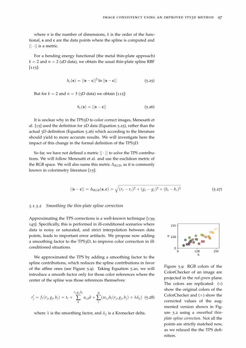
image consistency using an improved tps3d method 97
where n is the number of dimensions, k is the order of the func-tional, s and c are the data points where the spline is computed and|| · || is a metric.
For a bending energy functional (the metal thin-plate approach)k = 2 and n = 2 (2D data), we obtain the usual thin-plate spline RBF[115]:
hc(s) = ||s− c||2 ln ||s− c|| (5.25)
But for k = 2 and n = 3 (3D data) we obtain [115]:
hc(s) = ||s− c|| (5.26)
It is unclear why in the TPS3D to color correct images, Menesatti etal. [15] used the definition for 2D data (Equation 5.25), rather than theactual 3D definition (Equation 5.26) which according to the literatureshould yield to more accurate results. We will investigate here theimpact of this change in the formal definition of the TPS3D.
So far, we have not defined a metric || · || to solve the TPS contribu-tions. We will follow Menesatti et al. and use the euclidean metric ofthe RGB space. We will also name this metric ∆RGB, as it is commonlyknown in colorimetry literature [15]:
||s− c|| = ∆RGB(s, c) =√
(rs − rc)2 + (gs − gc)2 + (bs − bc)2 (5.27)
5.1.3.2 Smoothing the thin-plate spline correction
Approximating the TPS corrections is a well-known technique [139;145]. Specifically, this is performed in ill-conditioned scenarios wheredata is noisy or saturated, and strict interpolation between datapoints, leads to important error artifacts. We propose now addinga smoothing factor to the TPS3D, to improve color correction in ill-conditioned situations.
We approximated the TPS by adding a smoothing factor to thespline contributions, which reduces the spline contributions in favorof the affine ones (see Figure 5.9). Taking Equation 5.20, we willintroduce a smooth factor only for those color references where thecenter of the spline was those references themselves:
Figure 5.9: RGB colors of theColorChecker of an image areprojected in the red-green plane.The colors are replicated: (◦)show the original colors of theColorChecker and (×) show thecorrected values of the aug-mented version shown in Fig-ure 5.2 using a smoothed thin-
plate spline correction. Not all thepoints are strictly matched now,as we relaxed the the TPS defi-nition.
r′j = fr(rj, gj, bj) = tr +
rj ,gj ,bj
∑k
ar,kk +N
∑i
(wr,ihi(rj, gj, bj) + λδij) (5.28)
where λ is the smoothing factor, and δij is a Kronecker delta.
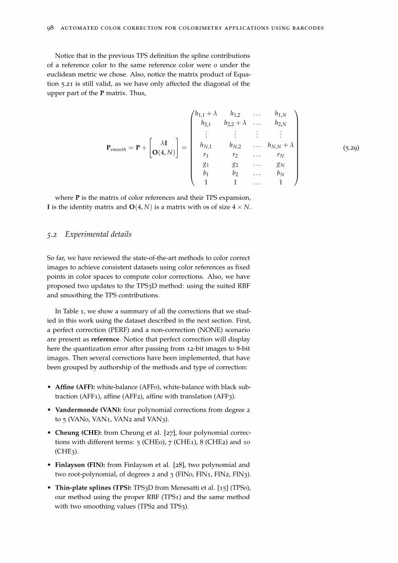
98 automated color correction for colorimetry applications using barcodes
Notice that in the previous TPS definition the spline contributionsof a reference color to the same reference color were 0 under theeuclidean metric we chose. Also, notice the matrix product of Equa-tion 5.21 is still valid, as we have only affected the diagonal of theupper part of the P matrix. Thus,
Psmooth = P +
[
λI
O(4, N)
]
=
h1,1 + λ h1,2 . . . h1,N
h2,1 h2,2 + λ . . . h2,N...
......
...hN,1 hN,2 . . . hN,N + λ
r1 r2 . . . rN
g1 g2 . . . gN
b1 b2 . . . bN
1 1 . . . 1
(5.29)
where P is the matrix of color references and their TPS expansion,I is the identity matrix and O(4, N) is a matrix with 0s of size 4× N.
5.2 Experimental details
So far, we have reviewed the state-of-the-art methods to color correctimages to achieve consistent datasets using color references as fixedpoints in color spaces to compute color corrections. Also, we haveproposed two updates to the TPS3D method: using the suited RBFand smoothing the TPS contributions.
In Table 1, we show a summary of all the corrections that we stud-ied in this work using the dataset described in the next section. First,a perfect correction (PERF) and a non-correction (NONE) scenarioare present as reference. Notice that perfect correction will displayhere the quantization error after passing from 12-bit images to 8-bitimages. Then several corrections have been implemented, that havebeen grouped by authorship of the methods and type of correction:
• Affine (AFF): white-balance (AFF0), white-balance with black sub-traction (AFF1), affine (AFF2), affine with translation (AFF3).
• Vandermonde (VAN): four polynomial corrections from degree 2
to 5 (VAN0, VAN1, VAN2 and VAN3).
• Cheung (CHE): from Cheung et al. [27], four polynomial correc-tions with different terms: 5 (CHE0), 7 (CHE1), 8 (CHE2) and 10
(CHE3).
• Finlayson (FIN): from Finlayson et al. [28], two polynomial andtwo root-polynomial, of degrees 2 and 3 (FIN0, FIN1, FIN2, FIN3).
• Thin-plate splines (TPS): TPS3D from Menesatti et al. [15] (TPS0),our method using the proper RBF (TPS1) and the same methodwith two smoothing values (TPS2 and TPS3).
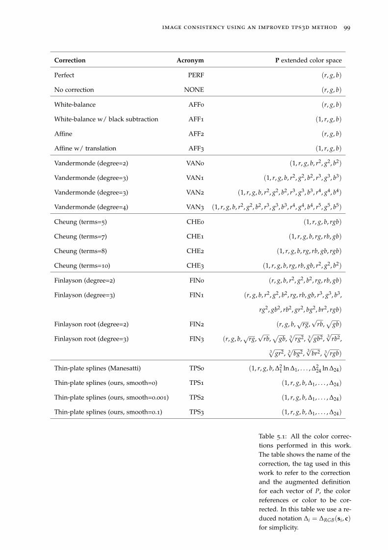
image consistency using an improved tps3d method 99
Correction Acronym P extended color space
Perfect PERF (r, g, b)
No correction NONE (r, g, b)
White-balance AFF0 (r, g, b)
White-balance w/ black subtraction AFF1 (1, r, g, b)
Affine AFF2 (r, g, b)
Affine w/ translation AFF3 (1, r, g, b)
Vandermonde (degree=2) VAN0 (1, r, g, b, r2, g2, b2)
Vandermonde (degree=3) VAN1 (1, r, g, b, r2, g2, b2, r3, g3, b3)
Vandermonde (degree=3) VAN2 (1, r, g, b, r2, g2, b2, r3, g3, b3, r4, g4, b4)
Vandermonde (degree=4) VAN3 (1, r, g, b, r2, g2, b2, r3, g3, b3, r4, g4, b4, r5, g5, b5)
Cheung (terms=5) CHE0 (1, r, g, b, rgb)
Cheung (terms=7) CHE1 (1, r, g, b, rg, rb, gb)
Cheung (terms=8) CHE2 (1, r, g, b, rg, rb, gb, rgb)
Cheung (terms=10) CHE3 (1, r, g, b, rg, rb, gb, r2, g2, b2)
Finlayson (degree=2) FIN0 (r, g, b, r2, g2, b2, rg, rb, gb)
Finlayson (degree=3) FIN1 (r, g, b, r2, g2, b2, rg, rb, gb, r3, g3, b3,
rg2, gb2, rb2, gr2, bg2, br2, rgb)
Finlayson root (degree=2) FIN2 (r, g, b,√
rg,√
rb,√
gb)
Finlayson root (degree=3) FIN3 (r, g, b,√
rg,√
rb,√
gb, 3√
rg2, 3√
gb2, 3√
rb2,
3√
gr2, 3√
bg2, 3√
br2, 3√
rgb)
Thin-plate splines (Manesatti) TPS0 (1, r, g, b, ∆21 ln ∆1, . . . , ∆2
24 ln ∆24)
Thin-plate splines (ours, smooth=0) TPS1 (1, r, g, b, ∆1, . . . , ∆24)
Thin-plate splines (ours, smooth=0.001) TPS2 (1, r, g, b, ∆1, . . . , ∆24)
Thin-plate splines (ours, smooth=0.1) TPS3 (1, r, g, b, ∆1, . . . , ∆24)
Table 5.1: All the color correc-tions performed in this work.The table shows the name of thecorrection, the tag used in thiswork to refer to the correctionand the augmented definitionfor each vector of P, the colorreferences or color to be cor-rected. In this table we use a re-duced notation ∆i = ∆RGB(si, c)
for simplicity.
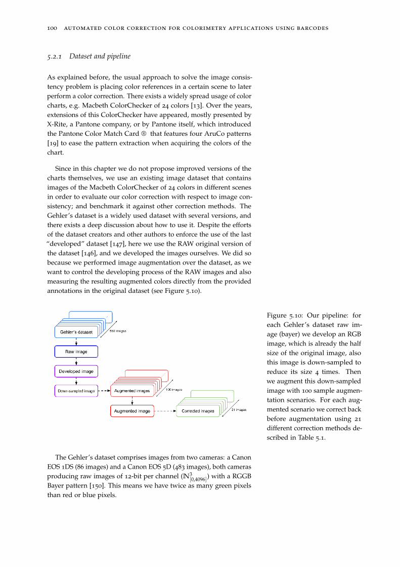
100 automated color correction for colorimetry applications using barcodes
5.2.1 Dataset and pipeline
As explained before, the usual approach to solve the image consis-tency problem is placing color references in a certain scene to laterperform a color correction. There exists a widely spread usage of colorcharts, e.g. Macbeth ColorChecker of 24 colors [13]. Over the years,extensions of this ColorChecker have appeared, mostly presented byX-Rite, a Pantone company, or by Pantone itself, which introducedthe Pantone Color Match Card ® that features four AruCo patterns[19] to ease the pattern extraction when acquiring the colors of thechart.
Since in this chapter we do not propose improved versions of thecharts themselves, we use an existing image dataset that containsimages of the Macbeth ColorChecker of 24 colors in different scenesin order to evaluate our color correction with respect to image con-sistency; and benchmark it against other correction methods. TheGehler’s dataset is a widely used dataset with several versions, andthere exists a deep discussion about how to use it. Despite the effortsof the dataset creators and other authors to enforce the use of the last“developed” dataset [147], here we use the RAW original version ofthe dataset [146], and we developed the images ourselves. We did sobecause we performed image augmentation over the dataset, as wewant to control the developing process of the RAW images and alsomeasuring the resulting augmented colors directly from the providedannotations in the original dataset (see Figure 5.10).
Figure 5.10: Our pipeline: foreach Gehler’s dataset raw im-age (bayer) we develop an RGBimage, which is already the halfsize of the original image, alsothis image is down-sampled toreduce its size 4 times. Thenwe augment this down-sampledimage with 100 sample augmen-tation scenarios. For each aug-mented scenario we correct backbefore augmentation using 21
different correction methods de-scribed in Table 5.1.
The Gehler’s dataset comprises images from two cameras: a CanonEOS 1DS (86 images) and a Canon EOS 5D (483 images), both camerasproducing raw images of 12-bit per channel (N3
[0,4096]) with a RGGBBayer pattern [150]. This means we have twice as many green pixelsthan red or blue pixels.
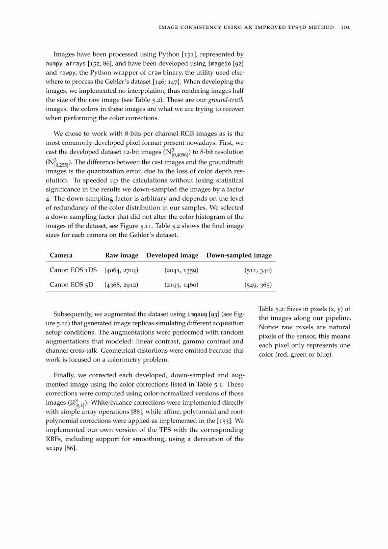
image consistency using an improved tps3d method 101
Images have been processed using Python [151], represented bynumpy arrays [152; 86], and have been developed using imageio [92]and rawpy, the Python wrapper of craw binary, the utility used else-where to process the Gehler’s dataset [146; 147]. When developing theimages, we implemented no interpolation, thus rendering images halfthe size of the raw image (see Table 5.2). These are our ground-truth
images: the colors in these images are what we are trying to recoverwhen performing the color corrections.
We chose to work with 8-bits per channel RGB images as is themost commonly developed pixel format present nowadays. First, wecast the developed dataset 12-bit images (N3
[0,4096]) to 8-bit resolution
(N3[0,255]). The difference between the cast images and the groundtruth
images is the quantization error, due to the loss of color depth res-olution. To speeded up the calculations without losing statisticalsignificance in the results we down-sampled the images by a factor4. The down-sampling factor is arbitrary and depends on the levelof redundancy of the color distribution in our samples. We selecteda down-sampling factor that did not alter the color histogram of theimages of the dataset, see Figure 5.11. Table 5.2 shows the final imagesizes for each camera on the Gehler’s dataset.
Camera Raw image Developed image Down-sampled image
Canon EOS 1DS (4064, 2704) (2041, 1359) (511, 340)
Canon EOS 5D (4368, 2912) (2193, 1460) (549, 365)
Table 5.2: Sizes in pixels (x, y) ofthe images along our pipeline.Notice raw pixels are naturalpixels of the sensor, this meanseach pixel only represents onecolor (red, green or blue).
Subsequently, we augmented the dataset using imgaug [93] (see Fig-ure 5.12) that generated image replicas simulating different acquisitionsetup conditions. The augmentations were performed with randomaugmentations that modeled: linear contrast, gamma contrast andchannel cross-talk. Geometrical distortions were omitted because thiswork is focused on a colorimetry problem.
Finally, we corrected each developed, down-sampled and aug-mented image using the color corrections listed in Table 5.1. Thesecorrections were computed using color-normalized versions of thoseimages (R3
[0,1]). White-balance corrections were implemented directlywith simple array operations [86]; while affine, polynomial and root-polynomial corrections were applied as implemented in the [153]. Weimplemented our own version of the TPS with the correspondingRBFs, including support for smoothing, using a derivation of thescipy [86].
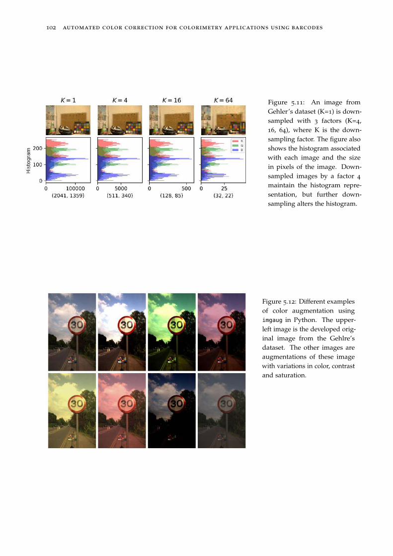
102 automated color correction for colorimetry applications using barcodes
Figure 5.11: An image fromGehler’s dataset (K=1) is down-sampled with 3 factors (K=4,16, 64), where K is the down-sampling factor. The figure alsoshows the histogram associatedwith each image and the sizein pixels of the image. Down-sampled images by a factor 4
maintain the histogram repre-sentation, but further down-sampling alters the histogram.
Figure 5.12: Different examplesof color augmentation usingimgaug in Python. The upper-left image is the developed orig-inal image from the Gehlre’sdataset. The other images areaugmentations of these imagewith variations in color, contrastand saturation.
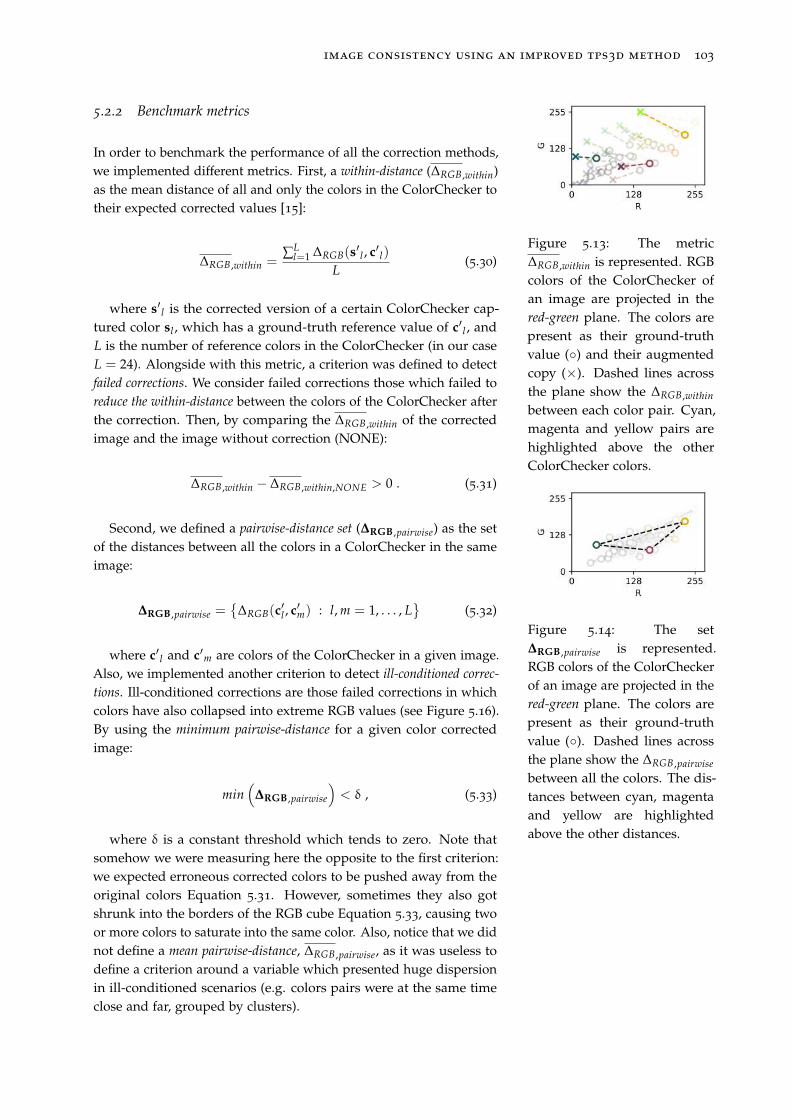
image consistency using an improved tps3d method 103
5.2.2 Benchmark metrics
In order to benchmark the performance of all the correction methods,we implemented different metrics. First, a within-distance (∆RGB ,within)as the mean distance of all and only the colors in the ColorChecker totheir expected corrected values [15]:
Figure 5.13: The metric∆RGB ,within is represented. RGBcolors of the ColorChecker ofan image are projected in thered-green plane. The colors arepresent as their ground-truthvalue (◦) and their augmentedcopy (×). Dashed lines acrossthe plane show the ∆RGB ,within
between each color pair. Cyan,magenta and yellow pairs arehighlighted above the otherColorChecker colors.
∆RGB ,within =∑
Ll=1 ∆RGB(s
′l , c′ l)
L(5.30)
where s′ l is the corrected version of a certain ColorChecker cap-tured color sl , which has a ground-truth reference value of c′ l , andL is the number of reference colors in the ColorChecker (in our caseL = 24). Alongside with this metric, a criterion was defined to detectfailed corrections. We consider failed corrections those which failed toreduce the within-distance between the colors of the ColorChecker afterthe correction. Then, by comparing the ∆RGB ,within of the correctedimage and the image without correction (NONE):
∆RGB ,within − ∆RGB ,within,NONE > 0 . (5.31)
Second, we defined a pairwise-distance set (∆RGB ,pairwise) as the setof the distances between all the colors in a ColorChecker in the sameimage:
Figure 5.14: The set∆RGB ,pairwise is represented.RGB colors of the ColorCheckerof an image are projected in thered-green plane. The colors arepresent as their ground-truthvalue (◦). Dashed lines acrossthe plane show the ∆RGB ,pairwise
between all the colors. The dis-tances between cyan, magentaand yellow are highlightedabove the other distances.
∆RGB ,pairwise ={
∆RGB(c′l , c′m) : l, m = 1, . . . , L
}
(5.32)
where c′ l and c′m are colors of the ColorChecker in a given image.Also, we implemented another criterion to detect ill-conditioned correc-
tions. Ill-conditioned corrections are those failed corrections in whichcolors have also collapsed into extreme RGB values (see Figure 5.16).By using the minimum pairwise-distance for a given color correctedimage:
min(
∆RGB ,pairwise
)
< δ , (5.33)
where δ is a constant threshold which tends to zero. Note thatsomehow we were measuring here the opposite to the first criterion:we expected erroneous corrected colors to be pushed away from theoriginal colors Equation 5.31. However, sometimes they also gotshrunk into the borders of the RGB cube Equation 5.33, causing twoor more colors to saturate into the same color. Also, notice that we didnot define a mean pairwise-distance, ∆RGB ,pairwise, as it was useless todefine a criterion around a variable which presented huge dispersionin ill-conditioned scenarios (e.g. colors pairs were at the same timeclose and far, grouped by clusters).
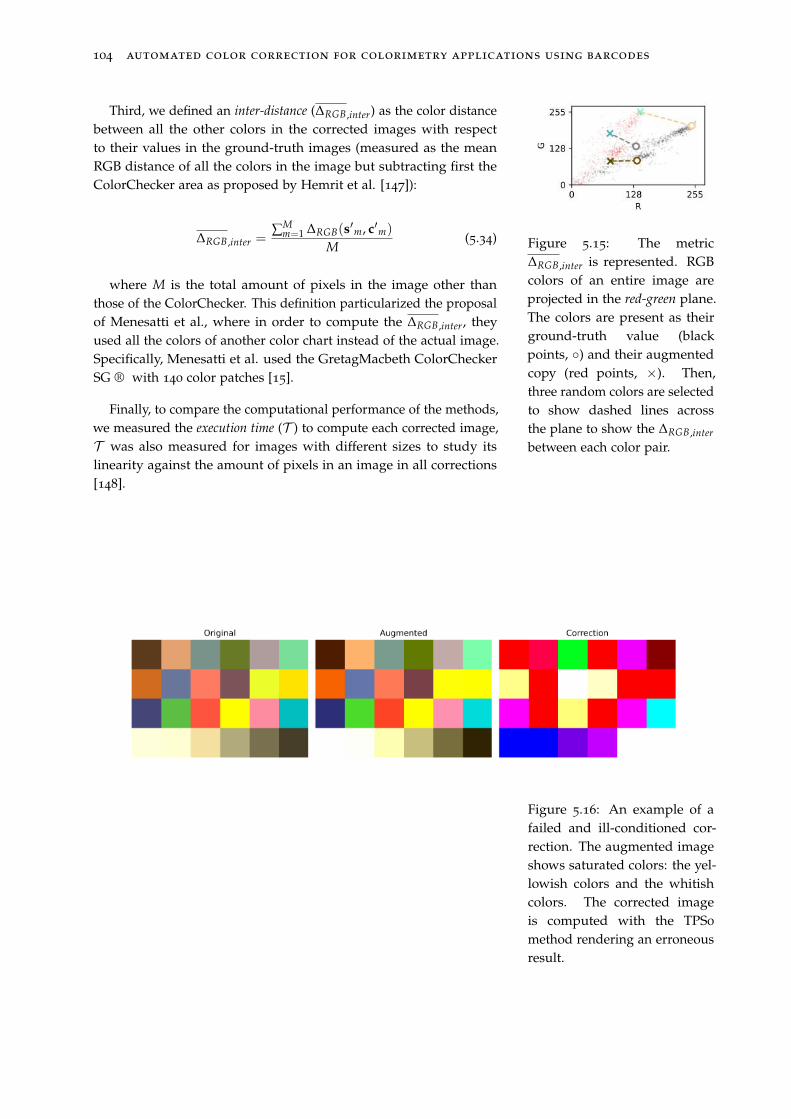
104 automated color correction for colorimetry applications using barcodes
Third, we defined an inter-distance (∆RGB ,inter) as the color distancebetween all the other colors in the corrected images with respectto their values in the ground-truth images (measured as the meanRGB distance of all the colors in the image but subtracting first theColorChecker area as proposed by Hemrit et al. [147]):
Figure 5.15: The metric∆RGB ,inter is represented. RGBcolors of an entire image areprojected in the red-green plane.The colors are present as theirground-truth value (blackpoints, ◦) and their augmentedcopy (red points, ×). Then,three random colors are selectedto show dashed lines acrossthe plane to show the ∆RGB ,inter
between each color pair.
∆RGB ,inter =∑
Mm=1 ∆RGB(s
′m, c′m)
M(5.34)
where M is the total amount of pixels in the image other thanthose of the ColorChecker. This definition particularized the proposalof Menesatti et al., where in order to compute the ∆RGB ,inter, theyused all the colors of another color chart instead of the actual image.Specifically, Menesatti et al. used the GretagMacbeth ColorCheckerSG ® with 140 color patches [15].
Finally, to compare the computational performance of the methods,we measured the execution time (T ) to compute each corrected image,T was also measured for images with different sizes to study itslinearity against the amount of pixels in an image in all corrections[148].
Figure 5.16: An example of afailed and ill-conditioned cor-rection. The augmented imageshows saturated colors: the yel-lowish colors and the whitishcolors. The corrected imageis computed with the TPS0
method rendering an erroneousresult.
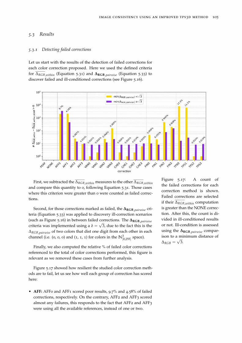
image consistency using an improved tps3d method 105
5.3 Results
5.3.1 Detecting failed corrections
Let us start with the results of the detection of failed corrections foreach color correction proposed. Here we used the defined criteriafor ∆RGB ,within (Equation 5.31) and ∆RGB ,pairwise (Equation 5.33) todiscover failed and ill-conditioned corrections (see Figure 5.16).
Figure 5.17: A count ofthe failed corrections for eachcorrection method is shown.Failed corrections are selectedif their ∆RGB ,within computationis greater than the NONE correc-tion. After this, the count is di-vided in ill-conditioned resultsor not. Ill-condition is assessedusing the ∆RGB ,pairwise compar-ison to a minimum distance of∆RGB =
√3.
First, we subtracted the ∆RGB ,within measures to the other ∆RGB ,within
and compare this quantity to 0, following Equation 5.31. Those caseswhere this criterion were greater than 0 were counted as failed correc-tions.
Second, for those corrections marked as failed, the ∆RGB ,pairwise cri-teria (Equation 5.33) was applied to discovery ill-correction scenarios(such as Figure 5.16) in between failed corrections. The ∆RGB ,pairwise
criteria was implemented using a δ =√
3, due to the fact this is the∆RGB ,pairwise of two colors that dist one digit from each other in eachchannel (i.e. (0, 0, 0) and (1, 1, 1) for colors in the N
3[0,255] space).
Finally, we also computed the relative % of failed color correctionsreferenced to the total of color corrections performed, this figure isrelevant as we removed these cases from further analysis.
Figure 5.17 showed how resilient the studied color correction meth-ods are to fail, let us see how well each group of correction has scoredhere:
• AFF: AFF0 and AFF1 scored poor results, 9.7% and 4.58% of failedcorrections, respectively. On the contrary, AFF2 and AFF3 scoredalmost any failures, this responds to the fact that AFF2 and AFF3
were using all the available references, instead of one or two.
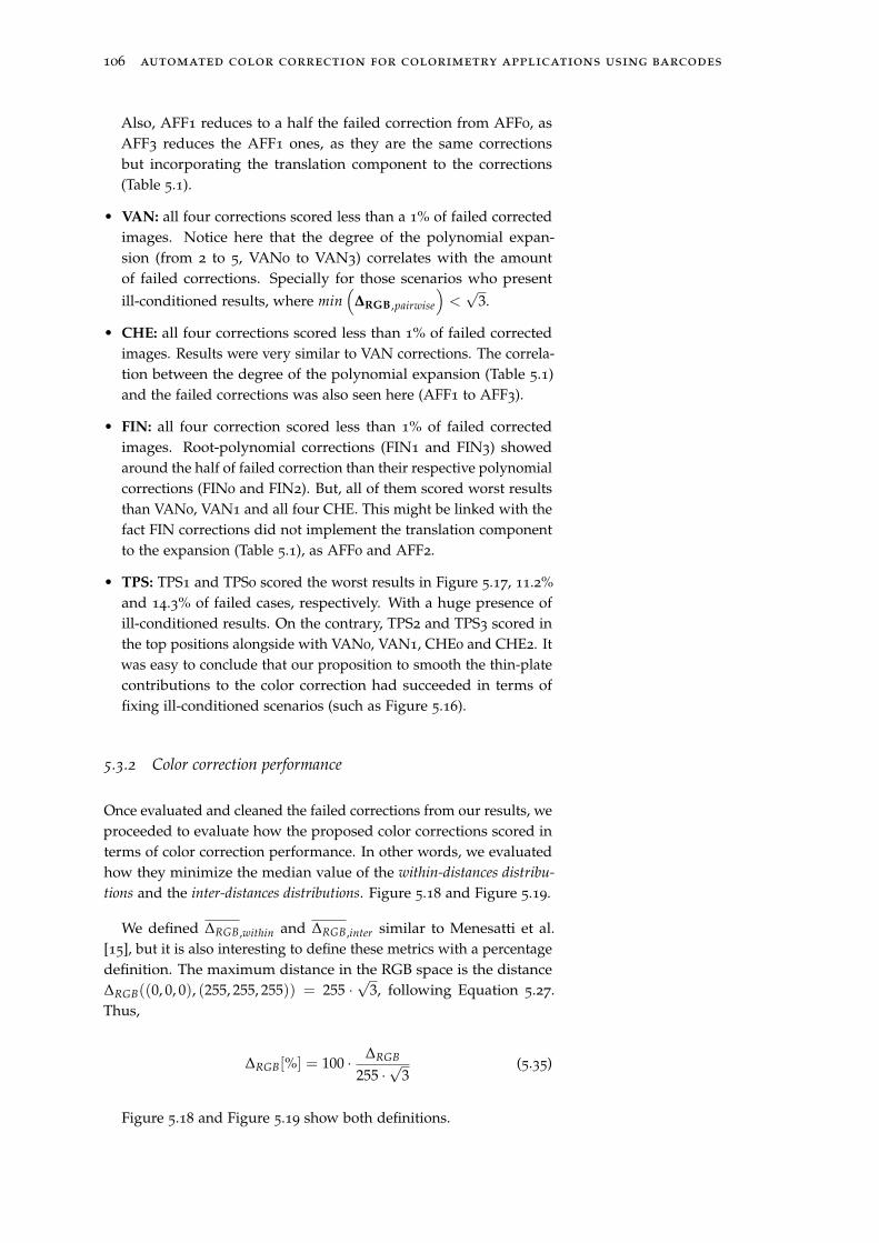
106 automated color correction for colorimetry applications using barcodes
Also, AFF1 reduces to a half the failed correction from AFF0, asAFF3 reduces the AFF1 ones, as they are the same correctionsbut incorporating the translation component to the corrections(Table 5.1).
• VAN: all four corrections scored less than a 1% of failed correctedimages. Notice here that the degree of the polynomial expan-sion (from 2 to 5, VAN0 to VAN3) correlates with the amountof failed corrections. Specially for those scenarios who present
ill-conditioned results, where min(
∆RGB ,pairwise
)
<
√3.
• CHE: all four corrections scored less than 1% of failed correctedimages. Results were very similar to VAN corrections. The correla-tion between the degree of the polynomial expansion (Table 5.1)and the failed corrections was also seen here (AFF1 to AFF3).
• FIN: all four correction scored less than 1% of failed correctedimages. Root-polynomial corrections (FIN1 and FIN3) showedaround the half of failed correction than their respective polynomialcorrections (FIN0 and FIN2). But, all of them scored worst resultsthan VAN0, VAN1 and all four CHE. This might be linked with thefact FIN corrections did not implement the translation componentto the expansion (Table 5.1), as AFF0 and AFF2.
• TPS: TPS1 and TPS0 scored the worst results in Figure 5.17, 11.2%and 14.3% of failed cases, respectively. With a huge presence ofill-conditioned results. On the contrary, TPS2 and TPS3 scored inthe top positions alongside with VAN0, VAN1, CHE0 and CHE2. Itwas easy to conclude that our proposition to smooth the thin-platecontributions to the color correction had succeeded in terms offixing ill-conditioned scenarios (such as Figure 5.16).
5.3.2 Color correction performance
Once evaluated and cleaned the failed corrections from our results, weproceeded to evaluate how the proposed color corrections scored interms of color correction performance. In other words, we evaluatedhow they minimize the median value of the within-distances distribu-
tions and the inter-distances distributions. Figure 5.18 and Figure 5.19.
We defined ∆RGB ,within and ∆RGB ,inter similar to Menesatti et al.[15], but it is also interesting to define these metrics with a percentagedefinition. The maximum distance in the RGB space is the distance∆RGB((0, 0, 0), (255, 255, 255)) = 255 ·
√3, following Equation 5.27.
Thus,
∆RGB[%] = 100 · ∆RGB
255 ·√
3(5.35)
Figure 5.18 and Figure 5.19 show both definitions.
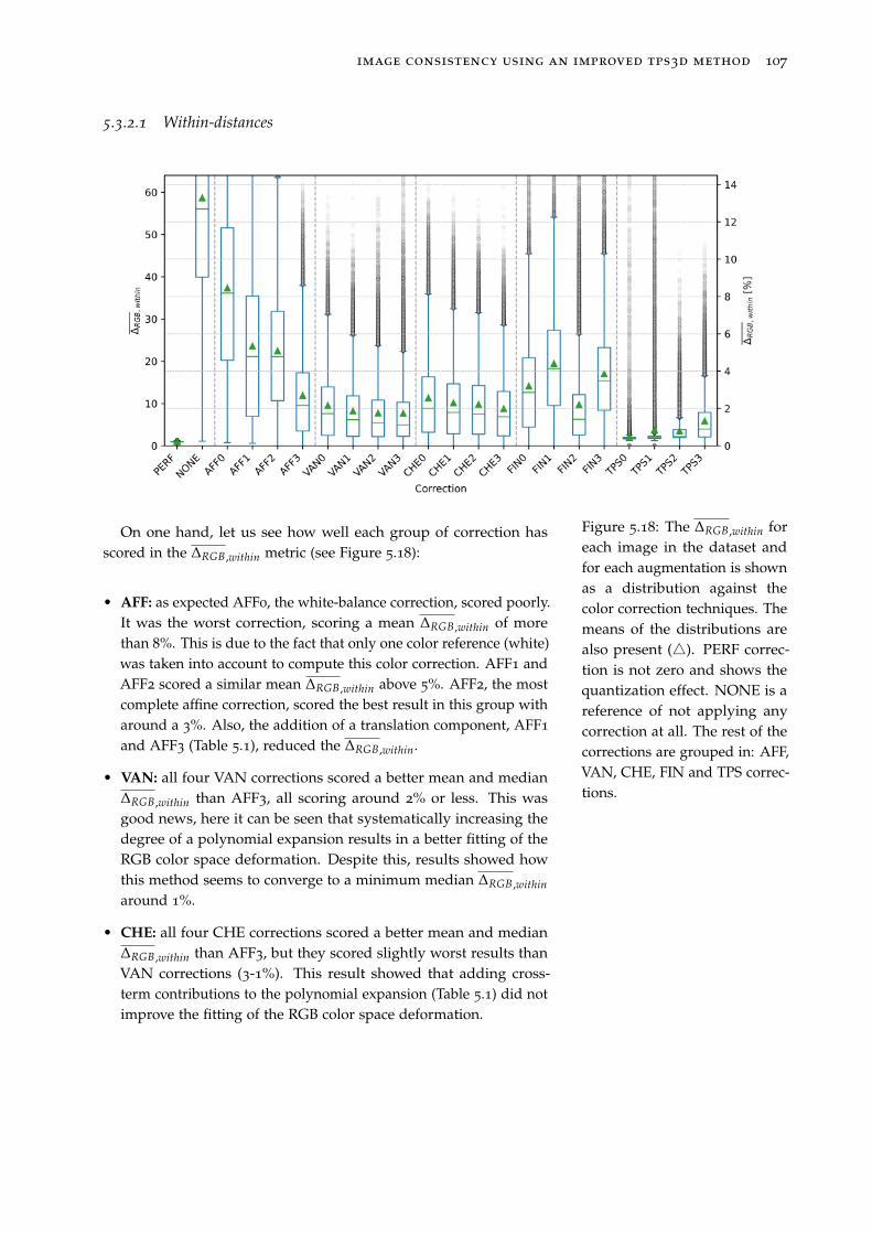
image consistency using an improved tps3d method 107
5.3.2.1 Within-distances
Figure 5.18: The ∆RGB ,within foreach image in the dataset andfor each augmentation is shownas a distribution against thecolor correction techniques. Themeans of the distributions arealso present (△). PERF correc-tion is not zero and shows thequantization effect. NONE is areference of not applying anycorrection at all. The rest of thecorrections are grouped in: AFF,VAN, CHE, FIN and TPS correc-tions.
On one hand, let us see how well each group of correction hasscored in the ∆RGB ,within metric (see Figure 5.18):
• AFF: as expected AFF0, the white-balance correction, scored poorly.It was the worst correction, scoring a mean ∆RGB ,within of morethan 8%. This is due to the fact that only one color reference (white)was taken into account to compute this color correction. AFF1 andAFF2 scored a similar mean ∆RGB ,within above 5%. AFF2, the mostcomplete affine correction, scored the best result in this group witharound a 3%. Also, the addition of a translation component, AFF1
and AFF3 (Table 5.1), reduced the ∆RGB ,within.
• VAN: all four VAN corrections scored a better mean and median∆RGB ,within than AFF3, all scoring around 2% or less. This wasgood news, here it can be seen that systematically increasing thedegree of a polynomial expansion results in a better fitting of theRGB color space deformation. Despite this, results showed howthis method seems to converge to a minimum median ∆RGB ,within
around 1%.
• CHE: all four CHE corrections scored a better mean and median∆RGB ,within than AFF3, but they scored slightly worst results thanVAN corrections (3-1%). This result showed that adding cross-term contributions to the polynomial expansion (Table 5.1) did notimprove the fitting of the RGB color space deformation.
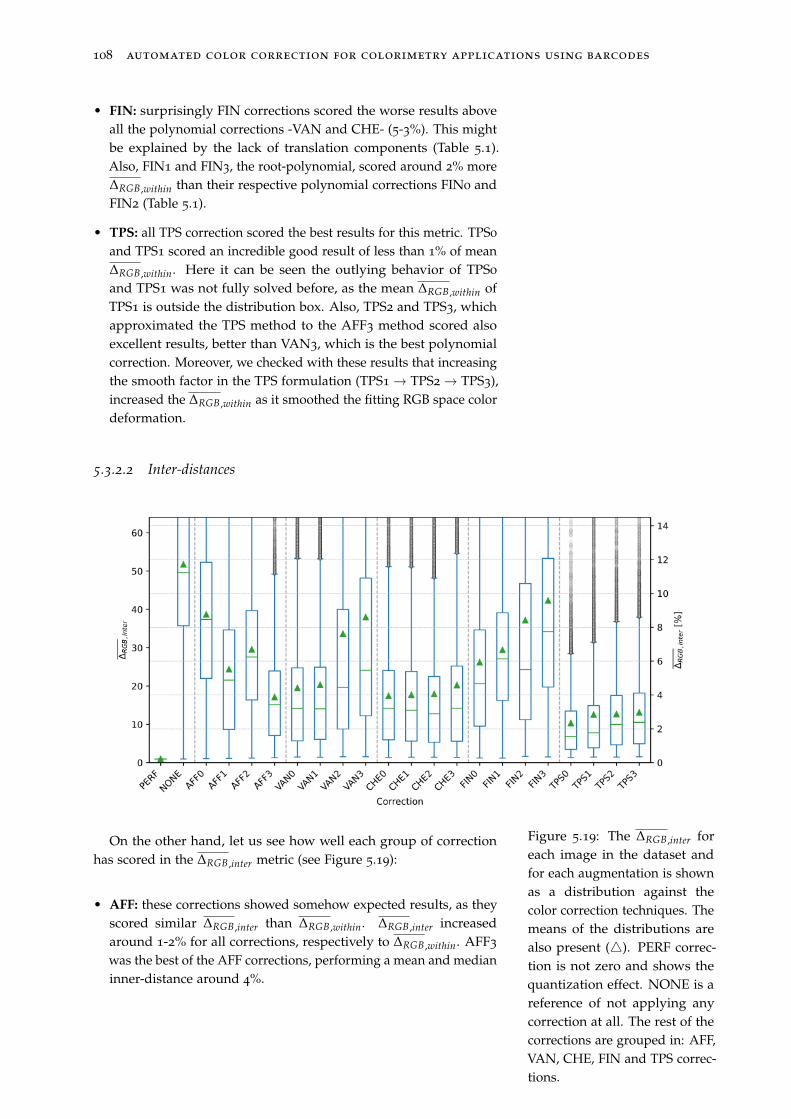
108 automated color correction for colorimetry applications using barcodes
• FIN: surprisingly FIN corrections scored the worse results aboveall the polynomial corrections -VAN and CHE- (5-3%). This mightbe explained by the lack of translation components (Table 5.1).Also, FIN1 and FIN3, the root-polynomial, scored around 2% more∆RGB ,within than their respective polynomial corrections FIN0 andFIN2 (Table 5.1).
• TPS: all TPS correction scored the best results for this metric. TPS0
and TPS1 scored an incredible good result of less than 1% of mean∆RGB ,within. Here it can be seen the outlying behavior of TPS0
and TPS1 was not fully solved before, as the mean ∆RGB ,within ofTPS1 is outside the distribution box. Also, TPS2 and TPS3, whichapproximated the TPS method to the AFF3 method scored alsoexcellent results, better than VAN3, which is the best polynomialcorrection. Moreover, we checked with these results that increasingthe smooth factor in the TPS formulation (TPS1 → TPS2 → TPS3),increased the ∆RGB ,within as it smoothed the fitting RGB space colordeformation.
5.3.2.2 Inter-distances
Figure 5.19: The ∆RGB ,inter foreach image in the dataset andfor each augmentation is shownas a distribution against thecolor correction techniques. Themeans of the distributions arealso present (△). PERF correc-tion is not zero and shows thequantization effect. NONE is areference of not applying anycorrection at all. The rest of thecorrections are grouped in: AFF,VAN, CHE, FIN and TPS correc-tions.
On the other hand, let us see how well each group of correctionhas scored in the ∆RGB ,inter metric (see Figure 5.19):
• AFF: these corrections showed somehow expected results, as theyscored similar ∆RGB ,inter than ∆RGB ,within. ∆RGB ,inter increasedaround 1-2% for all corrections, respectively to ∆RGB ,within. AFF3
was the best of the AFF corrections, performing a mean and medianinner-distance around 4%.
image consistency using an improved tps3d method 109
• VAN: VAN0 and VAN1 presented similar results to AFF3, mean∆RGB ,inter were around 4%, and the distribution matched AFF3
distribution (mean, median, box and outliers). VAN2 and VAN3
presented worst results, their distributions got spread. VAN2 andVAN3 scored mean ∆RGB ,inter around 8%. Despite the higher de-gree polynomial expansions systematically reduced the ∆RGB ,within,they increased the ∆RGB ,inter.
• CHE: all four corrections scored similar results to AFF3, matchingthe AFF3 distribution (mean, median, box and outliers). Thus,performing a mean and median inner-distance around 4%.
• FIN: all four corrections scored the worst results. FIN0 and FIN1
scored similar to AFF1 and AFF2. FIN3 showed the worst correc-tion of the overall data, above AFF0 and VAN3, with a median∆RGB ,within of almost 10%, and a mean of almost 8%. Once again,it was observed that root-polynomial presents worst results thantheir respective polynomial correction.
• TPS: all four correction scored the best results also for this metric.The effect of smoothing or not the TPS correction was reduced inthis metric. All four corrections scored median and mean ∆RGB ,inter
around 2%.
All in all, TPS corrections proved to provide the best solution tocolor correct images in our dataset. The original Menesatti et al.[15] proposal (TPS0) worked slightly better than our first proposal ofusing the recommended RBF for 3D spaces (TPS1). The smoothedTPS proposals (TPS2 and TPS3) scored the subsequent best results forboth metrics, ∆RGB ,within and ∆RGB ,inter. VAN3 proved to be a goodcompetitor in the within-distance metric, on the contrary had one ofthe poor results in the ∆RGB ,inter metric. AFF3, VAN0, VAN1 and allCHE methods proved to be good competitors in the ∆RGB ,inter metric,that is an interesting result as it opens the possibility to have fall-backmethods if the TPS fails.
5.3.3 Execution time performance
Let us see how the proposed color correction methods scored interms of execution time for each image corrected. As our datasethas images from two cameras, with different sizes, we decided tofocus only in one camera to ensure results were not affected bythe disparity in size. We chose to work with the larger subset ofimages: the Canon EOS 5D with 483 images. These images have549× 365 pixels = 200385 pixels ≈ 0.2 Mpx (see Table 5.2), as wedown-sampled them (K = 4) to speed up the global computation timeof our pipeline (see Figure 5.10).
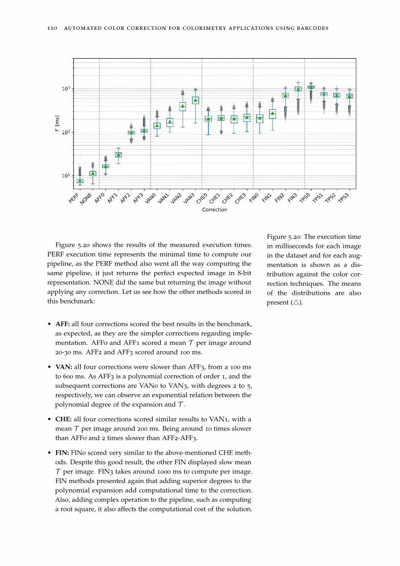
110 automated color correction for colorimetry applications using barcodes
Figure 5.20: The execution timein milliseconds for each imagein the dataset and for each aug-mentation is shown as a dis-tribution against the color cor-rection techniques. The meansof the distributions are alsopresent (△).
Figure 5.20 shows the results of the measured execution times.PERF execution time represents the minimal time to compute ourpipeline, as the PERF method also went all the way computing thesame pipeline, it just returns the perfect expected image in 8-bitrepresentation. NONE did the same but returning the image withoutapplying any correction. Let us see how the other methods scored inthis benchmark:
• AFF: all four corrections scored the best results in the benchmark,as expected, as they are the simpler corrections regarding imple-mentation. AFF0 and AFF1 scored a mean T per image around20-30 ms. AFF2 and AFF3 scored around 100 ms.
• VAN: all four corrections were slower than AFF3, from a 100 msto 600 ms. As AFF3 is a polynomial correction of order 1, and thesubsequent corrections are VAN0 to VAN3, with degrees 2 to 5,respectively, we can observe an exponential relation between thepolynomial degree of the expansion and T .
• CHE: all four corrections scored similar results to VAN1, with amean T per image around 200 ms. Being around 10 times slowerthan AFF0 and 2 times slower than AFF2-AFF3.
• FIN: FIN0 scored very similar to the above-mentioned CHE meth-ods. Despite this good result, the other FIN displayed slow meanT per image. FIN3 takes around 1000 ms to compute per image.FIN methods presented again that adding superior degrees to thepolynomial expansion add computational time to the correction.Also, adding complex operation to the pipeline, such as computinga root square, it also affects the computational cost of the solution.
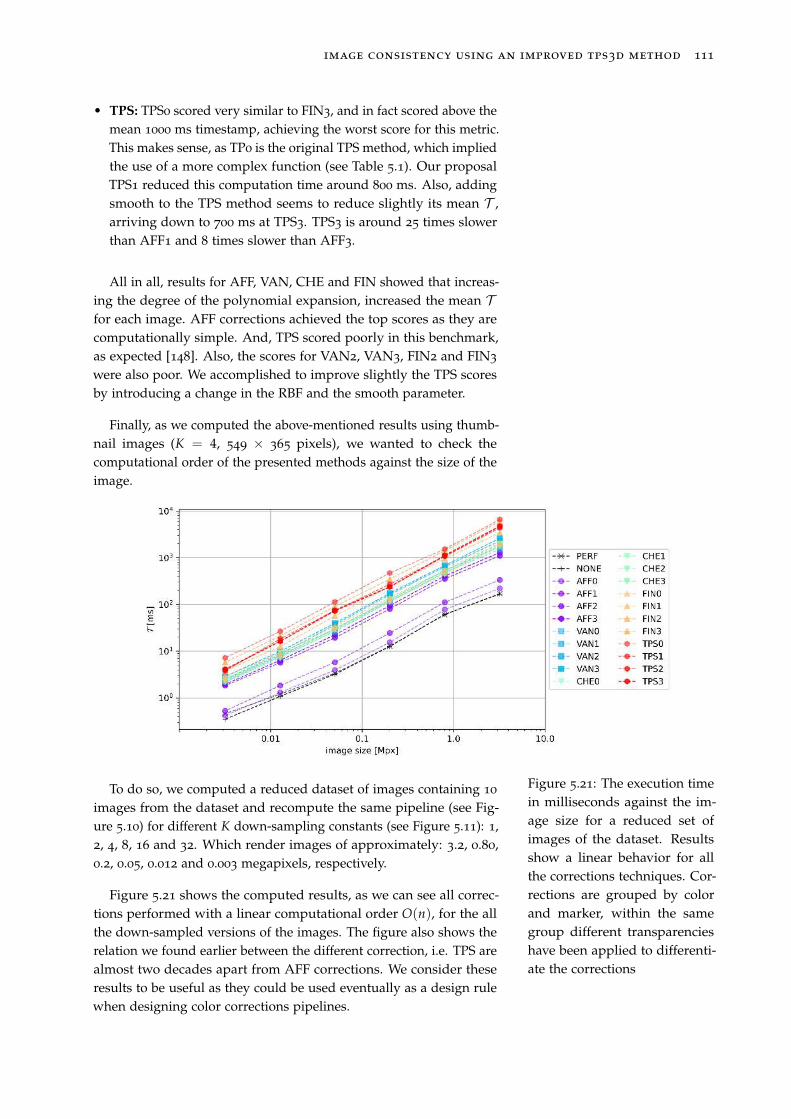
image consistency using an improved tps3d method 111
• TPS: TPS0 scored very similar to FIN3, and in fact scored above themean 1000 ms timestamp, achieving the worst score for this metric.This makes sense, as TP0 is the original TPS method, which impliedthe use of a more complex function (see Table 5.1). Our proposalTPS1 reduced this computation time around 800 ms. Also, addingsmooth to the TPS method seems to reduce slightly its mean T ,arriving down to 700 ms at TPS3. TPS3 is around 25 times slowerthan AFF1 and 8 times slower than AFF3.
All in all, results for AFF, VAN, CHE and FIN showed that increas-ing the degree of the polynomial expansion, increased the mean Tfor each image. AFF corrections achieved the top scores as they arecomputationally simple. And, TPS scored poorly in this benchmark,as expected [148]. Also, the scores for VAN2, VAN3, FIN2 and FIN3
were also poor. We accomplished to improve slightly the TPS scoresby introducing a change in the RBF and the smooth parameter.
Finally, as we computed the above-mentioned results using thumb-nail images (K = 4, 549 × 365 pixels), we wanted to check thecomputational order of the presented methods against the size of theimage.
Figure 5.21: The execution timein milliseconds against the im-age size for a reduced set ofimages of the dataset. Resultsshow a linear behavior for allthe corrections techniques. Cor-rections are grouped by colorand marker, within the samegroup different transparencieshave been applied to differenti-ate the corrections
To do so, we computed a reduced dataset of images containing 10
images from the dataset and recompute the same pipeline (see Fig-ure 5.10) for different K down-sampling constants (see Figure 5.11): 1,2, 4, 8, 16 and 32. Which render images of approximately: 3.2, 0.80,0.2, 0.05, 0.012 and 0.003 megapixels, respectively.
Figure 5.21 shows the computed results, as we can see all correc-tions performed with a linear computational order O(n), for the allthe down-sampled versions of the images. The figure also shows therelation we found earlier between the different correction, i.e. TPS arealmost two decades apart from AFF corrections. We consider theseresults to be useful as they could be used eventually as a design rulewhen designing color corrections pipelines.
112 automated color correction for colorimetry applications using barcodes
5.4 Conclusions
In this chapter, we improved the work done by Menesatti et al. [15].We successfully reproduced their findings about the TPS3D methodfor color correction to achieve image consistency in datasets. It canbe shown that our results match theirs not only qualitatively but alsoquantitatively. For this purpose, Table 5.3 shows a summary of theresults above-presented for future comparison.
Also, we extended the study to other state-of-the-art methods,Gong et al. [44], Cheung et al. [27] and Finlayson et al. [28], that canbe found in standard libraries [153]. The TPS3D proved to be the bestcorrection color method among the other in terms of color correctionperformance, both in ∆RGB ,within and ∆RGB ,inter metrics. Despite this,TPS3D has a heavy implementation compared to simpler methodsuch as AFF color corrections, resulting in T per image 20 to 100
times superior to AFF color corrections.
Moreover, we proposed 2 criteria to detect failed corrections usingthe ∆RGB ,within and ∆RGB ,pairwise metrics. These criteria discoveredfailed corrections over the dataset which heavily affected TPS3D. Ourproposal to approximate the TPS3D formulation by a smoothing factorproved the right way to systemically remove those ill-conditionedscenarios.
Furthermore, we compared different RBF into the TPS3D formu-lation. We did not prove a significance improvement in the colorcorrection, although we did find that our proposed RBF would im-prove by a 30% the results regarding the T per image.
Finally, we demonstrated the T increases linearly with the imagesize for all the compared color corrections, enabling to take intoaccount this variable when designing future color correction pipelines.
Regarding future work to improve this color correction framework,let us highlight some alternatives.
First, the systematic increase of color references should lead toa systematic improvement. This was not explored in the presentedwork in the chapter, as explained we preferred to use an establisheddataset which contained only images with the original ColorCheckerwith 24 color patches [13].
Thus, if creating a new dataset, one could add to the imagesmodern color charts from X-Rite ® which include up to 140 colors,as other authors did [15; 154; 155]. Or, one could use directly ourproposal of chapter 4 to encode the same 140 color references in ourproposed back-compatible QR Code.
image consistency using an improved tps3d method 113
We deepen into this idea of using our machine-readable patternsin chapter 6, where we used a Color QR Code to embed 125 colorsof the RGB cube and use those colors with the above-presented colorcorrection framework.
Second, we proposed this color correction framework as a solutionto a general-purpose image consistency scenario. Often, colorimetricproblems present themselves as a more reduced problem, i.e. we onlyneed to seek for color correction in a certain subset of colors. If thisis the case, instead of increasing the amount of correction colors wecould reduce the colors to perform the color correction.
When doing so, we ought to select the color references which arenear our data points, or at least they are the most representative versionof our data within our correction colors. If not, the mapping will bepoor in some parts of the data, as Donato et al. pointed out whendiscussing different approximation techniques for TPS mappings[125].
Third, there exist several authors that have explored different RBFthat could be placed in the kernel definition of the TPS3D method,here we only discussed between two RBF which were solutions for 2Dand 3D for the thin-plate spline solution. Theoretically, any RBF couldbe used [144], even more modern smooth bump functions [156; 157]
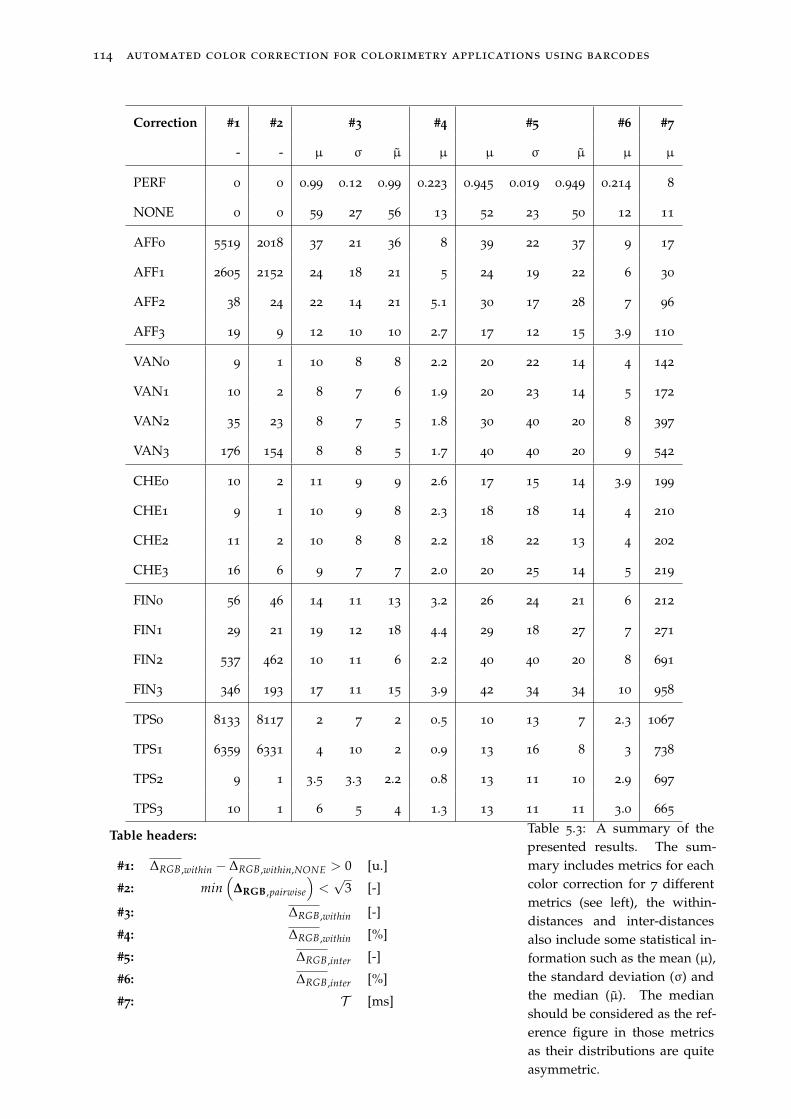
114 automated color correction for colorimetry applications using barcodes
Correction #1 #2 #3 #4 #5 #6 #7
- - µ σ µ µ µ σ µ µ µ
PERF 0 0 0.99 0.12 0.99 0.223 0.945 0.019 0.949 0.214 8
NONE 0 0 59 27 56 13 52 23 50 12 11
AFF0 5519 2018 37 21 36 8 39 22 37 9 17
AFF1 2605 2152 24 18 21 5 24 19 22 6 30
AFF2 38 24 22 14 21 5.1 30 17 28 7 96
AFF3 19 9 12 10 10 2.7 17 12 15 3.9 110
VAN0 9 1 10 8 8 2.2 20 22 14 4 142
VAN1 10 2 8 7 6 1.9 20 23 14 5 172
VAN2 35 23 8 7 5 1.8 30 40 20 8 397
VAN3 176 154 8 8 5 1.7 40 40 20 9 542
CHE0 10 2 11 9 9 2.6 17 15 14 3.9 199
CHE1 9 1 10 9 8 2.3 18 18 14 4 210
CHE2 11 2 10 8 8 2.2 18 22 13 4 202
CHE3 16 6 9 7 7 2.0 20 25 14 5 219
FIN0 56 46 14 11 13 3.2 26 24 21 6 212
FIN1 29 21 19 12 18 4.4 29 18 27 7 271
FIN2 537 462 10 11 6 2.2 40 40 20 8 691
FIN3 346 193 17 11 15 3.9 42 34 34 10 958
TPS0 8133 8117 2 7 2 0.5 10 13 7 2.3 1067
TPS1 6359 6331 4 10 2 0.9 13 16 8 3 738
TPS2 9 1 3.5 3.3 2.2 0.8 13 11 10 2.9 697
TPS3 10 1 6 5 4 1.3 13 11 11 3.0 665
Table 5.3: A summary of thepresented results. The sum-mary includes metrics for eachcolor correction for 7 differentmetrics (see left), the within-distances and inter-distancesalso include some statistical in-formation such as the mean (µ),the standard deviation (σ) andthe median (µ). The medianshould be considered as the ref-erence figure in those metricsas their distributions are quiteasymmetric.
Table headers:
#1: ∆RGB ,within − ∆RGB ,within,NONE > 0 [u.]
#2: min(
∆RGB ,pairwise
)
<
√3 [-]
#3: ∆RGB ,within [-]
#4: ∆RGB ,within [%]
#5: ∆RGB ,inter [-]
#6: ∆RGB ,inter [%]
#7: T [ms]
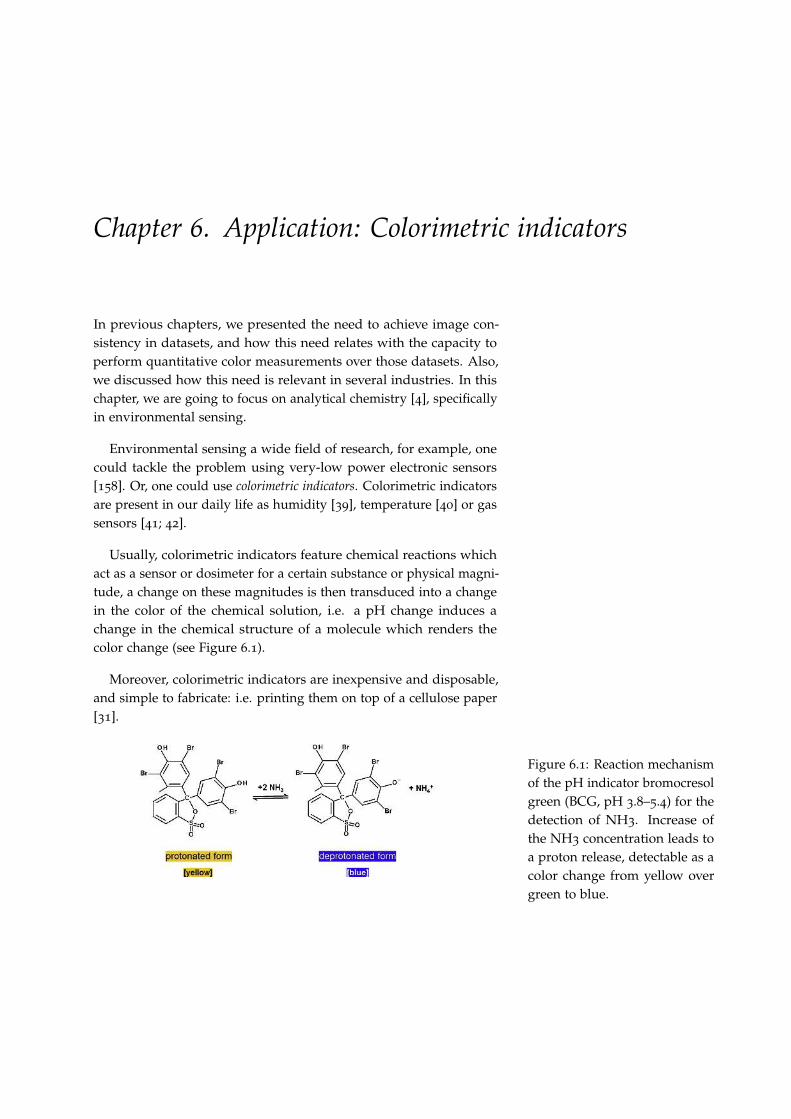
Chapter 6. Application: Colorimetric indicators
In previous chapters, we presented the need to achieve image con-sistency in datasets, and how this need relates with the capacity toperform quantitative color measurements over those datasets. Also,we discussed how this need is relevant in several industries. In thischapter, we are going to focus on analytical chemistry [4], specificallyin environmental sensing.
Environmental sensing a wide field of research, for example, onecould tackle the problem using very-low power electronic sensors[158]. Or, one could use colorimetric indicators. Colorimetric indicatorsare present in our daily life as humidity [39], temperature [40] or gassensors [41; 42].
Usually, colorimetric indicators feature chemical reactions whichact as a sensor or dosimeter for a certain substance or physical magni-tude, a change on these magnitudes is then transduced into a changein the color of the chemical solution, i.e. a pH change induces achange in the chemical structure of a molecule which renders thecolor change (see Figure 6.1).
Moreover, colorimetric indicators are inexpensive and disposable,and simple to fabricate: i.e. printing them on top of a cellulose paper[31].
Figure 6.1: Reaction mechanismof the pH indicator bromocresolgreen (BCG, pH 3.8–5.4) for thedetection of NH3. Increase ofthe NH3 concentration leads toa proton release, detectable as acolor change from yellow overgreen to blue.
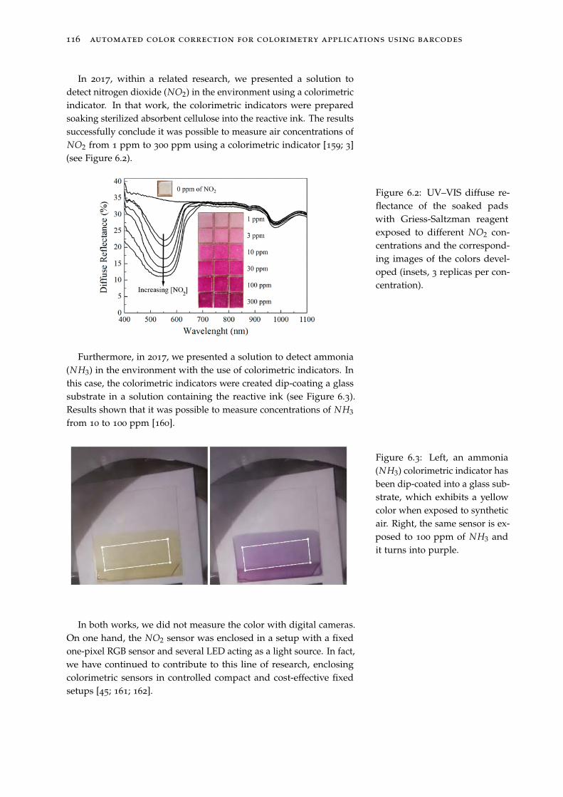
116 automated color correction for colorimetry applications using barcodes
In 2017, within a related research, we presented a solution todetect nitrogen dioxide (NO2) in the environment using a colorimetricindicator. In that work, the colorimetric indicators were preparedsoaking sterilized absorbent cellulose into the reactive ink. The resultssuccessfully conclude it was possible to measure air concentrations ofNO2 from 1 ppm to 300 ppm using a colorimetric indicator [159; 3](see Figure 6.2).
Figure 6.2: UV–VIS diffuse re-flectance of the soaked padswith Griess-Saltzman reagentexposed to different NO2 con-centrations and the correspond-ing images of the colors devel-oped (insets, 3 replicas per con-centration).
Furthermore, in 2017, we presented a solution to detect ammonia(NH3) in the environment with the use of colorimetric indicators. Inthis case, the colorimetric indicators were created dip-coating a glasssubstrate in a solution containing the reactive ink (see Figure 6.3).Results shown that it was possible to measure concentrations of NH3
from 10 to 100 ppm [160].
Figure 6.3: Left, an ammonia(NH3) colorimetric indicator hasbeen dip-coated into a glass sub-strate, which exhibits a yellowcolor when exposed to syntheticair. Right, the same sensor is ex-posed to 100 ppm of NH3 andit turns into purple.
In both works, we did not measure the color with digital cameras.On one hand, the NO2 sensor was enclosed in a setup with a fixedone-pixel RGB sensor and several LED acting as a light source. In fact,we have continued to contribute to this line of research, enclosingcolorimetric sensors in controlled compact and cost-effective fixedsetups [45; 161; 162].
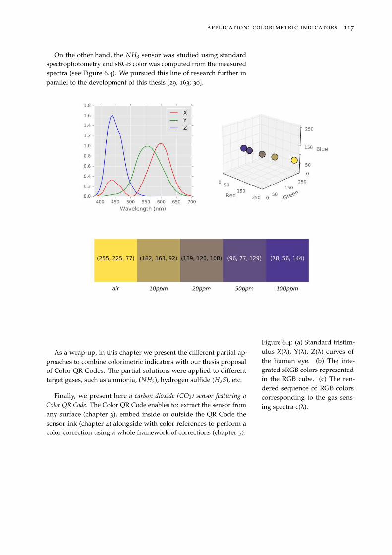
application: colorimetric indicators 117
On the other hand, the NH3 sensor was studied using standardspectrophotometry and sRGB color was computed from the measuredspectra (see Figure 6.4). We pursued this line of research further inparallel to the development of this thesis [29; 163; 30].
Figure 6.4: (a) Standard tristim-ulus X(λ), Y(λ), Z(λ) curves ofthe human eye. (b) The inte-grated sRGB colors representedin the RGB cube. (c) The ren-dered sequence of RGB colorscorresponding to the gas sens-ing spectra c(λ).
As a wrap-up, in this chapter we present the different partial ap-proaches to combine colorimetric indicators with our thesis proposalof Color QR Codes. The partial solutions were applied to differenttarget gases, such as ammonia, (NH3), hydrogen sulfide (H2S), etc.
Finally, we present here a carbon dioxide (CO2) sensor featuring a
Color QR Code. The Color QR Code enables to: extract the sensor fromany surface (chapter 3), embed inside or outside the QR Code thesensor ink (chapter 4) alongside with color references to perform acolor correction using a whole framework of corrections (chapter 5).
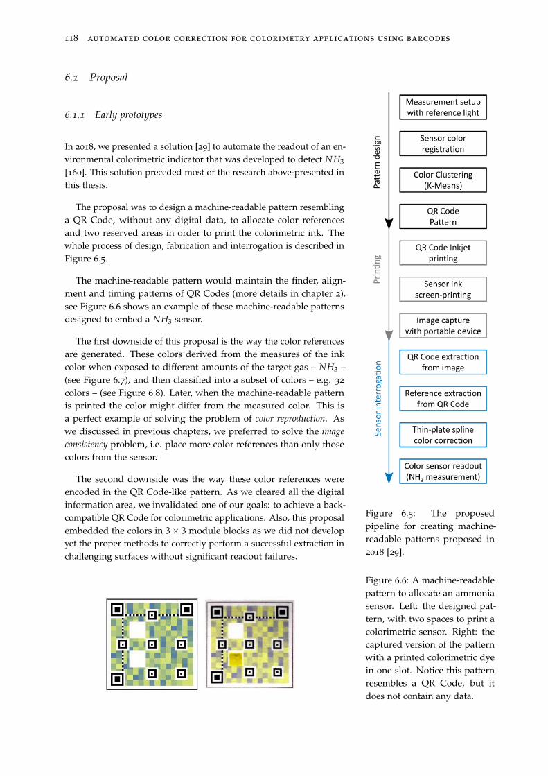
118 automated color correction for colorimetry applications using barcodes
6.1 Proposal
6.1.1 Early prototypes
In 2018, we presented a solution [29] to automate the readout of an en-vironmental colorimetric indicator that was developed to detect NH3
[160]. This solution preceded most of the research above-presented inthis thesis.
The proposal was to design a machine-readable pattern resemblinga QR Code, without any digital data, to allocate color referencesand two reserved areas in order to print the colorimetric ink. Thewhole process of design, fabrication and interrogation is described inFigure 6.5.
The machine-readable pattern would maintain the finder, align-ment and timing patterns of QR Codes (more details in chapter 2).see Figure 6.6 shows an example of these machine-readable patternsdesigned to embed a NH3 sensor.
Figure 6.5: The proposedpipeline for creating machine-readable patterns proposed in2018 [29].
The first downside of this proposal is the way the color referencesare generated. These colors derived from the measures of the inkcolor when exposed to different amounts of the target gas – NH3 –(see Figure 6.7), and then classified into a subset of colors – e.g. 32
colors – (see Figure 6.8). Later, when the machine-readable patternis printed the color might differ from the measured color. This isa perfect example of solving the problem of color reproduction. Aswe discussed in previous chapters, we preferred to solve the image
consistency problem, i.e. place more color references than only thosecolors from the sensor.
The second downside was the way these color references wereencoded in the QR Code-like pattern. As we cleared all the digitalinformation area, we invalidated one of our goals: to achieve a back-compatible QR Code for colorimetric applications. Also, this proposalembedded the colors in 3× 3 module blocks as we did not developyet the proper methods to correctly perform a successful extraction inchallenging surfaces without significant readout failures.
Figure 6.6: A machine-readablepattern to allocate an ammoniasensor. Left: the designed pat-tern, with two spaces to print acolorimetric sensor. Right: thecaptured version of the patternwith a printed colorimetric dyein one slot. Notice this patternresembles a QR Code, but itdoes not contain any data.
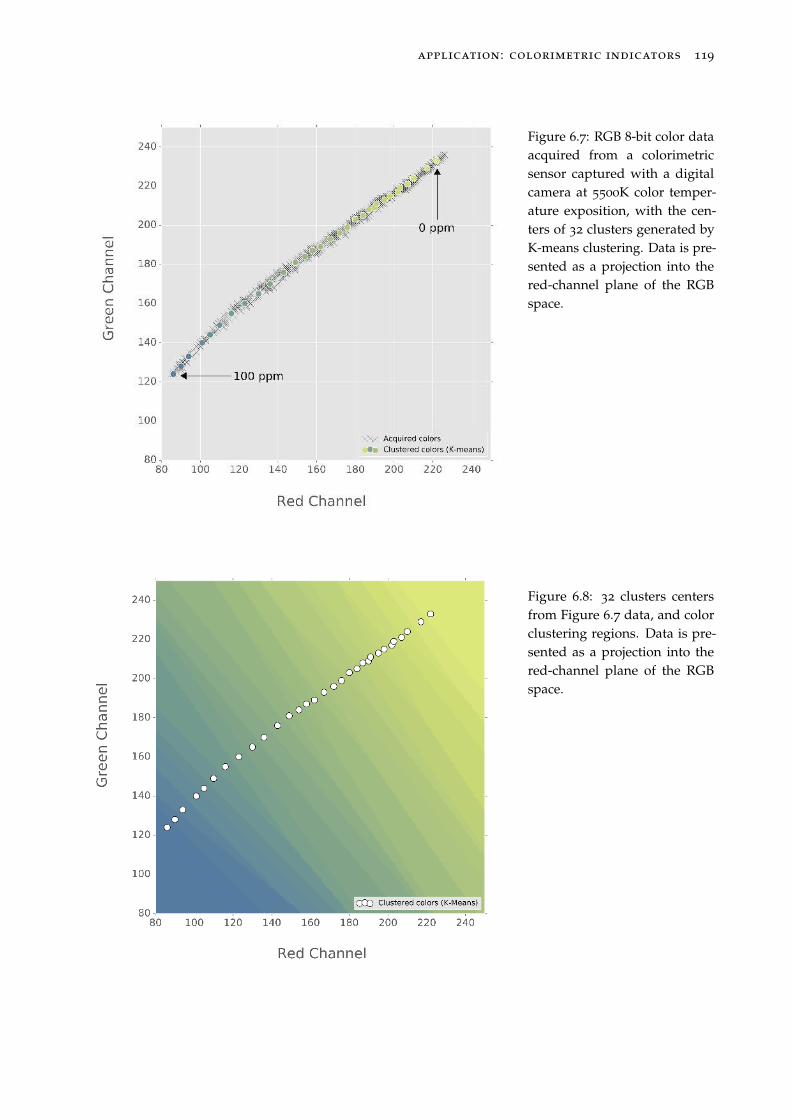
application: colorimetric indicators 119
Figure 6.7: RGB 8-bit color dataacquired from a colorimetricsensor captured with a digitalcamera at 5500K color temper-ature exposition, with the cen-ters of 32 clusters generated byK-means clustering. Data is pre-sented as a projection into thered-channel plane of the RGBspace.
Figure 6.8: 32 clusters centersfrom Figure 6.7 data, and colorclustering regions. Data is pre-sented as a projection into thered-channel plane of the RGBspace.
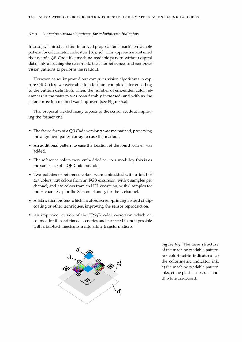
120 automated color correction for colorimetry applications using barcodes
6.1.2 A machine-readable pattern for colorimetric indicators
In 2020, we introduced our improved proposal for a machine-readablepattern for colorimetric indicators [163; 30]. This approach maintainedthe use of a QR Code-like machine-readable pattern without digitaldata, only allocating the sensor ink, the color references and computervision patterns to perform the readout.
However, as we improved our computer vision algorithms to cap-ture QR Codes, we were able to add more complex color encodingto the pattern definition. Then, the number of embedded color ref-erences in the pattern was considerably increased, and with so thecolor correction method was improved (see Figure 6.9).
This proposal tackled many aspects of the sensor readout improv-ing the former one:
• The factor form of a QR Code version 7 was maintained, preservingthe alignment pattern array to ease the readout.
• An additional pattern to ease the location of the fourth corner wasadded.
• The reference colors were embedded as 1 x 1 modules, this is asthe same size of a QR Code module.
• Two palettes of reference colors were embedded with a total of245 colors: 125 colors from an RGB excursion, with 5 samples perchannel; and 120 colors from an HSL excursion, with 6 samples forthe H channel, 4 for the S channel and 5 for the L channel.
• A fabrication process which involved screen-printing instead of dip-coating or other techniques, improving the sensor reproduction.
• An improved version of the TPS3D color correction which ac-counted for ill-conditioned scenarios and corrected them if possiblewith a fall-back mechanism into affine transformations.
Figure 6.9: The layer structureof the machine-readable patternfor colorimetric indicators: a)the colorimetric indicator ink,b) the machine-readable patterninks, c) the plastic substrate andd) white cardboard.
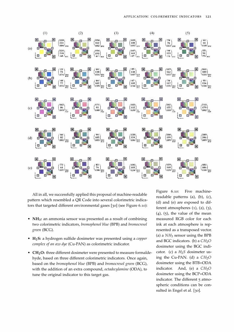
application: colorimetric indicators 121
Figure 6.10: Five machine-readable patterns (a), (b), (c),(d) and (e) are exposed to dif-ferent atmospheres (1), (2), (3),(4), (5), the value of the meanmeasured RGB color for eachink at each atmosphere is rep-resented as a transposed vector.(a) a NH3 sensor using the BPBand BGC indicators. (b) a CH2O
dosimeter using the BGC indi-cator. (c) a H2S dosimeter us-ing the Cu-PAN. (d) a CH2O
dosimeter using the BTB+ODAindicator. And, (e) a CH2O
dosimeter using the BCP+ODAindicator. The different 5 atmo-spheric conditions can be con-sulted in Engel et al. [30].
All in all, we successfully applied this proposal of machine-readablepattern which resembled a QR Code into several colorimetric indica-tors that targeted different environmental gases [30] (see Figure 6.10):
• NH3: an ammonia sensor was presented as a result of combiningtwo colorimetric indicators, bromophenol blue (BPB) and bromocresol
green (BCG).
• H2S: a hydrogen sulfide dosimeter was presented using a copper
complex of an azo dye (Cu-PAN) as colorimetric indicator.
• CH2O: three different dosimeter were presented to measure formalde-hyde, based on three different colorimetric indicators. Once again,based on the bromophenol blue (BPB) and bromocresol green (BCG),with the addition of an extra compound, octadecylamine (ODA), totune the original indicator to this target gas.
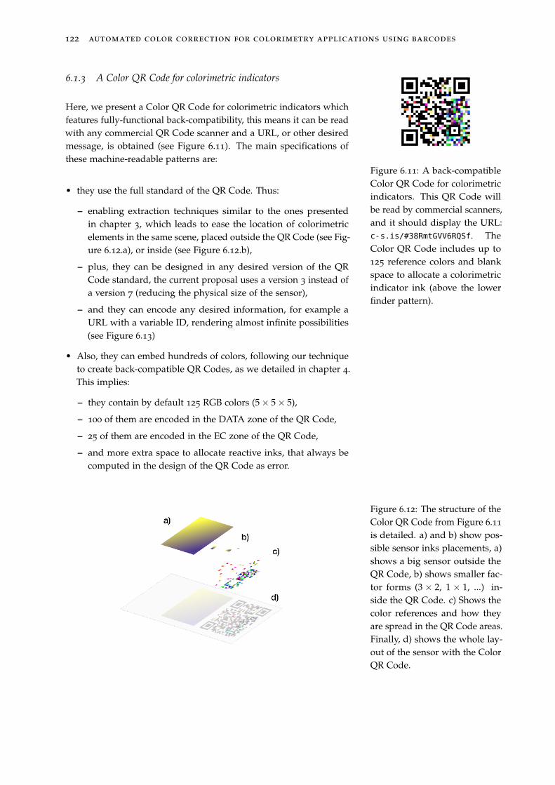
122 automated color correction for colorimetry applications using barcodes
6.1.3 A Color QR Code for colorimetric indicators
Here, we present a Color QR Code for colorimetric indicators whichfeatures fully-functional back-compatibility, this means it can be readwith any commercial QR Code scanner and a URL, or other desiredmessage, is obtained (see Figure 6.11). The main specifications ofthese machine-readable patterns are:
Figure 6.11: A back-compatibleColor QR Code for colorimetricindicators. This QR Code willbe read by commercial scanners,and it should display the URL:c-s.is/#38RmtGVV6RQSf. TheColor QR Code includes up to125 reference colors and blankspace to allocate a colorimetricindicator ink (above the lowerfinder pattern).
• they use the full standard of the QR Code. Thus:
– enabling extraction techniques similar to the ones presentedin chapter 3, which leads to ease the location of colorimetricelements in the same scene, placed outside the QR Code (see Fig-ure 6.12.a), or inside (see Figure 6.12.b),
– plus, they can be designed in any desired version of the QRCode standard, the current proposal uses a version 3 instead ofa version 7 (reducing the physical size of the sensor),
– and they can encode any desired information, for example aURL with a variable ID, rendering almost infinite possibilities(see Figure 6.13)
• Also, they can embed hundreds of colors, following our techniqueto create back-compatible QR Codes, as we detailed in chapter 4.This implies:
– they contain by default 125 RGB colors (5× 5× 5),
– 100 of them are encoded in the DATA zone of the QR Code,
– 25 of them are encoded in the EC zone of the QR Code,
– and more extra space to allocate reactive inks, that always becomputed in the design of the QR Code as error.
Figure 6.12: The structure of theColor QR Code from Figure 6.11
is detailed. a) and b) show pos-sible sensor inks placements, a)shows a big sensor outside theQR Code, b) shows smaller fac-tor forms (3 × 2, 1 × 1, ...) in-side the QR Code. c) Shows thecolor references and how theyare spread in the QR Code areas.Finally, d) shows the whole lay-out of the sensor with the ColorQR Code.
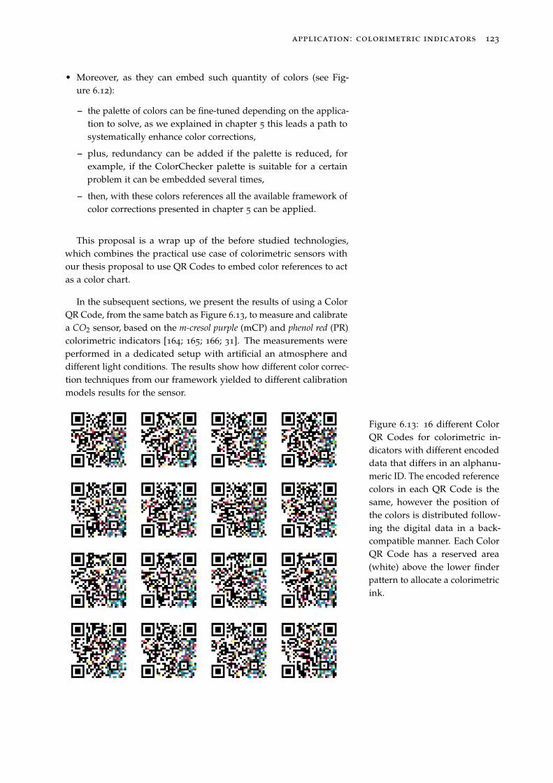
application: colorimetric indicators 123
• Moreover, as they can embed such quantity of colors (see Fig-ure 6.12):
– the palette of colors can be fine-tuned depending on the applica-tion to solve, as we explained in chapter 5 this leads a path tosystematically enhance color corrections,
– plus, redundancy can be added if the palette is reduced, forexample, if the ColorChecker palette is suitable for a certainproblem it can be embedded several times,
– then, with these colors references all the available framework ofcolor corrections presented in chapter 5 can be applied.
This proposal is a wrap up of the before studied technologies,which combines the practical use case of colorimetric sensors withour thesis proposal to use QR Codes to embed color references to actas a color chart.
In the subsequent sections, we present the results of using a ColorQR Code, from the same batch as Figure 6.13, to measure and calibratea CO2 sensor, based on the m-cresol purple (mCP) and phenol red (PR)colorimetric indicators [164; 165; 166; 31]. The measurements wereperformed in a dedicated setup with artificial an atmosphere anddifferent light conditions. The results show how different color correc-tion techniques from our framework yielded to different calibrationmodels results for the sensor.
Figure 6.13: 16 different ColorQR Codes for colorimetric in-dicators with different encodeddata that differs in an alphanu-meric ID. The encoded referencecolors in each QR Code is thesame, however the position ofthe colors is distributed follow-ing the digital data in a back-compatible manner. Each ColorQR Code has a reserved area(white) above the lower finderpattern to allocate a colorimetricink.
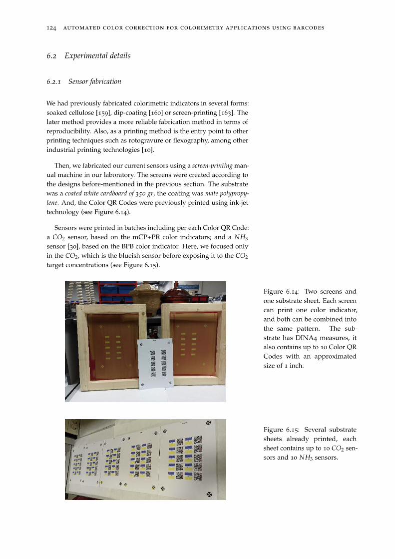
124 automated color correction for colorimetry applications using barcodes
6.2 Experimental details
6.2.1 Sensor fabrication
We had previously fabricated colorimetric indicators in several forms:soaked cellulose [159], dip-coating [160] or screen-printing [163]. Thelater method provides a more reliable fabrication method in terms ofreproducibility. Also, as a printing method is the entry point to otherprinting techniques such as rotogravure or flexography, among otherindustrial printing technologies [10].
Then, we fabricated our current sensors using a screen-printing man-ual machine in our laboratory. The screens were created according tothe designs before-mentioned in the previous section. The substratewas a coated white cardboard of 350 gr, the coating was mate polypropy-
lene. And, the Color QR Codes were previously printed using ink-jettechnology (see Figure 6.14).
Sensors were printed in batches including per each Color QR Code:a CO2 sensor, based on the mCP+PR color indicators; and a NH3
sensor [30], based on the BPB color indicator. Here, we focused onlyin the CO2, which is the blueish sensor before exposing it to the CO2
target concentrations (see Figure 6.15).
Figure 6.14: Two screens andone substrate sheet. Each screencan print one color indicator,and both can be combined intothe same pattern. The sub-strate has DINA4 measures, italso contains up to 10 Color QRCodes with an approximatedsize of 1 inch.
Figure 6.15: Several substratesheets already printed, eachsheet contains up to 10 CO2 sen-sors and 10 NH3 sensors.
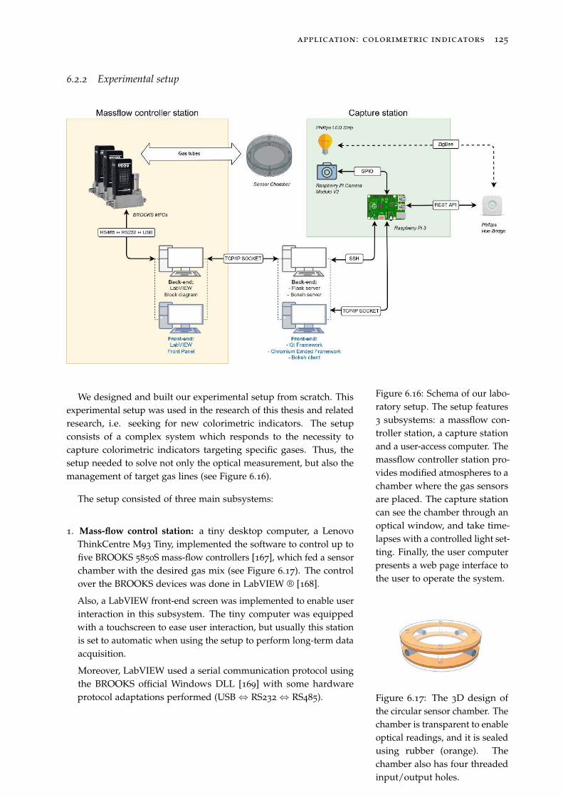
application: colorimetric indicators 125
6.2.2 Experimental setup
Figure 6.16: Schema of our labo-ratory setup. The setup features3 subsystems: a massflow con-troller station, a capture stationand a user-access computer. Themassflow controller station pro-vides modified atmospheres to achamber where the gas sensorsare placed. The capture stationcan see the chamber through anoptical window, and take time-lapses with a controlled light set-ting. Finally, the user computerpresents a web page interface tothe user to operate the system.
We designed and built our experimental setup from scratch. Thisexperimental setup was used in the research of this thesis and relatedresearch, i.e. seeking for new colorimetric indicators. The setupconsists of a complex system which responds to the necessity tocapture colorimetric indicators targeting specific gases. Thus, thesetup needed to solve not only the optical measurement, but also themanagement of target gas lines (see Figure 6.16).
The setup consisted of three main subsystems:
1. Mass-flow control station: a tiny desktop computer, a LenovoThinkCentre M93 Tiny, implemented the software to control up tofive BROOKS 5850S mass-flow controllers [167], which fed a sensorchamber with the desired gas mix (see Figure 6.17). The controlover the BROOKS devices was done in LabVIEW ® [168].
Also, a LabVIEW front-end screen was implemented to enable userinteraction in this subsystem. The tiny computer was equippedwith a touchscreen to ease user interaction, but usually this stationis set to automatic when using the setup to perform long-term dataacquisition.
Moreover, LabVIEW used a serial communication protocol usingthe BROOKS official Windows DLL [169] with some hardwareprotocol adaptations performed (USB⇔ RS232⇔ RS485). Figure 6.17: The 3D design of
the circular sensor chamber. Thechamber is transparent to enableoptical readings, and it is sealedusing rubber (orange). Thechamber also has four threadedinput/output holes.
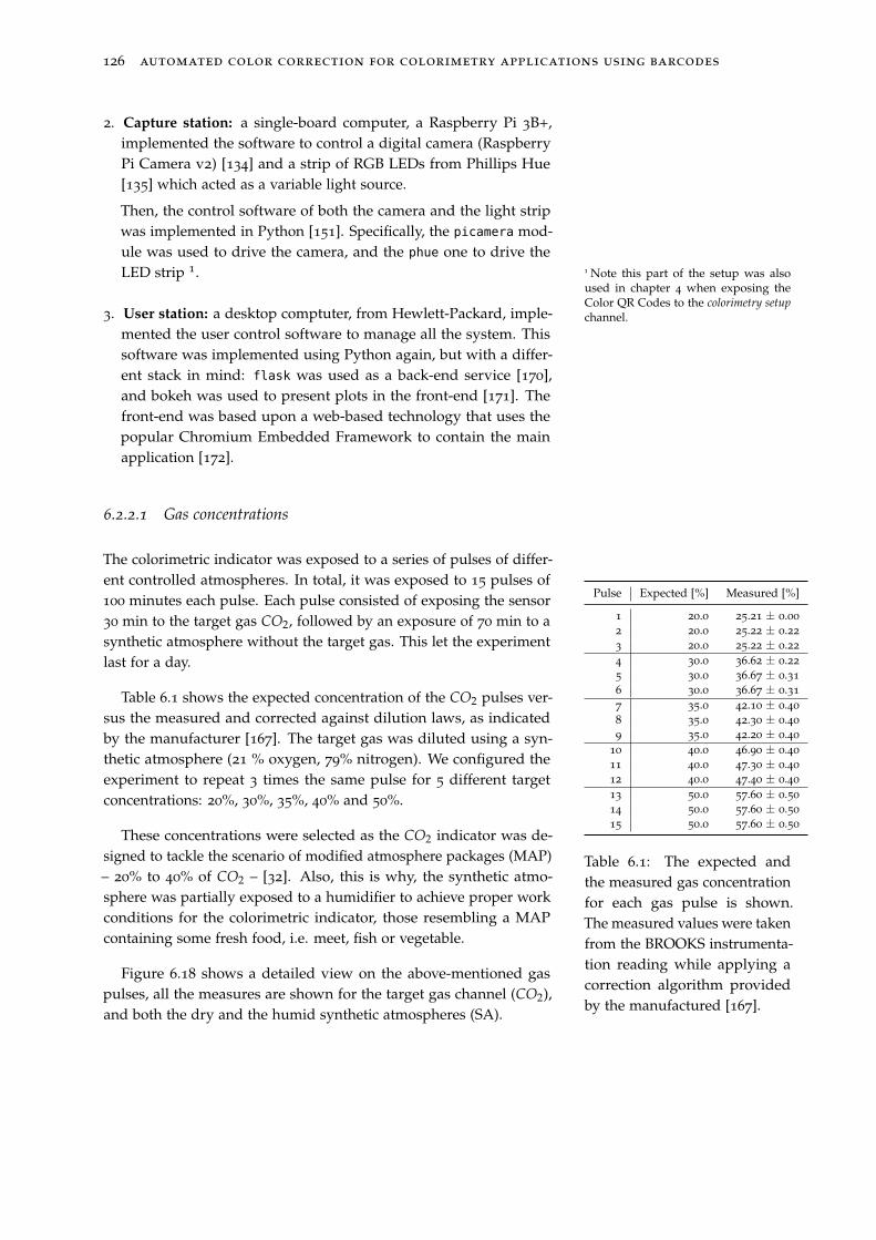
126 automated color correction for colorimetry applications using barcodes
2. Capture station: a single-board computer, a Raspberry Pi 3B+,implemented the software to control a digital camera (RaspberryPi Camera v2) [134] and a strip of RGB LEDs from Phillips Hue[135] which acted as a variable light source.
Then, the control software of both the camera and the light stripwas implemented in Python [151]. Specifically, the picamera mod-ule was used to drive the camera, and the phue one to drive theLED strip 1. 1 Note this part of the setup was also
used in chapter 4 when exposing theColor QR Codes to the colorimetry setupchannel.3. User station: a desktop comptuter, from Hewlett-Packard, imple-
mented the user control software to manage all the system. Thissoftware was implemented using Python again, but with a differ-ent stack in mind: flask was used as a back-end service [170],and bokeh was used to present plots in the front-end [171]. Thefront-end was based upon a web-based technology that uses thepopular Chromium Embedded Framework to contain the mainapplication [172].
6.2.2.1 Gas concentrations
The colorimetric indicator was exposed to a series of pulses of differ-ent controlled atmospheres. In total, it was exposed to 15 pulses of100 minutes each pulse. Each pulse consisted of exposing the sensor30 min to the target gas CO2, followed by an exposure of 70 min to asynthetic atmosphere without the target gas. This let the experimentlast for a day.
Table 6.1 shows the expected concentration of the CO2 pulses ver-sus the measured and corrected against dilution laws, as indicatedby the manufacturer [167]. The target gas was diluted using a syn-thetic atmosphere (21 % oxygen, 79% nitrogen). We configured theexperiment to repeat 3 times the same pulse for 5 different targetconcentrations: 20%, 30%, 35%, 40% and 50%.
Pulse Expected [%] Measured [%]
1 20.0 25.21 ± 0.00
2 20.0 25.22 ± 0.22
3 20.0 25.22 ± 0.22
4 30.0 36.62 ± 0.22
5 30.0 36.67 ± 0.31
6 30.0 36.67 ± 0.31
7 35.0 42.10 ± 0.40
8 35.0 42.30 ± 0.40
9 35.0 42.20 ± 0.40
10 40.0 46.90 ± 0.40
11 40.0 47.30 ± 0.40
12 40.0 47.40 ± 0.40
13 50.0 57.60 ± 0.50
14 50.0 57.60 ± 0.50
15 50.0 57.60 ± 0.50
Table 6.1: The expected andthe measured gas concentrationfor each gas pulse is shown.The measured values were takenfrom the BROOKS instrumenta-tion reading while applying acorrection algorithm providedby the manufactured [167].
These concentrations were selected as the CO2 indicator was de-signed to tackle the scenario of modified atmosphere packages (MAP)– 20% to 40% of CO2 – [32]. Also, this is why, the synthetic atmo-sphere was partially exposed to a humidifier to achieve proper workconditions for the colorimetric indicator, those resembling a MAPcontaining some fresh food, i.e. meet, fish or vegetable.
Figure 6.18 shows a detailed view on the above-mentioned gaspulses, all the measures are shown for the target gas channel (CO2),and both the dry and the humid synthetic atmospheres (SA).
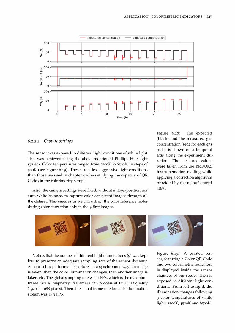
application: colorimetric indicators 127
Figure 6.18: The expected(black) and the measured gasconcentration (red) for each gaspulse is shown on a temporalaxis along the experiment du-ration. The measured valueswere taken from the BROOKSinstrumentation reading whileapplying a correction algorithmprovided by the manufactured[167].
6.2.2.2 Capture settings
The sensor was exposed to different light conditions of white light.This was achieved using the above-mentioned Phillips Hue lightsystem. Color temperatures ranged from 2500K to 6500K, in steps of500K (see Figure 6.19). These are a less aggressive light conditionsthan those we used in chapter 4 when studying the capacity of QRCodes in the colorimertry setup.
Also, the camera settings were fixed, without auto-exposition norauto white-balance, to capture color consistent images through allthe dataset. This ensures us we can extract the color reference tablesduring color correction only in the 9 first images.
Figure 6.19: A printed sen-sor, featuring a Color QR Codeand two colorimetric indicatorsis displayed inside the sensorchamber of our setup. Then isexposed to different light con-ditions. From left to right, theillumination changes following3 color temperatures of whitelight: 2500K, 4500K and 6500K.
Notice, that the number of different light illuminations (9) was keptlow to preserve an adequate sampling rate of the sensor dynamic.As, our setup performs the captures in a synchronous way: an imageis taken, then the color illumination changes, then another image istaken, etc. The global sampling rate was 1 FPS, which is the maximumframe rate a Raspberry Pi Camera can process at Full HD quality(1920 × 1088 pixels). Then, the actual frame rate for each illuminationstream was 1/9 FPS.
128 automated color correction for colorimetry applications using barcodes
6.2.3 Expected response model
In previous works, we already studied the relation between the col-orimetric response of an indicator with the presence of the target gas[30; 29; 160; 163]. The relation we found was:
S[%] = m log(c) + n (6.1)
where S is the colorimetric response of the sensor, c is the concen-tration of the target gas in the atmosphere, m and n are the constantsof a linear law. Then, the colorimetric response is linear with the loga-rithm of the gas concentration. m represents the sensitivity towardsthe logarithm of the gas concentration, and n the response at verylow concentrations.
Also, we can recover the sensitivity as a function of the gas concen-tration using derivates and use it to compute the error of the modelfor each concentration. To do so, we will use error propagation rules:
∆S
∆c
∣
∣
∣
∣
c
=m
c=⇒ ∆c|c = ∆S|c ·
c
m(6.2)
where c is a given concentration recovered with the inverted Equa-tion 6.1, m depends on each fitted model, ∆S|c is the error of themeasured signal response and ∆c|c is the model error for this givenconcentration.
Finally, the signal color response S[%] is usually normalized fol-lowing a metric. We defined this metric to resemble the normalizationperformed in an electronic gas sensor [30]. This kind of normalizationdivides the measured signal by the signal value assigned to zerogas concentration, this produces a metric that is not upper-bounded[0, ∞), the more the initial value is to zero resistance, the greater theresponse. Let us adapt this normalization for a red channel of acolorimetric indicator:
Sr[%] = 100 · r(c)− r0
r0 − rre f(6.3)
where Sr is the response in % of the red channel, c the concentrationof the target gas in %, r(c) the raw red sensor signal with an 8-bitresolution (0–255), r0 the value of r(c = 0%) and rre f an absolutecolor reference which acts as the zero resistance compared to electronicsensors, for our sensor the value is (rre f , gre f , bre f ) = (0, 0, 255), as ourmeasured blue channel signal decreases when the gas concentrationincreases [31].
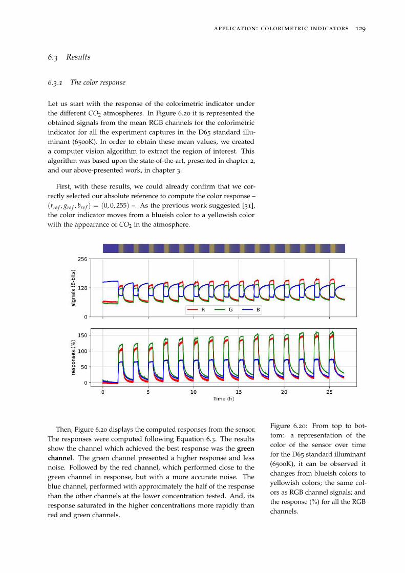
application: colorimetric indicators 129
6.3 Results
6.3.1 The color response
Let us start with the response of the colorimetric indicator underthe different CO2 atmospheres. In Figure 6.20 it is represented theobtained signals from the mean RGB channels for the colorimetricindicator for all the experiment captures in the D65 standard illu-minant (6500K). In order to obtain these mean values, we createda computer vision algorithm to extract the region of interest. Thisalgorithm was based upon the state-of-the-art, presented in chapter 2,and our above-presented work, in chapter 3.
First, with these results, we could already confirm that we cor-rectly selected our absolute reference to compute the color response –(rre f , gre f , bre f ) = (0, 0, 255) –. As the previous work suggested [31],the color indicator moves from a blueish color to a yellowish colorwith the appearance of CO2 in the atmosphere.
Figure 6.20: From top to bot-tom: a representation of thecolor of the sensor over timefor the D65 standard illuminant(6500K), it can be observed itchanges from blueish colors toyellowish colors; the same col-ors as RGB channel signals; andthe response (%) for all the RGBchannels.
Then, Figure 6.20 displays the computed responses from the sensor.The responses were computed following Equation 6.3. The resultsshow the channel which achieved the best response was the green
channel. The green channel presented a higher response and lessnoise. Followed by the red channel, which performed close to thegreen channel in response, but with a more accurate noise. Theblue channel, performed with approximately the half of the responsethan the other channels at the lower concentration tested. And, itsresponse saturated in the higher concentrations more rapidly thanred and green channels.
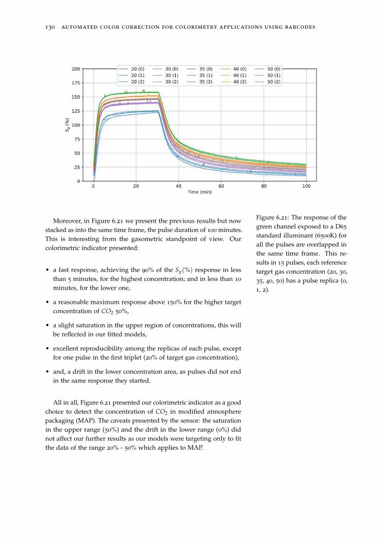
130 automated color correction for colorimetry applications using barcodes
Figure 6.21: The response of thegreen channel exposed to a D65
standard illuminant (6500K) forall the pulses are overlapped inthe same time frame. This re-sults in 15 pulses, each referencetarget gas concentration (20, 30,35, 40, 50) has a pulse replica (0,1, 2).
Moreover, in Figure 6.21 we present the previous results but nowstacked as into the same time frame, the pulse duration of 100 minutes.This is interesting from the gasometric standpoint of view. Ourcolorimetric indicator presented:
• a fast response, achieving the 90% of the Sg(%) response in lessthan 5 minutes, for the highest concentration; and in less than 10
minutes, for the lower one,
• a reasonable maximum response above 150% for the higher targetconcentration of CO2 50%,
• a slight saturation in the upper region of concentrations, this willbe reflected in our fitted models,
• excellent reproducibility among the replicas of each pulse, exceptfor one pulse in the first triplet (20% of target gas concentration),
• and, a drift in the lower concentration area, as pulses did not endin the same response they started.
All in all, Figure 6.21 presented our colorimetric indicator as a goodchoice to detect the concentration of CO2 in modified atmospherepackaging (MAP). The caveats presented by the sensor: the saturationin the upper range (50%) and the drift in the lower range (0%) didnot affect our further results as our models were targeting only to fitthe data of the range 20% - 50% which applies to MAP.
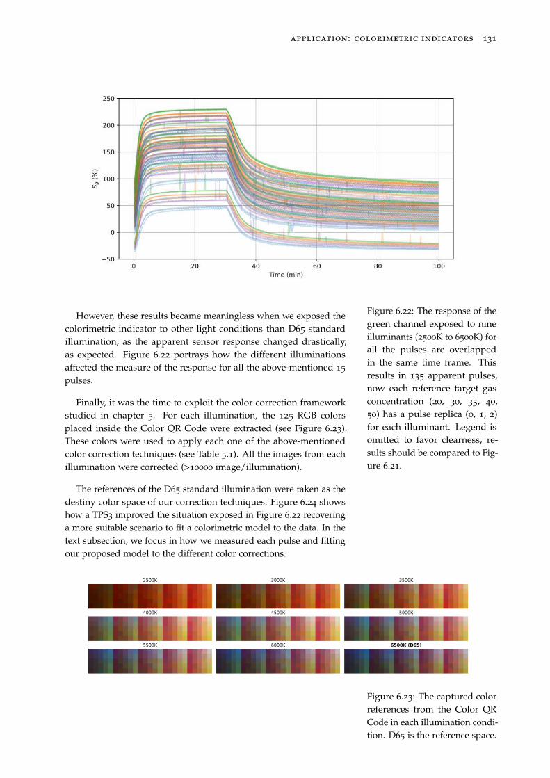
application: colorimetric indicators 131
Figure 6.22: The response of thegreen channel exposed to nineilluminants (2500K to 6500K) forall the pulses are overlappedin the same time frame. Thisresults in 135 apparent pulses,now each reference target gasconcentration (20, 30, 35, 40,50) has a pulse replica (0, 1, 2)for each illuminant. Legend isomitted to favor clearness, re-sults should be compared to Fig-ure 6.21.
However, these results became meaningless when we exposed thecolorimetric indicator to other light conditions than D65 standardillumination, as the apparent sensor response changed drastically,as expected. Figure 6.22 portrays how the different illuminationsaffected the measure of the response for all the above-mentioned 15
pulses.
Finally, it was the time to exploit the color correction frameworkstudied in chapter 5. For each illumination, the 125 RGB colorsplaced inside the Color QR Code were extracted (see Figure 6.23).These colors were used to apply each one of the above-mentionedcolor correction techniques (see Table 5.1). All the images from eachillumination were corrected (>10000 image/illumination).
The references of the D65 standard illumination were taken as thedestiny color space of our correction techniques. Figure 6.24 showshow a TPS3 improved the situation exposed in Figure 6.22 recoveringa more suitable scenario to fit a colorimetric model to the data. In thetext subsection, we focus in how we measured each pulse and fittingour proposed model to the different color corrections.
Figure 6.23: The captured colorreferences from the Color QRCode in each illumination condi-tion. D65 is the reference space.
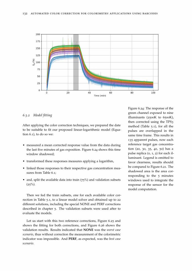
132 automated color correction for colorimetry applications using barcodes
Figure 6.24: The response of thegreen channel exposed to nineilluminants (2500K to 6500K),then corrected using the TPS3
method (Table 5.1), for all thepulses are overlapped in thesame time frame. This results in135 apparent pulses, now eachreference target gas concentra-tion (20, 30, 35, 40, 50) has apulse replica (0, 1, 2) for each il-luminant. Legend is omitted tofavor clearness, results shouldbe compared to Figure 6.21. Theshadowed area is the area cor-responding to the 5 minuteswindows used to integrate theresponse of the sensor for themodel computation.
6.3.2 Model fitting
After applying the color correction techniques, we prepared the dateto be suitable to fit our proposed linear-logarithmic model (Equa-tion 6.1), to do so we:
• measured a mean corrected response value from the data duringthe last five minutes of gas exposition. Figure 6.24 shows this timewindow shadowed;
• transformed these responses measures applying a logarithm,
• linked those responses to their respective gas concentration mea-sures from Table 6.1;
• and, split the available data into train (75%) and validation subsets(25%).
Then we fed the train subsets, one for each available color cor-rection in Table 5.1, to a linear model solver and obtained up to 22
different solutions, including the special NONE and PERF correctionsdescribed in chapter 5. The validation subsets were used after toevaluate the models.
Let us start with this two reference corrections, Figure 6.25 andshows the fitting for both corrections, and Figure 6.26 shows thevalidation results. Results indicated that NONE was the worst case
scenario, thus without correction the measurement of the colorimetricindicator was impossible. And PERF, as expected, was the best case
scenario.
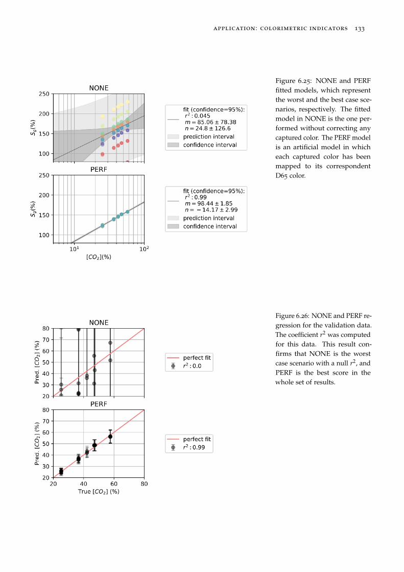
application: colorimetric indicators 133
Figure 6.25: NONE and PERFfitted models, which representthe worst and the best case sce-narios, respectively. The fittedmodel in NONE is the one per-formed without correcting anycaptured color. The PERF modelis an artificial model in whicheach captured color has beenmapped to its correspondentD65 color.
Figure 6.26: NONE and PERF re-gression for the validation data.The coefficient r2 was computedfor this data. This result con-firms that NONE is the worstcase scenario with a null r2, andPERF is the best score in thewhole set of results.
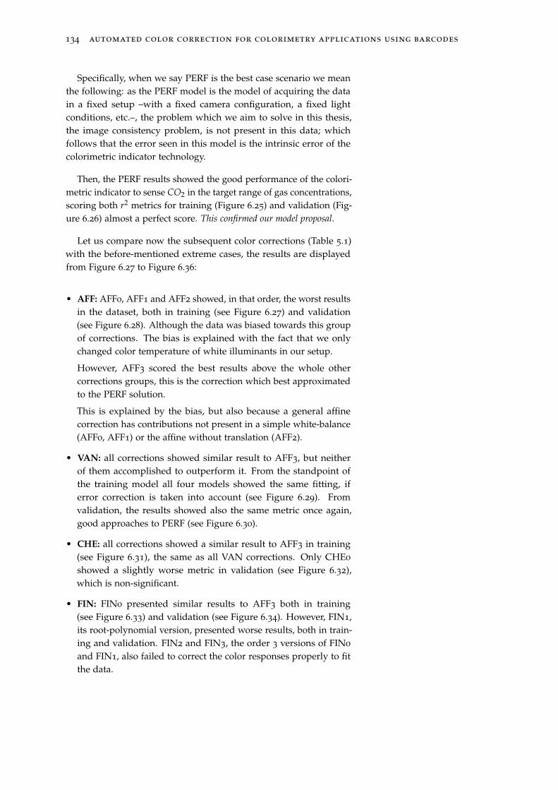
134 automated color correction for colorimetry applications using barcodes
Specifically, when we say PERF is the best case scenario we meanthe following: as the PERF model is the model of acquiring the datain a fixed setup –with a fixed camera configuration, a fixed lightconditions, etc.–, the problem which we aim to solve in this thesis,the image consistency problem, is not present in this data; whichfollows that the error seen in this model is the intrinsic error of thecolorimetric indicator technology.
Then, the PERF results showed the good performance of the colori-metric indicator to sense CO2 in the target range of gas concentrations,scoring both r2 metrics for training (Figure 6.25) and validation (Fig-ure 6.26) almost a perfect score. This confirmed our model proposal.
Let us compare now the subsequent color corrections (Table 5.1)with the before-mentioned extreme cases, the results are displayedfrom Figure 6.27 to Figure 6.36:
• AFF: AFF0, AFF1 and AFF2 showed, in that order, the worst resultsin the dataset, both in training (see Figure 6.27) and validation(see Figure 6.28). Although the data was biased towards this groupof corrections. The bias is explained with the fact that we onlychanged color temperature of white illuminants in our setup.
However, AFF3 scored the best results above the whole othercorrections groups, this is the correction which best approximatedto the PERF solution.
This is explained by the bias, but also because a general affinecorrection has contributions not present in a simple white-balance(AFF0, AFF1) or the affine without translation (AFF2).
• VAN: all corrections showed similar result to AFF3, but neitherof them accomplished to outperform it. From the standpoint ofthe training model all four models showed the same fitting, iferror correction is taken into account (see Figure 6.29). Fromvalidation, the results showed also the same metric once again,good approaches to PERF (see Figure 6.30).
• CHE: all corrections showed a similar result to AFF3 in training(see Figure 6.31), the same as all VAN corrections. Only CHE0
showed a slightly worse metric in validation (see Figure 6.32),which is non-significant.
• FIN: FIN0 presented similar results to AFF3 both in training(see Figure 6.33) and validation (see Figure 6.34). However, FIN1,its root-polynomial version, presented worse results, both in train-ing and validation. FIN2 and FIN3, the order 3 versions of FIN0
and FIN1, also failed to correct the color responses properly to fitthe data.
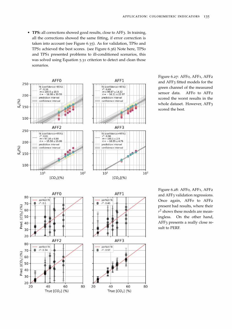
application: colorimetric indicators 135
• TPS: all corrections showed good results, close to AFF3. In training,all the corrections showed the same fitting, if error correction istaken into account (see Figure 6.35). As for validation, TPS0 andTPS1 achieved the best scores. (see Figure 6.36) Note here, TPS0
and TPS1 presented problems to ill-conditioned scenarios, thiswas solved using Equation 5.31 criterion to detect and clean thosescenarios.
Figure 6.27: AFF0, AFF1, AFF2
and AFF3 fitted models for thegreen channel of the measuredsensor data. AFF0 to AFF2
scored the worst results in thewhole dataset. However, AFF3
scored the best.
Figure 6.28: AFF0, AFF1, AFF2
and AFF3 validation regressions.Once again, AFF0 to AFF2
present bad results, where theirr2 shows these models are mean-ingless. On the other hand,AFF3 presents a really close re-sult to PERF.
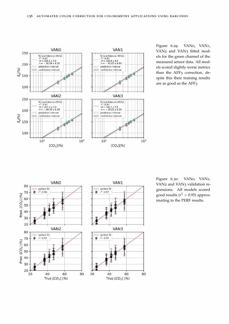
136 automated color correction for colorimetry applications using barcodes
Figure 6.29: VAN0, VAN1,VAN2 and VAN3 fitted mod-els for the green channel of themeasured sensor data. All mod-els scored slightly worse metricsthan the AFF3 correction, de-spite this their training resultsare as good as the AFF3.
Figure 6.30: VAN0, VAN1,VAN2 and VAN3 validation re-gressions. All models scoredgood results (r2
> 0.95) approx-imating to the PERF results.
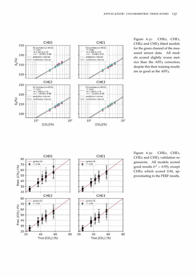
application: colorimetric indicators 137
Figure 6.31: CHE0, CHE1,CHE2 and CHE3 fitted modelsfor the green channel of the mea-sured sensor data. All mod-els scored slightly worse met-rics than the AFF3 correction,despite this their training resultsare as good as the AFF3.
Figure 6.32: CHE0, CHE1,CHE2 and CHE3 validation re-gressions. All models scoredgood results (r2
> 0.95), exceptCHE0 which scored 0.94, ap-proximating to the PERF results.

138 automated color correction for colorimetry applications using barcodes
Figure 6.33: FIN0, FIN1, FIN2
and FIN3 fitted models for thegreen channel of the measuredsensor data. Only FIN0 resem-bles to AFF3, the other threemethods performed worse.
Figure 6.34: FIN0, FIN1, FIN2
and FIN3 validation regressions.Only FIN0 scores good re-sults, compared to AFF3 (r2 =
0.95). The other methods scoredworse, resulting in meaninglessmodels.
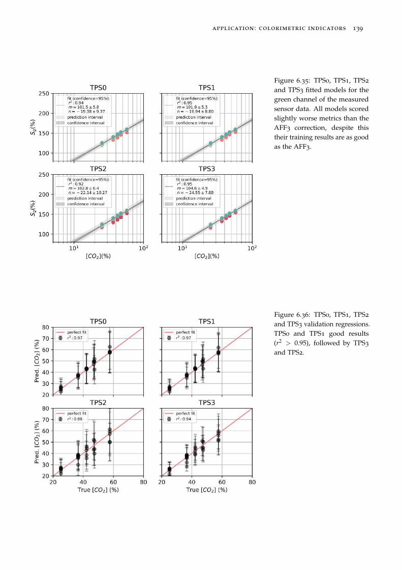
application: colorimetric indicators 139
Figure 6.35: TPS0, TPS1, TPS2
and TPS3 fitted models for thegreen channel of the measuredsensor data. All models scoredslightly worse metrics than theAFF3 correction, despite thistheir training results are as goodas the AFF3.
Figure 6.36: TPS0, TPS1, TPS2
and TPS3 validation regressions.TPS0 and TPS1 good results(r2
> 0.95), followed by TPS3
and TPS2.
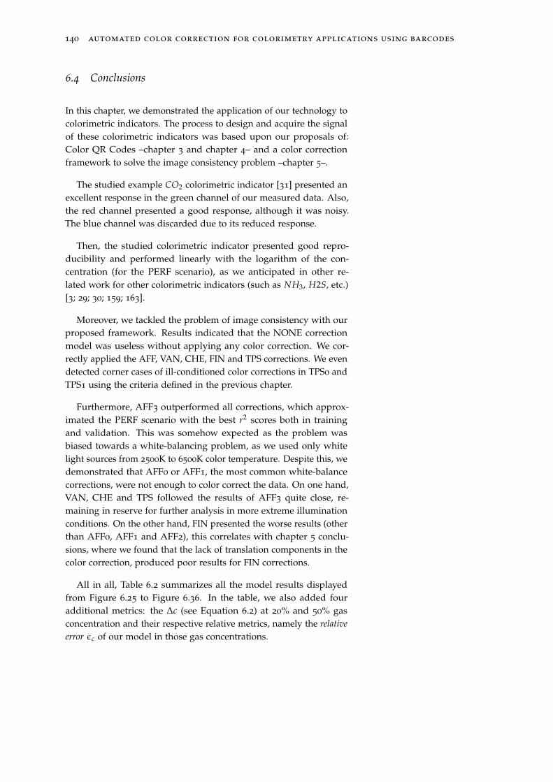
140 automated color correction for colorimetry applications using barcodes
6.4 Conclusions
In this chapter, we demonstrated the application of our technology tocolorimetric indicators. The process to design and acquire the signalof these colorimetric indicators was based upon our proposals of:Color QR Codes –chapter 3 and chapter 4– and a color correctionframework to solve the image consistency problem –chapter 5–.
The studied example CO2 colorimetric indicator [31] presented anexcellent response in the green channel of our measured data. Also,the red channel presented a good response, although it was noisy.The blue channel was discarded due to its reduced response.
Then, the studied colorimetric indicator presented good repro-ducibility and performed linearly with the logarithm of the con-centration (for the PERF scenario), as we anticipated in other re-lated work for other colorimetric indicators (such as NH3, H2S, etc.)[3; 29; 30; 159; 163].
Moreover, we tackled the problem of image consistency with ourproposed framework. Results indicated that the NONE correctionmodel was useless without applying any color correction. We cor-rectly applied the AFF, VAN, CHE, FIN and TPS corrections. We evendetected corner cases of ill-conditioned color corrections in TPS0 andTPS1 using the criteria defined in the previous chapter.
Furthermore, AFF3 outperformed all corrections, which approx-imated the PERF scenario with the best r2 scores both in trainingand validation. This was somehow expected as the problem wasbiased towards a white-balancing problem, as we used only whitelight sources from 2500K to 6500K color temperature. Despite this, wedemonstrated that AFF0 or AFF1, the most common white-balancecorrections, were not enough to color correct the data. On one hand,VAN, CHE and TPS followed the results of AFF3 quite close, re-maining in reserve for further analysis in more extreme illuminationconditions. On the other hand, FIN presented the worse results (otherthan AFF0, AFF1 and AFF2), this correlates with chapter 5 conclu-sions, where we found that the lack of translation components in thecolor correction, produced poor results for FIN corrections.
All in all, Table 6.2 summarizes all the model results displayedfrom Figure 6.25 to Figure 6.36. In the table, we also added fouradditional metrics: the ∆c (see Equation 6.2) at 20% and 50% gasconcentration and their respective relative metrics, namely the relative
error ǫc of our model in those gas concentrations.
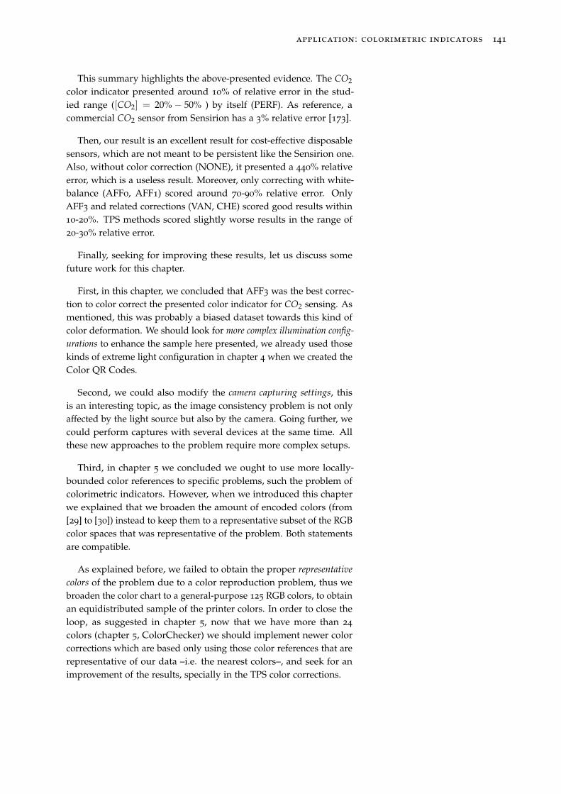
application: colorimetric indicators 141
This summary highlights the above-presented evidence. The CO2
color indicator presented around 10% of relative error in the stud-ied range ([CO2] = 20% − 50% ) by itself (PERF). As reference, acommercial CO2 sensor from Sensirion has a 3% relative error [173].
Then, our result is an excellent result for cost-effective disposablesensors, which are not meant to be persistent like the Sensirion one.Also, without color correction (NONE), it presented a 440% relativeerror, which is a useless result. Moreover, only correcting with white-balance (AFF0, AFF1) scored around 70-90% relative error. OnlyAFF3 and related corrections (VAN, CHE) scored good results within10-20%. TPS methods scored slightly worse results in the range of20-30% relative error.
Finally, seeking for improving these results, let us discuss somefuture work for this chapter.
First, in this chapter, we concluded that AFF3 was the best correc-tion to color correct the presented color indicator for CO2 sensing. Asmentioned, this was probably a biased dataset towards this kind ofcolor deformation. We should look for more complex illumination config-
urations to enhance the sample here presented, we already used thosekinds of extreme light configuration in chapter 4 when we created theColor QR Codes.
Second, we could also modify the camera capturing settings, thisis an interesting topic, as the image consistency problem is not onlyaffected by the light source but also by the camera. Going further, wecould perform captures with several devices at the same time. Allthese new approaches to the problem require more complex setups.
Third, in chapter 5 we concluded we ought to use more locally-bounded color references to specific problems, such the problem ofcolorimetric indicators. However, when we introduced this chapterwe explained that we broaden the amount of encoded colors (from[29] to [30]) instead to keep them to a representative subset of the RGBcolor spaces that was representative of the problem. Both statementsare compatible.
As explained before, we failed to obtain the proper representative
colors of the problem due to a color reproduction problem, thus webroaden the color chart to a general-purpose 125 RGB colors, to obtainan equidistributed sample of the printer colors. In order to close theloop, as suggested in chapter 5, now that we have more than 24
colors (chapter 5, ColorChecker) we should implement newer colorcorrections which are based only using those color references that arerepresentative of our data –i.e. the nearest colors–, and seek for animprovement of the results, specially in the TPS color corrections.
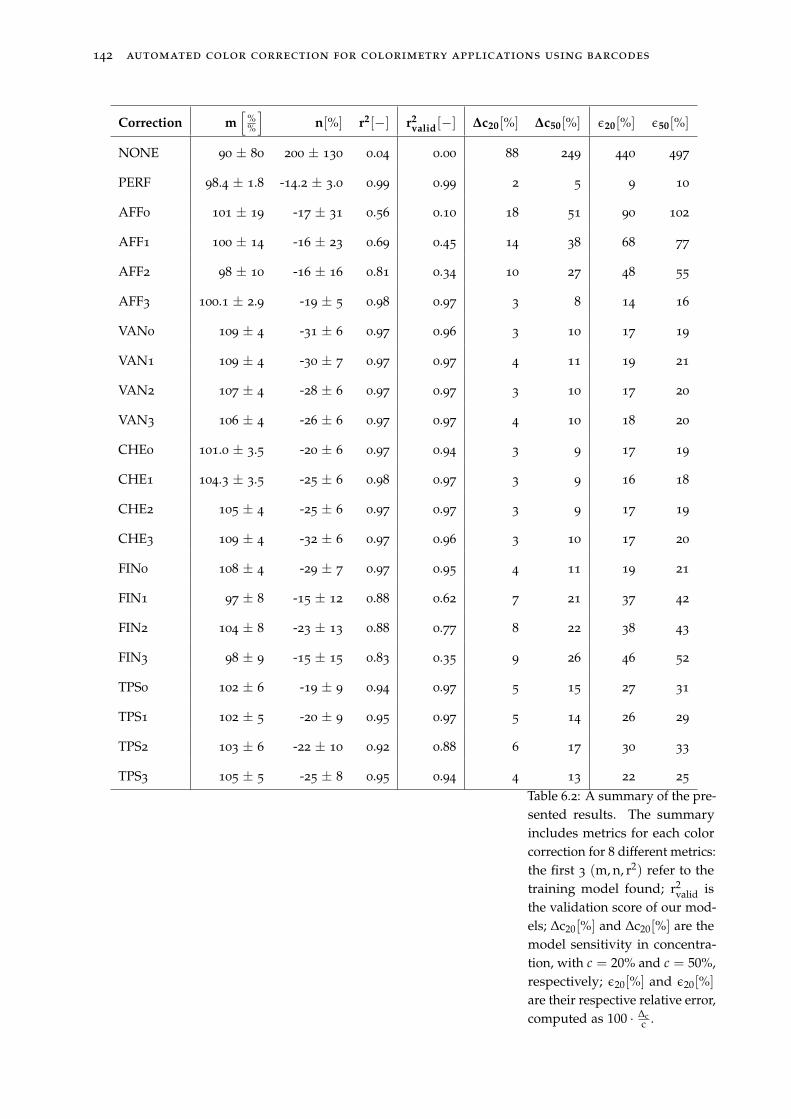
142 automated color correction for colorimetry applications using barcodes
Correction m[
%%
]
n[%] r2[−] r2valid[−] ∆c20[%] ∆c50[%] ǫ20[%] ǫ50[%]
NONE 90 ± 80 200 ± 130 0.04 0.00 88 249 440 497
PERF 98.4 ± 1.8 -14.2 ± 3.0 0.99 0.99 2 5 9 10
AFF0 101 ± 19 -17 ± 31 0.56 0.10 18 51 90 102
AFF1 100 ± 14 -16 ± 23 0.69 0.45 14 38 68 77
AFF2 98 ± 10 -16 ± 16 0.81 0.34 10 27 48 55
AFF3 100.1 ± 2.9 -19 ± 5 0.98 0.97 3 8 14 16
VAN0 109 ± 4 -31 ± 6 0.97 0.96 3 10 17 19
VAN1 109 ± 4 -30 ± 7 0.97 0.97 4 11 19 21
VAN2 107 ± 4 -28 ± 6 0.97 0.97 3 10 17 20
VAN3 106 ± 4 -26 ± 6 0.97 0.97 4 10 18 20
CHE0 101.0 ± 3.5 -20 ± 6 0.97 0.94 3 9 17 19
CHE1 104.3 ± 3.5 -25 ± 6 0.98 0.97 3 9 16 18
CHE2 105 ± 4 -25 ± 6 0.97 0.97 3 9 17 19
CHE3 109 ± 4 -32 ± 6 0.97 0.96 3 10 17 20
FIN0 108 ± 4 -29 ± 7 0.97 0.95 4 11 19 21
FIN1 97 ± 8 -15 ± 12 0.88 0.62 7 21 37 42
FIN2 104 ± 8 -23 ± 13 0.88 0.77 8 22 38 43
FIN3 98 ± 9 -15 ± 15 0.83 0.35 9 26 46 52
TPS0 102 ± 6 -19 ± 9 0.94 0.97 5 15 27 31
TPS1 102 ± 5 -20 ± 9 0.95 0.97 5 14 26 29
TPS2 103 ± 6 -22 ± 10 0.92 0.88 6 17 30 33
TPS3 105 ± 5 -25 ± 8 0.95 0.94 4 13 22 25
Table 6.2: A summary of the pre-sented results. The summaryincludes metrics for each colorcorrection for 8 different metrics:the first 3 (m, n, r2) refer to thetraining model found; r2
valid isthe validation score of our mod-els; ∆c20[%] and ∆c20[%] are themodel sensitivity in concentra-tion, with c = 20% and c = 50%,respectively; ǫ20[%] and ǫ20[%]
are their respective relative error,computed as 100 · ∆c
c .
Chapter 7. Conclusions
7.1 Thesis conclusions
This thesis tackled the problem of acquiring data in a quantitativemanner from colorimetric indicators, and other colorimetric applica-tions, to do so the problem of automating color calibration ought to beresolved in with a seamless integration to the colorimetric applicationwithout any additional barriers to the final consumer, thus usingwell-known 2D barcodes.
Here, we present a summary of the main conclusions for each oneof the thesis objectives:
I Capture machine-readable patterns placed on top of challeng-
ing surfaces. Results demonstrated that our method performedbetter than other extraction methods. We proved so by usingthe same commercial QR Code reader (ZBar) on the same imagewhich had been corrected by the above-mentioned methods forour three datasets (SYNT, FLAT and SURF), and computing adata readability factor R for each method and dataset.
For the SYNT and FLAT datasets our method scored similar tothe previous methods with almost a R = 100%, for the SURTdataset –where challenging surfaces were prsent–, AFF and PROmethods scored really poor results, a 0% and 2%, respectively.CYL method scored a 50%, and TPS up to 79%.
By combining both CYL and TPS methods, we arrived to a jointresult of 84%. We even benchmarked this against ZBar withoutany image correction, this proved our method (TPS+CYL) scored4 times better than a bare ZBar decoding (84% vs 19%).
II Define a back-compatible QR Code modification to extend QR
Codes to act as color charts. Results indicated our method mini-mized the error applied to a QR Code when color is present, bothSNR and BER figures demonstrated that for any of the channelsconsidered. We also demonstrated that the data zone (D) is themore suitable candidate to embed color references, as it presentsa higher resilience to be manipulated.
144 automated color correction for colorimetry applications using barcodes
Our method outperformed a random placed of colors by far, forexample for a version 5 QR Code, our method outperformed bya 150% the results of the random assignment method for the datazone, and almost a 500% for the global EC&D zone, embeddingmore than 300 colors in a QR Code.
III Achieve image consistency using color charts for any camera or
light setup, enabling colorimetric applications to yield quan-
titative results. Results proved all TPS methods to be the bestmethods both in ∆RGBwithin and ∆RGBinter metrics, scoring halfor less the distance of the nearest competitor, the general AFFcorrection.
Despite this, the original TPS3D method presented a huge num-ber of ill-conditioned cases where the image was not properlycorrected, around the 20% - 30% of the cases, this ill-conditionedscenarios were solved when imposing our smoothness proposal.
Also, results indicated that the change in the kernel RBF of theTPS did not improve, neither degrade, the TPS scores.
Moreover, regarding the execution time T , AFF methods werethe fastest methods available of the proposed framework, due totheir computational simplicity.
All the other methods scored worse times than these corrections,specially FIN (root-polynomial) and TPS corrections. TPS were20 to 100 times slower than AFF color corrections. Despite this,we proved that changing the kernel RBF of the TPS formulationdid speed up by a 30% the result computation.
IV Demonstrate a specific application of the technology based on
colorimetric indicators. Results demonstrated the general affinecorrection (AFF3) was the best correction in the color correctionframework, probably because our experiment was biased towardswhite-balance corrections.
Our color indicator proved to a good cost-effective indicator withonly a 10% relative error in the studied range (PERF), around10% - 20% when corrected with AFF3 and similar corrections(VAN, CHE), and 20%-30% with TPS corrections. In front of the440% relative error observed without any correction (NONE).
All in all, we demonstrated the feasibility of applying barcodetechnology to colorimetric applications, thus enhancing the previousstate-of-the-art technologies in the field. Our new Color QR Codeacted as substitutes of the traditional color charts, presenting morecolor capacity in a compact form. Altogether, with a new proposalfor color correcting scenes using an improved TPS3D method, wedemonstrate the use of our technology to colorimetric indicators.
conclusions 145
7.2 Future work
During the presented thesis, we presented some ideas to furthercontinue to work on the presented results in each chapter. How topursue these partial research was detailed there. Along with this,our integrated solution on how to automate color correction usingbarcodes can be applied somewhere else. Let us expose some ideason how to apply our technology beyond colorimetric indicators toother fields where color correction is still an open problem.
First, other biochemical analytes can be considered instead of envi-ronmental gases, temperature or humidity [2]. Taking as an examplewater, many authors have proposed colorimetric methods to detectsubstances in the water: such as chlorine [174] or fluorine [175], or even,coliphages [176].
All these examples, could be integrated straight-forward with ourtechnology as their similarity to colorimetry indicators. Here, thesolvent of the substance to sense is liquid (water), which is oftenmixed with a chemical reactive which contains a derivate of a colorindicator. The main gap between our technologies would be a com-puter vision problem, on how to embed our Color QR Code in theirsystem involving liquid water. Fortunately, in chapter 3 we tackledthis problem and proposed a combined method using both TPS andCYL correction which, theoretically, would solve the implementationof our technology on top cylindrical surfaces like reactive vials.
Second, another example is the wide-spread in-vitro diagnosticslateral-flow assays [17; 177]. Lateral-flow assays were already popularbefore 2021, they were popular due to self-diagnosis pregnancy tests,that were based on this technology. But nowadays, they are evenmore popular due to the pandemic situation derived from COVID-19
disease, and the use of this technology to provide to the people ofself-diagnosis antigen tests for detecting SARS-CoV-2 [178].
Many authors have attempt to perform readouts from lateral-flowassays using smartphones [179]. The most common approach fromthese authors is to overcome the image consistency problem by fixingthe illumination and capture conditions using ad hoc hardware to thesmartphone [180]. However, those extra hardware present a stopgapbetween their proposals and the final user, alongside with a priceincrease to fabricate and distribute the hardware.
Our solution here would overcome those problems, by simplyadding a Color QR Code to the lateral-flow cassette, which is a cost-effective solution. Thus, leveraging all the color correction to thesmartphone or remote post-processing.
146 automated color correction for colorimetry applications using barcodes
Third, there exists an increasing need for achieving image consis-tency in other health-care fields, one of these is dermatology [33; 34].Dermatology is a wide health-care field, we can find authors thathave used smartphone or neural networks to ease the diagnosis ofdifferent diseases like skin cancer [181], skin burns [182] or other skin
lesions [183].
Other authors have proposed to use previous color charts to colorcalibrate dermatology images [184; 185; 186]. For example, Vander-Heaghen et al. presented the use of a ColorChecker chart [13] toachieve consistent imaging in commercial cameras, and concludedthat despite their efforts, the resultant images already had too muchvariability which cannot be eliminated [185].
We could use our technology to improve their results. First, theysought to use the ColorChecker to color correct the images usingdevice-independent color spaces, as we discussed in this thesis, thereexist more modern approaches to this problem, working directly indevice-depending color spaces. Then, we could apply our color cor-rection framework directly to their dataset. Moreover, our completeproposal of Color QR Codes could add more colors to the color cor-rection that are representatives of the problem tackled. This is similarto the work presented by Cugmas et al. [186] in their teledermoscopysolution for canine skin, where they used two ColorChecker charts forthis purpose. With our proposal, this seems redundant, the Color QRCodes could embed the colors of both color charts.
Finally, any colorimetric application is potentially approachable byour technology presented in this thesis. The adoption of the technol-ogy relies on two further challenges: one, to adapt the color correctionto the colorimetric model present in the application, thus condition-ing the colors to be embedded in the barcode; and two, to adapt thebarcode definition to the desired conditions of the application.

list of figures 147

List of Figures
1.1 The GasApp proposal is presented. Left, GasApp changed the core sensing technology fromelectronic to colorimetric indicators. Right, the initial idea of the GasApp project, a cardwhere colorimetric dyes are printed alongside with color charts and a QR Code. . . . . . . 16
1.2 Simplified 1D representation of the color reproduction problem in reversible and in non-reversible conditions. For clarity only one color coordinate has been represented: x standsfor R, G, or B, and x′ stands for R’, G’, or B’. Object colors (x) appear to be different (x’) afterbeing acquired by digital means. In some situations, these alterations cannot be removed,because the transformation from x′ to x is not single-valued (the critical color ranges wherethis problem occurs are highly lighted with the green marker). . . . . . . . . . . . . . . . . . 17
1.3 Four examples of ArUco codes. These codes present certain feature uniqueness (rotation,non-symmetry, etc.), which enables easy location and identification on a scene. . . . . . . . 17
1.4 Our thesis proposal to create machine-readable patterns that can accommodate colorimetricsensors and color charts, alongside with the digital information of the QR Code. . . . . . . . 18
2.1 The color reproduction problem is represented: (a) a certain light source (I(λ)) illuminates acertain object with a certain reflectance (R(λ)), this scene is captured by a certain camerawith its sensor response (D(λ)) and (b) the reproduced image of the object (R′(λ)) is thenilluminated and captured again. . . . . . . . . . . . . . . . . . . . . . . . . . . . . . . . . . . . 22
2.2 The imaging consistency problem is represented: (a) a certain light source (I(λ)) illuminatesa certain object with a certain reflectance (R(λ)), this scene is captured by a certain camerawith its sensor response (D(λ)) and (b) the same object is now illuminated by another lightsource (I′(λ)) and captured by another camera (D′(λ)). . . . . . . . . . . . . . . . . . . . . . . 23
2.3 A ColorChecker chart. The first row shows a set of six “natural colors”; the second oneshows a set of "miscellaneous colors"; the third, primary and secondary colors; and the lastrow, a gray scale gradient. This set of colors samples the RGB space in a limited way, but itis convenient to carry out a few color corrections manually. . . . . . . . . . . . . . . . . . . . 24
2.4 Previous state-of-the-art color correction charts from Pantone and X-Rite. (a) The X-RiteColorChecker Passport Photo 2® kit. (b) The Pantone Color Match Card®. . . . . . . . . . . 25
2.5 Different 2D barcode standards. From left to right: a QR Code, a DataMatrix, an Aztec Code,a MaxiCode, a JAB Code and a HCC Barcode. . . . . . . . . . . . . . . . . . . . . . . . . . . . 26
150 automated color calibration for colorimetry applications using barcodes
2.6 Block diagram for a general encoding-decoding process of a QR Code which features theembedding of a color layer. This color layer could be used for a wide range of applications,such as placing a brand logo inside a QR Code. The process can be seen as a global encodingprocess (digital encode and color encode), followed by a channel (print and capture) and aglobal decoding process (remove colors and decode digital information). . . . . . . . . . . . 27
2.7 Some examples of QR Code versions. From left to right: Micro QR-Code (version M3),version 3 QR Code, and version 10 QR Code. Each of them can store up to 7, 42, 213 bytes,respectively, using a 15% of error correction capacity. . . . . . . . . . . . . . . . . . . . . . . . 28
2.8 Some examples of DataMatrix codes. From left to right: rectangular DataMatrix code, squareDataMatrix code and four square DataMatrix combined. Each of them can store up to 14, 28,202 bytes, respectively, using approximately a 20% of error correction capacity. . . . . . . . 28
2.9 QR Code encoding defines a complex layout with several patterns to be considered, some ofthem are non-variant patterns found in each QR Code, others may appear depending on thesize of the QR Code, and area related to the data changes for each encoding process. (a) AQR Code with high error correction level and version 5. (b) The complex pattern structureof the pattern. . . . . . . . . . . . . . . . . . . . . . . . . . . . . . . . . . . . . . . . . . . . . . . 29
2.10 QR Code simplified areas corresponding to the encode process. (a) A QR Code with higherror correction level and version 5. (c) Simplified view of the QR patterns, yellow framecorresponds to the “error correction” area and dark green frame corresponds to the “data”area. . . . . . . . . . . . . . . . . . . . . . . . . . . . . . . . . . . . . . . . . . . . . . . . . . . . 30
2.11 Different examples of Halftone QR Codes, introduced by HK. Chu et al. [56]. These QR Codesexploit the error correction features of the QR Code to achieve back-compatible QR Codeswith apparent grayscale –halftone– colors. . . . . . . . . . . . . . . . . . . . . . . . . . . . . . 31
2.12 Original figure from Garateguy et al. [57], different QR Codes with color art are shown: (a) aQR Code with a logo overlaid; (b) a QArt Code [58], (c) a Visual QR Code; and (d) Garateguyet al. proposal. . . . . . . . . . . . . . . . . . . . . . . . . . . . . . . . . . . . . . . . . . . . . . 31
2.13 Computer vision patterns featured in a QR Code. (a) Three finder or position patterns, (b)six alignment patterns, (c) two timing patterns and (d) the fourth corner that can be inferredfrom the external edges of the finder patterns. . . . . . . . . . . . . . . . . . . . . . . . . . . . 32
2.14 Finder pattern definition in terms of modules. Finder pattern measures always 7 × 7
modules. If scanned with a line barcode scanner the 1:1:3:1:1 ratio is maintained no matterthe direction of the scanner. If scanned using contour extraction the aspect ratio 7²:5²:3² ismaintained as well if the QR Code is captured within a projective scene (i.e. a handheldsmartphone). . . . . . . . . . . . . . . . . . . . . . . . . . . . . . . . . . . . . . . . . . . . . . . . 33
2.15 Alignment pattern definition in terms of modules. Alignment pattern measures always 5 ×5 modules. If scanned with a line barcode scanner the 1:1:1:1:1 ratio is maintained no matterthe direction of the scanner. If scanned using contour extraction the aspect ratio 5²:3²:1² ismaintained as well if the QR Code is captured within a projective scene (i.e. a handheldsmartphone). . . . . . . . . . . . . . . . . . . . . . . . . . . . . . . . . . . . . . . . . . . . . . . . 33
2.16 The QR Code contour detection method. a) A QR Code from a certain perspective. b) Allthe contours detected in the image. c) The location of the position patterns following thearea rule. Their respective centers of mass are indicated. . . . . . . . . . . . . . . . . . . . . . 34
list of figures 151
2.17 The different orientations of a QR Code are shown. (a) Representation of the slope of thediagonal connecting the corners m and the diagonal segment linked to the top-left corner s.(b) The four possible orientations of a QR-Code. . . . . . . . . . . . . . . . . . . . . . . . . . . 35
2.18 The QR Code projective correction steps. a) The orientation is deduced from the centers ofthe 3 finder patterns L, M, N. In this step, their contour corners are found. b) The fourthcorner O is found, based on the previous three corners. c) A first projective transformation iscarried out, but still subject to significant error shifts around the bottom-right corner; d) Thealignment patterns are localized in a restricted contour search. The centers of the alignmentpatters (shifted centers after the first projective correction (green) and the reference centersare both found (red). e) The error committed at this stage is shown by subtraction of theimages. f) Finally, a second projective transformation recovers the final QR Code image,based on the reference, tabulated, positions of the alignment patterns. . . . . . . . . . . . . . 36
2.19 A reduced representation of the reflectance model. For more details see Figure 2.1. . . . . . 37
2.20 125 colors of an RGB color space. Each channel of the color space has been sampled 5 times.Assuming the space is a 24-bit color space, the values of the sampled colors correspond to: 0,61, 127, 193 and 255. The combination (255, 255, 255) is the white color and (0, 0, 0) the blackcolor. . . . . . . . . . . . . . . . . . . . . . . . . . . . . . . . . . . . . . . . . . . . . . . . . . . . 38
2.21 An Airy disk is shown as a grayscale image with a color map (top) and as a function (bottom)with the same color map. . . . . . . . . . . . . . . . . . . . . . . . . . . . . . . . . . . . . . . . 41
3.1 An example of an adverse situation, image of a QR Code in a bike-sharing service inBarcelona, where the QR Code is bent over the bike frame. User experience shows thatcapturing these QR Codes is difficult when approaching the camera to the QR Code dueto the bending. (a) An image captured near the QR Code (∼20 cm), (b) an image capturedfarther (∼1 m) and (c) a zoomed version of (b) which despite the blur performs betterbecause the QR Code resembles more to a flat QR Code. . . . . . . . . . . . . . . . . . . . . 45
3.2 Projection of different surfaces into the capture plane (img) when acquiring images from adigital camera. A QR Code placed on each one of these surfaces will show different defor-mations(a) an affine (coplanar) plane, (b) a projective (noncoplanar) plane, (c) a cylindricalsurface and (d) a thin-plate spline surface, it is continuous and derivable. . . . . . . . . . . . 47
3.3 Projection of an affine surface into the capture plane (img) when acquiring images from adigital camera. . . . . . . . . . . . . . . . . . . . . . . . . . . . . . . . . . . . . . . . . . . . . . 48
3.4 Projection of a projective surface into the capture plane (img) when acquiring images from adigital camera. . . . . . . . . . . . . . . . . . . . . . . . . . . . . . . . . . . . . . . . . . . . . . 49
3.5 Projection of a cylindrical surface into the capture plane (img) when acquiring images froma digital camera. . . . . . . . . . . . . . . . . . . . . . . . . . . . . . . . . . . . . . . . . . . . . 49
3.6 Projection of an arbitrary surface into the capture plane (img) when acquiring images from adigital camera. . . . . . . . . . . . . . . . . . . . . . . . . . . . . . . . . . . . . . . . . . . . . . . 50
3.7 Example images from the three datasets - (a) SYNT, (b) FLAT and (c) SURF - showing similarQR codes in different surface deformations. . . . . . . . . . . . . . . . . . . . . . . . . . . . . 53
152 automated color calibration for colorimetry applications using barcodes
3.8 (a) Block diagram for a general encoding-decoding process of a QR Code. (b) A modifieddiagram with the addition of a deformation due to a noncoplanar surface topography andsurface fitting stage which contains a correction steps where image deformation is revertedto improve readout. In our experiments, also, an image augmentation step was added to beused in the proposed experiments for this work. . . . . . . . . . . . . . . . . . . . . . . . . . . 53
3.9 Two examples (a), (b) from the SYNT dataset. The surfaces were fitted by the four methodsdescribed (AFF, PRO, CYL and TPS). The surface fitting is shown as a lattice of red pointsback-projected onto the original image. . . . . . . . . . . . . . . . . . . . . . . . . . . . . . . . 55
3.10 Two examples (a), (b) from the FLAT dataset. The surfaces were fitted by the four methodsdescribed (AFF, PRO, CYL and TPS). The surface fitting is shown as a lattice of red pointsback-projected onto the original image. . . . . . . . . . . . . . . . . . . . . . . . . . . . . . . . 56
3.11 Three examples (a), (b), (c) from the SURF dataset. The surfaces were fitted by the fourmethods described (AFF, PRO, CYL and TPS). The surface fitting is shown as a lattice of redpoints back-projected onto the original image. . . . . . . . . . . . . . . . . . . . . . . . . . . . 57
3.12 Data readability (R) of each dataset (SYNT, FLAT, SURF) for each transformation method(AFF, PRO, CYL and TPS). . . . . . . . . . . . . . . . . . . . . . . . . . . . . . . . . . . . . . . . 59
3.13 Data readability (R) of the SYNT dataset, segregated by the kind of deformation (affine orperspective) that the QR Codes were exposed to, for each transformation method (AFF, PRO,CYL and TPS). . . . . . . . . . . . . . . . . . . . . . . . . . . . . . . . . . . . . . . . . . . . . . . 59
3.14 Data readability (R) of the SURF dataset segregated by the kind of deformation (cylindricalor other) that the QR Codes were exposed to, for each transformation method (AFF, PRO,CYL and TPS). . . . . . . . . . . . . . . . . . . . . . . . . . . . . . . . . . . . . . . . . . . . . . 59
3.15 Data readability (R) of the three datasets (SYNT, FLAT and SURF) when processed withZBar and our combined CYL and TPS methods. . . . . . . . . . . . . . . . . . . . . . . . . . . 60
4.1 A machine-readable pattern to allocate an ammonia sensor. Top: the designed pattern, withtwo spaces to print a colorimetric sensor. Bottom: the captured version of the pattern with aprinted colorimetric dye in one slot. Notice this pattern resembles a QR Code, but it doesnot contain any data. . . . . . . . . . . . . . . . . . . . . . . . . . . . . . . . . . . . . . . . . . 63
4.2 Block diagram for a back-compatible encoding-decoding process of a QR Code whichfeatures the embedding of a color layer for colorimetric applications. The process can be seenas a global encoding process (digital encode and color encode), followed by a channel (printand capture) and a global decoding process (extract colors and decode digital information).This process is back-compatible with state of the art scanners which remove colors andachieve the decoding of the data and compatible with new decoders which can benefit fromcolor interrogation. The back-compatibility is achieved by following certain rules in the colorencoding process (i.e. use the same threshold when placing the colors than when removingthem). . . . . . . . . . . . . . . . . . . . . . . . . . . . . . . . . . . . . . . . . . . . . . . . . . . . 64
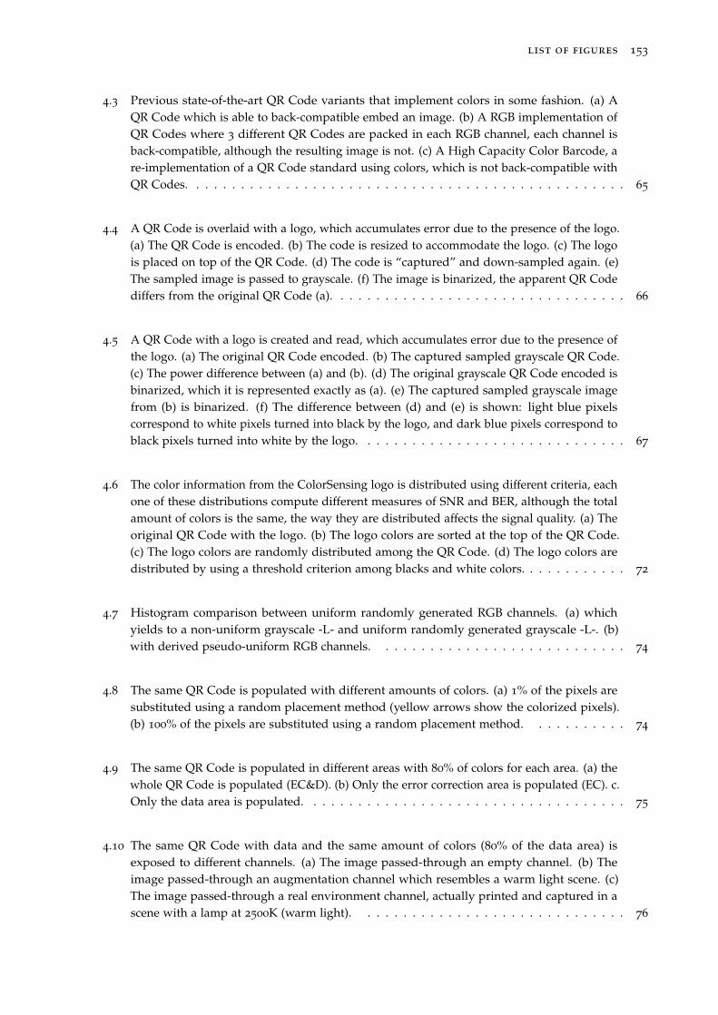
list of figures 153
4.3 Previous state-of-the-art QR Code variants that implement colors in some fashion. (a) AQR Code which is able to back-compatible embed an image. (b) A RGB implementation ofQR Codes where 3 different QR Codes are packed in each RGB channel, each channel isback-compatible, although the resulting image is not. (c) A High Capacity Color Barcode, are-implementation of a QR Code standard using colors, which is not back-compatible withQR Codes. . . . . . . . . . . . . . . . . . . . . . . . . . . . . . . . . . . . . . . . . . . . . . . . . 65
4.4 A QR Code is overlaid with a logo, which accumulates error due to the presence of the logo.(a) The QR Code is encoded. (b) The code is resized to accommodate the logo. (c) The logois placed on top of the QR Code. (d) The code is “captured” and down-sampled again. (e)The sampled image is passed to grayscale. (f) The image is binarized, the apparent QR Codediffers from the original QR Code (a). . . . . . . . . . . . . . . . . . . . . . . . . . . . . . . . . 66
4.5 A QR Code with a logo is created and read, which accumulates error due to the presence ofthe logo. (a) The original QR Code encoded. (b) The captured sampled grayscale QR Code.(c) The power difference between (a) and (b). (d) The original grayscale QR Code encoded isbinarized, which it is represented exactly as (a). (e) The captured sampled grayscale imagefrom (b) is binarized. (f) The difference between (d) and (e) is shown: light blue pixelscorrespond to white pixels turned into black by the logo, and dark blue pixels correspond toblack pixels turned into white by the logo. . . . . . . . . . . . . . . . . . . . . . . . . . . . . . 67
4.6 The color information from the ColorSensing logo is distributed using different criteria, eachone of these distributions compute different measures of SNR and BER, although the totalamount of colors is the same, the way they are distributed affects the signal quality. (a) Theoriginal QR Code with the logo. (b) The logo colors are sorted at the top of the QR Code.(c) The logo colors are randomly distributed among the QR Code. (d) The logo colors aredistributed by using a threshold criterion among blacks and white colors. . . . . . . . . . . . 72
4.7 Histogram comparison between uniform randomly generated RGB channels. (a) whichyields to a non-uniform grayscale -L- and uniform randomly generated grayscale -L-. (b)with derived pseudo-uniform RGB channels. . . . . . . . . . . . . . . . . . . . . . . . . . . . 74
4.8 The same QR Code is populated with different amounts of colors. (a) 1% of the pixels aresubstituted using a random placement method (yellow arrows show the colorized pixels).(b) 100% of the pixels are substituted using a random placement method. . . . . . . . . . . 74
4.9 The same QR Code is populated in different areas with 80% of colors for each area. (a) thewhole QR Code is populated (EC&D). (b) Only the error correction area is populated (EC). c.Only the data area is populated. . . . . . . . . . . . . . . . . . . . . . . . . . . . . . . . . . . . 75
4.10 The same QR Code with data and the same amount of colors (80% of the data area) isexposed to different channels. (a) The image passed-through an empty channel. (b) Theimage passed-through an augmentation channel which resembles a warm light scene. (c)The image passed-through a real environment channel, actually printed and captured in ascene with a lamp at 2500K (warm light). . . . . . . . . . . . . . . . . . . . . . . . . . . . . . 76
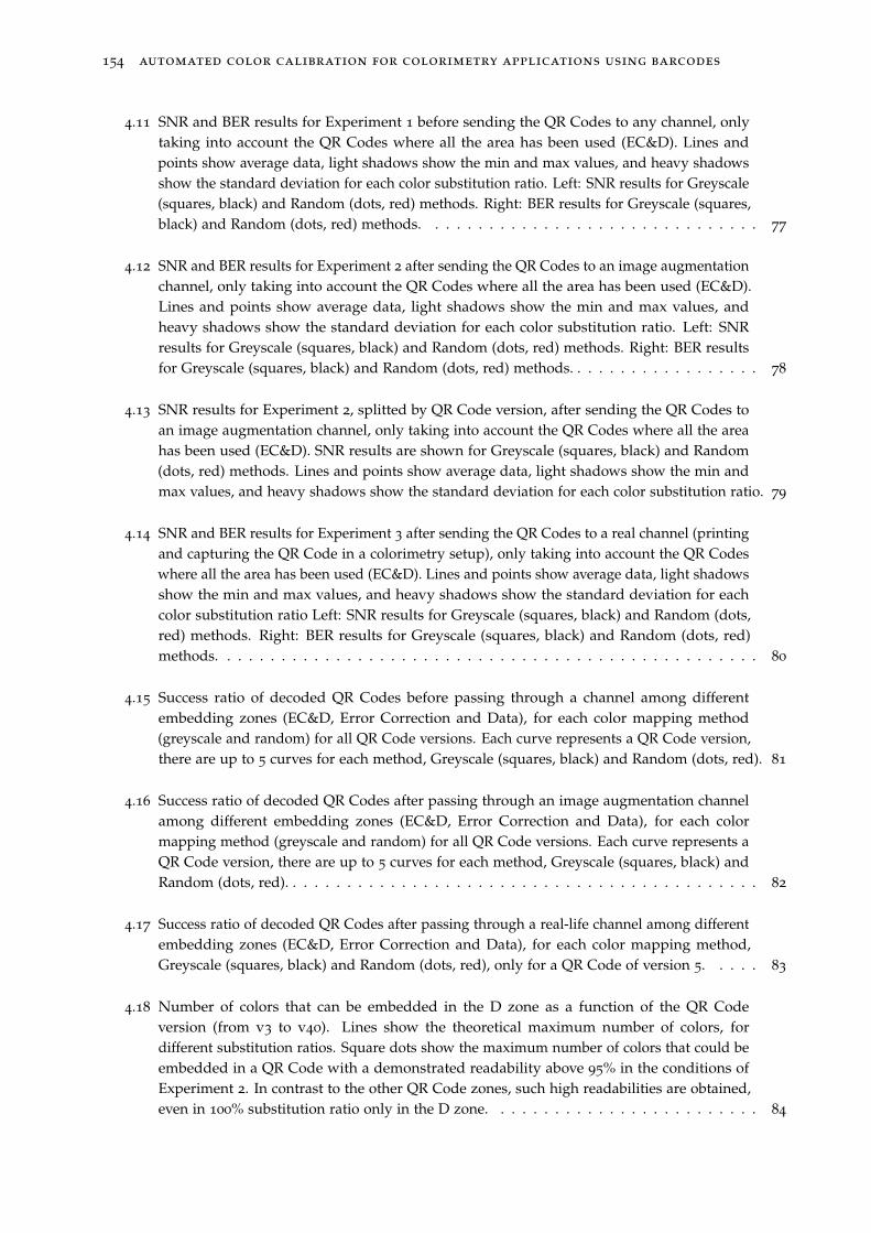
154 automated color calibration for colorimetry applications using barcodes
4.11 SNR and BER results for Experiment 1 before sending the QR Codes to any channel, onlytaking into account the QR Codes where all the area has been used (EC&D). Lines andpoints show average data, light shadows show the min and max values, and heavy shadowsshow the standard deviation for each color substitution ratio. Left: SNR results for Greyscale(squares, black) and Random (dots, red) methods. Right: BER results for Greyscale (squares,black) and Random (dots, red) methods. . . . . . . . . . . . . . . . . . . . . . . . . . . . . . . 77
4.12 SNR and BER results for Experiment 2 after sending the QR Codes to an image augmentationchannel, only taking into account the QR Codes where all the area has been used (EC&D).Lines and points show average data, light shadows show the min and max values, andheavy shadows show the standard deviation for each color substitution ratio. Left: SNRresults for Greyscale (squares, black) and Random (dots, red) methods. Right: BER resultsfor Greyscale (squares, black) and Random (dots, red) methods. . . . . . . . . . . . . . . . . . 78
4.13 SNR results for Experiment 2, splitted by QR Code version, after sending the QR Codes toan image augmentation channel, only taking into account the QR Codes where all the areahas been used (EC&D). SNR results are shown for Greyscale (squares, black) and Random(dots, red) methods. Lines and points show average data, light shadows show the min andmax values, and heavy shadows show the standard deviation for each color substitution ratio. 79
4.14 SNR and BER results for Experiment 3 after sending the QR Codes to a real channel (printingand capturing the QR Code in a colorimetry setup), only taking into account the QR Codeswhere all the area has been used (EC&D). Lines and points show average data, light shadowsshow the min and max values, and heavy shadows show the standard deviation for eachcolor substitution ratio Left: SNR results for Greyscale (squares, black) and Random (dots,red) methods. Right: BER results for Greyscale (squares, black) and Random (dots, red)methods. . . . . . . . . . . . . . . . . . . . . . . . . . . . . . . . . . . . . . . . . . . . . . . . . . 80
4.15 Success ratio of decoded QR Codes before passing through a channel among differentembedding zones (EC&D, Error Correction and Data), for each color mapping method(greyscale and random) for all QR Code versions. Each curve represents a QR Code version,there are up to 5 curves for each method, Greyscale (squares, black) and Random (dots, red). 81
4.16 Success ratio of decoded QR Codes after passing through an image augmentation channelamong different embedding zones (EC&D, Error Correction and Data), for each colormapping method (greyscale and random) for all QR Code versions. Each curve represents aQR Code version, there are up to 5 curves for each method, Greyscale (squares, black) andRandom (dots, red). . . . . . . . . . . . . . . . . . . . . . . . . . . . . . . . . . . . . . . . . . . . 82
4.17 Success ratio of decoded QR Codes after passing through a real-life channel among differentembedding zones (EC&D, Error Correction and Data), for each color mapping method,Greyscale (squares, black) and Random (dots, red), only for a QR Code of version 5. . . . . 83
4.18 Number of colors that can be embedded in the D zone as a function of the QR Codeversion (from v3 to v40). Lines show the theoretical maximum number of colors, fordifferent substitution ratios. Square dots show the maximum number of colors that could beembedded in a QR Code with a demonstrated readability above 95% in the conditions ofExperiment 2. In contrast to the other QR Code zones, such high readabilities are obtained,even in 100% substitution ratio only in the D zone. . . . . . . . . . . . . . . . . . . . . . . . . 84
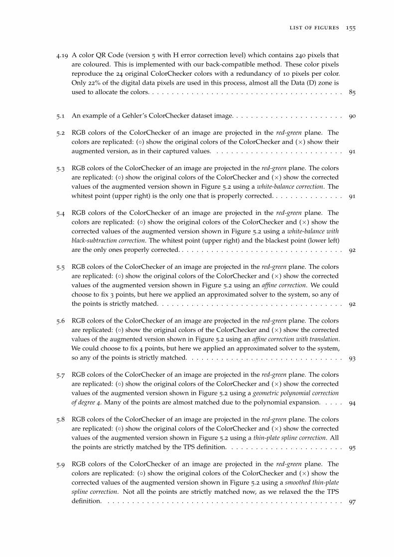
list of figures 155
4.19 A color QR Code (version 5 with H error correction level) which contains 240 pixels thatare coloured. This is implemented with our back-compatible method. These color pixelsreproduce the 24 original ColorChecker colors with a redundancy of 10 pixels per color.Only 22% of the digital data pixels are used in this process, almost all the Data (D) zone isused to allocate the colors. . . . . . . . . . . . . . . . . . . . . . . . . . . . . . . . . . . . . . . . 85
5.1 An example of a Gehler’s ColorChecker dataset image. . . . . . . . . . . . . . . . . . . . . . . 90
5.2 RGB colors of the ColorChecker of an image are projected in the red-green plane. Thecolors are replicated: (◦) show the original colors of the ColorChecker and (×) show theiraugmented version, as in their captured values. . . . . . . . . . . . . . . . . . . . . . . . . . . 91
5.3 RGB colors of the ColorChecker of an image are projected in the red-green plane. The colorsare replicated: (◦) show the original colors of the ColorChecker and (×) show the correctedvalues of the augmented version shown in Figure 5.2 using a white-balance correction. Thewhitest point (upper right) is the only one that is properly corrected. . . . . . . . . . . . . . . 91
5.4 RGB colors of the ColorChecker of an image are projected in the red-green plane. Thecolors are replicated: (◦) show the original colors of the ColorChecker and (×) show thecorrected values of the augmented version shown in Figure 5.2 using a white-balance with
black-subtraction correction. The whitest point (upper right) and the blackest point (lower left)are the only ones properly corrected. . . . . . . . . . . . . . . . . . . . . . . . . . . . . . . . . . 92
5.5 RGB colors of the ColorChecker of an image are projected in the red-green plane. The colorsare replicated: (◦) show the original colors of the ColorChecker and (×) show the correctedvalues of the augmented version shown in Figure 5.2 using an affine correction. We couldchoose to fix 3 points, but here we applied an approximated solver to the system, so any ofthe points is strictly matched. . . . . . . . . . . . . . . . . . . . . . . . . . . . . . . . . . . . . . 92
5.6 RGB colors of the ColorChecker of an image are projected in the red-green plane. The colorsare replicated: (◦) show the original colors of the ColorChecker and (×) show the correctedvalues of the augmented version shown in Figure 5.2 using an affine correction with translation.We could choose to fix 4 points, but here we applied an approximated solver to the system,so any of the points is strictly matched. . . . . . . . . . . . . . . . . . . . . . . . . . . . . . . . 93
5.7 RGB colors of the ColorChecker of an image are projected in the red-green plane. The colorsare replicated: (◦) show the original colors of the ColorChecker and (×) show the correctedvalues of the augmented version shown in Figure 5.2 using a geometric polynomial correction
of degree 4. Many of the points are almost matched due to the polynomial expansion. . . . . 94
5.8 RGB colors of the ColorChecker of an image are projected in the red-green plane. The colorsare replicated: (◦) show the original colors of the ColorChecker and (×) show the correctedvalues of the augmented version shown in Figure 5.2 using a thin-plate spline correction. Allthe points are strictly matched by the TPS definition. . . . . . . . . . . . . . . . . . . . . . . . 95
5.9 RGB colors of the ColorChecker of an image are projected in the red-green plane. Thecolors are replicated: (◦) show the original colors of the ColorChecker and (×) show thecorrected values of the augmented version shown in Figure 5.2 using a smoothed thin-plate
spline correction. Not all the points are strictly matched now, as we relaxed the the TPSdefinition. . . . . . . . . . . . . . . . . . . . . . . . . . . . . . . . . . . . . . . . . . . . . . . . . 97
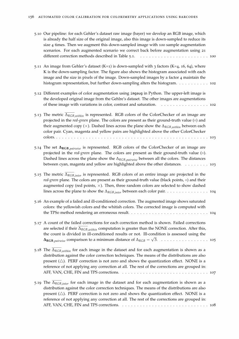
156 automated color calibration for colorimetry applications using barcodes
5.10 Our pipeline: for each Gehler’s dataset raw image (bayer) we develop an RGB image, whichis already the half size of the original image, also this image is down-sampled to reduce itssize 4 times. Then we augment this down-sampled image with 100 sample augmentationscenarios. For each augmented scenario we correct back before augmentation using 21
different correction methods described in Table 5.1. . . . . . . . . . . . . . . . . . . . . . . . 100
5.11 An image from Gehler’s dataset (K=1) is down-sampled with 3 factors (K=4, 16, 64), whereK is the down-sampling factor. The figure also shows the histogram associated with eachimage and the size in pixels of the image. Down-sampled images by a factor 4 maintain thehistogram representation, but further down-sampling alters the histogram. . . . . . . . . . . 102
5.12 Different examples of color augmentation using imgaug in Python. The upper-left image isthe developed original image from the Gehlre’s dataset. The other images are augmentationsof these image with variations in color, contrast and saturation. . . . . . . . . . . . . . . . . 102
5.13 The metric ∆RGB ,within is represented. RGB colors of the ColorChecker of an image areprojected in the red-green plane. The colors are present as their ground-truth value (◦) andtheir augmented copy (×). Dashed lines across the plane show the ∆RGB ,within between eachcolor pair. Cyan, magenta and yellow pairs are highlighted above the other ColorCheckercolors. . . . . . . . . . . . . . . . . . . . . . . . . . . . . . . . . . . . . . . . . . . . . . . . . . . . 103
5.14 The set ∆RGB ,pairwise is represented. RGB colors of the ColorChecker of an image areprojected in the red-green plane. The colors are present as their ground-truth value (◦).Dashed lines across the plane show the ∆RGB ,pairwise between all the colors. The distancesbetween cyan, magenta and yellow are highlighted above the other distances. . . . . . . . . 103
5.15 The metric ∆RGB ,inter is represented. RGB colors of an entire image are projected in thered-green plane. The colors are present as their ground-truth value (black points, ◦) and theiraugmented copy (red points, ×). Then, three random colors are selected to show dashedlines across the plane to show the ∆RGB ,inter between each color pair. . . . . . . . . . . . . . . 104
5.16 An example of a failed and ill-conditioned correction. The augmented image shows saturatedcolors: the yellowish colors and the whitish colors. The corrected image is computed withthe TPS0 method rendering an erroneous result. . . . . . . . . . . . . . . . . . . . . . . . . . . 104
5.17 A count of the failed corrections for each correction method is shown. Failed correctionsare selected if their ∆RGB ,within computation is greater than the NONE correction. After this,the count is divided in ill-conditioned results or not. Ill-condition is assessed using the∆RGB ,pairwise comparison to a minimum distance of ∆RGB =
√3. . . . . . . . . . . . . . . . . 105
5.18 The ∆RGB ,within for each image in the dataset and for each augmentation is shown as adistribution against the color correction techniques. The means of the distributions are alsopresent (△). PERF correction is not zero and shows the quantization effect. NONE is areference of not applying any correction at all. The rest of the corrections are grouped in:AFF, VAN, CHE, FIN and TPS corrections. . . . . . . . . . . . . . . . . . . . . . . . . . . . . . 107
5.19 The ∆RGB ,inter for each image in the dataset and for each augmentation is shown as adistribution against the color correction techniques. The means of the distributions are alsopresent (△). PERF correction is not zero and shows the quantization effect. NONE is areference of not applying any correction at all. The rest of the corrections are grouped in:AFF, VAN, CHE, FIN and TPS corrections. . . . . . . . . . . . . . . . . . . . . . . . . . . . . . 108
list of figures 157
5.20 The execution time in milliseconds for each image in the dataset and for each augmentationis shown as a distribution against the color correction techniques. The means of thedistributions are also present (△). . . . . . . . . . . . . . . . . . . . . . . . . . . . . . . . . . . 110
5.21 The execution time in milliseconds against the image size for a reduced set of images of thedataset. Results show a linear behavior for all the corrections techniques. Corrections aregrouped by color and marker, within the same group different transparencies have beenapplied to differentiate the corrections . . . . . . . . . . . . . . . . . . . . . . . . . . . . . . . . 111
6.1 Reaction mechanism of the pH indicator bromocresol green (BCG, pH 3.8–5.4) for thedetection of NH3. Increase of the NH3 concentration leads to a proton release, detectable asa color change from yellow over green to blue. . . . . . . . . . . . . . . . . . . . . . . . . . . . 115
6.2 UV–VIS diffuse reflectance of the soaked pads with Griess-Saltzman reagent exposed todifferent NO2 concentrations and the corresponding images of the colors developed (insets,3 replicas per concentration). . . . . . . . . . . . . . . . . . . . . . . . . . . . . . . . . . . . . . 116
6.3 Left, an ammonia (NH3) colorimetric indicator has been dip-coated into a glass substrate,which exhibits a yellow color when exposed to synthetic air. Right, the same sensor isexposed to 100 ppm of NH3 and it turns into purple. . . . . . . . . . . . . . . . . . . . . . . . 116
6.4 (a) Standard tristimulus X(λ), Y(λ), Z(λ) curves of the human eye. (b) The integrated sRGBcolors represented in the RGB cube. (c) The rendered sequence of RGB colors correspondingto the gas sensing spectra c(λ). . . . . . . . . . . . . . . . . . . . . . . . . . . . . . . . . . . . . 117
6.5 The proposed pipeline for creating machine-readable patterns proposed in 2018 [29]. . . . . 118
6.6 A machine-readable pattern to allocate an ammonia sensor. Left: the designed pattern, withtwo spaces to print a colorimetric sensor. Right: the captured version of the pattern with aprinted colorimetric dye in one slot. Notice this pattern resembles a QR Code, but it doesnot contain any data. . . . . . . . . . . . . . . . . . . . . . . . . . . . . . . . . . . . . . . . . . . 118
6.7 RGB 8-bit color data acquired from a colorimetric sensor captured with a digital camera at5500K color temperature exposition, with the centers of 32 clusters generated by K-meansclustering. Data is presented as a projection into the red-channel plane of the RGB space. . . 119
6.8 32 clusters centers from Figure 6.7 data, and color clustering regions. Data is presented as aprojection into the red-channel plane of the RGB space. . . . . . . . . . . . . . . . . . . . . . . 119
6.9 The layer structure of the machine-readable pattern for colorimetric indicators: a) thecolorimetric indicator ink, b) the machine-readable pattern inks, c) the plastic substrate andd) white cardboard. . . . . . . . . . . . . . . . . . . . . . . . . . . . . . . . . . . . . . . . . . . . 120
6.10 Five machine-readable patterns (a), (b), (c), (d) and (e) are exposed to different atmospheres(1), (2), (3), (4), (5), the value of the mean measured RGB color for each ink at each atmosphereis represented as a transposed vector. (a) a NH3 sensor using the BPB and BGC indicators.(b) a CH2O dosimeter using the BGC indicator. (c) a H2S dosimeter using the Cu-PAN. (d)a CH2O dosimeter using the BTB+ODA indicator. And, (e) a CH2O dosimeter using theBCP+ODA indicator. The different 5 atmospheric conditions can be consulted in Engel et al.[30]. . . . . . . . . . . . . . . . . . . . . . . . . . . . . . . . . . . . . . . . . . . . . . . . . . . . . 121
158 automated color calibration for colorimetry applications using barcodes
6.11 A back-compatible Color QR Code for colorimetric indicators. This QR Code will be read bycommercial scanners, and it should display the URL: c-s.is/#38RmtGVV6RQSf. The ColorQR Code includes up to 125 reference colors and blank space to allocate a colorimetricindicator ink (above the lower finder pattern). . . . . . . . . . . . . . . . . . . . . . . . . . . . 122
6.12 The structure of the Color QR Code from Figure 6.11 is detailed. a) and b) show possiblesensor inks placements, a) shows a big sensor outside the QR Code, b) shows smaller factorforms (3× 2, 1× 1, ...) inside the QR Code. c) Shows the color references and how they arespread in the QR Code areas. Finally, d) shows the whole layout of the sensor with the ColorQR Code. . . . . . . . . . . . . . . . . . . . . . . . . . . . . . . . . . . . . . . . . . . . . . . . . . 122
6.13 16 different Color QR Codes for colorimetric indicators with different encoded data thatdiffers in an alphanumeric ID. The encoded reference colors in each QR Code is the same,however the position of the colors is distributed following the digital data in a back-compatible manner. Each Color QR Code has a reserved area (white) above the lower finderpattern to allocate a colorimetric ink. . . . . . . . . . . . . . . . . . . . . . . . . . . . . . . . . . 123
6.14 Two screens and one substrate sheet. Each screen can print one color indicator, and both canbe combined into the same pattern. The substrate has DINA4 measures, it also contains upto 10 Color QR Codes with an approximated size of 1 inch. . . . . . . . . . . . . . . . . . . . 124
6.15 Several substrate sheets already printed, each sheet contains up to 10 CO2 sensors and 10
NH3 sensors. . . . . . . . . . . . . . . . . . . . . . . . . . . . . . . . . . . . . . . . . . . . . . . . 124
6.16 Schema of our laboratory setup. The setup features 3 subsystems: a massflow controllerstation, a capture station and a user-access computer. The massflow controller stationprovides modified atmospheres to a chamber where the gas sensors are placed. Thecapture station can see the chamber through an optical window, and take time-lapses with acontrolled light setting. Finally, the user computer presents a web page interface to the userto operate the system. . . . . . . . . . . . . . . . . . . . . . . . . . . . . . . . . . . . . . . . . . 125
6.17 The 3D design of the circular sensor chamber. The chamber is transparent to enable opticalreadings, and it is sealed using rubber (orange). The chamber also has four threadedinput/output holes. . . . . . . . . . . . . . . . . . . . . . . . . . . . . . . . . . . . . . . . . . . . 125
6.18 The expected (black) and the measured gas concentration (red) for each gas pulse is shownon a temporal axis along the experiment duration. The measured values were taken fromthe BROOKS instrumentation reading while applying a correction algorithm provided bythe manufactured [167]. . . . . . . . . . . . . . . . . . . . . . . . . . . . . . . . . . . . . . . . . 127
6.19 A printed sensor, featuring a Color QR Code and two colorimetric indicators is displayedinside the sensor chamber of our setup. Then is exposed to different light conditions. Fromleft to right, the illumination changes following 3 color temperatures of white light: 2500K,4500K and 6500K. . . . . . . . . . . . . . . . . . . . . . . . . . . . . . . . . . . . . . . . . . . . . 127
6.20 From top to bottom: a representation of the color of the sensor over time for the D65 standardilluminant (6500K), it can be observed it changes from blueish colors to yellowish colors; thesame colors as RGB channel signals; and the response (%) for all the RGB channels. . . . . . 129
6.21 The response of the green channel exposed to a D65 standard illuminant (6500K) for all thepulses are overlapped in the same time frame. This results in 15 pulses, each reference targetgas concentration (20, 30, 35, 40, 50) has a pulse replica (0, 1, 2). . . . . . . . . . . . . . . . . . 130
list of figures 159
6.22 The response of the green channel exposed to nine illuminants (2500K to 6500K) for all thepulses are overlapped in the same time frame. This results in 135 apparent pulses, now eachreference target gas concentration (20, 30, 35, 40, 50) has a pulse replica (0, 1, 2) for eachilluminant. Legend is omitted to favor clearness, results should be compared to Figure 6.21. 131
6.23 The captured color references from the Color QR Code in each illumination condition. D65
is the reference space. . . . . . . . . . . . . . . . . . . . . . . . . . . . . . . . . . . . . . . . . . 131
6.24 The response of the green channel exposed to nine illuminants (2500K to 6500K), thencorrected using the TPS3 method (Table 5.1), for all the pulses are overlapped in the sametime frame. This results in 135 apparent pulses, now each reference target gas concentration(20, 30, 35, 40, 50) has a pulse replica (0, 1, 2) for each illuminant. Legend is omitted tofavor clearness, results should be compared to Figure 6.21. The shadowed area is the areacorresponding to the 5 minutes windows used to integrate the response of the sensor for themodel computation. . . . . . . . . . . . . . . . . . . . . . . . . . . . . . . . . . . . . . . . . . . 132
6.25 NONE and PERF fitted models, which represent the worst and the best case scenarios,respectively. The fitted model in NONE is the one performed without correcting anycaptured color. The PERF model is an artificial model in which each captured color has beenmapped to its correspondent D65 color. . . . . . . . . . . . . . . . . . . . . . . . . . . . . . . . 133
6.26 NONE and PERF regression for the validation data. The coefficient r2 was computed for thisdata. This result confirms that NONE is the worst case scenario with a null r2, and PERF isthe best score in the whole set of results. . . . . . . . . . . . . . . . . . . . . . . . . . . . . . . 133
6.27 AFF0, AFF1, AFF2 and AFF3 fitted models for the green channel of the measured sensordata. AFF0 to AFF2 scored the worst results in the whole dataset. However, AFF3 scored thebest. . . . . . . . . . . . . . . . . . . . . . . . . . . . . . . . . . . . . . . . . . . . . . . . . . . . . 135
6.28 AFF0, AFF1, AFF2 and AFF3 validation regressions. Once again, AFF0 to AFF2 presentbad results, where their r2 shows these models are meaningless. On the other hand, AFF3
presents a really close result to PERF. . . . . . . . . . . . . . . . . . . . . . . . . . . . . . . . . 135
6.29 VAN0, VAN1, VAN2 and VAN3 fitted models for the green channel of the measured sensordata. All models scored slightly worse metrics than the AFF3 correction, despite this theirtraining results are as good as the AFF3. . . . . . . . . . . . . . . . . . . . . . . . . . . . . . . 136
6.30 VAN0, VAN1, VAN2 and VAN3 validation regressions. All models scored good results(r2
> 0.95) approximating to the PERF results. . . . . . . . . . . . . . . . . . . . . . . . . . . . 136
6.31 CHE0, CHE1, CHE2 and CHE3 fitted models for the green channel of the measured sensordata. All models scored slightly worse metrics than the AFF3 correction, despite this theirtraining results are as good as the AFF3. . . . . . . . . . . . . . . . . . . . . . . . . . . . . . . 137
6.32 CHE0, CHE1, CHE2 and CHE3 validation regressions. All models scored good results(r2
> 0.95), except CHE0 which scored 0.94, approximating to the PERF results. . . . . . . . 137
6.33 FIN0, FIN1, FIN2 and FIN3 fitted models for the green channel of the measured sensor data.Only FIN0 resembles to AFF3, the other three methods performed worse. . . . . . . . . . . . 138
6.34 FIN0, FIN1, FIN2 and FIN3 validation regressions. Only FIN0 scores good results, comparedto AFF3 (r2 = 0.95). The other methods scored worse, resulting in meaningless models. . . . 138

160 automated color calibration for colorimetry applications using barcodes
6.35 TPS0, TPS1, TPS2 and TPS3 fitted models for the green channel of the measured sensor data.All models scored slightly worse metrics than the AFF3 correction, despite this their trainingresults are as good as the AFF3. . . . . . . . . . . . . . . . . . . . . . . . . . . . . . . . . . . . . 139
6.36 TPS0, TPS1, TPS2 and TPS3 validation regressions. TPS0 and TPS1 good results (r2> 0.95),
followed by TPS3 and TPS2. . . . . . . . . . . . . . . . . . . . . . . . . . . . . . . . . . . . . . . 139
List of Tables
2.1 A summary of QR Code data encoding capacity is shown. The total capacity for eachconfiguration is expressed in symbol capacity. Columns are ordered left to right from higherto lower capacity. . . . . . . . . . . . . . . . . . . . . . . . . . . . . . . . . . . . . . . . . . . . . 30
3.1 Summary of dataset sizes. All datasets attempt to have the same size employing QR Codegeneration, different captures or image augmentation. . . . . . . . . . . . . . . . . . . . . . . 54
4.1 The values for the SNR and BER are computed for the QR Code with a logo from Figure 4.4.The SNR is computed using grayscale images. The BER is computed using binary images(see Figure 4.4). . . . . . . . . . . . . . . . . . . . . . . . . . . . . . . . . . . . . . . . . . . . . . 68
4.2 Values of SNR and BER computed for each criteria in Figure 4.6. Using the logo as it is, thesorted criteria and random criteria yield to similar results. However, the use of a simplegrayscale threshold criteria slightly increases the SNR and hugely depletes the BER, showinga good result for encoding colors in a back-compatible way. . . . . . . . . . . . . . . . . . . . 72
4.3 Summary of parameter values for each experiment designed. All experiments share commonparameters, at least each experiment has 72 different QR Codes that will be generated usingas reference the multiplication of the shared parameters. Experiment 1 generates 360.000
different QR Codes. . . . . . . . . . . . . . . . . . . . . . . . . . . . . . . . . . . . . . . . . . . 73
4.4 Number of different colors that can be embedded inside a QR Code with a 95% successratio during the decoding process for each insertion mask (EC&D, EC or D), for both colormapping methods (greyscale and random). In absolute terms, the mask corresponding withonly the Data zone beats the other two, as expected the Grayscale method performs betterthan the Random one. . . . . . . . . . . . . . . . . . . . . . . . . . . . . . . . . . . . . . . . . . 84
4.5 Properties of the proposed QR Code with the ColorChecker colors embedded in it. Propertiesare related with different steps in the QR Code life-cycle, from encoding to decoding. . . . 85
5.1 All the color corrections performed in this work. The table shows the name of the correction,the tag used in this work to refer to the correction and the augmented definition for eachvector of P, the color references or color to be corrected. In this table we use a reducednotation ∆i = ∆RGB(si, c) for simplicity. . . . . . . . . . . . . . . . . . . . . . . . . . . . . . . . 99
5.2 Sizes in pixels (x, y) of the images along our pipeline. Notice raw pixels are natural pixels ofthe sensor, this means each pixel only represents one color (red, green or blue). . . . . . . . 101
162 automated color calibration for colorimetry applications using barcodes
5.3 A summary of the presented results. The summary includes metrics for each color correctionfor 7 different metrics (see left), the within-distances and inter-distances also include somestatistical information such as the mean (µ), the standard deviation (σ) and the median(µ). The median should be considered as the reference figure in those metrics as theirdistributions are quite asymmetric. . . . . . . . . . . . . . . . . . . . . . . . . . . . . . . . . . . 114
6.1 The expected and the measured gas concentration for each gas pulse is shown. The measuredvalues were taken from the BROOKS instrumentation reading while applying a correctionalgorithm provided by the manufactured [167]. . . . . . . . . . . . . . . . . . . . . . . . . . . 126
6.2 A summary of the presented results. The summary includes metrics for each color correctionfor 8 different metrics: the first 3 (m, n, r2) refer to the training model found; r2
valid is the val-idation score of our models; ∆c20[%] and ∆c20[%] are the model sensitivity in concentration,with c = 20% and c = 50%, respectively; ǫ20[%] and ǫ20[%] are their respective relative error,computed as 100 · ∆c
c . . . . . . . . . . . . . . . . . . . . . . . . . . . . . . . . . . . . . . . . . . 142
Bibliography
[1] Jose C. Contreras-Naranjo, Qingshan Wei, and Aydogan Ozcan. Mobile phone-based microscopy,sensing, and diagnostics. IEEE Journal of Selected Topics in Quantum Electronics, 22(3):1–14, May 2016.doi: 10.1109/jstqe.2015.2478657. URL https://doi.org/10.1109/jstqe.2015.2478657.
[2] Ajay Piriya V.S, Printo Joseph, Kiruba Daniel S.C.G., Susithra Lakshmanan, Takatoshi Kinoshita,and Sivakumar Muthusamy. Colorimetric sensors for rapid detection of various analytes. Materials
Science and Engineering: C, 78:1231–1245, September 2017. doi: 10.1016/j.msec.2017.05.018. URLhttps://doi.org/10.1016/j.msec.2017.05.018.
[3] Cristian Fàbrega, Luis Fernández, Oriol Monereo, Alba Pons-Balagué, Elena Xuriguera, Olga Casals,Andreas Waag, and Joan Daniel Prades. Highly specific and wide range NO2 sensor with colorreadout. ACS Sensors, 2(11):1612–1618, October 2017. doi: 10.1021/acssensors.7b00463. URLhttps://doi.org/10.1021/acssensors.7b00463.
[4] Gabriel Martins Fernandes, Weida R. Silva, Diandra Nunes Barreto, Rafaela S. Lamarca, PauloClairmont F. Lima Gomes, João Flávio da S Petruci, and Alex D. Batista. Novel approaches forcolorimetric measurements in analytical chemistry – a review. Analytica Chimica Acta, 1135:187–203,October 2020. doi: 10.1016/j.aca.2020.07.030. URL https://doi.org/10.1016/j.aca.2020.07.030.
[5] Bettersense – nanodevice engineering for a better chemical gas sensing technology. http://www.
bettersense.eu/default.asp, 2014-2019.
[6] Gasapp – making complex gas analytics friendly and available asap. https://cordis.europa.eu/project/id/727297, 2017-2018.
[7] Snapgas – a smartphone-based dosimeter of the exposure to toxic gases. http://snap-gas.eu/,2018-2020.
[8] Ana Moya, Gemma Gabriel, Rosa Villa, and F. Javier del Campo. Inkjet-printed electrochemicalsensors. Current Opinion in Electrochemistry, 3(1):29–39, June 2017. doi: 10.1016/j.coelec.2017.05.003.URL https://doi.org/10.1016/j.coelec.2017.05.003.
[9] Ahmed Salim and Sungjoon Lim. Review of recent inkjet-printed capacitive tactile sensors. Sensors,17(11):2593, November 2017. doi: 10.3390/s17112593. URL https://doi.org/10.3390/s17112593.
[10] R.H. Leach, R. Leach, and R. Pierce. The Printing Ink Manual. Springer, 1993. ISBN 9780948905810.URL https://books.google.es/books?id=2PwKTqO5dioC.
[11] R.W.G. Hunt. The reproduction of colour. Color Research & Application, 30(6):466–467, 2005. ISSN0361-2317. doi: 10.1002/col.20163.
[12] Mahmoud Afifi, Brian Price, Scott Cohen, and Michael S. Brown. When color constancy goeswrong: Correcting improperly white-balanced images. In 2019 IEEE/CVF Conference on Computer
Vision and Pattern Recognition (CVPR). IEEE, June 2019. doi: 10.1109/cvpr.2019.00163. URL https:
//doi.org/10.1109/cvpr.2019.00163.
164 automated color calibration for colorimetry applications using barcodes
[13] C. S. McCamy, H. Marcus, and J. G. Davidson. COLOR-RENDITION CHART. J Appl Photogr Eng, 2
(3):95–99, 1976.
[14] G.D. Finlayson, S.D. Hordley, and R. Xu. Convex programming colour constancy with adiagonal-offset model. In IEEE International Conference on Image Processing 2005. IEEE, 2005. doi:10.1109/icip.2005.1530550. URL https://doi.org/10.1109/icip.2005.1530550.
[15] Paolo Menesatti, Claudio Angelini, Federico Pallottino, Francesca Antonucci, Jacopo Aguzzi, and Cor-rado Costa. RGB color calibration for quantitative image analysis: The "3D Thin-Plate Spline" warpingapproach. Sensors (Switzerland), 12(6):7063–7079, 2012. ISSN 14248220. doi: 10.3390/s120607063.
[16] Kenneth D. Long, Elizabeth V. Woodburn, Huy M. Le, Utsav K. Shah, Steven S. Lumetta, andBrian T. Cunningham. Multimode smartphone biosensing: the transmission, reflection, and intensityspectral (TRI)-analyzer. Lab on a Chip, 17(19):3246–3257, 2017. doi: 10.1039/c7lc00633k. URLhttps://doi.org/10.1039/c7lc00633k.
[17] Joonchul Shin, Sudesna Chakravarty, Wooseok Choi, Kyungyeon Lee, Dongsik Han, HyundooHwang, Jaekyu Choi, and Hyo-Il Jung. Mobile diagnostics: next-generation technologies forinvitrodiagnostics. The Analyst, 143(7):1515–1525, 2018. doi: 10.1039/c7an01945a. URL https:
//doi.org/10.1039/c7an01945a.
[18] Rafael C. Gonzalez, Richard E. Woods, and Steven L. Eddins. Digital image processing using MATLAB.Tata McGraw Hill Education, 2. ed., 4. repr edition, 2011. ISBN 9780070702622.
[19] S. Garrido-Jurado, R. Muñoz-Salinas, F. J. Madrid-Cuevas, and R. Medina-Carnicer. Generationof fiducial marker dictionaries using Mixed Integer Linear Programming. Pattern Recognition, 51:481–491, 2016. ISSN 00313203. doi: 10.1016/j.patcog.2015.09.023.
[20] ISO Central Secretary. Information technology - automatic identification and data capture techniques- qr code bar code symbology specification. ISO ISO/IEC 18004:2015, International Organization forStandardization, 2015. URL https://www.iso.org/standard/62021.html.
[21] Yuan Xu, Zhangming Liu, Rui Liu, Mengxue Luo, Qi Wang, Liqin Cao, and Shuangli Ye. Inkjet-printed pH-sensitive QR code labels for real-time food freshness monitoring. Journal of Materials
Science, 56(33):18453–18462, September 2021. doi: 10.1007/s10853-021-06477-x. URL https://doi.
org/10.1007/s10853-021-06477-x.
[22] João F.C.B. Ramalho, L.C.F. António, S.F.H. Correia, L.S. Fu, A.S. Pinho, C.D.S. Brites, L.D. Carlos,P.S. André, and R.A.S. Ferreira. [INVITED] luminescent QR codes for smart labelling and sensing.Optics & Laser Technology, 101:304–311, May 2018. doi: 10.1016/j.optlastec.2017.11.023. URL https:
//doi.org/10.1016/j.optlastec.2017.11.023.
[23] Ismael Benito Altamirano, Olga Casals Guillen, Cristian Fàbrega Gallego, Juan Daniel Prades García,Andreas Hans Wilhelm Waag. Colour correction, August 2019. URL https://patents.google.com/
patent/WO2019145390A1/.
[24] Colorsensing – color imaging revolution. http://color-sensing.com/, 2018.
[25] Laslo Tarjan, Ivana Šenk, Srdjan Tegeltija, Stevan Stankovski, and Gordana Ostojic. A readabilityanalysis for qr code application in a traceability system. Computers and Electronics in Agriculture,109:1–11, 2014. ISSN 0168-1699. doi: https://doi.org/10.1016/j.compag.2014.08.015. URL https:
//www.sciencedirect.com/science/article/pii/S0168169914002142.
[26] Jianping Qian, Bin Xing, Baohui Zhang, and Han Yang. Optimizing QR code readability forcurved agro-food packages using response surface methodology to improve mobile phone-basedtraceability. Food Packaging and Shelf Life, 28:100638, June 2021. doi: 10.1016/j.fpsl.2021.100638. URLhttps://doi.org/10.1016/j.fpsl.2021.100638.
bibliogrpahy 165
[27] Vien Cheung, Stephen Westland, David Connah, and Caterina Ripamonti. A comparative study ofthe characterisation of colour cameras by means of neural networks and polynomial transforms.Coloration Technology, 120(1):19–25, 2004. ISSN 14723581. doi: 10.1111/j.1478-4408.2004.tb00201.x.
[28] Graham D. Finlayson, Michal MacKiewicz, and Anya Hurlbert. Color Correction Using Root-Polynomial Regression. IEEE Transactions on Image Processing, 24(5):1460–1470, 2015. ISSN 10577149.doi: 10.1109/TIP.2015.2405336.
[29] Ismael Benito-Altamirano, Peter Pfeiffer, Oriol Cusola, and J. Daniel Prades. Machine-ReadablePattern for Colorimetric Sensor Interrogation. Proceedings, 2(13):906, 2018. ISSN 2504-3900. doi:10.3390/proceedings2130906.
[30] Laura Engel, Ismael Benito-Altamirano, Karina R. Tarantik, Carolin Pannek, Martin Dold, J. DanielPrades, and Jürgen Wöllenstein. Printed sensor labels for colorimetric detection of ammonia,formaldehyde and hydrogen sulfide from the ambient air. Sensors and Actuators, B: Chemical, 330
(December 2020), 2021. ISSN 09254005. doi: 10.1016/j.snb.2020.129281.
[31] Yanan Zhang and Loong-Tak Lim. Inkjet-printed CO2 colorimetric indicators. Talanta, 161:105–113,December 2016. doi: 10.1016/j.talanta.2016.08.014. URL https://doi.org/10.1016/j.talanta.
2016.08.014.
[32] Ivor J Church and Anthony L Parsons. Modified atmosphere packaging technology: A review. Journal
of the Science of Food and Agriculture, 67(2):143–152, February 1995. doi: 10.1002/jsfa.2740670202.URL https://doi.org/10.1002/jsfa.2740670202.
[33] Newton M. Kinyanjui, Timothy Odonga, Celia Cintas, Noel C. F. Codella, Rameswar Panda, PrasannaSattigeri, and Kush R. Varshney. Fairness of classifiers across skin tones in dermatology. In Anne L.Martel, Purang Abolmaesumi, Danail Stoyanov, Diana Mateus, Maria A. Zuluaga, S. Kevin Zhou,Daniel Racoceanu, and Leo Joskowicz, editors, Medical Image Computing and Computer Assisted
Intervention – MICCAI 2020, pages 320–329, Cham, 2020. Springer International Publishing. ISBN978-3-030-59725-2.
[34] Kerstin Bunte, Michael Biehl, Marcel F. Jonkman, and Nicolai Petkov. Learning effective color featuresfor content based image retrieval in dermatology. Pattern Recognition, 44(9):1892–1902, 2011. ISSN0031-3203. doi: https://doi.org/10.1016/j.patcog.2010.10.024. URL https://www.sciencedirect.
com/science/article/pii/S003132031000508X. Computer Analysis of Images and Patterns.
[35] Zhongyu Li, Xiaofan Zhang, Henning Müller, and Shaoting Zhang. Large-scale retrieval for medicalimage analytics: A comprehensive review. Medical Image Analysis, 43:66–84, 2018. ISSN 1361-8415.doi: https://doi.org/10.1016/j.media.2017.09.007. URL https://www.sciencedirect.com/science/
article/pii/S136184151730138X.
[36] Sergio Cubero, Nuria Aleixos, Enrique Moltó, Juan Gómez-Sanchis, and Jose Blasco. Advances inmachine vision applications for automatic inspection and quality evaluation of fruits and vegetables.Food and Bioprocess Technology, 4(4):487–504, July 2010. doi: 10.1007/s11947-010-0411-8. URLhttps://doi.org/10.1007/s11947-010-0411-8.
[37] Pankaj B. Pathare, Umezuruike Linus Opara, and Fahad Al-Julanda Al-Said. Colour measurementand analysis in fresh and processed foods: A review. Food and Bioprocess Technology, 6(1):36–60, May2012. doi: 10.1007/s11947-012-0867-9. URL https://doi.org/10.1007/s11947-012-0867-9.
[38] Di Wu and Da-Wen Sun. Colour measurements by computer vision for food quality control – areview. Trends in Food Science & Technology, 29(1):5–20, January 2013. doi: 10.1016/j.tifs.2012.08.004.URL https://doi.org/10.1016/j.tifs.2012.08.004.
[39] Hyo Sung Jung, Peter Verwilst, Won Young Kim, and Jong Seung Kim. Fluorescent and colorimetricsensors for the detection of humidity or water content. Chem. Soc. Rev., 45(5):1242–1256, 2016. doi:10.1039/c5cs00494b. URL https://doi.org/10.1039/c5cs00494b.
166 automated color calibration for colorimetry applications using barcodes
[40] Arno Seeboth, Detlef Lötzsch, Ralf Ruhmann, and Olaf Muehling. Thermochromic poly-mers—function by design. Chemical Reviews, 114(5):3037–3068, January 2014. doi: 10.1021/cr400462e.URL https://doi.org/10.1021/cr400462e.
[41] Yanan Zhang and Loong-Tak Lim. Colorimetric array indicator for NH3 and CO2 detection. Sensors
and Actuators B: Chemical, 255:3216–3226, February 2018. doi: 10.1016/j.snb.2017.09.148. URLhttps://doi.org/10.1016/j.snb.2017.09.148.
[42] Xu dong Wang and Otto S. Wolfbeis. Optical methods for sensing and imaging oxygen: materials,spectroscopies and applications. Chem. Soc. Rev., 43(10):3666–3761, 2014. doi: 10.1039/c4cs00039k.URL https://doi.org/10.1039/c4cs00039k.
[43] Steven A. Shafer. Using color to separate reflection components. Color Research & Application, 10(4):210–218, 1985. doi: 10.1002/col.5080100409. URL https://doi.org/10.1002/col.5080100409.
[44] Ming Gong, Hua Li, and Weiguo Cao. Moment invariants to affine transformation of colours.Pattern Recognition Letters, 34(11):1240–1251, August 2013. doi: 10.1016/j.patrec.2013.03.038. URLhttps://doi.org/10.1016/j.patrec.2013.03.038.
[45] Christian Driau, Cristian Fàbrega, Ismael Benito-Altamirano, Peter Pfeiffer, Olga Casals, HongqiangLi, and Joan Daniel Prades. How to implement a selective colorimetric gas sensor with off the shelfcomponents? Sensors and Actuators, B: Chemical, 293(October 2018):41–44, 2019. ISSN 09254005. doi:10.1016/j.snb.2019.04.117.
[46] ISO Central Secretary. Information technology - automatic identification and data capture techniques- qr code bar code symbology specification. ISO ISO/IEC 16022:2006, International Organization forStandardization, 2006. URL https://www.iso.org/standard/44230.html.
[47] ISO Central Secretary. Information technology — international symbology specification — maxicode.ISO ISO/IEC 16023:2000, International Organization for Standardization, 2000. URL https://www.
iso.org/standard/29835.html.
[48] ISO Central Secretary. Information technology — automatic identification and data capture tech-niques — aztec code bar code symbology specification. ISO ISO/IEC 24778:2008, InternationalOrganization for Standardization, 2000. URL https://www.iso.org/standard/41548.html.
[49] Waldemar Berchtold, Huajian Liu, Martin Steinebach, Dominik Klein, Tobias Senger, and NicolasThenee. JAB code - a versatile polychrome 2d barcode. Electronic Imaging, 2020(3):207–207, Jan-uary 2020. doi: 10.2352/issn.2470-1173.2020.3.mobmu-207. URL https://doi.org/10.2352/issn.
2470-1173.2020.3.mobmu-207.
[50] Gavin Jancke. High capacity color barcodes (hccb) - microsoft research, 2021. URL https://www.
microsoft.com/en-us/research/project/high-capacity-color-barcodes-hccb/.
[51] Hazem Al-Otum and Nour Emad Al-Shalabi. Copyright protection of color images for android-basedsmartphones using watermarking with quick-response code. Multimedia Tools and Applications, 77(12):15625–15655, 2018. ISSN 15737721. doi: 10.1007/s11042-017-5138-3.
[52] Luis Rosales-Roldan, Jinhui Chao, Mariko Nakano-Miyatake, and Hector Perez-Meana. Color imageownership protection based on spectral domain watermarking using QR codes and QIM. Multimedia
Tools and Applications, 77(13):16031–16052, 2018. ISSN 15737721. doi: 10.1007/s11042-017-5178-8.
[53] S Annadurai. Fundamentals of digital image processing. Pearson Education India, 2007.
[54] Gang Xu, Renzhe Li, Lu Yang, and Xiaochen Liu. Identification and recovery of the blurred qr codeimage. In 2012 International Conference on Computer Science and Service System, pages 2257–2260, 2012.doi: 10.1109/CSSS.2012.560.
[55] Stephen B Wicker and Vijay K Bhargava. Reed-Solomon codes and their applications. John Wiley & Sons,1999.
bibliogrpahy 167
[56] Hung Kuo Chu, Chia Sheng Chang, Ruen Rone Lee, and Niloy J. Mitra. Halftone QR codes. ACM
Transactions on Graphics, 32(6):1–8, 2013. ISSN 07300301. doi: 10.1145/2508363.2508408.
[57] Gonzalo J. Garateguy, Gonzalo R. Arce, Daniel L. Lau, and Ofelia P. Villarreal. QR images: Optimizedimage embedding in QR codes. IEEE Transactions on Image Processing, 23(7):2842–2853, 2014. ISSN10577149. doi: 10.1109/TIP.2014.2321501.
[58] Russ Cox. Qart codes. https://research.swtch.com/qart, 2012.
[59] Itseez. Open source computer vision library. https://github.com/itseez/opencv, 2015.
[60] Lindsey M. Higgins, Marianne McGarry Wolf, and Mitchell J. Wolf. Technological change in thewine market? the role of qr codes and wine apps in consumer wine purchases. Wine Economics
and Policy, 3(1):19–27, 2014. ISSN 2212-9774. doi: https://doi.org/10.1016/j.wep.2014.01.002. URLhttps://www.sciencedirect.com/science/article/pii/S2212977414000039.
[61] Simona Violino, Francesca Antonucci, Federico Pallottino, Cristina Cecchini, Simone Figorilli, andCorrado Costa. Food traceability: a term map analysis basic review. European Food Research and
Technology, 245(10):2089–2099, Oct 2019. ISSN 1438-2385. doi: 10.1007/s00217-019-03321-0. URLhttps://doi.org/10.1007/s00217-019-03321-0.
[62] P. Márquez-Neila, J. López-Alberca, J. M. Buenaposada, and L. Baumela. Speeding-up homographyestimation in mobile devices. Journal of Real-Time Image Processing, 11(1):141–154, 2016. URLwww.scopus.com.
[63] Hugh S. Fairman, Michael H. Brill, and Henry Hemmendinger. How the CIE 1931 color-matchingfunctions were derived from wright-guild data. Color Research & Application, 22(1):11–23, February1997. doi: 10.1002/(sici)1520-6378(199702)22:1<11::aid-col4>3.0.co;2-7. URL https://doi.org/10.
1002/(sici)1520-6378(199702)22:1<11::aid-col4>3.0.co;2-7.
[64] Practice for computing the colors of objects by using the CIE system. URL https://doi.org/10.
1520/e0308-15.
[65] David L. Fridge. Aberration synthesizer. Journal of the Optical Society of America, 50(1):87, January1960. doi: 10.1364/josa.50.000087. URL https://doi.org/10.1364/josa.50.000087.
[66] Günter Wyszecki. Proposal for a new color-difference formula. Journal of the Optical Society of America,53(11):1318, November 1963. doi: 10.1364/josa.53.001318. URL https://doi.org/10.1364/josa.53.
001318.
[67] Alan R. Robertson. The CIE 1976 color-difference formulae. Color Research & Application, 2(1):7–11,March 1977. doi: 10.1002/j.1520-6378.1977.tb00104.x. URL https://doi.org/10.1002/j.1520-6378.
1977.tb00104.x.
[68] Janos Schanda. Colorimetry : understanding the CIE system. CIE/Commission internationale del’eclairage Wiley-Interscience, Vienna, Austria Hoboken, N.J, 2007. ISBN 9780470049044.
[69] Li Long and Shan Dongri. Review of camera calibration algorithms. In Advances in Intelligent Systems
and Computing, pages 723–732. Springer Singapore, 2019. doi: 10.1007/978-981-13-6861-5_61. URLhttps://doi.org/10.1007/978-981-13-6861-5_61.
[70] J.-P. Braquelaire and L. Brun. Comparison and optimization of methods of color image quantization.IEEE Transactions on Image Processing, 6(7):1048–1052, July 1997. doi: 10.1109/83.597280. URLhttps://doi.org/10.1109/83.597280.
[71] Mary Nielsen and Michael Stokes. The creation of the srgb icc profile. In Color and Imaging Conference,volume 1998, pages 253–257. Society for Imaging Science and Technology, 1998.
[72] Huw Morgan and Miloslav Druckmüller. Multi-scale gaussian normalization for solar imageprocessing. Solar Physics, 289(8):2945–2955, April 2014. doi: 10.1007/s11207-014-0523-9. URLhttps://doi.org/10.1007/s11207-014-0523-9.
168 automated color calibration for colorimetry applications using barcodes
[73] Magudeeswaran Veluchamy and Bharath Subramani. Image contrast and color enhancement usingadaptive gamma correction and histogram equalization. Optik, 183:329–337, April 2019. doi:10.1016/j.ijleo.2019.02.054. URL https://doi.org/10.1016/j.ijleo.2019.02.054.
[74] Payel Roy, Saurab Dutta, Nilanjan Dey, Goutami Dey, Sayan Chakraborty, and Ruben Ray. Adaptivethresholding: A comparative study. In 2014 International Conference on Control, Instrumentation, Commu-
nication and Computational Technologies (ICCICCT). IEEE, July 2014. doi: 10.1109/iccicct.2014.6993140.URL https://doi.org/10.1109/iccicct.2014.6993140.
[75] Yao Xiang, Beiji Zou, and Hong Li. Selective color transfer with multi-source images. Pattern
Recognition Letters, 30(7):682–689, May 2009. doi: 10.1016/j.patrec.2009.01.004. URL https://doi.
org/10.1016/j.patrec.2009.01.004.
[76] John E Greivenkamp. Field guide to geometrical optics, volume 1. SPIE press Bellingham, WA, 2004.
[77] Naoto Yokoya, Claas Grohnfeldt, and Jocelyn Chanussot. Hyperspectral and multispectral data fusion:A comparative review of the recent literature. IEEE Geoscience and Remote Sensing Magazine, 5(2):29–56,June 2017. doi: 10.1109/mgrs.2016.2637824. URL https://doi.org/10.1109/mgrs.2016.2637824.
[78] Guido van Rossum. Python programming language. Python Software Foundation, 1990. URLhttps://www.python.org.
[79] Guido Van Rossum et al. Python programming language. In USENIX annual technical conference,volume 41, page 36, 2007.
[80] Jan Erik Solem. Programming Computer Vision with Python: Tools and algorithms for analyzing images. "O’Reilly Media, Inc.", 2012.
[81] Huaxiong Cao, Naijie Gu, Kaixin Ren, and Yi Li. Performance research and optimization onCPython’s interpreter. In Annals of Computer Science and Information Systems. IEEE, October 2015.doi: 10.15439/2015f139. URL https://doi.org/10.15439/2015f139.
[82] Joseph Howse, Prateek Joshi, and Michael Beyeler. Opencv: computer vision projects with python. PacktPublishing Ltd, 2016.
[83] Anaconda software distribution, 2020. URL https://docs.anaconda.com/.
[84] pyenv. pyenv – simple python version management. https://github.com/pyenv/pyenv, 2022.
[85] Dirk Merkel. Docker – lightweight linux containers for consistent development and deployment.Linux journal, 2014(239):2, 2014.
[86] Charles R. Harris, K. Jarrod Millman, Stéfan J. van der Walt, Ralf Gommers, Pauli Virtanen, DavidCournapeau, Eric Wieser, Julian Taylor, Sebastian Berg, Nathaniel J. Smith, Robert Kern, MattiPicus, Stephan Hoyer, Marten H. van Kerkwijk, Matthew Brett, Allan Haldane, Jaime Fernándezdel Río, Mark Wiebe, Pearu Peterson, Pierre Gérard-Marchant, Kevin Sheppard, Tyler Reddy,Warren Weckesser, Hameer Abbasi, Christoph Gohlke, and Travis E. Oliphant. Array programmingwith NumPy. Nature, 585(7825):357–362, September 2020. doi: 10.1038/s41586-020-2649-2. URLhttps://doi.org/10.1038/s41586-020-2649-2.
[87] Ralf Gommers, Pauli Virtanen, Evgeni Burovski, Warren Weckesser, Travis E. Oliphant, DavidCournapeau, Tyler Reddy, Matt Haberland, alexbrc, Pearu Peterson, Andrew Nelson, Josh Wilson,endolith, Nikolay Mayorov, Ilhan Polat, Stefan van der Walt, Denis Laxalde, Matthew Brett, EricLarson, Jarrod Millman, Lars, peterbell10, Paul van Mulbregt, Pamphile Roy, CJ Carey, eric jones,Atsushi Sakai, Eric Moore, Robert Kern, and Kai. scipy/scipy: Scipy 1.8.0rc2, December 2021. URLhttps://doi.org/10.5281/zenodo.5796897.
[88] John D. Hunter. Matplotlib: A 2d graphics environment. Computing in Science & Engineering, 9(3):90–95, 2007. doi: 10.1109/mcse.2007.55. URL https://doi.org/10.1109/mcse.2007.55.
bibliogrpahy 169
[89] Jeff Reback, jbrockmendel, Wes McKinney, Joris Van den Bossche, Tom Augspurger, Phillip Cloud,Simon Hawkins, Matthew Roeschke, gfyoung, Sinhrks, Adam Klein, Patrick Hoefler, Terji Pe-tersen, Jeff Tratner, Chang She, William Ayd, Shahar Naveh, Marc Garcia, JHM Darbyshire, JeremySchendel, Andy Hayden, Richard Shadrach, Daniel Saxton, Marco Edward Gorelli, Fangchen Li,Matthew Zeitlin, Vytautas Jancauskas, Ali McMaster, Pietro Battiston, and Skipper Seabold. pandas-dev/pandas: Pandas 1.4.0rc0, January 2022. URL https://doi.org/10.5281/zenodo.5824773.
[90] Stephan Hoyer, Alex Kleeman and Eugene Brevdo. xarray – n-d labeled arrays and datasets inpython. https://github.com/pydata/xarray, 2014.
[91] Hugo van Kemenade, Andrew Murray, wiredfool, Alex Clark, Alexander Karpinsky, Ondrej Bara-novic, Christoph Gohlke, Jon Dufresne, Brian Crowell, David Schmidt, Konstantin Kopachev, AlastairHoughton, Sandro Mani, Steve Landey, vashek, Josh Ware, Jason Douglas, Stanislau T., David Caro,Uriel Martinez, Steve Kossouho, Riley Lahd, Antony Lee, Eric W. Brown, Oliver Tonnhofer, MickaelBonfill, Peter Rowlands, Fahad Al-Saidi, and German Novikov. python-pillow/pillow: 9.0.0, January2022. URL https://doi.org/10.5281/zenodo.5813885.
[92] Almar Klein, Sebastian Wallkötter, Steven Silvester, Anthony Tanbakuchi, Paul Müller, Juan Nunez-Iglesias, actions user, Mark Harfouche, Antony Lee, Matt McCormick, OrganicIrradiation, ArashRai, Ariel Ladegaard, Tim D. Smith, Ghislain Vaillant, jackwalker64, Joel Nises, Miloš Komarcevic,rreilink, lschr, Dennis, Hugo van Kemenade, Maximilian Schambach, Chris Dusold, DavidKorczynski,Felix Kohlgrüber, Ge Yang, Graham Inggs, Joe Singleton, and Michael. imageio/imageio: v2.13.5,December 2021. URL https://doi.org/10.5281/zenodo.5800390.
[93] Alexander B. Jung, Kentaro Wada, Jon Crall, Satoshi Tanaka, Jake Graving, Christoph Reinders,Sarthak Yadav, Joy Banerjee, Gábor Vecsei, Adam Kraft, Zheng Rui, Jirka Borovec, Christian Vallentin,Semen Zhydenko, Kilian Pfeiffer, Ben Cook, Ismael Fernández, François-Michel De Rainville, Chi-Hung Weng, Abner Ayala-Acevedo, Raphael Meudec, Matias Laporte, et al. imgaug. https:
//github.com/aleju/imgaug, 2020. Online; accessed 01-Feb-2020.
[94] Fabian Pedregosa, Gaël Varoquaux, Alexandre Gramfort, Vincent Michel, Bertrand Thirion, OlivierGrisel, Mathieu Blondel, Peter Prettenhofer, Ron Weiss, Vincent Dubourg, et al. Scikit-learn: Machinelearning in python. the Journal of machine Learning research, 12:2825–2830, 2011.
[95] Stéfan van der Walt, Johannes L. Schönberger, Juan Nunez-Iglesias, François Boulogne, Joshua D.Warner, Neil Yager, Emmanuelle Gouillart, Tony Yu, and the scikit-image contributors. scikit-image:image processing in Python. PeerJ, 2:e453, 6 2014. ISSN 2167-8359. doi: 10.7717/peerj.453. URLhttps://doi.org/10.7717/peerj.453.
[96] Nikhil Ketkar. Introduction to keras. In Deep learning with Python, pages 97–111. Springer, 2017.
[97] Lincoln Loop. Pure python qr code generator. https://github.com/lincolnloop/python-qrcode,2010.
[98] SourceForge. Zbar. http://zbar.sourceforge.net/, 2009.
[99] London Natural History Museum. pyzbar - python wrapper for zbar. https://github.com/
NaturalHistoryMuseum/pyzbar, 2016.
[100] Sean Owen, Daniel Switkin, and ZXing Team. Zxing ("zebra crossing"). https://github.com/zxing/zxing, 2008.
[101] Yaoqi Peng, Lingxian Zhang, Zhixing Song, Jin Yan, Xinxing Li, and Zhenbo Li. A qr code basedtracing method for fresh pork quality in cold chain. Journal of Food Process Engineering, 41(4):e12685,2018. doi: https://doi.org/10.1111/jfpe.12685. URL https://onlinelibrary.wiley.com/doi/abs/
10.1111/jfpe.12685.
[102] K. Seino, S. Kuwabara, S. Mikami, Y. Takahashi, M. Yoshikawa, H. Narumi, K. Koganezaki, T. Wak-abayashi, and A. Nagano. Development of the traceability system which secures the safety of fishery
170 automated color calibration for colorimetry applications using barcodes
products using the qr code and a digital signature. In Oceans ’04 MTS/IEEE Techno-Ocean ’04 (IEEE
Cat. No.04CH37600), volume 1, pages 476–481, Nov 2004. doi: 10.1109/OCEANS.2004.1402962.
[103] Jian-Ping Qian, Xin-Ting Yang, Xiao-Ming Wu, Li Zhao, Bei-Lei Fan, and Bin Xing. A traceabilitysystem incorporating 2d barcode and rfid technology for wheat flour mills. Computers and Electronics
in Agriculture, 89:76–85, 2012. ISSN 0168-1699. doi: https://doi.org/10.1016/j.compag.2012.08.004.URL https://www.sciencedirect.com/science/article/pii/S0168169912002050.
[104] Thomas F. Scherr, Sparsh Gupta, David W. Wright, and Frederick R. Haselton. An embeddedbarcode for “connected” malaria rapid diagnostic tests. Lab Chip, 17:1314–1322, 2017. doi:10.1039/C6LC01580H. URL http://dx.doi.org/10.1039/C6LC01580H.
[105] Bora Yoon, Hyora Shin, Eun-Mi Kang, Dae Won Cho, Kayeong Shin, Hoeil Chung, Chan Woo Lee, andJong-Man Kim. Inkjet-compatible single-component polydiacetylene precursors for thermochromicpaper sensors. ACS Applied Materials & Interfaces, 5(11):4527–4535, Jun 2013. ISSN 1944-8244. doi:10.1021/am303300g. URL https://doi.org/10.1021/am303300g.
[106] Aidong Sun, Yan Sun, and Caixing Liu. The QR-code reorganization in illegible snapshots taken bymobile phones. IEEE, 2007. doi: 10.1109/iccsa.2007.86.
[107] Jeng-An Lin and Chiou-Shann Fuh. 2D barcode image decoding. Hindawi Limited, pages 1–10, 2013.doi: 10.1155/2013/848276.
[108] Kejing Li, Fanwu Meng, Zhipeng Huang, and Qi Wang. A correction algorithm of QR code oncylindrical surface. Journal of Physics: Conference Series, 1237:022006, 6 2019. doi: 10.1088/1742-6596/1237/2/022006. URL https://doi.org/10.1088%2F1742-6596%2F1237%2F2%2F022006.
[109] K. Lay, L. Wang, and C. Wang. Rectification of qr-code images using the parametric cylindricalsurface model. 2015 International Symposium on Next-Generation Electronics (ISNE), pages 1–5, 2015.
[110] Kuen-Tsair Lay and Ming-Hao Zhou. Perspective projection for decoding of qr codes posted oncylinders. 2017 IEEE International Conference on Signal and Image Processing Applications (ICSIPA),pages 39–42, 2017.
[111] Xiaochao Li, Zhifeng Shi, Donghui Guo, and Shan He. Reconstruct argorithm of 2d barcode forreading the qr code on cylindrical surface. 2013 International Conference on Anti-Counterfeiting, Security
and Identification (ASID), pages 1–5, 2013.
[112] Kazumoto Tanaka. Bent qr code image rectification method based on image-to-image translationnetwork. In Xin-She Yang, Simon Sherratt, Nilanjan Dey, and Amit Joshi, editors, Proceedings of Sixth
International Congress on Information and Communication Technology, pages 685–692, Singapore, 2022.Springer Singapore. ISBN 978-981-16-2377-6.
[113] Lina Huo, Jianxing Zhu, Pradeep Kumar Singh, and Pljonkin Anton Pavlovich. Research on qr imagecode recognition system based on artificial intelligence algorithm. Journal of Intelligent Systems, 30(1):855–867, 2021. doi: doi:10.1515/jisys-2020-0143. URL https://doi.org/10.1515/jisys-2020-0143.
[114] Ryosuke Kikuchi, Sora Yoshikawa, Pradeep Kumar Jayaraman, Jianmin Zheng, and Takashi Maekawa.Embedding qr codes onto b-spline surfaces for 3d printing. Computer-Aided Design, 102:215–223, 2018.ISSN 0010-4485. doi: https://doi.org/10.1016/j.cad.2018.04.025. URL https://www.sciencedirect.
com/science/article/pii/S0010448518302537. Proceeding of SPM 2018 Symposium.
[115] F. L. Bookstein. Principal warps: thin-plate splines and the decomposition of deformations. IEEE
Transactions on Pattern Analysis and Machine Intelligence, 11(6):567–585, 1989.
[116] A.M. Bazen and Sabih H. Gerez. Fingerprint matching by thin-plate spline modelling of elasticdeformations. Pattern recognition, 36(8):1859–1867, 2003. ISSN 0031-3203. doi: 10.1016/S0031-3203(03)00036-0. SAS 03-061.
bibliogrpahy 171
[117] Arun Ross, Sarat Dass, and Anil Jain. A deformable model for fingerprint matching. Pattern
Recognition, 38(1):95–103, 2005. ISSN 0031-3203. doi: https://doi.org/10.1016/j.patcog.2003.12.021.URL https://www.sciencedirect.com/science/article/pii/S0031320304002444.
[118] Baoguang Shi, Mingkun Yang, Xinggang Wang, Pengyuan Lyu, Cong Yao, and Xiang Bai. ASTER:An attentional scene text recognizer with flexible rectification. IEEE Transactions on Pattern Analysis
and Machine Intelligence, 41(9):2035–2048, September 2019. doi: 10.1109/tpami.2018.2848939. URLhttps://doi.org/10.1109/tpami.2018.2848939.
[119] Yang Yang, Sim Heng Ong, and Kelvin Weng Chiong Foong. A robust global and local mixturedistance based non-rigid point set registration. Pattern Recognition, 48(1):156–173, January 2015. doi:10.1016/j.patcog.2014.06.017. URL https://doi.org/10.1016/j.patcog.2014.06.017.
[120] E. Casas-Alvero. Analytic Projective Geometry. European Mathematical Society, Zürich, Switzerland,2014.
[121] Alexander Jung. imgaug Documentation, 2018.
[122] Yves Van Gennip, Prashant Athavale, Jérôme Gilles, and Rustum Choksi. A Regularization Approachto Blind Deblurring and Denoising of QR Barcodes. IEEE Transactions on Image Processing, 24(9):2864–2873, 2015. ISSN 10577149. doi: 10.1109/TIP.2015.2432675.
[123] Adrien Bartoli, Mathieu Perriollat, and Sylvie Chambon. Generalized thin-plate spline warps.International Journal of Computer Vision, 88(1):85–110, October 2009. doi: 10.1007/s11263-009-0303-4.URL https://doi.org/10.1007/s11263-009-0303-4.
[124] N. Arad, N. Dyn, D. Reisfeld, and Y. Yeshurun. Image warping by radial basis functions: Applicationto facial expressions. CVGIP: Graphical Models and Image Processing, 56(2):161–172, 1994. ISSN1049-9652. doi: https://doi.org/10.1006/cgip.1994.1015. URL https://www.sciencedirect.com/
science/article/pii/S1049965284710157.
[125] Gianluca Donato and Serge Belongie. Approximate thin plate spline mappings. In Anders Heyden,Gunnar Sparr, Mads Nielsen, and Peter Johansen, editors, Computer Vision — ECCV 2002, pages21–31, Berlin, Heidelberg, 2002. Springer Berlin Heidelberg. ISBN 978-3-540-47977-2.
[126] Boxuan Li, Benfei Wang, Xiaojun Tan, Jiezhang Wu, and Liangliang Wei. Corner location andrecognition of single ArUco marker under occlusion based on YOLO algorithm. Journal of Electronic
Imaging, 30(03), May 2021. doi: 10.1117/1.jei.30.3.033012. URL https://doi.org/10.1117/1.jei.
30.3.033012.
[127] Joseph Redmon and Ali Farhadi. Yolov3: An incremental improvement. CoRR, abs/1804.02767, 2018.URL http://arxiv.org/abs/1804.02767.
[128] Markéta Dubská, Adam Herout, and Jirí Havel. Real-time precise detection of regular grids andmatrix codes. Journal of Real-Time Image Processing, 11(1):193–200, February 2013. doi: 10.1007/s11554-013-0325-6. URL https://doi.org/10.1007/s11554-013-0325-6.
[129] Christoph Ruppert, Navneet Phogat, Stefan Laufer, Matthias Kohl, and Hans Peter Deigner. Asmartphone readout system for gold nanoparticle-based lateral flow assays: application to monitoringof digoxigenin. Microchimica Acta, 186(2), 2019. ISSN 14365073. doi: 10.1007/s00604-018-3195-6.
[130] Henryk Blasinski, Orhan Bulan, and Gaurav Sharma. Per-colorant-channel color barcodes for mobileapplications: An interference cancellation framework. IEEE Transactions on Image Processing, 22(4):1498–1511, 2013. ISSN 10577149. doi: 10.1109/TIP.2012.2233483.
[131] Marco Querini and Giuseppe F. Italiano. Reliability and data density in high capacity color bar-codes. Computer Science and Information Systems, 11(4):1595–1616, 2014. ISSN 18200214. doi:10.2298/CSIS131218054Q.
172 automated color calibration for colorimetry applications using barcodes
[132] Max E. Vizcarra Melgar, Alexandre Zaghetto, Bruno Macchiavello, and Anderson C A Nascimento.CQR codes: Colored quick-response codes. In 2012 IEEE Second International Conference on Consumer
Electronics - Berlin (ICCE-Berlin), volume 2401, pages 321–325. IEEE, sep 2012. ISBN 978-1-4673-1547-0.doi: 10.1109/ICCE-Berlin.2012.6336526.
[133] Götz Trenkler. Continuous univariate distributions. Computational Statistics & Data Analysis, 21(1):119, 1996. ISSN 01679473. doi: 10.1016/0167-9473(96)90015-8.
[134] Mary Pagnutti, Robert E. Ryan, George Cazenavette, Maxwell Gold, Ryan Harlan, Edward Leggett,and James Pagnutti. Laying the foundation to use Raspberry Pi 3 V2 camera module imagery forscientific and engineering purposes. Journal of Electronic Imaging, 26(1):013014, 2017. ISSN 1017-9909.doi: 10.1117/1.jei.26.1.013014.
[135] Claudio Cusano, Paolo Napoletano, and Raimondo Schettini. Evaluating color texture descriptorsunder large variations of controlled lighting conditions. Journal of the Optical Society of America A, 33
(1):17, 2016. ISSN 1084-7529. doi: 10.1364/josaa.33.000017.
[136] A Grillo, A Lentini, M Querini, and G F Italiano. High capacity colored two dimensional codes. InProceedings of the International Multiconference on Computer Science and Information Technology. IEEE,October 2010. doi: 10.1109/imcsit.2010.5679869. URL https://doi.org/10.1109/imcsit.2010.
5679869.
[137] Jean Duchon. Interpolation des fonctions de deux variables suivant le principe de la flexion desplaques minces. Revue française d’automatique, informatique, recherche opérationnelle. Analyse numérique,10(R3):5–12, 1976.
[138] Jean Meinguet. Multivariate interpolation at arbitrary points made simple. Zeitschrift für angewandte
Mathematik und Physik ZAMP, 30(2):292–304, March 1979. doi: 10.1007/bf01601941. URL https:
//doi.org/10.1007/bf01601941.
[139] K. Rohr, H.S. Stiehl, R. Sprengel, T.M. Buzug, J. Weese, and M.H. Kuhn. Landmark-based elasticregistration using approximating thin-plate splines. IEEE Transactions on Medical Imaging, 20(6):526–534, June 2001. doi: 10.1109/42.929618. URL https://doi.org/10.1109/42.929618.
[140] W R Crum, T Hartkens, and D L G Hill. Non-rigid image registration: theory and practice. The
British Journal of Radiology, 77(suppl_2):S140–S153, December 2004. doi: 10.1259/bjr/25329214. URLhttps://doi.org/10.1259/bjr/25329214.
[141] Philippe Colantoni, Jean-Baptiste Thomas, and Jon Y. Hardeberg. High-end colorimetric displaycharacterization using an adaptive training set. Journal of the Society for Information Display, 19(8):520,2011. doi: 10.1889/jsid19.8.520. URL https://doi.org/10.1889/jsid19.8.520.
[142] Ante Poljicak, Jurica Dolic, and Jesenka Pibernik. An optimized radial basis function modelfor color characterization of a mobile device display. Displays, 41:61–68, January 2016. doi:10.1016/j.displa.2015.12.005. URL https://doi.org/10.1016/j.displa.2015.12.005.
[143] Gaurav Sharma and Mark Q. Shaw. Thin-plate splines for printer data interpolation. In 2006 14th
European Signal Processing Conference, pages 1–5, 2006.
[144] M. D. Buhmann. Radial basis functions. Acta Numerica, 9:1–38, January 2000. doi:10.1017/s0962492900000015. URL https://doi.org/10.1017/s0962492900000015.
[145] R. Sprengel, K. Rohr, and H.S. Stiehl. Thin-plate spline approximation for image registration. InProceedings of 18th Annual International Conference of the IEEE Engineering in Medicine and Biology Society.IEEE. doi: 10.1109/iembs.1996.652767. URL https://doi.org/10.1109/iembs.1996.652767.
[146] Peter Vincent Gehler, Carsten Rother, Andrew Blake, Tom Minka, and Toby Sharp. Bayesian colorconstancy revisited. In 2008 IEEE Conference on Computer Vision and Pattern Recognition. IEEE, June2008. doi: 10.1109/cvpr.2008.4587765. URL https://doi.org/10.1109/cvpr.2008.4587765.
bibliogrpahy 173
[147] Ghalia Hemrit, Graham D. Finlayson, Arjan Gijsenij, Peter V. Gehler, Simone Bianco, and Mark S.Drew. Rehabilitating the color checker dataset for illuminant estimation. CoRR, abs/1805.12262, 2018.URL http://arxiv.org/abs/1805.12262.
[148] Weixin Luo, Xuan Yang, Xiaoxiao Nan, and Bingfeng Hu. GPU accelerated 3d image deformationusing thin-plate splines. In 2014 IEEE Intl Conf on High Performance Computing and Communications,
2014 IEEE 6th Intl Symp on Cyberspace Safety and Security, 2014 IEEE 11th Intl Conf on Embedded
Software and Syst (HPCC, CSS, ICESS). IEEE, August 2014. doi: 10.1109/hpcc.2014.168. URLhttps://doi.org/10.1109/hpcc.2014.168.
[149] Dan Kalman. The generalized vandermonde matrix. Mathematics Magazine, 57(1):15–21, January 1984.doi: 10.1080/0025570x.1984.11977069. URL https://doi.org/10.1080/0025570x.1984.11977069.
[150] David R. Bull. Digital picture formats and representations. In Communicating Pictures, pages99–132. Elsevier, 2014. doi: 10.1016/b978-0-12-405906-1.00004-0. URL https://doi.org/10.1016/
b978-0-12-405906-1.00004-0.
[151] Guido Van Rossum and Fred L Drake Jr. Python reference manual. Centrum voor Wiskunde enInformatica Amsterdam, 1995.
[152] Stefan Van Der Walt, S Chris Colbert, and Gael Varoquaux. The numpy array: a structure for efficientnumerical computation. Computing in Science & Engineering, 13(2):22, 2011.
[153] Thomas Mansencal, Michael Mauderer, Michael Parsons, Nick Shaw, Kevin Wheatley, Sean Cooper,Jean D. Vandenberg, Luke Canavan, Katherine Crowson, Ofek Lev, Katrin Leinweber, ShriramanaSharma, Troy James Sobotka, Dominik Moritz, Matt Pppp, Chinmay Rane, Pavithra Eswaramoorthy,John Mertic, Ben Pearlstine, Manuel Leonhardt, Olli Niemitalo, Marek Szymanski, MaximilianSchambach, Sianyi Huang, Mike Wei, Nishant Joywardhan, Omar Wagih, Pawel Redman, JosephGoldstone, and Stephen Hill. Colour 0.3.16, January 2020. URL https://doi.org/10.5281/zenodo.
3757045.
[154] Dilip Prasad, Rang Nguyen, and Michael Brown. Quick approximation of camera’s spectral responsefrom casual lighting. In Proceedings of the IEEE International Conference on Computer Vision Workshops,pages 844–851, 2013.
[155] Roy S. Berns. Predicting camera color quality. Archiving Conference, 2021(1):61–64, June 2021. doi:10.2352/issn.2168-3204.2021.1.0.14. URL https://doi.org/10.2352/issn.2168-3204.2021.1.0.14.
[156] R. Fry and S. McManus. Smooth bump functions and the geometry of banach spaces. Expositiones
Mathematicae, 20(2):143–183, 2002. doi: 10.1016/s0723-0869(02)80017-2. URL https://doi.org/10.
1016/s0723-0869(02)80017-2.
[157] Bita Akram, Usman R. Alim, and Faramarz F. Samavati. Cinapact-splines: A family of infinitelysmooth, accurate and compactly supported splines. In George Bebis, Richard Boyle, Bahram Parvin,Darko Koracin, Ioannis Pavlidis, Rogerio Feris, Tim McGraw, Mark Elendt, Regis Kopper, Eric Ragan,Zhao Ye, and Gunther Weber, editors, Advances in Visual Computing, pages 819–829, Cham, 2015.Springer International Publishing. ISBN 978-3-319-27857-5.
[158] C. Fàbrega, O. Casals, F. Hernández-Ramírez, and J.D. Prades. A review on efficient self-heatingin nanowire sensors: Prospects for very-low power devices. Sensors and Actuators B: Chemical, 256:797–811, March 2018. doi: 10.1016/j.snb.2017.10.003. URL https://doi.org/10.1016/j.snb.2017.
10.003.
[159] Luis Fernández, Alba Pons, Oriol Monereo, Ismael Benito-Altamirano, Elena Xuriguera, Olga Casals,Cristian Fàbrega, Andreas Waag, and Joan Daniel Prades. NO2 measurements with RGB sensorsfor easy in-field test. Proceedings, 1(4):471, August 2017. doi: 10.3390/proceedings1040471. URLhttps://doi.org/10.3390/proceedings1040471.
174 automated color calibration for colorimetry applications using barcodes
[160] K. Schmitt, K. Tarantik, C. Pannek, I. Benito-Altamirano, O. Casals, C. Fàbrega, A. Romano-Rodríguez,J. Wöllenstein, and J. D. Prades. Colorimetric sensor for bad odor detection using automated colorcorrection. In Luis Fonseca, Mika Prunnila, and Erwin Peiner, editors, SPIE Proceedings. SPIE, June2017. doi: 10.1117/12.2265990. URL https://doi.org/10.1117/12.2265990.
[161] Christian Driau, Cristian Fabrega, Ismael Benito-Altamirano, Peter Pfeiffer, Olga Casals, andJoan Daniel Prades. Compact, versatile and cost-effective colorimetric gas sensors. In 2019
IEEE International Symposium on Olfaction and Electronic Nose (ISOEN). IEEE, May 2019. doi:10.1109/isoen.2019.8823240. URL https://doi.org/10.1109/isoen.2019.8823240.
[162] Christian Driau, Olga Casals, Ismael Benito-Altamirano, Joan Daniel Prades, and Cristian Fàbrega.Revisiting colorimetric gas sensors: Compact, versatile and cost-effective. Proceedings, 56(1):20, December 2020. doi: 10.3390/proceedings2020056020. URL https://doi.org/10.3390/
proceedings2020056020.
[163] Laura Engel, Ismael Benito-Altamirano, Karina R. Tarantik, Martin Dold, Carolin Pannek, J. DanielPrades, and Jürgen Wöllenstein. Printable colorimetric sensors for the detection of formaldehydein ambient air. ECS Meeting Abstracts, MA2020-01(27):2029–2029, May 2020. doi: 10.1149/ma2020-01272029mtgabs. URL https://doi.org/10.1149/ma2020-01272029mtgabs.
[164] Andrew Mills and Graham A. Skinner. Water-based colourimetric optical indicators for the detectionof carbon dioxide. The Analyst, 135(8):1912, 2010. doi: 10.1039/c000688b. URL https://doi.org/10.
1039/c000688b.
[165] Andrew Mills, Graham A. Skinner, and Pauline Grosshans. Intelligent pigments and plastics forCO2 detection. Journal of Materials Chemistry, 20(24):5008, 2010. doi: 10.1039/c0jm00582g. URLhttps://doi.org/10.1039/c0jm00582g.
[166] Pradeep Puligundla, Junho Jung, and Sanghoon Ko. Carbon dioxide sensors for intelligent foodpackaging applications. Food Control, 25(1):328–333, May 2012. doi: 10.1016/j.foodcont.2011.10.043.URL https://doi.org/10.1016/j.foodcont.2011.10.043.
[167] Brooks Instruments. Brooks® Smart-Series Digital Mass Flow Meters and Controllers – Models 5800-
S, 2008. URL https://www.brooksinstrument.com/~/media/brooks/documentation/products/
legacy%20products/brooks/x-tmf-5800s-mfc-eng.pdf?la=en.
[168] Rick Bitter, Taqi Mohiuddin, and Matt Nawrocki. LabVIEW: Advanced programming techniques. CrcPress, 2006.
[169] Brooks Instruments. Smart DDE Software – for use with Brooks Digital Mass Flow
Meter/Controller Series, 2013. URL https://www.brooksinstrument.com/-/media/
Brooks/documentation/products/Accessories-And-Software/Software/0162-Smart-DDE/
software-installation-manual-smart-dde.ashx?rev=a5f7e7e5b78b442bb1de389dcefbff29&
sc_lang=en.
[170] Miguel Grinberg. Flask web development: developing web applications with python. " O’Reilly Media,Inc.", 2018.
[171] Bokeh Development Team. Bokeh: Python library for interactive visualization, 2018. URL https:
//bokeh.pydata.org/en/latest/.
[172] Czarek Tomczak et al. cefpython. https://github.com/cztomczak/cefpython, 2022. Online; accessed09-Jan-2022.
[173] Datasheet Sensirion SCD30 Sensor Module – CO2, humidity, and temperature sensor. Sensirion, the sensorcompany, 07 2019. Version 0.94.
[174] Samuel Schaefer. Colorimetric water quality sensing with mobile smart phones. PhD thesis, University ofBritish Columbia, 2014.
bibliogrpahy 175
[175] Yunpeng Xing, Qian Zhu, Xiaohong Zhou, and Peishi Qi. A dual-functional smartphone-based sensorfor colorimetric and chemiluminescent detection: A case study for fluoride concentration mapping.Sensors and Actuators B: Chemical, 319:128254, September 2020. doi: 10.1016/j.snb.2020.128254. URLhttps://doi.org/10.1016/j.snb.2020.128254.
[176] M Muniesa, E Ballesté, Lejla Imamovic, M Pascual-Benito, D Toribio-Avedillo, F Lucena, AR Blanch,and J Jofre. Bluephage: A rapid method for the detection of somatic coliphages used as indicators offecal pollution in water. Water research, 128:10–19, 2018.
[177] I. Hernández-Neuta, F. Neumann, J. Brightmeyer, T. Ba Tis, N. Madaboosi, Q. Wei, A. Ozcan, andM. Nilsson. Smartphone-based clinical diagnostics: towards democratization of evidence-basedhealth care. Journal of Internal Medicine, 285(1):19–39, September 2018. doi: 10.1111/joim.12820. URLhttps://doi.org/10.1111/joim.12820.
[178] Wesley Wei-Wen Hsiao, Trong-Nghia Le, Dinh Minh Pham, Hui-Hsin Ko, Huan-Cheng Chang,Cheng-Chung Lee, Neha Sharma, Cheng-Kang Lee, and Wei-Hung Chiang. Recent advances innovel lateral flow technologies for detection of COVID-19. Biosensors, 11(9):295, August 2021. doi:10.3390/bios11090295. URL https://doi.org/10.3390/bios11090295.
[179] Evgeni Eltzov, Sarah Guttel, Adarina Low Yuen Kei, Prima Dewi Sinawang, Rodica E. Ionescu,and Robert S. Marks. Lateral flow immunoassays - from paper strip to smartphone technology.Electroanalysis, 27(9):2116–2130, August 2015. doi: 10.1002/elan.201500237. URL https://doi.org/
10.1002/elan.201500237.
[180] Andrew S. Paterson, Balakrishnan Raja, Vinay Mandadi, Blane Townsend, Miles Lee, Alex Buell,Binh Vu, Jakoah Brgoch, and Richard C. Willson. A low-cost smartphone-based platform for highlysensitive point-of-care testing with persistent luminescent phosphors. Lab on a Chip, 17(6):1051–1059,2017. doi: 10.1039/c6lc01167e. URL https://doi.org/10.1039/c6lc01167e.
[181] Fleur W. Kong, Caitlin Horsham, Alexander Ngoo, H. Peter Soyer, and Monika Janda. Reviewof smartphone mobile applications for skin cancer detection: what are the changes in availability,functionality, and costs to users over time? International Journal of Dermatology, 60(3):289–308,September 2020. doi: 10.1111/ijd.15132. URL https://doi.org/10.1111/ijd.15132.
[182] Evgin Goceri. Impact of deep learning and smartphone technologies in dermatology: Automateddiagnosis. In 2020 Tenth International Conference on Image Processing Theory, Tools and Applications
(IPTA). IEEE, November 2020. doi: 10.1109/ipta50016.2020.9286706. URL https://doi.org/10.
1109/ipta50016.2020.9286706.
[183] David Boccara, Farid Bekara, Sabri Soussi, Matthieu Legrand, Marc Chaouat, Maurice Mimoun,and Kevin Serror. Ongoing development and evaluation of a method of telemedicine: Burn caremanagement with a smartphone. Journal of Burn Care & Research, 39(4):580–584, December 2017. doi:10.1093/jbcr/irx022. URL https://doi.org/10.1093/jbcr/irx022.
[184] C. Grana, G. Pellacani, S. Seidenari, and R. Cucchiara. Color calibration for a dermatological videocamera system. In Proceedings of the 17th International Conference on Pattern Recognition, 2004. ICPR 2004.
IEEE, 2004. doi: 10.1109/icpr.2004.1334649. URL https://doi.org/10.1109/icpr.2004.1334649.
[185] Yves Vander Haeghen and Jean Marie Naeyaert. Consistent cutaneous imaging with commercialdigital cameras. Archives of Dermatology, 142(1), January 2006. doi: 10.1001/archderm.142.1.42. URLhttps://doi.org/10.1001/archderm.142.1.42.
[186] Blaž Cugmas and Eva Štruc. Accuracy of an affordable smartphone-based teledermoscopy systemfor color measurements in canine skin. Sensors, 20(21):6234, October 2020. doi: 10.3390/s20216234.URL https://doi.org/10.3390/s20216234.
Related Documents