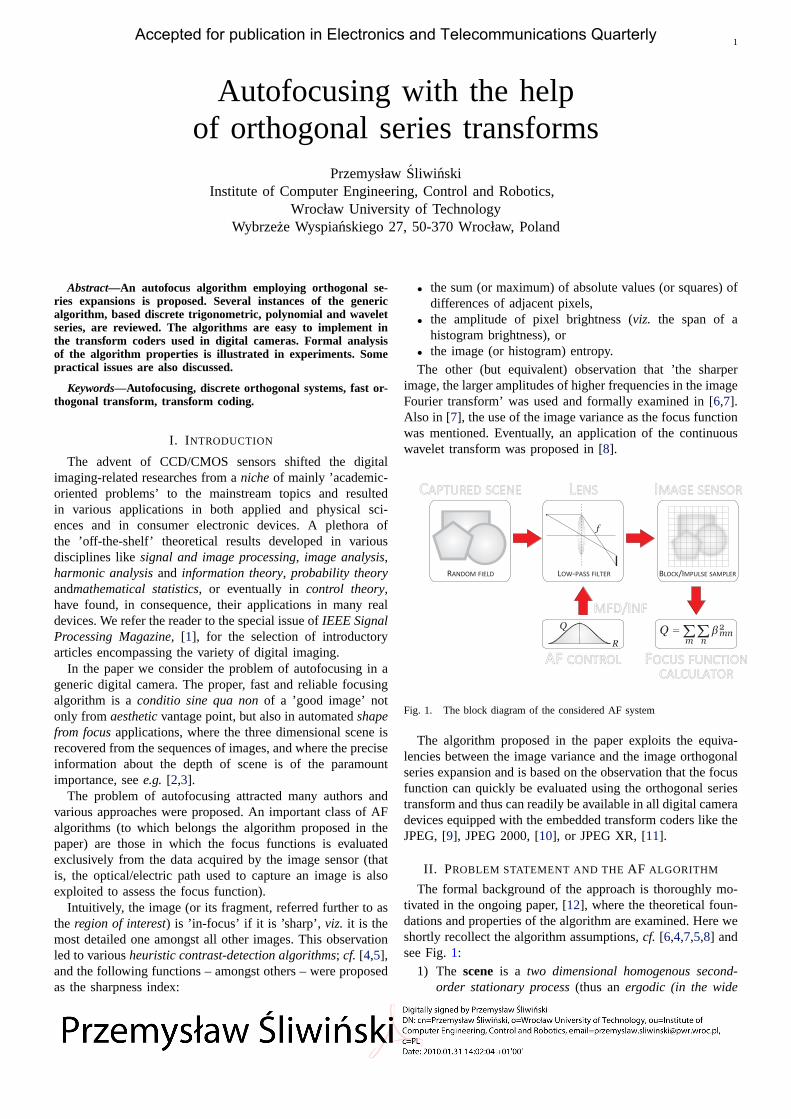
Autofocusing with the help of orthogonal series transforms

1

Autofocusing with the helpof orthogonal series transforms

PrzemysławSliwinskiInstitute of Computer Engineering, Control and Robotics,

Wrocław University of TechnologyWybrzeze Wyspianskiego 27, 50-370 Wrocław, Poland

Abstract—An autofocus algorithm employing orthogonal se-ries expansions is proposed. Several instances of the genericalgorithm, based discrete trigonometric, polynomial and waveletseries, are reviewed. The algorithms are easy to implement inthe transform coders used in digital cameras. Formal analysisof the algorithm properties is illustrated in experiments. Somepractical issues are also discussed.

Keywords—Autofocusing, discrete orthogonal systems, fast or-thogonal transform, transform coding.

I. I NTRODUCTION

The advent of CCD/CMOS sensors shifted the digitalimaging-related researches from anicheof mainly ’academic-oriented problems’ to the mainstream topics and resultedin various applications in both applied and physical sci-ences and in consumer electronic devices. A plethora ofthe ’off-the-shelf’ theoretical results developed in variousdisciplines likesignal and image processing,image analysis,harmonic analysisand information theory,probability theoryandmathematical statistics, or eventually incontrol theory,have found, in consequence, their applications in many realdevices. We refer the reader to the special issue ofIEEE SignalProcessing Magazine, [1], for the selection of introductoryarticles encompassing the variety of digital imaging.

In the paper we consider the problem of autofocusing in ageneric digital camera. The proper, fast and reliable focusingalgorithm is aconditio sine qua nonof a ’good image’ notonly from aestheticvantage point, but also in automatedshapefrom focusapplications, where the three dimensional scene isrecovered from the sequences of images, and where the preciseinformation about the depth of scene is of the paramountimportance, seee.g. [2,3].

The problem of autofocusing attracted many authors andvarious approaches were proposed. An important class of AFalgorithms (to which belongs the algorithm proposed in thepaper) are those in which the focus functions is evaluatedexclusively from the data acquired by the image sensor (thatis, the optical/electric path used to capture an image is alsoexploited to assess the focus function).

Intuitively, the image (or its fragment, referred further to asthe region of interest) is ’in-focus’ if it is ’sharp’, viz. it is themost detailed one amongst all other images. This observationled to variousheuristic contrast-detection algorithms;cf. [4,5],and the following functions – amongst others – were proposedas the sharpness index:

� the sum (or maximum) of absolute values (or squares) ofdifferences of adjacent pixels,

� the amplitude of pixel brightness (viz. the span of ahistogram brightness), or

� the image (or histogram) entropy.The other (but equivalent) observation that ’the sharper

image, the larger amplitudes of higher frequencies in the imageFourier transform’ was used and formally examined in [6,7].Also in [7], the use of the image variance as the focus functionwas mentioned. Eventually, an application of the continuouswavelet transform was proposed in [8].

CAPTURED SCENECAPTURED SCENE LENSLENS IMAGE SENSORIMAGE SENSOR

FOCUS FUNCTIONCALCULATOR

FOCUS FUNCTIONCALCULATOR

AF CONTROLAF CONTROL

MFD/INFMFD/INF

RANDOM FIELD BLOCK/IMPULSE SAMPLER

Q

R

Q = >m>nKmn

2

LOW-PASS FILTER

f

Fig. 1. The block diagram of the considered AF system

The algorithm proposed in the paper exploits the equiva-lencies between the image variance and the image orthogonalseries expansion and is based on the observation that the focusfunction can quickly be evaluated using the orthogonal seriestransform and thus can readily be available in all digital cameradevices equipped with the embedded transform coders like theJPEG, [9], JPEG 2000, [10], or JPEG XR, [11].

II. PROBLEM STATEMENT AND THE AF ALGORITHM

The formal background of the approach is thoroughly mo-tivated in the ongoing paper, [12], where the theoretical foun-dations and properties of the algorithm are examined. Here weshortly recollect the algorithm assumptions,cf. [6,4,7,5,8] andsee Fig.1:

1) The scene is a two dimensional homogenous second-order stationary process(thus anergodic (in the wide

Accepted for publication in Electronics and Telecommunications Quarterly

2

sense) random field) with unknown distribution andcorrelation functions;cf. [13].

2) Thelens assemblyis modeled with the help of thefirst-order optics laws, cf.[14], that is, the lens acts as asimple centered moving averagefilter with the orderproportional to the distance of the sensor plane fromthe image plane and to the size of the lens aperture.

3) A square (i.e.two dimensional)image sensoris mod-eled either by:

a) theblock sampler, orb) by the impulse samplerpreceded by a low pass

(AA – anti-aliasing) filter.

Both sensor models in Assumption 3 are inspired by thedevices widely used in digital photography. Theblock samplerapproximates the Foveon-type sensors, in which a single pixelconsists of three pairs of stacked color filters and correspond-ing sensors, seee.g. [15]. The impulse sampler,combinedwith the low-pass filter, corresponds to the widespreadBayer’sColor Filter Array combined with the opticalAA-filter, wherethe single image pixel is reconstructed from the sensor pixelsvia the special interpolation procedure calleddemosaicing;cf.[16,17,18]. In both cases the lens-produced image is assumedto be orthogonally projectedonto the respective functionsubspace. The block sampler projects the image onto the spaceof piecewise constant functions, while the impulse samplerpreceded by the low-pass filter projects the image onto thespace of band-limited functions.

Remark 1:The continuous image is projected onto the re-spective space and gets the approximate discrete representationin a given basis. Clearly, due to natural physical limitations,the sensor captures only a finite (square in our case) part ofthe scene.

The natural bases on squares are constructed as the tensorproducts of the one dimensional bases on the intervals, andin case of the block sampler they are piecewise-constantHaar andWalsh-Hadamardbases. In case of the band-limitedfunctions, the basis constituted by thesinc functions is usuallyreplaced by the Fourier basis, sine, or cosine bases. Notehowever that, regardless of the sensor type (and the resultingbasis), we can treat this representation as the matrix of pixelsvalues and decompose the matrix using any discrete seriesorthogonal on two-dimensional interval.

A. Algorithm

The crucial for the algorithm is the observation that theimage variance can serve as the focus function and thatthis variance can be approximated by orthogonal expansioncoefficients evaluated from the image acquired by the sensor;see Lemma1. The variance is the largest when the image is’in-focus’ and the AF algorithm is just an algorithm searchingfor the maximum of such function. Various (bi-)orthogonalexpansions can be used;cf. [19,20,21,22,23,24,25,26]:

� trigonometric, based onFourier, cosine, sine,Hartley,Walsh-Hadamardseries,

� wavelet,e.g., orthogonalHaar, Daubechies, biorthogonalLeGall (5/3)andCohen-Daubechies-Vial (9/7)series, or

� polynomial, e.g., Chebyshev, Legendre– or in general– any Jacobi family of discrete orthogonal polynomialsseries.

These expansions can be fast computed by the existingtransform coders (implementing transform coding compres-sion schemes; seee.g. [9,27,28,29,30,31,32,10,33,34]). Thefollowing discrete orthogonal series transforms used in theavailable transform coders are thus considered and comparedin the paper:� Cosinetransform (performed inJPEG coder),� Haar wavelettransform (employed inJPEG 2K (Part

II) coder, and� Walsh-Hadamardtransform (used inJPEG XR stan-

dard).The JPEG engine is applied in its standardized transfor-

mation of the 8x8 image subblocks, and moreover, used toimplement a hierarchical (progressive) DCT (H-DCT) trans-form, where the DC components of the 8x8 subblocks arecombined in the 8x8 macroblocks and treated as inputs in theanother 8x8 DCT transform step. TheJPEG 2K transform isperformed at various levels – from the maximum level in the’full transform’, to the single-level one (note that the latteressentially amounts to the classiccontrast-detectalgorithm).TheWalsh-Hadamardused inJPEG XR standard is mimickedby the Haar transform performed at 16x16 subblocks (being4x4 macroblocks built upon 4x4 subblocks).

B. Algorithm properties

The following lemma describes the formal justification ofthe proposed algorithm.

Lemma 1:Under Assumptions1-3, the variance of thesensor image isunimodal function with respect to the orderof the lens filter model and attains its maximum value for thein-focus image.

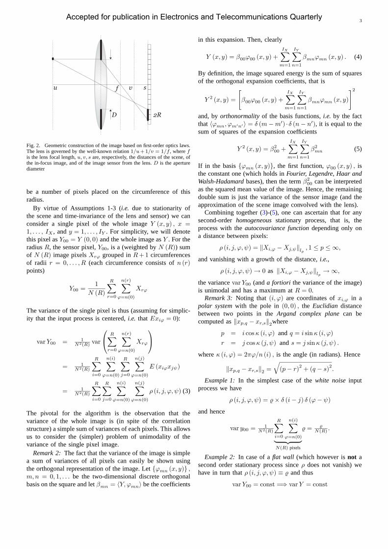
Proof: Using thefirst-order optics laws, one can easilyascertain that the image in the image plane (i.e.the imagebefore sampling by sensor) is the output of the linearsimplecentered moving averagefilter (viz. the lens) driven by thescene image. Then, the image, described by the convolution ofthe scene image with the filter impulse response, is sampled bythe sensor. The orderR of the moving average filter (countedin pixels of the image sensor) can be determined from theillustration in Fig.??.

Assume that the lens aperture is circular. Then the imageof the point light source at the scene is the uniformly filledcircle of the radius proportional to the lens aperture diameterD and the distancejs� vj between the image plane and thesensor plane;cf. e.g.[5]:

R � D � js� vj (1)

Clearly, the image is ’in-focus’ whens = v. Let now

N (R) = 1 + 4

RXr=0

jpR2 � r2

k(2)

bea number of square pixels with centers inside the boundaryof a circle of radiusR. Let also

n (R) = N (R)�N (R� 1)

Accepted for publication in Electronics and Telecommunications Quarterly

3

fu

D 2R

v s

Fig. 2. Geometric construction of the image based on first-order optics laws.The lens is governed by the well-known relation1=u+1=v = 1=f , wherefis the lens focal length,u; v; s are, respectively, the distances of the scene, ofthe in-focus image, and of the image sensor from the lens.D is the aperturediameter

be a number of pixels placed on the circumference of thisradius.

By virtue of Assumptions 1-3 (i.e.due to stationarity ofthe scene and time-invariance of the lens and sensor) we canconsider a single pixel of the whole imageY (x; y) ; x =1; : : : ; IX , andy = 1; : : : ; IY . For simplicity, we will denotethis pixel asY00 = Y (0; 0) and the whole image asY . For theradiusR, the sensor pixel,Y00, is a (weighted byN (R)) sumof N (R) image pixelsXr' grouped inR+1 circumferencesof radii r = 0; : : : ; R (each circumference consists ofn (r)points)

Y00 =1

N (R)

RXr=0

n(r)X'=n(0)

Xr'

The variance of the single pixel is thus (assuming for simplic-ity that the input process is centered,i.e. thatExi' = 0):

varY00 = 1N2(R) var

0@ RXr=0

n(r)X'=n(0)

Xr'

1A= 1

N2(R)

RXi=0

n(i)X'=n(0)

RXj=0

n(j)X'=n(0)

E (xi'xj )

= 1N2(R)

RXi=0

RXj=0

n(i)X'=n(0)

n(j)X'=n(0)

� (i; j; '; ) (3)

The pivotal for the algorithm is the observation that thevariance of the whole image is (in spite of the correlationstructure) a simple sum of variances of each pixels. This allowsus to consider the (simpler) problem of unimodality of thevariance of the single pixel image.

Remark 2:The fact that the variance of the image is simplea sum of variances of all pixels can easily be shown usingthe orthogonal representation of the image. Letf'mn (x; y)g ;m; n = 0; 1; : : : be the two-dimensional discrete orthogonalbasis on the square and let�mn = hY; 'mni be the coefficients

in this expansion. Then, clearly

Y (x; y) = �00'00 (x; y) +

IXXm=1

IYXn=1

�mn'mn (x; y) : (4)

By definition, the image squared energy is the sum of squaresof the orthogonal expansion coefficients, that is

Y 2 (x; y) =

"�00'00 (x; y) +

IXXm=1

IYXn=1

�mn'mn (x; y)

#2and, byorthonormalityof the basis functions,i.e. by the factthat h'mn; 'm0n0i = � (m�m0) �� (n� n0), it is equal to thesum of squares of the expansion coefficients

Y 2 (x; y) = �200 +

IXXm=1

IYXn=1

�2mn (5)

If in the basisf'mn (x; y)g, the first function,'00 (x; y) ; isthe constant one (which holds inFourier, Legendre, Haar andWalsh-Hadamardbases), then the term�200 can be interpretedas the squared mean value of the image. Hence, the remainingdouble sum is just the variance of the sensor image (and theapproximation of the scene image convolved with the lens).

Combining together (3)-(5), one can ascertain that for anysecond-orderhomogeneousstationary process, that is, theprocess with theautocovariance functiondepending only ona distance between pixels:

� (i; j; '; ) = kXi;' �Xj; klp ; 1 � p � 1;

and vanishing with a growth of the distance,i.e.,

� (i; j; '; )! 0 as kXi;' �Xj; klp !1;

the variancevarY00 (anda fortiori the variance of the image)is unimodal and has a maximum atR = 0.

Remark 3:Noting that (i; ') are coordinates ofxi;' in apolar systemwith the pole in(0; 0) ; the Euclidian distancebetween two points in theArgand complex planecan becomputed askxp;q � xr;sk2where

p = i cos� (i; ') andq = i sin� (i; ')

r = j cos� (j; ) ands = j sin� (j; ) :

where� (i; ') = 2�'=n (i) ; is the angle (in radians). Hence

kxp;q � xr;sk2 =q(p� r)2 + (q � s)2:

Example 1: In the simplest case of thewhite noiseinputprocess we have

� (i; j; '; ) = %� � (i� j) � ('� )

and hence

var y00 =1

N2(R)

RXi=0

n(i)X'=n(0)| {z }

N(R) pixels

% = %N(R) :

Example 2: In case of aflat wall (which however isnot asecond order stationary process since� does not vanish) wehave in turn that� (i; j; '; ) � % and thus

varY00 = const =) varY = const

Accepted for publication in Electronics and Telecommunications Quarterly

4

and the algorithm does not converge. Note however that it sucha case the image isalways in focus!

Remark 4:The image captured by the sensor is only afragment of the scene, and (which is – in fact – well known instatistic literature) in case when the scene is a highly correlatedprocess, the estimate of the variance can be very inaccurateand, in particular, does not resemble its unimodal origin.

C. AF criteria

In order to systematically describe the properties of theproposed focus function, we discuss the in the context of thefocus function criteria presented in [4]:

1) Unimodality. This condition is fulfilled – as shownformally in the paper. The sufficient condition of uni-modality requires only the autocorrelation function ofthe scene process to vanish with the distance. In prac-tice, the unimodality can be lost in low-light situationsbecause of the then-manifesting random character of thelight due to the shot, thermal and quantization noises(resulting in the poor signal-to-noise ratio,cf. Fig. 5).

2) Accuracy. It depends on the resolution of the sensor.Since the same sensor is used in autofocusing and incapturing the image of interest, the accuracy is clearlythe best attainable. In other words, since the capturedimage is the best approximation of the image yieldedby the lens, then the focus function is the largest whenthe lens-produced image has the largest variance.

3) Reproducibility. A sharp top of the extremum is – intheory – the consequence of the fact that the relationbetween image variance and the order of the lens filteris reciprocal; see (3). In practice, the sharpness of the topcan be attenuated by the influence of other (non-target)objects situated on the scene image.

4) Range. The variance of the image does not vanish forany finiteR � js� vj and this theoretically guaranteesconvergence from any initial position of the lens. Inpractice, however, the range is limited by the size ofthe sensor: if,e.g.,R is larger than the diameter of thelens aperture, then clearly, the unimodality is lost. Thisissue can be – to some extent – attenuated by reducingthe lens aperture diameter; see the experimental resultsin Fig. 6; cf. also the results of the analysis performedin Fourier domain in [6].

Fig. 3. Exemplary scene. Left – in focus, right – at minimum focus distance

5) General applicability. The generic class of processes isadmitted. For instance, it covers all stable ARMA mod-els, Markov fields, andCohen’s PSM models;cf. [35].Thetexture-rich images can be modeled, for example, bythe uniformly distributed white noise process while theseparated pointwise light sources process corresponds tothe binomial or Poisson process. Thefirst-order opticslaw seems to be sufficient to describe camera lenses –mainly because these lenses are carefully designed tobe free of higher-order distortions;cf. [14]. Finally, bothsensor models are close approximations of the two mostpopular sensor types.

6) Insensitivity to other parameters. Clearly, the varianceis independent of the mean intensity of the image, and,for instance, any change of the mean brightness of theimage (causede.g. by the varying backlight) does notaffect the focus index function. Note, however, that thescene objects situated in various distances from the lenscan also affect unimodality of the focus function.

7) Video signal compatibility. The focus function is eval-uated directly from the captured image. There is thusno disparity between the image and the data used forfocusing. Such a disparity can rather occur when thefocusing system is the autonomous one and exploits aseparate optical/electric elements (like ine.g.single-lensreflex (SLR) cameras).

8) Fast implementation. The algorithms based on or-thogonal expansions are usually fast – be ite.g. thefast Fourier transformand its real versions (i.e.DCT,or DST, amongst others), or thefast Walsh or fastwavelet transform. Furthermore, transform coders offershardware implementations which are both speed andpower consumption-optimized;cf. [10,36,37,38,39].

D. Experimental results

Several experiments have been performed to illustrate theaccuracy and natural limitations of the proposed algorithm. Inexperiments, an assembly of theCanon EOSdigital cameraand two lenses with the focal lengths85mmand100mmwereused. The camera was controlled by the application built uponthe CanonEDSDK library. In the experiments, the algorithmwas tested for:

� various lens aperture diameters,� orthogonal series, and various� AF region sizes.

The focus function was estimated as follows;cf. (4) and (5):

�Q� = log2

"Xm

Xn

��2mn � ��

200

#where

���mn

are the empirical (acquired by the image sensor)

image expansion coefficients calculated for a given discreteorthogonal basis (thelog2 function was used only to limit thedynamic range of the focus function estimate. This is a one-to-one map and hence does not affect unimodality).

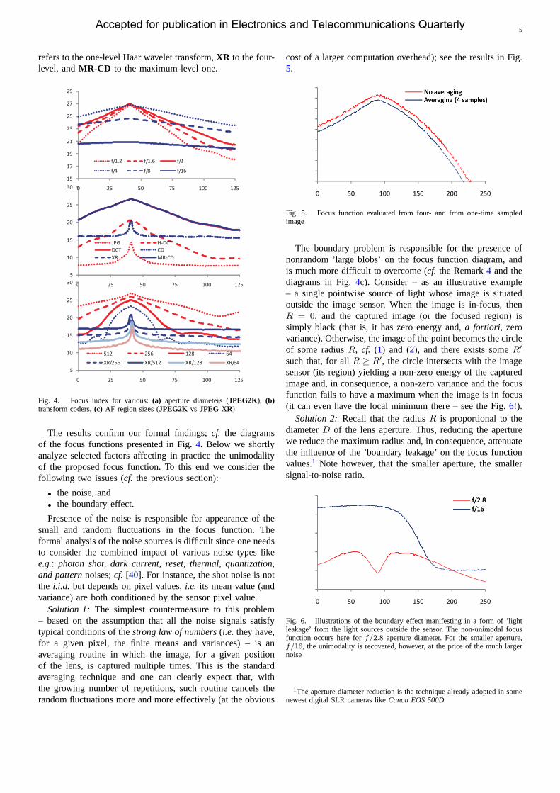
With an exception of the experiment presented in Fig.4b,the AF region was always a 256x256 square. Note thatCD

Accepted for publication in Electronics and Telecommunications Quarterly

5

refers to the one-level Haar wavelet transform,XR to the four-level, andMR-CD to the maximum-level one.

5

10

15

20

25

30

0 25 50 75 100 125

JPG H-DCTDCT CD

XR MR-CD

15

17

19

21

23

25

27

29

0 25 50 75 100 125

f/1.2 f/1.6 f/2

f/4 f/8 f/16

5

10

15

20

25

30

0 25 50 75 100 125

512 256 128 64

XR/256 XR/512 XR/128 XR/64

Fig. 4. Focus index for various:(a) aperture diameters (JPEG2K),(b)transform coders,(c) AF region sizes (JPEG2Kvs JPEG XR)

The results confirm our formal findings;cf. the diagramsof the focus functions presented in Fig.4. Below we shortlyanalyze selected factors affecting in practice the unimodalityof the proposed focus function. To this end we consider thefollowing two issues (cf.the previous section):

� the noise, and� the boundary effect.

Presence of the noise is responsible for appearance of thesmall and random fluctuations in the focus function. Theformal analysis of the noise sources is difficult since one needsto consider the combined impact of various noise types likee.g.: photon shot, dark current, reset, thermal, quantization,and patternnoises;cf. [40]. For instance, the shot noise is notthe i.i.d. but depends on pixel values,i.e. its mean value (andvariance) are both conditioned by the sensor pixel value.

Solution 1: The simplest countermeasure to this problem– based on the assumption that all the noise signals satisfytypical conditions of thestrong law of numbers(i.e. they have,for a given pixel, the finite means and variances) – is anaveraging routine in which the image, for a given positionof the lens, is captured multiple times. This is the standardaveraging technique and one can clearly expect that, withthe growing number of repetitions, such routine cancels therandom fluctuations more and more effectively (at the obvious

cost of a larger computation overhead); see the results in Fig.5.

No averagingAveraging (4 samples)

0 50 100 150 200 250

No averagingAveraging (4 samples)

Fig. 5. Focus function evaluated from four- and from one-time sampledimage

The boundary problem is responsible for the presence ofnonrandom ’large blobs’ on the focus function diagram, andis much more difficult to overcome (cf.the Remark4 andthediagrams in Fig.4c). Consider – as an illustrative example– a single pointwise source of light whose image is situatedoutside the image sensor. When the image is in-focus, thenR = 0, and the captured image (or the focused region) issimply black (that is, it has zero energy and,a fortiori, zerovariance). Otherwise, the image of the point becomes the circleof some radiusR, cf. (1) and (2), and there exists someR0

such that, for allR � R0, the circle intersects with the imagesensor (its region) yielding a non-zero energy of the capturedimage and, in consequence, a non-zero variance and the focusfunction fails to have a maximum when the image is in focus(it can even have the local minimum there – see the Fig.6!).

Solution 2: Recall that the radiusR is proportional to thediameterD of the lens aperture. Thus, reducing the aperturewe reduce the maximum radius and, in consequence, attenuatethe influence of the ’boundary leakage’ on the focus functionvalues.1 Note however, that the smaller aperture, the smallersignal-to-noise ratio.

f/2.8f/16

0 50 100 150 200 250

f/2.8f/16

Fig. 6. Illustrations of the boundary effect manifesting in a form of ’lightleakage’ from the light sources outside the sensor. The non-unimodal focusfunction occurs here forf=2:8 aperture diameter. For the smaller aperture,f=16, the unimodality is recovered, however, at the price of the much largernoise

1The aperture diameter reduction is the technique already adopted in somenewest digital SLR cameras likeCanon EOS 500D.

Accepted for publication in Electronics and Telecommunications Quarterly

6

E. Conclusions and final remarks

An application of the orthogonal series transforms, availablein various transform coders, has been proposed and formallymotivated for usage in AF algorithm. Efficiency of the ap-proach in real-life tests has been confirmed. It remains, how-ever, tempting (and easier to apply in practice) to exploit thewhole transform coder rather than only its part performing theorthogonal transform,i.e. to employ theentropyof the imagerather then itsvariancein the focus function machinery. Thiswould allow, amongst others, using thelengthof the producedcompressed stream as the focus function and employing thewhole transform coder as the focus function calculator. Thefollowing observation may be helpful in derivation of theformal basis of this proposition.

Conjecture 2:Assume adiscrete zero-meanrandom vari-ableX; its entropy and variance are, respectively, given bythe following well-known formulae:

H (X) = �nXi=1

pi � log2 pi and var (X) =nXi=1

pix2i :

wherefpi = Pr (X = xi)gni=1. Assume thatpi’s are arrangedin non-increasing order,i.e., pi � pj for i > j. Then, for anydistribution ofX such thatx2i � �c log2 pi, somec > 0, thevariance grows along with the growing entropy, which is, inturn, estimated by the size of the output stream produced bythe transform coder.

Example 3: In a special case of theuniformly distributedX we simply have

H (X) = �nXi=1

1

n� log2

1

n= log2 n

and

var (X) =1

6(2n+ 1) (n+ 1)

that is, thevariance of X grows with n. That theentropygrows is merely its natural property.

f/2.8 f/4.5 f/7.1f/11 f/18 f/29f/2.8 f/4.5 f/7.1f/11 f/18 f/29f/2.8 f/4.5 f/7.1f/11 f/18 f/29f/2.8 f/4.5 f/7.1f/11 f/18 f/29f/2.8 f/4.5 f/7.1f/11 f/18 f/29f/2.8 f/4.5 f/7.1f/11 f/18 f/29

0 100 200 300 400

f/2.8 f/4.5 f/7.1f/11 f/18 f/29

0 100 200 300 400

f/2.8 f/4.5 f/7.1f/11 f/18 f/29

Fig. 7. The JPG filesize as the focus funtion against various aperturediameters,D = f=2:8; : : : ; f=29, f = 100. All maxima (viz. the largestsizes of JPG files) correspond to the in-focus images

To illustrate the conjecture we used the standard (lossy)JPEG coder and to measure the size of the coded (output)stream we simply used the size of the.jpg file. The results

are presented in Fig.7 andsupport the conjecture. We wouldlike to emphasize that this algorithm can directly be used inalmost all off-the-shelf cameras (viz.without anymodificationof the existing hardware and with only slight tweaking of thecamera firmware).

REFERENCES

[1] “Special issue on color image processing,”IEEE Signal ProcessingMagazine, vol. 22, no. 1, 2005.

[2] S. K. Nayar and Y. Nakagawa, “Shape from focus,”IEEE Transactionson Pattern Analysis and Machine Intelligence, vol. 16, no. 8, pp. 824–831, 1994.

[3] K. S. Pradeep and A. N. Rajagopalan, “Improving shape from focususing defocus cue,”IEEE Transactions on Image Processing, vol. 16,no. 7, pp. 1920–1925, 2007.

[4] F. C. A. Groen, I. T. Young, and G. Ligthart, “A comparisonof different focus functions for use in autofocus algorithms,”Cytometry, vol. 6, no. 2, pp. 81–91, 1985. [Online]. Available:dx.doi.org/10.1002/cyto.990060202

[5] M. Subbarao and J.-K. Tyan, “Selecting the optimal focus measurefor autofocusing and depth-from-focus,”IEEE Transactions on PatternAnalysis and Machine Intelligence, vol. 20, no. 8, pp. 864–870, 1998.

[6] A. Erteza, “Depth of convergence of a sharpness index autofocussystem,”Applied Optics, vol. 16, no. 8, pp. 2273–2278, 1977.

[7] E. Krotkov, “Focusing,” International Journal of Computer Vision,vol. 1, no. 3, pp. 223–237, 1987.

[8] J. Widjaja and S. Jutamulia, “Wavelet transform-based autofocus camerasystems,”IEEE Proceedings, 1998.

[9] W. B. Pennebaker and J. L. Mitchel,JPEG: Still Image Data Compres-sion Standard. New York: Van Nostrand Reinhold, 1992.

[10] D. Taubman and M. Marcellin,JPEG2000. Image Compression Funda-mentals, Standards and Practice, ser. The Kluwer International Seriesin Engineering and Computer Science. Kluwer Academic Publishers,2002, vol. 642.

[11] F. Dufaux, G. Sullivan, and T. Ebrahimi, “The JPEG XR image codingstandard,”IEEE Signal Processing Magazine, vol. 26, no. 6, pp. 195–199, 204, 2009.

[12] P. Sliwinski, “Autofocusing with orthogonal series,” 2009, submitted forreview.

[13] J. W. Goodman,Statistical optics. New York: Willey-Interscience,2000.

[14] S. J. Ray,Applied Photographic Optics, 3rd Ed.Oxford: Focal Press,2002.

[15] L. D. Paulson, “Will new chip revolutionize digital photography?”IEEEComputer, vol. 35, no. 5, pp. 25–26, 2002.

[16] R. Ramanath, W. E. Snyder, Y. Yoo, and M. S. Drew, “Color imageprocessing pipeline. a general survey of digital still camera processing,”IEEE Signal Processing Magazine, vol. 22, no. 1, pp. 34–43, 2005.

[17] D. D. Muresan and T. W. Parks, “Demosaicing using optimal recovery,”IEEE Transactions on Information Theory, vol. 14, no. 2, pp. 267–278,2005.

[18] X. Li, “Demosaicing by successive approximation,”IEEE Transactionson Image Processing, vol. 14, no. 3, pp. 370–379, 2005.

[19] A. Haar, “Zur Theorie der Orthogonalen Funktionen-Systeme,”Annalsof Mathematics, vol. 69, 1910.

[20] G. Sansone,Orthogonal Functions. New York: Interscience, 1959.[21] T. Rivlin, Chebyshev Polynomials. New York: Wiley, 1974.[22] G. Szego,Orthogonal Polynomials, 3rd ed. Providence, R.I.: American

Mathematical Society, 1974.[23] M. Vetterli and D. Le Gall, “Perfect reconstruction FIR filter banks:

some properties and factorizations,”IEEE Transactions on Acoustics,Speech and Signal Processing, vol. 37, no. 7, pp. 1057–1071, 1989.

[24] I. Daubechies,Ten Lectures on Wavelets. Philadelphia: SIAM Edition,1992.

[25] G. G. Walter,Wavelets and other orthogonal systems with applications.Boca Raton: CRC Press, 2001.

[26] M. Unser and T. Blu, “Mathematical properties of the JPEG2000 waveletfilters,” IEEE Transactions on Image Processing, vol. 12, no. 9, pp.1080–1090, September 2003.

[27] M. Antonini, M. Barlaud, P. Mathieu, and I. Daubechies, “Image codingusing wavelet transform,”IEEE Transactions on Image Processing,vol. 1, no. 2, pp. 205–220, 1992.

Accepted for publication in Electronics and Telecommunications Quarterly

7

[28] R. A. DeVore, B. Jawerth, and B. Lucier, “Image compression throughwavelet transform coding,”IEEE Transactions on Information Theory,vol. 38, no. 2, pp. 719–746, 1992.

[29] D. L. Donoho, M. Vetterli, R. A. DeVore, and I. Daubechies, “Datacompression and harmonic analysis,”IEEE Transactions on InfromationTheory, vol. 44, no. 6, pp. 2435–2476, 1998.

[30] “Special issue on JPEG2000 standard,”IEEE Signal Processing Maga-zine, vol. 18, no. 5, 2001.

[31] “Special issue on JPEG 2000 standard,”Signal Processing: ImageCommunication, vol. 17, 2002.

[32] A. Cohen, I. Daubechies, O. G. Guleryuz, and M. T. Orchard, “On theimportance of combining wavelet-based nonlinear approximation withcoding strategies,”IEEE Transactions on Information Theory, vol. 48,no. 7, pp. 1895–1921, 2002.

[33] “Special section on JPEG 2000 digital imaging,”IEEE Transactions onConsumer Electronics, vol. 49, pp. 771–888, 2003.

[34] “Special section on the H.264/AVC video coding standard,”IEEETransactions on Circuits and Systems for Video Technology, vol. 13,no. 7, pp. 557–725, 2003.

[35] A. Cohen and J.-P. D’Ales, “Nonlinear approximation of random func-tions,” SIAM Journal of Applied Mathematics, vol. 57, no. 2, pp. 518–540, 1997.

[36] T. Acharya and P.-S. Tsai,JPEG2000 Standard for Image Compression:Concepts, Algorithms and VLSI Architectures. Wiley-Interscience,2005.

[37] D. T. Lee, “JPEG 2000: Retrospective and new developments,”Proceed-ings of the IEEE, vol. 93, no. 1, pp. 32–41, 2005.

[38] H.-C. Fang, Y.-W. Chang, C.-C. Cheng, and L.-G. Chen, “Memoryefficient JPEG 2000 architecture with stripe pipeline scheduling,”IEEETransactions on Signal Processing, vol. 54, no. 12, pp. 4807–4816, 2006.

[39] G. Savaton, E. Casseau, and E. Martin, “Design of a flexible 2-D discretewavelet transform IP core for JPEG2000 image coding in embeddedimaging systems,”Signal Processing, vol. 86, pp. 1375–1399, 2006.

[40] B. Fowler, M. D. Godfrey, and S. Mims, “Reset noise reductionin capacitive sensors,”IEEE Transaction on Circuits and Systems-I:Regular Papers, vol. 53, no. 8, pp. 1658–1669, 2006.

Accepted for publication in Electronics and Telecommunications Quarterly