Autocalibrating vision guided navigation of unmanned air ...

Graduate Theses and Dissertations Iowa State University Capstones, Theses andDissertations

2012

Autocalibrating vision guided navigation ofunmanned air vehicles via tactical monocularcameras in GPS denied environmentsKoray CelikIowa State University

Follow this and additional works at: https://lib.dr.iastate.edu/etd

Part of the Aerospace Engineering Commons, Computer Engineering Commons, and theElectrical and Electronics Commons

This Dissertation is brought to you for free and open access by the Iowa State University Capstones, Theses and Dissertations at Iowa State UniversityDigital Repository. It has been accepted for inclusion in Graduate Theses and Dissertations by an authorized administrator of Iowa State UniversityDigital Repository. For more information, please contact [email protected].

Recommended CitationCelik, Koray, "Autocalibrating vision guided navigation of unmanned air vehicles via tactical monocular cameras in GPS deniedenvironments" (2012). Graduate Theses and Dissertations. 12802.https://lib.dr.iastate.edu/etd/12802

http://lib.dr.iastate.edu/?utm_source=lib.dr.iastate.edu%2Fetd%2F12802&utm_medium=PDF&utm_campaign=PDFCoverPages

http://lib.dr.iastate.edu/?utm_source=lib.dr.iastate.edu%2Fetd%2F12802&utm_medium=PDF&utm_campaign=PDFCoverPages

https://lib.dr.iastate.edu/etd?utm_source=lib.dr.iastate.edu%2Fetd%2F12802&utm_medium=PDF&utm_campaign=PDFCoverPages

https://lib.dr.iastate.edu/theses?utm_source=lib.dr.iastate.edu%2Fetd%2F12802&utm_medium=PDF&utm_campaign=PDFCoverPages

https://lib.dr.iastate.edu/theses?utm_source=lib.dr.iastate.edu%2Fetd%2F12802&utm_medium=PDF&utm_campaign=PDFCoverPages

https://lib.dr.iastate.edu/etd?utm_source=lib.dr.iastate.edu%2Fetd%2F12802&utm_medium=PDF&utm_campaign=PDFCoverPages

http://network.bepress.com/hgg/discipline/218?utm_source=lib.dr.iastate.edu%2Fetd%2F12802&utm_medium=PDF&utm_campaign=PDFCoverPages



https://lib.dr.iastate.edu/etd/12802?utm_source=lib.dr.iastate.edu%2Fetd%2F12802&utm_medium=PDF&utm_campaign=PDFCoverPages

mailto:[email protected]

Autocalibrating vision guided navigation of unmanned air vehicles

via tactical monocular cameras in GPS denied environments

by

Koray Celik

A dissertation submitted to the graduate faculty

in partial fulfillment of the requirements for the degree of

DOCTOR OF PHILOSOPHY

Major: Computer Engineering

Program of Study Committee:

Arun K. Somani, Major Professor

Peter Sherman

Akhilesh Tyagi

Namrata Vaswani

Steve Holland

Manimaran Govindarasu

Iowa State University

Ames, Iowa

2012

Copyright c© Koray Celik, 2012. All rights reserved.

ii

Dedication

To the sacrifice of four angels, for the sake of one daemon, by whose hand thesis could be

given breath.

Ph.D. is a journey of endurance with no haven, apart from thinking yourself to death. Ev-

ery time I returned from campus, brains torpedoed out of the water, desperate, back to the

one-bedroom machine-shop I call home, at the oddest hours of dawn, eyes bloodshot, and a

self esteem riddled with bullet holes due to a burned circuit board, a dysfunctional algorithm,

a software bug, or another failure du jour, but still managed to show up at the lab next day

brave another storm full steam ahead, now you know my secret; my Mother, Father, Brother,

and the Beloved.

Koray Celik

Angel:“What is the trouble?”

Me: “Torpedoes. . . ”

Angel: “Damn the torpedoes.”

iii

TABLE OF CONTENTS

LIST OF TABLES . . . . . . . . . . . . . . . . . . . . . . . . . . . . . . . . . . . . iv

LIST OF FIGURES . . . . . . . . . . . . . . . . . . . . . . . . . . . . . . . . . . . v

ACKNOWLEDGEMENTS . . . . . . . . . . . . . . . . . . . . . . . . . . . . . . . vi

ABSTRACT . . . . . . . . . . . . . . . . . . . . . . . . . . . . . . . . . . . . . . . . x

CHAPTER 1. Inception . . . . . . . . . . . . . . . . . . . . . . . . . . . . . . . . 1

1.1 Prologue . . . . . . . . . . . . . . . . . . . . . . . . . . . . . . . . . . . . . . . . 2

1.2 A Vespertilinoid Encounter . . . . . . . . . . . . . . . . . . . . . . . . . . . . . 3

1.3 Biologically Inspired Machine Vision . . . . . . . . . . . . . . . . . . . . . . . . 6

1.4 A New Perceptive Vigilance . . . . . . . . . . . . . . . . . . . . . . . . . . . . . 12

1.5 Dance with the Angels . . . . . . . . . . . . . . . . . . . . . . . . . . . . . . . . 15

CHAPTER 2. Electric Helmsman . . . . . . . . . . . . . . . . . . . . . . . . . . 25

2.1 Shortcomings of Current Techniques . . . . . . . . . . . . . . . . . . . . . . . . 33

2.2 VINAR Mark-I . . . . . . . . . . . . . . . . . . . . . . . . . . . . . . . . . . . . 61

2.3 VINAR Mark-II . . . . . . . . . . . . . . . . . . . . . . . . . . . . . . . . . . . 72

2.3.1 VINAR Mark-I and Mark-II Comparison . . . . . . . . . . . . . . . . . 78

2.4 VINAR Mark-III . . . . . . . . . . . . . . . . . . . . . . . . . . . . . . . . . . . 83

2.5 VINAR Mark-IV . . . . . . . . . . . . . . . . . . . . . . . . . . . . . . . . . . . 84

2.6 VINAR SLAM Formulation . . . . . . . . . . . . . . . . . . . . . . . . . . . . . 89

2.6.1 Data Association . . . . . . . . . . . . . . . . . . . . . . . . . . . . . . . 97

iv

CHAPTER 3. Electric Angels . . . . . . . . . . . . . . . . . . . . . . . . . . . . . 110

3.1 Saint Vertigo . . . . . . . . . . . . . . . . . . . . . . . . . . . . . . . . . . . . . 113

3.1.1 Saint Vertigo Evolution . . . . . . . . . . . . . . . . . . . . . . . . . . . 128

3.1.2 Saint Vertigo PID Control Model . . . . . . . . . . . . . . . . . . . . . . 132

3.1.3 A Soft-Processor for Saint Vertigo . . . . . . . . . . . . . . . . . . . . . 140

3.2 Dante . . . . . . . . . . . . . . . . . . . . . . . . . . . . . . . . . . . . . . . . . 164

3.3 Michaelangelo . . . . . . . . . . . . . . . . . . . . . . . . . . . . . . . . . . . . . 172

3.4 µCART . . . . . . . . . . . . . . . . . . . . . . . . . . . . . . . . . . . . . . . . 175

3.5 Angelstrike . . . . . . . . . . . . . . . . . . . . . . . . . . . . . . . . . . . . . . 180

3.6 Virgil . . . . . . . . . . . . . . . . . . . . . . . . . . . . . . . . . . . . . . . . . 183

3.6.1 Chassis & Propulsion . . . . . . . . . . . . . . . . . . . . . . . . . . . . 187

3.6.2 Power . . . . . . . . . . . . . . . . . . . . . . . . . . . . . . . . . . . . . 187

3.6.3 Computation . . . . . . . . . . . . . . . . . . . . . . . . . . . . . . . . . 188

3.6.4 Communication & Control . . . . . . . . . . . . . . . . . . . . . . . . . 190

3.6.5 Arm . . . . . . . . . . . . . . . . . . . . . . . . . . . . . . . . . . . . . . 193

3.6.6 Sensing . . . . . . . . . . . . . . . . . . . . . . . . . . . . . . . . . . . . 193

3.6.7 Laser Range-Finder . . . . . . . . . . . . . . . . . . . . . . . . . . . . . 193

3.6.8 Digital HD-Camera . . . . . . . . . . . . . . . . . . . . . . . . . . . . . 193

3.6.9 Soil Probe . . . . . . . . . . . . . . . . . . . . . . . . . . . . . . . . . . . 200

3.6.10 Soil pH-Meter . . . . . . . . . . . . . . . . . . . . . . . . . . . . . . . . . 202

3.6.11 Microscope . . . . . . . . . . . . . . . . . . . . . . . . . . . . . . . . . . 202

3.7 Liquidator . . . . . . . . . . . . . . . . . . . . . . . . . . . . . . . . . . . . . . . 203

3.8 Ghostwalker . . . . . . . . . . . . . . . . . . . . . . . . . . . . . . . . . . . . . . 204

3.9 USCAP SARStorm . . . . . . . . . . . . . . . . . . . . . . . . . . . . . . . . . . 206

3.10 UH-1Y Venom Huey . . . . . . . . . . . . . . . . . . . . . . . . . . . . . . . . . 211

3.11 Bell 222X Black Shark . . . . . . . . . . . . . . . . . . . . . . . . . . . . . . . . 215

3.12 AH6LB Little Bird . . . . . . . . . . . . . . . . . . . . . . . . . . . . . . . . . . 217

3.13 MI8 HIP . . . . . . . . . . . . . . . . . . . . . . . . . . . . . . . . . . . . . . . . 219

3.14 AH1W Cobra & AH64 Apache . . . . . . . . . . . . . . . . . . . . . . . . . . . 219

v

3.15 FarmCopter . . . . . . . . . . . . . . . . . . . . . . . . . . . . . . . . . . . . . . 221

3.16 Boris-II . . . . . . . . . . . . . . . . . . . . . . . . . . . . . . . . . . . . . . . . 227

CHAPTER 4. Image Navigator Engines . . . . . . . . . . . . . . . . . . . . . . 229

4.1 The Fundamental Algorithm . . . . . . . . . . . . . . . . . . . . . . . . . . . . 232

4.1.1 Assumptions and Definitions . . . . . . . . . . . . . . . . . . . . . . . . 234

4.1.2 Nomenclature . . . . . . . . . . . . . . . . . . . . . . . . . . . . . . . . . 236

4.1.3 Pseudo Fundamental Algorithm . . . . . . . . . . . . . . . . . . . . . . . 237

4.2 Estimation Engine . . . . . . . . . . . . . . . . . . . . . . . . . . . . . . . . . . 241

4.2.1 Generic Structure . . . . . . . . . . . . . . . . . . . . . . . . . . . . . . 242

4.2.2 The Extended Kalman Filter (EKF) Engines . . . . . . . . . . . . . . . 242

4.2.3 Unscented Kalman Filter (UKF) Engines . . . . . . . . . . . . . . . . . 252

4.2.4 The Information Filter (IF) Engines . . . . . . . . . . . . . . . . . . . . 257

4.2.5 Particle Filter (PF) Engines . . . . . . . . . . . . . . . . . . . . . . . . . 267

4.2.6 Discrete Landmark Association (DLA) Engines . . . . . . . . . . . . . . 268

4.2.7 Map Interpretation . . . . . . . . . . . . . . . . . . . . . . . . . . . . . . 274

4.3 Performance Metrics . . . . . . . . . . . . . . . . . . . . . . . . . . . . . . . . . 285

4.4 Sensor Choices . . . . . . . . . . . . . . . . . . . . . . . . . . . . . . . . . . . . 291

4.4.1 MAIN SENSORS . . . . . . . . . . . . . . . . . . . . . . . . . . . . . . . 292

4.4.2 AUXILIARY SENSORS . . . . . . . . . . . . . . . . . . . . . . . . . . . 303

4.5 Conclusions & Future Goals . . . . . . . . . . . . . . . . . . . . . . . . . . . . . 306

CHAPTER 5. Autocalibration for Image Navigation . . . . . . . . . . . . . . . 307

5.1 n-Ocular Wandless Autocalibration . . . . . . . . . . . . . . . . . . . . . . . . . 308

5.1.1 Behavioral Analysis of n-Ocular Autocalibration . . . . . . . . . . . . . 321

5.1.2 Simulations - I . . . . . . . . . . . . . . . . . . . . . . . . . . . . . . . . 323

5.1.3 Simulations - II . . . . . . . . . . . . . . . . . . . . . . . . . . . . . . . . 325

5.1.4 Interpretations & Conclusions . . . . . . . . . . . . . . . . . . . . . . . . 327

5.2 n-Ocular Wandless Autocalibration with Lens Distortions . . . . . . . . . . . . 330

5.2.1 Methodology . . . . . . . . . . . . . . . . . . . . . . . . . . . . . . . . . 332

vi

5.2.2 Simulation Results for Center-Barrel Case . . . . . . . . . . . . . . . . . 335

5.2.3 Simulation Results for Edge-Barrel Case . . . . . . . . . . . . . . . . . . 339

5.2.4 Conclusions . . . . . . . . . . . . . . . . . . . . . . . . . . . . . . . . . . 339

5.3 n-Ocular Miscalibration Determinants . . . . . . . . . . . . . . . . . . . . . . . 339

5.3.1 Environmental Determinants for Calibration Endurance . . . . . . . . . 340

5.3.2 The Experimental Setup . . . . . . . . . . . . . . . . . . . . . . . . . . . 343

5.3.3 Experimental Results . . . . . . . . . . . . . . . . . . . . . . . . . . . . 344

5.3.4 Recommended Countermeasures . . . . . . . . . . . . . . . . . . . . . . 348

5.4 Monocular Miscalibration Determinants . . . . . . . . . . . . . . . . . . . . . . 351

5.4.1 Experimental Setup . . . . . . . . . . . . . . . . . . . . . . . . . . . . . 352

5.4.2 Methodology . . . . . . . . . . . . . . . . . . . . . . . . . . . . . . . . . 356

5.4.3 Analysis . . . . . . . . . . . . . . . . . . . . . . . . . . . . . . . . . . . . 360

5.4.4 Recommended Countermeasures . . . . . . . . . . . . . . . . . . . . . . 361

5.5 Literature . . . . . . . . . . . . . . . . . . . . . . . . . . . . . . . . . . . . . . . 363

5.5.1 Other CONOPS to Address . . . . . . . . . . . . . . . . . . . . . . . . . 364

5.5.2 Monocular Autocalibration Parameters of Interest . . . . . . . . . . . . 366

5.5.3 Applicable Methods . . . . . . . . . . . . . . . . . . . . . . . . . . . . . 369

5.5.4 Conclusion . . . . . . . . . . . . . . . . . . . . . . . . . . . . . . . . . . 374

5.6 Monocular Wandless Autocalibration . . . . . . . . . . . . . . . . . . . . . . . . 375

5.6.1 Introduction . . . . . . . . . . . . . . . . . . . . . . . . . . . . . . . . . 375

5.6.2 T6-System Approach . . . . . . . . . . . . . . . . . . . . . . . . . . . . . 377

5.6.3 T6 Hardware . . . . . . . . . . . . . . . . . . . . . . . . . . . . . . . . . 380

5.6.4 T6 Software . . . . . . . . . . . . . . . . . . . . . . . . . . . . . . . . . . 389

5.7 Wandless Monocular Autocalibration Test Drive . . . . . . . . . . . . . . . . . 403

5.7.1 Acquisition . . . . . . . . . . . . . . . . . . . . . . . . . . . . . . . . . . 404

5.7.2 Mapping . . . . . . . . . . . . . . . . . . . . . . . . . . . . . . . . . . . . 405

5.7.3 Calibration . . . . . . . . . . . . . . . . . . . . . . . . . . . . . . . . . . 407

5.7.4 Test Drive . . . . . . . . . . . . . . . . . . . . . . . . . . . . . . . . . . . 408

5.7.5 Conclusions . . . . . . . . . . . . . . . . . . . . . . . . . . . . . . . . . . 409

vii

CHAPTER 6. Map-Aided Navigation . . . . . . . . . . . . . . . . . . . . . . . . 418

6.1 Introduction . . . . . . . . . . . . . . . . . . . . . . . . . . . . . . . . . . . . . . 419

6.2 Transition Model & Observer Assumptions . . . . . . . . . . . . . . . . . . . . 420

6.3 Applicable Map Data & Navigation Techniques . . . . . . . . . . . . . . . . . . 427

6.4 Gravity Observation Model . . . . . . . . . . . . . . . . . . . . . . . . . . . . . 434

6.5 Map Associations . . . . . . . . . . . . . . . . . . . . . . . . . . . . . . . . . . . 439

6.6 Gerardus The Simulator Part-I . . . . . . . . . . . . . . . . . . . . . . . . . . . 440

6.7 Gerardus The Simulator Part-II . . . . . . . . . . . . . . . . . . . . . . . . . . . 446

6.8 Gerardus Examples . . . . . . . . . . . . . . . . . . . . . . . . . . . . . . . . . . 451

6.9 Conclusions . . . . . . . . . . . . . . . . . . . . . . . . . . . . . . . . . . . . . . 458

CHAPTER 7. Meta Image Navigation Augmenters . . . . . . . . . . . . . . . 460

7.1 MINA Functional Diagrams . . . . . . . . . . . . . . . . . . . . . . . . . . . . . 464

7.2 Metamap . . . . . . . . . . . . . . . . . . . . . . . . . . . . . . . . . . . . . . . 467

7.2.1 Selecting the Data Type for Metamap . . . . . . . . . . . . . . . . . . . 470

7.2.2 OSM Encoding . . . . . . . . . . . . . . . . . . . . . . . . . . . . . . . . 478

7.2.3 MINA Object Model: GIS Agents . . . . . . . . . . . . . . . . . . . . . 491

7.2.4 MINA RDBMS Concept . . . . . . . . . . . . . . . . . . . . . . . . . . . 500

7.3 Aircraft . . . . . . . . . . . . . . . . . . . . . . . . . . . . . . . . . . . . . . . . 508

7.3.1 MINA Flight Simulator . . . . . . . . . . . . . . . . . . . . . . . . . . . 508

7.4 FILTERPACK . . . . . . . . . . . . . . . . . . . . . . . . . . . . . . . . . . . . 519

7.4.1 Convolution & Spatial Kernels . . . . . . . . . . . . . . . . . . . . . . . 521

7.4.2 Spectral Decomposition . . . . . . . . . . . . . . . . . . . . . . . . . . . 534

7.5 EIGENPACK . . . . . . . . . . . . . . . . . . . . . . . . . . . . . . . . . . . . . 542

7.5.1 Eigenpack Scale Space . . . . . . . . . . . . . . . . . . . . . . . . . . . . 542

7.5.2 Local Contrast Enhancement . . . . . . . . . . . . . . . . . . . . . . . . 544

7.5.3 Eigenvalue Corners . . . . . . . . . . . . . . . . . . . . . . . . . . . . . . 556

7.5.4 Lines and Curves . . . . . . . . . . . . . . . . . . . . . . . . . . . . . . . 559

7.6 MINA IPACK . . . . . . . . . . . . . . . . . . . . . . . . . . . . . . . . . . . . . 560

7.6.1 WKNNC . . . . . . . . . . . . . . . . . . . . . . . . . . . . . . . . . . . 561

viii

7.6.2 TPST . . . . . . . . . . . . . . . . . . . . . . . . . . . . . . . . . . . . . 567

7.6.3 PCA . . . . . . . . . . . . . . . . . . . . . . . . . . . . . . . . . . . . . . 570

7.6.4 Performance of IPACK Algorithms . . . . . . . . . . . . . . . . . . . . . 579

7.7 MINA Optical Considerations & PVA . . . . . . . . . . . . . . . . . . . . . . . 584

7.7.1 Optical Considerations (Optipack) . . . . . . . . . . . . . . . . . . . . . 584

7.7.2 PVA . . . . . . . . . . . . . . . . . . . . . . . . . . . . . . . . . . . . . . 588

7.7.3 UAV Camera Matrix . . . . . . . . . . . . . . . . . . . . . . . . . . . . . 592

7.8 MINA Test Drive . . . . . . . . . . . . . . . . . . . . . . . . . . . . . . . . . . . 594

7.8.1 MINA Algorithm . . . . . . . . . . . . . . . . . . . . . . . . . . . . . . . 594

7.8.2 Design of Experiments . . . . . . . . . . . . . . . . . . . . . . . . . . . . 595

7.8.3 Concluding Remarks . . . . . . . . . . . . . . . . . . . . . . . . . . . . . 599

7.9 MINA MK4 . . . . . . . . . . . . . . . . . . . . . . . . . . . . . . . . . . . . . . 606

CHAPTER 8. Project Battlespace . . . . . . . . . . . . . . . . . . . . . . . . . . 608

CHAPTER 9. Epilogue . . . . . . . . . . . . . . . . . . . . . . . . . . . . . . . . . 623

APPENDIX A. Additional Plots and Tables . . . . . . . . . . . . . . . . . . . . 626

A.1 n-Ocular Autocalibration PLOTS . . . . . . . . . . . . . . . . . . . . . . . . . . 627

A.2 n-Ocular Autocalibration PLOTS with Lens Distortions . . . . . . . . . . . . . 649

A.3 n-Ocular Miscalibration PLOTS . . . . . . . . . . . . . . . . . . . . . . . . . . 657

A.4 Monocular Miscalibration PLOTS . . . . . . . . . . . . . . . . . . . . . . . . . 669

BIBLIOGRAPHY . . . . . . . . . . . . . . . . . . . . . . . . . . . . . . . . . . . . 677

ix

LIST OF TABLES

Table 2.1 A Pseudo Auto-Focusing Algorithm. . . . . . . . . . . . . . . . . . . . 34

Table 2.2 Algorithm: Disjoint cluster identification from heat map M . . . . . . 87

Table 2.3 CPU Utilization of the Proposed Algorithms . . . . . . . . . . . . . . . 105

Table 3.1 Six forces and moments acting on the UAV during flight. . . . . . . . . 120

Table 3.2 Saint Vertigo Parameters. Lift curve slopes calculated from NACA0012,

and torsional stiffness of rotor disc from angular responses. . . . . . . . 121

Table 3.3 Symbols and variables used in equations of motion . . . . . . . . . . . 170

Table 4.1 Algorithm: Occupancy Grid Mapping; lt−1,i, xt, zt . . . . . . . . . . . 239

Table 4.2 Algorithm: Generic Inverse Sensor Model . . . . . . . . . . . . . . . . 240

Table 5.1 n-Ocular Particle Filter Autocalibration results for six experiments. The

noise added to all six parameters of camera pose is 0.002, added ev-

ery iteration to simulate the drift typical of dead reckoning with iner-

tial measurements. System was run with normal parameters first, then

measurement covariance of the Kalman filter was artificially reduced for

faster convergence, and later increased for opposite effect. Experiment

was conducted with no pitch change, therefore vertical focal length is

difficult to estimate. . . . . . . . . . . . . . . . . . . . . . . . . . . . . 320

Table 5.2 Mean Squared Position Error of n-Ocular Miscalibration Study . . . . 348

Table A.1 Mean Squared Position Error Table . . . . . . . . . . . . . . . . . . . . 671

x

LIST OF FIGURES

Figure 1.1 “When the machine had been fastened with a wire to the track, so that

it could not start until released by the operator, and the motor had been

run to make sure that it was in condition, we tossed a coin to decide

who should have the first trial. Wilbur won.” Orville Wright. . . . . . 1

Figure 1.2 Contrary to popular myth, bats have acute vision able to distinguish

shapes and colors. Vision is used by micro bats to navigate over long

distances, beyond the range of echolocation. . . . . . . . . . . . . . . . 3

Figure 1.3 In addition to acute vision, bats are equipped with razor like teeth

and claws. They are well aware of this and not hesitant to show the

armament when threatened. . . . . . . . . . . . . . . . . . . . . . . . . 5

Figure 1.4 One of the two human vestibular organs. . . . . . . . . . . . . . . . . . 7

Figure 1.5 Lunch atop a skyscraper on September 20, 1932. The girder is 256

meters above the street (840 feet). The men have no safety harness,

which was linked to the Great Depression, when people were willing to

take any job. . . . . . . . . . . . . . . . . . . . . . . . . . . . . . . . . . 15

Figure 1.6 I do not know how many M5 issues I really own; we had to get them

bounded. These were some of my favorites. . . . . . . . . . . . . . . . . 18

Figure 1.7 The Reaper UAV. Despite popular belief, this is a remote controlled

aircraft and not a robot. . . . . . . . . . . . . . . . . . . . . . . . . . . 22

Figure 2.1 No land information exists on nautical charts; it is irrelevant. . . . . . 25

xi

Figure 2.2 We first marked the earth with ruin, but our control stopped with the

shore. . . . . . . . . . . . . . . . . . . . . . . . . . . . . . . . . . . . . . 26

Figure 2.3 Graph representation of the Online SLAM problem, where the goal is

to estimate a posterior over the current robot pose and the map. The

rounded rectangle indicates estimation region. . . . . . . . . . . . . . . 30

Figure 2.4 Graph representation of the Offline SLAM problem, where the goal is

to estimate a posterior over the entire robot poses and the map. The

rounded rectangle indicates estimation region. . . . . . . . . . . . . . . 31

Figure 2.5 Depth-of-field Effect. . . . . . . . . . . . . . . . . . . . . . . . . . . . . 33

Figure 2.6 Structure From Motion over image sequences. . . . . . . . . . . . . . . 36

Figure 2.7 Modern panoramic, parabolic and trinocular cameras, and omnidirec-

tional images. . . . . . . . . . . . . . . . . . . . . . . . . . . . . . . . . 37

Figure 2.8 Geometry used to calculate the distance in between two laser updates,

where Ts is the time in between updates. . . . . . . . . . . . . . . . . . 38

Figure 2.9 Operation of the ultrasonic sensor, located in the center of the pie. The

narrow cone represents the detection cone, and inverse cone represents

reflection from an object. . . . . . . . . . . . . . . . . . . . . . . . . . . 39

Figure 2.10 These six figures illustrate the initialization and operation of MonoSLAM,

which also gives an idea about its range. The black square of known

dimensions is used as the initialization (and calibration) device. Note

the image patches 1, 2, 3 and 4 which represent the first four features

manually chosen to calibrate the algorithm. Without this procedure

MonoSLAM will fail. . . . . . . . . . . . . . . . . . . . . . . . . . . . . 42

Figure 2.11 Depth estimation in MonoSLAM. The shaded area represents the ini-

tial uniform distribution of certainty in landmark depth, and the ellip-

soid represents its evolution over time as the camera performs sideways

movement. . . . . . . . . . . . . . . . . . . . . . . . . . . . . . . . . . . 46

xii

Figure 2.12 A comparison of the CONDENSATION algorithm and a Kalman Fil-

ter tracker performance in high visual clutter. The Kalman Filter is

soon confused by the clutter and in presence of continuously increasing

uncertainty, it never recovers. . . . . . . . . . . . . . . . . . . . . . . . 47

Figure 2.13 The effect of an external observation on Gaussian prior when clutter is

negligible or not present, which superimposes a reactive effect on the

diffusion and the density tends to peak in the vicinity of observations. 48

Figure 2.14 The effect of an external observation on non-Gaussian prior in dense

clutter. Several competing observations are present. . . . . . . . . . . . 49

Figure 2.15 A visual representation of the factored sampling (84). The size of blobs

represent the weight πi of that particular sample. . . . . . . . . . . . 49

Figure 2.16 A visual representation of one iteration in CONDENSATION algorithm. 50

Figure 2.17 The CONDENSATION Algorithm. . . . . . . . . . . . . . . . . . . . . 51

Figure 2.18 The operation of the CONDENSATION Algorithm in which it tracks

a person moving sideways in front of other statistically similar people.

Note the initial roughly Gaussian distribution, which rapidly becomes

multi modal. In between timesteps 1200-1600, the peak representing the

moving person seems to be disappearing (shaded area), which indeed,

it is only camouflaging another person in the background - the moving

person is still in the front layer and the distribution peak at time 2000

belongs to him. . . . . . . . . . . . . . . . . . . . . . . . . . . . . . . . 52

Figure 2.19 The mosaic map provided to the Minerva. . . . . . . . . . . . . . . . . 54

Figure 2.20 Probability densities and particle clouds for a single iteration of the

localization algorithm. . . . . . . . . . . . . . . . . . . . . . . . . . . . 55

Figure 2.21 Evolution of global localization. . . . . . . . . . . . . . . . . . . . . . . 56

Figure 2.22 A Cognitive Map. Triangles represent robot positions. . . . . . . . . . 58

xiii

Figure 2.23 Note the statistical uniqueness of the orthogonal patches, which are

distinguishable and thus, act as high level landmarks. The blue (dark)

polyline is the robot path obtained via odometry, the green polyline is

calculated with SLAM. . . . . . . . . . . . . . . . . . . . . . . . . . . . 61

Figure 2.24 VINAR block diagram illustrating the operational steps of the monoc-

ular vision navigation and ranging at high level, and its relations with

the flight systems. The scheme is directly applicable to other mobile

platforms. . . . . . . . . . . . . . . . . . . . . . . . . . . . . . . . . . . 62

Figure 2.25 The image shows a conceptual cutaway of the corridor from the left.

The angle β represents the angle at which the camera is pointing down. 65

Figure 2.26 A three dimensional representation of the corridor, and the MAV. RangeB

represents the range to the landmark ul, which equals√W 2l +X2 where

θ = tan−1(Wl/X) is the bearing to that landmark. RangeA is range to

another independent landmark whose parameters are not shown. At

any time there may be multiple such landmarks in question. If by co-

incidence, two different landmarks on two different walls have the same

range, then Wl +W gives the width of the corridor. . . . . . . . . . . . 68

Figure 2.27 The image plane of the camera. . . . . . . . . . . . . . . . . . . . . . . 69

Figure 2.28 VINAR1 in Live Operation. . . . . . . . . . . . . . . . . . . . . . . . . 71

Figure 2.29 Initial stages after filtering for line extraction, in which the line seg-

ments are being formed. Note that the horizontal lines across the image

denote the artificial horizon for the MAV; these are not architectural

detections, but the on-screen-display provided by the MAV. This pro-

cedure is robust to transient disturbances such as people walking by or

trees occluding the architecture. . . . . . . . . . . . . . . . . . . . . . . 74

Figure 2.30 The final stage of extracting hallway lines in which segments are being

analyzed for collinearity. Note that detection of two lines is preferred

and sufficient, but not necessary. The system will operate with one to

four hallway lines. . . . . . . . . . . . . . . . . . . . . . . . . . . . . . . 76

xiv

Figure 2.31 A visual description the world as perceived by the Infinity-Point Method. 79

Figure 2.32 On-the-fly range measurements. Note the cross-hair indicating the al-

gorithm is currently using the infinity point for heading. . . . . . . . . 81

Figure 2.33 Top: illustrates the accuracy of the two range measurement methods

with respect to ground truth (flat line). Bottom: residuals for the top

figure. . . . . . . . . . . . . . . . . . . . . . . . . . . . . . . . . . . . . 81

Figure 2.34 While this thesis emphasizes hallway like indoor environments, our range

measurement strategy is compatible with a variety of other environ-

ments, including outdoors, office environments, ceilings, sidewalks, build-

ing sides, where orthogonality in architecture is present. A minimum of

one perspective line and one feature intersection is sufficient. . . . . . . 82

Figure 2.35 Researchers at University of Illinois Urbana Champaign, Aerospace En-

gineering Department, using some of the robotic platforms author has

developed. . . . . . . . . . . . . . . . . . . . . . . . . . . . . . . . . . . 83

Figure 2.36 VINAR4 exploits the optical flow field resulting from the features not

associated with architectural lines. A reduced helix association set is

shown for clarity. Helix velocities that form statistically identifiable

clusters indicate the presence of large objects, such as doors, that can

provide estimation for the angular rate of the aircraft during the turn. 85

Figure 2.37 This graph illustrates the accuracy of the Helix bearing algorithm esti-

mating 200 samples of perfect 95 degree turns (calibrated with a digital

protractor) performed at various locations with increasing clutter, at

random angular rates not exceeding 1 radian-per-second, in the absence

of known objects. . . . . . . . . . . . . . . . . . . . . . . . . . . . . . . 87

Figure 2.38 Left, Middle: VINAR4 in action. An arrow represents the instantaneous

velocity vector of a detected helix. All units are in pixels. Reduced sets

are displayed for visual clarity; typically, dozens are detected at a time.

Right: the heat map. . . . . . . . . . . . . . . . . . . . . . . . . . . . . 88

xv

Figure 2.39 3D representation of an instantaneous shot of the helicopter camera

flying through a corridor towards a wall, with bearing angle θ. Note the

laser cone increases in diameter with distance. . . . . . . . . . . . . . . 88

Figure 2.40 TOP: A top-down view of how VINAR treats the features. The red

cone represents laser ranging. BOTTOM: VINAR using two monocular

cameras.(200) . . . . . . . . . . . . . . . . . . . . . . . . . . . . . . . . 89

Figure 2.41 The visual radar that displays the aircraft and the world map. At this

time, MCVSLAM is limited to mapping straight hallways. When mak-

ing a turn, most (if not all) visual architectural features become invisible,

and the ranging information is lost. We have started the development

of a solution that considers exploiting optical-flow fields and laser beam

ranging as described earlier to develop a vision based calibrated angular

turn-rate sensor to address this issue. . . . . . . . . . . . . . . . . . . . 91

Figure 2.42 Resemblance of urban environments from the perspective of VINAR1,

and the breakdown of time-complexity of modules. . . . . . . . . . . . 92

Figure 2.43 One of the early wireless monocular cameras used on the Saint Vertigo

platform. . . . . . . . . . . . . . . . . . . . . . . . . . . . . . . . . . . . 93

Figure 2.44 Radial distortion of the orthogonal architecture caused by the use of

pinhole camera - coordinate axes are given for reference. Also note

the poor resolution provided by the camera, converted into blur after

interpolation. . . . . . . . . . . . . . . . . . . . . . . . . . . . . . . . . 94

Figure 2.45 Non-Gaussian Artifacts. . . . . . . . . . . . . . . . . . . . . . . . . . . 94

Figure 2.46 Feature extraction from live digital video stream using Shi-Tomasi Al-

gorithm (61). . . . . . . . . . . . . . . . . . . . . . . . . . . . . . . . . 95

Figure 2.47 A three dimensional representation of the corridor with respect to the

MAV. Note that the width of the hallway is not provided to the algo-

rithm and the MAV does not have any sensors that can detect walls. . 95

Figure 2.48 Graphical User Interface of VINAR-I with GERARDUS-I Mapping En-

gine. . . . . . . . . . . . . . . . . . . . . . . . . . . . . . . . . . . . . . 98

xvi

Figure 2.49 Graphical User Interface of VINAR-II with GERARDUS-II Mapping

Engine. This is also an actual screenshot of the Saint Vertigo Helicopter

during flight, as it appears at a ground station. . . . . . . . . . . . . . 98

Figure 2.50 Early loop closure performance of VINAR where positioning error was

reduced to 1.5 meters for a travel distance of 120 meters. In later ver-

sions the loop closure error was further reduced with the introduction

of better landmark association algorithms. . . . . . . . . . . . . . . . . 99

Figure 2.51 VINAR-III with GERARDUS-III Mapping Engine, in non-hallway envi-

ronments. VINAR compass is visible at the corner, representing camera

heading with respect to the origin of the relative map, where up direc-

tion represents North of the relative map. This is not to be confused

with magnetic North, which may be different. . . . . . . . . . . . . . . 100

Figure 2.52 Large ellipses indicate new, untrusted landmarks. Uncertainty decreases

with observations. . . . . . . . . . . . . . . . . . . . . . . . . . . . . . . 101

Figure 2.53 Data association metric used in Saint Vertigo where a descriptor is

shown on the middle. . . . . . . . . . . . . . . . . . . . . . . . . . . . . 103

Figure 2.54 Map drift is one of the classic errors introduced by poor data association,

or lack thereof, negatively impacting the loop-closing performance. . . 103

Figure 2.55 Experimental results of the proposed ranging and SLAM algorithm;

showing the landmarks added to the map, representing the structure of

the environment. All measurements are in meters. The experiment was

conducted under incandescent ambient lightning. . . . . . . . . . . . . 104

Figure 2.56 Top: Experimental results of the proposed ranging and SLAM algorithm

with state observer odometer trail. Actual floor-plan of the building is

superimposed later on a mature map to illustrate the accuracy of our

method. Note that the floor-plan was not provided to the system a-

priori. Bottom: The same environment mapped by a ground robot with

a different starting point, to illustrate that our algorithm is compatible

with different platforms. . . . . . . . . . . . . . . . . . . . . . . . . . . 105

xvii

Figure 2.57 Results of the proposed ranging and SLAM algorithm from a different

experiment, with state observer ground truth. All measurements are

in meters. The experiment was conducted under fluorescent ambient

lightning, and sunlight where applicable. . . . . . . . . . . . . . . . . . 105

Figure 2.58 Results of the proposed ranging and SLAM algorithm from an outdoor

experiment in an urban area. A small map of the area is provided

for reference purposes (not provided to the algorithm) and it indicates

the robot path. All measurements are in meters. The experiment was

conducted under sunlight ambient conditions and dry weather. . . . . . 106

Figure 2.59 Cartesian (x, y, z) position of the UAV in a hallway as reported by pro-

posed ranging and SLAM algorithm with time-varying altitude. The

altitude is represented by the z axis and it is initially at 25cm as this

is the ground clearance of the ultrasonic altimeter when the aircraft

has landed. UAV altitude was intentionally varied by large amounts to

demonstrate the robustness of our method to the climb and descent of

the aircraft, whereas in a typical mission natural altitude changes are

in the range of a few centimeters. . . . . . . . . . . . . . . . . . . . . . 106

Figure 2.60 Two random paths calculated based on sensor readings. These paths

are indicative of how far the robot belief could have diverged without

appropriate landmark association strategy. . . . . . . . . . . . . . . . . 107

Figure 2.61 Proposed algorithms of this thesis have been tested on a diverse set

of mobile platforms shown here. Picture courtesy of Space Systems

and Controls Lab, Aerospace Robotics Lab, Digitalsmithy Lab, and

Rockwell Collins Advanced technology Center. . . . . . . . . . . . . . . 108

Figure 2.62 Maps of Howe and Durham. . . . . . . . . . . . . . . . . . . . . . . . . 109

Figure 3.1 “Never regret thy fall, O Icarus of the fearless flight, for the greatest

tragedy of them all, is never to feel the burning light.” Oscar Wilde,

Poet, 1854-1900. . . . . . . . . . . . . . . . . . . . . . . . . . . . . . . 111

xviii

Figure 3.2 Saint Vertigo Version 6.0. Aircraft consists of four decks. The A-deck

contains custom built collective pitch rotor head mechanics. Up un-

til version 7.0, all versions are equipped with a stabilizer bar. This

device provides lagged attitude rate feedback for controllability. The

B-deck comprises the fuselage which houses the power-plant, transmis-

sion, actuators, gyroscope, and the tail rotor. The C-deck is the au-

topilot compartment which contains the inertial measurement unit, all

communication systems, and all sensors. The D-deck carries the navi-

gation computer which is attached to a digital video camera visible at

the front. The undercarriage is custom designed to handle automated

landings, and protect the fuel cells at the bottom. . . . . . . . . . . . . 114

Figure 3.3 Saint Vertigo, after her last flight before the transfer to Office of Naval

Research, taken for a news article. . . . . . . . . . . . . . . . . . . . . . 115

Figure 3.4 Long hours of wind-tunnel testing had to be performed on Saint Vertigo

to determine the optimal rotorhead and powerplant combinations. After

experimenting with several different rotor designs, phasing angles, and

multi-blade systems, wind-tunnel data gathered during the conception

stage indicated the optimal lift ratio is achieved with two blades and

even then aircraft flies with heavy wing loading. Propulsive efficiency

is poor at this scale airfoils because our atmosphere does not scale with

the aircraft. Induced drag from increasing the number of blades did not

bring justifiable gains in flight performance, so two bladed design was

kept. . . . . . . . . . . . . . . . . . . . . . . . . . . . . . . . . . . . . . 116

xix

Figure 3.5 Torsional pendulum tests of Saint Vertigo V2.0 to determine moments

of inertia around the fuselage around center of gravity. Blades rotate

clockwise, in contrast to most full-size helicopters. The direction does

not have an effect on aircraft performance. Clockwise rotation was se-

lected because counter-clockwise one-way bearings at this small scale

were not available at the time, and cost of manufacturing one did not

justify the gains. . . . . . . . . . . . . . . . . . . . . . . . . . . . . . . 118

Figure 3.6 Forces and moments acting on Saint Vertigo during flight. FF is fuselage

drag. FV F and TTR are drag due to spinning tail rotor disc, and tail

rotor torque, respectively. TMR is lift due to main rotor. β angles

represent the deflection of fuselage due to main rotor moments. Center

of gravity is indicated with the universal CG symbol. Aircraft is shown

here with the payload removed. . . . . . . . . . . . . . . . . . . . . . . 118

Figure 3.7 Saint Vertigo, take-off procedure. Take-offs are automatic. For safety

reasons landings are supervised, due to the blind spots of the aircraft. 119

Figure 3.8 Saint Vertigo charging before a new mission. . . . . . . . . . . . . . . . 120

Figure 3.9 Subsonic simulation of Saint Vertigo main rotor blade, displaying con-

servation of energy in fluid flow, where blade tips operate at a Reynolds

number in the range of 1 to 2 million. While it is possible to have a heli-

copter with flat plate wings, curvature improves efficiency significantly;

a design feature influenced by the observation of bird wings. Thicker is

better, at least up to a thickness of about 12% . . . . . . . . . . . . . . 122

xx

Figure 3.10 This simulation shows stagnation pressure regions, low pressure regions,

surface pressure distribution, boundary layer, separation, vortices, and

reverse flow, in Saint Vertigo. Top left, flow attaches most of the sur-

face with a thin, small wake. This is typical during aircraft startup,

and rarely encountered in flight. Top right, Saint Vertigo near maxi-

mum efficiency where flow is mostly attached, with small wake region.

If at all possible this is the angle of attack to maintain for optimal

flight performance. Bottom right, this is when Saint Vertigo is at

near stall. Flow is attached at front half, separating at mid chord and

creating vortices, with significant wake region, resulting in substantial

pressure drag. This situation occurs when the aircraft is heavily loaded,

or climbing too fast, the effect can be heard during the flight as a deep

whooshing sound from the blades. It is a warning sign to either reduce

the payload or reduce the control rates. Bottom right, Saint Vertigo

stalling. Flow separated on the airfoil with large wake and reverse flow.

This condition should be avoided at all costs, as it will result in very

rapid loss of altitude. . . . . . . . . . . . . . . . . . . . . . . . . . . . . 122

Figure 3.11 Incompressible Potential Flow Field for Saint Vertigo during forward

flight. . . . . . . . . . . . . . . . . . . . . . . . . . . . . . . . . . . . . . 123

Figure 3.12 Retreating blade stall simulation illustrated on the CAD model of Saint

Vertigo; this effect occurs during high speed forward flight due to re-

treating blade escaping from wind. Note the laminar flow on advancing

blade, and compare to flow separation on retreating blade. Flapping

remedies this problem; Saint Vertigo uses three types of flapping, at the

hub by means of rubber grommets, and at the stabilizer bar, and at the

autopilot. . . . . . . . . . . . . . . . . . . . . . . . . . . . . . . . . . . 126

Figure 3.13 An earlier version of Saint Vertigo with stainless steel construction,

shown before the control systems design equipment used to model the

aircraft. . . . . . . . . . . . . . . . . . . . . . . . . . . . . . . . . . . . 127

xxi

Figure 3.14 Saint Vertigo wake due to main rotor during different flight conditions,

hover, low hover, and full forward flight. This wake also renders a

barometric altimeter unreliable in this scale aircraft, for that reason

Saint Vertigo uses air-coupled ultrasonic proximity altimeter. . . . . . 128

Figure 3.15 Saint Vertigo, outdoor missions. . . . . . . . . . . . . . . . . . . . . . . 129

Figure 3.16 Airborne Riverine Mapping performed by Saint Vertigo, photo cour-

tesy of UIUC Department of Aerospace Engineering. This project was

funded by Office of Naval Research. . . . . . . . . . . . . . . . . . . . . 129

Figure 3.18 Unity Feedback System used in Saint Vertigo. . . . . . . . . . . . . . . 133

Figure 3.19 Swashplate mechanics of Saint Vertigo, shown next to the CAD model

that was used to design the aircraft. The swashplate mechanically alters

the pitch of a rotor blade, independent from other rotor blade(s) in the

main rotor, in the opposite direction of control input. That is to say

to move forward, Saint Vertigo first needs to pitch forward, therefore

increase φ, which increases the angle of incidence of the rotor blade

flying through the aft section of the helicopter with a 90 degree phase

angle. Under normal flight conditions that action increases angle of

attack, causes the aircraft to generate more lift in the aft section, and

thus tilts the fuselage forwards. In other words there is a 90 degree lag

in between the control input and the aircraft response; control is sent

to the rotor disc 90 degrees in advance before the blade is in position

to apply the additional lift. This phenomenon is called the gyroscopic

procession. If control was applied in-place, due to inertia the blade

would not increase angle of incidence in time. Retarding the 90 degree

phase angle can make the helicopter lag, and advancing it can cause the

aircraft become overly aggressive, both are undesirable at this scale. . 134

xxii

Figure 3.20 Tail rotor mechanics of Saint Vertigo, shown next to the CAD model

that was used to design the aircraft. The tail rotor is a simpler swash-

plate which mechanically alters the pitch of all blades in tail rotor to

compensate for the main rotor torque. A finless rotor model was con-

sidered to improve tail rotor efficiency. . . . . . . . . . . . . . . . . . . 135

Figure 3.17 Critical Mach plot for Saint Vertigo and the pressure coefficient for

incompressible potential flow; charts which help determine the optimal

rotor RPM in flight, maintained within 5 RPM of desired setting by an

electronic speed governor. . . . . . . . . . . . . . . . . . . . . . . . . . 137

Figure 3.21 Sorbothane vibration dampening system design used in Saint Vertigo. 139

Figure 3.23 Potential applications of MAV’s. . . . . . . . . . . . . . . . . . . . . . . 141

Figure 3.24 The Saint Vertigo, with navigation computer detached from the airframe.142

Figure 3.22 Saint Vertigo version III during a live demonstration. The small scale

of this aircraft enables a variety of indoor missions. . . . . . . . . . . . 143

Figure 3.25 The task level breakdown and precedence graph for realtime navigation

software, VINAR. . . . . . . . . . . . . . . . . . . . . . . . . . . . . . . 145

Figure 3.26 The register-transfer level architecture of the EE Soft Processor. The

transmission box is responsible for power consumption adjustments. . . 147

Figure 3.27 The component level architecture of the EE Soft Processor. . . . . . . 147

Figure 3.28 The instruction format for EE. . . . . . . . . . . . . . . . . . . . . . . 148

Figure 3.29 The PLL logic. If fin 6= fvco, the phase-error signal causes the VCO

frequency to deviate in the direction of fin forming a negative feedback

control system. The VCO rapidly “locks” to fin maintaining a fixed

relationship with the input signal. . . . . . . . . . . . . . . . . . . . . . 150

Figure 3.30 The FPGA Device used in implementing the EE processor. Circled, is

the 50 Mhz oscillator on the left side of the chip. There is also a 27

MHz oscillator available on the development board, visible on the far

left corner. . . . . . . . . . . . . . . . . . . . . . . . . . . . . . . . . . . 150

Figure 3.31 Saint Vertigo interrupt controller logic. . . . . . . . . . . . . . . . . . . 151

xxiii

Figure 3.32 The Agilent HP33120A arbitrary clock generator. . . . . . . . . . . . . 152

Figure 3.33 The measurement method for real-time power usage of the EE CPU. . 153

Figure 3.34 API level illustration of the µC-OS-II. The RTOS is implemented in

ROM. . . . . . . . . . . . . . . . . . . . . . . . . . . . . . . . . . . . . 155

Figure 3.35 Mutually exclusive shared resource management at the OS level. . . . 157

Figure 3.36 Entropy response of the landmark task. Note how the landmarks are

attracted to areas with higher entropy. Uniform surfaces, such as walls,

do not attract landmarks. . . . . . . . . . . . . . . . . . . . . . . . . . 157

Figure 3.37 Execution time PDF of the landmark task. . . . . . . . . . . . . . . . . 157

Figure 3.38 Power consumption response of the EE processor when it is set to cycle

its throttle periodically. The red line indicates baseline power. This

graph is a Voltage-Time graph. Power is a quadratic function of voltage. 158

Figure 3.39 The 8. period with and without throttling. . . . . . . . . . . . . . . . . 159

Figure 3.40 A SLAM application like VINAR makes a special case; the map can pro-

vide comparable prediction performance over a periodic checkpointing

approach, without incurring a significant overhead. . . . . . . . . . . . 160

Figure 3.41 This graph illustrates the percentage of available slack that was available

during the execution at full power, versus time. It could also be thought

as an inverse-system-utilization graph. . . . . . . . . . . . . . . . . . . 160

Figure 3.42 This graph illustrates the voltage response of the EE processor (running

at full-throttle) to the system utilization, versus time (61 seconds). . . 161

Figure 3.43 This graph illustrates the first 7 periods of the voltage response of the

EE processor when running at DVS/DFS mode. Note that there is

no time synchronization in between the EE processor and the voltage

plotter, therefore the yellow grid is not an accurate representation of

CPU timing - it therefore must be interpreted by the peaks and valleys.

Also note that this graph is at much higher zoom level compared to Fig.

3.42. . . . . . . . . . . . . . . . . . . . . . . . . . . . . . . . . . . . . . 161

xxiv

Figure 3.44 The EE processor will speed up if a task is at risk of missing its deadline,

and slow down to ensure optimal energy savings if a task is to finish

earlier than expected. Note how EE processor selectively executes a

task slower. . . . . . . . . . . . . . . . . . . . . . . . . . . . . . . . . . 162

Figure 3.45 The physical EE Processor Setup; showing the system development com-

puter, the programming computer which also hosts an oscilloscope card,

measurement equipment, and the FPGA device. . . . . . . . . . . . . . 164

Figure 3.46 Air Force ROTC AEROE462 students, supervised by the author, are

presenting their structural analysis of Dante fuselage. . . . . . . . . . . 165

Figure 3.47 Cross section of Dante configured for magnetic scanning where a mag-

netic coil and detector scan a concrete bridge deck. . . . . . . . . . . . 165

Figure 3.48 CAD model of the Dante shock absorbers. . . . . . . . . . . . . . . . . 167

Figure 3.49 Illustration of Dante airborne sensor platform inspecting the Hoover

Dam Bridge. . . . . . . . . . . . . . . . . . . . . . . . . . . . . . . . . . 168

Figure 3.50 CAD flight of Dante over Hoover Bridge; judge by the scale of the author

for an approximation of the size of this aircraft. . . . . . . . . . . . . . 171

Figure 3.51 Cross section of Dante configured for magnetic scanning where a mag-

netic coil and detector scan a concrete bridge deck. . . . . . . . . . . . 171

Figure 3.52 Michaelangelo during autonomous flight with VINAR. . . . . . . . . . 173

Figure 3.53 Michaelangelo gyrobalanced self aligning monocular camera for VINAR,

designed by the author. . . . . . . . . . . . . . . . . . . . . . . . . . . . 174

Figure 3.54 The µCART aircraft engineering design team, seen here with the author

and engineering students he was mentoring. . . . . . . . . . . . . . . . 176

Figure 3.55 The µCART aircraft, flying herself autonomously. . . . . . . . . . . . . 177

Figure 3.56 The µCART aircraft ground station computer. This is a generic Linux

machine with custom flight management software designed specifically

for this aircraft. User graphical interface is shown in the right. . . . . . 177

xxv

Figure 3.57 The µCART aircraft controls interface circuit. As in every engineering

project including NASA missions, a roll of duct tape is your friend. The

aircraft plant model is shown on the right. . . . . . . . . . . . . . . . . 177

Figure 3.58 The µCART aircraft before a mission, at full payload, standing by for

fueling. Engine starting and refueling are about the only manual oper-

ations for this machine. . . . . . . . . . . . . . . . . . . . . . . . . . . . 178

Figure 3.59 The µCART aircraft during take-off procedure. . . . . . . . . . . . . . 178

Figure 3.60 The µCART aircraft seen here with the author as the backup pilot.

While the aircraft is autonomous, its large size presents a grave danger

in case of an emergency. With the flip of a switch the flight computer

is demultiplexed and a human pilot takes over all control. . . . . . . . 179

Figure 3.61 The µCART aircraft avionics box. . . . . . . . . . . . . . . . . . . . . . 179

Figure 3.62 Angelstrike Controls Team, showing two models of Angelstrike Aircraft

for the AUVSI Competition. Angelstrike project was supervised by the

author. . . . . . . . . . . . . . . . . . . . . . . . . . . . . . . . . . . . . 181

Figure 3.63 The Angelstrike aircraft in a hallway application. . . . . . . . . . . . . 182

Figure 3.64 CAD model of the Angelstrike aircraft which led to the manufacturing. 182

Figure 3.65 µVirgil Mobile UAV Launcher. This semi-autonomous MAV carrier de-

ployment vehicle carries a pneumatic catapult designed to launch a small

aircraft at high speed. It is more fuel efficient than most flying vehicles

which makes it an ideal choice to bring the UAV as close as possible

to mission site. It further allows take-off in virtually any environment,

because it can negotiate a very wide variety of rough terrain. . . . . . 184

xxvi

Figure 3.66 In this functionality demonstration Virgil-I is picking up trash from the

trashcan and putting it back on the floor, for a Roomba robot to find

it. Virgil-I being an immeasurably smarter machine it is attempting

to get Roomba excited and give it a purpose. Virgil turns on Roomba

when Virgil thinks the room needs a sweeping, and chases it and turns

it off when the room is clean enough to a given threshold. He can

control more than one Roomba. Blue Roomba is the wet version of

white Roomba. Because Virgil sees the world at 2 megapixel resolution,

it can spot even human hairs on the floor and map their position with

submillimeter accuracy. Here, Virgil attends to Roomba, ensuring it

performs its job properly and efficiently. . . . . . . . . . . . . . . . . . 184

Figure 3.67 Virgil-I and Virgil-II . . . . . . . . . . . . . . . . . . . . . . . . . . . . 185

Figure 3.68 An LED based tactical light system on Virgil-II provides visible and

invisible spectrum illumination for better feature detection under any

ambient lightning conditions. . . . . . . . . . . . . . . . . . . . . . . . 185

Figure 3.69 Left: Intended to be human portable Virgil-II weighs only 10 kilograms

while providing sufficient torque to penetrate 15mm plywood. Right:

Live high definition video stream from Virgil claw. This stream serves

both machine vision and surveillance purposes. . . . . . . . . . . . . . 185

Figure 3.71 The Munsell color system for soil research is a color space that distin-

guishes soil fertility based on three color dimensions: hue, lightness, and

saturation. . . . . . . . . . . . . . . . . . . . . . . . . . . . . . . . . . . 186

Figure 3.70 The Dustbowl. . . . . . . . . . . . . . . . . . . . . . . . . . . . . . . . . 187

Figure 3.72 Caterpillar mobility system enables Virgil to climb obstacles, and at

the same time and to turn around its center of gravity, allowing for

high precision localization. The track size varies in between 1 to 3 feet

depending on application. . . . . . . . . . . . . . . . . . . . . . . . . . 188

Figure 3.73 Virgil Motherboard. . . . . . . . . . . . . . . . . . . . . . . . . . . . . . 189

xxvii

Figure 3.74 Topologies for wireless field deployment of Virgils. Lines represent con-

nections within range. Types A and B represent vehicles configured

with different tools, for instance A with soil probes and video camera,

and B with microscope and still camera. . . . . . . . . . . . . . . . . . 190

Figure 3.75 Resolution comparison chart. . . . . . . . . . . . . . . . . . . . . . . . 191

Figure 3.76 Panasonic BB-HCM531A. . . . . . . . . . . . . . . . . . . . . . . . . . 194

Figure 3.77 Vector Video Sizes Comparison Chart. . . . . . . . . . . . . . . . . . . 195

Figure 3.78 AVT Pike Military Grade Block Camera, and the more affordable alter-

native, Stingray. . . . . . . . . . . . . . . . . . . . . . . . . . . . . . . . 195

Figure 3.79 Sony FCB-EH4300 military grade block camera. . . . . . . . . . . . . . 196

Figure 3.80 Sony XCDU100CR without lens. A wide variety of lenses can be used

with this camera. . . . . . . . . . . . . . . . . . . . . . . . . . . . . . . 197

Figure 3.81 Panasonic BB-HCM531A. . . . . . . . . . . . . . . . . . . . . . . . . . 197

Figure 3.82 Canon BU-51H . . . . . . . . . . . . . . . . . . . . . . . . . . . . . . . 198

Figure 3.83 Panasonic WV-NF302. . . . . . . . . . . . . . . . . . . . . . . . . . . . 199

Figure 3.84 Virgil Prototype - I, shown in both field rover and field gateway config-

urations. . . . . . . . . . . . . . . . . . . . . . . . . . . . . . . . . . . . 202

Figure 3.85 Various soil probes with different capabilities that are supported by the

Virgil. . . . . . . . . . . . . . . . . . . . . . . . . . . . . . . . . . . . . 203

Figure 3.86 The Liquidator. . . . . . . . . . . . . . . . . . . . . . . . . . . . . . . . 204

Figure 3.87 The Liquidator exploring a hallway. On the right, a directed energy

weapon is shown, built by the author, to test the resilience of the monoc-

ular image navigation system on this robot in the presence of harmful

microwave radiation. . . . . . . . . . . . . . . . . . . . . . . . . . . . . 204

Figure 3.88 The Ghostwalker Tactical Vest, which uses VINAR and, other algo-

rithms developed in this thesis. Photo courtesy of Rockwell Collins. . . 205

Figure 3.89 SARStorm Views. . . . . . . . . . . . . . . . . . . . . . . . . . . . . . . 207

Figure 3.90 Aircraft VINAR hardware is blended into the fuselage without requiring

use of an external turret, providing improved aerodynamic efficiency. . 208

xxviii

Figure 3.92 Aerodynamic analysis of SARStorm. . . . . . . . . . . . . . . . . . . . 209

Figure 3.93 One of the earlier implementations of SARStorm. . . . . . . . . . . . . 210

Figure 3.94 SARStorm in flight, designed for high visibility. Multiple aircraft are

meant to be transported in a semi-trailer with detachable wings. . . . 210

Figure 3.95 SARStorm graphical user interface in flight. Colored areas represent

probability of finding a missing person, where red is higher probability

than yellow, and yellow than green. Note the actual position of missing

human. . . . . . . . . . . . . . . . . . . . . . . . . . . . . . . . . . . . . 211

Figure 3.91 SARStorm Block Diagram. . . . . . . . . . . . . . . . . . . . . . . . . . 211

Figure 3.96 The UH-1Y Venom Huey UAV, designed and built by the author in

University of Illinois Urbana Champaign, Talbot Labs. . . . . . . . . . 212

Figure 3.97 The UH-1Y Venom Huey UAV, designed and built by the author in

University of Illinois Urbana Champaign, Talbot Labs, shown in flight.

This aircraft is amphibious and night-capable. . . . . . . . . . . . . . . 213

Figure 3.98 The UH-1Y Venom Huey is an all-weather utility UAV. . . . . . . . . . 214

Figure 3.99 The B222X Black Shark designed and built by the author in Iowa State

University, Ames, shown in flight. This is one of the fastest aircraft in

my fleet, and the only one with a lifting body concept. . . . . . . . . . 215

Figure 3.100 The B222X Black Shark designed and built by the author in Iowa State

University, Ames, shown landed at tarmac. . . . . . . . . . . . . . . . . 216

Figure 3.101 The AH-6 Little Bird; a.k.a. Saint Vertigo V7. . . . . . . . . . . . . . . 218

Figure 3.102 Presenting the AH-6 to NASA Chief Technology Officer. . . . . . . . . 218

Figure 3.103 The sliding door is functional, and removable. The cockpit is authentic

to the aircraft. Fuel cells are loaded through this door, as well as the

cargo doors. Just like the real-life counterpart, my MI8 features driven

tail and can capably autorotate. THis is the smallest aircraft so far to

benefit from VINAR. . . . . . . . . . . . . . . . . . . . . . . . . . . . . 220

Figure 3.104 The AH64 and AH1W VINAR enabled helicopters designed and built

by the author. . . . . . . . . . . . . . . . . . . . . . . . . . . . . . . . . 221

xxix

Figure 3.105 Installing the powerplant on FarmCopter. Avionics and sensor package

are attached below the powerplant. . . . . . . . . . . . . . . . . . . . . 223

Figure 3.106 FarmCopter taking off. . . . . . . . . . . . . . . . . . . . . . . . . . . . 224

Figure 3.107 FarmCopter UAV in flight. . . . . . . . . . . . . . . . . . . . . . . . . . 226

Figure 3.108 Re-engineering Boris. . . . . . . . . . . . . . . . . . . . . . . . . . . . . 227

Figure 3.109 Robotic Engineered Flapping Flight. . . . . . . . . . . . . . . . . . . . 228

Figure 4.1 Thus is his cheek the map of days outworn! Shakespeare. . . . . . . . . 229

Figure 4.2 Though analogy is often misleading, it is the least misleading thing we

have. Samuel Butler. . . . . . . . . . . . . . . . . . . . . . . . . . . . . 232

Figure 4.3 Stereoscopic FOV for a human state observer is approximately 120

including stereoscopic peripheral vision, and 100 excluding it. . . . . . 235

Figure 4.4 Left: Inverse Range Sensor Model in Occupancy Grid. Note that this

is a very coarse occupancy grid for illustration purposes. Advanced

maps feature occupancy grids at pixel level. Right: Coarse occupancy

grid with state observer poses, and floor plan superimposed. The data

in this experiment was collected via sonar. Note that state observer

posterior is finer grained than the map. This is intentional. . . . . . . 239

Figure 4.5 Log of odds (a.k.a. logit) describes the strength of association between

two binary data values. We use this notation as it filters out instability

for probabilities very close to 0 or 1. . . . . . . . . . . . . . . . . . . . 240

Figure 4.6 The Rhino robot in the Deutsches Museum Bonn. Note the sheer size

of Rhino. This type of robot is easy to build, it can carry very powerful

computers and high quality sensors (and quite a wide array of them) on

board to make the task of an EKF engine easier. . . . . . . . . . . . . 244

xxx

Figure 4.7 AIBO robots on the RoboCup soccer competition. Note the engineered

landmarks positioned at the corners and the middle of the soccer field.

AIBO being a relatively small robot, its limitations on computational

resources requires both conspicuous and unique landmarks. The field is

tracked by color via a small optical sensor under the robot, and the ball

by color. In the original robot kit developed by SONY, AIBO comes

with a plastic bone and a ball to play with. Both items are colored

neon-pink such that they would not possibly blend in with the furniture

in a typical home, so they could attract the sensors of AIBO under any

circumstances. . . . . . . . . . . . . . . . . . . . . . . . . . . . . . . . . 245

Figure 4.8 EKF engine simulation. Dotted line represents state observer shaded

ellipses represent its position. Eight engineered landmarks are intro-

duced. Note that although these landmarks are designed to make cor-

respondence easier their locations are not known by the EKF engine

initially. The simulation shows positional uncertainty increasing, along

with uncertainty about the landmarks encountered. Finally once the

state observer senses the first landmark again, correspondence loops is

complete and the uncertainty of all landmarks decrease collectively. . . 249

Figure 4.9 This mapping algorithm developed by the author Celik uses EKF engine

with unknown correspondences and range-bearing type landmarks. It

draws the map shown here on-the-fly, where the green and red lines rep-

resent the coordinate axes, black line represents the path, small colored

dots represent the original starting position. State observer features

frontal sensor with 60 FOV. Landmark association is performed by

maximum likelihood. The red circle is the state observer where the tan-

gent dot represents sensor direction, and the circle diameter represents

pose uncertainty. It was written in Visual C++ and runs at 12 Hz on

an Intel T2500 processor for the map shown here. . . . . . . . . . . . . 250

xxxi

Figure 4.10 Image courtesy of Celik et al. (200): EKF engine with unknown cor-

respondences, where landmarks are observed by a monocular camera.

Landmarks are not engineered, in other words there are no modifications

to the corridor. Landmark selection is automatic. Ellipses represent

landmark uncertainty. . . . . . . . . . . . . . . . . . . . . . . . . . . . 252

Figure 4.11 Left: EKF engine estimating the Σt versus ground truth. Right: UKF

engine estimating the Σt versus ground truth. The choice of UKF over

EKF is a choice of accuracy over performance. . . . . . . . . . . . . . . 253

Figure 4.12 Linearization results for the UKF engine for highly nonlinear behavior

- compared to EKF engine. UKF engine incurs smaller approximation

errors, indicated by the better correlation between the dashed and the

solid Gaussians. . . . . . . . . . . . . . . . . . . . . . . . . . . . . . . . 254

Figure 4.13 Prediction step of the UKF algorithm with different motion noise pa-

rameters. The initial state observer position estimate is represented by

the ellipse centered at the mean. State observer moves on a 0.9 meter

circular arc, turning 45. Left: motion noise is relatively small in both

translation and rotation. Right: High translational noise. . . . . . . . . 255

Figure 4.14 Left: Sigma points predicted from two motion updates, shown here

with the resulting uncertainty ellipses. White circle and the bold line

represent ground truth. Right: Resulting measurement prediction sigma

points where white arrows indicate the innovations. . . . . . . . . . . . 256

Figure 4.15 Left: Measurement prediction. Note the two landmarks visible here.

Right: Resulting corrections that update the mean estimate and reduce

the position uncertainty (ellipses shrink). . . . . . . . . . . . . . . . . . 257

Figure 4.16 CEKF Vehicle in Victoria Park. Note the scanning laser range-finder

mounted on the front bumper - this is the main sensor for the vehicle

with a 180 to 240 FOV depending on the model. . . . . . . . . . . . . 260

xxxii

Figure 4.17 The correlation matrix of an EKF is shown (middle) for a matured map,

next to a normalized version of it by SEIF sparsficator, which is now

sparse. This sparseness leads to a more efficient algorithm. Landmarks

that were encountered (i.e. fell into FOV at least once) have ellipses on

them, representing uncertainty. Since not all landmarks have yet been

encountered this map has not matured yet. The matrix on the right

is the covariance matrix, a.k.a. correlation matrix, for landmarks with

ellipses (indeed, this matrix is how those ellipses are calculated). This

matrix correlates all x coordinates with y coordinates. Darker elements

on this matrix represent stronger correlation, where lowest correlation

is 0 indicating statistical independence, and highest possible correlation

is 1. Typically it is implemented as a short integer matrix in which

256 correlation levels are possible. Note that this matrix will grow as

new landmarks are added to the map (i.e. map matures), and since it is

growing in two dimensions, more landmarks will put an exponential time

demand on the computer. It must be noted that most of the information

in this matrix is also redundant. . . . . . . . . . . . . . . . . . . . . . . 260

Figure 4.18 A sparse information matrix and landmarks whose information matrix

elements are non-zero after the statistical normalization. The triangle

represents the state observer, black landmarks are in the FOV and,

white landmarks are not. . . . . . . . . . . . . . . . . . . . . . . . . . . 261

Figure 4.19 This figure is an algorithm visualization for the subsection titled Step-

IV, Sparsification. . . . . . . . . . . . . . . . . . . . . . . . . . . . . 266

Figure 4.20 Img. courtesy of Michael Montemerlo, Stanford - SEIF engine state

observer path estimation implemented on the vehicle shown in fig. 4.16.

The landmarks are trees. Note that a scanning laser range finder was

used, which is a precision sensor with virtually negligible noise. . . . . 266

xxxiii

Figure 4.21 Img. courtesy of Celik et al: this 2D map and its 3D path recovery uses

PF engine with unknown correspondences on a system developed by

the author. State observer altitude is recovered via an ultrasonic range

finder, and the landmarks are detected and measured using a single 60

FOV camera. The algorithm runs at an average of 15 Hz. . . . . . . . 270

Figure 4.22 Howe Hall Second floor map, Iowa State University. This 80× 50 meter

map recovered on-the-fly via PF engine. The mapping algorithm was

implemented on the MAVRIC-Jr robot, also designed and built by the

author. A 2 mega-pixel rectilinear pincushion lens camera was used as

the range-bearing sensor. This test was run on a fixed-altitude state

observer (i.e. 1.2 meters from floor level), however it supports time

varying altitude. There was no IMU on this system - all angular rates

were handled optically. Scale provided is in meters. . . . . . . . . . . . 270

Figure 4.23 Howe Hall Second floor map, Iowa State University with state observer

path recovery. The path becomes an integral part of the PF engine and

is retained as long as the engine runs. Scale provided is in meters. . . . 271

Figure 4.24 Shape context representing a hallway, original figure being a letter H.

Each point pi on the shape tries to find a landmark such that an optimal

the matching with the landmark arrangement minimizes total disparity

from the original figure. That is to say if a map contains a hallway that

looks like this descriptor, such as in fig. 4.23 the QIE will find it and

highlight it. As mentioned earlier it is possible to construct any abstract

shape as a context descriptor for a QIE. . . . . . . . . . . . . . . . . . 276

Figure 4.25 This figure shows a flat wall in an occupancy grid map at 1600× mag-

nification where individual pixels are visible. Darker colors indicate ob-

stacles. The dents in the wall are indeed sensor noise, which make the

wall look like it was riddled with bullets at this level of magnification,

which is not true. . . . . . . . . . . . . . . . . . . . . . . . . . . . . . . 277

xxxiv

Figure 4.26 Minimum spanning tree interpretation of a map on a 2 meter wide

hallway. The algorithm consists of several stages. It accepts input in the

from of a matured map; a collection of landmarks. Top: Stage-1 involves

determining the spatial relationship of the landmarks, which are stored

in a matrix to be passed to the next stage. Bottom: Stage-2 goal is

to connect the graph based on the information provided in the previous

stage, starting at an arbitrary node and then connecting it to the closest

neighboring node. Topological sorting can be used (time complexity

being O(V +E)) which is a linear ordering of landmarks in which each

landmarks comes before all others to which it has outbound edges. The

weight of the connecting link is set as per the intermediary distance

of the neighbors. Stage-3 expects a connected graph as an input, as

per definition of spanning tree. This stage is essentially a spanning-

tree detection procedure such as the Kruskal’s Algorithm. Once the

minimum spanning tree is found (out of possibly many spanning trees),

walls can be extracted from it in terms of removing edges with very

high cost. What amount constitutes to high cost can be determined

statistically from the results obtained in Stage-1, as illustrated by the

red edges - which are marked for removal. . . . . . . . . . . . . . . . . 280

Figure 4.27 Hypothetical scatter plot of normalized landmark arrangement in an

oval room. A trend is evident, but landmarks are too populated for

spanning trees to reveal walls. The middle table shows the histogram. 281

Figure 4.28 Linear regression estimates two adjoining walls instead of a parabolic

wall. . . . . . . . . . . . . . . . . . . . . . . . . . . . . . . . . . . . . . 283

Figure 4.29 Polynomial regression accurately recovers the true wall from the map. 285

Figure 4.30 There is more to life than simply increasing its speed. Gandhi. . . . . . 286

Figure 4.31 Benchmark map. . . . . . . . . . . . . . . . . . . . . . . . . . . . . . . 286

xxxv

Figure 4.32 EKF Engine with unknown correspondences. All times are in millisec-

onds. Left: Computational demand. Right: State observer error with

99% bounds - from top down, X error, Y error, and φ error, respectively.287

Figure 4.33 EKF Engine with known correspondences. Note the similarity to fig.

4.32. All times are in milliseconds. Left: Computational demand. Right:

State observer error with 99% bounds - from top down, X error, Y error,

and φ error, respectively. . . . . . . . . . . . . . . . . . . . . . . . . . . 288

Figure 4.34 UKF Engine with unknown correspondences and 5 sigma points. All

times are in milliseconds. Left: Computational demand. Right: State

observer error with 99% bounds - from top down, X error, Y error, and

φ error, respectively. . . . . . . . . . . . . . . . . . . . . . . . . . . . . 289

Figure 4.35 UKF Engine with known correspondences. All times are in milliseconds.

Left: Computational demand. Right: State observer error with 99%

bounds - from top down, X error, Y error, and φ error, respectively. . 289

Figure 4.36 SEIF engine versus EKF engine with unknown correspondences. All

times (vertical) are in seconds, provided versus number of landmarks

(horizontal). The red plots indicate memory use in megabytes. . . . . . 290

Figure 4.37 CPU time behavior of EKF (red) versus PF engines, when new land-

marks are introduced with time. Every vertical division is 100 seconds

of runtime, where vertical scale is processor utilization in terms of per-

centage. Every 100 seconds, 25 new landmarks are introduced. . . . . . 290

Figure 4.38 Habit is the 6th sense that overrules the other 5. Arabian Proverb. . . 291

Figure 4.39 MAVRIC - The Mars Rover Competition Autonomous Vehicle version

1.0 developed at Iowa State University under the supervision of the

author, which uses a SICK LMS200 LIDAR device visible on the front.

On the right, in author’s hand, SICK LMS291, a longer range version. 294

Figure 4.40 The Devantech SRF08 Sonar with the beam-pattern. . . . . . . . . . . 295

Figure 4.41 Infrared Rangefinder. . . . . . . . . . . . . . . . . . . . . . . . . . . . . 297

Figure 4.42 The VICON Bonita Near-IR Motion Capture Device. . . . . . . . . . . 298

xxxvi

Figure 4.43 Unibrain Fire-i Firewire-400 industrial camera for industrial imaging

applications. It uses IEEE-1394a to capture color video signal. . . . . . 299

Figure 4.44 Omnidirectional capture. . . . . . . . . . . . . . . . . . . . . . . . . . . 301

Figure 4.45 Image from a FLIR camera. There is no color in this picture; colormap

was artificially added later on. . . . . . . . . . . . . . . . . . . . . . . . 303

Figure 4.46 The ADNS-2610 is smaller than a penny in size, making them suitable

for array deployment. . . . . . . . . . . . . . . . . . . . . . . . . . . . . 304

Figure 4.47 The ADIS16365 IMU from Analog Devices. . . . . . . . . . . . . . . . 305

Figure 5.1 “If the map doesn’t agree with the ground the map is wrong.” Gordon

Livingston, Child Psychiatrist. . . . . . . . . . . . . . . . . . . . . . . . 307

Figure 5.2 Binocular camera, courtesy of Rockwell Collins, provided for the ex-

periments in this thesis so a comparative study with that of monocular

systems could be developed. . . . . . . . . . . . . . . . . . . . . . . . . 309

Figure 5.3 Absolute range measurement using two non-identical, non-rectified cam-

eras, using the techniques described in this section. . . . . . . . . . . . 319

Figure 5.4 Flowchart of Particle Filter Autocalibration Algorithm. . . . . . . . . . 322

Figure 5.5 Particle Cloud with Zero Noise Injection. . . . . . . . . . . . . . . . . . 323

Figure 5.6 Particle Cloud with Medium Noise Injection. . . . . . . . . . . . . . . . 324

Figure 5.7 Particle Cloud with High Noise Injection. . . . . . . . . . . . . . . . . . 325

Figure 5.8 Mean Squared Positioning Error . . . . . . . . . . . . . . . . . . . . . . 326

Figure 5.9 Spherical protection of an image plane surrounds in shrink-wrap fashion

a virtual sphere object. A seam and mapping singularities at the top

and bottom of the sphere where the bitmap edges meet at the spherical

poles will occur at 100% distortion. . . . . . . . . . . . . . . . . . . . . 333

Figure 5.10 Left to right, the Tessar, Biogon, and BH Sky compound lens designs,

with varying radial distortion characteristics. . . . . . . . . . . . . . . 335

Figure 5.11 Top: Original & Tangential. Middle-1/2: Center & Edge / Interpo-

lated. Bottom: Video. . . . . . . . . . . . . . . . . . . . . . . . . . . . 336

xxxvii

Figure 5.12 False Feature Pairs. . . . . . . . . . . . . . . . . . . . . . . . . . . . . . 338

Figure 5.13 The Liquidator, a Data Collector Robot custom built for camera stress

testing the author, with a laser aligned and optically encoded stereo

camera rig built on aircraft grade rigid aluminum. . . . . . . . . . . . . 345

Figure 5.14 The hallway shape and translation vector used in Sections 5.3 and 5.4. 345

Figure 5.15 Top Left: Control Group. Top Right: Condensation. Middle Left:

Varifocals. Middlep Left: Pyro. Bottom Left: Fog. Bottom

Right: Radiation Artifacts (transient). . . . . . . . . . . . . . . . . . . 346

Figure 5.16 Directed Radio Energy Effects on Test Cameras . . . . . . . . . . . . . 350

Figure 5.17 Microscope images we have recorded of various imaging sensors used

in the n-Ocular Autocalibration and Monocular Autocalibration study.

A, B, D, E magnified 200×, and C 20× and scope-needle in A & E is

10 µm at the sharp tip. A & B belong to a very high quality CCD;

single glass element with no solder or glue involved, and it has a pixel

optic center true with die dimensions. The housing mechanically couples

with the lens assembly and machined to a precision of 0.1 µm (subpixel).

Whereas C, D and E are one poor quality device. Note that in C, pixels

are not properly aligned with the die, and non-uniform glue is seen in D

holding the sensor down − which results in sensor not perfectly parallel

to the lens (verifiable by the microscope). In E we observe microparticles

of dust and dirt that got stuck inside the glue holding the assembly

together during manufacture. Nonuniformities in the solder job are also

perceptible. . . . . . . . . . . . . . . . . . . . . . . . . . . . . . . . . . 353

Figure 5.18 Pixel structure of Dell 1905FP under microscope. An individual pixel

is made up of three transistors representing color channels. All three

must be applied the same voltage for an aligned, square pixel to be

obtained (controllable from the video memory with a resolution of 24-

bits, yielding 16777216 fine intensity adjustments - 256 of which are

used in this experiment). . . . . . . . . . . . . . . . . . . . . . . . . . . 355

xxxviii

Figure 5.19 The 16 unique affine transformations used in monocular calibration, as

generated by the T6-Simulator, 8×6×29.99mm each (as it appears on a

1905FP, each square is precisely 102×102 pixels before a transformation

is applied). Maximum viewing angle does not exceed 30o which is well

within the limits of 1905FP. . . . . . . . . . . . . . . . . . . . . . . . . 359

Figure 5.20 The orientations from Fig. 5.19 with respect to the image plane, as

perceived by the camera. . . . . . . . . . . . . . . . . . . . . . . . . . . 359

Figure 5.21 Monocular Miscalibration Experiment Mechanical Setup. It is designed

to isolate effects of environmental determinants on camera calibration

parameters. Structural elements used are made of rolled steel and very

rigid. . . . . . . . . . . . . . . . . . . . . . . . . . . . . . . . . . . . . . 360

Figure 5.22 Master-table of Monocular Miscalibration Experiment Measurements.

F(x,y) given in millimeters, P2 dimensionless, everything else in pixel. 362

Figure 5.23 SpyderLensCal is a popular commercially available raster calibration

wand with an integrated level and tripod mount. The OptiTrack Square

is another such tool based on infra-red or LED technology allowing pre-

cisely adjustable marker points. It is possible to utilize other improvised

objects as a calibration wand. The purpose remains the same; to ensure

accuracy and repeatability of camera measurements taken with same

camera body but different lenses. . . . . . . . . . . . . . . . . . . . . . 365

xxxix

Figure 5.24 This experiment aims to demonstrate many side effects of changing

lenses while keeping the scenery and the camera constant. The red

vertical line is post-processed as a visual alignment aid. Subject is 39-

57 year old caucasian male without primary pathological evidence or

major trauma, code name Charlie. Mandible and cranium are placed

466 mm apart, and 329.5 mm behind each other. All pictures taken

in 5000K fluorescent ambiance with 21.06 cd/m2 intensity. Note that

due to anamorphosis Charlie appears to be rotating as f increases, and

looking at the camera. Creepy if he did that. Also note the decline

in microcontrast, mild radial distortion, longitudinal chromatic aberra-

tion, and shift of optical center. Vingette is unnoticeable as the f/x was

used to compensate. The 1982 movie Poltergeist is notorious for using

such camera techniques. . . . . . . . . . . . . . . . . . . . . . . . . . . 370

Figure 5.25 When the F-Stop value is large, edges of the lens where aberrations

are more severe are given more emphasis for forming the image. Back-

grounds, as well as foregrounds, are parametrically blurred, thus isolat-

ing subjects. Not a desirable effect for an automatic feature detector,

but a useful property for monocular depth estimation. . . . . . . . . . 371

Figure 5.26 There are 32 well known compound lens designs. The Tessar (left,

middle) is classified as the standard high-quality, moderate-aperture,

normal-perspective lens. The Sonnar (right) is a wide aperture lens

with moderate distortions. . . . . . . . . . . . . . . . . . . . . . . . . . 376

xl

Figure 5.27 n−view calibration of a monocular camera with a calibration wand (i.e.,

control volume of a house object) is typically performed with the as-

sumption the real world coordinates (x, y, z) of the 10 control points

are known. It is also assumed the control volume is a rigid formation

(186). An interesting property of this control volume is that control

points 1 . . . 5 are planar, which means the set of their perceived veloci-

ties on the image plane as the camera translates from C1 to C2 can be

described with a linear relationship, which implies they are on the same

depth plane from the camera. If the camera acceleration is known, we

can estimate this depth from the camera observation model. . . . . . . 378

Figure 5.28 Screenshots of our initial simulation development with n-view calibra-

tion support and correction for lens distortions. . . . . . . . . . . . . . 381

Figure 5.29 T6 Mark-I Concept. . . . . . . . . . . . . . . . . . . . . . . . . . . . . . 381

Figure 5.30 When interchanging lenses, do not touch the imaging sensor, or let it

come in contact with bright lights, or dust. Do not overtighten adapter

screws as they will strip the adapter. Mount the adapter snugly such

that it does not allow parasitic light seep in between the lens and the

sensor. . . . . . . . . . . . . . . . . . . . . . . . . . . . . . . . . . . . . 382

Figure 5.31 Lenses should only be interchanged when the camera is not mounted

on the T6 Mark-I. Currently, the device is not designed to handle the

torque resulting from mounting a lens, it may get damaged. When

interchanging lenses ground yourself properly or perform this action on

an anti-static mat as shown here. . . . . . . . . . . . . . . . . . . . . . 383

Figure 5.32 When adding a camera module, first loosen the levers and adjust the

mount to the mounting holes on the board. T6 Mark-I will not accept a

circuit board without mounting holes. The holes should be connected to

the ground plane of the circuit. Do not overtighten the mount, tighten

only 1/8 of a turn after snug. . . . . . . . . . . . . . . . . . . . . . . . 383

xli

Figure 5.33 The mount levers hinge open and close to accommodate different cam-

eras as small as 6 mm wide, and (97 mm wide × 60 mm tall maximum).

Loosen hinge pins, adjust hinges, mount camera, position it as desired,

and tighten hinge pins after the camera is mounted. . . . . . . . . . . . 384

Figure 5.34 T6 can integrate body accelerations and correlate the result with per-

ceived velocity. . . . . . . . . . . . . . . . . . . . . . . . . . . . . . . . 385

Figure 5.35 Pre-mission calibration can be performed with a conventional calibration

wand. . . . . . . . . . . . . . . . . . . . . . . . . . . . . . . . . . . . . . 385

Figure 5.36 The device is an opportunistic calibrator and will constantly monitor

dominant planes. . . . . . . . . . . . . . . . . . . . . . . . . . . . . . . 386

Figure 5.37 If more than one dominant plane is available the device will use the one

with most number of features. . . . . . . . . . . . . . . . . . . . . . . . 386

Figure 5.38 T6 System & Algorithmic Components. . . . . . . . . . . . . . . . . . 387

Figure 5.39 An ideal lens will map a line in real life into a line on the image plane

regardless of where the line occurs. . . . . . . . . . . . . . . . . . . . . 391

Figure 5.40 A radially distorting lens will map a line in real life into a curve on the

depth plane if the line crosses optic centers. The shadow of this curve

will appear to the image plane as a straight line, but the length of the

line will be shorter than it would have been if the lens was non distorting.392

Figure 5.41 Radon Transform. . . . . . . . . . . . . . . . . . . . . . . . . . . . . . . 393

Figure 5.42 A Radon Snake. It is a graph of line segments that can fully articulate

at each vertex. This enables it to conform to curves. . . . . . . . . . . 394

Figure 5.43 Image of a keyboard taken with our Sonnar lens - our strongest distort-

ing lens. T6-Lenser can correct situations like these on-the-fly. . . . . . 395

xlii

Figure 5.44 All these four images have been taken with the same distorting Sonnar

lens. Compare the ceiling line in A and C; the same line that appears

straight in A because it passes very close to optic centers is very distorted

in C because it is near the edge. Radon Transform on image A that

detected this line would lose track of it in C. However if such distorting

lines are to be broken into many segments such as shown in B, they can

linearly approximate curves. In D, we see the same image in C, but

corrected for radial distortion with the help of Radon Snake in B. . . . 395

Figure 5.45 Top Left: Raw video from a Sonnar lens, looking at two pieces of paper

with a rectangle. Paper at the bottom is drawn with radial distortion in

real life and it is drawn using the distortion matrix of the Sonnar lens -

for this reason we see it twice as distorted than in real life. Paper at top

is a true quadrilateral. Top Left: A true quadrilateral. Bottom Left:

T6-Lenser corrects the true quadrilateral to true dimensions, and the

false quadrilateral to half of its distortion. Bottom Right: Corrected

quadrilateral. . . . . . . . . . . . . . . . . . . . . . . . . . . . . . . . . 396

Figure 5.46 The broken keyboard in Fig. 5.43 repaired by T6-Lenser. . . . . . . . . 397

Figure 5.47 T6-Lenser detecting lines and points. Points can be tracked more ro-

bustly than lines, even in distortion. For that reason points that natu-

rally reside on lines are particularly useful because they can be used to

form a Radon Snake. . . . . . . . . . . . . . . . . . . . . . . . . . . . . 397

Figure 5.48 T6-Lenser Radon Snake conforming to an edge curve, and correcting it. 398

Figure 5.49 T6-Parallax Dashboard. . . . . . . . . . . . . . . . . . . . . . . . . . . 399

Figure 5.50 Potential Dominant Planes. . . . . . . . . . . . . . . . . . . . . . . . . 400

Figure 5.51 Dominant Plane Transformations. . . . . . . . . . . . . . . . . . . . . . 400

Figure 5.52 T6-Parallax in operation. . . . . . . . . . . . . . . . . . . . . . . . . . . 401

Figure 5.53 Bad Data Examples. . . . . . . . . . . . . . . . . . . . . . . . . . . . . 402

xliii

Figure 5.54 If the camera is equipped with an infra-red projector, T6-Parallax can

filter infra-red reflections and map them to pixels on the depth plane.

This information is then used to augment the search for dominant planes.403

Figure 5.55 Four dimensional world, with and without distortions. . . . . . . . . . 405

Figure 5.56 Triangle in higher dimensions, representing radial and pincushion lens

distortions. . . . . . . . . . . . . . . . . . . . . . . . . . . . . . . . . . . 406

Figure 5.57 Left: Scaled Virtual World. Right: Distorted Virtual World. . . . . . 407

Figure 5.58 T6 Simulator with positive first-order (pincushion) virtual world. . . . 410

Figure 5.59 T6 Simulator with negative first-order (radial) worlds. . . . . . . . . . 411

Figure 5.60 T6 Simulator with positive and negative second-order worlds. . . . . . 412

Figure 5.61 T6 Simulator with positive and negative fourth-order world. . . . . . . 413

Figure 5.62 T6 Simulator with third-order worlds. . . . . . . . . . . . . . . . . . . 413

Figure 5.63 T6 Simulator in various stages of transformations, feature fitting, and

calibration, with mismatches. . . . . . . . . . . . . . . . . . . . . . . . 414

Figure 5.64 T6 Simulator in various stages of transformations, feature fitting, and

calibration - with virtual and optical world matching each other. . . . 415

Figure 5.65 Calibration time-series convergence of the experiment in Fig. 5.64. This

is an ideal case where proper mapping occurs, resulting in quick conver-

gence. Vertical values in pixels. Ground truths are provided. . . . . . . 415

Figure 5.66 Calibration time-series for focal length in the experiment in Fig. 5.63.

Vertical values in pixels. Ground truths and second-order regressions

are provided. In this experiment the virtual world is distorted more

than the real one, and the simulator is tying to keep up with increasing

rate of re projection errors (shown in Fig. 5.68). . . . . . . . . . . . . . 416

Figure 5.67 Calibration time-series for optic centers in the experiment in Fig. 5.63.

Vertical values in pixels. Ground truth expected values, and second-

order regressions are provided. In this experiment the virtual world is

distorted more than the real one, and the simulator is tying to keep up

with increasing rate of re projection errors (shown in Fig. 5.68). . . . . 417

xliv

Figure 5.68 Calibration time-series for average reprojection error in the experiment

in Fig. 5.63. Vertical values in pixels. Second-order regressions are

provided. The reprojection error is an indication of mismatch in between

the virtual world and the real one. If it is behaving like in this graph,

it is indicating a miscalibration trend of some sort, for instance it could

be due to increasing temperature. . . . . . . . . . . . . . . . . . . . . . 417

Figure 6.1 “The church says the earth is flat, but I know that it is round, for I

have seen the shadow on the moon, and I have more faith in a shadow

than in the church” Ferdinand Magellan, Navigator and Explorer, 1480-

1521. The map in this figure, illustrating Magellan’s journey, is the

Descriptio Maris Pacifici, the first dedicated map of the Pacific to be

printed and is considered an important advancement in cartography,

drawn by Abraham Ortelius in 1589, based upon naval measurements

of America. Some details of the map may have been influenced by a

1568 description of Japan in a manuscript, rather than a map, hence

the peculiar shape. . . . . . . . . . . . . . . . . . . . . . . . . . . . . . 418

Figure 6.2 Kinematic model and uncertainty. . . . . . . . . . . . . . . . . . . . . . 424

Figure 6.3 Simplified human model of mobility. . . . . . . . . . . . . . . . . . . . 425

Figure 6.4 Inverse Kinematic Model. . . . . . . . . . . . . . . . . . . . . . . . . . 426

Figure 6.5 Propagation of positioning error. . . . . . . . . . . . . . . . . . . . . . 427

Figure 6.6 Different types of map data considered in the simulation. We have

unified all those different types into a single model, as shown in Fig. 6.7. 433

Figure 6.7 Different types of map data unified into a single model. . . . . . . . . . 434

xlv

Figure 6.8 Gravity Observation Model distorting the z plane of a map. For demon-

stration purposes, in this simulation map information (i.e., map vectors)

and force vectors are intentionally at mismatch, to show the parametric

nature of the model. In this experiment Gaussian probability density

was distributed over a logarithmic spiral. If the map also contained a

spiral wall the model would have been accurate. . . . . . . . . . . . . . 435

Figure 6.9 Gravity Observation Model properly associated with map. A logarith-

mic scale is provided below for better visibility. Temperature color scale

is used to represent field strength. . . . . . . . . . . . . . . . . . . . . . 437

Figure 6.10 Gravity Observation Model properly associated with map and sensor

noise. Height mapping represents gravitational forces sensed. While

state observer always sees all nearby (i.e. FOV) objects and measures

range-bearing to them, error arises from limitations of sensors or mea-

surement methods used (Specular reflections, multipath errors, electrical

faults, etc). Also, while a map is static, environment for a state observer

is dynamic and objects not originally contained in the map can appear

in measurements. Gravity observation model maps these events into

probability domain. . . . . . . . . . . . . . . . . . . . . . . . . . . . . . 438

Figure 6.11 State observer on flat terrain with no map, no world objects (other than

the ground) and no errors. Ground truth equals state observer belief. . 443

Figure 6.12 Effects of different error parameters on state observer belief. . . . . . . 443

Figure 6.13 State observer interacting with the world, both floor-plan and BEV

maps are displayed. . . . . . . . . . . . . . . . . . . . . . . . . . . . . . 444

xlvi

Figure 6.14 A typical input provided to Gerardus. This is the same map included in

Iowa State University welcome package for visitors and prospective stu-

dents, a mix of floor-plan and BEV type map. In this configuration only

five real world structures are included in the real world; the Marston

Water Tower, Howe Hall, Sweeney Hall, Coover Hall, and Durham Cen-

ter. That is to say the state observer has a map of entire campus area

(outdoors only, no indoor maps) but there are only five buildings visible. 445

Figure 6.15 Real world structures that are visible to Gerardus are 3D OpenGL ob-

jects. Based on sensor configuration they can be associated with the

map in a variety of ways. . . . . . . . . . . . . . . . . . . . . . . . . . . 445

Figure 6.16 Although not included in this study, Gerardus game engine supports

three dimensions and flying state observers can as well be simulated,

providing camera views like this one. . . . . . . . . . . . . . . . . . . . 446

Figure 6.17 TOP: Ground truth. The fan represents field-of-view (Φ). BOTTOM:

100 random paths inside a system of constraints set forth by the state

observer observation model; a set encompassing the ground truth and

100 out of all possible paths that can deviate from it due to error. The

ellipsoid represents positioning error (i.e., covariance of error parameters).448

Figure 6.18 Evolution of positioning error in time as the state observer associates

map information to real world. Top figure shows initial stages and bot-

tom shows mature stage. In this simulation a map of indoors (Howe

Hall, basement) was provided, but not of outdoors. Note as the path

matures (i.e. move forward in time) the number of random paths de-

crease and the positioning error consequently diminishes. This, is map

information helping a navigation problem. . . . . . . . . . . . . . . . . 449

Figure 6.19 Positioning error propagation when the map provided is too sparse. This

is when a map (or lack thereof) is not helping. . . . . . . . . . . . . . . 450

Figure 6.20 Positioning error resulting from a broken (i.e.,biased) compass; state

observer believes an otherwise straight road is curved. . . . . . . . . . 450

xlvii

Figure 6.21 Coordinates 42.043449,−93.642007. . . . . . . . . . . . . . . . . . . . . 451

Figure 6.22 Outcome of Example-1. Yellow path is belief, black path is ground truth.452

Figure 6.23 Example-1 positioning error propagation in time. Vertical scale is in m2

and horizontal scale in state observer motion steps. . . . . . . . . . . . 452

Figure 6.24 Example-2 positioning error propagation in time. Vertical scale is in m2

and horizontal scale in state observer motion steps. . . . . . . . . . . . 453

Figure 6.25 Example-2 posterior propagation in time. Yellow path is belief, black

path is ground truth. . . . . . . . . . . . . . . . . . . . . . . . . . . . . 454

Figure 6.26 Example-2, at the moment first successful map association is about to

occur. Notice this is happening at the ∞ shaped street. At this time

the largest ellipse represents the highest point on Fig. 6.24. . . . . . . 455

Figure 6.27 State observer during Example-3. Yellow path represents belief, black

path represents ground truth. . . . . . . . . . . . . . . . . . . . . . . . 455

Figure 6.28 Example-3. Vertical scale is in m2. There are five distinct peaks in this

plot to pay attention, each representing one building associated with

the map, starting with the water tower. (See them reducing positioning

error in Fig. 6.29). When the state observer first notices a real world

object it results in a spike in positioning error - because now we are

also considering errors in the observation model. This trend peaks at

the moment the structure is recognized and map relationship is used to

rectify the positioning error. The more times a structure is visited the

better it gets. In this experiment each structure was circumnavigated

visited once, with the exception of water tower which was visited twice. 456

Figure 6.29 Example-3, second part of Gerardus during evolution of positioning error.457

Figure 7.1 Come to the edge he said. She said, I am afraid. Come to the edge he

said. She said I can’t; I might fall. Come to the edge he said. She said

no! it is too high. Come, to the edge, he said. Then she came. And he

pushed. And she flew. . . . . . . . . . . . . . . . . . . . . . . . . . . . 460

xlviii

Figure 7.2 MINA MK1; the first generation of MINA. It introduced WKNNC cou-

pled with machine learning. Despite several improvements down the

road in newer versions, the principle flow of MK1 remains. . . . . . . . 465

Figure 7.3 MINA MK2; which removes Delugepack and Neural Nets, and instead

introduces two New Matching Algorithms with Triple Modular Redun-

dancy Voting. In MK2, fstream support was added to Net API and

SVG Filtering was replaced by SVG Rendering. . . . . . . . . . . . . . 465

Figure 7.4 MINA MK3; the most up-to-date stable version of MINA as of the day of

this document. MK3 Introduced Spectral Decomposition Filters (to re-

place Eigenpack), OPTIPACK to cut down on reflections, Building De-

tection Support (BPACK). MK3 prefers PCA algorithm over WKNNC

and TPST. . . . . . . . . . . . . . . . . . . . . . . . . . . . . . . . . . . 466

Figure 7.5 MINA MK4 with implementation details by language and by technology.

MK4 implements a 6-DOF Flight Simulation of Missions. . . . . . . . . 466

Figure 7.6 The METAMAP module. . . . . . . . . . . . . . . . . . . . . . . . . . 467

Figure 7.7 MINA rendering a coastline and hotel buildings from XML data; both

actual data and render output are shown. . . . . . . . . . . . . . . . . 468

Figure 7.8 MINA’s rendering of Athens (OSM based), Ohio area emphasizing par-

ticular visual features of choice. Compare to an implementation of

Google API on MATLAB, rendering a (KML based) region of inter-

est, which allows no room for such customization. . . . . . . . . . . . . 470

Figure 7.9 An OSM file for Athens, Ohio, composed of 2990 nodes, organized into

144 ways via 8 relations. Note by the bounds that this particular area

does not cover the entire city; only part of Ohio University Campus. . 471

Figure 7.10 Renderings of Athens OH by five different commercial map suppliers.

Note the proprietary styling and many inconsistencies. . . . . . . . . . 472

Figure 7.11 A node in OSM Encoding. . . . . . . . . . . . . . . . . . . . . . . . . . 479

Figure 7.12 W Mulberry St and N McKinley sharing a node. . . . . . . . . . . . . 479

xlix

Figure 7.13 Pedens Statium in Ohio University campus is visually very significant.

As a consequence of its multi-layered structure it is represented in OSM

by a multipolygon relation. These objects are particularly considered

by MINA. . . . . . . . . . . . . . . . . . . . . . . . . . . . . . . . . . . 482

Figure 7.14 A relation that describes Ohio State Highway 682 (SR682), composed

of 17 individual segments of way elements. This is a short road with

an approximate length of 7.7 miles, therefore 17 segments were enough

to adequately describe it. Usually, the more ways a relation hosts and

the smaller its boundary is, the more visually descriptive an object it

represents for MINA. . . . . . . . . . . . . . . . . . . . . . . . . . . . . 483

Figure 7.15 Class decomposition of a WAY object. . . . . . . . . . . . . . . . . . . 486

Figure 7.16 Representation of West Mulberry Street in OSM. This is one of the

interconnection streets of Ohio University Campus. Note the hierarchy.

Seven nodes make up the street (because it is a very short alley), all

linked to nodes by node ID numbers shown here. A MINA rendering of

this area is shown on Figure 7.12. . . . . . . . . . . . . . . . . . . . . . 486

Figure 7.17 Class decomposition of an OSM file. . . . . . . . . . . . . . . . . . . . 487

Figure 7.18 A pond, a river, and two buildings, rendered from OSM data. Pond

being a natural shape can be better approximated with a high number

of nodes, as opposed to a building, which can have few nodes and still

remain descriptive. MINA confirms that objects with small number of

nodes are rectilinear. . . . . . . . . . . . . . . . . . . . . . . . . . . . . 488

Figure 7.19 Connection flow in between MINA and OSM servers. . . . . . . . . . . 491

Figure 7.20 A way in OSM Encoding. Way is a collection of nodes, denoted nd,

each linked to a node element via node-ID. . . . . . . . . . . . . . . . . 492

l

Figure 7.21 When a GIS Agent renders itself the result looks like this; isolated ob-

ject(s) of interest with an appropriate styling and affine transformations

applied according to aircraft heading and altitude. In this particular ex-

ample the GIS Agent removes residential roads and parking lots, leaving

only a highway and a river. The reasoning here depends on inherent vis-

ibility and ease of segmentation for these classes of objects in real life. 494

Figure 7.22 Structure of a RELATION element. The k and v stand for Key and

Value. . . . . . . . . . . . . . . . . . . . . . . . . . . . . . . . . . . . . 495

Figure 7.23 Structure of a WAY element. The k and v stand for Key and Value. . 496

Figure 7.24 Callgraph of OSMXMLParser . . . . . . . . . . . . . . . . . . . . . . . 497

Figure 7.25 Typical structure of a GIS Agent. . . . . . . . . . . . . . . . . . . . . . 498

Figure 7.26 Callgraph of Way . . . . . . . . . . . . . . . . . . . . . . . . . . . . . . 498

Figure 7.27 Callgraph of Tag . . . . . . . . . . . . . . . . . . . . . . . . . . . . . . . 498

Figure 7.28 Operational callgraph of GIS Agents. . . . . . . . . . . . . . . . . . . . 499

Figure 7.29 Structure of a typical OSM file. The k and v stand for Key and Value. 500

Figure 7.30 Entity-Relationship Diagram of MINA RDBMS, arrows represent one-

to-many relationships. . . . . . . . . . . . . . . . . . . . . . . . . . . . 503

Figure 7.31 VFR, WAC and low-IFR maps of KUNI in Athens, OH. . . . . . . . . 504

Figure 7.32 Visually significant objects in OSM are those that have real-life coun-

terparts which look similar. A forest area in OSM, in real life, may look

very different due to inherent seasonality of plants, as well as defor-

estation, erosion, et cetera. Whereas a highway junction is very robust

about preserving its shape. . . . . . . . . . . . . . . . . . . . . . . . . . 505

Figure 7.33 . . . . . . . . . . . . . . . . . . . . . . . . . . . . . . . . . . . . . . . . 506

Figure 7.34 . . . . . . . . . . . . . . . . . . . . . . . . . . . . . . . . . . . . . . . . 507

Figure 7.35 The AIRCRAFT module. . . . . . . . . . . . . . . . . . . . . . . . . . 509

li

Figure 7.36 MINA Flight Simulator rendered in chase-view. A single patch of scenery

from aerial images is shown opposed to tile-generated scenery. Chase-

view is there to help a human pilot control the aircraft for custom flights,

the HUD serves the same purpose. These are not needed for the autopi-

lot system and not rendered on output frames. . . . . . . . . . . . . . . 510

Figure 7.37 Functional diagram of MINA Flight Simulator. . . . . . . . . . . . . . 511

Figure 7.38 Various components of the MINA Flight Simulator Plant for fixed wing

aircraft. This is not an all inclusive figure. . . . . . . . . . . . . . . . . 514

Figure 7.39 Various components of the MINA Flight Simulator Plant for rotary wing

aircraft, or other aerial platforms capable of hovering. This is not an all

inclusive figure. . . . . . . . . . . . . . . . . . . . . . . . . . . . . . . . 515

Figure 7.40 The CAD drawing of flying wing aircraft modelled in MINA Flight

Simulator. Note the pan-tilt-zoom camera mounting location at the

bottom of the nose section. Figure 7.42 shows the aircraft in simulation

environment. . . . . . . . . . . . . . . . . . . . . . . . . . . . . . . . . . 516

Figure 7.41 Pure CAD model of the aircraft (right), and its appearance in simulation

environment in chase view (left). . . . . . . . . . . . . . . . . . . . . . 517

Figure 7.42 A sample frame output of the MINA Flight Simulator with the aircraft

camera tilted forwards. Note that the camera is set to look down at 0o

during actual experiments - this is a demonstration of simulated camera

capability. . . . . . . . . . . . . . . . . . . . . . . . . . . . . . . . . . . 518

Figure 7.43 Sample frame thumbnails from a MINA flight output over Athens, OH. 518

Figure 7.44 Random paths generated based on the dynamics of a lost aircraft, to

represent potential deviations from the intended ground truth. . . . . . 519

Figure 7.45 FILTERPACK implementing convolution kernels. The design of kernel

matrix determines end effect of the filter. A box filter, also known as

a 2D Weierstrass transform, produces uniform effect as opposed to a

circle filter which produces a radial effect. . . . . . . . . . . . . . . . . 520

lii

Figure 7.46 FILTERPACK is a discrete differentiation class which contains Convo-

lution Kernels, Spectral Operators and Segmentation Algorithms, for

image enhancement. . . . . . . . . . . . . . . . . . . . . . . . . . . . . 521

Figure 7.47 FILTERPACK operating a DoG filter on a digital image. . . . . . . . . 524

Figure 7.48 FILTERPACK operating a Laplace filter on a digital image. Two differ-

ent kernels are used to process left and right sides of resulting image, as

shown in equation 7.10. Laplace can produce lighter backgrounds with

more emphasized, embossed looking edges, this is however not desireable

in MINA as colors black and white have special meaning. . . . . . . . . 526

Figure 7.49 FILTERPACK operating a despeckling filter on a digital image. . . . . 527

Figure 7.50 FILTERPACK operating an anisotropic filter on a digital image. . . . 529

Figure 7.51 FILTERPACK operating selective and non-selective Gaussian on a dig-

ital image. . . . . . . . . . . . . . . . . . . . . . . . . . . . . . . . . . . 532

Figure 7.52 Selective Gaussian Filter in Spatial Domain. Note how in the output

signal, edge is preserved while noise is suppressed. . . . . . . . . . . . . 533

Figure 7.53 Filterpack applying a combination of three filters. . . . . . . . . . . . . 534

Figure 7.54 MINA’s wavelet decomposition of a color image. . . . . . . . . . . . . . 537

Figure 7.55 Uniformity versus entropy in spectral domain of the image shown in

Figure 7.56. . . . . . . . . . . . . . . . . . . . . . . . . . . . . . . . . . 538

Figure 7.56 Spectral domain of a single image is much larger than the image itself,

and contains a very rich resolution of information. . . . . . . . . . . . . 538

Figure 7.57 MINA’s wavelet modification and resulting extraction of a road shape.

Here, all road pieces in image respond to spectral decomposition due

to the unique frequency band their asphalt material represents to the

imager. . . . . . . . . . . . . . . . . . . . . . . . . . . . . . . . . . . . . 539

liii

Figure 7.58 Filterpack applying spectral decomposition. Images on the left are orig-

inals in spatial domain, middle are reverse transform reconstructed ver-

sions of spatial domain, and right side are the spectral domains. On

the first row there is 1:1 reconstruction. On second row, low-pass filter

is applied by removing outer perimeters. On third row, high-pass filter

is applied in similar fashion. Fourth row is the most important, where

application of a band filter is shown. Band filters are most useful for

MINA because features of interest tend to occur at particular bands.

Fifth row demonstrates Gaussian style low pass filtering. Smooth ver-

sion of the same high pass filter above, it results in reduced ringing, and

large regions of constant low frequency content. . . . . . . . . . . . . . 540

Figure 7.59 After successful wavelet decomposition, the spectral layers can be ren-

dered in a meshgrid as different heights with respect to frequency band,

resulting in an image where objects of interest are embossed, such as

roads and parking lots shown here on a curve of Interstate 35. . . . . . 541

Figure 7.60 Using the techniques described in spectral decomposition section MINA

segments a lake and a road from a single image. . . . . . . . . . . . . . 541

Figure 7.61 A set of synthesized textures. . . . . . . . . . . . . . . . . . . . . . . . 548

Figure 7.63 Algorithm 7 on natural textures. . . . . . . . . . . . . . . . . . . . . . 549

Figure 7.62 Unsupervised texture mapping on synthesized textures. . . . . . . . . . 549

Figure 7.64 Effect of window size for algorithm 6. . . . . . . . . . . . . . . . . . . . 551

Figure 7.65 Modification of algorithm 6 for texture mapping on natural images. . . 553

Figure 7.66 With application of first order statistics only, textures that are affine

transforms of each other may be difficult to detect. First order statistics

with the addition of variance can address some, but not all of this issue. 554

Figure 7.67 Texture mapping using second order statistics. . . . . . . . . . . . . . . 555

Figure 7.68 Radon transforms implemented in eigenpack. . . . . . . . . . . . . . . 560

Figure 7.69 MINA IPACK Structure. . . . . . . . . . . . . . . . . . . . . . . . . . . 561

Figure 7.70 Typical sample presented to WKNNC to classify. . . . . . . . . . . . . 565

liv

Figure 7.71 Typical training set presented to WKNNC. . . . . . . . . . . . . . . . 566

Figure 7.72 Typical matching results of WKNNC. Trained with 1000 samples pro-

vided by 10 GIS Agents, WKNNC was tested here using hand-dawn

approximations of shapes represented by GIS Agents. . . . . . . . . . . 567

Figure 7.74 Two inputs samples provided to TPST, and control points extracted

before the start of algorithm’s optimization step. . . . . . . . . . . . . 570

Figure 7.75 TPST Operating. . . . . . . . . . . . . . . . . . . . . . . . . . . . . . . 570

Figure 7.76 TPST Operating on two different image tuples; top 8 a good match

and bottom 4 a bad match. The goodness is determined by the number

of creases, bends and wrinkles left after the energy in the system is

minimized. Fewer such artefacts indicate better match. . . . . . . . . . 571

Figure 7.73 TPST concept; two input images to be fed to the algorithm, one raster

and one vectorized. . . . . . . . . . . . . . . . . . . . . . . . . . . . . . 573

Figure 7.77 Simulated data (xA, yA) for camera A in (a), where signal and noise

variances are shown in (b). Rotating these axes yields an optimal p∗

which maximizes the SNR; ratio of variance along p∗. In (c) a spectrum

of possible redundancies are shown in different rotations. . . . . . . . . 575

Figure 7.78 Part of a typical MINA training set supplied to PCA, rendered by GIS

Agents. Training sets can have several thousand samples in them, how-

ever the set size must be divisible by the number of object classes in it.

Also, all images in training set must be of same size, and bit depth. . . 579

lv

Figure 7.79 PCA trained with 20 classes, classifying six input images. The θ repre-

sents PCA threshold for classifying objects. If an input object receives

a rating below this threshold, it is classified as belonging to one of the

classes in PCA training set. Note that the training set might have mul-

tiple instances of same object, all of which together represent one class.

First four objects have been successfully classified, including those that

have damaged data. The last two objects were not in the training set,

although similar objects existed in the training set - and they were re-

jected. . . . . . . . . . . . . . . . . . . . . . . . . . . . . . . . . . . . . 580

Figure 7.80 PCA trained with 700 classes, classifying an input image. . . . . . . . 581

Figure 7.81 TOP: Simulated flares applied to aerial imagery using subtle parame-

ters, where top left image is the original. BOTTOM: Lens flare from

the object point of view. Notice how the bright spot changes shape, size

and color as it repeats itself down the lens elements. The more elements

in a compound lens, the worse the problem becomes. . . . . . . . . . . 586

Figure 7.82 Geometric conditions necessary for glare to occur. The angles depend on

refractive index of waterbody and can slightly vary depending on water

composition. Because glare scatters over distance, its adverse effects are

more severe at low altitudes. . . . . . . . . . . . . . . . . . . . . . . . . 588

Figure 7.83 Conceptual workings of a polarizing filter. . . . . . . . . . . . . . . . . 589

Figure 7.84 Polarizing filter in front of the lens removing adverse effects of glare. . 589

Figure 7.85 MINA flight over Athens. Red and yellow circles represent some of the

potential objects of high visual significance in the area. Blue circles rep-

resent objects that may be visible in metamap but not distinguishable

in physical setting due to excessive tree coverage. . . . . . . . . . . . . 599

Figure 7.86 MINA Simulated flight over Athens to cover additional landmarks. . . 600

Figure 7.87 MINA Simulated flight over Ames, Iowa. . . . . . . . . . . . . . . . . . 600

Figure 7.88 MINA Simulated flight over Des Moines, Iowa. . . . . . . . . . . . . . . 600

lvi

Figure 7.89 MINA detections during AFRL flight over Athens; compare to Figure

7.90. A small dot indicates ground truth as well as dead reckoning.

A square indicates a match with high certainty. A large dot indicates

a match with medium certainty. There is some evident clustering of

matches, which indicates they have been matched across multiple frames.601

Figure 7.90 MINA detections during simulated AFRL flight over Athens; compare

to Figure 7.89. A small dot indicates ground truth as well as dead

reckoning. A square indicates a match with high certainty. A large

dot indicates a match with medium certainty. There is some evident

clustering of matches, which indicates they have been matched across

multiple frames. . . . . . . . . . . . . . . . . . . . . . . . . . . . . . . . 602

Figure 7.91 MINA detections during simulated flight over Athens. A small dot in-

dicates ground truth as well as dead reckoning. A square indicates a

match with high certainty. A large dot indicates a match with medium

certainty. There is some evident clustering of matches, which indicates

they have been matched across multiple frames. . . . . . . . . . . . . . 602

Figure 7.92 MINA detections during simulated flight over Ames. A small dot in-

dicates ground truth as well as dead reckoning. A square indicates a




Figure 7.93 MINA detections during simulated flight over Des Moines. A small dot

indicates ground truth as well as dead reckoning. A square indicates a




lvii

Figure 7.94 LEFT: Images taken with a conventional camera with the infrared

blocking filter. RIGHT: Same images taken with same camera where

the infrared blocking filter is replaced by yellow filter and colors are

remapped as aforementioned. Note how the concept applies to both

land plantation and water algae. . . . . . . . . . . . . . . . . . . . . . . 606

Figure 8.1 Project Battlespace is where the preceding chapters of thesis have been

put to the ultimate test: http://www.vrac.iastate.edu/uav/ . . . . . . 608

Figure 8.2 The Battlespace mission editor where, before virtualization data from

robots arrives, known entities can be defined. . . . . . . . . . . . . . . 612

Figure 8.3 64% of all U.S. lives lost in Iraq and Afghanistan so far, were lost due

to IED explosions. . . . . . . . . . . . . . . . . . . . . . . . . . . . . . 613

Figure 8.4 While bullets in Battlespace are virtual, if you are hit by any of them

the tactical vest introduces pain. . . . . . . . . . . . . . . . . . . . . . 613

Figure 8.5 The C6 Command Environment. . . . . . . . . . . . . . . . . . . . . . 614

Figure 8.6 Battlespace command center during an actual training exercise with

VINAR enabled robots and IED’s. . . . . . . . . . . . . . . . . . . . . 614

Figure 8.7 Speech to text recognition capability of Virgil enables digitization of

soldier conversations. . . . . . . . . . . . . . . . . . . . . . . . . . . . . 615

Figure 8.8 Virgil-Michaelangelo cooperating with VINAR to find a planted IED. . 615

Figure 8.9 Detonations in real world are reflected in the virtual world with their

true physics. The advantage of LVC training is that a virtual detonation

can be introduced without actually putting ayone in harms way in the

real world, but still training them. . . . . . . . . . . . . . . . . . . . . . 616

Figure 8.10 A diorama of the US Army base for mission planning purposes; a small

model of the actual base where Battlespace IED scenario takes place. . 616

Figure 8.11 Virgil, pulling the detonator out of an artillery shell based IED. . . . . 617

lviii

Figure 8.12 Virgil, inspecting an alpha emitter based mock IED - both real and vir-

tual environments are shown. The bag contains a small ore of Ameri-

cium which attracts the Geiger counter on the robot, and VINAR is

used to navigate to the bag. . . . . . . . . . . . . . . . . . . . . . . . . 617

Figure 8.13 Virtual representation of a perpetrator planting an IED. Note that there

is an actual perpetrator, but outside the immediate view of soldiers due

to the parked vehicles. This is not the case for flying robots, which

detect the suspicious activity and augment the Battlespace with this

new piece of intelligence. . . . . . . . . . . . . . . . . . . . . . . . . . . 617

Figure 8.14 Michaelangelo UAV, shown before the virtual environment representing

the robot’s belief of the world. It is an accurate depiction of the real

training base. . . . . . . . . . . . . . . . . . . . . . . . . . . . . . . . . 618

Figure 8.15 Live screenshot of Virgil-Dante cooperation while the robots team up to

find and disable an IED. There are three cameras; one on each robot and

an independent observer, not connected to any of the systems but there

for reporting purpose only. For each robot camera, there is a virtual

camera representing the robot belief of 3D objects around. . . . . . . . 618

Figure 8.16 Virgil dropping a detonatior inside a suspicious package. . . . . . . . . 619

Figure 8.17 Soldiers in LVC training with VINAR enabled Virgil and Dante. On

the bottom, Battlespace belief of soldiers are shown. . . . . . . . . . . 619

Figure 8.18 Red dots indicate range and bearing measurements Virgil is taking via

VINAR. Each of these have potential to become a landmark and help

Virgil map the environment. . . . . . . . . . . . . . . . . . . . . . . . . 620

Figure 8.19 UAV camera virtualization of actual aircraft camera feed in Battlespace. 620

Figure 8.20 Virgil placing a remote controlled detonator inside a suspicious package.

In order for the mission to succeed the robot must recognize the foreign

object in the map, find it, and place detonator without triggering any

charges. . . . . . . . . . . . . . . . . . . . . . . . . . . . . . . . . . . . 620

lix

Figure 8.21 Cooperative belief of two robots, showing objects of interest for the

robots as seen by their respective monocular cameras. . . . . . . . . . 621

Figure 8.22 Virtual cameras of Virgil and Dante. . . . . . . . . . . . . . . . . . . . 621

Figure 8.23 VINAR map and threat map (Americium traces, shown in red) of the

environment by Virgil. In the red area there is an IED planted, while

the robot was not looking. The robot scouts around the base and had

a matured understanding of the base map, where introduction of new

objects and senses are considered threats and flagged accordingly. This

information is propagated to all Battlespace units. . . . . . . . . . . . 622

Figure A.1 3D x Position Variation . . . . . . . . . . . . . . . . . . . . . . . . . . 627

Figure A.2 3D y Position Variation . . . . . . . . . . . . . . . . . . . . . . . . . . 627

Figure A.3 3D z Position Variation . . . . . . . . . . . . . . . . . . . . . . . . . . . 628

Figure A.4 x Position Variation on varying disparity . . . . . . . . . . . . . . . . . 629

Figure A.5 y Position Variation on varying disparity . . . . . . . . . . . . . . . . . 629

Figure A.6 z Position Variation on varying disparity . . . . . . . . . . . . . . . . . 630

Figure A.7 x Position Variation on varying fx . . . . . . . . . . . . . . . . . . . . 631

Figure A.8 y Position Variation on varying fy . . . . . . . . . . . . . . . . . . . . . 631

Figure A.9 z Position Variation on varying fx . . . . . . . . . . . . . . . . . . . . . 632

Figure A.10 x Position Variation on varying fy . . . . . . . . . . . . . . . . . . . . 633

Figure A.11 y Position Variation on varying fy . . . . . . . . . . . . . . . . . . . . . 633

Figure A.12 z Position Variation on varying fy . . . . . . . . . . . . . . . . . . . . . 634

Figure A.13 x Position Variation on varying cx . . . . . . . . . . . . . . . . . . . . . 635

Figure A.14 y Position Variation on varying cx . . . . . . . . . . . . . . . . . . . . . 635

Figure A.15 z Position Variation on varying cx . . . . . . . . . . . . . . . . . . . . . 636

Figure A.16 x Position Variation on varying cy . . . . . . . . . . . . . . . . . . . . . 637

Figure A.17 y Position Variation on varying cy . . . . . . . . . . . . . . . . . . . . . 637

Figure A.18 z Position Variation on varying cy . . . . . . . . . . . . . . . . . . . . . 638

Figure A.19 Propagation of Parameters Across Runs . . . . . . . . . . . . . . . . . 638

lx

Figure A.20 Position Error(Overall Mean Each Case) . . . . . . . . . . . . . . . . . 639

Figure A.21 Mean Optical Parameter Estimation Accuracy . . . . . . . . . . . . . . 639

Figure A.22 Position Error (Case 1) . . . . . . . . . . . . . . . . . . . . . . . . . . . 639

Figure A.23 Position Error (Case 2) . . . . . . . . . . . . . . . . . . . . . . . . . . . 640

Figure A.24 Position Error(Case 3) . . . . . . . . . . . . . . . . . . . . . . . . . . . 640

Figure A.25 Position Error(Case 4) . . . . . . . . . . . . . . . . . . . . . . . . . . . 640

Figure A.26 Focal length (Left and Right) versus Step (Case 1) . . . . . . . . . . . 641


Figure A.28 Focal length(Left and Right) versus Step (Case 3) . . . . . . . . . . . . 642


Figure A.30 Calibration (Y Direction) versus Step (Case 1) . . . . . . . . . . . . . . 643




Figure A.34 Optical Centers (X Direction - L/R) versus Step (Case 1) . . . . . . . 645




Figure A.38 Position Error(Case 2 - 3rd run) . . . . . . . . . . . . . . . . . . . . . . 647



Figure A.41 Calibration versus Radial Distortion. Also see Fig.A.42 for a broader

look. . . . . . . . . . . . . . . . . . . . . . . . . . . . . . . . . . . . . . 649

Figure A.42 Calibration versus Radial Distortion (Zoomed out). Horizontal scale is

from 0 to 50, and vertical from 0.85 to 1.15. . . . . . . . . . . . . . . . 650

Figure A.43 Position Error Versus Radial Distortion . . . . . . . . . . . . . . . . . 650

Figure A.44 Focal Length Autocalibration with 5% Center-Barrel distortion. . . . . 651

Figure A.45 Optical Center Calibration Parameters 5% Center Barrel Distortion . . 651

lxi

Figure A.46 Mean Positioning Error at 5% Center Barrel Distortion. Six real world

points are shown. . . . . . . . . . . . . . . . . . . . . . . . . . . . . . . 652

Figure A.47 Mean Position Error (10% Center-Barrel) . . . . . . . . . . . . . . . . 652

Figure A.48 Mean position error for 25% Center Barrel. . . . . . . . . . . . . . . . 653

Figure A.49 Mean Position Error (40% Center-Barrel) . . . . . . . . . . . . . . . . 653

Figure A.50 Position Error Versus Radial Distortion; Edge-Barrel Case . . . . . . . 654

Figure A.51 Focal Length Autocalibration with 5% Edge-Barrel distortion. . . . . . 654

Figure A.52 Optical Center Calibration Parameters 5% Edge-Barrel Distortion . . . 655

Figure A.53 Mean Positioning Error at 5% Edge-Barrel Distortion. Six real world

points are shown. . . . . . . . . . . . . . . . . . . . . . . . . . . . . . . 655

Figure A.54 Mean Position Error (10% Edge-Barrel) . . . . . . . . . . . . . . . . . 656

Figure A.55 Mean position error for 25% Edge Barrel. . . . . . . . . . . . . . . . . 656

Figure A.56 Calibration Group Fy (Rectified) . . . . . . . . . . . . . . . . . . . . . 657

Figure A.57 Calibration Group Fx (Unrectified) . . . . . . . . . . . . . . . . . . . . 658

Figure A.58 Calibration Group Mean Positioning Error . . . . . . . . . . . . . . . . 658

Figure A.59 Negative Calibration Group Mean Positioning Error . . . . . . . . . . 659

Figure A.60 Calibration Group Fy (Rectified Negative) . . . . . . . . . . . . . . . . 659

Figure A.61 Calibration Group Fx (Unrectified Negative) . . . . . . . . . . . . . . . 660

Figure A.62 Control Group Fx (Negative) . . . . . . . . . . . . . . . . . . . . . . . 660

Figure A.63 Control Group Fy (Negative) . . . . . . . . . . . . . . . . . . . . . . . 661

Figure A.64 Control Group Optical Center (Negative) . . . . . . . . . . . . . . . . . 661

Figure A.65 Control Group Position Error (Negative) . . . . . . . . . . . . . . . . . 662

Figure A.66 Control Group Fx . . . . . . . . . . . . . . . . . . . . . . . . . . . . . . 662

Figure A.67 Control Group Fy . . . . . . . . . . . . . . . . . . . . . . . . . . . . . . 663

Figure A.68 Control Group Estimated Optical Center . . . . . . . . . . . . . . . . . 663

Figure A.69 Control Group Position Error . . . . . . . . . . . . . . . . . . . . . . . 664

Figure A.70 Vibration Group Fx . . . . . . . . . . . . . . . . . . . . . . . . . . . . . 664

Figure A.71 Vibration Group Fy . . . . . . . . . . . . . . . . . . . . . . . . . . . . . 665

Figure A.72 Humidity Group Fx . . . . . . . . . . . . . . . . . . . . . . . . . . . . . 665

lxii

Figure A.73 Humidity Group Fy . . . . . . . . . . . . . . . . . . . . . . . . . . . . . 666

Figure A.74 Temperature Group Fx . . . . . . . . . . . . . . . . . . . . . . . . . . . 666

Figure A.75 Temperature Group Fy . . . . . . . . . . . . . . . . . . . . . . . . . . . 667

Figure A.76 Temperature Group Optical Center . . . . . . . . . . . . . . . . . . . . 667

Figure A.77 Temperature Group Mean Positioning Error . . . . . . . . . . . . . . . 668

Figure A.78 Mean Position Error (cm) of individual experiments. From top to bot-

tom, (1) wand calibration, (2) negative wand calibration, (3) negative

control group, (4) positive control group, (5) vibration, (6) radiation,

(7) humidity, and (8) temperature. . . . . . . . . . . . . . . . . . . . . 668

Figure A.79 Temperature effects on focal length estimations. Vertical scale mea-

sures the focal length in mm and horizontal scale indicates calibrations.

There are three (3) groups represented in this graph. First 20 calibra-

tions represent the control group (70oF), any spikes here are due to the

sensor noise of the camera. Calibrations 20-30 represent the hot group

(100oF) and 30-40 represent the cold group (40oF). Note that this is

not a time series; cameras were allowed sufficient time to stabilize their

temperatures before next calibrations were performed and this time is

not uniform due to physical nature of the device. At measurement 39

& 40 weather box was opened allowing room temperature air back inside.669

lxiii

Figure A.80 Temperature effects on optic center estimations. Vertical scale measures

the optic center in pixels (640×480 video, center theoretically occurring

at 320×240) and horizontal scale indicates calibrations. There are three

(3) groups represented in this graph. First 20 calibrations represent the

control group (70oF), any spikes here are due to the sensor noise of the

camera. Calibrations 20-30 represent the hot group (100oF) and 30-40

represent the cold group (40oF). Note that this is not a time series;

cameras were allowed sufficient time to stabilize their temperatures be-

fore next calibrations were performed and this time is not uniform due

to physical nature of the device. At measurement 39 & 40 weather box

was opened allowing room temperature air back inside. . . . . . . . . . 669

Figure A.81 Temperature effects on average reprojection error. This is the geometric

sub-pixel error corresponding to the image distance between a projected

point on image plane and a measured 3D one. Vertical scale measures

the error in pixels. There are three (3) groups represented in this graph.

First 20 calibrations represent the control group (70oF), any spikes here

are due to the sensor noise of the camera. Calibrations 20-30 represent

the hot group (100oF) and 30-40 represent the cold group (40oF). Note

that this is not a time series; cameras were allowed sufficient time to

stabilize their temperatures before next calibrations were performed and

this time is not uniform due to physical nature of the device. At mea-

surement 39 & 40 weather box was opened allowing room temperature

air back inside. The spike at the end is attributed to condensation. . . 670

lxiv

Figure A.82 Temperature effects on radial distortion estimation. This is the dis-

tortion coefficient P2 which defines edges (vertical scale) and a dimen-

sionless number. Negative numbers mean radial distortion, whereas

positive represent pincushion. There are three (3) groups represented in

this graph. First 20 calibrations represent the control group (70oF), any

spikes here are due to the sensor noise of the camera. Calibrations 20-

30 represent the hot group (100oF) and 30-40 represent the cold group

(40oF). Note that this is not a time series; cameras were allowed suffi-

cient time to stabilize their temperatures before next calibrations were

performed and this time is not uniform due to physical nature of the

device. At measurement 39 & 40 weather box was opened allowing room

temperature air back inside. . . . . . . . . . . . . . . . . . . . . . . . . 670

Figure A.83 Humidity effects on focal length estimations. Vertical scale measures the

focal length in mm and horizontal scale indicates calibrations. There are

two (2) groups represented in this graph. First 20 calibrations represent

the control group (40% Humidity), any spikes here are due to the sensor

noise of the camera. Calibrations 20-30 represent the wet group where

humidity is taken up to the dew point (60% for 70oF). Note that this

is not a time series; cameras were allowed sufficient time to stabilize to

new humidity levels. . . . . . . . . . . . . . . . . . . . . . . . . . . . . 671

Figure A.84 Humidity effects on optic center estimations. Vertical scale measures the

optic center in pixels (640× 480 video, center theoretically occurring at

320 × 240) and horizontal scale indicates calibrations. There are two


control group (40% Humidity), any spikes here are due to the sensor

noise of the camera. Calibrations 20-30 represent the wet group where

humidity is taken up to the dew point (60% for 70oF). Note that this

is not a time series; cameras were allowed sufficient time to stabilize to

new humidity levels. . . . . . . . . . . . . . . . . . . . . . . . . . . . . 671

lxv

Figure A.85 Humidity effects on average reprojection error (below) and radial distor-

tion estimation (above). Reprojection error is the geometric sub-pixel

error corresponding to the image distance between a projected point on

image plane and a measured 3D one. Vertical scale measures the error

in pixels. Distortion coefficient P2 defines distortion on edges (vertical

scale) and a dimensionless number. There are two (2) groups repre-

sented in this graph. First 20 calibrations represent the control group

(40%). Calibrations 20-30 represent the wet group (dew point). Note

that this is not a time series; cameras were allowed sufficient time to

stabilize to new humidity. . . . . . . . . . . . . . . . . . . . . . . . . . 672

Figure A.86 RF Energy and Acoustic Vibration effects on focal length estimations.


tions represent the control group (no RF, no vibration). Calibrations

20-30 represent the RF group (10-30 mW/cm2), and 30-40 represent the

vibration group (20-60 Hz). Note that this is not a time series. . . . . 672

Figure A.87 RF Energy and Acoustic Vibration effects on optic center estimations.


tions represent the control group (no RF, no vibration). Calibrations

20-30 represent the RF group (10-30 mW/cm2), and 30-40 represent the

vibration group (20-60 Hz). Note that this is not a time series. . . . . 673

lxvi

Figure A.88 RF Energy and Acoustic Vibration effectsaverage reprojection error (be-

low) and radial distortion estimation (above). Reprojection error is the

geometric sub-pixel error corresponding to the image distance between

a projected point on image plane and a measured 3D one. Vertical scale

measures the error in pixels. Distortion coefficient P2 defines distortion

on edges (vertical scale) and a dimensionless number. There are three


control group (no RF, no vibration). Calibrations 20-30 represent the

RF group (10-30 mW/cm2), and 30-40 represent the vibration group

(20-60 Hz). Note that this is not a time series. . . . . . . . . . . . . . 673

Figure A.89 Performance Comparison of PCA, WKNNC and TPST for Ames Flight. 674

Figure A.90 Performance Comparison of PCA, WKNNC and TPST for Athens Flight.674

Figure A.91 Comparison of WKNNC, TPST and PCA approaches . . . . . . . . . . 675

Figure A.92 Comparison of WKNNC, TPST and PCA performances. . . . . . . . . 676

lxvii

ACKNOWLEDGEMENTS

If these pages smell like gunpowder, do not be alarmed. For this thesis commemorates the

Second Academic World War of my life; a culmination of seven years of industrialized, no-holds-

barred, damn the torpedoes, shoot-anything-that-moves category research, an amaranthine

academic predicament between the devil and deep blue sea, battling with the darkest secrets

of digital nature. The sheer gravity of writing it all down today feels like the reaching of the

meridian by a celestial body.

In the course of this endeavour twenty-eight scientific calculator batteries, thirty gallons of

nitromethane1, and nearly 1.9 gigawatts of electricity2 have been transformed into a convex

dent in human knowledge. That is roughly 2.5 million horsepower3.

Over the years, this struggle has been termed many things - my brain child, the fruit of my

suffering, my war of production and lately, war of machines. Whatever else it is, so far as I am

concerned, it has been a war of logistics. While strategy and tactics provide the scheme for the

conduct on paper, in the fields the art of war is the art of logistically feasible. Therefore behind

every great hero, there was an even greater logistician. This section is dedicated to recognize

them.

Have I seen any farther, it is because I was standing on their shoulders.

1A monopropellant aircraft fuel (i.e., burns with or without oxygen) about 2.3 times more powerful thanhigh octane gasoline, with high-explosive properties energetic above than that of TNT. It costs $26/gallon +HAZMAT charges to ship.

2To run over sixty computers and robotic platforms involved, most of them non-stop. Four of those computershave been utterly destroyed in the process. Two simply could not take the heat, one was auto-deliberately seton fire when the microwave shield protecting it from the experiment described in Section 5.3.2 fell off, and oneis showing signs of imminent breakdown as this thesis is being written.

3Enough to operate a U.S. Nimitz Class Nuclear Aircraft Carrier displacing over 70000 long tons, for 300nautical miles.

lxviii

• Founding Fathers: I sincerely do not know how to properly thank Professor Arun K.

Somani, for being my wingmate and navigator since the first day. One of every two

bullets fired towards, or from this thesis, had to do with the business end of his armor

& armament. It is a medal of honor having been his student. The first day we met, he

had said “there are seven nights in a week, [in Ph.D.] you sleep six of them”. Little did I

know then the night of which calendar system he was referring to, but today I can state

with pride and confidence, it must have been polar nights. I would also like to express

my gratitude to Professor Soon-Jo Chung for pushing me to the limits I never knew I had

in an age people believed I was mad as a hatter. And by all means, they were right. All

my engineering designs have been in one form or another, a controlled fantasy, propelled

by madness, but navigated by reason.

• Thesis Committee & Professors of Influence: The captain of this thesis would

like to acknowledge seven lighthouses, without any of which this thesis could have ran

aground, professors Peter Sherman, Namrata Vaswani, Akhilesh Tyagi, John Basart,

Steve Holland, Ali Okatan, and Govindarasu Manimaran. Thank you from the bottom

of my heart, for raising my standards of excellence.

• Rockwell Collins: I am honored to have had Principal Engineers from Rockwell Collins

Advanced Technology Center peer-review my work every month; Bernie Schnaufer, Patrick

Hywang, Gary McGraw, and Jeremy Nadke. Rockwell Collins is the leading U.S. Defense

Electronics Company which provides tactical defense electronics to the U.S. Department

of Defense, responsible for 70% of all U.S. military airborne systems.

• Wright Patterson Air Force Base (WPAFB): I consider it a major privilege, and I

would like to thank Air Force Research Laboratory Program Manager for providing me

access to WPAFB resources. Chapter 7 would not have been possible without it.

• CUAerospace & Aerovironment: I would like to thank the founders and principal

engineers for peer-reviewing my dissertation work (and the job offers). CUAerospace is

a NASA contractor and Aerovironment is a leading U.S. UAV manufacturer.

lxix

• SSCL: The NASA sponsored Space Systems and Controls Laboratory, funded by NASA

Iowa Space Grant Consortium, Lockheed-Martin, and Boeing, has harbored the creation

and testing of some of the most influential machines built as a part of this thesis.

• University of Illinois Urbana-Champaign: I treasure the visiting scholar appoint-

ment at UIUC Department of Aerospace Engineering. The Office of Naval Research

(ONR) sponsored Aerospace Robotics Laboratory, located in UIUC, is the current home

of the principal product of this thesis, and is carrying it into the future.

• VRAC: I am thankful to the Virtual Reality Applications Center for hiring me to inte-

grate my research as a principal component of a $10 million research project with U.S.

Air Force (AFOSR and AFRL), namely the “Virtual Teleoperation of Unmanned Air

Vehicles”, also known as “Project Battlespace”.

• Independent Researchers & Reviewers: I would like to thank the following inde-

pendent authors for using my research platform(s) in their publications and developing

it even further; Seth Hutchkinson4, Wolfram Burgard and Dieter Fox5, Don J. Yates6,

Allen Wu7, Bahrach, Ahrens, and Achtelik8. I also would like to thank my anonymous

peer-reviewers for helping me improve my work and learn how to self-critisize, whoever

and wherever you are.

• U.S. Missile Defense Agency: Thank you for the generous reviews of Battlespace

work.

4Editor IEEE TRO Journal, University of Illinois in Urbana-Champaign5Authors of Seminal Books on robotics by MIT-Press6Second Lieutenant, USAF, AIR FORCE INSTITUTE OF TECHNOLOGY, WPAFB7Georgia Institute of Technology, Aerospace Engineering8MIT, and Technische Universitat Munchen

lxx

• Student Research Collaborators: Thank you for the hard work, the company when

I was spending nights in the laboratory, and tolerating my tall expectations. I hope

you had as much fun as I had engineering this, despite the unorthodox pursuits. Those

afraid to keep food past expiration date never discover penicillin either. A brief survey

shows today you have been employed by Intel, Lockheed-Martin, Boeing, Aerovironment,

US Patent Office, National Robotics Engineering Center (Carnegie Mellon), German

Aerospace Center (DLR), FCStone (A Fortune-500 company), Mayo-Clinic, as well as

US Army 298th Support Maintenance Company. Some of you won NSF fellowships and

admitted to MIT for Ph.D, some of you are already pursuing Ph.D, and some even

started your own tech-company. If the experience you earned having worked with me had

anything to do with it, I guess, keeping bread past expiration date was not such a bad

idea after all.

• External Funding: The research described in this thesis have been in part funded by, or

have been integrated into other research which have been in part funded by, National Sci-

ence Foundation (NSF), Rockwell Collins Advanced Technology Center (RCI), Air Force

Office of Scientific Research (AFOSR), Air Force Research Laboratory (AFRL), Office of

Naval Research (ONR), Lockheed-Martin, U.S. Army RDECOM, Virtual Reality Appli-

cations Center (VRAC), Center for Nondestructive Evaluation (CNDE), Space Systems

and Controls Laboratory (SSCL), The Information Infrastructure Institute (iCUBE),

Aerospace Robotics Laboratory (ARL), and ISU Electrical and Computer Engineering

(ECpE).

My most sincere thanks to all who trusted in my ability to made this effort possible.

lxxi

ABSTRACT

This thesis presents a novel robotic navigation strategy by using a conventional tactical

monocular camera, proving the feasibility of using a monocular camera as the sole proximity

sensing, object avoidance, mapping, and path-planning mechanism to fly and navigate small to

medium scale unmanned rotary-wing aircraft in an autonomous manner. The range measure-

ment strategy is scalable, self-calibrating, indoor-outdoor capable, and has been biologically

inspired by the key adaptive mechanisms for depth perception and pattern recognition found in

humans and intelligent animals (particularly bats), designed to assume operations in previously

unknown, GPS-denied environments. It proposes novel electronics, aircraft, aircraft systems,

systems, and procedures and algorithms that come together to form airborne systems which

measure absolute ranges from a monocular camera via passive photometry, mimicking that of a

human-pilot like judgement. The research is intended to bridge the gap between practical GPS

coverage and precision localization and mapping problem in a small aircraft. In the context

of this study, several robotic platforms, airborne and ground alike, have been developed, some

of which have been integrated in real-life field trials, for experimental validation. Albeit the

emphasis on miniature robotic aircraft this research has been tested and found compatible with

tactical vests and helmets, and it can be used to augment the reliability of many other types

of proximity sensors.

This thesis includes color images and color coded graphics which may become

difficult to read or interpret if printed in black and white.

1

CHAPTER 1

Inception

Figure 1.1: “When the machine had been fastened with a wire to the track, so that it could not start until released bythe operator, and the motor had been run to make sure that it was in condition, we tossed a coin to decide who shouldhave the first trial. Wilbur won.” Orville Wright.

“...my observations have only convinced me more firmly that human flight is possible...”

Wilbur Wright, May 30th 1899.

2

1.1 Prologue

The eyelids of little Aiko opened without warning, exposing her lapis lazuli eyes to the velvety darkness of the

night. Her four year old female instincts had the presentiment of a disquietingly sinister presence in the room.

Presence that was not human, but just as alive. The thought peregrinated through her like men in black raincoats

and hats walking from her heart towards her skin, sealing every mouth they came across. In the quiet she bit

the blanket to stop herself from screaming, auscultate like a World War II submarine in silent run, she laid still

as a mummy, waiting, for what felt like years, until her eyes were accustomed to darkness. Through the black

curtain of the night, she noticed a shadow on the ceiling, flying smoothly above her in circles. Making absolutely

no audible sound, it resembled a black velvet cape hung from a ceiling fan. Nonetheless, there are no ceiling fans

in a traditional Japanese house. Even if there were, they have sound and are not known to rotate backwards

every once in a while, let alone fly figure-eight patterns like it was doing now. To make sure her hearing was still

on air, she touched her right ear. She could clearly hear the brushing of her finger. At that moment the black

cape decided to stop flying above her, flew across, and hung itself on the wall. In the moonlight she could see it

squirm and writhe like an earthworm. Aiko would rather believe she was having a nightmare, if it weren’t for the

entity on the wall catching on fire spontaneously. The fire was real; she could feel the heat. Flames surrounded

the paper construction room like a thousand hungry snakes devouring white mice. Hiding under her blanket could

offer no more safety. Her eyes scrutinized the flames for an opening, like a ladybug in a burning boxcar trying

to find her way out. A profound, bitter taste blanketed the air. The taste of soot. Desperate, she threw herself

through the burning window and out, fell on wet soil, crawling away from the house like a handicapped rabbit.

The house hummed and grunted and turned under the flames, like a dinosaur trying to get out of a tar pit, and

collapsed, like the every other house on the street she lived were about to, as they were all on fire. She saw black

figures in the sky, like that what she saw in her room, but a deluge of them, spreading fire. They resembled angels

with candles, but she doubted they came from heaven.

3

1.2 A Vespertilinoid Encounter

Figure 1.2: Contrary to popular myth, bats have acute vi-

sion able to distinguish shapes and colors. Vision is used by

micro bats to navigate over long distances, beyond the range

of echolocation.

It was a velvet, brooding, stormy Ohio

night. I remember my eyes peeling open to

a weather-struck Lasiurus Borealis1 hovering

above my face. Quiet like the picture on the

wall. Sophisticated. Poised. Elegant. Inside

the moonlit room the awe inspiring animal

gave me an up close, personal, private flight

demonstration with piloting skill of sophisti-

cation found only in warbird aces. That was

the night it all began, the series of unfortu-

nate events that led to this thesis.

At first, the eerie lack of sound in this air-

show led me to believe it was a dream; a delu-

sion quickly collapsed by the gentle sensation

of air on my face, the silky downwash of those dark wings. Most people scream under similar

circumstances. We vociferate as a defense mechanism; an alarm to call attention to ourselves,

increasing the possibility of receiving assistance. Having lived alone for many years however

my instincts are probably different than that of many. I just knew nobody would come. No

point embarrassing myself to a bat who found his way into my home research laboratory2. So

I kept watching, admiring, learning, contemplating. So much power, being able to do what

Boris can, at such a small package. What an engineering accomplishment.

It was dark, early hours in the morning, I was tired of waiting for a code to finish compiling

and had fallen asleep on the chair to the lullaby drone of rain. Bats avoid flying in the rain.

Raindrops interfere with their echolocation system and can be disorienting. That is why, I

figured, it must have occurred to Boris, as I named him, as a bright idea to keep me company.

1A beautiful North American bat, distinctly reddish vespertilinoid, short ears, broad, rounded, and partlyfurred especially upper surface of the interfemoral membrane, long tail, long and narrow wings. Well adaptedto cold temperatures like that of Ohio.

2Yes, I have a home research laboratory and it better equipped than some universities across the nation.

4

And Boris somehow managed to get past my defenses without even registering on any of

the strategically placed condenser microphones3. In a room tiled with acoustically absorptive

polyester designed to trap and deflect high frequency sound energy, I asked myself, how did Boris

manage to fly with such skill? His echolocation could not work. The only possible explanation

was, vision guided navigation skills of this tiny creature. Plausible indicator of acute bat

vision, and thus, vision guided navigation of a vespertilinoid, in other words a beetlejuice fueled

unmanned air vehicle. Boris got me started thinking, very hard I might add, how to devise

a machine to replicate it - for uses of such machine to improve the human condition could be

virtually endless. You will encounter bat-like flying machines in this thesis, for which I must

acknowledge Boris. For this inspiration, thank you, little Boris, wherever you are today.

I had almost forgotten about the bat, one morning much later, when I woke up, and

discovered in a rather unpleasant way I no longer possessed the ability neither to stand nor

to walk, despite no apparent ambulatory problems. Sitting at the doctors office after my first

Dix-Hallpike test, I was told I had hurt my vestibular4 system rendering me unable to walk with

an otherwise perfectly intact anatomy. It is not everyday people get to kick themselves in a

device so deep inside their cranium, so I was naturally curious and inquisitive as to how it could

have happened. When I was then asked about any history of blunt force trauma, or animal

bites, it dawned on me. Mentioning the encounter with Boris, and the consensus was I could

have been bitten during my sleep. A plausible prognosis as some of the viral parasites they

carry have long incubation periods, and like the British would have said it, throw a spanner in

the vestibular cogs.

Now you might be thinking, a bat will not bite a human in their sleep, so it must be

something else5. If you were planning to sleep tonight, you can and should keep telling that

to yourself. The Borealis are beautiful, lovely, graceful animals but not human-friendly, if not

3These were 48 volt capacitor electrostatic microphones with gold diaphragms forming a polarizing voltagenetwork, with an unbelievable sensitivity to sound pressure @ 1 kHz pf 10 mV/Pa. That is capability to picksounds weaker than -120 decibels.

4System of organs that contribute to balance and sense of spatial orientation.5If you are someone who knows me in person you might also be wondering what unspeakable mad-science

pursuit I was after again and so had it coming anyway, that is to imply bat and the medical condition areindependent events. And you too would be wrong, I did not bring this onto myself. To your credit, not this one,at least.

5

human-diabolical. Up until 1997 such behavior of bats used to be poorly documented and

hard to believe (111). Their teeth and claws are tinier and sharper than hypodermic needles.

A laceration can be delivered without the host registering any pain from the minor trauma.

Wound may not necessarily be recognized with naked eye. Bat landing on bare skin is enough

for skin breach, like that of small heels on high-heeled shoes exert more force on the floor than

do the broader counterpart. This is a well-known phenomenon called the principle of stress

concentration, exaggerated by the landing force of a silent flying animal who likes to cuddle

with sleepers, and knows where all the holes are in your house that you do not. So, I wish you

pleasant dreams tonight.

Figure 1.3: In addition to acute vision, bats are equipped with razor

like teeth and claws. They are well aware of this and not hesitant to show

the armament when threatened.

My life, however, like that

of flipping an hourglass, promptly

turned into a living nightmare.

When encountered no inertia, there

was no problem. It is when I moved

my head for any reason, the world

moved with me in a helix, spinning,

and falling. If we strapped you to an

office chair and spun it around for

ten minutes, can you imagine how

successful you would be at walking

away from the chair? How far would

you make it? That pretty much defines what I had been going through. Human movement

can be described as a combination of rotations and translations. Human vestibular system is

so aptly put, made up of two components; (i) the semicircular canal which indicate rotational

movements, and (ii) the otoliths, which indicate linear accelerations. These components are

analogous to that of gyroscopes and accelerometers, respectively. The vestibular system sends

signals to the neural structures that control eye movement, also known as the anatomical basis

of the vestibulo-ocular reflex6 and to muscles that dynamically control our posture. When these

6Human body’s way of fighting motion blur; required for clear vision

6

systems stop working, human body cannot sense which way it is falling. Strange as this might

sound, falling is a natural component of our daily movements. Body falls in one direction,

vestibular system senses it and corrects automatically by applying muscles to shift weight in

opposite direction. When this chain breaks at the vestibular link, falls still happen, but cannot

be sensed, not in time anyway, thereby ending in a complete collapse. The risk of injury is very

high. Therefore, most everyday tasks I took for granted became impossible, if not suicidal at

times. Imagine taking the bus but every time it stops you become the floor mat.

When people lose one sense, skill(s) based on other senses develop(s) to compensate (112).

When my falling sensation stopped functioning, I mentally developed new ways to use my eyes

to compensate7. For a very long time, longer it seemed than it is today, I had to live with

this condition, until pure vision guided navigation became a motor skill. One day during a

casual encounter, an engineer from aerospace industry found my self-proclaimed new vision

guided mental skill useful; impossible, but useful nevertheless, if applied to aircraft navigation,

so challenged me to implement it as a computer algorithm, thus VINAR8 was born, and so

started my relationship with the aerospace industry which continues to this day. The rest is,

for the lack of a better word, history.

1.3 Biologically Inspired Machine Vision

Many people believe that we carry on our face, a pair of ultimate ocular equipment with

cutting edge optical imaging technology. Boris humbled me to infer the sad truth, from facts

that became abundantly clear when I lost my ability to sense inertia, how primitive human

eyes really are. How many times have you lost your keys, and after a frantic search and rescue

attempt, found them sitting right in front of you? If you lost your keys in a three square mile

radius, you could spot them in a snap, simply by climbing over to the roof of a multi story

building and swiveling your head around, have we surgically swapped your eyes now with that

of an eagle. How about that?

While you are up there, you could also see ants on the sidewalk too. If there is a lake

7We do not normally use our eyes to sense falling. They are too slow to develop proper reaction in time.8Vision Navigation and Ranging; one of the primary contributions of this thesis.

7

in the region, you could spot fish underwater.9 Everything would appear brilliantly colored,

and you could find yourself discriminating between more color shades. Your vision would cut

right through fog and haze, and see through reflective windows. You could also see ultraviolet

light.10 When you looked at a highway, you could accurately measure the speed and distance

of oncoming vehicles. And before crossing a road you could see both directions simultaneously

without having to look both ways ever again. With double the field of view life would be like

you have eyes on the back of our head, a life where you could zoom with your eyes, magnify

objects directly in front of your face, resolve fine details, and see through your closed eyelids

while you blink.

Figure 1.4: One of the two human vestibular organs.

That being said, look around the

room you are in. Can you imagine

seeing up to eight times better than

that? It is an ill posed challenge

even to imagine that, due to the

subjectiveness of perception. If you

were born blind, could anyone make

you mentally visualize the color of

an orange? Similarly, you cannot

know how life as an eagle eyed hu-

man would be like. For same rea-

sons you do not depend on your eyes as much as you believe you do. It is widely believed the

development of vision, coupled with opposable thumbs, allowed humans to evolve to such a

high level by decoupling hands from locomotion. Certainly, we are highly visual creatures and

take our eyes for granted, there is no denying it. Nevertheless, we decouple our hands from

locomotion not by eyes primarily, but by nociception11, proprioception12, and the vestibular

9Fish are counter-shaded; darker on top and thus harder to see from above. Fishermen can confirm howdifficult it is to see a fish beneath the surface.

10Whether it is desirable for a human to see ultraviolet light is an open argument. Eagles see ultravioletbecause urine trails of rodents glow under such spectrum. You probably would never again want to stay in ahotel room if your eyes had such capability.

11Ability to sense pain.12Ability to connect limbs without visual confirmation.

8

system13. When this synergy is broken, inherent limitations of our eyes begin to show, at

seemingly the simplest tasks of daily life such as taking the bus to work.

Suppose you have a medical condition which prevents you from sensing inertial forces. You

are 6 feet tall, and standing inside a bus moving at constant velocity. You are distracted.

The bus driver suddenly applies brakes. The following biological changes take place in your

metabolism;

1. Body is firmly pushed forward due to inertia. The rubber shoes trip on the rubber floor

mat around which body begins to pivot. Neither push nor deceleration are sensed.

2. Light reflecting off of bus surfaces enter the eye and strike the retina.

3. Light energy collected at the retina is converted to electrical signals by rhodopsin, an

extremely light sensitive G-protein pigment.

4. While eye is regenerating rhodopsin, an image signal travels through the optic nerves

to reach the lateral geniculate nucleus. The cranial optic nerve is about 6 centimeters

long where approximately 60% resides inside the orbit of the eye, and remainder travels

through the brain to the visual cortex. This nerve has four segments each with different

characteristics; intraocular, intraorbital, intracanalicular, and intracranial. According to

experiments in (5) the bandwidth is 8.75 megabits per second; up to 13 bits per second

per cell for brisk vision cells and, 2.1 bits per second in sluggish cells. Ratio of brisk cells

to sluggish is approximately 0.3 in human eye, therefore sluggish cells end up doing most

of the work.

5. Image reaches to the primary and secondary visual cortex. It can be represented with

about 40 kilobytes per eye.

6. Image is transferred to the superior colliculus.

7. Once fully propagated, image is processed in a hierarchical fashion by different parts of

the brain, from the retina upstream to central ganglia. The brain requires many frames

from the eyes to be able to understand the body is falling.

8. Brain commands the eyes into saccadic14 mode where they scan and seek focus on the

13Ability to sense accelerations.14Type of eye movement that is used to rapidly scan a particular scene.

9

motion of most contrasting object. If this objects is near peripheral vision it is likely

to be missed because human eye socket is elliptic to prevent light going across the eye

enter the retina. But in case multiple such objects are available the one nearest to optic

center of the eye will be considered. Human retina is composed of single foveae. That

intuitively means we cannot focus on multiple subjects at once. In other words it means

at a given time we are tracking a single significant object. The foveal vision adds detailed

information to the peripheral first impression.

9. Assuming an object is focused, eyes switch to vergence15 mode. Brain is now attempting

to calculate the collision path.

10. While the brain estimates range and bearing to the floor danger is sensed, and panic

sets in. Corpus-amygdaloideum16 disables the pre-motor cortex, the system associated

with contemplation17. Cortisol and norepinephrine are released; hormones which act

by mobilizing energy from storage to muscles, increasing heart rate, blood pressure and

breathing rate and shutting down metabolic processes such as digestion, reproduction,

growth and immunity.

11. Once the time the brain has visually figured a fall is occurring, calculated the rate and

direction, and generated an appropriate opposite reaction to counter it based on the

image it sees, these commands are propagated to the muscles to counter the fall.

By comparison, a healthy person would have their vestibular system react to inertia without

the brain and optic nerves ever involved, so above steps would not have to be taken. Large

nerve fibers reserved for emergency response would conduct impulses to muscles at whiplash

speeds of up to 100 m/s through the body. This suggests one can react to a split-second fall at

a blazing rate of 100 Hz, more than enough response to stand upright, if not thinking about the

fall. But if vestibular system is not working. . . brain will have to respond. This implies there

will be overheads due to seeing and then thinking, and then responding using nerves that are

reserved for scholarly pursuits, things that may require a lifetime of thought given how long it

15Cooperation of both eyes to allow for an image to fall on the same area of both retinas to obtain a singlefocused image.

16Part of human brain that generates emotional reactions in response to acute psychic tension.17Mind stops whatever it was doing, and proceeds to tacit knowledge to resolve the current situation.

10

takes to fall inside a vehicle. These fibers are up to five times slower.18

Let us put an unassisted fall of adult human body to numbers. Let us assume acceleration

due to gravity at the location of the bus is 9.80665 m/s2 and bus to be in motion at V0 = 37

MPH. A sudden deceleration will be setting you in projectile motion where motion of your

head can be described as a projection from initial height with velocity. Unassisted, your flight

duration is about 0.61 seconds19. It is a split second you have to understand you are falling,

calculate a reaction, and execute it. Human eye requires, on average, 40 milliseconds of exposure

to form a clear image. This is how long it takes for rhodopsin to react to daylight and dimmer

the ambient light, such as insides of a bus, longer this reaction can take. In other words, like the

ISO-speed of photographic film, rhodopsin determines how fast we see in terms of how much

exposure time the eye needs at a given light level. Once rhodopsin has reacted to photons

from light and given off electrons, the electrical output begins traveling down the optic nerve.

During this phase eye chemically regenerates rhodopsin to un-photobleached state, a process

which requires breakdown of Vitamin A.20

If body is moving faster than the speed of rhodopsin chemical process, motion begins to

be perceived as fluidity, resulting in poor contrast, and inability of your brain to track motion.

Your flight time suggests up to 15 frames reaching the brain. Brain will drop some frames

when distracted. Further, some frames will almost certainly be unintelligible due to motion

blur anyway. Let us assume 10 frames are left for your brain to work with. On average,

brain processes one frame in 250 milliseconds depending on age and frame content21 (113).

Numbers suggest that a proper motor reaction to roughly three frames can be calculated in

the given flight time. Three is the minimum number brain needs to calculate a collision path.

The numbers suggest, and I have lived through them, that by the time last frame is still being

processed, before muscles even receive the signals to correct the fall, your head strikes the floor.

18Scientific evidence suggests these slow fibers are an evolutionary cost-benefit analysis to optimize energyuse, because humans rarely need energy-guzzling nerve impulses at 100 Hz.

190.61071384629694 seconds to be precise, based on assumed numbers. This is a generous number becauseyour feet will break the fall and head will travel a shorter path.

20That is why you should eat your carrots.21150 milliseconds to decipher Arabic digits, 190 milliseconds for comparisons, 330 milliseconds for movement

and 470 milliseconds for error corrections. These are based on human reaction studies to visual stimuli duringmental chronometry tests and various comparison tasks derived from EEG and fMRI studies, and they get slowerby age, and other clinical factors.

11

Before getting into describing what lengths had I have to go to remedy the situation, let me

try to describe numerically, how seriously you may be injured with that - so we know why this

was worth trying. I would like to make sure you understand how scary life can become when you

cannot sense accelerations. At initial velocity vs = 37MPH, initial head angle θs = 0o, your

velocity at meeting the bus floor is given by ve =√

(vscosθs)2 + 2gh where g is gravity and h is

how tall you are. In other words you will land at a velocity of almost 40 MPH22. Human head

typically comprises 8% of the body mass. In other words an adult human cadaver head severed

off around vertebra C3, with no hair, weighs on average, 5 kilograms. A human head, which

we hereby assume to be a 5 kilogram object striking the floor at 40 MPH, means an inelastic

collision of 5 kilogram mass with hard bus surface. Let us assume collision lasts for 0.1 seconds,

where final and initial velocities of the head are vi = −17.88m/s and vf = 2.60m/s. Therefore

initial and final momenta of the head would be Pi = mvi = 5kg×−17.88m/s = −89.4kg.m/s,

and Pf = mvf = 5kg × 2.60m/s = 13kg.m/s respectively. Based on these numbers, impulse

in this collision is I = ∆P = Pf − Pi = 13kg.m/s− (−89.4kg.m/s) = 102.4kg.m/s, therefore,

force exerted on the head is, F =∆P

∆t= 95.7kg.m/s

0.1seconds = 1024 Newtons. To put that number into

perspective, it is equivalent of someone parking a Harley Davidson motorcycle on your head.

For a cranial contact area of approximately 6.5cm2, or 1′′× 1′′, the force required to produce a

clinically significant skull fracture starts at a mere 73 Newtons, which is comparable to walking

into a solid object. Unrestrained fall from standing has been clinically shown to produce a

minimal force of 873 Newtons, which is more than enough to expose your brains to sunlight

(114; 115), and nothing would ever be the same again.

So I describe life with vestibular disease as consisting of long periods of boredom speckled

with moments of inevitable, irresistible, sheer terror, and they rarely call upon you at a moment

of your choosing. I had to do something about it. And I decided to train myself in visual

attitude stabilization. The question is, where would I even begin?

2239.350772911391 MPH to be precise.

12

1.4 A New Perceptive Vigilance

Little can be done about one’s inherent eye exposure time, or visual acuity23. Nonetheless

the conventional visual algorithm healthy of us use, is a different story. Thinking about it I

figured it had become inefficient due to the way we use it in our daily routines. Mine was in

desperate need of optimizing (3) and I believed I could accomplish that. In other words one

cannot control the wind, but that is why ships have adjustable sails. Our brains are not so

different from sails.

Living among conveniences of civilized society, we no longer depend on our eyes for survival

as much as our ancestors might have. We do not have to hunt, and we have no immediate

predators, to name a few reasons. We presumably have been losing some of our visual dexterity

our ancestors used to enjoy.24 This does not necessarily mean our eyes are optically getting

worse, but when we are looking at the world, we are seeing it in a less efficient way. Look

around the room once again. If you were to fall, what would be the objects of priority to

avoid? Corner of your mahogany desk? That steel door frame? Your landmine collection

perhaps? Or a pillow? Despite the richness, or dare say redundancy of the world around us,

navigational cues that matter are very sparse if the purpose is getting from point A to point

B with while maintaining a preferably intact skull. An eagle copes with that by tracking the

range and bearing to only a handful relevant objects, a minimum of three contrasting points

in space. Imagine yourself an eagle flying over Karakum desert east of Caspian sea. What

would your eyes track? Water, sand, or the shoreline? And what percentage of the image a

thin shoreline really comprises? Think about it.

While you are thinking let us observe sight efficiency and adaptations in intelligent animals.

Dog is a monochromatic25 species, which means they cannot see camouflage like that of rodent

fur above mulch, but they cope with excellent peripheral vision rendering them extremely

sensitive to most modest of movement. A mosquito cannot even see stationary objects. Because

23Which, in my case, odds were not exactly in my favor as I have hypermetropia - something I picked up alongthe way looking at tiny electronics since the dawn of time.

24When something is no longer a determinant for survival natural selection tends to suppress it. A myopiceagle however, is for all intents and purposes a dead eagle, and dead eagles are unlikely to reproduce and passpoor vision genes.

25Colorblind

13

mosquito algorithm is simple and fit for running on a tiny brain; if(it moves) then (it is

probably alive AND full of blood), and else(try again). Snake eyes are sensitive to 10-400

nanometer infra-red range of the visual spectrum26 and this enables snakes to see prey by heat

signature. In other words snakes only see warm objects, and measure their size with respect

to cold objects to determine if they can kill it. An object that is same temperature with the

environment is probably not alive, and therefore not interesting for a snake, and they do not

even see it. Horses have a simple color vision which only processes green, because for the

interests of a horse green means food and other colored objects are irrelevant. Honeybee has

compound eyes sensitive to wavelengths 700 to 1000 nanometers ultraviolet range27. Because

when you look at a flower under ultraviolet light, it begins to look like airport landing strips

which point to the pollen and nectar. Flowers evolved in such a way because it is to a flower’s

best interest a bee pollinates it. Crayfish, like most marine crustaceans, are highly myopic

and can see very little detail, if any. They however are hyperspectral and have 12 types

of photoreceptor, in contrast to three in humans, which allows them to see polarized light,

where countershaded fish appear black and crayfish can easily catch them. Shark eye, which is

curiously similar to human eye, has extra tapetum lucidum layer of crystals behind the retina

which means shark can see under water 10 times farther than a human can, 4000 meters below

sea level. A cat will only track sharp corners while in motion, to keep most of the eyesight28

on prey (181; 9; 11; 13; 15). Nocturnal bats have bispectral cone photoreceptor types for

daylight and colour vision, with increased sensitivity to ultraviolet light in cone-stimulating

light conditions, which allows detection of ultraviolet reflecting flowers and benefits bats that

feed on nectar (14). . .

After reading a large section of literature on vision adaptations in intelligent animals, as

well as observing them in their habitat, it has dawned upon me to try seeing the world with

different priorities. Like animals that prioritize objects by their relation to food, I started a

mental prioritizing objects with respect to the danger they represented. This may give you a

26Invisible to humans.27Invisible to humans.28They also echolocate like bats; cat can judge within 7.5 cm the location of a sound being made at approxi-

mately 91 cm away.

14

headache now if you think about it too hard, because you are not desperate to will yourself

into it. I had a right-handed friend in high school who almost lost the right thumb in a self-

inflicted accident during midterm season, and none of the teachers, in all their cruelty, gave

him any break, believing he did it on purpose to escape duty. Determined, he taught himself

how to write left-handed in a matter of days, and to this day remains ambidextrous. His left

handwriting looked like a bulldozer parked inside a porcelain shop, but it was legible, and

that was all that was needed to cross that bridge. Human brain can be peculiarly adaptive.

It has to be. The primary function of our brain, after all, is to ensure survival. In similar

analogy I started training myself in how to see efficiently so I could react to falling. This was

a comprehensive effort consisting of all around meditation as well as physical therapy. First I

learned how to stop noticing everything that is soft, shock-absorbing, and otherwise forgiving

if I were to collapse onto them. This includes people, and so begun a whole new life consisting

of corners and other generally pointy objects and awkward social interactions.

Every object in life, I mentally put in one of the two simple categories; the hurts, and the

irrelevant. By meditation I began distorting my judgment and decision making by an array of

cognitive, perceptual and motivational biases about all objects in my daily life that could hurt

me. If you know me close, even today long after healing you might have observed me cupping

my hand over furniture corners or the sharp end of a car door. I do not do that consciously. My

selective perception is trained to detect risks of blunt force trauma before most people recognize

it. This behavior to see based on my particular frame of reference would make great study

material for psychology students on how cognitive biases are related to the way expectations

affect perception. See Figure 1.5 and picture yourself on a thin girder 69 stories high with no

safety harness. Then only object that matters there, is the girder, and you have to train your

brain not to see anything else. Looking at the streets below, vehicles, other buildings, sky,

and other objects which have nothing to do with your survival will only serve to increase the

time it takes for your brain to process images. Designing a similar experiment consisting of

a suspended plank and airbeds, is in part how I conducted my physical training. I placed an

airbed in the middle of different rooms, around the house, in the street, and try to cross the

plank. Letting myself fall onto airbed, again and again, and again, every time observing how

15

Figure 1.5: Lunch atop a skyscraper on September 20, 1932. The girder is 256 meters above the street (840 feet). Themen have no safety harness, which was linked to the Great Depression, when people were willing to take any job.

the environment behaved during the fall, taking notes, contemplating. I continued this practice

until the airbed gave but I promptly purchased another one. Several airbeds later I noticed I

was getting better at maintaining balance with eyesight only. I was, for the lack of a better

word, executing vision guided navigation.

1.5 Dance with the Angels

The aircraft part of the equation in the grand scheme of things you are reading, would

not arrive until later in this endeavour, but the seeds had been there for a very long time.

I was born a Professional Problem Child, and from my childhood, not a single day has gone

by without me trying to build one sort of unmanned aircraft or another. Explains the entire

journey to the point in time of writing this thesis, but allow me to elaborate.

People often inquire when did I start with avionics. I started at birth. The better question

is, “when did your parents know?” Imagine the pre-internet era of yesteryear. You are proud

owner of an analog GRUNDIG phase alternating line television. It is one of those beautiful

wood cased devices with rotary capacitors on the front panel for tuning it. You recently

16

purchased it, and are still making payments on it. It is so precious, you asked your wife to knit

a silk dustcover for it. Then you come home and catch your single-digit-age child in the act of

making holes on your TV with an electric drill. The TV is on. What would be your reaction?

A child psychologist would tell you, children do these things because they find adult tem-

perament patterns entertaining and result to guerilla tactics to get it. And recommend the

right course of action is not to startle the child in the act, lest you make a bad situation worse;

hit the main circuit breaker if it is nearby, if not, approach the kid in a calm, casual manner

and negotiate letting go of the power tool. But nothing can prepare you for a child who is

ready to put the drill down himself and argue with you until blue in the face, he was doing it

because your TV had design flaws. It is difficult to refute that claim when he demonstrates

your TV is now functionally superior, despite aesthetically challenged, the hole is intended

for an AM antenna for the receiver he built, for an AM transmitter he also had built, to add

remote-control. Would you not agree a hole is a small price to pay if it means you will own the

only TV in town with a remote control? You see, being my parent, in no uncertain terms, was

an electrifying adventure every day. My mother used to say I am dancing with the angels, a

tribute to my “extra-curricular activities” with gasoline, electron emitters, wind tunnels, com-

puter languages, pyrotechnic compounds, airfoils, gunpowder, and parts of the family car my

parents did not know they were missing in ways they did not understand, among other curious

things.

I wonder how many parents have been given bats in the belfry to enter their elementary-

schooler’s room. But if you were my parent, it somewhat went like this: you came to replace

a fluorescent light bulb, it glowed in your hand as you entered, and I noted down the Gauss

readings that caused this curious effect may be why the other one burned out in the first place,

while you are still screaming. First time we moved, a two yard dumpster was needed to haul

the scrap electrical parts from my room. Picture that now; a 454 gallon container - something

most kids would rather play inside, than own electrical components to fill it. I would demand

to be taken to a junkyard for my birthdays. And if you were my parent you would say yes.

The choice was simple; take me to the junkyard today, or take the bus to work tomorrow

because your car will be the organ donor tonight. It was not uncommon dinner conversation to

17

us, starting with a template “so, your mother found ambulance parts in your room today. . . ”,

where you can replace ambulance with other curious things, followed by a long silence, and

a lot of explaining. My father always used to say “I fear the day you will build something

using everything in your room”, because he was convinced it would be some kind of doomsday

machine. And to his credit he is probably right.

My obsession to fiddle with electronics was so indomitable, even in the hospital I was

tempted to take apart the monitoring equipment. Initially, I was destructive. I would open

your gadget, remove everything that looked electromechanical, sort them, and put them in

orderly small boxes and hide it under my bed; reassemble the empty shell and leave it where

it once functioned. In my eyes the salvaged components were Legos. I used real components

to make my own toys. Had the Lego actually existed in my country back in the day, perhaps

things would have been different. But it did not. In fact Lego was the last of our worries.

The country was fresh out of a civil war. Right-wing/left-wing armed conflicts had gone

through people like a wrecking ball. Proxy wars between them had fostered a brother-against-

brother environment. It was a time when your neighbors could throw a grenade at your house

because you did not share their political views, or your bedroom could be riddled with bullets

when someone got the wrong street number to politically intimidate. To create a pretext for

a decisive intervention, the military allowed the conflicts to escalate. Some say they actively

adopted a strategy of tension, and then, taken over the government. Those were dark days.

It is quite a sight to see 50-caliber ammunition in hands smaller than the casing, trading

them like baseball cards. People around me had different worries than importing toys and

entertaining kids. And I, still a child, had to improvise. Today, when I look at all the toys

one can conveniently buy at the supermarket, I see insults to children’s intelligence, for how

sub-optimized and feature-poor and imagination-throttling they are. Even the Lego has lost

its charm with all the worked-out scenarios and little room left for the child to innovate.

When people ask me why I became an engineer I cannot help but wonder what is it that

makes them think it was a choice. My parents were not open supporters of either wing which

gave me a significant bully infestation problem. These were not the soft Hollywood movie

bullies either, but armed, dangerous and hell-bent on causing harm. They would push you

18

under a bus and watch you die. Little did they know I was befriends with someone who had

the power to protect me from all that was evil. His name, Nikolai Tesla. Voltage is a universal

language - I of all people had figured that out very early. And I knew, people quickly learn,

that the business end of a walking Tesla-Coil with wires running through his school uniform is,

for all intents and purposes, not where they wanted to be. Despite I was physically defenseless,

if you cornered me, your grandchildren would one day keep asking you the story of your first

defibrillation experience. Offense may be the best defense in close encounters, but distance is

the best armor. I had to develop the technological superiority to gather surveillance so I could

always be a step ahead of the enemy. My life could depend on it. That is when I started

reading the M5.

M5 is a monthly weapons and aerospace magazine published in my country. My father

had been collecting them before I was born, and I continued the tradition before I knew how

to read. I have been in large part inspired by M5. See some of my favorite issues in Figure

1.6. In fact, inspired is a rather weak word, I was obsessed with avionics. The M5 was soon

followed with me cutting airfoil shapes from balsa and covering them with cling wrap, taping a

Kodak VR3529 to it and trying to perform aerial surveillance. Did you know there is a word in

psychology for stamp collecting which classifies it as a compulsive disorder?30 I am convinced

the doctrine needs another word for this rather irrational passion I developed for flight, and

the preoccupation thereof. Is there an activity to partake you would rather see yourself prefer

to die doing? Do you see it better alternative to gently dying in your own bed, surrounded

with loved ones, an old dog at your feet, and a gentle breeze through the window on a rainy

November day? Beethoven died while composing the tenth symphony. I can see engineering

myself to death either when flying something, or trying to, in one or other effort to contribute

to the human condition like the Wright Brothers did. October 9th 1903 issue of New York

Times had the following headline: “The flying machine which will really fly might be evolved by

the combined and continuous efforts of mathematicians and mechanicians in from one million

29This was a camera with 38mm / F5.6 lens, and uses 135 type film. By US MSRP it cost $200 in its day,which for today’s economy would be worth well over $400. Factor in the prices in my country and it meant halfa decent salary. Do not tell my parents.

30The word is timbromania.

19

to ten million years”. Same day on the diary of Orville Wright we read: “We started assembly

today”. Well, this is my such diary you are reading. Ever since the M5 I cannot look at a

bicycle without thinking what would it take to turn it into a helicopter31.

Figure 1.6: I do not know how many M5 issues I really own; we had to

get them bounded. These were some of my favorites.

Today I am an FAI class F3C pi-

lot, getting close to 1000 hours air-

borne as we speak. More than the

piloting, designing fully mission ca-

pable aircraft attracts me; I imag-

ine and build them in my modest

machine shop at home, and then go

fly them.32 I have been acclaimed

by many seasoned pilots who have

seen them and you are welcome you

to attend an airshow and judge for

yourself. When you are so up-close

and personal with aircraft, and lose

your sense of inertia someday, you

ask yourself this principal question:

“what has eyes but will fall, what is

blind but can’t fall?”. This occurred

to me when flying one day; it de-

scribed at the time the principal dif-

ference in between myself, and rotary wing aircraft. I could see quite well but could not sense

inertia, whereas a helicopter with the precision avionics could very well sense inertia, and could

not fall out of the sky due to gyroscopic precession, but cannot see. I saw for the aircraft. I

were its eyes and it was my ears33. We completed each other. So if I could learn to walk

31Similarly I cannot look at a helicopter without thinking had it been fast enough would it function as a timemachine. The advice do not try this at home irritates me to the core.

32In my opinion there is no better way to hone one’s engineering skills to straight-razor edges.33I am implying the vestibular system here, not hearing.

20

without inertial sensor equipage, could a helicopter learn to fly with vision? Why not.

I discussed my theory with an engineer from Rockwell Collins Inc.34 asking the same

question, and the company decided to provide seed funding for me to algorithmify the concept

in MATLAB, and that is where I have first implemented VINAR. I am not going to deny that

at the time, I wanted to do this more so than for the sake of biology, or machine vision, but

because Rockwell Collins meant aircraft and aircraft is the one offer I cannot refuse.

Any sufficiently advanced technology to ours is, for the lack of a better word, magic. In that

respect the universe is full of magical phenomena patiently waiting for our wits to grow sharper,

such as the capabilities of little bat Boris - the fruit size animal who at one time held my life in

the hand. For the better part of them, being a human has become enough limitation to keep us

at bay from discovery. An entity that has captivated me since the beginning to address newest

frontiers of the human condition, is self-aware action at a distance, via collaborative operation

of smaller electric-brains. That is why I have devoted myself to aerospace robotics. To innovate

machines to venture where no human has set foot before and beyond. It has allowed me to stay

as close to the edge without going over, and out on the edge I see all the wonders that are not as

immediately visible from the center. And I believe my timing is just about right to become part

of the robotic transformation of our society. We are at a cusp with robots. By 2015 one third

of US fighting strength will be composed of robots, according to Department of Defense Future

Combat Systems Report. This is the largest technology project in American history, and it

will be followed by robots capable of performing surgery35, handle our agriculture36, manage

nuclear power plants37, and assemble our newest space stations. I am here to help make it

happen in our life time and starting with the UAV38. UAV is my partner in my dance with the

angels. It is a blind partner to which I have given the gift of electric sight with VINAR.

It is safe to say there are others who agree with my vision with this. US DOD39 invests $16

34Rockwell Collins is the leading U.S. Defense Electronics Company which provides tactical defense electronicsto the U.S. Department of Defense, responsible for 70% of all U.S. military airborne systems. If you have everflown with any major airline you owe your life to their electronics.

35Perhaps at places where there is no surgeon, such as space36Perhaps not on earth anymore.37Perhaps on the moon this time.38Unmanned Air Vehicle39Department of Defense

21

billion in UAV research and the numbers are only expected to grow (42), with UAV platforms

expected to vary in size from vehicles as small as an insect to vehicles the size of a passenger

aircraft, participate in commercial endeavors, provide valuable public service (119). DOD hopes

that by 2015 UAV will make up at least 25% of all military aircraft and DOD roadmap calls

for an immediate and sustained increase in the use of unmanned units, starting with UAV and

projects that fighter aircraft scale UAVs will perform a complete range of combat and combat

support missions, including suppression of enemy air defenses, electronic attack , and even deep

strike interdiction. From the dull, dirty and dangerous mission category UAV is expected to

evolve into strike aircraft category responsible for destroying high-risk high-priority targets.

Further, because UAV can hover over areas for a very long time without suffering fatigue they

can provide additional agents to bring to bear on a target if a window of opportunity opens.

DOD nonetheless realizes that this aggressive expansion cannot happen with current genera-

tion of UAV technology where several skilled operators are required to control one. Considering

DOD views UAV as a future force multiplier, its road map calls for visual autonomy (120).

Further, UAV platforms are soon expected to fulfill peaceful roles as well, which call for visual

autonomy. Applications include, but certainly are not limited to aerial photography, border pa-

trol, asset monitoring (i.e., examining bridges for structural defects, monitoring power grids, et

cetera), weather forecast, wireless sensor network management, traffic monitoring, agricultural

assistance (crop dusting, growth rate monitoring, et cetera), civil surveillance, a non-invasive

way of monitoring the behavior of wildlife in Amazon rain forest. . . the list is growing every

day. The military has a firm hold on the picture that in the upcoming decades integration

of manned and unmanned units will decrease the danger soldiers face. FAA40 is researching

integration of unmanned vehicles in civilian airspace. Federal Express and UPS are already

looking into technologies that will allow UAV delivery of packages, and major airlines by the

end of this decade could be flying without pilots (121).

These requirements might sound to you like science fiction today because the common belief

is they cannot41 be met by current state of technologies. UAV flight requires too much operator

40Federal Aviation Administration41This is not an entirely incorrect, but misguided belief.

22

Figure 1.7: The Reaper UAV. Despite popular belief, this is a remote controlled aircraft and not a robot.

attention and there is significant difficulty for a human in maintaining situational awareness.

Let us take the Predator for an example (119), or Reaper in Figure 1.7. This type of UAV

has seen prolific use in current military operations. It is not a self aware system; it is piloted

by a ground control station that is usually in reasonable proximity to the UAV operational

environment. This causes conflicts with manned operations through the lack of a centralized

control station. Further, Predator requires four pilots; one to fly the aircraft, one to manage the

camera and weapons mounted on it, and other two to break off into teams of two and alternate

controlling and resting. The field of view afforded to the pilot is described by most pilots to

resemble looking at the world through a soda straw (123). Knowledge of a location and what

is occurring near the aircraft is critical when operating a vehicle in a hostile environment. A

good number of Predator aircraft were lost due to operator error, since it is hard to land. If

it takes at least two people to control one Predator, how many pilots do we have to train to

fly hundreds of them at the enemy? DOD roadmap states that the ground control station

must evolve as UAV grows in autonomy such that UAV must be controllable by non-specialist

operators whose primary job is something other than controlling the UAV.

The idea to decouple human factor from the control of UAV is attractive. A fully self

contained, autonomous UAVs which is self-capable of taking off, navigating to a mission area,

completing the mission such as conducting surveillance, dropping a package or striking a target,

and then returning to base, landing. Better part of the world is not yet ready for this; people

are not ready to trust machines. The FAA is not prepared to allow a UAV carry human

passengers, or weapons, all with a mind of its own. The New York Times article “Who do

23

you trust: G.I. Joe or A.I. Joe” (124) outlines these concerns, which are further elaborated by

IEEE Spectrum article “When Will We Have Unmanned Commercial Airliners?”. Albeit it is

unrealistic to expect perfect artificial intelligence, human mind is far from perfect either; we

make more piloting errors than any machine is ever capable of. Whenever I say that people ask

me “would you trust your child to a self-flying machine?” the answer is yes, especially if I had

something to do with building it, but irrelevant, because those who ask the question already are

trusting their children to machines that make decisions. Has your child ever flown anywhere?

There you have it; three independent autopilot systems worked in concert to transport that

child and made flight decisions. All major airlines today trust autoland systems and encourage

their pilots to use it instead of manually landing the aircraft. One of the developers of this

system, Triplex-Autoland, also one of my external advisory thesis reviewers, is right here in

Iowa, a principal engineering manager at Rockwell Collins. Autolander makes landing possible

in visibility too poor to permit any form of visual landing. Once autoland is engaged and the

instrument landing system signals have been acquired by the aircraft it will proceed to landing

without further intervention. It cannot be disengaged without completely disconnecting the

autopilot. Are you getting depressed yet?

There was a time when you would enter the “ascending room”, a uniformed man would

close a metal gate after you, throw a switch, and take you to the destination floor. Few people

ever anticipated this job would one day cease to exist. When first automatic elevators appeared

in 1924, it took 30 years before they could be fully introduced in skyscrapers because riders

feared them, and complained about the disappearance of human elevator operators. People

simply did not trust an elevator which knew when to stop itself 90 stories up; they could not

imagine it was possible. Similarly, some riders today are uncomfortable surrendering control of

their ride to a computer with the new buttonless destination elevators. I agree that few people,

if any, foresaw the impact that Wilbur Wright’s controlled flight would have on the humanity.

It is doubtful even us the UAV researchers today are able to fully appreciate the impact that

an effective autonomous UAV on the future. There is no reason, however, to fear the UAV just

because it is different. Besides, the contributions of this thesis start with small UAV platforms

incapable of human transport and do not pose significant danger to life and property. It is my

24

belief therefore, with the help of research like that of this thesis, the UAV revolution will start

at small aircraft, and work its way up to jetliners.

The smaller the UAV gets, the more useful they become, but the more they push Reynold’s

Physics and introduce the current state of the art in avionics, the GPS42, to a new set of

challenges. GPS was not designed with millimeter accuracy in mind. It did not matter at the

time, for the platforms intended were so large any error would be comparable to that of it.

And COCOM43 required noise injected into civilian band and system automatically disables

when moving faster than 1000 knots at higher than 60000 feet to avoid the use of GPS in

intercontinental ballistic missile-like applications. Today it is a different story than when GPS

was first introduced and COCOM limits are frequent obstacles encountered by researchers. In

the context of this thesis I have designed aircraft that will fit inside a shoe-box, and for such

platform the GPS error can represent the entire range of a mission. GPS is ageing, our orbit

is a shooting gallery of debris, we do not have the same economy as when we first launched

the satellites, it is not a question of if but when GPS fails. My contribution with this thesis

is not limited to remedy from a constellation failure; GPS spoofing and jamming are more

immediate threats, which are also addressed. Jamming or spoofing a GPS receiver is trivial.

Transmitting on the same radio frequencies at a high enough power will deny the service of the

radio spectrum to the GPS receiver. If you have ever flown with any major airline, dear reader,

this concerns you, because chances are your flight was brought to a safe landing by GPS, that

is to say your flight was at the mercy of anyone with a soldering iron, big antenna, and a degree

in electrical engineering. The grave ramifications range from your automobile directing you to

train tracks to guided munitions and re-entry vehicles getting re-routed. I invite you to visit

Wikipedia and search for “Iran−U.S. RQ-170 incident”, which was one loss of top level U.S.

military UAV technology captured intact inside Iranian airspace. Such strategic loss could have

been prevented with this research. So let me dance with the angels.

42Global Positioning System43Coordinating Committee for Multilateral Export Controls

25

CHAPTER 2

Electric Helmsman

Figure 2.1: No land information exists on nautical charts; it is irrelevant.

“Skill’d in the globe and sphere he gravely stands, with his compass measures seas and lands.”

Sixth Satire of Juvenal, l.760

26

Figure 2.2: We first marked the earth with ruin, but our control stopped with the shore.

To take advantage of the trade possibilities offered by water, civilizations needed to learn

how to survive the rough seas. It meant finding the courage to lose the sight of the shore,

try the deep. Essentials of navigation, the sextant1, the chronometer, the compass, and the

nautical chart, are naval inventions. It so happens that the principles of marine navigation

apply to VINAR, so before going deep into it allow me to elaborate with a thought experiment.

We will call this the Bermuda Experiment, for reference purposes later.

Imagine you wake up in a dark, damp, salty room with walls of rusty iron. You are in

complete amnesia; no recollection of events leading you to this place. You wait for your eyes

to adjust to the darkness. There is a bitter taste in the air. The taste of soot. Feels like

jogging through the path of a recent forest fire. You see a corridor full of pipes, cranks, and

other mechanical dragons. A long, tall, gothic chamber, hot, gigantic machinery everywhere,

humming and puffing scalding steam, shooting sparks and flames. You think that in the

unlikely case you are walking through hell, it is a great idea to keep walking. So guided by the

unmistakable radiation of heat you walk across the place, partially comatose in all the carbon

monoxide you should have been breathing for who know how long.

1An opto-mechanical tool for celestial navigation; to measure the angle of the stars above the horizon.

27

You feel your way to a rounded rectangular door. It yields open with a century old squeak

from the hinges. You step into a corridor, of what resembles the bowels of some kind of ship.

You start walking around, calling for help. There is no response. It is as if everyone on board

have vanished into thin air. Through the corridors you walk, like a ladybug in a boxcar trying

to find a way out. Every time you see stairs you climb up. Gravity seems about the only

guidance there is. After what feels like walking through the catacombs under Paris, you reach

the deck. There is no person there either. Absolutely none. If it weren’t for you on board, the

proper nautical term to call that boat would be ghost-ship.

A moonless night, thick could cover, no stars, greet you. Black waters, black horizon, black

everything. You do not even remotely know where the ship is. You do not know what time of

the day it is. In desperation you walk past lifeboats with orange waterproof canvas over them.

You find your way up and ahead to the bridge. You hope to see a captain, helmsman, anyone,

or call for help. Bridge is deserted. A large rudder casts a long skeletal shadow, as if to say you

have just been promoted to captain. You think very hard about how you got here again, but

cannot remember. Perhaps the vessel is crossing Bermuda Triangle, you do not know. And it

does not matter. What matters is you are alive now. But not for long unless you find some

civilization. First thing, you check the ship systems for operation:

• Starboard Engine, check X

• Port Engine, check X

• Rudder, check X

• GPS, dead ×

• Spotlight, check X

• CB Radio, dead ×

• Blank Nautical Charts, check X

• Satellite Phone, dead ×

• Marine Radar, check X

• Gyrocompass, check X

• Sextant, check, but cannot be used due to cloud cover ×

• Inmarsat, dead ×

28

Apparently, you are completely cut-off from the world. All radio based communications

equipment, including the GPS, are dead due to some enigmatic interference. Perhaps this is

the Bermuda triangle, who knows, but one thing is certain, you are not talking to anyone

tonight. To test the engines, you push the engine telegraph to ahead-full. The floor rumbles

like a volcanic eruption. Pencils and mugs almost fall off the table. A deep, persistent growl like

a giant woman sewing a giant theater curtain with a giant old sewing machine under the ocean.

Sound of things moving back and forth, up and down, around and around, in a very harmonic

pattern, but in church-organ-dark tones. Black smoke billows above the bridge. Outside you

hear splashes of sort you would expect from forty horses trying to swim to the shore together.

You look through the gunwale; waves are moving away very fast, as the propellers stir the ocean

like Poseidon rising. The ship hums and grunts and turns, like a dinosaur trying to get out of

a tar pit. You return to the bridge. With limited supplies on board, you need to figure out

your position and navigate the ship to the nearest safe haven as soon as possible. This means

the need control the ship, while avoiding any obstacles, and in doing so map your immediate

environment, figure where you are, so as to know where to go next.

Please mentally picture an electronic system to solve the problem in Bermuda Experiment;

imagine an electric helmsman. That is what VINAR does with a UAV. The statement about

sums up the story how the vision guided UAV in this thesis operates; ship is the UAV, you are

VINAR the electric helmsman, together comprising the system invented in the context of this

thesis. The marine radar is your camera where spotlight is your field of view, rocks and buoys

are landmarks, and the blank nautical chart is the map being built. Shortly we will move from

naval terminology to aviation but for now, it is convenient to keep things to a two dimensional

vessel.

Suppose you control the engines and rudder in discrete time steps, and the control com-

mands you write down on your captain’s log as u0:t. You use the marine radar to seek rocks,

buoys, lighthouses, and such landmarks. You illuminate them with the spotlight to verify they

are solid and stationary. When light illuminates a landmark, say a rock, you draw the unique

shape of that particular rock on a blank nautical chart, at a position you estimate it may

be located. Then next to this rock drawing, you write down the range to it, the bearing to

29

it, noting down these measurements in captain’s log as z0:t. You take care to only consider

stationary landmarks in your map, for example you disregard icebergs, because they move.

At discrete time steps you sample the speed and direction of the vessel and plot this estimate

on the map, but you do it in an unorthodox way. Because you do not, strictly speaking, have a

map yet, only a blank nautical chart with a sprinkle of point based landmarks on it, you consider

yourself to be the centerpoint of the map. Every time you sample your speed and direction,

instead of moving yourself on the nautical chart, you move everything else around yourself;

rocks, stars. . . When you use this information estimating the ship posterior over the momentary

pose along with the map you are drawing, the problem can be expressed as p(xt,m|z0:t, u0:t).

This is known as the Online SLAM 2 problem (19). The xt represents the pose of the ship,

and m represents the map. Online SLAM involves incremental algorithms that only have to

estimate variables which exist at time t. Past measurements and controls are discarded. See

Figure 2.3. While solving this problem one eventually faces a crucial aspect of localization the

Bermuda Experiment is missing; associating each measurement by the correct landmark rock,

particularly if you observe them more than once. If the spotlight of the ship has a narrow beam,

the aperture problem arises as a consequence of the ambiguity of features it may illuminate as

the true nature of the feature might be concealed by the occluding darkness, and the perceptual

system of the ship might face a direction of motion ambiguity (51).

Online SLAM is, in essence, integrations of past poses from another SLAM problem called

the Offline SLAM problem. See Equation 2.1.

p(xt,m|z0:t, u0:t) =

∫ ∫· · ·∫p(xt,m|z0:t, u0:t)dx0dx1dx2 · · · dxt−1 (2.1)

Now assume that, in the previous scenario, your engines were also dead. Ship is drifting

along with some oceanic current. The current is such that it avoids any rock, and seems to

know the way. At each time-step, t, you still take the same measurements, however have

neither control over the current nor a-priori knowledge of the intentions of it. Calculating the

posterior of the ship over the entire path x0:t along with the ground truth map of the current,

2Simultaneous Localization and Mapping.

30

Figure 2.3: Graph representation of the Online SLAM problem, where the goal is to estimate a posterior over the currentrobot pose and the map. The rounded rectangle indicates estimation region.

m, is known as the Offline SLAM problem, in some contexts, Full SLAM, and is expressed as

p(x0:t,m|z0:t, u0:t). See Figure 2.4.

Contrary to what the movie industry has led the masses into believing, any machine ca-

pable of performing complex human tasks autonomously is a robot and robots do not have to

resemble humans. A UAV is not less of a robot than an android just because it is an aircraft.

UAV is a six-degrees-of-freedom robot in three-dimensional space. Most fundamental require-

ment of such an intelligent robot is understanding the environment which implies autonomous

navigation. The concept should not be confused with autonomous flight because attitude can

be straightforwardly automated via lightweight sensors such as gyroscopes and with minimal

information about the environment, or even lack thereof. Using some of the principles described

in Bermuda Experiment, in 1917, Dr. Peter Cooper and Elmer A. Sperry invented the auto-

matic gyroscopic stabilizer, leading to a US Navy Curtiss N-9 airplane being flown 50 miles,

unmanned, while carrying a 300-pound bomb. It is known as the “Sperry Aerial Torpedo”,

but it had no spatial awareness and cannot be considered UAV in the context of this research.

Navigation requires gathering and aggregation of excessive amounts of information about the

environment, particularly true for a vehicle that would be destroyed in even the most superficial

31

Figure 2.4: Graph representation of the Offline SLAM problem, where the goal is to estimate a posterior over the entirerobot poses and the map. The rounded rectangle indicates estimation region.

impact with the surroundings. This capability depends on obtaining a compact representation

of the robot surroundings and the robot is also required to remain localized with respect to

the portion of the environment that has already been mapped, concurrently estimating its

ego-motion. This complex problem is called SLAM, or in some contexts, “SPLAM”, where the

extra letter stands for planning.

SLAM is a naturally occurring ability of the brain in humans and most other advanced

animals, although the intricate details of how it achieves this ability are not well known. It

is known though, that the brain is protected inside a solid enclosure, insulated from light,

sound, heat, physical shock, and other such sensible forms of energy. Therefore it must solely

depend on the flow of information via electrical signals from the five main senses, and several

other auxiliary sensors. Nearly all SLAM algorithms are biologically inspired, and thus are

implemented on platforms with an insulated electronic brain and a set of electronic sensors.

One striking example is the Grand Challenge (46) by DARPA in which a computer drives an

automobile based on the information obtained via the sensors, mimicking a human driver.

The most famous sensors in the robot SLAM community today are sonars and laser range

32

finders. Nevertheless, neither of these classes of sensing devices have the intuitive appeal of vi-

sion when it comes to bio-inspired robot designs, since it comprises the main navigation sensor

in humans and advanced animals. A flying robot is inherently limited on payload, size, and

power, and a camera possesses far better information-to-weight ratio than any other sensor

available today. However, cameras capture the geometry of its environment indirectly through

photometric effects, thus the information comprises a surpassingly high level of abstraction and

redundancy, which is particularly aggravated in cluttered environments. A rich kaleidoscope

of computational challenges exist in the field since there is no standard formulation of how

a particular high level computer vision problem should be solved and, methods proposed for

solving well-defined application-specific problems can seldom be generalized. Even after three

decades of research in machine vision, the problem with understanding sequences of images

stands bordering on being uninfluenced, as it requires acutely specialized knowledge to inter-

pret. Ironically, the lack of such knowledge is often the main motivation behind conducting a

reconnaissance mission with a UAV, and one of the problems this thesis solves.

The critical advantage of vision over active proximity sensors, such as laser range-finders,

is the information to weight ratio. Nevertheless, as the surroundings are captured indirectly

through photometric effects, extracting absolute depth information from a single monocular

image alone is an ill posed problem. This thesis aimed to address this problem with as minimal

use of additional information as possible for the specific case of a rotorcraft-MAV where size,

weight and power (SWaP) constraints are severe, and investigate the feasibility of low-weight

and low-power monocular vision based navigation solution. Although UAV is emphasized the

approach has been tested and proved perfectly compatible with ground based mobile robots,

as well as wearable cameras such as helmet or tactical vest mounted device, and further, it

can be used to augment the reliability of several other types of sensors. Considering the

foreseeable future of intelligence, surveillance and reconnaissance missions will involve GPS-

denied environments, portable vision-SLAM capabilities such as this one can pave the way for

a GPS-free navigation systems.

33

Figure 2.5: Depth-of-field Effect.

2.1 Shortcomings of Current Techniques

An image is a projection of a three dimensional world on a two dimensional surface, a shadow

that contains no depth information to those without comprehensive knowledge pertaining to its

content. This section covers the systems, methods and alternative approaches in the literature

to mitigate the complications entailed by the absence of direct depth information in a computer

vision application involving a monocular camera; landmark based visual SLAM methods, which

are by far the most advanced approaches to the problem. This section is intended to describe

why the problems addressed by this thesis could not have been solved with the state of the art.

The works cited here are very powerful; do not read this section as to why you should avoid

them, but rather why UAV systems require different approaches in visual navigation.

The Scheimpflug Principle (47), widely known as the depth-of-field effect, is a favorite in

the arsenal of a professional photographer. See Figure 2.5. The distance in front of and beyond

the particular subject in front of a camera appears to be out of focus when the lens axis is

perpendicular to the image plane. Therefore, the distance of a particular area in an image

where the camera has the sharpest focus can be acquired.

Scheimpflug principle is based on blurring depth-relevant sections of the image. Blur will

destroy the discrete tonal features and their spatial relationships. Uniformity, density, coarse-

ness, roughness, regularity, intensity, and directionality in an image comprises the statistical

34

Table 2.1: A Pseudo Auto-Focusing Algorithm.

Autofocus: Scheimpflung Algorithm

1 Iterate i.

2 Iterate j.

2 Consider a nxn image patch, W , over the area I(i, j).

4 Calculate entropy, Hi(i, j), over this area.

5 Shift the window right by (i, j).

6 When finished, report max(Hi(x, y)).

signature of it (219), or a particular region of interest for that matter. Decrease in these propor-

tionally decreases the entropy of an image, making it more ambiguous. This is also known as

entropy, a concept from the third law of thermodynamics and second order statistics, a measure

of disorder in a closed system. It can be thought of the collection of micro events, resulting in

one macro event. Entropy assumes that disorder is more probable than order. For instance,

in a glass of water the number of molecules is astronomical, but there are more possibilities

they can be arranged when they are in liquid form than solid. Ice places limits on the number

of ways the molecules can be arranged. So liquid water has greater multiplicity and therefore,

greater entropy, therefore ice has higher entropy to melt.

H = −∑i,j

Pi,j logPi,j (2.2)

Equation 2.2 is the formula for entropy. Assume an iterative algorithm such as the one in

table 2.1 with a search window W . The algorithm traverses the search window over the entire

image in discrete steps such that two instances of the search window never overlap, it would

find the point where highest entropy is detected, whose coordinates would yield the most likely

point of focus. Granularity and precision of the algorithm can be adjusted by changing the

size of n at the cost of performance. Modern digital cameras use this principle for auto-focus

functionality.

Using a camera with an adjustable focus via moving lenses for depth extraction has been

discussed in the literature (210). Nonetheless, the focus of interest returned may not be a

35

useful feature to begin with. If a large3 and orthogonal object is entirely in focus for instance,

a two dimensional multi-modal probability distribution will be returned for the location of the

measured depth. Therefore the method alone is not reliable enough for SLAM. In addition,

unless the lenses can be moved at a very high frequency, beyond possible today, this approach

will significantly reduce the sensor bandwidth. Calibration issues specific to different cameras

and lenses, and limitations of cameras currently available that are suitable for UAV use are

some of the further complications involved.

Vision research has been particularly concentrated on reconstruction problems from small

image sets, giving breath to the field known as SFM4 (48), (50), (49), (52). SFM systems have

to analyze a complete image sequence to produce a reconstruction of the camera trajectory

and scene structure observed. For this reason they may be suitable for solving the Offline

SLAM problem only. Automatic analysis of arbitrary image sets such as recorded footage

from a completed robot mission will not scale to consistent localization over arbitrarily long

sequences in real time due to lack of measurement to correct for errors introduced by video noise

and uncertainty in the SFM methods themselves. An image-based modeling that automatically

computes the viewpoint of each photograph to obtain a sparse 3D model of the scene and image

to model correspondences cannot obtain globally consistent estimates unless intra-frame local

motion estimates are refined in a global optimization moving backward and forward through

the whole sequence several times.

Binocular and trinocular cameras such as in Figure 2.7 for stereo-vision have been promising

tools for range measurement for purposes of path planning and obstacle avoidance where the

computer compares the images while shifting the two images together over top of each other to

find the parts that match. The disparity at which objects in the image best match is used by

the computer to calculate their distance. (68). Be that as it may, binocular cameras are heavier

and more expensive than their monocular counterparts, they are difficult to calibrate and keep

calibration, and stereo-vision has intrinsic limitations in its ability to measure the range (53),

particularly when large regions of the image contain a homogeneous texture such as a wall or a

3Large with respect to the frame4Structure from Motion

36

Figure 2.6: Structure From Motion over image sequences.

carpet. Furthermore, human eyes change their angle according to the distance to the observed

object to detect different ranges, which represents a significant mechanical complexity for a

UAV mounted lens assembly and a considerable challenge in the geometrical calculations for a

computer.

Parabolic and panoramic cameras are often considered due to their extremely wide field

of view (72). (73), (74), (75). However, they are large, heavy and mechanically complicated

devices. In addition, their raw images cannot be used without being converted to Cartesian

projection via computationally complex transformations, which adds significant overhead, es-

pecially in higher frame rates.

Literature discusses distance measurement via attaching photo lenses to optical flow sensors

such as those typically found inside an optical mouse. Agilent ADNS-2610 (57) is a very

common one. For UAV navigation (214), (55) this extremely light-weight sensor, which is

in essence an 18x18 pixel CMOS, outputs two values, δpx, δpy, representing the total optical

flow (56) across the field-of-view. Owing to their tiny resolution, these sensors operate at 1.5

KHz, an impressive speed. For a comparison, most consumer cameras operate at 30 Hz, with

industrial models reaching up to 200 Hz (205), (204). Often, the sensor is mounted pointing

down to determine altitude and perform for terrain following. If the lens properties are well

37

known, it is possible to use these sensors to measure distances by exploiting the parallax effect

(58), in other words they can perform as an optical altimeter. There are however some major

flaws in this approach. First, the device expects motion, and becomes useless in a stationary-

capable UAV such as a helicopter. Assumptions made pertaining to the surface shape and

orientation are constraining, as the intended purpose of these sensors is operation on a flat,

textured surface. Although the alteration of the sensor with a lens allows it to be operated

farther away from the surface, it cannot determine correct orientation of the surface. Therefore

if the surface topography is rough, the signal to noise ratio will suffer a major impact leading

to unreliable measurements. Perhaps the most important issue is that an 18x18 image patch is

too ambiguous to be used for advanced computer vision problems such as object identification,

and tracking - essential steps for a vision based SLAM. It is worth noting that all of these

tasks described that the optical flow sensor is capable of can be performed with a camera, at

far superior accuracy but with the cost of increased weight (59). For that reason these sensors

may be used in micro UAV’s which can afford little to no procession power.

Figure 2.7: Modern panoramic, parabolic and trinocular

cameras, and omnidirectional images.

Active sensing devices are often used to

aid computer vision, since they reliable ab-

solute depth measurement. The state of the

art device at the time this document is writ-

ten is the laser range-finder, which deter-

mines distance to a reflective object via a laser

beam, operating on the time of flight princi-

ple by sending a laser pulse in a narrow beam

towards the object and measuring the time

taken by the pulse to be reflected off the target and returned to the device. See Fig 2.8. A

laser range finder alone is suitable for solving most SLAM problems, and indeed, the most

impressive results in terms of mapping accuracy and scale have come from robots using laser

range-finder sensors. The attachment of additional sensors to a camera, such as laser range

finders and cross validating the precise depth information provided by the laser range finder

with the interpretations from the camera, or using nodding laser range finders have been dis-

38

cussed in the literature (54), (46) as well. However, this technological superiority is a luxury

for most UAV’s. These devices are very heavy, and thus more appropriate for a land based

robot with no practical weight constraints. Even if a theoretical laser range finder could be

designed as light as a camera, their range-to-weight ratio is much worse in comparison with

a vision solution and, since they make a one dimensional slit through the scene versus the

two dimensional signal created by a video-camera a complicated mechanical gimbal assembly

is required to allow the laser range finder to perform a two-dimensional scan, adding to the

overall weight and power consumption of the device.

Figure 2.8: Geometry used to calculate the distance in be-

tween two laser updates, where Ts is the time in between

updates.

Ultrasonic sensors are alike laser range

finders in theory of operation, except the use

of sound waves. The sensor evaluates at-

tributes of an obstacle by interpreting the

echoes. Ultrasonic sensors generate high fre-

quency sound waves and calculate the time

interval between sending the signal and re-

ceiving the echo to determine the distance to

an object. Systems typically use a transducer

which generates sound waves beyond 20,000

Hz. However, measurements have high ambi-

guity as they are constrained by the surface

shape, material density and consistency. Objects must enter the sensor’s range perpendicular

to the sensor axis. If its position deviates from this axis, the object must be brought nearer

since sound waves hitting an object an a steep angle become more unlikely to be reflected back

with distance. Finally, they cannot identify object properties like a camera can. Therefore

they are not well suited for a SLAM solution, but often used for UAV altimetry. Their altitude

measurements will be far superior in accuracy to optical flow sensors, but their range is severely

limited due to attenuation of sound waves in atmospheric medium. See Fig. 2.9.

One of the important algorithms prior to this thesis is MonoSLAM; (205) an EKF5 (63)

5Extended Kalman Filter.

39

(19) (64) based approach to landmark based, fully probabilistic vision SLAM, with minimum

assumptions about the free movement of the camera. It is often cited as a complete SLAM

technique whereas in reality it is a localization method. Algorithm has received attention in

the community, and can be summarized in three broad steps; (1) Detect and match feature

points, (2) Predict motion via analyzing feature points with error estimates, and (3) Update a

map with locations of feature points.

Figure 2.9: Operation of the ultrasonic sensor, located in

the center of the pie. The narrow cone represents the de-

tection cone, and inverse cone represents reflection from an

object.

The outcome is a probabilistic feature-

based map. It represents a snapshot of the

current estimates of the state of the cam-

era, and all features of interest. These error

estimates along with the map containing all

known feature points, allow the algorithm to

correct for drift when a feature point is re-

discovered, providing a precise tracking sys-

tem in which other than a standard initializa-

tion target defining the origin and orientation

of the world coordinate frame. The reliabil-

ity and repeatability of the technique for the

most part, depend on the kinematic model of the camera which the algorithm also estimates.

In other words, MonoSLAM treats the locations mapped visual features as firmly coupled esti-

mation problems, with particular attention to the strong correlations introduced by the camera

motion, unlike in approaches like (65).

It should be underlined that, albeit this algorithm claims to address the Online SLAM

problem, the main focus is repeatable camera localization. Even though mapping and localiza-

tion are intricately coupled challenges, the map produced by the MonoSLAM is coarse grained

and primitive, aimed to be minimally sufficient to meet the realtime performance constraints

claimed. For that reason, MonoSLAM suffers from range deficiency, restricted to a room sized

domain in which loop-closing corrections over a growing history of past poses will not be pos-

sible if the camera is moved beyond the immediate vicinity of initial landmarks and thus,

40

MonoSLAM should not be considered suitable for vision guided navigation of a robotic UAV.

Naturally, those machines are explorers and they are designed to traverse long distances, and

in that regard MonoSLAM will not bring much benefit over an alternative approach like (71) in

which the localization and mapping are separated due to the neglect of estimating correlations

in between landmarks.

Before MonoSLAM, (66) and (67) can be considered some of the closest approaches to

the problems the paper claims to have solved. These earlier methods were composed of over-

confident mapping and localization estimates, in which drift is inevitable and loop-closing is

rendered impossible, due to the fact they did not keep track of a correlation network, and the

world geometry was not calibrated with their equipment.

The efficiency of MonoSLAM algorithm in capturing smooth 3D real-world camera move-

ment in 30 Hz owes to the sparseness of its map, and persistent landmarks it selects. In

contrast to SFM methods, sequential SLAM will operate on salient but sparse features with

simple mapping heuristics. MonoSLAM exploits this to the full extent, thereby reducing the

computationally intensive image processing algorithms to run on tiny search regions of incom-

ing images. Assuming the camera motion is restricted, the algorithm is bounded such that

continuous realtime operation can be maintained. This is however, only true when the camera

never leaves the immediate area it was activated. This is due to two aspects of the design of

MonoSLAM:

• Standard EKF and the single state vector and full covariance approach, is an O(N2)

algorithm, severely limiting the size of a manageable map with reasonable computing

power for a robotic platform (34). SLAM systems based on probabilistic filters such as

the EKF will yield impressive results in short term, however in the long term deviation

from the standard EKF will be necessary when the goal is aimed at building-scale large

maps where EKF will suffer computational complexity issues, and of course, inaccuracy

due to linearization, and assumption of Gaussian noise. In many cases this assumption

will not hold.

• MonoSLAM algorithm is designed to remember every feature it has seen, without replace-

ment. This is in analogy with the ship lost in Bermuda example given at the beginning

41

of this chapter, as you writes down a description of what was illuminated by the ship

spotlight. Except in MonoSLAM, features themselves are stored in form of small pictures,

such that they can be recognized later. It is an idle speculation to note that any prac-

tical SLAM solution will potentially involve thousands of those. This number is much

more than the average 12 active and 100 mapped features MonoSLAM can manage at

30Hz. They will overwhelm the limited memory resources of a robotic UAV. In addition,

recognition of these image patches is performed using a straightforward 2D normalized

cross correlation as a template matching method. Since it is a computationally expen-

sive method, a search window is implemented outside which the algorithm will assume

the feature is lost. This statistical approach is also not robust to affine transformations

the features may undergo as the camera moves, tilts, and rotates, unlike more advanced

matching methods not considered by the paper. Instead, the assumption made is that

the features are initially flat surfaces, and their surface normal is parallel to the viewing

direction, and the statistical certainty in the assumption is low. It should also be un-

derlined that the algorithm does not update the saved templates for features over time,

thus, over time with changing ambient lighting conditions the features may potentially

become unrecognizable causing the MonoSLAM to become lost in a UAV mission.

MonoSLAM aims to create a landmark based probabilistic map. The map has to be ini-

tialized before use, and the system also needs to know the approximate starting location of the

camera. It should be stressed that this initialization procedure is in contrast with the claims of

the paper about starting at an arbitrary location in an arbitrary environment. See Figure 2.10.

The map evolves in time by the discrete EKF updates. The correctness in the probabilistic

state estimates of EKF depends on reliability of measurements obtained via feature observa-

tion. Initial set of features, including the calibration set are manually chosen. However, one the

initialization procedure is complete the selection and tracking of the features is handed over to

a Lucas-Kanade based optical flow tracker, proposed by Shi and Tomasi (61). One competing

approach is (62) which is not considered. When a new feature is observed6 it is added to the

map with the assumption feature itself is stationary, and the map is enlarged with new states.

6Not before seen, and not in the map

42

Figure 2.10: These six figures illustrate the initialization and operation of MonoSLAM, which also gives an idea aboutits range. The black square of known dimensions is used as the initialization (and calibration) device. Note the imagepatches 1, 2, 3 and 4 which represent the first four features manually chosen to calibrate the algorithm. Without thisprocedure MonoSLAM will fail.

43

The probabilistic map propagates over time with the mean7 estimates of the state vector x,

and a first order uncertainty distribution describing the size of possible deviations from these

values, P , the covariance matrix. Structures in 2.3 describe the mathematical properties of

x and P , in which xv represents the state vector of the camera itself, and each yi represents

Cartesian 3D positions of features. The uncertainty in these features is stored in P , it is

illustrated as an ellipse, whose direction indicates the direction of uncertainty.

x =

xv

y1

y2

...

, P =

Pxx Pxy1 Pxy2 · · ·

Py1x Py1y1 Py1y2 · · ·

Py2x Py2y1 Py2y2 · · ·...

......

. . .

. (2.3)

The structure 2.4 represents the state vector of the camera itself, in which rW contains the

3D position of the camera in the map space, qWR is a quaternion representing the orientation of

the camera with respect to origin, vW is the linear velocity of the camera, and ωR is the angular

velocity. As obvious, The camera is modelled as a rigid body, with translation and rotation

parameters describing its position. Linear and angular velocity are estimated values. Reader

is encouraged to read Section 5.2 of MonoSLAM paper which describes how these estimates

can be replaced with readings from a three axis gyroscope, yielding nearly perfect results. This

however, defeats the purpose of a vision-only SLAM solution.

xv =

rW

qWR

vW

ωR

(2.4)

Although there are some superior variants (37), (77), and GraphSLAM (19), MonoSLAM

uses the standard, single, full-covariance EKF SLAM. This is due to the focus of this al;gorithm

being on localization, not mapping, and within small volumes. There is no moving of the camera

through man-made topologies like in (200), or (199) in which a miniature UAV circumnavigates

the corridors of a building until it comes back to places it has seen before, at that stage

7Best.

44

correcting drift around loops. In MonoSLAM a free camera moves and rotates in 3D around

a restricted space, where individual features come in and out of the field of view. It has to

be so because this is the only computationally feasible method for the problem this algorithm

addresses and the way it does so.

The camera dynamics assumed by the EKF consists of constant velocity and constant

angular velocity. Which means accelerations will inflate the process uncertainty over time,

which is assumed to have a Gaussian profile. This assumption may not hold since the intentions

of the camera bearer are unknown. The update equation for the state vector is given in 2.5.

Note that the updated xv is now referred as fv. For each category in the state vector the

updates are applied obtaining the new state estimate. The q((ωR + ΩR)∆t) is the orientation

quaternion defined by the angle-axis rotation.

fv =

rWnew

qWRnew

vWnew

ωRnew

=

rW + (vW + V W )∆t

qWRxq((ωR + ΩR)∆t)

vW + V W

ωR + ΩR

(2.5)

Once EKF obtains a new state estimate, the process noise covariance is inflated accordingly,

obtained via Jacobians as in Equation 2.6 in which n represents a composed of linear acceler-

ation V W = aW∆t and angular acceleration ΩR = αR∆t. Reader must note the critical role

of Pn, whose size corresponds to the rate of growth of uncertainty in the motion model where

small Pn is well suited to track smooth motion with constant velocity and constant angular

velocity. Naturally, rapid and unexpected movement of the camera can only be handled by a

large Pn. It should be stressed a large Pn is not necessarily a good thing, since it comes at a

significant cost in EKF in the form of a vast increase in the number of high quality measure-

ments necessary in an O(N2) complexity environment. It must be underlined that an EKF

also requires the Jacobian ∂fv/∂xv

Qv =∂fv∂n

Pn∂fv∂n

T

(2.6)

Like the camera, the landmarks themselves are also updated by EKF with respect to cam-

45

era position. A landmark is expected to be found at hRL = RRW (yWi − rW ) where, inside the

parentheses are the landmark position and camera position, respectively. See the state vector

2.3 for a description of these variables. The h literally is a representation of where the land-

marks are expected to appear on the 2D projection, given as a vector of the Cartesian (u, v)

coordinates. The derivation of this vector is based on the standard pinhole camera model. This

simplification comes at a cost; most, if not all modern cameras have a lens. A pinhole camera

aperture does not include lenses. Using the pinhole model on a lens camera to describe the

mathematical relationship between the coordinates of a 3D point and its projection onto the

image plane of the camera omits geometric distortions or blurring of unfocused objects caused

by lenses and finite sized apertures. The effects that the pinhole camera model does not take

into account have to be compensated for, which will otherwise end up inflating the error in

the system, let alone disregard calibration issues. Further, in outdoor scenes containing one

dominant plane this may give good results estimating the initial hypothesized orientations as

all features being orthogonal however an indoor scene containing several different planes will

pose a problem.

At this point the MonoSLAM algorithm knows where the landmark most likely is on the

two dimensional image plane, but has no information about the depth. For depth estimation,

a virtual ray is assumed that starts at the camera aperture and passes through the landmark,

whose direction is the viewing direction of the camera. The landmark must lie somewhere on

this ray. All possible 3D locations of the landmark forms a one-degree-of-freedom uniform prob-

ability distribution along this line. In other words, the landmark can be anywhere on the ray

with equal probability, which is the highest level of uncertainty. See Figure 2.11. MonoSLAM

at this point expects the camera to perform sideways movement, because it exploits the paral-

lax effect (58) to estimate the depth. Sideways motion of the camera over time translates the

uniform distribution along the line into an ellipsoid along the line as the probability is assumed

to become Gaussian.

Statistical threshold values are used to assume a distribution has become Gaussian where

the expected value for landmark location is the peak of the uni-modal distribution. Discrete

time-step in between the distributions assumed in the algorithm are arbitrary values larger than

46

Figure 2.11: Depth estimation in MonoSLAM. The shaded area represents the initial uniform distribution of certaintyin landmark depth, and the ellipsoid represents its evolution over time as the camera performs sideways movement.

the EKF update intervals. Since parallax effect is the key concept in the depth estimation of

MonoSLAM motion along the optic axis of the camera will result in poor SLAM performance.

CondensationSLAM8 (78; 79; 80) Algorithm is a second order statistical method to address

the problem of tracking arbitrary shapes, curved in particular, in dense visual clutter where

other mimicking objects may potentially exist such as a school of birds. See Figure 2.14. The

algorithm uses factored sampling, a method that involves representing probability distributions

of possible interpretations by a randomly generated set. Aggregating learned dynamical models

and visual observations, this random set is propagated over time. Although a Kalman Filter

(64) is an excellent tool for tracking an arbitrary object, including curved objects, with a

highly contrasting background, this is one area it will fail since it cannot adequately represent

simultaneous alternative hypotheses. See Figure 2.13. The Kalman Filter as a recursive linear

estimator is a special case, due to the design of the filter which is based on the naturally

unimodal Gaussian density, thus a multi-modal distribution will act as an efficient statistical

camouflage. Surprisingly, the CONDENSATION algorithm is simpler than a Kalman Filter

implementation, which achieves better robustness in camouflaging clutter. See Figure 2.12

Note that CONDENSATION algorithm represents objects by their shape9 instead of con-

sidering the internal composition. A recommended read is Shape Contexts by Belongie et al.

(198) which uses the similar approach. Object can be convex or concave, however the assump-

8abbr. “Conditional Density Propagation”9outer boundaries

47

Figure 2.12: A comparison of the CONDENSATION algorithm and a Kalman Filter tracker performance in high visualclutter. The Kalman Filter is soon confused by the clutter and in presence of continuously increasing uncertainty, it neverrecovers.

tion is that the shape will be persistent over time, which suggests that a deforming object

may deceive the algorithm. The shape to track is approximated via parametric curves. The

technique prefers B-spline curves (81), whereas other methods also exist such as Bezier Curves

(82).

The algorithm models the motion of the shape along with the shape itself. Given a curve

state x, an observation density representative of the variance of image data z, a posterior

distribution is estimated at discrete time steps t as, p(xt|zt). History of xt and zt are represented

as χt = x1, x2, ...xt and Zt = z1, z2, ...zt respectively. It is crucial to underline here, that the

CONDENSATION algorithm makes no assumptions about linearity or being Gaussian, which

sets it apart from a Kalman Filter. The new state is independent of the earlier history10 and

the system dynamics are stochastic, described as p(xt|χt−1) = p(xt|xt−1). Observations are also

assumed to be independent, expressed probabilistically in Equation 2.7, which implies Equation

2.8 since integrating over xt brings forth the mutual conditional independence of observations.

Since the observation density is not Gaussian, generally, so isn’t the evolving state density,

p(xt|χt). The algorithm applies a non-linear filter to evaluate this state density over time.

p(Zt−1, xt|χt−1) = p(xt|χt−1)

t−1∏i=1

p(zi|xi) (2.7)

10Markov Chain

48

Figure 2.13: The effect of an external observation on Gaussian prior when clutter is negligible or not present, whichsuperimposes a reactive effect on the diffusion and the density tends to peak in the vicinity of observations.

p(Zt|χt) =t−1∏i=1

p(zi|xi) (2.8)

Statistical pattern recognition (83) recognizes this standard problem to detect a parametric

object x with prior p(x), with help from data z, an observation on a single image. The

CONDENSATION algorithm exploits this case, called factored sampling (84) which generates

a random variate x from a distribution p(x) that approximates the posterior p(x|z). First,

a sample set s(1), ..., s(N) is generated from the prior, then an index iε1, ..., N is chosen with

probability πi = pz(s(i))/∑N

j=1 pz(s(j)). Intuitively, this represents the weight of each sample.

Elements with higher weight stand a higher chance to be chosen for the new set, note that a

particle is allowed to be chosen more then once. Weighted point set is representative of the

posterior density, p(x|z). For a visual representation of a single dimension, and a single iteration

of the algorithm, see figures 2.15 and 2.16 respectively. An algorithmic flow representation is

provided in Fig. 2.17. The operation of the algorithm on real images is illustrated in Fig. 2.18.

ConsensationSLAM solves a global mobile-robot localization problem using vision, and also

49

Figure 2.14: The effect of an external observation on non-Gaussian prior in dense clutter. Several competing observationsare present.

Figure 2.15: A visual representation of the factored sampling (84). The size of blobs represent the weight πi of thatparticular sample.

50

Figure 2.16: A visual representation of one iteration in CONDENSATION algorithm.

51

Figure 2.17: The CONDENSATION Algorithm.

52

Figure 2.18: The operation of the CONDENSATION Algorithm in which it tracks a person moving sideways in frontof other statistically similar people. Note the initial roughly Gaussian distribution, which rapidly becomes multi modal.In between timesteps 1200-1600, the peak representing the moving person seems to be disappearing (shaded area), whichindeed, it is only camouflaging another person in the background - the moving person is still in the front layer and thedistribution peak at time 2000 belongs to him.

53

deals with tracking the robot position once its location is known. A merit of this technique is

that it requires no modification of the environment unlike (69) and (70), and there is no cali-

bration or initialization procedures unlike MonoSLAM (205), (204). The localization method

based on the CONDENSATION algorithm, which is essentially a Bayesian filtering method

that uses a sampling-based density representation. The name CondensationSLAM however is

a misnomer, since a full map is provided to the robot before the mission, and this defeats the

fundamental purpose of the Online SLAM problem. It ought to be called Condensationfull-

SLAM instead.

The test-bed for the experiment is the famous Minerva robot (85), (86), (87), (88), (89),

(90), a land based mobile robot controlled from via a web-site whose mission is to be a tour guide

for people visiting the Smithsonian’s national Museum of American History, online. Minerva is

fitted with a monocular camera, whose viewing direction is the normal of the museum ceiling.

Surprising to the reader, albeit the camera is a fairly advanced high resolution model11 the

measurements12 are intentionally so, only 25x25 pixels. The idea behind this is to minimize

the computational burden on the limited resources of the robot, and the reader will soon note

that the 25x25 pixel measurement is the essence of the algorithm. An analogy is puzzles.

Assuming the dimensions of the puzzle is constant, the more parts there is, the more ambiguity

per part, and hence, the more challenging the puzzle becomes. This ambiguity is the reasoning

in using the CONDENSATION algorithm.

The map formed by CondensationSLAM is composed of a large scale picture of a museum

ceiling, an area 40×60 meters in size. It is obtained by the Minerva robot under remote control

of a human operator, taking pictures of the ceiling. After as many as 250 pictures are taken

at different locations, they are stitched together via mosaicing13 which is analogous to aerial

mapping of large regions. As mentioned earlier, this map is provided to the robot a-priori.

Minerva is to determine its position and orientation with respect to this map, and the 25x25

pixel measurements it periodically makes. See Figure 2.19.

11Comparable with the camera in (204)12Literally, pictures of the ceiling directly above the robot13Variants of (91), (92), (93)

54

Figure 2.19: The mosaic map provided to the Minerva.

The Monte Carlo localization algorithm14 is in essence a Bayesian filter15 which esti-

mates the position of Minerva at discrete time steps, represented in the state vector form

as x = [x, y, θ]T where θ is the orientation. The posterior density p(xk|Zk) where k is the

time and Z contains the measurements is constructed, which represents the entire knowledge

about the system state. The reader must note that more than often this density is unimodal,

effectively rendering a Kalman Filter approach useless. The localization algorithm is recursive,

and consists of two main phases:

• PREDICTION: Assuming the state vector forms a Markov chain over time, and a

known control input to Minerva, uk−1, the position and orientation of Minerva given the

measurement history is obtained as p(xk|Zk−1) =∫p(xk|xk−1, uk−1)p(xk − 1|Zk−1)dxk−1.

Here, the p(xk|Zk−1) is the predictive density, and the first part of the integral is the mo-

tion model.

• UPDATE: A measurement model is used to incorporate the information from the

sensors of Minerva to obtain the robot posterior, p(xk|Zk) with Markovian assumption

14Not to be confused with CONDENSATION algorithm, which is a tracker15Belonging to the general class of particle filters

55

Figure 2.20: Probability densities and particle clouds for a single iteration of the localization algorithm.

for any measurement zk. Then from the Bayes theorem the posterior is p(xk|Zk) =

[p(zk|xk)p(xk|Zk−1)]/p(zk|Zk−1).

An iteration of the localization algorithm is graphically represented in Figure 2.20 in the

particle cloud form. The top row represents the mathematical probability densities and the

bottom row represents actual particle clouds formed by the measurements. Interpreting this

figure is from left to right: in A, the uncertainty in the position and orientation of the robot

forms a dense cloud, which literally means the robot is confident on its whereabouts but has no

certainty pertaining to its orientation. When a known control input uk is given, say for instance

“move forward, 1 meter”, the cloud takes the form in B in which the uncertainty of the robot

pertaining to its whereabouts becomes a circle16, since the orientation is unknown it might

have moved anywhere in this circle. Then a landmark is observed in top-right corner, thus in

C, the circular cloud narrows accordingly. And in D, the robot obtains a better estimate of

its orientation. The faith of Minerva about its position over 15, 38 and 126 iterations of the

localization algorithm respectively, is also illustrated in Figure 2.21. Note the ambiguity at

iteration 38.

Unlike ideal robots with perfectly encoded kinematics17 the Minerva, as is the case for any

16Of 1 meter radius, based on previous command17Robots that operate on toothed rails such as the ink head on your printer

56

Figure 2.21: Evolution of global localization.

mobile robot on 2D pivot mechanics, when operating by odometry alone, is destined to get

lost eventually. This is because no odometry encoder is perfect, and, stochastic consequences

of unpredictable events can neither be predicted, nor can they be modeled statistically. For

instance, a water spill on the floor causing wheel slippage. Utilizing a CONDENSATION

Algorithm based tracker in a Monte Carlo localization method, Minerva ends up at its desired

position with over 99% precision. With these figures the robot does not need many samples

to complete the mission. An adaptive scheme for determining the size of the sample set is

not considered, which would bring considerable computational efficiency. It should be

stressed that CondensationSLAM is more technology demonstration and application specific

implementation of another successful algorithm than its own novel contributions, and is too

brief in describing them. It is a survey of how conservative on can be in keeping the sensing

size small, and still navigate a highly advanced robot. Since the map is provided to the robot

before the mission the technique cannot be used for solving the Online SLAM problem. The

solution is territory specific, which is to say it owes its success to the ceiling of the particular

museum being well suited for visual tracking. Pay attention to the ceiling structure of Howe

Hall at Iowa State University, for example, in which lightning fixtures are directional and hang

down from a complex maze of pipes, cables, some of them even reflective. A camera pointed

up will eventually be saturated by the bright lights. Most higher end cameras will respond

by automatically decreasing the exposure time18 which will cause the background to black out

and trackable details to be lost. Only the state-of-the-art cameras which feature multi-point

exposure can deal with this kind of ceiling, which are too heavy for miniature flight.

18By increasing shutter speed

57

CognitiveSLAM is a biologically-inspired algorithm that aims to model the the hippocampal

cognitive-mapping system (39). The hippocampus is a large part of the forebrain anatomy in

mammals, argued in medical philosophy to be the core of a neural memory system, a spatial

network that stores, organizes and interrelates experiences of the organism. The organ is a

favorite subject in experiments involving mice and a labyrinth. Technique is unique so far in

this chapter in choice of vision equipment; a 200 degree panoramic camera. Curvature based

features, 32 × 32 pixels wide, Zk = [u, v, θ]T where θ is the azimuth in degrees, are extracted

from this panoramic image at discrete time steps, k, via Difference of Gaussians algorithm

(94), which is also believed to be representative of the retina neural processing that extracts

details from images. A compass is used as a reference to North, with respect to which all the

azimuth information is stored. The image patches containing the features are saved in log-polar

transform instead of raw pixels, which provides better robustness against affine transformations.

Note that no vision based obstacle avoidance is present; the success of the algorithm depends

on additional active sensing mechanisms for this purpose.

Neural model that is used to interrelate the landmarks to azimuth is such that when the

robot19 moves from location A to B, a transition cell named AB is created, linked with the

direction from the compass. This translation of the rigid body is assumed linear, whereas in

real life this assumption may not hold. A transition cell is a matrix Ti, iε(0, 1, ...∞) that merges

landmarks to their azimuth - the key concept in recognition of places.

The map formed by CognitiveSLAM is a directional graph, G = (V,EW ), where nodes

represent places and the edges represent how to move from a place to the other, such that, if

an edge exists in between nodes A and B a direct path20 exists in between them. When an

edge is created it is assigned a weight, W = 1, which is incremented every time it is used, and

it self-decrements over time if the edge is not used. An edge is removed from the graph when

W = 0. This suggests that the topology changes over time21 as roads less traveled by the robot

will eventually disappear and, since the exploration is constrained by obstacles, paths leading

to obstacles will eventually vanish.

19Presumably a planar, swivel-steerable mobile platform equipped with 12 infrared proximity sensors20Without obstacles21Without disturbing the global embedding

58

Note that above behavior is highly parametric in nature and will require delicate tuning of

the graph with a-priori thresholds, which are not described in disambiguation, nor an adaptive

scheme is suggested. Place building is an exploratory process. A variation of the random walk

algorithm is used unless an obstacle is encountered. Once a sufficiently dense graph is built,

the robot can perform goal-oriented tasks, for instance, attempt to solve the traveling salesman

problem, minimum spanning tree, open shortest path, gravity-pressure routing (95), and such.

See Figure 2.22.

Since all locations are centered on the robot in CognitiveSLAM, building a Cartesian map

with this approach is impossible, although, a skeletal description of the environment will be

achieved. The approach will not work in environments which feature low entropy, even with

log-polar transform, since landmarks will become indistinguishable. The approach will become

unreliable in environments that have magnetic disturbances since the compass will fail and

the interrelations in between obstacles and the landmark-azimuth model will mismatch. Most

modern buildings also act as a Faraday cage22 leading to a less intense magnetic field, which

in effect can render a compass less accurate and unresponsive. How CognitiveSLAM can be

used in UAV navigation is thereby unclear, at least from the vision perspective, since the

accomplishments could have been performed with a laser range finder which most, if not all,

land based robots can afford to use. A panoramic camera does not offer a significant benefit

over a laser range finder in terms of cost, size, complexity, or weight.

3DSLAM (54) shares some notably common approaches to the SLAM problem with monoc-

ular vision based solutions such as (199) and (200). The platform of preference is a land robot

with swivel mechanics, which benefits from a 3D laser range finder, obtained by rotating23 a

2D laser range finder 90 degrees on a gimbal along its horizontal latitude, in a simple harmonic

motion. Underline that this is not a novel approach, but a fairly common technique used in

several places in the literature (46), (96), (98), (100), (97), (99), (101). Although it yields

powerful results, it comes with some considerable trade-offs. The laser range finder used in

the development of this technique is the SICK LMS-200, which weighs nearly 10 pounds. In

22Coover Hall is one great example.23Also known as nodding.

59

theory, it is desirable to nod rapidly24, however, the power consumption in nodding such a

mass at high frequency is overwhelming for the power resources of most robots. When the nod-

ding is performed slowly however, the gimbal mechanism becomes a bottleneck for observation

bandwidth.

Figure 2.22: A Cognitive Map. Triangles rep-

resent robot positions.

Consistency being the most challenging part of any

SLAM problem, more dimensions only make the prob-

lem worse. However, most engineered indoor architec-

ture is built with a common orthogonality constraint

and the algorithm takes it for granted. Orthogonality

keeps the uncertainty of a robot bounded, neverthe-

less it also leads to ambiguity. Per each scan a laser

range finder returns a set of orientionless points on a

plane, Pi = [r, θ], with range and bearing, and without

a direct way to distinguish them from each other indi-

vidually. Landmarks detected by a stereo camera for

instance, would be easily distinguishable assuming the surface has enough unique texture. The

set P however may include clusters that are distinguishable to serve as high level features for

navigation as shown in figure 2.23. Exploiting this behavior, orthogonal patches of planes25

are extracted using principal component analysis and 2D least squares fitting of a plane inside

a point cloud. For a patch to be considered planar, at least 80% fit is required, which is a

threshold that has to be selected by a human.

Landmark extraction is in part, also based on corners. With a laser range finder, this

procedure becomes fundamentally different than a vision based approach such as (36). A

corner is defined as the intersection of three orthogonal planes26. However, with the way the

laser range finder is installed and rotated on the robot, it will be difficult to detect corners as

most will fall into the blind spots of the device.

For these reasons 3DSLAM is more engineering than science, and not unique contribution

24LMS-200 completes a 180 degree horizontal scan in the milliseconds range25walls, floor, ceiling. . .26With an angular error allowance of 2 degrees and standard deviation of 2 centimeters

60

to the literature. It is only applicable to engineered locations where the sensing device of

preference can only be supported by sufficiently large robotic platforms which are naturally

clumsy in an indoor environment. One merit of 3DSLAM that may be useful for robotic UAV

purposes is the plane detection methods27.

Figure 2.23: Note the statistical uniqueness of

the orthogonal patches, which are distinguishable

and thus, act as high level landmarks. The blue

(dark) polyline is the robot path obtained via

odometry, the green polyline is calculated with

SLAM.

In summary, addressing the depth problem, the

literature resorted to various methods such as the

Scheimpflug principle, structure from motion, optical

flow, and stereo vision. The use of moving lenses

for monocular depth extraction (210) is not practical

for SLAM since this method cannot focus at multiple

depths at once. The dependence of stereo vision on oc-

ular separation (208) limits its useful range. And image

patches obtained via optical flow sensors (214; 55) are

too ambiguous for the landmark association procedure

for SLAM. In sensing, efforts to retrieve depth information from a still image by using machine

learning such as the Markov Random Field learning algorithm (212; 215) are shown to be effec-

tive. However, a-priori information about the environment must be obtained from a training

set of images, which disqualifies them for an online-SLAM algorithm in an unknown environ-

ment. Structure from Motion (SFM) (208; 216; 207) may be suitable for the offline-SLAM

problem. However, an automatic analysis of the recorded footage from a completed mission

cannot scale to a consistent localization over arbitrarily long sequences in real-time. Methods

such as monoSLAM (205), and (204) which depend on movement for depth estimation and

offer a relative recovered scale may not provide reliable object avoidance for an agile MAV in an

indoor environment. A rotorcraft MAV needs to bank to move the camera sideways; a move-

ment severely limited in a hallway for helicopter dynamics; it has to be able to perform depth

measurement from a still, or nearly-still platform. In SLAM, Extended Kalman Filter based

approaches with full-covariance have a limitation for the size of a manageable map in real-time,

considering the quadratic nature of the algorithm versus computational resources of an MAV.

27Which are statistics, primarily

61

Global localization techniques such as CondensationSLAM (206) require a full map to be pro-

vided to the robot a-priori. Azimuth learning based techniques such as CognitiveSLAM (10)

are parametric, and locations are centered on the robot which naturally becomes incompat-

ible with ambiguous landmarks - such as the landmarks our MAV has to work with. Image

registration based methods, such as (217), propose a different formulation of the vision-based

SLAM problem based on motion, structure, and illumination parameters without first having

to find feature correspondences. For a real-time implementation, however, a local optimization

procedure is required, and there is a possibility of getting trapped in a local minimum. Further,

without merging regions with a similar structure, the method becomes computationally inten-

sive for an MAV. Structure extraction methods (12) have some limitations since an incorrect

incorporation of points into higher level features will have an adverse effect on consistency.

Further, these systems depend on a successful selection of thresholds.

This thesis addresses shortcomings mentioned in this section using a tiny monocular camera.

By exploiting the architectural orthogonality of the indoor and urban outdoor environments,

as well as natural shapes, it introduces a novel method for monocular vision based SLAM by

computing absolute range and bearing information without using active ranging sensors in GPS

denied environments.

2.2 VINAR Mark-I

VINAR Mark-I, or VINAR1 for short, is abbreviation for Vision Navigation and Ranging,

version-1. There are four versions. VINAR1, VINAR2 and VINAR4 are direct contributions

of this thesis. VINAR3 has been built by other researchers, based on contributions of this

thesis. VINAR measures absolute depth and absolute bearing to a landmark using a monocular

camera. Either VINAR1, or VINAR2 may be used in place of each other depending on context,

as they are designed to address slightly different circumstances. VINAR3 is strictly designed

for outdoor use and VINAR4 is primarily meant for turn coordination and autocalibration. It is

possible to use them simultaneously. VINAR solves the intricate research problem of designing a

Multifunction Optical Sensor with the potential to replace multiple subsystems including IMU,

62

Figure 2.24: VINAR block diagram illustrating the operational steps of the monocular vision navigation and ranging athigh level, and its relations with the flight systems. The scheme is directly applicable to other mobile platforms.

GPS, and air data sensors in a UAV with a single optical sensor. VINAR determines UAV

platform attitude and location while simultaneously providing tactical imaging information

in GPS denied environments, such as indoors. A block diagram is provided in Figure 2.24.

To facilitate better understanding, until aircraft are introduced, assume the UAV consists of

nothing but a camera. Picture a magically flying camera in your mind and let us start with

that.

Remember the Bermuda Experiment? The SLAM approach the Electric Helmsman takes

in there would never be a dependable solution without dependable landmarks, which also aid in

tracking motion and trajectory of the vessel. VINAR ensures such landmarks can be obtained.

Considering the limited computational resources of a UAV it is imperative maintaining a set

of landmarks large enough to allow for accurate motion estimations, yet sparse enough so as

not to produce a negative impact on the system performance.

63

One of the primary challenges of a vision based approach to automatic landmark extraction,

without using an extensive statistical pattern matching strategies, is the similitude of features.

Which is further exaggerated by features being orientation-less, and the depth information for

a feature being uniformly distributed on a line that starts at the camera lens, passes through

the landmark on the image plane and goes to infinity. There are works in the literature that try

to deal with this by free use of the parallax effect, so as to transform the uniform distribution

into Gaussian. However, sideways motion of a UAV is often difficult or impossible. Think of

the Bermuda Experiment and imagine having to sail sideways. . . This is particularly true when

flying through corridors and valleys; UAV simply cannot depend on parallax effect.

When promoting features to landmarks, think of this as distinguishing between rocks and

icebergs in Bermuda Experiment, for a practical SLAM solution without help from odometry,

absolute depth and bearing information are needed. A feature is not automatically a landmark

until its depth is known. In Bermuda Experiment you used marine radar to obtain this infor-

mation. In VINAR you have to work with photometry, you cannot use an active proximity

sensor. Let us assume for now such mechanism exists. Landmarks that neither vanish nor

shift positions with respect to a stationary observer dynamically, but only with respect to the

moving observer, are considered superordinate. The question is, what are some examples of

such landmarks that are readily available to a UAV?

This is where you go back to the Section1.2 and consider the biological, perceptive vigilance

algorithm mentioned. In that algorithm every object in life had been mentally put in one of

the two simple categories; the hurts, and the irrelevant. What are some of the hurts? Corners.

They are sharp, pointy, and out to get the unsuspecting walker. On the other hand, by visually

tracking corners, and corners only, it is possible to navigate oneself. In other words a blindfolded

person would be able to successfully walk through a corridor without collisions if the range and

bearing to corners could be made known to them somehow. Better yet, if the corners were

unique the person would remember them and be able to learn the environment by building a

cognitive map. The beauty of it, is that this part is not necessarily limited to corners that

are pointing at the observer, but pointing away as well. The question then becomes, what are

some algorithmic approaches to extract these corners?

64

Several different methods have been considered for this, starting with an extension of the

Harris - Stephens - Plessey Corner Detection Algorithm (36). This is mainly because, like in

3DSLAM (54) architectural corners at the intersection of three orthogonal walls make some

of the most consistent landmarks. This is, in theory, true. However, the Harris Algorithm

is a feature detector, not a feature tracker. When run on a sequence of correlated images

the algorithm will seem to behave like a corner tracker, however in essence the procedure is

Markovian. Every frame is considered independently and no history of features is kept. The

method is based on the local auto-correlation function of a two-dimensional signal; a measure of

the local changes in the signal when small image patches shifted by a small amount in different

directions. In slow image sequences Harris Algorithm will provide a sparse, and consistent

set of corners due to its immunity to rotation, scale, illumination variation and image noise.

However it is not suited for tracking in agile motion.

A better consideration for both feature detection and tracking performance can come from

the continuous algorithm proposed by Shi and al.(61). The algorithm is a minimization-of-

dissimilarity based feature tracker, in which past images are also considered as well as the

present image in a sequence. Features are chosen based on their properties such as textured-

ness, dissimilarity, and convergence; sections of an image with large eigenvalues are to be

considered “good” features. (62) presents a more refined feature goodness measure to optimize

this technique, in which a variation of the approach is proposed to estimate the size of the

tracking procedure convergence region for each feature, based on the Lucas-Kanade tracker

(56) performance. The method selects a large number of features based on the criteria set forth

by Shi and Tomasi and then removes the ones with small convergence region. Although this

improves the consistency of the earlier method, it is still probabilistic and therefore, it cannot

make an educated distinction in between a feature and a landmark.

For both aforementioned methods, when landmarks need to be extracted from a set of

features, some pitfalls exist due to the deceptive nature of vision. For instance, the algorithm

will get attracted to a bright spot on a glossy surface, which could be the reflection of ambient

lightning, therefore an inconsistent, or deceptive feature. Therefore, a rich set of features does

not necessarily mean a set that is capable of yielding the same or compatible results in different

65

Figure 2.25: The image shows a conceptual cutaway of the corridor from the left. The angle β represents the angle atwhich the camera is pointing down.

statistical trials. In SLAM, a sparse set of reliable landmarks is preferable over a populated set

of questionable ones.

It is possible to capture uniqueness from point based landmarks using scale invariant fea-

ture transforms, however very expensive. For any object there are many features, interesting

points on the object that can be extracted to provide a feature description of the object. This

description can then be used when attempting to locate the object in an image containing

many other objects. There are many considerations when extracting these features and how to

record them. Scale invariant features provide a set of features of an object that are not affected

by many of the affine complications experienced in other methods such as object scaling and

rotation, and non-affine such as noise. While allowing for an object to be recognized in a larger

image, they allow for objects in multiple images of the same location, taken from different posi-

tions within the environment, to be recognized. The algorithm takes an image and transforms

it into a large collection of local feature vectors. Each of these feature vectors is invariant to

any scaling, rotation or translation of the image. It is a four-stage filtering approach:

1. Scale-Space Extrema Detection: This stage of the filtering attempts to identify those

locations and scales those are identifiable from different views of the same object. This

can be efficiently achieved using a scale space function. Further it has been shown under

reasonable assumptions it must be based on the Gaussian function. The scale space is

defined by the function:

L(x, y, σ) = G(x, y, σ)× I(x, y)

Where × is the convolution operator, G(x, y, σ) is a variable-scale Gaussian and I(x, y) is

the input image. Various techniques can then be used to detect stable keypoint locations

66

in the scale-space. Difference of Gaussians (DoG) is one such technique, locating scale-

space extrema, D(x, y, σ) by computing the difference between two images, one with scale

k times the other. D(x, y, σ) is then given by:

D(x, y, σ) = L(x, y, kσ)−L(x, y, σ) To detect the local maxima and minima of D(x, y, σ)

each point is compared with its 8 neighbors at the same scale, and its 9 neighbors up and

down one scale. If this value is the minimum or maximum of all these points then this

point is an extrema.

2. Keypoint Localisation: This stage attempts to eliminate more points from the list of

keypoints by finding those that have low contrast or are poorly localised on an edge. This

is achieved by calculating the Laplacian; value for each keypoint found in stage 1. The

location of extremum, z, is given by:

z =∂2D−1

∂x2

∂D

∂x

If the function value at z is below a threshold value then this point is excluded. This

removes extrema with low contrast. To eliminate extrema based on poor localisation it is

noted that in these cases there is a large principle curvature across the edge but a small

curvature in the perpendicular direction in the difference of Gaussian function. If this

difference is below the ratio of largest to smallest eigenvector, from the 2 × 2 Hessian

matrix at the location and scale of the keypoint, the keypoint is rejected.

3. Orientation Assignment: This step aims to assign a consistent orientation to the

keypoints based on local image properties. The keypoint descriptor, described below, can

then be represented relative to this orientation, achieving invariance to rotation. The

approach taken to find an orientation is:

• Use the keypoints scale to select the Gaussian smoothed image L, from above

• Compute gradient magnitude, m

• m(x, y) =√

((L(x+ 1, y)− L(x− 1, y))2 + (L(x, y + 1)− L(x, y − 1))2)

• Compute orientation, θ

• θ(x, y) = tan( − 1)?(L(x, y + 1)− L(x, y − 1)/(L(x+ 1, y)− L(x− 1, y)))

• Form an orientation histogram from gradient orientations of sample points

• Locate the highest peak in the histogram.

67

• Use this peak and any other local peak within 80% of the height of this peak to

create a keypoint with that orientation

• Some points will be assigned multiple orientations, this is normal

• Fit a parabola to the 3 histogram values closest to each peak to interpolate the peaks

position

4. Keypoint Descriptor: The local gradient data, used above, is also used to create

keypoint descriptors. The gradient information is rotated to line up with the orientation

of the keypoint and then weighted by a Gaussian with variance of 1.5 * keypoint scale.

This data is then used to create a set of histograms over a window centred on the keypoint.

Keypoint descriptors typically uses a set of 16 histograms, aligned in a 4 × 4 grid, each

with 8 orientation bins, one for each of the main compass directions and one for each of

the mid-points of these directions. This yields feature vector containing 128 elements.

These resulting vectors are known as scale invariant keys and are used in a nearest-neighbor

approach to identify possible objects in an image. When three or more keys agree on the model

parameters this model is evident in the image with high probability. Typically a 500×500 pixel

image will generate in the region of 2000 features, substantial levels of occlusion are possible

and the image will still be recognized. As mentioned earlier this is a particularly expensive

algorithm. There have been attempts to make it more robust, or efficient, but not both.

Section 7.5.3 describes in detail, the latest methods VINAR uses to extract

these corners.

Once corners are detected by appropriate method, VINAR1 range and bearing measurement

strategy using a monocular camera assumes that the height of the camera from the ground, H,

is known a priori - which can be conveniently obtained from altimeter reading of the aircraft.

Alternatively, for a ground platform, the height of the platform can be used. The camera is

pointed at the far end of a corridor, tilted down with an angle β. This can be measured by

the tilt sensor on the aircraft, or calculated from the image plane. The incorporation of the

downward tilt angle of the camera was inspired by the human perception system (102). X

denotes the distance from the normal of the camera with the ground, to the first detected

feature, as shown in Figure 2.25. The two lines that define the ground plane of the corridor

68

Figure 2.26: A three dimensional representation of the corridor, and the MAV. RangeB represents the range to the

landmark ul, which equals√W 2l +X2 where θ = tan−1(Wl/X) is the bearing to that landmark. RangeA is range to

another independent landmark whose parameters are not shown. At any time there may be multiple such landmarks inquestion. If by coincidence, two different landmarks on two different walls have the same range, then Wl + W gives thewidth of the corridor.

are of particular interest, indicated by blue arrows in Figure 2.26. By applying successive

rotational and translational transformations (104; 103) among the camera image frame, the

camera frame, and the target corner frame, we can compute the slope angles for these lines,

denoted by φ in Figure 2.27.

tanφ1 =H

Wl cosβ= L1, tanφ2 =

H

Wr cosβ= L2 (2.9)

From (2.9), we can determine the individual slopes, L1 and L2. If the left and right corners

coincidentally have the same relative distance X and the orientation of the vehicle is aligned

with the corridor, Wr +Wl gives the width of the corridor as shown in Figure 2.26. Equation

(2.2) shows how these coordinates are obtained for the left side of the hallway.

uL = uo +α(Wl)

cosβx+ sinβHvL = vo +

cosβH − sinβx

cosβx+ sinβH(2.10)

69

Figure 2.27: The image plane of the camera.

where (uL, vL) and (uR, vR) denote the perspective-projected coordinates of the two corners

at the left and right side of the corridor. The ratio α of the camera focal length (f) to the

camera pixel size (d) is given by

α =f

d(2.11)

From the two equations given in (2.2), we can solve for H in (2.12).

H =αWl

uL − uosinβ +

(vL − vouL − uo

)Wl cosβ (2.12)

We can rewrite (2.12) using cosβ = HL1Wl

from (2.9).

CH =αWl

uL − uosinβ, C = 1− vL − vo

uL − uo1

L1(2.13)

Finally, we solve for the longitudinal distance X and the transverse distance Wl, by com-

bining the preceding equations:

Wl =(uL − uo)H

α

√C2 +

α2

(uL − uo)2L21

70

Figure 2.28: VINAR1 in Live Operation.

. . . assume uL > uo;

cosβ =H

WlL1X =

(αWl

uL − uo− sinβH

)1

cosβ

The process is recursive for all features visible, on the ground, and close to hallway lines.

Exploiting the geometry of the corners present in the corridor, the absolute range and bearing

of the features are computed, effectively turning them into landmarks needed for the SLAM

formulation. Results of empirical tests suggest that the preceding equations accurately measure

the range and bearing angles given that the height of the camera H and the focal ratio α are

accurate, where the precision depends of the resolution of the camera frame, i.e., the number

of pixels per frame.

71

2.3 VINAR Mark-II

One problem indirectly disturbing the precision of VINAR1 was the high measurement

noise in slopes, resulting in uncertainty of tanφ1 and tanφ2. VINAR1 used Hough Transform

on pre-filtered frames to detect lines with slope φ and curvature κ = 0. A comprehensive

coverage of these filtering concepts are provided in Section 7.4. Detections are then sorted

with assumption of orthogonality of the environment, and lines referring to the ground edges

are extracted. Although they are virtually parallel in the real world, on the image plane they

intersect and the horizontal coordinate of this intersection point is used as a heading guide.

The problem is, the concept of ground lines in a hallway is a logical entity, and in reality it is

fuzzy.

See Figure 2.27 and observe that doors, reflections from carpet, and of course, moving

objects continuously segment, sometimes even replace the lines entirely. In Figure 2.46, on the

left frame, the bench forms a very strong line which often deceives VINAR1 into believing that

is where the wall actually begins. The stochastic presence and absence of these perturbations

result in lines that are inconsistent about their position, even when the camera is at still

causing noisy slope measurement, leading to noisy landmarks. In Kalman Filter based SLAM

this will swell the landmark uncertainty, and in a particle filter based SLAM the particle cloud

will scatter. A strategy had to be developed for consistent extraction of hallway lines. The

potential for innovations will not end there when lines could be made consistent. VINAR2

estimates absolute depth of features using a monocular camera as a sole means of navigation.

The camera is, like in VINAR1, mounted with a slight downward tilt and the only a-priori

information required is the altitude above ground. The only assumption made is that the

landmarks are stationary. It is acceptable the camera translates or tilts with respect to the

platform it is mounted on, such as a robotic arm, as long as the mount is properly encoded

to indicate altitude. VINAR2 accepts time-varying altitude. The ground is assumed to be

relatively flat28. VINAR2 has capability to adapt to inclines if the camera tilt can be controlled.

Similar to VINAR1, VINAR2 considers a landmark as a conspicuous, distinguishing land-

28Within 5 degrees of inclination within a 10 meter perimeter

72

scape feature marking a location. A minimal landmark can consist of two measurements with

respect to robot position; range and bearing. Extraction strategy is a three step automatic

process where all three steps are performed on a frame, It, before moving onto the next frame,

It + 1. The first step involves finding prominent parts of It that tend to be more attractive

than other parts in terms of texture, dissimilarity, and convergence. These parts tend to be

immune to rotation, scale, illumination, and image noise, and we refer to them as features,

which have the form fn(u, v). Directional features are particularly useful where the platform

dynamics are diverse, such as human body, or UAV applications in gusty environments. This

is because directional features are more robust in terms of associating them with architectural

lines, where instead of a single distance threshold, the direction of feature itself also becomes

a metric. It is also useful when ceilings are used where lines are usually segmented and more

difficult to detect.

Conceptually, landmarks exist in the 3D inertial frame and they are distinctive. Whereas

features in Ψ = f1, f2, ..., fn exist on a 2D image plane, and they contain ambiguity. In

other words our knowledge of their range and bearing information with respect to the camera

is uniformly distributed across It. Considering the limited mobility of our platform in the

particular environment, parallax among the features is very limited. Thus, we should attempt to

correlate the contents of Ψ with the real world via their relationship with the perspective lines.

On a well-lit, well-contrasting, non-cluttered hallway, perspective lines are obvious. Practical

hallways have random objects that segment or even falsely mimic these lines. Moreover, on a

monocular camera, objects are aliased with distance making it more difficult to find consistent

ends of perspective lines as they tends to be considerably far from the camera. For these

reasons, the construction of those lines should be an adaptive approach.

We begin the adaptive procedure by edge filtering the image, I, through a discrete differ-

entiation operator with more weight on the horizontal convolution, such as

I ′x = Fh ∗ I, and I ′y = Fv ∗ I (2.14)

where ∗ denotes the convolution operator, and F is a 3 × 3 kernel for horizontal and vertical

derivative approximations. I ′x and I ′y are combined with weights whose ratio determine the

73

Figure 2.29: Initial stages after filtering for line extraction, in which the line segments are being formed. Note that thehorizontal lines across the image denote the artificial horizon for the MAV; these are not architectural detections, but theon-screen-display provided by the MAV. This procedure is robust to transient disturbances such as people walking by ortrees occluding the architecture.

range of angles through which edges will be filtered. This in effect returns a binary image

plane, I ′, with potential edges that are more horizontal than vertical. It is possible to reverse

this effect to detect other edges of interest, such as ceiling lines, or door frames. At this point,

edges will disintegrate the more vertical they get (see Fig. 2.29 for an illustration). Application

of the Hough Transform to I ′ will return all possible lines, automatically excluding discrete

point sets, out of which it is possible to sort out lines with a finite slope φ 6= 0 and curvature

κ = 0. This is a significantly expensive operation (i.e., considering the limited computational

resources of an MAV) to perform on a real-time video feed since the transform has to run over

the entire frame, including the redundant parts.

To improve the overall performance in terms of efficiency, in VINAR2 Hough Transform

is replaced with an adaptive algorithm that only runs on parts of I ′ that contain data. This

approach begins by dividing I ′ into square blocks, Bx,y. Optimal block size is the smallest block

that can still capture the texture elements in I ′. Camera resolution and filtering methods used

to obtain I ′ affect the resulting texture element structure. The blocks are sorted to bring the

highest number of data points with the lowest entropy first, equation 2.15, as this is a block

74

most likely to contain lines. Blocks that are empty, or have a few scattered points in them,

are excluded from further analysis. Entropy is the characteristic of an image patch that makes

it more ambiguous, by means of disorder in a closed system. This assumes that disorder is

more probable than order, and thereby, lower disorder has higher likelihood of containing an

architectural feature, such as a line. Entropy can be expressed as

−∑x,y

Bx,y logBx,y (2.15)

The set of candidate blocks resulting at this point are to be searched for lines. Although a

block Bn is a binary matrix, it can be thought as a coordinate system which contains a set of

points (i.e., pixels) with (x, y) coordinates such that positive x is right, and positive y is down.

Since we are more interested in lines that are more horizontal than vertical, it is safe to assume

that the errors in the y values outweigh that of in the x values. Equation for a ground line

is in the form y = mx + b, and the deviations of data points in the block from this line are,

di = yi − (mxi + b). Therefore, the most likely line is the one that is composed of data points

that minimize the deviation such that d2i = (yi−mxi− b)2. Using determinants, the deviation

can be obtained as in (2.16).

di =

∣∣∣∣∣∣∣∑

(x2i )

∑xi∑

xi i

∣∣∣∣∣∣∣ , m× di =

∣∣∣∣∣∣∣∑

(xi.yi)∑xi∑

yi i

∣∣∣∣∣∣∣ (2.16)

b× di =

∣∣∣∣∣∣∣∑

(x2i )

∑(xi.yi)∑

xi∑yi

∣∣∣∣∣∣∣Since VINAR2 depends on these lines, the overall line-slope accuracy is affected by the reliability

in detecting and measuring the hallway lines, or road lines, sidewalk lines, depending on context.

The high measurement noise in slopes has adverse effects on SLAM and should be minimized

to prevent inflating the uncertainty in L1 = tanφ1 and L2 = tanφ2 or the infinity point

(Px, Py). To reduce this noise, lines are cross-validated for the longest collinearity via pixel

neighborhood based line extraction, in which the results obtained rely only on a local analysis.

Their coherence is further improved using a post-processing step via exploiting the texture

gradient. With an assumption of the orthogonality of the environment, lines from the ground

75

Figure 2.30: The final stage of extracting hallway lines in which segments are being analyzed for collinearity. Note thatdetection of two lines is preferred and sufficient, but not necessary. The system will operate with one to four hallway lines.

edges are extracted. Note that this is also applicable to ceiling lines. Although ground lines,

and ceiling lines, if applicable, are virtually parallel in the real world, on the image plane they

intersect. The horizontal coordinate of this intersection point is later used as a heading guide

for the camera bearing UAV, as illustrated in Fig. 2.32. Features that happen to coincide with

these lines are potential landmark candidates. When this step is complete, a set of features

cross validated with the perspective lines, Ψ′, which is a subset of Ψ with the non-useful features

removed, is passed to the next step.

In this step VINAR2 accurately measures the absolute distance to features in Ψ′ by inte-

grating local patches of the ground information into a global surface reference frame. This new

method significantly differs from optical flows in that the depth measurement does not require

a successive history of images. The strategy here assumes that the height of the camera from

the ground, H, is known a priori, as shown in Figure 2.47. It is assumed the camera bearer

provides real-time altitude and, camera is initially pointed at the general direction of the far

end. This later assumption is not a requirement; if the camera is pointed at a wall, the system

will switch to visual steering mode and attempt to recover camera path without mapping until

hallway structure becomes available.

The camera is tilted down, or up, depending on preference, with an angle β to facilitate

continuous capture of feature movement across perspective lines. The infinity point, (Px, Py),

76

is an imaginary concept where the projections of the two parallel perspective lines appear to

intersect on the image plane. Since this intersection point is, in theory, infinitely far from

the camera, it should present no parallax in response to the translations of the camera. It

does, however, effectively represent the yaw and the pitch of the camera. Note the crosshair

in Figure 2.32. Assume that the end points of the perspective lines are EH1 = (l, d,−H)T and

EH2 = (l, d− w,−H)T where l is length and w is the width of the hallway, d is the horizontal

displacement of the camera from the left wall, and H is the camera altitude as in Figure 2.31.

The Euler rotation matrix to convert from the camera frame to the hallway frame is given in

(2.17),

A =

cψcβ cβsψ −sβ

cψsφsβ − cφsψ cφcψ + sφsψsβ cβsφ

sφsψ + cφcψsβ cφsψsβ − cψsφ cφcβ

(2.17)

where c and s are abbreviations for cos and sin functions respectively. The vehicle yaw angle

is denoted by ψ, the pitch by β, and the roll by φ. In a UAV, since the roll angle is controlled

by the onboard autopilot system, it can be set to be zero.

The points EH1 and EH2 are transformed into the camera frame via multiplication with

the transpose of A in (2.17)

EC1 = AT . (l, d,−H)T , EC2 = AT . (l, d− w,−H)T (2.18)

This 3D system is then transformed into the 2D image plane via

u = yf/x, and v = zf/x (2.19)

where u is the pixel horizontal position from center (right is positive), v is the pixel vertical

position from center (up is positive), and f is the focal length (3.7 mm for the particular

camera we have used). The end points of the perspective lines have now transformed from

EH1 and EH2 to (Px1, Py1)T and (Px2, Py2)T , respectively. An infinitely long hallway can be

represented by

liml→∞

Px1 = liml→∞

Px2 = f tanψ

liml→∞

Py1 = liml→∞

Py2 = −f tanβ/ cosψ

(2.20)

77

which is conceptually same as extending the perspective lines to infinity. The fact that Px1 =

Px2 and Py1 = Py2 indicates that the intersection of the lines in the image plane is the end of

such an infinitely long hallway. Solving the resulting equations for ψ and β yields the camera

yaw and pitch respectively,

ψ = tan−1(Px/f), β = − tan−1(Py cosψ/f) (2.21)

A generic form of the transformation from the pixel position, (u, v) to (x, y, z), can be derived

in a similar fashion (208). The equations for u and v also provide general coordinates in the

camera frame as (zcf/v, uzc/v, zc) where zc is the z position of the object in the camera frame.

Multiplying with (2.17) transforms the hallway frame coordinates (x, y, z) into functions of u,

v, and zc. Solving the new z equation for zc and substituting into the equations for x and y

yields,

x = ((a12u+ a13v + a11f)/(a32u+ a33v + a31f))z

y = ((a22u+ a23v + a21f)/(a32u+ a33v + a31f))z

(2.22)

where aij denotes the elements of the matrix in (2.17). See Fig. 2.47 for the descriptions of x

and y.

For objects likely to be on the floor, the height of the camera above the ground is the z

position of the object. Also, if the platform roll can be measured, or assumed negligible, then

the combination of the infinity point with the height can be used to obtain the range to any

object on the floor of the hallway. This same concept applies to objects which are likely to be on

the same wall or the ceiling. By exploiting the geometry of the corners present in the corridor,

our method computes the absolute range and bearing of the features, effectively turning them

into landmarks needed for the SLAM formulation. See Figure 2.32 which illustrates the final

appearance of the ranging algorithm.

2.3.1 VINAR Mark-I and Mark-II Comparison

VINAR2 is an improvement to VINAR1 that in terms of accuracy and reliability. However,

in the rare event when only one hallway line is detectable and thus the infinity point is lost,

the system switches from the VINAR2 back to VINAR1 until both lines are detected again.

78

Figure 2.31: A visual description the world as perceived by the Infinity-Point Method.

VINAR1 applies successive rotational and translational transformations (208) among the cam-

era image frame, the camera frame, and the target corner frame to compute the slope angles

for ground lines.

L1 = tanφ1 = H/(yl cosβ), L2 = tanφ2 = H/(yr cosβ) (2.23)

From (2.9), we can determine the left and right slopes, L1 and L2. If the left and right corners

coincidentally have the same relative distance x and the orientation of the vehicle is aligned

with the corridor, yl + yr gives the width of the corridor. Finally, we solve for the longitudinal

distance x and the transverse distance yl, by combining the preceding equations:

yl = ueH/α√

(1− ve/ue/L1)2 + α2/ue2/L21 (2.24)

cosβ = H/yl/L1, x = (αyl/ue − sinβH) /cosβ

where α = f/d, ue = uL − u0, ve = vL − v0, and

H = αyl/ue sinβ + ve/ueyl cosβ

79

The process is recursive for all features visible and close to the hallway lines. Results of our

empirical tests suggest that the preceding equations accurately measure the range and bearing

angles given that the height of the camera H and the focal ratio α = f/d are accurate, where

the precision depends on the resolution of the camera frame, i.e., the number of pixels per

frame.

The graph in Figure 2.33 illustrates the disagreement between VINAR1 and VINAR2 on

a typical mission in an experiment in which both algorithms executed simultaneously on the

same video feed. With the particular camera, C905 used in the experiments, the VINAR2

method yields 93% accuracy. These numbers are functions of camera resolution, camera noise,

calibration, and the consequent line extraction noise. Therefore disagreements not exceeding

0.5 meters are in the favor of VINAR2 with respect to accuracy. Disagreements from the

ground truth include all transient measurement errors such as camera shake, or occasional

introduction of moving objects that deceptively mimic the environment and other anomalies.

The divergence between the two ranges that is visible between samples 20 and 40 in Figure 2.33

is caused by a hallway line anomaly from the line extraction process, independent of ranging.

In this particular case, both the hallway lines have shifted, causing the infinity point to move

left. Horizontal translations of the infinity point has a minimal effect on the measurement

performance of the VINAR2, being one of its main advantages.

The bias between the two measurements shown in Figure 2.33 is due to shifts in camera

calibration parameters in between different experiments. Certain environmental factors have

dramatic effects on lens precision, such as acceleration, corrosive atmosphere, acoustic noise,

fluid contamination, low pressure, vibration ballistic shock, electromagnetic radiation, temper-

ature, and humidity. Most of those conditions readily occur on a UAV, and most other camera

platforms, including human body, due to parts rotating at high speeds, powerful air currents,

static electricity, radio interference, and so on. Autocalibration is the only solution to this

issue, where this thesis has other original contributions. This is explored in Chapter 5.

80

Figure 2.32: On-the-fly range measurements. Note the cross-hair indicating the algorithm is currently using the infinitypoint for heading.

Figure 2.33: Top: illustrates the accuracy of the two range measurement methods with respect to ground truth (flatline). Bottom: residuals for the top figure.

81

Figure 2.34: While this thesis emphasizes hallway like indoor environments, our range measurement strategy is compati-ble with a variety of other environments, including outdoors, office environments, ceilings, sidewalks, building sides, whereorthogonality in architecture is present. A minimum of one perspective line and one feature intersection is sufficient.

82

2.4 VINAR Mark-III

VINAR3, (7), has been developed in University of Illinois Urbana Champaign, Department

of Aerospace Engineering, using the principles and tools developed in this thesis. A picture of

the authors of VINAR3 is shown in Figure 2.35, where almost every robotic unit you see has

been designed and build by yours truly. VINAR3 improves upon VINAR1 and VINAR2 to add

capability for outdoor operations.

Figure 2.35: Researchers at University of Illinois Urbana Champaign, Aerospace Engineering Department, using someof the robotic platforms author has developed.

After first few chapters of this thesis started publishing author received an invitation from

the department of Aerospace Engineering at University of Illinois at Urbana-Champaign29, to

serve as a visiting scholar. Duty was to help them establish a research laboratory focusing on

aerospace robotics; a cutting-edge UAV research facility which would develop the technology

and train research personnel in the use of it. It is called Aerospace Robotics Laboratory,

or ARL. Having built most of the robotic systems in ARL and author is honored to have

been a part of it and would like to acknowledge the team. ARL is a leading provider of

29UIUC, est. 1867, one of the top five engineering programs in the U.S.

83

aerospace science to the U.S. today. To be eligible to work in ARL, a GRE score of 800 is

required. Soon after its foundation, ARL received a $600.000 external research grant from U.S.

Office of Naval Research (ONR) to research possible integration of Saint-Vertigo and VINAR

technology for use in riverine and jungle environments, to help possible Intelligence, Surveillance

and Reconnaissance missions for U.S. Navy Seals. The grant provided research jobs for U.S.

Citizens, and also marks the time Saint Vertigo becomes Export Restricted technology.

After the visiting scholar duty, research papers started to appear using Saint Vertigo and

procedures for developing new vision guidance technologies. This is a tribute to the scientific

impact of this thesis; a sophisticated research platform, made it possible for other distinguished

engineers advance the state of art. Note that this research was performed using the

Saint Vertigo platform.

2.5 VINAR Mark-IV

VINAR4 is designed to address the conditions when the camera approaches a turn, an

exit, a T-section, or a dead-end, and such places where both ground lines tend to disappear

simultaneously. Consequently, range and heading measurement methods cease to function. A

set of features might still be detected, and we can make a confident estimate of their spatial

pose. However, in the absence of depth information, a one-dimensional probability density over

the depth is represented by a two-dimensional particle distribution.

VINAR4 is a turn-sensing algorithm to estimate ψ in the absence of orthogonality cues.

This situation automatically triggers the turn-exploration mode in the UAV. A yaw rotation

of the body frame is initiated until another passage is found. The challenge is to estimate

ψ accurately enough to update the SLAM map correctly. This procedure combines machine

vision with the data matching and dynamic estimation problem. For instance, if the UAV

approaches a left-turn after exploring one leg of an “L” shaped hallway, turns left 90 degrees,

and continues through the next leg, the map is expected to display two hallways joined at a

90 degree angle. Similarly, a 180 degree turn before finding another hallway would indicate

a dead-end. This way, the UAV can also determine where turns are located the next time

84

Figure 2.36: VINAR4 exploits the optical flow field resulting from the features not associated with architectural lines.A reduced helix association set is shown for clarity. Helix velocities that form statistically identifiable clusters indicate thepresence of large objects, such as doors, that can provide estimation for the angular rate of the aircraft during the turn.

they are visited. The new measurement problem at turns is to compute the instantaneous

velocity, (u, v) of every helix30 that the UAV is able to detect as shown in Figure 2.36. In other

words, an attempt is made to recover V (x, y, t) = (u(x, y, t), (v(x, y, t)) = (dx/dt, dy/dt) using

a variation of the pyramidal Lucas-Kanade method. This recovery leads to a 2D vector field

obtained via perspective projection of the 3D velocity field onto the image plane. At discrete

time steps, the next frame is defined as a function of a previous frame as It+1(x, y, z, t) =

It(x+ dx, y + dy, z + dz, t+ dt). By applying the Taylor series expansion,

I(x, y, z, t) +∂I

∂xδx+

∂I

∂yδy +

∂I

∂zδz +

∂I

∂tδt (2.25)

then by differentiating with respect to time yields, the helix velocity is obtained in terms of

pixel distance per time step k.

At this point, each helix is assumed to be identically distributed and independently posi-

tioned on the image plane. And each helix is associated with a velocity vector Vi = (v, ϕ)T

where ϕ is the angular displacement of velocity direction from the north of the image plane

where π/2 is east, π is south and 3π/2 is west. Although the associated depths of the helix set

30moving feature

85

appearing at stochastic points on the image plane are unknown, assuming a constant ψ, there

is a relationship between distance of a helix from the camera and its instantaneous velocity

on the image plane. This suggests that a helix cluster with respect to closeness of individual

instantaneous velocities is likely to belong on the surface of one planar object, such as a door

frame. Let a helix with a directional velocity be the triple hi = (Vi, ui, vi)T where (ui, vi)

represents the position of this particle on the image plane. At any given time (k), let Ψ be a

set containing all these features on the image plane such that Ψ(k) = h1, h2, · · · , hn. The z

component of velocity as obtained in (2.25) is the determining factor for ϕ. Since we are most

interested in the set of helix in which this component is minimized, Ψ(k) is re-sampled such

that,

Ψ′(k) = ∀hi, ϕ ≈ π/2 ∪ ϕ ≈ 3π/2 (2.26)

sorted in increasing velocity order. Ψ′(k) is then processed through histogram sorting to reveal

the modal helix set such that,

Ψ′′(k) = max

if (hi = hi+1),

n∑i=0

i

else, 0

(2.27)

Ψ′′(k) is likely to contain clusters that tend to be distributed with respect to objects in the

scene, whereas the rest of the initial helix set from Ψ(k) may not fit this model. An agglomer-

ative hierarchical tree T is used to identify the clusters. To construct the tree, Ψ′′(k) is heat

mapped, represented as a symmetric matrix M , with respect to Manhattan distance between

each individual helix,

M =

h0 − h0 · · · h0 − hn

.... . .

...

hn − h0 · · · hn − hn

(2.28)

The algorithm to construct the tree from M is given in Table 2.2.

The tree should be cut at the sequence m such that m+1 does not provide significant benefit

in terms of modeling the clusters. After this step, the set of velocities in Ψ′′′(k) represent the

largest planar object in the field of view with the most consistent rate of pixel displacement in

time. The system is updated such that Ψ(k+ 1) = Ψ(k) +µ(Ψ′′′(k)) as the best effort estimate

86

Table 2.2: Algorithm: Disjoint cluster identification from heat map M

1 Start from level L(0) = 0 and sequence m = 0

2 Find d = min(ha − hb) in M where ha 6= hb3 m = m+ 1, Ψ′′′(k) = merge([ha, hb]), L(m) = d

4 Delete from M : rows and columns corresponding to Ψ′′′(k)

5 Add to M : a row and a column representing Ψ′′′(k)

6 if(∀hi ∈ Ψ′′′(k)), stop

7 else, go to 2

Figure 2.37: This graph illustrates the accuracy of the Helix bearing algorithm estimating 200 samples of perfect 95degree turns (calibrated with a digital protractor) performed at various locations with increasing clutter, at random angularrates not exceeding 1 radian-per-second, in the absence of known objects.

as shown in figure 2.37. It is a future goal to improve the accuracy of this algorithm by

exploiting known properties of typical objects. For instance, single doors are typically a meter

wide. It is trivial to build an internal object database with templates for typical consistent

objects found indoors. If such an object of interest could be identified by an arbitrary object

detection algorithm, and that world object of known dimensions, dim = (x, y)T , and a cluster

Ψ′′′(k) may sufficiently coincide, cluster depth can be measured via dim(f/dim′) where dim is

the actual object dimensions, f is the focal length and dim′ represents object dimensions on

image plane.

87

Figure 2.38: Left, Middle: VINAR4 in action. An arrow represents the instantaneous velocity vector of a detected helix.All units are in pixels. Reduced sets are displayed for visual clarity; typically, dozens are detected at a time. Right: theheat map.

Figure 2.39: 3D representation of an instantaneous shot of the helicopter camera flying through a corridor towards awall, with bearing angle θ. Note the laser cone increases in diameter with distance.

88

Figure 2.40: TOP: A top-down view of how VINAR treats the features. The red cone represents laser ranging. BOTTOM:VINAR using two monocular cameras.(200)

2.6 VINAR SLAM Formulation

To better illustrate the relationship in between VINAR and SLAM, remember the Bermuda

Experiment from the beginning of Chapter 2. VINAR is to SLAM like the Electric Helmsman is

to the blank nautical chart, which gets populated as the ship moves through the scene. VINAR

obtains landmarks from a monocular camera in terms of range and bearing, and SLAM maps

them. This section is intended to provide a brief overview of how the two are interfaced, without

going too deep into how the SLAM section was designed. SLAM is a complex topic and

required its own chapter. Please refer to Chapter 4 for a detailed analysis on how

the SLAM engines designed for use in VINAR work internally.

Consider one instantaneous field of view of the camera, shown in Figure 2.39, in which the

center of the four corners, shown in red, is shifted. In this example only the ground landmarks

will be considered. xv(k) = (xr(k), yr(k), θr(k))T is the state vector of the camera assuming

it is mounted on a 2D vehicle kinematic model, where xci(k) and yci represent the x and y

coordinates of the i-th landmark. w(k) denotes the measurement noise. The system states

89

x(k) consists of the camera state vector xv(k) and the positions of the corners such as

x(k) =(xv(k)T , xc1(k), yc1(k), · · · , xcn(k), ycn(k)

)T(2.29)

where n is the total number of the existing corners in the feature map. One of our future

goals is to incorporate the three-dimensional camera model, hence at this time we focus on the

two-dimensional car-like vehicle model. A UAV allows mimicking a car-like kinematic model,

but this certainly does not make use of the full capabilities of the aircraft.

When VINAR was first implemented, an EKF based SLAM formulation was used to si-

multaneously estimate the camera pose and the location of the corners. The standard EKF

routines iterate the prediction step and measurement update step using the Jacobian matrices.

Care must be taken to determine if the detected corners exist and can be associated with the

existing corners in the map. An acute component that empowers VINAR is the mechanism that

associates range and bearing measurements with landmarks; as a prerequisite for the method

to function comme il faut, each measurement must correspond to the correct landmark.

The camera is assumed to start with uncertainty about its position. The measurements

obtained by VINAR are with respect to the location of the camera which incrementally becomes

the navigation map. VINAR treats new landmarks differently; a new landmark is given a high

level of uncertainty, as illustrated in Figure 2.41, and it has to prove its consistency in order for

the uncertainty to decrease. Only then, the landmark is considered eligible to be incorporated

into the state vector and consequently becomes a part of the navigation map. Otherwise, the

map would be populated with a vast number of high-uncertainty landmarks which presumably

do not contribute to SLAM.

To achieve a significant reduction on computation requirements when the camera navigates

for a long period of time compressed EKF was considered (34). Even then, the covariance

matrix P exponentially grows, due to the inefficient landmark association strategy VINAR had

been using at the time. This association strategy decides if a new corner is sufficiently different

from the existing ones to warrant a new landmark, by comparing every landmark to every

other landmark in a O(N2) scheme. For the data association, the measure of the innovation is

90

Figure 2.41: The visual radar that displays the aircraft and the world map. At this time, MCVSLAM is limited tomapping straight hallways. When making a turn, most (if not all) visual architectural features become invisible, and theranging information is lost. We have started the development of a solution that considers exploiting optical-flow fields andlaser beam ranging as described earlier to develop a vision based calibrated angular turn-rate sensor to address this issue.

written as:

Iv = (y(k)− h(x(k)))T S−1 (y(k)− h(x(k))) (2.30)

and the innovation covariance S is given by

S =∂h

∂xP∂h

∂x

T

+ R (2.31)

where P is the error covariance matrix, and R is the covariance matrix of the measurement

noise. The S is checked for the two different threshold values, which determine whether to

associate with the existing corners or augment as a new corner. These values only depend on the

distance new features appear from landmarks, and no statistical signatures uniquely identifying

exist, leading to landmark ambiguity. In order to improve the computational efficiency, data

association value is computed in VINAR1 S only for the corners in front of the camera within

the camera field of view, which provides improvement, albeit small.

As depicted in Figure 2.41, VINAR1 correctly locates the corner locations and builds a

top-down map of its environment. The red circle with the tangent yellow dot represents the

camera and its heading. Red and blue dots represents the landmarks in which, red landmarks

are the first few good ones that were detected when the mission started. The camera assumes

91

Figure 2.42: Resemblance of urban environments from the perspective of VINAR1, and the breakdown of time-complexityof modules.

it is at (0, 0) Cartesian coordinates at mission start, and this initial position is marked by four

colored pixels around the origin. The maroon and green lines are x and y axes, respectively.

The black plot represents the trail of the camera. Gray lines are virtual laser lines which

represent the range in between the camera and the landmarks. Orange lines represent the

doors, or other similar openings. An orange elliptical figure around a landmark represents

the uncertainty for that particular landmark with respect to the ellipse axes. A large ellipse

axis represents an inconsistent feature in that direction which might have been introduced

when external disturbances are present, for example, a person walking in front of the camera.

The system is robust to such transient disturbances since the corner-like features that might

have been introduced by the walking person will have very high uncertainty, and will not be

considered for the map.

Preliminary experiments with VINAR1 were based on a CIF31 resolution analog pinhole-lens

video camera, which was then digitally interpolated to QVGA32 at the ground station after

31352 × 28832320 × 240

92

Figure 2.43: One of the early wireless monocular cameras used on the Saint Vertigo platform.

wireless transmission. At merely 25 grams this was then the lightest wireless video camera

available. However, pinhole cameras are notorious for radial distortion of the image plane

which had to be compensated for in the software. See Fig. 2.44, whose correction was adding

unnecessary computational overhead, at that point in time yielding only 3Hz updates for SLAM.

Automatic management of radial distortion is another contribution of this thesis,

and is covered in detail in Chapter 5.2.

It is desirable to perform as much of the rudimentary image processing as possible on hard-

ware, be that the camera itself or an intermediary reconfigurable hardware solution. In VINAR2

the camera was upgraded with a rectilinear pincushion distortion lens and native QVGA CCD

such that the projection of straight lines on the image plane would appear straighter, in other

words closer to reality.

The upgrade however, was still a low cost camera with a low-cost amplitude modulated

radio for wireless transmission of analog video to a ground station for processing, prone to noise

and artifacts. See Figure 2.45. UAV’s are full of coreless pulse-width-modulated DC motors,

three-phase AC motors with neodymium magnets, switching rates of 37.7KHz or higher, and

many antennas, including the fuselage, therefore vast amounts of electromagnetic interference

is present. This noise was being picked up by the radio, getting multiplied with the video

signal. The result was a multi-modal distribution of random artifacts, causing non-Gaussian

perturbations of our visual landmarks. VINAR1 being based on EKF such non-Gaussian

perturbations due to radio interference will cause it to fail. This case would not benefit from

CONDENSATION algorithm since the multi-modality is random but not stochastic. With this

93

Figure 2.44: Radial distortion of the orthogonal architecture caused by the use of pinhole camera - coordinate axes aregiven for reference. Also note the poor resolution provided by the camera, converted into blur after interpolation.

setup the average SLAM updates were at 7 Hz.

The solution was to remove the wireless video downlink, which meant all the SLAM com-

putations had to be performed on board the camera. For this purpose, a lightweight embedded

X86 architecture with multimedia and specialized video instructions single board computer was

considered which runs a custom kernel of RT-Linux. And the camera was upgraded to a na-

tive, non-interpolated VGA digital video camera with a 480 MBps bandwidth and a motorized

rectilinear pincushion lens assembly. It is possible to exploit the Scheimpflug Principle with

Figure 2.45: Non-Gaussian Artifacts.

94

Figure 2.46: Feature extraction from live digital video stream using Shi-Tomasi Algorithm (61).

Figure 2.47: A three dimensional representation of the corridor with respect to the MAV. Note that the width of thehallway is not provided to the algorithm and the MAV does not have any sensors that can detect walls.

this camera, however, for the reasons described in Section 2.1 this option was not considered.

With this setup, 12 Hz updates were possible. See Figure 2.46 to assess the quality and noise

immunity of this setup.

Due to the highly nonlinear nature of the observation equations, traditional nonlinear ob-

servers such as EKF do not scale to SLAM in larger environments containing a vast number of

potential landmarks. Measurement updates in EKF require quadratic time complexity due to

the covariance matrix, rendering the data association increasingly difficult as the map grows.

A UAV with limited computational resources is particularly impacted from this complexity

behavior. For this reason, with the design of VINAR2, EKF was gradually replaced with

a Rao-Blackwellized Particle Filter; a dynamic Bayesian approach to SLAM, exploiting the

95

conditional independence of measurements.

In VINAR2, a random set of particles is generated using the noise model and dynamics

of the vehicle in which each particle is considered a potential location for the vehicle. A

reduced Kalman filter per particle is then associated with each of the current measurements.

Considering the limited computational resources of a UAV maintaining a set of landmarks

large enough to allow for accurate motion estimations, yet sparse enough so as not to produce a

negative impact on the system performance is imperative. The noise model of the measurements

along with the new measurement and old position of the feature are used to generate a statistical

weight. This weight in essence is a measure of how well the landmarks in the previous sensor

position correlate with the measured position, taking noise into account. Since each of the

particles has a different estimate of the vehicle position resulting in a different perspective for

the measurement, each particle is assigned different weights. Particles are re-sampled every

iteration such that the lower weight particles are removed, and higher weight particles are

replicated. This results in a cloud of random particles of track towards the best estimation

results, which are the positions that yield the best correlation between the previous position of

the features, and the new measurement data.

The positions of landmarks are stored by the particles such as Parn = (XTL , P ) where

XL = (xci, yci) and P is the 2× 2 covariance matrix for the particular Kalman Filter contained

by Parn. The 6DOF camera state vector, xv, can be updated in discrete time steps of (k) as

shown in (2.32) where R = (xr, yr, H)T is the position in inertial frame, from which the velocity

in inertial frame can be derived as R = vE . The vector vB = (vx, vy, vz)T represents linear

velocity of the body frame, and ω = (p, q, r)T represents the body angular rate. Γ = (φ, θ, ψ)T

is the Euler angle vector, and LEB is the Euler angle transformation matrix for (φ, θ, ψ). The

3× 3 matrix T converts (p, q, r)T to (φ, θ, ψ). At every step, camera is assumed to experience

unknown linear and angular accelerations, VB = aB∆t and Ω = αB∆t respectively.

xv(k + 1) =

R(k) + LEB(φ, θ, ψ)(vB + VB)∆t

Γ(k) + T (φ, θ, ψ)(ω + Ω)∆t

vB(k) + VB

ω(k) + Ω

(2.32)

96

There is only a limited set of orientations a UAV is capable of sustaining in the air at any given

time without partial or complete loss of control. For instance, no useful lift is generated when

the rotor disc is oriented sideways with respect to gravity in rotary-wing designs. Therefore we

can simplify the 6DOF system dynamics to simplified 2D system dynamics with an autopilot.

Accordingly, the particle filter then simultaneously locates the landmarks and updates the

vehicle states xr, yr, θr described by

xv(k + 1) =

cos θr(k)u1(k) + xr(k)

sin θr(k)u1(k) + yr(k)

u2(k) + θr(k)

+ γ(k) (2.33)

where γ(k) is the linearized input signal noise, u1(k) is the forward speed, and u2(k) the angular

velocity. Let us consider one instantaneous field of view of the camera, in which the center of

two ground corners on opposite walls is shifted. From the distance measurements described

earlier, we can derive the relative range and bearing of a corner of interest (index i) as follows

yi = h(x) =

(√x2i + y2

i , tan−1 [±yi/xi] , ψ

)T(2.34)

where ψ measurement is provided by the Infinity-Point method.

This measurement equation can be related with the states of the vehicle and the i-th

landmark at each time stamp (k) as shown in (2.35) where xv(k) = (xr(k), yr(k), θr(k))T is the

vehicle state vector of the 2D vehicle kinematic model. The measurement equation hi(x(k))

can be related with the states of the vehicle and the i-th corner (landmark) at each time stamp

(k) as given in (2.35),

hi(x(k)) =

√

(xr(k)− xci(k))2 + (yr(k)− yci(k))2

tan−1( yr(k)−yci(k)xr(k)−xci(k))− θr(k)

θr

(2.35)

where xci and yci denote the position of the i-th landmark.

2.6.1 Data Association

Recently detected landmarks need to be associated with the existing landmarks in the map

such that each new measurement either corresponds to the correct existent landmark, or else

97

Figure 2.48: Graphical User Interface of VINAR-I with GERARDUS-I Mapping Engine.

Figure 2.49: Graphical User Interface of VINAR-II with GERARDUS-II Mapping Engine. This is also an actualscreenshot of the Saint Vertigo Helicopter during flight, as it appears at a ground station.

98

Figure 2.50: Early loop closure performance of VINAR where positioning error was reduced to 1.5 meters for a traveldistance of 120 meters. In later versions the loop closure error was further reduced with the introduction of better landmarkassociation algorithms.

99

Figure 2.51: VINAR-III with GERARDUS-III Mapping Engine, in non-hallway environments. VINAR compass is visibleat the corner, representing camera heading with respect to the origin of the relative map, where up direction representsNorth of the relative map. This is not to be confused with magnetic North, which may be different.

register as a not-before-seen landmark. This is a requirement for any SLAM approach to func-

tion properly, such as shown in Figure 2.54. Typically, the association metric depends on the

measurement innovation vector. An exhaustive search algorithm that compares every measure-

ment with every feature on the map associates landmarks if the newly measured landmarks

is sufficiently close to an existing one. This not only leads to landmark ambiguity, but also

computationally infeasible for large maps. Moreover, since the measurement is relative, the

error of the camera position is additive with the absolute location of the measurement.

This thesis presents a lean and accurate solution, which takes advantage of predicted

landmark locations on the image plane. Figure 2.32 gives a reference how landmarks ap-

pear on the image plane to move along the ground lines as the camera moves. Assume that

pk(x,y), k = 0, 1, 2, 3, . . . , n represents a pixel in time which happens to be contained by a land-

mark, and this pixel moves along a ground line at the velocity vp. Although landmarks often

contain a cluster of pixels size of which is inversely proportional with landmark distance, here

the center pixel of a landmark is referred.

100

Figure 2.52: Large ellipses indicate new, untrusted land-

marks. Uncertainty decreases with observations.

Given that the expected maximum veloc-

ity, VBmax, is known, a pixel is expected to

appear at

pk+1(x,y) = f((pk(x,y) + (vB + VB)∆t)) (2.36)

where√(pk+1

(x) − pk(x))

2 + (pk+1(y) − p

k(y))

2 (2.37)

cannot be larger than VBmax∆t while f(·) is a

function that converts a landmark range to a

position on the image plane.

A landmark appearing at time k+1 is to be associated with a landmark that has appeared at

time k if and only if their pixel locations are within the association threshold. In other words,

the association information from k is used. Otherwise, if the maximum expected change in

pixel location is exceeded, the landmark is considered new. We save computational resources

by using the association data from k when a match is found, instead of searching the large

global map. In addition, since the pixel location of a landmark is independent of the noise

in the camera position, the association has an improved accuracy. To further improve the

accuracy, there is also a maximum range beyond which VINAR will not consider for data

association. This range is determined taking the camera resolution into consideration. The

farther a landmark is, the fewer pixels it has in its cluster, thus the more ambiguity and noise

it may contain. Considering the physical camera parameters resolution, shutter speed, and

noise model of the camera. VINAR2 is set to ignore landmarks farther than 8 meters. Note

that this is a limitation of the camera, not the proposed method.

Although representing the map as a tree based data structure which, in theory, yields an

association time of O(NlogN), the pixel-neighborhood based approach in VINAR2 already

covers over 90% of the features at any time, therefore a tree based solution does not offer a

significant benefit.

A viewing transformation invariant scene matching algorithm based on spatial relationships

among objects in the images, and illumination parameters in the scene, is utilized. This is

101

to determine if two frames acquired under different extrinsic camera parameters have indeed

captured the same scene. Therefore if the camera visits a particular place more than once,

it can distinguish whether it has been to that spot before. This approach maps the features

and illumination parameters from one view in the past to the other in the present via affine-

invariant image descriptors. A descriptor Dt consists of an image region in a scene that contains

a high amount of disorder. This reduces the probability of finding multiple targets later. The

system will pick a region on the image plane with the most crowded cluster of landmarks to

look for a descriptor, which is likely to be the part of the image where there is most clutter,

hence creating a more unique signature. Descriptor generation is automatic, and triggered

when turns are encountered, or in other words VINAR4 is activated. A turn is a significant,

repeatable event in the life of a map which makes it interesting for data association purposes.

The starting of the algorithm is also a significant event, for which the first descriptor D0 is

collected, which helps the camera in recognizing the starting location if it is revisited.

Every time a descriptor Dt is recorded, it contains the current time t in terms of frame

number, the disorderly region Ix,y of size x×y, and the estimate of the position and orientation

of the camera at frame t. Thus every time a turn is encountered, the system can check if it

happened before. For instance, if it indeed has happened at time t = k where t > k, Dk is

compared with that of Dt in terms of descriptor and landmarks, and the map positions of the

camera at times t and k are expected to match closely, else it means the map is diverging in a

quantifiable manner.

The comparison formulation can be summarized as in equation 2.38 where a perfect match

is 0, and poor matches are represented by larger values up to 1. We use this to determine the

degree to which two descriptors are related as it represents the fraction of the variation in one

descriptor that may be explained by the other.

R(x, y) =

∑x′,y′ (T (x′, y′)− I(x+ x′, y + y′))2√∑

x′,y′ T (x′, y′)2.∑

x′,y′ I(x+ x′, y + y′))2(2.38)

As illustrated in Figures 2.55 and 2.56, VINAR SLAM correctly locates and associates

landmarks with respect to the real world. A 3D map is built by the addition of time-varying

102

Figure 2.53: Data association metric used in Saint Vertigo where a descriptor is shown on the middle.

Figure 2.54: Map drift is one of the classic errors introduced by poor data association, or lack thereof, negativelyimpacting the loop-closing performance.

103

Figure 2.55: Experimental results of the proposed ranging and SLAM algorithm; showing the landmarks added to themap, representing the structure of the environment. All measurements are in meters. The experiment was conductedunder incandescent ambient lightning.

altitude and wall-positions, as shown in Figure 2.59. The proposed methods prove robust to

transient disturbances since features inconsistent about their position are removed from the

map. The camera assumes that it is positioned at (0, 0, 0) Cartesian coordinates at the start of

a mission, with the camera pointed at the positive x axis, therefore, the width of the corridor is

represented by the y axis. Note that since this is online-SLAM, there is no need for completing

the mission before a map can be generated. At anytime during the mission, a partial map can

be requested from the system. VINAR also stores the map and important33 video frames on-

board for a later retrieval. Video frames are time-linked to the map. It is therefore possible to

obtain a still image of the surroundings of any landmark for the surveillance and identification

purposes.

In Figure 2.55, the traveled distance is on the kilometer scale. When the system completes

the mission and returns to the starting point, the belief is within one meter of where the mission

had originally started.

Table 2.3 shows a typical breakdown of the average processor utilization per one video frame

for VINAR. Each corresponding task, elucidated in this paper, is visualized in Fig. 2.24. The

numbers in Table 2.3 are gathered after the map has matured. Methods highlighted with † are

mutually exclusive, e.g., VINAR4 runs only when camera is performing turns, while ranging

33i.e., when a new landmark is discovered

104

Figure 2.56: Top: Experimental results of the proposed ranging and SLAM algorithm with state observer odometertrail. Actual floor-plan of the building is superimposed later on a mature map to illustrate the accuracy of our method.Note that the floor-plan was not provided to the system a-priori. Bottom: The same environment mapped by a groundrobot with a different starting point, to illustrate that our algorithm is compatible with different platforms.

Figure 2.57: Results of the proposed ranging and SLAM algorithm from a different experiment, with state observerground truth. All measurements are in meters. The experiment was conducted under fluorescent ambient lightning, andsunlight where applicable.

Table 2.3: CPU Utilization of the Proposed Algorithms

Image Acquisition and Edge Filtering 10%

Line and Slope Extraction 2%

Landmark Extraction 20%†Helix Bearing 20%†Ranging Algorithms Below 1%

Rao-Blackwellized Particle Filter 50%

105

Figure 2.58: Results of the proposed ranging and SLAM algorithm from an outdoor experiment in an urban area. Asmall map of the area is provided for reference purposes (not provided to the algorithm) and it indicates the robot path.All measurements are in meters. The experiment was conducted under sunlight ambient conditions and dry weather.

Figure 2.59: Cartesian (x, y, z) position of the UAV in a hallway as reported by proposed ranging and SLAM algorithmwith time-varying altitude. The altitude is represented by the z axis and it is initially at 25cm as this is the groundclearance of the ultrasonic altimeter when the aircraft has landed. UAV altitude was intentionally varied by large amountsto demonstrate the robustness of our method to the climb and descent of the aircraft, whereas in a typical mission naturalaltitude changes are in the range of a few centimeters.

106

Figure 2.60: Two random paths calculated based on sensor readings. These paths are indicative of how far the robotbelief could have diverged without appropriate landmark association strategy.

107

Figure 2.61: Proposed algorithms of this thesis have been tested on a diverse set of mobile platforms shown here. Picturecourtesy of Space Systems and Controls Lab, Aerospace Robotics Lab, Digitalsmithy Lab, and Rockwell Collins Advancedtechnology Center.

108

Figure 2.62: Maps of Howe and Durham.

task is on standby. Particle filtering has a roughly constant load on the system once the map is

populated. Here we only consider a limited point cloud with landmarks in the front detection

range of the camera.

On a 1.6 GHz system VINAR operates at 80 to 90% utilization range depending on number

of active measurements. It should be stressed that this numerical figure includes operating

system kernel processes which involve video-memory procedures. VINAR is programmed to

construct the SLAM results and other miscellaneous on-screen display information inside the

video-memory in real-time. This is used to monitor the system for debugging purposes but

not required for the VINAR operation. The native resolution of VINAR display output is

1600 × 1200 pixels, thereby drawing procedures require a significant amount of time. While

the system will operate normally while doing this, it is not necessary to have it enabled.

Disabling this feature reduces the load and frees up processor time for other tasks that may be

implemented, such as path planning and closed-loop position control.

109

CHAPTER 3

Electric Angels

“No data on air propellers was available, but we had always understood that it was not a

difficult matter to secure an efficiency of 50% with marine propellers.” - Orville Wright

Caution: Cape does not enable user to fly, said a Batman costume warning label

sold in Wal-Mart stores, 1995 (2). What a dream killer. Mind and spirit grow with the space

in which they are allowed to operate. Sometimes one cannot help but think children today are

being warned to death. World needs more Icarus1 minded people. Unfortunately, or perhaps

fortunately, depending on whom you ask, such warning labels did not exist during my childhood.

Coming from a country with no age restrictions on sale of munitions, gasoline, or pretty much

anything else imaginable, whether a warning label like “improper use may result in instant user

death” on a stick of dynamite would have helped change anything is debatable. Whether they

would stop me is a whole another question, for a child who started every sentence with what-if.

Has some OSHA2-nightmare industrial business ever call you to report some 4-feet-tall child

of your surname applied for a job today? They would have, have you been my parent. Child

labor laws completely implemented in my childhood country. Most businesses readily accept

labor from minors regardless of occupational hazards. The society praises, if not encourages

it. You are seven and want to crawl under a bus engine? Be our guest. Your baby teeth are

1Icarus is the mythical pioneer in Greece’s attempt to conquer the skies. Son of the master craftsman, heattempts to escape from city of Crete by wings constructed from feathers and wax. Excited, flying too close tothe sun, melting wax brings him down into the sea. Portrait in Figure 3.1 is the famous The Lament for Icarus.

2Occupational Safety and Health Administration.

110

Figure 3.1: “Never regret thy fall, O Icarus of the fearless flight, for the greatest tragedy of them all, is never to feel theburning light.” Oscar Wilde, Poet, 1854-1900.

still falling but want to play with this 6330 oF oxy-acetylene torch? Sure; just do not point

it at the carbide tank, we are still cleaning up what is left of the last kid from the ceiling.

I volunteered for such jobs and I did not even ask for money in return. My family was not

particularly against me working, work teaches one well, but working on flyback-transformers

after school at 1st grade? It is ones like that which crossed the line. Every time I made such

attempt to stare death in the face behind their back, my old people would have me grounded.

If you once saw my room it would immediately occur to you locking me in there was more

like a reward, so they figured, also removing the fuse would shut down my “operations”. Bad

move. Because this is what would happen; Family car parked under my window? Check X

111

Jumper cables? Check X Big bad analog amplifier? Check X 60Hz Sine generator? Check X

Doorknob touch sensor? Check X Shall the family car be starting tomorrow? Sorry, that is

not my department.

Knowing these, you should not be surprised I have tried to fly things. I did not get it right

on the first try, but fear of falling never kept me from the joy of flying, and eventually. . . and

once you have tasted flight, you will forever walk the earth with your eyes turned skyward,

for there you have been, and there you will always long to return. Call it sacrifice, poetry, or

adventure, it is always the same voice that calls me to do it. I left my heart up there the first

time I flew. And every time I designed something that flew it was named after an angel. And

had it crawled on the ground, then that of a daemon, respectively. This is to pay tribute to

the millennium of lore and mythology of humanity dreaming themselves with wings. The sad

fact aerodynamics do not apply in space, means angels are just as doomed to this planet as we

have been. But just because something is a fantasy, does not mean we have to stop dreaming

about it. First of all mathematicians would be out of a job, and next, how will we ever get

to go to work with jetpacks, flying cars, and beam teleporters if we stop dreaming? If you

think this is beautiful engineering but half-baked science, take a number. And while in the

line, think about this: a rational understanding of how Marconi’s transmission of radio waves

across the Atlantic actually worked had not been established for many years after first radios

were mission capable, and busy changing the course of the history. And the Wright Brothers,

they repaired bicycles for a living one might add. Engineering has always been the root cause

of searches for new scientific principles. There is nothing wrong with being Icarus.

VINAR has been invented to serve a then hypothetical aircraft, and this aircraft was no

closer to reality than angels are. The broader impact of this thesis today, one way to look

at it, are in the side effects. And that is wonderful; we use side effects of certain medicine

to cure ailments the medicine itself was never designed for. The hypothetical aircraft, needed

a “Multifunction Optical Sensor”. This aircraft would be small, autonomous, designed for

useful Intelligence, Surveillance and Reconnaissance, to support and enhance the effectiveness

of warfighters in urban environments. The size, weight and power challenges, however, would

be substantial. A Multifunction Optical Sensor that has the potential to replace multiple

112

subsystems including inertial measurement units, GPS, and air data sensors with a single

optical sensor that determines platform attitude and location while simultaneously providing

tactical imaging information would make this aircraft a reality.

Combination of platform attitude determination and imaging in a single multifunction opti-

cal sensor subsystem was an aggressive, but exceptionally useful goal. However, a solid analysis

of the problem, and a proof-of-feasibility demonstration of the concept was needed. Saint Ver-

tigo was the first airborne platform imagined and given breath for this very purpose of hosting

the novel, experimental image navigation algorithms. During the evolution of VINAR tech-

nology Saint Vertigo has been the primary host. Later in the endeavour VINAR moved on

to many other robotic platforms for their unique benefit. Each and every of these vehicles is

unique and could be considered a thesis topic of their own in different contexts. It would be

however beyond the scope of this thesis to probe a comprehensive coverage of all of them. For

this reason, this chapter will introduce some of these platforms, while elaborating in depth, on

a detailed systems and aerodynamic model of Saint Vertigo, the first and primary product of

this thesis.

3.1 Saint Vertigo

This thesis applies to a broad spectrum of UAV and UGV3 species, some of which will

be presented in this chapter. The author has designed and built, with a complete systems

perspective, from a blank CAD model to the machine shop to the soldering iron to the compiler,

a large number of these. Saint Vertigo, however, is the first zenith of achievements and should

receive the scientific elaboration she deserves for enabling a new wave of changes in robotics.

Saint Vertigo is a human-portable, self contained, autonomous, vision guided helicopter UAV.

Why helicopters? people have asked me too many times. Igor Sikorsky once said in 1947, “If

you are in trouble anywhere in the world, an airplane can fly over and drop flowers, but a

helicopter can land and save your life”. The word Vertigo is from Latin Vertere, meaning to

spin around oneself - and the Saint prefix refers to an angel, spinning aground herself. Saint

3Unattended Ground Vehicle; a non-flying robot.

113

Figure 3.2: Saint Vertigo Version 6.0. Aircraft consists of four decks. The A-deck contains custom built collective pitchrotor head mechanics. Up until version 7.0, all versions are equipped with a stabilizer bar. This device provides laggedattitude rate feedback for controllability. The B-deck comprises the fuselage which houses the power-plant, transmission,actuators, gyroscope, and the tail rotor. The C-deck is the autopilot compartment which contains the inertial measurementunit, all communication systems, and all sensors. The D-deck carries the navigation computer which is attached to a digitalvideo camera visible at the front. The undercarriage is custom designed to handle automated landings, and protect thefuel cells at the bottom.

114

Figure 3.3: Saint Vertigo, after her last flight before the transfer to Office of Naval Research, taken for a news article.

Vertigo is perhaps the only angel afraid of heights. Afraid, because main rotor wake in this

aircraft renders a barometric altimeter unreliable, air-coupled ultrasonic proximity altimeter

had to be used, which will not work beyond seven meters of altitude. Therefore after seven

meters up, she will refuse to climb, at least not autonomously, behaving as if she is afraid of

heights.

This section describes the analytic and low-order dynamic model of Saint Vertigo, in addi-

tion to her configuration space, controllability, and other principles of design for vision guidance.

Note that Saint Vertigo was built for vision guidance. I have built an aircraft around VINAR,

like they built an airplane around the GAU-8/A Avenger4.

The equivalent fuselage frontal drag of Saint Vertigo, at least not up until the seventh re-

vision of the platform, is not winning any air races. However she is capable of extreme flight

agility; highly maneuverable, and fast. Saint Vertigo is naturally agile for several reasons,

most important of which being the physical scale, followed by her specific design features. In

4This is a 30 mm hydraulically-driven seven-barrel cannon carried by the A10 Thunderbolt-II; the gun is thereason the airplane exists, not the other way around.

115

helicopters, moments of inertia scale with the fifth power whereas thrust decreases proportion-

ally with the curb weight which is only the third power. The difference yields an impressive

thrust-to-weight ratio. Saint Vertigo, by the sixth revision, developed well over a horsepower.

One horsepower is 33000 ft-lbs/minute. What that intuitively means is, a UAV exerting one

horsepower can lift 330 pounds 100 feet in a minute, or 33 pounds 1000 feet in one minute,

or 1000 pounds 33 feet in one minute. Make up whatever combination of feet and pounds; as

long as the product is 33000. Saint Vertigo was tipping the scales at just about two pounds.

What climb rate that translates into, for the pleasure of discovery, is left to the student as an

exercise.

Figure 3.4: Long hours of wind-tunnel testing had to be per-

formed on Saint Vertigo to determine the optimal rotorhead

and powerplant combinations. After experimenting with sev-

eral different rotor designs, phasing angles, and multi-blade

systems, wind-tunnel data gathered during the conception

stage indicated the optimal lift ratio is achieved with two

blades and even then aircraft flies with heavy wing loading.

Propulsive efficiency is poor at this scale airfoils because our

atmosphere does not scale with the aircraft. Induced drag

from increasing the number of blades did not bring justifiable

gains in flight performance, so two bladed design was kept.

Rotor head of Saint Vertigo is a rigid two-

bladed design with carbon-fiber composite ro-

tor blades. This setup permits high rotor

speeds, efficient transmission of control mo-

ments to the fuselage, and with up to 15 de-

grees of angle of attack in both positive and

negative, yields impressive control moments

with lightning fast angular rates. Saint Ver-

tigo can complete barrel roll in a second, far

outperforming the most agile full-scale air-

craft, and she is not limited to the g-loading

a human pilot can afford to take. An elec-

tronic proportional-integral feedback gover-

nor maintains constant rotor speed, where

electromotor force from the powerplant is

read and multiplied with the gear ratio. An

increase in the aerodynamic torque leads to a temporary decrease in rotor RPM which further

leads to a delayed application of the yawing torque to the airframe and is compensated by the

yaw rate gyroscope. The reverse is true during autorotations in which the rotor extracts en-

ergy from the air, and leads to an increase in rotorspeed, and lagged decrease in torque applied

116

to the airframe. The governor also ensures the load on the gear train is maintained within

engineering tolerances of the main spur gear; this gear was cut from acetal and will strip at

sudden changes of powerplant torque. The aircraft could also throw rotor blades, leading to a

dangerous5 situation.

Saint Vertigo has a custom avionics package designed and built specifically for this aircraft.

In contrast with other prior works that predominantly used wireless video feeds and Vicon

vision tracking system for vehicle state estimation (209), Saint Vertigo performs all image pro-

cessing and SLAM computations on-board, with a 1GHz CPU, 1GB RAM, and 4GB storage.

The unit measures 50 cm with a ready-to-fly weight of 0.9 kg and 0.9 kg of payload for adapt-

ability to different missions. In essence, the UAV features two independent computers. The

flight computer is responsible for flight stabilization, flight automation, and sensory manage-

ment. The navigation computer is responsible for image processing, range measurement, SLAM

computations, networking, mass-storage, and as a future goal, path planning. The pathway

between them is a dedicated on-board link, through which the sensory feedback and supervi-

sory control commands are shared. These commands are simple directives which are converted

to the appropriate helicopter flight surface responses by the flight computer. The aircraft is

IEEE 802.11 enabled, and all its features are accessible over the Internet or an ad-hoc TCP-IP

network.

• Altitude and Range: 2000+ ft above sea level, 6 miles.

• Payload: 2.0 lbs via 0.5 BHP Powerplant.

• Airfoil: 335 mm NACA-0012, or 325 mm CLARK-Y, depending on mission.

• Speed: 40+ MPH in calm weather.

• Avionics: 3D IMU, Altimeter, Barometer, GPS, Compass, 2MP Digital Camera

• Computer: 1GHz VIA CPU (x86), 1GB RAM, 4GB Mass Storage.

• Communications: 115KBps Wireless RS232, IEEE802.11.

The physical parameters of Saint Vertigo are shown in Table 3.2. Forces and moments acting

on the aircraft are shown in Figure 3.6. The formula for critical Mach number is provided in

5You could be stabbed by a rotor blade; they are sharp, and build up several hundred pounds of centrifugalforce in flight. One such blade once missed me by inches; flying past the area in between author’s left arm andtorso.

117

Figure 3.5: Torsional pendulum tests of Saint Vertigo V2.0 to determine moments of inertia around the fuselage aroundcenter of gravity. Blades rotate clockwise, in contrast to most full-size helicopters. The direction does not have an effecton aircraft performance. Clockwise rotation was selected because counter-clockwise one-way bearings at this small scalewere not available at the time, and cost of manufacturing one did not justify the gains.

Figure 3.6: Forces and moments acting on Saint Vertigo during flight. FF is fuselage drag. FV F and TTR are dragdue to spinning tail rotor disc, and tail rotor torque, respectively. TMR is lift due to main rotor. β angles represent thedeflection of fuselage due to main rotor moments. Center of gravity is indicated with the universal CG symbol. Aircraftis shown here with the payload removed.

118

Figure 3.7: Saint Vertigo, take-off procedure. Take-offs are automatic. For safety reasons landings are supervised, dueto the blind spots of the aircraft.

Equation 3.1 using which lift curves in the table are obtained based on NACA00126 airfoil

behavior, which is plotted in Figure 3.17. NACA0012 is one of the two airfoil designs that have

been extensively testes with Saint Vertigo, the other being a Clark-Y which is characterized by

a flat bottom and blunt nose. Clark-Y is a high lift airfoil, which is also easier to build as the

ribs lay flat on the machining table. However, it is not well suited for gusty conditions and by

the time Saint Vertigo became outdoor capable it had to be abandoned. For transmission the

aircraft uses a driven tail with autorotation bearing. This intuitively means the rotation of tail

rotor is indexed with that of the main rotor using a Kevlar timing belt7, and the wing system

will spin clockwise viewed from above the rotor, when the powerplant spins governor direction of

counterclockwise viewed from same direction, but will continue to spin when powerplant stops

for any reason. There is no engine-brake in Saint Vertigo, unlike that of S. Dante, described in

Section 3.2. This is a safety feature allowing the aircraft perform a safe landing at intermittent,

partial or complete loss of power.

Cp,O√1−M2

cr

=

2

(((γ−1)M2

cr+2γ+1

) γγ−1 − 1

)γM2

cr

(3.1)

6First digit describes maximum camber as percentage of the chord, second digit describing the distance ofmaximum camber from the airfoil leading edge in tens of percent of the chord and last two digits describingmaximum thickness of the airfoil as percent of the chord.

7This timing belt functions as a Van De Graaf generator in flight; it is not wise to touch a helicopter in flightfor obvious reasons, but here is another one; electric shock.

119

Figure 3.8: Saint Vertigo charging before a new mission.

Table 3.1: Six forces and moments acting on the UAV during flight.

Simplified Equations of Motion

u = vr − wq − g sin θ + (Xmr +Xfus)/m

v = wp− ur + g sinφ cos θ + (Ymr + Yfus + Ytr + Yvf )/m

w = uq − vp+ g cosφ cos θ + (Zmr + Zfus + Zht)/m

p = qr(Iyy − Izz)/Ixx + (Lmr + Lvf + Ltr)/Ixxq = pr(Izz − Ixx)/Iyy + (Mmr +Mht)/Iyyr = pq(Ixx − Iyy)/Izz + (−Qe +Nvf +Ntr)/Izz

120

Table 3.2: Saint Vertigo Parameters. Lift curve slopes calculated from NACA0012, and torsional stiffness of rotor discfrom angular responses.

Aircraft Specifications Functional Summary

m = 8.2 kg GTOW (Gross Take-Off Weight)

Ixx = 0.022 kg m2 Aileron Moment of Inertia

Iyy = 0.041 kg m2 Elevator Moment of Inertia

Izz = 0.034 kg m2 Rudder Moment of Inertia

Kβ = 54N ·m/rad Rotor Mast Torsional Stiffness

γfb = 0.8 Stabilizer Bar Lock No

Bnomδlt= 5 rad/rad Lateral Cyclic to Flap Gain

Anomδln= 5 rad /rad Longitudinal Cyclic to Flap Gain

Kµ = 0.2 Scaling of Flap Response to RPM

3318 Revolutions/Min Governor Main Rotor RPM

72cm Wingspan (Main Rotor Diameter)

32mm Rotor Blade Chord

ntr = 1/4.4 Main Rotor to Tail Gear Ratio

nes = 11/150 Powerplant to Rotor Gear Ratio

δtrimr = 0 rad Tail Rotor Pitch Curve

0.597 Lift Coefficient

0.492 Critical Mach number

0.170 Blade Center of Pressure in fraction of chord

0.0 Maximum Camber from Leading Edge in fraction of chord

0.12 Maximum Thickness in fraction of chord

-0.155 Leading Edge Pitching Moment Coefficient

P ieen = 0.0 Watts Idle Power

Pmaxen = 900.0 Watts Flight Power

Kp = 0.02 sec /rad Governor P-Gain

Ki = 0.021/rad Governot I-Gain

Sfusx = 100× 200mm Front Drag Area

Sfus = 200× 200mm Flank Drag Area

121

Figure 3.9: Subsonic simulation of Saint Vertigo main rotor blade, displaying conservation of energy in fluid flow, whereblade tips operate at a Reynolds number in the range of 1 to 2 million. While it is possible to have a helicopter withflat plate wings, curvature improves efficiency significantly; a design feature influenced by the observation of bird wings.Thicker is better, at least up to a thickness of about 12%

Figure 3.10: This simulation shows stagnation pressure regions, low pressure regions, surface pressure distribution,boundary layer, separation, vortices, and reverse flow, in Saint Vertigo. Top left, flow attaches most of the surface witha thin, small wake. This is typical during aircraft startup, and rarely encountered in flight. Top right, Saint Vertigonear maximum efficiency where flow is mostly attached, with small wake region. If at all possible this is the angle ofattack to maintain for optimal flight performance. Bottom right, this is when Saint Vertigo is at near stall. Flow isattached at front half, separating at mid chord and creating vortices, with significant wake region, resulting in substantialpressure drag. This situation occurs when the aircraft is heavily loaded, or climbing too fast, the effect can be heardduring the flight as a deep whooshing sound from the blades. It is a warning sign to either reduce the payload or reducethe control rates. Bottom right, Saint Vertigo stalling. Flow separated on the airfoil with large wake and reverse flow.This condition should be avoided at all costs, as it will result in very rapid loss of altitude.

122

Figure 3.11: Incompressible Potential Flow Field for Saint Vertigo during forward flight.

Thrust from the main rotor at steady conditions can be calculated by τλ =0.849

4λtrimΩmr.

Induced velocity at hover can be derived from momentum such that Vimr =√

2ρπR2mrmg =

4.2m/ sec. The tip speed of the main rotor is V tipmr = ΩmrRmr = 125 m/sec, from which

the inflow ratio is about λimr = Vimr/Vtipmr = 0.033. These numbers suggest the time it

takes for inflow settlement, about τλ = 0.04sec; much faster than the rigid body dynamics.

This is a consequence of Saint Vertigo cyclic control authority depending on hub torsional

stiffness. Thrust coefficient whete T is main rotor thrust can be calculated by equation 3.2.

Given that a is lift curve slope, θ0 is commanded collective angle and ηw is coefficient of non-

ideal wake contraction, shown in equation 3.3 is the advance ratio, µz =w − wwind

ΩRis the

normal airflow component and is the σ =2c

πRsolidity ratio, maximum thrust can be obtained

CmaxT = Tmax/ρ(ΩR)2πR2.

CT =T

ρ(ΩR)2πR2(3.2)

µ =

√(u− uwind)2 + (v − vwind)2

ΩR(3.3)

Blade lift curve slope coefficient a can be determined from experiments of thrust for a wide

range of advance ratios and collective pitch angles using a three dimensional force-moment

sensor, as shown in Figure 3.1. When hovering, the vertical acceleration can be represented by a

123

linear relation az = Zww+Zcolδcol, where vertical speed damping stability derivative Zw and the

collective pitch control derivative Zcol due to the stabilizer bar are Zw = −ρ(ΩR)πR2

m

2aσλ0

16λ0 + aσ

and Zcol = −ρ(ΩR)2πR2

m

8

3

aσλ0

16λ0 + aσrespectively.

When Saint Vertigo is in the air a torque is applied to the main rotor, which is compensated

by the tail rotor in order to keep the aircraft heading and prevent an uncontrolled pirouette.

Given CQ is the torque coefficient and CD0 is the profile drag coefficient of the main rotor blade

this torque can be approximated as a sum of induced torque due to generated thrust plus torque

due to profile drag on the blades, CQ =Q

ρ(ΩR)2πR3= CT (λ0 − µz) +

CD0σ

8(1 +

7

3µ2). See

Figure 3.10. The resulting yawing moment is Qmr = CQρ(ΩR)2πR3. To compensate for the

yawing moment a MEMS8 gyroscope is used in the context of a PID9 negative feedback loop.

An electromechanically actuated gyro-servo10 adjusts the angle of attack in tail rotor blades in

between +15o and −15o such that, at 0o no torque compensation is provided, at +15o the tail

rotor far overpowers the torque and, −15o, which should never be used because it renders cyclic

control ineffective, where tail rotor exaggerates pirouetting to the maximum physical limit. A

high speed digital servo, JR3400G was installed for this purpose. Torque required from the tail

rotor servo is dwarfed by that of the swashplate (Figure 3.19) therefore adequate model of the

servo was obtained via no-load small-signal bandwidth tests, as a result of which servo transfer

function was approximated by a second order system.

Because Saint Vertigo uses stiff blades with a teetering stabilizer bar, no rotor disc coning

occurs during flight, as opposed to scale helicopters which use flexible blades that themselves

flap. This can exaggerate asymmetry of lift due to retreating blade stall and introduces a

rolling moment in forward flight. Depending on the positioning of tail rotor this can cause

the helicopter to turn sideways. Figure 3.12 illustrates the problem. This implies a Fourier

series of the blade azimuth angle ψ with first three coefficients can sufficiently represent the

stiff dynamics main rotor flapping angle β such that β(ψ) = a0 + a1 cosψ+ b1 sinψ. The same

concept applies to the stabilizer bar such that βs(ψ) = a1s sinψ+ b1s cosψ. Saint Vertigo flight

controls are arranged such that the stabilizer bar flapping contributes to the change of the

8Micro Electro Mechanical System9Proportional Integral Derivative

10Gyro-servos are up to 100% faster than conventional PWM servos which operate at 50Hz.

124

main rotor blade pitch angle through a mechanical linkage such that θ(ψ) = θ0 + θlon sinψ +

θlat cosψ + ksβs. In other words swashplate, shown in Figure 3.19 changes the cyclic pitch

angle of the stabilizer bar which changes angle of attack of the main rotor. This not only

serves as an aerodynamic servo, but dampens the stiff flapping motion, or lack thereof, of main

rotor blades. Since the stabilizer bar has inertia and reasonably symmetric aerodynamic forces

acting on its paddles, it acts as an air-spring in between the flight controls and the rotor disc;

the helicopter would otherwise been nearly impossible to fly due to rapid moments, a sudden

control response could cause it to enter a resonant condition or zero-g condition where a tail-

strike can occur or the machine could disintegrate in the air. This coupled behavior of which

can be represented as second-order differential equations for Fourier coefficients of the main

rotor and stabilizer bar flapping. Stabilizer bar has a lock number, γ which represents the

ratio of aerodynamic to inertial forces such that γ =ρcaR4

Iβ. Lateral and longitudinal flapping

dynamics are given by the first-order equations: b1 = −p− b1τe− 1

τe

∂b1∂µv

v − vwΩR

+Bδlatτe

δlat and

a1 = −q − a1

τe+

1

τe(∂a1

∂µ

u− uwΩR

+∂a1

∂µz

w − wwΩR

) +Aδlonτe

δlon where Bδlat and Aδlon are effective

steady-state lateral and longitudinal gains from the cyclic inputs to the main rotor flap angles.

The δlat and δlon are the lateral and longitudinal cyclic control inputs, uw, vw and ww are the

wind components along body axes. The τe is the effective rotor time constant for a rotor with

the stabilizer bar. Total main rotor rolling moment is represented Lmr = (Kβ + Thmr)b1 and

pitching moment Mmr = (Kβ + Thmr)a1.

For gentle forward flight, small flapping angles allow use of linear approximation for the

main rotor force components along the helicopter body axes; Xmr = −Tmra1, Ymr = Tmrb1

and Zmr = −Tmr.

The speed of main rotor can be modeled by Ω = r +1

Irot[Qe − Qmr − ntrQtr] where Qe

is powerplant torque where clockwise direction is positive. Qmr = CQρ(ΩR)2πR3 is the main

rotor torque where clockwise is negative, and Qtr is the tail rotor torque, where ntr is the tail

rotor gear ratio, Irot is the total rotating inertia referenced to the main rotor speed, and Ω is the

rotor RPM. Torque depends on the throttle setting δt controlled by the governor. This governor

can be modeled as a proportional-integral feedback controller such that δt = Kp·(Ωc−Ω)+Ki·ωi

125

Figure 3.12: Retreating blade stall simulation illustrated on the CAD model of Saint Vertigo; this effect occurs duringhigh speed forward flight due to retreating blade escaping from wind. Note the laminar flow on advancing blade, andcompare to flow separation on retreating blade. Flapping remedies this problem; Saint Vertigo uses three types of flapping,at the hub by means of rubber grommets, and at the stabilizer bar, and at the autopilot.

and ωi = Ωc −Ω in which Ωc represents desired rotor RPM, Kp and Ki are proportional and

integral feedback gains. This is a simplified model, nonetheless reflects the aggressive flight

trends of Saint Vertigo with large and rapid variation of the aerodynamic torque on the rotor.

During hover and slow forward flights rotor downwash is deflected by the forward and side

velocity which exerts a force opposing the movement. This drag force can be expressed byt

Xfus = Sfusx12ρV

2imr

uVimr

and Yfus = Sfusy12ρV

2imr

vVimr

where Sfusx and Sfusy are effective

drag areas of the aircraft on the flight plane. Perturbations to the fuselage forces during flight

due to deflections from ground, or nearby objects are Xfus = Sfusx12ρU

2euUe

and Yfus =

Sfusy12ρU

2evUe

where Ue is airspeed. Given these forces, fuselage forces can be obtained via

V∞ =√u2a + v2

a + (wa + Vimr)2 and Xfus = −0.5ρSfusx uaV∞ and Yfus = −0.5ρSfusy vaV∞

and Zfus = −0.5ρSfusz (wa + Vimr)V∞, where Sfusx , Sfusy and Sfusz are effective frontal,

side and vertical drag. Because Saint Vertigo, up until much later versions, did not have

aerodynamic fuselage, but exposed cables, mechanical linkages, circuit boards, and such areas

where laminar flow would be perturbed, and further the design of the aircraft has gone through

many changes, it is difficult to measure these drag forces, therefore they have been estimated

and small moments generated by the fuselage during flight are neglected.

126

Figure 3.13: An earlier version of Saint Vertigo with stainless steel construction, shown before the control systems designequipment used to model the aircraft.

Tail rotor of a helicopter is a source of quite a few complications. Flying through its

own wake at a low in-plane airspeeds, the clash of tip vortices as well as asymmetry of lift.

The main rotor wake affects the tail rotor thrust in a complex way as well, as illustrated in

simulations shown in Figure 3.14. To reduce the wake from tip vortices colliding and perturbing

the aircraft, the main and tail rotor positions in Saint Vertigo are indexed such that tip of the

main rotor blade will not fly close to tip of the tail rotor blade. Vortex being undesirable

effect because it does not contribute to flight, shorter blades may be used which will reduce

it. However shorter blades also mean reduced lift at given RPM, which suggests an increase to

rotor speed and create an overly aggressive helicopter, further they can also break the sound

barrier in flight which is very undesirable in a helicopter. To reduce the lift asymmetry a slight

upwards cantilever is introduced to the disc of tail rotor plane. This causes a coupling problem

where increasing throttle, or rudder input, introduces a slight fore-pitching moment. This is

compensated by a lookup table based on the torque curve of the powerplant where Saint Vertigo

will automatically apply a slight negative pitch trim to the swashplate. Lookup table is static

and not implemented as a control loop, mainly because Saint Vertigo could, given her then

127

Figure 3.14: Saint Vertigo wake due to main rotor during different flight conditions, hover, low hover, and full forwardflight. This wake also renders a barometric altimeter unreliable in this scale aircraft, for that reason Saint Vertigo usesair-coupled ultrasonic proximity altimeter.

processing power, execute six control loops where a seventh one would be beyond her real-time

capabilities. This causes the aircraft to fly less efficient in terms of fuel mileage; up to 30% of

all available power can be used by the tail rotor, power which does not fully contribute to flight

but rather, orientation. Despite very aerodynamic by nature, the maximum thrust coefficient

that determines stall of the blades, in addition to other viscous losses affect the thrust tail

rotor can produce. Tail rotor thrust can be evaluated by the following where boom blockage is

ignored, Ωtr = ntrΩmr is tail rotor RPM where ntr is the gear ratio.

CtrTµtrZ

=∂CtrT∂µtrz

(|µtr|, µtrz = 0, δtrimr ) CtrTδr=∂CtrT∂δr

(|µtr|, µtrz = 0, δtrimr )

Ytr = mY trδrδr +mY tr

v µtrz ΩtrRtr

3.1.1 Saint Vertigo Evolution

Seven versions of Saint Vertigo exist. Sixth version is the latest stable version, which has

provided most of the experimental results for this thesis. A seventh version is the current

development version. Saint Vertigo V1, the machine that started it all, was a 0.40 HP machine

with 315mm blades designed to carry an on-board wireless camera. The analog video signal

128

Figure 3.15: Saint Vertigo, outdoor missions.

Figure 3.16: Airborne Riverine Mapping performed by Saint Vertigo, photo courtesy of UIUC Department of AerospaceEngineering. This project was funded by Office of Naval Research.

129

broadcast from the aircraft was captured and digitized by Simulink in MATLAB, interpreted,

and appropriate control commands were generated. These commands were then sent to an

X6102 transmitter as PWM signals to physically control the flight sticks. Owing to radio

interference and delays in the control path, the updates were at 3 Hz, far too slow to control an

aircraft in tight spaces. V1 was decommissioned, and sold. She continues her life as a training

helicopter in Maine, USA.

Saint Vertigo V2 is the first version of Saint Vertigo to feature computer assisted flight, 0.40

HP, with 325 mm blades. She was meant to be a test platform for the autopilot, however not

fully autonomous. Scratch-built from household items in the research laboratory, V2 lacked

the electronic servo mixing of V1 since her embedded autopilot did not support it, making

this helicopter a mechanical nightmare for computerized control. The entire frame consisted

of light and flexible parts to bounce back in case of a ground proximity incident. However the

shock absorption came at the expense of control commands from the onboard stabilizer being

distorted as the frame twisted during flight. During a flight test V2 flexed so much, the main

blades touched the body, instantly destroying a $500 digital compass. V2 was decommissioned

after proving that the idea of an onboard autopilot might work, and recycled.

Saint Vertigo V3, owing to the lessons learned from V2, was built like a Mack truck designed

to address the structural weakness, consisting mainly from aluminum and stainless steel. In

search of rigidity the side frames and tail were upgraded to carbon-fiber composites. And to

cope with the increased weight, the power was increased to 0.46 HP, with 335 mm blades.

The V3 was able to generate an additional 270 RPM over V1 and V2 during flight, which

was barely enough to hover with a steel roll-cage. Due to the excessive use of metal on an

aircraft that contains 4 radios and 6 antennas, V3 was plagues with radio interference issues,

corrupting data packets during flight. Tethered flight attempts were made, although, were

unsuccessful due to the weight of the cables. V3 was decommissioned after a near-miss with

the architecture building due to tilt sensors troubled from interference and excessive vibration,

making the aircraft believe the ground and sky are changing places. V3 is also responsible for

breaking mount points on our expensive circuit boards since she lacked any means of flex thus

devoid of shock absorption. The carbon parts of V3 were used in creating the V4.

130

Saint Vertigo V4 is the first fully autonomous indoor helicopter in the world to feature

vision-SLAM in real-time with 12Hz state observer updates. V4 is basically V3 where steel

components were replaced with aluminum and servomechanisms were upgraded to digital from

analog. She was designed so that the frame would be rigid and controls be precise, but the

undercarriage would be flexible to absorb shock from rough landings. This is the first multi-

deck design attempt which carried to other versions. The wireless camera was also upgraded

to a pincushion-lens version. This was done not only because the wireless pin-hole cameras

exhibit severe radial distortion of the image plane, but because V3 simply burned her camera in

a voltage spike. V4 was once completely rebuilt after having a proximity-incident with a laptop

screen during an autonomous flight trial. The event was caused by a disagreement in between

the gyroscopes. It was an amazing demonstration of Murphys Laws; in a control conflict, an

autonomous aircraft will crash into most expensive object available.

Saint Vertigo V5 is a breakthrough in the history of Saint Vertigo. Not only she is the first

aircraft revision to achieve fully-autonomous flight, in other words stayed in the air without

any human intervention or collateral damage, she also featured an on-board image processing

computer, rendering this aircraft a fully self contained platform. The wireless video downlink

was completely eliminated, and all the SLAM computations were now to be performed on

board by the x86 single board computer with SIMD instructions. The camera was upgraded to

a digital non-interpolated 2 megapixel system with motorized rectilinear lens assembly. Unlike

previous versions which used symmetrical airfoils, V5 utilized a flat-bottom airfoil for improved

lift efficiency, to cope with the additional weight. All these features came at the expense of

weight; V5 became the heaviest Saint Vertigo ever made. 70% heavier than the rated capacity

for her scale class of helicopters. For this reason V5 was not able to carry more than 2 minutes’

worth of fuel. After every flight the power-plant would overheat to temperatures sufficient to

melt solder. After two power-plants liquefied, V5 proved to be too expensive to operate &

maintain.

Saint Vertigo V6, also called Saint Vertigo Ultimate, contains all the features and none of

the weaknesses of Saint Vertigo line helicopters. V6 is a 100% self-contained elegant monster

producing 1.20 HP with 350 mm NACA0012 airfoil, 110% more powerful than the nearest

131

competitor in earlier versions, yet still the same size airframe. The V6 is powerful enough

to vacuum the dust from ceiling pipes before even leaving the ground. This power combined

with a 30% lighter airframe consisting entirely of aviation grade materials, V6 is the first

vision guided rotary wing aircraft that is able to fly without refueling to complete a useful

and practical SLAM mission. With vertically mounted circuits for improved cooling, V6 can

operate for indefinite amounts of time. The modular design can be disassembled in minutes to

four main decks for easy transport, and reassembled with ease at mission time. The roll-cage

is reinforced with hardened steel to withstand over a meter free-fall direct impact to concrete,

thus the V6 can hit a concrete wall in flight without suffering significant damage, and can be

restored to flying condition in one hour. Super-rigid frames coupled with scale-realistic shock

absorbing undercarriage V6 also eliminates the undercarriage deformation problems of V5 was

plagued with, which was resulting in unpredictable changes to camera angles at every landing.

V6 features state-of-the-art vision based SLAM algorithms and simply the best Saint Vertigo

ever built, with plenty of room to grow. The unit features a dedicated 1GHz x86 architecture

image processing CPU with SIMD instructions running a custom high-performance real-time

Linux kernel, 1GB of DDR2 RAM, 4GB of on-board mass storage, a 900 MHz modem, a

microphone, a three-axis inertial measurement unit, a gyroscope, an ultrasonic altimeter, a

barometric altimeter, a digital compass, a magnetometer, a 2.4GHz dual-redundant manual

override, four digital servomechanisms, all operated via a 15 volt battery and and DC-DC

switching voltage regulators for powering 12, 6, 5, and 3.3 volt systems. An additional 2lbs

of payload is available for adaptability to different mission requirements; additional equipment

can be added to expand the vehicles capabilities such as a robotic manipulator to deploy sensors

or perform simple repairs and maintenance work, and instruments to take measurements on

site.

For Saint Vertigo V7 please refer to Section 3.12.

3.1.2 Saint Vertigo PID Control Model

132

Figure 3.18: Unity Feedback System used in Saint Vertigo.

Saint Vertigo uses PID11 control for flight. PID controller automatically adjusts control

surfaces to hold the aircraft at a set position and orientation. There are six PID controllers on

Saint Vertigo; x, y, z, φ, λ and ω. Here, ω measures heading either from the digital compass, or

one of the two yaw rate gyroscopes, or uses VINAR-IV measurements, to control the heading

by adjusting the angle of attack of tail rotor blades, as shown on Figure 3.20. φ and λ are

elevator and ailerons respectively, they measure the banking angles both via gyroscopes and

optically, and then pitch and roll the swashplate, circular double-bearing mechanism shown

on Figure 3.19, to compensate and keep the aircraft level. z maintains altitude by measuring

absolute distance to ground at 5Hz, using a 20kHz air-coupled sonar ping, and raises or lowers

the swashplate to compensate for altitude loss or gains. (x, y) are more complex controllers that

manipulate the desired parameters for z, φ, λ, ω to safely position the aircraft with respect to

a landmark. One cannot simply drag a helicopter to a position; it is a complicated procedure.

One first have to turn in the direction of that position, then fly forward without accelerating to

an uncontrollable velocity, and begin slowing down before landmark is reached. Helicopters do

not have brakes. Much like trains, they cannot stop on a dime. They need some considerable

distance margin before the intended hover position to slow down to, by using reverse thrust.

Note that these are not actual GPS coordinates x and y use; Saint Vertigo is designed for GPS

denied operations. However, sometimes in between missions the aircraft could fly through a

GPS area and benefit from GPS, therefore for compatibility with the existing WGS84 system

they use NMEA sentences.

In PID control, error is defined as the difference between a set-point for a PID controller

11Proportional Integral Derivative

133

Figure 3.19: Swashplate mechanics of Saint Vertigo, shown next to the CAD model that was used to design the aircraft.The swashplate mechanically alters the pitch of a rotor blade, independent from other rotor blade(s) in the main rotor, inthe opposite direction of control input. That is to say to move forward, Saint Vertigo first needs to pitch forward, thereforeincrease φ, which increases the angle of incidence of the rotor blade flying through the aft section of the helicopter with a90 degree phase angle. Under normal flight conditions that action increases angle of attack, causes the aircraft to generatemore lift in the aft section, and thus tilts the fuselage forwards. In other words there is a 90 degree lag in between thecontrol input and the aircraft response; control is sent to the rotor disc 90 degrees in advance before the blade is in positionto apply the additional lift. This phenomenon is called the gyroscopic procession. If control was applied in-place, dueto inertia the blade would not increase angle of incidence in time. Retarding the 90 degree phase angle can make thehelicopter lag, and advancing it can cause the aircraft become overly aggressive, both are undesirable at this scale.

134

Figure 3.20: Tail rotor mechanics of Saint Vertigo, shown next to the CAD model that was used to design the aircraft.The tail rotor is a simpler swashplate which mechanically alters the pitch of all blades in tail rotor to compensate for themain rotor torque. A finless rotor model was considered to improve tail rotor efficiency.

135

and a measurement. For example, set-point for Saint Vertigo heading is 270 degrees and mea-

surement is 240 degrees, an error condition of 30 degrees exist. The variable being adjusted is

called the manipulated variable, preferably equal to the output of the controller. PID controller

responds to changes in a measurement such that, with proportional band the controller output

is proportional to the error or a change in measurement, with integral action, the controller

output is proportional to the amount of time the error is present, and with derivative action, the

controller output is proportional to the rate of change of the measurement or error. Assuming

the example presented here, P gain will correct the heading in proportion with the error, in

other words the more error there is the more angle of incidence will be introduced at the tail

rotor. P gain alone is not the ideal way to control a helicopter heading because the tail rotor

angle of incidence will max-out at 15 degrees, which is an extremely steep angle and can result

in tail rotor stalling. Further, rapid change of tail rotor angle of incidence can damage the

mechanism as there is substantial load on that rotor due to main rotor torque. P gain alone

will introduce an offset which causes a deviation from set-point and increasing the P gain will

make the condition worse; loop will go unstable and the helicopter “hunts”, where tail oscillates

and drifts. Integral gain, or I gain is included to eliminate this offset. I gain integrates the

total error in the system in opposite direction of the error. I gain therefore gives the controller

a large gain, but does so at low frequencies, which results in eliminating offset and load dis-

turbances. I gain must be used carefully because too high of an I gain will also make the loop

unstable. D gain provides derivative action which acts like a damper; it can compensate for

a changing measurement. Like an inductor coil inhibits current spikes, D gain inhibits rapid

changes of the measurement. When a load or set-point change occurs, the derivative action

causes the controller gain to move in the opposite way when the measurement is nearing the

set-point, thereby avoiding an overshoot condition. For example, when the heading is brought

back to 270 degrees it is too late to reduce tail rotor angle of incidence; this operation takes

time due to centrifugal forces acting on the tail rotor, and in that time the heading will go past

270. Derivative action adds phase lead, which prevents this condition and thus can stabilize

loops, stop oscillations. Too much D gain however, will result in drifting, and eventually loss

of control.

136

Figure 3.17: Critical Mach plot for Saint Vertigo and the

pressure coefficient for incompressible potential flow; charts

which help determine the optimal rotor RPM in flight, main-

tained within 5 RPM of desired setting by an electronic speed

governor.

Concepts mentioned in above paragraph

imply that a PID controller requires tuning

before it can be feasibly put to use. For

Saint Vertigo, a tuning matrix TPID is used

as shown in equation 3.1.2.

TPID =

φP φI φD

θP θI θD

ψP ψI ψD

hP hI hD

lP lI lD

µP µI µD

(3.4)

Tuning a PID controller is well established

in literature, and is as much an art as it is a

science. While it is possible to provide some

general tips in terms of how to tune a given

PID controller, each aircraft is different in

terms of mechanics and aerodynamics, and

those differences will need to be taken into consideration when tuning for that particular air-

craft. Once one aircraft has been tuned the particular tuning parameters may not be drop-in

compatible to work for just another aircraft, unless the other aircraft is of an identical design.

With the exception of GPS-only control system developed at Stanford University, which

cannot apply to Saint Vertigo due to GPS-Denied environments, majority of unmanned he-

licopter control systems use angular rate gyroscopes and accelerometers. These devices may

introduce lags in the feedback path due to antialiasing filters, suspension system dynamics,

as well as mounting on the aircraft. Saint Vertigo uses solid-state, MEMS technology inter-

tial sensors to address tradeoff between the vibration isolation requirements, size, power and

performance. A soft suspension system based on Sorbothane disc membranes was designed,

137

mounting offset from the elastic center where the sensors are allowed to translate in the ro-

tor disc plane. Sorbothone is a viscoelastic compound which combines properties of rubber,

silicone, and other elastic polymers for a good vibration damping material. The feel and damp-

ing qualities of Sorbothane have been likened to flesh. Alternative materials could have been

neoprene, polynorbornene, Noene, and Astro-sorb. The monocular camera uses a similar shock-

mount. When selecting appropriate isolator for Saint Vertigo, intention was to create a system

natural frequency at least one third lower than the excitation frequency. Primary source of

the vibration coming from a 3300 RPM rotor (approximate), this yields excitation frequency

of 3300/60 = 55 Hz. In other words the resultant damped system natural frequency should

not exceed 18 Hz. Damping ratio of Sorbothane was particularly suitable for this purpose, for

a rapid attenuation at the cost of resonance peak amplification. The movements of camera

and circuit boards with respect to the fuselage represent reciprocal moments on the helicopter,

however these are extremely small, and have been neglected. Suspension rotational dynamics

are modeled by decoupled second order transfer functions to represent the resonant modes.

Translational and rotational modes are decoupled. Translational dynamics of the suspensions

systems are above order of magnitude faster than that of the aircraft body.

Due to the integrating nature of PID control, left to themselves, all accelerometers and

gyroscopes are subject to drift. Particular quantitative characteristics of drift are sensor and

manufacturer specific, but in any case primarily driven by vibration and temperature variations.

Both of these parasitic environmental determinants are readily available on a helicopter in a

plentiful way and difficult, if not impossible to contain. Drifts can be thought as first-order

Markov processes. As illustrated in (1) typical integration of such inertial sensors to combat

drift depend on some absolute positioning system such as GPS, as well as ComSat Doppler,

Baro, VOR, and Ground Speed Doppler. A low-latency, high update rate GPS receiver is

needed for high-bandwidth helicopter control. Considering Saint Vertigo, an update rate of 15

Hz with latency of 40 milliseconds are desirable. These specifications are above and beyond

most GPS receivers that can be mounted on such a small aircraft and airlifted. Therefore

relative GPS-like coordinates are provided to their respective PID loops by VINAR. While

any GPS receiver is plagued by multipath errors, ionospheric and tropospheric delays, satellite

138

and receiver clock drifts, VINAR does not suffer from any of these issues. When an aircraft

under GPS navigation inevitably loses track of satellites, a typical hot reacquisition time is

three seconds. This is sufficiently low for large aircraft to maintain adequate state estimate

with dead-reckoning, nevertheless for smaller and thus much more agile aircraft in crowded

environments it inevitably leads to a collision. VINAR does not have a reacquisition time as

long as the camera can see some landmarks.

Figure 3.21: Sorbothane vibration dampening system design used in Saint Vertigo.

An altitude that is ap-

proximately at or below

the same distance as the

helicopter rotor diameter

is known by helicopter pi-

lots as the dead man’s

zone, where most notice-

able ground effect is en-

countered. On most air-

craft a barometric pres-

sure altimeter provides an

accurate source of sea-

level altitude information.

For a helicopter like Saint

Vertigo, this is problem-

atic due to the ground effect. This dangerous condition is caused by the ground interrupting

the rotortip vortices and downwash behind the rotor. This yields increased lift and decreased

drag that the rotor disc generates when they are close to a fixed surface and it creates the

illusion that the aircraft is floating, reducing stall speed. The local pressure zones around the

aircraft are affected, and the difference in air pressure gradients between the upper and lower

rotor surfaces renders a barometric altimeter unreliable until aircraft is out of ground effect.

Problem is, during indoor missions Saint Vertigo is rarely out of ground effect, which means

sensor quantization and measurement noise are sources of error in altitude measurement. To

139

remedy this situation Saint Vertigo uses an air coupled sonar with a resolution of 2cm12. Al-

ternatively, an infrared based proximity sensor can be used, however this idea was abandoned

due to the substantially shorter range of these devices compared to that of a sonar.

3.1.3 A Soft-Processor for Saint Vertigo

This section introduces the design and analysis of an experimental 32-bit embedded soft

processor with hardware dynamic frequency scaling, a miniature RTOS, and C programming

language support, to investigate whether the use of energy aware real-time systems effectuate

statistically significant increase for the in flight endurance benefit of micro autonomous rotor-

craft, such as Saint Vertigo. Although DFS has become common practice in mobile computers

recently, they only use it at two levels based on whether the computer is running on battery,

or connected to a wall socket. A task level DFS is not considered by general purpose operating

systems. This design differs from such a general purpose system as it uses DFS at task level

through a miniature RTOS, yielding much more sophisticated control over real-time power

consumption. This section will explain the design using a context that describes in detail the

procedures involved, and the feasibility issues that governed the key decisions in constructing

the experiment, followed by an analysis of the gathered data.

With the latest advances advances in materials science and, undoubtedly, the introduction

of lithium-polymer and lithium-manganese chemistry in battery technology, UAV platforms

are no longer restricted to open sky. Models that can fly indoors and through confined spaces

are becoming possible, and one of the most active topics in aviation research. It is an idle

speculation to note that hunting a whale is far easier than hunting a school of several thousand

fish. The same analogy applies to air defense; a swarm of micro UAV aircraft poses a far greater

challenge when it comes to preventing all of them from completing one single mission, owing

to the distribute nature of their operations.

The capability of vision based Simultaneous Localization and mapping in an autonomous

UAV is vital for situation awareness, particularly complex urban environments which pose

unique challenges and risks for the military forces to conduct urban operations. A vision-

12Compared to that of 60 centimeters in most barometric sensors, it is a substantial improvement

140

Figure 3.23: Potential applications of MAV’s.

based solution does not emit light or radio signals, it is portable, compact, cost-effective and

power-efficient. Such a platform has a broad range of potential military applications including

navigation of airborne robotic systems. Moreover, an MAV with the ability to hover can

play a key role in Intelligence, Surveillance and Reconnaissance missions held at GPS denied

environments which are not suitable for fixed wing flight. (Fig. 3.23).

Nonetheless, the limitations on payload, size, and power, inherent in small UAVs, pose tech-

nological challenges due to the direct proportionality in between the quality and the weight of

conventional sensors available. Under these circumstances, a theory for developing autonomous

systems based on the information gathered from images is appealing, since a video-camera pos-

sesses a far better information-to-weight ratio than any other sensors available today. On

the other hand, it breeds another rich kaleidoscope of computational challenges. A video

stream includes more information about the surrounding environment than other sensors alone

can provide. Nevertheless, this information comprises a surpassingly high level of abstraction

and redundancy, which is particularly aggravated in cluttered environments. Even after three

decades of research in machine vision, the problem with understanding sequences of images

stands bordering on being uninfluenced, as it requires acutely specialized knowledge to inter-

pret. Ironically, the lack of such knowledge is often the main motivation behind conducting a

141

Figure 3.24: The Saint Vertigo, with navigation computer detached from the airframe.

reconnaissance mission with an MAV. Since there is no standard formulation of how a partic-

ular high level computer vision problem should be solved and, methods proposed for solving

well-defined application-specific problems can seldom be generalized, vision processing is com-

putationally very expensive, and its demands over time are stochastic. It is this stochastic

nature that calls for energy aware approaches to such a hard realtime system.

With the most current battery technology available at the time of this paper the endurance

of Saint Vertigo without payload is approximately 10 minutes, with up to a mile of communi-

cations range. Mechanically identical to its full-size counterparts, the UAV features true-to-life

collective pitch helicopter flight dynamics. There are two computers on the aircraft. The first

computer is the flight stability and control system, a realtim autopilot. The second computer

is the navigation computer, another realtime system, but far more powerful than the first one

and consequently, more power consuming. Since the UAV does not have any GPS reception

indoors, the autopilot is merely responsible for flying the MAV but not navigating it, since it

has no way of measuring the consequential results of its actions. Navigation, including obstacle

avoidance and SLAM are performed by vision, via the navigation computer.

142

Figure 3.22: Saint Vertigo version III during a live demonstration. The

small scale of this aircraft enables a variety of indoor missions.

According to the laws of physics

as it applies to aviation, the engine

in Saint Vertigo dissipates over a

horsepower to fly, generating up to

64 ounces of static thrust, and there

is no room for improvement in that

regard since the propulsion systems

in Saint Vertigo are already 98% ef-

ficient, if not better. Every hour,

35 to 60 amperes are drawn by the

helicopter, just to keep flying. The

payload is 2 lbs, and 26 ounces of it

is in use by the two on-board com-

puters. Since the state-of-the-art in

battery technology offers the power

to weight ratio of 333 milliamperes

per ounce, under the circumstances

the largest battery pack Saint Ver-

tigo can safely lift will last about 4

minutes, beyond which it will over-

heat and spontaneously combust. A

safety cut-off system prevents this

incident by automatically reducing

throttle and landing the aircraft.

Considering the typical endurance ratings of miniature UAV’s with the current technology

in the field and the heavy wing loading of Saint Vertigo, this figure is acceptable. The power

consumption of the computer accounts for less than 2% reduction in flight time, and is therefore

also within acceptable bounds. Nonetheless, the navigation computer consists of a 1 GHz x86

architecture CPU with a fan-forced heat-sink, 1 GB RAM, 4 GB mass storage, IEEE 802.11,

143

wireless RS232, interpreting frames from a video camera at 30 Hz over a 480 Mbit link. When

the navigation computer is sharing power with the engine, a 25% decline in flight endurance

occurs.

Video frames are discarded after 1/30 seconds and a new frame overwrites current frame,

so missing the deadline for one frame potentially leads to lost landmarks, and it may lead to

a helicopter heading for the wall. Considering the nature of the real-time vision system, the

CPU does not have to run at maximum frequency at all times. Sometimes, the aircraft may

face a scenario in which there are fewer visual landmarks. For example, when a person walks

in front of the aircraft blocking the camera, or, when lightning conditions are poor, aircraft

encounters an obstacle, etc. The occurrence of such scenarios is nondeterministic. However

it is known that, when they occur, some of the algorithms (i.e. tasks) will finish before their

worst-case-execution-time (WCET), and there will be time left for other background tasks to

run at a lower frequency and still meet the 30Hz deadline. Considering the quadratic time

complexity of SLAM algorithms even a relatively small decline in visual cues may yield large

power savings, which will automatically contribute to longer flight times.

Software Structure of the Navigation Computer

VINAR is a multidisciplinary software system consisting of several modules, which have

to be executed in a particular order. See Fig. 3.25. At 30 Hz, the camera sends 320x240

24-bit frames over a dedicated 480MBit link, each of which overwrites the previous frame in

the memory. All tasks that comprise VINAR either use the frame directly or use some higher

level information extracted directly from it, and they all have to be completed successfully at,

or before the time the next frame arrives.

Once a frame is processed, VINAR updates a map of the environment with the information

extracted. It also generates appropriate flight control commands for the autopilot about what

to do next depending on the situation. Autopilot corrects the aircraft attitude at 30Hz, it

therefore expects a flight command at that rate. The navigation computer will keep providing

flight commands at 30Hz even if the frames are missed, however the uncertainty in these

commands will progressively increase. This will in turn, collectively inflate the uncertainty

of the aircraft about its own position, and positions of the obstacles with respect to it. The

144

Figure 3.25: The task level breakdown and precedence graph for realtime navigation software, VINAR.

decision making process becomes increasingly fuzzy. Considering Saint Vertigo is capable of

reaching 40 MPH with rotor blades spinning at 2200 RPM, this is a dangerous situation.

To prevent that dangerous situation from developing, an overpowered navigation computer

was considered to ensure frames can be processed at the required rate regardless of their

content, which is usually high in redundancy. Processing this redundancy without regard to

limited battery life is a waste of battery power which could otherwise contribute to the flight

endurance. Execution time of one iteration of VINAR is proportional to the entropy (219) of

the frame, a statistical measure of randomness. The WCET of one iteration of VINAR assumes

the frame consists of nothing but Gaussian noise.

3.1.3.1 General Architecture of the EE Processor

In the interest of designing a predictable real-time processor, the architecture of EE pro-

cessor has been kept relatively simple. See Fig. 3.26. The Verilog soft CPU is implemented on

a Cyclone-II FPGA device following a computer-on-chip design, which includes the processor

and a combination of peripherals and memory on the single chip. See Fig. 3.30. EE consists

of a general-purpose RISC processor core, providing the following features:

• 32-bit instruction set, data path, and address space

• 32 general-purpose registers

• 32 external interrupt sources

• 32 bit by 32 bit multiply and divide

145

• On chip SRAM

• 5 stage pipeline with in-order execution

• Data and Instruction buffers

• No branch prediction

• No prefetch

• Single-instruction speed shifter

• µC RTOS with GNU C/C++ Support

• Performance up to 250 DMIPS

EE implements some extra logic in addition to the processor system in order to provide

flexibility to add features and enhance performance and power savings of the system-on-chip.

Unnecessary processor features and peripherals are eliminated to fit the design in a smaller,

lower-cost device (i.e. the Cyclone-II). The pins on the chip have been rearranged to simplify

the board design. An SRAM memory is also implemented on-chip to shorten board traces and

improve fetching performance. A memory mapped control bus exits the processor for speed

control functions unrelated to the internal clockwork of the processor.

EE is a configurable soft-core processor, as opposed to an ASIC fixed, off-the-shelf micro-

controller. In other words it is possible to add or remove features from it. Since EE is not

fixed in silicon it can be targeted to many different FPGA devices. And since EE was meant

to be a power-aware system, a custom peripheral that implements an adjustment of the power

consumption is implemented in hardware. This approach offers a double performance benefit:

the hardware implementation is faster than software; and the processor is free to perform other

functions in parallel while the custom peripheral operates. A custom instruction allows to

increase system performance by augmenting the processor with this custom hardware. From

the software perspective, the custom instructions appears as a C function, so programmers do

not need to understand assembly language to use it.

Arithmetic Logic Unit: The ALU operates on data stored in general-purpose registers.

Operations take one or two inputs from registers, and store a result back in a register. Six main

types of instructions are used; arithmetic (add, sub, mult, div), relational (==, ! =, >=, <),

logical (AND, OR, NOR, XOR), shift, rotate, and load-store.

146

Figure 3.26: The register-transfer level architecture of the EE Soft Processor. The transmission box is responsible forpower consumption adjustments.

Figure 3.27: The component level architecture of the EE Soft Processor.

147

Figure 3.28: The instruction format for EE.

A specialized store instruction, stwio, is recognized by the ALU which is used to control

the on-chip phase-locked-loop clock generators. The instruction writes a 32 bit unsigned integer

value to a memory address, which is a protected address memory mapped to the transmission

box (see Fig. 3.26).

Instruction Set Format for Custom Instructions: See Fig. 3.28 for an illustration

of the 32 bit instruction format used in the EE processor. The instruction of interest for the

purposes of this project it the stwio instruction which stores a word to the I/O peripherals.

The stwio computes the effective byte address specified by the sum of rA and the instruction’s

signed 16-bit immediate value, it stores rB to the memory location specified by the word aligned

effective byte address. An example machine syntax for the instruction is as follows:

0x000086b4 <main+24>: stwio 0x0000,0(r2)

The number 0x000086b4 is simply the value in the program counter register, the <main+24>

indicates which C function is running at the time, in this case it is the main() function, entry

point of the program. The IMM16 field (fig. 3.28) in the above example contains a parameter

for the processor to choose what speed to run at. The register r2 contains the address for

the memory mapped adjustable clock generator logic. EE is designed such that 0x0000 sets

the processor to run at 20 MHz. Other possible speeds supported are 30, 40 and 50 MHz

respectively. The reasons for choosing these particular speeds are explained in the PLL section

of this document.

Exception Controller: A simple and non-vectored exception controller handles excep-

tions, such as div/0. Exceptions cause the processor to transfer execution to an exception

address which happens right after the processor has completed execution of all instructions

preceding the faulting instruction and not started execution of instructions following the fault-

ing instruction. An exception handler at this address determines the cause of the exception.

148

Since Saint vertigo is a helicopter, in the interest of flight safety, during exceptions, the EE

processor is designed to resume program execution, but notify the software that an exception

has occurred. Since there is potential the following calculations might be in error, the navigation

computer generates a ”hover-in-place” command for the autopilot, preventing the aircraft from

entering a ground proximity incident.

Interrupt Controller: In the interest of being able to use an RTOS on the EE processor,

there is a simple interrupt controller with 32 hardware interrupts. See Fig. 3.1.3.1. The EE

core has 32 level-sensitive IRQ inputs, irq0....irq31. IRQ priority is to be determined by

RTOS. Interrupts can be enabled and disabled individually through a control register, which

contains an interrupt-enable bit for each of the IRQ inputs. It is also possible to globally turn

off all interrupts via the PIE bit of the status control register. A hardware interrupt is generated

when the following conditions hold:

• PIE bit of the status register == 1

• Any IRQ input is asserted on irq(n)

• The corresponding bit n of the IRQ control register == 1

The PLL: The EE processor uses a set of adjustable Phase Locked Loops (PLL) to adjust

the external clock frequency based on system load at any given time, which are both imple-

mented in Verilog and exist on the same chip with the processor. A PLL is a closed loop clock

control system based on the phase sensitive detection of phase difference between the input and

output signals of a controlled oscillator (abbr. CO). A PLL contains a phase detector, ampli-

fier, and a voltage-controlled oscillator (VCO). The phase detector is a device that compares

two input frequencies, generating an output based on the error in between the inputs. The

error is a measure of the phase difference of input signals. For instance, if the signals differ in

frequency, PLL gives a periodic output at the difference frequency. The output of the phase

detector is a DC signal, and the control input to the VCO is a measure of the input frequency;

a locally generated frequency equal to fin, a clean (i.e. noiseless) replica of it. See Fig. 3.29

Two fixed frequency oscillators were available for this project, a 50 MHz and a 27 MHz

crystal, accurate to six significant figures. The crystals are wired to drive two PLL circuits.

The 50 MHz crystal drives a 1/5, 4/5, 3/5 PLL, and the 27 MHz crystal drives a 20/27 PLL,

149

Figure 3.29: The PLL logic. If fin 6= fvco, the phase-error signal causes the VCO frequency to deviate in the directionof fin forming a negative feedback control system. The VCO rapidly “locks” to fin maintaining a fixed relationship withthe input signal.

Figure 3.30: The FPGA Device used in implementing the EE processor. Circled, is the 50 Mhz oscillator on the leftside of the chip. There is also a 27 MHz oscillator available on the development board, visible on the far left corner.

150

collectively generating four frequencies of 50, 40, 30, and 20 MHz respectively. See Fig. 3.27.

Generally, a PLL is used to multiply the output of a fixed oscillator crystal to a higher frequency

that meets the timing constraints of the front side bus. It is also common to use series of

multiplying and dividing PLL blocks to achieve a particular higher frequency. It is rare to use

a PLL for clock division of a fixed oscillator crystal only. Indeed, the EE processor is capable

of running at far higher frequencies than 50 MHz. These numbers were chosen with respect

to the capabilities of the power consumption monitoring devices available at the time of the

experiment. Otherwise the EE processor would be switching so fast, the power monitor would

not be able to plot it, thus, it would be impossible to know if the proof of concept is working,

and debug as necessary. It is worth noting that since EE is a reconfigurable processor, later on

the clock speeds can be moved up to 1 GHz with ease. For the interest of this project, lower

clock speeds are preferred, which also makes it easier to follow the progression of the tasks for

a human.

Figure 3.31: Saint Vertigo interrupt controller

logic.

One might argue that PLL is a complicated ap-

proach considering it is possible to achieve clock mul-

tiplication and division with a far simpler device such

as a Johnson Counter. There are two problems in this

approach. One, a counter can only multiply and divide

by the powers of two. (Given a 27 MHz signal one can-

not possibly generate 20 and 30 MHz signals out of it

with such device). Two, the direct output of a logic

device is never meant to drive a clock, because there

will be a propagation delay and, at higher speeds the

counter will not be able to keep up, and the precision

of the clock frequency will begin to suffer.

Another argument might be that an external clock

generator could have been used instead, such as the HP33120A, standard laboratory equipment.

See Fig. 3.32. Although it sounds intuitive, there are serious problems with that approach as

well. Not only it will not be able to generate frequencies over 15 MHz, the output of HP33120A

151

Figure 3.32: The Agilent HP33120A arbitrary clock generator.

can only be adjusted dynamically via an RS232 port in the back. In order for the EE processor

to be able to change the frequency it would have to generate a hardware interrupt to serve a

transmission request to the UART on RS232, and then wait for an answer confirming that the

frequency is now set to the desired level. RS232 UART is far too slow to cope with the rates EE

processor might need a new frequency, not to mention its delays are unpredictable, definitely

unacceptable in a real-time system. In either case the performance impact would render

this project impracticable. Even if the EE processor could switch frequencies with no time

penalty, still the clock signal would have to run through a coaxial SME connector, introducing

an analog component in a digital circuit that acts like an antenna for noise.

3.1.3.2 Measurement Method for Real-Time Power Consumption

The Cyclone-II FPGA used in this experiment was already soldered to the motherboard.

See Fig. 3.30. It was therefore not practical to connect a voltmeter across, or an ammeter

through the VCC pin. Besides, even if that could be done, no useful results could be obtained.

Core voltage of the FPGA is 1.2 volts, and even the state of the art measurement equipment

are not sensitive enough to detect any differences in current flow in FPGA operating range.

The measurements would be indistinguishable from the noise already present in the power line.

To amplify the microscopic changes in current with response to an energy aware realtime

system, Kirchoff’s Voltage Law was considered. The motherboard features a switching voltage

regulator, externally powered from a fixed 9 volt DC supply. The regulator feeds the FPGA

152

Figure 3.33: The measurement method for real-time power usage of the EE CPU.

dynamically. The more the FPGA demands power the more current it will sink, and to keep

the VCC pins at a fixed voltage the harder the regulator will have to work. A 1Ω resistor was

placed in serial with the regulator. Normally, the regulator is designed to power several FPGA

devices simultaneously, therefore such a small (and constant over time) resistance is simply

treated as a second, non-functional FPGA which has no effect on measurements. This constant

power leak is dissipated by the resistor as heat. As the entire amount of current to the EE

processor has to go through this small resistance, but this time in 9 volt range (instead of 1.2)

a measurable voltage drop occurs across the resistor, with a far more cleaner signal to noise

ratio. An RS232 enabled voltmeter monitors this voltage drop in real-time, whose output is

fed to a graphing application on a separate computer. See Fig. 3.33.

According to Ohm’s Law, voltage drop across a resistor directly gives the current flow-

ing through it, assuming the resistor value is known. With this method the real-time power

consumption of the EE processor is obtained via the electrical power formula, measured in

Watts.

153

3.1.3.3 Timing

The EE processor keeps the track of time with extreme precision, and virtually no impact

on the processor performance. A 64 bit counter made of two general purpose registers is

implemented through which the main clock enters the processor. See Fig. 3.27. This counter

keeps track of the number of ticks since the system started. It runs in parallel with the CPU,

it is completely independent from the CPU pipeline, and does not interrupt the execution.

Whenever the EE needs to know the time it can simply check the time register in one single

load instruction (ldw). The C function equivalent is alt nticks() which returns the number

of ticks since last reset.

Since the EE processor knows, at all times, which frequency it is running at, the ticks give a

very accurate reading of elapsed time. At 50 MHz each tick corresponds to 0.00000002 seconds

of real world time. At 40 MHz, each tick lasts 0.000000025 seconds, and so on.

3.1.3.4 The µC/OS-II Real Time Operating System

The final part of the hardware development of the EE processor was to implement a simple

but powerful RTOS. The µC/OS-II is a tiny RTOS kernel designed for safety critical systems

such as avionics. It is a preemptive, deterministic, multitasking kernel for microprocessors.

µC/OS-II provides semaphores (with priority-inversion protection), event flags, mutual exclu-

sion, message mailboxes, message queues, task management, time management, and memory

management. The execution time for these services is constant and deterministic, such that

the execution times do not depend on the number of user tasks running.

The kernel supports ANSI C and C++. The footprint can be scaled to fit the needs of

a particular application. For instance, in this project C++ support was removed due to the

larger memory footprint of it not fitting inside the Cyclone-II FPGA. All services provided by

the µC start with the prefix “OS”, to make it easier to distinguish kernel services from user

applications. The services are grouped by categories, for instance OSTask....() relate to task

management functions, OSQ....() relate to message queue management, OSSem....() relate

to semaphore management and so on.

154

Figure 3.34: API level illustration of the µC-OS-II. The RTOS is implemented in ROM.

Note that the µC/OS-II is a ROM based RTOS. It is implemented in hardware alongside

the EE processor, and the kernel is not modifiable at runtime, although changes can be made

later, since the ROM is erasable at design time. See Figures 3.27 and 3.34.

3.1.3.5 Task Structure used in the Experiment

VINAR is a sophisticated system two years in the development, consisting of over 40 mod-

ules. A fully functional version of VINAR on the FPGA is not feasible for Cyclone-II device

being not large enough to contain enough memory for a full-scale VINAR to run effectively. A

simplified version of VINAR was considered for proof-of-concept. In this version, VINAR was

reduced to three very intensive tasks named acquisition, landmark, and kalman, which will be

referred as T1, T2, T3 respectively. Task details are as follows:

• acquisition: This IO-intensive task is responsible for transferring one 225 KB video

frame from the camera to the video memory. It is interrupt driven by the IRQ channel

that belongs to the camera. The task is periodic with the frequency of 30Hz, which is the

rate the camera triggers its IRQ channel. Regardless of frame contents, this task always

takes the same amount of time to run.

• landmark : This is the calculus-intensive task responsible for extracting landmarks

155

from the frame obtained by the previous task, acquisition. Based on the image entropy,

there may be a different number of possible landmarks in each image. The higher the

entropy (i.e. more cluttered environment), the more the possibility for finding landmarks.

See Fig. 2.46. The more possible landmarks, the longer this task will take. The execution

time of this task is stochastic, since the UAV has no control or clairvoyance over what it

may see next. Thus to obtain a deterministic WCET, an upper threshold for the number

of detected landmarks is programmed into the task, after which it will stop detecting

landmarks and exit. It is known that the execution time of this task assumes a gaussian

distribution. See Fig.3.37. For more details about this task, see (61).

• kalman: This is the matrix-algebra-intensive task that interprets the landmarks to

map the environment and localize the UAV with respect to this map. It is based on a

Compressed Extended Kalman Filter (64), (34). Assuming all of the landmarks detected

by the landmark task are new (i.e. never before seen), the time complexity is O(N2new)

whereNnew is the number of landmarks. The landmarks that are not new (i.e. seen before;

already in the map) are not added to the map, so if old landmarks are re-detected, as it

may be the case when UAV is exploring, the time complexity becomes O((Nnew−Nold)2).

The ratio of new landmarks to old landmarks in a frame is also stochastic, which in can

also be modeled with a Gaussian, or Poisson distribution.

There is a producer-consumer relationship with mutually exclusive resource access in be-

tween T1 and T2 as the former puts a video frame in a memory area and the latter reads it

from the same area. There is no buffering of video frames - next frame overwrites previous

one automatically. But the memory in EE processor is on a shared bus and two simultaneous

memory calls cannot be answered. Mutual exclusion is achieved via semaphores provided by

the µC/OS-II. The semaphores implement PIP at OS level to prevent priority inversion. See

Fig.3.35.

Tasks landmark and kalman do not have resource or precedence constraints. If kalman is

scheduled to execute in advance it will predict the measurements instead, and update the map

with this prediction. Once results become available it will use them to correct any error in the

prediction step.

156

Figure 3.35: Mutually exclusive shared resource management at the OS level.

Figure 3.36: Entropy response of the landmark task. Note how the landmarks are attracted to areas with higher entropy.Uniform surfaces, such as walls, do not attract landmarks.

Figure 3.37: Execution time PDF of the landmark task.

157

Figure 3.38: Power consumption response of the EE processor when it is set to cycle its throttle periodically. The redline indicates baseline power. This graph is a Voltage-Time graph. Power is a quadratic function of voltage.

3.1.3.6 Experimental Results

Interpreting the Readings: Since the EE processor is implemented on an FPGA device,

interpreting its power response is different than that of an ASIC chip. An FPGA implements

functions via memory blocks organized as lookup tables (LUTs). The EE processor consists of

2021 such logic elements and a hierarchy of reconfigurable interconnects that allow the blocks to

be wired together. For any given semiconductor process, an FPGA draws more power, simply

because the LUT’s will draw power to be kept alive, like in SDRAM, regardless of switching

activity. In an ASIC chip, CPU components can be turned off completely, and they will stop

drawing power. However in FPGA there is a baseline power the FPGA will draw whether or

not the EE processor is running. Even when the EE processor is completely idle (i.e. no clock

signal) power is required in order the LUTs can keep their table contents which implement

functions that define the CPU systems at logic level. This baseline power results in a 400 mV

voltage drop across the resistor in Fig. 3.33. According to Ohm’s Law, 400 mA of current

should be passing through the resistor, which is the exact amount of current wasted by the

FPGA in the form of heat to keep the 2021 LUTs online. Any voltage spike above 400 mV

indicates EE processor activity. See Fig. 3.38. It is worth mentioning here that power increases

quadratically with voltage. At 20 MHz the processor dissipates only 100 mW, at 30 MHz it

needs 400 mW, at 40 MHz it needs 900 mW and at 50 MHz, 1600 mW is dissipated; 16 times

the power-consumption compared to the lowest speed grade.

Admission Control: Admission control ensures that QoS requirements are being met,

so that the tasks do not attack the guarantees of other tasks. Admission control is present

158

at task spawn time. Tasks that are not admitted are discarded, since in VINAR solving the

SLAM problem, re-executing delayed tasks at best brings zero benefit, if not negative benefit.

Tasks, Ti < Ci, Pi, µi, σi > are scheduled via statistical RMS algorithm (220) (SRMS) (218),

a generalization of the RMS for periodic tasks with variable execution times and statistical

QoS requirements. The µ and σ are the statistical parameters representing the probability

the task may take shorter than Ci. These statistical parameters are obtained from the profiles

of hundreds of trials during the development of VINAR, by fitting statistical models to them

(offline profiling). (221). Tasks are ordered rate monotonically in which task with the highest

frequency assumes the highest priority. At start of every Pi units of time a new instance of

task Ti is available with a hard deadline at the end of that period.

Figure 3.39: The 8. period with and without

throttling.

Approaches such as checkpointing, and compile-

time analysis (222; 223; 224) have been considered in

the literature as an attempt to predict the run-time

of a task in advance. Checkpoints certain code loca-

tions are used to act as hints to estimate the remaining

execution time. However, frequent checkpoints brings

a considerable overhead. Further, VINAR may only

benefit from this kind of approach for a short time.

Because VINAR builds a map of the environment in-

crementally, it can drop these hints into the map, and over time as the map evolves it can

predict how complex of an area the UAV is about to enter by using the map as a reference.

See Fig. 3.40

Slack Stealing Frequency Power Scaler: Under circumstances when the average-case

and worst-case execution times show high variance, by dynamically throttling its frequency the

EE processor trades off system performance with energy consumption when holes occur in the

SRMS schedule. See Fig. 3.44. The processor supports 4 clock frequencies as explained in the

earlier sections, the default frequency being 50 MHz. For real-time applications it is important

to select a clock frequency that allows the tasks to meet their deadlines while optimizing power

usage.

159

Figure 3.40: A SLAM application like VINAR makes a special case; the map can provide comparable predictionperformance over a periodic checkpointing approach, without incurring a significant overhead.

Saving Power: An SRMS schedule with the three tasks T1, T2, T3 was run for 79 seconds

at full power (50MHz), in other words, throttling function of EE processor was disabled. Mean

computation times are 0.06, 0.53 and 0.26 seconds respectively, with gaussian assumptions of

deviation, except the task T1 which always takes 0.06 seconds. Tasks T2 and T3 have a standard

deviation of 0.26 and 0.13 seconds. The schedule had 21% of slack in it, during which the EE

processor was idle. See Fig.3.41. Overall, 61.7 seconds were spent at 50MHz. See Fig. 3.42.

The same schedule then was run with the same sequence of data, however this time, throt-

Figure 3.41: This graph illustrates the percentage of available slack that was available during the execution at full power,versus time. It could also be thought as an inverse-system-utilization graph.

160

Figure 3.42: This graph illustrates the voltage response of the EE processor (running at full-throttle) to the systemutilization, versus time (61 seconds).

Figure 3.43: This graph illustrates the first 7 periods of the voltage response of the EE processor when running atDVS/DFS mode. Note that there is no time synchronization in between the EE processor and the voltage plotter,therefore the yellow grid is not an accurate representation of CPU timing - it therefore must be interpreted by the peaksand valleys. Also note that this graph is at much higher zoom level compared to Fig. 3.42.

tling was enabled. The slack was reduced to 17% as the EE processor exploited it as much as

possible to run at a low power state. At any period, if a task finished earlier, the lowest speed

was selected for the following task to meet the deadline of the available slack. 58.3 seconds were

spent at 50MHz, 1.33 seconds at 40MHz, 1.83 seconds at 30MHz and 2.25 seconds at 20MHz.

In overall, the schedule took 64.83 seconds with the constraint of meeting all deadlines. See

Fig.3.43.

3.1.3.7 Conclusions

The results are conclusive that the EE processor designed and programmed in this ex-

periment has demonstrated a power efficiency potential by exploiting a DVS/DFS approach to

SRMS scheduling on an RTOS in which task progress is used to determine if and how to change

the clock frequency. Since EE processor is reconfigurable, it can be adapted to several different

real-time applications. A future consideration to remove the overhead involved in deciding to

throttle the processor is implementing the admission controller in hardware as well, as a fully

parallel functional unit of the EE processor. Although this would have an impact on overall idle

energy consumption, considering the far higher clock speeds and more speed grades possible

on a larger FPGA, that impact would be negligible. The overall power savings was relatively

small when compared to the effort involved in developing the EE processor. This is in part

161

Figure 3.44: The EE processor will speed up if a task is at risk of missing its deadline, and slow down to ensure optimalenergy savings if a task is to finish earlier than expected. Note how EE processor selectively executes a task slower.

due to the small number of speed grades that were available13, and in part due to the coarse

task granularity. See Fig.3.1.3.6. It must be noted that even at power conserving mode, there

was 17% slack in the schedule, which means the EE processor simply did not have a suitable

speed grade available14 to fill that slack and still meet the task deadline. The 50 MHz was

too fast and 40 MHz was too slow, so the EE processor had no choice but run at full power.

Adding more oscillator crystals and more PLL circuitry could alleviate this problem at the cost

of requiring a more sophisticated FPGA device, such as Cyclone-III. Further, it must also be

noted that the EE processor was highly utilized even when it was running at full power. This

suggests that the 50 MHz clock speed was barely enough for the given task load, thus had the

frequency scaling have begun from a higher frequency, there could me more power savings. It

all in all, the more speed grades the better, in analogy with the fact that cars with a 5-speed

transmission are more fuel efficient than those with a 4-speed transmission.

Another future goal is to investigate how VINAR can benefit from adopting an (m, k)−firm

model15, as this model is best suited for highly loaded and overloaded systems that can allow

imprecise computations. At 30 frames per second with a non-linear Kalman Filter after each

13This is a limitation of the Cyclone-II14Other than full speed15Speaking from a power-savings perspective

162

frame (i.e. measurement), it is undeniable that the helicopter can afford to miss a few frames

and still complete its mission. Kalman Filter is a probabilistic filter; it is designed for state

estimation in presence of noisy, uncertain, missing, or otherwise faulty measurements. If the

environment is poor, frames will not contain useful information, thus the possibility always

exists that the aircraft may not be able to extract any useful landmarks, whether or not 30

frames are all being successfully processed in one second. If a useless frame is processed, EKF

in VINAR will naturally attempt regression and predict missing measurements based on the

dynamic and kinematic model of the aircraft. A useless frame is no different than a missing

frame. Since processing useless frames is a waste of power, and their statistical pattern of

appearance can be studied, dropping these useless frames in an (m, k) approach instead of

processing them fully will increase the available slack that the EE processor can exploit. Every

time a frame is dropped, the aircraft automatically responds by predicting its own state and

the environment with respect to the environment based on the past and its own capabilities as

a helicopter, but to quantify the confidence interval of this estimation it also inflates its process

noise, in other words, it becomes more uncertain about the environment, as if it is suddenly

flying through a fog. As long as this situation continues, SLAM performance will gracefully

degrade. However, as soon as it is resolved VINAR will correct any errors in the map - as

if they never happened. There is a safety margin that defines how much uncertainty can be

handled before a hazardous situation occurs. It is this safety margin that can allow the EE

processor run at its full power-saving potential, offering increased flight endurance.

163

Figure 3.45: The physical EE Processor Setup; showing the system development computer, the programming computerwhich also hosts an oscilloscope card, measurement equipment, and the FPGA device.

3.2 Dante

Dante, named after the supreme Italian poet Durante-degli Alighieri, is a quad-tandem rotor

helicopter designed by the author, and built in part by a team of aerospace engineering students

mentored by the author in the context of AEROE462 Design of Aerospace Systems, shown in

Figure 3.46. Dante features multiple monocular cameras that use the VINAR technology.

Dante is 100% composite and the first doubletandem helicopter in the world; likened to

a quadrocopter with thrust vectoring capability. This aircraft is designed as an autonomous

airborne sensory platform that can negotiate with obstacles in terms of touching them, with-

stand in-fight impact and generally difficult to shoot down. The first role is non-destructive

evaluation and inspection of bridges, skyscrapers, power grid, and other such critical infrastruc-

ture. Dante is autonomous, but also remote capable, to become a General Purpose Multi-Role

VTOL-UAV that is reliable, safe and easy to operate for everyone. Its dimensions are approx-

imately 1 × 1 meters, with a GTOW or 7lbs. Dante uses 205mm carbon-fiber symmetrical

airfoil with chord-wise taper, distributed among 8 blades with fully articulated rotors. On-

board Electrical Power consists of 15 volt bus operating at 6 Ah supply. Communications

164

Figure 3.46: Air Force ROTC AEROE462 students, supervised by the author, are presenting their structural analysisof Dante fuselage.

Figure 3.47: Cross section of Dante configured for magnetic scanning where a magnetic coil and detector scan a concretebridge deck.

include 2.4GHz modem, IEEE 802.11, and on-board CAN bus. FLight automation is based on

an Atmel processor, ADIS 16355 IMU, four co-pilot boards, and an Intel based Linux computer

with adhoc wireless networking support. Current sensor considerations are air-coupled sonar,

FLIR camera, TV camera, and scanning laser rangefinder.

Primary motivation for creation of Dante has been the aging US civil infrastructure. Speak-

ing in 2007 figures 72524 highway bridges out of 599766 nationwide, are considered structurally

deficient, which is a fact further proven by the recent collapse of I-35W Mississippi River bridge

(officially, Bridge 9340). This was an eight-lane, steel truss arch bridge that went down during

the evening rush hour killing 13 people and injuring 145. A school bus carrying 63 children

ended up resting precariously against the guardrail of the collapsed structure, near the burn-

ing semi-trailer truck. While pictures of the bridge taken few years back clearly indicated the

165

gusset plates were bowing16, this was easy to overlook because the development of the defect

was very gradual, which led to it being assumed a typical construction irregularity. Routine

inspection of such bridge based on human labor is not practical. US federal regulations demand

regular inspections at two year intervals which can take days depending on the complexity and

condition, where process depends on human visual inspection, and typically recorded by a few

photographs plus written documentation of any anomalies found. This type of inspection is

not limited to bridges. Power lines, wind turbines, dams can be inspected in similar fashion.

Dante is intended to automate the inspection of civil structures, and detect problems before

structural integrity is catastrophically compromised. For example, consider the Hoover Dam

Bypass. It is the highest and longest arched concrete bridge in the Western Hemisphere, second-

highest bridge of any kind in the United States, and 14th in the world, using the tallest concrete

columns of their kind in the planet. It is perched 890 feet above Colorado River, hosting a four-

lane highway removing a 75 mile detour, removing stress from the dam and saving huge amounts

of fuel. This bridge demands new approaches to inspection, and airborne visual, ultrasonic, and

magnetic imaging by Dante is the solution to that. Dante allows the widespread automated

use of modern scannable nondestructive evaluation techniques in addition to recording detailed

visual images and geometry or profile, all in an automated, repeatable process without human

intervention. Modification of the structure is not required and damage to the structure is not

possible. Dante could have helped avoid the I-35W disaster. Airborne scanning of Dante offers

the potential for rapid imaging over an entire bridge deck without necessarily disrupting traffic.

Repeated over the years, it would allow monitoring of the growth of cracks or delaminations,

so that they can be repaired before they become safety critical.

Dante features a sensor package capable of scanning the deck and girders. The aircraft is

precisely maneuverable with firm control stability for immunity to gusts and downwind tur-

bulence coming off of the bridge structure. Most importantly, Dante is designed by aerospace

engineering mechanical principles to physically contact the structures. This serves to the pur-

pose of contact based sensors such as ground penetrating radar. In addition it enables Dante

16This was due to a design flaw. Non-redundant gusset plates were used for connecting steel girders, half asthick as they should have been, and they had to support over 140000 vehicles driving over daily.

166

Figure 3.48: CAD model of the Dante shock absorbers.

survive a gust-induced impact, which would instantly destroy another aircraft. Figure 3.47

shows how the aircraft receives impact via carbon-fiber composite suspension bumpers, shown

in Figure 3.48, and it is distributed and absorbed through the outer fuselage using monofila-

ments of polyethylene terephthalate, while rotors and sensors extrinsically remain rigid.

Non destructive evaluation sensors of Dante range from optical, to geometry, to air-coupled

ultrasound, to magnetic, to radar, to x-ray, to thermal. Magnetic sensing is a promising

technique for finding early signs of rebar corrosion. The sensor requires very close17 proximity

to the structure for which Dante is uniquely suited. Radar can also be used to image rebar. X-

ray techniques can also image through concrete, but are currently of limited use due to safety

issues and with the exception of backscatter mode, need for access to both sides. However

Dante can hold an X-ray detector under a bridge deck as the source is moved on a ground

vehicle above, perhaps by a Virgil robot. Thermal methods can image the subsurface through

surface temperature changes in response to a heat source such as the sun, but only work in

ideal conditions such as good weather, specific times of day, and low wind-induced thermal

losses.

Dante features four identical helicopter rotor assemblies in a shock absorbing protective

shroud. Unlike a conventional helicopter, or any other aircraft today, Dante can survive most

collisions by simply bouncing off with the shock absorption system. Sensors are typically

17in the order of a few centimeters

167

Figure 3.49: Illustration of Dante airborne sensor platform inspecting the Hoover Dam Bridge.

mounted in the center which provides impact protection and balancing. Rotors, despite being

small, provide substantial amounts of lift enabling Dante to airlift a 7lb payload; more than

sufficient for most usable sensors, while maintaining a relatively narrow wind cross section.

Cyclic swashplate characteristic, similar to that of Saint Vertigo, provides very agile control

response as Dante can instantaneously vector thrust and control lift by adjusting blade pitch

individually for each of its eight blades, using the rotational inertia of the blade as an energy

source or sink. By comparison, traditional quadrotors use propellers, not rotors, which can

only modulate lift by accelerating or decelerating the propeller RPM, which means the motor

has to overcome rotational inertia of the propeller, introducing unnecessary lag in the control

loop. In addition changing blade pitch individually Dante can perform rapid shifting of the

center of lift and redirection of airflow to compensate for wind gusts. Four cyclic pitch rotors

provide Dante with far more degrees of control than any comparable aircraft. For example,

Dante can fly horizontally without tilting; an impossible task for a more traditional helicopter

such as Saint Vertigo. As each rotor has an independent cyclic control, they can vector thrush

outwards which dramatically increases stability and Dante can obtain lateral thrust without

tilting the entire platform. This is a critical advantage which enables Dante to position sensors

without having to tilt them. Figure 3.51 illustrates a cross section of Dante inspecting concrete

from below.

168

Equations of motion for Dante are given in Table 3.3 where p and H represent the change

in linear and angular momentum of the rotorcraft respectively, HRi represents the change in

angular momentum of rotor i. ti represents the thrust vector from rotor i, in the thrust direction

corrected for flapping ti. di represents the vector from the center of mass to the center of lift

of rotor i, including a component due to mounting dMi and a component representing the

position of the cyclic control dCi . mi represents motor torque in the rotor mount direction tMi .

gi represents a force couple between rotor and craft due to gyroscopic and flapping effects. qi

represents rotor torque. Cm is motor gain. CiT and CiQ are thrust and torque coefficients for

rotor i, both controlled by, and to first approximation proportional to, the collective input. ωi

is the rotation rate of rotor i.

p = mgz +∑

North,South,East,West

ti

H =∑

N,S,E,W

(rCM + di)× ti +mitMi + gi

HRi = qi −mit

Mi − gi

di = dMi − dCi

ti = ρAω2i r

2CiT tTi

qi = ρAω2i r

3CiQtMi

mi = Cm(ωi − ω0)

HRi = IRωit

Mi

Because Dante has no tail rotor, the yaw control is simplified and crosscoupling of control

responses fundamental to controlling the platform are performed by adjusting differential rotor

RPM. Four external controls, represented by six scalars; desired collective c, cyclic vector dC ,

sideslip thrust vector s, and rudder torque r. From the dominant terms in the equations of

motion,

c =∑

N,S,E,W

ti · zP s =∑

N,S,E,W

ti − (ti · zP )zP

dC = inv(skew(t))∑

N,S,E,W

di × ti r =∑

N,S,E,W

mitMi · zP

Solving these equations gives the mechanical control inputs, cyclic vector dCi and collective

ci on each of the four rotors, which is 12 scalars. With six scalar inputs and twelve outputs,

169

Symbol Meaning

p Linear momentum vector of plat-

form (rotorcraft)

H Angular momentum vector of

platform

HRi Angular momentum vector of ro-

tor i

(x, y, z) Lab reference frame

(xP , yP , zP ) Platform reference frame

dCi In-plane center-of-lift offset for

rotor i due to cyclic control

dMi Vector from platform center of

mass to rotor i

di Vector from platform center of

mass to center of thrust of rotor i

dC Vector from platform center of

mass to center of thrust

rCM Vector from origin to platform

center of mass

Symbol Meaning

ti Thrust vector for rotor i

t Total thrust

mi torque of motor i

tMi Orientation of motor i

tTi Thrust direction of motor i

gi Gyroscopic couple on rotor i

qi Torque on rotor i

ρ Density of air

A Area of each rotor disc

ωi Angular rotation frequency of ro-

tor i

r rotor radius

CiT Thrust coefficient of rotor i, as

determined by collective control

CiQ Torque coefficient of rotor i, as

determined by collective control

CM Motor speed controller gain

Table 3.3: Symbols and variables used in equations of motion

the basic controller is underdetermined and thus a minimum norm solution can be used, or

additional constraints applied such as minimizing blade flapping. In addition the controller

could be used to actively damp structural vibration.

Model Reference Adaptive Control is considered for Dante which provides a means to take

advantage of a-priori knowledge of the fundamental system dynamics while retaining the flexi-

bility to accommodate variations and non-ideal behavior. Stabilization while scanning can be

further improved by using ultrasonic rangefinders as standoff sensors. Wind and gust flow can

be included in the model, estimated with a Kalman filter that updates estimates of airflow vec-

tor, airflow gradient, and circulation based on measurements from a series of pressure sensors

on the outside of the bumpers.

Upset-induced loss of control is part of the nature Dante flies in, and rapid upset recovery

is key to survivability. Large gusts and turbulent air have the potential to overwhelm the

stabilization. Dante is however not expected to have any stable out-of-control flight regimes

besides vortex ring state. Dante dynamics are nonlinear and an approach to upset recovery

170

Figure 3.50: CAD flight of Dante over Hoover Bridge; judge by the scale of the author for an approximation of the sizeof this aircraft.

Figure 3.51: Cross section of Dante configured for magnetic scanning where a magnetic coil and detector scan a concretebridge deck.

171

should be through forward modeling of its dynamics where aircraft must attempt to return to

flight envelope of near flat attitude and constrained airspeed. If the key dynamic variables are

given by x and the control inputs by θ, equations of motion can be simplified such that,

x = f(x) + g(x, θ),

where f(x) and g(x, θ) are nonlinear functions of fundamental dynamics and control response.

Dante calculates this model with different control inputs until a satisfactory trajectory is found.

It provides a sequence of values (xdesired, xdesired, θpredicted) representing the desired trajectory and

the predicted control inputs. Guiding the aircraft is performed by minimizing the residual of the

time derivative, x− xdesired. The control response g(x, θ) can be represented by a linearization

around the predicted value, g(x, θ) ≈ g(x, θpredicted)+(Jθg)(θ−θpredicted) where Jθg is the Jacobian

matrix of g with respect to θ. The control inputs are then

θ = θpredicted + pinv(Jθg) [xdesired − f(x)− g(x, θpredicted)] ,

which provides a first order correction for model error and external forcing. This process

is recursive compensate for imperfections of the environment and accumulated error. While

traditional stabilization relies primarily mostly on inertial sensing, measuring gust or turbulence

induced rotations and accelerations and compensating using active control is difficult, this is

where VINAR technology comes in, optically positioning the aircraft relative to the structure

being inspected.

3.3 Michaelangelo

Michaelangelo, designed by the author, named after the mythical archangel who slain Lu-

cifer, is a quad multirotor fuselage conversion of the Saint Vertigo avionics, utilizing VINAR

technology. Shown in Figure 3.52 Michaelangelo was created to serve in Battlespace project,

funded by US Air Force. Both the project and the aircraft are described in more detail Chap-

ter 8. The major benefits over Saint Vertigo are, aside from being smaller, quieter, less scary,

and about 30% longer flight endurance due to lack of tail rotor, Michaelangelo features a gy-

robalanced pan-tilt monocular camera, shown in Figure 3.53. This enables this aircraft to fly

172

Figure 3.52: Michaelangelo during autonomous flight with VINAR.

faster while mapping, as tilting no longer affects VINAR performance. The major drawback of

Michaleangelo is the wind resistance, agility, and top speed, where capabilities of Saint Vertigo

are no contest to this aircraft. In addition, while Saint Vertigo can recover from most in-flight

failures and land safely, Michaelangelo will become ballistic in case of a propulsive failure.

Michaelangelo has also taken active role in MINA project, funded by Rockwell Collins and

supported by Air Force Research Laboratory, described in Chapter 7.

173

Figure 3.53: Michaelangelo gyrobalanced self aligning monocular camera for VINAR, designed by the author.

174

3.4 µCART

µCART is a large scale, gasoline operated unmanned helicopter, funded by Lockheed Mar-

tin. The aircraft, fuselage designed by the Miniature Aircraft Incorporated, and avionics de-

signed by the µCART team, was intended for the IARC competition, as well as an educational

tool for control engineers and various aerospace courses. Besides benefiting from VINAR tech-

nology for GPS-denied involvements, this was one of the many engineering senior design teams

mentored by the author, a team composed of aerospace and electrical engineers. Figures 3.54,

3.55, 3.56, 3.57, 3.58, 3.59, 3.60 and 3.61 illustrate the aircraft. The design rules this aircraft

had to meet are as follows:

• The aircraft shall be fully autonomous.

• The aircraft shall not employ tethers for communications with ground station.

• The aircraft shall be able to fly 3 km.

• The aircraft shall have communications that can span 3 km.

• The aircraft shall be able to fly to within 1 meter of a designated GPS way point.

• The aircraft shall be equipped with a completely independent termination mechanism

that can render the aircraft ballistic upon command.

• The aircraft shall be able to hover at a GPS point.

• The aircraft shall be able to take off.

• The aircraft shall be able to safely land.

• The aircraft shall be able to relay sensor information back to a ground station.

• The aircraft shall be able to be controlled manually by an operator in the event that the

aircraft becomes unstable or a hazard to bystanders.

• The aircraft shall be able to be receive GPS way points from a ground station.

• The aircraft shall be able to carry a sensor probe to a defined way point.

• The aircraft must be able to fly continuously for at least 20 minutes.

• The aircraft shall be able to reach an altitude of 50 ft.

• The aircraft shall be able to sense position and attitude to a height of 50 ft AGL.

• The aircraft shall be able to reach and maintain a horizontal airspeed of 13.03 KTS.

175

Figure 3.54: The µCART aircraft engineering design team, seen here with the author and engineering students he wasmentoring.

• The ground station shall have a GUI with which users can enter information to define a

mission.

• The ground station shall be able to display the current state of the aircraft on a GUI.

• The aircraft must weigh less than 14 lbs to not exceed the payload of the motor.

176

Figure 3.55: The µCART aircraft, flying herself autonomously.

Figure 3.56: The µCART aircraft ground station computer. This is a generic Linux machine with custom flight man-agement software designed specifically for this aircraft. User graphical interface is shown in the right.

Figure 3.57: The µCART aircraft controls interface circuit. As in every engineering project including NASA missions,a roll of duct tape is your friend. The aircraft plant model is shown on the right.

177

Figure 3.58: The µCART aircraft before a mission, at full payload, standing by for fueling. Engine starting and refuelingare about the only manual operations for this machine.

Figure 3.59: The µCART aircraft during take-off procedure.

178

Figure 3.60: The µCART aircraft seen here with the author as the backup pilot. While the aircraft is autonomous, itslarge size presents a grave danger in case of an emergency. With the flip of a switch the flight computer is demultiplexedand a human pilot takes over all control.

Figure 3.61: The µCART aircraft avionics box.

179

3.5 Angelstrike

Angelstrike, designed from the ground up by a senior engineering team supervised by the

author, is a fully autonomous quad multirotor created to serve in the US Army funded AUVSI

design competition. It is another aircraft to benefir from VINAR technology, guided by monoc-

ular cameras. Angelstrike is an espionage platform, designed to be dropped from a mothership

or launched by another robot such as the µVirgil (section 3.6). The aircraft infiltrates a build-

ing by means of an available opening such as a window or a door where it does not detect any

motion. Once inside the building, the mission is to map the building interiors, find an object

of interest18, mechanically retrieve the object, drop a decoy, and fly back out, all in the time

frame of 10 minutes. No human intervention is allowed. And the aircraft has to avoid other

humans guarding the area. Aircraft payload cannot exceed 1500 grams.

To meet these demands Angelstrike featured three monocular cameras; two side looking

and one down looking. Two cameras were used for navigation while the third camera provided

object search capability as well as speed and altitude control. Aircraft uses four counter-

spinning brushless electric motors with fixed pitch propellers, each featuring two blades. Rotor

pitch does not vary as the blades rotate, unlike that of Dante. Control of vehicle motion is

achieved by varying the relative speed of each rotor to change the thrust and torque produced by

each. Angelstrike used a Gumstix Linux board and a 16 bit PIC microcontroller for computing.

Two versions of the aircraft have been built, including a complete ground telemetry station

and a full featured flight simulator.

18in this case, a USB thumb drive with sensitive files

180

Figure 3.62: Angelstrike Controls Team, showing two models of Angelstrike Aircraft for the AUVSI Competition.Angelstrike project was supervised by the author.

181

Figure 3.63: The Angelstrike aircraft in a hallway application.

Figure 3.64: CAD model of the Angelstrike aircraft which led to the manufacturing.

182

3.6 Virgil

Virgil, designed and built by the author, named after the spiritual guide of Dante in Divine

Comedy, is a series of human portable multi-role telepresence utility robots designed and built

by the author to address robotic challenges in a variety of large scale engineering projects in-

cluding asset monitoring, agricultural automation, disaster response, IED disposal, and virtual

battlespace teleoperation. Four major versions exist; µVirgil, Virgil-I, Virgil-II and Virgil-III.

µVirgil (figure 3.65) is a mobile robotic catapult designed to transport and deploy small UAV’s

in otherwise unforgiving terrain, featuring a 3000 psi pneumatic launch system custom de-

signed for this vehicle. Virgil-I is a small footprint infiltration robot whose primary purpose

is to control and interact with other robots, as shown in Figure 3.67 and 3.66. The Virgil-II

is the latest stable version that played active role in US military LVC training, and Virgil-III

is the current development version which features, among all capabilities of Virgil-II, active

suspension, metal caterpillars, and terrain sensing. Virgil-III at the time of writing this thesis,

is in early stages of design and reader is encouraged to contact the author for updates. All

Virgil platforms feature one or more monocular cameras that use VINAR technology.

One of the many uses of Virgil platforms is soil monitoring, which will be elaborated here.

For military applications, please refer to Chapter 8. It had taken a thousand years for nature

to build an inch of fertile topsoil on the Southern Plains. During the drought of the 1930s,

over 100 million acres of it took a one-way flight right into the Atlantic Ocean. Estimated 850

million metric tons of dust engulfed entire towns, blocking sunlight for days at a time. Water

level of lakes dropped several feet. Nearly one-third of the nation was forced to leave their

homes, travel from farm to farm, picking fruit at starvation wages. It costed the United States

Economy nearly a decade and an estimated $75 million in recovery efforts until the plains once

again become golden with wheat. In 1930, that amount had the same buying power as nearly

$941 million had in year 2010.

Soil is an essential natural resource, just as the air and water that surround us are. Un-

fortunately it has been taken for granted in the past with disastrous results. Today, the role

of soil health on our ecosystem as a whole is taken seriously and agricultural research focuses

183

Figure 3.65: µVirgil Mobile UAV Launcher. This semi-autonomous MAV carrier deployment vehicle carries a pneumaticcatapult designed to launch a small aircraft at high speed. It is more fuel efficient than most flying vehicles which makes itan ideal choice to bring the UAV as close as possible to mission site. It further allows take-off in virtually any environment,because it can negotiate a very wide variety of rough terrain.

Figure 3.66: In this functionality demonstration Virgil-I is picking up trash from the trashcan and putting it back onthe floor, for a Roomba robot to find it. Virgil-I being an immeasurably smarter machine it is attempting to get Roombaexcited and give it a purpose. Virgil turns on Roomba when Virgil thinks the room needs a sweeping, and chases it andturns it off when the room is clean enough to a given threshold. He can control more than one Roomba. Blue Roomba isthe wet version of white Roomba. Because Virgil sees the world at 2 megapixel resolution, it can spot even human hairson the floor and map their position with submillimeter accuracy. Here, Virgil attends to Roomba, ensuring it performs itsjob properly and efficiently.

184

Figure 3.67: Virgil-I and Virgil-II

Figure 3.68: An LED based tactical light system on Virgil-II provides visible and invisible spectrum illumination forbetter feature detection under any ambient lightning conditions.

Figure 3.69: Left: Intended to be human portable Virgil-II weighs only 10 kilograms while providing sufficient torqueto penetrate 15mm plywood. Right: Live high definition video stream from Virgil claw. This stream serves both machinevision and surveillance purposes.

185

Figure 3.71: The Munsell color system for soil research is a color space that distinguishes soil fertility based on threecolor dimensions: hue, lightness, and saturation.

on how soil interacts with the rest of our environment in detail. As research in soil health and

sustainability grows, monitoring soil in a more substantial and quantifiable way is becoming in-

creasingly important. In the past, monitoring the soil meant going out and physically handling

the soil, taking samples, and comparing what was found to existing knowledge banks of soil

information, shown in Figure 3.71. The human element in those measurements adds a level of

variability that is difficult or impossible to control. Virgil offers a remote sensing and imaging

technology to render it possible to remotely monitor soil and track parameters that simply

cannot be measured by hand and quantified by eye. This technology will make it possible to

conduct large-scale, real-time, repeatable, quantifiable, economically feasible soil monitoring,

and represent soil parameters in a digital color management system such as the CIECAM02

which correlates color via six technically-defined dimensions of color appearance: luminance,

lightness, colorfulness, chroma, saturation, and hue19.

Virgils are swarm capable small scale field robots. They comprise an ad-hoc wide area

wireless sensor network of highly developed mobile sensing nodes, each capable of inspecting

soil in an extremely accurate manner, both at top and subsoil level, for a number of areas. These

areas are including, but not limited to the following parameters: Color, Crust, Compaction,

Aeration, Profile, Structure, Texture, Moisture Content, Salinity, pH, Temperature, Fertility

19Versus three in older systems. CIECAM02 is today the basis for the color system of the Microsoft Windows

186

(i.e., humus - organic content), CO2 and Nitrogen Retention, Erosion, Soil-borne Diseases,

Cyanobacteria.

3.6.1 Chassis & Propulsion

Figure 3.70: The Dustbowl.

The chassis is built on small and compact cater-

pillar tracks for vehicle propulsion, in which modular

plates linked into a continuous band are driven by two

wheels and tensioned by one or more idler bogies (i.e.

riding wheels - fig. 3.72). The large surface area of the

tracks distributes the weight of Virgil more uniformly

than rubber tires on an equivalent vehicle, enabling it

to traverse soft ground without sinking, or damaging

the ground in the process. The tracks are independent, electrically operated, and controlled

by four individual motors with dedicated transmission, each capable of 256 speed resolutions

in forward and reverse - enabling the vehicle to move at extremely low speeds to track grad-

ual soil changes, or keep a position with sub-millimeter precision. Tracks also allow Virgil to

gently navigate in between crops and perform diagnosis without damaging them. All units

are RTK-GPS enabled to allow localization in large fields, but fully capable of GPS-denied

operation.

3.6.2 Power

Virgil uses environmentally-friendly Lithium-Ion Polymer battery technology which yields

nearly 300% improvement in power to weight ratio with respect to comparable batteries based

on heavy metals such as lead, nickel, or cadmium. The power system is self-sustaining via solar

panels and it can operate the unit at full capacity for up to 8 hours. This is an 12-volt system

that is both safe for humans, and it can be field-charged rapidly from the lighter socket of any

car. The units can also be connected to uninterruptible power supplies for extended operation

without recharging.

187

Figure 3.72: Caterpillar mobility system enables Virgil to climb obstacles, and at the same time and to turn aroundits center of gravity, allowing for high precision localization. The track size varies in between 1 to 3 feet depending onapplication.

3.6.3 Computation

Each unit feature a small, silent and fanless computer that consumes about 20 watts.

These computers are GPIO linked to an Altera Cyclone FPGA device for custom hardware

reconfiguration and acceleration. Configuration depends on mission parameters, however they

typically use an Intel Core Duo (x86), Intel Atom (x86), Atmel ARM9 (MIPS), NIOSII (MIPS),

or VIA C7 (x86) series processor ranging from 667MHz to 2 GHz, 1 to 2.5 DMIPS/MHz per

core. The motherboards support one or two 168-pin DIMM memory sockets for PC100/133

SDRAM. An integrated SAVAGE-4 graphics acceleration unit provides video processing. On-

board mass storage is provided by industry grade solid state SATA hard-drives that are shock-

proof and weather resistant which enables the unit to record over 16 hours of full-HD video, or

over 100000 full HD pictures. There is also support for Firewire, USB, EPP/ECP, RS232/422,

S-Video, RCA, S/PDIF, PCI, LVDS, and VGA.

This computational power enables Virgil with a number of features for simple autonomy

via machine vision, as well as remote supervisory control, including but not limited to:

1. Virgil can accurately characterize and distinguish soil types in a numerical manner based

188

Figure 3.73: Virgil Motherboard.

on color and texture, effectively replacing Munsell charts. Unlike human eyes, two dif-

ferent Virgils would never have two different opinions as to what type of soil they are

looking at.

2. A swarm of Virgils can autonomously investigate a very large field, and map the field by

soil type, and superimpose the findings on topography via GPS.

3. Virgils can watch topsoil texture over a period of time and determine whether the land

is moving.

4. Virgils can detect many types soil problems automatically, such as topsoil loss or crusta-

tion, and alert the supervisory control center.

5. Virgils can count vegetation yield, sort them by health, and map areas in which crops

are diseased - then link that with respective soil parameters.

6. They can also cut and remove diseased crop leaves to prevent the spread of the disease.

7. The Virgil can spray parts of the soil with chemicals for research purposes.

8. Virgils can detect and track most critters that cause soil damage.

9. Virgils can be set to record and/or notify when someone or something enters the experi-

ment field. It can even automatically move to a preset location when triggered.

10. Use of the built-in microphone and an on-board amp-equipped speaker enables two-way

voice communication (transceiver system) between the Virgil and the user, in addition

to the the camera image. Voice messages can be transmitted from the user to the Virgil,

and heard over the Virgil to talk to field personnel.

189

Figure 3.74: Topologies for wireless field deployment of Virgils. Lines represent connections within range. Types Aand B represent vehicles configured with different tools, for instance A with soil probes and video camera, and B withmicroscope and still camera.

3.6.4 Communication & Control

3.6.4.1 Wireless

Virgils primarily communicate ad-hoc via 802.11g which offers up to 54 Mbit/s (6750 KBps)

bandwidth. (This is under ideal conditions - if the wireless signal between two connected units

weakens, transmission speed needs to be reduced to maintain the connection). The range varies;

standard antennas require the units to be located within 300 feet of each other whereas high gain

directional antennas can span this coverage across a mile or more in between two neighboring

units. Virgils also feature a 900 MHz modem which allows 115 Kbps transmission rates spanning

over a line-of-sight range of 40 miles. This is a point-to-point connection for telemetry exchange

and programming purposes, and not intended to be a network. The topology should be such

that at any given time, at least two Virgils should be within the range of each other, so that

they are all accessible. A field gateway is highly recommended for reliability; it is possible to

configure one of the Virgils to act as this device. The end user is intended to be connected to

the field gateway. See figures 3.6.9 and 3.74.

These figures offer a decent compromise in between bandwidth, topology and mobility. HD

Video with MPEG-4 AVC compression typically requires 8 to 15 Mbit/s available bandwidth

which yields a streaming HD-1080p TV quality viewing experience at 15 to 24 frames per sec-

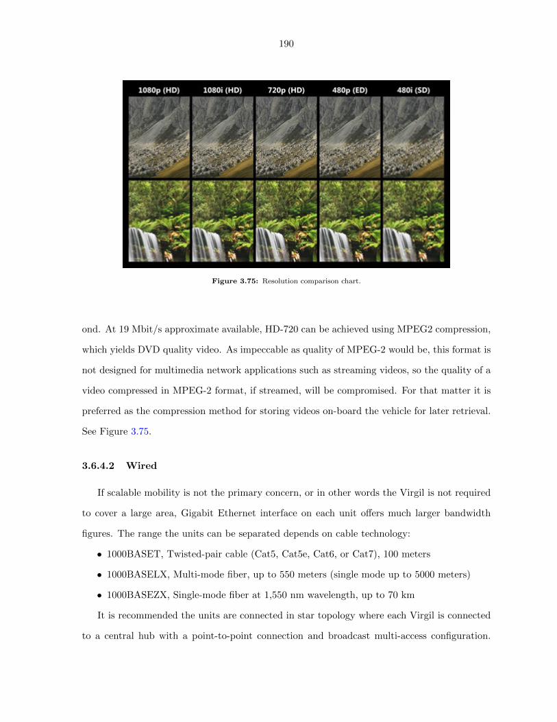
190

Figure 3.75: Resolution comparison chart.

ond. At 19 Mbit/s approximate available, HD-720 can be achieved using MPEG2 compression,

which yields DVD quality video. As impeccable as quality of MPEG-2 would be, this format is

not designed for multimedia network applications such as streaming videos, so the quality of a

video compressed in MPEG-2 format, if streamed, will be compromised. For that matter it is

preferred as the compression method for storing videos on-board the vehicle for later retrieval.

See Figure 3.75.

3.6.4.2 Wired

If scalable mobility is not the primary concern, or in other words the Virgil is not required

to cover a large area, Gigabit Ethernet interface on each unit offers much larger bandwidth

figures. The range the units can be separated depends on cable technology:

• 1000BASET, Twisted-pair cable (Cat5, Cat5e, Cat6, or Cat7), 100 meters

• 1000BASELX, Multi-mode fiber, up to 550 meters (single mode up to 5000 meters)

• 1000BASEZX, Single-mode fiber at 1,550 nm wavelength, up to 70 km

It is recommended the units are connected in star topology where each Virgil is connected

to a central hub with a point-to-point connection and broadcast multi-access configuration.

191

Since all traffic that traverses the network passes through the central hub, it acts as a signal

booster and/or repeater in between distant Virgils. The star topology is the easiest topology

for field deployment and and more nodes can be added or removed any time.

3.6.4.3 Control

Virgils are Internet enabled vehicles, in other words, the user can take complete supervisory

control of any vehicle over any broadband connection - without the need to be at or near the

field of experiment. At least one Virgil in the swarm should have Internet access, preferably

the field gateway, if the swarm is to be accessed over the Internet. This could be a wired

network such as Gigabit Ethernet, mobile broadband such as 4G, or an infrastructure network

nearby such as city or campus wide WiFi. The units can be set to automatically record video

at certain times and certain speeds. In addition, it is possible for the Virgil to email, text, or or

record when triggered by motion, sound, light, timer, or even a push button. These convenient

functions eliminate user need to constantly check the image. They can also act as servers,

stream images over a website (e.g., http://Virgil.student.iastate.edu) at which the live images

can be accessed via any web browser. However the connection speeds are going to be higher as

the user is located closer to the Virgil network, and preferably, physically a part of the network

for full performance. The user interface is very simple and intuitive; all control commands are

conducted via a conventional gaming joystick, and the mouse. The user can drive the Virgil,

operate the arm, stream from the cameras, download images or videos, and read telemetry data

from all on-board sensors.

The true power of Virgils is in the way they can work as a team and automate simple tasks

to reduce user workload. For instance, in wireless mode, using GPS, they can automatically

localize themselves in such a way that every Virgil always has another one nearby within

optimal communication range, hence forming a cellular ad-hoc network of Virgils. They can

then use this to their advantage, for instance, one unit detecting soil disease can instantly alert

other units to look for the same type of problem in their area.

192

3.6.5 Arm

Every Virgil features a multi-role five degree-of-freedom robotic arm with human-like dex-

terity. The arm consists of a 360o waist, 120o shoulder, 270o elbow, 360o wrist, and a hand

with two fingers. The wrist features a high-definition video camera (see camera section for

details) and a powerful LED based tactical multi-spectral illuminator which can turn the arm

into a remote operated mobile pan-tilt-zoom tripod any time. It also doubles as an electric drill

accepting standard #3 drill and screwdriver bits open precise holes in soil or plant material.

The hand can grab and manipulate a variety of simple tools such as soil probes, shovels, and

scissors.

3.6.6 Sensing

Virgils are equipped with a variety of sensing mechanisms, most important of which are

listed here.

3.6.7 Laser Range-Finder

This device determines range and bearing to nearby objects by measuring the time delay

between transmission of a pulse and detection of the reflected laser. It fires a narrow pulse laser

beam and scans the targets around the unit. It is possible to use Doppler effect techniques to

judge whether those objects are moving towards or away, and if so how fast. This device is

accurate to a few millimeters, but more accurate at closer distance than farther as a laser beam

eventually spreads over long distances due to the divergence, scintillation, and beam wander

effects caused by the presence of pressure bubbles and water droplets in the air acting like

tiny lenses. Virgil uses this sensor for object avoidance, such as when navigating through a

cornfield.

3.6.8 Digital HD-Camera

A high-definition digital CCD camera is the principal sensor of any Virgil, capable of record-

ing both HD-video and still images. When it comes to HD, there are two main types; HD 720

193

Figure 3.76: Panasonic BB-HCM531A.

and HD 1080 respectively. See fig. 3.77. It is up to the user to determine which video quality

is needed. It should be noted that higher video quality demands higher network bandwidth,

which in turn requires the Virgil to be located closer together, or offer a lower frame rate, or

both. This section covers a set of cameras the Virgil is compatible with.

1. AVT Oscar, Pike, and Stingray: (fig. 3.78) Designed for both high speed and very

high quality applications in machine vision industry, the AVT family of cameras offer

resolutions of HD (1928 x 1084 pixels), 4MP (2056 x 2062 pixels), 5MP (2452 x 2054),

and up to 15 MP (4872 x 3248). The primary imaging device is a 35mm Progressive

Scan CCD Kodak KAI-16000, and they accept a wide variety of interchangeable varifocal

lenses. The AVT series are open-source, which means they do not need proprietary

hardware or software to interface with them, which makes them very versatile, highly

configurable, very high image quality camera systems.

2. Sony FCB-EH4300: (fig. 3.79) The FCB-EH4300 is one of the best integrated lens

camera modules available on the market today. Featuring a 20x optical zoom lens (f=4.7

mm (wide) to 94.0 mm (tele), and F1.6 to F3.5) and 1080p/30/25, 1080i/59.94/50, or

720p/59.94/50 HD video, the FCB-EH4300 is a military grade 12 volt camera module,

ideally suited for targeting, tracking, scientific monitoring and high speed surveillance

applications. It is typically used in speed traps to capture license plates, which means

this is a very fast camera (1/10000 shutter speed to be specific - found in studio grade

194

Figure 3.77: Vector Video Sizes Comparison Chart.

Figure 3.78: AVT Pike Military Grade Block Camera, and the more affordable alternative, Stingray.

195

Figure 3.79: Sony FCB-EH4300 military grade block camera.

cameras only) with excellent low light and telephoto capabilities. It has a viewing angle

of over 50o and it can focus on objects as close as 1 centimeter. It supports IP and

Gigabit Ethernet applications without significant video signal deterioration. The camera

is temperature compensated, and offers a number of color enhancement options, ideally

suited for low vision applications, which can make reading soil status challenging. The

new FCB-EH4300 camera monitors the luminance differences within an image in high

contrast environments and automatically adapts the dynamic range to enhance certain

visual properties of the soil. Its extremely sensitive image sensor can operate at light

levels less than 0.5 lux and it can operate below freezing temperatures. It consumes

about 5 watts during normal operation.

3. Sony XCDU100CR: (fig. 3.80) This is an IEEE 1394.B UXGA color camera module

intended for machine vision applications with outstanding picture quality. The XCD-

U100 incorporates a 1/1.8-type IT CCD that captures extremely, high-quality, detailed

images with UXGA resolution (i.e. equivalent to HD-720 grade) at 15 fps. By utiliz-

ing IEEE 1394.B, the camera can transfer images to the Virgil at speeds of up to 800

Mb/s. Moreover multiple cameras can be connected in a daisy-chain configuration with

196

Figure 3.80: Sony XCDU100CR without lens. A wide variety of lenses can be used with this camera.

Figure 3.81: Panasonic BB-HCM531A.

bus synchronization and broadcast delivery. With these features users can capture images

from different angles simultaneously simply by sending a single trigger from the command

center; using a software trigger instead of a hardware trigger helps to minimize the occur-

rence of false triggers. It is an ideal unit for object recognition, inspection, measurement,

alignment, and for microscopy. It consumes about 3 watts during normal operation.

4. PixeLINK Aptina: This series of cameras offer up to 6.6 megapixel (2048 x 1536;

larger than HD 1080, 15 fps) color CMOS arrays, and come in IEEE 1384 or Gigabit

Ethernet versions. They are primarily intended for machine vision applications, and have

electronic shutters, and interchangeable lenses.

5. Canon BU-46H and BU-51H: (fig. 3.81) This 1/3” full HD 3-CCD camera offers 20x

optical zoom via focal length of 4.5 to 90mm, and f-stop value of 1.6 to 0.5. Frame rates

197

Figure 3.82: Canon BU-51H

are up to 50 fps, however at the lower shutter speeds of 1/1000 max. It can amplify light

up to 36dB, and equipped with advanced image stabilizer technology. It is meant to be

a weatherproof standalone field unit with built-in electrical wiper and operational angles

of 340o panning, and +30o to -50o tilting, however it can be mounted on an Embriyont.

These models can address a wide range of applications, mostly used for high quality

surveillance, and they allow enhancements for master pedestal, R-gain and B-gain, G-

gain, hue, knee point, gamma curve, sharpness, set up level, color matrix, black gain, and

horizontal detail. Using 70 watts, it is the most power demanding model among those

listed.

6. Panasonic AW-HE50S/H: (fig. 3.81) This 12 volt 1/3 CCD Full-HD (HD 1080 and

720, 24 fps) camera from Panasonic offers 18x optical zoom, f1.6 to 2.8 (f=4.7 to 84.6

mm,35 mm equivalent: 36.9 mm to 664.5 mm), six step 1/100 - 1/10000 shutter. It

has full IP capabilities. The most important feature of this camera is the dynamic range

stretching; gamma curve and knee slope are optimized to match the contrast of each pixel

in real time, which increases the dynamic range without affecting the normal pixels. This

in turn yields more uniform images in difficult lighting conditions that still bring out the

texture and color details. It is also capable of Digital Noise Reduction that suppresses

198

Figure 3.83: Panasonic WV-NF302.

afterimages.

7. Panasonic WV-NF302: (fig. 3.83) This model is a Day/Night dome type network

camera with full IP capabilities. It has a resolution of 1280×960 of 1/3 inch progressive

scan CCD (progressive-scan reduces motion blur of moving subjects). It is a slower, lower

resolution version of the AW-HE50S, with a low light sensitivity of 1.5 lux (3 times that of

previous models listed). It has an electronic shutter (slower, as opposed to global shutter

on previous models) with a 2.8 to 10 mm (3.6x zoom, and it can focus on objects as close

as 1.2 m) varifocal lens built-in.

8. Panasonic BB-HCM531A: (fig. 3.76) This economical alternative from Panasonic is

the most affordable on the list, a CCD based SXGA resolution (comparable to HD720)

camera with 30 fps over 110 Kbps uplink. It is designed for outdoor operation and meets

both IPX4 and UL6500 standards of outdoor equipment. It does not offer advanced

features such as offer optical zoom, motorized lenses, or image enhancements. These

effects can be achieved by software on-board the Virgil.

199

3.6.8.1 Night Vision Cameras

Night vision cameras have a combination of sufficient spectral range, sufficient intensity

range, and large diameter objectives to allow vision under adverse lightning conditions as they

can sense radiation that is invisible to conventional cameras. Night vision technologies can be

broadly divided into three main categories:

• Image Intensification: They magnify the amount of received photons from various

natural sources such as starlight or moonlight. Contrary to popular belief, the famous

green color of these devices is the reflection of the Light Interference Filters in them, and

not a glow.

• Active Illumination: They couple imaging intensification technology with an active

source of illumination in the near-IR or shortwave-IR band (spectral range of 700nm to

1000nm). They cannot produce color at that spectral range thus they appear monochrome.

• Thermal Imaging: Forward Looking Infrared (FLIR) is a technology that works by

detecting the temperature difference between the background and the foreground objects.

They are excellent tools for night vision as they do not need a source of illumination; they

can produce an image in the darkest of nights and can see through light fog, rain and

smoke.

3.6.9 Soil Probe

The Virgil arm contains an interchangeable soil probe, shown in Figure 3.85. In order for

any soil probe to work, it must make contact with the soil (preferably fully immersed with no

gaps). With the help of this high-dexterity arm, Virgil can precisely dig soil and bury a soil

probe at a particular desired depth, for instance to track water as it moves down through soil

horizons. The probe then sends electrical signals into the soil, measures the responses, and

relays this information to the Virgil. This information can be utilized in several ways. For

example, to irrigate a particular crop at the optimum level, several Virgils insert probes; one

just below the surface, one in the root zone, and one below the root zone. Locations of these

zones are plotted on a GPS map. When water is applied to this soil, these sensors reveal data

200

about how quickly the water penetrates down through the soil, whether it stagnates are certain

depths, and such. By knowing how long it takes for the water the reach the root zone, irrigation

schedule can be adjusted to an optimum. Another example is the study of land slides. Again,

several GPS tracked Virgils bury probes in different soil horizons, which enables them to chart

how water is moving between the layers of soil. After charting information during the wet

season and analyzing it, it is possible to visualize what types of soil absorb water more readily,

which in turn yields how much rain will cause a wasting event in specific soil types and where

this type of soil may be located. The Virgil has support for a wide range different types of

technologies in soil probes:

1. Frequency Domain Reflectometry (FDR): These are capacitance sensors; soil probes

that use the Frequency Domain Reflectometry employ an oscillator to generate an elec-

tromagnetic signal that is propagated through the unit and into the soil. Part of this

signal will be reflected back to the unit by the soil. This reflected wave is measured by

the FDR probe, telling the user what the water content of the soil is. These probes are

considered highly accurate but must be calibrated for the type of soil they will be buried

in. They offer a faster response time compared to Time Domain Reflectometer (TDR)

probes. Example: Adcon C-probe.

2. Time Domain Reflectometry (TDR): Probes that use the Time Domain Reflectom-

etry (TDR) function propagate a pulse down a line into the soil, which is terminated at

the end by a probe with wave guides. TDR systems measure the determine the water

content of the soil by measuring how long it takes the pulse to come back. These probes

are also sensitive to the saline content of salt and relatively expensive compared to some

measurement methods. Examples: Campbell CR616.

3. Gypsum Probe: Gypsum probe uses two electrodes placed into a small block of gypsum

to measure soil water tension. Gypsum blocks are inexpensive and easy to install, however

they have to be replaced periodically as the gypsum disintegrates. Gypsum blocks are

also more sensitive to having readings throwing off by soil with high salinity. Example:

Soilmoistures 5201F1.

4. Neutron Probe: Neutron probes when inserted in the ground, emit low-level radiation

201

in the form of neutrons. These collide with the hydrogen atoms contained in water,

which is detected by the probe to determine compaction, wet and dry density, and voids.

The more water content in the soil, the more neutrons are scattered back at the device.

Neutron probes are extremely accurate measurement devices when used properly, but

problematic due to radioactive elements used. Virgil eliminates the complications in

handling radioactive elements and other hazardous chemicals. Example: Troxlerlabs

Model 4301/02.

3.6.10 Soil pH-Meter

Figure 3.84: Virgil Prototype - I, shown in both

field rover and field gateway configurations.

Soil pH is important because of the many effects it

has on biological and chemical activity of the soil, which

affects plant metabolism. The Virgil arm also features

General Hydroponics Ph Soil Meter, which it can ma-

nipulate and bury at precise locations, shown in Figure

3.85. This allows the unit to test soil with accuracy

and determine if soil acidity needs adjustment. The

unit perforates the ground with a HI-1292D pH elec-

trode, which incorporates a temperature sensor right

near the tip to enable it to measure and quickly com-

pensate for temperature. For stony ground where the

electrode may be damaged, the arm physically shov-

els a small sample, saturates it with a soil preparation

solution, then inserts the probe into the solution and

measure pH by dilution.

3.6.11 Microscope

The Virgil includes a Celestron 44302 or equivalent illuminated digital microscope which

allows diagnosis of soil-borne diseases due to pathogenic bacteria such as nematode infections,

detection and enumeration of individual bacteria or fungi, or analysis of organic content such

202

Figure 3.85: Various soil probes with different capabilities that are supported by the Virgil.

as cyanobacteria. Cyanobacteria obtain their energy through oxygenic photosynthesis. They

can be found in almost every terrestrial and aquatic habitat where life flourishes. Soil samples

gathered by Virgil can be investigated right on the field for such organic characteristics.

3.7 Liquidator

Liquidator is the name given in the former USSR to people who were called upon to work

in efforts to deal with consequences of the April 26, 1986, Chernobyl disaster on the site of the

event. Liquidator robot, designed and built by the author, was built for one purpose: test and

quantify the survivability of VINAR cameras in hostile environments where camera structural

integrity may be compromised. Key feature of this robot is the capability to replicate a camera

motion path with extreme precision and repeatability. Once camera motion can be controlled

with such precision, this allows for controlled manipulation of other environmental factors, such

as temperature, radiation, and many others20, one at a time, and observe their effects on a

camera. Liquidator robot thus made it possible for the procedures described in Section 5.3.2 to

20MILSPEC 810G Criteria was used

203

Figure 3.86: The Liquidator.

Figure 3.87: The Liquidator exploring a hallway. On the right, a directed energy weapon is shown, built by the author, totest the resilience of the monocular image navigation system on this robot in the presence of harmful microwave radiation.

be performed, later leading to the development of novel monocular autocalibration techniques

described in Chapter 5.

3.8 Ghostwalker

During September 11 attacks, World Trade Center Stairwell-A remained intact after the

second plane hit the South Tower. Only 14 people noticed that and actually used it to escape.

Numerous 911 operators who received calls from the building were not well informed of the

situation. They told callers not to descend the tower on their own.

204

Figure 3.88: The Ghostwalker Tactical Vest, which uses VINAR and, other algorithms developed in this thesis. Photocourtesy of Rockwell Collins.

Ghostwalker is a small arms protective tactical vest developed by Rockwell Collins, which

is intended for wearable image navigation. it is is made up of stiffened mesh nylon with hidden

document pockets, grab handles, hydration pockets, high impact plastic clips, a barometer,

an inertial navigation system, a computer, and a wide angle monocular camera. It is a load-

bearing vest designed for special operations and tactical situations, while allowing ventilation

and breathability. Because the vest implements VINAR technology on a human, getting lost

in GPS denied environments is no longer a concern. Despite the emphasis on aircraft and

robotic use, with Ghostwalker, VINAR proved beneficial for a very unique platform, using the

natural dynamics of the human body as calibration metric. Strategic objective of the system

is to allow US Army troops and special forces to be able to map and image-navigate GPS

denied environments while walking through them, so they can get out quickly without getting

lost, and have a computer calculate safest egress routes for them, with the floorplan stored in

the vest. The vest depends on monocular camera. Contributions of this thesis helped this life

saving technology become a reality. Without these unique contributions the working conditions

US forces experience would easily tamper with camera parameters, leading to false navigation

solutions, rendering the system ineffective. These life-saving vests are not limited to military;

they can also be used by firefighters and other emergency response personnel. More information

about this vest can be found in Chapters 5 and 8.

205

3.9 USCAP SARStorm

Some of the current Problems in Aerial Search-and-Rescue (SAR) are lack of distributed

aerial sensors, excessive workload on pilots, long response and organization time, as well as

dangerous flying conditions. SARStorm is a large scale fixed wing UAV for short take-off

from very rough terrain, payload capable, and autonomous. It was designed for the USCAP21

using a scalable system of systems approach. USCAP saves about 75 lives per year. Design

was completed by a senior aerospace engineering team mentored by the author, intended to

implement VINAR technology via thermal monocular cameras as shown in figure 3.9. Primary

visual system consists of a monocular FLIR Photon 640 with 100mm lens, at 640×512, with

capability of human detection as far as 1500 meters, and identification at 200 meters. Secondary

visual system consists of a 380P TV camera with gyrobalanced gimbal system by cloud cap

technology TASE LT. Cameras are nose mounted and no turret is necessary. Rockwell Collins

Athena 111m Baseline Avionics are considered.

Propulsion and visual guidance system design belong to the author. Primary purpose of the

aircraft is to aid in search-and-rescue missions during disaster response. For example, during a

wildfire or radioactive spill, finding lost people as quickly as possible and mapping their position

is one of primary uses for this aircraft, and dropping help packages to them if necessary.

SARStorm has a wingspan of 10ft22 with a GTOW of 100lbs, cruise speed of 55 knots, and

19BHP gasoline engine in pusher configuration. The engine is four cylinder two stroke spark

ignition reciprocating type, naturally aspirated and double carburated, with a displacement

of 12.20ci(20cc), weighs10.95 lbs(4.95 kilograms), providing a practical RPM Range of 900

to 6700 with a 3-bladed, 29 inch pusher propeller. Fuel consumption is 4.5 oz/min @ 6,000

RPM under ideal atmospheric conditions. There are two fuel tanks composed of 9×4.75 inch

cylinders. A Sullivan S675-500 alternator provides 500 Watt output at the cost of 0.5 HP draw

from the engine, which powers the 28V electrical systems on board. A Twin-Boom airframe

was considered as it provides a good balance of stability, structural efficiency, and unimproved

surface performance due to tall ground clearance. Fuselage consists of skin, 2 ribs, and I-beam

21Air Force Auxiliary Civil Air Patrol22intended to fit inside a trailer; detachable outer sections to fit within 8ft semi-trailer width

206

Figure 3.89: SARStorm Views.

207

ribs. Skin thickness is 0.025 inches, fuselage is 22.675 inches long. Aircraft weighs 102.5lbs

where structures take 35.9% of the weight, fuel system 36.5%, power system 23.2%, avionics

4.3% and VINAR, 2.6% respectively. All structures use 7075-T6 Aluminum Alloy, which is

one of the hardest alloys of this metal comparable to most steels in hardness, however offers

repairability, easy maintenance, resistance to weather conditions, reliability, lower cost and

most importantly, lower weight.

Figure 3.90: Aircraft VINAR hardware is blended into the

fuselage without requiring use of an external turret, providing

improved aerodynamic efficiency.

Aircraft has a 10 mile operational radius

with an hourly on-station endurance, an op-

erational altitude of 500ft AGL and capabil-

ity to identify human target from this alti-

tude. In other words camera design and res-

olution affects algorithmic capability to iden-

tify a human from distance, which in turn

dictates operational altitude. Aircraft oper-

ational requirements are fast deployment and

turn-around times in unprepared field oper-

ations, adequate poor weather performance

and a low maintenance design. Few, if any,

existing UAV systems in weight range are ei-

ther over engineered for the problem or sim-

ply too light for all-weather operations.

A detailed aerodynamic and structural analysis of the airframe has been conducted using

Vortex Lattice Method (XFLR5) at α = 0.5 degrees and CI = 0.8606, and a -3 degree horizontal

tail tilt to balance the pitching moment, as shown in figure 3.92. NACA 6416 airfoil is used with

a CI ≈ 1.30 and thickness/chord ratio of 0.15. The thick airfoil provides structural efficiency

and stall characteristics. NACA 0012 is used for Horizontal/Vertical Tail, which is the same

airfoil used by Saint Vertigo. Performance estimates for ground roll is 205 feet, determined

by takeoff velocity and acceleration terms. Landing gear are fixed hollow cylinders an angle

of 15 degrees from the vertical weight. Plain ailerons with gap sealing design are used which

208

Figure 3.92: Aerodynamic analysis of SARStorm.

prevents rolling moment loss up to 30%. Ailerons have 28 inches span with 5 inch chord at 25%

of MAC, positioned at 10 inches from shaped wing tips. Elevators have 3 feet span considering

full horizontal stab, with 4 inch chord representing 33% of horizontal stab area. Rudders have

1.25 feet span considering the full vertical stab where 2.5 inch chord is used representing 28%

of vertical stab area. Flight surfaces use JR8711HV digital servos providing a torque of 480

oz-in, at speed of 0.12 degrees per second. A preliminary version with tractor configuration

is shown in figure 3.93, capable of airlifting a 35 kilogram package.

209

Figure 3.93: One of the earlier implementations of SARStorm.

Figure 3.94: SARStorm in flight, designed for high visibility. Multiple aircraft are meant to be transported in a semi-trailer with detachable wings.

210

Figure 3.95: SARStorm graphical user interface in flight. Colored areas represent probability of finding a missing person,where red is higher probability than yellow, and yellow than green. Note the actual position of missing human.

3.10 UH-1Y Venom Huey

Figure 3.91: SARStorm Block Diagram.

Huey is author’s brainchild in scale un-

manned helicopters, designed and handmade

by the author at University of Illinois at Ur-

bana Champaign Talbot Aerospace Labora-

tory. This is a multi-role utility UAV de-

signed for high-lift in all weather conditions.

The aircraft has a nose attachment where

a gimbaling monocular camera implements

VINAR technology, in addition to a ground

scanning LIDAR. This design started as what

is essentially a Bell-412, and evolved into

Marines edition of this historic airframe. The

fuselage is 65 inches long, 15 pounds with all

three fuel tanks full, rotor blades are 570 mm

each, use NACA0012 airfoil with 55mm chord and they terminate with aeroflat tips. The first

version of this aircraft had 600 mm semi-symmetrical flat tip blades as they would be most

representative of the 412, but shorter blades proved to perform better because the powerplant

211

Figure 3.96: The UH-1Y Venom Huey UAV, designed and built by the author in University of Illinois Urbana Champaign,Talbot Labs.

on this helicopter is substantially powerful compared to that of the 412.

Huey utilizes a bearingless composite rotor head and a full featured fly-by-wire system. This

aircraft is unique with respect to Saint Vertigo such that there is no mechanical swashplate

lock; gyroscopic precession is 90 degrees, which is provided by the pitchlinks alone. Unlike any

other helicopter that would use a straight round dogbone design, the links are made of square

tube steel. This is for strength as they are bent in a 90 degrees curve, reaching swashplate

directly under the advancing blade grip. This design eliminates the need for locking the upper

swashplate to main shaft, substantially reducing vibration. It also allows the rotor control

assembly sit closer to center of gravity and hide inside the fuselage, providing aerodynamic

benefit which is also the case in full-scale counterpart. Since the rotor assembly of this aircraft

is fully rigid, in other words pivots but does not dampen, the flapping behavior is electronically

implemented via four gyroscopes and three accelerometers, made possible by the 11-bit digital

servomechanisms. Huey is capable of a hover-assist feature to reduce pilot workload, which

also comes from the same inertial sensors. There are 4 hardpoints on the aircraft which can

be used to attach various equipment up to 10 lbs, including cameras, drop tanks, weapons.

212

Figure 3.97: The UH-1Y Venom Huey UAV, designed and built by the author in University of Illinois Urbana Champaign,Talbot Labs, shown in flight. This aircraft is amphibious and night-capable.

The sliding doors are functional, and field removable, like in the full size counterpart. This

also makes it easier to overhaul. With doors closed, it is water resistant and mission capable in

temperatures from 0 to 100 degrees Fahrenheit. With doors open, improved cooling is achieved

and more attachments are possible.

A sophisticated engine control system is used on Huey with on-board ignition and piston

head temperature control. It will automatically heat the engine to make cold weather startups

easier. It will prevent fuel from gelling, something that will prevent all other liquid fuel operated

aircraft presented in this chapter from flying in freezing conditions. It will heat the fuel when

helicopter is close to ground, which increases the volatility and viscosity, and if there is a dust-

off condition this is one way to prevent the engine from stalling due to oxygen starvation. Huey

built in safety modes disable ignition if the engine is off and throttle is not at idle position. It

also prevents the helicopter from starting when the ignition key is inserted. In contrast to cars,

Huey starts when ignition key is removed, and will not stop until it is replaced and fuel cutoff

button is pressed; this failsafe design is chosen such that if the ignition key falls off in flight

213

Figure 3.98: The UH-1Y Venom Huey is an all-weather utility UAV.

the engine controller defaults to ON state. Fuel system is pressurized, and it is charged with

carbondioxide for safety. Engine is equipped with a demand regulator that allows consistent

fuel flow at any attitude and weather conditions.

The tail section of this aircraft had to be designed from scratch, yielding a different, and

in fact better than that of the full-size aircraft. Rudder is electrically actuated and it has 2048

individual angles which makes yaw control on this aircraft very precise. Tail section is hollow

fiberglass, just like in full-size fuselage, and there are three transmissions for the driven tail.

Another authentic feature of this helicopter is that the rotor is disengaged from the engine, there

is no mechanical link from the engine to rotor, but main rotor drives tail and it is synchronized

to reduce interactions in between tip vortices. There is a powerful halogen landing light at the

tail, and a strobe.

Electrical system on Huey is dual-redundant, capable of powering 672 watts worth of elec-

trical equipment. In addition to day/night capability and focusing searchlight, my Huey is also

amphibious. It has inflatable floats that allow landing on water. Preferably, still water.

214

Figure 3.99: The B222X Black Shark designed and built by the author in Iowa State University, Ames, shown in flight.This is one of the fastest aircraft in my fleet, and the only one with a lifting body concept.

3.11 Bell 222X Black Shark

The Bell 222X UAV, figure 3.100, the only aircraft in this chapter capable of hovertaxi,

is also one of the largest and fastest helicopters author has ever designed and built. This is

a streamlined high speed lifting body surveillance platform with four camera mounts at the

bottom of the fuselage, and two in the front hidden inside air intakes. Front cameras use VINAR

technology. Rotor blades are 620 mm each, use NACA0012 airfoil with 55mm chord and they

terminate with aeroflat tips. The tricycle landing gear on this aircraft is designed and machined

specifically for it. All undercarriage elements have complete shock absorbing capability with

spring and damper. They are true OLEO struts that collapse into a piston during landing and

extend-down during takeoff. The tires are soft rubber compound. These capabilities allow this

helicopter to comfortably hovertaxi to take-off position, perform rolling takeoffs (and landings),

and park itself after returning to tarmac. The undercarriage retracts into the aircraft after

takeoff, the retraction system is pneumatic, driven by electrically actuated valves and uses 100

PSI to function. There is a safety override to prevent the pilot from retracting the undercarriage

215

Figure 3.100: The B222X Black Shark designed and built by the author in Iowa State University, Ames, shown landedat tarmac.

while on ground. And if it experiences a loss of pressure in the air undercarriage automatically

comes down. In case that too fails, aircraft can still land on its belly. There is proper ground

clearance and tail guard to accomplish that in safety.

The tail-plane and vertical stabilizer are true airfoil flight surfaces, and functional. The

fuselage is a lifting body, responsible for up to 25% of the total lift in full forward flight.

However at low speeds and steep banked turns the inner fuselage tends to lose lift resulting

in tendency to roll. This is electronically compensated, but can be turned off if so desired.

Regardless, this is the fastest helicopter among all other aircraft mentioned in this section,

clocked at 70 MPH, and can comfortably handle 20MPH weather and has successfully flown in

30MPH gusts. Theoretically speaking, based on engine loading at full tilt, it has room to go

faster up to 100 MPH; however due to the delicate structure of the aircraft stress cracks have

begun developing in the fuselage resulting in an intentional limitation of shaft power output as

a countermeasure.

A full featured engine control system is implemented. For example, if fuel to oxygen ratio

is below 7%, fuel mixture will lean out and not ignite. Above 12% fuel mixture will be too

rich and not ignite. Since this aircraft can reach significant altitudes, changes in atmospheric

conditions can cause abnormal fuel behavior which can overheat or stall the engine. Engine

control prevents this by dynamically adjusting the mixture. It also governs the engine and

prevents it from over-revving. Fuel system is carbondioxide-charged to prevent fumes from

igniting inside the tanks or fuel lines, or manifolds. Governor has 28 preset flight modes for

216

the pilot to choose from. For example there is a flight mode for hovertaxi that will prevent the

aircraft from leaving tarmac but allows the pilot to steer and drive.

Its electrical system is opto-isolated and dual-redundant, capable of powering 640 watts

worth of electrical equipment. The strobe lights on this aircraft are connected to a smart

controller, thus besides FAA patterns it also enables the aircraft to encode warning messages

in terms of different blink patterns.

3.12 AH6LB Little Bird

Designed and built by the author, this aircraft is the seventh, and latest version of Saint

Vertigo line of UAV’s, first in the series to feature aerodynamic fuselage. The aircraft features

a fiber fuselage, functional multi-bladed rigid rotor head, and independent swashplate lock.

Unique with respect to Saint Vertigo, there is no stabilizer bar; this function is performed

electronically. Rotorhead is phased at 85 degrees of gyroscopic precession to tame the aggressive

flight behavior, as well as to counteract the dyssimetry due to tail rotor. A power to weight ratio

of 7.20 HP/lb is achieved, which makes it an extremely agile aircraft, capable of 50 MPH. A

hall-effect governor controls the powerplant for consistency. It has three flight modes to achieve

optimum efficiency; hover, full, aggressive. To withstand the punishment this engine develops

all drive systems are made of titanium and kevlar, suspended by 12 ceramic ball bearings. The

tailplane is functional, adjustable, and angled specifically for this rotorhead to prevent pitching

behavior at high speeds. It has one hardpoint to sling-hook a small payload of 2 lbs. It also

has a functional hoist that can be attached to this hardpoint. There are two racks on the sides

which are for weapons loadout, but in this aircraft they serve to mount monocular cameras

for VINAR. AH6LB is a day-night capable aircraft that features a full set of FAA designation

nav-lites, strobes and landing lights bright enough to be visible in full daylight, and can be

spotted from one mile at night.

217

Figure 3.101: The AH-6 Little Bird; a.k.a. Saint Vertigo V7.

Figure 3.102: Presenting the AH-6 to NASA Chief Technology Officer.

218

3.13 MI8 HIP

The smallest helicopter author ever built, small enough to fit inside a shoebox, the MI8 is

fully functional, true-to-life 1/35 implementation of the famous transport medium-helicopter

with Bell-Hiller articulating rotor head and a full 120 degree swashplate. A 5.8 GHz wireless

camera is implemented for VINAR. In fact, the sheer scale of this aircraft prevents it from

carrying any other sensor than VINAR technology. Aircraft develops 0.24 Horsepower, can

handle 15 MPH wind and achieves a top speed of 35 MPH. The 5 cent coin in figure 3.103 is

provided to give a size reference. Everything on the aircraft is a functional system. Turbine

doors open to provide access to the power plant. Tricycle landing gear allows it negotiate many

surfaces. The exhaust grille is to aid in cooling cyclic servos. The sliding door is functional,

and removable. The cockpit is authentic to the aircraft. Fuel cells are loaded through this

door, as well as the cargo doors. Just like the real-life counterpart, my MI8 features driven tail

and can capably autorotate.

3.14 AH1W Cobra & AH64 Apache

The AH64 Longbow is the first time author deviated from dampening rotorhead versus rigid

blade design into rigid rotorhead with flexible blades that fully replicate flapping behavior. This

is evident from the figure 3.104 as the blades sag down when they are at rest. In flight, they

cone up accordingly. This allowed use of 28% thinner chord which substantially decreases

the parasitic drag therefore its blades did not have to be acrylic coated like others, which is

why they are not glossy in contrast to that of Saint Vertigo. But the airframe is not very

streamlined, which keeps the top speed lower compared to my other similar scale machines.

Blade tips are swept to reduce noise and improve aerodynamic efficiency. The raised tail uses

a 65 degree gearbox. Author has built the scissors tail rotor with 55 and 125 degree intervals,

however found this to be overloading the powerplant at this gear ratio, and it was difficult

to machine a smaller ratio without weakening the metal. Two bladed tail rotor does fly the

aircraft, however at the cost of great angles of incidence. The aircraft has landing lights,

functional shock absorbing landing gear and four functional hardpoints at the stub wings to

219

Figure 3.103: The sliding door is functional, and removable. The cockpit is authentic to the aircraft. Fuel cells areloaded through this door, as well as the cargo doors. Just like the real-life counterpart, my MI8 features driven tail andcan capably autorotate. THis is the smallest aircraft so far to benefit from VINAR.

install cameras for VINAR use.

The AH1W is the Marines edition of this historic aircraft, which differs from the Army

version with dual turbines and sidewinder missiles. It uses 65 degree raised tail, nav-lites,

rotary beacon, and strobes. This helicopter is, by design, older than AH64 and thus does not

have the electronic stabilization systems; it takes some talent to design an autopilot for this

machine due to the extremely responsive nature. The streamlined and thin fuselage is fully

authentic. Rotor spins clockwise, as opposed to the counterclockwise in full-scale version, due

to the way blades were manufactured. Another reason to chose those blades was rigidity, which

prevents the zero-g condition which can lead to a boom strike.

220

Figure 3.104: The AH64 and AH1W VINAR enabled helicopters designed and built by the author.

3.15 FarmCopter

The FarmCopter is an autonomous UAV, designed and developed by the author for the De-

partment of Agriculture. It uses VINAR and scanning LIDAR technology to inspect corn fields

at close range for important features such as stalk height, tassel formation and ear coloration.

FarmCopter is unique with respect to Saint Vertigo such that is maps the plants, rather than

mapping the environment, where plants become landmarks and also objects of interest. The

intended purpose of the aircraft is to assist in plant phenomics. Over the past 15 years, the field

of phenomics23 has emerged as natural complement to genome sequencing as a route to rapid

advances in biology. Phenomics is as compelling now as the case for genomics was 25 years

ago and indeed shares many similarities with that case. Phenomics is the acquisition of high

dimensional phenotypic data on an organism wide scale. While phenomics is defined in analogy

to genomics, the informationcontent of phenomes dwarves those of genomes: phenotypes vary

from cell to cell and from moment to moment and therefore can never be completely character-

ized. Thus, phenomics will always involve prioritizing what to measure and a balance between

exploratory and explanatory goals. Phenomiclevel data are necessary to understand which ge-

nomic variants affect phenotypes (and under which environments), to understand pleiotropy

and to furnish the raw data that are needed to decipher the causes of complex phenomena, in-

cluding crop growth rates, yield and responses to environmental stresses24. The current limited

ability to understand many important biological phenomena suggests that we are not measur-

23large scale phenotyping of corn24both biotic and abiotic

221

ing all the important variables and that broadening the possibilities will pay rich dividends.

Phenotypic data continue to be the most powerful predictors of important biological outcomes,

such as crops yields. Although analyses of genomic data have been successful at uncovering bi-

ological phenomena, they are in most cases supplementing rather than supplanting phenotypic

information.

Phenomics is most frequently justified as enabling us to trace causal links between genotypes

and environmental factors and phenotypes, summarized in the GPS maps. Studies of both the

genomes and the phenomes of individuals in segregating populations can be carried out in

an approach known as Mendelian randomizations. Indeed, phenomic projects that combine

genomic data with data on quantitative variation in phenotypes have recently been initiated in

many species with the aim of understanding the GP maps.

End objective of FarmCopter was to enable phenotyping maize genotypes using robotic

platforms. Corn is one of the most important crops. It is not only highly productive but serves

as a nutritious source of food and feed, as well an an essential ingredient in a variety of biochem-

ical products including biofuels. We have technical, scientific and financial incentives to develop

a precision, high throughput measurement system. Motivation for robotic solutions to maize

phenomics are physical and biochemical traits of the plant that change in response to genetic

mutation and environmental influences. Typical parameters of interest are plant morphology,

e.g., plant height, leaf sizes and configuration including leaf angles, stem thickness, ear number,

and flowering time. Other phenotypes such as water and nutrient status are also important.

As an instrument for the systematic characterization of the plants in different growth stages,

standard measurement scales have been developed, such as the BBCH scale. This analysis is

typically executed manually by experts judging the field situation by measuring random sam-

ples in field plots. The result is a statistical overview on the plant physical characteristics in

the field. Since this analysis has to be done manually, it is very time consuming, generates

high costs and has varying reliability. Moreover, because phenotyping is performed by different

individuals, additional measurement variation is introduced. These changes being intrinsically

gradual and stochastic require vast plant variety, coverage and amount of measurements to ob-

tain the necessary statistical confidence. This unprecedented challenge cannot be accomplished

222

Figure 3.105: Installing the powerplant on FarmCopter. Avionics and sensor package are attached below the powerplant.

223

Figure 3.106: FarmCopter taking off.

by human, but must instead rely on robotic measuring machines.

The Australian Plant Phenomics Facility, an initiative of the Australian government, is

a landmark example for systematic and automatic phenomics. It focuses on automated glass

houses with controlled environmental parameters. This approach has the advantage of precisely

controlling and measuring the environment parameters, thus, facilitating the scientific process

of determining causes and effects. Besides the high infrastructural costs, we argue that the

resulting environment is quite artificial and the results could be inconsistent with experiments

run in the natural growing environments of the plants. Thus, instead of bringing the plants

to the technology in a conveyor belt in a greenhouse environment, FarmCopter brings the

technology to the plants in their natural habitat. While there are numerous examples of

autonomous machines for agriculture applications, most focus on tractor like machines, aerial

spraying or photogrammetry. Robotic platforms for precision agriculture have been researched,

such as BoniRob by the Federal Ministry of Food, Agriculture and Consumer Protection and

224

Federal Ministry of Education and Research of Germany. However be stable, it needs to be

wide. Thus, it slides over multiple rows of corn. Moreover, because the distance between rows

varies, its width also needs adjustable within certain amount. The thin wheels have limited

traction, and the speed of the robot is limited especially at the maximum height, limiting its

application to small plots. Finally, due to its size, the robot is not easily transportable to the

various fields.

The typical distance between two rows of maize plants in the US corn belt is 30 inches and

the distance between two plants in a row is about 10 inches (or closer). The typical maximal

height of a fully grown plant will exceed 8 feet, taller than most adults. This density of plants

and their height put serious constraints on the size, shape, and geometry of the robots that can

be deployed to make the measurements. FarmCopter operates in the open field environment

and move along the rows of plants and/or above them. This is different from the classical close

controlled factory environment and it means moving and navigating over uneven terrain, and

in tightly constrained isles between rows of plants. The measurements need to be taken under

different atmospheric conditions during the growing season in the presence of humans, animals

and other machines. These last two requirements make big bulky machines less appealing, and

points to a small light agile solution. Also, with FarmCopter cost of each platform is moderate.

FarmCopter cooperates with ground robots such as Virgil. The couple moves along the corn

isle in synchronism, maintaining a formation with the aerial vehicle on the vertical of the

ground vehicle and at a fixed, controlled, height. The two vehicles will behave as if a long rigid

mechanical link is connecting them, without the physical and control limitations typical of such

mechanical systems and without entangling with the plants dense canopies. The mechanical link

is replaced by VINAR based machine vision. The two robots work in symbiosis and cooperate

to form a more complex autonomous system. FarmCopter maintains a formation with Virgil,

move at the same speed, maintain the vertical distance, keep the horizontal distance close to

zero, so to be on top of each other. However, the agents are physically heterogeneous, and also

have difference capabilities and responsibilities. The ground vehicle has more computational

power, while the aerial vehicle provides necessary measurements, sensing and measurement

system are integrated with each other but distributed between the two vehicles. There is not a

225

Figure 3.107: FarmCopter UAV in flight.

clear master/slave relationship between the two. Also the control objectives need to be achieved

in a partially distributed fashion. Each vehicle is in charge of its own motion; however, the

motion coordination is distributed between them. A precise coordinated motion is essential

to obtain and precise measure of distance from the ground robot, and thus, a precise height

measurement of the plant. Maintaining formation becomes more challenging with the speed

of the robot. The task is further complicated has it also relies on video feedback and by the

different dynamics of the two vehicles.

Many of the measurements are based on machine vision. Once one picture is acquired, it is

quickly analyzed for its usability. Blurry or moved pictures do due to the fast robot motion or

just to wind, are discarded and new one will be taken. Well pictures could still be not usable for

extracting measures from them due to occlusions, light and contrast conditions may require to

acquire more pictures. Once these are obtained they are correlated with LIDAR measurements

and each plant is uniquely mapped. Thus, the imaging system serves three main purposes:

measuring, localization/positioning and control.

226

Figure 3.108: Re-engineering Boris.

3.16 Boris-II

Developed by the Aerobotics research team at University of Illinois at Urbana Champaign,

this is an attempt to re-engineer the Boris, little bat who might as well have started it all.

Author has, in part, designed the shoulder joints and performed wind tunnel testing of this

most unique machine and would like to thank the research group for this opportunity. More

information about Boris is provided in the first chapter. This unique air vehicle is an achieve-

ment in engineered flapping flight in low Reynolds number regimes where rigid fixed wings drop

substantially in aerodynamic performance. Saint Vertigo, for instance, is already a push of low

Reynold physics, and going smaller requires a very different approach. Natural flyers such as

bats, birds, and insects have captured the imaginations of scientists and engineers for centuries,

the maneuvering characteristics of aircraft we have designed are nowhere near the agility and

efficiency of animal flight. Bats can fly with damaged wings or while carrying 50% of their orig-

inal weight. Many insects can also carry loads exceeding their body weight. Boris-II integrates

neurobiological principles with the rigorous mathematical tools borrowed from nonlinear syn-

227

Figure 3.109: Robotic Engineered Flapping Flight.

chronization theory and flight dynamics and controls, to achieve flapping flight. Equipped with

intelligent sensors, such as VINAR, this robotic platform cam make paradigm-shifting advances

in monitoring of critical infrastructures such as power grids, bridges, and borders, as well as

in intelligence, surveillance, and reconnaissance applications. Successful reverse-engineering of

flapping fight will potentially result in a transformative innovation in aircraft design, which has

been dominated by fixed-wing airplanes.

228

CHAPTER 4

Image Navigator Engines

Figure 4.1: Thus is his cheek the map of days outworn! Shakespeare.

From the last quarter of the 20th century, the indispensable tool of the cartographer has

been the computer. Map functionality has been vastly advanced by technology simplifying

the superimposition of spatially located variables onto existing geographical maps. And we

do not have to figure out how to refold them anymore - a time proven impossible task even

for a navigation engineer. Electronic maps allow us make more efficient analyses over a wide

kaleidoscope of geopolitical cosmos. (That is precisely how Dr. John Snow discovers the cause

229

of cholera long before electronic maps appear; laying out variables on a map and studying

them). Agencies ranging from wildlife research to armed forces use interactive digital maps.

Lately, in-vehicle global navigation satellite systems can even tell us which gas station was the

last one we can afford to miss.

In between all this and the humble world of trying to map the North Wells St. in downtown

Chicago to produce an accurate “you are here” arrow, is a death valley. When the already-

weak GPS signals reach the planet over Chicago, they bounce off of buildings like wildfire.

To top that, one of the CTA trains have tracks suspended 14 feet above the street. It is the

ultimate test for a GPS receiver in terms of signal filtering. Even the most expensive devices

report errors up to an entire city block. Military has access to better GPS receivers than we

do, but theoretically speaking, it is doubtful theirs can penetrate several feet of steel reinforced

concrete either. What difference does it make if you were looking for a sandwich shop and miss

it by one block? Even if you drove by it on the first attempt the traffic was going to make you

park somewhere at least one block away anyway. Nonetheless, if we must go about sending the

BEAR (193) to locate and extract victims of nerve agent exposure from that area who are in

desperate need for an injection of atropine, pralidoxime, and diazepam, a city block becomes

the ultimate difference; the one between life, and death.

This chapter is an in-depth theoretical and experimental study of mapping to bridge the

aforementioned gap, to permit GPS-free navigation. In the context of this chapter, a map refers

to a dynamic, multi-dimensional, symbolic, interactive, and geometrically accurate depiction,

highlighting the relationships between elements of a state space with respect to a non-linear

state observer with a field-of-view (FOV) of known boundaries, and a set of distinguishable

landmarks with confidence intervals about their location. The state observer models the map

with an estimate of its internal state, and given the measurements of the real system, and that

of itself. The actions of a state observer are referred as a mission. In theory, an observable

system allows the state observer perform a complete reconstruction the system state from

measurements. In practice however, often, the complete physical state of the system is such

that it cannot be determined by direct observation. This is particularly true for large maps (i.e.

larger than the observer) in which the complete layout of the landmarks cannot be observed

230

simultaneously. This could happen at multiple situations, such as when the algorithm has just

started generating the map, or the observer has a FOV smaller than 360 so that it has a blind

zone. In that case indirect effects of the internal state are observed and unobservable states

are estimated until a direct observation can be made.

Maps can be static, or dynamic, based on the generating algorithm, and the current system

state in time, X(t). Although this thesis is meant to focus on dynamic maps, static maps

will be covered in brief as an extension of a dynamic map. Dynamic map involves incremental

algorithms that only have to estimate variables which exist at time t. In a dynamic map the

state observer wakes up to a completely unknown surrounding environment where none of its

extrinsic parameters are known and a map is also unavailable. State observer has to take

measurements from available sensors, z0:t, and use this information for estimating its posterior

over the momentary pose along with the map.

The problem can be expressed as p(xt,m|z0:t, u0:t), where u0:t contains the control inputs to

the state observer, xt represents the state observer and m represents the map. Mathematically

this concept can be expressed as shown in equation 4.1.



Once a dynamic map reaches a state where it is no longer changing, it is said to have

matured, and hence converged into a static map.

Static maps start with an oracle of the measurements, in other words a complete z vector

(and u vector depending on state observer) and build the entire map at once - in contrast to a

dynamic map, this is performed after the mission is complete, instead of during it, i.e, on-the-

fly. The oracle, at each time-step during the mission, t, takes the same measurements described

in dynamic maps. However the state observer has neither control over the oracle nor a-priori

knowledge of the intentions of the oracle. Calculating the posterior of the state observer over

the entire path x0:t along with the oracle’s map, m can be expressed as p(x0:t,m|z0:t, u0:t).

At the heart of every map is a fundamental algorithm, building a map from a mission. The

fundamental algorithm is more or less the same in principle for all map generation methods.

231

The distinguishing feature of different maps is the modular core of every fundamental algorithm,

referred as the estimation engine, or engine for short - we use the two terms interchangeably.

Above all, the performance and the accuracy of on-the-fly map generation depends on mating

the correct engine with the correct application. Equally important, is the tuning of this engine,

as the following chapters will elaborate, engines have tuning parameters and power bands at

which they operate most efficiently.

4.1 The Fundamental Algorithm

Figure 4.2: Though analogy is often misleading, it is the least misleading thing we have. Samuel Butler.

Cartography (Greek ; chartis = map, graphein = write) is a naturally occurring feature of

human cognitive behavior, whose neurological clockwork is still a mystery, nevertheless end

results have been well observed. (181). Written communication in humans works much the

same way bacteria share immunity genes; given that Earth is 70.2% is covered by oceans, and

50% of the remaining land mass is either desert, high mountains, or frozen tundra, we cannot

afford getting lost. The ability to communicate our surroundings to others in terms of toponyms

and political boundaries, while eliminating characteristics that are not relevant to the purpose,

was a survival skill so essential, it is now a permanent part of the US Army training manual

section 071-329-1006.

TRADOC 071-329-1006: Given a standard 1:50,000 scale military map of the area, a coor-

232

dinate scale and protractor, compass, and pencil and paper, move on foot from the start point

to the correct destination or objective by the most advantageous route to negotiate based on the

terrain and the tactical situation. The Fundamental Algorithm therefore can be inferred from

the military performance steps on training for navigation skills in the absence of technological

superiority such as GPS. US Army TRADOC Navigation performance steps are as follows:

1. Identify topographic symbols on a military map.

2. Identify the marginal information found on the legend.

3. Identify the five major and three minor terrain features on a military map (MAJOR:

hills, ridges, valleys, saddles, and depressions, MINOR: draws, spurs, and cliffs)

4. Determine grid coordinates for the point on the map to a six-digit grid coordinate. A

six-digit coordinate will locate a point on the ground within 100 meters.

5. Determine grid coordinates for the point on the map to an eight-digit grid coordinate.

An eight-digit coordinate will locate a point on the ground within 10 meters.

6. Measure distance on a map.

7. Determine a grid azimuth using a protractor.

8. Convert a magnetic azimuth to a grid azimuth and a grid azimuth to magnetic azimuth.

9. Locate an unknown point on a map and on the ground by resection.

10. Compute back azimuths to degrees or mils.

11. Determine a magnetic azimuth with a lensatic compass.

12. Determine the elevation of a point on the ground using a map.

13. Orient a map using a lensatic compass.

14. Orient a map to the ground by map-terrain association.

15. Select a movement route using a map. Your route must take advantage of maximum

cover and concealment, ensure observation and fields of fire for the overwatch or fire sup-

port elements, allow positive control of all elements, and accomplish the mission quickly

without unnecessary or prolonged exposure to enemy fire.

This list effectively describes a pseudo Fundamental Algorithm with one major flaw in it;

the map is given to you. (i.e. static map). What if the map was not given, but a blank sheet

233

of paper; all else being equal can you draw the map yourself with a reasonable accuracy, based

on your own measurements and tracking of your own moves?

4.1.1 Assumptions and Definitions

Maps in the context of this thesis are two dimensional occupancy grids where height-

mapping is limited to the body altitude of the state observer. They represent a planar slice out

of a three dimensional world, similar to that of an MRI scan. This is not a limitation since 2D

maps can generalize to 3D maps, however at the expense of computational demand. Relatively

flat terrain is assumed, such as indoors, urban environments, or plateaus, where landmarks

are expected at roughly the same altitude from sea level. Dynamic to static landmark ratio

is assumed to be statistically insignificant, in other words, landmarks should not move. It is

however acceptable for landmarks to disappear, as long as a statistically significant portion of

landmarks are persistent.

The state observer is assumed to travel freely (randomly, or with intents and purposes

unknown to the fundamental algorithm) in XY plane (i.e. surface plane) and also move in Z

plane (i.e. altitude plane) but stable in attitude and continuous in translation such that sensors

for measurement remain within measurement boundaries. For instance, the state observer is

not expected to teleport to different locations but travel in a continuous manner - that is to

say, state observer is never blindfolded and taken to another random location or else map

information up to that point can diverge, or the new environment can cause incorrect map

associations. In the same context, the state observer is not expected to experience excessive

and random accelerations such as a sudden somersault or tumble. If the state observer is an

agile platform by nature, an inertial measurement unit (IMU) is highly recommended to obtain

a better picture of instantaneous system dynamics and thus collect sensor readings accordingly

- with the knowledge that due to the transient agile motion they might be getting out of

calibration, blurring, saturating, et cetera. A sensor that has undergone such abuse may drop

to zero signal-to-noise ratio (SNR). Zero SNR sensor readings should not be fed to any mapping

algorithm to prevent divergence, which may become irrecoverable.

State observer is expected to wake up in vicinity of at least one landmark (and the more

234

Figure 4.3: Stereoscopic FOV for a human state observer is approximately 120 including stereoscopic peripheral vision,and 100 excluding it.

the better), and have at least one sensing mechanism that can see that landmark in the FOV,

detect it, and provide measurements to it in terms of range and bearing. If these measurements

have noise, the noise model is assumed to be known, else Gaussian noise will be assumed. For

a 360 FOV, a landmark of any bearing will be visible, whereas narrower FOV cannot see

landmarks that fall in the blind zone, as illustrated in Figure 4.3.

Landmarks are assumed to be non-ambiguous. That is to say, they have unique signatures

such that at least one sensor can distinguish landmarks from each other, and recognize if a

landmark had been seen before (and if yes, how many times). If the state observer wakes up on

an infinite chess board, and black squares are to be landmarks, they are said to be ambiguous. If

such is the case where the sensor cannot successfully distinguish landmarks, their constellations

should form distinguishable patterns. A chess board with some of the black squares cracked

is such case. On a perfect chessboard there are no such patterns and hence, any fundamental

algorithm is bound to get lost. Since this concept is a natural part of human cognitive memory,

one may think that one could simply count the black squares. Not if you are depending on a

sensor to do it for you, and that sensor has measurement noise. Cognitive learning does not

automatically come with a fundamental algorithm to correct for such problems. The hypothesis

space of a map has infinitely many dimensions. Even after discrete approximations a map can

have hundreds of variables describing it. The sheer size of this high dimensional space makes

235

it a challenge to calculate full posterior of the state observer. The US Army approach that

worked well for localization is inapplicable to the problem of learning maps, at least given the

naive form discussed so far.

Finally, it is assumed that the state observer does not have access to a lensatic compass, or

GPS. For that reason the azimuth given in all experiments in this thesis is with respect to a

conceptual North, and not the actual magnetic pole. Although GPS and compass information

are absent, if they become available, even intermittently, it is straightforward to use this limited

information to correct errors in the map. Regardless how seldom these updates might be, as

long as they are accurate, they will help.

4.1.2 Nomenclature

• The bar notation denotes an estimation variable, but the estimation is based on control

inputs and system dynamics - not measurements. That is to say if we have a robot that

moves forward 1 meter every time a button is pressed, then the estimated trajectory of

the robot would be 1 meters off of its current position, that is to say xt+1 − xt = 1. This

is an estimation because we have no guarantee the robot will indeed move exactly one

meter. It might move 98.7 cm due to an encoder error or faulty motor or slippery surface.

• If a variable has a caret on it (i.e. x) it is called the hat notation and denotes an

estimation variable, but the estimation is based on prediction and regression. We need

this symbol because is because it is extremely rare for actual data points to fall exactly

on a probability distribution function.

• The letter T always denotes matrix transpose when used as a superscript, i.e. XT .

• If two variables are in form x.y they are being arithmetically multiplied, and if they are

in the form xy it is to be taken as matrix multiplication.

• In the context of this thesis, a superscript of −1 always denotes matrix inverse.

• In the context of this thesis, ∆ is an operator and not a variable.

• Unless otherwise noted, µ represents mean belief of state observer about where it is, σ is

standard deviation, Σ or P represent covariance, and m represents a map.

• Anywhere pseudo-code is provided, C++ syntax is assumed.

236

• All noise models are Gaussian unless otherwise noted.

• All sections, equations, figures and tables are numbered with the following syntax: SEC-

TION.ITEM. To prevent confusion, unless explicitly noted otherwise, a standalone num-

ber in the text like 4.7 represents an equation. It it is a figure it will be dubbed fig. before

it. It it is a table, it will be referred starting with the word table. If it is a section, it will

be referred starting with the word section. If a number has brackets (i.e. []) around it, it

is a citation.

• Any abbreviation is explained before first use, and any bold text (except that one) are

section titles.

4.1.3 Pseudo Fundamental Algorithm

The fundamental algorithm is at best a “chicken-and-egg” problem. It is the drive-train of

any mapping approach; same four wheels that can be coupled with different engines. When a

state observer with given system dynamics moves through the environment without a map (or

with a blank map that is), it accumulates errors in odometry. These errors gradually render the

state observer less and less certain about its own position. Methods for determining the position

of a state observer given a map, and constructing a map when the state observer posterior is

known are substantially easier, but statistically independent problems. In the absence of both,

the state observer has to do both:

• I: estimate the map

• II: localize itself relative to this map

Other factors that contribute to the difficulty are as follows:

• Map Size: The larger the environment relative to the perceptual range of the state

observer, the more difficult it is to acquire a map.

• Measurement Noise and Process Noise: All practical sensors have noise in measure-

ments and all state observers have noise about their own parameters. Simply put, signal

to noise ratio is a determining factor for the difficulty here. Higher noise will result the

fundamental algorithm to act more pessimistic (i.e. give more certainty to estimates than

to measurements). This is also where the calibration of sensors plays the major role.

237

• Ambiguity: The more the different places in an unknown environment begin to look

alike, the more lost you are. Establishing correspondence between different locations

traversed at different points in time relies on unique landmarks. If you are in a maple

forest, maple trees are poor choice of landmarks.

It can be deduced from the aforementioned that a reliable mapping solution is best achieved

with reliable landmarks; conspicuous, distinguishing landscape features marking a particular

location. This definition is sufficient, but not necessary. A minimal landmark can consist of

three measurements with respect to state observer; range, bearing, and signature. The intricate

details of how that landmark information is obtained accurately is beyond the scope of this

chapter, as it has been discussed in previous chapters. However in the upcoming chapters,

common sensor types will be discussed which can give an insight as to how to choose the

right device to collect better landmarks. The assumption made at this point, is that the state

observer has a sensor that is calibrated, compensated, has known noise model, limited FOV of

60 to 120, and limited perception range (below 10 meters). State observer will not make an

educated distinction in between landmarks in terms of their quality - but expect to receive a

sparse set of reliable landmarks from a populated set of questionable land features available.

The algorithm calculates a map, m = mi, given a set of discrete measurements, z1:t, and

a set of state observer poses, x1:t. The m represents an occupancy grid and mi denotes a grid

cell with index i. Grid cells are binary where 1 represents an obstacle and 0 represents open

space. We write p(mi) to represent the probability of an occupied cell. Therefore, the algorithm

estimates p(mi|z1:t, x1:t) for every grid cell. The final map therefore becomes a product of its

marginals, p(m|z1:t, x1:t) =∏ip(mi|z1:t, x1:t). Estimation of the occupancy probability for each

grid cell thus becomes a binary estimation problem with static state. See Table 4.1. The

algorithm loops all grid cells, looking for those that fall into the FOV. Those that do are

updated via an inverse sensor model (ISM) function. Otherwise it leaves the occupancy value

untouched.

238

Table 4.1: Algorithm: Occupancy Grid Mapping; lt−1,i, xt, zt

1 for(a = 0; a < i; a+ +)2 if( mi ⊂ FOV (zt) )3 lt,i = lt−1,i + ISM(mi, xt, zt)− l0 //l0 represents prior of occupancy

4 else lt,i = lt−1,i

5 6 return lt,i

Figure 4.4: Left: Inverse Range Sensor Model in Occupancy Grid. Note that this is a very coarse occupancy grid forillustration purposes. Advanced maps feature occupancy grids at pixel level. Right: Coarse occupancy grid with stateobserver poses, and floor plan superimposed. The data in this experiment was collected via sonar. Note that state observerposterior is finer grained than the map. This is intentional.

Table 4.1 uses log odds representation of occupancy (see fig. 4.5);

lt,i = logp(mi|z1:t, x1:t)

1− p(mi|z1:t, x1:t)(4.2)

The clockwork of the ISM function mentioned in table 4.1 depends on the sensor taking

measurements. Such a function for a generic sensor, such as the one described in the previous

section, may be as shown in table 4.2. Here, xi, yi represent the mid-point of a grid cell mi, the

α and β represent obstacle size and FOV, respectively. A return value of locc writes the cell as

occupied, lfree frees the cell, and l0 leaves it untouched.

239

Figure 4.5: Log of odds (a.k.a. logit) describes the strength of association between two binary data values. We use thisnotation as it filters out instability for probabilities very close to 0 or 1.

Table 4.2: Algorithm: Generic Inverse Sensor Model

1 r =√

(xi − x)2 + (yi − y)2

2 φ = a tan 2(yi − y, xi − x)− θ3 k = argminj |φ− θj,sens|4 if(r > min(zmax, z

tk + α/2)||(|φ− θk,sens|) > β/2)return l0

5 if((zmax > ztk)&&(|r − ztk|) < α/2)return locc6 if(r < ztk)return lfree

240

4.2 Estimation Engine

If the fundamental algorithm was a car, estimation engine would be, well, the engine. With

the absence of an a-priori map comes uncertainty and an estimation engine is the algorithm

that converts uncertainty into an educated guess (i.e., estimation) using inferential statistics. If

there were 100 landmarks in the state space and the state observer knew the range and bearing

to all 100 landmarks with respect to itself at a given time t, then there is no uncertainty, thus

no need for an estimation engine, but a table with 100 landmark entries would be sufficient for

the fundamental algorithm. But what if the state observer needs to learn something about the

spatial arrangement of a whole population of landmarks, and all it can see are 100 individuals

selected randomly from the population? Luckily, the selection is not that random, but focused

by the measurement model. Even still it is a sample that may or may not represent a much

larger picture - i.e. some uncertainty is present. However at the same time knowledge of

these 100 figures still reduces the uncertainty of the state observer about its own position, and

it can almost eliminate the uncertainty about its own orientation. Given the state observer

orientation, a control model, a measurement model, a noise model, and a history of previous

measurements, the estimation engine attempts to quantify the overall uncertainty, estimate the

next state of the map and the state observer.

Whether a set of such estimations will converge or diverge is a producer-consumer problem.

Uncertainty is generated by a plethora of factors such as sensor noise, system noise, FOV,

landmark availability and ambiguity, et cetera, and consumed by the estimation engine. If

uncertainty is being generated at at rate faster than the engine can consume it, the engine will

flood and the map diverges.

The rest of this chapter investigates state-of-the-art estimation engines. It should be noted

that an estimation engine is somewhat a construction toy that can be assembled and connected

in many ways, resulting adaptable algorithms that then can be tuned in many different ways,

to suit different needs, and given a different name based on this customization. It is advisable

to think application specific when building these engines, as estimation engines that are built

like Swiss-knives will perform like them: jack of all trades, master of none.

241

4.2.1 Generic Structure

The engines are expected to estimate the posterior of the state observer over the current

pose xt, while building a map around it, given a set of measurements z1:t and a set of controls

u1:t, to achieve the generic form p(xt,m|z1:t, u1:t) where m now represents the map. Note how

the map will now become part of the state observer, as estimation engines are also responsible

for quantifying uncertainty over landmarks. Many estimation engines work incrementally with

focus on correctly estimating state at t+1, that is to say past measurements and control inputs

are discarded once they are processed, and estimation of variables persist at time t. A graphical

representation of this behavior is shown in Figure 2.4.

Estimation engines feature both a continuous and a discrete component. As mentioned

earlier, the state observer is expected (and assumed) to translate in a continuous manner.

Consequently, so should the landmarks as observed by it. Continuous component thus deals

with locations of landmarks (and objects that they, or their constellations may represent)

and the location of the state observer with respect to them. The discrete component deals

with landmark correspondence. Whenever the state observer encounters a landmark, it has to

determine whether that landmark has been observed before - and this is a discrete reasoning;

either the landmark was seen before (so presumably it is part of the map already), or it is a

completely new one thus the state observer is in uncharted territory.

With the correspondences, the estimation takes the form p(xt,m, ct|z1:t, u1:t) where ct rep-

resents correspondences of landmarks. The equation 4.1 then takes the form as in 4.3.


∫ ∫· · ·∫ ∑

c1

∑c2

· · ·∑ct−1

p(xt,m, c1:t|z0:t, u0:t)dx1dx2 · · · dxt−1 (4.3)

4.2.2 The Extended Kalman Filter (EKF) Engines

EKF engine yielded powerful results in terms of accuracy and can be the engine that sets

the standards against which other engines presented in this section may be judged. It assumes

feature based maps (i.e. point type landmarks) and estimates correspondences via maximum

likelihood - underlying reason for its computational complexity price tag which renders the

242

EKF engine highly efficient for applications requiring small number of landmarks (below 1000,

and it rapidly becomes intractable beyond that). The engine is polynomial in measurement

dimensionality k and state dimensionality n such that it executes as O(k2.376 + n2).

EKF engine is not optimal for the following reasons:

• Although it appears to work well even when all assumptions are violated, it does not

tolerate landmark ambiguity very well. For that reason it requires substantial amounts of

engineering for ultra-high quality sensors. Typically, artificially engineered beacons are

used as landmarks to improve sensor performance.

• Extended Kalman Filter by its very nature makes Gaussian noise assumption for both

process and measurement noise. Not all sensors behave with Gaussian uncertainty. CCD’s

for instance, feature Poisson noise. If the sensor of choice is a camera and the uncertainty

is small, EKF will still work. However, the Jacobian linearization step as an integral

part of the filter will introduce irrecoverable errors, resulting in EKF engine to diverge.

Diverged EKF engine destroys the map it built (since the map is part of the state vector)

and needs to be re-initialized to work again.

• EKF cannot process landmarks it cannot see, that is, landmarks in the blind zone of its

sensors. Those landmarks are assumed to stay in place with Gaussian uncertainty. For

this reason if some landmarks disappear, or new ones are introduced, EKF engine will

not tolerate it well.

• EKF engine does not like highly non-linear state observer - it tends to diverge. Save for

the Jacobian linearization step, EKF is essentially a generalization of regular (i.e. linear)

Kalman Filter (KF). If non-linearity is mild, EKF approximates KF. Large non-linear

behavior undermines this estimation. A parabolic sensor with barrel distortion mounted

on a hummingbird, is bad. A rectilinear sensor with inverse sensor model mounted on a

shopping cart, is good.

These features and limitations make EKF engine an excellent match for robotic applications

that require precise localization, and are restricted to a small, unambiguous, and well structured

area, such as a factory, a warehouse, or a museum. Take a museum, for instance; artifacts in a

museum are some of most reliable landmarks. They are always at the same spot, in the same

243

Figure 4.6: The Rhino robot in the Deutsches Museum Bonn. Note the sheer size of Rhino. This type of robot is easy tobuild, it can carry very powerful computers and high quality sensors (and quite a wide array of them) on board to makethe task of an EKF engine easier.

orientation, under the same ambient conditions. Suppose that every artifact in this museum

carries an RFID tag and a state observer is equipped with an antenna that can detect those

tags at 4 meters or less, measure the absolute distance of the tag to sensor, and also report

the relative bearing of the tag. Everything else the sensors can ignore, thus a museum crowded

with people poses little challenge to an EKF engine, given that it was allowed to mature. See

fig. 4.6 for a real-world application.

Celik et al. in (200) present one state-of-the-art applications that uses EKF engine, which

implements it with unknown correspondences (fig. 4.9). For reference purposes, we will inves-

tigate both cases.

4.2.2.1 EKF Engine for Known Correspondences

EKF engine with known correspondences does not address the discrete part of the algo-

rithm - therefore the state observer assumes the sensor not only identifies landmarks but also

distinguishes them. This requires well engineered sensors and in most cases, landmarks as well.

See fig. 4.7 for a real-world application.

This type of engine features a state vector that stores the state observer position in xt, and

244

Figure 4.7: AIBO robots on the RoboCup soccer competition. Note the engineered landmarks positioned at the cornersand the middle of the soccer field. AIBO being a relatively small robot, its limitations on computational resources requiresboth conspicuous and unique landmarks. The field is tracked by color via a small optical sensor under the robot, and theball by color. In the original robot kit developed by SONY, AIBO comes with a plastic bone and a ball to play with.Both items are colored neon-pink such that they would not possibly blend in with the furniture in a typical home, so theycould attract the sensors of AIBO under any circumstances.

all landmarks in m in terms of their positions and signatures, as shown in equation 4.4. Note

in this equation how the state vector is constructed like a snake game - a head and a growing

tail. Often it is preferred to use a linked list for this data structure. Here, x, y and θ are the

head and they indicate the position and bearing of the state observer. It is also worthwhile to

note that this is a simplified assumption for orientation, and it is possible to add other degrees

of freedom such as pan and tilt as necessary. The tail contains landmarks. When the algorithm

starts, the tail has zero length, and landmarks are added as they are detected. It is possible in

a hypothetical case that a complete or partial oracle is provided to the engine before it starts.

xt

m

= (x, y, θ, [mx,my, s]1, [mx,my, s]2, · · · , [mx,my, s]N )T (4.4)

The algorithm proceeds from equation 4.5 to 4.18. The loop counter i counts i = 1, · · · , N

where N is the N’th (i.e last added) landmark in the map, which is also the number of total

landmarks in the map. The structure [mx,my, s]i represents the position of i. landmark, and

a signature identifying it. For the example shown in fig. 4.7 this signature could have been

an RGB color code - green for first landmark, pink for second, orange for the ball, et cetera.

245

During the algorithm, t represents a discrete time step. Time step is often based on the sensor

updates, so say for an 30 Hz sensor, ∆t would be 1/30sec.

Equations 4.5 to 4.8 apply motion updates of the state observer:

Fx =

1 0 0 0 · · · 0

0 1 0 0 · · · 0

0 0 1 0 · · · 0

(4.5)

On equation 4.5 the length of the trailing zeros is 3N . Note how the matrix scales with

number of landmarks.

µt = µt−1 + F Tx

− vtωt

sinµt−1, θ + vtωt

sin(µt−1,θ + ωt∆t)

vtωt

cosµt−1, θ + vtωt

cos(µt−1,θ + ωt∆t)

ωt∆t

(4.6)

On equation 4.6 we represent the system dynamics of a mobile state observer that can travel

on a plane and rotate around itself.

Gt = I + F Tx

0 0 − vt

ωtsinµt−1, θ + vt

ωtsin(µt−1,θ + ωt∆t)

0 0 vtωt

cosµt−1, θ + vtωt

cos(µt−1,θ + ωt∆t)

0 0 ωt∆t

Fx (4.7)

∑t= GtΣt−1G

Tt + F Tx RtFx (4.8)

Equations 4.9 to 4.18 incorporate the measurements into the map, as well as propagating the

mean belief and uncertainty. On equation 4.9 we represent the measurement noise. This noise

represents the ability of a state observer to take an accurate measurement. Sensor noise inflates

this term. Sensor manufacturers often provide the noise in their systems in the datasheet, which

246

must be considered when picking numbers for this term. Well engineered landmarks reduce this

term. There is another noise term for an EKF engine; process noise. This applies to robotic

platforms and indicates its ability to execute commands with accuracy. For instance if a robot

has a wheel that slips on slick surfaces the resulting odometry error becomes process noise.

Humans naturally have process noise because we cannot make absolute measurements with our

senses. Higher process noise has the most impact on state observer position uncertainty.

Qt =

σ2r 0 0

0 σ2φ 0

0 0 σ2s

(4.9)

Up to this point the algorithm was in setup mode. Starting with 4.10 it enters a neverending

loop (for as long as the algorithm runs) that processes each and every landmark. Adding new

landmarks to the state vector is often performed from an outside function that modifies that

matrix. When no new landmarks are being added and this loop runs with the same landmarks

over and over again, the map is said to have matured - as mentioned earlier.

For− all− landmarks− observed− up− to− now→ zit = (ritφitsit)Tdo; (4.10)

j = cit (4.11)

If landmark j was never been seen before, equation 4.12 will be executed. If not the

algorithm skips over this step.

µj,x

µj,y

µj,s

=

µt,x

µt,x

sit

+

rit cos(θit + µt,θ)

rit sin(θit + µt,θ)

0

(4.12)

247

δ =

δx

δy

=

µj,x − µt,x

µj,y − µt,y

(4.13)

δ = δT δ (4.14)

zit =

√q

a tan 2(δy, δx)− µt,θ

µj,s

(4.15)

On matrix 4.16 the length of the first column of trailing zeros is 3j− 3, and the second one

is 3N − 3j. Note how the covariance matrix scales with number of landmarks. This is why

EKF engine runs in exponential time with respect to number of landmarks.

Fx,j =

1 0 0 0 · · · 0 0 0 0 0 · · · 0

0 1 0 0 · · · 0 0 0 0 0 · · · 0

0 0 1 0 · · · 0 0 0 0 0 · · · 0

0 0 0 0 · · · 0 1 0 0 0 · · · 0

0 0 0 0 · · · 0 0 1 0 0 · · · 0

0 0 0 0 · · · 0 0 0 1 0 · · · 0

(4.16)

H it = 1/q

−√qδx −√qδy 0

√qδx

√qδy 0

δy −δx −q −δy δx 0

0 0 0 0 0 q

Fx,j (4.17)

The equations in 4.18 are the familiar Kalman Filter equations once linearization process

of EKF is complete, starting with computing the Kalman gain as a 3×3N + 3 matrix, K, then

continuing with updating the mean and covariance where innovation I is folded back into the

statistical belief. This also completes the loop that started with 4.10, after which the algorithm

248

Figure 4.8: EKF engine simulation. Dotted line represents state observer shaded ellipses represent its position. Eightengineered landmarks are introduced. Note that although these landmarks are designed to make correspondence easiertheir locations are not known by the EKF engine initially. The simulation shows positional uncertainty increasing, alongwith uncertainty about the landmarks encountered. Finally once the state observer senses the first landmark again,correspondence loops is complete and the uncertainty of all landmarks decrease collectively.

will jump back to 4.10 and continue down again. It is important at this moment that the K is

not sparse, but populated for all state variables. Because observing a single landmark improves

the pose estimate of the state observer, which in turn reduces the uncertainty about all other

landmarks.

Kit = Σt(H

it)T (H i

t Σt(Hit)T +Qt)

−1

µt = µt +Kit(z

it − zit)

Σt = (I −KitH

it)Σt

(4.18)

If the EKF engine must draw the map on some display device, or perform logging activities,

this would be a good spot to do that. Because if the algorithm ever goes beyond 4.18, it is

usually an indication that the system is shutting down. Typically, routines are implemented

here to save the map to a file, et cetera. See Figure 4.8 for a visual representation of the

algorithm.

249

Figure 4.9: This mapping algorithm developed by the author Celik uses EKF engine with unknown correspondencesand range-bearing type landmarks. It draws the map shown here on-the-fly, where the green and red lines represent thecoordinate axes, black line represents the path, small colored dots represent the original starting position. State observerfeatures frontal sensor with 60 FOV. Landmark association is performed by maximum likelihood. The red circle is thestate observer where the tangent dot represents sensor direction, and the circle diameter represents pose uncertainty. Itwas written in Visual C++ and runs at 12 Hz on an Intel T2500 processor for the map shown here.

4.2.2.2 EKF Engine for Unknown Correspondences

EKF engine with unknown correspondences must address the discrete part of the algorithm

- therefore the state observer only assumes that the sensor identifies landmarks. It is up to

another algorithm within the engine to distinguish them from each other, for instance like

shown in fig. 4.8 when the state observer sees the first landmark again. This type of engine can

work with natural (i.e. more ambiguous) landmarks as well as engineered landmarks, therefore

it does not need the best sensors available. Nevertheless, more conspicuous and more unique

landmarks still yield better results.

This type of engine has a maximum likelihood estimation routine added to the algorithm

previously described. The difference will be in the measurement update loop, with the rest of

the two algorithms being identical. We begin by removing 4.11 completely. And 4.12 becomes:

250

µNt+1,x

µNt+1,y

µNt+1,s

=

µt,x

µt,x

sit

+

rit cos(θit + µt,θ)

rit sin(θit + µt,θ)

0

(4.19)

Then we start another internal loop as described in 4.20 and continue with 4.21 which is

replacing 4.13 anf 4.14:

for(k = 1, k < Nt + 1, k + +) (4.20)

δk =

δk,x

δk,y

=

µk,x − µt,x

µk,y − µt,y

, qk = δTk δk (4.21)

We include 4.15 and 4.16 as is, and also 4.17. After that, the following equations in 4.22

are added:

Ψk = Hkt Σt(H

kt )T +Qt

πk = (zit − zkt )TΨ−1k (zit − zkt )

(4.22)

And the loop we opened in 4.20 closes at this point. Before computing the Kalman Gain

as usual and performing filter updates, the equations given in 4.23 must also be performed:

πNt+1 = α

j(i) = argmin kπk

Nt = max[Nt, j(i)]

(4.23)

The rest of the algorithm is identical. In this version we dealt with the momentary size

of the map, Nt−1 instead of correspondence variables, ct. We first created a hypothesis of a

new landmark with index Nt+1 (see 4.20) - one that is not in the map yet. Then in 4.21 we

251

Figure 4.10: Image courtesy of Celik et al. (200): EKF engine with unknown correspondences, where landmarks areobserved by a monocular camera. Landmarks are not engineered, in other words there are no modifications to the corridor.Landmark selection is automatic. Ellipses represent landmark uncertainty.

initialized a position for it. The line πNt+1 = α in 4.23 represents a threshold for the creation

of a landmark with maximum likelihood method, in terms of Mahalanobis distance. Typically

this threshold is set based on sensor accuracy. For example, if a sensor has the accuracy of six

inches, and a new landmark is observed within six inches of one of the landmarks in the map,

and the α is also six inches, then instead of creating a landmark the state observer believes it is

seeing a previous one. This is one of the many tuning actions for an estimation engine to make

it work properly under different applications. Figure 4.10 shows an on-the-fly implementation

of this algorithm in action where maximum likelihood algorithm performs.

4.2.3 Unscented Kalman Filter (UKF) Engines

UKF engine (21) is nearly identical to EKF engine in terms of implementation, and they

are equally efficient as well (i.e. same complexity as EKF, and still not optimal), with the

exception that UKF offers one adaptability benefit.

That benefit is that it does not need Jacobians. This might have sounded like a performance

benefit, nevertheless UKF engine is often slower than a comparable EKF engine. The main

252

Figure 4.11: Left: EKF engine estimating the Σt versus ground truth. Right: UKF engine estimating the Σt versusground truth. The choice of UKF over EKF is a choice of accuracy over performance.

reason to prefer an UKF engine over EKF is when the state transition and observation models

(predict and update equations of the filter) are highly non-linear. As mentioned earlier, EKF

engines cannot handle extreme types of non-linear state observers because EKF propagates the

covariance through simple linearization of the underlying non-linear model. UKF engine uses a

deterministic sampling technique (i.e. unscented transform) to choose a minimal set of sample

points around the mean. These points are called σ points, which are propagated through non-

linear functions. Mean and covariance of the estimate are then recovered this way, yielding a

filter which captures the true mean and covariance more accurately. UKF is thus accurate in

first two terms of Taylor expansion while EKF being only in the first term. See figs. 4.11 and

4.12

With the assumption that prediction uncertainty and measurement noise are additive, UKF

engine typically operates as follows when formulated for range-bearing type landmarks. This

version assumes known correspondences. We begin by generating an augmented mean and

covariance from 4.24 to 4.27. This is the trick in UKF engine; we are adding additional

components to the state to represent control and measurement noise, and augmented state

has a dimensionality of L. The engine needs some startup initialization for the statistical

parameters µt−1 and Σt−1 (i.e. they should not be too far off or the engine diverges), controls

and measurements ut and zt, and a data structure for storing the map m.

253

Figure 4.12: Linearization results for the UKF engine for highly nonlinear behavior - compared to EKF engine. UKFengine incurs smaller approximation errors, indicated by the better correlation between the dashed and the solid Gaussians.

Mt =

α1v2t + α2ω

2t 0

0 α3v2t + α4ω

2t

(4.24)

Qt =

σ2r 0

0 σ2φ

(4.25)

In 4.26, since Gaussian noise is assumed with a zero mean, the mean µat−1 of the augmented

state estimate is given by the mean of the state observer position estimate, namely the µt−1

and zero vectors for the measurement noise, as well as process noise.

µat−1 =

(µTt−1 ( 0 0 )T ( 0 0 )

T)T(4.26)

The covariance Σat−1 of the augmented state is given by a combination of the covariance

over state observer position Σt−1, the process noise Mt and the measurement noise Qt.

254

Σat−1 =

Σt−1 0 0

0 Mt 0

0 0 Qt

(4.27)

Step 4.28 generates the sigma point representation of the augmented state UKF is fa-

mous for. χat−1 contains 2L + 1 sigma points. Each of these points have their individual

components in state, process, and measurement space. The data structure looks like this:

χat−1 = ([χxt−1]T [χut ]T [χzt ]T )T where χxt−1 refers to xt−1, and process and measurement compo-

nents refer to ut and zt in similar way.

χat−1 =

(µat−1 µat−1 + γ

√Σat−1 µat−1 − γ

√Σat−1

)(4.28)

In the following three steps 4.29 to 4.31, we pass the sigma points we just generated in

4.28 through the motion model, and compute Gaussian statistics. The 4.29 applies the velocity

motion model using the controls ut and added process noise for each sigma point.

χxt = g(ut + χut , χut−1) (4.29)

Equations 4.30 and 4.31 compute the predicted mean and covariance of the state observer

position with respect to given landmarks, employing the unscented transform (hence, Unscented

Kalman Filter). Note that in 4.31 addition of a noise term is no longer required due to the state

augmentation. State augmentation offers in predicted sigma points, the already incorporated

process noise.

µt = Σ2Li=0w

(m)i χxi,t (4.30)

255

Figure 4.13: Prediction step of the UKF algorithm with different motion noise parameters. The initial state observerposition estimate is represented by the ellipse centered at the mean. State observer moves on a 0.9 meter circular arc,turning 45. Left: motion noise is relatively small in both translation and rotation. Right: High translational noise.

Σt = Σ2Li=0w

(c)i (χxi,t − µt)(χxi,t − µt)T (4.31)

In steps 4.32 to 4.35 the engine predicts observations at sigma points and computes Gaussian

statistics.

Zt = h(χtx) + χzt (4.32)

zt = Σ2Li−0w

(m)i Zi,t (4.33)

St = Σ2Li−0w

(c)i (Zi,t − zt)(Zi,t − zt)T (4.34)

The step 4.35 determines the cross covariance in between state observer position and the

predicted measurement.

Σx,zt = Σ2L

i−0w(c)i (Zi,t − µt)(Zi,t − zt)T (4.35)

256

Figure 4.14: Left: Sigma points predicted from two motion updates, shown here with the resulting uncertainty ellipses.White circle and the bold line represent ground truth. Right: Resulting measurement prediction sigma points where whitearrows indicate the innovations.

The following up to 4.39 are Kalman filter equations to update the mean and covariance.

Kt = Σx,zt S−1

t (4.36)

µt = µt +Kt(zt − zt) (4.37)

Σt = Σt −KtStKTt (4.38)

pzt = det(2πSt)−1/2 exp

−1

2(zt − zt)TS−1

t (zt − zt)

(4.39)

The engine then loops, collecting the information we look for in µt, Σt and pzt. The 4.24

to 4.31 are the prediction step (fig. 4.13), the 4.32 to 4.34 are the measurement prediction

steps (fig. 4.14), and 4.36 to 4.39 are the correction steps (fig. 4.15) where we can also collect

the estimation update (i.e. to draw on the screen, et cetera). Owing to its sophisticated

implementation and performance impact, it is often preferred to support a brittle EKF engine

with a decent IMU and sensor fusion instead of constructing a robust but heavy UKF engine.

257

Figure 4.15: Left: Measurement prediction. Note the two landmarks visible here. Right: Resulting corrections thatupdate the mean estimate and reduce the position uncertainty (ellipses shrink).

4.2.4 The Information Filter (IF) Engines

Information filter has certain advantages over the Kalman Filter, consequently it was in-

vestigated as an alternative for an estimation engine. First of all, IF offers a simpler correction

step, computationally speaking. Be that as it may the prediction equations become more com-

plex, prediction depends on a propagation coefficient which is independent of the observations

which makes it easy to decouple and decentralize. Finally, there is no gain or innovation co-

variance matrices in IF engine. The maximum dimension of a matrix to be inverted is the

state dimension. Since matrix inversion is a taxing task (196) for a computer, handling inver-

sions with matrices usually smaller than the observation dimensions in a multi-sensor system

brings scalability benefits. It is thus preferable to implement the IF engine and invert smaller

information matrices than use the Kalman filter and invert the larger innovation covariance

matrices. Anderson et al. discusses this in more detail in (22).

In this section we will investigate the Sparse Extended Information Filter (SEIF) engine.

Many different approaches has lead to the development of this sophisticated engine, thus it is

important to mention them first.

The CEKF engine where C stands for compressed is another state-of-the-art application

of the EKF engine with unknown correspondences, developed by Guivant et al. (34) where

they address the issue of exponential growth. They show that EKF engine can be scalable

to campus sized domains. Their choice of sensor is a 2D scanning laser range finder and a

258

differential GPS receiver, with which they have equipped a pickup truck (fig. 4.16). State

observer odometry is obtained from wheel encoders which are typically found on any vehicle

with equipped with ABS. They also have added a steering sensor, as when forming the motion

model for a car, system dynamics heavily depend on the steering angle and overall steering

system setup. The CEKF approach is similar to the memory management model of most studio

level multimedia editing software. Since these software have to work with pictures, sounds, and

videos of immense size and resolution (with respect to typical PC resources even today), the

software are typically designed to open only a the part of the file currently being edited. This

is known as the Decoupled Stochastic Tile Cache behavior. Once a state observer is wandering

through a campus sized environment and it has collected thousands of landmarks, chances are

it will be observing a tiny fraction of the total number of all landmarks in the map (not to be

confused with the number of possible landmarks in the environment - although the two might

be equal) at any given time. If the state observer map has many, many more landmarks with

respect to its FOV coverage, it makes sense not to loop through all those landmarks running

double for loops comparing every landmark with every other landmark every time the sensor

sends in a measurement. Thus the idea of CEKF is to decompose the map into many smaller

submaps and maintain a separate covariance matrix for each.

It does not however, offer a mechanism to propagate information among submaps, and thus

overall it offers less accuracy than a conventional EKF engine can achieve. And even CEKF

achieves the same rate of convergence as the full covariance EKF approach, thus incurring

O(n2) computational demand. The O(n2) demand can be further reduced via a process called

sparsification, if done in a smart way. Essentially this process aims to fill the covariance matrix

with as many zeros as possible without hurting essential landmark correspondences. The JPEG

algorithm achieves essentially the same goal over, say, a bitmap image file, however sparsfication

uses statistical normalization, hence entirely turning-off values it determines to be redundant.

SEIF engine addresses the issue of sparsification of a covariance matrix in a full-covariance EKF

approach, thus also offering a way to propagate information among submaps - an improvement

over CEKF. SEIF is a hybrid method to address the shortcomings of CEKF using graph theory,

and it is loosely based on the ideas presented by Lu an Milios (20). It was later implemented

259

Figure 4.16: CEKF Vehicle in Victoria Park. Note the scanning laser range-finder mounted on the front bumper - thisis the main sensor for the vehicle with a 180 to 240 FOV depending on the model.

by different authors, most notably Gutmann and Nebel (195), Duckett et al. (187), and Frese

(35).

SEIF engine maintains a belief over the same state vector as described earlier: (xt,m)T

where xt is the state observer state and m is the map, as usual. For organization purposes we

will investigate the engine as if it operates in four discrete steps:

• Motion Update

• Measurement Update

• Sparsification

• State Estimation

4.2.4.1 Step-I, SEIF Engine Motion Update

In this part of the algorithm control inputs (ut) are processed by means of processing the

information matrix (Ωt−1) and the information vector (ξt−1) to produce a new matrix and a

new vector (Ωt, ξt). The more sparse the information matrix is, the more the computational

complexity of this step becomes independent from map size. SEIF redefines motion update over

the information vector in a different way than how EKF engines do it so that the algorithm

260

Figure 4.17: The correlation matrix of an EKF is shown (middle) for a matured map, next to a normalized version ofit by SEIF sparsficator, which is now sparse. This sparseness leads to a more efficient algorithm. Landmarks that wereencountered (i.e. fell into FOV at least once) have ellipses on them, representing uncertainty. Since not all landmarks haveyet been encountered this map has not matured yet. The matrix on the right is the covariance matrix, a.k.a. correlationmatrix, for landmarks with ellipses (indeed, this matrix is how those ellipses are calculated). This matrix correlates all xcoordinates with y coordinates. Darker elements on this matrix represent stronger correlation, where lowest correlation is0 indicating statistical independence, and highest possible correlation is 1. Typically it is implemented as a short integermatrix in which 256 correlation levels are possible. Note that this matrix will grow as new landmarks are added to themap (i.e. map matures), and since it is growing in two dimensions, more landmarks will put an exponential time demandon the computer. It must be noted that most of the information in this matrix is also redundant.

Figure 4.18: A sparse information matrix and landmarks whose information matrix elements are non-zero after thestatistical normalization. The triangle represents the state observer, black landmarks are in the FOV and, white landmarksare not.

261

can be implemented in constant time. That statement is like saying π = 22/7, thus needs to

be taken with a grain of salt. Recovering the state estimates of a map and a state observer

is a computer science challenge for which no linear-time solution exists so far, especially for

large maps. A more accurate way of saying that, is the algorithm approximates constant time

behavior.

Fx =

1 0 0 0 · · · 0

0 1 0 0 · · · 0

0 0 1 0 · · · 0

(4.40)

The width of the dotted columns in 4.40 is 3N .

δ =

−vt/wt sinµt−1,θ + vt/wt sin(µt−1,θ + wt∆t)

vt/wt cosµt−1,θ − vt/wt cos(µt−1,θ + wt∆t)

wt∆t

(4.41)

∆ =

0 0 vt/wt cosµt−1,θ − vt/wt cos(µt−1,θ + wt∆t)

0 0 vt/wt sinµt−1,θ − vt/wt sin(µt−1,θ + wt∆t)

0 0 0

(4.42)

Ψt = F Tx [(I + ∆)−1 − I]Fx (4.43)

λt = ΨTt Ωt−1 + Ωt−1Ψt + ΨT

t Ωt−1Ψt (4.44)

Φt = Ωt−1λt (4.45)

262

κt = ΦtFTx (R−1

t + FxΦtFTx )−1FxΦt (4.46)

Ωt = Φt − κt (4.47)

ξt = ξt−1 + (λt − κt)µt−1 + ΩtFTx δt (4.48)

µt = µt−1 + F Tx δ (4.49)

The section runs from 4.40 through 4.49, then passes three variabbles to Step-II: ξt, Ωt and

µt.

4.2.4.2 Step-II, SEIF State Estimate Update

For the routine in 4.50 the widths of the dotted lines in Fi are 2(N − i) and 2(i − 1)x,

respectively and the for loop runs for a subset (n < N) of landmarks (i.e. ones linked to the

state observer at that time). For all other landmarks, 4.51 is executed.

for(i = 0; i < n; i+ +)

Fi =

0 · · · 0 1 0 0 · · · 0

0 · · · 0 0 1 0 · · · 0

µi,t = (FiΩtF

Ti )−1Fi[ξt − Ωtµt + ΩtF

Ti Fiµt]

(4.50)

for(all other landmarks)

µi,t = µi,t(4.51)

263

Fx =

1 0 0 0 · · · 0

0 1 0 0 · · · 0

0 0 1 0 · · · 0

(4.52)

µx,t = (FxΩtFTx )−1Fx[ξt − Ωtµt + ΩtF

Tx Fxµt] (4.53)

The section exits by passing µt to Step-III.

4.2.4.3 Step-III, SEIF Measurement Update

This step incorporates measurements with the associated noise term - however in terms of

state observer motion. Landmarks are stored the same way with EKF engines: zit = (ritφitsit)T ,

that is to say they are range-bearing-signature type points on a 2D horizontal plane as far as

the state observer is concerned. The notion of all landmarks in 4.55 refers to ones that have

been observed (i.e. zt contents). Note that there might be landmarks in a map state observer

has never seen yet. Also, the for loop in 4.55 exclusively covers all steps up to 4.60.

Qt =

σr 0 0

0 σφ 0

0 0 σs

(4.54)

for(all landmarks)

j = cit

(4.55)

If the landmark j was never seen before, 4.56 will be executed. Else, engine will skip directly

to 4.57.

µj,x

µj,y

µj,x

=

µt,x

µt,y

sit

+ rit

cos(φit + µt,θ)

sin(φit + µt,θ)

0

(4.56)

264

δ =

δx

δy

µj,x − µt,x

µj,y − µt,y

(4.57)

q = δT δ (4.58)

zit =

√q

atan2(δy, δx)− µt,θ

µj,s

(4.59)

H = 1/q

√qδx −√qδy 0 0 · · · 0 −√qδx

√qδy 0 0 · · · 0

δy δx −1 0 · · · 0 −δy −δx 0 0 · · · 0

0 0 0 0 · · · 0 0 0 1 0 · · · 0

(4.60)

Note that the for loop from 4.55 has now closed.

ξt = ξt + ΣiHiTt Q−1

t [zit − zit −H itµt] (4.61)

Ωt = Ωt + ΣiHiTt Q−1

t H iTt (4.62)

The section exits by passing ξt and Ωt to Step-IV.

4.2.4.4 Step-IV, Sparsification

Sparsfication is best described intuitively. For this description please refer to fig. 4.19. The

figure shows six iterations starting at top-left, then moving right, and down, et cetera. Some

descriptions made here make use of graph theory, in which a graph G = [V,E] is defined to have

V vertices (i.e. nodes) and E edges (i.e links), which might have a flow value f associated with

265

Figure 4.19: This figure is an algorithm visualization for the subsection titled Step-IV, Sparsification.

them indicating link strength. When the landmark m1 is in the FOV, an off-diagonal element in

its information matrix is set, and also a link is constructed in between m1 and the state observer,

to show that state observer is observing this landmark. In a similar way observing m2 leads to

another update that links state observer pose xt to landmark m2. Note that the state observer

is not moving here. As can be inferred from this progression, incorporating a measurement into

the information matrix is independent from the size of the map, computationally speaking - as

the effects of the update are strictly local. This however comes at the cost of eliminating past

pose estimates.

Middle section of Figure 4.19 illustrates how the motion of state observer affects the graph

G by means of introducing a link in between m1 and m2 to show that the state observer has

moved from seeing one landmark to another. The link in between the state observer and the

landmarks weaken (in terms of f) as the state observer is moving away from them. Finally,

at the bottom, sparsfication takes place; a landmark is deactivated in terms of removing the

link that connects it to the state observer, and note how the information matrix now becomes

sparser.

266

Figure 4.20: Img. courtesy of Michael Montemerlo, Stanford - SEIF engine state observer path estimation implementedon the vehicle shown in fig. 4.16. The landmarks are trees. Note that a scanning laser range finder was used, which is aprecision sensor with virtually negligible noise.

4.2.5 Particle Filter (PF) Engines

Particle filters are simulation based, sophisticated model estimation tools used to estimate

Bayesian models. A particle filter approaches the Bayesian optimal estimate (i.e. EKF or UKF)

nevertheless when the simulated sample is not sufficiently large, it could suffer from sample

impoverishment. The main advantage of PF engines are their speed; a well designed PF engine

can and will beat any of the other engines we have discussed so far, however, designing them

well has its implications; they are brittle systems which, when poorly designed, will diverge

catastrophically. Most notable implementation of PF engine is (37).

PF engine borrows from every other engine; first of all, while all other engines use a sin-

gle Gaussian to estimate the location of all landmarks simultaneously and maintain a full-

covariance approach, PF engine estimates landmarks by utilizing separate (and tiny) EKF

engines for each and managing them in the leaves of a binary tree. Therefore none of the little

EKF engines can grow an immense matrix to become computationally intractable. Due to the

tree algorithms involved, PF engines operate at O(MlogN) (assuming implemented correctly

and efficiently) time where M is the number of particles and N is map size. It is also worth-

267

while to note that PF engine is naturally suited for non-linear systems as it does not need to

approximate them via linear functions.

Intuitively, the PF engine is composed of a cloud of particles. Each particle contains a

path estimate for the state observer, and a set of little EKF engines with their individual

covariance matrices for landmark locations. Overall there are M particles and N landmarks -

not interchangeable and not to be confused with each other. Each particle ki = k1, k2, · · · , kM

in the cloud has the format kM = [XM , (m1,m2, · · · ,mN )] where X = x[M ]1:t (x, y, θ)T

[M ]1:t is the

state observer path and m = (µ[M ]N ,Σ

[M ]N ) denotes a landmark with associated mean location

estimate and covariance. The engine has two main cycles, one of which has four internal steps.

Refer to Algorithm-1 for details:

• for (i = 0; i < M ; i+ +)

1. Retrieve a pose from particle cloud (Lines 0-1). Note that we assume a particle cloud

has been assembled here - it does not need to include the most accurate particles yet.

It is possible to make an educated guess to form an initial cloud that is reasonable

by means of a prediction based on state observer system dynamics.

2. Predict a new pose by sampling. (Lines 2-8).

3. Incorporate measurements and check correspondences. (Lines 9-34).

4. Associate weights to each particle for statistical importance.

• Resample particles with replacement, based on their weight.

PF engine is somewhat bio-inspired. As can be inferred from the engine cycles, PF is a

natural selection like engine; it attempts to maintain a high quality gene pool by means of

keeping a cloud of particles that contain the heaviest particles and discarding lighter ones,

statistically speaking. Whoever has the most weight also has most accurate information. We

will investigate PF engine with unknown correspondences in this section, which is the more

sophisticated, pessimistic implementation of the engine that expects less from the sensors.

This thesis uses PF engine in the latest versions of VINAR, which implements it with un-

known correspondences. The main problem of a PF engine that make it inferior to its Gaussian

sisters involves loop closure. EKF, UKF and SEIF engines maintain landmark correspondences

directly, such that when the state observer encounters a landmark it has seen before they are

268

for k = 1 to M do

Retrieve(x[k]t−1, N

kt−1) ← Yt−1, then, x

[k]t∼= p(xt|x

[k]t−1, ut) // Get x

[k]t−1 & all N particles ← Yt−1, sample new pose

1 for j = 1 to k < N[k]t−1 do

// loop through measurement likelihood

2 zj = h(µ[k]j,t−1, x

[k]t ) // predict measurement

3 Hj = h′(µ[k]j,t−1, x

[k]t ) // Jacobians for EKF

4 Qj = HjΣ[k]j,t−1H

Tj +Qt // Measurement Residual Covariance

5 wj = |2πQj |−1/2exp[−1/2(zt − zt)TQ−1j (zt − zj)] /* incorporate measurement noise for likelihood of correspondence */

6 end

7 w1+N

[k]t−1

= p0 // Calculate importance weights

8 w[k] = max[wj ] // Maximum likelihood

9 c = argmaxwj // Maximum likelihood index

10 N[k]t = max[N

[k]t−1, c] // Update number of landmarks in map

11 for j = 1 to N[k]t do

// for all particles, if landmark never seen before...

12 if (j == c && j == N[k]t−1 + 1) then

13 µ[k]j,t = h−1(zt, x

[k]t ) // initialize µ (i.e. belief)

14 Hj = h′(µ[k]j,t, x

[k]t ) // initialize measurement

15 Σ[k]j,t = (H−1

j )TQtH−1j // initialize measurement covariance

16 i[k]j,t = 1// reset counter

17 end

// if feature was already in the map

18 else if c <= N[k]t−1 then

19 K = Σ[k]j,t−1H

Tj Q−1c

// Compute Kalman Gain

20 µ[k]j,t = µ

[k]j,t−1 +K((zt − zc)) // Update Mean

21 Σ[k]j,t = (I −KHj)Σ

[k]j,t−1 // Update Covariance

22 i[k]j,t = i

[k]j,t−1 + + // Increment Counter

// for all landmarks that did not fit above

23 else

24 µ[k]j,t = µ

[k]j,t−1 // restore previous belief

25 Σ[k]j,t = Σ

[k]j,t−1 // restore previous covariance

26 if Landmark is beyond FOV then

// do nothing (i.e., use old counter)

27 end

28 else

29 (i[k]j,t = i

[k]j,t−1 −−) // decrement counter

30 end

31 if (i[k]j,t−1 < 0) then

32 Discard(j) // because it was an unreliable landmark

33 end

34 end

35 end

36 end

end

Algorithm 1: PF Engine, Unknown Correspondences. M particles are resampled with probability w[k] every loop.

269

Figure 4.21: Img. courtesy of Celik et al: this 2D map and its 3D path recovery uses PF engine with unknowncorrespondences on a system developed by the author. State observer altitude is recovered via an ultrasonic range finder,and the landmarks are detected and measured using a single 60 FOV camera. The algorithm runs at an average of 15Hz.

likely to distinguish it. However PF engine maintains this information in particle sets which

are naturally discrete. Therefore its ability to properly close a loop depends on the number of

particles, M , and better particle diversity. Since PF engine removes state observer trajectories

it deems improbable, that which being part of the secret behind its performance, it eventually

causes all particles to share the same history and new observations cannot change that.

4.2.6 Discrete Landmark Association (DLA) Engines

The DLA engine is not so much an engine in the sense we used the term so far (i.e.

estimating a map) but a component that can attach to any engine, and make it run better (i.e.

more accurately). DLA is an auxiliary power unit that helps an engine distinguish landmarks

from each other when the sensor package does not, or cannot do it. More specifically, it

provides the landmark correspondence information (signature; sit) mentioned earlier. When a

state observer has observed a set of landmarks m1,m2, · · · ,mn such that each landmark has

been seen exactly once, and say m1 is encountered again, it is up to the DLA engine to say

that landmark is not a new landmark, but it was seen before.

There are two ways to implement them:

• Hardware DLA: Sensor or sensors are engineered to distinguish landmarks, or land-

marks are engineered to be easily distinguishable. For instance, RFID tags. Estimation

engine is implemented with known correspondences. This is a trade-off in between having

270

Figure 4.22: Howe Hall Second floor map, Iowa State University. This 80 × 50 meter map recovered on-the-fly via PFengine. The mapping algorithm was implemented on the MAVRIC-Jr robot, also designed and built by the author. A 2mega-pixel rectilinear pincushion lens camera was used as the range-bearing sensor. This test was run on a fixed-altitudestate observer (i.e. 1.2 meters from floor level), however it supports time varying altitude. There was no IMU on thissystem - all angular rates were handled optically. Scale provided is in meters.

Figure 4.23: Howe Hall Second floor map, Iowa State University with state observer path recovery. The path becomesan integral part of the PF engine and is retained as long as the engine runs. Scale provided is in meters.

271

to use expensive sensors for less demand on computational resources. End result is more

robust but applications are more specific.

• Software DLA: Sensor or sensors cannot distinguish landmarks, or landmarks are am-

biguous. Estimation engine is implemented with unknown correspondences. This is a

trade-off in between having to use cheap (e.g. weight restrictions) sensors for significant

demand on computational resources. End result is more brittle but applications are more

generic.

DLA is an open field of research of its own. There is even more diversity in DLA engine

tryouts than estimation engines, and it would be beyond the scope of this thesis to cover

them all. To give an intuitive idea, some basic methods will be discussed here in terms of

implementing software DLA. Note that there is no written law that states a hardware DLA

and software DLA engine cannot work together. Often the decision is made on the basis how

much redundancy could the system afford. Hardware DLA concepts will be covered in the

sensors section.

4.2.6.1 Maximum Likelihood

This one of the intuitive and popular statistical methods for fitting a statistical model to

data, and it is based on Bayesian statistics. It is also referred as curve fitting, but we are

using parametric curves with the simplest polynomial. The heart of the algorithm is based on

selecting values of the model parameters such that the fit maximizes the likelihood function.

it is a unified approach to estimation. It works well for Gaussian models such as the Normal

distribution or the T distribution and many other similar probability density functions, but it

cannot handle multivariate distributions.

For example, suppose that given a state observer pose xt we are interested in the range

and bearings of landmarks that fall into a particularly narrow range. We have a sample of

some number of such landmarks but not the entire population (i.e. beyond FOV) and we are

assuming that range-bearing information is normally distributed with some unknown mean and

variance. The sample mean is then the maximum likelihood estimator of the population mean,

and the sample variance is a close approximation to the maximum likelihood estimator of the

272

population variance. We use these metrics to determine, based on location and pose, whether

an otherwise ambiguous landmark was seen before or not.

Revisiting this sentence from earlier sections: “If you are in a maple forest, maple trees

are poor choice of landmarks”, we now can say, if you are in a maple forest and have to use

maple trees as landmarks, your choice of DLA engine must be maximum likelihood (there is

not much of a choice actually, in between using this or not using a DLA at all). How well it will

work depends on many factors, but most importantly the sensor setup and odometry. Note

that maximum likelihood is a threshold based method, and there are no laws to pick those

thresholds - often a trial and error approach is used until the best tuning is achieved. If you

are using a laser based sensor and tuned it for buildings, you will want to increase power to

the laser diode for trees will not be as reflective as concrete, and a DLA engine tuned as such

will then fail.

4.2.6.2 Signature

If a landmark has a unique, distinguishing feature that can be mathematically explained

in a statistical relationship between two or more random variables, then it can be statistically

exploited in terms of correlation and dependence to form a signature. Dependent phenomena

allows us to determine if a landmark was seen before, as it can indicate a predictive relationship

that can be exploited in practice. Most notable use of this technique is presented by Davidson

et. al in (205) which we will take a closer look. They detect landmarks in video based on

feature energy. The Harris Corner Detection Algorithm (36) is one such of many techniques

(i.e. (23), (62), et cetera) on the local auto-correlation function of a two-dimensional signal to

pick corner like features on video; a measure of the local changes in the signal with small image

patches shifted by a small amount in different directions. If a small window is placed over an

image, and if that window is placed on a corner-like feature, then if it is moved in any direction

there will be a large change in intensity. If the window is over a flat area of the image then

there will be no intensity change when the window moves. If the window is over an edge there

will only be an intensity change if the window moves in one direction. If the window is over a

corner then there will be a change in all directions. Harris method will provide a more sparse,

273

yet stronger and more consistent set of corner-like features due to its immunity to rotation,

scale, illumination variation and image noise. Nevertheless, albeit these methods are capable

of creating a rich set of features, when landmarks need to be extracted from that set, some

pitfalls to its operation appear due to the deceptive nature of vision. For instance, the method

will get attracted to a bright spot on a glossy surface, which could be the reflection of ambient

lightning, therefore an inconsistent, or deceptive landmark. Therefore, a rich set of features

does not necessarily mean a set that is capable of yielding the same or compatible results in

different statistical trials. Davidson et. al. take an 11× 11 pixel picture around any landmark

and store those in a linked list. Once maximum likelihood (the two can be used together) offers

a landmark which has a high probability of being seen before, another such image is taken and

compared with the ones in the list.

4.2.6.3 Constellations

There are maps that the landmarks are so ambiguous it is simply impossible to implement

a DLA engine based on matching landmarks individually. There is still one distinguishing

feature to exploit about them however and that is the spatial arrangement of landmarks,

namely the constellations. This not only helps with loop closing and map stitching, but it

also provides a framework for techniques for aggregating mapped points to lines or objects of

multiple connected segments, which can possibly be abstracted to create simple, higher level

object representations of the environment, as it is easier to interpret a map that has contiguous

lines or shapes of objects in the environment that provide an outline of known objects. For

that reason we will investigate how to go about interpreting constellations in the next section.

4.2.7 Map Interpretation

Map interpretation is the study of how to use a map for navigation and measurement -

which starts with understanding the environment in represents. There are two types of map

interpretation: qualitative and quantitative. Qualitative underlines the overall aspect of a

map; i.e., does there appear to be strong structural control or not? That can be answered best

through experience, through comparison of the map at hand with many other examples, and

274

through the recognition of anomalous features which serve to differentiate the map at hand

from those other examples. Quantitative interpretation, on the other hand, answers different

questions. What are the slope angles? To what degree is there a preferred orientation to

features on the map? Although these questions are similar as per what they want to achieve,

they differ by the introduction of a measurable quantity to the analysis. Neither alone is

sufficient for the understanding of topography, but both can enhance the understanding of the

resisting landmark arrangement.

All mapping engines discussed in this document represent maps in terms of point like

features as a projection of the three-dimensional world into a two-dimensional format, much

like a puzzle. Reconstruction of the world from the map is then a matter of the following

questions; how many pieces of the puzzle are already on the map, how accurately are they

positioned, scaled, and oriented, and what does the map user know about the big picture, i.e.,

the environment? When visualizing the maps in this section, unless explicitly stated otherwise,

note that Y is East-West, X is North-South, and Z is up-down. This is somewhat arbitrary, and

was not chosen in that arrangement for a particular reason other than to prevent confusion.

Note that all landmarks are on the XY plane, but the state observer can be on any plane

involving Z axis - preferably above the XY plane. As mentioned earlier, planar maps generalize

to volumetric maps, thus it is possible to have several layers of an XY plane with a unique set

of landmarks and a single state observer to travel from one to another in the Z axis - it is a

matter of computational complexity budget at that point.

4.2.7.1 Qualitative

Qualitative interpretation of a map is, for the lack of a better word, difficult. Computers

and Kalman Filters do not think like we do. To them a map is a matter of matrix algebra,

and the relationships in between numbers are purely statistical. Humans, nevertheless, have

a type of apophenial phenomenon of cognitive psychology called pareidolia. Have you ever

looked at your car from the front, and wondered if it is staring back at you? Have you ever

thought it maybe looks happy, sad, or aggressive? (To me any BMW always looks angrier

than a 1961 VW Transporter). You are trying to construct a human face out of a pair of

275

headlights, a radiator grille and a bumper. That is to say we tend to perceive vague stimulus

as significant and meaningful. Unfortunately, this is a very personal phenomenon and it cannot

be generalized into an algorithm. We have to change our way of thinking a little; think like a

backwards estimation engine. There are two ways about doing this: shape fitting, and curve

fitting. The latter is more qualitative, so we will investigate it in the upcoming sections. How

do we go about fitting abstract shapes to a map?

The maps illustrated so far, such as figure 4.22, were all dynamic multivariate occupancy

grids describing the spatial arrangement, with some extra information stored about each land-

mark (e.g. Σ) and a covariance or information matrix describing the relations in between the

landmarks. If we were to design a Qualitative Interpretation Engine (QIE1), first thing to

decide is how to feed a matured map into it in terms of data structure. Two examples of

approaching this might be, one (1) is to use the map as a discrete vector field, and two (2)

is to take it as a multidimensional signal such as a video frame. The map shown in 4.22, as

it appears on this page, is a 24-bit bitmap. But it was rendered using the data in, what is

basically a multi dimensional array. In rendered (i.e. image) form it can be fed directly (i.e. as

input image) into an algorithm like (198) where Belongie et. al. represent a feature descriptor

for object recognition. If a feature descriptor is also provided to the algorithm such that it

defines a right-angle, then the algorithm will look for all such angles. Feature descriptors can

be more complicated than that; it is possible to design one for any arbitrary shape as long as

it has well defined edges. An QIE based on shape contexts is then intended to be a way of

describing shapes that allows for quantifying shape similarity, and therefore recovery of point

correspondences. The basic idea here s to pick n points on the contours of a shape. For each

point pi on the shape, n− 1 vectors are obtained by connecting the pi to all other points. The

set of all these vectors is a rich description of the shape localized at that point. The algorithm

then uses this distribution over relative positions as a highly discriminative descriptor, as shown

in fig. 4.24.

This, of course, will try to fit a known object or an abstract shape into a map. If the need

is to compare an entire map with another image, say a floor plan, and still do it in the image

domain, Turk and Petland in (38) present a method that can be used for such purpose, based

276

Figure 4.24: Shape context representing a hallway, original figure being a letter H. Each point pi on the shape tries tofind a landmark such that an optimal the matching with the landmark arrangement minimizes total disparity from theoriginal figure. That is to say if a map contains a hallway that looks like this descriptor, such as in fig. 4.23 the QIE willfind it and highlight it. As mentioned earlier it is possible to construct any abstract shape as a context descriptor for aQIE.

Figure 4.25: This figure shows a flat wall in an occupancy grid map at 1600× magnification where individual pixels arevisible. Darker colors indicate obstacles. The dents in the wall are indeed sensor noise, which make the wall look like itwas riddled with bullets at this level of magnification, which is not true.

on principal component analysis. However none of these techniques can overcome the main

problem with using a rendered image of a map which is that noise becomes an integral part of

the entire concept, turning a mapping problem into a filtering problem - otherwise which the

algorithms mentioned so far will try to interpret, much like we do in pareidolia, such as in fig.

4.25. It is thus preferable to represent maps to a QIE in their unassembled form.

4.2.7.2 Quantitative

Maps when they are represented in time series are complex organisms in which every land-

mark is alive. In all the map representations used for describing estimation engines that was

277

how maps are represented. Thus, if we take 4.23 before the rasterization step, we would have

several matrices representing the landmarks, the state observer, state observer posterior, and

a set of vectors for representing beliefs and uncertainties. This allows us quantify noise in a

more flexible, layered way, which we can later represent it as ellipses (fig. 4.10) surrounding

the landmarks for instance, to indicate that the landmark might be anywhere within that el-

lipse with equal probability. Therefore, if there are more than one landmarks in one ellipse for

instance, we know some are certainly outliers. When maps are rendered into images the same

ellipse would appear as a faint gray level, often visually indistinguishable from sensor noise.

We should then focus the pareidolia skills on the spatial relationship of landmarks, and

represent the map as a graph, G = [V,E]: an abstract representation of a set of objects where

some pairs of the objects are connected by links. The interconnected objects (landmarks in this

case) are represented by mathematical abstractions called vertices (a.k.a. nodes, also plural

form of vertex), and the links that connect some pairs of those vertices are called edges. It is

possible to represent a map in mathematical terms such that every landmark is a vertex (V ) and

relationships in between the vertices are edges, E, i.e., line segments connecting them in some

meaningful way. Graphs and graph matching plays a key role in many areas of computing where

there is a need to determine correspondences between the components (vertices and edges) of

two attributed structures.

There are astronomically many ways to go about connecting landmarks together with line

segments. One such arrangement is when every landmark is connected to every other other

landmark, resulting in a connected graph, with no fruits however. The objects of interest, such

as walls, would become indistinguishable in such a graph. Graphs however have some nice

properties, such as spanning trees (fig. 4.26). A spanning tree, T , is defined in a connected

graph G as a collection of vertices and edges of G such that this selection forms a tree which

is spanning every vertex; i.e., every vertex lies in the tree, and there are no cycles in T . There

can be many spanning trees in one graph, as a maximal set of edges of G that contains no

cycle is a spanning tree, but also is a minimal set of edges that connect all vertices. Spanning

trees become particularly interesting in graphs where edges are weighted where a weight w of

an edge represents its cost factor. This is a number representing how unfavorable it is to take

278

that edge over another when traversing. A minimum spanning tree then naturally attracts to

walls, as they are an optimization problem and they try to minimize the total link length of

hops while traveling from one landmark to another. Since landmarks are naturally clustered to

represent indoor walls, wall edges seem to be that optimum path such that jumping from one

wall or one hallway to another means a link of very high cost whereas on the average landmarks

themselves are often found in rather tight clusters. The more landmarks that are on the object

we are trying to represent, the more the accurate the spanning tree will work, so note that a

lot of the success here depends on the quality of the sensor.

Given a connected graph G, a spanning tree of that graph is a subgraph which is a tree

and connects all the vertices together. It is already mentioned that G can have many many

many different spanning trees; we are interested in the spanning tree that is has the smallest

link cost, where shorter links cost less. By computing the sum of the weights of the edges in

that spanning tree, we can achieve a minimum weight spanning tree with weight less than or

equal to the weight of every other possible spanning tree of G. One can think of this as a phone

company laying cable to a new neighborhood, but constrained to bury the cable along certain

paths to avoid hitting gas lines. Then there would be a graph representing which points are

connected by those paths, some being more expensive based on how long of cable must be used.

These paths therefore would be represented by edges with larger weights. The aim is to form

a path that forms no cycles, but still connects every house to the circuit and do so with the

lowest cost. An edge cutting algorithm then can be used to trim the minimum spanning tree

such that only the longest connections remain.

Statistical fitting methods can further enhance our understanding of a map and help with

matching or acquisition of hybrid semantic objects in maps, especially for indoor household

environments or urban outdoors. They become particularly useful in maps that have multiple

XY planes, such as maps obtained via scanning laser range finders (24) which 3D point cloud

data is present and thus a spanning tree now has an extra degree of freedom and it may

no longer represent a wall in such deterministic manner. Statistics offers tools for us fit lines,

curves, and planes (for multidimensional data) to point clouds, such as least squares, maximum

likelihood, and non-linear regression. We can investigate this with a simulation. See fig. 4.27

279

Figure 4.26: Minimum spanning tree interpretation of a map on a 2 meter wide hallway. The algorithm consists of severalstages. It accepts input in the from of a matured map; a collection of landmarks. Top: Stage-1 involves determiningthe spatial relationship of the landmarks, which are stored in a matrix to be passed to the next stage. Bottom: Stage-2goal is to connect the graph based on the information provided in the previous stage, starting at an arbitrary node andthen connecting it to the closest neighboring node. Topological sorting can be used (time complexity being O(V + E))which is a linear ordering of landmarks in which each landmarks comes before all others to which it has outbound edges.The weight of the connecting link is set as per the intermediary distance of the neighbors. Stage-3 expects a connectedgraph as an input, as per definition of spanning tree. This stage is essentially a spanning-tree detection procedure such asthe Kruskal’s Algorithm. Once the minimum spanning tree is found (out of possibly many spanning trees), walls can beextracted from it in terms of removing edges with very high cost. What amount constitutes to high cost can be determinedstatistically from the results obtained in Stage-1, as illustrated by the red edges - which are marked for removal.

280

Figure 4.27: Hypothetical scatter plot of normalized landmark arrangement in an oval room. A trend is evident, butlandmarks are too populated for spanning trees to reveal walls. The middle table shows the histogram.

which represents wall based landmarks collected in an oval room, such as an atrium (Howe Hall

Lee Auditorium is shaped as such). Obviously the shape we are looking for is some sort of a

letter U. However, a minimum spanning tree will not work well in this instance because the

spatial arrangement of the landmarks is riddled with uncertainty.

We begin by estimating the means and correlation coefficient associated with the XY plane

and then use this information to obtain a linear model, Z = mX+b. Estimating the mean from

a frequency distribution - we begin by creating a table, showing frequencies of certain groups.

This table can be obtained from a histogram. Let us begin with a histogram of X, with 12

bins, fig. 4.27 helps us in determining bin ranges. From this table it is possible to make a fair

estimate for the X set of data, assuming X values are spread evenly throughout the group.

(Same figure can tell us a lot about the validity of that assumption). The mean for each bin

ought to be the median for that bin. In other words, the midpoint in between bin extremes,

obtained by adding the lower boundary to the higher boundary, and dividing the sum by 2.

That yields the medians; a case of weighted means, such that if we multiply each midpoint

by its frequency, and then divide by the total number of values in the frequency distribution,

281

we will have estimated the mean for X. And with the knowledge of midpoints we can employ

them as Estimate −mean(X) = Σf.mn where n is the number of landmarks (there are 1000),

f is the bin frequency and m is the midpoint. Intuitively it turns out to be the sum of the

frequency ×midpoint. The sum of the product of the midpoints and frequencies is -47.865,

which when divided 1000 landmarks we estimate the mean to be -0.047865. (Actual mean for

this data was -0.0431 which is pretty close to what we have estimated parametrically).

Correlation coefficient in between the two sets of data (X and Y) is a measure of the

relationship in between them. When we look at the map, halfway through the graph Y decreases

as X increases, then it reverses behavior and begins to increase with X. If we print that on

paper and then cut along the vertical line, we would find a significant negative correlation on

one side and a significant positive correlation on the other. Altogether, the two cancels out.

Since the shape is not symmetric, the correlation coefficient should be very small, and negative.

We can obtain this by calculating covariance of two data sets, divided by the product of their

standard deviations, as illustrated in equation 4.63.

Running 4.63 on the data sets we have, the correlation coefficient comes out to be -

0.091264648. A very weak negative correlation - which basically tells us this map is random.

That is certainly deceiving.

ρX,Y =cov(X,Y )

σX .σZ=

1nΣ(x− µx).(z − µz)√

1nΣ(X − µx)2

√1nΣ(Y − µy)2

(4.63)

We can now try to fit a linear model to our map; we are looking for the best linear unbiased

estimator independent of the underlying distribution. We can use least-squares regression

to find the simplest linear regression model, for which we need to estimate the regression

coefficients m and b. Note that even if we find the best linear unbiased estimator this may not be

the best approach because our scatter plot is parabolic. But it will get us elsewhere more useful,

later on. So for the linear model estimation Z = mX + b we have m =σX,Yσ2X

= −0.12085508,

and with that we obtain the intercept b = µY −m.µX = 1.38804193.

Fig. 4.28 is how our linear model now looks like. Since our data is obviously not linear (in

fact, it is parabolic and making linear regression inappropriate), the plot appears to only tell us

282

Figure 4.28: Linear regression estimates two adjoining walls instead of a parabolic wall.

the center of gravity of the map. However note that linear regression does not test whether our

data is linear it simply assumes so, and finds the slope and intercept that make a straight line

best fit the data. It accomplishes this by finding the line that minimizes the sum of the squares

of the vertical distances (errors) of the points from the line. There is no linear relationship

between X and Y, and the method eventually thinks the best-fit line is a horizontal line going

through the mean of all Y values. Notice the slope is very slight (and negative). This is an

indication of the very small negative correlation. Again, it would be a (horizontally) flat line if

the map was perfectly symmetrical, or in other words if our landmark locations by coincidence

turned out to be completely uncorrelated.

Note that we only made two regression runs so far, resulting in two line segments. Consid-

erably closer approximations are possible with nonlinear estimators and polynomials of higher

degree. Or in other words the more line segments the better. How many line segments would

be the best? There is no straightforward answer for this; we can take it all the way to infinity.

Perhaps one should say optimum instead, speaking from a computer science perspective. There

is a trade-off as the number of calculations required significantly increases in inverse proportion

283

with the window size. Eventually there would be a sweet spot so as to call it, that making

even smaller line segments would no longer help due to the error in the data. This sweet-spot

is application specific and must be determined by taking into account factors like measurement

noise and process noise in the estimation engine.

We no consider a non-linear model Y = aX2 + bX + c instead, and find the expression for

the model parameters such that the following two constraints are satisfied: (1), E(Y ) = E(Y ),

and (2), Cov(Y − Y , X) = Cov(Z − Z,X2) = 0. First constraint means means the sample

mean being equal to the expected value of random variable Y (the population mean). This

condition is met when the least squares estimate is minimized, and then the model should

precisely follow the distribution of Y, in other words when we plot the model the shape of the

plot should represent a parabola of the same proportions and proximity with the somewhat

parabolic map arrangement we have. As for as the second constraint goes, let us call X2 = W ,

making this look like a multiple linear regression model. Covariance is the measure of how

much the variables in the multiple regression vary together and zero covariance calls for their

independence.

We than can write cov[Y,W ] = cov[Y,X2] = E[(Y −µY )(X2−(σ2X+µ2

x))]. Since E(· · · ) is a

linear operator, we can thus say cov[Y,W ] = E(Y X2)−(σ2X+µ2

x)−µZE(X2)+µZ(σ2X+µ2

x). To

make matters easier here, let us say W = X2 such that X2 = (X1)2 and X = X1. Substituting,

the nonlinear model becomes Y = aX2 + bX1 + c.

This now looks a lot more like a multiple linear regression problem. To obtain X2 data from

here, we simply square all X1 values, and call this new data set as X2. For instance, if we want

the covariance, now that we have X2 data in static form, we can get covariance in between X1

and X2 easily as well. Now we have an optimization problem at hand (like in the case of linear

programming) we want to make the least squares estimate for these coefficients the minimum

such that, minimize q =n∑i=1

[Yi − (c+ bX1 + aX2)]2. That being said, we have to differentiate

this partially with respect to a, b and c and make sure these derivatives are zero in order to

obtain the values for these coefficients (4.64) which yields a=1.0056, b=-0.0051 and c = 0.4969,

to obtain fig. 4.30

284

Figure 4.29: Polynomial regression accurately recovers the true wall from the map.

dqdc =

1000∑i=1

(−2)[zi − (c+ bx1 + ax2)] = 0

dqdb =

1000∑i=1

(−2)x1[zi − (c+ bx1 + ax2)] = 0

dqda =

1000∑i=1

(−2)x2[zi − (c+ bx1 + ax2)] = 0

(4.64)

Σy = c.n+ bΣx1 + aΣx2

Σx1y = cΣx1 + bΣx21 + aΣx1x2

Σx2z = cΣx2 + bΣx2x1 + aΣx22

(4.65)

4.3 Performance Metrics

This chapter aims to provide an assessment of engines in terms of performance and scal-

ability. It should be noted that there is no such thing as the ultimate engine that will solve

every mapping problem, there are only marriages of mapping problems and engines. Few turn

out to be more successful than others, just like in real life.

285

Figure 4.30: There is more to life than simply increasing its speed. Gandhi.

All experiments in this chapter were run on a square corridor with 80 landmarks, and a

single sensor with 140 FOV coverage, as illustrated in fig. 4.31. All experiments were run on

an ultra-portable computer, with the intent that such a system might be mounted on a wearable

device and weight becomes an issue, as well as the power consumption. The computer features

an Intel P8600 processor with a clock speed of 2401 MHz and level-1 cache of 3072 KB. This

is an 64-bit processor with 36-bit physical and 48-bit virtual addressing, however experiments

were performed on a 32-bit Linux core. 1024 MB of RAM is allocated for each thread with no

virtual addressing involved. Sensor bandwidth is 480 MBit/s with 30 Hz updates. The system

uses on average, 20 Watts of power, and weighs about 1 pound including the batteries.

4.3.0.3 EKF Engine, Unknown Correspondences with Maximum Likelihood DLA

- Fig. 4.32

EKF is a high precision engine; as can be inferred from the error bounds, it is very much

to the point in terms of where it believes it is on the map, and at which orientation. Being an

exponential time algorithm, for the first 200 milliseconds the computational demand increases

very quickly (and exponentially, as evident), and then saturates at about 8 ms per update

286

Figure 4.31: Benchmark map.

when the map has matured with 80 landmarks. Were there more landmarks than that, the

EKF engine would continue to demand more processing power at exponential rates. If the

map has more landmarks than the computer can satisfy the demand of the engine, it will bog

down the machine and lose its on-the-fly properties. This kind of behavior makes EKF engine

suitable for small maps with a known number of landmarks and requiring very high level of

precision, such as a robot working on an assembly line.

4.3.0.4 EKF Engine, Known Correspondences - Fig. 4.33

EKF engine with known correspondences (i.e. sensor distinguishes landmarks) will perform

very similarly to the one with unknown correspondences, as evident in fig. 4.33 - except that it

will saturate at a lower time (i.e. run faster) since an additional DLA does not need to run at

every update of the filter. The instances which the sensor makes an error in correspondences

from which the engine has to recover, will result in burst behavior in computational demand.

This indicates how much more brittle an engine becomes without a DLA, and simply depends

on the sensor.

4.3.0.5 UKF Engine, Unknown Correspondences with Maximum Likelihood DLA

- Fig. 4.34

UKF is also a precision engine meant for highly nonlinear systems. It can be more or less

accurate than EKF based on the number of sigma points. It is an exponential time algorithm

287

Figure 4.32: EKF Engine with unknown correspondences. All times are in milliseconds. Left: Computational demand.Right: State observer error with 99% bounds - from top down, X error, Y error, and φ error, respectively.

Figure 4.33: EKF Engine with known correspondences. Note the similarity to fig. 4.32. All times are in milliseconds.Left: Computational demand. Right: State observer error with 99% bounds - from top down, X error, Y error, and φerror, respectively.

288

Figure 4.34: UKF Engine with unknown correspondences and 5 sigma points. All times are in milliseconds. Left:Computational demand. Right: State observer error with 99% bounds - from top down, X error, Y error, and φ error,respectively.

and usually slower than EKF for the same amount of coverage and precision. This version

was built on using 5 sigma points, therefore it has greater positional errors than EKF, and

still takes longer time to converge. Number of sigma points has a significant impact on how it

performs in terms of speed, which should be taken into consideration when using this engine.

A scheme based on increasing or decreasing the number of sigma points in an adaptive fashion

is suggested.

4.3.0.6 UKF Engine, Known Correspondences - Fig. 4.35

UKF engine with known correspondences (i.e. sensor distinguishes landmarks) will perform

very similarly to the one with unknown correspondences, except it will be faster due to lack of

DLA.

4.3.0.7 SEIF Engine, Unknown Correspondences with Maximum Likelihood DLA

- Fig. 4.36

Since the SEIF engine uses a sparse covariance matrix, it offers a more discrete (i.e., nor-

malized) representation of landmarks, thus it needs significantly smaller CPU time per update

289

Figure 4.35: UKF Engine with known correspondences. All times are in milliseconds. Left: Computational demand.Right: State observer error with 99% bounds - from top down, X error, Y error, and φ error, respectively.

versus EKF which uses a probabilistic representation. The sparsfication also helps SEIF engine

run with significantly smaller memory footprint, where EKF also scales exponentially with the

number of landmarks. SEIF engine is the efficient but lazy sister of EKF engine. The EKF

engine will try to spread landmark information proactively on each new landmark and maintain

a joint covariance - mainly because EKF is not designed for mapping - in this thesis it was

rather adopted to do it. The downside of SEIF engine is its poor accuracy versus EKF.

4.3.0.8 PF Engine, Unknown Correspondences with Maximum Likelihood DLA

- Fig. 4.37

PF engine by far offers the most scalable behavior in terms of computational demand. It

will use less processor time than SEIF, but demand more memory and make even more memory

calls, therefore its performance also depends on the front side bus bandwidth. The way PF

engine works, it is extremely sensitive to memory leaks and fragmentation since particles are

(preferably) word aligned, and an error in one variable can propagate from one particle to

another in terms of overwriting it without altering the data structure integrity. Such events

are virtually guaranteed to cause the particle cloud to diverge. PF engine cannot recover from

such condition; entire map will be lost. It might be a more robust design to store the particles

290

Figure 4.36: SEIF engine versus EKF engine with unknown correspondences. All times (vertical) are in seconds, providedversus number of landmarks (horizontal). The red plots indicate memory use in megabytes.

Figure 4.37: CPU time behavior of EKF (red) versus PF engines, when new landmarks are introduced with time. Everyvertical division is 100 seconds of runtime, where vertical scale is processor utilization in terms of percentage. Every 100seconds, 25 new landmarks are introduced.

291

apart from each other in memory, however this comes at the cost of worse memory times and

even log time behavior it can bring PF engine to par with equivalent EKF. It is wise to take

the cache architecture of the processor this engine is to be implemented on when building data

structures for the particles.

4.4 Sensor Choices

Figure 4.38: Habit is the 6th sense that overrules the other 5. Arabian Proverb.

Up to this point in the document, we have taken for granted that that landmarks magically

appear in zt, sometimes with correspondence signatures even (st). We have mentioned sensor

coverage (FOV) and sensor noise (Qt), but never explained where they originate from. This

chapter aims to give an insight in terms of how they get there. Just like estimation engines,

there is no such thing as an ultimate sensor - often, multiple sensors are fused together as they

cover the weak spots of one another. Therefore this section should be taken as a guideline to

pairing sensors with engines with applications.

292

4.4.1 MAIN SENSORS

4.4.1.1 Laser Range-Finder

Like the similar radar technology which uses radio waves, this device determines range to

a landmark by measuring the time delay between transmission of a pulse and detection of the

reflected signal. It fires a narrow pulse laser beam towards the landmark (hopefully, because it

must be aimed at it) and assumes the pulse to be reflected off the target and returned to the unit.

It is possible to use Doppler effect techniques to judge whether the landmark (more often, the

device itself for that matter) is moving towards or away, and if so how fast. They are typically

accurate to a few millimeters, margins of which depend on the rise or fall time of the laser

pulse and the speed of the receiver. They are more accurate at closer distance than farther - a

laser beam eventually spreads over long distances due to the divergence, scintillation, and beam

wander effects caused by the presence of pressure bubbles and water droplets in the air acting

like tiny lenses. These atmospheric distortions coupled with the transverse air currents may

combine to make it difficult to get an accurate reading of the distance of an object, especially

it is beneath some canopy - in which case laser light might reflect off leaves or branches which

are closer than the landmark.

This device provide an exact distance, but no azimuth, therefore it is a range sensor and not

a range-bearing sensor. Only when coupled with a digital magnetic compass and inclinometer,

or a high resolution camera, it becomes capable of providing magnetic azimuth, inclination,

and height of landmarks.

They are typically heavy sensors that require up to 24 volts of tightly regulated DC power

supply, which should be taken into consideration when weight and power budget are small.

Although this sensor can work with any engine, it cannot distinguish landmarks, thus it is

best suited for engines that offer DLA to deal with unknown correspondences. It is possible to

modify the device for such functionality by means of fusing it with a camera that can identify

unique properties of a landmark.

Best devices in the category are available from Vectronix, with day and night capabilities.

293

4.4.1.2 LIDAR Device

LIDAR (Light Detection And Ranging) measures properties of scattered laser to find range

and bearing of a distant landmark. Literally, it is a laser range finder with a rotating mirror

- similar to bar-code scanners found in shopping malls. They have significantly shorter range

than laser range finders (orders of magnitude) however their FOV is typically very wide, ranging

anywhere from 140 to 270 degrees. Due to the high speed of light, this device is not appropriate

for very high precision measurements.

Albeit they are not for scientific or surgical applications they are still accurate in the sub-

centimeter range.

There are two kinds of detection schemes:

• Incoherent: direct energy detection (amplitude measurement)

• Coherent: optical heterodyne detection (more sensitive, uses less power, but more com-

plex transceiver)

LIDAR was developed as a result of the ever increasing amount of computer power available

combined with advances in laser technology. It is an extremely capable sensor that can measure

range and bearing to landmarks, but it cannot distinguish them - thus a software DLA is

recommended for reducing the load on estimation engines. They also were not meant to be

portable. Their downsides are weight and power requirements. Due to stringent calibration

needs and sophisticated spinning mirrors which are extremely vulnerable to dust particles,

LIDAR devices often have to be enclosed in cast iron or steel cases. They thus weigh more than

a loaded M16 rifle, require regulated 24 volts to operate, and need high bandwidth interfaces

(i.e., RS422 or equivalent). Not the best friend of the foot soldier - it was meant to be a vehicle

mounted sensor.

Best devices in this category are made by the German company SICK, such as the LMS-200

(fig. 4.39). Smaller units have been developed by companies like HOYUKO, however they have

severe limitations in terms of range to classify as eye-safe class-I laser devices.

294

Figure 4.39: MAVRIC - The Mars Rover Competition Autonomous Vehicle version 1.0 developed at Iowa State Universityunder the supervision of the author, which uses a SICK LMS200 LIDAR device visible on the front. On the right, inauthor’s hand, SICK LMS291, a longer range version.

4.4.1.3 Air Coupled Ultrasound

Air coupled SONAR (sound navigation and ranging) also works similarly to RADAR; a

sound pulse above 20 kHz (40 to 300 kHz typical) is generated by a piezo-transducer in a

particular direction and if there is a landmark in the path of this pulse, part or all of the pulse

will be reflected back to the transmitter as an echo and can be detected through the receiver

path. By measuring the difference in time between the pulse being transmitted and the echo

being received, it is possible to determine how far away the landmark is.

Similar to laser range finder but more vague, SONAR has about 45 beam pattern (i.e.

FOV, fig. 4.40) in which it can report range and bearing - with much higher certainty in

bearing than range. They cannot distinguish landmarks from each other, or other objects that

might not be landmarks at all, thus a single sensor might cause any engine to diverge due to

high sensor noise. The measured travel time of SONAR pulses in air is also strongly dependent

on the temperature and the humidity, and range is typically very short due to dispersion of

sound waves in air. Best devices have accuracy in the inches range.

Ultrasonic sensors are very light and compact, and their power requirements are very for-

giving, which allows them to be deployed in arrays for greater coverage. Ultrasound drivers

295

Figure 4.40: The Devantech SRF08 Sonar with the beam-pattern.

operate at high voltages (around 300 volts typical) and high switching frequencies, which, if

not shielded properly, tends to affect other sensors and electronics around them. It is best

to isolate them optically from the rest of the circuit. Also the high voltage in the sensor can

cause sparks, and will deliver a painful bite if the user accidentally comes in contact with it.

(Don’t ask me how I know). It is also worthwhile to note that larger ultrasound transducers

(i.e. longer range, better resolution) tend to make an audible clicking sound even though they

are producing inaudible sound waves - it is a property of the piezo material they use. This

periodic noise tends to be annoying and distracting after a while for the user, and it can be

heard by the enemy.

There are kits available, however they tend to be underpowered for safety reasons, thus it

is best to build one’s own device for the particular application.

4.4.1.4 Infrared Proximity Sensor (IPS)

IPS devices offer an infra-red emitter, or an array of such emitters, and a Passive InfraRed

sensor (PIR sensor) that measures infrared light radiating from objects in its FOV. At the

core of a PIR sensor is a solid state sensor or set of sensors, made from natural or artificial

pyroelectric materials (gallium nitride, caesium nitrate, polyvinyl fluorides, phenylpyrazine,

cobalt phthalocyanine, lithium tantalate, et cetera) exhibiting both piezoelectric and pyroelec-

tric properties. Those materials react to IR radiation.

IPS devices work almost exactly like air coupled ultrasound, but not affected off of the

atmospheric conditions. They all use triangulation and a small linear CCD array to compute

296

Figure 4.41: Infrared Rangefinder.

the distance and/or presence of landmarks in the FOV. The pulse of IR light emitted by the

emitter travels out in the FOV and either hits a landmark or just keeps on going. In the case

of open spaces the light is never reflected and the reading shows no landmarks in FOV. If the

light reflects off it returns to the detector and creates a triangle between the point of reflection,

the emitter, and the detector. The angles in this triangle vary based on the distance to the

landmark. The receiver portion of the device is actually a precision lens that transmits the

reflected light onto various portions of the enclosed linear CCD array based on the angle of

the triangle. The CCD array can then determine what angle the reflected light came back

at and therefore, it can calculate the distance to the object. They are virtually immune to

interference from ambient light and offer amazing indifference to the color of object being

detected. Detecting a black wall in full sunlight is possible. They however quickly become

problematic when humans are present in between them and the potential landmarks - since the

device is sensitive to an infrared source, such as a human, when one passes in front of another

infrared source (i.e. landmark) with another temperature, such as a wall, the sensor will be

triggered by the human and not the landmark, and there is virtually no way to tell it happened

unless another sensor is used to distinguish a human. If the landmarks are humans however,

then it is an excellent sensor of choice, given the upper hand only by a FLIR camera.

Sharp produces some of the best sensors, such as the R120-GP2Y0D02YK.

297

4.4.1.5 VICON

Vicon is a company that offers a range of products to meet motion tracking needs. A

VICON system is, for the lack of a better word, an IRS on steroids. It consists of a set of up to

10 high resolution (up to 16 MP on higher models), high speed (up to 120 Hz on higher models)

cameras, connected together via Gigabit-Ethernet. Cameras are completely blindfolded by an

IR filter, i.e., they produce a black video signal even under direct sunlight. A ring array of IR

emitters are installed around the lens assembly to illuminate the environment with IR light.

This is different from night-vision cameras; the filter is designed such that it will only allow

IR at a very particular frequency to pass through. When an omnireflective landmark is placed

in the FOV (such as traffic signs), it becomes visible to the cameras. VICON is very popular

in the movie industry for precision motion capture, often to animate virtual characters, or for

stunt scenes.

There are two main downsides to VICON - cost and portability. A typical system will

cost upwards of $80.000, and it needs to be permanently installed, and calibrated precisely -

and o nce calibrated the arrangement of the cameras must not change. This is natural, as the

system was never meant for use in mapping. But then again, so was not the Kalman Filter.

In medical arts, there are medicines whose side effects are later discovered to treat diseases

that they were not even remotely designed for. Recently the company has introduced a new,

smaller (122 × 80 × 79 mm), more affordable camera model called Bonita. Tis is a 240 Hz

camera with VGA resolution that is tuned sensitive to 780nm IR, and comes with an 12 mm

lens which offers an FOV up to 93.7. Capture accuracy is 1 mm in 4 meters. Although

Bonita was not meant for what we are proposing here, it can be adopted for this purpose as

long as some reflective landmarks are present. The device is capable of measuring landmark

bearings. Obtaining range information from a single camera, for any type of camera, is an ill

posed problem since it is missing a complete degree of freedom. However there are two ways

to attack this problem:

• If landmark sizes are known precisely, their apparent size on image plane can be used to

calculate distance when lens properties are known.

298

Figure 4.42: The VICON Bonita Near-IR Motion Capture Device.

• Two or more of such devices can be used to triangulate and measure the distance to any

landmark as long as it is visible to at least two or more devices simultaneously.

4.4.1.6 Digital Cameras

CCD and CMOS sensors are by far the most popular, and controversial sensors, for on the

fly mapping. All of the maps illustrated in this document have used a camera at some point

as a sensor. They offer the best information to weight ratio of any sensor technology available

today, they are the least power hungry devices and they can distinguish landmarks easily. They

however capture the environment through photometric effects, which means they are passive

sensors which results in a challenging ranging solution.

Monocular: A monocular camera is a 1-view geometry sensor with a single lens - if it has

one. It is possible to have a monocular camera that has no true lens, this is called a pinhole

camera - essentially a CMOS sensor in a light-proof box with a small hole in one side. Odds are

your cell phone has one. Although they are called pinhole cameras, they do not always quite fit

the true pinhole camera model. Which means, for example, geometric distortions or blurring

of unfocused objects caused by the finite sized aperture is not taken into account. Since most

practical cameras have only discrete image coordinates the model can be used as a first order

approximation of the mapping from a 3D scene to a 2D image, and its validity depends on the

quality of the camera and, in general, decreases from the center of the image to the edges as

distortion effects increase. One either has to assume the sensor closely approximates this model

299

Figure 4.43: Unibrain Fire-i Firewire-400 industrial camera for industrial imaging applications. It uses IEEE-1394a tocapture color video signal.

like they assume in (205), such that light from the scene passes through this single point hole

(which is larger, actually) and projects an inverted image on the opposite side of the box, or

use a real lens with known properties.

Monocular cameras with true lenses are easier to work with - once the lens properties are

known we can rectify the image and calibrate that camera to reflect the world more accurately.

This yields a very effective bearing sensor that can distinguish landmarks from each other, but

cannot measure the range to them unless under specific conditions. Author Celik et. al. in

(202) show one way of using a monocular camera to measure both absolute range and bearing,

by means of exploring the orthogonal architectures, however this model will only work in man-

made environments where distinct lines, angles, and such architectural geometry is present.

Monocular camera pairs well with any engine, but particularly well with UKF and PF

engines. They also perform nicely in mutual sensor fusion for almost any other sensor described

in this section, and augment their operation. For example a monocular camera paired with a

laser range-finder gives the range-finder device the ability to distinguish landmarks and thus

act as a hardware DLA. A monocular camera paired with an IPS or SONAR can help them

eliminate false positives.

We will not recommend a particular camera here - there are simply too many good ones.

(But we like the fig. 4.43, and the SONY XC-HR70). It is best to prefer a camera that has a

300

CCD versus CMOS (more sensitive to low light), at least 2 megapixel native resolution, has a

lens with minimal distortion, has an update rate better than 30 Hz, offers high contrast, and

allows the user to change or even disable any and all camera parameters. We have found that

the auto-focusing and auto-exposure systems do not like to cooperate well with the estimation

engines. As the camera is always trying to take the most dramatic looking picture possible, but

the engine simply looks for a clean landmark, sudden changes in ambient lightning can cause

loss of landmarks.

Binocular: A binocular camera (a.k.a. stereo camera) is a 2-view geometry sensor, and as

far as humans are concerned it is the most intuitive sensor available today. Binocular cameras

offer depth discontinuities as a result of a pair of images taken from slightly different positions,

thus producing a disparity plot. They therefore allow us to implement algorithms like this one

offered by Birchfield et. al. (25), turning this device into an effective range and bearing type

sensor that can also distinguish landmarks.

Binocular cameras are best paired with the EKF engine; they have a very limited range and

wide FOV (160 typical), and they tend to make increasingly more erroneous measurements

near the edges of that FOV. But the true Achilles Heel for the binocular camera is maintaining

a calibration. The ideal camera model for binocular assembly assumes the extrinsic parameters

of the contraption will be time invariant. Only under those circumstances might a binocular

camera take accurate measurements. That is in part why VICON asks their customers to bolt

their products to a concrete wall or steel beam before calibration. Many environmental factors

work against binocular cameras to throw their calibration off, the worst being temperature.

You will find useful information about how to handle this issue and auto-calibrate a binocular

camera assembly in the Section 5.1.

Trinocular: A trinocular camera begins a path that leads to n-view geometry in computer

vision (106). This is effectively a binocular camera with a third lens placed either in between

the two lenses to form a line, or above the two lenses to form an equilateral triangle. The linear

formation is more interesting, as it allows us to change the baseline of a binocular camera on

the fly without losing calibration. Modifying the ocular separation (197) of a binocular camera

extends its range, at the cost of decreasing its SNR.

301

Figure 4.44: Omnidirectional capture.

The main problem with using a trinocular camera (other than it is the ugly duckling) is

the amount of sheer electronic challenge of designing a computer to receive three video frames

simultaneously.

Omnidirectional Cameras: When the convex surface of a parabolic mirror is paired

with a monocular camera such that the focal axis of the mirror coincides with that of the

camera lens, the result is a 360 FOV sensor with excellent bearing tracking for a large set

of landmarks, however with no direct range measurements. They are very suitable for being

mounted on top of a helmet and they can see all around the wearer. Their main problem is

the significant barrel distortion they introduce which needs to be rectified in software, and that

adds considerable overhead. They are best paired with a LIDAR device to help the LIDAR

identify the landmarks, and LIDAR provides range information for the landmarks this device

might be seeing. Authors in (39) and (26) employ this technology and describe how to pair

that with an estimation engine.

4.4.1.7 Night Vision Cameras

Night vision cameras have a combination of sufficient spectral range, sufficient intensity

range, and large diameter objectives to allow vision under adverse lightning conditions as they

can sense radiation that is invisible to conventional cameras. Night vision technologies can be

broadly divided into three main categories:

• Image Intensification: They magnify the amount of received photons from various

302

natural sources such as starlight or moonlight. Contrary to popular belief, the famous

green color of these devices is the reflection of the Light Interference Filters in them, and

not a glow.

• Active Illumination: They couple imaging intensification technology with an active

source of illumination in the near-IR or shortwave-IR band (spectral range of 700nm to

1000nm). They cannot produce color at that spectral range thus they appear monochrome.

• Thermal Imaging: Forward Looking Infrared (FLIR) is a technology that works by

detecting the temperature difference between the background and the foreground objects.

They are excellent tools for night vision as they do not need a source of illumination; they

can produce an image in the darkest of nights and can see through light fog, rain and

smoke.

From a computer vision standpoint as far as using a camera to extract potential landmarks

and take measurements, chromatic features such as color are not necessary. Nearly all algo-

rithms are energy based, thus it does not matter if the image looks green, as long as there are

transitions and intensities in it to produce corners and edges. Most, if not all systems that

use cameras for mapping do remove color channels and reduce the signal to intensity, then

further reduce it to an edge map before even considering any measurements. Therefore any

night-vision camera is going to perform equal or better compared to an equivalent conventional

camera for this purpose - with the exception of thermal cameras and landmarks that do not

have any heat signature, which is quite an exception.

Main problem with these devices is their high cost, and the fact that they will tend to

bleach out when faced with a bright light or heat source, thus easy to jam.

4.4.2 AUXILIARY SENSORS

These sensors do not provide landmark information, but they can help estimation engines

in terms of reducing the process or control noise (Rt).

303

Figure 4.45: Image from a FLIR camera. There is no color in this picture; colormap was artificially added later on.

4.4.2.1 Optical Flow Sensor

Sensors found in optical mice, such as the ADNS-2610 from Avago, offer optical navigation

technology by means of measures changes in position by optically acquiring sequential surface

images and mathematically determining the direction and magnitude of movement. It is housed

in an 8-pin staggered dual inline package and designed for use with the HDNS-2100 lens and

some artificial illumination source. The resolution is 400 counts per inch with rates of motion

up to 12 inches per second.

These devices stop working as soon as the computer mouse is lifted off of the surface, and

this is due to the HDNS-2100 lens. Although unorthodox, it is possible to replace that lens

with a conventional photo lens that can focus surface textures from greater distances, provided

there is ample intensity of ambient light. Three of these devices mounted such that their optical

axes coincide with X, Y and Z axes creates a small, lightweight three-axis optical-flow based

inertial measurement unit which can sense small movements that the main sensor might have

missed, and prevent the estimation engine from drifting. Author Celik et. al. in (201) present

an algorithm to do this on a single axis using a monocular camera for estimating angular rates

without resorting to a gyroscope or compass.

304

Figure 4.46: The ADNS-2610 is smaller than a penny in size, making them suitable for array deployment.

4.4.2.2 Inertial Measurement Unit

An inertial measurement unit (IMU) is composed of three gyroscopes (pitch, roll, and yaw)

and three linear accelerometers to reports on the velocity and orientation of a state observer.

Typically used to maneuver aircraft, an IMU is highly recommended if a state observer is agile

and non-linear, such as the case in helmet mounted systems. In this capacity, the data collected

from the IMU allows the estimation engine to track the position of the state observer when

no landmarks are available, which is also known as dead reckoning. The system dynamics

of a state observer with an IMU can be described with the equation 4.66 that allows random

accelerations and Euler angles, which is a more capable system dynamics model than the planar

models we have assumed so far.

xv(k + 1) =

R(k) + LEB(φ, θ, ψ)(vB + VB)∆t

Γ(k) + T (φ, θ, ψ)(ω + Ω)∆t

vB(k) + VB

ω(k) + Ω

(4.66)

A major disadvantage of IMU is that they typically suffer from accumulated error (i.e. gyro

305

Figure 4.47: The ADIS16365 IMU from Analog Devices.

drift). Thus it is preferable to keep dead reckoning to a minimum, because an ever-increasing

difference between where the state observer thinks it is located, and the actual location, will

result - and when landmarks are acquired again the difference might be so high that the engine

can diverge.

Author prefers the cute little ADIS16365, fig. 4.47.

4.4.2.3 Digital Magnetic Compass

Electronic compasses such as the HMR3000 from Honeywell offer high accuracy compassing

solutions for dead reckoning. Coupled with and IMU, or any other sensor described here, a

digital magnetic compass can help an estimation engine measure the φt term accurately (and

better than an optical sensor or a camera can), thus reducing the overall rotational error in the

filter. Three-axis magnetic compasses contain magnetic sensors in all three orthogonal vectors

of an electronic compass assembly to capture the horizontal and vertical components of the

earth’s magnetic field to provide an electronic gimbal to the compass. This ability to sense

gravity offers tilt compensation for greater accuracy.

The only downside to using such a sensor is, if the state observer has a cell phone in one

pocket, the Kalman Filter will think that phone is the North Pole.

306

4.5 Conclusions & Future Goals

This chapter investigated the feasibility and performance of Real-Time Image Navigation

and Mapping with minimal assumptions, and minimal aid from other sensors in applications

which require precise localization and accurate range measurement, and automatic handling of

calibration and initialization procedures. It is hereby evident that the idea is only limited by

the capabilities of the sensors -camera in this experiment- such as resolution and bandwidth.

All of those limitations can be overcome with the proper use of appropriate fidelity sensors.

In this study, we have used a consumer-grade USB camera. Since the ability to extract good

landmarks is a function of the camera capabilities, a purpose-built camera is suggested which

could better take advantage of the intermediate image processing data.

Our future strategy for this project is the ability to recognize higher level structures inside

sparsely matured maps by means of exploiting known landmarks, such as staircases, which also

allows the system to traverse multiple floors and generate a comprehensive volumetric indoor

map. This will also permit vision-based 3D path planning and closed-loop position control

which we plan to extend to the outdoor perimeter of buildings, and stitch GPS denied indoor

maps with GPS enabled outdoor maps.

307

CHAPTER 5

Autocalibration for Image

Navigation

Figure 5.1: “If the map doesn’t agree with the ground the map is wrong.” Gordon Livingston, Child Psychiatrist.

Up until American Civil War, the word calibration was not known. Like many innovations

it too is born out of military purposes; there was need for precise division of angles using

a dividing engine and it had to correspond to, or calibrated to linear distances for artillery.

Calibration begins with the design of the measuring instrument that needs to be calibrated.

308

The design has to be able to hold a calibration through its calibration interval. A very common

calibration interval in the United States is six months, for use of 40 hours per week and it is

required to have the results accepted by outside organizations and subsequent measurements

to be traceable to the internationally defined measurement units, such as NIST in the USA.

Cameras are surgically precise optical instruments, and like that of any precise instrument

they too require periodic calibration. Calibrating a camera ensures that the true parameters

of the lens, sensor and camera body combination that produced a given image are reflected

in that image as the manufacturer intended. A camera maps a 2D point, [u v 1]T in pixel

coordinates, to a 3D point [xw yw zw 1]T in reality. This mapping is defined by a camera matrix

which denotes a projective transformation from the physical realm to pixel realm. A camera

with the manufacturer specified focal length of 200mm will not behave like 200mm camera

when exposed to elements, such as heat, because the camera matrix A will change.

P =

αx γ u0

0 αy v0

0 0 1

(5.1)

P is the intrinsic matrix that defines focal length, image format, and sensor principal point.

The parameters αx = f ·mx and αy = f ·my represent focal length in terms of pixels, where

mx and my are the scale factors relating pixels to distance. γ represents the skew coefficient

between the x and the y axis. u0 and v0 represent the principal point, which would be ideally

in the centre of the image, but not necessarily. Nonlinear intrinsic parameters such as lens

distortion cannot be included in the linear camera model described by the intrinsic parameter

matrix; they are estimated in a different way which is described in the Section 5.2.

5.1 n-Ocular Wandless Autocalibration

Ocular separation is a common feature in humans and intelligent animals such as eagles.

Life however, is vastly more monocular than we are conditioned to believe. We humans cannot

use our eyes independently; our brains are pipelined for one thought at a time and there is

little, if any, parallel processing. Eagles too, have two eyes, but they use them very differently

309

Figure 5.2: Binocular camera, courtesy of Rockwell Collins, provided for the experiments in this thesis so a comparativestudy with that of monocular systems could be developed.

than that of us. In flight, each eye can look in different direction and track a different target.

At the altitudes an eagle lives, binocular vision is hardly useful because objects are so far

disparity simply cannot work. When at the nest, however, feeding their young, eagles do use

the two eyes together to pinpoint where the beaks of their chicks are at any given moment.

This is very important, because eagle chicks, carnivores from birth, are very large birds. They

do not learn to fly until much later in life, so at the time they reach adult size they are still

fed by the parents. This means the eagle has to feed a nest full of long, slender, streamlined,

aerodynamic, scalpel-sharp beaks with a hook on the end, as if all other weapon properties were

not enough. Eagle parents are in grave danger during tending their young. Can you imagine

feeding baby sharks holding food with your mouth? That about sums it up what an eagle has

to go through every day parenting. If you reading this are a parent yourself, you do not need

to tell me something in the order of “oh that is nothing, you should see my kids”. I know. I

am the president of all professional problem children, and I speak for my people when I say we

have been sent to this planet to make your life miserable. Looks like we are winning. If this

last bit did not make sense it means you did not read the introduction of Chapter 3 ,

The reason we have two eyes is not that nature intended the spare tire equivalent of facial

optical equipment. Two eyes see in unison from slightly different angles for better depth

310

perception. And this works great, for us, because most of the objects we play with in our daily

lives are right in front of us and our brains have the cognitive clockwork to stitch it together.

Robots are better off with a single electric eye. Cameras that have more than one lens have been

introduced to mimic human vision. However humans are a bad example for reverse engineering

of many things. We do not, and cannot, take measurements with our eyes. For that reason,

our eyes never had to be calibrated. They happily change their intrinsic parameters during

lifetime. They even change during the course of the day. They are not perfectly aligned due to

development of eye sockets - if you have ever seen a human skull, and it was not a Halloween

decoration, you know what I mean. And they are not truly parallel either, nor are they even

close to identical, again, for the same reasons.

Stereo vision is an exciting frontier for robotics, however, they are far more limiting than

monocular cameras. Unlike human eyes stereo cameras are fixed focus and have fixed extrinsic

parameters; they depend on epipolar geometry for depth perception, which intuitively means

a stereo camera can perceive depth at a fixed position in space, above and beyond of which

will be blurred1. Further, in order for epipolar geometry to work cameras have to be identical,

in perfect alignment, and properly calibrated. These requirements are easy to meed under

laboratory conditions, however on a UAV where they are subject to vibration, temperature,

pressure, and many other environmental elements, which will promptly miscalibrate them and

render the system useless. This section describes these cameras and suggests how they might

be calibrated with help from on-board sensors of the UAV. This is not to suggest they will

be superior to monocular cameras. All things being equal a stereo camera is not simply two

monocular cameras; it is a rig that couples an ocular separation of two lenses which makes

it substantially heavier and larger than a monocular camera for all intents and purposes, as

shown in Figure 5.2.

Camera calibration matrix of a stereo camera estimates the extrinsic parameters to trans-

form the axes of one coordinate system to the axes of the other. Assuming# »

Xc is a 3 element

column vector containing the 3D coordinates xc, yc, and zc, and xc, yc, zc are the 3D coordi-

nates in the camera space and xw, yw, and zw are the 3D coordinates in the world space, P3×4

1This is similar to the Scheimpflug principle in terms of symptoms, but principally it is a different problem.

311

is a matrix and# »

Xw is a 4 element column vector containing the 3D coordinates xw, yw, zw;

# »

Xc = P# »

Xw

xc

yc

zc

=

p11 p12 p13 p14

p21 p22 p23 p24

p31 p32 p33 p34

xw

yw

zw

1

(5.2)

The number 1 in the vector representing the physical realm enables us to decouple the

origin of the camera coordinate system from the Cartesian origin and add offsets; P14, P24, and

P34 when computing the camera coordinates to transform in between physical realm and image

plane. The camera model is given below where (u, v) are pixel positions, fh and fv are the

horizontal and vertical focal length expressed in pixels, and (x, y, z) are the 3D coordinates. At

this time we are ignoring lens distortions for simplification; these are described in Section 5.2.

u = fh ∗ x/z

v = fv ∗ y/z(5.3)

u ∗ zc/fh

v ∗ zc/fv

zc

=

xc

yc

zc

=

u/fh

v/fv

1

∗ 1/zc (5.4)

Simplifying equations 5.3 and 5.4, we obtain the ideal camera with a focal length of 1 and

optical center at the origin, as shown in equation 5.5; also known as a homography; when P3×4

is used to determine locations on the camera plane the vector must be scaled to render the

third element a scalar of 1.

u

v

1

=

xc

yc

zc

(5.5)

QR decomposition of P3×4 provides all real world parameters about the camera system we

312

would be interested to know such as translations and rotations around camera optic center;

∣∣∣∣∣∣∣∣∣∣p11 p12 p13 p14

p21 p22 p23 p24

p31 p32 p33 p34

∣∣∣∣∣∣∣∣∣∣=

∣∣∣∣∣∣∣∣∣∣k11 k12 k13 t1

k21 k22 k23 t2

k31 k32 k33 t3

∣∣∣∣∣∣∣∣∣∣(5.6)

K = QR =

∣∣∣∣∣∣∣∣∣∣q11 q12 q13

q21 q22 q23

q31 q32 q33

∣∣∣∣∣∣∣∣∣∣

∣∣∣∣∣∣∣∣∣∣αx s px

0 αy py

0 0 1

∣∣∣∣∣∣∣∣∣∣(5.7)

Where αx and αy are the horizontal and vertical scale factors, and for a camera of square

pixels they are identical. Note that not all cameras have square pixels, it depends on the

sensor array, and this information should be known a-priori. s is the skew factor and for a

high quality camera this number should be negligible. Ignoring pose of the camera P3×4 can

be concatenated by a column of zeros to obtain a simplified intrinsic parameter matrix;

P =

∣∣∣∣∣∣∣∣∣∣αx s px 0

0 αy py 0

0 0 1 0

∣∣∣∣∣∣∣∣∣∣(5.8)

In a camera with more than one lens, each lens will have their own P3×4. For simplification

purposes it is customary to pick one camera, typically the left one, as principal camera and set

the coordinate system around it, where other camera(s) are rigidly coupled with this system.

Let us call left camera P3×4 and right camera Right3×4. See equation 5.8 with no rotation

or translation; these are maintained by the right camera with respect to the left such that

Right = (RD|t) where R, t are rotation and translations. From one camera to the other,

projection of a 3D line onto the image plane creates a line that appears in both cameras; this is

an epipolar line and for properly calibrated cameras, a given pixel in one camera, the same 3D

point for that pixel will lie on the corresponding epipolar line in the other. There are infinitely

many valid epipolar lines, however for simplicity the vertical resolution of a camera is used to

limit them. The 3 × 3 matrix which describes this mechanical coupling is F3×2 the Camera

Fundamental Matrix. If both of the camera matrices P and Right are known, F can be derived

313

from them, however knowing F does not allow us to derive P and Right because while F . for

a given two lenses is unique, P and Right for a particular F are not necessarily unique. F as

a function of one lens and one epipole is F = [e′]xP′P+ where [e]x represents the vector cross

product as a matrix multiplication, e′ is the right epipole, and P+ is the psuedo-inverse of P

such that P+P = I.

x1

x2

x3

x

=

0 −x3 x2

x3 0 −x1

−x2 0 x1

(5.9)

On a properly calibrated binocular camera epipole is at infinity; camera optic centers are

perfectly parallel. This implies a point projected onto one camera should have the same hor-

izontal pixel value on the other and this is only possible when two cameras have same scale

factor and principal point such that there is no rotation between the two image planes and the

following holds;

P =

fx 0 cx 0

0 fy cy 0

0 0 1 0

P ′ =

f ′x 0 c′x d

0 fy cy 0

0 0 1 0

(5.10)

And fundamental matrix for two such rectified cameras is given by;

F =

0 0 0

0 0 −df ′x

0 df ′x 0

(5.11)

This matrix can be estimated using particle filters if one of the two cameras is not in perfect

alignment due to UAV vibration, making use of the accelerometers and gyroscopes on board the

aircraft. Saint Vertigo already implements particle filters which makes it convenient to experi-

ment with this concept. Particle filter estimates unknown parameters when a system model for

how the parameters change over time, and measurements as functions of these parameters are

known. Particle filter can be a substitute for Kalman filter for certain circumstances; Kalman

filter propagates a mean and keep a large covariance matrix to estimate the random variables.

314

Particle filter keeps a set of discrete guesses of the value for a random variable where number of

particles represent number of guesses. If more than one random variable, or state in some con-

texts, are being estimated, then each particle contains one set of guesses for all of the random

variables, using which the particle filter attempts to estimate the state of a system as a whole.

By using a large number of guesses, particle filter does not have to depend on assumptions

of distribution such as white noise assumption in Kalman filter. This allows particle filter to

follow multiple hypotheses.

Particle filter requires to be randomly seeded with a series of initial, appropriate guesses

about the state of the system, and these should be well spread, lest it could diverge. Algorithm

2 performs this during the first loop. partCount represents number of particles. Selecting an

appropriate number of particles is part of tuning a particle filter and not a straightforward

procedure, particularly so in non-linear systems. Too low particle count means low particle

density and decreases probability at least one particle will have a good score of system states.

And for the same reason, increasing the number of states requires increasing the number of

particles as well for stability purposes. Too high a particle count for the application at hand is

a performance issue in the order of O(partCount log States).

When a measurement is made, and this could be cameras measuring depth to an object

for instance, each particle must be scored. A scoring function, or weighting function is used;

this function determines the tolerance of a particle filter to low particle count. Several different

score functions exist such as sum of absolute error of the measurements or the sum of squares of

the error of the measurements. Aggressive score function renders particles which are a medium

distance from the measurement less likely to get the reward they deserve. On the other hand

particles close to the solution are rewarded generously and this can result in faster convergence,

at the cost of low stability. Higher stability can be obtained by a peaceful score function which

will substantially delay convergence. A Kalman filter can be used as a form of score function

and is very effective.

In Algorithm 2 computeScore is the scoring function and designed to reward particles with

a state estimate closest to the measurements. After scoring, the next step is resampling; and is

performed by the resampleParticles, details of which are given in Algorithm 3, where particles

315

which the lowest scores are dropped, and in their place, particles with the highest scores are

replicated, such that particle count does not change. This is followed by the propagation

method of the particle filter, propogateParticles, which involves adding stabilizing noise to

each particle and making them more uncertain. The filter is iterative and particle cloud is

expected to converge to the system state. Spread of the cloud can be thought as the standard

deviation of the estimate.

for n=1 to partCount do

particle[n]=randn(mean, std)

end for

loop


score[n]=computeScore(particle[n], measurement)

end for

particle = resampleParticles(particle, score)

particle = propogateParticles(particle, expectedMotion)

end loopAlgorithm 2: Pseudoalgorithm of a Particle Filter

When using a Kalman filter as a scoring function, it can be designed to estimate the range

and bearing to point based landmarks the cameras are looking at and Kalman filter tracks the

covariance of the landmark position. If the uncertainty of the measurement is known a Kalman

filter based score function can be derived such that w = e(−y′∗R−1∗y)/(e(−1/det(P )0.5/det(R)) +0.1)

where yis the measurement residual, P is the system covariance, and R is the measurement

covariance.

316

totalScore = 0

for n=1 to numParts do

totalScore = totalScore + scores[n]

end for


scaledScore[n] = scores[n] / totalScore

end for

randList = rand(numParts)

randListSorted = sortAscending(randList)

totalScore = 0

pos = 1


replicationCount[n] = 0

end for


totalScore = totalScore + scaledScore[pos]

if totalScore > randListScorted[n] then

replicationCount[pos]=replicationCount[pos] + 1

else

pos=pos+1

if pos > numParts then

break

end if

end if

end for

pos=1


if replicationCount[pos] > 0 then

newParticles[n] = particles[pos]

replicationCount[pos] = replicationCount[pos] - 1

else

pos = pos + 1

end if

end for

return newParticlesAlgorithm 3: Pseudoalgorithm for Particle Filter Resampling

317

u1 ∗ u′1 u1 ∗ v′1 u1 v1 ∗ u′1 v1 ∗ v′1 v1 u′1 v′1 1

u2 ∗ u′2 u2 ∗ v′2 u2 v2 ∗ u′2 v2 ∗ v′2 v2 u′2 v′2 1

u3 ∗ u′3 u3 ∗ v′3 u3 v3 ∗ u′3 v3 ∗ v′3 v3 u′3 v′3 1

u4 ∗ u′4 u4 ∗ v′4 u4 v4 ∗ u′4 v4 ∗ v′4 v4 u′4 v′4 1

u5 ∗ u′5 u5 ∗ v′5 u4 v5 ∗ u′5 v5 ∗ v′5 v5 u′5 v′5 1

u6 ∗ u′6 u6 ∗ v′6 u5 v6 ∗ u′6 v6 ∗ v′6 v6 u′6 v′6 1

u7 ∗ u′7 u7 ∗ v′7 u6 v7 ∗ u′7 v7 ∗ v′7 v7 u′7 v′7 1

u8 ∗ u′8 u8 ∗ v′8 u7 v8 ∗ u′8 v8 ∗ v′8 v8 u′8 v′8 1

u9 ∗ u′9 u9 ∗ v′9 u8 v9 ∗ u′9 v9 ∗ v′9 v9 u′9 v′9 1

u10 ∗ u′10 u10 ∗ v′10 u10 v10 ∗ u′10 v10 ∗ v′10 v10 u′10 v′10 1

F11

F21

F31

F12

F22

F32

F13

F23

F33

= 0 (5.12)

The algorithm presented in this section, whose flowchart is shown on Figure 5.4, is intended

to calibrate a set of arbitrary cameras and convert this system into a stereo camera. For

example, two cameras, not necessarily identical but preferably close, can be attached to a piece

of aluminium with sticky tape and mounted on Saint Vertigo, that would be such an arbitrary

setup, unlike the rigid setup shown in Figure 5.2, however can be used for that one as well.

The main requirement is such that the cameras generally look in the same direction and a

reliable set of feature pairs can be found, which would be impossible if the two images did not

overlap. The system records a brief set of images while camera system is in motion as a whole.

Simultaneously, inertial data is also recorded. A corner detector is used to pick features from

each image, and a 11× 11 patch around each corner such that the corner pixel is at the center.

The patches are either correlated or differentiated to find correspondences. It is desirable to

have both cameras set to an exposure time as close as possible. Once a set of stereo feature

pairs are found, the outliers are removed and RANSAC is used to find a set of inliers that agree

with the same fundamental matrix, because for a stereo feature pair of x and x′ which are

homogeneous coordinates, relationship with the fundamental matrix is given as x′T ∗F ∗x = 0.

The fundamental matrix can then be determined the right hand null of A ∗ Fv = 0 where A is

the matrix of pixel locations and Fv is the fundamental matrix transformed as column vector.

(u, v) are pixel coordinates and each row of A is a different feature pair. For a small number

318

of feature pairs a null may be difficult to exist, therefore singular value decomposition can be

used to find and approximation, where eigenvalues returned by singular value decomposition

indicate strength of it. The ratio between the two smallest singular values gives a measure of

the strength of the null. If there was a perfect null, the smallest singular value would be a zero.

For a given point in right camera fundamental matrix is used to find how far the left point would

be from the epipolar line; a distance known as the re-projection error. Once re-projection error

is determined for all stereo pairs for a given RANSAC seed, the number of inliers gives the score

associated with the current RANSAC seed which implies these inliers should be used to create

a new Fundamental Matrix, containing the new best estimate of the cameras, as described in

Algorithm 5. Because RANSAC is a random process with no exact answer a threshold number

of inliers with another threshold of reprojection error may be used to terminate RANSAC,

noting that this affects the time it takes for the algorithm to process one pair of frames and

the computational resources of underlying hardware should be considered.

Having the lens pair rectified, camera matrices become:

P =

fx 0 cx 0

0 fy cy 0

0 0 1 0

Right =

f ′x 0 c′x d

0 fy cy 0

0 0 1 0

(5.13)

particles = generateRandomInitialValues(n);

loop


for k=1 to measurmentCount do

score[n,k]=computeScore(particle[n], measurement[k])

end for

worstScore[n] = min(score[n,:])

end for

particle = resampleParticles(particle, worstScore)

particle = propogateReplicaParticles(particle, expectedMotion)

end loopAlgorithm 4: Calibration-II: Determine New Camera Matrices

When a combination of particle filters and Kalman filters are used such that particle filter

holds a randomly generated set of poses for the cameras and Kalman filter tracks the features

319

Figure 5.3: Absolute range measurement using two non-identical, non-rectified cameras, using the techniques describedin this section.

hence becoming a score function, a difficulty arises in estimating the camera parameters, stem-

ming from the motion model of the system. If not at least one particle contains the correct

answer to the camera motion, the particle filter can diverge, which implies adding random noise

at this time will only cause the map to no longer agree with the camera parameters. Solution is

to add random noise to the replications of the particles instead of the original particle they were

inherited from, ensuring that at least one good particle will remain. Table 5.1 presents results

of six experiments that illustrate the operation of the algorithm; changing the measurement co-

variance has slight effect on the means, however depriving the cameras of rotational movement

causes a major impact. This is because when the cameras are not rotated on all axes during

the calibration the particle filter does not always properly converge as the measurements come

out incomplete.

320

Table 5.1: n-Ocular Particle Filter Autocalibration results for six experiments. The noise added to all six parametersof camera pose is 0.002, added every iteration to simulate the drift typical of dead reckoning with inertial measurements.System was run with normal parameters first, then measurement covariance of the Kalman filter was artificially reducedfor faster convergence, and later increased for opposite effect. Experiment was conducted with no pitch change, thereforevertical focal length is difficult to estimate.

Experiment Behavior Disparity fX fY Common OC Y OC Left X OC Right X1 Balanced 1.0191 0.9955 1.0064 0.0333 -0.0045 0.01402 Aggressive 1.0307 1.0094 1.0025 0.0259 -0.009 0.00993 Slow 0.9957 1.0081 1.0086 0.0251 -0.0069 0.01384 No Pitch 0.9752 0.9732 0.9592 0.0257 0.0008 0.02245 Late Pitch 1.0701 0.9527 0.9549 0.0294 0.0006 0.01496 All 7 Params 1.0364 0.9697 0.9882 0.0218 -0.0071 0.0145

pairs = findStereoPairs(leftImg, rightImg)

bestError = 1000000000

for k=1 to maxRansacTries do

for n=1 to 10 do

seedList[n] = pairs[rand(1 to numPairs)]

end for

currFund = findFund(seedList)

inlierCount = 0;

errorTotal = 0

for n=1 to numPairs do

error = errorTotal + reprojectionError(pairs[n], currFund)

if error < maxError then

inlierCount = inlierCount + 1

currSet[inlierCount] = pairs[n]

errorTotal = errorTotal + error

end if

end for

if inlierCount > minInliers then

errorTotal = errorTotal / inlierCount

if errorTotal < bestError then

bestError = errorTotal

bestSet = currSet

end if

end if

end for

FundMatrix = findFund(bestSet)

return FundMatrixAlgorithm 5: Calibration-I: Determine New Fundamental Matrix

321

5.1.1 Behavioral Analysis of n-Ocular Autocalibration

This section studies the relationship in between calibration accuracy versus position accu-

racy in the n-Ocular Autocalibration algorithm, using data provided by independent sources.

A stereo video sequence was provided by Rockwell Collins, independently recorded in Cedar

Rapids, Iowa, using a camera system identical to the one shown in Figure 5.2 and mechanically

coupled with an inertial navigation system. A functional overview of n-Ocular Autocalibra-

tion algorithm is provided by Figure 5.4 for reference. Camera parameters of interest in this

study are fxl, fxr, fyl, fyr, Horizontal and Vertical Focal Length for Left and Right lenses re-

spectively, and [cxl, cyl], [cxr, cyr], Optical Centers of Left and Right Cameras respectively, and

the Disparity.

n-Ocular Autocalibration algorithm uses a particle filter approach for estimation of camera

parameters, where the estimate is maintained by the mean of a particle cloud. The probability

of a particle filter in estimating the true states is initially low; the solution converges over a

period of time. The conventional behavior of the particle filters it is, that good initial state

condition estimates are required for fast convergence. Poor such estimations will result in

slower convergence, and if wrong enough, divergence. It is preferable to disturb a particle filter

(intentionally) to observe its convergence performance, and determine the limits of its current

design as well as tuning. This is made possible by designing a test-bench algorithm that cradles

n-Ocular Autocalibration algorithm and introduces controlled disturbances by noise injection

(Figs. 5.5, 5.6 and 5.7) while charting the algorithm vitals. Noise injection is in the form of

step increments of weighted noise where at each step, the estimated point is to be measured

over a period of time. The test-bench algorithm assumes two different experimental setups:

1. Noise gain parameters are kept constant; the strategy is exclusively tested on a set of

world points (x, y, z), simulating the accuracy of the system in a controlled environment.

2. Noise gain parameters are time-variant, one camera parameter at a time, simulating which

camera parameter has a greater impact on the position accuracy.

322

Figure 5.4: Flowchart of Particle Filter Autocalibration Algorithm.

323

Figure 5.5: Particle Cloud with Zero Noise Injection.

5.1.2 Simulations - I

Fig.A.1, Fig.A.2 and Fig.A.3 illustrate the particle filter recovery on a constant noise gain

factor for all camera parameters. Each color line represents different 3D coordinates (x, y, z)

as estimated by the n-Ocular Autocalibration algorithm. Added weighted noise gain factor is

on the lower side and kept constant through the simulation.

Next we vary the noise gain factor one parameter at a time. The results of the following

scenarios help determine the threshold of noise beyond which the particle cloud drifts rapidly

resulting in poor accuracy. The study of one camera parameter behavior on the estimated

position results in determining which factors result in a more significant impact on the 3D

estimated position. The plots are on a time step increments of 0.1 units each, with variations

of noise gain factor in the range of 0− 10. The measured position of the particle cloud for that

particular noise step is plotted. As illustrated from Fig.A.4, Fig.A.5 and Fig.A.6, notice the

effect of variation in the disparity parameter on position. The estimated position converges

324

Figure 5.6: Particle Cloud with Medium Noise Injection.

over a period of time clearly determining the impact of disparity on the position accuracy is

less significant.

The next set of simulations plot variations in the noise gain of different camera parameters,

one at a time. The Fig.A.7 shows the x position variation as the noise gain of the fx varies. The

particle cloud diverges, indicating the criticality for this camera parameter. Significant error

on the estimated x position is clearly visible. Fig.A.8 and Fig.A.9 show the positional variation

for y and z position coordinates on varying fx. In all the three plots, major fluctuations in

the estimated point position are noticeable. The drift of the position is considerably large over

a period of time with the particle filter unable to correct. We interpret this such that larger

drifts in the fx affect positional accuracy significantly.

Fig.A.10, Fig.A.11 and Fig.A.12 depicts the positional variation on varying focal length Y.

In contrast to the fx, the impact of the fy on the estimated position is less significant. This

makes sense considering the dramatic effect of fx on disparity. The fy is somewhat corrected

with the help of feature correspondences whereas no such help is available about correcting fx.

325

Figure 5.7: Particle Cloud with High Noise Injection.

Fig.A.13, Fig.A.14 and Fig.A.15 illustrate the positional variation on varying cxl. The plots

show that cxl, similar to the fx, has significant impact on the position accuracy. Even for minor

variations of cxl result in uncertainty in the positional accuracy. The right camera showed very

similar variations and, is not shown. On studying the simulation plots for the stereo camera

system, one can interpret that both cxl and cxr errors will result in poor 3D position accuracy.

Fig.A.16, Fig.A.17 and Fig.A.18 shows the positional variation on varying cy series in con-

trast to the cx, implying that optical center calibration accuracy on the positional accuracy is

less significant.

5.1.3 Simulations - II

This section describes our additional simulation scenarios based on different posSigma val-

ues. The 6-element vector posSigma, which is added to posDelta, is used by the particle

filter for the particle states position estimation. The noise variable posSigma is typical of a

Dead Reckoning System which is an integral assumption used by the n-Ocular Autocalibration

326

Figure 5.8: Mean Squared Positioning Error

algorithm. The simulations are performed according to the following four cases:

1. posSigma = [0.002 0.002 0.002 0.002 0.002 0.002]

2. posSigma = [0.05 0.05 0.05 0.001 0.001 0.001]

3. posSigma = [0.1 0.1 0.1 0.001 0.001 0.001]

4. posSigma = [0.05 0.05 0.05 0.0 0.0 0.0]

Each case described above captures both the position error and the effect each camera

parameter (on determining the estimated simulated position) while posSigma is deviated. Only

the posSigma value is changed and the algorithm runs on a constant noise gain factor. On each

change of posSigma, both the position error of the system and the estimated camera parameter

accuracy is plotted. posSigma is added to posDelta, which is an estimate of the camera position

in space. Table in Fig 5.8 shows the corresponding values of the position error in pixels. Note

the Case 3 performing the worst in terms of position accuracy while the best average position

accuracy of the system is given by posSigma values used in Case 1. Lower values of posSigma

are better. Closest estimated position accuracy comes with an average error of 6.2 pixels.

The positioning error in this scenario is illustrated in Fig. A.22, A.23, A.24, and A.25. The

first case shows stability with regards to the particle filter being able to correct itself. The

posDelta determines the estimated position of the calibration algorithm. Cases 2, 3 and 4 show

that on increased values of posSigma (and thereby posDelta) lead to poor position estimations

and hence the position error is increased. Fig. A.20 is the overall representation of mean of

the position errors per each case. This plot illustrates that more accurate camera position

estimates to the particle filter are required and optimum value of posSigma and thereby the

position of the input to the particle filter is critical to the behavior of the algorithm. The

327

results illustrated from the data and plots does signify that an accurate posSigma and hence

posDelta value which is a estimate of the camera position updated at each step results in better

calibration accuracy.

Table in Fig. A.21 shows the corresponding values of the optical parameters. The first

row is the desired values of the estimation parameters. The data demonstrated is the mean

at the end of the simulation for each of the camera parameters. The data illustrates the

entire experimental results which are carried out for each of the four possible cases of values

of posSigma. The Focal length for each of the cases are illustrated in figures A.26, A.27, A.28,

and A.29.

Calibration in the Y direction for each of the cases are been illustrated figures A.30, A.31,

A.32, and A.33. The Optical Centers of both the left and right camera for each of the four

cases are illustrated in figures A.34, A.35, A.36, and A.37.

The figures A.38, A.39, and A.40 plots on a 3rd run for Cases 2-4. We notice stabilization

of the plots when multiple runs are carried out compared to the deviations noticed during the

first runs.

5.1.4 Interpretations & Conclusions

Second part of the n-Ocular Autocalibration algorithm uses “INS measurements” which

are estimates of the stereo camera location used in the processing that ultimately computes

the unknown parameters of the camera matrices. The vector possigma is used as a estimated

measurement of the camera’s location which is used to update posDelta which is used by

the particle filter. The particle filter state vector - which estimates the position is updated

based on this value. The computation of the unknown parameters of the camera matrices is

performed by the iterative method of Fast SLAM using the particle filter and Kalman Filter

weighting approach as specified in n-Ocular Autocalibration Study report. The INS data, the

XY stereo pairs, and each particles estimate of camera parameters to generate a unique set

of x,y,z locations for each particle. At the end of the entire simulation the estimated particle

state vector which contains the position and the various camera parameters estimate have

been determined. It was noticed that slight variation on possigma results in the particle cloud

328

behaving indifferently and being to sensitive to variations in possigma. Thereby, the possigma

impact on the position is not taken into consideration.

n-Ocular Autocalibration algorithm converts the pixel values into real world measurements

(i.e. meters). The conversion process is a triangulation based on disparity, focal length, and

pixel size. Pixel is a square with a given area (square of pixel size - a device dependent

value), whereas a position in space is dimensionless, the area of the pixel represents a level of

uncertainty which is error being injected into the system. The code then approximates a mea-

surement covariance (i.e. injects random noise) to simulate the actual erroneous measurement

introduced by the pixel conversion. The space represented by the pixel is taken as a Gaussian

PDF which implies that that the point is most likely to be around where pixel diagonals cross,

and exponential-increasingly-less likely to be around the pixel edges. The initial stereo match-

ing process is also subject to noise since each pixel chooses its disparity independently of all

the other pixels.

The runs of the particle filter happen in separate threads. n-Ocular Autocalibration algo-

rithm behaves such that once calibrated to an extent it will eventually converge over a period

of time. For that reason the first run helps in calibrating the camera system. The resulting

calibration information is propagated from one run to another. This explains why, in some

cases, the results converge after multiple runs of 100 steps each. When the number of steps is

changed to 200 steps , for instance, we observe convergence results as illustrated in Fig.A.19.

A couple runs of 100 steps yield results equivalent to that of a single run of 200 steps.

The re-sampling procedure works as follows:

• Sorting algorithm results in the particles with best weights (i.e. particles with lesser

noise) sinking to bottom of an array.

• There is a manual threshold for where to cut off the top of that array.

• A calibration function is called, which returns the mean of those remaining particles as

consensus to camera position.

The mean position error for each particular 3D axis is calculated as the root-mean-square

error of all three directions. By averaging out the error across the 6 positions Fig. Fig 5.8 was

obtained. The computation for the mean position error is determined by mean of the sum of

329

the individual means of the 6 estimated position coordinates and this is repeated for each case.

The position error for the algorithm uses the measurement systems in terms of pixels, for

the images extracted and the processing performed. Pixels are an occupancy-grid abstraction

of real-world units. The representation of the measurement units in pixels (instead of say,

meters) creates an abstraction in measurements which is compatible with all cameras where

final conversion is to be performed. Conversion of pixels to a suitable real-world measurement

varies from camera to camera and the display device resolution and has to be determined

depending on the calibration setup and the cameras used.

Fig A.21 reflects the converged values by computing the mean of the last 10 iterations.

This results in more accurate optical parameter values taking into account convergence of the

particles. The posSigma value in Cases 2 - 4 play a determining factor in the position estimation.

The posDelta is the variable which is the measure of the cameras position which is continuously

estimated over a period of time and posSigma is continuously added to this estimation. Higher

values of posSigma results in poor estimation of the cameras position and thereby the position

measurement and corresponding position error show a significant deviation as compared to

the cases of lower posSigma. Low values of posSigma are more accurate measurements of the

camera position typical of Dead Reckoning System. The results are compiled for just a single

run.

Multiple runs of Cases 2-4 have been carried out. The position error shows a significant

reduction here. The particle states estimation for the point position are dependent on the

camera position and hence optimum posSigma value results in position error reduction in a

single run while multiple runs of the calibration may be required for higher posSigma values

for a reduced position error. In Case 4 the mean position error reduces from 14.8 pixels to 8.2

pixels on the 3rd run which is quite significant.

As illustrated in Fig A.23, we notice the purple and yellow plots showing a different behavior

as opposed to the others. This can be explained with the plane geometry of a camera system.

There are three planes; image plane (fixed in Y, expands in XZ), depth plane, and height plane.

Cameras naturally perform best on tracking features that translate on the image plane, since

that involves parallax and does not include depth estimation noise due to motion. The image

330

plane which is same as the Y-axis of the camera system suggests the camera can track the

position accuracy of the purple and yellow which are fixed on image plane more accurately

as compared to others that also include varying amounts of depth plane information. This

explains the behavior of these two points in Case 2. Figures Fig A.24 and A.25 do show similar

behavior with respect to the black plot.

The sharp spikes presented by black are due to a couple of reasons:

1. Due to increased magnitude of noise introduced as compared to that of Case 1 (more

than 2 orders of magnitude increase)

2. The depth information of the black point, which is the Z co-ordinate, is farthest away

from the camera system.

The farther in depth a point is away from the camera the harder it becomes for the algorithm

to make accurate estimates. The position error of the camera system on the depth plane is

thus worse which explains the spikes and the noticeable position error which the particle filter

is unable to correct for as well. The plots are time-variant, that is to say each step increment

corresponds to increasing time steps of the particle cloud estimation. These plots show various

trends for each case. Convergence is noticed in Fig A.28 while we observe stochastic oscillatory

behavior as well as noisy behavior in some other plots. Figure A.30 does not show any sort of

convergence with an oscillatory behavior at all, while noisy behavior is noticed in A.32.

5.2 n-Ocular Wandless Autocalibration with Lens Distortions

Most machine vision algorithms rely on the pinhole camera model because of the intuitive-

ness of it. Real optics however, never truly behave like that model. An ideal lens would render

straight lines as straight regardless of where they occur. But spherical surfaces are not the

ideal shape with which to make a lens. Yet, they are by far the simplest shape to which glass

can be ground and polished, thus so are often used. The result is a radial lens that bends

lines outwards (barrel distortion) or inwards (pincushion distortion), introducing complex dis-

placement functions for all points on an image plane from their corresponding true positions

in the world frame. This causes the image to seem distort spherically outward, most visible

331

on lines close to the edge of an image, where a square object would appear to have curved

edges. These non-linear distortions, in some applications like stereo vision measurements and

calibration, can be critical. Stereo camera calibration involves finding the mapping between

the three dimensional space and the camera image plane in the form of two transformations:

1. The relationship in between the global coordinate system origin and that of the camera

coordinate system, a.k.a. extrinsic parameters (rotation & translation).

2. The mapping between real world points in space and pixels on the image plane, a.k.a.

intrinsic parameters.

Both transformations rely on the information provided through the lens, and, if the lens

has distortions the transformations will be affected.

There are two types of distortion; radial and tangential. In this technical report, we address

radial distortion - as tangential is often a camera defect caused by errors of centration which

results in the displacement of image points perpendicular to a radius from the center of the

field, and we assume cameras in this application are not defective. There are also two types

of radial distortion; pincushion distortion particular to telephoto lenses and barrel distortion

particular to wide angle lenses (short focal length). Radial distortion due to wide-angle lenses

is much more common. Modern camera lenses can be considered relatively free of distortion,

but there is always a small remaining amount even with the most expensive lenses. Radial

distortion can be adequately corrected by applying a polynomial transformation which requires

three constants affecting the image content as a function of the distance from the center and

symmetrical about it.

The main objective of this section is to characterize the effect of radial lens distortion

on the autocalibration performance of the n-Ocular Autocalibration algorithm. Since radial

distortion is considered an undesirable side effect and not a photography parameter, all but

most basic digital cameras offer some on-the-fly correction scheme for lens distortion in their

firmware. This is one of the lesser-known ways to manufacture very compact cameras while

hiding imperfections optical design alone can not eliminate. To have ultimate control over

radial distortion, we have reverse engineered this concept to work both ways, and created a

system that is capable of not only correcting radial distortion, but also introducing it at a

332

desired amount − yet another technique that has no darkroom analogue.

5.2.1 Methodology

To create a statistically controlled experiment, one of the stereo control videos originally

created for Section 5.3 was used, under meticulously controlled laboratory conditions. For

detailed information about how these videos were created, please refer to Section

5.3.2.

The control video used for this experiment was originally obtained from a pre-calibrated,

virtually perfect pair of cameras, resulting in a near-perfect perspective transformation. Lenses

had zero decentering with focal length of 3.7 mm, with a focal length multiplier of approxi-

mately 1.35, and 2 megapixel digital quadrilateral imaging sensors were used. We have run

this video through the n-Ocular Autocalibration algorithm to obtain a ground truth, to which

the rest of the results (i.e., input with distortion) are referred. To simulate the use of dis-

torting lenses, we have then added varying levels of radial distortion to the control video by

performing radial distortion in reverse. In other words, by causing an analytical displacement

of image plane points from their true position, we have created sets of distorted stereo videos

where the distortion level is varied on a percentage scale. This scale is such that if a radially

distorted image is imagined as a picture wrapped around a sphere, 100% distortion is when the

image plane becomes completely hemispherical. The procedure can be explained by spherical

projection as exemplified in Figure 5.9.

The distortion simulator accepts the control video as input, and applies the effect of different

interchangeable lenses. Lenses are changed in pairs, and not individually. The principle in this

experiment is that, the more fish-eye like a lens is, the more rectilinear objects appear on

the image as curvilinear, but better FOV in return. Barrel distortions were simulated with

zero tangential distortion. This is because we assume cameras are within normal operating

conditions, tangential distortion does not apply here as it is a result of damage to camera, not

the lens geometry.

When choosing the distortion levels, we have investigated several different popular com-

pound lens designs, such as:

333

Figure 5.9: Spherical protection of an image plane surrounds in shrink-wrap fashion a virtual sphere object. A seamand mapping singularities at the top and bottom of the sphere where the bitmap edges meet at the spherical poles willoccur at 100% distortion.

• 65 Tessar (a lens that offers excellent perspective projection)

• 60 Fujinon (a narrow angle telephoto lens with noticeable distortion)

• 110 Biogon (a wide angle lens with decent distortion performance)

• 180 BH Sky (an ultra-wide angle retrofocus lens with no attempt to correct for distortion

- see fig. 5.10)

...while 0% representing the control video (Tessar), and 50% which can be considered a

maximally feasible case (Biogon) − a level of distortion we can expect from a tactical helmet

mounted camera such as the Hero. Note that true 180 rectilinear coverage is optically impos-

sible because of light falloff (vingette), therefore 120 is about the practical limit. Under these

criteria, 36 experiments were created as follows:

• Edge Barrel Algorithm: A radial distortion simulation that considers the second and

third polynomial coefficients of the Brown model (185). (More details available in Chapter

5.6). It results in a distortion that is most emphasized at the edges of the image plane,

whereas the center remains undistorted. It is analogous to the image seen through a sheet

of glass when the sheet is pressed against an inflated balloon, creating a circular flat spot

in the center. In our simulations this spot has zero eccentricity. Most wide angle lenses

are designed to minimize vingette, which results in the lens optical center ground more

334

flat than the edges, which causes the lens distortion to behave this way. Nine experiments

were created, with distortion increasing in 5% intervals.

• Center Barrel Algorithm: A radial distortion simulation that considers the first poly-

nomial coefficient of the Brown model (i.e., complete spherical projection), such as the

distortion model observed in narrow angle lenses. Nine experiments were created, with

distortion increasing in 5% intervals.

• Edge Barrel Interpolated: Whenever radial distortion occurs, simulation or optical,

an image is created that is not a quadrilateral, but an approximation to one. All image

sensors are true quadrilaterals. For that reason, dark areas appear at the edges of the

sensor due to light fall-off, resulting in a pincushion like appearance. Normally a second

pincushion lens and quadrilateral aperture would be employed in a physical camera to

take a 4:3 rectangular viewport out if this. (a.k.a. f multiplier factor). Our simulation

also includes this optical correction step in this algorithm. The interpolated version of

Edge Barrel simulation corrects the black areas by interpolating the image such that a

true quadrilateral is placed inside the false one. Some very small area of the image will be

cropped and lost during this procedure. Nine experiments were created, with distortion

increasing in 5% intervals.

• Center Barrel Interpolated: Same as Edge Barrel Interpolated, but with the Center

Barrel parameters. Nine experiments were created, with distortion increasing in 5%

intervals.

• See Figure 5.11 for a visual description of these simulation effects. This figure illustrates

the capabilities of our lens distortion simulations.

• We also made a sample video available at:

http://www.youtube.com/watch?v=Ejei8XBy63c

Transforming a standard lens distorted image into one with a perfect perspective projection,

and vice versa to turn an ideal or optically corrected (with other lenses) perspective projection

into what one would get with a practical lens, is possible with equation 5.14 where the ||

notation indicates the modulus of a vector (compared to | which is absolute value of a scalar).

Note that this is a reverse transform for radial distortion correction that turns a perspective

335

Figure 5.10: Left to right, the Tessar, Biogon, and BH Sky compound lens designs, with varying radial distortioncharacteristics.

image into one with lens curvature to a first approximation.

Px =P ′x

1− ax|| P(1−ax||P ||2)

||2(5.14)

Tangential distortion was neglected in this experiment. Tangential distortion occurs in a

camera that is either damaged, or equipped with a swivel lens. In the context of this section

the assumption is the test cameras were not going to be structurally compromised, and in the

same manner used intact cameras.

5.2.2 Simulation Results for Center-Barrel Case

This section present the simulation results to obtain a series of graphical representations

illustrating the convergence/divergence behavior of time-variant calibration parameters, versus

increasing radial distortion levels. This allows us to quantify the effect of radial distortion

on the autocalibration performance of n-Ocular Autocalibration algorithm. Control values

(ground truth) for the calibration parameters are provided on the plots. Since a large number

of experiments were conducted, a very large number of graphs (95 to be precise) are available.

We will be showing the most interesting and representative of these results.

Fig.A.44 illustrates the effect of a 5% Center-Barrel on calibration parameters fl, fr. Slight

overshoot is observed after the estimation has converged. The distortion is fooling the algorithm

into believing that the lens behaved longer than it optically was.

336

Figure 5.11: Top: Original & Tangential. Middle-1/2: Center & Edge / Interpolated. Bottom: Video.

337

Similarly, Fig.A.45 and Fig.A.46 illustrates the effect of 5% Center-Barrel radial distortion

on the optical center and the mean position error of the system. Although the optical center

managed to converge, it oscillated, and the mean position error is still affected. However we

can confirm the autocalibration converges with 5% radial distortion. The mean position error

of the system is a measure of the accuracy of the estimated 3D world point by the algorithm

under distortion. Since distortion results in a displacement of points, the position error is a

measurement of the autocalibration accuracy.

Fig.A.47 illustrates the effect of 10% Center-Barrel on the mean position error of the system,

where an increase in the position error is noticeable with respect to the 5% group (Fig. A.46).

The Figure A.48 shows the position error for 25% case where we observe the mean position

error increasing by 15.61%. By comparison, see Fig. A.49 for the effect of 40 % radial distortion

on position error. Note the sharpness of the variations in the latter case; we observe a 24.83%

increase in mean position error. This is not only the case of highest positioning error, it is also

the limit beyond which n-Ocular Autocalibration algorithm loses the ability to operate.

Fig.A.43 show the overall effect of radial distortion on the calibration information. As illus-

trated here, the calibration performance is at a steady decline with increasing radial distortion.

As radial distortion reaches a reasonably high level however, we observe the positioning error

getting better. This is an illusion. At high distortion level, but before achieving our maximum

test level, the n-Ocular Autocalibration algorithm breaks and starts to follow a false belief,

where the calibration parameters converge to false values. The phenomena can be attributed

to two reasons:

1. At higher levels of lens distortion, the morphing effect renders the quadrilateral frames

to that of a pincushion, similar to an old TV CRT shape. This is called a scaling pinch

affine transformation and it is a part of the image data. Black areas that form at the

edges of the image plane proportionally grow with distortion level. Black is one of the two

extreme end of contrast in an image. Whenever there is sharp transition to black, from

any other intensity level, the feature detector in the n-Ocular Autocalibration algorithm

is attracted to it (instead of other valid, but somewhat less emphasized features) because

this sharp transition falsely resembles strongest of features. As the extrinsic parameters of

338

Figure 5.12: False Feature Pairs.

the cameras change, the black areas behave as if they are coupled with these parameters.

This results in a set of feature pairs for the algorithm that are persistent and seem to

follow the cameras, but in fact do not move with the cameras at all. The resulting false

disparity figures falsely aid the calibration process. The position error for the system

shows a gradual linear increase, but it is not because it is getting better, it is because it

is getting lost. See Figure 5.12.

2. When the scaling pinch affine transformation is corrected the n-Ocular Autocalibration

algorithm is no longer attracted to false features due to black areas, but we still observe

calibration parameters declining, then falsely getting better after some high distortion

point. This is a side effect of interpolation. Interpolation converts a sampled digital

image to a higher sampling rate using convolution with a frequency-limited impulse. Since

it is a form of approximation, interpolation causes the pixels to grow and introduces

blockiness to the image. Conventionally, the pixel-to-pixel transition is smoothed by

applying Gaussian blur to make it more pleasing to the human eye. That to a feature

detector however, means loss of features. We did not apply smoothing in our experiment,

the side effect of which causes the feature detector in n-Ocular Autocalibration algorithm

find artificially higher number of features as it is now getting attracted to the blocks.

While n-Ocular Autocalibration thinks this is a good thing and error seems to be reducing,

it is indicative that the distortion is too high and algorithm has broken down.

339

5.2.3 Simulation Results for Edge-Barrel Case

We observe the Edge-Barrel case follows the same pattern with that of Center-Barrel case,

with a slight advantage in favor of Edge-Barrel. The Center-Barrel case ensures each and

every feature pair is affected from radial distortion, because all points on the image plane were

misplaced. Edge case leaves the center area of the image plane reasonably intact while bending

the edges backwards. Therefore, feature points that were captured near the optical center are

features that were unaffected. This results in a somewhat more accurate autocalibration, but it

is also responsible for the strange error behavior we observe in Figure A.50. The reason for this

behavior is the sharp transition in distortion (and hence, disparity error) from the undistorted

center ellipsoid to the distorted edge skirt of the image plane. A feature pair that were in the

center area and associated with a large confidence weight by the algorithm may later move to

the edge area as the camera system moves, hence becoming a misguiding pair that still appears

legitimate.

5.2.4 Conclusions

This section studied the overall effect of radial distortion on the autocalibration. While

autocalibration performance decreases in inverse proportion with that of distortion level, which

is expected, there are exceptions which increasing distortion level may appear to be helping

the autocalibration; an effect observed at levels 40% and beyond − roughly corresponding to

lenses that have a field of view 100 and above.

In Table A.1 we list the mean position error of the system for radial distortion varying from

5% - 50% with respect to the control group. Disparity is the single most affected parameter.

5.3 n-Ocular Miscalibration Determinants

This section presents environmental engineering considerations & laboratory tests concern-

ing calibration endurance of digital imaging systems. Camera miscalibration occurs due to

various environmental factors that compromise factory-calibrated lens precision, which results

in a gradual deviation in calibration parameters over time. This section is aimed to explore

340

these factors which dictate miscalibration for binocular cameras and characterize the effects on

all the relevant camera parameters.

5.3.1 Environmental Determinants for Calibration Endurance

Based on our previous experience working with digital cameras and other optical measure-

ment devices in general, we can provide the following list of factors that either tend to have

direct dramatic effect on lens precision, or make calibration difficult. Most of the following

apply to both monocular and binocular cameras, however in principle a binocular optical setup

also suffers from extrinsic parameter shift, whereas monocular camera issues are often internal

parameters.

• Acceleration & Deceleration

• Corrosive Atmosphere (e.g., oceanic fog)

• Acoustic Noise

• Immersion & Fluid Contamination

• Low Pressure (Altitude)

• Multi-Excitation (Vibration)

• Ballistic Shock

• Sand

• Electromagnetic Radiation

• Pyroshock, including Freeze/Thaw

• Fungus

• Humidity

We will elaborate on some most prominent of these determinants:

• Temperature: Although the typical operational temperature range for cameras is wide

(+32 ↔ +104 F), variations in temperature leads to compound lenses flexing, which

can change calibration parameters such as focal length and optical center. Depending on

exposure level these errors can be transient or permanent. Depending on the imaging sen-

sor used, lower temperatures also tend to decrease the response time of the sensor, which

directly affects how quickly the calibration can be performed. (CMOS sensors are more

341

prone to this due to their chemistry). Considering human temperature levels of comfort a

dramatic change in temperature is required for the error to manifest, for instance, moving

the device from indoors to outdoors during a cold winters day, or conversely, leaving it in

a closed vehicle during a hot summer day and then bringing it to air conditioned indoors.

Temperature affects all types of cameras, but more so for binocular.

• Humidity & Fog: Ratio of the partial pressure of water vapor in a parcel of air to the

saturated vapor pressure of water vapor at a prescribed temperature dictates whether

moisture will condensate on the lens. Although the typical operational humidity range

for cameras is wide (10-80%, non condensing), and humidity cannot change calibration

parameters (transient; camera will return back to the calibrated state once air is dry

again), it can make calibration process difficult or impossible. Water droplets on the

lens, or fog in the air, bend the light in such ways humidity induced focusing error occurs

and it shows itself as Gaussian blur. While condensation is often uniformly distributed

across the lens fog is less predictable and it often reduces visibility rather than distorting

it. Gaussian blur makes it difficult for a feature detector to pick strong features, which in

return destroys correspondences. It is virtually impossible to determine exact parameters

of this error due to the fact that formation of microscopic water droplets on the lens

(or lens assembly internals, and sometimes even the sensor itself) is, at droplet level,

stochastic. Since condensation is closely coupled with temperature, and temperature can

cause the calibration to shift, and efforts to recalibrate during high humidity can lead to

mis-calibration. Humidity affects all types of cameras, but in particular, cameras that

have air coupled lens assemblies, which is more common in monocular cameras.

• Vibration: Oscillatory variations in value of one or more acceleration vectors about an

equilibrium point have adverse effect on all mechanical systems, cameras alike. Oscilla-

tions may be periodic such as the motion of an unbalanced electric motor, or random

such as the movement of a tire on a gravel road. All cameras have somewhat vibration

tolerance and advanced models even have image stabilization systems based on the phe-

nomena, however few, if any, can recover from resonance. Unless the camera is assembled

with a quality thread locking compound resonance can kick the lens assembly loose and

342

the consequently result in mis-calibration. Binocular cameras are more vulnerable to

vibration effects than monocular, simply due to the fact that there is more mechani-

cal complexity and camera extrinsic parameters depend on the integrity of how the two

cameras are assembled together.

• Electrical Noise & Radio Interference: The adverse effects of electrical noise (par-

ticularly sensor noise) are transient, small and negligible for most applications. On our

previous experiences we have found that sensor noise has an impact as small as 5.5×10−4

percent. However the particular application may require higher sensitivity, or the noise

can be amplified by other environmental factors, thus affecting calibration accuracy with

respect to where the calibration was performed. Although virtually all cameras to be used

in this experiment will have digital interfaces, which is to say we have decent control over

data integrity, random fluctuations in the internal electrical signals of the imaging sensor

can still be mis-interpreted by the camera circuitry as intensity variations and thus affect

calibration. Noise can be introduced by several different effects, internal and external.

We do not have control over internal noise, such as noise due to the solder joints and such

manufacturing quality aspects, but external noise can be controlled and its effects on the

image sensor can be studied. Electrical noise is applicable to all types of optical setups.

• Varifocals: Most compound lenses today involve a linear servo mechanism for moving

the lens assembly back and forth with respect to the imaging sensor. They are often

coupled with a closed loop controller that adjusts focus based on image sharpness. Since

this results in a changing focal length, if the camera were calibrated when the lens was

at a particular position of f.00mm, during recalibration it should be brought back to

f.00mm again. The success of that directly depends on the mechanical precision of the

lens assembly and the dead-band of the linear actuator. Most consumer grade digital

cameras for still photography have similar systems built in, and unless disabled they can

activate automatically.

343

5.3.2 The Experimental Setup

To collect data for this experiment we had to expose a calibrated set of digital camera(s)

to a set of elements, varying one parameter at a time and keeping the rest under strict control,

while recording a real-time video scene to be used for quantifying miscalibration. To create a

scientific, statistically controlled experiment the following questions had to be answered:

• Question-1: How can we precisely duplicate the translation of extrinsic camera param-

eters?

• Question-2: What are scientific procedures, engineering, and technical roles in the en-

vironmental design and test tailoring process?

• Question-3: What test criteria is representative of the specific environmental conditions

camera systems are likely to encounter during service life?

To answer Question-1 we have rigidly mounted the cameras inside a weather-proof box

with transparent front cover. These are hard, durable, airtight boxes; the same we use to

protect our satellite equipment during high altitude experiments. The box was then rigidly

mounted on a wheel based robot (Fig. 5.13) with 200kg (450lbs) payload capacity and equipped

with an ADIS16550 Inertial measurement Unit, SICK LMS200 Infrared Laser Scanner, and

Quadrature Encoders. The tires were inflated to 100psi and suspension set firm. The robot

was programmed to traverse a 22 meter (90’) section of a 2.3876 meter (94”) wide hallway at

walking pace (1.09728 km/h, or 90’/m), while keeping the cameras aligned down the hallway

at the middle. The most important role of the robot is the ability to accurately repeat this

particular displacement vector over and over again. See Fig. 5.14.

To answer Question-2, the test methodology had to ensure that the environmental de-

sign and test tailoring process were implemented and documented according to a disciplined,

but flexible approach. For that reason, the tests were conducted according to DoD 5000.1

MILSTD810G compliance; US Army standards for semi-ruggedness qualification in electronic

devices, including optical. This breaks the experiment down to the following groups, also

illustrated by Figure 5.15:

• Control Group: No environmental disturbances. Calibrated, intact cameras travel at

344

constant velocity, ambient temperature and humidity.

• Varifocal Group: One or more of the lenses have varifocal error of 0.561mm.

• Excitation Group: The rig vibrates at 50Hz.

• Wet Group: Vapor is applied at 14.69 lb/in2, increasing humidity by 30%.

• Pyro Group: Temperature was raised up to 93 C (200 F).

• Radiation Group: Cameras were exposed to directed energy in excess of 100mW/cm2.

To answer Question-3, we have sealed the hallway to traffic, light, and weather, and ensured

the hallway objects would remain stationary in their original positions for the entire experiment.

We have set the ambient temperature to 21.16 C (70.1 F), and allowed the cameras to

stabilize before starting each experiment. (The particular cameras we used warm and stabilize

at 27.83 C = 82.1 F). Ambient humidity was set to 64%. Ambient lightning was set to 21

cd/m2. We equipped the camera box with a heating element, a DS1820 Electrothermistor and

a FLUKE179 Thermocouple. A FLUKE561 IR Noncontact Thermometer was used to verify

temperature readings. A HIH4000 Electrohygrometer was added to track humidity around the

cameras. We mounted an industrial grade encoded brushless motor to generate vibrations.

A TB6612FNGCTN bridge was used to control varifocals. Cameras were powered by a TI

PTN78060WAH Regulator, supplied from a 12V car battery on-board the robot. To create

controlled RF radiation we used a 8660C Signal Generator, ICOM IC760 CB, Narda UHF

Horn Waveguide, Tessco Andrew Grid Reflector, Maxrad Yagi / Isotropic Antenna, TESSCO

UHF Repeater Amp, and a Diamond SX1000 ERP Meter. All equipment we used were properly

calibrated prior to the experiments.

5.3.3 Experimental Results

This section explains the analysis carried out on the input videos and the effect the experi-

ments had on the calibration performance of the n-Ocular Autocalibration algorithm. We will

elaborate on temperature, humidity, and vibration effects. Analysis consists of determining the

calibration accuracy of the system in terms of how it differs from that of the control group.

Figures A.56, A.57 and A.58 illustrate the calibration parameters which we take as the normal-

ized standard of assigned correctness for the rest of the experiments. We have obtained these

345

Figure 5.13: The Liquidator, a Data Collector Robot custom built for camera stress testing the author, with a laseraligned and optically encoded stereo camera rig built on aircraft grade rigid aluminum.

Figure 5.14: The hallway shape and translation vector used in Sections 5.3 and 5.4.

346

Figure 5.15: Top Left: Control Group. Top Right: Condensation. Middle Left: Varifocals. Middlep Left: Pyro.Bottom Left: Fog. Bottom Right: Radiation Artifacts (transient).

347

parameters using perfect cameras under ideal conditions, and we have provided a checkerboard

calibration wand, to optimize the performance of the n-Ocular Autocalibration algorithm as

much as possible − to illustrate how various calibration parameters behave under most ideal

conditions. This was to ensure that our control group video, which is representative of the

entire experiment, was recorded in an environment that is rich enough to yield reasonable cal-

ibration performance (otherwise, other experiments could have error in them not due to the

environmental factor alone). We then executed the control group (no calibration wand) to yield

Fig. A.66, A.67, A.68 and A.69 and we observe that the wand method yields only about 5%

better calibration performance than that of the control group. We also performed a second set

of wand and non-wand based calibration, using a second identical set of control group videos,

but recorded with negative intensity, as it renders lights black which makes it easier for us to

spot immediate sensor related problems. This is what is being referred when an image caption

in the appendix mentions negative.

The effects of vibration on the focal lengths of the system are illustrated by figures A.70

and A.71. When vibrations were introduced the mean position error with respect to the control

group increased by 2.38%. Vibration was least hurtful, followed by humidity effects which are

presented in figures A.72, and A.73. The side effects of these two particular environmental

factors on the calibration are significant. But the most dramatic side effects were those that

of the temperature group. Temperature is directly influential on lens optical properties, but

it also hurts the image sensor performance which results in reduced feature pairs. Thus not

only there are now fewer correspondences, they are also optically wrong, resulting in an overall

poor calibration. Figures A.74, A.75, A.76, and A.77 illustrate the effects of temperature on

the calibration parameters. With temperature, the average position error increases by 16.6%

with respect to the control group.

Figure A.78 and table 5.2 summarize the mean position error of the system for each of the

test cases in this report.

348

Percentage Distortion Mean Squared Position Error (cm)

Calibration 5.9111

Calibration Negative 5.4221

Control Negative 5.5457

Control Group 5.5370

Mosaic 6.0960

Vibration 6.4949

RF 6.2150

Humidity 6.5243

Temperature 6.6313

Table 5.2: Mean Squared Position Error of n-Ocular Miscalibration Study

5.3.4 Recommended Countermeasures

Electronic automatic temperature compensator (EATC) systems are a de-facto standard in

precision instruments such as inertial measurement units, pH probes, and such. However we do

not see this trend in cameras, especially consumer grade. Using surface-mount technology we

can develop a temperature compensated camera system which can recalibrate itself in response

to temperature changes, for increased measurement accuracy, flexibility and convenience. This

approach is non-destructive and it does not require significant modification of the camera

system in question. Temperature sensor can be one of several types but we recommend the

thermistor and the PRTD (platinum resistance temperature device) types as they perform with

a high degree of accuracy (0.29 F) and offer faster response times than the refresh rate of most

camera sensors.

Similarly we can determine in software, which humidity levels in the air permit healthy

on-the-fly calibration or not which can achieved in terms of ambient temperature (obtained

from the camera’s EATC) and condensation on the lens (assuming it forms - as if it does not,

there is no adverse effect).

Strong magnetic fields, such as ones generated by electric motors, high gain antennas,

and and fluorescent lamps can cause random statistical fluctuations of the electric currents

in the imaging sensor which can have a significant effect on calibration if it happens during

the calibration procedure is executing, with respect to a calibration performed in a relatively

noise free environment where the internal noise of the camera is the only bias factor. After

349

our radiation experiment we have found that the required effective radiated power to cause

artifacts is over 10× that of OSHA standard allowable for radar operators. Therefore it is

unlikely directed radio energy will be present during a calibration. But if it is, there are two

primary concerns. (1), it can cause the lens assembly to vibrate, as most compound lenses

have electromagnets that are used to move varifocal elements. (2), it can cause artifacts, some

permanent, on the imaging sensor. We can say CCD and CMOS will be differently affected

from electromagnetic interference; CCD artifacts do not tend to extend multiple frames and

more transient. This is due to the design constraints of those technologies. CCD image sensors

employ an electronic shutter mechanism where the entire image is reset before integration to

remove any residual signal in the pixels. All charges are simultaneously transferred to light

shielded area of the sensor. Thus when a frame is obtained the scene will be frozen in time.

CMOS imaging devices on the other hand use line scanning for image acquisition; scanning

across the frame vertically (or horizontally, sometimes) which results in not all parts of the

image are recorded at exactly the same time.

350

Figure 5.16: Directed Radio Energy Effects on Test Cameras

351

5.4 Monocular Miscalibration Determinants

The better part of the material pertaining to environmental determinants that

cause miscalibration of binocular cameras introduced in the previous sections also

apply to monocular cameras, and it will not be repeated here. It is recommended

to read Section 5.3 first. The tools used in this part have been developed in the

context of this thesis, please refer to sections 5.6 and 5.7 for details.

Due to the inherent design of a monocular camera its extrinsic parameters are virtually

immune to disturbances. It will not, for example, lose precision in disparity with temperature

like a binocular camera can. Monocular camera miscalibration issues are all internal, relating

to the lens for the most part. Air coupled compound lenses such as varifocals suffer more

more about lens internal issues, such as fogging and pressure. Other lenses such as fixed

focus types are immune to those, however they are vulnerable to the parameters that can

affect the lens adapter such as temperature and vibration. As far as economical cameras are

concerned miscalibration can also be related to the imaging sensor itself, even though the lens

was virtually perfect. The cheaper a camera gets, the more attention is spared from the VLSI

manufacturing process. This is where we start observing imaging sensors that are glued rather

than rigidly mounted (glue can loosen up with temperature), or hand soldered rather than

automated surface mount techniques (may crack with vibration), or worse, the pixels may or

may not be properly centered within the die thus even if the die was perfectly mounted to a

printed circuit board it will not align with lens optic centers properly. (Fig. 5.17). Considering

pixels are barely perceptible to human eye even under a microscope, an imaging sensor is a

surgically precise unit and it will not take much of such manufacturing disregard to throw it

off of calibration.

In this chapter we will consider the following environmental factors (provided here in sum-

mary form − please refer to Section 5.3.1 for details):

• Temperature Effects: Flexing of compound lenses, increase/decrease in air pressure

in between the lens elements (pushing lenses against each other - can be problematic in

varifocal lenses), changes in sensor behavior (salt-pepper noise, blur, slow exposure, etc)

352

• Humidity & Fog: Transient blur on outer lens elements (also on inner elements for

air coupled lens assemblies - no problem for nitrogen charged or glued compound lens

elements, or coated lenses).

• Vibration: Unscrewing in compound lenses, tilt in varifocals, and motion blur at image

sensor. (Varifocal errors can destroy a calibration entirely).

• Electrical Noise & Radio Interference: The adverse effects of electrical noise (those

that particularly show themselves as sensor noise) are transient in nature and they will not

alter calibration. However they can confuse calibration algorithms if it happens during

any calibration procedure.

5.4.1 Experimental Setup

A monocular camera can be exposed to same environmental determinants as mentioned

in Section 5.3.1 and it is expected to suffer, more or less the same way a binocular setup

would. Monocular calibration (and thus miscalibration, respectively) however needs to be

measured and quantified in a fundamentally different approach with respect to that of binocular.

Consequently, techniques used in the previous chapter pertaining to those involving the n-

Ocular Autocalibration algorithm no longer apply. This is one of the principal reasons why

this part can benefit from tools developed in the context of Section 5.6 and 5.7.

The calibration procedure for a monocular camera involves multiple view geometry. This

is different from the binocular counterpart since the multiple views are already there and

more importantly, they are tightly coupled within extrinsic camera parameters. It is this

tight coupling (in between multiple views) that we need to replicate in a monocular camera in

order to achieve a signal to noise ratio, which is significant enough such that the deviations

in the calibration can be attributed to environmental determinants alone. This implies a

camera of fixed extrinsic parameters, while the photometric environment changes in a controlled

calibration pattern. It is of paramount importance these two phenomena remain constant

through the experiment, while the environmental determinants, one at a time, are varied.

In theory, bare minimum, it is possible to calibrate a monocular camera with a single view

containing three 3D points of known origin. This would however only work for an ideal camera.

353

Figure 5.17: Microscope images we have recorded of various imaging sensors used in the n-Ocular Autocalibration andMonocular Autocalibration study. A, B, D, E magnified 200×, and C 20× and scope-needle in A & E is 10 µm at thesharp tip. A & B belong to a very high quality CCD; single glass element with no solder or glue involved, and it has apixel optic center true with die dimensions. The housing mechanically couples with the lens assembly and machined to aprecision of 0.1 µm (subpixel). Whereas C, D and E are one poor quality device. Note that in C, pixels are not properlyaligned with the die, and non-uniform glue is seen in D holding the sensor down − which results in sensor not perfectlyparallel to the lens (verifiable by the microscope). In E we observe microparticles of dust and dirt that got stuck insidethe glue holding the assembly together during manufacture. Nonuniformities in the solder job are also perceptible.

354

For practical cameras additional views and as many points as possible per view are desired.

This is a robustness measure; the more views the better the transformation and the more

points per view the better the rectification will result. There is no upper limit as to how many

points or views to utilize, but for the sake of realism we will be using 48 points × 16 views per

camera matrix. To generate these views in front of a real camera, the experiment involves a

Dell 1905FP Monitor, and the T6 Mark-I device rigidly mounted to it. Mounting is such that

the extrinsic parameters of the camera may no longer change with respect to the monitor, or

in other words if the monitor was moved or rotated the camera would move with it.

The camera is enclosed in a weather-proof box (same as in Chapter 5.3) to capture en-

vironmental determinants. The box is microcontroller equipped and capable of applying and

maintaining heated or chilled air and adjust humidity to the insides in a very controlled man-

ner. T6 Mark-I device has built in vibration capabilities, but very high frequencies only. Low

frequency vibrations were provided via a sub-woofer speaker. The test environment is illumi-

nated to 1000 lux with a color temperature of 5000 Kelvin. This literally means temperature

of an ideal black-body radiator that radiates light of comparable hue to that of the light source

used. 5000K yields cool colors (blueish white) and very representative of nearly all office in-

door and most somewhat-overcast daylight outdoor conditions. This value is chosen because

photographic emulsion tends to exaggerate certain colors of the light, due to imaging sensors

not being able to adapt to lighting color as human visual perception does. We do not want a

color balance that may need to be corrected while the camera is in operation - this can cause

chromatic aberrations which may result in pixels on the monitor not appearing square (Fig.

5.18). The mechanical setup is illustrated in Fig. 5.21.

The 1905FP was chosen for the following reasons:

• Self-Calibrating: The monitor automatically adjusts itself for optimal viewing parame-

ters depending on the test signal, and these values are locked until the device is unplugged.

• 3H anti-glare hard-coating on front polarizer: This prevents the camera from

picking reflections in the background due to ambient lightning.

• True Flat Panel: Flatness2 is an assumption made by the underlying linear transforms

2Condition of all five distortion coefficients being zero

355

Figure 5.18: Pixel structure of Dell 1905FP under microscope. An individual pixel is made up of three transistorsrepresenting color channels. All three must be applied the same voltage for an aligned, square pixel to be obtained(controllable from the video memory with a resolution of 24-bits, yielding 16777216 fine intensity adjustments - 256 ofwhich are used in this experiment).

356

involved in calibration process. A monitor that is non-flat will cause significant errors.

• Thin-Film-Transistor LCD: This improves contrast of a monitor − an essential factor

for the feature detectors to work correctly. The contrast ratio offered is 1/800, which is

more than enough for the feature extraction algorithms we used. It also offers a 170o

uniform viewing angle which means affine transformations up to 85o are possible, out of

45o typically required.

• 376mm× 301mm Viewing Area: Yielding a pixel pitch of 0.294 mm, it allows subpixel

precision for the cameras utilized.

• 250 CD/m2 (lux) Luminance: Outdoor light level is approximately 10000 lux on a clear

day. This will cause most cameras assume a 1/250 shutter setting (with matching aperture

if equipped), or decrease sensor gain to prevent overexposure - this is an undesirable

response. For fixed aperture cameras like the ones we used, a shutter setting of 1/30

is the minimum requirement to be maintained before camera shake begins to introduce

motion blur. This implies a well-lit office environment is required, and 250 lux falls well in

that area such that the displayed image and the ambiance are not at great contrast, thus

preventing lens flares. Most cameras will respond to sub-optimal light levels by increasing

sensor gain (resulting in grainy image noise), or decreasing sensor speed (slowing down

the physical world), both are also undesirable responses.

• 1280 x 1024 at 60 Hz: Yields a typical response time of 20ms. Considering the response

time of the cameras used are 33ms at best, changes on the screen will be reasonably

captured in real-time.

5.4.2 Methodology

The experimental procedure is as follows:

1. Experiment Begins.

2. Once the mechanical setup is complete the 1905FP is left alone in the room for 24 hours

under 70.0oF ambient temperature and 40.0% humidity. Since the device also generates

its own heat during operation, when it is time for the experiment it is powered with a

white-noise test signal and allowed to stabilize for another 2 hours.

357

3. The T6-Simulator, Section 5.7, is connected to the 1905FP and the camera via DVI

to display 15 unique patterns of varying affine transformations, changing at precisely 2

second intervals3. It is among the capabilities of the simulator generating the calibration

patterns, ensuring these patterns are consistent through the experiment, and calibrating

a camera as well.

4. There are multiple cameras; one for each environmental determinant. They are new and

intact devices that have not been used in another experiment. A mildly distorting short

focus lens is selected for this experiment and each camera is equipped as such. Lenses are

focused, and bolted down tightly with thread-locking compound to prevent mechanical

loosening.

5. Each camera is allowed to stabilize with the environment. Since cameras generate their

own heat during operation, during normal use they will stabilize to a temperature 15

degrees Fahrenheit above that of the environment. Cameras are operated looking at

random scenes until this higher temperature is achieved and stable.

6. Each device is then calibrated 20 times with this setup, at 640×480 resolution and 29.50

frames/second update rate, and while most ideal conditions4 are maintained. This allows

us to quantify the inherent electrical noise present in the device. Calibration parameters

for each device are recorded as control groups. The precision of this procedure, and all

those following it from this point, are fourteen (14) significant figures.

7. Temperature group camera is mounted. Heat is applied gradually, allowing time for the

camera to stabilize. Calibration is repeated 10× as hot temperature group. Temperatures

are selected such that they would not harm a human, but can be uncomfortable, and may

be experienced during one’s daily life. Camera is allowed to cool to room temperature and

calibration is verified to return to normal values. Cold air is applied gradually, allowing

time for the camera to stabilize. Calibration is repeated 10× as cold temperature group.

Temperatures are selected such that they would not harm a human, but can be chilling,

and may be experienced during one’s daily life.

3400× the time needed to stabilize an image470.0oF, 40.0% humidity, 0.0Hz vibration

358

8. Weather-box returned to ideal conditions.

9. Humidity group camera is mounted. Humid air is applied, allowing time for condensation

to occur. Calibration is repeated 10× as humidity group. Since humidity cannot possibly

harm humans, not unless you have a serious asthma related condition, safe ranges are

not applicable, but the levels are selected such that condensation is not severe enough to

render the camera completely blind5.


11. RF group camera is mounted. A mild microwave pattern is applied from a horn antenna.

Since the effects are transient unless the energy is dense enough to cause RF burns,

and the test is aimed at being non-destructive, and that level of RF is also harmful to

humans, the directed energy application is during calibration procedure, and not before.

Calibration performed 10× and values are recorded as RF group. Microwave intensities

are selected such that they would not harm6 a human but may be over FCC limits for

undesired operation in electronics, and may be experienced during one’s daily life.


13. Vibration group camera is mounted. Sporadic vibrations are applied at 20Hz and 60Hz

- representative of traveling in an off-road vehicle. Since vibration cannot affect intrinsic

parameters unless it compromises the structural integrity of the camera in a permanent

way, and the test is aimed at being non-destructive, and that much vibration is also

harmful to humans, the application is during the calibration procedure and not before.

Calibration is repeated 10× as vibration group. Vibration amplitudes are selected such

that they would not harm a human, but extended exposure may be harmful, and may be

experienced during one’s daily life.

14. Experiment Ends.

5In which case quantifying a calibration is impossible because visible light cannot penetrate condensationwithout severe refraction

6...but extended exposure may be harmful and not recommended.

359

Figure 5.19: The 16 unique affine transformations used in monocular calibration, as generated by the T6-Simulator,8 × 6 × 29.99mm each (as it appears on a 1905FP, each square is precisely 102×102 pixels before a transformation isapplied). Maximum viewing angle does not exceed 30o which is well within the limits of 1905FP.

Figure 5.20: The orientations from Fig. 5.19 with respect to the image plane, as perceived by the camera.

360

Figure 5.21: Monocular Miscalibration Experiment Mechanical Setup. It is designed to isolate effects of environmentaldeterminants on camera calibration parameters. Structural elements used are made of rolled steel and very rigid.

5.4.3 Analysis

The results conclusively indicate the power of environmental determinants to cause mis-

calibration of a monocular camera are rather significant. Before reading this section and in-

terpreting results, it is beneficial to review the master-table in Fig. 5.22, where mean values

of all control and experimented parameters are provided, as well as standard deviations. Also

keep in mind that focal length of the cameras are 3.7mm, optic centers are expected to occur

at 320× 240, radial distortion is very mild on edges (coefficient P2 expected in between 0 and

−1/2) and average reprojection error around 0.15 pixels.

In Fig. A.79 we observe fx and fy respond to higher and lower temperature by increasing

and decreasing, respectively. Temperature changes, even small, change focal length of a lens -

more so in compound lenses. This is due to lens enclosure flexing with temperature, but also air

trapped inside the enclosure changing density. Due to the physical construction of compound

lenses there is more room to expand and contract along the optic axis, rather than across it,

which is why in Fig. A.80 optic centers are somewhat less affected. In Figure A.81 we observe

colder temperatures have worse effect on average reprojection error, with a spike in the cold

361

section which us due to dew point dropping with lower temperature and causing condensation

− not the cold itself. In Figure A.82 the effect of cold on radial distortion is more severe than

heat, which can also be attributed to the same reason (i.e. humidity affecting lens curvature).

In Fig. A.83 we observe fx and fy respond to higher humidity by dropping. This is

primarily due to condensation on the powerful front element of the lens (more on the center

less on the edges - due to heat distribution from image sensor), and secondarily due to changes

in refraction index of air trapped in between lens elements. Due to radially uniform nature of

condensation Fig. A.84 does not show significant changes in optic center estimation. Radial

distortion however is significantly affected, as well as the reprojection error. Since the device

generates heat during operation and it depends on the amount of light entering the device

measurements at a given time the deviations are noisy.

RF Energy has negligible effect on fx and fy mainly because it affects the imaging sensor

and not the lens, as Fig. A.86 clearly shows. Deviations in focal length estimations are due

to artifacts on the video signal caused by the RF energy colliding with pixels and flipping

them. Note that if RF was strong enough it could resonate the lens or cause image sensor to

crack, but that takes enough energy to harm humans as well. These artifacts in turn cause

the calibration to be performed incorrectly, as evident in the reprojection error (Fig. A.88).

Acoustic vibrations have the most severe effect. This can be attributed to two reasons; either

they vibrate the lens loose, or they introduce motion blur. In this experiment lenses were

tightly mounted with thread-locking compound to prevent such mechanical loosening which

rules out the first option. It is also possible to say vibrations were not strong enough to induce

structural compromise. However motion blur was present and that in itself enough reason to

measure focal length incorrectly. Optic centers as shown in Fig. A.87 are mildly affected due

to same reasons and the transient nature of the determinants.

5.4.4 Recommended Countermeasures

Temperature is the primary concern as far as the optical properties of a camera are con-

cerned, it also acts as the catalyst in other determinants such as humidity. The effects however

are particular to the type of lens used, which implies an electronic automatic temperature

362

Figure 5.22: Master-table of Monocular Miscalibration Experiment Measurements. F(x,y) given in millimeters, P2dimensionless, everything else in pixel.

compensator (EATC) system based on the mounted lens can correct for temperature based

deviations on-the-fly. Modern camera lenses (unfortunately, the most high-end ones) are no

longer merely a collection of glass elements inside a rigid tube; they are fitted with various

sensors and actuators, with whom the camera body communicates. We see it as a feasible goal

to equip a lens with temperature sensing equipment and allow the camera apply temperature

compensation on-the-fly.

It is recommended to choose compound lenses that have glued or nitrogen-charged elements

rather than air coupled. This minimizes the undesirable side effects due to air inside the lens

assembly. Note that this trapped air takes longer to adjust to environmental changes than

the rest of the camera, which means a camera brought into room temperature from, say, cold

outdoors, will act like a cold camera for an extended amount of time with this type of lens.

Side effects of acoustic or mechanical vibrations are best prevented by absorbing them,

which means proper dampening of the camera, and/or a gyro-balanced sensor mount. Image

stabilization technology we see in consumer grade cameras today make use of the latter. It is

more desirable to dampen the body rather than move the sensor around, because that in itself

will significantly alter calibration parameters. Energy fields can cause random statistical

fluctuations of the electric currents in the imaging sensor which can have a significant effect

363

on calibration if it happens during the calibration procedure is executing, with respect to a

calibration performed in a relatively noise free environment where the internal noise of the

camera is the only bias factor. Required effective radiated power to cause artifacts is high;

more likely to be found around a radar dish rather than a cellular phone, and even then we

were able to eliminate most side effects by shielding the camera with aluminum. The only

problem is when the directed energy comes from optic axis, because it can penetrate lenses and

lens elements cannot be shielded easily. Pilkington Architectural is a company who developed

a range of security glasses, marketed under the trademark “DATASTOP”. These are laminated

glass panels that reduce the transmission of EMI/RF. It has good electrical attenuation over

a wide range of frequencies and decent optical clarity. We are not aware of any product that

uses this technology in lens form, however placing the camera behind a piece of such glass and

surrounding it with an aluminum box should rectify problems due to RF.

5.5 Literature

Monocular lens calibration is the process of calculating the quantities internal to the monoc-

ular camera (henceforth, camera) that affect the imaging process. Calibrating a camera, like

calibrating any instrument for experimental readouts, is a comparison between a measurement

of known magnitude made with one camera, and another measurement taken in similar manner

as possible with a second camera, or representative instrument (a.k.a calibration wand − see fig-

ure 5.23). The device with the assigned correctness is called the standard, and cameras are said

to be calibrated to a standard. The camera being calibrated uses some standard(s) to minimize

the error in its belief-intrinsic-parameters versus that of the actual intrinsic parameters.

Ideally, a camera needs calibration only once, which might as well be the factory calibration.

After all they are remarkably precise instruments constructed under the strict laws of optics.

In practice though, exposed to elements, lens precision is compromised. During this study we

will assume a calibrated camera can hold a calibration through one calibration interval, i.e.,

intrinsic parameters remain within engineering tolerance when the device is used within the

stated environmental conditions for a reasonable period of operating hours has elapsed. This

364

is in fact a very representative assumption, which also implies calibration must be a consistent

and systematic procedure. The complexity of this procedure is a determining factor how often

it can be performed and to what degree of precision and accuracy. Theoretically, in laboratory

conditions anyone who can follow directions can perform camera calibration. In a demanding,

time-critical real-life application there are four primary challenges to address, preferably in an

automatic manner:

• Recognizing unexpected observations in the device indicating the need for calibration.

• Performing a calibration with sub-standard(s) (i.e., with a poor calibration wand/device,

or lack thereof → loss of precision).

• Estimating the resulting degree(s) of randomness (i.e., with loss of accuracy).

• Rectifying the possible negative effects of randomness in a probabilistic manner.

This process is referred as on-the-fly calibration, a.k.a. autocalibration. Autocalibration is

most useful when the following criteria are reasonably met:

1. Autonomous: Algorithm should not require operator intervention.

2. Adaptive: Algorithm should not require initial guesses for certain parameters.

3. Accurate: The algorithm should have the potential of converging to accuracy require-

ments (one part in a few thousand of the working range is typical). This is only possible

when the theoretical modeling of the imaging process is accurate, for instance, it considers

lens distortion and perspective projection.

4. Efficient: The complete procedure should not include very high dimensional nonlinear

search, allowing potential for real-time implementation on a mobile computing platform.

5. Versatile: The algorithm should operate with a wide range of accuracy requirements.

6. Off-the-shelf Camera and Lens Professional cameras or calibration instruments that

may prohibit full automation should not be required.

5.5.1 Other CONOPS to Address

1. Fixed-Focus Monocular: Optically speaking, the camera(s) we are using, are all fixed

focus monocular type. Our Sonnar lenses are 11 mm threaded prime lenses, meaning fixed

compound glass elements with an aluminum enclosure, intended to be threaded into the

365

Figure 5.23: SpyderLensCal is a popular commercially available raster calibration wand with an integrated level andtripod mount. The OptiTrack Square is another such tool based on infra-red or LED technology allowing preciselyadjustable marker points. It is possible to utilize other improvised objects as a calibration wand. The purpose remains thesame; to ensure accuracy and repeatability of camera measurements taken with same camera body but different lenses.

camera where rotating clockwise gets the lens closer to the image sensor. Our Tessar

lenses have steel enclosure, and do not have threads, but instead are electromagnetically

suspended above the imaging sensor. The lens is attracted by a powerful NdFeB perma-

nent magnet and mechanically rests against the imaging sensor at a fixed focal length.

When the camera is powered, it is practically impossible to move the lens away, and

unlike that of threaded lenses rotating it makes no optical difference. It can be further

glued in place, if so desired.

2. Ruggedly mounted (military type packaging) & Multi-sensor navigation sys-

tem (low SWAP, body worn IMU, baro-altimeter): Camera and rugged-mount

are two different disciplines. MILSPEC grade mount technology is an industry in itself,

such as the BX-4004 from Visntec which is a temperature compensated, RFI shielded,

nitrogen charged reinforced 3.5 x 2.95 x 2.41 inch fiberglass box - inside which a low

SWAP system, such as our 11 mm prime optics and circuitry may reside. Currently we

do not have any such enclosures available to us, only camera optics & electronics, but the

techniques we are developing can be adapted to one.

We have experience with such sensor fusion and we have conducted research where IMU

and baro-altimeters were involved with a camera. Baro-altimeter can be installed any-

where convenient. A body-worn IMU can be utilized, but we expect the IMU and the

camera to be somehow rigidly coupled. For example, both can be installed on the helmet.

366

A helmet mounted camera versus a chest mounted IMU for instance, implies the human

neck mechanically coupling the two devices. Due to individuality of human anatomy, a

both generic and accurate model of human head dynamics versus that of the body is not

feasible.

3. Calibrated immediately before the mission under benign environmental con-

ditions, then have sporadic exposure to moderately harsh conditions, and not

intended to be manually adjusted later: We have made the same assumption when

conducting Tasks 3 and 4, and while developing T6. In some experiments we also utilized

a small microprocessor controlled electromagnet, where the focal length of a magnetic

lens can be precisely and automatically controlled in hardware. This way to compensate

for environmental factors that may cause expansion, such as temperature. This precision

is comparable to that of a hard-disk read-write head, which uses the same principle of

operation.

5.5.2 Monocular Autocalibration Parameters of Interest

Many of the advantages of monocular cameras derive from viewing and focusing the image

through the single interchangeable compound lens. This ensures subjects the image sensor view

is not different from that of the lens, and there is no parallax error. It also allows precise and

accurate management of focus− especially useful when using long focus lenses. Having a variety

of lenses allows the use of a single type camera (perhaps integrated with another system and

by itself not so feasibly interchangeable) in differing light, distance, and movement conditions

with considerably more control over how the image is framed and how it corresponds to the

real world. However, an interchangeable lens also means a larger and more complex retrofocus

designs which are not necessarily compatible with each other in terms of holding a calibration.

The principal intrinsic parameters of interest for a monocular camera, and some of their

most prominent functions, can be classified as follows − which are also illustrated in Fig. 5.24:

• Optical Center. This is the position of the true image center as it appears in the image

plane. Expected value is the geometric center of image plane, E[cx, cy] = (w/2, h/2) of an

image, where w, h are resolution parameters. It is an important property for triangulation

367

when calculating a perspective transformation. It is possible to have the optical center to

shift; a classic example of tangential lens distortion. This is a property of irregular radial

symmetry, swivel lenses, and also lenses that are cross-threaded or otherwise damaged.

• Focal Length; f is the distance from the lens to the imaging sensor when lens is focused

at f = ∞. It is also correct to specify focal length as image distance for a very far

subject. To focus on something closer than infinity, the lens is moved farther away from

the imaging sensor (i.e., varifocal). This implies, say, a 35mm lens should be indeed

35mm from the imaging sensor, however typically a lens will be shorter than the specified

focal length as most photographic lenses in use today are compound lenses that behave

longer than they physically are. A lens calibrated with a particular f value will lose

its calibration when the lenses are moved for any reason, which can be accomplished by

twisting the lens housing, or the telephoto ring if equipped.

• F-Stop; f/x is the aperture representing focal length divided by the diameter of the lens

as it appears to the imaging sensor. A 400mm f/4 lens appears 100mm and f/2 lens

appears 200mm wide for light to pass. Most lenses have a series of f/x where progression

is typically powers of the√

2, each graduation thus allowing half as much light. Increasing

F-Stop also increases the distance between the nearest and farthest objects in a scene that

appear acceptably sharp in an image narrows. This will not change the current calibration

of a camera but it can (and will) make the next calibration wrong, or impossible. It is

desirable to have the entire image sharp, but control over F-Stop values do have some

useful depth estimation properties for autocalibration. See Fig. 5.25.

• Scaling Factors; sx, sy intuitively represents the ratio of true size of a real world object

to that of its reflection on the image plane. Ideally sx = sy.

• Skew Factor. Camera pixels are not necessarily square and lenses are not necessarily

radially symmetric. When sx 6= sy, the camera perspective distorts the true size of an

object. For example, taking a portrait with a telephoto lens up close tends to shrink the

distance from nose to ears, resulting in a diminished proboscis. Wide angle lenses (i.e.,

short focal length) do the opposite, making a person in the center of the picture appear

taller, but one at the outside edges of the picture look wider. Reader is expected to have

368

heard the popular movie industry expression “camera adds 10 lbs”.

• Parametric Lens Distortions.

1. Radial: An ideal lens would render straight lines as straight regardless of where

they occur. But because spherical surfaces are not the ideal shape with which to

make a lens (yet they are by far the simplest shape to which glass can be ground and

polished, thus so are often used) practical radial lenses bend lines outwards (barrel

distortion) or inwards (pincushion distortion), introducing complex displacement

functions for all points on an image plane from their corresponding true positions in

the world frame. This causes the image to seem distort spherically outward, most

visible on lines close to the edge of an image, where a square object would appear to

have curved edges. The wider-angle the lens or the wider-range zoom the lenses, the

worse the effect becomes. Architectural photographers are well-known for seeking to

avoid lens distortion; it becomes even more readily noticeable when shooting objects

with straight lines.

2. Vingette: Since light fall-off occurs at lens edges, monocular lenses tend to form an

image that is brighter (overexposed) in the center than at the edges (underexposed).

Effect worsens with higher F-Stop values. Because light is so central to machine

vision, even minor luminance transitions risk affecting the way whether a feature

detector will perceive a scene, thus whether a potential feature will be detected or

not.

3. Lateral Chromatic Aberration: This is the astigmatism of cameras. Unwanted

fringes around picture elements, particularly noticeable around high-contrast transi-

tions, are produced when radial distortion results in object points coming to a focus

at different points on the imaging sensor, depending on the wavelength of the light.

Cameras with higher sensor resolution suffer worse.

4. Longitudinal Chromatic Aberration: When the lens brings light from the object

to a focus in different image planes according to its wavelength, this results in an

image spot that is less sharp (i.e., larger) from one wavelength to another, producing

a halo effect.

369

5. Softness. Depending on the lens used, image of a single point can vary in size. The

larger the spot, the more pixels it covers, and the blurrier the image appears. The

result is detail loss, and lack of micro-contrast, both of which impact the performance

of feature detectors in a negative way.

6. Anamorphosis. During perspective transformation, three-dimensional objects that

are not on the optical axis of the camera appear stretched out. The steeper the angle

at which rays from the subject reach the lens, the greater the apparent error. The

effect gets worse with wide-angle lenses. Relevant factors are lens type, focal length,

and position in the field.

7. Keystone. Although not strictly speaking a lens distortion, keystoning is a per-

spective distortion resulting from the imaging sensor not being perfectly parallel or

centered to the lens. This a recent issue introduced by cameras that offer mechanical

image stabilization. Based on analysis of the apparent acceleration of the camera

causing angular or parallax error, imaging sensor is physically moved to maintain

the projection of the image onto the image plane, which is a function of the focal

length of the lens being used.

5.5.3 Applicable Methods

Lens calibration, the concept, is one of the most enigmatic camera maintenance procedures

dating back to the camera-obscura. Autocalibration nevertheless is an emerging field of research

− consequent to recent technological advances in digital imaging. Even the run-of-the-mill

camera of today is right out of Star Wars compared to that of Eastman’s Kodak Model # 2 ;

literally a cardboard-box with a meniscus lens and a shutter at one end. After taking 117 pieces

of 5.7×5.7 mm pictures, it had to be mailed back to the factory if the user wanted to see them,

given it was not torn in the process. Given the present and emerging sensor technology, we

speculate more profound roles for cameras in the future than just still or moving photography.

In this section, we merge together our own experience (e.g., (180)) and vision with image

navigation using monocular lenses, with other few but relevant papers, to investigate applicable

autocalibration approaches.

370

Figure 5.24: This experiment aims to demonstrate many side effects of changing lenses while keeping the scenery andthe camera constant. The red vertical line is post-processed as a visual alignment aid. Subject is 39-57 year old caucasianmale without primary pathological evidence or major trauma, code name Charlie. Mandible and cranium are placed 466mm apart, and 329.5 mm behind each other. All pictures taken in 5000K fluorescent ambiance with 21.06 cd/m2 intensity.Note that due to anamorphosis Charlie appears to be rotating as f increases, and looking at the camera. Creepy if he didthat. Also note the decline in microcontrast, mild radial distortion, longitudinal chromatic aberration, and shift of opticalcenter. Vingette is unnoticeable as the f/x was used to compensate. The 1982 movie Poltergeist is notorious for usingsuch camera techniques.

371

Figure 5.25: When the F-Stop value is large, edges of the lens where aberrations are more severe are given more emphasisfor forming the image. Backgrounds, as well as foregrounds, are parametrically blurred, thus isolating subjects. Not adesirable effect for an automatic feature detector, but a useful property for monocular depth estimation.

It is safe to say the most conventional camera calibration method is one of the many vari-

ations of direct linear transformation (henceforth DLT) proposed by Aziz et. al. (179), but

tested by Tsai (16) using off-the-shelf cameras and lenses. DLT takes as input, a set of control

points whose real world coordinates are assumed to be known a-priori, such as in the case

of a calibration wand where control points are fixed to a rigid frame with known geometrical

properties. In addition to requiring a calibration wand, and disregarding lens distortions, the

primary shortcoming of standard DLT is that the covariance of calibration parameters is not

zero, which implies the orthogonality of the rotation matrix is compromised. Specifically, stan-

dard DLT equations contain 10 independent unknown parameters ([xo, yo, zo], [uo, vo], [du, dv]

and 3 Eulerian Angles). Principal distance d and scale factors relating x, y, z coordinates to u, v

pixel locations are mutually dependent and reduces to 2 independent parameters, du, dv. The

problem emerges here: DLT equations consist of 11 DLT parameters even though the system

has only 10 independent unknown factors. One of the DLT parameters must be redundant;

a non-linear constraint needs to be added to the system. Computing 11 parameters inde-

pendently using the least square method impairs the dependency among the 10 independent

factors resulting in a non-orthogonal transformation from the object-space reference frame to

the image-plane reference frame. Hatze introduced an alternative approach (107) to address

372

this problem, known as Modified-DLT (MDLT) which does the following:

1. Compute 11 DLT parameters using the standard DLT.

2. Remove one parameter by using the value obtained from the previous iteration and reduce

the system to 10 parameters

3. Solve the system for the 10 parameters.

4. Compute the parameter removed earlier based on the 10 estimated parameters.

5. Repeat until a stable (converged) set of solution is obtained.

DLT accuracy is determined by the accuracy of the calibration wand. This is a function

of the number of available control points and the digitizing errors. Control volume (a virtual

volumetric object whose corner ends are the control points) is limited by the physical size of

the calibration wand. It is possible to reconstruct the geometry outside the control volume

(i.e., extrapolation), but a bad idea due to the intrinsic problem of DLT. When a huge control

volume is needed, such as the case in image navigation, the calibration wand approach does not

work. Kwon provides an alternative in (182) where a set of range poles are used and control

points are marked on the range poles. The coordinates of the control points are calculated each

time, case by case, and it is required to measure the horizontal angular positions of the poles

and the vertical angular positions of the control points marked on the poles. The method has

two major disadvantages; control points must be computed in each iteration, and a theodolite

is required in measuring the angular positions. A theodolite is extremely precise instrument

that weights over 4 kilograms and its handling procedures are very intricate.

Celik et al. in (180) propose an algorithm called Helix, similar to that of Kwon’s, but

without the requirement for a calibration wand, range poles, or a theodolite like range finding

device. The algorithm however mimics a theodolite as it would be perceived by the visual

cortex of a cat (181) and uses that information as if it were a calibration wand to estimate

extrinsic camera body rates. Although the probabilistic algorithm was not originally designed

to estimate intrinsic camera parameters it is possible to adapt it for this particular problem.

Helix assumes a conventional monocular camera that is able to rotate around a point,

while presumably observing a cluttered environment. Algorithm can not, and will not work in

highly uniform environments - such as looking at the sky on a clear day. First step involves

373

a set of features, where available, to be automatically picked such that a confident estimate

of their spatial pose can be made. Initially, a one-dimensional probability density over the

depth is represented by a two-dimensional particle distribution per feature. The measurement

estimation problem is to compute the instantaneous velocity, (u, v) of every moving feature

(henceforth helix ) and recover velocity as shown in equation 5.15 using a variation of the

pyramidal Lucas-Kanade method. This recovery leads to a planar vector field obtained via

perspective projection of the real world velocity field onto the image plane. At this point,

each helix is assumed to be identically distributed and independently positioned on the image

plane, and associated with a velocity vector Vi = (v, ϕ)T where ϕ is the angular displacement

of velocity direction with respect to the image plane. Although the associated depths of the

helix set appearing at stochastic points on the image plane are unknown, there is a relationship

that describes principal distance of a helix from the camera versus its perceived instantaneous

velocity on the image plane. This suggests that a helix cluster with respect to closeness of

individual instantaneous velocities, is likely to be a set of features that belong on the surface of

a rigid planar object, such as a door frame which can well mimic a calibration wand. Further,

the more this cluster is arranged in somewhat a geometric pattern the better.

V (x, y, t) = (u(x, y, t), (v(x, y, t)) = (dx/dt, dy/dt) (5.15)

Similarly in (17), authors improve the observation model of Celik et al. with assumption

of a platform to which the camera is rigidly attached, which is sensitive to accelerations. Al-

though Helix algorithm operated on a platform that indeed did have accelerometers, the aim

was to illustrate this could be accomplished without resorting to such device, and the resulting

accuracy was withing engineering tolerances for the application as the navigation strategy was

backed up with a powerful particle filter. That was then. Today, inertial sensors have became

so small in size and so widely available, most consumer cameras (not to mention mobile phones,

tablets, et cetera) come equipped with embedded tri-axis accelerometers, gyroscopes, and even

magnetometers in some models. The primary purpose of including inertial measurement sen-

sors in a camera is active image stabilization. However, fusing monocular vision measurements

of perceived acceleration with inertial sensor measurements is a feasible sensing strategy for

374

determining the distance between a moving camera and stationary objects, since the acceler-

ation metric then becomes a standard. This alone is not enough for autocalibration, however,

it is one essential step that, when used in conjunction with the Helix algorithm, can create an

artificial calibration wand out of clutter. Certainly these measurements require a stable model

of camera dynamics to be precise.

Another technique worthy of consideration is based on the Scheimpflug Principle (184),

originally used for correcting perspective distortion in aerial photography. Using a camera

with moving compound lenses has been discussed in the literature (210), which is an effort

to exploit this principle, that way the distance of a particular area in an image where the

camera has the sharpest focus can be acquired. This however implies control over lens intrinsic

parameters, which is equivalent to creating more problems than ones solved for the interests

of this document. There is though another way to obtain Scheimpflug depth from defocus

information, which is by means of exploiting the aperture of a camera. All but the simplest

compound lenses have aperture control of some sort. Aperture is one unique lens property that

can be controlled without affecting intrinsic or extrinsic parameters. Aperture functions much

like the iris of the eye; it only changes the amount of light passing through the lens. Aperture

size describes the extent to which subject matter lying closer than or farther from the actual

plane of focus appears to be in focus. Smaller the aperture (larger f/x) means greater distance

from the plane of focus the subject matter may be, while still appearing in focus. With that in

mind, Zhang et al. (108) show how exploiting the defocus information by different apertures

of the same scene enables us to estimate the camera calibration parameters. The induced blur

is mathematically expressed, by which camera intrinsic parameters can be estimated.

5.5.4 Conclusion

This chapter presented the review of calibration literature to investigate, with particular

attention to prior influential work, and develop applicable methods for handheld, or vehicular

or helmet-mounted monocular autocalibration and improve the literature. Our findings and

preliminary results to this point indicate that monocular autocalibration is, in theory, feasible

when the missing degree of freedom can be replaced with information already available in the

375

scene, and on the camera dynamic model. Section 5.6 efforts are focused in this direction.

5.6 Monocular Wandless Autocalibration

5.6.1 Introduction

In the light of sections thus far, I have imagined the wandless monocular autocalibrator

(henceforth T6-System, or T6 for short) to consist of a single digital monocular camera with

removable compound lens and a 4×4mm QFN footprint three-axis accelerometer to which the

camera might be attached or vice versa or it may be embedded in the camera by default (as

it is the case in most cameras today), algorithm(s) for rectification and autocalibration, and a

mobile computing platform to which the camera may also be attached. An off-line calibration

prior to mission is assumed. As a starting camera a 2 megapixel digital imaging sensor was

chosen, and out of the many different compound lens designs available I have picked two lenses

most representative of the application:

• TESSAR: a f = 3.7mm−∞, f/2.0, 75oFOV monocular varifocal Tessar derivative (Fig.

5.26), one of the best short focus designs with virtually no distortion.

• SONNAR: a f = 6.0mm −∞, f/1.8, 85oFOV monocular fixed Sonnar/Ernostar deriva-

tive; a rather bad case of distortion due to fast aperture it offers (i.e., allows photography

in lower light or with faster shutter speeds).

This is one combination we are particularly familiar with, it exhibits all parameters of lens

distortion if necessary, and it can be used to emulate all monocular calibration issues. It is

also the combination used to run the experiments in Sections 5.2, 5.3 and 5.4.

Tessar is a well known photographic lens design by Zeiss optical company. They are frequently

found in mid-range cameras, recently including advanced mobile phone cameras, as Tessar can

provide excellent optical performance while being quite compact. It is a four-element design:

• 1× plano-convex crown glass element at the front (3× power of the whole lens)

• 1× biconcave flint glass element at the center

• 1× plano-concave flint glass element

• 1× biconvex crown glass element at the rear (glued to previous element)

376

Figure 5.26: There are 32 well known compound lens designs. The Tessar (left, middle) is classified as the standardhigh-quality, moderate-aperture, normal-perspective lens. The Sonnar (right) is a wide aperture lens with moderatedistortions.

Tessar allows a maximum aperture of f/6.3 and provides more contrast than many com-

peting lens designs due to the limited number of air-to-glass surfaces. This makes it an ideal

candidate for machine vision applications, and autocalibration is no exception. Tessar can be

focused by moving lens elements relative to each other with 32-bit precision. My design here

is fail-safe such that if the microcontroller ever fails the lens mechanically snaps to fixed focus

position at an instant. The airspace between the first and second elements allows focusing

by moving the front element only. Since the displacement is very small compared with the

airspace, there is no adverse effect on image performance. Tessar is the lens of preference in

architectural photography where lens distortions are very undesirable, due to building edges

reflecting it.

The Sonnar is a photographic lens notable for its relatively simple design and fast aperture.

It is focused by twisting the compound element, to micrometer precision. Sonnar lenses have

more aberrations, but with fewer glass-to-air surfaces they offer better contrast and less flare.

This lens is always at least slightly telephoto because of its powerful front positive elements.

Though compared to the earlier Tessar design, its faster aperture and lower chromatic aber-

ration was a significant improvement, as well as the excellent sharpness. Sonnar lenses are

typically found in surveillance cameras due to nice ranging features they offer. It is a five

element design:

• 1× plano-convex crown glass element at the front

• 1× secondary plano-convex crown glass element (less magnification than the first)

• 1× semi-biconcave flint glass element at the center

• 1× plano-concave flint glass element

377

• 1× biconvex crown glass element at the rear

5.6.2 T6-System Approach

There primarily are four ways to go about calibrating a camera, the last, reader may rec-

ognize as the approach of n-Ocular Autocalibration algorithm:

• calibrate the camera to another calibrated camera (exchange intrinsic parameters)

• calibrate the camera to a calibration wand (using extrinsic parameters and perspective

transformation of a few control points, calculate intrinsic parameters)

• calibrate the camera to extrinsic-coupled laser range finder readings (183) (correlate con-

trol points with laser data to form a calibration wand, calculate intrinsic parameters)

• calibrate n−ocular cameras to disparity (106) (with rigid coupled extrinsic parameters,

exploit disparity in between two or more cameras to gather n-view control points of

correspondence, then calculate or estimate intrinsic parameters)

T6 is then, determining how we can accomplish autocalibration when conditions are not

favorable for any of these methods; a calibrated camera, calibration wand, a proximity sensor,

or a binocular/trinocular etc. optical setup is unavailable. In other words we assume each

and every of those methods is missing one or more degrees of freedom. We further assume the

monocular lens may have radial distortions, but not necessarily. Since we cannot possibly speak

about disparity/correspondence when it comes to monocular camera, calibration-wand based

approach makes a good starting point, that is to say in the absence of a physical calibration

wand we should look for ways to mimic one as possible, without modifications to the scenery.

As illustrated in Fig. 5.27 by estimating the control volume depth from camera dynamics

T6-System can proceed to the following steps:

I/ Expect random camera movement and integrate inertial readings. Movement cannot be

faster than shutter speed, and there should be enough light for timely exposure.

II/ Automatically pick a cloud of feature points.

III/ Obtain perceived translation from optical flow of the cloud.

IV/ Attempt to fit a calibration wand to flow field via Radon transform and obtain an artificial

378

Figure 5.27: n−view calibration of a monocular camera with a calibration wand (i.e., control volume of a house object)is typically performed with the assumption the real world coordinates (x, y, z) of the 10 control points are known. It isalso assumed the control volume is a rigid formation (186). An interesting property of this control volume is that controlpoints 1 . . . 5 are planar, which means the set of their perceived velocities on the image plane as the camera translates fromC1 to C2 can be described with a linear relationship, which implies they are on the same depth plane from the camera. Ifthe camera acceleration is known, we can estimate this depth from the camera observation model.

control volume.

V/ Estimate depth of the control volume.

VI/ Seek lines around the control volume and estimate radial distortion via Hough transform.

VII/ Calibrate via direct linear transform.

Camera dynamic model is shown in equation 5.16 where q((ωR + ΩR)∆t) is the orientation

quaternion defined by the angle-axis rotation, with constant velocity and constant angular

velocity; which means accelerations will inflate the process uncertainty over time, which we

assume to have a Gaussian profile. This assumption may not hold since the intentions of

the camera bearer are unknown, but a measurement update is presumably provided from the

accelerometers.

fv =

rWnew

qWRnew

vWnew

ωRnew

=

rW + (vW + V W )∆t

qWRxq((ωR + ΩR)∆t)

vW + V W

ωR + ΩR

(5.16)

We assume that the camera may be mounted on a helmet or similar wearable device,

for which accelerations of zero mean and Gaussian distribution are expected. Depending on

379

how the camera is mounted translation and rotation may be coupled. We assume a single

force impulse is applied to the rigid shape of the body carrying the camera, hence producing

correlated changes in velocity:

n =

V W

ΩR

=

aW∆t

αR∆t

(5.17)

We start calibration definition with the camera matrix which describes the perspective

transformation:

~Xc = A ~Xw (5.18)

Where ~Xc is a 3 element column vector containing of the camera space 3D coordinates xc,

yc, and zc, A is a 3 × 4 camera matrix and ~Xw is a 4 element column vector containing real

world coordinates of a point xw, yw, zw. The relation in between the world coordinate frame

and the camera coordinate frame can be described as sm′ = A[R|t]M ′, elaborating it denotes

the following:

s

u

v

1

=

fx 0 cx

0 fy cy

0 0 1

r11 r12 r13 t1

r21 r22 r21 t2

r31 r32 r33 t3

X

Y

Z

1

(5.19)

...where u and v of m′ represent the pixel locations of a projected point, fx, fy, cx and cy of

A are calibration parameters, and [R|t] is the unified rotation and translation matrix. Camera

matrix has six degrees of freedom (if considered as a projective element one degree of freedom

related to scalar multiplication must be subtracted leaving five degrees of freedom). Rotation

matrix and the translation vector have three degrees of freedom each. If the camera translates

on reasonably flat plane and we can assume Z ≈ 0 for instance, we express the pixel locations

of real world features in terms of focal length and the x and y world coordinates as follows:

u = fx ∗ (x/z) + cx (5.20)

380

v = fy ∗ (y/z) + cy (5.21)

...where x′ = x/z and y′ = y/z, derived from the transformation:

x

y

z

= R

X

Y

Z

+ t (5.22)

Autocalibrating a monocular camera, alone, is analogous to an anatomically correct human

attempting to touch the nose with the palm without bending the elbow. Similarly, the scaling

factor s is the point of articulation that relates a camera to the reality, which is missing, and

without this degree of freedom (or equivalent aid), accurate and repeatable autocalibration

becomes impossible. Somehow s needs to be determined, and this is where camera inertial

measurements and Scheimpflung principle can help.

We then include lens distortion in our model using the Brown equations 5.23 and 5.24 (185):

x′′

= x′(1 + k1r

2 + k2r4 + k3r

6) + 2p1x′y′ + p2(r2 + 2x

′2) (5.23)

y′′

= y′(1 + k1r

2 + k2r4 + k3r

6) + p1(r2 + 2y′2) + 2p2x

′y′ (5.24)

where x” & y” represent the rectified coordinates, x′

& y′

are distorted coordinates, k and

p ae coefficients for radial and tangential distortion. The r2 = x2 +y2 for a radial lens element.

For a Tessar lens tangential distortion is zero, and one can approximate the k series to the first

two coefficients of the Taylor’s series. Image plane pixel locations then with lens distortions

corrected become uradial = fxx′′

+ cx and vradial = fyy′′

+ cx.

5.6.3 T6 Hardware

The T6 Mark-I is a hand-held, cell-phone size wireless emulation device we have developed,

ultimately to provide real-life data to simulations we designed in this context, but also study

feasibility of performing on-the-fly calibration in real-time. (Fig. 5.29). The device can measure

381

Figure 5.28: Screenshots of our initial simulation development with n-view calibration support and correction for lensdistortions.

Figure 5.29: T6 Mark-I Concept.

382

Figure 5.30: When interchanging lenses, do not touch the imaging sensor, or let it come in contact with bright lights, ordust. Do not overtighten adapter screws as they will strip the adapter. Mount the adapter snugly such that it does notallow parasitic light seep in between the lens and the sensor.

383

Figure 5.31: Lenses should only be interchanged when the camera is not mounted on the T6 Mark-I. Currently, thedevice is not designed to handle the torque resulting from mounting a lens, it may get damaged. When interchanginglenses ground yourself properly or perform this action on an anti-static mat as shown here.

Figure 5.32: When adding a camera module, first loosen the levers and adjust the mount to the mounting holes on theboard. T6 Mark-I will not accept a circuit board without mounting holes. The holes should be connected to the groundplane of the circuit. Do not overtighten the mount, tighten only 1/8 of a turn after snug.

384

Figure 5.33: The mount levers hinge open and close to accommodate different cameras as small as 6 mm wide, and (97mm wide × 60 mm tall maximum). Loosen hinge pins, adjust hinges, mount camera, position it as desired, and tightenhinge pins after the camera is mounted.

385

Figure 5.34: T6 can integrate body accelerations and correlate the result with perceived velocity.

Figure 5.35: Pre-mission calibration can be performed with a conventional calibration wand.

386

Figure 5.36: The device is an opportunistic calibrator and will constantly monitor dominant planes.

Figure 5.37: If more than one dominant plane is available the device will use the one with most number of features.

387

Figure 5.38: T6 System & Algorithmic Components.

extrinsic camera parameters (including rotations) at a rate of 100 Hz. It requires 3 volts to

operate with a 10% tolerance, which can be supplied to it from a wide variety of sources:

• 2x AA batteries of any chemistry (Zn-C, Zn-MnO2, Li-FeS2, NiCd, NiMH, NiZn... et

cetera)

• 1x Lithium Cell (including polymer) + regulator

• 1x Button Cell(s) (CR2032 or equivalent) in parallel

• Any USB port, cell-phone charger, or equivalent 5V source

It will run up to 30 hours on zinc-manganese AA batteries, which is the chemistry found on

typical supermarket brands (high quality ones, preferably). Dramatically longer run-times can

be obtained with lithium-polymer batteries. The device consists of the following electronics,

all of which are fully programmable:

• 2-Megapixel CCD with interchangeable lens mount (Tessar or Sonnar selectable) and IR

filter

• BCM2042 Bluetooth Human Interface

• 4x LED’s, 11x Buttons, a vibramotor and a pizeo-speaker

388

• ADXL330 3-Axis MEMS Accelerometer (4x4x1.45 mm, +3g/-3g minimum, 10000g sur-

vival, 1.6 kHz, 2.3e4 g/sq(Hz))

The device expects a mobile computer nearby. The software that accompanies T6 device is

multi-threaded (i.e. parallel), and we designed some of the software components to work with

a minimum of two physical CPU’s (2.40 GHz or better each), with shared 3MB L2 cache archi-

tecture and DDR3 memory with 1066 MHz or better front side bus, and a POSIX compatible

host with Bluetooth support. Although it will possibly run on a somewhat lower configuration,

reliability cannot be guaranteed in terms of meeting real-time constraints. For lower configura-

tions we recommend an off-line procedure via the T6-Simulator (for more information see next

chapter). The device creates detailed, synchronized logs of runtime parameters, including all

individual video frames recorded to make this type of analysis possible.

5.6.3.1 Instructions

This part describes the typical usage of T6 Mark-I. This part is subject to change during

further development, but in principle the steps should remain similar.

1. Mount desired lens to a camera using the two screws on the back. Be careful not to get

dust inside the lens assembly or imaging sensor, also do not touch the imaging sensor

(fingerprints aside, it is a static sensitive device). Do not expose it to bright lights such

as sunlight. (Fig. 5.31).

2. Mount a lensed camera to T6 Mark-I using the 2 × 2mm metric bolts and tighten until

snug. The mount is made of aircraft grade stainless steel, and adjusts to accommodate

different size camera circuit boards from 6 to 97 mm wide. (Fig. 5.33). Do not overtighten

the mount as this can strip the delicate threads, crack the mount base or damage the

camera. It is recommended to apply non-permanent thread-locking compound. (Fig.

5.30)

3. Adjust camera position using the lower steel levers. Plug in the 5-pin camera cable (4-pin

for analog and serial cameras, 32-pin for board cameras). You can use a wireless camera

if desired but antenna should not come in contact with the mount. (Fig. 5.32).

4. Start T6 Software.

389

5. Turn on the device by pressing buttons 1 and 2 together. Verify the blue lights on the

device begin flashing simultaneously. (If not replace batteries). Also verify amber light

on the camera turn on.

6. Press the trigger, then set down and allow a few seconds for the device to self-calibrate

to ambient light and noise.

7. Perform the first (i.e., pre-mission) calibration by holding a calibration object before the

device. (Fig. 5.35). Device will beep. When beep is heard, change orientation of the

calibration object. This will be repeated a number of times (16 by default). When device

no longer beeps it has obtained calibration.

8. Alternative to previous step, desired calibration parameters can be entered manually to

T6 Software. This functionality is for debugging purposes and should not be used unless

the camera parameters are known to extreme precision.

9. Pick the device up and use it like a conventional camera. Monitor the LED’s on device

as they indicate calibration quality.

10. If the device vibrates during use, it is trying to recalibrate itself. You can help this

procedure by moving the device sideways in a linear fashion, as shown on Figures 5.35,

5.35 and 5.35.

5.6.4 T6 Software

The T6 Software Suite is composed of multiple software components that are designed

to work together. The entire package has been written in C++ and makes use of hardware

acceleration. For debugging purposes, at the time of this report there is no single monolithic

application that encapsulates all of the following parts. The complete version is likely to utilize

a socket interface for the components to pass information to one another. See Fig. 5.38.

5.6.4.1 T6-Lenser

The T6-Lenser is responsible for rectification from lens distortions. It is an on-the-fly

algorithm that is capable of:

390

1. Detect and correct optically radial, pincushion, and tangential distortions. But it is

optimized for radial distortions in particular such as in Fig. 5.43.

2. Simulate lens distortion on a lens that is not optically distorting. (Useful for testing other

algorithms, as in Chapter 5.2). In practice, this is reverse of what happens in Fig. 5.45; if

equipped with a non-distorting lens but calibrated with a distorted object, the T6-lenser

calculates the distortion matrix of that object and remaps the lens as a distorting one.

The algorithm uses five coefficient adoption of Brown model to represent distortion (185).

Chapter 5.2 and Section 5.6.2 describe the model in detail. As far as radial distortion is

concerned the first two coefficients, P1 and P2 are the most prominent and the rectification is

primarily based on them.

T6-Lenser needs two pieces of information to work, a camera matrix and a distortion vector.

It can obtain these from two sources:

• Calibration wand during pre-mission calibration.

• Straight lines in the environment and T6-Parallax.

Radial lenses, even distorting ones, have a property which T6-Lenser exploits. This prop-

erty is that if a lens has radial distortion, it cannot occur at the optic centers of a camera.

(Technically it can, but it will be invisible to the camera because the arc occurs on the depth

plane instead of the image plane - this concept is illustrated in Fig. 5.40). It happens at the

edges and proportionally increases with the distance from optical centers on the image plane.

That is to say straight lines in real world will still appear straight if they coincide with the

optic center. You can observe this in Fig.5.11 when we simulated radial distortions on live

video; watch the center lines of the chess board stay unaffected. It is also evident in Fig. See

Fig. 5.44. Therefore if we could capture a straight line passing cx, cy using Radon transform or

similar, in presence of distortion, we expect this line to curve up and become undetectable to

the transform when the camera is moved sideways. Conversely, if there is no distortion the line

should travel along the image plane and exit from any edge without flickering or disappearing

before reaching the edge. This is illustrated with Figure 5.39

The T6-Lenser uses Radon Transform to detect straight lines occurring in the image. This is

a linear transform for detecting straight lines on an image plane. A line is of form y = mx+b is

391

Figure 5.39: An ideal lens will map a line in real life into a line on the image plane regardless of where the line occurs.

392

Figure 5.40: A radially distorting lens will map a line in real life into a curve on the depth plane if the line crosses opticcenters. The shadow of this curve will appear to the image plane as a straight line, but the length of the line will beshorter than it would have been if the lens was non distorting.

393

represented as image points (x1, y1), (x2, y2) on an image plane, but when that is transformed

into Radon plane a line is now represented in terms of a point in polar coordinates (r, θ).

These appear as bright spots on the radon plane, that can be, with back-projection, converted

into line equations and drawn onto an image plane. Radon Transform is very powerful; it can

extract any shape which can be represented by a set of parameters. For example, a circle can

transform into a set of two parameters (m, r), where each circle is voting for a parallelogram

in Radon Plane. A plane can transform into a normal vector n (spherical coordinates) and

distance from the origin ρ where each point in the input data is voting for a sinusoidal surface

in Radon Space. These concepts are illustrated in Fig. 5.41.

The algorithm is opportunistic and it will always be on the lookout for lines until it finds

one or more that are sufficiently long (i.e. compared to the image plane height) and coincide

with the optic centers. Whenever such line is found, T6-Lenser calculates the equation for this

line G = mx+ b. Based on this equation, it breaks the line into many smaller line segments of

equal size. The number of segments vary, but the rule is they must be small enough to trick

the Radon Transform into believing they are still lines if G ever begins to morph into a curve.

(Otherwise G will become a tangent and the transform will lose track of it). Each segment

is connected to the neighboring segment with a virtual hinge, thus forming a Radon-Snake.

Radon-Snake can be defined as G = [V,E]; a line-graph of n vertices and n − 1 connecting

edges. It is an adaptive line that can bend and linearly approximate curves. The snake looks

like in Fig. 5.42.

The vertices V that are viscera (V1...n−1 ⊂ V0...n) each contain an angle parameter φn, which

defines at what angle the two edges coming out of it intersect. Iff, ∀φn = 0⇔ we have a straight

line. If not, the amount of curvature is determined from the vertices and cross validated with

the position on image plane to estimate radial distortion parameters. A reverse distortion is

then created to re-map lens-distorted points onto a flat image plane. For radial distortion,

pincushion distortion is the mathematical reverse, vice versa being also true.

394

Figure 5.41: Radon Transform.

395

Figure 5.42: A Radon Snake. It is a graph of line segments that can fully articulate at each vertex. This enables it toconform to curves.

Figure 5.43: Image of a keyboard taken with our Sonnar lens - our strongest distorting lens. T6-Lenser can correctsituations like these on-the-fly.

396

Figure 5.44: All these four images have been taken with the same distorting Sonnar lens. Compare the ceiling line in Aand C; the same line that appears straight in A because it passes very close to optic centers is very distorted in C becauseit is near the edge. Radon Transform on image A that detected this line would lose track of it in C. However if suchdistorting lines are to be broken into many segments such as shown in B, they can linearly approximate curves. In D, wesee the same image in C, but corrected for radial distortion with the help of Radon Snake in B.

Figure 5.45: Top Left: Raw video from a Sonnar lens, looking at two pieces of paper with a rectangle. Paper at thebottom is drawn with radial distortion in real life and it is drawn using the distortion matrix of the Sonnar lens - for thisreason we see it twice as distorted than in real life. Paper at top is a true quadrilateral. Top Left: A true quadrilateral.Bottom Left: T6-Lenser corrects the true quadrilateral to true dimensions, and the false quadrilateral to half of itsdistortion. Bottom Right: Corrected quadrilateral.

397

Figure 5.46: The broken keyboard in Fig. 5.43 repaired by T6-Lenser.

Figure 5.47: T6-Lenser detecting lines and points. Points can be tracked more robustly than lines, even in distortion.For that reason points that naturally reside on lines are particularly useful because they can be used to form a RadonSnake.

398

Figure 5.48: T6-Lenser Radon Snake conforming to an edge curve, and correcting it.

5.6.4.2 T6-Parallax

The T6-Parallax both an algorithm and a device driver in one. It is responsible for interfac-

ing with the inertial measurement unit in T6 Mark-I (as well as other peripherals such as the

vibration motor) and thus measure extrinsic camera parameters, but it also receives rectified

video from T6-Lenser and further processes it to measure the perceived camera velocity. The

inherent relationship in between perceived velocity of a camera and that of its time variant ex-

trinsic parameters is the key factor in calibrating on-the-fly and this information is exclusively

used by the T6-Simulator (Section 5.7).

In Chapter 5.5 and Section 5.6.2 we have covered how T6-Parallax works in concept. In this

section we will provide screen-shots and describe its functionality. T6-Parallax has a dashboard

like in Figure 5.49. It will read and display body accelerations of the camera up to 39.2m/s2 in

either direction, (including the parasitic static acceleration from gravity which is used for tilt

compensation). It gets fuzzy beyond that due to inherent limitations of the model accelerometer

we have used, but 39.2m/s2 is the kind of acceleration to experience in a Formula-1 vehicle, and

covers about all healthy accelerations human body experiences in daily life. More importantly,

it is faster than all the cameras we are currently using can take images without motion blur.

The acceleration at which motion blur occurs is thus the ultimate limit. A high-speed camera

can take advantage of a better accelerometer.

T6-Parallax makes use of parallel computing and executes on separate processors simultane-

399

ously, while performing interprocess synchronization in between video and body measurements.

Therefore once body rates are received the corresponding video frames are searched for dom-

inant planes. A dominant plane, as shown on Fig. 5.50, is a planar surface that is textured,

cluttered, or otherwise rough enough to attract the point detector of T6-Lenser. It can be

populated with dozens of points, the more the better - the algorithm has no control over how

many points available but it can adaptively adjust its threshold to be more or less sensitive for

detecting them (too much sensitivity can lead to false positives). Planes in real world behave

in particular ways on an image plane which T6-Parallax exploits to fit virtual planes into video

as shown in Fig. 5.50, 5.51 and 5.52. When the camera is moving linear to the side the points

will move in the opposite direction and have perceived velocity inversely proportional to depth.

When camera is rotating points will move in the opposite direction and have perceived velocity

proportional to depth. When camera is moving along optic axis points follow vanishing per-

spective lines. T6-Parallax can tell if the camera is sidestepping, rotating, or moving forwards

- something impossible to discern from video alone due to deceptive nature of photometric

effects.

T6-Parallax is opportunistic; it will always run in the background but only supply new

calibration information to the T6-Simulator when such information is potentially available.

Certainly, there is a lot of information available to T6-Parallax, but for the most part it will be

useless for some reason (Fig. 5.53). Only information that behaves properly will be considered

(i.e. planes). Chances of finding dominant planes increases in urban environments and office-

like indoors. It decreases out in the country where environmental composition is not geometric

(but it can still work if flat ground is available).

T6-Parallax can also detect and enumerate infra-red emitters or reflectors in the world and

use them to augment its operation, such as shown in Fig. 5.54. It allows the system to calibrate

in sub-optimal lightning conditions. This capability is camera dependent; it must allow infra-

red. Most conventional cameras have filters that allow only wavelengths in the visible light

spectrum. This is a measure to achieve proper chromatic clarity. Infra-red and visible light

are not compatibles. Color, as we know it, happens in the visible spectrum. Beyond that the

concept does not register with our visual cortex properly and a camera that allows light beyond

400

Figure 5.49: T6-Parallax Dashboard.

401

Figure 5.50: Potential Dominant Planes.

Figure 5.51: Dominant Plane Transformations.

402

Figure 5.52: T6-Parallax in operation.

403

Figure 5.53: Bad Data Examples.

visible spectrum will tend to develop colors that look washed out or otherwise inconsistent to

us. It will also overexpose easily due to the high-energy nature of UV rays which are also filtered

out. The solution is either use two cameras, one with infra-red filter and one with visible-light

filter, or install a partial filter that is half visible. Infra-red blockers can be embedded on the

imaging sensor directly, or mounted after the rear lens elements. Sunlight at zenith provides

an irradiation nearly 1000 Watt/m2 at sea level, 52.7% of which is infrared. More infra-red ia

available than any other light.

With the success in proof-of-concept with the first prototype, it appears feasible for a next

step to move on implementing the T6 Mark-II in hardware, creating a small, portable, wearable,

low-power, real-time solution for image navigation.

404

Figure 5.54: If the camera is equipped with an infra-red projector, T6-Parallax can filter infra-red reflections and mapthem to pixels on the depth plane. This information is then used to augment the search for dominant planes.

5.7 Wandless Monocular Autocalibration Test Drive

The T6-Simulator is the final software component of the T6-System. It started as an at-

tempt to create a virtual environment to model a hypothetical monocular on-the-fly calibration

scheme and in that respect it predates other T6 components. It was used in depth to study

how the system behaves and gain insight into the feasibility of the operation, relevant selection

of key characteristics, proper use of simplifying approximations and assumptions within the

fidelity and validity of the outcome. T6-Simulator is a powerful abstraction tool that is capable

of calculating the eventual real effects of alternative conditions and courses of action taken with

many different monocular camera and lens combinations. Many of the algorithmic concepts

used in T6-Simulator have been described in earlier chapters. This chapter will describe its

functionality.

T6-Simulator is comprehensive and can be used as a standalone tool where the user enters all

camera and world parameters, and it will simulate time variant calibration. These parameters

fall into the following categories:

• A Virtual Camera (an ideal camera with an ideal lens)

• A Virtual World (encapsulating the Virtual Camera)

405

• A Real World (optical world as seen through some real lens of a real camera)

Alternatively it integrates well with any combination of other T6-Software components to

collect this information. It is capable of simulating these components individually and it can

work if one or more of them are missing. The more of them are made available from the real

world however the more realistic it will get. It is a three step procedure consisting of acquisi-

tion, mapping, and calibration.

5.7.1 Acquisition

T6-Simulator concept can best be described as likened to that of a dynamic orthotope; an

n-dimensional quadrilateral. (Fig. 5.57). It is the mathematical generalization for 3D volumes

into higher dimensions in terms of Cartesian product of intervals (quadrilateral analogue of a

Klein bottle). It can be imagined as a zero-volume, one-sided, non-orientable, boundary-free

convex skeletal geometric shape. It consists of groups of opposite parallel line segments aligned

in each dimension of the n spaces, perpendicular to each other. The first three dimensions the

system uses to represent the world. A virtual world with a virtual camera of its own (i.e., the

fourth dimension) is folded onto the real counterpart based on the information available to the

simulator, be that a model or real-world measurements.

This virtual dimension is also capable to project itself onto an n-sphere; a compact, simply-

connected, n-dimensional manifold without boundaries (Fig. 5.55). What this means, loosely

speaking, is that any circular path on this dimension can be continuously shrunk to a point

without ever leaving the surface; a property of lenses. This way T6 simulator can replicate

the surface of any lens and project the virtual world as such. In the T6-Simulator, the world

is projection of the camera, not vice versa. Virtual camera is always ideal (i.e., the virtual

image plane is representative); it is the virtual world that has simulated anomalies in it, such

as distortions. This can be thought of like shooting with color film in a strictly monochrome

world; the film will develop monochrome and it is impossible to tell the real world had an

anomaly. Similarly, the virtual world is a hyperplane of anomalies where for example, lines

can indeed be curved based on distortion parameters and the virtual camera simply captures

406

Figure 5.55: Four dimensional world, with and without distortions.

that as it is. Imagine a triangle (ABC) with interior angles a, b, c. When drawn on this virtual

world (ABC) could have a+ b+ c ≥ 180 or a+ b+ c ≤ 180 because it is now a hypertriangle,

like in Fig. 5.56. Brought into the real would it would have a + b + c = 180 again, but this

time the real camera would picture it like the way it appears in the virtual world.

Pieces of information required for proper setting of this theme consist of a video of the

real world (T6-Device), camera extrinsic matrix with at least one dominant plane in it (T6-

Parallax), and a distortion vector (T6-Lenser).

5.7.2 Mapping

The simulator will map the virtual world onto a video frame provided externally from a

real camera. Initially this mapping can occur without the knowledge of real world. By default

the simulator is going to map a virtual world onto the reality free of any anomalies, and it will

expect that assumption to be challenged by external information. If the real camera indeed

had a non-distorting lens that initial assumption would be the 1 : 1 mapping but usually this

is not the case. Some transformations of the virtual world often takes place during mapping in

which the virtual world is be distorted to conform to the real one.

Once mapping is complete, the simulator will render virtual calibration objects directly

on the video stream. These objects will stick to dominant planes as reported by T6-Parallax

while they assume the exact same affine transformations that the virtual world once underwent

407

Figure 5.56: Triangle in higher dimensions, representing radial and pincushion lens distortions.

during acquisition. They will thus appear as if they came through the lens of the real camera

assuming any distortions that lens originally had - but in reality they will have happened after

the lens thus bypassing it. This is the crux of T6-Simulator; it simulates calibration objects by

injecting (i.e., rendering) them directly into the video signal of a camera, leading the calibration

algorithm behind that camera to believe it is really looking at one. Any conventional calibration

procedure can then be undertaken and the camera can be calibrated on-the-fly. The virtual

calibration object is not visible to the end-user of the camera, only to the T6-Simulator. The

simulator has precise control over the calibration object:

• It can be one, two, or three dimensional. (2D most common).

• It can have as many virtual 3D points as the dominant plane provided along with the

extrinsic matrix.

• It can be oriented with three positions and three rotations.

• It can be distorted with five coefficients.

• There is no upper limit how many calibration objects can be fitted into a single cam-

era view. (But practical considerations are made in terms of processing demand, and

information readily available about the real world).

408

Figure 5.57: Left: Scaled Virtual World. Right: Distorted Virtual World.

5.7.3 Calibration

The calibrator in T6-Simulator calculates a floating-point camera intrinsic matrix from

several views of a virtual calibration object. It accepts a vector of vectors of virtual 3D points

(one vector per view of the virtual calibration object, often one vector per dominant plane).

It is possible to use single vector and calibrate multiple times with it, however this is not

recommended due to the additive nature of camera noise. It is better to try as many vectors

as possible, even if some were partially occluded patterns. Some or all of the intrinsic matrix

must be initialized before this step - the initial pre-mission calibration values can be used. If

not, the simulator will assume the principal point (i.e. optic centers) based on the video aspect

ratio and resolution, and based on that the focal lengths will be estimated via least-squares.

Intrinsic camera parameters are then estimated for each virtual calibration object based on

the virtual 3D coordinates and their corresponding 2D projections on the image plane. The

procedure is as follows:

• Guess initial intrinsic matrix, or read it from another source.

• Estimate initial camera pose as if the intrinsic matrix has already been known.

• Using the current estimates for intrinsic matrix and camera poses run a global Levenberg-

Marquardt optimization algorithm (18) to minimize reprojection error (sum of squared

distances between the observed and projected virtual points).

• Return the new intrinsic matrix and average reprojection error.

409

• Using multivariate regression, compare the estimated intrinsic matrix to previously stored

values. (The simulator stores time variant calibration history starting from the pre-

mission calibration).

• Monitor deviation patterns in calibration by comparing current calibration to the history

of calibrations.

• If camera parameters are deviating slowly and gradually in time and reprojection errors

are very small, (see Chapter 5.4) this is indicative of miscalibration. Therefore update

the camera calibration with the latest calibration parameters, and push latest calibration

parameters into a time-series.

• If the reprojection error is high or there is otherwise a big contrast in between latest

calibration and the history, discard latest calibration. More than likely this was an error

(e.g., Fig. 5.53 or similar), or the camera is broken. This ensures the simulator behaves

like a low-pass filter for changes in calibration.

5.7.4 Test Drive

This section will show sample runs of the T6-Simulator. Note that the virtual world in T6-

Simulator is like gravity; it can only be felt by the calibration objects and thus only perceived

in the different ways those objects behave in its presence. It is otherwise invisible.

Figures mentioned in this paragraph rendered on a video that has no lens distortions. More

specifically, T6-Lenser corrected them but this was intentionally not reported to the simulator

for demonstration purposes. Note that these are intentionally extreme anomalies so that human

eye can distinguish them. Figure 5.58 is a spherically outward volume (similar to that of the

blue sphere in Fig. 5.57) representing what would normally be a pincushion distorting lens. In

Fig. 5.59 note the virtual world is powerful enough to collapse into a single manifold, meaning

it can simulate the behavior of any radial (i.e., radially distorting) lens. Fig. 5.60 is a world

distorted only at the edges whereas the center is intact - typical of wide angle lenses. Fig. 5.61

and 5.62 are parabolic and tangential asymptotic worlds, representing distortion in a camera

whose imaging sensor was mounted at an angle.

Calibrations work best when the real (optical) world and the virtual world match consis-

410

tently as it happens so in Fig. 5.64 (and not so in Fig. 5.63). Under these conditions primary

calibration parameters of interest behave as in Fig. 5.65. This matching can be achieved in

different ways:

• Video is optically undistorted and T6-Simulator runs with default settings.

• Video rectified and T6-Simulator runs with a rectification matrix (T6-Lenser can provide).

• Video is optically distorted and T6-Simulator runs with a distortion vector (T6-Lenser

can provide).

Momentary mismatches in between the two worlds will result in spikes, but the simula-

tor should return to expected values as soon as mismatch is corrected. It is the persistent,

time variant mismatches that can gradually push a calibration away. These usually have a pre-

dictable trend to them, because more than othen they are due to an environmental determinant

(temperature, most likely). T6-Simulator keeps history of calibrations and can thus monitor

the camera vitals for such characterizable trends. This is illustrated in Fig.5.66.

5.7.5 Conclusions

The systems and procedures we developed in the scope of this study are conclusive that on-

the-fly calibration of a fixed lens fixed focus monocular camera, despite environmental determi-

nants, is a demanding but feasible escapade of several adaptive algorithms working collectively.

At the time this report was prepared the computational complexity involved in running this

procedure as a monolithic system required a decent portable computer with multi-processor

cores. Using a 1.8 GHz dual-core system and 320×240 24-bit color uncompressed video we have

been able to achieve up to 12 Hz update rates. (And up to 15 Hz with a 2.4 GHz equivalent,

and processor specific optimizations). The system is highly parallelized, implying a suitable

nature for hardware acceleration.

Monocular cameras do not get the luxury of n-view geometry their binocular, trinocular,

or n-ocular counterparts get. For this reason they have to generate their own essential degree

of freedom into the world of depth in a best effort approach. The algorithmic procedures we

have developed in this study are all opportunistic approaches. Their performance is therefore

dramatically coupled with the available clutter in the environment. The more of this clutter

411

Figure 5.58: T6 Simulator with positive first-order (pincushion) virtual world.

has spatially related clusters in it, the more opportunities will rise to find a dominant plane

and fit virtual calibration objects into it.

We have discovered that, while many environmental determinants affect the calibration of

a camera, most of them are transient in nature and the device rapidly returns to normal values

once the disturbances are removed. That is with the exception of temperature - time variant

temperature, we observe, is the public enemy #1 for calibration consistency. The side effects

are exaggerated in compound lenses, with increasing number of glass elements, but also with

air coupled elements. We highly recommend glue coupled compound lenses in this application.

412

Figure 5.59: T6 Simulator with negative first-order (radial) worlds.

413

Figure 5.60: T6 Simulator with positive and negative second-order worlds.

414

Figure 5.61: T6 Simulator with positive and negative fourth-order world.

Figure 5.62: T6 Simulator with third-order worlds.

415

Figure 5.63: T6 Simulator in various stages of transformations, feature fitting, and calibration, with mismatches.

416

Figure 5.64: T6 Simulator in various stages of transformations, feature fitting, and calibration - with virtual and opticalworld matching each other.

Figure 5.65: Calibration time-series convergence of the experiment in Fig. 5.64. This is an ideal case where propermapping occurs, resulting in quick convergence. Vertical values in pixels. Ground truths are provided.

417

Figure 5.66: Calibration time-series for focal length in the experiment in Fig. 5.63. Vertical values in pixels. Groundtruths and second-order regressions are provided. In this experiment the virtual world is distorted more than the real one,and the simulator is tying to keep up with increasing rate of re projection errors (shown in Fig. 5.68).

418

Figure 5.67: Calibration time-series for optic centers in the experiment in Fig. 5.63. Vertical values in pixels. Groundtruth expected values, and second-order regressions are provided. In this experiment the virtual world is distorted morethan the real one, and the simulator is tying to keep up with increasing rate of re projection errors (shown in Fig. 5.68).

Figure 5.68: Calibration time-series for average reprojection error in the experiment in Fig. 5.63. Vertical values inpixels. Second-order regressions are provided. The reprojection error is an indication of mismatch in between the virtualworld and the real one. If it is behaving like in this graph, it is indicating a miscalibration trend of some sort, for instanceit could be due to increasing temperature.

419

CHAPTER 6

Map-Aided Navigation

Figure 6.1: “The church says the earth is flat, but I know that it is round, for I have seen the shadow on the moon, andI have more faith in a shadow than in the church” Ferdinand Magellan, Navigator and Explorer, 1480-1521. The mapin this figure, illustrating Magellan’s journey, is the Descriptio Maris Pacifici, the first dedicated map of the Pacific tobe printed and is considered an important advancement in cartography, drawn by Abraham Ortelius in 1589, based uponnaval measurements of America. Some details of the map may have been influenced by a 1568 description of Japan in amanuscript, rather than a map, hence the peculiar shape.

420

6.1 Introduction

This chapter takes the concepts introduced in Chapter 4 from the domain of mapping

itself, into the domain of procedures for getting assistance from them. More specifically, via

structural-augmentation of mature maps or associative augmentation of real-life observations

with any map, utilizing those augmentations for improvement of a navigation solution. In

this effort the term map is not constrained, however map types that are friendly with use of

imaging devices were given priority, and applicability of supplemental map information is also

considered when determining the order of significance.

This particular study assumes high-level structures may be camouflaged in low-level map

data. Like the angel inside the marble Michelangelo, quoting his own words, saw and carved

until he set him free, several different entities can become “supplementary map information” to

inspire an algorithm to carve-out map redundancies in favor of a navigation solution or improve-

ment thereof. What different types of such information are most effective has been investigated,

and considered on the performance/demand basis, performance meaning the positive contri-

bution to navigation solution minus typical positioning errors, versus demand meaning the

computational requirements.

In this effort, we develop a comprehensive simulator1 for the parts where simulation study is

applicable to characterize and document the navigation performance improvement of using map

information2 compared to not having the map information. Initially, a path-planning algorithm

was considered to navigate the map in a self-guided fashion where algorithm parameters are

going to be controlled3. Later on this part was replaced with a joystick interface, because a

human is a true random way of guidance - they cannot precisely replicate mechanized tasks

even if they intended to. The simulation accepts a very open and relaxed format to represent

map data, which in turn can represent many different types of maps. The map is be assumed to

exist on a personal navigation device, the navigator is assumed to have a goal4, and navigator

system dynamics are assumed to be stochastic, but not necessarily random.

1Henceforth Gerardus, named after the famous Roman cartographer2i.e., map integration with other existing knowledge3i.e., kept constant and neutral4i.e., locate an exit, navigate to a spot, et cetera

421

6.2 Transition Model & Observer Assumptions

This section is involved in investigating different data structures that may be used to rep-

resent a map, and typical associated positioning errors with each type. In the context of

this document, a map refers to a dynamic, multi-dimensional, symbolic, interactive depiction,

highlighting the relationships between elements of a state space with respect to a non-linear

state observer with a field-of-view (FOV) of known boundaries, and a set of distinguishable

landmarks in the real world with confidence intervals about their location. Within reasonable

limits, maps may or may not be complete, or geometrically accurate.

The state observer is assumed to be human5. It is further assumed this human is an infantry

soldier with 20/20 vision, located in a suburban environment. This assumption was made for

two reasons; (1), to simplify the sensors required to conform to a generic inverse sensor model6

that may be involved in measurement, and (2), to imply GPS-denied nature. Our map model

can generalize to represent any environment, it can be as structured as downtown Manhattan

and as random as the Amazon Rainforest. The soldier is assumed to carry the following

standard-issue equipment:

• Scoped Assault Rifle.

• Lensatic Field Compass.

• Paper Map and protractor.

• Pencil & Notepad.

We also assume in the absence of technological superiority such as GPS he is further capable

of TRADOC 071-329-1006 context: Given a standard 1:50,000 scale military map of the area,

a coordinate scale and protractor, compass, and pencil and paper, move on foot from the start

point to the correct destination or objective by the most advantageous route to negotiate based

on the terrain and the tactical situation:

1. Identify topographic symbols on a military map.

2. Identify the marginal information found on the legend.

5This is a sufficient but not necessary assumption; the dynamic model presented can trivially extend tovehicles

6Recall table 4.2 for available sensor data, z0:t

422

3. Identify the five major and three minor terrain features on a military map (MAJOR:

hills, ridges, valleys, saddles, and depressions, MINOR: draws, spurs, and cliffs)

4. Determine grid coordinates for the point on the map to a six-digit grid coordinate. A

six-digit coordinate will locate a point on the ground within 100 meters.

5. Determine grid coordinates for the point on the map to an eight-digit grid coordinate.

An eight-digit coordinate will locate a point on the ground within 10 meters.

6. Measure distance on a map.

7. Determine a grid azimuth using a protractor.

8. Convert a magnetic azimuth to a grid azimuth and a grid azimuth to magnetic azimuth.

9. Locate an unknown point on a map and on the ground by resection.

10. Compute back azimuths to degrees or mils.

11. Determine a magnetic azimuth with a lensatic compass.

12. Determine the elevation of a point on the ground using a map.

13. Orient a map using a lensatic compass.

14. Orient a map to the ground by map-terrain association.

15. Select a movement route using a map. Your route must take advantage of maximum

cover and concealment, ensure observation and fields of fire for the overwatch or fire sup-

port elements, allow positive control of all elements, and accomplish the mission quickly

without unnecessary or prolonged exposure to enemy fire.

The soldier maintains an estimate of his internal state, which consists of position and orien-

tation. This internal state (current system state in time, X(t)) is updated with measurements

from conventional tools, such as azimuth from a lensatic compass and distance measurements

from a rifle scope. Due to the human component involved, as well as the accuracy of the tolls

and methods, these measurements are subject to error (i.e., positioning error, the main param-

eter of interest) with respect to the real world system. In theory, an observable system allows

a state observer perform a complete reconstruction the system state from measurements alone.

In practice however, often, the complete physical state of the system cannot be determined by

direct observation, particularly in large areas which implies the complete layout of the world

cannot be observed simultaneously.

423

The overall problem can be expressed as p(xt,m|z0:t, u0:t), where u0:t contains the control

inputs to the state observer. For instance, the soldier deciding to march 100 meters is a

control input. The xt represents the soldier himself in terms of position and orientation, and

m represents the map. Mathematically this concept can be expressed as shown in equation 6.1

and calculating the posterior of the state observer over the entire path x0:t can be expressed as

p(x0:t,m|z0:t, u0:t).



Maps in the context of this document are all ray-cast two dimensional occupancy grids that

generalize to 3D maps (at the expense of computational demand) by layering. Ray-casting is

the use of ray-surface intersection tests to solve a variety of problems in computer graphics

which enables spatial selections of objects in a scene by providing users a virtual beam as a

visual cue extending from devices such as a baton or glove extending and intersecting with

objects in the environment. It is a principal technique used in 3D computer games.

We assume the soldier can travel freely (randomly, or with intents and purposes unknown),

but constrained to human dynamics. That is to say he is not expected to beam to different

locations; he has to walk to there and negotiate any obstacles in the way. He also is not

blindfolded and taken to another random location. Landmarks he observes are assumed to

have unique signatures such that they can be distinguished from each other. In a rainforest,

all trees look alike and hence are very ambiguous.

A map, m = mi, given a set of discrete measurements, z1:t, and a set of poses, x1:t,

represents an occupancy grid where mi denotes a grid cell with index i. p(mi) represents the

probability of an occupied cell, therefore we estimate p(mi|z1:t, x1:t) for every grid cell to obtain

a product of marginals, p(m|z1:t, x1:t) =∏ip(mi|z1:t, x1:t). See Table 4.1 which uses log odds

representation of occupancy;

lt,i = logp(mi|z1:t, x1:t)

1− p(mi|z1:t, x1:t)(6.2)

424

The state observer transition model is as follows (eq. 6.3);

~P =

x

y

→ [x y z α φ θ

]T→

x

y

θ

(6.3)

...where x, y, z represent position in meters and θ represent orientation in degrees. We

assume the z plane is relatively flat terrain, thus translation and rotation are modeled as

~Pr = ~P0 + ~Pt and ~Pl = R~Pt where rotation matrix is as in eq. 6.4.

R =

1 0 0

0 cosα − sinα

0 sinα cosα

(6.4)

We unify this model with a scaling factor s such that,

~P =

[sX sY sZ s

]T→ x = sX/s, y = sY/s, z = sZ/s (6.5)

...thereby achieving a unified transformer T with a rotator, translator, perspective trans-

former and a scaler, such as:

T =

R ~P

~f s

(6.6)

...where translation now occurs as shown in eq. 6.7, and rotation now occurs as shown in

eq. 6.8, resulting kinematic behavior as illustrated in Fig. 6.2.

Ttran =

1 0 0 dx

0 1 0 dy

0 0 1 dz

0 0 0 1

(6.7)

425

Figure 6.2: Kinematic model and uncertainty.

Trot =

1 0 0 0

0 cosα − sinα 0

0 sinα cosα 0

0 0 0 0

(6.8)

Our state observer uses differential kinematics to move and capable of performing revolute

motion about an instantaneous center of curvature. This is a simplified model of human mobility

which can be likened to that of a person with a wheelchair; each leg is modeled like a single-

spoke wheel rotating about the waist. Because the rate of rotation ω about an instantaneous

center of curvature must be the same for both feet of a standing human, we can write the

following equations (6.9):

ω(R+ l/2 = Vr)

ω(R− l/2 = Vl)(6.9)

...where V represents velocity of each leg and l is the ankle separation. Therefore we can

further write the equations in Fig. 6.3.

A related question is then, how can we control the state observer to reach a given config-

uration, i.e., (x, y, ). The transition Model imposes non-holonomic constraints on establishing

426

Figure 6.3: Simplified human model of mobility.

its position such that:

• State Observer cannot move laterally (because it is inefficient, humans do not prefer to

move that way).

• Thus we cannot simply specify an arbitrary pose (x, y, ) and find the velocities that will

get us there.

• Positioning error sensitive to slight changes in velocity in each feet.

• Positioning error sensitive to slight errors in heading.

• Positioning error sensitive to small variations in the ground plane.

• Positioning error sensitive to traction.

By manipulating the control parameters (Vl, Vr) we can get the state observer to move

to different positions and orientations. Inversely, by knowing control parameters we can find

the ICC location, and at calculate the pose at a time, as shown in Fig. 6.4. Due to the

integrating nature of inverse kinematics any measurement error becomes time-additive, yielding

a propagation of positioning error as shown in Fig 6.5. This part of the simulation model thus

becomes representative of how positioning error behaves in real life.

427

Figure 6.4: Inverse Kinematic Model.

428

Figure 6.5: Propagation of positioning error.

6.3 Applicable Map Data & Navigation Techniques

1. Landmark-point Map (Ambiguous & Disambiguated): This category represents

the primary type of maps featured in the Chapter 4. Landmark-point maps, once com-

pletely converged to mature state, identify the range-bearing type of relationship, if any,

between two (i.e. (x, y)|r, b, and three, (x, y, z)|r, b if volumetric map) coordinate

variables with a quantifiable amount of positional uncertainty. Uncertainty is also part

of the data structure comprising a landmark. It is customary to represent uncertainty as

an ellipsoid (i.e., one σ error ellipse in this case) surrounding the landmark, meaning the

actual landmark might be anywhere inside that ellipse with a probability distribution.

More sophisticated probability distributions as to whereabouts of a landmark within its

own ellipse of uncertainty becomes available as the landmark ambiguity decreases. Land-

marks are discretely sampled, and generally speaking a higher sample rate yields a more

densely populated map. However the relationship in between the sample rate and map

accuracy tends to be non linear, and there will be a point of diminishing returns when

it comes to at what sparsity level landmark quality (i.e. accuracy) is manageable by the

429

underlying map engine, and the mapping system in general.

Landmark point maps are planar in nature - which makes them suitable to be investigated

by graph theory tools such as rigidity theorem. Volumetric landmark-point maps involve

multiple layers of planar ones, typically three axial planes or many layers of parallel

stacked planes. These allow for the visualization of multivariate data of up to four

dimensions, as the map accepts multiple scalar variables and uses them for different

axes in phase space. Phase space implies a space in which all possible states of a system

are represented, with each possible state of the system corresponding to one unique point

in the phase space. In this case, all possible states are the set of all possible landmark

positions. Since it is virtually impossible (and not necessarily useful) to fully populate the

phase space, whatever sparse but reliable set of landmark data is displayed as a collection

of points, each having the value of one variable determining the position on the horizontal

axis and the value of the other variable determining the position on the vertical axis and

so on so forth.

Landmark-point maps work best when at least one map variable exists that is statistically

controllable (i.e., a control parameter). For instance, a point cloud that populates along

on a wall represents one such axis, as it follows a predictable pattern, or in other words

it is systematically modified and other map variables become interesting if they exhibit

varying levels of statistical dependence on it. Thus the rest of the map becomes a plot

of measured variables. If the measured variable is not statistically independent the map

then illustrates both the degree of correlation between two variables, and the causation.

The correlation can be determined by polynomial fitting procedures and even regression,

which is guaranteed to generate a correct solution in finite time.

No such universal procedure however exists to determine any and all causation, or is

guaranteed to generate a correct solution for arbitrary map relationships. That is where

supplemental map information comes in. We investigate the procedures for incorporating

this higher level of abstraction with the lower level data using mathematical and statistical

tools, and attempt to draw conclusions from it.

Landmark-Point type map can be constructed from the inverse sensor model where a

430

sensor exists such that it provides the polar coordinates, (r, θ) to an object of inter-

est in the real world, which is further identified with a signature or geo−tag. Often,

there are a vast number of these, particularly in automated landmark selection schemes.

Landmark−Point Maps thus are best represented as matrices, which can be implemented

as a data structure consisting of a collection of elements each identified by at least one

index. The way they are stored, the position of each element can be computed from its

index tuple by a mathematical formula which is analogous to the mathematical concepts

of the vector, the matrix, and the tensor. It makes performance sense to store them

word-aligned in memory which exploits the addressing logic of computers where element

indices can be computed at run time. The structure further needs to be random access

and variable-size such that it allows elements to be added or removed in runtime. It is

important to keep in mind that the structure may need to grow as the information about

the world increases and a fixed−size data structure may be a shortsighted approach.

Resizing most data structures is an expensive task, involving copying the entire contents.

Gerardus can represent this map data structure.

2. Floor-plan Map: A floor-plan type map is an orthographic or axonometric projection

representative of the relationships between various physical features at one pre-determined

level of detail. Here, instead of point style landmarks, geometric primitives are used

resulting in a higher level of abstraction in mapping strategy where a-priori or a-posteriori

map information is involved. That is to say parts of it can be derived from a landmark-

point map, or parts of it yet can be used to match and identify possible structure in a

landmark-point map. In any case this map type can be a valuable tool for interpolation

of scattered map data, particularly when there are replicates or when the data has many

collinear points (i.e., ambiguity).

There are two types of floor-plan type maps, depending on whether it was drawn to

scale and proportion or not. An architectural floor-plan strictly obeys the structural

proportions (assuming the structure was built properly, or not modified since the plan

- hence the map data is up to date). Campus maps that were intended to be visitor

guides on the other hand tend to represent the environment by shape rather than by

431

scale, depending on human cognitive skills to interpret the map and come up with a

navigation solution. It is not uncommon to find maps that contain both features. We

investigated both procedures for fitting geometric primitives into landmark-point maps

to upgrade them into floor-plan maps, and procedures to correlate floor-plan maps to

landmark-point maps, where applicable, complete the missing parts of one map from the

information provided by the other.

Floor-Plan map is essentially a collection of vectors, and most efficiently represented in the

form of vector-graphics. In other words, using geometrical primitives which are all based

on mathematical equations, to represent images. This allows for simple and fast-rendering

primitive objects such as lines, polylines, polygons, Bzier curves, bezigons, circles, ellipses,

Catmull-Rom splines, Non-uniform rational basis splines, metaballs, as well as TrueType

text. This is a better performing approach than to use raster graphics, which is the

representation in pixels, as is typically used for the representation of photographic images.

Since vector graphics are stored as mathematical expressions (as opposed to pixels) they

dramatically improve memory footprint and performance of implementing such map.

If the vector elements have strong linear sequences they can also be represented as a

sequence container which allows accessing individual elements by their position index,

iterating over the elements in any order, and add and remove elements from its end in

either linear or constant amortized time.


3. BEV Map: The abbreviation BEV stands for bird’s-eye-view. This section is intended

to represent maps that were obtained via high altitude photography, such as ones provided

by a satellite or aerial photography/videography from an unmanned air vehicle. BEV map

can be monoscopic, stereoscopic, or pseudoscopic, and although latter methods contain

more information they are not meant to be replacements to each other, but complements,

and the interpretation techniques are similar. BEV is a physical map in comparison to

floor-plan type maps which are drawn like political maps. Political maps make deliberate

statements about which areas of the mapped environment correspond to which nation

state, without accurate regard to topography or physical world dynamism. For instance

432

Africa is often drawn about the same size, height, and temperature as Greenland, where

it is in fact over ten times as large. In that regard, a floor-plan map is only as accurate as

the projection method used, and still, its vulnerable to environmental changes that were

not planned during map creation. Adding new rooms, removing walls, or demolishing

buildings, all of which may possibly have been landmarks earlier, may become lost or

misplaced. BEV maps are better suited to bridge these gaps.

It is interesting and useful if immediate optical map data obtained on the surface can

be used to locate oneself on a BEV map where GPS information may be unavailable.

BEV maps generally correlate well with floor-plan type maps as far as urban areas are

concerned, nevertheless the effects of skew and perspective should be taken into consider-

ation as the geometry of a BEV map in part depends on aircraft control and atmospheric

conditions, and thus axonometric projections may contain errors in absolute parallax.

Still, as far as humans are concerned pictures can far better define the edges of buildings

when the point cloud footprint may not be immediately visible to everyone.

We assume a BEV map or parts of it may be provided as additional map informa-

tion, and investigate the procedures for correlating it to floor-plan maps and eventually,

landmark-point maps. As opposed to landmark-point maps which are matrices as far as

data structure is concerned, and floor-plan maps which are represented as vectors, BEV

maps are raster images. They may be augmented by information provided from lower

abstraction maps; Photogrammetry is one such procedure for determining the geometric

properties of objects from photographic images for the purposes of topographic mapping,

where we typically express the problem as that of minimizing the sum of the squares of

a set of errors via mathematical tools like the LevenbergMarquardt algorithm (18). This

technique is both considered an art as well as science.

There is hardly another way to represent a BEV map other than a raster graphic; a data

structure representing a generally rectangular grid of pixels bit-for-bit, generally in the

same format used for storage in the video memory. Raster images are stored in varying

formats but as far as our interests in this application are concerned these can be roughly

classified into two categories, compressed or raw. Compressed images for map definition

433

are trade-off in between performance and memory footprint.


The literature on GPS-denied map-aided navigation techniques (i.e., robust and accurate

localization in urban neighborhood environments such as university campuses as well as indoor

spaces) is evolving, and there are few relevant research papers in this area as far as addressing

the current state of the art in technology is concerned. Some of the key research papers we

took a deeper look in the scope of this project are listed as follows. Lee et. al propose a

reliable localization technique intended for vehicle use (30) where they address shortcomings of

conventional and classical approaches based on GPS in closed and densely populated spaces.

They define a framework that enables the fusion of the different localization techniques; a

road network topology constrained unified localization scheme based on the general Bayesian

probabilistic estimation theory. However their approach is not strictly constrained to optical

means. Davidson et al. (31) present in their work on floor-plans which a simulation on the

accuracy and reliability for a floor plan kind of map for building interiors. The measurements

are a function of the floor plan and used to calculate the position of the state observer inside the

building. It makes heavy use of dead reckoning the position and applying the map constraints to

the navigation solution. Andrew et al. (33) describe a method for discovering and incorporating

higher level map structure in point clouds to facilitate localization with scene representation,

providing the inherent redundancy amongst features resulting from physical structure in the

scene. They use a bottom-up process in which subsets of low level features are parameterized

into a set of associated higher level features, thus collapsing the state space as well as building

structure into the map. The method has some limitations; incorrect incorporation of points into

higher level features can have an adverse effect on consistency which will tend to propagate, as

the technique discovers higher level structures purely from information contained in the map,

leaving out the real-time information from the visual sensor.

434

Figure 6.6: Different types of map data considered in the simulation. We have unified all those different types into asingle model, as shown in Fig. 6.7.

435

Figure 6.7: Different types of map data unified into a single model.

6.4 Gravity Observation Model

Whether a map is a floor-plan, BEV, or landmark-point, there needs to be a way a state

observer can correlate it with the real world. There is a well established science of using maps

for navigation dating back to naval history. There was always, however, a human component,

who performed the association in between the position on the map, and that of the current

position. We are supposed to replace that component with a computer which implies the

procedure should be broken to mathematical primitives.

We can achieve this with a twist of the inverse sensor model. We assume there will always

be a sensor of some sort to provide range and bearing measurements to objects of interest

in the immediate vicinity, be that a lensatic compass, binoculars, sextant, doppler-radar, or

laser even, regardless of sensor technology it is particularly useful to combine the behavior

of all such different mechanisms under one representation. We have adapted the Gravity

Observation Model to serve this purpose. Earlier during the development stage of Gerardus

we needed to define ways to automate how a state observer might move around a map in a

fashion stochastic to a second observer and the model happens to serve that purpose too. This

436

Figure 6.8: Gravity Observation Model distorting the z plane of a map. For demonstration purposes, in this simulationmap information (i.e., map vectors) and force vectors are intentionally at mismatch, to show the parametric nature ofthe model. In this experiment Gaussian probability density was distributed over a logarithmic spiral. If the map alsocontained a spiral wall the model would have been accurate.

however was abandoned as we later decided to program a joystick driver instead, which allowed

the experiment to keep its random nature, but in a more useful, repeatable way.

The Gravity Observation Model defines the evaluation of the map as a repelling mass where

gravitational force(s) are sensed by the state observer. This may sound like it goes against

physics but it does not. Gravity is the result of following a spatial geometry altered by local

mass-energy and thus, negative mass is indeed capable to produce a repulsive gravitational

field. Standard Model of particle physics does not include negative mass, but cosmological

dark matter contains particles whose nature is unknown to us which encompasses negative

mass as well as antimatter. Once we accept negative mass can exist we can define a unified

sensor that can feel those forces in vector form. The process can be likened to that of an

accelerometer moving inside several fields of gravity, just like a satellite moving across planets

and other orbital bodies, but in much smaller scale. In out model instead of being physically

attracted the satellite simply senses (and documents) the presence of these objects because

437

they impose negative parasitic components on the internal accelerometer. We further assume

that the repelling mass can be identified as a landmark such that the force caused by it can

be associated with it. In this model we represent a map as a bivariate function. These

functions are capable of modeling complex surfaces, which can be as complex as shown in Fig.

6.8, although this figure is not, intentionally, accurate of the underlying map. To obtain such

matching map objects that are associated with the real world in some ways need to be defined

as negative mass, with an artificial gravitational constant. Universal constant of gravity, the

6.67384 × 10−11N(m/kg)2 is so small, to be able to visibly graph its effects a typical hallway

would have to be made approximately 320 million miles wide. If you had enough fuel to traverse

that distance it would take you to the sun, allow circumnavigate it once, and there would be

still plenty left to come back home. For that reason we imagined an alternative universe where

the gravitational constant is scaled to 1000N(m/kg)2 with a standard deviation of 1.2 × 100.

With these parameters we obtain Fig. 6.9. What is powerful about this figure is that it can not

only model sensor behavior but also sensor noise, in which being closer to objects yield more

reliable measurements - a primary reason for positioning errors which is effectively represented

here. This is illustrated in Fig. 6.10

438

Figure 6.9: Gravity Observation Model properly associated with map. A logarithmic scale is provided below for bettervisibility. Temperature color scale is used to represent field strength.

439

Figure 6.10: Gravity Observation Model properly associated with map and sensor noise. Height mapping representsgravitational forces sensed. While state observer always sees all nearby (i.e. FOV) objects and measures range-bearingto them, error arises from limitations of sensors or measurement methods used (Specular reflections, multipath errors,electrical faults, etc). Also, while a map is static, environment for a state observer is dynamic and objects not originallycontained in the map can appear in measurements. Gravity observation model maps these events into probability domain.

440

6.5 Map Associations

The landmark correspondence information (signature; sit) in between the world and the map

is an essential link. When a state observer has observed a set of landmarks m1,m2, · · · ,mn

such that each landmark has been seen exactly once, and say m1 is encountered again, we need

to be able to say whether a landmark is not a new landmark or was seen before.

Maximum likelihood is one of the intuitive and popular statistical methods for fitting a

statistical model to data, and it is based on Bayesian statistics. It is also referred as curve

fitting, but we are using parametric curves with the simplest polynomial. The heart of the

algorithm is based on selecting values of the model parameters such that the fit maximizes the

likelihood function. It is a unified approach to estimation. It works well for Gaussian models

such as the Normal distribution or the T distribution and many other similar probability density

functions, but it cannot handle multivariate distributions.

For example, suppose that given a state observer pose xt we are interested in the range

and bearings of landmarks that fall into a particularly narrow range. We have a sample of

some number of such landmarks but not the entire population (i.e. beyond FOV) and we are

assuming that range-bearing information is normally distributed with some unknown mean and

variance. The sample mean is then the maximum likelihood estimator of the population mean,

and the sample variance is a close approximation to the maximum likelihood estimator of the

population variance. We use these metrics to determine, based on location and pose, whether

an otherwise ambiguous landmark was seen before or not.

If the state observer is moving through a maple forest, and the map contains trees as

landmarks, so he has to use maple trees as landmarks, the choice of association must be

maximum likelihood. How well it will work depends on many factors, but most importantly

the sensor setup and odometry. Since maximum likelihood is a threshold based method, and

there are no laws to pick those thresholds, a trial and error approach is used until the best

tuning is achieved. If you are using a laser based sensor and tuned it for buildings, you will

want to increase power to the laser diode for trees will not be as reflective as concrete, and the

method will then fail.

441

Signature method is another approach; if a landmark has a unique, distinguishing feature

(such as a geotag or similar) that can be mathematically explained in a statistical relationship

between two or more random variables, then it can be statistically exploited in terms of corre-

lation and dependence to form a signature. Dependent phenomena allows us to determine if a

landmark was seen before, as it can indicate a predictive relationship that can be exploited in

practice.

Constellations can also provide useful association information. There are maps that the

landmarks are so ambiguous it is simply impossible to implement associations based on match-

ing landmarks individually. There is still one distinguishing feature to exploit about them

however and that is the spatial arrangement of landmarks, namely the constellations. This

not only helps with loop closing and map stitching, but it also provides a framework for tech-

niques for aggregating mapped points to lines or objects of multiple connected segments, which

can possibly be abstracted to create simple, higher level object representations of the environ-

ment, as it is easier to interpret a map that has contiguous lines or shapes of objects in the

environment that provide an outline of known objects.

6.6 Gerardus The Simulator Part-I

Gerardus, comprehensive as it is, can be roughly broken into two parts. Part-I implements

all the concepts mentioned thus far (transition model, observation model, etc). This is the part

that accepts various types of map data as input. Current version supports PDF, PNG, and

SVG format - three formats which can cover all map types simulated. It then simulates a state

observer in the real world, who is equipped with this map (or lack thereof). The parts of the

map which do correspond to real world objects to some extent, state observer will distinguish,

and note that down (right there on the map) as an observation. The state observer is controlled

via joystick.

Before starting Gerardus it is necessary to setup a few peripherals and parameters:

• A USB proportional human interface device is required. This can be a joystick, gamepad,

or similar. At least 3 axes and 8 buttons, or higher is expected. If multiple such devices

442

are connected Gerardus will pick the first one in order of connection. We had good

performance with the SideWinder joystick and also an XBox 360 gamepad due to their

exceptional centering performance. Other compatible devices will also work. Force-

feedback devices are currently not supported but this functionality will be added in the

future.

• Gerardus is capable of creating very large amounts of data. It is recommended to keep

at least 1GB free space per simulation.

• Gerardus will expect a map file (representing map information, i.e. the map itself) and an

environment file (representing world information from measurements). We have unified

the two into a single file for convenience (Fig.6.14). It is expected there is more detail

in the world than that of the map. These information are not tied to files, they can

come from other sources too, such as a real sensor. We obtain our maps externally from

sources such as the Iowa State University Facilities Planning and Management (FPM),

OpenStreetMap, etc. Real world information comes from multiple sources such as our

robots, or 3D models of campus buildings maintained by the FPM.

• Gerardus expects the map scale with respect to real world provided a-priori, it has no

way of determining this on its own. Some minute inaccuracy will be tolerated but this

can otherwise lead the simulator to make false associations or stop associating altogether.

• There are three primary positioning error parameters, µx, µy, µφ, representing the amount

of bias, dimensions being in in meters, meters, and degrees. A negative bias in y for

instance, will cause the state observer to believe he has traveled less than he actually did

when moving forward. Bias in φ is representative of compass errors. See Fig. 6.12. If

these parameters are all zero the simulation will develop no positioning error even if there

was no map provided, such as in Fig. 6.11.

• For each error parameter aforementioned there is a randomness parameter, complicating

the direction as well as the magnitude of bias in measurements. This effectively simulates

positioning measurement noise. Gerardus uses a pseudo-random number generator to

obtain this randomness and it is seeded by the system clock of the computer it runs on,

therefore every time the simulation is run the randomization will be unique.

443

• There is a field-of-view parameter Φ that represents the angular extent of the observable

world that is seen by the state observer at any given time. (Fig. 6.13). Humans have up

to 180-degree forward-facing horizontal field of view. The range of visual abilities is not

uniform across a field of view. For example, binocular vision only covers 120 degrees; the

remaining peripheral 60 degrees have no binocular vision due to the lack of overlap in the

images from either eye for those parts of the field of view, for which we get poor depth

perception if any. This parameter is adjustable from the joystick during runtime.

• To fine-tune the visual acuity of the state observer, for any given Φ there are three other

error parameters that define the error within range perception, bearing perception, as

well as the number of such measurements allowed.

• The visibility parameter λ is the fog-of-war parameter which determines how far the state

observer can see anything in the world, regardless they are in the map or not.

• State observer kinematic model parameters limit the maximum velocity and accelerations

it can achieve - and by default these are hardwired into human-like numbers (i.e., 5 MPH

walking, 15 MPH running, no more than 2g’s of acceleration, cannot fly, etc). These do

not need adjustment unless another type of vessel is to be modeled such as a vehicle or

aircraft.

Once Gerardus is started properly, it expects the user to execute a mission by means of

controlling a state observer from the joystick. There is no limit (other than computer memory)

how long the mission can take and it is entirely up to the user what to do in the world.

444

Figure 6.11: State observer on flat terrain with no map, no world objects (other than the ground) and no errors. Groundtruth equals state observer belief.

Figure 6.12: Effects of different error parameters on state observer belief.

445

Figure 6.13: State observer interacting with the world, both floor-plan and BEV maps are displayed.

446

Figure 6.14: A typical input provided to Gerardus. This is the same map included in Iowa State University welcomepackage for visitors and prospective students, a mix of floor-plan and BEV type map. In this configuration only five realworld structures are included in the real world; the Marston Water Tower, Howe Hall, Sweeney Hall, Coover Hall, andDurham Center. That is to say the state observer has a map of entire campus area (outdoors only, no indoor maps) butthere are only five buildings visible.

Figure 6.15: Real world structures that are visible to Gerardus are 3D OpenGL objects. Based on sensor configurationthey can be associated with the map in a variety of ways.

447

Figure 6.16: Although not included in this study, Gerardus game engine supports three dimensions and flying stateobservers can as well be simulated, providing camera views like this one.

6.7 Gerardus The Simulator Part-II

In theory, the two parts of Gerardus execute simultaneously, part-I passing information

to part-II at every time step of state updates. However due to the extent of this data and

computational constraints, the system is designed to execute part-I, log all data in a time-

synchronized database during the operation, and then call part-II to process it. This part

implements sequential Monte-Carlo methods to track and quantify the evolution of positioning

error7 in time with respect to:

• having a map

• not having a map

• having a partial map

• having an incorrect map

• having different types of map

SMC8 is a sophisticated model estimation technique in which latent variables are connected

in a Markov chain and the state space of the latent variables is continuous and unrestricted

7and the navigation performance improvement thereof8Sequential Monte Carlo

448

in how an exact inference is tracked when determining the distribution of a latent variable

at a specific time, given all observations up to that time. Based on this information and the

error parameters of the system, part-II generates a set of differently-weighted samples of the

distribution of many possible state observer posteriors.

In other words, the algorithm generates many differently weighted scenarios each represent-

ing a potential belief of position. When the state observer has some error parameters with

random noise, for every move made, at any given time, there is a rich set of beliefs as to where

the belief will propagate next (away from the ground truth). For instance, if the state observer

moved forward exactly 100 meters, but there was a noise of 10 meters and 2 degrees, his belief

as to where he ended up constitutes a set of many paths. This often ends up looking like in Fig.

6.17. And with sufficient such paths calculated the system approaches the Bayesian optimal

estimate and thus true state observer position is revealed despite the error. This however exe-

cutes in O(mlogn) time where m is the number of paths and n is the number of associations in

between map data and real world. To keep the algorithm tractable we often execute Gerardus

with 100 random paths or so. Each of these paths deviate from the ground truth to some

extent, and the sum of all those deviations collectively makes up the positioning error.

Although initially a high number of paths is spawned, as the algorithm progresses, and more

information becomes available (that is, more associations from map to real world), the paths are

re-weighted based on how well they correlate (i.e., observations in real world happening on that

path associating with the map of that area) and low weight paths are removed. In eventuality, if

the map was good enough, there will only be a handful of paths left and they will well converge

to the ground truth. This is illustrated in Fig.6.18. If the map was inadequate or inconsistent,

it will take longer to converge, or the algorithm may not converge at all. This is illustrated in

Fig.6.19. In both figures watch the ellipsoid (representing the covariance of positioning error)

grow and shrink. The method maintains a distributed covariance approach with eigenvalue

decomposition to keep track of positioning error, where the mean of all positioning variables

for the state observer are maintained in a cloud of path estimates. At each iteration a pose

from the cloud is sampled via RANSAC. Even if it does not include the most accurate paths

it is possible to make an estimation from a cloud that is reasonable by means of a prediction

449

Figure 6.17: TOP: Ground truth. The fan represents field-of-view (Φ). BOTTOM: 100 random paths inside a systemof constraints set forth by the state observer observation model; a set encompassing the ground truth and 100 out of allpossible paths that can deviate from it due to error. The ellipsoid represents positioning error (i.e., covariance of errorparameters).

based on state observer system dynamics. Every time a measurement is taken it is checked for

map correspondences and based on the outcome each path gets associated weights denoting

statistical importance. And during every resampling by RANSAC paths may get removed or

replaced based on their weight.

450

Figure 6.18: Evolution of positioning error in time as the state observer associates map information to real world. Topfigure shows initial stages and bottom shows mature stage. In this simulation a map of indoors (Howe Hall, basement)was provided, but not of outdoors. Note as the path matures (i.e. move forward in time) the number of random pathsdecrease and the positioning error consequently diminishes. This, is map information helping a navigation problem.

451

Figure 6.19: Positioning error propagation when the map provided is too sparse. This is when a map (or lack thereof)is not helping.

Figure 6.20: Positioning error resulting from a broken (i.e.,biased) compass; state observer believes an otherwise straightroad is curved.

452

6.8 Gerardus Examples

In order to demonstrate the capabilities of Gerardus and characterize map information

versus positioning error together, we will walk through a set of example runs.

EXAMPLE-1: In this example we will be using the Schilletter & University Villages area

north of Iowa State University campus (Fig. 6.21). The state observer will not be provided

with a map of this area. We will assume default error parameters on transition model (5 cm

bias with movement, 0.1 degrees of bias in compass). Observation model parameters will not

matter at this scenario since there is no map to associate observations with. This can be likened

to state observer relying on eyesight only. The mission consists of the state observer exploring

the area.

With a small amount of compass error, walking though a virtually unknown set of streets,

the state observer experiences exponential growth in positioning error (Fig. 6.23) and diver-

gence, resulting in a belief propagation as in Fig. 6.22. Since, in this scenario, everything

the state observer sees is both unknown and new to him (i.e. never seen before) regardless of

true accuracy of his memory of remembering what he has seen the associations in between the

memory and the real world will grow worse over time. Consequently the state observer will

give the his memory an increasingly lower confidence, eventually abandoning it.

EXAMPLE-2: This example is a repetition of Example-1 with a comparable mission, but

this time, a map of the streets (i.e. street boundaries) is provided in in landmark-point format.

Figure 6.21: Coordinates 42.043449,−93.642007.

453

Figure 6.22: Outcome of Example-1. Yellow path is belief, black path is ground truth.

Figure 6.23: Example-1 positioning error propagation in time. Vertical scale is in m2 and horizontal scale in stateobserver motion steps.

454

Figure 6.24: Example-2 positioning error propagation in time. Vertical scale is in m2 and horizontal scale in stateobserver motion steps.

He is also equipped with better measurement tools. See Figures 6.25 and 6.24. Note that this

time positioning error behaves in such a way that initially there is a steep increase, followed

by a prompt decline. This is convergence behavior of Gerardus. The point where the trend

reverses (i.e., Fig. 6.26) is the point where state observer makes the first successful large scale

association in between the map and the real world. Also note that this time the positioning

error reaches a maximum of 100m2 whereas in Example-1 it hit nearly 1700m2.

EXAMPLE-3: In this example we will be using the campus map shown in Fig. 6.14.

The state observer is provided with a piece of this map. That is to say he has not the entire

map, but only the section that covers the Marston Water Tower, Howe Hall, Sweeney Hall,

Coover Hall, and Durham Center; buildings shown in Fig. 6.15, which is also how the state

observer will see them. The map provided can be thought of a BEV type map where buildings

are landmarks, and inside each building there is a floor-plan type map. The mission consists of

the state observer securing the area, while reporting his position. It is expected he maintains

minimum positioning error. Fig. 6.27 illustrates the state observer during first part of the

simulation and Fig. 6.28 plots positioning error behavior.

455

Figure 6.25: Example-2 posterior propagation in time. Yellow path is belief, black path is ground truth.

456

Figure 6.26: Example-2, at the moment first successful map association is about to occur. Notice this is happening atthe ∞ shaped street. At this time the largest ellipse represents the highest point on Fig. 6.24.

Figure 6.27: State observer during Example-3. Yellow path represents belief, black path represents ground truth.

457

Figure 6.28: Example-3. Vertical scale is in m2. There are five distinct peaks in this plot to pay attention, eachrepresenting one building associated with the map, starting with the water tower. (See them reducing positioning error inFig. 6.29). When the state observer first notices a real world object it results in a spike in positioning error - because nowwe are also considering errors in the observation model. This trend peaks at the moment the structure is recognized andmap relationship is used to rectify the positioning error. The more times a structure is visited the better it gets. In thisexperiment each structure was circumnavigated visited once, with the exception of water tower which was visited twice.

458

Figure 6.29: Example-3, second part of Gerardus during evolution of positioning error.

459

6.9 Conclusions

In this part we investigated map based navigation and its contribution to positioning error.

To help with this investigation we have developed Gerardus, a powerful simulation environment

that can replicate the limited capabilities of modern sensors, recognize higher level structures

inside sparsely matured maps by means of exploiting known landmarks, and stitch GPS denied

indoor maps with GPS denied outdoor maps, as well as GPS maps. Gerardus offers scalable

performance behavior for up to campus-sized domains, and it is safe to say it hungers for

memory rather than processor which also means it is sensitive to memory fragmentation. Con-

sidering the typical mobile computers of the day Gerardus should not be considered a real-time

system, but an off-line simulator. Due to the complicated nature of this more priority was

given to make the system accurate, than fast. For instance, we are not taking advantage of

hardware acceleration in this part.

Due to the vast kaleidoscope of simulation parameters Gerardus allows, we ran a handful

but representative simulations to address how positioning error may be rectified with the aid

of map data. We have related maps to real world via Bayesian statistics, and represented

positioning error in terms of eigendecomposition position estimate covariance. While it is safe

to say any (accurate) map is helpful, it is difficult to say one type map is more helpful than the

other when it comes to choosing among floor-plan, BEV, and landmark-point type maps. Each

have their pros and cons, and better suited for different applications. Floor-plan type maps

are best for indoor and urban applications where geometric primitives are dominant. They

however are expensive to use in areas where non-parametric curves are dominant. Landmark-

point maps are more robust with such non-geometric terrain elements and as far as landmarks

are unique and consistent it also offers a scalable solution for large areas. but they can be very

ambiguous and require much more observations to associate. BEV maps offer the most robust

associations among others due to the abundance of signature information contained and they

might as well be considered the best performing maps overall. This comes at the expense of

high overheads, large memory footprint, and also, their vulnerability to ambient elements such

as darkness, snow, fog, etc.

460

BEV maps aside, both floor-plan and landmark-point maps have a high ambiguity factor

and thus require n-view associations. They will perform best when map landmarks are visited

multiple times (or observed from multiple angles). It is definitely possible to combine different

types of map data in a unified form that adds the pros together. For instance, replacing

important landmarks in a landmark-point type map with small images from a BEV map creates

a hybrid map that is both scalable and non-ambiguous. BEV maps and floor-plan maps also

work well in such hybrid form. We have attempted combining floor-plan maps with landmark-

point data type by means of generating one from the other via Radon transform, but this is an

expensive operation to consider.

461

CHAPTER 7

Meta Image Navigation Augmenters

Figure 7.1: Come to the edge he said. She said, I am afraid. Come to the edge he said. She said I can’t; I might fall.Come to the edge he said. She said no! it is too high. Come, to the edge, he said. Then she came. And he pushed. Andshe flew.

462

GPS is a critical sensor for Unmanned Aircraft Systems (UAS) due to its accuracy, global

coverage and small hardware footprint, but is subject to denial due to signal blockage or RF

interference. When GPS is unavailable, position, velocity and attitude1 performance from

other inertial and air data sensors is not sufficient, especially for small UASs. Recently, image-

based navigation algorithms have been developed to address GPS outages for UASs, since

most of these platforms already include a camera as standard equipage. Performing absolute

navigation with real-time aerial images requires georeferenced data, either images or landmarks,

as a reference. Georeferenced imagery is readily available today, but requires a large amount of

storage, whereas collections of discrete landmarks are compact but must be generated by pre-

processing. An alternative, compact source of georeferenced data having large coverage area

is open source vector maps from which meta-objects can be extracted for matching against

real-time acquired imagery. This chapter presents a novel, automated approach called Meta

Image Navigation Augmenters, or MINA, which is a synergy of machine-vision and machine-

learning algorithms for map aided navigation. As opposed to existing image map matching

algorithms, MINA utilizes publicly available open source geo-referenced vector map data, such

as OpenStreetMap, in conjunction with real-time optical imagery from an on-board, monocular

camera to augment the UAV navigation computer when GPS is not available. The MINA

approach has been experimentally validated with both actual flight data and flight simulation

data.

This chapter is intended to demonstrate the feasibility of MINA aerial image-based map-

aided navigation by using real images captured with an aerial platform with open source map

data and provide high-level performance assessment of position, velocity and attitude solution

or measurement quality produced from map-aided navigation algorithm. It serves to present

the following concepts:

• I: Data-structures to represent accessible map databases in a format which an airborne

computer can feasibly interpret.

• II: Algorithms utilizing previously defined data structures to augment aerial platform

PVA state estimation.

1henceforth, PVA

463

• III: Functional demonstration and performance analysis of aerial image map-aided nav-

igation components presented in I and II.

Some of the experiments presented on and after this chapter depend on resources provided

by Wright Patterson Air Force Base and Rockwell Collins. Some of these resources are classified,

or not approved for public release, and either had to be removed or replaced with equivalents

approved for public release. While restricted components are not disclosed technique material

developed in this context such as systems, algorithms, formulas, procedures, are described in

the interest of scientific contribution. Author would like to acknowledge the invaluable support,

guidance and feedback received from Rockwell Collins Advanced Technology Center during the

execution of this project, and also thankful to AFRL for giving the permission to use their

resources for testing and validation.

Meta Image Navigation Augmenters2 is a system of machine vision algorithms for map-

aided navigation of aerial platforms in GPS challenged environments. These environments are

assumed include, but are not limited to jamming or spoofing of GPS signal, multi-path, and

blockage. While emphasize small to medium scale Unmanned Aerial Vehicles3 are emphasized

such as the Insitu ScanEagle or similar, the developed technique is applicable to a wide variety

of airframes. And while the primary concern this year has been to address the robustness

of approach, from an implementation perspective it is safe to say MINA can be optimized to

adapt to SWaP challenged platforms as well.

It is safe to say an imager4 is becoming standard equipment for UAV platforms today. MINA

is designed to utilize real-time, captured imagery from this sensor in conjunction with publicly

available open source geo-referenced map5 data to augment the UAV navigation computer to

produce more accurate PVA state information for the aerial vehicle when GPS is not completely

available. While several species of metamap is available, and most of them have been tested

with MINA, heavy use of the OpenStreetMap6 format is involved. MINA contains both the

2henceforth, MINA - in the course of this study, three versions have been implemented and most up-to-datestable version is MINA MK3, and current development version is MK4. The MK3 is the version assumed in allparts of this thesis.

3UAV up to 55 lbs GTOW4sufficient but not necessary to be optical5henceforth, metamap6henceforth, OSM, also meant to imply OSM encoding

464

OpenStreetMap API, and its own renderer to interpret raw OSM data. While it can work on

either one of the two7, the API requires a functioning network connection, and the renderer

requires the metamap to be stored on-board the aircraft.

Currently, various sensor data is used to compute vehicle PVA state information such as

GPS, INS, barometric altimeter, 3-D magnetic sensor and air data. None of these sensors can

perform ideally in a real-life application. For example, INS cannot be used to sense accelerations

below a threshold8, and has its own parasitic measurement noise. Because these systems

integrate over time, their measurement errors are cumulative and the rate of PVA state drift

from this error depends on the performance grade of these different sensors, which varies based

on size and value of the aerial platform. In other words when GPS is not available PVA

performance from sensor equipage alone is not sufficient and an alternative global reference is

needed.

MINA is directed at processing of real-time image data utilizing openly available map data

to generate additional inputs or measurements for a navigation computer that is also capable of

processing the legacy sensor data from IMUs, altimeters, magnetic sensors and air data sensors

for enhanced PVA state determination. No human interaction of any of the image sensor data

is assumed or considered in the scope of this study effort. Only the following pre-mission

measures are assumed:

1. The imager is mounted firmly and squarely with the aircraft body.

2. The imager is properly cleaned and calibrated, with known lens model.

3. The imager is gyro-stabilized.

4. The imager is fast enough to capture without motion blur or artefacts.

7i.e., both need not be available8to include constant velocity

465

7.1 MINA Functional Diagrams

This chapter is organized into sections where each section elaborates on one functional

block of MINA. Each functional block consists of several coupled and decoupled algorithms,

procedures, and systems. To facilitate the description and modularity of MINA, all of those

functional blocks are coded by an abstract pictorial description of that particular block. A map

of these block working together, also known as a functional map, is provided in this section

intended for convenient reference to the entire functional scope of MINA across versions, usually

showing all or many blocks together. Following pages display large size figures, 7.2, 7.3 and 7.4

and 7.5 which describe the MINA in abstract algorithm and procedural flows in the three major

stable version revisions, MK1, MK2 and MK3. As of September 2012, MK3 is the latest stable

version, and MK4 is the most current development version. The reader is encouraged to visit

these figures when moving across sections, for a better understanding of how the functional

blocks work together as a system.

Thin arrows in the aforementioned figures are control buses. When two MINA functional

blocks are connected by a thin arrow, or set of thin arrows, this indicates these blocks share some

mutual control structure, where the hierarchy moves down in the direction of the arrow. These

buses share small throughput data at high frequencies. They are usually used for feedback

purposes and most of them implement controllers. Large arrows represent the data buses.

When two blocks are connected by a thick arrow with red background, this indicates there

exists some data dependency in between them. Data flows in the direction of arrow, not vice

versa. Feedback based on data content may travel backwards through control lines depending

on data. Data may be subject to processing at each block. Some blocks might bypass data as is,

depending on necessity. For example, a brighly lit image would not need contrast enhancement,

and filterpack could bypass that frame. This behavior is controlled via the control lines.

466

Figure 7.2: MINA MK1; the first generation of MINA. It introduced WKNNC coupled with machine learning. Despiteseveral improvements down the road in newer versions, the principle flow of MK1 remains.

Figure 7.3: MINA MK2; which removes Delugepack and Neural Nets, and instead introduces two New MatchingAlgorithms with Triple Modular Redundancy Voting. In MK2, fstream support was added to Net API and SVG Filteringwas replaced by SVG Rendering.

467

Figure 7.4: MINA MK3; the most up-to-date stable version of MINA as of the day of this document. MK3 IntroducedSpectral Decomposition Filters (to replace Eigenpack), OPTIPACK to cut down on reflections, Building Detection Support(BPACK). MK3 prefers PCA algorithm over WKNNC and TPST.

Figure 7.5: MINA MK4 with implementation details by language and by technology. MK4 implements a 6-DOF FlightSimulation of Missions.

468

7.2 Metamap

Figure 7.6: The METAMAP module.

The decision-making process for UAV navigation

under GPS-denied conditions is a problem swimming

in sensors and drowning in data. From aircraft sensors

through digital archives to image analysis, escalating

data volumes must be integrated, some from sources

not originally meant for aircraft use. Innovative appli-

cation of computer science and engineering are crucial,

in the interest of organizing this data in ways it can be

utilized in an optimally efficiently manner by the com-

puter. In this part of the study it is sought to describe

strategies for managing large volumes of geographical

information system data (a.k.a., GIS data) and rep-

resent it in forms better suited for informed decision

making by MINA.

MINA interprets existing GIS data at transporta-

tion layer to render metamaps, later used for recognition purposes. GIS is an abstract system

intended to capture, store, manipulate, analyze, manage, and present all types of geograph-

ical data; it is a merge of cartography, statistical analysis, and database technology. Spatial

areas represented by GIS may be jurisdictional, purpose, or application-oriented. Because

GIS is a spatial data infrastructure that has no other restrictive boundaries, typically, one is

custom-designed for one particular organization, therefore it is not safe to assume any GIS is

interoperable with another.

Further, GIS is most often imperfect, incomplete, heterogeneous, and created (and con-

sumed) by diverse set of end-users ranging from analysts to field soldiers. GIS data may come

in semi-structured forms such as tabular, relational, categorical, or meta. Or it may be unstruc-

tured such as, text, image or video. Different kinds of data structures are suited to different

kinds of applications, and some are highly specialized to specific tasks. For example, B-trees

469

are particularly well-suited for implementation of databases, while compiler implementations

usually use hash tables to look up identifiers. In this study meta-data will be focused on, such as

XML. XML is most favorable as it can mimic several structures including hybrid combinations,

is scalable to volume, can be made to make efficient use of computer memory architectures,

and suitable for field trials.

Figure 7.7: MINA rendering a coastline and hotel build-

ings from XML data; both actual data and render output are

shown.

A wide variety of map providers have

been considered and experimented with, be-

fore deciding to evaluate and integrate OSM

in MINA, an open source XML provider. Em-

phasis is on using commodity hardware, to

develop an adaptive, scalable structure to

contain possibly imperfect data which may

stem from distributed data stores. Acceler-

ated by the proliferation of GPS enabled mo-

bile devices and the Internet, OSM is an in-

credible resource created by everyone for ev-

erybody else, and used in all stages of lo-

gistics. It can be characterized as semi-

structured, heterogeneous, and semi-scientifically collected with varied amounts of completeness

and standardization. More importantly, OSM is not a one-size-fits-all end-to-end system. It

can be tailored to problem at hand.

OSM has the following advantages:

• OSM is open-source. That is to say OSM provides raw GIS data in XML format for a

particular map tile whereas other providers will rather provide a raster image of the same

tile.

• For above reason OSM data is based on ASCII text, which is both a very convenient

debugging feature, and very resistant to data corruption. That is to say partial OSM

maps will still render.

• While OSM can be used in quadrilateral tiles this is not an obligation. It can be down-

470

loaded at any size, shape, or proportions, and does not have to be complete. Despite

on some servers it is arranged into regions, there is always a “planet.osm” file available.

This is an approximately 250 GB monolithic text file which contains the transportation

map of entire planet.

• OSM does not carry any watermarks, legends, brand logos, and other artefacts to be

forcibly rendered on map. These are very undesirable artefacts as they could be inter-

preted by MINA.

• OSM is ultimately customizable, and that is the primary reason it can be made to suit

this application. With other map providers, the map always looks like how the provider

wants it to look. Rendering, aliasing, coloring, compression, line-styles, and many more

parameters are their proprietary style of map and cannot be modified. This is illustrated

in Figure 7.8.

• OSM allows finer control over emphasizing particular features of interest. For example,

cycle routes can be hidden while motorways are emboldened. (Most other maps do not

even have cycle routes to begin with). Lakes can be drawn in different color than blue

while subway and bus stops can be ignored. There are no limits.

• OSM is constantly and locally updated by over 500.000 volunteers (and growing) with

a GPS receiver, every day, every hour, sometimes every minute. These are people who

are locals to that area and know it very well. OSM is therefore very rich, accurate, and

up-to-date. Commercial providers, by comparison, update once a month at best. New

roads and buildings can be missing from commercial datasets long after they have been

introduced. Further, most only consider streets. OSM is more inclusive for natural and

man-made features, bus routes, footpaths, cycleways, administrative boundaries, shops,

rivers, canals, buildings... at the time of writing this document there were 1023 unique

tags in total, where each tag describes an object type. Not all these tags can be used

by MINA; the criteria is such that a tag must have a useful size set of latitude-longitude

tuples 9 attached to it. That is to say the GPS-Set must be large enough such that

when rendered it can mimic an object as it would be seen from altitude. For example,

9henceforth, node, representing coordinates

471

Figure 7.8: MINA’s rendering of Athens (OSM based), Ohio area emphasizing particular visual features of choice.Compare to an implementation of Google API on MATLAB, rendering a (KML based) region of interest, which allows noroom for such customization.

a lake has a large and geometrically descriptive GPS-Set attached to its corresponding

natural.coastline or natural.water tag. Prohibitively small objects such as a stop sign or

fire hydrant having only one single tuple to pinpoint location, but no shape descriptors,

cannot be used by MINA.

7.2.1 Selecting the Data Type for Metamap

Metamap is an abstract description of a map for a geographical layout, drawn (or rendered)

using scalable vector graphics. This is a family of image specifications for two-dimensional static

vector graphics, which is an open standard of W3C. Scalable vector graphics are very different

than raster images; they can be searched, indexed, scripted, compressed10 and, regardless of

10in lossless way

472

Figure 7.9: An OSM file for Athens, Ohio, composed of 2990 nodes, organized into 144 ways via 8 relations. Note bythe bounds that this particular area does not cover the entire city; only part of Ohio University Campus.

zoom level they will not pixelate. This is because raster images are made up of a fixed set of

dots, while scalable vector images are composed of set of shape and color descriptions. SCaling

a raster image will reveal its dots11 however scaling a vector image preserves the shape.

7.2.1.1 Selecting a Data Provider

Many companies, mostly commercial and one open-source, provide abstract map services

at one level or another. For the purpose of choosing which one of these is most suitable for

MINA, five most famous providers shown in Figure 7.10 have been test driven, in addition

to one open-source provider, all of them vector based. Non-vector maps, such as raster maps

provided by UTI or aeronautical charts for VFR flight have been disregarded, as in their scale

they cannot contain nearly enough visual details of the geographical layout for the purposes of

MINA.

MapQuest: MapQuest is an American free online web mapping service based on GeoSys-

tems Global Corporation, with an estimated 23 million users. MapQuest originally began as a

cartographic service that created free road maps for gas station customers. Ironically, today,

MapQuest the website is one of the most printed. MapQuest provides some extent of street-

level detail and/or driving directions for a variety of countries. It locates addresses through

11pixels

473

Figure 7.10: Renderings of Athens OH by five different commercial map suppliers. Note the proprietary styling andmany inconsistencies.

geocoding, which assigns a latitude-longitude coordinate to an address so it can be displayed

on a map or used in a spatial search. It is a proprietary map system with a tendency to be

wrong on very important details, not suitable for MINA for that, and the following reasons:

1. MapQuest is known to generate not-contiguous maps and those breaks can become arte-

facts with not real counterpart.

2. MapQuest does not take into account highway repairs, new roads or street name changes.

3. MapQuest often draws one-way roads the wrong way and renders “unnamed streets” that

do not exist.

4. MapQuest never picks the shortest or fastest routes, but tends to draw the most con-

voluted one. Despite this can be an advantage at times when highways are isolated, it

makes matters unnecessarily difficult in urban areas.

5. MapQuest uses an address interpolation algorithm which will fail in certain cases, such

as when an address is ambiguous or new. If that happens, the API will attempt to assign

coordinates to an address based on the ZIP code. Because much of MapQuest address

information is derived from postal information but the U.S. Post Office does not officially

recognize a street until it is dedicated, it can take up to year or longer to add a new road

to the database.

6. The system tends to learn user behaviors and changes the map accordingly. This is a very

474

undesirable condition for MINA because maps will not be consistent when MapQuest API

may choose one data set over another depending upon what action the user takes most

frequently. In MINA case user being an aircraft system, it is very difficult to predict how

MapQuest will behave.

7. MapQuest does a major data update once every three months, which depends on users

to report driving direction inaccuracies and missing data.

8. MapQuest vegetation boundaries tend to be incorrect.

9. Mapquest highway merges are drawn unrealistically.

10. Bridges, and important visual feature, are not drawn in MapQuest.

11. Building outlines, ponds, and creeks are not drawn in MapQuest.

Yahoo! (NOKIA): This service started in 2007 by Yahoo! is a GeoRSS formatted map

system designed by the cartography company Cartifact, who also supplies data and imagery,

including shaded relief showing land surface features and land cover coloring indicating major

environmental zones. It can be embedded into an application through the Yahoo! Maps

Developer API which can be based on Adobe Flash, JavaScript, ActionScript, or Ajax API.

The majority of vector data comes from a mixture of Navteq, Tele Atlas, and public domain

sources. Despite its API is more openly available than that of MapQuest, Yahoo! is not suitable

for MINA for the following reasons:

1. Yahoo! renders landmark features in purple and their backgrounds off-purple, which

makes a very poor contrast.

2. Highway shields are rendered directly on the highways, occluding an essential feature by

an artefact.

3. Vegetation boundaries do not exist in Yahoo!

4. Buildings do not exist in Yahoo!

5. Bridges, and important visual feature, are not drawn.

6. Ponds and creeks are not drawn.

ViaMichelin (TeleAtlas): ViaMichelin, a subsidiary of Michelin Group, provides TeleAt-

las based digital mapping services with street level coverage of Europe, USA, Australia, and

parts of Asia and South America, with their own portable GPS navigation system available

475

to vehicle manufacturers. Due to its highly proprietary nature documentation for the API

is incomplete or non-existent, and user cannot perform any other action than to designate a

start point and a destination. Buildings, bridges, rivers, ponds, and residential roads are not

included. The lack of control over the system and issues drawing lane choices at junctions

exiting dual carriageways, especially in complicated routes, makes ViaMichelin unsuitable for

MINA.

Google Maps & Google Earth (TeleAtlas): Google Maps offers street level maps using

a close variant of the Mercator projection (cannot show areas around the poles, in contrast to

Google Earth). Vector data is based on TeleAtlas, whereas a variety of other services are

used for image data ranging from DigitalGlobe to USDA. As of version 6.9 offline access to

downloaded maps of certain countries is allowed, however an area not larger than 20×20 square

miles. In areas where Google Map Maker is available (much of Asia, Africa, Latin America

and East Europe as well as the United States) anyone who logs into their Google account can

directly improve the map.

Despite being rather rich Google Maps is unsuitable for MINA for the following reasons:

1. API is too restrictive. For example, it is IP bound and will not operate on another

computer, or on the same computer moved to a different network.

2. Map is several months to years old.

3. There is difficulty processing zip code data when dealing with cross-boundary situations.

For example, a route from Hong Kong to Shenzhen via Shatoujiao cannot be drawn

because Google Maps does not display and plan the road map of two overlapping places.

4. Names of geographical locations are inaccurate. For example, Google Maps Laona, Wis-

consin identifies one of the town’s two major lakes as “Dawson Lake” whereas the USGS,

State of Wisconsin, and local government maps all identify that map feature as “Scat-

tered Rice Lake”. This is a very serious problem for MINA, as it depends on accurate

labeling of features for position accuracy.

5. In 2011, Google Maps mislabeled the entire length of U.S. Route 30 from Astoria, Oregon

to Atlantic City, New Jersey as being concurrent with Quebec Route 366.

6. Street map overlays may not match up precisely with the corresponding satellite images.

476

The street data may be entirely erroneous, or simply out of date.

7. Restrictions have been placed on Google Maps through the apparent censoring of locations

deemed potential security threats. In some cases the area of redaction is for specific

buildings, but in other cases, such as Washington, D.C., the restriction is to use outdated

imagery. These locations are intentionally listed with missing or unclear data.

8. There are some differences in frontier alignments for areas in dispute regarding to natural

and man-made features. For example, Indian highways end abruptly at the Chinese claim

line. This is due to sections of the Chinese border with India and Pakistan, South Tibet

region being claimed by China but administered by India.

Bing & RAND McNally (NAVTEQ): Bing Maps is part of Microsoft’s Bing suite of

search engines providing NAVTEQ licensed map service. The map is topographically-shaded

with built-in points of interest, such as metro stations, stadiums, hospitals, and other facilities.

Bing also incorporates public, user-created points of interest. These user contributed entries

are part of an RSS feed and may be toggled on or off. Bing, in certain parts of the world, makes

available road view maps from alternative data providers such as OpenStreetMap. (Conversely,

since 2010 OpenStreetMap users are allowed to use imagery of Bing Aerial as backdrop). Aerial

imagery in Bing is captured by low-flying aircraft (as opposed to satellite in others) which offers

a very significant improvement in resolution. As of 2010, DigitalGlobe, is included as a content

provider making available imagery from the company’s Advanced Ortho Aerial Program which

is wall-to-wall, 30 cm aerial coverage of the contiguous United States and Western Europe.

Bing further adds a 3D maps feature incorporates 3D building models that can be rotated in

addition to panning and zooming. These 3D buildings are textured using composites of aerial

photography. This feature however is available only in limited areas; at the time of writing this

document, only 68 major cities worldwide.

Despite Bing is a very promising map system with an API licensing less restrictive than

that of others, local download of map data is not possible. Even if it were, it would not have

been practicable due to unnecessarily large data volumes. Map updates are released on roughly

a monthly basis, and necessary time-lapse means that a particular location can be several years

out-of-date, particularly noticeable in locations that have undergone rapid recent development

477

or experienced other dramatic changes such as a natural disaster.

7.2.1.2 Selecting an Encoding Grammar

While all vector map providers do use some form of XML based representation for a data

endoskeleton, there are many12 encoding formats available. In this study, GML, KML, GPX

and OSM have been considered for inclusion in MINA. OSM was chosen due to its primitive

nature (a performance and customizability bonus) and unrestricted availability due to open-

source nature.

GML Encoding: The Geography Markup Language (GML) is the XML grammar defined

by the Open Geospatial Consortium to express geographical features. It is an open interchange

format for geographic transactions. While other encoders for geography use schema constructs,

GML builds on the existing XML schema model instead of creating a new schema language.

GML is therefore a very generic encoder therefore not limited to conventional vector objects;

it also covers sensor data (i.e., chemical sniffer, thermometer, gravity meter, stream velocity

profiler, atmospheric profiler, Doppler radar, ozone sniffer, satellite radiometer, camera, et

cetera) to improve utility. GML encodes the GML geometries, or geometric characteristics, of

geographic objects as elements within GML documents according to the vector model therefore

geometries of those objects may describe, for example, roads, rivers, or bridges. A rich set of

primitives are included, many of which are not needed by MINA however; Feature, Geometry,

Coordinate reference system, Topology, Time, Dynamic feature, Coverage (including geographic

images), Unit of measure, Directions, Observations, Map presentation styling rules . . .

GML incorporates a set of profiles which define logical restrictions to GML renderers. These

profiles are intended to simplify adoption of GML. A few public profiles have been adopted,

none of which designed to address the needs of MINA.

KML Encoding: KML (Keyhole Markup Language) is an XML based encoding scheme

made popular by Google, intended for any geospatial software implementing the KML encoding,

but primarly adopted by Google Earth. KML is a complement of GML. While GML focuses

12CSW, GeoRSS, GML, KML, O&M, OGC, SensorML, SFA, SLD, SRID, TransducerML, TMS, WCS, WFS,WMS, WPS, WRS, . . .

478

on encoding geographic content for any application, by describing a spectrum of application

objects and their properties (e.g. bridges, roads, buoys, vehicles etc.), KML is a language for

the visualization of geographic information tailored for web and HTML. In other words, many

items in KML are intended for HTML formatting (making text bolder, et cetera) which have no

use in MINA, and will need to be removed. KML can be used to carry GML content, and GML

can be styled to KML for the purposes of presentation. KML instances may be transformed to

GML in a lossless form, however majority of GML structures (metadata, coordinate reference

systems, horizontal and vertical datums, to name a few) cannot be transformed to KML.

KML uses a tag-based structure with nested elements and attributes. It specifies a set of

features in abstract classes such as place marks, images, polygons, 3D models, icons, textual

descriptions, et cetera. “Place” is the principal class and each place always has following

attributes; longitude, latitude, tilt, heading, and altitude. These parameters combine together

to form an extrinsic matrix for a camera, thereby determine a particular camera view of the

object in question. KML uses 3D geographic coordinates using WGS84: longitude, latitude

and altitude, in that order, with negative values for west, south and below mean sea level if

the altitude data is available. Altitude is measured from the WGS84 EGM96 Geoid vertical

datum. If altitude is omitted KML defaults to zero (approximately sea level).

Unlike GML, KML defaults to a preset coordinate system when none is specified explicitly,

which is a limitation for MINA such that MINA’s coordinate system must be built on KML

default. Also, KML files are distributed in KMZ files13. This requires implementation of an on-

the-fly ZIP decoder in MINA, which is another reason why KML was considered an undesirable

option.

GPX Encoding: GPX (GPS Exchange Format) is an GPX is an open development effort

for an XML based GPS data format that can encapsulate GPS waypoints, routes, and tracks

for mapping ang geocaching. Current version is GPX 1.1, and a de-facto XML standard for

lightweight interchange of GPS data across mobile devices and software packages. Due to

widespread use of GPX cross-platform exchange of GPS data is convenient. In the unlikely

case there is a tool that cannot interpret GPX, GPX can be transformed into other file formats

13zipped files with a .kmz extension and ZIP 2.0 compression as a single root KML document

479

easily14. GPX was a favorable option due to these benefits and during initial phases of MINA

development, was the format of choice. Nevertheless, OSM later became the final format of

choice, because OpenStreetMap API natively outputs OSM and, by removing GPX a redundant

conversion step was removed from the algorithm flow.

7.2.2 OSM Encoding

Inspired by community projects such as Wikipedia, OSM Encoding was designed to be

human-readable with a clear tree-like structure, and emphasis on community editing, while

complete revision history is maintained. OSM is machine independent due to exact definitions,

and readily accepts parsing. It has a fair compression15 ratio. OSM is the metamap encoding

supported by MINA. If another encoding scheme is desired, it should first be converted to

OSM. The binary version of OSM is not compatible with MINA and should not be used.

Note that all OSM is created by a community of volunteers who are not part of

or ruled by any organization, and MINA has no control over any of them. The ac-

curacy of OSM features ultimately depends on people who have taken and uploaded

(and periodically updated) these measurements. MINA assumes OSM measure-

ments have been taken in sound judgement and are accurate within tolerances of

consumer grade GPS surveying tools.

7.2.2.1 OSM Elements

Elements are the primitives of OSM from which everything else is inherited and instantiated,

including objects of visual significance for MINA. These are;

• NODE: A point in space n[lat, lon, alt] composed of a GPS coordinate tuple concatenated

with an altitude parameter. Latitude and Longitude coordinates are in degrees where

North of equator is positive, using WGS84 projection. The precision is 32-bit IEEE

floating point. Altitude dimension, despite optional, uses same level of precision. Nodes

rarely appear standalone, but when they do it is to represent a small landmark such as

14many free tools are available for this purpose15XML variant of planet.osm is over 250GB uncompressed, and 16GB compressed ZIP, 14GB PBF

480

Figure 7.11: A node in OSM Encoding.

Figure 7.12: W Mulberry St and N McKinley sharing a node.

481

a traffic light, such a node will have a place=* and name=* property. A node may also

be used without any tags as part of a way, when used as such does not need to have any

tags. In a few cases nodes along a way need tags, for example to represent a pylon along

a power line. A node can be a member of a relation. Each node has an ID, an integer

unique only between nodes. If an ID appears as a negative integer is considered dirty ;

i.e., not yet saved to the server thereby not coherent in all versions of the OSM. A node

ID is persistent, in othwer words it will not change when data is added or corrected. An

ID is forever node bound, that is to say in the very unlikely case a note is deleted, that

ID is not re-used. Nodes look like in Figure 7.11.

• EDGE & WAY: A linear feature (a vector, open polyline) such as a road as shown in

Figure 7.16, or area (closed polyline) such as a lake, composed of a series of nodes, which

share a first and last node. Way uses a linked list like structure where each node is linked

via edges, into forming a way, via an ordering of their node-ID, as the way defines them.

Open polylines can be up to 2000 nodes long, however chains longer than 2000 nodes can

be linked into multiple chains via some relation. Therefore the 2000 node limitation does

not affect MINA. Some ways intersect in OSM, and where this happens, they have to

share one node, such as in Figure 7.12. Ways are illustrated in Figure 7.20.

• RELATION: Defines relations between nodes and ways. They comprise an ordered list

of nodes, ways and even other relations (relations can be members of other relations). A

relation can have tags, and each of its elements can have a defined role. A single element

may appear multiple times in a relation. An example is shown in Figure 7.14.

• TAG: Despite not literally an element but more of a property, tag is a small unit of data

attached to one of the above elements consisting of two pieces of Unicode ASCII text up to

255 Bytes each; a key and a value. For example, a residential road has a key highway and

a value residential, for which the tag becomes highway.residential (MINA representation)

or highway=residential (SQL representation). Keys have optional namespaces; a prefix

or suffix within a key to provide detailed information about a particular aspect of it. For

example, if a highway has a tag that states maxspeed:winter.55 this means the speed limit

during winter is 55 units of measure for the region. A key with a namespace is treated

482

as any other key by MINA, as they are often traffic related rather than visual.

All OSM elements also have the following common attributes:

• ID: This integer is used for uniquely identifying an element. Because element types have

their own ID space, it is possible to have identical ID numbers for two separate nodes

such as, n1 = 85 and n2 = 85. Nonetheless, these would belong to different objects, and

neither be related nor geographically near each other. ID is one of the critical attributes

for MINA, as it determines which order the nodes should be drawn, thereby determining

the shape of a geographical object.

• USER and UID: The display name and user ID of the user who last modified the

object, not to be confused with element ID’s. Display name can change, however, user

ID is account-bound. Some users on OSM are bots.

• TIMESTAMP: W3C Date and Time for last modification of the element. MINA con-

siders older objects to be more mature, and a higher weight is attached to them.

• VISIBLE: A boolean value that determines whether the object is deleted or not in the

database. Deleted objects are only returned in history calls. This is disregarded by

MINA, because (1) it will be invisible and (2) MINA uses a different criteria to decide

whether or not to render an object.

• VERSION: Every OSM object begins at version 1 and the value is incremented every

time it is updated. MINA considers objects with a higher version to be more accurate,

and a higher weight is attached to them.

7.2.2.2 Multipolygons

Complex objects in OSM, particularly those that may have holes, such as volcanic islands

or multi wing buildings, are usually represented as a relation. This relation is known as type

multipolygon. A simple object such as an elliptical lake can be represented with a circular way,

tagged with a word that suggests an area such as landuse.water, and MINA will assume it is

an area. However, if the lake is part of a park where its outer perimeter is also a walkway, it

may be more appropriate to tag it junction.roundabout, which to MINA, will not represent an

483

Figure 7.13: Pedens Statium in Ohio University campus is visually very significant. As a consequence of its multi-layeredstructure it is represented in OSM by a multipolygon relation. These objects are particularly considered by MINA.

area. Multipolygons are identified by the use of type.multipolygon for boundary relations16. A

boundary relation is easily spotted by a boundary.* tag 17. A multipolygon relation can have

any number of ways in the outline role and any number of ways in the hole role. Multipolygons

are objects of special interest for MINA since they are likely to be visually significant. Figure

7.13 illustrates this concept.

7.2.2.3 Analysis of Visual Significance, Stage-I: Significant Keys

When classifying objects MINA considers their key, k. When objects are evaluated, one

of the criteria is whether that object is likely to be useful or not. Here, useful means visible

and visually distinguishing as seen from the sky. It further means, the XML version can be

16This is not to be confused with type.boundary17and not 1a type=boundary

484

Figure 7.14: A relation that describes Ohio State Highway 682 (SR682), composed of 17 individual segments of wayelements. This is a short road with an approximate length of 7.7 miles, therefore 17 segments were enough to adequatelydescribe it. Usually, the more ways a relation hosts and the smaller its boundary is, the more visually descriptive an objectit represents for MINA.

rendered in such a way it would look visually similar to the real life object. For this reason

each key has a priority for MINA. There are 29 keys in OSM as of date of this document, each

of which can assume hundreds of values, v, as shown in Figure 7.2.4;

1. aerialway: indicates the use of cable suspended systems such as overhead trams. MINA

disregards them because cables are difficult to see even for humans; that is why most

helicopters are equipped with cable guides.

2. aeroway: indicates airports, runways, helipads, and similar land objects used for air

traffic in general. These are highly valuable visual landmarks to MINA because they

have to conform to strict rules and regulations, they are large, contrasting, and affine

invariant.

3. amenity: indicates public services ranging from hotels to graveyards to radar stations,

denoted by an appropriate value. Amenities are not useful for MINA because they are

often single nodes and not at all visually descriptive.

4. barrier: indicates various types of fencing and ditches. Not useful for MINA.

5. boundary: indicates civil divisions of land use and therefore not physical; not useful for

485

MINA.

6. building: indicates a building. There are 34 values for this key to classify anything from

apartments to train stations. Buildings are useful for MINA, given the condition they

are defined by WAY type relations and not NODE. If the outer shape of a building is not

encoded in OSM MINA cannot use it. Therefore single-node buildings are disregarded.

7. denomination: indicates the general political affiliation of a place (Democrat, Republi-

can, et cetera) and not useful for MINA.

8. emergency: indicates 911, Coast Guard, and other SOS related amenities. These are

usually well defined features and useful for MINA.

9. footway: indicates sidewalks. They are very thin and often occluded by other objects

cluttering the scene around them, therefore difficult to see. MINA disregards footways.

10. highway: indicates any road designed for motor vehicles, with 42 sub categories ranging

from Interstates to raceways. Highways are one of the principal visual objects for MINA.

A highway is the first object MINA will search for, before moving on to other significant

objects. Long stretches of highways are less precious than forks, exits, and interchanges,

because strips are not rotation invariant and could appear the same way when flown in

towards them from separate headings.

11. historic: indicates a place of historical significance such as a battlefield or a shipwreck.

These are rarely, if at all, visually distinguishing. MINA disregards this key.

12. junction: indicates a meeting of highways such as an intersection or roundabout. Junc-

tions are very unique, and visually distinguishing objects which are also large, contrasting,

and affine invariant. MINA isolates junctions and searches for them as individual land-

marks.

13. landuse: indicates soil utility in 37 categories ranging from forest to salt pond. These

values have varying degree of usefulness for MINA. For example, ponds are useful but

forests are not.

14. leisure: indicates a picnic site or similar, and not useful for MINA.

15. man made: indicates a small man made object such as a windmill or mine shaft. Most

man made objects in this category are not visible from the sky (e.g., submarine cables)

486

therefore not useful to MINA.

16. military: indicates a military base. Whether to fly or not, above a designated military

zone, is not a decision MINA can make. However if feasible option, and the base has an

airstrip, this is very useful for MINA, for the same reason aeroway key is.

17. natural: indicates works of mother nature, such as lakes. Lakes are very distinguishing,

and therefore very useful for MINA. However, the size of the lake matters. If it is a lake

so large it can only be seen at suborbital altitudes MINA will not consider it.

18. office: indicates (usually) a government building. Large and well shaped buildings are

useful for MINA.

19. place: indicates a region. Seas and oceans are considered regions, as well as neighbor-

hoods. Not useful for MINA.

20. power: indicates a segment or component of a generation, transmission or distribution

network. Size plays an important role here; a hydro-electric dam is useful for MINA

whereas a 500kV pylon is not.

21. railway: indicates train tracks. While it is reasonable to expect these would make useful

features, they are thin, skeletal, and often occluded by rocks, vegetation, or soil. For

these reasons train tracks are only useful at very low altitudes.

22. route: indicates a dedicated bus route. Not useful for MINA.

23. service: indicates a parking lot or simialr structure. While parking lots are quite visually

significant, more than often they are poorly modelled in OSM, if at all a model even exists.

This key is disregarded by MINA.

24. shop: indicates a place of sale. Unfortunately they are often NODE based and not useful

for MINA.

25. sport: indicates a sport activity with 62 subcategories. Some sports are useful for MINA

because they involve a stadium.

26. tourism: indicates attractions. Not useful for MINA.

27. type: this is a classification key for objects that did not fit any other description.

28. waterway: indicates flowing water, anything from a canal to a river are waterways in

OSM. These are useful objects for MINA, however they are more difficult to detect due

487

Figure 7.15: Class decomposition of a WAY object.

Figure 7.16: Representation of West Mulberry Street in OSM. This is one of the interconnection streets of Ohio UniversityCampus. Note the hierarchy. Seven nodes make up the street (because it is a very short alley), all linked to nodes bynode ID numbers shown here. A MINA rendering of this area is shown on Figure 7.12.

to the seasonality of rivers. If the river has dried in summer due to a drought, MINA

will search for it, but will not be able to find it (i.e., MINA cannot detect a riverbed and

classify it was a river).

29. zoo: indicates a zoo. Not useful for MINA.

7.2.2.4 Analysis of Visual Significance, Stage-II: Vector Analysis

As illustrated in Figures 7.32, 7.33, and 7.34, once objects have been filtered for usefulness

based on their key, MINA runs selected objects through a second stage filter which incorporates

the following analysis to increases the likelihood of catching an object by the machine vision

488

Figure 7.17: Class decomposition of an OSM file.

algorithms MINA hosts. To satisfy this stage a key bearer must also meet the following criteria:

• Must be rectilinear18 if composed of less than 40 nodes. This rule enforces optimal

sampling rates for natural objects. It ensures that MINA will not be forced to look for

a kidney shaped pond encoded in OSM by only three nodes due to user error, thereby

resembling a triangle, or four nodes and resembling a box, et cetera. Rectilinearity is

a property of man made objects only, which can be defined with few nodes. This is

illustrated in Figure 7.2.2.4.

• Must cover no less than 10% of the frame when rendered at eye altitude. This

rule ensures that an object appears large enough the aircraft to provide ample signal

to noise ratio for machine vision, and reduce likelihood of a false positive. The smaller

objects get, the more ambiguous they become.

• Has more polygons than curves. This rule gives higher priority to objects that are

more geometric than random. Geometric objects are more likely to be man made, which

further implies uniformity in materials used (asphalt, et cetera).

• Has a balanced aspect ratio. This rule ensures object has ample geographical volume.

While it is difficult to give hard numbers for what comprises a good aspect ratio and what

18edges joining at approximately right angles

489

does not, it is generally acceptable to say objects become more difficult to detect when

they approach single dimensional properties, such as starting to look like a thin line.

• Contains at least 3 corners. This rule ensures the object has bends19, and not nec-

essarily 90o, but any bends. Such corners add signature to an object and make it less

ambiguous.

7.2.2.5 OSM API in MINA

Figure 7.18: A pond, a river, and two buildings, rendered from OSM

data. Pond being a natural shape can be better approximated with a high

number of nodes, as opposed to a building, which can have few nodes and

still remain descriptive. MINA confirms that objects with small number

of nodes are rectilinear.

There are two ways metamap

data can reach MINA, through a

TCP/IP network connection using

the appropriate sockets for OSM

Net API as shown in Figure 7.19, or

through a text based OSM file tree,

locally stored on the aircraft.

OSM NetAPI 0.6: The Net

API accepts ROI20 queries from a

client, and returns an XML repre-

sentation of area map as an HTTP

download. Net API for OSM is very

similar to that of Google’s, never-

theless Google API being very restrictive in terms of where it can be used, at which computer,

how many times, at what resolution, et cetera, is no longer considered in MINA.

MINA implements a simple telnet client to connect to the OSM Net API. This is a bidi-

rectional, 8-bit byte oriented, ASCII text based communication standard. Telnet uses the

Transmission Control Protocol (TCP). It is defined by IETF Standard STD 8. It is usually

used to access to a command-line interface of an operating system on a remote host. Due to

security issues with telnet however, it is highly recommended the telnet interface in MINA to

19singular nodes at which ways join at an angle that is not 180o20region of interest

490

be replaced with an appropriate SSH connection. Note that telnet was chosen as a proof of

concept; networking and network security concerns are beyond the scope of this project.

To initiate a connection to OSM Net API, MINA uses port 80. The communication typically

follows as such,

MINA: telnet api06.dev.openstreetmap.org 80

The uniform resource locator is parsed to a nearest domain name server which returns the

IP address for the Net API server,

DNS: Trying 192.168.1.100...

At this time MINA waits for 300 milliseconds for a confirmation,

API: Connected to api06.dev.openstreetmap.org. Escape character is ^

Escape character is a metacharacter that invokes an alternative interpretation on subsequent

characters to encode a syntactic entity, such as device commands or special data which cannot

be directly represented by the alphabet. It can also represent characters which cannot be typed

in current context such as a line break, as it would have an undesired interpretation by Net

API.

MINA is now ready to request a ROI isung the GET command, a common command also

used by web browsers. GET requests a representation of the specified resource and retrieves

data;

MINA: GET /api/0.6/map?bbox=39.33191,39.30044,-82.12221,-82.07741

At this time Net API will perform checks that the request observes the following constraints,

and if any are exceeded the API will drop the connection:

• Maximum area in square degrees that can be queried by API calls is 0.25

• Maximum number of nodes a single GPS trace is 5000

• Maximum number of nodes a way may contain is 2000

• Maximum number of elements in a ROI21 is 50000

• Maximum network delay before closing connection is 300 ms

If all criteria are met, Net API responds with a description of resource,

API: XML/1.0 host: api06.dev.openstreetmap.org

21region of interest bounded by four nodes

491

XML/1.0 200 OK

Date: Mon, 02 Apr 2012 00:38:00 GMT

Server: Apache/1.3.27 (Unix) (Red-Hat/Linux)

mod ssl/2.8.12 OpenSSL/0.9.6

PHP/4.1.2 mod perl/1.27

Modified: Thu, 01 Jul 2010 01:16:05 GMT ETag: "158e008c-182c-40e365d5"

Accept-Ranges: bytes

Content-Length: 6188

Connection: close

Content-Type: text/xml

At this time both MINA and Net API are ready to exchange the XML file. The file is sent

to MINA at a character basis, and MINA stores it into a temporary text file. The actual

XML data exchange will not be printed in this document, because it would have

taken more than 450 pages. After the transmission is finished, Net API automatically

closes the connection, and MINA receives the following message from the socket:

Connection closed by foreign host.

The advantage of using this method of receiving XML is that it requires no data storage

on aircraft and the data is presumed always up-to-date.22 The most obvious disadvantage is

the requirement for perpetual Internet access, with no QoS23 guarantees. Any of the Net API

servers may be down without prior notice, at which MINA will receive a Server-Error-500.

Net API is also a serious security risk, because aircraft will be accessing files that are also open

to a community of people who can change their content.

MINA Planet XML Tree: If it is at all feasible to store the metamap of mission area

on-board the aircraft, which is a reasonable engineering assumption considering the technology

of the day of this document, MINA can access the map locally without requiring any network

API. This means the system is now only limited by the hardware interface through which MINA

22which can be a bad thing, because not all updates are always correct23Quality of Service

492

Figure 7.19: Connection flow in between MINA and OSM servers.

is accessing it. And such interfaces almost always have the bandwidth advantage. Moreover,

by storing the map on the aircraft, unauthorized users are prevented from updating the map

during a mission.

MINA uses the C++ Standard Library for stream-based input/output capabilities of XML

data. Because C++ stream classes are generalized templates, they can operate on any data type

imaginable. MINA uses 8-bit char. There are two categories of classes MINA can instantiate

to read XML data, abstractions and implementations. Abstractions provide an interface which

can use any24 type of an XML stream and does not depend on the exact location of the XML

data on aircraft. Data could be on a file, disk cache, memory buffer, or even an operating system

socket. Implementation classes inherit the abstraction classes and provide an implementation

for concrete type of data source or sink.

7.2.3 MINA Object Model: GIS Agents

GIS Agents comprise the underlying mechanism that MINA uses to store, organize, and

use XML landmarks. They are activated once an XML dump is received from either source

described in Section 7.2.2.5. Agents are analogous to partially self-governing states, united by

24to include Net API streams, but not necessarily

493

Figure 7.20: A way in OSM Encoding. Way is a collection of nodes, denoted nd, each linked to a node element vianode-ID.

a federal government (MINA). Each agent is an independent machine with a distinct role or

responsibility. This agent-based, encapsulation oriented, relational database allows MINA to

manage a metamap in a scalable and efficient manner for an aircraft computer. Raw metamaps

are inherently redundant, with a sparse graph of significant landmarks. MINA identifies these

landmarks and converts them into GIS Agents; simple abstractions that allow vertical integra-

tion of hardware and software.

Each agent is instance of a key, as described in Section 7.2.2.3. They consist of a data field,

containing nodes as well as their interactions, and a method field, containing small applications

to perform certain tasks on agent’s data such as calculations25, abstractions, messaging, et

cetera. This is illustrated by Figure 7.25. The overall database is therefore a collection of inter-

acting GIS Agents, each capable of receiving messages, processing data, and sending messages

to other Agents. Agent data is not directly accessible by other agents, or even MINA; this data

is accessed by calling the appropriate method of that agent to act as the intermediary.

25if MINA wants to know the geographical area covered by an GIS Agent named Hayden, representing theAda Hayden Lake, it simply calls Hayden.area() method of that agent

494

MINA will usually maintain a large number of different agents, corresponding to a particular

real-world landmark with a significant chance of being detected by a machine vision algorithm.

Each agent is unique and, cannot instantiate each other. For example, there cannot be two

agents for the White House building. However, a large geographical object can be divided

among several agents, for example the Mississippi river. Each agent is alike in the methods they

offer for manipulating XML data they contain bot the methods can operate in different ways

based on data at hand. For example, the .area() method of each agent performs area calculation

the same way. However the .render() method will draw a highway differently with respect to

a lake. This dynamic dispatch feature distinguishes an agent from an abstract data structure

which has a static implementation of the operations for all instances. Agent methodology offers

modular component development while at the same time being very efficient. Regardless, all

agents safeguard their data and provide simple, standardized methods for performing particular

operations on it. Specifics of how those tasks are accomplished are concealed within an agent.

Therefore alterations can be made to the internal structure of MINA without requiring agents

to be modified. A screenshot of GIS agents in action is shown in Figure 7.21.

7.2.3.1 Anatomy of a GIS Agent

A GIS agent is a collection of four classes, where one manages the other three. These are

Node , Way , Tag , and OSMXMLParser implemented using Apache Xerces-C++ and g++

compiler. The overall structure is illustrated in Figure 7.28.

OSMXMLParser : This class is a validating XML parser that gives MINA the ability to

read, write, and render XML data, and is the endoskeleton of a GIS agent. It is responsible

for parsing, manipulating, and validating XML documents - as well as rendering them into

scalable vector graphics26 and affine-transforming them to mimic aircraft body motions. OS-

MXMLParser instances are instantiated by main(), as illustrated in Figure 7.24. Specifically,

OSMXMLParser does the following;

• Read in an .osm file from a stream (OSM Net API 0.6, or fstream exported from

www.openstreetmap.org)

26henceforth, SVG, implemented using PNG image format

495

Figure 7.21: When a GIS Agent renders itself the result looks like this; isolated object(s) of interest with an appropriatestyling and affine transformations applied according to aircraft heading and altitude. In this particular example the GISAgent removes residential roads and parking lots, leaving only a highway and a river. The reasoning here depends oninherent visibility and ease of segmentation for these classes of objects in real life.

496

• Parse the .osm file via DOM27 of Xerces-3.1.1.1

• Extract Nodes of Interest28 into appropriate GIS agents based on visual significance

criteria described in sections 7.2.2.3 and 7.2.2.4. As of MINA version MK3, it is set

to extract categories major highways, junctions, small to medium water bodies, and

descriptive buildings only, however any other OSM features can be defined, there is no

limit. Further, the visual significance criteria are not set in stone; they can be modified

as metamap technology evolves.

• Apply Affine Transformations to metamap landmark imitate aircraft body motions.

• Render a training set of images of the features to be observed, intended for machine vision

algorithms in MINA.

Figure 7.22: Structure of a RELATION ele-

ment. The k and v stand for Key and Value.

OSMXMLParser can use DOM, SAX, as well as

SAX2 APIs, however DOM was preferred for MINA.

DOM is a particularly suitable data structure for ap-

plications where the document elements may need to

be accessed and manipulated in an unpredictable se-

quence, as it can be in aircraft navigation. DOM uses

a tree like hierarchy by which can be used to navigate

through the nodes in a fast and reliable manner. SAX

has an event-driven model which creates some draw-

backs for MINA. XML validation in MINA requires

access to the entire .osm stream. For instance, an at-

tribute declared in OSM requires that there be an ele-

ment that uses the same value for an ID attribute. To validate this in SAX MINA would have

to keep track of all ID attributes. Similarly, to validate that each element has an acceptable

sequence of child elements, information about what child elements have been seen for each

parent would have to be kept until the parent closes. Further, MINA may need to be able to

access any node at any time in the parsed XML tree. While SAX can be used to construct

27Document Object Model28NOI

497

Figure 7.23: Structure of a WAY element. The k and v stand for Key and Value.

such a tree, it offers no facilities to later process it as a whole.

OSMXMLParser can call rendering functions from OpenGL and OpenCV - cxcore libraries.

OpenGL provides support for rendering 3D object models and their parallax, such as tall

buildings. OpenCV is used for rendering 2D training sets. In version MK3, OpenCV is used

exclusively, as 3D object models are planned for MK4. When 2D training sets are rendered,

the class generates a blank white PNG format image and begins drawing the OSM primitives

using point, line and polygons, which, if everything is to be drawn will yield an output as shown

in Figure 7.2. Specific configuration settings are observed in terms of deciding colors and line

styles.

After drawing is complete affine transformations are applied as appropriate; this func-

tionality have been implemented using cxcore primitives and, accepts a mapMatrix29 and a

combination of interpolation methods. For example, all of the destination image pixels, if some

of them correspond to outliers in the source image, are filled white as an interpolation step.

MK3 only considers three transforms; scaling, translation and rotation, to imitate the aircraft

approaching a landmark from any heading, at any altitude, and passing by. There is func-

tionality in OSMXMLParser to apply perspective, warp, and skew, to imitate baking of the

29this is a 2 × 3 transformation matrix

498

Figure 7.24: Callgraph of OSMXMLParser .

aircraft - these however have been deactivated since the the first stage of the project did not

consider agile aircraft motion.

Node : Node is one of the child classes of OSMXMLParser , and it represents OSM

nodes, it has public member functions to retrieve, sort and modify (rename or re-label) NODE

ID’s, as well as GPS coordinates attached to those. Node internally protects this data from

modification by other components of MINA; only Node is authorized to organize ID’s. Node

uses IEEE 754 FP64 double precision format30 to represent the coordinates, which is higher

than that of OSM.

Way : Way is one of the child classes of OSMXMLParser , and it represents relations in

between OSM nodes, as illustrated in Figure 7.26.

Tag : Tag is one of the child classes of OSMXMLParser , and it represents keys k (and

their values, v) for visually significant OSM objects, as illustrated in Figure 7.27. It has public

member functions to retrieve, sort and modify these parameters. Section 7.2.2.3 discusses the

structure and significance of keys and values in detail.

30occupies two adjacent storage locations in 32-bit computers

499

Figure 7.25: Typical structure of a GIS Agent.

Figure 7.26: Callgraph of Way .

Figure 7.27: Callgraph of Tag .

500

Figure 7.28: Operational callgraph of GIS Agents.

501

7.2.4 MINA RDBMS Concept

Figure 7.29: Structure of a typical OSM file.

The k and v stand for Key and Value.

Up to version MK3, MINA operates on raw XML

data directly. It is important to keep in mind that XML

based transportation maps were not designed with avi-

ation use in mind. They are transportation maps for

land use. Compare to aeronautical charts in Figure

7.31; there are barely any resemblances. The set of

information an aircraft needs to navigate is starkly dif-

ferent than that of a bus. Because MINA bridges the

gap in between an aeronautical chart and a transporta-

tion map, it is natural it needs to borrow from both.

However as far as XML is concerned there is no need

to store everything in an OSM file; most of it can be

redundant. Significant reduction of size and boost in

performance can be achieved by representing XML in

a relational database management setting31.

It is a common misconception XML is a new way of

representing data and is a means to an end for RDBMS for good. XML is a markup language

for a means to format data, and neither intended nor can compete as a potential replacement for

a structured query language32 based RDBMS. It is the combined power of the two that makes

a robust, data-centric system. XML was intended by W3C to be straightforwardly usable

over the Internet, support a wide variety of applications, compatible, easy to parse, human-

legible and reasonably clear, formal, concise, easy to create, and with minimal emphasis on

terseness. None of its conception goals were data-centric in terms of optimal utility of storage

and retrieval. The beauty of XML is in its flexibility, which MINA exploits to full extent when

interpreting them.

RDBMS is based on first-order predicate logic, where all data is represented in terms of

31henceforth, RDBMS32SQL

502

tuples which are further grouped into data relations33 and linked together with a key34. It

provides a declarative method for specifying data in tables as the visual representation of a

data relation, describing constraints on the possible values and combinations of values, using

the SQL data definition and query language. The basic relational building block is the data-

type, which can be a scalar value for a number or text, or a more complex type such as an

image.

Unlike XML, consistency of an RDBMS is enforced and these enforcements are not the

responsibility of applications that use the data, but rather via constraints, built into the RB-

DBMS itself and declared as part of the logical schema. For example, a mission area for an

aircraft can contain many objects of visual significance, but for a single aircraft, all those ob-

jects belong to one mission, and only a subset of that mission contents can be visible, since

aircraft cannot be in two places at once and it cannot employ an imager that can see entire

continents. The correspondence between the free variables of the predicate and the constraints

is open ended, such that absence of a tuple might mean that the truth of the corresponding

proposition is unknown. For example, the absence of the tuple (’Athens’, ’Junction’) from a

table of crossroads cannot necessarily be taken as evidence that there is no highway junction

in Athens, when that crossroads table is further constrained by aircraft path.

Figure 7.30 illustrates the RDBMS concept in MINA for efficient storage of XML metamap

on-board the aircraft. It is composed of ten entities;

• AIRCRAFT entity stores a list of aircraft to be equipped with MINA. Each aircraft

may have different physics, based on which, can generate different anticipated routes

when confronted with loss of GPS, and each can play role in multiple missions.

• MISSION entity stores the map boundaries for mission area for an aircraft. While each

aircraft can partake in multiple missions (though not at the same time) each mission is

bound to one aircraft. This also holds true in case of formation flights, as each aircraft will

fly a unique path. Each mission can contain multiple categories of potential landmarks,

and anticipated routes in case of GPS loss.

33not to be confused with OSM relations34not to be confused with OSM key

503

• ANTICIPATED ROUTE entity is a collection of random paths which an aircraft

might take. They are not uniformy random; they follow a Markovian model and observe

the aircraft physics. Each anticipated route belongs to one single aircraft and may fly

over multiple XML objects. Figure 7.44 shows an example.

• CATEGORY entity stores categories of objects that may be upcoming based on the

aircraft position and heading. A category plays host to many landmarks. For example,

water category includes several water bodies such as lakes, ponds, as well as rivers. On

the other hand each landmark must belong to one category and cannot belong to multiple

categories.

• XML OBJECT entity stores XML objects of interest, or in other words it is the name

allocation table for GIS agents. These objects are vector descriptions of visually significant

landmarks. Many of them can be grouped under a single category, or anticipated flight

route. Each XML object is composed of one or more relations of polygons and ways.

• RELATION, WAY, NODE, POLYGON: See Section 7.2.2.1

504

Figure 7.30: Entity-Relationship Diagram of MINA RDBMS, arrows represent one-to-many relationships.

505

Figure 7.31: VFR, WAC and low-IFR maps of KUNI in Athens, OH.

506

Figure 7.32: Visually significant objects in OSM are those that have real-life counterparts which look similar. A forestarea in OSM, in real life, may look very different due to inherent seasonality of plants, as well as deforestation, erosion, etcetera. Whereas a highway junction is very robust about preserving its shape.

507

Figure 7.33

508

Figure 7.34

509

7.3 Aircraft

7.3.1 MINA Flight Simulator

7.3.1.1 Mission Acquisition Mode

Mission acquisition mode is the default usage of MINA where flight data is provided for

MINA to process. This mode allows MINA to use on-line or off-line flight data recorded from

physical flights. While MINA is intended to be an on-the-fly technique, up to version MK3

majority of testing have been inherently off-line nature, requiring flight data from a pre-flown

mission. This data may include, but is not restricted by or limited to the following:

• OSM based map of mission area.

• Digital frames from the imager in sequential order, and named numerically, one at a

time, in a time series. These can be of any type, size and aspect ratio, however, all of

them must uniform size and resolution. They should not have motion blur. While it is

possible to sharpen blurred images from sequences if camera dynamics are well known,

MINA neither anticipates nor implements methods to correct for motion blur. If images

come out motion blurry, a faster imager needs to be used. Smaller aspect ratios are

preferred. It is better to supply MINA with as many frames per second of aircraft motion

as technically possible, as this will increase the rate of PVA updates. However, MINA

has been shown to work at frame rates as low as GPS update rates.

• Imager intrinsic matrix. If this is not provided MINA cannot calculate a complete PVA

solution, but only positioning.

• Frame synchronized GPS truth. At the point of GPS denial this parameter may be left

blank and MINA can be supplied with NULL coordinates, which it will interpret as loss

of GPS.

• Frame synchronized FADEC35 data from applicable electronic engine controller or engine

control unit for air density and throttle lever position.

• Indicated airspeed and, if available, true airspeed.

• Barometric altitude and, if available, radar altitude.

35Full authority digital engine (or electronics) control

510

Figure 7.35: The AIRCRAFT module.

• Doppler weather radar - this data is useful for MINA to know cloud positions, which can

have a negative effect on detection performance.

• Complete three-axis inertial measurement unit data36.

• Aircraft center-of-gravity.

• Aircraft type.

At the bare minimum, frames and OSM data are required. All other data are optional,

however when provided the will help improve the accuracy and richness of PVA solutions.

7.3.1.2 Mission Generation Mode

As of MK4 MINA incorporates a six degree of freedom flight simulator with true small

aircraft dynamics and detailed camera rendering. It simulates the behavior of a flying camera

as it would, mounted at the bottom of an aircraft fuselage. This has been developed for two

purposes: (i) to help provide additional testing data for MINA when actual flight data is not

conveniently available, and (ii) to re-create AFRL flights in a simulation environment. By re-

creating AFRL missions it is possible to verify MINA results on physical AFRL mission, and

36IMU

511

Figure 7.36: MINA Flight Simulator rendered in chase-view. A single patch of scenery from aerial images is shownopposed to tile-generated scenery. Chase-view is there to help a human pilot control the aircraft for custom flights, theHUD serves the same purpose. These are not needed for the autopilot system and not rendered on output frames.

also, quantify the effect of changing parameters that could not have been modified on original

data, such as camera fidelity and various other environmental variables.

Flight simulator plant has been developed in SIMULINK. There are two plants; one for

fixed wing aircraft and one for rotary wing aircraft, as illustrated in Figures 7.39 and 7.38. In

this chapter, fixed-wing version will be elaborated. The plant can be controlled in two ways;

(i) a joystick and (ii) auto-pilot. Joystick can be used to command part, or all flight surfaces.

In the second mode the aircraft will perform autonomous level flight at altitude-hold mode,

following a set of pre-defined waypoints. The aircraft modelled in the flight simulator is a simple

flying wing with two flaperons and a single engine driving a two bladed pusher propeller. It

is equipped with a nose mounted imager which is set to look down, however, can look in any

direction. A sample is shown in Figure 7.42.

Mission generation mode uses an open source rendering engine to animate a flight while

rendering aerial photography on the ground. It is capable of rendering 3D objects as well as

raster images. As the simulated camera is flown over these scenes a video is produced, frame

512

Figure 7.37: Functional diagram of MINA Flight Simulator.

synchronized with aircraft position and dynamics. This data is then fed to Mission Acquisition

Mode and MINA operates on it normally.

7.3.1.3 Control Plant

The plant in MINA flight simulator controls air vehicle by disturbing its equilibrium angles,

which affects orientation in three dimensions in terms of angles of rotation in three dimensions

about the aircraft center of gravity. These are roll, pitch and jaw of the aircraft body. The

aircraft modelled includes two electrical servomotor based open-loop actuators on trailing edges

of either wing. These actuators operate flight surfaces that exert forces to the wing in up or

down directions with proportional intensity. Based on the combined position of flight surfaces,

rotational forces or moments about the center of gravity of the aircraft are generated. For

example, when both actuators pull, a pitching moment occurs applying a downward vertical

force at a distance aft from the center of gravity, causing it to nose up, increase angle of attack

and as a consequence of that, climb. Other forces rotate the aircraft in pitch, roll, or yaw

in similar fashion. Note that the fixed-wing aircraft modelled does not have a true rudder,

therefore no direct yaw control. Rotary wing version has this functionality. The plant consists

of four main components, described in following sections.

Autopilot: Autopilot represents either a physical joystick device representing conventional

aircraft controls where a human could assume partial or complete control of the aircraft, a

text file of recorded joystick commands from such device, or alternatively a text file with

waypoints; 3D positions in space for the aircraft to head itself to. These waypoints are defined

513

as W = [l, µ, h] for latitude, longitude and altitude, where altitude is in meters above mean sea

level.

Environment: Environment represents a flight environment consisting of gravity, atmo-

sphere, wind, and terrain.

• Gravity is obtained from the WGS84 Gravity Model; a mathematical representation of

the geocentric equipotential ellipsoid of the World Geodetic System (WGS84) to estimate

gravity at a specific location. The WGS84 gravity calculations are based on the assump-

tion of a geocentric equipotential ellipsoid of revolution. Since the gravity potential is

assumed to be the same everywhere on the ellipsoid, there must be a specific theoretical

gravity potential that can be uniquely determined from the four independent constants

defining the ellipsoid. Gravity precision is based on a Taylor Series approximation, which

is acceptable at low altitudes. Gravitational field excludes the mass of the atmosphere.

Calculated gravity is based on attraction resulting from the normal gravitational poten-

tial; centrifugal force of Earth angular velocity is ignored.

• Wind simulation is simple; there is no wind. However, there are small simulated turbu-

lences, probabilistically hitting the aircraft, and affecting it on lateral axis represented

by equations 7.1 and 7.2 where b is wingspan, the L variables represent turbulence scale

and σ variables represent turbulence intensity. Aircraft speed is provided by V and, ω

represents circular frequency which is speed multiplied by spatial frequency in radians per

meter. Turbulence perturbation is injected to roll axis by means of passing band-limited

white noise through appropriate forming filters using the transfer functions in equations

7.3 and 7.4. Turbulence is assumed to be a stochastic process defined by velocity spectra,

and randomly perturb banking of the aircraft to create imager frames which are imperfect

in terms of how MINA expects to received them (ortho-rectified, down-looking). Wind

shear is not modelled.

Φv(ω) =1 + 3

(Lv

ωV

)2[1 +

(Lv

ωV

)2]2 .σ2vLvπV

(7.1)

514

Φv(ω) =±(ωV

)2[1 +

(3bωπV

)2] .Φv(ω) (7.2)

Hv(s) = σv

√LvπV

.1 + s

(√3Lv/V

)1 + Lv

V s(7.3)

Hr(s) =± sV(

1 + s[

3bπV

]) .Hv(s) (7.4)

• Terrain uses WGS84 to model the surface of the planet as a two dimensional curve.

On this surface, appropriate aerial imagery is morphed using a spline transform and

rendered as such. The surface can be perturbed according to a DEM file 37. There are

many resources for DEM freely available on the Internet, such as USGS or WEBGIS,

and can be viewed or manipulated by QuantumGIS or similar tool. DEM provides a

regularly spaced grid of elevation points according to the U.S. Geological Surveys. A 7.5

minute DEM is used where ground spacing is 30 meters at one arc per second. DEM

incorporates a root-mean-square error of how closely a data set matches the actual world.

In experiments use of DEM files did not bring significant improvement over not using

them when flying over relatively flat areas. In addition to DEM data the terrain can

contain 3D objects imported from CAD models of real world constructs such as buildings.

MINA simulator does not model collisions. Contact with the terrain will be detected, but

ignored. Motion towards the terrain will be blocked by the terrain such that simulation

will stop at ground proximity.

• Atmosphere implements a mathematical representation of the COESA38 lower atmo-

spheric values for temperature, pressure, density, and speed of sound for the input geopo-

tential altitude. These are used to calculate atmospheric drag on the aircraft. COESA is

based on perfect gas theory; atmospheric variables are represented as such, modelling an

ideal steady-state atmosphere. There is no solar activity, and daylight is modelled with

sun at zenith, and high visibility conditions.

37Digital Elevation Model381976 Committee on Extension to the Standard Atmosphere United States Standard

515

Figure 7.38: Various components of the MINA Flight Simulator Plant for fixed wing aircraft. This is not an all inclusivefigure.

Aircraft Systems: MINA Flight Simulator models the UAV shown in Figure 7.40, using

the plant shown in Figure 7.38. Tailless aircraft in flying wing configuration have been ex-

tensively studied in aerospace engineering. Theoretically speaking, a flying wing is the most

aerodynamically efficient fixed wing aircraft with great structural efficiency. Despite their in-

herent lack of directional stability and difficulty of control due to lack of conventional stabilizing

surfaces, proliferation of low cost, small size fly-by-wire systems have made them popular choice

today to implement small to medium UAV’s due to their robust construction capable of sustain-

ing incredible amounts of stress39 and potentially low radar reflection cross-sections. Concept

is most practical for slow-to-medium speed range. Most of these aircraft are propeller driven.

The aircraft is a tailless streamlined flying wing with no definite fuselage; a NACA0012

airfoil from nose to tail, with no dihedral or anhedral, to reduce drag and keep the sideslip angle

low. All payload and equipment are housed either above or below the main wing structure.

These are, servomotors, avionics, engine, battery, and imager. Imager and battery are located

at the bottom of the fuselage. These items on the wing represent small protuberances to the

39Insitu ScanEagle has no landing gear. It is designed to be caught by the wing in flight, using a tensionedstring. The abrupt stop is very severe and could rip a wing off of most conventional aircraft.

516

Figure 7.39: Various components of the MINA Flight Simulator Plant for rotary wing aircraft, or other aerial platformscapable of hovering. This is not an all inclusive figure.

airflow, such as servo horns and control linkages, but parasitic drag resulting from them is not

modelled in the simulation. Because flying wings lack convenient attachment points for efficient

vertical stabilizers, these fins are attached at the wing tips, resembling winglets, however serve

different purpose. They provide small moments from the aerodynamic center to keep the wing

stable in forward flight. Their weight and drag penalties are optimized by increasing the leading

edge sweepback. Since stabilizing are too far forward to have much effect on yaw, there is no

direct yaw control. Alternative means for yaw control can be obtained by differential drag from

flaperons. The aircraft modelled however, does not feature split-flaperons.

The avionics bay contain the following main items:

1. Communication System: flight controls are transmitted to the aircraft using inter-

process communication from SIMULINK via operating system sockets. In the aircraft

model, these are received by a RF communications interface.

2. Three Axis IMU: Three accelerometers, three gyroscopes and a magnetometer are

modelled, mounted at the center of gravity and rigidly coupled with the body. Statistically

controlled noise can be injected to all sensors in IMU. This unit is sensitive to changes

in velocity, orientation, and gravitational forces, and is used to maneuver the aircraft.

517

Figure 7.40: The CAD drawing of flying wing aircraft modelled in MINA Flight Simulator. Note the pan-tilt-zoomcamera mounting location at the bottom of the nose section. Figure 7.42 shows the aircraft in simulation environment.

The major drawback of IMU is that they suffer from drift40 due to accumulated error.

Because aircraft guidance system is based on integration adding detected changes to

previously-calculated position causes errors in measurement accumulate.

3. GPS Altimeter: This box models GPS receiver output of aircraft ground truth. It also

provides altitude information.

4. FADEC: This box controls the speed of the aircraft by compensating aerodynamic drag

with appropriate thrust from the propulsion system. Thrusth values are retrieved from

a look-up table. This module is a simple closed loop PID controller which measures

indicated speed from aircraft sensors and tries to keep it at a desired level. Propulsion

system consists of a single engine driving a single, two bladed propeller. It has linear

throttle response, and operates in similar way to an electric motor.

5. Equations of Motion: The dynamics implement quaternion representation of six-

degrees-of-freedom equations of motion in ECEF41 coordinates. NMKS units are used for

representing forces, moments, accelerations, velocity, position, mass and inertia. These

are Newtons, Meters, Seconds, and Kilograms. Applied forces are assumed to be act-

ing at the center of gravity of the aircraft. Mass and inertia are assumed constant42.

Geodetic latitudes are in ±90o and longitude in ±180o, and MSL altitude is approximate.

Nutation, precession and polar motion of planet are not modelled.

40difference between where the aircraft belief versus posterior; the actual location41Earth-centered Earth-fixed; origin is at the center of the planet, x intersects Greenwich meridian and the

equator, z is the mean North-positive spin axis and y completes right-hand system.42modelled aircraft being electrically powered, as most small UAV systems are, this assumption holds

518

Figure 7.41: Pure CAD model of the aircraft (right), and its appearance in simulation environment in chase view (left).

Flight Data Manager: Flight Data Manager is responsible for transferring applicable

aircraft flight parameters from SIMULINK to the renderer. It operates at 30Hz. While ren-

dering engine is capable of up to 120Hz updates, 30Hz has proved sufficient for aircraft with

gentle characteristics and flight videos can be generated at 30 frames per second at a reso-

lution up to 1920 × 1080, and 24-bit color. The exchange of data among multiple threads is

performed via interprocess communication using operating system sockets for two simultane-

ous processes. A data packet is generated by SIMULINK which serves as a virtual bus for

all avionics signals. Zeros are inserted for packet values that are inactive. These signals are,

geodetic longitude l, geodetic altitude µ, altitude above sea level h, angle of attack α, sideslip

angle β, roll - pitch- yaw

[φ θ ψ

]where ψ is also true heading, rates for roll pitch and yaw[

dφ/dt dθ/dt dψ/dt

], calibrated airspeed [vcas], climb/descend rate, velocities in all axes,

accelerations in all axes, control surface positions (left and right flaperon) which are coupled to

further produce flap and rudder, spoiler (inactive signal), engine state (rpm, which translates

to thrust via look-up table), battery voltage, landing gear position (inactive), landing gear

steering (inactive), current UNIX time, offset in UNIX time, and visibility (in meters).

519

Figure 7.42: A sample frame output of the MINA Flight Simulator with the aircraft camera tilted forwards. Note thatthe camera is set to look down at 0o during actual experiments - this is a demonstration of simulated camera capability.

Figure 7.43: Sample frame thumbnails from a MINA flight output over Athens, OH.

520

Figure 7.44: Random paths generated based on the dynamics of a lost aircraft, to represent potential deviations fromthe intended ground truth.

7.4 FILTERPACK

Filterpack is a mechanism (of algorithms) that removes from a two dimensional discrete

signal some unwanted component(s) or feature(s). Because this is 2D phenomena, filterpack

specifications are not necessarily the kind of idealized frequency-domain characteristics consid-

ered in 1D filtering. For example, effects of the filter in the spatial domain are more interesting

for filterpack, therefore FWHM43 of an impulse response may be more useful here than cut-off

frequency. The exception is anti-alias filtering where analog filter behavior is desired as close

as possible to the ideal lowpass filter. The more an ideal lens and sensor is used to obtain the

images44, the less anti-aliasing will be required. That being said Filterpack does not exclusively

act in the frequency domain. It does contain signal processing elements performed on digital

images with the purpose of complete or partial suppression of some aspect. However this might

mean more than removing some frequencies and not others. Filterpack employs procedures that

are context sensitive and procedures that treat the entire image equally. Signal combination in

Fourier space, emphasizing edges while blurring entropy areas, graph-coloring areas of interest,

flood-painting blobs, or simply suppress interfering parts of an image to reduce salt-pepper

noise45, are some of its many functionalities. It is a modular system where each filter is a

43full width at half maximum44as these act as low pass filters45impulsive noise

521

plug-in that can be inserted or removed in the processing chain to achieve a desired result.

Each plug-in come with a set of parameters that control various aspects of its operation and

amount of filtering to be applied. Despite filterpack accepts one image at a time, it is capable

of producing more than one filtered versions of it in the output where each might contain a

different layer of features.

Figure 7.45: FILTERPACK implementing convolution kernels. The

design of kernel matrix determines end effect of the filter. A box filter,

also known as a 2D Weierstrass transform, produces uniform effect as

opposed to a circle filter which produces a radial effect.

Filterpack is one of the critical

components of MINA. The degree

of success in any MINA operation

depends on correct use of Filter-

pack. Note that filterpack can be

made adaptive but not automatic;

it needs to be driven by some other

process for an optimal setting of

filters and parameters. There is

no single filter or filter combination

within the realm of practical possi-

bility that can perform equally per-

fect segmentation in every possible

image regardless of camera matri-

ces, dynamic ranges, noise, ambi-

ence, as well as content, and many

other parameters that can vary.

That is a human capability, and even beyond that at some instances. Using filterpack without

a driver brings the drawback of possible loss of information from the image associated with its

(incorrect) use.

In MINA, filterpack is made context sensitive by the INTERPRETER; the module which

extracts objects of visual significance from OSM. Each object in OSM, in the real world,

responds better to a particular filtering strategy.

522

Figure 7.46: FILTERPACK is a discrete differentiation class which contains Convolution Kernels, Spectral Operatorsand Segmentation Algorithms, for image enhancement.

7.4.1 Convolution & Spatial Kernels

Convolution is a mathematical operation similar to cross-correlation; it operates on two

functions, f(x) and g(x) where a third function, h(x) is generates that which is a modified

version of either f or g depending on context. Area overlap between f and g is the extent one

of the original functions is translated into the other. Functions f and g need not be in Euclidean

space for convolution to work46. Convolution operators in filterpack are mostly discrete time,

and FIR47 filters that exploit the correlation between adjacent pixels in image data. This is

in spite of highly computationally efficient implementations of the latter, IIR48. For a given

specification on the frequency response, efficient implementation of an IIR filter requires fewer

additions and multiplications than a corresponding FIR filter. Nonetheless the primary focus in

designing MINA has been robustness rather than speed. Direct convolution which is practical

for FIR where the double sum is infinite can be implemented as shown in equation 7.5, and

difference equations for single dimensional IIR filters (less common in image processing) can

be implemented as shown in equation 7.6.

g[n,m] =∑k

∑l

h[k, l]f [n− k,m− l] (7.5)

46it can be applied to periodic functions too.47finite impulse response filter48infinite impulse response

523

g[n,m] =∑k

∑l

aklg[n− k,m− l] +∑k

∑l

bklf [n− k,m− l]

x[n,m] 7→ bFFT c 7→ X[k, l]→ ⊗↑H[k,l]

7→ Y [k, l] 7→ inverse bFFT c 7→ y[n,m](7.6)

DTFT49 which looks attractive on theory, as shown in equation 7.7 is impractical in filter-

pack. Because DTFT frequency-domain representation is always a periodic function; spatial

support of digital images in individual is almost always finite, due to their inherent nature50.

Zero phase IIR filters are non-causal in such application. Applying such filter left to tight and

then back right to left, overall response would be zero phase.

f [n,m] 7→ bDSFT c 7→ F (ωx, ωy)→ ⊗↑H(ωx,ωy)

7→ G(ωx, ωy) 7→ inverse bDSFT c 7→ g[n,m]

(7.7)

There are other tradeoffs in between either implementation;

• Techniques in 1D FIR filter design can be applied to 2D FIR filter design. Windowing

is one example which is used in parts of filterpack. Only for 2D IIR filters that are

separable51, may conventional 1D IIR filter design techniques can be used per component

basis.

• Zero phase design of IIR filters and testing for stability in 2D is unnecessarily complicated.

FIR filters are trivially renderable to zero phase by making them symmetric52.

• FIR filters are always BIBO53 stable.

7.4.1.1 DoG

DoG is a wavelet mother function of null total sum. It implements an image filtering method

based on subtraction of one Gaussian of an original image from another (less) Gaussian, as

49Discrete-time Fourier Transform50analog video on the other hand, is a different story, however not covered in MINA51h[n,m] = h1[n]h2[m]52h[n,m] = h[−n,−m]53BIBO stability is a form of stability for linear signals and systems that take inputs, it stands for Bounded-

Input Bounded-Output and it implies the output will be bounded for every input to the system that is alsobounded.

524

illustrated in equation 7.8, hence named Difference of Gaussians. The Gaussians are obtained

by convolving the original frame with Gaussian kernels of differing standard deviations. Because

a Gaussian kernel suppresses high-frequency spatial information, subtracting one from the other

preserves spatial information in between the range of frequencies, thereby in effect acting like

a band-pass filter that discards spatial frequencies of choice. For this feature DoG is apt in

distinguishing uniform textures, which implies it can be used to filter out textured areas such

as water ripples or grass, as shown in Figure 7.47. DoG can also be considered for increasing

the visibility of edges. In contrast to alternative edge sharpening filters, DoG will not enhance

high frequency detail54 which is a plus for images with high noise. The primary disadvantage

of DoG is it narrows the dynamic range of the image. Despite it is a grayscale enhancement

algorithm it can be implemented in color images as well.

f(u, v, σ) =(

1/2πσ2

)e−(u2 + v2

/2σ2

)−(

1/2πK2σ2

)e−(u2 + v2

/2K2σ2

)(7.8)

7.4.1.2 Laplacian

Laplace Filter is a simple differential elliptic operator given by the divergence of the gradient

of a function on Euclidean space; sum of second partial derivatives of the function with respect

to each independent variable. It estimates directional motion in an image, which makes it

particularly suitable for removing motion blur. The convolution kernel in Laplacian doubles as

weak55 blob and edge detector, if its parameters are set accordingly. In other words Laplace

kernel is unique such that it can include diagonals, thereby amplifies light at edges in the

image. Thereby it can be used to emphasize features in an image that are known to be

vertical, horizontal, or diagonal orientation, while suppressing everything else. Canny, Scharr

and Prewitt, which are strong edge detectors, are based on Laplacian56. Laplacian is defined

by the equation 7.9 and uses kernels which may look like in 7.10. Modifying the diagonal

determines edge illumination whereas modifying the kernel center entry determines the contrast.

54noise also has a high spatial frequency55weak, because it will not remove noise56Sobel edge detector, also strong and can distinguish horizontal edges from vertical, is based on Canny

525

Figure 7.47: FILTERPACK operating a DoG filter on a digital image.

526

The end effect is shown in Figure 7.48.

∆f = ∂2f/∂x2 + ∂2f

/∂y2 (7.9)

D2xy =

0 1 0

1 −4 1

0 1 0

D2xy =

0.5 1 0.5

1 −6 1

0.5 1 0.5

(7.10)

Assume MINA needs to differentiate a frame along the horizontal direction. It will be

shown in upcoming sections that this is useful for detecting vertical edges. The ideal frequency

response would be Hd(ωx, ωy) = vωxwhere(ωx, ωy) ∈ [−π, π] × [−π, π]. Applying an FFT

at this point would result in wrap-around effects where image would begin to shift in its

canvas, therefore a small FIR filter with frequency sampling technique is used instead, such

that Hd

(2πN k,

2πM l)

= l 2πN k. It is desirable to use this expression for k = 0, . . . , N − 1, and

l = 0, . . . ,M−1, however, because Hd is valid only in the [−π, π] domain it is more appropriate

to use k = −N/2, . . . , N/2−1 and l = −M/2, . . . ,M/2−1 and then apply a shift zero-frequency

component to center of spectrum befire inverse FFT is performed.

7.4.1.3 Despeckler

Descpeckling filter is designed to remove multiplicative noise, also known as speckle, or

grain. It can remove this noise from images without blurring edges as it attempts to detect

complex areas and leave these intact while smoothing areas where noise is noticeable. it cal-

culates standard deviation of each pixel and respective neighbors to segment areas of entropy

as low or high. It was originally intended to remove inherent CCD noise, however has a host

of useful properties for MINA when oversaturated. Despeckling filter blurs areas of low con-

trast, while maintaining contours. This implies it can reduce the color bandwidth, allowing

for segmentation of the image by color tone clusters, producing a cartoon like effect with crisp

527

Figure 7.48: FILTERPACK operating a Laplace filter on a digital image. Two different kernels are used to processleft and right sides of resulting image, as shown in equation 7.10. Laplace can produce lighter backgrounds with moreemphasized, embossed looking edges, this is however not desireable in MINA as colors black and white have specialmeaning.

528

Figure 7.49: FILTERPACK operating a despeckling filter on a digital image.

transitions of color. It has a threshold parameter that determines level of entropy above which

the image should not be smoothed. Smoothing is performed by a simple mean filter. More

information about filter internals is available at (156). The filter effect is demonstrated in

Figure 7.49.

7.4.1.4 Anisotropic Diffusion & Weighted Least Squares

Anisotropic diffusion filter (157), (158), (159), a non-linear and space-variant transformation

of the original image, is formulated as a partial differential equation, ∂tX = −∇g(|∇X|2

).∇X

.

In discrete application it yields same results as a robust estimation filter and the line-process

techniques; reducing image noise without removing significant parts of edges and lines. Anisotropic

diffusion creates a scale space where an image generates a parameterized family of successively

529

more and more blurred images based on diffusion. Each resulting image is given as a Gaussian

convolution from original, but width of the filter increases. This linear and space-invariant

transformation of the original image produces parameterized images each a combination be-

tween the original and a filter that depends on the local content in original.

Weighted least squares is a one sample shift operator, that is to say x−∂x in equation 7.11

is a discrete one sided derivative, which provides a spatial smoothness in terms of proximity

to the measured pixel. Edge preserving functionality is added in equation 7.12 with weights;

based on y samples belonging to smooth regions are assigned with large weight and samples

suspected of being edge points are assigned with small weight. These techniques are not used in

standalone form by filterpack; they are highly computationally demanding, require too many57

parameters to tune, and may need to be applied several times to produce a significant result for

MINA. Instead, they form building blocks of Selective Gaussian described in Section 7.4.1.5.

Output of these filters is shown on Figure 7.50.

εleastSQ x =1

2

[x− y

]T [x− y

]+λ

2[x− ∂x]T [x− ∂x] (7.11)

εleastSQw x =1

2

[x− y

]T [x− y

]+λ

2[x− ∂x]T w(y) [x− ∂x] (7.12)

7.4.1.5 Selective Gaussian

Gaussian blur is a low pass filter for images controlled by a Gaussian function. Fourier

transform of a Gaussian is another Gaussian, therefore Gaussian blur reduces high frequency

components and eliminates image details. It results in a smooth blur similar to translucent

film, however starkly different from that of an out-of-focus lens, or object shadows. Filterpack

applies Gaussian blur by convolving the image with a Gaussian function58.

Gaussian filter is a naive filter and indeed detrimental for filterpack purposes when used on

its own. In combinations Gaussian can be used to produce powerful results59. However on its

57In Selective Gaussian, tuning parameters are reduced from 9 to 258Convolving by a circle instead of a box would more accurately reproduce out-of-focus lens effect - however

this is not implemented in filterpack as the outcome has no practical use59EIGENPACK chapter describes how it is used for scale space representation to enhance image structures

530

Figure 7.50: FILTERPACK operating an anisotropic filter on a digital image.

531

own it will not stop at removing noise, it will also apply an averaging gradient to all edges and

corners, therefore at higher levels of filtering none of the principal features in the image will

remain legible.

Selective Gaussian is an adaptive Gaussian filter which changes kernel based on image con-

text, by means of multiplying the spatial kernel with a kernel of influence. It thus becomes a

bilateral, edge preserving, texture smoothing filter. In other words it produces an output signal

close to the measured signal, is a smooth function, and preserves edges. It can be thought as

a low pass audio filter which does not smooth sudden transitions of volume - applied in two

dimensions. This radiometrically selective nature makes it useful for blurring surfaces without

destroying edges. The drawback is, it is a brute force algorithm which is computationally ex-

pensive. Greedy implementations can operate faster if dynamic range of the image is improved.

EIGENPACK implements functions that can perform such improvement.

This algorithm replaces every sample by a weighted60 average of its neighbors. These

weights reflect two forces; (i) closeness of the the neighbor and the center sample where larger

weight is assigned to closer samples, and similarity similar of the neighbor and the center

sample, where larger weight is assigned to similar samples. Weights are normalized to preserve

the local mean. For each sample a unique61 kernel is defined that averages its neighborhood

where sum of the kernel entries is always 162. Kernel center entry is the largest number in

kernel.

Selective Gaussian is controlled by two principal parameters. The following list displays

three parameters, last two of which are coupled;

• N , Size of filter support. This can be selected proportional to image size; 2% of the

diagonal produces a good starting point.

• σr, Variance range of spatial distances in columns - this parameter converges to Gaussian

Filter

• σs, Variance range of spatial distances in rows

The principal equation of this technique is shown in equation 7.13. Here, 1Wp

is the nor-

60see Section 7.4.1.4 for the building block61as opposed to filters which are monotonically decreasing62because of the normalization step

532

malization factor, and a new component for Gaussian. Gσs (‖p− q‖) is the space weight; this

component is not new. It is a parameter for the spatial extent of the kernel; it denotes the size

of pixel neighborhood considered. It intuitively represents the complete range of a Gaussian

distribution, in other words the entire bell curve. Gσr (|Ip − Iq|) Iq represents the range weight,

which is also a new component, and limits which parts of a Gaussian distribution are consid-

ered, in other words it vertically clips the bell curve. It determines the minimum amplitude of

an edge to be considered. This is visually depicted in Figure 7.52.

BF [I]p =1

Wp

∑q∈S

Gσs (‖p− q‖)Gσr (|Ip − Iq|) Iq (7.13)

7.4.1.6 Median

Median filter is a nonlinear digital filter for noise removal. It runs through the two dimen-

sional signal in a sliding window, entry by entry, where each entry is replaced by median of

neighboring entries. Complex window patterns are possible; for example a cross window can be

used as opposed to a box window. For a window with odd number of entries, median is simple

to define; the middle value after all the entries in the window are sorted numerically. For even

number of entries there can be more than one median. Majority of the computational effort

and time is spent on calculating the median of each window.

A median implementation was included in earlier versions of MINA as under certain con-

ditions it can be made to preserves edges. Median filter can remove noise in smooth patches

of a signal for small levels of Gaussian noise, and it performs demonstrably better than Gaus-

sian techniques for a given window size. However, its performance is not that much better

than Gaussian blur for high levels of noise, such as forested patches and use of Median is not

recommended on such areas.

7.4.1.7 Combination Filters

Sometimes it is necessary to apply multiple convolving filters in a row, at a particular

order to achieve desired results. One such useful combination is the alliance of a selective

Gaussian, inverse Laplacian, and a grain filter. Grain filter was originally designed to extract

533

Figure 7.51: FILTERPACK operating selective and non-selective Gaussian on a digital image.

534

Figure 7.52: Selective Gaussian Filter in Spatial Domain. Note how in the output signal, edge is preserved while noiseis suppressed.

535

Figure 7.53: Filterpack applying a combination of three filters.

the undesirable film grain effect from developed images; the granularity from random optical

texture of processed photographic film due to the presence of small particles in silver halide.

The technique, when implemented mathematically, also works on digital images where it burns

blurred areas. The chemical-burn like output of this filter is shown in Figure 7.53.

7.4.2 Spectral Decomposition

Spectral functions in filterpack are based on proportional application Fourier transforms to

decompose images, in layers, into their respective sine and cosine components. In other words,

an image in spatial domain is decomposed into magnitude and phase components, thereby

represented in spectral domain. Because images in MINA are digital, discrete transform is used

which means not all possible frequencies can be considered; number of frequencies correspond

to the number of pixels and pixel depth.

536

Spectral decomposition provides some advantages over convolving filters (even adaptive

ones) in terms of image segmentation. The primary advantage of spectral decomposition is

that, edge and noise components in an image that can appear next to each other in spatial

domain, represent different spectral domains, which would appear in different spectral layers.

Therefore, by modifying one layer and applying reverse transform, images can be band-pass

filtered for two types of objects; uniform objects such as roads and lakes, and entropy objects

such as forestation.

Discrete transform contains frequencies large enough to fully describe the spatial domain

image. The number of frequencies corresponds to the number of pixels in the spatial domain

image, in other words image in the spatial and Fourier domain must be of the same size.

Assuming a square aspect ration where N denotes pixels in a row the transform is given in

equation 7.14, and its inverse transform that recomposes the image is given in equation 7.15

where F (a, b) represents image in the spatial domain. The exponential term is the basis function

corresponding to each point F (k, l) in the Fourier space. The equation intuitively means the

value of each point F (k, l) is obtained by multiplying the spatial image with the corresponding

base function and summing the result where sine and cosine waves with increasing frequencies

are basis functions. For example a layer of F (0, 0) is the DC component of the image which

corresponds to the average brightness. F (N − 1, N − 1) represents the highest frequency. And

so on so forth. In the inverse transform 1/N2 is a normalization term similar to that of in

equation 7.13. Normalization may be applied to either forward or reverse of the decomposition

but not both at the same time.

F (k, l) =N−1∑i=0

N−1∑j=0

f(i, j)e−ι2π(kiN

+ ljN ) (7.14)

F (a, b) = 1/N2

N−1∑i=0

N−1∑j=0

F (k, l)e−ι2π(kaN

+ lbN ) (7.15)

There are two concepts contributing to computational complexity of the method, the double

sum and the need to move from integers to floats when representing the image. Spectral domain

images hold significantly greater ranges than that of spatial domain and integers would no longer

537

be sufficient, as illustrated in Figure 7.56. The computational complexity can be reduced by

exploiting the separability of the transform and writing it as two equations as shown in 7.16

and 7.17. Transform produces a complex number valued output image which can be processed

with two new images, either with the real and imaginary part or with magnitude and phase

form. Magnitude contains most of the information of the geometric structure of the spatial

domain image.

F (k, l) = 1/N

N−1∑b=0

P (k, b)e−ι2π(lbN ) (7.16)

P (k, b) = 1/N

N−1∑a=0

f(a, b)e−ι2π(kaN ) (7.17)

To modify the geometric characteristics of a spatial domain image, decomposed sinusoidal

components can be modified independently from each other thereby influencing one geometric

structure in the spatial domain without touching another. In spectral domain image is shifted

such that the DC value63 appears at the center and represents lowest frequency. This is where

edge-primary components are more likely to accumulate, such as roads. The further away from

the center a spectral point is, the higher its corresponding frequency, where higher entropy

components are positioned, such as grass, forestation, or similar. The concept is easier to

demonstrate if a single and uncomplicated image is used. For that reason a standard test

image from USC-SIPI64 database will be shown as first example, in Figure 7.58. This is the

cameraman image, it was chosen to represent a natural scene with balanced distribution of fine

detail and texture, sharp transitions and edges, and uniform regions, including sky and grass.

Fourth row in this figure demonstrates the use of band-pass filtering which is most useful for

MINA, because features of interest for MINA tend to occur in particular frequency bands; this is

illustrated in Figure 7.54. Note how band-pass filter emphasizes the cameraman shape context

while suppressing other image components. The shape and diameter of concentric frequency

bands is crucial and their optimal parameters depend on the application. In other words it is

impossible to give a single band pass filter that will work on every image and segment every

63the image mean; F (0, 0)64University of Southern California Signal and Image Processing Institute

538

Figure 7.54: MINA’s wavelet decomposition of a color image.

feature of interest and only them. Multiple bands must be considered based on the nature of

upcoming features.

Because more information, in terms of resolution, is generated by the transform than the

image itself, and not all is visible, the operation is reversible. Before reversion, by classifying

removing luminosity components it is possible to sort an image into areas of uniformity versus

areas of entropy. See Figure 7.55 for a visual depiction of this concept. After spectral decom-

position and band-pass filtering is performed, subtracting particular bands from the original

image will yield features of interest while everything else will turn black. An example of this

wavelet modification is shown in Figure 7.57.

Successful wavelet decomposition of an image allows MINA to recreate it in three dimensions

and render only parts that belong to an object of interest. For example, spectral layers can be

rendered as different heights with respect to frequency band, resulting in an image like in Figure

7.59. This technique comes to fruition in Figure 7.60 where MINA successfully decomposes an

aerial image of Ada Hayden lake in Ames, Iowa, removing the smape of the lake, as well as the

shape of a nearby road network and rendering them as separate binary images.

As it will be elaborated in later chapters, binary images have significance in MINA where

colors black and white have special meaning. White represents to MINA, areas in an image

where object of interest is not likely to appear, and in contrast black indicates areas where

539

Figure 7.55: Uniformity versus entropy in spectral domain of the image shown in Figure 7.56.

Figure 7.56: Spectral domain of a single image is much larger than the image itself, and contains a very rich resolutionof information.

one is likely to appear. The word likely must be emphasized here, because all matching tech-

niques considered in MINA where an OSM render is compared to a spectrally decomposed or

convoluted image as a result of filterpack, are probabilistic approaches.

540

Figure 7.57: MINA’s wavelet modification and resulting extraction of a road shape. Here, all road pieces in imagerespond to spectral decomposition due to the unique frequency band their asphalt material represents to the imager.

541

Figure 7.58: Filterpack applying spectral decomposition. Images on the left are originals in spatial domain, middle arereverse transform reconstructed versions of spatial domain, and right side are the spectral domains. On the first row thereis 1:1 reconstruction. On second row, low-pass filter is applied by removing outer perimeters. On third row, high-passfilter is applied in similar fashion. Fourth row is the most important, where application of a band filter is shown. Bandfilters are most useful for MINA because features of interest tend to occur at particular bands. Fifth row demonstratesGaussian style low pass filtering. Smooth version of the same high pass filter above, it results in reduced ringing, and largeregions of constant low frequency content.

542

Figure 7.59: After successful wavelet decomposition, the spectral layers can be rendered in a meshgrid as different heightswith respect to frequency band, resulting in an image where objects of interest are embossed, such as roads and parkinglots shown here on a curve of Interstate 35.

Figure 7.60: Using the techniques described in spectral decomposition section MINA segments a lake and a road froma single image.

543

7.5 EIGENPACK

Eigen is a German word meaning “self”. Eigenpack contains algorithms that primarily

operate on eigenvalues and eigenvectors of an image itself, after filterpack is done with it, as

opposed to frequency and convolution components in filterpack. Despite this, filterpack and

eigenpack algorithms are related, and best work together65. Eigenvector is a concept of a square

matrix; it is a non-zero vector which can be multiplied by the matrix itself to yield a vector

that is parallel66 to the original in direction. Suppose the element vectors in a 3D space, an

eigenvector of a 3×3 matrix A is then an arrow whose direction is parallel after multiplication by

A. The operation results in a corresponding eigenvalue which defines the length and direction

of the resulting arrow. In other words, a column vector V is an eigenvector of matrix A iff a

number λ exists and, AV = λV is satisfied, where λ is the eigenvalue of that vector.

Primary purposes of eigenpack are;

• decompose image in scale space

• use scale space to enhance objects of interest

• use scale space to detect scale invariant features

• dilate boundaries of objects of interest

• erode boundaries of outliers

• vectorize raster objects using lines and points

• track image motion from optical flows

7.5.1 Eigenpack Scale Space

Scale space theory has been inspired from biological vision; it is an abstract link recep-

tive field profiles recorded from the mammalian retina and the first stages in the visual cor-

tex. Scale space represents a multi-scale signal as a one-parameter family of smoothed images

parametrized by the size of the smoothing kernel. This parameter is the scale parameter. Image

structures of spatial size smaller than square root of this parameter are smoothed away in the

scale-space level. Principal scale space is the linear version which us based on Gaussians, and

65As of MINA MK3 eigenpack and filterpack are mostly integrated66direction can be reverse, however

544

has a wide applicability. Gaussian scale space is derived from a small set of axioms and encom-

passes a theory for Gaussian derivative operators. These operators are one basis for expressing

a large class of visual operations which can be made scale invariant. Scale invariance is the

useful property for MINA; most objects of interest for MINA are scale invariant, whereas most

useless objects do not exhibit this behavior. Scale invariance refers to a local image description

that remains invariant when the scale of the image is changed. Local maximas over scales of

normalized derivative responses provide a means to extract these objects.

Scale representation is similar, in concept, to spectral decomposition, however instead of

decomposing into frequency bands this time image is decomposed into convolutions. For an

image f(x, y) its Gaussian scale space is given by L(x, y; t) defined by convolution of image

f(x, y) by some Gaussian kernel such as g(x, y; t) = (1/2πt)e−(x2+y2)/2t which satisfies L(., .; t) =

g(., .; t) ∗ f(., .) where L indicates convolution over variables x and y and t is the variance of

Gaussian. At t = 0 the filter g is an impulse function. As t increases L becomes result of

more smoothing, increasingly removing image detail. There is a reason to use Gaussian filter in

scale space. The smoothing filter used should absolutely not introduce new spurious structures

at coarse scales that do not correspond to simplifications of corresponding structures at finer

scales. Gaussian scale space constitutes the canonical way to generate a linear scale space.

Implementing just any filter g of low-pass nature with a parameter t will be counterproductive.

Because real-world objects are composed of different structures at different scales, in con-

trast to idealized mathematical entities such as points or lines, physical landmarks for MINA

may appear in different ways depending on the scale of observation. A bus stop is an applicable

object for a scale of meters whereas an airport tarmac should not be considered at same fine

scale. While it is not possible to know in advance, which scale is appropriate for which object

reasonable approach is to consider descriptions at multiple scales.

After an image is decomposed to state space, eigenpack can perform many advanced opera-

tions. For example, lines can be detected by tracing collinear edges retrieved from a set of points

that satisfy the gradient of magnitude Lv =√L2x + L2

y

Tand assume a local maxima in its di-

rection such that ∇L = (Lx, Ly)T . A more refined second-order edge detection which automat-

ically detects edges with sub-pixel accuracy via differential approach of detecting zero-crossings

545

of the second-order directional derivative in the gradient direction can be implemented such that

L2v = L2

x Lxx+2Lx Ly Lxy+L2y Lyy = 0 which satisfies this following greater than zero condition

on a third-order differential invariant, L3v = L3

x Lxxx+3L2x Ly Lxxy+3Lx L

2y Lxyy+L3

y Lyyy < 0.

A blob detector can be derived from local maxima and local minima of either a Laplacian op-

erator ∇2L = Lxx + Lyy, or determinant of Hessian matrix detHL(x, y; t) = (LxxLyy − L2xy).

Corner detection can be expressed as local maxima, minima or zero-crossings of multi-scale

differential invariants defined from Gaussian derivatives. The tools provided by scale-space

operation allow many advanced operations from image correspondence matching to multi-scale

image segmentation. Different types of scale adaptive and scale invariant feature detectors

can be expressed which are particularly suited for affine shape adaptation, and can be used to

extract affine invariant objects from an image.

Often, it is necessary for MINA to choose a scale because real-world objects usually come at

different geographical sizes and layouts unknown to MINA. Also, distance between the ground

based object and the UAV camera can vary based on many factors. Scale space representation

has an useful property that image representations can be made invariant to scales by automatic

local scale selection based on local maxima over scales of normalized derivatives such that

Lξmηn(x, y; t) = t(m+n)γ/2Lxmyn(x, y; t) where γ ∈ [0, 1] relates to the dimensionality of the

image feature. This originates from normalized derivatives such as ∂ξ = tγ/2∂x and ∂η =

tγ/2∂y. A scale selection can be automated if it will satisfy for a certain type of image feature,

for which a local maximum t0, after rescaling by a scale factor s, gets transformed to s2t0.

7.5.2 Local Contrast Enhancement

Dynamic range of an image defines the theoretical distance between lightest and darkest

areas. If dynamic range is low, as this was the case in AFRL missions, images represent objects

less accurately, if at all. Human eye constantly adapts to the brightness requirements of image

subject, however human visual cortex is at work with more than fundamentals with an iris

opening and closing. Eye and brain work together to improve small scale contrast between

adjacent areas in the image, stitching different exposures so that shadow and highlight areas

where contrast is most compressed appear broader. From the brightest non-specular highlights

546

in a scene to the deepest shadow, physical world has a substantially greater dynamic range

than does a camera can capture. In most optical imaging applications, camera takes picture at

one exposure level with a limited contrast range and higher dynamic range is not possible to

achieve on a single frame. Imaging devices often cost substantially more to optimize to improve

sharpness physically. Multiple shots of different exposure are usually needed, as different objects

respond to different exposure better. Thereby at each frame there is loss of partial information

at different sections of image.

Eigenpack implements these techniques in software to merge multiple low dynamic range

images via unsharp masking and local texture mapping, to produce a resulting image with

exaggerated overall contrast. It is possible to achieve similar result via histogram normalization

or application of an S-Curve to the image, where the dynamic range both in the highlights

and in the shadows is compressed to provide a greater percentage of the available contrast

to the mid-tones. Because human eye is more sensitive to these tones, so are cameras, and

machine vision algorithms designed by humans. Nevertheless with normalization and curves

alone images would end up with a lot of mid-tone contrast and lack of detail in the shadows

and highlights.

Unsharp masking means to take a blurred (unsharp) positive and create a mask from it,

then combine the mask with the negative. It is a multi-stage nonlinear filter that amplifies

high-frequency components. Eigenpack applies this technique as follows:

• Apply Gaussian blur to a copy of the original image

• Compare blurry image to original

• If the difference is greater than a threshold setting, subtract images

• Subtracting images applies sharpening of small image details and suppression of high

frequency such as photographic grain

• It is easy to create unwanted edge effects or increase image noise; these are reduced by

using a mask created by edge detection, so as to apply sharpening only to desired regions

There are three settings that control this process:

• AMOUNT: Percentage which controls the magnitude of how much darker and how

much lighter the edge borders become.

547

• RADIUS: Dilation of the edges to be enhanced. Smaller radius enhances smaller-scale

detail while higher radius values can cause halos at the edges. Radius and amount are

coupled.

• THRESHOLD: How far apart adjacent tonal values have to be before the filter does

anything. Higher threshold exclude areas of lower contrast thereby prevent smooth areas

from becoming speckled.

It depends on implementation what some good starting values for above parameters are.

For MINA purposes a large radius and a small amount setting, for example 30 to 100 pixel

radius and 520% amount value, result in adequate local contrast enhancement. Here eigenpack

is effectively inverting the process that caused the image to be blurred and dark to begin with.

This may be a linear image convolution by a kernel that is the Dirac delta minus, Bokeh67, or

simply Gaussian blur kernel. Deconvolution, the inverse problem, is best solved by nonlinear

approaches and increases the apparent sharpness of an image from most distortions in the light

path used in capturing the image.

Eigenpack enhancement approaches are most effective when intrinsic matrix of capturing

device is known, including lens refractive index. Applying the proposed techniques to pinhole

camera model means the view geometries are not set, and eigenpack can recover some lost

image detail during local contrast enhancement, it is however impossible to verify recovered

detail is 100% accurate.

Texture mapping is introduced to bridge this gap by turning off areas that are getting

enhanced, however, not uniform in texture. Albeit no formal definition of texture exists, intu-

itively it can be defined as the,

• Uniformity

• Density

• Coarseness

• Roughness

• Regularity

67a convolution with an adaptive kernel which changes based on distance of each image point to lens (at leastin principle); Bokeh models lens blur

548

• Intensity

• Directionality

. . . of discrete tonal features and their spatial relationships in a 2D image. (219) defines

14 statistical features that capture textural characteristics such as homogeneity, contrast, or-

ganized structure, and complexity. Texture is commonly found in natural scenes, particularly

in outdoor scenes containing both natural and human-made objects. None of these definitions

are commonly accepted, but generally true, and approaches to texture description are derived

out of these. Texture analysis is a set of methods to obtain information about the spatial ar-

rangement of colors and intensities in the image and quantify its texture content. This extends

to the problem of Texture Segmentation which involves subdividing an image into differently

textured regions of it - that is assuming the image has multiple textures in it. There are two

main categories of textures, natural and man-made. Evidently, man-made textures are more

regular (less random), and natural textures are more chaotic 68. Both of these categories have

distinct properties that respond better or worse to different approaches. Whether an effect is

a texture or not depends on the scale at which it is viewed.

Regardless of the rich diversity of textures out there, the approaches for characterizing and

measuring texture can be grouped into two main categories structural and statistical:

7.5.2.1 Structural Approaches

They use the idea that textures are made up of texels69 appearing in a somewhat-regular

repetitive arrangement. These methods work well in man-made textures70. There is no single

universally accepted structural method, but there are several more-or-less application specific

methods that fall into this area. For this method to work the texels must be identifiable and

the relationship in between them must be computable.

The texture in Figure 7.5.2.1 is a computer generated set of patterns. Being geometrically

perfect in the way it repeats itself it is expected to respond to a structural approach. Structural

approaches require identifiable texels and repeatable relationships in between them. So the first

68more random69“texels” means texture elements, or primitives70fails in natural textures

549

step would be to find these texels. Although not readily visible to human eye, there are more

than two texels in Figure 7.5.2.1. Human visual perception thrives to relate shapes with other

real world objects, and therefore most people will see diagonal tiles and say these are the texels.

True, however, they are not the best texels to choose from. A diagonal square shaped texel

appears to a human such that, arranging those together on a flat surface should regenerate the

texture. However, to a computer, the regeneration will be far from perfect, mainly because this

texel shares a node with its neighbors. For the shape to be a perfect texel, two of its corner

pixels should be omitted, so that when they are stacked together side by side on a flat surface

the neighbor should complete the omitted two pixels, and the correct pattern is regenerated

revealing the correct pattern as a letter x. Choosing texels smaller than diamonds or x’es

will not be able to capture the patterns in the picture, and choosing larger texels yet will be

redundant.

Figure 7.61: A set of synthe-

sized textures.

Neighborhood windows are one structural approach to defining a

texel. In fact, neighborhood windows are rather used to rebuild tex-

tures rather than segmenting them, however it is possible to modify

the approach and use it for both purposes. A neighborhood window

has an optimum size, of which, when smaller than that size it can-

not capture the texture features completely, and when larger than

that size it becomes redundant. Our best interest is to capture the

neighborhood window in an unsupervised fashion. A pseudo-algorithm for one unsupervised

segmentation approach using neighborhood window if given in Figure 7.5.2.1 and algorithm 7.

Pseudoalgorithm in algorithm 7 attempts to find an optimal neighborhood window by means

of growing one from zero and at each growth step correlating it with its immediate neighborhood

windows of the same size ω and analyzing correlation outcome. This is in analogy with growing

an apple inside an apple basket until it looks as alike as possible with other apples. When the

neighborhood window best correlates with the neighbors the algorithm concludes that it has

found the optimum window size. Once the optimum window size is found, the algorithm

synthesizes the whole texture to cover entire image size using a sample texture and subtracts

this mask from the original image. Any areas containing the texture are turned off. If n

550

Figure 7.63: Algorithm 7 on natural textures.

denotes the number of textures to be segmented, this algorithm must run n1 times to segment

all textures.

Figure 7.62: Unsupervised texture mapping on

synthesized textures.

Although the Pseudoalgorithm in 7 has segmented

the two computer generated textures unsupervised, it

has some inherent limitations when it comes to natural

textures such as in Figure 7.63. Neighborhood win-

dow for natural textures may be much larger71. When

neighborhood window is large and not convenient to

fit together in the frame with its instances, synthesizer

part of the algorithm should be reconsidered for im-

provements, which in the form it is represented, is con-

catenation based and assumes perfect texels and tiles

them together and creates a perfectly accurate replica of the texture. This is possible because

the texture itself is perfect.

When the algorithm 7 attempts to regenerate the texture from large texel it is still a fairly

successful replica, but when it comes to subtracting, there will be artifacts and the procedure

might end up reducing the problem into yet another texture segmentation problem because

natural textures do not repeat themselves perfectly. It is therefore necessary to approach the

7145 × 45 pixels in comparison to 8 × 8

551

problem by considering similarities rather than perfections. A better algorithm, (164), takes

a sample of some texture, and synthesizes a new image containing a similar texture where

strategy is to generate each new pixel in the image using a neighborhood of already generated

pixels, by means of looking in the sample for similar neighborhoods, selecting one of these

similar neighborhoods at random and copying the corresponding pixel into the new image.

Assume S contains a sample of the texture and T contains a small, (2n + 1) × (2n + 1)

neighborhood of pixels, of which not all of them may be filled in with valid values. The mask,

M which determines only perform the computation on some pixels is a (2n + 1) × (2n + 1)

matrix that contains a 1 for each position in which T contains a valid pixel, and a 0 whenever

the corresponding pixel in T should be ignored. Shifting the template over every position in

the sample, and computing a separate result for each position so that its center is adjacent

above S(i, j), and taking the difference between each valid pixel in T and the corresponding

pixel in S, finally squaring the result and summing it together, every other part of the sample

can be built. This is the sum of squared difference (Equation 7.18) between a small sample of

the new image and every other part of the sample, derived from equations 7.19 and 7.20.

D(x, y) =∑n

i=−n

∑n

i=−n(S(x+ i, y + j)− T (i, j)2) (7.18)

D(x, y) =∑n

i=−n

∑n

i=−n(S(x+ i, y + j)2 − 2T (i, j)S(x+ i, y + j) + T (i, j)2) (7.19)

D(x, y) =∑n

i=−n

∑n

i=−nS(x+ i, y + j)2 − C (7.20)

C =∑n

i=−n

∑n

i=−n2T (i, j)S(x+ i, y + j) +

∑n

i=−n

∑n

i=−nT (i, j)2 (7.21)

Equation 7.20 indicates it is possible to combine three separate summations, and the

middle term becomes −2× the result of correlating the template, T , with the sample im-

age, S. This is now in the form that can be computed using a standard filtering func-

tion in MATLAB such as imfilter. This is in effect reducing the problem to computing

552

Figure 7.64: Effect of window size for algorithm 6.

the first term,∑n

i=−n∑n

i=−n S(x+ i, y + j)2 and a mask, which is equivalent to D(x, y) =∑ni=−n

∑ni=−n (S(x+ i, y + j)− T (i, j)2)M(i, j). A pseudoalgorithm to implement this con-

cept it as follows;function Synthesize(SampleImage,Image,WindowSize)

// SampleImage = image to sample from

// Image = empty image to fill in

// WindowSize = neighborhood window size

1 while Image != filled do

// loop through measurement neighborhood

2 progress = 0

// Unfilleds() returns a list of unfilled pixels

3 PixelList = Unfilleds(Image)

4 foreach Pixel in PixelList do

5 Template = GetNeighborhoodWindow(Pixel)

6 BestMatches = MatchFinder(Template, SampleImage)

7 BestMatch = RandomPick(BestMatches)

8 Pixel.value = BestMatch.value

9 end

10 return image

Algorithm 6: Pseudoalgorithm for mapping natural textures

553

ω = 0 // window size; initially zero

1 λ = 1// optimum window flag

2 I = image(m× n)

3 while λ == 1 do

4 z ← image[1 : ω, 1 : ω]

5 if max(correlate2D(Z,I(1:w,w+1:2*w))) then

6 λ = 0

7 end

8 if λ = 1 then

9 ω + +

10 end

11 end

// an optimal window size is obtained

12 Z = regenerate(Z,m/ω, n/ω);// synthesize texture

13 return drawImage(I − Z)

Algorithm 7: Pseudoalgorithm for mapping synthesized textures

Algorithm 6 synthesizes new images with increasing neighborhood windows where intu-

itively, the window size corresponds to the degree of randomness in the resulting textures. In

natural textures, end result will still deviate from original, since for any pixel the values of only

some of its neighborhood pixels can be be known, the outcome will however look consistent.

Considering the joint probability of all pixels together may be one escape route but not fea-

sible for images of realistic size. The better approach to try is a modification of algorithm 6

randomized, patch-based texture synthesis approach where the synthesizer randomly samples

a number of texture patches from the input image and pastes the patch which has the low-

est match error against the destination area in the output image. Figure 7.65 illustrates this

approach where synthesized natural texture looks more consistent. There are some problem

areas in the synthesis, mainly due to imperfections in the original sample being replicated, so

when blended together, creating new types of imperfections. It would be wrong by definition

to call these “artifacts” but when used for segmentation they will create small artifacts. This

is not a problem for MINA as the matching algorithms in the system are designed for inexact

computing.

554

Figure 7.65: Modification of algorithm 6 for texture mapping on natural images.

7.5.2.2 Statistical Approaches

While human-made textures are best processed structurally natural textures are best an-

alyzed statistically. Statistical methods are concerned with the interpretation of quantitative

data and the use of probability theory to estimate population parameters, developing knowledge

through the use of empirical data expressed in quantitative form. Randomness and uncertainty

are interpreted to produce the best information from available data. In this case the data is an

arrangement of intensities. Segmenting out the texels is difficult in real images, if not at times

impossible when individuality and imperfections are part of the equation. When there are no

mathematically or geometrically repeatable structures, but rather likelihoods, relationships in

between texels deviate from being deterministic. Statistical approaches are less intuitive but

often work well on real images and structural alike.

Using first order statistical tools it is possible to deal with how often a given intensity value

occurs and how much other values deviate from that using histograms and thresholds. This is

illustrated in Figure 7.66. The new texture in this figure, which is a rotation of the original

shown in Figure 7.5.2.1, and by definition different from each other, and given that structural

segmentation method would discriminate them very well, first order statistical tools have nearly

failed to capture the breakpoint of two textures. Note how the transition from one texture to

the other is dramatically close. This is a consequence of first order statistics dealing only

555

Figure 7.66: With application of first order statistics only, textures that are affine transforms of each other may bedifficult to detect. First order statistics with the addition of variance can address some, but not all of this issue.

with population parameters and containing no information about the relative position of the

pixels with respect to each other, and it is not possible to discriminate certain images this way.

Variance, equation 7.22, is an interesting property of first order statistics, and can serve as a

measure of gray level contrast to describe relative smoothness. For example, R = 1−(1/1+σ2)

converges to zero in areas where intensity is uniform.

σ2 =1

N

∑p

(i(p)− µ)2 (7.22)

Second Order Statistics deal with how often do intensity values co-occur at two pixels

separated at a distance and direction. This deeper form is better suited for describing texture

properties because they can be more discriminating for texture analysis. Provided two textures

are structurally different from each other, even if they have same values for first order statistics,

they will have different values for second order statistics. Statistics of higher order than of order

two do exist, however are not any more useful in texture analysis - they are useful in image

stenography domain which is counterproductive for MINA. Entropy is one useful property in

second order that can be exploited.

Entropy the concept belongs to the third law of thermodynamics where the disorder of

matter is related to its absolute temperature. Entropy is a measure of randomness in a closed

system. It can be thought of the collection of micro events, resulting in one macro event.

Entropy assumes that disorder is more probable than order. It assumes if a tornado hits a

556

Figure 7.67: Texture mapping using second order statistics.

building, there is higher entropy the building being destroyed than building getting another

functional floor upgrade. Entropy function, equation 7.23, defines a neighborhood around the

pixel of interest and calculates the statistic for the neighborhood to determine the pixel value

in the output image72. A 9 × 9 neighborhood around the pixel is a goos starting point. Note

that Entropy is a probabilistic measure, not geometric or structural. It will yield better results

when there is more data available, as it is the case in any statistical analysis. It is worth noting

that entropy has better performance when the texture is in less of disorder, but it will still work

where structural methods and first order statistics fail, and achieve results in Figure 7.67.

H = −∑i,j

Pi,j logPi,j (7.23)

Clustering is another statistical method of classifying data, where the k-means clustering

is useful in texture mapping. This is an algorithm to classify image areas based on their

attributes into k number of groups where k is positive integer. The grouping is performed

by minimizing the sum of squares of distances between data and the corresponding cluster

centroid. It can help in texture segmentation where textures are rather smooth. The algorithm

works iteratively. Given an image and a positive integer k, indicating the number of clusters to

produce, algorithm begins by guessing some reasonable intensity values for the central intensity

of each cluster. Number k, intensity groups, and the image are provided to the algorithm as

input. The algorithm then assigns a pixel, i(x, y) to a cluster k whose centroid intensity

is closest to the individual intensity of the pixel. Then, for every cluster, it recalculates the

72An alternative to Entropy is to calculate the standard deviation of all the values in the neighborhood

557

central intensity, which is mean intensity of all pixels that have been assigned to that particular

cluster. The algorithm quits when centroids stop changing.

Application of techniques discussed thus far enables eigenpack to achieve results where

extreme oversaturation of local contrast enhancement with texture mapping can be used to

isolate objects of interest by their texture properties.

7.5.3 Eigenvalue Corners

Eigenpack implements an algorithm similar to (165) implements to maintain a set of features

large enough to allow for accurate motion estimations, yet sparse enough so as not to produce

a negative impact on the system performance. The main difficulty for challenge of a vision

based approach to landmark extraction is the common similitude of landmarks and other

features. When ranking the landmarks, the ones that neither vanish nor shift positions with

respect to a stationary observer dynamically, but only with respect to the moving observer,

are considered superordinate. Properties such as texturedness, dissimilarity, and convergence,

result in sections of an image with large eigenvalues, and are to be considered “good” features.

As the video frames advance in time, changes between two frames is described as I1(~xf ) =

I0(~xf+δ(~xf )) which denotes that by moving the points from the frame I0(~xf ) by δ(~xf ), the new

frame I1(~xf ) is reconstructed. The vector ~xf = [xf yf ]T is a representation of the Cartesian

coordinates of the two-dimensional video frame f . The image motion model in between f and

f + 1 is then given by 7.24.

~d = ~δ(~xf ) =

dx

dy

(7.24)

The general method involves calculating minimal eigenvalue for every source image pixel,

followed by a non-maxima suppression in 3x3 neighborhood. The features with minimal eigen-

value less than a threshold value are rejected, leaving only stronger features. This is mathemat-

ically expressed as finding the A and d that minimizes the standard measure of dissimilarity

in 7.25 which denotes summing over all the image pixels within the patch where w(x) is a

558

weighting function and W represents the window of the given feature patch.

ε =x

W

[J(Ax+ d)− I(x)]2w(x)dx (7.25)

Here, eigenpack makes the following assumptions: the motion in the video corresponds to

real world 3D motion projected on the frame, which is the case in MINA, and the optical flow is

the same everywhere, which is also a reasonable assumption for a down-looking camera, (7.25)

can be written as (7.26):

J(~d) =x

W

[I1(~xf )− I0(~xf + ~d)]2d~xf (7.26)

Linearizing the equation (7.25) with respect to ~d using the Taylor expansion:

I0(~xf + ~d) = I0(~xf ) + ~g(~xf )T ~d (7.27)

In (7.27), ~gx(~xf ) and ~gy(~xf ) are the derivatives of the frame in xf and yf direction at the

point ~xf , where ~g(~xf ) = [~gx(~xf ) ~gy(~xf )]T . The dissimilarity that minimizes 7.26 is the solution

of Z~d = ~e, in which ~e =sW (I0 − I1)[gx gy]

Td~xf and,

Z =x

W

g2x gxgy

gxgy g2y

d~xf (7.28)

Albeit these methods are capable of creating a rich set of features, when landmarks need to

be extracted from that set, some pitfalls to its operation appear due to the deceptive nature of

vision. For instance, the method will get attracted to a bright spot on a glossy surface, which

could be the reflection of ambient lightning, therefore an inconsistent, or deceptive feature.

Therefore, a rich set of features does not necessarily mean a set that is capable of yielding

the same or compatible results in different statistical trials. A better description for point like

feature goodness measure is to estimate the size of the tracking procedure convergence region

for each feature, based on the Lucas-Kanade tracker (211) performance. The method selects a

large number of features and then removes the ones with small convergence region. Although

559

this improves the consistency of the earlier method, it is still probabilistic and therefore, it

cannot make an educated distinction in between a feature and a landmark.

Another method to detect these features is based on the local auto-correlation function of

a two-dimensional signal; a measure of the local changes in the signal with small image patches

shifted by a small amount in different directions. If a small window is placed over an image,

and if that window is placed on a corner-like feature, then if it is moved in any direction there

will be a large change in intensity. If the window is over a flat area of the image then there

will be no intensity change when the window moves. If the window is over an edge there will

only be an intensity change if the window moves in one direction. If the window is over a

corner then there will be a change in all directions. This method will provide a more sparse,

yet stronger and more consistent set of corner-like features due to its immunity to rotation,

scale, illumination variation and image noise.

Consider Ixy to be a 2D gray-scale image. Assuming I(xi + ∆x, yi + ∆y) is the image

function, (xi, yi) represent the points in the small window W centered on the point (x, y) the

auto-correlation function c(x, y) is defined as:

c(x, y) =∑W

[I(xi, yi)− I(xi + ∆x, yi + ∆y)]2 (7.29)

After the image patch over the area is shifted by (x, y), sum of square difference between

(u, v) and (x, y) is calculated and the shifted image is approximated with a 2nd. order Taylor

series expansion in 7.30 cropped to the first order terms, where Ix and Iy are partial derivatives

which express the approximation:

I(xi + ∆x, yi + ∆y, ) ≈ I(xiyi) + [Ix(xiyi)Iy(xiyi)]

∆x

∆y

(7.30)

By substitution of 7.30 into 7.29,

c(x, y) =∑W

[Ix(xiyi)Iy(xiyi)

∆x

∆y

2

(7.31)

560

Algorithm: Eigenvalue based Feature Selection Criteria

1 If(λ1 ' 0 AND λ2 ' 0)

2 Then, There is no feature of interest at this pixel.

3 If(eigenvalue[1] ' 0 AND eigenvalue[2] 0)

4 Then, An edge is found.

5 If(λ1 > 0 and λ2 > 0)

6 Then, A corner is found.

c(x, y) =

∆x

∆y

T

∑W

([Ix(xiyi))2 ∑

W

([Ix(xiyi)Iy(xiyi))∑W

([Ix(xiyi)Iy(xiyi))∑W

([Iy(xiyi))2

∆x

∆y

=

∆x

∆y

(7.32)

where P (x, y) = [∆x∆y]T represents the intensity structure of the local neighborhood.

Assume the eigenvalues of this matrix are λ1 and λ2. Then, the corners are selected as follows:

Although it is not trivial to generalize why one feature extraction method is better than

the other, one that can better segregate exceptional features is more preferable. Architectural

objects present many sharp corners which comprise extraordinary landmarks. The level of

consistency they can offer for the purpose of understanding the surrounding environment is

superior to detecting a larger set of corner-like features. Architectural corners are unlikely to

change their position in three dimensional space and the positions of corners can be further

exploited to infer about the location and size of surrounding area, providing rigid points of

identification which makes the comparison of features scalable.

7.5.4 Lines and Curves

After local contrast enhancements, eigenpack uses Radon Transform to detect straight lines

and curves occurring in the image. This is a linear transform for detecting straight or para-

metric lines on an image plane. A line is of form y = mx + b is represented as image points

(x1, y1), (x2, y2) on an image plane, but when that is transformed into Radon plane a line is

now represented in terms of a point in polar coordinates (r, θ). These appear as bright spots

on the radon plane, that can be, with back-projection, converted into line equations and drawn

561

Figure 7.68: Radon transforms implemented in eigenpack.

onto an image plane. Radon Transform is very powerful; it can extract any shape which can

be represented by a set of parameters. For example, a circle can transform into a set of two

parameters (m, r), where each circle is voting for a parallelogram in Radon Plane. A plane

can transform into a normal vector n73 and distance from the origin ρ where each point in the

input data is voting for a sinusoidal surface in Radon Space. These concepts are illustrated

in Figure 7.68. Extracted lines and curves are used for generating a sample which, eigenpack

sends to matching algorithms, which compare it to the GIS Agents.

7.6 MINA IPACK

Ipack is an abbreviation for intelligent algorithms package. This is the module in MINA

where machine vision and machine learning are brought together for the first time. The purpose

73spherical coordinates

562

of ipack is to study GIS Agents74 and learn from them, how particular objects are supposed

to look like at particular altitudes and approach headings. Ipack considers other disturbances

such as turbulence and uncertainties that perturb the camera orientation thereby introducing

small affine transforms, as well as inexact appearances of objects due to errors encountered in

filterpack, eigenpack, or physical world itself such as patchy cloud cover or snow blocking small

parts of the object.

Figure 7.69: MINA IPACK Structure.

Ipack module is one of the modules that evolved

with MINA versions. Different algorithms and ap-

proaches have been implemented into it, including

at times, modular redundancy based majority voting

among completely different algorithms has been con-

sidered. As of version MK3, preferred algorithm of

ipack is PCA75. This is not to imply PCA is the an-

swer to every object matching problem, however, for

the purposes of MINA it is so far the most promising.

The rest of this chapter describes the three algorithms considered for ipack, as well as

providing a performance comparison for them.

7.6.1 WKNNC

WKNNC76 is a classification algorithm based partially on fuzzy set theory and partially on

control theory. Fuzzy sets are an extension of the classical notion of set theory where sets are

crisp; membership of elements is assessed in binary terms according to a bivalent condition. In

fuzzy set theory, gradual assessment of the membership of elements in a set is allowed through

a membership function valued in between 0 and 1. Fuzzy set theory is useful in many statistical

74Section 7.2.3.175principal component analysis76Weighted K-Nearest Neighbor Classifier

563

experiments where information is incomplete or imprecise.

while 1 do

if Temperature.cold then

AC.power = 0

end

else if !Temperature.cold then

AC.power = 100

end

end

Algorithm 8: Simplest pseudoalgorithm for classical sets

while 1 do

if Temperature == “very cold” then

AC.power = 0

end

if Temperature == “cold” then

AC.power = AC.power –

end

if Temperature == “comfortable” then

// no change

end

if !Temperature == “hot” then

AC.power = AC.power ++

end

if !Temperature == “very hot” then

AC.power = 100

end

end

Algorithm 9: Simplest pseudoalgorithm for fuzzy classical sets

While both fuzzy sets and probability can be used to represent subjective belief, fuzzy sets

in WKNNC and probability in PCA are different ways of expressing uncertainty. One uses the

concept of set membership77 and probability theory uses the concept of subjective probability78.

The two are not not directly equivalent, although they seem so.

Assuming some points (x1, y1) . . . (xn, yn) are provided where x represents coordinates such

77that is, how much an object is in a set78that is, how probable does MINA think that an object is in a set

564

that ∇x ∈ < and ∇y ∈ [1 . . . n], WKNNC tries to answer P (ym|xm). Algorithm is based

on majority voting of neighbors in training samples, that is, the majority vote of k nearest

coordinates that classify a coordinate as either it belongs to a GIS Agent, it looks like multiple

GIS Agents, or it is not in the training set.

WKNNC is a non parametric lazy learning algorithm which tries to estimate the posterior

probability of a point to be labeled and apply Bayesian decision theory based on the posterior

probability. It calculates the decision surface, implicitly or explicitly, and uses it to decide

on the class of the new points. It does not make any assumptions on the underlying data

distribution. Because most of the data in MINA does not observe theoretical assumptions such

as Gaussian properties or linearity, non parametric nature of WKNNC is useful. Lazy means

WKNNC does not use training data for any generalization, and training phase is minimally

invasive. This means WKNNC keeps all the training data and makes decision based on the

entire training data set, which makes training phase is fast compared to other algorithms in

this section that discard non support vectors. It also means while there is a fast training phase,

testing phase is more costly in terms of processing and memory foot print.

WKNNC assumes data is in a feature space, it could have been represented as scalars

vectors. Since the points are in feature space, they have a notion of distance. The concept of

distance is based on Voronoi tessellation79; a special kind of decomposition of a metric space

determined by distances to a specified family of objects in the space. The implementation in

MINA uses Mahalanobis as the distance metric, despite other distance metrics exist, such as

Euclidian, Levenberg-Marquart, et cetera. Euclidian shown in equation 7.33.

d(xi, xj)2 = ‖xi − xj‖2 =

d∑k=param

(xik, xjk)2 (7.33)

Training data is a set of vectors and an associated class name for each (highway, junction,

et cetera), these names are obtained from GIS Agents. WKNNC can work with an arbitrary

number of classes. The number k decides how many neighbors80 influence the classification. k

should be an odd number. When k = 1 WKNNC generalizes to nearest neighbor.

79set of all points in the given space whose distance to the given object is not greater than their distance tothe other objects

80defined based on the distance metric

565

Being non parametric WKNNC is capable of estimation for arbitrary distributions, similar

to that of a Parzen window. For estimating the density at a point x, WKNNC places a

hypercube centered at x and keeps increasing its size until k neighbors are captured in the

kernel. The density is then p(x) = (k/n)/V where n is the number of points and V is the

volume of the hypercube, which has most influence on density. If then density at x is very

high it is easy to find k points near x. If density around x is low volume of the hypercube

needed to encompass k nearest neighbors inflates, thus lowering the ratio. V plays a role like

a bandwidth parameter in kernel density estimation.

Assume some data points are provided by GIS Agents for training, and a new unlabelled

data arrives from eigenpack for testing. Let x be the point to be labeled. WKNNC finds the

point closest to x, let that be y. Nearest neighbor rule assigns label of y to x. If the number of

data points is very large, then odds are label of x and y are same, which also indicates it is not a

good idea to use WKNNC in a scenario where data points are so dense they show ambiguities,

as it can result in a false positive labeling. If it is assumed all points are in a D dimensional

plane number of points is reasonably large and the density of the plane at any point is high.

Therefore within any subspace there is adequate number of points. Consider x in the subspace

which has many neighbors, where y is a nearest neighbor. If x and y are close enough by the

predefined distance metric, probability that x and y belong to same class is fairly same, and

decision theory in WKNNC will label them as belonging to same class. There is a tight error

bound to the nearest neighbor rule, (167), such that P∗ ≤ P ≤ P ∗(

2− Pc/c− 1

). Intuitively,

this means if the number of points is large then the error rate of WKNNC is less that twice

the Bayes error rate.

After k nearest neighbors are found majority voting is performed. Neighboring points have

a higher vote than the farther points. Assume k = 5 and there are 10 GIS Agents used in

training, and WKNNC says that new point has to be labeled as GIS Agent #1 it forms the

majority. This is where the point has a weight update which is typically calculated using its

distance. There are many possible ways to apply weights, a popular technique is the Shephards

method. This is an inverse distance weighting method for multivariate interpolation with a

known scattered set of points. Shephard presents a general form of finding an interpolated

566

Figure 7.70: Typical sample presented to WKNNC to classify.

value u at a given point x based on samples ui = u(xi) for i = 0, 1, ..., N using an interpolating

function. u(x) =∑N

i=0wi(x)ui∑Nj=0 wj(x)

where wi(x) = 1d(x,xi)p

.

k is a critical number to choose. Small k means noise will have a higher influence on the

result while large k defeats the purpose of WKNNC that points that are near might have similar

densities. It is an acceptable compromise to have k =√n. WKNNC accuracy usually increases

with higher values of k at a significant cost of computation. If points are d-dimensional,

WKNNC executes in O(dn) time. It is difficult to have it perform better unless other assump-

tions are allowed, or efficient data structures like KD-Tree are considered in implementation.

While KD-Tree does reduce the time complexity, it ends up increasing training time and com-

plexity rather significantly.

567

Figure 7.71: Typical training set presented to WKNNC.

568

Figure 7.72: Typical matching results of WKNNC. Trained with 1000 samples provided by 10 GIS Agents, WKNNCwas tested here using hand-dawn approximations of shapes represented by GIS Agents.

7.6.2 TPST

TPST81 a closed form solution of smoothing splines described by (168); a statistical method.

The algorithm exploits physical analogy in between bending thin metal sheets over an endoskele-

ton to create aircraft flight surfaces, and morphing images. Imagine aircraft livery is printed

on a thin metal sheet with a latex based paint that does not crack, before it is bent to form

a fuselage component. What happens to the image during bending? The transformation is

called morphing. Image will morph into an affine transform of itself. Nevertheless the metal

can always be bent back such that image will coincide with its original when superimposed.

The principal idea is, if the two images are simply affine transformed versions of each other

the energy function involved in the bending one back into another should be a small amount.

Conversely, energy required to bend one image to make it look like a completely different image

is fairly high. If the aircraft livery was a circle, it would require buckling of metal, wrinkles

and other irreversible creases to make it look like a square.

81Thin Plate Spline Transform

569

During bending of metal, the deflection is assumed orthogonal to the plane of the metal. It

can be imagined as a coordinate transformation such that lifting or compressing of the plate

in some z direction vector as a displacement function over the distribution of x and y points.

If a set of k points in the xy plane are sampled randomly, 2(k + 3) parameters are needed to

mathematically describe the warp with 6 global affine motion parameters and 2k coefficients.

TPST has a λ parameter that describes rigidity of the metal plate. In MINA λ depends on

how much density an image has after it is output by eigenpack, in other words the ratio of

black to white in it. More complicated objects are assumed to be more rigid, that is to say

more difficult to bend.

TPST needs a set of control points to be chosen manually depending on the bending ap-

plication requirements. For MINA purposes these can be picked by RANSAC method. The

points are picked both from the eigenpack output and GIS Agent render, based on the condi-

tion they are both black, which implies they both are some pixel on an object. When such a

set of control points wi, i = 1, 2, . . . ,K is provided, TPST defines a spatial mapping which

maps any pixel x in the original image to a new location in the GIS Agent render, f(x) such

that f(x) =∑K

i=1 ciϕ(‖x− wi‖) where ‖·‖ is Euclidean norm and ci contains the mapping

coefficients. ϕ is a kernel function, which is ϕ(r) = r2 log r. Other kernels are also possible such

as Gaussian kernel ϕ(r) = exp(−r2/σ2) but it would represent an interpolation that would not

resemble a spline, but rather minimization of an infinite sum of derivative terms.

To minimize energy function while finding a mapping from x to f(x), TPST attempts to

minimize integral of the squared second derivative in two dimensions for ϕ with a measure

of smoothness as shown in equation 7.34. When rigidity is introduced equation 7.34 becomes

equation 7.35, which implies TPST can be, in short, given as ftps = arg minf Etps.

E =x[(

∂2f

∂x2

)2

+ 2

(∂2f

∂xy

)2

+

(∂2f

∂y2

)2]

dx dy (7.34)

Etps =K∑i=1

‖yi − f(xi)‖2 + λx[(

∂2f

∂x2

)2

+ 2

(∂2f

∂x∂y

)2

+

(∂2f

∂y2

)2]

dx dy (7.35)

A point yi is represented as a vector (1, yix, yiy) so f is parameterized by α made up of (α =

570

d, c) where d and c are matrices, such that ftps(z, α) = ftps(z, d, c) = z ·d+∑K

i=1 φ(‖z−xi‖)·ci

where d is a (D+ 1)× (D+ 1) matrix for affine transformation and c is a K × (D+ 1) warping

coefficient for non-affine deformation. φ(z) is a 1×K vector for each point z, where each entry

φi(z) = ‖z−xi‖2 log ‖z−xi‖ for each dimension - in MINA there ate two. Control points wi

have to be chosen to be the same as the set of points to be warped xi. If it turns out that the

image is larger (by density) than the GIS agent render or vice versa, they will be brought to

same sampling size. Substituting for f , Etps becomes Etps(d, c) = ‖Y −Xd−Φc‖2 +λTr(cTΦc)

where Y and X are concatenated versions of the point coordinates yi and xi, and Φ is a (K×K)

matrix formed from the φ(‖xi − xj‖).

Matrix Φ here, is the TPST kernel which represents internal structural relationship and cor-

respondences of the point set. When combined with warping coefficients a warping is generated.

QR decomposition is applied, as TPST is separable into affine and non-affine warping spaces

(168), such that X = [Q1|Q2]

R

0

where Q1 and Q2 are K × (D+ 1) and K × (K −D− 1)

orthonormal matrices and R is upper triangular matrix. After QR decomposition the equation

becomes Etps(γ, d) = ‖QT2 Y − QT2 ΦQ2γ‖2 + ‖QT1 Y − Rd − QT1 ΦQ2γ‖2 + λtrace(γTQT2 ΦQ2γ)

where γ is a (K − D − 1) × (D + 1) matrix. Assuming c = Q2γ so that XT c = 0 enables

separation of the first term into a non-affine term and an affine term. By applying Tikhonov

regularization minimum value of the TPS energy function obtained at the optimum (c, d) as

Ebending = λ trace[Q2(QT2 ΦQ2 + λI(k−D−1))−1QT2 Y Y

T ].

Unlike other algorithms in this section, TPST is unique in two ways:

• TPST is not a learning algorithm and does not involve any training. It needs to received

two images to bend into each other, and report an energy expenditure as a result. While

this is an advantage that no training is involved, it also means TPST must consider every

potential GIS Agent instance MINA has created for that particular region and compare

them with the current frame.

• TPST cannot, and does not work with raster image content directly. It is based on two

2D planes with corresponding control points on each. Therefore the two images must,

each, provide equal size sets of control points to the algorithm. Selection of these control

571

Figure 7.74: Two inputs samples provided to TPST, and control points extracted before the start of algorithm’soptimization step.

Figure 7.75: TPST Operating.

points is a field of research in itself. MINA cannot perform an informed point selection

and has to sample them randomly from dense parts of images.

7.6.3 PCA

Principal components are the longest axes of data reach and encompass the most information

possible in an orthogonal transformation. In other words they are eigenvectors of a covariance

matrix with largest eigenvalues. If a 3D object is to be projected in a 2D image, there are some

particular angles of view for the camera that best describe the object features. For a cube,

this would be a corner, because at other angles it might be indistinguishable from a square. A

corner view of the cube displays its diagonals to the camera, hence longest axes; the principal

572

Figure 7.76: TPST Operating on two different image tuples; top 8 a good match and bottom 4 a bad match. Thegoodness is determined by the number of creases, bends and wrinkles left after the energy in the system is minimized.Fewer such artefacts indicate better match.

573

components. PCA82 is a dimensionality reduction algorithm in multivariate analysis based on

this analogy. PCA reduces a complex data set to a lower dimension to reveal any simplified

structure that may exist in it. While it has also been interpreted as a neural network model

in some contexts (169) PCA is a non-parametric method of extracting relevant information

from clouded, redundant, deceptive, or otherwise confusing data sets. While both WKNNC

and TPST are about similarity of images PCA analyzes their differences. PCA seeks to answer

which features of a landmark are important for classification. The algorithm is initialized

by a training set of size M . This is different than actual AI term training but a statistical

procedure to observe population parameters. PCA reduces the dimensionality of a training

set, leaving only those features that are critical for recognition. Eigenvectors and Eigenvalues

are computed on the covariance matrix of the training images. Both are uniquely identifying

moments. Eigenvectors with better (i.e. larger) Eigenvalues do classify. So, the M highest

eigenvectors are kept. Results are projected into the training space, and their weights are

stored, recursively as necessary. The weights indicate individual statistical distance of the

landmark from everyone in the training set. If one of these distances is below a threshold θ,

PCA classifies the owner of that distance is the label for the input sample.

PCA first calculates the mean landmark from a training set. It then normalizes the training

set and subtracts the mean landmark from everyone else. These operations intend to capture

individual differences inherently contained in the training set. These are the principal compo-

nents; a reduced dimension where only the classifying features are kept. In other words features

that everyone have are destroyed.

MINA’s use of PCA can be likened to that of observing a frictionless mass spring setup from

above, where the mass is a three dimensional geographical object, spring represents motion of

aircraft, which is the observer, and has access to three virtual cameras83. In this example

aircraft is assumed stationery and the world moves from under it84. Mass is released a small

distance away from equilibrium and is moving along x axis such that motion along x is an

explicit function of time. The camera records frames at a preset frames-per-second rate in-

82Principal Component Analysis83one of its own down looking and two from GIS agents’ point of view84similar to how MINA flight simulator works internally

574

dicating a two dimensional projection for the position of the object. The true 3D axes x, y

and z are not known to MINA, only camera axes are known which can be arbitrarily ~a, ~b,~c,

close to but not necessarily at 90o, and not necessarily have to coincide with the world. Also,

there are imperfect cameras, imperfect objects, and imperfect camera motion to consider. The

system is recording more dimensions than needed, and some contain noise.

Figure 7.73: TPST concept; two input images to be fed to

the algorithm, one raster and one vectorized.

Purpose of PCA is to compute the most

meaningful basis to re-express noisy data,

such that this new basis will act as a filter for

the noise and embolden the hidden structure

if any. In the spring example the purpose is to

determine dynamics are along the x axis such

that x, the unit basis vector along x is the

important dimension. Every time the cam-

eras record a frame multiple measurements

are made with respect to the object. At one

point in time, camera A records a correspond-

ing object position (xA, yA), which is six di-

mensional column vector

~X =

xA

yA

xB

yB

xC

yC

Each camera contributes a 2-dimensional projection s to ~X. Each sample ~X is an m-

dimensional vector, where m is the number of measurement types so every sample is a vector

m-dimensional vector space. Assuming the camera operates at 120Hz and record for 10 minutes,

10 60 120 = 72000 of these vectors would have been recorded. Assume the experiment is setup

575

as such however, only one camera is considered, which is A with orthonormal basis for (xA, yA)

is (1, 0), (0, 1) as a naive basis that reflects the method of gathering the data. Assume the

camera records the object at position (2, 2). It has not recorded a vector 2√

2 in (√

22 ,√

22 )

direction and zero in the perpendicular. The basis of observation reflects the measurement

method for data. To express this naive basis in linear algebra in the two dimensional case of

(1, 0), (0, 1), this can be expressed as individual row vectors and a matrix constructed out of

these row vectors is the 2× 2 identity matrix I. This can be generalized to an m×m identity

matrix where rows are orthornormal basis vectors bi with m components, and recorded data is

simply expressed as a linear combination of bi:

B =

b1

b2...

bm

=

1 0 · · · 0

0 1 · · · 0

......

. . ....

0 0 · · · 1

= I

Is there another basis such that it is a linear combination of the original basis that best

re-expresses the data set? Linearity assumption of PCA simplifies the problem by restricting

the set of potential bases and formalizing the implicit assumption of continuity in a data set.

Therefore PCA is now limited to re-expressing the data as a linear combination of its basis

vectors. Let X be the original data set, where each column is a single sample of the data set

( ~X). In the example X is an m × n matrix where m = 6 and n = 72000. Let Y be another

m× n matrix related by a linear transformation P . X is the original recorded data set and Y

is a re-representation of that data set such that PX = Y . Also, pi represent the rows of P , xi

represent columns of X or an individual ~X, and yi represent columns of Y . PX = Y represents

a change of basis and can be interpreted in several ways:

• P is a matrix that transforms X into Y .

• P is a rotation and a stretch (geometric sense) which transforms X into Y .

• Rows of P, p1, . . . , pm, are a set of new basis vectors for expressing the columns of

X.

Last interpretation can be visualized by writing explicit dot products of PX and note the

576

Figure 7.77: Simulated data (xA, yA) for camera A in (a), where signal and noise variances are shown in (b). Rotatingthese axes yields an optimal p∗ which maximizes the SNR; ratio of variance along p∗. In (c) a spectrum of possibleredundancies are shown in different rotations.

form of each column of Y .

PX =

p1

...

pm

[x1 · · · xn

]

Y =

p1.x1 · · · p1.xn

.... . .

...

pm.x1 · · · pm.xn

yi =

p1.x1

...

pm.xi

Each coefficient of yi is a dot-product of xi with the corresponding row in P such that the

jth coefficient of yi is a projection on to the jth row of P . This is the very form of an equation

where yi is a projection on to the basis of p1, . . . , pm. Therefore, the rows of P are a new

set of basis vectors for representing of columns of X.

The most important question is what does best express the data mean when data can

include noise, rotation and redundancy. Each of these issues must be handled individually.

There is no absolute scale for noise, but a common measure is the signal-to-noise ratio (SNR)

or a ratio of variances σ2 such that SNR =σ2signal

σ2noise

. SNR( 1) is a high SNR and indicates

high precision data, not contaminated with noise.

If all data from camera A is plotted in Figure 7.77, because a spring travels in a straight

577

line every individual camera should record motion in a straight line and any deviation from

straight line motion should indicate noise. Variance due to the signal, and variance due to

the noise is shown in the figure by straight orthogonal lines, where ratio of their lengths is

SNR. The bulbousness of the data cloud represents the range of possibilities the object could

have been measured at. Geometrically speaking, the more elliptical this cloud is the worse

the SNR, the absolute worst being a circle. By positing reasonable measurements, it can be

quantitatively assumed directions with largest variances in vector space of measurement are

most likely to contain the dynamics of interest. In the figure largest variance is not xA = (1, 0)

nor yA = (0, 1), but the direction along the long axis of the cloud, therefore by assumption the

dynamics of interest must be along directions with largest variance and presumably highest

SNR.

Earlier assumption made suggests the basis for which data is being searched is not the

naive basis (xA, yA) because the directions shown in figure do not correspond to the directions

of largest variance. Maximizing the SNR then corresponds to finding the appropriate rotation

of the naive basis such that finding the direction p∗ in Figure 7.77. Rotating the naive basis to

lie parallel to p∗ would reveal the direction of motion of the spring for the 2-D case. PCA is a

generalization of this notion to an arbitrary number of dimensions. In Figure 7.77 (c), it would

be more meaningful to have recorded a single variable instead of both r1 can be calculated from

r2 or vice versa using the linear data model. This is the concept of dimensional reduction in

PCA.

It is straightforward to identify redundant cases in two variables by quality of fit in a

best fit line. Arbitrarily higher dimensions require different approach. Assume two sets of

measurements with zero means

A = a1, a2, . . . , an, B = b1, b2, . . . , bn

where the subscript denotes the sample number. These sets are in mean deviation form since

means have been subtracted off, or are zero. Variance of A and B are

σ2A = 〈aiai〉i σ2

B = 〈bibi〉i

578

where the expectation is the average over n variables and covariance between A and B is a

straight-forward generalization such that covariance of A and B ≡ σ2AB = 〈aibi〉i. Covariance

measures the degree of the linear relationship between two variables where large value indicates

high redundancy. Also, σ2AB ≥ 0 because σAB is zero iff A and B are uncorrelated. And,

σ2AB = σ2

A if A = B.

A and B can be converted into row vectors a = [a1a2 . . . an] and b = [b1b2 . . . bn] so that

covariance can be expressed as a dot product where1

n− 1is a constant for normalization;

σ2ab ≡

1

n− 1abT

Thereby it can be generalized from two vectors to arbitrary dimensions and row vectors can

be relabeled x1 ≡ a, x2 ≡ b. Consider additional indexed row vectors x3 . . . xm, so that a new

matrix m× n, matrix X can be defined such that,

X =

x1

|

xm

For X, each row corresponds to all measurements of a particular type (xi) and each column

corresponds to a set of measurements from one particular trial. Therefore the covariance matrix

CX can be defined as,

CX ≡1

n− 1XXT

The matrix form XXT computes the desired value for the ijth element of CX. ijth element of

CX is the dot product between the vector of the ith measurement type with the vector of the jth

measurement type. Summarizing the covariance matrix, it is a square symmetric m×m matrix.

Diagonal terms of CX are the variance of particular measurement types and off-diagonal terms

are covariance between measurement types. CX captures the correlations between all possible

pairs of measurements, where correlation values reflect the noise and redundancy. In the

diagonal terms, large values correspond to interesting85 dynamics and in the off-diagonal terms

large values correspond to high redundancy.

85as opposed to noise

579

PCA is solved via eigenvectors of covariance. The algebraic solution is based on an impor-

tant property of eigenvector decomposition. Assume the data set is X which is an m×n matrix,

where m is the number of measurement types and n is the number of samples. The idea is to

find some orthonormal matrix P where Y = PX such that CY ≡1

n− 1YYT is diagonalized.

Then, rows of P are the principal components of X. Rewriting CY in terms of the variable of

choice P ;

CY =1

n− 1YYT

=1

n− 1(PX) (PX)T

=1

n− 1PXXTPT

=1

n− 1P(XXT )PT

CY =1

n− 1PAPT

Note that a new matrix is defined, A ≡ XXT , where A is symmetric. The point here

is to recognize that a symmetric matrix (A) is diagonalized by an orthogonal matrix of its

eigenvectors. For a symmetric matrix A theorems of linear algebra provides A = EDET where

D is a diagonal matrix and E is a matrix of eigenvectors of A arranged as columns. A has

r ≤ m orthonormal eigenvectors where r is the rank of the matrix. The rank of A is less than

m when A is degenerate, or all data occupy a subspace of dimension r ≤ m. Maintaining

orthogonality constraint, selecting (m− r) additional orthonormal vectors to fill the matrix E

remedies this issue and these additional vectors do not effect the final solution since variances

associated with their directions are zero. Finally, the matrix P is selected to be a matrix where

each row pi is an eigenvector of XXT and because of that selection, P ≡ ET. By substitution,

A = PTDP. With this relation CY can be evaluated as;

CY =1

n− 1PAPT

=1

n− 1P(PTDP)PT

=1

n− 1(PPT )D(PPT )

=1

n− 1(PP−1)D(PP−1)

580

Figure 7.78: Part of a typical MINA training set supplied to PCA, rendered by GIS Agents. Training sets can haveseveral thousand samples in them, however the set size must be divisible by the number of object classes in it. Also, allimages in training set must be of same size, and bit depth.

CY =1

n− 1D

Choice of P diagonalizes CY, which was the ultimate purpose of PCA. The principal

components of X are the eigenvectors of XXT ; or the rows of P . It can be summarized to these

steps:

• Organize a data set as an m × n matrix, where m is the number of measurement types

and n is the number of trials.

• Subtract off the mean for each measurement type or row xi.

• Calculate the eigenvectors86 of the covariance.

7.6.4 Performance of IPACK Algorithms

This section is intended to compare and contrast the three algorithms considered for MINA

IPACK, the PCA, WKNNC and TPST. WHile all three are very potent algorithms, PCA was

chosen over TPST and WKNNC. The primary determinant of that choice was the computa-

tional intractability of TPST where classification performance does not justify their complexity,

and high rate of false positives on WKNNC in the presence of deceptive objects, over that of

PCA.

86or, singular value decomposition is another alternative

581

Figure 7.79: PCA trained with 20 classes, classifying six input images. The θ represents PCA threshold for classifyingobjects. If an input object receives a rating below this threshold, it is classified as belonging to one of the classes in PCAtraining set. Note that the training set might have multiple instances of same object, all of which together represent oneclass. First four objects have been successfully classified, including those that have damaged data. The last two objectswere not in the training set, although similar objects existed in the training set - and they were rejected.

582

Figure 7.80: PCA trained with 700 classes, classifying an input image.

7.6.4.1 TPST

• TPST is an approach quite invariant to noise, outliers, as well as substantial amounts of

scaling.

• TPST is affine tolerant, but not invariant, for rotation, as rotations can be interpreted

as energy consuming unless the entire image rotates without other transformations in it.

• There are no parameters to tune. Rigidity parameter is either a constant or an adaptive

automatic variable, which leaves the only tuning to selection of control points. In MINA

this section is automated via RANSAC.

• TPST requires no training set. The concept of training is not even applicable. TPST

compares tuples object shapes one tuple at a time and returns a single error value87

where lower value indicates better match. If a training set is used anyway, TPST returns

a histogram of errors smallest of which is the optimal match.

• Primary disadvantage of TPST also stems from one of its advantages; TPST being a

fourth order algorithm in crude implementations, and third in better implementations, it

is very computationally demanding and can easily get intractable if the supplied training

set is redundant.

• High sampling is particularly expensive in TPST, while low sampling can result in a false

positive; as the more control points are sampled the better an idea TPST has about the

shape. Note that TPST does not work with the image directly, therefore it does not know

87this error is literally a chi-square distance

583

anything about image content other than sampled control points. TPST can hit a local

minima at low sampling.

• TPST cannot work on rectangular images. Images do have to be reduced to a square

matrix and it can be difficult to determine what is an optimum region of interest to crop

an input image before feeding it to TPST.

• Exactly same number of samples have to be drawn from both images. TPST will discard

extras. This implies that, if TPST is comparing a densely described object in an image,

to a possible low quality render provided by GIS Agent due to lack of OSM information

in that area, TPST will have to erode the better data to have it match worse data.

7.6.4.2 WKNNC

• WKNNC is a probabilistic approach which is extremely tolerant to noise, outliers.

• It is however not at all affine tolerant, particularly for rotation.

• The k parameter is the only critical parameter to tune. Choice of this parameter alone

can determine success of the algorithm. Small k means noise will have a higher influence

on the result while large k defeats the purpose of WKNNC that points that are near

might have similar densities. It is an acceptable compromise to have k =√n. WKNNC

accuracy usually increases with higher values of k at a significant cost of computation.

• If points are d-dimensional, WKNNC executes in O(dn) time. It is difficult to have it

perform better unless other assumptions are allowed, or efficient data structures like KD-

Tree are considered in implementation. While KD-Tree does reduce the time complexity,

it ends up increasing training time and complexity rather significantly.

• WKNNC keeps an entire training set. This results in a large memory footprint, as training

sets can be redundant. In fact part of a training set’s power comes from its redundancy.

• Primary disadvantage of WKNNC is that it has no notion of covariances like PCA, and

considers population parameters first. That means two shapes which are very different

than each other can be considered a match simply because their first order statistics

match. The situation is exaggerated in low values of k and, in high values of k the

purpose of algorithm is defeated.

584

• WKNNC cannot work on rectangular images. Images do have to be reduced to a square

matrix and it can be difficult to determine what is an optimum region of interest to crop

an input image.

7.6.4.3 PCA

• PCA requires training only once and it can be trained with very large regions.

• Training is fast compared to WKNNC, but slower than TPST (which needs zero training).

• PCA matches are robust even with small training sets.

• PCA is robust to between-class scatter.

• PCA is not very robust to within-class scatter, however filterpack and eigenpack are

designed to attempt to take care of that problem.

• PCA projection may suppress important details. Small variances may not always contain

negligible information; an inherent assumption to make with PCA.

• Similar to prior point, large variances may not always have important information if the

data has poor SNR.

• PCA is not affine invariant; this invariance needs to be built into the training set. GIS

Agents are responsible for this.

• PCA detects results from actual differences in intrinsic landmark features from one breed

to another - as opposed to others which work by similarities. And similarities tend to be

more deceiving than differences, which are more distinguishing.

• PCA captures the extrinsic differences within the image, such as lighting direction.

• PCA assumes linearity which frames the problem as a change of basis. The literature

explores applying a nonlinearity to PCA, termed kernel PCA, which can solve this issue

in nonlinear systems.

• PCA assumes mean and variance are sufficient statistics, such that they successfully de-

scribe a probability distribution. This assumption implies the SNR and the covariance

matrix fully characterize the noise and redundancies. The only class of probability distri-

butions that are fully described by the first two moments are exponential distributions,

such as Gaussian. Deviations from Gaussian could invalidate this assumption or PCA,

585

in which case diagonalizing a covariance matrix might not produce satisfactory results.

• Principal components must be orthogonal.

7.7 MINA Optical Considerations & PVA

7.7.1 Optical Considerations (Optipack)

There are certain optical phenomena, parasitic in nature, and outside the control of MINA,

which can influence its performance. While filterpack can handle most of these issues, there

are some that cannot possibly be remedied by software means, such as lens flares, and glare.

Using appropriate camera and lenses can, in effect, eliminate most of these issues and improve

MINA performance.

7.7.1.1 Flare

Lens flare is the consequence of non-essential88 light entering the lens due to vastly bright

objects, and reflecting off of internal optics of compound lenses. The condition worsens if

material inhomogeneities are present in the lens, which is usually the case for low quality

lenses. Flares are unlikely to occur in a down looking UAV camera setting unless highly

reflective objects are encountered and sun, reflector, and the UAV just happen to be in the

right position and orientations. One-way mirrors on building tops, or a vehicle transporting

a mirror, or similar event can cause a flare. Despite the rarity when flares do occur, veiling

bright streaks, starbursts, rings, and a halo effect are created whose shape depends on the shape

of the lens diaphragm89. Anamorphic lenses can further attract horizontal lines as a form of

lens flare. Flare can make the picture look like it was taken from behind cracked glass. Flare

moves very fast across the image, even subtle changes of the camera can modify the position,

intensity and shape of it, which makes it very difficult, if not impossible to predict its spatial

distribution. Lens flare substantially lowers overall contrast in an image and introduces very

undesirable artefacts into it. These artefacts can occlude potential landmarks, or worse yet

they can mimic landmarks that are not really present in physical world.

88non-image forming; usually denotes frequencies not visible or bothersome to humans89a six blade aperture is likely to create a hexagonal flare pattern

586

Quality lenses contain anti-reflective coating to minimize flare, however no multi-element

lens eliminates it entirely. The most effective technique is to use a good quality lens combined

with a lens hood to block stray light from outside the angle of view. The hood must have a

100% absorption of light, it can be covered with material such as black felt to achieve this.

When choosing a hood one must take into account the aspect ratio of the camera digital sensor

such that angle of view is greater in one direction than the other. Best type of lens hoods are

adjustable bellows which can be designed to automatically set themselves to precisely match

the field of view for a given focal length.

Fixed focus lenses are less susceptible to lens flare than zoom lenses. Zoom lenses are

optically more complicated and have more lens elements than a prime lens would have needed,

which implies more internal surfaces from which light can bounce. Wide angle lenses are more

susceptible to flare, therefore they carry heavier anti-flare coating to behave extra flare resistant

to bright light sources. Modern high-end lenses feature better anti-reflective coatings compared

to older lenses sometimes do not even have any coating. Filters or domes in front of the lens

also contribute to flare as they represent additional surfaces which light can reflect from.

A comprehensive solution does not exit in the domain of camera based imagers that can

eliminate all flares. Because they are difficult to catch, simulated flares based on pre-assumed

lens models are demonstrated in Figure 7.81. Subtle simulation parameters are used. In real life

the artefacts can get much worse than the simulated setting. Lens flare like internal scattering

is also present in the human eye when viewing very bright lights or highly reflective surfaces.

7.7.1.2 Glare

Significant ratio of luminance between the subject being looked at, and a light source, or

collection of such sources typical of water surfaces, it creates patches of light saturated areas

on the digital sensor. These artefacts are impossible to remove from the image with any digital

post-processing means after the image has been taken. Analogous to spilling bleach on dark

clothes, there is no stain remover that can repair such accident because bleach spots are not

stains they are chemical burns. Similarly, glare spots on a photographic film are microwave

587

Figure 7.81: TOP: Simulated flares applied to aerial imagery using subtle parameters, where top left image is theoriginal. BOTTOM: Lens flare from the object point of view. Notice how the bright spot changes shape, size and coloras it repeats itself down the lens elements. The more elements in a compound lens, the worse the problem becomes.

588

burns and on a digital sensor they are saturations90. Glare can cause partial to complete

visual disability and render the subject impossible to view. Glare works in two ways, (1) by

reducing the contrast between subject and background to the point where subject is no longer

distinguishable, and (2) when glare is so intense it will introduce false edges in the image that

can look like objects that are not physically there to begin with. This is a consequence of

bloom surrounding objects in front of glare. Despite glare is a problem in lower91 altitudes

than higher, further reduction in contrast is possible if scattering particles in the air are dense,

such as in misty conditions, and glare can be impeding vision at larger distance.

The geometrical conditions for glare to occur are rather strict. Angle between the subject

and the reflection source and camera adaptation have substantial impact. The concept is by

large part driven by Snell’s Law, and is likely to occur when flying over calm water bodies

such as ponds, small lakes, swimming pools, and such. Other transparent medium such as

glass, polished metals, certain plastics, certain car paints, can also act as glare agents - but the

surface required to cause glare at class-B airspace is rather large. When a waterbody causes

glare, it is known as veiling glare which causes the sky is reflected on water such that bottom

of the water cannot be seen. For MINA, it is very important the camera can see through water

in an uniform way; it does not need to see the bottom strictly speaking but it is very beneficial

even if it can penetrate just below the surface. That way, true outer edges of the waterbody

can be extracted as opposed to glare-driven false edges.

There are three ways to combat glare;

• Anti-reflective treatment on lenses reduces the glare exaggerated by light bouncing off

the lens.

• Light field measurements can allow prediction of glare.

• A combination of UV and polarizing filters before the lens can minimize or eliminate

glare if the filters are at correct orientation. The light that causes glare is elliptically

polarized due to strong phase correlation, as opposed to essential light which is circularly

polarized. A polarizing filter blocks polarized light from entering the camera, thereby

90and if they are bright enough they can actually cause burns in digital sensors just as likely913000 feet and below AGL

589

Figure 7.82: Geometric conditions necessary for glare to occur. The angles depend on refractive index of waterbody andcan slightly vary depending on water composition. Because glare scatters over distance, its adverse effects are more severeat low altitudes.

effectively blocking all glare causing reflections. This filter can, for example, allow the

UAV see through windows or under water surface. Its inner workings are illustrated in

Figure 7.83.

• Utilizing a digital imaging sensor that does not involve a bayes filter can help reduce glare.

This is because most of the glare occurs in green light region and, traditional digital

imaging sensors have twice as many green receptors as red and blue. The design has

been inspired from human eye, which sees green better, as green is the most structurally

descriptive light for edges and corners. For the same reasons, eliminating a bayes filtered

digital sensor is likely to make it more difficult for edge based algorithms of MINA to

work, therefore not recommended.

7.7.2 PVA

With concepts discussed up to this section, MINA has all the tools and information required

to calculate a PVA solution. Generation of PVA information in MINA happens in multiple

590

Figure 7.83: Conceptual workings of a polarizing filter.

Figure 7.84: Polarizing filter in front of the lens removing adverse effects of glare.

591

stages and is composed of three components each of which come from different places in the

system flow and at different times. This relationship might not have been made clear on the

diagrams, as is not easily described by drawing. This section is intended to describe how MINA

findings can be converted back into a PVA solution.

7.7.2.1 Position

Aircraft position is assumed to be a vector stemming from the optical center of on board

camera, P = [l, µ, ψ] where the terms are latitude, longitude, and heading, respectively, with

an orientation in space given by

[φ θ ψ

]. Aircraft is assumed to maintain a reasonably

level flight, that is to say not diving, climbing, or banking. Aircraft can be at different altitudes

and small perturbations are acceptable.

Ideal Case: In the most ideal case, the aircraft in level flight, at time t will be positioned

directly above the center of mass of a landmark L and at the same time MINA will match

that landmark with a GIS Agent. Therefore P is going to assume coordinates of [l, µ, h]

where h is elevation.92 MINA can request center of mass coordinates directly from GIS Agent

representing containing L; GIS Agents can either calculate it on their own, or pass the perimeter

coordinates beck so the receiving end can perform the calculation. Altitude of the aircraft

inherently determines the scaling of the landmark on the image plane. GIS Agents are capable

of rendering their objects at differing eye altitudes. If the aircraft altitude is known, GIS Agents

can use that information to calculate appropriative scaling. If aircraft altitude is not known,

GIS Agent can prepare a training set that contains multiple altitude ranges. Although this

increases necessary training time for IPACK algorithms where applicable (section 7.6.3), it can

also provide an initial estimate of altitude.

Rotation Case: In the second ideal case, the aircraft in level flight, at time t will be

positioned directly above the center of mass of a landmark L and at the same time MINA will

match that landmark with a GIS Agent. However the aircraft will have approached L from

a heading such that L does not appear in the conventional North-upwards orientation to the

aircraft, unlike that of the metamap definition. GIS Agents do model rotations in training sets.

92if recorded in OSM - note that some metamaps do not record elevation

592

Therefore MINA will match the landmark to a GIS Agent that has modelled the closest rotation

of the landmark L, and P is going to assume coordinates of [l, µ, h, ω] where h is elevation and

ω is the degrees corresponding GIS Agent has rotated the landmark from zero degrees North,

increasing in clockwise direction. MINA then can request center of mass coordinates directly

from GIS Agent representing containing L.

Alternatively heading can come from some pre-calibrated digital compass and, beacon as-

sistance (Doppler-VOR, etc). In that case the training set can be reduced to include only such

rotations.

Translation Case, and Combination Case: The most common case MINA is likely to

encounter is when the aircraft in level flight, and at time t an object begins to enter the frame,

and after a significant portion of the object is visible it gets matched before93 reaching camera

optic center. In fact some objects may never reach the optic center, but simply move past near

it, and MINA may still recognize them assuming object is reasonably visible to the camera, or

in other words within field-of-view. Translations may be combined with rotations depending

on the aircraft approach.

Extrinsic parameters of the aircraft body and that of the camera rigidly coupled with it

apply some transformations to the image-plane of L. A world object of known dimensions

allows calculation of intrinsic and extrinsic parameters of the camera by reverse transforms.

Flipping that paradigm around, a camera of known intrinsic parameters and an object of known

dimensions, allows calculating the camera extrinsic parameters. GIS Agents are capable of

calculating geographical area and geometric shape of L from metadata.

7.7.2.2 Altitude

It is assumed the aircraft has access to mean sea level or above ground level altitude via

barometric, radar, lidar, or even sonar means. If none of these sensors are available altitude

can be estimated, or calculated visually. The scaling parameter of camera matrix94 allows

comparison of a landmark to metamap in terms of scaling affine transformation and calculate

93technique described in Section 7.6.3, combined with a well prepared training set of GIS Agents, is capableof matching partially visible objects

94section 7.7.3

593

the distance of that object from the lens. This is the ideal case when object is located on optic

axis. If not, a linear transformation is applied to compensate.95. An alternative is based on

parallax effect where optical flow96 to the aircraft true airspeed using the camera matrix. This

is of course, assuming true velocities are known, and works best on relatively flat terrain. This

alternative will not work on water because fluids create their own illusion of motion.

Another technique worthy of consideration is based on the Scheimpflug Principle originally

used for correcting perspective distortion in aerial photography. Using a camera with moving

compound lenses in an effort to exploit this principle, the distance of a particular area in

an image where the camera has the sharpest focus can be acquired. Another way to obtain

Scheimpflug depth from defocus information, which is by means of exploiting the aperture of

a camera is also possible.

7.7.2.3 Velocity

If true velocity is not known, however access to altitude is possible, perceived optical flow

can be related to the altitude using the camera matrix.

7.7.3 UAV Camera Matrix

It is assumed the aircraft is equipped with a monocular camera and viewing and focusing

the image through the single interchangeable compound97 lens. This ensures subjects the image

sensor view is not different from that of the lens, and there is no parallax error. It also allows

precise and accurate management of focus, especially useful when using long focus lenses.

The principal intrinsic parameters of interest for a monocular camera, and some of their

most prominent functions, can be classified as follows:

• Optical Center. This is the position of the true image center as it appears in the image

plane. Expected value is the geometric center of image plane, E[cx, cy] = (w/2, h/2) of an

image, where w, h are resolution parameters. It is an important property for triangulation

95For distorting lenses, linear transformation will not successfully map it, so that issue must be rectified first,either optically or mathematically

96readily available from eigenpack97or prime

594

when calculating a perspective transformation. It is assumed optical center is not shifting;

a classic example of tangential lens distortion, irregular radial symmetry, or damaged

lenses due to cross-threading.

• Focal Length; f is the distance from the lens to the imaging sensor when lens is focused

at f = ∞. It is also correct to specify focal length as image distance for a very far

subject. To focus on something closer than infinity, the lens is moved farther away from

the imaging sensor.

• F-Stop; f/x is the aperture representing focal length divided by the diameter of the lens

as it appears to the imaging sensor. A 400mm f/4 lens appears 100mm and f/2 lens

appears 200mm wide for light to pass. Most lenses have a series of f/x where progression

is typically powers of the√

2, each graduation thus allowing half as much light. Increasing

F-Stop also increases the distance between the nearest and farthest objects in a scene that

appear acceptably sharp in an image narrows.

• Scaling Factors; sx, sy intuitively represent the ratio of true size of a real world object

to that of its reflection on the image plane. Ideally sx = sy.

• Skew Factor. Camera pixels are not necessarily square for all sensors, and lenses are

not necessarily radially symmetric. When sx 6= sy, the camera perspective distorts the

true size of an object. For example, taking a portrait with a telephoto lens up close tends

to shrink the distance from nose to ears, resulting in a diminished proboscis. Wide angle

lenses do the opposite, making a person in the center of the picture appear taller, but

one at the outside edges of the picture look wider.

The conventional method to derive camera extrinsic parameters given a camera intrinsic

matrix and true scale of a known object, is a variation of DLT98. DLT solves a set of variables

from a set of similarity relations, xk ∝ A ykfor k = 1, . . . , N where xk and yk are known

vectors, the ∝ operator denotes equality up to an unknown scalar multiplication, and A is a

matrix99 that contains the unknowns to be solved. DLT takes as input, a set of control points

whose Euclidian distances to each other are known, such as in the case of a metamap where node

98direct linear transformation99or it can be a linear transformation

595

distances to each other can be calculated from the WGS84 representation, and control points

are rigidly fixed, that is to say not moving. Standard DLT equation contains 10 independent

unknown parameters; [xo, yo, zo], [uo, vo], [du, dv] and three Eulerian Angles. Principal distance

d and scale factors relating x, y, z coordinates to u, v pixel locations are mutually dependent

and reduces to 2 independent parameters, du, dv. DLT accuracy is determined by the accuracy

of metamap representation, and proper calibration of the camera; a function of the number of

available control points and the digitizing errors.

7.8 MINA Test Drive

This section is intended to demonstrate the capabilities of MINA, assess its performance

and comment on the shortcomings, thereby derive suggestions for improvements in the next

version.

7.8.1 MINA Algorithm

MINA is a collection of data structures and algorithms. Each of these subsystems have

their own section that describe their internal function. This section is intended to illustrate

the function of these modules as a system, and is the algorithm used during experiments.

596

struct ROI[double lat1, double lat2, double lon1, double lon2] myROI;

struct CurrentPosition[double lat, double lon, double alt] myCurrentPosition;

struct Airways[CurrentPosition**] myAirways;

myCurrentPosition.lat = GPS.lat;

myCurrentPosition.lon = GPS.lon;

myCurrentPosition.alt = GPS.alt;

while MINA.Enable && MINA.QueryFrame != NULL do

// MINA.Enable is an imaginary signal created during loss of GPS assistance

// A set of linked lists for possible aircraft paths after GPS loss is maintained, it is generated according to constraints set

forth by aircraft dynamics

1 myAirways = Aircraft.CalculateRandomPaths(myCurrentPosition); myROI = Aircraft.CalculateROI(myAirways);

// Based on the ROI, altitude, and camera matrix A, a training set of size n, Tn is generated by METAMAP. Tn contains

pointers to resulting GIS Agents, ordered according to aircraft motion

2 METAMAP(myROI, h, A3×3, &Tn);

3 while i!=n do

4 for i=0; i<n; i++ do

// The purpose here is to have filterpack generate a list of most appropriate filters an parameters accroding to

upcoming objects - the loop is simplified to illustrate the concept

5 if Tn → GISagent.Tag == ’highway’ then

6 filterpack.SelectFilter(HighwayFilter)

7 end

8 if Tn → GISagent.Tag == ’lake’ then

9 filterpack.SelectFilter(LakeFilter)

10 end

11 if Tn → GISagent.Tag == ’particularObject’ then

12 filterpack.SelectFilter(particularObject])

13 end

14 end

15 end

16 Icamx×camy = MINA.QueryFrame(); Icamx×camy = filterpack(Icamx×camy);

17 if IPACK.PCA(Icamx×camy , Tn) then

18 calculatePVA();

19 end

end

Algorithm 10: Pseudoalgorithm of MINA

7.8.2 Design of Experiments

The experiments consist of MINA being provided three pieces of information;

• A set of images where all images taken by a single camera where all frames are the same

size and bit depth

• GPS coordinates at the first image

• OSM based map of the general area such that entire mission can be encompassed in its

boundaries

597

A GPS truth of the aircraft is useful100 for comparison purposes later. The experiments

both include those that use actual AFRL missions and those that use data generated by MINA

Flight Simulator. In all experiments MINA generates training sets and, using them to train

a classifier, which attempts to recognize landmarks and associate them with a known object

on a pre-processed image that has passed through filterpack, eigenpack, or both, depending on

context. Positive associations in between camera scenes and OSM are used for PVA purposes

where GPS survey data is retrieved from OSM data and used to estimate aircraft position by

exploiting camera model. If camera model is not known, ideal camera is assumed and some

stabilizing noise is added. MINA is a passive observer and does not have functionality to

control the flight for active navigation. While a flight simulator is included and theoretically

capable of closed loop control, this type of flight correction mechanism has not been the focus

of MINA up until MK4, and not yet implemented. There is however, consideration that an

aircraft which has lost GPS signal might deviate from an intended course. For this reason,

a number of random coursed constrained by aircraft dynamics are considered when creating

training sets. MINA has an extensive graphical user interface, which cannot be shown here due

to classified status.

7.8.2.1 AFRL Lowflyer

This experiment consists of low altitude flight of Boeing Insitu ScanEagle over City of

Athens for 6.28 knots (7.23 miles) at about 700 meters MSL. Athens being a qualified Tree

City USA as recognized by the National Arbor Day Foundation, implies an additional challenge

as trees are some of the most difficult objects to handle in any machine vision application.

Athens is located along the Hocking River in the southeastern part of Ohio, surrounded

by three highway systems. Both the river and highway junctions are principal candidates for

recognition by MINA, highways more so than the river due to the seasonality of water levels.

There are no major lakes encountered in AFRL data, although there are a few around the city

that could have been helpful. Athens is home to Ohio University whose campus buildings are

somewhat well defined in OSM and are also detectable to some extent.

100but not necessary

598

In this mission MINA was trained with a training set which had 20 object classes and a

total of 1000 instances. MINA was able to recover 13 landmarks during flight, most of them

have been detected multiple times across frames. These were the following landmarks;

• Residential Bean Hollow road at 39o22′19.69′′N, 82o04′47.02′W

• Ohio Highway 33 at 39o21′20.14′′N, 82o05′46.45′W

• Columbus Road at 39o21′06.17′′N, 82o05′51.85′W

• Columbus Road at 39o20′45.30′′N, 82o05′43.69′W

• Putnam Hall Campus Building at 39o19′39.98′′N, 82o05′51.33′W

• South Garden Tennis Courts Building at 39o19′16.46′′N, 82o05′46.75′W

• A pond located on Ohio University golf course at 39o19′07.45′′N, 82o05′49.98′W

• Ohio Highway 33 - 682 junction at 39o18′50.67′′N, 82o05′53.47′W

• Residential road at 39o18′24.57′′N, 82o05′48.99′W

• Residential road at 39o18′06.82′′N, 82o05′55.23′W

• Exits of Ohio Highway 33 at 39o18′03.41′′N, 82o06′10.13′W

• Highway 50 at 39o17′56.84′′N, 82o06′43.77′W

• A farm at 39o18′23.24′′N, 82o07′28.12′W

The detections are illustrated on Figure 7.89.

7.8.2.2 LowFlyer Simulated

This experiment consists of a MINA flight simulator recreation of the low altitude flight

in previous section. This was intended to verify MINA simulator accuracy in replicating true

missions. It has the same number of measurements and frames and geo-tagged images of a

mission flown over City of Athens for 6.28 knots (7.23 miles) at about 700 meters MSL. The

images are 24-bit color aerial images courtesy of NAVTEQ. They have sharp focus, reasonable

dynamic range, and arrive ortho-rectified. MINA was trained with the same training set as

before; a training set which had 20 object classes and a total of 1000 instances. MINA was

then able to recover the original 13 landmarks, and in addition to that a few more, either by

detecting the same landmark across more frames or recognizing additional ones. The results

are plotted in Figure7.90. The slight boost in detection performance can be directly attributed

599

to the following determinants;

• Images were clearly focused, which decreases outliers

• There was no radial distortion to make physical objects appear different than OSM de-

scription

• Dynamic range was better, which allows better edge detection

• Images were in color, which allows better image segmentation

7.8.2.3 Athens Bumblebee

The bumblebee is a simulated flight over Athens area which is 22.9 knots (26.4 miles) long

at 999 meters MSL. The flight path is shown in Figure 7.86. It was intended for two purposes;

• Investigate effects of higher altitude

• Fly over other potential landmarks AFRL flights omit

MINA detections in this flight are shown in Figure 7.91. It can be said that MINA performs

slightly better in terms of number of matches at the higher altitude of about 1000 meters,

but slightly worse in terms of quality of each match. This can be attributed to more of the

discriminating features of a landmark being visible at once, and the flight intentionally covering

more visually significant objects. On the other hand the higher altitude hurts textures and

makes edges on thin objects more difficult to distinguish, particularly in highways.

7.8.2.4 Ames and DSM Flights

The Ames flight is a 29.0 knots (33.4 miles) long flight at 1500 meters MSL, starting at

Ames Municipal Airport, and DSM flight it a 55.5 knots (63.8 miles) long flight around the

perimeter of city of Des Moines, at 1280m MSL, starting at DSM Airport. The flight paths

are shown in Figures 7.87 and 7.88. These are both high altitude and long distance flights

compared to AFRL missions. Ames flight covers a lake in addition to highways and junctions.

MINA detections in these flights are illustrated in Figures 7.92 and 7.93.

In Ames truth, lake Ada Hayden presents a significant landmark at this altitude. This lake

however is very seasonal; speaking from experience in winter flights over this lake, it completely

600

Figure 7.85: MINA flight over Athens. Red and yellow circles represent some of the potential objects of high visualsignificance in the area. Blue circles represent objects that may be visible in metamap but not distinguishable in physicalsetting due to excessive tree coverage.

freezes101 over in winter, gets covered in snow and its edges practically disappear from aerial

view. During dry summers the lake loses several feet of water and visibly changes shape.

NAVTEQ images of Ames area appear to have been taken during spring or fall, when rains are

plenty and the lake is most descriptive. Other objects of significance in Ames are the airport

which is readily recognized by MINA, some sections of the Iowa State University campus, and

junctions of highways I30 and I35. This high altitude makes it difficult to distinguish buildings

unless they are very large, such as our Aerospace Engineering building.

In DSM flight the airport is the most significant visual landmark. Des Moines river has

been encountered, however not detected strong enough to register, due to significant blending

with tree coverage. By contrast highway junctions are never missed, although their confidence

is lower at higher altitudes, especially if they are composed of largely flat sections, which can

represent ambiguity.

7.8.3 Concluding Remarks

In this chapter, a new Map-Aided Navigation technique has been developed for aircraft use,

applicable to a wide variety of airframes, but developed with SWaP challenged platforms in

mind. Data-structures to represent accessible map databases in a format which an airborne

computer can feasibly interpret have been presented. And by means of algorithms using these

101it is a popular spot for ice fishing

601

Figure 7.86: MINA Simulated flight over Athens to cover additional landmarks.

Figure 7.87: MINA Simulated flight over Ames, Iowa.

Figure 7.88: MINA Simulated flight over Des Moines, Iowa.

602

Figure 7.89: MINA detections during AFRL flight over Athens; compare to Figure 7.90. A small dot indicates groundtruth as well as dead reckoning. A square indicates a match with high certainty. A large dot indicates a match withmedium certainty. There is some evident clustering of matches, which indicates they have been matched across multipleframes.

603

Figure 7.90: MINA detections during simulated AFRL flight over Athens; compare to Figure 7.89. A small dot indicatesground truth as well as dead reckoning. A square indicates a match with high certainty. A large dot indicates a match withmedium certainty. There is some evident clustering of matches, which indicates they have been matched across multipleframes.

Figure 7.91: MINA detections during simulated flight over Athens. A small dot indicates ground truth as well as deadreckoning. A square indicates a match with high certainty. A large dot indicates a match with medium certainty. Thereis some evident clustering of matches, which indicates they have been matched across multiple frames.

604

Figure 7.92: MINA detections during simulated flight over Ames. A small dot indicates ground truth as well as deadreckoning. A square indicates a match with high certainty. A large dot indicates a match with medium certainty. Thereis some evident clustering of matches, which indicates they have been matched across multiple frames.

Figure 7.93: MINA detections during simulated flight over Des Moines. A small dot indicates ground truth as well asdead reckoning. A square indicates a match with high certainty. A large dot indicates a match with medium certainty.There is some evident clustering of matches, which indicates they have been matched across multiple frames.

605

structures the feasibility of aerial image-based map-aided navigation by using real images cap-

tured with an aerial platform with open source map data and provide high-level performance

assessment of position, velocity and attitude have been demonstrated. The results are conclu-

sive that MINA, as a system of machine vision algorithms for map-aided navigation of aerial

platforms in GPS challenged environments, is a feasible and robust system. It is particularly

effective in lower altitudes of a Class D airspace of flight level up to 30.

This is not to imply MINA will not work at higher altitudes, but only to say not with the

particular camera setup used in AFRL flights. With higher altitudes, either proportionally

larger landmarks, or, different optical accommodations should be considered. These accommo-

dations can be in the form of higher fidelity image sensors, different lens coatings, telephoto

lenses, gyrobalancing, polarizing, UV filtering and infrared imaging to name a few. Flying at

an eye altitude of flight level 320 while using the exact same imaging setup considered for a

flight level 30 would be an ill posed challenge. A camera that, at FL30 can recognize very

texture of asphalt, at FL320 would have difficulty to tell whether there is a highway in the

picture. Not even human visual interpretation skills may be able to distinguish a highway at

such altitude without the use of appropriate optical aid and MINA is no different.

Another crucial point is to let MINA know the camera matrix. It has been demonstrated

that MINA works in absence of this information, even with somewhat radially distorted images.

However, without proper knowledge of camera matrix, in theory, MINA may never know how

to produce the most accurate renderings possible of scalable vector graphics from OSM data.

This can potentially reduce its detection performance in an unnecessary way. If a road section

looks like a curve due to radial distortion, MINA cannot tell if it is indeed a straight line in

physical world. Because the OSM would list it as a straight object, it might get past detection.

Another remark about MINA, is that it is not limited to essential light based photography.

MINA can be adapted work with different imagers, such as infrared or thermal photography.

While essential light is prone to loss of contrast or occlusion due to haze, atmospheric absorp-

tion, as well as cloud coverage, infrared frequencies are more successful at penetrating those.

Infrared light considered here is longer in wavelength than the red end of the essential light102.

102but shorter than microwave region where it would be experienced as heat

606

This area of the spectrum has some interesting and useful interactions with vegetation, and

algae. Green plants look green because they absorb two peak colours around 450 nm or blue

light and 670 nm or red light, and reflect nearly 50% of the green light. Most, if not all con-

ventional cameras are twice as sensitive to green as they are to blue or red, because they have

been modelled after human eye which has twice the receptors for green103. This is because

efficiency in number of photons absorbed matter to the plant and they act regarding to where

sunlight peaks104 in photon density. Wavelengths above 750 nm correspond to infrared light

which green plants do not directly utilise105, but it results in chlorophyll fluorescence which

makes plants turn intense white in infrared photography. This concept also applies to

algae, and makes water bodies easier to detect. Normalized ratio between red bands

and near infrared band indicates vegetative density in an image.

Traditional CCD sensor is sensitive to infrared, however maps near-infrared to red channel.

To prevent this from producing alien colors, all conventional cameras use a glass filter for

blocking near-infared. This is often installed directly above the sensor, however in some cameras

it can be found behind the lens, or floating somewhere in between. Few of them are intended to

be user removable, nevertheless, it is possible to remove this filter. By doing so, and replacing

it with a yellow filter instead, a new advantage could be created for MINA. Yellow filter blocks

blue light, but allows all near-infrared. When forming colors such modified the camera is

combining wavelengths as follows:

• RED = red light + nIR

• GREEN = green light + nIR

• BLUE = nIR exclusively, as blue is blocked

Therefore, subtracting the infrared value from the red channel and the green channel returns

images that represent green and red. These sections in the image indicates presence of plants,

and unplants, respectively. (Chloroplast / No Chloroplast). The exact mix of spectral bands

will vary with lighting conditions and camera sensitivity to spectrum, but the general principle

103which maybe nature’s way of telling us to go vegetarian104technically sunlight peaks in photon density at below 300 nm ultraviolet range, however these rays are

absorbed by the ozone layer; if they weren’t, all living organisms could be killed105purple bacteria do that, but MINA cannot see them

607

Figure 7.94: LEFT: Images taken with a conventional camera with the infrared blocking filter. RIGHT: Sameimages taken with same camera where the infrared blocking filter is replaced by yellow filter and colors are remapped asaforementioned. Note how the concept applies to both land plantation and water algae.

remains. Results like that os shown in Figure 7.94 can be obtained, which will increase MINA

performance.

7.9 MINA MK4

MINA MK4 is officially scheduled for release in September 2013, currently

under development in collaboration with Rockwell Collins and other industrial or

government partners in aerospace industry. Unfortunately, MINA MK4 will not

make it in time to be included in this thesis. However, please feel free to contact

author any time, or follow the publications next year to learn more about it. Some

of the contributions MINA MK4 will make, are the following.

MINA MK4 will extend and refine MINA MK3 to enhance the approach from a computa-

tional and performance standpoint, and more completely characterize algorithm performance

under different operational constraints. It will utilize more types of map objects by taking ad-

vantage of a priori pose information form the aircraft that enables a constrained search space

while maintaining robustness of object acquisition. MINA MK3 uses very large search regions,

exploiting little the information camera orientation can provide. MINA MK4 is intended to

608

match more types of features with a higher reliability while studying tradeoff between search

space size and number and reliability matches with various types of map objects. MINA MK4

will also present novel algorithms for processing a priori georeferenced imagery and other GIS

sources, this time including 3D vector sources, to create custom map databases that can be

effectively used in MINA. While MINA up to MK3 depended on XML, MK4 will focus on

developing algorithms that take other existing GIS data and creating a custom map database

that can be used as an additional source of map data for MINA.

609

CHAPTER 8

Project Battlespace

Figure 8.1: Project Battlespace is where the preceding chapters of thesis have been put to the ultimate test:http://www.vrac.iastate.edu/uav/

610

The Virtual Reality Applications Center, or VRAC, is an independent research laboratory

which specializes on computer interfaces that integrate virtual environments and pervasive

computing with novel user interfaces to amplify human creativity and productivity. VRAC

owns the most sophisticated back-projected stereoscopic virtual-reality rooms in the world,

shown in figure 8.5. They further operate several synthetic training arenas for the U.S. Army

for Live, Virtual, and Constructive training through augmented reality. This research enables

U.S. soldiers to engage both live and virtual combatants and give them the unfair advantage

in training. VRAC research projects are primarily military oriented, however VRAC has many

industry collaborators too, Boeing, Rockwell Collins, Air Force Research Laboratory, U.S.

Army RDECOM, National Science Foundation, US Department of Energy to name a few.

One of these projects is a five year, $10 million research effort with the U.S. Air Force Re-

search Laboratory and Air Force Office of Scientific Research. The project is named Battlespace,

involving immersive command and control of unmanned combat air and ground vehicles from

an augmented-reality environment, so as to allow one Air Force commander to control multiple

vehicles, such as a single pilot fly an entire squadron. This is a critical strategic advantage

because piloting a UAV or UCAV, a weaponized version, or an UCGV, a weaponized ground

version, is a distressing experience for human pilots. Missions involve very high altitudes and

relatively narrow fields of view, this can last for days, and pilots have to be rotated every two

hours to prevent many hazardous side effects to their health. Ask any Air Force pilot and

they will describe, flying one of those aircraft remotely feels like looking at the world through

a paper towel tubes for hours at end. Try this at home today; look through two paper towels

and walk around. Try to accomplish some of your daily tasks. Imagine yourself driving to work

every day in this setting. That is what these pilots go through every day; our limitations as

humans are hurting the U.S. Military due to decreased effectiveness in command.

The typical paradigm for UAV/UCAV control is the First-Person-View flight, also known

as IFR of FPV flight. In FPV, the flight-deck experience is brought to a remote pilot via

augmenting the real-time visual information with other sensory data. The involvement of

this thesis in that was to help flip this paradigm around for navigation by attempting to

augment real-time visual information, with higher-abstraction information derived from itself.

611

That is to say, develop a cyberphysical interface by using the UCAV or UCGV sensors as the

primary interface context, augment the spatial and temporal context with the myriad of sensory

information as it is available. The mathematics behind this undertaking are so intense such

that 96 servers are required to calculate it. Battlespace program director appointed the author

as chief-engineer, and provided a team of three aerospace engineers under his management to

lead the development of cyberphysical interfaces for the U.S. Air Force Battlespace Simulator,

enabling the software to control real life vehicles. It allowed these 96 computers go beyond the

simulation, and, (1) control real life UCAV and UCGV platforms, and (2), augment virtual

reality with the information gathered from the vehicles.

Most real-time tactical strategy games such as Command & Conquer, or World in Conflict,

resemble the Battlespace experience. What the contributions of this thesis accomplished in

Battlespace are similar in concept, except, all military units on the screen are real. To prove

this would work in a real-world U.S. Army LVC training scenario, two unarmed man-portable

military robots, an IUAV and a UCGV, these being Michaelangelo, Virgil and Dante respec-

tively, from Chapter 3, to work alongside U.S. warfighters. These robots have many advanced

capabilities, including the ability to follow the helmets of US soldiers, talk to them, accept voice

commands and more. See figures 8.7, 8.8 and 8.23. They can detect poisonous, asphyxiant or

explosive gases, radioactive emitters, from only a few parts per million in the atmosphere, and

immediately move the soldiers away from the threat area.

The training scenario these robots had to play involved an isolated US Military settlement

in a primitive suburban setting with desert theme. There are six real soldiers; two with weapons

on guard duty; a private first class and a sergeant, a sergeant major, and two command center

operators. In addition, four virtual enemy soldiers, four virtual environments, three physical

locations, two physical robotic combat vehicles, their respective virtual counterparts, and sev-

eral other virtual military vehicles. Soldiers, as well as robots and algorithms of this thesis,

had to face both real and virtual combatants. Further, soldiers were wearing Ghostwalker-like

vests, which we modified with electronic solenoids to cause a harmless and temporary sensa-

tion of pain in torso area, allowing the wearer to notice they have been shot from a particular

direction, experienced pressure, or other ballistic impact. This is shown on figure 8.4. Their

612

weapons were real M4 rifles with firing mechanisms removed, replaced with electronics to help

calculate bullet trajectories. The helmets they were wearing are standard U.S. Army issue.

Following is the scenario U.S. soldiers experienced during the training exercise:

U.S. Army LVC Scenario-1: A military aged male civilian parks a white pickup truck in

front of the base and approaches the U.S. troops guarding it. He is warned to stop where he is

and show his hands. Despite the clearly stated commands, he acts he is unable to understand

English and continues his eccentric, aggressive move towards the base, until the soldiers are

agitated and have to take aim at him, and resort to body language to convince him to stop,

and get down on the ground. After about ten minutes of confrontation the compelling civilian

cooperates, allows himself to be searched and detained.

Unfortunately the soldiers never notice the other military aged male who crawls out of

the pickup truck bed (where the soldiers had no visual) and plants an improvised explosive

device (IED) on the side of the road, in front of a casually parked civilian car-bomb on the

street. The distracting civilian is on a suicide mission; only obliges for detention after allowing

enough time for the IED to be successfully buried. The intent of the perpetrators is to wait for

U.S. HUMVEEs to roll out of the base, and detonate the charges remotely when U.S. soldiers

drive past them. Enough ordnance was planted in a matter of seconds to utterly destroy two

HUMVEEs. This training scenario is, unfortunately, very real. 64% of all U.S. lives lost in Iraq

and Afghanistan so far, were lost due to IED explosions that have been treacherously planted

like this, exploiting the humanity and rules of engagement of U.S. soldiers, as shown in figure

8.3. Let us look at the next scenario where my research comes in for the rescue.

U.S. Army LVC Scenario-2: Using the same setup, but different soldiers, and VINAR

assisted robots joining them from the ground and air, Scenario-1 plays out. That is to say the

physical robots join along the live soldiers but they also appear in the virtual environment, as

their sensory perceptions are fed into the system. The sergeant major has the complete digital

coverage of the battlefield thanks to the new ability for one commanding officer to command

many UCAV/UCGVs with ease. As soon as the white pickup truck pulls over in front of

the base, IUAV, which had been patrolling the area at high altitude, invisible to humans on

ground, spots two people leaving the truck and starts tracking them both. The novelty here, is

613

Figure 8.2: The Battlespace mission editor where, before virtualization data from robots arrives, known entities can bedefined.

that when you have an intelligent UAV performing the patrol, unlike humans it can focus on

hundreds of moving subjects at once. It will never get tired or distracted, or suffer any of the

aforementioned paper-towel tunnel-vision adverse effects. The IUAV reports to the sergeant

major a second military aged male is engaging in suspicious activity in front of a parked white

van. This report looks like what is shown in figure 8.13. Sergeant major sends this information

to my UCGV. My UCGV immediately creates a threat-zone; a blast perimeter, and instructs

any U.S. soldier involved to stay out of it. It then enters the threat zone and begins scanning

for explosives. It soon determines the position of the buried IED, replaces its ignition circuit

with a U.S. detonator. All explosives disarmed with no collateral damage. All perpetrators

caught.

These training scenarios were watched live, as the robots and algorithms of this thesis dis-

armed buried improvised explosive devices, by twenty US Government and industry leaders

including Wright Patterson Air Force Base and U.S. Missile Defense Agency. After the demon-

stration, MDA director publicly stated his opinion of the demonstration author as “U.S. Army

should hire you”. Let us underline, this comment came from someone who plays with intercon-

tinental ballistic missiles and airborne laser weapons for a day job, so it should be safe to say

this thesis meant something.

614

Figure 8.3: 64% of all U.S. lives lost in Iraq and Afghanistan so far, were lost due to IED explosions.

Figure 8.4: While bullets in Battlespace are virtual, if you are hit by any of them the tactical vest introduces pain.

615

Figure 8.5: The C6 Command Environment.

Figure 8.6: Battlespace command center during an actual training exercise with VINAR enabled robots and IED’s.

616

Figure 8.7: Speech to text recognition capability of Virgil enables digitization of soldier conversations.

Figure 8.8: Virgil-Michaelangelo cooperating with VINAR to find a planted IED.

617

Figure 8.9: Detonations in real world are reflected in the virtual world with their true physics. The advantage of LVCtraining is that a virtual detonation can be introduced without actually putting ayone in harms way in the real world, butstill training them.

Figure 8.10: A diorama of the US Army base for mission planning purposes; a small model of the actual base whereBattlespace IED scenario takes place.

618

Figure 8.11: Virgil, pulling the detonator out of an artillery shell based IED.

Figure 8.12: Virgil, inspecting an alpha emitter based mock IED - both real and virtual environments are shown. Thebag contains a small ore of Americium which attracts the Geiger counter on the robot, and VINAR is used to navigate tothe bag.

Figure 8.13: Virtual representation of a perpetrator planting an IED. Note that there is an actual perpetrator, butoutside the immediate view of soldiers due to the parked vehicles. This is not the case for flying robots, which detect thesuspicious activity and augment the Battlespace with this new piece of intelligence.

619

Figure 8.14: Michaelangelo UAV, shown before the virtual environment representing the robot’s belief of the world. Itis an accurate depiction of the real training base.

Figure 8.15: Live screenshot of Virgil-Dante cooperation while the robots team up to find and disable an IED. There arethree cameras; one on each robot and an independent observer, not connected to any of the systems but there for reportingpurpose only. For each robot camera, there is a virtual camera representing the robot belief of 3D objects around.

620

Figure 8.16: Virgil dropping a detonatior inside a suspicious package.

Figure 8.17: Soldiers in LVC training with VINAR enabled Virgil and Dante. On the bottom, Battlespace belief ofsoldiers are shown.

621

Figure 8.18: Red dots indicate range and bearing measurements Virgil is taking via VINAR. Each of these have potentialto become a landmark and help Virgil map the environment.

Figure 8.19: UAV camera virtualization of actual aircraft camera feed in Battlespace.

Figure 8.20: Virgil placing a remote controlled detonator inside a suspicious package. In order for the mission to succeedthe robot must recognize the foreign object in the map, find it, and place detonator without triggering any charges.

622

Figure 8.21: Cooperative belief of two robots, showing objects of interest for the robots as seen by their respectivemonocular cameras.

Figure 8.22: Virtual cameras of Virgil and Dante.

623

Figure 8.23: VINAR map and threat map (Americium traces, shown in red) of the environment by Virgil. In the redarea there is an IED planted, while the robot was not looking. The robot scouts around the base and had a maturedunderstanding of the base map, where introduction of new objects and senses are considered threats and flagged accordingly.This information is propagated to all Battlespace units.

624

CHAPTER 9

Epilogue

The eyelids of Aiko opened without warning, exposing her lapis lazuli eyes to the velvety dimness of the

air. Her 80 year old female instincts had the presentiment of a disquietingly sinister presence around her.

Presence that was not human, but just as alive. The thought peregrinated through her like men in black raincoats

and hats walking from her heart towards her skin, sealing every mouth they came across. Aiko could not hear

anything. She could only feel. Auscultate like a World War II submarine in silent run, she laid still as a mummy,

waiting, for what felt like years, until her eyes were accustomed to the scene. Through the emerald curtain of

the forest canopy, she noticed a dark shadow among the trees, flying smoothly towards her in circles, roaring like

an earthquake. It resembled thousands upon thousands of black velvet capes hung from a ceiling fan, spinning.

Walking. Contemplating. Nonetheless, there are no ceiling fans in the forest and, certainly if there were they

would have made the matters worse by fanning the flames. Aiko stood on her knees. To make sure her hearing

was still on air, she touched her right ear. She could not hear the brushing of her finger, as if an explosion must

have hurt them. But she could feel something coming. At that moment the black capes decided to stop flying

above her, but show teeth; suddenly flames like the teeth of a shark burst out of it squirming and writhing like an

earthworm. Aiko would rather believe she was having a nightmare, if it weren’t for the intense heat. The fire was

real. Flames surrounded her like a thousand hungry snakes devouring white mice. Not running, keeping position

could offer no more safety, but she also noticed there was little left to run to. Her eyes scrutinized the flames

for an opening, like a ladybug in a burning boxcar trying to find her way out. A profound, bitter taste blanketed

the air. The taste of soot. Desperate, she threw herself through the burning trees, fell on wet soil, crawling away

like a handicapped rabbit. Suddenly, behind her, the sky hummed and grunted and turned under the flames, like

a dinosaur trying to get out of a tar pit, flames opened way and collapsed. She saw figures in the sky. Spinning

wings. Electric eyes on her. A deluge of them, fighting the wildfire. They resembled carbon-fiber angels. This

time Aiko had no doubt where they came from. Heaven; it was an aerospace robotics laboratory.

625

During the turmoil of the Second World War, At a time when a state-of-the-art fighter airplane cost $50985,

funding for a $2M defense project was approved by President Roosevelt (41) to design aerodynamic casings,

each containing forty bats with a small canister of Napalm fluid per animal. Bats can carry more than their own

weight in flight, which is more than enough Napalm for an effective incendiary device. The so called “Bat-Bomb”

was to be dropped from a B-17 bomber at dawn, deploy a parachute during descent, and release the bats at low

altitude. Since bats naturally roost in secretive places like attics during the day, the bombs could then be timed,

or ignited remotely, starting simultaneous fires in Japanese cities by the thousands, breaking out simultaneously

over a circle of forty miles in diameter for every bomb. This was the first example of fire-and-forget artificial

intelligence using pre-programmed, vision guided unmanned air vehicles. Overshadowed by the atomic bomb

the project never saw combat use. Prologue and epilogue of this thesis presented the reader with an alternative

history and alternative future based on how vision guided unmanned flight affects human life, so as long as the

author is part of it, he is in part responsible which story it ultimately ends up becoming.

This thesis presented monocular image navigation in autonomous operation of various unmanned vehicles,

with minimal assumptions and minimal aid from other sensors, to be a feasible GPS replacement on considerably

large geographical scales, superior to dead reckoning. The design is self calibrating, does not require initialization

procedures, limited only by the optical and electrical capabilities of the camera. All of those limitations can

be overcome with the proper use of lenses and higher fidelity imaging sensors. While widely recognized robotic

navigation methods have been mainly developed for use with laser range finders, this thesis presented novel

systems and algorithms for monocular vision based depth perception and bearing sensing to accurately mimic

the operation of such a device without the added weight and power usage. The intuitive bio-inspired use of

monocular optical cameras for auto-navigation and mapping is comparable to the simian cognitive behavior.

This enabled a new breed of small, low power, and light-weight auto-pilots that not only can fly a UAV, but also

learn about the environment, localize, and self-navigate. This artificial intelligence is not imitative; its advances

are through trial and error or by autonomous comprehension of the key facts of the environment. And it further

enabled UAV systems to be built smaller and lighter. These platforms have become a major research topic in

themselves evident by the Nano Air Vehicle Program of DARPA Defense Sciences Office.

The research described herein led to design and development of probabilistic synergetic robotics for the

benefit of U.S. Unmanned Air Systems, Smart Tactical Vest and Helmet Mounted Navigators, and Live-Virtual-

Constructive Virtual Battlespace Training Systems of the U.S. Military, all operating in GPS-denied environ-

ments. Significant contributions were made in many large scale research projects which have been in part funded

by, including but not limited to the National Science Foundation, Rockwell Collins Advanced Technology Cen-

ter, Air Force Office of Scientific Research, Air Force Research Laboratory, Office of Naval Research, Rockwell

Collins Company, and the Information Infrastructure Institute. The inter-disciplinary nature of this work has

brought multiple engineering departments, a top U.S. Defense company, U.S. Air force, and U.S. Missile Defense

Agency into alliance. Even before getting published, this thesis won research grants for continuation of endeavor

626

the year after, as has always been the practice for every year it was being written.

Projects in the context of this thesis have offered unique multidisciplinary educational opportunities to

engineering students involved in it over the years. The students had the possibility to work on a large variety

of practical and theoretical problems, motivated by the scientific applications and fundamental questions in

cooperative robotics. An ideal environment was provided that allowed students learn about integrated control,

communication, image processing, machine vision, aerodynamics, software analysis and data synthesis skills.

They were presented with a complete research cycle, from theoretical development of relevant practical problems

to the implementation and hands-on experience on the final system. Particular effort was made to include some

of the topics and results into undergraduate education. Undergraduate students with the help of author have

designed and built their own autonomous unmanned air vehicles. Every year these senior design projects has

been among the most popular. Five senior design teams were supervised, and numerous engineering students

were employed as research assistants. Senior design teams performed several demonstrations on campus, some

to and to visiting elementary and high-school students. This hands-on experience is much needed in engineering

education to ground the relatively abstract concepts of signals and systems into physical reality, and it is a great

opportunity to attract and fascinate students on a leading edge scientific application.

All research, with the exception of classified parts, have been reported to community and published in top

scholarly venues. Specifically, six chapters of this thesis have been published with best paper award (IEEE, AIAA,

IPCV), two chapters currently under review (IJE, SPIE). Most of the systems were tested and implemented in

the industry, or multi-million dollar research projects. Research teams other than the author have used the

technology to advance the state of the art even further and publish it.

Whatever stranger tides lay ahead, the future of this thesis is promising. What the caterpillar calls the end

of the world, the butterfly calls a new dawn. This thesis was never intended as a means to an end. Thank you

for reading it and please do your part to take it a step further. In the end, it is not the years in a thesis that

count. It is the thesis in the years.

Koray B. Celik

627

APPENDIX A

Additional Plots and Tables

628

A.1 n-Ocular Autocalibration PLOTS

Figure A.1: 3D x Position Variation

Figure A.2: 3D y Position Variation

629

Figure A.3: 3D z Position Variation

630

Figure A.4: x Position Variation on varying disparity

Figure A.5: y Position Variation on varying disparity

631

Figure A.6: z Position Variation on varying disparity

632

Figure A.7: x Position Variation on varying fx

Figure A.8: y Position Variation on varying fy

633

Figure A.9: z Position Variation on varying fx

634

Figure A.10: x Position Variation on varying fy

Figure A.11: y Position Variation on varying fy

635

Figure A.12: z Position Variation on varying fy

636

Figure A.13: x Position Variation on varying cx

Figure A.14: y Position Variation on varying cx

637

Figure A.15: z Position Variation on varying cx

638

Figure A.16: x Position Variation on varying cy

Figure A.17: y Position Variation on varying cy

639

Figure A.18: z Position Variation on varying cy

Figure A.19: Propagation of Parameters Across Runs

640

Figure A.20: Position Error(Overall Mean Each Case)

Figure A.21: Mean Optical Parameter Estimation Accuracy

Figure A.22: Position Error (Case 1)

641

Figure A.23: Position Error (Case 2)

Figure A.24: Position Error(Case 3)

Figure A.25: Position Error(Case 4)

642

Figure A.26: Focal length (Left and Right) versus Step (Case 1)


643

Figure A.28: Focal length(Left and Right) versus Step (Case 3)


644

Figure A.30: Calibration (Y Direction) versus Step (Case 1)


645



646

Figure A.34: Optical Centers (X Direction - L/R) versus Step (Case 1)


647



648

Figure A.38: Position Error(Case 2 - 3rd run)


649


650

A.2 n-Ocular Autocalibration PLOTS with Lens Distortions

Figure A.41: Calibration versus Radial Distortion. Also see Fig.A.42 for a broader look.

651

Figure A.42: Calibration versus Radial Distortion (Zoomed out). Horizontal scale is from 0 to 50, and vertical from0.85 to 1.15.

Figure A.43: Position Error Versus Radial Distortion

652

Figure A.44: Focal Length Autocalibration with 5% Center-Barrel distortion.

Figure A.45: Optical Center Calibration Parameters 5% Center Barrel Distortion

653

Figure A.46: Mean Positioning Error at 5% Center Barrel Distortion. Six real world points are shown.

Figure A.47: Mean Position Error (10% Center-Barrel)

654

Figure A.48: Mean position error for 25% Center Barrel.

Figure A.49: Mean Position Error (40% Center-Barrel)

655

Figure A.50: Position Error Versus Radial Distortion; Edge-Barrel Case

Figure A.51: Focal Length Autocalibration with 5% Edge-Barrel distortion.

656

Figure A.52: Optical Center Calibration Parameters 5% Edge-Barrel Distortion

Figure A.53: Mean Positioning Error at 5% Edge-Barrel Distortion. Six real world points are shown.

657

Figure A.54: Mean Position Error (10% Edge-Barrel)

Figure A.55: Mean position error for 25% Edge Barrel.

658

A.3 n-Ocular Miscalibration PLOTS

• LEGEND:

• Fy = Cameras have been Rectified.

• Fx = Cameras have been Unrectified.

• According to epipolar geometry, a point in the real world will appear on the same horizontal line in

both left and right cameras, once the image planes of these cameras are properly rectified. Rectification

involves affine transformation of one camera image in a morphing such that the two images have same

number of horizontal lines and they match 1 to 1. After rectification procedure is completed successfully,

we need only consider the disparity. Therefore the estimating of the camera parameters at this stage of

the experiment is based on disparity, i.e., when two corresponding points are found on an epipolar line,

what is the horizontal distance with respect to the optic center of one camera they present. Plots marked

Fx allow points to also move in between epipolar lines.

Figure A.56: Calibration Group Fy (Rectified)

659

Figure A.57: Calibration Group Fx (Unrectified)

Figure A.58: Calibration Group Mean Positioning Error

660

Figure A.59: Negative Calibration Group Mean Positioning Error

Figure A.60: Calibration Group Fy (Rectified Negative)

661

Figure A.61: Calibration Group Fx (Unrectified Negative)

Figure A.62: Control Group Fx (Negative)

662

Figure A.63: Control Group Fy (Negative)

Figure A.64: Control Group Optical Center (Negative)

663

Figure A.65: Control Group Position Error (Negative)

Figure A.66: Control Group Fx

664

Figure A.67: Control Group Fy

Figure A.68: Control Group Estimated Optical Center

665

Figure A.69: Control Group Position Error

Figure A.70: Vibration Group Fx

666

Figure A.71: Vibration Group Fy

Figure A.72: Humidity Group Fx

667

Figure A.73: Humidity Group Fy

Figure A.74: Temperature Group Fx

668

Figure A.75: Temperature Group Fy

Figure A.76: Temperature Group Optical Center

669

Figure A.77: Temperature Group Mean Positioning Error

Figure A.78: Mean Position Error (cm) of individual experiments. From top to bottom, (1) wand calibration, (2)negative wand calibration, (3) negative control group, (4) positive control group, (5) vibration, (6) radiation, (7) humidity,and (8) temperature.

670

A.4 Monocular Miscalibration PLOTS

Figure A.79: Temperature effects on focal length estimations. Vertical scale measures the focal length in mm andhorizontal scale indicates calibrations. There are three (3) groups represented in this graph. First 20 calibrations representthe control group (70oF), any spikes here are due to the sensor noise of the camera. Calibrations 20-30 represent the hotgroup (100oF) and 30-40 represent the cold group (40oF). Note that this is not a time series; cameras were allowedsufficient time to stabilize their temperatures before next calibrations were performed and this time is not uniform dueto physical nature of the device. At measurement 39 & 40 weather box was opened allowing room temperature air backinside.

Figure A.80: Temperature effects on optic center estimations. Vertical scale measures the optic center in pixels (640×480video, center theoretically occurring at 320× 240) and horizontal scale indicates calibrations. There are three (3) groupsrepresented in this graph. First 20 calibrations represent the control group (70oF), any spikes here are due to the sensornoise of the camera. Calibrations 20-30 represent the hot group (100oF) and 30-40 represent the cold group (40oF). Notethat this is not a time series; cameras were allowed sufficient time to stabilize their temperatures before next calibrationswere performed and this time is not uniform due to physical nature of the device. At measurement 39 & 40 weather boxwas opened allowing room temperature air back inside.

671

Figure A.81: Temperature effects on average reprojection error. This is the geometric sub-pixel error corresponding tothe image distance between a projected point on image plane and a measured 3D one. Vertical scale measures the errorin pixels. There are three (3) groups represented in this graph. First 20 calibrations represent the control group (70oF),any spikes here are due to the sensor noise of the camera. Calibrations 20-30 represent the hot group (100oF) and 30-40represent the cold group (40oF). Note that this is not a time series; cameras were allowed sufficient time to stabilize theirtemperatures before next calibrations were performed and this time is not uniform due to physical nature of the device.At measurement 39 & 40 weather box was opened allowing room temperature air back inside. The spike at the end isattributed to condensation.

Figure A.82: Temperature effects on radial distortion estimation. This is the distortion coefficient P2 which definesedges (vertical scale) and a dimensionless number. Negative numbers mean radial distortion, whereas positive representpincushion. There are three (3) groups represented in this graph. First 20 calibrations represent the control group (70oF),any spikes here are due to the sensor noise of the camera. Calibrations 20-30 represent the hot group (100oF) and 30-40represent the cold group (40oF). Note that this is not a time series; cameras were allowed sufficient time to stabilize theirtemperatures before next calibrations were performed and this time is not uniform due to physical nature of the device.At measurement 39 & 40 weather box was opened allowing room temperature air back inside.

672

Figure A.83: Humidity effects on focal length estimations. Vertical scale measures the focal length in mm and horizontalscale indicates calibrations. There are two (2) groups represented in this graph. First 20 calibrations represent the controlgroup (40% Humidity), any spikes here are due to the sensor noise of the camera. Calibrations 20-30 represent the wetgroup where humidity is taken up to the dew point (60% for 70oF). Note that this is not a time series; cameras wereallowed sufficient time to stabilize to new humidity levels.

Figure A.84: Humidity effects on optic center estimations. Vertical scale measures the optic center in pixels (640× 480video, center theoretically occurring at 320 × 240) and horizontal scale indicates calibrations. There are two (2) groupsrepresented in this graph. First 20 calibrations represent the control group (40% Humidity), any spikes here are due to thesensor noise of the camera. Calibrations 20-30 represent the wet group where humidity is taken up to the dew point (60%for 70oF). Note that this is not a time series; cameras were allowed sufficient time to stabilize to new humidity levels.

Percentage Distortion Mean Squared Position Error (cm) Disparity

CONTROL GROUP (0%) 5.5370 1.0158

5 5.8556 1.0360

10 6.0693 0.9752

15 6.2894 0.9828

20 6.3293 0.9750

25 6.5613 0.9471

30 6.7966 0.9619

35 6.9236 0.9778

40 7.3660 0.9471

45 7.1452 0.9537

50 6.0576 1.0230

Table A.1: Mean Squared Position Error Table

673

Figure A.85: Humidity effects on average reprojection error (below) and radial distortion estimation (above). Reprojec-tion error is the geometric sub-pixel error corresponding to the image distance between a projected point on image planeand a measured 3D one. Vertical scale measures the error in pixels. Distortion coefficient P2 defines distortion on edges(vertical scale) and a dimensionless number. There are two (2) groups represented in this graph. First 20 calibrationsrepresent the control group (40%). Calibrations 20-30 represent the wet group (dew point). Note that this is not a timeseries; cameras were allowed sufficient time to stabilize to new humidity.

Figure A.86: RF Energy and Acoustic Vibration effects on focal length estimations. There are three (3) groups repre-sented in this graph. First 20 calibrations represent the control group (no RF, no vibration). Calibrations 20-30 representthe RF group (10-30 mW/cm2), and 30-40 represent the vibration group (20-60 Hz). Note that this is not a time series.

674

Figure A.87: RF Energy and Acoustic Vibration effects on optic center estimations. There are three (3) groupsrepresented in this graph. First 20 calibrations represent the control group (no RF, no vibration). Calibrations 20-30represent the RF group (10-30 mW/cm2), and 30-40 represent the vibration group (20-60 Hz). Note that this is not atime series.

Figure A.88: RF Energy and Acoustic Vibration effectsaverage reprojection error (below) and radial distortion estimation(above). Reprojection error is the geometric sub-pixel error corresponding to the image distance between a projectedpoint on image plane and a measured 3D one. Vertical scale measures the error in pixels. Distortion coefficient P2 definesdistortion on edges (vertical scale) and a dimensionless number. There are three (3) groups represented in this graph.First 20 calibrations represent the control group (no RF, no vibration). Calibrations 20-30 represent the RF group (10-30mW/cm2), and 30-40 represent the vibration group (20-60 Hz). Note that this is not a time series.

675

Figure A.89: Performance Comparison of PCA, WKNNC and TPST for Ames Flight.

Figure A.90: Performance Comparison of PCA, WKNNC and TPST for Athens Flight.

676

Figure A.91: Comparison of WKNNC, TPST and PCA approaches

677

Figure A.92: Comparison of WKNNC, TPST and PCA performances.

678

BIBLIOGRAPHY

[1] Schmidt, G.T., Richard, E.P., “INS/GPS Integration Architectures”, NATO RTO-EN-SET-116, 2011

[2] Broder, J. M. (1997, March 5). “Warning: A Batman cape won’t help you fly”. New York Times, pp. A1,

C2.

[3] Andrew B., Albert J., “Model of human visual-motion sensing”, J. Opt. Soc. Am. A/Vol. 2, No 2, Feb

1985

[4] D.C. Herath, K.R.S. Kodagoda and G. Dissanayake, “Stereo Vision Based SLAM Issues and Solutions”,

Source: Vision Systems: Applications, ISBN 978-3-902613-01-1

[5] V. Balasubramanian, “Calculating the Speed of Sight” Journal of Current Biology, vol 16, p 1428

[6] K. Celik, and A. K. Somani, “Wandless Realtime Autocalibration of Tactical Monocular Cameras”,

IPCV’12, July 16-19, 2012, USA

[7] J. Yang, D. Rao, S.-J. Chung, and S. Hutchinson, “Monocular Vision based Navigation in GPS Denied

Riverine Environments,” AIAA Infotech@Aerospace, St. Louis, MO, Mar. 2011, AIAA-2011-1403.

[8] H. Farid and A.C. Popescu, “Blind removal of Lens Distortion”, Journal of the Optical Society of America,

2001

[9] Manh Nguyen Trong (Max Planck Institute for Human Cognitive and Brain Sciences, Leipzig), Ingo Bojak

(School of Psychology (CN-CR), University of Birmingham), Thomas Knsche (Max Planck Institute for

Human Cognitive and Brain Sciences, Leipzig), “Associating spontaneous with evoked activity in a neural

mass model of cat visual cortex”

[10] N. Cuperlier, M. Quoy, P. Gaussier, and C. Giovanangeli, “Navigation and planning in an unknown

environment using vision and a cognitive map,” IJCAI Workshop, Reasoning with Uncertainty in Robotics,

2005.

679

[11] Hughes A (1975). “A quantitative analysis of the cat retinal ganglion cell topography”. J. Comp. Neurol.

163 (1): 10728. doi:10.1002/cne.901630107. PMID 1159109.

[12] A. P. Gee, D. Chekhlov, A. Calway, and W. Mayol-Cuevas, “Discovering higher level structure in visual

SLAM,” IEEE Trans. Robot., vol. 24, no. 5, pp. 980–990, Oct. 2008.

[13] Schneider H, Beller FK (1 April 1993). “The Spectral Sensitivity of Dark- and Light-adapted Cat Retinal

Ganglion Cells”. Journal of Neuroscience 13 (4): 15431550. PMID 8463834.

[14] B. Muller, L. Peichl, Y. Winter, O. von Helverse3 and M. Glsmann, “Cone Photoreceptors and Ultravi-

olet Vision in the Flower Bat Glossophaga Soricina (Microchiroptera, Phyllostomidae)”, DFG grant MU

2338/1-1, Invest Ophthalmol Vis Sci 2007;48: E-Abstract 5951.

[15] J. Eklof, “Vision in echolocating bats,” Thesis, Zoology Dept, Gteborg Uni, 2003.

[16] Tsai, R. “A Versatile Camera Calibration Technique for High-Accuracy 3D Machine Vision Methodology

Using Off-the-shelf TV Cameras and Lenses” IJRA VOL. RA-3, NO. 4, 1987

[17] X. Wang and K. Ishii, ”Depth Perception Using a Monocular Vision System.”, Proceedings of the 15th

international conference on Advances in neuro-information processing - Volume Part I, pp. 779–786 , 2009.

[18] Kenneth Levenberg. “A Method for the Solution of Certain Non-Linear Problems in Least Squares”. The

Quarterly of Applied Mathematics 2: 164168.

[19] Burgard, W., Thrun, S., and Fox, D., Probabilistic Robotics, The MIT Press.

[20] F. Lu, E. Milios: “Globally Consistent Range Scan Alignment for Environment Mapping”, Autonomous

Robots, vol. 4, No. 4, pp. 333-349, 1997.

[21] Julier, S.J.; Uhlmann, J.K. “A new extension of the Kalman filter to nonlinear systems”. Int. Symp.

Aerospace/Defense Sensing, Simul. and Controls 3. 2008.

[22] Anderson, D.O. Brian and John B. Moore. “Optimal Filtering”. Prentice Hall.

[23] Shi, J., and Tomasi, C., “Good features to track,” IEEE Conference on Computer Vision and Pattern

Recognition (CVPR), pp. 593-600, June 1994.

[24] “Model-based and Learned Semantic Object Labeling in 3D Point Cloud Maps of Kitchen Environments”,

Radu Bogdan Rusu, Zoltan Csaba Marton, Nico Blodow, Andreas Holzbach, Michael Beetz, The 2009

IEEE/RSJ International Conference on Intelligent Robots and Systems October 11-15, 2009 St. Louis,

USA

680

[25] S. Birchfield and C. Tomasi, “Depth Discontinuities by Pixel-to-Pixel Stereo”, International Journal of

Computer Vision, 35(3): 269-293, December 1999

[26] N. Cuperlier, M. Quoy, P. Gaussier, C. Giovanangeli. “Navigation and planning in an unknown environment

using vision and a cognitive map”. IJCAI Workshop, Reasoning with Uncertainty in robotics, 2005

[27] A. Basu, “Active calibration of cameras: theory and implementation,” IEEE Transactions on Systems,

Man and Cybernetics, vol. 25, no. 2, pp. 256-265, Feb 1995.

[28] J. Weng, P. Cohen, and M. Herniou, “Camera calibration with distortion models and accuracy evaluation,”

IEEE Transactions on Pattern Analysis and Machine Intelligence, vol. 14, no. 10, pp. 965-980, Oct 1992.

[29] Qizhi Wang and Xinyu Cheng, “The simple camera calibration approach based on a triangle and depth es-

timation from monocular vision,” IEEE/RSJ International Conference on Intelligent Robots and Systems,

IROS 2009, pp. 316-320, 10-15 Oct. 2009.

[30] K.W Lee, W.S Wijesoma, and J Ibanez-Guzman, “Map aided SLAM in neighborhood environments,” IEE

Intelligent Vehicles Symposium, 2004, pp. 836- 841, 14-17 June 2004.

[31] P Davidson, J Collin, and J Takala, “Application of particle filters for indoor positioning using floor

plans,” Ubiquitous Positioning Indoor Navigation and Location Based Service (UPINLBS), pp.1-4, 14-15

Oct. 2010

[32] M Miksch, M,Bin Yang,K Zimmermann, “Automatic extrinsic camera self-calibration based on homog-

raphy and epipolar geometry” , IEEEIntelligent Vehicles Symposium (IV), 2010 , vol., no., pp.832-839,

21-24 June 2010.

[33] Andrew P. Gee, Denis Chekhlov, Andrew Calway and Walterio Mayol-Cuevas, “Discovering Higher Level

Structure in Visual SLAM”, IEEE Transactions on Robotics.

[34] Guivant, J.E. and Eduardo M.N., “Optimization of the Simultaneous Localization and map-Building

Algorithm for Real-Time Implementation”, IEEE Transactions on Robotics adn Automation, Vol. 17, No.

3, 2001

[35] U. Frese (2006). “A Discussion of Simultaneous Localization and Mapping”. In Autonomous Robots, 20

(1), pp. 2542

[36] Harris, C., and Stephens, M., “A combined corner and edge detector,” Proc. of the 4th. Alvey Vision

Conference, pp. 147-151, 1988.

[37] M. Montemerlo, S. Thrun, D. Koller, and B. Wegbreit, “FastSLAM: a factored solution to the simultaneous

localization and mapping problem,” Proc. AAAI Natl. Conf. AI., pp. 593–598, 2002.

681

[38] M. Turk and A. Pentland (1991). “Eigenfaces for recognition”. Journal of Cognitive Neuroscience 3 (1):

7186. doi:10.1162/jocn.1991.3.1.71.

[39] John O’Keefe and Lynn Nadel. “The Hippocampus as a Cognitive Map”. Oxford University Press, 1978.

[40] http://en.wikipedia.org/wiki/Bat bomb

[41] The Bat Bombers C. V. Glines, Journal of the Airforce Association, October 1990, Vol. 73, No. 10.

Retrieved 1 October 2006.

[42] Valavanis, K. P. (2007). Advances in Unmanned Aerial Vehicles; State of the Art and the Road to Auton-

omy. Published by Springer.

[43] Murphy, R., “Unifying Artificial Intelligence Robotics: An Undergraduate Robotics Textbook: Introduc-

tion to AI Robotics”, MIT Press, 2000.

[44] http://www.ns.umich.edu/htdocs/releases/story.php?id=6409

[45] O. Uzol and I. Yavrucuk, (2008), Collaborative Target Tracking for Swarming MAVs Using Potential Fields

and Panel Methods. AIAA GNC, Honolulu.

[46] http://www.darpa.mil/GRANDCHALLENGE/

[47] Scheimpflug, T. 1904. Improved Method and Apparatus for the Systematic Alteration or Distortion of

Plane Pictures and Images by Means of Lenses and Mirrors for Photography and for other purposes. GB

Patent No. 1196.

[48] A.W. Fitzgibbon and A. Zisserman, Automatic Camera Recovery for Closed or Open Image Sequences,

Proc. European Conf. Computer Vision, pp. 311-326, June 1998.

[49] M. Pollefeys, R. Koch, and L.V. Gool, Self-Calibration and Metric Reconstruction in Spite of Varying and

Unknown Internal Camera Parameters, Proc. Sixth Intl Conf. Computer Vision, pp. 90-96, 1998.

[50] 2d3 Web Based Literature, URL http://www.2d3.com/, 2005.

[51] Richard Mann, Michael S. Langer, “Optical Snow and the Aperture Problem,” icpr,pp.40264, 16th Inter-

national Conference on Pattern Recognition (ICPR’02) - Volume 4, 2002

[52] Noah Snavely, Steven M. Seitz, and Richard Szeliski, Photo Tourism: Exploring photo collections in 3D,”

ACM Transactions on Graphics, 25(3), August 2006

[53] Saxena, A., Schulte, J., and Andrew, Y. Ng, “Depth Estimation using Monocular and Stereo Cues,” Proc.

of International Joint Conferences on Artificial Intelligence (IJCAI), pp 2197-2203, 2007.

682

[54] Harati, A., and Siegwart, R., “Orthogonal 3D-SLAM for Indoor Environments Using Right Angle Corners,”

Proceedings of the IEEE/RSJ Intenational Conference on Intelligent Robots and Systems, IROS, Beijing,

China, 2006.

[55] F. Ruffier, S. Viollet, S. Amic, and N. Franceschini, “BIO-INSPIRED OPTICAL FLOW CIRCUITS

FOR THE VISUAL GUIDANCE OF MICRO-AIR VEHICLES”. Proc. IEEE International Symposium

on Circuits And Systems (ISCAS 2003), Vol. III, pp. 846-849 May 25-28, 2003, Bangkok, Thailand

[56] Lucas, B., and Kanade, T., “An iterative image registration technique with an application to stereo vision,”

International Joint Conferences on Artificial Intelligence (IJCAI), pp. 674679, 1981.

[57] http://cp.literature.agilent.com/litweb/pdf/5988-9774EN.pdf

[58] Zeilik, Michael A.; Gregory, Stephan A. (1998), Introductory Astronomy & Astrophysics (4th ed.), Saun-

ders College Publishing, ISBN 0030062284 .

[59] O. Amidi, T. Kanade, and K. Fujita. “A visual odometer for autonomous helicopter flight”. Journal of

Robotics and Autonomous Systems, Vol. 28, August, 1999, pp. 185 - 193.

[60] http://www.uavforum.com/vehicles/developmental/blackwidow.htm

[61] Shi, J., and Tomasi, C., “Good features to track,” IEEE Conference on Computer Vision and Pattern

Recognition (CVPR), pp. 593-600, June 1994.

[62] Zivkovic, Z., and Heijden, F., “Better Features to Track by Estimating the Tracking Convergence Region,”

IEEE International Conference on Pattern Recognition (ICPR), Vol. 2, p. 20635, 2002.

[63] Choset, H., Lynch, K. M., Hutchinson, S., Kantor, G., Burgard, W., Kavraki, L. E., and Thrun., S.,

Principles of Robot Motion - Theory, Algorithms, and Implementations, The MIT Press.

[64] Kalman, R., “A New Approach to Linear Filtering and Prediction Problems,” Transactions of the American

Society Of Mechanical Engineers (ASME), Journal of Basic Engineering, Volume 82, Series D, pp 35-45,

1960.

[65] C.G. Harris and J.M. Pike, “3D Positional Integration from Image Sequences,” Proc. Third Alvey Vision

Conf., pp. 233-236, 1987.

[66] N. Ayache, Artificial Vision for Mobile Robots: Stereo Vision and Multisensory Perception. MIT Press,

1991.

[67] P.A. Beardsley, I.D. Reid, A. Zisserman, and D.W. Murray, “Active Visual Navigation Using Non-Metric

Structure,” Proc. Fifth Intl Conf. Computer Vision, pp. 58-65, 1995.

683

[68] I. Jung and S. Lacroix, “High Resolution Terrain Mapping Using Low Altitude Aerial Stereo Imagery,”

Proc. Ninth Intl Conf. Computer Vision, 2003.

[69] J.H. Kim and S. Sukkarieh, “Airborne Simultaneous Localisation and Map Building,” Proc. IEEE Intl

Conf. Robotics and Automation, pp. 406-411, 2003.

[70] E. Foxlin, “Generalized Architecture for Simultaneous Localization, Auto-Calibration and Map-Building,”

Proc. IEEE/RSJ Conf. Intelligent Robots and Systems, 2002.

[71] D. Burschka and G.D. Hager, “V-GPS(SLAM): Vision-Based Inertial System for Mobile Robots,” Proc.

IEEE Intl Conf. Robotics and Automation, 2004.

[72] M. Bosse, P. Newman, J. Leonard, M. Soika, W. Feiten, and S. Teller, “An Atlas Framework for Scalable

Mapping,” Proc. IEEE Intl Conf. Robotics and Automation, 2003.

[73] M. Bosse, R. Rikoski, J. Leonard, and S. Teller, “Vanishing Points and 3D Lines from Omnidirectional

Video,” Proc. IEEE Intl Conf. Image Processing, 2002.

[74] Vandapel, N., Kuffner, J. and Amidi, O., “Planning 3-D Path Networks in Unstructured Environments,”

Proc. of International Conference on Robotics and Automation (ICRA), Barcelona, Spain, April 2005.

[75] Kim, S., and Oh, S., “SLAM in Indoor Environments using Omni-directional Vertical and Horizontal Line

Features,” Journal of Intelligent and Robotic Systems, Vol. 51, Issue 1, pp. 31-43, ISSN:0921-0296, Jan.

2008.

[76] P. Belhumeur, J. Hespanha, and D. Kriegman (july 1997). “Eigenfaces vs. Fisherfaces: Recognition Using

Class Specific Linear Projection”. IEEE Transactions on pattern analysis and machine intelligence 19 (7).

[77] E. Eade and T. Drummond, “Scalable Monocular SLAM,” Proc. IEEE Conf. Computer Vision and Pattern

Recognition, 2006.

[78] F. Dellaert, W. Burgard, D. Fox, and S. Thrun “Using the CONDENSATION Algorithm for Robust,

Vision-based Mobile Robot Localization”. IEEE Computer Society Conference on Computer Vision and

Pattern Recognition ( CVPR’99 ), June, 1999.

[79] M. Isard and A. Blake. “Contour tracking by stochastic propagation of conditional density.” In Eur. Conf.

on Computer Vision (ECCV), pages 343356, 1996.

[80] M. Isard and A. Blake. “Condensation conditional density propagation for visual tracking.” International

Journal of Computer Vision, 29(1):528, 1998.

[81] http://mathworld.wolfram.com/B-Spline.html

684

[82] http://mathworld.wolfram.com/BezierCurve.html

[83] Anil K. Jain, Robert P.W. Duin, and Jianchang Mao. “Statistical Pattern Recognition: A Review” IEEE

PAMI, VOL. 22, NO. 1, JANUARY 2000

[84] Grenander, Chow, et al. - 1991, “The effectiveness of factored sampling and Markov chain Monte Carlo

for Theoretical Study of Biological Shapes”

[85] S. Thrun, M. Bennewitz, W. Burgard, F. Dellaert, D. Fox, D. Haehnel, C. Rosenberg, N. Roy, J. Schulte,

and D. Schulz. “MINERVA: A second generation mobile tour-guide robot”

[86] N. Roy, W. Burgard, D. Fox, and S. Thrun, 1998. “Coastal Navigation: Robot Navigation under Uncer-

tainty in Dynamic Environments”

[87] J. Schulte, C. Rosenberg, and S. Thrun, 1998. “Spontaneous Short-term Interaction with Mobile Robots

in Public Places”

[88] N. Roy and S. Thrun, 1998. “Online Self-Calibration For Mobile Robots”

[89] D. Schulz, W. Burgard, and A.B. Cremers, 1998. “Predictive Simulation of Autonomous Robots for Reliable

Visualization over the Internet”

[90] F. Dellaert, D. Fox, W. Burgard, and S. Thrun, 1998. “Monte Carlo Localization For Mobile Robots.”

[91] H.-Y. Shum and R. Szeliski. “Panoramic image mosaicing”. Technical Report MSR-TR-97-23, Microsoft

Research, September 1997

[92] R. Szeliski. “Image mosaicing for tele-reality applications” In IEEE Workshop on Applications of Computer

Vision (WACV’94), pages 44-53, Sarasota, December 1994. IEEE Computer Society.

[93] F. Lu and E Milios. “Globally consistent range scan alignment for environment mapping”. Technical report,

Department of Computer Science, York University, April 1997

[94] Michael W. Davidson, Mortimer Abramowitz, “Molecular Expressions Microscopy Primer: Digital Image

Processing - Difference of Gaussians Edge Enhancement Algorithm”.

[95] Andrej Cvetkovski, and Mark Crovella. “Hyperbolic Embedding and Routing for Dynamic Graphs”. Info-

com 2009.

[96] D. Cole, A. Harrison, and P. Newman. “Using naturally salient regions for SLAM with 3D laser data.” In

Robotics and Automation, Workshop, 2005. Proceedings. ICRA 05. 2005 IEEE International Conference

on, 2005.

685

[97] P. Kohlhepp, P. Pozzo, M. Walther, and R. Dillmann. “Sequential 3D-SLAM for mobile action plan-

ning.” In Intelligent Robots and Systems, 2004. (IROS 2004). Proceedings. 2004 IEEE/RSJ International

Conference on, volume 1, pages 722729, 28 Sept.-2 Oct. 2004.

[98] M. Montemerlo and S. Thrun. “A multi-resolution pyramid for outdoor robot terrain perception.” In

Proceedings of the AAAI National Conference on Artificial Intelligence, San Jose, CA, 2004. AAAI.

[99] A. Nuchter, K. Lingemann, J. Hertzberg, and H. Surmann. “Heuristic based laser scan matching for

outdoor 6D SLAM.” In Advances in Artificial Intelligence. KI 2005. Proceedings Springer LNAI. 28th

Annual German Conference on, volume 3698, pages 304319, September 2005.

[100] J. Weingarten and R. Siegwart. “3D SLAM using planar segments.” In Robotics and Automation, 2006.

Proceedings. ICRA 06. 2006 IEEE International Conference on, volume in press, 2006.

[101] O. Wulf, K.O. Arras, H.I. Christensen, and B. Wagner. “2D mapping of cluttered indoor environments

by means of 3D perception.” In Robotics and Automation, 2004. Proceedings. ICRA 04. 2004 IEEE

International Conference on, volume 4, pages 42044209, Apr 26-May 1, 2004.

[102] Wu, B., Ooi, T. L., and He, Z. J., Perceiving distance accurately by a directional process of integrating

ground information, Nature Vol. 428, pp. 73-77, March 2004.

[103] Davis, E. R., Machine Vision : Theory, Algorithms, Practicalities, 3rd ed., Morgan Kaufmann, 2004.

[104] Boussard, C., Hauti‘ere, N., and dAndrea-Novel, B., “Vision Guided by Vehicle Dynamics for Onboard

Estimation of the Visibility Range,” International Federation of Automatic Control (IFAC) Symposium

on Autonomous Vehicles, IAV Sept. 3-5, 2007.

[105] HOUGH, P.V.C. Method and means for recognizing complex patterns. U.S. patent 3069654.

[106] “Multiple View Geometry in Computer Vision”, Second Edition, Richard Hartley and Andrew Zisserman,

Cambridge University Press, March 2004.

[107] Hatze, H. (1988). “High-precision three-dimensional photogrammetric calibration and object space recon-

struction using a modified DLT-approach.” J. Biomechanics 21, 533-538.

[108] Q. Zhang, Y. Gong, ”A Novel Technique of Image-Based Camera Calibration in Depth-from-Defocus”,

First International Conference on Intelligent Networks and Intelligent Systems, pp. 483-486, 2008.

[183] D. Scaramuzza, A. Harati, R. Siegwart,”Extrinsic self calibration of a camera and a 3D laser range finder

from natural scenes”, IEEE/RSJ International Conference on Intelligent Robots and Systems, IROS 2007,

pp.4164-4169, 2007

686

[184] Paine, David P., “Aerial Photography and Image Interpretation”, Second Edition, Wiley Publishing.

[111] Henry M Feder, Randall Nelson, Herbert W Reiher, “Bat Bite?”, Lancet Medical Journal, Volume 350,

Issue 9087, November 1997, DOI 10.1016/S0140-6736(08)61345-8

[112] Ashmead, D. H., Wall, R. S., Ebinger, K. A., Eaton, S. B., Snook-Hill, M. M., & Yang, X. (1998). “Spatial

hearing in children with visual disabilities.”, Perception, 27(1), 105-22.

[113] Jensen, A. R. (2006). “Clocking the mind: Mental chronometry and individual differences”. Amsterdam:

Elsevier. (ISBN 978-0-08-044939-5)

[114] http://www.portfolio.mvm.ed.ac.uk/studentwebs/session2/group62/head.htm

[115] http://www.edc.gsph.pitt.edu/neurotrauma/thebook/Chap02.pdf

[116] http://www.vrac.iastate.edu/uav/

[117] B.E. Walter, “Virtual environment UAV swarm management using GPU calculated digital pheromones.”,

Ph.D. Dissertation, Iowa State University, Ames, IA, 2005.

[118] J.S. Knutzon, “Managing multiple unmanned aerial vehicles from a 3D virtual environment.”, Ph.D.

Dissertation, Iowa State University, Ames, IA, 2006.

[119] L. Newcome, “Unmanned Aviation: a brief history of unmanned aerial vehicles”, American Institute of

Aeronautics and Astronautics, Reston, Virginia, 2004.

[120] US Department of Defense, Unmanned Aerial Vehicles Roadmap 2002-2027

[121] S. Macsween-George, “Will the public accept UAVs for cargo and passenger transportation?”, Proc. IEEE

Aerospace Conf. March 8-15, 2003.

[122] H. Wu, D. Sun, Z. Zhou, “Micro air vehicle: configuration, analysis, fabrication, and test”, Mechatronics,

IEEE/ASME Trans. On, March 2004.

[123] Grant, Rebecca, “Reach-Forward,” Air Force, Journal of the Air Force Association, vol. 85.10, 2002.

[124] Johnson, George. “Ideas & Trends: Who Do You Trust: G.I. Joe or A.I. Joe?” New York Times, retrieved

Feb. 2005 from www.nytimes.com, 2005.

[125] “Financial Releases Page: Rockwell Collins selected by Army for MCAP III program,” Rockwell Collins

Website, http://www.shareholder.com/col/ReleaseDetail.cfm?ReleaseID=141058, July 2005

687

[126] Posdamer, J., Dantone, J., Gershon, N., Hamburger, T., Page, W., “Battlespace Visualization: A Grand

Challenge,” Proceedings of the IEEE Symposium on Information Visualization 2001 (INFOVIS01), San

Diego, CA, October 2001.

[127] Jense, G., Kuijpers, N., Dumay, A., “DIS and HLA : Connecting People, Simulations and Simulators

in the Military, Space and Civil Domains,” Simulations and Simulators in the Military, Space and Civil

Domains, 48th International Astronautical Congress, Turin, Italy, October 6-10, 1997.

[128] Durbin, J., Swan II, J., Colbert, B., Crowe, J., King, R., King, T., Scannell, C., Wartell, Z., Welsh,

T.,. “Battlefield Visualization on the Responsive Workbench”, Proceedings IEEE Visualization 98, IEEE

Computer Society Press, pp. 463-466, 1998.

[129] Hix, D., Swan II, J., Gabbard, J., McGee, M., Durbin, J., King, T., “User-Centered Design and Evaluation

of a Real-Time Battlefield Visualization Virtual Environment”, Proceedings IEEE Virtual Reality 99, IEEE

Computer Society Press, pp. 96103, 1999.

[130] Walter, B., “Virtual Reality Aided Teleoperation,” Thesis, Mechanical Engineering Department, Iowa

State University at Ames, August 2003.

[131] R. M. Haralick, A. K. Somani, C. Wittenbrink, R. Johnson, K. Cooper, L. G. Shapiro, I. T. Phillips, J.

N. Hwang, W. Cheung, Y. H. Yao, C.-H Chen, L. Yang, B. Daugherty, B. Lorbeski, K. Loving, T. Miller,

L. Parkins, and S. Soos, “Proteus: A Reconfigurable Computational Network for Computer Vision,” in

Machine Vision and Applications, Volume 8, Issue 2, February 1995, pp. 85-100.

[132] A.Gupte and P.Jones. “Towards hardware support for common sensor processing tasks.” In Proceedings

of the IEEE Internal Conference on Embedded and Real Time Computing Systems and Applications

(RTCSA), 2009.

[133] W.Zhao, B.H.Kim, A.C.Larson, and R.M.Voyles. “FPGA implementation of closed loop control system

for small scale robot.” In in Proceedings of the 2005 International Conference on Advanced Robotics, page

70, 2005.

[134] Y.Chan, M.Moallem, and W.Wang. “Efficient implementation of pid control algorithm using FPGA tech-

nology” Volume 5, pages 4885 4890 Vol.5, dec.2004.

[135] Y.F.Chan, M.Moallem, and W.Wang. “Design and implementation of modular FPGA based pid con-

trollers.” Industrial Electronics, IEEE Transactions on, 54(4):1898 1906, aug.2007.

[136] A.Stentz, C.Dima, C.Wellington, H.Herman and D.Stager “A System for Semi Autonomous Tractor Op-

erations Autonomous Robots”, Vol 13, No.1, 87 104,

688

[137] A.Reske Nielsen, A.Mejnertsen, N.A .Andersen, O.Ravn, M.Noerremark, H.W.Griepentrog, “Multilayer

controller for an outdoor vehicle” In: Proceedings Automation Technology for Off Road Equipment

(ATOE), September 2006, Bonn, Germany.

[138] H.T.Soegaard, I.Lund, Application “Accuracy of a Machine Vision controlled Robotic Micro dosing Sys-

tem”.Biosystems Engineering 96(3) 2007, p.315 322.

[139] A.H.Gktogan, S.Sukkarieh, M.Bryson, J.Randle, T.Lupton and C.Hung, A Rotary wing Unmanned Air

Vehicle for Aquatic Weed Surveillance and Management, Journal of Intelligent and Robotic Systems,

Volume 57, Numbers 1 4, 467 484.

[140] H.Eisenbeiss, “UAV photogrammetry” Diss.ETH No.18515, Institute of Geodesy and Photogrammetry,

ETH Zurich, Switzerland, Mitteilungen , 2009, Nr.105, p.235.

[141] J.H.Kim and S.Sukkarieh, “Airborne simultaneous localization and map building”, IEEE Intl.5th European

Conf.Computer Vision, 1998.

[142] A.Jadbabaie, J.Lin and A.S.Morse, “Coordination of groups of mobile autonomous agents using nearest

neighbor rules,” IEEE Trans.Automat.Contr., vol.48, no.6, pp.988 1001, June 2003.

[143] J.M. Hendrickx, B.D.O. Anderson, and V.D. Blondel, “Rigidity and persistence of directed graphs”, 44.

IEEE Conf. on Decision and Control, Seville, Spain, Dec. 2005.

[144] L. M. Nicolai, “FUNDAMENTALS OF AIRCRAFT DESIGN”, E.P. Domicone Printing, University of

Dayton, Ohio

[145] J.S.R. Jang, C.T. Sun, E. Mizutani, “Neuro-Fuzzy AND Soft Computing - A Computational Approach to

Learning and Machine Intelligence”, Matlab Curriculum Series

[146] David D. Paine, James D. Kiser, “Aerial Photography and Image Interpretation” , Wiley Press.

[147] D.K. Appelquist, “XML and SQL, Developing Web Applications”, Addison-Wesley Press

[148] S. Harrington, “Computer Graphics - A Programming Approach”, Second Edition, McGrawHill Computer

Science Series

[149] Serway, Hewett, “Physics: for Scientists and Engineers with Modern Physics”, 6. Edition, Thomson Brook-

s/Cole Publ.

[150] Anil K. Jain, “Fundamentals of Digital Image Processing”, Prentice Hall

[151] R. C. Gonzales, R. E. Woods, “Digital Image Processing”, Second Edition, Pearson Education

689

[152] C. Ashbacher, “Teach Yourself XML in 24 Hours” , SAMS.

[153] NIMA TR8350.2: “Department of Defense World Geodetic System 1984, Its Definition and Relationship

with Local Geodetic Systems.”

[154] J. S. Lim. “Two-dimensional signal and image processing”. Prentice-Hall

[155] M. Unser. “Splines: A perfect fit for signal and image processing.” SPMAG Nov 99, 16(6):2238

[156] Wu, Jungzeng, “A despeckling algorithm combining curvelet and wavelet transforms of high resolution

SAR images”, ICCDA 2010

[157] P. Perona and J. Malik (November 1987). “Scale-space and edge detection using anisotropic diffusion”.

Proceedings of IEEE Computer Society Workshop on Computer Vision,. pp. 1622.

[158] Peter, AM, Rangarajan, A, “An information geometry approach to shape density minimum description

length model selection”, Computer Vision Workshops (ICCV Workshops), 2011 IEEE International Con-

ference

[159] Black, M. J. and Sapiro, G., “Edges as outliers: Anisotropic smoothing using local image statistics”,

Scale-Space Theories in Computer Vision, Second Int. Conf., Scale-Space ’99, Corfu, Greece, LNCS 1682,

Springer, Sept. 1999, pp. 259-270

[160] D. Ballard and C. Brown “Computer Vision”, Prentice-Hall, 1982, pp 24 - 30.

[161] R. Gonzales, R. Woods “Digital Image Processing”, Addison-Wesley Publishing Company, 1992, pp 81 -

125.

[162] B. Horn “Robot Vision”, MIT Press, 1986, Chaps 6, 7.

[163] A. Marion “An Introduction to Image Processing”, Chapman and Hall, 1991, Chap. 9.

[164] Alexei A. Efros and Thomas K. Leung, “Texture Synthesis by Non-parametric Sampling”, International

Conference on Computer Vision, 1999

[165] Zivkovic, Z., and Heijden, F., “Better Features to Track by Estimating the Tracking Convergence Region,”

IEEE International Conference on Pattern Recognition (ICPR), Vol. 2, p. 20635, 2002.

[211] Lucas, B., and Kanade, T., “An iterative image registration technique with an application to stereo vision,”

International Joint Conferences on Artificial Intelligence (IJCAI), pp. 674-79, 1981.

[167] Richard O. Duda, Peter E. Hart, David G. Stork, “Pattern Classification”, Wiley Interscience Publication

690

[168] G. Wahbe, “Spline Models for Observational Data”, 1990, ISBN-13: 978-0-898712-44-5, ISBN-10: 0-89871-

244-0

[169] Diamantaras and Kung, 1996; Abdi, Valentin, and Edelman, 1999.

[170] H. Abdi, L. J. Williams, “Computational Statistics”, Wiley Press

[171] Bell, Anthony and Sejnowski, Terry. “The Independent Components of Natural Scenes are Edge Filters.”

Vision Research, 37(23), 3327-3338.

[172] Bishop, Christopher “Neural Networks for Pattern Recognition”, Clarendon, Oxford, UK.

[173] Lay, David, “Linear Algebra and Its Applications”, Chapter 7. Addison-Wesley, New York.

[174] Mitra, Partha and Pesaran, Bijan. “Analysis of Dynamic Brain Imaging Data.” Biophysical Journal. 76,

691-708.

[175] Will, Todd, “Introduction to the Singular Value Decomposition”, Davidson College.

[176] F. Devernay and O. Faugeras. “Automatic calibration and removal of distortion from scenes of structured

environments.” SPIE Conference on investigative and trial image processing SanDiego, CA, 1995

[177] R. Swaminatha and S.K. Nayer “Non-metric calibration of wide angle lenses and poly-cameras”, IEEE

Conference on computer Vision and pattern recognition, pp 413, 1999

[178] G. Taubin, Lecture notes for EE-148, “Camera Model for Triangulation”, Caltech, 2001

[179] Abdel-Aziz, Y. and Karara, H.: “Direct linear transformation from comparator coordinates into object

space coordinates in close-range photogrammetry”. Proceedings of the Symposium on Close Range Pho-

togrammetry, American Society of Photogammetry, Falls Church, USA (1971)

[180] K. Celik, S.-J. Chung, M. Clausman, and A. K. Somani, “Monocular Vision SLAM for Indoor Aerial

Vehicles,” The 2009 IEEE/RSJ International Conference on Intelligent Robots and Systems October 11-

15, 2009 St. Louis, USA

[181] D. H. Hubel, T. N. Wiesel, “Receptive fields, binocular interaction and functional architecture in the cat’s

visual cortex,” J. Physiol, vol. 160, pp. 106-154, 1962.

[182] Kwon, Y.-H. (1996). “Effects of the method of body segment parameter estimation on airborne angular

momentum.

Journal of Applied Biomechanics, 12, 413-430.

691

[183] D. Scaramuzza, A. Harati, R. Siegwart,”Extrinsic self calibration of a camera and a 3D laser range finder

from natural scenes”, IEEE/RSJ International Conference on Intelligent Robots and Systems, IROS 2007,

pp.4164-4169, 2007

[184] Paine, David P., “Aerial Photography and Image Interpretation”, Second Edition, Wiley Publishing.

[185] Brown, D.C., “Decentering distortion of lenses”, Photogrammetric Engineering. 7: 444462.

[186] Anderson, B., “Rigid Graph Control Architectures for Autonomous Formations”, IEEE Contol Systems

Magazine, December 2008

[187] Duckett et al., “Learning globally consistent maps by relaxation”, ICRA 2000

[188] R. Y. “A versatile camera calibration technique for high-accuracy 3d machine vision metrology using

of-the-shelf tv cameras and lenses,” IEEE Journal of Robotics and Automation 3, pp. 323344, 1987.

[189] Z. Zhang, “A Flexible new technique for camera calibration,” IEEE Transactions on Pattern Analysis and

Machine Intelligence, 22(11):13301334, November 2000.

[190] Ben Tordoff and David W. Murray, “The impact of radial distortion on the self-calibration of rotating

cameras,” Comput. Vis. Image Underst. 96, pp. 17-34, October 2004.

[191] I.Y Abdel-Aziz and & M.H Karara, “Direct linear transformation from comparator coordinates into ob-

ject space coordinates in close-range photogrammetry,” Proceedings of the Symposium on Close-Range

Photogrammetry, pp. 1-18, Falls Church, VA: American Society of Photogrammetry, 1971.

[192] David D. Paine, James D. Kiser, “Aerial Photography and Image Interpretation” , Wiley Press.

[193] “Battlefield Extraction-Assist Robot” developed by VECNA Robotics. http://www.vecnarobotics.com

[200] Celik, K., Chung, S. Somani, A., “MVCSLAM: Mono-Vision Corner SLAM for Autonomous Micro-

Helicopters in GPS Denied Environments”. AIAA Guidance and Navigation Conference and Exhibit,

Honolulu, Hawaii. Aug. 2008.

[195] “Navigation mobiler Roboter mit Laserscans”, Gutmann, Nebel - 1997

[196] Mutambara, G.O. “Decentralized Estimation and Control for Multisensor Systems”, CRC press. 1998.

[197] W. H. Ehrenstein, B. E. Arnold-Schulz-Gahmen, and W. Jaschinski, “Eye preference within the context

of binocular functions,” Graefes Arch. Clin. Exp. Ophthalmol., vol. 243, no. 9: pp. 926–932, 2005.

[198] S. Belongie and J. Malik (2000). “Matching with Shape Contexts”. IEEE Workshop on Contentbased

Access of Image and Video Libraries”, CBAIVL-2000

692

[199] K. Celik, S.-J. Chung, and A. K. Somani, “Mono-vision corner SLAM for indoor navigation”. Proc. IEEE

Int’l Conf. on Electro-Information Technology, Ames, Iowa, May 2008, pp. 343–348.

[200] K. Celik, S.-J. Chung, and A. K. Somani, “MVCSLAM: mono-vision corner SLAM for autonomous micro-

helicopters in GPS denied environments”. AIAA GNC., Honolulu, Hawaii. Aug. 2008.

[201] K. Celik, S.-J. Chung, and A. K. Somani,“Biologically inspired monocular vision based navigation and

mapping in GPS-denied environments,” Proc. AIAA Conf. Infotech at Aerospace and Unmanned Unlimited,

Seattle, WA, 6-9 April 2009.

[202] K. Celik, S.-J. Chung, M. Clausman, and A. K. Somani, “Monocular Vision SLAM for Indoor Aerial

Vehicles,” Proc. 2009 IEEE/RSJ Int’l Conf. on Intelligent Robots and Systems, St Louis, MO, October

11-15, 2009.

[203] K. Celik and A. K. Somani, “Wandless Realtime Autocalibration of tactical Monocular Cameras”, Proc.

IPCV 2012, Las vegas, Nevada, USA

[204] L. Clemente, A. Davison, I. Reid, J. Neira, and J. Tardos, “Mapping Large Loops with a Single Hand-Held

Camera,” In Proc. RSS III, 2007.

[205] A. Davison, M. Nicholas, and S. Olivier, “MonoSLAM: real-time single camera SLAM,” PAMI, vol. 29,

no. 6, pp. 1052–1067, 2007.

[206] F. Dellaert, W. Burgard, D. Fox, and S. Thrun “Using the condensation algorithm for robust, vision-based

mobile robot localization,” IEEE Conf. Computer Vision and Pattern Recog., June, 1999.

[207] A. W. Fitzgibbon and A. Zisserman, “Automatic camera recovery for closed or open image sequences”,

Proc. European Conf. Computer Vision, pp. 311-326, June 1998.

[208] R. Hartley and A. Zisserman, Multiple View Geometry in Computer Vision, 2nd ed., Cambridge University

Press, 2003.

[209] J. P. How, B. Bethke, A. Frank, D. Dale, and J. Vian, “Real-time indoor autonomous vehicle test envi-

ronment,” IEEE Control Systems Magazine, vol. 28, no. 2, pp: 51–64, Apr. 2008.

[210] N. Isoda, K. Terada, S. Oe, and K. IKaida, “Improvement of accuracy for distance measurement method

by using movable CCD,” SICE, pp. 29–31, Tokushima, July 29-31, 1997.

[211] B. Lucas and T. Kanade, “An iterative image registration technique with an application to stereo vision,”

IJCAI, pp. 674679, 1981.

[212] J. Michels, A. Saxena, and A. Y. Ng., “High speed obstacle avoidance using monocular vision and rein-

forcement learning, ” Proc. the 22nd Int’l Conf. on Machine Learning, vol. 119, pp. 593–600, 2005.

693

[213] Herbert Bay, Andreas Ess, Tinne Tuytelaars, Luc Van Gool “SURF: Speeded Up Robust Features”, CVIU,

Vol. 110, No. 3, pp. 346–359, 2008

[214] F. Ruffier, and N. Franceschini, “Visually guided micro-aerial vehicle: automatic take off, terrain following,

landing and wind reaction,” Proc. IEEE Int. Conf. on Robot. and Auto., pp. 2339–2346, New Orleans,

2004.

[215] A. Saxena, J. Schulte, and A. Y. Ng. , “Depth estimation using monocular and stereo cues,” IJCAI,

article-ID:1543220, 2007.

[216] N. Snavely, S. M. Seitz, and R. Szeliski, “Photo tourism: exploring photo collections in 3D,” ACM Trans-

actions on Graphics, vol. 25, no. 3, Aug 2006.

[217] G. Silveira, E. Malis, and P. Rives, “An efficient direct approach to visual SLAM”, IEEE Trans. Robot.,

vol. 24, no. 5, pp. 969–979, Oct. 2008.

[218] Alia Atlas, Azer Bestavros, “The Statistical Rate Monotonic Scheduling Workbench”, 1998-012 Publ.

Boston University

[219] Haralick et al. (SMC 1973) Textural Features for Image Classification

[220] C.L. Liu and J.W. Layland. Scheduling algorithms for multiprogramming in a hard-real-time environment.

Journal of the ACM, 20(1), 1973.

[221] Tiz, Deng, Shankar, Storch, Sun, Wu and Liu. Probabilistic performance guarantees for real-time tasks

with varying computational times. In Real-Time Technology and Applications Symposium, pp 164-173,

May 1995.

[222] N. Aboughazaleh, B. Childers, D. Mosse, R. Melhem, and M. Craven. “Energy Management for Real-

Time Embedded Applications With Compiler Support”. In Proc. of Languages, Compilers, and Tools for

Embedded Systems (LCTES) Conference, June 2003.

[223] A. Azevedo, I. Issenin, R. Comea, R. Gupta, N. Dutt, A. Veidenbaum, and A. Nicolau. “Profile-based

Dynamic Voltage Scheduling using Program Checkpoints”. In Proc. of Design Automation and Test in

Europe, 2002.

[224] E. Vivancos, C. Healy, F. Mueller, and D.Whalley. “Parametric Timing Analysis”. In Proc. of the Workshop

on Language, Compilers, and Tools for Embedded Systems, 2001.

694

Vita

Koray Celik of electrician and accountant parents, influenced by both in the dark secrets of high voltage

and mathematics, received his B.S. in Computer Engineering from BAU Istanbul, with exchange studentship

from San Diego State University. He earned Ms.T. in Computer Engineering from Kent State University College

of Applied Engineering. His Ph.D. innovation in Computer Engineering has been identified as exceptional by

the graduate committee, winning the Golden Key and ISU Research Excellence Award. He spearheaded six

large scale industry alliance projects in the aerospace and defense, supervised five senior engineering design

teams and mentored numerous engineering students in research. Koray served as a visiting scholar in University

of Illinois Urbana Champaign where he helped establish a cutting-edge UAV research facility where he also

served as a research associate. Other laboratories he served are Dependable Computing and Networking Lab,

Aerobotics Lab, Space Systems and Controls Lab, Virtual Reality Applications Center, Computer Information

Systems Lab, and BAU Mechatronics Lab. His teaching experience includes AerE462 (Design of Aerospace

Systems), AerE531 (Automatic Control of Flight Vehicles), AerE355 (Flight Dynamics and Control), CprE281

(Digital Logic Design), CprE211 Laboratory, (PowerPC Architectures), TECH21021 (Survey of Electronics),

and TECH23224 (Electrical Circuits-II), with various graduate workshops. He is a machinist, AMA chapter

515 aircraft designer, and FAI-F3C pilot. His designs have been integrated into the Air Force Battlespace

Simulator, the ONR Autonomous Flight in Riverine Environments, and the Ghostwalker Navigator. He is an

ACM, AIAA, RAS, and IEEE member with an IEEE Best Paper Award. His research appeared in CH-13 News,

New Scientist, Iowa State Daily, Research Highlights, Yuri’s Night, EEWeb Featured Engineer, and at live system

demonstrations to USAF & USMDA. His DRCN09 paper has become distinguished lectures in JCAM, IEEENB,

IEEE-COMSOC, and IEEE Buenaventura Section.

Autocalibrating vision guided navigation of unmanned air ...

Documents