Author's personal copy - University of Thessaly · Author's personal copy European Journal of Mechanics A/Solids 26 (2007) 936 955 Constitutive modeling of porous viscoelastic materials

This article was published in an Elsevier journal. The attached copyis furnished to the author for non-commercial research and

education use, including for instruction at the author’s institution,sharing with colleagues and providing to institution administration.

Other uses, including reproduction and distribution, or selling orlicensing copies, or posting to personal, institutional or third party

websites are prohibited.

In most cases authors are permitted to post their version of thearticle (e.g. in Word or Tex form) to their personal website orinstitutional repository. Authors requiring further information

regarding Elsevier’s archiving and manuscript policies areencouraged to visit:

http://www.elsevier.com/copyright

http://www.elsevier.com/copyright

Author's personal copy

European Journal of Mechanics A/Solids 26 (2007) 936–955

Constitutive modeling of porous viscoelastic materials

F. Xu a, P. Sofronis a,∗, N. Aravas b, S. Meyer a

a Department of Mechanical Science and Engineering, University of Illinois at Urbana-Champaign, 1206 West Green Street,Urbana, IL 61801, USA

b Department of Mechanical and Industrial Engineering, University of Thessaly, Pedion Areos, 38334 Volos, Greece

Received 24 October 2006; accepted 9 May 2007

Available online 6 June 2007

Abstract

The effect of porosity on the constitutive response of an isotropic linearly viscoelastic solid that obeys a constitutive law ofthe standard differential form is investigated under small strain deformation conditions. The correspondence principle of linearviscoelasticity is used to solve the viscoelastic boundary value problem at a unit cell containing a spherical void and loadedaxisymmetrically by macroscopic stresses. The results are used to devise a constitutive potential for the description of the porousmaterial for any arbitrary combination of hydrostatic and deviatoric loadings, and the associated 3-D constitutive relationship isdetermined in the Laplace transform domain. Inversion to the time domain yields the constitutive law of the porous material as afunction of porosity in the standard form of convolution integrals. The presence of porosity establishes relaxation time scales forthe porous body that differ from the relaxation time of the pure matrix material and brings about a viscous character to the overallhydrostatic response. The numerical implementation of the model in a general purpose finite element code is outlined. The modelis used to predict the response of a porous solid propellant material in uniaxial tension and cyclic loading at room temperature.© 2007 Elsevier Masson SAS. All rights reserved.

Keywords: Viscoelasticity; Porous media; Void; Constitutive law; Propellant

1. Introduction

The objective of this work is to describe the effect of porosity on the constitutive response of a linearly visocelasticmatrix material obeying a differential constitutive relationship. In polymer materials and polymer-matrix compositematerials, microvoids may arise during the fabrication or aging process. By way of example, microvoid formation wasobserved during the curing process of epoxy raisins (Eom et al., 2001a, 2001b), compression moulding of glass matthermoplastics (Nilsson et al., 2002), manufacture of solid propellants (Cohen, 1960; Rao, 1992; Gent and Park, 1984;Oberth and Bruenner, 1965), drawing of filled polyester films (Nevalainen et al., 2005), injection molding of reinforcedpolymeric composites (Smith and Weitsman, 1998), and aging of graphite-fabric reinforced epoxy composites (Birgeret al., 1989) and filled polyurethane (Trong Ming et al., 1991). The presence of voids alters the viscoelastic propertiesof the material; examples are the dynamic and relaxation moduli of foamed elastomers (Park et al., 2003) and the re-laxation moduli of porous latex/PS-bead composites (Alberola et al., 1995). Development of quantitative constitutive

* Corresponding author. Fax: +(217) 244 6534.E-mail address: [email protected] (P. Sofronis).

0997-7538/$ – see front matter © 2007 Elsevier Masson SAS. All rights reserved.doi:10.1016/j.euromechsol.2007.05.008


F. Xu et al. / European Journal of Mechanics A/Solids 26 (2007) 936–955 937

models for porous viscoelastic media is a prerequisite for the modeling and simulation of the mechanical response ofsuch materials under load (Harvey and Cebon, 2003; Thomason and Groenewoud, 1996).

The general framework of the homogenization theory for periodic composite materials with a linearly viscoelasticmatrix obeying a constitutive law of the differential form is outlined in the works of Francfort et al. (1983), Francfortand Suquet (1986), and Suquet (1987). In particular, these authors demonstrated that constituents with “short memo-ry” response of the differential type yield a homogenized response characterized by “long memory effect”, that is, ofhereditary type. Self similar and transient void growth in a viscoelastic matrix characterized constitutively by a dif-ferential relation was studied by Wang and Weng (1990, 1993) under axisymmetric uniaxial tension and small straindeformation. The approach was by extension of the Mori and Tanaka (1973) field theory for an elastic composite to vis-coelastic media through the correspondence principle of linear viscoelasticity. The analysis was based on the assump-tion that the Poisson’s ratio in the corresponding elastic problem and in the viscoelastic problem was the same. Thisway the authors treated the Eshelby tensor needed in their calculations as independent of time. Under the same assump-tion, Li and Weng (1995a, 1995b) calculated the stress–strain response of the viscoelastic medium in uniaxial tension.An interesting result of this work is that changes of the void shape and fraction are strain-rate independent and dependonly on the strain. The same methodology and assumptions were also used by the same authors (Li and Weng, 1995a,1995b) to predict the response of the porous medium under axisymmetric loading at various degrees of triaxiality.

The present paper addresses the constitutive response of a porous viscoelastic medium by analyzing the responseof a unit cell containing a spherical void under macroscopic axisymmetric stressing. In view of the complexity of thecalculations, the pure matrix material is assumed to be described by the standard isotropic linear viscoelastic model(Christensen, 1982). The analysis is based on a small strain formulation and this is the reason why no shape changesof the void were considered during deformation. In addition, the model does not address interaction between voidsand therefore it applies only to dilute cases. On the basis of the methodology established by Sofronis and McMeeking(1992) for the constitutive description of porous creeping solids and with the use of the correspondence principleof linear viscoelasticity, a constitutive potential is determined analytically for the response of the porous medium inthe transformed domain for any combination of hydrostatic and deviatoric loads. By inverting the associated con-stitutive equation from the Laplace transform domain, the time-dependent response of the porous medium undertime-dependent loads is established. It is emphasized that apart from the axisymmetry of the unit cell no other as-sumptions were made regarding the calculations. The influence of voids on the intrinsic time scales of viscoelasticityof the voided material is examined and quantitatively described.

The paper is organized as follows: In Section 2, the viscoelastic problem of the unit cell is described and the solu-tion of the corresponding viscoelastic problem is obtained from the corresponding 3-D elastic fields of the cell underaxisymmetric straining. In Section 3, a macroscopic constitutive potential for the corresponding problem is calculatedand the associated constitutive relationship is determined. In Section 4, the parameters of the calculated constitutiverelationship are calibrated by matching the model predictions of shear relaxation with experimental data. The modelis then used to predict propellant material response under constant strain rate uniaxial tension and cyclic loading.Section 5 describes the numerical implementation of the constitutive model for the porous medium into ABAQUSthrough a user material routine UMAT.

2. Unit cell: the viscoelastic problem

The response of a porous viscoelastic solid is modeled in the unit cell shown in Fig. 1. The inner radius of thespherical shell is a, the outer radius b, and hence the porosity of the cell is D = (a/b)3. The cell is loaded by principalmacroscopic axisymmetric stresses Σ11 = Σ22 = T , and Σ33 = S on the outer boundary ρ = b. To account for the factthat the void may be embedded in a particle-reinforced viscoelastic matrix the viscoelasticity of the matrix materialis modeled by a Maxwell element in parallel to a spring as shown in Fig. 2. As will be discussed in the concludingSection 6, the constitutive methodology to be presented in this work can be applied to matrix material models ofhereditary type which are more pertinent to real world material response. The three-element model shown in Fig. 2was adopted for the sake of simplicity in the calculations. Spring p has shear and bulk moduli μp and Kp respectively,and spring v has moduli μv and Kv . The parameter η having units of stress multiplied by time is a damping viscosityconstant used in the standard differential model to describe the viscosity of the material, and τ = η/(2μv) is the timeconstant of the system. The overall constitutive response of the matrix material is stated as

N : ε + P : ε = T : σ + Q : σ (1)


938 F. Xu et al. / European Journal of Mechanics A/Solids 26 (2007) 936–955

Fig. 1. The unit cell model in an axisymmetric state of macroscopic stress with Cartesian (x1, x2, x3), spherical (ρ, θ,ϕ), and cylindrical (r, ϕ, x3)

coordinate systems centered at the void.

Fig. 2. Standard linear isotropic viscoelastic model for the pure matrix material.

where ε is the infinitesimal strain tensor equal to the symmetric part of the displacement gradient, σ is the stress, asuperposed dot denotes differentiation with respect to time (“material derivative”),

N = ηI (2)

is the fourth order viscosity tensor, I is the symmetric fourth order identity tensor with Cartesian components Iijkl =(δikδjl + δjkδil)/2, δij is the Kronecker delta,

P = 2μpμv

μI, (3)

T = η

(1

2μK + 1

3KJ)

(4)

is the fourth order time constant tensor, J = δδ/3 is the hydrostatic part of the identity tensor I, δ is the second orderidentity tensor, K = I − J is the deviatoric part of the identity tensor I,μ = μp + μv,K = Kp + Kv ,

Q = 2μpμv

μ

(1

2μpK + 1

3KJ)

, (5)



A : B = AijklBkl where A and B are respectively fourth and second order tensors, and the summation convention isimplied over a repeated index. At time t = 0, the response of the matrix material is elastic and its constitutive equationis given described by

ε0 =(

1

2μK + 1

3KJ)

: σ 0. (6)

By virtue of N : ε0 = T : σ 0, the Laplace transform of Eq. (1) with respect to time yields

(sN + P) : ε = (sT + Q) : σ , (7)

where A(x, s) = ∫ ∞0 A(x, t)e−st dt for any tensor field A(x, t) function of position x and time t . Introducing

Eqs. (2)–(5) into Eq. (7), one finds

ε = M : σ , M = 1

2μc

K + 1

3Kc

J, (8)

where

μc = μτs + μp

τs + 1, Kc = Kp + Kv (9)

are respectively the shear and bulk moduli in the “corresponding elastic problem”. Then, according to Lee (1960), thetransformed viscoelastic operator corresponding to the expression for the Poisson’s ratio is calculated through

νc = 3Kc − 2μc

2(3Kc + μc). (10)

It is emphasized that νc as given by Eq. (10) is not the Laplace transform of a viscoelastic Poisson’s ratio (Pipkin, 1986;Hilton, 2001).

Due to symmetry, the solution to the corresponding elasticity boundary value problem for the domain shown inFig. 1 is independent of the angle ϕ and can be obtained by the Papkovich–Neuber formulation (Luré, 1964) inspherical coordinates (ρ, θ,ϕ) under boundary conditions phrased in terms of the macroscopic stresses as

σρρ = T sin2 θ + S cos2 θ, σρθ = (T − S) sin θ cos θ (11)

at ρ = b, and σρρ = σρθ = 0 at ρ = a. The elastic solution for the stresses and displacements for the matrix materialhas the form

σαβ = σαβ(μ, ν, a0, d0, a2, b2, c2, d2, θ, ρ), (12)

uα = uα(μ, ν, a0, d0, a2, b2, c2, d2, θ, ρ), (13)

where the indices α and β take the values (ρ, θ) or (ϕ,ϕ), and a0, d0, a2, b2, c2, and d2 are the only non-zero coeffi-cients in the harmonic series solution and are given in Appendix A as functions of the principal axisymmetric tractionsT and S applied on the outer boundary ρ = b, the shear modulus μ, and the Poisson’s ratio ν.

By the correspondence principle of linear viscoelasticity, the Laplace transform of the solution to the viscoelasticproblem is expressed as follows:

σαβ = σαβ

(μc, νc, a

c0, d

c0, ac

2, bc2, c

c2, d

c2, θ, ρ

), (14)

uα = uα

(μc, νc, a

c0, d

c0, ac

2, bc2, c

c2, d

c2, θ, ρ

)(15)

where μc and νc are the corresponding moduli given by Eqs. (9) and (10), respectively, and the parameters ac0, d

c0, ac

2,bc

2, cc2, and dc

2 are calculated respectively equal to a0, d0, a2, b2, c2, and d2 as given in Appendix A for the correspond-ing elastic solution, but with μ,ν,T , and S replaced respectively by μc, νc, T , and S. Inversion of the transformedsolution as stated by Eqs. (14)–(15) is carried out analytically. This yields the time dependent viscoelastic solutionfor the matrix material of the spherical cell loaded axisymmetrically by macroscopic stresses T and S which can befunctions of time.

In view of the algebraic complexity of the functions in Eqs. (14)–(15), the viscoelastic solution was validatedby comparing it to numerical solutions in the case of purely hydrostatic (S = T = p) and deviatoric (S = −2T )

stresses applied macroscopically. The numerical solutions were obtained by the finite element method through using



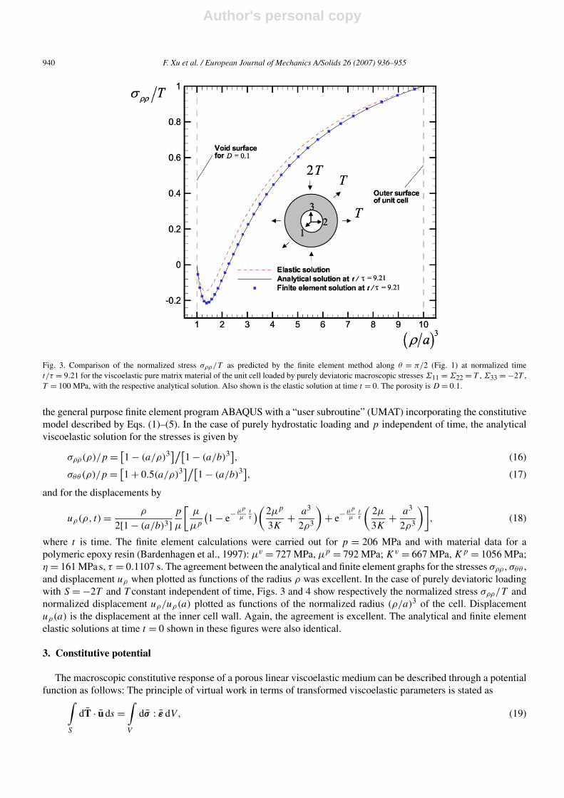
Fig. 3. Comparison of the normalized stress σρρ/T as predicted by the finite element method along θ = π/2 (Fig. 1) at normalized timet/τ = 9.21 for the viscoelastic pure matrix material of the unit cell loaded by purely deviatoric macroscopic stresses Σ11 = Σ22 = T , Σ33 = −2T ,T = 100 MPa, with the respective analytical solution. Also shown is the elastic solution at time t = 0. The porosity is D = 0.1.

the general purpose finite element program ABAQUS with a “user subroutine” (UMAT) incorporating the constitutivemodel described by Eqs. (1)–(5). In the case of purely hydrostatic loading and p independent of time, the analyticalviscoelastic solution for the stresses is given by

σρρ(ρ)/p = [1 − (a/ρ)3]/[

1 − (a/b)3], (16)

σθθ (ρ)/p = [1 + 0.5(a/ρ)3]/[

1 − (a/b)3], (17)

and for the displacements by

uρ(ρ, t) = ρ

2[1 − (a/b)3]p

μ

[μ

μp

(1 − e− μp

μtτ)(2μp

3K+ a3

2ρ3

)+ e− μp

μtτ

(2μ

3K+ a3

2ρ3

)], (18)

where t is time. The finite element calculations were carried out for p = 206 MPa and with material data for apolymeric epoxy resin (Bardenhagen et al., 1997): μv = 727 MPa, μp = 792 MPa; Kv = 667 MPa, Kp = 1056 MPa;η = 161 MPa s, τ = 0.1107 s. The agreement between the analytical and finite element graphs for the stresses σρρ , σθθ ,and displacement uρ when plotted as functions of the radius ρ was excellent. In the case of purely deviatoric loadingwith S = −2T and T constant independent of time, Figs. 3 and 4 show respectively the normalized stress σρρ/T andnormalized displacement uρ/uρ(a) plotted as functions of the normalized radius (ρ/a)3 of the cell. Displacementuρ(a) is the displacement at the inner cell wall. Again, the agreement is excellent. The analytical and finite elementelastic solutions at time t = 0 shown in these figures were also identical.

3. Constitutive potential

The macroscopic constitutive response of a porous linear viscoelastic medium can be described through a potentialfunction as follows: The principle of virtual work in terms of transformed viscoelastic parameters is stated as∫

S

dT · u ds =∫V

dσ : ε dV, (19)



Fig. 4. Comparison of the normalized displacement uρ/uρ(a) as predicted by the finite element method along θ = π/2 (Fig. 1) at normalized timet/τ = 9.21 for the viscoelastic pure matrix material of the unit cell loaded by purely deviatoric macroscopic stresses Σ11 = Σ22 = T , Σ33 = −2T ,T = 100 MPa, with the respective analytical solution. Also shown is the elastic solution at time t = 0. The porosity is D = 0.1 and uρ(a) is thedisplacement at ρ = a.

where dT is a statically admissible transformed increment to the tractions applied on the bounding surface S of a bodyoccupying volume V , dσ is the corresponding statically admissible transformed increment to the stress field, u and ε

are respectively the transformed solutions for the displacements and strains under traction T, and A : B = AijBij forany second order tensors A and B. It should be pointed out that Eq. (19) expresses virtual equilibrium in terms of thetransformed equilibrium and strain-displacement equations in the Laplace domain. Consider now the case in whichT = Σn where Σ is a macroscopic stress independent of position on the surface S and n is the outward unit normal.When the tractions are incremented by dT = dΣn, the internal stresses are incremented by dσ . Following Hill (1967)and Duva and Hutchinson (1984) and using Eq. (19), one obtains

dΣ : E = 1

V

∫V

dσ : ε dV, (20)

where the components of the macroscopic strain tensor E are defined through the displacements on the externalboundary S as

Eij = 1

2V

∫S

(uinj + ujni)dS. (21)

From Eq. (8) it is readily seen that dσ : ε = dφ, where φ = 12 σ : M : σ . Substituting this result into Eq. (20), one

obtains

dΣ : E = 1

V

∫V

dφ dV ≡ dΦ (22)

and so

E = ∂Φ(Σ)

∂Σ, Φ = 1

V

∫V

φ dV. (23)



As Cocks (1989) has shown, this potential function is useful for presenting numerical results for cell calculations.The constitutive response of the porous viscoelastic material can be presented by contours of constant Φ in the stressspace. Using the principle of virtual work (19) with fields dT and dσ replaced correspondingly by fields T and σ , onecan readily show that

Φ(Σ

) = 1

2Σ : E

(Σ

). (24)

Having the transformed solution u to the viscoelastic problem with macroscopic tractions Σn, one can determinefrom Eq. (21) the macroscopic strain tensor E that arises in response to Σ , and then use Eq. (24) to calculate thepotential function Φ in terms of Σ . It should be noted that in view of the linearity of the problem, E is in general ofthe form E = R : Σ and Φ = (1/2)Σ : R : Σ , where R is a fourth order tensor independent of Σ (Suquet, 1987), i.e.,Φ is quadratic in Σ . The isotropy of the problem implies that the general form of Φ is of the type

Φ

Kτ 2= A

(Σe

Kτ

)2

+ B

(Σm

Kτ

)2

, (25)

where Σe =√

3Σ ′ij Σ

′ij /2, Σ ′ is the transformed macroscopic stress deviator, Σm = Σkk/3 is the transformed macro-

scopic mean stress, and dimensionless parameters A and B are independent of Σ . It is emphasized at this point thatno restriction is placed on the type of macroscopic loading regarding the applicability of Eq. (25). The parameters A

and B are independent of Σ and can be determined by using the Laplace transform of the viscoelastic solution for theunit cell problem under any arbitrary macroscopic stress state Σ11 = Σ22 = T and Σ33 = S. However, in view of thefact that the hydrostatic and deviatoric stress contributions to the elliptic form of Eq. (25) are separable, parametersA and B can be determined by considering two special load cases: hydrostatic for the calculation of B and purelydeviatoric for A.

3.1. Evaluation of the potential in the unit cell

The potential is calculated in the case of the unit cell loaded by principal axisymmetric macroscopic stressesΣ11 = Σ22 = T , and Σ33 = S on the outer boundary ρ = b (Fig. 1). Under these conditions Σe = |T − S| andΣm = (2T + S)/3. In polar cylindrical coordinates (r, θ, z = x3; see Fig. 1), Eq. (24) becomes

Φ = 1

2

(2Σrr Err + ΣzzEzz

) = 1

2

(2T Err + SEzz

), (26)

where

Err = 1

2V

∫S

urnr dS, Ezz = 1

V

∫S

uznz dS, (27)

ur = uρ sin θ + uθ cos θ, uz = uρ cos θ − uθ sin θ, (28)

nr = sin θ = r/ρ, nz = cos θ = z/ρ, ρ = √r2 + z2, V = 4πb3/3 is the volume of the cell, and S = 4πb2 is its outer

bounding surface. Substituting the transformed viscoelastic displacements uρ and uθ as given by Eq. (15) into theequations above for the two special cases of purely hydrostatic (S = T ) and purely deviatoric (S = −2T ) loadings,one determines the dimensionless parameters A and B of the elliptical form (25) as follows:

A = K

5μc

[21λa + 5λb + 18(2μp + 2μτs + K + Kτs)

μp + μτs + 3K + 3Kτsλc

], (29)

B = 3K

4(1 − D)(μp + μτs)

[(D

2+ 2μp

3K

)+ τs

(D

2+ 2μ

3K

)], (30)

λa = −5(D5/3 − D)

Π, (31)

λb = − (−175 + 25ν2c )D7/3 + (49 − 25ν2

c ) + 126D5/3

6Π, (32)

λc = 5(7 + 5νc)(D10/3 − D)

12Π, (33)



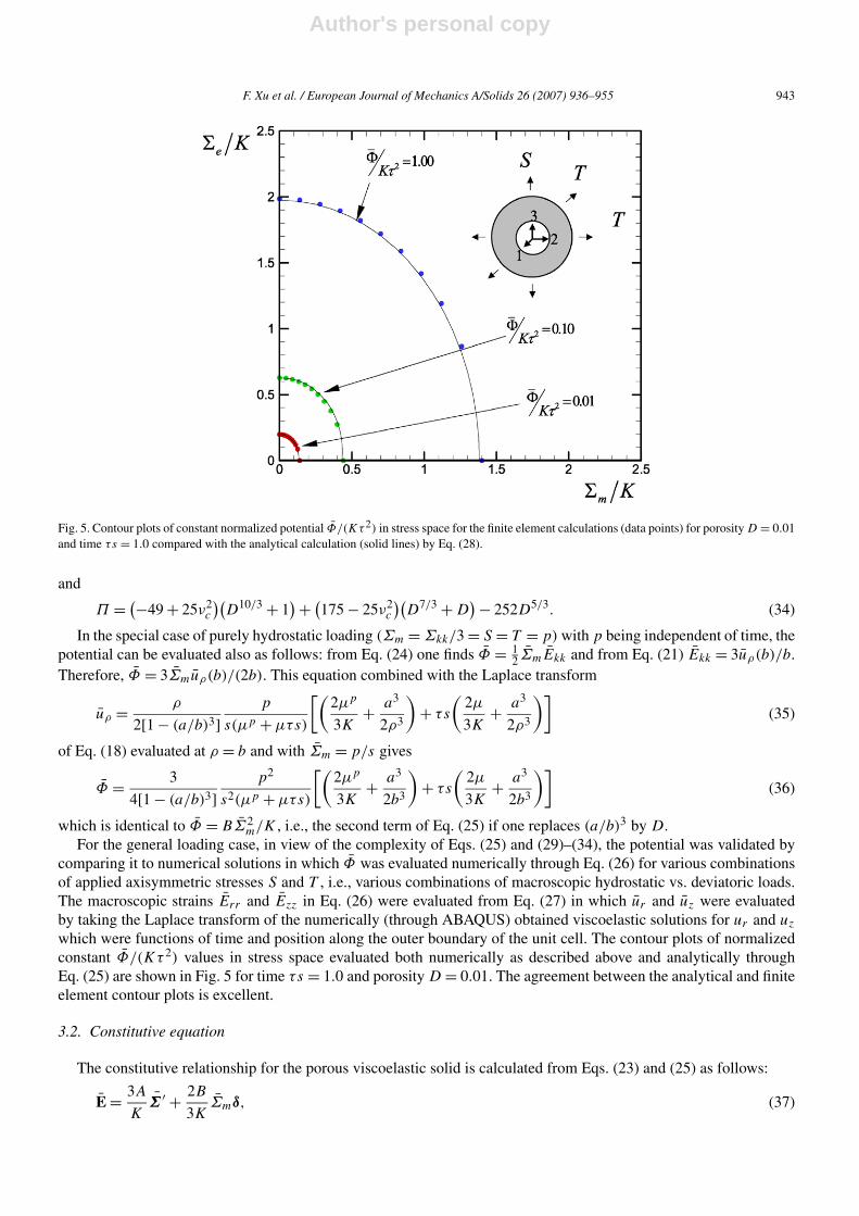
Fig. 5. Contour plots of constant normalized potential Φ/(Kτ2) in stress space for the finite element calculations (data points) for porosity D = 0.01and time τs = 1.0 compared with the analytical calculation (solid lines) by Eq. (28).

and

Π = (−49 + 25ν2c

)(D10/3 + 1

) + (175 − 25ν2

c

)(D7/3 + D

) − 252D5/3. (34)

In the special case of purely hydrostatic loading (Σm = Σkk/3 = S = T = p) with p being independent of time, thepotential can be evaluated also as follows: from Eq. (24) one finds Φ = 1

2ΣmEkk and from Eq. (21) Ekk = 3uρ(b)/b.Therefore, Φ = 3Σmuρ(b)/(2b). This equation combined with the Laplace transform

uρ = ρ

2[1 − (a/b)3]p

s(μp + μτs)

[(2μp

3K+ a3

2ρ3

)+ τs

(2μ

3K+ a3

2ρ3

)](35)

of Eq. (18) evaluated at ρ = b and with Σm = p/s gives

Φ = 3

4[1 − (a/b)3]p2

s2(μp + μτs)

[(2μp

3K+ a3

2b3

)+ τs

(2μ

3K+ a3

2b3

)](36)

which is identical to Φ = BΣ2m/K , i.e., the second term of Eq. (25) if one replaces (a/b)3 by D.

For the general loading case, in view of the complexity of Eqs. (25) and (29)–(34), the potential was validated bycomparing it to numerical solutions in which Φ was evaluated numerically through Eq. (26) for various combinationsof applied axisymmetric stresses S and T , i.e., various combinations of macroscopic hydrostatic vs. deviatoric loads.The macroscopic strains Err and Ezz in Eq. (26) were evaluated from Eq. (27) in which ur and uz were evaluatedby taking the Laplace transform of the numerically (through ABAQUS) obtained viscoelastic solutions for ur and uz

which were functions of time and position along the outer boundary of the unit cell. The contour plots of normalizedconstant Φ/(Kτ 2) values in stress space evaluated both numerically as described above and analytically throughEq. (25) are shown in Fig. 5 for time τs = 1.0 and porosity D = 0.01. The agreement between the analytical and finiteelement contour plots is excellent.

3.2. Constitutive equation

The constitutive relationship for the porous viscoelastic solid is calculated from Eqs. (23) and (25) as follows:

E = 3A

KΣ ′ + 2B

3KΣmδ, (37)



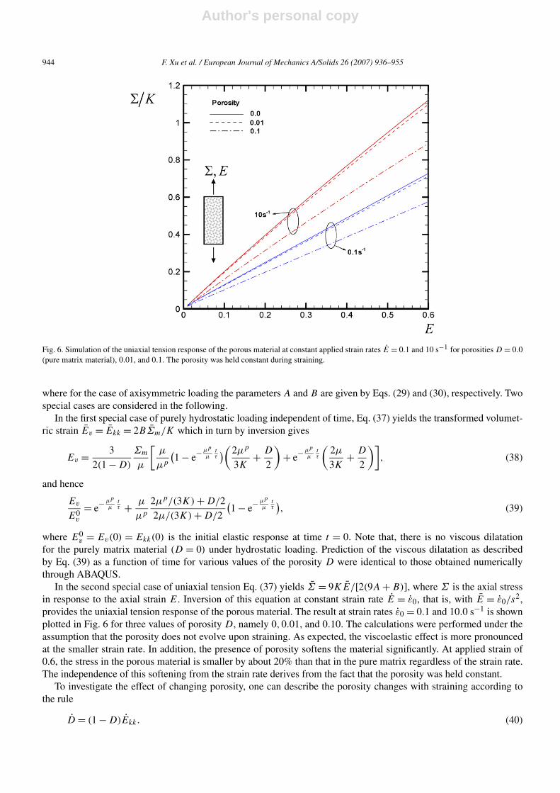
Fig. 6. Simulation of the uniaxial tension response of the porous material at constant applied strain rates E = 0.1 and 10 s−1 for porosities D = 0.0(pure matrix material), 0.01, and 0.1. The porosity was held constant during straining.

where for the case of axisymmetric loading the parameters A and B are given by Eqs. (29) and (30), respectively. Twospecial cases are considered in the following.

In the first special case of purely hydrostatic loading independent of time, Eq. (37) yields the transformed volumet-ric strain Ev = Ekk = 2BΣm/K which in turn by inversion gives

Ev = 3

2(1 − D)

Σm

μ

[μ

μp

(1 − e− μp

μtτ)(2μp

3K+ D

2

)+ e− μp

μtτ

(2μ

3K+ D

2

)], (38)

and hence

Ev

E0v

= e− μp

μtτ + μ

μp

2μp/(3K) + D/2

2μ/(3K) + D/2

(1 − e− μp

μtτ), (39)

where E0v = Ev(0) = Ekk(0) is the initial elastic response at time t = 0. Note that, there is no viscous dilatation

for the purely matrix material (D = 0) under hydrostatic loading. Prediction of the viscous dilatation as describedby Eq. (39) as a function of time for various values of the porosity D were identical to those obtained numericallythrough ABAQUS.

In the second special case of uniaxial tension Eq. (37) yields Σ = 9KE/[2(9A + B)], where Σ is the axial stressin response to the axial strain E. Inversion of this equation at constant strain rate E = ε0, that is, with E = ε0/s

2,provides the uniaxial tension response of the porous material. The result at strain rates ε0 = 0.1 and 10.0 s−1 is shownplotted in Fig. 6 for three values of porosity D, namely 0,0.01, and 0.10. The calculations were performed under theassumption that the porosity does not evolve upon straining. As expected, the viscoelastic effect is more pronouncedat the smaller strain rate. In addition, the presence of porosity softens the material significantly. At applied strain of0.6, the stress in the porous material is smaller by about 20% than that in the pure matrix regardless of the strain rate.The independence of this softening from the strain rate derives from the fact that the porosity was held constant.

To investigate the effect of changing porosity, one can describe the porosity changes with straining according tothe rule

D = (1 − D)Ekk. (40)



Fig. 7. Simulation of the uniaxial tension response of the porous material at constant applied strain rate E = 10.0 s−1 for porosity equal toD0 = 0.1 at time t = 0 and held either constant during straining or varying according to Eq. (41). Results are also shown for the pure matrixmaterial (D = 0.0).

This equation can be integrated to yield an expression for the porosity D in terms of the volumetric strain Ev = Ekk :

D = 1 − (1 − D0)e−(Ev−E0

v ) (41)

where D0 is the initial porosity at time t = 0 when Ev = E0v . It should be emphasized though that the constitutive

model developed herein is based on “linear kinematics”, i.e., on the assumption that all spatial displacement gradientsare “small” so that no distinction should be made between the deformed and undeformed configurations. In such cases,all components of the strain tensor are small and the variation of D with strain is minimal. However, the developedconstitutive model can be used also in problems of finite strains, provided the principal stretching directions are fixedas the material deforms (e.g., uniaxial tension, hydrostatic loading, etc.); in such cases, E and Σ should be interpretedas the Eulerian logarithmic (true) strain and the Cauchy (true) stress respectively, and the variation of D can besubstantial if the volumetric strain is finite.

The stress–strain (Σ,E) response of the porous material in uniaxial tension is governed by Σ = 9KE/[2(9A +B)] along with Ekk = 3BE/(9A + B). In these equations, the porosity D varies with time as dictated by Eq. (41).Numerical integration and inversion furnishes the stress–strain curve of a porous material with an initial porosityD0 = 0.10 as shown in Fig. 7 for straining at constant strain rate E = 10.0 s−1. The evolution of the porosity D withstraining is also shown in the figure. Clearly, when the void change is accounted for, the response is predicted to bemuch softer and nonlinear than when the porosity is kept fixed at its initial value.

4. Application: straining of solid propellants

Solid propellants are solid-fuel materials for rocket motors. They are particulate composites with an elastomericmatrix (Özüpek and Becker, 1992) whose response over strains less than about 8% is predominantly viscoelastic.Microvoids arise around the particles during fabrication or by aging or by long term slow chemical reactions (Cohen,1960; Rao, 1992; Gent and Park, 1984; Oberth and Bruenner, 1965). Holes may also form during straining wherebyparticles debond from the surrounding viscous matrix (Farris and Schapery, 1973; Farber and Farris, 1987; Vratsanosand Farris, 1993), a phenomenon termed dewetting. Özüpek and Becker (1992) modeled the deviatoric response of a



high-elongation solid propellant with the use of a hereditary integral weighed with a softening multiplier g in orderto account for the damage effect due to particle dewetting from the matrix. The hydrostatic response was modeledthrough an effective nonlinear bulk modulus that accounted for the macroscopic compressibility due to damage. Themodel was very successful in reproducing constant strain rate uniaxial tension experiments.

In this section the constitutive model of Eq. (37) is used to reproduce the macroscopic relaxation under constantshear strain, the stress response in uniaxial tension under constant macroscopic strain rate, and the stress responsein cyclic uniaxial tension observed experimentally by Özüpek and Becker (1992, 1997) at room temperature. Stress-induced damage in the solid propellant is simulated by the presence and evolution of porosity as dictated by Eq. (41).Obviously the initial value of the porosity D0 at time t = 0 is an input parameter to the model, but its evolution ispredicted on the basis of the local deformation and no assumptions or calibrations need be made. Of course, the modelpredictions are limited to small strains over which the matrix material does not undergo localized large deformationswhereby the constitutive Eq. (8) is not valid. To proceed with comparisons of the present model predictions withthe measurements from the experiments of Özüpek and Becker (1992, 1997), one needs to (i) calibrate the materialparameters D,μp,μv,K, τ of the present model, and (ii) numerically integrate the general constitutive Eq. (37)for implementation through a “user subroutine” (UMAT) in ABAQUS. Calibration is carried out through the shearrelaxation test and the numerical integration of Eq. (37) is discussed in the following Section 5.

4.1. Calibration

The bulk modulus K of the matrix material is assumed equal to the propellant modulus. Under the assumptionthat no dewetting takes place in compression, the bulk modulus can be considered as reflecting the matrix-material’scompressibility.

The calibration of the shear moduli μp , μv , and the time relaxation constant τ can only be done approximatelysince any real-world solid propellant material exhibits a relaxation response that is characterized by a collectionof relaxation time constants and not by a single relaxation time constant as assumed in the differential constitutiverelation of Eq. (1). The calibration is carried out by requiring that the shear relaxation response of the present model aspredicted by Eq. (37) reproduce the corresponding response measured experimentally. At room temperature (∼ 70 F),the measured relaxation modulus is phrased as

Gexp(t) = Gexpeq +

m∑n=1

Gexpi e−t/τi , (42)

where the superscript “exp” denotes experimental data, m is the number of relaxation time constants τi,Gexpi are the

associated individual shear relaxation moduli, and Gexpeq is the equilibrium shear relaxation modulus. For relaxation

under constant shear strain, the constitutive law (37) yields

Gmod = K/(6As), (43)

where the superscript “mod” denotes present model prediction. Since under shear the present model does not predictany changes in the volumetric response, one is consistent with the model by setting D = D0 during relaxation. Thusfor the given bulk modulus K , and for assumed values for the initial porosity D0 and relaxation time τ , the modulias given by Eqs. (42) and (43) were forced to be equal at short and long times, that is, Gmod(0) = Gexp(0) andGmod(t → ∞) = Gexp(t → ∞) = G

expeq . These equations were solved with respect to μp and μv by Newton iteration

which involved inversion of Eq. (43) in each iteration for the calculation of Gmod(t).

4.2. Uniaxial tension under constant strain rate

The calibration procedure with the shear relaxation data from the work of Özüpek and Becker (1992) for a highelongation solid propellant yields: bulk modulus K of the matrix material equal to 3.447 GPa and values of μp andμ for assumed initial porosities D0 = 0.001,0.01, and 0.1 and relaxation time constants τ = 0.006,0.06,0.6, and 6 sindependent of the parameters τ and D0 for D0 less than 0.1. Therefore, one may conclude that for initial porositiesless than 0.1, μp = 0.929 MPa and μ = 3.604 MPa. It is noted that such levels of porosity (� 0.1) are close to thedilute limit for which the underlying assumption about small deformations and non-interacting voids in this work



Fig. 8. Plot of the calibrated shear relaxation modulus of the porous solid propellant as function of time for given assumed values for the shearrelaxation time τ of the pure matrix material.

is relevant. Substituting these values into Eq. (43), one obtains by inversion the calibrated relaxation modulus as afunction of time. The result is shown plotted in Fig. 8 for various values of assumed relaxation times τ and for initialporosities less than 0.1. In the same figure also superposed is the experimental result of Özüpek and Becker (1992)as given by Eq. (42) with m = 8. As has already been discussed, calibration for all times, 0 � t � ∞, is impossible.However, as can be seen from Fig. 8, for time t � 0.1 s the model predictions agree with the experimental relaxationcurve very well when the relaxation time is taken τ = 0.305 s.

The simulation of the uniaxial tension straining was carried out at constant applied strain rate. The evolution ofporosity as described by Eq. (41) was accounted for in the simulation. The comparison between the model predictionsand the experimental data of Özüpek and Becker (1992) is shown in Fig. 9 for strains less than 10%, i.e., for the rangeover which the calibration of the relaxation response was satisfactory. At the high strain rate of 105 min−1 = 1.75 s−1,the model prediction is remarkably away from the experimental measurement. This is explained by the fact that atsuch high strain rate (loading time 0.057 s) the response of the porous material is predominantly elastic if one con-siders that the smallest relaxation time of the porous material is 0.305 s. As is demonstrated in the next section,the porous material exhibits a viscoelastic response whose deviatoric component is characterized by three relax-ation modes with corresponding times 0.305,0.320, and 0.510 s, and the hydrostatic component is characterizedby a relaxation time equal to 1.000 s. Therefore, no time is given to the viscous effects to bring about deforma-tion at such fast strain rate of loading. Absence of viscous deformation causes the model response of the poroussolid to be rather stiff. Hence, modeling of damage by porosity at the high strain rate of 105 min−1 = 1.75 s−1

is not a good mechanistic suggestion for the degradation of this high elongation propellant. However, at the lowerstrain rates of 0.25 min−1 = 4.2 × 10−3 s−1 and 3.7 min−1 = 6.2 × 10−2 s−1, the model and experimental pre-dictions compare better. Clearly, slow strain rates allow for viscous deformation which softens the response of theporous solid. Indeed, the respective loading time durations of 1.622 and 24.0 s are large compared to the relaxationtimes.

A very interesting result is that the porosity evolution during straining is almost identical for all three strain rates.Such independence of the dilatation from the strain rate has been also pointed out by Li and Weng (1995a, 1995b)and has been the case in the experiments of Özüpek and Becker (1997). As has been discussed the response underapplied rate of 105 min−1 = 1.75 s−1 is elastic. Indeed, at this strain rate the test duration time 0.057 s is much smallerthan the volumetric relaxation time of 1.0 s. On the other hand, viscous dilatation should be the case at strain rates of



Fig. 9. Analytical calculation of the uniaxial tension response of a high elongation solid propellant with initial porosity D0 = 0.1 at various appliedstrain rates. The data points are experimental data by Özüpek and Becker (1992). The porosity D evolves during straining according to Eq. (41).

Fig. 10. Comparison between the shear relaxation modulus as predicted by the present model with initial porosity D0 = 0.01 and the experimentallymeasured modulus of the Space Shuttle redesigned solid rocket motor (RSRM) propellant (Özüpek and Becker, 1997) at temperature 77 F.

0.25 min−1 and 3.7 min−1 given that the corresponding test duration times are 1.622 and 24.0 s, respectively. Alsoas shown by Fig. 9, the hydrostatic stress at a given strain increases as the applied strain rate increases. The almostidentical values of dilatation predicted for the three applied strain rates at a given strain may be explained by the



Fig. 11. Comparison between the model prediction under uniaxial tensile cyclic loading with initial porosity 0.01 and the experimentally measuredresponse of the Space Shuttle RSRM propellant (Özüpek and Becker, 1997) under loading rate of 0.714 min−1, with strain cycles at 0.1 and 0.15,and temperature 77 F. The data points denote experimental measurements. In the model, the porosity D evolves during straining according toEq. (41).

fact that for a given porosity level the viscous dilatation is a nonlinearly increasing function of the hydrostatic stressat fixed strain rate and nonlinearly decreasing function of strain rate at fixed hydrostatic stress. So small strain rateswith low corresponding hydrostatic stresses can give the same dilatation as large strain rates with high hydrostaticstresses.

4.3. Cyclic uniaxial tension

In order to test the model performance under cyclic loading conditions, the porous model was re-calibrated withthe Space Shuttle redesigned solid rocket motor (RSRM) propellant (Özüpek and Becker, 1997). The bulk modulus K

of the matrix material is equal to 100 GPa. The calculated values of μp and μ for assumed initial porosity D0 = 0.01and relaxation time constant τ = 0.01 s are 1.95 MPa and 31.6 MPa, respectively. Again, as with the high elongationpropellant calibrated in the preceding subsection, the calibrated parameters were found independent of the initialporosity D0 for D0 now less than 0.01. The comparison of the shear relaxation as predicted by the model equation (42)with the experimental shear relaxation curve is shown plotted in Fig. 10.

Fig. 11 shows the comparison of the model predictions with the experimental curve for the uniaxial cyclic tensiletest at the strain rate of 0.714/min and temperature (77 F) with strain cycles of 0.1 and 0.15. The model predictsthe loading response satisfactorily. However, for the unloading paths, the model over-predicts the stress response.It is also observed that the loading and unloading model-predictions are symmetric. This is due to the fact that theporous model has only one damage mechanism, which is void growth or shrinkage. Even though the model andexperiment agree over the loading paths, which means that void growth can be considered as a damage mechanismcapable of reproducing the propellant response, the deviation between model predictions and experimental data uponunloading shows that void shrinkage perhaps is not the only microstructural damage parameter characterizing thepropellant response during unloading. Incidentally, Özüpek and Becker (1997) used different damage functions tosimulate loading and unloading response.



5. Inversion of the constitutive law: numerical implementation

To use the general constitutive Eq. (37) in the study of three-dimensional boundary value problems of porous vis-coelastic materials one needs to transform it back in the real time domain. The deviatoric and hydrostatic componentsof Eq. (37) can be written as

Σ ′ = K

3AE′ = K

3As

(sE′ − E′0) + K

3AsE′0, (44)

Σm = K

2BEv = K

2Bs

(sEv − E0

v

) + K

2BsE0

v , (45)

where E′ is the macroscopic strain deviator, Ev = Ekk is the macroscopic volumetric strain, and the superscript “0”indicates the value at time t = 0. Inversion of Eq. (44) yields

Σ ′(t) = f (t)E′0 +t∫

0

f (ζ )dE′(t − ζ )

dζdζ, (46)

Σm(t) = g(t)E0v +

t∫0

g(ζ )dEv(t − ζ )

dζdζ (47)

where

f (t) = L−1(

K

3As

), g(t) = L−1

(K

2Bs

), (48)

and L−1 denotes inverse Laplace transform. The inversions of Eqs. (48) are carried out by first observing that

K

3As= −2μa1

b1

[β0

s+ β1

s + (1/τ1)+ β2

s + (1/τ2)+ β3

s + (1/τ3)

], (49)

K

2Bs= 4K(1 − D)(μp/μ + τs)

s[4μp/μ + 4τs + (3K/μ)D(1 + τs)] , (50)

and τ1 = τ . The parameters a1, b1, β0, β1, β2, β3, τ2, τ3 are all complicated functions of D,μp,μv,K , and τ . Thefinal result has the form

f (t) = f∞ + f1e−t/τ1 + f2e−t/τ2 + f3e−t/τ3, (51)

where f∞, f1, f2 and f3 are functions1 of D,μp,μv,K , and τ through a1, b1, β0, β1, β2, β3, τ2, τ3; and

g(t) = g∞ + g1e−t/τg , (52)

where

g∞ = 4(1 − D)

3D + (4μp/K)μp, g1 = −D[1 − (μ/μp)]

3D + (4μ/K)g∞, τg = D + (4μ/3K)

D + (4μp/3K)τ. (53)

Summarizing, we note that the constitutive equations are given by Eqs. (46) and (47) in which f (t) and g(t) aredefined by Eqs. (51) and (52).

In the case of purely hydrostatic loading by a constant pressure Σ0m = Σ0

kk/3 applied instantaneously at time t = 0,Eq. (47) yields Σ0

m = g(0)E0v . Noting that g(0) = g∞ + g1 and using Eqs. (53), one finds Σ0

m/K = {4(1 − D)/[4 +3D(K/μ)]}E0

v which is exactly the relationship between Σ0m and E0

v dictated by Eq. (38) at t = 0. It is worth notingthat Eqs. (46) and (47) of the porous viscoelastic material are of the classical hereditary form in which the modulifunctions f and g are expressed in a classical prony series form as indicated by Eqs. (51) and (52). The number ofterms in the prony series for the porous medium is directly related to the spring model of Fig. 2 used to describe the

1 Expressions for the parameters a1, b1, β0, β1, β2, β3, τ2, τ3 and functions f1, f2, and f3 are available upon request.



pure matrix material. It should be also noted that the presence of voids makes the hydrostatic response of the porousmaterial viscous, despite the fact that the matrix material response under hydrostatic loading is purely elastic.

Using Eqs. (51) and (52) and setting u = t − ζ , one concludes that the constitutive equations (46) and (47) can bewritten in the alternative form

Σ ′(t) = f0E′(t) −3∑

i=1

fi

t∫0

[1 − e−(t−ζ )/τi

]dE′(ζ )

dζdζ, (54)

and

Σm(t) = g0Ev(t) − g1

t∫0

[1 − e−(t−ζ )/τg

]dEv(ζ )

dζdζ, (55)

where f0 = f (0) = f∞ + ∑3i=1 fi and g0 = g(0) = g∞ + g1. It should be remembered that the coefficients

f0, f1, f2, f3, g0, and g1 are all functions of the porosity D.The last equations are now used to derive a scheme for the numerical integration of the developed constitutive

model in a finite element environment. The solution is developed incrementally and the constitutive equations areintegrated at the element Gauss integration points. At every Gauss point the solution (En,Σn,Dn) at time tn as wellas the strain En+1 = En + �E at time tn+1 = tn + �t are known, and the problem is to determine (Σn+1,Dn+1). Theintegration algorithm is as follows:

The porosity is updated first by integrating analytically the evolution equation D = (1 − D)Ev over the timeincrement (tn, tn+1) to find

Dn+1 = 1 − (1 − Dn)e−�Ev (56)

where subscripts n and n + 1 indicate values at tn and tn+1 respectively. Once Dn+1 is found, one can evaluate thecoefficients f0, f1, f2, f3, g0, and g1 at tn+1.

Eqs. (54) and (55) imply that

Σ ′n+1 = f0|n+1E′

n+1 −3∑

i=1

fi |n+1Tin+1, Σm|n+1 = g0|n+1Ev|n+1 − g1|n+1Hn+1, (57)

where

Ti (t) =t∫

0

[1 − e−(t−ζ )/τi

]dE′(ζ )

dζdζ, H(t) =

t∫0

[1 − e−(t−ζ )/τg

]dEv(ζ )

dζdζ. (58)

The quantities Tin+1 and Hn+1 that enter Eq. (57) are evaluated using Eqs. (58):

Tin+1 =

tn+�t∫0

[1 − e−(tn+�t−ζ )/τi

]dE′(ζ )

dζdζ

= (1 − e−�t/τi

)E′

n + e−�t/τi Tin +

tn+�t∫tn

[1 − e−(tn+�t−ζ )/τi

]dE′(ζ )

dζdζ (59)

and

Hn+1 =tn+�t∫

0

[1 − e−(tn+�t−ζ )/τg

]dEv(ζ )

dζdζ

= (1 − e−�t/τg

)Ev|n + e−�t/τgHn +

tn+�t∫tn

[1 − e−(tn+�t−ζ )/τg

]dEv(ζ )

dζdζ. (60)



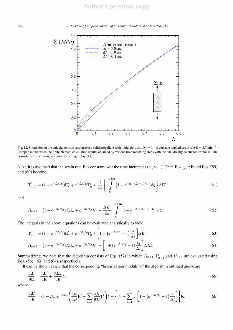
Fig. 12. Simulation of the uniaxial tension response of a solid propellant with initial porosity D0 = 0.1 at constant applied strain rate E = 3.7 min−1.Comparison between the finite element calculation results obtained by various time marching steps with the analytically calculated response. Theporosity evolves during straining according to Eq. (41).

Next, it is assumed that the strain rate E is constant over the time increment (tn, tn+1). Then E = 1�t

�E and Eqs. (59)and (60) become

Tin+1 = (

1 − e−�t/τi)E′

n + e−�t/τi Tin + 1

�t

{ tn+�t∫tn

[1 − e−(tn+�t−ζ )/τi

]dζ

}�E′ (61)

and

Hn+1 = (1 − e−�t/τg

)Ev|n + e−�t/τgHn + �Ev

�t

tn+�t∫tn

[1 − e−(tn+�t−ζ )/τg

]dζ. (62)

The integrals in the above equations can be evaluated analytically to yield

Tin+1 = (

1 − e−�t/τi)E′

n + e−�t/τi Tin +

[1 + (

e−�t/τi − 1) τi

�t

]�E′, (63)

Hn+1 = (1 − e−�t/τg

)Ev|n + e−�t/τgHn +

[1 + (e−�t/τg − 1)

τg

�t

]�Ev. (64)

Summarizing, we note that the algorithm consists of Eqs. (57) in which Dn+1,Tin+1 and Hn+1 are evaluated using

Eqs. (56), (63) and (64), respectively.It can be shown easily that the corresponding “linearization moduli” of the algorithm outlined above are

∂Σ

∂E= ∂Σ ′

∂E+ ∂Σm

∂Eδ, (65)

where

∂Σ ′

∂E= (1 − Dn)e

−�Ev

(∂f0

∂DE′ −

3∑i=1

∂fi

∂DTi

)δ +

{f0 −

3∑i=1

fi

[1 + (

e−�t/τi − 1) τi

�t

]}K, (66)



∂Σm

∂E= (1 − Dn)e

−�Ev

(∂g0

∂DEv − ∂g1

∂DH

)δ +

{g0 − g1

[1 + (

e−�t/τg − 1) τg

�t

]}δ. (67)

All quantities in Eqs. (66) and (67) are evaluated at the end of the increment, i.e., at t = tn+1.The above integration scheme is implemented in ABAQUS. The finite element results in uniaxial tension at strain

rate 3.7 min−1 = 6.2 × 10−2 s−1 are shown in Fig. 12 along with the corresponding analytical results discussed inSection 3.2. The material model was the calibrated one with the data of Özüpek and Becker (1992) as discussed inSection 4. The corresponding relaxation times for initial porosity D0 = 0.1 were τ = 0.305 s for the matrix material;τ1 = τ , τ2 = 0.320 s, τ3 = 0.510 s for the porous-material deviatoric response; and τg = 1.000 s for the porous-material hydrostatic response. Clearly for time step that compares to the relaxation times, the finite element results areidentical to the analytical result.

6. Concluding discussion

A constitutive law has been proposed for the response of a porous viscoelastic solid under 3-D triaxial stress states.The elastic response of the pure matrix material was linear and isotropic and the viscous response purely deviatoric.The law was derived from the axisymmetric stressing of a unit spherical cell by using the constitutive potentialapproach of Hill (1967) in the corresponding problem of linear viscoelasticity. It is phrased in terms of hereditaryintegrals in which the relaxation and viscous moduli are functions of porosity. Implementation of the constitutive lawin a general purpose finite element code along with a porosity evolution scheme is straightforward.

The model was calibrated through the shear relaxation test and used to predict the uniaxial tension response atconstant applied strain rate of a solid propellant whose damage during straining was simulated by the presence ofchanging porosity. In agreement with experimental evidence, the numerical calculations indicate no strain rate de-pendence of the dilatation of the porous material. This has been attributed to the fact that at a given porosity levelthe viscous dilatation is a nonlinearly increasing function of the hydrostatic stress at fixed strain rate and nonlinearlydecreasing function of strain rate at fixed hydrostatic stress. For the behavior under cycling loading, the model re-produces the loading response observed in the experiments of Özüpek and Becker (1997), but it does not capture thenonlinear features of the response upon unloading. The conclusion here is that nonlinear unloading response cannotbe simulated successfully through a mechanism of damage that only involves the closing of porosity.

As is well known, the response of a real-world viscoelastic solid is best described by a series of relaxation timeconstants in the form of hereditary integrals. One could definitely consider such a law for the constitution of thematrix material instead of the differential form of Eq. (1) to derive the constitutive potential described by Eq. (23).However, while the parameters A and B in the present approach that led to Eq. (25) can be obtained analytically fromEqs. (29) and (30), no such analytical representation could be found easily for a matrix material with a hereditaryrule. Of course, one could proceed and evaluate the potential numerically for the case of a matrix with a hereditaryconstitutive law, but this may not offer any advantages over the present relatively simple approach of Eq. (25) whenused in connection with the calibration discussed in Section 4.

For the case of a rigid particle instead of a void embedded in a viscoelastic matrix, one could repeat the analysispresented in this paper and come up with a corresponding constitutive law for the particle/reinforced viscoelasticcomposite material. Such a result is of interest in calculating the decohesion energy at the interface of a particleembedded in the homogenized matrix material.

Lastly, it should be noted that if the response of a porous viscoelastic medium is to be found for strains that involvelarge geometry changes, one needs to proceed with a large strain formulation of the entire problem. The analysis ofnonlinear viscous matrix behavior under large geometry changes is the subject of a subsequent publication.

Acknowledgements

This work was supported by the Center for Simulation of Advanced Rockets, funded by the U.S. Departmentof Energy through the University of California under subcontract number DOE/LLNL/B523819. The finite elementcalculations were carried out at the National Center for Supercomputing Applications at the University of Illinois atUrbana-Champaign.



Appendix A. Elastic solution for the spherical shell loaded axisymmetrically

In spherical coordinates the elastic solution for the stresses is given by

σρρ

2μ= −2a0(1 + ν) + 2d0

ρ3+

[−6a2νρ2 + 2b2 − 4(5 − ν)c2

ρ3+ 12d2

ρ5

]3 cos2 θ − 1

2, (68)

σρθ

2μ= −3

2

[a2(7 + 2ν)ρ2 + b2 + 2(1 + ν)c2

ρ3− 4d2

ρ5

]sin 2θ, (69)

σθθ

2μ= −2a0(1 + ν) − d0

ρ3−

[6a2(7 + ν)ρ2 + 4b2 + 2(1 − 2ν)c2

ρ3+ 9d2

ρ5

]3 cos2 θ − 1

2

+ 3

[a2(7 − 4ν)ρ2 + b2 + 2(1 − 2ν)c2

ρ3+ d2

ρ5

]cos2 θ, (70)

σϕϕ

2μ= −2a0(1 + ν) − d0

ρ3+

[−30a2νρ2 + 2b2 + 10(1 − 2ν)c2

ρ3− 3d2

ρ5

]3 cos2 θ − 1

2

−[a2(7 − 4ν)ρ2 + b2 + 2(1 − 2ν)c2

ρ3+ d2

ρ5

]cos2 θ, (71)

and the elastic solution for the displacements is given by

uρ

b= −2a0(1 − 2ν)ρ − d0

ρ2+

[12a2νρ3 + 2b2ρ + 2(5 − 4ν)c2

ρ2− 3d2

ρ4

]3 cos2 θ − 1

2, (72)

uθ

b= −3

2

[a2(7 − 4ν)ρ3 + b2ρ + 2(1 − 2ν)c2

ρ2+ d2

ρ4

]sin 2θ, (73)

where ρ = ρ/b is the dimensionless radial position, and

a0 = − S + 2T

12μ(1 + ν)

1

1 − a3, d0 = −S + 2T

12μ

a3

1 − a3, (74)

a2 = −5S − T

μ

a3(a2 − 1)

Π, b2 = −S − T

6μ

(−175 + 25ν2)a7 + 126a5 + 49 − 25ν2

Π, (75)

c2 = 5S − T

12μ

(7 + 5ν)a3(a7 − 1)

Π, d2 = S − T

2μ

(7 + 5ν)a5(a5 − 1)

Π, (76)

Π = (−49 + 25ν2)(a10 + 1) + 25

(7 − ν2)(a7 + a3) − 252a5, (77)

a = a/b = D1/3, and μ and ν are the elastic shear modulus and Poisson’s ratio, respectively.

References

Alberola, N.D., Lesueur, D., Granier, V., Joanicot, M., 1995. Viscoelasticity of porous composite materials: experimentals and theory. PolymerComposites 16, 170–179.

Bardenhagen, S.G., Stout, M.G., Gray, G.T., 1997. Three-dimensional, finite deformation, viscoelastic constitutive models for polymeric materials.Mech. Mater. 25, 235–253.

Birger, S., Moshonov, A., Kenig, S., 1989. The effects of thermal and hygrothermal ageing on the failure mechanisms of graphite-fabric epoxycomposites subjected to flexural loading. Composites 20, 341–348.

Christensen, R.M., 1982. Theory of Viscoelasticity. Dover Publications, New York.Cocks, A.C.F., 1989. Inelastic deformation of porous materials. J. Mech. Physics Solids 37, 693–715.Cohen, W., 1960. Rheological problems of solid-propellant rocketry. In: Lee, E.H., Symonds, P.S. (Eds.), Plasticity, Proceedings of the Second

Symposium on Naval Structural Mechanics Held at Brown University, RI. Pergamon Press, New York, pp. 568–579.Duva, J.M., Hutchinson, J.W., 1984. Constitutive potentials for dilutely voided materials. Mech. Mater. 3, 41–54.Eom, Y., Boogh, L., Michaud, V., Sunderland, P., Manson, J.-A., 2001a. Stress induced void formation during cure of a three-dimensionally

constrained thermoset raisin. Pol. Eng. Sci. 41, 492–503.Eom, Y., Boogh, L., Michaud, V., Manson, J.-A., 2001b. A structure and property based process window for void free thermoset composites.

Polymer Composites 22, 22–31.



Farber, J.N., Farris, R.J., 1987. Model for prediction of the elastic response of reinforced materials over wide ranges of concentration. J. Appl. Pol.Sci. 34, 2093–2104.

Farris, R.J., Schapery, R.A., 1973. Development of a solid rocket propellant nonlinear viscoelastic constitutive theory. AFRPL-TR-73-50 I.Francfort, G., Leguillon, D., Suquet, P., 1983. Mathematical problems in mechanics-Homogenization for linearly viscoelastic bodies. C. R. Acad.

Paris, Ser. I 296, 287–290.Francfort, G., Suquet, P., 1986. Homogenization and mechanical dissipation in thermoviscoelasticity. Arch. Rat. Mech. Anal. 96, 265–293.Gent, N., Park, B., 1984. Failure processes in elastomers at or near a rigid spherical inclusion. J. Mater. Sci. 19, 1947–1956.Harvey, J.A., Cebon, D., 2003. Failure mechanisms in viscoelastic films. J. Mater. Sci. 38, 1021–1032.Hill, R., 1967. The essential structure of constitutive laws for metal composites and polycrystals. J. Mech. Phys. Solids 15, 79–95.Hilton, H.H., 2001. Implications and constraints of time-independent Poisson ratios in linear isotropic and anisotropic viscoelasticity. J. Elastic-

ity 63, 221–251.Lee, R.H., 1960. Viscoelastic stress analysis. In: Goodier, J.N., Hoff, N.J. (Eds.), Structural Mechanics, Proceedings of the First Symposium on

Naval Structural Mechanics Held at Stanford University, CA. Pergamon Press, New York, pp. 456–482.Li, J., Weng, G.J., 1995a. Void growth and stress–strain relations of a class of viscoelastic porous materials. Mech. Mater. 22, 179–188.Li, J., Weng, G.J., 1995b. Void growth in viscoelastic polymeric materials. In: Mechanics of Plastics and Plastic Composites ASME MD-

Vol. 68/AMD 215, pp. 409–421.Luré, A.I., 1964. Three-Dimensional Problems of the Theory of Elasticity. Interscience Publishers, New York.Mori, T., Tanaka, K., 1973. Average stress in the matrix and average elastic energy of materials with misfitting inclusions. Acta Metall. 21, 571–574.Nevalainen, K., MacKerron, D.H., Kuusipalo, J., 2005. Voiding behaviour and microstructure of a filled polyester film. Mater. Chem. Phys. 92,

540–547.Nilsson, G., Fernberg, S.P., Berqlund, L.A., 2002. Strain field inhomogeneities and stiffness changes in GMT containing voids. Composites

Part A 32, 75–85.Oberth, A.E., Bruenner, R.S., 1965. Tear phenomena around solid inclusions in castable elastomers. Trans. Soc. Rheology 9, 165–185.Özüpek, S., Becker, E.B., 1992. Constitutive modeling of high-elongation solid propellants. Int. J. Engrg. Mat. Tech. 114, 111–115.Özüpek, S., Becker, E.B., 1997. Constitutive equations for solid propellants. Int. J. Engrg. Mat. Tech. 119, 125–132.Park, J., Siegmund, T., Mogneau, L., 2003. Viscoelastic properties of foamed thermoplastic vulcanizates and their dependence on void fraction.

Cellular Polymers 22, 137–156.Pipkin, A.C., 1986. Lectures on Viscoelasticity Theory. Springer-Verlag, New York.Rao, B.N., 1992. Fracture of solid propellant grains. Eng. Fracture Mech. 43, 455–459.Smith, L.V., Weitsman, Y.J., 1998. Inelastic behavior of randomly reinforced polymeric composites under cyclic loading. Mechanics of Time-

Dependent Materials 1, 293–305.Sofronis, P., McMeeking, R.M., 1992. Creep of power-law material containing spherical voids. J. Appl. Mech. 59, 88–95.Suquet, P.M., 1987. Elements of homogenization for inelastic solid mechanics. In: Sanchez-Palencia, Zaoui, A. (Eds.), Homogenization Techniques

for Composite Media. In: Lecture Notes in Physics, vol. 272. Springer-Verlag, New York, pp. 193–278.Thomason, J.L., Groenewoud, W.M., 1996. The influence of fibre length and concentration on the properties of glass fibre reinforced polypropylene:

2. Thermal properties. Composites A 27A, 555–565.Trong Ming, D., Chiu, W.-Y., Hsieh, K.-H., 1991. The thermal aging of filled polyurethane. J. Appl. Polymer Sci. 43, 2193–2199.Vratsanos, L.A., Farris, R.J., 1993. A predictive model for the mechanical behavior of particulate composites, Part I: model derivation. Pol. Engrg.

Sci. 33, 1458–1465.Wang, Y.M., Weng, G.J., 1990. Self-similar void growth in viscoelastic media. In: Damage Mechanics in Engineering Materials, ASME AMD 109

pp. 211–226.Wang, Y.M., Weng, G.J., 1993. Self-similar and transient void growth in viscoelastic media at low concentration. Int. J. Frac. 61, 1–16.

Author's personal copy - University of Thessaly · Author's personal copy European Journal of Mechanics A/Solids 26 (2007) 936 955 Constitutive modeling of porous viscoelastic materials

Documents