Author's personal copy - Startseite TU Ilmenaus personal copy ... Doppler Velocimetry (LDV) System from Dantec Dynamics with ... was taken from the user manual of the atomizer.

Author's personal copy

Properties of large-scale flow structures in an isothermal ventilated room

M. Körner a,*, O. Shishkina b, C. Wagner b, A. Thess a

a Institute of Thermodynamics and Fluid Mechanics, Ilmenau University of Technology, P.O. Box 100565, 98684 Ilmenau, GermanybDLR e Institute for Aerodynamics and Fluid Technology, Bunsenstrasse 10, 37073 Göttingen, Germany

a r t i c l e i n f o

Article history:Received 25 July 2012Received in revised form16 October 2012Accepted 17 October 2012

Keywords:Isothermal ventilationTurbulent large-scale flow structureAuto-oscillationLaser Doppler VelocimetryDirect numerical simulation

a b s t r a c t

In the present work experimental and numerical investigations of the large-scale structures ofisothermal air flow in a highly simplified model room are reported and discussed. We compare themeasured velocity distribution with direct numerical simulations (DNSs) for the reference Reynoldsnumber Reref ¼ 2.4 � 104, which is based on the maximum inlet velocity and the height of the room. Thiscomparison shows a high similarity concerning the flow structures. Furthermore, we investigate thedependence of the spatial and temporal behavior of flow structures on the Reynolds number frommeasurements covering a Reynolds number range of 1.0 � 104 � Re � 7.0 � 104. The major finding is thatthere is a coherent oscillation of the large-scale flow structures, which depends on the Reynolds number.Our findings show that the frequencies of the oscillations are in a good agreement with an empiricalmodel, which describes the auto-oscillation of two colliding planar jets with respect to the Reynoldsnumber and the geometry relations of the inlets. Moreover, the present work indicates that the chosenflow geometry is well suited as a simplified model for problems of room ventilation and can serve asa base for forthcoming studies of non-isothermal cases.

� 2012 Elsevier Ltd. All rights reserved.

1. Introduction

In view of the increasing significance of the energy efficiency ofventilation systems and the thermal comfort of persons insidea roomwithin the past three decades, the knowledge of the spatialand temporal properties of large-scale air flows inside rooms hasbecome more and more important. That knowledge can influencethe complete design of rooms like passenger cabins or office rooms.In most cases the indoor air flow is a buoyancy- and momentum-driven flow with highly complex structures. To understand thesecomplex non-isothermal air flows, it is necessary to fully under-stand the behavior of the isothermal air flow. Thus, we experi-mentally and numerically investigated the properties of the large-scale flow structures in a ventilated model room for theisothermal case in the present paper.

First experimental and numerical investigations of isothermalventilation of rooms have been reported by Nielsen et al. [1]. In thisinvestigation a simple model roomwith rectangular cross-sectionsand one inlet and one outlet, the so called Nielsen room, has beenused to study the fundamental behavior of the isothermal air flow.

Nielsen reported that the flow structures have a high dependencyon the geometrical dimensions of the room and the inlets but alsoon the inlet flow velocity. Nielsen’s model room has been investi-gated in several further investigations, for example by Kato et al.[2], Gosman et al. [3], Mora et al. [4] or Mushatet [5]. Nielson’sfindings regarding the ventilation of amodel room are often used toverify numerical simulation like Mora et al. [4] did. Other investi-gations related to this model room concerned about fundamentalinformation of the ventilation efficiency [2] or to get furtherinformation regarding the dependency of the flow on the boundaryconditions [3,5].

In the present work, the geometry of the model room to beinvestigated experimentally and numerically relates in general aswell to Nielsen’s work and is shown in Fig. 1a.

The model roomwe use could be understood as an extension ofthe Nielsen room to a more complex geometry. We also considera box with rectangular cross section. But in contrast to Nielsen’sroom ourmodel room contains four rectangular flow obstacles nearthe bottom which extend over the full depth of the room. Theventilation is realized through two opposed horizontal inlets nearthe ceiling of the room. The air exits the room through two outletsat the bottom. The inlets and outlets also extend over the full depthof the room. So, the room geometry is in general and in contrast toNielsen’s geometry more related to a passenger cabin, e.g. anaircraft cabin.

* Corresponding author. Tel.: þ49 3677 69 4402.E-mail addresses: [email protected] (M. Körner), olga.shishkina@

dlr.de (O. Shishkina), [email protected] (C. Wagner), [email protected](A. Thess).

Contents lists available at SciVerse ScienceDirect

Building and Environment

journal homepage: www.elsevier .com/locate/bui ldenv

0360-1323/$ e see front matter � 2012 Elsevier Ltd. All rights reserved.http://dx.doi.org/10.1016/j.buildenv.2012.10.011

Building and Environment 59 (2013) 563e574


With respect to this room geometry, we are interested inanswering particularly the following questions: What are thespatial properties of the large-scale structure of the flow? Howwellcan a direct numerical simulation (DNS) in a box with a smallerdepth than the experimental one reproduce the large-scale flowstructures? Is there a spatial and temporal dependency of thebehavior of the large-scale flow structure on the Reynolds numberRe?

Here, the Reynolds number is defined as

Re ¼ uin$Hn

(1)

with uin as the maximum velocity of the inlet flow, H as the heightof the room and n as the kinematic viscosity of dry air.

The outline of the present work is as follows. In Section 2 wedescribe the experimental setup, the used measurement setup andthe data processing. In Section 3, we describe the numericaldomain and the computational algorithms of the DNS. Section 4contains the description and the discussion of the results of ourinvestigation. We finish the present work with a conclusion inSection 5.

2. Experimental setup

Fig. 1a depicts a sketch of the cross-section of the investigatedmodel room. The model room is equipped with two inlets in theside walls and close to the ceiling of the room. The shape of theinlets is shown in Fig. 1b. Two outlets are arranged in the same sidewalls like the inlets but close to the bottom of the room. Near thebottom of the room are four rectangular flow obstacles. Thisgeometry is extended over the full depth D. The model room ismade of Plexiglas and the flow obstacles are made of aluminum.

We define the origin of the coordinate system in the left, lowercorner with the x-direction along the length L, the y-direction alongthe height H and the z-direction along the depth D. The height ofthe model room is H ¼ 300 mm. Other dimensions describing themodel room are Gxy ¼ L/H ¼ 1.33; Gzy ¼ D/H ¼ 1.67; hin/H ¼ 0.0067and hout/H¼ 0.05, as shown in Fig. 1. The inlets and outlets have thesame depth as the model room (din/D¼ 1; dout/D¼ 1). So, accordingto the findings of Nielsen [1], we can assume that the large-scale

flow is nearly 2-dimensional. To abide this assumption, it isnecessary to generate an inlet flow with a homogeneous velocitydistribution along the z-direction. This is realized by a nozzle, asshown in Fig. 1b, and prechambers in front of the inlets. The inletflow is generated with air from a pressure vessel with an adjustableoutlet pressure for adjusting the inlet velocity.

The obstacles within the room have a cross-section of ho/H¼ 0.2and lo/L ¼ 0.1. The depth of the obstacles is almost of the same sizeas the depth of the model room. Only a small gap of do/D ¼ 0.01 ateach side of the model room exists. The obstacles are arranged atthe positions x/L¼ [0.1, 0.3, 0.6, 0.8] related to the origin and the leftside of the obstacles in Fig. 1a. The distance from the bottom ish/H ¼ 0.05.

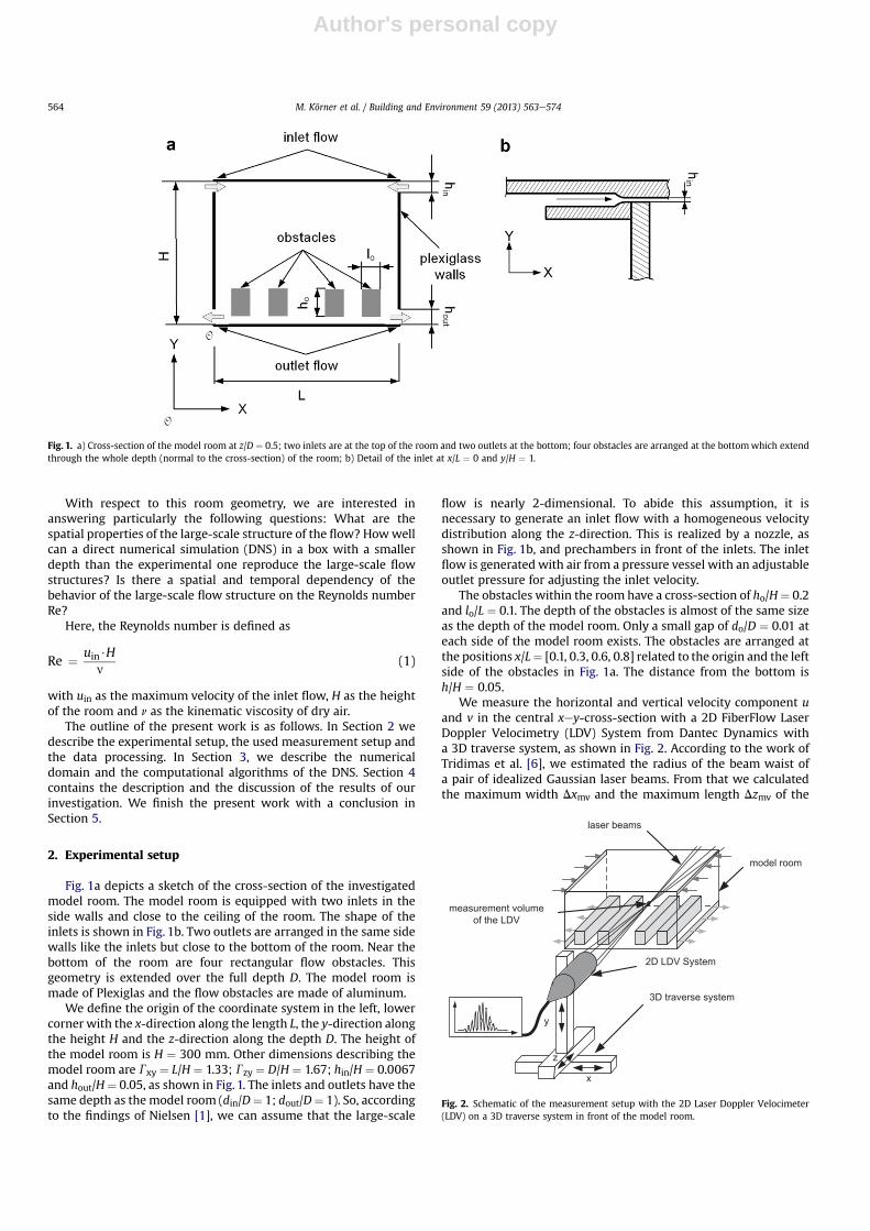
We measure the horizontal and vertical velocity component uand v in the central xey-cross-section with a 2D FiberFlow LaserDoppler Velocimetry (LDV) System from Dantec Dynamics witha 3D traverse system, as shown in Fig. 2. According to the work ofTridimas et al. [6], we estimated the radius of the beam waist ofa pair of idealized Gaussian laser beams. From that we calculatedthe maximum width Dxmv and the maximum length Dzmv of the

Fig. 1. a) Cross-section of the model room at z/D ¼ 0.5; two inlets are at the top of the room and two outlets at the bottom; four obstacles are arranged at the bottomwhich extendthrough the whole depth (normal to the cross-section) of the room; b) Detail of the inlet at x/L ¼ 0 and y/H ¼ 1.

2D LDV System

model room

3D traverse system

laser beams

measurement volumeof the LDV

x

y

z

Fig. 2. Schematic of the measurement setup with the 2D Laser Doppler Velocimeter(LDV) on a 3D traverse system in front of the model room.

M. Körner et al. / Building and Environment 59 (2013) 563e574564


measurement volume related to the used focal length f ¼ 310 mm,a beam separation at the lens of b ¼ 72 mm and the two used wavelengths of the lasers l ¼ [488, 514.5] nm. The maximum size of themeasurement volume is Dxmv ¼ 419.2 mm and Dzmv ¼ 48.7 mm, asshown in Table 1. The light power of the laser was P z 250 mW.

The tracer particles, needed for LDV measurements are gener-ated by an atomizer in a bypass inside the inlet flow system.We usedi(2-ethylhexyl) sebacate (DEHS), atomized to drops of the averagesize of dp ¼ 0.4 mmwith a PALAS AGF 10.0. The average particle sizewas taken from the user manual of the atomizer. With respect toa minimum fringe spacing of df ¼ 2.1 mm for l ¼ 488 nm the size ofthe particles is small enough to achieve reliable LDV-signals.

In order to visualize the flow we use a laser light sheet with anaverage thickness of the light sheet of 2 mm and a laser light powerof P ¼ 100 mW. As particles we use the same DEHS-particles asdescribed above. The pictures are taken with a customary digitalsingle-lens reflex (DLSR) camera system.

The measurement positions shown in Fig. 3 are distributedin the central xey-cross-section of the room at z/D ¼ 0.5 andx/L ¼ [0.08, 0.25, 0.50, 0.75, 0.92]. In vertical direction we measureat 11 points from underneath the ceiling at y/H¼ 0.997 to the top ofthe obstacles at y/H ¼ 0.347. The long term measurements areperformed at 5 points at x/L ¼ [0.08, 0.25, 0.50, 0.75, 0.92],y/H ¼ 0.63 and z/D ¼ 0.5. These positions are meant to be themost significant for characterizing the flow structure withrespect to the findings of the experimental visualizations andnumerical simulations. In order to compare the experiment withthe numerical simulation we define a reference case at a Reynoldsnumber Reref ¼ 2.4 � 104 with an inlet velocity of uin ¼ 1.25 m/s,the height of the room H and the viscosity of air ofn(q ¼ 22 �C) ¼ 1.55 � 10�5 m2 s�1. Moreover, we experimentallystudy the dependency of the flow on the Reynolds number withRe ¼ [1.0; 1.5; 2.4; 4.0; 6.0; 7.0] � 104 which corresponds to themaximum inlet velocities of uin ¼ [0.52; 0.77; 1.25; 2.06; 3.10;3.61] m s�1.

Using the characteristic velocity uc ¼ uin.max ¼ 1.25 m/s and thecharacteristic length scale lc ¼ H ¼ 0.3 m, the characteristic timescale of the system amounts to tc ¼ lc/uc ¼ 0.24 s. Regarding thetime scale tc and the Shannon theorem, fs ¼ 2/tc ¼ 8.33 Hz is theminimum data rate for the LDV-velocity measurements for char-acterizing the large-scale flow structures. The typical data rates inthe experiments are between fs ¼ 20e100 Hz.

The minimum acquisition time to ensure a statistical uncer-tainty of 10% from the real velocity value û is determined byanalyzing a test time series of the flow. At the reference Reynoldsnumber of Reref ¼ 2.4 � 104 we determine the correlation time sc,the mean velocity hui and the standard deviation s(u). The calcu-lated minimum acquisition time amounts to ta.min z 8 min, soa reasonable acquisition time for the velocity profiles is ta ¼ 10min.The acquisition time for long term measurements of the velocity ista ¼ 60 min. The resampling of the LDV-data to create equidistanttime steps between the measurement samples is done by a linearinterpolation of the LDV-data with a constant time step oftlin ¼ 2 � 103$tmin with tmin as the minimummeasured time step ofthe raw data. A typical minimum time step is tmin ¼ 1 �10�5 s. Weanalyze the resampled velocity time series by determining the

frequency distribution P(u0), the probability density function (PDF)PG(u0) and the power spectral density PSD(u0) of the velocity fluc-tuations u0 ¼ u � hui with u ¼ (u, v) as the measured velocity andhui as the mean velocity. The frequency distribution P(u0) is deter-mined out of the resampled LDV-data with 5000 intervals of thevelocity. The PDF PG(u0) is determined out of the mean velocity huiof the time series and its standard deviation s(u0). The PSD’s areobtained with the fast Fourier transformation (FFT) out of theautocorrelation function of the resampled LDV-data. In the FFT weuse 2048 data points and the maximum frequency is f ¼ 1/tmin.

In order to provide data for the definition of the inlet flow asa boundary condition for the experiment and particularly for thenumerical investigation we measure the velocity distribution u(y,z)inside the inlet. To realize this task we use nearly the sameexperimental setup as described above. For geometrical reasons, anon-axis-alignment of the 2D-LDV-System with the optical axispointing in y-direction was more reasonable. The vertical profileu(y) of the inlet velocity was measured at z/D ¼ 0.2 and from0.986� y/H� 1.002. The horizontal velocity distribution of the inletflow is measured from 0.01 � z/D � 0.99 at the maximum of thevertical velocity profile y/H¼ 0.997. Both the vertical and horizontalmeasurements are made at x/L¼ 1.25�10�3. The Reynolds numberRein.y ¼ uin$hin/n of the inlet flow, which is based on the maximuminlet velocity uin ¼ 4.5 m/s, which can be achieved in the experi-mental setup and twice the height of the inlet hin, which mustbe assumed for h � D, gives Rein.y ¼ 9.4 � 102. Therefore weexpect a laminar behavior of the flow with a parabolic velocitydistribution in y-direction within the inlet. The Reynolds numberRein.z ¼ uin$D/n, which is based on the depth D of the room, givesRein.z ¼ 1.5 � 105. Thus, we expect a turbulent regime of the inletflow with a rectangular shaped velocity distribution in z-direction.

3. Numerical simulation

The system of the governing momentum and continuity equa-tions for the velocity field u and pressure p reads as follows

ut þ u$VuDr�1Vp ¼ nDu; (2)

V$u ¼ 0; (3)

where ut denotes the time derivative of the velocity field, r is thedensity and n the kinematic velocity.

Table 1Estimation of the maximum width Dxmv and length Dzmv of the measurementvolume.

Wave length l 488 nm 514.5 nm

Focal length f Dxmv [mm] Dzmv 10�2 [mm] Dxmv [mm] Dzmv 10�2 [mm]

310 mm 0.3976 4.617 0.4192 4.868

Fig. 3. Cross-section of the model room showing the LDV-measurement positions formeasuring velocity profiles (dashed line) and velocity time series (circles); velocityprofiles are measured at 5 � 11 ¼ 55 points in horizontal (M1eM5) and verticaldirection; to acquire the velocity time series, five measurement points are situated atthe height of the core of the large eddies at y/H ¼ 0.633.

M. Körner et al. / Building and Environment 59 (2013) 563e574 565


The boundary conditions of the numerical simulation are equal tothose in the experiment. But in order to reduce the temporalcomputational effort, we choose a smaller depthwith a ratio ofDnum/Dexp ¼ 0.16 for the DNS. The length, height, and depth of the domainare L, H, and Dnum, respectively. The length, height, and width of theinlets are H/150 and Dnum, respectively. Two outlets with the sizes H/20 and Dnum are located close to the bottom. We setup a parabolicshaped velocity distribution in vertical direction y and an almostconstant velocity distribution in horizontal direction z. Furthermore,additional ducts are arranged in front of the inlets and after theoutlets, to generate similar inlet and outlet flow conditions related tothe experiment. The obstacles in the room are in similar size andposition like in the experiment. The depth of the obstacle are of theroom dimensions Dobs ¼ Dnum and have no gap to the walls.According to Equations (2) and (3) the velocities at the outerboundaries of the inlet ducts are fixed; the velocity vector is put touin¼ (uin, 0, 0). At the outer boundaries of the outlet ducts du/dn¼ 0,where n is the normal vector. At all solid walls u ¼ 0 due to imper-meability and no-slip conditions.

In order to non-dimensionalize the governing equations, we usethe following reference constants: xref ¼ L for distance, uref ¼ uin forvelocity, tref ¼ xref/uref for time and pref ¼ u2ref r for pressure. Thus,we obtain the following system of the governing dimensionlessequations

u*t þ u*$Vu* þ Vp ¼ Re�1G�1Du*; (4)

V$u* ¼ 0: (5)

Here u* is the dimensionless velocity vector-function, u*t its time

derivative, p the pressure and Re ¼ Reref the Reynolds number andG ¼ Gxy the aspect ratio of the computational domain. Within thepresentedwork we investigate numerically isothermal ventilation inthe above discussed geometry for a much smaller depth of the roomof L/D ¼ 5 in order to keep the computational effort relatively low.

In order to simulate these turbulent forced convection flows, weuse a finite volume method originally developed by Schmitt et al.[7]. It is based on the volume balance procedure developed bySchumann [8], on fourth-order finite-volume discretizationschemes in space and the explicit Euler-leapfrog discretizationscheme in time. The code is a Cartesian version of the one we usedin our direct numerical simulations (DNS) of turbulent RayleigheBénard convection [9,10]. To solve the problem discussed abovesome changes were necessary in the Poisson solver, which isneeded to couple the pressure and the velocity fields. The newPoisson solver uses the capacitance matrix technique together withthe separation of variables method, which was developed anddescribed in detail in Ref. [11]. The developed numerical methodgenerally allows to conduct DNS of turbulent natural, forced ormixed convection flows in enclosures using computational meshes,which are non-equidistant in all 3 directions and irregular in any 2directions. To resolve all relevant turbulent scales, one needs to usefine enough computations meshes with a spatial increment oforder of the smallest Kolmogorov scale h ¼ (n3/ 3)1/4. Here 3is thetime and volume-averaged rate of kinetic energy dissipation. Onecan estimate 3by multiplying the momentum equation scalarly bythe velocity vector-function and further averaging the resultingequation in time and over the whole domain. From this one obtainsthe following estimation of the upper bound of 3:

3zSinV

u3in; (6)

where Sin denotes the area of the vertical cross-section of the inletducts and V the volume of the convection cell. Using this estimate,

one concludes that the number of nodes in the horizontal directionxof the computationalmesh, which guarantees a good resolution inDNS, is estimated as follows:

Lh¼ Re3=4

�hinL3

H4

�1=4

; (7)

which is about 600. Therefore in our DNS of forced convection forReref ¼ 2.4 � 104 we use a mesh with 600 nodes in the x-direction,80 nodes in the other horizontal z-direction and 320 nodes in thevertical y-direction. The computational mesh is non-equidistant inall 3 directions and is especially fine near the inlet ducts. The nodesof the mesh are clustered near the walls to fulfill the requirementyþ < 1 and are distributed in accordance with Ref. [12]. The griddependency check for this particular geometry was not conducteddue to the high consumption of the computational resourcesneeded for that, but from DNS of thermal convection in rectangulardomains [13] and DNS of isothermal turbulent pipe flow [14] weknow that the grid is sufficiently fine to be used in DNS if the meshsize in the main part of the domain apart from the boundary layersis smaller than the Kolmogorov microscale and if the requirementyþ < 1 near the rigid walls is fulfilled. Because of the very highcomputational effort, time series and the dependency of solutionson the Reynolds number are not investigated by means of the DNS.

4. Results

We start the presentation and discussion of our results with thecase Reref¼ 2.4�104. For this value of the Reynolds number we candirectly compare our experimental and numerical results. Becauseof the above mentioned reasons, Sections 4.2 and 4.3 only containexperimental results.

4.1. Comparison between experiment and numerical simulation

4.1.1. Characterization of the inlet flowThe curves in Fig. 4a and b show the measured horizontal

velocity u in front of the inlet as a function of y and z, respectively.The measurement of the vertical velocity profile starts inside thewall of the inlet. The velocity profile u(y/H) in Fig. 4a showsa parabolic velocity distribution. Furthermore, Fig. 4b shows thatthe inlet velocity is homogenously distributed over the depth D ofthe model room. The maximum deviation from the meanmaximum velocity in z-direction is (u(z/D) � u(z/D)mean)/u(z/D)mean ¼ 0.0336. So, the results of the velocity measurementswithin the inlet show that the assumption of a parabolic velocityprofile in y-direction and a uniform velocity in z-direction is wellsatisfied. The chosen boundary conditions regarding the inlet flowof the DNS are also well suited to describe the present problem.

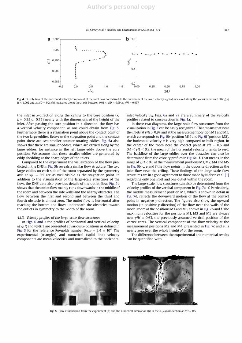
4.1.2. Visualized large-scale flow structuresFig. 5 shows the visualizations of the flow in the experiment (a)

and the numerical simulation (b) in the chosen xey-planes (Fig. 3)at the reference Reynolds number of Reref ¼ 2.4 � 104. Both visu-alizations reflect a distinct large-scale flow structure. The experi-mental flow visualization in Fig. 5a shows two large counter-rotating eddies driven by the inlet flow. These eddies have equaldimensions and are situated left and right of the center of the room.The cores of the large eddies are assumed to be at x/L ¼ 0.25 andx/L ¼ 0.75 and y/H ¼ 0.63. Thus, the diameter of the large eddies isone half of the width of the room, limited by the walls of the room,the obstacles at the bottom and the contact point of the large eddiesin the middle of the room (x/L ¼ 0.5). Another finding from thevisualizations in Fig. 5a is, that the flow from each sidemoves out of



the inlet in x-direction along the ceiling to the core position (x/L ¼ 0.25 or 0.75) nearly with the dimensions of the height of theinlet. After passing the core position in x-direction, the flow hasa vertical velocity component, as one could obtain from Fig. 5.Furthermore there is a stagnation point above the contact point ofthe two large eddies. Between the stagnation point and the contactpoint there are two smaller counter-rotating eddies. Fig. 5a alsoshows that there are smaller eddies, which are carried along by thelarge eddies, for instance in the left large eddy above the coreposition. We assume that these smaller eddies are generated byeddy shedding at the sharp edges of the inlets.

Compared to the experiment the visualization of the flow pre-dicted in the DNS in Fig. 5b reveals a similar flow structure. The twolarge eddies on each side of the room separated by the symmetryaxis at x/L ¼ 0.5 are as well visible as the stagnation point. Inaddition to the visualization of the large-scale structures of theflow, the DNS data also provides details of the outlet flow. Fig. 5bshows that the outlet flowmainly runs downwards in themiddle ofthe room and between the side walls and the nearby obstacles. Theflow between the first and second and between the third andfourth obstacle is almost zero. The outlet flow is horizontal afterreaching the bottom and flows underneath the obstacles towardthe outlets in symmetry to the width of the room.

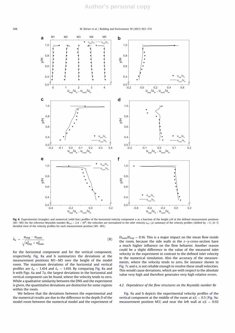
4.1.3. Velocity profiles of the large-scale flow structuresIn Figs. 6 and 7 the profiles of horizontal and vertical velocity,

u(y/H) and v(y/H), are presented at various x-positions as defined inFig. 3 for the reference Reynolds number Reref ¼ 2.4 � 104. Theexperimental (triangles) and numerical (solid line) velocitycomponents are mean velocities and normalized to the horizontal

inlet velocity uin. Figs. 6a and 7a are a summary of the velocityprofiles related to cross-section in Fig. 1a.

In these two diagrams, the large-scale flow structures from thevisualization in Fig. 5 can be easily recognized. That means that nearthe inlets at y/H> 0.97 and at themeasurement positionM1 andM5,which corresponds to Fig. 6b (position M1) and Fig. 6f (position M5),the horizontal velocity u is very high compared to bulk region. Inthe center of the room near the contact point at x/L ¼ 0.5 and0.4 � y/L � 0.9, the mean of the horizontal velocity u tends to zero.The backflow of the large eddies over the obstacles can also bedetermined from the velocity profiles in Fig. 6aef. Thatmeans, in therange of y/H< 0.6 at themeasurement positionsM1, M2,M4 andM5in Fig. 6b, c, e and f the flow points in the opposite direction as theinlet flow near the ceiling. These findings of the large-scale flowstructures are in a good agreement to thosemade by Nielsen et al. [1]regarding only one inlet and one outlet within the room.

The large-scale flow structures can also be determined from thevelocity profiles of the vertical component in Fig. 7aef. Particularly,the middle measurement position M3, which is shown in detail inFig. 7d, reflects the downward motion of the flow at the contactpoint in negative y-direction. The figures also show the upwardmotion (in positive y-direction) of the flow near the walls of themodel room at the positionsM1 andM5, shown in Fig. 7b and f. Themaximum velocities for the positions M1, M3 and M5 are alwaysnear y/H ¼ 0.63, the previously assumed vertical position of thevortex cores. The vertical component of the flow velocity at themeasurement positions M2 and M4, presented in Fig. 7c and e, isnearly zero over the whole height H of the room.

The difference between the experimental and numerical resultscan be quantified with

-0,5 0,0 0,5 1,0 1,5

0,985

0,990

0,995

1,000

1,005

y/H

u/uin

a b

0,00 0,25 0,50 0,75 1,000,0

0,5

1,0

1,5

u/u in

z/D

Fig. 4. Distribution of the horizontal velocity component of the inlet flow normalized to the maximum of the inlet velocity uin: (a) measured along the y-axis between 0.987 � y/H � 1.002 and at z/D ¼ 0.2; (b) measured along the z-axis between 0.01 � z/D � 0.99 at y/H ¼ 0.997.

Fig. 5. Flow visualization from the experiment (a) and the numerical simulation (b) in the xey-cross-section at z/D ¼ 0.5.



du ¼ uexp � unumffiffiffiffiffiffiffiffiffiffiffiffiffiffiffiffiffiffiffiffiffiffiffiffiffiffiu2exp þ u2num

q (8)

for the horizontal component and for the vertical component,respectively. Fig. 8a and b summarizes the deviations at themeasurement positions M1eM5 over the height of the modelroom. The maximum deviations of the horizontal and verticalprofiles are du ¼ 1.414 and dv ¼ 1.410. By comparing Fig. 8a andb with Figs. 6a and 7a, the largest deviations in the horizontal andvertical component can be found, where the velocity tends to zero.While a qualitative similarity between the DNS and the experimentis given, the quantitative deviations are distinctive for some regionswithin the room.

We believe that the deviations between the experimental andthe numerical results are due to the difference in the depth D of themodel room between the numerical model and the experiment of

Dnum/Dexp ¼ 0.16. This is a major impact on the mean flow insidethe room, because the side walls in the zey-cross-section havea much higher influence on the flow behavior. Another reasoncould be a slight difference in the value of the measured inletvelocity in the experiment in contrast to the defined inlet velocityin the numerical simulation. Also the accuracy of the measure-ments, where the velocity tends to zero, for instance shown inFig. 7c and e, is not reliable enough to resolve these small velocities.This would cause deviations, which are with respect to the absolutevalue very high and therefore generates very high relative errors.

4.2. Dependence of the flow structures on the Reynolds number Re

Fig. 9a and b depicts the experimental velocity profiles of thevertical component at the middle of the room at x/L ¼ 0.5 (Fig. 9a;measurement position M3) and near the left wall at x/L ¼ 0.92

0,0

0,4

0,6

0,8

1,0

0 1 2 3 4

M1 M2 M3 M4 M5

y/H

uexp/uin , unum/uin

uexp/uin unum/uin

0,0

0,4

0,6

0,8

1,0

-0,2 0,0 0,2 0,4 0,6

y/H

uexp/uin , unum/uin

uexp/uin

unum/uin

0,0

0,4

0,6

0,8

1,0

-0,2 -0,1 0,0 0,1 0,2 0,3 0,4

y/H

uexp/uin , unum/uin

uexp/uin

unum/uin

0,0

0,4

0,6

0,8

1,0

-0,2 -0,1 0,0 0,1 0,2

y/H

uexp/uin , unum/uin

uexp/uin

unum/uin

0,0

0,4

0,6

0,8

1,0

-0,4 -0,2 0,0 0,2

y/H

uexp/uin , unum/uin

uexp/uin

unum/uin

0,0

0,4

0,6

0,8

1,0

-0,6 -0,4 -0,2 0,0 0,2

y/H

uexp/uin , unum/uin

uexp/uin

unum/uin

dc

e f

ba

Fig. 6. Experimental (triangles) and numerical (solid line) profiles of the horizontal velocity component u as a function of the height y/H at the defined measurement positions(M1eM5) for the reference Reynolds number Reref ¼ 2.4 � 104; the velocities are normalized to the inlet velocity uin; (a) summary of the velocity profiles (shifted by þ1); (bef)detailed view of the velocity profiles for each measurement position (M1eM5).



0 5 10 15 200,0

0,4

0,6

0,8

1,0

M1 M2 M3 M4 M5

y/H

δu

100%

0 5 10 15 200,0

0,4

0,6

0,8

1,0

M1 M2 M3 M4 M5

y/H

δv

100%

a b

Fig. 8. Relative deviation d of the velocities between the experiment and the numerical simulation as a function of the height of the room y/H at the reference Reynolds numberReref ¼ 2.4 � 104; data points are shifted by þ5; (a) deviations of the horizontal velocity component du; (b) deviations of the vertical velocity component dv.

0,0

0,4

0,6

0,8

1,0

-0,1 0,0 0,1 0,2

y/H

vexp/uin , vnum/uin

v /u v /u

0,0

0,4

0,6

0,8

1,0

-0,2 -0,1 0,0 0,1 0,2

y/H

vexp/uin , vnum/uin

v /u v /u

0,0

0,4

0,6

0,8

1,0

-0,2 -0,1 0,0 0,1 0,2

y/H

vexp/uin , vnum/uin

v /u v /u

0,0

0,4

0,6

0,8

1,0

-0,3 -0,2 -0,1 0,0 0,1

y/H

vexp/uin , vnum/uin

v /u v /u

0,0

0,4

0,6

0,8

1,0

-0,1 0,0 0,1 0,2

y/H

vexp/uin , vnum/uin

v /u v /u

0,0

0,4

0,6

0,8

1,0

0 1 2 3 4

M1 M2 M3 M4 M5

y/H

vexp/uin , vnum/uin

v /u v /u

fe

dc

a b

Fig. 7. Experimental (triangles) and numerical (solid line) profiles of the vertical velocity component v as a function of the height y/H at the defined measurement positions (M1eM5) for the reference Reynolds number Reref ¼ 2.4 � 104; the velocities are normalized to the inlet velocity uin; (a) summary of the velocity profiles (shifted by þ1); (bef) detailedview of the velocity profiles for each measurement position (M1eM5).



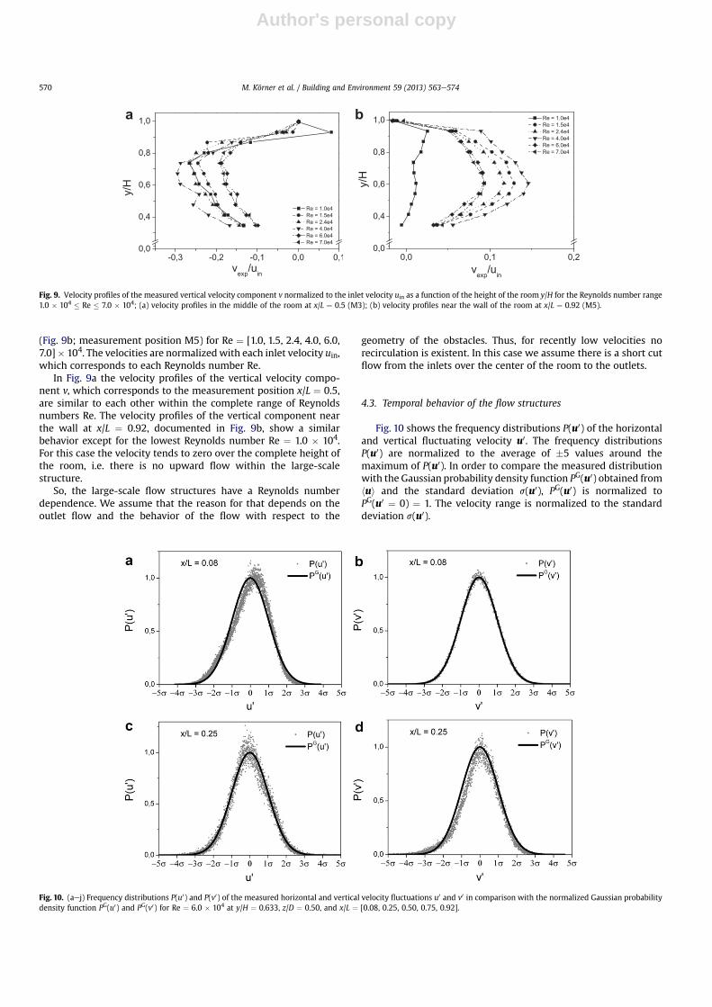
(Fig. 9b; measurement position M5) for Re ¼ [1.0, 1.5, 2.4, 4.0, 6.0,7.0]� 104. The velocities are normalizedwith each inlet velocity uin,which corresponds to each Reynolds number Re.

In Fig. 9a the velocity profiles of the vertical velocity compo-nent v, which corresponds to the measurement position x/L ¼ 0.5,are similar to each other within the complete range of Reynoldsnumbers Re. The velocity profiles of the vertical component nearthe wall at x/L ¼ 0.92, documented in Fig. 9b, show a similarbehavior except for the lowest Reynolds number Re ¼ 1.0 � 104.For this case the velocity tends to zero over the complete height ofthe room, i.e. there is no upward flow within the large-scalestructure.

So, the large-scale flow structures have a Reynolds numberdependence. We assume that the reason for that depends on theoutlet flow and the behavior of the flow with respect to the

geometry of the obstacles. Thus, for recently low velocities norecirculation is existent. In this case we assume there is a short cutflow from the inlets over the center of the room to the outlets.

4.3. Temporal behavior of the flow structures

Fig. 10 shows the frequency distributions P(u0) of the horizontaland vertical fluctuating velocity u0. The frequency distributionsP(u0) are normalized to the average of �5 values around themaximum of P(u0). In order to compare the measured distributionwith the Gaussian probability density function PG(u0) obtained fromhui and the standard deviation s(u0), PG(u0) is normalized toPG(u0 ¼ 0) ¼ 1. The velocity range is normalized to the standarddeviation s(u0).

Fig. 10. (aej) Frequency distributions P(u0) and P(v0) of the measured horizontal and vertical velocity fluctuations u0 and v0 in comparison with the normalized Gaussian probabilitydensity function PG(u0) and PG(v0) for Re ¼ 6.0 � 104 at y/H ¼ 0.633, z/D ¼ 0.50, and x/L ¼ [0.08, 0.25, 0.50, 0.75, 0.92].

0,0 0,1 0,20,0

0,4

0,6

0,8

1,0 Re = 1.0e4 Re = 1.5e4 Re = 2.4e4 Re = 4.0e4 Re = 6.0e4 Re = 7.0e4

y/H

vexp/uin

0,0

0,4

0,6

0,8

1,0

-0,3 -0,2 -0,1 0,0 0,1

Re = 1.0e4 Re = 1.5e4 Re = 2.4e4 Re = 4.0e4 Re = 6.0e4 Re = 7.0e4

y/H

vexp/uin

a b

Fig. 9. Velocity profiles of the measured vertical velocity component v normalized to the inlet velocity uin as a function of the height of the room y/H for the Reynolds number range1.0 � 104 � Re � 7.0 � 104; (a) velocity profiles in the middle of the room at x/L ¼ 0.5 (M3); (b) velocity profiles near the wall of the room at x/L ¼ 0.92 (M5).



Fig. 10 reflects that the frequency distribution of the horizontaland vertical velocity fluctuations show a nearly Gaussian distri-bution within the whole room, except for the horizontal fluctua-tions in the middle position of the room at x/L ¼ 0.50, y/H ¼ 0.63,and z/D ¼ 0.50 which is presented in Fig. 10e. At this middleposition the frequency distribution of the horizontal velocityfluctuations P(u0) show two peaks and gives rise to the conclusion,that there are self-induced oscillations of the large-scale flowstructures. Furthermore, we found that the phenomenon neitherappears in the frequency distribution of vertical fluctuations P(v0)at the same position nor in the other frequency distributions ofthe horizontal and vertical fluctuations at all the other measure-ment positions. We believe that the reason for the absence of theoscillations in the vertical velocity in the middle of the roommight be that the amplitude of the horizontal oscillation of theflow at the chosen measurement point is smaller than the halfwidth of the fully developed vertical flow within the contact pointof the counter-rotating eddies.

Fig. 11aef shows the frequency distributions of the horizontalvelocity fluctuations at x/L ¼ 0.50, y/H ¼ 0.63, and z/D ¼ 0.50

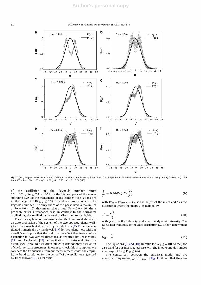
for the complete investigated set of Reynolds numbers Re.The normalization rules are equal to that used in Fig. 10. Fromthis we infer that the probability density functions always showtwo peaks within the complete Reynolds number range1.0 � 104 � Re � 7.0 � 104. Here, the frequency distributions alsoreflect a Reynolds number dependence, because for Re ¼ 2.4 � 104

and Re¼ 4.0� 104 the values of the amplitude of the two peaks arenot equal, i.e. the left peak is smaller than the right peak. We nowcannot find a reasonable explanation for this phenomenon, whichtherefore needs further investigation in future studies.

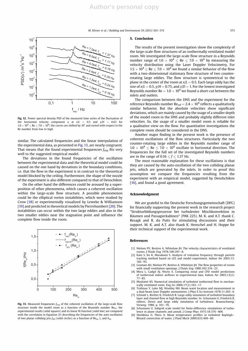
The PSD’s of the horizontal velocity fluctuations u0 for theinvestigated Reynolds number range of 1.0� 104� Re� 7.0� 104areshown in Fig. 12. We found for all Reynolds numbers Re � 4.0 � 104

a significant peak, which indicates, that there is a coherent oscillationof the large-scale flow structure in the horizontal direction x.

In the Reynolds numbers range 1.0 � 104 � Re � 2.4 � 104 thereis no significant peak in the PSD. But we found for each Reynoldsnumber two peaks in the PDFs in Fig. 11aec, which gives rise tothe assumption that there also must be an oscillation of the flowin the region of the contact point. Thus, we estimate the frequency

Fig. 10. (continued).



of the oscillation in the Reynolds number range1.0 � 104 � Re � 2.4 � 104 from the highest peak of the corre-sponding PSD. So the frequencies of the coherent oscillations arein the range of 0.16 � f � 1.37 Hz and are proportional to theReynolds number. The amplitudes of the peaks have a maximumat Re ¼ 6.0 � 104, that means that around Re ¼ 6.0 � 104 thereprobably exists a resonance case. In contrast to the horizontaloscillations, the oscillations in vertical direction are negligible.

For a first explanation, we assume that the found oscillations arean auto-oscillation of the system of the two opposed planar wall-jets, which was first described by Denshchikov [15,16] and inves-tigated numerically by Pawlowski [17] for two planar jets withouta wall. We suppose that the wall has the effect that instead of anoscillation in two vertical directions, as reported by Denshchikov[15] and Pawlowski [17], an oscillation in horizontal directionestablishes. This auto-oscillation influences the coherent oscillationof the large-scale structures. In order to check this assumption, wecompare the frequencies from our measurements with the empir-ically found correlation for the period T of the oscillation suggestedby Denshchikov [16] as follows:

TT*

¼ 0:34$Re�1:0in $

�d

L

�; (9)

with Rein ¼ Rein.y, d h hin as the height of the inlets and L as thedistance between the inlets. T* is defined by

T* ¼ rL2

h; (10)

with r as the fluid density and h as the dynamic viscosity. Thecalculated frequency of the auto-oscillation fAO is than determinedby

fAO ¼ 1T: (11)

The Equations (9) and (10) are valid for Rein � 4800, so they arealso valid for our investigated case with the inlet Reynolds numberin a range of 67 � Rein � 464.

The comparison between the empirical model and themeasured frequencies fAO and fexp in Fig. 13 shows that they are

Fig. 11. (aef) Frequency distributions P(u0) of the measured horizontal velocity fluctuations u0 in comparison with the normalized Gaussian probability density function PG(u0) for1.0 � 104 � Re � 7.0 � 104 at x/L ¼ 0.50, y/H ¼ 0.63, and z/D ¼ 0.50 (M3).



similar. The calculated frequencies and the linear interpolation ofthe experimental data, as presented in Fig. 13, are nearly congruent.That means that the found experimental frequencies fexp fits verywell to the suggested empirical model.

The deviations in the found frequencies of the oscillationbetween the experimental data and the theoretical model could becaused on the one hand by deviations in the boundary conditions,i.e. that the flow in the experiment is in contrast to the theoreticalmodel blocked by the ceiling. Furthermore, the shape of the nozzleof the experiment is also different compared to that of Denschikov.

On the other hand the differences could be aroused by a super-position of other phenomena, which causes a coherent oscillationwithin the large-scale flow structure. A possible phenomenoncould be the elliptical vortex instabilities, which were studied byCrow [18] or experimentally visualized by Leweke & Williamson[19] and predicted in theoretical models by Pierrehumbert [20]. Theinstabilities can occur within the two large eddies and also in thetwo smaller eddies near the stagnation point and influence thecomplete flow inside the room.

5. Conclusion

The results of the present investigation show the complexity ofthe large-scale flow structures of an isothermally ventilated modelroom. We investigated the large-scale flow structure in a Reynoldsnumber range of 1.0 � 104 � Re � 7.0 � 104 by measuring thevelocity distribution using the Laser Doppler Velocimetry. For1.5 � 104 � Re � 7.0 � 104 we found a similar behavior of the flowwith a two-dimensional stationary flow structure of two counter-rotating large eddies. The flow structure is symmetrical to theplane in the center of the room at x/L ¼ 0.5. Each large eddy has thesize of x/L¼ 0.5, y/H¼ 0.75, and z/D¼ 1. For the lowest investigatedReynolds number Re ¼ 1.0 � 104 we found a short-cut between theinlets and outlets.

The comparison between the DNS and the experiment for thereference Reynolds number Reref ¼ 2.4 � 104 reflects a qualitativelysimilar behavior. But the absolute velocities show significantdeviations, which aremainly caused by the usage of a smaller depthof the model room in the DNS and probably slightly different inletvelocities. So, the usage of a smaller model room is reliable fora qualitative view on the flow. For quantitative investigations thecomplete room should be considered in the DNS.

Another major finding in the present work is the presence ofcoherent oscillations of the flow structures. Particularly the twocounter-rotating large eddies in the Reynolds number range of1.0 � 104 � Re � 7.0 � 104 oscillate in horizontal direction. Thefrequencies for the full set of the investigated Reynolds numbersare in the range of 0.16 � f � 1.37 Hz.

The most reasonable explanation for these oscillations is thatthey are caused by the auto-oscillation of the two colliding planarjets, which are generated by the inlets. In order to proof thisassumption we compare the frequencies resulting from theexperiment with an empirical model, suggested by Denshchikov[16], and found a good agreement.

Acknowledgment

We are grateful to the Deutsche Forschungsgemeinschaft (DFG)for financially supporting the present work in the research project“Strukturbildungsprozesse bei turbulenter Mischkonvektion inRäumen und Passagierkabinen” (PAK 225). M. K. and A.T. thank C.Resagk and R. du Puits for stimulating discussions and theirsupport. M. K. and A.T. also thank K. Henschel and H. Hoppe fortheir technical support of the experimental work.

References

[1] Nielsen PV, Restivo A, Whitelaw JH. The velocity characteristics of ventilatedrooms. J Fluids Eng 1978;100:291e8.

[2] Kato S, Ito K, Murakami S. Analysis of visitation frequency through particletracking method based on LES and model experiment. Indoor Air 2003;13:182e93.

[3] Gosman AD, Nielsen PV, Restivo A, Whitelaw JH. The flow properties of roomswith small ventilation openings. J Fluids Eng 1980;102:316e23.

[4] Mora L, Gadgil AJ, Wurtz E. Comparing zonal and CFD model predictionsof isothermal indoor airflows to experimental data. Indoor Air 2003;13(2):77e85.

[5] Mushatet KS. Numerical simulation of turbulent isothermal flow in mechan-ically ventilated room. Eng Sci 2006;17(2):103e17.

[6] Tridimas Y, Lalor MJ, Woolley NH. Beam waist location and measurement ina dual-beam laser Doppler anemometer. J Phys E Sci Instrum 1978;11:203e6.

[7] Schmitt L, Richter K, Friedrich R. Large-eddy simulation of turbulent boundarylayer and channel flow at high Reynolds number. In: Schumann U, Friedrich R,editors. Direct and large eddy simulation of turbulence. Braunschweig:Vieweg; 1986. p. 161e76.

[8] Schumann U. Subgrid scale model for finite-difference simulations of turbu-lence in plane channels and annuli. J Comp Phys 1975;18:376e404.

[9] Shishkina O, Thess A. Mean temperature profiles in turbulent RayleigheBénard convection of water. J Fluid Mech 2009;633:449e60.

0 100 200 300 400 500

0,0

0,5

1,0

1,5 fexp(Rein)fexp.lin(Rein) fAO (Rein )

f(Re in

)/Hz

Rein

Fig. 13. Measured frequencies fexp of the coherent oscillation of the large-scale flowstructure inside the model room as a function of the Reynolds number Rein; theexperimental results (solid squares) and its linear fit function (solid line) are comparedwith the correlation in Equation (9) describing the frequencies of the auto-oscillationof two planar colliding jets fAO (solid circles) as a function of Rein, L, and hin.

0,1 1 10 100

100

101

102

103

104

105

106

107

Re = 7.0e4; fexp = 1.37 Hz

Re = 6.0e4; fexp = 1.17 HzRe = 4.0e4; fexp = 0.78 HzRe = 2.4e4; f

exp = 0.39 HzRe = 1.5e4; fexp = 0.24 Hz

PSD

(u')

/m2 s-2

Hz-1

fexp / Hz

Re = 1.0e4; fexp = 0.16 Hz

Fig. 12. Power spectral density PSD of the measured time series of the fluctuation ofthe horizontal velocity component u at x/L ¼ 0.5 and y/H ¼ 0.63 for1.0 � 104 � Re � 7.0 � 104; the curves are shifted by 101 and sorted with respect to theRe number from low to high.



[10] Shishkina O, Wagner C. A fourth order accurate finite volume scheme fornumerical simulations of turbulent RayleigheBénard convection in cylindricalcontainers. C R Mec 2005;333(1):17e28.

[11] Shishkina O, Shishkin A, Wagner C. Simulation of turbulent thermal convec-tion in complicated domains. J Comput Appl Math 2009;226(2):336e44.

[12] Shishkina O, Wagner C. Adaptive meshes for simulations of turbulent Ray-leigheBénard convection. J Numer Anal Indust Appl Math 2006;1(2):219e28.

[13] Kaczorowski M, Wagner C. Study on the resolution requirements for DNS inturbulent Rayleigh-Bénard convection. In: Proc. 2nd int. conf. on turbulenceand interactions. Sainte-Luce: 2010.

[14] Feldmann D, Wagner C. Direct numerical simulation of fully-developedturbulent and oscillatory pipe flows at Res ¼ 1440. J Turbul 2012;13:1e28.

[15] Denshchikov VA, Kondrat’ev VN, Romashov AN. Interaction between twoopposed jets. Fluid Dyn 1978;13(6):924e6.

[16] Denshchikov VA, Kondrat’ev VN, Romashov AN, Chubarov VM. Auto-oscilla-tions of planar colliding jets. Fluid Dyn 1983;18(3):460e2.

[17] Pawlowski RP, Salinger AG, Shadid JN, Mountziaris TJ. Bifurcation and stabilityanalysis of laminar isothermal counterflowing jets. J Fluid Mech 2006;551:117e39.

[18] Crow SC. Stability theory for a pair of trailing vortices. AIAA J 1970;8(12):2172e9.[19] Leweke T, Williamson CH. Cooperative elliptic instability of a vortex pair.

J Fluid Mech 1998;360:85e119.[20] Pierrehumbert RT. Universal short-wave instability of two-dimensional

eddies in an inviscid fluid. Phys Rev Lett 1986;57(17):2157e9.


Author's personal copy - Startseite TU Ilmenaus personal copy ... Doppler Velocimetry (LDV) System from Dantec Dynamics with ... was taken from the user manual of the atomizer.

Documents