Author(s) Mendy, Paul B. Title Multiple satellite

Calhoun: The NPS Institutional ArchiveDSpace Repository

Theses and Dissertations 1. Thesis and Dissertation Collection, all items

2004-12

Multiple satellite trajectory optimization

Mendy, Paul B., Jr.Monterey California. Naval Postgraduate School

http://hdl.handle.net/10945/1255

This publication is a work of the U.S. Government as defined in Title 17, UnitedStates Code, Section 101. Copyright protection is not available for this work in theUnited States.

Downloaded from NPS Archive: Calhoun

NAVAL

POSTGRADUATE SCHOOL

MONTEREY, CALIFORNIA

THESIS

Approved for public release; distribution is unlimited

MULTIPLE SATELLITE TRAJECTORY OPTIMIZATION

by

Paul B. Mendy, Jr.

December 2004

Thesis Advisor: I. Michael Ross Thesis Co-Advisor: D. A. Danielson

THIS PAGE INTENTIONALLY LEFT BLANK

i

REPORT DOCUMENTATION PAGE Form Approved OMB No. 0704-0188 Public reporting burden for this collection of information is estimated to average 1 hour per response, including the time for reviewing instruction, searching existing data sources, gathering and maintaining the data needed, and completing and reviewing the collection of information. Send comments regarding this burden estimate or any other aspect of this collection of information, including suggestions for reducing this burden, to Washington headquarters Services, Directorate for Information Operations and Reports, 1215 Jefferson Davis Highway, Suite 1204, Arlington, VA 22202-4302, and to the Office of Management and Budget, Paperwork Reduction Project (0704-0188) Washington DC 20503. 1. AGENCY USE ONLY (Leave blank)

2. REPORT DATE December 2004

3. REPORT TYPE AND DATES COVERED Astronautical Engineer’s Thesis

4. TITLE AND SUBTITLE: Multiple Satellite Trajectory Optimization 6. AUTHOR(S) Paul B. Mendy, Jr.

5. FUNDING NUMBERS

7. PERFORMING ORGANIZATION NAME(S) AND ADDRESS(ES) Naval Postgraduate School Monterey, CA 93943-5000

8. PERFORMING ORGANIZATION REPORT NUMBER

9. SPONSORING /MONITORING AGENCY NAME(S) AND ADDRESS(ES) N/A

10. SPONSORING/MONITORING AGENCY REPORT NUMBER

11. SUPPLEMENTARY NOTES The views expressed in this thesis are those of the author and do not reflect the official policy or position of the Department of Defense or the U.S. Government. 12a. DISTRIBUTION / AVAILABILITY STATEMENT Approved for public release; distribution is unlimited

12b. DISTRIBUTION CODE

13. ABSTRACT (maximum 200 words) This thesis develops and validates a satellite trajectory optimization model. A summary is given of the general

mathematical principles of dynamic optimal control to minimize fuel consumed or transfer time. The dynamic equations of

motion for a satellite are based upon equinoctial orbital elements in order to avoid singularities for circular or equatorial orbits.

The study is restricted to the two-body problem, with engine thrust as the only possible perturbation. The optimal control

problems are solved using the general purpose dynamic optimization software, DIDO. The dynamical model together with the

fuel optimal control problem is validated by simulating several well known orbit transfers. By replicating the single satellite

model, this thesis shows that a multi-satellite model which optimizes all vehicles concurrently can be easily built. The specific

scenario under study involves the injection of multiple satellites from a common launch vehicle; however, the methods and

model are applicable to spacecraft formation problems as well.

15. NUMBER OF PAGES

111

14. SUBJECT TERMS Satellite Trajectory Control, Multi-Agent Optimization, Optimal Control, DIDO, Dynamic Optimization

16. PRICE CODE

17. SECURITY CLASSIFICATION OF REPORT

Unclassified

18. SECURITY CLASSIFICATION OF THIS PAGE

Unclassified

19. SECURITY CLASSIFICATION OF ABSTRACT

Unclassified

20. LIMITATION OF ABSTRACT

UL NSN 7540-01-280-5500 Standard Form 298 (Rev. 2-89) Prescribed by ANSI Std. 239-18

ii


iii

Approved for public release; distribution is unlimited

MULTIPLE SATELLITE TRAJECTORY OPTIMIZATION

Paul B. Mendy, Jr. Major, United States Air Force B.S., Clarkson University, 1991

Submitted in partial fulfillment of the requirements for the degrees of

MASTER OF SCIENCE IN ASTRONAUTICAL ENGINEERING

AND

ASTRONAUTICAL ENGINEER

from the

NAVAL POSTGRADUATE SCHOOL December 2004

Author: Paul B. Mendy, Jr.

Approved by: I. Michael Ross

Thesis Advisor

D. A. Danielson Thesis Co-Advisor

Anthony J. Healey Chairman, Department of Mechanical and Astronautical Engineering

iv


v

ABSTRACT

This thesis develops and validates a satellite trajectory optimization model. A

summary is given of the general mathematical principles of dynamic optimal control to

minimize fuel consumed or transfer time. The dynamic equations of motion for a

satellite are based upon equinoctial orbital elements in order to avoid singularities for

circular or equatorial orbits. The study is restricted to the two-body problem, with engine

thrust as the only possible perturbation. The optimal control problems are solved using

the general purpose dynamic optimization software, DIDO. The dynamical model

together with the fuel optimal control problem is validated by simulating several well

known orbit transfers. By replicating the single satellite model, this thesis shows that a

multi-satellite model which optimizes all vehicles concurrently can be easily built. The

specific scenario under study involves the injection of multiple satellites from a common

launch vehicle; however, the methods and model are applicable to spacecraft formation

problems as well.

vi


vii

TABLE OF CONTENTS

I. INTRODUCTION........................................................................................................1 A. PROBLEM .......................................................................................................1 B. PROPOSED SOLUTION................................................................................2 C. DIDO AND THE MULTI-SATELLITE OPTIMIZATION MODEL .......3

II. PRINCIPLES OF DYNAMIC OPTIMIZATION ....................................................5 A. SOLVING OPTIMAL CONTROL PROBLEMS ........................................5

1. Define the Performance Index, States, and Controls........................5 2. Develop the Dynamic Equations.........................................................6 3. Develop the Boundary Conditions......................................................7 4. Develop the Path Constraints .............................................................7 5. Develop the Hamiltonian.....................................................................7 6. Develop the Lagrangian of the Hamiltonian .....................................7 7. Apply Karush-Kuhn-Tucker (KKT) Theorem .................................8

B. OBSERVING NECESSARY CONDITIONS OF OPTIMALITY..............8 1. Feasibility..............................................................................................8 2. Behavior of the Hamiltonian...............................................................9 3. Minimized Lagrangian of the Hamiltonian with Respect to

Controls...............................................................................................11 4. Complementarity Condition .............................................................12 5. Others..................................................................................................13

C. SCALING .......................................................................................................14 D. CONCLUSIONS ............................................................................................14

III. THE EQUINOCTIAL ELEMENT SET..................................................................15 A. DRAWBACKS OF THE ORBITAL ELEMENT SET ..............................15 B. DEFINITION OF THE EQUINOCTIAL ELEMENTS ............................15 C. FEATURES OF THE EQUINOCTIAL ELEMENT SET.........................18

1. Elimination of Singularities ..............................................................18 2. Scaling .................................................................................................19 3. Mathematical Complexity .................................................................20

D. TRANSFORMATION OF EQUINOCTIAL ELEMENTS TO POSITION AND VELOCITY......................................................................21

E. CONCLUSIONS ............................................................................................22

IV. FORMULATION OF THE PROBLEM .................................................................23 A. STATES AND CONTROLS .........................................................................23 B. COST...............................................................................................................24 C. DYNAMIC EQUATIONS OF MOTION ....................................................25 D. EVENTS..........................................................................................................26 E. STATE AND CONTROL BOUNDS............................................................26

1. State Bounds .......................................................................................27 2. Control Bounds ..................................................................................28

viii

F. PATH CONSTRAINTS ................................................................................28 G. DEVELOPMENT OF THE HAMILTONIAN ...........................................29 H. DEVELOPMENT OF THE LAGRANGIAN OF THE

HAMILTONIAN............................................................................................30 I. COMPLEMENTARITY CONDITION.......................................................32 J. CONCLUSIONS ............................................................................................33

V. MODEL VALIDATION ...........................................................................................35 A. MODEL NOTES............................................................................................35 B. HOHMANN TRANSFER SCENARIO .......................................................36

1. Hohmann Transfer Input Parameters .............................................37 2. Hohmann Transfer Performance .....................................................37 3. Hohmann Transfer Model Optimal Behavior.................................40

a. Hohmann Transfer Feasibility Analysis................................40 b. Hohmann Transfer Hamiltonian Behavior ...........................40 c. Hohmann Transfer Lagrangian Behavior.............................41 d. Hohmann Transfer KKT Complementarity Condition ........42

4. Hohmann Transfer Scenario Conclusions.......................................44 C. INCLINATION CHANGE SCENARIO .....................................................44

1. Inclination Change Parameters ........................................................44 2. Inclination Change Performance......................................................45 3. Inclination Change Optimal Behavior .............................................47

a. Inclination Change Feasibility...............................................47 b. Inclination Change Hamiltonian Behavior ...........................48 c. Inclination Change Lagrangian Behavior ............................48 d. Inclination Change KKT Complementarity Condition .........49

4. Inclination Change Scenario Conclusions .......................................51 D. SEMIMAJOR AXIS CHANGE SCENARIO .............................................51

1. Semimajor Axis Change Parameters ...............................................51 2. Semimajor Axis Change Performance.............................................52 3. Semimajor Axis Change Optimal Behavior ....................................54

a. Semimajor Axis Change Feasibility .......................................54 b. Semimajor Axis Change Hamiltonian Behavior ...................55 c. Semimajor Axis Change Lagrangian Behavior.....................56 d. Semimajor Axis Change KKT Complementarity Condition..56

4. Semimajor Axis Change Scenario Conclusions ..............................57 E. MINIMUM TIME TRANSFER SCENARIO.............................................58

1. Minimum Time Transfer Input Parameters ...................................58 2. Minimum Time Transfer Performance ...........................................59 3. Minimum Time Transfer Optimal Behavior...................................61

a. Minimum Time Transfer Feasibility......................................61 b. Minimum Time Transfer Hamiltonian Behavior ..................62 c. Minimum Time Transfer Lagrangian Behavior ...................63 d. Minimum Time Transfer KKT Complementarity

Condition .................................................................................64 4. Minimum Time Transfer Scenario Conclusions.............................66

ix

F. CONCLUSIONS ............................................................................................68

VI. MULTI-AGENT CONTROL ...................................................................................71 A. MODEL MODIFICATIONS........................................................................71 B. TWO-AGENT MODEL ................................................................................72

1. Two-Agent Input Parameters ...........................................................73 a. Agent 1 (Positive Inclination Change)...................................73 b. Agent 2 (Negative Inclination Change) .................................73

2. Two-Agent Model Performance .......................................................74 3. Two-Agent Model Optimal Behavior...............................................77

a. Agent 1 Feasibility and Optimality Analysis..........................77 b. Agent 2 Feasibility and Optimality Analysis..........................79

4. Two-Agent Model Overconstraint Issue..........................................81 5. Two-Agent Model Conclusions.........................................................85

C. CONCLUSIONS ............................................................................................86

VII. CONCLUSIONS AND FUTURE WORK...............................................................87 A. CONCLUSIONS ............................................................................................87 B. MODEL ISSUES............................................................................................88

1. Limitation on Number of Variables .................................................88 2. True Retrograde Orbit ......................................................................89 3. Scaling and Tolerance........................................................................90

C. FUTURE WORK...........................................................................................90 1. Extension to N Agents........................................................................90 2. Scaling Investigation..........................................................................90 3. Increased Model Fidelity...................................................................91 4. Sensitivity Analysis ............................................................................91 5. Extension to Constellation / Formation Control .............................91 6. Proportional Fuel Expenditure.........................................................92 7. Interface to Graphical Visualizer and GUI Input ..........................92

LIST OF REFERENCES......................................................................................................93

INITIAL DISTRIBUTION LIST .........................................................................................95

x


xi

LIST OF FIGURES Figure 1 Sample graph of solution behavior vs. independent propagation (for six

controls) .............................................................................................................9 Figure 2 Representative Hamiltonian behavior for optimal solution .............................11 Figure 3 Representative behavior of the stationary Lagrangian of the Hamiltonian

with respect to controls for optimal solution (six controls) .............................12 Figure 4 Representative optimal control switching behavior (one control)...................13 Figure 5 Equinoctial reference frame.............................................................................16 Figure 6 Equinoctial Orbital Elements...........................................................................17 Figure 7 Satellite thrust convention diagram. Note, positive normal thrust Tn1 not

shown ...............................................................................................................24 Figure 8 Hohmann transfer state and control histories...................................................38 Figure 9 Hohmann transfer mass flow ...........................................................................38 Figure 10 Hohmann transfer.............................................................................................39 Figure 11 Plots of Hohmann transfer model performance vs. ODE45 propagation ........40 Figure 12 Hohmann transfer Hamiltonian behavior.........................................................41 Figure 13 Hohmann transfer minimized Lagrangian behavior ........................................42 Figure 14 Switching structure for Hohmann transfer.......................................................43 Figure 15 Detailed switching structure for positive transverse thrust, Tt1, including

expanded blowup (bottom). Behavior approaches that reported by Lawden.............................................................................................................43

Figure 16 State and control histories for inclination change............................................46 Figure 17 Mass flow for inclination change.....................................................................46 Figure 18 Inclination change............................................................................................47 Figure 19 Plots of inclination change model performance vs. ODE45 propagation........48 Figure 20 Hamiltonian behavior for inclination change ..................................................49 Figure 21 Inclination change minimized Lagrangian behavior........................................49 Figure 22 Switching behavior for inclination change ......................................................50 Figure 23 Switching detail for thruster Tn1, with blow-up...............................................51 Figure 24 State and control histories for semimajor axis change.....................................53 Figure 25 Mass flow for semimajor axis change .............................................................53 Figure 26 Semimajor axis change transfer orbit ..............................................................54 Figure 27 Plots of semimajor axis change model performance vs. ODE45

propagation ......................................................................................................55 Figure 28 Hamiltonian behavior for semimajor axis change ...........................................55 Figure 29 Semimajor axis change minimized Lagrangian behavior................................56 Figure 30 Switching behavior for semimajor axis change ...............................................57 Figure 31 Single burn semimajor axis change maneuver.................................................58 Figure 32 State and control histories for minimum time transfer ....................................60 Figure 33 Minimum time transfer mass flow...................................................................60 Figure 34 Minimum time transfer. Note period of zero net thrust ..................................61

xii

Figure 35 Plots of minimum time transfer model performance vs. ODE45 propagation ......................................................................................................62

Figure 36 Hamiltonian behavior for minimum time transfer ...........................................62 Figure 37 Minimum time transfer minimized Lagrangian behavior................................64 Figure 38 Switching structure for minimum time transfer...............................................65 Figure 39 Switching detail for minimum time transfer, Tt1 and Tt2 .................................65 Figure 40 State and control history for minimum time transfer (normal thrusters

disabled)...........................................................................................................67 Figure 41 Minimum time transfer (normal thrusters disabled) ........................................68 Figure 42 Complex orbit transfer, all classical elements modified..................................69 Figure 43 Satellite 1 state and control histories ...............................................................75 Figure 44 Satellite 2 state and control histories ...............................................................75 Figure 45 Satellite 1 and 2 mass flow ..............................................................................76 Figure 46 Two satellite orbit transfer with inclination change ........................................76 Figure 47 Plots of satellite 1 performance vs. ODE45 propagation.................................77 Figure 48 Multi-agent Hamiltonian behavior (both satellites) .........................................78 Figure 49 Satellite 1 minimized Lagrangian behavior .....................................................78 Figure 50 Switching structure for satellite 1 ....................................................................79 Figure 51 Plots of satellite 2 performance vs. ODE45 propagation.................................80 Figure 52 Satellite 2 minimized Lagrangian behavior .....................................................80 Figure 53 Switching structure for satellite 2 ....................................................................81 Figure 54 Multi-agent maneuver involving time constraint difficulty. Note satellite 1

orbit raise to loiter............................................................................................82 Figure 55 Satellite 2 (slave) not provided adequate time to perform Hohmann

transfer, resulting in radial thrusting to meet final orbit ..................................84 Figure 56 Satellite 1 (master) given longer execution time to facilitate Hohmann

transfer by satellite 2........................................................................................84 Figure 57 Satellite 1 (master, performing Hohmann transfer) sets constellation

execution time, allowing adequate time for transfer and for satellite 2 inclination change. Note: satellite 1&2 designations switched from previous examples............................................................................................85

Figure 58 Complex two-agent scenario............................................................................86

xiii

ACKNOWLEDGMENTS

To my wife, best friend, and confidant, Alyshia, for supportively enduring many

long days and late nights of study. I Love You, and these academic triumphs pale in

comparison to what we have built.

To my children, Chase and Nicole, for continuing to be my greatest and most

amazing accomplishment. The quest for knowledge is a lifelong endeavor, and I hope I

can be an example that helps fuel this fire in you both.

To my advisor, Mike Ross, for your continued inspiration, tutelage, mentorship,

and friendship. I look forward to researching broad-ranging topics over many beers in

the future.

xiv


1

I. INTRODUCTION

A. PROBLEM In the space business, available fuel can be directly equated to mission life.

Depletion of a satellite’s fuel and the associated loss of maneuvering capability generally

renders useless whatever remaining capabilities a satellite may have. Add to this a

tremendous cost of launching satellites, where the mass of the payload needs to be

maximized, and careful trades must be made to make sure every ounce of fuel onboard

has a purpose. Therefore the task of ensuring efficient maneuvering during the life of the

vehicle takes great scrutiny, for every gram of fuel saved early is a gram that can be used

later to extend the mission life.

Designing fuel efficient maneuvers for a single vehicle is a time consuming

process, involving iterative checks to ensure that the minimum amount of fuel is

expended. Attempting to do this concurrently for multiple vehicles is very difficult;

instead, a more serial approach from vehicle to vehicle is usually preferred. For some

scenarios, the process does not necessarily take into account relationships and

interactions between vehicles. In situations where spacecraft are closely spaced, parallel

computations are difficult to perform because engineers must understand where the first

satellite is and where it will go before they can calculate what the second should do.

Therefore, it is a mathematically complex and labor-intensive process, involving

numerous semi-automated tools.

These methods are tried and true, and to some degree are considered black art

practiced by highly knowledgeable and experienced specialists. The space industry is

notorious in its conservatism and caution in moving away from “what works” for

promises of improvement that don’t always bear fruit, but one can still question whether

these methods are the most effective use of time and energy given the advancements in

computation and optimization. An automated tool that could handle this process without

fail for any circumstance would be ideal; however, this is a highly unrealistic prospect.

Perhaps nearer at hand are methods and tools that can quickly provide a starting point to

this process, enabling a much shortened timeline to completion. It could also enable

2

quick calculation of several different possible scenarios to choose from, with a minimal

resource impact. The research for this thesis explores these new methods.

B. PROPOSED SOLUTION Tools have been developed over the past few years at the Naval Postgraduate

School that can be used to great effect in almost any imaginable dynamic optimization

problem. Specifically, a generic optimization engine, DIDO, has been developed which

allows the user to quickly perform dynamic optimization on any problem that can be

properly framed in mathematical terms, and this tool has been at the heart of several

recent theses and dissertations published at the school [King (2002), Stephens (2002),

Josselyn (2003), Shaffer (2004), Fleming (2004)]. The generic capability that DIDO

presents is startling, for the only resemblance of these problems (outside of the

coincidence of all being aerospace related) is in the underlying DIDO/MATLAB™

toolset.

The primary goal of this research is to show that a DIDO based optimization tool

can be developed which can predict fuel optimal control maneuvers for orbital

application. Some previous work has been done in this area specific to single satellite

models. However, this research aims to extend this work most notably by extending

developed ideas and methods to optimal control prediction for multiple satellites

simultaneously. Additionally, the model will be constructed so that it is universally

applicable to all elliptical orbits, whereas previous models have been narrowly focused

on orbital regimes of interest (which allows for equations which exhibit singularities in

some cases outside of study). As a fundamental premise of this research, it is believed

that a validated single satellite model can be replicated into several nearly identical

versions of itself and interconnected in such a way that they can all be run

simultaneously. By doing so, it is hoped that multi-agent optimal control can be shown

as nothing more than a slight extension of well understood theories, and that, in theory, a

large number of agents can be controlled through this process.

3

C. DIDO AND THE MULTI-SATELLITE OPTIMIZATION MODEL Although it will be discussed very little through the rest of this thesis, the DIDO

optimization tool developed at the Naval Postgraduate School by Dr. I. Michael Ross and

Dr. Fariba Fahroo represents the enabling technology which has made this research

possible. It is the first and only object-oriented computer program for solving dynamic

optimization programs [Ross and Fahroo (2002)], and it uses a Legendre pseudospectral

method to perform this task. However, one of the great benefits of this tool is that the

computation method is almost completely transparent to the casual user, provided inputs

are framed in a structured manner understood by the DIDO interface, as explained in the

DIDO User’s Manual. Therefore its inner workings are left to be considered a black box

for this research, and the curious reader is invited to browse several papers by Ross and

Fahroo to discover more about this tool.

All programming for this research was performed in MATLAB™ release 13

(version 6.5) and release 14 (version 7.0). All developed MATLAB™ codes supporting

the multi-satellite optimization model (hereafter referred to as “the model”) and a

common version of the DIDO engine (DIDO 2003) are portable between the two versions

with little apparent difference for this application, other than a significant increase in

processing speed with the later version. The vast majority of this thesis will focus on

more general mathematics upon which the model is built, and will not generally discuss

actual code language. However, it is assumed to be understood that the mathematical

generalities and specifics discussed throughout this work is fully implemented into an

operational MATLAB™ based code structure wrapped around the DIDO optimization

tool.

4


5

II. PRINCIPLES OF DYNAMIC OPTIMIZATION

A. SOLVING OPTIMAL CONTROL PROBLEMS The driving principle used to solve optimal control problems was first formalized

by the Soviet mathematician Pontryagin in the 1950s [Kopp (1962)], and is generally

known as the Minimum Principle1. His work showed conclusively that optimal solutions

to all differential equations exhibit several observable characteristics, even though the

solutions themselves do not readily announce themselves as optimal. By verifying these

observables numerically, we can use engineering judgment to conclude that a given

solution is in fact optimal. Stated another way, optimal solutions must meet several

necessary conditions as proof of optimality, and by some reverse logic, if we can observe

the necessary conditions of optimality, we can with fair confidence conclude that a

solution is optimal. In order to determine the optimal controls, several steps must first be

taken, as detailed below.2

1. Define the Performance Index, States, and Controls Bryson (1999) defines optimal control as “the process of determining control and

state histories for a dynamic system over a finite time period to minimize a performance

index.” In order to solve for optimality, we must first decide what index we want to

minimize (or maximize). The majority of this research has focused on minimizing the

amount of fuel that is consumed by the spacecraft in performing their combined

maneuvers. This can also be described as maximizing the end mass of the satellite. In

truth, maximum and minimum conditions are largely interchangeable and are realizable

simply with a change of sign (i.e., a minimized condition can also be considered a

negative maximized condition).

Regardless of the performance index chosen, the fundamental problem is based on

minimizing (or maximizing) the index (or cost). We can generically state this cost as:

1 In truth, Pontryagin’s work was known as the Maximum Principle, but for reasons to be discussed

the two titles are largely interchangeable 2 The following development largely follows the course notes of Dr. I.M. Ross for AA3830 –

Spacecraft Guidance and Control

6

0

[ ( ), ( ), ] [ ( ), ] [ ( ), ( ), ]ft

f f f tJ x u t E x t t F x t u t t dt⋅ ⋅ = + ∫ (2.1)

Here E is the end point (Mayer) cost and F is the running (Lagrange) cost. As we

will soon see, the research in this thesis focuses exclusively on Mayer cost indices.

The variables x and u represent state and control vectors. This is the standard

notational convention that will be used throughout this document. The state variables are

required to completely describe the condition of the system at any point in time, and need

to be chosen wisely and in concert with selection of the dynamic equations. Care and

consideration should be given in the choices of state and control to most accurately model

the system under study as well as to gain whatever residual benefits a particular set of

variables has to offer.

2. Develop the Dynamic Equations

The next step in modeling is to develop a set of dynamic equations of motion

suitable for the task at hand. These equations are time derivatives of the state variables

denoted simply by dxxdt

= .

A given set of equations is not a silver bullet; any set of equations can be used if

they properly mathematically describe the physics of the problem at hand. Our

application is orbital, and one could envision using equations based on classical elements,

equinoctial elements, Delaunay elements, Poincaré elements [Vallado (2001)], or any

number of representations one could imagine. The choice of equations matters only in

that they must be completely capable of describing the dynamics of the scenarios under

study.

The study at hand is then fundamentally the determination of state and control

pairs which minimize the cost index, subject to the dynamic equations:

( ) [ ( ), ( ), ]x t f x t u t t= (2.2)

This determination necessarily involves two boundary values: an initial condition,

and an end manifold. For this reason, this system is termed a two point boundary value

problem.

7

3. Develop the Boundary Conditions

A set of starting values for the state variables, 0 0( )x t x= , must be created to

provide initial conditions for the dynamic differential equations. A set of end conditions,

( )f fx t x= , must also be created to provide an end manifold and to complete the two

point boundary value problem. Simply stated, these conditions determine the state that

the model starts from, and the state in which we desire the model to end.

4. Develop the Path Constraints A set of path constraints, g, must be developed to constrain the problem solution

to some less-than-infinite set for computational purposes. This set of path constraints can

be a family of possible variables which includes constraints on the controls, which will be

our primary concern. Upper and lower path constraints must be set, where

( , , )l ug g x u t g≤ ≤ . These path constraints determine the maximum and minimum values

that the variables can achieve, and effectively bound the solution space of the problem.

5. Develop the Hamiltonian The first real step in checking optimality involves development of the

Hamiltonian function, H:

( , , , ) ( , , ) ( ) ( , , )TH x u t F x u t t f x u tλ λ= + (2.3)

Here ( )tλ generically represents Lagrangian multipliers associated with the

dynamic constraint equations (our equations of motion), also known as costates.

6. Develop the Lagrangian of the Hamiltonian

In order to find the optimal control for this problem, at each instant in time we

must minimize the Hamiltonian with respect to the control vector (u). In order to do this,

we next need to form the Lagrangian of the Hamiltonian:

( , , , , ) ( , , , ) ( ) ( , , )TH x u t H x u t t g x u tλ φ λ φ= + (2.4)

Here ( )tφ generically represents Lagrange multipliers associated with the path

constraints (including control duals, as we will later see)

8

7. Apply Karush-Kuhn-Tucker (KKT) Theorem By applying KKT theorem to the above developed forms, we can observe the

following conditions necessary for optimality:

0Hu

∂=

∂ (2.5)

lg ( , , )0( , , )0

( , , )0

u

l u

l u

g x u tg x u t g

ifg g x u t g

g gunrestricted

φ

=≤ =≥= < <= =

(2.6)

Here gl represents the lower bound on the path constraint (e.g., a minimum

control value), and gu represents the upper bound.

The Minimum Principle states that an optimal solution must meet these three

conditions, which are necessary but not sufficient in proving optimality. In observing the

above necessary conditions then, we can use reverse logic and engineering judgment to

conclude with reasonable certainty that a particular solution meeting these conditions is

optimal. This is the primary method of proof of optimality used in this research, and will

be a recurring theme throughout the remainder of this thesis.

B. OBSERVING NECESSARY CONDITIONS OF OPTIMALITY As mentioned above, an optimal solution must meet several necessary conditions

according to the Minimum Principle. The following discussion will focus on the methods

with which numerical observations were performed using the previously described tools.

1. Feasibility

Although this condition does not prove optimality per se, it is first necessary to

show that a given solution is feasible as a potential optimal solution. If the solution does

not meet the feasibility test, there is little point in carrying through the rest of the

necessary calculations to determine optimality. Because the equations of motion used in

this thesis are ordinary differential equations, the easiest way of showing feasibility is to

9

independently propagate a solution from initial conditions to see how closely the solution

matches model results. Since MATLAB™ provides the processing engine around which

our model is wrapped, the on-board differential equation solvers generally known as the

ODE toolset provide a natural choice for this task. Although there are a number of these

tools for various conditions using different methods, it was found that ODE_45 works

sufficiently well for this application. By graphing the performance of the model against

an independently propagated solution, it could be very quickly determined visually

whether or not a solution provided a feasible answer. A representative example of this

graphical technique is shown as Figure 1 in order to begin familiarizing the reader with

the process to be used later in the document.

Figure 1 Sample graph of solution behavior vs. independent propagation (for six

controls)

2. Behavior of the Hamiltonian For optimal control problems, the Hamiltonian follows a simple rule as dictated

by the Hamiltonian Evolution Equation, where:

dH Hdt t

∂=

∂ (2.7)

10

For the types of problem under consideration this value generally is equal to zero,

indicating that the Hamiltonian maintains a constant value over the optimal time span

(since 0dHdt

= ). This development will be shown once specifics for this family of

problems are discussed.

The actual value of the constant value Hamiltonian depends on the type of

problem solved. The value is dependent on a terminal transversality condition called the

Hamiltonian Value Condition, which can be stated as:

( )ff

EH tt∂

= −∂

(2.8)

Here, E is the end-point Mayer cost, and E is developed as follows:

1

number of equations defining the endpoint manifold( )

end state Lagrange multiplier

eN

i ii

e

i i f i

i

E E e

whereNe x t x

ν

ν

=

= +

== −

=

∑

(2.9)

As we will see in a later chapter, the value of the Hamiltonian is generally zero

for minimum fuel problems. Using this fact coupled with the Hamiltonian Evolution

equation, it can be concluded that the Hamiltonian will remain zero over the optimal

control period. For minimum time problems, this constant value is -1. As with the

feasibility analysis, a quick graphical method will be used to verify compliance with this

condition, and a representative graph sample is shown as Figure 2.

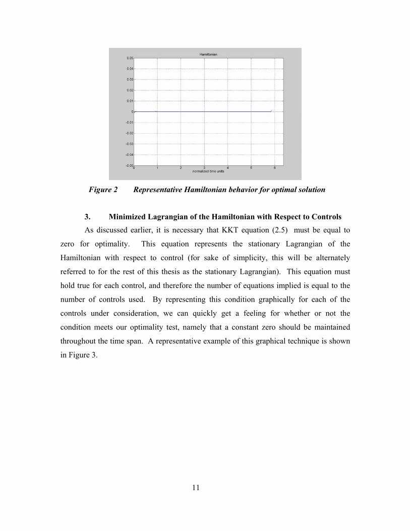
11

Figure 2 Representative Hamiltonian behavior for optimal solution

3. Minimized Lagrangian of the Hamiltonian with Respect to Controls As discussed earlier, it is necessary that KKT equation (2.5) must be equal to

zero for optimality. This equation represents the stationary Lagrangian of the

Hamiltonian with respect to control (for sake of simplicity, this will be alternately

referred to for the rest of this thesis as the stationary Lagrangian). This equation must

hold true for each control, and therefore the number of equations implied is equal to the

number of controls used. By representing this condition graphically for each of the

controls under consideration, we can quickly get a feeling for whether or not the

condition meets our optimality test, namely that a constant zero should be maintained

throughout the time span. A representative example of this graphical technique is shown

in Figure 3.

12

Figure 3 Representative behavior of the stationary Lagrangian of the

Hamiltonian with respect to controls for optimal solution (six controls)

4. Complementarity Condition As described by equation (2.6), a relationship exists between the Lagrange

multipliers and the controls under observation. By graphically representing these

together, a definite pattern of switching should occur. For example, when the control

multiplier is less than zero, its associated control should be at its minimum value.

Similarly, when the multiplier is greater than zero, the control should be at its maximum.

When the multiplier crosses through zero, the control should demonstrate a switch from

one condition to the other, consistent with the direction of the crossing. Again, a

graphical technique will be used for compliance, and a representative example is shown

as Figure 4.

13

Figure 4 Representative optimal control switching behavior (one control)

Some further explanation of control switching behavior and model behavior is

warranted here. One of the input parameters used with the model is the number of

discrete time nodes to be used for a given scenario run. This can be roughly equated as a

measure of resolution with which the discrete solution can approximate a continuous time

result. For the sake of processing speed, the number of nodes can be set low. When

observing the switching behavior, this can sometimes have the adverse effect of making

the control appear as if it is not achieving maximum or minimum (bang-bang) control,

but that the control is throttling in some manner. When the number of nodes for a given

scenario is increased, bang-bang control is more evidently displayed.

Generally, the nodal number for the scenarios studied is set at what is to be

considered mid-range. In some cases, bang-bang control is not immediately evident,

however, when the number of nodes is increased, bang-bang control can generally be

observed.

5. Others Although the above mentioned conditions were primarily used as verification of

optimality for modeling, there are other conditions which were deemed overly complex

14

to prove for little residual return for the already complicated equations of motion under

consideration in this research. These conditions include development of adjoint

equations and determination of further terminal transversality conditions, which can be

reviewed in greater depth in the text by Bryson and Ho (1975).

C. SCALING

One of the peculiarities of working with optimal control codes is that they

perform best when the inputs are well scaled relative to one another [Ross and Fahroo,

(2002)]. The inputs used should be numerically close to each other in an attempt to avoid

calculations involving vastly different number ranges which might throw answers outside

the bounds of computational precision. By scaling inputs prior to computation, we can

avoid these problems entirely as long as we maintain the understanding that outputs of

the system will also be in scaled variables. This can be easily rectified by reversing the

scaling process at the end of the computation to achieve results in the same units as the

original inputs.

The choice of a particular set of state variables can go a long way in assisting with

this scaling problem. If the elements of the state vector are naturally well scaled, matters

are simplified somewhat, as will be demonstrated in the following chapter.

D. CONCLUSIONS

The basic theory of the Minimum Principle has been summarized, and the

following chapters will show how this theory will be applied to the specific topic of this

research. The tenets of the Minimum Principle will be used throughout this thesis, and

form the basis for all verifications of optimality that will be discussed.

15

III. THE EQUINOCTIAL ELEMENT SET

In order to build a model which is universally applicable to any orbit transfer

problem, we need to define equations of motion which can be applied to all potential

conditions. These equations can be defined in any way that ultimately describes orbital

motion of a body around a central gravitational force; however, we want to simplify this

as much as possible so that no “special cases” exist that fall outside the chosen equations

and complicate the algorithms.

A. DRAWBACKS OF THE ORBITAL ELEMENT SET One of the most commonly used element sets in orbital mechanics is the classical

orbital element (COE) set. Although this set is fairly easily understood, it has well

known cases for which it exhibits singularities [Vallado (2001)]. In particular, certain

elements become undefined in either perfectly circular orbits or equatorial orbits. For

zero eccentricity orbits, the argument of periapsis has no meaning. For zero inclination

orbits, the right ascension does not exist. Substitutions for these “special cases” must be

accounted for in order to have a universally applicable tool. Although scaled to canonical

values, Delaunay elements exhibit similar difficulties with these special cases. While the

difficulties are not large enough to discount these element sets from use (workarounds

can be coded into the model), these reasons as well as a new challenge drove the early

decision to research the use of an alternate element set which did not pose these

problems, namely the equinoctial orbital element (EOE) set.

B. DEFINITION OF THE EQUINOCTIAL ELEMENTS

An overview of the equinoctial elements, widely credited to Broucke and Cefola

(1972) for initial exploration, is provided in this section. Although several conventions

have been used in various published discussions of these elements, the convention used

by Battin (1999) has been adopted, and a more detailed derivation of these elements

exists there. Although these elements can be applied to parabolic and hyperbolic orbits

16

with some variation [Coverstone and Prussing (2003)], this version of the model has been

limited to elliptical orbits (including circular orbits) only.

To begin describing the equinoctial element set, the reference frame will first be

defined. The equinoctial elements are best defined within the fgw equinoctial frame as

illustrated in Figure 5. This frame can be described as a three rotation sequence from the

xyz frame: a positive Ω rotation about z , a positive i rotation about f , and a negative Ω

rotation about w .

Figure 5 Equinoctial reference frame

There are six elements in the equinoctial element set, listed below and depicted in

Figure 6:

• a = semimajor axis

• P1 = g-component of the eccentricity vector

• P2 = f-component of the eccentricity vector

• Q1 = g-component of the ascending node vector

• Q2 = f-component of the ascending node vector

17

• L = true longitude

Figure 6 Equinoctial Orbital Elements

In order to help understanding, we can define these elements as they relate to the

classical elements: semimajor axis, eccentricity, inclination, right ascension of ascending

node, argument of perigee, and true anomaly ( , , , , ,a e i ω νΩ ), as discussed by Danielson

et al (1995).

The semimajor axis for the EOE set is the same as that of the COE set, in line

with standard conic geometry, and will be assumed to require no further explanation.

The P1 and P2 elements together have a magnitude equal to the eccentricity of the

orbit and form a vector that points to periapsis from the gravitational center, where:

1 sin( )P e Iω= + Ω (3.1)

2 cos( )P e Iω= + Ω (3.2)

The variable I as used here is a retrograde factor, which is +1 for direct orbits and

-1 for retrograde orbits. However, this is ignored by many texts since the -1 factor is only

required for true retrograde orbits (i.e. – exhibiting 180° inclination), which are very

rarely used.

18

The Q1 and Q2 elements together have a magnitude dependent on the inclination

and form a vector that points to the ascending node from the gravitational center, where:

1 tan sin2

IiQ = Ω

(3.3)

2 tan cos2

IiQ = Ω

(3.4)

The L element defines position of the satellite in the orbit, and is considered the

only rapidly changing variable in this element set. It is related to the classical true

anomaly, right ascension, and argument of perigee by the following:

L Iω ν= + + Ω (3.5)

C. FEATURES OF THE EQUINOCTIAL ELEMENT SET Equinoctial elements are a very good candidate for this thesis for reasons

discussed below. Unfortunately, they can be mathematically challenging to use in

practice, and this perhaps remains their principal drawback. However, through careful

and thorough coding, this problem can be overcome.

1. Elimination of Singularities The primary reason EOEs were chosen for the model is that they do not suffer the

singularity problems exhibited by the COE set and others in dealing with circular and

equatorial orbits. Since (ideally) equatorial orbits and (ideally) circular orbits play such a

prominent role in the satellite systems that we use, it was desired to model using a system

which could easily handle these cases. In fact, the only orbit for which the principal

equinoctial elements exhibit a singularity is direct retrograde (i.e., – exhibiting 180°

inclination), and this can be rectified by using a retrograde factor as discussed

previously3.

3 Similarly, using the retrograde factor at -1, the only orbit where the retrograde elements exhibit singularity is for inclination of 0°.

19

2. Scaling

As discussed previously, scaling is a major consideration when performing

optimal control computations, and using naturally well scaled state variables has instant

benefit. Equinoctial orbital elements are such variables, and with the possible exception

of the semimajor axis, the rest of the variables are already well scaled. Several constants

that are used globally within the modeling code also need to be scaled in order to ensure

efficient computation. The following is a discussion of how scaling is performed for the

model used in this research.

First, four primary constants are defined which seed the scaling process.

Although these values remain constant for a given run of the model, these values are

modeled as variables for ease of modification for different runs. The constants used are

thruster exit velocity (ve=Isp*g0; where specific impulse (Isp) and Earth’s gravitational

acceleration (g0=9.81*10-3 km/sec) are inputs not used beyond this calculation), max

thrust (Tmax), the gravitational constant for an Earth centered system (µ0=398600.4415

km3/s2), and the initial mass of the satellite (M0). These constants serve as the basis for

further scaling, and are used in scaled form globally within the model.

Next, generic scaling factors are developed to convert physical units to scaled

units. The five principal scaling factors are:

• Du (Distance Unit) = Radius of the Earth, 6378.1363 km

• Mu (Mass Unit) = M0

• Tu (Time Unit) = 3

0

DUµ

• Fu (Force Unit) = 2

*Mu DuTu

• Vu (Velocity Unit) = DuTu

Using these factors, scaled versions of the principal constants are developed for

further use throughout the model code:

20

Scaled ve = vVu

e (3.6)

Scaled Tmax= maxTFu

(3.7)

Scaled µ0 = 2

0 3

TuDu

µ (3.8)

Scaled M0 = 0MMu

(3.9)

As mentioned above, the equinoctial orbit elements are naturally suited to scaling.

With the exception of the semimajor axis, which when provided in kilometers must be

divided by the Du scale factor to normalize, the remainder of the elements are well

scaled. The P1 and P2 variables are converted from COEs using sin and cos functions and

therefore fall between 0 and 1 automatically. The Q1 and Q2 variables are converted

using a tan function, and although they are well behaved for most values, they exhibit

difficulty as inclination approaches 180˚ (when I = 1) and must be limited by enforcing

bounds, as will be discussed in the following chapter. The true longitude is measured in

radians in orbit and therefore increases slowly enough (2π per orbit) not to be an issue

over relatively short periods.

3. Mathematical Complexity

Unfortunately, the benefits of EOEs do not come without a price. Working with

the elements can quickly become very complicated mathematically, as evidenced in the

works of Betts (2001), Kechichian (1990, 1991), and others. Although these sources

provide excellent treatments of the complicated matrix mathematics required for classical

application, the use of the tools involved in this research have made replication of most of

this work unnecessary outside of a formulation of the equations of motion. This in itself

has proven to be one of the major benefits of this research, and will be covered in more

detail in the following chapter.

21

D. TRANSFORMATION OF EQUINOCTIAL ELEMENTS TO POSITION AND VELOCITY

Transformations of equinoctial elements to classical elements can be

accomplished simply by reversing the equations provided earlier in this chapter.

However, for some applications, transformation directly to position and velocity vectors

is preferred. The following equations [Battin, (1999)] provide the means of this

transformation.

cossin

0

Lr L =

r (3.10)

1

2

sincos0

P Lh P Lp

− − = +

v (3.11)

2 20 1 2

2 21 2

1 22 2

1 2

0

where:

h = angular momentum = (1 )

(1 )radius from gravitational center = 1 sin( ) cos( )

semiparameter (1 ) gravitational constant

a P P

a P PrP L P L

p a P P

µ

µ

− −

− −=

+ +

= = − −=

A rotation matrix must be used to transform these resultant vectors from fgw

coordinates to xyz coordinates:

2 21 2 1 2 1

2 21 2 1 2 22 2

1 2 2 21 2 1 2

1 2 21 2 1 2

12 2 1

Q Q Q Q QQ Q Q Q Q

Q QQ Q Q Q

− + = + − − + + − − −

R (3.12)

Using these together:

xyz frame fgw frame

xyz frame fgw frame

=

=

r R *r

v R * v (3.13)

22

E. CONCLUSIONS The judicious selection of state variables can provide much benefit to a particular

problem. For this research, equinoctical orbit elements have been chosen due to

favorable scaling properties and lack of singularities for all orbits. The following chapter

will describe how these states will be employed into dynamic equations completely

describing orbital motion, and form the foundation for all of the research that follows.

23

IV. FORMULATION OF THE PROBLEM

In order to move away from the broad theory that has been discussed thus far and

work into the specific applications for the problem under study, a specific optimal control

problem used throughout this research will be formulated. The following development

will be performed for a single agent; however as will be later shown, the desired multi-

satellite problem is a relatively simple extension of this basic problem.

A. STATES AND CONTROLS As discussed earlier, the states are the equinoctial orbital elements. The state

vector is symbolically expressed as follows:

1

2

1

2

aPP

x QQLM

=

(4.1)

Mass is required to represent changes as fuel is consumed by the satellite’s

thrusters.

The control variables for this problem were decided to be six body-fixed thrusters:

one for each direction in the +/- XYZ scheme. This decision was in part based on

considerations of using the L1 control norm for mass flow calculation, and follows

discussion by Ross (2004) regarding minimum fuel controllers. Thus, the controls used

for this problem are:

24

1

1

1

2

2

2

r

t

n

r

t

n

TTT

uTTT

=

(4.2)

Here T represents thrust, r, t, and n represent radial, transverse, and normal directions,

and the 1 and 2 subscripts represent positive and negative directions respectively. Thus,

1 1 1 r2 2 2, , 0 while T , , 0r t n t nT T T T T≥ ≤ . A diagram of this convention is shown in Figure 7.

Figure 7 Satellite thrust convention diagram. Note, positive normal thrust Tn1 not

shown

B. COST The main goal of this research is to minimize the amount of fuel consumed during

commanded maneuvers. As discussed previously, this can also be stated as maximizing

the final mass of the vehicle. If we consider the Bolza cost functional, then only the end-

point Mayer cost E needs to be considered, so that:

( ( ), )f f fJ E x t t M= = − (4.3)

Here the state variable M is the mass of the satellite at any point in time, and Mf is the

final mass of the vehicle, the variable to be maximized.

25

C. DYNAMIC EQUATIONS OF MOTION The maximization of the performance index Mf must be accomplished subject to

dynamic equations governing orbital motion. These equations are based on the

derivatives of the state variables, and can be represented simply as:

1

2

1

2

( , )

aPP

x f x uQQLM

= =

(4.4)

The right hand sides of seven the differential equations, f(x,u), are intricately

coupled. As stated previously, the derivation of the full equations is based on Battin’s

text (1999) coupled with the chosen controls. The full equations of motion can be written

as follows:

21 21 2

2 1 = 2 ( sin( ) cos( ))h

t tr r T TT Ta pa P L P LM r M

++ − +

(4.5)

1 21 21 1

1 22 1 2

cos( ) 1 sin( )

( cos( ) sin( ))

t tr r

n n

T TT Tr p pP L P Lh r M r M

T Tr P Q L Q Lh M

++ = − + + + + − −

(4.6)

1 21 22 2

1 21 1 2

sin( ) 1 cos( )

+ ( cos( ) sin( ))

t tr r

n n

T TT Tr p pP L P Lh r M r M

T Tr P Q L Q Lh M

++ = + + + + −

(4.7)

2 2 1 21 1 2(1 )sin( )

2n nT TrQ Q Q L

h M+ = + +

(4.8)

2 2 1 22 1 2(1 )cos( )

2n nT TrQ Q Q L

h M+ = + +

(4.9)

26

( ) 1 22 12

0

= sin( ) cos( ) n nT Th rhL Q L Q Lr p Mµ

+ + −

(4.10)

1 2 1 2 1 2( ) ( ) ( )- r r t t n n

e

T T T T T TMv

− + − + −= (4.11)

2 20 1 2

2 21 2

1 22 2

1 2

0

e

where:

= angular momentum = (1 )



v exit velocity of thruster

h a P P

a P PrP L P L

p a P P

µ

µ

− −

− −=

+ +

= = − −==

D. EVENTS Since this is a two point boundary value problem, the only events required are the

initial and final boundary conditions for the state variables. Further, since we are looking

to maximize final mass, Mf can be left undefined. Thus, our relevant boundary events

are:

0

1 0 1

2 0 2

1 0 1

2 0 2

0

0

( )( )( )( )( )

( )( )

i

i

i

i

i

i

i

a t aP t PP t PQ t QQ t QL t LM t M

===

====

1 1

2 2

1 1

2 2

( )

( )

( )

( )

( )

( )

f f

f f

f f

f f

f f

f f

a t a

P t P

P t P

Q t Q

Q t Q

L t L

=

=

=

=

=

=

Outside of some path constraints and defining constants, these are the only inputs

required by the model to determine optimal control.

E. STATE AND CONTROL BOUNDS Some boundaries need to be enforced on states and controls in order to define a

subset of possible solutions inside of which we will find a locally optimum one. This

27

helps to constrain a potentially mathematically infinite range of possible solutions to

some reasonable (but not overconstrained) subset. Each of the set boundaries bears some

discussion, but state bounds have been set as follows. Note that all values shown are

scaled as previously discussed.

1. State Bounds The bounds on semiparameter are straightforward, and are simply 1 Earth radius

as the lower bound (to avoid “Earth intercept” orbits), and an arbitrarily large number

(not infinity for computational reasons) as the upper bound.

1 10000a≤ ≤ (4.12)

The bounds on P1 and P2 are set in order to constrain the possible set to elliptical

orbits only, since the two parameters are based upon the orbit’s eccentricity

( )2 21 2e P P= + . This relationship is also defined as a path constraint in order to

maintain ellipticity within the transfer (i.e., 0 1e≤ < ). In reality, both P1 and P2 can not

be at the maximum (or minimum) value at the same time; however, the bound is set at

less than 1 so that a parabolic orbit (i.e., where e=1) is not achieved if one value equals 1

while the other is 0.

1

2

.999 .999.999 .999

PP

− ≤ ≤− ≤ ≤

(4.13)

The bounds on Q1 and Q2 are again simply set arbitrarily high. Since the

conversion to the Q variables is reliant on a function involving tan(i/2), most values are

within reasonable scaled ranges. However, as i approaches 180°, these values begin to

grow towards infinity, so must be given room to run.

1

2

10000 1000010000 10000

QQ

− ≤ ≤− ≤ ≤

(4.14)

28

The bounds on true longitude are set between zero and an arbitrarily high upper

value which is set as a constant within the model code.

0 10000L≤ ≤ (4.15)

The bounds on mass are set between an arbitrary non-zero minimum, with the

initial mass of the satellite used for the upper bound. The minimum can be set as a way

of defining the usuable propellant portion of the satellite mass and must be greater than

zero (since equations (4.5) - (4.10) are singular for M=0).

minf iM M M≤ ≤ (4.16)

2. Control Bounds The bounds levied on the control variables are fairly straightforward. A

maximum thrust is defined as a constant based on the individual thruster being modeled.

The positive and negative directions for each dimension are then just set by convention as

being between 0 and the max thrust for that direction. The upper and lower bounds are

determined by which direction that thruster operates, as follows:

1 max

1 max

1 max

max 2

max 2

max 2

0 0 0

000

r

t

n

r

t

n

T TT TT T

T TT TT T

≤ ≤≤ ≤≤ ≤

− ≤ ≤− ≤ ≤− ≤ ≤

(4.17)

F. PATH CONSTRAINTS For the single agent model, only one path constraint has been levied on the

system. As has been previously mentioned, a path constraint was created in order to

ensure that orbits remained elliptical at all times, including transfer. This was done to

keep parabolic and hyperbolic trajectories from being considered during transfer, and to

assist computational efficiency. Since this model was built to only consider the

mathematics of elliptical orbits, this constraint serves to keep solutions within an

29

understood regime and avoid wandering into territory for which the system has not been

suitably tested4. The path constraint simply stated is:

2 21 20 1P P≤ + < (4.18)

As we will show later, additional path constraints must be added once we consider

multi-agent models in order to ensure that collision avoidance between agents can be

maintained, as well as to provide relational operating windows between agents.

G. DEVELOPMENT OF THE HAMILTONIAN The Hamiltonian of the subject system of equations can be represented in a fairly

straightforward manner (avoiding full expansion for the time being):

1 2 1 21 2 1 2( ) ( ) ( ) ( ) ( ) ( ) ( )f a P P Q Q L MH M a P P Q Q L Mλ λ λ λ λ λ λ= − + + + + + + + (4.19)

Here λ represents Lagrangian multipliers of the state variables, as previously

discussed. Since none of the dynamic equations are explicitly dependent on time, and

following the previously discussed Hamiltonian Evolution equation (2.7), we find:

0dH Hdt t

∂= =∂

(4.20)

The natural conclusion to this statement is that the Hamiltonian must exhibit

constant behavior at all points in time during the optimal span, since 0H = . Further,

following the discussion of the Hamiltonian Value condition (2.8), we find:

4 However, by altering the semimajor axis state to semiparameter (p=a(1-e2)), it is believed that this

model can be developed to work with hyperbolic orbits as well

30

1 1 2 2 1 1 2 2

1

2

1

2

1 1

2 2

1 1

2 2

( )

( )

( )

( )

( )

( )

( )

( )

:

( ) 0

ff

i i f a a P P P P Q Q Q Q L L M M

a f

P f

P f

Q f

Q f

L f

M f

ff

EH tt

E E e M e e e e e e e

e a t a

e P t P

e P t P

e Q t Q

e Q t Q

e L t

e M t

SoEH tt

ν ν ν ν ν ν ν ν

∂= −

∂

= + = − + + + + + + +

= −

= −

= −

= −

= −

=

=

∂= − =

∂

(4.21)

Since the Hamiltonian is zero at the end state, and we have shown that the

Hamiltonian must remain constant throughout the optimal control span, we must

conclude that a constant zero must be maintained throughout the control span for a given

solution to this problem to be considered optimal.

H. DEVELOPMENT OF THE LAGRANGIAN OF THE HAMILTONIAN Using the above results, we can now express the Lagrangian of the Hamiltonian

as follows:

1 2 1 2

1 1 1 2 2 2

1 2 1 2

1 1 1 2 2 2

( ) ( ) ( ) ( ) ( ) ( ) ( )

r t n r t n

f a P P Q Q L M

T r T t T n T r T t T n

H M a P P Q Q L M

T T T T T T

λ λ λ λ λ λ λ

µ µ µ µ µ µ

= − + + + + + + +

+ + + + + + (4.22)

Here µ represents Lagrangian multipliers on the control variables, as previously

discussed. According to KKT theory, the Lagrangian of the Hamiltonian is stationary

with respect to the optimal control at all points in time over the optimized interval, as

previously shown in equation (2.5) , so that:

0Hu

∂=

∂ (2.5)

31

If we expand this relationship to its full glory, we get the following set of

equations which represent the stationarity of the Lagrangian of the Hamiltonian with

respect to the controls, and which will be used for further proof of optimality:

1

2

1

2

2 11

2 ( sin cos ) cos

sin 0v r

Pa

r

P MT

e

H a pP L P L LT M h M h

p LM h

λλ

λ λ µ

∂ = − − ∂

+ − + =

(4.23)

1

2

2

2

2 12

2 ( sin cos ) cos

sin 0v r

Pa

r

P MT

e

H a pP L P L LT M h M h

p LM h

λλ

λ λ µ

∂ = − − ∂

+ + + =

(4.24)

1

2

1

2

11

2

2 1 sin

1 cos 0v t

Pa

t

P MT

e

H a p r pP LT M h r M h r

r pP LM h r

λλ

λ λ µ

∂ = + + + ∂ + + + − + =

(4.25)

1

2

2

2

12

2

2 1 sin

1 cos 0v t

Pa

t

P MT

e

H a p r pP LT M h r M h r

r pP LM h r

λλ

λ λ µ

∂ = + + + ∂ + + + + + =

(4.26)

( )( ) ( )( )

( ) ( )

( )

1 2

1

1

2 1 2 1 1 21

22 2 2 21 2 1 2

2 10

cos sin cos sin

1 sin 1 cos2 2

sin cos 0v n

P P

n

Q Q

L MT

e

H r rP Q L Q L P Q L Q LT M h M h

r rQ Q L Q Q LM h M h

rh Q L Q LM p

λ λ

λ λ

λ λ µµ

∂ = − + − + + − ∂

+ + + + + +

+ − − + =

(4.27)

( )( ) ( )( )

( ) ( )

( )

1 2

1

2

2 1 2 1 1 22

22 2 2 21 2 1 2

2 10

cos sin cos sin

1 sin 1 cos2 2

sin cos 0v n

P P

n

Q Q

L MT

e

H r rP Q L Q L P Q L Q LT M h M h

r rQ Q L Q Q LM h M h

rh Q L Q LM p

λ λ

λ λ

λ λ µµ

∂ = − + − + + − ∂

+ + + + + +

+ − + + =

(4.28)

32

2 20 1 2

2 21 2

1 22 2

1 2

0

e

again where:

h = angular momentum = (1 )



v exit velocity of thruster

a P P

a P PrP L P L

p a P P

µ

µ

− −

− −=

+ +

= = − −=

=

It should be noted that these equations look almost identical for any given +/-

thruster pair, the only differences being the sign on the v

M

e

λ term, as well as the differing

values of the individual Lagrangian control multipliers.

I. COMPLEMENTARITY CONDITION At each instant of time, the multiplier-control pair must satisfy the KKT

complementarity condition, which defines the switching structure of the optimal control:

00

0

i il

i iui

il iu

il iu

u uu u

ifu u u

u uunrestricted

µ

=≤ =≥= < <= =

(4.29)

As an example of this, and using previously discussed values for one of the

controls (Tr1), we can observe:

1

1

1 max

1 max

max

000

00

0

r

r

rT

r

TT T

ifT T

Tunrestricted

µ

=≤ =≥= < <= =

(4.30)

By observing behavior following this discussion, we can use this as a third data

point in validating optimal control.

33

J. CONCLUSIONS Having now developed the specific equations, conditions, and tools for achieving

and proving optimal control, we can now focus on validating that these building blocks

and the model built upon them works according to the Minimum Principle.

34


35

V. MODEL VALIDATION

Having established the basic methods and processes of solving optimal control

problems, this section will demonstrate how the formulations work as expected.

Once coded, the model was validated by running well documented simple optimal

control scenarios and observing the results for agreement. The rest of this chapter

discusses the efforts performed and their results in confirming optimal control behavior

by the model.

A. MODEL NOTES As has been alluded to previously, the MATLAB™ based model accepts inputs in

the form of Keplerian orbital elements, then automatically performs the conversion to

equinoctial elements, including automatic scaling for computational efficiency. This was

deemed the most appropriate and easily understood method of input, since classical

elements are considered somewhat of a basic standard among astrodynamicists.

However, once the conversion is made to equinoctial elements by the model, all internal

calculations are in scaled equinoctial variables for purposes of singularity avoidance.

For the purposes of all of the scenarios run used in this thesis, a uniform set of

constants was used, and they are:

20

0

max

3 20

0

320 s

0.00981 km/sv * 3.1392 km/s

T 10 N

398600.4415 km /3000 kg

sp

e sp

I

gI g

sMµ

=

== =

=

=

=

(5.1)

During the following scenarios, no judgment was made as to how much fuel was

consumed by the spacecraft, only proving that it was the optimal amount required for the

requested transfer. This is to say there was no constraint placed on using for example

90% of a vehicle’s mass in fuel to perform a given transfer. For the purposes of this

36

research, this type of constraint was not imposed, but would be the job of mission

planners to determine reasonable fuel-to-payload ratios.

Scenario run speed was not a major focus of this effort, outside of the desire to

generally speed up and automate the process of determining fuel optimal maneuvers.

This is not considered an issue, since current execution times on the order of man-days

are practiced, and this research has produced run times of minutes or less. Approximate

times that individual runs have taken will be noted in the following sections. However,

these times are to be taken with some suspicion since they are platform and software

version specific, and some overhead variance is incurred by running on a network based

Windows operating system. For purposes of general discussion, all scenario runs were

performed on a 3Ghz Intel® Pentium® 4 notebook computer using MATLAB™ 7.0

running DIDO.

B. HOHMANN TRANSFER SCENARIO For the first validation scenario, a classic Hohmann transfer was performed. First

suggested by Walter Hohmann in 1925, the Hohmann maneuver is mathematically

accepted as the most fuel efficient transfer between two circular coplanar orbits,

involving two tangential impulsive burns to start and stop the transfer, and is well

documented by Vallado (1999), Chobotov (2002), Bate, Mueller, and White (1971) and

most introductory texts on orbital dynamics. Although Hohmann’s work only considered

circular orbits, further work by Lawden (1952) validated that tangential burns are also

optimal for some elliptic scenarios.

This orbital transfer was chosen as a classic example of a known two-dimensional

orbit transfer with a known optimal result. Performance compliant with this known

behavior will serve to validate this model for a two-dimensional coplanar transfer, the

first step in validating an overall three-dimensional model.

It should be noted that true Hohmann behavior is not expected from the

simulation since the Hohmann transfer involves impulsive burns at the tangent points.

Since this model involves discrete finite burns, a similar behavior is expected, however

identical performance is not.

37

1. Hohmann Transfer Input Parameters The following Keplerian inputs were provided to the model for evaluation:

i

i

i

7015 km0.0

35* rad180

30* rad180

45* rad180

0* rad180

i

i

i

ae

i π

π

πω

πν

==

=

Ω =

=

=

f

f

f

9567 km

0.0

35* rad180

30* rad180

45* rad180

235* rad180

f

f

f

a

e

i π

π

πω

πν

=

=

=

Ω =

=

=

(5.2)

The number N of discrete nodes used by the model for this scenario is 80. This

number is considered to be reasonably high, and impacts the computational run speed of

the scenario. However it offers the benefit of increased resolution for illustrative

purposes. Computationally speaking, the model independently solves equations

involving the number of state plus control variables times the number of nodes across the

optimal time span:

# variables ( )*x u N= + (5.3)

For this example, this equates to a (7+6)*80=1040 variable problem being

optimized for each instant of time.

2. Hohmann Transfer Performance Given only the above end point conditions, and subject to the cost and dynamic

equations discussed earlier, the following performance was recorded. Graphical

representations of the state and control histories are shown as Figure 8. Mass flow rate is

shown as Figure 9. A pictorial plot of orbital performance is shown as Figure 10. It

should be noted that thrusts occur only in the positive transverse thruster, as expected,

and that the thrust points all fall in the vicinity of the nominal tangent points for this

maneuver. An 80 node run took approximately 124 seconds to execute.

38

Figure 8 Hohmann transfer state and control histories

Figure 9 Hohmann transfer mass flow

39

Figure 10 Hohmann transfer.

It is obvious by observation that this performance does not appear to be a strict

two burn impulsive maneuver, but as expected, a finite burn over several discrete points

closely simulating this behavior. Since limits have been placed on the maximum amount

of thrust available within the model representative of a reasonably sized chemical

thruster, the thruster is never allowed to reach the force required to accelerate the vehicle

by the amount needed for an impulsive maneuver. These differences between theory and

a more realistic model are accentuated by the fact that the model used is based upon

discrete time points rather than a time continuum, which tends to magnify differences in

the thrusting behavior, particularly at low discrete nodal resolution. As the number of

nodes is increased, the behavior becomes more like the theoretical solution. This

seeming discrepancy is one of the sacrifices made for computational efficiency in the

Legendre pseudospectral method, but classical behavior can be extrapolated from these

approximations, and indeed recognized as the number of nodes increases. This will be

seen as a continuous theme through the performance of the scenario runs through this

research, but is no cause for alarm.

40

3. Hohmann Transfer Model Optimal Behavior

a. Hohmann Transfer Feasibility Analysis Feasibility was shown by independently propagating the initial conditions

through the equations of motion using interpolated controls. A graphical representation

of the result is shown as Figure 11, and shows very good behavior. Note that the

propagated solution perfectly overlays the model solution. It can be concluded that the

result is within the feasible set of optimal solutions.

Figure 11 Plots of Hohmann transfer model performance vs. ODE45 propagation

b. Hohmann Transfer Hamiltonian Behavior Graphical representation of the Hamiltonian during the performance

period is shown as Figure 12. In line with our previous discussion, it can be observed

that the Hamiltonian exhibits a near constant zero value for the majority of the run. By

this test condition, it can be concluded that optimal control is being performed.

41

Figure 12 Hohmann transfer Hamiltonian behavior

c. Hohmann Transfer Lagrangian Behavior Graphical representation of the stationarity of the Lagrangian of the

Hamiltonian (with respect to controls) during the performance period is shown as Figure

13 for all six controls. In line with our previous discussion, it can be observed that the

Lagrangian exhibits a near zero value for the majority of the run. By this test condition,

it can be concluded that optimal control is being performed.

42

Figure 13 Hohmann transfer minimized Lagrangian behavior

d. Hohmann Transfer KKT Complementarity Condition Graphical representation of the switching structure for each of the

control/dual pairs is shown as Figure 14, with greater detail visible in Figure 15. This

switching generally follows the criteria described by equation (4.29), and therefore the

conclusion can be made that optimal control is being performed.

Note in Figure 15 that the switch seems to be commanded before the

control dual crosses zero. It is also observed that the value of the costate remains very

close to zero during the thrusting period. This close zero approach by the costate begins

to very closely resemble control/dual behavior reported by Lawden (1963) for an

impulsive maneuver, particularly since a prolonged period of maximum thrust is not

observed. In these plots, the control does not appear to reach maximum value at the

second peak as might be expected; however the control dual is effectively zero at this

point so KKT theorem still holds. It is believed that this behavior is due to internal

tolerance settings perhaps coupled with some scaling issues, which is not a cause for

immediate concern but which will be addressed further in a later section on future work.

43

Figure 14 Switching structure for Hohmann transfer

Figure 15 Detailed switching structure for positive transverse thrust, Tt1, including

expanded blowup (bottom). Behavior approaches that reported by Lawden.

44

4. Hohmann Transfer Scenario Conclusions Based on the performance of the model and our observed compliance with several

of the necessary conditions of optimality, we can reasonably conclude that the model

exhibits optimal control for a two-dimensional (i.e.- coplanar) orbit transfer. As a non-

numerical check, the performance of the model also meets our expectations on how we

believe a Hohmann transfer should be performed. As an added benefit, this scenario has

verified that circular orbits (i.e. – zero eccentricity orbits) do not pose a singularity

problem to the model. This is the first step in validating overall three-dimensional

compliance with the mathematics and physics involved in Keplerian orbits. It also

validates that our derived equinoctial based equations of motion appear to be working as

expected. However, we must perform further validation to ensure the system works for a

three-dimensional case.

C. INCLINATION CHANGE SCENARIO Since the model has been validated for a two dimensional scenario, the next step

is to prove that it works for a three dimensional scenario. For this reason, a simple

inclination change was chosen to be modeled, since we know that the mathematically

optimal control solution occurs at the ascending and/or descending nodes. Additionally,

an eccentricity was added for the initial and final orbits to introduce a new element into

the puzzle. The presentation of this scenario will follow much like the presentation of the

previous scenario, so some of the explanatory details of the methodology will be omitted

as they should now be familiar to the reader.

1. Inclination Change Parameters The following COE inputs were provided to the model for evaluation:

45

i

i

i

9567 km 0.5

35* rad180

10* rad180

225* rad180

0* rad180

i

i

i

ae

i π

π

πω

πν

==

=

Ω =

=

=

f

f

f

9567 km

0.5

45* rad180

10* rad180

225* rad180

359* rad180

f

f

f

a

e

i π

π

πω

πν

=

=

=

Ω =

=

=

(5.4)

Again, an 80 node solution was requested.

2. Inclination Change Performance Given only the above end point conditions, and subject to the cost and dynamic

equations, the following performance was recorded. Graphical representations of the

state and control histories are shown as Figure 16. Mass flow rate is shown as Figure 17.

A pictorial plot of orbital performance is shown as Figure 18. It should be noted that

thrusts occur only in the normal direction in the vicinity of the ascending node, as

expected. An 80 node run took approximately 271 seconds.

Again, it can be observed that this scenario does not behave in impulsive burns at

the nodes as predicted by theory, but rather finite burn limitations still hold true for the

model. The locations of the burns as expected by optimal behavior is unmistakable, and

the previous discussion of bang-bang control is still valid, indicating a period of

maximum thrust at the nodal point results in optimal control.

46

Figure 16 State and control histories for inclination change

Figure 17 Mass flow for inclination change

47

Figure 18 Inclination change

3. Inclination Change Optimal Behavior

a. Inclination Change Feasibility

Feasibility was again shown by independently propagating the initial

conditions through the equations of motion using interpolated controls. A graphical

representation of the result is shown as Figure 19 and shows very good behavior. We can

conclude that the result is within the feasible set of solutions.

48

Figure 19 Plots of inclination change model performance vs. ODE45 propagation

b. Inclination Change Hamiltonian Behavior Graphical representation of the Hamiltonian during the performance

period is shown as Figure 20. In line with our previous discussion, we observe that the

Hamiltonian exhibits a near constant zero value for the majority of the run. By this test

condition, we can conclude that optimal control is being performed.

c. Inclination Change Lagrangian Behavior Graphical representation of the stationary Lagrangian during the

performance period is shown as Figure 21 for all six controls. In line with our previous

discussion, we observe that the stationary Lagrangian exhibits a near zero value for the

majority of the run. By this test condition, we can conclude that optimal control is being

performed.

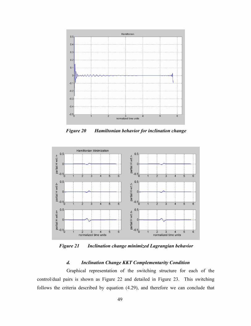
49

Figure 20 Hamiltonian behavior for inclination change

Figure 21 Inclination change minimized Lagrangian behavior

d. Inclination Change KKT Complementarity Condition Graphical representation of the switching structure for each of the

control/dual pairs is shown as Figure 22 and detailed in Figure 23. This switching

follows the criteria described by equation (4.29), and therefore we can conclude that

50

optimal control is being performed. It can be observed that the only control being

exercised is by the –n thruster, Tn2. It can also be observed in Figure 23 that this behavior

again appears to very closely approach Lawden’s (1963) dual/control behavior for an

impulsive burn. Again, manifestations of the scaling/tolerance behavior observed in the

Hohmann scenario can be noted, although in this scenario we do observe the occurrence

of maximum thrust (0.34 scaled units).

Figure 22 Switching behavior for inclination change

51

Figure 23 Switching detail for thruster Tn1, with blow-up

4. Inclination Change Scenario Conclusions Based on the performance of the model and our observed compliance with several

of the necessary conditions of optimality, we can reasonably conclude that the model

exhibits optimal control for a three-dimensional orbit transfer. As a non-numerical

check, the performance of the model also meets our expectations on how we believe an

optimal inclination change should be performed. At first blush, this seems to validate

that our derived equinoctial based equations of motion appear to be working as expected.

However, we researched further scenarios to try to get a better feeling that this was in fact

the case.

D. SEMIMAJOR AXIS CHANGE SCENARIO Although two- and three-dimensional model behavior had been proven, the next

step was to get further data points on model performance in known optimal problems. A

semimajor axis change maneuver was attempted, as first proposed by Lawden (1962).

1. Semimajor Axis Change Parameters The following COE inputs were provided to the model for evaluation:

52

i

i

i

9567 km0.5

35* rad180

10* rad180

225* rad180

0* rad180

i

i

i

ae

i π

π

πω

πν

==

=

Ω =

=

=

f

f

f

9567 km

0.5

35* rad180

10* rad180

315* rad180

359* rad180

f

f

f

a

e

i π

π

πω

πν

=

=

=

Ω =

=

=

(5.5)

2. Semimajor Axis Change Performance Given only the above end point conditions, and subject to the cost and dynamic



A pictorial plot of orbital performance is shown as Figure 26. A 100 node run took

approximately 368 seconds. It should be noted that the optimal controls for the two burn

maneuver occur as predicted by Lawden. Again as discussed previously, differences

between these results and true impulsive behavior can be explained by the discrete time

nature of this modeling.

53

Figure 24 State and control histories for semimajor axis change

Figure 25 Mass flow for semimajor axis change

54

Figure 26 Semimajor axis change transfer orbit

3. Semimajor Axis Change Optimal Behavior

a. Semimajor Axis Change Feasibility Feasibility was once again shown by independently propagating the initial


representation of the result is shown as Figure 27. We can conclude that the result is

within the feasible set of solutions.

55

Figure 27 Plots of semimajor axis change model performance vs. ODE45

propagation

b. Semimajor Axis Change Hamiltonian Behavior Graphical representation of the Hamiltonian during the performance

period is shown as Figure 28. It can be noted that the Hamiltonian exhibits a near

constant zero value for the majority of the run. By this test condition, we can conclude

that optimal control is being performed.

Figure 28 Hamiltonian behavior for semimajor axis change

56

c. Semimajor Axis Change Lagrangian Behavior Graphical representation of the stationary Lagrangian during the

performance period is shown as Figure 29 for all six controls. We again observe that the

minimized Lagrangian exhibits a near zero value for the majority of the run. By this test

condition, we can conclude that optimal control is being performed.

Figure 29 Semimajor axis change minimized Lagrangian behavior

d. Semimajor Axis Change KKT Complementarity Condition Graphical representation of the switching structure for each of the

control/dual pairs is shown as Figure 30. This switching generally follows the criteria

described by equation (4.29), and therefore we can conclude that optimal control is being

performed. It can be observed that the only controls being exercised are by the + and - t

thrusters, Tt1 and Tt2. Although not shown again, expansion of these plots again

illustrates scaling and tolerance issues noted previously.

57

Figure 30 Switching behavior for semimajor axis change

4. Semimajor Axis Change Scenario Conclusions Based on the results of this scenario, we can again conclude that optimal control

is being performed. Although we have already shown this for a coplanar transfer through

the Hohmann scenario, this scenario added complexities in non-zero eccentric orbits, and

provided additional “feel good” data for the model against a known result.

The semimajor axis change actually has two known optimal solutions [Chobotov

(2002)], one involving two burns as has been shown, and one involving a single

impulsive burn at either the upper or lower intersection points of the initial and terminal

orbits. It should be noted that given the right conditions, the model can also approximate

the single burn maneuver. This solution is shown as Figure 31, and it meets all tests for

feasibility and optimality. Again, it does not exactly match the classical impulsive

maneuver, but resemblance to this maneuver is beginning to be achieved, and differences

can be attributed to the particular constraints imposed.

58

Figure 31 Single burn semimajor axis change maneuver

E. MINIMUM TIME TRANSFER SCENARIO

For the final validation, we decided to use the model to perform optimal controls

for a minimum time problem. This involved some additional changes to the model

parameters, since the other problems (and the ultimate aim of the research) all involve

minimizing fuel. However, by using the model in a slightly different context, it was

hoped that final validation of the equations of motion could be achieved independent of

the type of application.

This problem was modeled to replicate a minimum time problem as reproduced in

the text by Bryson (1999), but first documented by Moyer and Pinkham (1964).

1. Minimum Time Transfer Input Parameters The first major change relative to previous validations was a difference in the cost

functional. Since the goal of the minimum time problem is obviously to execute a

maneuver in the minimum amount of time possible, fuel consumption was no longer to

be considered an issue. The cost index was changed to reflect this, from final mass to

final time.

59

The input parameters for this problem are based upon Bryson’s textbook

formulation (pp. 126-128). The unusual values of the numbers are to simulate the

geometry of an Earth to Mars transfer as closely as possible, and therefore the initial

constant values for the model as used previously were modified to simulate Bryson’s

numerical solution. The constant Isp was changed to 492.4567 seconds to match Bryson’s

conditions for this problem. All other constants were left the same. It should be noted,

since the problem as calculated is scaled to make the gravitational constant equal to 1.0, it

is not necessary to change gravity to a sun centered system for this validation.

The Keplerian inputs, per Bryson, were provided as follows:

i

i

i

6378.1 km 0.0

35* rad180

45* rad180

45* rad180

0* rad180

i

i

i

ae

i π

π

πω

πν

==

=

Ω =

=

=

f

f

f

9718.2 km

0.0

35* rad180

45* rad180

45* rad180

235* rad180

f

f

f

a

e

i π

π

πω

πν

=

=

=

Ω =

=

=

(5.6)

2. Minimum Time Transfer Performance Given only the above end point conditions, and subject to the cost and dynamic



A pictorial plot of orbital performance is shown as Figure 34. A 100 node run took

approximately 122 seconds.

60

Figure 32 State and control histories for minimum time transfer

Figure 33 Minimum time transfer mass flow

61

Figure 34 Minimum time transfer. Note period of zero net thrust

An important revelation was made through this performance. It can be readily

observed that this behavior is similar in some respects to that documented by Bryson, but

it can not be considered an extrapolated result as could the other validation scenarios.

Although the thrusting profile appears to spiral similar to what is predicted by Bryson’s

work (Figure 34), a significant portion of the orbit transfer undergoes an unexpected

period of zero net thrust. This is due a major difference between Bryson’s model and

ours, namely his model’s use of a single gimbaled thruster with constant thrust vs. our six

fixed thruster model. Still, intuition would have us believe that a constant thrusting

profile would be necessary for a minimum time maneuver. This apparently troublesome

point will turn out to be very significant, and will be discussed later in the section.

3. Minimum Time Transfer Optimal Behavior

a. Minimum Time Transfer Feasibility Feasibility was once again shown by independently propagating the initial


62

representation of the result is shown as Figure 35. From this, we can conclude that the

result is within the feasible set of optimal solutions.

Figure 35 Plots of minimum time transfer model performance vs. ODE45

propagation

b. Minimum Time Transfer Hamiltonian Behavior Graphical representation of the Hamiltonian during the performance

period is shown as Figure 36. It can be noted that the Hamiltonian exhibits a near

constant value for the majority of the run.

Figure 36 Hamiltonian behavior for minimum time transfer

63

It is observed that the constant value of the Hamiltonian for this case is -1

vs. the zero value observed for the minimum fuel scenarios. This can be expected by

revisiting the Hamiltonian evolution and value condition, similar to the development

carried out in equations (4.19) through (4.21). For the minimum time case, the

Hamiltonian can be written as:

1 2 1 21 2 1 2( ) ( ) ( ) ( ) ( ) ( ) ( )f a P P Q Q L MH t a P P Q Q L Mλ λ λ λ λ λ λ= + + + + + + + (5.7)

The Hamiltonian Evolution then indicates that a constant value must be maintained for optimality, because:

0dH Hdt t

∂= =∂

(5.8)

The Hamiltonian Value condition can then be derived as:

1 1 2 2 1 1 2 2

( )

:

( ) 1

ff

i i f a a P P P P Q Q Q Q L L M M

ff

EH tt

E E e t e e e e e e e

SoEH tt

ν ν ν ν ν ν ν ν

∂= −

∂

= + = + + + + + + +

∂= − = −

∂

(5.9)

Combining the Hamiltonian Value with the Hamiltonian Evolution

indicates that a value of -1 must be maintained by the Hamiltonian during the optimal

control span. By this test condition and our observations then, we can conclude that

optimal control is being performed during this scenario.

c. Minimum Time Transfer Lagrangian Behavior Graphical representation of the stationary Lagrangian during the

performance period is shown as Figure 37 for all six controls. We again observe that the

stationary Lagrangian exhibits a near zero value for the majority of the run. This

particular scenario appears to exhibit some difficulty maintaining optimal control at

64

periods in the vicinity of the large spiral direction shift where thrust is momentarily

directed in a non-optimal manner, however optimality is quickly regained. By this test

condition, we can conclude that optimal control is being performed for the majority of the

run.

Figure 37 Minimum time transfer minimized Lagrangian behavior

d. Minimum Time Transfer KKT Complementarity Condition Graphical representation of the switching structure for each of the

control/dual pairs is shown as Figure 38. This switching follows the criteria described by

equation (4.29), and therefore we can conclude that optimal control is being performed.

A detailed view of this switching on a tighter scale for two of the controls (Figure 39)

indicates that bang-bang control is clearly achieved. This is the type of result sought but

not observed earlier in the minimum fuel scenarios. We can note in this case that the

costate does not remain near zero, but instead passes cleanly and quickly through the zero

crossing, offering some credence to the scaling and tolerance issues noted earlier.

65

Figure 38 Switching structure for minimum time transfer

Figure 39 Switching detail for minimum time transfer, Tt1 and Tt2

66

4. Minimum Time Transfer Scenario Conclusions From the observations of the preceding sections, we can again conclude that

optimal control is being performed. However, as we have noted previously, the thrusting

profile of the maneuver does not instantly meet our intuitive expectations. Despite this

initial observation, upon closer inspection and analysis we find that the model is actually

performing remarkably.

We have already drawn attention to the period of zero net thrust observed in the

plot shown in Figure 34. This was unexpected based on what we were predisposed to

look for based on Bryson’s work. However, the difference between six thrusters and one

(as modeled in Bryson’s text) turns out to be more surprising than we would believe. If

we look closer at the control history shown in Figure 32, we now note two subtle

characteristics. First, the positive and negative normal thrusters are firing at maximum

capacity, equal in magnitude and opposite in direction, for the duration of the scenario.

The net effect of these firings is zero net thrust out of the orbital plane. Second, during a

short period of time during the scenario (approximately TU 1.4 – 1.7), all thrusters are

firing at maximum capacity, with each pair equal in magnitude and opposite in direction,

resulting in zero net thrust during that short period.

The reason for this behavior is explained simply: the model is predicting that

optimal control to achieve a minimum time maneuver given the provided end point

conditions (including the initial fuel load) is to spend energy on zero net thrust maneuvers

in order to dump fuel. By doing so, the satellite lightens its mass in order to achieve the

maximum acceleration possible, an obvious tactic for any maximum speed maneuver.

The model calculates how much fuel it needs to perform the maneuver, and offloads the

rest in order to speed up execution.

We can challenge this assertion by commanding the normal thrusters off for the

duration of the scenario, leaving all other conditions the same (note: this scenario meets

all feasibility and optimality tests as provided previously, but are not shown here for

brevity). By doing this, we can observe in Figure 40 that the transfer takes more time to

execute (2.739 TU vs. 2.365 with normal thrusters on). This result validates that fuel

dumping provides for a faster time solution. It is also observed that the system is firing in

67

plane throughout the profile, and does not go through a period of full fuel dump (Figure

41), more consistent with Bryson’s result5. The time of the switch from positive radial to

negative radial still does not quite match the Bryson profile (which occurs symmetrically

at the transfer halfway point), offering further insight into the differences between one

thruster and effectively four for this case. This appears to be a manifestation of the

difference between an l2 norm based model and our l1 norm based model in associated

mass flow rate characteristics [see Ross (2004)].

Figure 40 State and control history for minimum time transfer (normal thrusters

disabled)

5 However, if we increase the starting mass of the vehicle, fuel dumping again occurs. The lack of fuel

dumping in this case is most likely due to the use of input values scaled from the numerical results reported by Bryson.

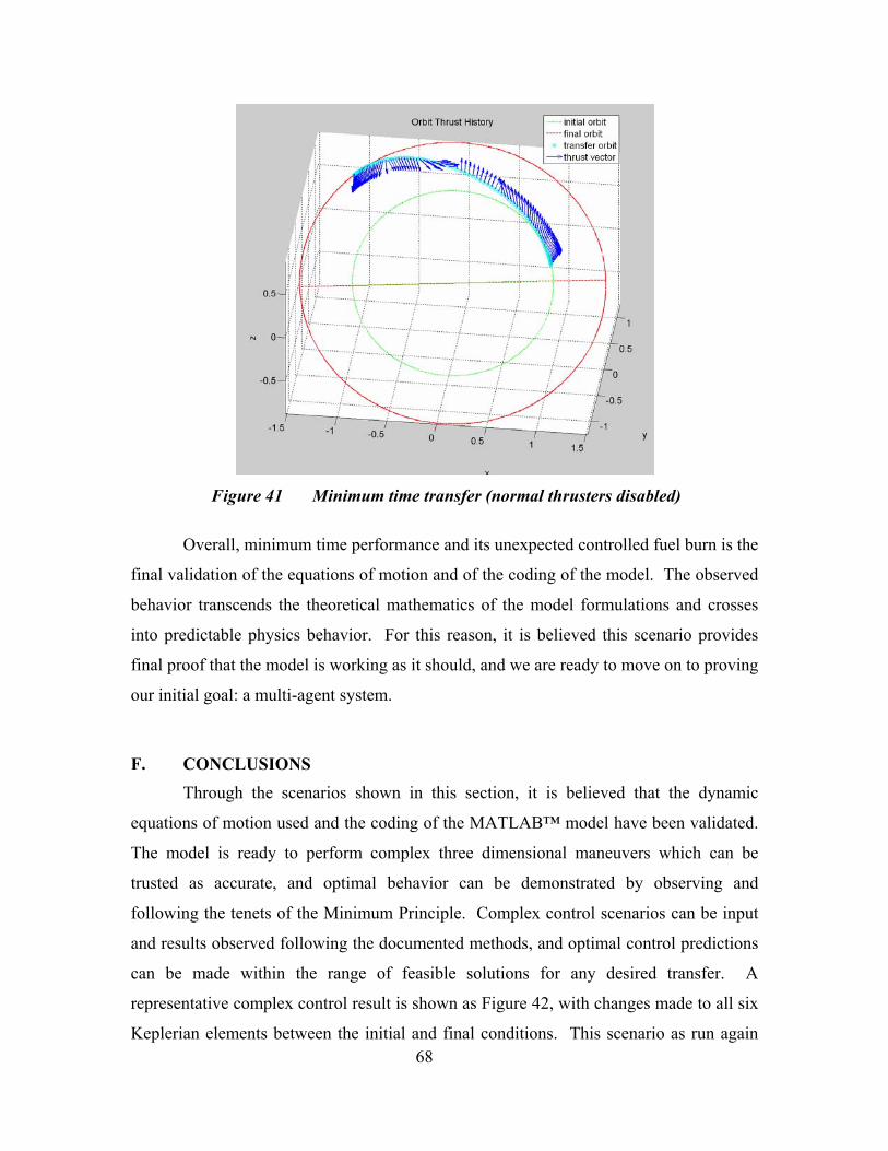
68

Figure 41 Minimum time transfer (normal thrusters disabled)

Overall, minimum time performance and its unexpected controlled fuel burn is the

final validation of the equations of motion and of the coding of the model. The observed

behavior transcends the theoretical mathematics of the model formulations and crosses

into predictable physics behavior. For this reason, it is believed this scenario provides

final proof that the model is working as it should, and we are ready to move on to proving

our initial goal: a multi-agent system.

F. CONCLUSIONS Through the scenarios shown in this section, it is believed that the dynamic

equations of motion used and the coding of the MATLAB™ model have been validated.

The model is ready to perform complex three dimensional maneuvers which can be

trusted as accurate, and optimal behavior can be demonstrated by observing and

following the tenets of the Minimum Principle. Complex control scenarios can be input

and results observed following the documented methods, and optimal control predictions

can be made within the range of feasible solutions for any desired transfer. A

representative complex control result is shown as Figure 42, with changes made to all six

Keplerian elements between the initial and final conditions. This scenario as run again

69

meets all feasibility and optimality tests, although the details are not shown for sake of

brevity. By using this methodology as a baseline, it is hoped that multiple simultaneous

scenarios can be run and predicted for optimal control.

Figure 42 Complex orbit transfer, all classical elements modified

70


71

VI. MULTI-AGENT CONTROL

Having validated behavior of the orbital model for three dimensional motion, the

next step is to modify it for processing multiple agents. The primary goal of this research

was to prove that this could be done by effectively replicating a validated single satellite

problem so that multiple agents could be solved simultaneously. The simultaneous

distinction is important, since relationships can exist between satellites which complicate

matters tremendously if performed in a serial and iterative fashion.

The term “agent” is used generically to refer to the body being optimized. For

this research, an agent can be considered synonymous with a satellite, and the terms will

be used interchangeably within this context.

A. MODEL MODIFICATIONS In order to modify the model to process multiple simultaneous satellites, a careful

act of replication had to be carried out. Far from a simple copy and paste exercise, great

care was maintained in instilling multiple sets of similar variables into the new version.

Certain variables, constants, and subroutines were used universally for all agents, while

others were maintained as agent specific. However, once this process was carried out, it

turned out to be the most difficult part of the leap from single agent to multi agent

problems.

A new consideration in multi-agent problems is establishing relationships

between agents. This is necessary to define certain conditions which the user would like

to maintain. Foremost is collision avoidance: by establishing a minimum safe distance

between satellites, the model can programmed so that two bodies cannot occupy the same

space at the same time. Similarly, a maximum distance can be established. By using the

two together, a relative operating window can be created for the purpose of establishing

formation patterns.

Another new consideration for multi-agent problems is establishing a new

performance index which considers all satellites. Again, for this research minimum fuel

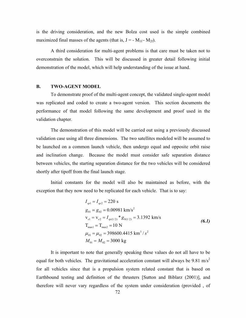
72

is the driving consideration, and the new Bolza cost used is the simple combined

maximized final masses of the agents (that is, J = - M1f - M2f).

A third consideration for multi-agent problems is that care must be taken not to

overconstrain the solution. This will be discussed in greater detail following initial

demonstration of the model, which will help understanding of the issue at hand.

B. TWO-AGENT MODEL To demonstrate proof of the multi-agent concept, the validated single-agent model

was replicated and coded to create a two-agent version. This section documents the

performance of that model following the same development and proof used in the

validation chapter.

The demonstration of this model will be carried out using a previously discussed

validation case using all three dimensions. The two satellites modeled will be assumed to

be launched on a common launch vehicle, then undergo equal and opposite orbit raise

and inclination change. Because the model must consider safe separation distance

between vehicles, the starting separation distance for the two vehicles will be considered

shortly after tipoff from the final launch stage.

Initial constants for the model will also be maintained as before, with the

exception that they now need to be replicated for each vehicle. That is to say:

1 2

201 02

1 2 (1/ 2) 0(1/ 2)

max1 max2

3 201 02

01 02

220 s

0.00981 km/sv v * 3.1392 km/s

T T 10 N

398600.4415 km /3000 kg

sp sp

e e sp

I I

g gI g

sM Mµ µ

= =

= == = =

= =

= == =

(6.1)

It is important to note that generally speaking these values do not all have to be

equal for both vehicles. The gravitational acceleration constant will always be 9.81 m/s2

for all vehicles since that is a propulsion system related constant that is based on

Earthbound testing and definition of the thrusters [Sutton and Biblarz (2001)], and

therefore will never vary regardless of the system under consideration (provided , of

73

course, that these thrusters are manufactured on the Earth). The gravitational parameter µ

is not required to be equal for all agents; however, it will in all likelihood be equal for

most practical applications. All other constants can vary between vehicles, and the model

has capacity for these situations6.

1. Two-Agent Input Parameters For the two-agent model, two sets of initial and final conditions must be

considered. Following the verification cases in chapter V, these parameters are as

follows:

a. Agent 1 (Positive Inclination Change) The maneuver by satellite 1 can be considered much like a combination

between a Hohmann transfer and an inclination change. The initial and final boundary

condition inputs to the model are as follows:

1

1

1

i1

i1

i1

9567.2 km0.0

35* rad180

10* rad180

225* rad180

0* rad180

i

i

i

ae

i π

π

πω

πν

=

=

=

Ω =

=

=

1

1

1

f1

f1

f1

9567.2 km

0.0

55* rad180

10* rad180

225* rad180

200* rad180

f

f

f

a

e

i π

π

πω

πν

=

=

=

Ω =

=

=

(6.2)

b. Agent 2 (Negative Inclination Change) The second agent inputs are identical to the equations in (6.2), with the

exception that the final inclination changes -20˚ rather than +20˚. Additionally, the initial

6 Further, the model has some limited capacity to deal with differences in thrust between thrusters on

the same vehicle, coded as an efficiency factor constant that can be independently set for each thruster. For this thesis, however, the efficiency setting will be left at 100% of the maximum available thrust.

74

true anomaly is slightly different that for satellite 1 for the purpose starting at a safe

keepaway distance for collision avoidance.

1

1

1

i1

i1

i1

9567.20445 km =1.5 RE0.0

35* rad180

10* rad180

225* rad180

.1* rad180

i

i

i

ae

i π

π

πω

πν

==

=

Ω =

=

=

1

1

1

f1

f1

f1

9567.20445 km =2.0 RE

0.0

15* rad180

10* rad180

225* rad180

200* rad180

f

f

f

a

e

i π

π

πω

πν

=

=

=

Ω =

=

=

(6.3)

2. Two-Agent Model Performance State and control history for satellite 1 (performing the positive inclination

change) is shown in Figure 43. History for satellite 2 (performing the negative

inclination change) is shown in Figure 44. Mass flow for both satellites is shown in

Figure 45. Orbital performance for both vehicles is shown in Figure 46.

It can be observed that the two independent satellites closely follow results

demonstrated during the model validation for a Hohmann transfer combined with an out

of plane inclination change maneuver. The individual maneuvers are performed as we

would expect from previous maneuvers, with thruster firings occurring at perigee and

apogee tangent points, as well as at the nodal line for inclination change.

75

Figure 43 Satellite 1 state and control histories

Figure 44 Satellite 2 state and control histories

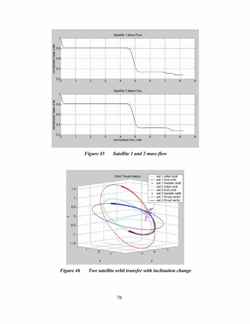
76

Figure 45 Satellite 1 and 2 mass flow

Figure 46 Two satellite orbit transfer with inclination change

77

3. Two-Agent Model Optimal Behavior

a. Agent 1 Feasibility and Optimality Analysis Similar to the methods shown during validation, feasibility and optimality

for satellite 1 are shown below. Feasibility is shown by Figure 47. Hamiltonian behavior

is shown in Figure 48. The minimized Hamiltonian with respect to controls is shown as

Figure 49. Switching behavior for satellite 1 is shown as Figure 50 (note tolerance issues

once again). Observing this data and using the same logic provided during validation, it

can be concluded that satellite 1 is demonstrating optimal control.

Figure 47 Plots of satellite 1 performance vs. ODE45 propagation

78

Figure 48 Multi-agent Hamiltonian behavior (both satellites)

Figure 49 Satellite 1 minimized Lagrangian behavior

79

Figure 50 Switching structure for satellite 1

b. Agent 2 Feasibility and Optimality Analysis Similar to satellite 1, feasibility and optimality for satellite 2 are shown

below. Feasibility is shown by Figure 51. Hamiltonian behavior is shown in Figure 48.

This is the same plot as for satellite 1, since a single Hamiltonian represents the entire

multi-agent problem. The minimized Hamiltonian with respect to controls is shown as

Figure 52. Switching behavior for satellite 1 is shown as Figure 53 (again observing

scaling and tolerance). Observing this data and using the same logic provided during

validation, it can be concluded that satellite 2 is demonstrating optimal control.

80

Figure 51 Plots of satellite 2 performance vs. ODE45 propagation

Figure 52 Satellite 2 minimized Lagrangian behavior

81

Figure 53 Switching structure for satellite 2

4. Two-Agent Model Overconstraint Issue As performed, the two agent model appears to provide accurate prediction of

optimal behavior. The individual satellites behave the same as they do would in a single

satellite model, and defined inter-agent relationships appear to be maintained as desired.

This scenario helps fulfill the goal of our research, and following the work performed in

formulating and validating the problem seems rather anticlimactic. However, at least one

point here bears visitation.

This scenario was largely symmetric, and because of this both satellites were able

to finish in their final required positions at the same time. However, this is not

necessarily true if “mirror image” cases are not requested for the two satellites. If

concurrent solutions are possible, a feasible locally optimal solution may be found that

meets the criteria required (i.e., an overconstrained solution), but is not the best or most

fuel-efficient solution possible if constraints were relaxed. This is the equivalent to

providing a good answer to a bad question.

82

As an example, a scenario was run requesting satellite 1 to perform an inclination

change only (maintaining the initial orbital radius), and satellite 2 to perform a Hohmann

transfer. All constraining end conditions were maintained similar to the double

inclination case. Phasing of the two satellites within their respective final orbits was

requested to be the same (200°), however since satellite 2 terminates in a higher orbit, it

requires a greater amount of time to get there. Performance of this maneuvering is shown

as Figure 54, and all tests for feasibility and optimality are met (but not shown for

brevity).

Figure 54 Multi-agent maneuver involving time constraint difficulty. Note satellite

1 orbit raise to loiter.

It can be observed that with the discussed overconstraint present, the optimal

solution resulted in satellite 1 raising its orbit some to in effect “loiter” and allow satellite

2 time to reach its final position, at which time satellite 1 returns to its lower orbit to

reach its final position at the same time. This does not match what intuitively makes

sense to us, whereby satellite 1 would remain at the same altitude throughout the

maneuver and change inclination at the node, much like the inclination change validation

case discussed in chapter V. The demonstrated maneuver appears comparatively

νf1=200° νf2=200°

83

wasteful of fuel, and is referred to it as a “false positive”, however it needs to be noted

that the requirement that both satellites reach their final locations at the same time drives

this result, and that this is in fact the optimal solution meeting these requirements (again,

a great answer to a bad question).

A solution to this issue is to constrain only one of the vehicles to a final achieved

position, leaving the other to reach all orbital conditions required except for phasing.

Instead, the second agent is allowed to phase itself in its orbit wherever it can while

achieving all other conditions, including orbit and required operating distance with

respect to satellite 1. In this way, a kind of “master/slave” relationship between the

vehicles is implied, whereby satellite 1 dictates to some degree the final positioning of

the constellation. But even this is not enough to avoid all problems, for some care must

be taken in this case to allow enough time for satellite 2 to perform its necessary

maneuvering, or else another less fuel efficient maneuver may occur. For example, using

the same model (sat 1: inclination change; sat 2: Hohmann transfer) if satellite 1 is again

allowed a phase change of 200° to perform its inclination change, and satellite 2 is to

perform a Hohmann transfer, it can be observed that enough time is still not being

allowed for this transfer to occur, and therefore another solution to the problem will be

found which is less fuel efficient (but meeting the conditions requested) (Figure 55).

This is because a Hohmann transfer must undergo a 180° in-plane phase shift in addition

to a radial change, which requires more time to execute than does satellite 1’s maneuver.

Since final position is tied to satellite 1 (the “master”) reaching 200°, and in this time

satellite 2 only shifts 163.4˚, satellite 2 must expend additional fuel at both ends of the

transfer to reach its proper orbit within the allotted time. We can fix this discrepancy by

either setting a larger phase change for satellite 1 which allows satellite 2 to complete a

180° maneuver (Figure 56), or by setting the vehicle with the longer execution time as

the master vehicle (Figure 57). The net fuel consumed is the same for both cases.

84

Figure 55 Satellite 2 (slave) not provided adequate time to perform Hohmann

transfer, resulting in radial thrusting to meet final orbit

Figure 56 Satellite 1 (master) given longer execution time to facilitate Hohmann

transfer by satellite 2

νf1=200° νf2=unprescribed


85

Figure 57 Satellite 1 (master, performing Hohmann transfer) sets constellation

execution time, allowing adequate time for transfer and for satellite 2 inclination change. Note: satellite 1&2 designations switched from previous examples

5. Two-Agent Model Conclusions The two-agent model appears to predict optimal control behavior as expected.

Model performance meets all tests for feasibility and optimality previously used during

validation, and results of individual agents within the multi-agent construct appear to

behave the same as similar single agent validations. Moreover, by observing the

behavior of the Hamiltonian for the entire model, we can conclude that the model as a

whole is behaving in an optimal manner. Some care and consideration had to be paid to

some slight behavioral differences between a single-agent model and a two-agent model,

and the two agent model is more sensitive to how data is input due to time based

relationships between the agents. However, once addressed the two-agent model appears

to perform as expected.

The performance exhibited by this model in a scenario with a somewhat expected

outcome provides proof that this model can be run for any number of scenarios, and using

the Minimum Principle as a guide optimal control can be predicted with confidence. A


86

complex three dimensional two-agent scenario is shown as Figure 58, that meets all tests

for feasibility and optimality using the methods outlined throughout this thesis.

Figure 58 Complex two-agent scenario

C. CONCLUSIONS The proof of concept for a two-agent model is a critical step in proving full multi-

agent optimization capability, for the replication process for three or more agents is

essentially the same as the replication process from one agent to two. Given the

methodology of replication for the two agent model, there is no reason that a greater

number of agents can not be similarly modeled. At the present time, it is believed that

the only limitation on the number of agents possible for simultaneous optimization

involves processing power, which continues to improve with time.

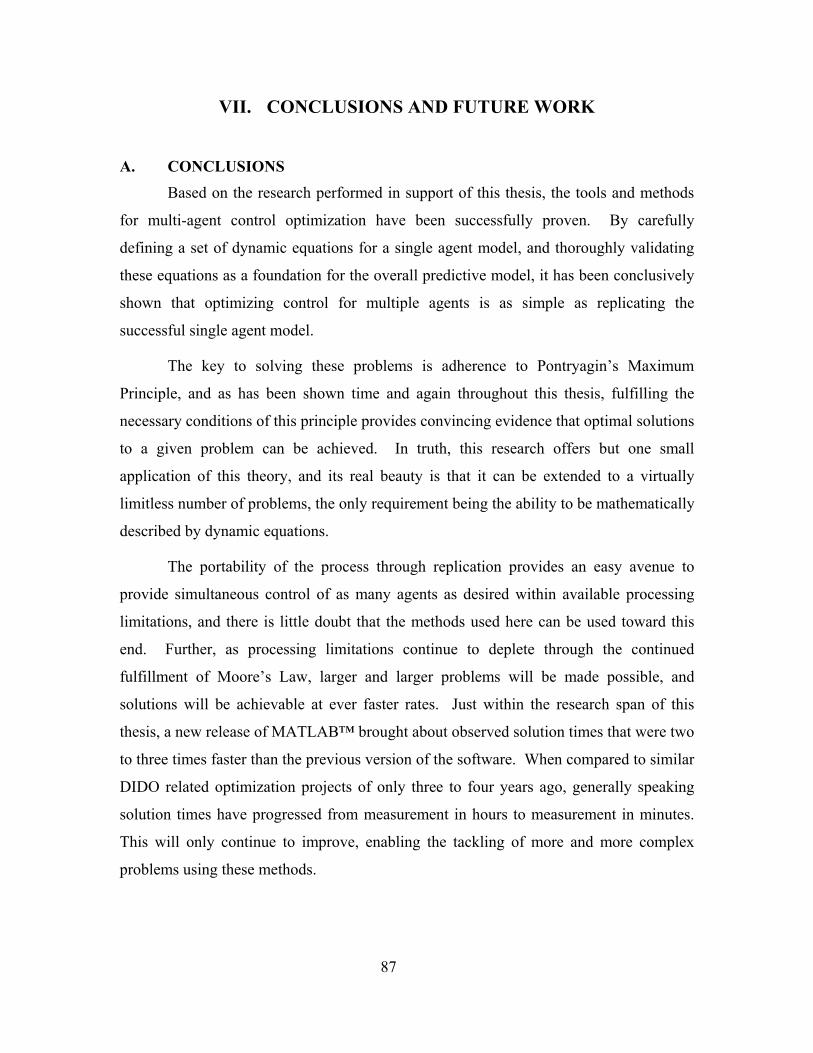
87

VII. CONCLUSIONS AND FUTURE WORK

A. CONCLUSIONS Based on the research performed in support of this thesis, the tools and methods

for multi-agent control optimization have been successfully proven. By carefully

defining a set of dynamic equations for a single agent model, and thoroughly validating

these equations as a foundation for the overall predictive model, it has been conclusively

shown that optimizing control for multiple agents is as simple as replicating the

successful single agent model.

The key to solving these problems is adherence to Pontryagin’s Maximum

Principle, and as has been shown time and again throughout this thesis, fulfilling the

necessary conditions of this principle provides convincing evidence that optimal solutions

to a given problem can be achieved. In truth, this research offers but one small

application of this theory, and its real beauty is that it can be extended to a virtually

limitless number of problems, the only requirement being the ability to be mathematically

described by dynamic equations.

The portability of the process through replication provides an easy avenue to

provide simultaneous control of as many agents as desired within available processing

limitations, and there is little doubt that the methods used here can be used toward this

end. Further, as processing limitations continue to deplete through the continued

fulfillment of Moore’s Law, larger and larger problems will be made possible, and

solutions will be achievable at ever faster rates. Just within the research span of this

thesis, a new release of MATLAB™ brought about observed solution times that were two

to three times faster than the previous version of the software. When compared to similar

DIDO related optimization projects of only three to four years ago, generally speaking

solution times have progressed from measurement in hours to measurement in minutes.

This will only continue to improve, enabling the tackling of more and more complex

problems using these methods.

88

The model and the tools currently have some limitations specific to the studied

orbital problem that have not been discussed in any detail thus far. They will be captured

in the following sections.

B. MODEL ISSUES

1. Limitation on Number of Variables As was touched upon in chapter V of this thesis, the underlying number of

computations inherent in the model can be envisioned as a directly linear function of the

number of discrete points in time (i.e., nodes) chosen for any given scenario (equation

(5.3)). The number of nodes chosen can be simply equated as a measure of achievable

resolution in the problem solution, and this has been illustrated to some degree in the

discussion on bang-bang control.

All of the scenarios that have been demonstrated through this thesis have involved

a small number of orbits, usually less than one. Combining this with a reasonably large

number of nodes has provided a fairly high resolution through the orbital path, which has

resulted in getting a good picture of the necessary controls to achieve a desired result. A

problem starts to rear its head, however, as the number of orbits is increased for a

maneuver. This can be illustrated by first envisioning a 100 node solution for a maneuver

that is constrained to less than one orbit: here 100 points can describe the maneuvers

within the one orbit span adequately for most purposes. Now suppose the maneuver span

is opened up to include potentially 25 orbits using the same 100 nodes spread across the

span. Now only four points on average can be considered per orbit7. If a significant

number of thrust points are required (in a continuous sense), then much of this detail will

be lost in the result.

An obvious solution to this problem is to continue to increase the number of

nodes to as high a resolution as possible, perhaps only at the expense of computation

time. However, the computation engine used within the model appears to suffer for high

7 This is not precisely true, since the mathematical workings of the engine does not spread the nodes linearly across the span. Instead, higher nodal concentrations tend to cluster around the endpoints of the span, which can be easily seen in any of the plots used throughout the validation and multi-agent sections of the thesis.

89

numbers of nodes (on the order of 150 and greater). Although this engine is in theory

unlimited, it involves computations of large matrices which begin to exhibit greater

problems of ill-conditioning. This presents a fundamental problem for higher numbers of

orbits which require large numbers of nodes for good resolution, especially since a great

number of orbital problems are spread over large timeframes for increased fuel

efficiency. For these cases, the only current workaround is to be able to divide the

problem into discrete legs which can be independently run. However, help appears to be

on the way.

The fundamental drawback in the engine appears to originate with the SNOPT

algorithms around which the DIDO optimization tool is wrapped. The makers of SNOPT

appear on the verge of delivering a new version which is much more highly capable,

reportedly to the point of managing variables in the millions vs. the thousands currently.

If this happens, it will render this issue moot, and we can again fall back to complaining

about processing speed.

2. True Retrograde Orbit Despite the promise of zero singularities by using the equinoctial orbital elements,

the model does not work for an absolute retrograde orbit (i.e.- inclination of 180˚) as of

the writing of this thesis. Mathematically, the issue is understood as has been touched

upon in discussion of the “retrograde factor” earlier in this thesis, however as a relatively

late addition to this research, full coding issues throughout the many files, functions, and

subroutines of the otherwise operating model were never fully resolved for this case.

This problem begins to manifest itself greater as inclination approaches 180˚, and only

significantly beyond even 179˚. For this reason, the difficulty is considered a coding

issue and left largely as a footnote at this point, for it is believed solvable with some

significant debugging time, however only useful for a very limited number of realistic

cases and perhaps as an academic exercise. A great number of other cases ranging from

0˚ to greater than 179˚ have been performed with no difficulty. Perhaps this is a major

reason why the subject is completely ignored in many texts, as the vast majority of cases

are performed without the added mathematical complexity, no matter how seemingly

minor.

90

3. Scaling and Tolerance As was noted in several places in this thesis, it is believed that there exist some

issues of scaling and tolerance that are unresolved as of this writing. The scaling issues

appear to manifest in the control duals in minimum fuel problems, and perhaps this

coupled with behavior beginning to approach impulsive behavior [Lawden (1963)] along

with internal zero-tolerance settings provides results which are not completely explained

at this point. It is suggested that this be investigated further in future work on this topic.

C. FUTURE WORK

1. Extension to N Agents The most obvious continuation of this work should involve proof and

characterization of performance for greater numbers of satellites. It is believed at this

point that this exercise should be fairly painless, however no words can substitute for

actually performing the task to show that this is true. Some unanticipated issues arose

with the jump from one to two agents, and some of these issues (such as master/slave

relationships and collision avoidance issues) become more complicated with the addition

of agents. The variable limitation issue discussed above will likely play some factor in

the number of agents achievable until worked out.

2. Scaling Investigation There appear to be issues which manifest in some scenarios run in the model

where the switching structure does not appear to exhibit clean bang-bang behavior as

expected, but rather appears to peak at relatively low number of nodes and “chatter” at a

high number of nodes. These scenarios exhibit control costates which remain relatively

close to zero through the duration of the control chattering, lending to the belief that an

issue of scaling or tolerance may exist within the model. Certain scenarios, such as the

minimum time scenario run in this research, do not exhibit this phenomenon, while most

of the minimum fuel scenarios did to some extent. An investigation into this behavior

should be continued

91

3. Increased Model Fidelity The model in its current form is ideal in the sense that it does not consider

perturbation or drag effects on long term orbit. Since the thrust of this thesis was aimed

at injections of multiple satellites spawned from a single launch vehicle, and it is believed

that these effects are very minor in a relatively frequent thrusting environment, they were

not concentrated on during the proof of concept phase of this research. However, now

that the concept has been proven, addition of these effects is necessary, particularly if this

model is to be extended to other ideas.

4. Sensitivity Analysis A characterization of the model’s sensitivity to various inputs vs. its optimality

signatures should be performed in order to offer a better understanding of effects that the

questions have on the answers. Such an analysis would be useful in helping the operator

determine how to best provide inputs which ensure that optimal solutions are provided in

the most time efficient manner.

5. Extension to Constellation / Formation Control The model has been built to be as generic as possible, and throughout its

development an end goal of realistic long term orbit simulation was envisioned.

Although the concept of trajectory insertion provided a relevant issue on which to

concentrate effort, ideas and problems of formation flying are becoming more and more

widespread in the literature. It is believed that these tools and methods can be adapted

for use in this regime, and therefore maximum and minimum operating distances between

agents have been accounted for in this work with this end in mind. It is believed that this

area offers perhaps the most significant long term extension of this work, and the

prospects in this field are exciting. However, the issues mentioned in the fidelity

discussion above will very likely have to be worked in concert for a truly useful tool to be

achieved.

92

6. Proportional Fuel Expenditure If formation modeling is attempted, great consideration should be given to

ensuring that fuel burn vehicle to vehicle is performed in order to ensure proportional fuel

consumption occurs. This will help to ensure that all vehicles in the constellation deplete

their fuel load at the same time, and making sure that the constellation mission remains

intact for as long as possible. This model accounts for the possibility of different vehicle

masses and fuel loads across all agents, so installation of this type of feature should

merely be application of additional path constraints or a similar means of employment.

7. Interface to Graphical Visualizer and GUI Input Although never accomplished, an interface to some graphical visualization tool,

such as AGI’s Satellite Toolkit® would be a very useful addition to this tool.

Additionally, a long term objective should be made to make this tool as user friendly and

transparent to the operator as possible. Some kind of graphical user interface could easily

be envisioned which removes the user’s need to understand the inner workings of this

model, instead concerning him or herself with only inputs and outputs and not so much

on how to feed the model.

93

LIST OF REFERENCES

Bate, R.R., Mueller, D.B., and White, J.E., Fundamentals of Astrodynamics, New York: Dover Publishing, Inc., 1971 Battin, R.H., An Introduction to the Mathematics and Methods of Astrodynamics, Revised Edition, New York: AIAA, 1999 Betts, J.T., Practical Methods for Optimal Control using Nonlinear Programming, Society for Industrial and Applied Mathematics, 2001 Broucke, R.A., and Cefola, P.J., “On the Equinoctial Orbit Elements”, Celestial Mechanics 5, 1972 Bryson, A.E., Dynamic Optimization, Menlo Park: Addison Wesley Longman, Inc., 1999 Bryson, A.E., and Ho, Y.C., Applied Optimal Control, Washington D.C.: Hemisphere Publishing Corp., 1975

Chobotov, V.A. (ed.), Orbital Mechanics, Third Edition, New York: AIAA, 2002 Coverstone, V.L., and Prussing, J.E., “Technique for Escape from Geosynchronous Transfer Orbit Using a Solar Sail”, AIAA Journal of Guidance Control and Dynamics, Vol. 26, No. 4, 2003 Danielson, D.A., Sagovac, C.P., Neta, B., and Early, L.W., Semianalytic Satellite Theory, NPS-MA-95-002, Naval Postgraduate School, Monterey, CA, 1995 Fleming, A., Real-Time Optimal Slew Maneuver Design and Control, Naval Postgraduate School, Monterey, CA, 2004 Josselyn, S.B., Optimization of Low Thrust Trajectories with Terminal Aerocapture, Naval Postgraduate School, Monterey, CA, 2003 Kechichian, J.A., “Equinoctial Orbit Elements: Application to Optimal Transfer Problems”, in AAS/AIAA Astrodynamics Specialist Conference, AIAA 90-2976-C, Portland, OR, Aug. 1990 Kechichian, J.A., “Trajectory Optimization with a Modified Set of Equinoctial Orbit Elements”, in AAS/AIAA Astrodynamics Specialist Conference, AAS 91-524, Durango, CO, Aug. 1991 King, J.T., A Framework for Designing Optimal Spacecraft Formations, Naval Postgraduate School, Monterey, CA, 2002

94

Kopp, R.E., “Pontryagin Maximum Principle”, in Optimization Techniques, George Leitman, ed., New York: Academic Press, Inc., 1962

Lawden, D.F., “Optimal Transfer Via Tangential Ellipses”, British Interplanetary Society Journal 11, No. 6., 1952 Lawden, D.F., “Impulsive Transfer between Elliptical Orbits”, in Optimization Techniques, George Leitman, ed., New York: Academic Press, Inc., 1962 Lawden, D.F., Optimal Trajectories for Space Navigation, London: Butterworth & Co. (Publishers) Ltd., 1963 Moyer, H.G., and Pinkham, G., “Several Trajectory Optimization Techniques”, in Computing Methods in Optimization Problems, A.V. Balakrishnan and L.W. Neustadt, ed., New York: Academic Press, 1964 Ross, I.M., Fahroo, F., User’s Manual for DIDO 2003: A MATLAB™ Application Package for Dynamic Optimization, Naval Postgraduate School, Monterey, CA, 2002

Ross, I.M., “How to Find Minimum-Fuel Controllers”, Proceedings of the AIAA Guidance, Navagation, and Control Conference, AIAA Paper No. 2004-5346, Providence, RI, August 2004 Shaffer, P.J., Optimal Trajectory Reconfiguration and Retargeting for the X-33 Reusable Launch Vehicle , Naval Postgraduate School, Monterey, CA, 2004 Stevens, R.E., Design of Optimal Cyclers Using Solar Sails, Naval Postgraduate School, Monterey, CA, 2002 Sutton, G.P., and Biblarz, O., Rocket Propulsion Elements, Seventh Edition, New York: John Wiley & Sons, 2001 Vallado, D.A., Fundamentals of Astrodynamics and Applications, El Segundo: Microcosm Press, 2001

95

INITIAL DISTRIBUTION LIST

1. Defense Technical Information Center Ft. Belvoir, Virginia

2. Dudley Knox Library Naval Postgraduate School Monterey, California

3. LCDR Jeff King SPAWAR Space Field Activity Falls Church, Virginia

4. ENS Jay Chaplin SPAWAR Space Field Activity Falls Church, Virginia

Author(s) Mendy, Paul B. Title Multiple satellite

Documents