Ausgew ahlte Mathematische Hilfsmittel Formelsammlung zu ... · U. Thiele Formelsammlung Physik I M arz 2015 Dies ist eine Zusammenstellung einiger mathematischer Hilfsmittel, wie

Ausgewahlte Mathematische Hilfsmittel

Formelsammlung zu Physik I

Uwe Thiele

Institut fur Theoretische PhysikWestfalische Wilhelms-Universitat Munster

Version vom 5. April 2015

Inhaltsverzeichnis

1 Grundlagen der Vektoralgebra 11.1 Vektoren und ihre Produkte . . . . . . . . . . . . . . . . . . . . . . . . . . . . . . 11.2 Einige Identitaten . . . . . . . . . . . . . . . . . . . . . . . . . . . . . . . . . . . 3

2 Koordinatensysteme 32.1 Orthonormierte Basis . . . . . . . . . . . . . . . . . . . . . . . . . . . . . . . . . 32.2 Komponentendarstellung der Produkte . . . . . . . . . . . . . . . . . . . . . . . . 42.3 Auswahl orthonormaler Koordinatensysteme . . . . . . . . . . . . . . . . . . . . . 5

2.3.1 Kartesische Koordinaten . . . . . . . . . . . . . . . . . . . . . . . . . . . . 52.3.2 Polarkoordinaten . . . . . . . . . . . . . . . . . . . . . . . . . . . . . . . . 62.3.3 Zylinderkoordinaten . . . . . . . . . . . . . . . . . . . . . . . . . . . . . . 72.3.4 Kugelkoordinaten . . . . . . . . . . . . . . . . . . . . . . . . . . . . . . . . 8

3 Beschreibung von Bahnkurven 93.1 Parametrisierung von Raumkurven . . . . . . . . . . . . . . . . . . . . . . . . . . 93.2 Differentiation vektorwertiger Funktionen . . . . . . . . . . . . . . . . . . . . . . 9

4 Ableitungen von Feldern 104.1 Skalares Feld . . . . . . . . . . . . . . . . . . . . . . . . . . . . . . . . . . . . . . 104.2 Vektorfeld . . . . . . . . . . . . . . . . . . . . . . . . . . . . . . . . . . . . . . . . 114.3 Partielle Ableitung . . . . . . . . . . . . . . . . . . . . . . . . . . . . . . . . . . . 114.4 Diverse Ableitungen . . . . . . . . . . . . . . . . . . . . . . . . . . . . . . . . . . 11

U. Thiele Formelsammlung Physik I Marz 2015

Dies ist eine Zusammenstellung einiger mathematischer Hilfsmittel, wie sie in Physik I ein-gefuhrt worden sind. Sie ist als Merkhilfe gedacht und kann das regelmaßige Konsultieren vonFormelsammlungen wie [Bronstein] oder [Gradstein] nicht ersetzen. Auch haben die meistenLehrbucher der theoretischen Physik ausfuhrliche Einfuhrungen zu mathematischen Hilfsmit-teln, die auf jeden Fall konsultiert werden sollten, um die jeweils verwendeten Konventionenund Notationen zu verstehen.

1 Grundlagen der Vektoralgebra

1.1 Vektoren und ihre Produkte

Vektor ~a ist geometrisch bestimmt durch Richtung und Betrag (a = |~a|).

Einheitsvektor ~e, e mit |~e| = 1 → ~ea =~a

|~a|hat Betrag

|~a||~a|

= 1.

Addition von Vektoren

~a+~b = ~b+ ~a = ~c

Nullvektor, inverser Vektor

~b+ (−~b) = ~0

Subtraktion von Vektoren

~a+ (−~b) = ~a−~b = ~d

Skalare Multiplikation

~b = λ~a mit λ ∈ R, λ =|~b||~a|

1


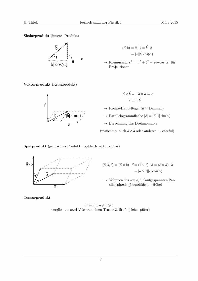
Skalarprodukt (inneres Produkt)

(~a,~b) = ~a ·~b = ~b · ~a

= |~a||~b| cos(α)

→ Kosinussatz c2 = a2 + b2 − 2ab cos(α) furProjektionen

Vektorprodukt (Kreuzprodukt)

~a×~b = −~b× ~a = ~c

~c ⊥ ~a,~b

→ Rechte-Hand-Regel (~a = Daumen)

→ Parallelogrammflache |~c| = |~a||~b| sin(α)

→ Berechnung des Drehmoments

(manchmal auch ~a ∧~b oder anderes → careful)

Spatprodukt (gemischtes Produkt – zyklisch vertauschbar)

(~a,~b,~c) = (~a×~b) · ~c = (~b× ~c) · ~a = (~c× ~a) ·~b

= |~a×~b||~c| cos(α)

→ Volumen des von ~a,~b,~c aufgespannten Par-allelepipeds (Grundflache · Hohe)

Tensorprodukt

~a~b = ~a⊗~b 6= ~b⊗ ~a→ ergibt aus zwei Vektoren einen Tensor 2. Stufe (siehe spater)

2


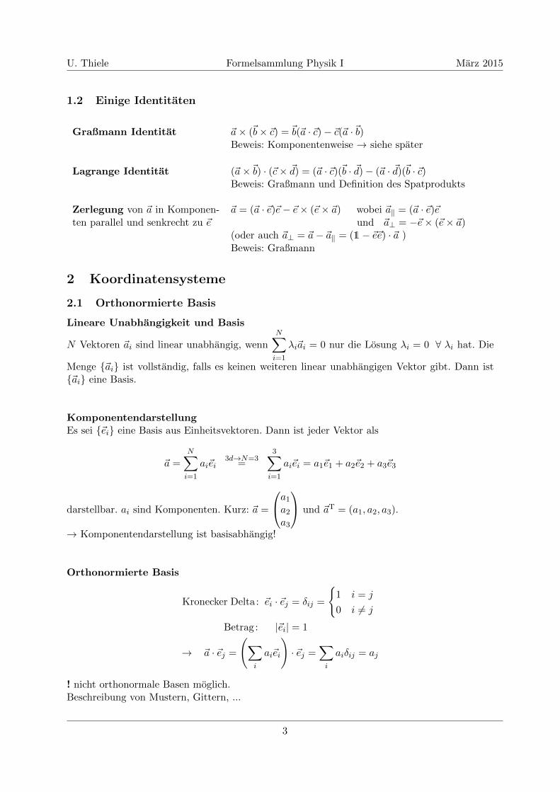
1.2 Einige Identitaten

Graßmann Identitat ~a× (~b× ~c) = ~b(~a · ~c)− ~c(~a ·~b)Beweis: Komponentenweise → siehe spater

Lagrange Identitat (~a×~b) · (~c× ~d) = (~a · ~c)(~b · ~d)− (~a · ~d)(~b · ~c)Beweis: Graßmann und Definition des Spatprodukts

Zerlegung von ~a in Komponen- ~a = (~a · ~e)~e− ~e× (~e× ~a) wobei ~a‖ = (~a · ~e)~eten parallel und senkrecht zu ~e und ~a⊥ = −~e× (~e× ~a)

(oder auch ~a⊥ = ~a− ~a‖ = (1− ~e~e) · ~a )

Beweis: Graßmann

2 Koordinatensysteme

2.1 Orthonormierte Basis

Lineare Unabhangigkeit und Basis

N Vektoren ~ai sind linear unabhangig, wenn

N∑i=1

λi~ai = 0 nur die Losung λi = 0 ∀ λi hat. Die

Menge {~ai} ist vollstandig, falls es keinen weiteren linear unabhangigen Vektor gibt. Dann ist{~ai} eine Basis.

KomponentendarstellungEs sei {~ei} eine Basis aus Einheitsvektoren. Dann ist jeder Vektor als

~a =N∑i=1

ai~ei3d→N=3

=3∑i=1

ai~ei = a1~e1 + a2~e2 + a3~e3

darstellbar. ai sind Komponenten. Kurz: ~a =

a1

a2

a3

und ~aT = (a1, a2, a3).

→ Komponentendarstellung ist basisabhangig!

Orthonormierte Basis

Kronecker Delta : ~ei · ~ej = δij =

{1 i = j

0 i 6= j

Betrag : |~ei| = 1

→ ~a · ~ej =

(∑i

ai~ei

)· ~ej =

∑i

aiδij = aj

! nicht orthonormale Basen moglich.Beschreibung von Mustern, Gittern, ...

3


Zerlegung von ~a in Komponenten bezuglich einer Basis {~ei} ist eindeutig.Beweis: Annahme, es gibt zwei Zerlegungen

~a =∑i

ai~ei ~a =∑i

ai~ei

dann

~a− ~a =∑i

(ai − ai)~ei = 0.

Da {~ei} linear unabhangig ist, muss ai − ai = 0 sein.

2.2 Komponentendarstellung der Produkte

(allg. orthonormale Basen)

Skalarprodukt

~a ·~b =

(∑i

ai~ei

)·

∑j

bj~ej

=∑i

aibi

nutze ~ei · ~ej = δij

Vektorprodukt

~a×~b =

a1

a2

a3

×b1b2b3

=

a2b3 − a3b2a3b1 − a1b3a1b2 − a2b1

=∑i,j,k

εijkaibj~ek

εijk =

+1 ijk = 123 oder zyklische Vertauschung

−1 ijk = 213 oder zyklische Vertauschung

0 sonst

Epsilon-Tensor oder Levi-Civita-Symbol: total antisymmetrischer Tensor 3. Stufe.

Nutze ~ei × ~ej =∑i,j,k

εijk~ek.

Nutzliche Beziehung:∑j

εikjεjlm = δilδkm − δimδkl

Matrixreprasentation Vektorprodukt

~a×~b = A ·~b

mit A =

0 −a3 a2

a3 0 −a1

−a2 a1 0

︸︷︷︸

antisymmetrische Matrix

4


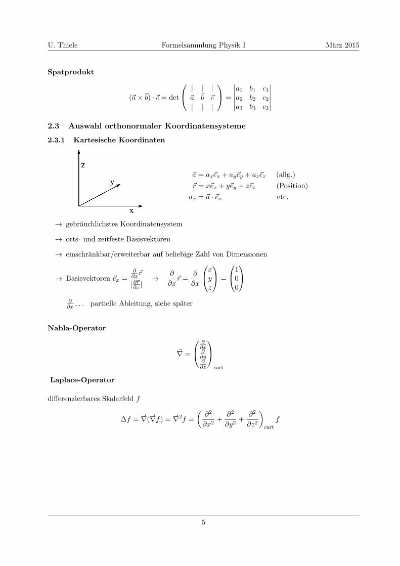
Spatprodukt

(~a×~b) · ~c = det

| | |~a ~b ~c| | |

=

∣∣∣∣∣∣a1 b1 c1

a2 b2 c2

a3 b3 c3

∣∣∣∣∣∣2.3 Auswahl orthonormaler Koordinatensysteme

2.3.1 Kartesische Koordinaten

~a = ax~ex + ay~ey + az~ez (allg.)

~r = x~ex + y~ey + z~ez (Position)

ax = ~a · ~ex etc.

→ gebrauchlichstes Koordinatensystem

→ orts- und zeitfeste Basisvektoren

→ einschrankbar/erweiterbar auf beliebige Zahl von Dimensionen

→ Basisvektoren ~ex =∂∂x~r

| ∂~r∂x |→ ∂

∂x~r =

∂

∂x

xyz

=

100

∂∂x . . . partielle Ableitung, siehe spater

Nabla-Operator

~∇ =

∂∂x∂∂y∂∂z

cart

Laplace-Operator

differenzierbares Skalarfeld f

∆f = ~∇(~∇f) = ~∇2f =

(∂2

∂x2+

∂2

∂y2+

∂2

∂z2

)cart

f

5


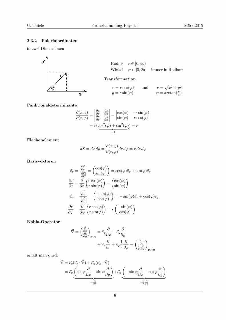
2.3.2 Polarkoordinaten

in zwei Dimensionen

Radius r ∈ [0,∞)

Winkel ϕ ∈ [0, 2π] immer in Radiant

Transformation

x = r cos(ϕ) und r =√x2 + y2

y = r sin(ϕ) ϕ = arctan( yx)

Funktionaldeterminante

∂(x, y)

∂(r, ϕ)=

∣∣∣∣∣∂x∂r ∂x∂ϕ

∂y∂r

∂y∂ϕ

∣∣∣∣∣ =

∣∣∣∣cos(ϕ) −r sin(ϕ)sin(ϕ) r cos(ϕ)

∣∣∣∣= r(cos2(ϕ) + sin2(ϕ)︸︷︷︸

=1

) = r

Flachenelement

dS = dx dy =∂(x, y)

∂(r, ϕ)dr dϕ = r dr dϕ

Basisvektoren

~er =∂~r∂r

|∂~r∂r |=

(cos(ϕ)sin(ϕ)

)= cos(ϕ)~ex + sin(ϕ)~ey

∂~r

∂r=

∂

∂r

(r cos(ϕ)r sin(ϕ)

)=

(cos(ϕ)sin(ϕ)

)~eϕ =

∂~r∂ϕ

| ∂~r∂ϕ |=

(− sin(ϕ)cos(ϕ)

)= − sin(ϕ)~ex + cos(ϕ)~ey

∂~r

∂ϕ=

∂

∂ϕ

(r cos(ϕ)r sin(ϕ)

)= r

(− sin(ϕ)cos(ϕ)

)Nabla-Operator

~∇ =

( ∂∂x∂∂y

)cart

= ~ex∂

∂x+ ~ey

∂

∂y

= ~er∂

∂r+ ~eϕ

1

r

∂

∂ϕ=

( ∂∂r

1r∂∂ϕ

)polar

erhalt man durch

~∇ = ~er(~er · ~∇) + ~eϕ(~eϕ · ~∇)

= ~er

(cosϕ

∂

∂x+ sinϕ

∂

∂y

)︸︷︷︸

= ∂∂r

+~eϕ

(− sinϕ

∂

∂x+ cosϕ

∂

∂y

)︸︷︷︸

= 1r

∂∂ϕ

6


mit

∂

∂r=∂x

∂r

∂

∂x+∂y

∂r

∂

∂y

∂

∂ϕ=∂x

∂ϕ

∂

∂x+∂y

∂ϕ

∂

∂y

Laplace-Operator

∆ =

(1

r

∂

∂r

(r∂

∂r

)+

1

r2

∂2

∂ϕ2

)polar

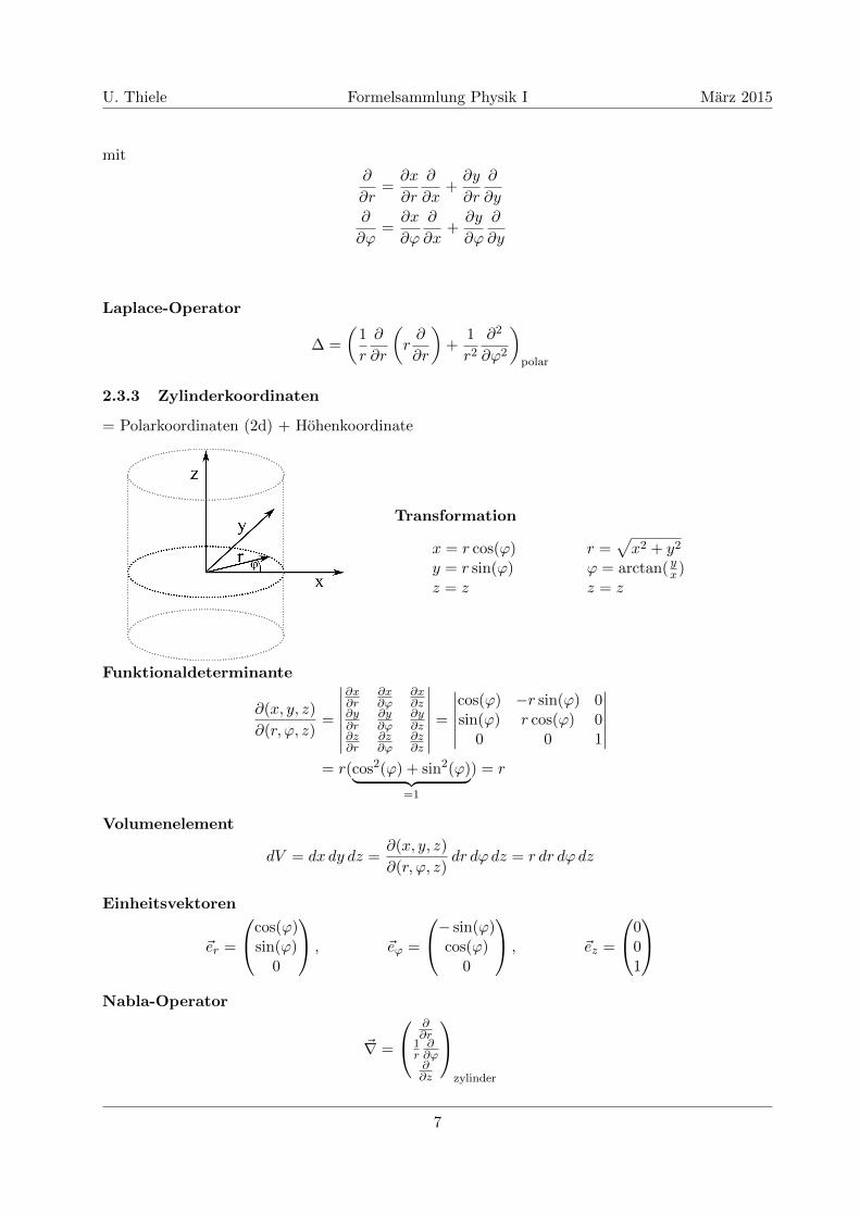
2.3.3 Zylinderkoordinaten

= Polarkoordinaten (2d) + Hohenkoordinate

Transformation

x = r cos(ϕ) r =√x2 + y2

y = r sin(ϕ) ϕ = arctan( yx)z = z z = z


∂(x, y, z)

∂(r, ϕ, z)=

∣∣∣∣∣∣∣∂x∂r

∂x∂ϕ

∂x∂z

∂y∂r

∂y∂ϕ

∂y∂z

∂z∂r

∂z∂ϕ

∂z∂z

∣∣∣∣∣∣∣ =

∣∣∣∣∣∣cos(ϕ) −r sin(ϕ) 0sin(ϕ) r cos(ϕ) 0

0 0 1

∣∣∣∣∣∣= r(cos2(ϕ) + sin2(ϕ)︸︷︷︸

=1

) = r

Volumenelement

dV = dx dy dz =∂(x, y, z)

∂(r, ϕ, z)dr dϕ dz = r dr dϕ dz

Einheitsvektoren

~er =

cos(ϕ)sin(ϕ)

0

, ~eϕ =

− sin(ϕ)cos(ϕ)

0

, ~ez =

001

Nabla-Operator

~∇ =

∂∂r

1r∂∂ϕ∂∂z

zylinder

7


Laplace-Operator

∆ =

(1

r

∂

∂r

(r∂

∂r

)+

1

r2

∂2

∂ϕ2+

∂2

∂z2

)zylinder

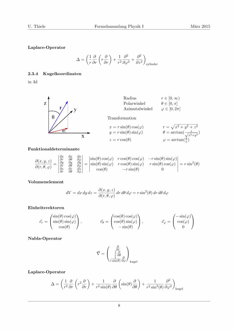
2.3.4 Kugelkoordinaten

in 3d

Radius r ∈ [0,∞)Polarwinkel θ ∈ [0, π]Azimutalwinkel ϕ ∈ [0, 2π]

Transformation

x = r sin(θ) cos(ϕ) r =√x2 + y2 + z2

y = r sin(θ) sin(ϕ) θ = arctan( z√x2+y2

)

z = r cos(θ) ϕ = arctan( yx)


∂(x, y, z)

∂(r, θ, ϕ)=

∣∣∣∣∣∣∣∂x∂r

∂x∂θ

∂x∂ϕ

∂y∂r

∂y∂θ

∂y∂ϕ

∂z∂r

∂z∂θ

∂z∂ϕ

∣∣∣∣∣∣∣ =

∣∣∣∣∣∣sin(θ) cos(ϕ) r cos(θ) cos(ϕ) −r sin(θ) sin(ϕ)sin(θ) sin(ϕ) r cos(θ) sin(ϕ) r sin(θ) cos(ϕ)

cos(θ) −r sin(θ) 0

∣∣∣∣∣∣ = r sin2(θ)

Volumenelement

dV = dx dy dz =∂(x, y, z)

∂(r, θ, ϕ)dr dθ dϕ = r sin2(θ) dr dθ dϕ

Einheitsvektoren

~er =

sin(θ) cos(ϕ)sin(θ) sin(ϕ)

cos(θ)

, ~eθ =

cos(θ) cos(ϕ)cos(θ) sin(ϕ)− sin(θ)

, ~eϕ =

− sin(ϕ)cos(ϕ)

0

Nabla-Operator

~∇ =

∂∂r

1r∂∂θ

1r sin(θ)

∂∂ϕ

kugel

Laplace-Operator

∆ =

(1

r2

∂

∂r

(r2 ∂

∂r

)+

1

r2 sin(θ)

∂

∂θ

(sin(θ)

∂

∂θ

)+

1

r2 sin2(θ)

∂2

∂ϕ2

)kugel

8


3 Beschreibung von Bahnkurven

3.1 Parametrisierung von Raumkurven

Vektorwertige Funktion ~r(t) ∈ R3 mit t ∈ R. Raumkurven (Trajektorien) beschreiben diePosition eines Punktteilchens in Abhangigkeit der Zeit t.Wahl einer zeitunabhangigen Basis {~ei} gibt die Komponentendarstellung fur die Position:

~r(t) =3∑i=1

ri(t)~ei =

r1(t)r2(t)r3(t)

=

x(t)y(t)z(t)

.

Man sagt, die skalare Große t parametrisiert die Raumkurve ~r(t).

Einheiten : [~r] = m und [t] = s

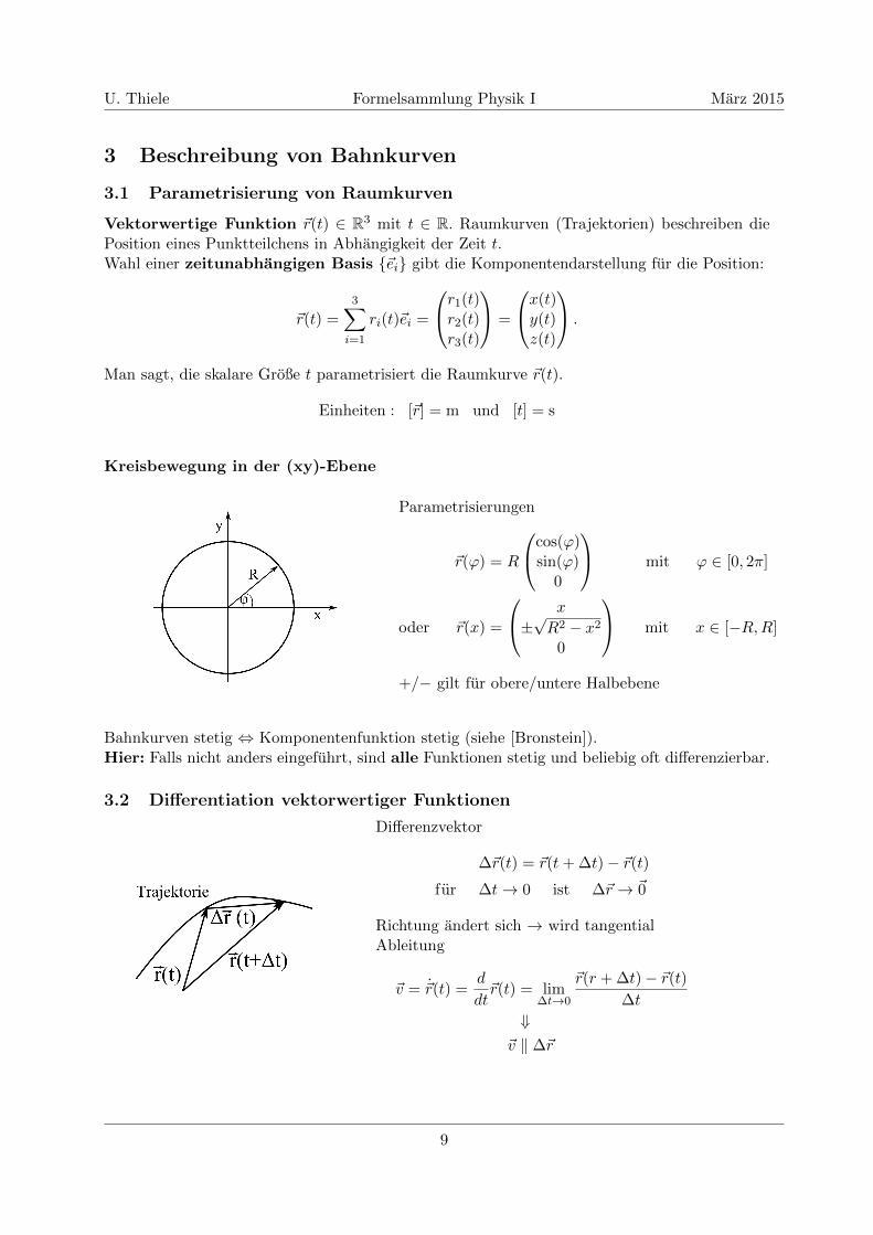
Kreisbewegung in der (xy)-Ebene

Parametrisierungen

~r(ϕ) = R

cos(ϕ)sin(ϕ)

0

mit ϕ ∈ [0, 2π]

oder ~r(x) =

x

±√R2 − x2

0

mit x ∈ [−R,R]

+/− gilt fur obere/untere Halbebene

Bahnkurven stetig ⇔ Komponentenfunktion stetig (siehe [Bronstein]).Hier: Falls nicht anders eingefuhrt, sind alle Funktionen stetig und beliebig oft differenzierbar.

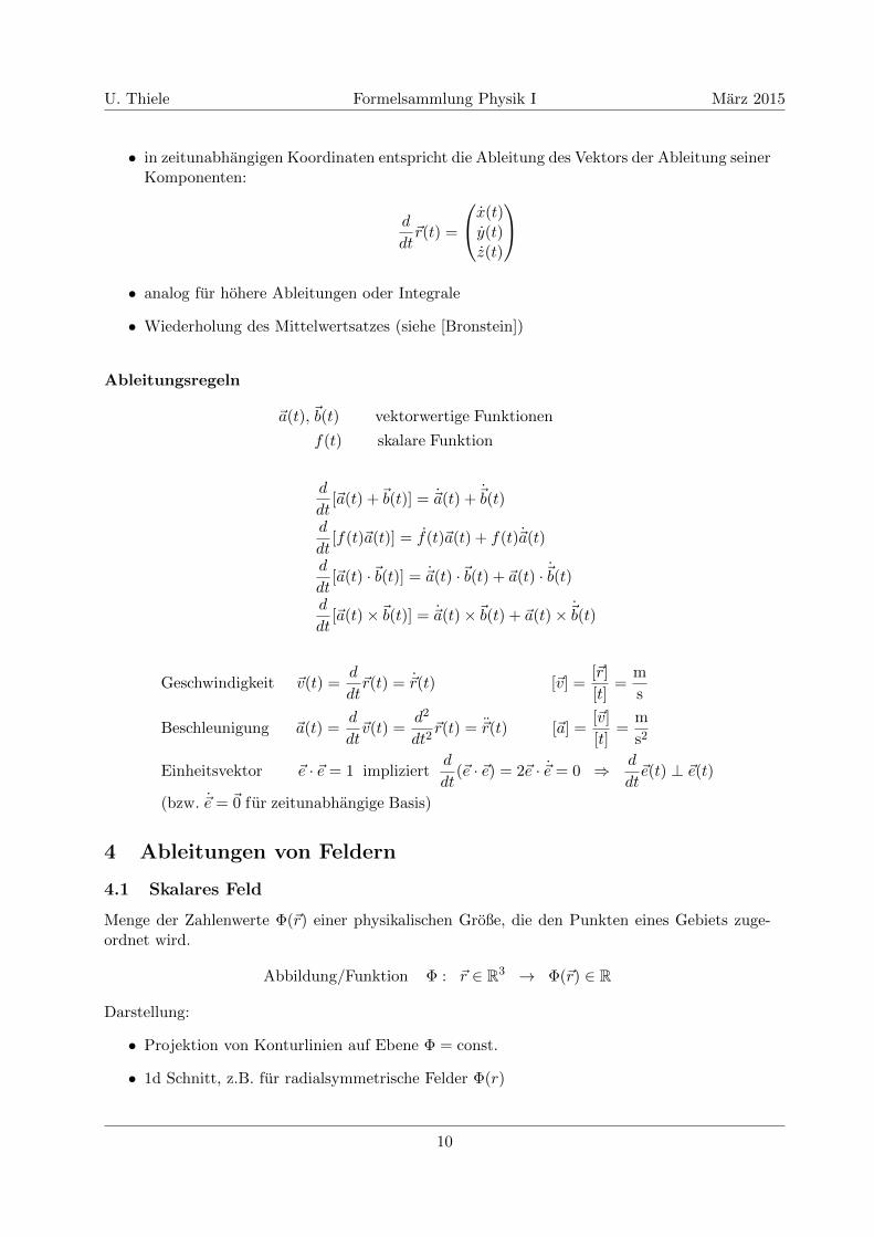
3.2 Differentiation vektorwertiger Funktionen

Differenzvektor

∆~r(t) = ~r(t+ ∆t)− ~r(t)fur ∆t→ 0 ist ∆~r → ~0

Richtung andert sich → wird tangentialAbleitung

~v = ~r(t) =d

dt~r(t) = lim

∆t→0

~r(r + ∆t)− ~r(t)∆t

⇓~v ‖ ∆~r

9


• in zeitunabhangigen Koordinaten entspricht die Ableitung des Vektors der Ableitung seinerKomponenten:

d

dt~r(t) =

x(t)y(t)z(t)

• analog fur hohere Ableitungen oder Integrale

• Wiederholung des Mittelwertsatzes (siehe [Bronstein])

Ableitungsregeln

~a(t), ~b(t) vektorwertige Funktionen

f(t) skalare Funktion

d

dt[~a(t) +~b(t)] = ~a(t) + ~b(t)

d

dt[f(t)~a(t)] = f(t)~a(t) + f(t)~a(t)

d

dt[~a(t) ·~b(t)] = ~a(t) ·~b(t) + ~a(t) · ~b(t)

d

dt[~a(t)×~b(t)] = ~a(t)×~b(t) + ~a(t)× ~b(t)

Geschwindigkeit ~v(t) =d

dt~r(t) = ~r(t) [~v] =

[~r]

[t]=

m

s

Beschleunigung ~a(t) =d

dt~v(t) =

d2

dt2~r(t) = ~r(t) [~a] =

[~v]

[t]=

m

s2

Einheitsvektor ~e · ~e = 1 impliziertd

dt(~e · ~e) = 2~e · ~e = 0 ⇒ d

dt~e(t) ⊥ ~e(t)

(bzw. ~e = ~0 fur zeitunabhangige Basis)

4 Ableitungen von Feldern

4.1 Skalares Feld

Menge der Zahlenwerte Φ(~r) einer physikalischen Große, die den Punkten eines Gebiets zuge-ordnet wird.

Abbildung/Funktion Φ : ~r ∈ R3 → Φ(~r) ∈ R

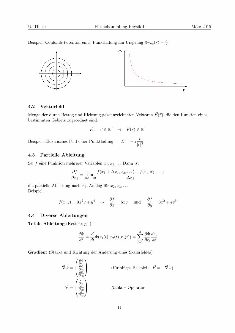
Darstellung:

• Projektion von Konturlinien auf Ebene Φ = const.

• 1d Schnitt, z.B. fur radialsymmetrische Felder Φ(r)

10


Beispiel: Coulomb-Potential einer Punktladung am Ursprung ΦCou(~r) = αr

4.2 Vektorfeld

Menge der durch Betrag und Richtung gekennzeichneten Vektoren ~E(~r), die den Punkten einesbestimmten Gebiets zugeordnet sind.

~E : ~r ∈ R3 → ~E(~r) ∈ R3

Beispiel: Elektrisches Feld einer Punktladung ~E = −α ~r

|~r|3

4.3 Partielle Ableitung

Sei f eine Funktion mehrerer Variablen x1, x2, . . . Dann ist

∂f

∂x1= lim

∆x1→0

f(x1 + ∆x1, x2, . . . )− f(x1, x2, . . . )

∆x1

die partielle Ableitung nach x1. Analog fur x2, x3, . . .Beispiel:

f(x, y) = 3x2y + y4 → ∂f

∂x= 6xy und

∂f

∂y= 3x2 + 4y3

4.4 Diverse Ableitungen

Totale Ableitung (Kettenregel)

dΦ

dt=

d

dtΦ(r1(t), r2(t), r3(t)) =

3∑i=1

∂Φ

∂ri

dridt

Gradient (Starke und Richtung der Anderung eines Skalarfeldes)

~∇Φ =

∂Φ∂r1∂Φ∂r2∂Φ∂r3

(fur obiges Beispiel : ~E = −~∇Φ)

~∇ =

∂∂r1∂∂r2∂∂r3

Nabla−Operator

11


Divergenz (Quellstarke eines Vektorfeldes)

~∇ · ~E =3∑i=1

∂

∂riEi

Rotation (Wirbelstarke eines Vektorfeldes)

~∇× ~E =∑i,j,k

εijk

(∂Ej∂ri

)~ek

Danksagung

Mein Dank gilt Gabi Wenzel fur das sorgfaltige Erstellen dieser Version nach meinen hand-schriftlichen Notizen.

Literatur

[Bronstein] Bronstein, I. N., Muhlig, H., Musiol, G. und Semendjajew, K. A.(2013): Taschenbuch der Mathematik, Verlag Europa-Lehrmittel, 9.Auflage, ISBN 978-3-8085-5671-9

[Gradstein] Gradstein, I. S., Ryshik, I. W. (1981): Summen-, Produkt- und Inte-graltafeln, Harri Deutsch Verlag, 5. Auflage, ISBN 978-3-87144-350-3

[Nolting] Nolting, W. (2012): Grundkurs Theoretische Physik 1: Klassische Me-chanik, Springer Verlag, 10. Auflage, ISBN 978-3-64229-936-0

12

Ausgew ahlte Mathematische Hilfsmittel Formelsammlung zu ... · U. Thiele Formelsammlung Physik I M arz 2015 Dies ist eine Zusammenstellung einiger mathematischer Hilfsmittel, wie

Documents