Music Processing Meinard Müller Lecture Audio Retrieval International Audio Laboratories Erlangen [email protected] Music Retrieval Textual metadata – Traditional retrieval – Searching for artist, title, … Rich and expressive metadata – Generated by experts – Crowd tagging, social networks Content-based retrieval – Automatic generation of tags – Query-by-example

Welcome message from author
This document is posted to help you gain knowledge. Please leave a comment to let me know what you think about it! Share it to your friends and learn new things together.
Transcript
Music Processing
Meinard Müller
Lecture
Audio Retrieval
International Audio Laboratories [email protected]
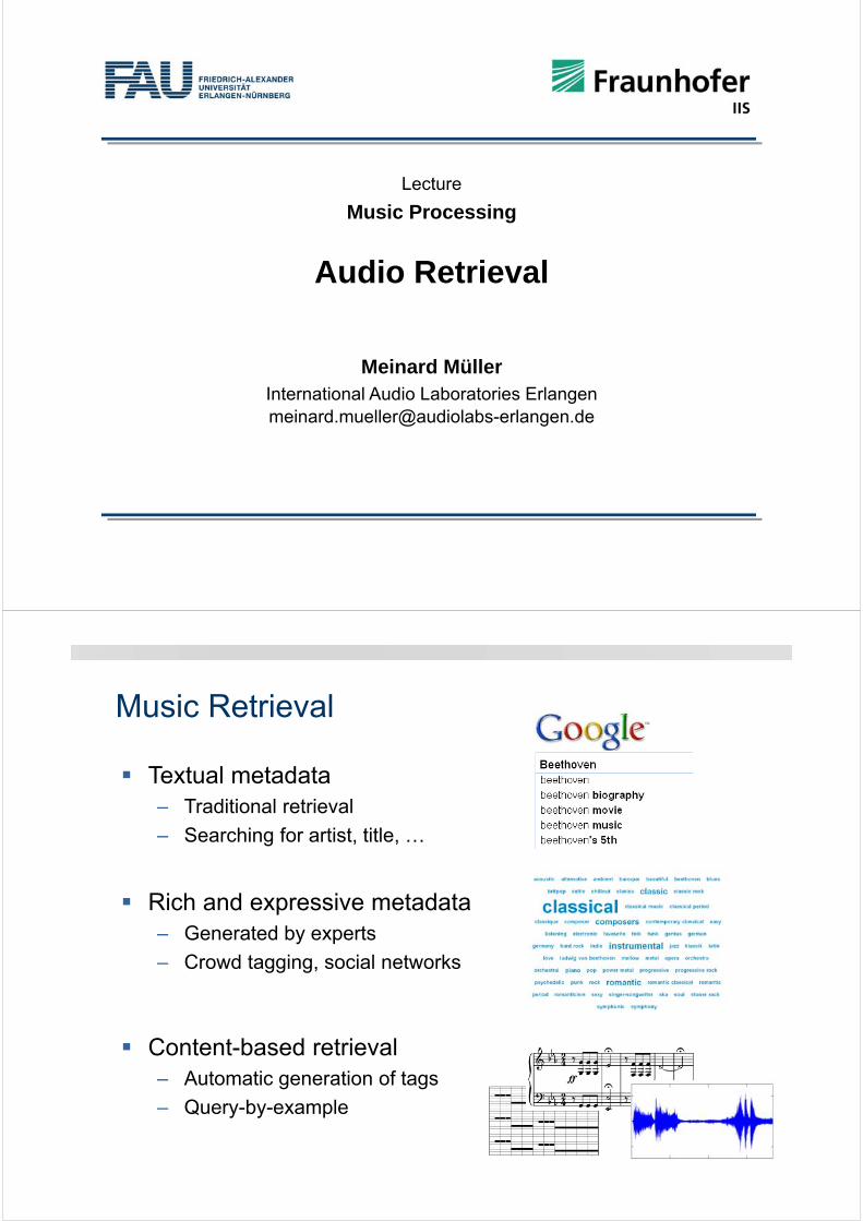
Music Retrieval
Textual metadata– Traditional retrieval
– Searching for artist, title, …
Rich and expressive metadata– Generated by experts
– Crowd tagging, social networks
Content-based retrieval– Automatic generation of tags
– Query-by-example
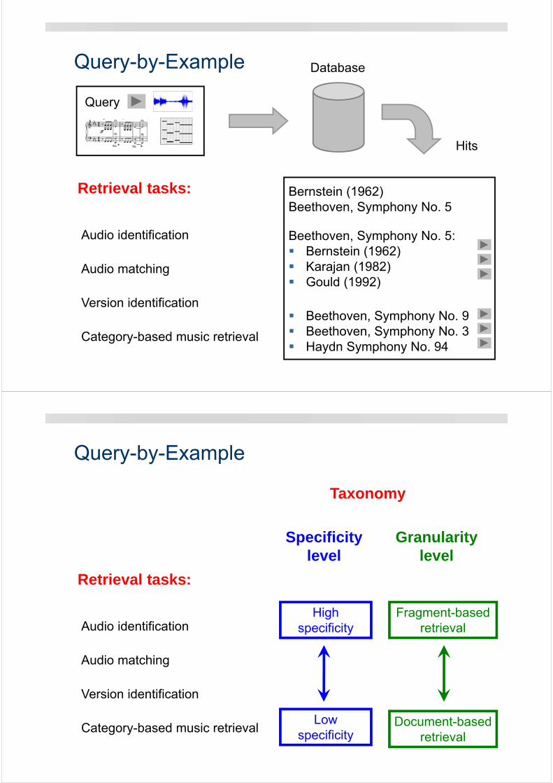
Query-by-Example
Query
Audio identification
Audio matching
Version identification
Category-based music retrieval
Retrieval tasks:
Database
Hits
Bernstein (1962) Beethoven, Symphony No. 5
Beethoven, Symphony No. 5: Bernstein (1962) Karajan (1982) Gould (1992)
Beethoven, Symphony No. 9 Beethoven, Symphony No. 3 Haydn Symphony No. 94
Query-by-Example
Audio identification
Audio matching
Version identification
Category-based music retrieval
Retrieval tasks:
Highspecificity
Lowspecificity
Fragment-based retrieval
Document-based retrieval
Specificitylevel
Granularitylevel
Taxonomy
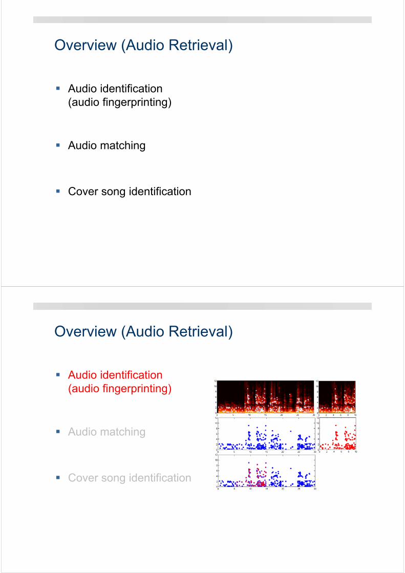
Overview (Audio Retrieval)
Audio identification(audio fingerprinting)
Audio matching
Cover song identification
Overview (Audio Retrieval)
Audio identification(audio fingerprinting)
Audio matching
Cover song identification
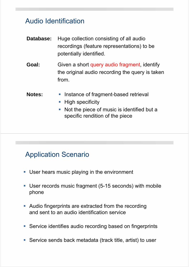
Audio Identification
Database: Huge collection consisting of all audio
recordings (feature representations) to be
potentially identified.
Goal: Given a short query audio fragment, identify
the original audio recording the query is taken
from.
Notes: Instance of fragment-based retrieval
High specificity
Not the piece of music is identified but aspecific rendition of the piece
Application Scenario
User hears music playing in the environment
User records music fragment (5-15 seconds) with mobile phone
Audio fingerprints are extracted from the recording and sent to an audio identification service
Service identifies audio recording based on fingerprints
Service sends back metadata (track title, artist) to user
Audio Fingerprints
Requirements:
Discriminative power
Invariance to distortions
Compactness
Computational simplicity
An audio fingerprint is a content-based compact signature that summarizes some specific audio content.
Audio Fingerprints
Requirements:
Discriminative power
Invariance to distortions
Compactness
Computational simplicity
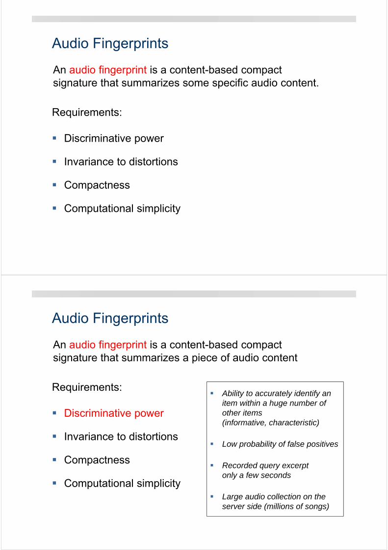
An audio fingerprint is a content-based compact signature that summarizes a piece of audio content
Ability to accurately identify an item within a huge number of other items(informative, characteristic)
Low probability of false positives
Recorded query excerptonly a few seconds
Large audio collection on theserver side (millions of songs)
Audio Fingerprints
Requirements:
Discriminative power
Invariance to distortions
Compactness
Computational simplicity
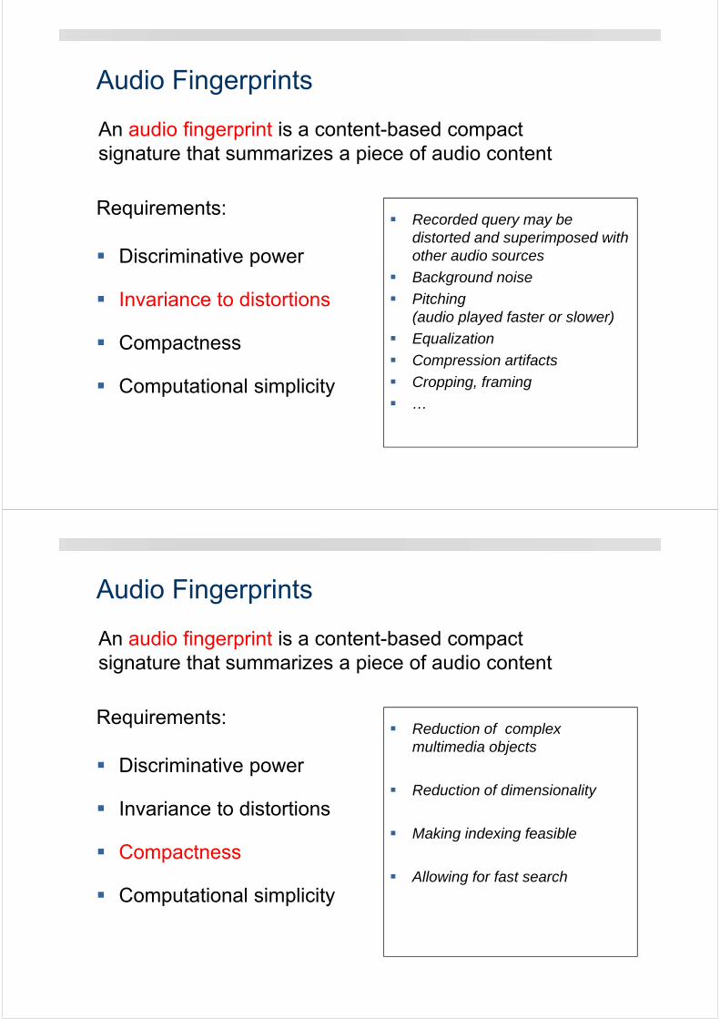
An audio fingerprint is a content-based compact signature that summarizes a piece of audio content
Recorded query may be distorted and superimposed with other audio sources
Background noise
Pitching(audio played faster or slower)
Equalization
Compression artifacts
Cropping, framing
…
Audio Fingerprints
Requirements:
Discriminative power
Invariance to distortions
Compactness
Computational simplicity
An audio fingerprint is a content-based compact signature that summarizes a piece of audio content
Reduction of complexmultimedia objects
Reduction of dimensionality
Making indexing feasible
Allowing for fast search
Audio Fingerprints
Requirements:
Discriminative power
Invariance to distortions
Compactness
Computational simplicity
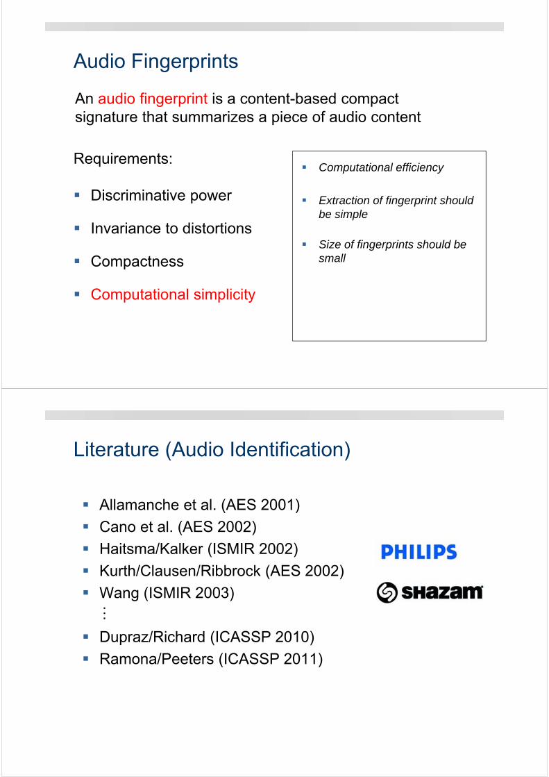
An audio fingerprint is a content-based compact signature that summarizes a piece of audio content
Computational efficiency
Extraction of fingerprint should be simple
Size of fingerprints should be small
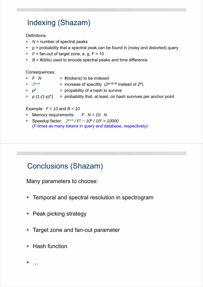
Literature (Audio Identification)
Allamanche et al. (AES 2001)
Cano et al. (AES 2002)
Haitsma/Kalker (ISMIR 2002)
Kurth/Clausen/Ribbrock (AES 2002)
Wang (ISMIR 2003)
Dupraz/Richard (ICASSP 2010)
Ramona/Peeters (ICASSP 2011)
…
Literature (Audio Identification)
Allamanche et al. (AES 2001)
Cano et al. (AES 2002)
Haitsma/Kalker (ISMIR 2002)
Kurth/Clausen/Ribbrock (AES 2002)
Wang (ISMIR 2003)
Dupraz/Richard (ICASSP 2010)
Ramona/Peeters (ICASSP 2011)
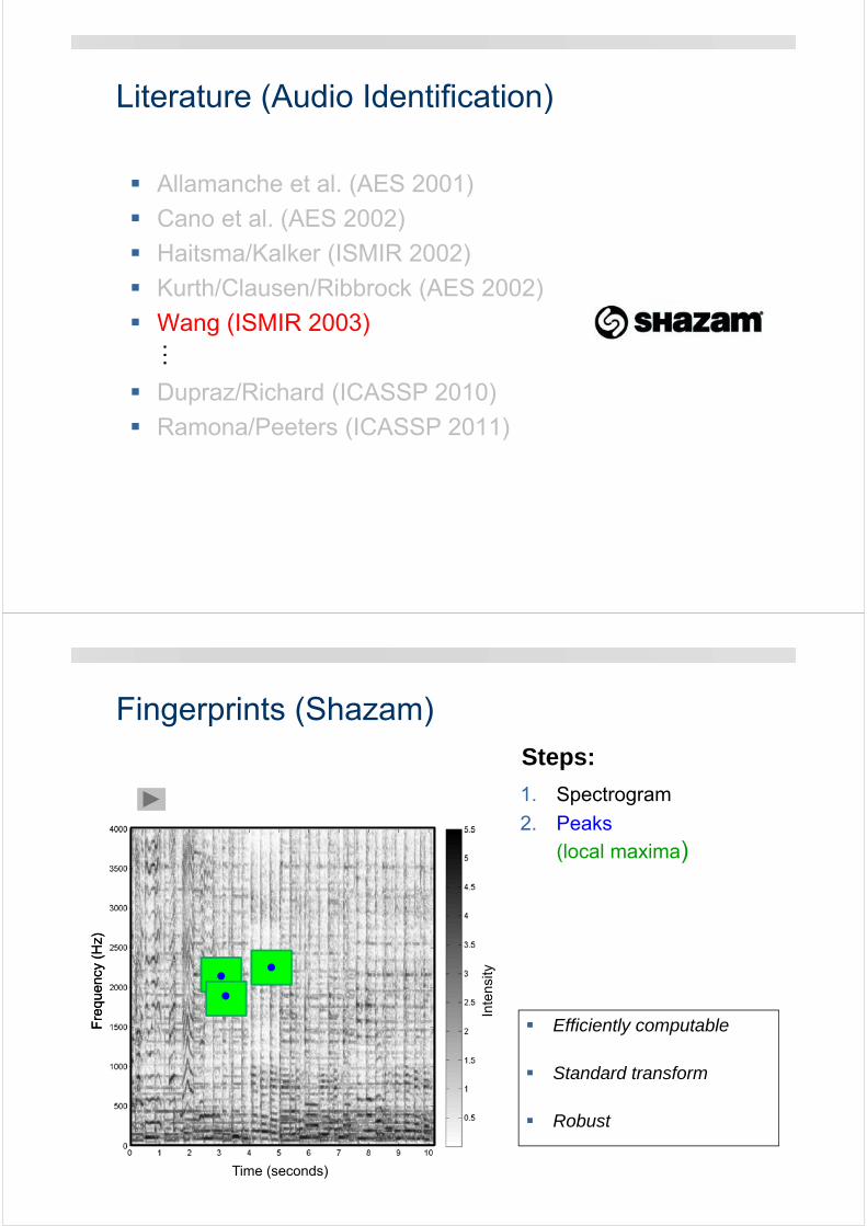
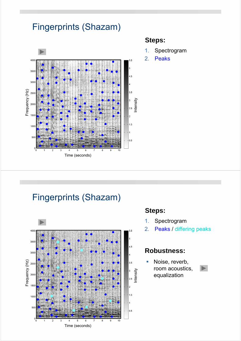
…Fingerprints (Shazam)
Steps:
1. Spectrogram
2. Peaks
(local maxima)
Fre
quen
cy (
Hz)
Fre
quen
cy (
Hz)
Inte
nsity
Efficiently computable
Standard transform
Robust
Time (seconds)
Fingerprints (Shazam)
Steps:
1. Spectrogram
2. Peaks
Time (seconds)
Fre
quen
cy (
Hz)
Inte
nsity
Fingerprints (Shazam)
Steps:
1. Spectrogram
2. Peaks / differing peaks
Time (seconds)
Fre
quen
cy (
Hz)
Inte
nsity
Noise, reverb, room acoustics, equalization
Robustness:
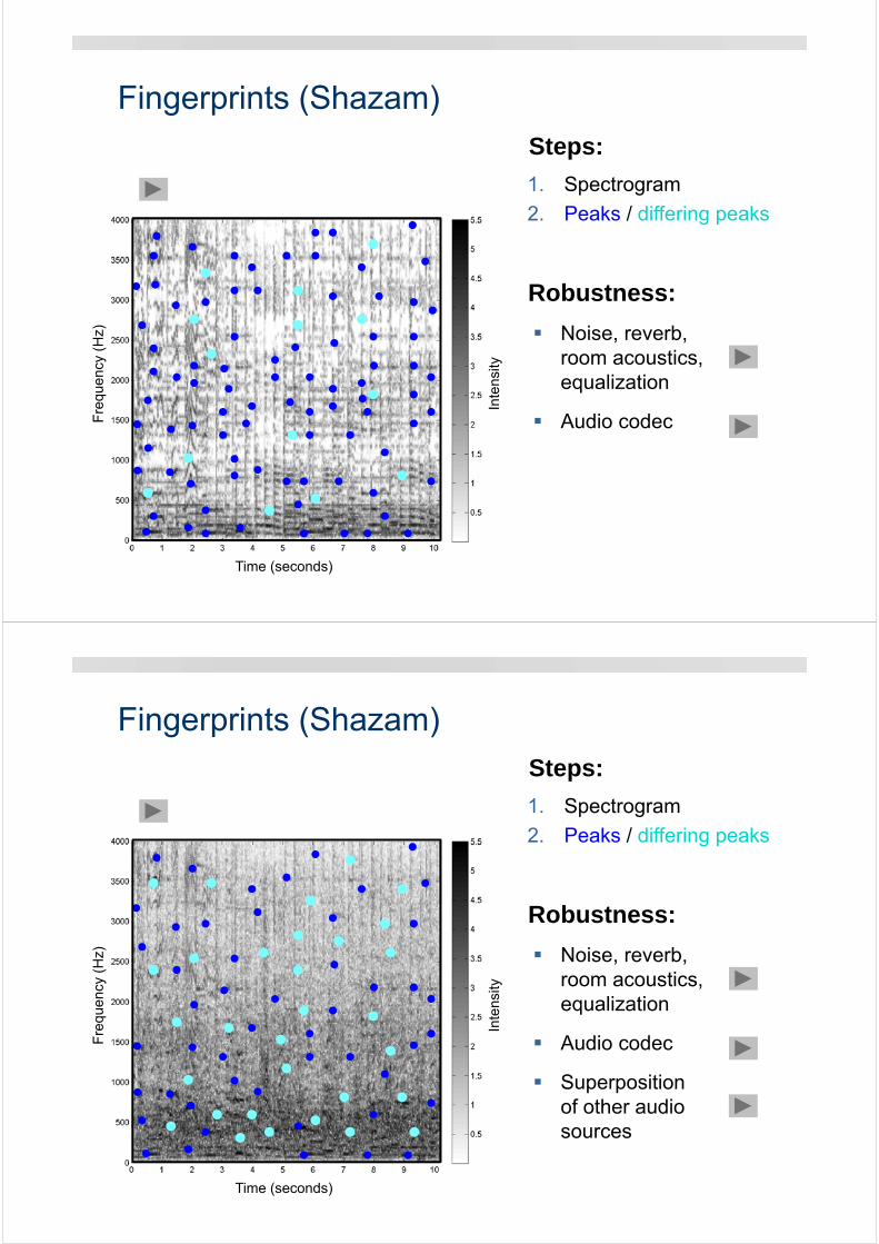
Fingerprints (Shazam)
Steps:
1. Spectrogram
2. Peaks / differing peaks
Time (seconds)
Fre
quen
cy (
Hz)
Inte
nsity
Noise, reverb, room acoustics, equalization
Audio codec
Robustness:
Fingerprints (Shazam)
Steps:
Time (seconds)
Fre
quen
cy (
Hz)
Inte
nsity
Noise, reverb, room acoustics, equalization
Audio codec
Superposition of other audio sources
Robustness:
1. Spectrogram
2. Peaks / differing peaks
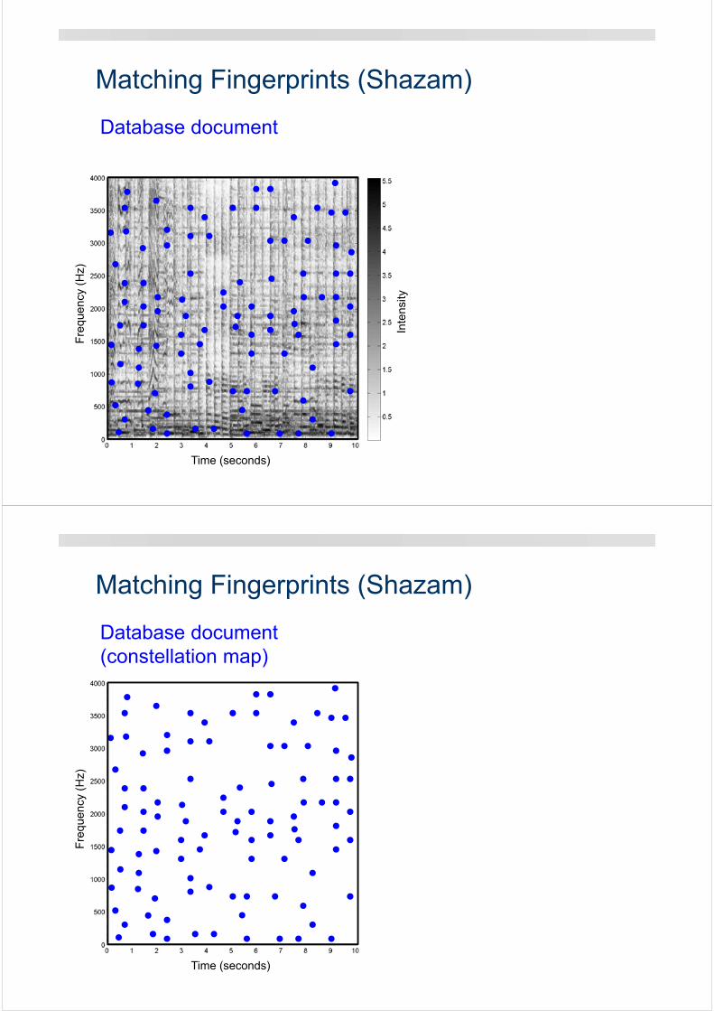
Matching Fingerprints (Shazam)
Database document
Time (seconds)
Fre
quen
cy (
Hz)
Inte
nsity
Matching Fingerprints (Shazam)
Time (seconds)
Fre
quen
cy (
Hz)
Database document(constellation map)
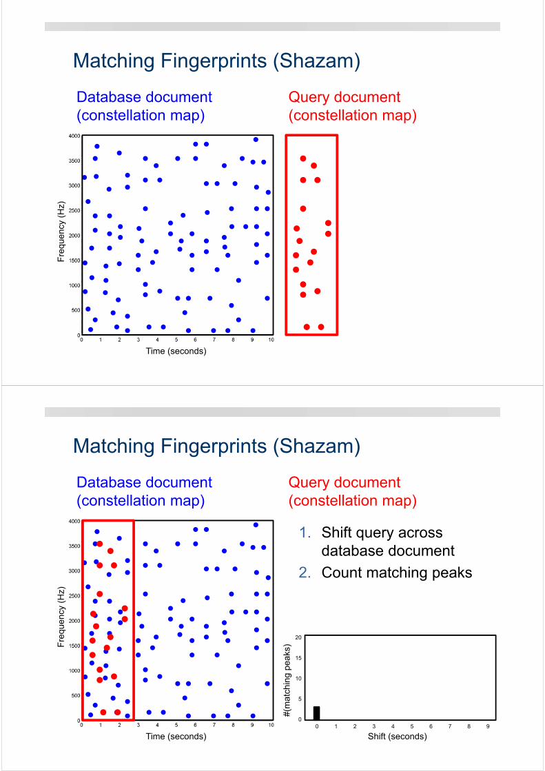
Matching Fingerprints (Shazam)
Time (seconds)
Fre
quen
cy (
Hz)
Database document(constellation map)
Query document(constellation map)
Matching Fingerprints (Shazam)
Time (seconds)
Fre
quen
cy (
Hz)
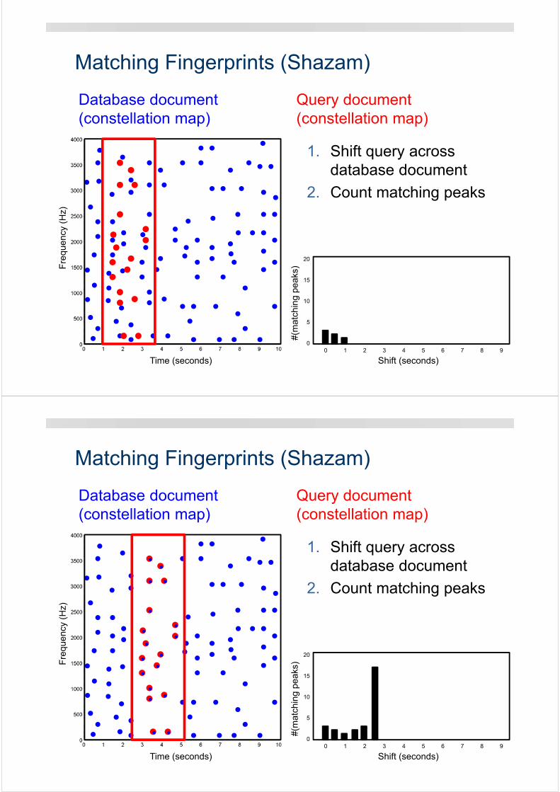
Database document(constellation map)
Query document(constellation map)
1. Shift query across database document
2. Count matching peaks
Shift (seconds)0 1 2 3 4 5 6 7 8 9
#(m
atch
ing
peak
s)
20
15
10
5
0
Matching Fingerprints (Shazam)
Time (seconds)
Fre
quen
cy (
Hz)
Database document(constellation map)
Query document(constellation map)
0 1 2 3 4 5 6 7 8 9
#(m
atch
ing
peak
s)
20
15
10
5
0
1. Shift query across database document
2. Count matching peaks
Shift (seconds)
Matching Fingerprints (Shazam)
Time (seconds)
Fre
quen
cy (
Hz)
Database document(constellation map)
Query document(constellation map)
1. Shift query across database document
2. Count matching peaks
0 1 2 3 4 5 6 7 8 9
#(m
atch
ing
peak
s)
20
15
10
5
0
Shift (seconds)
Matching Fingerprints (Shazam)
Time (seconds)
Fre
quen
cy (
Hz)
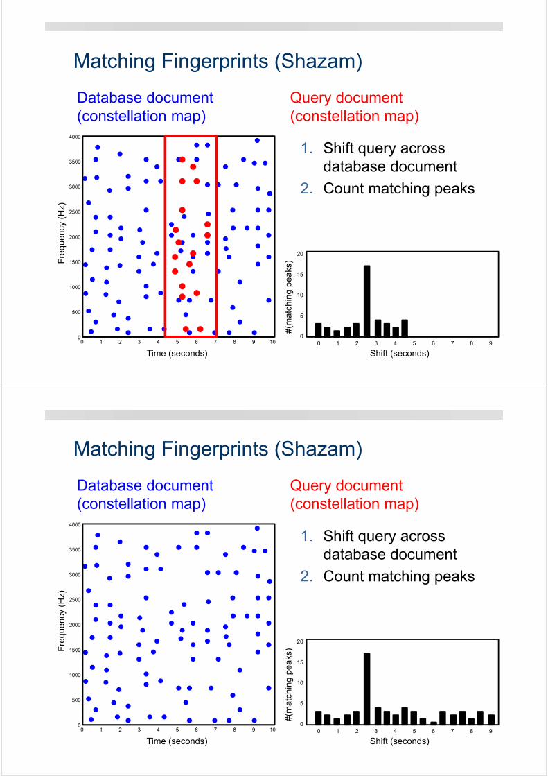
Database document(constellation map)
Query document(constellation map)
1. Shift query across database document
2. Count matching peaks
0 1 2 3 4 5 6 7 8 9
#(m
atch
ing
peak
s)
20
15
10
5
0
Shift (seconds)
Matching Fingerprints (Shazam)
Time (seconds)
Fre
quen
cy (
Hz)
Database document(constellation map)
Query document(constellation map)
1. Shift query across database document
2. Count matching peaks
0 1 2 3 4 5 6 7 8 9
20
15
10
5
0
#(m
atch
ing
peak
s)
Shift (seconds)
Matching Fingerprints (Shazam)
Time (seconds)
Fre
quen
cy (
Hz)
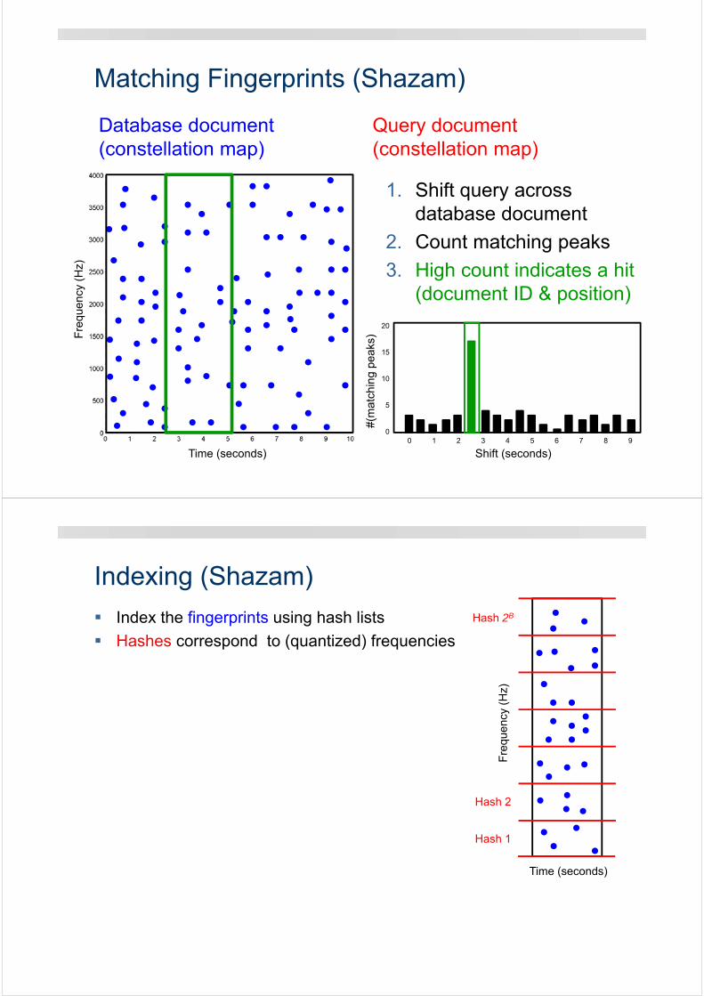
Database document(constellation map)
Query document(constellation map)
1. Shift query across database document
2. Count matching peaks
3. High count indicates a hit(document ID & position)
0 1 2 3 4 5 6 7 8 9
20
15
10
5
0
#(m
atch
ing
peak
s)
Shift (seconds)
Indexing (Shazam)
Index the fingerprints using hash lists
Hashes correspond to (quantized) frequencies
Time (seconds)
Fre
quen
cy (
Hz)
Hash 1
Hash 2
Hash 2B
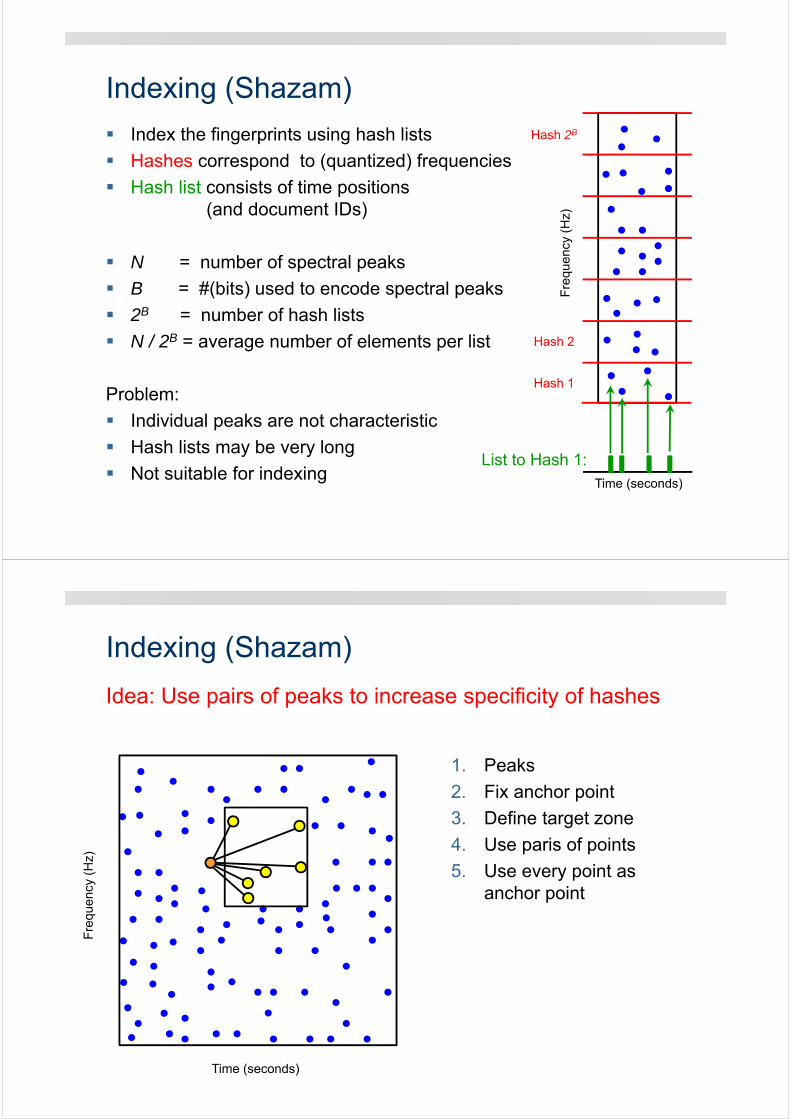
Indexing (Shazam)
Index the fingerprints using hash lists
Hashes correspond to (quantized) frequencies
Hash list consists of time positions(and document IDs)
N = number of spectral peaks
B = #(bits) used to encode spectral peaks
2B = number of hash lists
N / 2B = average number of elements per list
Problem:
Individual peaks are not characteristic
Hash lists may be very long
Not suitable for indexingTime (seconds)
Fre
quen
cy (
Hz)
Hash 1
Hash 2
Hash 2B
List to Hash 1:
Indexing (Shazam)
Time (seconds)
Fre
quen
cy (
Hz)
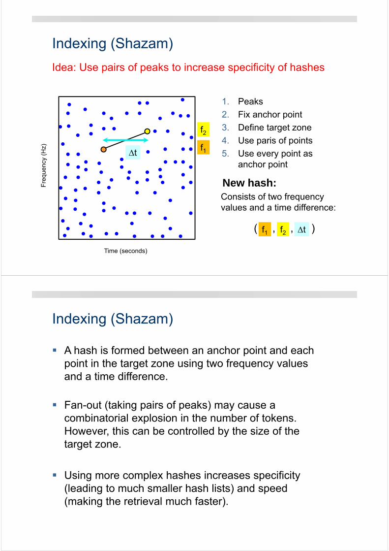
Idea: Use pairs of peaks to increase specificity of hashes
1. Peaks
2. Fix anchor point
3. Define target zone
4. Use paris of points
5. Use every point as anchor point
Indexing (Shazam)
Time (seconds)
Fre
quen
cy (
Hz)
Idea: Use pairs of peaks to increase specificity of hashes
New hash:
1. Peaks
2. Fix anchor point
3. Define target zone
4. Use paris of points
5. Use every point as anchor point
Consists of two frequencyvalues and a time difference:
( , , )
f1
f2
∆t
f1 f2 ∆t
Indexing (Shazam)
A hash is formed between an anchor point and each point in the target zone using two frequency values and a time difference.
Fan-out (taking pairs of peaks) may cause a combinatorial explosion in the number of tokens. However, this can be controlled by the size of the target zone.
Using more complex hashes increases specificity (leading to much smaller hash lists) and speed (making the retrieval much faster).
Indexing (Shazam)
Definitions:
N = number of spectral peaks
p = probability that a spectral peak can be found in (noisy and distorted) query
F = fan-out of target zone, e. g. F = 10
B = #(bits) used to encode spectral peaks and time difference
Consequences:
F · N = #(tokens) to be indexed
2B+B = increase of specifity (2B+B+B instead of 2B)
p2 = propability of a hash to survive
p·(1-(1-p)F) = probability that, at least, on hash survives per anchor point
Example: F = 10 and B = 10
Memory requirements: F · N = 10 · N
Speedup factor: 2B+B / F2 ~ 106 / 102 = 10000 (F times as many tokens in query and database, respectively)
Conclusions (Shazam)
Many parameters to choose:
Temporal and spectral resolution in spectrogram
Peak picking strategy
Target zone and fan-out parameter
Hash function
…
Literature (Audio Identification)
Allamanche et al. (AES 2001)
Cano et al. (AES 2002)
Haitsma/Kalker (ISMIR 2002)
Kurth/Clausen/Ribbrock (AES 2002)
Wang (ISMIR 2003)
Dupraz/Richard (ICASSP 2010)
Ramona/Peeters (ICASSP 2011)
…
Steps:
1. Spectrogram
Fre
quen
cy (
Hz)
Fre
quen
cy (
Hz)
Inte
nsity
Efficiently computable
Standard transform
Robust
Time (seconds)
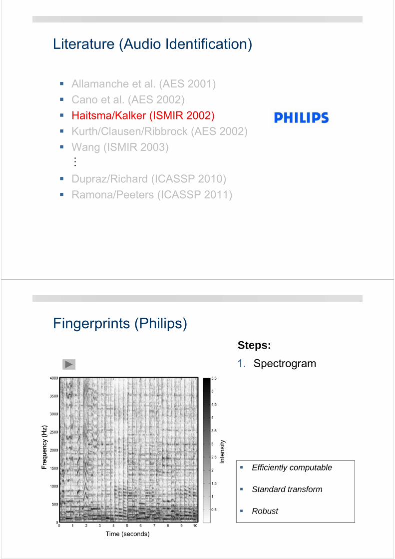
Fingerprints (Philips)
Steps:
1. Spectrogram(long window)
Fre
quen
cy (
Hz)
Fre
quen
cy (
Hz)
Inte
nsity
Coarse temporal resolution
Large overlap of windows
Robust to temporal distortion
Time (seconds)
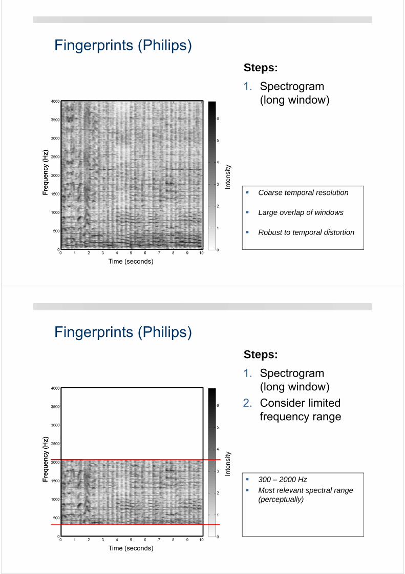
Fingerprints (Philips)
Steps:
Fre
quen
cy (
Hz)
Fre
quen
cy (
Hz)
Inte
nsity
300 – 2000 Hz
Most relevant spectral range (perceptually)
Time (seconds)
1. Spectrogram(long window)
2. Consider limited frequency range
Fingerprints (Philips)
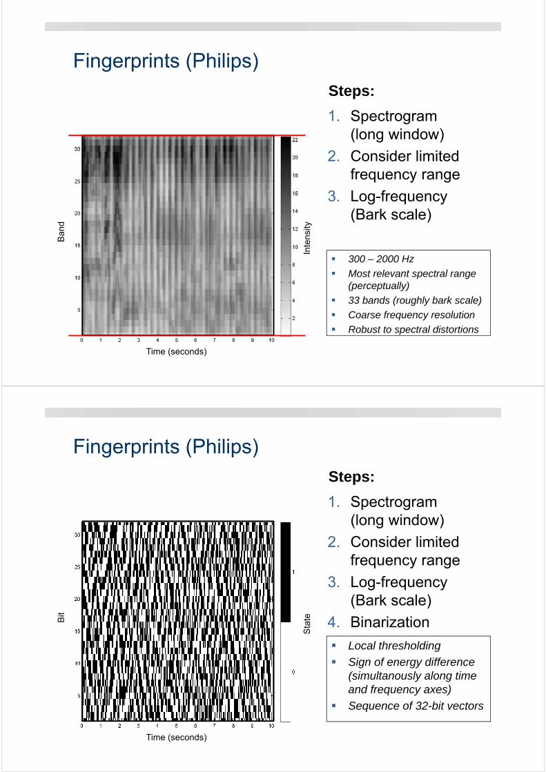
Steps:
Ban
d
Inte
nsity
300 – 2000 Hz
Most relevant spectral range (perceptually)
33 bands (roughly bark scale)
Coarse frequency resolution
Robust to spectral distortions
Time (seconds)
Fingerprints (Philips)
1. Spectrogram(long window)
2. Consider limited frequency range
3. Log-frequency (Bark scale)
Steps:
Sta
te
Local thresholding
Sign of energy difference(simultanously along time and frequency axes)
Sequence of 32-bit vectors
Time (seconds)
Bit
Fingerprints (Philips)
1. Spectrogram(long window)
2. Consider limited frequency range
3. Log-frequency (Bark scale)
4. Binarization
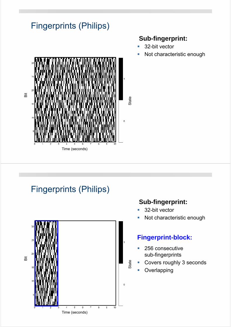
Fingerprints (Philips)
Sta
te
Time (seconds)
Bit
32-bit vector
Not characteristic enough
Sub-fingerprint:
Fingerprints (Philips)
Sta
te
Time (seconds)
Bit
32-bit vector
Not characteristic enough
Sub-fingerprint:
Fingerprint-block:
256 consecutive sub-fingerprints
Covers roughly 3 seconds
Overlapping
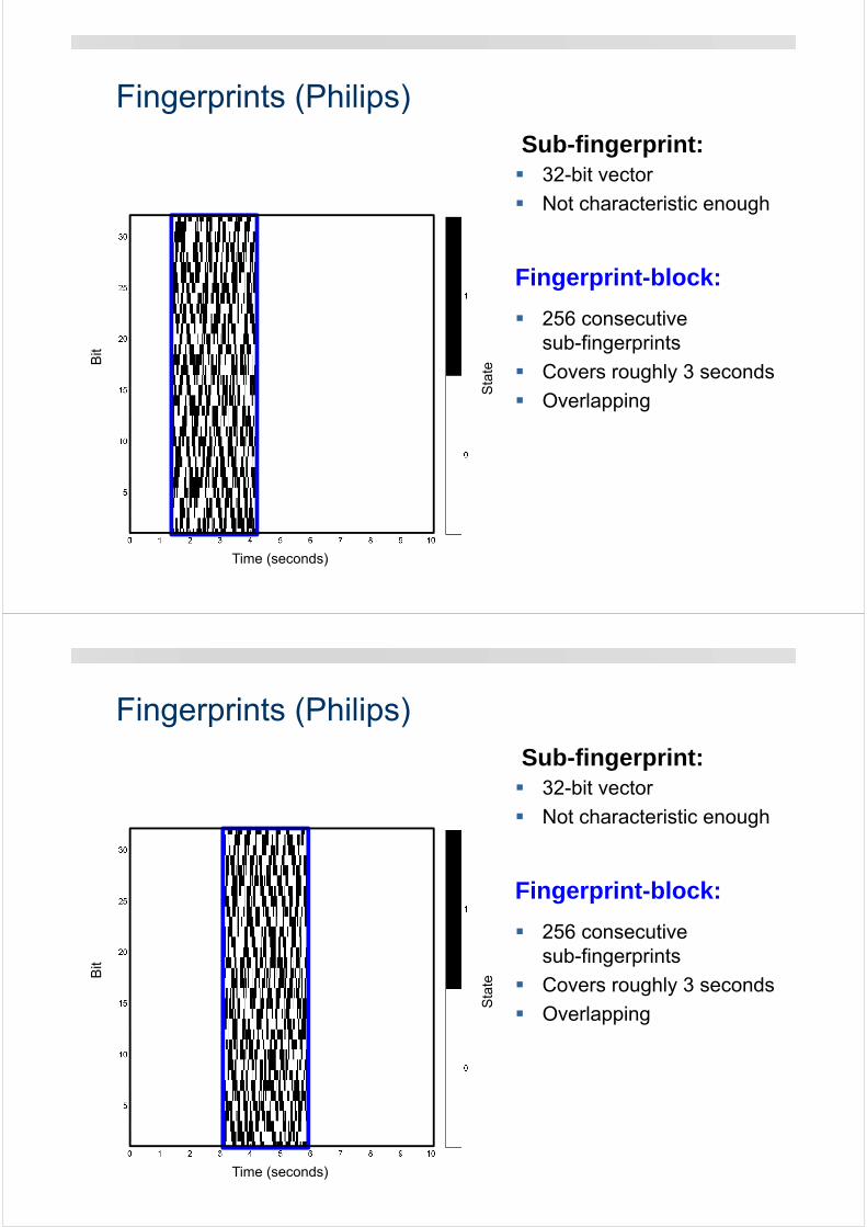
Fingerprints (Philips)
Sta
te
Time (seconds)
Bit
32-bit vector
Not characteristic enough
Sub-fingerprint:
Fingerprint-block:
256 consecutive sub-fingerprints
Covers roughly 3 seconds
Overlapping
Fingerprints (Philips)
Sta
te
Time (seconds)
Bit
32-bit vector
Not characteristic enough
Sub-fingerprint:
Fingerprint-block:
256 consecutive sub-fingerprints
Covers roughly 3 seconds
Overlapping
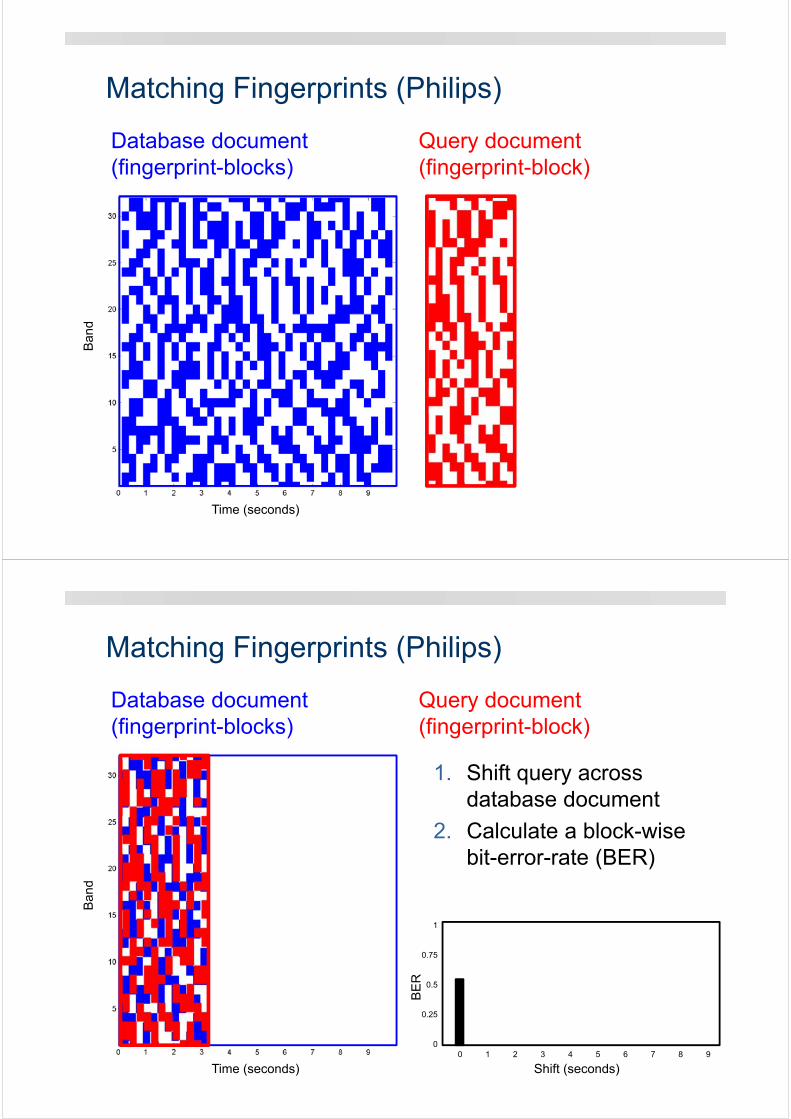
Matching Fingerprints (Philips)
Database document (fingerprint-blocks)
Inte
nsity
Time (seconds)
Ban
d
Query document(fingerprint-block)
Matching Fingerprints (Philips)
Inte
nsity
Time (seconds)
Ban
d
1. Shift query across database document
2. Calculate a block-wisebit-error-rate (BER)
Shift (seconds)0 1 2 3 4 5 6 7 8 9
BE
R
1
0.75
0.5
0.25
0
Database document (fingerprint-blocks)
Query document(fingerprint-block)
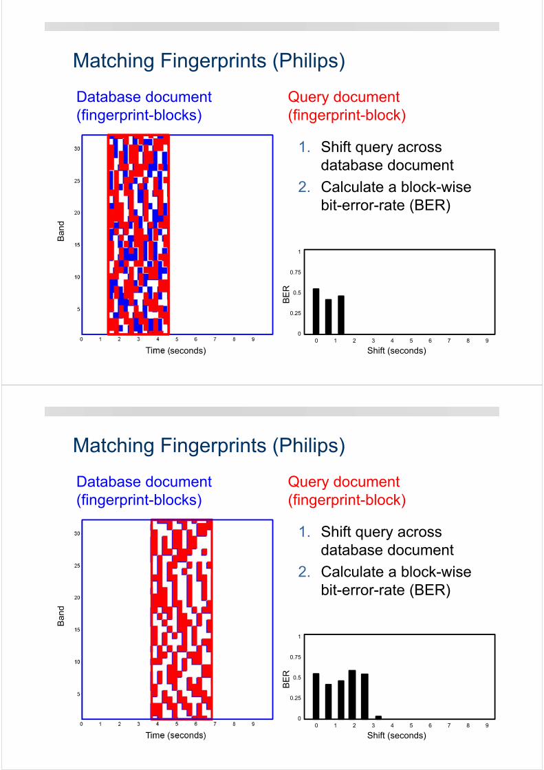
Matching Fingerprints (Philips)
Inte
nsity
Time (seconds)
Ban
d
1. Shift query across database document
2. Calculate a block-wisebit-error-rate (BER)
Shift (seconds)0 1 2 3 4 5 6 7 8 9
BE
R
1
0.75
0.5
0.25
0
Database document (fingerprint-blocks)
Query document(fingerprint-block)
Matching Fingerprints (Philips)
Inte
nsity
Time (seconds)
Ban
d
1. Shift query across database document
2. Calculate a block-wisebit-error-rate (BER)
Shift (seconds)0 1 2 3 4 5 6 7 8 9
BE
R
1
0.75
0.5
0.25
0
Database document (fingerprint-blocks)
Query document(fingerprint-block)
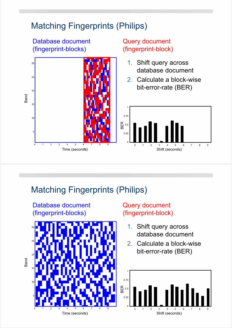
Matching Fingerprints (Philips)
Inte
nsity
Time (seconds)
Ban
d
1. Shift query across database document
2. Calculate a block-wisebit-error-rate (BER)
Shift (seconds)0 1 2 3 4 5 6 7 8 9
BE
R
1
0.75
0.5
0.25
0
Database document (fingerprint-blocks)
Query document(fingerprint-block)
Matching Fingerprints (Philips)
Inte
nsity
Time (seconds)
Ban
d
1. Shift query across database document
2. Calculate a block-wisebit-error-rate (BER)
Shift (seconds)0 1 2 3 4 5 6 7 8 9
BE
R
1
0.75
0.5
0.25
0
Database document (fingerprint-blocks)
Query document(fingerprint-block)
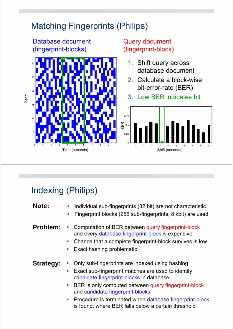
Matching Fingerprints (Philips)
Inte
nsity
Time (seconds)
Ban
d
1. Shift query across database document
2. Calculate a block-wisebit-error-rate (BER)
3. Low BER indicates hit
Shift (seconds)0 1 2 3 4 5 6 7 8 9
BE
R
1
0.75
0.5
0.25
0
Database document (fingerprint-blocks)
Query document(fingerprint-block)
Indexing (Philips)
Computation of BER between query fingerprint-block and every database fingerprint-block is expensive
Chance that a complete fingerprint-block survives is low
Exact hashing problematic
Note:
Problem:
Individual sub-fingerprints (32 bit) are not characteristic
Fingerprint blocks (256 sub-fingerprints, 8 kbit) are used
Strategy: Only sub-fingerprints are indexed using hashing
Exact sub-fingerprint matches are used to identify candidate fingerprint-blocks in database.
BER is only computed between query fingerprint-block and candidate fingerprint-blocks
Procedure is terminated when database fingerprint-block is found, where BER falls below a certain threshold
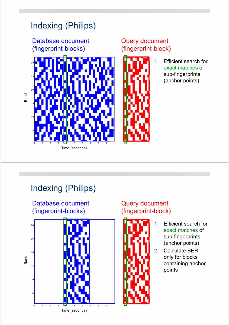
Indexing (Philips)
1. Efficient search for exact matches of sub-fingerprints (anchor points)
Inte
nsity
Time (seconds)
Ban
d
Database document (fingerprint-blocks)
Query document(fingerprint-block)
Indexing (Philips)
1. Efficient search for exact matches of sub-fingerprints (anchor points)
2. Calculate BER only for blocks containing anchor pointsIn
tens
ity
Time (seconds)
Ban
d
Database document (fingerprint-blocks)
Query document(fingerprint-block)
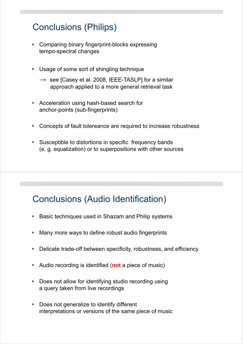
Conclusions (Philips)
Comparing binary fingerprint-blocks expressing tempo-spectral changes
Usage of some sort of shingling technique
→ see [Casey et al. 2008, IEEE-TASLP] for a similarapproach applied to a more general retrieval task
Acceleration using hash-based search for anchor-points (sub-fingerprints)
Concepts of fault tolereance are required to increase robustness
Susceptible to distortions in specific frequency bands (e. g. equalization) or to superpositions with other sources
Conclusions (Audio Identification)
Basic techniques used in Shazam and Philip systems
Many more ways to define robust audio fingerprints
Delicate trade-off between specificity, robustness, and efficiency
Audio recording is identified (not a piece of music)
Does not allow for identifying studio recording using a query taken from live recordings
Does not generalize to identify different interpretations or versions of the same piece of music
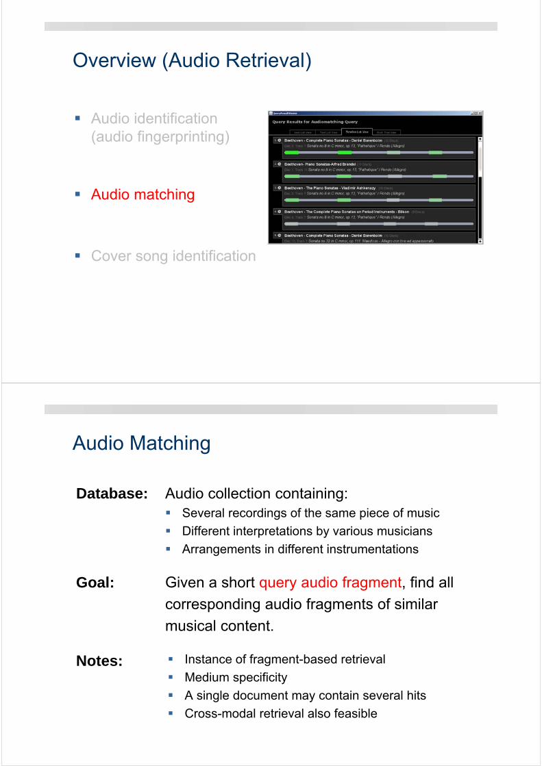
Overview (Audio Retrieval)
Audio identification(audio fingerprinting)
Audio matching
Cover song identification
Audio Matching
Database: Audio collection containing: Several recordings of the same piece of music
Different interpretations by various musicians
Arrangements in different instrumentations
Goal: Given a short query audio fragment, find all
corresponding audio fragments of similar
musical content.
Notes: Instance of fragment-based retrieval
Medium specificity
A single document may contain several hits
Cross-modal retrieval also feasible
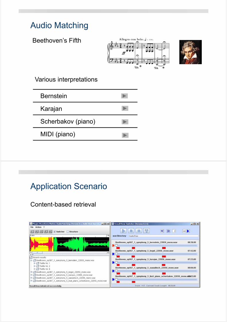
Bernstein
Karajan
Scherbakov (piano)
MIDI (piano)
Audio Matching
Beethoven’s Fifth
Various interpretations
Application Scenario
Content-based retrieval
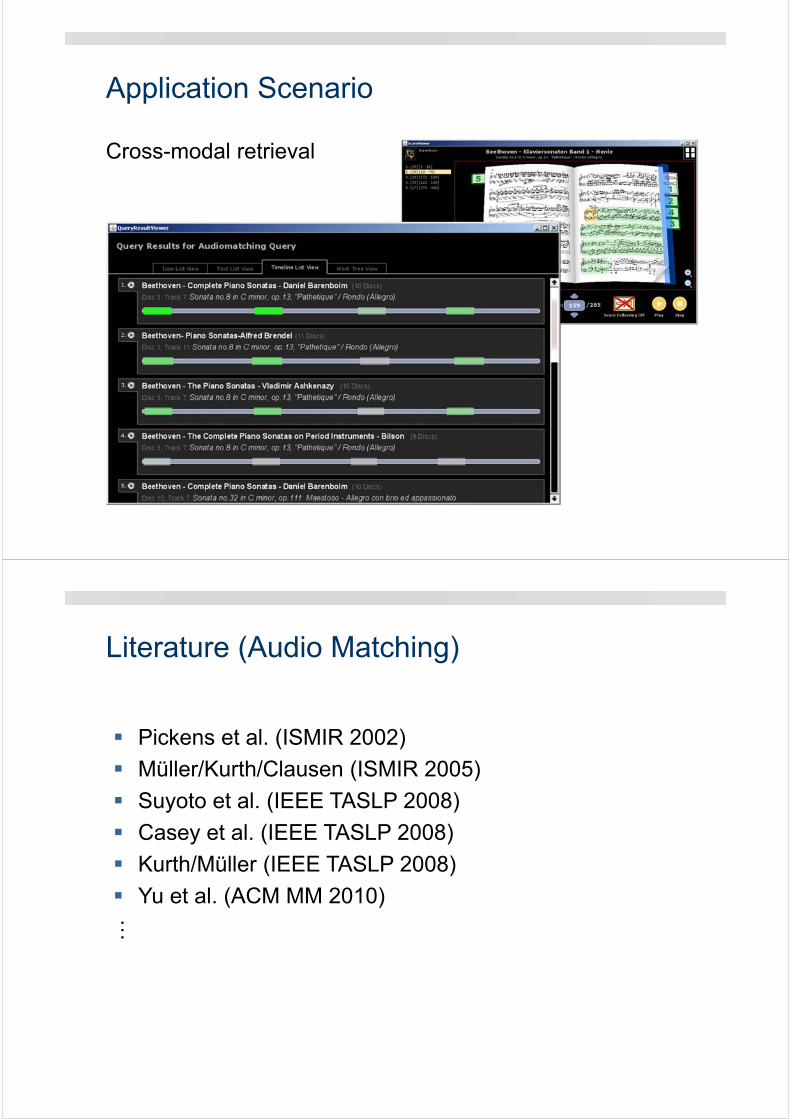
Application Scenario
Cross-modal retrieval
Literature (Audio Matching)
Pickens et al. (ISMIR 2002)
Müller/Kurth/Clausen (ISMIR 2005)
Suyoto et al. (IEEE TASLP 2008)
Casey et al. (IEEE TASLP 2008)
Kurth/Müller (IEEE TASLP 2008)
Yu et al. (ACM MM 2010)
…
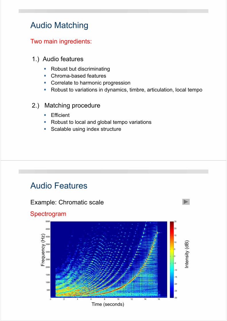
Audio Matching
Two main ingredients:
Robust but discriminating Chroma-based features Correlate to harmonic progression Robust to variations in dynamics, timbre, articulation, local tempo
1.) Audio features
Efficient Robust to local and global tempo variations Scalable using index structure
2.) Matching procedure
Audio Features
Example: Chromatic scale
Time (seconds)
Fre
quen
cy (
Hz)
Inte
nsity
(dB
)
Spectrogram
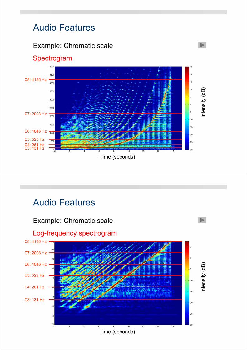
Audio Features
Example: Chromatic scale
Time (seconds)
Inte
nsity
(dB
)
Spectrogram
C4: 261 HzC5: 523 Hz
C6: 1046 Hz
C7: 2093 Hz
C8: 4186 Hz
C3: 131 Hz
Audio Features
Example: Chromatic scale
Inte
nsity
(dB
)
Log-frequency spectrogram
Time (seconds)
C4: 261 Hz
C5: 523 Hz
C6: 1046 Hz
C7: 2093 Hz
C8: 4186 Hz
C3: 131 Hz
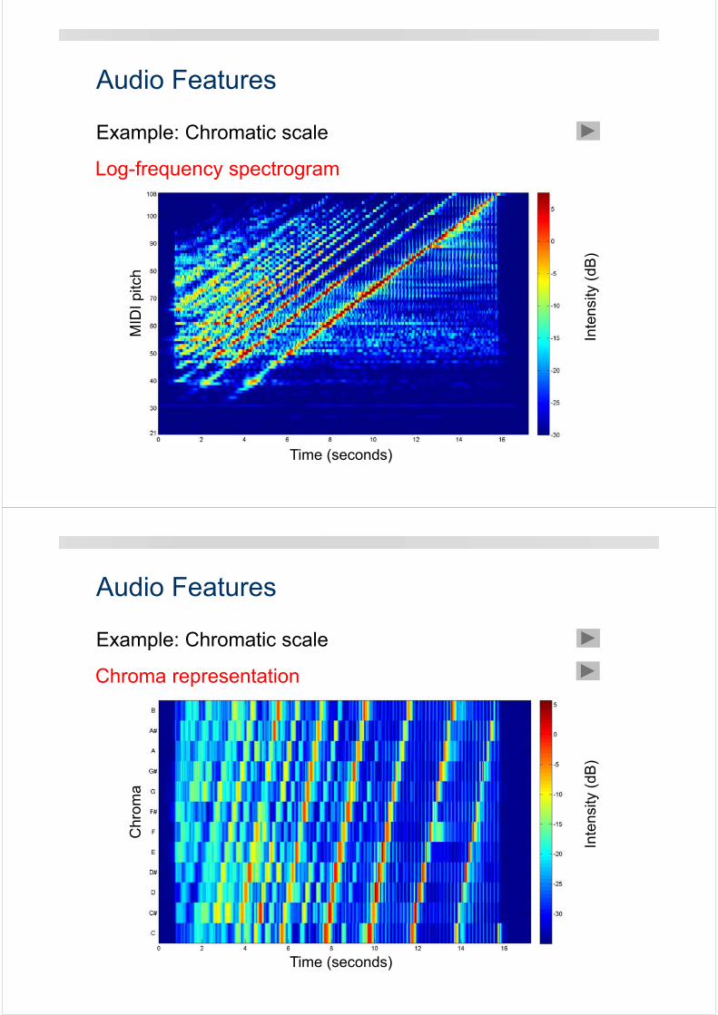
Audio Features
Example: Chromatic scaleM
IDI
pitc
h
Inte
nsity
(dB
)
Log-frequency spectrogram
Time (seconds)
Audio Features
Example: Chromatic scale
Chr
oma
Inte
nsity
(dB
)
Chroma representation
Time (seconds)
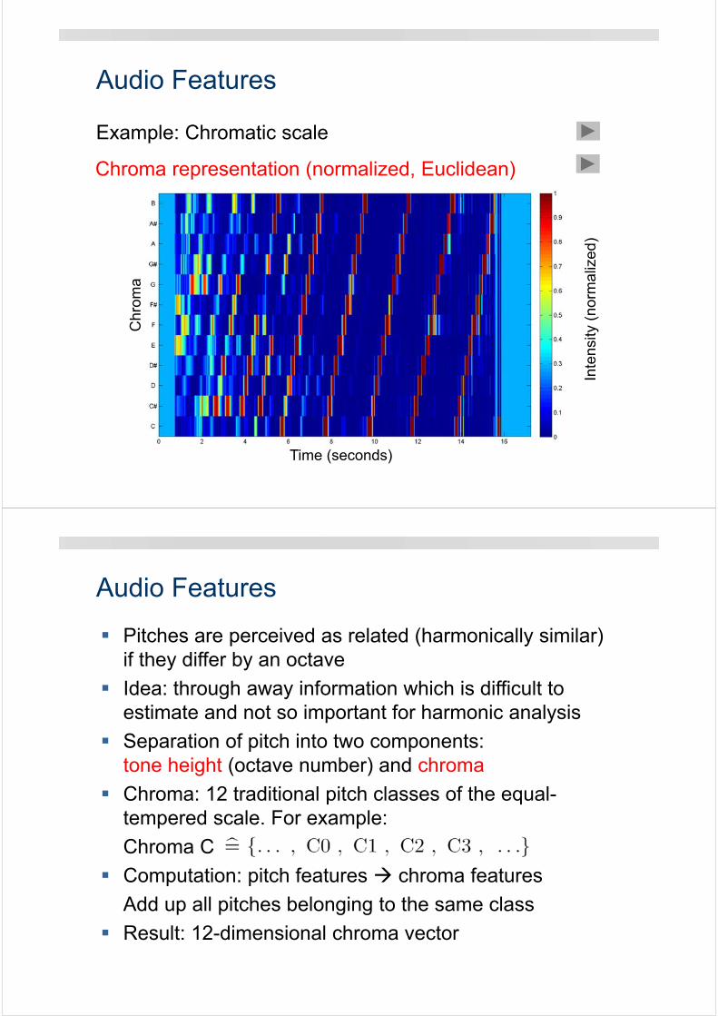
Audio Features
Example: Chromatic scale
Inte
nsity
(no
rmal
ized
)
Chroma representation (normalized, Euclidean)
Chr
oma
Time (seconds)
Pitches are perceived as related (harmonically similar) if they differ by an octave
Idea: through away information which is difficult to estimate and not so important for harmonic analysis
Separation of pitch into two components: tone height (octave number) and chroma
Chroma: 12 traditional pitch classes of the equal-tempered scale. For example:
Chroma C
Computation: pitch features chroma features
Add up all pitches belonging to the same class
Result: 12-dimensional chroma vector
Audio Features
Audio Features
Time (seconds) Time (seconds)Time (seconds) Time (seconds)
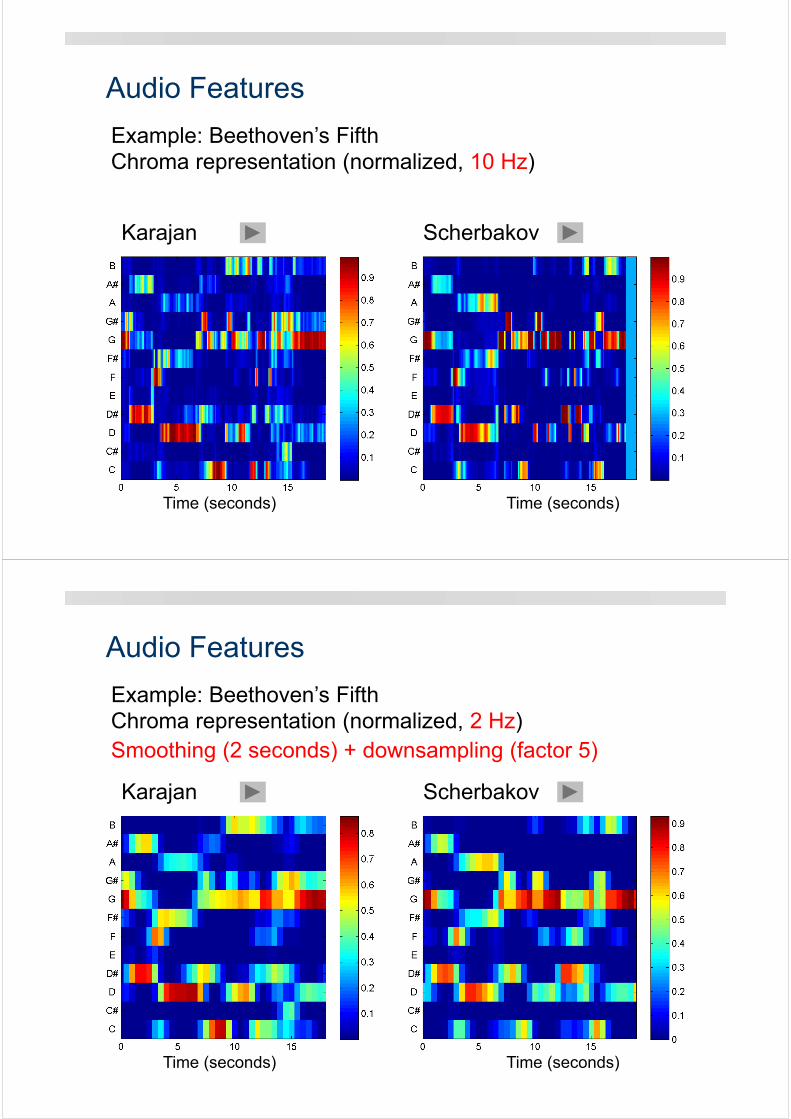
Example: Beethoven’s Fifth
Karajan Scherbakov
Chroma representation (normalized, 10 Hz)
Audio Features
Time (seconds) Time (seconds)Time (seconds) Time (seconds)
Example: Beethoven’s Fifth
Karajan Scherbakov
Smoothing (2 seconds) + downsampling (factor 5)Chroma representation (normalized, 2 Hz)
Audio Features
Time (seconds) Time (seconds)Time (seconds) Time (seconds)
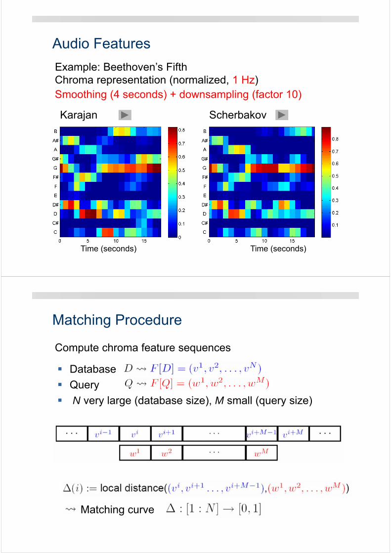
Example: Beethoven’s Fifth
Karajan Scherbakov
Smoothing (4 seconds) + downsampling (factor 10)Chroma representation (normalized, 1 Hz)
Matching Procedure
Compute chroma feature sequences
Database
Query
N very large (database size), M small (query size)
Matching curve
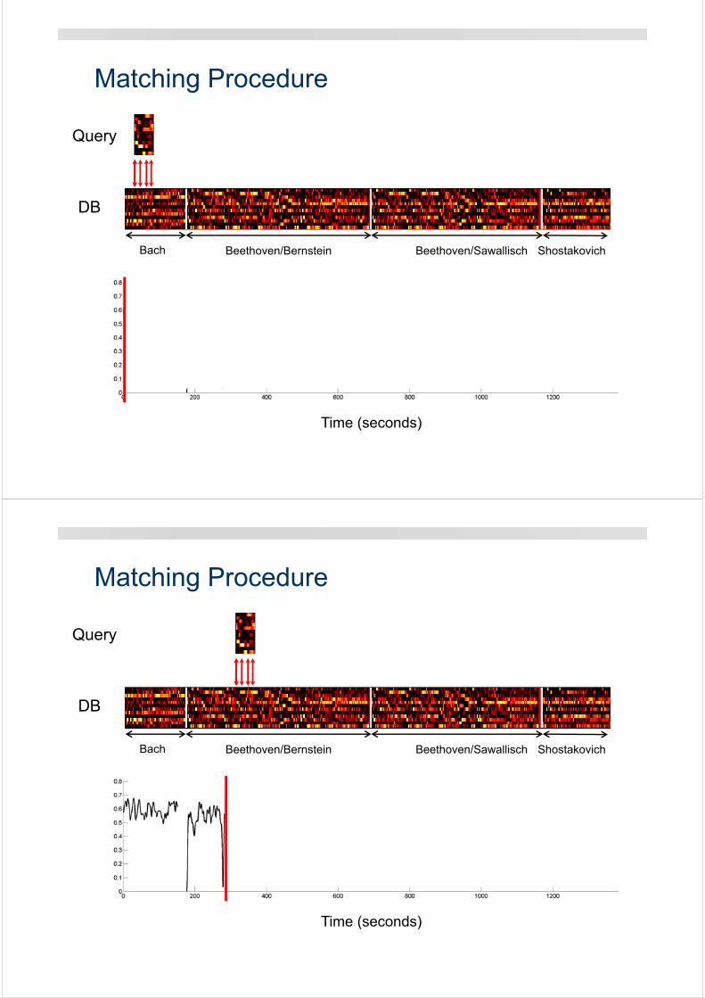
Matching Procedure
Query
DB
Bach Beethoven/Bernstein Shostakovich
Time (seconds)
Beethoven/Sawallisch
Matching Procedure
Query
DB
Bach Beethoven/Bernstein ShostakovichBeethoven/Sawallisch
Time (seconds)
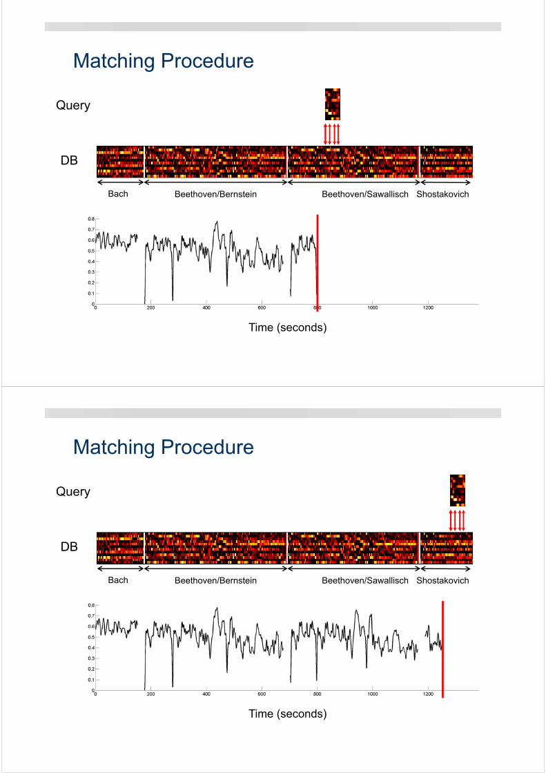
Matching Procedure
Query
DB
Bach Beethoven/Bernstein ShostakovichBeethoven/Sawallisch
Time (seconds)
Matching Procedure
Query
DB
Bach Beethoven/Bernstein ShostakovichBeethoven/Sawallisch
Time (seconds)
Matching Procedure
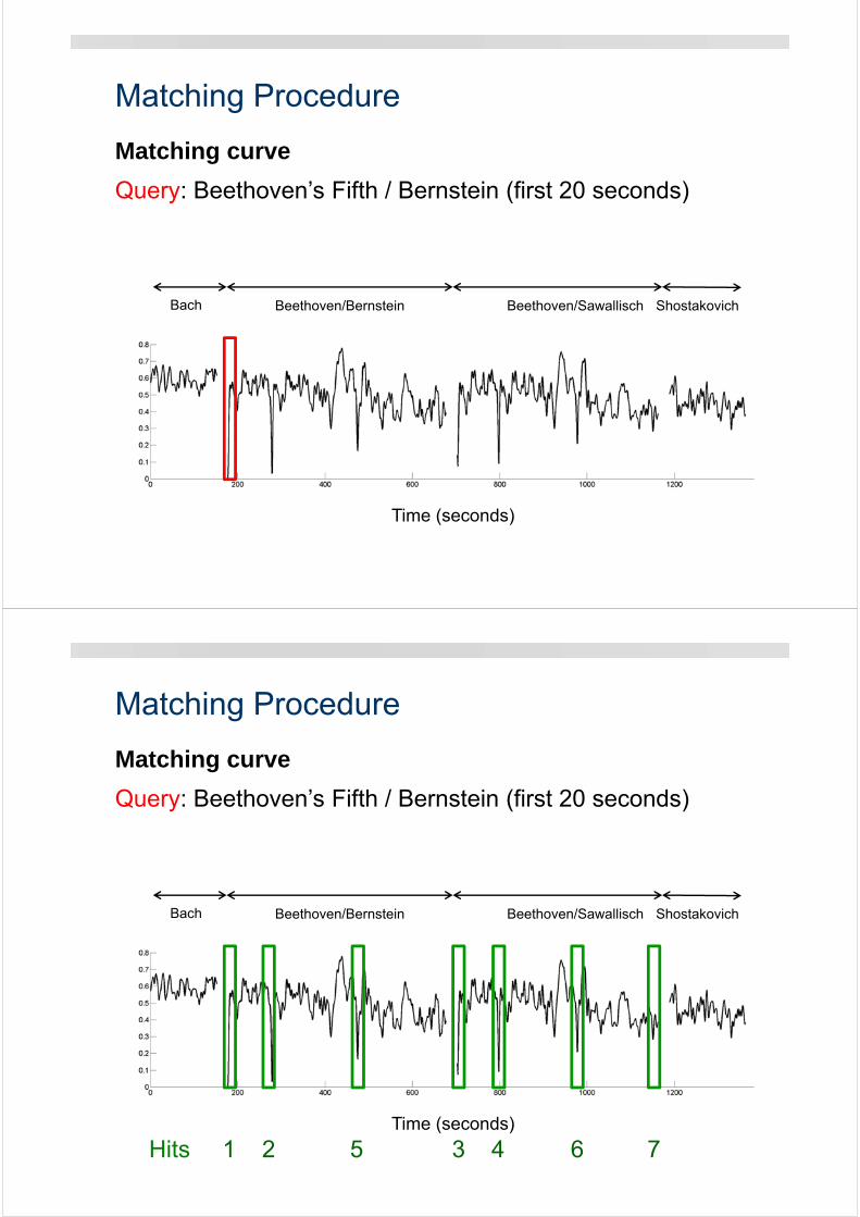
Bach Beethoven/Bernstein ShostakovichBeethoven/Sawallisch
Query: Beethoven’s Fifth / Bernstein (first 20 seconds)
Matching curve
Time (seconds)
Matching Procedure
Query: Beethoven’s Fifth / Bernstein (first 20 seconds)
Bach Beethoven/Bernstein ShostakovichBeethoven/Sawallisch
1 2 5 3 4 6 7Hits
Matching curve
Time (seconds)
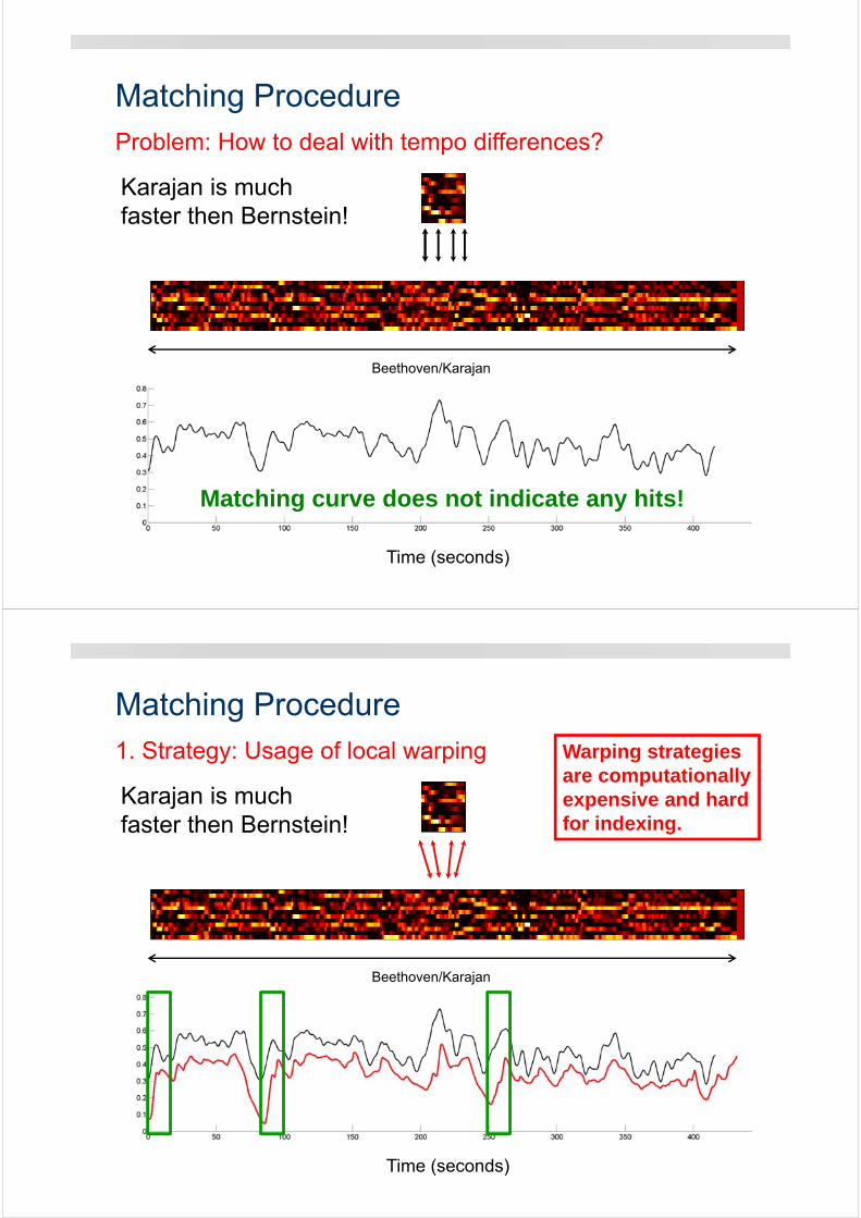
Matching Procedure
Time (seconds)
Problem: How to deal with tempo differences?
Karajan is much faster then Bernstein!
Matching curve does not indicate any hits!
Beethoven/Karajan
Matching Procedure1. Strategy: Usage of local warping
Karajan is much faster then Bernstein!
Beethoven/Karajan
Warping strategies are computationally expensive and hard for indexing.
Time (seconds)

Matching Procedure2. Strategy: Usage of multiple scaling
Beethoven/Karajan
Time (seconds)
Matching Procedure2. Strategy: Usage of multiple scaling
Beethoven/Karajan
Time (seconds)
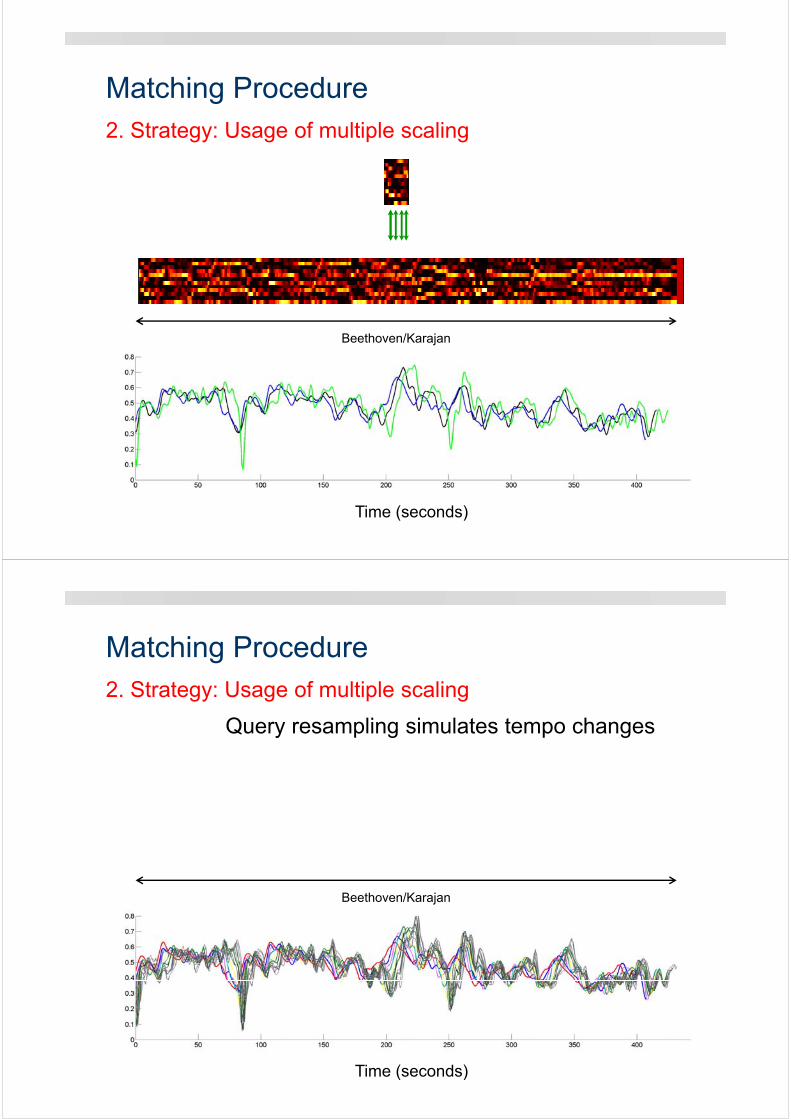
Matching Procedure2. Strategy: Usage of multiple scaling
Beethoven/Karajan
Time (seconds)
Matching Procedure2. Strategy: Usage of multiple scaling
Query resampling simulates tempo changes
Beethoven/Karajan
Time (seconds)
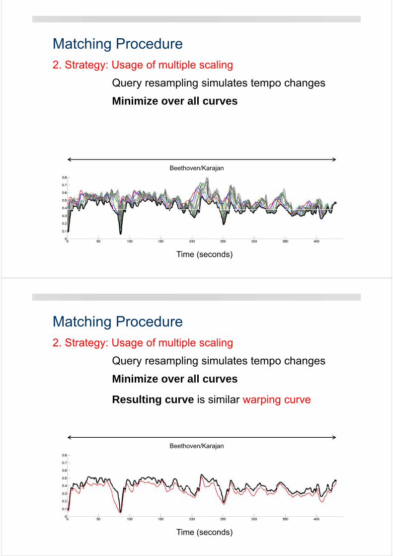
Matching Procedure2. Strategy: Usage of multiple scaling
Minimize over all curves
Beethoven/Karajan
Query resampling simulates tempo changes
Time (seconds)
Matching Procedure2. Strategy: Usage of multiple scaling
Minimize over all curves
Beethoven/Karajan
Query resampling simulates tempo changes
Resulting curve is similar warping curve
Time (seconds)
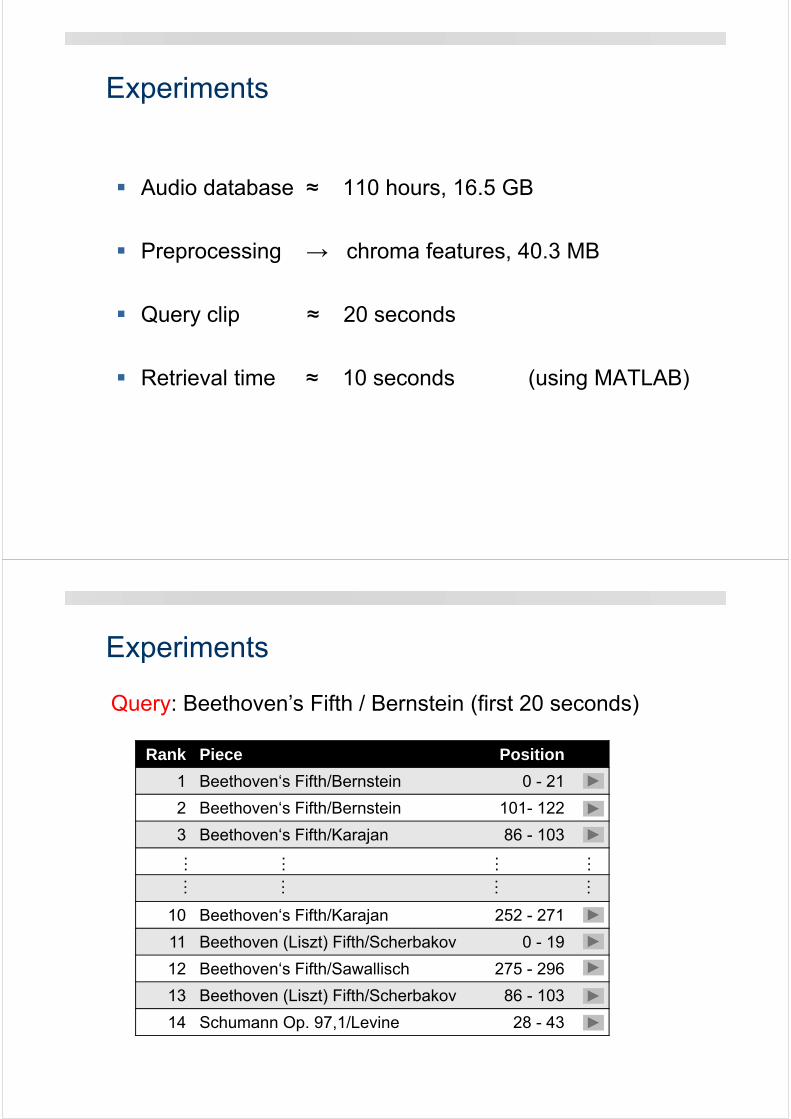
Experiments
Audio database ≈ 110 hours, 16.5 GB
Preprocessing → chroma features, 40.3 MB
Query clip ≈ 20 seconds
Retrieval time ≈ 10 seconds (using MATLAB)
Experiments
Rank Piece Position
1 Beethoven‘s Fifth/Bernstein 0 - 21
2 Beethoven‘s Fifth/Bernstein 101- 122
3 Beethoven‘s Fifth/Karajan 86 - 103
10 Beethoven‘s Fifth/Karajan 252 - 271
11 Beethoven (Liszt) Fifth/Scherbakov 0 - 19
12 Beethoven‘s Fifth/Sawallisch 275 - 296
13 Beethoven (Liszt) Fifth/Scherbakov 86 - 103
14 Schumann Op. 97,1/Levine 28 - 43
Query: Beethoven’s Fifth / Bernstein (first 20 seconds)
……
……
……
……
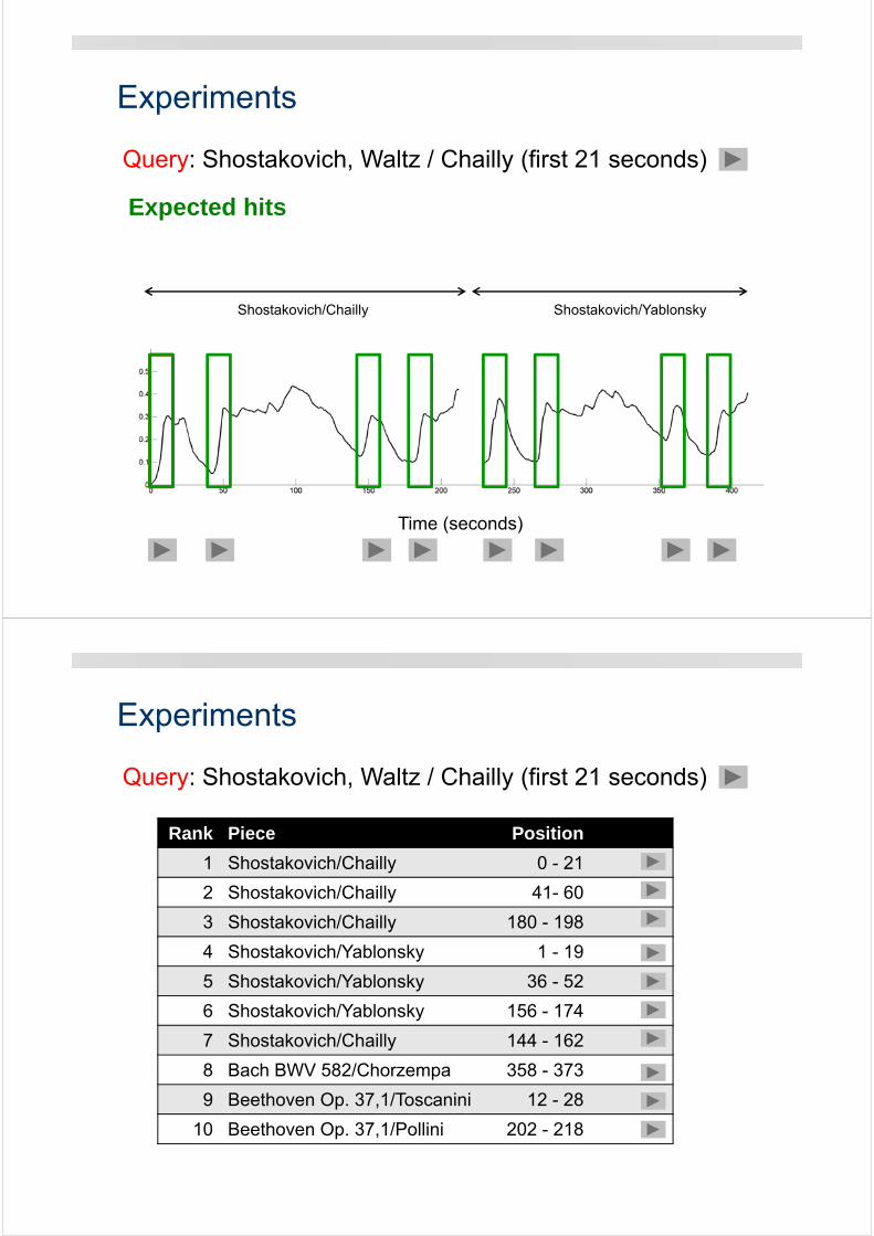
Experiments
Shostakovich/Chailly Shostakovich/Yablonsky
Time (seconds)
Query: Shostakovich, Waltz / Chailly (first 21 seconds)
Expected hits
Experiments
Rank Piece Position
1 Shostakovich/Chailly 0 - 21
2 Shostakovich/Chailly 41- 60
3 Shostakovich/Chailly 180 - 198
4 Shostakovich/Yablonsky 1 - 19
5 Shostakovich/Yablonsky 36 - 52
6 Shostakovich/Yablonsky 156 - 174
7 Shostakovich/Chailly 144 - 162
8 Bach BWV 582/Chorzempa 358 - 373
9 Beethoven Op. 37,1/Toscanini 12 - 28
10 Beethoven Op. 37,1/Pollini 202 - 218
Query: Shostakovich, Waltz / Chailly (first 21 seconds)
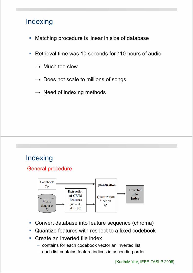
Indexing
Matching procedure is linear in size of database
Retrieval time was 10 seconds for 110 hours of audio
→ Much too slow
→ Does not scale to millions of songs
→ Need of indexing methods
Indexing
Convert database into feature sequence (chroma)
Quantize features with respect to a fixed codebook
Create an inverted file index– contains for each codebook vector an inverted list
– each list contains feature indices in ascending order
General procedure
[Kurth/Müller, IEEE-TASLP 2008]
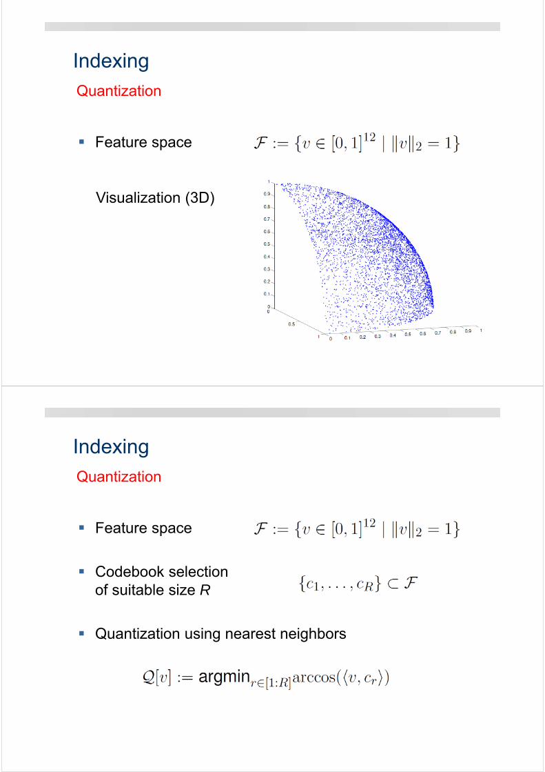
Indexing
Visualization (3D)
Quantization
Feature space
Indexing
Feature space
Codebook selectionof suitable size R
Quantization using nearest neighbors
Quantization
Indexing
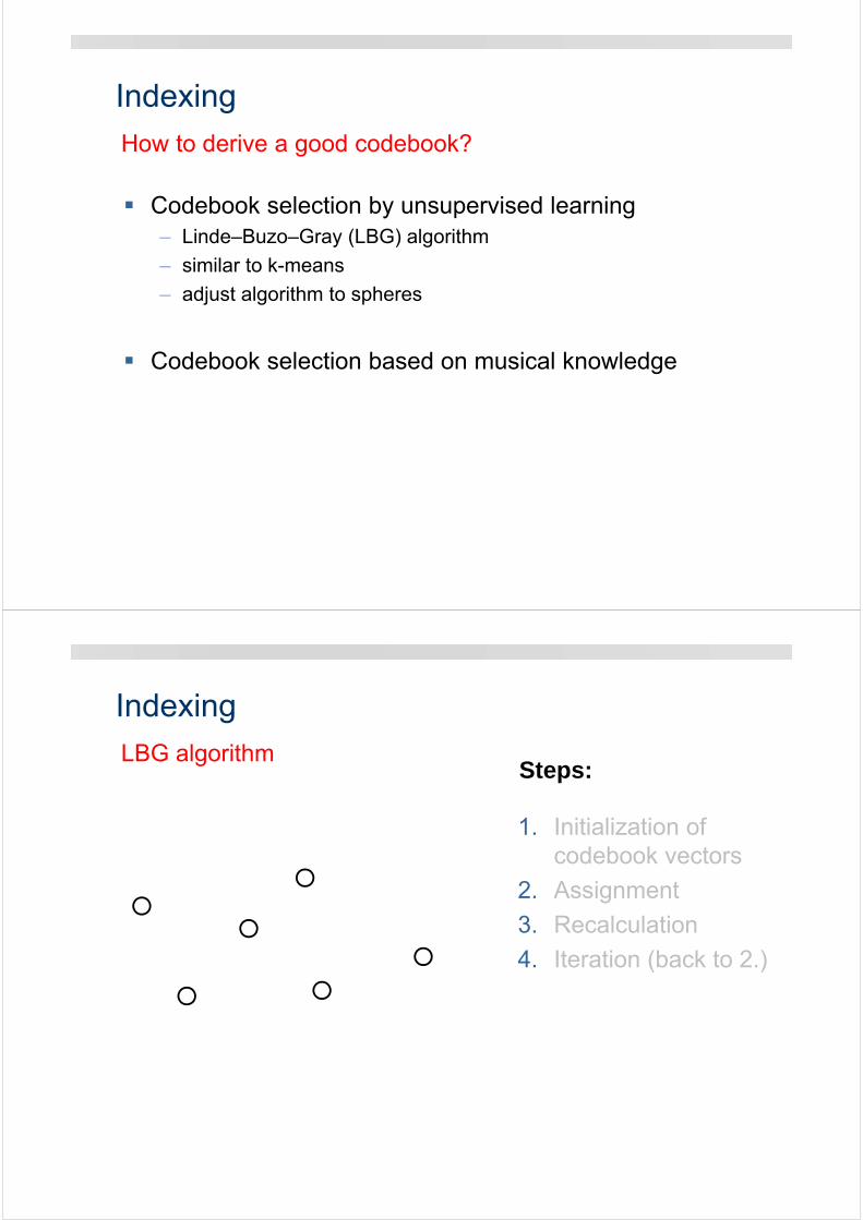
Codebook selection by unsupervised learning– Linde–Buzo–Gray (LBG) algorithm
– similar to k-means
– adjust algorithm to spheres
Codebook selection based on musical knowledge
How to derive a good codebook?
Indexing
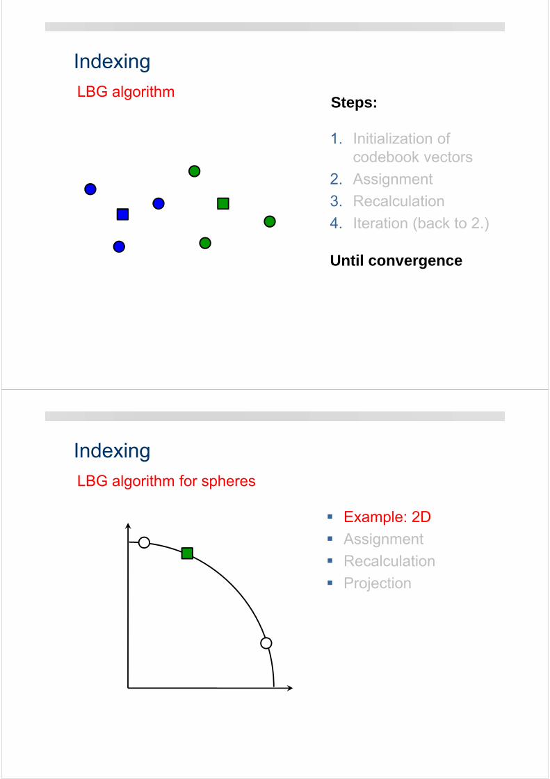
LBG algorithmSteps:
1. Initialization ofcodebook vectors
2. Assignment
3. Recalculation
4. Iteration (back to 2.)
Indexing
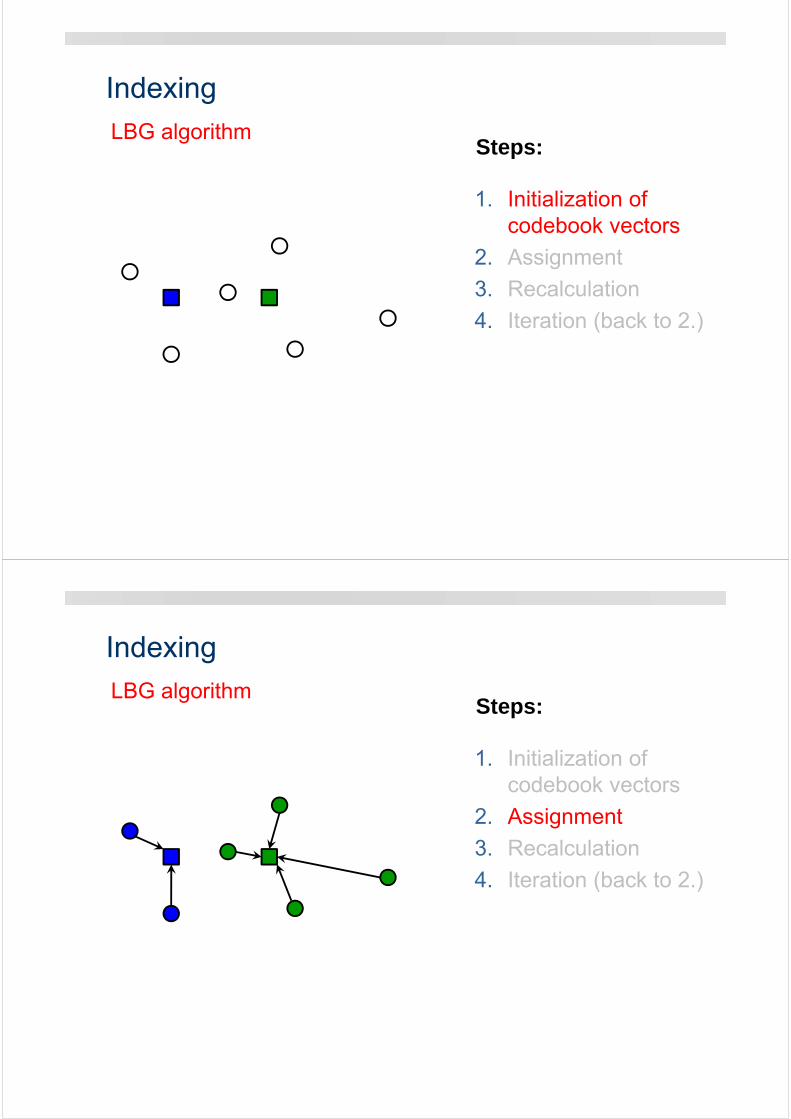
LBG algorithmSteps:
1. Initialization ofcodebook vectors
2. Assignment
3. Recalculation
4. Iteration (back to 2.)
Indexing
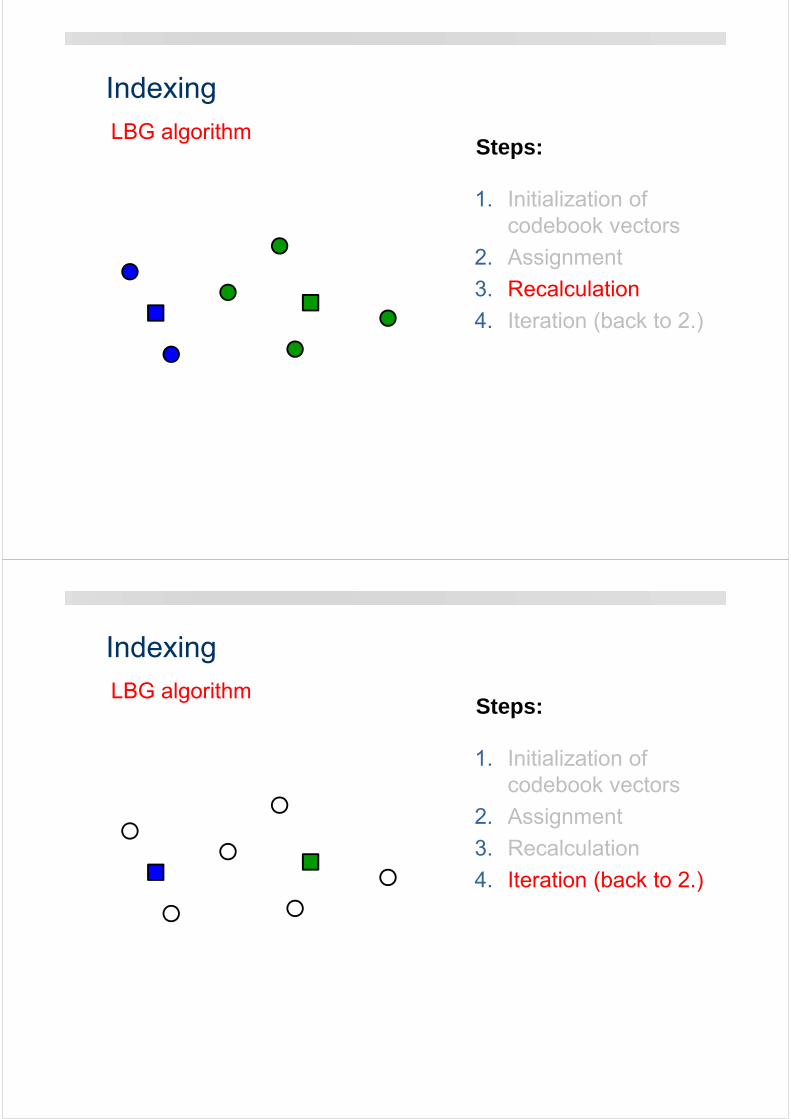
LBG algorithmSteps:
1. Initialization ofcodebook vectors
2. Assignment
3. Recalculation
4. Iteration (back to 2.)
Indexing
LBG algorithmSteps:
1. Initialization ofcodebook vectors
2. Assignment
3. Recalculation
4. Iteration (back to 2.)
Indexing
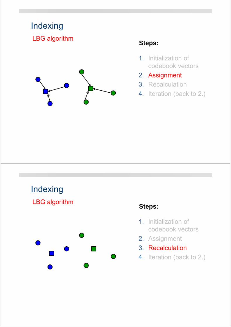
LBG algorithmSteps:
1. Initialization ofcodebook vectors
2. Assignment
3. Recalculation
4. Iteration (back to 2.)
Indexing
LBG algorithmSteps:
1. Initialization ofcodebook vectors
2. Assignment
3. Recalculation
4. Iteration (back to 2.)
Indexing
LBG algorithmSteps:
1. Initialization ofcodebook vectors
2. Assignment
3. Recalculation
4. Iteration (back to 2.)
Indexing
LBG algorithmSteps:
1. Initialization ofcodebook vectors
2. Assignment
3. Recalculation
4. Iteration (back to 2.)
Until convergence
Indexing
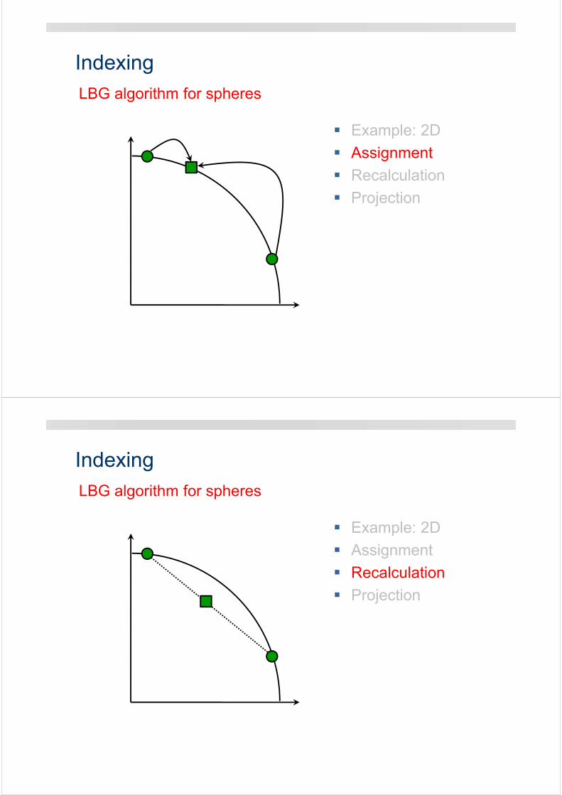
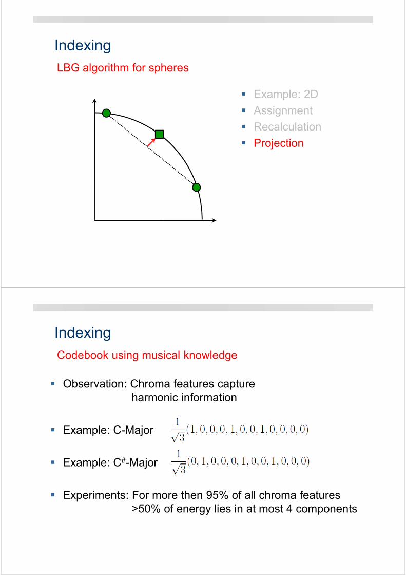
LBG algorithm for spheres
Example: 2D
Assignment
Recalculation
Projection
Indexing
LBG algorithm for spheres
Example: 2D
Assignment
Recalculation
Projection
Indexing
LBG algorithm for spheres
Example: 2D
Assignment
Recalculation
Projection
Indexing
LBG algorithm for spheres
Example: 2D
Assignment
Recalculation
Projection
Indexing
Codebook using musical knowledge
Observation: Chroma features captureharmonic information
Example: C-Major
Example: C#-Major
Experiments: For more then 95% of all chroma features>50% of energy lies in at most 4 components
n 1 2 3 4
template
# 12 66 220 495 793
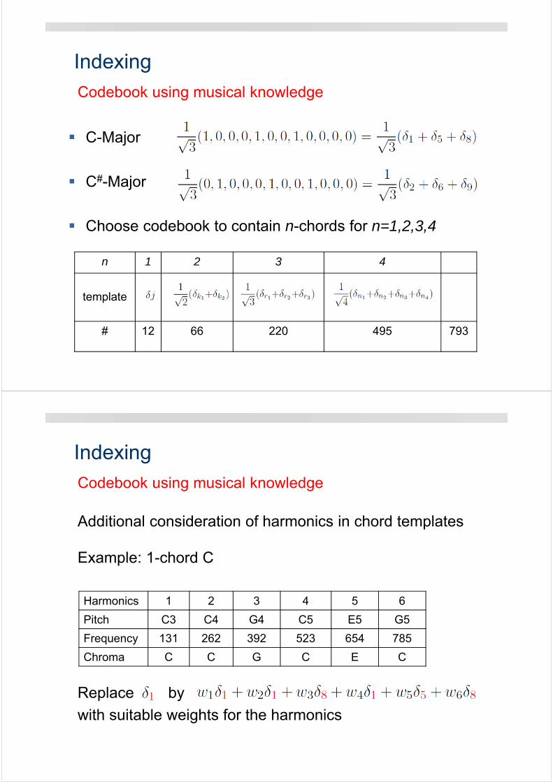
Indexing
Codebook using musical knowledge
C-Major
C#-Major
Choose codebook to contain n-chords for n=1,2,3,4
Replace by
with suitable weights for the harmonics
Indexing
Codebook using musical knowledge
Additional consideration of harmonics in chord templates
Harmonics 1 2 3 4 5 6
Pitch C3 C4 G4 C5 E5 G5
Frequency 131 262 392 523 654 785
Chroma C C G C E C
Example: 1-chord C
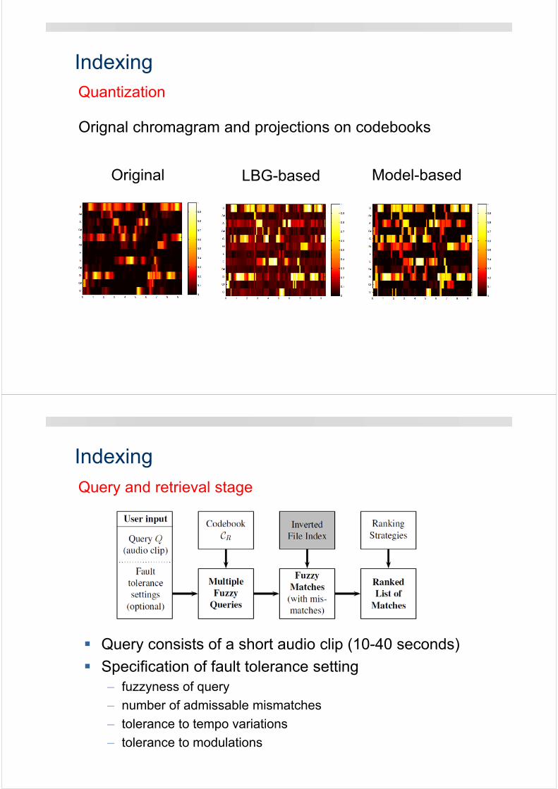
IndexingQuantization
Original
Orignal chromagram and projections on codebooks
LBG-based Model-based
Indexing
Query consists of a short audio clip (10-40 seconds)
Specification of fault tolerance setting– fuzzyness of query
– number of admissable mismatches
– tolerance to tempo variations
– tolerance to modulations
Query and retrieval stage
Indexing
Medium sized database– 500 pieces
– 112 hours of audio
– mostly classical music
Selection of various queries– 36 queries
– duration between 10 and 40 seconds
– hand-labelled matches in database
Indexing leads to speed-up factor between 15 and 20 (depending on query length)
Only small degradation in precision and recall
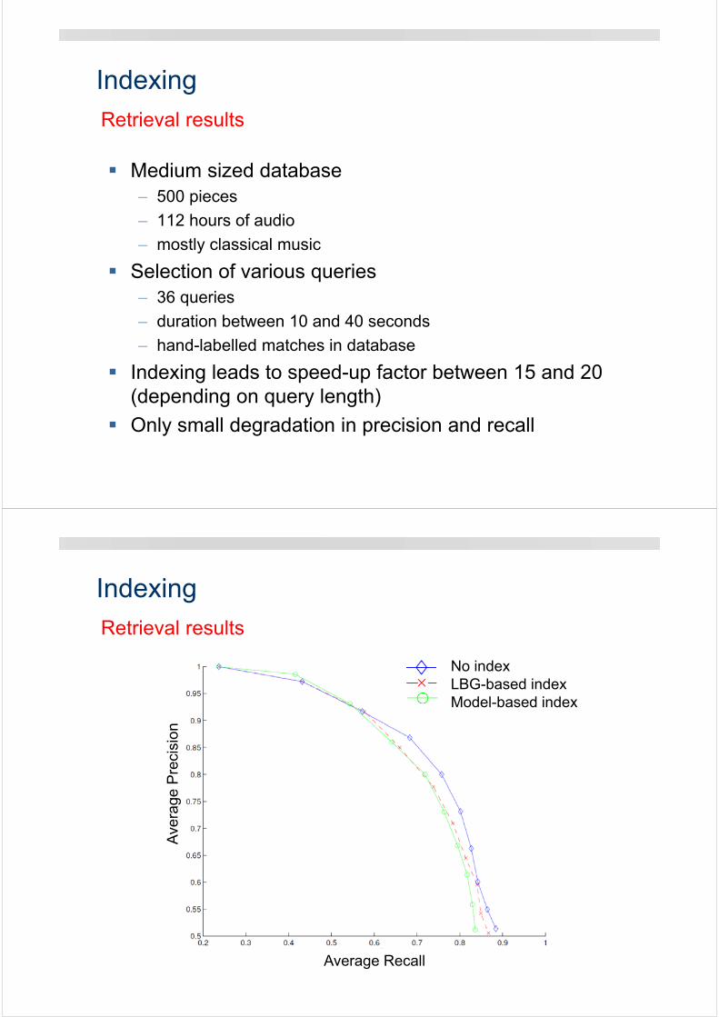
Retrieval results
Indexing
Retrieval results
Average Recall
Ave
rage
Pre
cisi
on
No indexLBG-based indexModel-based index
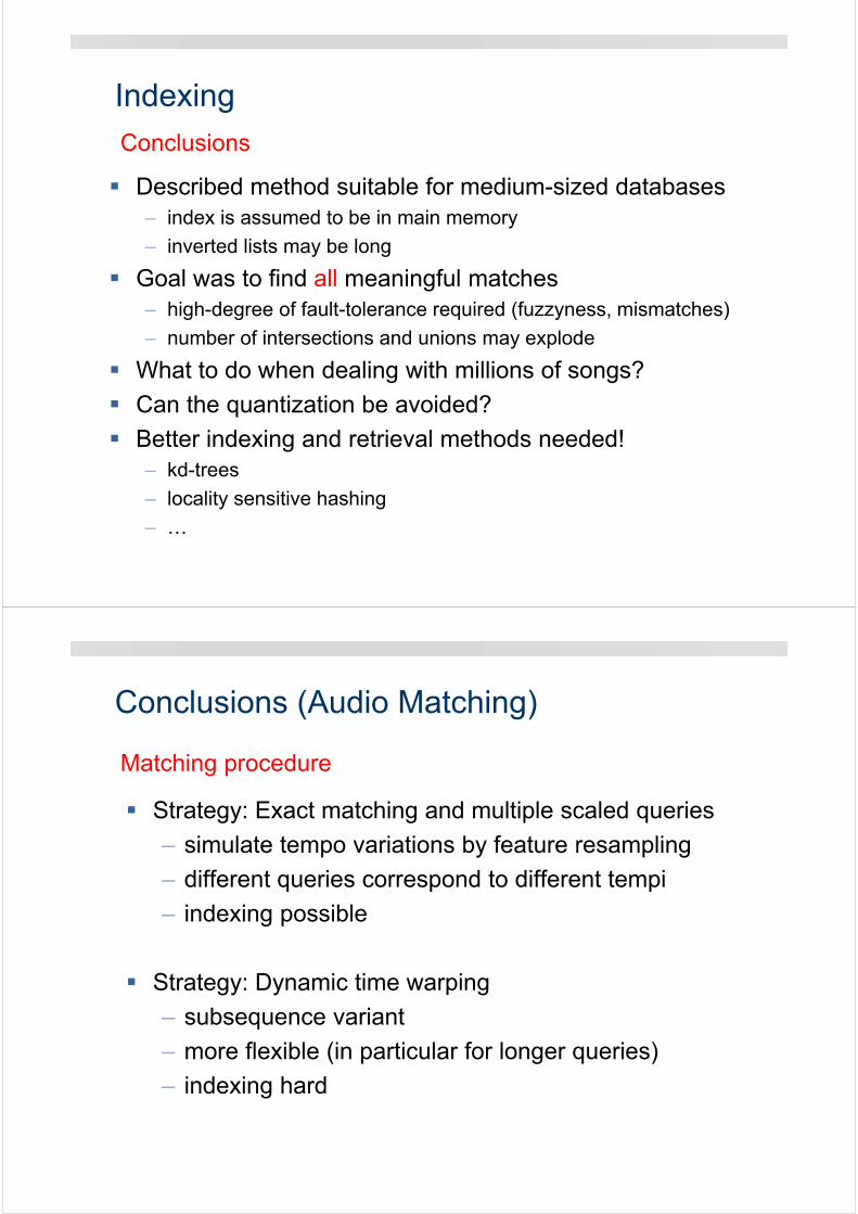
Indexing
Described method suitable for medium-sized databases– index is assumed to be in main memory
– inverted lists may be long
Goal was to find all meaningful matches – high-degree of fault-tolerance required (fuzzyness, mismatches)
– number of intersections and unions may explode
What to do when dealing with millions of songs?
Can the quantization be avoided?
Better indexing and retrieval methods needed!– kd-trees
– locality sensitive hashing
– …
Conclusions
Conclusions (Audio Matching)
Matching procedure
Strategy: Exact matching and multiple scaled queries
– simulate tempo variations by feature resampling
– different queries correspond to different tempi
– indexing possible
Strategy: Dynamic time warping
– subsequence variant
– more flexible (in particular for longer queries)
– indexing hard
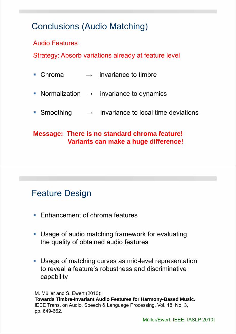
Conclusions (Audio Matching)
Audio Features
Chroma → invariance to timbre
Normalization → invariance to dynamics
Smoothing → invariance to local time deviations
Strategy: Absorb variations already at feature level
Message: There is no standard chroma feature!Variants can make a huge difference!
Feature Design
Enhancement of chroma features
Usage of audio matching framework for evaluatingthe quality of obtained audio features
Usage of matching curves as mid-level representationto reveal a feature’s robustness and discriminativecapability
[Müller/Ewert, IEEE-TASLP 2010]
M. Müller and S. Ewert (2010):Towards Timbre-Invariant Audio Features for Harmony-Based Music.IEEE Trans. on Audio, Speech & Language Processing, Vol. 18, No. 3, pp. 649-662.
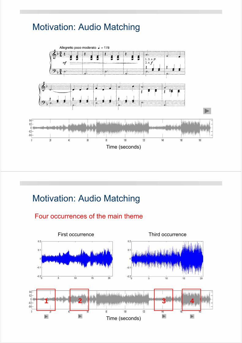
Motivation: Audio Matching
Time (seconds)
Motivation: Audio Matching
Four occurrences of the main theme
Third occurrenceFirst occurrence
1 2 3 4
Time (seconds)
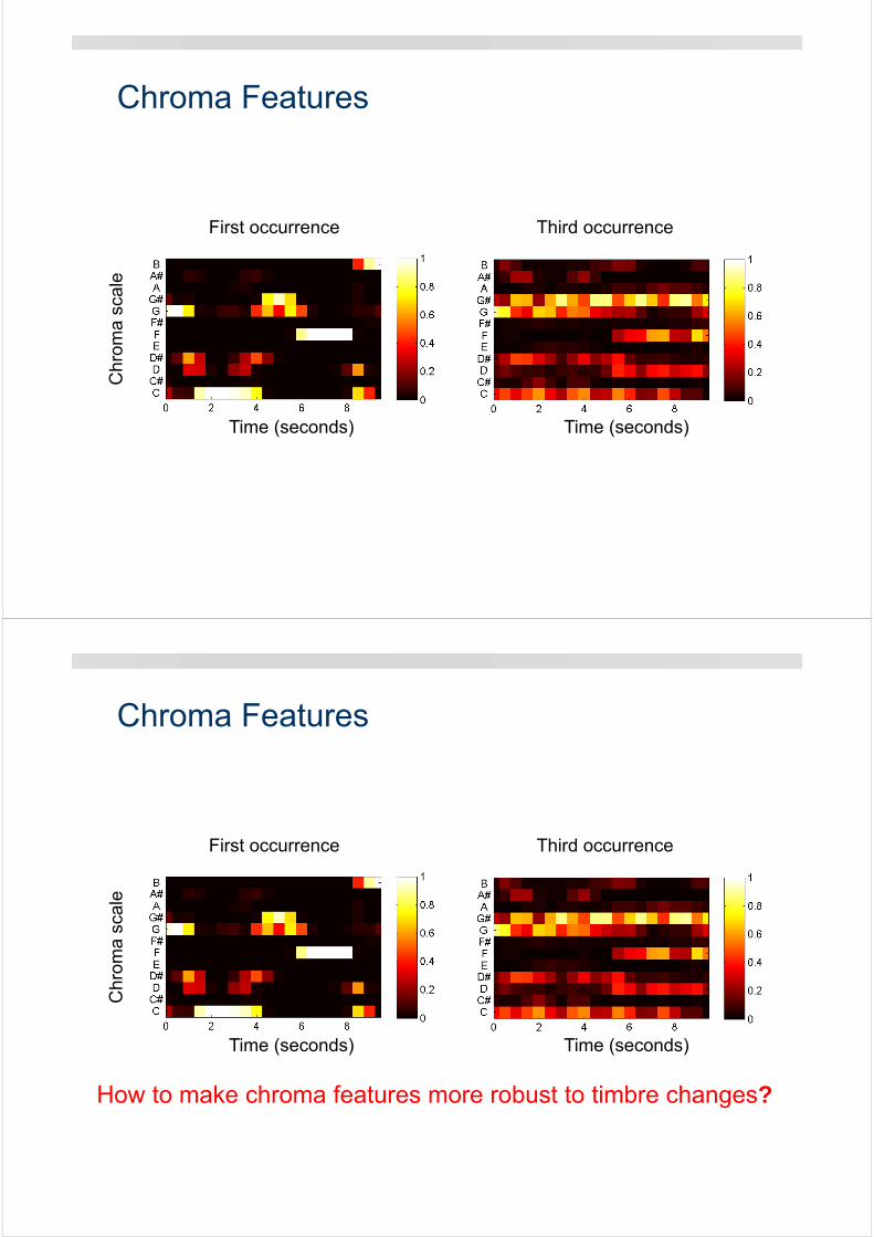
Chroma Features
First occurrence Third occurrence
Time (seconds)Time (seconds)
Chr
oma
scal
e
Chroma Features
First occurrence Third occurrence
How to make chroma features more robust to timbre changes?
Chr
oma
scal
e
Time (seconds) Time (seconds)
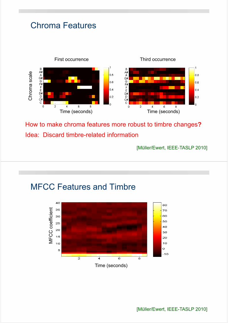
Chroma Features
First occurrence Third occurrence
How to make chroma features more robust to timbre changes?
Idea: Discard timbre-related information
Chr
oma
scal
e
[Müller/Ewert, IEEE-TASLP 2010]
Time (seconds) Time (seconds)
MFCC Features and Timbre
Time (seconds)
MF
CC
coe
ffici
ent
[Müller/Ewert, IEEE-TASLP 2010]
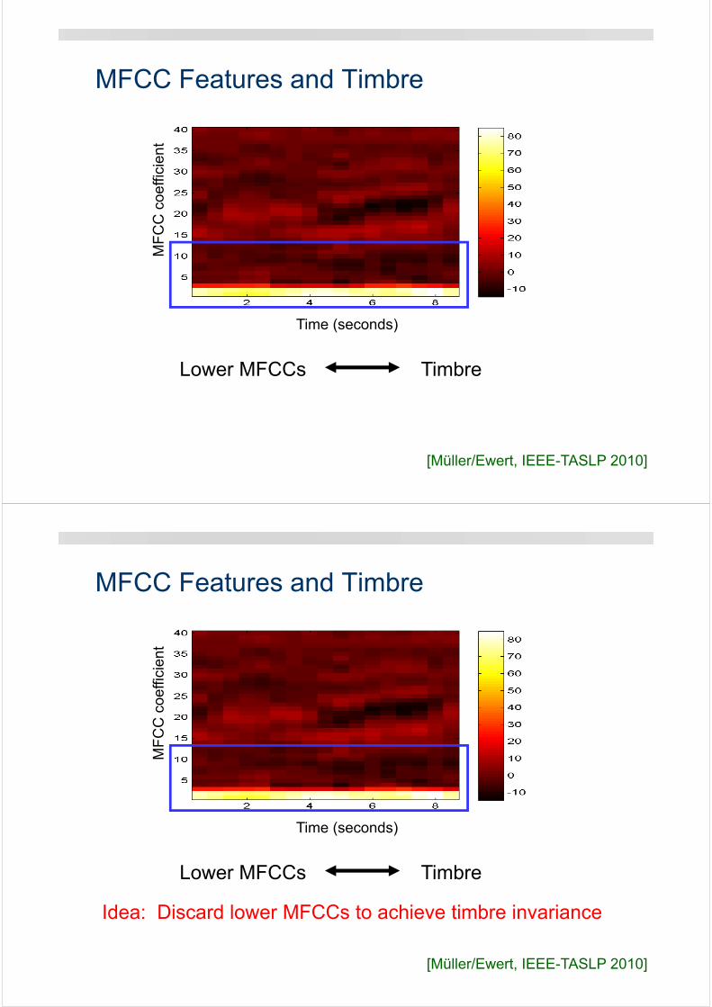
MFCC Features and Timbre
Lower MFCCs Timbre
[Müller/Ewert, IEEE-TASLP 2010]
MF
CC
coe
ffici
ent
Time (seconds)
MFCC Features and Timbre
Idea: Discard lower MFCCs to achieve timbre invariance
Lower MFCCs Timbre
[Müller/Ewert, IEEE-TASLP 2010]
MF
CC
coe
ffici
ent
Time (seconds)
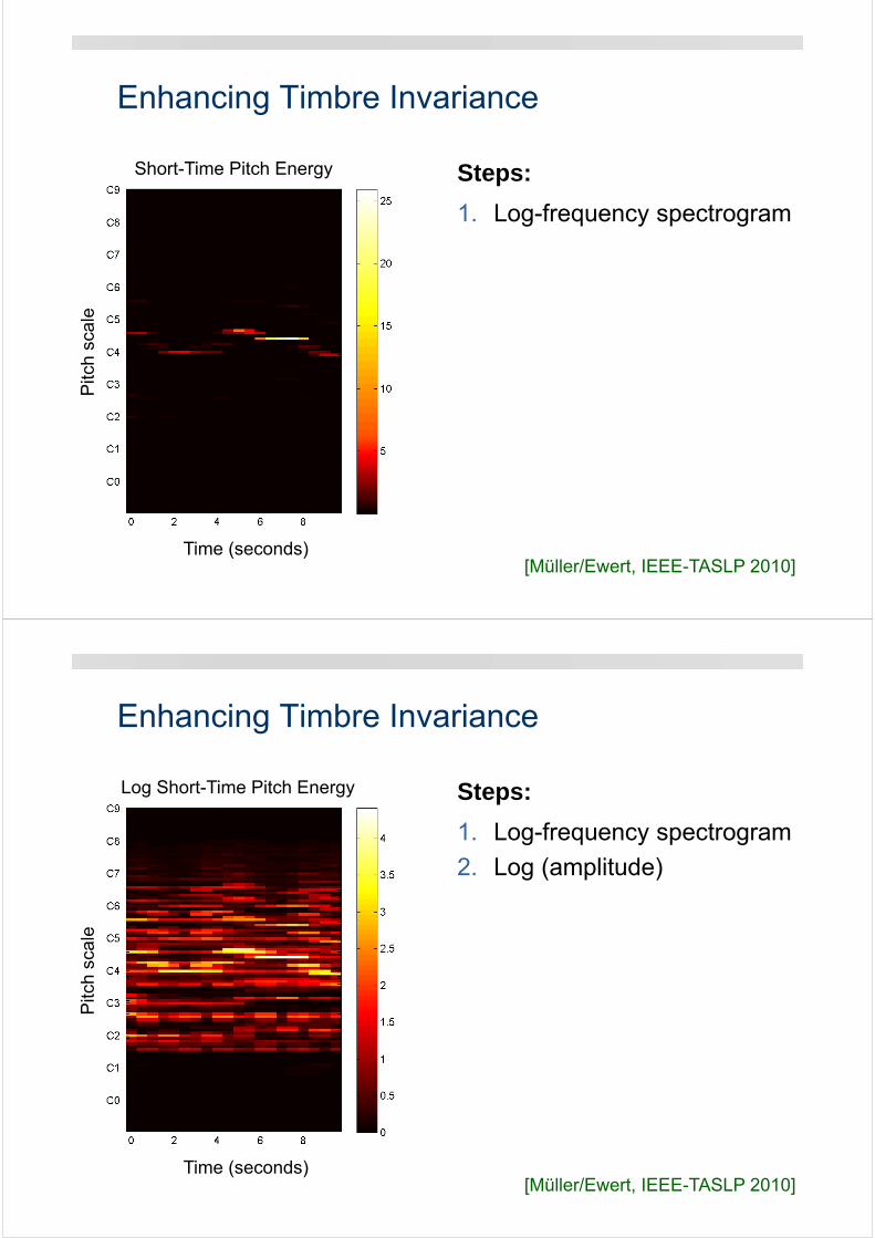
Enhancing Timbre Invariance
Short-Time Pitch Energy
Pitc
h sc
ale
Time (seconds)[Müller/Ewert, IEEE-TASLP 2010]
1. Log-frequency spectrogram
Steps:
Enhancing Timbre Invariance
Log Short-Time Pitch Energy
Pitc
h sc
ale
[Müller/Ewert, IEEE-TASLP 2010]
1. Log-frequency spectrogram
2. Log (amplitude)
Steps:
Time (seconds)
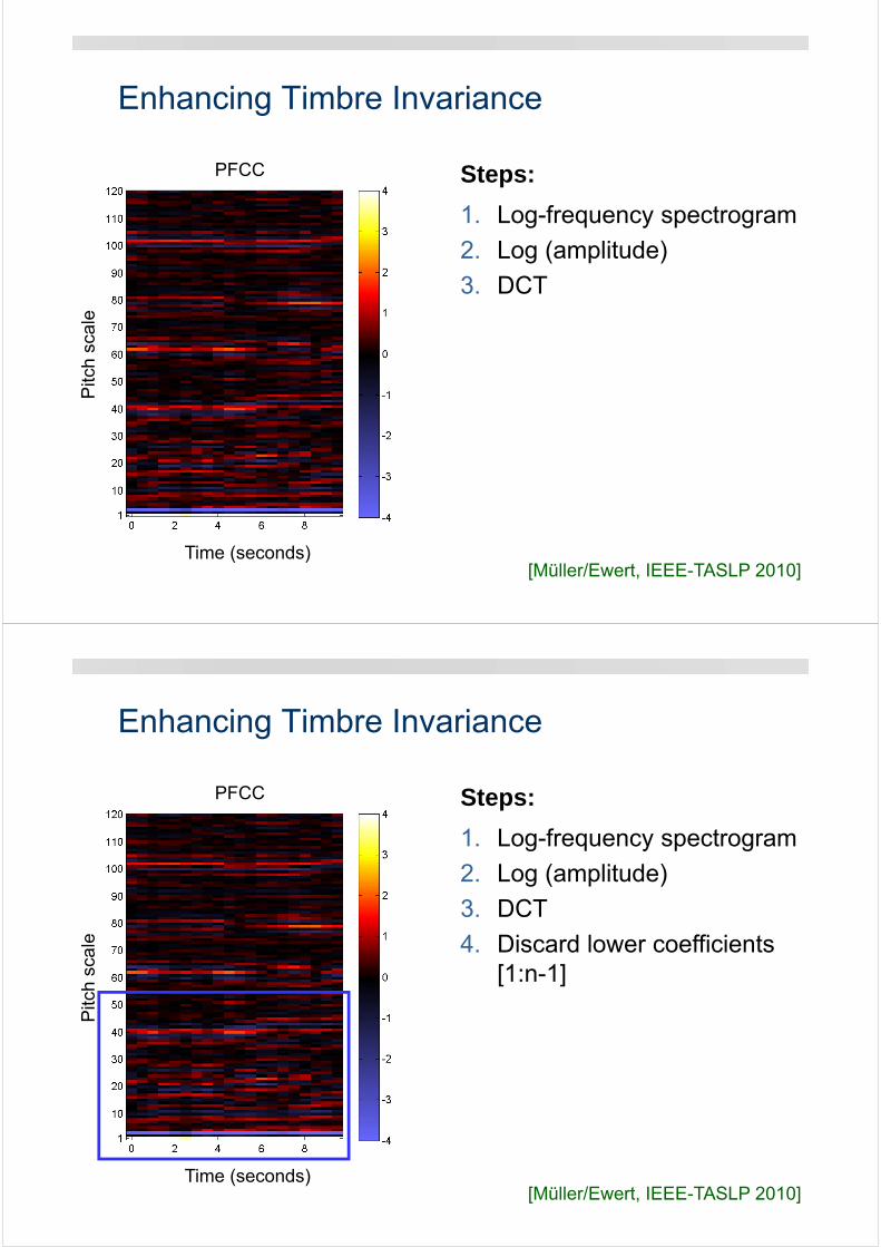
Enhancing Timbre Invariance
PFCC
Pitc
h sc
ale
[Müller/Ewert, IEEE-TASLP 2010]
1. Log-frequency spectrogram
2. Log (amplitude)
3. DCT
Steps:
Time (seconds)
Enhancing Timbre Invariance
PFCC
Pitc
h sc
ale
[Müller/Ewert, IEEE-TASLP 2010]
1. Log-frequency spectrogram
2. Log (amplitude)
3. DCT
4. Discard lower coefficients [1:n-1]
Steps:
Time (seconds)
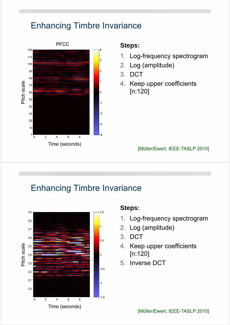
Enhancing Timbre Invariance
PFCC
Pitc
h sc
ale
[Müller/Ewert, IEEE-TASLP 2010]
1. Log-frequency spectrogram
2. Log (amplitude)
3. DCT
4. Keep upper coefficients[n:120]
Steps:
Time (seconds)
Enhancing Timbre Invariance
Pitc
h sc
ale
[Müller/Ewert, IEEE-TASLP 2010]
1. Log-frequency spectrogram
2. Log (amplitude)
3. DCT
4. Keep upper coefficients[n:120]
5. Inverse DCT
Steps:
Time (seconds)
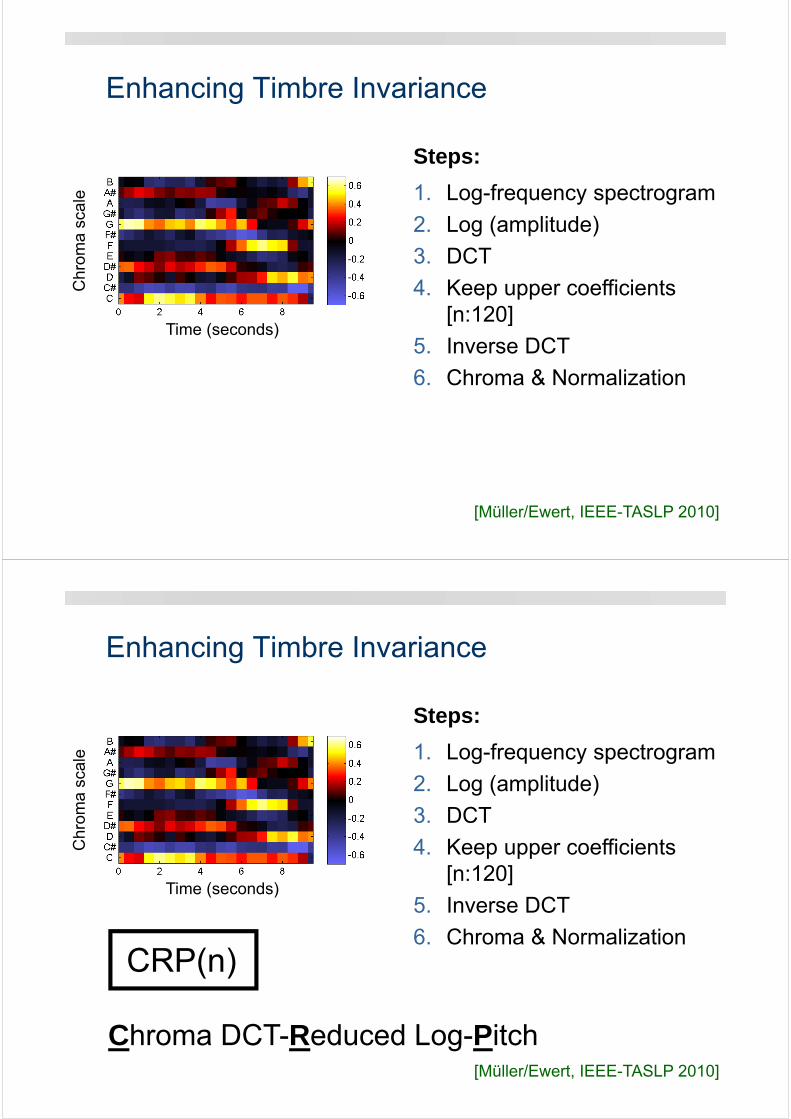
Enhancing Timbre InvarianceC
hrom
a sc
ale
Time (seconds)
[Müller/Ewert, IEEE-TASLP 2010]
1. Log-frequency spectrogram
2. Log (amplitude)
3. DCT
4. Keep upper coefficients[n:120]
5. Inverse DCT
6. Chroma & Normalization
Steps:
Enhancing Timbre Invariance
1. Log-frequency spectrogram
2. Log (amplitude)
3. DCT
4. Keep upper coefficients[n:120]
5. Inverse DCT
6. Chroma & Normalization
Steps:
Chroma DCT-Reduced Log-Pitch
CRP(n)
Chr
oma
scal
e
[Müller/Ewert, IEEE-TASLP 2010]
Time (seconds)
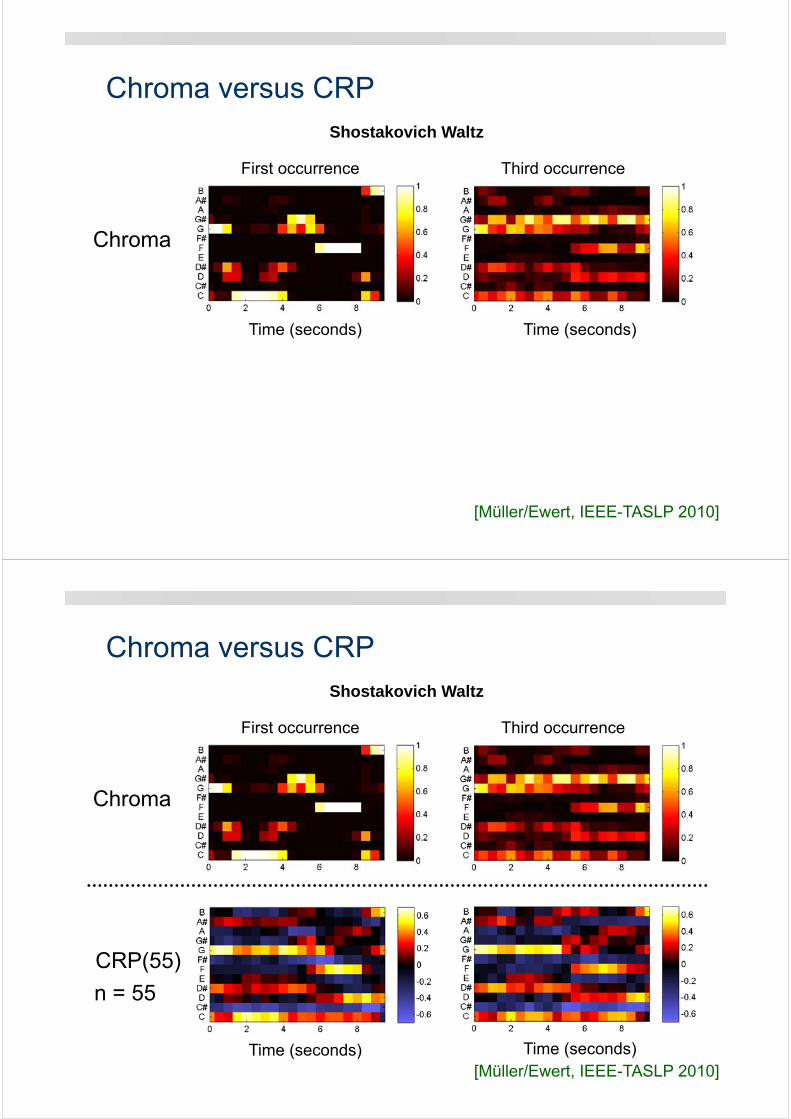
Chroma versus CRPShostakovich Waltz
Third occurrenceFirst occurrence
Chroma
Time (seconds) Time (seconds)
[Müller/Ewert, IEEE-TASLP 2010]
Chroma versus CRPShostakovich Waltz
Third occurrenceFirst occurrence
Chroma
CRP(55)
n = 55
Time (seconds) Time (seconds)[Müller/Ewert, IEEE-TASLP 2010]
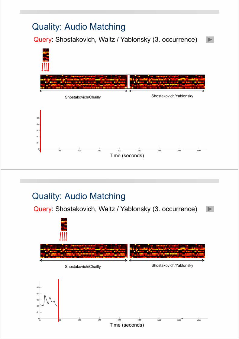
Quality: Audio Matching
Shostakovich/Chailly Shostakovich/Yablonsky
Query: Shostakovich, Waltz / Yablonsky (3. occurrence)
Time (seconds)
Quality: Audio Matching
Shostakovich/Chailly Shostakovich/Yablonsky
Query: Shostakovich, Waltz / Yablonsky (3. occurrence)
Time (seconds)
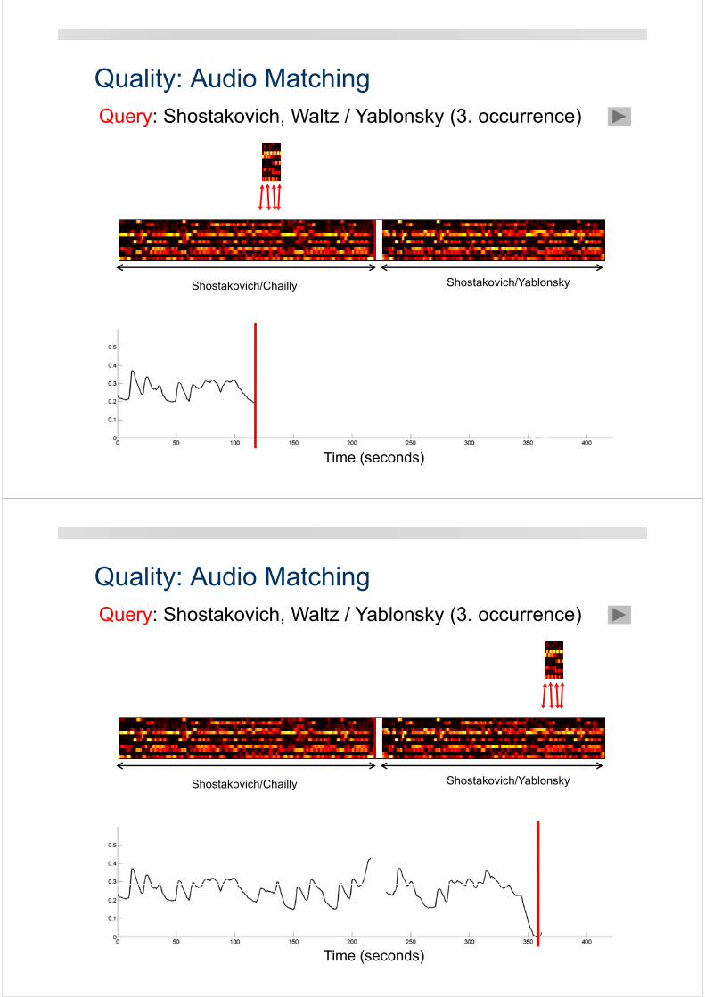
Quality: Audio Matching
Shostakovich/Chailly Shostakovich/Yablonsky
Query: Shostakovich, Waltz / Yablonsky (3. occurrence)
Time (seconds)
Quality: Audio Matching
Shostakovich/Chailly Shostakovich/Yablonsky
Query: Shostakovich, Waltz / Yablonsky (3. occurrence)
Time (seconds)
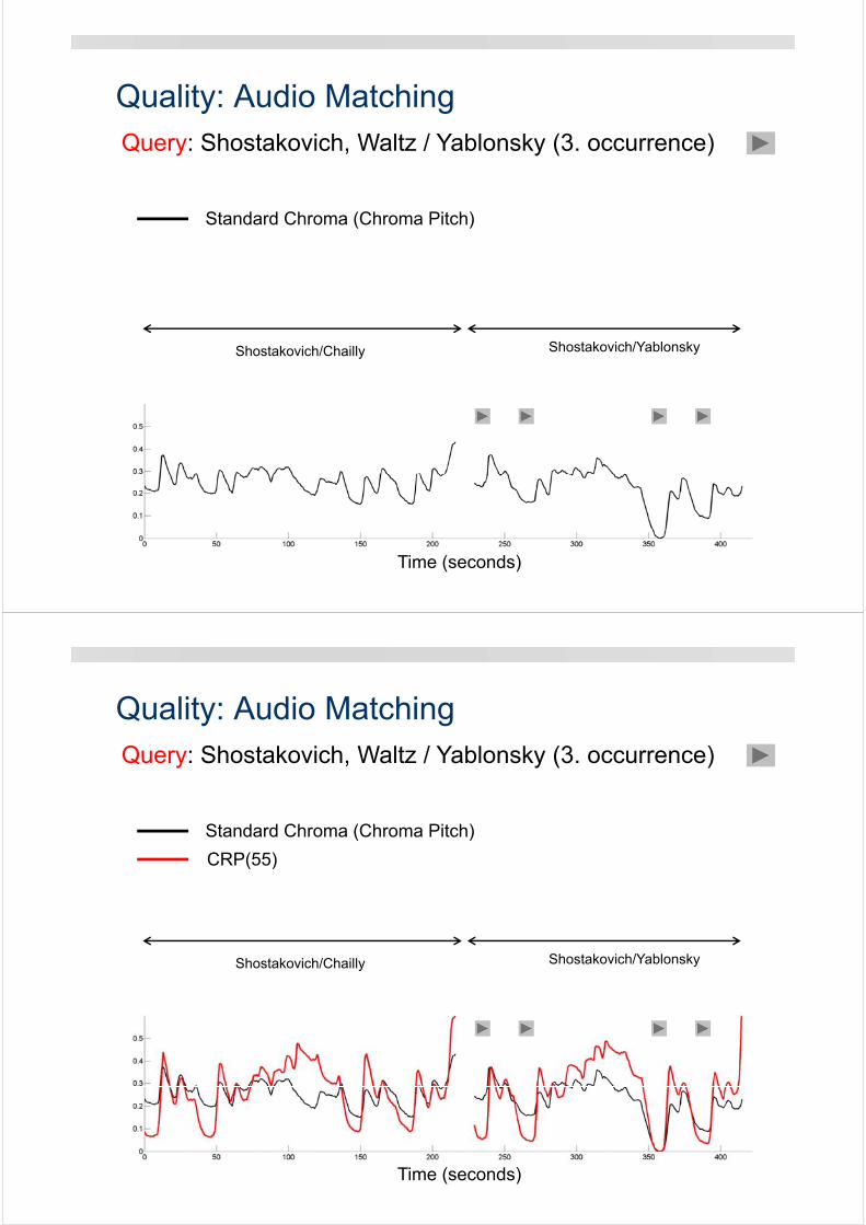
Quality: Audio Matching
Shostakovich/Chailly Shostakovich/Yablonsky
Standard Chroma (Chroma Pitch)
Query: Shostakovich, Waltz / Yablonsky (3. occurrence)
Time (seconds)
Quality: Audio Matching
Shostakovich/Chailly Shostakovich/Yablonsky
Standard Chroma (Chroma Pitch)
CRP(55)
Query: Shostakovich, Waltz / Yablonsky (3. occurrence)
Time (seconds)
Quality: Audio Matching
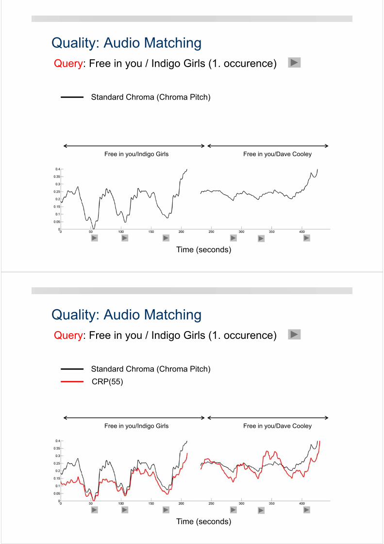
Standard Chroma (Chroma Pitch)
Free in you/Indigo Girls Free in you/Dave Cooley
Query: Free in you / Indigo Girls (1. occurence)
Time (seconds)
Quality: Audio Matching
Standard Chroma (Chroma Pitch)
CRP(55)
Free in you/Indigo Girls Free in you/Dave Cooley
Query: Free in you / Indigo Girls (1. occurence)
Time (seconds)
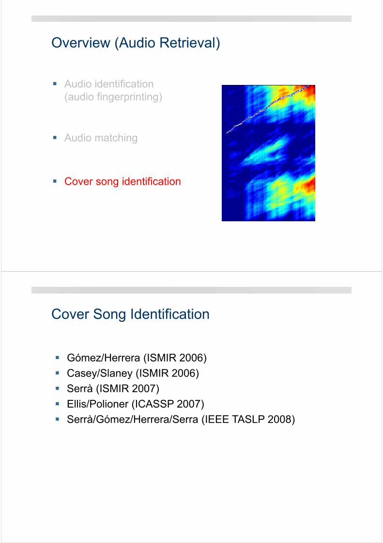
Overview (Audio Retrieval)
Audio identification(audio fingerprinting)
Audio matching
Cover song identification
Cover Song Identification
Gómez/Herrera (ISMIR 2006)
Casey/Slaney (ISMIR 2006)
Serrà (ISMIR 2007)
Ellis/Polioner (ICASSP 2007)
Serrà/Gómez/Herrera/Serra (IEEE TASLP 2008)
Cover Song Identification
Goal: Given a music recording of a song or piece of music, find all corresponding music recordings within a huge collection that can be regarded as a kind of version, interpretation, or cover song.
Instance of document-based retrieval!
Live versions
Versions adapted to particular country/region/language
Contemporary versions of an old song
Radically different interpretations of a musical piece
…
Cover Song Identification
Automated organization of music collections
“Find me all covers of …”
Musical rights management
Learning about music itself
“Understanding the essence of a song”
Motivation
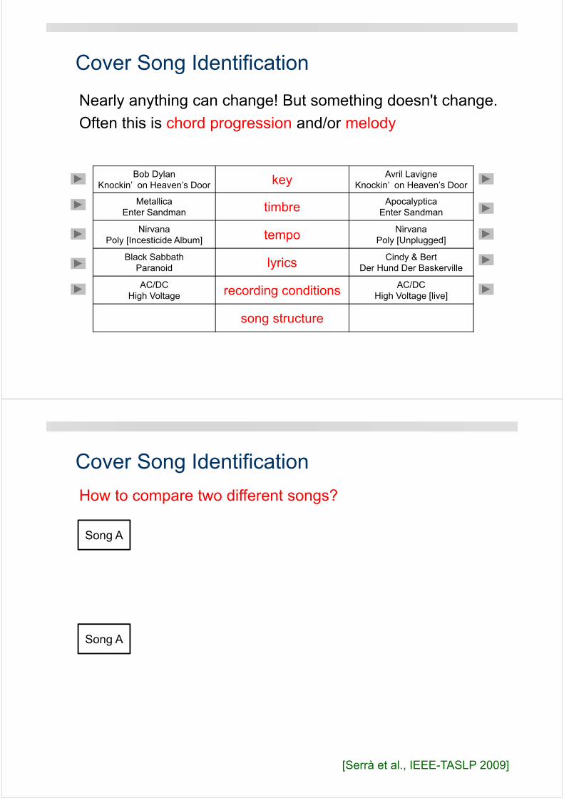
Cover Song Identification
Bob DylanKnockin’ on Heaven’s Door key Avril Lavigne
Knockin’ on Heaven’s Door
MetallicaEnter Sandman timbre Apocalyptica
Enter Sandman
NirvanaPoly [Incesticide Album] tempo Nirvana
Poly [Unplugged]
Black SabbathParanoid lyrics Cindy & Bert
Der Hund Der Baskerville
AC/DCHigh Voltage recording conditions AC/DC
High Voltage [live]
song structure
Nearly anything can change! But something doesn't change.
Often this is chord progression and/or melody
Cover Song Identification
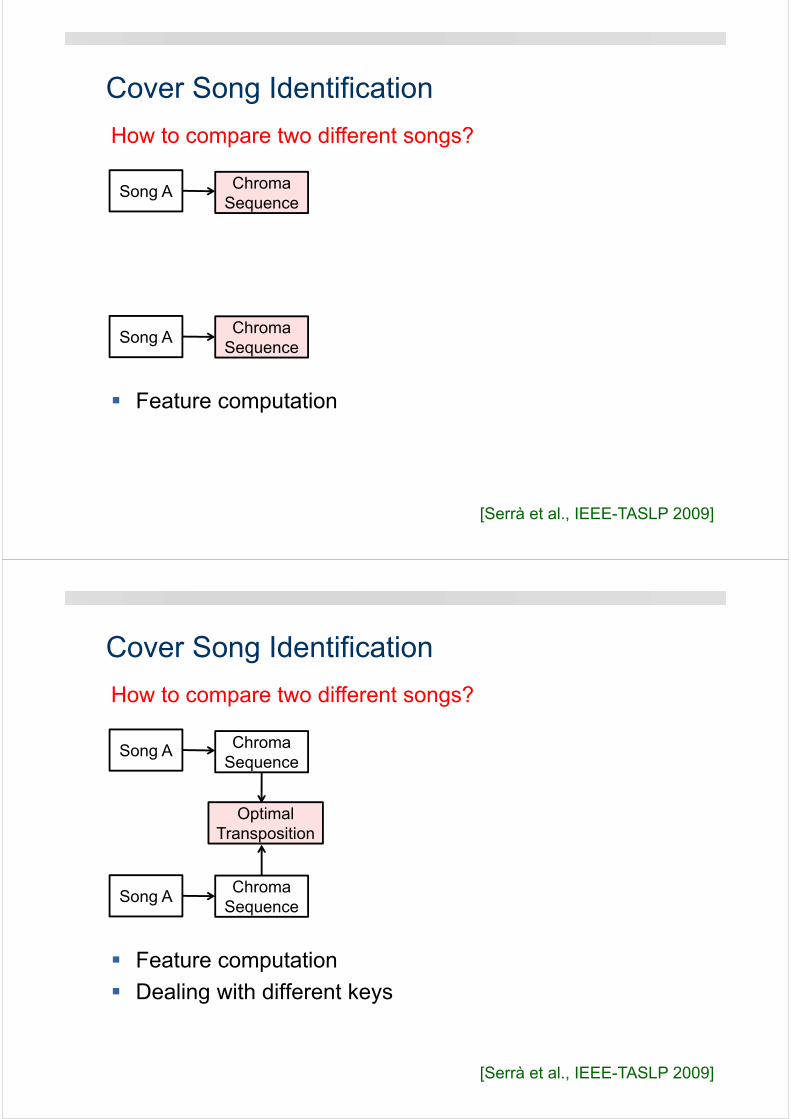
How to compare two different songs?
Song A
Song A
[Serrà et al., IEEE-TASLP 2009]
Cover Song Identification
ChromaSequence
ChromaSequence
How to compare two different songs?
Song A
Song A
Feature computation
[Serrà et al., IEEE-TASLP 2009]
Cover Song Identification
ChromaSequence
ChromaSequence
How to compare two different songs?
Optimal Transposition
Song A
Song A
Feature computation
Dealing with different keys
[Serrà et al., IEEE-TASLP 2009]
Cover Song Identification
ChromaSequence
ChromaSequence
Binary Similarity
Matrix
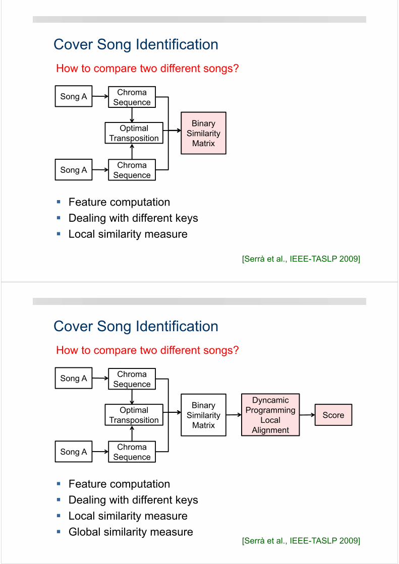
How to compare two different songs?
Optimal Transposition
Song A
Song A
Feature computation
Dealing with different keys
Local similarity measure
[Serrà et al., IEEE-TASLP 2009]
Cover Song Identification
ChromaSequence
ChromaSequence
Binary Similarity
Matrix
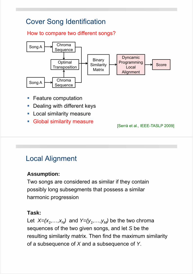
How to compare two different songs?
Optimal Transposition
DyncamicProgramming
LocalAlignment
Score
Song A
Song A
Feature computation
Dealing with different keys
Local similarity measure
Global similarity measure[Serrà et al., IEEE-TASLP 2009]
Cover Song Identification
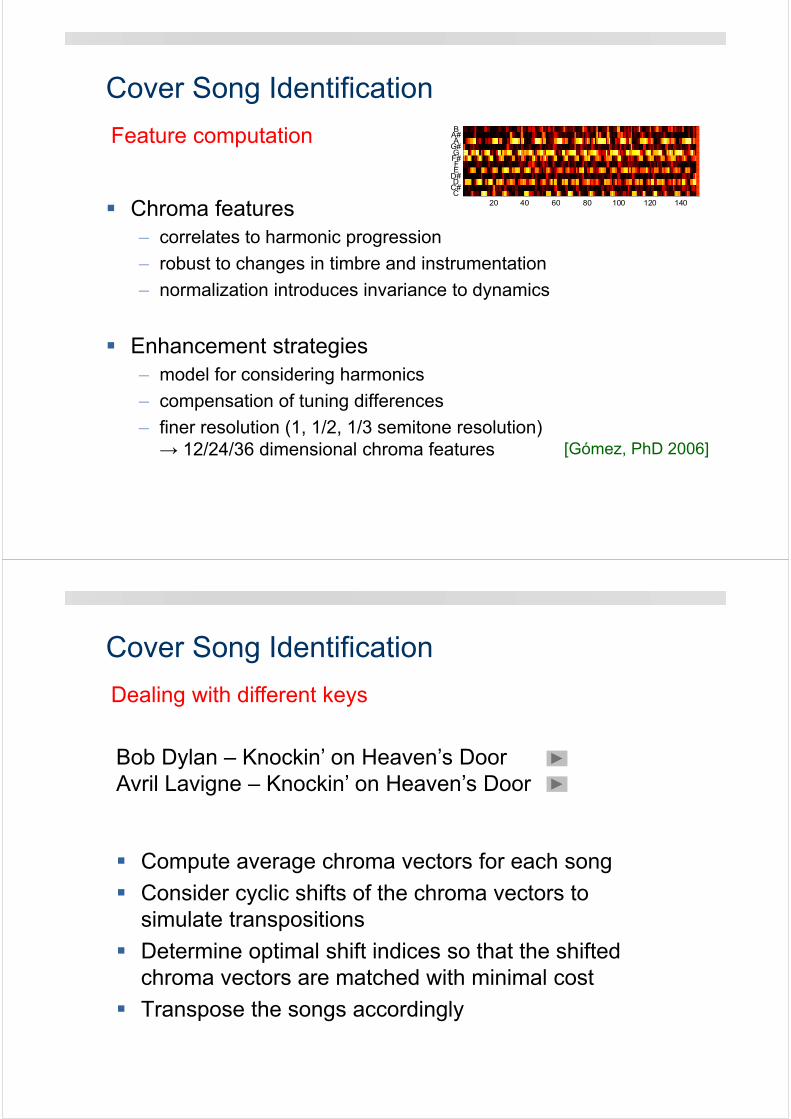
Feature computation
Chroma features– correlates to harmonic progression
– robust to changes in timbre and instrumentation
– normalization introduces invariance to dynamics
Enhancement strategies– model for considering harmonics
– compensation of tuning differences
– finer resolution (1, 1/2, 1/3 semitone resolution)→ 12/24/36 dimensional chroma features [Gómez, PhD 2006]
20 40 60 80 100 120 140C
C#D
D#E F
F#G
G#A
A#B
Cover Song Identification
Dealing with different keys
Bob Dylan – Knockin’ on Heaven’s DoorAvril Lavigne – Knockin’ on Heaven’s Door
Compute average chroma vectors for each song
Consider cyclic shifts of the chroma vectors to simulate transpositions
Determine optimal shift indices so that the shifted chroma vectors are matched with minimal cost
Transpose the songs accordingly
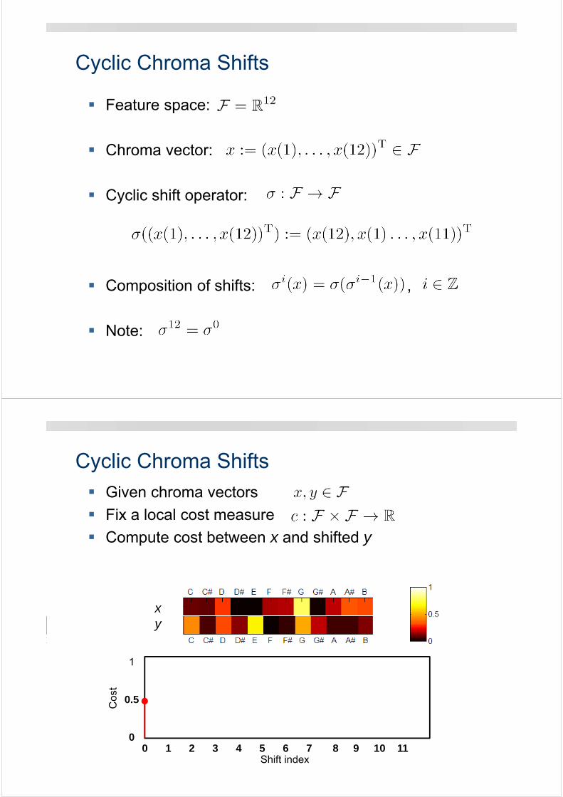
Cyclic Chroma Shifts
Feature space:
Chroma vector:
Cyclic shift operator:
Composition of shifts: ,
Note:
Cyclic Chroma Shifts
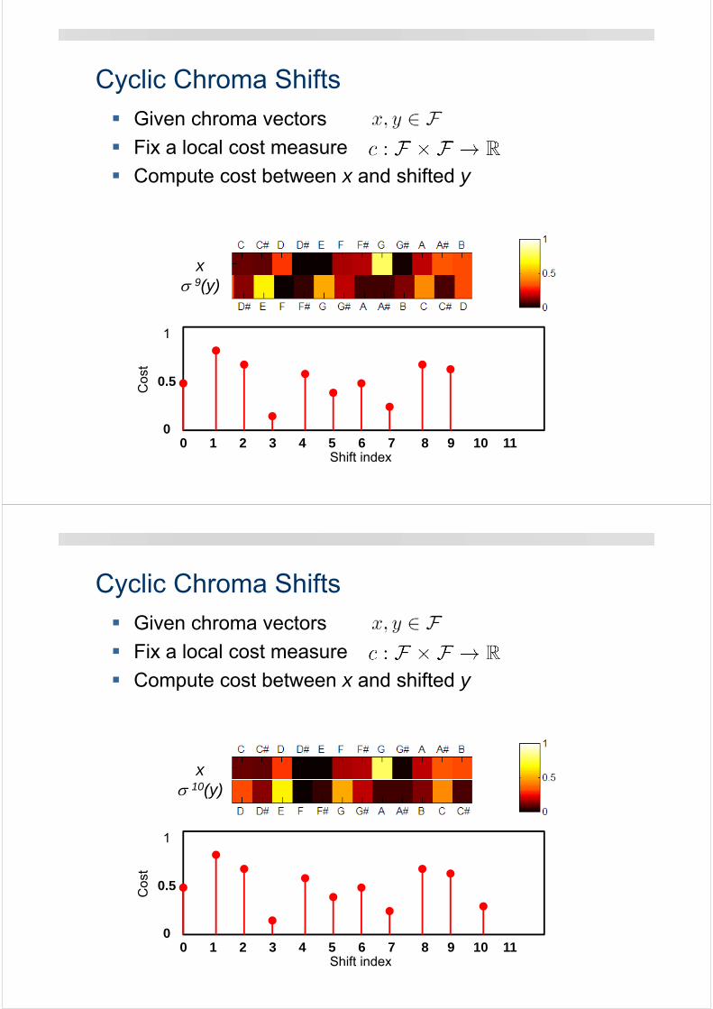
Given chroma vectors
Fix a local cost measure
Compute cost between x and shifted y
x y
Shift index
Cos
t
0 1 2 3 4 5 6 7 8 9 10 11
1
0.5
0
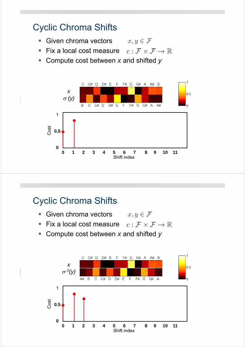
Cyclic Chroma Shifts
x (y)
Shift index0 1 2 3 4 5 6 7 8 9 10 11
1
0.5
0
Cos
t
Given chroma vectors
Fix a local cost measure
Compute cost between x and shifted y
Cyclic Chroma Shifts
x 2(y)
Shift index0 1 2 3 4 5 6 7 8 9 10 11
1
0.5
0
Cos
t
Given chroma vectors
Fix a local cost measure
Compute cost between x and shifted y
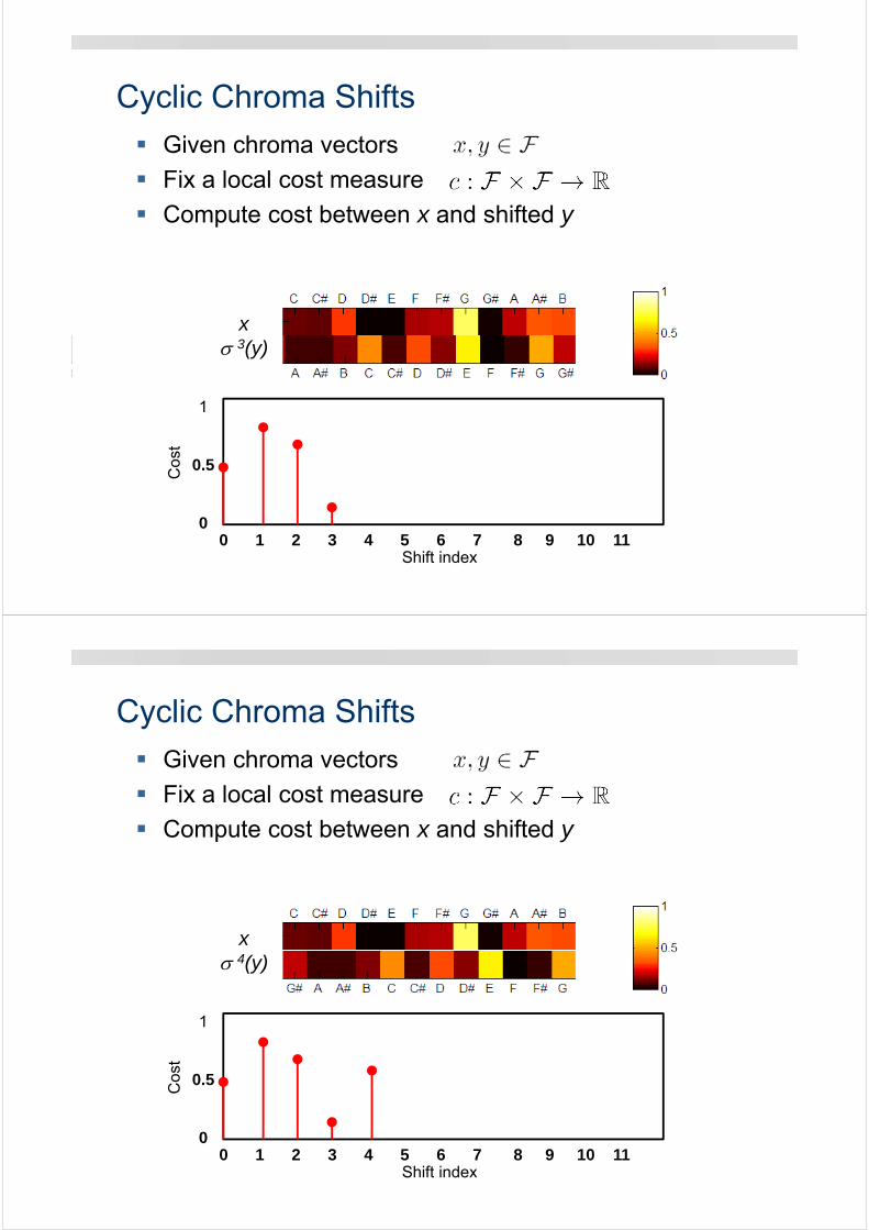
Cyclic Chroma Shifts
Shift index
x 3(y)
Shift index0 1 2 3 4 5 6 7 8 9 10 11
1
0.5
0
Cos
t
Given chroma vectors
Fix a local cost measure
Compute cost between x and shifted y
Cyclic Chroma Shifts
x 4(y)
Shift index0 1 2 3 4 5 6 7 8 9 10 11
1
0.5
0
Cos
t
Given chroma vectors
Fix a local cost measure
Compute cost between x and shifted y
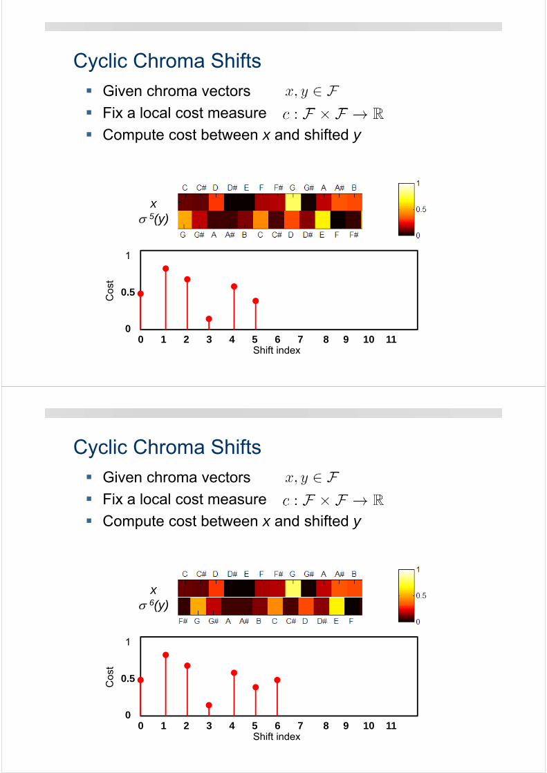
Cyclic Chroma Shifts
x 5(y)
Shift index0 1 2 3 4 5 6 7 8 9 10 11
1
0.5
0
Cos
t
Given chroma vectors
Fix a local cost measure
Compute cost between x and shifted y
Cyclic Chroma Shifts
Shift index
x 6(y)
Shift index0 1 2 3 4 5 6 7 8 9 10 11
1
0.5
0
Cos
t
Given chroma vectors
Fix a local cost measure
Compute cost between x and shifted y
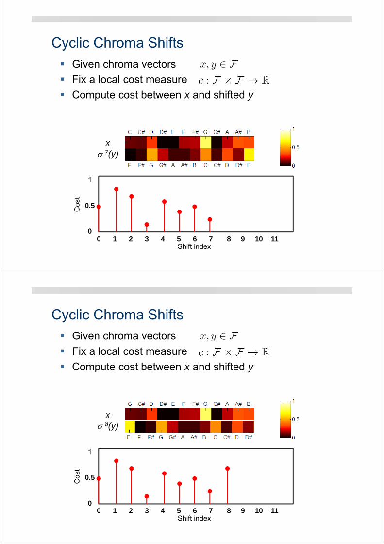
Cyclic Chroma Shifts
x 7(y)
Shift index0 1 2 3 4 5 6 7 8 9 10 11
1
0.5
0
Cos
t
Given chroma vectors
Fix a local cost measure
Compute cost between x and shifted y
Cyclic Chroma Shifts
x 8(y)
Shift index0 1 2 3 4 5 6 7 8 9 10 11
1
0.5
0
Cos
t
Given chroma vectors
Fix a local cost measure
Compute cost between x and shifted y
Cyclic Chroma Shifts
x 9(y)
Shift index0 1 2 3 4 5 6 7 8 9 10 11
1
0.5
0
Cos
t
Given chroma vectors
Fix a local cost measure
Compute cost between x and shifted y
Cyclic Chroma Shifts
x 10(y)
Shift index0 1 2 3 4 5 6 7 8 9 10 11
1
0.5
0
Cos
t
Given chroma vectors
Fix a local cost measure
Compute cost between x and shifted y
Cyclic Chroma Shifts
Shift index
x 11(y)
0 1 2 3 4 5 6 7 8 9 10 11
1
0.5
0
Cos
t
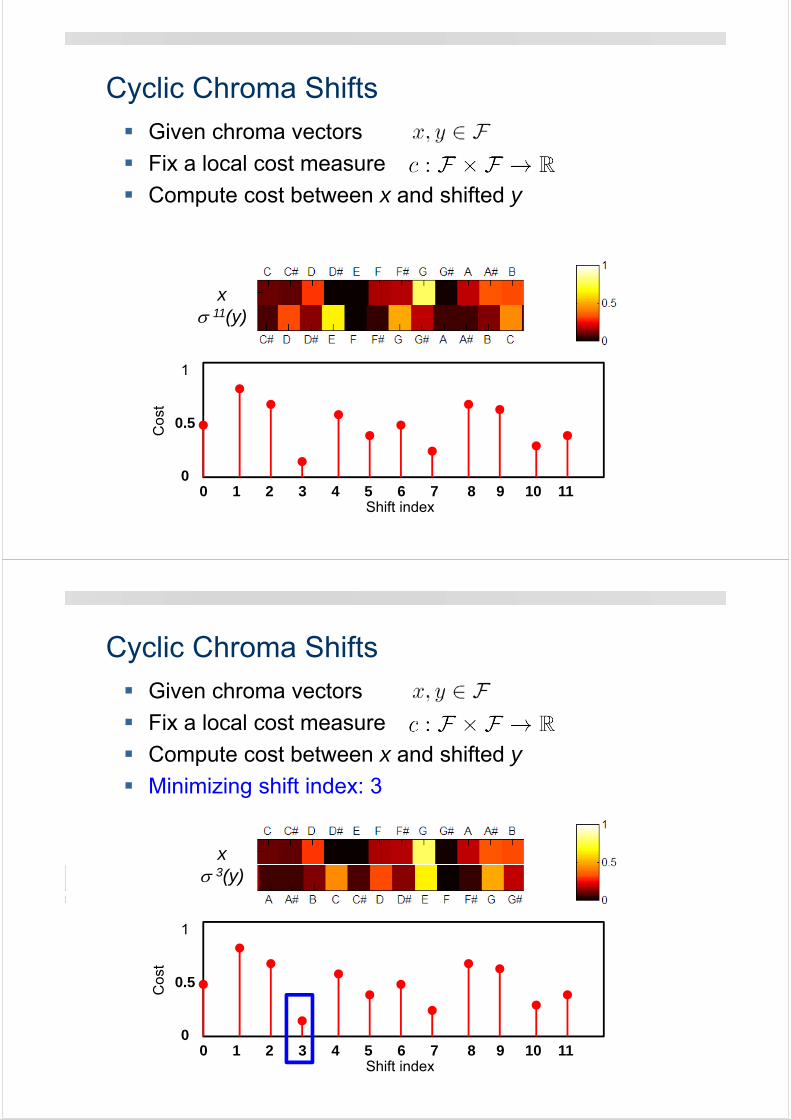
Given chroma vectors
Fix a local cost measure
Compute cost between x and shifted y
Cyclic Chroma Shifts
Shift index0 1 2 3 4 5 6 7 8 9 10 11
1
0.5
0
Cos
t
Given chroma vectors
Fix a local cost measure
Compute cost between x and shifted y
Minimizing shift index: 3
x 3(y)
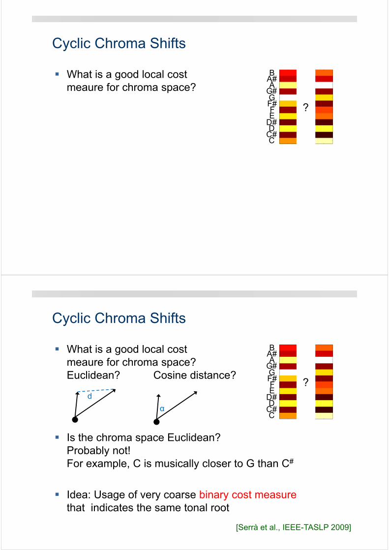
What is a good local costmeaure for chroma space?
Cyclic Chroma Shifts
1 2 3C
C#D
D#E F
F#G
G#A
A#B
?
What is a good local costmeaure for chroma space?Euclidean? Cosine distance?
Is the chroma space Euclidean? Probably not!For example, C is musically closer to G than C#
Idea: Usage of very coarse binary cost measurethat indicates the same tonal root
Cyclic Chroma Shifts
1 2 3C
C#D
D#E F
F#G
G#A
A#B
d
α
?
[Serrà et al., IEEE-TASLP 2009]
Cyclic Chroma Shifts
[Serrà et al., IEEE-TASLP 2009]
Original local cost measure
Binary cost measure
for
Cyclic Chroma Shifts
[Serrà et al., IEEE-TASLP 2009]
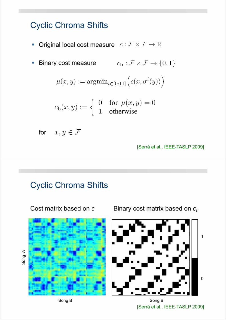
Cost matrix based on c
Song B
Binary cost matrix based on cb
Son
g A
Song B
1
0
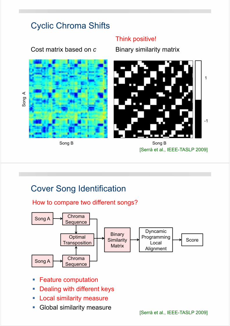
Cyclic Chroma Shifts
[Serrà et al., IEEE-TASLP 2009]Song B
Binary similarity matrix
Song B
-1
Cost matrix based on c
Think positive!
Son
g A
1
Cover Song Identification
ChromaSequence
ChromaSequence
Binary Similarity
Matrix
How to compare two different songs?
Optimal Transposition
DyncamicProgramming
LocalAlignment
Score
Song A
Song A
Feature computation
Dealing with different keys
Local similarity measure
Global similarity measure[Serrà et al., IEEE-TASLP 2009]
Cover Song Identification
ChromaSequence
ChromaSequence
Binary Similarity
Matrix
How to compare two different songs?
Optimal Transposition
DyncamicProgramming
LocalAlignment
Score
Song A
Song A
Feature computation
Dealing with different keys
Local similarity measure
Global similarity measure[Serrà et al., IEEE-TASLP 2009]
Local Alignment
Assumption:
Two songs are considered as similar if they contain
possibly long subsegments that possess a similar
harmonic progression
Task:
Let X=(x1,…,xN) and Y=(y1,…,yM) be the two chroma
sequences of the two given songs, and let S be the
resulting similarity matrix. Then find the maximum similarity
of a subsequence of X and a subsequence of Y.
Local Alignment
Note:
This problem is also known from bioinformatics.
The Smith-Waterman algorithm is a well-known algorithm
for performing local sequence alignment; that is, for
determining similar regions between two nucleotide or
protein sequences.
Strategy:
We use a variant of the Smith-Waterman algorithm.
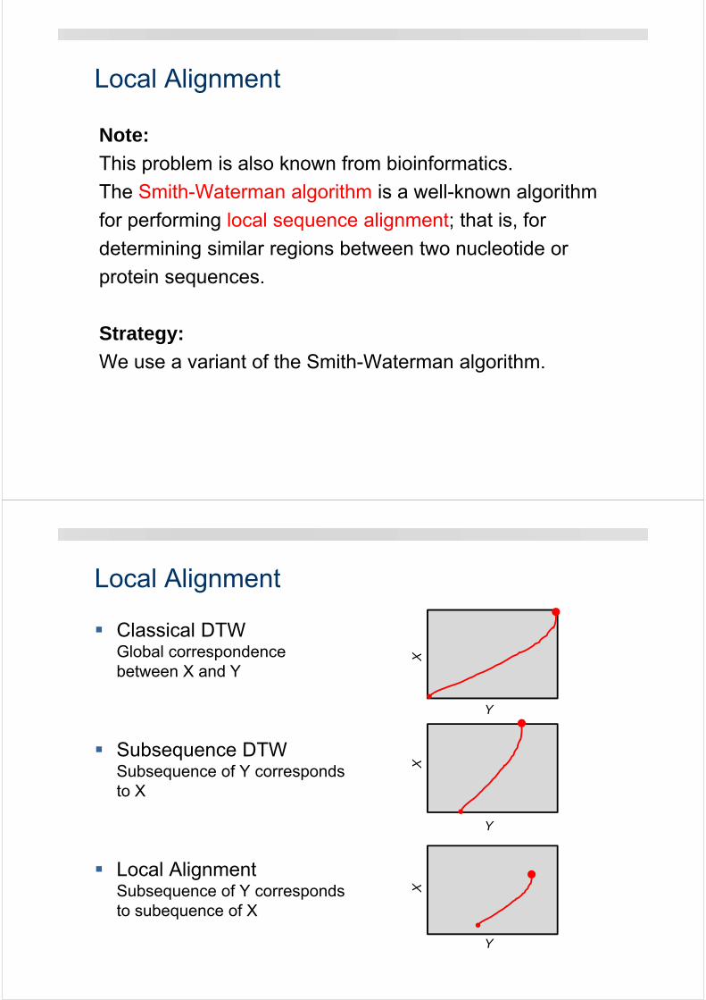
Local Alignment
X
Classical DTWGlobal correspondencebetween X and Y
Subsequence DTWSubsequence of Y correspondsto X
Local AlignmentSubsequence of Y correspondsto subequence of X
XX
Y
Y
Y
Local Alignment
Zero-entry allows for jumping to any cell without penalty
g penalizes “inserts” and “delets” in alignment
Best local alignment score is the highest value in D
Best local alignment ends at cell of highest value
Start is obtained by backtracking to first cell of value zero
Computation of accumulated score matrix Dfrom given binary similarity (score) matrix S
Guns and Roses
Bob
Dyl
an
Knockin' on Heaven's Door
50 100 150 200 250 300
20
40
60
80
100
120
140
-0.8
-0.6
-0.4
-0.2
0
0.2
0.4
0.6
0.8
1
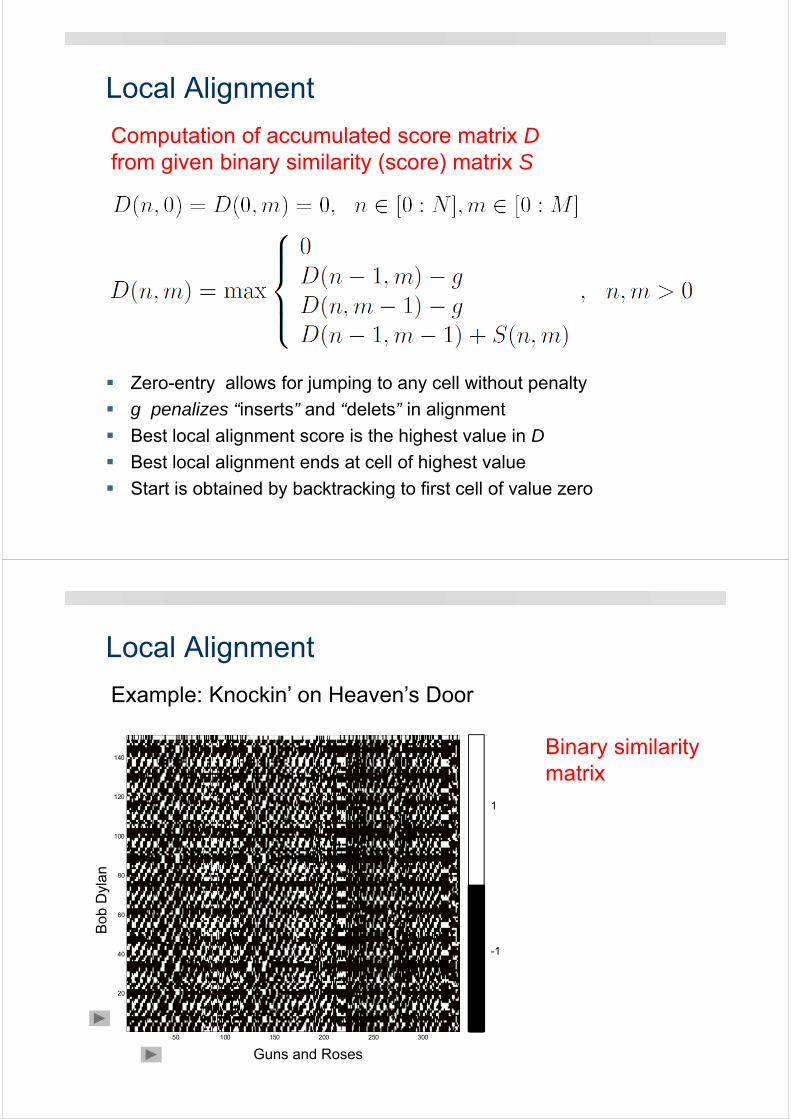
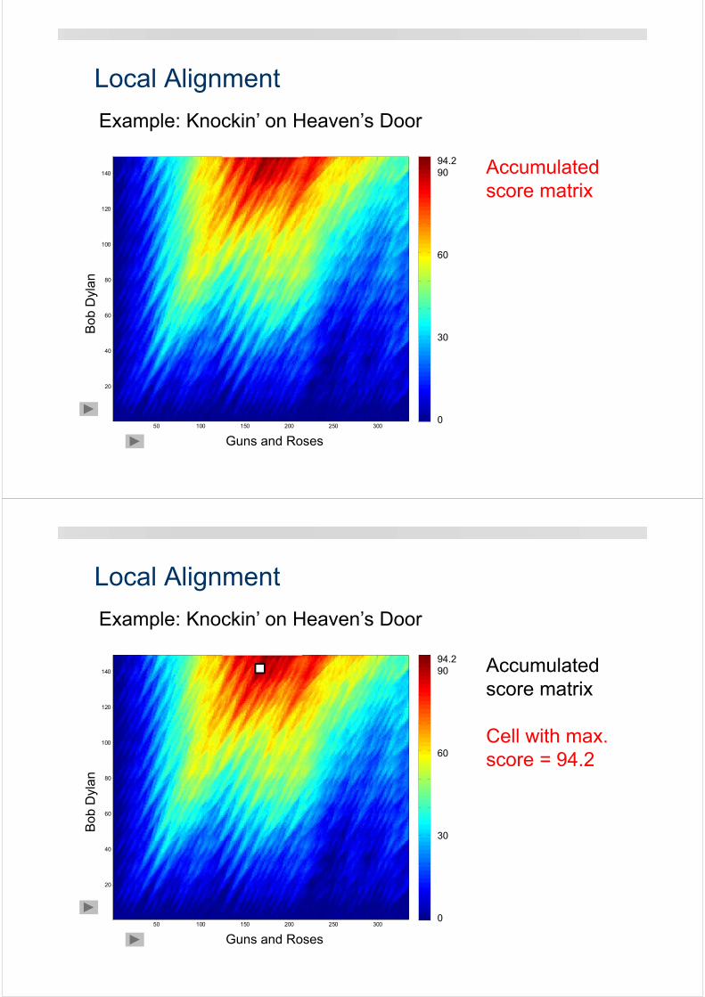
Example: Knockin’ on Heaven’s Door
Guns and Roses
Bob
Dyl
an
1
-1
Binary similarity matrix
Local Alignment
Guns and Roses
Bob
Dyl
an
Knockin' on Heavens's Door
50 100 150 200 250 300
20
40
60
80
100
120
140
10
20
30
40
50
60
70
80
90
Example: Knockin’ on Heaven’s Door
Guns and Roses
Bob
Dyl
an
Accumulatedscore matrix
Local Alignment
94.290
60
30
0
Guns and Roses
Bob
Dyl
an
Knockin' on Heavens's Door
50 100 150 200 250 300
20
40
60
80
100
120
140
10
20
30
40
50
60
70
80
90
Example: Knockin’ on Heaven’s Door
Guns and Roses
Bob
Dyl
an
Accumulatedscore matrix
Cell with max.score = 94.2
Local Alignment
94.290
60
30
0
Guns and Roses
Bob
Dyl
an
Knockin' on Heaven's Door
50 100 150 200 250 300
20
40
60
80
100
120
140
10
20
30
40
50
60
70
80
90
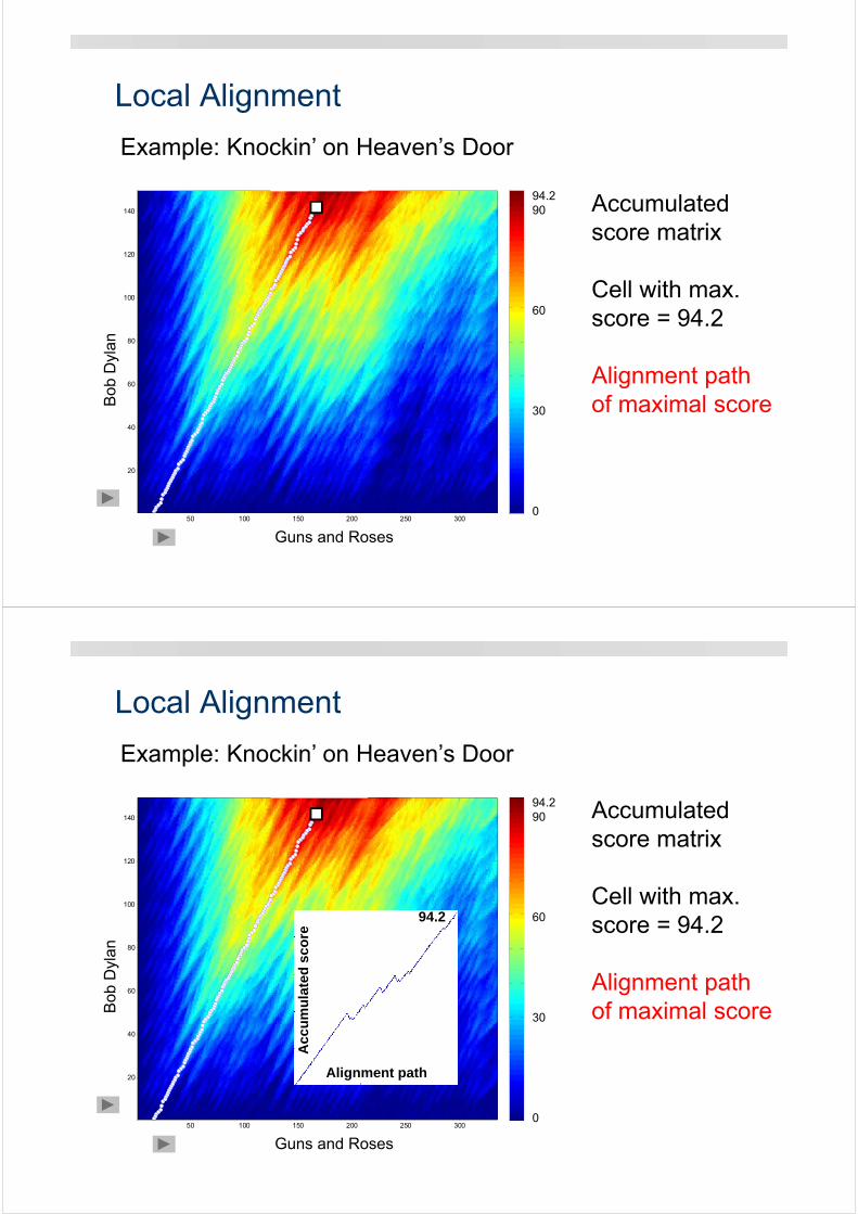
Example: Knockin’ on Heaven’s Door
Guns and Roses
Bob
Dyl
an
Accumulatedscore matrix
Cell with max.score = 94.2
Alignment pathof maximal score
Local Alignment
94.290
60
30
0
Guns and Roses
Bob
Dyl
an
Knockin' on Heaven's Door
50 100 150 200 250 300
20
40
60
80
100
120
140
10
20
30
40
50
60
70
80
90
Example: Knockin’ on Heaven’s Door
Guns and Roses
Bob
Dyl
an
94.290
60
30
0
Accumulatedscore matrix
Cell with max.score = 94.2
Alignment pathof maximal score
Local Alignment
Acc
um
ula
ted
sco
re
Alignment path
94.2
Guns and Roses
Bob
Dyl
an
Knockin' on Heaven's Door
50 100 150 200 250 300
20
40
60
80
100
120
140
10
20
30
40
50
60
70
80
90
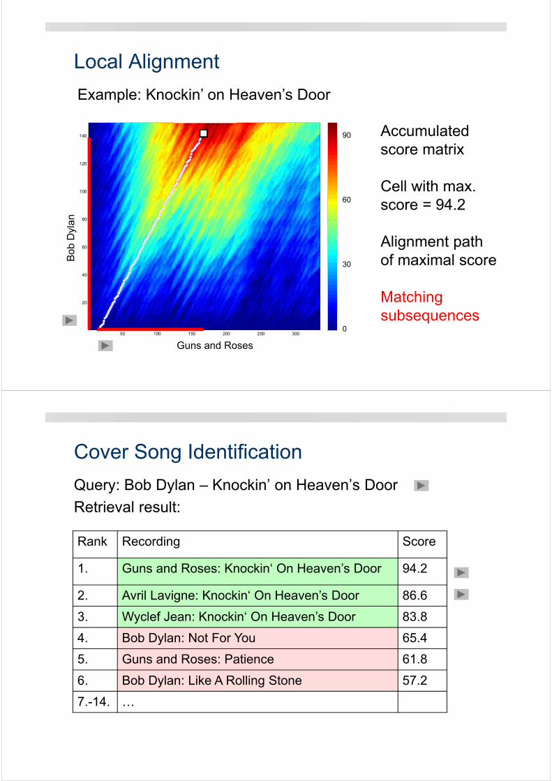
Example: Knockin’ on Heaven’s Door
Guns and Roses
Bob
Dyl
an
90
60
30
0
Accumulatedscore matrix
Cell with max.score = 94.2
Alignment pathof maximal score
Matching subsequences
Local Alignment
Cover Song Identification
Query: Bob Dylan – Knockin’ on Heaven’s Door
Retrieval result:
Rank Recording Score
1. Guns and Roses: Knockin‘ On Heaven’s Door 94.2
2. Avril Lavigne: Knockin‘ On Heaven’s Door 86.6
3. Wyclef Jean: Knockin‘ On Heaven’s Door 83.8
4. Bob Dylan: Not For You 65.4
5. Guns and Roses: Patience 61.8
6. Bob Dylan: Like A Rolling Stone 57.2
7.-14. …
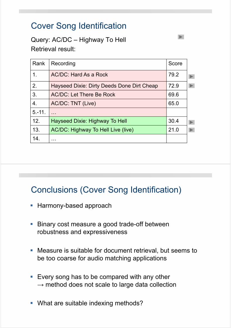
Cover Song Identification
Query: AC/DC – Highway To Hell
Retrieval result:
Rank Recording Score
1. AC/DC: Hard As a Rock 79.2
2. Hayseed Dixie: Dirty Deeds Done Dirt Cheap 72.9
3. AC/DC: Let There Be Rock 69.6
4. AC/DC: TNT (Live) 65.0
5.-11. …
12. Hayseed Dixie: Highway To Hell 30.4
13. AC/DC: Highway To Hell Live (live) 21.0
14. …
Conclusions (Cover Song Identification)
Harmony-based approach
Binary cost measure a good trade-off between robustness and expressiveness
Measure is suitable for document retrieval, but seems to be too coarse for audio matching applications
Every song has to be compared with any other→ method does not scale to large data collection
What are suitable indexing methods?
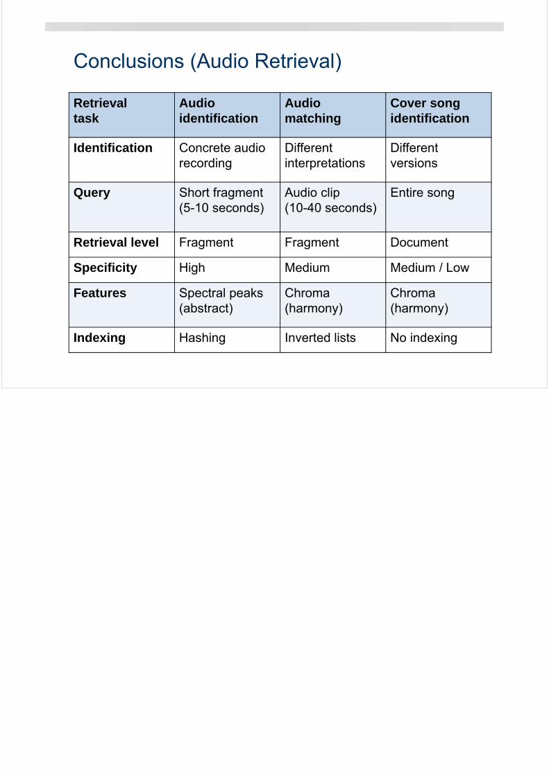
Conclusions (Audio Retrieval)
Retrievaltask
Audio identification
Audio matching
Cover songidentification
Identification Concrete audio recording
Different interpretations
Different versions
Query Short fragment(5-10 seconds)
Audio clip(10-40 seconds)
Entire song
Retrieval level Fragment Fragment Document
Specificity High Medium Medium / Low
Features Spectral peaks(abstract)
Chroma(harmony)
Chroma(harmony)
Indexing Hashing Inverted lists No indexing
Related Documents