Audio Coding Introduction - Startseite TU Ilmenau · Audio Coding Introduction Lecture WS 2013/2014 ... • 1999 - MPEG 4 AAC • 2002 ... 48 kbp/s for two channels)

Prof. Dr.-Ing. K. Brandenburg, [email protected] Prof. Dr.-Ing. G. Schuller, [email protected] Page ‹Nr.›

Audio Coding Introduction

Lecture

WS 2013/2014

Prof. Dr.-Ing. Karlheinz Brandenburg

[email protected]

Prof. Dr.-Ing. Gerald Schuller [email protected]

1


Organisatorial Details - Overview

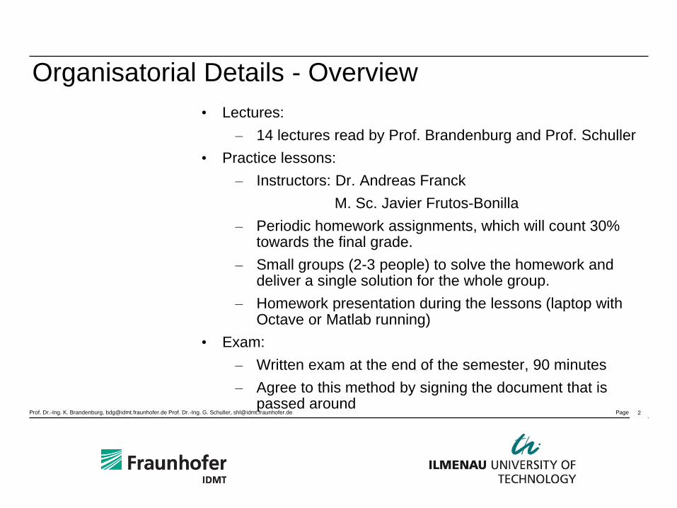
• Lectures:

– 14 lectures read by Prof. Brandenburg and Prof. Schuller

• Practice lessons:

– Instructors: Dr. Andreas Franck

M. Sc. Javier Frutos-Bonilla

– Periodic homework assignments, which will count 30% towards the final grade.

– Small groups (2-3 people) to solve the homework and deliver a single solution for the whole group.

– Homework presentation during the lessons (laptop with Octave or Matlab running)

• Exam:

– Written exam at the end of the semester, 90 minutes

– Agree to this method by signing the document that is passed around

2


Organisatorial Details – Time and Place

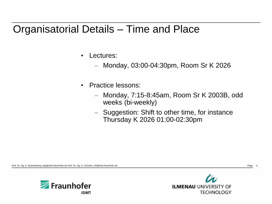
• Lectures:

– Monday, 03:00-04:30pm, Room Sr K 2026


– Monday, 7:15-8:45am, Room Sr K 2003B, odd weeks (bi-weekly)

– Suggestion: Shift to other time, for instance Thursday K 2026 01:00-02:30pm

3


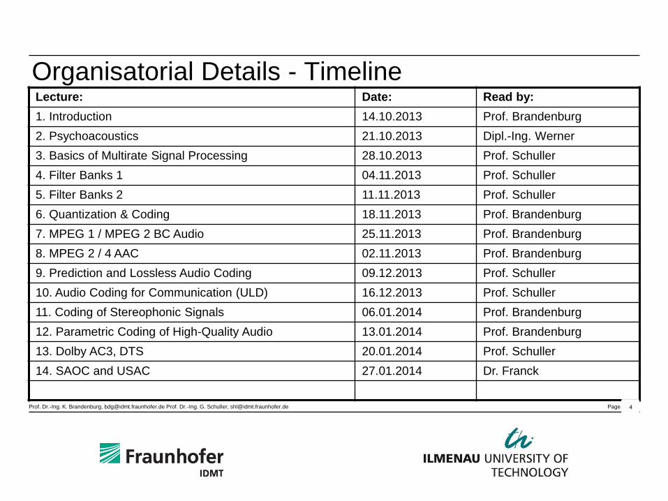
Organisatorial Details - Timeline Lecture: Date: Read by:

1. Introduction 14.10.2013 Prof. Brandenburg

2. Psychoacoustics 21.10.2013 Dipl.-Ing. Werner

3. Basics of Multirate Signal Processing 28.10.2013 Prof. Schuller

4. Filter Banks 1 04.11.2013 Prof. Schuller


6. Quantization & Coding 18.11.2013 Prof. Brandenburg

7. MPEG 1 / MPEG 2 BC Audio 25.11.2013 Prof. Brandenburg

8. MPEG 2 / 4 AAC 02.11.2013 Prof. Brandenburg

9. Prediction and Lossless Audio Coding 09.12.2013 Prof. Schuller

10. Audio Coding for Communication (ULD) 16.12.2013 Prof. Schuller

11. Coding of Stereophonic Signals 06.01.2014 Prof. Brandenburg

12. Parametric Coding of High-Quality Audio 13.01.2014 Prof. Brandenburg

13. Dolby AC3, DTS 20.01.2014 Prof. Schuller

14. SAOC and USAC 27.01.2014 Dr. Franck

4


Current Applications (1)

• Digital audio broadcasting

- EU 147 (Layer 2)

- WorldSpace (Layer 3)

- XM Radio (HeAAC)

• ISDN Transmission of Audio

• Digital TV

- MPEG-1/2 Layer 2

- Dolby AC-3 multichannel coding

- MPEG- 2 AAC

• Storage of large music volumes (archives)

• DVD

- Dolby Digital

- DTS 5


Current Applications (2)

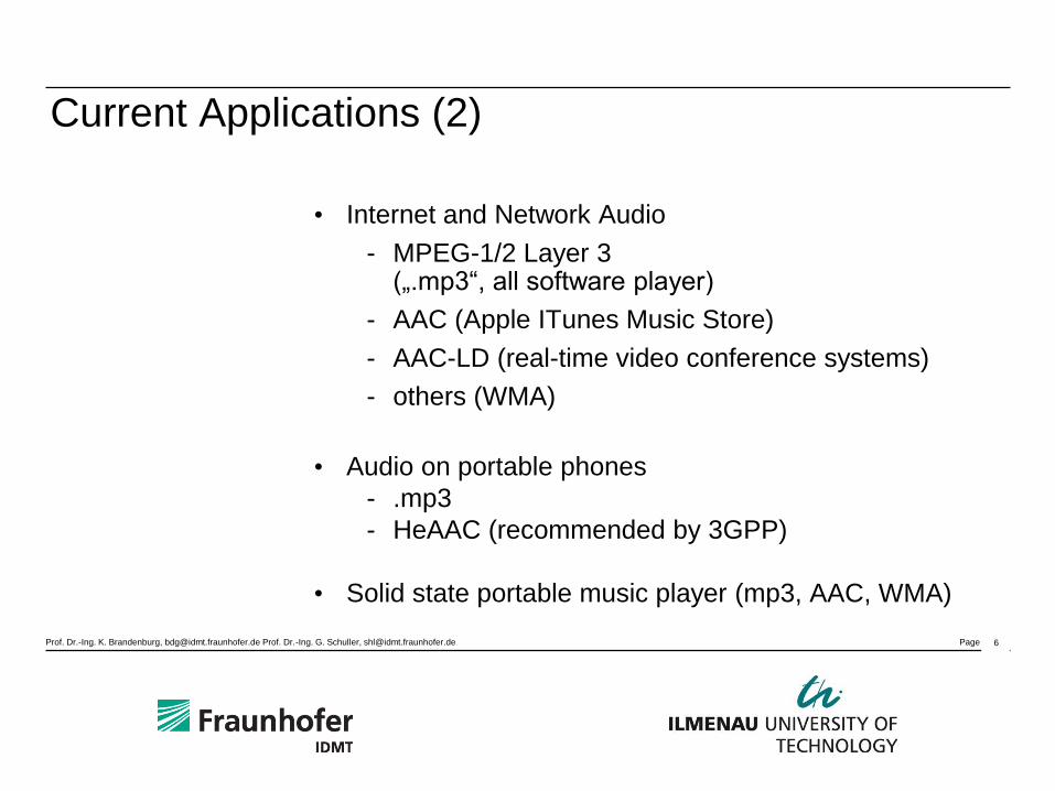
• Internet and Network Audio

- MPEG-1/2 Layer 3 („.mp3“, all software player)

- AAC (Apple ITunes Music Store)

- AAC-LD (real-time video conference systems)

- others (WMA)

• Audio on portable phones

- .mp3

- HeAAC (recommended by 3GPP)

• Solid state portable music player (mp3, AAC, WMA)

6


Basics of High Quality Audio Coding

• The goal: “transparent” coding of music signals

• The source is not known in advance

• Use information about the sink, not the source

• The solution: Modeling of the masking threshold of the ear

• The quantization noise has to be kept below the masked

threshold

7


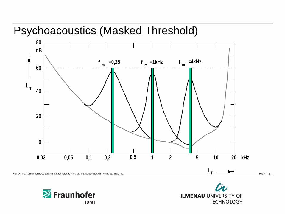
Psychoacoustics (Masked Threshold)

L

0

20

40

60

dB

80

0,02 0,05 0,1 0,2 0,5 1 2 5 10 20 kHz

Tf

mf =0,25

T

mf =1kHz

mf =4kHz

8


Demo: The "13 dB-miracle"

• Original signal

• Original + white noise, SNR = 13,6 dB

• Original + noise at threshold, S/N = 13,6 dB

• Difference (modulated white noise)

• Difference (noise at threshold)

9


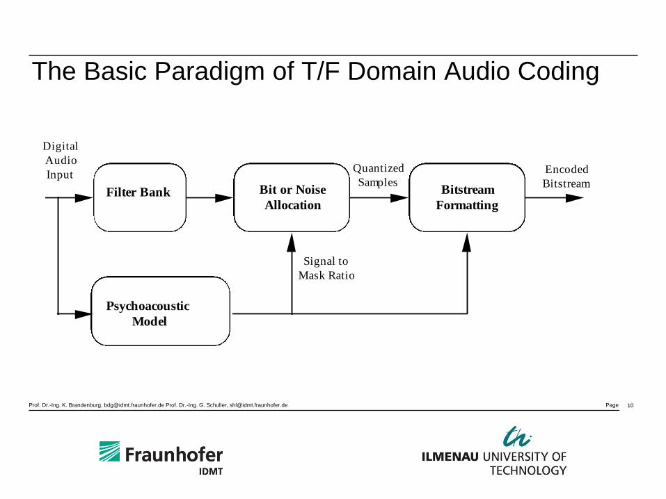
The Basic Paradigm of T/F Domain Audio Coding

Digital

Audio

Input

Filter Bank

Psychoacoustic

Model

Bitstream

Formatting

Signal to

Mask Ratio

Quantized

SamplesEncoded

BitstreamBit or Noise

Allocation

10


Differences between Audio and Speech Coding (1)

• Generic audio coding is similar to speech coding

except:

Larger bandwidth

• speech coders usually use up to 7 kHz

bandwidth

Fewer audible artifacts

Use of psycho-acoustic model for irrelevancy

removal

11


Differences between Audio and Speech Coding (2)

Different requirements for bitrate

• speech aims for as small as possible

(e.g. GSM: <=13kbps)

• audio demands more for quality

(>=64 kbps, decreasing)

Not specialized to speech model

12


History of Audio Coding

• 1979 - the „Critical Band Coder“

• 1982 - „classic ATC“ for Music

• 1985 - MSC

• 1987 - OCF

• 1987 - MASCAM

• 1987 - PXFM

• 1990 - ASPEC, MUSICAM

• 1992 - MPEG 1

• 1996 - ePAC

• 1997 - MPEG 2 AAC

• 1999 - MPEG 4 AAC

• 2002 - HE AAC

• 2012 - USAC

• MPEG-H: Coding for 3D audio

13


The time line for near-CD-quality

• 1990 256 kbit/s ASPEC, MUSICAM would fail today’s listening tests

• 1992 192 kbit/s MPEG-1 Layer-3

• 1994 128 kbit/s MPEG-1 Layer-3 (".mp3") including combined joint stereo coding bad quality for some signals

• 1997 96 kbit/s MPEG-2 Advanced Audio Coding better than MP3 at 128, not fully transparent

• 2000 64 kbit/s AAC-based MPEG-4

• 2003 48 kbit/s MPEG-4 HeAAC (AAC+ in 2000) e.g. used for XM Radio

14


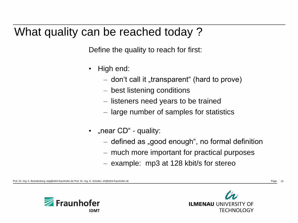
What quality can be reached today ?

Define the quality to reach for first:

• High end:

– don‘t call it „transparent“ (hard to prove)

– best listening conditions

– listeners need years to be trained

– large number of samples for statistics

• „near CD“ - quality:

– defined as „good enough“, no formal definition

– much more important for practical purposes

– example: mp3 at 128 kbit/s for stereo

15


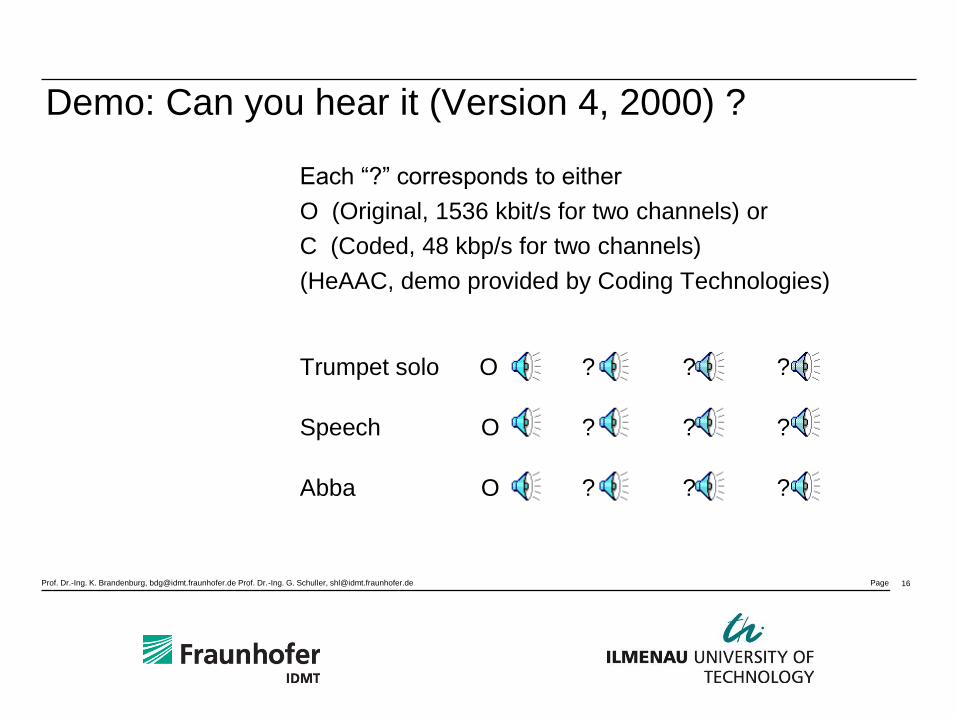
Demo: Can you hear it (Version 4, 2000) ?

Each “?” corresponds to either

O (Original, 1536 kbit/s for two channels) or

C (Coded, 48 kbp/s for two channels)

(HeAAC, demo provided by Coding Technologies)

Trumpet solo O ? ? ?

Speech O ? ? ?

Abba O ? ? ?

16


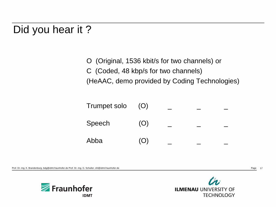
Did you hear it ?

O (Original, 1536 kbit/s for two channels) or

C (Coded, 48 kbp/s for two channels)

(HeAAC, demo provided by Coding Technologies)

Trumpet solo (O) _ _ _

Speech (O) _ _ _

Abba (O) _ _ _

17


Extra Material

18


Organisatorial Details – Overview (Repetition)

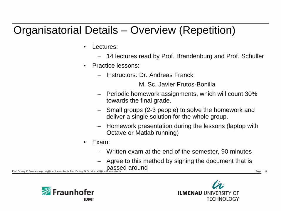
• Lectures:

– 14 lectures read by Prof. Brandenburg and Prof. Schuller


– Instructors: Dr. Andreas Franck

M. Sc. Javier Frutos-Bonilla

– Periodic homework assignments, which will count 30% towards the final grade.

– Small groups (2-3 people) to solve the homework and deliver a single solution for the whole group.

– Homework presentation during the lessons (laptop with Octave or Matlab running)

• Exam:

– Written exam at the end of the semester, 90 minutes

– Agree to this method by signing the document that is passed around

19


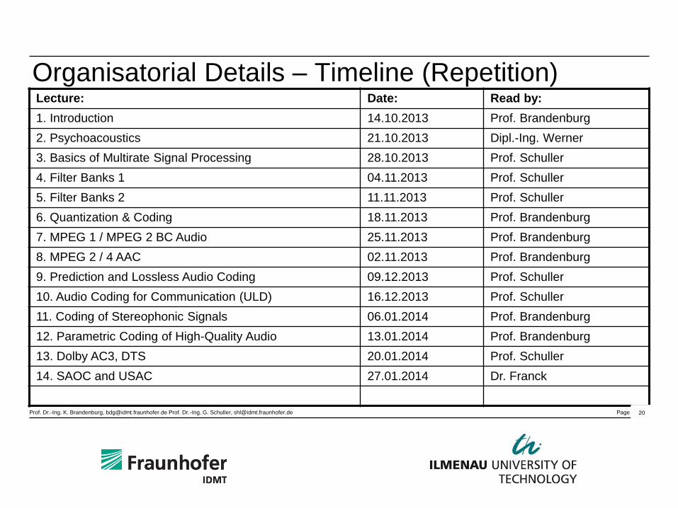
Organisatorial Details – Timeline (Repetition) Lecture: Date: Read by:

1. Introduction 14.10.2013 Prof. Brandenburg

2. Psychoacoustics 21.10.2013 Dipl.-Ing. Werner

3. Basics of Multirate Signal Processing 28.10.2013 Prof. Schuller



6. Quantization & Coding 18.11.2013 Prof. Brandenburg

7. MPEG 1 / MPEG 2 BC Audio 25.11.2013 Prof. Brandenburg

8. MPEG 2 / 4 AAC 02.11.2013 Prof. Brandenburg

9. Prediction and Lossless Audio Coding 09.12.2013 Prof. Schuller

10. Audio Coding for Communication (ULD) 16.12.2013 Prof. Schuller

11. Coding of Stereophonic Signals 06.01.2014 Prof. Brandenburg

12. Parametric Coding of High-Quality Audio 13.01.2014 Prof. Brandenburg

13. Dolby AC3, DTS 20.01.2014 Prof. Schuller

14. SAOC and USAC 27.01.2014 Dr. Franck

20


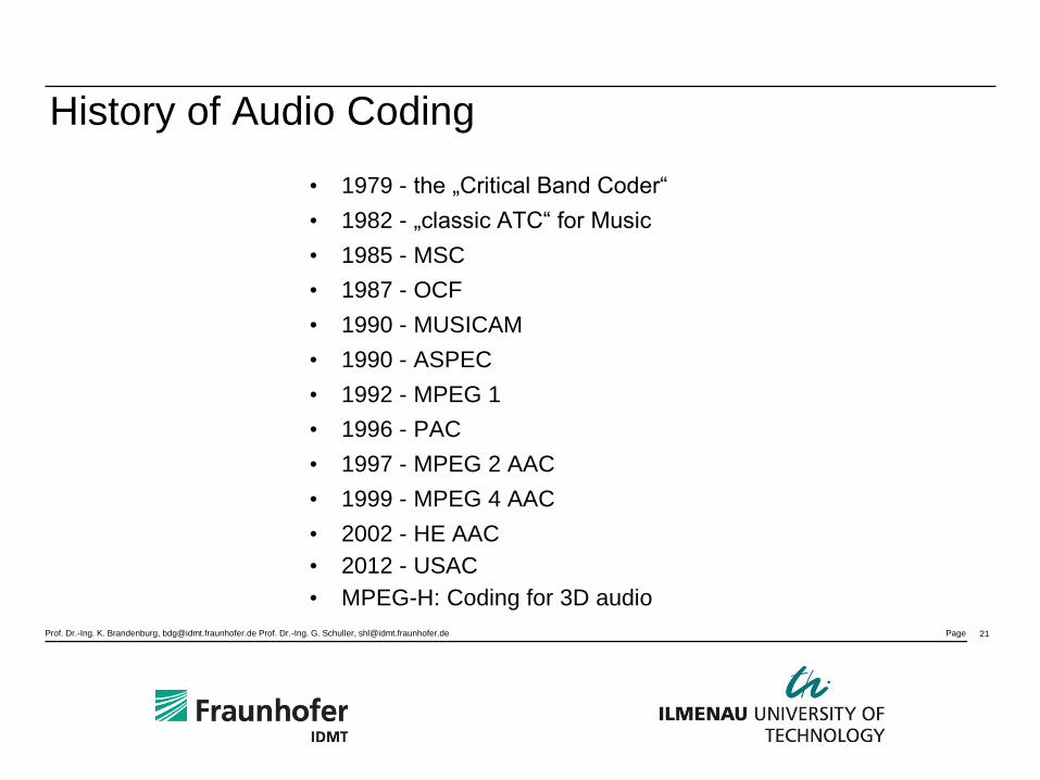
History of Audio Coding

• 1979 - the „Critical Band Coder“

• 1982 - „classic ATC“ for Music

• 1985 - MSC

• 1987 - OCF

• 1990 - MUSICAM

• 1990 - ASPEC

• 1992 - MPEG 1

• 1996 - PAC

• 1997 - MPEG 2 AAC

• 1999 - MPEG 4 AAC

• 2002 - HE AAC

• 2012 - USAC

• MPEG-H: Coding for 3D audio

21


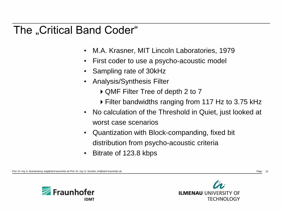
The „Critical Band Coder“

• M.A. Krasner, MIT Lincoln Laboratories, 1979

• First coder to use a psycho-acoustic model

• Sampling rate of 30kHz

• Analysis/Synthesis Filter

QMF Filter Tree of depth 2 to 7

Filter bandwidths ranging from 117 Hz to 3.75 kHz

• No calculation of the Threshold in Quiet, just looked at

worst case scenarios

• Quantization with Block-companding, fixed bit

distribution from psycho-acoustic criteria

• Bitrate of 123.8 kbps

22


„classic ATC“ for Music

• Universität Erlangen-Nürnberg, 1982

• First real-time music coder

• Sampling rate between 30-32 kHz

• Does not use a psycho-acoustic model → bad quality for some music pieces

• Block length of 128 samples (about 4 ms)

• Bitrate: 3bits/sample (about 100 kbps)

23


MSC (Multiple Adaptive Spectral Audio Coding)

• Krahe and others, Universität Duisburg, 1985

• First Coder to use both psycho-acoustic model and

transformation-coding

• Analysis/Synthesis:

FFT with conversion of Amplitude & Phase

window length of 1024 samples

window ends sine-tapered with an overlap of 64

samples

• Threshold estimation is only using in-band masking

• Quantization uses block-companding with 2 bits per

sample

24


OCF (Optimum Coding in Frequency Domain)

• Brandenburg, Universität Erlangen, 1987, 1988

• MDCT-Filter bank with window length of 1024 or 512

• Explicit calculation of the masking threshold with a

simple model

Calculation per critical band

No tonality criteria used

Maximum calculation instead of convolution

• Non-uniform quantization (quantization noise dependant

on amplitude)

• Huffman coding from pairs of spectral values

25


ASPEC- Adaptive Spectral Perceptual Entropy Coding (1) • Uni Erlangen, FhG, AT&T Bell Labs, Deutsche

Thomson-Brandt, CNET, 1990

• Analysis/Synthesis: MDCT with switchable block lengths

• Use of 2 models for psycho-acoustic

Simple: like OCF

Better: like PXFM + 1/3 Frequency grouping resolution + local tonality criteria (like Hybrid)

• Quantization/Coding: like OCF,

Choice of Huffman-code-books

Further division of the spectrum

• Control of window length (switching the number of

bands)

26


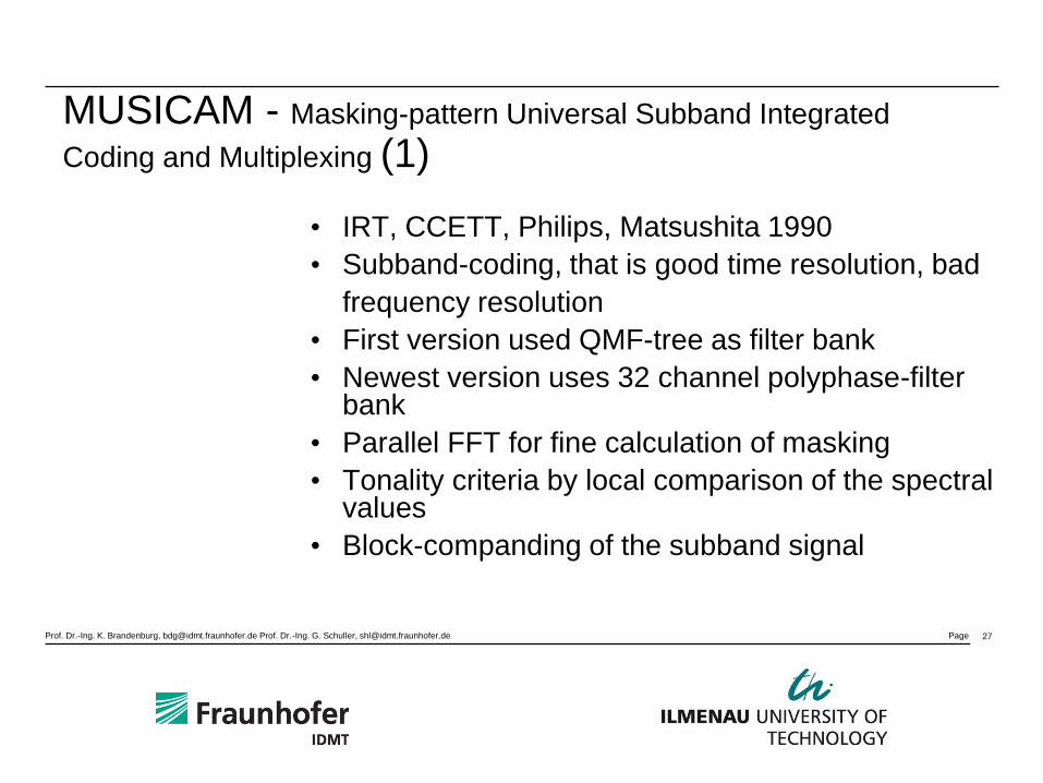
MUSICAM - Masking-pattern Universal Subband Integrated

Coding and Multiplexing (1)

• IRT, CCETT, Philips, Matsushita 1990

• Subband-coding, that is good time resolution, bad

frequency resolution

• First version used QMF-tree as filter bank

• Newest version uses 32 channel polyphase-filter bank

• Parallel FFT for fine calculation of masking

• Tonality criteria by local comparison of the spectral values

• Block-companding of the subband signal

27


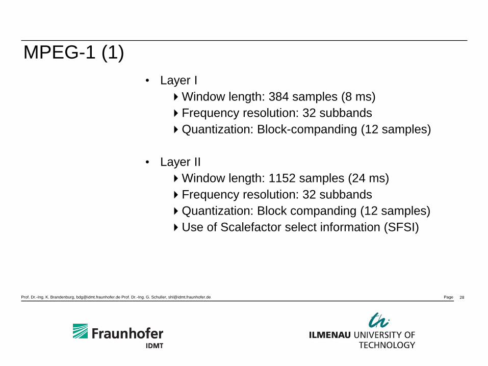
MPEG-1 (1)

• Layer I

Window length: 384 samples (8 ms)

Frequency resolution: 32 subbands

Quantization: Block-companding (12 samples)

• Layer II


Frequency resolution: 32 subbands

Quantization: Block companding (12 samples)

Use of Scalefactor select information (SFSI)

28


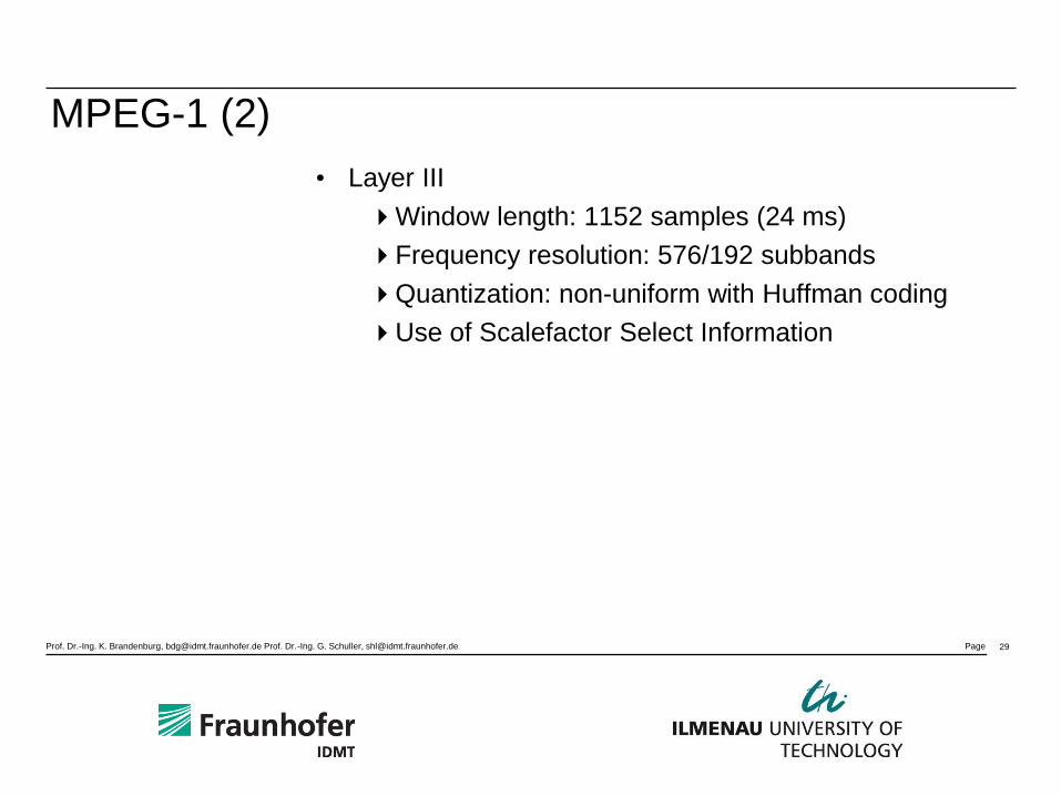
MPEG-1 (2)

• Layer III


Frequency resolution: 576/192 subbands

Quantization: non-uniform with Huffman coding

Use of Scalefactor Select Information

29


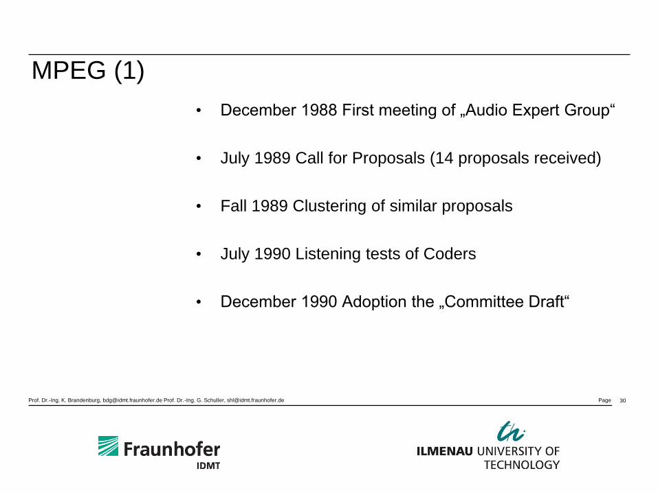
MPEG (1)

• December 1988 First meeting of „Audio Expert Group“

• July 1989 Call for Proposals (14 proposals received)

• Fall 1989 Clustering of similar proposals

• July 1990 Listening tests of Coders

• December 1990 Adoption the „Committee Draft“

30


MPEG (2)

• The results of the „Stockholm-Tests“ showed

2 proposals were best, ASPEC and MUSICAM

Listening tests show that ASPEC is better especially at low bitrates

In comparison of complexity parameters MUSICAM is better

• RESULT: collaboration between ASPEC & MUSICAM in a Layered solution (hence Layer 1, Layer 2, & Layer 3)

31


PAC

• Resulted from split of AT&T and Lucent

Technologies

• Branched off from MPEG-AAC, proprietary instead

of standardized technology

• Used in American Satellite Broadcast System (XM, Sirius)

32


MPEG 2 AAC (1)

• first named MPEG-2 NBC (non backwards compatible),

later named AAC (advanced audio coding)

• MPEG-2 AAC (ISO/IEC 13818-7)

• offers very high quality compressed audio

• Allows 1 to 48 channels, Sampling rates from 8 to 96

kHz, with multi-channel, multi-lingual, and multi-program

possibilities.

• AAC works at bit-rates from 8 kbit/s for mono Speech

signals and up to 160 kbit/s/channel for very high quality, allows tandem coding

33


MPEG 2 AAC (2)

• 3 Profiles from AAC with varying levels of

complexity and scalability.

• ‘Joint Stereo’-Mode is more flexible compared

to MP3 in that it is switchable for individual

scale factor bands whereas MP3 was only

switchable for the whole spectrum.

34


MPEG 2 AAC

Basic Features

• High frequency resolution filter bank-based

coder (1024 subbands MDCT with 50% overlap)

• 1: 8 block switching (1024/128 subbands MDCT)

• Non- uniform quantizer

• Noise shaping in half critical bands (scalefactor

bands)

• Huffman coding of scalefactors and spectral

coefficients

35


HE AAC

• Combination of the MPEG-4 AAC Low Complexity (LC)

Object and the MPEG-4 Spectral Band Replication (SBR) Object

• SBR: parametric coding of high frequency envelope with

small amount of control data

• Parametric stereo and multi-channel coding

• Backwards compatible to AAC

• 5.1 surround sound at 128 kbps

• Good quality stereo at 32 kbps or above

36

Audio Coding Introduction - Startseite TU Ilmenau · Audio Coding Introduction Lecture WS 2013/2014 ... • 1999 - MPEG 4 AAC • 2002 ... 48 kbp/s for two channels)

Documents