Munich Personal RePEc Archive Audi vs. BMW – On the Physical Heterogeneity of German Luxury Cars Vistesen, Claus Global Economy Matters, Copenhagen Business School 18 December 2009 Online at https://mpra.ub.uni-muenchen.de/19516/ MPRA Paper No. 19516, posted 22 Dec 2009 08:51 UTC

Welcome message from author
This document is posted to help you gain knowledge. Please leave a comment to let me know what you think about it! Share it to your friends and learn new things together.
Transcript
Munich Personal RePEc Archive
Audi vs. BMW – On the Physical
Heterogeneity of German Luxury Cars
Vistesen, Claus
Global Economy Matters, Copenhagen Business School
18 December 2009
Online at https://mpra.ub.uni-muenchen.de/19516/
MPRA Paper No. 19516, posted 22 Dec 2009 08:51 UTC
1
Audi vs. BMW – On the Physical Heterogeneity of
German Luxury Cars Working Paper 03-09
Claus Vistesen
[email protected] and www.clausvistesen.squarespace.com
MSc. Applied Economics and Finance
Copenhagen Business School
JEL: L62
Key words: luxury cars, BMW, Audi, pure characteristics demand models
Database can be obtained by contacting the author through the e-mail above
2
Audi vs BMW – On the Physcial Heterogenity of German Luxury Cars
Claus Vistesen
Abstract
This paper uses Logit and Probit regressions to test for and quantify the physical heterogeneity
between German luxury cars. Using a matched sample database, the binary response variable
consisting of Audis and BMWs is fitted to a matrix of physical characteristics such as power,
torque, fuel consumption, engine displacement etc. The results indicate that having a forced
induction engine (e.g. turbo) is associated with a 51% lower probability of observing a BMW and
that increasing fuel consumption by 1 liter per 100km lowers the probability of observing a BMW
with 61%. The results are discussed in relation to the idea that consumers may not differentiate
across luxury products on the basis of physical characteristics and how this may introduce a bias
with respect to predicting demand in the context of available market data.
1.0 Introduction
The idea that you can take some of the most arcane tools of the economist’s toolbox and apply
them directly to the unstable and complex reality of the real world remain a difficult aspiration in
most contexts. Still, the estimation and identification of demand systems remain a panacea in the
context of empirical microeconomics and although this paper, by no stretch of the word,
represents a panacea, it is within this theoretical context that it makes its main argument.
Formally, this takes us into the world of so-called pure characteristics demand models (PCDM)
which are defined as discrete choice models in which consumers derive utility from physical
product characteristics and, more specifically, choose between differentiated products and rank
them based on these product characteristics Berry and Pakes (2007) and Thomassen (2007). This
paper does not make use of market data and in this way does not fit and estimate a PCDM. Rather,
it asks the simple question that the extent to which economists assume consumers to differentiate
products on the basis of physical characteristics, it would be interesting to check along which lines
differentiated products might differ in the context of physical characteristics.
In order to deliver a stab to answer this question, the attention is turned to one of the most
revered products in the world in the form of German luxury cars and specifically the two super
brands Audi, as part of the VW group, and the independent make BMW. The choice of Audi and
BMW as subjects of analysis is interesting for two reasons in particular. First of all, they are main
competitors on most markets where they are both present and thus can, to a high degree, be
viewed as close substitutes. This is interesting because of the extent to which consumers are
expected to substitute on the basis of physical characteristics it would be interesting to see
whether Audis and BMWs especially differ along physical dimensions. Secondly, Audis and BMWs
represent interesting subjects of analysis precisely because they are luxury products and thus how
3
their main difference may not be captured by a physical characteristics model. In short, there is
more to product heterogeneity amongst luxury products than physical characteristics Vickers and
Renand (2003). The discussion of this issue will be deferred to after the empirical results have
been presented.
In general, the small theoretical framework which serves to frame the empirical estimations relies
closely on the intuition, results and discussion provided in Thomassen (2007) who exactly sets out
to estimate (and identify) a pure characteristics model for cars with data on the Norwegian
market. The empirical analysis is based on data from the German market1 where a matched
sample is created on the basis of the most popular competitive product lines in the Audi and BMW
setup.
The paper proceeds with the presentation of a small theoretical framework in section 2 before
section 3 presents the estimation and results as well as a discussion of the relative benefits of the
LPM and discrete choice models. Section 4 contains a small discussion on the obtained results with
specific focus on the difference between the three estimated models2 as well as a perspective on
what it means that I am analyzing luxury products. Section 5 concludes.
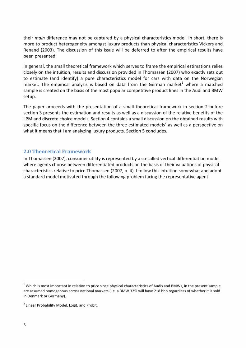
2.0 Theoretical Framework
In Thomassen (2007), consumer utility is represented by a so-called vertical differentiation model
where agents choose between differentiated products on the basis of their valuations of physical
characteristics relative to price Thomassen (2007, p. 4). I follow this intuition somewhat and adopt
a standard model motivated through the following problem facing the representative agent.
1 Which is most important in relation to price since physical characteristics of Audis and BMWs, in the present sample,
are assumed homogenous across national markets (i.e. a BMW 325i will have 218 bhp regardless of whether it is sold
in Denmark or Germany).
2 Linear Probability Model, Logit, and Probit.
4
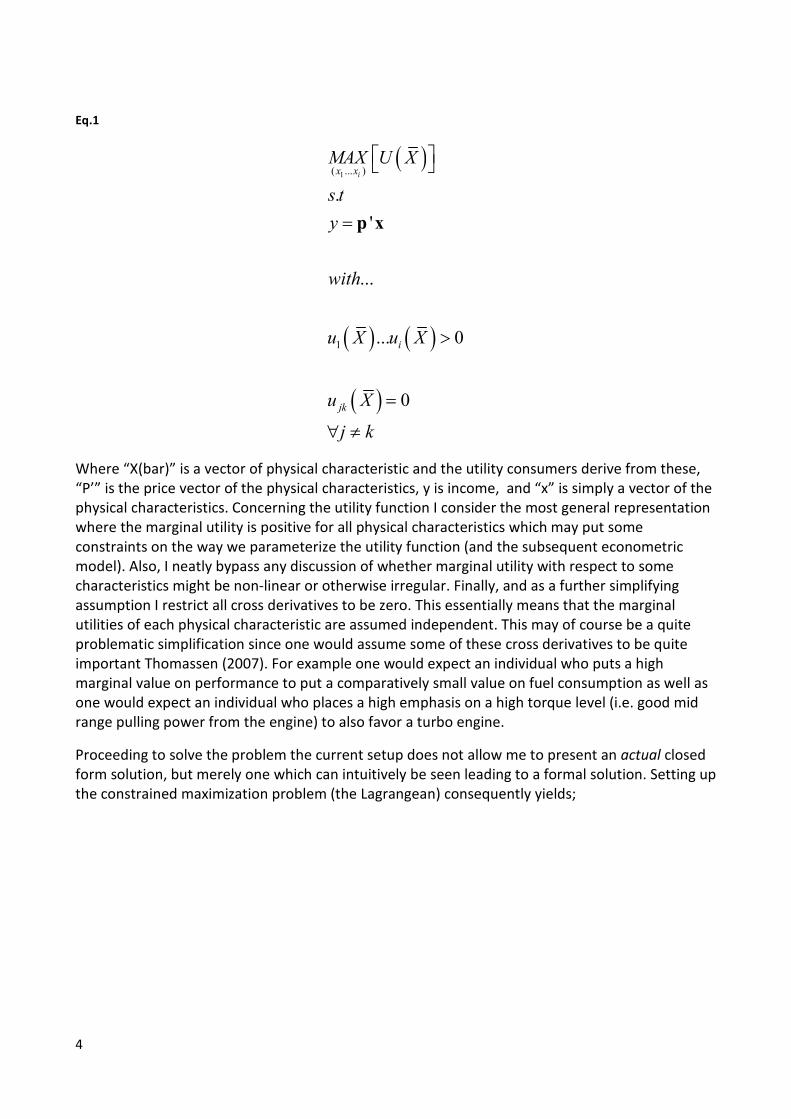
Eq.1
( )
( ) ( )
( )
�� ��� �
�
�
�
���
��� �
�
�� �
�
��
��� � �
�
��
� � � �
� �
� �
=
>
=
∀ ≠
p x
Where “X(bar)” is a vector of physical characteristic and the utility consumers derive from these,
“P’” is the price vector of the physical characteristics, y is income, and “x” is simply a vector of the
physical characteristics. Concerning the utility function I consider the most general representation
where the marginal utility is positive for all physical characteristics which may put some
constraints on the way we parameterize the utility function (and the subsequent econometric
model). Also, I neatly bypass any discussion of whether marginal utility with respect to some
characteristics might be non-linear or otherwise irregular. Finally, and as a further simplifying
assumption I restrict all cross derivatives to be zero. This essentially means that the marginal
utilities of each physical characteristic are assumed independent. This may of course be a quite
problematic simplification since one would assume some of these cross derivatives to be quite
important Thomassen (2007). For example one would expect an individual who puts a high
marginal value on performance to put a comparatively small value on fuel consumption as well as
one would expect an individual who places a high emphasis on a high torque level (i.e. good mid
range pulling power from the engine) to also favor a turbo engine.
Proceeding to solve the problem the current setup does not allow me to present an actual closed
form solution, but merely one which can intuitively be seen leading to a formal solution. Setting up
the constrained maximization problem (the Lagrangean) consequently yields;
5
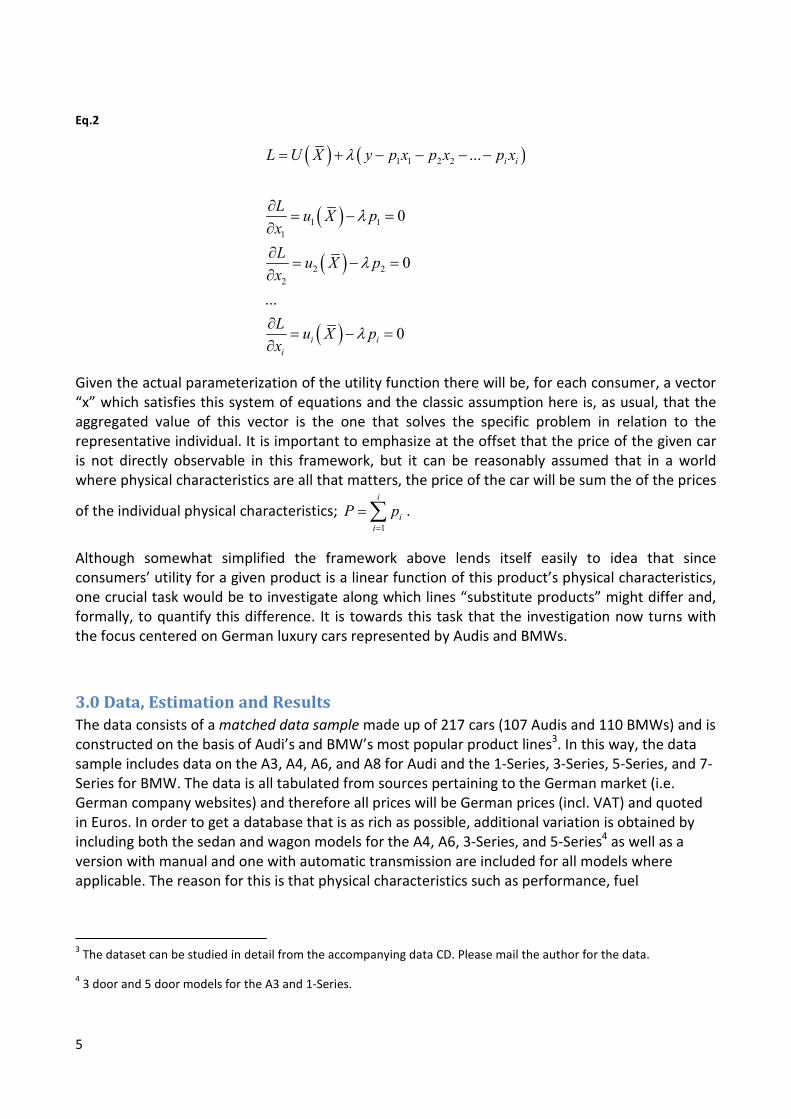
Eq.2
( ) ( )
( )
( )
( )
� � � �
� �
�
� �
�
���
�
�
���
�
� �
� �
�
� � � � � � � � � �
�� � �
�
�� � �
�
�� � �
�
λ
λ
λ
λ
= + − − − −
∂= − =
∂
∂= − =
∂
∂= − =
∂
Given the actual parameterization of the utility function there will be, for each consumer, a vector
“x” which satisfies this system of equations and the classic assumption here is, as usual, that the
aggregated value of this vector is the one that solves the specific problem in relation to the
representative individual. It is important to emphasize at the offset that the price of the given car
is not directly observable in this framework, but it can be reasonably assumed that in a world
where physical characteristics are all that matters, the price of the car will be sum the of the prices
of the individual physical characteristics; �
�
�
�
� �=
=∑ .
Although somewhat simplified the framework above lends itself easily to idea that since
consumers’ utility for a given product is a linear function of this product’s physical characteristics,
one crucial task would be to investigate along which lines “substitute products” might differ and,
formally, to quantify this difference. It is towards this task that the investigation now turns with
the focus centered on German luxury cars represented by Audis and BMWs.
3.0 Data, Estimation and Results
The data consists of a matched data sample made up of 217 cars (107 Audis and 110 BMWs) and is
constructed on the basis of Audi’s and BMW’s most popular product lines3. In this way, the data
sample includes data on the A3, A4, A6, and A8 for Audi and the 1-Series, 3-Series, 5-Series, and 7-
Series for BMW. The data is all tabulated from sources pertaining to the German market (i.e.
German company websites) and therefore all prices will be German prices (incl. VAT) and quoted
in Euros. In order to get a database that is as rich as possible, additional variation is obtained by
including both the sedan and wagon models for the A4, A6, 3-Series, and 5-Series4 as well as a
version with manual and one with automatic transmission are included for all models where
applicable. The reason for this is that physical characteristics such as performance, fuel
3 The dataset can be studied in detail from the accompanying data CD. Please mail the author for the data.
4 3 door and 5 door models for the A3 and 1-Series.
6
consumption and size may change as a function whether the car is a sedan or wagon model as well
as whether it is equipped with a manual or automatic transmission.
A natural question to ask at this point is naturally why not the whole model line-up has been
chosen in order to provide the richest analysis. After all, in the present context one could even
argue that by taking all models currently offered by Audi and BMW we would not only get a richer
basis for analysis, we would also, de-facto, have the entire universe of BMW and Audi models and
thus in some sense a population and not a sample. This however is only partially true and apart
from the fact that punching in all models manually in excel would have required your humble
scribe to fork over some cash for a student assistant, it is important to realize this
universe/population of Audi and BMW models also has a time dimension in which not only
existing models change but also where new models are introduced and old ones retired. For this
reason it would not have been more consistent to include the entire model line-up. Finally, there
is an argument, in itself, in including only the most popular model line-up and specifically to make
a sample which is made up of competitive models. In this way, it is assumed that this method
makes the analysis most relevant for a possible empirical application with actual sales data.
Moving on to the actual physical characteristics used as independent variables they have been
chosen with an eye to being easily quantifiable as well as offering, in total, the best generic
description of the cars in question. There are 14 in total of which 3 are binary and 11 continuous.
•� Dependent variable (BMW = 1, Audi = 0)
•� Power Output in bhp (break horse power)
•� Torque in NM (newtonmeters)5
•� Cylinders (e.g. 4, 6, or 8)
•� Engine Displacement (measured in CM^3)
•� Engine type (1 = naturally aspirated (NA) and 0 = Forced Induction (i.e. turbo, compressor
etc)
•� Automatic gearbox (1 = yes, 0 = no)
•� Drive train (1=AWD (all wheel drive), 0 = other (e.g. rear wheel drive or front wheel drive))
•� Top Speed (in kilometers per hour (kph))
•� Acceleration (in 0-100 kph time)
•� Fuel Consumption (in l/100 km)6
5 This is a performance measure and indicates, unlike, horse power, the car’s ability to accelerate in the low and mid
range revs area (i.e. not from a standstill). Usually cars equipped with Turbos, Compressors or other form of forced
induction benefit from high torque figures.
6 Combined driving.
7
•� CO2 Emissions (in g/km)
•� Weight (in kg)
•� Power/weight (measured as power/weight; this is meant as a unifying performance
indicator. performance is expected to increase in this ratio.)
Apart from these variables, I also report the price in Euros which is not included in the formal
estimation framework.7 Excel
8 was used to generate the following table which plots the most
important summary statistics for the variables mentioned above.
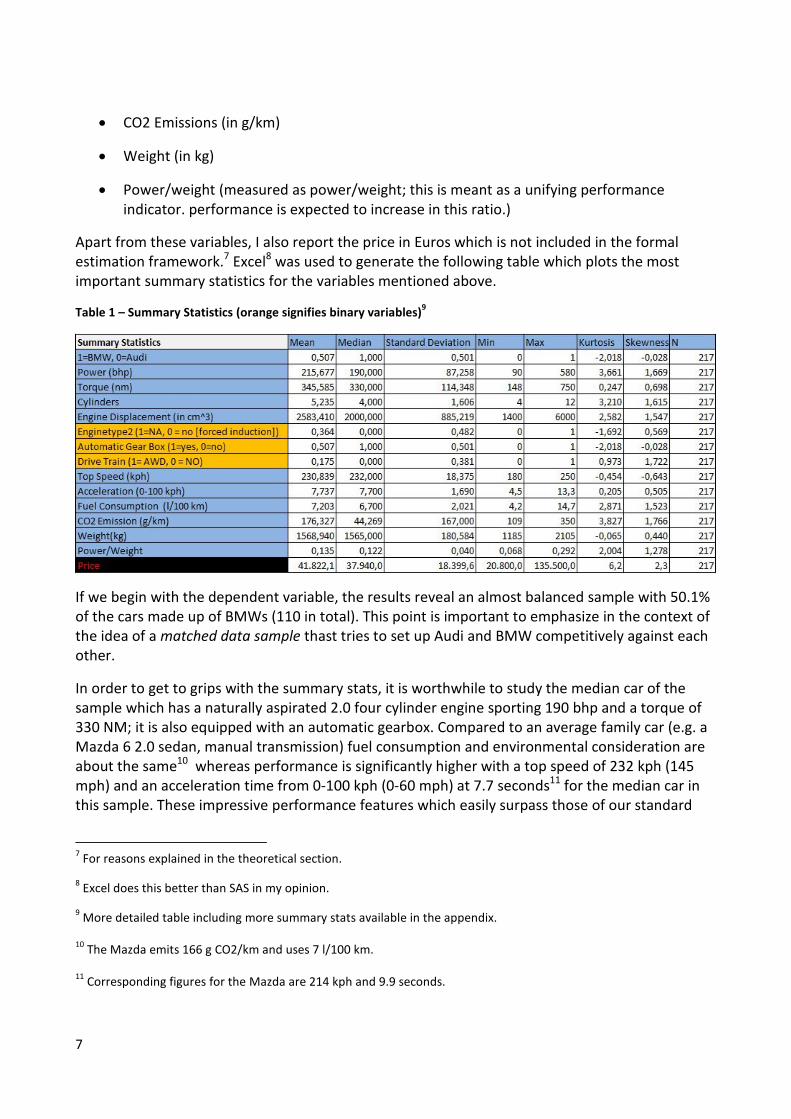
Table 1 – Summary Statistics (orange signifies binary variables)9
If we begin with the dependent variable, the results reveal an almost balanced sample with 50.1%
of the cars made up of BMWs (110 in total). This point is important to emphasize in the context of
the idea of a matched data sample thast tries to set up Audi and BMW competitively against each
other.
In order to get to grips with the summary stats, it is worthwhile to study the median car of the
sample which has a naturally aspirated 2.0 four cylinder engine sporting 190 bhp and a torque of
330 NM; it is also equipped with an automatic gearbox. Compared to an average family car (e.g. a
Mazda 6 2.0 sedan, manual transmission) fuel consumption and environmental consideration are
about the same10
whereas performance is significantly higher with a top speed of 232 kph (145
mph) and an acceleration time from 0-100 kph (0-60 mph) at 7.7 seconds11
for the median car in
this sample. These impressive performance features which easily surpass those of our standard
7 For reasons explained in the theoretical section.
8 Excel does this better than SAS in my opinion.
9 More detailed table including more summary stats available in the appendix.
10 The Mazda emits 166 g CO2/km and uses 7 l/100 km.
11 Corresponding figures for the Mazda are 214 kph and 9.9 seconds.
8
family car likely owe themselves to the fact that we are scrutinizing two luxury brands where high
performance is an important distinguishing trait with the important qualifier that the price of the
median car (€ 37.940) is also significantly higher than for the Mazda (€ 29.200).
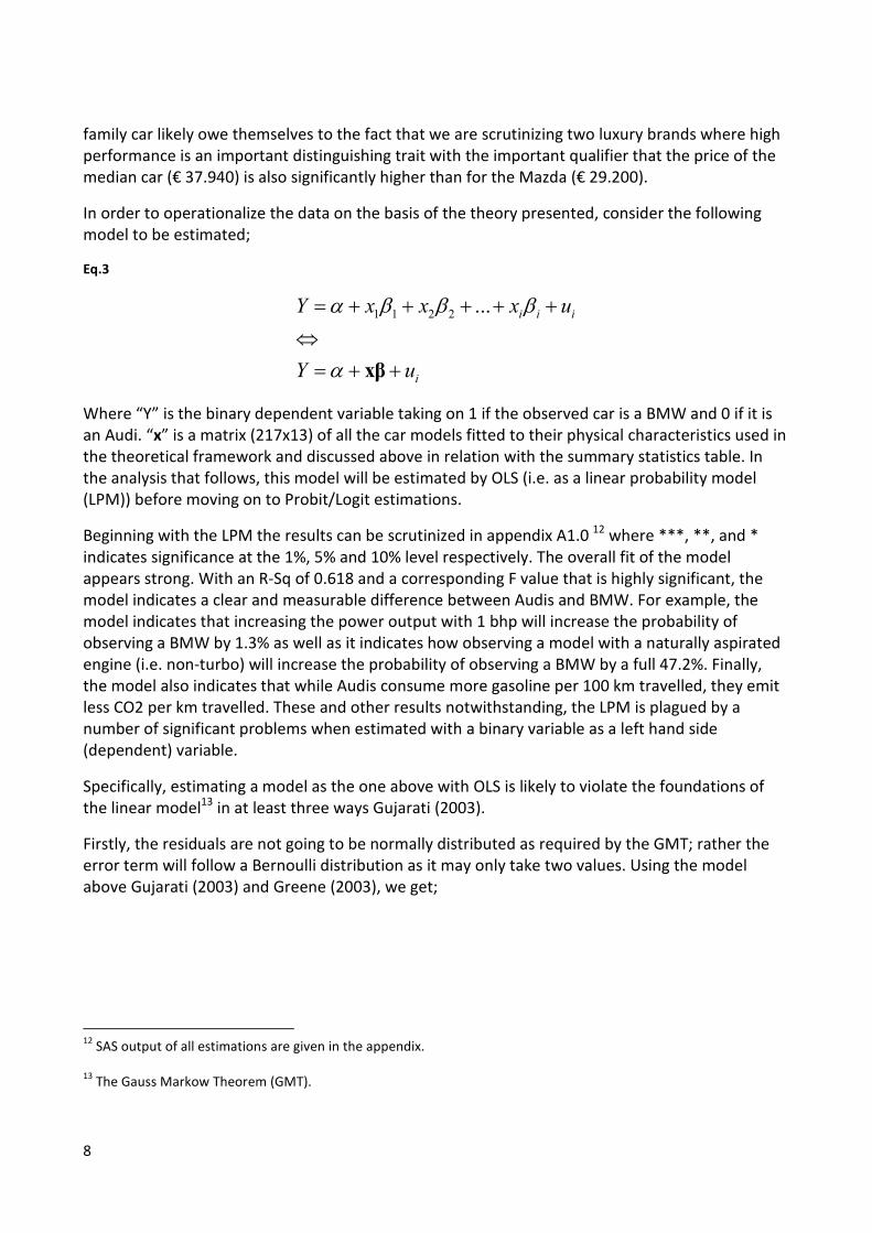
In order to operationalize the data on the basis of the theory presented, consider the following
model to be estimated;
Eq.3
� � � � ��� � � �
�
� � � � �
� �
α β β β
α
= + + + + +
⇔
= + +xβ
Where “Y” is the binary dependent variable taking on 1 if the observed car is a BMW and 0 if it is
an Audi. “x” is a matrix (217x13) of all the car models fitted to their physical characteristics used in
the theoretical framework and discussed above in relation with the summary statistics table. In
the analysis that follows, this model will be estimated by OLS (i.e. as a linear probability model
(LPM)) before moving on to Probit/Logit estimations.
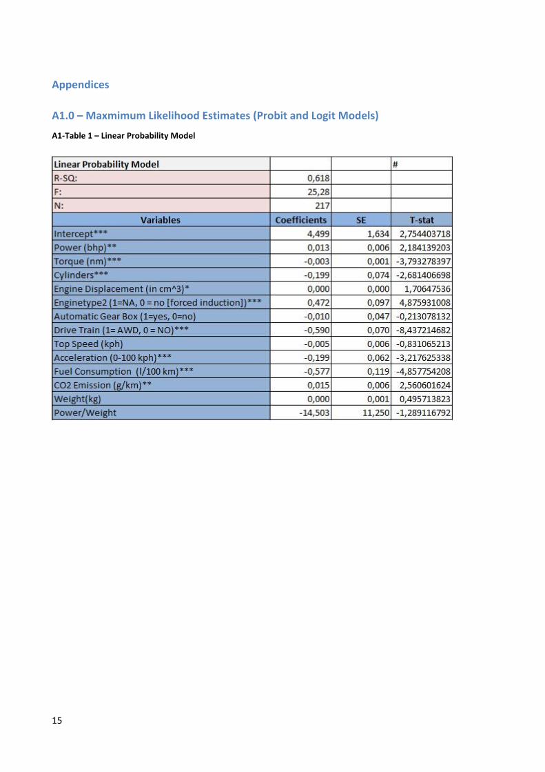
Beginning with the LPM the results can be scrutinized in appendix A1.0 12
where ***, **, and *
indicates significance at the 1%, 5% and 10% level respectively. The overall fit of the model
appears strong. With an R-Sq of 0.618 and a corresponding F value that is highly significant, the
model indicates a clear and measurable difference between Audis and BMW. For example, the
model indicates that increasing the power output with 1 bhp will increase the probability of
observing a BMW by 1.3% as well as it indicates how observing a model with a naturally aspirated
engine (i.e. non-turbo) will increase the probability of observing a BMW by a full 47.2%. Finally,
the model also indicates that while Audis consume more gasoline per 100 km travelled, they emit
less CO2 per km travelled. These and other results notwithstanding, the LPM is plagued by a
number of significant problems when estimated with a binary variable as a left hand side
(dependent) variable.
Specifically, estimating a model as the one above with OLS is likely to violate the foundations of
the linear model13
in at least three ways Gujarati (2003).
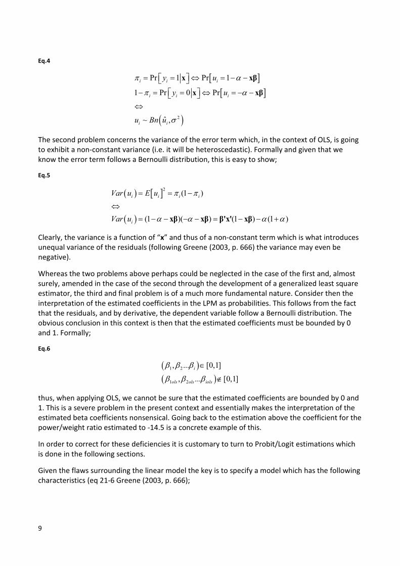
Firstly, the residuals are not going to be normally distributed as required by the GMT; rather the
error term will follow a Bernoulli distribution as it may only take two values. Using the model
above Gujarati (2003) and Greene (2003), we get;
12
SAS output of all estimations are given in the appendix.
13 The Gauss Markow Theorem (GMT).
9
Eq.4
[ ][ ]
( )�
� � � �
� � � �
� �
� � �
� � �
� �
� �
� �
� �� �
π α
π α
σ
= = ⇔ = − −
− = = ⇔ = − − ⇔
x xβ
x xβ
The second problem concerns the variance of the error term which, in the context of OLS, is going
to exhibit a non-constant variance (i.e. it will be heteroscedastic). Formally and given that we
know the error term follows a Bernoulli distribution, this is easy to show;
Eq.5
( ) [ ]
( )
��� �
�� �� � �� � �� �
� � � �
�
��� � � �
��� �
π π
α α α α
= = −
⇔
= − − − − = − − +xβ xβ β'x' xβ
Clearly, the variance is a function of “x” and thus of a non-constant term which is what introduces
unequal variance of the residuals (following Greene (2003, p. 666) the variance may even be
negative).
Whereas the two problems above perhaps could be neglected in the case of the first and, almost
surely, amended in the case of the second through the development of a generalized least square
estimator, the third and final problem is of a much more fundamental nature. Consider then the
interpretation of the estimated coefficients in the LPM as probabilities. This follows from the fact
that the residuals, and by derivative, the dependent variable follow a Bernoulli distribution. The
obvious conclusion in this context is then that the estimated coefficients must be bounded by 0
and 1. Formally;
Eq.6
( )( )
� �
� �
� ��� ����
� ��� ����
�
�� �� ���
β β β
β β β
∈
∉
thus, when applying OLS, we cannot be sure that the estimated coefficients are bounded by 0 and
1. This is a severe problem in the present context and essentially makes the interpretation of the
estimated beta coefficients nonsensical. Going back to the estimation above the coefficient for the
power/weight ratio estimated to -14.5 is a concrete example of this.
In order to correct for these deficiencies it is customary to turn to Probit/Logit estimations which
is done in the following sections.
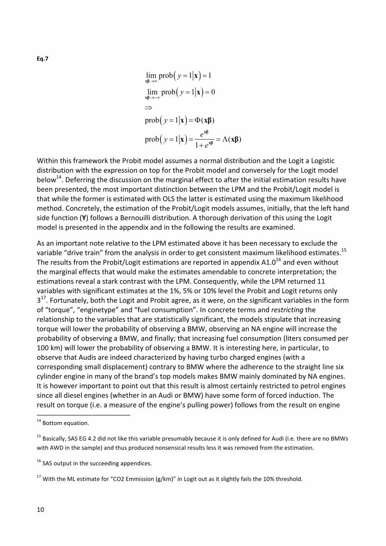
Given the flaws surrounding the linear model the key is to specify a model which has the following
characteristics (eq 21-6 Greene (2003, p. 666);
10
Eq.7
( )
( )
( )
( )
��� ��� � �
��� ��� � �
��� � � �
��� � � ��
�
�
�
��
�
→∞
→−∞
= =
= =
⇒
= = Φ
= = = Λ+
xβ
xβ
xβ
xβ
x
x
x xβ
x xβ
Within this framework the Probit model assumes a normal distribution and the Logit a Logistic
distribution with the expression on top for the Probit model and conversely for the Logit model
below14
. Deferring the discussion on the marginal effect to after the initial estimation results have
been presented, the most important distinction between the LPM and the Probit/Logit model is
that while the former is estimated with OLS the latter is estimated using the maximum likelihood
method. Concretely, the estimation of the Probit/Logit models assumes, initially, that the left hand
side function (Y) follows a Bernouilli distribution. A thorough derivation of this using the Logit
model is presented in the appendix and in the following the results are examined.
As an important note relative to the LPM estimated above it has been necessary to exclude the
variable “drive train” from the analysis in order to get consistent maximum likelihood estimates.15
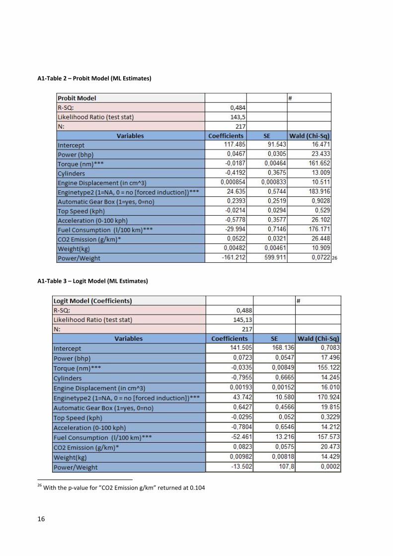
The results from the Probit/Logit estimations are reported in appendix A1.016
and even without
the marginal effects that would make the estimates amendable to concrete interpretation; the
estimations reveal a stark contrast with the LPM. Consequently, while the LPM returned 11
variables with significant estimates at the 1%, 5% or 10% level the Probit and Logit returns only
317
. Fortunately, both the Logit and Probit agree, as it were, on the significant variables in the form
of “torque”, “enginetype” and “fuel consumption”. In concrete terms and restricting the
relationship to the variables that are statistically significant, the models stipulate that increasing
torque will lower the probability of observing a BMW, observing an NA engine will increase the
probability of observing a BMW, and finally; that increasing fuel consumption (liters consumed per
100 km) will lower the probability of observing a BMW. It is interesting here, in particular, to
observe that Audis are indeed characterized by having turbo charged engines (with a
corresponding small displacement) contrary to BMW where the adherence to the straight line six
cylinder engine in many of the brand’s top models makes BMW mainly dominated by NA engines.
It is however important to point out that this result is almost certainly restricted to petrol engines
since all diesel engines (whether in an Audi or BMW) have some form of forced induction. The
result on torque (i.e. a measure of the engine’s pulling power) follows from the result on engine
14
Bottom equation.
15 Basically, SAS EG 4.2 did not like this variable presumably because it is only defined for Audi (i.e. there are no BMWs
with AWD in the sample) and thus produced nonsensical results less it was removed from the estimation.
16 SAS output in the succeeding appendices.
17 With the ML estimate for ”CO2 Emmission (g/km)” in Logit out as it slightly fails the 10% threshold.
11
type in the sense that engines with forced induction exactly are characterized by a higher torque
than NA engines. In the case of fuel consumption it appears that BMWs are notably more fuel
efficient than Audis, a result which is interesting in so far as goes the idea that having forced
induction (e.g. in the form of a turbo) should make it easier to drive the car efficiently.
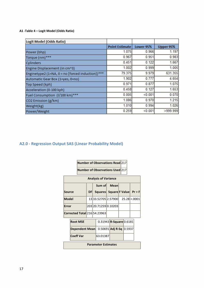
In terms of quantitative interpretation and although the odds ratio reported for the Logit model is
fairly simple to interpret, it is inherently difficult to interpret the coefficients since these do not
represent the marginal effects. In order to see this simply go back to eq. 7 and take the derivative
with respect to “x” and realize (following the chain rule of differentiation) that this is not equal to
the estimated coefficients;
Eq. 8
� ��� � �
��β
∂Φ= Φ
∂xβ
xβ .
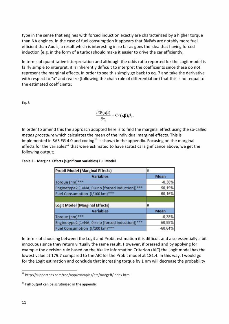
In order to amend this the approach adopted here is to find the marginal effect using the so-called
means procedure which calculates the mean of the individual marginal effects. This is
implemented in SAS EG 4.0 and coding18
is shown in the appendix. Focusing on the marginal
effects for the variables19
that were estimated to have statistical significance above; we get the
following output;
Table 2 – Marginal Effects (significant variables) Full Model
In terms of choosing between the Logit and Probit estimation it is difficult and also essentially a bit
innocuous since they return virtually the same result. However, if pressed and by applying for
example the decision rule based on the Akaike Information Criterion (AIC) the Logit model has the
lowest value at 179.7 compared to the AIC for the Probit model at 181.4. In this way, I would go
for the Logit estimation and conclude that increasing torque by 1 nm will decrease the probability
18
http://support.sas.com/rnd/app/examples/ets/margeff/index.html
19 Full output can be scrutinized in the appendix.
12
of observing a BMW by 0.38%, observing an NA engine will increase the probability of observing a
BMW by 50.88% and finally, increasing the liters of petrol/diesel per 100 km will decrease the
probability of observing a BMW by 60.64%.
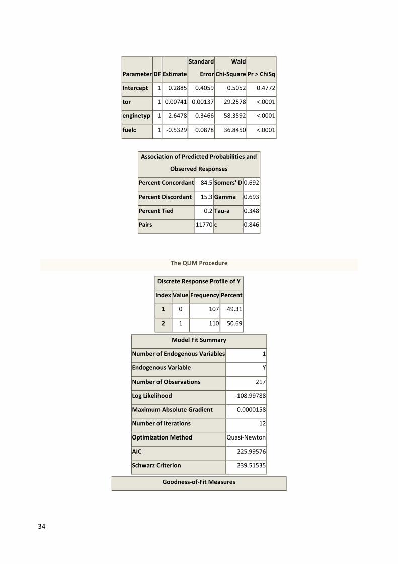
As a final remark before moving on to a perspective and discussion on the results, it is worth
noting that when it comes to the robustness of these results, the coefficient estimated for torque
does not seem to be robust. Consequently, the appendix contains the output of a model estimated
with only the three variables above as explanatory variables and in this estimation the sign for
torque changes from negative to positive as well as the variable remains significant20
.
4.0 Discussion and Perspectives
The estimation of the LPM indicated that Audis and BMWs differ across a wide range of physical
characteristics, but this result was qualified significantly with the introduction of binary regression
models where the number of significant (and robust) variables changed significantly. Without a
doubt, this highlights the difficulties and inaccuracies in relation to the OLS framework when used
to fit variables to explain a discrete dependent variable. On the difference between the Logit and
Probit estimation there is very little between the two models in the present context. On the basis
of the AIC the Logit model would be the chosen specification, but since the two models assume
different probability distributions of the dependent variable, the AIC selection method is not
strictly valid. In this sense, it is safe to say that the Probit and Logit estimations in this paper are
very close substitutes.
Turning to the concrete results and their general robustness it is important to realize that they are
bound to be very sensitive to the sample strategy chosen. In this sense and following the intuition
above, the idea of matched data sample in which the two brands are paired competitively is
bound to produce different results than if all models and variants had been included. The
important point here is that while the results would almost surely be quantitatively different, they
might also be qualitatively different (i.e. the signs/statistical significance of coefficients could also
differ markedly).
As a perspective on the results it would naturally be apt to go back to the theoretical framework
and see whether we can draw some interesting links between this and the empirical estimation.
Initially, and if we might have hoped to be able to match our representative consumer with a
utility function containing a rich set of parameters with an equally rich variance in the estimation,
this hope cannot be fulfilled. In the present context, the estimated difference between Audis and
BMWs based exclusively on physical characteristics consequently does not seem to conform well
with the idea that consumers are very sensitive to physical differences between cars. Surely
though the measured difference between Audis and BMWs with respect to engine type represents
an important distinction between the two brands and could arguably be directly translated into
the prediction that buyers of Audis and BMWs, to some extent, will be driven by their preference
for a specific engine type. In the context of fuel consumption, one finds it intuitively difficult to
believe that buyers of Audis and BMWs will choose one over the other based on fuel consumption,
20
The two other variables ”behave” as expected.
13
but given the fact that BMWs do indeed appear to have better fuel consumption it will mean that
they are valued higher (based exclusively on physical characteristics21
) than Audis.
The fundamental question we are centering on here is then whether in fact Audis and BMWs
might not be differentiated across other aspects than their physical characteristics?
It is here that the notion of Audi and BMW as luxury products becomes important. In order to see
this, it is possible to use the framework developed in Vickers and Renand (2003) where luxury
goods are defined on the basis of three conceptual dimensions; instrumental performance
(functionalist/physical characteristics), experimentalism, and symbolic interactionism. Using a
qualitative survey study the empirical results reveal that in the context of cars, a standard car will
be defined mainly on the basis of its functionalist profile whereas a luxury car will predominantly
be defined on the basis symbolic interactionism that includes variables broadly defined as
signaling effect variables and thus what kind of signals the owner sends by owning e.g. an Audi or
BMW Vickers and Renand (2003). To put it simply; while standard cars are indeed differentiated,
in the minds of customers, on the basis of their tangible differences non-standard (luxury) cars are
differentiated on the basis of their intangible differences which we might, rather insubstantially,
coin as their brand value.
This naturally introduces an important qualifier to the results shown here. In quantitative terms,
Vickers and Renand (2003) present results to suggest that for luxury cars, only 12% of the variance
in consumer preference is explained by physical characteristics. Taking this value to heart in the
present case and taking the estimated R-SQ for the Logit model chosen as the preferred
specification (0.488)22
, we would need to scale down this by 0.12 (12%) which gives 0.059 as the
estimated degree to which we can explain the variance in consumer preferences for luxury
products solely on the basis of physical characteristics. This is naturally highly stylized, but it
indicates that the extent to which we may find significant physical characteristics between Audis
and BMWs these are likely to account for only a small part of the final variance in consumer
preferences for these two products.
Finally, it provides an important perspective to studies who might seek to use pure characteristics
demand models (PCDM) in the context of luxury products or even product classes where both
luxury and standard products are included. It is thus not unreasonable to expect that the potential
difference in the way consumers perceive product classes could translate into a significant bias of
the results.
21
I.e. price notwithstanding!
22 McFadden’s pseudo R-SQ
14
5.0 Conclusion
This paper has used Logit/Probit estimations to investigate and quantify the physical differences
between Audis and BMWs. As expected and while the initial estimation with a LPM indicated a
strong difference between Audis and BMWs based on a range of physical characteristics, the
introduction of Logit/Probit models qualified this results significantly. In the context of a matched
sample the results indicate that observing a car with a forced induction engine (e.g. Turbo) will
decrease the probability of observing a BMW by 51%. The results also suggest that BMWs have
better fuel consumption than Audis (in this sample) as increasing the liters of fuel consumed per
100 KM by 1 liter will decrease the probability of observing a BMW by 61%. The strongest result in
this context has to be the first one which seems to provide an important perspective on the
differences between Audis and BMWs. Consequently, consumers who prefer forced induction in
relation to gasoline engines (since all diesels are turbo charged) can be expected to choose Audis
over BMW and vice versa for naturally aspirated engines of course. These results were discussed
in the context of research that shows how consumers traditionally attach little value to physical
characteristics in the context of luxury products.
Further studies should attempt to widen the sample (potentially with Mercedes) to find more
robust physical differences between the three big Germany luxury automakers.
6.0 List of References
Audi and BMW websites (Germany, price catalogues); see data CD for BMW catalogues. The data
for Audi is tabulated directly from Audi.de.
Berry, Steven & Bakes, Alan (2007) – The Pure Characteristics Demand Model, International
Economic Review, Vol. 48, Issue 4, pp. 1193-1225, November 200723
Greene, William H (2003) – Econometric Analysis, 5th
Edition Prentice Hall
Gujarati, Damodar N. (2003) – Basic Econometrics 4th
edition McGrawHill
Thomassen, Øyvind (2007) – A Pure Characteristics Model of Demand for Cars, University of
Oxford (February 28th 2007)24
Vickers, Jonathan S & Renand Franck (2003) – The Marketing of Luxury Goods: An exploratory
study – three conceptual dimensions, the Marketing Review, 2003 ; 3, pp. 459-47825
23
http://papers.ssrn.com/sol3/papers.cfm?abstract_id=1071228
24 http://www.cepr.org/meets/wkcn/6/6652/papers/Thomassen.pdf
25 http://www.ingentaconnect.com/content/westburn/tmr/2003/00000003/00000004/art00006
15
Appendices
A1.0 – Maxmimum Likelihood Estimates (Probit and Logit Models)
A1-Table 1 – Linear Probability Model
16
A1-Table 2 – Probit Model (ML Estimates)
26
A1-Table 3 – Logit Model (ML Estimates)
26
With the p-value for ”CO2 Emission g/km” returned at 0.104
17
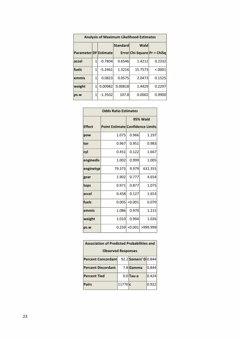
A1 -Table 4 – Logit Model (Odds Ratio)
A2.0 - Regression Output SAS (Linear Probability Model)
Number of Observations Read 217
Number of Observations Used 217
Analysis of Variance
Source DF
Sum of
Squares
Mean
Square F Value Pr > F
Model 13 33.52705 2.57900 25.28 <.0001
Error 203 20.71259 0.10203
Corrected Total 216 54.23963
Root MSE 0.31943 R-Square 0.6181
Dependent Mean 0.50691 Adj R-Sq 0.5937
Coeff Var 63.01387
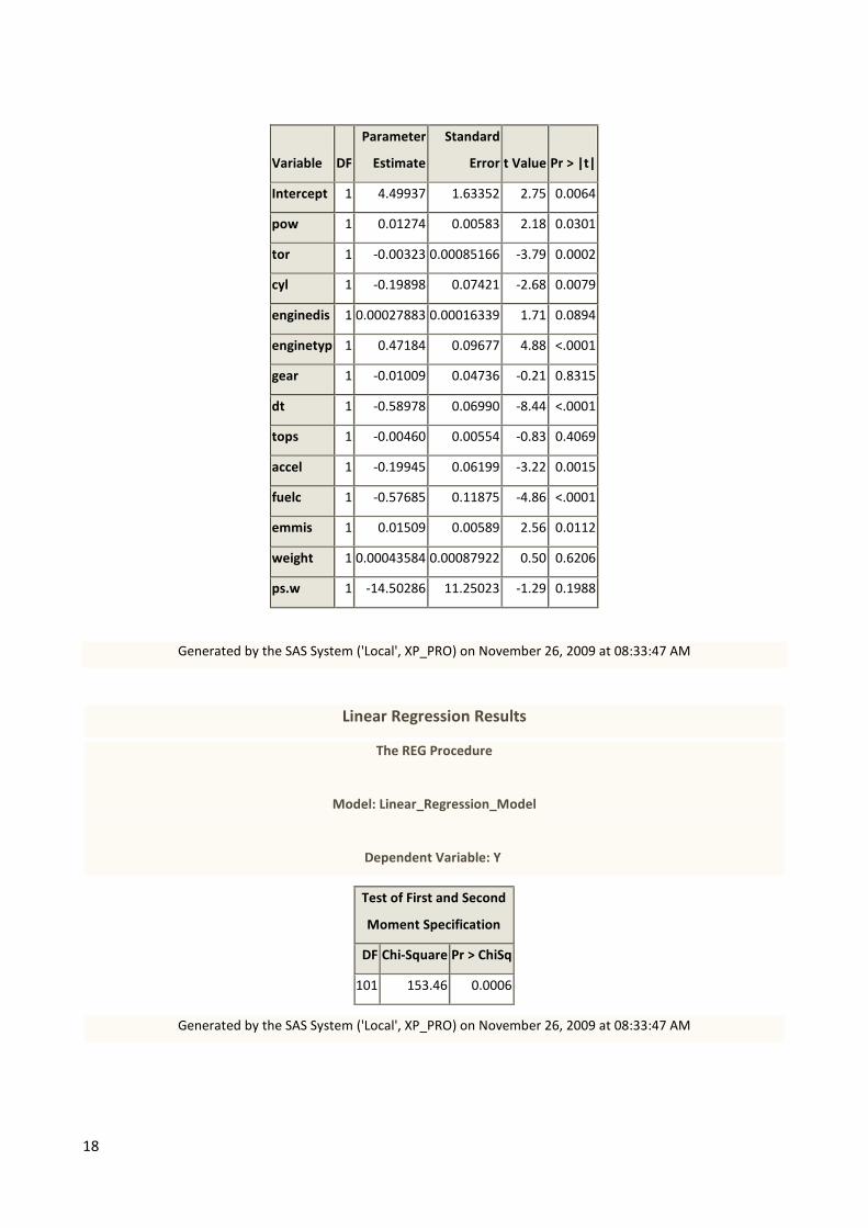
Parameter Estimates
18
Variable DF
Parameter
Estimate
Standard
Error t Value Pr > |t|
Intercept 1 4.49937 1.63352 2.75 0.0064
pow 1 0.01274 0.00583 2.18 0.0301
tor 1 -0.00323 0.00085166 -3.79 0.0002
cyl 1 -0.19898 0.07421 -2.68 0.0079
enginedis 1 0.00027883 0.00016339 1.71 0.0894
enginetyp 1 0.47184 0.09677 4.88 <.0001
gear 1 -0.01009 0.04736 -0.21 0.8315
dt 1 -0.58978 0.06990 -8.44 <.0001
tops 1 -0.00460 0.00554 -0.83 0.4069
accel 1 -0.19945 0.06199 -3.22 0.0015
fuelc 1 -0.57685 0.11875 -4.86 <.0001
emmis 1 0.01509 0.00589 2.56 0.0112
weight 1 0.00043584 0.00087922 0.50 0.6206
ps.w 1 -14.50286 11.25023 -1.29 0.1988
Generated by the SAS System ('Local', XP_PRO) on November 26, 2009 at 08:33:47 AM
Linear Regression Results
The REG Procedure
Model: Linear_Regression_Model
Dependent Variable: Y
Test of First and Second
Moment Specification
DF Chi-Square Pr > ChiSq
101 153.46 0.0006
Generated by the SAS System ('Local', XP_PRO) on November 26, 2009 at 08:33:47 AM
19
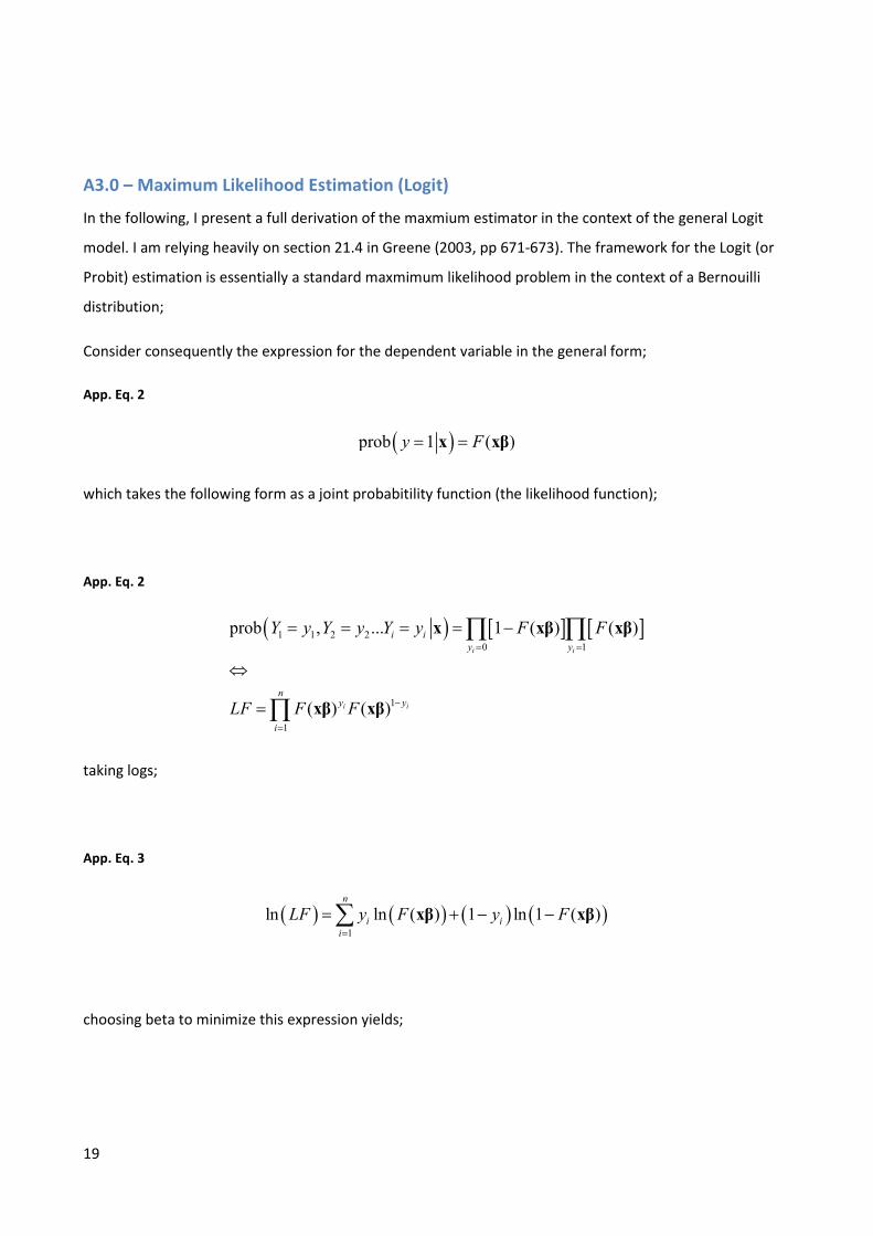
A3.0 – Maximum Likelihood Estimation (Logit)
In the following, I present a full derivation of the maxmium estimator in the context of the general Logit
model. I am relying heavily on section 21.4 in Greene (2003, pp 671-673). The framework for the Logit (or
Probit) estimation is essentially a standard maxmimum likelihood problem in the context of a Bernouilli
distribution;
Consider consequently the expression for the dependent variable in the general form;
App. Eq. 2
( )��� � � �� �= =x xβ
which takes the following form as a joint probabitility function (the likelihood function);
App. Eq. 2
( ) [ ] [ ]� � � �
� �
�
�
��� � ��� � � � � �
� � � �
� �
� �
� �
� �
�� �
�
� � � � � � � �
�� � �
= =
−
=
= = = = −
⇔
=
∏ ∏
∏
x xβ xβ
xβ xβ
taking logs;
App. Eq. 3
( ) ( ) ( ) ( )�
�� �� � � � �� � � ��
� �
�
�� � � � �=
= + − −∑ xβ xβ
choosing beta to minimize this expression yields;
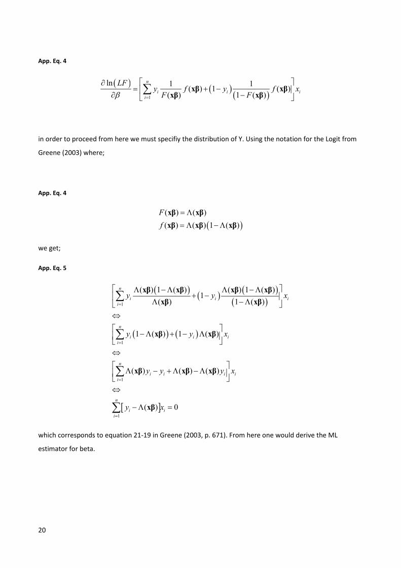
20
App. Eq. 4
( ) ( )( )�
�� � �� � � � �
� � � � �
�
� � �
�
��� � � � �� �β =
∂= + −
∂ − ∑ xβ xβ
xβ xβ
in order to proceed from here we must specifiy the distribution of Y. Using the notation for the Logit from
Greene (2003) where;
App. Eq. 4
( )� � � �
� � � � � � �
�
�
= Λ
= Λ −Λ
xβ xβ
xβ xβ xβ
we get;
App. Eq. 5
( ) ( ) ( )( )
( ) ( )
[ ]
�
�
�
�
� � � � � � � � � ��
� � � � �
� � � � � �
� � � � � �
� � �
�
� � �
�
�
� � �
�
�
� � � �
�
�
� �
�
� � �
� � �
� � � �
� �
=
=
=
=
Λ −Λ Λ −Λ+ −
Λ −Λ ⇔
−Λ + − Λ
⇔
Λ − +Λ −Λ
⇔
−Λ =
∑
∑
∑
∑
xβ xβ xβ xβ
xβ xβ
xβ xβ
xβ xβ xβ
xβ
which corresponds to equation 21-19 in Greene (2003, p. 671). From here one would derive the ML
estimator for beta.
21
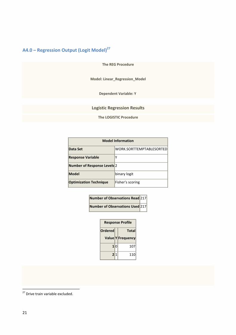
A4.0 – Regression Output (Logit Model)27
The REG Procedure
Model: Linear_Regression_Model
Dependent Variable: Y
Logistic Regression Results
The LOGISTIC Procedure
Model Information
Data Set WORK.SORTTEMPTABLESORTED
Response Variable Y
Number of Response Levels 2
Model binary logit
Optimization Technique Fisher's scoring
Number of Observations Read 217
Number of Observations Used 217
Response Profile
Ordered
Value Y
Total
Frequency
1 0 107
2 1 110
27
Drive train variable excluded.
22
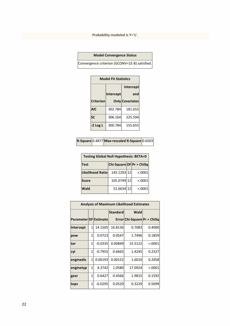
Probability modeled is Y='1'.
Model Convergence Status
Convergence criterion (GCONV=1E-8) satisfied.
Model Fit Statistics
Criterion
Intercept
Only
Intercept
and
Covariates
AIC 302.784 181.655
SC 306.164 225.594
-2 Log L 300.784 155.655
R-Square 0.4877 Max-rescaled R-Square 0.6503
Testing Global Null Hypothesis: BETA=0
Test Chi-Square DF Pr > ChiSq
Likelihood Ratio 145.1293 12 <.0001
Score 105.0749 12 <.0001
Wald 52.6634 12 <.0001
Analysis of Maximum Likelihood Estimates
Parameter DF Estimate
Standard
Error
Wald
Chi-Square Pr > ChiSq
Intercept 1 14.1505 16.8136 0.7083 0.4000
pow 1 0.0723 0.0547 1.7496 0.1859
tor 1 -0.0335 0.00849 15.5122 <.0001
cyl 1 -0.7955 0.6665 1.4245 0.2327
enginedis 1 0.00193 0.00152 1.6010 0.2058
enginetyp 1 4.3742 1.0580 17.0924 <.0001
gear 1 0.6427 0.4566 1.9815 0.1592
tops 1 -0.0295 0.0520 0.3229 0.5699
23
Analysis of Maximum Likelihood Estimates
Parameter DF Estimate
Standard
Error
Wald
Chi-Square Pr > ChiSq
accel 1 -0.7804 0.6546 1.4212 0.2332
fuelc 1 -5.2461 1.3216 15.7573 <.0001
emmis 1 0.0823 0.0575 2.0473 0.1525
weight 1 0.00982 0.00818 1.4429 0.2297
ps.w 1 -1.3502 107.8 0.0002 0.9900
Odds Ratio Estimates
Effect Point Estimate
95% Wald
Confidence Limits
pow 1.075 0.966 1.197
tor 0.967 0.951 0.983
cyl 0.451 0.122 1.667
enginedis 1.002 0.999 1.005
enginetyp 79.375 9.979 631.355
gear 1.902 0.777 4.654
tops 0.971 0.877 1.075
accel 0.458 0.127 1.653
fuelc 0.005 <0.001 0.070
emmis 1.086 0.970 1.215
weight 1.010 0.994 1.026
ps.w 0.259 <0.001 >999.999
Association of Predicted Probabilities and
Observed Responses
Percent Concordant 92.2 Somers' D 0.844
Percent Discordant 7.8 Gamma 0.844
Percent Tied 0.0 Tau-a 0.424
Pairs 11770 c 0.922
24
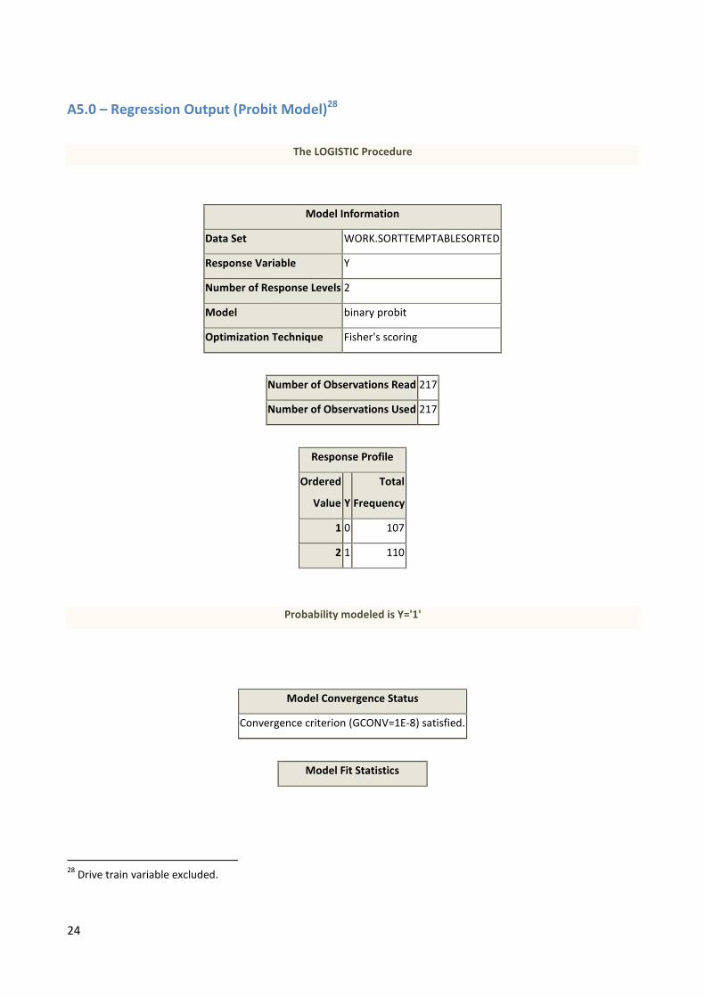
A5.0 – Regression Output (Probit Model)28
The LOGISTIC Procedure
Model Information
Data Set WORK.SORTTEMPTABLESORTED
Response Variable Y
Number of Response Levels 2
Model binary probit
Optimization Technique Fisher's scoring
Number of Observations Read 217
Number of Observations Used 217
Response Profile
Ordered
Value Y
Total
Frequency
1 0 107
2 1 110
Probability modeled is Y='1'
Model Convergence Status
Convergence criterion (GCONV=1E-8) satisfied.
Model Fit Statistics
28
Drive train variable excluded.
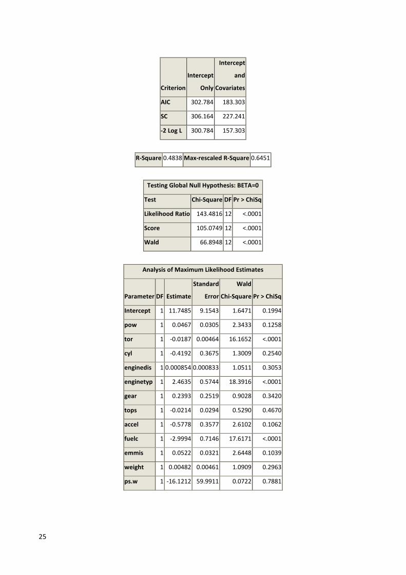
25
Criterion
Intercept
Only
Intercept
and
Covariates
AIC 302.784 183.303
SC 306.164 227.241
-2 Log L 300.784 157.303
R-Square 0.4838 Max-rescaled R-Square 0.6451
Testing Global Null Hypothesis: BETA=0
Test Chi-Square DF Pr > ChiSq
Likelihood Ratio 143.4816 12 <.0001
Score 105.0749 12 <.0001
Wald 66.8948 12 <.0001
Analysis of Maximum Likelihood Estimates
Parameter DF Estimate
Standard
Error
Wald
Chi-Square Pr > ChiSq
Intercept 1 11.7485 9.1543 1.6471 0.1994
pow 1 0.0467 0.0305 2.3433 0.1258
tor 1 -0.0187 0.00464 16.1652 <.0001
cyl 1 -0.4192 0.3675 1.3009 0.2540
enginedis 1 0.000854 0.000833 1.0511 0.3053
enginetyp 1 2.4635 0.5744 18.3916 <.0001
gear 1 0.2393 0.2519 0.9028 0.3420
tops 1 -0.0214 0.0294 0.5290 0.4670
accel 1 -0.5778 0.3577 2.6102 0.1062
fuelc 1 -2.9994 0.7146 17.6171 <.0001
emmis 1 0.0522 0.0321 2.6448 0.1039
weight 1 0.00482 0.00461 1.0909 0.2963
ps.w 1 -16.1212 59.9911 0.0722 0.7881
26
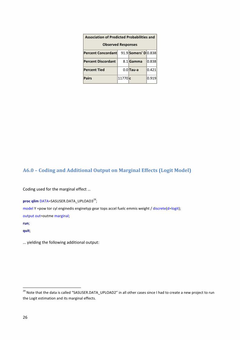
Association of Predicted Probabilities and
Observed Responses
Percent Concordant 91.9 Somers' D 0.838
Percent Discordant 8.1 Gamma 0.838
Percent Tied 0.0 Tau-a 0.421
Pairs 11770 c 0.919
A6.0 – Coding and Additional Output on Marginal Effects (Logit Model)
Coding used for the marginal effect …
proc qlim DATA=SASUSER.DATA_UPLOAD329
;
model Y =pow tor cyl enginedis enginetyp gear tops accel fuelc emmis weight / discrete(d=logit);
output out=outme marginal;
run;
quit;
… yielding the following additional output:
29
Note that the data is called “SASUSER.DATA_UPLOAD2” in all other cases since I had to create a new project to run
the Logit estimation and its marginal effects.
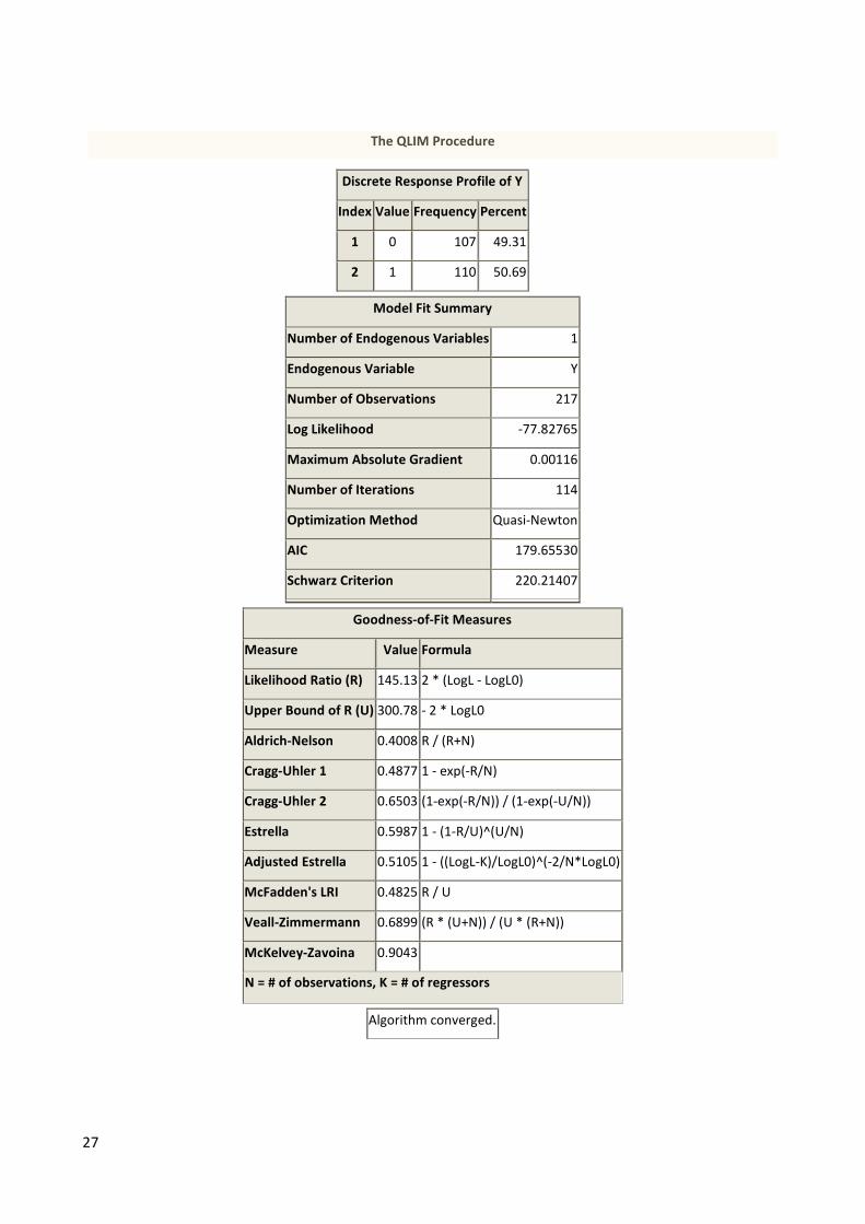
27
The QLIM Procedure
Discrete Response Profile of Y
Index Value Frequency Percent
1 0 107 49.31
2 1 110 50.69
Model Fit Summary
Number of Endogenous Variables 1
Endogenous Variable Y
Number of Observations 217
Log Likelihood -77.82765
Maximum Absolute Gradient 0.00116
Number of Iterations 114
Optimization Method Quasi-Newton
AIC 179.65530
Schwarz Criterion 220.21407
Goodness-of-Fit Measures
Measure Value Formula
Likelihood Ratio (R) 145.13 2 * (LogL - LogL0)
Upper Bound of R (U) 300.78 - 2 * LogL0
Aldrich-Nelson 0.4008 R / (R+N)
Cragg-Uhler 1 0.4877 1 - exp(-R/N)
Cragg-Uhler 2 0.6503 (1-exp(-R/N)) / (1-exp(-U/N))
Estrella 0.5987 1 - (1-R/U)^(U/N)
Adjusted Estrella 0.5105 1 - ((LogL-K)/LogL0)^(-2/N*LogL0)
McFadden's LRI 0.4825 R / U
Veall-Zimmermann 0.6899 (R * (U+N)) / (U * (R+N))
McKelvey-Zavoina 0.9043
N = # of observations, K = # of regressors
Algorithm converged.
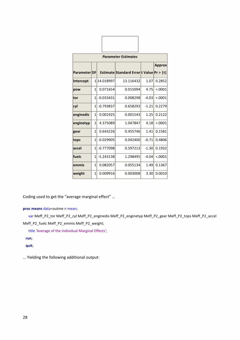
28
Parameter Estimates
Parameter DF Estimate Standard Error t Value
Approx
Pr > |t|
Intercept 1 14.018997 13.116432 1.07 0.2852
pow 1 0.071654 0.015094 4.75 <.0001
tor 1 -0.033431 0.008298 -4.03 <.0001
cyl 1 -0.793837 0.658293 -1.21 0.2279
enginedis 1 0.001925 0.001543 1.25 0.2122
enginetyp 1 4.375089 1.047847 4.18 <.0001
gear 1 0.643226 0.455746 1.41 0.1581
tops 1 -0.029905 0.042400 -0.71 0.4806
accel 1 -0.777098 0.597213 -1.30 0.1932
fuelc 1 -5.243138 1.298495 -4.04 <.0001
emmis 1 0.082057 0.055134 1.49 0.1367
weight 1 0.009916 0.003008 3.30 0.0010
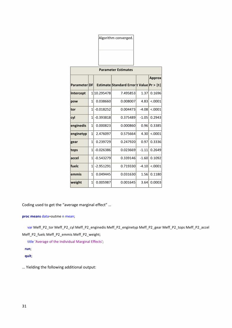
Coding used to get the “average marginal effect” …
proc means data=outme n mean;
var Meff_P2_tor Meff_P2_cyl Meff_P2_enginedis Meff_P2_enginetyp Meff_P2_gear Meff_P2_tops Meff_P2_accel
Meff_P2_fuelc Meff_P2_emmis Meff_P2_weight;
title 'Average of the Individual Marginal Effects';
run;
quit;
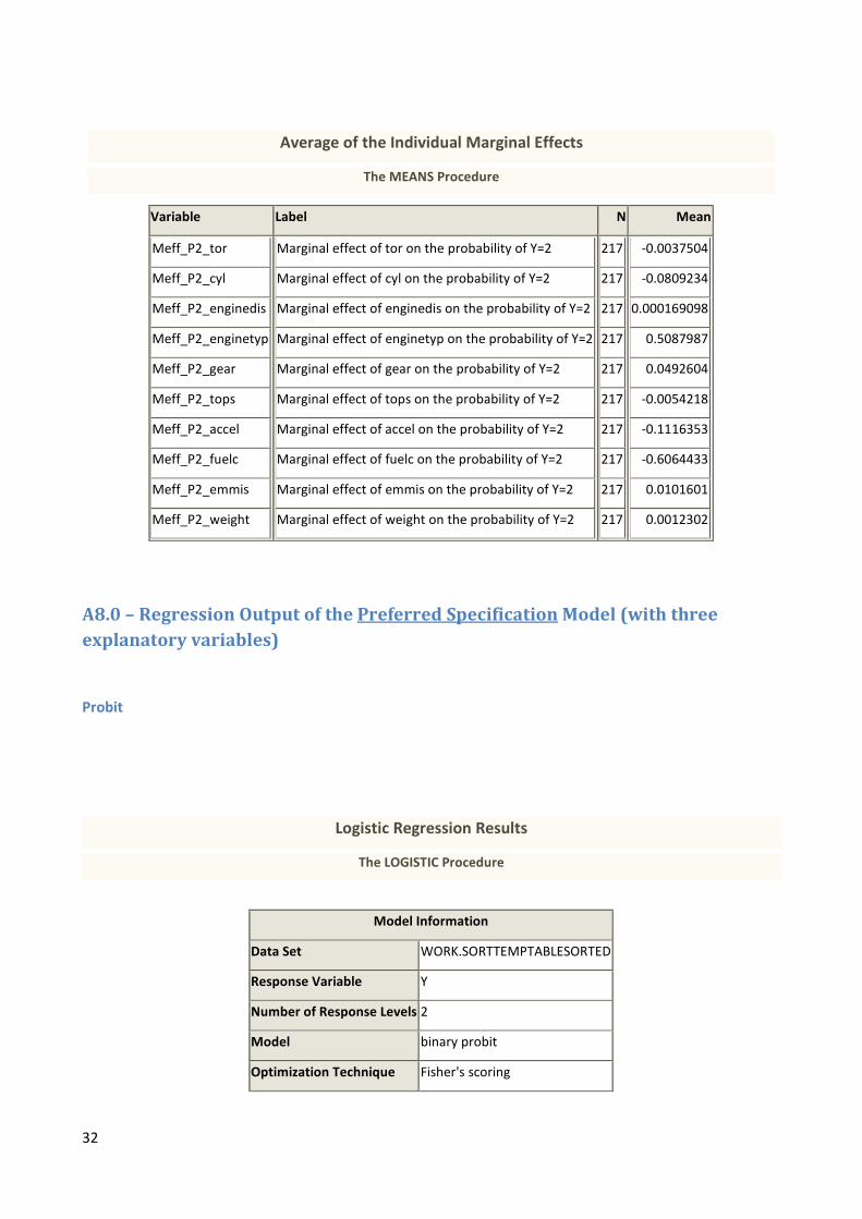
… Yielding the following additional output:
29
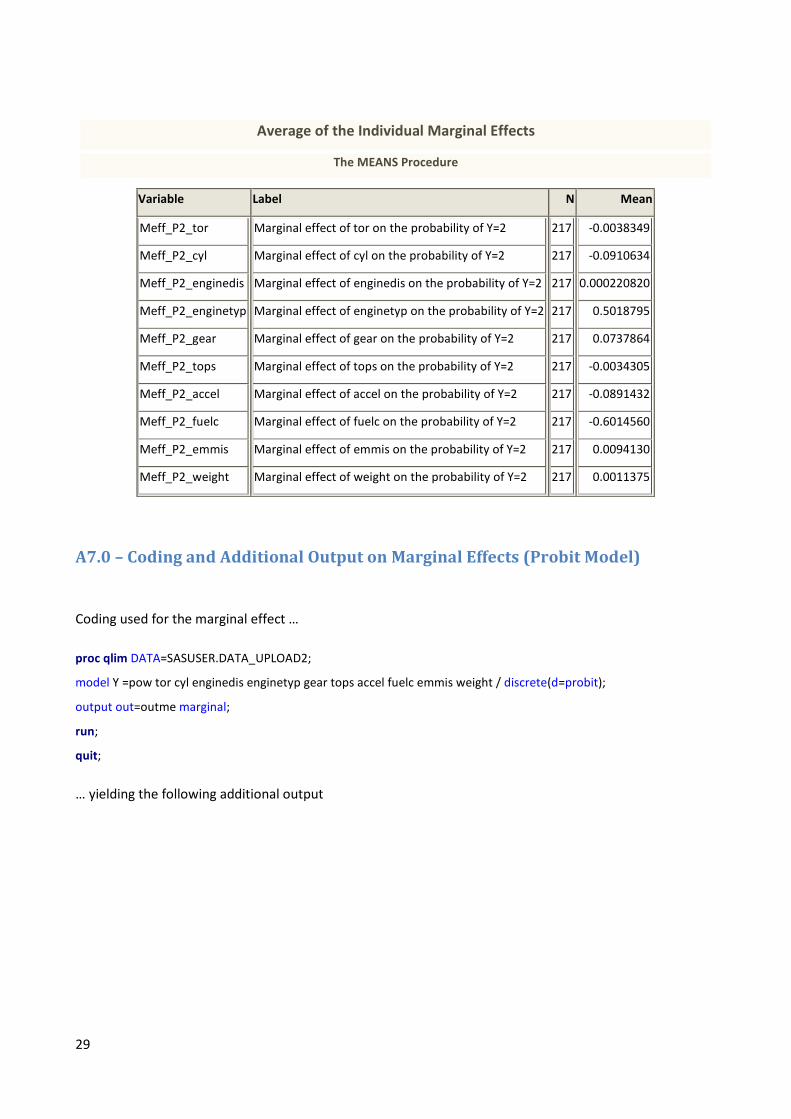
Average of the Individual Marginal Effects
The MEANS Procedure
Variable Label N Mean
Meff_P2_tor
Meff_P2_cyl
Meff_P2_enginedis
Meff_P2_enginetyp
Meff_P2_gear
Meff_P2_tops
Meff_P2_accel
Meff_P2_fuelc
Meff_P2_emmis
Meff_P2_weight
Marginal effect of tor on the probability of Y=2
Marginal effect of cyl on the probability of Y=2
Marginal effect of enginedis on the probability of Y=2
Marginal effect of enginetyp on the probability of Y=2
Marginal effect of gear on the probability of Y=2
Marginal effect of tops on the probability of Y=2
Marginal effect of accel on the probability of Y=2
Marginal effect of fuelc on the probability of Y=2
Marginal effect of emmis on the probability of Y=2
Marginal effect of weight on the probability of Y=2
217
217
217
217
217
217
217
217
217
217
-0.0038349
-0.0910634
0.000220820
0.5018795
0.0737864
-0.0034305
-0.0891432
-0.6014560
0.0094130
0.0011375
A7.0 – Coding and Additional Output on Marginal Effects (Probit Model)
Coding used for the marginal effect …
proc qlim DATA=SASUSER.DATA_UPLOAD2;
model Y =pow tor cyl enginedis enginetyp gear tops accel fuelc emmis weight / discrete(d=probit);
output out=outme marginal;
run;
quit;
… yielding the following additional output
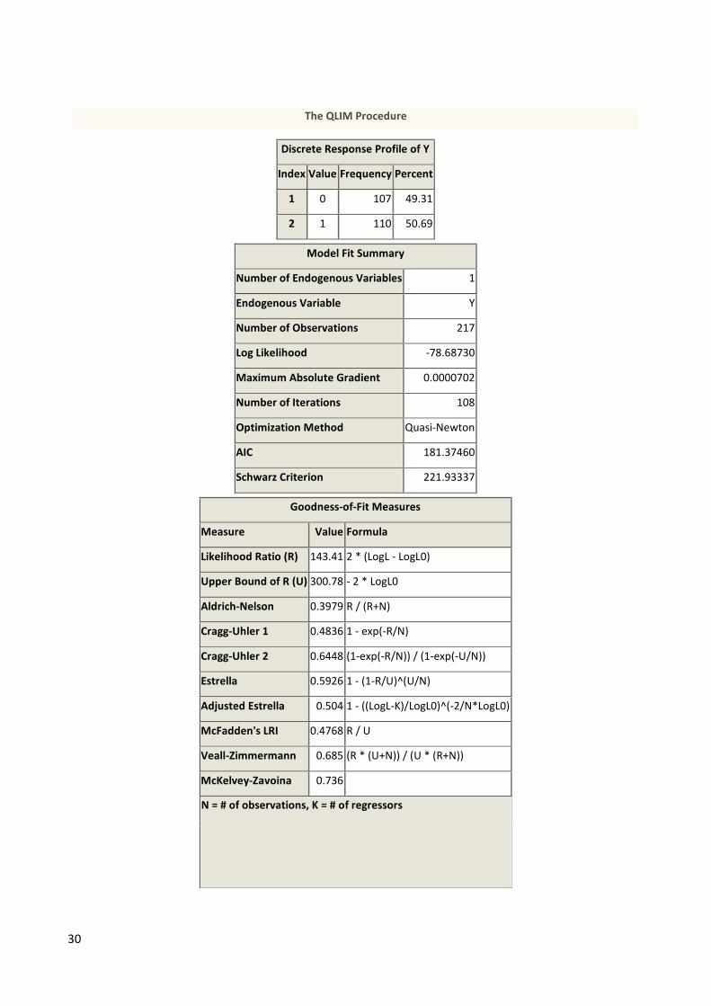
30
The QLIM Procedure
Discrete Response Profile of Y
Index Value Frequency Percent
1 0 107 49.31
2 1 110 50.69
Model Fit Summary
Number of Endogenous Variables 1
Endogenous Variable Y
Number of Observations 217
Log Likelihood -78.68730
Maximum Absolute Gradient 0.0000702
Number of Iterations 108
Optimization Method Quasi-Newton
AIC 181.37460
Schwarz Criterion 221.93337
Goodness-of-Fit Measures
Measure Value Formula
Likelihood Ratio (R) 143.41 2 * (LogL - LogL0)
Upper Bound of R (U) 300.78 - 2 * LogL0
Aldrich-Nelson 0.3979 R / (R+N)
Cragg-Uhler 1 0.4836 1 - exp(-R/N)
Cragg-Uhler 2 0.6448 (1-exp(-R/N)) / (1-exp(-U/N))
Estrella 0.5926 1 - (1-R/U)^(U/N)
Adjusted Estrella 0.504 1 - ((LogL-K)/LogL0)^(-2/N*LogL0)
McFadden's LRI 0.4768 R / U
Veall-Zimmermann 0.685 (R * (U+N)) / (U * (R+N))
McKelvey-Zavoina 0.736
N = # of observations, K = # of regressors
31
Algorithm converged.
Parameter Estimates
Parameter DF Estimate Standard Error t Value
Approx
Pr > |t|
Intercept 1 10.295478 7.495853 1.37 0.1696
pow 1 0.038660 0.008007 4.83 <.0001
tor 1 -0.018252 0.004473 -4.08 <.0001
cyl 1 -0.393818 0.375489 -1.05 0.2943
enginedis 1 0.000823 0.000860 0.96 0.3385
enginetyp 1 2.476097 0.575664 4.30 <.0001
gear 1 0.239729 0.247920 0.97 0.3336
tops 1 -0.026386 0.023669 -1.11 0.2649
accel 1 -0.543279 0.339146 -1.60 0.1092
fuelc 1 -2.951291 0.719330 -4.10 <.0001
emmis 1 0.049445 0.031630 1.56 0.1180
weight 1 0.005987 0.001645 3.64 0.0003
Coding used to get the “average marginal effect” …
proc means data=outme n mean;
var Meff_P2_tor Meff_P2_cyl Meff_P2_enginedis Meff_P2_enginetyp Meff_P2_gear Meff_P2_tops Meff_P2_accel
Meff_P2_fuelc Meff_P2_emmis Meff_P2_weight;
title 'Average of the Individual Marginal Effects';
run;
quit;
… Yielding the following additional output:
32
Average of the Individual Marginal Effects
The MEANS Procedure
Variable Label N Mean
Meff_P2_tor
Meff_P2_cyl
Meff_P2_enginedis
Meff_P2_enginetyp
Meff_P2_gear
Meff_P2_tops
Meff_P2_accel
Meff_P2_fuelc
Meff_P2_emmis
Meff_P2_weight
Marginal effect of tor on the probability of Y=2
Marginal effect of cyl on the probability of Y=2
Marginal effect of enginedis on the probability of Y=2
Marginal effect of enginetyp on the probability of Y=2
Marginal effect of gear on the probability of Y=2
Marginal effect of tops on the probability of Y=2
Marginal effect of accel on the probability of Y=2
Marginal effect of fuelc on the probability of Y=2
Marginal effect of emmis on the probability of Y=2
Marginal effect of weight on the probability of Y=2
217
217
217
217
217
217
217
217
217
217
-0.0037504
-0.0809234
0.000169098
0.5087987
0.0492604
-0.0054218
-0.1116353
-0.6064433
0.0101601
0.0012302
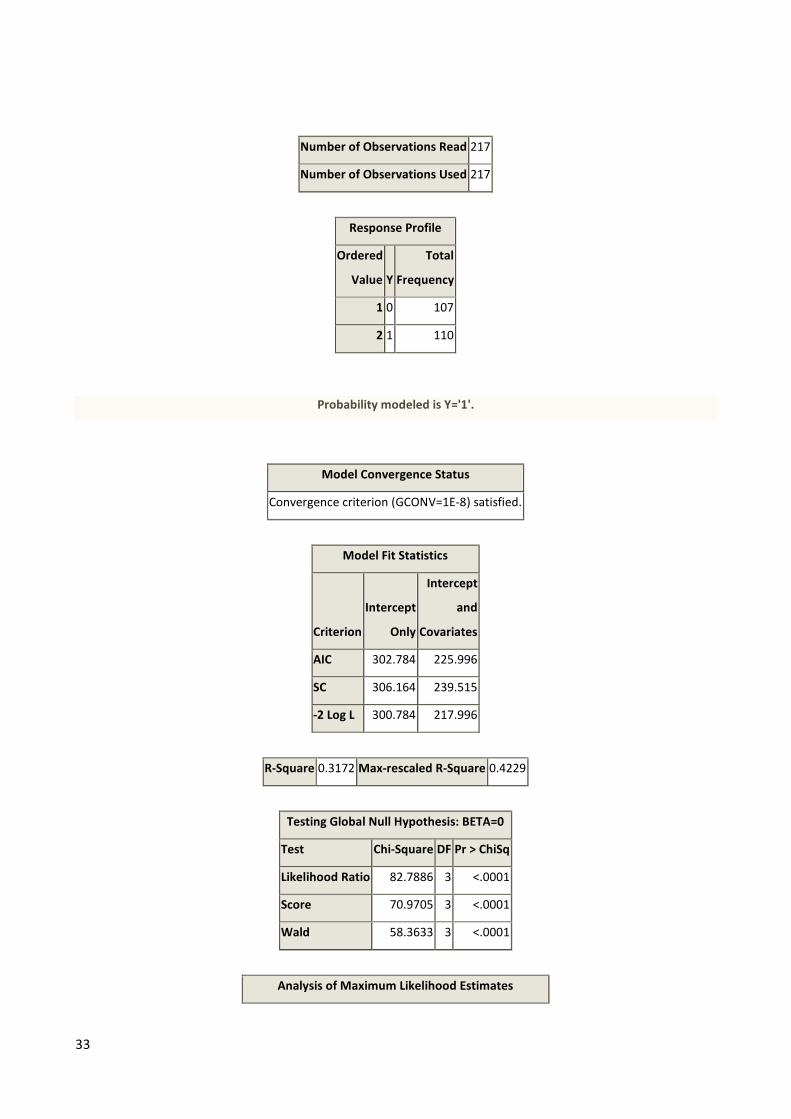
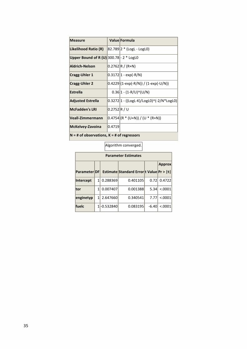
A8.0 – Regression Output of the Preferred Specification Model (with three
explanatory variables)
Probit
Logistic Regression Results
The LOGISTIC Procedure
Model Information
Data Set WORK.SORTTEMPTABLESORTED
Response Variable Y
Number of Response Levels 2
Model binary probit
Optimization Technique Fisher's scoring
33
Number of Observations Read 217
Number of Observations Used 217
Response Profile
Ordered
Value Y
Total
Frequency
1 0 107
2 1 110
Probability modeled is Y='1'.
Model Convergence Status
Convergence criterion (GCONV=1E-8) satisfied.
Model Fit Statistics
Criterion
Intercept
Only
Intercept
and
Covariates
AIC 302.784 225.996
SC 306.164 239.515
-2 Log L 300.784 217.996
R-Square 0.3172 Max-rescaled R-Square 0.4229
Testing Global Null Hypothesis: BETA=0
Test Chi-Square DF Pr > ChiSq
Likelihood Ratio 82.7886 3 <.0001
Score 70.9705 3 <.0001
Wald 58.3633 3 <.0001
Analysis of Maximum Likelihood Estimates
34
Parameter DF Estimate
Standard
Error
Wald
Chi-Square Pr > ChiSq
Intercept 1 0.2885 0.4059 0.5052 0.4772
tor 1 0.00741 0.00137 29.2578 <.0001
enginetyp 1 2.6478 0.3466 58.3592 <.0001
fuelc 1 -0.5329 0.0878 36.8450 <.0001
Association of Predicted Probabilities and
Observed Responses
Percent Concordant 84.5 Somers' D 0.692
Percent Discordant 15.3 Gamma 0.693
Percent Tied 0.2 Tau-a 0.348
Pairs 11770 c 0.846
The QLIM Procedure
Discrete Response Profile of Y
Index Value Frequency Percent
1 0 107 49.31
2 1 110 50.69
Model Fit Summary
Number of Endogenous Variables 1
Endogenous Variable Y
Number of Observations 217
Log Likelihood -108.99788
Maximum Absolute Gradient 0.0000158
Number of Iterations 12
Optimization Method Quasi-Newton
AIC 225.99576
Schwarz Criterion 239.51535
Goodness-of-Fit Measures
35
Measure Value Formula
Likelihood Ratio (R) 82.789 2 * (LogL - LogL0)
Upper Bound of R (U) 300.78 - 2 * LogL0
Aldrich-Nelson 0.2762 R / (R+N)
Cragg-Uhler 1 0.3172 1 - exp(-R/N)
Cragg-Uhler 2 0.4229 (1-exp(-R/N)) / (1-exp(-U/N))
Estrella 0.36 1 - (1-R/U)^(U/N)
Adjusted Estrella 0.3272 1 - ((LogL-K)/LogL0)^(-2/N*LogL0)
McFadden's LRI 0.2752 R / U
Veall-Zimmermann 0.4754 (R * (U+N)) / (U * (R+N))
McKelvey-Zavoina 0.4719
N = # of observations, K = # of regressors
Algorithm converged.
Parameter Estimates
Parameter DF Estimate Standard Error t Value
Approx
Pr > |t|
Intercept 1 0.288369 0.401105 0.72 0.4722
tor 1 0.007407 0.001388 5.34 <.0001
enginetyp 1 2.647660 0.340541 7.77 <.0001
fuelc 1 -0.532840 0.083195 -6.40 <.0001
36
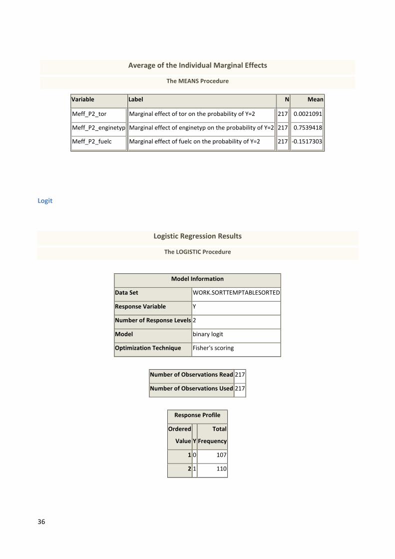
Average of the Individual Marginal Effects
The MEANS Procedure
Variable Label N Mean
Meff_P2_tor
Meff_P2_enginetyp
Meff_P2_fuelc
Marginal effect of tor on the probability of Y=2
Marginal effect of enginetyp on the probability of Y=2
Marginal effect of fuelc on the probability of Y=2
217
217
217
0.0021091
0.7539418
-0.1517303
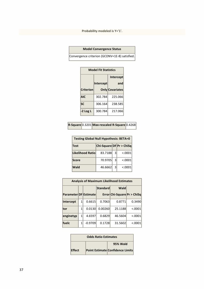
Logit
Logistic Regression Results
The LOGISTIC Procedure
Model Information
Data Set WORK.SORTTEMPTABLESORTED
Response Variable Y
Number of Response Levels 2
Model binary logit
Optimization Technique Fisher's scoring
Number of Observations Read 217
Number of Observations Used 217
Response Profile
Ordered
Value Y
Total
Frequency
1 0 107
2 1 110
37
Probability modeled is Y='1'.
Model Convergence Status
Convergence criterion (GCONV=1E-8) satisfied.
Model Fit Statistics
Criterion
Intercept
Only
Intercept
and
Covariates
AIC 302.784 225.066
SC 306.164 238.585
-2 Log L 300.784 217.066
R-Square 0.3201 Max-rescaled R-Square 0.4268
Testing Global Null Hypothesis: BETA=0
Test Chi-Square DF Pr > ChiSq
Likelihood Ratio 83.7188 3 <.0001
Score 70.9705 3 <.0001
Wald 46.6662 3 <.0001
Analysis of Maximum Likelihood Estimates
Parameter DF Estimate
Standard
Error
Wald
Chi-Square Pr > ChiSq
Intercept 1 0.6615 0.7063 0.8771 0.3490
tor 1 0.0130 0.00260 25.1188 <.0001
enginetyp 1 4.6597 0.6829 46.5604 <.0001
fuelc 1 -0.9709 0.1728 31.5602 <.0001
Odds Ratio Estimates
Effect Point Estimate
95% Wald
Confidence Limits
38
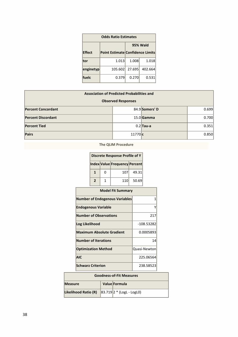
Odds Ratio Estimates
Effect Point Estimate
95% Wald
Confidence Limits
tor 1.013 1.008 1.018
enginetyp 105.602 27.695 402.664
fuelc 0.379 0.270 0.531
Association of Predicted Probabilities and
Observed Responses
Percent Concordant 84.9 Somers' D 0.699
Percent Discordant 15.0 Gamma 0.700
Percent Tied 0.2 Tau-a 0.351
Pairs 11770 c 0.850
The QLIM Procedure
Discrete Response Profile of Y
Index Value Frequency Percent
1 0 107 49.31
2 1 110 50.69
Model Fit Summary
Number of Endogenous Variables 1
Endogenous Variable Y
Number of Observations 217
Log Likelihood -108.53282
Maximum Absolute Gradient 0.0005893
Number of Iterations 14
Optimization Method Quasi-Newton
AIC 225.06564
Schwarz Criterion 238.58523
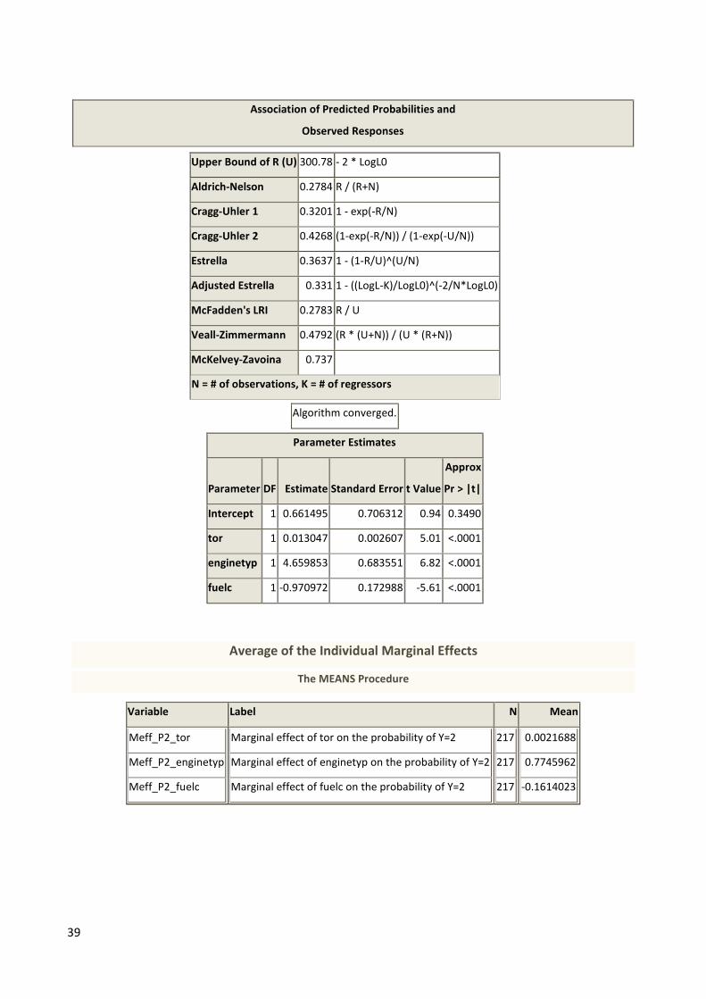
Goodness-of-Fit Measures
Measure Value Formula
Likelihood Ratio (R) 83.719 2 * (LogL - LogL0)
39
Association of Predicted Probabilities and
Observed Responses
Upper Bound of R (U) 300.78 - 2 * LogL0
Aldrich-Nelson 0.2784 R / (R+N)
Cragg-Uhler 1 0.3201 1 - exp(-R/N)
Cragg-Uhler 2 0.4268 (1-exp(-R/N)) / (1-exp(-U/N))
Estrella 0.3637 1 - (1-R/U)^(U/N)
Adjusted Estrella 0.331 1 - ((LogL-K)/LogL0)^(-2/N*LogL0)
McFadden's LRI 0.2783 R / U
Veall-Zimmermann 0.4792 (R * (U+N)) / (U * (R+N))
McKelvey-Zavoina 0.737
N = # of observations, K = # of regressors
Algorithm converged.
Parameter Estimates
Parameter DF Estimate Standard Error t Value
Approx
Pr > |t|
Intercept 1 0.661495 0.706312 0.94 0.3490
tor 1 0.013047 0.002607 5.01 <.0001
enginetyp 1 4.659853 0.683551 6.82 <.0001
fuelc 1 -0.970972 0.172988 -5.61 <.0001
Average of the Individual Marginal Effects
The MEANS Procedure
Variable Label N Mean
Meff_P2_tor
Meff_P2_enginetyp
Meff_P2_fuelc
Marginal effect of tor on the probability of Y=2
Marginal effect of enginetyp on the probability of Y=2
Marginal effect of fuelc on the probability of Y=2
217
217
217
0.0021688
0.7745962
-0.1614023
Related Documents