Auction design for composite goods : The natural gas industry

Journal of Economic Behavior and Organization 14 (1990) 127-149. North-Holland

AUCTION DESIGN FOR COMPOSITE GOODS:

The Natural Gas Industry*

Kevin A. MCCABE, Stephen J. RASSENTI and Vernon L. SMITH

University of Arizona, Tucson, AZ 85721, USA

Received January 1989, final version received March 1990

Experiments examine the price and efficiency performance of a simple production, parallel transmission and wholesale consumption model of a natural gas pipeline system. A center determines prices and allocations to buyers, producers and transporters to maximize surplus based on the location-specific bids of buyers, producers and transporters. Efficiency tends to grow asymptotically to 100% in stationary environments; prices stabilize quickly in the neighborhood of predicted competitive equilibrium levels. Over time agents settle into an equilibrium with elastic bid schedules and numerous tied bids and offers. These strategies allow each agent class to protect itself from manipulation by the other classes.

1. Introduction

In this paper, we use experimental methods to investigate some funda- mental properties of market institutions and property right systems for the trading of a composite good. A composite good is a collection of well defined constituent goods (and/or services). In this study we examine a class of economic institutions for the pricing and exchange of composite goods which is based on the uniform price sealed bid-offer auction.

Attempts to allocate composite goods can lead to complex coordination problems. Examples include coordinating the flow of Natural Gas in a network [McCabe et al. (1989)]; the provision of airport time slots for airplane routing [Rassenti et al. (1982)]; the assignment of heterogenous labor to teams; the provision of programming to local public TV [Rassenti (1982)]; the allocation of space on space shuttles [Banks et al. (1989)]; and the allocation of computer resources to programs. In all of the indicated references experimental economists have designed ‘computer assisted’ markets

*This research was supported by a grant from the Federal Energy Regulatory Commission, but our sponsors are not responsible for any errors, omissions or conclusions that we reach. We wish to express our appreciation for the many comments and suggestions by Daniel Alger (Federal Energy Regulatory Commission) and Douglas Hale (Energy Information Administration).

0167-2681/90/$03.50 0 1990-Elsevier Science Publishers B.V. (North-Holland)

J.E.B.O. F

128 K.A. McCabe et al., Auction design for composite goods

which handle the coordination problem well. However, it is difftcult to separate behavioral and institutional effects in these complex environments.

We study ‘computer assisted’ markets in a single composite goods environment. This environment lets us study behavior while controlling for complexity. The research is motivated by problems associated with recent regulatory changes that have been designed to move toward freer pricing of wellhead gas. Historically all gas was purchased from pipelines that either owned or had under contract all the gas they delivered to buyers. Buyers are now able to contract for gas directly at wellheads, and then separately contract for transportation. The status quo is bilateral bargaining for both gas and its transportation. This has created coordination problems in the industry, and a move toward further deregulation is likely to exacerbate this problem. We study two institutions: (1) bilateral bargaining for gas followed by an auction market for transportation; (2) a proposed new institution in which gas and its transportation are determined simultaneously at auction. While historically pipelines bundled gas with transportation, we propose a decentralized market mechanism to perform this ‘bundling’ function.

In our experimental markets subjects buy property rights in two constituent goods, natural gas and pipeline transporation, to obtain a resulting right in a composite good, delivered natural gas. In our baseline institution which we call Gas Bargain, buyers first contract for gas and then obtain transportation in an auction market. The resulting coordination problem makes it difficult to attain an efficient allocation, although more experienced subjects were able to achieve reasonably high efficiency through the forma- tion of bilateral relationships which resulted in discriminatory pricing.

Our proposed institution, called Gas Auction, generalizes the sealed bid- offer auction. Sellers submit written offers on units of the constituent goods while buyers simultaneously submit written bids on units of the composite good. We then calculate a Marshallian equilibrium price and quantity with respect to the revealed supply and demand schedules for the composite good. Our institution vertically integrates the property right in the composite good by having buyers simultaneously contract for the different constituent goods. Thus we call our proposed institution a vertical sealed bid-offer market.

Gas Auction combines the coordination advantages of centralization with the information input advantages of decentralization. It achieves a high level of economic efficiency and possesses some politically persuasive properties. There is no price discrimination since all subjects of the same type receive a uniform price even when the market is out of equilibrium; and the institution self-regulates since the revealed supply and demand schedules offer clear rationing rules in the event that there is a quantity curtailment.

In section 2 we describe the general features of the experimental design; section 3 summarizes the experimental procedures; section 4 describes the spatial experimental design features of Gas Bargain; section 5 reports

K.A. McCabe et al., Auction design for composite goods 129

experimental results from Gas Bargain; section 6 discusses Gas Auction and reports our experimental results; section 7 compares the results of Gas Auction and Gas Bargain; and the last section offers some conclusions and extensions.

2. Experimental design

In our experimental as Delivered Natural

markets the instructions describe the composite good Gas (DNG). In each experiment, 12 subjects were

divided into three types. There were six wholesale buyers of DNG, three larger capacity producers of wellhead gas (NG), and three small capacity producers of NG who also owned pipelines offering a delivery service (D). A unit of DNG was composed of a unit each of D and NG. This design captures some of the features of the natural gas industry (i.e., the existence of both large and small producers and joint ownership of pipelines and wellheads by some decision units) while maintaining a feasible size for laboratory experiments.

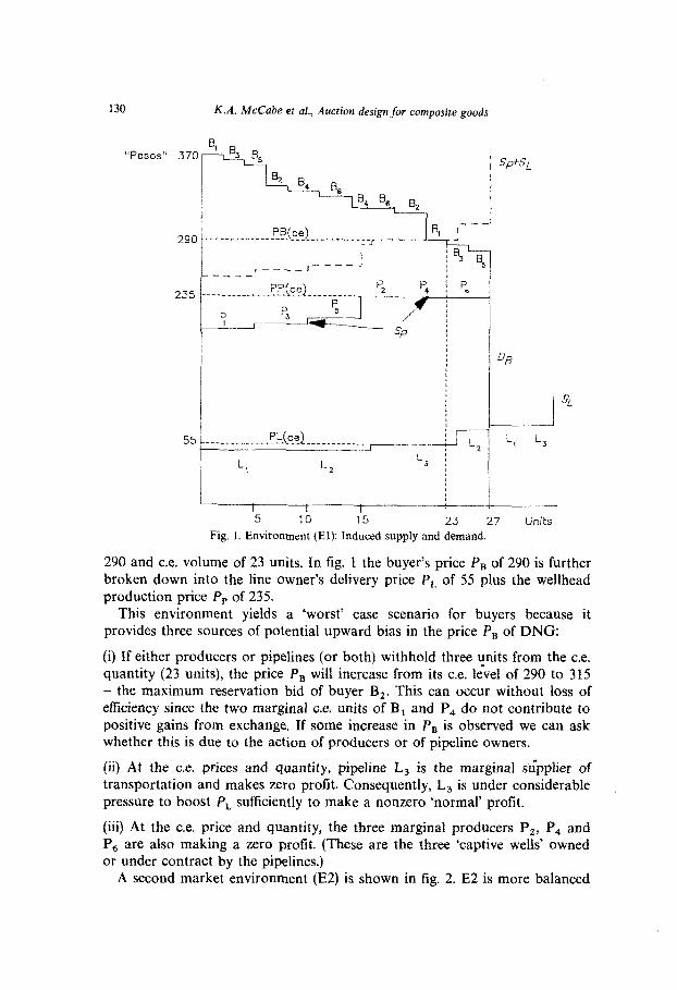
Associated with each wholesale buyer is a demand schedule for units of DNG. This demand schedule is induced by giving buyers resale values (in ‘pesos’ which convert to dollars through an exchange rate) for each unit bought. If we aggregate (add horizontally) all buyers resale values we get the industry demand curve D, (for units of DNG) in fig. 1 (environment El). Associated with each wellhead producer is a constant marginal cost of production up to capacity for each unit of NG. Producers’ cost schedules are induced as follows: Subjects who are well head producers are told that for each unit sold they will earn the market production price minus their unit cost. Aggregating production cost schedules horizontally results in the well head supply curve S, (for units of NG) in fig. 1. Finally, associated with each pipeline is a marginal cost schedule for units of delivery service, D. Pipelines are given a two step cost schedule. For each unit of NG their line delivers they received a unit profit equal to the market delivery price minus their unit cost of delivery. Aggregating delivery cost schedules results in the transportation supply curve S, (for units of D) in fig. 1.’

If we add S, and S, vertically we get the industry supply curve for DNG, i.e., S,+S,. Notice that the competitive equilibrium (ce.) prediction is the intersection of supply (S, + S,) and demand D,. This results in a ce. price of

‘The values and cost for individual buyers and producers were the same for all experiments using inexperienced subjects. In the experiments using experienced subjects these values and costs were shifted by a constant, and had no effect on any individual’s relative position in the market. For example in experiment 7ee (fig. 7) values and costs were shifted down by 80 pesos (compared to tig. 1).

130 K.A. McCabe et al., Auction designfor composite goods

“Pesos”

PB(ce) 290 ‘_____________‘_________________~_~_ - _ -

I

r-___-I----A --_--

235 ___..___._~___~~_~~~~_____~____ pz p4 1; P6

F: r---L-- ?3

i L’f i L2 i / 1 5 10 15 23 27 Units

Fig. 1. Environment (El): Induced supply and demand.

290 and c.e. volume of 23 units. In fig. 1 the buyer’s price PB of 290 is further broken down into the line owner’s delivery price PL of 55 plus the wellhead production price P, of 235.

This environment yields a ‘worst’ case scenario for buyers because it provides three sources of potential upward bias in the price P, of DNG:

(i) If either producers or pipelines (or both) withhold three units from the c.e. quantity (23 units), the price P, will increase from its c.e. live1 of 290 to 315 - the maximum reservation bid of buyer B,. This can occur without loss of efficiency since the two marginal c.e. units of B, and P, do not contribute to positive gains from exchange. If some increase in PB is observed we can ask whether this is due to the action of producers or of pipeline owners.

(ii) At the c.e. prices and quantity, pipeline L, is the marginal stipplier of transportation and makes zero profit. Consequently, L, is under considerable pressure to boost P, sufficiently to make a nonzero ‘normal’ profit.

(iii) At the c.e. price and quantity, the three marginal producers PZ, P, and P, are also making a zero profit. {These are the three ‘captive wells’ owned or under contract by the pipelines.)

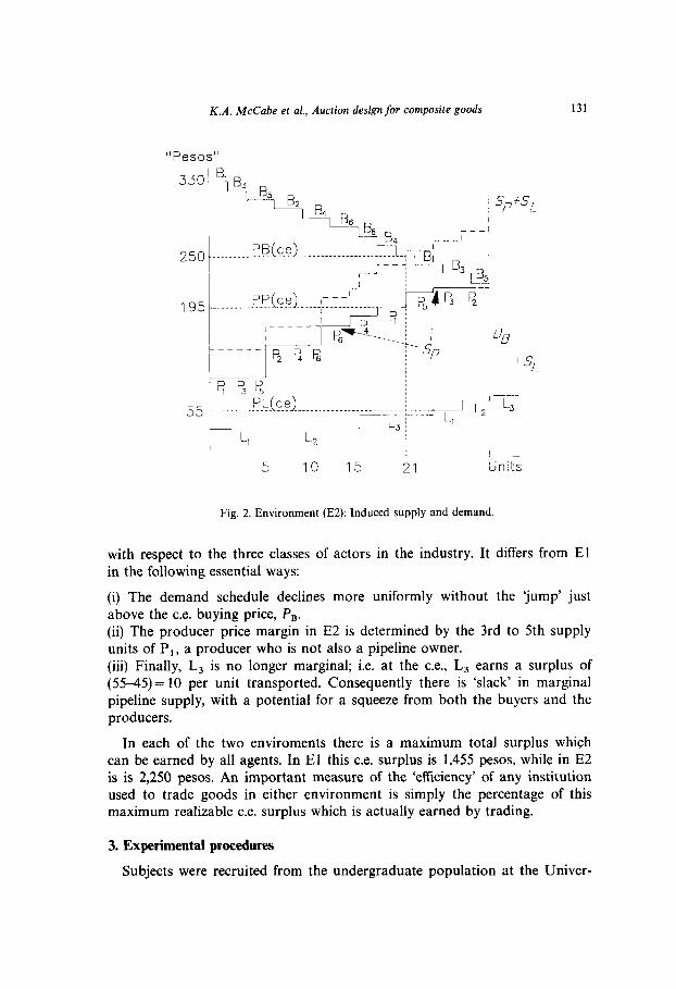
A second market environment (E2) is shown in fig. 2. E2 is more balanced

s,+s,

-.I 4.

L,


“Pesos”

Fig. 2. Environment (E2): Induced supply and demand.

with respect to the three classes of actors in the industry. It differs from El in the following essential ways:

(i) The demand schedule declines more uniformly without the ‘jump’ just above the c.e. buying price, P,. (ii) The producer price margin in E2 is determined by the 3rd to 5th supply units of P,, a producer who is not also a pipeline owner. (iii) Finally, L, is no longer marginal; i.e. at the c.e., L3 earns a surplus of (55-45) = 10 per unit transported. Consequently there is ‘slack’ in marginal pipeline supply, with a potential for a squeeze from both the buyers and the producers.

In each of the two enviroments there is a maximum total surplus which can be earned by all agents. In El this c.e. surplus is 1,455 pesos, while in E2 is is 2,250 pesos. An important measure of the ‘efficiency’ of any institution used to trade goods in either environment is simply the percentage of this maximum realizable c.e. surplus which is actually earned by trading.

3. Experimental procedures

Subjects were recruited from the undergraduate population at the Univer-


sity of Arizona. They were paid three dollars at the beginning of each experiment as an incentive to show up. At the end of each experiment subjects were paid their salient earnings in U.S. dollars. These payouts varied from six to thirty dollars.

All experiments were run on the Plato Computer system. This system was used to instruct subjects in the experimental institution, to enforce the message rules which define the institution, and to record profits. Experi- menters were on hand both to assist subjects who had difficulty in understanding the rules and to enforce privacy.

After everyone had arrived they were randomly assigned to be a particular agent in our ‘design.’ Subjects then went through the instructions at their own pace. After everyone had finished reading the instructions and any questions were answered, inexperienced subjects were put through a one period trial run. When the trial period was concluded subjects were asked to verify their understanding of their profit page in light of their market decisions. Ensuing questions were answered, and the experiment was begun.

Experience with human subjects suggests that fatigue problems may arise if one runs an experiment for more than two consecutive hours. For this reason the experiments in our inexperienced treatment lasted a maximum of 15 periods. On the other hand, experienced players finished the instructions more quickly allowing us to run up to 30 or more periods. In all of our experiments subjects were uninformed as to the actual number of periods. This was to minimize ‘end play.’

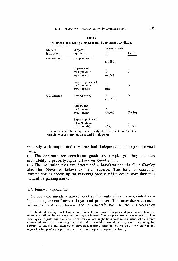
We study two market institutions in this paper: Gas Bargain in subsection 4, and Gas Auction in subsection 5. Table 1 summarizes our 3 x 2 x 2 treatment conditions: Three levels of subject experience; two types of institutions; and two market environments.

4. Gas bargain

In each period of our Gas Bargain experiments, the six buyers and six producers are paired according to size and preference. Each pair indepen- dently negotiates the price and quantity of a natural gas contract. After all natural gas contracts are negotiated (or bargaining time expires) a uniform transportation price for gas is determined in a sealed offer market in which the three pipeline owners made offers and the demand for transportation is fixed, having already been determined by bargaining between producers and buyers. Buyers pay the cost of shipping gas as determined by the sealed offer auction price. These experiments allow us to study an institution which separates gas pricing from pipeline pricing.

Our Gas Bargain institution has the following features:

(i) It imitates some of the properties of the composite goods market which exists in the natural gas industry: Firms vary in size, pumping costs vary


Table 1

Number and labelling of experiments by treatment condition.

Market institution

Gas Bargain

Subject experience

Inexperienced”

Experienced (in 1 previous experiment)

Super experienced (in 2 previous experiments)

Gas Auction Inexperienced

Experienced (in 1 previous experiment)

Super experienced (in 2 previous experiments)

Environments

El E2

fli,2i,3i) 0

(24e, 54

0

1 0 (6ee)

tli,2i,4i) 0

:3e, 6e) (“se, 9e)

1

(7ee) :lOee)

aResults from the inexperienced subject experiments in the Gas Bargain Markets are not discussed in this paper.

modestly with output, and there are both independent and pipeline owned wells. (ii) The contracts for constituent goods are simple, yet they maintain separability in property rights in the constituent goods. (iii) The institution uses size determined submarkets and the Gale-Shapley algorithm (described below) to match subjects. This form of computer assisted sorting speeds up the matching process which occurs over time in a natural bargaining market.

4.1. Bilateral negotiation

In our experiments a market contract for natural gas is negotiated as a bilateral agreement between buyer and producer. This necessitates a mechanism for matching buyers and producers.’ We use the Gale-Shapley

‘A bilateral trading market must coordinate the meeting of buyers and producers. There are many possibilities for such a coordinating mechanism. The simplest mechanism allows random meetings of agents, while one self-select mechanism might be a telephone market where agents choose whom to call and negotiate with. We thought it would be very time consuming for subjects to learn about each other through unassisted selection. So we used the Gale-Shapley algorithm to speed up a process that one would expect to operate naturally.


algorithm to solve this matching problem. This algorithm has two advantages for an experimental market. First, the algorithm is fast in both its application and the time spent in soliciting inputs from subjects. Second, the algorithm guarantees an efficient outcome with respect to reported rankings.3

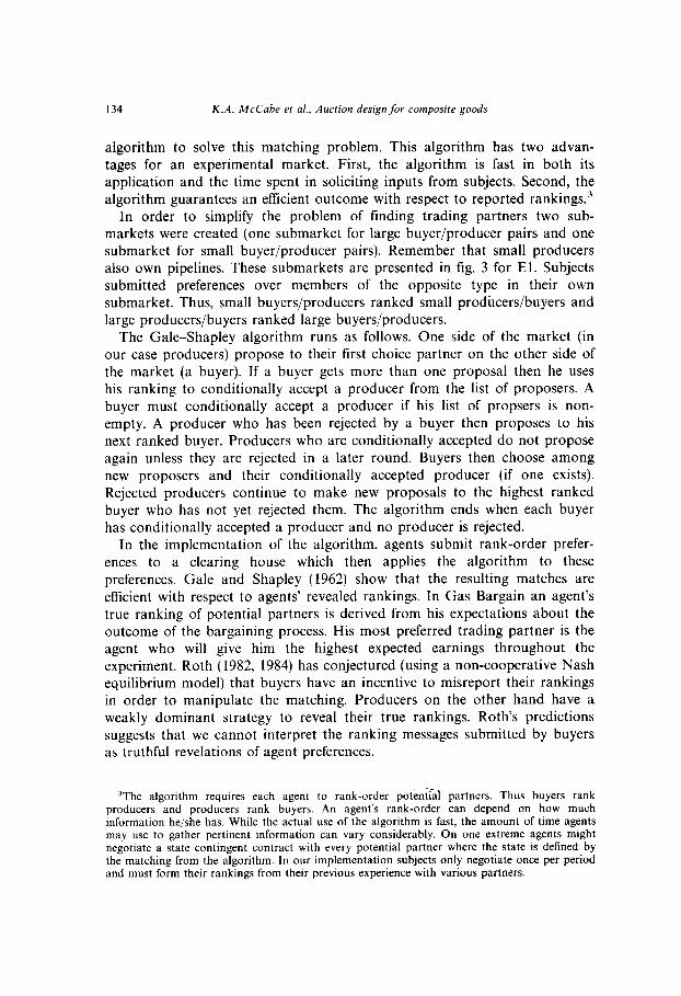
In order to simplify the problem of finding trading partners two submarkets were created (one submarket for large buyer/producer pairs and one submarket for small buyer/producer pairs). Remember that small producers also own pipelines. These submarkets are presented in fig. 3 for El. Subjects submitted preferences over members of the opposite type in their own submarket. Thus, small buyers/producers ranked small producers/buyers and large producers/buyers ranked large buyers/producers.

The Gale-Shapley algorithm runs as follows. One side of the market (in our case producers) propose to their first choice partner on the other side of the market (a buyer). If a buyer gets more than one proposal then he uses his ranking to conditionally accept a producer from the list of proposers. A buyer must conditionally accept a producer if his list of propsers is non- empty. A producer who has been rejected by a buyer then proposes to his next ranked buyer. Producers who are conditionally accepted do not propose again unless they are rejected in a later round. Buyers then choose among new proposers and their conditionally accepted producer (if one exists). Rejected producers continue to make new proposals to the highest ranked buyer who has not yet rejected them. The algorithm ends when each buyer has conditionally accepted a producer and no producer is rejected.

In the implementation of the algorithm, agents submit rank-order preferences to a clearing house which then applies the algorithm to these preferences. Gale and Shapley (1962) show that the resulting matches are efficient with respect to agents’ revealed rankings. In Gas Bargain an agent’s true ranking of potential partners is derived from his expectations about the outcome of the bargaining process. His most preferred trading partner is the agent who will give him the highest expected earnings throughout the experiment. Roth (1982, 1984) has conjectured (using a non-cooperative Nash equilibrium model) that buyers have an incentive to misreport their rankings in order to manipulate the matching. Producers on the other hand have a weakly dominant strategy to reveal their true rankings. Roth’s predictions suggests that we cannot interpret the ranking messages submitted by buyers as truthful revelations of agent preferences.

‘The algorithm requires each agent to rank-order potential partners. Thus buyers rank producers and producers rank buyers. An agent’s rank-order can depend on how much information he/she has. While the actual use of the algorithm is fast, the amount of time agents may use to gather pertinent information can vary considerably. On one extreme agents might negotiate a state contingent contract with every potential partner where the state is defined by the matching from the algorithm. In our implementation subjects only negotiate once per period and must form their rankings from their previous experience with various partners.

“Pesos”

350

300

250

200


Small Buyers/Producers B,

Large Buyers/Producers

-. -1

L

P

B,

Buyer’s Gas

Values

yw I Producer’s

I Gas I costs

“Pesos’

3 6 9 12

UNITS

Fig. 3

-1 L___

I ---,

,__-_ Buyer’s 4’--

Gas Values Net

of Equilibrium

Transportation

Price

5 10 15

UNITS

4.2. The transportation market

The contract results of the bilateral bargaining for NG in any period yield a fixed inelastic demand for delivery services D. In part 2 of each period pipeline owners submit sealed offer schedules (two price-quantity pairs), and the transportation market is cleared at a market delivery price that equalized the inelastic demand quantity with the supply of delivery services.

5. Experimental results for gas bargain

Gas Bargain is complex, consisting of two matching markets, two bargaining markets, and a transportation market. Because of this complexity it took inexperienced subjects close to an hour to read the instructions! Conse- quently, in experiments with inexperienced subjects (experiments li, 2i, and 3i), only live to 15 periods of trading could be realized. Experienced subjects,


280

275

270

265

260

255 ~ 250

245

240 1

E 235 ,

230

225

220

Small Buyers/Producers

l

*A

0 l A . .

l . A AAAAAA

.

.

. . *

8 . . S8 .

. .

.

l

0 Producer 2 ‘s

Contract Price

0 indicates no

contract

m Producer 4 ‘S

Contract price

o indicates no

contract

A Producer 6 ‘s

Contract Price

n indicates fl0

contract

Period 1 5 10 15 20

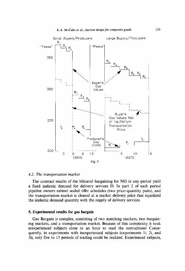
Fig. 4. Experiment 6ee: Bilateral contract prices by producer (PP).

having played once, finished the instructions more quickly with fewer questions, and their experiments, 4e, 5e, and 6ee (ee indicates that subjects have played twice in this design) each lasted 20 periods. The inexperienced experiments exhibit low efficiencies with high variances, so we concentrate our analysis on experiments 4e, 5e, and 6ee. Figs. 4, 5 and 6 provide charts of contract prices for experiment 6ee. The contract data is charted by submarket (the small buyer/producer submarket appears in fig. 4 while the large buyer/producer submarket appears in fig. 5). At the bottom of these figures we indicate failed contracts. In fig. 6 we graph the transportation price in each period of the experiment.

5.1. The transporation market

Although delivery services D are the last to be exchanged, we begin our analysis of the data with the transportation market because the expected terms of trade for delivery of NG directly impacts the bargaining behavior for NG. The markets behaved quite differently in each experiment. In Se and


240

“Pesos’

235

230

225

AA A A

0 Producer 1 ‘s

Contract Price

0 indicates no

contract

. Producer 3 ‘s

Contract price

0 indicates no

contract

A Producer 5 ‘s

Contract Price

A indicates no

contract

q q n 00 0

1 5 10 15 20 Period

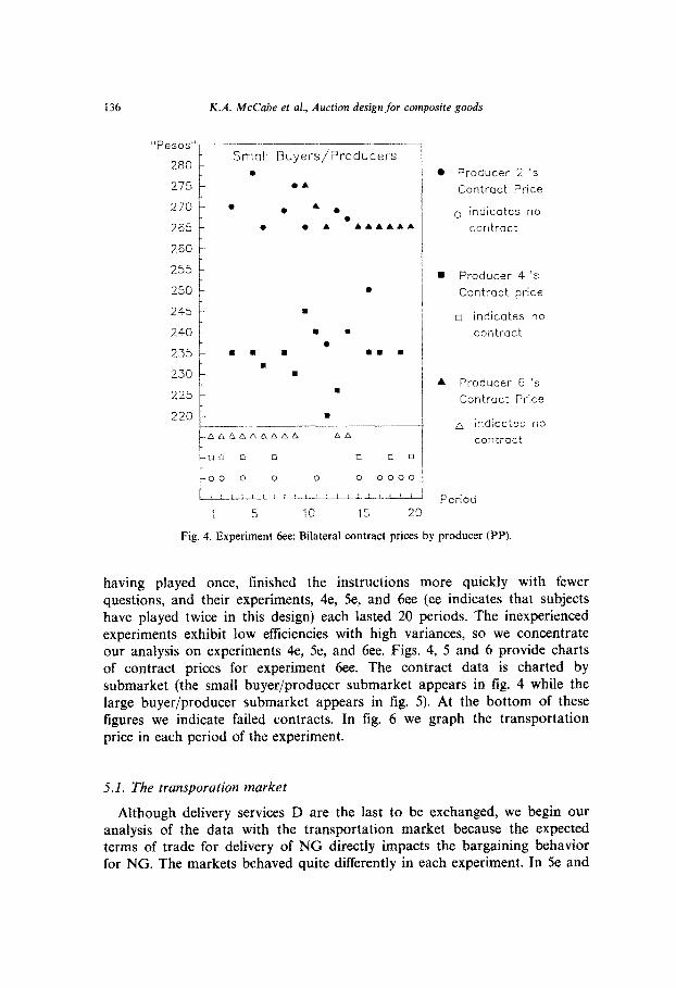
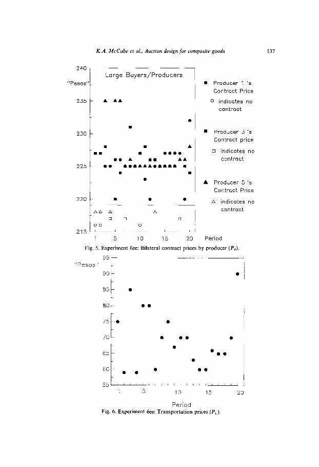
Fig. 5. Experiment 6ee: Bilateral contract prices by producer (PP)

“Pesos”

a5

1 l

a0

t

1 5 10 15

Period Fig. 6. Experiment 6ee: Transportation prices (PL).


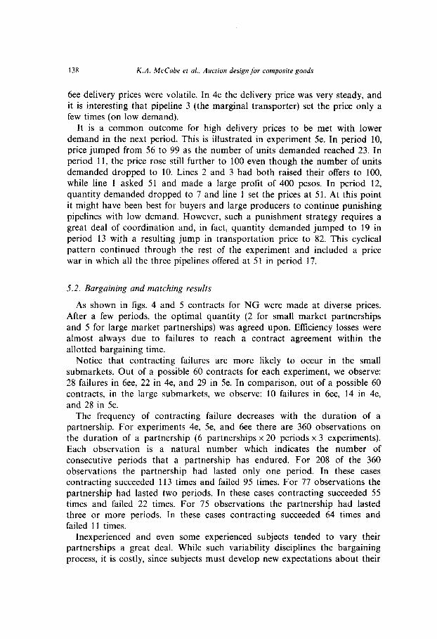
6ee delivery prices were volatile. In 4e the delivery price was very steady, and it is interesting that pipeline 3 (the marginal transporter) set the price only a few times (on low demand).

It is a common outcome for high delivery prices to be met with lower demand in the next period. This is illustrated in experiment 5e. In period 10, price jumped from 56 to 99 as the number of units demanded reached 23. In period 11, the price rose still further to 100 even though the number of units demanded dropped to 10. -Lines 2 and 3 had both raised their offers to 100, while line 1 asked 51 and made a large profit of 400 pesos. In period 12, quantity demanded dropped to 7 and line 1 set the prices at 51. At this point it might have been best for buyers and large producers to continue punishing pipelines with low demand. However, such a punishment strategy requires a great deal of coordination and, in fact, quantity demanded jumped to 19 in period 13 with a resulting jump in transportation price to 82. This cyclical pattern continued through the rest of the experiment and included a price war in which all the three pipelines offered at 51 in period 17.

5.2. Bargaining and matching results

As shown in figs. 4 and 5 contracts for NG were made at diverse prices. After a few periods, the optimal quantity (2 for small market partnerships and 5 for large market partnerships) was agreed upon. Efficiency losses were almost always due to failures to reach a contract agreement within the allotted bargaining time.

Notice that contracting failures are more likely to occur in the small submarkets. Out of a possible 60 contracts for each experiment, we observe: 28 failures in 6ee, 22 in 4e, and 29 in 5e. In comparison, out of a possible 60 contracts, in the large submarkets, we observe: 10 failures in 6ee, 14 in 4e, and 28 in 5e.

The frequency of contracting failure decreases with the duration of a partnership. For experiments 4e, 5e, and 6ee there are 360 observations on the duration of a partnership (6 partnerships x 20 periods x 3 experiments). Each observation is a natural number which indicates the number of consecutive periods that a partnership has endured. For 208 of the 360 observations the partnership had lasted only one period. In these cases contracting succeeded 113 times and failed 95 times. For 77 observations the partnership had lasted two periods. In these cases contracting succeeded 55 times and failed 22 times. For 75 observations the partnership had lasted three or more periods. In these cases contracting succeeded 64 times and failed 11 times.

Inexperienced and even some experienced subjects tended to vary their partnerships a great deal. While such variability disciplines the bargaining process, it is costly, since subjects must develop new expectations about their


partner and a failure to trade is likely. The longer a partnership lasts the more likely it is that partners will develop common expectations. At the same time these expectations become idiosyncratic as partners lose touch with the rest of the market. In summary, subjects trade off the value of common partnership expectations in long term partnerships against the value of market information in short term variable partnerships. Our twice experienced subjects revealed a preference for longer partnerships at the end of the experiment.

The gas bargain markets perform badly. Prices are volatile and the average efficiency (% c.e. surplus) which is achieved by experienced subjects during the last five periods of their experiments is only 72%. We conjecture that this occurs because gas pricing is separated from transport pricing. Given the prior gas contracts, pipelines face an inelastic demand for fixed quantities of gas. This leads to variable transportation prices which in turn makes it difficult for buyer/seller pairs to agree on a common expectation of the cost of transportation. An alternative institution in which buyers and sellers write contracts contingent on transportation price is likely to improve efficiency. But such a change would bring us closer to the allocation constraints of the vertical sealed bid-offer market: Gas Auction.

6. Gas auction

Since there are three subject types in the market for gas - buyers, producers and transporters - we need a triple bid-offer version of the competitive sealed auction [see Smith et al. (1980) for experiments with the double sealed bid-offer auction]. The determination of prices and allocations is illustrated in fig. 1. If subjects were to reveal their true costs and values they would generate the bid and offer schedules graphed. We add, vertically, the producer supply, Sp, to the line haul transport suppply, S,, to get the willingness-to-accept for delivered gas, S, + S,. This yields a ‘stop-out’ price for delivered gas, P,= 290, paid by all buyers Bl to B6, a corresponding’ price for well-head producer gas, P,=235, received by all producers Pl to P6, and a competitive price for transport, P,= P,- P,= 55.4 The quantity produced, consumed and delivered at these prices is 23 units. In this allocation each of the final two-unit bids by buyers B3 and B5 are rejected. Producers P2, P4 and P6, tied at offer prices of 235, would be rationed since their combined offer is twelve units, but only eight can be accepted. This can

“There are a large number of supply and demand conligurations yielding different price determination modes. In the double sealed bid-offer auction illustrated in fig. 1, the market clearing price, P, is defined as follows: on the buy side of the market let Bu=lowest accepted bid and Bo+t= highest rejected bid; on the sell side let A*= highest accepted offer and A,, , = lowest rejected offer; Q = number of accepted bids ( = accepted offers) = largest integer such that BP+, <Aa+, and B,L A,. Then P=[min(BQ,Ap+ I)+max(AQ,Bp+1)]/2.


be achieved by pro-rationing or by randomly rejecting some of the offered units. Random rejection is the rule we chose to implement. Finally, lines L, and L, are allocated eight units each of transportation and line L3 seven units of transportation.

In the absence of institution-specific models of individual behavior for Gas Auction, we take the ce. prices and quantity as the predicted equilibrium outcome (Pr,, P,, P,; Q) =(290, 235, 55; 23).

6.1. Experimental results: Environment 1

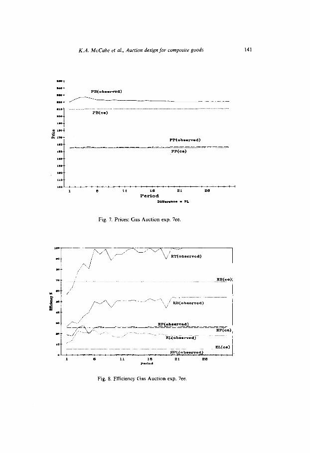
The principal market results for super experienced subjects in the Gas Auction experiments are displayed in figs. 7 and 8.

Prices

The top line (solid) in fig. 7 is the observed price to buyers, P, (observed), and the associated horizontal line (dotted) is the buyers’ c.e. price, P,(ce). The lower lines (dashed) is the observed price to producers, P, (observed) and the associated horizontal line (dotted) is the producers’ c.e. price P,(ce). The difference in each case is the price of pipeline transportation; i.e., P, (observed) = PB( .) -Pp( .), and P,(ce) = P, (ce) - P,(ce).

In both the inexperienced (i) and experienced (e and ee) subject groups for environment 1, the delivered price of gas to buyers, P,, tends to exceed the c.e. predictions. In most of the experiments this increase above the c.e. price is largely accounted for by an increased price of transportation with only very slight increases in the price received by producers, as is seen in fig. 7 for experiment 7ee. Consequently, the design characteristics of El, discussed in subsection 2, do lead to an increase in P,, but most of the benefit goes to pipelines, not to producers. Also we note that generally less than half of the potential increase in price is realized by the pipelines. (Recall that if P, is pushed up to step B,, P, is 75 whereas pipelines are getting P,=65 over most of the horizon.) This suggests that the mechansim may have the ability to blunt even the ‘advantage’ of pipelines in El. Furthermore, line owner L, is the major beneficiary of any increase in P,, since L, makes positive instead of zero profits.

All the price charts show the substantial price stability of the vertical sealed bid-offer institution. Prices tend to converge or adjust slowly from period to period.

Efficiency and the distribution of surplus

Fig. 8 plots the percentage of the c.e. surplus (1,455 ‘pesos’) actually


PB(ob..rvsd)

,,.I ____.______________.............,................................................................................... PB(C.3)

*ao--

IO0 : : : : : : : : : : : : : : : : : : : : : : : : : i : : : : + 1 2 11 12 21 22

Period DIff.rmna. - PL

Fig. 7. Prices: Gas Auction exp. 7ee.

Fig. 8. Efficiency Gas Auction exp. 7ee.


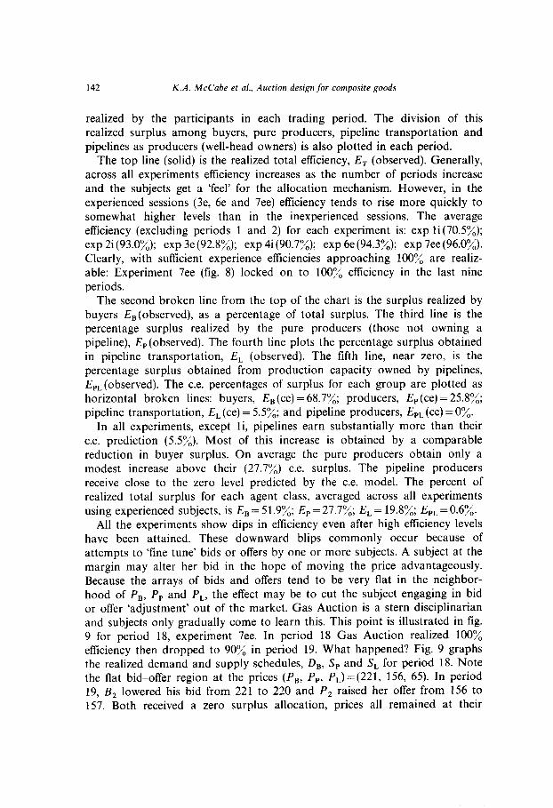
realized by the participants in each trading period. The division of this realized surplus among buyers, pure producers, pipeline transportation and pipelines as producers (well-head owners) is also plotted in each period.

The top line (solid) is the realized total efliciency, E, (observed). Generally, across all experiments efficiency increases as the number of periods increase and the subjects get a ‘feel’ for the allocation mechanism. However, in the experienced sessions (3e, 6e and 7ee) efficiency tends to rise more quickly to somewhat higher levels than in the inexperienced sessions. The average efficiency (excluding periods 1 and 2) for each experiment is: exp li(70.5%); exp 2i (93.0%); exp 3e (92.8%); exp 4i (90.7%); exp 6e (94.3%); exp 7ee (96.0%). Clearly, with sufficient experience efficiencies approaching 100% are realizable: Experiment 7ee (fig. 8) locked on to 100% efficiency in the last nine periods.

The second broken line from the top of the chart is the surplus realized by buyers E,(observed), as a percentage of total surplus. The third line is the percentage surplus realized by the pure producers (those not owning a pipeline), E,(observed). The fourth line plots the percentage surplus obtained in pipeline transportation, E, (observed). The fifth line, near zero, is the percentage surplus obtained from production capacity owned by pipelines, E,,(observed). The c.e. percentages of surplus for each group are plotted as horizontal broken lines: buyers, E, (ce) = 68.7%; producers, E, (ce) = 25.8%; pipeline transportation, E, (ce) = 5.5%; and pipeline producers, E,, (ce) = 0%.

In all experiments, except li, pipelines earn substantially more than their

c.e. prediction (5.5%). Most of this increase is obtained by a comparable reduction in buyer surplus. On average the pure producers obtain only a modest increase above their (27.7%) c.e. surplus. The pipeline producers receive close to the zero level predicted by the c.e. model. The percent of realized total surplus for each agent class, averaged across all experiments using experienced subjects, is E, = 5 1.9%; E, = 27.7%; E, = 19.8%; E,, = 0.6%.

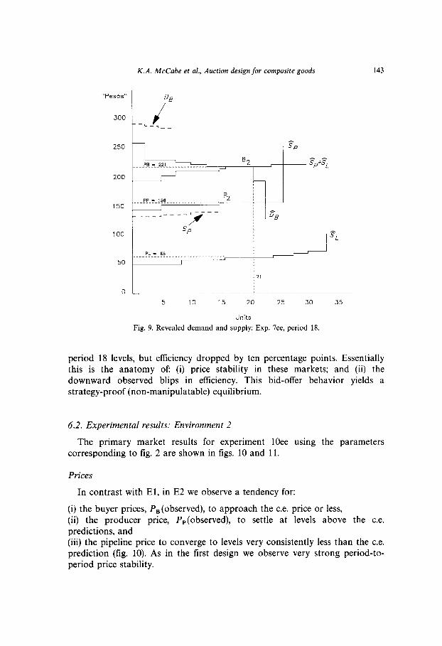
All the experiments show dips in efficiency even after high efficiency levels have been attained. These downward blips commonly occur because of attempts to ‘fine tune’ bids or offers by one or more subjects. A subject at the margin may alter her bid in the hope of moving the price advantageously. Because the arrays of bids and offers tend to be very flat in the neighborhood of P,, P, and P,, the effect may be to cut the subject engaging in bid or offer ‘adjustment’ out of the market. Gas Auction is a stern disciplinarian and subjects only gradually come to learn this. This point is illustrated in fig. 9 for period 18, experiment 7ee. In period 18 Gas Auction realized 100% efficiency then dropped to 90% in period 19. What happened? Fig. 9 graphs the realized demand and supply schedules, D,, SP and S, for period 18. Note the flat bid-offer region at the prices (PR, P,, PL) =(221, 156, 65). In period 19, B, lowered his bid from 221 to 220 and P, raised her offer from 156 to 157. Both received a zero surplus allocation, prices all remained at their


“P.ZXd’

300

250

200

150

100

50

0

DE

_J L-7__

___qp_,_!ZB__ __________..... P2

I ___>----

,----’

Y

I _ I DE

SP

: 21

5 10 15 20 25 30 35

Units

Fig. 9. Revealed demand and supply: Exp. 7ee, period 18.

period 18 levels, but efficiency dropped by ten percentage points. Essentially this is the anatomy of: (i) price stability in these markets; and (ii) the downward observed blips in efficiency. This bid-offer behavior yields a strategy-proof (non-manipulatable) equilibrium.

6.2. Experimental results: Environment 2

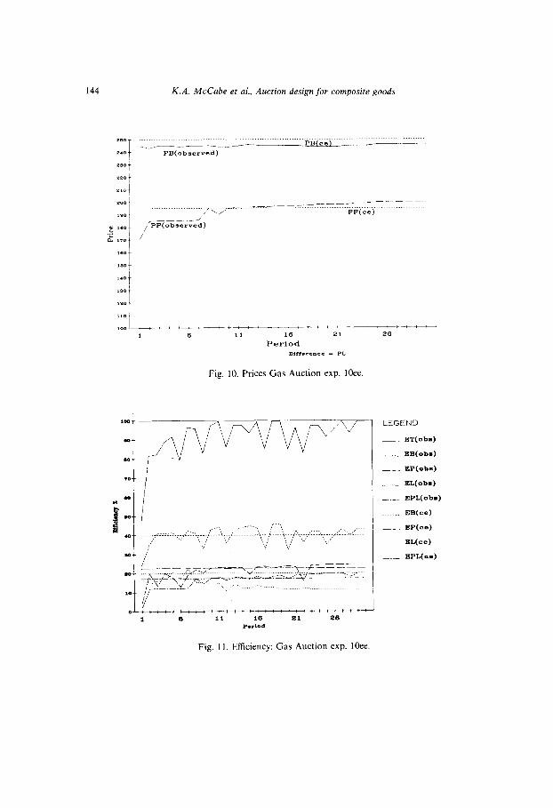
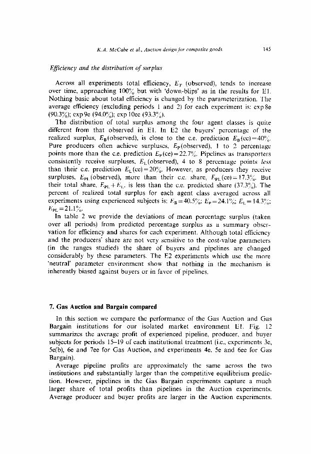
The primary market results for experiment 1Oee using the parameters corresponding to fig. 2 are shown in figs. 10 and 11.

Prices

In contrast with El, in E2 we observe a tendency for:

(i) the buyer prices, P,(observed), to approach the ce. price or less, (ii) the producer price, P,(observed), to settle at levels above the c.e. predictions, and (iii) the pipeline price to converge to levels very consistently less than the ce. prediction (fig. 10). As in the first design we observe very strong period-to- period price stability.

K.A. McCabe et al., Auction design for composite goods

Fig. 10. Prices Gas Auction exp. 1Oee.

LEGEND

_ ET(ob.)

._..___ EB(ob.)

__ EP(obs)

EL(obs)

_._ EPL(ob9)

..__ EB(ce)

__ EP(ce)

EL(m)

_._ EPL(c.)

Fig. 1 I. Effkiency: Gas Auction exp. IOee.


Efficiency and the distribution of surplus

Across all experiments total efficiency, E, (observed), tends to increase over time, approaching 100% but with ‘down-blips’ as in the results for El. Nothing basic about total efficiency is changed by the parameterization. The average efficiency (excluding periods 1 and 2) for each experiment is: exp8e (90.3%); exp9e (94.0%); exp 1Oee (93.3%).

The distribution of total surplus among the four agent classes is quite different from that observed in El. In E2 the buyers’ percentage of the realized surplus, E,(observed), is close to the c.e. prediction E,(ce) =409,. Pure producers often achieve surpluses, E,(observed), 1 to 2 percentage points more than the c.e. prediction E, (ce) = 22.7%. Pipelines as transporters consistently receive surpluses, E,(observed), 4 to 8 percentage points 1e.s.s than their c.e. prediction E, (ce) = 20%. However, as producers they receive surpluses, E,,(observed), more than their c.e. share, E,,(ce) = 17.3”;. But their total share, E,,+E,, is less than the c.e. predicted share (37.3%). The percent of realized total surplus for each agent class averaged across all experiments using experienced subjects is: E, = 40.5%; E, = 24.1 ?A; E, = 14.376; E,,=21.1%.

In table 2 we provide the deviations of mean percentage surplus (taken over all periods) from predicted percentage surplus as a summary observation for efficiency and shares for each experiment. Although total efficiency and the producers’ share are not very sensitive to the cost-value parameters (in the ranges studied) the share of buyers and pipelines are changed considerably by these parameters. The E2 experiments which use the more ‘neutral’ parameter environment show that nothing in the mechanism is inherently biased against buyers or in favor of pipelines.

7. Gas Auction and Bargain compared

In this section we compare the performance of the Gas Auction and Gas Bargain institutions for our isolated market environment El. Fig. 12 summarizes the average profit of experienced pipeline, producer, and buyer subjects for periods 15-19 of each institutional treatment (i.e., experiments 3e, 5e(b), 6e and 7ee for Gas Auction, and experiments 4e, 5e and 6ee for Gas Bargain).

Average pipeline profits are approximately the same across the two institutions and substantially larger than the competitive equilibrium prediction. However, pipelines in the Gas Bargain experiments capture a much larger share of total profits than pipelines in the Auction experiments.

Average producer and buyer profits are larger in the Auction experiments.


Table 2

Estimation of efficiency and shares as a proportion of c.e. values.”

Efficiency Design I Design II

measure Experiment r, n Experiment Y, n

Total 3e 0.928 24 8e 0.903 30 6e 0.943 30 9e 0.940 30 7ee 0.960 30 1Oce 0.933 30

Buyers 3e 0.176 24 8e 0.847 30 6e 0.652 30 9e 0.951 30 7ee 0.727 30 1Oee 1.02 30

Producers 3e 1.01 24 8e 1.00 30 6e 1.01 30 9e 0.988 30 7ee 1.02 30 l&e 0.963 30

Line owners 3e 2.24 24 8e 0.613 30 6e 4.19 30 9e 0.889 30 7ee 3.52 30 1Oee 0.781 30

Production 3e 0.0106 24 8e 1.16 30 owned by 6e 0.0040 30 9e 0.9 1 30 lines 7ee 0.0030 30 1Oee 0.86 30

“All efficiencies, Y,= E,(observed)/E,(c.e.), normalized as a fraction of their respective c.e. surpluses. An exception is for production by pipelines in Design I with zero c.e. surplus which is measured as a fraction of the maximal total surplus.

“PfZSOS”

1400

1200

1000

800

600

400

r

t

t

t

t

i 0 Gas Competitive Gas

Auction Equilibrium Bargain Prediction

I Efficiency L

EB Pipelines

Producers

Buyers

Fig. 12. Comparison of profit shares: Environment (El).


Producers and buyers capture roughly the same share of total profits across institutions.

From this data we draw the following conclusions. First, Gas Auction is Pareto superior to Gas Bargaining since buyers and producers are made better off while pipelines are made no worse off. Second, the relative rent seeking power of pipelines is reduced in the Gas Auction experiments. Third, buyers and producers pay an equal share of the cost of the inefficiency caused- by the Gas Bargain institution. We also note that Gas Auction dramatically reduces price volatility,

We conjecture that the two-stage pricing of our bargaining institution is responsible for our results. In Gas Bargain pipelines face a perfectly inelastic demand schedule when making their pricing decisions. When demand is high (near the c.e.) all pipelines transport units and price tends to increase. Producers and buyers can discipline pipelines only by reducing the quantity of gas they trade, thus forcing pipelines to lower price in order to compete for market share or access.

From the individual data it is clear that the decline in buyer/producer contracts was not a conscious disciplining strategy. The complexity involved in coordinating such a strategy is tremendous. It was rather a failure to come to agreement in light of diminishing gains from exchange. Once transportation price fell, the number of units contracted between buyers and producers would increase, starting the process over again. This accounts for the consistent loss and erratic changes in efficiency within our Gas Bargain experiments.

In contrast, in Gas Auction pipelines face an elastic demand. This demand is made even more elastic by buyers’ underrevelation of their highest reservation prices. In this institution pipelines are not disciplined by negotiation failures but rather by the revealed market demand. Underrevelation by buyers can be viewed as a form of risk sharing with respect to market inefficiencies. In the extreme if every buyer revealed a willingness to buy equal to the market clearing price then, given our random rationing rule, each buyer shares equally the risk of not buying (if and when quantity drops).

8. Conclusion and extensions

The following summary of our results should be read with the understanding that they apply only for the value, cost and capacity parameters, defined by El and E2. Similarly, we make no claim that the parameters used are ‘realistic’ representations of field conditions. In this paper we have completely ignored the network complications of an actual transportation market. We report separately our network version of Gas Auction [see McCabe et al. (1989)J


(1) Essentially all of our experiments with the vertical sealed/bid auction mechanism record a high degree of price stability. The price convergence process is not erratic and does not take many periods. This extends previous sealed bid-offer experimental price behavior results to our composite good environment.

(2) Total efficiency and the surplus shares of all agent classes tend to show greater period-to-period variability than prices. This is a consequence of attempts by individua! buyers, producers and/or pipeline owners to obtain marginally improved (lower or higher) prices. But small changes in bids or offers tend to impact allocations and pipeline flows, and thus efficiency and agent profits, much more than prices.

(3) The sensitivity of efficiency and shares in market surplus to small changes in bid or offer prices is frequently the result of the following behavioral characteristics of the bid-offer data. Buyers underbid their more valuable units much more than their least valuable marginal units. Similarly, sellers offer their low cost units at higher relative prices than their high cost marginal units. This yields very elastic revealed demand and supply schedules, oftern with several buyers and sellers entering tied bids and offers at the market clearing price. As illustrated in tig. 9 any increased offer or decreased bid will cause the person making a change to suffer a reduced allocation. The individual is priced out of the market. Since there are other bids and offers at or near the market clearing price, the latter changes very little, if at all, when one or two individuals alter their bids or offers in this manner. We think this problem can be solved by substituting a real time iterative procedure for the simple sealed bid-offer version of Gas Auction.

(4) Our experiments offer no support for the proposition that, in general, the gas auction mechanism prices gas and its transportation unfavorably to buyers and favorably to pipelines. This result is obtained only in experiments in which special demand and cost parameters are chosen to favor prices above competitive equilibrium levels for pipelines and below such levels for buyers.

(5) The number of observations reported in this paper is small. However, we are confident in our conclusions concerning Gas Auction since we have run further experiments with this institution in more complex environments [see McCabe et al. (1989) and Rassenti et al. (1989)]. All of the Gas Bargain experiments are more volatile and less efficient than our various Gas Auction experiments. It is unlikely that more experiments will change this observation. Instead we suspect Gas Bargain will work only after serious modification to allow contingent contracts and multi-lateral bargaining. It still may be difficult, even in a stationary non-networked market, to solve the coordination problem using decentralized markets. In the complex field


environment the Natural Gas industry is coming to the same conclusion [see Hogan ( 1989)].

References

Banks, J.S., J.O. Ledyard and D.P. Porter, 1989, Uncertain and unresponsive resources: An experimental approach, The Rand Journal of Economics 20, Spring, l-25.

Dubins, L.E. and D.A. Freedman, 1981, Machiavelli and the Gale-Shapley algorithm, American Mathematical Monthly 88, August,‘444485.

Gale, David and Lloyd S. Shapley, 1962, College admissions and the stability of marriage, American Mathematical Monthly 69, Jan., 9-15.

Harrison, Glenn W. and Kevin A. McCabe, 1987, Stability and preference distortion in resource matching, Working paper (University of Arizona, Tuscan, AZ) Oct.

Hogan, William W., 1989, Firm natural gas transportation: A priority capacity allocation model (Putnam, Hayes and Bartlett, New York).

McCabe, Kevin A., Stephen J. Rassenti and Vernon L. Smith, 1989, Designing smart computer assisted markets: An experimental auction for gas networks, European Journal of Political Economy (forthcoming).

Rassenti, Stephen J., 1982, Zero/one decision problems with multiple resource constraints, Doctoral thesis (University of Arizona, Tucson, AZ).

Rassenti, Stephen J., V.L. Smith and R.L. Bultin, 1982, A combinatorial auction mechanism for airport time slot allocation, Bell Journal of Economics 13, 402417.

Rassenti, Stephen J., Stanely S. Reynolds and Vernon L. Smith, 1989, Cotenancy and competition in an experimental auction market for natural gas pipeline networks, Oct.

Roth, Alvin E., 1982, The economics of matching: Stability and incentives, Mathematics of Operations Research 7, Nov., 617-628.

Roth, Alvin F., 1984, Misrepresentation and stability in the marriage problem, Journal of Economic Theory 34, 3833387.

Smith, Vernon L., Arlington W. Williams, William Bratton and Michael G. Vannoni, 1980, Competitive market institutions: Double auctions versus sealed bid-offer auctions, American Economic Review 72, March, 59-77.

Auction design for composite goods : The natural gas industry

Documents