386 IEEE TRANSACTIONS ON SIGNAL PROCESSING, VOL. 59, NO. 1, JANUARY 2011 Attribute-Distributed Learning: Models, Limits, and Algorithms Haipeng Zheng, Sanjeev R. Kulkarni, Fellow, IEEE, and H. Vincent Poor, Fellow, IEEE Abstract—This paper introduces a framework for distributed learning (regression) on attribute-distributed data. First, the con- vergence properties of attribute-distributed regression with an ad- ditive model and a fusion center are discussed, and the convergence rate and uniqueness of the limit are shown for some special cases. Then, taking residual refitting (or boosting) as a prototype al- gorithm, three different schemes, Simple Iterative Projection, a greedy algorithm, and a parallel algorithm (with its derivatives), are proposed and compared. Among these algorithms, the first two are sequential and have low communication overhead, but are sus- ceptible to overtraining. The parallel algorithm has the best perfor- mance, but has significant communication requirements. Instead of directly refitting the ensemble residual sequentially, the parallel algorithm redistributes the residual to each agent in proportion to the coefficients of the optimal linear combination of the current individual estimators. Designing residual redistribution schemes also improves the ability to eliminate irrelevant attributes. The per- formance of the algorithms is compared via extensive simulations. Communication issues are also considered: the amount of data to be exchanged among the three algorithms is compared, and the three methods are generalized to scenarios without a fusion center. Index Terms—Distributed information systems, distributed pro- cessing, statistical learning. I. INTRODUCTION D ISTRIBUTED learning is a field that generalizes classical machine learning algorithms to a distributed framework. Unlike the classical learning framework, in which one has full access to the entire dataset and has unlimited central computa- tional capability, in the framework of distributed learning, the data are distributed among a number of agents. These agents are capable of exchanging certain types of information, which, due to limited computational power and communication restric- tions (limited bandwidth, limited power or confidentiality), is usually restricted in terms of content and amount. Research in distributed learning seeks effective learning algorithms and the- oretical limits within such constraints on computation, commu- nication, and confidentiality. Manuscript received April 09, 2010; accepted September 22, 2010. Date of publication October 18, 2010; date of current version December 17, 2010. This research was supported in part by the U.S. Office of Naval Research under Grant N00014-07-1-0555 and N00014-09-1-0342, the U.S. Army Research Office under Grant W911NF-07-1-0185, and the National Science Foundation under Grant CNS-09-05398 and under Science & Technology Center Grant CCF-0939370. The associate editor coordinating the review of this manuscript and approving it for publication was Dr. Mathini Sellathurai. The authors are with the Department of Electrical Engineering, Princeton University, Princeton, NJ 08544 USA (e-mail: [email protected]; [email protected]; [email protected]). Color versions of one or more of the figures in this paper are available online at http://ieeexplore.ieee.org. Digital Object Identifier 10.1109/TSP.2010.2088393 Fig. 1. Two basic scenarios for distributed data: instance-distributed (left) and attribute-distributed (right). In the instance-distributed scenario, each agent (A, B, and C) observes a subset of the instances, with complete information on all attributes; alternatively, in the attribute-distributed scenario, each agent observes all the instances, with a subset of attributes. In a typical setting of a distributed learning system, there are a number of agents, which are capable of collecting, processing (local training), and communicating a certain amount of data to one another, or to a fusion center. A fusion center may not be required if the links of the agents form a connected component of a graph. One key issue in distributed learning is the way in which data are distributed among the agents. If each agent observes the en- tire attribute space with a subset of the instances of the entire data set, then we call the data instance-distributed (or homo- geneous data/horizontally partitioned data). On the other hand, if each agent observes all the data instances within a subset of the attribute space, then we call the data attribute-distributed (or heterogeneous data/vertically partitioned data). Of course, there are other hybrid ways to distribute data, but instance- and attribute-distributed data are the two most fundamental cases. Fig. 1 illustrates these two ways to distribute data. Problems involving instance-distributed data have been widely studied. Two important types of models are established in [17] and [16], respectively: instance-distributed learning with and without a fusion center. The relationship between the information transmitted among individual agents and the fusion center, and the ensemble learning capability, are discussed in these papers. One of the essential questions about distributed learning is what type of information should be exchanged among the agents. For instance-distributed cases, exchanging estimator information among the agents is a direct, effective and natural choice because the estimator of one agent has exactly the same form (takes input on the same domain) as those of other agents, and hence can be directly applied and evaluated on the data of other agents. Moreover, since estimators to a great extent char- acterize the statistical properties of the training data, sharing individual estimators can be an efficient way of exchanging information. This is why classical learning algorithms are more easily adapted to the homogeneous data cases with the form 1053-587X/$26.00 © 2010 IEEE

Welcome message from author
This document is posted to help you gain knowledge. Please leave a comment to let me know what you think about it! Share it to your friends and learn new things together.
Transcript
386 IEEE TRANSACTIONS ON SIGNAL PROCESSING, VOL. 59, NO. 1, JANUARY 2011
Attribute-Distributed Learning: Models,Limits, and Algorithms
Haipeng Zheng, Sanjeev R. Kulkarni, Fellow, IEEE, and H. Vincent Poor, Fellow, IEEE
Abstract—This paper introduces a framework for distributedlearning (regression) on attribute-distributed data. First, the con-vergence properties of attribute-distributed regression with an ad-ditive model and a fusion center are discussed, and the convergencerate and uniqueness of the limit are shown for some special cases.Then, taking residual refitting (or � boosting) as a prototype al-gorithm, three different schemes, Simple Iterative Projection, agreedy algorithm, and a parallel algorithm (with its derivatives),are proposed and compared. Among these algorithms, the first twoare sequential and have low communication overhead, but are sus-ceptible to overtraining. The parallel algorithm has the best perfor-mance, but has significant communication requirements. Insteadof directly refitting the ensemble residual sequentially, the parallelalgorithm redistributes the residual to each agent in proportion tothe coefficients of the optimal linear combination of the currentindividual estimators. Designing residual redistribution schemesalso improves the ability to eliminate irrelevant attributes. The per-formance of the algorithms is compared via extensive simulations.Communication issues are also considered: the amount of data tobe exchanged among the three algorithms is compared, and thethree methods are generalized to scenarios without a fusion center.
Index Terms—Distributed information systems, distributed pro-cessing, statistical learning.
I. INTRODUCTION
D ISTRIBUTED learning is a field that generalizes classicalmachine learning algorithms to a distributed framework.
Unlike the classical learning framework, in which one has fullaccess to the entire dataset and has unlimited central computa-tional capability, in the framework of distributed learning, thedata are distributed among a number of agents. These agentsare capable of exchanging certain types of information, which,due to limited computational power and communication restric-tions (limited bandwidth, limited power or confidentiality), isusually restricted in terms of content and amount. Research indistributed learning seeks effective learning algorithms and the-oretical limits within such constraints on computation, commu-nication, and confidentiality.
Manuscript received April 09, 2010; accepted September 22, 2010. Date ofpublication October 18, 2010; date of current version December 17, 2010. Thisresearch was supported in part by the U.S. Office of Naval Research underGrant N00014-07-1-0555 and N00014-09-1-0342, the U.S. Army ResearchOffice under Grant W911NF-07-1-0185, and the National Science Foundationunder Grant CNS-09-05398 and under Science & Technology Center GrantCCF-0939370. The associate editor coordinating the review of this manuscriptand approving it for publication was Dr. Mathini Sellathurai.
The authors are with the Department of Electrical Engineering, PrincetonUniversity, Princeton, NJ 08544 USA (e-mail: [email protected];[email protected]; [email protected]).
Color versions of one or more of the figures in this paper are available onlineat http://ieeexplore.ieee.org.
Digital Object Identifier 10.1109/TSP.2010.2088393
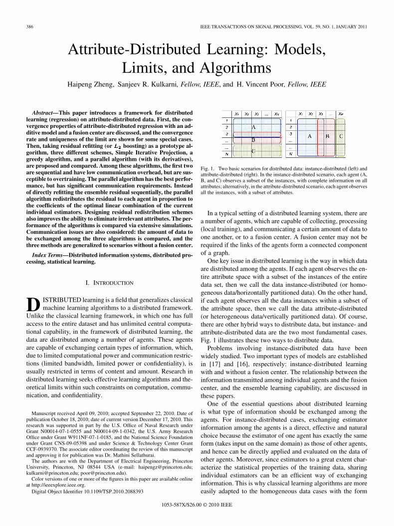
Fig. 1. Two basic scenarios for distributed data: instance-distributed (left) andattribute-distributed (right). In the instance-distributed scenario, each agent (A,B, and C) observes a subset of the instances, with complete information on allattributes; alternatively, in the attribute-distributed scenario, each agent observesall the instances, with a subset of attributes.
In a typical setting of a distributed learning system, there area number of agents, which are capable of collecting, processing(local training), and communicating a certain amount of data toone another, or to a fusion center. A fusion center may not berequired if the links of the agents form a connected componentof a graph.
One key issue in distributed learning is the way in which dataare distributed among the agents. If each agent observes the en-tire attribute space with a subset of the instances of the entiredata set, then we call the data instance-distributed (or homo-geneous data/horizontally partitioned data). On the other hand,if each agent observes all the data instances within a subset ofthe attribute space, then we call the data attribute-distributed(or heterogeneous data/vertically partitioned data). Of course,there are other hybrid ways to distribute data, but instance- andattribute-distributed data are the two most fundamental cases.Fig. 1 illustrates these two ways to distribute data.
Problems involving instance-distributed data have beenwidely studied. Two important types of models are establishedin [17] and [16], respectively: instance-distributed learningwith and without a fusion center. The relationship between theinformation transmitted among individual agents and the fusioncenter, and the ensemble learning capability, are discussed inthese papers.
One of the essential questions about distributed learningis what type of information should be exchanged among theagents. For instance-distributed cases, exchanging estimatorinformation among the agents is a direct, effective and naturalchoice because the estimator of one agent has exactly the sameform (takes input on the same domain) as those of other agents,and hence can be directly applied and evaluated on the data ofother agents. Moreover, since estimators to a great extent char-acterize the statistical properties of the training data, sharingindividual estimators can be an efficient way of exchanginginformation. This is why classical learning algorithms are moreeasily adapted to the homogeneous data cases with the form
1053-587X/$26.00 © 2010 IEEE
ZHENG et al.: ATTRIBUTE-DISTRIBUTED LEARNING: MODELS, LIMITS, AND ALGORITHMS 387
of the classifier/estimator being exactly the same as that of thecentralized learning algorithm. Homogeneity in the individualclassifiers/estimators is a great advantage for designing dis-tributed learning algorithms that compare and combine them.However, these advantages disappear in the attribute-distributedscenario, in which different agents observe different attributes,and thus have many different forms of classifiers/estimators.This makes it harder to evaluate, compare and combine theestimators.
In this paper, we concentrate on solving distributed learningproblems with attribute-distributed data. In particular, we ad-dress several fundamental questions:
1) Given the constraints on the observations of each agent,what is the optimal ensemble estimator?
2) Is there an efficient protocol for collaborative training sothat the agents can reach the optimal choice of this en-semble estimator?
3) What is the tradeoff between performance and the amountof data exchanged?
In this paper, we will answer these questions in part. InSection II, we briefly review the existing methods in thisfield, highlighting the residual refitting scheme in detail. InSection III, we pose a fundamental optimization problem: underthe residual refitting scheme, find the best thing that we can do,given that we have an infinite amount of data and no noise. Thenwe propose a solution to this problem. In Section IV, we seekalgorithms that perform well with finite, noisy observation data,and we present simulation results to support our conclusionsin Section V. In Section VI, we discuss communication issuesassociated with the distributed learning algorithms, and thenconclude our paper in Section VII.
II. REVIEW OF EXISTING METHODS
Despite the difficulties of attribute-distributed learning,there are many research results in this area. Basak [1] sets upa general paradigm for classification problem on verticallypartitioned data (i.e., attribute-distributed data). There are manyalgorithms that are distributed versions of different centralizedclassification algorithms on attribute-distributed data, for in-stance, -nearest neighbor [5], support vector machine [13],[23], Bayesian networks [24], [25] and decision trees [6], [22].In addition, researchers have also generalized unsupervisedlearning algorithms to attribute-distributed data. For instance,[21] considers -means clustering problems with attribute-dis-tributed data and [10] generalizes it to arbitrarily partitioneddata.
In most of these approaches, the privacy-preservation aspectof distributed algorithms is also highlighted. In other words, inall the algorithms, the protocols under which the agents shareinformation with one another do not involve direct communica-tion of private data.
On the other hand, there are also many works that considerregression problems and emphasize the estimation error of theensemble estimator, e.g., [14] or [26]. Some basic ideas includevoting/averaging, meta-learning, collective data mining, andresidual refitting. In terms of the training process, the firsttwo are non-collaborative, i.e., each agent individually trainsits own classifier/estimator and fixes it before sending it to
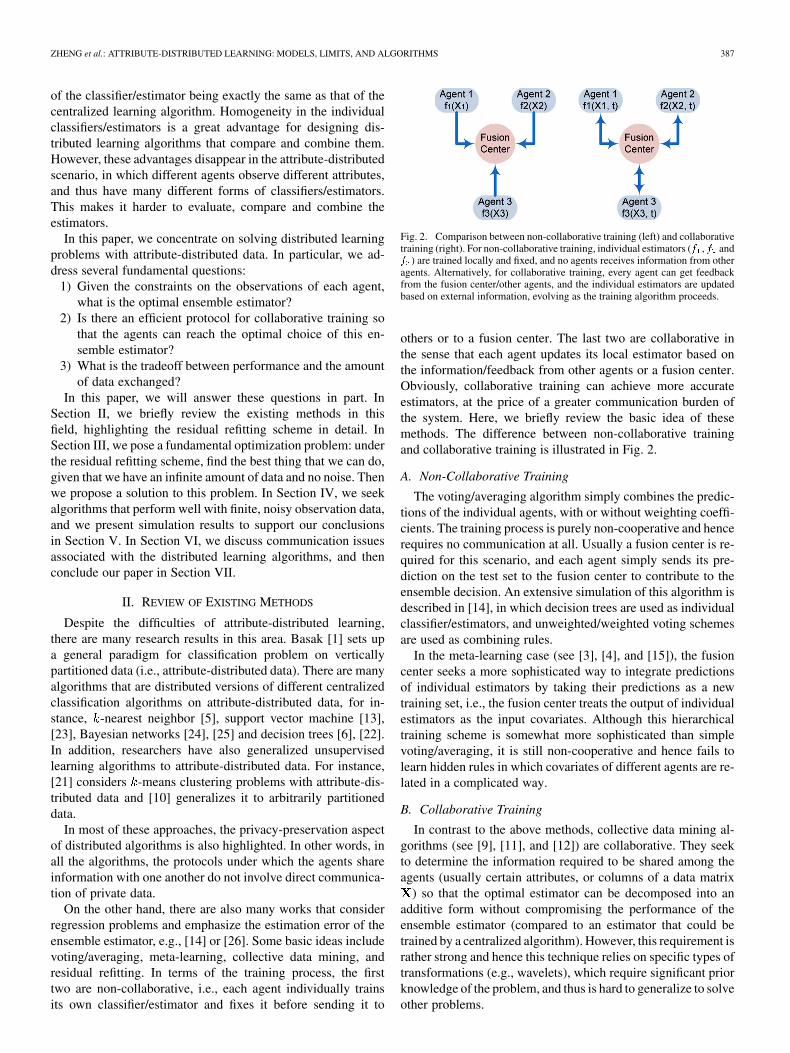
Fig. 2. Comparison between non-collaborative training (left) and collaborativetraining (right). For non-collaborative training, individual estimators (� , � and� ) are trained locally and fixed, and no agents receives information from otheragents. Alternatively, for collaborative training, every agent can get feedbackfrom the fusion center/other agents, and the individual estimators are updatedbased on external information, evolving as the training algorithm proceeds.
others or to a fusion center. The last two are collaborative inthe sense that each agent updates its local estimator based onthe information/feedback from other agents or a fusion center.Obviously, collaborative training can achieve more accurateestimators, at the price of a greater communication burden ofthe system. Here, we briefly review the basic idea of thesemethods. The difference between non-collaborative trainingand collaborative training is illustrated in Fig. 2.
A. Non-Collaborative Training
The voting/averaging algorithm simply combines the predic-tions of the individual agents, with or without weighting coeffi-cients. The training process is purely non-cooperative and hencerequires no communication at all. Usually a fusion center is re-quired for this scenario, and each agent simply sends its pre-diction on the test set to the fusion center to contribute to theensemble decision. An extensive simulation of this algorithm isdescribed in [14], in which decision trees are used as individualclassifier/estimators, and unweighted/weighted voting schemesare used as combining rules.
In the meta-learning case (see [3], [4], and [15]), the fusioncenter seeks a more sophisticated way to integrate predictionsof individual estimators by taking their predictions as a newtraining set, i.e., the fusion center treats the output of individualestimators as the input covariates. Although this hierarchicaltraining scheme is somewhat more sophisticated than simplevoting/averaging, it is still non-cooperative and hence fails tolearn hidden rules in which covariates of different agents are re-lated in a complicated way.
B. Collaborative Training
In contrast to the above methods, collective data mining al-gorithms (see [9], [11], and [12]) are collaborative. They seekto determine the information required to be shared among theagents (usually certain attributes, or columns of a data matrix
) so that the optimal estimator can be decomposed into anadditive form without compromising the performance of theensemble estimator (compared to an estimator that could betrained by a centralized algorithm). However, this requirement israther strong and hence this technique relies on specific types oftransformations (e.g., wavelets), which require significant priorknowledge of the problem, and thus is hard to generalize to solveother problems.
388 IEEE TRANSACTIONS ON SIGNAL PROCESSING, VOL. 59, NO. 1, JANUARY 2011
Another class of cooperative training algorithms, the residualrefittingalgorithmandalgorithmsderivedfromit [19], [26]–[28],has the advantage of not being dependent on individual learningalgorithms. The only information the agents communicate witheach other is their training residuals. Sharing training residualsis a promising choice for attribute-distributed learning becausethe training residual of one agent represents the “unexplainable”part of the outcome based on that agent’s attributes. Moreover,since residual refitting algorithms bear a natural resemblance tothe -boostingalgorithm of classical machine learning,many ofthe conclusions and methodologies of boosting can be borrowedand revised. Nonetheless, there are still many unique problemsassociated with distributed residual refitting.
An interesting question is the following: If we adopt theresidual refitting scheme and assume that each individual agentis able to find its conditional expectation estimator (optimalin terms of mean square error), then what is the limit of theresidual refitting algorithm? Reference [26] partly answersthis question by demonstrating that repeatedly finding theconditional-mean estimator of the current ensemble residual(iterative projection) is a non-expansive map, and under cer-tain additional assumptions, is a contractive map, and henceconverges to a unique limit, which is the optimal estimator ofthe form of a linear combination of individual estimators. Theanalysis in [26] justifies the efficacy of the residual refittingalgorithm in the infinite instance, noise-free data scenario.
However, since training data is generally limited an noisy, di-rect residual refitting on ensemble training error in a round robinmanner fails to perform well, especially in the presence of irrel-evant attributes (attributes that are completely unrelated to theoutcome). Usually, this phenomenon is considered to be a formof overtraining in the parlance of machine learning. [19], [27]and [28] have proposed different ways of solving this problem.In [27], uncertainty about the covariance of individual trainingresiduals is introduced so that the ensemble estimator can besearched in a minimax manner to avoid overtraining. In [19]and [28], different ways of agent selection/pruning schemes areproposed to eliminate irrelevant agents so that the final ensembleestimator has a sparser form, leading to better generalization ca-pability. Moreover, selecting/pruning agents can also reduce theamount of data exchange to some extent, making the algorithmsmore efficient in terms of communication requirements.
In this paper, we consider an alternative residual-based al-gorithm that addresses this problem in a different manner. In-stead of projecting the ensemble residual sequentially on theagents (selected or unselected), which is greedy and myopic,we use the training residual (or equivalently, the prediction ontraining data) in a holistic way, reshaping the entire predic-tion matrix using gradient descent. This essentially reduces to aproblem of parallel residual refitting in which current ensembletraining residuals are distributed in proportion to the weightingcoefficients of the best linear combination of individual estima-tors. In addition, if we do not strictly follow gradient descent,and instead adjust the weighting coefficients to emphasize morepromising agents and de-emphasize the less promising ones, abetter ensemble estimator can be obtained, with most irrelevantagents being eliminated, and only a few of the most importantagents surviving.
III. LIMITS OF ADDITIVE MODELS
A. Model and Problem Definition
Suppose that there are attributes, instances andagents. Define the set of indexes of attributes as
(1)
and the set of indexes of instances as
(2)
then the observation data matrix composed of elementscan be divided into many small parts
, of the general form
(3)
If we add some extra structural constraints to the sets , thenwe can describe instance-distributed and attribute-distributeddata. To be more specific, if
(4)
then each data set contains only complete rows of , i.e.,each agent observes all the attributes for a subset of the in-stances. In this case, we call the collectioninstance-distributed data.
On the other hand, if
(5)
then each data set contains only complete columns of , i.e.,each agent observes all the instances of a subset of the attributes.In such situation, we call the collectionattribute-distributed data.
Our further discussion is based on an estimation/regressionproblem with attribute-distributed data. Suppose attribute
, and outcome . Then the entire dataset can bewritten as
or, for simplicity
where is the th instance of attribute , and is theth instance of .
We assume that there exists a hidden deterministic function(or rule/hypothesis)
such that
(6)
where is an independently drawn sample froma zero-mean random variable that is independent of
and . For simplicity, we denote the hidden ruleas
(7)
ZHENG et al.: ATTRIBUTE-DISTRIBUTED LEARNING: MODELS, LIMITS, AND ALGORITHMS 389
Suppose there are agents and one fusion center. Each of theagents has only limited access to certain attributes. As defined inthe introduction, denotes the set of attributesaccessible by agent , and , assuming that
. For centralized data, the set of possible estimators is givenby
and for each agent , the set is reduced to
We will restrict and to include only functions satisfying
(8)
The fusion center observes the outcome , with all its instances. These assumptions specify the “attribute-dis-
tributed” properties of our problem.Suppose is the random variable that generates the samples
with a fixed (but unknown) distribution; then ide-ally, we need to solve the following problem:
(9)
where
(10)
If we assume that the ensemble estimator is of additive form
(11)
then problem (9) can be reduced to a simpler form
(12)
In practice, if we have only finite, noisy data, it is impossible toexactly solve (12). Instead, we use the training error as a proxyof the objective specified in (12). Then, we have the problem
(13)
of minimizing the mean square training error.In Section III, we concentrate on showing some results con-
cerning problem (12), closely relating to the question “What isthe best we can do?” In Section IV, we go further to find a prac-tical algorithm for solving problem (13).
B. Iterative Conditional Expectation Projection
Now, let us consider a very naive approach to iteratively solveproblem (12). Suppose that we have two agents. We initialize
and both as 0. Suppose ,and Agent 1 and Agent 2 then update their estimators in the
following manner:
(14)
and
(15)
In other words, each agent repeatedly finds the conditional ex-pectation (conditioned on the set of covariates visible to agent, i.e., ) of the difference between the hidden rule
and the current projection of the other agent. This is compatiblewith our intuition because the conditional expectations givenby (14) and (15) are the minimum-mean-square-error (MMSE)estimators of the fitting residuals of the other agents. For sim-plicity, we henceforth denote as .
If this conditional expectation projection process is iterated,then hopefully we can asymptotically achieve a limitthat best approximates . To investigate the limit behavior ofthe iterative conditional expectation projection, we define thedistance between two functions and on the space as
(16)
then we can show that the map defined by (14) and (15) fromto is a non-expansive map. More specifically,
we have the following theorem.Theorem 1: For two functions and , the
map specified by (14) and (15), i.e.,
(17)
satisfies the property
(18)
That is, is a non-expansive map on the metric space withdistance defined by (16).
Non-expansive is weaker than contractive, and “fixed-point”theorems generally require a contractive map. The followingtheorem shows that if the covariates of the two agents are jointlyGaussian and the hidden rule is a finite-order polynomial, then
is a contractive map.Theorem 2: If the hidden rule is a finite-order
polynomial function with zero mean, and its input covariatesare jointly Gaussian with correlation coeffi-
cients , then defined by (17) is a contractive map, with con-traction factor , i.e.,
(19)
The proofs of Theorems 1 and 2 can be found inAppendixes A and B, respectively.
By the fixed-point theorem for metric spaces, under the as-sumptions of Theorem 2, the iterative conditional expectationalgorithm specified by (14) and (15) converges to a unique limit,which is the solution of the simultaneous equations
(20)
(21)
390 IEEE TRANSACTIONS ON SIGNAL PROCESSING, VOL. 59, NO. 1, JANUARY 2011
Moreover, the convergence speed is , where is thenumber of iterations. If the covariates of the two agents are in-dependent, then the algorithm converges in one iteration.
In [26], a detailed example is provided to support Theorem 2in the section containing our simulation results. In the example,the limit of the iterative conditional expectation projection isexactly the same as the one that is found by solving (20) and(21). Moreover, the distance, as defined by (16), between theestimated function and the limit (i.e., the fixed point) convergeswith a rate of .
We now turn to the realistic case in which the data are fi-nite and noisy. Moreover, we do not assume that each agent isperfect at finding the conditional expectation of the current en-semble residual projected onto its local data. On the contrary,we assume that the agents may employ different learning algo-rithms.
With these new relaxed assumptions, we turn to designing analgorithm to solve problem (13) iteratively to create an ensembleestimator with the least possible generalization error.
IV. METHODS AND ALGORITHMS
A. Minimizing Training Error Sequentially
If we directly employ the iterative conditional expectation al-gorithm in the last section specified by (14) and (15) and applyit to solve the finite, noisy data case (13), i.e., to refit the currentensemble residual in a round robin manner, then we can obtainAlgorithm 1, in which denotes the index of the agent atiteration , which, for a round robin refitting, is given by
(22)
Applying Algorithm 1 with specified by (22), henceforthcalled Simple Iterative Projection, does not achieve very de-sirable results, especially in the presence of many irrelevantattributes. Since the algorithm treats every agent equally,neglecting the fact that some of them are better at predictingthe outcome than others, and thereby projecting the ensembleresidual onto some spaces orthogonal to the outcome, it canoverfit the data.
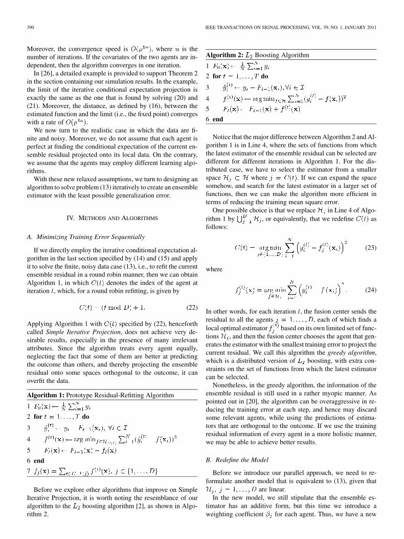
Algorithm 1: Prototype Residual-Refitting Algorithm
1
2 for do
3
4
5
6 end
7
Before we explore other algorithms that improve on SimpleIterative Projection, it is worth noting the resemblance of ouralgorithm to the boosting algorithm [2], as shown in Algo-rithm 2.
Algorithm 2: Boosting Algorithm
1
2 for do
3
4
5
6 end
Notice that the major difference between Algorithm 2 and Al-gorithm 1 is in Line 4, where the sets of functions from whichthe latest estimator of the ensemble residual can be selected aredifferent for different iterations in Algorithm 1. For the dis-tributed case, we have to select the estimator from a smallerspace where . If we can expand the spacesomehow, and search for the latest estimator in a larger set offunctions, then we can make the algorithm more efficient interms of reducing the training mean square error.
One possible choice is that we replace in Line 4 of Algo-rithm 1 by , or equivalently, that we redefine asfollows:
(23)
where
(24)
In other words, for each iteration , the fusion center sends theresidual to all the agents , each of which finds alocal optimal estimator based on its own limited set of func-tions , and then the fusion center chooses the agent that gen-erates the estimator with the smallest training error to project thecurrent residual. We call this algorithm the greedy algorithm,which is a distributed version of boosting, with extra con-straints on the set of functions from which the latest estimatorcan be selected.
Nonetheless, in the greedy algorithm, the information of theensemble residual is still used in a rather myopic manner. Aspointed out in [20], the algorithm can be overaggressive in re-ducing the training error at each step, and hence may discardsome relevant agents, while using the predictions of estima-tors that are orthogonal to the outcome. If we use the trainingresidual information of every agent in a more holistic manner,we may be able to achieve better results.
B. Redefine the Model
Before we introduce our parallel approach, we need to re-formulate another model that is equivalent to (13), given that
are linear.In the new model, we still stipulate that the ensemble es-
timator has an additive form, but this time we introduce aweighting coefficient for each agent. Thus, we have a new
ZHENG et al.: ATTRIBUTE-DISTRIBUTED LEARNING: MODELS, LIMITS, AND ALGORITHMS 391
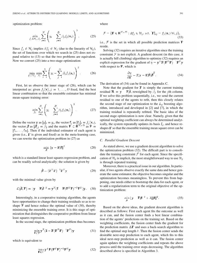
optimization problem:
(25)
Since implies (due to the linearity of ),the set of functions over which we search in (25) does not ex-pand relative to (13) so that the two problems are equivalent.Now we convert (25) into a two-stage optimization:
(26)
First, let us observe the inner stage of (26), which can beinterpreted as: given fixed, find the bestlinear combination so that the ensemble estimator has minimalmean-square training error:
(27)
Define the vector as , the vector as ,the vector as and the matrix as
. Then if the individual estimator of each agent isgiven (i.e., is given and fixed) as in the meta-learning case,we can rewrite the optimization problem in (27) as
(28)
which is a standard linear least squares regression problem, andcan be readily solved analytically: the solution is given by
(29)
with the minimal value given by
(30)
Interestingly, in a cooperative training algorithm, the agentshave opportunities to change their training residuals so as to re-shape and hence reduce the optimal value of (30), therebyminimizing the ensemble training error. It is this stage of opti-mization that distinguishes the cooperative problem from linearleast squares regression.
In the second stage, the optimization problem thus becomes
(31)
which is equivalent to
(32)
where
(33)
i.e., is the set in which all possible prediction matricesreside.
Solving (32) requires an iterative algorithm since the trainingconstraint is not explicit. A gradient descent (in this case, itis actually hill climbing) algorithm to optimize (32) requires anexplicit expression for the gradient ofwith respect to , which is
(34)
The derivation of (34) can be found in Appendix C.Note that the gradient for is simply the current training
residual , reweighted by for the th column.If we solve this problem sequentially, i.e., we send the currentresidual to one of the agents to refit, then this closely relatesthe second stage of our optimization to the boosting algo-rithm, introduced and developed in [2] and [7], in which thetraining residual is repeatedly refitted. The basic idea of thesecond stage optimization is now clear. Namely, given that theoptimal weighting coefficient can always be determined analyt-ically, the system repeatedly updates its basis , and hence re-shapes so that the ensemble training mean square error can beminimized.
C. Parallel Gradient Descent
As stated above, we use a gradient descent algorithm to solvethe optimization problem (32). The difficult part is to consoli-date the training constraint for each agent. Since the specifi-cation of is implicit, the most straightforward way to useis through repeated training.
Moreover, there is a practical issue in our algorithm. In partic-ular, if two agents observe exactly the same data and hence gen-erate the same estimator, the objective becomes singular and theoptimization becomes meaningless. To prevent this from hap-pening, one needs either to bootstrap the data for each agent, orto add a regularization term to the original objective of the op-timization problem:
(35)
Based on the above ideas, the gradient descent algorithm isdescribed as follows: First each agent fits the outcome as wellas it can, and the fusion center finds a best linear combina-tion of the agents’ predictions on the training set. Based on theweighting coefficients, the fusion center finds the gradient forthe prediction matrix and uses a back-search algorithm tofind the optimal step length . Then the fusion center sends thedesirable next-step prediction to each agent, which fits to thisideal next-step prediction as well as it can. The fusion centeragain updates the weighting coefficients and repeats the aboveprocess until the training error stops decreasing. The algorithmdescribed above is specified in Algorithm 3.
392 IEEE TRANSACTIONS ON SIGNAL PROCESSING, VOL. 59, NO. 1, JANUARY 2011
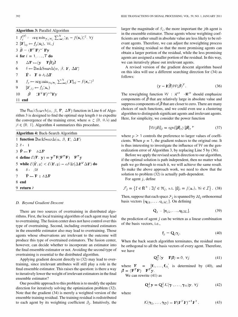
Algorithm 3: Parallel Algorithm
1
2
3
4 for do
5
6
7
8
9
10
11 end
The function in Line 6 of Algo-rithm 3 is designed to find the optimal step length to expeditethe convergence of the training error, where and
. Algorithm 4 summarizes this procedure.
Algorithm 4: Back-Search Algorithm
1 function
2
3
4 define
5 while do
6
7
8 end
9 return
D. Beyond Gradient Descent
There are two sources of overtraining in distributed algo-rithms. First, the local training algorithm of each agent may leadto overtraining. The fusion center does not have control over thistype of overtraining. Second, including overtrained estimatorsin the ensemble estimator also may lead to overtraining. Thoseagents whose observations are irrelevant to the outcome willproduce this type of overtrained estimators. The fusion center,however, can decide whether to incorporate an estimator intothe final ensemble estimator or not. Avoiding the second type ofovertraining is essential to the distributed algorithm.
Applying gradient descent directly to (32) may lead to over-training, since irrelevant attributes will still play a role in thefinal ensemble estimator. This raises the question: is there a wayto iteratively lower the weight of irrelevant estimators in the finalensemble estimator?
One possible approach to this problem is to modify the updatedirection for iteratively solving the optimization problem (32).Note that the gradient (34) is merely a weighted version of theensemble training residual. The training residual is redistributedto each agent by its weighting coefficient . Intuitively, the
larger the magnitude of , the more important the th agent isin the ensemble estimator. Those agents whose weighting coef-ficients are rather small in absolute value are less likely to be rel-evant agents. Therefore, we can adjust the reweighting processof the training residual so that the more promising agents canobtain a larger portion of the residual, while the less promisingagents are assigned a smaller portion of the residual. In this way,we can iteratively phase out irrelevant agents.
A revised version of the gradient descent algorithm basedon this idea will use a different searching direction for (34) asfollows:
(36)
The reweighting function should emphasizecomponents of that are relatively large in absolute value andsuppress components of that are closer to zero. There are manychoices of such functions, and we could even use a clusteringalgorithm to distinguish significant agents and irrelevant agents.Here, for simplicity, we consider the power function
(37)
where controls the preference to larger values of coeffi-cients. When , the gradient reduces to the original one. Itis thus interesting to investigate the influence of on the gen-eralization error of Algorithm 3, by replacing Line 5 by (36).
Before we apply the revised search direction to our algorithm,if the optimal solution is path independent, then no matter whatpath we go through to reach it, we will achieve the same result.To make the above approach work, we need to show that thesolution to problem (32) is actually path-dependent.
For agent , define
(38)
Then, suppose that each space is spanned by orthonormalbasis vectors . On defining
(39)
the prediction of agent can be written as a linear combinationof the basis vectors, i.e.,
(40)
When the back search algorithm terminates, the residual mustbe orthogonal to all the basis vectors of every agent. Therefore,we have
(41)
where is determined by (40), and.
We can rewrite (41) as
(42)
where
(43)
ZHENG et al.: ATTRIBUTE-DISTRIBUTED LEARNING: MODELS, LIMITS, AND ALGORITHMS 393
Notice that (42) can be simplified into a polynomial equationof high order (each of the equations has order ). As long as
are not trivial (e.g., mutually identical), we have anequal number of unknown variables and equations. This meansthat we have many solutions for , and problem (32) isindeed path dependent. The simulations in the next section willdemonstrate the influence of search direction on the generaliza-tion error of the ensemble estimator.
V. SIMULATION RESULTS
In this section, we examine the efficacy of our parallel algo-rithm (Algorithm 3 in Section IV) and its variants on several dif-ferent data sets, and compare it with Simple Iterative Projection(Algorithm 1 with (22) in Section IV) and the greedy algorithm(Algorithm 1 with (23) in Section IV) in different simulationscenarios.
A. Generalization Error
We test the algorithms on both artificial and real data sets. Forartificial data, we employ three functions used in [18] (originallyfrom [8]) as the hidden rule to generate our simulation trainingdata sets. The three functions and the corresponding joint distri-butions of the covariates are as follows:
• Friedman-1:
where ;• Friedman-2:
where , , ,and ;
• Friedman-3:
where the distributions of the attributes are the same asthose of Friedman-2.
All these attributes are independent of one another, and be-fore running the algorithm, the variance of the outcomes is nor-malized to 1. In our simulations, we choose 2000 training datainstances and 2000 test data instances, and the standard devia-tion of white noise is set to .
Moreover, to examine the algorithms’ performance onreal data, we further test them on the concrete compressivestrength (CCS) dataset from the UCI Machine Learning Repos-itory. This is a multivariate regression dataset withattributes and 1030 instances, from which we randomly select
as the training set, leaving the rest for testing. More-over, since in practice it is very likely that there exist someattributes irrelevant to the outcome, to test the algorithms underthe presence of nuisance attributes, we added eight nuisanceattributes to the CCS dataset and also compared the algorithms.
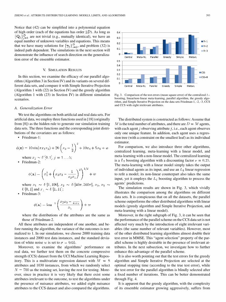
Fig. 3. Comparison of the test errors (mean square error) of the centralized �boosting, linear/non-linear meta-learning, parallel algorithm, the greedy algo-rithm, and Simple Iterative Projection on the data sets Friedman-1, -2, -3, CCSand CCS with eight irrelevant attributes.
The distributed system is constructed as follows: Assume thatis the total number of attributes, and there are agents,
with each agent observing attribute , i.e., each agent observesonly one unique feature. In addition, each agent uses a regres-sion tree (with a constraint on the smallest leaf) as its individualestimator.
For comparison, we also introduce three other algorithms,centralized learning, meta-learning with a linear model, andmeta-learning with a non-linear model. The centralized learningis a boosting algorithm with a discounting factor .The meta-learning with a linear model simply takes the outputof individual agents as its input, and use an linear regressionto refit a model; its non-linear counterpart also takes the sameinput, yet it employs the boosting algorithm to process theagents’ predictions.
The simulation results are shown in Fig. 3, which vividlyillustrates the comparison among the algorithms on differentdata sets. It is conspicuous that on all the datasets, the parallelscheme outperforms the other distributed algorithms with linearmodels (greedy algorithm and Simple Iterative Projection, andmeta-learning with a linear model).
Moreover, in the right subgraph of Fig. 3, it can be seen thatthe performance of the parallel scheme on the CCS data set is notaffected very much by the introduction of eight irrelevant vari-ables (the same number of relevant variables). However, mostof the other distributed learning algorithms almost double theirtest error in MMSE. This “agent selection” property of the par-allel scheme is highly desirable in the presence of irrelevant at-tributes. In the next subsection, we investigate how to furtherenhance this advantage of the parallel scheme.
It is also worth pointing out that the test errors for the greedyalgorithm and Simple Iterative Projection are selected at theoptimal stopping time (according to the true test error), whilethe test error for the parallel algorithm is blindly selected aftera fixed number of iterations. This can be better demonstratedthrough Fig. 4.
It is apparent that the greedy algorithm, with the complexityof its ensemble estimator growing aggressively, suffers from
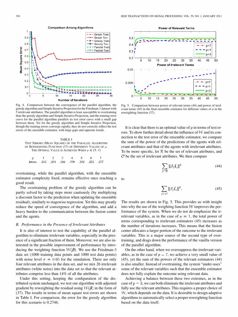
394 IEEE TRANSACTIONS ON SIGNAL PROCESSING, VOL. 59, NO. 1, JANUARY 2011
Fig. 4. Comparison between the convergence of the parallel algorithm, thegreedy algorithm and Simple Iterative Projection for the Friedman-1 dataset with5 irrelevant attributes. The parallel algorithm is least susceptible to overtrainingthan the greedy algorithm and Simple Iterative Projection, and the training errorcurve for the parallel algorithm parallels its test error curve with a small gapbetween them. Yet for the greedy algorithm and Simple Iterative Projection,though the training errors converge rapidly, they do not correctly reflect the testerrors of the ensemble estimator, with large gaps and opposite trends.
TABLE ITEST ERRORS (MEAN SQUARE) OF THE PARALLEL ALGORITHM
OF REWEIGHTING FUNCTION (37) OF DIFFERENT VALUES OF �.THE OPTIMAL VALUE IS ACHIEVED WHEN � � ��� ��
overtraining, while the parallel algorithm, with the ensembleestimator complexity fixed, remains effective once reaching agood result.
The overtraining problem of the greedy algorithm can bepartly solved by taking steps more cautiously (by multiplyinga discount factor to the prediction when updating the ensembleresidual), similarly to stagewise regression. Yet this may greatlyreduce the speed of convergence of the algorithm, and add aheavy burden to the communication between the fusion centerand the agents.
B. Performance in the Presence of Irrelevant Attributes
It is also of interest to test the capability of the parallel al-gorithm to eliminate irrelevant variables, especially in the pres-ence of a significant fraction of them. Moreover, we are also in-terested in the possible improvement of performance by intro-ducing the weighting function . We use the Friedman-3data set (1000 training data points and 1000 test data points)with noise level for the simulation. There are onlyfour relevant attributes in the data set, and we mix 26 irrelevantattributes (white noise) into the data set so that the relevant at-tributes comprise less than 14% of all the attributes.
Under this setting, keeping the configuration of the dis-tributed system unchanged, we test our algorithm with adjustedgradient by reweighting the residual using in the form of(37). The results in terms of mean square test errors are shownin Table I. For comparison, the error for the greedy algorithmfor this scenario is 0.2746.
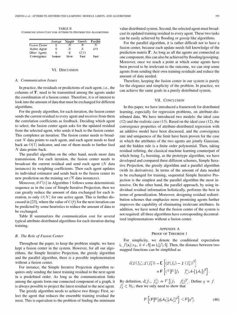
Fig. 5. Comparison between power of relevant terms (44) and power of irrel-evant terms (45) in the final ensemble estimator for different values of � in thereweighting function (37).
It is clear that there is an optimal value of in terms of test er-rors. To show further detail about the influence of and its con-nection to the test error of the ensemble estimator, we comparethe sum of the power of the predictions of the agents with rel-evant attributes and that of the agents with irrelevant attributes.To be more specific, let be the set of relevant attributes, and
be the set of irrelevant attributes. We then compare
(44)
to
(45)
The results are shown in Fig. 5. This provides us with insightinto why the use of the weighting function improves the per-formance of the system. When we do not de-emphasize the ir-relevant variables, as in the case of , the total power ofterms corresponding to irrelevant estimators (45) increases asthe number of iterations increases. This means that the fusioncenter allocates a larger portion of the outcome to the irrelevantvariables. This is a major source of the second type of over-training, and drags down the performance of the vanilla versionof the parallel algorithm.
On the other hand, when we oversuppress the irrelevant vari-ables, as in the case of , we achieve a very small value of(45), yet the sum of the powers of the relevant estimators (44)is also smaller. Instead of overtraining, the system “under-uses”some of the relevant variables such that the ensemble estimatordoes not fully explain the outcome using relevant data.
Achieving a balance between these two extremes, as in thecase of , we can both eliminate the irrelevant attributes andfully use the relevant attributes. This requires a proper choice of
, which depends on the data. It is desirable to design adaptivealgorithms to automatically select a proper reweighting functionbased on the data itself.
ZHENG et al.: ATTRIBUTE-DISTRIBUTED LEARNING: MODELS, LIMITS, AND ALGORITHMS 395
TABLE IICOMMUNICATION COST FOR ATTRIBUTE-DISTRIBUTED ALGORITHMS
VI. DISCUSSION
A. Communication Issues
In practice, the residuals or predictions of each agent, i.e., thecolumns of , need to be transmitted among the agents underthe coordination of a fusion center. Therefore, it is of interest tolook into the amount of data that must be exchanged for differentalgorithms.
For the greedy algorithm, for each iteration, the fusion centersends the current residual to every agent and receives from themthe correlation coefficients as feedback. Deciding which agentto select, the fusion center again asks for the updated residualfrom the selected agent, who sends it back to the fusion center.This completes an iteration. The fusion center needs to broad-cast data points to each agent, and each agent needs to feedback an indicator, and one of them needs to further feed
data points back.The parallel algorithm on the other hand, needs more data
transmission. For each iteration, the fusion center needs tobroadcast the current residual and send each agent ( datainstances) its weighting coefficients. Then each agent updatesits individual estimator and sends back to the fusion center itsnew prediction on the training set ( data instances).
Moreover, if in Algorithm 1 follows some deterministicsequence as in the case of Simple Iterative Projection, then wecan greatly reduce the amount of data exchanged for each it-eration, to only for one active agent. This is further dis-cussed in [23], where the value of for the next iteration canbe predicted by some heuristics to reduce the amount of data tobe exchanged.
Table II summarizes the communication cost for severaltypical attribute-distributed algorithms for each iteration duringtraining.
B. The Role of Fusion Center
Throughout the paper, to keep the problem simple, we havekept a fusion center in the system. However, for all our algo-rithms, the Simple Iterative Projection, the greedy algorithmand the parallel algorithm, there is a possible implementationwithout a fusion center.
For instance, the Simple Iterative Projection algorithm re-quires only sending the latest training residual to the next agentin a predefined order. As long as the communication linksamong the agents form one connected component of a graph, itis always possible to project the latest residual to the next agent.
The greedy algorithm needs to achieve two things: First, se-lect the agent that reduces the ensemble training residual themost. This is equivalent to the problem of finding the minimum
value distributed system. Second, the selected agent must broad-cast its updated training residual to every agent. These two taskscan be easily achieved by flooding or gossip like algorithms.
For the parallel algorithm, it is rather difficult not to have afusion center, because each update needs full knowledge of theprediction matrix . As long as all the agents are connected asone component, this can also be achieved by flooding/gossiping.Moreover, once we reach a point at which some agents havebeen proved to be irrelevant to the outcome, we can stop someagents from sending their own training residuals and reduce theamount of data needed.
Therefore, keeping the fusion center in our system is purelyfor the elegance and simplicity of the problem. In practice, wecan achieve the same goals in a purely distributed system.
VII. CONCLUSION
In this paper, we have introduced a framework for distributedlearning, especially for regression problems, on attribute-dis-tributed data. We have introduced two models: the ideal case(12) and the realistic case (13). Based on the ideal case (12), theconvergence properties of attribute-distributed regression withan additive model have been discussed, and the convergencerate and uniqueness of the limit have been proven for the casein which the attributes of the two agents are jointly Gaussian,and the hidden rule is a finite order polynomial. Then, takingresidual refitting, the classical machine learning counterpart ofwhich being boosting, as the prototype algorithm, we havedeveloped and compared three different schemes, Simple Itera-tive Projection, the greedy algorithm and a parallel algorithm(with its derivatives). In terms of the amount of data neededto be exchanged for training, sequential Simple Iterative Pro-jection is the simplest and the parallel algorithm the most in-tensive. On the other hand, the parallel approach, by using in-dividual residual information holistically, performs the best interms of generalization. Moreover, designing residual redistri-bution schemes that emphasize more promising agents furtherimproves the capability of eliminating irrelevant attributes. Inaddition, we have noted that the fusion center of the system isnot required: all three algorithms have corresponding decentral-ized implementations without a fusion center.
APPENDIX APROOF OF THEOREM 1
For simplicity, we denote the conditional expectationas . Then, the distance between two
mapped functions can be simplified as
By definition, . Define; then we only need to show that
(46)
396 IEEE TRANSACTIONS ON SIGNAL PROCESSING, VOL. 59, NO. 1, JANUARY 2011
Define , then . Notice thefact
equation (46) is then equivalent to
(47)
of which the left-hand side satisfies
The inequality step is due to Jensen’s inequality, and the laststep is due to the tower property.
On noting that
(48)
we hence have that the left-hand side satisfies
LHS
Moreover, the right-hand side of (47) satisfies
RHS
On noting an important relationship
(49)
we hence have
RHS LHS LHS (50)
Equation (50) guarantees that map is a non-expansive map.
APPENDIX BPROOF OF THEOREM 2
Lemma: Suppose is a polynomial of order ,, and is given by
Then, with the additional assumption that, we have the inequality
where , , and are all probability densities derivedfrom the joint Gaussian distribution with zero mean, unit vari-ance and correlation .
Proof: The conditional distribution of given and thedistribution of given are, respectively,
and Therefore, we have
Notice that the exponential term, with proper manipulation, canbe expressed in the form of the sum of Hermite polynomials.Thus, on defining
we have
Then the expression of can be rewritten as
Therefore, we have a closed-form expression for , whichis also an -order polynomial:
It is straight forward to derive that
and
Moreover, since is of zero mean,
ZHENG et al.: ATTRIBUTE-DISTRIBUTED LEARNING: MODELS, LIMITS, AND ALGORITHMS 397
Therefore,
If the hidden rule is restricted to a bivariate polyno-mial with finite order and zero mean, and andare both initialized as 0, then after each iteration, and
will remain in the space of zero-mean polynomials offinite order . If we define the distance between two polyno-mials and as , then, according to theabove lemma, the map that converts to is a con-tractive map.
APPENDIX CDERIVATION OF THE GRADIENT (34)
Given the expression for weighting coefficients
(51)
and the objective function
(52)
we have
REFERENCES
[1] J. Basak and R. Kothari, A Classification Paradigm for Distributed Ver-tically Partitioned Data. Cambridge, MA: MIT Press, 2004, vol. 16,pp. 1525–1544.
[2] P. Buhlmann and B. Yu, “Boosting with the l2-loss: Regression andclassification,” J. Amer. Statist. Assoc., vol. 98, pp. 324–339, 2003.
[3] P. Chan and S. J. Stolfo, “Experiments in multistrategy learning bymeta-learning,” in Proc. 2nd Int. Conf. Information Knowledge Man-agement, Washington, DC, 1993, pp. 314–323.
[4] P. Chan and S. J. Stolfo, “Toward parallel and distributed learning bymeta-learning,” in Working Notes of the AAAI Workshop, KnowledgeDiscovery in Databases, Washington, DC, 1993, pp. 227–240.
[5] E. Dellis, B. Seeger, and A. Vlachou, “Nearest neighbor search on ver-tically partitioned high-dimensional data,” in Proc. 7th Int. Conf. DataWarehousing and Knowledge Discovery, Copenhagen, Denmark, Aug.2005, pp. 243–253.
[6] W. Fang and B. Yang, “Privacy preserving decision tree learning oververtically partitioned data,” in Proc. 2008 Int. Conf. Computer Scienceand Software Engineering, Washington, DC, 2008, pp. 1049–1052.
[7] J. H. Friedman, “Greedy function approximation: A gradient boostingmachine,” Ann. Statist., vol. 29, pp. 1189–1232, 2000.
[8] J. H. Friedman, E. Grosse, and W. Stuetzle, “Multidimensional additivespline approximation,” SIAM J. Scientif. Statist. Comput., vol. 4, no. 2,pp. 291–301, 1983.
[9] D. E. Hershberger and H. Kargupta, “Distributed multivariate regres-sion using wavelet-based collective data mining,” J. Parallel Distrib.Comput., vol. 61, no. 3, pp. 372–400, 2001.
[10] G. Jagannathan and R. N. Wright, “Privacy-preserving distributedk-means clustering over arbitrarily partitioned data,” in Proc. 11thACM SIGKDD Int. Conf. Knowledge Discovery Data Mining, NewYork, 2005, pp. 593–599.
[11] H. Kargupta, E. Johnson, E. R. Sanseverino, B. H. Park, L. D. Sil-vestre, and D. Hershberger, “Collective data mining from distributedvertically partitioned feature space,” in Proc. Workshop on DistributedData Mining, New York, 1998, pp. 70–91.
[12] H. Kargupta, B. Park, D. Hershberger, and E. Johnson, “Collectivedata mining: A new perspective toward distributed data mining,” inAdvances in Distributed and Parallel Knowledge Discovery. Cam-bridge, MA: AAAI/MIT Press, 1999, pp. 133–184.
[13] O. L. Mangasarian, E. W. Wild, and G. M. Fung, “Privacy-preservingclassification of vertically partitioned data via random kernels,” ACMTrans. Knowl. Discov. Data, vol. 2, no. 3, pp. 1–16, 2008.
[14] S. McConnell and D. B. Skillicorn, “Building predictors from verticallydistributed data,” in Proc. 2004 Conf. Centre for Advanced Studies onCollaborative Research, Markham, ON, Canada, 2004, pp. 150–162.
[15] S. Merugu and J. Ghosh, “A distributed learning framework for hetero-geneous data sources,” in Proc. 11th ACM SIGKDD Int. Conf. Knowl-edge Discovery Data Mining, Chicago, IL, Aug. 2005, pp. 208–217.
[16] J. B. Predd, “Topics in distributed inference,” Ph.D. dissertation, Elect.Eng. Dept., Princeton Univ., Princeton, NJ, 2006.
[17] J. B. Predd, S. B. Kulkarni, and H. V. Poor, “Distributed learning inwireless sensor networks,” IEEE Signal Process. Mag., vol. 23, no. 4,pp. 56–69, Jul. 2006.
[18] G. Ridgeway, D. Madigan, and T. Richardson, “Boosting methodologyfor regression problems,” in Proc. 7th Int. Workshop Artificial Intelli-gence Statistics, Fort Lauderdale, FL, 1999, pp. 152–161.
[19] D. Shutin, H. Zheng, B. H. Fleury, S. R. Kulkarni, and H. V. Poor,“Space-alternating attribute-distributed sparse learning,” in Proc. 2ndInt. Workshop Cognitive Information Processing, Elba, Italy, Jun. 2010.
[20] R. Tibshirani, “Regression shrinkage and selection via the lasso,” J.Roy. Statist. Soc., Series B, vol. 58, pp. 267–288, 1994.
[21] J. Vaidya and C. Clifton, “Privacy-preserving �-means clustering oververtically partitioned data,” in Proc. 9th Int. Conf. Knowledge Dis-covery Data Mining, New York, 2003, pp. 206–215.
[22] J. Vaidya, C. Clifton, M. Kantarcioglu, and A. S. Patterson, “Privacy-preserving decision trees over vertically partitioned data,” ACM Trans.Knowl. Discov. Data, vol. 2, no. 3, pp. 1–27, 2008.
[23] J. Vaidya, H. Yu, and X. Jiang, “Privacy-preserving SVM classifica-tion,” Knowl. Inf. Syst., vol. 14, no. 2, pp. 161–178, 2008.
[24] Z. Yang and R. N. Wright, “Improved privacy-preserving Bayesian net-work parameter learning on vertically partitioned data,” in Proc. 21stInt. Conf. Data Engineering Workshops (ICDEW), Washington, DC,2005, pp. 1196–1196.
[25] Z. Yang and R. N. Wright, “Privacy-preserving computation ofBayesian networks on vertically partitioned data,” IEEE Trans. Knowl.Data Eng., vol. 18, no. 9, pp. 1253–1264, 2006.
[26] H. Zheng, S. R. Kulkarni, and H. V. Poor, “Dimensionally distributedlearning: Models and algorithm,” in Proc. 11th Int. Conf. InformationFusion, Cologne, Germany, Jul. 2008, pp. 1–8.
[27] H. Zheng, S. R. Kulkarni, and H. V. Poor, “Cooperative training for at-tribute-distributed data: Trade-off between data transmission and per-formance,” in Proc. 12th Int. Conf. Information Fusion, Seattle, WA,Jul. 2009, pp. 664–671.
[28] H. Zheng, S. R. Kulkarni, and H. V. Poor, “Agent selection for regres-sion on attribute distributed data,” in Proc. 35th IEEE Int. Conf. Acous-tics, Speech, Signal Processing, Dallas, TX, Mar. 2010.
398 IEEE TRANSACTIONS ON SIGNAL PROCESSING, VOL. 59, NO. 1, JANUARY 2011
Haipeng Zheng received the B.Eng. degree from Ts-inghua University, Beijing, China, in 2006 and theM.A. degree from Princeton University, Princeton,NJ, in 2008, both in electrical engineering. He is cur-rently working towards the Ph.D. degree in electricalengineering at Princeton University.
His research interests include statistical learning/inference on distributed system, robust shape recon-struction, multiuser precoding, and intelligent trans-portation.
Sanjeev R. Kulkarni (M’91–SM’96–F’04) receivedthe B.S. degree in mathematics and the B.S. inelectrical engineering and the M.S. degree in math-ematics from Clarkson University, Potsdam, NY, in1983, 1984, and 1985, respectively; the M.S. degreein electrical engineering from Stanford University,Stanford, CA, in 1985; and the Ph.D. degree in elec-trical engineering from the Massachusetts Instituteof Technology (MIT), Cambridge, in 1991.
From 1985 to 1991, he was a Member of the Tech-nical Staff at the MIT Lincoln Laboratory, Lexington,
MA, working on the modeling and processing of laser radar measurements. Inspring 1986, he was a part-time faculty member at the University of Massa-chusetts, Boston. Since 1991, he has been with Princeton University, Princeton,NJ, where he is currently Professor of Electrical Engineering and an affiliatedfaculty member in the Department of Operations Research and Financial Engi-neering and the Department of Philosophy. He spent January 1996 as a ResearchFellow at the Australian National University, 1998 with Susquehanna Interna-tional Group, and summer 2001 with Flarion Technologies. His research inter-ests include statistical pattern recognition, nonparametric estimation, learningand adaptive systems, information theory, wireless networks, and image/videoprocessing.
Prof. Kulkarni received an ARO Young Investigator Award in 1992, an NSFYoung Investigator Award in 1994, and several teaching awards at PrincetonUniversity. He has served as an Associate Editor for the IEEE TRANSACTIONS
ON INFORMATION THEORY.
H. Vincent Poor (S’72–M’77–SM’82–F’87) re-ceived the Ph.D. degree in electrical engineeringand computer science from Princeton University,Princeton, NJ, in 1977.
From 1977 until 1990, he was on the faculty ofthe University of Illinois at Urbana-Champaign.Since 1990, he has been on the faculty of PrincetonUniversity, where he is the Dean of Engineeringand Applied Science, and the Michael Henry StraterUniversity Professor of Electrical Engineering.His research interests are in the areas of stochastic
analysis, statistical signal processing, and information theory, and their ap-plications in wireless networks and related fields. Among his publications inthese areas are the recent books Quickest Detection (Cambridge Univ. Press,2009), coauthored with O. Hadjiliadis, and Information Theoretic Security(Now Publishers, 2009), coauthored with Y. Liang and S. Shamai.
Dr. Poor is a member of the National Academy of Engineering, a Fellow ofthe American Academy of Arts and Sciences, and an International Fellow ofthe Royal Academy of Engineering of the United Kingdom. He is also a Fellowof the Institute of Mathematical Statistics, the Optical Society of America, andother organizations. In 1990, he served as President of the IEEE InformationTheory Society, and from 2004 to 2007 as the Editor-in-Chief of the IEEETRANSACTIONS ON INFORMATION THEORY. He was the recipient of the 2005IEEE Education Medal. Recent recognition of his work includes the 2009 EdwinHoward Armstrong Achievement Award of the IEEE Communications Society,the 2010 IET Ambrose Fleming Medal for Achievement in Communications,and the 2011 IEEE Eric E. Sumner Award.
Related Documents