Attitude Determination and RTK Performances Amelioration ...

HAL Id: hal-02984329https://hal-enac.archives-ouvertes.fr/hal-02984329v2

Submitted on 3 Mar 2021

HAL is a multi-disciplinary open accessarchive for the deposit and dissemination of sci-entific research documents, whether they are pub-lished or not. The documents may come fromteaching and research institutions in France orabroad, or from public or private research centers.

L’archive ouverte pluridisciplinaire HAL, estdestinée au dépôt et à la diffusion de documentsscientifiques de niveau recherche, publiés ou non,émanant des établissements d’enseignement et derecherche français ou étrangers, des laboratoirespublics ou privés.

Attitude Determination and RTK PerformancesAmelioration Using Multiple Low-Cost Receivers with

Known GeometryXiao Hu, Paul Thevenon, Christophe Macabiau

To cite this version:Xiao Hu, Paul Thevenon, Christophe Macabiau. Attitude Determination and RTK PerformancesAmelioration Using Multiple Low-Cost Receivers with Known Geometry. ION ITM 2021, Inter-national Technical Meeting, Jan 2021, Virtual event, France. pp. 439-453, �10.33012/2021.17841�.�hal-02984329v2�

https://hal-enac.archives-ouvertes.fr/hal-02984329v2

https://hal.archives-ouvertes.fr

Attitude Determination and RTK Performances

Amelioration Using Multiple Low-Cost Receivers

with Known Geometry

Xiao Hu, Paul Thevenon, Christophe Macabiau, ENAC, Université de Toulouse, France

BIOGRAPHY

Xiao Hu graduated as electronic engineer in digital communications and received the M.S. double degree in Navigation and

Telecommunications from the French Civil Aviation University (ENAC), in Toulouse, France, in 2017. Since 2017, he is a Ph.D.

student within the SIGnal processing and NAVigation (SIGNAV) research group of the TELECOM laboratory inside ENAC.

His current research interests focus on Precise GNSS Positioning and hybridization of GNSS with other sensors. Dr. Paul Thevenon graduated as electronic engineer from Ecole Centrale de Lille in 2004 and obtained in 2007 a research

master at ISAE in space telecommunications. In 2010, he obtained a PhD degree in the signal processing laboratory of ENAC in

Toulouse, France. From 2010 to 2013, he was employed by CNES, to supervise GNSS research activities. Since the July 2013,

he is employed by ENAC as Assistant Professor. His current activities are GNSS signal processing, GNSS integrity monitoring

and hybridization of GNSS with other sensors. Dr. Christophe Macabiau graduated as electronics engineer in 1992 from the ENAC (Ecole Nationale de l’Aviation Civile) in

Toulouse, France. Since 1994, he has been working on the application of satellite navigation techniques to civil aviation. He

received his Ph.D in 1997 and has been in charge of the signal processing lab of ENAC since 2000, where he also started dealing

with navigation techniques for urban navigation. He is currently the head of the TELECOM team of ENAC, that includes research

groups on signal processing and navigation, electromagnetics, and data communication networks.

ABSTRACT

Precise positioning with a stand-alone GPS receiver or using differential corrections is known to be strongly degraded in a

constrained environment (urban or sub-urban conditions) due to frequent signal masking, strong multipath effect, frequent cycle

slips on carrier phase, etc. The objective of this work is to explore the possibility of achieving precise positioning with a low-

cost architecture: using multiple low-cost receivers with known geometry to enable the vehicle attitude determination and RTK

performance amelioration. In this paper, we firstly use a method that includes an array of receivers with known geometry to

enhance the performance of the RTK in different environments. Taking advantage of the attitude information and the known

geometry of the array of receivers, the improvement of some internal steps of RTK precise positioning can be realized. This

concept is tested on real data sets, where different scenarios are conducted including varying the distance between the 2 antennas

of the receiver array and the environmental conditions (open sky, suburban, and constrained urban environments). The results

show that our multi-receiver RTK system is more robust to degraded GNSS environment in terms of ambiguity fixing rate and

gets a better position accuracy under the same conditions when comparing with the single receiver system.

INTRODUCTION

The concept of autonomous driving has become more and more a central topic for the automobile industry, where a precise

position and attitude information is essential for this kind of application. Over the past decade, the universal GNSS has been

dramatically utilized in various domains, such as aviation, marine, precise agriculture, geodesy and surveying, automotive, etc.

However, the accuracy or integrity that a low-cost GNSS receiver can provide in a constrained urban or indoor environment is

far from satisfactory for applications where decimeter or centimeter accuracy and error bounds are mostly envisioned. To reach

this level of accuracy, techniques using raw carrier phase measurements have been developed. Carrier phase measurements are

more precise than code measurements by a factor of a hundred [1]. Nevertheless, they are also less robust and include a so-called

integer ambiguity that requires to implement a specific integer ambiguity resolution (IAR) process in order to use them for

positioning. In some harsh environments, severe multipath and losses of lock of the receiver tracking loops create carrier cycle

slips, which result in sudden changes of these ambiguities. If not detected, the cycle slips will create a bias on the carrier pseudo-

range measurement resulting in a reduction of position accuracy. Even if detected, the IAR process has to be, at least partially,

re-initialized, leading also to a loss of positioning accuracy. To increase confidence and accelerate the IAR process by limiting

the search space, restrictions can be established from the use of an array of two or more receivers with prior known and fixed

geometry which includes the length of the baseline vectors between the antennas of the receiver array and the orientation of the

vectors. In recent years, several studies have focused on the use of an array of receivers for attitude determination [2], Gabrielle et al.[3]

studies the viability of attitude determination by using a new ambiguity-attitude estimator which improves the probability of

successful integer ambiguity resolution. Nonetheless, the improvement of RTK positioning performance was not studied. Daniel

et al. [4] developed a method for the recursive estimation of the positioning and attitude problems using GNSS carrier phase

observations from an array of receivers, but they calculated the position of each receiver separately thus they did not take

advantage of the known geometry. Farhad et al.[5] used an adaptive KF for 3-dimensional attitude determination and position

estimation of a mobile robot by fusing the information from a system of two RTK GPSs and an IMU, however, they also did not

consider the known geometry of the receiver as a constraint to help improve the positioning performance. Zheng et al. [6]

presented a methodology for integrating carrier phase attitude determination and positioning systems by considering one of the

receiver pairs in the attitude determination system also used as the rover for the relative positioning system. Nevertheless, their

attitude determination and positioning systems remained independent which did not much ameliorate the success rate of IAR for

the RTK. Khodabandeh et al. [7] introduced a concept of array-based between-satellite single difference satellite phase biases

determination to accelerate the single-receiver IAR, but they did not take into consideration the attitude information of the vehicle

which cannot analyze the influence with attitude consideration. Peirong Fan et al.[8] proposed a dual-antenna constraint RTK

algorithm to improve the system AR success rate, which combines GNSS measurements of both antennas by making use of the

baseline vector constraint between them. However, the attitude information of the vehicle is still not taken into account. To the author’s best knowledge, very few publications can be found that address the use of an array of receivers to improve the

accuracy of the array position or for some internal steps of precise position computation for RTK processing with vehicle attitude

determination, such as cycle slip detection or integer ambiguity resolution. The objective of this contribution is then to explore

the possibility of achieving precise positioning with a low-cost architecture: using multiple low-cost receivers with known

geometry to enable the vehicle attitude determination and RTK performances amelioration. The concept of RTK positioning

using an array of GNSS receivers has already been introduced in our previous work [9]. In [10], we discussed the improvement

of cycle-slip detection and repair for RTK processing by using an array of two receivers with known geometry.

In this paper, while we refer to our earlier work, the focus is different. In both our previous contributions, the proposed precise

position and attitude determination algorithm was verified with only simulated measurements to enable the conduction of several

specific comparison scenarios between our multi-receiver system and the traditional single receiver system. The present paper is

the extension and improvement of our previous work, which aims at validating its application to actual situations by using the

real measurement collected from different environments with different length of array antenna baselines, in terms of the

positioning accuracy, the fixing rate, and the attitude determination accuracy.

SYSTEM GEOMETRY AND CONFIGURATION

With the intention of performing precise attitude estimation, a dual antenna set-up has been considered, where two GNSS

antennas with a known baseline length are mounted on the vehicle's rooftop to get an attitude estimation. Furthermore, the

absolute position accuracy is augmented using the real-time kinematics (RTK) approach, in which the vehicle is positioned

relative to a third receiver as the virtual reference station (VRS), whose position is static and known. By knowing the position

of the VRS, the vehicle can be positioned absolutely, too. In the positioning algorithm, we strongly rely on carrier phase

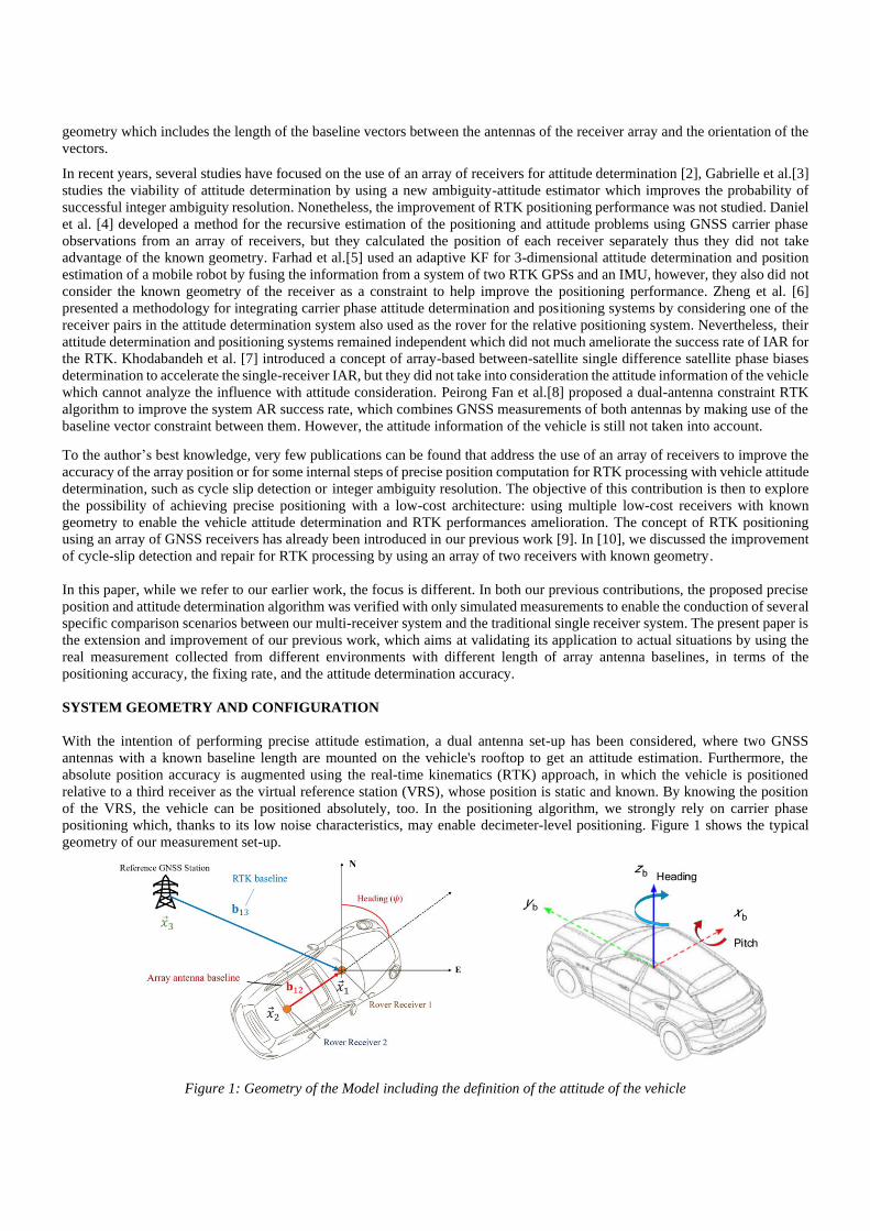
positioning which, thanks to its low noise characteristics, may enable decimeter-level positioning. Figure 1 shows the typical

geometry of our measurement set-up.

Figure 1: Geometry of the Model including the definition of the attitude of the vehicle

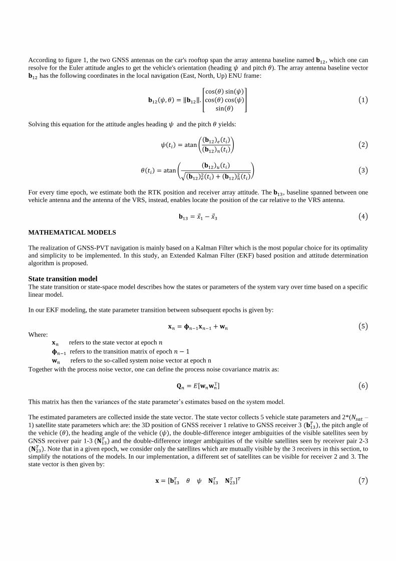
https://www.wordhippo.com/what-is/another-word-for/with_the_intention_of.html

According to figure 1, the two GNSS antennas on the car's rooftop span the array antenna baseline named 𝐛12, which one can

resolve for the Euler attitude angles to get the vehicle's orientation (heading 𝜓 and pitch 𝜃). The array antenna baseline vector

𝐛12 has the following coordinates in the local navigation (East, North, Up) ENU frame:

𝐛12(𝜓, 𝜃) = ‖𝐛12‖. [

cos(𝜃) sin(𝜓)

cos(𝜃) cos(𝜓)

sin(𝜃)] (1)

Solving this equation for the attitude angles heading 𝜓 and the pitch 𝜃 yields:

𝜓(𝑡𝑖) = atan ((𝐛12)𝑒(𝑡𝑖)

(𝐛12)𝑛(𝑡𝑖)) (2)

𝜃(𝑡𝑖) = atan ((𝐛12)𝑢(𝑡𝑖)

√(𝐛12)𝑒2(𝑡𝑖) + (𝐛12)𝑛

2(𝑡𝑖)) (3)

For every time epoch, we estimate both the RTK position and receiver array attitude. The 𝐛13, baseline spanned between one

vehicle antenna and the antenna of the VRS, instead, enables locate the position of the car relative to the VRS antenna.

𝐛13 = �⃗�1 − �⃗�3 (4)

MATHEMATICAL MODELS

The realization of GNSS-PVT navigation is mainly based on a Kalman Filter which is the most popular choice for its optimality

and simplicity to be implemented. In this study, an Extended Kalman Filter (EKF) based position and attitude determination

algorithm is proposed.

State transition model The state transition or state-space model describes how the states or parameters of the system vary over time based on a specific

linear model.

In our EKF modeling, the state parameter transition between subsequent epochs is given by:

𝐱𝑛 = 𝛟𝑛−1𝐱𝑛−1 + 𝐰𝑛 (5)

Where:

𝐱𝑛 refers to the state vector at epoch 𝑛

𝛟𝑛−1 refers to the transition matrix of epoch 𝑛 − 1

𝐰𝑛 refers to the so-called system noise vector at epoch n

Together with the process noise vector, one can define the process noise covariance matrix as:

𝐐𝑛 = 𝐸[𝐰𝑛𝐰𝑛T] (6)

This matrix has then the variances of the state parameter’s estimates based on the system model.

The estimated parameters are collected inside the state vector. The state vector collects 5 vehicle state parameters and 2*(𝑁𝑠𝑎𝑡 –

1) satellite state parameters which are: the 3D position of GNSS receiver 1 relative to GNSS receiver 3 (𝐛13𝑇 ), the pitch angle of

the vehicle (𝜃), the heading angle of the vehicle (𝜓), the double-difference integer ambiguities of the visible satellites seen by

GNSS receiver pair 1-3 (𝐍13𝑇 ) and the double-difference integer ambiguities of the visible satellites seen by receiver pair 2-3

(𝐍23𝑇 ). Note that in a given epoch, we consider only the satellites which are mutually visible by the 3 receivers in this section, to

simplify the notations of the models. In our implementation, a different set of satellites can be visible for receiver 2 and 3. The

state vector is then given by:

𝐱 = [𝐛13𝑇 𝜃 𝜓 𝐍13

𝑇 𝐍23𝑇 ]𝑇 (7)

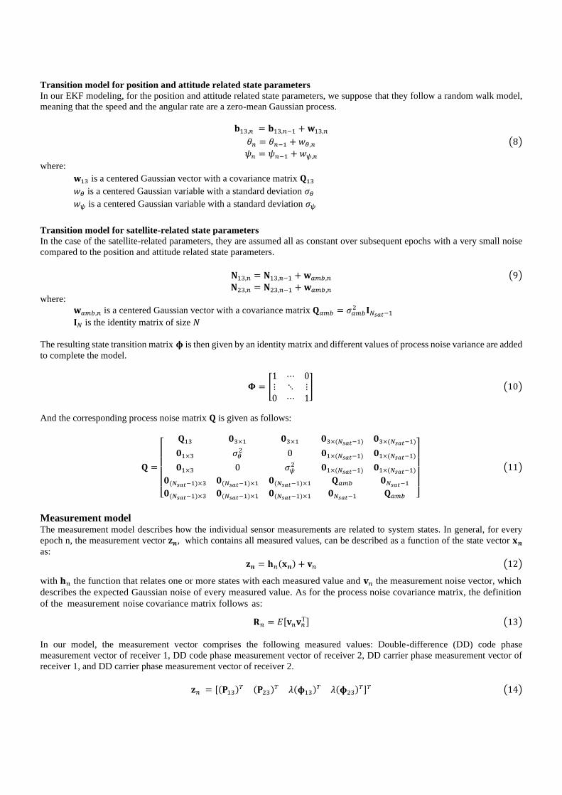
Transition model for position and attitude related state parameters

In our EKF modeling, for the position and attitude related state parameters, we suppose that they follow a random walk model,

meaning that the speed and the angular rate are a zero-mean Gaussian process.

𝐛13,𝑛 = 𝐛13,𝑛−1 + 𝐰13,𝑛

𝜃𝑛 = 𝜃𝑛−1 + 𝑤𝜃,𝑛 (8)

𝜓𝑛 = 𝜓𝑛−1 + 𝑤𝜓,𝑛

where:

𝐰13 is a centered Gaussian vector with a covariance matrix 𝐐13

𝑤𝜃 is a centered Gaussian variable with a standard deviation 𝜎𝜃

𝑤𝜓 is a centered Gaussian variable with a standard deviation 𝜎𝜓

Transition model for satellite-related state parameters

In the case of the satellite-related parameters, they are assumed all as constant over subsequent epochs with a very small noise

compared to the position and attitude related state parameters.

𝐍13,𝑛 = 𝐍13,𝑛−1 + 𝐰𝑎𝑚𝑏,𝑛 (9)

𝐍23,𝑛 = 𝐍23,𝑛−1 + 𝐰𝑎𝑚𝑏,𝑛

where:

𝐰𝑎𝑚𝑏,𝑛 is a centered Gaussian vector with a covariance matrix 𝐐𝑎𝑚𝑏 = 𝜎𝑎𝑚𝑏2 𝐈𝑁𝑠𝑎𝑡−1

𝐈𝑁 is the identity matrix of size 𝑁

The resulting state transition matrix 𝛟 is then given by an identity matrix and different values of process noise variance are added

to complete the model.

𝚽 = [1 ⋯ 0⋮ ⋱ ⋮0 ⋯ 1

] (10)

And the corresponding process noise matrix 𝐐 is given as follows:

𝐐 =

[

𝐐13 𝟎3×1 𝟎3×1 𝟎3×(𝑁𝑠𝑎𝑡−1) 𝟎3×(𝑁𝑠𝑎𝑡−1)

𝟎1×3 𝜎𝜃2 0 𝟎1×(𝑁𝑠𝑎𝑡−1) 𝟎1×(𝑁𝑠𝑎𝑡−1)

𝟎1×3 0 𝜎𝜓2 𝟎1×(𝑁𝑠𝑎𝑡−1) 𝟎1×(𝑁𝑠𝑎𝑡−1)

𝟎(𝑁𝑠𝑎𝑡−1)×3 𝟎(𝑁𝑠𝑎𝑡−1)×1 𝟎(𝑁𝑠𝑎𝑡−1)×1 𝐐𝑎𝑚𝑏 𝟎𝑁𝑠𝑎𝑡−1

𝟎(𝑁𝑠𝑎𝑡−1)×3 𝟎(𝑁𝑠𝑎𝑡−1)×1 𝟎(𝑁𝑠𝑎𝑡−1)×1 𝟎𝑁𝑠𝑎𝑡−1 𝐐𝑎𝑚𝑏 ]

(11)

Measurement model The measurement model describes how the individual sensor measurements are related to system states. In general, for every

epoch n, the measurement vector 𝐳𝒏, which contains all measured values, can be described as a function of the state vector 𝐱𝒏

as:

𝐳𝒏 = 𝐡𝑛(𝐱𝒏) + 𝐯𝑛 (12)

with 𝐡𝑛 the function that relates one or more states with each measured value and 𝐯𝑛 the measurement noise vector, which

describes the expected Gaussian noise of every measured value. As for the process noise covariance matrix, the definition

of the measurement noise covariance matrix follows as:

𝐑𝑛 = 𝐸[𝐯𝑛𝐯𝑛T] (13)

In our model, the measurement vector comprises the following measured values: Double-difference (DD) code phase

measurement vector of receiver 1, DD code phase measurement vector of receiver 2, DD carrier phase measurement vector of

receiver 1, and DD carrier phase measurement vector of receiver 2.

𝐳𝑛 = [(𝐏13)𝑇 (𝐏23)

𝑇 𝜆(𝛟13)𝑇 𝜆(𝛟23)

𝑇]𝑇 (14)

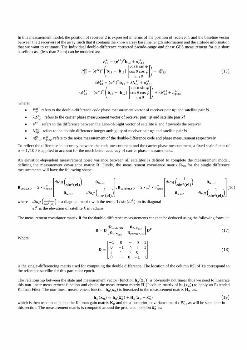
In this measurement model, the position of receiver 2 is expressed in terms of the position of receiver 1 and the baseline vector

between the 2 receivers of the array, such that it contains the known array baseline length information and the attitude information

that we want to estimate. The individual double-difference corrected pseudo-range and phase GPS measurement for our short

baseline case (less than 3 km) can be modeled as:

𝑃13𝑘𝑙 = (𝐞𝑘𝑙)𝑇𝐛13 + 𝑛𝑃,13

𝑘𝑙

𝑃23𝑘𝑙 = (𝐞𝑘𝑙)𝑇 (𝐛13 − |𝐛12| [

cos 𝜃 sin𝜓cos 𝜃 cos𝜓

sin 𝜃

]) + 𝑛𝑃,23𝑘𝑙 (15)

𝜆𝜙13

𝑘𝑙 = (𝐞𝑘𝑙)𝑇𝐛13 + 𝜆𝑁13𝑘𝑙 + 𝑛𝜙,13

𝑘𝑙

𝜆𝜙23𝑘𝑙 = (𝐞𝑘𝑙)𝑇 (𝐛13 − |𝐛12| [

cos 𝜃 sin𝜓cos 𝜃 cos𝜓

sin 𝜃

]) + 𝜆𝑁23𝑘𝑙 + 𝑛𝜙,23

𝑘𝑙

where:

• 𝑃𝑛𝑝𝑘𝑙 refers to the double-difference code phase measurement vector of receiver pair 𝑛𝑝 and satellite pair 𝑘𝑙

• 𝜆𝜙𝑛𝑝𝑘𝑙 refers to the carrier phase measurement vector of receiver pair 𝑛𝑝 and satellite pair 𝑘𝑙

• 𝐞𝑘𝑙 refers to the difference between the Line-of-Sight vector of satellite 𝑘 and l towards the receiver

• 𝑁𝑛𝑝𝑘𝑙 refers to the double-difference integer ambiguity of receiver pair 𝑛𝑝 and satellite pair 𝑘𝑙

• 𝑛𝑃,𝑛𝑝𝑘𝑙 , 𝑛𝜙,𝑛𝑝

𝑘𝑙 refers to the noise measurement of the double-difference code and phase measurement respectively

To reflect the difference in accuracy between the code measurement and the carrier phase measurement, a fixed scale factor of

𝑎 = 1/100 is applied to account for the much better accuracy of carrier phase measurements.

An elevation-dependent measurement noise variance between all satellites is defined to complete the measurement model,

defining the measurement covariance matrix 𝐑 . Firstly, the measurement covariance matrix 𝐑SD for the single difference

measurements will have the following shape:

𝐑code,SD = 2 ∗ 𝜎𝑐𝑜𝑑𝑒2

[ 𝑑𝑖𝑎𝑔 (

1

sin2(𝐞𝐥)) 𝟎𝑁𝑠𝑎𝑡

𝟎𝑁𝑠𝑎𝑡 𝑑𝑖𝑎𝑔 (1

sin2(𝐞𝐥))]

, 𝐑carrier,SD = 2 ∗ 𝑎2 ∗ 𝜎𝑐𝑜𝑑𝑒2

[ 𝑑𝑖𝑎𝑔 (

1

sin2(𝐞𝐥)) 𝟎𝑁𝑠𝑎𝑡

𝟎𝑁𝑠𝑎𝑡 𝑑𝑖𝑎𝑔 (1

sin2(𝐞𝐥))]

(16)

where 𝑑𝑖𝑎𝑔 (1

sin2(𝐞𝐥)) is a diagonal matrix with the terms 1/ sin(𝑒𝑙𝑘) on its diagonal

𝑒𝑙𝑘 is the elevation of satellite 𝑘 in radians

The measurement covariance matrix 𝐑 for the double-difference measurements can then be deduced using the following formula:

𝐑 = 𝐃 [𝐑code,SD 𝟎2∗𝑁𝑠𝑎𝑡

𝟎2∗𝑁𝑠𝑎𝑡𝐑carrier,SD

]𝐃𝑻 (17)

Where

𝑫 = [

−1 0 ⋯ 0 10 −1 ⋱ ⋮ 1⋮ ⋱ ⋱ 0 ⋮0 ⋯ 0 −1 1

] (18)

is the single-differencing matrix used for computing the double difference. The location of the column full of 1's correspond to

the reference satellite for this particular epoch.

The relationship between the state and measurement vector (function 𝐡𝑛(𝐱𝒏)) is obviously not linear thus we need to linearize this non-linear measurement function and obtain the measurement matrix H (Jacobian matrix of 𝐡𝑛(𝐱𝒏)) to apply an Extended Kalman Filter. The non-linear measurement function 𝐡𝑛(𝐱𝑛) is linearized to the measurement matrix 𝐇𝑛 as:

𝐡𝑛(𝐱𝑛) ≈ 𝐡𝑛(�̂�𝑛−) + 𝐇𝑛(𝐱𝑛 − �̂�𝑛

−) (19)

which is then used to calculate the Kalman gain matrix 𝐊𝑛 and the a-posteriori covariance matrix 𝐏𝑛+ , as will be seen later in

this section. The measurement matrix is computed around the predicted position �̂�𝑛− as:

𝐇𝑛|𝐱𝑛=�̂�𝑛− =

𝜕

𝜕𝐱𝑛

𝐡𝑛(𝐱𝑛)|𝐱𝑛=�̂�𝑛

−

(20)

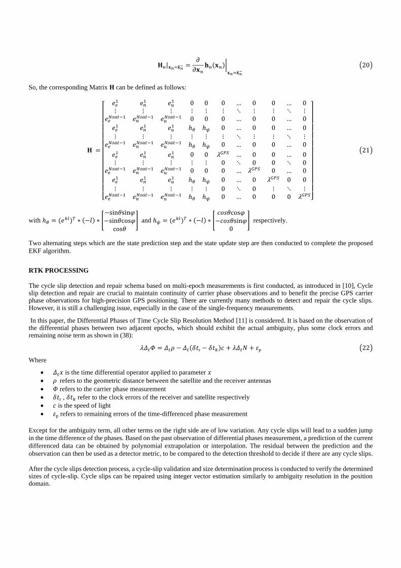
So, the corresponding Matrix 𝐇 can be defined as follows:

𝐇 =

[

𝑒𝑒1 𝑒𝑛

1 𝑒𝑢1 0 0 0 … 0 0 … 0

⋮ ⋮ ⋮ ⋮ ⋮ ⋮ ⋱ ⋮ ⋮ ⋱ ⋮𝑒𝑒

𝑁𝑠𝑎𝑡−1 𝑒𝑛𝑁𝑠𝑎𝑡−1 𝑒𝑢

𝑁𝑠𝑎𝑡−1 0 0 0 … 0 0 … 0

𝑒𝑒1 𝑒𝑛

1 𝑒𝑢1 ℎ𝜃 ℎ𝜓 0 … 0 0 … 0

⋮ ⋮ ⋮ ⋮ ⋮ ⋮ ⋱ ⋮ ⋮ ⋱ ⋮𝑒𝑒


𝑁𝑠𝑎𝑡−1 ℎ𝜃 ℎ𝜓 0 … 0 0 … 0

𝑒𝑒1 𝑒𝑛

1 𝑒𝑢1 0 0 𝜆𝐺𝑃𝑆 … 0 0 … 0

⋮ ⋮ ⋮ ⋮ ⋮ 0 ⋱ 0 0 ⋱ 0𝑒𝑒


𝑁𝑠𝑎𝑡−1 0 0 0 … 𝜆𝐺𝑃𝑆 0 … 0

𝑒𝑒1 𝑒𝑛

1 𝑒𝑢1 ℎ𝜃 ℎ𝜓 0 … 0 𝜆𝐺𝑃𝑆 0 0

⋮ ⋮ ⋮ ⋮ ⋮ 0 ⋱ 0 ⋮ ⋱ ⋮𝑒𝑒


𝑁𝑠𝑎𝑡−1 ℎ𝜃 ℎ𝜓 0 … 0 0 0 𝜆𝐺𝑃𝑆]

(21)

with ℎ𝜃 = (𝑒𝑘𝑙)𝑇 ∗ (−𝑙) ∗ [−sin𝜃sin𝜑−sin𝜃cos𝜑

cos𝜃

] and ℎ𝜓 = (𝑒𝑘𝑙)𝑇 ∗ (−𝑙) ∗ [𝑐𝑜𝑠𝜃cos𝜑−𝑐𝑜𝑠𝜃sin𝜑

0

] respectively.

Two alternating steps which are the state prediction step and the state update step are then conducted to complete the proposed

EKF algorithm.

RTK PROCESSING

The cycle slip detection and repair schema based on multi-epoch measurements is first conducted, as introduced in [10], Cycle slip detection and repair are crucial to maintain continuity of carrier phase observations and to benefit the precise GPS carrier phase observations for high-precision GPS positioning. There are currently many methods to detect and repair the cycle slips. However, it is still a challenging issue, especially in the case of the single-frequency measurements.

In this paper, the Differential Phases of Time Cycle Slip Resolution Method [11] is considered. It is based on the observation of the differential phases between two adjacent epochs, which should exhibit the actual ambiguity, plus some clock errors and remaining noise term as shown in (38):

𝜆𝛥𝑡𝛷 = 𝛥𝑡𝜌 − 𝛥𝑡(𝛿𝑡r − 𝛿𝑡𝑘)𝑐 + 𝜆𝛥𝑡𝑁 + 휀p (22)

Where

• 𝛥𝑡𝑥 is the time differential operator applied to parameter 𝑥

• 𝜌 refers to the geometric distance between the satellite and the receiver antennas

• 𝛷 refers to the carrier phase measurement

• 𝛿𝑡r , 𝛿𝑡𝑘 refer to the clock errors of the receiver and satellite respectively

• 𝑐 is the speed of light

• 휀p refers to remaining errors of the time-differenced phase measurement

Except for the ambiguity term, all other terms on the right side are of low variation. Any cycle slips will lead to a sudden jump

in the time difference of the phases. Based on the past observation of differential phases measurement, a prediction of the current

differenced data can be obtained by polynomial extrapolation or interpolation. The residual between the prediction and the

observation can then be used as a detector metric, to be compared to the detection threshold to decide if there are any cycle slips.

After the cycle slips detection process, a cycle-slip validation and size determination process is conducted to verify the determined sizes of cycle-slip. Cycle slips can be repaired using integer vector estimation similarly to ambiguity resolution in the position domain.

After repairing the existing cycle slips, the RTK processing began to be implemented. From the previously described EKF process, we firstly obtain a float estimation of the double-difference integer ambiguity. The accuracy of the position state estimate is further improved by fixing the DD ambiguities to integer numbers by using the well-known LAMBDA [12] [13] algorithm.

One selects the integer candidates based on the sum of squared errors to get a fixed solution. The candidate with the lowest error

norm is chosen once the ratio of the Maximum A Posteriori error norm between the second-best candidate and the best candidate

is bigger than a threshold. It is a pre-defined threshold or the critical value that the squared norm of ambiguity residuals of the

best and second-best candidates should overpass to validate the integer estimation. In our paper, an empirical fixed value of 3 is

taken as in [14].

Once the IAR process is declared successful, a new position is computed using the DD carrier phase measurements corrected by

the validated DD integer ambiguities. This final position is a fixed solution. If the IAR process is not declared successful, the

final position is kept as the float solution.

EXPERIMENTAL DATA COLLECT SET-UP AND SCENARIOS

Data collect set-up

In this section, the proposed precise position and attitude determination algorithm is verified with real measurements from two

low-cost GNSS receivers and one normal GNSS Receiver. First, the hardware set-up is described. Subsequently, the

measurement and process noise will be provided, and the obtained measurement results will be analyzed.

To investigate the feasibility of our proposed precise positioning and attitude determination algorithm, we set up a measurement

campaign using 4 low-cost GNSS antennas. Measurements have been taken by recording GPS pseudo-range and carrier phase

measurements simultaneously. We took measurements by putting the 4 patch antennas at various distances between each other,

from 60 cm up to about 2.0 meters. Besides, we performed the recordings in several different environments including an urban

environment, a suburban environment, and an open sky environment.

Figure 2: Real data collection set-up: 4 GNSS u-blox antennas and one Novatel SPAN Receiver on the car rooftop

Figure 2 shows a typical set-up of the GNSS antennas for one of the measurement sessions. According to Figure 1, the two GNSS antennas on the car's rooftop span the 𝐛12 vehicle antenna baseline, which one can resolve for the pitch and heading

attitude angles to get the vehicle's orientation. The 𝐛13 baseline spanned between one vehicle antenna and the VRS antenna,

instead, is able to position the car relative to the VRS antenna. If the VRS antenna location is known, the absolute position of

the car can be determined.

The measurement test was performed with a vehicle on which the following hardware was mounted:

• 4 u-blox F9P GPS Receivers with 1 Hz data rate

• 4 L1 patch antennas mounted on the roof of a vehicle along its longitudinal axis

• 1 Septentrio AsteRx-U Receiver on the roof of a building as the reference station for RTK processing

• 1 Novatel Propak6 SPAN Receiver tightly-coupled with tactical grade IMU, on multi-baseline post-processing RTK to

give the reference position and attitude of the vehicle

Data collect scenarios

Data ID Description Duration Comment

1 a fixed point in the open sky 20 mins Mainly used for validation of the algorithm

implementation. Only 2 receivers separated by 1 m

2 Car driving in a light urban environment 1 hour 4 receivers separated by [0.6, 1.3, 2.0] m

3 Car driving in a constrained urban environment 3 hours 4 receivers separated by [0.6, 1.3, 2.0] m

Table 1 – Summary of data collects

As shown in Table 1, several data collects are processed in this study.

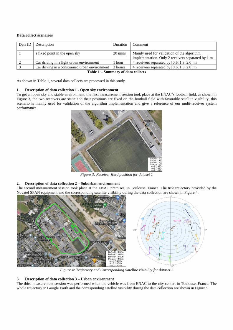
1. Description of data collection 1 - Open sky environment

To get an open sky and stable environment, the first measurement session took place at the ENAC’s football field, as shown in

Figure 3, the two receivers are static and their positions are fixed on the football field with favorable satellite visibility, this

scenario is mainly used for validation of the algorithm implementation and give a reference of our multi-receiver system

performance.

Figure 3: Receiver fixed position for dataset 1

2. Description of data collection 2 – Suburban environment

The second measurement session took place at the ENAC premises, in Toulouse, France. The true trajectory provided by the

Novatel SPAN equipment and the corresponding satellite visibility during the data collection are shown in Figure 4.

Figure 4: Trajectory and Corresponding Satellite visibility for dataset 2

3. Description of data collection 3 – Urban environment

The third measurement session was performed when the vehicle was from ENAC to the city center, in Toulouse, France. The

whole trajectory in Google Earth and the corresponding satellite visibility during the data collection are shown in Figure 5.

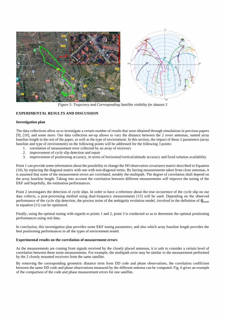
Figure 5: Trajectory and Corresponding Satellite visibility for dataset 3

EXPERIMENTAL RESULTS AND DISCUSSION

Investigation plan

The data collections allow us to investigate a certain number of results that were obtained through simulations in previous papers

[9], [10], and some more. Our data collection set-up allows to vary the distance between the 2 rover antennas, named array

baseline length in the rest of the paper, as well as the type of environment. In this section, the impact of these 2 parameters (array

baseline and type of environment) on the following points will be addressed for the following 3 points:

1. correlation of measurement error collected by an array of receivers

2. improvement of cycle slip detection and repair

3. improvement of positioning accuracy, in terms of horizontal/vertical/attitude accuracy and fixed solution availability

Point 1 can provide some information about the possibility to change the SD observation covariance matrix described in Equation

(16), by replacing the diagonal matrix with one with non-diagonal terms. By having measurements taken from close antennas, it

is assumed that some of the measurement errors are correlated, notably the multipath. The degree of correlation shall depend on

the array baseline length. Taking into account the correlation between different measurements will improve the tuning of the

EKF and hopefully, the estimation performances.

Point 2 investigates the detection of cycle slips. In order to have a reference about the true occurrence of the cycle slip on our

data collects, a post-processing method using dual-frequency measurements [15] will be used. Depending on the observed

performance of the cycle slip detection, the process noise of the ambiguity evolution model, involved in the definition of 𝐐𝑎𝑚𝑏

in equation (11) can be optimized.

Finally, using the optimal tuning with regards to points 1 and 2, point 3 is conducted so as to determine the optimal positioning

performances using real data.

In conclusion, this investigation plan provides some EKF tuning parameters, and also which array baseline length provides the

best positioning performances in all the types of environment tested.

Experimental results on the correlation of measurement errors

As the measurements are coming from signals received by the closely placed antennas, it is safe to consider a certain level of correlation between these noise measurements. For example, the multipath error may be similar to the measurement performed by the 2 closely mounted receivers from the same satellite.

By removing the corresponding geometric distance term from DD code and phase observations, the correlation coefficient

between the same DD code and phase observations measured by the different antenna can be computed. Fig. 6 gives an example

of the comparison of the code and phase measurement errors for one satellite.

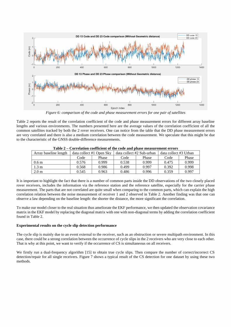
Figure 6: comparison of the code and phase measurement errors for one pair of satellites

Table 2 reports the result of the correlation coefficient of the code and phase measurement errors for different array baseline

lengths and various environments. The numbers presented here are the average values of the correlation coefficient of all the

common satellites tracked by both the 2 rover receivers. One can notice from the table that the DD phase measurement errors

are very correlated and there is also a medium correlation between the code measurement. We speculate that this might be due

to the characteristic of the GNSS double-difference measurements.

Table 2 – Correlation coefficient of the code and phase measurement errors

Array baseline length data collect #1 Open Sky data collect #2 Sub-urban data collect #3 Urban

Code Phase Code Phase Code Phase

0.6 m 0.576 0.999 0.538 0.999 0.475 0.999

1.3 m 0.568 0.986 0.499 0.997 0.392 0.998

2.0 m 0.545 0.963 0.486 0.996 0.359 0.997

It is important to highlight the fact that there is a number of common parts inside the DD observations of the two closely placed

rover receivers, includes the information via the reference station and the reference satellite, especially for the carrier phase

measurement. The parts that are not correlated are quite small when comparing to the common parts, which can explain the high

correlation relation between the noise measurement of receiver 1 and 2 observed in Table 2. Another finding was that one can

observe a law depending on the baseline length: the shorter the distance, the more significant the correlation.

To make our model closer to the real situation thus ameliorate the EKF performance, we then updated the observation covariance

matrix in the EKF model by replacing the diagonal matrix with one with non-diagonal terms by adding the correlation coefficient

found in Table 2.

Experimental results on the cycle slip detection performance

The cycle slip is mainly due to an event external to the receiver, such as an obstruction or severe multipath environment. In this

case, there could be a strong correlation between the occurrence of cycle slips in the 2 receivers who are very close to each other.

That is why at this point, we want to verify if the occurrence of CS is simultaneous on all receivers.

We firstly run a dual-frequency algorithm [15] to obtain true cycle slips. Then compare the number of correct/incorrect CS

detection/repair for all single receivers. Figure 7 shows a typical result of the CS detection for one dataset by using these two

methods.

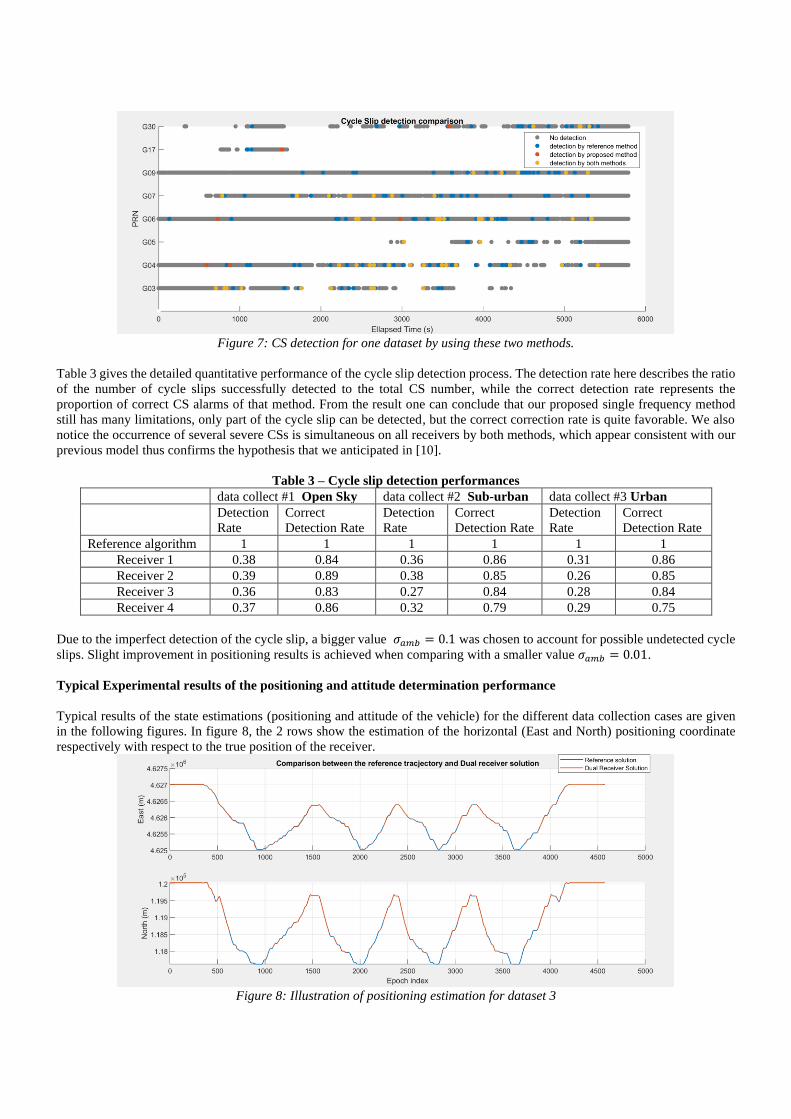
Figure 7: CS detection for one dataset by using these two methods.

Table 3 gives the detailed quantitative performance of the cycle slip detection process. The detection rate here describes the ratio

of the number of cycle slips successfully detected to the total CS number, while the correct detection rate represents the

proportion of correct CS alarms of that method. From the result one can conclude that our proposed single frequency method

still has many limitations, only part of the cycle slip can be detected, but the correct correction rate is quite favorable. We also

notice the occurrence of several severe CSs is simultaneous on all receivers by both methods, which appear consistent with our

previous model thus confirms the hypothesis that we anticipated in [10].

Table 3 – Cycle slip detection performances

data collect #1 Open Sky data collect #2 Sub-urban data collect #3 Urban

Detection

Rate

Correct

Detection Rate

Detection

Rate

Correct

Detection Rate

Detection

Rate

Correct

Detection Rate

Reference algorithm 1 1 1 1 1 1

Receiver 1 0.38 0.84 0.36 0.86 0.31 0.86

Receiver 2 0.39 0.89 0.38 0.85 0.26 0.85

Receiver 3 0.36 0.83 0.27 0.84 0.28 0.84

Receiver 4 0.37 0.86 0.32 0.79 0.29 0.75

Due to the imperfect detection of the cycle slip, a bigger value 𝜎𝑎𝑚𝑏 = 0.1 was chosen to account for possible undetected cycle

slips. Slight improvement in positioning results is achieved when comparing with a smaller value 𝜎𝑎𝑚𝑏 = 0.01.

Typical Experimental results of the positioning and attitude determination performance

Typical results of the state estimations (positioning and attitude of the vehicle) for the different data collection cases are given

in the following figures. In figure 8, the 2 rows show the estimation of the horizontal (East and North) positioning coordinate

respectively with respect to the true position of the receiver.

Figure 8: Illustration of positioning estimation for dataset 3

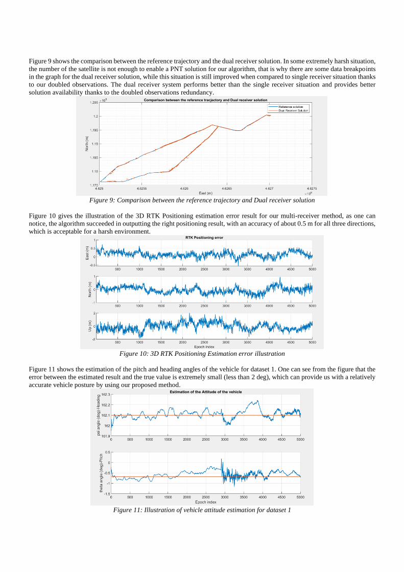
Figure 9 shows the comparison between the reference trajectory and the dual receiver solution. In some extremely harsh situation,

the number of the satellite is not enough to enable a PNT solution for our algorithm, that is why there are some data breakpoints

in the graph for the dual receiver solution, while this situation is still improved when compared to single receiver situation thanks

to our doubled observations. The dual receiver system performs better than the single receiver situation and provides better

solution availability thanks to the doubled observations redundancy.

Figure 9: Comparison between the reference trajectory and Dual receiver solution

Figure 10 gives the illustration of the 3D RTK Positioning estimation error result for our multi-receiver method, as one can

notice, the algorithm succeeded in outputting the right positioning result, with an accuracy of about 0.5 m for all three directions,

which is acceptable for a harsh environment.

Figure 10: 3D RTK Positioning Estimation error illustration

Figure 11 shows the estimation of the pitch and heading angles of the vehicle for dataset 1. One can see from the figure that the

error between the estimated result and the true value is extremely small (less than 2 deg), which can provide us with a relatively

accurate vehicle posture by using our proposed method.

Figure 11: Illustration of vehicle attitude estimation for dataset 1

Experimental results of the RTK performance comparison for different array baseline and various data collections

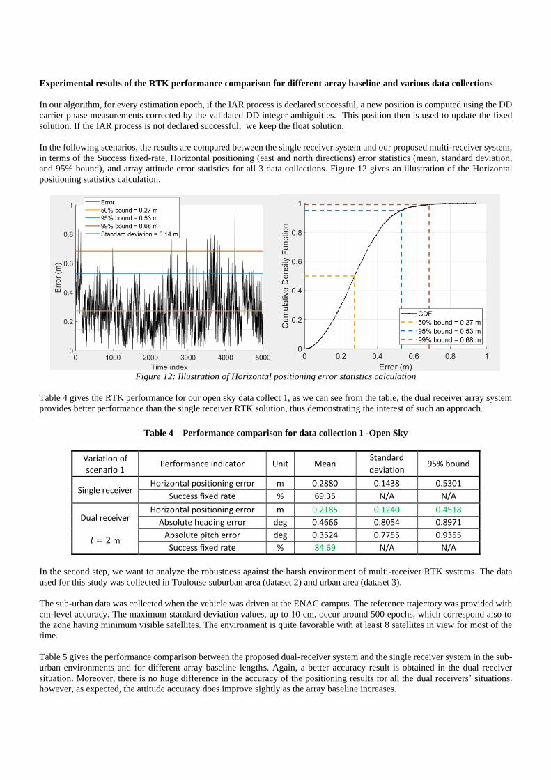
In our algorithm, for every estimation epoch, if the IAR process is declared successful, a new position is computed using the DD

carrier phase measurements corrected by the validated DD integer ambiguities. This position then is used to update the fixed

solution. If the IAR process is not declared successful, we keep the float solution.

In the following scenarios, the results are compared between the single receiver system and our proposed multi-receiver system,

in terms of the Success fixed-rate, Horizontal positioning (east and north directions) error statistics (mean, standard deviation,

and 95% bound), and array attitude error statistics for all 3 data collections. Figure 12 gives an illustration of the Horizontal

positioning statistics calculation.

Figure 12: Illustration of Horizontal positioning error statistics calculation

Table 4 gives the RTK performance for our open sky data collect 1, as we can see from the table, the dual receiver array system

provides better performance than the single receiver RTK solution, thus demonstrating the interest of such an approach.

Table 4 – Performance comparison for data collection 1 -Open Sky

In the second step, we want to analyze the robustness against the harsh environment of multi-receiver RTK systems. The data

used for this study was collected in Toulouse suburban area (dataset 2) and urban area (dataset 3).

The sub-urban data was collected when the vehicle was driven at the ENAC campus. The reference trajectory was provided with

cm-level accuracy. The maximum standard deviation values, up to 10 cm, occur around 500 epochs, which correspond also to

the zone having minimum visible satellites. The environment is quite favorable with at least 8 satellites in view for most of the

time.

Table 5 gives the performance comparison between the proposed dual-receiver system and the single receiver system in the sub-

urban environments and for different array baseline lengths. Again, a better accuracy result is obtained in the dual receiver

situation. Moreover, there is no huge difference in the accuracy of the positioning results for all the dual receivers’ situations.

however, as expected, the attitude accuracy does improve sightly as the array baseline increases.

Variation of scenario 1

Performance indicator Unit Mean Standard

deviation 95% bound

Single receiver Horizontal positioning error m 0.2880 0.1438 0.5301

Success fixed rate % 69.35 N/A N/A

Dual receiver

𝑙 = 2 m

Horizontal positioning error m 0.2185 0.1240 0.4518

Absolute heading error deg 0.4666 0.8054 0.8971

Absolute pitch error deg 0.3524 0.7755 0.9355


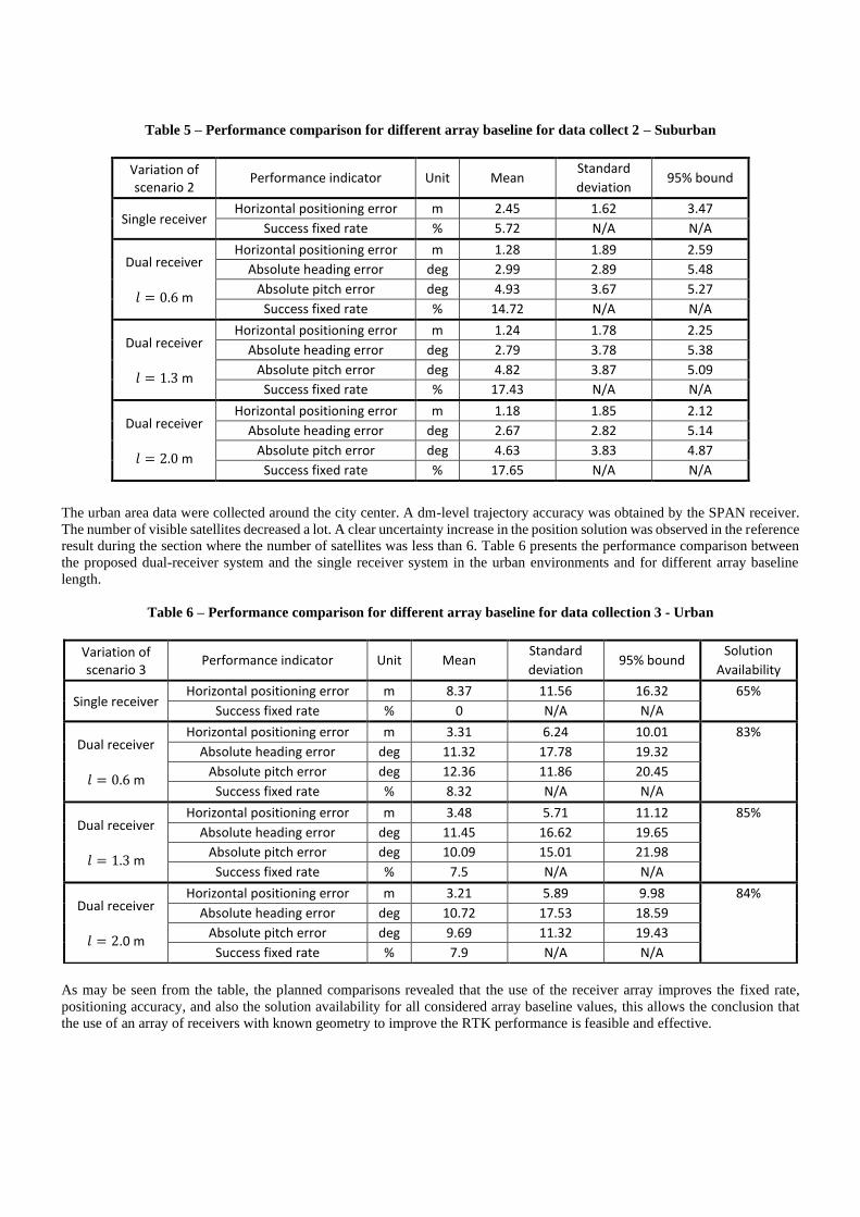
Table 5 – Performance comparison for different array baseline for data collect 2 – Suburban

The urban area data were collected around the city center. A dm-level trajectory accuracy was obtained by the SPAN receiver.

The number of visible satellites decreased a lot. A clear uncertainty increase in the position solution was observed in the reference

result during the section where the number of satellites was less than 6. Table 6 presents the performance comparison between

the proposed dual-receiver system and the single receiver system in the urban environments and for different array baseline

length.

Table 6 – Performance comparison for different array baseline for data collection 3 - Urban

As may be seen from the table, the planned comparisons revealed that the use of the receiver array improves the fixed rate,

positioning accuracy, and also the solution availability for all considered array baseline values, this allows the conclusion that

the use of an array of receivers with known geometry to improve the RTK performance is feasible and effective.



deviation 95% bound

Single receiver Horizontal positioning error m 2.45 1.62 3.47


Dual receiver

𝑙 = 0.6 m





Dual receiver

𝑙 = 1.3 m





Dual receiver

𝑙 = 2.0 m







deviation 95% bound

Solution

Availability

Single receiver Horizontal positioning error m 8.37 11.56 16.32 65%

Success fixed rate % 0 N/A N/A

Dual receiver

𝑙 = 0.6 m

Horizontal positioning error m 3.31 6.24 10.01 83%




Dual receiver

𝑙 = 1.3 m





Dual receiver

𝑙 = 2.0 m





CONCLUSION

This paper is the extension and improvement of our previous work [9], [10]. In this contribution, we present a method that

includes an array of receivers with known geometry to enable the vehicle attitude determination and enhance the RTK

performance in different environments. Taking advantage of the attitude information and the known geometry of the array of

receivers, we are able to improve some internal steps of precise position computation.

In order to optimize our processing, the correlation of the measurement errors affecting observations taken by our array of

receivers has been determined. Then, the performance of our real-time single frequency cycle-slip detection and repair algorithm

has been assessed, by comparing it to the cycle slips detected by a dual-frequency algorithm performed in post-processing. These

two investigations yielded important information so as to tune our Kalman Filter. Additionally, our method achieves a relatively

accurate estimation of the attitude of the vehicle which provides additional information beyond the positioning.

Finally, we demonstrate through real data processing results that our multi-receiver RTK system is more robust to degraded

satellite geometry, in terms of ambiguity fixing rate, and get a better position accuracy under the same conditions when

comparing with the single receiver system. Our experiments correlate favorably with our previous simulation results and further

support the idea of using an array of receivers with known geometry to improve the RTK performance.

ACKNOWLEDGEMENTS

This work has been supported by the China Scholarship Council (CSC). It is the Chinese Ministry of Education's non-profit

organization that provides support for international academic exchange with China.

REFERENCES

[1] P. Misra and P. Enge, Global positioning system: signals, measurements, and performance. Lincoln, Mass.: Ganga-Jamuna

Press, 2006.

[2] M. Iafrancesco, “GPS/INS Tightly coupled position and attitude determination with low-cost sensors Master Thesis,” p. 69.

[3] I. GNSS, “GNSS-Based Attitude Determination,” Inside GNSS - Global Navigation Satellite Systems Engineering, Policy,

and Design, Jul. 11, 2011. https://insidegnss.com/gnss-based-attitude-determination/ (accessed Jan. 22, 2021).

[4] D. Medina, A. Heselbarth, R. Buscher, R. Ziebold, and J. Garcia, “On the Kalman filtering formulation for RTK joint

positioning and attitude quaternion determination,” in 2018 IEEE/ION Position, Location and Navigation Symposium

(PLANS), Monterey, CA, Apr. 2018, pp. 597–604, doi: 10.1109/PLANS.2018.8373432.

[5] F. Aghili and A. Salerno, “Attitude determination and localization of mobile robots using two RTK GPSs and IMU,” in

2009 IEEE/RSJ International Conference on Intelligent Robots and Systems, St. Louis, MO, USA, Oct. 2009, pp. 2045–

2052, doi: 10.1109/IROS.2009.5354770.

[6] G. Zheng and D. Gebre-Egziabher, “Enhancing Ambiguity Resolution Performance Using Attitude Determination

Constraints,” presented at the ION GNSS, Savannah, Georgia, Sep. 2009, [Online].

[7] A. Khodabandeh and P. J. G. Teunissen, “Single-Epoch GNSS Array Integrity: An Analytical Study,” in VIII Hotine-

Marussi Symposium on Mathematical Geodesy, vol. 142, N. Sneeuw, P. Novák, M. Crespi, and F. Sansò, Eds. Cham:

Springer International Publishing, 2015, pp. 263–272.

[8] Fan, Li, Cui, and Lu, “Precise and Robust RTK-GNSS Positioning in Urban Environments with Dual-Antenna

Configuration,” Sensors, vol. 19, no. 16, p. 3586, Aug. 2019, doi: 10.3390/s19163586.

[9] X. Hu, P. Thevenon, and C. Macabiau, “Improvement of RTK performances using an array of receivers with known

geometry,” ION ITM 2020 Conf. San Diego Calif. U. S. 2020, p. 4.

[10] X. Hu, P. Thevenon, and C. Macabiau, “Cycle-slip Detection and Repair Using an Array of Receivers with Known

Geometry for RTK Positioning,” ION PLANS Conf. Portland Or. U. S. 2020, p. 10.

[11] G. Xu and Y. Xu, GPS: theory, algorithms and applications. Berlin, Heidelberg: Springer Berlin Heidelberg, 2016.

[12] P. J. G. Teunissen, “The least-squares ambiguity decorrelation adjustment: a method for fast GPS integer ambiguity

estimation,” J. Geod., vol. 70, no. 1–2, pp. 65–82, Nov. 1995, doi: 10.1007/BF00863419.

[13] P. Buist, “The Baseline Constrained LAMBDA Method for Single Epoch, Single Frequency Attitude Determination

Applications,” presented at the ION GNSS, Fort Worth, Texas, Sep. 2007

[14] P. Teunissen and S. Verhagen, “On the Foundation of the Popular Ratio Test for GNSS Ambiguity Resolution,” presented

at the ION GNSS, Long Beach, California, Sep. 2004, Accessed: May 26, 2016.

Attitude Determination and RTK Performances Amelioration ...

Documents