Attia, John Okyere. “ Fourier Analysis.” Electronics …taz.newffr.com/TAZ/Cryptologie/Cryptanalyse/Fourier Analysis.pdf · For the full-wave rectifier waveform shown in Figure

Attia, John Okyere. “Fourier Analysis.”Electronics and Circuit Analysis using MATLAB.Ed. John Okyere AttiaBoca Raton: CRC Press LLC, 1999

© 1999 by CRC PRESS LLC

CHAPTER EIGHT

FOURIER ANALYSIS In this chapter, Fourier analysis will be discussed. Topics covered are Fou-rier series expansion, Fourier transform, discrete Fourier transform, and fast Fourier transform. Some applications of Fourier analysis, using MATLAB, will also be discussed.

8.1 FOURIER SERIES If a function g t( ) is periodic with period Tp , i.e., g t g t Tp( ) ( )= ± (8.1) and in any finite interval g t( ) has at most a finite number of discontinuities and a finite number of maxima and minima (Dirichlets conditions), and in addition,

g t dtTp

( ) < ∞∫0

(8.2)

then g t( ) can be expressed with series of sinusoids. That is,

g ta

a nw t b nw tn nn

( ) cos( ) sin( )= + +=

∞

∑00 0

12 (8.3)

where

wTp

0

2=

π (8.4)

and the Fourier coefficients an and bn are determined by the following equa-tions.

aT

g t nw t dtnp t

t T

o

o p

=+

∫2

0( ) cos( ) n = 0, 1,2, … (8.5)

© 1999 CRC Press LLC


bT

g t nw t dtnp t

t T

o

o p

=+

∫2

0( ) sin( ) n = 0, 1, 2 … (8.6)

Equation (8.3) is called the trigonometric Fourier series. The term a0

2 in

Equation (8.3) is the dc component of the series and is the average value of g t( ) over a period. The term a nw t b nw tn ncos( ) sin( )0 0+ is called the n-th harmonic. The first harmonic is obtained when n = 1. The latter is also called the fundamental with the fundamental frequency of ωo . When n = 2, we have the second harmonic and so on. Equation (8.3) can be rewritten as

g ta

A nw tn nn

( ) cos( )= + +=

∞

∑00

12Θ (8.7)

where

A a bn n n= +2 2 (8.8) and

Θnn

n

ba

= −

−tan 1 (8.9)

The total power in g t( ) is given by the Parseval’s equation:

PT

g t dt AA

p t

t T

dcn

no

o p

= = ++

=

∞

∫ ∑12

2 22

1( ) (8.10)

where

Aa

dc2 0

2

2=

(8.11)

The following example shows the synthesis of a square wave using Fourier series expansion.



Example 8.1 Using Fourier series expansion, a square wave with a period of 2 ms, peak-to-peak value of 2 volts and average value of zero volt can be expressed as

g tn

n f tn

( )( )

sin[( ) ]=−

−=

∞

∑4 12 1

2 1 2 01π

π (8.12)

where

f 0 500= Hz if a t( ) is given as

a tn

n f tn

( )( )

sin[( ) ]=−

−=

∑4 12 1

2 1 2 01

12

ππ (8.13)

Write a MATLAB program to plot a t( ) from 0 to 4 ms at intervals of 0.05 ms and to show that a t( ) is a good approximation of g(t). Solution MATLAB Script

% fourier series expansion f = 500; c = 4/pi; dt = 5.0e-05; tpts = (4.0e-3/5.0e-5) + 1; for n = 1: 12 for m = 1: tpts s1(n,m) = (4/pi)*(1/(2*n - 1))*sin((2*n - 1)*2*pi*f*dt*(m-1)); end end for m = 1:tpts a1 = s1(:,m); a2(m) = sum(a1); end f1 = a2'; t = 0.0:5.0e-5:4.0e-3; clg plot(t,f1) xlabel('Time, s')



ylabel('Amplitude, V') title('Fourier series expansion')

Figure 8.1 shows the plot of a t( ) .

Figure 8.1 Approximation to Square Wave By using the Euler’s identity, the cosine and sine functions of Equation (8.3) can be replaced by exponential equivalents, yielding the expression

g t c jnw tnn

( ) exp( )==−∞

∞

∑ 0 (8.14)

where

cT

g t jnw t dtnp t

T

p

p

= −−∫

1

2

2

0( ) exp( )/

/

(8.15)

and

wTp

0

2=

π



Equation (8.14) is termed the exponential Fourier series expansion. The coeffi-cient cn is related to the coefficients an and bn of Equations (8.5) and (8.6) by the expression

c a bban n n

n

n= + ∠ − −1

22 2 1tan ( ) (8.16)

In addition, cn relates to An and φn of Equations (8.8) and (8.9) by the rela-tion

cA

nn

n= ∠Θ2

(8.17)

The plot of cn versus frequency is termed the discrete amplitude spectrum or the line spectrum. It provides information on the amplitude spectral compo-nents of g t( ). A similar plot of ∠ cn versus frequency is called the dis-crete phase spectrum and the latter gives information on the phase components with respect to the frequency of g t( ) . If an input signal x tn ( ) x t c jnw tn n o( ) exp( )= (8.18) passes through a system with transfer function H w( ) , then the output of the system y tn ( ) is y t H jnw c jnw tn o n o( ) ( ) exp( )= (8.19) The block diagram of the input/output relation is shown in Figure 8.2.

H(s)xn(t) yn(t)

Figure 8.2 Input/Output Relationship However, with an input x t( ) consisting of a linear combination of complex excitations,



x t c jnw tnn

n o( ) exp( )==−∞

∞

∑ (8.20)

the response at the output of the system is

y t H jnw c jnw tnn

o n o( ) ( ) exp( )==−∞

∞

∑ (8.21)

The following two examples show how to use MATLAB to obtain the coeffi-cients of Fourier series expansion. Example 8.2 For the full-wave rectifier waveform shown in Figure 8.3, the period is 0.0333s and the amplitude is 169.71 Volts. (a) Write a MATLAB program to obtain the exponential Fourier series coefficients cn for n = 0,1, 2, .. , 19 (b) Find the dc value. (c) Plot the amplitude and phase spectrum.

Figure 8.3 Full-wave Rectifier Waveform



Solution

diary ex8_2.dat % generate the full-wave rectifier waveform f1 = 60; inv = 1/f1; inc = 1/(80*f1); tnum = 3*inv; t = 0:inc:tnum; g1 = 120*sqrt(2)*sin(2*pi*f1*t); g = abs(g1); N = length(g); % % obtain the exponential Fourier series coefficients num = 20; for i = 1:num for m = 1:N cint(m) = exp(-j*2*pi*(i-1)*m/N)*g(m); end c(i) = sum(cint)/N; end cmag = abs(c); cphase = angle(c); %print dc value disp('dc value of g(t)'); cmag(1) % plot the magnitude and phase spectrum f = (0:num-1)*60; subplot(121), stem(f(1:5),cmag(1:5)) title('Amplitude spectrum') xlabel('Frequency, Hz') subplot(122), stem(f(1:5),cphase(1:5)) title('Phase spectrum') xlabel('Frequency, Hz') diary

dc value of g(t)

ans = 107.5344

Figure 8.4 shows the magnitude and phase spectra of Figure 8.3.



Figure 8.4 Magnitude and Phase Spectra of a Full-wave Rectification Waveform Example 8.3 The periodic signal shown in Figure 8.5 can be expressed as

g t e tg t g t

t( )( ) ( )

= − ≤ <+ =

−2 1 12

(i) Show that its exponential Fourier series expansion can be expressed as

g te e

jnjn t

n

n( )

( ) ( )( )

exp( )=− −

+

−

=−∞

∞

∑ 12 2

2 2

ππ (8.22)

(ii) Using a MATLAB program, synthesize g t( ) using 20 terms, i.e.,



g te e

jnjn t

n

n( )

( ) ( )( )

exp( )∧ −

=−=

− −+∑ 1

2 2

2 2

10

10

ππ

0 2 4 t(s)

g(t)

1

Figure 8.5 Periodic Exponential Signal Solution (i)

g t c jnw tn on

( ) exp( )==−∞

∞

∑

where

cT

g t jnw t dtnp T

T

op

p

= −−∫

1

2

2

( ) exp( )/

/

and

wTo

p= = =

2 22

π ππ

c t jn t dtn = − −−∫

12

21

1

exp( ) exp( )π

ce e

jnn

n

=− −

+

−( ) ( )( )

12 2

2 2

π

thus



g te e

jnjn t

n

n( )

( ) ( )( )

exp( )=− −

+

−

=−∞

∞

∑ 12 2

2 2

ππ

(ii) MATLAB Script

% synthesis of g(t) using exponential Fourier series expansion dt = 0.05; tpts = 8.0/dt +1; cst = exp(2) - exp(-2); for n = -10:10 for m = 1:tpts g1(n+11,m) = ((0.5*cst*((-1)^n))/(2+j*n*pi))*(exp(j*n*pi*dt*(m-1))); end end for m = 1: tpts g2 = g1(:,m); g3(m) = sum(g2); end g = g3'; t = -4:0.05:4.0; plot(t,g) xlabel('Time, s') ylabel('Amplitude') title('Approximation of g(t)')

Figure 8.6 shows the approximation of g t( ) .



Figure 8.6 An Approximation of g t( ) .

8.2 FOURIER TRANSFORMS If g t( ) is a nonperiodic deterministic signal expressed as a function of time t, then the Fourier transform of g t( ) is given by the integral expression:

G f g t j ft dt( ) ( ) exp( )= −−∞

∞

∫ 2π (8.23)

where j = −1 and

f denotes frequency g t( ) can be obtained from the Fourier transform G f( ) by the Inverse Fou-rier Transform formula:



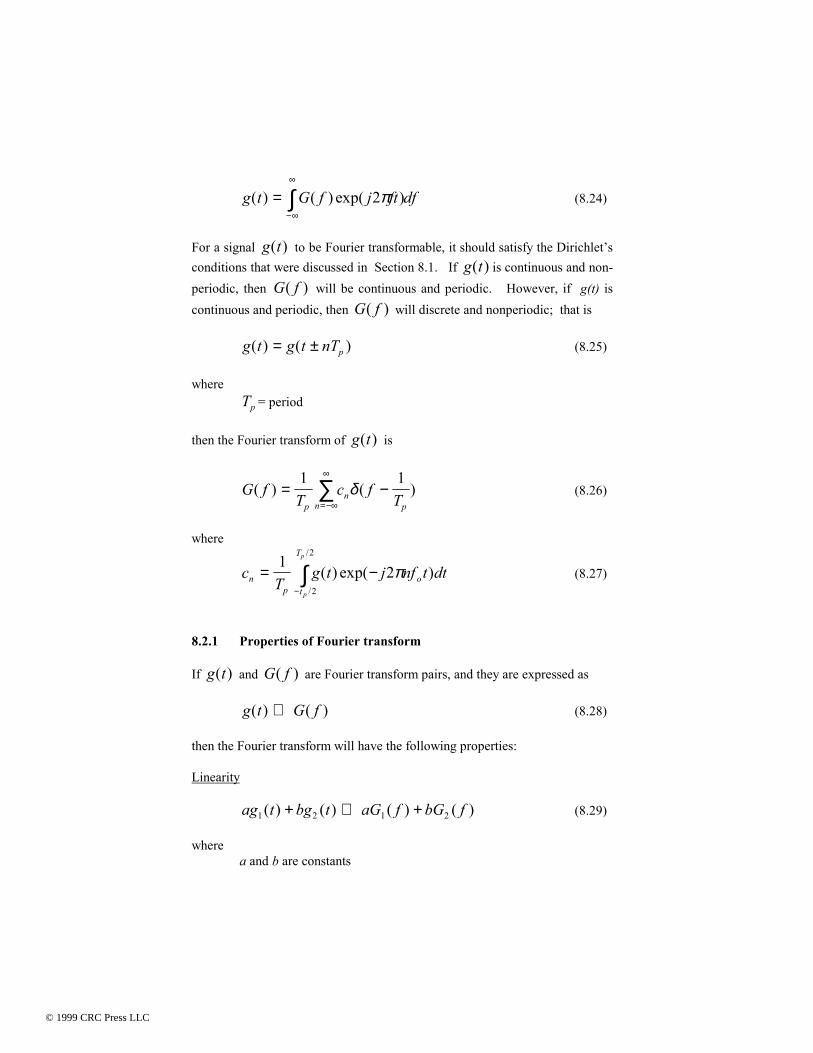
g t G f j ft df( ) ( ) exp( )=−∞

∞

∫ 2π (8.24)

For a signal g t( ) to be Fourier transformable, it should satisfy the Dirichlet’s conditions that were discussed in Section 8.1. If g t( ) is continuous and non-periodic, then G f( ) will be continuous and periodic. However, if g(t) is continuous and periodic, then G f( ) will discrete and nonperiodic; that is g t g t nTp( ) ( )= ± (8.25) where Tp = period then the Fourier transform of g t( ) is

G fT

c fTp

nn p

( ) ( )= −=−∞

∞

∑1 1δ (8.26)

where

cT

g t j nf t dtnp t

T

op

p

= −−∫

12

2

2

( ) exp( )/

/

π (8.27)

8.2.1 Properties of Fourier transform If g t( ) and G f( ) are Fourier transform pairs, and they are expressed as g t G f( ) ( )⇔ (8.28) then the Fourier transform will have the following properties: Linearity ag t bg t aG f bG f1 2 1 2( ) ( ) ( ) ( )+ ⇔ + (8.29) where

a and b are constants



Time scaling

g ata

Gfa

( ) ⇔

1 (8.30)

Duality G t g f( ) ( )⇔ − (8.31) Time shifting g t t G f j ft( ) ( ) exp( )− ⇔ −0 02π (8.32) Frequency Shifting exp( ) ( ) ( )j f t g t G f fC C2 ⇔ − (8.33) Definition in the time domain

dg t

dtj fG f

( )( )⇔ 2π (8.34)

Integration in the time domain

g dj f

G fG

ft

( ) ( )( )

( )τ τπ

δ−∞∫ ⇔ +

12

02

δ (f) (8.35)

Multiplication in the time domain

g t g t G G f d1 2 1 2( ) ( ) ( ) ( )⇔ −−∞

∞

∫ λ λ λ (8.36)

Convolution in the time domain

g g t d G f G f1 2 1 2( ) ( ) ( ) ( )τ τ τ− ⇔−∞

∞

∫ (8.37)



8.3 DISCRETE AND FAST FOURIER TRANSFORMS Fourier series links a continuous time signal into the discrete-frequency do-main. The periodicity of the time-domain signal forces the spectrum to be dis-crete. The discrete Fourier transform of a discrete-time signal g n[ ] is given as

G k g n j nk Nn

N

[ ] [ ]exp( / )= −=

−

∑ 20

1

π k = 0,1, …, N-1 (8.38)

The inverse discrete Fourier transform, g n[ ] is

g n G k j nk Nk

N

[ ] [ ]exp( / )==

−

∑ 20

1

π n = 0,1,…, N-1 (8.39)

where N is the number of time sequence values of g n[ ] . It is also the total number frequency sequence values in G k[ ] . T is the time interval between two consecutive samples of the input sequence g n[ ] . F is the frequency interval between two consecutive samples of the output sequence G k[ ] . N, T, and F are related by the expression

NTF

=1

(8.40)

NT is also equal to the record length. The time interval, T, between samples

should be chosen such that the Shannon’s Sampling theorem is satisfied. This means that T should be less than the reciprocal of 2 f H , where f H is the highest significant frequency component in the continuous time signal g t( ) from which the sequence g n[ ] was obtained. Several fast DFT algorithms require N to be an integer power of 2. A discrete-time function will have a periodic spectrum. In DFT, both the time function and frequency functions are periodic. Because of the periodicity of DFT, it is common to regard points from n = 1 through n = N/2 as positive,



and points from n = N/2 through n = N - 1 as negative frequencies. In addi-tion, since both the time and frequency sequences are periodic, DFT values at points n = N/2 through n = N - 1 are equal to the DFT values at points n = N/2 through n = 1. In general, if the time-sequence is real-valued, then the DFT will have real components which are even and imaginary components that are odd. Simi-larly, for an imaginary valued time sequence, the DFT values will have an odd real component and an even imaginary component. If we define the weighting function WN as

W e eN

jN j FT= =

−−

22

ππ (8.41)

Equations (8.38) and (8.39) can be re-expressed as

G k g n WNkn

n

N

[ ] [ ]==

−

∑0

1

(8.42)

and

g n G k WNkn

k

N

[ ] [ ]= −

=

−

∑0

1

(8.43)

The Fast Fourier Transform, FFT, is an efficient method for computing the discrete Fourier transform. FFT reduces the number of computations needed for computing DFT. For example, if a sequence has N points, and N is an in-tegral power of 2, then DFT requires N 2 operations, whereas FFT requires N

N2 2log ( ) complex multiplication,

NN

2 2log ( ) complex additions and

NN

2 2log ( ) subtractions. For N = 1024, the computational reduction from

DFT to FFT is more than 200 to 1. The FFT can be used to (a) obtain the power spectrum of a signal, (b) do digi-tal filtering, and (c) obtain the correlation between two signals.



8.3.1 MATLAB function fft The MATLAB function for performing Fast Fourier Transforms is fft x( ) where x is the vector to be transformed. fft x N( , ) is also MATLAB command that can be used to obtain N-point fft. The vector x is truncated or zeros are added to N, if necessary. The MATLAB functions for performing inverse fft is ifft x( ).

[ ]z z fftplot x tsm p, ( , )=

is used to obtain fft and plot the magnitude zm and z p of DFT of x. The sampling interval is ts. Its default value is 1. The spectra are plotted versus the digital frequency F. The following three examples illustrate usage of MATLAB function fft. Example 8.4 Given the sequence x n[ ] = ( 1, 2, 1). (a) Calculate the DFT of x n[ ] . (b) Use the fft algorithm to find DFT of x n[ ] . (c) Compare the results of (a) and (b). Solution (a) From Equation (8.42)

G k g n WNkn

n

N

[ ] [ ]==

−

∑0

1

From Equation (8.41)



W

W e j

W e jW WW W

j

j

30

31

23

32

43

33

30

34

31

1

05 0866

05 0 8661

=

= = − −

= = − +

= =

=

−

−

π

π

. .

. .

Using Equation (8.41), we have

G g n Wn

[ ] [ ]0 1 2 1 430

0

2

= = + + ==

∑

G g n W g W g W g W

j j j

n

n[ ] [ ] [ ] [ ] [ ]

( . . ) ( . . ) . .

1 0 1 2

1 2 05 0866 05 0866 05 0866

30

2

30

31

32= = + +

= + − − + − + = − −=∑

G g n W g W g W g W

j j j

n

n[ ] [ ] [ ] [ ] [ ]

( . . ) ( . . ) . .

2 0 1 2

1 2 05 0866 05 0866 05 0866

32

0

2

30

32

34= = + +

= + − + + − − = − +=∑

(b) The MATLAB program for performing the DFT of x n[ ] is MATLAB Script

diary ex8_4.dat % x = [1 2 1]; xfft = fft(x) diary

The results are

xfft = 4.0000 -0.5000 - 0.8660i -0.5000 + 0.8660i

(c) It can be seen that the answers obtained from parts (a) and (b) are identical.



Example 8.5 Signal g t( ) is given as

[ ]g t e t u tt( ) cos ( ) ( )= −4 2 102 π (a) Find the Fourier transform of g t( ) , i.e., G f( ) . (b) Find the DFT of g t( ) when the sampling interval is 0.05 s with N = 1000. (c) Find the DFT of g t( ) when the sampling interval is 0.2 s with N = 250. (d) Compare the results obtained from parts a, b, and c. Solution (a) g t( ) can be expressed as

g t e e e u tt j t j t( ) ( )= +

− −412

12

2 20 20π π

Using the frequency shifting property of the Fourier Transform, we get

G fj f j f

( )( ) ( )

=+ −

++ +

22 2 10

22 2 10π π

(b, c) The MATLAB program for computing the DFT of g t( ) is MATLAB Script

% DFT of g(t) % Sample 1, Sampling interval of 0.05 s ts1 = 0.05; % sampling interval fs1 = 1/ts1; % Sampling frequency n1 = 1000; % Total Samples m1 = 1:n1; % Number of bins sint1 = ts1*(m1 - 1); % Sampling instants freq1 = (m1 - 1)*fs1/n1; % frequencies gb = (4*exp(-2*sint1)).*cos(2*pi*10*sint1); gb_abs = abs(fft(gb)); subplot(121)



plot(freq1, gb_abs) title('DFT of g(t), 0.05s Sampling interval') xlabel('Frequency (Hz)') % Sample 2, Sampling interval of 0.2 s ts2 = 0.2; % sampling interval fs2 = 1/ts2; % Sampling frequency n2 = 250; % Total Samples m2 = 1:n2; % Number of bins sint2 = ts2*(m2 - 1); % Sampling instants freq2 = (m2 - 1)*fs2/n2; % frequencies gc = (4*exp(-2*sint2)).*cos(2*pi*10*sint2); gc_abs = abs(fft(gc)); subplot(122) plot(freq2, gc_abs) title('DFT of g(t), 0.2s Sampling interval') xlabel('Frequency (Hz)')

The two plots are shown in Figure 8.7.

Figure 8.7 DFT of g t( ) (d) From Figure 8.7, it can be seen that with the sample interval of 0.05 s,

there was no aliasing and spectrum of G k[ ] in part (b) is almost the same



as that of G f( ) of part (a). With the sampling interval being 0.2 s (less than the Nyquist rate), there is aliasing and the spectrum of G k[ ] is dif-ferent from that of G f( ) .

Example 8.6 Given a noisy signal g t f t n t( ) sin( ) . ( )= +2 0 51π where

f1 = 100 Hz n(t) is a normally distributed white noise. The duration of g t( ) is 0.5 sec-onds. Use MATLAB function rand to generate the noise signal. Use MATLAB to obtain the power spectral density of g t( ) . Solution A representative program that can be used to plot the noisy signal and obtain the power spectral density is MATLAB Script

% power spectral estimation of noisy signal t = 0.0:0.002:0.5; f1 =100; % generate the sine portion of signal x = sin(2*pi*f1*t); % generate a normally distributed white noise n = 0.5*randn(size(t)); % generate the noisy signal y = x+n; subplot(211), plot(t(1:50),y(1:50)), title('Nosiy time domain signal') % power spectral estimation is done yfft = fft(y,256);



len = length(yfft); pyy = yfft.*conj(yfft)/len; f = (500./256)*(0:127); subplot(212), plot(f,pyy(1:128)), title('power spectral density'), xlabel('frequency in Hz')

The plot of the noisy signal and its spectrum is shown in Figure 8.8. The am-plitude of the noise and the sinusoidal signal can be changed to observe their effects on the spectrum.

Figure 8.8 Noisy Signal and Its Spectrum

SELECTED BIBLIOGRAPHY 1. Math Works Inc., MATLAB, High Performance Numeric Computation Software, 1995. 2. Etter, D. M., Engineering Problem Solving with MATLAB, 2nd Edition, Prentice Hall, 1997.



3. Nilsson, J. W., Electric Circuits, 3rd Edition, Addison-Wesley Publishing Company, 1990. 4. Johnson, D. E., Johnson, J.R., and Hilburn, J.L., Electric Circuit Analysis, 3rd Edition, Prentice Hall, 1997.

EXERCISES 8.1 The triangular waveform, shown in Figure P8.1 can be expressed as

( )g tA

nn w t

n

n( )

( )cos ( )=

−−

−+

=

∞

∑8 14 1

2 12

1

21

0π

where

wTp

0

1=

Tp2Tp

A

-A

g(t)

Figure P8.1 Triangular Waveform

If A = 1, T = 8 ms, and sampling interval is 0.1 ms.

(a) Write MATLAB program to resynthesize g t( ) if 20



terms are used. (b) What is the root-mean-squared value of the function that is

the difference between g t( ) and the approximation to g t( ) when 20 terms are used for the calculation of g t( ) ? 8.2 A periodic pulse train g t( ) is shown in Figure P8.2.

1 2 3 4 5 6 7 8

4

g(t)

t(s)0

Figure P8.2 Periodic Pulse Train

If g t( ) can be expressed by Equation (8.3) , (a) Derive expressions for determining the Fourier Series coeffi-cients an and bn . (b) Write a MATLAB program to obtain an and bn for n = 0 , 1, ......, 10 by using Equations (8.5) and (8.6). (c) Resynthesis g(t) using 10 terms of the values an , bn

obtained from part (b). 8.3 For the half-wave rectifier waveform, shown in Figure P8.3, with a period of 0.01 s and a peak voltage of 17 volts.

(a) Write a MATLAB program to obtain the exponential Fourier series coefficients cn for n = 0, 1, ......., 20. (b) Plot the amplitude spectrum. (c) Using the values obtained in (a), use MATLAB to

regenerate the approximation to g t( ) when 20 terms of the exponential Fourier series are used.



Figure P8.3 Half-Wave Rectifier Waveform 8.4 Figure P8.4(a) is a periodic triangular waveform.

v(t)

-2 0 2 4 6 t(s)

2

Figure P8.4(a) Periodic Triangular Waveform

(a) Derive the Fourier series coefficients an and bn . (b) With the signal v t( ) of the circuit shown in P8.4(b), derive the expression for the current i t( ) .



V(t)

VL(t)

VR(t)

4 H

3Ω

i(t)

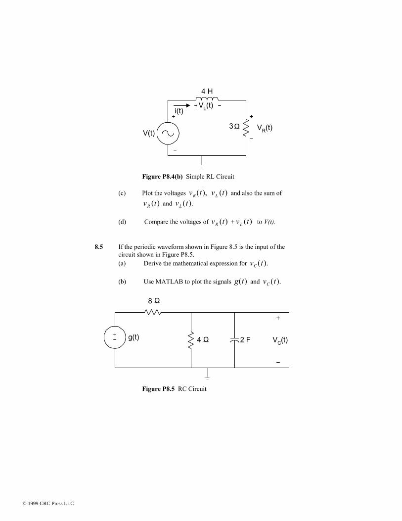
Figure P8.4(b) Simple RL Circuit

(c) Plot the voltages v tR ( ), v tL ( ) and also the sum of v tR ( ) and v tL ( ). (d) Compare the voltages of v tR ( ) + v tL ( ) to V(t).

8.5 If the periodic waveform shown in Figure 8.5 is the input of the circuit shown in Figure P8.5.

(a) Derive the mathematical expression for v tC ( ). (b) Use MATLAB to plot the signals g t( ) and v tC ( ).

VC(t)

8 Ω

4 Ω 2 Fg(t)

Figure P8.5 RC Circuit



8.6 The unit sample response of a filter is given as

( )h n[ ] = − −0 1 1 0 1 1 0

(a) Find the discrete Fourier transform of h n[ ] ; assume that the values of h n[ ] not shown are zero.

(b) If the input to the filter is x nn

u n[ ] sin [ ]=

8

, find the

output of the filter. 8.7 g t t t( ) sin( ) sin( )= +200 400π π

(a) Generate 512 points of g t( ). Using the FFT algorithm, generate and plot the frequency content of g t( ) . Assume a sampling rate of 1200 Hz. Find the power spectrum. (b) Verify that the frequencies in g t( ) are observable in the

FFT plot. 8.8 Find the DFT of g t e u tt( ) ( )= −5

(a) Find the Fourier transform of g t( ) . (b) Find the DFT of g t( ) using the sampling interval of 0.01 s and time duration of 5 seconds. (c) Compare the results obtained from parts (a) and (b).



Attia, John Okyere. “ Fourier Analysis.” Electronics …taz.newffr.com/TAZ/Cryptologie/Cryptanalyse/Fourier Analysis.pdf · For the full-wave rectifier waveform shown in Figure

Documents