Attention, predictive learning, and the inverse base-rate effect: evidence from event-related potentials

1

Running title: ATTENTION AND PREDICTIVE LEARNING

Attention, predictive learning, and the inverse base-rate effect: Evidence from event-

related potentials

Andy J. Willsa, Aureliu Lavricb, Yvonne Hemmingsb, Ed Surreyb

a. School of Psychology, Plymouth University, Drake Circus, Plymouth. PL4

8AA. United Kingdom.

b. School of Psychology, Exeter University, Exeter. EX4 4QG. United Kingdom.

To appear in NeuroImage

2

Abstract

We report the first electrophysiological investigation of the inverse base-rate effect

(IBRE), a robust non-rational bias in predictive learning. In the IBRE, participants

learn that one pair of symptoms (AB) predicts a frequently occurring disease, whilst

an overlapping pair of symptoms (AC) predicts a rarely occurring disease.

Participants subsequently infer that BC predicts the rare disease, a non-rational

decision made in opposition to the underlying base rates of the two diseases. Error-

driven attention theories of learning state the IBRE occurs because C attracts more

attention than B. On the basis of this account we predicted and observed the

occurrence of brain potentials associated with visual attention: a posterior Selection

Negativity, and a concurrent anterior Selection Positivity, for C vs. B in a post-

training test phase. Error-driven attention theories further predict no Selection

Negativity, Selection Positivity or IBRE, for control symptoms matched on frequency

to B and C, but for which there was no shared symptom (A) during training. These

predictions were also confirmed, and this confirmation discounts alternative

explanations of the IBRE based on the relative novelty of B and C. Further, we

observed higher response accuracy for B alone than for C alone; this dissociation of

response accuracy (B > C) from attentional allocation (C > B) discounts the

possibility that the observed attentional difference was caused by the difference in

response accuracy.

Keywords: EEG, visual attention, learning, categorization

3

1. Introduction

We seem to learn more about events for which our initial predictions were

incorrect than we do about events for which our initial predictions were correct—the

element of surprise seems conducive to learning (Kamin, 1969). Using an event-

related potential methodology, Wills et al. (2007) provided evidence that one process

underlying this phenomenon is the rapid re-direction of visual attention in response to

prediction errors. Specifically, Wills et al. (2007) found a brain potential previously

associated with attention to features (e.g. shape, color, spatial frequency)—the

selection negativity (SN)—for a cue involved in multiple prediction errors, relative to

an equally frequent control cue involved in fewer prediction errors. In the current

article, we report that a comparable event-related component is observed in the

inverse base-rate effect—a robust non-rational preference observed in post-category-

learning decision making (Medin & Edelson, 1988).

The inverse base-rate procedure, in its canonical form, can be considered both

as a category-learning phenomenon (because it involves inference from learned items

to unseen items, see Pothos & Wills, 2011), and a predictive learning phenomenon

(because it involves learning to predict outcomes on the basis of presented stimuli).

For this reason, we use the terms ‘predictive learning’ and ‘category learning’ inter-

changeably in the current article, although we accept that they are not entirely

synonymous when considering the associative- and category- learning literatures in

their entirety (see e.g. Bott, Hoffman & Murphy, 2007).

In the sections that follow, we describe the inverse base-rate effect, explain how

the effect may be accommodated by theories of error-driven attention, and justify our

prediction of the presence of a SN on the basis of these theories and related work. An

experiment testing this prediction is then reported.

4

1.1. The inverse base-rate effect

Imagine the following fictitious scenario. You are a physician in training who

has just seen a series of patients. You have noticed that all patients with the symptoms

dizziness and skin rash have Jominy fever, whilst all patients with dizziness and back

pain have Phipp’s syndrome. You have seen three times as many cases of Jominy

fever as you have of Phipp’s syndrome. The next patient you see has back pain and

skin rash. Is this patient more likely to have Jominy fever or Phipp’s syndrome?

When posed the question in this manner, people typically answer that Jominy

fever is more likely (Johansen et al., 2007). Such an answer is not unreasonable

because, in the microcosm of this scenario, skin rash perfectly predicts Jominy fever,

and back pain perfectly predicts Phipp’s syndrome, but Jominy fever is more common

overall. Indeed, medical students are often encouraged to heed the aphorism “when

you hear hoof beats behind you, don’t expect to see a zebra” (Imperato, 1979). In the

presence of two perfectly predictive but conflicting symptoms, the underlying base

rates of the diseases provide one basis on which to make a decision. The current

article focuses on the opposite result where participants respond that a patient with

back pain and skin rash is more likely to have the rare disease Phipp’s syndrome. This

non-rational response bias is robustly found when participants are presented with the

same information sequentially as a series of cases (e.g. Juslin et al., 2001; Kruschke,

1996; Lamberts & Kent, 2007; Medin & Edelson, 1988; Sherman et al., 2009).

One class of theory of this inverse base-rate effect (IBRE) is that it is a relative-

novelty effect (Binder & Estes, 1966). This theory combines the idea that novel or

surprising events are particularly memorable (Rhetorica ad Herennium, 85BC; Von

Restorff, 1933), with the availability heuristic (Tversky & Kahneman, 1973), which

5

states that memorable events are judged more probable. The idea that the IBRE is

driven by the relative novelty of the two diseases is disconfirmed by the fact that

participants predict the common disease if presented with just the symptom common

to both diseases (dizziness), a response that is consistent with the underlying base

rates. Participants also predict the common disease if presented with all three

symptoms (dizziness, skin rash and back pain; see e.g. Kruschke, 1996); this response

is also consistent with the underlying base rates and inconsistent with a relative

disease novelty account of the IBRE.

Another variant of the relative-novelty explanation of the IBRE focuses on the

relative novelty of the symptoms. The symptom back pain is relatively novel in this

scenario compared to skin rash, which makes it more memorable, and hence its

associated disease (Phipp’s syndrome) is judged more probable. However, this

version of a relative-novelty account is disconfirmed by the observation that the IBRE

is only observed if there is a shared cue during training (Kruschke, 2001a; Medin &

Edelson, 1988; Medin & Robbins, 1971). The shared cue in the above example is

dizziness, which occurs in all presented cases. If the shared cue is replaced by further

perfectly predictive cues, base-rate following is observed. For example, if dizziness

and skin rash predict the common disease Jominy fever, but ear ache and back pain

predict the rare disease Phipp’s syndrome, then participants’ modal response to the

symptom combination skin rash and back pain is now Jominy fever, in agreement

with the underlying base rates. Under a relative novelty account, the IBRE should still

be observed, because back pain is more novel than skin rash. In summary, the shared-

cue effect disconfirms the relative-novelty account of the IBRE.

The shared-cue effect also disconfirms the eliminative-inference account

suggested by Juslin et al. (2001). For an extended discussion of this point see

6

Kruschke (2001a) but, in essence, the eliminative-inference account proposes that

participants are more likely to remember what skin rash predicts than what back pain

predicts because they see skin rash more often. Faced with novel symptom

combination skin rash and back pain, participants may therefore forget what back pain

predicts (the rare disease) but remember what skin rash predicts (the common

disease). However, skin rash plus back pain is a novel symptom combination and

participants are assumed (under eliminative inference theory) to respond to this novel

combination with a novel response. Specifically, they respond that skin rash and back

pain predict the rare disease, because this is a novel response (responding “common

disease” would be the familiar response because it is brought to mind by the more

frequent symptom skin rash). Such a theory applies equally in the presence or absence

of a shared cue, yet the IBRE effect depends on the presence of a shared cue. Hence,

the shared-cue effect disconfirms the eliminative-inference account of the IBRE.

--- Table 1 about here, please ---

Although the above examples of the IBRE involve verbal descriptions of

symptoms within a fictitious medical scenario, the IBRE has also been observed with

abstract pictorial stimuli, and in non-medical scenarios (Binder & Estes, 1966;

Johansen et al., 2010; Lamberts & Kent, 2007; Kalish, 2001; Sherman et al., 2009).

We therefore subsequently discuss the IBRE and the shared-cue effect in terms of

their abstract structure, which is summarized in Table 1. In Table 1, A is the shared

cue, B and D are perfect predictors of the common disease com, C and E are perfect

predictors of the rare disease rare, and F and G are further perfect predictors whose

main role is to replace the shared cue. The result that the rare outcome is more likely

to be predicted than the common outcome in response to a particular cue combination

can be represented as: rare > com. Thus, the three key results of the IBRE and

7

shared-cue effect, expressed in terms of the abstract design of Table 1 are (1) com <

rare for BC, (2) com > rare for DE, and (3) com > rare for A. In interpreting Table 1,

it is important to note that compounds (e.g. AB) are presented simultaneously – in

other words, the two component cues (e.g. A and B in AB) appear on the screen at the

same time. It is also important to note that trial order is randomized, and thus the

order of the rows in Table 1 is arbitrary.

1.2. Error-driven attention

Certain error-driven attention theories of learning (e.g. Kruschke, 2001b) can

accommodate both the IBRE and the shared-cue effect. These theories are expressed

in mathematical terms but, for current purposes, a natural-language approximation

(Wills & Pothos, 2012) will suffice. The central concept behind these theories of

error-driven attention is that people re-direct their attention to particular components

of a presented stimulus in order to minimize future prediction errors. In the context of

the IBRE, one has to make the additional assumption that participants learn more

quickly about what predicts the common outcome than about what predicts the rare

outcome. Such an assumption is not unreasonable given that participants see the

common disease more often, and it is supported by previous studies of the IBRE (e.g.

Kruschke, 1996, Figure 1).

In approximate terms, the explanation provided by error-driven attention theory

on the basis of these premises is as follows. Relatively early in the case series,

participants learn AB → com. This leads them to initially predict AC → com, because

of the similarity of AC to AB. The participant’s prediction turns out to be wrong,

because AC → rare. The participant concludes that it was cue A that led to this

8

erroneous prediction (nothing has been learned about C yet). Error-driven attention

theory states that people act to reduce the likelihood of a subsequent error in

predicting the outcome of AC by reducing the attention paid to A and increasing the

attention paid to C. The cue B does not see a corresponding increase in attention,

because the participant has already learned AB → com. When AB was originally

learned, the participant knew nothing about A or B, so any initial errors would not

lead to B being differentially attended relative to A.

When subsequently asked about the cue combination BC, these error-driven

changes in attention are assumed to persist, and thus C attracts more attention than B.

This difference in attention is presumably sufficiently large that C (which is

associated with the rare disease) dominates the decision. Note that this explanation of

the IBRE, like the IBRE itself, depends on the presence of the shared cue A. In the

absence of A, base-rate following is expected because there is no shared cue to cause

the re-direction of attention, and the participant has had more opportunity to learn

about D than E, because D occurs more often. For similar reasons, A presented alone

leads to the common outcome being predicted, because A has been followed by com

more often than it has been followed by rare.

1.3. Correlates of selective attention

An extensive literature on the ERP correlates of selective attention to perceptual

attributes has revealed a number of brain potentials elicited or modulated by attention.

In the visual modality these include the P1 and N1 peaks of the ERP waveform, and

the difference potentials N2pc, Selection Negativity (SN) and Selection Positivity

(SP) obtained by subtraction of the ERPs for unattended/non-target stimuli from those

for attended/target stimuli (for reviews see Hillyard & Anllo-Vento, 1998; Luck et al.,

9

2000). Of particular relevance for the current study are the potentials elicited by non-

spatial attention (attention to features such as color, shape and spatial frequency): SN,

which has a posterior scalp distribution and is sometimes preceded or accompanied by

SP over the anterior scalp (cf. Anllo-Vento & Hillyard , 1996). Feature-based

attention can also elicit the N2pc potential, but this requires lateralized presentation of

target features, which was not a feature of the current study, hence the present focus

on SN and SP. Importantly, SN has been previously observed in response to a cue

involved in multiple prediction errors relative to an equally frequent cue involved in

fewer prediction errors. Specifically, Wills et al. (2007) employed a forward cue

competition design in which participants first learned that cue A predicted the

presence of a disease, whilst cue B predicted the absence of that disease. Participants

subsequently learned that cue combination AX predicted the presence of the disease

and that cue combination BY also predicted the presence of the disease (filler cues

predicted the absence of the disease in this phase). The critical part of this design is

that participants tend to make fewer prediction errors on AX than on BY. By the end

of this second training phase, cues X and Y have thus been presented an equal number

of times, but Y has been involved in more prediction errors than X. In a subsequent

test phase in which X and Y were presented singly in the absence of feedback, Wills

et al. (2007) found a SN for Y relative to X. This result is consistent with the idea that

the difference in prediction errors led to a difference in attention to Y compared to X,

a difference that persisted beyond the training phase and outside the context of the

specific training stimuli (AX and BY).

The current study employed the same shape-based stimuli as Wills et al. (2007)

in an IBRE procedure (see Table 1). As previously stated, certain error-driven

attention theories (e.g. Kruschke, 2001) predict that, after training on AB → com and

10

AC → rare, C will be more attended than B. Given the evidence that the attentional

changes predicted by error-driven attention theory can be indexed by a SN (Wills et

al., 2007), our prediction was that a SN would be observed to cue C relative to cue B.

In addition, the same error-driven attention theories (e.g. Kruschke, 2001) predict that

after training on FD → com and GE → rare, D and E will not be differentially

attended, due to the absence of a shared cue (the shared cue A being the thing that

drives attention towards C on AC trials, according to these theories). We therefore

also predicted that no SN should be observed for E relative to D. Cues E and D thus

provide a frequency-matched control for the C − B SN. Confirmation of these

predictions would provide further support for these error-driven attention theories of

the IBRE.

In the IBRE procedure, and as described in Table 1, during training the cues are

presented solely as part of compounds. For our stimuli one could not separate the ERP

effects elicited by individual cues within a compound; other methodologies,

particularly eye-tracking, are better suited for achieving such separation (Kruschke et

al., 2005). Hence, as in Wills et al. (2007), an EEG analysis of the training phase of

the current study would be uninformative for the hypotheses under test. We therefore

did not perform an EEG analysis of the training phase (for further discussion of this

decision, see the General Discussion). Instead, following Wills et al. (2007), we

examined the ERPs in a test phase during which the cues B and C (and D and E) were

presented individually, and the SN computed as the difference waveform of these two

trial types. Subsequent testing of singly presented cues avoids the difficulty of

attempting to detect within-stimulus attentional allocation with an ERP methodology,

and provides a particularly stringent test for error-driven attention theories. Such

theories hypothesize that attentional allocation is persistent and should be observable

11

outside the original training context. This issue is returned to in more detail in the

General Discussion.

One shortcoming of Wills et al. (2007), and of a number of other related

experiments (Beesley & Le Pelley, 2011; Le Pelley, 2010; Le Pelley et al., 2011, in

press; Livesey, Harris, & Harris, 2009), is that the cues expected to differ in

attentional allocation showed a corresponding difference in response accuracy during

the test phase (or, in the case of Le Pelley et al., in press, the difference is not directly

measured but can be inferred). In other words, the cue predicted to be more attended

was also responded to more accurately than the cue predicted to be less attended. As

discussed by Wills et al. (2007), this leaves open the possibility that we pay more

attention to those things for which we already know the answer; in other words,

attention is a consequence of learning. Although this is not an unreasonable

hypothesis, error-driven attention theory assumes that changes in attention lead to

differences in rate of learning (and hence accuracy), not (just) the other way around.

One useful feature of the inverse base-rate design is that it provides the potential

for dissociating response accuracy from predicted attentional allocation. As

previously discussed, error-driven attention theory predicts that C will be more

attended than B. However, cue B is also presented more often than cue C during

training so it seems possible that, in a subsequent test, participants would be more

accurate on B presented alone than on C presented alone. Thus, in the inverse base-

rate design, one might expect to see a dissociation of response accuracy (B > C) from

attentional allocation (C > B). If this dissociation is observed, then it seems unlikely

that our results could be explained by the idea that people attend to things for which

they already know the answer. Such a pattern of results would increase support for an

error-driven attention account of the IBRE.

12

1.4. The current study

We employ the basic paradigm of Wills et al. (2007) to implement an inverse

base-rate training design (see Table 1), followed by a subsequent test phase that

includes the critical test items B, C, D and E, presented individually. These four

individually presented cues are the focus of the event-related potential analysis. The

test phase also includes the behavioral test items A, BC and DE, which behaviorally

test for the presence of the IBRE and the shared-cue effect in participants’

responding. The behavioral test items are critical for establishing the presence of the

IBRE in our study, but are uninformative in terms of the EEG analysis. In particular,

and as previously discussed, it is not possible in our procedure to detect attention

within stimulus compounds – for example, to distinguish between attention to B and

attention to C when stimulus compound BC is presented. Thus, these behavioral test

items do not form part of the event-related potential analysis (there are, in any case,

insufficient trials for a meaningful ERP analysis of the behavioral test items, which

were presented less frequently than the ERP test items in order to reduce overall

session length). ERP test items B and C also serve as a behavioral test of the relative

response accuracy of these two cues, where the result B > C for accuracy, if found in

conjunction with a Selection Negativity for C relative to B, would be incompatible

with an account of attention as a mere consequence of superior learning, thus

providing support for an error-driven attention account of the IBRE.

The event-related potential methodology requires a large number of test trials,

and performance should ideally be stable over the test period. In order to achieve this,

we tripled the number of cues relative to the abstract design shown in Table 1. Thus,

A represents three distinct cues (A1, A2, A3), similarly for B, and so on. A review of

13

the literature on the IBRE reveals that doubling or tripling the number of cues is

common practice (Bohil et al., 2005; Juslin et al., 2001; Lamberts & Kent, 2007;

Kalish, 2001; Kruschke, 1996; Medin & Bettger, 1991; Medin & Edelson, 1988;

Shanks, 1992; Sherman et al., 2009; Wood & Blair, 2011; Winman et al., 2005). A

review of the same literature also reveals that the frequency difference between

common and rare outcomes is smaller in the current study than in previous reports of

the IBRE (the most typical ratio is 3:1, the ratio in the current study was 2:1). We

were thus taking a calculated risk that we would not observe the IBRE in our study.

We considered this to be a risk worth taking, as it reduced the overall length of an

already-long experimental session.

Another aspect of the current design that was unusual for studies of the IBRE is

that further training trials were interspersed within the test phase; this technique was

also employed by Wills et al. (2007), and it helps maintain stable performance across

a necessarily long test phase. The current study also used abstract shapes, rather than

the more typical symptom names. Abstract forms have been used successfully in a

previous demonstration of the IBRE (e.g. Lamberts & Kent, 2007). Abstract shapes

were employed here, and in Wills et al. (2007), in order to elicit the brain potential

associated with attention to the shape/spatial frequency of the stimulus.

2. Materials and Methods

2.1. Participants and apparatus

Eighteen right-handed undergraduate students from Exeter University (age

range: 19–29 years; modal age: 20 years; 9 female, 9 male) participated on a

voluntary basis. Stimulus presentation and response collection was via a PC and the

14

E-prime package (Version 1.1, Psychology Software Tools, Pittsburgh, USA). The

electroencephalogram (EEG) was recorded from 64 Ag/AgCl electrodes embedded in

an elastic headcap (ElectroCap International, Eaton, OH, USA) connected to Brain

Amp amplifiers (Brain Products, Munich, Germany). There were 58 scalp electrodes,

placed in an extended 10-20 configuration; one electrode was placed on the outer

canthus of each eye, one below and one above the right eye and one on each earlobe.

The EEG and EOG were sampled at 500 Hz with a 0.016-100 Hz bandpass, the online

reference at Cz and ground at AFz.

2.2. Stimuli

Twenty-one abstract pictures were selected from a pool of 36 items employed in

several previous studies (Jones et al., 1998; Wills et al., 2007; Wills & McLaren,

1997; Wills et al., 2000; the pool of items is most clearly illustrated in Jones et al.,

1998, Figure 1), colored red with a yellow outline, and presented against a black

background. The pictures were 0.64° of visual angle in diameter, presented inside a

white outline square 2.5° in visual angle. On trials where two pictures were presented,

they were vertically aligned, one appearing 0.36° of visual angle above the midpoint,

and the other an equivalent distance below. On trials where one picture was presented,

it was positioned in the center of the square.

2.3. Procedure

Participants were asked to imagine that they worked for a medical referral

service, and that their job was to predict which of two fictitious diseases (“Jominy

Fever” or “Phipp’s Syndrome”) each patient had contracted, on the basis of “cell

bodies” in their blood samples (represented by abstract pictures). The allocation of the

15

labels Jominy Fever and Phipp’s Syndrome to the common and rare disease was

counterbalanced across participants. The 21 pictures of cell bodies were, separately

for each participant, randomly divided into seven cell types (three cell bodies each)

corresponding to the stimulus types A − G in Table 1. Hence, there were three

instantiations of basic structure shown in Table 1; with each letter in the table

representing three randomly selected cell bodies. The same two fictitious diseases

(Jominy Fever and Phipps Syndrome) were used for all three instantiations of the

abstract design.

--- Figure 1 about here, please ---

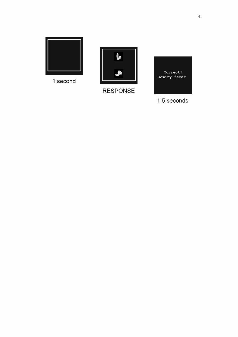
The structure of each trial is illustrated in Figure 1. Trials began with the

presentation of an outline square. After 1 sec, one or two “cell bodies” appeared

inside the square. Participants were expected to make either a “Jominy” or a

“Phipp’s” response by pressing one of two keys on a standard PC keyboard.

Allocation of “Jominy” and “Phipp’s” responses to these two keys was

counterbalanced across participants. Once the participant had responded, the abstract

pictures and outline square were replaced with a feedback message that indicated

whether the participant’s response was correct or incorrect, and also indicated the

correct response. If no response was made within 2 sec of the onset of the “cell

bodies”, the screen cleared and the message “Out of Time–Please Speed Up!” was

presented for 1.5 sec. The next trial followed immediately after this message. In the

test phase of the experiment, test trials were followed by the uninformative feedback

message “????–DATA MISSING”.

The experiment had two phases, a training phase, followed by a test phase. Trial

order within each phase was randomized within each of several latent sequential

blocks; starts of blocks were not signaled to participants in any way. Block length was

16

18 trials for the training phase, with AC and GE trial types each occurring three times

per block, and AB and FD trial types each occurring six times per block. Block length

in the test phase was 51 trials—the 18 trials of a training block, plus 33 test trials for

which feedback was uninformative. The 33 test trials comprised six presentations of

each of the B, C, D and E stimulus types, plus three presentations of each of the A,

BC and DE trial types. There were 20 blocks in the training phase and 8 blocks in test

phase; thus, the training phase comprised a total of 360 trials whilst the test phase

comprised a total of 408 trials. Each of the three abstract pictures within any given

stimulus group (i.e. A − G) occurred equally often in each block.

2.4. Electrophysiological analysis

Offline, the EEG was low-pass filtered at 40 Hz (24 dB/oct.), re-referenced to

the averaged ear channels and segmented into 600 ms epochs, comprising 500 ms

post-stimulus onset plus 100 ms pre-stimulus baseline. Following baseline correction,

all epochs were inspected for ocular, muscle, movement and other artifacts and the

contaminated epochs discarded. The remaining epochs were averaged, collapsing

across response type (Jominy, Phipps) to yield the ERPs for the four stimulus types of

interest: B, C, D and E.

We aimed to analyze the ERPs in a manner that was both comprehensive and

specific, whilst controlling the rate of false positives in multiple tests (Type 1 error).

To achieve this, we employed a two-stage procedure. The first stage focused on

“temporal scanning” of ERPs for any differences between the trial types of interest (B

vs. C; D vs. E) using a spatially non-specific technique that controls the likelihood of

Type 1 error. The second stage ascertained the presence of spatially circumscribed

effects such as SN with a more spatially specific ANOVA-based analysis and tested

17

for the critical interaction between condition (experimental vs. control) and frequency

(high vs. low).

In the first stage, in order to examine the entire ERP waveform for potential

differences between trial types, the ERPs were submitted to Topographic Analysis of

Variance (TANOVA; Pascual-Marqui et al., 1995), which examines the differences

between conditions not at the level of individual electrodes or groups of electrodes,

but at the level of entire scalp distributions (maps). As a measure of “global”

dissimilarity, it is well suited for testing multiple time ranges, because it reduces the

problem of correction for inflation for Type 1 error in multiple tests from two

dimensions (time x space) to one dimension (time) 1. TANOVA was run for several

time-windows (hence the need to control Type 1 error, see footnote). These time

windows were determined by inspecting the difference map between conditions (i.e.

the scalp distribution of the C − B difference wave), identifying the points of large

changes in the scalp distribution and defining the intervals of relative topographic

stability between these points as the intervals to be analyzed. Because one would not

expect the current manipulations to affect very early sensory ERPs (latency < 50 ms),

time windows were defined in the 50–500 ms post-stimulus-onset range. Relative to

1 TANOVA treats the scalp map of each condition as a vector defined by the scalp electrodes (58 in the present analysis). Since the difference between the vectors of two experimental conditions (e.g. C − B difference map) is also a vector, one can compute the magnitude of this difference map as the square root of the sum of squared differences between conditions at each electrode (the length of the difference vector). To assess the statistical significance of this difference, we used 5000 random permutations – this provides robust, if somewhat conservative, control for Type 1 error (Nichols & Holmes, 2002) in performing TANOVA tests repeatedly over the entire length (duration) of the ERP. TANOVA has been used successfully in previous cognitive ERP paradigms (cf. Lavric, Forstmeier, & Pizzagalli, 2004; Lavric, Mizon, & Monsell, 2008).

18

performing TANOVA across all time points (cf. Lavric et al., 2008), defining

intervals in this way increases statistical sensitivity because it reduces considerably

the number of tests; note that the temporal autocorrelation of ERP data also renders

correction for multiple point-by-point tests (see Footnote 1) somewhat conservative.

ERPs were referenced to an average-free montage (the average reference) to

ensure that the contributions of individual electrodes to the TANOVA calculations

were not determined by their spatial relation to the reference channels (ear channels).

The graphics (Figures 3 and 4) and ANOVA analyses (below) were based on ear-

referenced data. For completeness, TANOVA was also run on the control pair of

conditions (D and E).

In the second stage of the analysis, the time windows for which TANOVA

revealed reliable differences were submitted to ANOVAs run on the trial types of

interest (B and C) along with the control trial types (D and E). Prior to ANOVAs,

ERP electrodes were averaged in 12 scalp regions covering a 4 (anterior-to-posterior)

x 3 (laterality) spatial matrix, see Figure 4; region and laterality were both included as

factors in the ANOVA. The purpose of this grouping was to achieve an optimal

compromise between spatial specificity and adequate signal-to-noise ratio through

spatial smoothing, whilst also ensuring complete scalp coverage. The Huynh-Feldt

correction for violations of sphericity was applied when necessary in ANOVAs

(uncorrected degrees of freedom are reported).

3. Results

Two participants failed to achieve above-chance accuracy in the training phase

and were excluded from all subsequent behavioral and electrophysiological analyses.

19

3.1. Behavioral results

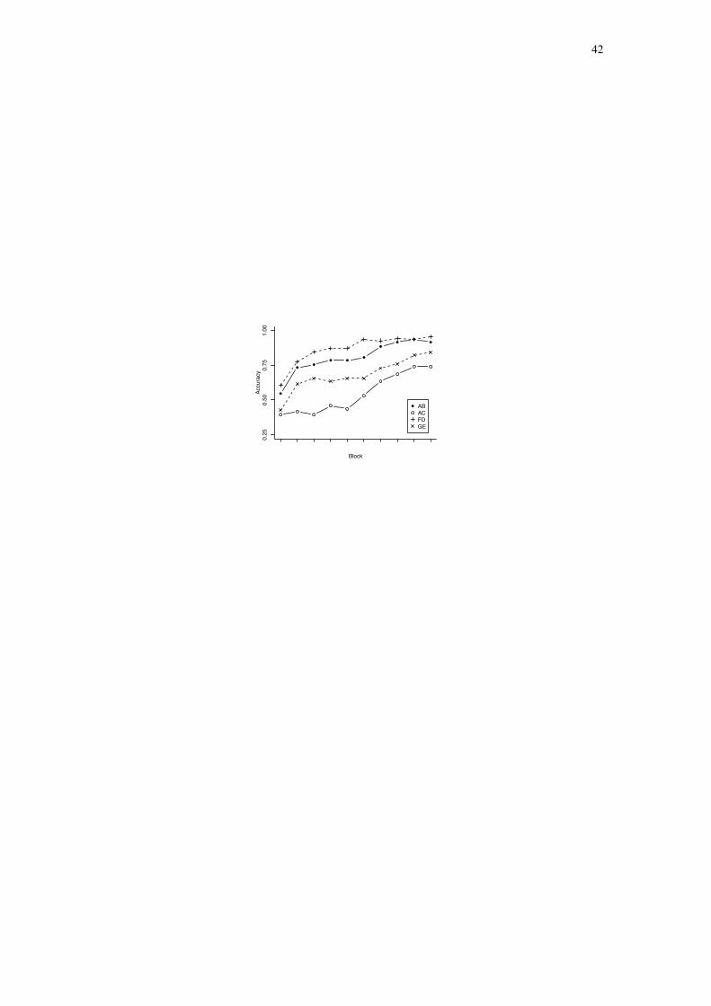
Figure 2 illustrates performance across the training phase. Accuracy was higher

in the final block of training than the first, F(1, 15) = 105.65, p < .001; higher for

common (AB, FD) than for rare (AC, GE) stimuli, F(1, 15) = 12.76, p = .003, and

lower in the presence of a shared cue (AB, AC) than in its absence (FD, GE), F(1, 15)

= 4.66, p = .047. These factors did not significantly interact, max. F(1, 15) = 2.65, p =

.125. In the final block of training, the effects of stimulus frequency remained

significant, F(1, 15) = 15.02, p = .001, as did the effects of a shared cue, F(1, 15) =

5.12, p = .039. These two factors did not significantly interact, F(1, 15) = 1.43, p =

.251. The effect of a shared cue on accuracy is not unexpected (the shared cue

increases associative interference) and it does not affect the interpretability of the

ERP results (because they are based on difference waveforms).

For test item BC, the proportion of common-disease responses was significantly

lower than the proportion of rare-disease responses, mean common-disease proportion

= .36, t(15) = 2.24, p = .041, indicating the presence of an inverse base-rate effect. For

test item A, the proportion of common-disease responses was significantly higher

than the proportion of rare-disease responses, mean = .69, t(15) = 4.81, p < .001

confirming that the IBRE we observed was not due to the relative novelty of the two

diseases. The proportion of common-disease responses for DE was significantly

higher than the proportion of rare-disease responses, mean = .95, t(15) = 28.99, p <

.001 confirming that the IBRE observed was contingent on the presence of a common

cue, and was not due to the relative novelty of cue C compared to cue B. The

proportion of common-disease responses to cue B, mean = .88, significantly exceeded

the proportion of rare-disease responses to cue C, mean = .67, t(15) = 2.88, p = .011,

20

indicating greater response accuracy for cue B than cue C. The presence of this

difference is important for the demonstration of a dissociation between attention and

response accuracy. The mean reaction times were BC 731 ms, A 835 ms, DE 785 ms,

B 731 ms, and C 763 ms.

--- Figures 3 and 4 about here, please ---

3.2. Event-related potentials.

Figure 3 shows ERP waveforms for the conditions of interest (B, C) and the

control conditions (D, E) for a subset of 12 electrodes. An examination of the time

course of ERP differences between conditions C and B (Figure 4, top panel) reveals

several apparent effects. The earliest difference seemed to emerge at ~120-170 ms

and was characterized by a more positive voltage distribution for the C condition over

the right-central scalp, followed at ~200-250 ms by a central midline positivity for C.

From ~250-270 ms the positivity for C became more anterior and increasingly left

lateralized, and was accompanied by occipital negativity on C trials (relative to B

trials). This posterior negative and anterior positive distribution of the C − B

difference was stable until ~320 ms, when the anterior positivity shifted to the

midline, whilst the posterior negativity remained relatively unchanged until ~360 ms.

Subsequently, the posterior negativity faded whereas the anterior positivity persisted

at midline until ~440 ms, after which the positivity for C became more centrally

distributed and more widespread towards the end of the ERP epoch.

Some of the effects in the contrast between the control conditions (E − D,

Figure 4, middle panel) seemed to resemble the C − B differences: a right-central

positivity at ~120-170 ms and a mid-central positivity at 230-240 ms. However, there

were also marked differences, particularly after 200 ms post-stimulus. The anterior

21

positivity (~250-440 ms) and the posterior negativity (270-360 ms) seen in the C − B

difference are not apparent in the E − D difference maps (there is instead some mid-

central positivity at ~270-330 ms, followed later by mid-central negativity at ~370-

410 ms). Overall, E − D differences appear reduced relative to C − B differences,

particularly from 200 ms after stimulus onset.

3.2.1. Stage 1 analysis

Based on the scalp distribution of the difference waveform, seven time windows

were defined and submitted to TANOVA of the C − B difference: 50–120 ms, 120–

170 ms, 170–270 ms, 270–320 ms, 320–360 ms, 360–440 ms and 440–500 ms (see

Figure 4, top panel). TANOVA and the permutation-based correction for multiple

comparisons found the difference between the scalp maps of B and C trial types to be

statistically significant in the 270–320 ms time window. This time window was

associated with scalp distributions characteristic for the posterior selection negativity

(SN) and frontal selection positivity (SP) (see Figure 4, top panel). The SN was right

lateralized and the SP was left lateralized, possibly suggesting overlapping intra-

cerebral generators; the magnitudes of the SN and SP were comparable. The

differences between the B and C conditions were not significant in the other time-

windows, the nearest to significance (p = 0.11, corrected for multiple comparisons)

was the difference in the immediately following time window (320–360 ms),

characterized by some persistence of the SN and a shift in the distribution of the SP to

a more midline positivity. A similar set of time windows was defined for the E − D

difference (see Figure 4, middle panel). TANOVA found no statistically significant

effects in any of these time-windows (largest p = 0.3, corrected).

22

3.2.2. Stage 2 analysis

In order to better characterize the difference revealed by TANOVA between the

B and C conditions, ERP amplitudes in the 270–320 ms time window were submitted

to a condition (B vs. C) by anterior-posterior (4) by laterality (3) ANOVA. As

expected the condition by anterior-posterior interaction was reliable, F (3, 45) = 5.66,

p = 0.002, confirming the presence of the posterior SN along with the anterior SP.

The interaction between condition and laterality was nearly significant, F(2, 30) =

2.82, p = 0.075, suggesting a tendency for the lateralization of these effects. No main

effects or interactions were significant in the corresponding ANOVA comparing D

and E. In order to confirm that the B vs. C difference was not reducible to effects of

the difference in their frequency, the ERP amplitudes in the two scalp regions where

SN and SP were observed (left frontal and right occipital) were submitted to an

ANOVA along with the corresponding regions for the control conditions D and E.

The critical interaction between condition (experimental vs. control), frequency (high

vs. low), and region (left frontal vs. right occipital) was statistically significant, F (1,

15) = 4.72, p = 0.046.

4. Discussion

We reported an ERP investigation of the inverse base-rate effect (IBRE), a

paradoxical yet robust phenomenon in predictive learning. Participants were trained

that stimulus compound AB predicted a frequently occurring outcome, whilst AC

predicted a rare outcome. As expected on the basis of previous behavioral studies

(e.g. Medin & Edelson, 1988), participants inferred that BC predicted the rare

outcome. This inference seems non-rational, but can be predicted by certain error-

driven attention theories of predictive learning (e.g. Kruschke, 2001b). Such theories

23

predict that, under conditions where there is a shared cue (A) and where AB is more

frequent than AC, C will come to be more attended than B. This difference in

attention is assumed to dominate responding to BC. On the basis of this prediction,

combined with an extensive literature on the ERP correlates of selective attention

(Hillyard & Anllo-Vento, 1998), we predicted and observed a posterior selection

negativity (SN), and a concurrent frontal selection positivity (SP), for C relative to B

in the test phase of our IBRE procedure. The frontal SP seemed to also be present in

the time-window preceding the SN, though this effect was not statistically reliable.

We further predicted that no corresponding effect would be observed for a pair

of control stimuli (D and E), which had the same relative frequency as B and C, but

for which there was no shared cue during training (and hence for which no IBRE

should be observed according to error-driven attention theory). These predictions

were also confirmed, with participants inferring that DE predicted the common

outcome, and with the E versus D difference in the ERPs being both non-significant,

and significantly smaller than the C versus B difference.

The SN for C relative to B was observed under conditions where response

accuracy for B exceeded response accuracy for C. Consequently, it appears that C was

both the more attended stimulus and the one about which participants were less

certain. This dissociation between attention and response accuracy appears difficult to

explain if one assumes that the attentional differences observed merely reflect people

attending to those stimuli for which they know the outcome. Such an account suffices

for the only previous study of error-driven attention in predictive learning to use an

ERP methodology (Wills et al., 2007), and it can also accommodate a range of results

using eye-tracking and other methodologies (Beesley & Le Pelley, 2011; Le Pelley,

2010; Le Pelley et al., 2011; Livesey et al., 2009). However, for the current results,

24

such an account is disconfirmed, due to the presence of the aforementioned

dissociation.

The occipital negativity we documented in response to C relative to B had a

later onset than the ‘classical’ SN which, according to the influential review by

Hillyard and Anllo-Vento (1998) emerges between 125 and 200 ms. However, the

early SN literature was based on discriminating (typically) one or two basic feature(s),

such as color, orientation, spatial frequency, direction of apparent motion, etc.,

defined a-priori and explicitly for the participant. In contrast, in our procedure

participants had to discriminate the cues based on complex features with which they

were not initially familiar. The onset of SNs reported for complex target object

discriminations (e.g. letters/symbols, Potts & Tucker, 2001; photographic images,

Schupp et al., 2007) is at ~200-250 ms following the stimulus onset, which is more in

line with our data. The topography of the ERP in the range of the SN in these studies

(with a prominent frontal positivity accompanying the occipital negativity) is also

consistent with the topography we documented.

4.1. Theories of the inverse base-rate effect

In the current article, we employed the term “error-driven attention theory” as a

natural language approximation for a class of mathematically expressed theories of

learning. This was a simplification, as this class of theories is not homogenous, and

different members vary in the extent to which they can accommodate the results we

have presented. In the current section, we consider the application of some specific

members of the class to our data.

One of the earlier formal expressions of error-driven attention theory is due to

Mackintosh (1975; see also Sutherland & Mackintosh, 1971). Mackintosh’s (1975)

25

formulation of error-driven attention theory (hereafter, Mack75) is not consistent with

the current results because response accuracy for B presented alone exceeds that for C

presented alone in our experiment. In Mack75, the associative strength for B must

therefore exceed that for C, and thus the dominant response to BC is predicted to be

the same as that for B. This is opposite to our current study, where the dominant

response to BC is the same as for C (an inverse base-rate effect). Hence, Mack75

cannot predict the presence of an IBRE in our experiment.

Kruschke’s EXIT model (Kruschke, 2001b), however, can accommodate the

presence of an IBRE under conditions where the response accuracy for B presented

alone exceeds the response strength for C presented alone; this ability is illustrated in

previously published simulations of the EXIT model, see Kruschke (2003, Table 1).

One reason EXIT succeeds where Mack75 fails is that in the former attention affects

both responding and future learning, whilst in the latter it only affects future learning.

EXIT learns to direct attention toward C in AC during training, because doing so

reduces the likelihood of the error that would otherwise be caused by the association

of A to the common disease. At test, the presentation of compound BC leads to

attention being directed towards C, due to the similarity of BC to AC. If this

attentional allocation is sufficiently strong, C can dominate responding, leading to an

IBRE. Of course, BC is also similar to training item AB, but attentional re-allocation

is not required to respond correctly to AB during training, so the overall effect is that

when BC is presented at test, C is attended more than B.

A further critical aspect of EXIT that allows it to accommodate our results is

that learned attention is normalized before it exerts its effect on responding. This is

important because on trials such as B and C, where only one stimulus component is

presented, the presented component is fully in control of responding; it is only where

26

multiple stimulus components are presented (e.g. BC) that learned attention affects

the relative control those components have over responding. This permits the model

to predict more accurate responding to B alone than to C alone, despite the greater

learned attention to C than to B. A consequence of this formulation is that, if EXIT is

the correct account of the IBRE, then the Selection Negativity in the current study

presumably reflects pre-normalized learned attention in the EXIT model. This might

be because normalization takes time and the Selection Negativity is quite an early

component. It might alternatively be because the Selection Negativity indexes activity

in EXIT’s gain nodes; the gain nodes represent non-normalized learned attention in

EXIT, which is subsequently normalized further down the processing stream.

However, in the absence of further data, further speculation would be inappropriate.

In the current paper, we have focused on the class of error-driven attention

learning theory exemplified by Mack75 and EXIT. An alternative class of theory is

that attention is directed towards stimuli that are followed by surprising outcomes

(e.g. Pearce & Hall, 1980; Wagner, 1978). There is at least one published theory of

the IBRE within this alternative framework (Shanks, 1992). As things stand, this class

of account seems to suffer from the same problem as Mack75 and for the same reason

– in other words, it cannot predict an IBRE under conditions where response accuracy

to B alone exceeds that to C alone, because attention is assumed to affect only future

learning, not responding. However, it seems entirely possible that such accounts

could be modified along the lines of the EXIT model in order to accommodate this

result (i.e. the addition of a process where attention affects responding, not just future

learning).

Yet another type of error-driven attention theory states that attentional

allocation occurs at the level of stimulus dimensions, rather than at the level of

27

particular stimulus features within those dimensions. Sutherland and Mackintosh

(1971), and the Generalized Context Model (Nosofsky, 1984), are examples of this

class of account. Recent work by Johansen et al. (2010) suggests that feature-based

attention is a better model of the IBRE than dimension-based attention.

Other than error-driven attention theories, we are not aware of any other class of

explanation that can account for the results observed in the current study. The class of

theory most similar to error-driven attentional theory states that prediction errors gate

learning about outcomes; in other words, predictive relationships between cues and

outcomes are learned to the extent that the outcomes they predict are not already well

predicted (Schultz et al., 1997; Rescorla & Wagner, 1972; Gluck, 1992; Harris, 2006).

Such theories do not incorporate stimulus-based attention per se, but they can

accommodate a range of attentional phenomena in learning via the additional

assumption that stimuli strongly associated to an outcome attract attention. Such

theories cannot accommodate the dissociation between attention and response

accuracy observed in the current study. Indeed, standard versions of these theories

cannot accommodate the IBRE (Markman, 1989). Some stimulus-sampling variants

of these theories can accommodate the behavioral phenomena in the current study

(e.g. Gluck, 1992), but they have no mechanism by which they can explain the

dissociation of response accuracy from attention.

Bayesian inference provides another class of account of predictive learning

(Anderson, 1991; Sanborn et al., 2010). Although there have been some attempts to

accommodate the IBRE within a Bayesian framework (Anderson, 1991), such

accounts struggle to accommodate the known IBRE behavioral phenomena

(Kruschke, 2006). This is perhaps unsurprising given that Bayesian accounts assume

human inference is approximately rational, and the IBRE appears to be a strikingly

28

non-rational phenomenon. Kruschke (2006) proposes that the IBRE can be

accommodated within a Bayesian framework by assuming that predictive learning is

locally rather than globally Bayesian. Specifically, Kruschke assumes the presence of

a locally-Bayesian subsystem that determines attentional allocation, feeding into a

subsequent locally-Bayesian subsystem that infers cue-outcome relationships on the

basis of attentionally-modulated input. In the context of the IBRE, such an account

has much in common with error-driven attentional theories.

Mitchell et al. (2009) state that theories such as Mackintosh (1975) and

Kruschke (2001b) are usually assumed to describe the operation of an automatic link-

formation mechanism; the intended implication being that such theories predict

learning and attentional allocation to be automatic, uninstructable and unconscious.

The position taken in the current article is that error-driven attentional theories of

predictive learning are largely silent about such issues. In agreement with Mitchell et

al. (2009), our position is that nothing in those theories, or in the data of the current

study, discounts the rather likely possibility that the phenomena we have observed are

mediated and moderated by conscious, deliberate processes.

4.2. Critiques and limitations

One potential criticism of the current study, and of Wills et al. (2007), is that

theories of error-driven attention assume attentional re-allocation occurs during

training as a result of prediction errors produced by compound cues, whilst the current

methodology assesses attention toward single cues in a post-training test phase. In

response, we’d argue that the current methodology provides a particularly

illuminating test of such theories, because they predict (as discussed above) that

attentional allocation persists beyond the original training context. The current results

29

imply that this is indeed the case, providing additional support for such theories.

Nevertheless, one possible topic for future research would be to examine the N2pc

component (Eimer, 1996; Kiss et al., 2007; Luck & Hillyard, 1994) with respect to

stimuli BC and DE. Such an analysis was not possible in the current study because

our stimuli were small and centrally positioned. This was a deliberate choice,

designed to minimize eye-movement artifacts, and to maximize comparability with

Wills et al. (2007). An investigation of the N2pc would require the two components

of the compound cues (e.g. BC) to be left-right lateralized.

The current study focused on a test-phase analysis of ERPs locked to stimulus

onset; this was because we had clear predictions about what would be observed,

predictions made on the basis of previous work (Wills et al., 2007) and formal theory

(Kruschke, 2001b). Those predictions were confirmed. A complementary approach to

studying the electrophysiology of predictive learning is to consider training-phase

ERPs locked to the onset of feedback (Luque et al., 2012; see also Moris et al., in

press). This approach represents an important contribution to the study of the

electrophysiology of predictive learning; it was not pursued in the current study for

two reasons.

The first reason was a lack of any clear predictions concerning event-related

potentials during training that would allow one to distinguish error-driven attentional

theories of the IBRE from other classes of account. More generally, it is hard to see

how event-related potentials to vertically-presented compound stimuli could be

informative with regard to selective attention to an element of that compound (e.g.,

attention to B in AB or C in AC). The second reason was that, even if such

predictions could be derived, analysis of event-related potentials during training poses

seemingly insurmountable technical issues in the current study. Performance during

30

the training phase of a predictive learning study is, by definition, dynamic.

Participants start the training phase at chance, and end with high levels of

performance. Meaningful analysis thus requires subdivision of the training phase into

a series of sub-sections for which error rate is relatively homogenous. However, given

the relatively rapid rate of learning in such studies, these sub-divisions result in too

few trials per sub-section for a meaningful ERP analysis. The solution to this problem

employed by Luque et al. (2012) was to ask each participant to learn the same abstract

structure 30 times within the same session. However, the length and complexity of

our behavioral procedure (relative to Luque’s) rendered this solution impractical in

the current study.

For similar reasons, we did not conditionalize our analysis of stimulus-locked

ERPs by response type (common disease predicted vs. rare disease predicted). For

example, about one third of responses to test item C predicted the common disease,

whilst two-thirds predicted the rare disease. Thus, there was an average of 16 trials

per participant for the common-disease response to C; insufficient for a clear ERP

analysis. Although in principle it would have been possible to extend the test session,

the experiment was already rather long and, as far as we are aware, current theories

make no clear predictions about the outcome of such an analysis.

Turning to possible critiques of our behavioral data, it is noticeable that

response accuracy at test for the perfect predictors (B and C) was lower than in some

previous studies of the IBRE. For example, Kruschke (1996, Experiment 1) reports a

perfect predictor response accuracy of 0.92 (when averaged across B and C), while in

the current study the corresponding figure is 0.78. However, the IBRE has been

observed across a wide range of perfect-predictor response accuracies, ranging from

0.60 in Juslin et al. (2001, Experiment 3) to 0.95 in Johansen et al. (2007, Experiment

31

3). The current study sits roughly in the middle of that range. Accuracy on the perfect

predictors at test is presumably a function of a number of variables, including length

of training and the type of stimuli employed.

As previously discussed, response accuracy for the common perfect predictor

(B) exceeded response accuracy for the rare perfect predictor (C) in the current study.

An informal review of the literature indicates that both B > C (Bohil et al., 2005;

Juslin et al., 2001; Medin & Edelson, 1988; Winman et al., 2005) and C > B (Juslin et

al., 2001; Kruschke, 1996; Lamberts & Kent, 2007; Medin & Edelson, 1988; Wood &

Blair, 2011) are observed in different studies of the IBRE. There is some indication

that B > C becomes more likely as mean performance on B and C increases, with no

reports of B > C in studies where mean accuracy is substantially below .8. Mean

accuracy in the current study was 0.78, and hence the presence of the B > C pattern

was not entirely unexpected. Nevertheless, further research is required to adequately

determine what causes the presence of B > C versus C > B, and whether error-driven

attention theories provide the best account of the IBRE in conditions where C > B.

Finally, the SN observed in the current study is later than that observed in Wills

et al. (2007). Although the two studies employed similar stimulus elements, the

designs were quite different. Notably, in the current design (but not in Wills et al.,

2007) certain cues are, from the outset, encountered in two different compounds (e.g.

A in AB and in AC). This may have necessitated more thorough perceptual analysis

in the current study, delaying the onset of the SN relative to Wills et al. (2007).

4.3. Conclusions

We presented the first electrophysiological investigation of the inverse base-rate

effect, a robust non-rational bias in predictive learning. Error-driven attention theory

32

predicts both the presence of the inverse base-rate effect, and the presence of a

corresponding attentional ERP component, in our study. It further predicts the

absence of an inverse base-rate effect, and the absence of the corresponding ERP

component, under conditions where there is no shared cue during training. These

results were observed. No other class of theory appears able to accommodate these

results.

33

Acknowledgements

The authors thank Mike Le Pelley, Ian McLaren, Chris Mitchell and Haline

Schendan for their helpful comments.

34

References

Anderson JR. 1991. The adaptive nature of human categorization. Psychol Rev.

98:409-429.

Beesley T, Le Pelley ME. 2011. The influence of blocking on overt attention and

associability in human learning. J Exp Psychol Anim Behav Process. 37:114-120.

Bott L, Hoffman AB, Murphy GL. 2007. Blocking in category learning. J Exp

Psychol Gen. 136:685–99.

Binder A, Estes WK. 1966. Transfer of response in visual recognition situations as a

function of frequency variables. Psychol Monogr. 80:Whole No. 631.

Bohil CJ, Markman AB, Maddox WT. 2005. A feature-salience analogue of the

inverse base-rate effect. Korean J Think Prob Solv. 15:17-28.

Eimer M. 1996. The N2pc component as an indicator of attentional selectivity.

Electroencephalogr Clin Neurophysiol. 99:225-234.

Gluck MA. 1992. Stimulus sampling and distributed representations in adaptive

network theories of learning. In: Healy AF, Kosslyn SM, Shiffrin RM, editors.

From learning theory to connectionist theory: Essays in honor of William K. Estes.

Hillsdale (NJ): Lawrence Erlbaum Associates. p. 169-199.

Harris JA. 2006. Elemental representations of stimuli in associative learning. Psychol

Rev.113:584-605.

Hillyard SA, Anllo-Vento L. 1998. Event-related brain potentials in the study of

visual selective attention. Proc Natl Acad Sci USA. 95:781-787.

Imperato PJ. 1979. Medical detective. New York (NY): Richard Marek.

Johansen MK, Fouqet N, Shanks, DR. 2007. Paradoxical effects of base rates and

representation in category learning. Mem Cognition. 35:1365-1379.

35

Johansen MK, Fouquet N, Shanks, DR. 2010. Featural selective attention, exemplar

representation, and the inverse base-rate effect. Psychon B Rev. 17:637-643.

Jones FW, Wills AJ, McLaren IPL. 1998. Perceptual categorization: connectionist

modelling and decision rules. Q J Exp Psychol. 51B:33-58.

Juslin P, Wennerholm P, Winman A. 2001. High-level reasoning and base-rate use:

Do we need cue-competition to explain the inverse base-rate effect? J Exp Psychol

Learn Mem Cogn. 27:849-871.

Kalish M. 2001. An inverse base rate effect with continuously valued stimuli. Mem.

Cognition. 29:587-597.

Kamin LJ. 1969. Attention-like processes in classical conditioning. In: Jones MR,

editor. Miami symposium on the prediction of behavior: Aversive stimulation.

Coral Gables (FL): University of Miami Press. p. 9-33.

Kiss M, Van Velzen J, Eimer M. 2007. The N2pc component and its links to attention

shifts and spatially selective visual processing. Psychophysiology. 45:240-249.

Kruschke JK. 1996. Base rates in category learning. J Exp Psychol Lear. Mem Cogn.

22:3-26.

Kruschke JK. 2001a. The inverse base rate effect is not explained by eliminative

inference. J Exp Psychol Learn Mem Cogn. 27:1385-1400.

Kruschke JK. 2001b. Toward a unified model of attention in associative learning. J

Math Psychol. 45:812-863.

Kruschke JK. 2003. Attentional theory is a viable explanation of the inverse base rate

effect: A reply to Winman, Wennerholm, and Juslin (2003). J Exp Psychol Learn

Mem Cogn. 29:1396-1400.

Kruschke JK. 2006. Locally Bayesian learning with applications to retrospective

revaluation and highlighting. Psychol Rev. 113:677-699.

36

Kruschke JK, Kappenman ES, Hetrick WP. 2005. Eye gaze and individual differences

consistent with learned attention in associative blocking and highlighting. J Exp

Psychol Learn Mem Cogn. 31:830-845.

Lamberts K, Kent C. 2007. No evidence for rule-based processing in the inverse base-

rate effect. Mem Cognition. 35:2097-2105.

Lavric A, Forstmeier S, Pizzagalli D. 2004. When go and nogo are equally frequent:

ERP components and cortical tomography. Eur J Neurosci. 20:2483-2488.

Lavric A, Mizon, GA, Monsell S. 2008. Neurophysiological signature of effective

anticipatory task-set control: a task-switching investigation. Eur J Neurosci.

28:1016-1029.

Le Pelley ME. 2010. Attention and human associative learning. In: Mitchell CJ, Le

Pelley ME, editors. Attention and associative learning. Oxford (UK): Oxford

University Press. p. 187-216.

Le Pelley ME, Beesley T, Griffiths O. 2011. Overt attention and predictiveness in

human contingency learning. J Exp Psychol Anim Behav Process. 37:220-229.

Le Pelley ME, Vadillo MA, Luque D. in press. Learned predictiveness influences

rapid attentional capture: Evidence from the dot probe task. J Exp Psychol Learn

Mem Cog.

Livesey EJ, Harris IM, Harris JA. 2009. Attentional changes during implicit learning:

Signal validity protects a target stimulus from the attentional blink. J Exp Psychol

Learn Mem Cogn. 35:408-422.

Luck SJ, Hillyard SA. 1994. Electrophysiological correlates of feature analysis during

visual search. Psychophysiology. 31:291-308.

Luck SJ, Woodman JF, Vogel EK. 2000. Event-related potential studies of attention.

Trends Cogn Sci. 4: 432-440.

37

Luque D, López F, Marco-Pallares J, Càmara E, Rodríguez-Fornells A. 2012.

Feedback-related brain potential activity complies with basic assumptions of

associative learning theory. J Cogn Neurosci. 24. 794-808.

Mackintosh NJ. 1975. A theory of attention: Variations in the associability of stimuli

with reinforcement. Psychol Rev. 82:276-298.

Markman AB. 1989. LMS rules and the inverse base-rate effect: Comment on Gluck

and Bower (1988). J Exp Psychol Gen. 118:417-421.

Medin DL, Bettger JG. 1991. Sensitivity to changes in base-rate information. Am J

Psychol. 104:311-332.

Medin DL, Edelson SM. 1988. Problem structure and the use of base-rate information

from experience. J Exp Psychol Gen. 117:68-85.

Medin DL, Robbins D. 1971. Effects of frequency on transfer performance after

successive discrimination training. J Exp Psychol. 87:434-436.

Mitchell CJ, De Houwer J, Lovibond P. 2009. The propositional nature of human

associative learning. Behav Brain Sci. 32:183-198.

Moris J, Luque D, Rodríguez-Fornells A. in press. Learning induced modulation of

the stimulus-preceding negativity. Psychophysiology.

Nichols T, Holmes A. 2002. Nonparametric permutation tests for functional

neuroimaging: A primer with examples. Hum Brain Mapp. 15:1-25.

Nosofsky RM. 1984. Choice, similarity, and the context theory of classification. J Exp

Psychol Learn Mem Cogn. 10:104-114.

Pascual-Marqui R, Michel CM, Lehmann D. 1995. Segmentation of brain electrical

activity into microstates: Model estimation and validation. IEEE Tr Biomed Eng.

42:658-665.

Pearce JM, Hall G. 1980. A model of Pavlovian conditioning: variations in the

38

effectiveness of conditioned but not of unconditioned stimuli. Psychol Rev.

87:532-552.

Pothos EM, Wills AJ. Introduction. In Pothos, EM, Wills AJ, editors. Cambridge,

UK: Cambridge University Press. Formal approaches in categorization. p. 1–17.

Potts GF, Tucker DM. 2001. Frontal evaluation and posterior representation in target

detection. Cogn Brain Res. 11:147-156.

Rescorla RA, Wagner AR. 1972. A theory of Pavlovian conditioning: Variations in

the effectiveness of reinforcement and nonreinforcement. In: Black AH, Prokasy WF,

editors. Classical conditioning II: Current research and theory. New York (NY):

Appleton Century Crofts. p. 64-99.

Rhetorica ad herennium. 85BC. London (UK): Heinemann. English Translation.

Caplan H. 1954.

Sanborn AN, Griffiths TL, Navarro DJ. 2010. Rational approximations to rational

models: alternative algorithms for category learning. Psychol Rev. 117:1144-1167.

Schultz W, Dayan P, Montague PR. 1997. A neural substrate of prediction and

reward. Science. 275:1593-1599.

Schupp HT, Stockburger J, Codispoti M, Junghofer M, Weike AI, Hamm AO. 2007.

Selective visual attention to emotion. J Neurosci. 27:1082-1089.

Shanks DR. 1992. Connectionist accounts of the inverse base-rate effect in

categorization. Connect Sci. 4:3-18.

Sherman JW, Kruschke JK, Sherman SJ, Percy EJ, Petrocelli JV, Conrey FR. 2009.

Attentional processes in stereotype formation: A common model for category

accentuation and illusory correlation. J Pers Soc Psychol. 96:305-323.

Sutherland NS, Mackintosh NJ. 1971. Mechanisms of animal discrimination learning.

New York: Academic Press.

39

Tversky A, Kahneman D. 1973. Availability: A heuristic for judging frequency and

probability. Cognit Psychol. 5:207-232.

Von Restorff H .1933. Uber die Wirkung von Bereichsbildungen im Spurenfeld.

Psychol Res. 18:299-342.

Wagner AR. 1978. Expectancies and the priming of STM. In: Hulse SH, Fowler H,

Honig WH, editors. Hillsdale (NJ): Lawrence Erlbaum Associates. Cognitive

processes in animal behavior. p. 177–210.

Wills AJ, Lavric A, Croft G, Hodgson TL. 2007. Predictive learning, prediction errors

and attention: Evidence from event-related potentials and eye tracking. J Cogn

Neurosci. 19:843-854.

Wills AJ, McLaren IPL. 1997. Generalization in human category learning: A

connectionist explanation of differences in gradient after discriminative and non-

discriminative training. Q J Exp Psychol. 50A:607-630.

Wills AJ, Pothos EM. 2012. On the adequacy of current empirical evaluations of

formal models of categorization. Psychol Bull. 138:102-125.

Wills AJ, Reimers S, Stewart N, Suret MB, McLaren IPL. 2000. Tests of the ratio rule

in categorization. Q J Exp Psychol. 53A:983-1011.

Winman A, Wennerholm P, Juslin P, Shanks DR. 2005. Evidence for rule-based

processes in the inverse base-rate effect. Q J Exp Psychol. 58A:789-815.

Wood MJ, Blair MR. 2011. Informed inferences of unknown feature values in

categorization. Mem Cognition. 39:666-674.

40

Figure Captions

Figure 1. Trial structure.

Figure 2. Accuracy in the training phase as a function of stimulus type (see Table 1)

and training block. Each plot point is the mean of two consecutive training blocks

(blocks 1& 2, 3 & 4, … 19 & 20).

Figure 3. ERP waveforms for the conditions of interest (B, C) and the control

conditions (D, E) shown for a subset of 12 electrodes; as in the actual EEG cap,

lateral electrodes vary in their distances from the midline (e.g., F5, C3, O1).

Inspection of the waveforms reveals from ~250-300 ms a more negative-going ERP

for C relative to B at posterior electrodes (particularly over the right hemiscalp) and

more positive amplitudes for C relative to B over frontal electrodes (particularly over

the left hemiscalp); neither effect is apparent in the D vs. E contrast (see Fig. 3 for the

scalp distribution of the contrasts between the two pairs of conditions).

Figure 4. ERP contrasts presented in the upper and middle panels as spherical spline

interpolated difference maps framed to represent windows used for TANOVA (the

solid red frame with grey fill shows the window of reliable differences corrected for

multiple tests; the broken red frame shows the window that approached significance),

and in the lower panel as ERP plots for representative electrodes; a schematic of the

scalp regions used in the ANOVA is also shown.

41

42

Block

Accuracy

0.25

0.50

0.75

1.00

ABACFDGE

43

44