Atomistic Simulations of Materials for Nuclear Fusion Submitted in part fulfilment of the requirements for the degree of Doctor of Philosophy in Material Science and Engineering and the Diploma of Imperial College London, October 2017 Matthew Lee Jackson Department of Material Science and Engineering Imperial College London

Welcome message from author
This document is posted to help you gain knowledge. Please leave a comment to let me know what you think about it! Share it to your friends and learn new things together.
Transcript
Atomistic Simulations of Materialsfor Nuclear Fusion
Submitted in part fulfilment of the requirements for the degree ofDoctor of Philosophy in Material Science and Engineeringand the Diploma of Imperial College London, October 2017
Matthew Lee Jackson
Department of Material Science and EngineeringImperial College London

Declaration of originality: The work presented herein is my own, with contributions
from others appropriately referenced and acknowledged.
The copyright of this thesis rests with the author and is made available under a Creative
Commons Attribution Non Commercial No Derivatives licence. Researchers are free
to copy, distribute or transmit the thesis on the condition that they attribute it, that
they do not use it for commercial purposes and that they do not alter, transform or
build upon it. For any reuse or redistribution, researchers must make clear to others
the licence terms of this work
ii

Abstract
Nuclear fusion has held the promise of unlimited clean energy for over fifty years. How-
ever, owing to the technical challenges of achieving a sustained reaction, this promise
remains unrealised. Chief among these challenges is the survivability of reactor mate-
rials, which are subject to extreme temperatures and flux of fast neutrons. To aid in
understanding damage processes, atomistic simulations have been employed to model
the fundamental processes of radiation damage, with some models validated by com-
parison to inelastic neutron scattering results.
Beryllium rich beryllides, in particular the Be12M materials (where M is a transition
metal), are under consideration for neutron multiplying applications in fusion reactors,
however the basic properties of some of these materials remain poorly characterised.
Herein, DFT simulations have been used to clarify the structure of Be12Ti, which was
previously in contention. Further, several basic properties of Be12Ti have been pre-
dicted, including the thermal expansion, bulk modulus, elastic constants and lattice
parameters.
The phonon density of states of Be12M (M=Ti/V/Mo/Ta/Nb) and Be13Zr have been
predicted, with trends observed based on the mass of the M species. Inelastic neutron
scattering has also been performed, and results compared with the simulated phonon
density of states. The experimental results were significantly broadened, making anal-
ysis difficult. It was found that signal at low energies is attributed to second order
iii

reflections, and has better energy resolution than the first order data. When simulated
results are artificially broadened, they bear strong qualitative resemblance to experi-
mental results for all materials.
Point defects including vacancies, interstitials and antisite defects were investigated in
Be12M materials (M=Ti,V,Mo,W) using DFT, with interstitial sites identified for the
first time. Beryllium defects are consistently more favourable than transition metal de-
fects. Schottky disorder is the lowest energy intrinsic disorder process in all materials,
although beryllium Frenkel is comparable for Be12Ti and Be12V. Small defect clusters
were also investigated. Several VBeVBe, VBeVM and MBeBe clusters are stable with re-
spect to the isolated species, although their energies are highly orientation dependent.
BeiBei formation is almost always unfavourable, and VMVM is always unfavourable.
Non-stochiometry is extremely limited, to the extent that these intermetallics may be
considered line compounds. Migration is predicted to be dominated by VBe mediated
processes and to be weakly anisotropic.
Low energy displacement simulations using empirical potentials were performed for
beryllium, tungsten, carbon and tungsten carbide. Displacement was predicted to
be strongly dependent on the potential used, as well as the local environment of the
displaced species. For beryllium, tungsten and diamond, defect recovery is predicted
to be important immediately following the displacement event at energies above the
threshold displacement energy. The threshold displacement energy is a strong function
of crystallographic direction for all materials. New models have been developed to
predict the maximum displacement as a result of a displacement event.
iv
Acknowledgements
I would like to thank all my friends and family for supporting me in innumerable ways
throughout my PhD, and for making it a valuable (and, at times, amusing) chapter of
my life. In particular I would like to thank everyone in the CNE, foremost amongst
whom is my supervisor Prof. Robin W. Grimes. He has been supportive throughout,
provided invaluable direction and guidance, and, despite having an impossibly busy
schedule, always made time for his students.
In addition, I would like to thank Dr. Michael Rushton, Dr. Paul Fossati and Dr.
Patrick Burr for continuing insight and advice, without which I can only imagine how
many more months of writing I would now be facing. I would particularly like to thank
Patrick for his support leading up to and during my time performing experiments at
ANSTO. My involvement was only made possible through his insistence, and during
which time he kindly opened his home to me.
Thanks also go to my fellow PhD students and postdocs for both their useful comments
and, perhaps even more so, entertaining antics that have made the long hours more
bearable. In particular I would like to thank “the Bois” (and Jim). Special mention
is also made for Dr. Jonathan Tate and Ms. Emma Warris, who have facilitated my
PhD and generally kept the rabble under control.
I would be remiss without mentioning my greatest benefactors: my mum and dad,
who have supported me unwaveringly for 26 years, and without whose encouragement
v
I would without a doubt not be here. Last but most certainly not least, I would like to
thank my wonderful partner, Ola Gwozdz. More than anyone, she has been there for
me throughout, supported me in every way imaginable and given me reason to smile
even on the hardest of days.
I would also like to acknowledge CCFE for financial support from EUROfusion (EU-
RATOM grant number No 633053), the Imperial College HPC for providing computing
resources, and ANSTO for beam time on the Taipan instrument, grant number 5338.
vi

Contents
Abstract iii
Acknowledgements v
1 Introduction 1
1.1 The Nuclear option . . . . . . . . . . . . . . . . . . . . . . . . . . . . . 1
1.2 Fusion and Fission . . . . . . . . . . . . . . . . . . . . . . . . . . . . . 3
1.3 Fission . . . . . . . . . . . . . . . . . . . . . . . . . . . . . . . . . . . . 5
1.4 Fusion . . . . . . . . . . . . . . . . . . . . . . . . . . . . . . . . . . . . 10
1.4.1 Lawson Criteria and the Triple Product . . . . . . . . . . . . . 11
1.4.2 Achieving Fusion . . . . . . . . . . . . . . . . . . . . . . . . . . 13
1.5 Components of Fusion . . . . . . . . . . . . . . . . . . . . . . . . . . . 19
1.5.1 The First Wall . . . . . . . . . . . . . . . . . . . . . . . . . . . 20
1.5.2 The Divertor . . . . . . . . . . . . . . . . . . . . . . . . . . . . 22
1.5.3 Tritium Breeding Modules . . . . . . . . . . . . . . . . . . . . . 23
vii
CONTENTS viii
1.6 Materials of Interest . . . . . . . . . . . . . . . . . . . . . . . . . . . . 24
1.6.1 Beryllium . . . . . . . . . . . . . . . . . . . . . . . . . . . . . . 25
1.6.2 Beryllium Intermetallics . . . . . . . . . . . . . . . . . . . . . . 29
1.6.3 Tungsten . . . . . . . . . . . . . . . . . . . . . . . . . . . . . . . 32
1.6.4 Tungsten Carbide . . . . . . . . . . . . . . . . . . . . . . . . . . 33
1.7 Modelling Radiation Damage in Materials . . . . . . . . . . . . . . . . 35
1.7.1 Theory of Radiation Damage . . . . . . . . . . . . . . . . . . . 36
1.7.2 Multiscale Modelling . . . . . . . . . . . . . . . . . . . . . . . . 41
1.8 Structure of this Thesis . . . . . . . . . . . . . . . . . . . . . . . . . . . 44
2 Methodology 45
2.1 Density Functional Theory . . . . . . . . . . . . . . . . . . . . . . . . . 46
2.1.1 Hohenberg, Kohn and Sham . . . . . . . . . . . . . . . . . . . . 47
2.1.2 Exchange-Correlation Functional . . . . . . . . . . . . . . . . . 50
2.1.3 Spin Polarisation . . . . . . . . . . . . . . . . . . . . . . . . . . 52
2.1.4 Pseudopotentials . . . . . . . . . . . . . . . . . . . . . . . . . . 53
2.1.5 A note on Metals . . . . . . . . . . . . . . . . . . . . . . . . . . 60
2.1.6 Computational Details . . . . . . . . . . . . . . . . . . . . . . . 61
2.2 Static Techniques . . . . . . . . . . . . . . . . . . . . . . . . . . . . . . 62
2.2.1 Transition State Search and Nudged Elastic Band . . . . . . . . 64

CONTENTS ix
2.2.2 Phonons: Harmonic and Quasi-Harmonic Approximations . . . 67
2.3 Empirical Potentials . . . . . . . . . . . . . . . . . . . . . . . . . . . . 69
2.3.1 Embedded Atom Method . . . . . . . . . . . . . . . . . . . . . . 70
2.3.2 EAM Potential for Beryllium . . . . . . . . . . . . . . . . . . . 71
2.3.3 Bond Order Potentials . . . . . . . . . . . . . . . . . . . . . . . 74
2.3.4 Bond Order Potentials for the Tungsten - Carbon System and
Beryllium . . . . . . . . . . . . . . . . . . . . . . . . . . . . . . 75
2.3.5 ZBL modifications . . . . . . . . . . . . . . . . . . . . . . . . . 78
2.4 Molecular Dynamics . . . . . . . . . . . . . . . . . . . . . . . . . . . . 80
2.5 Inelastic Neutron Scattering . . . . . . . . . . . . . . . . . . . . . . . . 83
2.5.1 Experimental Setup . . . . . . . . . . . . . . . . . . . . . . . . . 85
3 Structural Investigations of Beryllides 88
3.1 Introduction . . . . . . . . . . . . . . . . . . . . . . . . . . . . . . . . . 88
3.2 Resolving the Structure of Be12Ti . . . . . . . . . . . . . . . . . . . . . 89
3.2.1 Density Functional Theory Simulations . . . . . . . . . . . . . . 92
3.2.2 Calculated Material Properties of Be12Ti . . . . . . . . . . . . . 96
3.3 Inelastic Neutron Scattering in Beryllides . . . . . . . . . . . . . . . . . 99
3.3.1 Theoretical Investigations . . . . . . . . . . . . . . . . . . . . . 100
3.3.2 Neutron Scattering . . . . . . . . . . . . . . . . . . . . . . . . . 103

CONTENTS x
3.3.3 Data and Analysis . . . . . . . . . . . . . . . . . . . . . . . . . 108
3.3.4 Comparison . . . . . . . . . . . . . . . . . . . . . . . . . . . . . 114
3.4 Summary and Conclusions . . . . . . . . . . . . . . . . . . . . . . . . . 117
3.5 Contributions . . . . . . . . . . . . . . . . . . . . . . . . . . . . . . . . 118
4 Defects in Be12M Beryllides 119
4.1 Introduction . . . . . . . . . . . . . . . . . . . . . . . . . . . . . . . . . 119
4.2 Point Defects . . . . . . . . . . . . . . . . . . . . . . . . . . . . . . . . 121
4.3 Defect disorder processes . . . . . . . . . . . . . . . . . . . . . . . . . . 126
4.4 Defect Clusters . . . . . . . . . . . . . . . . . . . . . . . . . . . . . . . 127
4.5 Nonstochiometry . . . . . . . . . . . . . . . . . . . . . . . . . . . . . . 131
4.6 Defect Migration in Be12Ti . . . . . . . . . . . . . . . . . . . . . . . . . 139
4.6.1 Point Defect Migration . . . . . . . . . . . . . . . . . . . . . . . 140
4.6.2 Cluster Migration . . . . . . . . . . . . . . . . . . . . . . . . . . 144
4.7 Summary and Conclusions . . . . . . . . . . . . . . . . . . . . . . . . . 146
5 Displacement Processes in Fusion Materials 150
5.1 Introduction . . . . . . . . . . . . . . . . . . . . . . . . . . . . . . . . . 150
5.2 Threshold Displacement in Beryllium . . . . . . . . . . . . . . . . . . . 153
5.2.1 Computational Details . . . . . . . . . . . . . . . . . . . . . . . 153
5.2.2 Directionally Averaged Results and Analysis . . . . . . . . . . . 155
5.2.3 Directional Results . . . . . . . . . . . . . . . . . . . . . . . . . 160
5.3 Carbon, Tungsten and Tungsten Carbide . . . . . . . . . . . . . . . . . 162
5.3.1 Computational Details . . . . . . . . . . . . . . . . . . . . . . . 163
5.3.2 Directionally Averaged Results . . . . . . . . . . . . . . . . . . 164
5.3.3 Directional Results . . . . . . . . . . . . . . . . . . . . . . . . . 169
5.4 Summary and Conclusions . . . . . . . . . . . . . . . . . . . . . . . . . 173
6 Ongoing and Future Work 178
6.1 Inelastic Neutron Scattering . . . . . . . . . . . . . . . . . . . . . . . . 178
6.2 Point Defects and Phase Stability in Beryllides . . . . . . . . . . . . . . 179
6.3 Threshold Displacement . . . . . . . . . . . . . . . . . . . . . . . . . . 180
Bibliography 181
xi
List of Tables
1.1 Comparison of key achieved and planned parameters of the JET, Iter
and DEMO reactors. . . . . . . . . . . . . . . . . . . . . . . . . . . . . 19
1.2 Comparison of tritium breeding module concepts. Technological readi-
ness assessments from [57]. TSP stands for “technological simplicity
parameter”, which is an assessment of how many of the technical issues
are already solved, DAP is the “DEMO attractiveness parameter”, and
AAP the “advanced reactor attractiveness parameter”, an assessment of
the technologies ultimate potential. . . . . . . . . . . . . . . . . . . . . 25
2.1 Comparison of lattice parameters predicted by the LDA, GGA-PBE and
GGA-PW91 functionals with experimental values. . . . . . . . . . . . . 52
2.2 Selected experimental and DFT data compared to that predicted by the
Agrawal potential and several other available atomic potential sets for
the simulation of beryllium. Δ% is the % difference from experimental
values. . . . . . . . . . . . . . . . . . . . . . . . . . . . . . . . . . . . . 73
2.3 Parameters for the EAM function parameterised by Agrawal et al. [149]
for pure beryllium. . . . . . . . . . . . . . . . . . . . . . . . . . . . . . 75
xii

LIST OF TABLES xiii
2.4 Materials properties of tungsten, carbon and mixed tungsten-carbon ma-
terials. Experimental and DFT data are included for comparison [146]. 76
2.5 Parameters for the Tersoff potential [158] parameterised by Brenner et
al. [159, 160], Juslin et al. [146] and Bjorkas et al. [153] for tungsten,
tungsten-carbon, carbon and beryllium. . . . . . . . . . . . . . . . . . . 78
2.6 Parameters for the ZBL switching function for tungsten, tungsten-carbon,
carbon and beryllium [146, 153]. . . . . . . . . . . . . . . . . . . . . . 80
3.1 Simulated lattice parameters and elastic data of tetragonal Be12Ti with
comparison to experimental data. For the ground state simulations,
shear (G) and bulk (K) moduli were obtained from the stiffness constants
(cij) using the Hill averaging method [188]. . . . . . . . . . . . . . . . 99
3.2 Experimental and predicted lattice properties of Beryllides. . . . . . . . 101
3.3 Samples investigated by neutron scattering with mass and preliminary
characterisation technique. . . . . . . . . . . . . . . . . . . . . . . . . . 105
4.1 Fusion relevant materials properties of Be12Ti, Be12V and beryllium.
Reproduced from [82]. . . . . . . . . . . . . . . . . . . . . . . . . . . . 120
4.2 Defect formation enthalpy for Be interstitials and vacancies in Be12M
materials. Prior DFT data for Be12W and pure beryllium is shown for
comparison. . . . . . . . . . . . . . . . . . . . . . . . . . . . . . . . . . 124
4.3 Defect formation enthalpies of transition metal vacancies and intersti-
tials in Be12M compounds. DFT data from previous studies is shown
for Be12W for comparison. . . . . . . . . . . . . . . . . . . . . . . . . . 125
4.4 Formation energies of antisite defects in Be12M compounds. . . . . . . 126

LIST OF TABLES xiv
4.5 Energy ranges for intrinsic defect processes in Be12M compounds based
on defect formation energies presented in tables 4.2-4.4. . . . . . . . . . 127
4.6 Binding energies of beryllium and transition metal vacancies with re-
spect to VBe2 and VM. Negative values mean binding is favourable and
positive unfavourable. . . . . . . . . . . . . . . . . . . . . . . . . . . . . 129
4.7 Binding energies of BeiBei with respect to two Bei2. Negative values
mean binding is favourable and positive unfavourable. . . . . . . . . . . 130
4.8 Binding enthalpy of MBeBe with respect to MBe2 and VBe2. Negative
values mean binding is favourable and positive unfavourable. . . . . . . 131
4.9 Solution energy to closest compositional reference state that results in
the formation of a single defect and hence a change in stoichiometry.
Defect equations can be found in table 4.10. . . . . . . . . . . . . . . . 135
4.10 Defect equations and associated reference states evaluated to calculate
non-stochiometry. . . . . . . . . . . . . . . . . . . . . . . . . . . . . . . 136
4.11 Calculated hopping energies for beryllium and titanium vacancies in
Be12Ti. The reactant (R) is the initial state and product (P) the final
state. . . . . . . . . . . . . . . . . . . . . . . . . . . . . . . . . . . . . . 140
4.12 Calculated hopping energies for beryllium and titanium interstitials in
Be12Ti. The reactant (R) is the initial state and product (P) the final
state. . . . . . . . . . . . . . . . . . . . . . . . . . . . . . . . . . . . . . 143
4.13 Hopping energy barrier to exchange one vacancy within beryllium and
beryllium-titanium divacancies in Be12Ti. . . . . . . . . . . . . . . . . . 145
5.1 Threshold displacement values calculated using the Robinsion model.
Edispd is not available for graphite due to large vibrations in the graphene
sheets, which makes displacement an unreliable measure in this material.
Error is the standard error. . . . . . . . . . . . . . . . . . . . . . . . . 166
5.2 Calculated threshold displacement values, experimental values (Eexpd )
and previous molecular dynamic results (EMDd ) where available. Edisp
d is
not available for graphite due to large vibrations in the graphene sheets
which make displacement an unreliable measure in this material. Error
is the standard error. . . . . . . . . . . . . . . . . . . . . . . . . . . . . 169
xv
List of Figures
1.1 Binding energy per nucleon of stable and long lived isotopes as a function
of the number of nucleons, with the binding energy of important isotopes
for fission (blue) and fusion (red) highlighted. Data from [10]. . . . . . 4
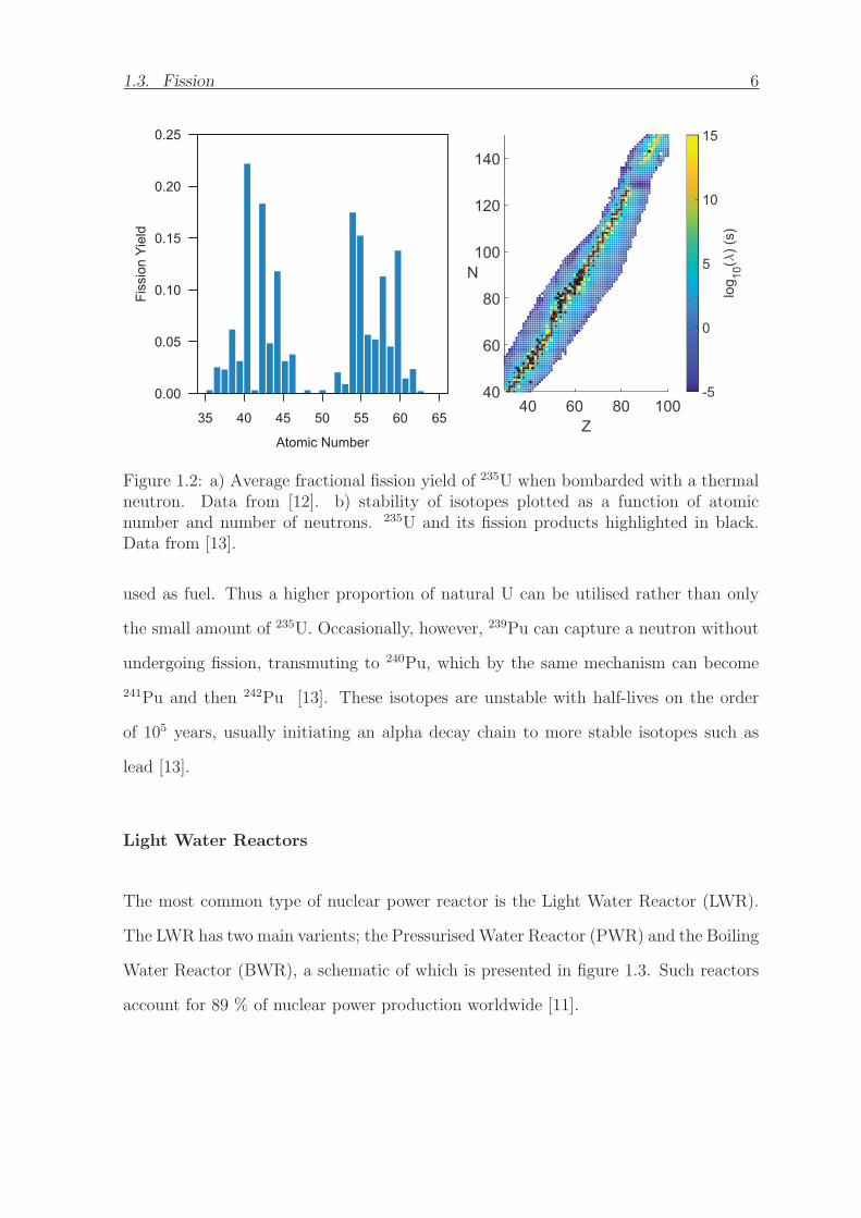
1.2 a) Average fractional fission yield of 235U when bombarded with a ther-
mal neutron. Data from [12]. b) stability of isotopes plotted as a func-
tion of atomic number and number of neutrons. 235U and its fission
products highlighted in black. Data from [13]. . . . . . . . . . . . . . . 6
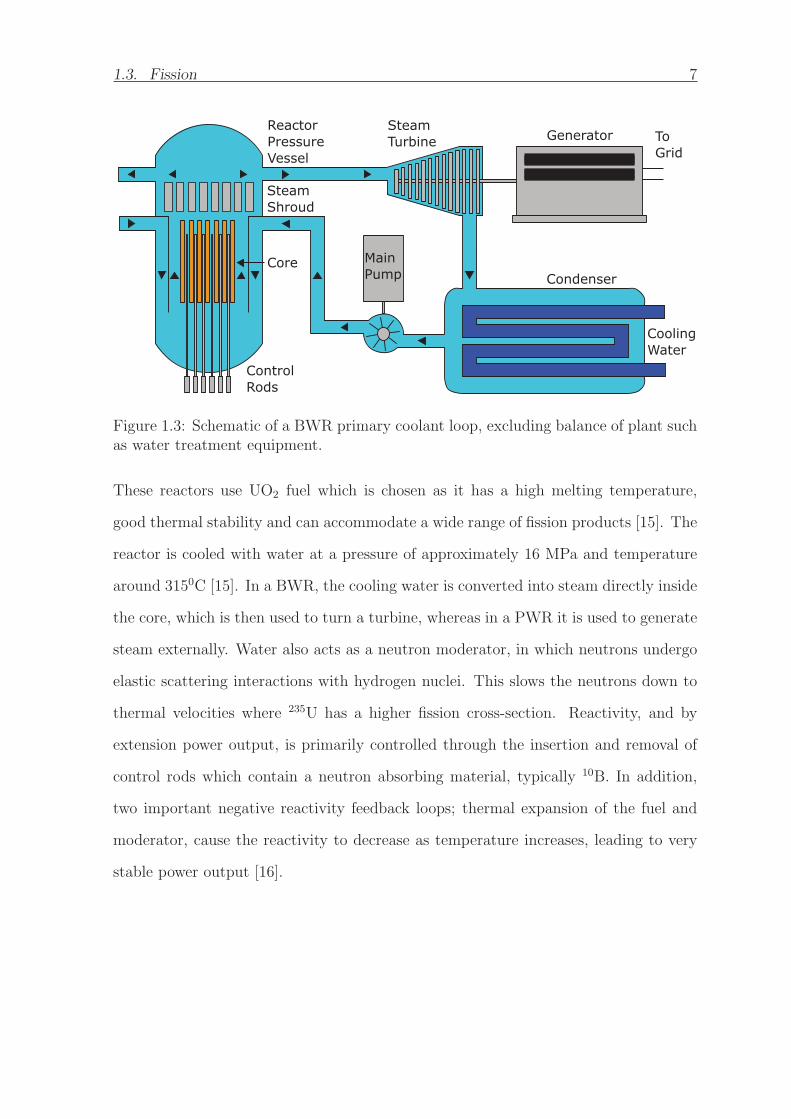
1.3 Schematic of a BWR primary coolant loop, excluding balance of plant
such as water treatment equipment. . . . . . . . . . . . . . . . . . . . . 7
1.4 Total capacity in GWe and total number of commercial power reactors
globally throughout the late 20th and early 21st century. Well publicised
nuclear accidents are highlighted. Data from [19]. . . . . . . . . . . . . 9
1.5 Triple product of two prospective nuclear fusion reactions considered for
fusion energy production. Red is D-D reaction, blue is D-T reaction.
Data from [25]. . . . . . . . . . . . . . . . . . . . . . . . . . . . . . . . 13
1.6 The sun. Image credit NASA. . . . . . . . . . . . . . . . . . . . . . . . 14
1.7 Ignition sequence of a NIF target capsule. Adapted from [33]. . . . . . 16
xvi
LIST OF FIGURES xvii
1.8 Magnetic fields and electrical currents in a section of a conventional
tokomak device. . . . . . . . . . . . . . . . . . . . . . . . . . . . . . . . 17
1.9 Schematic of the Iter reactor, with key components highlighted: Dark
blue denotes the divertor, orange: the vacuum vessel, light blue: mag-
nets, light green: the cryostat, red: the blanket. Modified from [42]. . . 20
1.10 Edge localised modes in the MAST reactor. Bright spots are where the
plasma impinges on the first wall and divertor materials, bright filaments
are the result of localised edge modes. Image credit: Culham Centre for
Fusion Energy. . . . . . . . . . . . . . . . . . . . . . . . . . . . . . . . 21
1.11 Annotated schematic of a typical divertor for a toroidal fusion device
and mock-up of three segments of the Iter divertor. Adapted from [49]. 23
1.12 Beryllium hexagonal close packed crystal structure with a) slip systems
and b) interstitial sites marked. Structure from [58]. . . . . . . . . . . . 27
1.13 Beryllium rich sections of the Be-Ti, Be-V, Be-Mo and Be-W phase
diagrams reproduced from [83], [84], [85] and [86] respectively. Non-
stochiometry of intermetallic compounds is, for the most part, poorly
characterised and is not presented here. . . . . . . . . . . . . . . . . . . 29
1.14 Tetragonal crystal Structure of Be12Ti viewed in the [001] direction. The
coordination of each site is highlighted with polyhedra (right). Structure
from [89]. . . . . . . . . . . . . . . . . . . . . . . . . . . . . . . . . . . 31
1.15 Tungsten BCC crystal structure with {101} family of planes shown.
Right: octahedral and tetrahedral interstitial sites within the tungsten
BCC crystal structure. . . . . . . . . . . . . . . . . . . . . . . . . . . . 33

LIST OF FIGURES xviii
1.16 Two full unit cells of the tungsten carbide crystal structure. Structure
from [101]. . . . . . . . . . . . . . . . . . . . . . . . . . . . . . . . . . . 34
1.17 Typical trajectory of energetic neutron and scattered ions in a material. 37
1.18 Graphical illustrations of the Kinchin-Pease, NRT and Greenwood dis-
placement models. Equations given right. . . . . . . . . . . . . . . . . . 38
1.19 Length and timescales typically accessible using several common mod-
elling methods. . . . . . . . . . . . . . . . . . . . . . . . . . . . . . . . 42
2.1 Wavefunctions for titanium pseudopotentials (solid lines) overlayed against
the all electron potential (dashed lines). The vertical line represents the
cutoff radius, beyond which the pseudopotentials and all electron poten-
tials are identical. . . . . . . . . . . . . . . . . . . . . . . . . . . . . . . 54
2.2 Energy cutoff convergence for elements studied for Castep 6 and 8.
Castep 8 was released part way through this work and includes modified
pseudopotentials. Convergence criteria of 10−2 eV/atom is shown with
a dotted black line. This is reached at 480 and 660 eV for all species in
Castep 6 and 8 respectively. . . . . . . . . . . . . . . . . . . . . . . . . 58
2.3 Energy convergence of the conventional tetragonal cell of Be12Ti with
respect to the number of k-points used with a Monkhorst and Pack
grid [138]. Note k-point convergence neither systematically over or un-
derestimates energy values. . . . . . . . . . . . . . . . . . . . . . . . . . 60
2.4 Supercell size energy convergence for a VM defect in the Be12M structure
with respect to a 3×3×3 supercell (containing 702 atoms). . . . . . . . 62

LIST OF FIGURES xix
2.5 Sketch of possible PEB (red line) and NEB (blue dashed line) results
on an imaginary energy landscape with a highly non linear minimum
energy pathway. Without the restorative perpendicular spring force,
the PEB pathway is dragged away from the minimum energy pathway
by the parallel spring force. . . . . . . . . . . . . . . . . . . . . . . . . 66
2.6 Morse potential for tungsten, utilised as part of the bond order potential
set derived by Juslin et al. [146]. De = 5.419 eV and re = 2.341 A. . . . 70
2.7 a) Morse and tapered Morse potential. b) Electron density as a function
of rij. c) Johnson density functional. All functions and functionals
parameterised for beryllium using the values in table 2.2. . . . . . . . . 74
2.8 Typical neutron scattering mechanisms as a function of energy trans-
fer probed using inelastic neutron scattering spectroscopy. Modified
from [172]. . . . . . . . . . . . . . . . . . . . . . . . . . . . . . . . . . . 85
2.9 Schematic of the TAIPAN triple axis spectrometer. Reproduced from [173]. 87
3.1 Left: unit cell of Be12Ti viewed in the [001] and [100] directions. Right:
correspondence of Be12Ti hexagonal pseudocell and Be17Ti2 unit cell
with tetragonal Be12Ti structure. To achieve Be17Ti2 stochiometry, ti-
tanium edge atoms in the Be17Ti2 structure are duplicated at (0,0,14)
and (0,0,34). . . . . . . . . . . . . . . . . . . . . . . . . . . . . . . . . . 91
3.2 Simulated X-ray diffraction patterns of pure beryllium, Be17Ti2, hexag-
onal Be12Ti, and tetragonal Be12Ti. X-ray wavelength used corresponds
to Cu K-alpha source (1.5406 A. . . . . . . . . . . . . . . . . . . . . . . 92
3.3 Simulated phonon band structure and density of states of hexagonal
Be12Ti. Image courtesy of P. Burr. . . . . . . . . . . . . . . . . . . . . 94
LIST OF FIGURES xx
3.4 Simulated phonon band structure and density of states of tetragonal
Be12Ti. Image courtesy of P. Burr. . . . . . . . . . . . . . . . . . . . . 95
3.5 Simulated internal and Helmholtz free energy of formation for the tetrag-
onal and hexagonal sub-cell of Be12Ti as a function of temperature, as
calculated by the harmonic and quasiharmonic (QH) approximations.
Harmonic and quasiharmonic results appear so close as to be indistin-
guishable. . . . . . . . . . . . . . . . . . . . . . . . . . . . . . . . . . . 97
3.6 Thermodynamic data from quasi-harmonic calculations at 50K intervals.
Dotted lines are fitted Birch-Murnaghan equations of state, and the
crosses represent the minima of those curves. Image courtesy of P. Burr. 98
3.7 Volumetric thermal expansion coefficient (αv) and bulk modulus (K0) of
tetragonal Be12Ti, predicted within the quasi-harmonic approximation,
and comparison to experimental data for αv [82]. . . . . . . . . . . . . 98
3.8 Crystal structure of cubic Fm3c(226) Be13Zr with drop shadows to high-
light atomic positions [189]. Zirconium sites are blue and beryllium sites
green. . . . . . . . . . . . . . . . . . . . . . . . . . . . . . . . . . . . . 102
3.9 Simulated phonon density of states for beryllide samples, normalised to
highest intensity peak. . . . . . . . . . . . . . . . . . . . . . . . . . . . 104
3.10 Left: sample in holder. Sample is secured in an aluminium frame with
aluminium foil, and frame shielded with cadmium. Right: sample setup
within the TAIPAN instrument. . . . . . . . . . . . . . . . . . . . . . . 107
3.11 Data collected at 2 K with the cryofurnace setup and at 295 K. . . . . 107
3.12 Detector and maximum intensity normalised neutron scattering data for
six Beryllides, Be12M, M=Ti,V,Nb,Mo,Ta and Be13Zr. . . . . . . . . . 109
LIST OF FIGURES xxi
3.13 Broadening contributions from the filter and monochromator as a func-
tion of energy. . . . . . . . . . . . . . . . . . . . . . . . . . . . . . . . . 110
3.14 Simulated broadening of DFT predicted DOS results for Be12Ti with
comparison to experimental results. a) predicted phonon DOS, b) phonon
DOS broadened with FWHM from the monochromator only, c) phonon
DOS broadened with FWHM from the filter only, d) phonon DOS broad-
ened with both contributions and e) experimental results. . . . . . . . . 111
3.15 Left: experimental neutron scattering data, with data in the 8-24 meV
region (assumed to be second order reflections) extrapolated and nor-
malised by monitor counts (CN) and originating monitor counts (OCN).
Right: simulated phonon density of states with simulated higher order
reflections. . . . . . . . . . . . . . . . . . . . . . . . . . . . . . . . . . . 113
3.16 Comparison of simulated phonon DOS and count normalised neutron
scattering data for Be12Ti (red), Be12V (orange) and Be12Mo (yellow).
Simulated phonon DOS 2nd harmonic spectrum is shown in grey (low
energy, top) superimposed on the predicted DOS, as is the extrapolated
experimental 2nd harmonic (high energy, bottom) superimposed on the
experimental data. . . . . . . . . . . . . . . . . . . . . . . . . . . . . . 115
3.17 Comparison of simulated phonon DOS and count normalised neutron
scattering data for Be12Nb (light green), Be12Ta (dark green) and Be13Zr
(purple). Simulated phonon DOS 2nd harmonic spectrum is shown in
grey (low energy, top) superimposed on the predicted DOS, as is the
extrapolated experimental 2nd harmonic (high energy, bottom) super-
imposed on the experimental data. . . . . . . . . . . . . . . . . . . . . 116
LIST OF FIGURES xxii
4.1 Left: intrinsic interstitial sites within the Be12Ti structure. Right: co-
ordination polyhedra of interstitial sites within the Be12Ti structure. . . 123
4.2 Figure 3 - Convex hull analysis calculated using the LDA and PBE
functionals of the Be-Ti, Be-V, Be-Mo and Be-W. Phases exhibiting
positive formation energies (relative to end members) are not included. 133
4.3 Phase field lines predicted from total defect concentrations calculated
using the Arrhenius approximation for materials with an excess of beryl-
lium and transition metal. . . . . . . . . . . . . . . . . . . . . . . . . . 137
4.4 Left: lowest energy migration pathways for beryllium and titanium va-
cancy migration in Be12Ti. Right: NEB pathways for the lowest energy
migration pathways. . . . . . . . . . . . . . . . . . . . . . . . . . . . . 142
4.5 Left: lowest energy migration pathways for Be and Ti interstitial migra-
tion in Be12Ti. Beryllium lattice sites have been omitted for legibility.
Right: NEB pathways for the lowest energy migration pathways. . . . . 144
5.1 Values of Pdispd simulated using the Bjorkas and Agrawal potentials, and
values of Pdefd for the Bjorkas potential. Lines are the Robinson model
fitted to the simulated data. . . . . . . . . . . . . . . . . . . . . . . . . 156
5.2 Potential energy (E) for an atom displaced toward its nearest neighbour
by displacement (x) in bulk beryllium at 0 K, as evaluated using the
Agrawal and Bjorkas potentials [153, 149]. . . . . . . . . . . . . . . . . 158
5.3 Simulated maximum displacement with increasing E for the Agrawal
potential (left) and Bjorkas potential (right). Lines denote the fitted
momentum based model (m1) and kinetic energy based model (m2). . . 159
5.4 Stereographic projections of Ed(θ, φ) in Be in the [0001] direction. Ed,0
(the lowest energy with non-zero probability of displacement) is shown
top and Ed,0 (the lowest energy with displacement probability of 0.5) is
shown bottom. . . . . . . . . . . . . . . . . . . . . . . . . . . . . . . . 162
5.5 Pdefd and Pdisp
d calculated from displacement simulations for diamond,
graphite, tungsten, and tungsten and carbon PKAs in tungsten carbide.
Lines are those from the Robinson model fitted to the simulated data,
which is used to predict Ed as presented in table 5.1. . . . . . . . . . . 165
5.6 Pdefd curves for W and C PKAs in tungsten carbide, showing total defect
formation probability, and probability of defect formation on the carbon
and tungsten sublattices. Dashed lines show one standard deviation.
Drop charts show the fraction of tungsten (blue) and carbon (green)
defects formed by each PKA. . . . . . . . . . . . . . . . . . . . . . . . 167
5.7 Stereographic projections of Edefd (θ, φ) in the [0001] direction for tung-
sten, graphite and diamond (Edispd (θ, φ) and Edef
d (θ, φ)). . . . . . . . . . 170
5.8 Stereographic projections of Edefd (θ, φ) in the [0001] direction for tungsten
and carbon PKAs in tungsten carbide. . . . . . . . . . . . . . . . . . . 173
xxiii

Chapter 1
Introduction
1.1 The Nuclear option
Throughout history, the combustion of organic matter has been used to generate use-
ful energy. Initially, it was used to cook food, for heat and for light. Eventually, the
discovery that heat could be converted to mechanical work ushered in the industrial
revolution, replacing hundreds of workers with the noisy clack of steam powered looms
and machining plants. As a consequence, demand for fuel became insatiable. Wood
and other plant materials were no longer enough, leading to the rise of fossil fuels: first
coal, and then oil and gas.
In essence, little has changed since then. Though energy is now distributed by means of
an electrical grid, for the most part it is still generated by burning fossil fuels. During
the first quarter of 2014, 82.0% of the world’s primary energy supply came from fossil
fuels [1].
The continued use of fossil fuels on such a large scale has a devastating impact on
1

1.1. The Nuclear option 2
the world’s climate. The concentration of carbon dioxide, a potent greenhouse gas, in
the atmosphere has increased from an average of 280 ppm during the pre-industrial era
to an average of 425 ppm in 2016 [2, 3]. With it, global temperatures have risen precip-
itously, 2010 being 0.87 ◦C warmer than the preindustrial average and current climate
models predicting a rise of 1.4 - 5.8◦C by 2100 [4, 5]. In addition, the particulate matter
released from the incomplete combustion of fossil fuels is estimated to contribute to
the premature deaths of 3 million people annually, the majority of these occurring in
developing and rapidly industrialising countries such as India and China [6].
Due to these calamitous effects there is a global effort to shift to low carbon energy
sources; either renewable or nuclear energy. Renewable options principally consist of
hydro, wind and solar. Excluding hydro, which makes up the bulk of renewable electric-
ity generation, but has limited capacity for expansion, renewables in 2014 constituted
6.3% of global electricity production [1]. Encouragingly, renewable energy production
(excluding hydro) increased by 20% in 2015. It should however be noted that in abso-
lute terms this is less than the increase in fossil fuels over the same period [7]. While
there have been great strides in reducing the cost of these technologies, significant
barriers remain to their widespread implementation. The capacity factor of wind and
solar is strongly dependent on local climate, rendering them inappropriate for some
countries and locations. In addition, these technologies generate energy intermittently,
necessitating the use of either energy storage or additional load following generating
capacity, which is most often provided by fossil fuels.
Nuclear energy is a somewhat contentious alternative. Currently it delivers 21% of
the UK electricity demand and 11% globally [8, 9]. Like renewables it is a low carbon
technology, however unlike renewables it produces a constant baseload electricity sup-
ply and can be built anywhere a large water source can be used as a heat sink. Post

1.2. Fusion and Fission 3
Fukashima-Daiichi however, attention has been refocused on the perceived safety risks
of nuclear energy, which has eroded public confidence in the technology, most notably
in Western Europe where several countries have chosen to phase it out altogether. Nu-
clear fusion may offer an alternative that can provide a continuous baseload of energy
without the perceived safety risks of conventional nuclear power and greenhouse gas
emissions of fossil fuels. However, to achieve this, significant scientific and engineering
challenges need to be overcome. These will be explored in this thesis.
1.2 Fusion and Fission
All nuclear energy is derived from the binding energy between nucleons in an atom.
The magnitude of this energy is dictated by the balance between the strong nuclear
force which binds the nucleons together, and the repulsive electrostatic interaction
which mutually repels the positively charged protons. This leads to the iconic binding
energy per nucleon curve reproduced in figure 1.1. Analogous to the shell structure of
electrons around an atom, nuclei also have an internal structure, with full shells of both
protons and neutrons resulting in more stable isotopes. This is particularly evident for
light elements such as 4He and 12C which both have filled protons and neutron shells,
and thus are significantly more stable than other isotopes of similar atomic number [10].
The effect of the nuclear shell structure notwithstanding, from figure 1.1 it is apparent
that there is a clear trend towards higher binding energy for moderately sized nuclei.
For light elements such as hydrogen, it is generally energetically favourable to fuse two
together to form a more massive one, up to the most stable nuclei, 62Ni (commonly
misquoted as 56Fe) [10]. For more massive elements such as uranium and plutonium, it
is energetically favourable to fission them into two smaller nuclei. These two processes,

1.2. Fusion and Fission 4
0 50 100 150 200
020
0040
0060
0080
00
number of nucleons
bind
ing
ener
gy (k
eV)
1 H (0.0 MeV)
2 D (1.112 MeV)
3 T (2.827 MeV)3 He (2.573 MeV)
4 He (7.074 MeV)
141 Ba (8.326 MeV
92 Kr (8.513 MeV)
235 U (7.591 MeV)
Figure 1.1: Binding energy per nucleon of stable and long lived isotopes as a functionof the number of nucleons, with the binding energy of important isotopes for fission(blue) and fusion (red) highlighted. Data from [10].
fusion and fission, are the two principal nuclear reactions that can be used to generate
energy.
It is worth noting that the binding energy of nucleons in a nucleus is several orders
of magnitude higher than that which binds valence electrons to an ion. Consequently,
nuclear reactions on average release around a million times more energy than chemical
reactions.
1.3. Fission 5
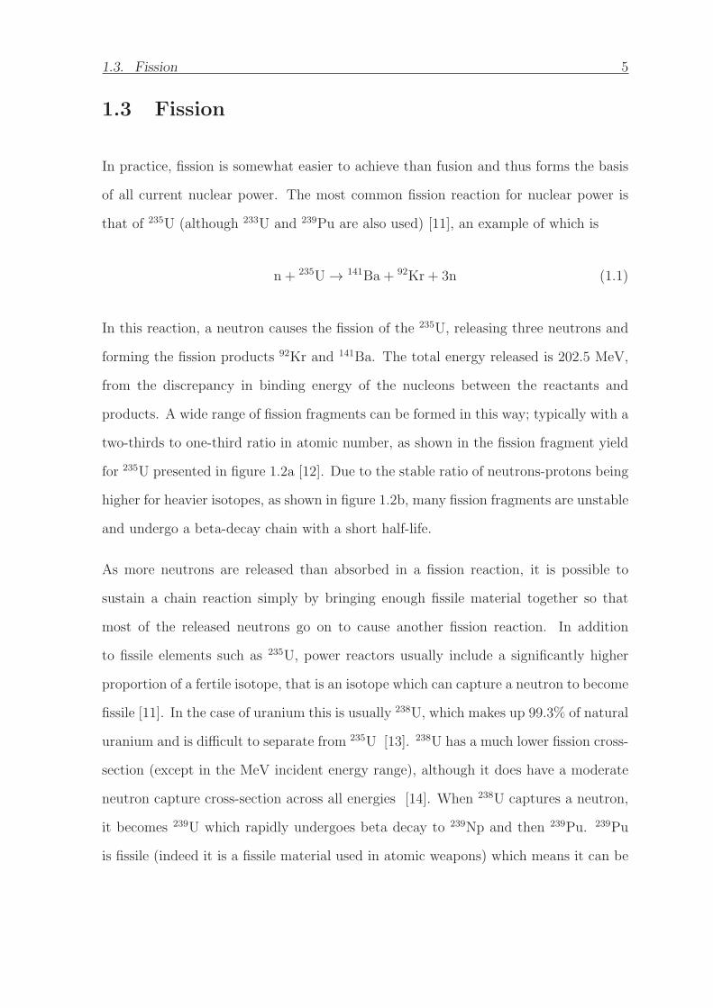
1.3 Fission
In practice, fission is somewhat easier to achieve than fusion and thus forms the basis
of all current nuclear power. The most common fission reaction for nuclear power is
that of 235U (although 233U and 239Pu are also used) [11], an example of which is
n + 235U → 141Ba + 92Kr + 3n (1.1)
In this reaction, a neutron causes the fission of the 235U, releasing three neutrons and
forming the fission products 92Kr and 141Ba. The total energy released is 202.5 MeV,
from the discrepancy in binding energy of the nucleons between the reactants and
products. A wide range of fission fragments can be formed in this way; typically with a
two-thirds to one-third ratio in atomic number, as shown in the fission fragment yield
for 235U presented in figure 1.2a [12]. Due to the stable ratio of neutrons-protons being
higher for heavier isotopes, as shown in figure 1.2b, many fission fragments are unstable
and undergo a beta-decay chain with a short half-life.
As more neutrons are released than absorbed in a fission reaction, it is possible to
sustain a chain reaction simply by bringing enough fissile material together so that
most of the released neutrons go on to cause another fission reaction. In addition
to fissile elements such as 235U, power reactors usually include a significantly higher
proportion of a fertile isotope, that is an isotope which can capture a neutron to become
fissile [11]. In the case of uranium this is usually 238U, which makes up 99.3% of natural
uranium and is difficult to separate from 235U [13]. 238U has a much lower fission cross-
section (except in the MeV incident energy range), although it does have a moderate
neutron capture cross-section across all energies [14]. When 238U captures a neutron,
it becomes 239U which rapidly undergoes beta decay to 239Np and then 239Pu. 239Pu
is fissile (indeed it is a fissile material used in atomic weapons) which means it can be
1.3. Fission 6
40 60 80 100Z
40
60
80
100
120
140
N
-5
0
5
10
15
log 10
() (
s)
Fiss
ion
Yiel
d
0.00
0.05
0.10
0.15
0.20
0.25
35 40 45 50 55 60 65
Atomic Number
Figure 1.2: a) Average fractional fission yield of 235U when bombarded with a thermalneutron. Data from [12]. b) stability of isotopes plotted as a function of atomicnumber and number of neutrons. 235U and its fission products highlighted in black.Data from [13].
used as fuel. Thus a higher proportion of natural U can be utilised rather than only
the small amount of 235U. Occasionally, however, 239Pu can capture a neutron without
undergoing fission, transmuting to 240Pu, which by the same mechanism can become
241Pu and then 242Pu [13]. These isotopes are unstable with half-lives on the order
of 105 years, usually initiating an alpha decay chain to more stable isotopes such as
lead [13].
Light Water Reactors
The most common type of nuclear power reactor is the Light Water Reactor (LWR).
The LWR has two main varients; the Pressurised Water Reactor (PWR) and the Boiling
Water Reactor (BWR), a schematic of which is presented in figure 1.3. Such reactors
account for 89 % of nuclear power production worldwide [11].
1.3. Fission 7
SteamTurbine
ControlRods
SteamShroud
Main Pump
Core
ReactorPressureVessel
Generator To Grid
CoolingWater
Condenser
Figure 1.3: Schematic of a BWR primary coolant loop, excluding balance of plant suchas water treatment equipment.
These reactors use UO2 fuel which is chosen as it has a high melting temperature,
good thermal stability and can accommodate a wide range of fission products [15]. The
reactor is cooled with water at a pressure of approximately 16 MPa and temperature
around 3150C [15]. In a BWR, the cooling water is converted into steam directly inside
the core, which is then used to turn a turbine, whereas in a PWR it is used to generate
steam externally. Water also acts as a neutron moderator, in which neutrons undergo
elastic scattering interactions with hydrogen nuclei. This slows the neutrons down to
thermal velocities where 235U has a higher fission cross-section. Reactivity, and by
extension power output, is primarily controlled through the insertion and removal of
control rods which contain a neutron absorbing material, typically 10B. In addition,
two important negative reactivity feedback loops; thermal expansion of the fuel and
moderator, cause the reactivity to decrease as temperature increases, leading to very
stable power output [16].
1.3. Fission 8
Safety Concerns
While the LWR design has been extremely successful, it has been shown to be suscepti-
ble to Loss of Coolant Accidents (LOCA), which have the potential to cause dispersal
of radioactive material. The susceptibility of these reactors to this type of accident
is due to the decay of fission products and higher actinides, which immediately after
reactor shutdown generate around 6% of the heat from full power operation [16]. For
a typical PWR which generates 4 GWt at full power, this is on the order of 250 MWt.
This is too much heat to remove from the reactor core via radiative and convective
losses should active cooling be compromised. Thus, without intervention, the tem-
perature of the core increases until it surpasses the melting point of the fuel. If this
occurs, it may lead to energetic dispersal of the fuel which has the potential to breach
the containment, particularly where the fuel is clad with zircalloy which, at elevated
temperatures, reacts violently with steam to produce hydrogen. Release of radioactive
fission products and higher actinides from the fuel into the environment can have seri-
ous negative health consequences to the surrounding population, particularly as some
isotopes (131I, 137Cs and 90Sr) accumulate in biological tissues [17]. Further, as some
of these isotopes have long half-lives, this can render areas uninhabitable for genera-
tions [18].
The possibility of such accidents was brought into sharp focus by the Three Mile Island
incident in 1979, in which a faulty valve allowed a large amount of coolant to escape
leading to a partial meltdown of the core [17]. Public opinion of nuclear power, already
tainted by its association with nuclear weapons, became significantly less favourable
due to perceived safety concerns, despite very little radiation being released. This was
compounded by the Chernobyl disaster in 1986, which, although not a LWR in the
usual sense, demonstrated the potential risks to wide segments of the population, with

1.3. Fission 9
thousands of square kilometres evacuated and a clean-up effort (which continues today)
running to billions of USD [17]. These events greatly slowed the uptake of new nuclear
reactors, as shown in figure 1.4. More recently, the partial melt down at the Fukushima
Daiichi plant following the earthquake of 2011 led to a drop in public support for nu-
clear power and subsequently the mothballing of the entire Japanese nuclear fleet and
the phase out of nuclear fission in several European countries [17].
1960 1970 1980 1990 2000 2010
010
020
030
040
0
Net
Ope
ratin
g C
apac
ity (G
We)
year
Thre
e M
ile Is
land
Che
rnob
yl
Fuku
shim
a
Num
ber o
f Rea
ctor
s
010
020
030
040
0
Capacity (GWe)
No. of Reactors
Figure 1.4: Total capacity in GWe and total number of commercial power reactorsglobally throughout the late 20th and early 21st century. Well publicised nuclearaccidents are highlighted. Data from [19].
The nuclear industry has responded to the negative public perception of nuclear safety
by adding multiply redundant and divergent safety systems to nuclear reactors which
has significantly increased capital and overall costs. Further, it could be argued that the
strict safety culture around nuclear power has inhibited the development and adoption
of other types of reactors which may potentially be safer and more economical than
PWRs and BWRs. Aside from safety, waste is also a key issue. Given the isotopic
1.4. Fusion 10
makeup of waste from reprocessed fuel, it remains significantly active such that it needs
to be isolated from biological systems for at least 3,000 years [20]. The prevailing
consensus on how to achieve this isolation is to vitrify it and store it in deep geological
repositories, however no such repository currently exists. This remains a source of
concern for the public, with a recent survey citing 35% of respondents believing long
term waste disposal cannot be safely achieved [21].
1.4 Fusion
In principle, nuclear fusion does not have the same issues with safety or waste as nuclear
fission, but maintains the key advantage of producing low carbon, continuous baseload
power. The only waste product is stable 4He, precluding the risk of a meltdown and
not requiring storage, although some reactor materials may be activated. As such, it
enjoys much greater public support than conventional fission power [22].
The most promising reaction for nuclear fusion power is the deuterium-tritium re-
action;
2D+ 3T → 4He(3.5MeV) + n(14.1MeV) (1.2)
although several others have been proposed. In this reaction, two isotopes of hydrogen
are fused to produce 4He and an energetic neutron. This reaction has a relatively
low activation energy, dictated by the Coulomb repulsion between the two positively
charged nuclei (which scales with atomic number) and high energy release per nucleon
as demonstrated in figure 1.1. Relative to the Coulomb interaction, the strong nuclear
force which binds nuclei together operates over much shorter length scales. Thus,
to achieve fusion, two nuclei must be brought close enough together that the strong
nuclear force overpowers the coulomb repulsion. In practice, this is usually achieved

1.4. Fusion 11
by maintaining extremely high temperatures and densities in the fuel, resulting in it
becoming a plasma.
1.4.1 Lawson Criteria and the Triple Product
To maintain the temperature, and thus nuclear fusion, any reactor must generate more
energy than is lost to the environment. This is laid out explicitly in the Lawson criteria
which defines the conditions necessary to achieve ignition, that is to say a self-sustained
fusion reaction, of a fuel plasma as an energy balance [23]:
P = η × (Pf −Q.) (1.3)
where P is the net power of the device, η the efficiency, Pf the power from fusion and Q.
the energy loss per unit time. Clearly, as the energy loss approaches the energy released
through fusion then the power tends to 0. One of the key aims for a fusion reactor
then, is to lower Q. such that fusion can be maintained. As mentioned previously, the
fusion power Pf is dependent on the temperature of the plasma. More specifically the
energy density can be estimated using the Maxwell-Boltzmann [24] distribution as:
dPf
dV=
1
4en2〈σF (T )v〉 (1.4)
where v is the relative velocity, e the energy/reaction, n the number density of the
reactants, σF (T ) the fusion cross-section as a function of temperature and 〈〉 denotesan average over the Maxwellian velocity distribution at that temperature. For devices
that operate in a steady state configuration, it is useful to think of the problem in
terms of the ratio of energy lost to total energy density W, also known as the energy
1.4. Fusion 12
confinement time, TE,
TE =W
Q.(1.5)
This can be rearranged to find Q., and W calculated using Boltzmann statistics to give
Q. =3nkBT
TE(1.6)
which, when substituted into the original statement of the Lawson criterion (ignoring
the efficiency term) along with the equation for Pf , returns the conditions necessary
to achieve ignition in terms of TE
nTE =12
e
kBT
〈σF (T )〉v (1.7)
Thus, the minimum product of reactant density and confinement time can be calculated
as a function of temperature. Most fusion reactor concepts (which are explored in
detail in section 1.4.2) can attain a maximum pressure p, but vary the density and
temperature of the fuel. In this case, assuming the ideal gas equation holds and thus
p ∝ nT , it is useful to express the Lawson criteria in terms of the triple product
nTET =12
e
KBT2
〈σF (T )〉v (1.8)
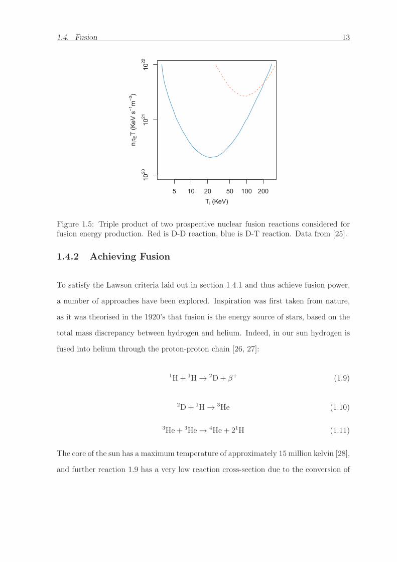
The nTET which satisfies the Lawson criteria is presented as a function of temperature
for the T-T and D-3He (which is considered for fusion as it is aneutronic) reactions in
figure 1.5. It can be seen the nTET required to achieve ignition is minimised at finite
temperature. This is due to the microscopic fusion cross-section falling off at higher
energies along with increasing radiative losses. It is clear that the D-T reaction has
the lowest minimum triple product of the two reactions, which is why it is considered
the best prospective fuel for a fusion reactor. The D-T minimum occurs at around 150
million kelvin which is thus the target for devices attempting to generate fusion energy.
1.4. Fusion 13
5 10 20 50 100 200Ti (KeV)
n iτ E
T (K
eV s
−1m
−3)
1020
1021
1022
Figure 1.5: Triple product of two prospective nuclear fusion reactions considered forfusion energy production. Red is D-D reaction, blue is D-T reaction. Data from [25].
1.4.2 Achieving Fusion
To satisfy the Lawson criteria laid out in section 1.4.1 and thus achieve fusion power,
a number of approaches have been explored. Inspiration was first taken from nature,
as it was theorised in the 1920’s that fusion is the energy source of stars, based on the
total mass discrepancy between hydrogen and helium. Indeed, in our sun hydrogen is
fused into helium through the proton-proton chain [26, 27]:
1H+ 1H → 2D+ β+ (1.9)
2D+ 1H → 3He (1.10)
3He + 3He → 4He + 21H (1.11)
The core of the sun has a maximum temperature of approximately 15 million kelvin [28],
and further reaction 1.9 has a very low reaction cross-section due to the conversion of

1.4. Fusion 14
a proton to a neutron. As such, at first glance it would seem unlikely that the Lawson
criteria could be met. Fusion is however sustained by the extremely high density of the
core (in excess of 150000 kgm−3 [28]) and extremely long confinement time. Despite
this, the average energy release per unit volume of the core is only 276.5 Wm−3 [29],
significantly less than the metabolism of an adult human. Given the overwhelming size
of the sun, this is enough to maintain the conditions for fusion to occur. It is obvious
however, that this approach is impractical for terrestrial fusion devices.
Figure 1.6: The sun. Image credit NASA.
Fusion was first achieved in a labarotary in 1932 by bombarding targets of deuterium,
tritium and 3helium with deuterium nuclei using a particle accelerator [30]. Such a
device requires much more energy than is released, and thus is not a practical solution
for fusion power.
Fusion remained a curious aside with no practical application until the advent of the
Manhattan project during World War Two. The aim of this project was to develop
the first nuclear fission bomb, an endeavour which was successfully concluded with the
Trinity test in 1945 [17]. Early in the project, it was theorised that the detonation of
1.4. Fusion 15
a conventional fission weapon could be used to achieve the temperature and pressure
required to ignite a fusion reaction, thus significantly boosting the yield of the weapon.
Work began on developing this concept, which continued throughout the Manhattan
project and accelerated with the onset of the Cold War. It culminated in the detona-
tion of the first “boosted fission weapon” (in which only a small portion of the energy
released comes from fusion) in 1950 [31], and then the first true thermonuclear bomb,
Ivy Mike in 1952 [17]. In these devices, a primary fission detonation is used to release
energy and neutrons which are focused on the fusion fuel. This fuel is surrounded by a
dense material (which may itself be fissionable) such that when this energy is focused
upon it, it collapses with enough inertia to compress and heat the fusion fuel to induce
fusion.
In parallel with this, work began on developing fusion for civil energy production.
This presented an additional problem to that of developing a weapon: how to con-
tain the fuel which, by necessity, must be at millions of kelvins? In the case of a
weapon, containment is only briefly achieved with an imploding mass of 238U. A civil
reactor however must operate in a (quasi)continuous state. This problem has aptly
been likened trying to create a “Sun in a bottle”; clearly no material could withstand
such temperatures and pressures, thus other means of containment are required, which
isolate reactor materials from direct contact with the plasma. Two main approaches
were developed: Inertial Confinement (ICF) and Magnetic Confinement (MCF).
Inertial Confinement Fusion
From the perspective of fusion power, the most successful ICF concept has been laser
inertial confinement [32]. In this approach, several high powered lasers are focused
on a small pellet of fusion fuel for a very short time, causing the surface to rapidly
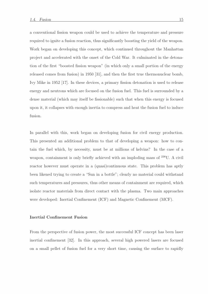
1.4. Fusion 16
vaporise creating a high pressure shockwave, compressing and heating the centre of the
fuel pellet to fusion conditions, as shown in figure 1.7.
Target Pellet(2mm)
D-T gasD-T icePolymer
UV laser beams
X-raysFusionburn/ignition
Hohlraum
1) 192 UV laser beams rapidlydeposit 1.85 MJ of energy in the inner surface of the Hohlraum
2) X rays from the Hohlraum vapourise the surface of thecapsule generating explosiveblowoff, heating and compressing the D-T fuel
3) The D-T fuel reaches temperatures and densitiessufficient to initiate fusion
Figure 1.7: Ignition sequence of a NIF target capsule. Adapted from [33].
The most recent incarnation of this concept is the National Ignition Facility (NIF),
which is used to test materials for the U.S. thermonuclear weapons stockpile. The de-
vice was originally designed and predicted to achieve ignition [34], however this has not
been achieved. Earlier attempts at laser ICF underperformed due to unpredicted non-
linear optic effects at high laser power, although these issues had already been addressed
at the conception of NIF [35]. Instead, it appears that hydrodynamic instabilities in the
outer layers of the target capsule, in particular Rayleigh-Taylor instabilities, prevent
the fuel from reaching the conditions necessary for ignition [35]. These unpredicted
issues have cast doubt on the feasibility of this approach to generate fusion energy.
Magnetic Confinement Fusion
MCF, the other key confinement approach, uses magnetic fields to confine a plasma
of the fuel. Plasmas are electrically charged, and as such subject to the Lorentz force
1.4. Fusion 17
(equation 1.12). Thus, when a current is passed through them in the presence of a
sufficient magnetic field they can be contained. The first of these devices was the Z-
pinch, developed from 1946 onwards, which uses a simple cylindrical reactor with a
magnetic coil around the centre. When an electrical current is applied to this coil, it
exerts a force,
F = qE+ qV ×B (1.12)
on the fuel plasma within, compressing and heating it [36]. While such devices were a
useful proof of concept, sustaining fusion was found to be impossible due to instabilities
in the plasma [36]. They did, however, provide the inspiration for more successful
devices operating on similar principles such as the Stellerator and the Tokomak, the
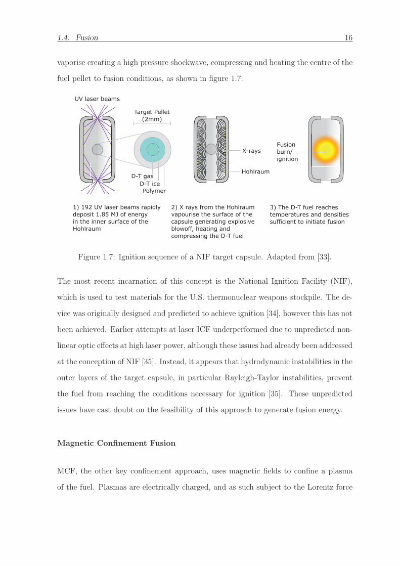
latter of which has been perhaps the most successful type of fusion reactor to date. The
Tokomak confines a ring of plasma using helical magnetic fields, which are generated
using a combination of a toroidal and poloidal field. The toroidal field is generated
by passing a current through the plasma and the poloidal field using electromagnets
surrounding the torus, as represented in figure 1.8 [37].
Plasma current. Induced by the central solenoid magnetic field.
Toroidal magnetic field. generated by large toroidal magnets.
Poloidal magnetic field. Generated by the poloidal magnets.
Overall magnetic field. The helical twist around the 'doughnut' axis applies a lorentz force on the movingplasma in the direction of the central axis
Figure 1.8: Magnetic fields and electrical currents in a section of a conventional toko-mak device.
1.4. Fusion 18
The confined plasma is heated through a combination of ohmic heating, neutral beam
injections and radio-frequency heating. These devices have been able to hold a mostly
stable plasma, although some serious instabilities in the plasma do occur, ranging from
global disruptions which can quench the plasma to localised edge disruptions which
impinge on the reactor wall but do not lead to discharge of the plasma [37]. Nonethe-
less, quasi-stable fusion was first achieved by the soviet T-4 reactor in 1968 [36]. More
recently, the flagship European reactor, the Joint European Torus (JET), recorded a
record 16 MWt of fusion power, and achieved a net fusion energy release (Q) of 0.7
times the heating power required [38].
In 1986, an international collaboration was agreed between the Japan, the Soviet Union,
United States and the European Union to create an international fusion facility that
would eventually become the Iter reactor, which is currently under construction in
France [39]. This reactor is planned to achieve sustained fusion with Q = 10 and
produce 500 MWt of fusion power. This will be achieved using a much larger plasma
volume and stronger magnetic fields than JET, resulting in a longer energy confine-
ment time and maximum achievable pressure. First plasma is planned to be achieved
in Iter in 2025, followed by the first D-T fusion in 2035 [40].
Iter will be followed by the DEMOnstration power reactor (DEMO), which is intended
as a demonstration nuclear fusion power reactor [40]. This reactor is planned to have
comparable electrical power output to a conventional fission reactor, and to begin op-
eration between 2040 and 2050. A comparison of the JET, Iter and DEMO reactors is
shown in table 1.1.
1.5. Components of Fusion 19
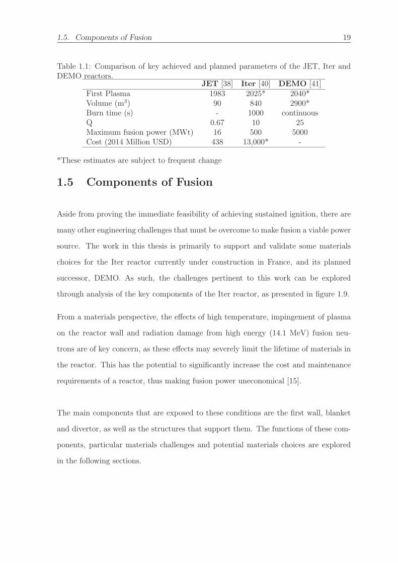
Table 1.1: Comparison of key achieved and planned parameters of the JET, Iter andDEMO reactors.
JET [38] Iter [40] DEMO [41]First Plasma 1983 2025* 2040*Volume (m3) 90 840 2900*Burn time (s) - 1000 continuousQ 0.67 10 25Maximum fusion power (MWt) 16 500 5000Cost (2014 Million USD) 438 13,000* -
*These estimates are subject to frequent change
1.5 Components of Fusion
Aside from proving the immediate feasibility of achieving sustained ignition, there are
many other engineering challenges that must be overcome to make fusion a viable power
source. The work in this thesis is primarily to support and validate some materials
choices for the Iter reactor currently under construction in France, and its planned
successor, DEMO. As such, the challenges pertinent to this work can be explored
through analysis of the key components of the Iter reactor, as presented in figure 1.9.
From a materials perspective, the effects of high temperature, impingement of plasma
on the reactor wall and radiation damage from high energy (14.1 MeV) fusion neu-
trons are of key concern, as these effects may severely limit the lifetime of materials in
the reactor. This has the potential to significantly increase the cost and maintenance
requirements of a reactor, thus making fusion power uneconomical [15].
The main components that are exposed to these conditions are the first wall, blanket
and divertor, as well as the structures that support them. The functions of these com-
ponents, particular materials challenges and potential materials choices are explored
in the following sections.
1.5. Components of Fusion 20
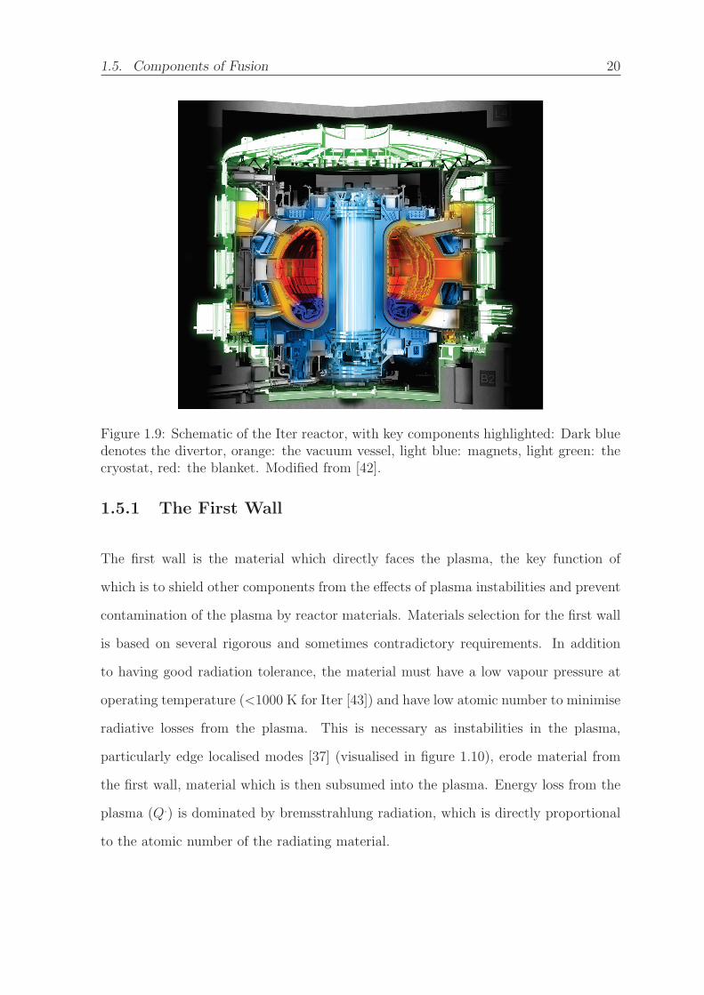
Figure 1.9: Schematic of the Iter reactor, with key components highlighted: Dark bluedenotes the divertor, orange: the vacuum vessel, light blue: magnets, light green: thecryostat, red: the blanket. Modified from [42].
1.5.1 The First Wall
The first wall is the material which directly faces the plasma, the key function of
which is to shield other components from the effects of plasma instabilities and prevent
contamination of the plasma by reactor materials. Materials selection for the first wall
is based on several rigorous and sometimes contradictory requirements. In addition
to having good radiation tolerance, the material must have a low vapour pressure at
operating temperature (<1000 K for Iter [43]) and have low atomic number to minimise
radiative losses from the plasma. This is necessary as instabilities in the plasma,
particularly edge localised modes [37] (visualised in figure 1.10), erode material from
the first wall, material which is then subsumed into the plasma. Energy loss from the
plasma (Q.) is dominated by bremsstrahlung radiation, which is directly proportional
to the atomic number of the radiating material.

1.5. Components of Fusion 21
Figure 1.10: Edge localised modes in the MAST reactor. Bright spots are where theplasma impinges on the first wall and divertor materials, bright filaments are the resultof localised edge modes. Image credit: Culham Centre for Fusion Energy.
The material of the first wall must also have adequate thermal conductivity and ther-
mal stability to prevent fatigue failure due to thermal cycling. Ideally the material
must also have no long lived activation products to prevent the generation of long term
nuclear waste (this being a key advantage of fusion over fission) and not be so acti-
vated or retain significant quantities of tritium so as to greatly increase the difficulty
of maintainance [44].
The two obvious materials choices that meet these criteria are carbon and beryllium,
the only materials with very low atomic mass that have reasonable structural and ther-
mal properties. Both of these choices were tested in the JET reactor, which initially
used a carbon first wall before transitioning to beryllium to more closely mimic the
planned environment of Iter [45]. It was found that installation of the beryllium first
wall dramatically decreased the fuel retained in the wall and led to lower radiative
1.5. Components of Fusion 22
losses in the plasma [46].
In the long term, for devices such as DEMO, plasma disruptions and edge localised
modes are likely to become less frequent due to improvements in plasma confine-
ment [47]. As such the requirement for low atomic number will be relaxed somewhat,
and it is envisaged that tungsten may be used due to its superior thermal, erosion and
hydrogen/helium implantation properties [48].
1.5.2 The Divertor
As the fusion reaction progresses, helium “ash” from the reaction as well as impurities
from the first wall accumulate in the fusion plasma, inhibiting further fusion reactions.
As such, “ash” must be removed during reactor operation. This is achieved by leaving
open magnetic field lines at the bottom of the target chamber, which allow some of
the plasma to escape. The escaping plasma contains both “ash” and fuel, the tritium
in which must be recycled if fusion is to be economical. The plasma travels along the
open field lines until it encounters the tiles of the divertor, before being channelled
through external pumps for recycling [41].
The key considerations for the materials of the divertor tiles are excellent temperature
stability and high thermal conductivity due to the very high thermal flux at the plasma
strike points. In addition, the material must be resistant to sputtering and remain
stable when implanted with hydrogen isotopes, helium and material sputtered from
the first wall [47, 50]. The recognised choice of material for this is tungsten, which
has an exceptionally high melting point (3697 K [51]), reasonable thermal conductivity
(1.75 Wcm−1K−1 [52]), low thermal expansion coefficient (4.5 × 10⁻⁶ K−1 [53]) and
good resistance to erosion by the plasma.
1.5. Components of Fusion 23
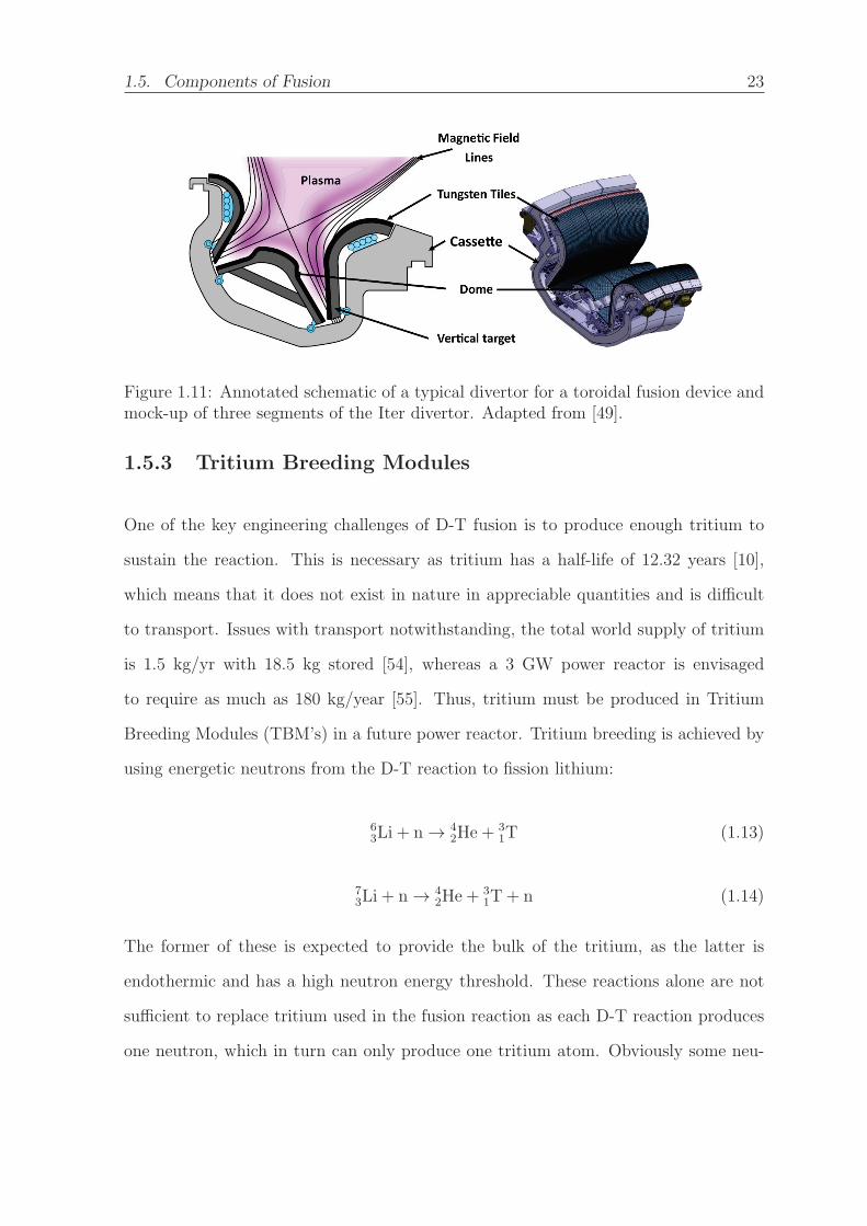
Figure 1.11: Annotated schematic of a typical divertor for a toroidal fusion device andmock-up of three segments of the Iter divertor. Adapted from [49].
1.5.3 Tritium Breeding Modules
One of the key engineering challenges of D-T fusion is to produce enough tritium to
sustain the reaction. This is necessary as tritium has a half-life of 12.32 years [10],
which means that it does not exist in nature in appreciable quantities and is difficult
to transport. Issues with transport notwithstanding, the total world supply of tritium
is 1.5 kg/yr with 18.5 kg stored [54], whereas a 3 GW power reactor is envisaged
to require as much as 180 kg/year [55]. Thus, tritium must be produced in Tritium
Breeding Modules (TBM’s) in a future power reactor. Tritium breeding is achieved by
using energetic neutrons from the D-T reaction to fission lithium:
63Li + n → 4
2He +31T (1.13)
73Li + n → 4
2He +31T + n (1.14)
The former of these is expected to provide the bulk of the tritium, as the latter is
endothermic and has a high neutron energy threshold. These reactions alone are not
sufficient to replace tritium used in the fusion reaction as each D-T reaction produces
one neutron, which in turn can only produce one tritium atom. Obviously some neu-
1.6. Materials of Interest 24
trons will be captured by other materials in the reactor, thus an additional source of
neutrons is required.
Sufficient neutron ecomony may be acheived through the introduction of a neutron
multiplier such as beryllium, lead or bismuth, which undergo (n,2n+) reactions. This
produces additional neutrons, and may be sufficient to replace the tritium used in the
fusion reaction, providing the breeding module is properly configured [56]. From this
standpoint, the relevant metric for TBM designs is the tritium breeding ratio (TBR)
(i.e. the overall ratio of tritium used/tritium produced for an entire reactor outfitted
with such modules). Theoretically, the TBR must be above 1, however in practice
some tritium will decay or be lost in the tritium recycling system, thus a TBR greater
than 1.43 is desirable [55]. In addition to breeding tritium, TBMs will also be used to
remove heat from the reactor for power generation.
Several design concepts exist, with six slated for testing in the Iter program. All are
based on two core tritium breeding materials mixtures; the Li2SiO4-Be pebble bed and
Li-Pb eutectic blankets, although in the long term liquid FLiBe ((LiF)2BeF2) concepts
have also been proposed. An overview of the technological readiness, key requirements
for further research, limitations and advantages of these designs is outlined in table 1.2.
1.6 Materials of Interest
Having examined the overall design and key components of the Iter and DEMO reac-
tors, the materials proposed for use in these components, and which are the focus of

1.6. Materials of Interest 25
Table 1.2: Comparison of tritium breeding module concepts. Technological readinessassessments from [57]. TSP stands for “technological simplicity parameter”, which is anassessment of how many of the technical issues are already solved, DAP is the “DEMOattractiveness parameter”, and AAP the “advanced reactor attractiveness parameter”,an assessment of the technologies ultimate potential.
TSP DAP AAP commentCeramic breeder(steel structures)
high high med.-low
Highest technological readi-ness of all concepts. Limitedin the long term by the availi-bility and toxicity of Be
Ceramic breeder(SiC structures)
low verylow
high More attractive than standardceramic breeder concept, how-ever suffers the same draw-backs in the long term
Dual coolant (steelstructures)
med.-high
high high high level of technologicalreadiness and reasonably at-tractive in the long term foruse in DEMO and a powerplant
Self-cooled PbLi(SiC structures)
low verylow
veryhigh
very attractive in principle,however SiC must be qualifiedas a structural material
Flibe med. med. med.-low
difficult chemistry, materialscompatibility issues and poorheat transfer characteristics
Helium verylow
verylow
veryhigh
long term project that relieson the qualification of W as astructural material
the work presented in this thesis, are examined. In this section, only an overview of
the basic properties of the materials are given, with more details relevant to the details
of the simulations reported in this thesis, outlined in chapters 3-6.
1.6.1 Beryllium
Beryllium is a metal with low atomic mass (9.012 amu [10]), very low density (1.85
g/cm3 [58]) and high stiffness (287 GPa [59]). It occurs relatively rarely within the

1.6. Materials of Interest 26
earth’s crust and forms ores of Bertrandite (Be4Si2O7(OH)2) and Beryl (Al2Be3Si6O18),
with a total recoverable reserve using current commercial technology in excess of
400,000 tonnes [60]. Extraction from the ore is difficult owing to beryllium’s high
affinity for oxygen, and is only carried out on an industrial scale in China, the US and
Kazakhstan [60]. Machining and working with pure beryllium is also difficult as when
inhaled, its dust can cause a significant allergic reaction known as berylliosis, even in
concentrations as low as 0.1 μgm−3 of beryllium during chronic exposure [61]. Thus
strict safety precautions must be in place when handling beryllium metal.
Due to its low natural abundance and difficulty in handling, it is expensive (510
USD/kg [62]) and thus used for relatively few niche applications where its unique
physical, chemical and nuclear properties are required. In particular, its exceptionally
low density, high stiffness and (relatively) high melting temperature are extremely at-
tractive for aerospace applications where it has been used as structural components in
rockets, missiles, planes and satellites as well as for precision instrumentation owing to
its low thermal expansion coefficient [63]. In addition, due to its low atomic number it
has a low interaction cross-section for high energy photons and charged particles mak-
ing it ideal for use as a radiation window in X-ray machines and particle detectors [63].
Another consequence of its low atomic mass is that it is an effective moderator, and
in the fission regime (n < 2MeV) has a low cross-section for inelastic interactions [64].
As such, Be and BeO have been used as neutron moderators and reflectors in several
fission reactors, in particular where compactness is important such as in some subma-
rine reactors, and more exotically, proposed nuclear rockets [65, 66, 67]. Beryllium is
also utilised to produce neutrons through an (α,n) reaction which 9Be (which com-
prises 99% of natural Be) undergoes when bombarded with alpha particles. For fusion
applications, it is utilised as a neutron multiplier as 9Be undergoes a (n,2n) reaction

1.6. Materials of Interest 27
when bombarded with energetic neutrons [64]:
94Be + n → 242He + 2n (1.15)
At room temperature beryllium has a hexagonal close packed crystal structure (see
figure 1.12) with an a parameter of 2.62 A and c/a ratio of 1.568, 2% below the ideal,
indicating some degree of directional bonding and which causes strongly anisotropic
thermal and mechanical properties [58]. The equilibrium nearest neighbour bond length
is 2.26 A, and second nearest neighbour 2.286 A. The HCP crystal structure has 3
independent slip systems, two of which are easy: basal {0002}〈1120〉 with two slip
modes and prismatic type-I planes {1010}〈1120〉 with two slip modes as well as pyra-
midal slip which is thermally activated. For effective ductility, at least six independent
slip modes are required, thus beryllium is brittle at low temperatures and undergoes
a brittle-ductile transition around 150◦C, although this is heavily dependent on grain
size [68, 69]. Within the HCP crystal structure there are six symmetrically distinct
interstitial sites as outlined in figure 1.12b.
Figure 1.12: Beryllium hexagonal close packed crystal structure with a) slip systemsand b) interstitial sites marked. Structure from [58].
From the perspective of fusion applications as a first wall and neutron multiplying ma-

1.6. Materials of Interest 28
terial in the TBM, there are three key concerns that may potentially limit its use. The
first is the tendency of hydrogen and helium, implanted or radiogenic, to segregate to
form large bubbles at fusion relevant temperatures [70, 71]. This leads to significant
embrittlement of beryllium and increases the tritium inventory of the breeder module,
making tritium recovery and maintenance difficult. The second is the general embrit-
tling effect: increasing the brittle-ductile transition temperature due to irradiation,
which, combined with void swelling leads to the formation of a fine powder which is
a particular hazard due to the potential for berylliousis when inhaled. Finally, for
first wall applications the resistance to thermal stresses and erosion caused by plasma
transient impingement is a key concern [72, 43].
These issues have been addressed extensively from an experimental perspective, how-
ever it is presently not possible to fully replicate the fusion environment for the pre-
dicted lifetime of these components [45, 73, 72]. As such, a mechanistic understand-
ing of radiation damage in beryllium is being pursued, underpinned by modelling ef-
forts [74, 75]. To this end, the intrinsic defect chemistry of beryllium has been modelled
systematically using Density Functional Theory (DFT) by Middleburg et al. [76]. Fur-
ther, the extrinsic defect behaviour of several common impurities, and where relevant
their segregation to secondary phases has also been investigated [77, 76, 78]. As men-
tioned previously, the accommodation and migration of hydrogen and helium is of
particular interest, and has thus been extensively studied [79, 80]. These results will
be discussed in more detail in chapter 3.
While defect behaviour at equilibrium is well understood, defect formation during
radiation damage is less so (although some studies of damage cascades do exist [81]).
As such, the work in this thesis focuses on simulating and characterising radiation
damage processes in beryllium.

1.6. Materials of Interest 29
1.6.2 Beryllium Intermetallics
Beryllium rich intermetallics, in particular the Be12M series (where M is a transition
metal) have been proposed to replace pure beryllium in fusion applications. They
potentially offer significant improvements in thermal stability, radiation tolerance, tri-
tium retention and other thermo-physical properties while maintaining similar neu-
tronic properties due to the large proportion of beryllium in the structure [56, 82]. To
maintain sufficient neutronic properties, the alloying element must have a low neutron
capture cross-section in the high and intermediate energy spectrum. Some of the sys-
tems identified for further investigation are Be-Ti, Be-V, Be-Mo and Be-W [56], the
beryllium rich portion of the relevant phase diagrams are presented in figure 1.13
Figure 1.13: Beryllium rich sections of the Be-Ti, Be-V, Be-Mo and Be-W phase di-agrams reproduced from [83], [84], [85] and [86] respectively. Non-stochiometry of in-termetallic compounds is, for the most part, poorly characterised and is not presentedhere.

1.6. Materials of Interest 30
From a neutronic perspective, the chief beryllium replacement candidates are Be22M
and Be12M as they have the composition most similar to pure beryllium. From a
thermal stability perspective, Be12M has a much higher melting temperature and is
therefore more attractive. Preliminary neutronic evaluations of Be12M substituted
beryllium breeder blankets revealed that Be12Mo and Be12W do not have sufficient
neutronic properties (i.e. a TBM designed with these materials would have too low a
breeding ratio), however this does not preclude their use as first wall materials [56].
Further, the Be-W system is of interest as during operation of Iter, erosion of the
beryllium first wall followed by transport and finally redeposition in the tungsten di-
vertor are anticipated. Several studies have shown that Be-W intermetallics are likely
to form, including Be12W [87]. For these reasons, the work in this thesis focuses on
Be12M materials.
The Be12M series have a tetragonal crystal structure [88], first identified for Be12Fe
and presented in figure 1.14. There is some controversy as to the structure of Be12Ti,
as it has also variously been reported as being hexagonal. This is addressed in detail
in chapter 3. The tetragonal I4/mmm structure consists of one transition metal site at
(0,0,0) and three beryllium sites. The transition metal site is coordinated entirely by
beryllium sites, whereas the beryllium sites are coordinated by a combination of other
beryllium sites and transition metal sites [88].
Unlike beryllium, which has a long and rich history of use in the nuclear industry,
Be12M compounds were only proposed as alternatives in the early 1990’s and have no
uses outside fusion applications. As such there is relatively little data regarding their
irradiation behaviour. Be12Ti and to a lesser extent Be12V have been better charac-
terised than other materials in this series as they have been identified as more suitable
for fusion applications [90, 91, 82]. Early results have been encouraging, with various
irradiation studies showing Be12Ti to exhibit lower swelling, less degradation of ther-

1.6. Materials of Interest 31
Figure 1.14: Tetragonal crystal Structure of Be12Ti viewed in the [001] direction. Thecoordination of each site is highlighted with polyhedra (right). Structure from [89].
mal conductivity and mechanical properties, and all round better survivability than
pure beryllium in thermal and fast neutron irradiation experiments [92, 93]. Further,
both irradiation and ion implantation show lower hydrogen and helium retention than
beryllium, as well as release at lower temperatures; potentially offering a significant
advantage in terms of tritium inventory [91, 94].
While some efforts have been made to develop a mechanistic understanding of ra-
diation damage in these systems, surprisingly little simulation work has been carried
out, with the exception of a few DFT studies investigating the basic materials proper-
ties of Be12Ti [95] and more recently, the work of Allouche et al. who investigated the
solution of hydrogen in Be12W [96]. Thus, significant work remains to be done.
1.6. Materials of Interest 32
1.6.3 Tungsten
Tungsten is a refractory metal with the highest melting temperature (3422◦C) and
lowest vapour pressure (above 1650◦C) of any metal, low thermal expansion coeffi-
cient (4.5 μm−1K−1) and high thermal conductivity (173 WK−1m−1) [97]. Further
it has extremely high density (19.25 gcm−3) owing to its high atomic mass (183.84)
and moderate bond length [97]. Tungsten is mined commercially in several countries,
resulting in a moderate price (28.5 USD/kg) which is subject to fluctuation. Most tung-
sten produced is converted into tungsten carbide (discussed in section 1.6.4), however
pure tungsten and tungsten alloys also have applications owing to their high melting
temperature and good thermal stability. Due to its high density it is commonly used
in munitions, particularly as the payload of kinetic energy penetrators. It is also a
component in some superalloys such as hastelloy which are used in turbine blades,
rocket nozzles and some nuclear reactors. These properties also make tungsten the
best candidate material for the divertor of fusion reactors, and a candidate material
for the first wall [48, 47].
Tungsten exhibits a BCC crystal structure, as shown in figure 1.15. The BCC crystal
structure has no truly close packed planes, with the {110} family being pseudo-close
packed, and only 8 close packed directions 〈111〉. As such, its only slip system is
thermally activated, meaning that it is brittle at low temperatures.
The use of tungsten in fusion reactors must take into account its neutronic proper-
ties. Natural tungsten is composed of five isotopes: 180W, 182W, 183W, 184W and 186W,
which have modest capture cross-sections for fast neutrons and undergo transmutation
to form osmium, tantalum and rhenium through capture followed by beta decay [10].
This causes significant activation, with some concerns that the high residual radiation
on shutdown may make maintenance difficult [98].

1.6. Materials of Interest 33
Figure 1.15: Tungsten BCC crystal structure with {101} family of planes shown. Right:octahedral and tetrahedral interstitial sites within the tungsten BCC crystal structure.
The irradiation properties of tungsten have been studied extensively via experimental
techniques and simulated damage cascades, while its interaction with hydrogen, helium
and beryllium have also been investigated experimentally and through the application
of DFT [99, 99].
1.6.4 Tungsten Carbide
Tungsten carbide is an exceptionally hard material, the principal use of which is as
coatings for cutting tools. Like pure tungsten, it also has high density (15.63 gcm−3)
so is commonly used in armour piercing munitions [100]. In addition, it has excellent
thermal stability, with a melting temperature of 2870oC, thermal expansion coefficient
of 110 Wm−1K−1, and a high thermal conductivity of (110WK−1m−1) [100].
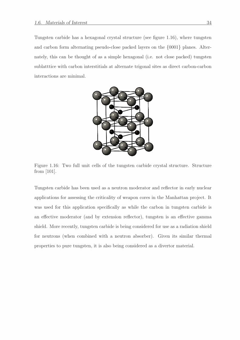
1.6. Materials of Interest 34
Tungsten carbide has a hexagonal crystal structure (see figure 1.16), where tungsten
and carbon form alternating pseudo-close packed layers on the {0001} planes. Alter-
nately, this can be thought of as a simple hexagonal (i.e. not close packed) tungsten
sublatttice with carbon interstitials at alternate trigonal sites as direct carbon-carbon
interactions are minimal.
Figure 1.16: Two full unit cells of the tungsten carbide crystal structure. Structurefrom [101].
Tungsten carbide has been used as a neutron moderator and reflector in early nuclear
applications for assessing the criticality of weapon cores in the Manhattan project. It
was used for this application specifically as while the carbon in tungsten carbide is
an effective moderator (and by extension reflector), tungsten is an effective gamma
shield. More recently, tungsten carbide is being considered for use as a radiation shield
for neutrons (when combined with a neutron absorber). Given its similar thermal
properties to pure tungsten, it is also being considered as a divertor material.
1.7. Modelling Radiation Damage in Materials 35
1.7 Modelling Radiation Damage in Materials
The primary motivation for work presented in this thesis is to contribute to predicting
the behaviour of materials in a nuclear fusion environment over their lifetime. This
section describes the basic theory of radiation damage in materials, and how materials
modelling can be used to aid in understanding these processes. Particular focus is
placed on contextualising the results of Density Functional Theory (DFT) and Molec-
ular Dynamic (MD) simulations, the two principal techniques used in this thesis.
As demonstrated in section 1.5, the nuclear fusion environment is an incredibly chal-
lenging environment for materials survivability, with high fluxes of fusion neutrons,
high thermal flux, thermal transients and high temperatures. This environment is dif-
ficult and expensive to replicate, and currently cannot be completely replicated as no
sufficiently high flux source of fusion neutrons exists. As such, materials behaviour
over the lifetime of the reactor must be extrapolated from limited and incomplete ex-
perimental data.
It is only possible to predict the behaviour of fusion materials with some degree of
reliability if a mechanistic understanding of the materials evolution under fusion con-
ditions is achieved; otherwise it is possible that hitherto unknown processes may cause
drastic divergence from extrapolated data [102]. This is where computational modelling
is useful, as it may be used to probe and simulate conditions, time scales and length
scales that cannot be accessed experimentally. That is, combined with experimental
data, a more complete picture of the materials behaviour may be constructed.

1.7. Modelling Radiation Damage in Materials 36
1.7.1 Theory of Radiation Damage
Interaction of Radiation with Matter: Defect Formation
In both fission and fusion reactors, the highest flux of radiation and principal cause of
radiation damage is that from neutrons. Energetic neutrons in the MeV range interact
with nuclei in the material either elastically, in which the total momentum of the inci-
dent neutron and nucleus is conserved, or inelastically where it is not. During inelastic
interactions, the incident neutron may either excite the internal structure of the nucleus
or be captured, transmuting the atom. Both processes are strongly element dependent,
and unless functionally necessary as in a neutron multiplier, are selected against when
choosing materials to avoid unwanted transmutation products and residual radiation.
Thus, in most structural materials used in reactors, the elastic interaction cross-section
is orders of magnitude higher than the inelastic cross-section. It is, however, still low
in absolute terms, hence neutrons can penetrate far into a material [103].
When an energetic neutron interacts with a nucleus elastically, it transfers kinetic
energy to that nucleus inversely proportional to the nucleus’ mass [104]. At sufficiently
high energy, this displaces the nucleus which may then itself be considered a form of
charged radiation (depending on the energy and material) referred to as a Primary
Knock-on Atom (PKA). As charged radiation, the PKA undergoes ballistic collisions
with other nuclei in the material generating other knock-on atoms thus causing a dam-
age cascade, but it also interacts electronically with the electrons in the material. These
interactions are summarised in figure 1.17.
Both these modes of interaction can cause defects, with electronic interactions causing

1.7. Modelling Radiation Damage in Materials 37
incident neutronPKA
damage cascades
Electronic stopping dominates
Nuclear stopping dominates
Figure 1.17: Typical trajectory of energetic neutron and scattered ions in a material.
electronic defects, such as charge defects:
AxA + Bx
B → A′A + B.
B (1.16)
Nuclear interactions may result in further atomic displacements creating Frenkel pairs,
denoted for pure beryllium as
BeBe → VBe + Bei (1.17)
In metals (which are the focus of this thesis), electronic defects are typically insignif-
icant as they rapidly recombine [15]. Frenkel pairs, however, form the basis of many
deleterious effects of radiation in materials and thus merit further consideration.
Several models aim to describe the number of Frenkel pairs or displacements produced
by a PKA as a function of energy, E. The original of these is the Kinchin-Pease (KP)
model [105], which was later modified to the Norgett-Robinson-Torrens (NRT) [106]
and Greenwood models [107]. These are presented in figure 1.18. There are two key
metrics in the Kinchin-Pease model; the energy at which nuclear stopping becomes
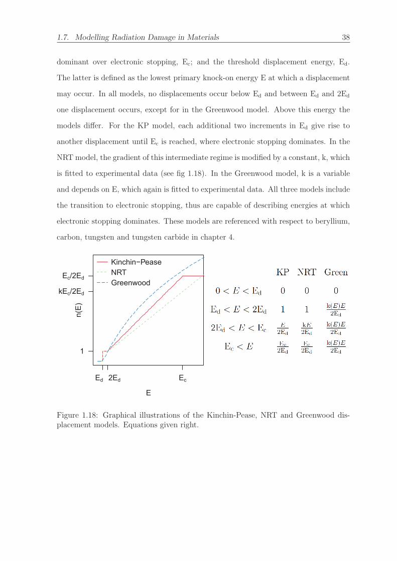
1.7. Modelling Radiation Damage in Materials 38
dominant over electronic stopping, Ec; and the threshold displacement energy, Ed.
The latter is defined as the lowest primary knock-on energy E at which a displacement
may occur. In all models, no displacements occur below Ed and between Ed and 2Ed
one displacement occurs, except for in the Greenwood model. Above this energy the
models differ. For the KP model, each additional two increments in Ed give rise to
another displacement until Ec is reached, where electronic stopping dominates. In the
NRT model, the gradient of this intermediate regime is modified by a constant, k, which
is fitted to experimental data (see fig 1.18). In the Greenwood model, k is a variable
and depends on E, which again is fitted to experimental data. All three models include
the transition to electronic stopping, thus are capable of describing energies at which
electronic stopping dominates. These models are referenced with respect to beryllium,
carbon, tungsten and tungsten carbide in chapter 4.
Ed 2Ed Ec
1
kEc/2Ed
Ec/2Ed
n(E)
E
Kinchin PeaseNRTGreenwood
Figure 1.18: Graphical illustrations of the Kinchin-Pease, NRT and Greenwood dis-placement models. Equations given right.
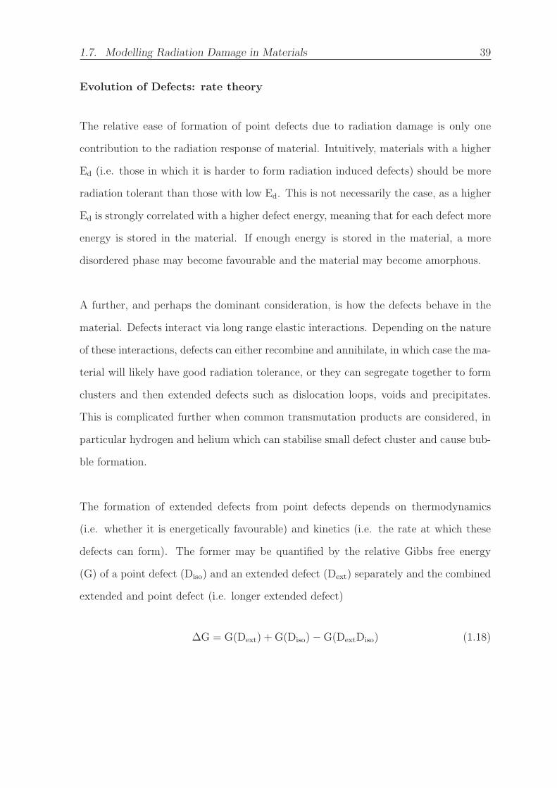
1.7. Modelling Radiation Damage in Materials 39
Evolution of Defects: rate theory
The relative ease of formation of point defects due to radiation damage is only one
contribution to the radiation response of material. Intuitively, materials with a higher
Ed (i.e. those in which it is harder to form radiation induced defects) should be more
radiation tolerant than those with low Ed. This is not necessarily the case, as a higher
Ed is strongly correlated with a higher defect energy, meaning that for each defect more
energy is stored in the material. If enough energy is stored in the material, a more
disordered phase may become favourable and the material may become amorphous.
A further, and perhaps the dominant consideration, is how the defects behave in the
material. Defects interact via long range elastic interactions. Depending on the nature
of these interactions, defects can either recombine and annihilate, in which case the ma-
terial will likely have good radiation tolerance, or they can segregate together to form
clusters and then extended defects such as dislocation loops, voids and precipitates.
This is complicated further when common transmutation products are considered, in
particular hydrogen and helium which can stabilise small defect cluster and cause bub-
ble formation.
The formation of extended defects from point defects depends on thermodynamics
(i.e. whether it is energetically favourable) and kinetics (i.e. the rate at which these
defects can form). The former may be quantified by the relative Gibbs free energy
(G) of a point defect (Diso) and an extended defect (Dext) separately and the combined
extended and point defect (i.e. longer extended defect)
ΔG = G(Dext) + G(Diso)−G(DextDiso) (1.18)

1.7. Modelling Radiation Damage in Materials 40
It should be noted that for the addition of a point defect to an extended defect, this
is likely to be a function of the size of the defect, particularly when the extended
defect is small, meaning that nucleation effects may be significant. The kinetics of
extended defect formation are influenced by the elastic interactions of extended and
point defects, but is principally dictated by the diffusivity of the point defects. The
diffusion coefficient can be approximated using equation 1.19,
D = D0exp
(Ea
kBT
)(1.19)
where Ea is the activation energy and D0 is the maximal diffusion coefficient. For a
thermal equilibrium concentration of defects, Ea is composed of two terms, the defect
formation energy and the lattice hop energy, Ehop. Radiation damage creates a defect
concentration far above equilibrium, so Ea can be approximated as Ehop. Equations
1.18 and 1.19 must be considered for each possible defect reaction and migrating species
respectively. Further, both ΔG and D are temperature dependant and as a result the
behaviour of a material can shift dramatically with temperature. Thus, extrapolation
of trends across temperature can only be achieved with confidence if the underlying
mechanisms driving these trends are well understood.
Evolution of macroscopic properties
The evolution of extended defects has consequences for the macroscopic properties of
materials. In metals, two effects which usually limit the lifetime of a component are
radiation induced embrittlement and swelling [15]. Embrittlement occurs when the
dramatically increased concentration of defects pins dislocations within the material,
and the dislocations themselves become entangled. This prevents movement of dislo-
cations, which is necessary for plastic deformation, causing the yield strength of the
material to increase to the ultimate tensile strength, resulting in brittle behaviour [15].

1.7. Modelling Radiation Damage in Materials 41
Swelling occurs when vacancies coalesce to form voids, increasing the void fraction
of the material and thus the macroscopic dimensions. This is heavily temperature
dependent [15], with low diffusion limiting void formation at low temperatures, and
thermal emission limiting it at high temperatures. Thus, metals typically undergo
swelling in the temperature range 0.3 Tm < T < 0.55Tm [15], where Tm is the melting
point of the material.
Transmutation may compound the effect of void swelling, particularly where hydrogen
and helium are evolved as they segregate to vacancies and vacancy clusters, eventually
forming bubbles. Further, a wide range of transmutation products may occur leading
the formation of secondary phases and precipitates. Many of these effects are lifetime
limiting for components in both fission and fusion reactors. As such, it is vital that a
mechanistic understanding of these processes is developed.
1.7.2 Multiscale Modelling
Given the complex process occurring on an atomistic scale that dictate the evolution
of materials properties during irradiation, simulation can be a valuable tool to develop
our understanding of radiation damage in materials. In the past 50 years, a rapid
increase in computational capacity has opened several fields of modelling for this pur-
pose. Each of these fields is limited in the length scales and timescales that can be
simulated, but together can access a broad range, as outlined in figure 1.19. Typically,
the longer length and time scales that can be simulated the more approximations must
be introduced.
On the smallest length and time scales, ab-initio techniques are used to simulate the
electronic structure of tens to hundreds of atoms for hundreds of picoseconds. These
1.7. Modelling Radiation Damage in Materials 42
time
(s)
10 9 10 6 10 3 100
10 12
10 9
10 6
10 3
100
length (m)
Continuum models
KineticMontecarlo
MolecularDynamicsDFT
AMD
Figure 1.19: Length and timescales typically accessible using several common modellingmethods.
can be used to calculate point defect properties such as formation energy and hopping
energies familiar from equations 1.18 and 1.19. In this thesis, such simulations are
performed using DFT, the details of which are explored in chapter 2, section 2.1.
Beyond this, MD simulations (see chapter 2 section 2.4) can access up to 109 atoms
and ns timescales. This allows the simulation of phenomena unavailable to DFT, such
as damage cascades and extended defects. Further, it can be used to identify complex
processes such as concerted migration, that are not accessible in static simulations
with few atoms [108]. MD simulations rely on empirical potentials, the form of which
approximate the physics of the real system, and which contain constants (parameters)
that must be fitted to experimental data. Where no such data exists, DFT data may
suffice. More often, properties predicted using empirical potentials are compared to
those predicted using DFT, which is more universally applicable and the limitations of
which are well understood, thereby providing useful validation.

1.7. Modelling Radiation Damage in Materials 43
The MD approach can be extended to longer timescales using Accelerated Molecular
Dynamics (AMD), which uses statistical mechanics to accelerate the rate of infrequent
events predicted by MD [15]. This approach similarly relies on the empirical potential
form, though further approximations and assumptions are introduced to achieve the
acceleration [15].
Even greater length and timescales can be accessed using kinetic Monte-Carlo methods.
In these methods, a known initial state is allowed to evolve over time through some
transition event that has a known probability of occurring [109]. A uniform random
number is generated to decide whether the transition occurs, and then the process is
repeated. Such approaches do not explicitly model each atom in the material unlike
MD and DFT, rather they only model the phenomenon of interest explicitly (e.g. dis-
locations). A typical example of such a method is the simulation of defect mobility
and clustering [109]. Again, defect diffusivity and thermodynamic data is necessary
for such a simulation, and can be provided either from the results of DFT and MD
simulations or from experimental data.
Another example of an accelerating method is the binary collision approximation, which
forms the basis of the popular SRIM software [110]. This method can be used to cal-
culate the final distribution of incident energetic ions in a material, along with the
distribution of atomic displacements and much other useful information. To calculate
the number of displacements, the code requires input of the threshold displacement
energy of the elemental species that make up the material, which can be determined
experimentally or through MD simulations [15].
Even longer time and length scales can be accessed using continuum modelling ap-

1.8. Structure of this Thesis 44
proaches such as finite element analysis. These approaches model the material (or
elements of it) as a continuum, the properties of which must be defined. These prop-
erties can be linked to the microstructural evolution of the material as outlined in
section 1.7.1. As such, properties that can be predicted using information about the
microstructure from KMC simulations may be used in such models in lieu of experi-
mental data where none is available.
1.8 Structure of this Thesis
Having outlined the components and requirements of nuclear fusion reactor components
and the materials considered for these applications, it is clear that additional work is
required to understand how such materials will evolve in a reactor. The techniques
used to address this challenge are outlined in the following methodology chapter. The
structure of Be12Ti and results of elastic neutron scattering experiments across the
Be12M materials series are presented in chapter 3. The properties and migration of
intrinsic defects in the Be12M series are investigated in chapter 4. Threshold displace-
ment damage profiles in the fusion reactor materials beryllium, tungsten, carbon and
tungsten carbide are investigated in chapter 5. Finally, ongoing work and areas that
require further investigation are outlined in chapter 6.
Chapter 2
Methodology
This chapter outlines the techniques employed in the simulations used throughout this
thesis. Particular focus is placed on the limitations and accuracy of these techniques
so that the results can be better contextualised.
Atomistic simulation requires two principal elements: a physical description of the
atomic configuration and a model by which to evaluate the energy landscape of the
atomic system. As the materials investigated in this thesis are all crystalline solids, a
description of the atomic configuration can be provided by a basis and a motif, that
is, a cell vector and a periodic repeating arrangement of atoms at each point. To make
atomistic simulation possible on such a system, several approximations must be made
regarding this description, which are outlined in sections 2.2 and 2.4.
The energy of the system for a static 3D arrangement of atoms can be described
in several ways, resulting from different approximations of the physics in the real sys-
tem. Two such descriptions are used in this thesis, quantum mechanical methods based
on a (partial) solution of the Schrodinger equation, and empirical methods that use
45
2.1. Density Functional Theory 46
functional forms to approximate various physical effects. Both these approaches have
advantages and disadvantages, outlined in chapters 2.1 and 2.3.
2.1 Density Functional Theory
Quantum Mechanical (QM) approaches to describing an atomic system have the ad-
vantage that they are constructed from first principles, and thus in their purest form,
are not compromised by empirically derived constants. In practice, many approxima-
tions and assumptions must be introduced to make these approaches tractable for all
but the simplest systems. This section provides an overview of the theory underlying
Density Functional Theory (DFT), with focus on the assumptions and approximations
required to make it a practical simulation technique.
All QM approaches are based fundamentally on finding a solution to the Schrodinger
equation,
EΨ = HΨ (2.1)
where E is the total energy of the system, H is the Hamiltonian operator and Ψ is
a set of solutions, or eigenstates, of the Hamiltonian. In the case of atomic systems,
these eigenstates correspond to individual electron wavefunctions. The definition of
the Hamiltonian depends on the physical system being described, and in the case of
an atomic system can be split into five constituent contributions;
EΨ =
[− h2
2mi
∑i=1
∇2ri︸ ︷︷ ︸
Tn
− h2
2Mi
∑i=1
∇2Ri]︸ ︷︷ ︸
TN
+∑i=1
e2
2|ri − rj|︸ ︷︷ ︸Unn
+∑i=1
Z2
2|Ri −Rj|︸ ︷︷ ︸UNN
−∑i=1
ZIe
2|Ri − rj|︸ ︷︷ ︸UnN
]Ψ
(2.2)

2.1. Density Functional Theory 47
where Tn is the kinetic energy of electrons (n), TN the kinetic energy of nuclei (N),
Unn the interactions of electrons with each other, UNN the interactions of nuclei with
other nuclei and UnN the interaction of nuclei with electrons. Φ is a many body
problem which has 4n dimensions (3 dimensions + spin for each electron, n) which
is prohibitively computational expensive to solve, thus several approximations must
be included. The first of these is the Born-Oppenheimer approximation [111], which
states that given the large discrepancy in mass between electrons and nuclei they may
be treated separately. Thus, UNN and TN are evaluated separately through classical
means, and the Schrodinger equation, with the now simplified Hamiltonian, is evaluated
for a stationary arrangement of nuclei in space. Further, the term for electron-nuclei
interactions, which are coulombic, can be treated as an external potential, Vext. There-
fore H is simplified to H = −Tn +Unn +Vext.
In effect, solving the Schrodinger equation for this reduced Hamiltonian defines the
electronic orbitals, which allows the total forces on each atom resulting from the elec-
tronic system to be evaluated. As a consequence, simulation techniques outlined in
sections 2.2 and 2.4 can be used to calculate various properties of the system.
2.1.1 Hohenberg, Kohn and Sham
Although greatly reduced in complexity, solving the reduced Schrodinger equation is
still non-trivial. The electronic wavefunction, Ψ, is a function for every spatial co-
ordinate of each of the n electrons (Ψ = Ψ(r1, ..., rn)), which using the Hartree ap-
proximation [112], can be described as a product of individual electron wavefunctions
(Ψ = Ψ1(r), ...,Ψn(r)). This is a necessary step, as the full wavefunction for a simple
molecule such as O2 would be a 48-dimensional function (3 dimensions for each electron
neglecting spin), which is impractical to solve.

2.1. Density Functional Theory 48
It should be noted that the electron wave function cannot be measured experimen-
tally. What can be measured however, is the probability of finding an electron in a
given space at a given time; the electron density, n(r). The electron density can con-
veniently be calculated from the wavefunction by taking the conjugate of the function.
For a generalised, ground state molecular system, in conjunction with the Hartree
approximation, this gives:
n(r) = 2∑i
Ψ∗i (r)Ψi(r) (2.3)
where the factor of two appears because the Pauli exclusion principle states that each
electron wavefunction can be occupied by two electrons if they have different spin.
The electron density gains additional significance considering the work by Kohn, Ho-
henberg and Sham [113, 114]. Kohn and Hohenberg proved two mathematical the-
orems that form the basis of DFT. The first states “The ground-state energy from
Schrodinger’s equation is a unique functional of the electron density”. The significance
of this, is that if the electron density, n(r), is known, the energy of the system can
be found if the functional relating the two, E[n(r)], is also known. Unfortunately, this
theorem says nothing as to the form of the functional.
The second Hohenberg-Kohn theorem states “The electron density that minimises the
energy of the overall functional is the true electron density corresponding to the full so-
lution of the Schrodinger equation”. The practical implication of this is that if the true
form of the functional is known, then the electron density could be varied to minimise
the energy given by the functional, thus providing a means to find the relevant electron
density. While the exact form the functional is not known, the general contributions
2.1. Density Functional Theory 49
can be surmised from the Hamiltonian as below:
E[(Ψi)] = Eknown[(Ψi)] + EXC[(Ψi)] (2.4)
Eknown[(Ψi)] = − h2
m
∑i
∫Ψ∗
i∇2Ψid3r
+
∫V (r)n(r)d3r +
e2
2
∫ ∫n(r)n(r′)|r− r′|
(2.5)
Where the known terms consist of the electron kinetic energies, the external potential
from the nuclei (Born-Oppenheimer approximation), the coulomb interactions between
electrons, and between nuclei. The final and unknown term, EXC, by definition con-
tains all the unknown quantities, but principally exchange and correlation effects.
This formulation, when combined with the Hartree approximation[112], leads to the
Kohn-Sham equations for single electron wavefunctions [113, 114]:
[− h2
2m∇2 + Vext(r) + VH(r) + VXC(r)
]Ψi(r) = εiΨi(r) (2.6)
VH(r) = e2∫
n(r′)|r− r′|d
3r′ (2.7)
Where Vext(r) is familiar from equation 2.2, and VH is the Hartree potential which
describes the coulombic interactions between electrons (including an unphysical self
interaction energy). The final term, VXC, is the exchange correlation potential, which
is formally defined as the functional derivative of the exchange-correlation energy, but
also must account for the unphysical interaction energy from VH.

2.1. Density Functional Theory 50
2.1.2 Exchange-Correlation Functional
Using the Kohn-Sham equation, the electron density and energy of the system can be
calculated iteratively from an initial, trial electron density. The only element that is
missing is the form of the Exchange-Correlation functional, VXC. The exact form of this
functional is not known, however there is one case where it can be defined exactly: a
uniform electron gas. This is not a particularly interesting case, as in a real system the
variations in electron density are exactly what give rise to properties such as bonding.
Fortunately (and perhaps surprisingly), it can be extended to real systems, by setting
the exchange-correlation functional to the known value for a uniform electron gas with
the local electron density observed at that position:
VXC(r) = VelectrongasXC [n(r)] (2.8)
This is known as the Local Density Approximation (LDA)[113, 114]. The LDA is
still widely used for DFT simulations to date, however it is important to remember
that this does not represent an exact solution of the Schrodinger equation, and thus
is not suitable for the simulation of some systems, particularly those in which there
is a steep gradient in the electron density (e.g. where covalent bonds are present).
As such, a wide variety of other functionals have been developed to improve on this
approximation. The most widely used and simplest of these is the Generalised Gradient
Approximation (GGA) [115, 116, 117]. In the GGA scheme, the local gradient of the
electron density is also incorporated into the functional:
VGGAXC (r) = VXC[n(r),∇n(r)] (2.9)
There are many ways to incorporate this additional information and hence several
variants of this scheme have been implemented, notably the Perdew-Wang functional
2.1. Density Functional Theory 51
(PW91)[115] and the Perdew-Burke-Ernzerhof (PBE)[118] functionals. This approach
is extended further in meta-GGA functionals[119], which take into account the second
derivative of the electron density:
VmGGAXC (r) = VXC[n(r),∇n(r),∇2n(r)] (2.10)
an example of which is the TaoPerdewStaroverovScuseria (TPSS) functional [119]. In
deciding which functional to use, it is important to consider the nature of the system as
encoding more physical parameters of the system does not necessarily translate to an
increase in accuracy. In particular, the LDA functional is typically more accurate for
systems where the electron density tends to be more uniform, whereas GGA funtionals
are often more accurate for systems with steep changes in the electron density such as
covalent and ionic materials [120].
The GGA-PBE functional has been selected for simulations in this work as it pre-
serves the accuracy of the LDA for metallic systems while correcting (and sometimes
overcorrecting) the LDA overbinding issue and discrepancy with experimentally derived
binding energies [121]. A comparison of predictions made using DFT in conjunction
with the LDA, GGA-PW91 and GGA-PBE functionals and compared to experimental
values is shown in table 2.1.
A further consideration is whether the functional contains empirically derived informa-
tion. Such functionals, by design, work extremely well for systems similar to those they
are fit to, however may become unphysical for dissimilar systems. All the functionals
mentioned thus far are nonempirical.
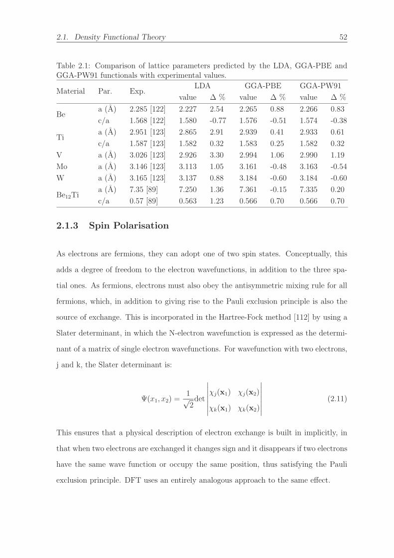
2.1. Density Functional Theory 52
Table 2.1: Comparison of lattice parameters predicted by the LDA, GGA-PBE andGGA-PW91 functionals with experimental values.
Material Par. Exp.LDA GGA-PBE GGA-PW91
value Δ % value Δ % value Δ %
Bea (A) 2.285 [122] 2.227 2.54 2.265 0.88 2.266 0.83
c/a 1.568 [122] 1.580 -0.77 1.576 -0.51 1.574 -0.38
Tia (A) 2.951 [123] 2.865 2.91 2.939 0.41 2.933 0.61
c/a 1.587 [123] 1.582 0.32 1.583 0.25 1.582 0.32
V a (A) 3.026 [123] 2.926 3.30 2.994 1.06 2.990 1.19
Mo a (A) 3.146 [123] 3.113 1.05 3.161 -0.48 3.163 -0.54
W a (A) 3.165 [123] 3.137 0.88 3.184 -0.60 3.184 -0.60
Be12Tia (A) 7.35 [89] 7.250 1.36 7.361 -0.15 7.335 0.20
c/a 0.57 [89] 0.563 1.23 0.566 0.70 0.566 0.70
2.1.3 Spin Polarisation
As electrons are fermions, they can adopt one of two spin states. Conceptually, this
adds a degree of freedom to the electron wavefunctions, in addition to the three spa-
tial ones. As fermions, electrons must also obey the antisymmetric mixing rule for all
fermions, which, in addition to giving rise to the Pauli exclusion principle is also the
source of exchange. This is incorporated in the Hartree-Fock method [112] by using a
Slater determinant, in which the N-electron wavefunction is expressed as the determi-
nant of a matrix of single electron wavefunctions. For wavefunction with two electrons,
j and k, the Slater determinant is:
Ψ(x1, x2) =1√2det
∣∣∣∣∣∣∣χj(x1) χj(x2)
χk(x1) χk(x2)
∣∣∣∣∣∣∣ (2.11)
This ensures that a physical description of electron exchange is built in implicitly, in
that when two electrons are exchanged it changes sign and it disappears if two electrons
have the same wave function or occupy the same position, thus satisfying the Pauli
exclusion principle. DFT uses an entirely analogous approach to the same effect.
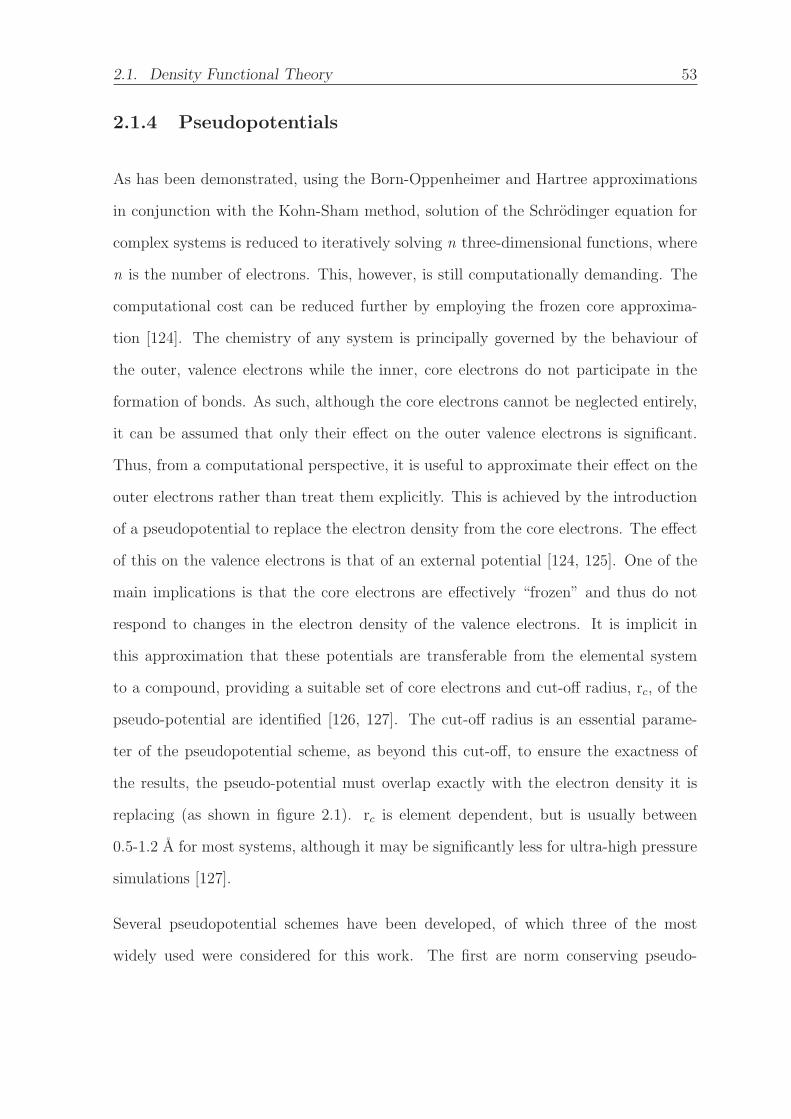
2.1. Density Functional Theory 53
2.1.4 Pseudopotentials
As has been demonstrated, using the Born-Oppenheimer and Hartree approximations
in conjunction with the Kohn-Sham method, solution of the Schrodinger equation for
complex systems is reduced to iteratively solving n three-dimensional functions, where
n is the number of electrons. This, however, is still computationally demanding. The
computational cost can be reduced further by employing the frozen core approxima-
tion [124]. The chemistry of any system is principally governed by the behaviour of
the outer, valence electrons while the inner, core electrons do not participate in the
formation of bonds. As such, although the core electrons cannot be neglected entirely,
it can be assumed that only their effect on the outer valence electrons is significant.
Thus, from a computational perspective, it is useful to approximate their effect on the
outer electrons rather than treat them explicitly. This is achieved by the introduction
of a pseudopotential to replace the electron density from the core electrons. The effect
of this on the valence electrons is that of an external potential [124, 125]. One of the
main implications is that the core electrons are effectively “frozen” and thus do not
respond to changes in the electron density of the valence electrons. It is implicit in
this approximation that these potentials are transferable from the elemental system
to a compound, providing a suitable set of core electrons and cut-off radius, rc, of the
pseudo-potential are identified [126, 127]. The cut-off radius is an essential parame-
ter of the pseudopotential scheme, as beyond this cut-off, to ensure the exactness of
the results, the pseudo-potential must overlap exactly with the electron density it is
replacing (as shown in figure 2.1). rc is element dependent, but is usually between
0.5-1.2 A for most systems, although it may be significantly less for ultra-high pressure
simulations [127].
Several pseudopotential schemes have been developed, of which three of the most
widely used were considered for this work. The first are norm conserving pseudo-
2.1. Density Functional Theory 54
−1.0
−0.5
0.0
0.5
1.0Ti (4s)
wav
efun
ctio
n
−1.0
−0.5
0.0
0.5
1.0Ti (3p)
0.0 0.5 1.0 1.5 2.0 2.5 3.0 3.5
−1.0
−0.5
0.0
0.5
1.0Ti (3d)
r (Bohr radius)
Figure 2.1: Wavefunctions for titanium pseudopotentials (solid lines) overlayed againstthe all electron potential (dashed lines). The vertical line represents the cutoff radius,beyond which the pseudopotentials and all electron potentials are identical.

2.1. Density Functional Theory 55
potentials [128], which impose the additional constraint that the total charge of the
pseudo-potential must be the same as the total norm of the all-electron potential.
This simplifies numerical operations within DFT, and is a good physical representa-
tion of the system. It does however lead to the need for harder pseudo-potentials [127]
(“harder” in this case refers to the need for a higher cutoff energy: see section 2.1.4),
which increases the computational expense of simulations.
Second are the ultrasoft pseudopotentials (USPP) based on work by Vanderbilt [129].
These potentials remove the criteria that the total charge of the wavefunction is con-
served, and consequently allow for significantly softer potentials, which by extension
are much more computationally efficient. One of the drawbacks of this approach is
that they contain at least one (and often many) empirical parameters, although for
commonly used potentials these have been rigorously qualified [130].
The final approach is the Projector Augmented Wave (PAW) method [131, 132, 133],
which combines the pseudo-potential approach with the linear augmented plane wave
method to reintroduce near core oscillations of the valence electron wavefunctions.
This is attractive as by comparison to USPPs it is a more physical representation and
contains no empirical parameters, it is however more computationally expensive. Ex-
tensive comparison has been made between the USPP, PAW, norm conserving and all
electron (no pseudo-potential) methods, which have shown excellent agreement in all
cases except where atoms have very different electronegativities or strong magnetic
moments [130, 134]. Considering this, USPPs were used in this work as none of the
materials investigated fall into these categories.

2.1. Density Functional Theory 56
Plane Waves
Even with the approximations outlined thus far, DFT is still computationally expensive
by comparison to empirical potentials and simulations are usually limited to hundreds
of atoms. This poses a challenge for the simulation of bulk properties, as for an isolated
cluster of a few hundred atoms, surface terms will dominate, obscuring bulk effects.
This necessitates the introduction of periodic boundaries, whereby an atom interacts
across the boundary of the cell with its periodic image.
Given that DFT is concerned with evaluating electron wavefunctions, the introduc-
tion of periodic boundaries has the additional implication that the wavefunctions (and
consequently any quantity derived from them) must also be periodic in space with the
same periodicity as the (repeat unit) supercell. This is stated by Bloch’s theorem [135]
for a wavefunction evaluated at a single k-point :
ψk(r) = u(r)eik·r (2.12)
By extension, the overall wave function is given:
ψ(r) =
∫ψk(r)d
3k (2.13)
and the electron density:
ρ(r) =
∫|ψk(r)|2d3k (2.14)
where uk is a function with the same periodicity as the unit cell and k is a vector rep-
resenting the position in reciprocal space. The functions eik·r, known as plane waves,
are simply an arbitrary phase factor which scales the periodic function in surrounding
cells. As such, it is only necessary to evaluate the integral of equation 2.12 over the
2.1. Density Functional Theory 57
unit cell as defined in reciprocal space, also known as the Brillouin zone.
u(r) from equation 2.12 can be expanded in terms of a special set of plane waves:
uk =∑G
CGeiG·r (2.15)
where G are wavevectors which satisfy the periodicity and symmetry of the crystal and
CG are Fourier coefficients. Equation 2.12 then becomes:
ψk(r) =∑G
Ck+Gei(k+G)r (2.16)
To solve this for even a single point in k-space G must be summed over infinite possible
values, which is obviously impossible. Fortunately, the physical meaning of solution at
each G gives some insight into how it may be evaluated; each G represents a solution
of the Schrodinger equation with kinetic energy given by:
E =h2
2m|k+G|2 (2.17)
Solutions with lower kinetic energy are more physically important than those at higher
energy, thus some energy cutoff, Gcut, may be employed, which reduces the infinite
sum in equation 2.16 to the readily solvable
ψk(r) =∑
|G+k|<Gcut
Ck+Gei(k+G)r (2.18)
Gcut is chosen to balance convergence to an exact solution and computational efficiency,
and further is element dependent. In this work, a convergence of at least 10−3eV atom−1
was employed (see figure 2.2), and the highest cutoff chosen for each element in a sys-
tem used for the overall system. Where quantities are compared between systems (e.g.

2.1. Density Functional Theory 58
a compound and elemental system, as is necessary to calculate formation energies) the
same cutoff is used for both systems to avoid the introduction of systematic errors.
A new form of the ultra-soft pseudo potentials is implemented in the most recent
versions of CASTEP [136, 137](The DFT code used in this work) and was used for
phonon calculations in this work, the convergence for which is shown in figure 2.2.
Based on these convergence tests, a cut-off energy of 480 eV was used for defect energy
calculations using Castep 6, while a cut-off of 660 eV was used for phonon calculations
using Castep 8 and later.
0 200 400 600 800
−3
−2
−1
0
1
2
Ecut(eV)
log(
Δ E)
(eV/
atom
)
Castep 6BeMoNbTaTiVW
0 200 400 600 800
−3
−2
−1
0
1
2
Ecut(eV)
log(
Δ E)
(eV/
atom
)
Castep 8BeMoNbTaTiVW
Figure 2.2: Energy cutoff convergence for elements studied for Castep 6 and 8. Castep8 was released part way through this work and includes modified pseudopotentials.Convergence criteria of 10−2 eV/atom is shown with a dotted black line. This isreached at 480 and 660 eV for all species in Castep 6 and 8 respectively.
2.1. Density Functional Theory 59
k-points
Returning to equation 2.12, provided the function varies slowly over k-space, it is suffi-
cient to evaluate it at a discrete series of k-points with in the Brillouin zone, and using
linear interpolation to approximate the integral. Typically, however, other methods of
interpolation such as Legendre Quadrature Methods provide a much faster convergence
with respect to the number of k-points so this approach is used instead [130].
The number and arrangement of k-points also has a significant impact on the accuracy
of the intergral, as well as on the computational cost of evaluating it. The scheme
developed by Monkhorst and Pack [138] is the most widely used method of choosing k-
points, which defines a linear array within the Brillouin zone. The number of k-points
can further be reduced when symmetry is considered, as equation 2.12 then only needs
to be evaluated over the irreducible Brillouin zone (IBZ). Convergence with the number
of k-points used, with uniform spacing based on the Monkhorst and Pack scheme is
shown in figure 2.3. Based on this convergence test, a grid of 4 × 4 × 8 k-points (from
which 12 are used) was selected for the Be12M structure, corresponding to a k-point
spacing of 0.02 A−1
which was then used for calculations of other structures. A more
dense k-point grid of 8 × 8 × 14, corresponding to a spacing of 0.012 A−1
was used
for phonon calculations which are more sensitive to small changes in the force field and
thus require a higher k-point density. An even number of k-points was chosen for the
Be12M structure so that 2 × 2 × 2 supercells could be investigated with exactly the
same k-point spacing.

2.1. Density Functional Theory 60
0 10 20 30 40 50 60 70
−4.0
−3.0
−2.0
−1.0
kpoints
log 1
0ΔE
(eV/
atom
)
Figure 2.3: Energy convergence of the conventional tetragonal cell of Be12Ti withrespect to the number of k-points used with a Monkhorst and Pack grid [138]. Notek-point convergence neither systematically over or underestimates energy values.
2.1.5 A note on Metals
One of the basic premises of the validity of the plane wave approach is that function
2.12, varies slowly over k space. This is not the case for metals, where regions of space
unoccupied by electrons are separated from occupied regions by the Fermi-surface. As
such, the function changes discontinuously from zero to non-zero values, and thus would
require an impractically dense grid of k-points to achieve well converged results. This
limitation is overcome using a smearing function to smooth out the discontinuity. To
exactly solve the problem at hand, it is important that the final result be extrapolated
to the limit where smearing is eliminated. The most common function which meets
this criteria is the Methfessel and Paxton function [139] which is used in this work with
a smearing width of 0.1 eV.
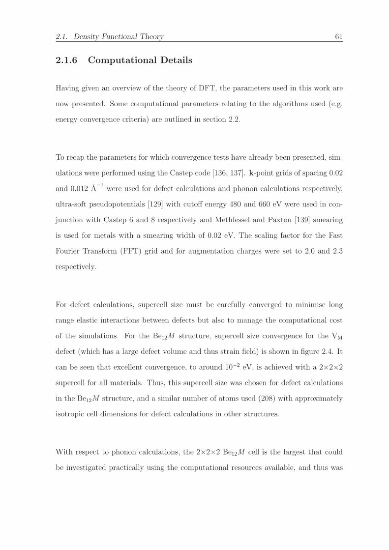
2.1. Density Functional Theory 61
2.1.6 Computational Details
Having given an overview of the theory of DFT, the parameters used in this work are
now presented. Some computational parameters relating to the algorithms used (e.g.
energy convergence criteria) are outlined in section 2.2.
To recap the parameters for which convergence tests have already been presented, sim-
ulations were performed using the Castep code [136, 137]. k-point grids of spacing 0.02
and 0.012 A−1
were used for defect calculations and phonon calculations respectively,
ultra-soft pseudopotentials [129] with cutoff energy 480 and 660 eV were used in con-
junction with Castep 6 and 8 respectively and Methfessel and Paxton [139] smearing
is used for metals with a smearing width of 0.02 eV. The scaling factor for the Fast
Fourier Transform (FFT) grid and for augmentation charges were set to 2.0 and 2.3
respectively.
For defect calculations, supercell size must be carefully converged to minimise long
range elastic interactions between defects but also to manage the computational cost
of the simulations. For the Be12M structure, supercell size convergence for the VM
defect (which has a large defect volume and thus strain field) is shown in figure 2.4. It
can be seen that excellent convergence, to around 10−2 eV, is achieved with a 2×2×2
supercell for all materials. Thus, this supercell size was chosen for defect calculations
in the Be12M structure, and a similar number of atoms used (208) with approximately
isotropic cell dimensions for defect calculations in other structures.
With respect to phonon calculations, the 2×2×2 Be12M cell is the largest that could
be investigated practically using the computational resources available, and thus was

2.2. Static Techniques 62
−3.0
−2.5
−2.0
−1.5
−1.0
−0.5
0.0
supercell size
log 1
0ΔE
(eV)
Be12MoBe12WBe12VBe12Ti
1x1x1 1x1x2 1x1x3 2x2x2 2x2x3
Figure 2.4: Supercell size energy convergence for a VM defect in the Be12M structurewith respect to a 3×3×3 supercell (containing 702 atoms).
used for all phonon calculations with the supercell method. Where other materials
were investigated, a supercell with at least 200 atoms was used.
2.2 Static Techniques
Static techniques are those that (unlike molecular dynamics) employ no concept of
temperature. They are less computationally demanding than dynamic simulations
with comparable number of atoms, and in this thesis are used primarily in conjunction
with DFT, although can equally be used with empirical potentials. As such, their
application to DFT simulations will be focused on in this section.
The simplest static technique is a calculation of the enthalpy of the system, whereby
the energy contributions from the electron density are evaluated for a given spatial
arrangement of atoms. More common is static energy minimisation, whereby the po-

2.2. Static Techniques 63
sitions of the atoms and dimensions of the cell are relaxed to a local energy minimum.
This is achieved using an iterative algorithm to move each atom in the system to a
position which minimises the total system energy, E, contributed from the electron
density.
In this work the conjugate gradient mechanism with a Broyden-Fletcher-Goldfarb-
Shanno (BFGS) Hessian [140] updating scheme is used for energy minimisation. The
direction and distance an atom is moved during a single iteration is determined by
the gradient of the energy hypersurface, with the direction given by the force vector
and magnitude by the second derivative. As the atomic positions evolve during this
process, the energy surface also evolves and thus must be recalculated for each itera-
tion. Complete convergence is achieved when the energy difference between two steps
falls to zero. In practice this is unlikely to occur as the closer to the local minima
the configuration becomes, the lower the forces and thus lower the magnitude of ge-
ometry change. As such, a cutoff energy must be specified, so that when the energy
change between steps falls below this value, the simulation is considered converged.
In addition to atomic positions, cell dimensions may also be minimised in this way.
In this work, for general geometry optimisations and defect calculations an energy
cutoff of 10−7 eV/atom was used, a force cutoff of 0.01 eV/A/atom and stress toler-
ance of 0.01 eV/A/atom. For phonon calculations, stricter values of 10−9 eV/atom,
10−4 eV/A/atom and 10−3 eV/A/atom were used respectively.
The main application of static methods in this work is to calculate the formation
enthalpy of a defect by comparing a the energy of a defective cell EDFTd to the perfect
cell EDFTp and the appropriate reference state of species added or removed μ(i):
Ef = EDFTd − EDFT
p ±∑i
μ(i) (2.19)

2.2. Static Techniques 64
Care must be taken to choose an appropriate supercell size (see section 2.1.6) to limit
the effects and energy contributions of long range elastic interactions across periodic
boundaries. In a similar way, the formation enthalpy (EF) of a given phase can be
calculated:
EF = EDFTp −
∑EDFTr (2.20)
where EDFTp is the enthalpy of the phase of interest, and
∑EDFTr is the total enthalpy
of the elemental reference states. This allows comparison of the relative stability of
different crystal structures and phases, which can be used to predict whether they are
likely to be observed experimentally.
2.2.1 Transition State Search and Nudged Elastic Band
Geometry optimised cells can also be used as the starting points for transition state
searches. Transition state searches are a way to determine the barrier to a chemical
reaction or the pathway and energy a diffusing species is most likely to take. In a
crystal, the atoms can be visualised as occupying a periodic array of energy wells. For
an atom to move to a new position, it must surmount a ridge of higher potential energy
before it can occupy a new stable (or metastable) state at the bottom of an energy well.
Usually, the atom will cross the ridge at its lowest point (the saddle point), therefore it
is imperative to determine where this is and the potential energy of the system relative
to the ground state as the atom transits this point, as this provides an approximation
of the hopping energy (Ehop) during diffusion.
To gain a first approximation of the energy at the saddle point, it is useful to perform
a Linear Synchronous Transit (LST) search [141]. In the LST method, the energy of
the system is calculated for a series of atomic positions which are linearly interpolated

2.2. Static Techniques 65
between the reactants and products, with the highest energy replica taken as the saddle
point. As there is no guarantee that the saddle point is along a linear interpolation
of points, this can at best be taken as an upper bound for the transition energy. This
can be improved by performing a constrained orthogonal optimisation of the saddle
point, that is to say, the position of the LST maximum is optimised while maintaining
the same reaction coordinate/relative separation from the product and reactant. This
is augmented by the Quadratic Synchronous Transit (QST) method [141], in which
a quadratic interpolation is performed through the reactant, product and LST maxi-
mum. The energy maximum along this pathway is then used as the QST prediction of
the transition state.
While the QST method usually provides a good description of the transition state,
there is no guarantee that the minimum energy pathway (MEP) follows a quadratic
trajectory. If it is desirable to find the full MEP rather than just the transition state,
it is necessary to use another technique, in this case the Nudged Elastic Band (NEB)
method [142]. In the NEB method, a number of replicas are created along a path-
way between the reactants and products. If a LST/QST simulation has already been
performed, one of these replicas is taken as the identified transition state to speed up
convergence. The replicas must be energy minimised to find the MEP, however doing
so will inevitably cause the replicas to converge back to the metastable product or
reactant. To prevent this, a spring force is applied parallel to the reaction pathway, τ||.
This in itself has been used in the precursor to NEB, the Plain Elastic Band (PEB)
method [143], however it is itself not sufficient to ensure the MEP is found. This is
because where the MEP is not a linear path between the reactants and products, the
spring force effectively acts to minimise the path length which results in the identified
path cutting the corner of the true MEP (see figure 2.5). This is exacerbated for higher
spring forces, however lowering the spring force causes the replicas around the saddle
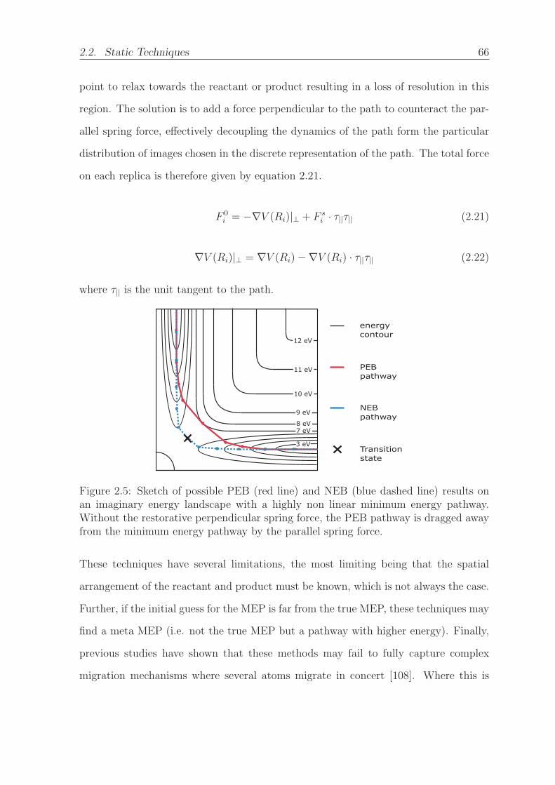
2.2. Static Techniques 66
point to relax towards the reactant or product resulting in a loss of resolution in this
region. The solution is to add a force perpendicular to the path to counteract the par-
allel spring force, effectively decoupling the dynamics of the path form the particular
distribution of images chosen in the discrete representation of the path. The total force
on each replica is therefore given by equation 2.21.
F 0i = −∇V (Ri)|⊥ + F s
i · τ||τ|| (2.21)
∇V (Ri)|⊥ = ∇V (Ri)−∇V (Ri) · τ||τ|| (2.22)
where τ|| is the unit tangent to the path.
energycontour
PEBpathway
NEBpathway
Transitionstate
10 eV
11 eV
12 eV
9 eV
8 eV7 eV
3 eV
Figure 2.5: Sketch of possible PEB (red line) and NEB (blue dashed line) results onan imaginary energy landscape with a highly non linear minimum energy pathway.Without the restorative perpendicular spring force, the PEB pathway is dragged awayfrom the minimum energy pathway by the parallel spring force.
These techniques have several limitations, the most limiting being that the spatial
arrangement of the reactant and product must be known, which is not always the case.
Further, if the initial guess for the MEP is far from the true MEP, these techniques may
find a meta MEP (i.e. not the true MEP but a pathway with higher energy). Finally,
previous studies have shown that these methods may fail to fully capture complex
migration mechanisms where several atoms migrate in concert [108]. Where this is

2.2. Static Techniques 67
the case, an entirely different approach using molecular dynamics (MD) to observe the
migration mechanism can be used, although this has its own limitations in that it is
impractical using DFT (due to being computationally intensive) and cannot capture
low temperature migration mechanisms. Full details of the implementation of these
methods in the Castep code are oulined in [144].
2.2.2 Phonons: Harmonic and Quasi-Harmonic Approxima-
tions
The vibrational behaviour of a material constitutes significant contributions to the en-
thalpy and entropy at finite temperature. As such, understanding the phonons in a
material is necessary in order to apply results calculated using static simulation tech-
niques to real world problems. In this work, phonons are treated using the harmonic
and quasiharmonic methods. These methods approximate the crystal as a series of sym-
metrical harmonic oscillators. In reality, the potential energy surface about an atom
is unlikely to be completely symmetrical, hence as the energy of the system increases
the space an atom can explore through thermal vibrations increases asymmetrically
leading to thermal expansion. This approximation is valid for low temperatures where
atomic displacement from equilibrium is small and allows the calculation of several
useful quantities to a high degree of accuracy.
One quantity that may be calculated is the Zero Point Energy (ZPE). This arises
as atoms have small enough mass that quantum mechanical effects are important, in
that the atom may only occupy discrete wave functions with non-zero energy, the fun-
damental representing the effective ground state. The ZPE is the energy difference
between this state and the classical description of the system, in which the atom sim-
ply sits at the bottom of the potential well. While inconsequential for massive atoms

2.2. Static Techniques 68
such as tungsten, the ZPE can be significant for less massive atom such as hydrogen
and beryllium.
The contribution of vibrational enthalpy to the total energy of a fixed volume sys-
tem can be calculated using the harmonic approximation. In this approximation, the
lattice parameters of the crystal are fixed, the contributions of the vibrational enthalpy
Hvib(T,V), which includes the ZPE, and vibrational entropy Svib(T,V) are evaluated by
integrating across the phonon density of states and phonon energy (according to Bose-
Einstein statistics). Combined with the formation enthalpy (HF), these contributions
constitute the Helmholtz free energy:
F(R,V) = HF +Hvib(T,V) + Svib(T,V) (2.23)
The quasi-harmonic method is essentially an extension of the harmonic approximation
to model systems with a variable lattice parameter (i.e. constant pressure rather than
constant volume). In this method, the potential wells are modelled as being harmonic
as in the harmonic approximation, but calculations are repeated for several lattice
volumes close to the ideal to characterise the energy wells at each lattice volume. For
each temperature an equation of state is then fitted to the data to determine the lowest
energy volume, in this case the third order Birch-Murnaghan equation of state:
E(V) = E0 +9
16K0V0
⎧⎨⎩[(
V0
V
) 23
− 1
]3K′
0 − 6
[(V0
V
) 23
− 1
]2 [2
3
(V0
V
) 23
− 1
]⎫⎬⎭
(2.24)
In this manner, the phonon contribution to the Gibbs free energy is estimated from
the contribution to the Helmholtz free energy at varying volumes:
G(T,P) = Vmin(Fphonon(T,P)) (2.25)

2.3. Empirical Potentials 69
To calculate the phonon density of states for a material, the force constants matrix
must be evaluated. This is achieved using the supercell method, in which positions of
the atoms are slightly perturbed and the reaction forces calculated. A supercell must
be used due to long range elastic interactions in crystalline solids, although the use of
a supercell is not necessary for molecules.
2.3 Empirical Potentials
In addition to DFT, classical potentials are another way to describe the energy of a
simulated atomic system. In this case, it is assumed that the energy of the system can
be evaluated by summating pairwise interactions between atoms. This approach has
an advantage over DFT in that it is considerably less computationally expensive since
the computational cost scales linearly with the number of atoms. Consequently, this
description can be used to access much greater length and timescales, on the order of
1 μm3 and 103 ns compared to 1 nm3 and 1 ns for DFT.
In this work, a classic Born description of the lattice is used, whereby ions are treated as
infinitesimally small points acting under pairwise interactions. Typically, these interac-
tions consist of a short range pairwise potential, Φab(rij) and a long range coulombic in-
teraction. This thesis examines only metallic and covalent systems, thus the coulombic
term can be discounted and the total energy of the system described as the summation
of all short range potentials:
E =1
2
∑i
∑i �=j
Φab(rij) (2.26)
where rij is the interatomic separation of atoms i and j which are species a and b re-
spectively. An iconic and widely used short range potential is the Morse potential [145],

2.3. Empirical Potentials 70
0 1 2 3 4 5
−6
−4
−2
0
2
re
De
r (Å)
pote
ntia
l ene
rgy
(eV)
Figure 2.6: Morse potential for tungsten, utilised as part of the bond order potentialset derived by Juslin et al. [146]. De = 5.419 eV and re = 2.341 A.
which has the form:
Φab(r) = De(1− e−α(rij−re))2 (2.27)
where De is the dissociation energy of the dimer, re is the equilibrium bond length,
and α is the force constant. The Morse functional has been widely used in part due
to its intuitive form, insofar that each constant is related to a physical concept (as
depicted in figure 2.6), and moreover can be parameterised explicitly from experimental
results [145]. Further, this potential form can provide a reasonable description of simple
systems such as dimers and some FCC metals.
2.3.1 Embedded Atom Method
Despite the success of simple pairwise potentials, they are inadequate to describe cer-
tain systems, in particular those materials in which bonding is strongly directional.
This is the case for HCP metals where the c/a ratio deviates from the ideal of 1.633.
Beryllium for example has a c/a ratio of 1.56(7) [122]. Covalently bonded materials
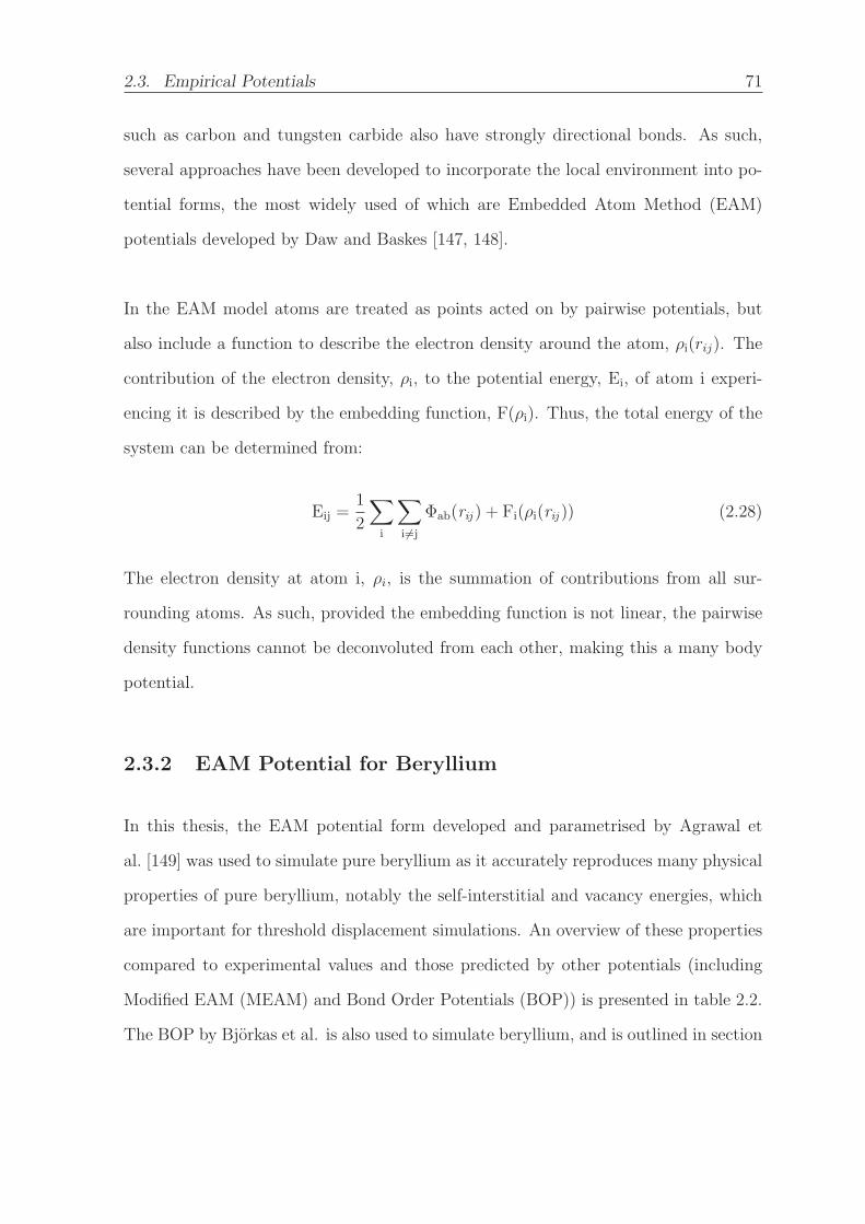
2.3. Empirical Potentials 71
such as carbon and tungsten carbide also have strongly directional bonds. As such,
several approaches have been developed to incorporate the local environment into po-
tential forms, the most widely used of which are Embedded Atom Method (EAM)
potentials developed by Daw and Baskes [147, 148].
In the EAM model atoms are treated as points acted on by pairwise potentials, but
also include a function to describe the electron density around the atom, ρi(rij). The
contribution of the electron density, ρi, to the potential energy, Ei, of atom i experi-
encing it is described by the embedding function, F(ρi). Thus, the total energy of the
system can be determined from:
Eij =1
2
∑i
∑i �=j
Φab(rij ) + Fi(ρi(rij )) (2.28)
The electron density at atom i, ρi, is the summation of contributions from all sur-
rounding atoms. As such, provided the embedding function is not linear, the pairwise
density functions cannot be deconvoluted from each other, making this a many body
potential.
2.3.2 EAM Potential for Beryllium
In this thesis, the EAM potential form developed and parametrised by Agrawal et
al. [149] was used to simulate pure beryllium as it accurately reproduces many physical
properties of pure beryllium, notably the self-interstitial and vacancy energies, which
are important for threshold displacement simulations. An overview of these properties
compared to experimental values and those predicted by other potentials (including
Modified EAM (MEAM) and Bond Order Potentials (BOP)) is presented in table 2.2.
The BOP by Bjorkas et al. is also used to simulate beryllium, and is outlined in section

2.3. Empirical Potentials 72
2.3.4.
For the Agrawal parametrisation of the EAM formalism, the pair potential is a Morse
potential, identical to equation 2.27. The electron density function, ρi(rij), is a simple
exponential:
ρ(rij ) = Ae−B(rij−re) (2.29)
where A and B are constants. To both the pair potentials and the electron density
function, the Voter taper function [154] is applied, which for the pair potentials is:
Φtapered = Φ(r)− Φ(rc) +rcm
[1−(
r
rc
)m]dΦ
dr
∣∣∣∣rc
(2.30)
where rc is the cutoff radius, and m is a constant. This cutoff function effectively limits
the interaction of the pair potentials and electron density and prevents a discontinuity
in the derivative of the energy gradient which would make the simulation unstable.
The embedding function used is the Johnson Function [155, 156]:
F = F0
[1− ln
ρiρ0
β]− F1
ρiρ0
γ
(2.31)
Where β,γ, F1 and F0 are empirically derived constants. The functional form of the
pair potentials, density function and embedding function, as parameterised for pure
beryllium using the constants outlined in table 2.3 are shown in figure 2.7.
It can be seen that the Johnson function has a minimum with respect to reduced elec-
tron density, thus subtly shifting the overall minimum position in the energy function
between two atoms when more atoms are added. This has the effect of stabilising the
HCP crystal structure, and altering the c/a ratio from the ideal of 1.633 to 1.568 which
is the experimental value for pure beryllium. To achieve this, it is necessary to use
quite a large cutoff (5 A) which makes this potential more computationally expensive

2.3. Empirical Potentials 73
Tab
le2.2:
Selectedexperim
entalan
dDFTdatacompared
tothat
predictedbytheAgraw
alpotential
andseveralother
available
atom
icpotential
sets
forthesimulation
ofberyllium.Δ%
isthe%
difference
from
experim
entalvalues.
EAM
aEAM
bMEAM
cMEAM
dMEAM
eABOPf
Param
eter
Exp.a
value
Δ%
value
Δ%
value
Δ%
value
Δ%
value
Δ%
value
Δ%
Ec(eV)
3.32
3.34
0.60
3.70
11.45
3.43
3.31
--
3.43
3.31
3.32
0
C11(G
Pa)
294
291
-1.02
89-69.73
3.62
-98.77
259
-11.90
331
12.59
280.5
-4.59
C33(G
Pa)
357
357
0.00
257
-28.01
193
-45.94
329
-7.84
309
-13.45
349.7
-2.04
C12(G
Pa)
2753
96.30
-59
-318.52
88225.93
77185.19
-11
-140.74
58.6
117.04
C13(G
Pa)
1410
-28.57
-37
-364.29
-22
-257.14
9-35.71
1828.57
13.5
-3.57
C44(G
Pa)
162
124
-23.46
107
-33.95
156
-3.70
65-59.88
19-88.27
198.2
22.35
C66(G
Pa)
133
119
-10.53
74-44.36
137
3.01
91-31.58
171
28.57
--
K(G
Pa)
117
121
3.42
116
-0.85
112
-4.27
115
-1.71
113
-3.42
--
G(G
Pa)
150
129
-14.00
153
2.00
137
-8.67
--
--
--
Ef(V
)(eV
)0.85
1.26
48.24
1.13
32.94
1.23
44.71
--
--
--
a:Agraw
alet
al.[149]b:Kaimiet
al.[150]c:
Baskesan
dJoh
nson[151]d:Thom
psonet
al.[151]e:
Dremov
etal.[152]
f:Bjorkas
etal.[153]
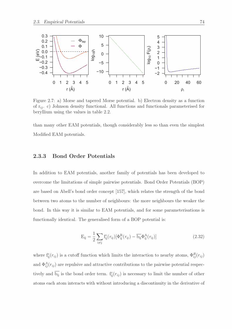
2.3. Empirical Potentials 74
0 1 2 3 4 5
−0.4−0.3−0.2−0.1
0.00.10.20.3
Φtap
Φ
E (e
V)
r (A° )0 1 2 3 4 5
−10
−5
0
5
10
log 1
0ρi
r (A° )0 20 40 60
−2−1
012345
log 1
0 F(ρ
i)
ρi
Figure 2.7: a) Morse and tapered Morse potential. b) Electron density as a functionof rij. c) Johnson density functional. All functions and functionals parameterised forberyllium using the values in table 2.2.
than many other EAM potentials, though considerably less so than even the simplest
Modified EAM potentials.
2.3.3 Bond Order Potentials
In addition to EAM potentials, another family of potentials has been developed to
overcome the limitations of simple pairwise potentials. Bond Order Potentials (BOP)
are based on Abell’s bond order concept [157], which relates the strength of the bond
between two atoms to the number of neighbours: the more neighbours the weaker the
bond. In this way it is similar to EAM potentials, and for some parameterisations is
functionally identical. The generalised form of a BOP potential is:
Eij =1
2
∑i �=j
fcij(rij )[ΦRij (rij )− bijΦ
Aij (rij )] (2.32)
where fcij(rij) is a cutoff function which limits the interaction to nearby atoms, ΦRij(rij)
and ΦAij(rij) are repulsive and attractive contributions to the pairwise potential respec-
tively and bij is the bond order term. fcij(rij) is necessary to limit the number of other
atoms each atom interacts with without introducing a discontinuity in the derivative of
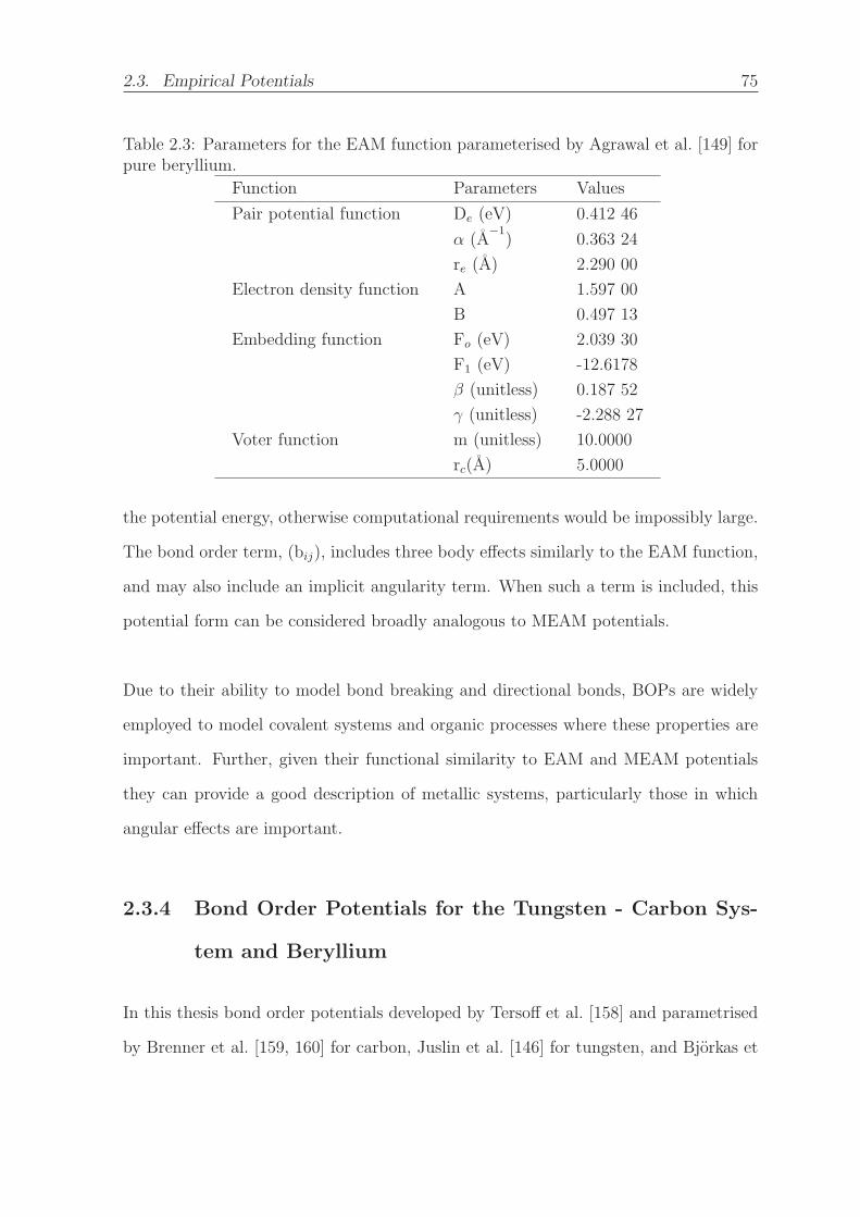
2.3. Empirical Potentials 75
Table 2.3: Parameters for the EAM function parameterised by Agrawal et al. [149] forpure beryllium.
Function Parameters Values
Pair potential function De (eV) 0.412 46
α (A−1) 0.363 24
re (A) 2.290 00
Electron density function A 1.597 00
B 0.497 13
Embedding function Fo (eV) 2.039 30
F1 (eV) -12.6178
β (unitless) 0.187 52
γ (unitless) -2.288 27
Voter function m (unitless) 10.0000
rc(A) 5.0000
the potential energy, otherwise computational requirements would be impossibly large.
The bond order term, (bij), includes three body effects similarly to the EAM function,
and may also include an implicit angularity term. When such a term is included, this
potential form can be considered broadly analogous to MEAM potentials.
Due to their ability to model bond breaking and directional bonds, BOPs are widely
employed to model covalent systems and organic processes where these properties are
important. Further, given their functional similarity to EAM and MEAM potentials
they can provide a good description of metallic systems, particularly those in which
angular effects are important.
2.3.4 Bond Order Potentials for the Tungsten - Carbon Sys-
tem and Beryllium
In this thesis bond order potentials developed by Tersoff et al. [158] and parametrised
by Brenner et al. [159, 160] for carbon, Juslin et al. [146] for tungsten, and Bjorkas et
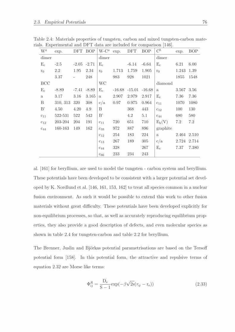
2.3. Empirical Potentials 76
Table 2.4: Materials properties of tungsten, carbon and mixed tungsten-carbon mate-rials. Experimental and DFT data are included for comparison [146].
Wa exp. DFT BOP W-Ca exp. DFT BOP Cb exp. BOP
dimer dimer dimer
Ec -2.5 -2.05 -2.71 Ec -6.14 -6.64 Ec 6.21 6.00
r0 2.2 1.95 2.34 r0 1.713 1.759 1.905 r0 1.243 1.39
3.37 - 248 983 928 1021 1855 1548
BCC WC diamond
Ec -8.89 -7.41 -8.89 Ec -16.68 -15.01 -16.68 a 3.567 3.56
a 3.17 3.16 3.165 a 2.907 2.979 2.917 Ec 7.36 7.36
B 310, 313 320 308 c/a 0.97 0.975 0.964 c11 1070 1080
B’ 4.50 4.20 4.9 B 368 443 c12 100 130
c11 522-531 522 542 B’ 4.2 5.1 c44 680 580
c12 203-204 204 191 c11 720 651 710 Eh(V) 7.2 7.2
c44 160-163 149 162 c33 972 887 896 graphite
c12 254 183 224 a 2.464 2.510
c13 267 189 305 c/a 2.724 2.714
c44 328 267 Ec 7.37 7.380
c66 233 234 243
al. [161] for beryllium, are used to model the tungsten - carbon system and beryllium.
These potentials have been developed to be consistent with a larger potential set devel-
oped by K. Nordlund et al. [146, 161, 153, 162] to treat all species common in a nuclear
fusion environment. As such it would be possible to extend this work to other fusion
materials without great difficulty. These potentials have been developed explicitly for
non-equilibrium processes, so that, as well as accurately reproducing equilibrium prop-
erties, they also provide a good description of defects, and even molecular species as
shown in table 2.4 for tungsten-carbon and table 2.2 for beryllium.
The Brenner, Juslin and Bjorkas potential parametrisations are based on the Tersoff
potential form [158]. In this potential form, the attractive and repulsive terms of
equation 2.32 are Morse like terms:
ΦRij =
De
S− 1exp(−β
√2s(rij − re)) (2.33)
2.3. Empirical Potentials 77
ΦAij =
SDe
S− 1exp(−β
√2s(rij − re)) (2.34)
where β can be calculated from the ground state oscillation frequency of the dimer and
S is an empirical constant. The cutoff function, f cij(r) is given by:
f c(r) =
⎧⎪⎪⎪⎪⎨⎪⎪⎪⎪⎩
1, r ≤ R−D,
12− 1
2sin
(π2(r −R)/D
), |R− r| ≤ D,
0, r ≥ R +D
(2.35)
where R and D are empirical constants chosen to restrict interaction to the nearest and
second nearest neighbour sphere. The bond order term, bij includes both three-body
terms (analogous to EAM) and an explicit angular term, g(θ):
bij = (1− χij)−1/2 (2.36)
χij =∑
k( �=i,j)
f cik(rik)gik(θijk)ωijke
αijk(rij−rik) (2.37)
g(θ) = γ
(1 +
c2
d2− c2
d2 + (h+ cosθ)2
)(2.38)
where ω, α, γ, c, d and h are empirical constants. The cutoff function fc(r) is also
applied to the three bond terms to prevent spurious non-physical interactions between
distant atoms. The empirical parameters used in this parameterisation for carbon,
tungsten and mixed interactions are shown in table 2.5.
One significant limitation of this potential form is that it does not include an explicit
dispersion term, and therefore cannot accurately describe van-der-Waals forces [163].
While these forces are negligible in bulk tungsten, tungsten carbide and diamond, they
are significant in graphite in that they are the main interaction between graphene
sheets [164]. Despite this, simulations of graphite with this potential show that it can
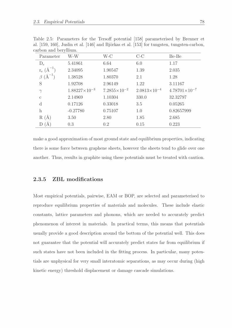
2.3. Empirical Potentials 78
Table 2.5: Parameters for the Tersoff potential [158] parameterised by Brenner etal. [159, 160], Juslin et al. [146] and Bjorkas et al. [153] for tungsten, tungsten-carbon,carbon and beryllium.
Parameter W-W W-C C-C Be-Be
De 5.41861 6.64 6.0 1.17
re (A−1) 2.34095 1.90547 1.39 2.035
β (A−1) 1.38528 1.80370 2.1 1.28
S 1.92708 2.96149 1.22 3.11167
γ 1.88227×10⁻³ 7.2855×10⁻² 2.0813×10⁻⁴ 4.78701×10⁻⁷
c 2.14969 1.10304 330.0 32.32797
d 0.17126 0.33018 3.5 0.05265
h -0.27780 0.75107 1.0 0.82657999
R (A) 3.50 2.80 1.85 2.685
D (A) 0.3 0.2 0.15 0.223
make a good approximation of most ground state and equilibrium properties, indicating
there is some force between graphene sheets, however the sheets tend to glide over one
another. Thus, results in graphite using these potentials must be treated with caution.
2.3.5 ZBL modifications
Most empirical potentials, pairwise, EAM or BOP, are selected and parameterised to
reproduce equilibrium properties of materials and molecules. These include elastic
constants, lattice parameters and phonons, which are needed to accurately predict
phenomenon of interest in materials. In practical terms, this means that potentials
usually provide a good description around the bottom of the potential well. This does
not guarantee that the potential will accurately predict states far from equilibrium if
such states have not been included in the fitting process. In particular, many poten-
tials are unphysical for very small interatomic separations, as may occur during (high
kinetic energy) threshold displacement or damage cascade simulations.

2.3. Empirical Potentials 79
This shortcoming is overcome using the Ziegler-Biersack-Littmark (ZBL) potential [110]
which models nuclear repulsion screened by electrons, and has the form:
ΦZBLij =
1
4πε0
ZiZje2
rijφ(rij/a) (2.39)
a =0.46850
Z0.23i + Z0.23
j
(2.40)
φ(x) = 0.18175e−3.19980x + 0.50986e−0.94229x
+0.28022e−0.40290x + 0.02817e−0.20162x
(2.41)
Where Zi and Zj are the atomic number of the two species, e the electron charge and ε0
the permativity of free space. This potential has the advantage that it is dependent only
on the atomic number of the atoms, and thus contains no fitted constants. The ZBL
potential replaces the pairwise component of an empirical potential at short interatomic
separations and is splined to the empirical potential with a switching function that
ensures there is no discontinuity in the second derivative of the overall potential form.
In the case of the bond order potential described above, the pairwise component is
modified with the ZBL potential using the function:
ΦVmod = ΦZBL(r)[1− F(r)] + ΦR(r)F(r) (2.42)
F(r) =1
1 + e−bf(r−rf)(2.43)
Bf and rf are empirical constants, in this case fit to create a smooth spline to DFT data
(which has been shown to accurately predict interatomic repulsion). The parameters
for the tungsten - carbon system are outlined in table 2.6.

2.4. Molecular Dynamics 80
Table 2.6: Parameters for the ZBL switching function for tungsten, tungsten-carbon,
carbon and beryllium [146, 153].
W-W W-C C-C Be-Be
rf (A) 1.3 1.2 0.6 0.8
bf (1/A) 12 7 8 7
2.4 Molecular Dynamics
Molecular Dynamics (MD) is a simulation technique in which the positions of atoms are
allowed to evolve over time, thereby allowing for the effective simulation of temperature.
The simulation proceeds as a series of discreet timesteps δt, with the evolution of each
atom’s acceleration, velocity and position between time t and t+δt calculated from
Newton’s equations of motion outlined in equation 2.44. The force, Fi is calculated
from the gradient of the potential energy surface ∇Φi as evaluated using empirical
potentials, or in the case of quantum-MD, DFT.
r(t) =Fi(r(t))
mi
=−∇Φi(r(t))
mi
(2.44)
Using these equations, the velocities and positions at t+δt are calculated using the
velocity verlet integration method [165, 166], which is computationally efficient, nu-
merically stable and conserves the overall energy of the system (providing a sensible
timestep is chosen). In this method, the second order equation of motion is split into
two first order differential equations, a = dvdt
and v = dxdt
which then undergo a taylor
expansion to give:
r(t+ δt) = r(t) + δtr(t) +δt2
2r(t) +Oδt3 (2.45)

2.4. Molecular Dynamics 81
v(t+ δt) = v(t) + δtv(t) +δt2
2v(t) +Oδt3 (2.46)
The second derivative of velocity v(t) is the only value that cannot be defined in terms
of known quantities, but it can be calculated through a taylor expansion of v(t), which
can then be substituted into the original equation to give:
r(t+ δt) = r(t) + δtv(t) +1
2δt2a(t) (2.47)
v(t+ δt) = v(t) +1
2δt [a(t) + a(t+ δt))] (2.48)
From these equations in conjunction with equation 2.44, the trajectory of atoms at
t+δt can be calculated from the atomic position, velocity and acceleration, whereby
equation 2.47 is first used to calculate the new positions, equation 2.48 to calculate
acceleration, and the force calculated as ΔΦi.
A key consideration when performing MD simulations is the length of the timestep δt.
Too long a timestep and the simulation may become unphysical, with atomic trajecto-
ries deviating significantly from those for an infinitesimaly small timestep. Particular
consideration of the timestep must be made when investigating energetic phenomenon
such as radiation damage, as deviation from the results of an infinitesimally small
timestep increases with increasing velocity and acceleration of the simulated atoms.
As such, it is desirable to use a much shorter timestep when performing such simula-
tions. There is however a strong pressure to maximise δt as computational intensity
increases linearly with decreasing timestep. Typically, for most systems simulated
around terrestrial temperatures (0 - 3000 K), it has been found that a timestep of 1 −4 fs is adequate to maintain the integrity of the simulation while minimising computa-
tional cost. This allows total simulation times on the order of 10−7 seconds, which is
still somewhat limited by comparison to many phenomena of interest.
2.4. Molecular Dynamics 82
An additional consideration for the practical implementation of MD is how to introduce
the concepts of temperature and pressure, which of course are important quantities for
a real experiment. To relate the atomic trajectories of an MD simulation to such macro-
scopic properties, statistical mechanics is applied through the use of a thermodynamic
ensemble. A themodynamical ensemble represents all possible states of a system that
have a set of common extrinsic properties. In MD simulations, unless accounting for
transmutation, it is implicit that the number of atoms, N, remains the same. Further,
if the volume, V, is fixed, and no energy, E, is artificially added or subtracted from the
system, then the state of the system at each timestep can be said to be a member of
the NVE micro canonical ensemble.
To calculate macroscopic properties, an ensemble average is taken, whereby an observ-
able value is averaged over all states of the system with a weighting factor in favour of
low energy states. This ensures that the bulk properties are averaged according to the
time spent in a given state. In practice, the states accessed in a MD simulation are
already effectively weighted according to the probability of being found in a particular
state, thus it is sufficient only to take an average of states sampled over a sufficient
number of timesteps.
In addition to the NVE ensemble, it may be useful to control temperature, T, and
pressure, P, as simulations often aim to mimic conditions of interest that occur at a
range of temperatures and pressures. This leads to the additional NPT (number, pres-
sure, temperature) and NVT (number, volume, temperature) ensembles. Temperature
is controlled using a thermostat, which scales the velocity of the simulated atoms to
maintain near constant temperature. Many thermostats use the concept of an external
heat bath to which the simulation is weakly coupled and thus energy can flow with
2.5. Inelastic Neutron Scattering 83
characteristic relaxation time, thereby gradually restoring the simulation to the desired
temperature. The relaxation time must be carefully selected to avoid resonant effects.
Similarly, a barostat scales the volume of the cell deterministically to maintain con-
stant pressure. Finally, similarly to static simulations, to simulate the bulk material,
periodic boundaries must be employed. In this work the Nose-Hoover thermostat and
barostat [167, 168, 169] and Berendsen barostat [170] are used in conjunction with the
NPT and NVT ensembles respectively for thermal equilibration of supercells. All MD
simulations in this work are implemented in the LAMMPS code [171].
2.5 Inelastic Neutron Scattering
Inelastic neutron scattering is a technique that can be used to probe the structure and
vibrational states of materials. Radiation can interact with matter either elastically,
where the total kinetic energy of the system is conserved, or inelastically where energy
is transferred. The latter includes many possible interactions, such as Compton scat-
tering (where energy is transferred from a photon to an electron), nuclear excitation
and phonon interactions. The latter of these simultaneously probes the structure and
dynamics of the material, and thus provides ample information for comparison with
theoretical results (e.g. from DFT).
When a monochromatic neutron beam with flux σi and wave vector ki is scattered
by a sample, it is useful to examine the differential cross-section and partial differential
cross-section relative to the total cross section, σT:
dσ
dΩ(2.49)

2.5. Inelastic Neutron Scattering 84
d2σ
dΩdEf
(2.50)
where σ is the scattered flux, Ω the angular area relative to the sample, and EF the
energy difference between the incident and scattered neutrons. These quantities are
related to the geometrical sample set-up in figure 2.9. The differential cross-section
probes only the change in momentum of the incident and scattered neutrons, which is
dominated by elastic scattering but includes inelastic contributions (although it cannot
provide information about the later). The partial differential cross-section provides
information about both momentum and energy changes and is therefore useful for
probing inelastic scattering. The partial differential cross-section can be integrated to
the differential cross-section which can be integrated to the total:
σT =
∫dσ
dΩdΩ =
∫d2σ
dΩdEf
dΩdEf (2.51)
Thus it is clear that the total cross section >> differential >> partial differential, with
the differential cross-section typically 106 times the partial. The partial differential
scattering cross-section is composed of two primary contributions, the neutron structure
factor S(Q,ω)and pair correlation function G(r,t):
d2σ
dΩdEf
= Nkfkib2S(Q, ω) (2.52)
S(Q, ω) =1
2πh
∫G(r, t)ei(Qr−ωt)drdt (2.53)
G(r, t) =1
2π
3 1
N
∫ ∑jj′
eiQr < e−iQrj′ (0)eiQrj(t) > dQ (2.54)
where k is the wavevector, b is an element/isotope dependent constant, Q is the scat-
tering vector, and ω is the frequency. This expression can further be split into contri-

2.5. Inelastic Neutron Scattering 85
1 20 3 4 5
Elastic Line
Quasielasticscattering
Lattice modes Intramolecularmodes
Comptonscattering
Magnetic scattering
log10(energy transfer/cm-1)
Figure 2.8: Typical neutron scattering mechanisms as a function of energy transferprobed using inelastic neutron scattering spectroscopy. Modified from [172].
butions from coherent (c) and incoherent scattering (i):
d2σ
dΩdEf
= σcSc(Q, ω) + σiSi(Q, ω) (2.55)
Coherent scattering measures the Fourier transform of the pair correlation function
(i.e. interference effects such as diffraction and phonons) while incoherent scattering
measures the Fourier transform of the self-correlation effect (i.e. single particle scat-
tering). The latter includes the vibrational density of states, which can be compared
to that simulated with DFT data. Typical scattering modes as a function of energy
transfer are shown in figure 2.8 below.
2.5.1 Experimental Setup
In this section a broad overview of the experimental setup is given. Details such as the
monochromator used and energy range scanned were changed during the experiment
in response to preliminary results, and thus are reported in detail in chapter 3.

2.5. Inelastic Neutron Scattering 86
For these experiments, the TAIPAN triple axis spectrometer based at the Australian
Nuclear Science and Technology Organisation (ANSTO) was used. A schematic of this
instrument is shown in figure 2.9. The OPAL reactor provided a source of thermal neu-
trons. Fast neutrons (around 2 MeV) are moderated through scattering interactions
with the D2O that is used to moderate neutrons to lower energies. When fully moder-
ated, the distribution of neutron energies can be considered a Maxwellian distribution
for the ambient temperature which is 300 K for the OPAL reactor. It is, however, likely
that the source will also include some fast and epithermal neutrons.
A thermal spectrum of neutrons is useful as the average energy (around 82 meV)
corresponds to a wavelength (0.2 nm) close to that of the lattice spacing for most crys-
talline solids, making them useful to probe structural information, for instance through
neutron diffraction. Most scattering techniques though, rely on having a monochro-
matic neutron source. This is achieved using a monochromator, which is usually a
single crystal of ultra pure beryllium, copper or graphite. When the thermal neutrons
interact with the single crystal, they are diffracted as per Braggs law:
nλ = 2d sin(θ) (2.56)
where n is the order of the reflection, d the interatomic spacing of the crystal and θ the
scattering angle. A strong single Bragg reflection is selected, for example for the (100)
planes, which produces a spectrum of diffracted monochromatic neutrons which can be
scanned over either by rotating the crystal, or in the case of the TAIPAN instrument,
the sample around the crystal. This produces a near monochromatic neutron beam,
the energy of which can be approximated as a Gaussian distribution with measured
full-width-half-maximum (FWHM). Given the uneven distribution of the thermal spec-
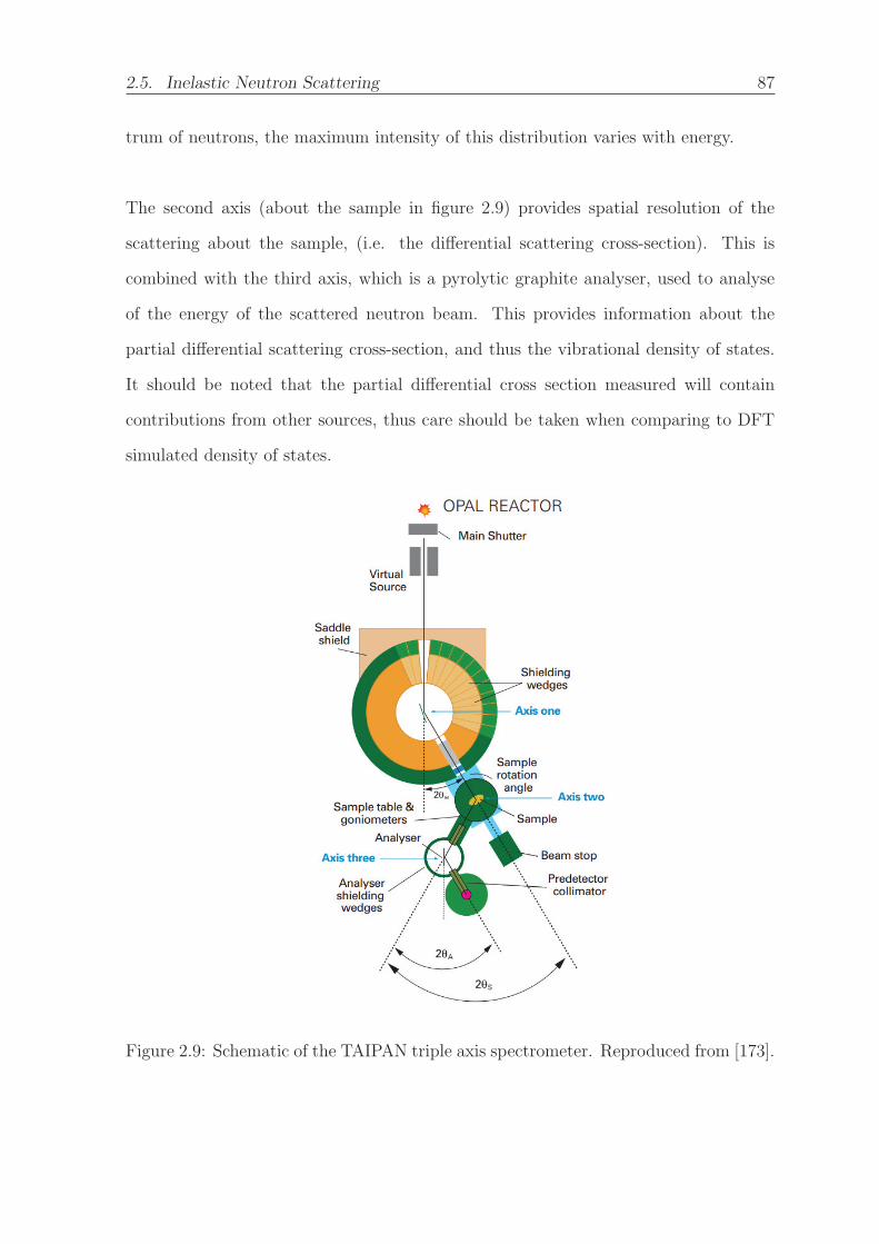
2.5. Inelastic Neutron Scattering 87
trum of neutrons, the maximum intensity of this distribution varies with energy.
The second axis (about the sample in figure 2.9) provides spatial resolution of the
scattering about the sample, (i.e. the differential scattering cross-section). This is
combined with the third axis, which is a pyrolytic graphite analyser, used to analyse
of the energy of the scattered neutron beam. This provides information about the
partial differential scattering cross-section, and thus the vibrational density of states.
It should be noted that the partial differential cross section measured will contain
contributions from other sources, thus care should be taken when comparing to DFT
simulated density of states.
Figure 2.9: Schematic of the TAIPAN triple axis spectrometer. Reproduced from [173].

Chapter 3
Structural Investigations of
Beryllides
This work is published in:
M. L. Jackson, P. A. Burr, R. W. Grimes “Resolving the Structure of TiBe12”, Acta
Crystallographica, 72, 277-280 (2016) [174]
3.1 Introduction
As explored in section 1.6, beryllium rich beryllides are candidates to replace beryllium
in the first wall and as neutron multipliers in future fusion reactors [56]. Before they
can be used in such applications however, their basic materials properties and irradi-
ation behaviour must be well understood and quantified. Due to the toxicity of these
materials [175], they have found few applications, and consequently few investigations
into their properties have been conducted.
88

3.2. Resolving the Structure of Be12Ti 89
Recently, Be12Ti and Be12V in particular have been investigated for fusion applica-
tions [176], with several experimental studies investigating basic properties such as
thermal conductivity [177], thermal expansivity [82] and yield strength [82], as well
as irradiation effects [93, 92, 178]. Despite this, significant work remains before they
can be qualified for these applications. Notably, and of significance to this work, there
remains some uncertainty regarding the crystal structure of Be12Ti. While the crystal
structures of other Be12M (where M is a transition metal) compounds are well de-
fined, to date there is some controversy as to whether Be12Ti exhibits a hexagonal or
tetragonal structure [179, 95, 180]. This is imperative to establish before proceeding
with computational studies, as the validity of the results of such studies are completely
predicated on the crystal structure assumed. As such, this is explored in section 3.2.
There is even less experimental data available for other Be12M and Be13M beryllides.
This poses an issues for computational investigations of these materials, as without
experimental data, the validation of such investigations is a challenge. Neutron scat-
tering data provides a particularly useful point of comparison for the validation of
computational models as it interrogates the vibrational states of the material, and by
extension the structure and energy landscape. It is highly desirable to be able to ac-
curately model both of these quantities. As such, in section 3.3, one Be13M sample
and five Be12M samples are investigated using inelastic neutron scattering, and results
compared to the simulated phonon density of states.
3.2 Resolving the Structure of Be12Ti
The crystal structure of Be12Ti was first identified by Raeuchle and Rundle in 1949
[181]. Samples were prepared by heating titanium with an excess of beryllium (1:15)
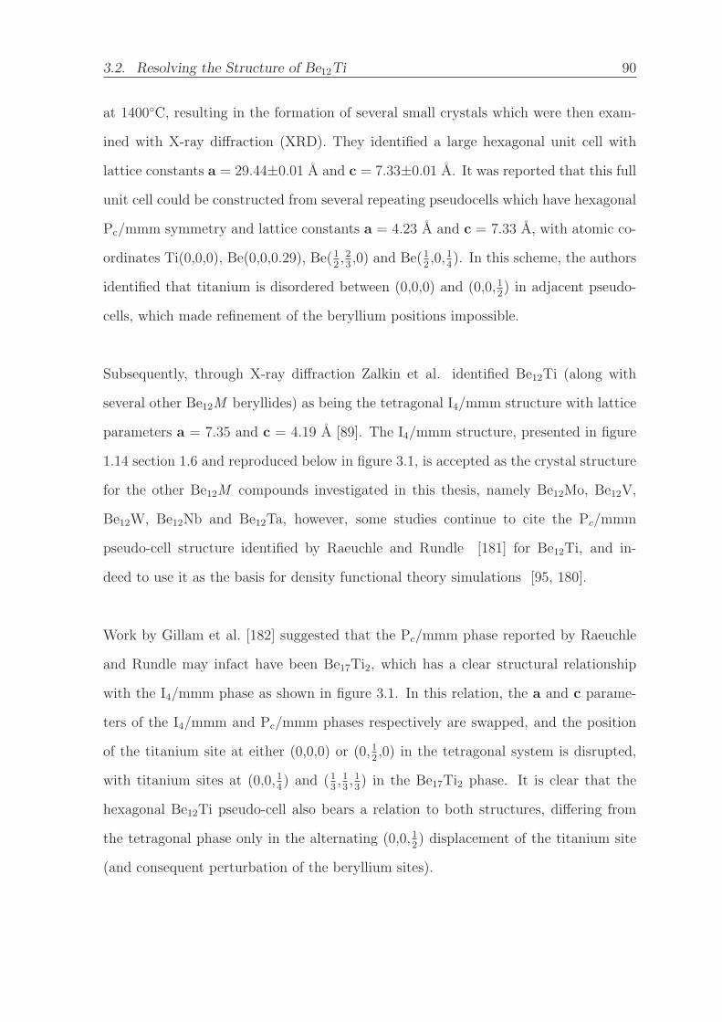
3.2. Resolving the Structure of Be12Ti 90
at 1400◦C, resulting in the formation of several small crystals which were then exam-
ined with X-ray diffraction (XRD). They identified a large hexagonal unit cell with
lattice constants a = 29.44±0.01 A and c = 7.33±0.01 A. It was reported that this full
unit cell could be constructed from several repeating pseudocells which have hexagonal
Pc/mmm symmetry and lattice constants a = 4.23 A and c = 7.33 A, with atomic co-
ordinates Ti(0,0,0), Be(0,0,0.29), Be(12,23,0) and Be(1
2,0,1
4). In this scheme, the authors
identified that titanium is disordered between (0,0,0) and (0,0,12) in adjacent pseudo-
cells, which made refinement of the beryllium positions impossible.
Subsequently, through X-ray diffraction Zalkin et al. identified Be12Ti (along with
several other Be12M beryllides) as being the tetragonal I4/mmm structure with lattice
parameters a = 7.35 and c = 4.19 A [89]. The I4/mmm structure, presented in figure
1.14 section 1.6 and reproduced below in figure 3.1, is accepted as the crystal structure
for the other Be12M compounds investigated in this thesis, namely Be12Mo, Be12V,
Be12W, Be12Nb and Be12Ta, however, some studies continue to cite the Pc/mmm
pseudo-cell structure identified by Raeuchle and Rundle [181] for Be12Ti, and in-
deed to use it as the basis for density functional theory simulations [95, 180].
Work by Gillam et al. [182] suggested that the Pc/mmm phase reported by Raeuchle
and Rundle may infact have been Be17Ti2, which has a clear structural relationship
with the I4/mmm phase as shown in figure 3.1. In this relation, the a and c parame-
ters of the I4/mmm and Pc/mmm phases respectively are swapped, and the position
of the titanium site at either (0,0,0) or (0,12,0) in the tetragonal system is disrupted,
with titanium sites at (0,0,14) and (1
3,13,13) in the Be17Ti2 phase. It is clear that the
hexagonal Be12Ti pseudo-cell also bears a relation to both structures, differing from
the tetragonal phase only in the alternating (0,0,12) displacement of the titanium site
(and consequent perturbation of the beryllium sites).

3.2. Resolving the Structure of Be12Ti 91
Be17Ti2 cellBe12Ti hexagonalpseudo-cell
Tetragonal Be12Tiunit cell
Ti (0,0,1)
Ti (0,0,1/2)
Be1
Be2
Be3
Figure 3.1: Left: unit cell of Be12Ti viewed in the [001] and [100] directions. Right:correspondence of Be12Ti hexagonal pseudocell and Be17Ti2 unit cell with tetragonalBe12Ti structure. To achieve Be17Ti2 stochiometry, titanium edge atoms in the Be17Ti2structure are duplicated at (0,0,1
4) and (0,0,3
4).
Despite the work of Gilliam et al. and Zalkin et al., various studies have continued
to reference the existence of the hexagonal Pc/mmm phase [95, 180]. While this may
not affect the key conclusions of experimental studies (given the close similarities of
the hexagonal and tetragonal phases), the validity of DFT simulations (like those per-
formed in this work) is completely predicated on the crystal structure. As such, it is
vital that this confusion be resolved before proceeding.
It is likely that the confusion between these phases has persisted due to their close
structural similarities and by extension, similar diffraction patterns. Simulated diffrac-
tion patterns from DFT data for the Pc/mmm Be12Ti, I4/mmm Be12Ti and Pc/mmm
Be17Ti2 structures, as well as pure Be, which is expected to be a common contaminant
in XRD samples, are presented in figure 3.2.
There is a strong correspondence between the diffraction patterns of the tetragonal cell

3.2. Resolving the Structure of Be12Ti 92
0 20 40 60 80
Be
Be17Ti2
Be12Ti (hex)
Be12Ti (tet)
2θ°
norm
alis
ed in
tens
ity
Figure 3.2: Simulated X-ray diffraction patterns of pure beryllium, Be17Ti2, hexagonalBe12Ti, and tetragonal Be12Ti. X-ray wavelength used corresponds to Cu K-alphasource (1.5406 A.
and hexagonal pseudo-cell, with all major peaks present in both materials occurring
at similar 2θ and with similar relative intensity. Some discrepancy does occur between
minor peaks, and notably large reflections at 24, 34, 42, and 51 2θ are split in the
tetragonal structure but not in the hexagonal structure. Interestingly there are broad
similarities between both Be12Ti patterns and Be17Ti2, although there are several dif-
ferences. In particular the peak at 18 2θ in both Be12Ti structures is not present in the
Be17Ti2 pattern. Nonetheless, it is clear that there is a strong correspondence between
the Be17Ti2 and Be12Ti structures. This lends credence to the assertion by Gillam et
al. that the work of Raeuchle and Rundle may have been performed on Be17Ti2 [182].
3.2.1 Density Functional Theory Simulations
To establish if the tetragonal phase is the stable phase at low temperature for Be12Ti
and can be used for further simulation study, DFT simulations of the tetragonal cell
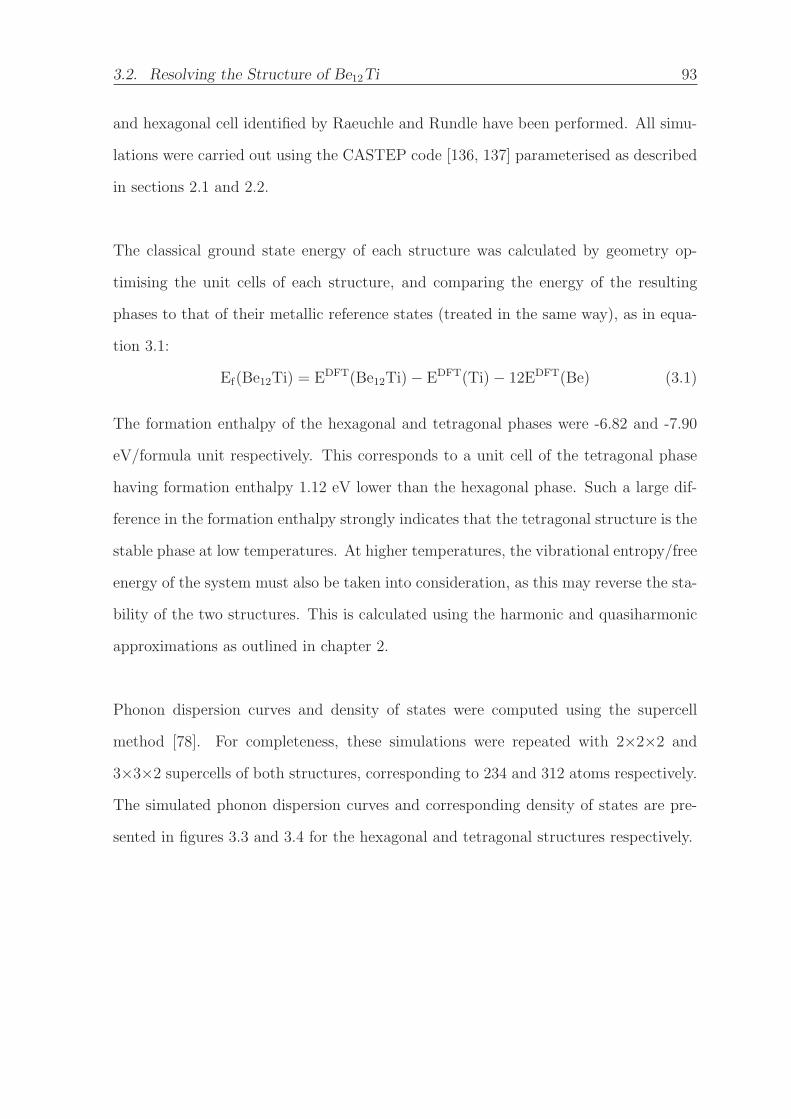
3.2. Resolving the Structure of Be12Ti 93
and hexagonal cell identified by Raeuchle and Rundle have been performed. All simu-
lations were carried out using the CASTEP code [136, 137] parameterised as described
in sections 2.1 and 2.2.
The classical ground state energy of each structure was calculated by geometry op-
timising the unit cells of each structure, and comparing the energy of the resulting
phases to that of their metallic reference states (treated in the same way), as in equa-
tion 3.1:
Ef(Be12Ti) = EDFT(Be12Ti)− EDFT(Ti)− 12EDFT(Be) (3.1)
The formation enthalpy of the hexagonal and tetragonal phases were -6.82 and -7.90
eV/formula unit respectively. This corresponds to a unit cell of the tetragonal phase
having formation enthalpy 1.12 eV lower than the hexagonal phase. Such a large dif-
ference in the formation enthalpy strongly indicates that the tetragonal structure is the
stable phase at low temperatures. At higher temperatures, the vibrational entropy/free
energy of the system must also be taken into consideration, as this may reverse the sta-
bility of the two structures. This is calculated using the harmonic and quasiharmonic
approximations as outlined in chapter 2.
Phonon dispersion curves and density of states were computed using the supercell
method [78]. For completeness, these simulations were repeated with 2×2×2 and
3×3×2 supercells of both structures, corresponding to 234 and 312 atoms respectively.
The simulated phonon dispersion curves and corresponding density of states are pre-
sented in figures 3.3 and 3.4 for the hexagonal and tetragonal structures respectively.

3.2. Resolving the Structure of Be12Ti 94
0
200
400
600
800
Γ K H A L M Γ
ω (c
m−1
)
0.00 0.05 0.10 0.15DOS (a.u.)
Figure 3.3: Simulated phonon band structure and density of states of hexagonal Be12Ti.
Image courtesy of P. Burr.
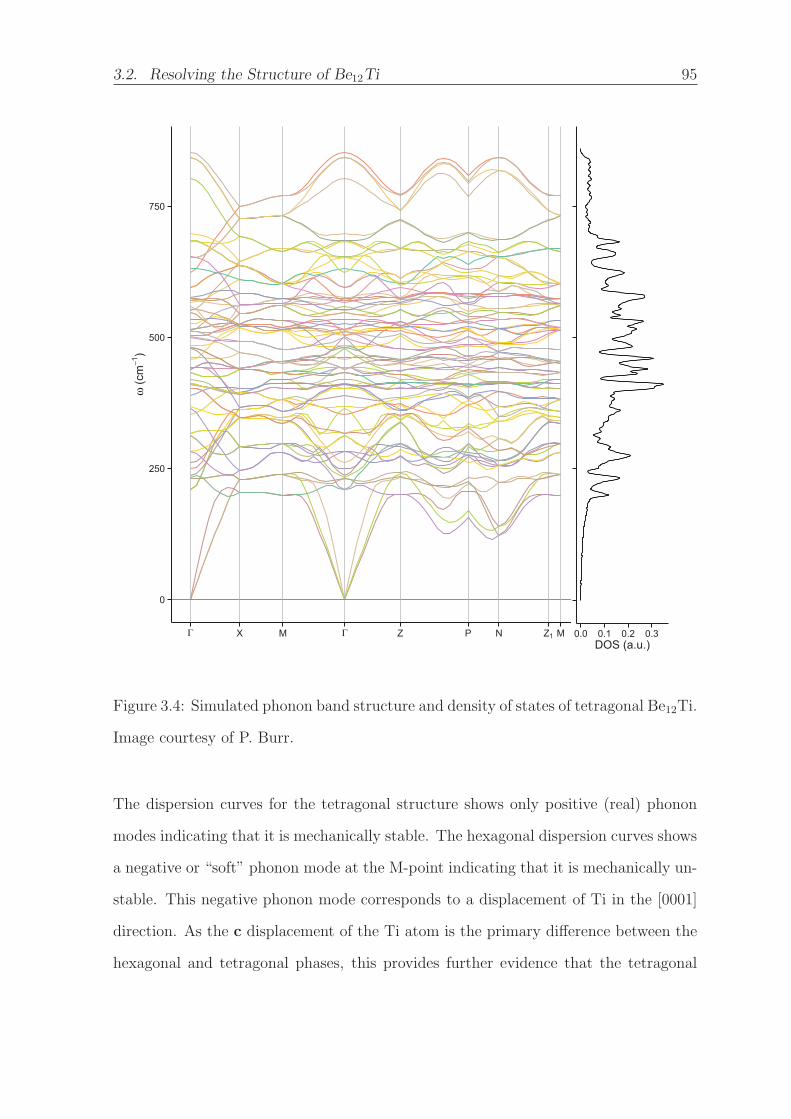
3.2. Resolving the Structure of Be12Ti 95
0
250
500
750
Γ X M Γ Z P N Z1 M
ω (c
m−1
)
0.0 0.1 0.2 0.3DOS (a.u.)
Figure 3.4: Simulated phonon band structure and density of states of tetragonal Be12Ti.
Image courtesy of P. Burr.
The dispersion curves for the tetragonal structure shows only positive (real) phonon
modes indicating that it is mechanically stable. The hexagonal dispersion curves shows
a negative or “soft” phonon mode at the M-point indicating that it is mechanically un-
stable. This negative phonon mode corresponds to a displacement of Ti in the [0001]
direction. As the c displacement of the Ti atom is the primary difference between the
hexagonal and tetragonal phases, this provides further evidence that the tetragonal
3.2. Resolving the Structure of Be12Ti 96
phase is more stable at temperatures of interest.
In addition, integration of the phonon DOS was used to calculate the zero-point energy
and constant volume vibrational contributions to the Helmholtz free energy (F). The
quasiharmonic approximation (as described in section 2.2.2) was applied to find the
same contributions, at constant pressure, to the Gibbs free energy. The Be12Ti struc-
ture is an ideal structure to perform this analysis on, as the vibrational contributions
to quantities such as heat capacity dominates below the Debye temperature, which
for pure beryllium is unusually high at 1440 K [183](only 110 K below the melting
temperature) owing to its high stiffness and low atomic mass. As Be12Ti is composed
of mostly beryllium, it is reasonable to assume that it will have a similarly high De-
bye temperature. Gibbs and Helmholtz free energies calculated for each structure are
shown in figure 3.5.
At temperatures up to 1550 K, which is the melting point of the pure Be reference state,
all calculations indicate the total energy of the tetragonal structure is approximately
6 eV per formula unit lower than the hexagonal structure, strongly indicating that
it is the equilibrium structure. Given that calculations based on both the harmonic
and quasiharmonic approximation, for all cell sizes, point to the same conclusion, this
provides strong evidence that the conclusion is robust.
3.2.2 Calculated Material Properties of Be12Ti
Having shown that the tetragonal phase is the equilibrium phase at relevant temper-
atures, the harmonic and quasiharmonic approximation are now used to predict some
fusion relevant materials properties of this phase. The thermal expansion and the bulk
modulus of the tetragonal phase were calculated by fitting the Birch-Murnaghan equa-
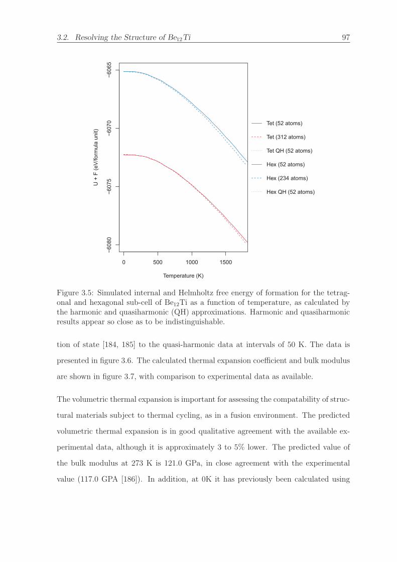
3.2. Resolving the Structure of Be12Ti 97
0 500 1000 1500
−608
0−6
075
−607
0−6
065
Temperature (K)
U +
F (e
V/fo
rmul
a un
it)
Tet (52 atoms)
Tet (312 atoms)
Tet QH (52 atoms)
Hex (52 atoms)
Hex (234 atoms)
Hex QH (52 atoms)
Figure 3.5: Simulated internal and Helmholtz free energy of formation for the tetrag-onal and hexagonal sub-cell of Be12Ti as a function of temperature, as calculated bythe harmonic and quasiharmonic (QH) approximations. Harmonic and quasiharmonicresults appear so close as to be indistinguishable.
tion of state [184, 185] to the quasi-harmonic data at intervals of 50 K. The data is
presented in figure 3.6. The calculated thermal expansion coefficient and bulk modulus
are shown in figure 3.7, with comparison to experimental data as available.
The volumetric thermal expansion is important for assessing the compatability of struc-
tural materials subject to thermal cycling, as in a fusion environment. The predicted
volumetric thermal expansion is in good qualitative agreement with the available ex-
perimental data, although it is approximately 3 to 5% lower. The predicted value of
the bulk modulus at 273 K is 121.0 GPa, in close agreement with the experimental
value (117.0 GPA [186]). In addition, at 0K it has previously been calculated using
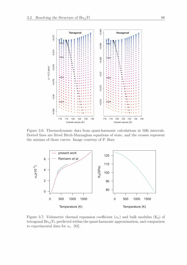
3.2. Resolving the Structure of Be12Ti 98
110 115 120 125 130 135Unitcell volume (A3)
U +
F(T
) (ke
V)
6.08
26.
086.
078
6.07
66.
074
6.07
2
0K
500K
1000K
1500K
2000K
Tetragonal
110 115 120 125 130 135 140Unitcell volume (A3)
6.07
46.
072
6.07
6.06
86.
066
6.06
4
0K
500K
1000K
1500K
2000K
Hexagonal
Figure 3.6: Thermodynamic data from quasi-harmonic calculations at 50K intervals.Dotted lines are fitted Birch-Murnaghan equations of state, and the crosses representthe minima of those curves. Image courtesy of P. Burr.
0 500 1000 1500
0
2
4
6
Temperature (K)
α v(x
10−5
)
present work
Reimann et al.
0 500 1000 1500
80
90
100
110
120
Temperature (K)
K 0(G
Pa)
Figure 3.7: Volumetric thermal expansion coefficient (αv) and bulk modulus (K0) oftetragonal Be12Ti, predicted within the quasi-harmonic approximation, and comparisonto experimental data for αv [82].

3.3. Inelastic Neutron Scattering in Beryllides 99
DFT to be 120.5 GPa (3 GPa less than the predicted value), although this data was
produced assuming the (incorrect) hexagonal pseudo-cell [95].
Further predicted properties, including elastic constants and lattice parameters are
reported in table 3.1. Comparing the room temperature quasiharmonic and experi-
mental lattice parameters, the quasiharmonic approximation overpredicts both the c
and a parameters by around 2% which is typical of DFT simulations with the PBE
exchange functional [187].
Table 3.1: Simulated lattice parameters and elastic data of tetragonal Be12Ti withcomparison to experimental data. For the ground state simulations, shear (G) andbulk (K) moduli were obtained from the stiffness constants (cij) using the Hill averagingmethod [188].
aA
cA
c11(GPa)
c12(GPa)
c13(GPa)
c33(GPa)
c44(GPa)
c66(GPa)
K(Gpa)
DFT 7.359 4.164 371.80 14.60 31.60 323.30 124.8 112.8 135.72DFT QH(T=0K)
7.446 4.216 - - - - - - 123.6
DFT QH(T=300K)
7.457 4.223 - - - - - - 121.4
exp.(T=298K)
7.35a 4.19a - - - - - - 117.0b
a [89] b [186]
3.3 Inelastic Neutron Scattering in Beryllides
In addition to Be12Ti, Be12V is another candidate material that has been explored for
fusion applications [82], while other Be12M and Be13M structures (i.e. Be12W and
Be13Zr) have been considered based on their beryllium content [56]. Until recently,
many of these compounds have not had any practical applications, thus there is a lack
of availible experimental data. Further, owing to the low atomic mass of beryllium, ex-
perimental techniques relying on charge density, (e.g. XRD and electron microscopy),

3.3. Inelastic Neutron Scattering in Beryllides 100
may be less effective in these materials. Conversely, inelastic neutron scattering is
ideally suited to these materials, and can probe information both about the crystal
structure and dynamic response of the lattice [183]. This makes it a good point of
comparison for both DFT simulations and future experimental studies.
As such, following theoretical investigation of the Be12Ti structure, further investi-
gations of other beryllides were undertaken for comparison with experimental neutron
scattering data, in order to further validate the DFT model.
3.3.1 Theoretical Investigations
Six structures were investigated: Be12Ti, Be12Nb, Be12V, Be12Mo, Be12Ta, and Be13Zr.
All of the Be12M compounds are isostructural with the Be12Ti tetragonal phase, while
Be13Zr has a complex cubic structure of Fm3c(226) symmetry [189] containing 8 for-
mula units, as presented in figure 3.8. The structure contains one unique Zr site at
(14, 14, 14) and two Be sites at (0,0,0) and (0, 0.112, 0.178). Geometry optimisation of
all structures was performed through DFT simulations in order to predict basic prop-
erties such as lattice parameters, which are compared to experimental values in table
3.2. Predicted values of the lattice parameters correspond closely to the experimental
data, typically underestimating values by 1−2%. Special positions of the Be sites in
the Be12M structure also compare favourably to experimental data where available.
In order to gain more detailed information about the vibrational states of these mate-
rials for comparison with inelastic neutron scattering data, finite displacement calcula-
tions with the supercell method were used to calculate phonon DOS. 2×2×2 supercells
were used for the Be12M structures. The choice of this supercell size is further vali-
dated by the close agreement of data calculated using the 52 and 312 atom cell shown
in figure 3.5 for Be12Ti. On this basis, for the Be13Zr structure, which has 108 atoms

3.3. Inelastic Neutron Scattering in Beryllides 101
Tab
le3.2:
Experim
entalan
dpredictedlatticeproperties
ofBeryllides.
property
Be 1
2V
Be 1
2Ti
Be 1
2Ta
Be 1
2Nb
Be 1
2Mo
Be 1
3Zr
Exp.
DFT
Exp.
DFT
Exp.
DFT
Exp.
DFT
Exp.
DFT
Exp.
DFT
a( A
)7.266a
7.278b
7.240
7.35
c7.361
7.334b
7.329e
7.309
7.376b
7.372e
7.328
7.251d
7.271b
7.239
10.05f
10.04g
9.996
c( A
)4.194a
4.212b
4.169
4.19
c4.163
4.267b
4.256e
4.203
4.258b
4.256e
4.203
4.232d
4.234b
4.221
10.05f
10.04g
9.996
V(A
3)
221.4a
223.1b
218.5
226.4c
225.6
229.5b
228.6e
224.6
231.7b
231.3e
225.7
222.5d
223.8b
221.2
1014
f
1013
g
998.8
x,Be2
0.361a
0.349
-0.350
-0.352
-0.352
0.351b
0.350
n/a
n/a
x,Be3
0.277a
0.288
-0.281
-0.283
-0.283
0.281b
0.289
n/a
n/a
a[190]b[88]
c[89]
d[191]e[123]f[189]g[192]
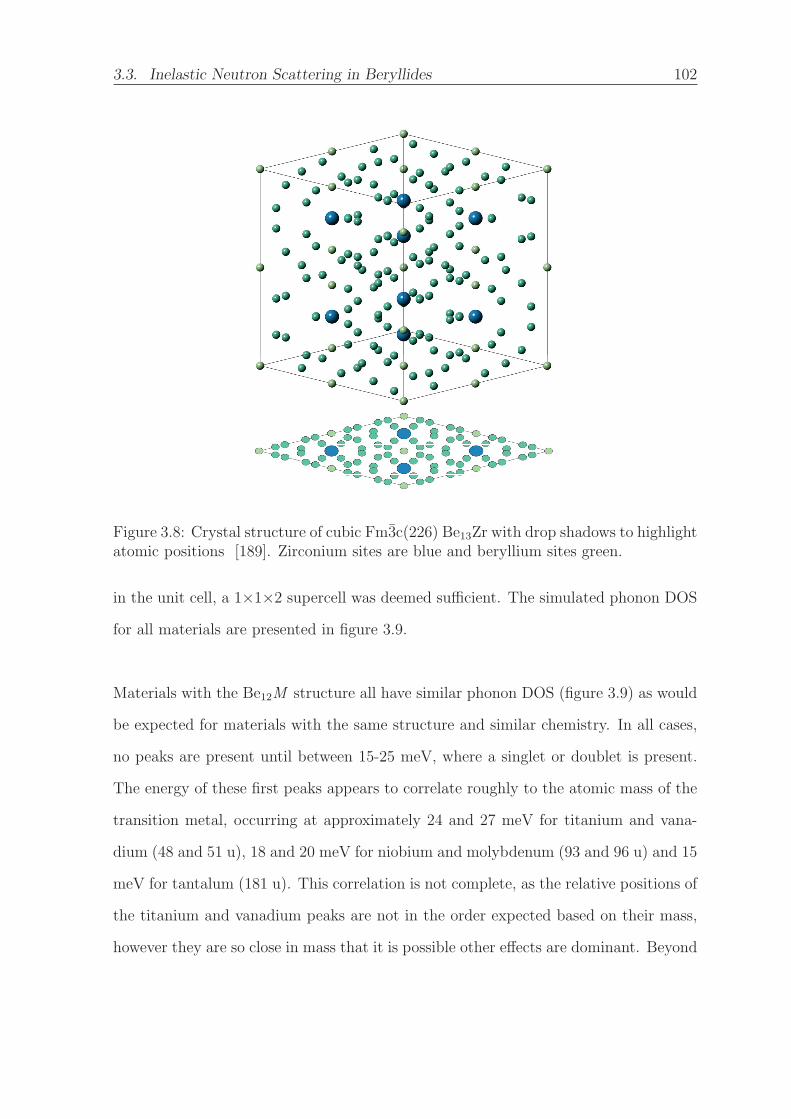
3.3. Inelastic Neutron Scattering in Beryllides 102
Figure 3.8: Crystal structure of cubic Fm3c(226) Be13Zr with drop shadows to highlightatomic positions [189]. Zirconium sites are blue and beryllium sites green.
in the unit cell, a 1×1×2 supercell was deemed sufficient. The simulated phonon DOS
for all materials are presented in figure 3.9.
Materials with the Be12M structure all have similar phonon DOS (figure 3.9) as would
be expected for materials with the same structure and similar chemistry. In all cases,
no peaks are present until between 15-25 meV, where a singlet or doublet is present.
The energy of these first peaks appears to correlate roughly to the atomic mass of the
transition metal, occurring at approximately 24 and 27 meV for titanium and vana-
dium (48 and 51 u), 18 and 20 meV for niobium and molybdenum (93 and 96 u) and 15
meV for tantalum (181 u). This correlation is not complete, as the relative positions of
the titanium and vanadium peaks are not in the order expected based on their mass,
however they are so close in mass that it is possible other effects are dominant. Beyond

3.3. Inelastic Neutron Scattering in Beryllides 103
these first peaks, these materials show other broad similarities in profile, although these
are difficult to quantify. The lowest energy phonon peaks in Be13Zr conform with the
described trend in atomic mass (zirconium 91 u), with a doublet occurring at around
22 meV. However, the DOS also contains two high intensity peaks at 79 and 91 meV,
contrary to the Be12M structures.
3.3.2 Neutron Scattering
As mentioned previously, neutron scattering data can provide useful information about
the elastic properties and structure of a material. In addition, it can lead to useful
validation of DFT data. Thus, having calculated the phonon density of states for these
materials, inelastic neutron scattering data is presented for comparison.
Samples
Six samples weighing approximately 5g were provided by C. Dorn of Materion Brush
Inc., the details of which are presented in table 3.3. Samples were prepared through
single stage synthesis in an induction furnace (i.e. elemental powders have been blended
and consolidated before being melted to form the compounds). The samples were
consolidated without a binder and heated to 1400◦C in a BeO crucible for a minimum
of one hour. Preliminary characterisation of the samples was carried out using XRD.
Unfortunately this was hampered significantly by the form of the samples, some of
which were too large to fit in the sample holder. Smaller samples could not be made
due to the lack of appropriate facilities to process the beryllium containing samples
(given that the dust poses an inhalation hazard). As such, it was not possible to polish
the samples to achieve a flat surface, nor break the samples to an appropriate size to
fit in the XRD instrument. Consequently, XRD analysis could not be performed on

3.3. Inelastic Neutron Scattering in Beryllides 104
0.0
0.2
0.4
0.6
0.8
1.0
Be12Ti
0.0
0.2
0.4
0.6
0.8
1.0
Be12V
0.0
0.2
0.4
0.6
0.8
1.0
Be12Nb
0.0
0.2
0.4
0.6
0.8
1.0
Be12Mo
0.0
0.2
0.4
0.6
0.8
1.0
Be12Ta
0 20 40 60 80 100
0.0
0.2
0.4
0.6
0.8
1.0
Be13Zr
energy (meV)
norm
alis
ed in
tens
ity
Figure 3.9: Simulated phonon density of states for beryllide samples, normalised tohighest intensity peak.

3.3. Inelastic Neutron Scattering in Beryllides 105
Be12Nb and Be12Mo samples. This was particularly problematic for the Be12Mo sample,
as it contained a large component of a second phase, which may have originated from
the BeO crucible in which it was synthesised, however without XRD analysis this could
not be verified.
Table 3.3: Samples investigated by neutron scattering with mass and preliminary char-acterisation technique.
Sample Weight (g) XRD
Be12Ti 4.57 Yes
Be12V 4.71 Yes
Be12Mo 4.76 No
Be12Ta 5.33 Yes
Be12Nb 6.19 No
Be13Zr 5.20 Yes
XRD analysis of the samples (where possible) were consistent with the stated com-
positions and structures. In all cases, small secondary XRD patterns were observed
which appear to be BeO, as would be expected owing to oxidisation of sample surfaces
and preparation in BeO crucibles. The Be13Zr sample also showed peaks attributed to
pure Be, suggesting it was synthesised with excess beryllium, and thus zirconium rich
Be17Zr2 was not present. It should be noted that the absence of beryllium peaks in
other samples does not preclude its existence as a second phase, as pure beryllium is
almost entirely X-ray transparent (and indeed is used as an X-ray window [64]) and
thus would not be expected to produce a strong signal.
Experimental Details
Experimental results were gathered using the TAIPAN triple-axis neutron spectrome-
ter, the general set-up of which is outlined in section 2.5. Two monochromators were
considered, a graphite (002) monochromator with energy range 6-70 meV, and a cop-
per monochromator with range 14-100 meV. Preliminary investigations showed the
3.3. Inelastic Neutron Scattering in Beryllides 106
graphite option to be more suitable as the 6-70 meV range contains ample information
about the phonon response of these materials. In particular, the 6-20 meV range was
found to include second order scattering contributions which, after further analysis,
proved to be useful (see subsection 3.3.3). In addition, given that this technique is in-
tensity limited and by extension time consuming, given the limited beam-time, it was
decided that the lengthy commissioning process of the copper monochromator would
have too greatly restricted the time over which experiments could be performed.
The graphite monochromator was used with continuous vertical and horizontal fo-
cusing, a sapphire high energy filter and no collimators (to increase signal). Samples
were mounted in a custom rectangular aluminium frame, and held in place with alu-
minium foil (see figure 3.10). This set-up was shown not to contribute significantly
to the background counts, has very low activation in the neutron beam and simplified
working with the beryllide samples (through hazard reduction) by fully encapsulating
them. To further reduce scatter from the sample holder, a mask of cadmium (which is
a strong neutron absorber) was applied. The setup of the sample and sample holder is
shown in figure 3.10.
Initial data collection was performed at 2 K with a cryofurnace, and 286 K without,
as presented for Be12Ti in figure 3.11. Comparison of the two data sets shows that
there is no tangible benefit from using the cryofurnace, with no increase in resolution
but a decrease in signal. Given that use of the cryofurnace significantly increased the
duration of the experiments, due to the time required for samples to reach temperature,
its use was discontinued in subsequent runs.
Data was collected over the full available energy range (8-70 meV) in increments of
0.2 meV with a collection time of 50 s. As the experiment proceeded, it became clear
that analysis of second order scattering in the 8-20 meV range could provide increased

3.3. Inelastic Neutron Scattering in Beryllides 107
Figure 3.10: Left: sample in holder. Sample is secured in an aluminium frame withaluminium foil, and frame shielded with cadmium. Right: sample setup within theTAIPAN instrument.
10 20 30 40 50 60 70
10000
15000
20000
25000
30000
energy (meV)
mon
itor c
ount
s
2 K295 K
Figure 3.11: Data collected at 2 K with the cryofurnace setup and at 295 K.
3.3. Inelastic Neutron Scattering in Beryllides 108
energy resolution and signal to noise ratio, which are degraded as a consequence of
broadening effects at higher energies. As such, scans were repeated in this region with
a step size of 0.1 meV and collection time of 100s (where possible).
3.3.3 Data and Analysis
Figure 3.12 shows the final collected data, normalised by monitor counts and by max-
imum intensity. It is clear there are significant differences between the experimental
data and the theoretical data (presented in figure 3.9). The experimental data shows no
sharp peaks, which are predicted in the theoretical data, instead appearing as broad
humps with what appears to be noise superimposed. Secondly, the intensity of the
experimental data appears to increase with increasing incident energy. Thirdly, the
sharpest peaks in the experimental data appear below 20 meV, where no peaks are
predicted in the DFT simulations.
In analysing these differences, it is necessary to deconvolute experimental effects from
the true phonon DOS. Firstly, the effect of instrument broadening must be taken into
consideration. There are two known experimental sources of broadening. The incident
neutron beam is not entirely monochromatic, rather it can be described as a Gaussian
distribution with Full-Width-Half-Maximum (FWHM) of 1.1 meV. This is independent
of the energy, E. Another source of broadening is associated with the monochromator,
which causes energy dependent broadening. This was characterised for the Taipan
instrument [173] using the Raytracing modelling of Stampfl and Bertinshaw [193] who
derived equation 3.2 to describe the broadening effect.
FWHM = 1.59× 10⁻⁷E4 − 3.57× 10⁻⁵E3 + 3.24× 10⁻³E2 + 1.53× 10⁻²E (3.2)
Based on this equation, the broadening is expected to increase from a minimum FWHM
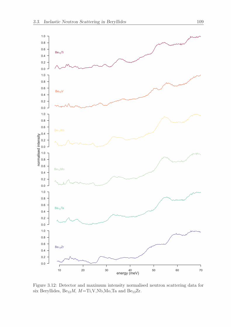
3.3. Inelastic Neutron Scattering in Beryllides 109
0.0
0.2
0.4
0.6
0.8
1.0
Be12Ti
0.0
0.2
0.4
0.6
0.8
1.0
Be12V
0.0
0.2
0.4
0.6
0.8
1.0
Be12Nb
0.0
0.2
0.4
0.6
0.8
1.0
Be12Mo
0.0
0.2
0.4
0.6
0.8
1.0
Be12Ta
10 20 30 40 50 60 70
0.0
0.2
0.4
0.6
0.8
1.0
Be13Zr
energy (meV)
norm
alis
ed in
tens
ity
Figure 3.12: Detector and maximum intensity normalised neutron scattering data forsix Beryllides, Be12M, M=Ti,V,Nb,Mo,Ta and Be13Zr.
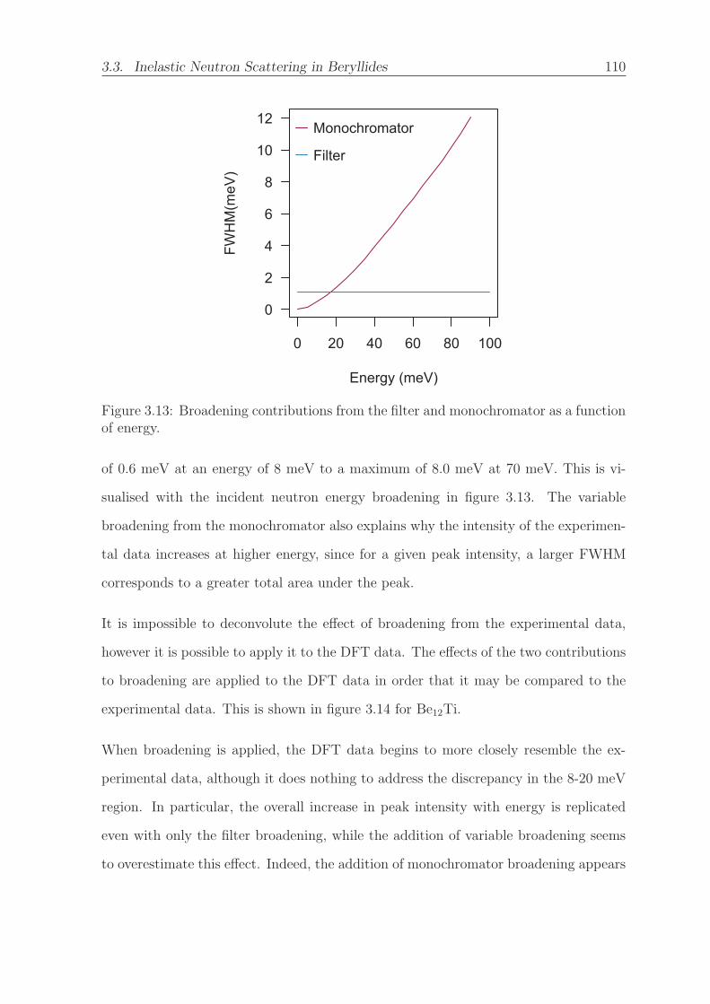
3.3. Inelastic Neutron Scattering in Beryllides 110
0 20 40 60 80 100
0
2
4
6
8
10
12
Energy (meV)
FWH
M(m
eV)
Monochromator
Filter
Figure 3.13: Broadening contributions from the filter and monochromator as a functionof energy.
of 0.6 meV at an energy of 8 meV to a maximum of 8.0 meV at 70 meV. This is vi-
sualised with the incident neutron energy broadening in figure 3.13. The variable
broadening from the monochromator also explains why the intensity of the experimen-
tal data increases at higher energy, since for a given peak intensity, a larger FWHM
corresponds to a greater total area under the peak.
It is impossible to deconvolute the effect of broadening from the experimental data,
however it is possible to apply it to the DFT data. The effects of the two contributions
to broadening are applied to the DFT data in order that it may be compared to the
experimental data. This is shown in figure 3.14 for Be12Ti.
When broadening is applied, the DFT data begins to more closely resemble the ex-
perimental data, although it does nothing to address the discrepancy in the 8-20 meV
region. In particular, the overall increase in peak intensity with energy is replicated
even with only the filter broadening, while the addition of variable broadening seems
to overestimate this effect. Indeed, the addition of monochromator broadening appears
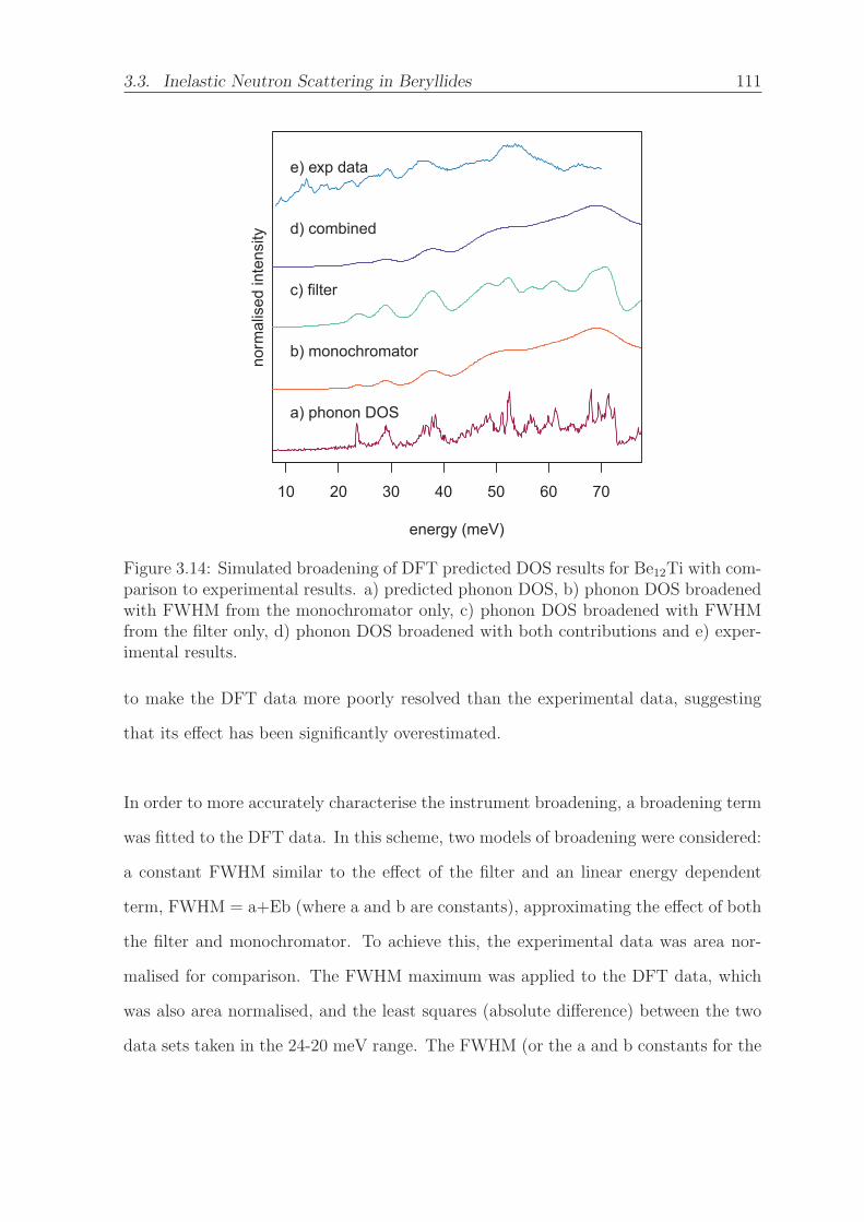
3.3. Inelastic Neutron Scattering in Beryllides 111
10 20 30 40 50 60 70
energy (meV)
b) monochromator
c) filter
d) combined
a) phonon DOS
e) exp data
norm
alis
ed in
tens
ity
Figure 3.14: Simulated broadening of DFT predicted DOS results for Be12Ti with com-parison to experimental results. a) predicted phonon DOS, b) phonon DOS broadenedwith FWHM from the monochromator only, c) phonon DOS broadened with FWHMfrom the filter only, d) phonon DOS broadened with both contributions and e) exper-imental results.
to make the DFT data more poorly resolved than the experimental data, suggesting
that its effect has been significantly overestimated.
In order to more accurately characterise the instrument broadening, a broadening term
was fitted to the DFT data. In this scheme, two models of broadening were considered:
a constant FWHM similar to the effect of the filter and an linear energy dependent
term, FWHM = a+Eb (where a and b are constants), approximating the effect of both
the filter and monochromator. To achieve this, the experimental data was area nor-
malised for comparison. The FWHM maximum was applied to the DFT data, which
was also area normalised, and the least squares (absolute difference) between the two
data sets taken in the 24-20 meV range. The FWHM (or the a and b constants for the

3.3. Inelastic Neutron Scattering in Beryllides 112
energy dependent model) was then iteratively altered to minimise the sum of the least
squares. While this approach did effectively minimise the absolute difference between
the DFT and experimental data, in all cases it to resulted in significant over-broadening
of the DFT data, and thus is not useful for further analysis. This does, however, sug-
gest that there are other reasons for the differences between the DFT and experimental
data apart from the instrument broadening.
The broadening effect does not explain the presence of peaks in the 8-20 meV range
in the experimental data, which are not predicted in the DFT data. This puzzle can
be resolved by noticing that the reflections in this region bear striking similarity to
the spectrum in the 32-80 meV region, compressed by a factor of 4 in the energy axis.
This suggests the low energy peaks may be attributed to the effects of second and third
order scattering, 4 and 9 times reduced from the energy of the fundamental modes. To
examine this possibility, figure 3.15 shows second and third order reflections of the DFT
predicted spectrum, as well as the experimental spectrum. For further confirmation,
enhanced resolution experimental data in the 8-20 meV range has been extrapolated
to the 32-80 meV, the range corresponding to the fundamental assuming that the 8-20
meV range is the second order reflection (see left hand side of figure 3.15).
Figure 3.15 shows that the third order reflection of the DFT and experimental data
is only significant below 10 meV and thus can be discounted from further analysis.
Further, peaks in the experimental data in the 8-20 meV range correspond very closely
with the fundamental reflections in the 32-80 meV range, compressed in the energy
axis by a factor of 4. Thus, the hypothesis that the experimental peaks below 20 meV
are a consequence of second order rather than first or third order reflections is consis-
tent with experiment, and helps explain the apparent discrepancy between DFT and
experimental data. Further, it appears that much better energy resolution is achieved
in the second order reflection in comparison to the first order reflection (presumably

3.3. Inelastic Neutron Scattering in Beryllides 113
0 10 20 30 40 50 60 70
norm
alis
ed in
tens
ity
energy (meV)
fundamentalextrapolated, CNextrapolated, OCN
0 10 20 30 40 50 60 70
norm
alis
ed in
tens
ity
energy (meV)
fundamental2nd harmonic3rd harmonic
Figure 3.15: Left: experimental neutron scattering data, with data in the 8-24 meVregion (assumed to be second order reflections) extrapolated and normalised by monitorcounts (CN) and originating monitor counts (OCN). Right: simulated phonon densityof states with simulated higher order reflections.
due to the much smaller contribution from monochromator broadening).
To modify DFT data to include the second order reflection, it must be scaled in line
with the experimental data. The magnitude of this scaling, however, is difficult to
establish. The simplest option is to scale by the average intensity of the second order
experimental data (8-18 meV) relative to the first order reflection (32-72 meV), which
suggests that the second order reflection would have a constant scaling factor of 0.66
relative to the fundamental.
When extrapolating second order experimental data to generate a second data set,
it is unclear whether to scale the data by the monitor counts in the 8−20 meV re-
gion, or, assuming the data is primarily the result of higher order reflections, from
the originating monitor counts (in the 32−80 meV region). In either case the data is
qualitatively very similar with all major peaks present in both data sets.

3.3. Inelastic Neutron Scattering in Beryllides 114
3.3.4 Comparison
Having examined the causes of discrepancy between DFT and experimental data, a
comparison can now be made. Presented in figures 3.16 and 3.17 is experimental data
(count and intensity normalised) and the normalised simulated phonon DOS for all
samples. Given the increased resolution of second order reflections in the experimental
data, the extrapolated second order data (originating count normalised and intensity
normalised) is also presented, as are second order reflections from the phonon DOS
(scaled by a factor of 0.66).
For all materials, it appears that the enhanced second order reflection is less broadened
and consequently has better energy resolution than the fundamental. Further there is a
strong correspondence between the extrapolated 8-20 meV data and the fundamental,
again consistent with the former being primarily composed of contributions from the
second order terms.
Given the better energy resolution of the extrapolated second order experimental data,
it is perhaps the best point of comparison for the DFT data. It can be seen that broadly,
there is a strong correspondence between the shape of the two data sets. Many peaks
do, however, seem significantly shifted between the experimental and DFT data, for
example the Be12Nb DFT peak at 37 meV appears at around 35 eV in the experimental
data. This underlines that DFT phonon DOS is a prediction and may not perfectly
reflect the real material. In particular, the phonon DOS is determined both by the
crystal structure and the energy landscape about the equilibrium atomic positions.
From table 3.2, DFT simulations typically under predict lattice parameters by 1−2%,
which would similarly shift peak positions in the phonon DOS.
While the general shape of the experimental data corroborates the DFT data, the
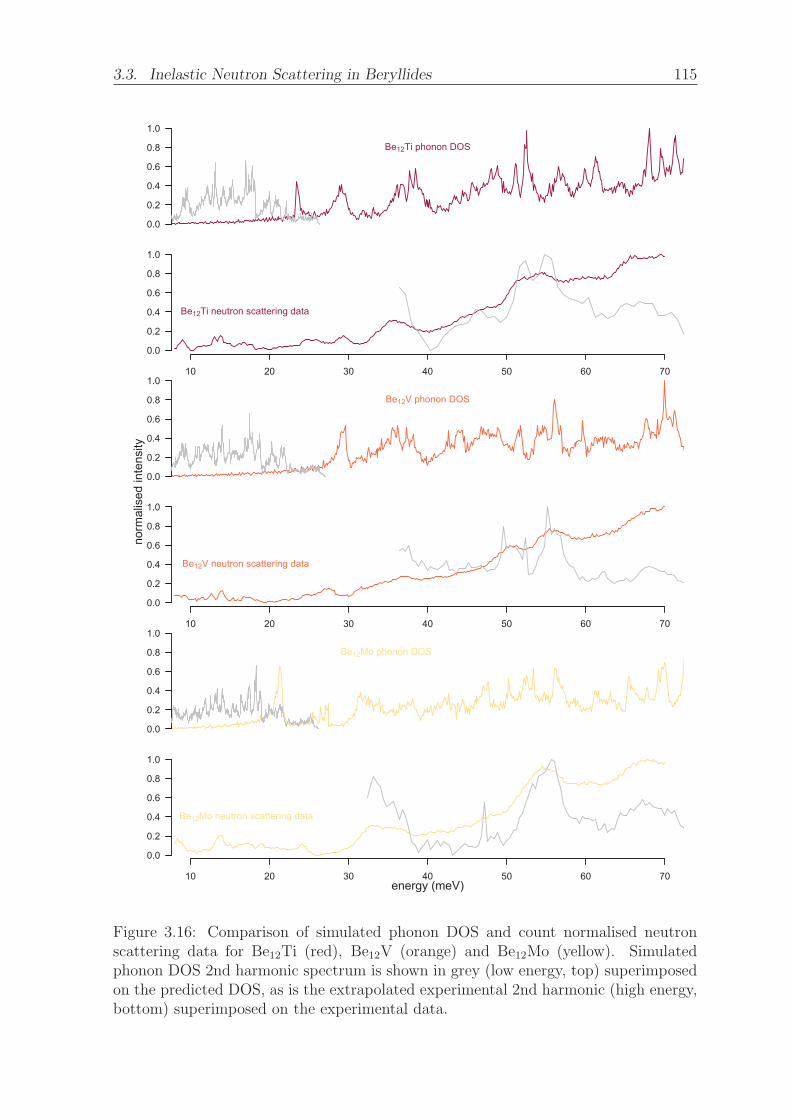
3.3. Inelastic Neutron Scattering in Beryllides 115
0.0
0.2
0.4
0.6
0.8
1.0
Be12Ti phonon DOS
10 20 30 40 50 60 70
0.0
0.2
0.4
0.6
0.8
1.0
Be12Ti neutron scattering data
0.0
0.2
0.4
0.6
0.8
1.0
Be12V phonon DOS
10 20 30 40 50 60 70
0.0
0.2
0.4
0.6
0.8
1.0
Be12V neutron scattering data
0.0
0.2
0.4
0.6
0.8
1.0
Be12Mo phonon DOS
10 20 30 40 50 60 70
0.0
0.2
0.4
0.6
0.8
1.0
Be12Mo neutron scattering data
energy (meV)
norm
alis
ed in
tens
ity
Figure 3.16: Comparison of simulated phonon DOS and count normalised neutronscattering data for Be12Ti (red), Be12V (orange) and Be12Mo (yellow). Simulatedphonon DOS 2nd harmonic spectrum is shown in grey (low energy, top) superimposedon the predicted DOS, as is the extrapolated experimental 2nd harmonic (high energy,bottom) superimposed on the experimental data.

3.3. Inelastic Neutron Scattering in Beryllides 116
0.0
0.2
0.4
0.6
0.8
1.0
Be12Nb phonon DOS
10 20 30 40 50 60 70
0.0
0.2
0.4
0.6
0.8
1.0
Be12Nb neutron scattering data
0.0
0.2
0.4
0.6
0.8
1.0
Be12Ta phonon DOS
10 20 30 40 50 60 70
0.0
0.2
0.4
0.6
0.8
1.0
Be12Ta neutron scattering data
0.0
0.2
0.4
0.6
0.8
1.0
Be13Zr phonon DOS
10 20 30 40 50 60 70
0.0
0.2
0.4
0.6
0.8
1.0
Be13Zr neutron scattering data
energy (meV)
norm
alis
ed in
tens
ity
Figure 3.17: Comparison of simulated phonon DOS and count normalised neutronscattering data for Be12Nb (light green), Be12Ta (dark green) and Be13Zr (purple).Simulated phonon DOS 2nd harmonic spectrum is shown in grey (low energy, top)superimposed on the predicted DOS, as is the extrapolated experimental 2nd harmonic(high energy, bottom) superimposed on the experimental data.
3.4. Summary and Conclusions 117
experimental data is so broadened that it is difficult to make conclusions beyond this.
In particular, the reasons for the shifting of certain peaks between the two data sets
cannot be identified with certainty. As such, while the experimental data can be quali-
tatively used to qualify the DFT data, meaningful quantitative comparison is difficult.
3.4 Summary and Conclusions
The crystal structure of Be12Ti has been confirmed as exhibiting the tetragonal/
I4/mmm symmetry rather than hexagonal/Pc/mmm symmetry at low temperature us-
ing the harmonic and quasiharmonic approximations. Further, given the large energy
difference between the two phases over all temperatures investigated, this conclusion is
also likely to hold true at elevated temperatures. The source of confusion between the
two phases is explained through the close relation of the phases, as well as the pres-
ence of the hexagonal Be17Ti2 phase, which shows strong similarities in the simulated
diffraction pattern. Some basic fusion relevant properties of Be12Ti have also been pre-
dicted as a function of temperature, including the bulk modulus, thermal expansivity
and heat capacity.
Phonon density of states have been simulated for Be12Ti, Be12V, Be12Ta, Be12Nb and
Be13Zr using DFT, and compared to inelastic neutron scattering data. It was found
that performing scattering experiments at room temperature was sufficient, without
the use of a cryo furnace. Broadening of the neutron scattering data occurred from two
sources; the filter and monochromator, although the latter proved to be less significant
than suggested by prior modelling [193]. Nonetheless, the data is so broadened that
direct quantative comparison to the DFT data is difficult. It was found that enhanced
energy resolution could be achieved by examining the second order reflections of the

3.5. Contributions 118
experimental data. These are at lower energy than the fundamental and thus were less
broadened, and, given the absence of peaks in the <20 meV DFT data can be easily
deconvoluted from the fundamental reflection.
Qualitative comparison between DFT and experimental data shows good agreement,
with the broadened DFT data having similar shape and peak positions to the experi-
mental data. Some peaks do, however, appear shifted by up to 3 meV between the two.
This may be explained as an artefact of the broadening inherent in the experimental
data, or due to differences in the energy surface or lattice parameters predicted by
DFT simulation, the latter of which may differ from experimental values by up to 2%.
3.5 Contributions
Inelastic neutron scattering experiments were performed using the TAIPAN facility
as part of the TAIPAN grant 5338. The experiments and analysis were conducted in
collaberation with P. A. Burr, A. P. J. Stampfl and E.G. Obbard. Analysis of QH
simulations in Be12Ti was also conducted in conjunction with P. A. Burr. Beryllide
samples were provided by C. K. Dorn of Materion Brush. Preliminary sample char-
acterisations were performed using facilities provided by the University of New South
Wales. Computing resources were provided by Imperial College London high perfor-
mance computing service.
Chapter 4
Defects in Be12M Beryllides
This work is published in:
M. L. Jackson, P. A. Burr, R. W. Grimes “Defect processes in Be12X (X = Ti, Mo, V,
W)”, Nuclear Fusion, 57, 8 (2017) [194]
4.1 Introduction
As discussed in chapters 1 and 3, the Be12M beryllides have been suggested for use as
neutron multipliers and first wall materials in future fusion reactors [56]. Indeed it
is expected that one of the TBM designs tested in Iter will use Be12Ti [195]. Having
investigated the basic properties of a wide range of beryllides in chapter 3, the focus
here is on the four most likely for use as neutron multipliers, as identified by Yamada
et al [56]. These are Be12Ti, Be12V, Be12Mo and Be12W. Of these, Be12V and Be12Ti
have been identified as leading candidates as they have better neutronic properties
than Be12Mo and Be12W. While Be12Ti and Be12V have very similar fusion relevant
thermo-physical properties, Be12Ti is significantly easier to fabricate [196], and thus is
considered most likely for fusion applications.
119
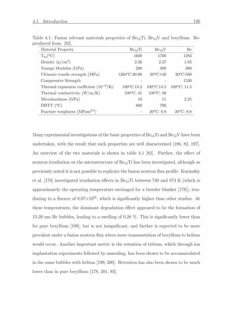
4.1. Introduction 120
Table 4.1: Fusion relevant materials properties of Be12Ti, Be12V and beryllium. Re-produced from [82].
Material Property Be12Ti Be12V Be
Tm(oC) 1600 1700 1283
Density (g/cm3) 2.26 2.37 1.85
Youngs Modulus (GPa) 280 300 300
Ultimate tensile strength (MPa) 1260oC:30-90 20oC:140 20oC:580
Compressive Strength - - 1530
Thermal expansion coefficient (10−6/K) 100oC:13.2 100oC:14.5 100oC: 11.5
Thermal conductivity (W/m/K) 100oC: 41 100oC: 38
Microhardness (GPa) 10 11 2.25
DBTT (oC) 860 790 -
Fracture toughness (MPam0.5) - 20oC: 0.8 20oC: 9.8
Many experimental investigations of the basic properties of Be12Ti and Be12V have been
undertaken, with the result that such properties are well characterised [186, 82, 197].
An overview of the two materials is shown in table 4.1 [82]. Further, the effect of
neutron irradiation on the microstructure of Be12Ti has been investigated, although as
previously noted it is not possible to replicate the fusion neutron flux profile. Kurinskiy
et al. [178] investigated irradiation effects in Be12Ti between 740 and 873 K (which is
approximately the operating temperature envisaged for a breeder blanket [178]), irra-
diating to a fluence of 8.07×1025, which is significantly higher than other studies. At
these temperatures, the dominant degradation effect appeared to be the formation of
15-20 nm He bubbles, leading to a swelling of 0.28 %. This is significantly lower than
for pure beryllium [198], but is not insignificant, and further is expected to be more
prevalent under a fusion neutron flux where more transmutation of beryllium to helium
would occur. Another important metric is the retention of tritium, which through ion
implantation experiments followed by annealing, has been shown to be accommodated
in the same bubbles with helium [199, 200]. Retention has also been shown to be much
lower than in pure beryllium [178, 201, 93].

4.2. Point Defects 121
It is important to understand the formation of helium and tritium bubbles in Be12Ti,
given they are the source of swelling and tritium retention. It is likely that bubbles
would be nucleated from smaller defects such as vacancies and vacancy clusters, thus to
understand their formation it is necessary to investigate the point defect chemistry of
the material. Surprisingly, no investigations of the intrinsic defect chemistry in Be12Ti
have been undertaken, although the accommodation of hydrogen at interstitial sites
has been investigated using DFT simulations by Fujii et al [91], who found six stable
interstitial sites with solution energies between 0.11 and 1.06 eV.
Allouche et al [96] investigated hydrogen accommodation in isostructural Be12W, and,
in addition to investigating accommodation interstitially also investigated accommo-
dation in Be vacancies. Vacancy formation energies for the Be1, Be2, Be3 and W sites
were calculated to be 1.38, 1.14, 1.48 and 3.25 eV respectively. It was also found that,
as for pure Be [79], several hydrogen atoms can be accommodated in a single vacancy.
Beyond vacancy formation energies of Be12W, no investigation of the intrinsic defect
chemistry of any of the Be12M compounds has been made previously, despite an un-
derstanding of defect behaviour being so important for understanding the mechanisms
dictating the radiation response of these materials. As such, this section presents a
thorough investigation of point defects and small clusters in Be12Ti, Be12V, Be12Mo
and Be12W.
4.2 Point Defects
During a radiation damage cascade in a material, two types of defect disorder may be
formed: Frenkel disorder, where an atom is displaced from its lattice site to form a
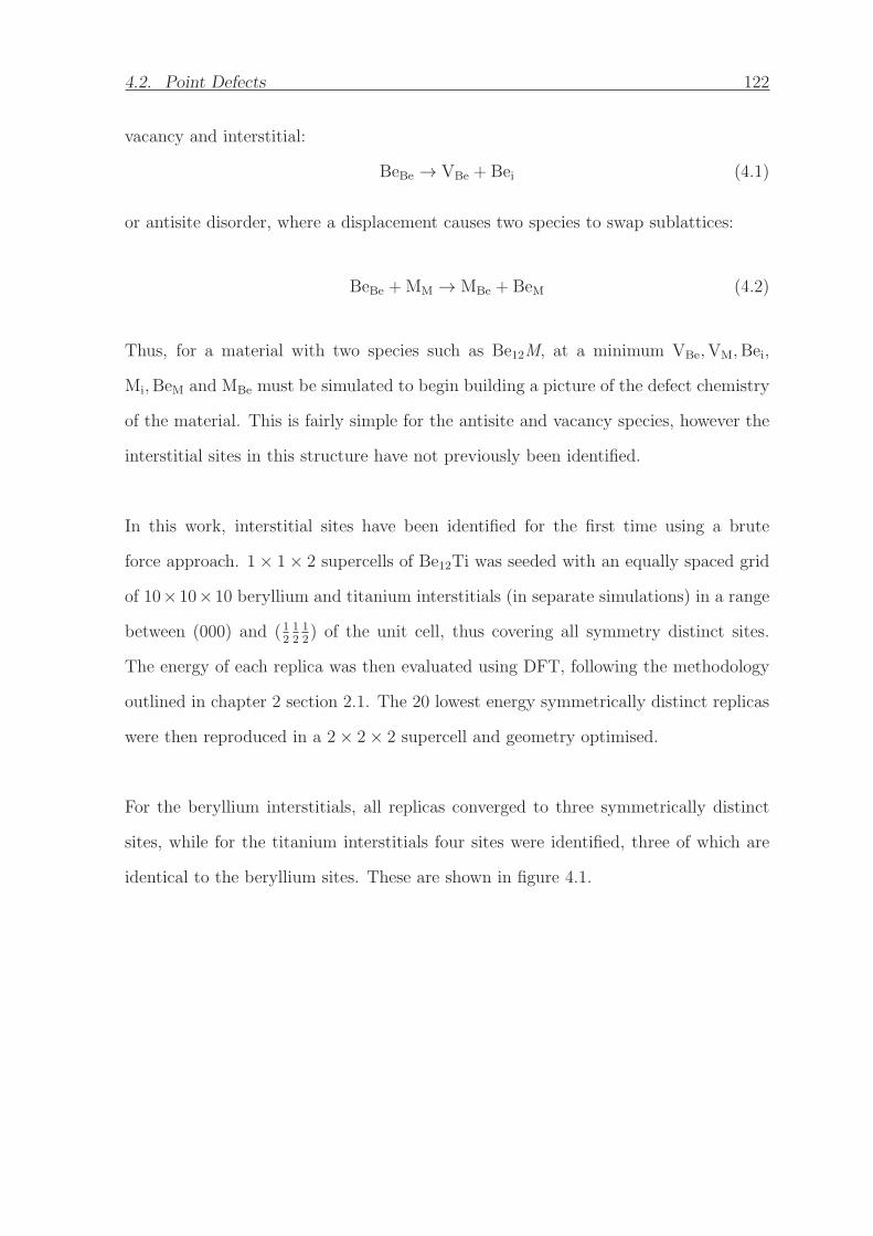
4.2. Point Defects 122
vacancy and interstitial:
BeBe → VBe + Bei (4.1)
or antisite disorder, where a displacement causes two species to swap sublattices:
BeBe +MM → MBe + BeM (4.2)
Thus, for a material with two species such as Be12M, at a minimum VBe,VM,Bei,
Mi,BeM and MBe must be simulated to begin building a picture of the defect chemistry
of the material. This is fairly simple for the antisite and vacancy species, however the
interstitial sites in this structure have not previously been identified.
In this work, interstitial sites have been identified for the first time using a brute
force approach. 1× 1× 2 supercells of Be12Ti was seeded with an equally spaced grid
of 10×10×10 beryllium and titanium interstitials (in separate simulations) in a range
between (000) and (121212) of the unit cell, thus covering all symmetry distinct sites.
The energy of each replica was then evaluated using DFT, following the methodology
outlined in chapter 2 section 2.1. The 20 lowest energy symmetrically distinct replicas
were then reproduced in a 2× 2× 2 supercell and geometry optimised.
For the beryllium interstitials, all replicas converged to three symmetrically distinct
sites, while for the titanium interstitials four sites were identified, three of which are
identical to the beryllium sites. These are shown in figure 4.1.
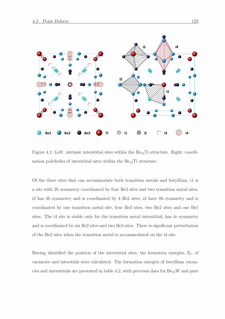
4.2. Point Defects 123
Figure 4.1: Left: intrinsic interstitial sites within the Be12Ti structure. Right: coordi-
nation polyhedra of interstitial sites within the Be12Ti structure.
Of the three sites that can accommodate both transition metals and beryllium, i1 is
a site with 2b symmetry coordinated by four Be3 sites and two transition metal sites,
i2 has 4b symmetry and is coordinated by 4 Be2 sites, i3 have 8h symmetry and is
coordinated by one transition metal site, four Be3 sites, two Be2 sites and one Be1
sites. The i4 site is stable only for the transition metal interstitial, has 4c symmetry
and is coordinated by six Be2 sites and two Be3 sites. There is significant perturbation
of the Be2 sites when the transition metal is accommodated on the i4 site.
Having identified the position of the interstitial sites, the formation energies, Ef , of
vacancies and interstials were calculated. The formation energies of beryllium vacan-
cies and interstitials are presented in table 4.2, with previous data for Be12W and pure
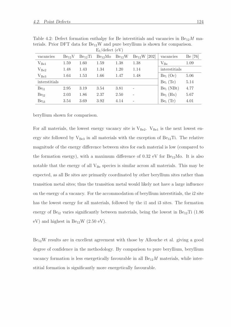
4.2. Point Defects 124
Table 4.2: Defect formation enthalpy for Be interstitials and vacancies in Be12M ma-terials. Prior DFT data for Be12W and pure beryllium is shown for comparison.
Ef/defect (eV)
vacancies Be12V Be12Ti Be12Mo Be12W Be12W [202] vacancies Be [76]
VBe1 1.59 1.60 1.59 1.38 1.38 VBe 1.09
VBe2 1.48 1.43 1.34 1.20 1.14 interstitials
VBe3 1.64 1.53 1.66 1.47 1.48 Bei (Oc) 5.06
interstitials Bei (Te) 5.14
Bei1 2.95 3.19 3.54 3.81 - Bei (NBt) 4.77
Bei2 2.03 1.86 2.37 2.50 - Bei (Hx) 5.67
Bei3 3.54 3.69 3.92 4.14 - Bei (Tr) 4.01
beryllium shown for comparison.
For all materials, the lowest energy vacancy site is VBe2. VBe1 is the next lowest en-
ergy site followed by VBe3 in all materials with the exception of Be12Ti. The relative
magnitude of the energy difference between sites for each material is low (compared to
the formation energy), with a maximum difference of 0.32 eV for Be12Mo. It is also
notable that the energy of all VBe species is similar across all materials. This may be
expected, as all Be sites are primarily coordinated by other beryllium sites rather than
transition metal sites; thus the transition metal would likely not have a large influence
on the energy of a vacancy. For the accommodation of beryllium interstitials, the i2 site
has the lowest energy for all materials, followed by the i1 and i3 sites. The formation
energy of Bei2 varies significantly between materials, being the lowest in Be12Ti (1.86
eV) and highest in Be12W (2.50 eV).
Be12W results are in excellent agreement with those by Allouche et al. giving a good
degree of confidence in the methodology. By comparison to pure beryllium, beryllium
vacancy formation is less energetically favourable in all Be12M materials, while inter-
stitial formation is significantly more energetically favourable.

4.2. Point Defects 125
Table 4.3: Defect formation enthalpies of transition metal vacancies and interstitialsin Be12M compounds. DFT data from previous studies is shown for Be12W for com-parison.
Ef/defect (eV)
Defect Be12V Be12Ti Be12Mo Be12W Be12W [202]
vacancies
VM 3.37 4.10 3.61 3.16 3.25
interstitials
Mi1 4.81 5.37 7.26 8.11 -
Mi2 4.79 5.10 5.60 6.48 -
Mi3 5.59 7.47 8.80 10.11 -
Mi4 4.69 4.19 4.84 5.95 -
The formation energies of transition metal vacancies and interstitials are shown in
table 4.3. The energy of formation for VM is lowest in Be12W (3.16 eV) and highest in
Be12Ti (4.10 eV). The lowest energy interstitial site for all materials is the i4 site, with
interstitial energies ranging from 4.19 eV in Be12Ti to 5.95 eV in Be12W. There is a
noticeable difference in the transition metal interstitial energy between Be12V/Ti and
Be12Mo/W, with it being significantly higher for the latter two materials for all sites.
Antisite formation energies are shown in table 4.4. Accommodation of beryllium on
a transition metal site has a high, relatively consistent formation energy of 2.76-3.55
eV for all materials. This is likely due to the large size mismatch between Be and the
transition metal species. The Be2 sites provide the lowest energy to accommodate a
transition metal for all materials, with formation enthalpy of 0.99 and 0.95 eV for VBe2
and TiBe2 respectively, although it is significantly higher for MoBe2 (1.56 eV) and in
particular WBe2 (3.81 eV). The Be2 site is the only site which is coordinated with only
one transition metal site, rather than two as for the Be1 and Be3 sites, which is likely
the reason for the lower formation energy.

4.3. Defect disorder processes 126
Table 4.4: Formation energies of antisite defects in Be12M compounds.
Ef/defect (eV)
defect Be12V Be12Ti Be12Mo Be12W
BeM 2.83 3.55 3.09 2.76
MBe1 3.10 3.26 4.13 4.43
MBe2 0.99 0.95 1.56 3.81
MBe3 1.79 2.50 3.40 3.81
4.3 Defect disorder processes
As mentioned, when a material is exposed to radiation, defects are formed through
radiation damage processes, namely Frenkel and Antisite disorder. As such, it is im-
portant to evaluate the overall energy of the defect process rather than only the isolated
defect. In addition, at elevated temperatures (such as may be experienced during fab-
rication) an equilibrium concentration of defects will exist dependent on the energy of
these defect processes. In addition to Frenkel and antisite disorder, Schottky disorder
will also contribute to the defect population under such circumstances. In this process,
vacancies are formed in a stoichiometric ratio:
12BeBe +MM → 12VBe +VM + Be12M (4.3)
It should be noted however that exact stochiometry is only entirely enforced in ionic
materials due to the need for charge balancing, and as such some other combinations
of defects may be formed in metallic Be12M causing the material to deviate from
stoichiometry (which will be examined in section 4.5). The energy per defect for defect
disorder processes are shown in table 4.5. An energy range is produced for each process
due to the range of formation energies for defects on different Be and interstitial sites.
At equilibrium the lowest energy defect process are the most likely to occur. This is not
the case, however, for radiation damage processes which are decidedly not equilibrium
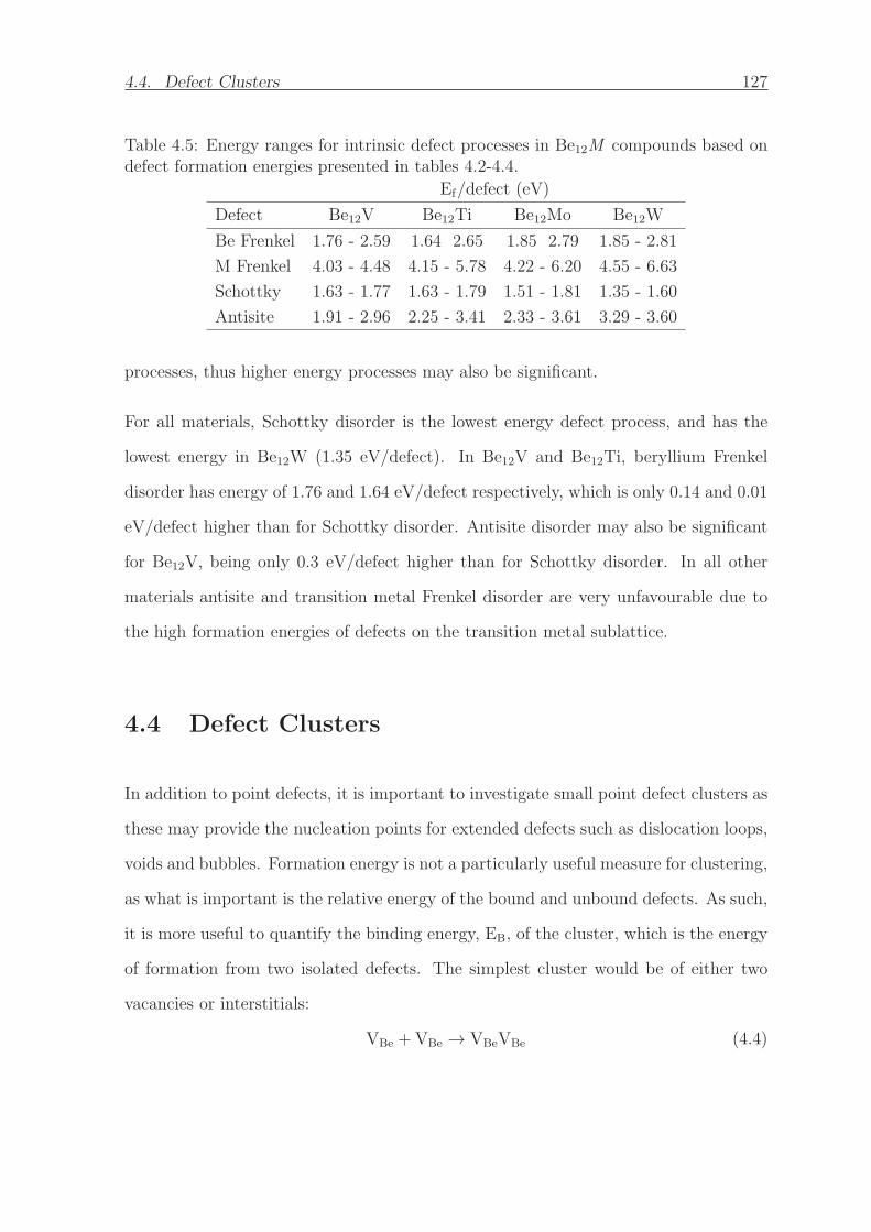
4.4. Defect Clusters 127
Table 4.5: Energy ranges for intrinsic defect processes in Be12M compounds based ondefect formation energies presented in tables 4.2-4.4.
Ef/defect (eV)
Defect Be12V Be12Ti Be12Mo Be12W
Be Frenkel 1.76 - 2.59 1.64 2.65 1.85 2.79 1.85 - 2.81
M Frenkel 4.03 - 4.48 4.15 - 5.78 4.22 - 6.20 4.55 - 6.63
Schottky 1.63 - 1.77 1.63 - 1.79 1.51 - 1.81 1.35 - 1.60
Antisite 1.91 - 2.96 2.25 - 3.41 2.33 - 3.61 3.29 - 3.60
processes, thus higher energy processes may also be significant.
For all materials, Schottky disorder is the lowest energy defect process, and has the
lowest energy in Be12W (1.35 eV/defect). In Be12V and Be12Ti, beryllium Frenkel
disorder has energy of 1.76 and 1.64 eV/defect respectively, which is only 0.14 and 0.01
eV/defect higher than for Schottky disorder. Antisite disorder may also be significant
for Be12V, being only 0.3 eV/defect higher than for Schottky disorder. In all other
materials antisite and transition metal Frenkel disorder are very unfavourable due to
the high formation energies of defects on the transition metal sublattice.
4.4 Defect Clusters
In addition to point defects, it is important to investigate small point defect clusters as
these may provide the nucleation points for extended defects such as dislocation loops,
voids and bubbles. Formation energy is not a particularly useful measure for clustering,
as what is important is the relative energy of the bound and unbound defects. As such,
it is more useful to quantify the binding energy, EB, of the cluster, which is the energy
of formation from two isolated defects. The simplest cluster would be of either two
vacancies or interstitials:
VBe +VBe → VBeVBe (4.4)

4.4. Defect Clusters 128
Bei + Bei → BeiBei (4.5)
Given that this structure has three beryllium sites, one metal site and four interstitial
sites however, there are many different possible configurations of these defects, which
may have significantly different formation enthalpies. Binding energies are calculated
with respect to the lowest formation energy defects of that type (e.g. for a divacancy
VBe2). The binding energy of all symmetrically distinct nearest neighbour vacancy
clusters, including VBeVBe, VBeVM and VMVM are shown in table 4.6.
For all materials, some orientations of VBeVBe clusters have negative binding energy,
suggesting formation of these clusters is favourable from the isolated vacancies. In par-
ticular, the VBe2VBe2 divacancy orientated out of the (001) plane is the most favourable
for all materials, with binding energy from -0.21 in Be12V to -0.02 eV in Be12W. Fur-
ther, in Be12V there are several other favourable clusters, while in the other materials
no other VBeVBe cluster is favourable, although some only have very small positive
binding energies.
All VMVM clusters are strongly unfavourable, with binding energies in excess of 0.50
eV. This is likely due to the large size of the transition metal species, which would cause
the formation of a divacancy to create large localised strains. Several VMVBe clusters
have negative binding energy and, notably, VMVBe2 has strongly negative binding en-
ergy in all materials, ranging from -0.54 to -0.19 eV in Be12V and Be12W respectively.
Given that there are several favourable vacancy clusters, these may form nucleation
points for voids and bubbles, although more work is needed to confirm this. It is also
possible that the introduction of radiogenic hydrogen and helium may stabilise some
vacancy clusters that have slight positive binding energy, although again further work
would be needed to confirm this.
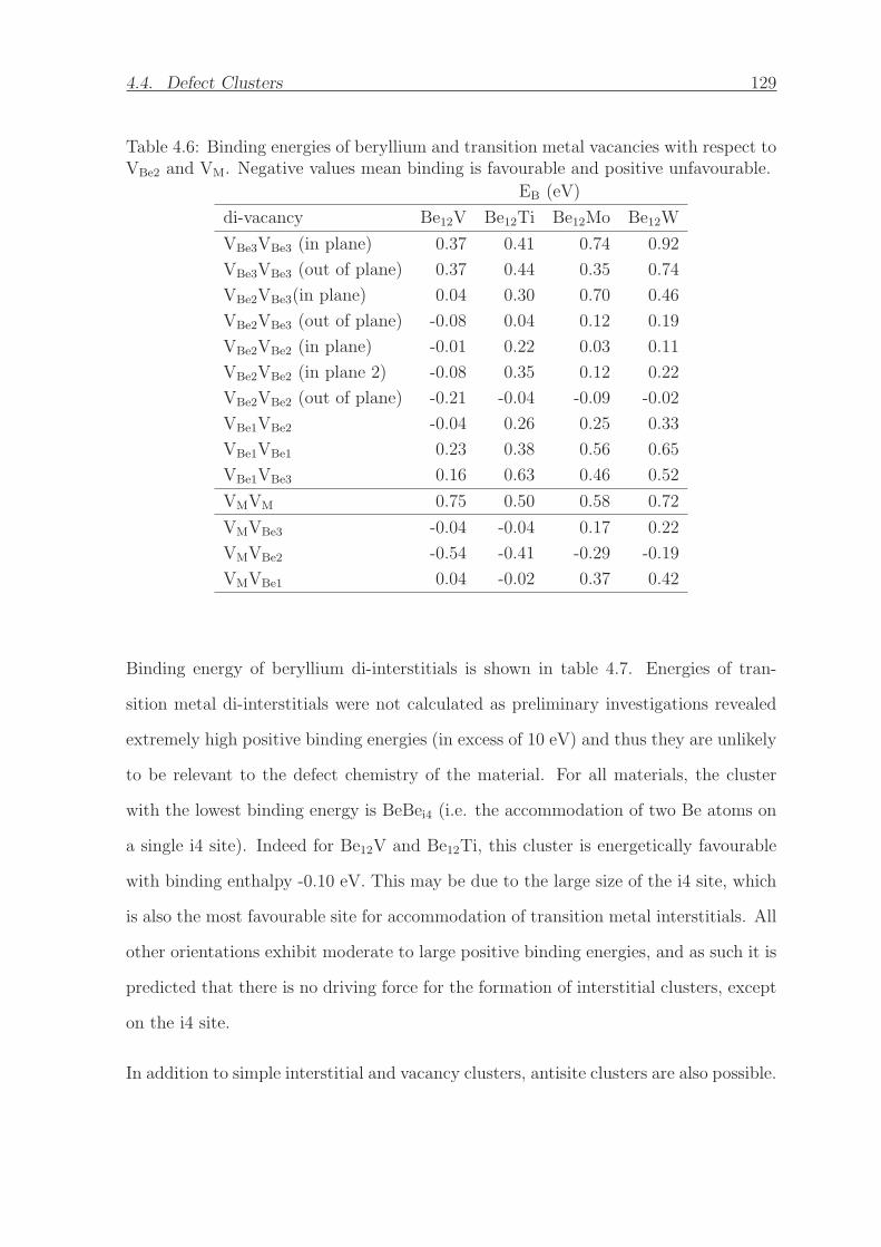
4.4. Defect Clusters 129
Table 4.6: Binding energies of beryllium and transition metal vacancies with respect toVBe2 and VM. Negative values mean binding is favourable and positive unfavourable.
EB (eV)
di-vacancy Be12V Be12Ti Be12Mo Be12W
VBe3VBe3 (in plane) 0.37 0.41 0.74 0.92
VBe3VBe3 (out of plane) 0.37 0.44 0.35 0.74
VBe2VBe3(in plane) 0.04 0.30 0.70 0.46
VBe2VBe3 (out of plane) -0.08 0.04 0.12 0.19
VBe2VBe2 (in plane) -0.01 0.22 0.03 0.11
VBe2VBe2 (in plane 2) -0.08 0.35 0.12 0.22
VBe2VBe2 (out of plane) -0.21 -0.04 -0.09 -0.02
VBe1VBe2 -0.04 0.26 0.25 0.33
VBe1VBe1 0.23 0.38 0.56 0.65
VBe1VBe3 0.16 0.63 0.46 0.52
VMVM 0.75 0.50 0.58 0.72
VMVBe3 -0.04 -0.04 0.17 0.22
VMVBe2 -0.54 -0.41 -0.29 -0.19
VMVBe1 0.04 -0.02 0.37 0.42
Binding energy of beryllium di-interstitials is shown in table 4.7. Energies of tran-
sition metal di-interstitials were not calculated as preliminary investigations revealed
extremely high positive binding energies (in excess of 10 eV) and thus they are unlikely
to be relevant to the defect chemistry of the material. For all materials, the cluster
with the lowest binding energy is BeBei4 (i.e. the accommodation of two Be atoms on
a single i4 site). Indeed for Be12V and Be12Ti, this cluster is energetically favourable
with binding enthalpy -0.10 eV. This may be due to the large size of the i4 site, which
is also the most favourable site for accommodation of transition metal interstitials. All
other orientations exhibit moderate to large positive binding energies, and as such it is
predicted that there is no driving force for the formation of interstitial clusters, except
on the i4 site.
In addition to simple interstitial and vacancy clusters, antisite clusters are also possible.
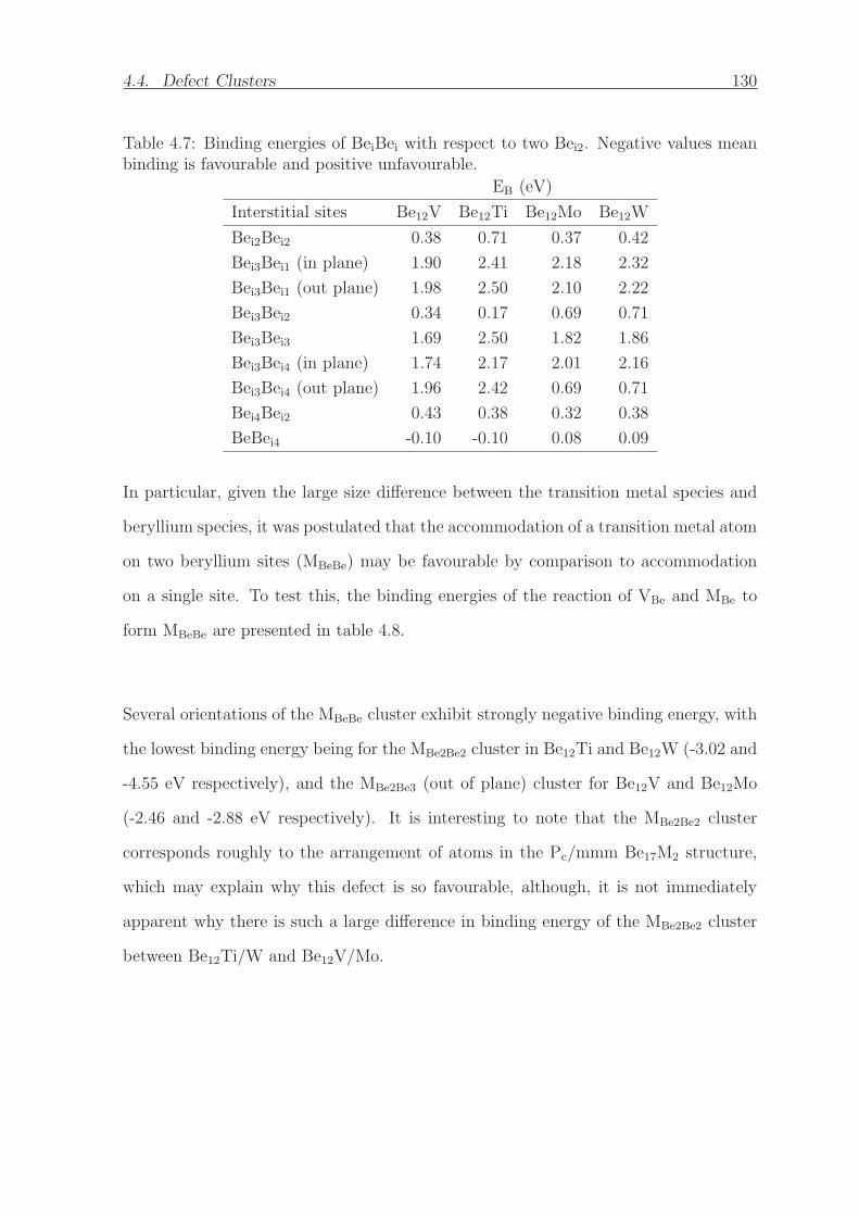
4.4. Defect Clusters 130
Table 4.7: Binding energies of BeiBei with respect to two Bei2. Negative values meanbinding is favourable and positive unfavourable.
EB (eV)
Interstitial sites Be12V Be12Ti Be12Mo Be12W
Bei2Bei2 0.38 0.71 0.37 0.42
Bei3Bei1 (in plane) 1.90 2.41 2.18 2.32
Bei3Bei1 (out plane) 1.98 2.50 2.10 2.22
Bei3Bei2 0.34 0.17 0.69 0.71
Bei3Bei3 1.69 2.50 1.82 1.86
Bei3Bei4 (in plane) 1.74 2.17 2.01 2.16
Bei3Bei4 (out plane) 1.96 2.42 0.69 0.71
Bei4Bei2 0.43 0.38 0.32 0.38
BeBei4 -0.10 -0.10 0.08 0.09
In particular, given the large size difference between the transition metal species and
beryllium species, it was postulated that the accommodation of a transition metal atom
on two beryllium sites (MBeBe) may be favourable by comparison to accommodation
on a single site. To test this, the binding energies of the reaction of VBe and MBe to
form MBeBe are presented in table 4.8.
Several orientations of the MBeBe cluster exhibit strongly negative binding energy, with
the lowest binding energy being for the MBe2Be2 cluster in Be12Ti and Be12W (-3.02 and
-4.55 eV respectively), and the MBe2Be3 (out of plane) cluster for Be12V and Be12Mo
(-2.46 and -2.88 eV respectively). It is interesting to note that the MBe2Be2 cluster
corresponds roughly to the arrangement of atoms in the Pc/mmm Be17M2 structure,
which may explain why this defect is so favourable, although, it is not immediately
apparent why there is such a large difference in binding energy of the MBe2Be2 cluster
between Be12Ti/W and Be12V/Mo.

4.5. Nonstochiometry 131
Table 4.8: Binding enthalpy of MBeBe with respect to MBe2 and VBe2. Negative valuesmean binding is favourable and positive unfavourable.
EB (eV)
Anti-site vacancy pair Be12V Be12Ti Be12Mo Be12W
MBe3Be3 (in plane) 0.33 1.35 0.63 -1.77
MBe3Be3 (out of plane) -0.42 0.17 -0.16 -1.28
MBe2Be3 (in plane) -0.51 -0.09 -0.45 -1.48
MBe2Be3 (out of plane) -2.46 -0.91 -2.88 -2.04
MBe2Be2 (in plane) -0.40 4.26 -0.02 -1.77
MBe2Be2 (in plane) 3.44 0.00 -0.32 -1.67
MBe2Be2 (out of plane) -0.40 -3.02 0.17 -4.55
MBe2Be1 -0.06 -0.38 -0.16 -2.22
MBe1Be3 0.75 -0.46 0.54 -1.93
MBe1Be2 0.75 0.00 0.03 -1.01
4.5 Nonstochiometry
When used as neutron multipliers, 9berylium in these materials will be depleted through
(n,2n) reactions, releasing radiogenic helium and tritium. This will alter the stoichiom-
etry of the material over time. It is therefore important to understand the stability of
the Be12M phases with decreasing beryllium content. This is achieved first through
convex hull analysis [78] of all the Be-M compounds that have been reported, to
establish which are stable at 0 K, followed by examination of the deviation from stoi-
chiometry of the Be12M phases. Examining the non-stochiometry of the Be12M phase
requires the defect analysis presented in sections 4.2-4.4 and knowledge of the nearest
stable reference phase, as will be calculated through the complex hull analysis.
Complex hull analysis was performed by minimising all structures that have been re-
ported in each Be - M phase diagram (see figure 1.13 section 1.6), even those that are
not reported to be stable at 0 K for completeness. This was repeated with the PBE
and LDA exchange-correlation functionals since they typically overbind and underbind

4.5. Nonstochiometry 132
respectively, therefore providing an upper and lower bound on the stability of phases.
The results of the convex hull analysis are shown in figure 4.2.
Phases corresponding to points that define the convex line of lowest energy (coloured
points) are those that are predicted to be stable. Phases corresponding to points above
this line are predicted to be unstable. While the results calculated with the LDA and
PBE functionals are for the most part in qualitative agreement, the PBE functional
predicts intermetallic phases to be significantly more stable relative to the elemental
metal. This is consistent with the fact that LDA calculations are known to over-
delocalise electrons, which may lead to an apparent increase in stability of the parent
metals. In addition, the simulations with the PBE functional predict the Be22M phase
to be stable for all systems, while simulations with the LDA simulation do not. Neither
of these is consistent with experimental results, with the Be22M phase having been ob-
served (at room temperature) for Be22Mo and Be22W, but not Be22V and Be22Ti. In
the Be-Ti and Be-V systems the PBE functional predicts the Be22M phase to be only
just below the line created between pure Be and the Be12M phase, thus suggesting it
is only just stable. As such, it is possible that it is destabilised by temperature effects
at elevated temperatures. Further, the phase transformation to form the Be22M phase
would require long range diffusion, which would inhibit its formation at low tempera-
ture.
The convex hull diagram for the Be-Mo and Be-W systems calculated with the PBE
functional (figure 4.2) are in complete agreement with the experimental phase diagrams
(chapter 1, figure 1.13, with only three stable phases: Be2M, Be12M and Be22M. An
additional BeMo3 phase was identified by a single experimental study [203], however
this was not corroborated by subsequent experiments, and is predicted to be unstable
by these calculations.
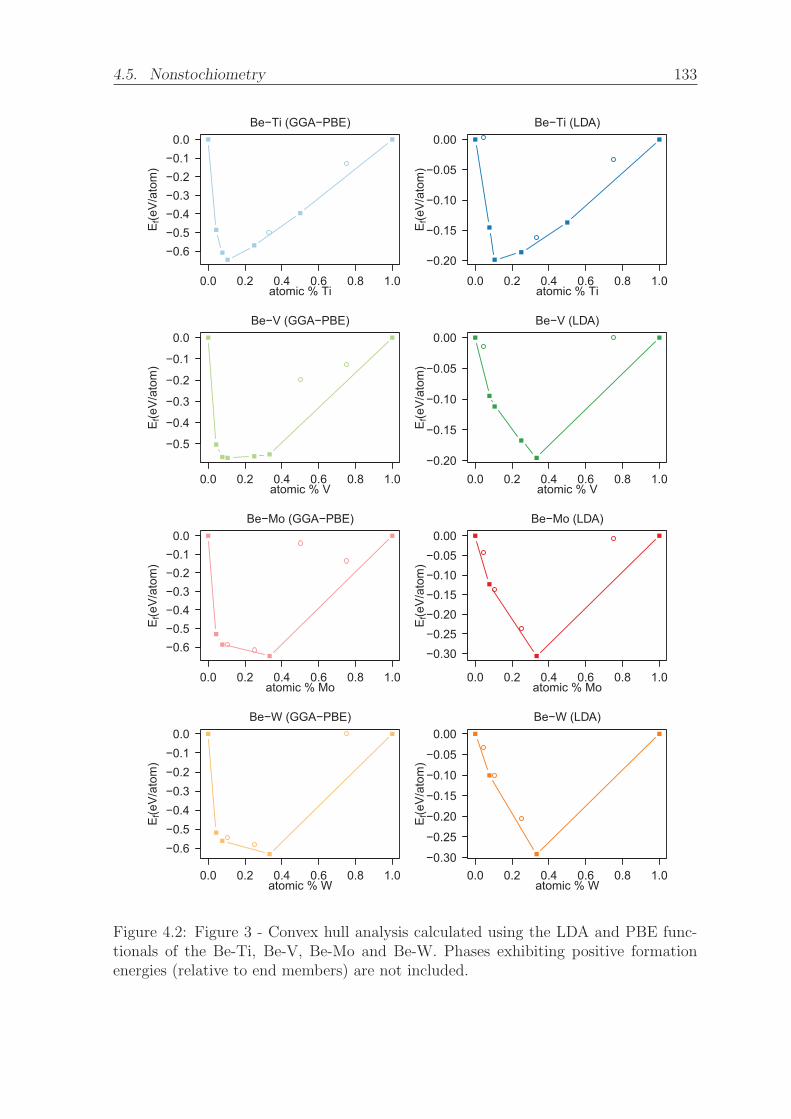
4.5. Nonstochiometry 133
0.0 0.2 0.4 0.6 0.8 1.0
−0.6−0.5−0.4−0.3−0.2−0.1
0.0Be−Ti (GGA−PBE)
E f(e
V/at
om)
atomic % Ti0.0 0.2 0.4 0.6 0.8 1.0
−0.20
−0.15
−0.10
−0.05
0.00Be−Ti (LDA)
E f(e
V/at
om)
atomic % Ti
0.0 0.2 0.4 0.6 0.8 1.0
−0.5
−0.4
−0.3
−0.2
−0.1
0.0Be−V (GGA−PBE)
E f(e
V/at
om)
atomic % V0.0 0.2 0.4 0.6 0.8 1.0
−0.20
−0.15
−0.10
−0.05
0.00Be−V (LDA)
E f(e
V/at
om)
atomic % V
0.0 0.2 0.4 0.6 0.8 1.0
−0.6−0.5−0.4−0.3−0.2−0.1
0.0Be−Mo (GGA−PBE)
E f(e
V/at
om)
atomic % Mo0.0 0.2 0.4 0.6 0.8 1.0
−0.30−0.25−0.20−0.15−0.10−0.05
0.00Be−Mo (LDA)
E f(e
V/at
om)
atomic % Mo
0.0 0.2 0.4 0.6 0.8 1.0
−0.6−0.5−0.4−0.3−0.2−0.1
0.0Be−W (GGA−PBE)
E f(e
V/at
om)
atomic % W0.0 0.2 0.4 0.6 0.8 1.0
−0.30
−0.25
−0.20
−0.15
−0.10
−0.05
0.00Be−W (LDA)
E f(e
V/at
om)
atomic % W
Figure 4.2: Figure 3 - Convex hull analysis calculated using the LDA and PBE func-tionals of the Be-Ti, Be-V, Be-Mo and Be-W. Phases exhibiting positive formationenergies (relative to end members) are not included.

4.5. Nonstochiometry 134
The Be-Ti and Be-V phase diagrams include significantly more intermetallic phases.
The simulated results using the PBE functional are in agreement with experiment
regarding the stability of Be2V, Be2Ti, Be17V2, Be17Ti2, Be12V and Be12Ti, however
Be22Ti, Be22V and Be3V are also predicted to be stable, while Be3Ti is predicted to be
unstable by a small margin. Again, it should be noted that the formation energies of
these phases lie extremely close to the boundary of stability. Thus, these discrepancies
are likely attributed to temperature effects (both enthalpy and entropy), which may
stabalise one phase relative to another. This has previously been shown to be the case
for the closely-related Be-Fe and Be-Fe-Al systems [78].
Despite the discrepancies between the experimental and predicted stabilities of the
Be-Ti and Be-V systems, it is still possible to investigate the deviation from stoichiom-
etry of the Be12M phases. This is achieved by considering the energy to dissolve a
formula unit of the nearest 0 K reference state into the Be12M phase (or vice versa) to
form defects on the Be12M lattice. An example of this is incorporation of Be17Ti2 into
Be12Ti to form beryllium vacancies:
Be17Ti2 + 7BeBe → 7VBe + 2Be12Ti (4.6)
where BeBe are Be atoms on Be sites in the host Be12Ti lattice. A complete list of the
equations used to calculate the formation energy of defects from the nearest reference
state is presented in table 4.10. Reference states are chosen based on the convex
hull analysis presented in figure 4.2. The minimum energy (since given the number
of possible vacancy and interstitial sites in Be12M there is a range of energies) for
incorporation of the reference states is shown in table 4.9.
Using these results, the Arrhenius approximation is used to calculate the total defect

4.5. Nonstochiometry 135
Table 4.9: Solution energy to closest compositional reference state that results in theformation of a single defect and hence a change in stoichiometry. Defect equations canbe found in table 4.10.
Ef/defect (eV)
Defect Be12Ti Be12V Be12Mo Be12W
VBe 1.52 1.53 1.36 1.26
VM 3.34 3.23 1.46 1.41
Bei 2.49 2.34 2.23 2.37
Mi 6.04 5.39 5.64 6.76
BeM 2.79 2.66 0.81 0.88
MBe 2.98 1.78 2.39 4.67
M2Be 1.48 0.84 0.88 1.38
VBeVBe 2.82 2.97 2.64 2.49
VMVBe 4.45 4.19 2.54 2.47
VMVM 7.18 7.17 3.50 3.54
BeiBei 4.89 4.59 4.54 4.82
population for beryllium rich and deficient environments, nd at elevated temperatures:
nd = Nexp( −Ef
2kBT
)(4.7)
Where N is the number of available defect sites and kB is Boltzmann constant. From
this, the maximum allowable deviation from stoichiometry before it is favourable to
form a second phase has been calculated. This is presented in figure 4.3.

4.5. Nonstochiometry 136
Tab
le4.10:Defectequationsan
dassociated
reference
states
evaluated
tocalculate
non
-stochiometry.
Material
Be 1
2W
andBe 1
2Mo
Be 1
2Tian
dBe 1
2V
Reference
states
Be 2
2W
/Be 2W
,Be 2
2Mo/Be 2Mo
Be/Be 1
7Ti 2,Be/
Be 1
7V
2
VBe
Be 2M
+10Be B
e↔
10V
Be+Be 1
2M
Be 1
7M
2+7B
e Be↔
7VBe+2B
e 12M
VM
6Be 2
2M
+5M
M↔
5VM+11Be 1
2M
12Be+M
M↔
VM+Be 1
2M
Be i
Be 2
2M
↔10Be i+Be 1
2M
Be 1
7M
2+8B
e↔
2Be 1
2M
+Be i
Mi
6Be 2M
↔5M
i+Be 1
2M
12Be 1
7M
2↔
7Mi+17Be 1
2M
2VBe
Be 2M
+10Be B
e↔
5(2V
Be)+Be 1
2M
2Be 1
7M
2+14Be B
e↔
7(2V
Be)+4B
e 12M
2VM
12Be 2
2M
+5M
M↔
5(2V
M)+22Be 1
2M
24Be+2M
M↔
(2V
M)+2B
e 12M
VBeV
M11Be 2
2M
+10M
M+10Be B
e↔
10V
BeV
M+21Be 1
2M
11Be+Be B
e+M
M↔
VBeV
M+Be 1
2M
2Be i
Be 2
2M
↔5(2B
e i)+Be 1
2M
2Be 1
7M
2+16Be↔
4Be 1
2M
+2B
e i
Be M
13Be 2
2M
+10M
M↔
10Be M
+23Be 1
2M
13Be+Be B
e+M
M↔
Be M
+Be 1
2M
MBe
13Be 2M
+10Be B
e↔
10M
Be+3B
e 12M
2Be 1
7M
2+Be B
e+Be↔
MBe+3B
e 12M
M2Be
14Be 2
M+20Be B
e↔
10M
2Be+4B
e 12M
2Be 1
7M
2+2B
e Be↔
M2Be+3B
e 12M

4.5. Nonstochiometry 137
7.68 7.70 7.72 7.74
800
1000
1200
1400
Be12Ti
at% M
T (K
)
7.68 7.70 7.72 7.74
800
1000
1200
1400
Be12V
at% MT
(K)
7.68 7.70 7.72 7.74
800
1000
1200
1400
Be12Mo
at% M
T (K
)
7.68 7.70 7.72 7.74
800
1000
1200
1400
Be12W
at% M
T (K
)
Figure 4.3: Phase field lines predicted from total defect concentrations calculated using
the Arrhenius approximation for materials with an excess of beryllium and transition
metal.
All compounds exhibit very little deviation from stochiometry in particular for Be12Ti
(note the very small x axis limits in figure 4.3 of 0.1% M). Be12V may accommodate
some limited beryllium sub-stoichiometry, Be12Mo may accommodate small deviation
on both sides of the stoichiometric composition and Be12W very minor levels of beryl-

4.5. Nonstochiometry 138
lium hyper-stochiometry, but only at elevated temperatures. These differences are
due to the relative energy of the three lowest energy defect reactions which form VBe,
MBe and MBeBe. In Be12Ti, the defect with the lowest energy is TiBeBe with energy
of 1.48eV. This is considerably higher than for other materials, and limits deviation
from stoichiometry. For Be12V, VBeBe also has the lowest formation energy (0.84 eV),
which is significantly lower than in Be12Ti and thus allows inclusion of excess transition
metal. This is similar for Be12Mo, where the MoBeBe species has a formation energy of
0.88 eV, although BeMo has a formation energy 0.81 eV, which allows for some non-
stochiometry in the beryllium rich region. The lowest energy defect in Be12W is BeW
with an energy of 0.88 eV, thus allowing for hyperstochiometry.
Given the very small magnitude of nonstochiometry predicted in these materials, even
at elevated temperature, they may effectively be considered line compounds. The im-
plication for their use as neutron multipliers is that to account for beryllium depletion
through (n,2n) reactions, it may be useful to manufacture them with excess beryllium
as a second phase. This is beneficial from a manufacturing perspective as it increases
the very limited ductility of the compounds. If excess beryllium is not included, these
materials are likely to form secondary phases with compositions Be17V2, Be17Ti2, Be2W
and Be2Mo as beryllium depletion proceeds. Be12Ti and Be12V are likely to be the least
effected by the formation of these secondary phases, not because they can accommodate
excess non-stochiometry, but because the Be17M2 phase bears clear structural relation
to the Be12M phase (as explored in chapter 3) and has similar composition. As such, it
is suggested that Be22Mo and Be22W might be considered as neutron multipliers over
Be12Mo and Be12W. This is further supported by their superior neutronic properties,
as preliminary studies have shown that a sufficient tritium breeding ratio cannot be
achieved with current module designs and the use of Be12W [56].
4.6. Defect Migration in Be12Ti 139
4.6 Defect Migration in Be12Ti
In addition to the enthalpy of formation of defects and clusters, how defects move and
interact will also determine the rate at which they coalesce to form larger extended
defects such as dislocations and voids. To date, migration of intrinsic defects has not
been investigated in any of these materials. To address this, the work presented in this
section explores intrinsic defect migration in Be12Ti, the most attractive candidate for
use as a neutron multiplier. The Linear Synchronous Transit (LST), Quadratic Syn-
chronous Transit (QST) and Nudged Elastic Band (NEB) methods [141, 142] were
used within the DFT framework (as outlined in chapter 2). These methods are signif-
icantly more computationally expensive than simple geometry optimisations, limiting
the number of simulations that could be performed. As such, it was decided to focus
on only one material (i.e. Be12Ti) so that a more comprehensive investigation could
be undertaken.
Diffusion in any material is limited by both the concentration of defects (which, for
equilibrium defect populations is determined by their formation energy) and the energy
for the defect to move from one site to another (the hopping energy, Ehop). Based on
the investigations of defect formation energies, intrinsic defect populations will likely
be dominated by Schottky disorder and beryllium Frenkel disorder, resulting in high
populations of VBe, VTi and Bei relative to other defects. Given the negative binding
enthalpy to form VBeVBe and the strongly negative binding enthalpy to form VBeVTi,
it is likely these will also contribute to the defect population. As such, in addition to
point defects, migration of these species is considered.
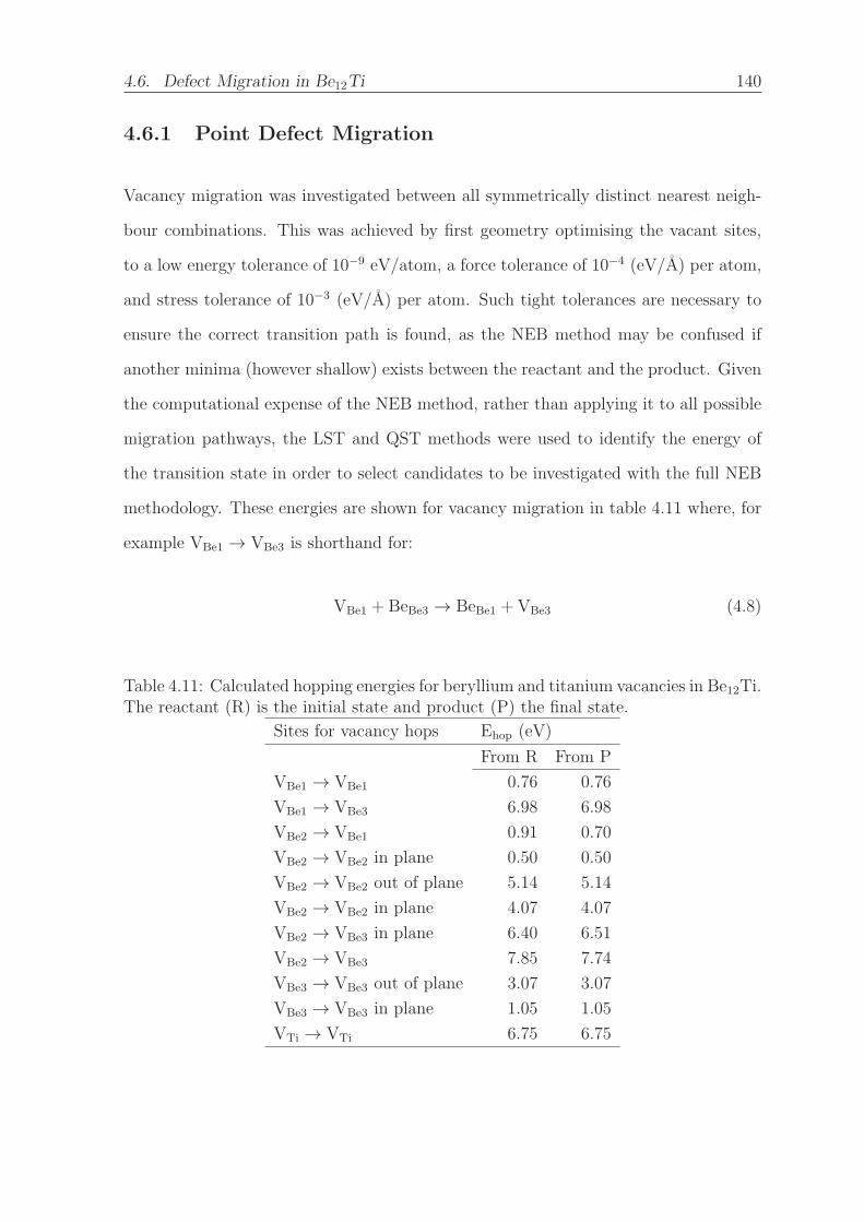
4.6. Defect Migration in Be12Ti 140
4.6.1 Point Defect Migration
Vacancy migration was investigated between all symmetrically distinct nearest neigh-
bour combinations. This was achieved by first geometry optimising the vacant sites,
to a low energy tolerance of 10−9 eV/atom, a force tolerance of 10−4 (eV/A) per atom,
and stress tolerance of 10−3 (eV/A) per atom. Such tight tolerances are necessary to
ensure the correct transition path is found, as the NEB method may be confused if
another minima (however shallow) exists between the reactant and the product. Given
the computational expense of the NEB method, rather than applying it to all possible
migration pathways, the LST and QST methods were used to identify the energy of
the transition state in order to select candidates to be investigated with the full NEB
methodology. These energies are shown for vacancy migration in table 4.11 where, for
example VBe1 → VBe3 is shorthand for:
VBe1 + BeBe3 → BeBe1 +VBe3 (4.8)
Table 4.11: Calculated hopping energies for beryllium and titanium vacancies in Be12Ti.The reactant (R) is the initial state and product (P) the final state.
Sites for vacancy hops Ehop (eV)
From R From P
VBe1 → VBe1 0.76 0.76
VBe1 → VBe3 6.98 6.98
VBe2 → VBe1 0.91 0.70
VBe2 → VBe2 in plane 0.50 0.50
VBe2 → VBe2 out of plane 5.14 5.14
VBe2 → VBe2 in plane 4.07 4.07
VBe2 → VBe3 in plane 6.40 6.51
VBe2 → VBe3 7.85 7.74
VBe3 → VBe3 out of plane 3.07 3.07
VBe3 → VBe3 in plane 1.05 1.05
VTi → VTi 6.75 6.75
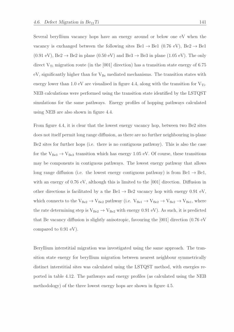
4.6. Defect Migration in Be12Ti 141
Several beryllium vacancy hops have an energy around or below one eV when the
vacancy is exchanged between the following sites Be1 → Be1 (0.76 eV), Be2 → Be1
(0.91 eV), Be2 → Be2 in plane (0.50 eV) and Be3 → Be3 in plane (1.05 eV). The only
direct VTi migration route (in the [001] direction) has a transition state energy of 6.75
eV, significantly higher than for VBe mediated mechanisms. The transition states with
energy lower than 1.0 eV are visualised in figure 4.4, along with the transition for VTi.
NEB calculations were performed using the transition state identified by the LSTQST
simulations for the same pathways. Energy profiles of hopping pathways calculated
using NEB are also shown in figure 4.4.
From figure 4.4, it is clear that the lowest energy vacancy hop, between two Be2 sites
does not itself permit long range diffusion, as there are no further neighbouring in-plane
Be2 sites for further hops (i.e. there is no contiguous pathway). This is also the case
for the VBe3 → VBe3 transition which has energy 1.05 eV. Of course, these transitions
may be components in contiguous pathways. The lowest energy pathway that allows
long range diffusion (i.e. the lowest energy contiguous pathway) is from Be1 → Be1,
with an energy of 0.76 eV, although this is limited to the [001] direction. Diffusion in
other directions is facilitated by a the Be1 → Be2 vacancy hop with energy 0.91 eV,
which connects to the VBe2 → VBe2 pathway (i.e. VBe1 → VBe2 → VBe2 → VBe1, where
the rate determining step is VBe2 → VBe2 with energy 0.91 eV). As such, it is predicted
that Be vacancy diffusion is slightly anisotropic, favouring the [001] direction (0.76 eV
compared to 0.91 eV).
Beryllium interstitial migration was investigated using the same approach. The tran-
sition state energy for beryllium migration between nearest neighbour symmetrically
distinct interstitial sites was calculated using the LSTQST method, with energies re-
ported in table 4.12. The pathways and energy profiles (as calculated using the NEB
methodology) of the three lowest energy hops are shown in figure 4.5.

4.6. Defect Migration in Be12Ti 142
Be1
Be1
Be2
Be3
VBe1
VBe2
VBe3
VTi
Ti
0.0
0.2
0.4
0.6
0.8
Be1 Be1
0.0
0.2
0.4
0.6
0.8
Be2 Be1
0.00.10.20.30.40.5
Be2 Be2
0.00.20.40.60.81.0
Be3 Be3
01234567
Ti Ti
E (e
V)
reaction coordinate
Be1
Be2 Be2
Be3
Be3
Ti
Ti
Figure 4.4: Left: lowest energy migration pathways for beryllium and titanium vacancymigration in Be12Ti. Right: NEB pathways for the lowest energy migration pathways.

4.6. Defect Migration in Be12Ti 143
Table 4.12: Calculated hopping energies for beryllium and titanium interstitials inBe12Ti. The reactant (R) is the initial state and product (P) the final state.
sites Ehop (eV)
From R From P
Bei2 → Bei2 1.19 1.19
Bei3 → Bei1 5.10 5.84
Bei3 → Bei1 0.77 1.29
Bei3 → Bei2 0.42 2.42
Bei1 → Bei2 1.44 2.71
Tii2 → Tii4 1.00 0.55
Tii3 → Tii1 7.20 5.10
Tii2 → Tii3 6.92 4.55
The lowest energy contiguous pathway is via the i2 sites with hopping energy 1.20 eV
(which also have the lowest interstitial formation energy of 1.86 eV). This pathway
proceeds only in the [001] direction. The next lowest energy paths, which are also
both contiguous, are from i3 to i1 and i3 to i2 with hopping energies of 1.29 eV and
2.42 eV respectively. It should be noted that both the i1 and i3 sites have significantly
higher formation energy (3.19 eV and 3.69 eV respectively), and thus migration through
these sites is further energetically challenged. As such, it is predicted that beryllium
interstitial migration in Be12Ti will be strongly anisotropic favouring the [001] direction
via the i2 sites.
For titanium interstitials, the lowest energy contiguous pathway is via the i2 and i4
sites, with hopping energy 1.00 eV. This pathway only allows diffusion in the [001]
direction. The next lowest energy pathways are from the i3 to i1 site and the i2 to
i3 sies, with hopping energy 7.20 and 6.92 eV respectively. Other potential pathways
investigated were all found to be energetically extremely unfavourable (with hopping
energy in excess of 15 eV), and thus are not reported here. Based on these results, it
is expected that Tii migration will be strongly anisotropic.
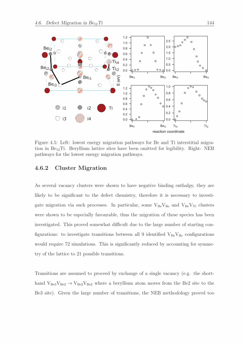
4.6. Defect Migration in Be12Ti 144
0.0
0.2
0.4
0.6
0.8
1.0
1.2
Bei2 Bei2
0.0
0.5
1.0
1.5
2.0
2.5
Bei3 Bei2
0.00.20.40.60.81.01.2
Bei1 Bei3
0.0
0.2
0.4
0.6
0.8
1.0
Tii4 Tii2
E (e
V)
reaction coordinate
E (e
V)
i1
i3
i2
i4
Ti
Bei2
Bei3
Bei1
Tii2Bei2Tii4
Figure 4.5: Left: lowest energy migration pathways for Be and Ti interstitial migra-tion in Be12Ti. Beryllium lattice sites have been omitted for legibility. Right: NEBpathways for the lowest energy migration pathways.
4.6.2 Cluster Migration
As several vacancy clusters were shown to have negative binding enthalpy, they are
likely to be significant to the defect chemistry, therefore it is necessary to investi-
gate migration via such processes. In particular, some VBeVBe and VBeVTi clusters
were shown to be especially favourable, thus the migration of these species has been
investigated. This proved somewhat difficult due to the large number of starting con-
figurations: to investigate transitions between all 9 identified VBeVBe configurations
would require 72 simulations. This is significantly reduced by accounting for symme-
try of the lattice to 21 possible transitions.
Transitions are assumed to proceed by exchange of a single vacancy (e.g. the short-
hand VBe3VBe2 → VBe2VBe2 where a beryllium atom moves from the Be2 site to the
Be3 site). Given the large number of transitions, the NEB methodology proved too
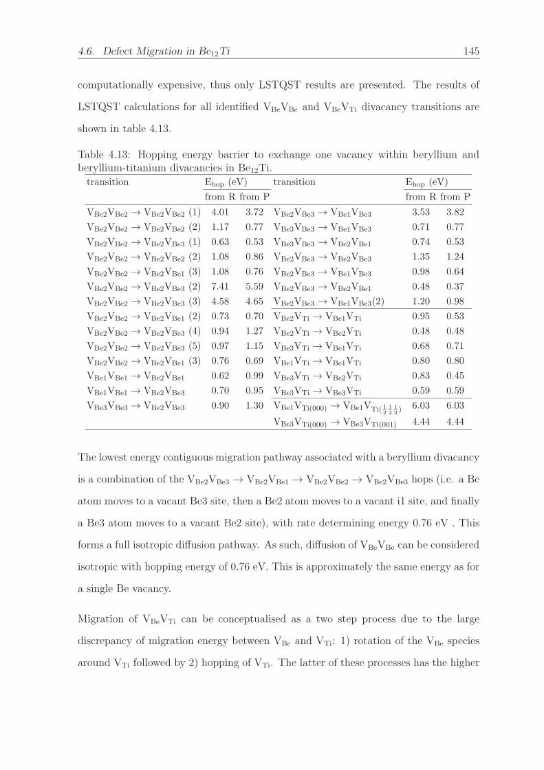
4.6. Defect Migration in Be12Ti 145
computationally expensive, thus only LSTQST results are presented. The results of
LSTQST calculations for all identified VBeVBe and VBeVTi divacancy transitions are
shown in table 4.13.
Table 4.13: Hopping energy barrier to exchange one vacancy within beryllium andberyllium-titanium divacancies in Be12Ti.
transition Ehop (eV) transition Ehop (eV)
from R from P from R from P
VBe2VBe2 → VBe2VBe2 (1) 4.01 3.72 VBe2VBe3 → VBe1VBe3 3.53 3.82
VBe2VBe2 → VBe2VBe2 (2) 1.17 0.77 VBe3VBe3 → VBe1VBe3 0.71 0.77
VBe2VBe2 → VBe2VBe3 (1) 0.63 0.53 VBe3VBe3 → VBe2VBe1 0.74 0.53
VBe2VBe2 → VBe2VBe2 (2) 1.08 0.86 VBe2VBe3 → VBe2VBe3 1.35 1.24
VBe2VBe2 → VBe2VBe1 (3) 1.08 0.76 VBe2VBe3 → VBe1VBe3 0.98 0.64
VBe2VBe2 → VBe2VBe3 (2) 7.41 5.59 VBe2VBe3 → VBe2VBe1 0.48 0.37
VBe2VBe2 → VBe2VBe3 (3) 4.58 4.65 VBe2VBe3 → VBe1VBe3(2) 1.20 0.98
VBe2VBe2 → VBe2VBe1 (2) 0.73 0.70 VBe2VTi → VBe1VTi 0.95 0.53
VBe2VBe2 → VBe2VBe3 (4) 0.94 1.27 VBe2VTi → VBe2VTi 0.48 0.48
VBe2VBe2 → VBe2VBe3 (5) 0.97 1.15 VBe3VTi → VBe1VTi 0.68 0.71
VBe2VBe2 → VBe2VBe1 (3) 0.76 0.69 VBe1VTi → VBe1VTi 0.80 0.80
VBe1VBe1 → VBe2VBe1 0.62 0.99 VBe3VTi → VBe2VTi 0.83 0.45
VBe1VBe1 → VBe2VBe3 0.70 0.95 VBe3VTi → VBe3VTi 0.59 0.59
VBe3VBe3 → VBe2VBe3 0.90 1.30 VBe1VTi(000) → VBe1VTi( 12
12
12) 6.03 6.03
VBe3VTi(000) → VBe3VTi(001) 4.44 4.44
The lowest energy contiguous migration pathway associated with a beryllium divacancy
is a combination of the VBe2VBe3 → VBe2VBe1 → VBe2VBe2 → VBe2VBe3 hops (i.e. a Be
atom moves to a vacant Be3 site, then a Be2 atom moves to a vacant i1 site, and finally
a Be3 atom moves to a vacant Be2 site), with rate determining energy 0.76 eV . This
forms a full isotropic diffusion pathway. As such, diffusion of VBeVBe can be considered
isotropic with hopping energy of 0.76 eV. This is approximately the same energy as for
a single Be vacancy.
Migration of VBeVTi can be conceptualised as a two step process due to the large
discrepancy of migration energy between VBe and VTi: 1) rotation of the VBe species
around VTi followed by 2) hopping of VTi. The latter of these processes has the higher

4.7. Summary and Conclusions 146
energy and is thus the rate limiting step. Two migration pathways have been identified,
one of which is anisotropic and another which is isotropic.
Diffusion of VBeVTi in the [001] direction may occur via the VBe3VTi(000) → VBe3VTi(001)
reaction, which has energy of 4.44 eV. Following this, for diffusion to proceed further
the VBe species must orientate around the VTi site, the lowest energy pathway being
VTiVBe3 → VTiVBe2 → VTiVBe3 with energy 0.83 eV. Isotropic diffusion may proceed
via the VBe1VTi(000) → VBe1VTi( 12
12
12) reaction, which has energy 6.03 eV. For diffusion
to proceed in the [001] direction, the VBe1 species must orientate around VTi( 12
12
12) from
VBe1( 14
14
14) to VBe1( 1
414
34) with energy 0.80 eV. For diffusion to proceed isotropically, the
VBe1 species must then orientate around VTi( 12
12
12) from VBe1( 1
414
14) to VBe1( 3
414
14), the
lowest energy pathway for which is VTiVBe1 → VTiVBe3 → VTiVBe1 and has energy
0.71 eV. Given that titanium migration via the Be3 site is lower in energy than via the
Be1 site, and lower than that for VTi migration (6.75 eV) it is predicted that titanium
vacancy diffusion will be anisotropic in Be12Ti favouring the [001] direction. The energy
of this pathway is however significantly higher than for a titanium interstitial in the
[001] direction (1.05 eV), which is expected to be the dominant diffusion mechanism
for titanium in this material. While this energy is comparable to that for migration
of a beryllium vacancy, given the significantly higher formation energy of a titanium
interstitial, beryllium diffusion overall has a significantly lower activation energy.
4.7 Summary and Conclusions
The intrinsic defect properties of Be12Ti, Be12V, Be12Mo and Be12W have been pre-
dicted using DFT simulations. Formation energies for common point defects, including
vacancies, interstitials and antisite defects. Further, four stable intrinsic interstitial
sites have been identified in the I4/mmm structure for the first time.
4.7. Summary and Conclusions 147
Defects on the beryllium sublattice have consistently lower formation enthalpy than on
the transition metal sublattice. For beryllium vacancies, the Be2 lattice site has the
lowest formation enthalpy for all materials studied (1.20-1.48 eV), although all three Be
sites are relatively close in energy (0.2 eV). Transition metal vacancies have formation
energy between 3.16 eV and 4.10 eV, with Be12W having the lowest and Be12Ti the
highest. These results are in excellent qualitative agreement with previous studies of
Be12W [96]. For beryllium interstitials, only three sites are stable. These are the i1,
i2 and i3 sites, of which the i2 site has the lowest formation energy for all materials,
from 1.86 eV in Be12Ti to 2.50 eV in Be12W. The other sites have formation energy
between 0.92 eV and 1.83 eV higher than the i2 site. Transition metal interstitials can
be accommodated in all three sites, as well as an additional i4 (4c) site. The i4 site
has the lowest formation energy for transition metal interstitials, ranging from 4.19 eV
in Be12Ti to 5.96 eV in Be12W. Antisites, consisting of beryllium accommodated on a
transition metal site have formation energies between 3.55 eV for Be12Ti and 2.76 eV
for Be12W, while for a transition metal accommodated on a beryllium site, the Be2
site has the lowest formation enthalpy, from 0.95 eV in Be12Ti to 3.81 eV in Be12W.
During radiation damage, defects are formed through intrinsic disorder processes, typ-
ically Frenkel, Schottky and Antisite disorder. Using the calculated defect energies,
it is predicted that Schottky disorder has the lowest energy (1.35 - 1.66 eV/defect),
although beryllium Frenkel disorder has similar energy in Be12V and Be12Ti.
Small clusters including beryllium divacancies and interstitials, mixed divacancies and
the accommodation of a transition metal on two beryllium sites were investigated.
Some beryllium and mixed divacancies exhibit negative binding energy (i.e. their
formation is favourable), although this is strongly orientation dependent. Only one
beryllium di-interstitial orientation exhibits modest negative binding energy in Be12Ti,
while all other combinations for all materials exhibit positive binding energy.
4.7. Summary and Conclusions 148
Several orientations of beryllium divacancy accommodate a transition metal with nega-
tive binding energy, with MBe2Be2 exhibiting strongly negative binding energy in Be12Ti
and Be12W (-3.02 eV and -4.55 eV respectively) and MBe2Be3 exhibiting strongly neg-
ative binding energy in Be12V and Be12Mo (-2.46 eV and -2.88 eV respectively). This
is attributed to the large size discrepancy between beryllium and the transition metal,
which leads to large strains when the transition metal is accommodated on an inter-
stitial site or as a simple antisite defect.
Convex hull analysis of the Be-V/Ti/Mo/W systems was undertaken using both the
PBE and LDA functionals. It was found that the PBE functional is more consistent
with observed results, correctly predicting the stability of all structures in the Be-Mo
and Be-W systems. In the Be-Ti and Be-V systems, simulations with the PBE func-
tional predict the Be22M phase to be stable, while this phase has not been observed
experimentally. Be3V is also predicted to be stable contrary to experimental observa-
tions. As these phases lie close to the bounds of stability, it is hypothesised that they
may only be stable at low temperatures, which could inhibit their formation on kinetic
grounds.
Nonstochiometry was predicted in the Be12M materials using the calculated defect
energies and convex hull analysis. All materials exhibit only very limited nonstochiom-
etry, in particular Be12Ti. Be12V exhibits limited hyperstochiometry, and Be12Mo lim-
ited hypo and hyperstochiometry. This suggests it is advisable to manufacture these
materials with an excess of beryllium for neutron multiplying applications, since will
be depleted by the transmutation process.
Point defect and cluster migration for Be12Ti was investigated using the LST, QST
and NEB methodologies. Defect species were investigated based on their predicted
concentrations from analysis of defect energies. Migration of beryllium vacancies is
predicted to have hopping energy of 0.76 eV in the [001] direction via Be1 sites, and

4.7. Summary and Conclusions 149
hopping energy of 0.91 eV for isotropic diffusion via Be1 and Be2 sites. As such, vacancy
diffusion is predicted to be weakly anisotropic. Ti vacancy migration is predicted to
only occur in the [001] direction with energy 6.75 eV.
Beryllium interstitial migration is predicted to exhibit a hopping energy of 1.19 eV in
the [001] direction and occurs via Be2 sites. Isotropic diffusion may be mediated by the
i2, i3 and i1 sites, with hopping energy of 2.42 eV. Titanium interstitial migration may
occur restricted to the [001] direction via the i2 and i4 sites with hopping energy of 1.00
eV. This is significantly lower than for any isotropic diffusion pathway (hopping energy
> 6.92 eV). As such both beryllium and titanium interstitial migration is predicted to
strongly favour the [001] direction.
Beryllium divacany migration is predicted to be isotropic, with hopping energy of 0.66
eV via the VBe2Be2, VBe2VBe3 and VBe2Be1 species, although there are several other tran-
sitions with only slightly higher energy. Mixed beryllium-titanium divacancy diffusion
is limited by migration of the titanium vacancy, which has a hopping energy of 6.03
eV for isotropic diffusion, and 4.44 eV for migration in the [001] direction.
Given intrinsic defect populations at thermal equilibrium are predicted to be dominated
by beryllium vacancies, divacancies, and, to a lesser extent, beryllium interstitials, it
is predicted that overall beryllium migration will be weakly anisotropic favouring the
[001] direction. Further, titanium migration has significantly higher migration energy
than beryllium.
Chapter 5
Displacement Processes in Fusion
Materials
This work is published in:
M. L. Jackson, P. C. M. Fossati, R. W. Grimes “Simulations of threshold displacement
in beryllium”, Journal of Applied Physics, 120, 045903 (2016) [204]
5.1 Introduction
As discussed in section 1.7, the threshold displacement energy, Ed, is an important
materials property that can be used to quantify radiation damage in a material. It
is an important parameter for models such as those due to Kinchin-Pease (KP) [105],
Norgett-Robinson-Torrens (NRT) [106] and Greenwood [107], which are used to esti-
mate the number of point defects created during a displacement cascade. By extension,
if the flux profile of the incident radiation is known, then the total number of point
defects created in the material can be estimated. This is key to predict the forma-
150

5.1. Introduction 151
tion of extended defects that are responsible for many of the deleterious effects on the
macroscopic properties of materials. Further, Ed is an important parameter in the
popular SRIM software [110], which uses a binary collision model to calculate the final
distribution of atomic displacements in a material, caused by incident energetic ions.
Despite being so important to the modelling of radiation damage, Ed has no con-
sistent definition, which complicates attempts to calculate it. This stems, in part, from
the fact that the probability of displacement (Pd) is not a step function with primary
knock on energy, E. Instead, Pd increases as a curve, approaching a value of one almost
asymptotically [205]. This is primarily due to two physical effects. Firstly, at finite
temperature, atoms in the material are vibrating while confined to their potential well
with some kinetic energy, which has an additive effect to the energy resulting from the
primary collision. More significantly, Ed is also strongly dependent on crystallographic
orientation. It is possible to define a probability of displacement for each lattice di-
rection, Pd(θ, φ), and further a threshold displacement energy, Ed(θ, φ). To generate
the average probability of displacement, Pd (as would be measured experimentally for
a polycrystalline sample), Pd(θ, φ) must be averaged across all directions:
Pd =
∫ 2π0
∫ π
0Pd(θ, φ)sinθdθdφ∫ 2π
0
∫ π
0sinθdθdφ
(5.1)
From the perspective of MD simulations, this can either be achieved by a random sam-
pling of directions (providing the sample size is large enough) [206] or through uniform
spatial sampling [205].
Because Pd is not a step function, the cutoff for Ed has been variously defined as
occurring either at the lowest energy with non-zero probability of displacement, Ed,0,
displacement probability of 0.1, Ed,0.1 or displacement probability of 0.5 Ed,0.5 [207].

5.1. Introduction 152
Further, it is not immediately clear which of these measures would be more appropriate
for use with models such as KP.
Experimentally, Ed is measured by varying the energy of an electron beam incident
upon the material, and measuring changes in the resistivity, which would indicate the
formation of defects. As such, it is likely that this is measuring Ed,0, thus this measure
will be used in this work so that results may be more easily compared with experimen-
tal data.
In addition to directional effects, the definition of Ed has been further complicated
since the advent of atomistic simulation as a tool to model it. Using atomistic simula-
tion, the displacement event can be directly simulated and monitored, allowing for the
detection of atomic displacements that do not form defects (i.e. whereby two atoms of
the same species switch lattice sites during the displacement event). Thus, Ed must be
further differentiated into Edispd , which is the threshold energy for displacement, regard-
less of whether a defect is formed, and Edefd , the threshold energy to create a defect.
The latter of these is more easily directly compared to experimental values, and is thus
more useful for quantifying radiation damage, given it is the point defects produced
that are ultimately responsible for the changes in materials properties. Edispd is, how-
ever, useful as a point of comparison for Edefd , as the difference between the two may be
useful for examining the role of recovery immediately following the displacement event.
In this chapter the displacement behaviour of beryllium, tungsten, carbon, and tung-
sten carbide is investigated using molecular dynamic simulations. These materials were
chosen due to the availability and suitability of interatomic potentials, their relevance
as materials for fusion, and in order to investigate the effect of local environment on Ed.
In SRIM, the approximation made is that Ed is a unique function of the PKA species,

5.2. Threshold Displacement in Beryllium 153
and no account is taken of the local environment. Previous MD studies comparing
the displacement behaviour of Ti and O in TiO2 have shown marked difference be-
tween different crystal structures, challenging this approximation [208]. An aim of this
work is to investigate this further by comparing displacement behaviour between dif-
ferent allotropes of carbon, and between elemental carbon and tungsten, and tungsten
carbide.
5.2 Threshold Displacement in Beryllium
Despite being used in nuclear applications for over 70 years, there has been little
investigation of low energy displacement processes in beryllium, although there has
been significant investigation, both experimental and simulated, of radiation damage
in general [15, 64]. As such, in this section displacement processes in beryllium are
explored. This is achieved using two interatomic potentials, as described in chapter 2.
5.2.1 Computational Details
Preliminary investigations began using the EAM potential developed and parame-
terised by Agrawal et al [149] (henceforth refered to as the Agrawal potential). This
potential was selected as it provides a good approximation of several materials proper-
ties of beryllium, including lattice parameters, elastic constants, melting temperature
and defect energies (see table 2.2). A key consideration for displacement simulations,
that is not normally fit to for more general empirical potentials, is the repulsive force
at short interatomic sepereations. For the Agrawal potential, the repulsive force due
to the overlap of electronic orbitals is modelled by a strongly repulsive embedding
function for high electron densities. Often, repulsive forces are modelled by a splined
5.2. Threshold Displacement in Beryllium 154
ZBL potential [110, 207], which is well characterised and has been shown to provide
a good approximation of such forces at low interatomic separations. However, given
that the repulsive force is encoded in the multi-body terms of the Agrawal potential,
it proved impossible to retroactively spline a ZBL potential to the pair potential. Con-
sequently, a second potential was employed: a bond order potential parameterised by
Bjorkas et al [153](henceforth refered to as the Bjorkas potential). This potential has
the benefit that, as well as reproducing many physical properties with similar accuracy
to the Agrawal potential, it has had a ZBL potential splined using the methodology
of Nordlund et al. [207], giving confidence that it accurately reproduces the repulsive
term at short interatomic separations.
Displacement simulations were performed in 15×15×10 supercells of beryllium con-
taining 4500 atoms. Cells were first geometry optimised and equilibrated to 300 K
for a minimum of 50 ps with a timestep of 0.2 fs in the NPT ensemble, during which
temperature and pressure were controlled using the Berendsen thermostat and baro-
stat [209]. To calculate the probability of displacement for each energy and direction,
each simulation must be repeated with different starting configurations. For this work,
simulations were repeated 20 times with starting configurations generated by equili-
brating the supercells for additional increments of 1 ps.
Simulations proceeded by imparting a central atom in the equilibrated supercell with
energies between 4-100 eV in increments of 4 eV for the Bjorkas potential, and 12-200
eV for the Agrawal potential . From the initial impact, supercells were run in the NVE
ensemble for 20,000 timesteps of 0.01 fs, 10,000 timesteps of 0.1 fs and 10,000 timesteps
of 1.0 fs for a total simulation time of 12.6 ps. Such a short timestep is necessary in
the collisional phase due to the very high velocity of the PKA.
5.2. Threshold Displacement in Beryllium 155
The crystallographic directions investigated were based on a segment of a geodesic
projection of directions representing at least twice the irreducible symmetry of the
crystal. For HCP beryllium this is an arc from 0-120oθ and 0-90oφ, with a spacing of
6o in both θ and φ.
In the first study, the distinction between defect formation (Pdefd ) and displacement
(Pdispd ) was not made, and thus simulations using the Agrawal potential only examined
displacement. In the second study, using the Bjorkas potential, both defect forma-
tion and displacement were investigated. An atom was considered displaced if during
the simulation, it was ‘permanently’ displaced (i.e. until the end of the simulation)
by half of the equilibrium bond length (or more). Defects were identified using local
environment analysis, as implemented by P Fossati [210]. In this method, the tridi-
mensional local average density field is used to characterise the local environment of
atoms and generate a configuration graph. Vacancies and interstitials create unique
patterns in this configuration graph thereby facilitating identification. Contrary to
other commonly used defect detection methods, this approach requires no reference
state, is readily adaptable to different crystal structures, and can reliably differentiate
between different types of defects such as vacancies, interstitials and split interstitials.
5.2.2 Directionally Averaged Results and Analysis
The directionally averaged probability of displacement, Pdispd , and probability of defect
formation, Pdefd , are presented with increasing primary knock on energy, E, in figure 5.1.
Directionally averaged threshold displacement (Edispd ) and threshold defect formation
energy Edefd are calculated from this data using the Robinson model [205], which relates

5.2. Threshold Displacement in Beryllium 156
0 50 100 150
0.0
0.2
0.4
0.6
0.8
1.0
Bjorkas, Pddisp
Bjorkas, Pddef
Agrawal, Pddisp
E (eV)
Pd
Figure 5.1: Values of Pdispd simulated using the Bjorkas and Agrawal potentials, and
values of Pdefd for the Bjorkas potential. Lines are the Robinson model fitted to the
simulated data.
Pd and Ed at low E:
Pd(E) =
{0 E ≤ Ed
1β
[Eα − Eα
d
]E ≥ Ed
(5.2)
In this scheme, β and α are fitting constants. To calculate Ed from this model, a least
squares fitting scheme was used to fit the model to the simulated Pd curve below a
displacement probability of 0.75. From this model, Edispd and Edef
d were calculated to
be 8.67±0.29 and 9.15±0.92 eV for the Bjorkas potential, and Edispd 34.80±0.55 eV for
the Agrawal potential. Examining the correspondence between the Robinson model
and simulated Pd curves in fig 5.1, the model reproduces the simulated data at low
E, and around the onset of non zero Pd, giving confidence in the calculated value of
Ed. The model does, however, overpredict Pdispd at higher E, where Pdisp
d approaches
one, as there is no inherent mechanism in the model to prevent it surpassing unity,
which is clearly unphysical. As such, this model is not suitable to predict displacement
probability at higher energy.
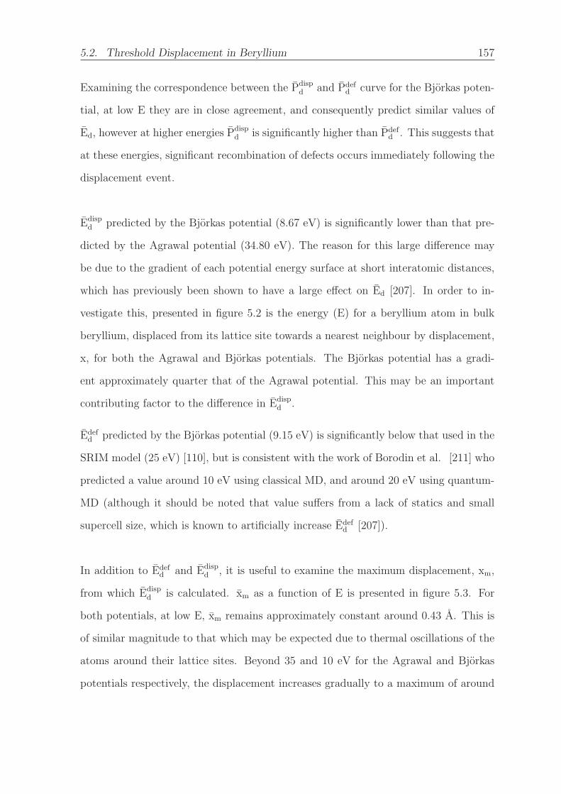
5.2. Threshold Displacement in Beryllium 157
Examining the correspondence between the Pdispd and Pdef
d curve for the Bjorkas poten-
tial, at low E they are in close agreement, and consequently predict similar values of
Ed, however at higher energies Pdispd is significantly higher than Pdef
d . This suggests that
at these energies, significant recombination of defects occurs immediately following the
displacement event.
Edispd predicted by the Bjorkas potential (8.67 eV) is significantly lower than that pre-
dicted by the Agrawal potential (34.80 eV). The reason for this large difference may
be due to the gradient of each potential energy surface at short interatomic distances,
which has previously been shown to have a large effect on Ed [207]. In order to in-
vestigate this, presented in figure 5.2 is the energy (E) for a beryllium atom in bulk
beryllium, displaced from its lattice site towards a nearest neighbour by displacement,
x, for both the Agrawal and Bjorkas potentials. The Bjorkas potential has a gradi-
ent approximately quarter that of the Agrawal potential. This may be an important
contributing factor to the difference in Edispd .
Edefd predicted by the Bjorkas potential (9.15 eV) is significantly below that used in the
SRIM model (25 eV) [110], but is consistent with the work of Borodin et al. [211] who
predicted a value around 10 eV using classical MD, and around 20 eV using quantum-
MD (although it should be noted that value suffers from a lack of statics and small
supercell size, which is known to artificially increase Edefd [207]).
In addition to Edefd and Edisp
d , it is useful to examine the maximum displacement, xm,
from which Edispd is calculated. xm as a function of E is presented in figure 5.3. For
both potentials, at low E, xm remains approximately constant around 0.43 A. This is
of similar magnitude to that which may be expected due to thermal oscillations of the
atoms around their lattice sites. Beyond 35 and 10 eV for the Agrawal and Bjorkas
potentials respectively, the displacement increases gradually to a maximum of around

5.2. Threshold Displacement in Beryllium 158
0.00 0.04 0.08
0
200
400
600
800
E (e
V)
BjorkasAgrawal
x (Å)
Figure 5.2: Potential energy (E) for an atom displaced toward its nearest neighbour bydisplacement (x) in bulk beryllium at 0 K, as evaluated using the Agrawal and Bjorkaspotentials [153, 149].
4 A and 8 A at 200 eV and 100 eV respectively. The cut-off at which xm begins to
increase is similar to Edispd as calculated using the Robinson model, which would be ex-
pected given the close relation of xm and Pdispd . Based on these observations, maximum
displacement as a function of E may be described in a similar manner to the Robinson
model.
Exactly what form a model should take above Edispd is not immediately apparent. A
first approach is to treat the material as a continuum force field that exerts a drag
force on the PKA. This can be modelled in two ways: either with the drag force (FD)
proportional to the momentum of the PKA or as proportional to the kinetic energy of
the PKA. This gives the following two equations:
FD = αmdx
dt(5.3)
FD =βm
2
(dxdt
)2(5.4)
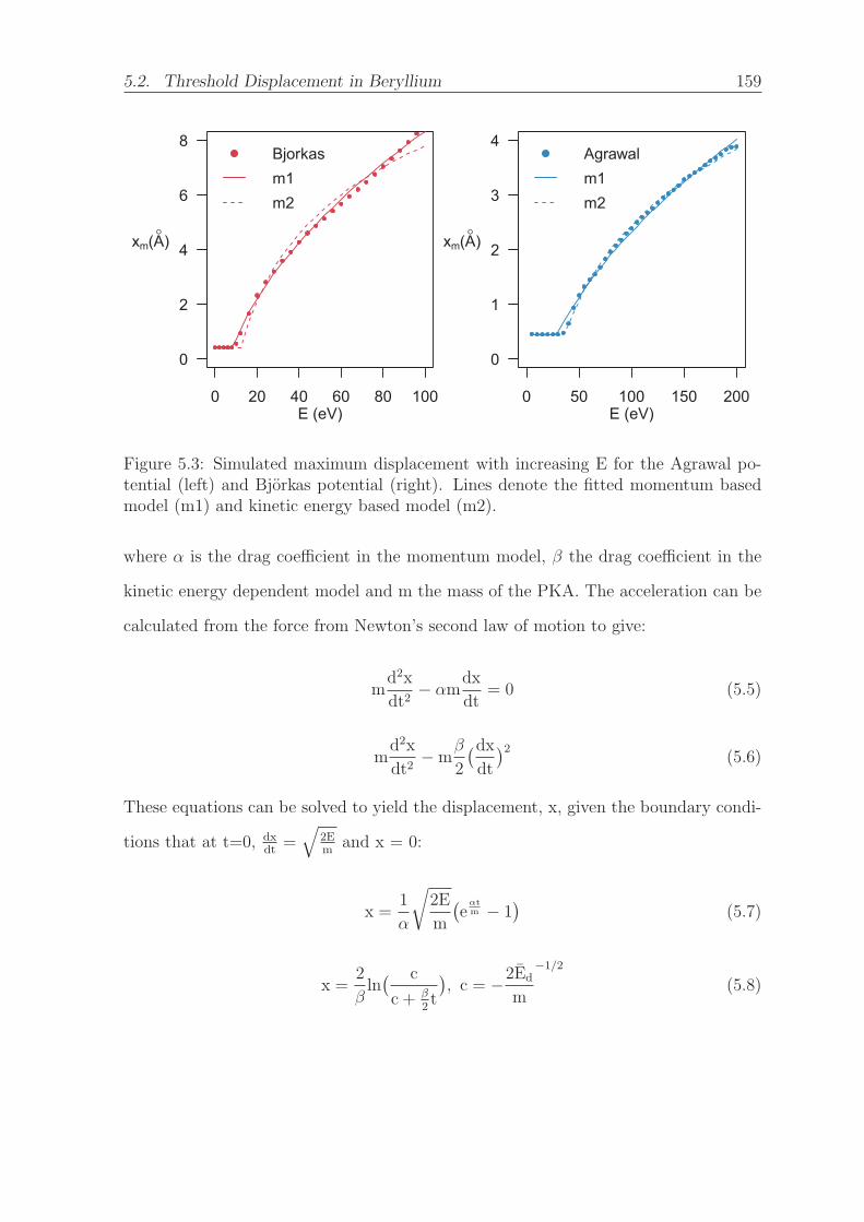
5.2. Threshold Displacement in Beryllium 159
0 20 40 60 80 100
0
2
4
6
8
E (eV)
xm(A° )
Bjorkasm1m2
0 50 100 150 200
0
1
2
3
4
E (eV)
xm(A° )
Agrawalm1m2
Figure 5.3: Simulated maximum displacement with increasing E for the Agrawal po-tential (left) and Bjorkas potential (right). Lines denote the fitted momentum basedmodel (m1) and kinetic energy based model (m2).
where α is the drag coefficient in the momentum model, β the drag coefficient in the
kinetic energy dependent model and m the mass of the PKA. The acceleration can be
calculated from the force from Newton’s second law of motion to give:
md2x
dt2− αm
dx
dt= 0 (5.5)
md2x
dt2−m
β
2
(dxdt
)2(5.6)
These equations can be solved to yield the displacement, x, given the boundary condi-
tions that at t=0, dxdt
=√
2Em
and x = 0:
x =1
α
√2E
m
(e
αtm − 1
)(5.7)
x =2
βln( c
c + β2t
), c = −2Ed
m
−1/2
(5.8)
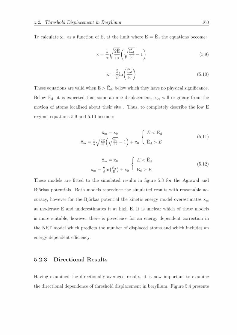
5.2. Threshold Displacement in Beryllium 160
To calculate xm as a function of E, at the limit where E = Ed the equations become:
x =1
α
√2E
m
(√Ed
E− 1
)(5.9)
x =2
βln
(Ed
E
)(5.10)
These equations are valid when E > Ed, below which they have no physical significance.
Below Ed, it is expected that some atomic displacement, x0, will originate from the
motion of atoms localised about their site . Thus, to completely describe the low E
regime, equations 5.9 and 5.10 become:
xm = x0
xm = 1α
√2Em
(√Ed
E− 1)+ x0
{E < Ed
Ed > E(5.11)
xm = x0
xm = 2βln(Ed
E
)+ x0
{E < Ed
Ed > E(5.12)
These models are fitted to the simulated results in figure 5.3 for the Agrawal and
Bjorkas potentials. Both models reproduce the simulated results with reasonable ac-
curacy, however for the Bjorkas potential the kinetic energy model overestimates xm
at moderate E and underestimates it at high E. It is unclear which of these models
is more suitable, however there is prescience for an energy dependent correction in
the NRT model which predicts the number of displaced atoms and which includes an
energy dependent efficiency.
5.2.3 Directional Results
Having examined the directionally averaged results, it is now important to examine
the directional dependence of threshold displacement in beryllium. Figure 5.4 presents

5.2. Threshold Displacement in Beryllium 161
stereographic projections in the [0001] direction of Edispd (θ, φ) and Edisp
d,50(θ, φ) for both
potentials, as well as Edefd (θ, φ) and Edef
d,50(θ, φ) for the Bjorkas potential. On first inspec-
tion, there are strong qualitative similarities for both potentials across all measures of
Ed. The directions with lowest Ed correspond to nearest neighbour directions: 〈1120〉in the basal plane and 〈2111〉 out of plane. This is consistent with the work of Thomas
et al. [212], who investigated Ed(θ, φ) in rutile using similar methodology. It was found
that displacement events in nearest neighbour directions caused a collision sequence
resulting in a larger separation of the interstitial-vacancy pair, which were thus more
likely to remain stable. Directions corresponding to glancing angle collisions have the
highest Ed across all measures and both potentials. Such collisions would effectively
divide the kinetic energy between the PKA and the impacted atom, thus dissipating
the energy in a small volume of material, not only making displacement less likely but
also promoting recombination.
Beyond the qualitative similarities, there are significant quantitative differences be-
tween the two sets of results. For the Agrawal potential, Edispd varies from 35 eV to 60
eV, while for the Bjorkas potential it varies from 8 to 20 eV. This is similar for Edispd,50,
which varies from 40 to 95 eV and 8 to 28 eV for the Agrawal and Bjorkas potential
respectively. Again, this may be explained by the relative “hardness” of the Agrawal
potential by comparison to the Bjorkas potential. Comparing Edispd and Edef
d for the
Bjorkas et al. potential, there is little quantative difference, however this is not the
case for Edispd,50 and Edef
d,50, with the latter covering a higher range of energies (12-55 eV
by comparison to 8-28 eV). This reflects the trends seen in the directionally averaged
results, and confirms that recombination is significant at high E, at least using the
Bjorkas potential.
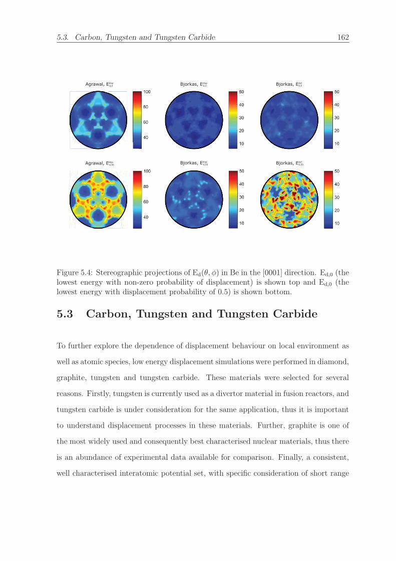
5.3. Carbon, Tungsten and Tungsten Carbide 162
Bjorkas, Edispd,0
Agrawal, Edispd,50
Agrawal, Edispd,0
Bjorkas, Edispd,50
Bjorkas, Edefd,0
Bjorkas, Edefd,50
Figure 5.4: Stereographic projections of Ed(θ, φ) in Be in the [0001] direction. Ed,0 (thelowest energy with non-zero probability of displacement) is shown top and Ed,0 (thelowest energy with displacement probability of 0.5) is shown bottom.
5.3 Carbon, Tungsten and Tungsten Carbide
To further explore the dependence of displacement behaviour on local environment as
well as atomic species, low energy displacement simulations were performed in diamond,
graphite, tungsten and tungsten carbide. These materials were selected for several
reasons. Firstly, tungsten is currently used as a divertor material in fusion reactors, and
tungsten carbide is under consideration for the same application, thus it is important
to understand displacement processes in these materials. Further, graphite is one of
the most widely used and consequently best characterised nuclear materials, thus there
is an abundance of experimental data available for comparison. Finally, a consistent,
well characterised interatomic potential set, with specific consideration of short range
5.3. Carbon, Tungsten and Tungsten Carbide 163
interactions, has been developed for the tungsten-carbon system by Juslin et al. [146]
for modelling nuclear fusion materials. This potential set is further part of an even
wider self-consistent potential set for all fusion materials: beryllium-tungsten-carbon-
hydrogen-helium (which includes the Bjorkas potential) leaving open the option of
extending this work to other fusion relevant materials.
5.3.1 Computational Details
Following from the experience of modelling threshold displacement in beryllium, the
same general methodology was used (i.e. supercells were set up and equilibrated in
the same way, and displacement simulations proceeded in the same manner). Like
for beryllium, supercells with approximately 5000 atoms and uniform dimensions were
created. For diamond this corresponds to an 8×8×8 supercell containing 4096 atoms,
BCC tungsten a 15×15×15 supercell containing 6750 atoms, and hexagonal tungsten
carbide a 14×14×14 supercell containing 5488 atoms. As mentioned in chapter 2, one
limitation of the Juslin potential is that it does not adequately describe Van-der-Waals
interactions, which are significant in graphite; they are the primary interactions be-
tween individual layers of graphene [164]. As a result, the way in which graphene sheets
slip over each other is not modelled well. As such, a larger graphite 24×24×7 supercell
containing 16128 atoms was used to limit slip as far as possible. Despite this, some
interlayer slip continued to occur, with the unintended consequence that no distinction
can be made between the two graphene sites in this model, as these sites differ only in
their position relative to carbon atoms in neighbouring graphene sheets.
To produce a representative sample of lattice directions, a geodesic projection of di-
rections with spacing of 6o was investigated. For all materials, at least double the
irreducible symmetry of the structure was simulated. For graphite and tungsten car-
5.3. Carbon, Tungsten and Tungsten Carbide 164
bide, this is from 0-120o θ and 0-90o φ, tungsten 0-90o θ and φ, and diamond 0-180o θ
and 0-90o φ.
Defects and displacements were detected in the same way as described for beryllium
in section 5.2.1. It should be noted, however, that because the magnitude of vibra-
tions within single graphene sheets in the graphite structure are often greater than
the nearest neighbour bond length, displacement detection based on maximum dis-
tance travelled is impossible in this structure. Further, given the large strain within
graphene sheets that these vibrations cause, the local tridimensional averaging method
of defect detection also proved unreliable. Instead, a simple coordination based ap-
proach, in which the local coordination environment is compared to the perfect cell,
was used to detect defects. Comparison to manual inspection of defect cells showed
perfect correspondence, thus this method can be considered to be reliable.
5.3.2 Directionally Averaged Results
Simulated results for Pdispd and Pdef
d as a function of E with the fitted Robinson model
are shown in figures 5.5.a and 5.5.b respectively. Edispd and Edef
d as calculated using the
fitted Robinson model are presented in table 5.1.
Observation of figure 5.5.a shows that the Robinson model closely reproduces the sim-
ulated Pdefd as a function of E. There are significant differences between the Pdef
d curves
for carbon in diamond, graphite and tungsten carbide, as well as for tungsten in BCC
tungsten and tungsten carbide. This leads to significantly different values of Edefd for
carbon in graphite (3.58 eV), diamond (19.8 eV) and tungsten carbide (22.2 eV), as
well as for tungsten in BCC tungsten (38.0 eV) and tungsten carbide (45.0 eV). This is
contrary to the common approximation that Ed is solely species dependent, and instead
suggests that it is also strongly dependent on the local environment of the displaced
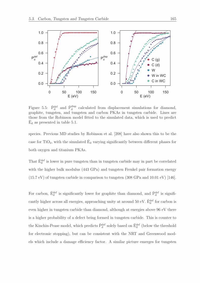
5.3. Carbon, Tungsten and Tungsten Carbide 165
0 50 100 150
0.0
0.2
0.4
0.6
0.8
1.0
E (eV)
Pddef
0 50 100 150
0.0
0.2
0.4
0.6
0.8
1.0
E (eV)
Pddisp
C (g)C (d)WW in WCC in WC
Figure 5.5: Pdefd and Pdisp
d calculated from displacement simulations for diamond,graphite, tungsten, and tungsten and carbon PKAs in tungsten carbide. Lines arethose from the Robinson model fitted to the simulated data, which is used to predictEd as presented in table 5.1.
species. Previous MD studies by Robinson et al. [208] have also shown this to be the
case for TiO2, with the simulated Ed varying significantly between different phases for
both oxygen and titanium PKAs.
That Edefd is lower in pure tungsten than in tungsten carbide may in part be correlated
with the higher bulk modulus (443 GPa) and tungsten Frenkel pair formation energy
(15.7 eV) of tungsten carbide in comparison to tungsten (308 GPa and 10.01 eV) [146].
For carbon, Edefd is significantly lower for graphite than diamond, and Pdef
d is signifi-
cantly higher across all energies, approaching unity at around 50 eV. Edefd for carbon is
even higher in tungsten carbide than diamond, although at energies above 96 eV there
is a higher probability of a defect being formed in tungsten carbide. This is counter to
the Kinchin-Pease model, which predicts Pdefd solely based on Edef
d (below the threshold
for electronic stopping), but can be consistent with the NRT and Greenwood mod-
els which include a damage efficiency factor. A similar picture emerges for tungsten
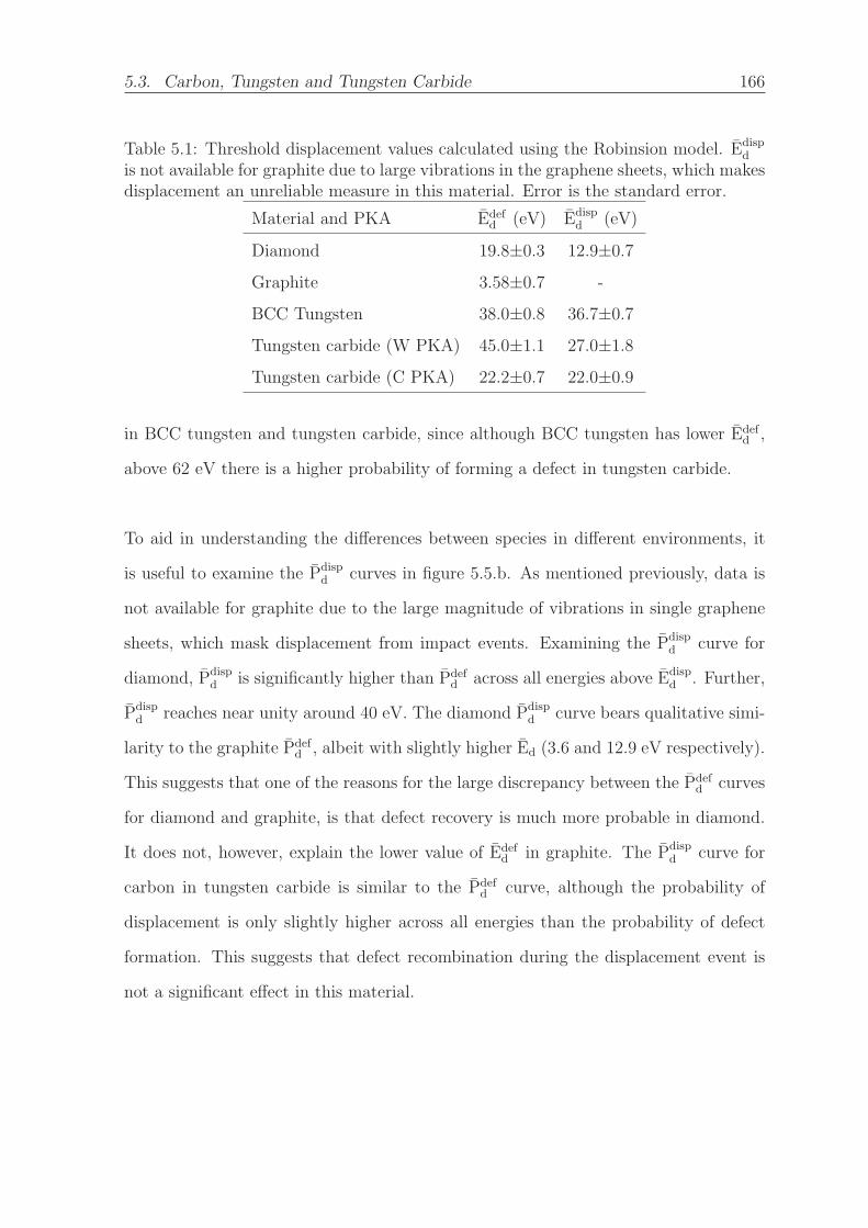
5.3. Carbon, Tungsten and Tungsten Carbide 166
Table 5.1: Threshold displacement values calculated using the Robinsion model. Edispd
is not available for graphite due to large vibrations in the graphene sheets, which makesdisplacement an unreliable measure in this material. Error is the standard error.
Material and PKA Edefd (eV) Edisp
d (eV)
Diamond 19.8±0.3 12.9±0.7
Graphite 3.58±0.7 -
BCC Tungsten 38.0±0.8 36.7±0.7
Tungsten carbide (W PKA) 45.0±1.1 27.0±1.8
Tungsten carbide (C PKA) 22.2±0.7 22.0±0.9
in BCC tungsten and tungsten carbide, since although BCC tungsten has lower Edefd ,
above 62 eV there is a higher probability of forming a defect in tungsten carbide.
To aid in understanding the differences between species in different environments, it
is useful to examine the Pdispd curves in figure 5.5.b. As mentioned previously, data is
not available for graphite due to the large magnitude of vibrations in single graphene
sheets, which mask displacement from impact events. Examining the Pdispd curve for
diamond, Pdispd is significantly higher than Pdef
d across all energies above Edispd . Further,
Pdispd reaches near unity around 40 eV. The diamond Pdisp
d curve bears qualitative simi-
larity to the graphite Pdefd , albeit with slightly higher Ed (3.6 and 12.9 eV respectively).
This suggests that one of the reasons for the large discrepancy between the Pdefd curves
for diamond and graphite, is that defect recovery is much more probable in diamond.
It does not, however, explain the lower value of Edefd in graphite. The Pdisp
d curve for
carbon in tungsten carbide is similar to the Pdefd curve, although the probability of
displacement is only slightly higher across all energies than the probability of defect
formation. This suggests that defect recombination during the displacement event is
not a significant effect in this material.
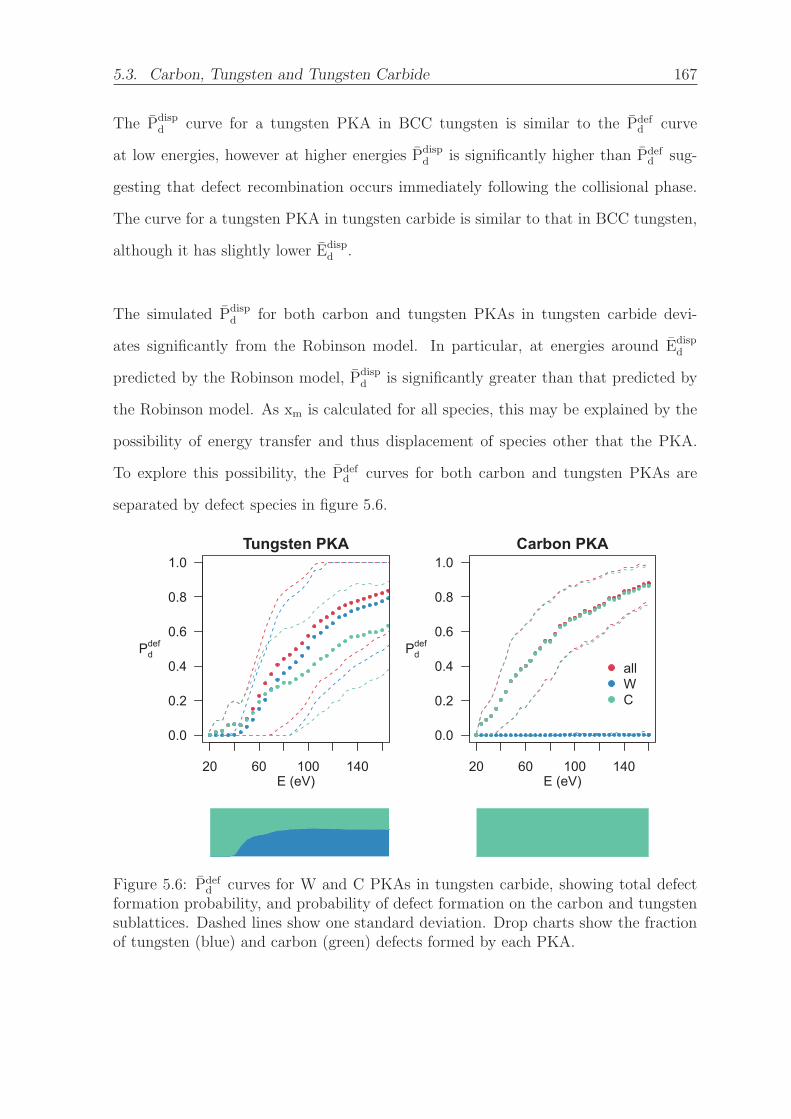
5.3. Carbon, Tungsten and Tungsten Carbide 167
The Pdispd curve for a tungsten PKA in BCC tungsten is similar to the Pdef
d curve
at low energies, however at higher energies Pdispd is significantly higher than Pdef
d sug-
gesting that defect recombination occurs immediately following the collisional phase.
The curve for a tungsten PKA in tungsten carbide is similar to that in BCC tungsten,
although it has slightly lower Edispd .
The simulated Pdispd for both carbon and tungsten PKAs in tungsten carbide devi-
ates significantly from the Robinson model. In particular, at energies around Edispd
predicted by the Robinson model, Pdispd is significantly greater than that predicted by
the Robinson model. As xm is calculated for all species, this may be explained by the
possibility of energy transfer and thus displacement of species other that the PKA.
To explore this possibility, the Pdefd curves for both carbon and tungsten PKAs are
separated by defect species in figure 5.6.
20 60 100 140
0.0
0.2
0.4
0.6
0.8
1.0Tungsten PKA
E (eV)
Pddef
20 60 100 140
0.0
0.2
0.4
0.6
0.8
1.0Carbon PKA
E (eV)
Pddef
allWC
Figure 5.6: Pdefd curves for W and C PKAs in tungsten carbide, showing total defect
formation probability, and probability of defect formation on the carbon and tungstensublattices. Dashed lines show one standard deviation. Drop charts show the fractionof tungsten (blue) and carbon (green) defects formed by each PKA.

5.3. Carbon, Tungsten and Tungsten Carbide 168
For a tungsten PKA, at low energies defect formation occurs exclusively on the car-
bon sublattice, while at higher energies defects are formed on both sublattices. This
is unsurprising given the significantly lower Edefd of carbon in tungsten carbide, and
further given the lower mass of carbon, should a tungsten PKA collide with carbon
in a head on collision, almost all its kinetic energy would be transferred. Conversely,
a carbon PKA only rarely causes tungsten displacements, as would be expected given
their relative mass and Edefd . As such, while this effect explains the deviation of the
simulated Pdispd data from the Robinson model for a tungsten PKA, the cause of the
deviation for a carbon PKA remains unexplained.
In order to examine the correspondence of simulated results with previous studies, sim-
ulated and experimental values of Ed are presented in table 5.2. The simulated value for
pure tungsten (38.0 eV) is similar to the experimental value (42.0 eV [213]), and lower
than for previous MD studies [214, 215]. The simulated value for diamond (19.8 eV) is
significantly lower than experimental values (35-47.6 eV [216, 217]), as is the simulated
value for graphite (3.58 eV by comparison to 30-35.3 eV [218]). Given that simulated
results are significantly lower for both carbon allotropes, this might be consistent with
the potential used being “softer” than the real energy surface. Examining final config-
urations for the graphite structure provides another potential reason for the low Edefd
value. All defects below 20 eV occur as an “intimate vacancy-interstitial pair” (in the
notation of [219]), whereby the PKA is displaced between the graphene sheets forming
tetrahedral coordination with the sheet above. Such defects have been observed to
form in previous threshold displacement simulations, and to have a formation energy
of 15.7 eV [219]. The major difference between these simulations and the simulations
performed herein, is that an additional force was applied between graphene sheets.
As such, it is possible that the lack of force between graphene sheets in these simu-
lations significantly reduces the formation energy of an intimate vacancy-interstitial
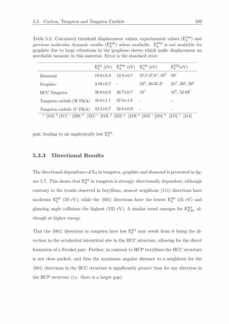
5.3. Carbon, Tungsten and Tungsten Carbide 169
Table 5.2: Calculated threshold displacement values, experimental values (Eexpd ) and
previous molecular dynamic results (EMDd ) where available. Edisp
d is not available forgraphite due to large vibrations in the graphene sheets which make displacement anunreliable measure in this material. Error is the standard error.
Edefd (eV) Edisp
d (eV) Eexpd (eV) EMD
d (eV)
Diamond 19.8±0.3 12.9±0.7 37.5-47.6a, 35b 50c
Graphite 3.58±0.7 - 33d, 30-35.3e 21f , 20g, 26h
BCC Tungsten 38.0±0.8 36.7±0.7 42i 41k, 52-68l
Tungsten carbide (W PKA) 45.0±1.1 27.0±1.8 - -
Tungsten carbide (C PKA) 22.2±0.7 22.0±0.9 - -
a [216] b [217] c [220] d [221] e [218] f [222] g [219] h [223] i [224] k [215] l [214]
pair, leading to an unphysically low Edefd .
5.3.3 Directional Results
The directional dependence of Ed in tungsten, graphite and diamond is presented in fig-
ure 5.7. This shows that Edefd in tungsten is strongly directionally dependent, although
contrary to the trends observed in beryllium, nearest neighbour 〈111〉 directions havemoderate Edef
d (50 eV), while the 〈001〉 directions have the lowest Edefd (35 eV) and
glancing angle collisions the highest (135 eV). A similar trend emerges for Edefd,50, al-
though at higher energy.
That the 〈001〉 directions in tungsten have low Edefd may result from it being the di-
rection to the octahedral interstitial site in the BCC structure, allowing for the direct
formation of a Frenkel pair. Further, in contrast to HCP beryllium the BCC structure
is not close packed, and thus the maximum angular distance to a neighbour for the
〈001〉 directions in the BCC structure is significantly greater than for any direction in
the HCP structure (i.e. there is a larger gap).

5.3. Carbon, Tungsten and Tungsten Carbide 170
diam
ond
Edis
pd,
0
diam
ond
Edis
pd,
50
tung
sten
Ede
fd,
0
tung
sten
Ede
fd,
50
diam
ond
Edef d,0
diam
ond
Edef d,50
grap
hite
Ede
fd,
0
grap
hite
Ede
fd,
50
Figure
5.7:
Stereographic
projectionsof
Edef
d(θ,φ
)in
the[0001]
direction
fortungsten,grap
hitean
ddiamon
d(E
disp
d(θ,φ
)an
dEdef
d(θ,φ
)).

5.3. Carbon, Tungsten and Tungsten Carbide 171
Examining the directional dependence of Edefd for graphite, results out of the (0001)
plane should be treated with caution, given the preclusion for graphene sheets to slide
over each other. It can be seen, however, than nearest 〈1010〉 neighbour directions
have the highest Edefd (18 eV), followed by other directions in the (0001) plane (16 eV),
whereas directions out of the (0001) plane have lower Edefd (3 eV), a trend replicated by
the Edefd,50 results. On examination of the final atomic configurations, it was found that
displacements out of plane result in the formation of “intimate vacancy-interstitial
pairs”, where the displaced atom is effectively pushed into tetrahedral coordination
with an atom in the neighbouring graphene sheets. Previous studies have calculated
the energy of such defects to be 15 eV [219], which is clearly inconsistent with the
minimum 3 eV Edefd observed here. The difference is likely to be as a result of the
inadequate description of interlayer forces, with the previous study adding an explicit
interlayer force term to compensate. The lack of such a force significantly decreases
the formation energy of the interstitial-vacancy pair, resulting in the abnormally low
threshold displacement energy.
For diamond, Edispd follows a similar trend to that observed for Edef
d in tungsten, with
Edispd moderate in 〈111〉 nearest neighbour directions (28 eV), lowest in directions far
from nearest neighbour (16 eV) and highest at glancing angles (36 eV), with the effect
even more pronounced for Edispd,50. Comparing with Edef
d , there is no clear distinction
between nearest neighbour and glancing angle collisions, although directions far from
nearest neighbours still have lowest Edefd . This is consistent with the hypothesis that
glancing angle collisions promote defect recovery. Edefd,50 follows similar trends to Edef
d ,
albeit with much higher energy (30-160 eV) and with significantly more scatter in the
data. That this is significantly higher than Edispd,50 confirms that in these simulations
significant defect recombination occurs at higher energies.
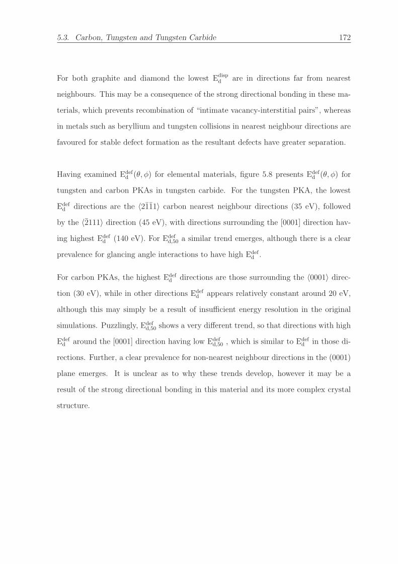
5.3. Carbon, Tungsten and Tungsten Carbide 172
For both graphite and diamond the lowest Edispd are in directions far from nearest
neighbours. This may be a consequence of the strong directional bonding in these ma-
terials, which prevents recombination of “intimate vacancy-interstitial pairs”, whereas
in metals such as beryllium and tungsten collisions in nearest neighbour directions are
favoured for stable defect formation as the resultant defects have greater separation.
Having examined Edefd (θ, φ) for elemental materials, figure 5.8 presents Edef
d (θ, φ) for
tungsten and carbon PKAs in tungsten carbide. For the tungsten PKA, the lowest
Edefd directions are the 〈2111〉 carbon nearest neighbour directions (35 eV), followed
by the 〈2111〉 direction (45 eV), with directions surrounding the [0001] direction hav-
ing highest Edefd (140 eV). For Edef
d,50 a similar trend emerges, although there is a clear
prevalence for glancing angle interactions to have high Edefd .
For carbon PKAs, the highest Edefd directions are those surrounding the 〈0001〉 direc-
tion (30 eV), while in other directions Edefd appears relatively constant around 20 eV,
although this may simply be a result of insufficient energy resolution in the original
simulations. Puzzlingly, Edefd,50 shows a very different trend, so that directions with high
Edefd around the [0001] direction having low Edef
d,50 , which is similar to Edefd in those di-
rections. Further, a clear prevalence for non-nearest neighbour directions in the (0001)
plane emerges. It is unclear as to why these trends develop, however it may be a
result of the strong directional bonding in this material and its more complex crystal
structure.
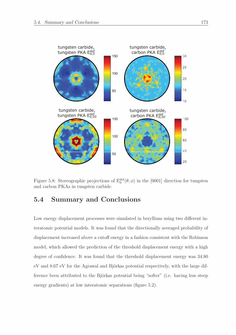
5.4. Summary and Conclusions 173
tungsten carbide,tungsten PKA Edef
d,0
tungsten carbide,tungsten PKA Edef
d,50
tungsten carbide,carbon PKA Edef
d,0
tungsten carbide,carbon PKA Edef
d,50
Figure 5.8: Stereographic projections of Edefd (θ, φ) in the [0001] direction for tungsten
and carbon PKAs in tungsten carbide.
5.4 Summary and Conclusions
Low energy displacement processes were simulated in beryllium using two different in-
teratomic potential models. It was found that the directionally averaged probability of
displacement increased above a cutoff energy in a fashion consistent with the Robinson
model, which allowed the prediction of the threshold displacement energy with a high
degree of confidence. It was found that the threshold displacement energy was 34.80
eV and 8.67 eV for the Agrawal and Bjorkas potential respectively, with the large dif-
ference been attributed to the Bjorkas potential being “softer” (i.e. having less steep
energy gradients) at low interatomic separations (figure 5.2).

5.4. Summary and Conclusions 174
Although not investigated for the Agrawal potential, for the Bjorkas potential, at
higher energies there is a significant difference between the probability of displacement
and the probability to form a defect, suggesting significant defect recombination im-
mediately following the displacement event. The threshold energy for defect formation
predicted using the Bjorkas potential is 9.15 eV, which is consistent with other work
that has used this potential but significantly lower than the 20 eV value predicted by
ab-initio simulations (although the methodology of the study in question is predisposed
to calculate higher threshold energies). Further, it is lower than the value commonly
used in the SRIM code (25 eV) which has implications for its predictions when applied
to beryllium.
The directional dependence of threshold displacement in beryllium with respect to
the crystallographic lattice was also investigated. For both potentials, it was found
that the 〈1010〉 and 〈2111〉 families of nearest neighbour directions have the lowest
threshold displacement and (for the Bjorkas potential) threshold defect formation en-
ergies, while directions representing glancing angle collisions to these directions have
the highest values. This was also true for the threshold at which there is a 50% chance
of a defect forming, although there is significantly more scatter in that data. These
results are consistent with the work of Bodorin et al. [211].
Displacement processes were also investigated in other fusion materials, namely carbon
(both diamond and graphite), tungsten and tungsten carbide, in order to interrogate
the common assumption that threshold displacement energy is solely species depen-
dent. It was found that carbon has significantly different threshold defect formation
energy in graphite (3.58 eV) in comparison to diamond (19.8 eV) and tungsten carbide
(22.5 eV), as does tungsten in BCC tungsten (38.0 eV) and tungsten carbide (45.0 eV).
5.4. Summary and Conclusions 175
The reason for such a significant difference between carbon in graphite and diamond,
and further the anonymously low value for graphite in comparison to experimental re-
sults, may be a result of inadequacies in the potential model. In particular, the model
used does not account for interlayer forces between graphene sheets, which significantly
reduces the formation energy of “intimate vacancy-interstitial pairs”, where the inter-
stitial sits is in tetrahedral coordination between graphene planes. Further, significant
defect combination is hypothesised to occur in the post ballistic phase in diamond,
given the significant difference between the probability of displacement and of defect
formation for this material at higher energies.
Directional dependence of threshold displacement and defect formation was investi-
gated in these materials. For BCC tungsten, it was found that unlike beryllium, near-
est neighbour 〈111〉 directions have moderate threshold displacement energy, although
directions indicating glancing angle collisions also have high threshold displacement
energy. The lowest threshold displacement (and defect formation energies) are the
〈001〉 directions, which correspond to the direction towards the octahedral interstitial
site and is the furthest from nearest neighbour directions. Diamond showed a similar
trend, with nearest neighbour directions having moderate threshold displacement and
defect formation energies, while glancing angle directions have the highest. Graphite,
due to the low formation barrier to intimate vacancy-interstitial pairs, has lowest dis-
placement energy out of the graphene plane, although this may be a consequence of
the limitations of the potential model used.
In addition, two new models to describe the maximum displacement of a PKA for
a given primary knock on energy have been developed. These models are based on
energy dependent and momentum dependent homogeneous drag models, and have
precedent in the Robinson model for displacement probability, and the NRT model for
5.4. Summary and Conclusions 176
the number of displacements as a function of energy. Both the developed models are
in good agreement for the simulated data for all materials and PKAs, and as such it
is currently not clear which describes the average effect better.
Directional dependence of threshold displacement and defect formation energies in
tungsten carbide is somewhat more complicated. For a tungsten PKA, the lowest
threshold displacement directions are the 〈2111〉 directions, corresponding to carbon
nearest neighbours, while the highest are those that cause glancing angle collisions to
the tungsten {1010} nearest neighbours. For a carbon PKA, the highest threshold
displacement directions are those surrounding the 〈0001〉 directions, while the study
used insufficient energy resolution to resolve clear trends across other parts of the stere-
ographic projection. Curiously, this trend is inverted when examining the threshold
at which there is a 50% chance of defect formation, where these directions have low
threshold energy, and further nearest neighbour tungsten atoms have the highest val-
ues. The reason for this remains unexplained, however it is possibly a result of the
(more) complex tungsten carbide structure and the presence of strongly directional
semi-covalent bonds.
The main practical implications of this work are that the large differences in displace-
ment behaviour between the two interatomic potentials for beryllium, as well as the
shortcomings of the potential used to describe graphite, highlight how sensitive dis-
placement behaviour is to the potential used. Potentials must therefore be thoroughly
characterised and validated before future displacement or cascade simulations are per-
formed. Further, the strong directional dependence predicted for displacement suggests
that when investigating single crystals experimentally, should a tool such as SRIM be
used to predict defect populations, this directional dependence should be considered.
Finally, significant differences were observed between the threshold displacement ener-

5.4. Summary and Conclusions 177
gies of both tungsten and carbon in different structures. This is consistent with the
work of Robinson et al. [208] in TiO2, confirming that threshold displacement energy is
a function of the local environment of the displaced species and undermines the com-
mon approximation that threshold displacement energy is solely species dependent.

Chapter 6
Ongoing and Future Work
6.1 Inelastic Neutron Scattering
Further work should be carried out to better characterise the broadening functions
of the Taipan instrument, as the good resolution of the experimental results suggests
that at present, the instrument broadening effect has been overestimated. It would
be useful to undertake additional studies of materials where no peaks are predicted
by DFT simulations in the low energy regime, in order to evaluate whether second
order reflections consistently provide better energy resolution than first order. If this is
indeed the case, the effect may be used to increase energy resolution in future neutron
scattering studies.
To better characterise the Be12M and Be13M materials investigated herein, it would
also be useful to perform inelastic neutron scattering on single crystal samples in order
to observe the phonon dispersion, however the difficulties in obtaining, and working
with, single crystals of these materials makes this unlikely. In addition, as DFT is
known to have errors of 1-2% in the predicted lattice parameter, it may be possible
178
6.2. Point Defects and Phase Stability in Beryllides 179
to improve correspondence between the DFT and experimental results by scaling the
DFT results by the experimental lattice parameter as appropriate.
6.2 Point Defects and Phase Stability in Beryllides
Having investigated point defects and small clusters in Be12M materials, the next step
is to simulate larger clusters, voids and extended defects, in order to better understand
the thermodynamics and kinetics of how these defects form. To aid in this, it may
also be necessary to develop empirical potentials capable of modelling these systems
as DFT is limited to small supercells (<400 atoms). Bjorkas et al. [161] has developed
a Be-W potential that provides a reasonable description of Be12W, however at present
it has not been possible to reproduce these results in the LAMMPS code [171]. The
development of such potentials would also open the possibility of simulating damage
cascades and extended defects.
In the near term, the present defect calculations may be improved upon by using
the harmonic and quasiharmonic approximations to calculate the contributions of vi-
brational enthalpy and entropy to the free energy. This would allow more accurate
predictions of properties derived from defect calculations at temperature, which is par-
ticularly important for the determination of non-stoichiometry.
The present results may also be used for Monte Carlo transport simulations, particu-
larly for cluster migration. Accelerated dynamics may also be useful to study migration,
as it can investigate complex migration mechanisms, which might be difficult to iden-
tify conventionally.
In addition to intrinsic defects, an examination of extrinsic defects should also be
performed. In particular, the accommodation of radiogenic H and He should be in-

6.3. Threshold Displacement 180
vestigated, although some investigations have already been made in Be12Ti [91] and
Be12W [96]. Many of the common impurities in beryllium [76] would also be expected
to be present in Be12M materials, and should be investigated. These include oxygen,
iron, uranium, carbon, silicon and aluminium.
Given that Be12Mo and Be12W have been shown to be unsuitable for neutron multiply-
ing applications from a neutronic perspective, Be22W and Be22Mo should be considered
more fully. This would include point defect calculations and a determination of the
degree of nonstochiometry.
6.3 Threshold Displacement
The work presented in chapter 5 has identified several trends with respect to the spatial
dependence of threshold displacement, and the dependence on local environment. It
would be useful to test the general applicability of these trends by extending the sys-
tematic approach to other materials, for which well characterised empirical potential
sets are available. In particular, other BCC and HCP metals may offer useful com-
parison with tungsten and beryllium respectively, and many have nuclear applications
(e.g. iron and zirconium). This may also aid in the models developed for maximum
displacement.
It is also planned to extend displacement simulations to higher energies (1 keV-1 MeV)
in the materials studied (with the exception of graphite), to test the validity of models
due to Kinchin-Pease [225], Norgett-Robinson-Torrens [106] and Greenwood [107]. At
these energies, electronic stopping may become significant, therefore the two tempera-
ture model should be parameterised and applied.
Finally, it is also envisaged that high energy displacement events will be simulated

6.3. Threshold Displacement 181
repeatedly in single supercells of tungsten, tungsten carbide and diamond, in order to
investigate how much energy may be stored in these materials (analogous to Wigner
energy in graphite).
Modelling graphite remains a challenge for empirical potentials but also for QM sim-
ulations. The work of Telling et al. [226] provides a good starting point to take such
work forward.

Bibliography
[1] International Energy Agency, “Key World Energy Statistics 2016,” tech. rep.,
International Energy Agency, Paris, 2016.
[2] R. A. Eggleton, A short introduction to climate change. Cambridge University
Press, 2013.
[3] “ESRL Global Monitoring Division - Global Greenhouse Gas Reference Net-
work,” 2017.
[4] J. Hansen, R. Ruedy, M. Sato, and K. Lo, “GLOBAL SURFACE TEMPERA-
TURE CHANGE,” Reviews of Geophysics, vol. 48, p. RG4004, dec 2010.
[5] N. Nakicenovic, “Special report on emissions scenarios : a special report of Work-
ing Group III of the Intergovernmental Panel on Climate Change,” tech. rep.,
2000.
[6] World Health Organization, Ambient Air Pollution: A global assessment of ex-
posure and burden of disease. 2016.
[7] K. Seyboth, F. Sverrisson, F. Appavou, A. Brown, B. Epp, A. Leidreiter, C. Lins,
E. Musolino, H. E. Murdock, K. Petrichenko, T. C. Farrell, T. T. Krader,
A. Tsakiris, J. L. Sawin, J. Skeen, and B. Sovacool, Renewables 2016 Global
Status Report. 2016.
182
BIBLIOGRAPHY 183
[8] “Digest of United Kingdom Energy Statistics (DUKES) 2016,” tech. rep., De-
partment for Business, Energy and Industrial Stratergy, London, 2016.
[9] IEA, “Electricity Information,” IEA Statistics, pp. 1–708, 2013.
[10] M. Wang, G. Audi, A. Wapstra, F. Kondev, M. MacCormick, X. Xu, and
B. Pfeiffer, “The Ame2012 atomic mass evaluation,” Chinese Physics C, vol. 36,
pp. 1603–2014, dec 2012.
[11] IAEA, “Nuclear Power Reactors in the World,” Tech. Rep. 2, 2016.
[12] V. Apalin, Y. Gritsyuk, I. Kutikov, V. Lebedev, and L. Mikaelyan, “On the
number of neutrons emitted by U235 fission fragments,” Nuclear Physics, vol. 55,
pp. 249–256, jun 1964.
[13] “Evaluated and Compiled Nuclear Structure Data: ENSDF Dataset Retrieval,”
2017.
[14] W. P. Poenitz, “Measurements of the Neutron Capture Cross Sections of Gold-
197 and Uranium-238 Between 20 and 3500 keV,” Nuclear Science and Engineer-
ing, vol. 57, no. 4, pp. 300–308, 1975.
[15] R. J. M. Konings, T. R. Allen, R. E. Stoller, and S. Yamanaka, Comprehensive
Nuclear Materials. Elsevier Ltd., Amsterdam, Netherlands, 1 ed., 2012.
[16] J. Wood, “Nuclear Power,” 2006.
[17] J. Mahaffey, “Atomic Accidents: A History of Nuclear Meltdowns and Disasters:
From the Ozark Mountains to Fukushima,” 2014.
[18] Exposure of the American People to Iodine-131 from Nevada Nuclear-Bomb Tests:
Review of the National Cancer Institute Report and Public Health Implications.
Washington: National Academy Press, 1999.
BIBLIOGRAPHY 184
[19] M. Schneider, A. Froggatt, J. Hazemann, T. Katsuta, and S. Thomas, “The
World Nuclear Industry: Status Report 2015,” tech. rep., World Nuclear Report,
Paris, London, 2015.
[20] M. Ojovan and W. Lee, An Introduction to Nuclear Waste Immobilisation. Else-
vier, 2014.
[21] OECD, Public Attitudes to Nuclear Power. No. 6859, 2010.
[22] L. Schmidt and A. Horta, “Comparative Analysis of the public discourse about
fusion and nuclear energy before and after Fukushima,” pp. 1–56, 2013.
[23] J. D. Lawson, “Some Criteria for a Power Producing Thermonuclear Reactor,”
Proceedings of the Physical Society. Section B, vol. 70, pp. 6–10, jan 1957.
[24] J. C. Maxwell, “Illustrations of the Dynamical Theory of Gases. Part I . On
the Motions and Collisions of Perfectly Elastic Spheres,” Philosophical Magazine
Series 4, vol. 19, no. 124, pp. 19–32, 1860.
[25] H. S. Bosch and G. M. Hale, “Improved formulas for fusion cross-sections and
thermal reactivities,” Nuclear Fusion, vol. 33, pp. 1919–1919, dec 2002.
[26] A. S. Eddington, “The internal constitution of the stars,” The Scientific Monthly,
vol. 11, no. 4, pp. 297–303, 1920.
[27] H. A. Bethe, “Energy Production in Stars,” Physical Review, vol. 55, pp. 434–456,
mar 1939.
[28] S. Basu, W. J. Chaplin, Y. Elsworth, R. New, and A. M. Serenelli, “Fresh Insights
on the Structure of the Solar Core,” The Astrophysical Journal, vol. 699, p. 1403,
jul 2009.

BIBLIOGRAPHY 185
[29] D. D. Clayton, Principles of stellar evolution and nucleosynthesis. Chicago, Lon-
don: The University of Chicago Press, 1968.
[30] M. L. E. Oliphant and E. Rutherford, “Experiments on the Transmutation of El-
ements by Protons,” Proceedings of the Royal Society A: Mathematical, Physical
and Engineering Sciences, vol. 141, no. 843, pp. 259–281, 1933.
[31] R. Rhodes, Dark Sun: The Making Of The Hydrogen Bomb. 1995.
[32] J. H. Nuckolls, “Early Steps Toward Inertial Fusion Enerfy,” tech. rep., Lawrence
Livermore National Laboratory (LLNL), Livermore, CA, jun 1998.
[33] G. Brumfiel, “Laser fusion put on slow burn,” Nature, dec 2012.
[34] L. Suter, J. Rothenberg, and D. Munro, “Feasibility of High Yield/High Gain
NIF capsules,” in Ist International Conference on Inertial Fusion Sciences and
Applications, pp. 1–8, 1999.
[35] D. H. Crandall, “External Review of the National Ignition Campaign,” pp. 1–7,
2012.
[36] A. Piel, Plasma Physics, vol. 2. Kiel: Springer, 2 ed., 2010.
[37] R. B. White, The Theory of Toroidally Confined Plasmas. London: Imperial
College Press, 2nd ed., 2013.
[38] A. Gibson, “Deuterium Tritium Plasmas in the Joint European Torus (JET):
Behavior and Implications,” Physics of Plasmas, vol. 5, no. 5, p. 1839, 1998.
[39] IAEA, “Agreement on the Establishment of the ITER International Fusion En-
ergy Organization for the Joint Implementation of the ITER Project,” 2007.
[40] ITER Organization, “What is ITER?,” 2016.

BIBLIOGRAPHY 186
[41] D. Stork, “DEMO and the Route to Fusion Power,” Atw. Internationale
Zeitschrift fuer Kernenergie, vol. 53, no. 10, pp. 631–634, 2009.
[42] ITER Organization, “The Machine,” 2017.
[43] J. Roth, E. Tsitrone, A. Loarte, T. Loarer, G. Counsell, R. Neu, V. Philipps,
S. Brezinsek, M. Lehnen, P. Coad, C. Grisolia, K. Schmid, K. Krieger, A. Kallen-
bach, B. Lipschultz, R. Doerner, R. Causey, V. Alimov, W. Shu, O. Ogorod-
nikova, A. Kirschner, G. Federici, and A. Kukushkin, “Recent analysis of key
plasma wall interactions issues for ITER,” Journal of Nuclear Materials, vol. 390-
391, pp. 1–9, jun 2009.
[44] D. R. Harries, G. J. Butterworth, A. Hishinuma, and F. W. Wiffen, “Evalua-
tion of reduced-activation options for fusion materials development,” Journal of
Nuclear Materials, vol. 191-194, no. 1, pp. 92–99, 1992.
[45] A. Widdowson, A. Baron-Wiechec, P. Batistoni, E. Belonohy, J. P. Coad,
P. Dinca, D. Flammini, F. Fox, K. Heinola, I. Jepu, J. Likonen, S. Lilley, C. P.
Lungu, G. F. Matthews, J. Naish, O. Pompilian, C. Porosnicu, M. Rubel, and
R. Villari, “Experience of handling beryllium, tritium and activated components
from JET ITER like wall,” Physica Scripta, vol. 167, p. 57, feb 2016.
[46] G. F. Matthews, “Plasma operation with an all metal first-wall: Comparison of
an ITER-like wall with a carbon wall in JET,” Journal of Nuclear Materials,
vol. 438, pp. 2–10, jul 2013.
[47] K. Ioki, V. Barabash, A. Cardella, F. Elio, Y. Gobar, G. Janeschitz, G. Johnson,
G. Kalinin, D. Lousteau, M. Onozuka, R. Parker, G. Sannazzaro, and R. Tivey,
“Design and material selection for ITER first wall/blanket, divertor and vacuum
vessel,” Journal of Nuclear Materials, vol. 258, pp. 74–84, oct 1998.
BIBLIOGRAPHY 187
[48] M. Kaufmann and R. Neu, “Tungsten as first wall material in fusion devices,”
Fusion Engineering and Design, vol. 82, pp. 521–527, oct 2007.
[49] Iter, “Divertor qualification phase well on track,” 2008.
[50] H. Bolt, V. Barabash, G. Federici, J. Linke, A. Loarte, J. Roth, and K. Sato,
“Plasma facing and high heat flux materials - Needs for ITER and beyond,”
Journal of Nuclear Materials, vol. 307-311, pp. 43–52, dec 2002.
[51] K. Korniyenko, “Carbon - Iron - Tungsten,” in Iron Systems Part 2, pp. 476–512,
Springer, 2008.
[52] R. W. Powell, C. Y. Ho, and P. E. Liley, “Thermal conductivity of selected mate-
rials,” National Standard Reference Data Series\-National Bureau of Standards
8, pp. 93–96, 1966.
[53] F. C. Nix and D. MacNair, “The thermal expansion of pure metals. II: Molyb-
denum, palladium, silver, tantalum, tungsten, platinum, and lead,” Physical Re-
view, vol. 61, pp. 74–78, jan 1942.
[54] S. Willms, “Tritium Supply Considerations,” in Atomic Energy, pp. 1–16, Los
Alamos National Laboratory, 2003.
[55] K. Tobita, H. Utoh, C. Liu, H. Tanigawa, D. Tsuru, M. Enoeda, T. Yoshida,
and N. Asakura, “Search for reality of solid breeder blanket for DEMO,” Fusion
Engineering and Design, vol. 85, pp. 1342–1347, dec 2010.
[56] H. Yamada, Y. Nagao, H. Kawamura, M. Nakao, M. Uchida, and H. Ito, “Prelim-
inary neutronic estimation for demo blanket with beryllide,” Fusion Engineering
and Design, vol. 69, pp. 269–273, sep 2003.
[57] T. Ihli, T. Basu, L. Giancarli, S. Konishi, S. Malang, F. Najmabadi, S. Nishio,
A. Raffray, C. Rao, A. Sagara, and Y. Wu, “Review of blanket designs for ad-

BIBLIOGRAPHY 188
vanced fusion reactors,” Fusion Engineering and Design, vol. 83, no. 7, pp. 912–
919, 2008.
[58] Y. W. Yang and P. Coppens, “The electron density and bonding in beryllium
metal as studied by Fourier methods,” Acta Crystallographica Section A, vol. 34,
pp. 61–65, jan 1978.
[59] J. C. Foley, S. P. Abeln, P. W. Stanek, B. D. Bartram, V. D. Vargas, and B. Aikin,
“An Overview of Current Research and Industrial Practices of Be Powder Metal-
lurgy,” in Materials Science and Technology, (Hoboken, NJ, USA), p. 3097, John
Wiley & Sons, Inc., jun 2003.
[60] J. Emsley, Nature’s building blocks : everything you need to know about the ele-
ments. Oxford University Press, 2011.
[61] P. K. Henneberger, S. K. Goe, W. E. Miller, B. Doney, and D. W. Groce, “Indus-
tries in the United States with Airborne Beryllium Exposure and Estimates of
the Number of Current Workers Potentially Exposed,” Journal of Occupational
and Environmental Hygiene, vol. 1, pp. 648–659, oct 2004.
[62] H. G. van Oss, “U.S. Geological Survey, Mineral Commodity Summaries, January
2016,” tech. rep., 2013.
[63] M. E. Kolanz, “Introduction to Beryllium: Uses, Regulatory History, and Dis-
ease,” Applied Occupational and Environmental Hygiene, vol. 16, pp. 559–567,
may 2001.
[64] T. A. Tomberlin, “Beryllium A Unique Material In Nuclear Applications,” tech.
rep., 2004.
[65] S. D. Schmid, Producing Power: The Pre-Chernobyl History of the Soviet Nuclear
Industry. 2015.
BIBLIOGRAPHY 189
[66] W. C. Moore, “Maritime Gas-Cooled Reactor Program,” jul 1961.
[67] W. H. Robbins and H. B. Finger, “An Historical Perspective of the NERVA
Nuclear Rocket Engine Technology Program,” Tech. Rep. July, NASA, Cleveland,
1991.
[68] W. Taylor and A. Moore, “Tensile deformation modes in polycrystalline beryllium
near the ductile-brittle transition,” Journal of Nuclear Materials, vol. 13, pp. 23–
27, jan 1964.
[69] R. W. Armstrong, “Theory of the tensile ductile-brittle behavior of poly-
crystalline h.c.p. materials, with application to beryllium,” Acta Metallurgica,
vol. 16, pp. 347–355, mar 1968.
[70] M. Dalle Donne, F. Scaffidi-Argentina, C. Ferrero, and C. Ronchi, “Modelling of
swelling and tritium release in irradiated beryllium,” Journal of Nuclear Materi-
als, vol. 212-215, pp. 954–960, sep 1994.
[71] T. V. Kulsartov, Y. N. Gordienko, I. L. Tazhibayeva, E. A. Kenzhin, N. I. Bar-
sukov, A. O. Sadvakasova, A. V. Kulsartova, and Z. A. Zaurbekova, “Tritium
migration in the materials proposed for fusion reactors: Li2TiO3 and beryllium,”
Journal of Nuclear Materials, vol. 442, pp. 740–745, nov 2013.
[72] S. Carpentier, R. A. Pitts, P. C. Stangeby, J. D. Elder, A. S. Kukushkin, S. Lisgo,
W. Fundamenski, and D. Moulton, “Modelling of beryllium erosion-redeposition
on ITER first wall panels,” in Journal of Nuclear Materials, vol. 415, pp. 165–169,
aug 2011.
[73] F. Scaffidi-Argentina, “Tritium and helium release from neutron irradiated beryl-
lium pebbles from the EXOTIC-8 irradiation,” Fusion Engineering and Design,
vol. 58-59, pp. 641–645, nov 2001.
BIBLIOGRAPHY 190
[74] E. Rabaglino, C. Ronchi, and A. Cardella, “Recent progress in the modelling of
helium and tritium behaviour in irradiated beryllium pebbles,” Fusion Engineer-
ing and Design, vol. 69, pp. 455–461, sep 2003.
[75] D. M. Duffy, “Modelling materials for fusion power,” International Materials
Reviews, vol. 56, pp. 324–340, nov 2011.
[76] S. C. Middleburgh and R. W. Grimes, “Defects and transport processes in beryl-
lium,” Acta Materialia, vol. 59, pp. 7095–7103, oct 2011.
[77] A. Allouche, M. Oberkofler, M. Reinelt, and C. Linsmeier, “Quantum Modeling
of Hydrogen Retention in Beryllium Bulk and Vacancies,” Journal of Physical
Chemistry C, vol. 114, pp. 3588–3598, mar 2010.
[78] P. A. P. Burr, S. C. S. Middleburgh, and R. R. W. Grimes, “Crystal structure,
thermodynamics, magnetics and disorder properties of Be-Fe-Al intermetallics,”
Journal of Alloys and Compounds, vol. 639, pp. 111–122, jul 2014.
[79] M. Ganchenkova, V. Borodin, and R. Nieminen, “Hydrogen in beryllium: Solu-
bility, transport, and trapping,” Physical Review B, vol. 79, pp. 1–11, apr 2009.
[80] P. Zhang, J. Zhao, and B. Wen, “Retention and diffusion of H, He, O, C impurities
in Be,” Journal of Nuclear Materials, vol. 423, pp. 164–169, apr 2012.
[81] V. A. Borodin and P. V. Vladimirov, “Molecular Dynamics Simulation of Atomic
Displacement Cascades in Beryllium,” in Proceedings of the 11th IEA Interna-
tional Workshop on Beryllium Technology (BeWS-11), (Barcelona), p. 236, KIT
Scientific Publishing, 2013.
[82] J. Reimann, P. Kurinskiy, R. Lindau, A. Moeslang, M. Rohde, C. Dorn, W. Haws,
A. Goraieb, H. Harsch, and C. Linsmeier, “Beryllides for fusion reactors,” in 23rd
IEEE/NPSS Symposium on Fusion Engineering, pp. 1–4, IEEE, jun 2009.

BIBLIOGRAPHY 191
[83] T. Tokunaga, H. Ohtani, and M. Hasebe, “Thermodynamic evaluation of the
phase equilibria and glass-forming ability of the TiBe system,” Journal of Phase
Equilibria and Diffusion, vol. 27, pp. 83–91, feb 2006.
[84] K.-J. Jang, J.-H. Jung, D.-M. Kim, J.-S. Yu, and J.-Y. Lee, “Self-discharge mech-
anism of VanadiumTitanium metal hydride electrodes for NiMH rechargeable
battery,” Journal of Alloys and Compounds, vol. 268, pp. 290–294, mar 1998.
[85] R. W. Cahn, “Binary Alloy Phase Diagrams-Second edition,” Advanced Materi-
als, vol. 3, pp. 628–629, dec 1991.
[86] K. Nakashima, T. Tokunaga, H. Ohtani, and M. Hasebe, “Thermodynamic Anal-
ysis of the Be-Mo Binary Phase Diagram,” Journal of the Japan Institute of,
2007.
[87] A. Allouche and C. Linsmeier, “Quantum study of tungsten interaction with
beryllium (0001),” Journal of Physics: Conference Series, vol. 117, p. 012002,
jun 2008.
[88] F. W. Von Batchelder and R. F. Raeuchle, “The structure of a new series of M
Be12 compounds,” Acta Crystallographica, vol. 10, pp. 648–649, oct 1957.
[89] A. Zalkin, D. E. Sands, R. G. Bedford, and O. H. Krikorian, “The beryllides of
Ti, V, Cr, Zr, Nb, Mo, Hf and Ta,” Acta Crystallographica, vol. 14, pp. 63–65,
jan 1961.
[90] M. Nakamichi, J. H. Kim, and M. Miyamoto, “Fabrication and characterization of
advanced neutron multipliers for DEMO blanket,” Nuclear Materials and Energy,
vol. 9, pp. 55–58, 2016.
BIBLIOGRAPHY 192
[91] Y. Fujii, M. Miyamoto, J. Kim, M. Nakamichi, N. Murayoshi, and H. Iwakiri,
“Hydrogen retention behavior of beryllides as advanced neutron multipliers,”
Nuclear Materials and Energy, vol. 9, pp. 233–236, 2015.
[92] A. V. Fedorov, S. Van Til, M. P. Stijkel, M. Nakamichi, and M. Zmitko, “Post
irradiation characterization of beryllium and beryllides after high temperature
irradiation up to 3000 appm helium production in HIDOBE-01,” Fusion Engi-
neering and Design, vol. 102, pp. 74–80, 2016.
[93] V. Chakin, M. Klimenkov, R. Rolli, P. Kurinskiy, A. Moeslang, and C. Dorn,
“Microstructural and tritium release examination of titanium beryllides,” Journal
of Nuclear Materials, vol. 417, pp. 769–774, oct 2011.
[94] V. Chakin, R. Rolli, A. Moeslang, P. Kurinskiy, P. Vladimirov, C. Dorn, and
I. Kupriyanov, “Tritium release from advanced beryllium materials after loading
by tritium/hydrogen gas mixture,” Fusion Engineering and Design, vol. 107,
pp. 75–81, 2016.
[95] S. M. Peng, “Theoretical investigations on the structural, elastic and electronic
properties of binary Beryllides under pressure,” Journal of Nuclear Materials,
vol. 464, pp. 230–235, sep 2015.
[96] A. Allouche, N. Fernandez, and Y. Ferro, “Hydrogen retention and diffusion in
tungsten beryllide.,” Journal of physics. Condensed matter, vol. 26, pp. 315–322,
aug 2014.
[97] D. R. Lide, CRC Handbook of Chemistry and Physics, vol. 131. CRC Press, 2009.
[98] N. P. Taylor and R. Pampin, “Activation properties of tungsten as a first wall pro-
tection in fusion power plants,” Fusion Engineering and Design, vol. 81, pp. 1333–
1338, feb 2006.

BIBLIOGRAPHY 193
[99] A. De Backer, A. Sand, C. J. Ortiz, C. Domain, P. Olsson, E. Berthod, and C. S.
Becquart, “Primary damage in tungsten using the binary collision approxima-
tion, molecular dynamic simulations and the density functional theory,” Physica
Scripta, vol. 167, pp. 14–18, feb 2016.
[100] K. Liu, Tungsten Carbide - Processing and applications. InTech, dec 2012.
[101] K. Page, J. Li, R. Savinelli, H. N. Szumila, J. Zhang, J. K. Stalick, T. Proffen,
S. L. Scott, and R. Seshadri, “Reciprocal-space and real-space neutron investiga-
tion of nanostructured Mo2C and WC,” Solid State Sciences, vol. 10, pp. 1499–
1510, nov 2008.
[102] R. W. Grimes, R. J. M. Konings, and L. Edwards, “Greater tolerance for nuclear
materials.,” Nature materials, vol. 7, no. 9, pp. 683–685, 2008.
[103] T. Troev, N. Nankov, and T. Yoshiie, “Simulation of displacement cascades
in tungsten irradiated by fusion neutrons,” Nuclear Instruments and Methods
in Physics Research Section B: Beam Interactions with Materials and Atoms,
vol. 269, pp. 566–571, mar 2011.
[104] W. M. Stacey, Nuclear reactor physics, vol. 1. Wiley, 2 ed., 2007.
[105] G. H. Kinchin and R. S. Pease, “The mechanism of the irradiation disordering
of alloys,” Journal of Nuclear Energy (1954), vol. 1, pp. 200–202, jan 1955.
[106] M. J. Norgett, M. T. Robinson, and I. M. Torrens, “A proposed method of
calculating displacement dose rates,” Nuclear Engineering and Design, vol. 33,
pp. 50–54, aug 1975.
[107] L. R. Greenwood and R. K. Smither, “SPECTER; neutron damage calculations
for materials irradiations,” IJI, vol. 3, p. 8, 1985.
BIBLIOGRAPHY 194
[108] M. L. Jackson, E. E. Jay, M. J. D. Rushton, and R. W. Grimes, “A con-
certed mechanism for Cl migration in chlorapatite,” J. Mater. Chem. A, vol. 2,
pp. 16157–16164, aug 2014.
[109] A. Voter, “Introduction To the Kinetic Monte Carlo Method,” Radiation Effects
in Solids, vol. 235, pp. 1–23, 2007.
[110] J. F. Ziegler, J. P. Biersack, and U. Littmark, The stopping and range of ions in
matter. New York: Pergamon, 1985.
[111] M. Born, “Born-oppenheimer approximation,” Annalen der Physik, 1927.
[112] D. R. Hartree, “The Wave Mechanics of an Atom with a Non-Coulomb Central
Field. Part I. Theory and Methods,” Mathematical Proceedings of the Cambridge
Philosophical Society, vol. 24, no. 01, p. 89, 1928.
[113] P. Hohenberg and W. Kohn, “Inhomogeneous electron gas,” Phys. Rev., vol. 136,
no. 3B, pp. B864–B871, 1964.
[114] W. Kohn and L. J. Sham, “Self-Consistent Equations Including Exchange and
Correlation Effects,” Physical review, vol. 140, p. 1133, 1965.
[115] J. P. Perdew, J. A. Chevary, S. H. Vosko, K. A. Jackson, M. R. Pederson, D. J.
Singh, and C. Fiolhais, “Atoms, molecules, solids, and surfaces: Applications of
the generalized gradient approximation for exchange and correlation,” Physical
Review B, vol. 46, pp. 6671–6687, sep 1992.
[116] A. D. Becke, “Density-functional exchange-energy approximation with correct
asymptotic behavior,” Physical Review A, vol. 38, pp. 3098–3100, sep 1988.
[117] D. C. Langreth and M. J. Mehl, “Beyond the local-density approximation in
calculations of ground-state electronic properties,” Physical Review B, vol. 28,
pp. 1809–1834, aug 1983.
BIBLIOGRAPHY 195
[118] J. P. Perdew, K. Burke, and M. Ernzerhof, “Generalized Gradient Approximation
Made Simple [Phys. Rev. Lett. 77, 3865 (1996)],” Physical Review Letters, vol. 78,
no. 7, pp. 1396–1396, 1997.
[119] J. Tao, J. P. Perdew, V. N. Staroverov, and G. E. Scuseria, “Climbing the Density
Functional Ladder: Non-Empirical Meta-Generalized Gradient Approximation
Designed for Molecules and Solids,” Physical Review Letters, vol. 91, p. 146401,
sep 2003.
[120] P. A. Burr, Ab-initio modelling of Zr and Be alloys for nuclear applications.
Dphil, Imperial College London, 2015.
[121] K. Burke, “Perspective on density functional theory,” Journal of Chemical
Physics, vol. 136, no. 15, 2012.
[122] Y. W. Yang and P. Coppens, “The electron density and bonding in beryllium
metal as studied by Fourier methods,” Acta Crystallographica Section A, vol. 34,
pp. 61–65, jan 1978.
[123] Z. N. Khimii, “X-ray investigation of some systems of transition metals,” vol. 3,
no. 3, pp. 650–653, 1958.
[124] J. H. Van Vleck and A. Sherman, “The quantum theory of valence,” jul 1935.
[125] J. C. Phillips, “Energy-band interpolation scheme based on a pseudopotential,”
Physical Review, vol. 112, pp. 685–695, nov 1958.
[126] M. L. Cohen and V. Heine, “The Fitting of Pseudopotentials to Experimental
Data and Their Subsequent Application,” Solid State Physics - Advances in Re-
search and Applications, vol. 24, no. C, pp. 37–248, 1970.
[127] P. Schwerdtfeger, “The pseudopotential approximation in electronic structure
theory,” Phys. Chem., vol. 12, pp. 3143–3155, dec 2011.

BIBLIOGRAPHY 196
[128] D. Hamann, M. Schluter, and C. Chiang, “Norm-Conserving Pseudopotentials,”
Physical Review Letters, vol. 43, pp. 1494–1497, nov 1979.
[129] D. Vanderbilt, “Soft self-consistent pseudopotentials in a generalized eigenvalue
formalism,” Physical Review B, vol. 41, pp. 7892–7895, apr 1990.
[130] D. S. Sholl and S. J. A., Density Functional Theory - A Practical Introduction.
Hoboken, NJ, USA: John Wiley & Sons, Inc., 1 ed., 2009.
[131] P. E. Blochl, “Projector augmented-wave method,” Physical Review B, vol. 50,
pp. 17953–17979, dec 1994.
[132] G. Kresse, “From ultrasoft pseudopotentials to the projector augmented-wave
method,” Physical Review B, vol. 59, pp. 1758–1775, jan 1999.
[133] M. Torrent, F. Jollet, F. Bottin, G. Zerah, and X. Gonze, “Implementation of the
projector augmented-wave method in the ABINIT code: Application to the study
of iron under pressure,” Computational Materials Science, vol. 42, pp. 337–351,
apr 2008.
[134] N. A. W. Holzwarth, G. E. Matthews, R. B. Dunning, A. R. Tackett, and Y. Zeng,
“Comparison of the projector augmented-wave, pseudopotential, and linearized
augmented-plane-wave formalisms for density-functional calculations of solids,”
Physical Review B, vol. 55, pp. 2005–2017, jan 1997.
[135] F. Bloch, “Uber die Quantenmechanik der Elektronen in Kristallgittern,”
Zeitschrift fur Physik, vol. 52, pp. 555–600, jul 1929.
[136] S. J. Clark, M. D. Segall, C. J. Pickard, P. J. Hasnip, M. I. J. Probert, K. Refson,
and M. C. Payne, “First principles methods using CASTEP,” Zeitschrift fur
Kristallographie, vol. 220, pp. 567–570, may 2005.

BIBLIOGRAPHY 197
[137] M. D. Segall, P. J. D. Lindan, M. J. Probert, C. J. Pickard, P. J. Hasnip, S. J.
Clark, and M. C. Payne, “First-principles simulation: ideas, illustrations and the
CASTEP code,” Journal of Physics: Condensed Matter, vol. 14, pp. 2717–2744,
mar 2002.
[138] H. J. Monkhorst and J. D. Pack, “Special points for Brillouin-zone integrations,”
Physical Review B, vol. 13, pp. 5188–5192, jun 1976.
[139] M. Methfessel and A. Paxton, “High-precision sampling for Brillouin-zone inte-
gration in metals,” Physical Review B, vol. 40, pp. 3616–3621, aug 1989.
[140] B. G. Pfrommer, M. Cote, S. G. Louie, and M. L. Cohen, “Relaxation of Crystals
with the Quasi-Newton Method,” Journal of Computational Physics, vol. 131,
pp. 233–240, feb 1997.
[141] T. A. Halgren and W. N. Lipscomb, “The synchronous-transit method for de-
termining reaction pathways and locating molecular transition states,” Chemical
Physics Letters, vol. 49, pp. 225–232, jul 1977.
[142] G. Henkelman, B. P. Uberuaga, and H. Jonsson, “Climbing image nudged elastic
band method for finding saddle points and minimum energy paths,” Journal of
Chemical Physics, vol. 113, pp. 9901–9904, nov 2000.
[143] A. Kuki and P. G. Wolynes, “Electron tunneling paths in proteins,” Science,
vol. 236, no. 4809, pp. 1647–1652, 1987.
[144] N. Govind, M. Petersen, G. Fitzgerald, D. King-Smith, and J. Andzelm, “A
generalized synchronous transit method for transition state location,” in Com-
putational Materials Science, vol. 28, pp. 250–258, 2003.
[145] P. M. Morse, “Diatomic molecules according to the wave mechanics. II. Vibra-
tional levels,” Physical Review, vol. 34, pp. 57–64, jul 1929.
BIBLIOGRAPHY 198
[146] N. Juslin, P. Erhart, P. Traskelin, J. Nord, K. O. E. Henriksson, K. Nordlund,
E. Salonen, and K. Albe, “Analytical interatomic potential for modeling nonequi-
librium processes in the W-C-H system,” 2005.
[147] M. S. Daw and M. I. Baskes, “Embedded-atom method: Derivation and appli-
cation to impurities, surfaces, and other defects in metals,” Physical Review B,
vol. 29, pp. 6443–6453, jun 1984.
[148] M. S. Daw, S. M. Foiles, and M. I. Baskes, “The embedded-atom method: a
review of theory and applications,” mar 1993.
[149] A. Agrawal, R. Mishra, L. Ward, K. M. Flores, and W. Windl, “An embedded
atom method potential of beryllium,” Modelling and Simulation in Materials
Science and Engineering, vol. 21, p. 085001, dec 2013.
[150] M. Karimi, Z. Yang, P. Tibbits, D. Ila, I. Dalins, and G. Vidali, “Application of
the Embedded Atom Method to Pb and Be,” MRS Proceedings, vol. 193, p. 83,
jan 1990.
[151] M. I. Baskes and R. A. Johnson, “Modified embedded atom potentials for HCP
metals,” Modelling and Simulation in Materials Science and Engineering, vol. 2,
pp. 147–163, jan 1994.
[152] V. V. Dremov, A. V. Karavaev, F. A. Sapozhnikov, M. A. Vorobyova, and
L. Soulard, “Molecular dynamics simulation of thermodynamic and mechanical
properties of Be (part II),” AIP Conference Proceedings, vol. 1195, pp. 837–840,
2009.
[153] C. Bjorkas, N. Juslin, H. Timko, K. Vortler, K. Nordlund, K. Henriksson, and
P. Erhart, “Interatomic potentials for the Be-C-H system.,” Journal of physics.
Condensed matter : an Institute of Physics journal, vol. 21, p. 445002, nov 2009.

BIBLIOGRAPHY 199
[154] A. F. Voter, “Embedded atom method potentials for seven fcc metals: Ni, Pd,
Pt, Cu, Ag, Au, and Al,” Los Alamos Unclassified Technical Report, no. LA-UR
93-2901, pp. 1–9, 1993.
[155] R. A. Johnson, “Analytic nearest-neighbor model for fcc metals,” Physical Review
B, vol. 37, pp. 3924–3931, mar 1988.
[156] R. A. Johnson, “Alloy models with the embedded-atom method,” Physical Re-
view B, vol. 39, pp. 12554–12559, jun 1989.
[157] G. C. Abell, “Empirical chemical pseudopotential theory of molecular and metal-
lic bonding,” Physical Review B, vol. 31, pp. 6184–6196, may 1985.
[158] J. Tersoff, “Empirical interatomic potential for carbon, with applications to amor-
phous carbon,” Physical Review Letters, vol. 61, pp. 2879–2882, dec 1988.
[159] D. W. Brenner, “Empirical potential for hydrocarbons for use in simulating
the chemical vapor deposition of diamond films,” Physical Review B, vol. 42,
pp. 9458–9471, nov 1990.
[160] D. W. Brenner, O. A. Shenderova, J. A. Harrison, S. J. Stuart, B. Ni, and S. B.
Sinnott, “A second-generation reactive empirical bond order (REBO) potential
energy expression for hydrocarbons,” Journal of Physics: Condensed Matter,
vol. 14, pp. 783–802, feb 2002.
[161] C. Bjorkas, K. O. E. Henriksson, M. Probst, and K. Nordlund, “A Be-W in-
teratomic potential.,” Journal of physics. Condensed matter : an Institute of
Physics journal, vol. 22, p. 352206, sep 2010.
[162] C. Bjorkas, “Interatomic potentials for fusion reactor material simulations,” nov
2009.

BIBLIOGRAPHY 200
[163] H. Hamaker, “The London-van der Waals attraction between spherical particles,”
Physica, vol. 4, pp. 1058–1072, oct 1937.
[164] J. C. Charlier, X. Gonze, and J. P. Michenaud, “Graphite Interplanar Bonding:
Electronic Delocalization and van der Waals Interaction,” Europhysics Letters,
vol. 28, p. 403, nov 1994.
[165] W. C. Swope, “A computer simulation method for the calculation of equilibrium
constants for the formation of physical clusters of molecules: Application to small
water clusters,” Journal of Chemical Physics, vol. 76, p. 637, jan 1982.
[166] L. Verlet, “Computer ”experiments” on classical fluids. I. Thermodynamical
properties of Lennard-Jones molecules,” Physical Review, vol. 159, pp. 98–103,
jul 1967.
[167] S. Nose, “A unified formulation of the constant temperature molecular dynamics
methods,” Jchep, vol. 81, p. 511, jul 1984.
[168] S. Nose, “A molecular dynamics method for simulations in the canonical ensem-
ble,” J. Chem. Phys., vol. 81, pp. 511–519, jun 1984.
[169] W. G. Hoover, “Canonical dynamics: Equilibrium phase-space distributions,”
Physical Review A, vol. 31, pp. 1695–1697, mar 1985.
[170] H. J. C. Berendsen, J. P. M. Postma, W. F. van Gunsteren, A. DiNola, and J. R.
Haak, “Molecular dynamics with coupling to an external bath,” The Journal of
Chemical Physics, vol. 81, pp. 3684–3690, oct 1984.
[171] S. Plimpton, “Fast Parallel Algorithms for Short-Range Molecular Dynamics,”
Journal of Computational Physics, vol. 117, pp. 1–19, mar 1995.
BIBLIOGRAPHY 201
[172] P. C. H. Mitchell, S. F. Parker, A. J. Ramirez-Cuesta, and J. Tomkinson, Vibra-
tional spectroscopy with neutrons, with applications in chemistry,biology, materi-
als science and catalysis. 2005.
[173] S. Danilkin and M. Yethiraj, “TAIPAN Triple-axis spectrometer,” 2015.
[174] M. L. Jackson, P. A. Burr, and R. W. Grimes, “Resolving the structure of TiBe
12,” Acta Crystallographica Section B Structural Science, Crystal Engineering
and Materials, vol. 72, pp. 277–280, apr 2016.
[175] D. Gelles, G. Sernyaev, M. Donne, and H. Kawamura, “Radiation effects in
beryllium used for plasma protection,” Journal of Nuclear Materials, vol. 212,
pp. 29–38, 1994.
[176] P. Kurinskiy, V. Chakin, A. Moeslang, R. Rolli, E. Alves, L. Alves, N. Franco,
C. Dorn, and A. Goraieb, “Comparative study of fusion relevant properties of
Be12V and Be12Ti,” Fusion Engineering and Design, vol. 86, pp. 2454–2457, oct
2011.
[177] M. Uchida, E. Ishitsuka, and H. Kawamura, “Thermal conductivity of neutron
irradiated Be12Ti,” Fusion Engineering and Design, vol. 69, pp. 499–503, sep
2003.
[178] O. Neubauer, R. Koch, P. Mertens, T. Verhoeven, P. Kurinskiy, A. Moeslang,
V. Chakin, M. Klimenkov, R. Rolli, S. van Til, and A. A. Goraieb, “Character-
istics of microstructure, swelling and mechanical behaviour of titanium beryllide
samples after high-dose neutron irradiation at 740 and 873K,” Fusion Engineer-
ing and Design, vol. 88, no. 9, pp. 2198–2201, 2013.
[179] R. E. Stoller, F. W. Wiffen, P. F. Tortorelli, H. Tanigawa, K. Munakata, H. Kawa-
mura, and M. Uchida, “Kinetics of reaction with water vapor and ab initio study
BIBLIOGRAPHY 202
of titanium beryllide,” Journal of Nuclear Materials, vol. 367, pp. 1057–1062,
2007.
[180] X. K. Liu, W. Zhou, X. Liu, and S. M. Peng, “First-principles investigation of
the structural and elastic properties of Be 12 Ti under high pressure,” RSC Adv.,
vol. 5, pp. 59648–59654, jul 2015.
[181] R. F. Raeuchle and R. E. Rundle, “The structure of TiBe12,” Acta Crystallo-
graphica, vol. 5, pp. 85–93, jan 1952.
[182] E. Gillam, H. P. Rooksby, and L. D. Brownlee, “Structural relationships in beryl-
liumtitanium alloys,” Acta Crystallographica, vol. 17, pp. 762–763, jun 1964.
[183] C. Kitte, “Introduction to Solid State Physics,” 1953.
[184] F. D. Murnaghan, “The Compressibility of Media under Extreme Pressures,”
Proceedings of the National Academy of Sciences, vol. 30, no. 9, pp. 244–247,
1944.
[185] F. Birch, “Finite elastic strain of cubic crystals,” Physical Review, vol. 71,
pp. 809–824, jun 1947.
[186] R. L. Fleischer and R. J. Zabala, “Mechanical properties of high- tempera-
ture beryllium intermetallic compounds,” Metallurgical Transactions A, vol. 20,
pp. 1279–1282, jul 1989.
[187] J. P. Perdew, K. Burke, and M. Ernzerhof, “Generalized Gradient Approximation
Made Simple,” Physical Review Letters, vol. 77, pp. 3865–3868, oct 1996.
[188] R. Hill, “The Elastic Behaviour of a Crystalline Aggregate,” Proceedings of the
Physical Society. Section A, vol. 65, pp. 349–354, may 1952.
BIBLIOGRAPHY 203
[189] N. C. Baenziger and R. E. Rundle, “The MBe13 compounds,” Acta Crystallo-
graphica, vol. 2, pp. 258–258, aug 1949.
[190] Doklady Akademii Nauk, “Crystal structure of the compounds Cr Be12, V Be12
and Nb Be12,” SSSR, vol. 104, pp. 82–84, 1955.
[191] D. M. Collins and M. C. Mahar, “The redetermination of the structure of beryl-
liummolybdenum MoBe12,” Acta Crystallographica Section C Crystal Structure
Communications, vol. 40, pp. 914–915, jun 1984.
[192] E. Rudy, F. Benesovsky, H. Nowotny, and L. E. Toth, “Die Kristallstruktur von
HfBe2, HfBe13 und HfBeSi; Teilsysteme: MeBe2-MeB2-MeSi2 (Me=Zr, Hf),”
Monatshefte fur Chemie, vol. 92, no. 3, pp. 692–700, 1961.
[193] A. A. Stampfl and J. A. Bertinshaw, “Raytracing Model of the Taipan Instru-
ment,” 2016.
[194] M. Jackson, P. Burr, and R. Grimes, “Defect processes in Be12X (X = Ti, Mo,
V, W),” Nuclear Fusion, vol. 57, p. 086049, aug 2017.
[195] M. Zmitko, Y. Poitevin, L. Boccaccini, J. F. Salavy, R. Knitter, A. Moslang, A. J.
Magielsen, J. B. J. Hegeman, and R. Lasser, “Development and qualification
of functional materials for the EU Test Blanket Modules: Strategy and R&D
activities,” Journal of Nuclear Materials, vol. 417, pp. 678–683, oct 2011.
[196] H. Kawamura, H. Takahashi, N. Yoshida, Y. Mishima, K. Ishida, T. Iwadachi,
a. Cardella, J. van der Laan, M. Uchida, K. Munakata, Y. Sato, V. Shestakov,
and S. Tanaka, “Present status of beryllide R&D as neutron multiplier,” Journal
of Nuclear Materials, vol. 329-333, pp. 112–118, aug 2004.
[197] H. Zohm, P. Kurinskiy, V. Chakin, A. Moeslang, R. Rolli, A. Goraieb, H. Harsch,
E. Alves, and N. Franco, “Characterisation of titanium beryllides with different

BIBLIOGRAPHY 204
microstructure,” Fusion Engineering and Design, vol. 84, no. 7, pp. 1136–1139,
2009.
[198] V. Chakin, R. Rolli, A. Moeslang, P. Vladimirov, P. Kurinskiy, S. van Til,
A. Magielsen, and M. Zmitko, “Characterization of constrained beryllium pebble
beds after neutron irradiation at HFR at high temperatures up to helium pro-
duction of 3000appm,” Fusion Engineering and Design, vol. 88, pp. 2309–2313,
oct 2013.
[199] H. Iwakiri, K. Yasunaga, N. Yoshida, M. Uchida, and H. Kawamura, “Thermal
desorption of deuterium from ion irradiated Be12Ti,” Journal of Nuclear Mate-
rials, vol. 329-333, pp. 880–884, aug 2004.
[200] V. Chakin, R. Rolli, A. Moeslang, and P. Kurinskiy, “Tritium and helium release
from highly neutron irradiated titanium beryllide,” Fusion Engineering and De-
sign, feb 2015.
[201] Y. Mishima, N. Yoshida, H. Takahashi, K. Ishida, H. Kawamura, T. Iwadachi,
T. Shibayama, I. Ohnuma, Y. Sato, K. Munakata, H. Iwakiri, and M. Uchida,
“Present status of beryllides for fusion and industrial applications in Japan,”
Fusion Engineering and Design, vol. 82, no. 1, pp. 91–97, 2007.
[202] A. Allouche, A. Wiltner, and C. Linsmeier, “Quantum modeling (DFT) and
experimental investigation of beryllium-tungsten alloy formation.,” Journal of
physics. Condensed matter : an Institute of Physics journal, vol. 21, p. 355011,
sep 2009.
[203] R. M. Paine and J. A. Carrabine, “Some new intermetallic compounds of beryl-
lium,” Acta Crystallographica, vol. 13, pp. 680–681, aug 1960.

BIBLIOGRAPHY 205
[204] M. L. Jackson, P. C. Fossati, and R. W. Grimes, “Simulations of threshold dis-
placement in beryllium,” Journal of Applied Physics, vol. 120, p. 045903, jul
2016.
[205] M. Robinson, N. A. Marks, K. R. Whittle, and G. R. Lumpkin, “Systematic
calculation of threshold displacement energies: Case study in rutile,” Physical
Review B, vol. 85, p. 104105, mar 2012.
[206] E. Holmstrom, A. Kuronen, and K. Nordlund, “Threshold defect production in
silicon determined by density functional theory molecular dynamics simulations,”
Physical Review B, vol. 78, p. 045202, jul 2008.
[207] K. Nordlund, J. Wallenius, and L. Malerba, “Molecular dynamics simulations
of threshold displacement energies in Fe,” Nuclear Instruments and Methods
in Physics Research Section B: Beam Interactions with Materials and Atoms,
vol. 246, pp. 322–332, may 2006.
[208] M. Robinson, N. A. Marks, and G. R. Lumpkin, “Structural dependence of
threshold displacement energies in rutile, anatase and brookite TiO2,” Materials
Chemistry and Physics, vol. 147, pp. 311–318, sep 2014.
[209] H. J. C. Berendsen, J. P. M. Postma, W. F. van Gunsteren, A. DiNola, and J. R.
Haak, “Molecular dynamics with coupling to an external bath,” The Journal of
Chemical Physics, vol. 81, p. 3684, oct 1984.
[210] P. C. M. Fossati, “Coredynamics,” 2017.
[211] P. Vladimirov and V. Borodin, “First-principles and classical molecular dynamics
study of threshold displacement energy in beryllium,” Nuclear Instruments and
Methods in Physics Research Section B: Beam Interactions with Materials and
Atoms, vol. 393, pp. 195–199, feb 2017.
BIBLIOGRAPHY 206
[212] B. S. Thomas, N. A. Marks, L. R. Corrales, and R. Devanathan, “Threshold
displacement energies in rutile TiO2: A molecular dynamics simulation study,”
Nuclear Instruments and Methods in Physics Research Section B: Beam Interac-
tions with Materials and Atoms, vol. 239, pp. 191–201, sep 2005.
[213] F. Maury, M. Biget, P. Vajda, A. Lucasson, and P. Lucasson, “Frenkel pair
creation and stage I recovery in W crystals irradiated near threshold,” Radiation
Effects, vol. 38, pp. 53–65, jan 1978.
[214] Q. Xu, T. Yoshiie, and H. C. Huang, “Molecular dynamics simulation of va-
cancy diffusion in tungsten induced by irradiation,” in Nuclear Instruments and
Methods in Physics Research, Section B: Beam Interactions with Materials and
Atoms, vol. 206, pp. 123–126, may 2003.
[215] C. Bjorkas, K. Nordlund, and S. Dudarev, “Modelling radiation effects using
the ab-initio based tungsten and vanadium potentials,” Nuclear Instruments and
Methods in Physics Research, Section B: Beam Interactions with Materials and
Atoms, vol. 267, pp. 3204–3208, sep 2009.
[216] J. Koike, D. M. Parkin, and T. E. Mitchell, “Displacement threshold energy for
type IIa diamond,” Applied Physics Letters, vol. 60, pp. 1450–1452, mar 1992.
[217] J. C. Bourgoin and B. Massarani, “Threshold energy for atomic displacements
in diamond,” Physical Review B, vol. 14, pp. 3690–3694, oct 1976.
[218] D. Marton, K. J. Boyd, T. Lytle, and J. W. Rabalais, “Near-threshold ion-
induced defect production in graphite,” Physical Review B, vol. 48, pp. 6757–
6766, sep 1993.
[219] O. V. Yazyev, I. Tavernelli, U. Rothlisberger, and L. Helm, “Early stages of radi-
ation damage in graphite and carbon nanostructures: A first-principles molecular
dynamics study,” Physical Review B, vol. 75, p. 115418, mar 2007.

BIBLIOGRAPHY 207
[220] W. Wu and S. Fahy, “Molecular-dynamics study of single-atom radiation damage
in diamond,” Physical Review B, vol. 49, pp. 3030–3035, feb 1994.
[221] G. L. Montet, “Threshold energy for the displacement of atoms in graphite,”
Carbon, vol. 5, pp. 19–23, feb 1967.
[222] R. Smith and K. Beardmore, “Molecular dynamics studies of particle impacts
with carbon-based materials,” Thin Solid Films, vol. 272, pp. 255–270, jan 1996.
[223] B. D. Hehr, A. I. Hawari, and V. H. Gillette, “Molecular dynamics simulations of
graphite at high temperatures,” Materials for Nuclear Systems, vol. 160, pp. 251–
256, nov 2007.
[224] F. Maury, M. Biget, P. Vajda, A. Lucasson, and P. Lucasson, “Frenkel pair
creation and stage I recovery in W crystals irradiated near threshold,” Radiation
Effects, vol. 38, pp. 53–65, jan 1978.
[225] G. H. Kinchin and R. S. Pease, “The Displacement of Atoms in Solids by Radi-
ation,” Reports on Progress in Physics, vol. 18, pp. 1–51, jan 1955.
[226] R. H. Telling, C. P. Ewels, A. A. El-Barbary, and M. I. Heggie, “Wigner defects
bridge the graphite gap,” Nature Materials, vol. 2, pp. 333–337, apr 2003.
Related Documents


![Concurrent atomistic-continuum simulations of uniaxial ...€¦ · atomic trajectory inside the materials in experiments, numerical simulations via atomistic methods [11,12] and discrete](https://static.cupdf.com/doc/110x72/5fb2485e21a30672d07b36b4/concurrent-atomistic-continuum-simulations-of-uniaxial-atomic-trajectory-inside.jpg)