ATOC 5051 INTRODUCTION TO PHYSICAL OCEANOGRAPHY class 17

ATOC 5051 INTRODUCTION TO PHYSICAL OCEANOGRAPHY

Lecture 17 Learning objectives: understand the concepts & physics of 1.  Ekman layer 2.  Ekman transport 3.  Ekman pumping

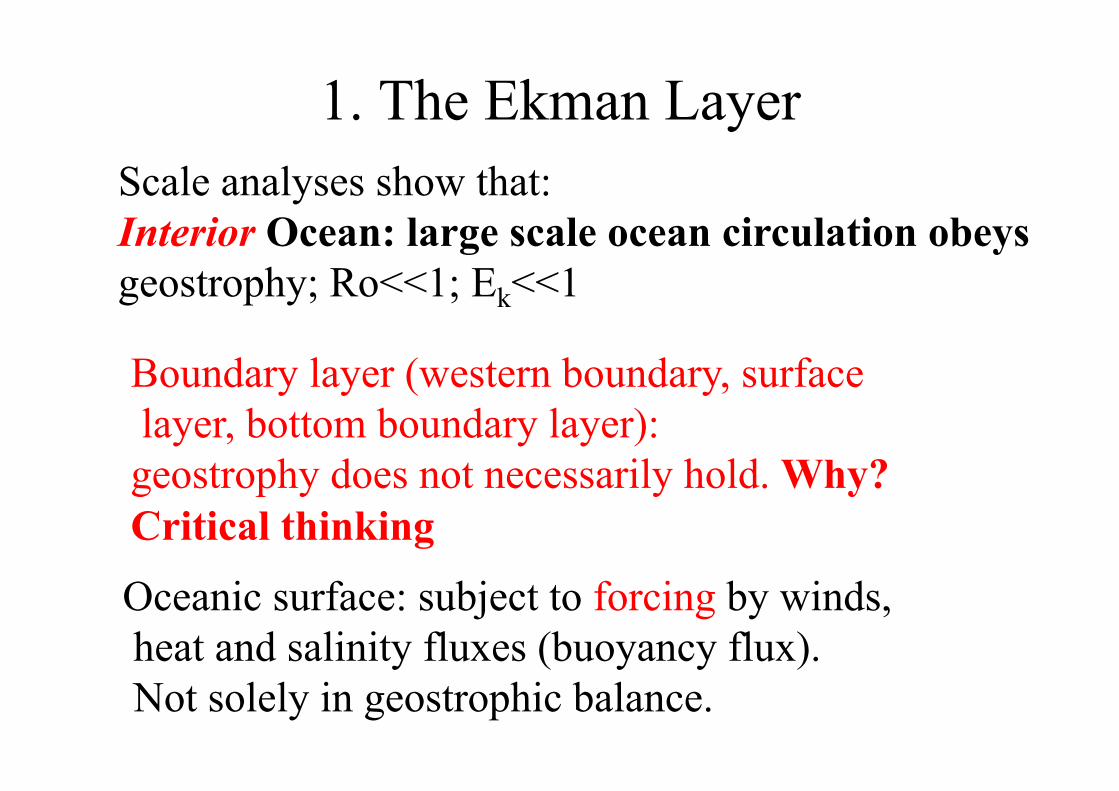
1. The Ekman Layer Scale analyses show that: Interior Ocean: large scale ocean circulation obeys geostrophy; Ro<<1; Ek<<1 Boundary layer (western boundary, surface layer, bottom boundary layer): geostrophy does not necessarily hold. Why? Critical thinking Oceanic surface: subject to forcing by winds, heat and salinity fluxes (buoyancy flux). Not solely in geostrophic balance.

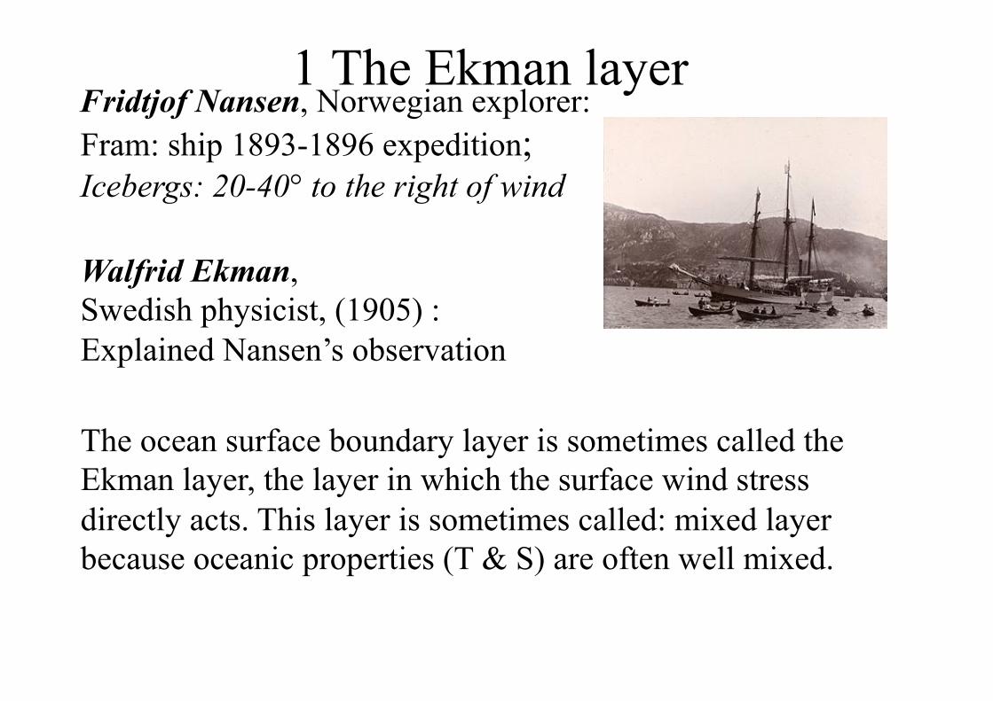
1 The Ekman layer Fridtjof Nansen, Norwegian explorer: Fram: ship 1893-1896 expedition; Icebergs: 20-40° to the right of wind Walfrid Ekman, Swedish physicist, (1905) : Explained Nansen’s observation

The ocean surface boundary layer is sometimes called the Ekman layer, the layer in which the surface wind stress directly acts. This layer is sometimes called: mixed layer because oceanic properties (T & S) are often well mixed.

In fact: Ekman layer thickness & Mixed layer depth: are not exactly the same Ekman layer: determined by wind Ekman layer thickness: will be defined later (determined by viscosity & f) Mixed layer: wind & buoyancy driven-turbulent mixing Usually: the depth at which density increase is equivalent to 0.5C (some uses 1C, etc) temperature decrease

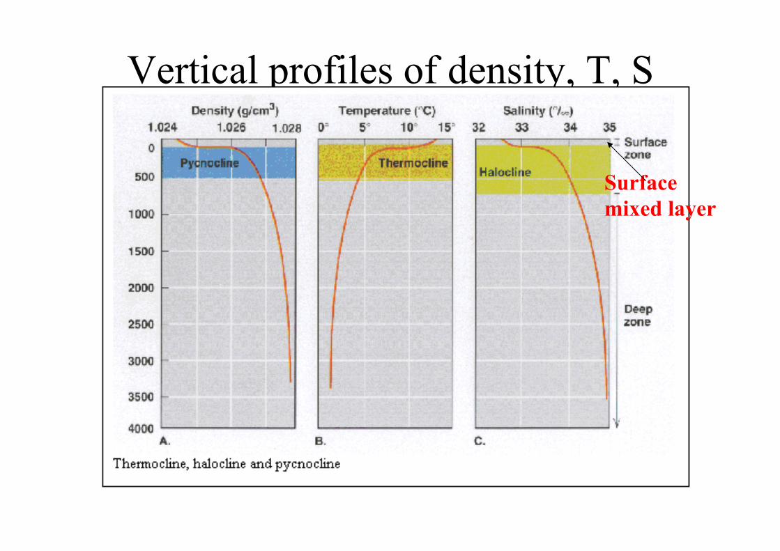
Vertical profiles of density, T, S

Surface mixed layer

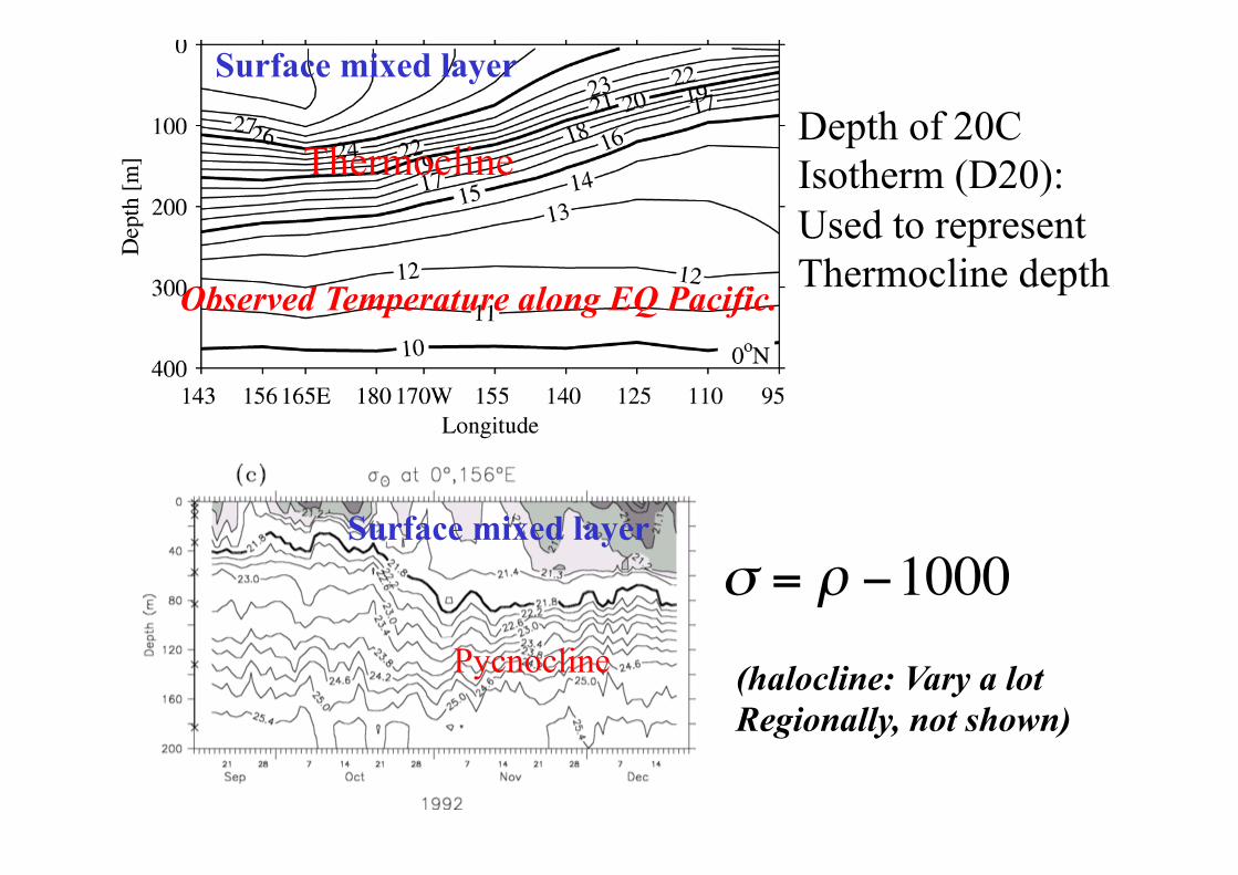
Observed Temperature along EQ Pacific.

Thermocline Depth of 20C Isotherm (D20): Used to represent Thermocline depth

Pycnocline (halocline: Vary a lot Regionally, not shown)

€

σ = ρ −1000

Surface mixed layer

Surface mixed layer

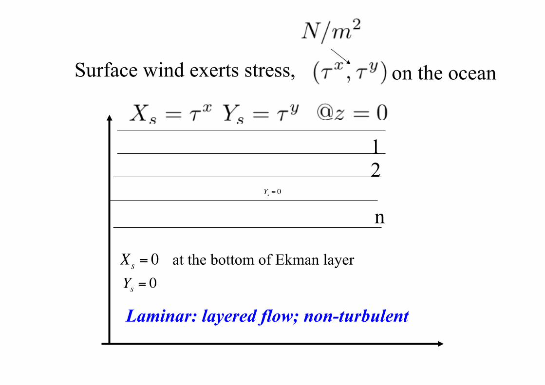
Surface wind exerts stress, on the ocean

1 2

n

€

Xs = 0 at the bottom of Ekman layer

Laminar: layered flow; non-turbulent

Ys = 0

Ys = 0

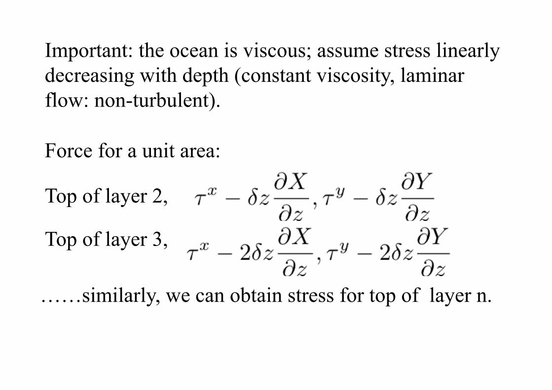
Important: the ocean is viscous; assume stress linearly decreasing with depth (constant viscosity, laminar flow: non-turbulent). Force for a unit area:

Top of layer 2,

Top of layer 3,

……similarly, we can obtain stress for top of layer n.

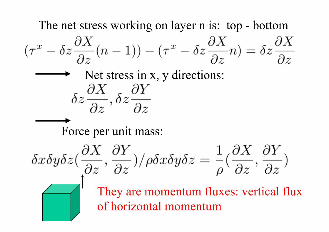
The net stress working on layer n is: top - bottom

Net stress in x, y directions:

Force per unit mass:

They are momentum fluxes: vertical flux of horizontal momentum

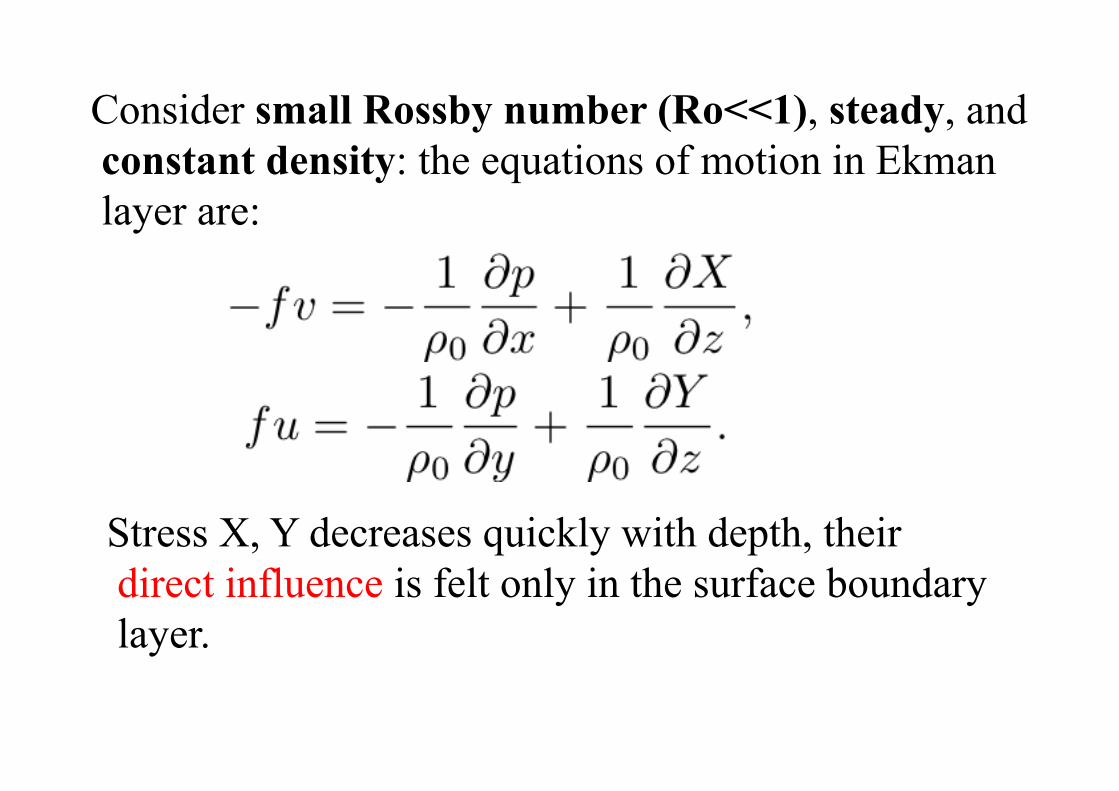
Consider small Rossby number (Ro<<1), steady, and constant density: the equations of motion in Ekman layer are:

Stress X, Y decreases quickly with depth, their direct influence is felt only in the surface boundary layer.

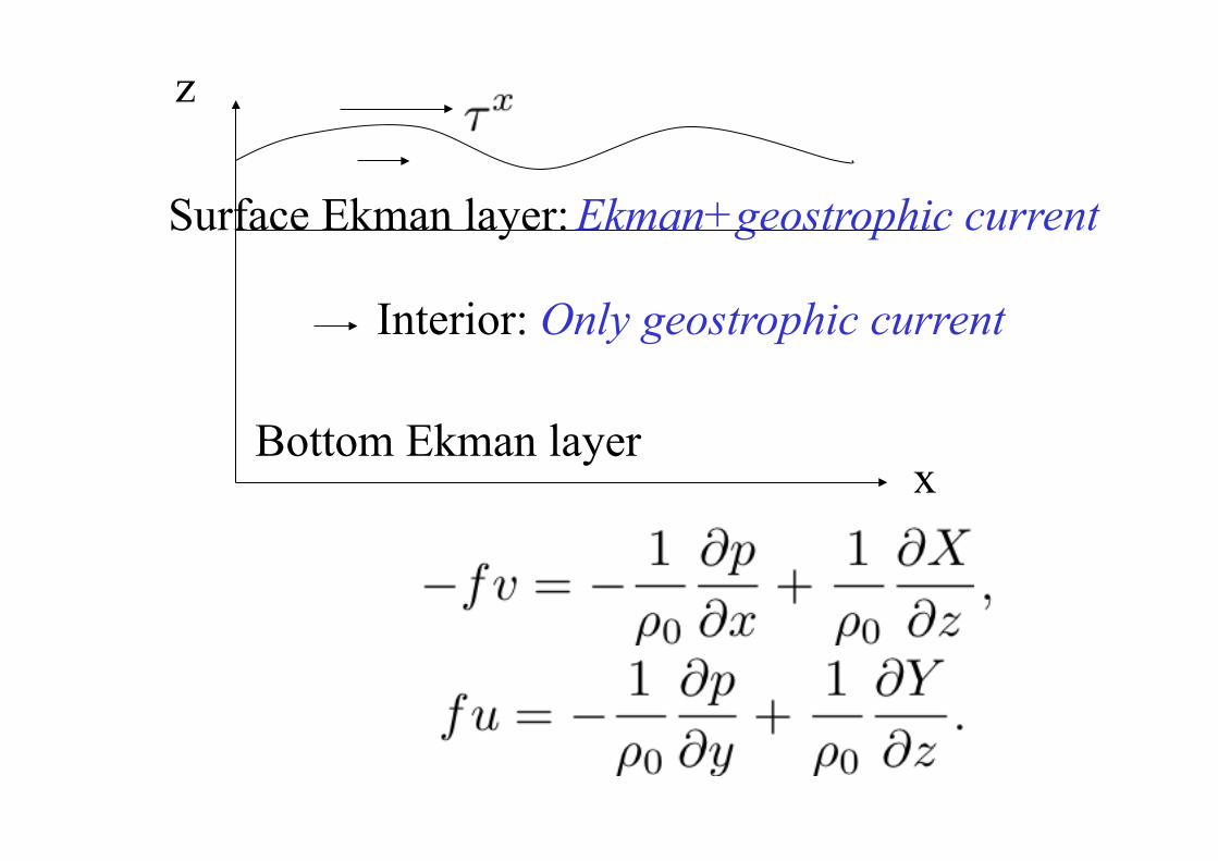
Ekman+geostrophic current

Interior: Only geostrophic current

Surface Ekman layer:

x

z

Bottom Ekman layer

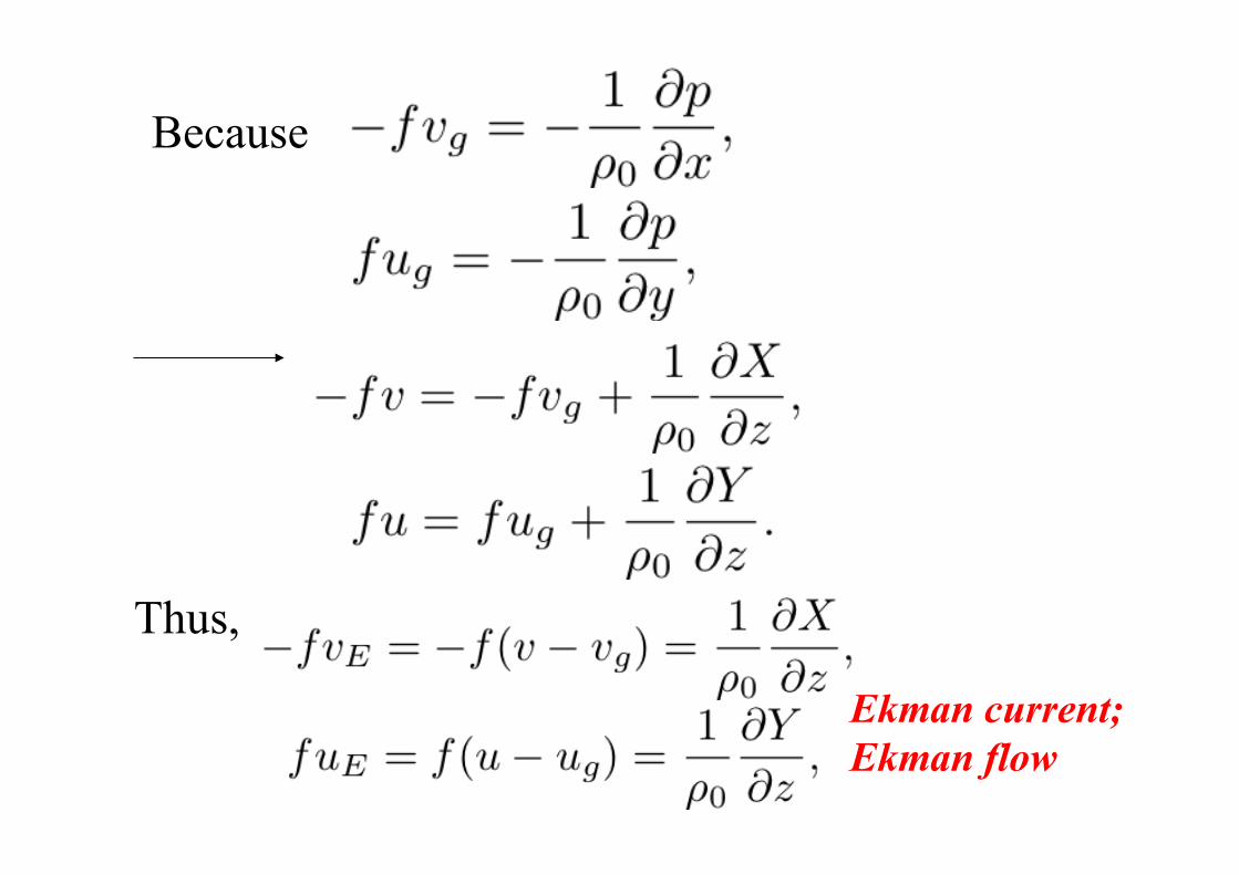
Because

Thus,

Ekman current; Ekman flow

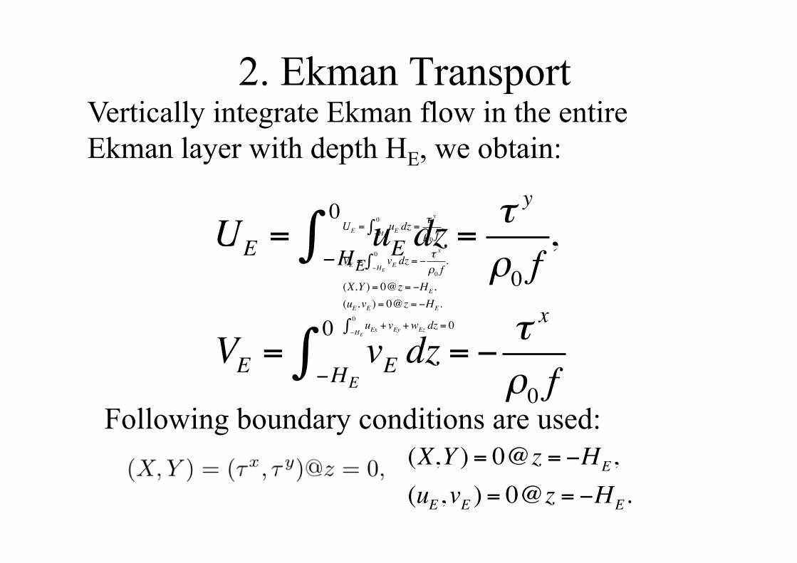
2. Ekman Transport Vertically integrate Ekman flow in the entire Ekman layer with depth HE, we obtain:

Following boundary conditions are used:

UE = uE dz =τ y

ρ0 f−HE

0∫ ,

VE = vE dz = −τ x

ρ0 f−HE

0∫ .

(X,Y ) = 0@z = −HE,(uE,vE ) = 0@z = −HE.

uEx + vEy +wEz dz = 0−HE

0∫

UE = uE dz =τ y

ρ0 f−HE

0∫ ,

VE = vE dz = −τ x

ρ0 f−HE

0∫

(X,Y ) = 0@z = −HE,(uE,vE ) = 0@z = −HE.

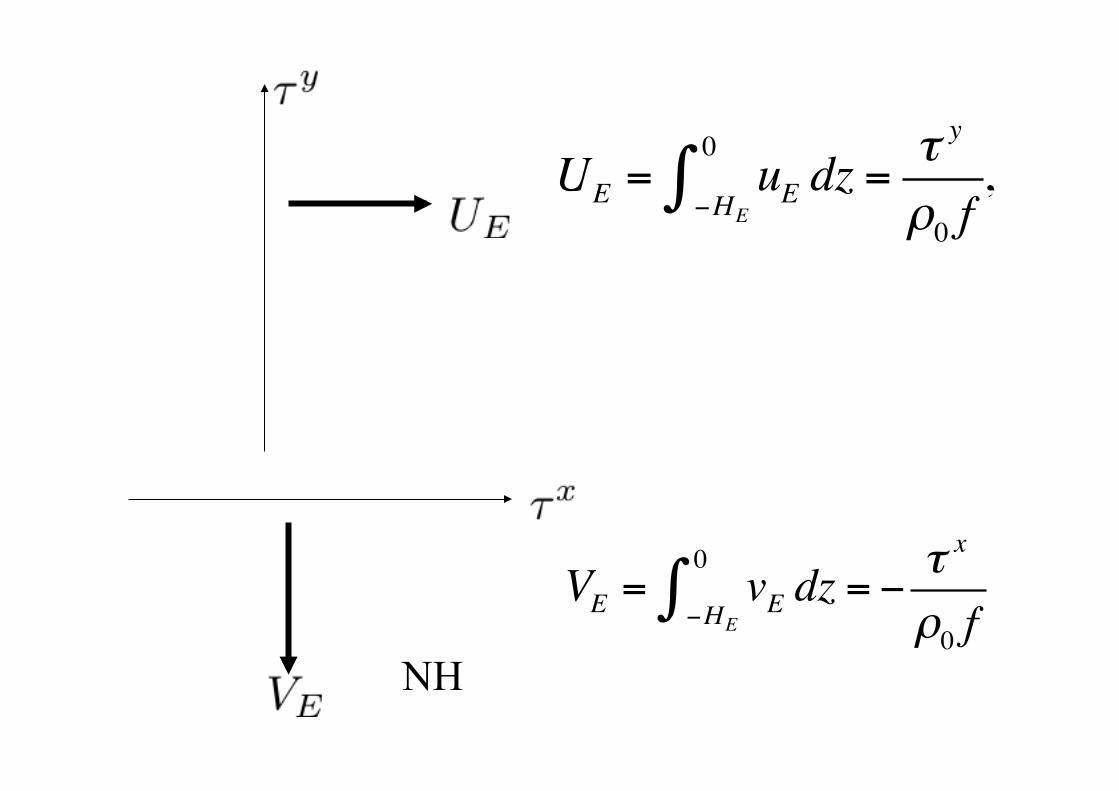
NH

UE = uE dz =τ y

ρ0 f−HE

0∫ ,

VE = vE dz = −τ x

ρ0 f−HE

0∫

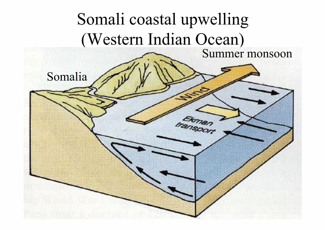
Somali coastal upwelling (Western Indian Ocean)

Somalia

Summer monsoon

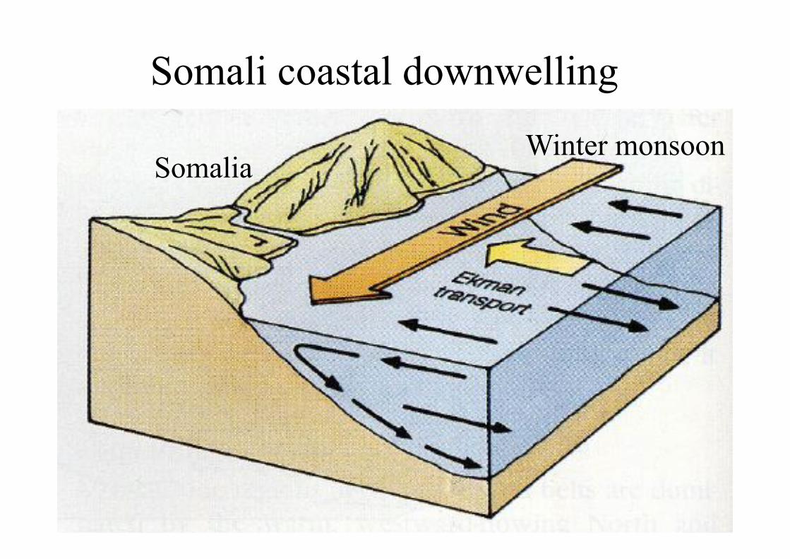
Somali coastal downwelling

Somalia Winter monsoon

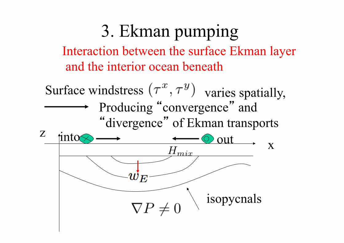
3. Ekman pumping Interaction between the surface Ekman layer and the interior ocean beneath

Surface windstress varies spatially, Producing “convergence” and “divergence” of Ekman transports

z x out into

isopycnals

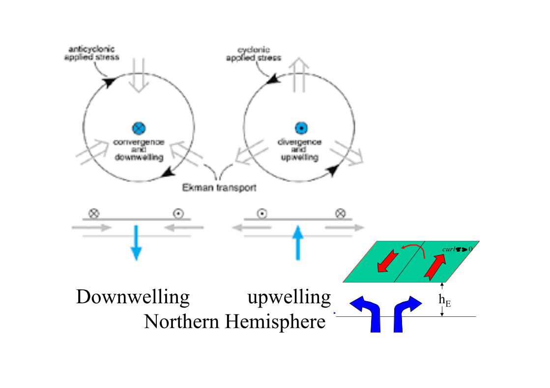
Downwelling upwelling Northern Hemisphere

Ekman Pumping:

xfy

V

x

Uwdz

z

w

y

v

x

u y

hz

hE

E∂

∂=

∂

∂+

∂

∂=⇒=

∂

∂+

∂

∂+

∂

∂−=

−

∫τ

ρ

10)(

0

If we extend it to a general case with x and y components of the wind, we get

€

wz= −hE

=∂U

∂x+∂V

∂y=1

ρf(∂τ y

∂x−∂τ x∂y

) =1

ρo fk ⋅ curlτ

The vertical velocity at the bottom of the surface Ekman layer is proportional to the vorticity of

the surface wind stress and it is independent of the detailed structure of the Ekman flow. the

vertical velocity is positive for the positive vorticity of the wind stress, and negative for the

negative vorticity of the wind stress.

€

curlτ > 0

hE Ekman pumping

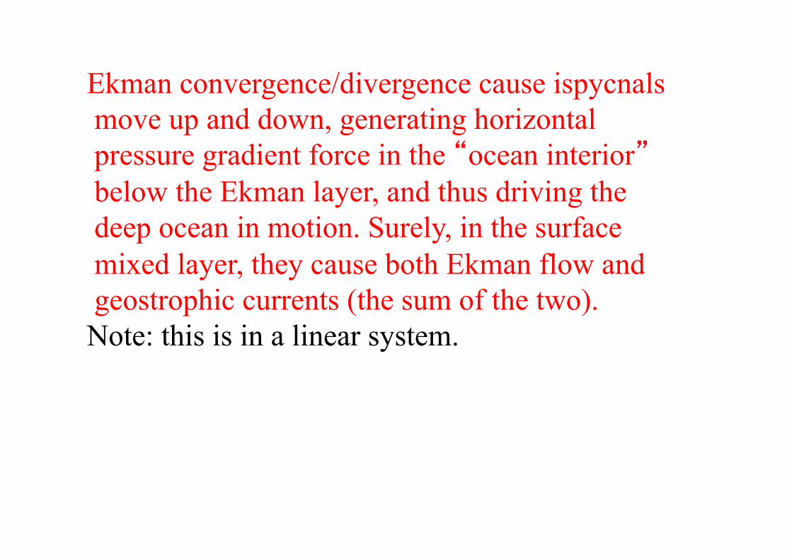
Ekman convergence/divergence cause ispycnals move up and down, generating horizontal pressure gradient force in the “ocean interior” below the Ekman layer, and thus driving the deep ocean in motion. Surely, in the surface mixed layer, they cause both Ekman flow and geostrophic currents (the sum of the two). Note: this is in a linear system.

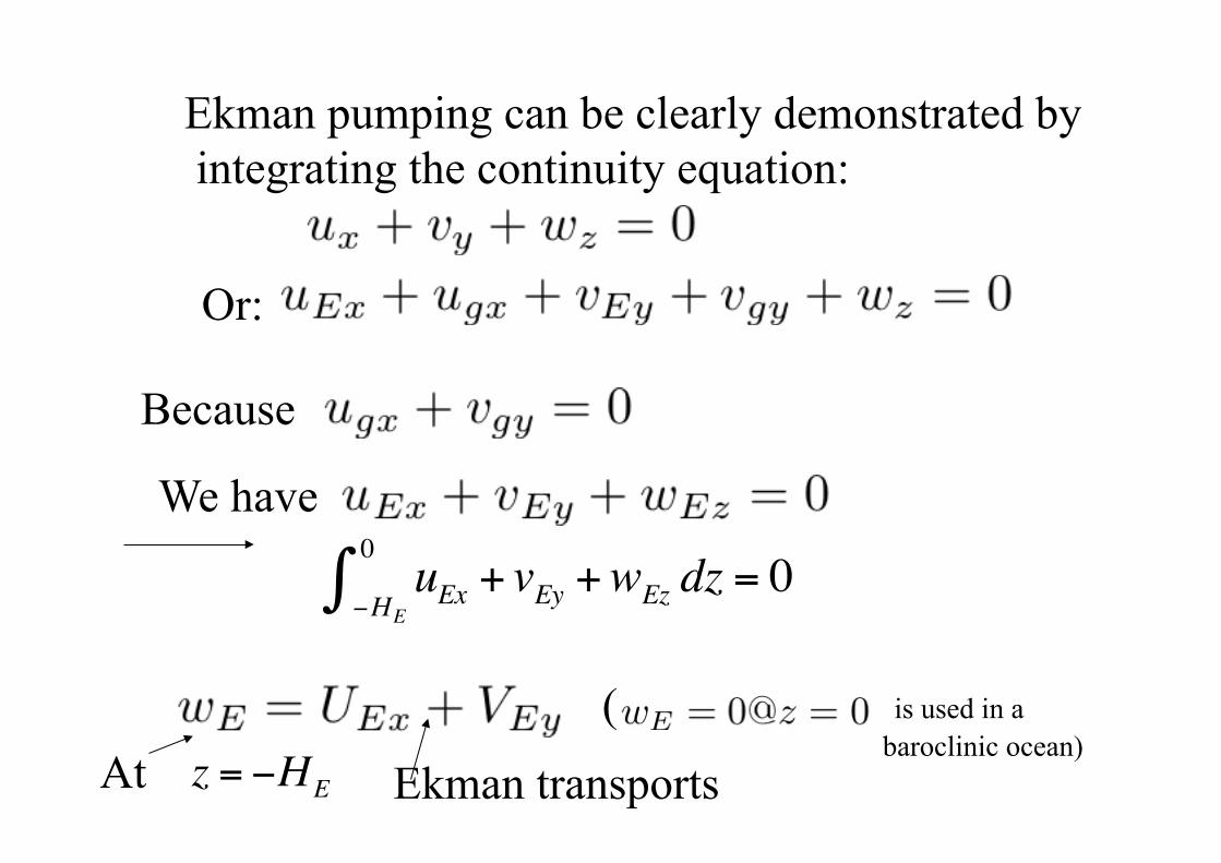
Ekman pumping can be clearly demonstrated by integrating the continuity equation:

Or:

Because

We have

( is used in a baroclinic ocean)

Ekman transports At

uEx + vEy +wEz dz = 0−HE

0∫

z = −HE

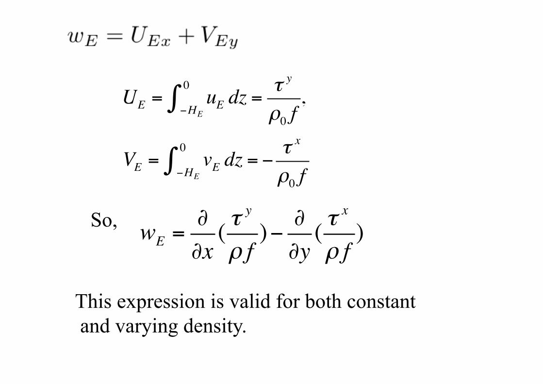
wE =∂∂x( τ

y

ρ f)− ∂∂y( τ

x

ρ f)So,

This expression is valid for both constant and varying density.

UE = uE dz =τ y

ρ0 f−HE

0∫ ,

VE = vE dz = −τ x

ρ0 f−HE

0∫

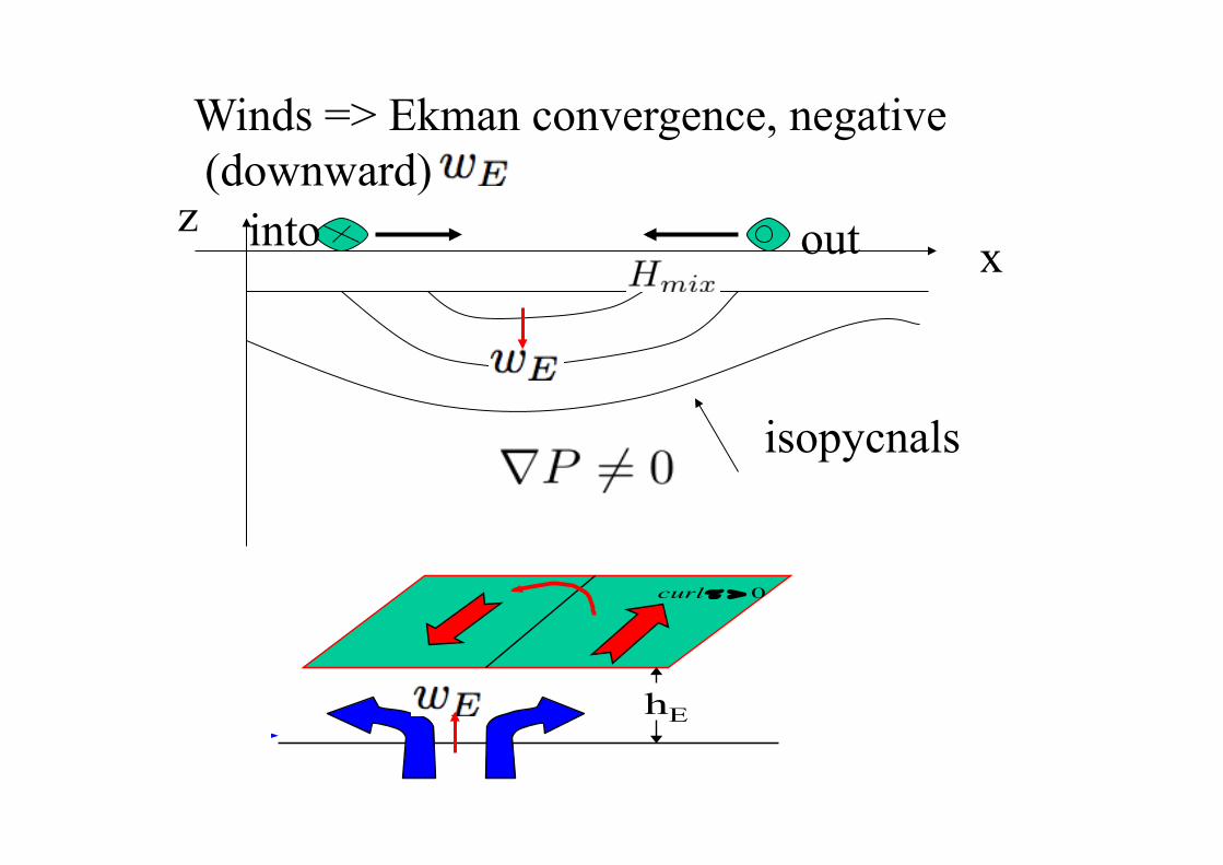
z x out into

isopycnals

Winds => Ekman convergence, negative (downward) Ekman Pumping:

xfy

V

x

Uwdz

z

w

y

v

x

u y

hz

hE

E∂

∂=

∂

∂+

∂

∂=⇒=

∂

∂+

∂

∂+

∂

∂−=

−

∫τ

ρ

10)(

0

If we extend it to a general case with x and y components of the wind, we get

€

wz= −hE

=∂U

∂x+∂V

∂y=1

ρf(∂τ y

∂x−∂τ x∂y

) =1

ρo fk ⋅ curlτ

The vertical velocity at the bottom of the surface Ekman layer is proportional to the vorticity of

the surface wind stress and it is independent of the detailed structure of the Ekman flow. the

vertical velocity is positive for the positive vorticity of the wind stress, and negative for the

negative vorticity of the wind stress.

€

curlτ > 0

hE Ekman pumping