Atmospheric Thermodynamics – III Adiabatic Processes Leila M. V. Carvalho Dept. Geography, UCSB.

Atmospheric Thermodynamics – IIIAdiabatic Processes

Leila M. V. CarvalhoDept. Geography, UCSB

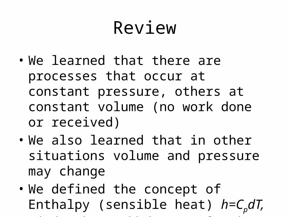
Review

• We learned that there are processes that occur at constant pressure, others at constant volume (no work done or received)

• We also learned that in other situations volume and pressure may change

• We defined the concept of Enthalpy (sensible heat) h=CpdT, which is the sensible heat transferred at constant pressure.

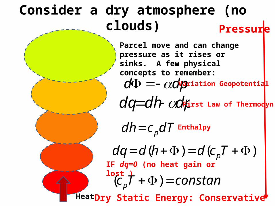
Consider a dry atmosphere (no clouds)Pressure

Heat

Parcel move and can change pressure as it rises or sinks. A few physical concepts to remember:

dpd dpdhdq

dTcdh p

)()( Tcdhddq pIF dq=0 (no heat gain or lost )

Variation Geopotential

First Law of Thermodyn.

Enthalpy

constantTcp )(Dry Static Energy: Conservative

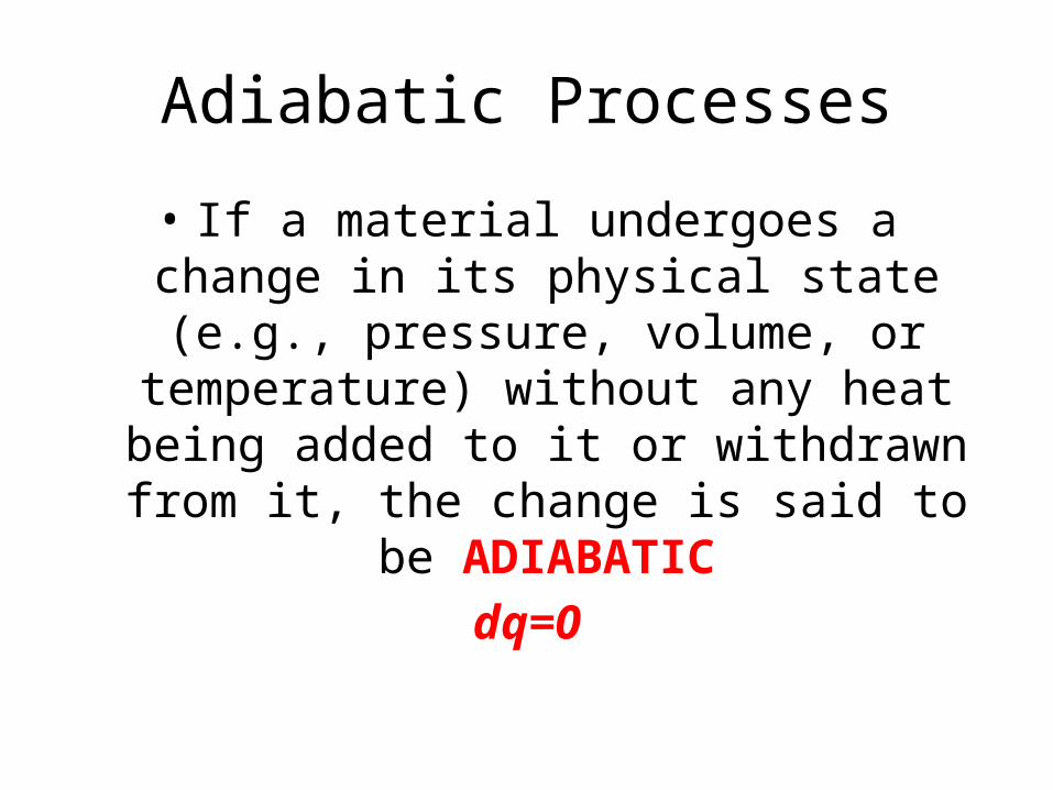
Adiabatic Processes

• If a material undergoes a change in its physical state (e.g., pressure, volume, or temperature)

without any heat being added to it or withdrawn from it, the change is said to be

ADIABATICdq=0

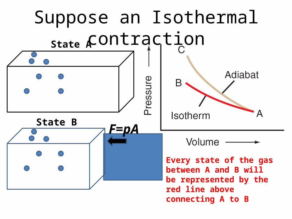
Suppose an Isothermal contraction

F=pA

State A

State B

Every state of the gas between A and B will be represented by the red line above connecting A to B

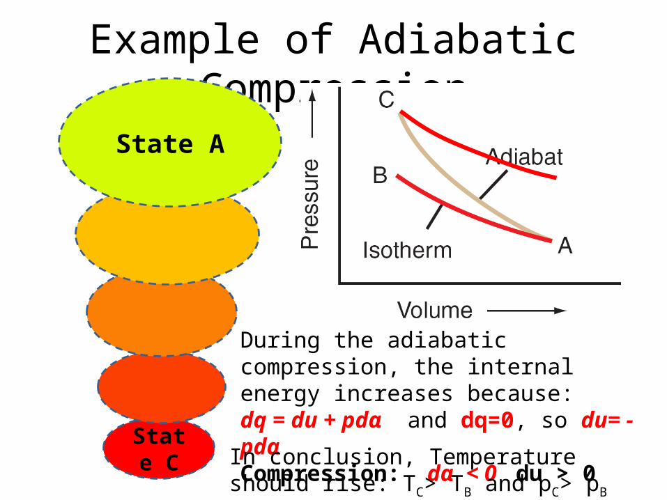
Example of Adiabatic Compression

State C

State A

During the adiabatic compression, the internal energy increases because: dq = du + pdα and dq=0, so du= - pdα Compression: dα < 0 du > 0

In conclusion, Temperature should rise: TC> TB and pC> pB

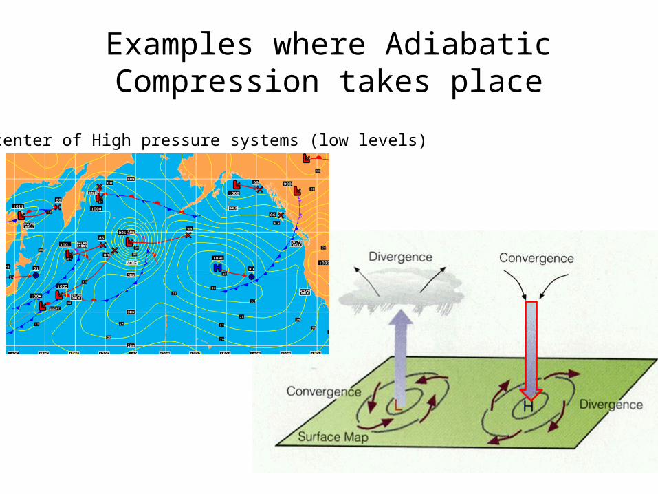
Examples where Adiabatic Compression takes place

In the center of High pressure systems (low levels)

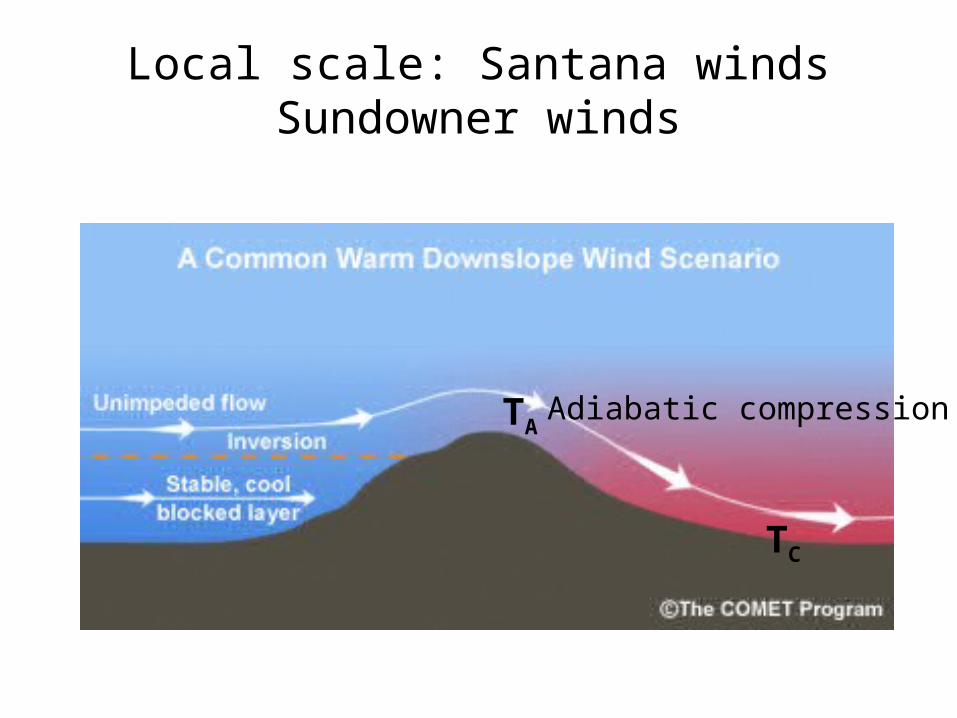
Local scale: Santana windsSundowner winds

Adiabatic compression

TC

TA

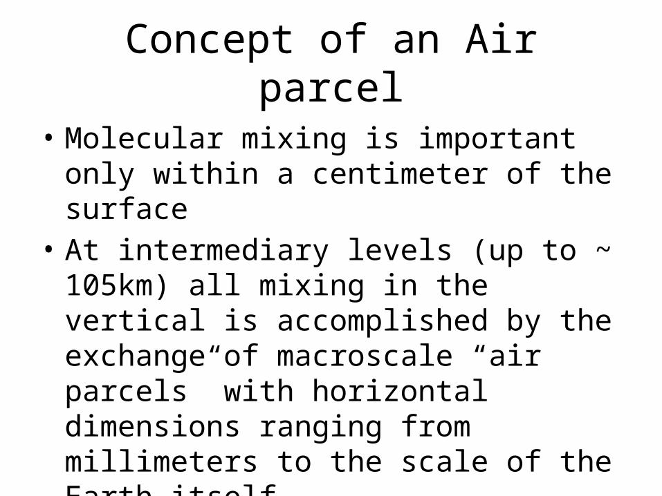
Concept of an Air parcel

• Molecular mixing is important only within a centimeter of the surface

• At intermediary levels (up to ~ 105km) all mixing in the vertical is accomplished by the exchange of macroscale “air parcels” with horizontal dimensions ranging from millimeters to the scale of the Earth itself

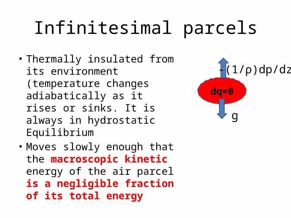
Infinitesimal parcels

• Thermally insulated from its environment (temperature changes adiabatically as it rises or sinks. It is always in hydrostatic Equilibrium

• Moves slowly enough that the macroscopic kinetic energy of the air parcel is a negligible fraction of its total energy

dq=0

g

-(1/ρ)dp/dz

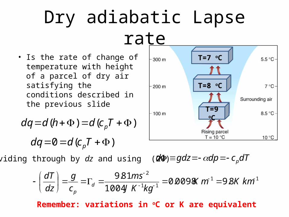
Dry adiabatic Lapse rate

• Is the rate of change of temperature with height of a parcel of dry air satisfying the conditions described in the previous slide

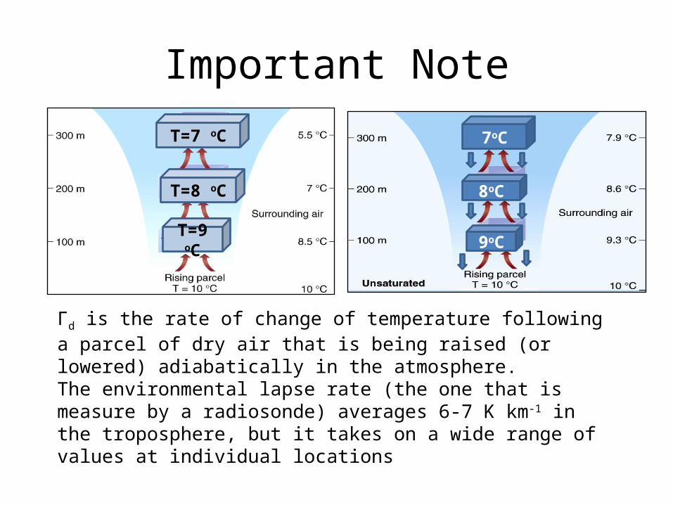
T=9 oC

T=8 oC

T=7 oC

)()( Tcdhddq p

)(0 Tcddq p

Dividing through by dz and using (20) dTcdpgdzd p

1111

2

8.90098.01004

81.9

kmKmK

kgKJ

sm

c

g

dz

dTd

p

Remember: variations in oC or K are equivalent

Important Note

7oC

8oC

9oCT=9 oC

T=8 oC

T=7 oC

Γd is the rate of change of temperature following a parcel of dry air that is being raised (or lowered) adiabatically in the atmosphere.The environmental lapse rate (the one that is measure by a radiosonde) averages 6-7 K km-1 in the troposphere, but it takes on a wide range of values at individual locations

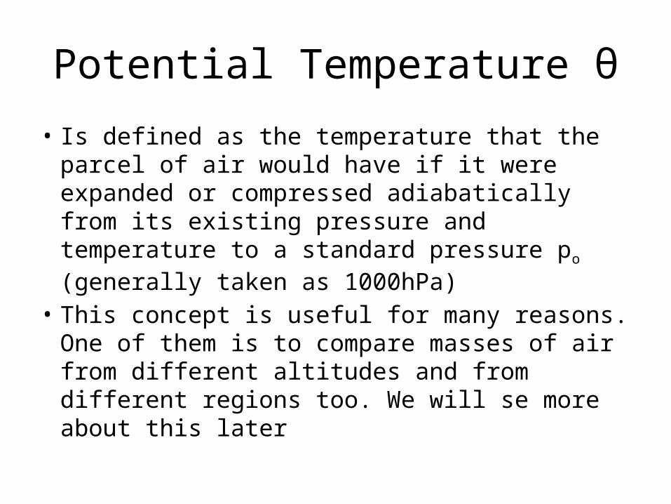
Potential Temperature θ

• Is defined as the temperature that the parcel of air would have if it were expanded or compressed adiabatically from its existing pressure and temperature to a standard pressure po (generally taken as 1000hPa)

• This concept is useful for many reasons. One of them is to compare masses of air from different altitudes and from different regions too. We will se more about this later

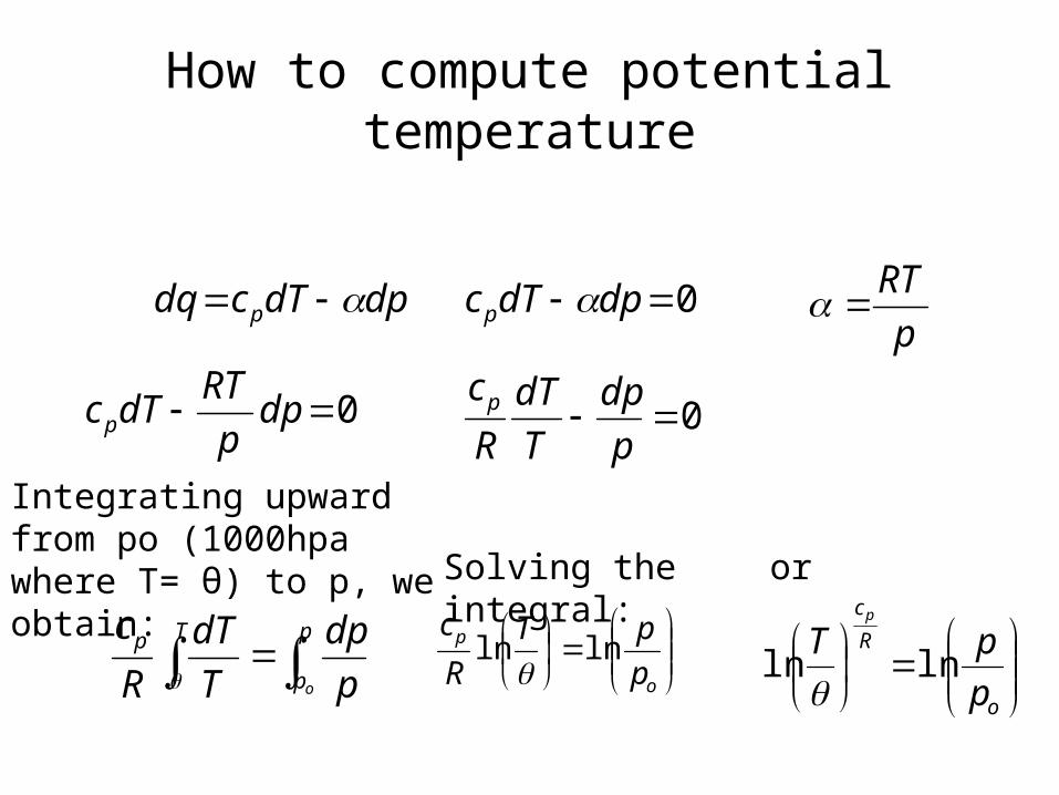
How to compute potential temperature

dpdTcdq p 0 dpdTcp p

RT

0 dpp

RTdTcp 0

p

dp

T

dT

R

cp

p

p

Tp

o p

dp

T

dT

R

c

Integrating upward from po (1000hpa where T= θ) to p, we obtain:

o

p

p

pT

R

clnln

Solving the integral:

o

R

c

p

pTp

lnln

or

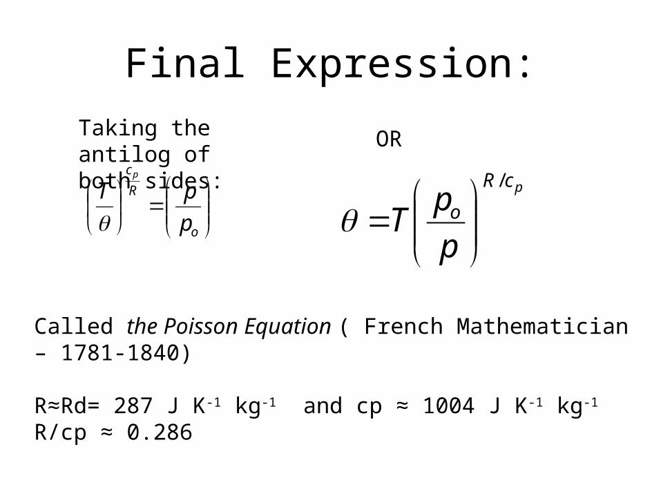
Final Expression:

o

R

c

p

pTp

Taking the antilog of both sides:

OR

pcR

o

p

pT

/

Called the Poisson Equation ( French Mathematician – 1781-1840)

R≈Rd= 287 J K-1 kg-1 and cp ≈ 1004 J K-1 kg-1

R/cp ≈ 0.286

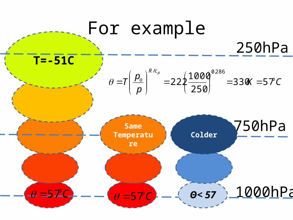
For example

T=-51C250hPa

750hPa

1000hPa

CKp

pT o

cR

op

57330250

1000222

286.0/

Same Temperature

Co57 Co57 Θ< 57

Colder

Considerations

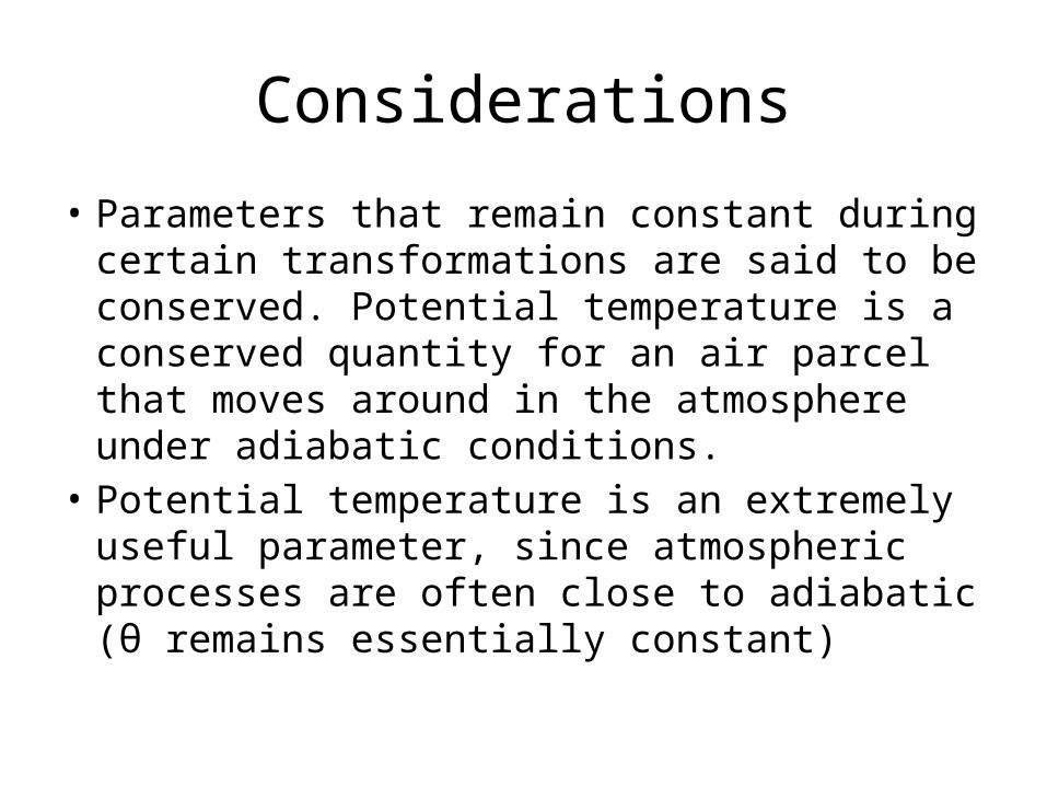
• Parameters that remain constant during certain transformations are said to be conserved. Potential temperature is a conserved quantity for an air parcel that moves around in the atmosphere under adiabatic conditions.

• Potential temperature is an extremely useful parameter, since atmospheric processes are often close to adiabatic (θ remains essentially constant)

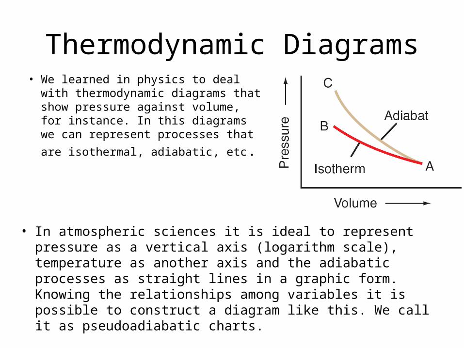
Thermodynamic Diagrams• We learned in physics to deal with

thermodynamic diagrams that show pressure against volume, for instance. In this diagrams we can represent processes

that are isothermal, adiabatic, etc.

• In atmospheric sciences it is ideal to represent pressure as a vertical axis (logarithm scale), temperature as another axis and the adiabatic processes as straight lines in a graphic form. Knowing the relationships among variables it is possible to construct a diagram like this. We call it as pseudoadiabatic charts.

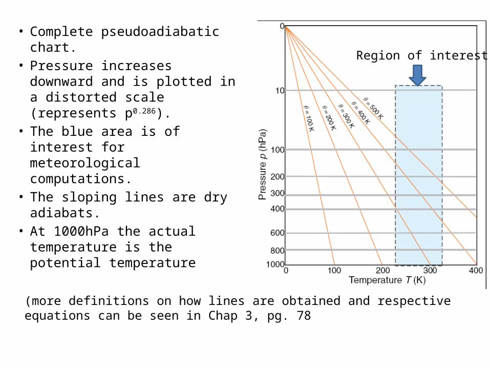
Region of interest

• Complete pseudoadiabatic chart.

• Pressure increases downward and is plotted in a distorted scale (represents p0.286).

• The blue area is of interest for meteorological computations.

• The sloping lines are dry adiabats.

• At 1000hPa the actual temperature is the potential temperature

(more definitions on how lines are obtained and respective equations can be seen in Chap 3, pg. 78

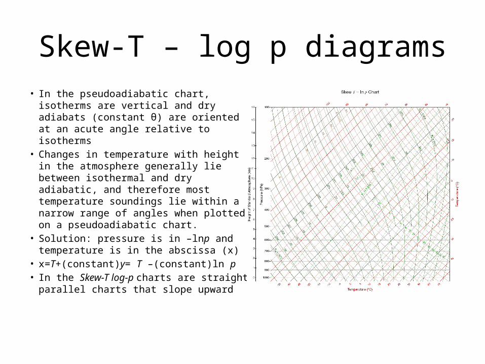
Skew-T – log p diagrams• In the pseudoadiabatic chart, isotherms

are vertical and dry adiabats (constant θ) are oriented at an acute angle relative to isotherms

• Changes in temperature with height in the atmosphere generally lie between isothermal and dry adiabatic, and therefore most temperature soundings lie within a narrow range of angles when plotted on a pseudoadiabatic chart.

• Solution: pressure is in –lnp and temperature is in the abscissa (x)

• x=T+(constant)y= T –(constant)ln p• In the Skew-T log-p charts are straight

parallel charts that slope upward

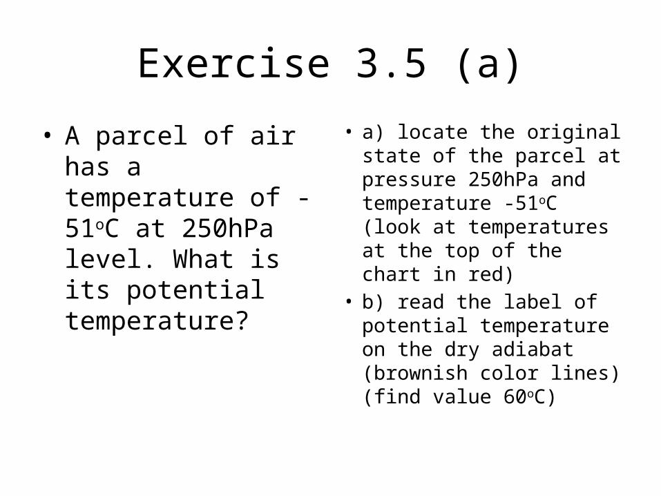
Exercise 3.5 (a)

• A parcel of air has a temperature of -51oC at 250hPa level. What is its potential temperature?

• a) locate the original state of the parcel at pressure 250hPa and temperature -51oC (look at temperatures at the top of the chart in red)

• b) read the label of potential temperature on the dry adiabat (brownish color lines) (find value 60oC)

Exercise 3.5 (b)

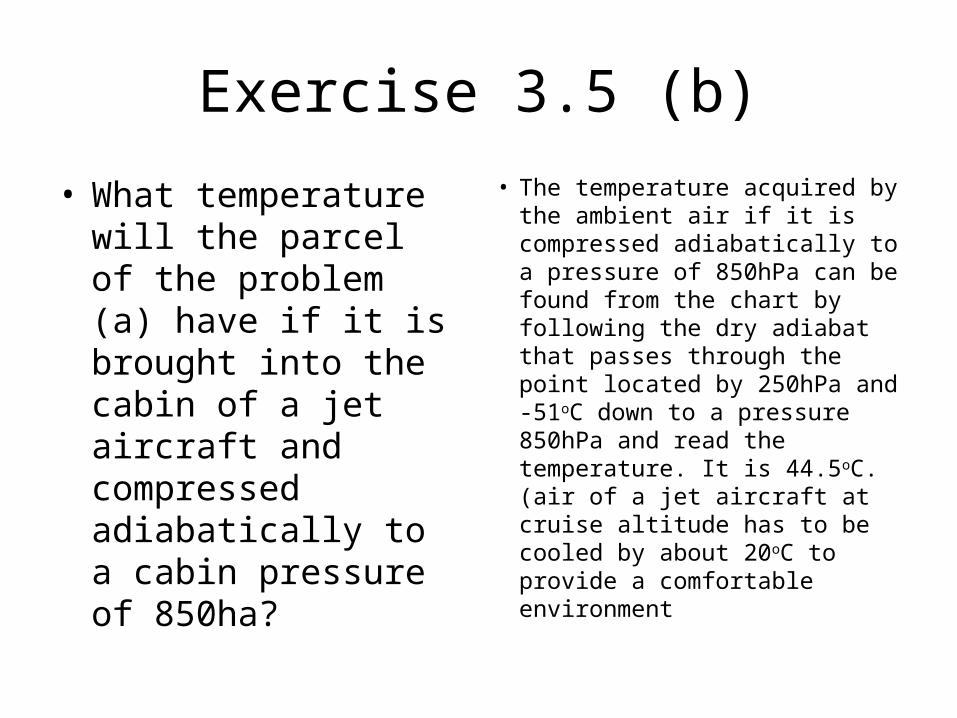
• What temperature will the parcel of the problem (a) have if it is brought into the cabin of a jet aircraft and compressed adiabatically to a cabin pressure of 850ha?

• The temperature acquired by the ambient air if it is compressed adiabatically to a pressure of 850hPa can be found from the chart by following the dry adiabat that passes through the point located by 250hPa and -51oC down to a pressure 850hPa and read the temperature. It is 44.5oC. (air of a jet aircraft at cruise altitude has to be cooled by about 20oC to provide a comfortable environment

Exercise for training

• Suppose that the ground level pressure in Santa Maria is 900hPa and temperature is 20oC. Suppose that a sundowner (downslope wind) occurs in these conditions. What should be the expected temperature downhill in Santa Barbara, supposing that pressure in SB is ~ 1000hPa?

• Use the skew-t log-p to answer this question. Find the initial condition in Santa Maria. Suppose that downslope winds descend the mountains following a dry adiabatic processes. Use the dry adiabat that pass through the initial condition to find the temperature in SB

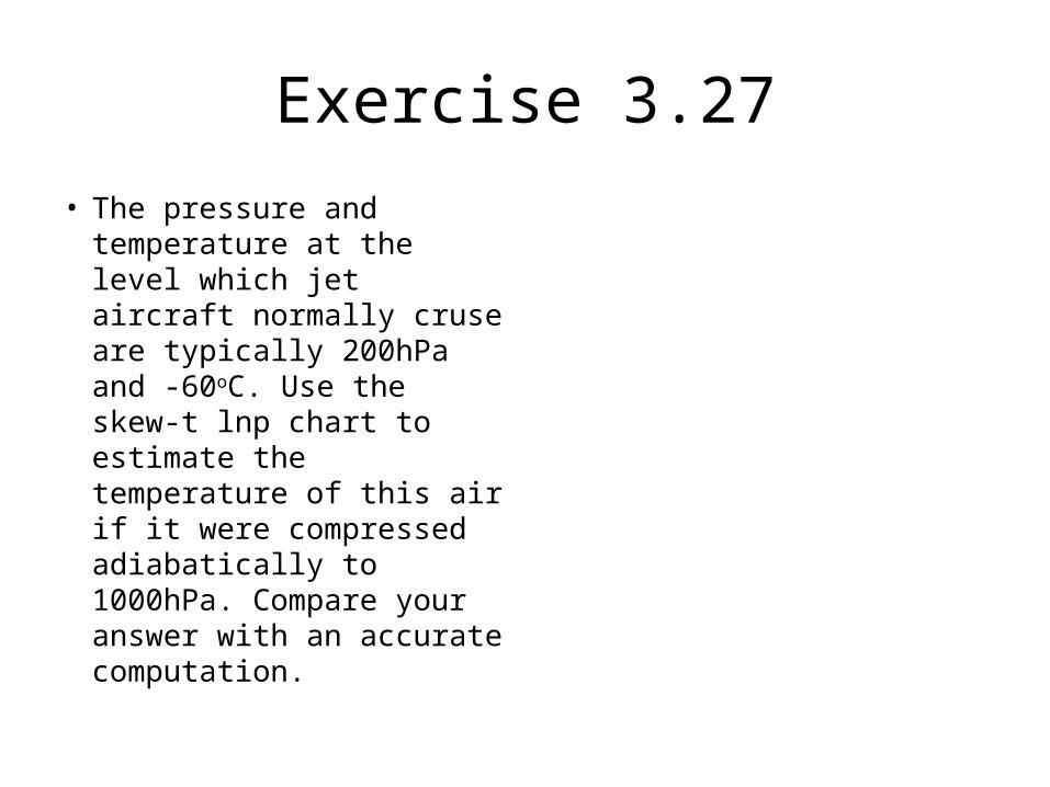
Exercise 3.27

• The pressure and temperature at the level which jet aircraft normally cruse are typically 200hPa and -60oC. Use the skew-t lnp chart to estimate the temperature of this air if it were compressed adiabatically to 1000hPa. Compare your answer with an accurate computation.

Water Vapor in Air

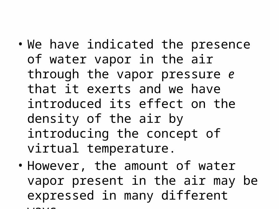
• We have indicated the presence of water vapor in the air through the vapor pressure e that it exerts and we have introduced its effect on the density of the air by introducing the concept of virtual temperature.

• However, the amount of water vapor present in the air may be expressed in many different ways.

Moisture Parameters

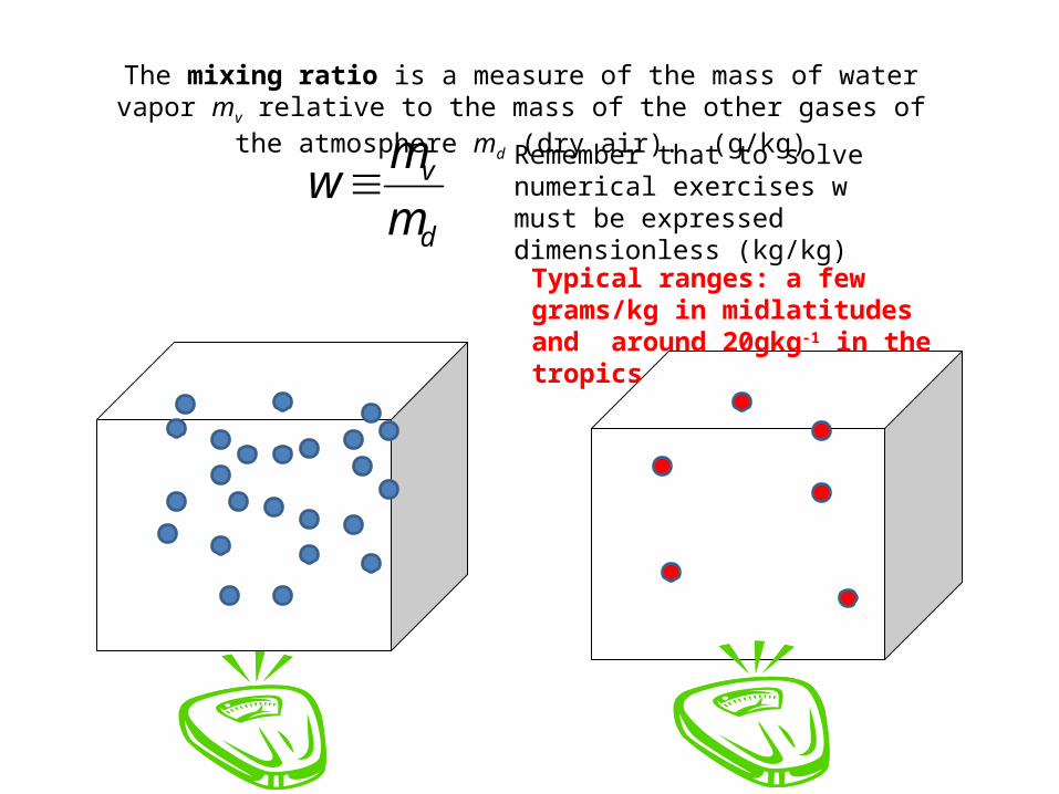
The mixing ratio is a measure of the mass of water vapor mv relative to the mass of the other gases of the atmosphere md (dry air). (g/kg)

d

v

m

mw

Remember that to solve numerical exercises w must be expressed dimensionless (kg/kg)

Typical ranges: a few grams/kg in midlatitudes and around 20gkg-1 in the tropics

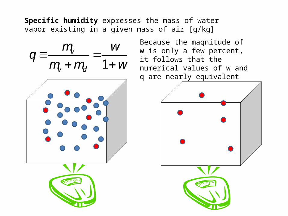
Specific humidity expresses the mass of water vapor existing in a given mass of air [g/kg]

w

w

mm

mq

dv

v

1

Because the magnitude of w is only a few percent, it follows that the numerical values of w and q are nearly equivalent

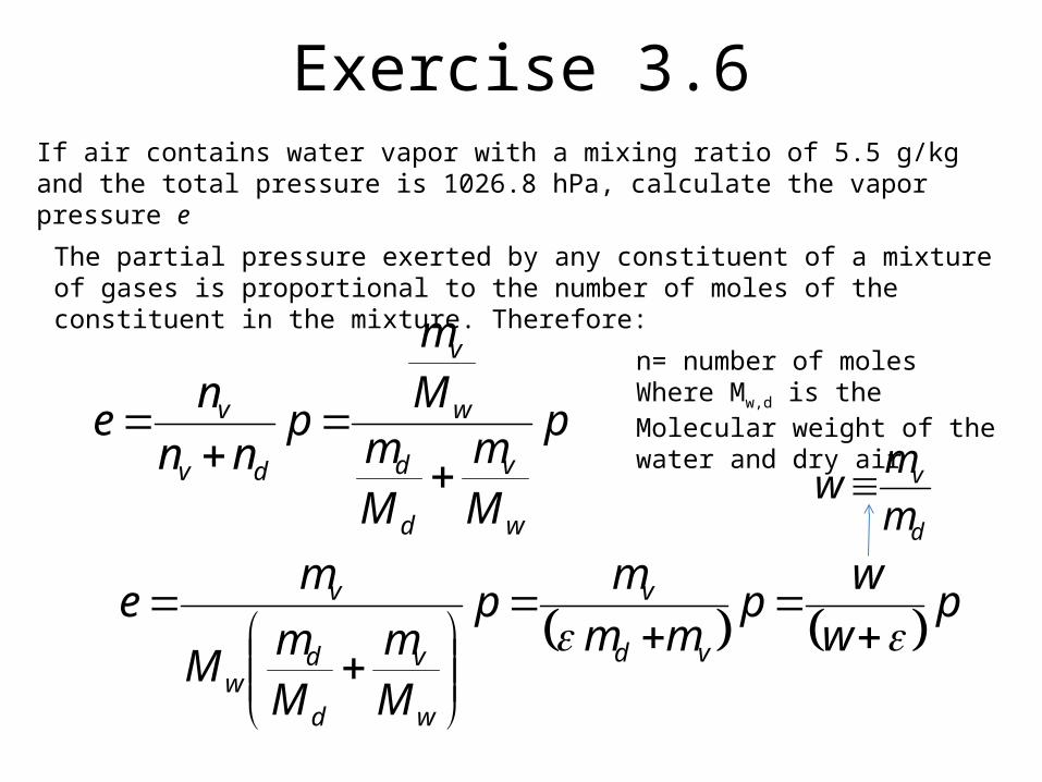
Exercise 3.6If air contains water vapor with a mixing ratio of 5.5 g/kg and the total pressure is 1026.8 hPa, calculate the vapor pressure e

The partial pressure exerted by any constituent of a mixture of gases is proportional to the number of moles of the constituent in the mixture. Therefore:

p

Mm

MmMm

pnn

ne

w

v

d

d

w

v

dv

v

n= number of molesWhere Mw,d is the Molecular weight of the water and dry air

pw

wp

mm

mp

Mm

Mm

M

me

vd

v

w

v

d

dw

v

d

v

m

mw

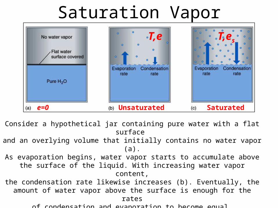
Consider a hypothetical jar containing pure water with a flat surface and an overlying volume that initially contains no water vapor (a).As evaporation begins, water vapor starts to accumulate abovethe surface of the liquid. With increasing water vapor content,the condensation rate likewise increases (b). Eventually, the

amount of water vapor above the surface is enough for the ratesof condensation and evaporation to become equal.

The resulting equilibrium state is called saturation and the water vapor pressure is called saturation vapor pressure over a plane surface of pures water at

temperature T(c).

Saturation Vapor pressure

SaturatedUnsaturatede=0

T,e T,es

Evaporation CondensRate Rate

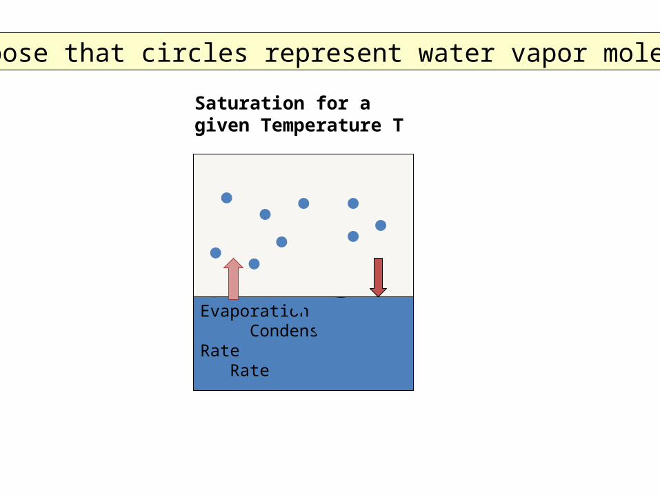
Suppose that circles represent water vapor molecules

Saturation for a given Temperature T

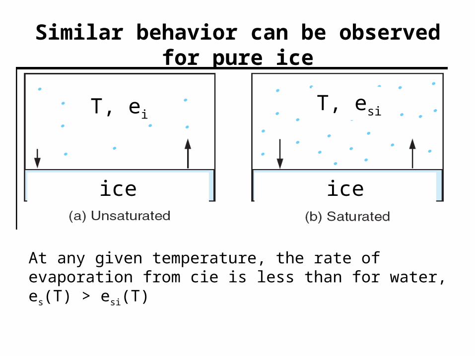
Similar behavior can be observed for pure ice

T, esiT, ei

ice ice

At any given temperature, the rate of evaporation from cie is less than for water, es(T) > esi(T)

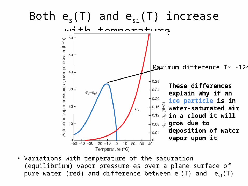
Both es(T) and esi(T) increase with temperature

• Variations with temperature of the saturation (equilibrium) vapor pressure es over a plane surface of pure water (red) and difference between es(T) and esi(T)

Maximum difference T~ -12oC

These differences explain why if an ice particle is in water-saturated air in a cloud it will grow due to deposition of water vapor upon it

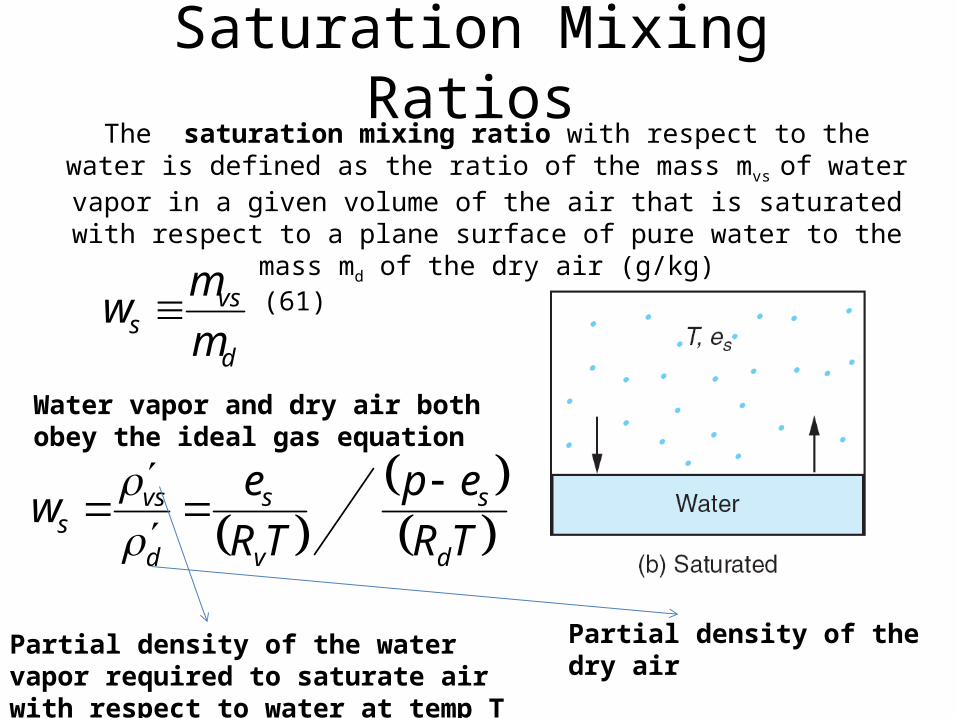
Saturation Mixing RatiosThe saturation mixing ratio with respect to the water is defined as

the ratio of the mass mvs of water vapor in a given volume of the air that is saturated with respect to a plane surface of pure water to the mass

md of the dry air (g/kg)

d

vss m

mw (61)

Water vapor and dry air both obey the ideal gas equation

TRep

TR

ew

d

s

v

s

d

vss

Partial density of the water vapor required to saturate air with respect to water at temp T

Partial density of the dry air

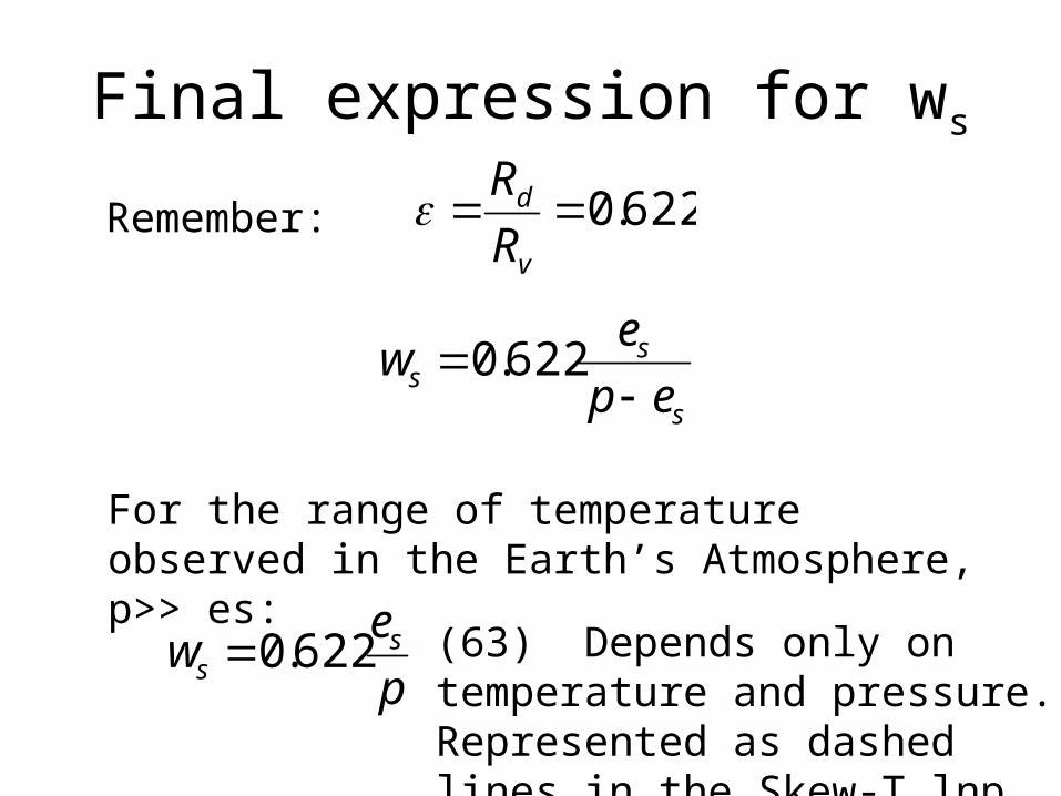
Final expression for ws

s

ss ep

ew

622.0

Remember: 622.0v

d

R

R

For the range of temperature observed in the Earth’s Atmosphere, p>> es:

p

ew ss 622.0 (63) Depends only on temperature

and pressure. Represented as dashed lines in the Skew-T lnp

Relative Humidity, Dew Point and Frost Point

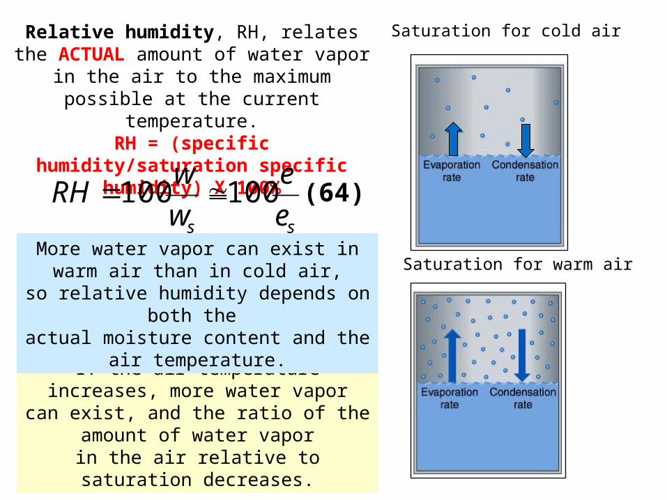
Relative humidity, RH, relates the ACTUAL amount of water vapor

in the air to the maximum possible at the current temperature.

RH = (specific humidity/saturation specific humidity) X 100%

Saturation for cold air

Saturation for warm air

If the air temperature increases, more water vapor

can exist, and the ratio of the amount of water vapor

in the air relative to saturation decreases.

More water vapor can exist in warm air than in cold air,

so relative humidity depends on both the actual moisture content and the air

temperature.

ss e

e

w

wRH 100100 (64)

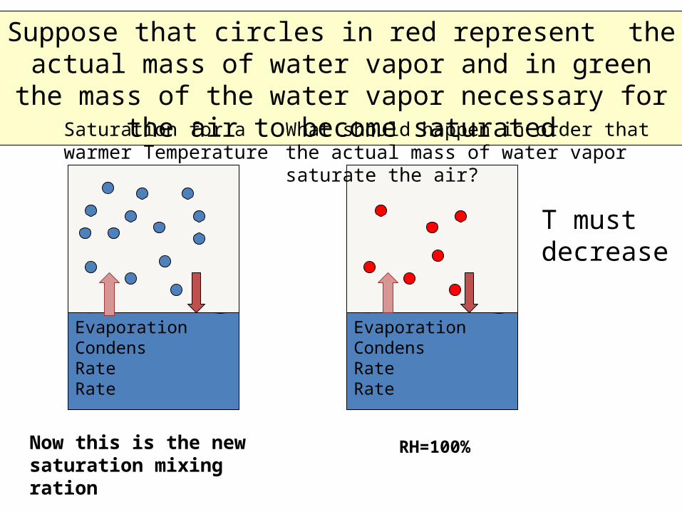
Dew

Dew is moisture condensed upon surfaces, specially during the night (why??)The dew point is the temperature to which the air must be cooled at constant pressure to become saturated with respect to a plane surface of pure water. In

other words, dew point the temperature at which saturation mixing ration ws with respect to liquid water becomes equal to the actual mixing ration w.

Evaporation CondensRate Rate

Evaporation CondensRate Rate

Suppose that circles in red represent the actual mass of water vapor and in green the mass of the water vapor necessary for

the air to become saturatedSaturation for a warmer Temperature

What should happen in order that the actual mass of water vapor saturate the air?

T must decrease

Now this is the new saturation mixing ration

RH=100%

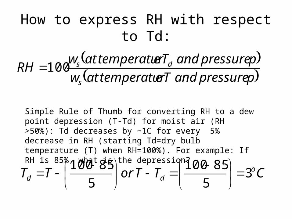
How to express RH with respect to Td:

ppressureandTetemperaturatw

ppressureandTetemperaturatwRH

s

ds100

Simple Rule of Thumb for converting RH to a dew point depression (T-Td) for moist air (RH >50%): Td decreases by ~1C for every 5% decrease in RH (starting Td=dry bulb temperature (T) when RH=100%). For example: If RH is 85%, what is the depression?

CTTorTT odd 3

5

85100

5

85100

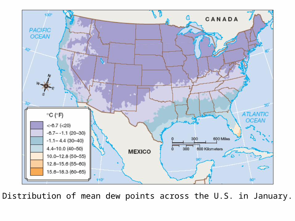
Distribution of mean dew points across the U.S. in January.

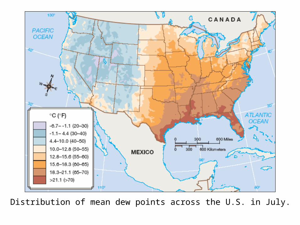
Distribution of mean dew points across the U.S. in July.

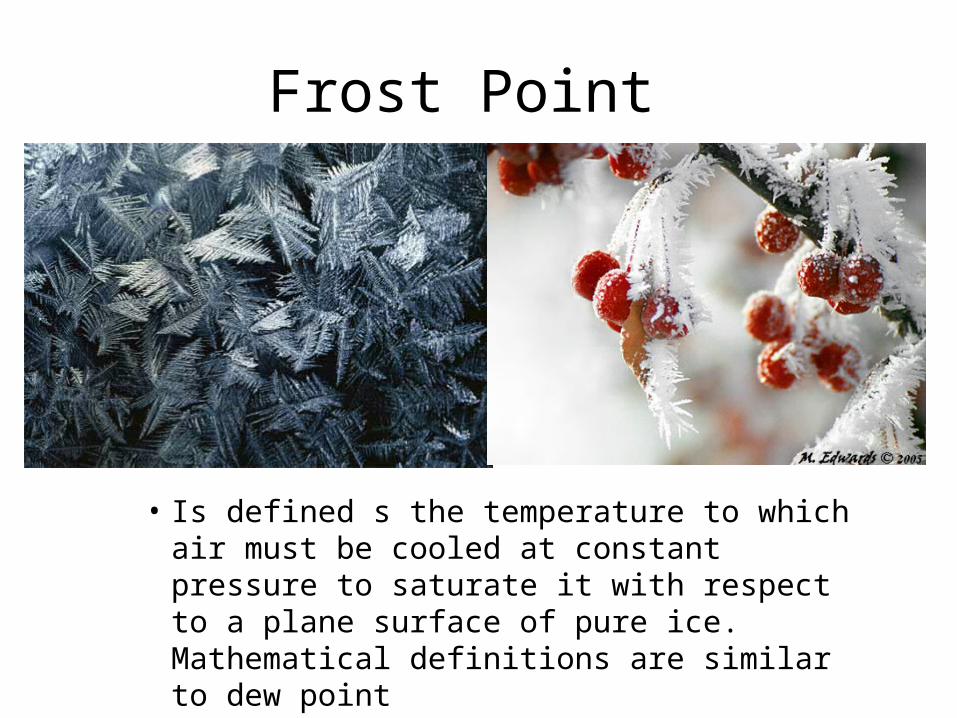
Frost Point

• Is defined s the temperature to which air must be cooled at constant pressure to saturate it with respect to a plane surface of pure ice. Mathematical definitions are similar to dew point

Exercise 3.8: Air at 1000 hPa has a mixing ratio of 6g/kg. What are the relative humidity and dew point of the air?

• Use the Skew-t lnp chart to answer this question. Use RH=100(w/ws) and Td is the temperature at w.