ATMOSPHERE PHYSICS LECTURE NOTES - Cors-Tr

T.C. ISTANBUL KÜLTÜR UNIVERSITY

ATMOSPHERE PHYSICS LECTURE NOTES

(15th August –5th September 2006)

Assoc. Prof. Dr. Ayşegül YILMAZ Project Supportive

Researcher Çanakkale Onsekiz Mart University

Publication No : 1

Contnents CHAPTER 1 : EARTH’S ATMOSPHERIC STRUCTURE 1.1 ATMOSPHERIC LAYERS 1 1.1.1 Troposphere 1 1.1.2 Stratosphere 2 1.1.3 Mesosphere 3 1.1.4 Thermosphere 4 1.1.5 Exosphere 5 1.2 IONOSPHERE 5 1.2.1 Ionospheric Layers 5 1.2.2 Ionospheric Density Profile 7 1.2.3 Aurora 7 CHAPTER 2 : TERRESTIAL IONOSPHERE AT HIGH LATITUDES 2.1 ELECTROMAGNETIC COUPLING 8 2.2CONVECTION ELECTRIC FIELDS 9 2.2.1 Convection Models 10 2.3.1 Effects of Convection Model 11 2.3 PARTICLE PRECIPITATION 11 2.4 CURRENT SYSYTEMS 12 2.5 LARGE SCALE ATMOSPHERIC STRUCTURES 13 2.6 GEOMAGNETIC STORMS 14 2.7 SUBSTORMS 14 2.8 POLAR WIND 14 CHAPTER 3 : PHYSICS OF NEUTRAL ATMOSPHERE 3.1 PHYSICS LAWS FOR THE NEUTRAL ATMOSPHERE 15 3.1.1 Equation of state 16 3.1.2 Hydrostatic Equilibrium 17 3.1.3 Snell’s law 18

3.2 WATER VAPOR 19 3.2.1 Mixing ratio 19 3.2.2 Virtual temperature 20 3.2.3 Partial pressure of saturated air 21 3.2.4 Relative humidity 22 3.3 PROPOGATION DELAY AND REFRACTIVITY 24 3.4 ATMOSPHERIC PROFILES 28 3.4.1 Refractivity profile of dry air 30 3.4.2 Saturation profile 30 CHAPTER 4: PHYSICS OF IONOSPHERE 4.1 HISTORY 32 4.2 THE REQUIREMENTS FOR AN IONOSPHERE 33 4.3 THE NEUTRAL ATMOSPHERE 34 4.4 ION PRODUCTION 35 4.5 PARTICLE IMPACT IONIZATION 39 4.6 ION LOSS 41 4.7 DETERMINING IONOSPHERIC DENSITY FROM PRODUCTION AND LOSS RATES 41 CHAPTER 5: ATMOSPHERIC WAVE PROPAGATION 5.1 RADIO WAVE PROPAGATION CHARACTERISTICS 43 5..1.1 REFRACTION 43 5.1.1.1 Layer density 43 5.1.1.2 Frequency 44 5.1.1 3 Angle of incidence and Critical angle 45 5.1.2 REFLECTION 47 5.1.3.DIFRACTION 48 5.2 ATMOSPHERIC EFFECTS ON PROPAGATION 50 5.2.1 REGULAR VARIATIONS 48 5.2.1.1 FADING 48 5.2..1.2 MULTIPATH 49 5.2.1.3 SEASONAL VARIATIONS IN THE IONOSPHERE 50

5.2.1.4 SUNSPOTS 50 5.2.1.4. 1 Twenty-seven day cycle 51 5.2.1.4.2 Eleven-year-cycle 52 5.2.2 IRREGULAR VARIATIONS 52 5.2.2 1 Spordic E 52 5.2.2.2 Sudden Ionospheric Disturbances 53 5.2.2 3 Ionospheric Storms 53 5.3 WEATHER 53 5.3.1.Rain 53 5.3.2 Fog 53 5.3.3 Snow 53 5.3.4 Hail 53 REFERENCES 54

Acknowledgements

We would like to thank Prof.Dr.Turgut UZEL for his invitation to give a seminar on Physics of Ionosphere,

Aug.15 and 30, 2006,İstanbul Kültür University, under TÜBİTAK CORS TR Project.

CHAPTER 1 : EARTH’S ATMOSPHERIC STRUCTURE

1. 1 ATMOSPHERİC LAYERS

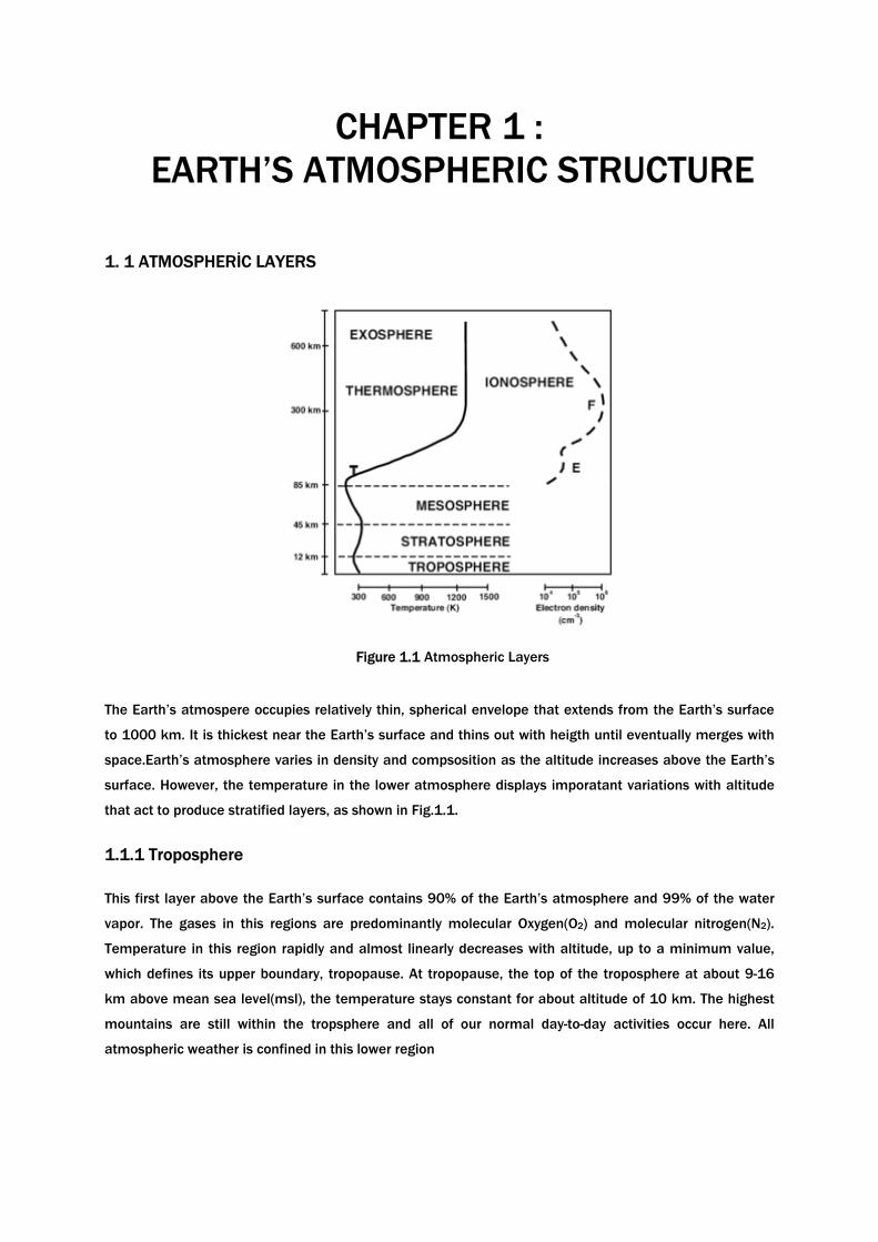
Figure 1.1 Atmospheric Layers

The Earth’s atmospere occupies relatively thin, spherical envelope that extends from the Earth’s surface

to 1000 km. It is thickest near the Earth’s surface and thins out with heigth until eventually merges with

space.Earth’s atmosphere varies in density and compsosition as the altitude increases above the Earth’s

surface. However, the temperature in the lower atmosphere displays imporatant variations with altitude

that act to produce stratified layers, as shown in Fig.1.1.

1.1.1 Troposphere

This first layer above the Earth’s surface contains 90% of the Earth’s atmosphere and 99% of the water

vapor. The gases in this regions are predominantly molecular Oxygen(O2) and molecular nitrogen(N2).

Temperature in this region rapidly and almost linearly decreases with altitude, up to a minimum value,

which defines its upper boundary, tropopause. At tropopause, the top of the troposphere at about 9-16

km above mean sea level(msl), the temperature stays constant for about altitude of 10 km. The highest

mountains are still within the tropsphere and all of our normal day-to-day activities occur here. All

atmospheric weather is confined in this lower region

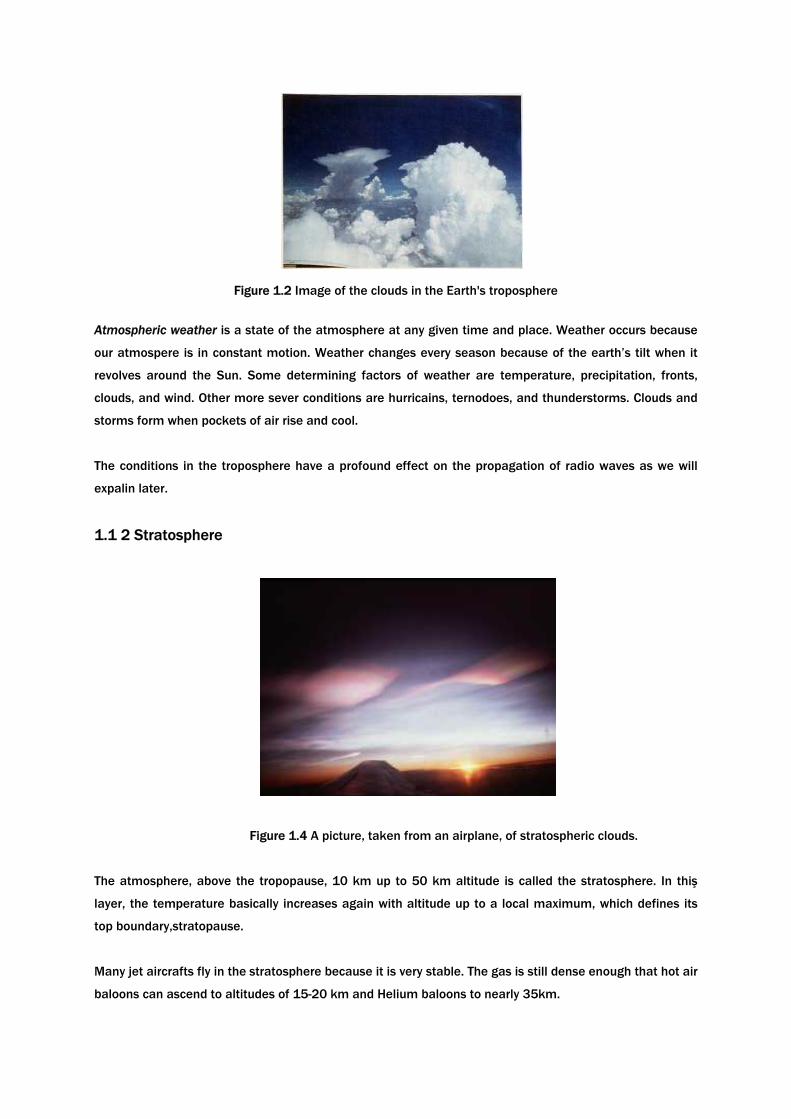
Figure 1.2 Image of the clouds in the Earth's troposphere

Atmospheric weather is a state of the atmosphere at any given time and place. Weather occurs because

our atmospere is in constant motion. Weather changes every season because of the earth’s tilt when it

revolves around the Sun. Some determining factors of weather are temperature, precipitation, fronts,

clouds, and wind. Other more sever conditions are hurricains, ternodoes, and thunderstorms. Clouds and

storms form when pockets of air rise and cool.

The conditions in the troposphere have a profound effect on the propagation of radio waves as we will

expalin later.

1.1 2 Stratosphere

Figure 1.4 A picture, taken from an airplane, of stratospheric clouds.

The atmosphere, above the tropopause, 10 km up to 50 km altitude is called the stratosphere. In thiş

layer, the temperature basically increases again with altitude up to a local maximum, which defines its

top boundary,stratopause.

Many jet aircrafts fly in the stratosphere because it is very stable. The gas is still dense enough that hot air

baloons can ascend to altitudes of 15-20 km and Helium baloons to nearly 35km.

The ozone layer exists in the stratosphere. The ozone molecules absorb dangerous kinds of sunlight,

which heats the air around them. On Earth, ozone causes the increasing temperature in the stratosphere.

Because it is a relatively calm region with little a little or no temperature change, the stratosphere has

almost no effecy on radio waves.

1.1 3 Mesosphere

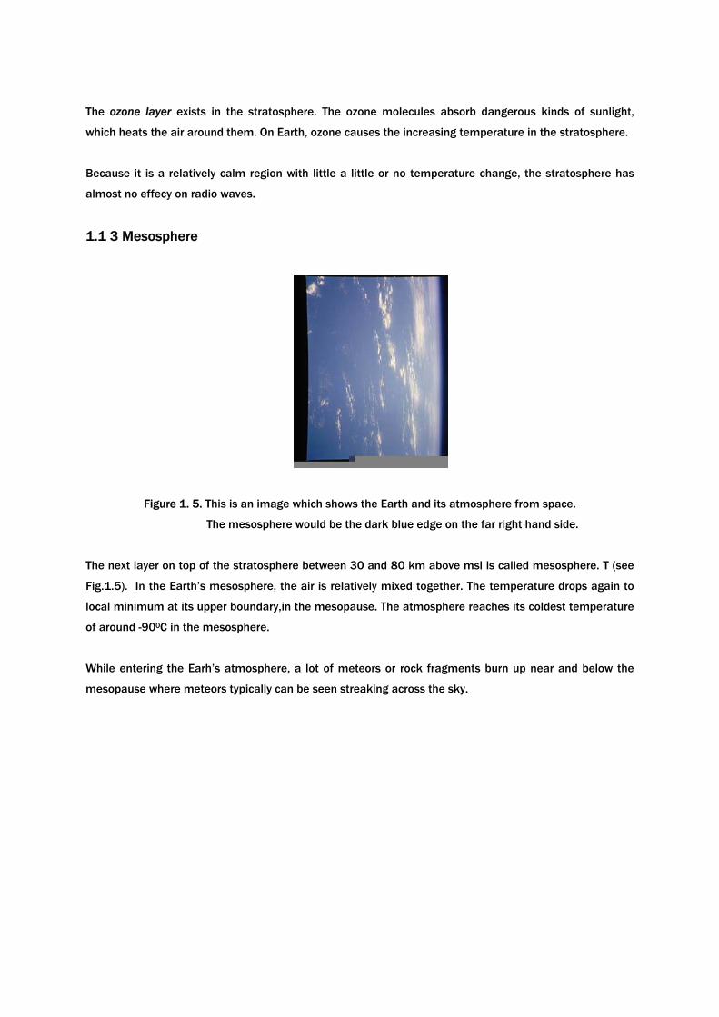
Figure 1. 5. This is an image which shows the Earth and its atmosphere from space.

The mesosphere would be the dark blue edge on the far right hand side.

The next layer on top of the stratosphere between 30 and 80 km above msl is called mesosphere. T (see

Fig.1.5). In the Earth’s mesosphere, the air is relatively mixed together. The temperature drops again to

local minimum at its upper boundary,in the mesopause. The atmosphere reaches its coldest temperature

of around -900C in the mesosphere.

While entering the Earh’s atmosphere, a lot of meteors or rock fragments burn up near and below the

mesopause where meteors typically can be seen streaking across the sky.

1.1 4. Thermosphere

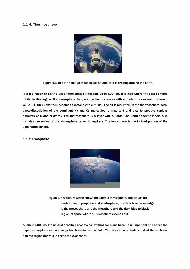
Figure 1.6 This is an image of the space shuttle as it is orbiting around the Earth.

It is the region of Earth’s upper atmosphere extending up to 500 km. It is also where the space shuttle

orbits. In this region, the atmospheric temperature first increases with altitude to an overall maximum

value (∼1000 K) and then becomes constant with altitude. The air is really thin in the thermosphere. Also,

photo-dissociation of the dominant N2 and O2 molecules is important and acts to produce copious

amounts of O and N atoms. The thermosphere is a layer with auroras. The Earth’s thermosphere also

includes the region of the atmosphere called ionosphere. The ionosphere is the ionized portion of the

upper atmosphere.

1.1 5 Exosphere

Figure 1.7 A picture which shows the Earth’s atmosphere. The clouds are

likely in the troposphere and stratosphere, the dark blue curve/edge

is the mesosphere and thermosphere and the dark blue to black

region of space where our exosphere extends out.

At about 500 km, the neutral densities become so low that collisions become unimportant and hence the

upper atmosphere can no longer be characterized as fluid. This transition altitude is called the exobase,

and the region above it is called the exosphere.

1.2 IONOSPHERE

The ionosphere extends form 60 km to 2000 km altitude. Because the composition of the atmosphere

changes with height, the ion production rate also changes and this leads to the formation of several

distinct ionization peaks, the "D"( 50 km to 90 km), "E" (90 km to 120 km), "F" layers. above the surface

of the Earth.

Different regions of the ionosphere make long distance, point-to-point radio communications possible by

reflecting the radio waves back to Earth.

1.2 1 Ionospheric Layers

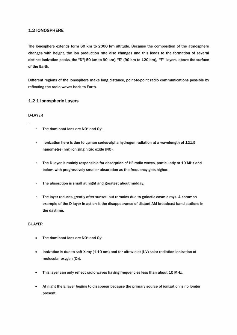
D-LAYER

.

• The dominant ions are NO+ and O2+.

• Ionization here is due to Lyman series-alpha hydrogen radiation at a wavelength of 121.5

nanometre (nm) ionizing nitric oxide (NO).

• The D layer is mainly responsible for absorption of HF radio waves, particularly at 10 MHz and

below, with progressively smaller absorption as the frequency gets higher.

• The absorption is small at night and greatest about midday.

• The layer reduces greatly after sunset, but remains due to galactic cosmic rays. A common

example of the D layer in action is the disappearance of distant AM broadcast band stations in

the daytime.

E-LAYER

• The dominant ions are NO+ and O2+.

• Ionization is due to soft X-ray (1-10 nm) and far ultraviolet (UV) solar radiation ionization of

molecular oxygen (O2).

• This layer can only reflect radio waves having frequencies less than about 10 MHz.

• At night the E layer begins to disappear because the primary source of ionization is no longer

present.

• The increase in the height of the E layer maximum increases the range to which radio waves can

travel by reflection from the layer.

• The E region peaks at about 105km.

ES-LAYER

• ES or Sporadic E propagation is characterized by small clouds of intense ionization, which can

support radio wave reflections from 25 – 225 MHz.

• Sporadic-E events may last for just a few minutes to several hours and make radio amateurs very

excited, as propagation paths which are generally unreachable, can open up.

• This propagation occurs most frequently during the summer months with major occurrences

during the summer, and minor occurrences during the winter.

• During the summer, this mode is popular due to its high signal levels.

F-LAYER

• In the F region O+ ion dominates.

• Above the F region is a region of exponentially decreasing density known as the "topside

ionosphere." This region extends to an altitude of a few thousand kilometers.

• Here extreme ultraviolet (UV) (10-100 nm) solar radiation ionizes atomic oxygen (O).

• The F region is the most important part of the ionosphere in terms of HF communications.

• During daytime, it divides into two layers, the F1 and F2.

• The F layers are thickest and most reflective of radio on the side of the Earth facing the sun.

On a more practical note, the D and E regions reflect AM radio waves back to Earth. Visible light,

television and FM wavelengths are all too short to be reflected by the ionosphere. So your tv. stations are

made possible by satellite transmissions.

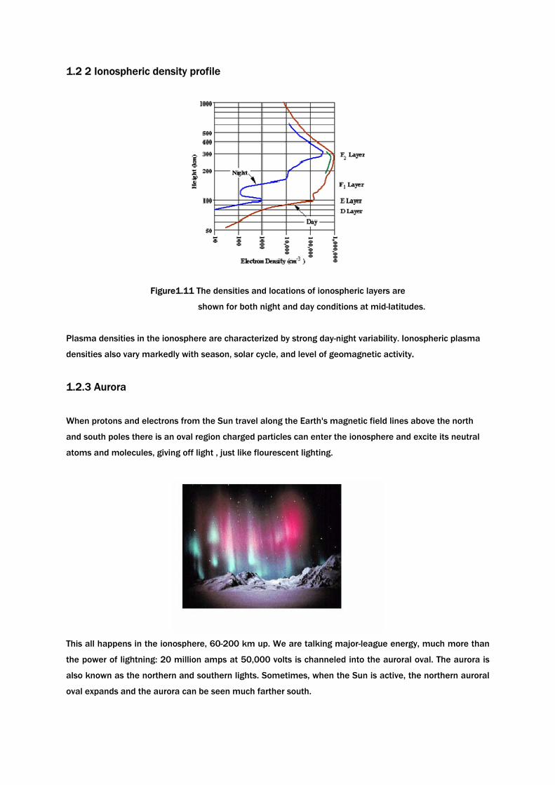
1.2 2 Ionospheric density profile

Figure1.11 The densities and locations of ionospheric layers are

shown for both night and day conditions at mid-latitudes.

Plasma densities in the ionosphere are characterized by strong day-night variability. Ionospheric plasma

densities also vary markedly with season, solar cycle, and level of geomagnetic activity.

1.2.3 Aurora

When protons and electrons from the Sun travel along the Earth's magnetic field lines above the north

and south poles there is an oval region charged particles can enter the ionosphere and excite its neutral

atoms and molecules, giving off light , just like flourescent lighting.

This all happens in the ionosphere, 60-200 km up. We are talking major-league energy, much more than

the power of lightning: 20 million amps at 50,000 volts is channeled into the auroral oval. The aurora is

also known as the northern and southern lights. Sometimes, when the Sun is active, the northern auroral

oval expands and the aurora can be seen much farther south.

CHAPTER 2:

THE TERRESTIAL-IONOSPHERE

AT HIGH LATITUDES

2.1.ELECTROMAGNETİC COUPLING

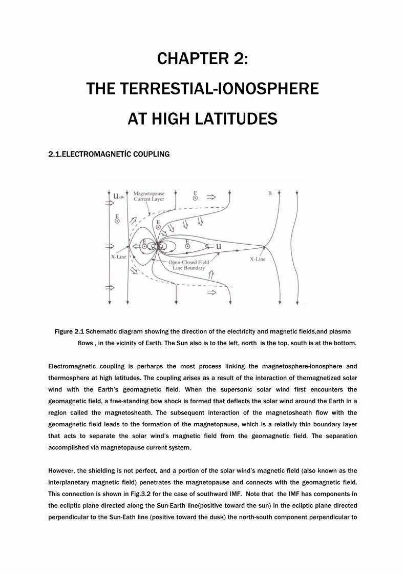
Figure 2.1 Schematic diagram showing the direction of the electricity and magnetic fields,and plasma

flows , in the vicinity of Earth. The Sun also is to the left, north is the top, south is at the bottom.

Electromagnetic coupling is perharps the most process linking the magnetosphere-ionosphere and

thermosphere at high latitudes. The coupling arises as a result of the interaction of themagnetized solar

wind with the Earth’s geomagnetic field. When the supersonic solar wind first encounters the

geomagnetic field, a free-standing bow shock is formed that deflects the solar wind around the Earth in a

region called the magnetosheath. The subsequent interaction of the magnetosheath flow with the

geomagnetic field leads to the formation of the magnetopause, which is a relativly thin boundary layer

that acts to separate the solar wind’s magnetic field from the geomagnetic field. The separation

accomplished via magnetopause current system.

However, the shielding is not perfect, and a portion of the solar wind’s magnetic field (also known as the

interplanetary magnetic field) penetrates the magnetopause and connects with the geomagnetic field.

This connection is shown in Fig.3.2 for the case of southward IMF. Note that the IMF has components in

the ecliptic plane directed along the Sun-Earth line(positive toward the sun) in the ecliptic plane directed

perpendicular to the Sun-Eath line (positive toward the dusk) the north-south component perpendicular to

the ecliptic plane (positive toward the north). The connection of the IMF and the geomagnetic field

ooccurs in a circular region known as the polar cap, and the connected field lines are referred to as open

field lines. The auroral oval is an intermediate region that lies between the open line region (polar region)

and the low-latitude region that contains dipolar magnetic field lines. The field lines in the auroral oval are

closed, but they are stretched deep in the magnetospheric tail.

2.2 CONVECTION ELECTRIC FIELDS

The solar wind is a highly conducting, collisionless, magnetized plasma that, to lower, can be derived by

ideal MHD equations. Therefore, the electric field in the solar wind is governed by the relation E = -uswxB ,

where usw is the velocity of solar wind. When the radial solar wind, with a southward IMF component

interacts with the Earth’s magnetic field (Fig.3.2), an electric field is imposed that points in the down-to-

dusk direction across the polar cap. This imposed electric field, which is directed perpendicular to B, maps

down to the ionospheric altitudes along highly conducting geomagnetic field lines. In the ionosphere, this

electric field causes the plasma in the polar cap to ExB drift in an antisunward direction. Further, from the

Earth, the plasma on the open polar cap field lines exhibits an ExB drift that is toward the equatorial plane

In the distant magnetospheric tail, the field lines reconnect, and the flown on those closed field lines is

toward and around the Earth. The existence of an electric field across the polar cap implies that the

boundary between open and closed magnetic field lines is charged. The charge is positive on the

dawnside and negative on the duskside, as shown in the solar wind out of the plane of the Fig.3.2 and

earth is at the top.

The charges on the polar cap boundary act to induce electric fields on nearby closed field lines that are

opposite to in direction to the electric fields in the polar cap. These oppositely directed electric fields are

situated in the regions just equatorward of the dawn and dusk sides of the polar cap. As with the polar

cap electric field, the electric fields on the closed field lines map down to the ionospereic altitudes and

cause the plasma to ExB drift in a sunward direction. On the field lines that separate the oppositely

directed fields, field-aligned (or Birkeland) currents flow between the ionoısphere and magnetosphere.

The current flow is along B and toward the ionosphere on the dawnside, across B and away from the

ionospere on the duskside.

The net effect of the electric configurationin Fig.3.2 is as follows. Closed dipolar magnetic field lines

connect to the IMF at the dayside magnetopause. When this connection occurs, the ionospheric foot of

the field line is at the dayside boundary of the polar cap. After connection, the open field line and

attached plasma, convect in an antisunward direction across the polar cap. When the ionospheric foot of

the open field line is at the nightside polar cap boundary, the magnetospheric end is in equatorial plane of

the distant magnetotail.

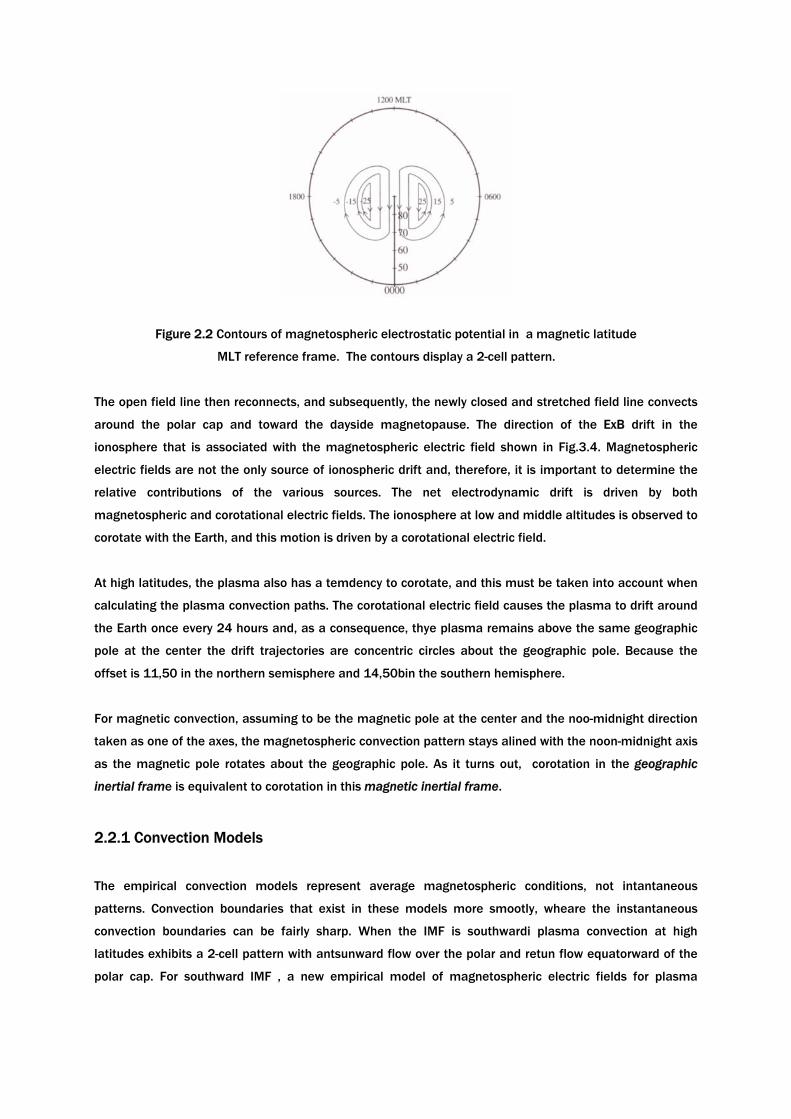
Figure 2.2 Contours of magnetospheric electrostatic potential in a magnetic latitude

MLT reference frame. The contours display a 2-cell pattern.

The open field line then reconnects, and subsequently, the newly closed and stretched field line convects

around the polar cap and toward the dayside magnetopause. The direction of the ExB drift in the

ionosphere that is associated with the magnetospheric electric field shown in Fig.3.4. Magnetospheric

electric fields are not the only source of ionospheric drift and, therefore, it is important to determine the

relative contributions of the various sources. The net electrodynamic drift is driven by both

magnetospheric and corotational electric fields. The ionosphere at low and middle altitudes is observed to

corotate with the Earth, and this motion is driven by a corotational electric field.

At high latitudes, the plasma also has a temdency to corotate, and this must be taken into account when

calculating the plasma convection paths. The corotational electric field causes the plasma to drift around

the Earth once every 24 hours and, as a consequence, thye plasma remains above the same geographic

pole at the center the drift trajectories are concentric circles about the geographic pole. Because the

offset is 11,50 in the northern semisphere and 14,50bin the southern hemisphere.

For magnetic convection, assuming to be the magnetic pole at the center and the noo-midnight direction

taken as one of the axes, the magnetospheric convection pattern stays alined with the noon-midnight axis

as the magnetic pole rotates about the geographic pole. As it turns out, corotation in the geographic

inertial frame is equivalent to corotation in this magnetic inertial frame.

2.2.1 Convection Models

The empirical convection models represent average magnetospheric conditions, not intantaneous

patterns. Convection boundaries that exist in these models more smootly, wheare the instantaneous

convection boundaries can be fairly sharp. When the IMF is southwardi plasma convection at high

latitudes exhibits a 2-cell pattern with antsunward flow over the polar and retun flow equatorward of the

polar cap. For southward IMF , a new empirical model of magnetospheric electric fields for plasma

convection constructed from a large database of satellite measurements yields multi-cell convection

pattern for northward.

2.2.2 Effects of Convection Model

The effect that convect ion electtric field have on the ionosphere depends on altitude. At ionospheric

altitudes, the electron-neutral collision frequency is much smaller than the electron cyclotron frequency

and hence , only the combined effect of the perpendicular electric field ,E, and the geomagnetic field, B, is

to induce and electric drift in the ExB direction. For ion, the ion-neutral colision frequencies are graeter

than the corresponding cyclotron frequencies at E-region, with the result that the ion drift in the direction

of the perpendiculaar electric field. Since the ion-neutral frequency decreases as the altidute increases,at

F-region altitudes both ions and electron drifts in the ExB direction.

At altitude above 800 km, the plasma begin to flow ouT ofthe topside ionosphere with a speed that

increases with altitude, and this phenomena is known as polar wind. The neutral wind vectors are

consistent with 2-cellplasma convection pattern, which occurs when the IMF is southwad. When the IMF

is northward, multi-cell signature should also be reflected in the thermosphere circulation pattern. The

ions are frictionally heated via ion-neutral collisions, as they convect through the slower moving neutral

gas, and this acts to raise the ion temperature.

2.3 PARTICLE PRECIPITATION

Energetic electron precipitation in the auroral oval not onlyis the source of optical emision, but also, is

a source of ionization due to electron impact with the neutral atmosphere,

A source of bulk heating for both ionosphere and atmosphere,

A source of heat that flows down from the lower magnetosphere into the iosphere

For a southward IMF, the electron precipitaiton cocurs in distinct regions in the aurora; diffusive auroral

precipitation, discrete arcs in the nocturnal oval, low energy polar rain precipitation, soft precipitation in

the cusp and diffusive auroral patches in the morning oval.

For a northward IMF, there are sun-aligned arcs in the polar cap. Ion precipitation also occurs in the

auroralzone and, on average, the ion precipitation pattern varies systematcally with magnetic latidute,

magnetic local time, and Kp.

The average energy of the percipitating ions is substantially greater than than that for the precipitating

electrons. For quiet magnetic conditions the maximum energy flux is about 1 erg cm -2 s-1. For active

conditions, the maximum energy flux reaches 8 ergcm-2 s-1. In general, the particle precipitation in the

auroral zone is structured and highly time dependent.

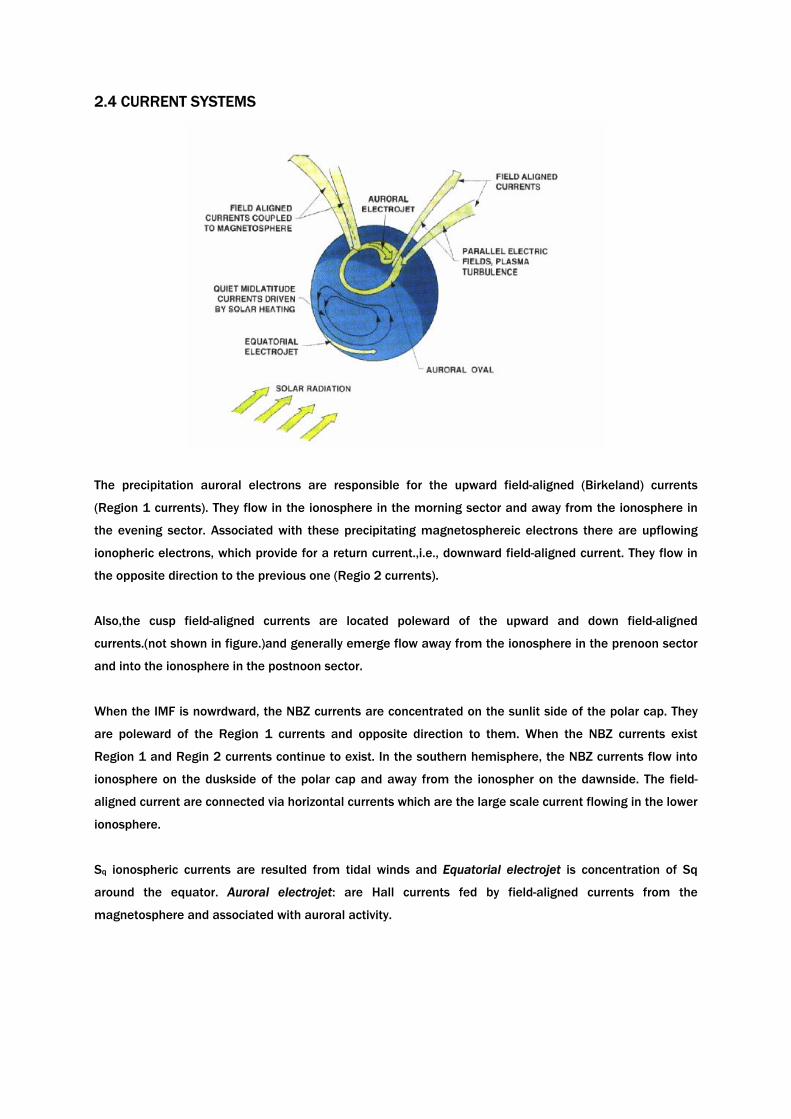
2.4 CURRENT SYSTEMS

The precipitation auroral electrons are responsible for the upward field-aligned (Birkeland) currents

(Region 1 currents). They flow in the ionosphere in the morning sector and away from the ionosphere in

the evening sector. Associated with these precipitating magnetosphereic electrons there are upflowing

ionopheric electrons, which provide for a return current.,i.e., downward field-aligned current. They flow in

the opposite direction to the previous one (Regio 2 currents).

Also,the cusp field-aligned currents are located poleward of the upward and down field-aligned

currents.(not shown in figure.)and generally emerge flow away from the ionosphere in the prenoon sector

and into the ionosphere in the postnoon sector.

When the IMF is nowrdward, the NBZ currents are concentrated on the sunlit side of the polar cap. They

are poleward of the Region 1 currents and opposite direction to them. When the NBZ currents exist

Region 1 and Regin 2 currents continue to exist. In the southern hemisphere, the NBZ currents flow into

ionosphere on the duskside of the polar cap and away from the ionospher on the dawnside. The field-

aligned current are connected via horizontal currents which are the large scale current flowing in the lower

ionosphere.

Sq ionospheric currents are resulted from tidal winds and Equatorial electrojet is concentration of Sq

around the equator. Auroral electrojet: are Hall currents fed by field-aligned currents from the

magnetosphere and associated with auroral activity.

2.5 LARGE SCALE IONOSPHERIC STRUCTURES

The magnetospheric electric fields, particle precipitation, and field-aligned currents act in concert to

produce large-scale ionospheric structures. These include

• Polar holes,

• Ionization troughs,

• Tongues of ionization,

• Plasma patches,

• Auroral ionization enhancements, and

• Electron and ion temperature hot spots.

Whether a feature occurs and the detailed characteristics of a feature depend on the phase of the solar

cycle, season, time of day (diurnal) type of convection pattern, and the strength of convection.

Most of the large-scale features that have been identifeid occur for southward IMF. In this case, 2-cell

convection pattern exists, with anti-sunward flow over the polar cap and sunward at lower altitudes. The

effect of the anti-sunward flow is to transport the high density dayside plasma into the polar cap. The

polar hole is a region on the nightside of the polar cap where reduced ionization exists because of the

long transport time of ionization from the dayside across the polar cap. In summer, when the bulk of the

polar cap is sunlit, difference in anti-sunward convection is not significant since the plasm density tend to

be uniform. In winter, it is important. In the auroral oval, the density is enhanced because of the impact

ionization due to precipitating electrons.

The net result is a polar hole if the antisunward convection speed is low and it situated just poleward of

the noctural oval. When the speed is high, high-density dayside plasma can be transported great

distances before it decays apprecably. The net result is a tongue of ionization extending across the polar

cap from the dayside to the nightside. Main or mid-altitude electron density trough which is located

equatorward of the nocturnal auroral oval is a region of low electron density that has a narrow latitudenal

extend, it is extended in longitude. Ion temperature hot spots can occur in the high-latitude ionosphere

during periods when the convection electric fields are strong and nearthe dusk and/or dawn meridians.

Electron temperature hot spots exist in high-latitude ionosphere due to mainly electron precipitation.

Plasma patches are created either in the dayside cusp or just equatorward of the cusp. Path densities are

a factor of 3-10 greater than the background densities and their horizontal dimensions vary from 200 to

1000 km

Sun-aligned polar cap arcs appear when the IMF is near zero or northward and as a result of electron

precipitation, with charecteristic energy varying from 300eV to 5 keV. They are relatively narrow (< or =

300 km) across polar cap, but extended along noon-midnight direction(1000-3000 km).

2.6 GEOMAGNETIC STORMS

A geomagnetic storm is a temporary intense disturbance of the Earth's magnetosphere. when there is a

sudden change in the solar wind dynamic pressure at magnetopause. It occurs when it is impacted by a

coronal mass ejection or solar flare material . There subsequent propagation toward lower latitude leads

to a travelling ionospheric disturbance.

2.7 SUBSTORMS

At mid-latitudes, the equatorward propagating waves drive the F region ionization toward higher altitude

which result in ionization enhancement. Associated with substorms are localized regions of enhanced

electric fields, particle precipitation, and both field-aligned and electrojet currents.

2.8 POLAR WIND

The classical polar wind is and amipolar outflow of thermal plasma from the high-latitıde ionosphere

As the light ion plasma flows up and out of the topside ionosphere along diverging geomagnetic field

lines, it undergoes four major transitions,

• A transition from chemical to diffusion dominance

• A transition from the subsonic to supersonic flow,

• A transition from collision-dominted to collissinless regimes, and

• A transition from a heavy (O+) to a light (H+) ion

At times,hower, O+ can remain the dominant ion to very high altitudes in the polar cap.

CHAPTER 3:

PHYSICS

OF

THE NEUTRAL ATMOSPHERE

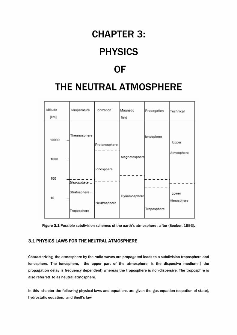
Figure 3.1 Possible subdivision schemes of the earth’s atmosphere , after (Seeber, 1993).

3.1 PHYSICS LAWS FOR THE NEUTRAL ATMOSPHERE

Characterizing the atmosphere by the radio waves are propagated leads to a subdivision troposphere and

ionosphere. The ionosphere, the upper part of the atmosphere, is the dispersive medium ( the

propagation delay is frequency dependent) whereas the troposphere is non-dispersive. The troposphre is

also referred to as neutral atmosphere.

In this chapter the following physical laws and equations are given the gas equation (equation of state),

hydrostatic equation, and Snell’s law

3.1.1 .Equation of state

In (Champion,1960) three laws for gases are given:

Charles’ constant pressure law:

“ At constant pressure for a rise in temperature of 1degree Celsius, all gases expand by a constant

amount, equal to 1/ 273 of their volume at 0 degree Celsius”.

Charles’ constant volume law:

“ If the volume is kept constant, all gases undergo an increase in pressure equal to 1/ 273 of their

pressure at 0 degree Celsius”.

Boyle’s law :

“ At constant temperature the product of pressure and volume is constant” .

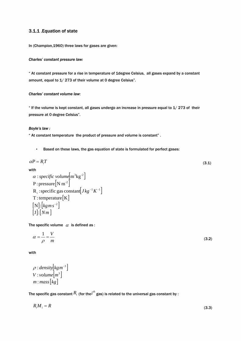
• Based on these laws, the gas equation of state is formulated for perfect gases:

(3.1)

with

The specific volume is defined as :

(3.2)

with

The specific gas constant (for the gas) is related to the universal gas constant by :

(3.3)

TRP i=α

[ ]-23kgm: volumespecificα[ ]-2m N pressure :P

[ ]11i constant gas specific :R −− KkgJ

[ ]K re temperatu:T[ ] [ ]2:N −smkg[ ] [ ]mN:J

α

mV

==ρ

α 1

[ ]3: −mkgdensityρ[ ]3: mvolumeV

[ ]kgmassm :

iR thi

RMR ii =

with

Although there is no perfect gases, the gas in the traposphere are nearly perfect and can often be treated

as such. as

The equation of state does not only hold for one specific gas, but also a mixture of gases. In that case,

is the sum of the particle pressures,

is the specific gas constant of the mixture, and

is the mean molecular mass of the mixture.

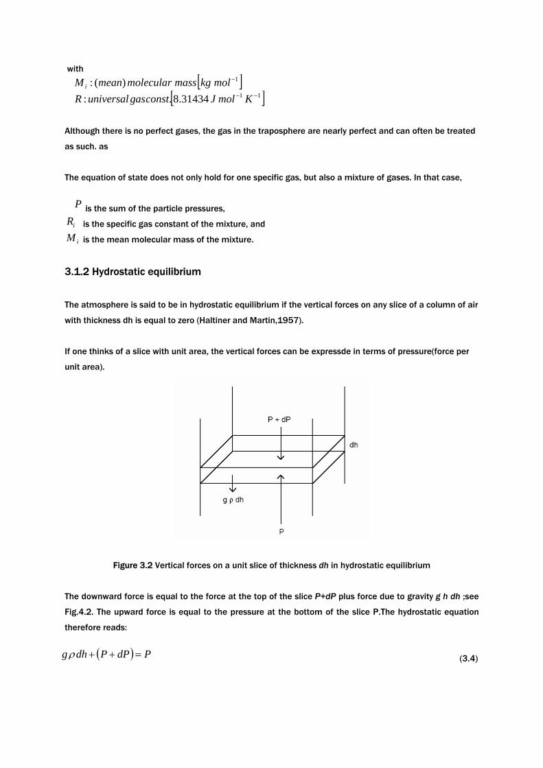
3.1.2 Hydrostatic equilibrium

The atmosphere is said to be in hydrostatic equilibrium if the vertical forces on any slice of a column of air

with thickness dh is equal to zero (Haltiner and Martin,1957).

If one thinks of a slice with unit area, the vertical forces can be expressde in terms of pressure(force per

unit area).

Figure 3.2 Vertical forces on a unit slice of thickness dh in hydrostatic equilibrium

The downward force is equal to the force at the top of the slice P+dP plus force due to gravity g h dh ;see

Fig.4.2. The upward force is equal to the pressure at the bottom of the slice P.The hydrostatic equation

therefore reads:

(3.4)

[ ]1)(: −molkgmassmolecularmeanMi

[ ]1131434.8.: −− KmolJconstgasuniversalR

P

iR

iM

( ) PdPPdhg =++ρ

Rewriting Eq.(3.4) gives:

(3.5)

with

Using the definition of Eq.(2), this may be also written as:

(3.6)

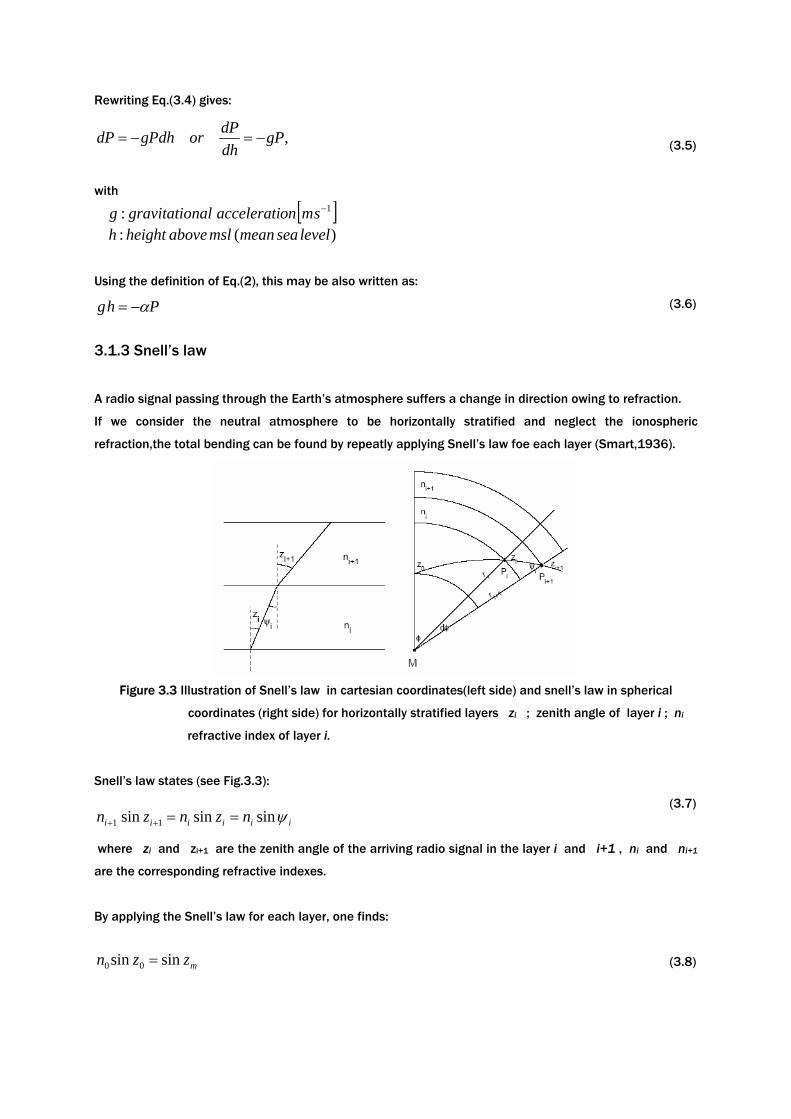
3.1.3 Snell’s law

A radio signal passing through the Earth’s atmosphere suffers a change in direction owing to refraction.

If we consider the neutral atmosphere to be horizontally stratified and neglect the ionospheric

refraction,the total bending can be found by repeatly applying Snell’s law foe each layer (Smart,1936).

Figure 3.3 Illustration of Snell’s law in cartesian coordinates(left side) and snell’s law in spherical

coordinates (right side) for horizontally stratified layers zi ; zenith angle of layer i ; ni

refractive index of layer i.

Snell’s law states (see Fig.3.3):

(3.7)

where zi and zi+1 are the zenith angle of the arriving radio signal in the layer i and i+1 , ni and ni+1

are the corresponding refractive indexes.

By applying the Snell’s law for each layer, one finds:

(3.8)

,gPdhdPorgPdhdP −=−=

)(: levelseameanmslaboveheighth[ ]1: −smonacceleratinalgravitatiog

Phg α−=

iiiiii nznzn ψsinsinsin 11 ==++

mzzn sinsin 00 =

where the index denotes the lowest layer and the index denotes the h,ghest layer, where the

refractive index reduces to 1. This formula holds for any refractivity profile.

For a spherical Earth we may formulate Snell’s law in spherical coordinates (Smart, 1936). Application of

sine rule in the triangle of Fig.4.2 gives:

(3.9)

where and are the distant and with two center of mass of the Earth.Combining

Eq.(7) and (9) gives SnellS law in spherical coordinates:

(3.10)

or simply

(3.11)

3.2 WATER VAPOR

The traposphere contains both dry air and water vapor. Dry has no significant variation in composition

with altitude an heigth (Smith and Weintrant, 1953). The amount of wator vapor, on the other hand,

varies widely, both spatially and temporally.

Water laso appears in the traposphere in liquid phase (fog, clouds, rain) and solid form (snow, hail, ice)

and the most important constituent in relation to weather processes, not only because of rain- and

snowfall but also because large amount of energy are released in condensation process.

In this section, we deal with some water—vapor related measures like mixing ratio, partial pressure of

vapor, relative humidity

3.2.1 Mixing ratio

The mixture of dry air and water vapor is called moist air. A measure of moisture air is the mixture ratio,

which is defined as the quotient of water-vapor mass per unit mass dry air (Haltiner and Martin, 1957).

(3.12)

1+iiPMP

( ) i

i

i

i

i

i

zr

zrr

sinsinsin11 ++ =

−=

πψ

ir 1+ir iMP 1+iMP M

000111 sinsinsin zrnzrnzrn iiiiii ==+++

mzzn sinsin 00 =

d

v

d

v

d

v

VmVm

mmw

ρρ

===

[ ]−ratiomixingw :[ ]kgvaporwaterofmassmv :

[ ]kgairdryofmassmd :

If we apply the equation of state, Eq.(3.1), for both water vapor and dry air, we obtain with use of

Eq.(3.13):

(3.13)

where

Another exprssion for the mixing ratio can be obtained from Eq.(4.12) and (4.13):

(3.14)

The approximation is allowed because the partial pressure of water vapor is typically about of the

total pressure. The constant in Eq.(3.14) are taken from (Mendes, 1999). An alternative to express the

humidity is the specific humidity

:

(3.15)

3.2.2 Virtual temperature

We can also apply the equation of state for moist air. In that case we have :

(3.16)

[ ]3: mvolumeV[ ]3: −mkgvaporwaterofdensityvρ

[ ]3: −mkgairdryofdensitydρ

TRePPTRe dddvv ρρ =−== ;

[ ]2: −mNvaporwaterofpressurepartiale[ ]2: −mNairdryofpressureparticlePd

[ ]2)(: −mNairmoistofpressuretotalP[ ]11tan: −− KkgJvaporwateroftconsgasspecificRv

[ ]11tan: −− KkgJairdryoftconsgasspecificRd

( ) TRePTRe

wd

v

−=∈

1101.006.237 −−±= KkgJRd11003.0525.461 −−±= KkgJRv

622.0=∈=v

d

RR

%1

wqm

≈=ρρ0

,TRP mmρ=

[ ]3: −mkgairmoistofdensitymρ

Since , combining Eq.(12),Eq.(13),and Eq.(16) gives as a function of the mixing air:

(3.17)

Substituting Eq.(4.17) in Eq.(4.16)

(3.18)

where

(3.19)

is the virtual temperature in kelvin.

In Eq.(3.18) the fixed gas constant is used instead of . The virtual temperature is acounted for

bt the use of a frictious temperature.

3.2.3 Partial presure of saturated air

In a closed system with no air, an equilibrium will be established when equal number of water molecules

are passing from liquid or solid to vapor, and vice versa. Under these circumstances the vapor is said to be

saturated. When the vapor is mixed with air, the mixture of air and water vapor under equilibrium

conditions is referred to as a saturated air. When saturated air comes in contact with unsaturated air,

diffusion takes place in the direction toward lower values of vapor.

The partial pressure of saturated water vapor is a function of temperature. Larger amounts of water vapor

can be contained by warmer air. By cooling saturated air, the surplus of water vapor above the satration

value at the new temperature condensates. The energy released(per unit mass) in the condensation is

called latent heat . The same amount of energy is required for vaporization. We also have the latent heat

of fusion, which is the amount of energy required in the change of a unit mass of ice to liquid water, the

latent heat of sublimation, which is the sum of the latent heats of vaporization and fusion.

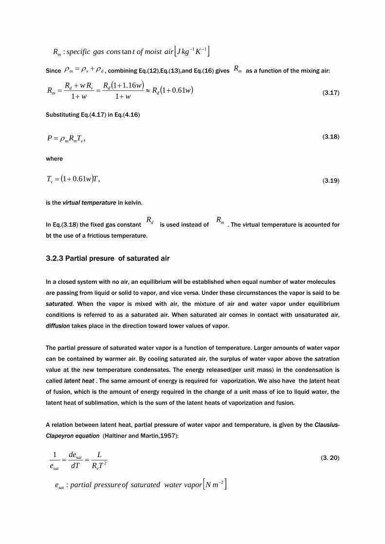
A relation between latent heat, partial pressure of water vapor and temperature, is given by the Clausius-

Clapeyron equation (Haltiner and Martin,1957):

(3. 20)

[ ]11tan: −− KkgJairmoistoftconsgasspecificRm

dvm ρρρ += mR

( ) ( )wRw

wRw

RwRR ddvd

m 61.011

16.111

+≈++

=++

=

,vmm TRP ρ=

( ) ,61.01 TwTv +=

dR mR

2

1TRL

dTde

e v

sat

sat

==

[ ]2: −mNvaporwatersaturatedofpressurepartialesat

In integration of Eq.4.(20) gives the partial pressure of water vapor as a function of temperature:

(3.21)

with either the latent heat of vaporization or sublimination The integration

constants are given at

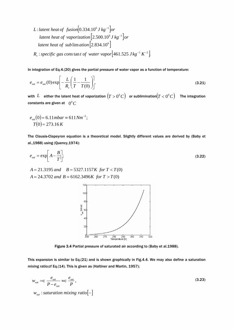
The Clausis-Clapeyron equation is a theoretical model. Slightly different values are derived by (Baby et

al.,1988) using (Quency,1974):

(3.22)

Figure 3.4 Partial pressure of saturated air according to (Baby et al.1988).

This expansion is similar to Eq.(21) and is shown graphically in Fig.4.4. We may also define a saturation

mixing ratio;cf Eq.(14). This is given as (Haltiner and Martin, 1957);

(3.23)

[ ][ ][ ]6

16

16

10.834.2lim10.500.2

10.334.0:

ationsubofheatlatentorkgJonvaporizatiofheatlatent

orkgJfusionofheatlatentL−

−

[ ].525.461tan: 21 −− KkgJvaporwateroftconsgasspecificRv

,)0(

11exp)0( ⎥⎦

⎤⎢⎣

⎡⎟⎟⎠

⎞⎜⎜⎝

⎛−−=

TTRLee

vsatsat

L ( )CT 00> ( )CT 00<C00

( ) ;61111.60 2−≡= Nmmbaresat

( ) KT 16.2730 =

;exp ⎥⎦⎤

⎢⎣⎡ −=

TBAesat

)0(3496.61623702.24)0(1157.53273195.21

TTforKBandATTforKBandA

>==<==

,P

eeP

ew sat

sat

satsat ≈∈

−=∈

[ ]−ratiomixingsaturationwsat :

3.2.4 Relative Humidity

The relative humidity is defined as the quotient the mixing ratio and saturation mixing ratio:

(3.24)

The relative humidity is often multiplied by hundred to express it in percentages.

3.3 PROPAGATION DELAY AND REFRACTIVITY

The total delay of a radio signal caused by the neutral atmosphere depends on the refractivity along the

travelled path, and The refractivity depends on pressure and temperature The basic physical law for

propagation is Fermat’s principle:

“Light (or any electromagnetic wave) will folow the path between two points involving the least travel

time”.

We define the electromagnetic (or optical) distance between source and receiver as:

(3.25)

where

The excess path length becomes

(3.27)

Where excess path length in the slant direction caused by troposphere .

satsath e

ewwr ≈=

[ ]−humidityrelativerh :

∫∫ ∫ ===S

dssndsvctdtS ,)(

[ ][ ]

[ ][ ]

[ ]−=

= −

−

indexrefractionvcn

msspeednpropagatiodldsv

smvacuuminligthofspeedcmpathneticelectromags

mcedisneticelectromagS

;

;

::

tan:

1

1

( )

1)(∫ ∫ ∫⎭⎬⎫

⎩⎨⎧

−+−=−=S S l

st dldsdssnLSD

stD

[ ] m

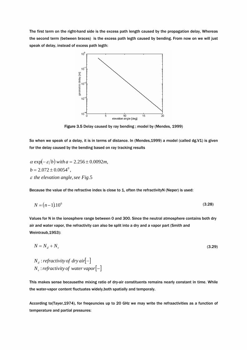
The first term on the right-hand side is the excess path length caused by the propagation delay, Whereas

the second term (between braces) is the excess path legth caused by bending. From now on we will just

speak of delay, instead of excess path legth:

Figure 3.5 Delay caused by ray bending ; model by (Mendes, 1999)

So when we speak of a delay, it is in terms of distance. In (Mendes,1999) a model (called dg.V1) is given

for the delay caused by the bending based on ray tracking results

Because the value of the refractive index is close to 1, often the refractivityN (Neper) is used:

(3.28)

Values for N in the ionosphere range between 0 and 300. Since the neutral atmosphere contains both dry

air and water vapor, the refractivity can also be split into a dry and a vapor part (Smith and

Weintraub,1953):

(3.29)

This makes sense becausethe mixing ratio of dry-air constituents remains nearly constant in time. While

the water-vapor content fluctuates widely,both spatially and temporaly.

According to(Tayer,1974), for freqeuncies up to 20 GHz we may write the refraactivities as a function of

temperature and partial pressures:

( )

5.,,0054.0072.2

,0092.0256.2exp0

Figseeangleelevationtheb

mawithb

ε

εα

±=

±=−

( ) 610.1−= nN

vd NNN +=

[ ][ ]−

−vaporwateroftyrefractiviN

airdryoftyrefractiviN

v

d

::

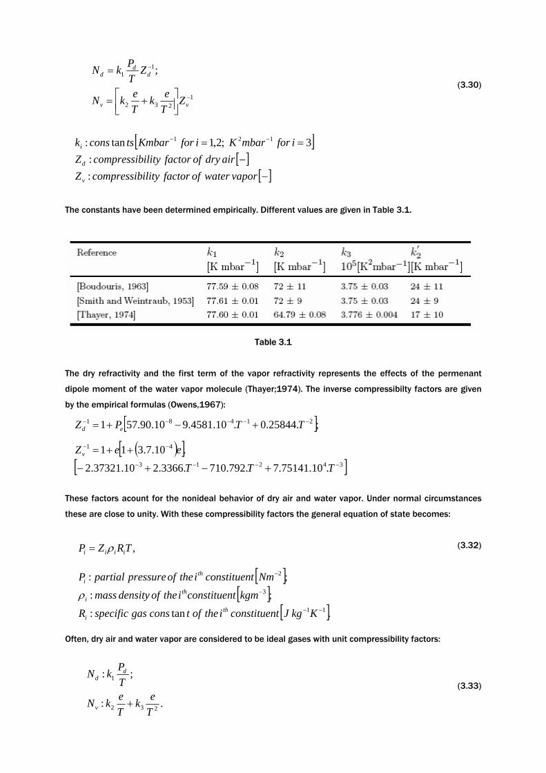
(3.30)

The constants have been determined empirically. Different values are given in Table 3.1.

Table 3.1

The dry refractivity and the first term of the vapor refractivity represents the effects of the permenant

dipole moment of the water vapor molecule (Thayer;1974). The inverse compressibilty factors are given

by the empirical formulas (Owens,1967):

These factors acount for the nonideal behavior of dry air and water vapor. Under normal circumstances

these are close to unity. With these compressibility factors the general equation of state becomes:

(3.32)

Often, dry air and water vapor are considered to be ideal gases with unit compressibility factors:

(3.33)

1232

11 ;

−

−

⎥⎦⎤

⎢⎣⎡ +=

=

vv

dd

d

ZTek

TekN

ZTPkN

[ ][ ]

[ ]−−

== −−

vaporwateroffactorilitycompressibZairdryoffactorilitycompressibZ

iformbarKiforKmbartsconsk

v

d

i

::

3;2,1tan: 121

[ ];.25844.0.10.4581.910.90.571 21481 −−−−− +−+= TTPZ ed

( )[ ][ ]34213

41

.10.75141.7.792.710.3366.210.37321.2

.10.7.311−−−−

−−

+−+−

++=

TTT

eeZv

.:

;:

232

1

Tek

TekN

TPkN

v

dd

+

,TRZP iiii ρ=

[ ][ ]

[ ].tan:

;:

;:

11

3

2

−−

−

−

KkgJtconstituenitheoftconsgasspecificR

kgmtconstituenitheofdensitymass

NmtconstituenitheofpressurepartialP

thi

thi

thi

ρ

Instead of splitting the refractivity into dry and a vapor part, we can also split into a hydrostatic and non-

hydrostatic part (Davis et at.,1985).

With Eq.(3.30) and the equation of state for dry air and water vapor (i=d,v) becomes:

(3.34)

where we used the density of moist air . If we define

(3.35)

and use the equation of state for water vapor.

Figure 3.6 Contribution of both parts of the wet refractivity for saturation pressures; k1, k2,

according to (Thayer, 1974)

Eq.(3.34) becomes:

(3.36)

123121

123211

12321

−

−

−

+⎟⎟⎠

⎞⎜⎜⎝

⎛−+=

++−=

++=

vvvv

dmd

vdvvdmd

vvvdd

ZTekR

RRkkRk

ZTekRkRkRk

ZTekRkRkN

ρρ

ρρρ

ρρ

∈−=−=′ 12122 kkRRkkk

v

d

vdm ρρρ =

[ ]112 tan: −− mbarKtconsk

wh

vmd

NN

ZTek

TekRkN

+=

⎟⎠⎞

⎜⎝⎛ +′+= −1

2321 ρ

The first term, is the hydrostatic refractivity. The second term, is the hydrostatic refractivity, but

usually this is called wet refractivity,, although this term is often also used for the earlier defined

3.4 ATMOSPHERIC PROFILES

In this section theoretical profiles are given for

• The temperature,dry-air, pressure, and the partial pressure of water vapor in saturated air.

• Based on the first two, a refractivity profile is given of dry air

As we have seen in the previous section,

• The propagation delay depends on the refractivity and the ray path,

• The refractivity and its turn depends on temperature and pressure.

To determine the propagation delay, we therefore need information on the temperature and pressure

along the ray path. Although real profiles of temperature, pressure, refractivity, and partial pressure of

water vapor can only be determined by actual measurements, obtained by, for example, radiosondes,

idealized or standart profiles can be given based on the temperature lapse rate and theoretical

assumptions.

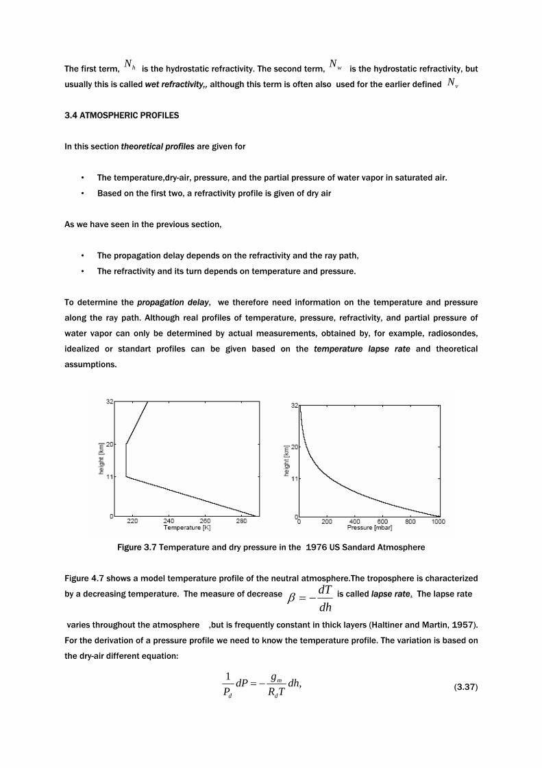
Figure 3.7 Temperature and dry pressure in the 1976 US Sandard Atmosphere

Figure 4.7 shows a model temperature profile of the neutral atmosphere.The troposphere is characterized

by a decreasing temperature. The measure of decrease is called lapse rate. The lapse rate

varies throughout the atmosphere ,but is frequently constant in thick layers (Haltiner and Martin, 1957).

For the derivation of a pressure profile we need to know the temperature profile. The variation is based on

the dry-air different equation:

(3.37)

hN wN

vN

dhdT

−=β

,1 dhTR

gdPP d

m

d

−=

which is obtained by the equation off state Eq.(1), the assumption of hydrostatic eqilibrium Eq.(4.2). We

consider the gravitation to be constant with height andequal to a mean value:

(3.38)

For the isothermal layers like troposphere, the pressure profile is found by integration of Eq.(37):

(3.39)

In the case of a polytropic layer like the protosphere and stratosphere, with assumption of a constant

lapse rate,

(3.40)

Troposphere delay models often use standard values for the temperature and pressure. An example of a

standard atmosphere is the 1976 US Standard Atmosphere in Table 3.2 (Stull,1995)

Table 3.2

( ) ( )

( )∫

∫∞

∞

=

0

0

hm

hm

m

dhh

dhhghg

ρ

ρ

[ ][ ]

[ ][ ]kmheightscaleH

kmlayertheofbasetheatmslaboveheighthkmmslaboveheighth

mbarlayertheofbasetheatairdryofpressurePg

TRHH

hhPP

d

m

ddd

:;:

;:;:

,;exp

0

0

00 ≡⎟

⎠⎞

⎜⎝⎛ −−=

,1,1

00 −=⎟⎟

⎠

⎞⎜⎜⎝

⎛=

+

βµ

µ

d

mdd R

gTTPP

[ ]KlayertheofbasetheatetemperaturT :0

3.4.1 Refractivity profile of dry air

From Eq.(3.33), (3.39), and (3.40), we can also derive the critical refractivity profiles of dry air. For

polytropic layers we have

(3.41)

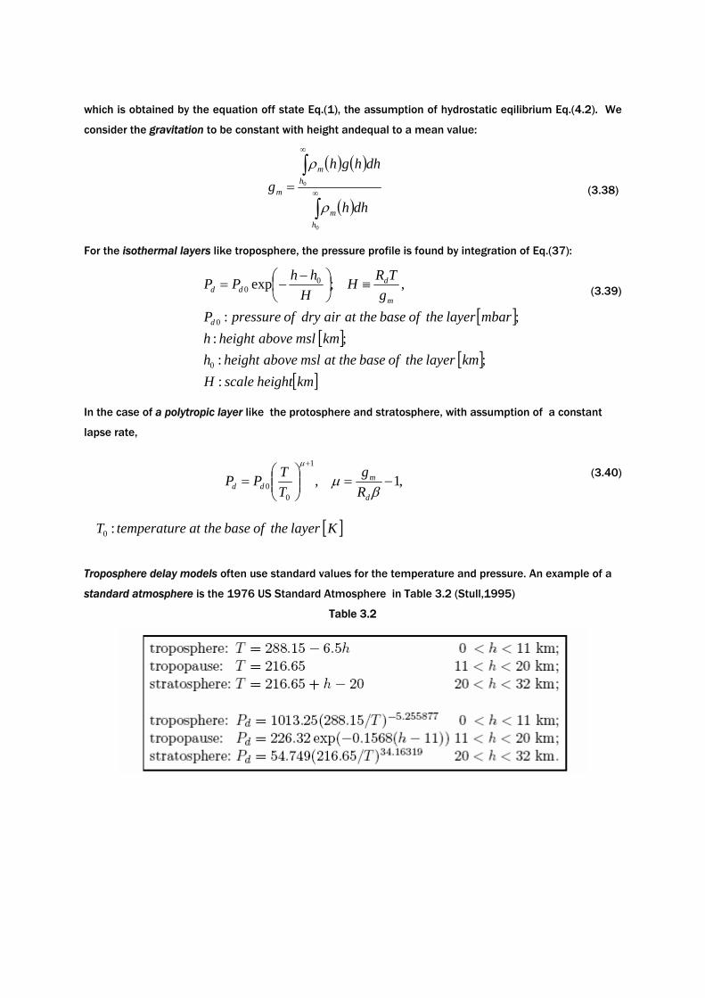
In Fig.3.8, the refractivity profiles is given for the 1976 US Standard Atmosphere

Figure 3.8 Refractivity profiles. Left: dry-air refractivity profile of the US Standard Atmosphere

Right: Wet-air refractivity profile for a surface pressure of 150C, a constant relative

humidity of 50% , a lapse rate of 6.5 K/ km, and constants of (Thayer, 1974).

Profiles of the hydrostatic refractivity are nearly the same as as these of dry air. Instead of for real

temperature we have to assume a profile for the lapse rate of the virtual temperature in the formulas

above. The virtual temperature is only the same as the real temperature for a mixing ratio of 0.

3.4.2 Saturation pressure profile

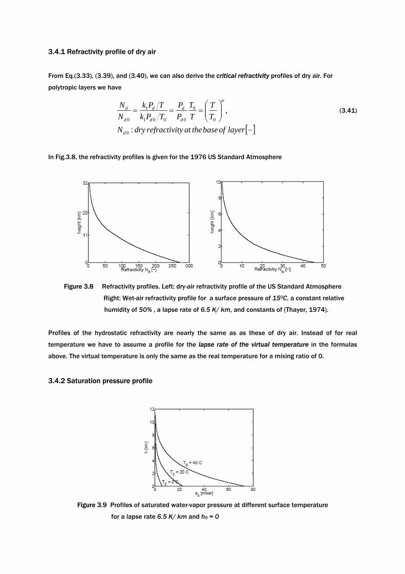
Figure 3.9 Profiles of saturated water-vapor pressure at different surface temperature

for a lapse rate 6.5 K/ km and h0 = 0

[ ]−⎟⎟⎠

⎞⎜⎜⎝

⎛===

layerofbasetheattyrefractividryNTT

TT

PP

TPkTPk

NN

d

d

d

d

d

d

d

:

,

0

0

0

0001

1

0

µ

From model (3.22) and the assumption of a constant lapse rate, the partial pressure of saturated air is

given as a function of height by:

(3.42)

Since hardlyany water vapor is present in or above the tropause, it is sufficient to consider only a

tropospheric profile. Three different profiles are given in Fig.3.9. Fig. 3.9 shows an example of a wet

refractivity profile based on Eq.(3.42).

The thickness of the traposphere is often exposed by the effective height, refractivity weighted mean

height:

For exponential profiles, the effective height is equal to scale height. The effective height of the dry and

wet tropsphere is about 8 km and 20 km respectively. The latter value holds if the relative humidity is

independent of height as in Fig.3.8.

• The smaller effective height of the weight troposphere causes the wet refractivity to drop much

faster with increasing altitude than the dry refrativity.

• The contribution of the wet part to the total refractivity is therefore at high altitudes smaller than

the surface.

( )

[ ][ ]kmmslabovesurfacetheofheighth

KetemperatursurfaceTairsaturatedpressurepartiale

hhTBAe

sat

sat

:::

,exp

0

0

00⎥⎦

⎤⎢⎣

⎡−−

−=β

( ) ( )

( )∫

∫∞

∞

−

=

0

0

0

h

hm

dhhN

dhhNhhH

CHAPTER 4:

PHYSICS OF IONOSPHERE

4.1 HISTORY

In 1899,.in a landmark experiment on December 12, 1901, Marconi, who is often called the "Father of

Wireless," demonstrated transatlantic communication by receiving a signal in St. John's Newfoundland

that had been sent from Cornwall, England. Because of his pioneering work in the use of electromagnetic

radiation for radio communications, Marconi was awarded the Nobel Prize in physics in 1909.

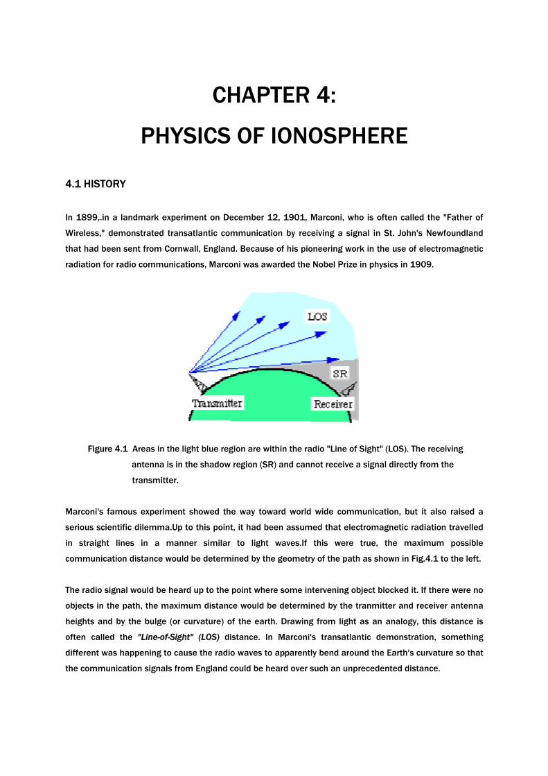
Figure 4.1 Areas in the light blue region are within the radio "Line of Sight" (LOS). The receiving

antenna is in the shadow region (SR) and cannot receive a signal directly from the

transmitter.

Marconi's famous experiment showed the way toward world wide communication, but it also raised a

serious scientific dilemma.Up to this point, it had been assumed that electromagnetic radiation travelled

in straight lines in a manner similar to light waves.If this were true, the maximum possible

communication distance would be determined by the geometry of the path as shown in Fig.4.1 to the left.

The radio signal would be heard up to the point where some intervening object blocked it. If there were no

objects in the path, the maximum distance would be determined by the tranmitter and receiver antenna

heights and by the bulge (or curvature) of the earth. Drawing from light as an analogy, this distance is

often called the "Line-of-Sight" (LOS) distance. In Marconi's transatlantic demonstration, something

different was happening to cause the radio waves to apparently bend around the Earth's curvature so that

the communication signals from England could be heard over such an unprecedented distance.

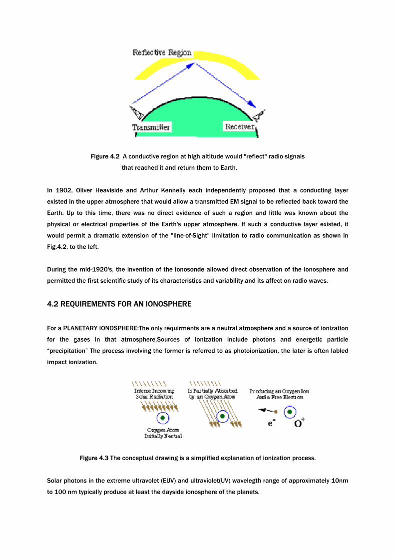
Figure 4.2 A conductive region at high altitude would "reflect" radio signals

that reached it and return them to Earth.

In 1902, Oliver Heaviside and Arthur Kennelly each independently proposed that a conducting layer

existed in the upper atmosphere that would allow a transmitted EM signal to be reflected back toward the

Earth. Up to this time, there was no direct evidence of such a region and little was known about the

physical or electrical properties of the Earth's upper atmosphere. If such a conductive layer existed, it

would permit a dramatic extension of the "line-of-Sight" limitation to radio communication as shown in

Fig.4.2. to the left.

During the mid-1920's, the invention of the ionosonde allowed direct observation of the ionosphere and

permitted the first scientific study of its characteristics and variability and its affect on radio waves.

4.2 REQUIREMENTS FOR AN IONOSPHERE

For a PLANETARY IONOSPHERE:The only requirments are a neutral atmosphere and a source of ionization

for the gases in that atmosphere.Sources of ionization include photons and energetic particle

“precipitation” The process involving the former is referred to as photoionization, the later is often labled

impact ionization.

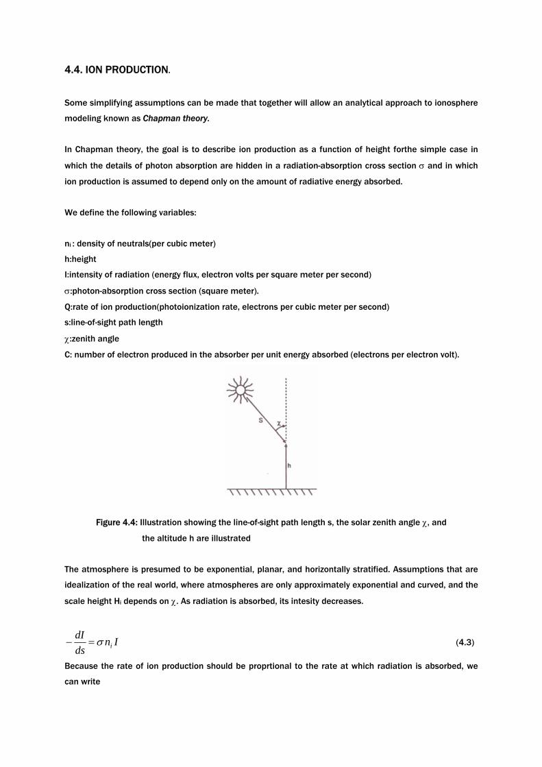
Figure 4.3 The conceptual drawing is a simplified explanation of ionization process.

Solar photons in the extreme ultravolet (EUV) and ultraviolet(UV) wavelegth range of approximately 10nm

to 100 nm typically produce at least the dayside ionosphere of the planets.

The photons come from primarily from the Sun.Ionizing particles can come from galaxy(cosmic rays), the

Sun, the magnetosphere, and the ionosphere itself if a process for local ion or electron acceleration is

operative. Precipitating energetic electrons produce additional ionizing photons within the atmosphere by

a process known as bremsstrahlung or breaking radiation.

The only requirment on the ionizing photons and particles is that their energies, i.e., hν in the case of

photons, and kinetic energy in case of particles exceed the ionization potential or binding of a neutral-

atmosphere atomic or molecular electron. In nature, atmospheric ionization usually is attributable to a

miture of these various source, but often one dominates

4.3 THE NEUTRAL ATMOSPHERE

The density in of a constituent of the upper neutral atmosphere obeys a hydrostatic equation:

( )iiii kTndhd

dhdPgmn −=−= (4.1)

which expresses as a balance between the vertical gravitational force and th thermal-pressure-gradient

force on the atmospheric gas.

Here,

mi:molecular or atomic mass,

g: the acceleration due to gravity,

h:altitude variable,

and

P:the thermal pressure, iikTn

k:Boltzmann’s constant,

Ti: temperature of the neutral gas under consideration

If iT is assumed indepent of h,this equation has the exponential solution

( )i

i Hhhnn 0

0 exp −−= (4.2)

where gmkTH iii = defines the scale height of the gas, and n0 the density at the reference altitude h0.

Note that the scale-height dependence on particle mass is such that the lightest molecules and atoms

have the largest scale-height.

Most planetary atmospheres are dominated at high altitude by hydrogen and helium. Of course, Ti may

depend on h, so that this simple exponential distribution will not always provide an accurate describtion.

4.4. ION PRODUCTION.

Some simplifying assumptions can be made that together will allow an analytical approach to ionosphere

modeling known as Chapman theory.

In Chapman theory, the goal is to describe ion production as a function of height forthe simple case in

which the details of photon absorption are hidden in a radiation-absorption cross section σ and in which

ion production is assumed to depend only on the amount of radiative energy absorbed.

We define the following variables:

ni : density of neutrals(per cubic meter)

h:height

I:intensity of radiation (energy flux, electron volts per square meter per second)

σ:photon-absorption cross section (square meter).

Q:rate of ion production(photoionization rate, electrons per cubic meter per second)

s:line-of-sight path length

χ:zenith angle

C: number of electron produced in the absorber per unit energy absorbed (electrons per electron volt).

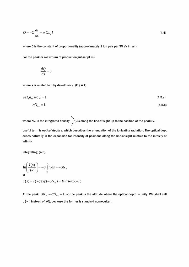
Figure 4.4: Illustration showing the line-of-sight path length s, the solar zenith angle χ, and

the altitude h are illustrated

The atmosphere is presumed to be exponential, planar, and horizontally stratified. Assumptions that are

idealization of the real world, where atmospheres are only approximately exponential and curved, and the

scale height Hi depends on χ. As radiation is absorbed, its intesity decreases.

IndsdI

iσ=− (4.3)

Because the rate of ion production should be proprtional to the rate at which radiation is absorbed, we

can write

InCdsdICQ iσ=−= (4.4)

where C is the constant of proportionality (approximately 1 ion pair per 35 eV in air).

For the peak or maximum of production(subscript m),

0=dsdQ

where s is related to h by ds=-dh secχ (Fig.4.4).

1sec =χσ minH (4.5.a)

1=imNσ (4.5.b)

where Nim is the integrated density ∫∞

mS

idsn along the line-of-sight up to the position of the peak Sm.

Useful term is optical depth τ, which describes the attenuation of the ionizating radiation. The optical dept

arises naturally in the expansion for intensity at positions along the line-of-sight relative to the intesity at

infinity.

Integrating, (4.3)

or

)exp()()exp()()( τσ −∞=−∞= INIsI is

At the peak, 1== imis NN σσ ; so the peak is the altitude where the optical depth is unity. We shall call

)(∞I instead of I(0), because the former is standard nomeculter).

is

s

i NdsnI

sI σσ −=−=⎟⎟⎠

⎞⎜⎜⎝

⎛∞ ∫

∞)()(ln

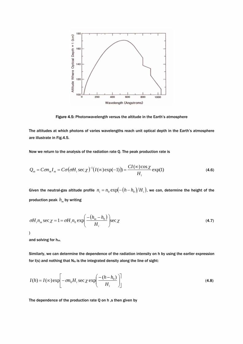
Figure 4.5: Photonwavelength versus the altitude in the Earth’s atmosphere

The altitudes at which photons of varies wavelengths reach unit optical depth in the Earth’s atmosphere

are illustrate in Fig.4.5.

Now we return to the analysis of the radiation rate Q. The peak production rate is

( ) ( ) )1exp(cos)())1exp()(sec 1

iimmm H

CIIHCInCQ χχσσσ ∞=−∞== −

(4.6)

Given the neutral-gas altitude profile ( )( )ii Hhhnn 00 exp −−= , we can, determine the height of the

production peak mh by writing

( ) χσχσ secexp1sec 00 ⎟⎟

⎠

⎞⎜⎜⎝

⎛ −−==

i

mimi H

hhnHnH (4.7)

)

and solving for hm.

Similarly, we can determine the dependence of the radiation intensity on h by using the earlier expression

for I(s) and nothing that Nis is the integrated density along the line of sight:

⎥⎦

⎤⎢⎣

⎡⎟⎟⎠

⎞⎜⎜⎝

⎛ −−−∞=

ii H

hhHnIhI )(expsecexp)()( 00 χσ (4.8)

The dependence of the production rate Q on h ,s then given by

( ) ( )⎥⎦

⎤⎢⎣

⎡⎟⎟⎠

⎞⎜⎜⎝

⎛ −−

−+=

i

m

i

mm H

hhH

hhQQ 00 exp1exp (4.9a)

with im HQCI χcos)1exp()( =∞ .

This can be simplified by defining ( ) iHhhy 0−= , hence

[ ])exp(1 yyQQ m −−−= (4.9b)

which is the Chapman production function. Note that far above the peak (y≥2), a good approximation is

Q∝exp(-y) (4.9c)

which says that because the radiation intensity is practically constant at high altitudes (not much

absorption occurs), Q is proportional to neutral density. The rate Q is the rate of production of ions and

photoelectrons, because these usually are produced in pairs most of ions are signly ionized in this

process. It is notable that in the expansion for Q, the proton-absorption cross section does not explicitly

appear. The properties of the absorber are contained in the constant C

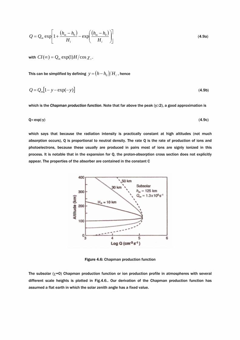
Figure 4.6: Chapman production function

The subsolar (χ=0) Chapman production function or ion production profile in atmospheres with several

different scale heights is plotted in Fig.4.6.. Our derivation of the Chapman production function has

assumed a flat earth in which the solar zenith angle has a fixed value.

4.5 PARTICLE IMPACT IONIZATION

In many situations of interest, solar photons can be assumed to compose the dominant source of

atmosphere ionization.However, an occasion, energetic (energies ≥ 1 keV) precipitating charged particles

are important. This can occur, for example, during the night magnetic latitudes in the case of planets with

dipolar magnetic field an satellites with atmospheres submerged in planetary atmospheres,

One simplified approach for particle impact ionization involves the use of an empirically determined

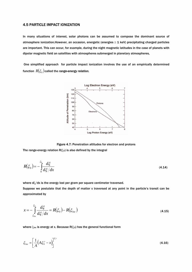
function ( )0ξR called the range-energy relation.

Figure 4.7: Penetration altitudes for electron and protons

The range-energy relation R(ξ0) is also defined by the integral

( ) ∫−=0

00

ξ

ξξξdxd

dR (4.14)

where dξ/dx is the energy lost per gram per square centimeter traversed.

Suppose we postulate that the depth of matter x traversed at any point in the particle’s transit can be

approximated by

( ) ( )locRRdxd

dxloc

ξξξξξ

ξ

−=−= ∫ 0

0

(4.15)

where ξloc is energy at x. Because R(ξ0) has the general functional form

( )γ

γξξ1

01

⎥⎦⎤

⎢⎣⎡ −= xA

Aloc (4.16)

It follows that the energy deposited at a given x is

γξξ γ

Adxd loc

−

−=1

(4.17)

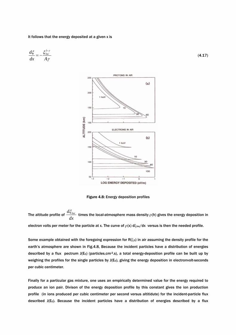
Figure 4.8: Energy deposition profiles

The altitude profile of dx

d locξ times the local-atmosphere mass density ρ(h) gives the energy deposition in

electron volts per meter for the particle at x. The curve of ρ(x) dξloc/dx versus is then the needed profile.

Some example obtained with the foregoing expression for R(ξ0) in air assuming the density profile for the

earth’s atmosphere are shown in Fig.4.8, Because the incident particles have a distribution of energies

described by a flux pectrum J(E0) (particles.cm-2.s), a total energy-deposition profile can be built up by

weighing the profiles for the single particles by J(E0), giving the energy deposition in electronvolt-seconds

per cubic centimeter.

Finally for a particular gas mixture, one uses an empirically determined value for the energy required to

produce an ion pair. Divison of the energy deposition profile by this constant gives the ion production

profile (in ions produced per cubic centimeter per second versus altitidute) for the incident-particle flux

described J(E0). Because the incident particles have a distribution of energies described by a flux

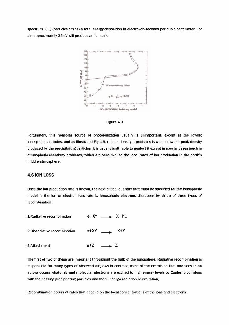
spectrum J(E0) (particles.cm-2.s),a total energy-deposition in electrovolt-seconds per cubic centimeter. For

air, approximately 35 eV will produce an ion pair.

Figure 4.9

Fortunately, this nonsolar source of photoionization usually is unimportant, except at the lowest

ionospheric altitudes, and as illustrated Fig.4.9, the ion density it produces is well below the peak density

produced by the precipitaitng particles. It is usually justtfiable to neglect it except in special cases (such in

atmospheric-chemisrty problems, which are sensitive to the local rates of ion production in the earth’s

middle atmosphere.

4.6 ION LOSS

Once the ion production rate is known, the next critical quantity that must be specified for the ionospheric

model is the ion or electron loss rate L. Ionospheric electrons disappear by virtue of three types of

recombination:

1-Radiative recombination e+X+ X+ hυ

2-Dissociative recombination e+XY+ X+Y

3-Attachment e+Z Z-

The first of two of these are important throughout the bulk of the ionosphere. Radiative recombination is

responsible for many types of observed airglows.In contrast, most of the emmision that one sees in an

aurora occurs whatomic and molecular electrons are excited to high energy levels by Coulomb collisions

with the passing precipitating particles and then undergo radiation re-excitation,

Recombination occurs at rates that depend on the local concentrations of the ions and electrons

L= α ne ni

where ne and ni are the electron and ion densities, and α is recombination coefficient is determined by

emprical and theoretical models. For the more important atmospheric dissocative recombination

reactions, such as

O2+e O+O

and

N2+ + e N +N

It is notable that α is often assumed constant, although Te generally depends on altitude.

4.7 DETERMINING IONOSPHERIC DENSITY FROM PRODUCTION AND LOSS RATE

Once the ion production rates and loss rates are established , we can consider the problem of finding the

altitude distribution of the ionospheric electron denity ne. If the electrons and ions do notmove very far

from where they are produced (e.g., by virtue of a strong horizontal ambient magnetic field), we can say

that ne(and thus ni) obeys the equilibrium-contiunity or particle-conservation equation

0=−= LQdt

dne (4.18)

and if the loss rate is due to electron-ion collisions

2enLQ α==

and hence

( ) 21αQne = (4.19)

describes the spatial distribution of the electrons or ions. This particular distributionis called

photochemical equilibrium distribution because it involes only local photochemistry. Chapman-layer

models of the ionosphere, for example, include the Chapman production function and the assumption of

photochemicl equilibrium. However, in many cases the electrons and ions wave significantly from their

points of creation before they recombine, and so we must consider a transport term in a more general

continuity equation.

CHAPTER 5: ATMOSPHERIC WAVE PROPAGATION

5.1 RADIO WAVE PROPAGATION CHARACTERISTICS

Within the atmosphere, radio waves can be refracted, reflected, and diffracted. In the following sections,

we will first recall history and then discuss the propagation characteristics in atmosphere.

5.1.1 REFRACTION

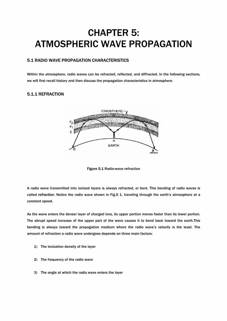
Figure 5.1 Radio-wave refraction

A radio wave transmitted into ionized layers is always refracted, or bent. This bending of radio waves is

called refraction. Notice the radio wave shown in Fig.5 1, traveling through the earth’s atmosphere at a

constant speed.

As the wave enters the denser layer of charged ions, its upper portion moves faster than its lower portion.

The abrupt speed increase of the upper part of the wave causes it to bend back toward the earth.This

bending is always toward the propagation medium where the radio wave’s velocity is the least. The

amount of refraction a radio wave undergoes depends on three main factors:

1) The ionization density of the layer

2) The frequency of the radio wave

3) The angle at which the radio wave enters the layer

5.1.1.1 Layer density

Figure 5.2 Effects of ionospheric density on radio waves

Fig. 5.2 shows the relationship between radio waves and ionization density. Each ionized layer has a

middle region of relatively dense ionization with less intensity above and below. As a radio wave enters a

region of increasing ionization,va velocity increase causes it to bend back toward the earth. In the highly

dense middle region, refraction occurs more slowly, because the ionization density is uniform. As the

wave enters the upper less dense region, the velocity of the upper part of the wave decreases and the

wave is bent away from the earth.

5.1.1.2 Frequency

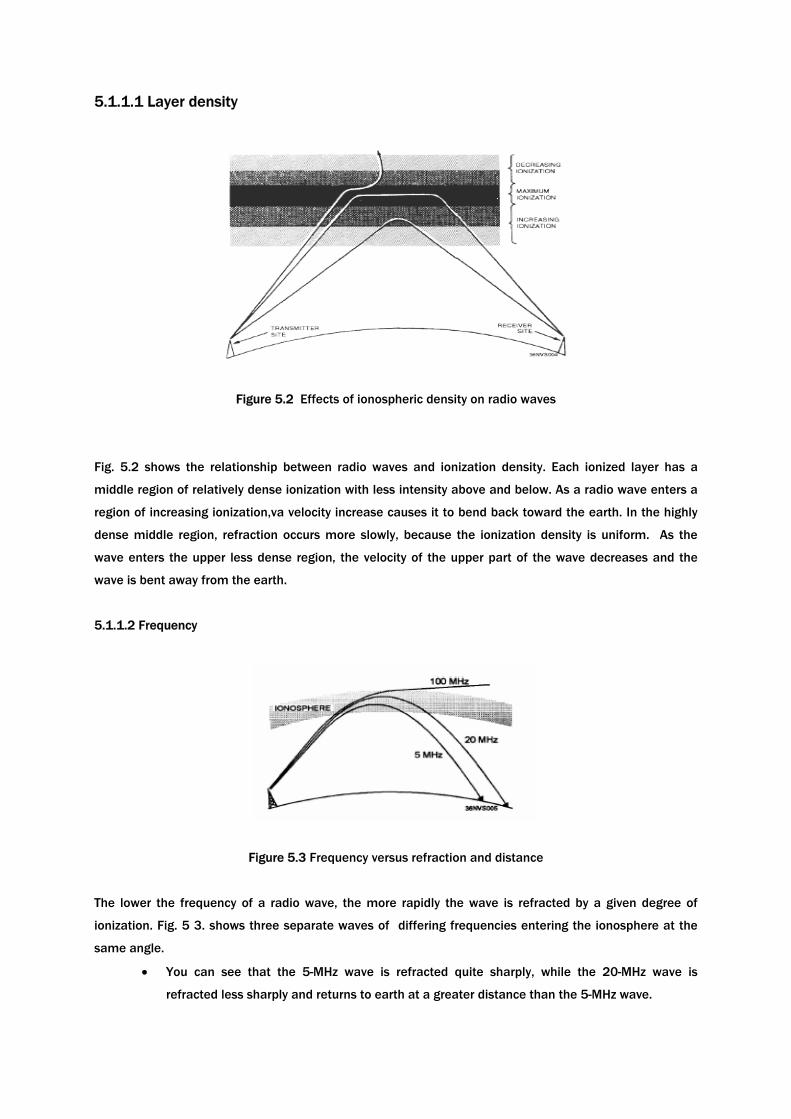
Figure 5.3 Frequency versus refraction and distance

The lower the frequency of a radio wave, the more rapidly the wave is refracted by a given degree of

ionization. Fig. 5 3. shows three separate waves of differing frequencies entering the ionosphere at the

same angle.

• You can see that the 5-MHz wave is refracted quite sharply, while the 20-MHz wave is

refracted less sharply and returns to earth at a greater distance than the 5-MHz wave.

• Notice that the 100-MHz wave is lost into space. Since the 100-MHz wave’s frequency is

greater than the critical frequency for that ionized layer.

For any given ionized layer, there is a frequency, called the escape point, at which energy transmitted

directly upward will escape into space.The maximum frequency just below the escape point is called the

critical frequency.The critical frequency of a layer depends upon the layer’s density. If a wave passes

through a particular layer, it may still be refracted by a higher layer if its frequency is lower than the higher

layer’s critical frequency.

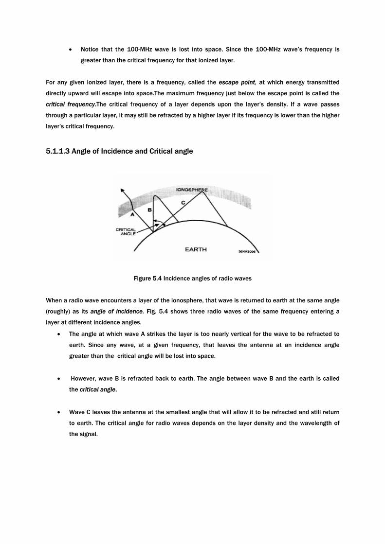
5.1.1.3 Angle of Incidence and Critical angle

Figure 5.4 Incidence angles of radio waves

When a radio wave encounters a layer of the ionosphere, that wave is returned to earth at the same angle

(roughly) as its angle of incidence. Fig. 5.4 shows three radio waves of the same frequency entering a

layer at different incidence angles.

• The angle at which wave A strikes the layer is too nearly vertical for the wave to be refracted to

earth. Since any wave, at a given frequency, that leaves the antenna at an incidence angle

greater than the critical angle will be lost into space.

• However, wave B is refracted back to earth. The angle between wave B and the earth is called

the critical angle.

• Wave C leaves the antenna at the smallest angle that will allow it to be refracted and still return

to earth. The critical angle for radio waves depends on the layer density and the wavelength of

the signal.

Figure 5.5 The effect of frequency onthe critical angle

As the frequency of a radio wave is increased, the critical angle must be reduced for refraction to occur.

Notice in Fig.5.5 that the 2-MHz wave strikes the ionosphere at the critical angle for that frequency and is

refracted. Although the 5-MHz line (broken line) strikes the ionosphere at a less critical angle it still

penetrates the layer and is lost As the angle is lowered, a critical angle is finally reached for the 5-MHz

wave and it is refracted back to earth.

5.1.2 REFLECTION

Figure 5.6 Phase shift of reflected waves

Reflection occurs when radio waves are “bounced” from a flat surface. There are basically two types of

reflection that occur in the atmosphere: earth reflection and ionospheric reflection.

Fig.5 6 shows two waves reflected from the earth’s surface. Waves A and B bounce off the earth’s surface

like light off of a mirror. Notice that the positive and negative alternations of radio waves A and B are in

phase before they strike the earth’s surface. However, after reflection the radio waves are approximately

180 degrees out of phase. A phase shift has occurred.

• The amount of phase shift that occurs is not constant. It varies, depending on the wave

polarization and the angle at which the wave strikes the surface..

• Normally, radio waves reflected in phase produce stronger signals, while those reflected out of

phase produce a weak or fading signal.

For ionospheric reflection to occur, the highly ionized layer can be approximately no thicker than one

wavelength of the wave.

• Although the radio waves are actually refracted, some may be bent back so rapidly that they

appear to be reflected.

• Since the ionized layers are often several miles thick, ionospheric reflection mostly occurs at long

wavelengths (low frequencies).

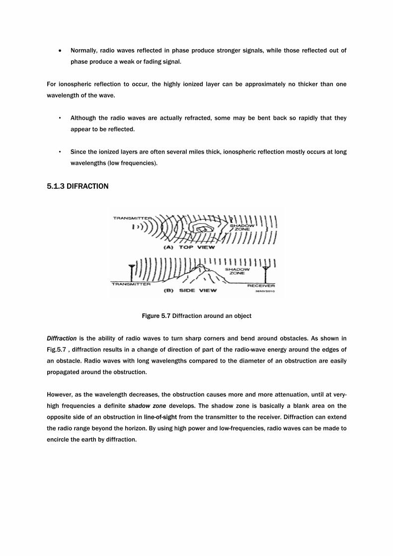
5.1.3 DIFRACTION

Figure 5.7 Diffraction around an object

Diffraction is the ability of radio waves to turn sharp corners and bend around obstacles. As shown in

Fig.5.7 , diffraction results in a change of direction of part of the radio-wave energy around the edges of

an obstacle. Radio waves with long wavelengths compared to the diameter of an obstruction are easily

propagated around the obstruction.

However, as the wavelength decreases, the obstruction causes more and more attenuation, until at very-

high frequencies a definite shadow zone develops. The shadow zone is basically a blank area on the

opposite side of an obstruction in line-of-sight from the transmitter to the receiver. Diffraction can extend

the radio range beyond the horizon. By using high power and low-frequencies, radio waves can be made to

encircle the earth by diffraction.

5.1.4 ABSORBTION AND SCATTERING

As a radio wave passes into the ionosphere, it loses some of its energy to the free electrons and ions

present there. Since the amount of absorption of the radio-wave energy varies with the density of the

ionospheric layers, there is no fixed relationship between distance and signal strength for ionospheric

propagation.

Energy absorbed from the incident wave by the charged particle is re-emitted as radio wave radiation.

Such a process is clearly equivalent to the scattering of the radio wave by the particle.

5.2. ATMOSPHERIC EFFECTS ON PROPAGATION

While radio waves traveling in free space have little outside influence to affect them, radio waves

traveling in the earth’s atmosphere have many influences that affect them. We have all experienced

problems with radio waves, caused by certain atmospheric conditions complicating what at first seemed

to be a relatively simple electronic problem. These problem-causing conditions result from a lack of

uniformity in the earth’s atmosphere. Many factors can affect atmospheric conditions,either positively or

negatively. Three of these are variations in geographic height, differences in geographic location, and

changes in time (day, night, season, year).

Changes in the ionosphere can produce dramatic changes in the ability to communicate. In some cases,

communications distances are greatly extended.In other cases, communications distances are greatly

reduced or eliminated. The paragraphs below explain the major problem of reduced communications

because of the phenomena of fading and selective fading.

Although daily changes in the ionosphere have the greatest effect on communications, other phenomena

also affect communications, both positively and negatively. Those phenomena are discussed briefly in the

following sections.

5.2.1 REGULAR VARIATONS

5.2.1 1 FADING

The most troublesome and frustrating problem in receiving radio signals is variations in signal

strength,most commonly known as fading. Several conditions can produce fading.

• When a radio wave is refracted by the ionosphere or reflected from the earth’s surface, random

changes in the polarization of the wave may occur.

• Fading also results from absorption of the RF energy in the ionosphere. Most ionospheric

absorption occurs in the lower regions of the ionosphere where ionization density is the greatest.

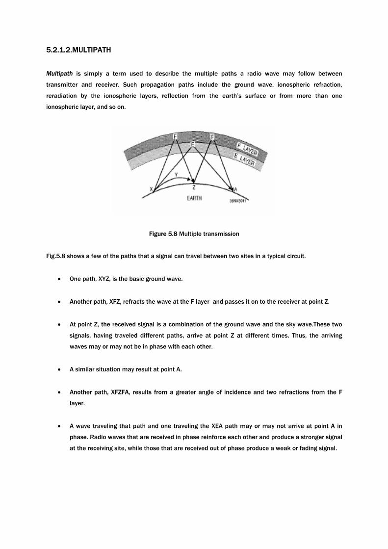
5.2.1.2.MULTIPATH

Multipath is simply a term used to describe the multiple paths a radio wave may follow between

transmitter and receiver. Such propagation paths include the ground wave, ionospheric refraction,

reradiation by the ionospheric layers, reflection from the earth’s surface or from more than one

ionospheric layer, and so on.

Figure 5.8 Multiple transmission

Fig.5.8 shows a few of the paths that a signal can travel between two sites in a typical circuit.

• One path, XYZ, is the basic ground wave.

• Another path, XFZ, refracts the wave at the F layer and passes it on to the receiver at point Z.

• At point Z, the received signal is a combination of the ground wave and the sky wave.These two

signals, having traveled different paths, arrive at point Z at different times. Thus, the arriving

waves may or may not be in phase with each other.

• A similar situation may result at point A.

• Another path, XFZFA, results from a greater angle of incidence and two refractions from the F

layer.

• A wave traveling that path and one traveling the XEA path may or may not arrive at point A in

phase. Radio waves that are received in phase reinforce each other and produce a stronger signal

at the receiving site, while those that are received out of phase produce a weak or fading signal.

5.2 1 .3 SEASONAL VARIATIONS IN THE IONOSPHERE

Seasonal variations are the result of the earth’s revolving around the sun, because the relative position of

the sun moves from one hemisphere to the other with the changes in seasons.

• Seasonal variations of the D, E, and F1 layers are directly related to the highest angle of the sun,

meaning the ionization density of this layer is greatest during the summer.

• The F2 layer is just the opposite. Its ionization is greatest during the winter, Therefore, operating

frequencies for F2 layer propagation are higher in the winter than the summer.

5.2. 1 4 SUNSPOTS

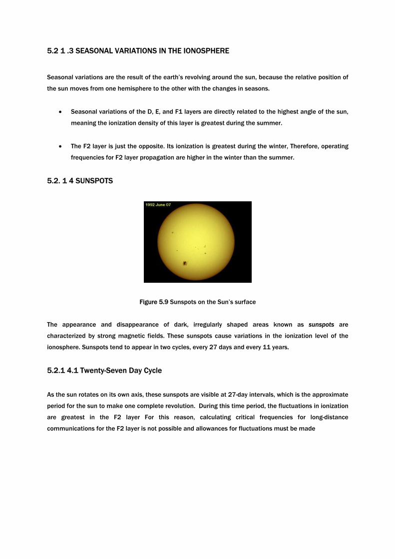
Figure 5.9 Sunspots on the Sun’s surface

The appearance and disappearance of dark, irregularly shaped areas known as sunspots are

characterized by strong magnetic fields. These sunspots cause variations in the ionization level of the

ionosphere. Sunspots tend to appear in two cycles, every 27 days and every 11 years.

5.2.1 4.1 Twenty-Seven Day Cycle

As the sun rotates on its own axis, these sunspots are visible at 27-day intervals, which is the approximate

period for the sun to make one complete revolution. During this time period, the fluctuations in ionization

are greatest in the F2 layer For this reason, calculating critical frequencies for long-distance

communications for the F2 layer is not possible and allowances for fluctuations must be made

5.2.1 4.2 Eleven-year cycle

Sunspots can occur unexpectedly, and the life span of individual sunspots is variable. The eleven-year

sunspot cycle is a regular cycle of sunspot activity that has a minimum and maximum level of activity that

occurs every 11 years. During periods of maximum activity, the ionization density of all the layers

increases. Because of this, the absorption in the D layer increases and the critical frequencies for the E,

F1, and F2 layers are higher. During these times, higher operating frequencies must be used for long-

range communications.

5.2.2 .IRREGULAR VARIATIONS

Irregular variations are just that unpredictable changes in the ionosphere that can drastically affect our

ability to communicate.The more common variations are sporadic E, ionospheric disturbances,and

ionospheric storms

5.2.2.1 Sporadic E

The sporadic E layer can be so thin that radio waves penetrate it easily and are returned to earth by the

upper layers, or it can be heavily ionized and extend up to several hundred miles into the ionosphere. This

condition may be either harmful or helpful to radio-wave propagation.

5.2.2.2 Sudden ionospheric disturbances

Commonly known as SID, these disturbances may occur without warning and may last for a few minutes

to several hours. When SID occurs, long-range hf communications are almost totally blanked out. The

radio operator listening during this time will believe his or her receiver has gone dead.

5.2.2 3 Ionospheric storms

Ionospheric storms are caused by disturbances in the earth’s magnetic field. They are associated with

both solar eruptions and the 27-day cycle, meaning they are related to the rotation of the sun.

The effects of ionospheric storms are a turbulent ionosphere and very erratic sky-wave propagation,

reducing its ion density and causing the critical frequencies to be lower than normal.

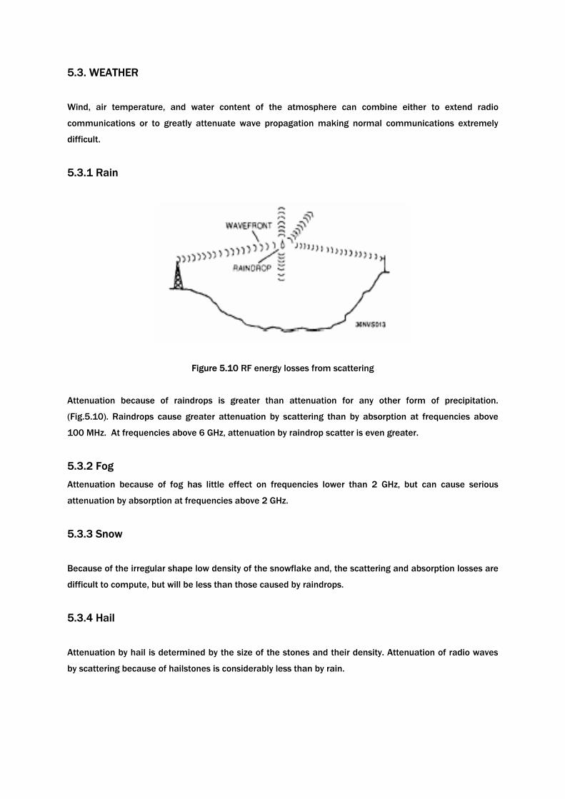
5.3. WEATHER

Wind, air temperature, and water content of the atmosphere can combine either to extend radio

communications or to greatly attenuate wave propagation making normal communications extremely

difficult.

5.3.1 Rain

Figure 5.10 RF energy losses from scattering

Attenuation because of raindrops is greater than attenuation for any other form of precipitation.

(Fig.5.10). Raindrops cause greater attenuation by scattering than by absorption at frequencies above

100 MHz. At frequencies above 6 GHz, attenuation by raindrop scatter is even greater.

5.3.2 Fog

Attenuation because of fog has little effect on frequencies lower than 2 GHz, but can cause serious

attenuation by absorption at frequencies above 2 GHz.

5.3.3 Snow

Because of the irregular shape low density of the snowflake and, the scattering and absorption losses are

difficult to compute, but will be less than those caused by raindrops.

5.3.4 Hail

Attenuation by hail is determined by the size of the stones and their density. Attenuation of radio waves

by scattering because of hailstones is considerably less than by rain.

REFERENCES 1. Houghton, J. (200) The Physics of Atmosphere (1st Edition), Cambridge: Cambridge Univesity Pres. 2 .Gombosi, T.I. (1998) Physics of the Space Environment (3rd Edition) Cambridge: Cambridge University Press. 3 . The American Practıcal Navigator, An Epitome of Navigation(1995), originally by Nathanel Bowdith, LL.D., 1995 Edition, published and prepared by National Imagery and Mapping Agency,Bethesda, Maryland. 4. Kleijer, F. (2004) Tropsphere Modeling and Filtering Precise for GPS Leveling, Publications on Geodesy 56, Netherlands Geodetic Commission, printed by Optima Grafishe Communicatie, The Netherlands.