Stock Assessement Report No. 10-02 of the Atlantic States Marine Fisheries Commission Atlantic Menhaden Stock Assessment and Review Panel Reports May 2010 REVISED MARCH 2011 Working towards healthy, self-sustaining populations for all Atlantic coast fish species or successful restoration well in progress by the year 2015 SEDAR 40 - 7

Welcome message from author
This document is posted to help you gain knowledge. Please leave a comment to let me know what you think about it! Share it to your friends and learn new things together.
Transcript

Stock Assessement Report No. 10-02 of the
Atlantic States Marine Fisheries Commission
Atlantic Menhaden Stock Assessment and Review Panel Reports
May 2010 REVISED MARCH 2011
Working towards healthy, self-sustaining populations for all Atlantic coast fish species or successful restoration well in progress by the year 2015
SEDAR 40 - 7

Preface The development and peer review of the 2010 Atlantic Menhaden Stock Assessment occurred through a joint Atlantic States Marine Fisheries Commission (ASMFC) and Southeast Data, Assessment, and Review (SEDAR) process. ASMFC organized and held a Data Workshop May 12–13, 2009 in Richmond, Virginia and an Assessment Workshop October 19-22, 2009 in Beaufort, North Carolina. SEDAR coordinated a Review Workshop from March 8-12, 2010 in Charleston, South Carolina. Participants included members of the Atlantic Menhaden Stock Assessment Subcommittee, and a Review Panel consisting of a chair, a reviewer appointed by ASMFC, and three reviewers appointed by the Center for Independent Experts. In November 2010 it was revealed that within the 2009 Atlantic menhaden base stock assessment model code there was a mistake. The model computes three types of number-at-age used for various purposes in the model. The code computes numbers at the beginning of the year, the mid-point of the year, and a variable fraction of the year to correspond to spawning. For menhaden, the spawning fraction is set to zero, such that the numbers at the beginning of the year equal those at the spawning time (both assumed to occur every March 1). The midpoint numbers are used to compute the predicted pound net index values, because the data for this index are collected during the summer and fall time periods. Unfortunately, the mid-point (instead of the beginning of the year) numbers at age were used for computing the predicted landings. The effect of this on the model is to apply an additional half-year of total mortality to the population. This has the net effect of changing the scale of the predicted model output, with limited effects on the trends of the output. As a result, stock status changed. This Assessment Report has been revised to reflect the changes in the assessment. Any changes to the document have been highlighted in yellow. This document contains the following reports: Section A – Executive Summary (Pages 1 – 4)
This section provides a summary of major findings and recommendations from the Stock Assessment and Review Panel Reports.
Section B – 2010 Stock Assessment Report Submitted for Peer Review (Pages 5 – 307) This report outlines the background information, data used, model calibration and results for the assessment submitted to the Review Panel.
Section C – Consensus Review Panel Report for the 2010 Stock Assessment (Pages 308 – 325)
This report, provided by the Review Panel Chair, provides the consensus opinions of the Review Panel on the final stock assessment for peer review. The report includes the Review Panel’s summary findings, detailed discussion of each Term of Reference, and a summary of the results of analytical requests made at the Review Workshop.
SEDAR 40 - 7

Section A – Executive Summary 2
Section A – Executive Summary This executive summary refers to the uncorrected (March 2010) assessment report. The does not contain the corrected stock status. Refer to Section 8 for the corrected results. Status of Stock The Panel supports the recommendation of the Assessment Team that the stock status determination is “not overfished” and there is “no overfishing”, relative to the current reference points. Further, the Panel also agrees with the Assessment Team that the uncertainties in the assessment are such that there could have been overfishing in 2008 (removal of the JAI from the base model gave that determination and many bootstrap runs also fell in the overfishing zone).
The Panel also notes that a strictly valid determination of the overfishing status requires comparison of full Fs and not number-weighted Fs. This is not a well-known result, but it is obvious once the problem is identified. Stock Identification and Distribution Based on size-frequency information and tagging studies, the Atlantic menhaden resource is believed to consist of a single unit stock or population. Recent genetic studies support the single stock hypothesis. Menhaden are distributed along the U.S. East Coast from Maine to Florida. The highest concentrations of this resource are regularly seen from Massachusetts to North Carolina. Management Unit The management unit for Atlantic menhaden (Brevoortia tyrannus) is defined in Amendment 1 as throughout the range of the species within U.S. waters of the northwest Atlantic Ocean from the estuaries eastward to the offshore boundary of the EEZ. The unit is coastwide from Maine to Florida. Landings The reduction fishery landings and biological sampling information have been collected since the 1950s in a consistent manner and represent one of the longest and most complete fisheries information series in the United States. Daily logbooks (Captains Daily Fishing Reports) have been collected since 1985, and detail purse-seine set locations and estimated catch. As reduction landings have declined in recent years, menhaden landings for bait have become relatively more important to the coastwide total landings of menhaden. Commercial landings of menhaden for bait occur in almost every Atlantic coast state and have been reported since 1985. Data and Assessment The Atlantic Menhaden Stock Assessment Subcommittee used commercial and recreational landings at age from Florida to Maine, a fishery dependent adult index developed from Potomac River Fisheries Commission (PRFC) pound net survey, and a juvenile index (JAI) developed from coastwide beach seine information. In addition, growth, weight, and maturity at age were
SEDAR 40 - 7

Section A – Executive Summary 3
developed using fishery dependent and independent information, while age and time variant natural mortality was estimated using a multi-species virtual population analysis (MSVPA-X). The Beaufort Assessment Model (BAM) was the only model used to produce final assessment results. This is a statistical forward-projection model with separable selectivities using the Baranov catch equation. The Panel identified several strengths and potential weaknesses in the base model. The Panel formulated an alternative BAM run which addressed the main problems identified with the base run. Given the other uncertainties, the differences in the assessment results between the two models are relatively minor Biological Reference Points Addendum I established the biological reference points used currently: FTARGET = 0.75, FTHRESHOLD= 1.18, fecundity target (trillions) = 26.6, and fecundity threshold (trillions) 13.3. The results indicate that the fecundity estimates for the terminal year are well above the threshold (limit), with not a single bootstrap estimate falling below 1.0. The results for the terminal year fishing mortality rate suggest that the base run estimate is just below the FMED threshold (limit) with 36.8% of the bootstrap runs exceeding the FMED threshold. The use of FMED based reference points is of concern. It appears that the stock has been at low levels of population fecundity for many years and yet the current reference points (and the FMED reference points of previous years) provide a determination of “not overfishing” and “not overfished”. The Panel recommends that alternative reference points be considered and chosen on the basis of providing better protection for SSB or population fecundity relative to the unfished level. Fishing Mortality When the fishing mortality rate (F) exceeds the F-limit, then overfishing is occurring; the rate of removal of fish by the fishery exceeds the ability of the stock to replenish itself. The Panel was concerned that the 2008 F estimate was very close to the threshold. If uncertainty in the estimate was considered there is a significant probability that overfishing occurred in 2008. Recruitment Recruitment was generally poor during the 1960s, with values below the 25th percentile (20.5 billion) for the recruitment time series. High recruitment occurred during the late 1970s and early 1980s to levels above the 75th percentile (59.6 billion). These values are comparable to the late 1950s (with the exception of the extraordinary 1958 year-class). Generally low recruitment has occurred since the early 1990s. There is a hint of a potential long-term cycle from this historical pattern of recruitment, but not enough data are present to draw any conclusions regarding the underlying cause at this point. There is no evidence for a relationship in the model estimates of fecundity and recruitment. However, recruitment is quite variable and there could be a stock-recruit relationship which is not discernable for this reason. Environmental factors that affect recruitment are generally viewed as density independent. These factors include physical processes, for example transport mechanisms, water temperature, DO,
SEDAR 40 - 7

Section A – Executive Summary 4
freshwater inflow and nutrient loadings. Biological factors, such as amount of food and competition for food, or predation by higher trophic levels which control survival and growth of young-of-the-year menhaden prior to recruitment to the fishery, can be either density independent or density dependent. Fecundity Population fecundity (FEC, number of maturing ova) was high in the late 1950s and early 1960s, low in the late 1960s, and generally increasing since then. The Panel was concerned about the use of Fmed and the fecundity associated with it as reference points. The concern is that there is no information on the relationship of the target and threshold fecundity in relation to virgin fecundity levels. Projections were run to examine this, and the estimated annual fecundity since 1998 was only 5 to 10% of the virgin fecundity. Bycatch Discard or bycatch information in the bait and reduction fisheries is undocumented. However, it is suspected that bycatch and discards of menhaden are trivial compared to total landings.
SEDAR 40 - 7

Section B – Stock Assessement Report 5
Section B - 2010 Stock Assessment Report Submitted for Peer Review
Atlantic States Marine Fisheries Commission
2010 Atlantic Menhaden Stock Assessment for Peer Review
Submitted to the Atlantic Menhaden Management Board on February 2010
Prepared by the ASMFC Atlantic Menhaden Stock Assessment Subcommittee
Dr. Douglas Vaughan (Chair), National Marine Fisheries Service
Mr. Jeff Brust, Department of Environmental Protection Bureau of Marine Fisheries Dr. Matt Cieri, Maine Department of Marine Resources Dr. Robert Latour, Virginia Institute of Marine Science
Dr. Behzad Mahmoudi, Florida Fish and Wildlife Research Institute Mr. Jason McNamee, Department of Environmental Management Marine Fisheries Section
Dr. Genevieve Nesslage, Atlantic States Marine Fisheries Commission Dr. Alexei Sharov, Maryland Department of Natural Resources
Mr. Joseph Smith, National Marine Fisheries Service Dr. Erik Williams, National Marine Fisheries Service
A publication of the Atlantic States Marine Fisheries Commission pursuant to National Oceanic
and Atmospheric Administration Award No. NA05NMF4741025
SEDAR 40 - 7

Section B – Stock Assessement Report 6
Acknowledgements The Atlantic States Marine Fisheries Commission (ASMFC or Commission) thanks all of the individuals who contributed to the development of the Atlantic menhaden stock assessment. The Commission specifically thanks the ASMFC Atlantic Menhaden Technical Committee (TC) and Stock Assessment Subcommittee (SASC) members who developed the consensus stock assessment report and Commission staff, Brad Spear and Genny Nesslage, who helped prepare the report for review.
SEDAR 40 - 7
Section B – Stock Assessement Report 7
Stock Assessment Summary The Atlantic States Marine Fisheries Commission (ASMFC) convened a stock assessment workshop (AW) at the NOAA Center for Coastal Fisheries and Habitat Research, Beaufort, North Carolina, on Monday, October 19, 2009. The workshop’s objective was to conduct a new benchmark assessment of the Atlantic menhaden (Brevoortia tyrannus) stock along the U.S. Atlantic coast. Members of the ASMFC Technical Committee’s Stock Assessment Subcommittee participated in this assessment (including state, commission, federal and university scientists), as well as several observers (Appendix A). The AW convened at Beaufort through October 22, 2009. All decisions regarding stock assessment methods and acceptable data were made by consensus. Available data on the species were evaluated during a Data Workshop (May 12–13, 2009) in Richmond, Virginia. These data were subsequently finalized for inclusion in the assessment model(s). Data included abundance indices, recorded landings, and samples of annual size and age compositions from the landings. Juvenile abundance seine indices from seven states were developed (two more than in the last peer reviewed assessment in 2003). The pound net index from the PRFC was improved to reflect a better unit of fishing effort. Landings and catch-in-numbers-at-age data were updated from the reduction and bait fisheries; landings data were reconstructed historically back to 1873 for use in an alternate model configuration. A matrix of natural mortality at age was obtained from a recent update of the peer-reviewed MSVPA-X model (SARC 2005), allowing for age- and year-varying estimates of M. During the assessment workshop, alternate assessment models were considered as potential base models. The statistical catch-at-age model developed at Beaufort was selected as the base assessment model. A base assessment model run was developed and sensitivity model runs were made to evaluate performance of the assessment model to different assumptions regarding input data and stock dynamics. Benchmarks for stock status were based on Addendum 1 to Amendment 1. FMED (= FREP) provides the reference value for judging overfishing (F-limit). The population fecundity (FECTARGET) corresponding to FMED provides the proxy for BMSY. FECLIMIT is one-half of FECtarget. A discussion of alternative benchmarks is provided in Section 8.2, including a discussion of the FMSY concept, equilibrium yield-per-recruit and spawner-per-recruit reference points, and environmental variability. This latter issue resulted in some debate on poor recruitment during last the two decades and its implications for benchmarks. Given the currently accepted benchmarks, status of stock was determined based on the terminal year (2008) estimate relative to its corresponding limit. Benchmarks have been estimated based on the results of the base run. The terminal year fishing mortality rate (weighted by number average for ages 2+) was estimated to be 1.26 year-1, which is 100% of its limit (and 206% of its target). Correspondingly, the terminal year estimate of population fecundity was estimated at 99% of its fecundity target (and 198% of its limit). Hence, the stock is not considered to be overfished, but overfishing was occurring in the terminal year (2008). Given the current
SEDAR 40 - 7

Section B – Stock Assessement Report 8
overfishing definition, overfishing has occurred in 32 of the last 54 years but was not occurring during the previous nine years, 1999-2007. Other indicators of stock status, such as trends in recruitment and fishing mortality on fully recruited ages, raise concerns about the appropriateness of the current reference points for Atlantic menhaden.
SEDAR 40 - 7

Section B – Stock Assessement Report 9
Table of Contents Acknowledgements ..........................................................................................................................6 Stock Assessment Summary ............................................................................................................7 Table of Contents .............................................................................................................................9 List of Tables .................................................................................................................................12 List of Figures ................................................................................................................................15 Terms of Reference ........................................................................................................................20 1.0 Introduction .............................................................................................................................21 1.1 Brief Overview and History of Fisheries ................................................................................21 1.2 Management Unit Definition ..................................................................................................23 1.3 Regulatory History ..................................................................................................................23 1.4 Assessment History .................................................................................................................24
1.4.1 History of Stock Assessments ......................................................................................24 1.4.2 Historical Retrospective Patterns .................................................................................26
2.0 Life History .............................................................................................................................28 2.1 Stock Definition ......................................................................................................................28 2.2 Migration Patterns ...................................................................................................................28 2.3 Age ..........................................................................................................................................29 2.4 Growth ....................................................................................................................................30 2.5 Reproduction ...........................................................................................................................32 2.6 Natural Mortality ....................................................................................................................36 2.7 Environmental Factors ............................................................................................................40 3.0 Habitat Description .................................................................................................................42 3.1 Overview .................................................................................................................................42 3.2 Spawning, Egg, and Larval Habitat ........................................................................................43 3.3 Juvenile Habitat ......................................................................................................................43 3.4 Adult Habitat ...........................................................................................................................44 3.5 Habitat Areas of Particular Concern .......................................................................................44 4.0 Fishery-Dependent Data Sources ............................................................................................45 4.1 Commercial Reduction Fishery ..............................................................................................45
4.1.1 Data Collection Methods .............................................................................................45 4.1.2 Commercial Reduction Landings ................................................................................46 4.1.3 Commercial Reduction Discards/Bycatch ...................................................................50 4.1.4 Commercial Reduction Catch Rates (CPUE) ..............................................................51 4.1.5 Commercial Reduction Catch-at-Age ..........................................................................53 4.1.6 Potential Biases, Uncertainty, and Measures of Precision ...........................................54
4.2 Commercial Bait Fishery ........................................................................................................55 4.2.1 Data Collection Methods .............................................................................................55 4.2.2 Commercial Bait Landings ..........................................................................................58 4.2.3 Commercial Bait Discards/Bycatch .............................................................................60 4.2.4 Commercial Bait Catch Rates (CPUE) ........................................................................60 4.2.5 Commercial Bait Catch-at-Age....................................................................................62 4.2.6 Potential biases, Uncertainty, and Measures of Precision ...........................................62
4.3 Recreational Fishery ...............................................................................................................63
SEDAR 40 - 7
Section B – Stock Assessement Report 10
4.3.1 Data Collection Methods .............................................................................................63 4.3.2 Recreational Landings .................................................................................................63 4.3.3 Recreational Discards/Bycatch ....................................................................................63 4.3.4 Recreational Catch Rates (CPUE) ...............................................................................64 4.3.5 Recreational Catch-at-Age ...........................................................................................64 4.3.6 Potential biases, Uncertainty, and Measures of Precision ...........................................64
5.0 Fishery-Independent Data – Juvenile Abundance Surveys ....................................................64 5.1 Data Collection and Treatment ...............................................................................................65
5.1.1 State Seine Survey Methods ........................................................................................65 5.1.2 Biological Sampling Methods......................................................................................66 5.1.3 Ageing Methods ...........................................................................................................66
5.2 Trends .....................................................................................................................................66 5.2.1 Catch Rates (Numbers) ................................................................................................66 5.2.2 Catch-at-Age ................................................................................................................68
5.3 Potential Biases, Uncertainty, and Measures of Precision ......................................................68 5.4 Relationship Among Juvenile and Adult Abundance Indices ................................................68 6.0 Methods...................................................................................................................................69 6.1 Assessment Model Description...............................................................................................69
6.1.1 Beaufort Assessment Model (BAM) ...........................................................................69 6.1.2 Stock Synthesis Model (SS3).......................................................................................70 6.1.3 University of British Columbia Model (UBC) ............................................................71 6.1.4 MSVPA-X....................................................................................................................72 6.1.5 Stock Reduction Analysis (SRA).................................................................................75
6.2 Model Configuration for Base Approach ...............................................................................76 6.2.1 Base Assessment Model (BAM) ..................................................................................76
7.0 Base Model Results.................................................................................................................83 7.1 Results of Base BAM Model ..................................................................................................83
7.1.1 Goodness of Fit ............................................................................................................83 7.1.2 Parameter Estimates .....................................................................................................83 7.1.3 Sensitivity Analyses .....................................................................................................85 7.1.4 Retrospective Analyses ................................................................................................86 7.1.5 Uncertainty Analysis ....................................................................................................86 7.1.6 Reference Point Results – Parameter Estimates and Sensitivity .................................86
8.0 Stock Status .............................................................................................................................87 8.1 Current Overfishing, Overfished/Depleted Definitions ..........................................................87
8.1.1 Amendment 1 Benchmarks ..........................................................................................87 8.1.2 Addendum 1 Benchmarks ............................................................................................88
8.2 Discussion of Alternate Reference Points...............................................................................89 8.2.1 FMSY Concept ............................................................................................................89 8.2.2. Equilibrium Yield per Recruit (YPR) and Spawner per Recruit- (SPR) Based Reference Points ....................................................................................................................89 8.2.3. Environmental Variability ..........................................................................................90
8.3 Stock Status Determination.....................................................................................................91 8.3.1 Overfishing Status ........................................................................................................91 8.3.2 Overfished Status .........................................................................................................91 8.3.3 Control Rules ...............................................................................................................91
SEDAR 40 - 7
Section B – Stock Assessement Report 11
8.3.4 Uncertainty ...................................................................................................................92 9.0 Research Recommendations ....................................................................................................92 10.0 Literature Cited ......................................................................................................................94 11.0 Tables ...................................................................................................................................104 12.0 Figures..................................................................................................................................171 Appendices ...................................................................................................................................258 Appendix A.1. Listing of participants in Data and Assessment Workshops ..............................264 Appendix A.2. Comparison of abundance and fishing mortality estimates between single species assessments and MSVPA-X for striped bass and menhaden. .........................................265 Appendix A.3. AD Model Builder data file from the base BAM model. ...................................267 Appendix A.4. AD Model Builder model code for the base BAM model. ................................279
Summary of findings............................................................................................................310 2.1 Comments on specific Terms of Reference (TORs) ......................................................311
SEDAR 40 - 7
Section B – Stock Assessement Report 12
List of Tables Table 2.1. Annual estimated parameters obtained from weight-length and length at age regressions from biological sampling of Atlantic menhaden, 1955-2008. ................................. 104
Table 2.2. Annual estimated parameters obtained from weight-length and cohort estimated length at age regressions from biological sampling of Atlantic menhaden, 1955-2008. ....................... 106
Table 2.3. Weighted mean fork length (mm) at age, with weightings based on annual catch in numbers by season and area. ....................................................................................................... 108
Table 2.4. Weighted mean weight (g) at age, with weightings based on annual catch in numbers by season and area. ..................................................................................................................... 110
Table 2.5. Correlation analysis (Pearson correlation coefficients) of Atlantic menhaden weighted mean fork length-at-age (L0-L4) and weighted mean weight-at-age (W0-W4). ........................ 112
Table 2.6. Estimated fork lengths and weights for Atlantic menhaden calculated at middle of fishing year averaged over 2001-2008 (annual estimates), and female maturity at age. ............ 113
Table 2.7. Fork length (mm) at age on March 1 (start of fishing year) estimated from annual von Bertalanffy growth parameters presented in Table 2.1. .............................................................. 114
Table 2.8. Fork length (mm) at age on March 1 (beginning of fishing year) estimated from year class von Bertalanffy growth parameters. ................................................................................... 116
Table 2.9. Weight (g) at age on September 1 (middle of fishing year) estimated from annual weight-length parameters presented in Table 2.1 and annual lengths at age in Table 2.5. ......... 118
Table 2.10. Weight (g) at age on September 1 (middle of fishing year) estimated from annual weight-length parameters presented in Table 2.1 and annual lengths at age in Table 2.6. ......... 120
Table 2.11. Annual estimates of fecundity (no. of maturing or ripe ova in billions) at age on March 1 (start of fishing year) by applying Eq. (4) to fork lengths at age on March 1 in Table 2.5...................................................................................................................................................... 122
Table 2.12. Annual estimates of fecundity (no. of maturing or ripe ova in billions) at age on March 1 (start of fishing year) by applying Eq. (4) to fork lengths at age on March 1 in Table 2.6...................................................................................................................................................... 124
Table 2.13. Constant M from life history approaches, using K & L∞ averaged across annual
values, either full period of 1955-2008 or recent period of 2000-2008. ..................................... 126
Table 2.14. Summaries of various age-specific estimates of M including those as inverse function of size at age, and the predator-prey approach used in MSVPA-X. ............................. 127
Table 2.15. Year- and age-varying estimates of M from MSVPA-X for 1982-2008, and average of age-varying values for 1982-2008 repeated for 1955-1981. .................................................. 128
Table 4.1. Years of activity for individual menhaden reduction plants along the U.S. Atlantic coast, 1955-2009. ........................................................................................................................ 130
Table 4.2. Atlantic menhaden landings and effort (vessel-weeks) of from the reduction purse-seine fishery, 1940-2008, landings from the bait fisheries, 1985-2008, landings estimated from the recreational fishery (MRFSS), 1981-2008, and total landings for all fisheries. ................... 132
Table 4.3. Historical catch statistics (in 1000 pounds) for menhaden with interpolated values by region, 1880-2000. ...................................................................................................................... 134
Table 4.4. Historical menhaden plants and landings (Atlantic and gulf menhaden) from the report Menhaden Fishery, 1873-1964. ........................................................................................ 137
Table 4.5. Historical landings (1,000 metric tons) by gear available from ACCSP, 1950-2008...................................................................................................................................................... 139
SEDAR 40 - 7
Section B – Stock Assessement Report 13
Table 4.6. Menhaden reduction landings (1,000 mt), nominal effort (vessel-week), and LPUE (landings per vessel-week), 1940-2008. ..................................................................................... 141
Table 4.7. Number of fishing trips by the Atlantic menhaden reduction fleet, 1955-2008. ...... 143
Table 4.8. Sample size (number of sets), mean catch per set (mt), and standard error of mean catch per set made by the Virginia and North Carolina reduction fleet, 1985-2008. ................. 145
Table 4.9. Sample size (n), landings in numbers of fish, landings in biomass (C), sampling ‘intensity’ (landings in metric tons per 100 fish measured), and mean weight of fish landed from the Atlantic menhaden reduction fishery, 1955-2005. ................................................................ 146
Table 4.10. Estimated reduction landings of Atlantic menhaden in numbers by age (in millions), 1955-2005. .................................................................................................................................. 148
Table 4.11. Number of fish sampled from Atlantic menhaden landed for bait, 1985-2008. ..... 150
Table 4.12. AIC based evaluation of model fits to the PRFC pound net CPUE data. ............... 151
Table 4.13. Atlantic menhaden catch in numbers (in millions) at age from the bait fishery, 1985-2008............................................................................................................................................. 152
Table 4.14. Recreational harvest (Type A+B1) in numbers of Atlantic menhaden in the recreational fishery by region (New England, Middle Atlantic, and South Atlantic states), 1981-2008............................................................................................................................................. 153
Table 4.15. Recreational released alive (Type B2) in numbers of Atlantic menhaden in the recreational fishery by region (New England, Middle Atlantic, and South Atlantic states), 1981-2008............................................................................................................................................. 154
Table 4.16. Total catch (A+B1+0.5*B2) in numbers of Atlantic menhaden in the recreational fishery (MRFSS) by region (New England, Middle Atlantic, and South Atlantic states), 1981-2008............................................................................................................................................. 155
Table 4.17. Total catch (A+B1+0.5*B2) in weight (1000 metric tons) of Atlantic menhaden in the recreational fishery (MRFSS) by region (New England, Middle Atlantic, and South Atlantic states), 1981-2008. ...................................................................................................................... 156
Table 6.1. Evaluation of potential assessment models for the menhaden stock assessment. ..... 157
Table 6.2 General definitions, input data, population model, and negative log-likelihood components of the BAM forward-projecting statistical age-structured model used for Atlantic menhaden. ................................................................................................................................... 158
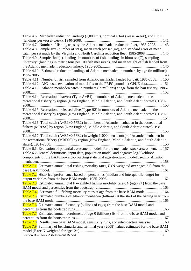
Table 7.1 Estimated annual total fishing mortality rates, F (N-weighted over ages 2+) from the base BAM model. ....................................................................................................................... 161
Table 7.2 Historical performance based on percentiles (median and interquartile range) for output variables from the base BAM model, 1955–2008. .......................................................... 162
Table 7.3 Estimated annual total N-weighted fishing mortality rates, F (ages 2+) from the base BAM model and percentiles from the bootstrap runs. ................................................................ 163
Table 7.4. Estimated full fishing mortality rates at age from the base BAM model. ................ 164
Table 7.5 Estimated numbers of Atlantic menhaden (billions) at the start of the fishing year from the base BAM model. ................................................................................................................. 165
Table 7.6 Estimated annual fecundity (billions of eggs) from the base BAM model and percentiles from the bootstrap runs. ............................................................................................ 166
Table 7.7 Estimated annual recruitment of age-0 (billions) fish from the base BAM model and percentiles from the bootstrap runs. ............................................................................................ 167
Table 7.8 Results from base BAM model, sensitivity runs, and retrospective analysis. ........... 168
Table 7.9 Summary of benchmarks and terminal year (2008) values estimated for the base BAM model (F are N-weighted for ages 2+). ....................................................................................... 169
SEDAR 40 - 7

Section B – Stock Assessement Report 14
Table 8.1 Summary of benchmarks and terminal year value from previous stock assessments (ASMFC 2004, Table 9.1; and ASMFC 2006, Table 7.1). ......................................................... 170
SEDAR 40 - 7
Section B – Stock Assessement Report 15
List of Figures Figure 1.1 VPA historical retrospective on fishing mortality (F), both as (a) fishing mortality F for terminal years 1992-2001, and (b) as proportional deviations from terminal year 2000 (1992-1999). .......................................................................................................................................... 171
Figure 1.2 VPA historical retrospective on spawning stock biomass (SSB), both as (a) SSB for terminal years 1990, 1992-2001, and (b) as proportional deviations from terminal year 2000 (1992-1999)................................................................................................................................. 172
Figure 1.3 VPA historical retrospective on recruits to age 1 (R1), both as (a) R1 for terminal years 1990, 1992-2001, and (b) as proportional deviations from terminal year 2000 (1992-1999). ... 173
Figure 1.4 Comparison of fishing mortality, F, from “untuned” VPA with preliminary statistical catch model for terminal years 2000 and 2001. .......................................................................... 174
Figure 1.5 Comparison of spawning stock biomass, SSB, from “untuned” VPA with preliminary statistical catch model for terminal years 2000 and 2001. .......................................................... 175
Figure 1.6 Comparison of recruits to age 1, R1, from “untuned” VPA with preliminary statistical catch model for terminal years 2000 and 2001. .......................................................................... 176
Figure 1.7 Comparison of fishing mortality, F, from statistical catch model for peer review (2003) and update (2006). ........................................................................................................... 177
Figure 1.8 Comparison of spawning stock biomass, SSB, from statistical catch model for peer review (2003) and update (2006). ............................................................................................... 178
Figure 1.9 Comparison of recruits to age 1, R1, from statistical catch model for peer review (2003) and update (2006). ........................................................................................................... 179
Figure 2.1. Matrix of paired age readings by scales for Atlantic menhaden from 2008. ......... 180
Figure 2.2. Weighted mean weight at age for Atlantic menhaden for ages 1 through 3. ........... 181
Figure 2.3. Weighted mean weight at age 0 plotted against recruits to age 0 obtained from latest Atlantic menhaden stock assessment (ASMFC 2006) for 1955-2005. ....................................... 182
Figure 2.4. Comparison of observed weighted mean length at age (ages 2 and 3) with values estimated from the year and cohort based von Bertalanffy growth equation for mid-year (t+0.5)...................................................................................................................................................... 183
Figure 2.5. Fecundity (no. of maturing or ripe ova) as a function of fork length (mm) for Atlantic menhaden. ................................................................................................................................... 184
Figure 2.6. Proportion of age 2 (11.8% mature) and age 3 (86.4%) spawning (essentially first time spawners) to total female spawning stock as estimated in numbers and in biomass from the most recent stock assessment (ASMFC 2006), 1955-2005. ....................................................... 185
Figure 2.7. Annual calculated values of M from age-constant M approaches and average M across ages 1-10 (constant for 6+) of MSVPA-X. ...................................................................... 186
Figure 2.8. Age-varying estimates of M averaged across all available years for three age-varying methods based on weight at age (Boudreau & Dickie, Peterson & Wroblewski, and Lorenzen) and MSVPA-X. ........................................................................................................................... 187
Figure 2.9. Comparison of several age-varying methods for estimating M scaled to average M over ages. .................................................................................................................................... 188
Figure 4.1. Landings from the reduction purse seine fishery (1940-2008) and bait fishery (1985-2008) for Atlantic menhaden. ..................................................................................................... 189
SEDAR 40 - 7
Section B – Stock Assessement Report 16
Figure 4.2. A comparison of commercial catch statistics taken from Historical Reports (linearly interpolated by region) with reduction landings statistics maintained at NOAA Fisheries at Beaufort, NC. .............................................................................................................................. 190
Figure 4.3. Comparison of menhaden landings (Atlantic and gulf menhaden combined) between two sources of historical data, 1873-1964. ................................................................................. 191
Figure 4.4. A comparison of purse seine landings obtained from the ACCSP Commercial Landings (Purse Seine) to purse-seine reduction landings (Reduction) maintained by NOAA Fisheries at Beaufort, NC. ........................................................................................................... 192
Figure 4.5. Reconstructed Atlantic menhaden landings along the coast of the U.S., 1873-2008...................................................................................................................................................... 193
Figure 4.6. Annual values of menhaden reduction landings (1,000 mt) and nominal effort (vessel-week), 1940-2008. ...................................................................................................................... 194
Figure 4.7. Comparison of catch per trip from all Atlantic menhaden reduction trips, subset sampled in biostatistical program (merged data), and LSMEANS from initial GLM runs based on coarse (area/season) input data with either normal or lognormal error structure. ...................... 195
Figure 4.8. Comparison of nominal fishing effort for Atlantic menhaden reduction fleet, 1955-2008............................................................................................................................................. 196
Figure 4.9. Comparison of calculated averages for CPUE across different measures of fishing effort, including landings per vessel week, landings per trip and catch per set. ......................... 197
Figure 4.10. Comparison of nominal fishing effort for Atlantic menhaden reduction fleet, 1985-2008............................................................................................................................................. 198
Figure 4.11. Comparison of mean landings by state from the bait fishery for Atlantic menhaden, 1985-2000 and 2001-2008. ......................................................................................................... 199
Figure 4.12. Non-purse seine landings obtained from the ACCSP Commercial Landings, 1950-2008............................................................................................................................................. 200
Figure 4.13. PRFC adult Atlantic menhaden (primarily ages-1 through 3) index of relative abundance calculated as the ratio of total annual landings to total annual pound net days fished...................................................................................................................................................... 201
Figure 4.14. AIC based evaluation of the distribution of the PRFC adult Atlantic menhaden pound net CPUE data. ................................................................................................................. 202
Figure 4.15. PRFC adult Atlantic menhaden (primarily ages-1 through 3) index of relative abundance based on a negative binomial GLM with year, month, and area as fixed factors. ... 203
Figure 4.16. Atlantic menhaden bait landings (1,000 metric tons) by region, 1985-2008. ....... 204
Figure 5.1. Proportion of seine hauls where at least one juvenile menhaden was captured by year for each state seine survey. ......................................................................................................... 205
Figure 5.2. AIC based evaluation of the distribution of the juvenile catch-per-haul data for each state seine survey. ....................................................................................................................... 206
Figure 5.3. Coastwide juvenile abundance index based on the full delta-lognormal GLM fitted to seine catch-per-haul data from all states combined. ................................................................... 207
Figure 5.4. Principle components analysis biplot used to investigate potential groupings of Region 1 juvenile abundance index based on delta-lognormal GLM fitted to seine catch-per-haul data from NC, VA, and MD combined. ...................................................................................... 208
Figure 5.5a. Region 1 juvenile abundance index based on the full delta-lognormal GLM fitted to seine catch-per-haul data from NC, VA, and MD combined. .................................................... 209
Figure 5.5b. Region 2 juvenile abundance index based on the full delta-lognormal GLM fitted to seine catch-per-haul data from NY and RI combined. ............................................................... 209
SEDAR 40 - 7
Section B – Stock Assessement Report 17
Figure 5.5c. Region 3 juvenile abundance index based on the full delta-lognormal GLM fitted to seine catch-per-haul data from NJ. ............................................................................................. 210
Figure 5.5d. Region 4 juvenile abundance index based on the full delta-lognormal GLM fitted to seine catch-per-haul data from CT. ............................................................................................. 210
Figure 5.6. Linear regression fitted to the coastwide YOY and PRFC adult indices lagged by two years. ........................................................................................................................................... 211
Figure 6.1. Comparison of age 2+ population size by year between Beaufort Assessment Model (BAM) and MSVPA-X. .............................................................................................................. 212
Figure 6.2. Comparison of unweighted average 2+ fishing mortality by year between Beaufort Assessment Model (BAM) and MSVPA-X. ............................................................................... 212
Figure 6.3. Estimates of vulnerable stock biomass generated from the stochastic SRA base runs with current exploitation rates (U) set at: U=0.1, U=0.2, U=0.3. ............................................... 213
Figure 6.4. Estimates of vulnerable stock biomass generated from the stochastic SRA base run2 (U=0.2) with associated cv values set at 0.1, 0.2, and 0.3. ......................................................... 213
Figure 6.5. MCMC sample distributions and likelihood profiles of UMSY and MSY generated from three simulation runs based on current exploitation rate (U) ............................................. 214
Figure 6.6. Posterior distributions of B/B0 and U2008/UMSY generated from three simulation runs based on current exploitation rate (U). ....................................................................................... 215
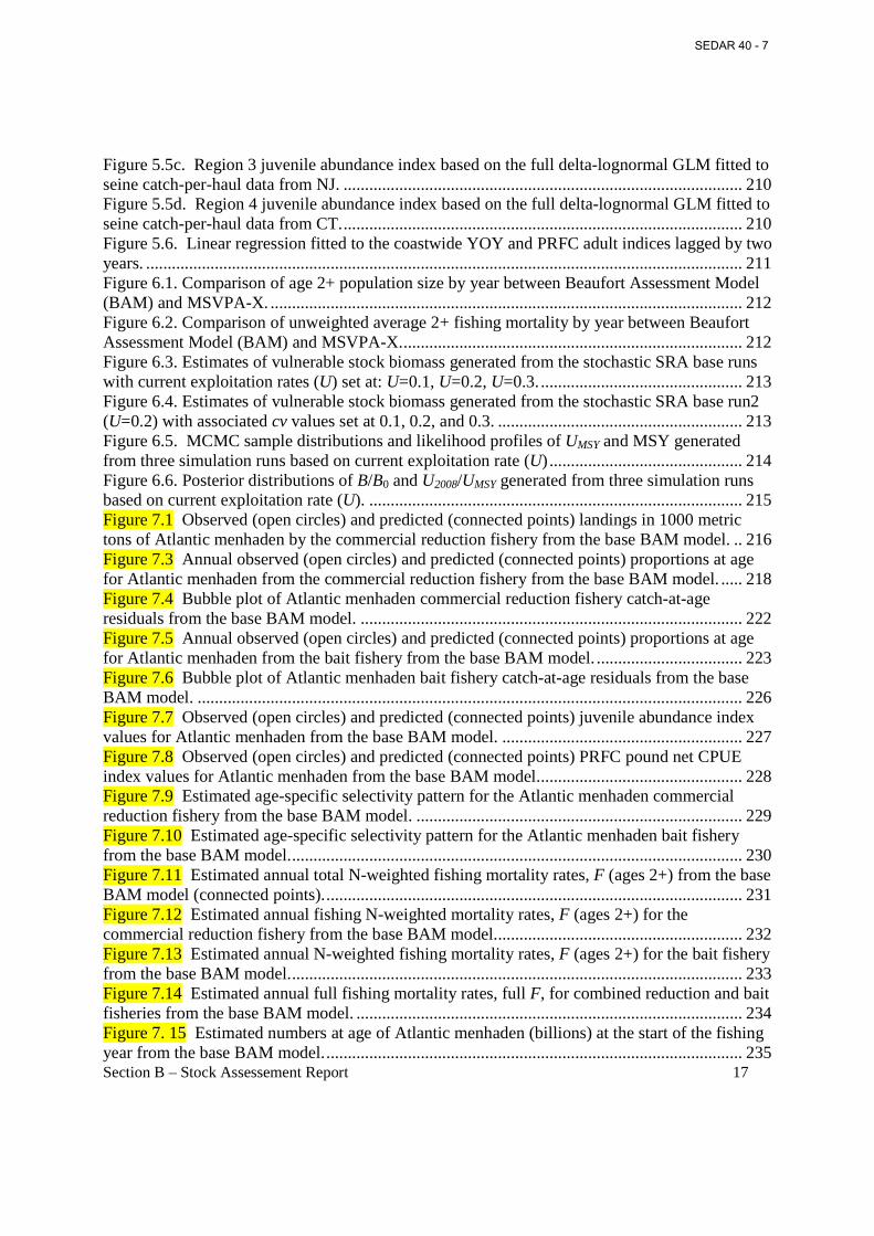
Figure 7.1 Observed (open circles) and predicted (connected points) landings in 1000 metric tons of Atlantic menhaden by the commercial reduction fishery from the base BAM model. .. 216
Figure 7.3 Annual observed (open circles) and predicted (connected points) proportions at age for Atlantic menhaden from the commercial reduction fishery from the base BAM model. ..... 218
Figure 7.4 Bubble plot of Atlantic menhaden commercial reduction fishery catch-at-age residuals from the base BAM model. ......................................................................................... 222
Figure 7.5 Annual observed (open circles) and predicted (connected points) proportions at age for Atlantic menhaden from the bait fishery from the base BAM model. .................................. 223
Figure 7.6 Bubble plot of Atlantic menhaden bait fishery catch-at-age residuals from the base BAM model. ............................................................................................................................... 226
Figure 7.7 Observed (open circles) and predicted (connected points) juvenile abundance index values for Atlantic menhaden from the base BAM model. ........................................................ 227
Figure 7.8 Observed (open circles) and predicted (connected points) PRFC pound net CPUE index values for Atlantic menhaden from the base BAM model. ............................................... 228
Figure 7.9 Estimated age-specific selectivity pattern for the Atlantic menhaden commercial reduction fishery from the base BAM model. ............................................................................ 229
Figure 7.10 Estimated age-specific selectivity pattern for the Atlantic menhaden bait fishery from the base BAM model. ......................................................................................................... 230
Figure 7.11 Estimated annual total N-weighted fishing mortality rates, F (ages 2+) from the base BAM model (connected points). ................................................................................................. 231
Figure 7.12 Estimated annual fishing N-weighted mortality rates, F (ages 2+) for the commercial reduction fishery from the base BAM model.......................................................... 232
Figure 7.13 Estimated annual N-weighted fishing mortality rates, F (ages 2+) for the bait fishery from the base BAM model. ......................................................................................................... 233
Figure 7.14 Estimated annual full fishing mortality rates, full F, for combined reduction and bait fisheries from the base BAM model. .......................................................................................... 234
Figure 7. 15 Estimated numbers at age of Atlantic menhaden (billions) at the start of the fishing year from the base BAM model. ................................................................................................. 235
SEDAR 40 - 7
Section B – Stock Assessement Report 18
Figure 7.16 Estimated annual fecundity (billions of eggs) from the base BAM model (connected points). Shaded area represents the 90% confidence interval of the bootstrap runs. ................. 236
Figure 7. 17 Estimated total fecundity (billions of mature ova) at age of Atlantic menhaden at the start of the fishing year from the base BAM model. ............................................................. 237
Figure 7.18 Estimated annual recruitment to age-0 (billions) from the base BAM model (connected points). Shaded area represents the 90% confidence interval of the bootstrap runs...................................................................................................................................................... 238
Figure 7.19 Estimated annual recruitment to age-0 (billions) from the base BAM model (connected points). ...................................................................................................................... 239
Figure 7.20 Estimated spawning stock (billions of mature ova) and recruitment (billions of age-0 fish) from the base BAM model (points). ................................................................................... 240
Figure 7.21 Estimated annual total N-weighted fishing mortality rates, F (ages 2+) from the base BAM model (connected open circles) and various sensitivity runs (see section 6.2.1.6 for details). ........................................................................................................................................ 241
Figure 7.22 Estimated annual recruitment of age-0 fish (billions) from the base BAM model (connected open circles) and various sensitivity runs (see section 6.2.1.6 for details). ............. 243
Figure 7.23 Estimated annual fecundity (billions of mature eggs) from the base BAM model (connected open circles) and various sensitivity runs (see section 6.2.1.6 for details). ............. 245
Figure 7.24 Estimated annual total N-weighted fishing mortality rates, F (ages 2+) from the base BAM model (connected open circles) and retrospective analysis runs. ..................................... 247
Figure 7.25 Estimated annual recruitment of age-0 fish (billions) from the base BAM model (connected open circles) and retrospective analysis runs. .......................................................... 248
Figure 7.26 Estimated annual population fecundity (billions of mature ova) from the base BAM model (connected open circles) and retrospective analysis runs. ............................................... 249
Figure 7.27 Estimates of the proportional (re-scaled to max of 1.0) fecundity-per-recruit as a function of the total N-weighted fishing mortality rate (age 2+) from the base BAM model. ... 250
Figure 7.28 Estimates of the yield-per-recruit (mt/million) as a function of the total fishing mortality rate (age 2+) from the base BAM model..................................................................... 251
Figure 7.29 Estimates of the total N-weighted fishing mortality rate (age 2+) relative to the FMED benchmark (fishing limit value) from the base BAM model (connected points). ...................... 252
Figure 7.30 Estimates of the population fecundity (SSB) relative to the target benchmark (SSBMED) from the base BAM model (connected points). ......................................................... 253
Figure 7.31 Phase plot of recent estimates of the population fecundity (mature ova in billions) and total N-weighted fishing mortality rate (age 2+) from the base BAM model. ..................... 254
Figure 7.32 Cumulative probability density distribution of total N-weighted fishing mortality rate (age 2+) in 2008 relative to the fishing limit value (FMED) from the bootstrap estimates from the base BAM model. ................................................................................................................. 255
Figure 7.33 Cumulative probability density distribution of the population fecundity in 2008 relative to the limit value from the bootstrap estimates from the base BAM model. ................. 256
Figure 7.34 Scatter plot of the 2008 estimates relative to the benchmarks (limits) from the 2,000 bootstrap estimates from the base BAM model. ......................................................................... 257
Figure 8.1. R/SSB plot for 1959 -2008. Horizontal lines represent average survival R/eggs for the 1970 - 1988 and 1989 – 2008 periods. .................................................................................. 258
Figure 8.2. Recruitment (age 0) versus spawning stock total fecundity for 1959 - 2008. .......... 259
Figure 8.3 Plot of Atlantic menhaden fecundity (billions of mature ova) and age-0 recruitment (billions) estimates lagged by one year from the base BAM model. .......................................... 260
SEDAR 40 - 7

Section B – Stock Assessement Report 19
Figure 8.4. Annual fishing mortality rate (full F) relative to FMED = 2.20 for base run (for comparison: Ftarget = 0.96). ......................................................................................................... 261
Figure 8.5. Annual fecundity compared to target and limit. ....................................................... 262
SEDAR 40 - 7

Section B – Stock Assessement Report 20
Terms of Reference
1. Evaluate precision and accuracy of fishery-dependent and fishery-independent data used in the assessment:
a. Discuss data strengths and weaknesses (e.g. temporal and spatial scale, gear selectivities, aging accuracy, sampling intensity).
b. Report metrics of precision for data inputs and use them to inform the model as appropriate.
c. Describe and justify index standardization methods. d. Justify weighting or elimination of available data sources.
2. Evaluate models used to estimate population parameters (e.g., F, biomass, abundance) and biological reference points.
a. Did the model have difficulty finding a stable solution? b. Were sensitivity analyses for starting parameter values, priors, etc. and other
model diagnostics performed? c. Have the model strengths and limitations been clearly and thoroughly explained? d. Have the models been used in other peer reviewed assessments? If not, has new
model code been verified with simulated data? e. Compare and discuss differences among alternative models.
3. Evaluate the potential for conducting assessments at a sub-regional level (e.g. Chesapeake Bay).
4. State and evaluate assumptions made for all models and explain the likely effects of assumption violations on model outputs, including:
a. Calculation of M. b. Choice to incorporate constant or time-varying M and catchability. c. Choice of selectivity patterns. d. Choice of time steps in models. e. Error in the catch-at-age matrix. f. Choice of a plus group for age-structured species. g. Constant ecosystem (abiotic and trophic) conditions. h. Choice of stock-recruitment function. i. Choice of reference points (e.g. equilibrium assumptions).
5. Evaluate uncertainty of model estimates and biological or empirical reference points. a. Choice of weighting likelihood components.
6. Perform retrospective analyses, assess magnitude and direction of retrospective patterns detected, and discuss implications of any observed retrospective pattern for uncertainty in population parameters (e.g., F, SSB), reference points, and/or management measures.
7. Recommend stock status as related to reference points. 8. Develop detailed short and long-term prioritized lists of recommendations for future
research, data collection, and assessment methodology. Highlight improvements to be made by next benchmark review.
SEDAR 40 - 7
Section B – Stock Assessement Report 21
1.0 Introduction
1.1 Brief Overview and History of Fisheries The Reduction Purse-Seine Fishery. Some fishing for Atlantic menhaden has occurred since colonial times, but the use of purse-seine gear began in New England by the mid-1800s (Ahrenholz et al. 1987b). No longer bound to shore-based seining sites, the purse-seine fishery spread south to the Mid-Atlantic States and the Carolinas by the late 1800s. Purse-seine landings reached their zenith in the 1950s, and peak landings of 712,100 metric tons occurred in 1956. At the time, over 20 menhaden factories ranged from northern Florida to southern Maine (ASMFC 2004a). In the 1960s, the Atlantic menhaden stock contracted geographically, and many of the fish factories north of Chesapeake Bay closed because of a scarcity of fish (Nicholson 1975). During the 1970s and 1980s, the menhaden population began to expand, primarily because of a series of above average year classes entering the fishery. Adult menhaden were again abundant in the northern half of their range, that is, Long Island Sound north to the southern Gulf of Maine. By the mid-1970s, reduction factories in Rhode Island, Massachusetts, and Maine began processing menhaden again. In 1987, a reduction plant in New Brunswick, Canada, processed menhaden harvested in southern Maine, but transported by steamer to Canada. Beginning in 1988, Maine entered into an Internal Waters Processing venture (IWP) with the Soviet Union which brought up to three foreign factory ships into Maine territorial waters (< 3 miles from the coast). American vessels harvested the menhaden and unloaded the catch for processing on the factory ships. By 1989 all shore-side reduction plants in New England had closed mainly because of odor abatement issues with local municipalities. A second Canadian plant in Nova Scotia also processed Atlantic menhaden caught in southern Maine in 1992-93. During the 1990s the Atlantic menhaden stock contracted again (as in the 1960s) mostly due to a series of poor to average year classes. Fish became scarce again north of Long Island Sound. The Russian-Maine IWP and the Canadian plants last processed menhaden during summer 1993. After 1993, only three factories remained in the reduction fishery, two factories in Reedville, VA, and one factory in Beaufort, NC. Virginia vessels (about 18-20) ranged north to New Jersey and south to about Cape Hatteras, NC, while the North Carolina vessels (generally two) fished mostly in North Carolina waters. A major change in the industry took place following the 1997 fishing season, when the two reduction plants operating in Reedville, VA, consolidated into a single company and a single factory; this significantly reduced effort and overall production capacity. Seven of the 20 vessels operating out of Reedville, VA, were removed from the fleet prior to the 1998 fishing year and 3 more vessels were removed prior to the 2000 fishing year, reducing the Virginia fleet to generally 10 vessels from 2000 through 2008. Another major event within the industry occurred in spring of 2005 when the fish factory at Beaufort, NC, closed and the owners sold the property to coastal developers. Since 2005 there has been only one operational reduction factory for processing Atlantic menhaden on the Atlantic coast of the US. This plant is owned by Omega Protein Inc., and is
SEDAR 40 - 7

Section B – Stock Assessement Report 22
located at Reedville, VA. The Omega Protein plant has a fleet of ten purse-seine vessels, which range in length from about 160 to 200 ft and in gross tonnage from about 500 to 600 tons. Fully loaded, these vessels on average carry about 500 tons of menhaden. Most of the catch and fishing effort by the Reedville fleet is in the Virginia portion of Chesapeake Bay and adjacent ocean waters. However, in summer and early fall the Virginia vessels may move north into Maryland, Delaware, and New Jersey ocean waters in search of fish. Regulations in these states prohibit harvest for reduction purposes in state waters, so the fishery is limited to the U.S. EEZ. In fall, the fleet may travel farther south and harvest migratory menhaden schools along the North Carolina Outer Banks. In 2008, landings of Atlantic menhaden for reduction at Reedville amounted to 141,133 metric tons. In recent years (2005-08) landings at Reedville have averaged 154,980 metric tons. The reduction process for menhaden yields three main processed products: fish meal, fish oil, and fish solubles. The Bait Purse-Seine Fishery. As reduction landings have declined in recent years, menhaden landings for bait have become relatively more important to the coastwide total landings of menhaden. Commercial landings of menhaden for bait occur in almost every Atlantic coast state. Recreational fishermen also catch Atlantic menhaden as bait for various game fish. A majority of the menhaden-for-bait landings are used commercially as bait for crab pots, lobster pots, and hook-and-line fisheries. The bait fishery utilizes a wide variety of gear and fishing techniques. Landings come from both directed menhaden fisheries, which make up the majority of the bait landings, and from non-directed, by-catch fisheries. Total landings of menhaden for bait along the US East coast have been relatively stable in recent years, averaging about 37,100 metric tons during 2001-2008, with peak landings of about 46,700 metric tons in 2008. In 2001, total Atlantic menhaden bait landings comprised 13% of total Atlantic menhaden landings (270,000 metric tons) increasing to 25% of total landings (187,800 metric tons) in 2008. Regional landings of menhaden for bait are dominated by harvests in Chesapeake Bay and New Jersey. Menhaden for bait landings in Maryland, Virginia, and the Potomac River combined amounted to about 21,200 mt in 2008, or 45% of the total menhaden-for-bait landings on the U.S. Atlantic coast, while New Jersey contributed nearly 37% of coastwide landings, primarily from purse-seine gear. Bait landings of menhaden in Virginia are dominated by purse-seine gear called ‘snapper rigs’, whose nets are somewhat smaller than the gear employed by the larger reduction vessels. ‘Snapper rig’ vessels are also smaller (about 100 ft long) than reduction ‘steamers’, and make fewer sets of the net each fishing day. In recent years, three ‘snapper rig’ vessels have operated from Northern Neck, VA, near Reedville. “Snapper rig’ vessels supply daily logbooks to the NMFS at Beaufort, from which their daily and annual catches are tabulated. A NMFS port agent also samples ‘snapper rig’ landings for age and size composition. Bait landings of menhaden in Maryland and the Potomac River are dominated by pound net catches. Purse seine and pound net bait fisheries for menhaden in New England occur intermittently and depend on whether northward migrating fish enter the northern estuaries. When they occur, bait catches are sampled for age and size composition in RI, MA, and ME by state agencies, and the samples are sent to the NMFS Laboratory for analysis.
SEDAR 40 - 7

Section B – Stock Assessement Report 23
Sport fishermen catch menhaden for bait primarily with cast nets. Anglers use menhaden as a live or “cut” bait for many species of game fishes, such as striped bass, bluefish, and sharks. Ground menhaden is preferred as a chum to attract many sport fishes. Quantities of menhaden harvested by sport fishermen are unknown, but thought to be minor in comparison to landings by the reduction fishery.
1.2 Management Unit Definition The management unit for Atlantic menhaden (Brevoortia tyrannus) is defined in Amendment 1 as throughout the range of the species within U.S. waters of the northwest Atlantic Ocean from the estuaries eastward to the offshore boundary of the EEZ. The unit is coastwide from Maine to Florida. The Amendment 1 definition is consistent with recent stock assessments (including this one; see Section 2.1) which treat the entire resource in U.S. waters of the northwest Atlantic as a single stock.
1.3 Regulatory History Throughout much of its history, the Atlantic menhaden fishery has been managed by unilateral regulatory actions imposed by individual states. The first coastwide management plan (FMP) for Atlantic menhaden was passed in 1981 (ASMFC 1981). At the time the FMP was passed, Maryland and Virginia were the two most restrictive states along the Atlantic coast. Maryland was the only state to prohibit the use of purse seine nets in its waters, thereby eliminating a commercial reduction fishery. Virginia was the only state to use both a closed season and mesh size limits to regulate the menhaden fishery. The 1981 FMP did not recommend or require specific management actions, but provided a suite of options should they be needed. After the FMP was approved, a combination of additional state restrictions, imposition of local land use rules, and changing economic conditions resulted in the closure of most reduction plants north of Virginia by the late 1980s (ASMFC 1992). In 1988, the ASMFC concluded that the 1981 FMP had become obsolete and initiated a revision to the plan. The 1992 Plan Revision included a suite of objectives to improve data collection and promote awareness of the fishery and its research needs (ASMFC 1992). Under this revision, the menhaden program was directed by the ASMFC Atlantic Menhaden Management Board, which at the time was composed of up to five state directors, up to five industry representatives, and one representative each from the National Marine Fisheries Service and the National Fish Meal and Oil Association. The 1992 Revision included six “management triggers” used to annually evaluate the menhaden stock and fishery:
• Landings in weight – recommend action if landings fell below 250,000 metric tons • Proportion of age-0 menhaden in landings – recommend action if more than 25%
harvested (by number) were age-0 fish • Proportion of adults in landings – recommend action if more than 25% harvested (by
number) were age 3 and older
SEDAR 40 - 7

Section B – Stock Assessement Report 24
• Recruits to age 1 – recommend action if estimates of age-1 fish fell below 2 billion • Spawning stock biomass (SSB) – recommend action if SSB fell below 17,000 metric
tons • Percent maximum spawning potential (%MSP) – recommend action if %MSP
dropped below 3% The Atlantic Menhaden Advisory Committee (AMAC) comprised of technical and industry representatives annually evaluated the “management triggers”. If one or more of the “management triggers” was reached and it indicated a problem, the AMAC was to recommend regulatory action to the Board. The ‘recruitment trigger’ was exceeded during several years while the triggers were in place. However, AMAC never recommended action because SSB was at high levels during those years, and they felt reduced recruitment was caused by environmental factors (as opposed to fishing pressure). Also, a retrospective bias was associated with the recruitment estimates. Scientists calculated initial low values for recruits in the terminal years, and higher values were obtained in subsequent years. Representation at the Management Board was revised in 2001 to include three representatives from each state Maine through Florida, including the state fisheries director, a legislator, and a governor’s appointee. The reformatted board has passed one amendment and four addenda to the 1992 FMP revision. Amendment 1, passed in 2001, provides specific biological, social/economic, ecological, and management objectives. Addendum I (2004) establishes the biological reference points that are currently in use. Addendum II (2005) initiated a five-year research program for Chesapeake Bay aimed at examining the possibility of localized depletion. Addendum III (2006) instituted a harvest cap for reduction landings from Chesapeake Bay during 2006 through 2010. The cap was set at 109,020 metric tons which could be increased to a maximum of 122,740 metric tons if there was a harvest underage of 13,720 metric tons or greater in the previous year. Addendum IV (2009) extends the Chesapeake harvest cap three additional years (2011-2013) at the same cap levels.
1.4 Assessment History
1.4.1 History of Stock Assessments There is a long history of analyses on the Atlantic menhaden population. Quantitative analyses began in the early 1970s, as the time series of detailed data developed (accurate reduction landings have been recorded since 1940, and detailed biostatistical sampling began in 1955). The first quantitative analysis was that of Henry (1971) who addressed the significant decline in the menhaden stock during the 1960s. Henry suggested that “(O)f major importance to the proper management of any fishery is the ability to estimate the strength of the year class, before it enters the fishery.” He noted that several large year classes were apparent in the catch data during the 1950s, including the “superabundant 1958 year class”. However, “(w)hen the 1958 year class virtually disappeared from the catch in 1963 and there were no subsequent strong year classes, it is not surprising that the landings declined.” Schaaf and Hunstman (1972) conducted a more
SEDAR 40 - 7

Section B – Stock Assessement Report 25
detailed analysis of the catch-at-age data to obtain estimates of age and year specific fishing mortality rates, and explore yield-per-recruit and stock recruitment relationships. Dryfoos et al. (1973) conducted a detailed analysis of the Atlantic menhaden population based on tag returns from a large tagging study. Various population-level analyses were conducted during the 1970s, building on the work of Schaaf and Huntsman (1972). Most notably was an investigation of the effects of Ekman transport on menhaden recruitment (Nelson et al. 1977; Schaaf 1979). In the early 1980s, a stochastic population model was developed under contract with NMFS to investigate among other things migration, density-dependent growth, and harvesting strategies (Reish et al. 1985; Ruppert et al. 1985). Two formal stock assessments were completed during the 1980s. The first (Ahrenholz et al. 1987b) included data through 1979, and the second (Vaughan and Smith 1988) included data through 1984. These assessments used an “untuned” virtual population analysis (VPA) approach based on the cohort-linked method described by Murphy (1965) to estimate age- and year-specific fishing mortality and population numbers from the catch-at-age matrix computed from the reduction fishery landings and biostatistical samples. Surplus production models, spawner-recruit relationships, and yield-per-recruit analyses were then developed. A similar set of analyses was later conducted to address the developing Internal Waters Processing agreement with Russian factory ships in Maine (Vaughan 1990). Stock assessment results were summarized in a special menhaden issue of Marine Fisheries Review (Vaughan and Merriner 1991). Further updates of Atlantic menhaden assessments were conducted during preparation of the revised fishery management plan for Atlantic menhaden (ASMFC 1992). Annual assessments were conducted by Dr. Douglas Vaughan for the ASMFC Atlantic Menhaden Advisory Committee (AMAC) from 1993-2002. These annual reports were initially limited to estimation of the trigger variables developed for the revised fishery management plan, but expanded beginning in 1998 to include additional analyses. A detailed retrospective analysis was conducted on these annual assessments (through 1996) by Cadrin and Vaughan (1997). This analysis of historical retrospective patterns has been recently updated by Dr. Douglas Vaughan for assessments through 2006 and is included in this assessment (see Section 1.5). Uncertainty and risk analyses of these assessments were explored by Vaughan (1993) and Vaughan et al (2002). As noted above, assessment methods used the “untuned” VPA method of Murphy (1965) as the primary assessment methodology through 2002. This method was accepted by a formal peer review in 1998 (ASMFC 1999a, 1999b). Amendment 1 to the Atlantic Menhaden Fishery Management Plan (ASMFC 2001) was issued in 2001. Among other changes, this amendment dropped the six triggers from the 1992 revision (ASMFC 1992) and replaced them with two benchmarks that conformed to the 1997 revision to the Magnuson-Stevens Fishery Conservation and Management Act (Restrepo et al. 1998). Concurrently, new statistical assessment methods (e.g., forward projection model) were introduced in 2001 and explored further in 2002 in parallel to the “untuned” VPA approach. Indices of juvenile abundance, and an “adult” abundance index (menhaden landings per poundnet license from the Potomac River Fishery Commission, PRFC) were developed for the statistical catch at age model, which then went through a formal peer review in 2003 (ASMFC 2004a, 2004b). In preparation for a formal peer review in 2003 (ASMFC 2004a, 2004b), several additional changes were made during the data workshop.
SEDAR 40 - 7
Section B – Stock Assessement Report 26
Conversion of bait landings to catch at age were further refined. The concept of age-varying M was introduced based on the multi-species VPA under development by ASMFC, and later peer reviewed (NEFSC 2006a, 2006b). The maturity schedule was modified, reflecting that some age 2 and most, but not all, age 3 were mature. A coastwide index of juvenile abundance and “adult” index from PRFC were developed for use in “tuning”. The most recent assessment was the update assessment conducted in 2006 with additional data through 2005 (ASMFC 2006). The most recently completed assessment of the status of the Atlantic menhaden stock was an update of the 2003 peer-reviewed assessment, and it included data through 2005 (ASMFC 2006). Data included abundance indices, recorded landings, and samples of annual size and age compositions from the landings. Six state juvenile abundance seine indices were developed; five of which were used in the 2003 peer-reviewed or benchmark assessment (ASMFC 2004a). The new seine index (New Jersey) was only used in an alternate model run. The pound net index from the PRFC was improved to better reflect fishing effort (from number of licenses which has been fixed at 100 licenses since 1994 to number of days fished). Landings and catch-in-numbers-at-age data were updated from the reduction and bait fisheries. A new vector of natural mortality at age was obtained from the recently peer-reviewed MSVPA-X model (NEFSC 2006a, 2006b) to replace the vector used in the benchmark assessment. The statistical model from the benchmark assessment was applied to these updated data. A base assessment model run was developed and sensitivity model runs were made to evaluate performance of the assessment model to these updated data. Because unrealistically high levels of adult natural mortality were estimated when the new M-at-age vector from the recent MSVPA-X base run was used, the ASMFC Menhaden Stock Assessment Subcommittee scaled this vector so that adult natural mortality matched historical tagging results (Madult = 0.5). This was in keeping with the peer-reviewed results which found that adult M from the peer-reviewed assessment (0.55) was reasonable because it provided an estimate of adult M similar to the historical adult M obtained from tagging (Reish et al. 1985). Status of stock was based on the terminal year (2005) estimate relative to its corresponding limit (or threshold). Benchmarks were estimated based on the results of the updated base run. The terminal year estimate of fishing mortality rate (F2+ weighted) was estimated to be 56% of its limit (and 91% of its target). Correspondingly, the terminal year estimate of population fecundity was estimated at 158% of its fecundity target (and 317% of its limit). Hence, the stock was not considered to be overfished, nor was overfishing occurring.
1.4.2 Historical Retrospective Patterns “Historical retrospective” can be investigated using annual stock assessments that have been conducted consistently over the years (Cadrin and Vaughan 1997). These analyses compare estimates of important management variables from the most recent assessment with contemporary estimates from prior stock assessments. In particular, Cadrin and Vaughan (1997) compared three management variables (or “triggers”) in their analysis, including spawning stock biomass, recruitment to age 1, and maximum spawning potential (%MSP). Amendment 1 to the
SEDAR 40 - 7

Section B – Stock Assessement Report 27
Atlantic Menhaden Fishery Management Plan (ASMFC 2001) dropped the six triggers from the 1992 revision (ASMFC 1992) and replaced them with two benchmark (management) variables that conformed to the 1998 revision to the Magnuson-Stevens Fishery Conservation and Management Act (Restrepo et al. 1998). So, for the purpose of this analysis, we have replaced %MSP with adult fishing mortality (F). The management variables analyzed in this section are:
• Fishing Mortality (F) – calculated historically as catch-weighted age-specific F for ages 2 and older; this was changed to N-weighted in the 2003 peer-reviewed assessment.
• Spawning Stock Biomass (SSB) – calculated as the weight of mature females in the population. Initially, all females age 3 and older were assumed mature, and younger fish were assumed immature. This was modified in 2003 to reflect that some age 2 may be mature (11.8%), and most, but not all age 3 are mature (84.6%).
• Recruits to Age 1 – directly estimated as number of age 1 fish in the population at the start of the fishing year (March 1 for Atlantic menhaden).
As already noted, a consistent assessment methodology was applied from 1990 through 2002, and this approach was accepted by a formal peer review in 1998 (ASMFC 1999a, 1999b). This consistent approach included the following:
• “Untuned” VPA method of Murphy (1965) • Catch at age matrix based on reduction fishery only (through 2000) • Constant natural mortality (M = 0.45) • Knife-edge maturity beginning with age 3
Two types of comparisons have been developed for the annual estimates of management variables. First, the time series of estimated values are overlayed for each of the management variables (Figures 1.1a, 1.2a, and 1.3a). These plots include annual assessments with terminal years 1990, 1992-2001, with the exception of fishing mortality in 1990. Second, proportional deviations were developed between the time series with terminal year 2000 and earlier terminal years (Figures 1.1b, 1.2b, and 1.3b). Note that bait landings were included in assessments beginning with 2001 (terminal year 2000). The primary effect of adding bait landings was to decrease estimates of F and increase estimates of SSB and R1. The selectivity of bait landings tends towards larger, older fish. Concurrent with the “untuned” VPAs, the new statistical catch-at-age (“forward projecting”) assessment model was introduced in 2001 and explored further in 2002. These analyses appeared as appendices to the 2001 and 2002 assessment reports. Results from the two assessment methods are compared in the next series of figures (Figures 1.4-1.6) for each of the three management variables. The last series of figures (Figures 1.7-1.9) compare fishing mortality rates, spawning stock biomass, and recruitment between the peer-reviewed and updated assessments.
SEDAR 40 - 7

Section B – Stock Assessement Report 28
2.0 Life History
2.1 Stock Definition Ahrenholz (1991) pointed out that historically, considerable debate existed relative to stock structure of Atlantic menhaden on the US East coast, with a northern and southern stock hypothesized based on meristics and morphometrics (Sutherland 1963; June 1965). Nicholson (1972) and Dryfoos et al. (1973) argued convincingly, from back-calculated length-frequency information and tag recoveries, for a single biological population of Atlantic menhaden. Ahrenholz (1991) noted that although different temporal spawning cohorts of menhaden exist, they appear to mix rapidly as a result of their extensive migratory movements and are virtually inseparable in the commercial fishery. Thus primarily based on size-frequency information and tagging studies (Nicholson 1972 and 1978; Dryfoos et al. 1973), the Atlantic menhaden resource is believed to consist of a single unit stock or population. Recent genetic studies (Anderson 2007; Lynch 2008) support the single stock hypothesis.
2.2 Migration Patterns Adult Atlantic menhaden undergo extensive seasonal migrations north and south along the US East coast (ASMFC 2004a). Roithmayr (1963) found evidence of this migratory behavior based on the decrease in the number of purse-seine sets north of Cape Cod in September. Also, Reintjes (1969) reported the disappearance of fish in October north of Chesapeake Bay and their appearance off the coast of North Carolina in November. Nicholson (1971b) examined latitudinal differences in length-frequency distributions of individual age groups at different times of year and described a cyclic north-south movement with the largest and oldest fish proceeding farthest north such that the population stratifies itself by age and size along the coast during summer. A study of length frequencies at the time of first annulus formation on scales (Nicholson 1972) supported the concept of a north-south migratory movement and also indicated that a great deal of mixing of fish from all areas occurs off the North Carolina coast before fish move northward in spring. Returns of tagged Atlantic menhaden (Dryfoos et al. 1973; Nicholson 1978) generally confirmed what was already concluded from earlier work and added some important details (ASMFC 2004a). Adults begin migrating inshore and north in early spring following the end of the major spawning season off the Carolinas during December-February. The oldest and largest fish migrate farthest, reaching southern New England by May and the Gulf of Maine by June. Fish begin migrating south from northern areas to the Carolinas in late fall. Adults that remain in the south Atlantic region for spring and summer migrate south later in the year, reaching northern Florida by fall. During November and December, most of the adult population that summered north of Chesapeake Bay moves south of the Virginia and North Carolina capes. After winter dispersal along the south Atlantic coast, adults again begin migrating north in early spring.
SEDAR 40 - 7
Section B – Stock Assessement Report 29
As with the adults, Kroger and Guthrie (1973) found that juvenile Atlantic menhaden also exhibit a seasonal north-south movement along the Eastern Seaboard. From tag recoveries during the late 1960s and early 1970s they reported that juveniles (age-0’s) migrate as far south as Florida in fall and winter, then redistribute northward along the coast by size as age-1 fish during the following spring and summer. Larger age-1 menhaden migrate north earlier and in greater numbers than smaller age-1 fish, which tend to remain along the south Atlantic coast; however, some age-1’s move from the south Atlantic and into Chesapeake Bay through mid-summer.
2.3 Age Background: The seminal study on ageing Atlantic menhaden was conducted by June and Roithmayr (1960) at the NMFS Beaufort Laboratory; their specimens were collected mostly from purse-seine landings during 1952-1956. They validated rings on the scales of menhaden as reliable age marks based on timing of scale ring deposition (generally March through May) and marginal increment analyses. Comparison of independent readings of scale ages showed a high percentage of agreement (= precision, >90%). Additionally, they examined scales from fish impounded for up to 14 months to further demonstrate that only one ring forms annually on menhaden scales. Based on these studies, menhaden are assigned to ages based on a March 1 “birthdate”. Menhaden field sampling protocols remain relatively unchanged from the 1950s. In the field, port agents measure specimens for fork length (mm) and weight (grams), then remove a scale patch (ca. 20-25 scales) from the mid-portion of the flank below the dorsal fin. Six scales per specimen are mounted between two microscope slides and labeled with a unique specimen number. At the laboratory, scales are viewed on an Eberbach macro-projector under 40x magnification. Specimens are assigned an age (in yrs) based on the number of scale rings. Precision: During the early decades of the Menhaden Program at the Beaufort Laboratory scales from individual menhaden specimens were read by two independent readers, with a third reader used to decide discrepancies. By the early 1970s – and probably because of budget constraints - only a single reader was retained on staff to age menhaden scales. This employee, Ethel A. Hall (EAH), has read menhaden scales at the Beaufort Laboratory beginning in 1969 to the present. In an effort to estimate contemporary precision of Atlantic menhaden age estimates, EAH re-read scale samples from the 2008 fishing season. Re-ageing efforts occurred during summer 2009. EAH was instructed to re-assign estimated ages, but not to make measurements to successive annuli (as per protocols for general menhaden ageing). Both sets of age estimates were stored in dBase files and analyzed in SAS. Overall, 80.3% (2,978 of 3,711) of the paired readings agreed. Younger age classes (age-0 through age-3) showed better agreement than older age classes (ages-4 and -5; Figure 2.1). Most disagreements were +/- one year for ages-1 through -3 (98.1%, 86.3%, and 96.5%, respectively). See Section 4.1.6 for additional details.
SEDAR 40 - 7

Section B – Stock Assessement Report 30
Accounting for error in age estimation is important for age composition data used in stock assessments (Punt et al. 2008). Thus, to account for any error associated with the age estimation process for Atlantic menhaden and to get contemporary precision estimates, an aging error analysis was completed using a program called “agemat” provided by André Punt. The data used for this analysis were the paired scale age estimates from the 2008 fishing season (n = 3,711). Agemat can use age estimation data from one reader at two points in time in order to estimate the standard deviation associated with age estimates. The data in Figure 2.1 were input to agemat, and a standard deviation maximum of 12 (which resulted in a coefficient of variation of 1 (A. Punt, personal communication) for the oldest age class was specified in the model. The standard deviation output from agemat was then used to provide the error associated with the age composition data for each age in the stock assessment models for Atlantic menhaden. These standard deviations were assumed constant over time. Scale-Otolith Paired Age estimates: Menhaden program managers at the Beaufort Laboratory realized it was impractical to utilize otoliths to age Atlantic menhaden because 1) sagittae were small and fragile, and 2) large amounts of time and effort would be required to extract, process, and read whole or sectioned otoliths. Moreover, large numbers of ageing parts (> ca. 10,000) would be required to adequately characterize the fishery with annual landings of several hundred thousand metric tons. Thus, scales were the ageing tool of choice for Atlantic menhaden (June and Roithmayr 1960). Ongoing work at Old Dominion University indicates good agreement between paired scale and otolith age estimates for Atlantic menhaden ages-0 through -3 (n = 70-80 fish), although relatively few age-2 and -3 have been processed (J. Schaffler, ODU, pers. comm., June 17, 2009). Indeed, menhaden otoliths are reported to be difficult and time consuming to age. Longevity and Contemporary Age Composition: Atlantic menhaden as old as age-8 were present in the spawning population during the 1950s and early 1960s, but fish older than age-6 have been uncommon since 1965. The oldest specimens aged from NMFS biological sampling were several 10-year old fish landed in 1955 (2), 1956 (3), 1958 (1) and 1964 (1) from more than 495,000 Atlantic menhaden aged between 1955 and 2008 (Table 2.1-2.2). Smith and O’Bier (1996) described an exceptionally large (433 mm FL; 1,551g; age-7) Atlantic menhaden from Chesapeake Bay taken in August 1996. In two of three years since 2006, age-2 Atlantic menhaden have comprised 65% or more of the total numbers of fish landed by the commercial reduction fishery. In 2006 the age composition of the coastwide landings was 1% age-0s, 40% age-1s, 40% age-2s, and 19% age-3+s; in 2007, it was <1% age-0s, 26% age-1s, 65% age-2s, and 8% age-3+s; and in 2008, it was 1% age-0s, 9% age-1s, 68% age-2s, and 22% age-3+s.
2.4 Growth The growing season begins in spring and ends in fall as water temperatures rise above and decline below 15o C (Kroger et al. 1974). Atlantic menhaden reach lengths of about 500 mm total
SEDAR 40 - 7
Section B – Stock Assessement Report 31
length (TL) and weights of over 1.5 kg (Cooper 1965). Due to their greater migratory range, larger fish of a given age are captured farther north than smaller fish of the same age (Nicholson 1978; Reish et al. 1985). This fact complicates any attempt to estimate overall growth for the entire stock from size-at-age data compiled from any individual area along the coast. To account for this, catch in numbers by year, season and fishing area were developed for weighting corresponding weights of individual Atlantic menhaden at age sampled when calculating mean fish weights (Figure 2.2) for 1955-2008. These “weighted” mean weights increased during the 1960s when stock size and recruitment are known to have declined, and then mean weights declined dramatically during the 1970s, and remained low during most of the 1980s when the stock was thought to have rebuilt. Increasing mean weights are estimated during the 1990s while recruitment was declining, followed by recent declines in mean weight. It has been suggested in various publications that density dependent growth is prevalent with Atlantic menhaden (Reish et al. 1985, Ahrenholz et al. 1987b, Ahrenholz 1991, Vaughan and Smith 1988). That is, there is an inverse relation between size of menhaden (size of age-0 menhaden) and number of recruits at age 0. In Figures 2.3, we plot annual values of weighted mean weight of age-0 menhaden against estimated recruits to age 0 from the last Atlantic menhaden stock assessment (ASMFC 2006). A statistically significant correlation of this inverse relation explains 49% of the annual variability in weighted mean weights (R2 = 0.49). Weighting by catch in numbers by year, season and fishing area is also applied to calculate average fork lengths (mm) and weights (g) by age and year (Tables 2.3 and 2.4). When sample size was less than 10 fish, substitution was accomplished by one of two methods: (1) use average of pre- and post-year values for that age when missing cell(s) are embedded between estimated values, or (2) average across all values when no post-year value is available. These mean values represent mean size at age at approximately mid-fishing year (August-September). Pair-wise Pearson correlations were estimated for these time series of weighted mean lengths and weights aligned by cohort (year class) or by calendar year (Table 2.5) for age 0-4. The differences in these correlations between these two alignments suggest that the relationship is stronger when aligned by cohort, so that density-dependent size at age is more characteristic of the cohort than of calendar year. Annual regressions of weight (W in g) on fork length (FL in mm) are conducted based on the natural logarithm transformation: ln W = a + b ln FL, (1) and corrected for transformation bias (root MSE) when retransformed back to: W = a(FL)b. (2) Annual estimates for parameters a and b along with sample size and root MSE are summarized in Table 2.1. We also have plotted annual estimates of b against recruits to age 0 to test whether there is a density dependent component to this parameter over time. No significant correlations were found.
SEDAR 40 - 7
Section B – Stock Assessement Report 32
As in previous menhaden assessments, regressions of fork length (mm) on age (yr) are based on the von Bertalanffy growth curve: FL = L∞(1 - exp(-K(age - t0))) (3) using the Marquardt algorithm for the nonlinear minimization (PROC NLIN in SAS). Annual parameters for these regressions are summarized with sample sizes in Table 2.1. Matrices of weight at ages-0 to -8 for 1955-2008 were developed from these equations to represent the average size-at-age of menhaden at the start of the fishing year (e.g., spawning biomass for appropriate ages) and middle of the fishing year (i.e., weight of fish landed) for use in population modeling. Parameters from regressions for equations (2) and (3) were averaged for the most recent eight years (2001-2008) and used to calculate lengths and weight at age at the middle of the fishing year (age+0.5; Table 2.6). Note that length and weight for age-0 menhaden is offset to 0.75 since they are not recruited to the fishery until late summer. An alternate set of von Bertalanffy fits were made with the size at age data aligned by cohort (year class) (Table 2.2). Because of concerns that density-dependent growth is a characteristic of the cohort, it was felt that this would be a better approach. Attempts were made to fit the von Bertalanffy growth equation to each year class from 1947 (age 8 in 1955) to 2008 (age 0 in 2008). For most cohorts, a full range of ages were available (1955-2001). For the incomplete cohorts at the beginning of the time period (1947-1955), all fits converged, although specific parameter estimates became progressively unrealistic for the earlier years (especially 1947-1949). However, these fits are only used for interpolation and not extrapolation, and were found useful for this limited purpose. Similarly, incomplete cohorts for the recent time period (2002-2008) generally converged with the exception of the last two years (2007-2008). With the exception of the two years for which the fits did not converge, reasonable estimates of the von Bertalanffy parameters were obtained, and estimates of size at age were interpolated from these fits. We compare the estimated lengths at ages 2 and 3 (mid-year) from the two series of fits to the von Bertalanffy growth equation with observed weighted mean lengths (Figure 2.4). Based on these two series of fits to the von Bertalanffy growth equation, annual estimates of fork length at age are interpolated from the annual and cohort based von Bertalanffy growth fits to represent the start of the fishing year (March 1) for use in estimating population fecundity (Tables 2.7 and 2.8). Similarly annual estimates of length-at-age were interpolated to represent the middle of the fishing year (September 1) and converted to weight-at-age (Eq. 2) for use in the statistical catch-at-age models when comparing model estimated catch to observed catch. (Tables 2.9 and 2.10).
2.5 Reproduction Spawning Times and Locations. Analysis of eggs and larvae collected at various locations along the Atlantic coast during 1953-75 (e.g., Judy and Lewis 1983) generally confirmed earlier knowledge of spawning times and location based on observations of adults with maturing or spent ovaries (e.g. Reintjes and Pacheco 1966). During December-March, most spawning-age
SEDAR 40 - 7
Section B – Stock Assessement Report 33
fish congregate in offshore waters south of Cape Hatteras. Maximum spawning probably occurs at this time. Checkley et al. (1988) reported maximum spawning off North Carolina in January 1986 during periods of strong northeast winds in up-welled water near the western edge of the Gulf Stream. Spawning continues at a decreasing rate closer inshore as fish migrate north in late March. By May, most spawning is restricted to coastal waters north of Cape Hatteras. Spawning reaches a minimum in June, but continues at a low level until September north of Long Island. As mature fish migrate south in October, spawning increases from Long Island to Virginia.
Adults move inshore and northward in spring and stratify by age and size along the Atlantic coast (Rogers and Van Den Avyle 1989). During this northern migration, spawning occurs progressively closer inshore and by late spring, some spawning occurs within coastal embayments. There are definite spring and fall spawning peaks in the middle and north Atlantic regions, with some spawning occurring during winter in the shelf waters of the mid-Atlantic region. Atlantic menhaden mature at smaller sizes at the southern end of their range - 180 mm fork length (FL) in the south Atlantic region versus 210 mm FL in the Chesapeake Bay area and 230 mm in the north and middle Atlantic regions because of latitudinal differences in size-at-age and the fact that larger fish of a given age are distributed farther north than smaller fish of the same cohort (Lewis et al. 1987).
Some limited spawning activity has been suspected during summer in the Gulf of Maine based on juvenile collections along the Maine coast (T. Creaser, Maine DMR, pers. comm.. as cited in ASMFC 1992) and the occurrence of ripe females (S. Young, Maine DMR observer on the M/V RIGA, pers. comm. as cited in ASMFC 1992). Indeed, Stokesbury and Stokesbury (1993) collected 209 young-of-year Atlantic menhaden (mean total length = 66.25 mm, range: 41-109 mm) in the Annapolis River, Nova Scotia, Canada, during 1985, 1986, and 1989. Coupled with citations of ripe fish in several rivers of New Brunswick, they argued that some spawning probably occurs in the Bay of Fundy during summer. Unfortunately, historic egg and larval surveys directed at Atlantic menhaden were restricted to waters south of Cape Cod (Judy and Lewis 1983) and did not produced any evidence for spawning in the Gulf of Maine. Maturity. Some Atlantic menhaden become sexually mature during their second year (late age-1), but most do not mature until their third year (late age-2) (Higham and Nicholson 1964; Lewis et al. 1987). Spawning occurs year-round throughout much of the species’ range, with maximum spawning off the North Carolina coast during late fall and winter. Thus, most Atlantic menhaden spawn for the first time at age-2 or -3 – prior to laying down their third annulus (by convention March 1) and continue spawning every year until death. First-spawning age-3 fish has accounted for most of the stock’s egg production since 1965 (Vaughan and Smith 1988).
Lewis et al. (1987) tabularized maturity schedules (number and percent of specimens by ages-1 and -2) for female Atlantic menhaden from their field collections and those of Higham and Nicholson (1964). Percent age-1 females with active ovaries ranged from 1.5% to 27.8%, while percent age-2 females with active ovaries ranged from 67.4% to 97.1% (see table below). All age-3 and older females were judged to be sexually mature.
SEDAR 40 - 7
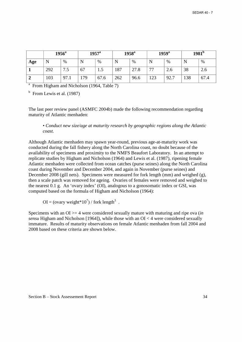
Section B – Stock Assessement Report 34
1956a 1957a 1958a 1959a 1981b
Age N % N % N % N % N %
1 292 7.5 67 1.5 187 27.8 77 2.6 38 2.6
2 103 97.1 179 67.6 262 96.6 123 92.7 138 67.4 a From Higham and Nicholson (1964, Table 7) b From Lewis et al. (1987)
The last peer review panel (ASMFC 2004b) made the following recommendation regarding maturity of Atlantic menhaden:
• Conduct new size/age at maturity research by geographic regions along the Atlantic coast.
Although Atlantic menhaden may spawn year-round, previous age-at-maturity work was conducted during the fall fishery along the North Carolina coast, no doubt because of the availability of specimens and proximity to the NMFS Beaufort Laboratory. In an attempt to replicate studies by Higham and Nicholson (1964) and Lewis et al. (1987), ripening female Atlantic menhaden were collected from ocean catches (purse seines) along the North Carolina coast during November and December 2004, and again in November (purse seines) and December 2008 (gill nets). Specimens were measured for fork length (mm) and weighed (g), then a scale patch was removed for ageing. Ovaries of females were removed and weighed to the nearest 0.1 g. An ‘ovary index’ (OI), analogous to a gonosomatic index or GSI, was computed based on the formula of Higham and Nicholson (1964): OI = (ovary weight*107) / fork length3 .
Specimens with an OI >= 4 were considered sexually mature with maturing and ripe ova (in sensu Higham and Nicholson [1964]), while those with an OI < 4 were considered sexually immature. Results of maturity observations on female Atlantic menhaden from fall 2004 and 2008 based on these criteria are shown below.
SEDAR 40 - 7
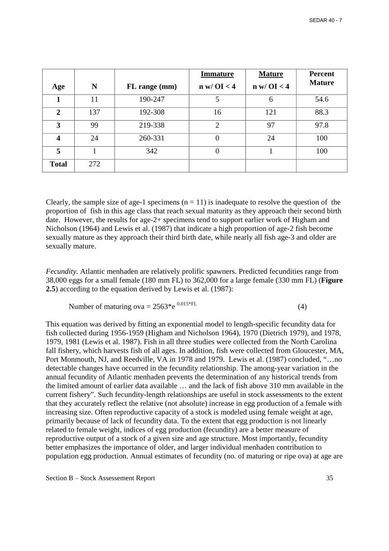
Section B – Stock Assessement Report 35
Age
N
FL range (mm)
Immature
n w/ OI < 4
Mature
n w/ OI < 4
Percent Mature
1 11 190-247 5 6 54.6
2 137 192-308 16 121 88.3
3 99 219-338 2 97 97.8
4 24 260-331 0 24 100
5 1 342 0 1 100
Total 272
Clearly, the sample size of age-1 specimens (n = 11) is inadequate to resolve the question of the proportion of fish in this age class that reach sexual maturity as they approach their second birth date. However, the results for age-2+ specimens tend to support earlier work of Higham and Nicholson (1964) and Lewis et al. (1987) that indicate a high proportion of age-2 fish become sexually mature as they approach their third birth date, while nearly all fish age-3 and older are sexually mature.
Fecundity. Atlantic menhaden are relatively prolific spawners. Predicted fecundities range from 38,000 eggs for a small female (180 mm FL) to 362,000 for a large female (330 mm FL) (Figure 2.5) according to the equation derived by Lewis et al. (1987): Number of maturing ova = 2563*e 0.015*FL (4) This equation was derived by fitting an exponential model to length-specific fecundity data for fish collected during 1956-1959 (Higham and Nicholson 1964), 1970 (Dietrich 1979), and 1978, 1979, 1981 (Lewis et al. 1987). Fish in all three studies were collected from the North Carolina fall fishery, which harvests fish of all ages. In addition, fish were collected from Gloucester, MA, Port Monmouth, NJ, and Reedville, VA in 1978 and 1979. Lewis et al. (1987) concluded, “…no detectable changes have occurred in the fecundity relationship. The among-year variation in the annual fecundity of Atlantic menhaden prevents the determination of any historical trends from the limited amount of earlier data available … and the lack of fish above 310 mm available in the current fishery”. Such fecundity-length relationships are useful in stock assessments to the extent that they accurately reflect the relative (not absolute) increase in egg production of a female with increasing size. Often reproductive capacity of a stock is modeled using female weight at age, primarily because of lack of fecundity data. To the extent that egg production is not linearly related to female weight, indices of egg production (fecundity) are a better measure of reproductive output of a stock of a given size and age structure. Most importantly, fecundity better emphasizes the importance of older, and larger individual menhaden contribution to population egg production. Annual estimates of fecundity (no. of maturing or ripe ova) at age are
SEDAR 40 - 7
Section B – Stock Assessement Report 36
summarized for both annually-based von Bertalanffy growth fits (Table 2.11) and year class-based von Bertalanffy growth fits (Table 2.12). Related to this issue, is the contribution of young (e.g., first age spawners) to the overall reproductive effort. This was noted in Vaughan and Smith (1988), and we have updated this analysis from output from the last menhaden stock assessment (ASMFC 2006). In assessments prior to 2003, females were assumed to be fully mature with age 3 (late age 2) and immature at younger ages. For this analysis age 2 (11.8% mature) and age 3 (86.4%) females are treated as “first age spawners”. We compare the number and biomass of these first year spawners to total, 1955-2005, in Figure 2.6. With the exception 1955 and 1962, these proportions have been high (generally >70% for biomass and >80% for numbers) for the full assessment period. The exceptions result from the passage of two exceptionally large year classes (1951 and 1958) through the stock. Otherwise a general decline in this proportion can be seen since the peak values in 1967. Lewis et al. (1987) surmised that Atlantic menhaden “are probably determinate multiple spawners, which spread their spawn over a broad geographical and temporal range.” Ahrenholz (1991) summarized spawning seasonality noting, “some spawning occurs during virtually every month of the year…some spawning occurs in the more northerly portions of the fishes’ range as the fish begin moving southward in September…spawning continues with increasing intensity as the fish move progressively farther southward in October and November…spawning intensity is believed to peak in waters off the North Carolina coast in winter…spawning continues, but with decreasing levels of intensity as the fish move northward in the following spring and early summer.” Despite the broad geographic range of spawning activity, most fecundity studies of Atlantic menhaden have concentrated on acquiring gravid females off the North Carolina coast during the fall fishery when most age classes in the stock tend to be available (Higham and Nicholson 1964, Dietrich 1979, Lewis et al. 1987). It can be argued that existing fecundity studies of Atlantic menhaden are underestimates of absolute spawning potential. Nevertheless, the extant studies focused on fall or early winter concentrations of gravid fish off the North Carolina coast, which is believed to be the area of greatest spawning intensity (Ahrenholz 1991). For assessment purposes, modeling increasing egg production with size is preferable to female biomass as a measure of reproductive ability of the stock. With density-dependent growth and fecundity a function of growth (in length), there is the potential that a larger, slower growing cohort will produce fewer eggs overall than a smaller, faster growing cohort.
2.6 Natural Mortality Age-structured models attempt to reconstruct the fish population and fishing mortality rates by age and year, where total instantaneous mortality rate (Z) is the sum of instantaneous rates of fishing (F) and natural (M) mortality. Historically, natural mortality has been assumed to be constant over ages and years. In many stock assessments, constant values for M have been obtained from life history analogies (e.g. maximum age, growth rate parameters, etc.). Because it is thought that younger fish are more vulnerable to predation, natural mortality may decline with size or age. Several approaches have been considered to provide such size-varying estimates of
SEDAR 40 - 7
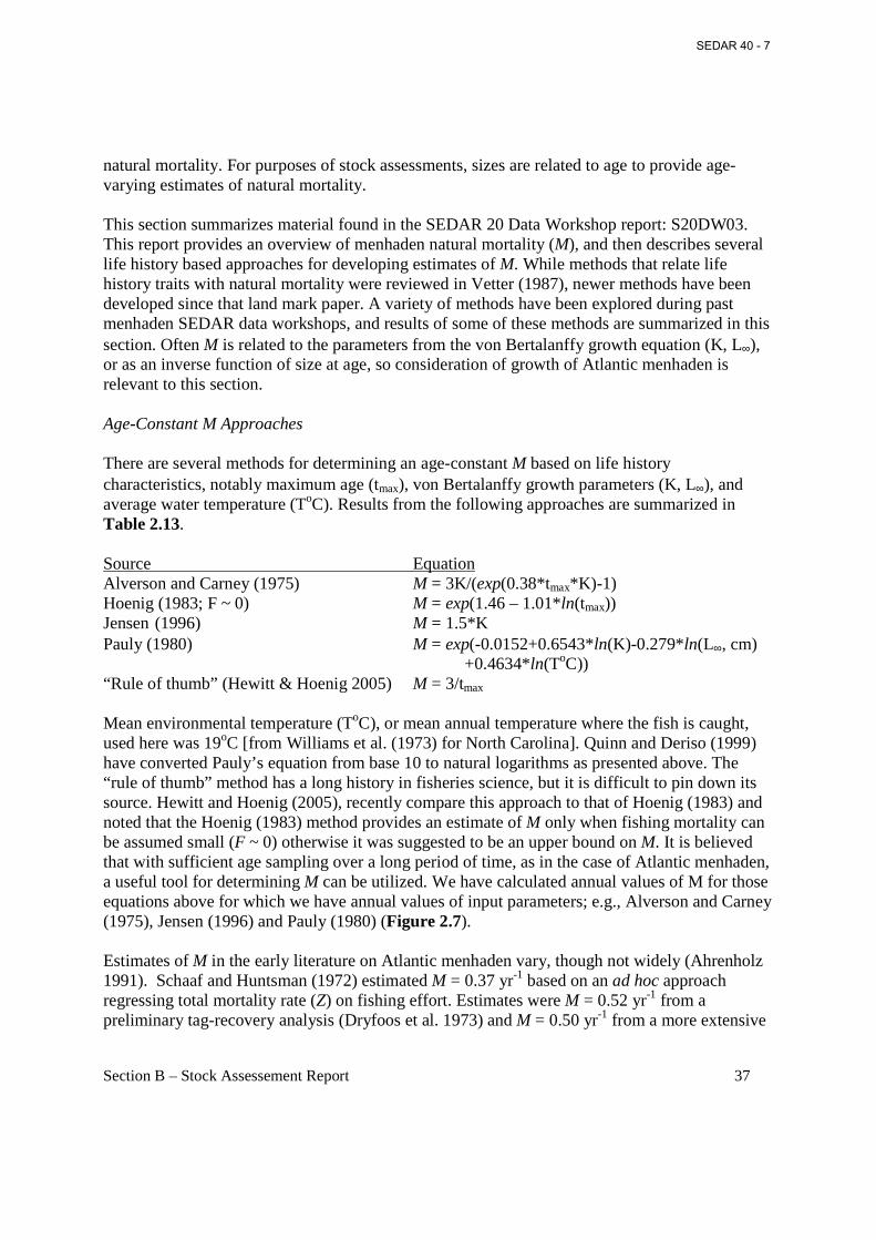
Section B – Stock Assessement Report 37
natural mortality. For purposes of stock assessments, sizes are related to age to provide age-varying estimates of natural mortality. This section summarizes material found in the SEDAR 20 Data Workshop report: S20DW03. This report provides an overview of menhaden natural mortality (M), and then describes several life history based approaches for developing estimates of M. While methods that relate life history traits with natural mortality were reviewed in Vetter (1987), newer methods have been developed since that land mark paper. A variety of methods have been explored during past menhaden SEDAR data workshops, and results of some of these methods are summarized in this section. Often M is related to the parameters from the von Bertalanffy growth equation (K, L∞), or as an inverse function of size at age, so consideration of growth of Atlantic menhaden is relevant to this section. Age-Constant M Approaches There are several methods for determining an age-constant M based on life history characteristics, notably maximum age (tmax), von Bertalanffy growth parameters (K, L∞), and average water temperature (ToC). Results from the following approaches are summarized in Table 2.13. Source Equation Alverson and Carney (1975) M = 3K/(exp(0.38*tmax*K)-1) Hoenig (1983; F ~ 0) M = exp(1.46 – 1.01*ln(tmax)) Jensen (1996) M = 1.5*K Pauly (1980) M = exp(-0.0152+0.6543*ln(K)-0.279*ln(L∞, cm) +0.4634*ln(ToC)) “Rule of thumb” (Hewitt & Hoenig 2005) M = 3/tmax Mean environmental temperature (ToC), or mean annual temperature where the fish is caught, used here was 19oC [from Williams et al. (1973) for North Carolina]. Quinn and Deriso (1999) have converted Pauly’s equation from base 10 to natural logarithms as presented above. The “rule of thumb” method has a long history in fisheries science, but it is difficult to pin down its source. Hewitt and Hoenig (2005), recently compare this approach to that of Hoenig (1983) and noted that the Hoenig (1983) method provides an estimate of M only when fishing mortality can be assumed small (F ~ 0) otherwise it was suggested to be an upper bound on M. It is believed that with sufficient age sampling over a long period of time, as in the case of Atlantic menhaden, a useful tool for determining M can be utilized. We have calculated annual values of M for those equations above for which we have annual values of input parameters; e.g., Alverson and Carney (1975), Jensen (1996) and Pauly (1980) (Figure 2.7). Estimates of M in the early literature on Atlantic menhaden vary, though not widely (Ahrenholz 1991). Schaaf and Huntsman (1972) estimated M = 0.37 yr-1 based on an ad hoc approach regressing total mortality rate (Z) on fishing effort. Estimates were M = 0.52 yr-1 from a preliminary tag-recovery analysis (Dryfoos et al. 1973) and M = 0.50 yr-1 from a more extensive
SEDAR 40 - 7
Section B – Stock Assessement Report 38
tag-recovery analysis (Reish et al. 1985). The mean of the range (M = 0.45 yr-1) was used routinely in Atlantic menhaden assessments beginning with Ahrenholz et al. (1987b). Beginning in 2003, age-varying estimates of M from the MSVPA-X have been favored in Atlantic menhaden stock assessments due to the MSVPA’s ability to explicitly account for predation effects through the incorporation of diet data (ASMFC 2004a). During the SEDAR 20 Data Workshop, all approaches were discussed, but the MSVPA-X results were recognized again as the favored approach due to the MSVPA’s estimation of both age- and year-varying M. Age-Varying M Approaches Several approaches have been developed to provide age-varying estimates of M (Peterson and Wroblewski 1984, Boudreau and Dickie 1989, Lorenzen 1996). All use an inverse relationship between size and natural mortality (M). The method of Peterson and Wroblewski (1984) recently was used to describe natural mortality for young-of-year Atlantic menhaden (Heimbuch et al. 2007), and uses a dry weight as its independent variable. The method of Boudreau and Dickie (1989) has been applied in several assessments, notably for gulf menhaden in Vaughan et al. (2007). However, the method of Lorenzen (1996) has gained favor in recent years, especially in the SEDAR arena (e.g., S10, S15, S17 S18, and S19). When applying the method of Lorenzen (1996), estimates of age-varying M are scaled such that cumulative survival from age 1 through the maximum age is equal to 1.5%. This cumulative survival value comes from the fixed M method of Hoenig (1983) as described in Hewitt and Hoenig (2005). When scaled, the resulting M from Peterson and Wroblewski (1984), Boudreau and Dickie (1989) and Lorenzen (1996) provide very similar results (Figure 2.8). Unscaled age-varying estimates of M are summarized for ages 0-10 (Table 2.14). During the course of the SEDAR 20 Data Workshop, the need for age-varying estimates of M that recognize higher natural mortality for the youngest ages was discussed. Natural Morality from Multi-Species VPA (MSVPA-X) Using an Expanded Multi-Species Virtual Population Analysis model (MSVPA-X) allows further decomposition of natural mortality (M) into predation mortality, M2, and other sources of natural mortality, M1. M2 is more appropriately described as natural mortality due to predators. Total instantaneous mortality rate, Z, can then be formulated as: 21 MMFZ ++=
Examinations of age variable predation mortality rates suggest greater mortality on the youngest age classes and subsequently lower predation mortality on older age classes, in keeping with the life history of short lived forage species. Incorporation of age variable mortality rates into age-structured population models usually results in increased abundance in younger age classes to offset this increase in natural mortality; particularly when the bulk of the increased natural mortality comes before full recruitment to the fishery. It should be noted that whether using age-variable and/or multi-species derived M, some component of the natural mortality is normally assumed, rather than empirically derived.
SEDAR 40 - 7
Section B – Stock Assessement Report 39
To address the concerns of menhaden as an important forage species and explore the role of M2
in the population dynamics of this stock, the Commission began developing the MSVPA-X in 2001. The MSVPA-X model initially focused on the effects of predation by bluefish, striped bass, and weakfish on the Atlantic menhaden population, and has since been extended to adjust for the population estimates of the predators and alternative prey species. The Commission also hosted several workshops to verify the data used in the model and obtain feedback from various technical committees on features to include in the model. Early versions of the MSVPA-X model were used by the Atlantic Menhaden Technical Committee to explore some basic questions about the abundance of age 0 and 1 menhaden, as well as effects on reference points. Additionally, an age-varying natural mortality was derived in some part by that version of the MSVPA-X. As with the scaling for age-varying M (previous section), scaling of M at age is carried out for ages 1-10 (maximum age observed). M for ages 6+ are assumed constant. These results were then used as a vector in the single species formulation for menhaden during the most recent bench mark assessment (ASMFC 2004a). A subsequent revision of the MSVPA-X was reviewed by the 42nd SAW (Stock Assessment Working-group; http://www.nefsc.noaa.gov/nefsc/publications/crd/crd0609) in December 2005 (NEFSC 2006a, 2006b). At that meeting the SAW suggested improvements to the model; however, overall the SAW- approved model formation, inputs, and its use in providing ancillary management advice on the predator prey interactions of these stocks. More recently, this model and data input have undergone an additional update as part of the ASMFC Multi-Species Technical Committee during 2008-2009. An open literature publication of the work that went to peer review in 2005 has recently been accepted for publication by the ICES Journal of Marine Sciences (Garrison et al., In press). While the model only explicitly models menhaden, bluefish (as a biomass predator), weakfish, and striped bass interactions and population dynamics, other prey items have been included to produce a more realistic ecosystem picture across the predators’ size and spatial ranges. These include: Sciaenids (spot, croaker) Bay anchovy Medium forage species (butterfish, squid) Other clupeids (Atlantic herring, Atlantic thread herring, and others) Benthic invertebrates (worms) Benthic crustaceans (lobster, blue crab, rock and Jonah crab) Macrozooplankton (shrimps, mysids, and amphipods) Estimates of age- and year-varying M from the MSVPA-X were updated during the Assessment Workshop (see Section 6.1.4). For the MSVPA-X, estimates of M decline with increasing age, similar in pattern to that obtained from the inverse growth pattern described in the previous section (Figure 2.8). In the last peer reviewed assessment (ASMFC 2004a), an average vector of age-specific M from an earlier version of MSVPA-X was scaled within the model. This approach failed to produce reasonable scaling in the subsequent update (ASMFC 2006). In that assessment, the age-specific vector of M was scaled to historical estimates of M from tagging
SEDAR 40 - 7

Section B – Stock Assessement Report 40
studies. The average age-varying estimates of M from MSVPA-X are computed for 1982-2008 (Table 2.15) to minimally provide input for a continuity model run. Because the age- and year-varying estimates of M from MSVPA-X are only available for 1982-2008 and the menhaden assessment includes the years 1955-2008, it was necessary to develop approaches for developing age- and year-varying estimates of M for the earlier years (i.e., 1955-1981). During the Data Workshop, alternate approaches were considered for developing year-varying estimates of M from the MSVPA-X estimates which were only available for 1982-2008. During the Assessment Workshop, it was determined to use the average age-varying M vector for the earlier period (1955-1981), rather than the M vector for 1982 considered earlier. This approach is summarized in Table 2.15. Annual estimates of M from MSVPA-X (averaged across ages) were compared with both the fixed, but annually varying, estimates of M (e.g., Alverson and Carney, Jensen, and Pauly) (Figure 2.7), and with the annually varying estimates of M from the inverse weight approaches of Peterson and Wroblewski, Boudreau and Dickie, and Lorenzen (also averaged across ages) (Figure 2.8 & 2.9). During the course of the SEDAR 20 Data Workshop, the following topics were discussed and decisions made:
• Given the availability of MSVPA-X, the SASC favored this approach over that of age-varying natural mortality based on inverse relation to weight at age.
• The SASC considered using the average age-vector for M from the MSVPA-X and scale to tagging as in the last assessment (2006 update), but prefered to explore using year- and age-varying estimates of M.
• The average age-varying estimates of M (1982-2008) from the MSVPA-X was provided as at least continuity with previous assessments, but the SASC wished to pursue year-varying M for the base run.
2.7 Environmental Factors Environmental factors that affect recruitment are generally viewed as density independent. These factors include physical processes, for example transport mechanisms, water temperature, DO, freshwater inflow and nutrient loadings. Biological factors, such as amount of food and competition for food, or predation by higher trophic levels which control survival and growth of young-of-the-year menhaden prior to recruitment to the fishery, can be either density independent or density dependent. Physical Processes: Nelson et al. (1977) developed a Ricker spawner-recruit model relating coastwide spawning stock of Atlantic menhaden as number of eggs produced to subsequent recruits. These authors further developed a recruit survival index from the deviations around the Ricker curve, which they then regressed on several environmental parameters. Most significant was zonal Ekman transport, acting as a mechanism for transporting larval menhaden from
SEDAR 40 - 7

Section B – Stock Assessement Report 41
offshore spawning areas to inshore nursery grounds. William Schaaf later conducted a retest in the mid-1980s (referred to in Myers (1998)). Because one value (1958 year class) had high statistical leverage in the original analysis, the addition of more years diluted the significance of the metric for Ekman transport, thus reducing its statistical significance. Such indices, while valuable in exploratory analysis, often fail in long time series. For example, Myers (1998) reviewed environment-recruitment correlations, finding that “the proportion of published correlations that have been verified upon retest is low.” Wood (2000) investigated synoptic scale climatic forcing of multispecies fish recruitment patterns in Chesapeake Bay. He developed recruitment patterns from five fishery-independent data sets which he then compared to spring climatic variability using a variety of multivariate statistical techniques. He found “that spring conditions in March, brought on by an early appearance of the Azores-Bermuda High, favor recruitment of shelf spawners [i.e., menhaden] while prolonged winter conditions, brought on by relative dominance of the Ohio Valley High, favor spawning success of anadromous fishes. Wood et al. (2004) later fit a modified Ricker model, with days of Azores-Bermuda High in spring months included, and obtained a fairly good fit to the coastwide recruitment time series for Atlantic menhaden. Austin (2002) and Wood and Austin (2009) suggested that a statistically significant regime shift occurred in 1992, when recruitment in anadromous fishes became favored at the expense of shelf-spawning, estuarine-dependent fishes. Stone (1976) conducted a series of stepwise regressions of gulf menhaden, B. patronus, catch and effort related to a wide range of environmental data (air temperature, water temperature, rainfall, tides, and wind speed and direction). Not unexpectedly, several significant correlations were found including minimum and mean air temperature, maximum water temperature, and wind direction at several locations, resulting in an R2 value of 0.86. Subsequently Guillory refined much of this work to forecast Louisiana gulf menhaden harvest (Guillory et al. 1983; Guillory 1993). As a congener of gulf menhaden, Atlantic menhaden might be expected to respond to similar environmental factors. Govoni (1997) demonstrated an inverse relationship between freshwater discharge from the Mississippi River on gulf menhaden recruitment. Subsequent analyses have shown this relationship continues to hold (Vaughan et al. 2000; and subsequent revisiting). This approach was applied to Atlantic menhaden using freshwater inflow to Chesapeake Bay from the major rivers in Maryland and Virginia without obtaining statistically significant results, presumably because the freshwater inflow to Chesapeake Bay does not dominate the recruitment success of Atlantic menhaden as it does for gulf menhaden affected by Mississippi River flow. Although not statistically significant in Chesapeake Bay, recruitment strength is negatively correlated with freshwater flow in spring and positively correlated with Secchi depth (Houde and Harding 2009). Overall, recruitment of menhaden to Chesapeake Bay tends to be low in years when late winter-early spring conditions are dominated by climatic patterns characterized by high precipitation and freshwater flow (Kimmel et al. 2009). Biological Processes: Predation is a process that potentially plays a major role in controlling recruitment level. Ahrenholz et al. (1991) noted that all life stages of menhaden are potential prey for a variety of predators, and describe in general terms how some of these predators may
SEDAR 40 - 7
Section B – Stock Assessement Report 42
impact life stages of menhaden. Juvenile and adult menhaden are prey to piscivorous fishes (including of course striped bass and bluefish), seabirds and marine mammals. Food and nutrition during the larval and juvenile stages are dependent on amounts and types of available prey and, as such, may serve to control recruitment. As larvae, menhaden eat zooplankton, which are captured as individual particles. As juveniles and adults, menhaden are filter-feeders, consuming phytoplankton and zooplankton. Consequently, variability in plankton concentrations in the coastal ocean and in the Chesapeake Bay could affect survival and growth, and be a significant factor controlling or regulating recruitment. Since 1989, there has been a significant relationship between YOY recruitment of Atlantic menhaden and annual levels of primary production, especially chlorophyll-a biomass, in Chesapeake Bay (Houde and Harding 2009). Additionally, Love et al. (2006) found a positive correlation between YOY recruitment level and phosphorous loading in Maryland tributaries, suggesting that level of primary productivity may be related to menhaden recruitment.
3.0 Habitat Description
3.1 Overview Atlantic menhaden occupy a wide variety of habitats during their life history. Adult Atlantic menhaden spawn primarily offshore in continental shelf waters. Larvae are carried by inshore currents to estuaries where they congregate in large concentrations near the upstream limits of the tidal zone and undergo metamorphosis into juveniles (June and Chamberlin 1959). As juvenile menhaden grow and develop, they form dense schools and range throughout the lower salinity portions of the estuary, eventually migrating to the ocean in late fall-winter. The geographic range of Atlantic menhaden contains three large subregions. The northernmost region is the Gulf of Maine, a semi-enclosed sea bordered on the east, north, and west by the coasts of Nova Scotia, New Brunswick, and the New England states and bordered to the south by the open ocean of Georges Bank. The mid-Atlantic region extends from Cape Cod, MA to Cape Hatteras, NC. The south Atlantic region extends from Cape Hatteras south to Biscayne Bay and the Florida Keys. Many factors in the estuarine environment affect the behavior and health of Atlantic menhaden. The combined influence of weather, tides, and river flow can expose estuarine fish to rapid changes in temperature and salinity. It has been reported that salinity affects menhaden temperature tolerance, activity and metabolic levels, and growth (Lewis 1966; Hettler 1976). Factors such as waves, currents, turbidity, and dissolved oxygen levels can impact the suitability of the habitat, as well as the distribution of fish and their feeding behavior (Reintjes and Pacheco 1966). However, the most important factors affecting natural mortality in Atlantic menhaden are considered to be predators, parasites, and fluctuating environmental conditions (Reish et al. 1985).
SEDAR 40 - 7

Section B – Stock Assessement Report 43
3.2 Spawning, Egg, and Larval Habitat Spawning occurs in oceanic waters along the continental shelf as well as in sounds and bays in the northern extent of their range (Judy and Lewis 1983). The majority of ovigerous females have been observed in the south Atlantic, indicating spawning activity is highest in this region (Nelson et al. 1977). Specific spawning sites have not been directly observed, but are indicated by the presence of pelagic eggs. Temperature, depth, and salinity at presumed spawning locations varies widely depending on latitude and distance from shore (Berrien and Sibunka 1999, Bourne and Govoni 1988, Checkley et al. 1999, Kendall and Reintjes 1975). Reported water temperatures are typically in the range of 13 to 24° C. Depths of approximately <10-20 m are most common. Salinity has been reported to be 29-36 ppt at offshore mid-Atlantic sites and 35.8-36.6 ppt at south-Atlantic sites. Inshore estuarine eggs have been found in waters with salinities of 18-28 ppt in Long Island Sound (Wheatland and Lewis 1956) and 10-22 ppt in Chesapeake Bay (Dovel 1971). Larvae are carried by inshore currents to estuaries from November to May in the south Atlantic area (Hettler and Barker 1993, Warlen 1994), October to June in the mid-Atlantic area (Reintjes and Pacheco 1966), and May to October in the New England area (Reintjes and Pacheco 1966). Thus, New England larval production spans the end of one spawning season and the beginning of the next (Ahrenholz 1991). Mid-Atlantic larvae are produced during both the southerly fall spawning stock migration and the northerly spring migration. South Atlantic larvae are produced from spawning events during late fall to early spring. Recorded depth of pelagic larval habitat varies widely from 5 m (Hettler and Hare 1998) to 200 m (Govoni 1993). In the mid-Atlantic, most larvae have been reported at temperatures of 15-20° C and salinities of 20-37 ppt (Kendall and Reintjes 1975). Larger, later-stage larvae being found at lower salinities (Hettler and Hare 1998).
3.3 Juvenile Habitat Fall immigrants (e.g. larvae in the Chesapeake Bay and south-Atlantic region) begin transformation soon upon arrival in an estuary, but typically do not complete transformation until the following spring due to cool fall and winter water temperature (Ahrenholz et al. 2000). Larvae metamorphose to the juvenile stage in low salinity (<10 ppt) estuarine waters, whereas larger juveniles are found at higher salinities (Hettler and Barker 1993). In the mid- and south-Atlantic nursery areas, bottom composition is “unconsolidated”, consisting of sand mud, and organic material which may be important to juvenile consumption in some areas (Lewis and Peters 1984, Peters and Schaaf 1991). Northern nursery areas are typically found in rocky coves with cobble, rock, and sand bottoms. Temperatures and depth of juveniles vary depending on location and timing of transport to lower salinity areas of the estuary (Forward et al. 1999). Juvenile menhaden remain in their estuarine nursery areas throughout the
SEDAR 40 - 7
Section B – Stock Assessement Report 44
summer. In fall, most juveniles emigrate southward in schools, however some overwinter in the Chesapeake Bay and south-Atlantic region estuaries.
3.4 Adult Habitat The major source of information about adult habitat use is information collected from the purse-seine fishery and associated tagging studies (Nicholson 1978). Immature adult menhaden are found in largest numbers in inshore and estuarine areas from Chesapeake Bay southward. Adults make extensive north-south migrations in the near-shore ocean. Older, larger adult menhaden are typically found in colder, rockier northerly habitats during summer. Overwintering occurs somewhere off the coast of North Carolina. Adults appear to prefer temperatures of about 18° C, a potential cause of inshore-offshore migrations.
3.5 Habitat Areas of Particular Concern
Almost all of the estuarine and nearshore waters along the Atlantic coast from Florida to Nova Scotia serves as important habitat for egg, juvenile, and some spawning adult Atlantic menhaden. Pollution and habitat degradation threaten the coastal menhaden population, particularly during the estuarine residency of larvae and juveniles. Concern has been expressed that the outbreaks of ulcerative mycosis in the 1980s may have been symptomatic of deteriorating water quality in estuarine waters along the east coast (Ahrenholz et al. 1987a). Increasing coastal development and industrialization are expected to further reduce water quality unless steps are taken to ameliorate their effect on the environment (Cross et al. 1985). Estuarine and coastal habitats have been significantly reduced and continue to be adversely stressed by dredging, filling, coastal construction, energy plant development, pollution, waste disposal, and other human related activities (ASMFC 1999a). Other potential threats to the coastal menhaden population are posed by the offshore dumping of sewage. Warlen et al. (1977) showed that DDT was taken up by menhaden as a result of their feeding on plankton and detritus. Estuaries of the mid-Atlantic and south Atlantic states provide most of the nursery areas utilized by Atlantic menhaden at the present time. Areas such as the Chesapeake Bay and the Albemarle-Pamlico system are especially susceptible to pollution because they are generally shallow, have a high total volume relative to freshwater inflow, low tidal exchange, and a long retention time. Most tributaries of these systems originate in the Coastal Plain and have relatively little freshwater flow to remove pollutants. Shorelines of most estuarine areas are becoming increasingly developed despite existing habitat protection programs. Thus, the specific habitats of greatest long-term importance to the menhaden stock and fishery are increasingly at risk.
SEDAR 40 - 7

Section B – Stock Assessement Report 45
4.0 Fishery-Dependent Data Sources
4.1 Commercial Reduction Fishery Menhaden purse-seine vessels are called ‘steamers’, and carry crews of about 14 men. Each steamer also carries two purse boats which hold the net used to encircle a school of menhaden. Purse-seine nets are about 1,200 feet long and may be up to 10 fathoms deep; in Virginia, net meshes can be no smaller than 1-3/4” in stretched length. Airplane spotter pilots locate schools of fish and direct the setting of the net by the purse boat crews via radio. Catches are ‘hardened’ into one corner of the net, then hydraulically pumped into the hold of the steamer. Vessel trips generally last one to three days. Weather conditions permitting, vessels make on average four to five ‘sets’ of the net per fishing day. Smith (1999b) found that on average vessels made at least one set of the net on 76-83% of the available fishing days during May through December. In Virginia the purse-seine season for menhaden begins on the first Monday of May and extends through the third Friday of November. After the close of ‘Bay Season’, Virginia permits purse-seine fishing in its ocean waters until the Friday before Christmas. Virginia menhaden vessels fish only Monday through Friday. Most menhaden fishing activity occurs in the Virginia portion of Chesapeake Bay from early June through mid-October. Smith (1999b) found that two statistical reporting areas near Smith Point and the Rappahannock River adjacent the fish factory at Reedville accounted for about 50% of the catch and effort by the purse-seine fleet within Chesapeake Bay. Historically, purse-seine fishing for menhaden has been prohibited in Maryland waters of Chesapeake Bay. North Carolina has numerous seasonal and temporal prohibitions on menhaden purse-seine fishing, as well as a minimum mesh size for netting. Beginning in 2006 and through 2010, the harvest of Atlantic menhaden for reduction in Chesapeake Bay was ‘capped’ by the Atlantic States Marine Fisheries Commission (Addendum III to Amendment 1 of the FMP) at 109,020 metric tons per year (with penalties for overages and credits for underages). The fishery has not exceeded the annual cap through 2009. Each month, the menhaden factory at Reedville reports its daily vessel unloading figures to the NMFS in Beaufort, NC. Vessels maintain daily logbooks which itemize catch and location information for each purse-seine set. Logbook data are supplied to the NMFS at Beaufort on a weekly basis and are used to monitor the ‘Chesapeake Bay Cap’. The NMFS employs a full-time port agent at Reedville to sample catches at dockside throughout the fishing season for age and size composition of the catch.
4.1.1 Data Collection Methods
4.1.1.1 Survey Methods Official commercial landings of Atlantic menhaden from the reduction purse-seine fleet have been maintained by the Beaufort Laboratory of the National Marine Fisheries Service since 1955. When the Menhaden Program began at the Beaufort Laboratory in the early 1950s, staff
SEDAR 40 - 7
Section B – Stock Assessement Report 46
visited menhaden plants along the Atlantic coast, obtaining fishery landings for reduction back to 1940. Subsequently detailed landings data from the reduction fishery have been maintained on computer files from 1955 through the present. These reduction landings are maintained by fishing year (March 1 through February 28 of the following year). Landings of Atlantic menhaden for reduction are reported to the Beaufort Laboratory monthly during the fishing year. Daily vessel unloads are provided in thousands of standard fish (1,000 standard fish = 670 lbs), which are converted to kilograms. The biostatistical data, or port samples, for length and weight at-age are available from 1955 through 2008, and represent one of the longest and most complete time series of fishery data sets in the nation. The Captains Daily Fishing Reports (CDFRs, or daily logbooks) itemize purse-seine set locations and estimated catch; vessel compliance is 100%. CDFR data for the Atlantic menhaden fleet are available for 1985-2008.
4.1.1.2 Biological Sampling Methods and Intensity
Biological sampling for the menhaden purse-seine fishery is based on a two-stage cluster design and is conducted over the range of the fishery, both temporally and geographically (Chester 1984). The number of fish sampled in the second cluster was reduced during the early 1970s from 20 fish to 10 fish to increase sampling of the second cluster (number of purse-seine sets). Port agents randomly select vessels and at dockside retrieve a bucket of fish (first cluster) from the top of the vessel’s fish hold. The sample is assumed to represent fish from the last purse-seine set of the day, not the entire boat load or trip. The agent ascertains from the crew the location and date of the last set. From the bucket the agent randomly selects ten fish (second cluster), which are measured (fork length in mm), weighed (grams), and scales are removed for ageing. June and Roithmayr (1960) performed detailed examinations (validation and verification) of Atlantic menhaden scales and determined that rings on the scales are reliable age marks (more discussion in S20DW04). Information on sample sizes can be found in the Life History section on growth.
4.1.1.3 Ageing methods
See Section 2.3 for a discussion on ageing.
4.1.2 Commercial Reduction Landings The reduction fishery for Atlantic menhaden employs purse-seine gear to encircle schools of menhaden. Two purse boats (ca. 40 ft long), each holding one-half of the seine, are deployed from a large carrier vessel (ca. 160-200 ft long; also called a ‘steamer’). A pilot in a spotter aircraft directs the purse boats via radio to the fish schools and assists in setting the net. The fish are ‘hardened’ into the bunt of the net, and then pumped onboard the steamer. The contemporary purse-seine fleet averages about 5 sets per fishing day (Smith 1999). At the end of the fishing trip, the catch is pumped at dockside into the fish factory, where it is reduced into the three main processed products of the menhaden industry - fish meal, fish oil, and fish solubles.
SEDAR 40 - 7

Section B – Stock Assessement Report 47
Prior to World War II, most menhaden was dried and sold as ‘fish scrap’ for fertilizer. By the early 1950s, the demand for fish meal as an ingredient in poultry feeds increased as the ‘fryer’ chicken industry expanded. During the latter half of the twentieth century, menhaden meal also became an integral component in swine and ruminant feeds. By the 1990s, menhaden meal was being milled in greater quantities into aquaculture feeds. Historically, most menhaden oil was exported to Europe where it was processed into cooking oil or margarines. Since the late 1990s, greater quantities of menhaden oil, a high-grade source of omega-3 fatty acids, are being utilized by the pharmaceutical and processed-food industries of the U.S. Landings at the menhaden reduction plants have been reported since 1940 and biostatistical samples of the catches have been continuously collected since 1955. A chronology of menhaden plant activity since 1955 is shown in Table 4.1. As the directed bait fishery for menhaden has grown in recent years, greater emphasis has been placed on acquiring more representative port samples and more accurate landings records from this segment of the fishery (Figure 4.1). Deck logbooks, or CDFRs, maintained by menhaden reduction vessels have helped reduce some sampling biases inherent in harvesting menhaden on distant fishing grounds. Landings and nominal fishing effort (vessel-weeks, measured as number of weeks a vessel unloaded at least one time during the fishing year) are available since 1940 (Table 4.2). Landings rose during the 1940s (from 167,000 t to 376,000 t), peaked during the late 1950s (> 600,000 t for four of five years), and then declined to low levels during the 1960s (from 576,000 t in 1961 to 162,000 t in 1969). During the 1970s the stock rebuilt (landings rose from 250,000 t in 1971 to 376,000 t in 1979) and then maintained intermediate levels during the 1980s (varying between 238,000 t in 1986 when fish meal prices were extremely low to 418,600 mt in 1983). Landings during the 1990s declined from 401,200 t in 1990 to 171,200 t in 1999. By 1998, the fishery had contracted to only two factories, one in VA and one in NC. Landings dipped to 167,200 t in 2000, rose to 233,700 t in 2001, and then varied annually from 174,000 t to 166,100 t to 183,400 t through 2004. Landings during 2000-04 when the fishery was relatively stable with two plants and about twelve vessels averaged 184,900 t. During 2005 to 2008 only the factory in Virginia operated and landings ranged 141,100 mt (2008) to 174,500 t (2007), and averaged 155,000 t. Reduction landings in 2008 accounted for 75% of total coastwide landings of Atlantic menhaden (bait and reduction combined); this is down from 80% in 2007 and 86% in 2006. During the 1980s, the menhaden industry suggested that a “topping off” bias occurred in the NMFS’ sampling routine. Virginia vessels, returning from more northerly waters with presumably larger and older fish, often made one final purse-seine set on relatively smaller and younger fish in Chesapeake Bay to “top off” the fish hold. Since port agents sample the top of the hold and hence the final set of the trip, larger and older fish could have been under-represented in the catch-at-age matrix. Annual CDFR data sets for 1985-2008 were used to better apportion weekly-plant catches by fishing area and to correct for this bias. Coastwide, only minor differences were found in catch-at-age estimates used for management. Thus, based on temporal and areal distribution of current and historical port samples for the reduction fishery, and the complete accounting of landings by the menhaden companies, biases in the reduction fishery sampling data set are believed to be minimal.
SEDAR 40 - 7

Section B – Stock Assessement Report 48
Smith (1999b) summarized the distribution of Atlantic menhaden purse-seine catches and sets during 1985-1996 using the CDFR data sets for the Virginia and North Carolina vessels. He found that on average the fleet (up to 22 vessels) made 10,488 sets annually. Virginia vessels made at least one set on 67-83% of the available fishing days between May and December. In most years, five was the median number of sets attempted each fishing day. Median catch per set ranged from 15-30 t annually. Spotter aircraft assisted in 83% of the sets. Regionally, median catch per set was: 24 t off Rhode Island, New York, New Jersey and Delaware; 23 t off the ocean beaches of Virginia; 18 t in the Virginia portion of Chesapeake Bay; 26 t off North Carolina in summer; and 38 t off North Carolina in the fall fishery.
In recent years, median catches in Chesapeake Bay have been near equivalent at 21 mt in 2006, and 22 mt in 2007 and 23 mt in 2008. Between 2000 to 2005 when the reduction fishery contracted to only one fish plant and about ten vessels in Virginia, removals from Chesapeake Bay by the reduction fleet averaged 104,400 t annually, a 28% decline versus 1990-99 when removals from the Bay averaged 145,700 t per year.
Commercial Catch Statistics from Historical Reports, 1879-2000 Atlantic menhaden commercial landings are available from a series of historical publications dating back to 1880. These include annual reports (Fishery Industries of the United States, 1920-1939, Fishery Statistics of the United States, 1939-1977, and Fisheries of the United States, 1966-2007). These data reported are available on excel spreadsheets, organized by state within region (New England, Middle Atlantic, Chesapeake Bay, and South Atlantic) for 1879-2000 (S20DW02). These data are summarized by calendar years 1879-1989 (Fisheries Statistics Division 1990), but they are not identified by gear, so these commercial landings are assumed to include both those for reduction and for other commercial uses (e.g., bait). Landings are incomplete from 1879 to 1928, followed by occasional data gaps by region through 1949. In particular, the South Atlantic region provides no landings information for 1941-1944 and 1946-1949. This has also been noted for other South Atlantic species (e.g., Spanish mackerel and snapper-grouper species in other SEDAR assessments). With detailed reduction landings available beginning in 1940, we considered using the difference to help fill in for non-reduction landings from 1940 (or 1950) through 1984 Because of the gaps in the data, particularly by region, we have used a process of linear interpolation to fill these gaps on a regional basis. These interpolated values are highlighted in Table 4.3. When comparing these catch statistics from Historical Reports (as interpolated) with the historical reduction landings maintained at the NOAA Fisheries Laboratory in Beaufort, NC, they compare fairly closely (Figure 4.2). Obviously there are some exceptions, including 1940 and interpolated value for 1942. There are more recent years when the deviations become more noticeable. It would be nice to ascribe these to bait landings (purse seines for bait and other gears), and this may be true for some years. However, there are other years when reduction landings exceed “Historical Records”. Regardless, these data do seem to provide a means of
SEDAR 40 - 7

Section B – Stock Assessement Report 49
reconstructing menhaden landings back to 1880, with obviously some increased level of uncertainty, in part due to the interpolation process. Menhaden Fishery, 1873-1964 We recently discovered an anonymous report titled, Menhaden Fishery, 1873-1964. This report, which can be found in USFWS (1966), contains a summary of landings in the menhaden fishery from 1873 – 1964 (a scanned pdf file is available). It was soon apparent that the landings presented include menhaden landings from both coasts: Atlantic and Gulf of Mexico. The landings data (“fish received”) are in thousands of pounds, and then converted to thousands of metric tons (kmt) (Table 4.4). First we compared the historical commercial landings from the previous section for both Atlantic and gulf menhaden to confirm our suspicions. Then we computed the average percent (2.5%) of gulf menhaden landings to Atlantic menhaden landings for the period 1918-1940. This proportion was applied to the menhaden landings from 1873-1917 to separate landings between the two coasts (Figure 4.3). In the back of this report, the author(s) indicate that this report was published in Statistical Digest No. 30 and revised and updated in Statistical Digest No. 57. These Statistical Digests are described as “Fisheries Statistics of the United States” with appropriate year. These results should be identical with those landings reported in the previous section. However, this report seems to contain landings (albeit not at the state level) for many years not otherwise available, and can thus be used to extend landings back to 1873, and may provide an alternate method for filling in missing years when available only from this source. Both data sources appear to be weak for the period 1899 to 1921. Generally these historical data sets agree reasonably well where they overlap as shown in Figure 4.3. ACCSP Commercial Landings, 1950-2008 Atlantic menhaden commercial landings are also available through the Atlantic Coast Cooperative Statistical Program (ACCSP). Commercial landings are available by gear (purse seine, poundnet, and other) for calendar years from 1950-2008 (Table 4.5). These data were provided in final download by Julie Defilippi (Data Coordinator ACCSP) on 15 June 2009. Historical commercial landings (1950 to present) for the Atlantic coast are maintained in the Atlantic Coastal Cooperative Statistics Program (ACCSP) Warehouse. The Warehouse was queried on 12 May 2009 for all menhaden landings (annual summaries by state and gear category) from 1950 to present for Florida (east coast), Georgia, South Carolina, North Carolina, Virginia, Maryland, Delaware, New Jersey, New York, Connecticut, Rhode Island, Massachusetts, New Hampshire and Maine. (ACCSP 2009). Data workshop gear categories were determined to be purse seine, pound net and other. The data were presented with specific ACCSP gear and gear category. Purse-seine landings were the dominant gear (95.9%), but purse seine gears cannot be separated between that for reduction and bait. Pound nets of various types rank next with 3.3% over the 1950-2008 period. Other gears such as gill nets (0.17%), trawls (0.03%), not coded (0.12%) and combined gears (0.19%) were quite small, and in aggregate are 0.8% of total commercial
SEDAR 40 - 7
Section B – Stock Assessement Report 50
landings. We compared collective (i.e., reduction and bait) purse-seine landings reported by ACCSP to the purse seine landings from the reduction fishery maintained by the NMFS in Beaufort, NC (Figure 4.4). The higher purse seine landings in recent years reflected the increase in bait landings by purse seine (predominantly in Virginia and New Jersey). However, there is no apparent explanation for why reduction landings exceed collective purse seine landings in other years (as recently as early the 1990s). Menhaden landings for other than purse seine were available from this data set for 1950-2008. However, more detailed bait landings have been developed through the ASMFC (first AMAC and now AMTC) for 1985 to the present. Bait landings by purse seine were recorded for Maine, Massachusetts, Rhode Island, New Jersey, Virginia and North Carolina since 1985 (and only in 2003 for New York). However, it is difficult to consistently separate out purse-seine landings for bait from purse-seine reduction landings prior to 1985. Reconstructed Historical Landings, 1873-2008 For purposes of historical perspective and use in the Stock Reduction Analysis, we reconstructed a time series of Atlantic menhaden landings for 1873-2008 as follows: Years Source 1873-1879 Menhaden Fishery, 1873-1964 (S20DW02) 1880-1939 Commercial Catch Statistics from Historical Reports, 1879-2000 (S20DW02) 1940-2008 Reduction Landings: official landings maintained at NMFS Beaufort (S20DW05) 1940-1949 Bait Landings: Average of poundnet & other gear for 1950-1984 (next) 1950-1984 Bait Landings: Poundnet & other gear from ACCSP (S20DW02) 1985-2008 Bait Landings: maintained by ASMFC Menhaden TC from state reporting (S20DW05) 1981-2008 Recreational Catches (MRFSS) (S20DW05) These reconstructed menhaden landings for 1873-2008 are summarized in Figure 4.5. Discussions on recent bait landings can be found in Section 4.2.
4.1.3 Commercial Reduction Discards/Bycatch
Discard or bycatch information in the reduction fishery is undocumented. However, it is suspected that bycatch and discards of menhaden are trivial compared to total landings.
SEDAR 40 - 7

Section B – Stock Assessement Report 51
4.1.4 Commercial Reduction Catch Rates (CPUE)
Because of the lack of an adult abundance index, the last peer review panel (ASMFC 2004b) provided the following recommendations:
• Evaluate commercial purse seine fishery effort (vessel/weeks) series as a possible tuning index in the model. Evaluate any measure of effort contained in this or other data series. • Evaluate the data collected in the Captain’s Daily Fishing Reports for an adult abundance index. If these data are not useful, explore the utility of a commercial fishery-based index, developed jointly with the fishermen, for future assessments.
In general, fishery-dependent indices of abundance are viewed with suspicion, particularly for purse-seine fisheries (Clark and Mangel 1979; Condrey 1984). In particular, the catchability coefficient for menhaden fisheries has been demonstrated to be inversely related to population abundance (Vaughan 1987; Vaughan and Smith 1988; Vaughan et al. 1996, 2000). Any attempt to incorporate menhaden CPUE into the model structure will need to acknowledge this relationship. Recently, a special workshop of SEDAR was held to address the issue of time-varying catchability, and a report has been drafted. Recent papers by Wilberg and Bence (2006) and Wilberg et al. (2010) address this issue. We summarize in the following sections estimates of nominal fishing effort estimated by three approaches: (1) the traditional vessel-week, (2) number of trips, and (3) number of sets. Effort Based on Vessel-Week, 1940-2008 Historic catch summations and estimates of fishing effort in the menhaden purse-seine fishery for reduction are based on company records of individual vessel unloads. At dockside, menhaden are hydraulically pumped from the carrier vessel, or ‘steamer’, into a rotating hopper device. By convention and throughout the industry, each segment of the hopper volumetrically holds 1,000 ‘standard’ fish. The actual number of fish of course varies with the size of the fish, but each measure of fish is estimated to weigh 670 pounds (June and Reintjes 1959). Companies report daily vessel unloads in terms of 1,000 of ‘standard’ fish, which are converted to kilograms. Normally, menhaden vessels unload their catches daily; however, trips of 2-3 days are common. The menhaden plant records, while showing the date and amount of fish unloaded per vessel, do not list number of days fished, or days when the catch was zero. Logbooks were placed on menhaden vessels during the late 1950s and early 1960s to try and capture better information on ‘fishing’ and ‘non-fishing’ days at sea (Roithmayr 1963), but compliance was incomplete (Nicholson 1971a). Thus, through about the 1970s there was no satisfactory way to acquire a complete at-sea history of each vessel.
SEDAR 40 - 7
Section B – Stock Assessement Report 52
Considering that menhaden vessels generally operate continuously over the course of a fishing season and fish every day that weather permits, Nicholson (1971) argued that the vessel-week (one vessel fishing at least one day of a given week) was a satisfactory unit of nominal fishing effort for the Atlantic menhaden purse-seine fishery. Thus, a vessel unloading a catch at least one time during a given week was assigned one vessel-week of effort. Vessel-weeks for all vessels in the fleet are calculated across all months of operation, and then summed for an estimate of annual nominal fishing effort for the fishery. These data are available for 1940-2008 (Table 4.6). Similar trends in menhaden reduction landings and nominal effort (vessel-weeks) have been noted (Figure 4.6). Effort Based on Trip, 1955-2008
Detailed catch data are available from the menhaden reduction fishery since 1955, representing almost 180,000 trips. In addition to landings, variables included in these files are offload date (year, month, and day), plant, and vessel. Location of fishing beyond plant location is not available on these records. To perform a more detailed analysis (e.g., general linear model) of these data, more detailed information on fishing location was thought useful. To accomplish this task, the landings record files were merged with the biostatistical sampling files at the trip level. Biostatistical samples are obtained from the top of the vessel hold, representing the location of the final set. These samples have been collected using a two-stage sampling framework since 1955 (Chester 1984). Information from this latter data set included not only fish length, weight and age, but also fishing location by general area (South Atlantic, Chesapeake Bay, Middle Atlantic, and New England) and by latitude (34o to 44o North in units of 10’ arc). The merged data set contained almost 30,000 trips, or about 17% of all trips made between 1955 and 2008. Sample sizes are summarized by year and area in Table 4.7. First, a simple annual landings per trip was calculated for both the complete landings file and for the merged subset file (Figure 4.7). Temporally, within-year factors were based on either month or season (Mar-May, Jun-Aug, Sep-Nov, and Dec-Feb) based on the fishing year of March 1 – February 28. Geographic area was based on either area or more finely on latitude. Separate GLMs were run using either the coarse level (area and season) or fine level (latitude and month). Furthermore, separate GLMS were run assuming either normal error (untransformed) or lognormal error (natural log transform). These analyses were run with PROC GLM in SAS and annual trends were obtained from the LSMEANS option. For the GLM runs on the lognormal catch per trip, the annual results from the LSMEANS option were retransformed back to normal space by applying the exp of LSMEANS plus bias corrections (RMSE/2). The results using “coarse” input data were compared to the averages (Figure 4.7). All factors were found to be highly significant. Overall, variance explained by the various GLMs ranged between 34% and 47%, with higher R2 values for the finer input data. Estimates of nominal fishing effort for Atlantic menhaden reduction fleet for 1955-2008 were compared (Figure 4.8). Measures of nominal effort for this comparison included: (1) vessel-week, (2) trips (all landings data), and (3) GLM LSMEANS (additive model) based on subset of trips. All effort estimates were standardized by dividing by respective value in 1955. The trends noted included a rapid decline in effort during the 1960s, a period of poor recruitment and low stock abundance. Effort temporarily stabilized during the 1970s, as the stock was rebuilding.
SEDAR 40 - 7

Section B – Stock Assessement Report 53
Declines in the 1980s were associated with low meal prices, and in 1986 one of the Reedville, VA, plants did not operate for economic reasons. Effort Based on Sets, 1985-2008 (CDFRs) Beginning in the late 1970s, the menhaden industry, state fisheries agencies, and the NMFS entered into a joint program called the Captains Daily Fishing Reports to better document menhaden catch and fishing effort. For each fishing day, captains are asked to specify, among other things, time and location of each purse-seine set, estimated catch, and distance from shore. Since the mid-1980s, compliance by menhaden fleets in Virginia and North Carolina has been almost 100%. CDFR data sets for fishing years 1985 through 2008 have been computerized at the NMFS Beaufort Laboratory. Smith (1999) summarized CDFR catch and effort information for fishing years 1985-1996. CDFR catch records for fishing years 1985-2008 were concatenated into one large data set containing over 190,000 records of purse-seine sets by the Virginia and North Carolina menhaden fleets. Variables in the file include plant, vessel, set date (year, month, and day), set start and set finish times, fishing location, and an at-sea estimate of catch in metric tons. Analyses of catch per set were calculated in various ways. First, mean annual catch per set was calculated for all sets (Table 4.8). A pair of GLM analyses were also conducted assuming either normal or lognormal error. The GLMs used the following class variables as factors: year, plant, month, area, duration, and vessel. An index of annual catch per set was obtained using LSMEANS as in the analyses for catch per trip. All results show a peak in 1986 when one of the two plants in Chesapeake Bay did not operate because of low fish meal prices. We scaled the different CPUE indices by dividing by their respective time series means for 1985-2008. We compared the observed CPUEs in Figure 4.9. In general, similar patterns were obtained from the different approaches to estimating fishery-dependent catch per effort from the menhaden reduction fishery. Finally, we compared the nominal effort obtained from these approaches (Figure 4.10) for the period 1985-2008. All three approaches for estimating nominal effort (vessel-week, trips, sets) showed similar patterns for this recent period. Following a period of low effort and low meal prices during the mid-1980s, effort peaked about 1990-1991, and has subsequently declined since then. Although we do not suggest that declining effort since 1990 implies declining fishing mortality, we note that the decline in fishing mortality found in past assessments can be explained in part by this decline in effort. In general, we are wary about using fishery dependent CPUE as a measure of population abundance and effort as a measure of fishing mortality. This is particularly true for a purse-seine fishery such as for Atlantic menhaden.
4.1.5 Commercial Reduction Catch-at-Age Detailed sampling of the reduction fishery permits landings in biomass to be converted to landings in numbers at age. For each port/week/area caught, biostatistical sampling provided an
SEDAR 40 - 7

Section B – Stock Assessement Report 54
estimate of mean weight and the age distribution of fish caught. Hence, dividing landings for that port/week/area caught by the mean weight of fish allowed the numbers of fish landed to be estimated. The age proportion then allowed numbers at age to be estimated. Adjustments in these estimates (using CDFRs) were made to account for potential bias resulting from “topping off” by vessels returning to Chesapeake Bay from outside and taking a final set before offloading (Chester 1984; Smith 1999). Developing the catch matrix at the port/week/area caught level of stratification provides for considerably greater precision than is typical for most assessments. About 2,650 Atlantic menhaden from the reduction fishery have been processed annually for size and age composition over the past three fishing seasons, 2006-08 (Table 4.9). In comparing menhaden sampling intensity to the rule-of-thumb criteria used by the Northeast Fisheries Science Center (e.g. <200 t/100n), this sampling level might be considered low, although the results of Chester (1984) suggest this sampling level is relatively high. In two of the past three years, age-2 Atlantic menhaden have comprised 60% or more of the total numbers of fish landed (Table 4.10). In 2006 the age composition of the coastwide landings for reduction was 1% age-0’s, 40% age-1’s, 40% age-2’s, and 19% age-3+’s; in 2007, it was <1% age-0’s, 26% age-1’s, 65% age-2’s, and 8% age-3+’s; and in 2008, it was 1% age-0’s, 9% age-1’s, 68% age-2’s, and 22% age-3+’s. Overall mean weights of Atlantic menhaden for reduction in port samples for 2006 through 2008 were 225 g, 196 g, and 246 g, respectively.
4.1.6 Potential Biases, Uncertainty, and Measures of Precision
When the menhaden program began in the early 1950s at Beaufort, staff visited all menhaden plants along the Atlantic coast to obtain detailed information back to 1940. These landings and those subsequently collected are thought to be quite accurate. A study1 was conducted to determine the quantity of fish passing through the plant based on the number of dumps (hopper). The results suggest that these are accurate to about 3.7% coefficient of variation. It was noted that greater uncertainty was associated with fish spoilage (more likely in the earlier years with unrefrigerated holds). Landings from earlier years, particularly those reconstructed through either linear interpolation for missing year data or through proportion of landings of Atlantic menhaden vs gulf menhaden are clearly subject to greater uncertainty. Reduction landings since 1940 are believed to be both accurate and precise compared to most other fisheries. Development of catch matrices depended on three data sources, including the landings, sampling for weight, and age determination. Sampling for size and age has been conducted weekly by port since 19552. The catch matrix was built from samples by port, week and area fished as noted in section 4.1.5. Concerns about bias related to “topping off” by vessels from Reedville fishing outside its fishing area have been addressed through post stratification using the Captain’s Daily Fishing Reports.
1 “Verification of menhaden conversion factor”, prepared by Joseph Kutkuhn (JHK), 1-26-66. PDF available. 2 “Instructions for menhaden sampling program”, revised May 1995 by Joseph Smith. PDF available.
SEDAR 40 - 7
Section B – Stock Assessement Report 55
Uncertainty associated with ageing: During the early decades of the Menhaden Program at NOAA’s Beaufort Laboratory scales from individual menhaden specimens were read multiple times by several readers. Disagreements on age estimates were decided by an additional reading. By the early 1970s, probably because of budget constraints, only a single reader was retained on staff to age menhaden scales. This employee, Ethel A. Hall (EAH), has been reading menhaden scales for the Beaufort Laboratory from 1969 to the present. In an effort to estimate contemporary precision of Atlantic menhaden age estimates, EAH was asked to re-read scale samples from the 2008 fishing season. Re-ageing efforts occurred during summer 2009. EAH was instructed to re-assign estimated ages, but not to make measurements to successive annuli (as per protocols for general menhaden ageing at the Beaufort Laboratory). Both sets of age estimates were stored in dBase files and analyzed in SAS. A total of 3,711 fish were re-aged from the 2008 fishing season; samples from the reduction and bait fisheries were pooled. Ages ranged from age-0 to age-5. Overall, 80.3% (n = 2,978) of the paired readings agreed. Within age classes, younger ages (ages-0 through age-3) showed the best agreement versus older specimens (ages-4 and -5). Paired readings for age-0's agreed 95.2% (n = 40) of the time; age-1's agreed 74.5% (n = 152), age-2's agreed 87.0% (n = 1,850), while age-3's agreed 74.4% (n = 821). Agreement for age-4’s was considerably less at 51.9% (n = 111), while agreement for age-5’s was poor at 19.1% (n = 4). Most disagreements for ages-1, -2, and -3 were +/- one year (98.1%, 86.3%, and 96.5%, respectively). Alternate to the percent agreement statistic, an average percent error, APE (Beamish and Fournier 1981), was calculated for all paired readings combined. The APE for paired Atlantic menhaden ageings was 0.041, suggesting generally good agreement between readings.
4.2 Commercial Bait Fishery
4.2.1 Data Collection Methods
Atlantic menhaden are harvested for bait in almost all Atlantic coast states and are used for bait in crab pots, lobster pots, and hook and line fisheries (both sport and commercial, often as ground chum). A specialized use involves live menhaden as bait for coastal pelagic fishes (ASMFC 2001); however, no data are available to quantify these landings, which are usually taken by cast net or beach seine for personal bait or supplied to tournaments. Information on the harvest and use of menhaden for bait is often difficult to obtain because of the nature of the bait fisheries and the various data collection systems. Bait harvest comes from directed fisheries, primarily small purse seines, pound nets, and gill nets, and by-catch in various food-fish fisheries, such as pound nets, haul seines, and trawls. Since the mid-1990s the Atlantic Menhaden Technical Committee (AMTC), and its predecessor the Atlantic Menhaden Advisory Committee (AMAC), recognized the increasing importance of landings of Atlantic menhaden for bait. Consequently, the AMTC has strived to better quantify
SEDAR 40 - 7

Section B – Stock Assessement Report 56
bait landings through better reporting and to characterize bait landings through better port sampling information. The AMTC has determined that accurate bait landings are only available since 1985. The AMTC continues to develop and update the reported annual coastal bait landings for all gear types. Commercial landings of menhaden for bait occur in almost every Atlantic coast state. The bait fishery utilizes a wide variety of gear and fishing techniques. Landings come from both directed menhaden fisheries, which make up the majority of the bait landings, and from non-directed, by-catch fisheries. As mentioned earlier, the presumed growth of the Atlantic coast bait fishery must be tempered by the knowledge that systems for reporting bait landings have historically been incomplete, particularly for Atlantic menhaden. In most cases, recent landings estimates are more accurate, although for some states bait landings may still be underestimated. The nature of the fishery and its unregulated marketing are causes of the under-reporting problem. There are some well-documented, large-scale, directed bait fisheries for menhaden using gears such as purse seines, pound nets, and gill nets. There are also many small-scale bait fisheries and by-catch fisheries whose catch may be under-reported. Menhaden taken as by-catch in other commercial fisheries is often reported as "bait" together with other fish species. Some "over-the-side" sale of menhaden for bait by commercial fishermen may go unreported. Common practices such as utilizing menhaden for bait or chum in sport fishing tournaments is difficult to estimate when quantity sales are made to individual marinas and fishing clubs (ASMFC 2001). Despite problems associated with estimating menhaden bait landings, data collection has improved in many areas. Some states license directed bait fisheries and require detailed landings records. Catch-per-unit-effort (CPUE) data, pounds caught per hour set, and pounds caught per yard of net set are also reported for directed gill net fisheries in some states. In New England, purse-seine landings in Maine, Massachusetts, and Rhode Island account for the majority of the recorded bait landings. An ocean trap net fishery has historically operated off Rhode Island and Massachusetts. In New Hampshire and Connecticut, smaller directed gill net fisheries are well-regulated and monitored. The bulk of menhaden landings for bait in New England are utilized in the lobster fishery. New Jersey dominates current menhaden bait landings among the Mid-Atlantic states. Within New Jersey, purse-seine gear accounts for over 95% of bait landings. New Jersey requires reports of catch by fishing area for licensed bait purse-seine vessels. Historically, pound nets and gill nets also contributed to bait landings in New York and New Jersey. Delaware closely regulates its directed gill net fishery, obtaining detailed catch/effort data each year (ASMFC 2001). Virginia snapper rigs (small purse seines) dominate (about 85%) the reported menhaden bait landings in Chesapeake Bay, as documented by Captain’s Daily Fishing Reports beginning in 1998. Pound net landings contribute significantly in Maryland, Virginia, and the Potomac River. Most of the catch is used in the blue crab pot fishery (ASMFC 2001).
SEDAR 40 - 7
Section B – Stock Assessement Report 57
Bait harvests in the South Atlantic were historically dominated by landings in Florida and North Carolina. Some landings in North Carolina are reported directly, while the rest are estimated from fishery-dependent sampling. The principal use for menhaden as bait in North Carolina is in the blue crab pot fishery. South Carolina and Georgia have no directed menhaden fisheries; shrimp trawl by-catch and cast nets supply menhaden to crab potters and sport fishermen in those states. Florida's East coast had substantial menhaden landings for bait from gill nets and purse seines prior to the implementation of a net ban in 1995 (ASMFC 2001).
4.2.1.1 Survey Methods
Prior to about 2006, biological sampling of bait landings had mostly been focused on directed-bait, purse-seine vessels in North Carolina, Virginia, and New Jersey. As adult menhaden have returned to more northern waters in recent years, additional effort has been made to acquire port samples from bait purse seines and pound nets in Narragansett Bay and purse seines in southern Maine (Table 4.11). Protocols for acquiring size-at-age data from the bait fisheries are similar to sampling procedures for the reduction fishery. In Virginia, a federal port agent meets bait vessels at dockside and then processes samples for size and age composition; samples from pound nets are made at dockside. In New Jersey most menhaden bait samples are acquired and frozen by the bait companies. New Jersey Fish and Wildlife personnel batch process the bait samples for length and weight; scale samples are aged at the Beaufort Laboratory. Likewise in Rhode Island, Massachusetts, and Maine, state fisheries personnel acquire bait port samples at dockside, process specimens for length and weight, then they ship scale samples to the Beaufort Laboratory. Sampling for bait has been at a similar level to that of the reduction fleet for North Carolina, Virginia, and New Jersey. Sampling intensity has increased recently in Massachusetts, Rhode Island, and Maine.
4.2.1.2 Biological Sampling Methods and Intensity
Sampling of the bait fishery for size and age has generally improved since 1988, especially beginning in 1994 when the AMAC emphasized greater biological sampling of the bait fishery (Table 4.11). A pilot study to sample the menhaden bait fishery was initiated in 1994 based on sampling intensity comparable to that used in the reduction fishery. In particular, bait landings were stratified by state into purse-seine, pound net and gill net landings. Sampling intensity of one to two 10-fish collections per million pounds of Atlantic menhaden was recommended. When fewer than two collections were suggested, then at least two to three collections were recommended. Bait landings were so low in New Hampshire, Connecticut, South Carolina and Georgia that no samples were recommended. In 1993, most of the recommended samples targeted Maine (10-20 collections), Rhode Island (12-24), New Jersey (16-30), Virginia (17-34) and North Carolina (8-14). Most samples recommended were from the purse-seine bait fishery (56-111). Fewer samples were recommended for the pound net (12-22) and gill net (10-16) bait fisheries. Although the goals of these recommendations were not uniformly met at that time, the process was set in motion to begin collecting these data.
SEDAR 40 - 7
Section B – Stock Assessement Report 58
4.2.1.3 Ageing Methods
Same procedure as for reduction fishery samples, see Life History section on ageing.
4.2.2 Commercial Bait Landings The commercial fisheries for Atlantic menhaden consist primarily of directed purse-seine fisheries for reduction and bait, and are nearly the exclusive sources of fishery-dependent data for the stock. As reduction landings have declined in recent years, menhaden landings for bait have become relatively more important to the coastwide total landings of menhaden. A mixed species aggregate by-catch of menhaden from pound nets, gill nets, and trawls also exists in several states; however, the landings are minor compared to the purse-seine fisheries. Coastwide bait landings of Atlantic menhaden have gradually increased from 1985 to present (Table 4.2). During 1985 to 1989 bait landings averaged 30,485 mt, and landings peaked at 36,257 mt in 1988. During the 1990s bait landings averaged 32,425 mt, with peak landings of 39,194 mt in 1998. Between 2000 to present average bait landings for the coast increased again to 35,967 mt. After falling to 26,768 mt in 2006, bait landings rebounded to 44,563 mt in 2007, and rose further to peak landings for the time series of 46,674 mt in 2008. In recent years (2006-2008) bait landings have averaged 20% of the total coastwide Atlantic menhaden landings (including landings for reduction) (Figure 4.1). This is up from an average of 11% of total landings for the period 1985-2000. The relative increase of bait as a percent of coastal landings since the late 1990s is attributed to better data collection in the Virginia ‘snapper rig’ bait seine fishery, and the decline in coastal reduction landings because of plant closures. Bait landings during 1985 to 1993 were widely distributed along the coast with major contributions from Maine, Massachusetts, Rhode Island, New Jersey, the PRFC, Virginia, North Carolina, and Florida (Figure 4.11). During the mid-1990s contributions from the New England states and Florida fell sharply. The decline in landings from New England waters was because of the scarcity of fish from about Long Island Sound and north after 1993; the decline in landings in Florida was no doubt due to the state’s ‘net ban’ in 1995. From about 1998 to present coastwide bait landings have been dominated by contributions from two areas, namely, New Jersey and Chesapeake Bay; within the latter area, landings in Virginia dominate over those from Maryland and the PRFC. Thus, bait landings in Chesapeake Bay (all gears combined) beginning in 1998 accounted for on average 63% of coastwide bait landings. Bait landings in New Jersey for the same time period accounted on average for 32% of coastwide bait landings. In terms of gear, on average purse seines accounted for 78% of all coastwide bait landings in recent years (2001-2008). Purse-seine fisheries for bait operate predominately in New Jersey and Virginia, with recent contributions from Narragansett Bay (Rhode Island and Massachusetts) and Maine (2008). A small purse-seine fishery for bait existed in North Carolina, but it ceased operation after 2003. Within Virginia in recent years (2000-2008), purse seines on average
SEDAR 40 - 7

Section B – Stock Assessement Report 59
accounted for 87% of the bait landings by gear; likewise in New Jersey, on average purse seines accounted for 97% of that state’s bait landings by gear (2000-2008). Pound net and small scale directed gill net fisheries for menhaden as bait exist in many states. These fisheries account for the majority of the remaining bait landings coastwide. Additionally, menhaden for bait are taken as an aggregate by-catch in other coastal states by a variety of gears such as trawls, haul seines, traps, and cast nets. To better document menhaden bait landings by purse seines in Virginia (snapper rigs), the AMAC requested that Virginia bait vessels voluntarily complete CDFRs during 1995-2001. With the adoption of Amendment 1 to the FMP, Virginia snapper rigs, beginning in 2002, were required to report their daily catches on CDFR forms, which are compiled at the Beaufort Laboratory. Bait vessels in New Jersey comply with Amendment 1 by completing daily logs documenting the amount and location of menhaden harvested to the NJ Division of Fish and Wildlife. The former bait purse-seine fishery in North Carolina reported daily catch activity on a state trip ticket to the NC Division of Marine Fisheries. Purse-seine vessels operating Narragansett Bay, RI report their daily catches to the RI Department of Environmental Management; similarly, purse-seine vessels operating in Maine waters report catches to the ME Department of Marine Resources. Recently, bait landings are again expanding in the New England area. In the 2006 Atlantic Menhaden Assessment Update, concern was raised about unreported landings from Virginia bait purse seines during 1993-1997. As an alternate data input for subsequent model runs, Virginia bait landings for 1993-1997 were linearly interpolated from estimated values for 1992 and 1998. Thus, a second set of bait landings (alternate) was developed for analysis. Staff at the Beaufort Laboratory recently ‘discovered’ daily catch records (= CDFRs) which were completed by two of the three or four Virginia ‘snapper rigs’ operating in 1995-1997. The data were probably overlooked because the entire ‘snapper rig’ fleet had not yet (not until 1998) enrolled in the voluntary CDFR reporting program to document their daily landings. For this assessment a preferred set of Virginia bait landings for 1995, 1996, and 1997 incorporates:
• reported landings by two vessels for all three years, • average landings of a third vessel for 1999 and 2000, years when it joined the voluntary
reporting system for all three years, and • estimated landings for a fourth vessel, which only operated in 1995, based on reported
landings of a similar-sized vessel which did report in 1995. Landings for 1993 and 1994 were linearly interpolated from estimated values in 1992 and 1995. Menhaden landings for gear other than purse seine are available for 1950-2008 (Figure 4.12). These are recommended for use in developing historical bait landings for 1940-1984. It is difficult to consistently separate out purse-seine landings for bait from purse-seine reduction landings prior to 1985.
SEDAR 40 - 7
Section B – Stock Assessement Report 60
4.2.3 Commercial Bait Discards/Bycatch
Discard or bycatch information in the bait fishery is undocumented. However, it is suspected that bycatch and discards of menhaden are trivial compared to total landings.
4.2.4 Commercial Bait Catch Rates (CPUE)
Pound net landings collected by the Potomac River Fisheries Commission (PRFC) were used to develop two fishery-dependent indices of relative abundance for adult menhaden. The pound net is a stationary presumably nonselective fishing gear that is used to harvest fishes in the Potomac River of Chesapeake Bay, including menhaden primarily aged-1 through 3 years. Other than the reduction landings, these data represent the only other available information that can be used to infer changes in relative abundance of adult menhaden along the east coast of the U.S. The first catch-per-unit-effort (CPUE) index was calculated as annual ratios of total pounds landed to total pound net days fished. Raw catch and effort data were available for the years 1976-1980 and 1988-2008. Recently, the PRFC was able to obtain and computerize more detailed data on pound net landings and effort, which allowed index values to be calculated for 1964-1975 and 1981-1987 (Carpenter 2005). To generate estimates of pound net landings (PN) for the missing years, a linear regression was fitted to annual PN and published landings (PB):
PB0.953 219035.8PN ⋅+= , which had an R2 value of 0.996 and was highly significant (p < 0.001, n = 26). During 1964–1993, there were no restrictions on the number of licenses sold to fishers operating in the Potomac River, however after 1993, the number of licenses was capped at 100 (A. C. Carpenter, PRFC, personal communication). Therefore, to generate estimates of pound net days fished (DF) for the missing years, a second linear regression was fitted to DF as a function of the number of licenses (L):
L17.944 3094.2DF ⋅+= , which had an R2 value of 0.485 and was significant at an α-level of 0.104 (n = 11). The shorter period of overlap among DF and L and greater variability associated with the regression increases the uncertainty of the index for the reconstructed years, but not for the most recent years (1988–2008). This index was constructed in the same manner as those used for the 2003 and 2006 menhaden assessments, and it shows a variable trend over time with low values in the 1960s-1970s, peak values in the early 1980s, and intermediate values in recent years (Figure 4.13) The second index was based on a generalized linear model (GLM). To identify the appropriate computational form of the index, four probability density/mass functions were fitted to the CPUE
SEDAR 40 - 7
Section B – Stock Assessement Report 61
data (PN/DF) via the method of maximum likelihood: normal, lognormal, gamma, and negative binomial (Dick 2004). The distribution of the CPUE data were evaluated for each year separately; that is, the data were collapsed over months and areas to allow for sufficient sample sizes when fitting the density/mass functions. It was reasoned that pooling across months and areas would provide a better indication of the actual distribution of catches possible for a given year. All probability density/mass functions were fitted using the software package R, version 2.9.2 (R Development Core Team, 2009). An information-theoretic approach was used to select from the set of candidate distributions fitted to the CPUE data (Burnham and Anderson 2002). Akaike’s Information Criterion (AIC) was used to select the best of the competing distributions:
pl 2))(ln(2AIC +⋅−= θ where l(θ) is the value of the maximized likelihood for the probability density/mass function of the fitted distribution and p is the number of estimated parameters. Models were compared using ∆AIC, where ∆AIC is the difference between the AIC values for each candidate distribution and the AIC value for the distribution with the smallest AIC. While AIC may be valuable for model selection, it may not necessarily permit identification of the true underlying distribution of the CPUE data (Burnham and Anderson 2002; Dick 2004) The results of the distributional analysis suggested that the pound net CPUE data generally followed the negative binomial distribution. For the candidate distributions considered, 62% (16 out of 26 years) of the ∆AIC values associated with the negative binomial were zero, followed by 34% (9 out of 26 years) for the lognormal (Figure 4.14). The gamma distribution had a ∆AIC of zero for 4% (1 out of 26 years) and the normal distribution was not supported for any years. Given these results, four parameterizations of a negative binomial GLM were fitted to the CPUE data: Model 1 specified year, month, and area (location of the pound net in the Potomac River) as fixed factors; Model 2 included year and month; Model 3 contained year and area; and Model 4 specified only year effects. The aforementioned approach used to fill in missing years could not be utilized within the GLM framework because relationships among PN to PB and DF to L could not be constructed for all levels of the model parameterizations. Hence, this second index of abundance spans a restricted number of years when compared to the first index. Again AIC was used to discriminate among competing models, and fits were achieved using the software package R, version 2.9.2 (R Development Core Team, 2009). AIC based evaluation of the negative binomial GLM analysis strongly suggested that Model 1 provided the best fit to the data (Table 4.12). It should be noted that the year 1988 had to be omitted from the analysis due to low sample size within the various levels of the factors for Model 1. The trend of the index is variable but decreasing from 1989 to 2003 followed by a fairly sharp increase in recent years (Figure 4.15)
SEDAR 40 - 7

Section B – Stock Assessement Report 62
4.2.5 Commercial Bait Catch-at-Age Because of the limited age composition data, characterizing the age distribution of the removals by the bait fishery has been done at the region/year level, rather than port/week/area fished used for the reduction fishery. Four regions are defined as follows: (1) New England (Connecticut and north); (2) Mid-Atlantic (coastal Maryland, and Delaware through New York); (3) Chesapeake Bay (including coastal waters of Virginia); and (4) South Atlantic (North Carolina to Florida). Recently, landings have been primarily from the Mid-Atlantic and Chesapeake Bay regions (Figure 4.16). When the number of samples for a given region and year was less than 50, data were pooled across the years available and substituted for that year. For the New England region, data for 1986-2008 were pooled and used for individual years 1986-1993 and 1996-2006. Data for 1985 was kept separate because these were particularly small fish. For the Mid-Atlantic region, data for 1994-2008 were pooled and substituted for individual years 1985-1993 and 2004-2005. For the Chesapeake Bay region, data for 1992-2008 were pooled and substituted for individual years 1985-1994. For the South Atlantic region, three temporal periods were used to pool data: (1) 1985-1989, (2) 1990-1996, and (3) 1997-2008. Years within the respective temporal periods for which substitution was necessary were 1988-1990, 1992, 1996, 1999-2001, and 2003-2008. The resultant catch-at-age matrix for the bait fishery is shown in Table 4.13. So as not to completely ignore the small amount of recreational catches (see next section), the catch matrix was inflated to reflect these additional landings. The inflation was based on a regional basis. From 1985-2000, 75% of the bait landings were age-2 and -3 menhaden (45% and 30%, respectively), with ages-1 and -4 significantly contributing to the landings (11% and 13%, respectively). Recently (2001-2008), age-2 and -3 menhaden comprised over 84% of the bait landings (54% and 31%, respectively), with age-1’s comprising 8% and age-4’s comprising 7%. Lower percentages for age-3 menhaden were obtained for the reduction fishery, ranging between 8% for 1985-2000 and 15% for 2001-2008.
4.2.6 Potential biases, Uncertainty, and Measures of Precision
Greater uncertainty is expected for the bait fishery as compared to the reduction fishery. Landings reconstructed for 1940-1984 likely underestimate actual bait landings because of a lack of information on purse-seine fishing for bait during this period. Bait landings since 1985 are significantly better, particularly for purse-seine landings for bait. The catch matrix is built from limited sampling for 1985 to present (computed by region and year), and is therefore subject to much greater uncertainty than the catch matrix for reduction landings. However, information on bait size and age has improved in recent years. See sections 2.3 and 4.1.6 for uncertainty associated with aging.
SEDAR 40 - 7

Section B – Stock Assessement Report 63
4.3 Recreational Fishery
4.3.1 Data Collection Methods
It was brought to our attention recently that the Marine Recreational Fisheries Statistics Survey (MRFSS) contained estimated Atlantic menhaden catches. These were downloaded from http://www.st.nmfs.noaa.gov/st1/recreational/queries/index.html using the Custom Query option.
4.3.1.1 Survey Methods
See MRFSS online for discussion of methods: http://www.st.nmfs.noaa.gov/st1/recreational/overview/overview.html#meth
4.3.1.2 Biological Sampling Methods and Intensity
Insufficient biological samples were available to develop a recreational catch at age matrix. See Section 4.3.5 for a discussion of the treatment of recreational landings.
4.3.2 Recreational Landings
Estimated recreational catches are reported as number of fish harvested (Type A+B1) and released alive (Type B2) (Tables 4.14 and 4.15, respectively). The fundamental cell structure for estimating recreational catches is by state [Maine – Florida], mode of fishing [beach/bank, manmade, shore, private/rental, charter], fishing area [inland, ocean (<=3mi), ocean (>3mi)], wave [six 2-month periods]. To put these removals into perspective, reduction landings have been on the order of 200,000 mt, bait landings around 30,000 to 40,000 mt, and recreational landings on the order of 300-400 mt. In general, the recreational landings represent less than about 1% of the combined bait and reduction landings, and at most 3% in 2006.
4.3.3 Recreational Discards/Bycatch To determine total harvest, an estimate of release mortality to apply to the B2 caught fish is necessary. Under the assumption that many of these recreationally caught fish was by castnet, the judgment of the data workshop participants was that 50% was a reasonable value. Based on this value, the total number of fish dying due recreational fishing (A+B1+0.5*B2) is summarized in Table 4.16.
SEDAR 40 - 7
Section B – Stock Assessement Report 64
4.3.4 Recreational Catch Rates (CPUE)
Available recreational data was insufficient to calculate recreational catch rates.
4.3.5 Recreational Catch-at-Age There are additional complications for estimating total biomass of fish dying due to recreational fishing. Because observed fish weights at this basic cell level are not always available for converting landings in numbers to landings in weight, or sample sizes are very small resulting in spurious estimates, reporting harvest (A+B1) in weight typically underestimates the actual harvest weight. Also, catches of released alive (B2) fish are only available in numbers. To provide estimates of harvest (Type A+B1) in weight, the catch records are retained at the basic cell level for which both harvest in numbers and harvest in weights are available. These landings were then pooled by region (NE, MA, SA) and the ratio used to obtain an average weight by region. Because it is remarkable that anglers would release menhaden, we make the assumption that the size (mean weight) of the B2 caught fish is similar to that of the A+B1 fish and combine them in calculating our harvest in weight. Thus, the average weight was applied by region to total harvest (A+B1+0.5*B2) in numbers to obtain harvest in weight (Table 4.17). For handling this source of mortality in our models, the decision of the data workshop participants was to combine the recreational landings with bait landings. Specifically, the bait catch-at-age matrix will be expanded to reflect these additional landings in numbers applied regionally and then combined.
4.3.6 Potential biases, Uncertainty, and Measures of Precision Uncertainty associated with recreational landings (MRFSS) is substantial, but probably no worse than for bait. The MRFSS provides estimates of PSE (proportional standard error) as a measure of precision in Table 4.16. With few exceptions, these values range between 15% and 30% and none exceed 50%. It can be noted that values under 20% are considered to be “good”. Potential biases are unknown.
5.0 Fishery-Independent Data – Juvenile Abundance Surveys Data collected from seine surveys conducted within several states along the east coast of the U.S. were used to develop two indices of relative abundance for juvenile menhaden. The primary objective of these seine surveys was to measure the recruitment strength of species other than menhaden, that is, the underlying sampling protocols were designed to target juvenile striped bass, alosines, or other fishes and species complexes. Although menhaden are a bycatch species in these surveys, the seine catch-per-haul data represent the best available information for the construction of a menhaden juvenile abundance index (JAI).
SEDAR 40 - 7

Section B – Stock Assessement Report 65
The calculation of the menhaden JAI was based on data from the following state seine surveys:
• North Carolina alosine seine survey (1972-2008) • Virginia striped bass seine survey (1968-1973, 1980-2008) • Maryland striped bass seine survey (1959-2008) • Connecticut seine survey (1987-2008) • New Jersey seine survey (1980-2008) • New York seine survey (1986-2008) • Rhode Island seine survey (1988-2008)
5.1 Data Collection and Treatment
5.1.1 State Seine Survey Methods The North Carolina Alosine seine survey (Program 100S) has operated continuously from 1972-present in the Albemarle Sound and surrounding estuarine areas. The survey targets juvenile alosine fishes and sampling is conducted monthly from June through October. The Virginia striped bass seine survey was conducted from 1968-1973 and 1980-present. The survey targets juvenile striped bass following a fixed station design, with most sampling occurring monthly from July through September and occasional collections in October and November. In 1986 the bag seine dimensions were changed from 2 m x 30.5 m x 6.4 mm to the “Maryland” style seine with the dimensions 1.2 m x 30.5 m x 6.4 mm. Rivers sampled in the southern Chesapeake Bay system include the James, Mattaponi, Pamunkey, Rappahannock, and York. The Maryland striped bass seine survey targets juvenile striped bass and has operated continuously from 1959-present. Survey stations are fixed and sampled in June and September with a beach seine of dimensions 1.2 m x 30.5 m x 6.4 mm. Permanent stations within the northern Chesapeake Bay system are sampled in four regions: Choptank River, Head of Bay, Nanticoke River, and Potomac River. The New Jersey seine survey targets a variety of fishes and has operated continuously in the Delaware River from 1980-present. The sampling scheme has been modified over the years but the core survey area, sampling locations, and field time frame (June–November) have remained consistent. The current sampling protocol, which was established in 1998, consists of 32 fixed stations sampled twice a month from June through November within three distinct habitats: Area 1 – brackish tidal water; Area 2 – brackish to fresh tidal water; Area 3 – tidal freshwater. A beach seine with dimensions 1.8 m x 30.5 m x 6.4 mm is used for sampling. The Connecticut seine survey targets juvenile alosines in the Connecticut River and has continuously operated from 1987-present. Sampling occurs monthly from July through October
SEDAR 40 - 7
Section B – Stock Assessement Report 66
with a beach seine of dimensions 2.44 m x 15.2 m x 0.5 cm. Approximately 14 hauls are taken annually in the Deep, Essex, Glastonbury, and Salmon Rivers. The Rhode Island seine survey targets a variety of fishes in Narragansett Bay and has operated continuously from 1988-present. A total of 18 fixed stations are sampled from June through October using a beach seine with dimensions 3.05 m x 61 m. The New York seine survey targets a variety of fishes in western Long Island Sound and has operated continuously from 1984-present. Sampling occurs with a 61 m beach seine primarily from May through October within three areas: Jamaica Bay, Little Neck Bay, and Manhasset Bay.
5.1.2 Biological Sampling Methods Length data (in mm) were available for the seine surveys conducted by North Carolina, Virginia, Maryland, and New Jersey; little or no length data are available for the seine surveys conducted by New York, Connecticut, and Rhode Island.
5.1.3 Ageing Methods For state seine surveys (North Carolina, Virginia, Maryland, and New Jersey) with length data, catch-per-haul data were adjusted based on the convention cut-off sizes by month for juvenile menhaden adopted by the Atlantic menhaden Technical Committee in March 2003. Juvenile length cutoffs were defined as: June 1-June 30, 110 mm FL; July 1-August 15, 125 mm FL; and August 16-November 30, 150 mm FL.
5.2 Trends
5.2.1 Catch Rates (Numbers) JAIs were based on generalized linear models (GLM). Examination of the raw catch-per-haul data for each state indicated that each data set contained a high proportion of zero catches, or alternatively, a low proportion of hauls where at least one juvenile menhaden was captured (Figure 5.1). Zero catches can arise for many reasons, and it was reasoned that the use of an active sampling gear combined with the schooling nature of menhaden was the likely cause (Maunder and Punt 2004). Although a variety of strategies can be used to deal with zero catches, a delta approach was adopted where the probability of obtaining a zero catch and the catch rate, given that the catch is non-zero, were modeled separately (Maunder and Punt 2004). The general form of a delta model is:
SEDAR 40 - 7
Section B – Stock Assessement Report 67
otherwise )()1(
0 )Pr(
−=
==yfw
ywyY
The probability of obtaining a zero observation was modeled using the binomial distribution and the distribution used to model the non-zero catches was the identified in a manner similar to that used to identify the appropriate computational form of the second PRFC pound net index of relative abundance. That is, a variety of probability density/mass functions were fitted to the non-zero catches collapsed over months and sampling locations via maximum likelihood, and AIC was used to discriminate among competing distributions (see section 4.2.2.1 for more details). All probability density/mass functions were fitted using the software package R, version 2.9.2 (R Development Core Team, 2009). The results of the distributional analysis strongly suggested that the non-zero juvenile catch data followed the lognormal distribution for all years of each state survey (Figure 5.2). Therefore, a delta-lognormal GLM was used as the computational form for both JAIs. The first index developed was a single coastwide JAI based on the raw catch-per-haul data from all states combined, under the notion that each state’s survey represented a component of a grand experiment to measure the relative abundance of juvenile menhaden coastally. Four parameterizations of a delta-lognormal GLM were fitted to the combined catch-per-haul data: Model 1 specified year, month, and state as fixed factors; Model 2 included year and month; Model 3 contained year and state; and Model 4 specified only year effects. Again AIC was used to discriminate among competing models, and fits were achieved using the software package R, version 2.9.2 (R Development Core Team, 2009). AIC based evaluation of the delta-lognormal GLM analysis strongly suggested that Model 1 provided the best fit to the data (Table 5.1). The trend of the index is generally low during the 1960s, high from the mid 1970s to mid 1980s, and low to moderate from the mid 1980s to the present (Figure 5.3). The second index developed was based on the creation of regional indices where the raw catch-per-haul data from particular groups of states were combined according to similarity among trends in state-specific JAIs. It was reasoned that regional indices would explicitly capture any spatial patterns in juvenile abundance, and that the creation of a single coastwide index could then be based on weights internally estimated by the age-structured assessment model. To determine the regional groupings, it was first necessary to develop state-specific indices. The same four parameterizations of the aforementioned delta-lognormal GLM were fitted to the catch-per-haul data of each state, with station as the spatial factor instead of state. Model 1 was strongly supported for all states except RI, where Model 4 provided the best fit to the data. These AIC selected state indices were introduced into a principle components analysis (PCA) for the years in which all state survey activities overlapped (1988-2008). The PCA was based on the correlation matrix of year by state index value, and a VARIMAX rotation was applied to the factors resulting from the PCA to simplify interpretation. Collinear variables load on the same composite factor during PCA, and VARIMAX rotation emphasizes the correlation of variables
SEDAR 40 - 7

Section B – Stock Assessement Report 68
within a factor by maximizing the loadings of variables that correlate strongly with it while simultaneously reducing the loadings of variables with lesser correlation. The results of the PCA suggested the following regional groupings: Region 1 included NC, VA, and MD; Region 2 included NY and RI; Region 3 was solely NJ, and Region 4 was solely CT (Figure 5.4). For each of these groupings, same four aforementioned parameterizations of the delta-lognormal GLM were fitted to the combined catch-per-haul data. Model comparisons using AIC strongly supported Model 1 for all regions. The trend in the JAI from Region 1 was generally similar to that of the single coastwide JAI (Figure 5.5a). The JAIs associated with Regions 2 and 4 were variable but higher in recent years (Figures 5.5b, 5.5d), and the JAI trend from Region 3 was generally low across the time series, although the true pattern is difficult to assess visually because of the influence of the 1981 index value (Figure 5.5c).
5.2.2 Catch-at-Age See Section 6.2.1.2 for treatment of index of age-specific selectivity in the base model.
5.3 Potential Biases, Uncertainty, and Measures of Precision Precision of indices in the form of CV’s were calculated from jackknife-derived standard errors from the delta-lognormal GLM (Figures 5.3 and 5.5). Because of the schooling nature of Atlantic menhaden combined with the fact that these seine surveys were originally designed to measure the abundance of other species, it is possible that the menhaden catch data are not truly representative of abundance.
5.4 Relationship Among Juvenile and Adult Abundance Indices Pearson’s product-moment correlation coefficient (r) was used to examine the strength of the relationship between the PRFC adult abundance index and the single coastwide YOY index. Estimation of r requires three assumptions: (i) the relative abundances of adult and juvenile menhaden are random variables; (ii) the observations of relative abundance for each component of the population are drawn from a bivariate normal distribution; and (iii) the relationship between the estimates of abundance is linear. YOY and PFRC adult index values were lagged two years (since the Potomac River pound nets collect adult menhaden primarily aged 1-3 years) and the correlation coefficient was estimated among YOY index values from 1962-2006 paired with PRFC index values from 1964-2008. The significance of r was determined using the t-distribution at an α level of 0.05. Forty-five years of data led to 43 degrees of freedom and corresponded to a tcrit ranging between 0.288 and 0.304 (taken from Table 25, Critical values correlation coefficients, Rohlf and Sokal 1969). A linear regression among the two indices yielded an estimated correlation coefficient of
712.0ˆ =r , which was highly significant (Figure 5.6). This result supports the use of the PRFC
SEDAR 40 - 7
Section B – Stock Assessement Report 69
index in the stock assessment and it further suggests that the PRFC index adequately reflects coastwide fluctuations in menhaden recruitment despite being based on landings and effort data from one tributary in Chesapeake Bay.
6.0 Methods
6.1 Assessment Model Description
In this section, we identify five modeling approaches that were considered as potential base models during the Data and Assessment Workshops. These modeling approaches include: (1) Beaufort Assessment Model (BAM), (2) Stock Synthesis Model (SS3), (3) University of British Columbia (UBC) Model, (4) Multi-Species VPA (MSVPA-X), and (5) Stock Reduction Analysis (SRA). During the Assessment Workshop, Table 6.1 was prepared for developing our recommendation of the base (preferred) assessment model. We selected the Beaufort Assessment Model (BAM) as the base (preferred) model. Two other models, SS3 and UBC, are both statistical catch at age models similar in many respects to the BAM. However, given concerns identified below, we did not proceed further with either the SS3 or UBC approach. The MSVPA-X could serve as an alternative assessment model, but the committee decided that the use of BAM as the principal assessment model is preferable for a number of reasons outlined below. At the same time, MSVPA-X served as an important supplement in the assessment process by providing critical estimates of age- and year-varying natural mortality (M) as input to the Beaufort Assessment Model. Finally, as an alternate approach with quite different assumptions, we also proceeded with the Stock Reduction Model for exploration purposes to define the possible range of Bmsy and Fmsy given the history of stock exploitation. However, model results were not robust to the choices of current exploitation rate (U) and associated cv values, so the utility of stochastic SRA for this assessment was determined to be limited.
6.1.1 Beaufort Assessment Model (BAM)
The essence of forward-projecting age-structured models is to simulate a population that is projected forward in time like the population being assessed. Aspects of the fishing process (i.e. gear selectivity) are also simulated. Quantities to be estimated are systematically varied from starting values until the simulated population’s characteristics match available data on the real population as closely as possible. Such data include total catch by fishery and year; observed age composition by gear and year; and observed indices of abundance. The method of forward projection has a long history in fishery models. It was introduced by Pella and Tomlinson (1969) for fitting production models. Additionally, forward projection was used by Fournier and Fournier and Archibald (1982) and Deriso et al. (1985) in their CAGEAN model and by Methot (1989) in his stock-synthesis model. The model developed for this assessment is an elaboration of the CAGEAN and stock-synthesis models and very similar in structure to models used for
SEDAR 40 - 7

Section B – Stock Assessement Report 70
assessment of Gulf of Mexico cobia (Williams 2001), South Atlantic red porgy (SEDAR 1 - 2002), South Atlantic black sea bass (SEDAR 2 in 2003 and SEDAR Update 2005), South Atlantic snowy grouper and tilefish (SEDAR 4 - 2004), and South Atlantic red snapper (SEDAR 15 - 2008). Forward-projecting age-structured models share many attributes with ADAPT-style tuned and untuned VPAs. The BAM was the forward-projecting age-structured model used in the previous menhaden assessment and update (2003 and 2006, respectively). Updates to this model and subsequent analyses are found in Section 6.2.2.
6.1.2 Stock Synthesis Model (SS3) “Stock Synthesis provides a statistical framework for calibration of a population dynamics model using a diversity of fishery and survey data. … The structure of Stock Synthesis allows for building of simple to complex models depending upon the data available” (NMFS Toolbox, SS3). Stock Synthesis was developed in the 1980s by Dr. Richard Methot and latest version (SS3) was added to the NMFS Toolbox in January 2009. A modification to SS3 was made by Dr. Methot, specifically for menhaden, which allows direct input of observed size at age rather than estimating an underlying growth model. Input for added menhaden capability included (1) mean weight at age from 1955-2008 to represent both reduction and bait fisheries, (2) fecundity at age (adjusted for sex ratio and maturity schedule), and (3) expected weight at age on March 1 to represent spawning size at age and September 1 to represent catch size at age (sample size for SS3 was based on trips sampled, not number of fish sampled). A working run had the following properties:
• Landings in metric tons, 1955-2008 for bait and reduction fisheries • CVs [SE log(catch)] for both fisheries: 0.03 reduction, 0.1 bait • Two surveys – JAI & Pound net (observations & se(log)) • Aging error – estimated by Punt’s agemat.exe • Age compositions (reduction 1955+, bait 1985+) • Single time block for selectivity (tried multiple blocks for reduction selectivity)
� Exponential logistic for reduction & bait (at Methot recommendation) � Age 0 only for JAI as in earlier assessments � Fixed for poundnet as in earlier assessments
• M which varied by age, but not annually • Tried both Beverton-Holt and Ricker spawner-recruit curves • Allowed autocorrelation in recruitment time series • Tried modeling random walk in q for JAI and poundnet indices
We found implementing and parameterizing selectivity functions difficult. Before arriving at a potential base run, further exploration of selectivity will be necessary. Also, we did not attempt to incorporate the year-varying age-vectors of natural mortality (M) at this time.
SEDAR 40 - 7

Section B – Stock Assessement Report 71
With development of environmental forcing functions for menhaden growth, SS3 would be capable of using this information directly to estimate a time-varying underlying growth relationship and related fecundity estimates, rather than as data input as used in BAM and our exploration of SS3. BAM would also be capable of handling environmental forcing functions. The SS3 is a relatively advanced model and was explored for use in the current menhaden assessment. SS3 has a steep learning curve. Although SS3 comes with a User’s Manual, the need still existed for Dr. Methot to add a major data input component for analyzing menhaden (i.e., year varying size and fecundity at age). Because this model did not provide more options or insights (with the currently available data) than the Beaufort Assessment Model, we do not recommend its use as a base model for this assessment cycle. The assessment team acknowledged that much further development is needed with help from its author, Dr. Methot, before it can be given full consideration for use as the primary model. It is feasible that this could happen within the medium to long term.
6.1.3 University of British Columbia Model (UBC)
An additional statistical catch-at-age model developed by Dr. Steven Martell from the University of British Columbia (Martell et al. 2008) was evaluated for use in the 2010 Atlantic menhaden stock assessment. The goal of this evaluation was to explore and compare the performance of the UBC modeling approach with that of the ASMFC. The major structural difference between the UBC and ASMFC modeling approaches is the way in which reference points are calculated. In recent ASMFC assessments, a statistical catch-at-age model was used to estimate population and fishery parameters (e.g. abundance-at-age, biomass, fishing mortality, selectivity). Outputs from the model were then used to calculate Fmed and fecundity reference points. In contrast, the UBC modeling approach involves internally estimating management parameters such as maximum sustainable yield (MSY) and the fishing mortality rate that would achieve MSY (Fmsy). In other words, MSY-based reference points are estimated simultaneously with population and fishery parameters. To successfully estimate these reference points, the model requires informative priors (constraints) be placed on the estimates of MSY and Fmsy. For comparison with the ASMFC modeling approach, Fmed and fecundity reference points can be calculated using UBC model outputs, but the results are still conditioned on the internally estimated MSY-based reference points. Given the overall similarity between these two modeling approaches, the SASC was interested in determining if the UBC approach would provide different management advice from that of the ASMFC approach if input data and model assumptions were similar. Methods and results UBC model code provided by Dr. Martell was modified to align Fmsy and MSY prior equations with modeling efforts previously conducted for menhaden at UBC (pers. comm.). This model
SEDAR 40 - 7
Section B – Stock Assessement Report 72
configuration included the assumption that effective sample size for the reduction age composition data was equal to 1 (effectively assuming there is little to no information in the catch-at-age matrix). This model run predicted that the stock was overfished and that overfishing was occurring. The assumption that there is no information in the catch-at-age matrix is unrealistic, so the UBC model was then reconfigured so that the effective sample size and landings error assumptions were similar to those made in the BAM model of ASMFC’s 2010 assessment. Effective sample sizes for the reduction and bait age composition data were set at 1,500 and 100, respectively. These effective sample sizes were chosen because they were in the range of the number of trips from which age samples were taken. Standard deviations for the reduction and bait landings were assumed to be 0.03 and 0.15, respectively; these values were similar to CVs assumed in the base run of the BAM model. Despite different model structure and methods for calculating reference points, the UBC and ASMFC modeling approaches produced the same determination of stock status - not overfished and overfishing not occurring – when model assumptions were similar. After examining UBC model performance relative to that of the ASMFC model, the SASC decided not to adopt the UBC modeling approach for several reasons. First, the UBC model code has not been as thoroughly vetted as the code used in ASMFC assessments. The SASC was particularly concerned that results previously reported by Dr. Martell (pers. comm.) could not be reproduced with the code provided. Second, the SASC was concerned that tight informative priors were required for the UBC model to perform well. The model could not estimate Fmsy and MSY without strong constraints on the possible values of these reference points. Given that the values of Fmsy and MSY are unknown, the SASC was uncomfortable using tightly constrained values for Fmsy and MSY with strong priors on these parameters. Finally, the SASC did not feel that the MSY-based reference points provided by the UBC model were appropriate at this time given the lack of a detectable stock-recruitment relationship. The SASC preferred the BAM model approach which estimates initial recruitment and annual deviations without relying on the estimation of a stock-recruitment relationship.
6.1.4 MSVPA-X
The Multispecies Virtual Population Analysis (MSVPA) approach was developed within International Council for the Exploration of the Seas (ICES) as a multispecies extension of cohort analysis or virtual population analysis (VPA). The basic approach was initially described by Pope (1979) and Helgason and Gislason (1979), and later modified and described in Gislason and Helgason (1985). The approach can be viewed essentially as a series of single-species virtual population analysis (SSVPA) models that are linked by a simple feeding model to calculate predation mortality rates. The system of linked single-species models is run iteratively until the predation mortality (M2) rates converge. The basic model is therefore performed in two primary iteration loops. First, all single-species VPAs are run to calculate population size at all ages for predators and prey, then predation mortality rates are calculated for all age classes of each species based upon the simple feeding model. The single-species VPA for modeled prey is run
SEDAR 40 - 7

Section B – Stock Assessement Report 73
again using the calculated M2 rates, and this iteration is repeated until convergence is achieved (reviewed in Magnusson 1995). The single-species VPAs for the ICES model employ the basic catch equation as described in Gulland (1983) using input values for terminal fishery mortality rates (F) that are generally derived from single-species assessments. A full detailed methodology for the modified version of MSVPA developed by the ASMFC can be found in ASMFC (2006). In 2000, ASMFC configured an MSVPA similar to the configurations used in the North Sea. After extensive internal review, the output from this MSVPA was used in the 2003 SEDAR for Atlantic menhaden. In that assessment, the MSVPA-estimated vector of M at age was used as input in the single species menhaden model; the M at age vector was further modified within the assessment model by an estimated scalar parameter (see ASMFC 2004a). In 2005, the full MSVPA-X was peer reviewed in the SARC venue (NEFSC 2006b) and that configuration was used to provide the M at age vector in the most recent update for Atlantic menhaden (ASMFC 2006). The MSVPA-X was updated in 2008 (ASMFC 2009) with data through 2006. This configuration was updated again in preparation for the 2010 menhaden assessment with data through 2008 using the most recent 2009 Atlantic striped bass update assessment (ASMFC 2009a), 2009 weakfish benchmark stock assessment (NEFSC 2009), 2009 bluefish update assessment (ASMFC 2009b), and 2009 Atlantic herring stock assessment (TRAC 2009). Not all information in the MSVPA-X could be updated through 2008, so the following assumptions and modifications to the 2008 model configuration were made for each major predator and some prey species: For weakfish, 1) 2007 and 2008 size-at-age was assumed to be the same as that calculated for 2006; 2) 2008 weight-at-age and catch-at-age was assumed to be the same as that calculated for 2007; and 3) the MRFSS harvest-per-trip index was the only index used in the single species Extended Survivors Analysis (XSA). The MRFSS-only run of the weakfish XSA was an alternative configuration in the 2009 MSVPA-X update and is most similar to the weakfish benchmark assessment; it performed similarly to the weakfish XSA base run which included all available indices. The menhaden catch-at-age was updated through 2008. Bluefish total biomass was also updated through 2008. The Striped bass catch at age matrix was updated for 2007 and 2008 based on the 2009 stock assessment report of the ASMFC Atlantic Striped Bass Technical Committee. The following age structured indices were updated and used in the analysis: Massachusetts commercial age specific CPUE, New Jersey trawl age-specific CPUE, Delaware age specific spawning survey CPUE, and Maryland age specific spawning survey CPUE. Since 2007, indices from several surveys were calculated as age aggregated only and therefore could not be updated beyond 2006. These include NEFSC trawl, Connecticut trawl, and recreational catch per trip, as well as MRFSS catch per trip. In addition, New York Ocean Haul Seine Survey was terminated in 2007 and the time series ends in 2006. All age-structured indices are geometric means except for the Maryland Spawning Survey, which uses arithmetic means. Young of the year geometric mean indices of abundance were updated through 2008 for New York, New Jersey, Maryland and Virginia based
SEDAR 40 - 7
Section B – Stock Assessement Report 74
on each states juvenile seine surveys and entered as age 1 on January 1 of the year following the survey year. Also, New York and Maryland Juvenile Surveys provided age 1 CPUEs which were entered as age 2 on January 1 of the year following the survey year. A number of updates to the other prey items in the MSVPA-X were also made: 1) because Atlantic herring is an important alternate prey to Atlantic menhaden for many predators, and 2) because a recent update on the status of Atlantic herring substantially changed the overall stock biomass (TRAC 2009). Thus assessment results from this most recent update were used in the calculation of “Other Clupeid” biomass in the MSVPA-X. For all other prey, the 2007 and 2008 biomass at season was assumed to be the same as that of 2006. Both the menhaden single species VPA (from the MSVPA-X) and BAM assessment methods for menhaden estimate similar patterns in menhaden population size, but not in fishing mortality. Abundance trends in recent years are similar, with some divergences in age 2+ abundance in less recent years (Figure 6.1). Both methods capture the recent declining trend in abundance as well as its magnitude. Fishing mortality estimates, however, differ widely between the two assessment methods in the first half of the time series then converge to similar values (Figure 6.2); note, however, that fishery selectivity is estimated differently between VPA and BAM methodologies. In general, the MSVPA shows less variability and some suggestion of increasing age 2+ F over the time series. In contrast, the BAM method shows higher but more variable age 2+ fishing mortality earlier in the time series. In general, MSVPA-X predator abundance and F estimates were similar in trend to that of recent (2009) single-species assessments; however, magnitude of those estimates varied during parts of the time series (A1-A2; Appendix A.2). One exception was weakfish F estimates which differed greatly due largely to different assumptions about natural mortality (A2). After careful consideration of model function and structure, the menhaden single species VPA from the MSVPA-X was not chosen as the base model for this benchmark assessment. In comparison with the BAM statistical catch-at-age approach, the VPA has two major drawbacks. Unlike the BAM model, the single species VPA does not have the ability to incorporate error in catch-at-age or to estimate uncertainty in model output. Uncertainty estimates are particularly important because they allow managers and stakeholders to understand the variability around population estimates, and they allow the population to be projected forward in time if needed. Although the menhaden VPA was not chosen as the final method for status determination, the MSVPA-X was determined to be the best available tool for synthesizing predator diet data and estimating changes in menhaden natural mortality at age over time. Age-structured assessment approaches like BAM are not designed to explicitly incorporate predator feeding ecology and therefore may not provide the most reliable estimates of time-varying, age-specific natural mortality of menhaden. This finding is consistent with the previous peer review of the MSVPA-X (NEFSC 2006b) which suggested that although the MSVPA-X cannot be used for stock status determination, it can be used to inform stock assessments with regard to natural morality.
SEDAR 40 - 7
Section B – Stock Assessement Report 75
6.1.5 Stock Reduction Analysis (SRA)
Stock reduction analysis (SRA) was used as an exploratory tool for evaluating likely estimates of important management parameters, e.g. UMSY and MSY under an assumption that maximum sustainable yield is the reference point against which the Atlantic menhaden status is determined. The SRA uses long-term landings time series to predict what recruitment could have feasibly produced the landings history and the current stock status. We used the stochastic version of the SRA (stochastic SRA in visual basic) developed by Walters et al. (2006). Unlike earlier versions of the stochastic SRA that estimated uncertainty for recruitment compensation (recK) and unfished population recruitment (R0), the new version estimates the uncertainty about population dynamic parameters that are of interest to managers, i.e. maximum sustainable yield (MSY) and the fishing mortality associated with this level of yield (FMSY but expressed as an exploitation rate, UMSY). The stochastic SRA is parameterized by taking UMSY (annual exploitation rate producing MSY at equilibrium) and MSY as leading parameters, then calculating the Beverton-Holt stock-recruit parameters from these and from per-recruit fished and unfished eggs and vulnerable biomasses. Under this parameterization, the modeling approach assumes a uniform Bayes prior for UMSY and MSY, rather than a uniform prior for the stock-recruitment parameters. The model randomly chooses values of MSY and UMSY from the prior, and then calculates the parameters for the spawner-recruit equation. Given a spawner-recruit relationship, an initial population age structure, and a lognormal set of recruitment anomalies, an age-structured population model in the SRA is used to project abundance of the population each year, given the observed catch is removed. This is repeated many times so that a set of UMSY and MSY pairs are determined that do not lead the population to extinction over the course of the projection, while supporting the observed annual catches and fitting a series of recent abundance indices. The resulting sample of possible historical stock trajectories is resampled using sampling importance resampling (SIR), or a large sample is taken using MCMC. Summing frequencies of occurrence of different values of leading population parameter values over this sample amounts to solving the full state-space estimation problem for the leading parameters (i.e. find marginal probability distribution for the leading population parameters integrated over the probability distribution of historical state trajectories implied by recruitment process errors and by the likelihood of observed population trend indices). Data and parameters input—Key data inputs to stochasticSRA were: landings time series, fisheries vulnerability at age, a tuning index, and various descriptors of growth and maturity. Historical landings for Atlantic menhaden were available for the period 1880-2008 (see section 4.1.2). The tuning index used in the SRA was the pound net catch rate (1964-2008, see section 5.2.1). The model fitted the catch rate data using a maximum likelihood function. The stochastic SRA requires a variety of life history information and assumptions about variability of recruitment and growth, and vulnerability to the fishery. The growth of Atlantic menhaden was assumed follow a von Bertalanffy growth equation with parameters (L∞, K, and t0): 40cm FL, 0.4 yr-1, and -0.412 years. For the fishery vulnerability, we used the fixed vulnerability-at-age information generated from the 2009 BAM model. Other input parameters included: current estimates of exploitation rate and vulnerable biomass and associated coefficient of variation (cv) values; survival from natural mortality (e-M), 0.65; the cv for length at age, 0.09; and maximum
SEDAR 40 - 7
Section B – Stock Assessement Report 76
weight, 1.2 kg. We modeled recruitment variability using log-normally distributed error (σR) of 0.5 around the mean stock recruitment relationship. This is within the range of 0.3 to 0.6 typical of fish populations (Walters et al. 2006). We assumed no autocorrelation among recruitment estimates. For the SIR sampling, we used 50,000 model runs and allowed the SIR to sample priors over a wide range of values for MSY (100,000-1,000,000 mt), UMSY (0.1- 0.8 yr-1), and S (survival from natural mortality, 0.4-0.7). We examined three base-run scenarios based on input values for current exploitation rate (U): base run1 (U=0.1,cv=0.1), base run2 (U=0.2,cv=0.1), and base run3 (U=0.3,cv=0.1). These reflected a range of fishing mortality rates estimated for the Atlantic menhaden fishery in recent years. Additional runs were made with cv values of 0.2 and 0.3.The sample distributions and likelihood profiles of MSY and UMSY were estimated using MCMC sampling with the stochastic SRA population models for the three base-run scenarios. The uncertainty associated with current stock condition (B/B0) and exploitation rate (U2008/ UMSY) was determined from the MCMC posterior distributions of these parameters. Results- In general, model results were not robust to the choices of current exploitation rate (U) and associated cv values. The estimates of vulnerable biomass were significantly higher for base run1 (U=0.1) than the biomass estimates from base runs 2 (U=0.2) and 3 (U=0.3) (Figure 6.3). The vulnerable biomass estimates increased as the cv value associated with the current U increased (Figure 6.4). The SRA model results indicated wide uncertainty about UMSY and somewhat lower uncertainty about MSY. The MCMC sample distributions and likelihood profiles for UMSY and MSY varied for different values of current U and cv (Figure 6.5). The wide uncertainty associated UMSY estimates could be due to a lack of contrast in the landings time series. The MCMC posterior distributions of the current stock condition (B/B0) and exploitation rate (U2008/UMSY) were also sensitive to the cv values associated with the current exploitation rate (Figure 6.6). The current stock condition improved as the cv associated with current U increased. The utility of stochastic SRA for this assessment is limited given the wide uncertainty associated with UMSY estimates. Additionally, model sensitivities to the values of current U and associated cvs indicate that unless we have a good estimate of the current stock size (e.g., from survey) or current exploitation rate (e.g., from tagging) we could expect wider uncertainty about the current status of the stock.
6.2 Model Configuration for Base Approach
6.2.1 Base Assessment Model (BAM)
The Beaufort Assessment Model (BAM) used for this assessment is a statistical catch-at-age model (Quinn and Deriso 1999), implemented with the AD Model Builder software (Otter Research 2004).
SEDAR 40 - 7
Section B – Stock Assessement Report 77
6.2.1.1 Spatial and Temporal Coverage The BAM model is not a spatially-explicit model and assumes one coastal population of Atlantic menhaden. Catches are reported by fishery and state, but are assumed to come from one population. During the1950s through the 1980s, reduction catches ranged from Maine to Florida. Recent catches by the reduction fishery range from North Carolina to New Jersey with a majority come from Virginia waters. Most catches by the menhaden bait fishery range from Virginia to Maine, with a majority harvested in Virginia and New Jersey waters. The abundance index data for Atlantic menhaden, which includes the PRFC pound net index and the state-specific juvenile abundance indices, are assumed to be measures of the coastwide population, as reflected by the age-specific selectivity vector applied to each survey. Little data are available reflecting explicit menhaden movements and patterns, limiting the modeling to the assumption of a single coastwide population, although recent genetic information supports the one stock hypothesis (See Section 2.1). The BAM model for Atlantic menhaden employs annual time steps, modeling the years 1955-2008. The 1955 starting year reflects the first year of catch-at-age data. Landings data for Atlantic menhaden extend farther back in time, however, age compositions and abundance information is unavailable before 1955, limiting the value of modeling efforts prior to 1955. For longer-lived finfish species or species with a shorter time series of landings, improved model fits are sometimes achievable by extending the data back to the earliest data points; this is interpreted as possibly reflecting “virgin” conditions. However, that is not the case for Atlantic menhaden as this species has been exploited since the early 1800s.
6.2.1.2 Selection and Treatment of Indices
As mentioned above two sources of information were used for abundance indices in the BAM model. Fishery-dependent PRFC pound net data were used to develop a CPUE adult abundance index. The PRFC pound net fishery presumably catches age 1-3 Atlantic menhaden, with the majority of them presumed to be age 2. The index is derived for the area from the center of the stock distribution and was shown to have strong correlation with the two-year lagged age-0 JAI measured in the upper portion of Chesapeake Bay (MD DNR data). Although this index is from a single river in Chesapeake Bay, it was treated in the model as a representation of the coastwide stock, following the age-specific selectivity vector determined by the Data Workshop. This assumed age-specific selectivity schedule was as follows: 0.25 for age-1, 1.0 for age-2, 0.25 for age-3, and 0.0 for all other ages. The level of error in this index is uncertain, but for the base run, the coefficient of variation was assumed to be 0.5. Sensitivity runs (see below) explored alternate levels of error in this index, as well as alternate methods for deriving the index. In the BAM model the estimates of the product of total numbers of fish at the midpoint of the year, a single catchability parameter, and the selectivity schedule were fit to the PRFC pound net index value in that same year. The error in this abundance index was assumed to follow a lognormal distribution. The other source of information used in the BAM model comes from a series of state-specific seine surveys. These surveys, ostensibly designed for other species and not designed for juvenile Atlantic menhaden, tend to capture primarily age-0 menhaden. Some older menhaden are
SEDAR 40 - 7

Section B – Stock Assessement Report 78
captured, but based on size measurements these older fish are removed from the computation of the final CPUE index, leaving only age-0 menhaden upon which to base the index. In the model the juvenile abundance index (JAI) was treated as an age-0 CPUE recruitment index, by fitting the product of the model estimated annual age-0 numbers at the beginning of the year and a single catchability parameter to the computed index values. As was the case with the PRFC pound net index above, the error in the JAI index was assumed to follow a lognormal distribution. Sensitivity runs (see below) explored alternate methods for deriving the JAI, including the use of multiple indices with weighting parameters estimated by the BAM model.
6.2.1.3 Parameterization
The ADMB model code and input data file are attached as Appendices A.3 and A.4. A summary of the model equations may be found in Table 6.2. The formulation’s major characteristics are summarized as follows:
Natural mortality: The age-specific natural mortality rate was assumed constant over time for early years 1955-1981, and was then based on estimates from the MSVPA-X analysis for years 1982-2008 (MSVPA-X discussed in Sections 2.7 and 6.1.4).
Stock dynamics: The standard Baranov catch equation was applied. This assumes exponential decay in population size because of fishing and natural mortality processes.
Growth/Maturity/Fecundity: Size, percent of females mature, and female fecundity-at-age for each year was fixed in the model.
Recruitment: Recruitment to age-0 was estimated in the assessment model for each year with a set of annual deviation parameters, conditioned about a mean and estimated in log-space.
Biological benchmarks: Biological benchmarks were calculated based on per recruit analysis following FMED, as in the previous Atlantic menhaden stock assessment.
Fishing: Two fisheries were modeled individually: reduction and bait. Separate fishing mortality rates and selectivity-at-age patterns were estimated for each fishery.
Selectivity functions: Selectivity was fit parametrically, using a logistic model for both the reduction fishery and the bait fishery, rather than estimating independent selectivity values for each age. This approach reduces the number of estimated parameters and imposes theoretical structure on the estimates. Selectivity was assumed constant for the entire time period in the assessment model.
In previous stock assessments for Atlantic menhaden a dome-shaped selectivity function was applied to the bait fishery. This assumption was discussed and examined during the assessment workshop. After comparison of age data between the reduction and bait fisheries, it was decided that the a priori assumption for the bait fishery should be a flat-topped or logistic selectivity function. This became the choice for the base BAM model.
Discards: Discards are believed to be negligible and were therefore ignored in the assessment model.
Abundance indices: The model used two indices of abundance that were modeled separately: a juvenile (age-0) index series (1959–2008) and a pound net CPUE index series (1964–2008).
SEDAR 40 - 7
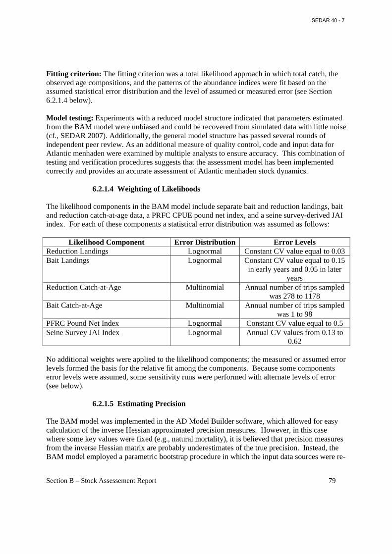
Section B – Stock Assessement Report 79
Fitting criterion: The fitting criterion was a total likelihood approach in which total catch, the observed age compositions, and the patterns of the abundance indices were fit based on the assumed statistical error distribution and the level of assumed or measured error (see Section 6.2.1.4 below). Model testing: Experiments with a reduced model structure indicated that parameters estimated from the BAM model were unbiased and could be recovered from simulated data with little noise (cf., SEDAR 2007). Additionally, the general model structure has passed several rounds of independent peer review. As an additional measure of quality control, code and input data for Atlantic menhaden were examined by multiple analysts to ensure accuracy. This combination of testing and verification procedures suggests that the assessment model has been implemented correctly and provides an accurate assessment of Atlantic menhaden stock dynamics.
6.2.1.4 Weighting of Likelihoods
The likelihood components in the BAM model include separate bait and reduction landings, bait and reduction catch-at-age data, a PRFC CPUE pound net index, and a seine survey-derived JAI index. For each of these components a statistical error distribution was assumed as follows:
Likelihood Component Error Distribution Error Levels Reduction Landings Lognormal Constant CV value equal to 0.03 Bait Landings Lognormal Constant CV value equal to 0.15
in early years and 0.05 in later years
Reduction Catch-at-Age Multinomial Annual number of trips sampled was 278 to 1178
Bait Catch-at-Age Multinomial Annual number of trips sampled was 1 to 98
PFRC Pound Net Index Lognormal Constant CV value equal to 0.5 Seine Survey JAI Index Lognormal Annual CV values from 0.13 to
0.62 No additional weights were applied to the likelihood components; the measured or assumed error levels formed the basis for the relative fit among the components. Because some components error levels were assumed, some sensitivity runs were performed with alternate levels of error (see below).
6.2.1.5 Estimating Precision
The BAM model was implemented in the AD Model Builder software, which allowed for easy calculation of the inverse Hessian approximated precision measures. However, in this case where some key values were fixed (e.g., natural mortality), it is believed that precision measures from the inverse Hessian matrix are probably underestimates of the true precision. Instead, the BAM model employed a parametric bootstrap procedure in which the input data sources were re-
SEDAR 40 - 7
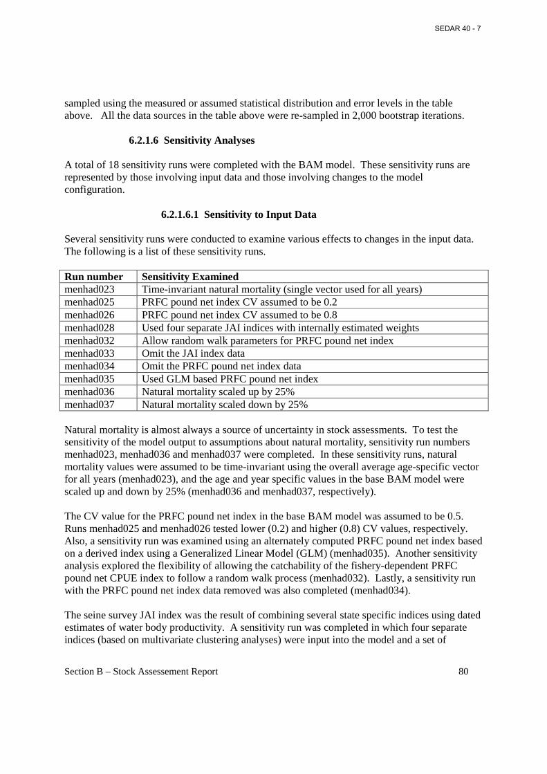
Section B – Stock Assessement Report 80
sampled using the measured or assumed statistical distribution and error levels in the table above. All the data sources in the table above were re-sampled in 2,000 bootstrap iterations.
6.2.1.6 Sensitivity Analyses A total of 18 sensitivity runs were completed with the BAM model. These sensitivity runs are represented by those involving input data and those involving changes to the model configuration.
6.2.1.6.1 Sensitivity to Input Data
Several sensitivity runs were conducted to examine various effects to changes in the input data. The following is a list of these sensitivity runs. Run number Sensitivity Examined menhad023 Time-invariant natural mortality (single vector used for all years) menhad025 PRFC pound net index CV assumed to be 0.2 menhad026 PRFC pound net index CV assumed to be 0.8 menhad028 Used four separate JAI indices with internally estimated weights menhad032 Allow random walk parameters for PRFC pound net index menhad033 Omit the JAI index data menhad034 Omit the PRFC pound net index data menhad035 Used GLM based PRFC pound net index menhad036 Natural mortality scaled up by 25% menhad037 Natural mortality scaled down by 25% Natural mortality is almost always a source of uncertainty in stock assessments. To test the sensitivity of the model output to assumptions about natural mortality, sensitivity run numbers menhad023, menhad036 and menhad037 were completed. In these sensitivity runs, natural mortality values were assumed to be time-invariant using the overall average age-specific vector for all years (menhad023), and the age and year specific values in the base BAM model were scaled up and down by 25% (menhad036 and menhad037, respectively). The CV value for the PRFC pound net index in the base BAM model was assumed to be 0.5. Runs menhad025 and menhad026 tested lower (0.2) and higher (0.8) CV values, respectively. Also, a sensitivity run was examined using an alternately computed PRFC pound net index based on a derived index using a Generalized Linear Model (GLM) (menhad035). Another sensitivity analysis explored the flexibility of allowing the catchability of the fishery-dependent PRFC pound net CPUE index to follow a random walk process (menhad032). Lastly, a sensitivity run with the PRFC pound net index data removed was also completed (menhad034). The seine survey JAI index was the result of combining several state specific indices using dated estimates of water body productivity. A sensitivity run was completed in which four separate indices (based on multivariate clustering analyses) were input into the model and a set of
SEDAR 40 - 7
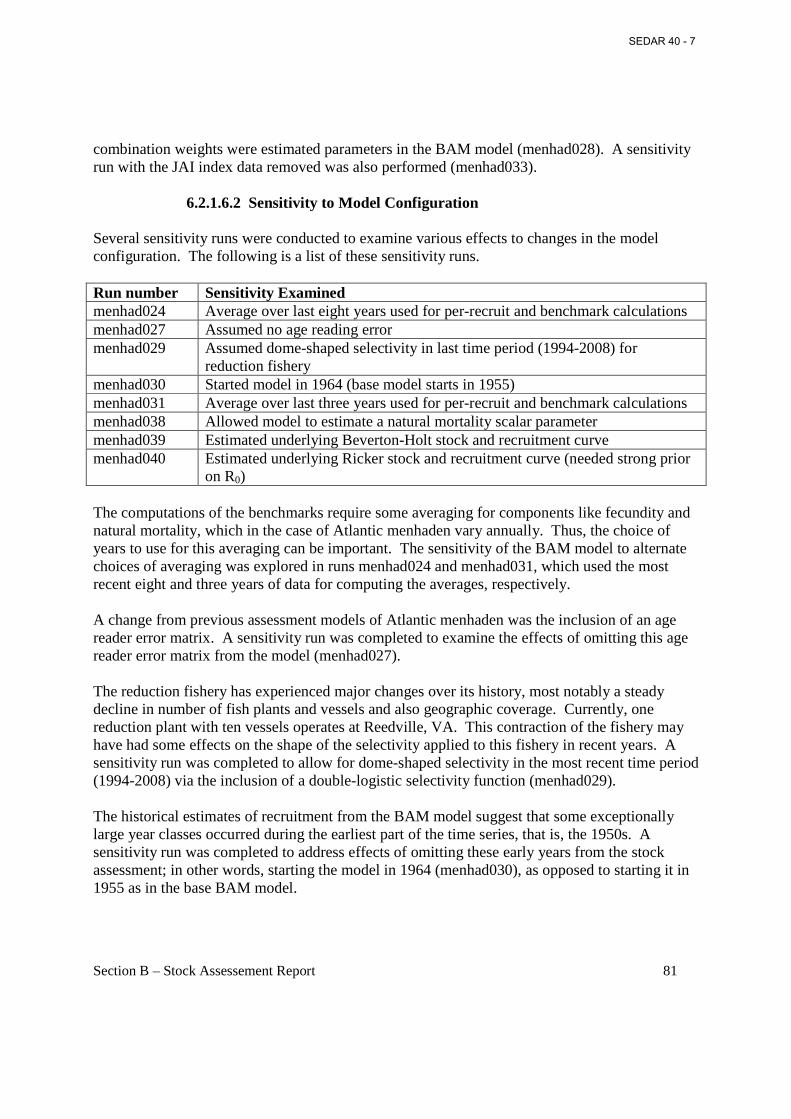
Section B – Stock Assessement Report 81
combination weights were estimated parameters in the BAM model (menhad028). A sensitivity run with the JAI index data removed was also performed (menhad033).
6.2.1.6.2 Sensitivity to Model Configuration
Several sensitivity runs were conducted to examine various effects to changes in the model configuration. The following is a list of these sensitivity runs. Run number Sensitivity Examined menhad024 Average over last eight years used for per-recruit and benchmark calculations menhad027 Assumed no age reading error menhad029 Assumed dome-shaped selectivity in last time period (1994-2008) for
reduction fishery menhad030 Started model in 1964 (base model starts in 1955) menhad031 Average over last three years used for per-recruit and benchmark calculations menhad038 Allowed model to estimate a natural mortality scalar parameter menhad039 Estimated underlying Beverton-Holt stock and recruitment curve menhad040 Estimated underlying Ricker stock and recruitment curve (needed strong prior
on R0) The computations of the benchmarks require some averaging for components like fecundity and natural mortality, which in the case of Atlantic menhaden vary annually. Thus, the choice of years to use for this averaging can be important. The sensitivity of the BAM model to alternate choices of averaging was explored in runs menhad024 and menhad031, which used the most recent eight and three years of data for computing the averages, respectively. A change from previous assessment models of Atlantic menhaden was the inclusion of an age reader error matrix. A sensitivity run was completed to examine the effects of omitting this age reader error matrix from the model (menhad027). The reduction fishery has experienced major changes over its history, most notably a steady decline in number of fish plants and vessels and also geographic coverage. Currently, one reduction plant with ten vessels operates at Reedville, VA. This contraction of the fishery may have had some effects on the shape of the selectivity applied to this fishery in recent years. A sensitivity run was completed to allow for dome-shaped selectivity in the most recent time period (1994-2008) via the inclusion of a double-logistic selectivity function (menhad029). The historical estimates of recruitment from the BAM model suggest that some exceptionally large year classes occurred during the earliest part of the time series, that is, the 1950s. A sensitivity run was completed to address effects of omitting these early years from the stock assessment; in other words, starting the model in 1964 (menhad030), as opposed to starting it in 1955 as in the base BAM model.
SEDAR 40 - 7
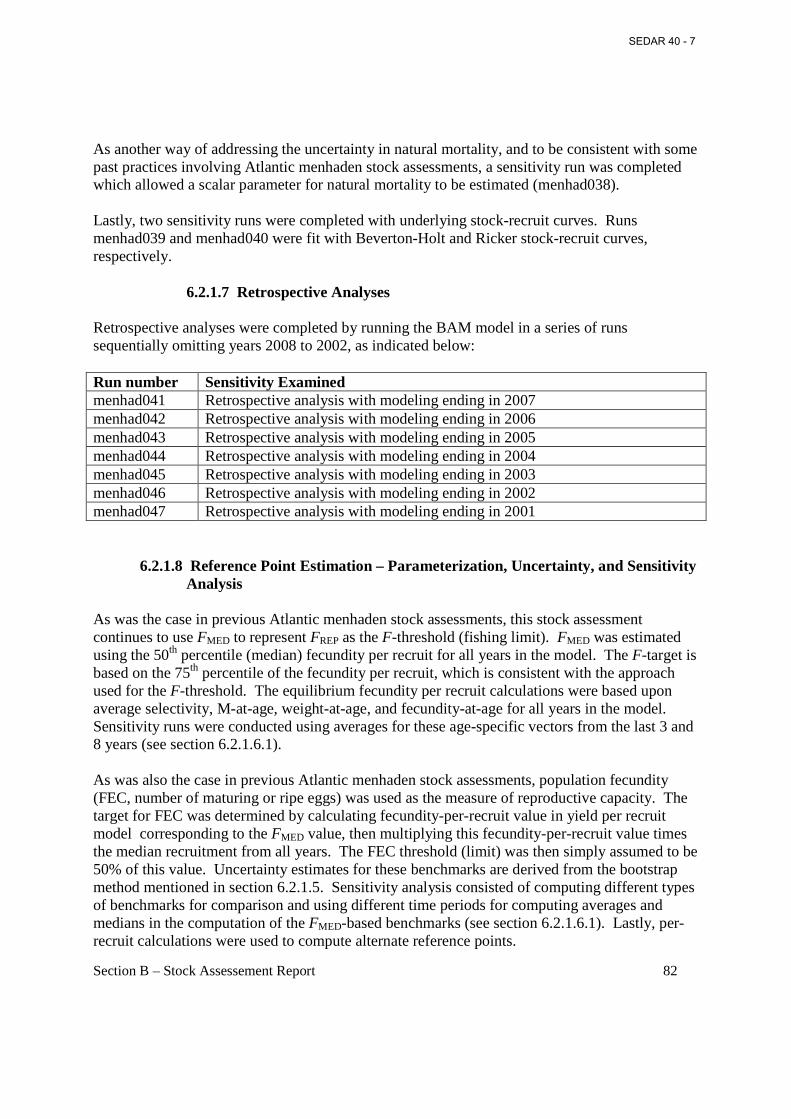
Section B – Stock Assessement Report 82
As another way of addressing the uncertainty in natural mortality, and to be consistent with some past practices involving Atlantic menhaden stock assessments, a sensitivity run was completed which allowed a scalar parameter for natural mortality to be estimated (menhad038). Lastly, two sensitivity runs were completed with underlying stock-recruit curves. Runs menhad039 and menhad040 were fit with Beverton-Holt and Ricker stock-recruit curves, respectively.
6.2.1.7 Retrospective Analyses
Retrospective analyses were completed by running the BAM model in a series of runs sequentially omitting years 2008 to 2002, as indicated below: Run number Sensitivity Examined menhad041 Retrospective analysis with modeling ending in 2007 menhad042 Retrospective analysis with modeling ending in 2006 menhad043 Retrospective analysis with modeling ending in 2005 menhad044 Retrospective analysis with modeling ending in 2004 menhad045 Retrospective analysis with modeling ending in 2003 menhad046 Retrospective analysis with modeling ending in 2002 menhad047 Retrospective analysis with modeling ending in 2001
6.2.1.8 Reference Point Estimation – Parameterization, Uncertainty, and Sensitivity
Analysis
As was the case in previous Atlantic menhaden stock assessments, this stock assessment continues to use FMED to represent FREP as the F-threshold (fishing limit). FMED was estimated using the 50th percentile (median) fecundity per recruit for all years in the model. The F-target is based on the 75th percentile of the fecundity per recruit, which is consistent with the approach used for the F-threshold. The equilibrium fecundity per recruit calculations were based upon average selectivity, M-at-age, weight-at-age, and fecundity-at-age for all years in the model. Sensitivity runs were conducted using averages for these age-specific vectors from the last 3 and 8 years (see section 6.2.1.6.1). As was also the case in previous Atlantic menhaden stock assessments, population fecundity (FEC, number of maturing or ripe eggs) was used as the measure of reproductive capacity. The target for FEC was determined by calculating fecundity-per-recruit value in yield per recruit model corresponding to the FMED value, then multiplying this fecundity-per-recruit value times the median recruitment from all years. The FEC threshold (limit) was then simply assumed to be 50% of this value. Uncertainty estimates for these benchmarks are derived from the bootstrap method mentioned in section 6.2.1.5. Sensitivity analysis consisted of computing different types of benchmarks for comparison and using different time periods for computing averages and medians in the computation of the FMED-based benchmarks (see section 6.2.1.6.1). Lastly, per-recruit calculations were used to compute alternate reference points.
SEDAR 40 - 7
Section B – Stock Assessement Report 83
7.0 Base Model Results
7.1 Results of Base BAM Model
7.1.1 Goodness of Fit
Goodness-of-fit was governed in the BAM assessment model by the likelihood components in the objective function (Table 6.2). The relative fit among the likelihood components was governed by the error levels for each data source (see section 6.2.1.4). During the assessment workshop, goodness of fit was also judged for each data source through examination of the model residuals.
Observed and model-predicted landings for the reduction fishery (1955–2008; Figure 7.1) and the bait fishery (1985–2008; Figure 7.2) were compared for the base model run. Reduction fishery landings, which are known fairly precisely, fit very well. The more poorly estimated bait landings show some deviations, but overall represent a good fit. Patterns in the annual comparisons of observed and predicted proportion catch-at-age for the reduction fishery (Figure 7.3) indicate a good overall model fit to the observed data. The bubble plot for the reduction fishery (Figure 7.4) indicates that the model fit overestimates age-1 and underestimates ages-0 and -2 in recent years. Patterns in annual comparisons of observed and predicted proportion catch-at-age for the bait fishery and associated bubble plots (Figures 7.5 and 7.6) indicate a good overall model fit to the observed data.
Observed and predicted coastwide juvenile abundance indices were compared for the base model run (1959–2008; Figure 7.7). The residual pattern suggests that the JAI index data did not fit well in years prior to 1978 as compared to the most recent years. Visual examination of the fit suggests that the overall pattern fit reasonably well, with the BAM model capturing the observed index values for the low-high-low recruitment pattern suggested for the years 1959-1973, 1974-1986, and 1987-2008, respectively. The observed and predicted PRFC pound net CPUE index (1964–2008; Figure 7.8) values do not fit as well as the JAI index values. The pattern of fit is similar in that the general high-low patterns are captured, but the relative fit within the time series is better in the early years and worse in the most recent years. The model estimates smaller numbers of fish in the last five years compared to the relative index values.
7.1.2 Parameter Estimates 7.1.2.1 Selectivities and Catchability Fishing mortality was related to an overall level of fishing and the selectivity (or availability) of menhaden to the two fisheries (reduction and bait). Model estimates of selectivity (availability)
SEDAR 40 - 7

Section B – Stock Assessement Report 84
for these fisheries were compared graphically in Figures 7.9 and 7.10. The results for both fisheries suggest very similar estimates of selectivity, with age-4 almost fully selected and age-5 and older fully selected. The big differences are in the amount of age-1 and age-2 fish that are selected. The reduction fishery selectivity estimates a higher proportion of age-1 and -2 fish compared to the bait fishery.
The base BAM model estimates a single, constant catchability parameter for each of the abundance indices, reflecting the assumption that catchability for these CPUE indices is believed to be constant through time. This is certainly a good assumption for the fishery-independent JAI abundance index since it is based on consistent, scientific survey collections, albeit the surveys are at fixed shore stations and ostensibly target other species. For the fishery-dependent PRFC pound net index, a sensitivity run was completed to examine a random walk process in catchability (see section 7.1.3).
7.1.2.2 Exploitation Rates
Total fishing mortality rates on ages-2 to -8+ (referred to as F age 2+) were calculated as the weighted average of age-specific Fs for those ages and population number-at-age (Figure 7.11). Highly variable fishing mortalities were noted throughout the entire time series, with a slight decline in fishing mortality from the mid-1960s to the early 1980s. Since the mid-1980s the fishing mortality rate has been quite variable, ranging between some of the highest and lowest values in the entire time series. In the most recent decade, the weighted average fishing mortality rate on ages 2-8+ has generally been below 1.0 (Table 7.1). The estimate of fishing mortality rate for 2008 of 1.26 is at the 43rd percentile of the historical estimates (Table 7.2).
The fishery-specific fishing mortality rates are shown in Figures 7.12 and 7.13. The estimates suggest a high degree of variability, but in general the reduction fishery has experienced declining fishing mortality rates since the mid-1960s, while the bait fishery has experienced increasing fishing mortality rates since the 1980s (Table 7.3). The annual trend in full F by age classes is analogous to the one described for the average weighted F, as one would expect when time invariant selectivity at age is used (Figure 7.14). However, F rates can vary substantially among age groups (Table 7.4). Selectivity on age-1 is small, greater on age-2, almost fully selected at age-3, and generally fully selected at older ages.
Average exploitation rate, defined as the proportion of the population removed annually by the fishery (Cij/��ij, where i=age, j=year), over the last decade was 6% for age-1, 47% for age-2, and 46% for age-3 and older. Average exploitation rate, defined as the proportion of total mortality
due to fishing (����
����
���
���� ���1 � ������� ����, where i=age, j=year) over the last decade was 8%
for age-1, 43% for age-2, 67% for age-3 and 70% for age 4 and older.
SEDAR 40 - 7
Section B – Stock Assessement Report 85
7.1.2.3 Abundance, Fecundity, and Recruitment Estimates The base BAM model estimated population numbers-at-age (ages 0-8) for 1955–2008 (Figure 7.15 and Table 7.5). From these estimates, along with growth and reproductive data (Section 2), different estimates of reproductive capacity were computed. Addendum 1 (ASMFC 2004b) adopted population fecundity as the preferred measure of reproductive output. Population fecundity (FEC, number of maturing ova) was high in the late 1950s and early 1960s, low in the late 1960s, and generally increasing since then (Figure 7.16 and Table 7.6). The largest values of population fecundity were present in 1955 and 1961, resulting from two very strong recruitment events in 1951 and 1958 as noted in earlier stock assessments (Ahrenholz et al. 1987b; Vaughan and Smith 1988; Vaughan et al. 2002b; ASMFC 2004a). The time period 1955-2008 produced a median population fecundity of 20.2 x 10¹² ova with an interquartile range between 15.1 x 10¹² and 29.4 x 10¹² (Table 7.2). The estimate for population fecundity in 2008 was 18.4 x 10¹², which was between the 25th and 50th percentile. Throughout the time series, the age-3 fish produced most of the total estimated number of eggs spawned annually (Figure 7.17).
Age-0 recruits of Atlantic menhaden (Figure 7.18 and Table 7.7) were high during the late 1950s, especially the 1958 year-class. Median and interquartile values for age-0 recruits are summarized in Table 7.2. The annual estimated recruitment values relative to the median are shown in Figure 7.19. Recruitment was generally poor during the 1960s, with values below the 25th percentile (13.2 billion) for the recruitment time series. High recruitment occurred during the late 1970s and early 1980s to levels above the 75th percentile (23.5 billion). These values are comparable to the late 1950s (with the exception of the extraordinary 1958 year-class). Generally low recruitment has occurred since the early 1990s. There is a hint of a potential long-term cycle from this historical pattern of recruitment, but not enough data are present to draw any conclusions regarding the underlying cause at this point (Figure 7.18 and 7.19). The most recent estimate for 2008 is quite low and likely to be modified in the future as more data from the cohort (age-1 in 2009, age-2 in 2010, etc.) are added to the analysis. The current estimate of recruits to age-0 in 2008 (4.4 billion) is below the 25th percentile (13.2 billion).
A plot of the fecundity (mature ova) to the recruits at age-0 indicated a weak relationship, suggesting Atlantic menhaden recruitment was only marginally governed by population fecundity (Figure 7.20). Additional discussion on dynamics of recruit per egg is presented in section 8.2.3. Figure 7.20 also shows the median recruitment and fecundity-per-recruit estimates which were used to determine the benchmarks for Atlantic menhaden (see Section 6.2.1.8 for more details).
7.1.3 Sensitivity Analyses The results of the 18 sensitivity runs suggest that the base BAM model is fairly robust to many of the induced changes (Figures 7.21-7.23). The largest changes in population estimates relative to base model estimates resulted from sensitivity runs which affected natural mortality. This
SEDAR 40 - 7
Section B – Stock Assessement Report 86
included four of the sensitivity runs which used a constant natural mortality vector over time (menhad023), allowed for an estimated scalar on natural mortality (menhad038), increased natural mortality by 25% (menhad036), and decreased natural mortality by 25% (menhad037). These changes were greatest for the fishing mortality and recruitment estimates (Figure 7.21 and 7.22). The fecundity estimates were very robust to these sensitivity runs (Figure 7.23). The resulting recruitment, N-weighted fishing mortality rates (F age 2+), fecundity, benchmarks, and stock status indicators appear to be largely robust to the explored sensitivity runs with the exception of natural mortality effects (Table 7.8).
7.1.4 Retrospective Analyses
Patterns and biases in the results of a retrospective analysis over time are unclear (Figures 7.24-7.26). Regardless, the results indicate that the terminal N-weighted fishing mortality rate (F2+) is highly variable (Figure 7.24). The resulting recruitment, fecundity, benchmarks, and stock status indicators do not show consistent biases or patterns (Figures 7.25 and 7.26; Table 7.8). However, the magnitude of stock status outcomes varies considerably in this set of retrospective model runs. In particular, the ratio of N-weighted fishing mortality (F2+/FMED) in terminal year to FMED ranges from 0.33 to 1.30 within this range of retrospective runs and shows some large year-to-year variations (Table 7.8).
7.1.5 Uncertainty Analysis
The parametric bootstrap procedure was run for 2,000 iterations; 1,995 converged. The resulting estimates from these runs have been summarized in Figures 7.11, 7.16 & 7.18 and Tables 7.3, 7.6-7.7, showing the 90% confidence region. In general the bootstrap results suggest fairly symmetrical error distributions about the base run results.
7.1.6 Reference Point Results – Parameter Estimates and Sensitivity Fecundity-per-recruit and yield-per-recruit (mt) estimates as a function of total N-weighted fishing mortality rates (F2+) are shown in Figures 7.27 and 7.28. These plots are offered as a reference for other fishing mortality rates. For example, the terminal year fishing mortality rate estimate (F2008) of 1.26 is equivalent to an F8% spawning potential, and the FMED estimate of 1.25 from the base BAM model is equivalent to an F8% mortality rate (Figure 7.27). The base BAM model estimates for the benchmarks and terminal year values are indicated in Table 7.9. This table also indicates the values for some per-recruit-based benchmarks of F30%, F25%, and F20%. The base BAM model estimated the stock status based on the FMED estimators. The results suggest that the current stock status is not overfished (FEC2008/FECthreshold > 1.0) but overfishing is occurring (F2008/FMED is 1.0). The fishing mortality rate is at the FMED threshold (limit) (Table 7.8).
SEDAR 40 - 7
Section B – Stock Assessement Report 87
The entire time series of relative estimates of N-weighted fishing mortality (F2+) and fecundity are shown in Figures 7.29 and 7.30 and a phase plot of the last ten years of estimates is shown in Figure 7.31. The history of fishing mortality rates in Figures 7.29 and 7.31 suggests that overfishing may have occurred 32 out of 54 years in the past. However, this plot can be deceptive and not entirely accurate since FMED benchmark estimates may change every year. A more accurate method to examine this scenario would be with a retrospective analysis which re-estimates the benchmark annually (Table 7.8). This retrospective analysis suggested a high degree of variability in terminal fishing mortality rates, with very small differences in estimated FMED. The uncertainty in the terminal year stock status indicators is expressed using the results of the 1,995 bootstrap runs of the base BAM model. The results indicate that the fecundity estimates for the terminal year are well above the threshold (limit), with not a single bootstrap estimate falling below 1.0 (Figures 7.32-7.34). The results for the terminal year fishing mortality rate suggest that the base run estimate is slightly above the FMED threshold (limit) with 53.3% of the bootstrap runs exceeding the FMED threshold (Figures 7.32-7.34).
8.0 Stock Status
Limit reference points (limits) are the basis for determining stock status (i.e., whether overfishing is occurring or a stock is overfished). When the fishing mortality rate (F) exceeds the F-limit, then overfishing is occurring; the rate of removal of fish by the fishery exceeds the ability of the stock to replenish itself. When the reproductive output (measured as spawning stock biomass or population fecundity) falls below the biomass-limit, then the stock is overfished, meaning there is insufficient mature female biomass (SSB) or egg production (population fecundity) to replenish the stock. The Magnuson-Stevens Reauthorization of 1997 (Restrepo et al. 1998) suggests that the target for spawning biomass (or population fecundity) be near BMSY (or its proxy). The target level chosen for fishing mortality is less clear, other than the stipulation that Ftarget be sufficiently below the Flimit.
8.1 Current Overfishing, Overfished/Depleted Definitions
8.1.1 Amendment 1 Benchmarks
Ideally, F-based and SSB-based reference points should be based on an underlying population dynamics model (e.g., FMSY and BMSY from Ricker or Beverton-Holt spawner-recruit models). However, traditional methods of specifying these reference points perform poorly when applied to historical Atlantic menhaden data. There is considerable scatter in the spawner-recruit relationship and this stock’s recruitment is suspected of being largely driven by environmental forces. Hence, the reference points in Amendment 1, adopted in 2001 (ASMFC 2001), were
SEDAR 40 - 7
Section B – Stock Assessement Report 88
developed from the historic spawning stock per recruit (SSB/R) relationship. As such, FMED was selected as Flimit (representing replacement level of stock, also known as FREP) and was calculated by inverting the median value of R/SSB and comparing to the SSB/R curve following the method of Sissenwine and Shepherd (1987). The spawning stock biomass corresponding to Flimit, was calculated as a product of median recruitment and SSB/R at FMED, from equilibrium YPR analysis, which became the SSBtarget. The limit for SSB (SSBlimit or MSST) was calculated to account for natural mortality [(1-M)*SSB-target, where M=0.45]. In Amendment 1, the Ftarget was based on FMAX (maximum fishing mortality before the process of recruitment overfishing begins). The values calculated for these reference points were 1.04 and 1.33 for the Ftarget and Flimit, respectively, while 37,400 mt and 20,570 mt were the SSBtarget and SSBlimit, respectively (Table 13 in ASMFC 2001).
8.1.2 Addendum 1 Benchmarks Based on the 2003 benchmark stock assessment for Atlantic menhaden, the benchmarks were modified by the ASMFC in Addendum 1 as recommended by the Technical Committee (ASMFC 2004a, 2004b). The TC recommended using population fecundity (number of maturing or ripe eggs) (FEC) as a more direct measure of reproductive output of the population compared to spawning stock biomass (the weight of mature females; SSB). For Atlantic menhaden, older menhaden release more eggs than younger menhaden per unit of female biomass. By using the number of eggs released, more reproductive importance is given to older fish in the population than accounted for simply by female biomass. They also recommended modifications to the fishing mortality (F) target and limit. The TC recommended continued use of FMED to represent FREP as the Flimit, but estimated it using fecundity per recruit rather the SSB per recruit. Because the analysis calculated an FMAX (target) that was greater than FMED (and may be infinite), they recommended instead that Ftarget be based on the 75th
percentile. This approach was consistent with the approach used for the Flimit. For biomass (or egg) benchmarks, the TC recommended following the approach of Amendment 1. Benchmark and terminal year values for the F-based and EGG-based reference points are summarized in Table 8.1 for the 2003 peer reviewed assessment (ASMFC 2004a, Table 9.1) and for the 2006 update assessment (ASMFC 2006, Table 7.1). Terminal years for these two assessments were 2002 and 2005, respectively. Because growth and fecundity at age vary annually, benchmarks may also vary annually. The changes in the biological reference points, while seemingly large for F, are a re-estimation of benchmarks based on updated population parameters, but using the same process defined in the 2003 peer-reviewed assessment (ASMFC 2004a). These changes primarily reflect annual growth patterns for the terminal year, and are neither more nor less conservative than the previous estimates.
SEDAR 40 - 7
Section B – Stock Assessement Report 89
8.2 Discussion of Alternate Reference Points
8.2.1 FMSY Concept On the federal level, preference has been given to managing US fisheries using MSY- (or Maximum Sustainable Yield) derived reference points such as Bmsy, Fmsy, etc, even though direct estimation of Bmsy and Fmsy is often not possible or reliable. Such reference points can be incorporated into control rules, which may then call for reductions in fishing effort or landings when a stock falls below an optimal population size (such as SSBmsy) or fishing mortality goes above what is sustainable in the long-term (such as Fmsy). For many species setting harvest at some precautionary fraction of MSY allows managers to set long term sustainable harvest based on a long-term sustainable population size. Implicit in that assumption of a long-term harvest being sustainable for a long-term population size (and vice versa), is that the stock recruitment relationship is well known and unchanging. For many species which exhibit a high degree of recruitment variability, setting reference points based around MSY may lead to rapid fluctuations in stock status. The greatest concern would be sharp population declines under MSY-level removals during periods of low recruitment, although the opposite is also possible. Such difficulties are more apparent when the species examined is short lived, as recruitment is a result of only a few age classes. In those cases, lower recruitment results in lower SSB within a few short years, further lowering the possibility for future recruitment. Management may not have time to react to such changes before complete stock collapse. Moreover, MSY-based reference points require equilibrium conditions, an assumption which is difficult to make for a forage species. As a result, many have called for the complete removal of MSY-based reference points all together (Larkin 1977; Gulland 1978, and Barber 1988). In the case of menhaden the stock-recruitment relationship is poorly known. Menhaden are also relatively short lived, with a preponderance of the SSB residing in the younger age classes, and having a high but variable degree of natural mortality (predation) before recruitment to the SSB. As such, basing reference points on actual stock performance and long term medians is more appropriate than basing them on a variable and poorly understood stock recruitment relationship.
8.2.2. Equilibrium Yield per Recruit (YPR) and Spawner per Recruit- (SPR) Based Reference Points
There is a long history of YPR-based reference points used in fisheries management. Fmax and F0.1 were widely used either as target or threshold levels of fishing mortality. These were often seen as proxy estimates to the Fmsy. In the case of menhaden, the Fmax =1.04 was used in Amendment 1 as a target fishing mortality (Section 8.1.1). However, recent updates in menhaden life history parameters resulted in a YPR curve with undefined maximum (asymptotic curve), primarily due to the new vector of natural mortality at age. The F0.1 value can still be estimated and is equal to 1.37 (F for ages 2 and older weighted by numbers) or 0.93 (full F). The F0.1 was
SEDAR 40 - 7
Section B – Stock Assessement Report 90
generally seen as a precautionary or conservative value for a target (compared to FMAX) . However, F0.1 does not reflect any compensatory effects of the underlying spawner–recruitment relationship or environmentally driven systematic changes in recruitment level. The concept of FMED was investigated by Mace and Sissenwine (1993) and compared to the percent of the maximum spawning potential (referred to as either %MSP and %SPR) that corresponds to FMED, thus maintaining population replacement. Mace and Sissenewine (1993) reported that most of the stocks require at least 20-30% of maximum spawning potential to be maintained for population replacement. Among 83 populations analyzed, they estimated replacement %MSP for 19 stocks of clupeids, 9 of them being Atlantic herring (slower growing and larger maximum age). The percent corresponding to replacement ranged between 7% and 65%, with a median value of 37%. This variability in percent replacement may result from differences in the range of observed SSB values (if the stock is heavily exploited through the entire time series, the range of SSB is not as a large as that of a lightly exploited stock which is likely to affect the FMED estimates). The %MSP appropriate for menhaden can only be selected arbitrarily based on the presumed population resilience. The current estimate of FMED is equivalent to F13% from the YPR/SPR equilibrium model.
8.2.3. Environmental Variability The historical pattern estimated by the BAM model suggests that Atlantic menhaden recruitment has varied from 4.0 to 75.0 billion fish annually, showing periods of high recruitment in the 1970s and 1980s, and periods of low recruitment in the 1960s, 1990s, and 2000s. The estimated population fecundity pattern shows very high levels in the 1950s, followed by some of the lowest values in the time series during the late 1960s. Since the 1970s, fecundity has varied between 7,000 and 45,000 billion mature ova. When age-0 recruitment is plotted with a one year lag against population fecundity estimates, no relationship appears (Figure 8.3). The cyclical pattern in recruitment seemingly has less to do with fecundity than it does outside forces (e.g. physical forcing, predation). The stock-recruit plot indicates that the fecundity levels which produced the highest recruitment values (above the 75th percentile) ranges from 11,000 to 101,000 billion mature ova, while most of the highest fecundity levels (40,000+ billion mature ova) produced recruitment values (9.3 billion) below the historical median (13.4 billion). It is often the case in other fisheries that the stock-recruit relationship is poor. However, in this case there is a complete absence of any high recruitment at the highest fecundity estimates, albeit there were few years in the time series with high fecundity estimates. The highest variability in recruitment occurs right around the median historical fecundity. Past performance of Atlantic menhaden suggests it has gone from periods of low recruitment and fecundity to periods with high recruitment and fecundity, while sustaining moderate to high landings. In recent years the fishery has experienced some of the lowest landings on record, yet recruitment remains near the 25th percentile. This outcome may be indicative of a stock with an undefined production function (e.g. stock-recruitment curve), whose population fluctuations are almost entirely driven by non-fishery sources.
SEDAR 40 - 7
Section B – Stock Assessement Report 91
Menhaden spawning occurs for a very protracted period of time along the entire US Atlantic coast while fish schools undergo significant migratory movements. Simple estimation of total number of eggs potentially produced by the population does not account for specifics of stock structure (spatial and temporal distribution) of spawners along the coast, probability of “right“ conditions for successful egg and larval survival and other potentially important factors. Identification of factors defining menhaden recruitment in the future may substantially improve our understanding of menhaden recruitment processes and offer possible modifications to our modeling that will account for more complex processes.
8.3 Stock Status Determination
8.3.1 Overfishing Status F (N-weighted F for age 2+)/Fmed for the terminal year (2008) was equal to 1 (Figure 7.29), therefore, overfishing is occurring. It should be noted that the terminal year value is at the limit (ratio of 1.00). Second, F has been below the limit in recent years. This is the first year since 1998 thatoverfishing is occuring. Third, as noted in a later section on uncertainty, about 53% of the bootstrapped values of F fall into the overfishing region. Fourth, numbers-weighted F is highly influenced by abundance of age 2 fish which are not fully recruited. A range of status determinations are shown based on the sensitivity runs (Table 7.8), some suggesting overfishing, although others do not. A corresponding figure for F based on Full F is presented with full F benchmarks for comparison in Figure 8.4.
8.3.2 Overfished Status FEC/FEClimit for the terminal year was greater than 1 (Figure 8.5). Hence, based on this criterion, the stock is not overfished. Furthermore, the terminal year value is equal to the target (ratio of 2.0). Unlike estimates of F, there is a relatively small amount of variation in FEC between years. Also, the bootstrapped values of FEC fall completely in the region that is considered not to be overfished, although values do fluctuate around the target. None of the sensitivity runs suggest the stock is overfished (Table 7.8).
8.3.3 Control Rules The phase plot shows the recent history of status variables relative to their benchmarks (Figure 7.31). Only the terminal year estimate of F suggests overfishing. But the stock was not overfished during this period since 1999. A phase plot for the terminal year based on 2000 bootstrapped experiments demonstrates the uncertainty relative to these control rules in the terminal year (Figure 7.34). With respect to the target F and fecundity, the stock has never been at or below target F, but has fluctuated around the fecundity target.
SEDAR 40 - 7

Section B – Stock Assessement Report 92
8.3.4 Uncertainty Uncertainty of the status of stock relative to the two benchmarks was investigated using several approaches. First sensitivity runs were made to explore the effect on benchmarks from changes in assumptions from the base run (Table 7.8). Next sensitivity of the estimates was investigated based on a bootstrapped analysis within the BAM model. Alternatively, we had hoped to use the stochastic SRA model, based on a very different approach, to interpret the status of Atlantic menhaden. However, the sensitivity of this model to certain assumptions precluded that approach.
9.0 Research Recommendations Research recommendations are broken down into two categories: data and modeling. While all recommendations are high priority, the first recommendation is the highest priority. Each category is further broken down into recommendations that can be completed in the short term and recommendations that will require long term commitment.
SEDAR 40 - 7

Section B – Stock Assessement Report 93
Annual Data Collection Long term:
1. [Highest Priority] Develop a coastwide fishery independent index of adult abundance at age to replace or augment the existing Potomac River pound net index in the model.
2. Work with industry to collect age structure data outside the range of the fishery. Short term:
1. Continue current level of sampling from bait fisheries, particularly in the mid-Atlantic and New England, and continue recovery of historical tagging data from paper data sheets.
2. Request annual samples of menhaden from the PRFC pound net fishery to better characterize age and size structure of catch.
Assessment Methodology Long term:
1. Develop multispecies statistical catch-at-age model to estimate menhaden natural mortality at age.
2. Develop spatially-explicit model, once sufficient age-specific data on movement rates of menhaden is available.
Short term:
1. Re-evaluate menhaden natural mortality-at-age and population response to changing predator populations by updating and augmenting the MSVPA (e.g. add additional predator, prey, and diet data when available).
2. Incorporate maturity at age variability in the assessment model. Future Research
1. Evaluate productivity of different estuaries (e.g., replicate similar methodology to Ahrenholz et al. 1987).
2. Collect age-specific data on movement rates of menhaden to develop regional abundance trends.
3. Determine selectivity of PRFC pound nets. 4. Update information on maturity, fecundity, spatial and temporal patterns of spawning,
and larval survivorship. 5. Investigate the effects of global climate change on distribution, movement, and behavior
of menhaden.
SEDAR 40 - 7
Section B – Stock Assessement Report 94
10.0 Literature Cited Ahrenholz, D.W. 1991. Population biology and life history of the North American menhadens,
Brevoortia spp. Mar. Fish. Rev. 53(4): 3-19. _____, J.F. Guthrie, and R.M. Clayton. 1987a. Observations of ulcerative mycosis infections on
Atlantic menhaden (Brevoortia tyrannus). NOAA Tech. Memo. NMFS-SEFC-196. _____, W.R. Nelson, and S.P. Epperly. 1987b. Population characteristics of Atlantic menhaden,
Brevoortia tyrannus. Fishery Bulletin 85:569-600. _____, D.D. Squires, J.A. Rice, S. W. Nixon, and G.R. Fitzhugh. 2000. Periodicity
of increment formation in otoliths of overwintering postlarval and prejuvenile Atlantic menhaden, Brevoortia tyrannus. Fish. Bull. 98: 421-426.
Alverson, D.L., and M.J. Carney. 1975. A graphic review of the growth and decay of population
cohorts. J. Cons. Int. Explor. Mer 36:133-143. Anderson, J.D. 2007. Systematics of the North American menhadens: molecular evolutionary
reconstructions in the genus Brevoortia (Clupeiformes: Clupeidae). Fish. Bull. 205:368-378.
Atlantic Coastal Cooperative Statistics Program (ACCSP). 2009. (1950-2007) Annual landings
by state and custom gear category; generated by Julie Defilippi; using ACCSP Data Warehouse, Washington, D.C: accessed May 12-14, 2009.
Atlantic States Marine Fisheries Commission (ASMFC). 1981. Fishery Management Plan for
Atlantic Menhaden. Atlantic States Marine Fisheries Commission, Fishery Management Report No. 81-02, 134 p.
_____. 1992. Fishery Management Plan for Atlantic Menhaden, 1992 Revision. Atlantic States
Marine Fisheries Commission, Fishery Management Report No. 22, 159 p. _____. 1999a. Terms of Reference & Advisory Report for the Atlantic Menhaden Stock
Assessment Peer Review. Atlantic States Marine Fisheries Commission, Stock Assessment Report No. 99-01, 16 p.
_____. 1999b. Atlantic Menhaden Stock Assessment Report for Peer Review. Atlantic States
Marine Fisheries Commission, Stock Assessment Report No. 99-01 (supplement), 146 p. _____. 2001. Amendment 1 to the Interstate Fishery Management Plan for Atlantic Menhaden.
Atlantic States Marine Fisheries Commission, Fishery Management Report No. 37, 127 p. _____. 2004a. Atlantic Menhaden Stock Assessment Report for Peer Review. Atlantic States
Marine Fisheries Commission, Stock Assessment Report No. 04-01 (supplement), 145 p.
SEDAR 40 - 7
Section B – Stock Assessement Report 95
_____. 2004b. Terms of Reference & Advisory Report for the Atlantic Menhaden Stock Assessment Peer Review. Atlantic States Marine Fisheries Commission, Stock Assessment Report No. 04-01, 16 p.
_____. 2006. 2006 Stock Assessment Report for Atlantic Menhaden. Atlantic States Marine
Fisheries Commission, 139 p. [Update assessment prepared for ASMFC Atlantic Menhaden Board dated Sept. 26, 2006]
_____. 2009. Update of the Multispecies Virtual Population Analysis. 54 pages. _____. 2009a. 2009 Stock assessment report for striped bass. 15 pages. _____. 2009b. 2009 Bluefish stock assessment update report. 42 pages. Austin, H. 2002. Decadal oscillations and regime shifts, a characterization of the Chesapeake
Bay Marine Climate. In Fisheries in a Changing Climate. Amer. Fish. Soc. Symp. 32:155-170.
Barber, W.E. 1988. Maximum sustainable yield lives on N. Amer. J. Fish. Manage. 8: 153-157. Berrien, P. and J. Sibunka. 1999. Distribution patterns of fish eggs in the United States
Northeast Continental Shelf ecosystem. U.S. Dep. Commer., NOAA Tech. Rep. NMFS 145, 310 p.
Boudreau, P.R., and L.M. Dickie. 1989. Biological model of fisheries production based on
physiological and ecological scalings of body size. Can. J. Fish. Aquat. Sci. 46:614-623. Bourne, D. W. and J. J. Govoni. 1988. Distribution of fish eggs and larvae and patterns of water
circulation in Naragansett Bay, 1972-1973. Am. Fish. Soc. Symp. 3:132-148. Cadrin, S.X., and D.S. Vaughan. 1997. Retrospective analysis of virtual population estimates for
Atlantic menhaden stock assessment. Fish. Bull. 95:445-455. Checkley, D.M., Jr., P.B. Ortner, F.E. Werner, L.R. Settle, and S.R. Cummings. 1999.
Spawning habitat of the Atlantic menhaden in Onslow Bay, North Carolina. Fish. Oceanogr. 8 (Suppl. 2): 22-36.
_____, S. Raman, G.L. Maillet, and K.M. Mason. 1988. Winter storm effects on the spawning
and larval drift of a pelagic fish. Nature 335(6188): 346–348. Chester, A.J. 1984. Sampling statistics in the Atlantic menhaden fishery. NOAA Tech. Rep.
NMFS 9, 16 p. Clark, C.W., and M. Mangel. 1979. Aggregation and fishery dynamics: A theoretical study of
schooling and the purse seine tuna fishery. Fish. Bull., U.S. 77:317-337.
SEDAR 40 - 7
Section B – Stock Assessement Report 96
Condrey, R.E. 1984. Density-dependent searching time: Implications in surplus-production models. Fish. Bull 82:449-453.
Cooper, R.A. 1965. An unusually large menhaden Brevoortia tyrannus (Latrobe), from Rhode
Island. Trans. Am. Fish. Soc. 94: 412. Cross, F.A., D.S. Peters, and W.E. Schaaf. 1985. Implications of waste disposal in coastal waters
on fish populations, p. 383-399 In: Cardwell, R.D., R. Purdy, and R.C. Bhaner (eds). 35 “Aquatic Toxicology and Hazard Assessment: Seventh Symposium”. ASTM STP854. American Society for Testing and Materials, Philadelphia. pp. 383–399.
Deriso, R.B., T.J. Quinn II, and P.R. Neal. 1985 Catch-age analysis with auxiliary information.
Can. J. Fish. Aquat. Sci. 42:815-824. Dietrich Jr., C.S. 1979. Fecundity of the Atlantic menhaden, Brevoortia tyrannus. Fish. Bull. 77:
308–311. Dryfoos, R.L., R.P. Cheek, and R.L. Kroger. 1973. Preliminary analyses of Atlantic menhaden,
Brevoortia tyrannus, migrations, population structure, survival and exploitation rates, and availability as indicated from tag returns. Fish.Bull. 71(3):719-734.
Dovel, W.L. 1971. Fish eggs and larvae of the upper Chesapeake Bay. Nat. Res. Inst., Univ.
Md. Spec. Rep. 4, 71 p. Forward, R.B., Jr. M.C. De Vries, R.A. Tankersley, D. Rittschof, W.F. Hettler, J.S. Burke, J.M.
Welch, and D.E. Hoss. 1999. Behaviour and sensory physiology of Atlantic menhaden larvae, Brevoortia tyrannus, during horizontal transport. Fish. Oceanogr. 8 (Suppl. 2): 37-56.
Fournier, D., and C.P. Archibald. 1982. A general theory for analyzing catch at age data. Can. J.
Fish. Aquat. Sci. 39: 1195–1207. Garrison, L.P., J.S. Link, D.P. Kilduff, M.D. Cieri, B. Muffley, D.S. Vaughan, A. Sharov, B.
Mahmoudi, and R.J. Latour. In press. An Expansion of the MSVPA Approach for Quantifying Predator-Prey Interactions in Exploited Fish Communities. ICES J. Mar. Sci.
Gislason, H. and Th. Helgason. 1985. Species interactions in assessment of fish stocks with
special application to the North Sea. Dana 5: 1-44. Govoni, J.J. 1993. Flux of larval fishes across frontal boundaries: examples from the
Mississippi River plume front and the western Gulf Stream front in winter. Bull. Mar. Sci. 53:538-566.
_____. 1997. The association of the population recruitment of gulf menhaden, Brevoortia patronus, with Mississippi River discharge.
SEDAR 40 - 7
Section B – Stock Assessement Report 97
Guillory, V. 1993. Predictive models for Louisiana gulf menhaden harvests: an update. Louisiana Dept. of Wildlife and Fisheries, Tech. Bull. No. 43, 45 p.
_____, J. Geaghan, and J. Russel. 1983. Influence of environmental factors of gulf menhaden
recruitment. Louisiana Dept. of Wildlife and Fisheries, Tech. Bull. No. 37, 32 p. Gulland, J.A. 1978. Fisheries management: New strategies for new conditions Trans. Amer. Fish
Soc. 107:1-11 _____. 1983. Fish stock assessment: a manual of basic methods. John Wiley & Sons, New York. Heimbuch, D.G., E. Lorda, D. Vaughan, L.W. Barnthouse, J. Uphoff, W. Van Winkle, A.
Kahnle, B. Young, J. Young, and L. Kline. 2007. Assessing coastwide effects of power plant entrainment and impingement on fish populations: Atlantic menhaden example. No. Amer. J. Fish. Manage. 27:569-577.
Helgason, Th. and H. Gislason. 1979. VPA-analysis with species interaction due to predation.
ICES C.M. 1979/G:52, 10 pp. Henry, K.A. 1971. Atlantic Menhaden (Brevoortia tyrannus) Resource and Fishery –Analysis of
Decline. NOAA Tech. Rep. NMFS SSRF-642, 32 p. Hettler, W.F. 1976. Influence of temperature and salinity on routine metabolic rate and growth of
young Atlantic menhaden. J. Fish Biol. 8: 55–65. _____ and D. L. Barker. 1993. Distribution and abundance of larval fishes at two North
Carolina inlets. Estuarine, Coastal, and Shelf Science 37:161-179. _____ and J.A. Hare. 1998. Abundance and size of larval fishes outside the entrance to
Beaufort Inlet, North Carolina. Estuaries 21:476-499. Hewitt, D.A., and J.M. Hoenig. 2005. Comparison of two approaches for estimating natural
mortality based on longevity. Fish. Bull. 103:433-437. Higham, J.R., and W.R. Nicholson. 1964. Sexual maturation and spawning of Atlantic
menhaden. Fish. Bull. 63: 255–271. Hoenig, J.M. 1983. Empirical use of longevity data to estimate mortality rates. Fish. Bull.
82:898-903. Houde , E.D., and L.W. Harding, Jr. 2009. Menhaden abundance and productivity in
Chesapeake Bay: linking the environment and primary production to variability in fish recruitment. Final Report to NOAA Chesapeake Bay Office, Project Number NA04NMF4570301. (UMCES Tech. Series TS-575-09)
SEDAR 40 - 7
Section B – Stock Assessement Report 98
Jensen, A.L. 1996. Beverton and Holt life history invariants result from optimal trade-off of reproduction and survival. Can. J. Fish. Aquat. Sci. 53:820-822.
Judy, M.H., and R.M. Lewis. 1983. Distribution of eggs and larvae of Atlantic menhaden,
Brevoortia tyrannus, along the Atlantic coast of the United States. U.S. NMFS. Special Scientific Report - Fisheries No. 774, 23 p.
June, F.C. 1965. Comparision of vertebral counts of Atlantic menhaden. U.S. Fish Wildl. Serv.
Spec. Sci. Rep. Fish. 513: 12. _____ and J.L. Chamberlin. 1959. The role of the estuary in the life history and biology of
Atlantic menhaden. Proc. Gulf and Carib. Fish. Inst. 11: 41–45. _____ and J.W. Reintjes. 1959. Age and size composition of the menhaden catch along the
Atlantic coast of the United States, 1952-1955; with a brief review of the commercial fishery. U.S. Fish Wildlife Serv., Spec. Sci. Rep., Fisheries No. 317, 65 p.
_____ and C.M. Roithmayr. 1960. Determining age of Atlantic menhaden from their scales.
Fish. Bull., U.S. 60:323-342. Kendall, A.W. and J. W. Reintjes. 1975. Geographic and hydrographic distribution of Atlantic
menhaden eggs and larvae along the middle Atlantic coast from RV Dolphin cruises, 1965-66. Fish. Bull. 73:317-335.
Kimmel, D.G., W.D. Miller, L.W. Harding Jr., E.D. Houde, and M.R. Roman. 2009. Estuarine
eco-system response captured using a synoptic climatology. Estuaries and Coasts 32:403-409.
Kroger, R.L., and J.F. Guthrie. 1973. Migrations of tagged juvenile Atlantic menhaden. Trans.
Amer. Fish. Soc. 2: 417-422. _____, J.F. Guthrie, and M.H. Judy. 1974. Growth and first annulus formation of tagged and
untagged Atlantic menhaden. Trans. Amer. Fish. Soc. 103(2): 292-296. Larkin, P.A. 1977. An epitaph for the concept of maximum sustainable yield. Trans. Amer. Fish
Soc. 106:1-11 Lewis, R.M. 1966. Effects of salinity and temperature on survival and development of larval
Atlantic menhaden, Brevoortia tyrannus. Trans. Am. Fish. Soc. 95: 423–426. Lewis, V.P., and D.S. Peters. 1984. Menhaden - a single step from vascular plant to fishery
harvest. J. Exp. Mar. Biol. Ecol. 84(1): 95–100. Lorenzen, K. 1996. The relationship between body weight and natural mortality in juvenile and
adult fish: A comparison of natural ecosystems and aquaculture. J. Fish. Biol. 49:627-647.
SEDAR 40 - 7

Section B – Stock Assessement Report 99
Love, J.W., A.K. Johnson, and E.B. May. 2006. Spatial and temporal differences of Atlantic menhaden (Brevoortia tyrannus) recruitment across major drainages (1966-2004) of the Chesapeake Bay watershed. Estuaries and Coasts 29:794-801
Lynch, A.J. 2008. A molecular analysis of Atlantic menhaden (Brevoortia tyrannus) stock
structure. Coll. of William and Mary, Masters Sci. thesis, 240 p. Mace P.M. and Sissenwine,M.P. 1993. How much spawning per recruit is enough? In Risk
Evaluation and Biological Reference Points for Fisheries Management, Can. Spec Pub. Of Fisheries and Aquatic Sciences 120. 101-118.
Magnusson, K.G. 1995. An overview of the multispecies VPA – theory and applications. Rev.
Fish. Biol. and Fisheries 5: 195-212. Martell, S., Pine III, W., and Walters, C. 2008. Parameterizing age-structured models from a
fisheries management perspective. Can. J. Fish. Aquat. Sci. 65: 1586-1600. Maunder, M.N. and A.E. Punt. 2004. Standardizing catch and effort data: a review of recent
approaches. Fisheries Research 70:141-159. Methot, R.M. 1989. Synthetic estimates of historical abundance and mortality for northern
anchovy. In: Edwards, E. and B. Megrey (eds) “Mathematical Analysis of Fish Stock Dynamics: Reviews and Current Applications”. Amer. Fish. Soc. Symposium No. 6 pp. 66-82.
Murphy, G.I. 1965. A solution of the catch equation. J. Fish. Res. Board Can. 22:191-201. Myers, R.A. 1998. When do environment-recruitment correlations work? Review in Fish
Biology and Fisheries 8:285-305. Nelson, W.R., M.C. Ingham, and W.E. Schaaf. 1977. Larval transport and year-class strength of
Atlantic menhaden, Brevoortia tyrannus. Fish Bull. 78(1):23-41. Nicholson, W.R. 1971a. Changes in catch and effort in the Atlantic menhaden purse-seine
fishery 1940-1968. Fish. Bull, U.S. 69:765-781. _____. 1971b. Coastal movements of Atlantic menhaden as inferred from changes in age and
length distributions. Trans. Amer. Fish. Soc. 100(4): 708-716. _____. 1972. Population structure and movements of Atlantic menhaden, Brevoortia tyrannus, as
inferred from back-calculated length frequencies. Ches. Sci. 13(3): 161-174. _____. 1975. Age and size composition of the Atlantic menhaden, Brevoortia tyrannus, purse
seine catch, 1963-71, with a brief discussion of the fishery. NOAA Tech. Rep. NMFS SSRF-684, 28 p.
SEDAR 40 - 7
Section B – Stock Assessement Report 100
_____. 1978. Movements and population structure of Atlantic menhaden indicated by tag returns. Estuaries 1(3): 141-150.
Northeast Fisheries Science Center (NEFSC). 2006a. 42nd Northeast Regional Stock Assessment
Workshop (42nd SAW): 42nd SAW assessment summary report. U.S. Dep. Commer., Northeast Fish. Sci. Cent. Ref. Doc. 06-01; 61 p.
_____. 2006b. 42nd Northeast Regional Stock Assessment Workshop (42nd SAW) stock
assessment report, part B: Expanded Multispecies Virtual Population Analysis (MSVPA-X) stock assessment model. U.S. Dep. Commer., Northeast Fish. Sci. Cent. Ref. Doc. 06-09b; 308 p.
_____. 2009. 48th Northeast Regional Stock Assessment Workshop (48th SAW) Assessment
Summary Report. US Dept Commer, Northeast Fish Sci Cent Ref Doc. 09-10; 50 p. Pauly, D. 1980. On the interrelationships between natural mortality, growth parameters, and
mean environmental temperature in 175 fish stocks. J. Cons. Int. Explor. Mer 39:175-192.
Pella, J.J., and P.K. Tomlinson. 1969. A generalized production model. Inter-Am. Trop. Tuna
Comm. Bull 13:421-496. Peters, D.S. and W.E. Schaaf. 1991. Empirical model of the trophic basis for fishery yield in
coastal waters of the eastern USA. Trans. Am. Fish. Soc. 120:459-473. Peterson, I., and J.S. Wroblewski. 1984. Mortality rate of fishes in the pelagic ecosystem. Can. J.
Fish. Aquat. Sci. 41:1117-1120. Pope, J.G. 1979. A modified cohort analysis in which constant mortality is replaced by estimates
of predation levels. ICES CM 1979/H:16, 8 pp.
Punt, A. E., D. C. Smith, K. Krusic Golub, and S. Robertson. 2008. Quantifying age-reading error for use in fisheries stock assessments, with application to species in Australia’s southern and eastern scalefish and shark fishery. Can. J. Fish. Aquat. Sci. 65:1991-2005.
Quinn, T.J. II, and R.B. Deriso. 1999. Quantitative Fish Dynamics. Oxford Press, 542 p.
R Development Core Team. 2009. R: A Language and Environment For Statistical Computing. Vienna: R Foundation for Statistical Computing.
Reintjes, J.W. 1969. Synopsis of biological data on the Atlantic menhaden, Brevoortia tyrannus.
FAO Species Synopsis 42. 30 p. _____, and A. Pacheco. 1966. The relation of menhaden to estuaries. Am. Fish. Soc. Spec. Publ.
No. 3. pp. 50–58.
SEDAR 40 - 7
Section B – Stock Assessement Report 101
Reish, R.L., R.B. Deriso, D. Ruppert, and R.J. Carroll. 1985. An investigation of the population dynamics of Atlantic menhaden (Brevoortia tyrannus). Can. J. Fish. Aquat. Sci. 42 (Suppl 1):147-157.
Restrepo, V.R., G.G. Thompson, P.M. Mace, W.L. Gabriel, L.L. Low, A.D. MacCall, R.D.
Methot, J.E. Powers, B.L. Taylor, P.R. Wade, and J.F. Wizig. 1998. Technical Guidance On the Use of Precautionary Approaches to Implementing National Standard 1 of the Magnuson-Stevens Fishery Conservation and Management Act. NOAA Tech. Memo. NMFS-F/SPO-31. 56 p.
Roithmayr, C.M. 1963. Distribution of fishing by purse-seine vessels for Atlantic menhaden,
1955-59. U.S. Fish Wildl. Serv. Spec. Sci. Rep. Fish. 434, 22 p. Rogers, S.G. and M.J. Van Den Avyle. 1989. Species profiles: Life histories and environmental
requirements of coastal fishes and invertebrates (Mid-Atlantic): Atlantic menhaden. Biol. Rep. U.S. Fish Wildl. Serv., 82 (11.108). 31 p.
Rohlf, F.J and R.R. Sokal. 1969. Statistical Tables, 2nd edition. W.H. Freeman and Company,
San Francisco, CA. Ruppert, D., R.L. Reish, R.B. Deriso, and R.J. Carroll. 1985. A stochastic population model for
managing the Atlantic menhaden (Brevoortia tyrannus) fishery and assessing managerial risks. Can. J. Fish Aquat. Sci. 42:1371-1379.
Schaaf, W.E. 1979. An analysis of the dynamic population response of Atlantic menhaden,
Brevoortia tyrannus, to an intensive fishery. Rapp. P.-v. Cons. Int. Explor. Merr 177:243-251.
_____, and G.R. Hunstman. 1972. Effects of fishing on the Atlantic menhaden stock, 1955-1969.
Trans. Amer. Fish. Soc. 101(2):290-297. Sissenwine, M.P. and J.G. Shepherd.1987. An alternative prospective on recruitment overfishing
and biological reference points. Can. J. Fish. Aquat. Sci. 44: 913-918. Smith, J.W. 1999. Distribution of Atlantic menhaden, Brevoortia tyrannus, purse-seine sets and
catches from southern New England to North Carolina, 1985-96, US Dep. Commerc. NOAA Tech. Rep. NMFS 144, 22 p.
_____ and W.B. O’Bier. 1996. An exceptionally large Atlantic menhaden, Brevoortia tyrannus,
from Chesapeake Bay, Virginia. J. Elisha Mitchell Sci. Soc. 112(3):121-123. Squire, J.L. 1972. Apparent abundance of some pelagic marine fishes off the southern and
central California coast as surveyed by an airborne monitoring program. Fish. Bull. 70(3): 1005-1019.
SEDAR 40 - 7
Section B – Stock Assessement Report 102
Stokesbury, M.J.W., and K.D.E. Stokesbury. 1993. Occurrence of juvenile Atlantic menhaden, Brevoortia tyrannus, in the Annapolis River, Nova Scotia. Estuaries 16: 827-829.
Stone, J.H. 1976. Environmental factors related to Louisiana menhaden harvests. Sea Grant
Publications No. LSU-T-76-004, Center for Wetland Resources, Louisiana State University, Baton Rouge, LA, 69 p.
Sutherland, D.F. 1963. Variation in vertebral numbers of juvenile Atlantic menhaden. U.S. Fish
Wildl. Serv. Spec. Sci. Rep. Fish. 435: 1-21. Transboundary Resources Assessment Committee (TRAC). 2009. Gulf Of Maine-Georges Bank
Herring Stock Complex. TRAC Status Report 2009/04. United States Fish and Wildlife Service (USFWS). 1966. Fishery statistics of the United States,
1964. Statistical Digest 58, pp. 452-454. Vaughan, D. S. 1987. A stock assessment of the gulf menhaden, Brevoortia patronus, fishery.
NOAA Technical Report NMFS 58, 18 p. _____. 1990. Assessment of the status of the Atlantic menhaden stock with reference to internal
waters processing. NOAA Tech. Memo. NMFS-SEFC-262, 28 p. _____. 1993. A comparison of event tree risk analysis to Ricker spawner-recruit simulation: An
example with Atlantic menhaden. Can. Spec. Publ. Fish. Aquat. Sci. 120:231-241. _____, E. J. Levi, and J. W. Smith. 1996. Population characteristics of gulf menhaden
Brevoortia patronus. NOAA Technical Report NMFS 125:1-18. _____, and J.V. Merriner. 1991. Assessment and management of Atlantic and gulf menhaden
stocks. Mar. Fish. Rev. 53(4):49-57. _____, M.H. Prager, and J.W. Smith. 2002. Consideration of uncertainty in stock assessment of
Atlantic menhaden. Amer. Fish. Soc. Symp. 27:83-112. _____, K.W. Shertzer, and J.W. Smith. 2007. Gulf menhaden (Brevoortia patronus) in the U.S.
Gulf of Mexico: Fishery characteristics and biological reference points for management. Fisheries Research 83:263-275.
_____ and J.W. Smith. 1988. Stock assessment of the Atlantic menhaden, Brevoortia tyrannus,
fishery. NOAA Tech. Rep. NMFS 63, 18 p. _____, J. W. Smith, and M. H. Prager. 2000. Population characteristics of gulf menhaden.
NOAA Technical Report NMFS 149, 19 p. Vetter, E.F. 1987. Estimation of natural mortality in fish stocks: A review. Fish. Bull. 86:25-43.
SEDAR 40 - 7
Section B – Stock Assessement Report 103
Walters, C.J., Korman, J., and Martell, S.J. 2006. A stochastic approach to stock reduction analysis. Can. J. Fish. Aquat. Sci. 63:212-223.
Warlen, S.M. 1994. Spawning time and recruitment dynamics of larval Atlantic menhaden,
Brevoortia tyrannus, into a North Carolina estuary. Fish. Bull. 92:420-433. _____, D.A. Wolfe, C.W. Lewis, and D.R. Colby. 1977. Accumulation and retention of
dietary 14C-DDT by Atlantic menhaden. Trans. Am. Fish. Soc. 106: 95–104. Wheatland, E.P.H. and R.M. Lewis. 1956. Abundance and distribution of young Atlantic
menhaden, Brevoortia tyrannus, in the White Oak River estuary, North Carolina. Fish. Bull. 69:783-789.
Wilberg, M.J., and J.R. Bence. 2006. Performance of time-varying catchability estimators in
statistical catch-at-age analysis. Can. J. Fish. Aquat. Sci. 63:2275-2285. _____, J. Thorson, B.C. Linton, and J. Berkson. 2010. Incorporating time-varying catchability
into population dynamic stock assessment models. Reviews in Fisheries Science 18(1):7-24.
Williams, A.B., G.S. Posner, W.J. Woods, and E.E. Deubler. 1973. A hydrographic atlas of
larger North Carolina sounds. University of North Carolina, Institute of Marine Science, Report UNC-SG-73-02, Morehead City.
Williams, E.H. 2001. Assessment of cobia, Rachycentron canadum, in the waters of the U.S.
Gulf of Mexico. NOAA Tech. Memo. NMFS-SEFSC-469. Wood, R.J. 2000. Synoptic scale climatic forcing of multispecies fish recruitment patterns in
Chesapeake Bay. Ph.D. thesis, University of Virginia, School of Marine Science, College of William and Mary, Gloucester Point, Va.
_____, and H.M. Austin. 2009. Synchronous multidecadal fish recruitment patterns in
Chesapeake Bay, USA. Can. J. Fish. Aquat. Sci. 66:496-508. _____, and E.D. Houde. 2003. Variability in the Dynamics of Forage Fish Abundances in
Chesapeake Bay: Retrospective Analysis, Models and Synthesis.. University of Maryland Center for Environmental Science, Chesapeake Biological Laboratory, P.O. Box 38, One Williams Street, Solomons MD 20688, 18 pages.
_____, E.D. Houde, and S. Jung. 2004. Variability in the dynamics of forage fish
abundances in Chesapeake Bay: retrospective analysis models and synthesis. Pages 97-107. In: Orner, D.M. (ed), Chesapeake Bay Fisheries Research Program, Symposium Report – 2003. NOAA Chesapeake Bay Office, Annapolis, MD.
SEDAR 40 - 7
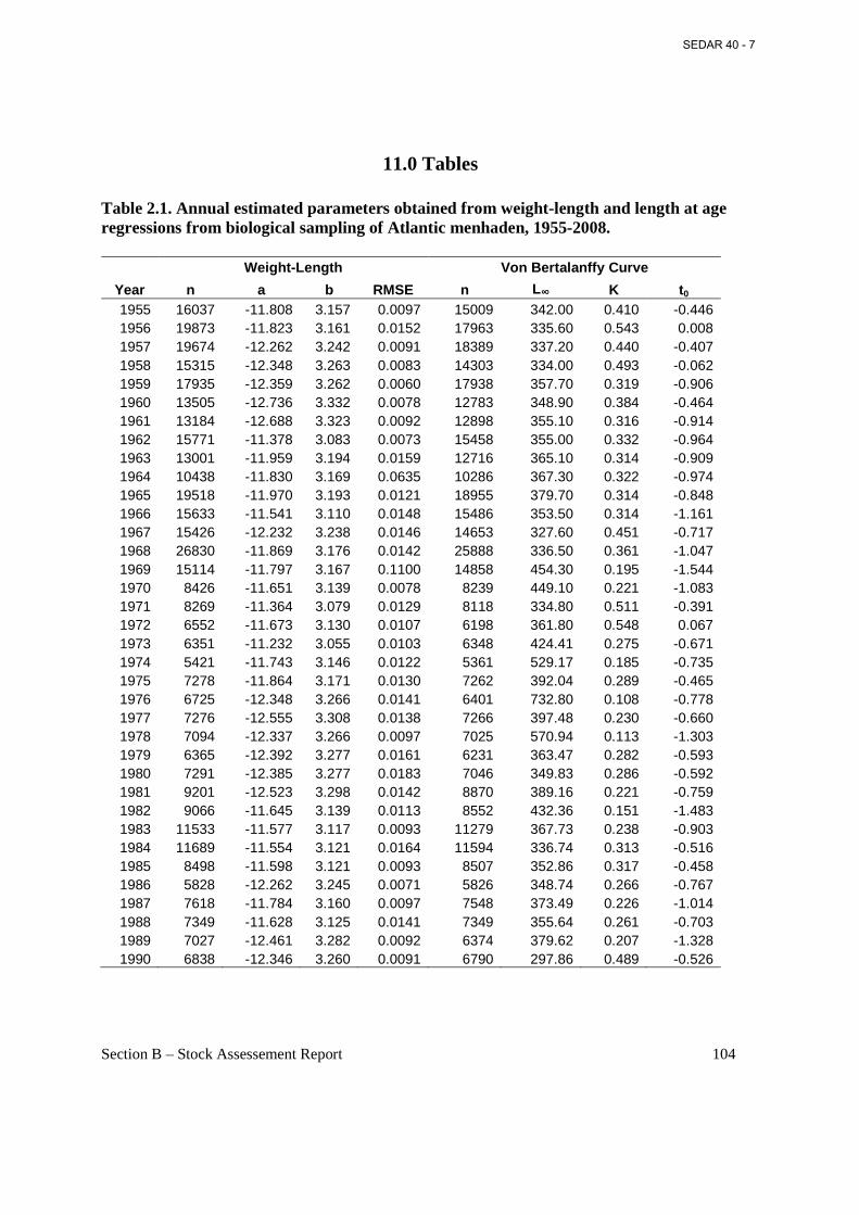
Section B – Stock Assessement Report 104
11.0 Tables Table 2.1. Annual estimated parameters obtained from weight-length and length at age regressions from biological sampling of Atlantic menhaden, 1955-2008.
Weight-Length Von Bertalanffy Curve
Year n a b RMSE n L∞ K t 0 1955 16037 -11.808 3.157 0.0097 15009 342.00 0.410 -0.446 1956 19873 -11.823 3.161 0.0152 17963 335.60 0.543 0.008 1957 19674 -12.262 3.242 0.0091 18389 337.20 0.440 -0.407 1958 15315 -12.348 3.263 0.0083 14303 334.00 0.493 -0.062 1959 17935 -12.359 3.262 0.0060 17938 357.70 0.319 -0.906 1960 13505 -12.736 3.332 0.0078 12783 348.90 0.384 -0.464 1961 13184 -12.688 3.323 0.0092 12898 355.10 0.316 -0.914 1962 15771 -11.378 3.083 0.0073 15458 355.00 0.332 -0.964 1963 13001 -11.959 3.194 0.0159 12716 365.10 0.314 -0.909 1964 10438 -11.830 3.169 0.0635 10286 367.30 0.322 -0.974 1965 19518 -11.970 3.193 0.0121 18955 379.70 0.314 -0.848 1966 15633 -11.541 3.110 0.0148 15486 353.50 0.314 -1.161 1967 15426 -12.232 3.238 0.0146 14653 327.60 0.451 -0.717 1968 26830 -11.869 3.176 0.0142 25888 336.50 0.361 -1.047 1969 15114 -11.797 3.167 0.1100 14858 454.30 0.195 -1.544 1970 8426 -11.651 3.139 0.0078 8239 449.10 0.221 -1.083 1971 8269 -11.364 3.079 0.0129 8118 334.80 0.511 -0.391 1972 6552 -11.673 3.130 0.0107 6198 361.80 0.548 0.067 1973 6351 -11.232 3.055 0.0103 6348 424.41 0.275 -0.671 1974 5421 -11.743 3.146 0.0122 5361 529.17 0.185 -0.735 1975 7278 -11.864 3.171 0.0130 7262 392.04 0.289 -0.465 1976 6725 -12.348 3.266 0.0141 6401 732.80 0.108 -0.778 1977 7276 -12.555 3.308 0.0138 7266 397.48 0.230 -0.660 1978 7094 -12.337 3.266 0.0097 7025 570.94 0.113 -1.303 1979 6365 -12.392 3.277 0.0161 6231 363.47 0.282 -0.593 1980 7291 -12.385 3.277 0.0183 7046 349.83 0.286 -0.592 1981 9201 -12.523 3.298 0.0142 8870 389.16 0.221 -0.759 1982 9066 -11.645 3.139 0.0113 8552 432.36 0.151 -1.483 1983 11533 -11.577 3.117 0.0093 11279 367.73 0.238 -0.903 1984 11689 -11.554 3.121 0.0164 11594 336.74 0.313 -0.516 1985 8498 -11.598 3.121 0.0093 8507 352.86 0.317 -0.458 1986 5828 -12.262 3.245 0.0071 5826 348.74 0.266 -0.767 1987 7618 -11.784 3.160 0.0097 7548 373.49 0.226 -1.014 1988 7349 -11.628 3.125 0.0141 7349 355.64 0.261 -0.703 1989 7027 -12.461 3.282 0.0092 6374 379.62 0.207 -1.328 1990 6838 -12.346 3.260 0.0091 6790 297.86 0.489 -0.526
SEDAR 40 - 7
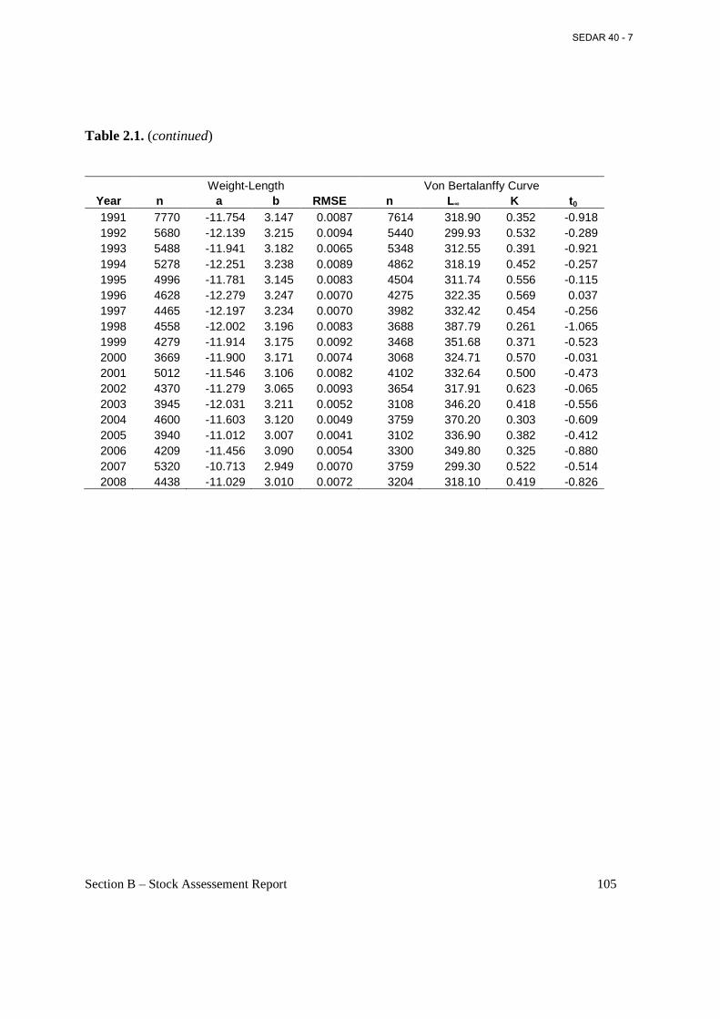
Section B – Stock Assessement Report 105
Table 2.1. (continued)
Weight-Length Von Bertalanffy Curve Year n a b RMSE n L ∞ K t 0 1991 7770 -11.754 3.147 0.0087 7614 318.90 0.352 -0.918 1992 5680 -12.139 3.215 0.0094 5440 299.93 0.532 -0.289 1993 5488 -11.941 3.182 0.0065 5348 312.55 0.391 -0.921 1994 5278 -12.251 3.238 0.0089 4862 318.19 0.452 -0.257 1995 4996 -11.781 3.145 0.0083 4504 311.74 0.556 -0.115 1996 4628 -12.279 3.247 0.0070 4275 322.35 0.569 0.037 1997 4465 -12.197 3.234 0.0070 3982 332.42 0.454 -0.256 1998 4558 -12.002 3.196 0.0083 3688 387.79 0.261 -1.065 1999 4279 -11.914 3.175 0.0092 3468 351.68 0.371 -0.523 2000 3669 -11.900 3.171 0.0074 3068 324.71 0.570 -0.031 2001 5012 -11.546 3.106 0.0082 4102 332.64 0.500 -0.473 2002 4370 -11.279 3.065 0.0093 3654 317.91 0.623 -0.065 2003 3945 -12.031 3.211 0.0052 3108 346.20 0.418 -0.556 2004 4600 -11.603 3.120 0.0049 3759 370.20 0.303 -0.609 2005 3940 -11.012 3.007 0.0041 3102 336.90 0.382 -0.412 2006 4209 -11.456 3.090 0.0054 3300 349.80 0.325 -0.880 2007 5320 -10.713 2.949 0.0070 3759 299.30 0.522 -0.514 2008 4438 -11.029 3.010 0.0072 3204 318.10 0.419 -0.826
SEDAR 40 - 7
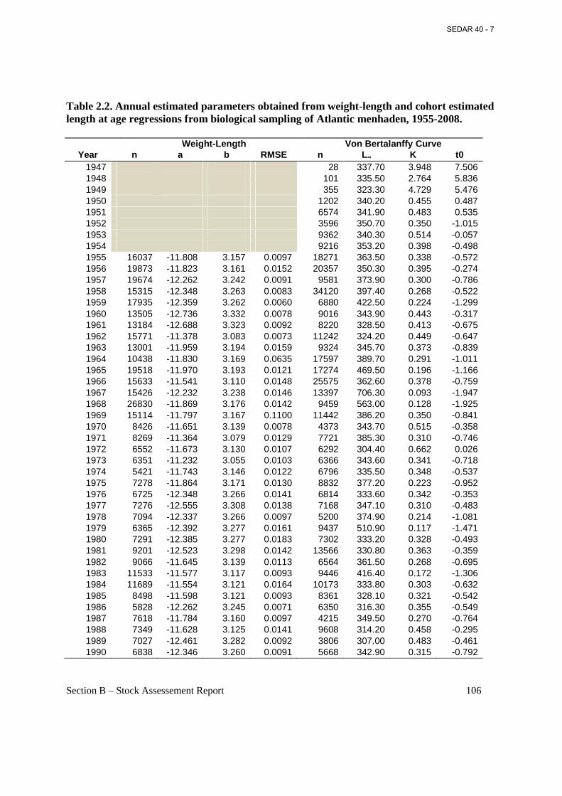
Section B – Stock Assessement Report 106
Table 2.2. Annual estimated parameters obtained from weight-length and cohort estimated length at age regressions from biological sampling of Atlantic menhaden, 1955-2008.
Weight-Length Von Bertalanffy Curve Year n a b RMSE n L∞ K t0
1947 28 337.70 3.948 7.506 1948 101 335.50 2.764 5.836 1949 355 323.30 4.729 5.476 1950 1202 340.20 0.455 0.487 1951 6574 341.90 0.483 0.535 1952 3596 350.70 0.350 -1.015 1953 9362 340.30 0.514 -0.057 1954 9216 353.20 0.398 -0.498 1955 16037 -11.808 3.157 0.0097 18271 363.50 0.338 -0.572 1956 19873 -11.823 3.161 0.0152 20357 350.30 0.395 -0.274 1957 19674 -12.262 3.242 0.0091 9581 373.90 0.300 -0.786 1958 15315 -12.348 3.263 0.0083 34120 397.40 0.268 -0.522 1959 17935 -12.359 3.262 0.0060 6880 422.50 0.224 -1.299 1960 13505 -12.736 3.332 0.0078 9016 343.90 0.443 -0.317 1961 13184 -12.688 3.323 0.0092 8220 328.50 0.413 -0.675 1962 15771 -11.378 3.083 0.0073 11242 324.20 0.449 -0.647 1963 13001 -11.959 3.194 0.0159 9324 345.70 0.373 -0.839 1964 10438 -11.830 3.169 0.0635 17597 389.70 0.291 -1.011 1965 19518 -11.970 3.193 0.0121 17274 469.50 0.196 -1.166 1966 15633 -11.541 3.110 0.0148 25575 362.60 0.378 -0.759 1967 15426 -12.232 3.238 0.0146 13397 706.30 0.093 -1.947 1968 26830 -11.869 3.176 0.0142 9459 563.00 0.128 -1.925 1969 15114 -11.797 3.167 0.1100 11442 386.20 0.350 -0.841 1970 8426 -11.651 3.139 0.0078 4373 343.70 0.515 -0.358 1971 8269 -11.364 3.079 0.0129 7721 385.30 0.310 -0.746 1972 6552 -11.673 3.130 0.0107 6292 304.40 0.662 0.026 1973 6351 -11.232 3.055 0.0103 6366 343.60 0.341 -0.718 1974 5421 -11.743 3.146 0.0122 6796 335.50 0.348 -0.537 1975 7278 -11.864 3.171 0.0130 8832 377.20 0.223 -0.952 1976 6725 -12.348 3.266 0.0141 6814 333.60 0.342 -0.353 1977 7276 -12.555 3.308 0.0138 7168 347.10 0.310 -0.483 1978 7094 -12.337 3.266 0.0097 5200 374.90 0.214 -1.081 1979 6365 -12.392 3.277 0.0161 9437 510.90 0.117 -1.471 1980 7291 -12.385 3.277 0.0183 7302 333.20 0.328 -0.493 1981 9201 -12.523 3.298 0.0142 13566 330.80 0.363 -0.359 1982 9066 -11.645 3.139 0.0113 6564 361.50 0.268 -0.695 1983 11533 -11.577 3.117 0.0093 9446 416.40 0.172 -1.306 1984 11689 -11.554 3.121 0.0164 10173 333.80 0.303 -0.632 1985 8498 -11.598 3.121 0.0093 8361 328.10 0.321 -0.542 1986 5828 -12.262 3.245 0.0071 6350 316.30 0.355 -0.549 1987 7618 -11.784 3.160 0.0097 4215 349.50 0.270 -0.764 1988 7349 -11.628 3.125 0.0141 9608 314.20 0.458 -0.295 1989 7027 -12.461 3.282 0.0092 3806 307.00 0.483 -0.461 1990 6838 -12.346 3.260 0.0091 5668 342.90 0.315 -0.792
SEDAR 40 - 7
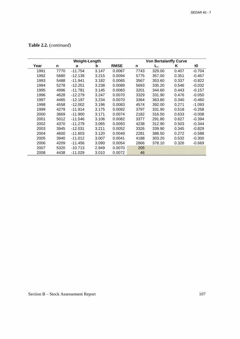
Section B – Stock Assessement Report 107
Table 2.2. (continued)
Weight-Length Von Bertalanffy Curve Year n a b RMSE n L∞ K t0
1991 7770 -11.754 3.147 0.0087 7743 329.00 0.407 -0.704 1992 5680 -12.139 3.215 0.0094 5775 357.00 0.351 -0.457 1993 5488 -11.941 3.182 0.0065 3567 353.60 0.337 -0.822 1994 5278 -12.251 3.238 0.0089 5693 335.20 0.546 -0.032 1995 4996 -11.781 3.145 0.0083 3201 344.60 0.443 -0.157 1996 4628 -12.279 3.247 0.0070 3329 331.90 0.476 -0.050 1997 4465 -12.197 3.234 0.0070 3364 363.80 0.340 -0.460 1998 4558 -12.002 3.196 0.0083 4574 392.00 0.271 -1.093 1999 4279 -11.914 3.175 0.0092 3797 331.90 0.518 -0.258 2000 3669 -11.900 3.171 0.0074 2182 316.50 0.633 -0.008 2001 5012 -11.546 3.106 0.0082 3377 291.80 0.627 -0.394 2002 4370 -11.279 3.065 0.0093 4238 312.90 0.503 -0.344 2003 3945 -12.031 3.211 0.0052 3326 339.90 0.345 -0.829 2004 4600 -11.603 3.120 0.0049 2281 388.50 0.272 -0.588 2005 3940 -11.012 3.007 0.0041 4188 303.20 0.532 -0.300 2006 4209 -11.456 3.090 0.0054 2866 378.10 0.326 -0.669 2007 5320 -10.713 2.949 0.0070 205 2008 4438 -11.029 3.010 0.0072 46
SEDAR 40 - 7
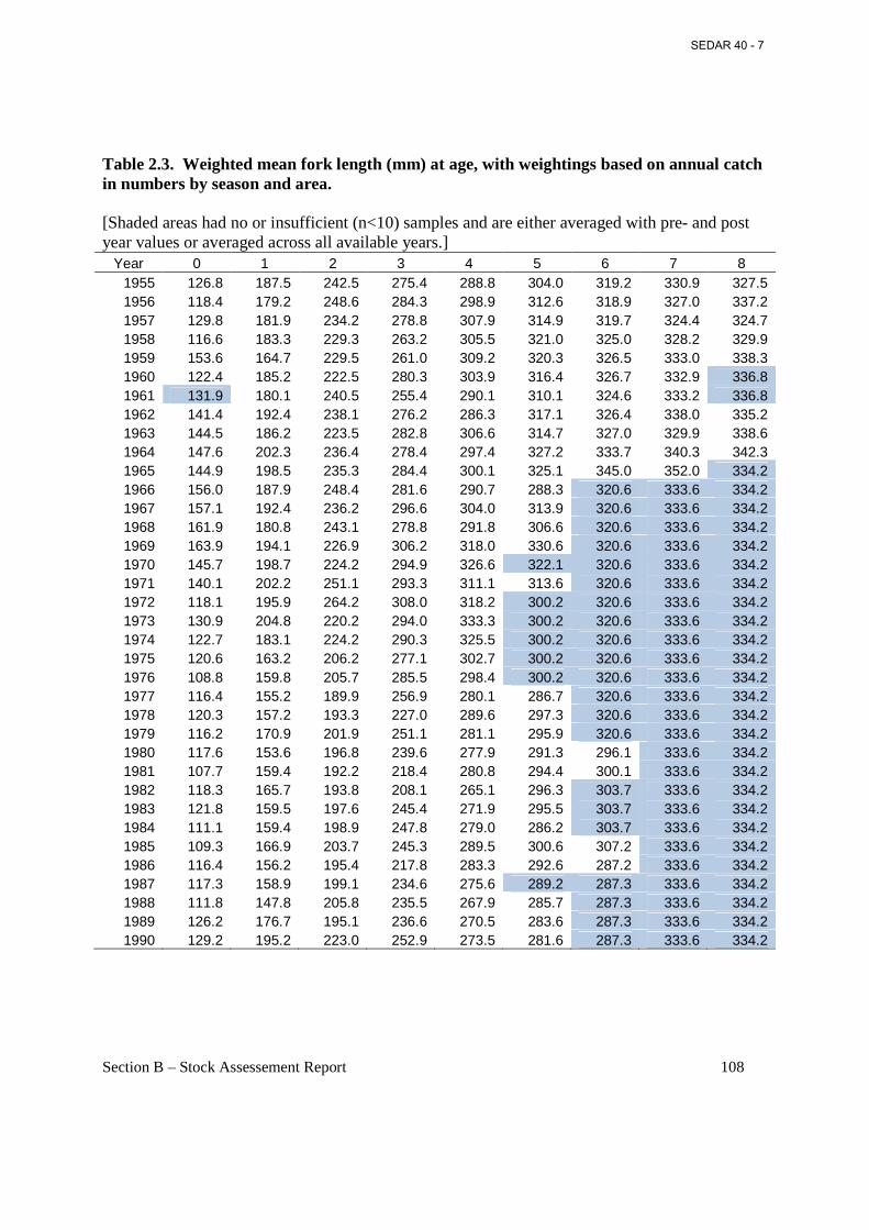
Section B – Stock Assessement Report 108
Table 2.3. Weighted mean fork length (mm) at age, with weightings based on annual catch in numbers by season and area. [Shaded areas had no or insufficient (n<10) samples and are either averaged with pre- and post year values or averaged across all available years.]
Year 0 1 2 3 4 5 6 7 8 1955 126.8 187.5 242.5 275.4 288.8 304.0 319.2 330.9 327.5 1956 118.4 179.2 248.6 284.3 298.9 312.6 318.9 327.0 337.2 1957 129.8 181.9 234.2 278.8 307.9 314.9 319.7 324.4 324.7 1958 116.6 183.3 229.3 263.2 305.5 321.0 325.0 328.2 329.9 1959 153.6 164.7 229.5 261.0 309.2 320.3 326.5 333.0 338.3 1960 122.4 185.2 222.5 280.3 303.9 316.4 326.7 332.9 336.8 1961 131.9 180.1 240.5 255.4 290.1 310.1 324.6 333.2 336.8 1962 141.4 192.4 238.1 276.2 286.3 317.1 326.4 338.0 335.2 1963 144.5 186.2 223.5 282.8 306.6 314.7 327.0 329.9 338.6 1964 147.6 202.3 236.4 278.4 297.4 327.2 333.7 340.3 342.3 1965 144.9 198.5 235.3 284.4 300.1 325.1 345.0 352.0 334.2 1966 156.0 187.9 248.4 281.6 290.7 288.3 320.6 333.6 334.2 1967 157.1 192.4 236.2 296.6 304.0 313.9 320.6 333.6 334.2 1968 161.9 180.8 243.1 278.8 291.8 306.6 320.6 333.6 334.2 1969 163.9 194.1 226.9 306.2 318.0 330.6 320.6 333.6 334.2 1970 145.7 198.7 224.2 294.9 326.6 322.1 320.6 333.6 334.2 1971 140.1 202.2 251.1 293.3 311.1 313.6 320.6 333.6 334.2 1972 118.1 195.9 264.2 308.0 318.2 300.2 320.6 333.6 334.2 1973 130.9 204.8 220.2 294.0 333.3 300.2 320.6 333.6 334.2 1974 122.7 183.1 224.2 290.3 325.5 300.2 320.6 333.6 334.2 1975 120.6 163.2 206.2 277.1 302.7 300.2 320.6 333.6 334.2 1976 108.8 159.8 205.7 285.5 298.4 300.2 320.6 333.6 334.2 1977 116.4 155.2 189.9 256.9 280.1 286.7 320.6 333.6 334.2 1978 120.3 157.2 193.3 227.0 289.6 297.3 320.6 333.6 334.2 1979 116.2 170.9 201.9 251.1 281.1 295.9 320.6 333.6 334.2 1980 117.6 153.6 196.8 239.6 277.9 291.3 296.1 333.6 334.2 1981 107.7 159.4 192.2 218.4 280.8 294.4 300.1 333.6 334.2 1982 118.3 165.7 193.8 208.1 265.1 296.3 303.7 333.6 334.2 1983 121.8 159.5 197.6 245.4 271.9 295.5 303.7 333.6 334.2 1984 111.1 159.4 198.9 247.8 279.0 286.2 303.7 333.6 334.2 1985 109.3 166.9 203.7 245.3 289.5 300.6 307.2 333.6 334.2 1986 116.4 156.2 195.4 217.8 283.3 292.6 287.2 333.6 334.2 1987 117.3 158.9 199.1 234.6 275.6 289.2 287.3 333.6 334.2 1988 111.8 147.8 205.8 235.5 267.9 285.7 287.3 333.6 334.2 1989 126.2 176.7 195.1 236.6 270.5 283.6 287.3 333.6 334.2 1990 129.2 195.2 223.0 252.9 273.5 281.6 287.3 333.6 334.2
SEDAR 40 - 7
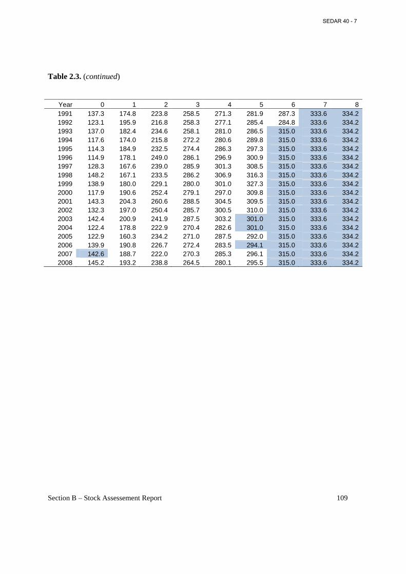
Section B – Stock Assessement Report 109
Table 2.3. (continued)
Year 0 1 2 3 4 5 6 7 8 1991 137.3 174.8 223.8 258.5 271.3 281.9 287.3 333.6 334.2 1992 123.1 195.9 216.8 258.3 277.1 285.4 284.8 333.6 334.2 1993 137.0 182.4 234.6 258.1 281.0 286.5 315.0 333.6 334.2 1994 117.6 174.0 215.8 272.2 280.6 289.8 315.0 333.6 334.2 1995 114.3 184.9 232.5 274.4 286.3 297.3 315.0 333.6 334.2 1996 114.9 178.1 249.0 286.1 296.9 300.9 315.0 333.6 334.2 1997 128.3 167.6 239.0 285.9 301.3 308.5 315.0 333.6 334.2 1998 148.2 167.1 233.5 286.2 306.9 316.3 315.0 333.6 334.2 1999 138.9 180.0 229.1 280.0 301.0 327.3 315.0 333.6 334.2 2000 117.9 190.6 252.4 279.1 297.0 309.8 315.0 333.6 334.2 2001 143.3 204.3 260.6 288.5 304.5 309.5 315.0 333.6 334.2 2002 132.3 197.0 250.4 285.7 300.5 310.0 315.0 333.6 334.2 2003 142.4 200.9 241.9 287.5 303.2 301.0 315.0 333.6 334.2 2004 122.4 178.8 222.9 270.4 282.6 301.0 315.0 333.6 334.2 2005 122.9 160.3 234.2 271.0 287.5 292.0 315.0 333.6 334.2 2006 139.9 190.8 226.7 272.4 283.5 294.1 315.0 333.6 334.2 2007 142.6 188.7 222.0 270.3 285.3 296.1 315.0 333.6 334.2 2008 145.2 193.2 238.8 264.5 280.1 295.5 315.0 333.6 334.2
SEDAR 40 - 7
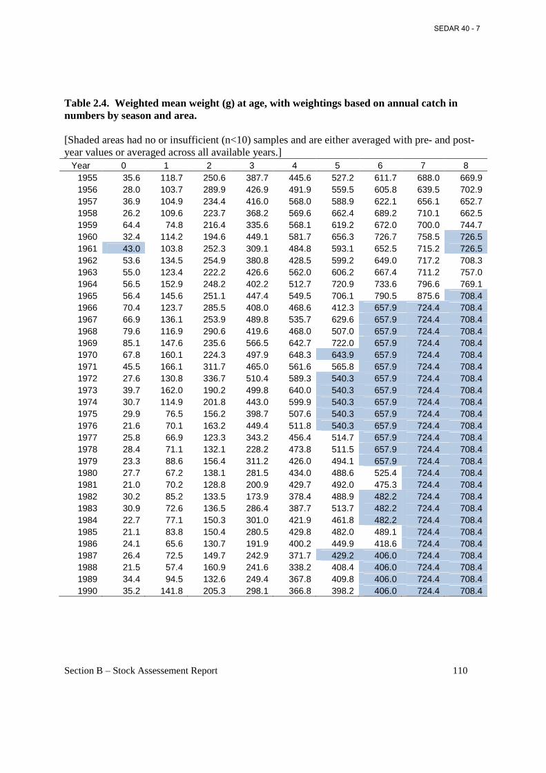
Section B – Stock Assessement Report 110
Table 2.4. Weighted mean weight (g) at age, with weightings based on annual catch in numbers by season and area. [Shaded areas had no or insufficient (n<10) samples and are either averaged with pre- and post-year values or averaged across all available years.]
Year 0 1 2 3 4 5 6 7 8 1955 35.6 118.7 250.6 387.7 445.6 527.2 611.7 688.0 669.9 1956 28.0 103.7 289.9 426.9 491.9 559.5 605.8 639.5 702.9 1957 36.9 104.9 234.4 416.0 568.0 588.9 622.1 656.1 652.7 1958 26.2 109.6 223.7 368.2 569.6 662.4 689.2 710.1 662.5 1959 64.4 74.8 216.4 335.6 568.1 619.2 672.0 700.0 744.7 1960 32.4 114.2 194.6 449.1 581.7 656.3 726.7 758.5 726.5 1961 43.0 103.8 252.3 309.1 484.8 593.1 652.5 715.2 726.5 1962 53.6 134.5 254.9 380.8 428.5 599.2 649.0 717.2 708.3 1963 55.0 123.4 222.2 426.6 562.0 606.2 667.4 711.2 757.0 1964 56.5 152.9 248.2 402.2 512.7 720.9 733.6 796.6 769.1 1965 56.4 145.6 251.1 447.4 549.5 706.1 790.5 875.6 708.4 1966 70.4 123.7 285.5 408.0 468.6 412.3 657.9 724.4 708.4 1967 66.9 136.1 253.9 489.8 535.7 629.6 657.9 724.4 708.4 1968 79.6 116.9 290.6 419.6 468.0 507.0 657.9 724.4 708.4 1969 85.1 147.6 235.6 566.5 642.7 722.0 657.9 724.4 708.4 1970 67.8 160.1 224.3 497.9 648.3 643.9 657.9 724.4 708.4 1971 45.5 166.1 311.7 465.0 561.6 565.8 657.9 724.4 708.4 1972 27.6 130.8 336.7 510.4 589.3 540.3 657.9 724.4 708.4 1973 39.7 162.0 190.2 499.8 640.0 540.3 657.9 724.4 708.4 1974 30.7 114.9 201.8 443.0 599.9 540.3 657.9 724.4 708.4 1975 29.9 76.5 156.2 398.7 507.6 540.3 657.9 724.4 708.4 1976 21.6 70.1 163.2 449.4 511.8 540.3 657.9 724.4 708.4 1977 25.8 66.9 123.3 343.2 456.4 514.7 657.9 724.4 708.4 1978 28.4 71.1 132.1 228.2 473.8 511.5 657.9 724.4 708.4 1979 23.3 88.6 156.4 311.2 426.0 494.1 657.9 724.4 708.4 1980 27.7 67.2 138.1 281.5 434.0 488.6 525.4 724.4 708.4 1981 21.0 70.2 128.8 200.9 429.7 492.0 475.3 724.4 708.4 1982 30.2 85.2 133.5 173.9 378.4 488.9 482.2 724.4 708.4 1983 30.9 72.6 136.5 286.4 387.7 513.7 482.2 724.4 708.4 1984 22.7 77.1 150.3 301.0 421.9 461.8 482.2 724.4 708.4 1985 21.1 83.8 150.4 280.5 429.8 482.0 489.1 724.4 708.4 1986 24.1 65.6 130.7 191.9 400.2 449.9 418.6 724.4 708.4 1987 26.4 72.5 149.7 242.9 371.7 429.2 406.0 724.4 708.4 1988 21.5 57.4 160.9 241.6 338.2 408.4 406.0 724.4 708.4 1989 34.4 94.5 132.6 249.4 367.8 409.8 406.0 724.4 708.4 1990 35.2 141.8 205.3 298.1 366.8 398.2 406.0 724.4 708.4
SEDAR 40 - 7
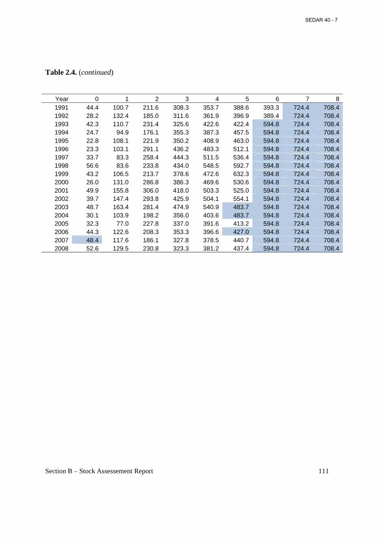
Section B – Stock Assessement Report 111
Table 2.4. (continued)
Year 0 1 2 3 4 5 6 7 8 1991 44.4 100.7 211.6 308.3 353.7 388.6 393.3 724.4 708.4 1992 28.2 132.4 185.0 311.6 361.9 396.9 389.4 724.4 708.4 1993 42.3 110.7 231.4 325.6 422.6 422.4 594.8 724.4 708.4 1994 24.7 94.9 176.1 355.3 387.3 457.5 594.8 724.4 708.4 1995 22.8 108.1 221.9 350.2 408.9 463.0 594.8 724.4 708.4 1996 23.3 103.1 291.1 436.2 483.3 512.1 594.8 724.4 708.4 1997 33.7 83.3 258.4 444.3 511.5 536.4 594.8 724.4 708.4 1998 56.6 83.6 233.8 434.0 548.5 592.7 594.8 724.4 708.4 1999 43.2 106.5 213.7 378.6 472.6 632.3 594.8 724.4 708.4 2000 26.0 131.0 286.8 386.3 469.6 530.6 594.8 724.4 708.4 2001 49.9 155.8 306.0 418.0 503.3 525.0 594.8 724.4 708.4 2002 39.7 147.4 293.8 425.9 504.1 554.1 594.8 724.4 708.4 2003 48.7 163.4 281.4 474.9 540.9 483.7 594.8 724.4 708.4 2004 30.1 103.9 198.2 356.0 403.6 483.7 594.8 724.4 708.4 2005 32.3 77.0 227.8 337.0 391.6 413.2 594.8 724.4 708.4 2006 44.3 122.6 208.3 353.3 396.6 427.0 594.8 724.4 708.4 2007 48.4 117.6 186.1 327.8 378.5 440.7 594.8 724.4 708.4 2008 52.6 129.5 230.8 323.3 381.2 437.4 594.8 724.4 708.4
SEDAR 40 - 7
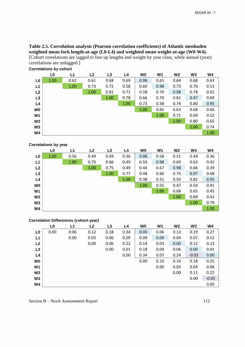
Section B – Stock Assessement Report 112
Table 2.5. Correlation analysis (Pearson correlation coefficients) of Atlantic menhaden weighted mean fork length-at-age (L0-L4) and weighted mean weight-at-age (W0-W4). [Cohort correlations are lagged to line up lengths and weight by year class, while annual (year) correlations are unlagged.] Correlations by cohort
L0 L1 L2 L3 L4 W0 W1 W2 W3 W4
L0 1.00 0.62 0.61 0.68 0.69 0.98 0.65 0.64 0.68 0.63
L1 1.00 0.73 0.72 0.58 0.60 0.98 0.73 0.70 0.53
L2
1.00 0.81 0.71 0.58 0.70 0.98 0.78 0.62
L3
1.00 0.78 0.66 0.70 0.81 0.97 0.69
L4
1.00 0.73 0.58 0.74 0.80 0.95
W0
1.00 0.65 0.63 0.68 0.66
W1
1.00 0.71 0.69 0.52
W2
1.00 0.80 0.65
W3
1.00 0.74
W4 1.00
Correlations by year
L0 L1 L2 L3 L4 W0 W1 W2 W3 W4
L0 1.00 0.56 0.49 0.49 0.36 0.98 0.58 0.51 0.49 0.36
L1 1.00 0.70 0.66 0.49 0.50 0.98 0.69 0.63 0.42
L2
1.00 0.75 0.49 0.44 0.67 0.98 0.66 0.39
L3
1.00 0.77 0.48 0.66 0.75 0.97 0.68
L4
1.00 0.38 0.51 0.50 0.82 0.95
W0
1.00 0.55 0.47 0.50 0.41
W1
1.00 0.68 0.65 0.45
W2
1.00 0.69 0.43
W3
1.00 0.79
W4 1.00
Correlation Differences (cohort-year)
L0 L1 L2 L3 L4 W0 W1 W2 W3 W4
L0 0.00 0.06 0.12 0.18 0.34 0.00 0.06 0.13 0.19 0.27
L1 0.00 0.03 0.06 0.09 0.09 0.00 0.04 0.07 0.12
L2
0.00 0.06 0.22 0.14 0.03 0.00 0.12 0.23
L3
0.00 0.01 0.18 0.04 0.06 0.00 0.01
L4
0.00 0.34 0.07 0.24 -0.03 0.00
W0
0.00 0.10 0.16 0.18 0.25
W1
0.00 0.03 0.04 0.06
W2
0.00 0.11 0.22
W3
0.00 -0.05
W4 0.00
SEDAR 40 - 7
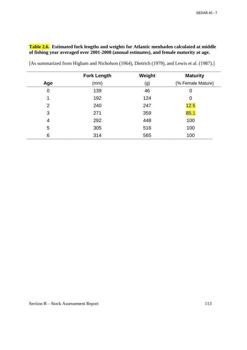
Section B – Stock Assessement Report 113
Table 2.6. Estimated fork lengths and weights for Atlantic menhaden calculated at middle of fishing year averaged over 2001-2008 (annual estimates), and female maturity at age. [As summarized from Higham and Nicholson (1964), Dietrich (1979), and Lewis et al. (1987).]
Fork Length Weight Maturity
Age (mm) (g) (% Female Mature)
0 139 46 0
1 192 124 0
2 240 247 12.5
3 271 359 85.1
4 292 448 100
5 305 516 100
6 314 565 100
SEDAR 40 - 7
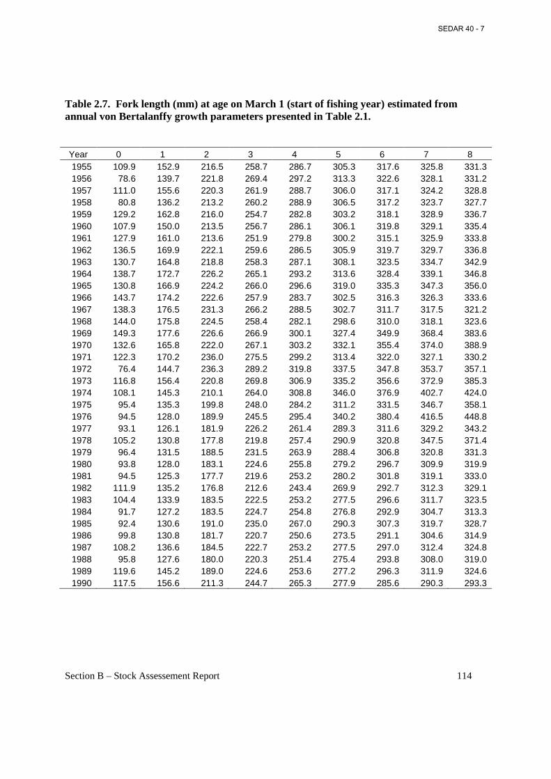
Section B – Stock Assessement Report 114
Table 2.7. Fork length (mm) at age on March 1 (start of fishing year) estimated from annual von Bertalanffy growth parameters presented in Table 2.1. Year 0 1 2 3 4 5 6 7 8 1955 109.9 152.9 216.5 258.7 286.7 305.3 317.6 325.8 331.3 1956 78.6 139.7 221.8 269.4 297.2 313.3 322.6 328.1 331.2 1957 111.0 155.6 220.3 261.9 288.7 306.0 317.1 324.2 328.8 1958 80.8 136.2 213.2 260.2 288.9 306.5 317.2 323.7 327.7 1959 129.2 162.8 216.0 254.7 282.8 303.2 318.1 328.9 336.7 1960 107.9 150.0 213.5 256.7 286.1 306.1 319.8 329.1 335.4 1961 127.9 161.0 213.6 251.9 279.8 300.2 315.1 325.9 333.8 1962 136.5 169.9 222.1 259.6 286.5 305.9 319.7 329.7 336.8 1963 130.7 164.8 218.8 258.3 287.1 308.1 323.5 334.7 342.9 1964 138.7 172.7 226.2 265.1 293.2 313.6 328.4 339.1 346.8 1965 130.8 166.9 224.2 266.0 296.6 319.0 335.3 347.3 356.0 1966 143.7 174.2 222.6 257.9 283.7 302.5 316.3 326.3 333.6 1967 138.3 176.5 231.3 266.2 288.5 302.7 311.7 317.5 321.2 1968 144.0 175.8 224.5 258.4 282.1 298.6 310.0 318.1 323.6 1969 149.3 177.6 226.6 266.9 300.1 327.4 349.9 368.4 383.6 1970 132.6 165.8 222.0 267.1 303.2 332.1 355.4 374.0 388.9 1971 122.3 170.2 236.0 275.5 299.2 313.4 322.0 327.1 330.2 1972 76.4 144.7 236.3 289.2 319.8 337.5 347.8 353.7 357.1 1973 116.8 156.4 220.8 269.8 306.9 335.2 356.6 372.9 385.3 1974 108.1 145.3 210.1 264.0 308.8 346.0 376.9 402.7 424.0 1975 95.4 135.3 199.8 248.0 284.2 311.2 331.5 346.7 358.1 1976 94.5 128.0 189.9 245.5 295.4 340.2 380.4 416.5 448.8 1977 93.1 126.1 181.9 226.2 261.4 289.3 311.6 329.2 343.2 1978 105.2 130.8 177.8 219.8 257.4 290.9 320.8 347.5 371.4 1979 96.4 131.5 188.5 231.5 263.9 288.4 306.8 320.8 331.3 1980 93.8 128.0 183.1 224.6 255.8 279.2 296.7 309.9 319.9 1981 94.5 125.3 177.7 219.6 253.2 280.2 301.8 319.1 333.0 1982 111.9 135.2 176.8 212.6 243.4 269.9 292.7 312.3 329.1 1983 104.4 133.9 183.5 222.5 253.2 277.5 296.6 311.7 323.5 1984 91.7 127.2 183.5 224.7 254.8 276.8 292.9 304.7 313.3 1985 92.4 130.6 191.0 235.0 267.0 290.3 307.3 319.7 328.7 1986 99.8 130.8 181.7 220.7 250.6 273.5 291.1 304.6 314.9 1987 108.2 136.6 184.5 222.7 253.2 277.5 297.0 312.4 324.8 1988 95.8 127.6 180.0 220.3 251.4 275.4 293.8 308.0 319.0 1989 119.6 145.2 189.0 224.6 253.6 277.2 296.3 311.9 324.6 1990 117.5 156.6 211.3 244.7 265.3 277.9 285.6 290.3 293.3
SEDAR 40 - 7
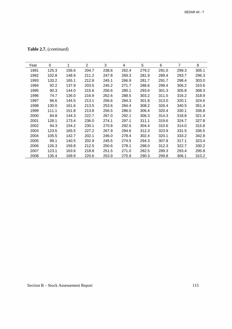
Section B – Stock Assessement Report 115
Table 2.7. (continued) Year 0 1 2 3 4 5 6 7 8 1991 125.3 156.6 204.7 238.6 262.4 279.2 291.0 299.3 305.1 1992 102.8 148.9 211.2 247.8 269.3 281.9 289.4 293.7 296.3 1993 133.2 165.1 212.8 245.1 266.9 281.7 291.7 298.4 303.0 1994 92.2 137.9 203.5 245.2 271.7 288.6 299.4 306.2 310.6 1995 90.3 144.0 215.6 256.6 280.1 293.6 301.3 305.8 308.3 1996 74.7 136.0 216.9 262.6 288.5 303.2 311.5 316.2 318.9 1997 96.6 144.5 213.1 256.6 284.3 301.8 313.0 320.1 324.6 1998 130.0 161.6 213.5 253.6 284.4 308.2 326.4 340.5 351.4 1999 111.1 151.8 213.8 256.5 286.0 306.4 320.4 330.1 336.8 2000 84.8 144.3 222.7 267.0 292.1 306.3 314.3 318.8 321.4 2001 128.1 173.4 236.0 274.1 297.1 311.1 319.6 324.7 327.8 2002 94.3 154.2 230.1 270.8 292.6 304.4 310.6 314.0 315.8 2003 123.5 165.5 227.2 267.9 294.6 312.3 323.9 331.5 336.5 2004 105.5 142.7 202.1 246.0 278.4 302.4 320.1 333.2 342.8 2005 99.1 140.5 202.9 245.5 274.5 294.3 307.8 317.1 323.4 2006 126.3 159.8 212.5 250.6 278.1 298.0 312.3 322.7 330.2 2007 123.1 163.6 218.8 251.5 271.0 282.5 289.3 293.4 295.8 2008 135.4 169.9 220.6 253.9 275.9 290.3 299.8 306.1 310.2
SEDAR 40 - 7
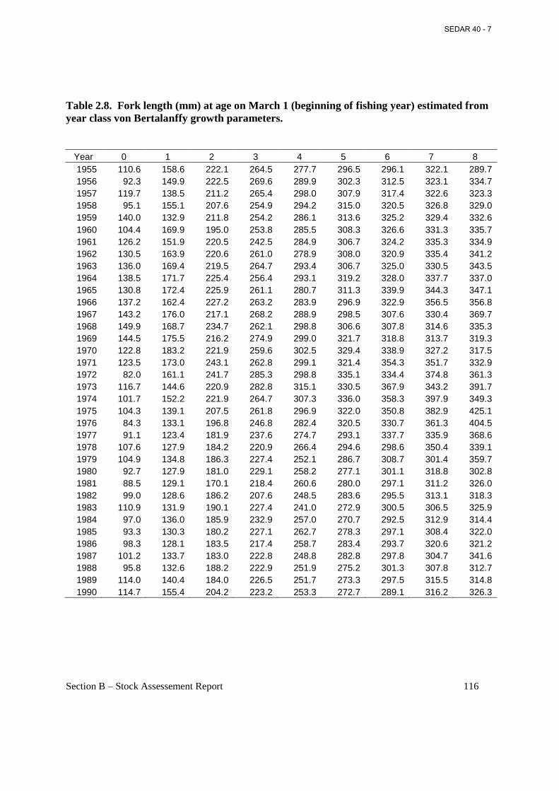
Section B – Stock Assessement Report 116
Table 2.8. Fork length (mm) at age on March 1 (beginning of fishing year) estimated from year class von Bertalanffy growth parameters.
Year 0 1 2 3 4 5 6 7 8 1955 110.6 158.6 222.1 264.5 277.7 296.5 296.1 322.1 289.7 1956 92.3 149.9 222.5 269.6 289.9 302.3 312.5 323.1 334.7 1957 119.7 138.5 211.2 265.4 298.0 307.9 317.4 322.6 323.3 1958 95.1 155.1 207.6 254.9 294.2 315.0 320.5 326.8 329.0 1959 140.0 132.9 211.8 254.2 286.1 313.6 325.2 329.4 332.6 1960 104.4 169.9 195.0 253.8 285.5 308.3 326.6 331.3 335.7 1961 126.2 151.9 220.5 242.5 284.9 306.7 324.2 335.3 334.9 1962 130.5 163.9 220.6 261.0 278.9 308.0 320.9 335.4 341.2 1963 136.0 169.4 219.5 264.7 293.4 306.7 325.0 330.5 343.5 1964 138.5 171.7 225.4 256.4 293.1 319.2 328.0 337.7 337.0 1965 130.8 172.4 225.9 261.1 280.7 311.3 339.9 344.3 347.1 1966 137.2 162.4 227.2 263.2 283.9 296.9 322.9 356.5 356.8 1967 143.2 176.0 217.1 268.2 288.9 298.5 307.6 330.4 369.7 1968 149.9 168.7 234.7 262.1 298.8 306.6 307.8 314.6 335.3 1969 144.5 175.5 216.2 274.9 299.0 321.7 318.8 313.7 319.3 1970 122.8 183.2 221.9 259.6 302.5 329.4 338.9 327.2 317.5 1971 123.5 173.0 243.1 262.8 299.1 321.4 354.3 351.7 332.9 1972 82.0 161.1 241.7 285.3 298.8 335.1 334.4 374.8 361.3 1973 116.7 144.6 220.9 282.8 315.1 330.5 367.9 343.2 391.7 1974 101.7 152.2 221.9 264.7 307.3 336.0 358.3 397.9 349.3 1975 104.3 139.1 207.5 261.8 296.9 322.0 350.8 382.9 425.1 1976 84.3 133.1 196.8 246.8 282.4 320.5 330.7 361.3 404.5 1977 91.1 123.4 181.9 237.6 274.7 293.1 337.7 335.9 368.6 1978 107.6 127.9 184.2 220.9 266.4 294.6 298.6 350.4 339.1 1979 104.9 134.8 186.3 227.4 252.1 286.7 308.7 301.4 359.7 1980 92.7 127.9 181.0 229.1 258.2 277.1 301.1 318.8 302.8 1981 88.5 129.1 170.1 218.4 260.6 280.0 297.1 311.2 326.0 1982 99.0 128.6 186.2 207.6 248.5 283.6 295.5 313.1 318.3 1983 110.9 131.9 190.1 227.4 241.0 272.9 300.5 306.5 325.9 1984 97.0 136.0 185.9 232.9 257.0 270.7 292.5 312.9 314.4 1985 93.3 130.3 180.2 227.1 262.7 278.3 297.1 308.4 322.0 1986 98.3 128.1 183.5 217.4 258.7 283.4 293.7 320.6 321.2 1987 101.2 133.7 183.0 222.8 248.8 282.8 297.8 304.7 341.6 1988 95.8 132.6 188.2 222.9 251.9 275.2 301.3 307.8 312.7 1989 114.0 140.4 184.0 226.5 251.7 273.3 297.5 315.5 314.8 1990 114.7 155.4 204.2 223.2 253.3 272.7 289.1 316.2 326.3
SEDAR 40 - 7
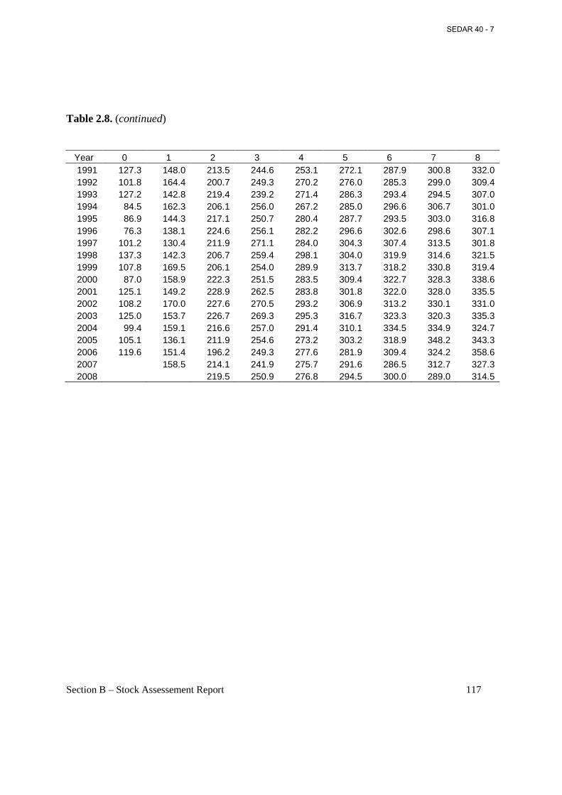
Section B – Stock Assessement Report 117
Table 2.8. (continued)
Year 0 1 2 3 4 5 6 7 8 1991 127.3 148.0 213.5 244.6 253.1 272.1 287.9 300.8 332.0 1992 101.8 164.4 200.7 249.3 270.2 276.0 285.3 299.0 309.4 1993 127.2 142.8 219.4 239.2 271.4 286.3 293.4 294.5 307.0 1994 84.5 162.3 206.1 256.0 267.2 285.0 296.6 306.7 301.0 1995 86.9 144.3 217.1 250.7 280.4 287.7 293.5 303.0 316.8 1996 76.3 138.1 224.6 256.1 282.2 296.6 302.6 298.6 307.1 1997 101.2 130.4 211.9 271.1 284.0 304.3 307.4 313.5 301.8 1998 137.3 142.3 206.7 259.4 298.1 304.0 319.9 314.6 321.5 1999 107.8 169.5 206.1 254.0 289.9 313.7 318.2 330.8 319.4 2000 87.0 158.9 222.3 251.5 283.5 309.4 322.7 328.3 338.6 2001 125.1 149.2 228.9 262.5 283.8 301.8 322.0 328.0 335.5 2002 108.2 170.0 227.6 270.5 293.2 306.9 313.2 330.1 331.0 2003 125.0 153.7 226.7 269.3 295.3 316.7 323.3 320.3 335.3 2004 99.4 159.1 216.6 257.0 291.4 310.1 334.5 334.9 324.7 2005 105.1 136.1 211.9 254.6 273.2 303.2 318.9 348.2 343.3 2006 119.6 151.4 196.2 249.3 277.6 281.9 309.4 324.2 358.6 2007 158.5 214.1 241.9 275.7 291.6 286.5 312.7 327.3 2008 219.5 250.9 276.8 294.5 300.0 289.0 314.5
SEDAR 40 - 7
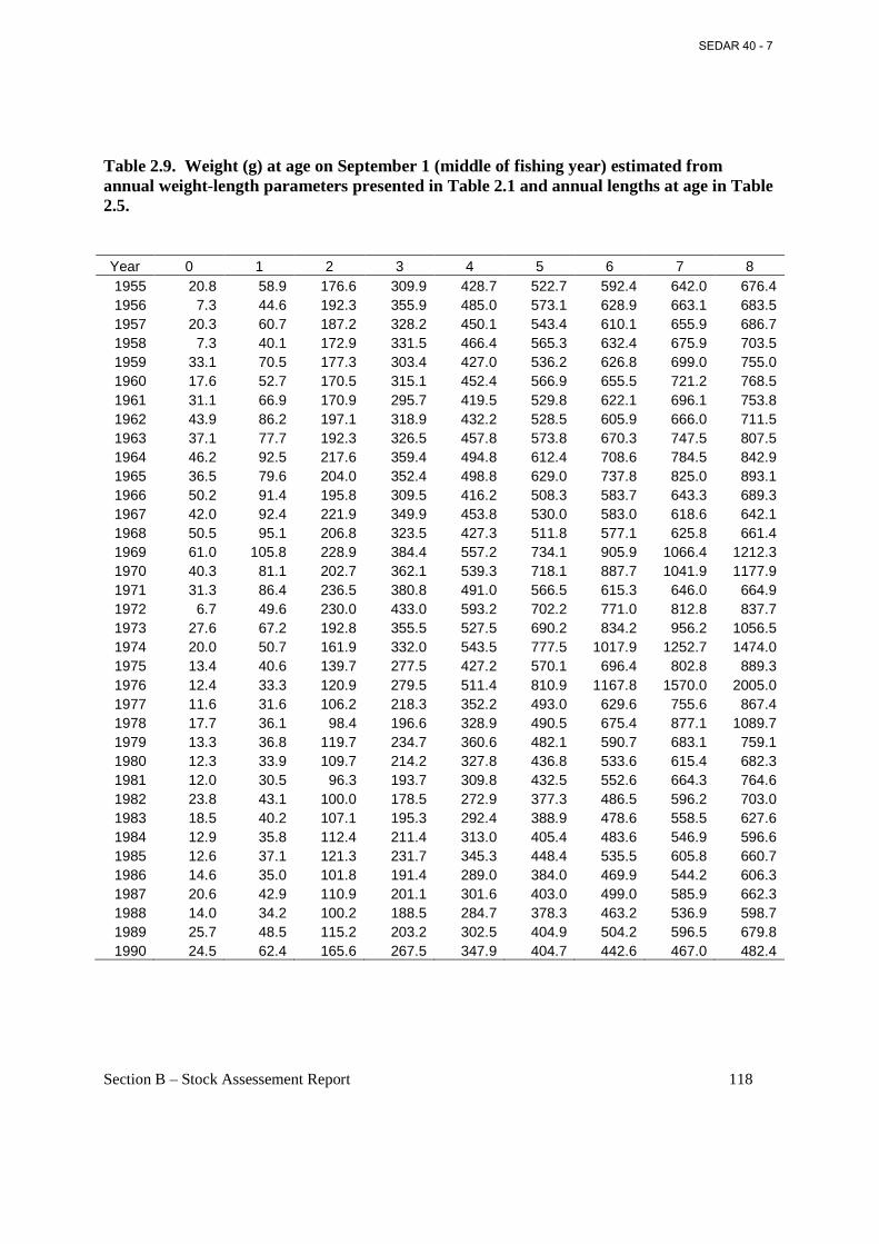
Section B – Stock Assessement Report 118
Table 2.9. Weight (g) at age on September 1 (middle of fishing year) estimated from annual weight-length parameters presented in Table 2.1 and annual lengths at age in Table 2.5. Year 0 1 2 3 4 5 6 7 8 1955 20.8 58.9 176.6 309.9 428.7 522.7 592.4 642.0 676.4 1956 7.3 44.6 192.3 355.9 485.0 573.1 628.9 663.1 683.5 1957 20.3 60.7 187.2 328.2 450.1 543.4 610.1 655.9 686.7 1958 7.3 40.1 172.9 331.5 466.4 565.3 632.4 675.9 703.5 1959 33.1 70.5 177.3 303.4 427.0 536.2 626.8 699.0 755.0 1960 17.6 52.7 170.5 315.1 452.4 566.9 655.5 721.2 768.5 1961 31.1 66.9 170.9 295.7 419.5 529.8 622.1 696.1 753.8 1962 43.9 86.2 197.1 318.9 432.2 528.5 605.9 666.0 711.5 1963 37.1 77.7 192.3 326.5 457.8 573.8 670.3 747.5 807.5 1964 46.2 92.5 217.6 359.4 494.8 612.4 708.6 784.5 842.9 1965 36.5 79.6 204.0 352.4 498.8 629.0 737.8 825.0 893.1 1966 50.2 91.4 195.8 309.5 416.2 508.3 583.7 643.3 689.3 1967 42.0 92.4 221.9 349.9 453.8 530.0 583.0 618.6 642.1 1968 50.5 95.1 206.8 323.5 427.3 511.8 577.1 625.8 661.4 1969 61.0 105.8 228.9 384.4 557.2 734.1 905.9 1066.4 1212.3 1970 40.3 81.1 202.7 362.1 539.3 718.1 887.7 1041.9 1177.9 1971 31.3 86.4 236.5 380.8 491.0 566.5 615.3 646.0 664.9 1972 6.7 49.6 230.0 433.0 593.2 702.2 771.0 812.8 837.7 1973 27.6 67.2 192.8 355.5 527.5 690.2 834.2 956.2 1056.5 1974 20.0 50.7 161.9 332.0 543.5 777.5 1017.9 1252.7 1474.0 1975 13.4 40.6 139.7 277.5 427.2 570.1 696.4 802.8 889.3 1976 12.4 33.3 120.9 279.5 511.4 810.9 1167.8 1570.0 2005.0 1977 11.6 31.6 106.2 218.3 352.2 493.0 629.6 755.6 867.4 1978 17.7 36.1 98.4 196.6 328.9 490.5 675.4 877.1 1089.7 1979 13.3 36.8 119.7 234.7 360.6 482.1 590.7 683.1 759.1 1980 12.3 33.9 109.7 214.2 327.8 436.8 533.6 615.4 682.3 1981 12.0 30.5 96.3 193.7 309.8 432.5 552.6 664.3 764.6 1982 23.8 43.1 100.0 178.5 272.9 377.3 486.5 596.2 703.0 1983 18.5 40.2 107.1 195.3 292.4 388.9 478.6 558.5 627.6 1984 12.9 35.8 112.4 211.4 313.0 405.4 483.6 546.9 596.6 1985 12.6 37.1 121.3 231.7 345.3 448.4 535.5 605.8 660.7 1986 14.6 35.0 101.8 191.4 289.0 384.0 469.9 544.2 606.3 1987 20.6 42.9 110.9 201.1 301.6 403.0 499.0 585.9 662.3 1988 14.0 34.2 100.2 188.5 284.7 378.3 463.2 536.9 598.7 1989 25.7 48.5 115.2 203.2 302.5 404.9 504.2 596.5 679.8 1990 24.5 62.4 165.6 267.5 347.9 404.7 442.6 467.0 482.4
SEDAR 40 - 7
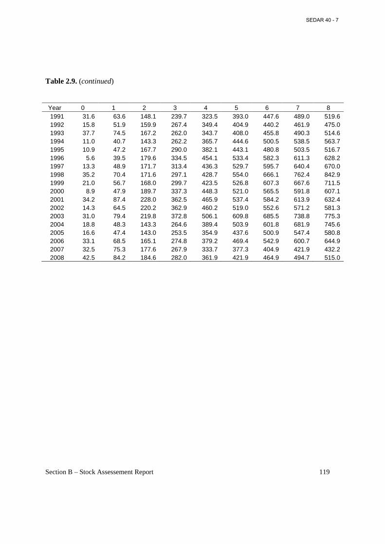
Section B – Stock Assessement Report 119
Table 2.9. (continued) Year 0 1 2 3 4 5 6 7 8 1991 31.6 63.6 148.1 239.7 323.5 393.0 447.6 489.0 519.6 1992 15.8 51.9 159.9 267.4 349.4 404.9 440.2 461.9 475.0 1993 37.7 74.5 167.2 262.0 343.7 408.0 455.8 490.3 514.6 1994 11.0 40.7 143.3 262.2 365.7 444.6 500.5 538.5 563.7 1995 10.9 47.2 167.7 290.0 382.1 443.1 480.8 503.5 516.7 1996 5.6 39.5 179.6 334.5 454.1 533.4 582.3 611.3 628.2 1997 13.3 48.9 171.7 313.4 436.3 529.7 595.7 640.4 670.0 1998 35.2 70.4 171.6 297.1 428.7 554.0 666.1 762.4 842.9 1999 21.0 56.7 168.0 299.7 423.5 526.8 607.3 667.6 711.5 2000 8.9 47.9 189.7 337.3 448.3 521.0 565.5 591.8 607.1 2001 34.2 87.4 228.0 362.5 465.9 537.4 584.2 613.9 632.4 2002 14.3 64.5 220.2 362.9 460.2 519.0 552.6 571.2 581.3 2003 31.0 79.4 219.8 372.8 506.1 609.8 685.5 738.8 775.3 2004 18.8 48.3 143.3 264.6 389.4 503.9 601.8 681.9 745.6 2005 16.6 47.4 143.0 253.5 354.9 437.6 500.9 547.4 580.8 2006 33.1 68.5 165.1 274.8 379.2 469.4 542.9 600.7 644.9 2007 32.5 75.3 177.6 267.9 333.7 377.3 404.9 421.9 432.2 2008 42.5 84.2 184.6 282.0 361.9 421.9 464.9 494.7 515.0
SEDAR 40 - 7
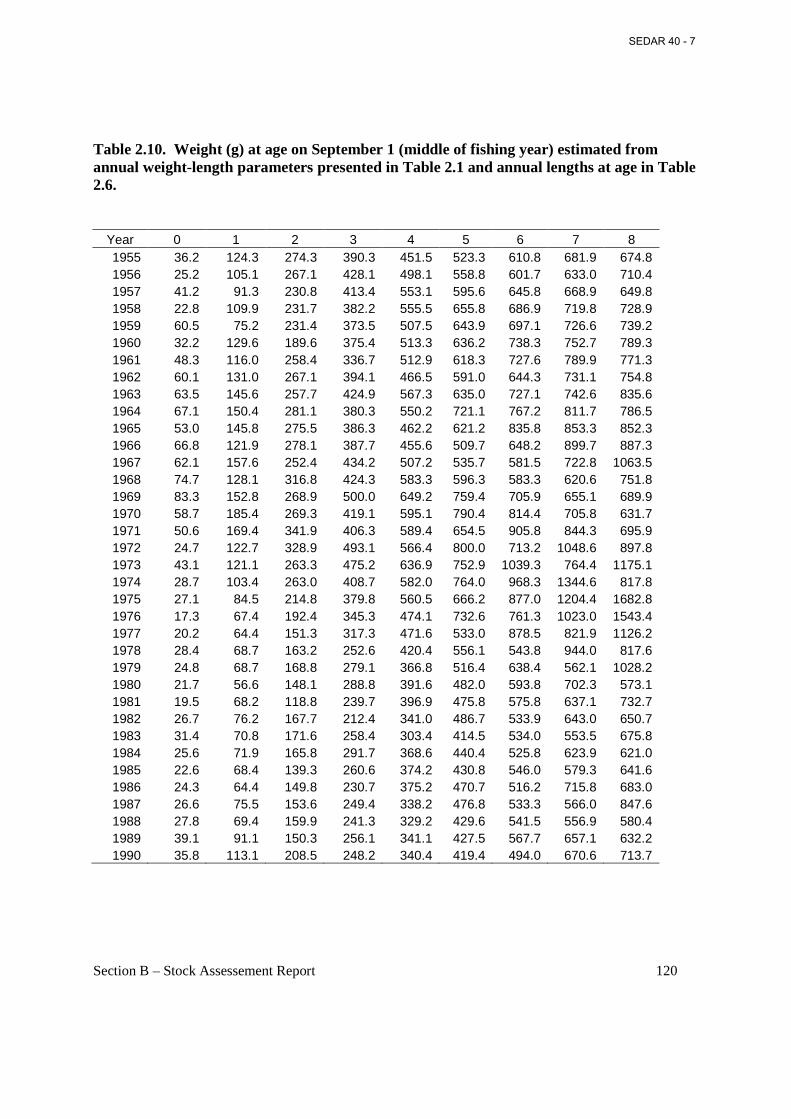
Section B – Stock Assessement Report 120
Table 2.10. Weight (g) at age on September 1 (middle of fishing year) estimated from annual weight-length parameters presented in Table 2.1 and annual lengths at age in Table 2.6.
Year 0 1 2 3 4 5 6 7 8 1955 36.2 124.3 274.3 390.3 451.5 523.3 610.8 681.9 674.8 1956 25.2 105.1 267.1 428.1 498.1 558.8 601.7 633.0 710.4 1957 41.2 91.3 230.8 413.4 553.1 595.6 645.8 668.9 649.8 1958 22.8 109.9 231.7 382.2 555.5 655.8 686.9 719.8 728.9 1959 60.5 75.2 231.4 373.5 507.5 643.9 697.1 726.6 739.2 1960 32.2 129.6 189.6 375.4 513.3 636.2 738.3 752.7 789.3 1961 48.3 116.0 258.4 336.7 512.9 618.3 727.6 789.9 771.3 1962 60.1 131.0 267.1 394.1 466.5 591.0 644.3 731.1 754.8 1963 63.5 145.6 257.7 424.9 567.3 635.0 727.1 742.6 835.6 1964 67.1 150.4 281.1 380.3 550.2 721.1 767.2 811.7 786.5 1965 53.0 145.8 275.5 386.3 462.2 621.2 835.8 853.3 852.3 1966 66.8 121.9 278.1 387.7 455.6 509.7 648.2 899.7 887.3 1967 62.1 157.6 252.4 434.2 507.2 535.7 581.5 722.8 1063.5 1968 74.7 128.1 316.8 424.3 583.3 596.3 583.3 620.6 751.8 1969 83.3 152.8 268.9 500.0 649.2 759.4 705.9 655.1 689.9 1970 58.7 185.4 269.3 419.1 595.1 790.4 814.4 705.8 631.7 1971 50.6 169.4 341.9 406.3 589.4 654.5 905.8 844.3 695.9 1972 24.7 122.7 328.9 493.1 566.4 800.0 713.2 1048.6 897.8 1973 43.1 121.1 263.3 475.2 636.9 752.9 1039.3 764.4 1175.1 1974 28.7 103.4 263.0 408.7 582.0 764.0 968.3 1344.6 817.8 1975 27.1 84.5 214.8 379.8 560.5 666.2 877.0 1204.4 1682.8 1976 17.3 67.4 192.4 345.3 474.1 732.6 761.3 1023.0 1543.4 1977 20.2 64.4 151.3 317.3 471.6 533.0 878.5 821.9 1126.2 1978 28.4 68.7 163.2 252.6 420.4 556.1 543.8 944.0 817.6 1979 24.8 68.7 168.8 279.1 366.8 516.4 638.4 562.1 1028.2 1980 21.7 56.6 148.1 288.8 391.6 482.0 593.8 702.3 573.1 1981 19.5 68.2 118.8 239.7 396.9 475.8 575.8 637.1 732.7 1982 26.7 76.2 167.7 212.4 341.0 486.7 533.9 643.0 650.7 1983 31.4 70.8 171.6 258.4 303.4 414.5 534.0 553.5 675.8 1984 25.6 71.9 165.8 291.7 368.6 440.4 525.8 623.9 621.0 1985 22.6 68.4 139.3 260.6 374.2 430.8 546.0 579.3 641.6 1986 24.3 64.4 149.8 230.7 375.2 470.7 516.2 715.8 683.0 1987 26.6 75.5 153.6 249.4 338.2 476.8 533.3 566.0 847.6 1988 27.8 69.4 159.9 241.3 329.2 429.6 541.5 556.9 580.4 1989 39.1 91.1 150.3 256.1 341.1 427.5 567.7 657.1 632.2 1990 35.8 113.1 208.5 248.2 340.4 419.4 494.0 670.6 713.7
SEDAR 40 - 7
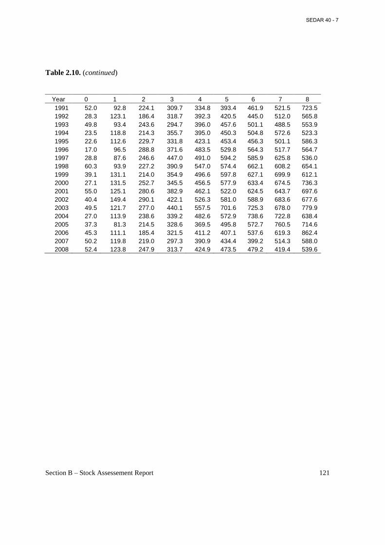
Section B – Stock Assessement Report 121
Table 2.10. (continued)
Year 0 1 2 3 4 5 6 7 8 1991 52.0 92.8 224.1 309.7 334.8 393.4 461.9 521.5 723.5 1992 28.3 123.1 186.4 318.7 392.3 420.5 445.0 512.0 565.8 1993 49.8 93.4 243.6 294.7 396.0 457.6 501.1 488.5 553.9 1994 23.5 118.8 214.3 355.7 395.0 450.3 504.8 572.6 523.3 1995 22.6 112.6 229.7 331.8 423.1 453.4 456.3 501.1 586.3 1996 17.0 96.5 288.8 371.6 483.5 529.8 564.3 517.7 564.7 1997 28.8 87.6 246.6 447.0 491.0 594.2 585.9 625.8 536.0 1998 60.3 93.9 227.2 390.9 547.0 574.4 662.1 608.2 654.1 1999 39.1 131.1 214.0 354.9 496.6 597.8 627.1 699.9 612.1 2000 27.1 131.5 252.7 345.5 456.5 577.9 633.4 674.5 736.3 2001 55.0 125.1 280.6 382.9 462.1 522.0 624.5 643.7 697.6 2002 40.4 149.4 290.1 422.1 526.3 581.0 588.9 683.6 677.6 2003 49.5 121.7 277.0 440.1 557.5 701.6 725.3 678.0 779.9 2004 27.0 113.9 238.6 339.2 482.6 572.9 738.6 722.8 638.4 2005 37.3 81.3 214.5 328.6 369.5 495.8 572.7 760.5 714.6 2006 45.3 111.1 185.4 321.5 411.2 407.1 537.6 619.3 862.4 2007 50.2 119.8 219.0 297.3 390.9 434.4 399.2 514.3 588.0 2008 52.4 123.8 247.9 313.7 424.9 473.5 479.2 419.4 539.6
SEDAR 40 - 7
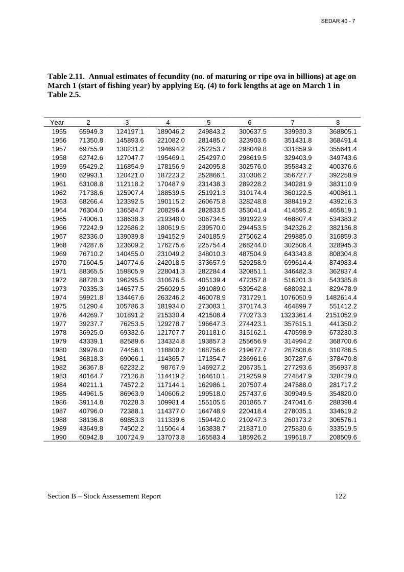
Section B – Stock Assessement Report 122
Table 2.11. Annual estimates of fecundity (no. of maturing or ripe ova in billions) at age on March 1 (start of fishing year) by applying Eq. (4) to fork lengths at age on March 1 in Table 2.5. Year 2 3 4 5 6 7 8 1955 65949.3 124197.1 189046.2 249843.2 300637.5 339930.3 368805.1 1956 71350.8 145893.6 221082.0 281485.0 323903.6 351431.8 368491.4 1957 69755.9 130231.2 194694.2 252253.7 298049.8 331859.9 355641.4 1958 62742.6 127047.7 195469.1 254297.0 298619.5 329403.9 349743.6 1959 65429.2 116854.9 178156.9 242095.8 302576.0 355843.2 400376.6 1960 62993.1 120421.0 187223.2 252866.1 310306.2 356727.7 392258.9 1961 63108.8 112118.2 170487.9 231438.3 289228.2 340281.9 383110.9 1962 71738.6 125907.4 188539.5 251921.3 310174.4 360122.5 400861.1 1963 68266.4 123392.5 190115.2 260675.8 328248.8 388419.2 439216.3 1964 76304.0 136584.7 208296.4 282833.5 353041.4 414595.2 465819.1 1965 74006.1 138638.3 219348.0 306734.5 391922.9 468807.4 534383.2 1966 72242.9 122686.2 180619.5 239570.0 294453.5 342326.2 382136.8 1967 82336.0 139039.8 194152.9 240185.9 275062.4 299885.0 316859.3 1968 74287.6 123609.2 176275.6 225754.4 268244.0 302506.4 328945.3 1969 76710.2 140455.0 231049.2 348010.3 487504.9 643343.8 808304.8 1970 71604.5 140774.6 242018.5 373657.9 529258.9 699614.4 874983.4 1971 88365.5 159805.9 228041.3 282284.4 320851.1 346482.3 362837.4 1972 88728.3 196295.5 310676.5 405139.4 472357.8 516201.3 543385.8 1973 70335.3 146577.5 256029.5 391089.0 539542.8 688932.1 829478.9 1974 59921.8 134467.6 263246.2 460078.9 731729.1 1076050.9 1482614.4 1975 51290.4 105786.3 181934.0 273083.1 370174.3 464899.7 551412.2 1976 44269.7 101891.2 215330.4 421508.4 770273.3 1323361.4 2151052.9 1977 39237.7 76253.5 129278.7 196647.3 274423.1 357615.1 441350.2 1978 36925.0 69332.6 121707.7 201181.0 315162.1 470598.9 673230.3 1979 43339.1 82589.6 134324.8 193857.3 255656.9 314994.2 368700.6 1980 39976.0 74456.1 118800.2 168756.6 219677.7 267808.6 310786.5 1981 36818.3 69066.1 114365.7 171354.7 236961.6 307287.6 378470.8 1982 36367.8 62232.2 98767.9 146927.2 206735.1 277293.6 356937.8 1983 40164.7 72126.8 114419.2 164610.1 219259.9 274847.9 328429.0 1984 40211.1 74572.2 117144.1 162986.1 207507.4 247588.0 281717.2 1985 44961.5 86963.9 140606.2 199518.0 257437.6 309949.5 354820.0 1986 39114.8 70228.3 109981.4 155105.5 201865.7 247041.6 288398.4 1987 40796.0 72388.1 114377.0 164748.9 220418.4 278035.1 334619.2 1988 38136.8 69853.3 111339.6 159442.0 210247.3 260173.2 306576.1 1989 43649.8 74502.2 115064.4 163838.7 218371.0 275830.6 333519.5 1990 60942.8 100724.9 137073.8 165583.4 185926.2 199618.7 208509.6
SEDAR 40 - 7
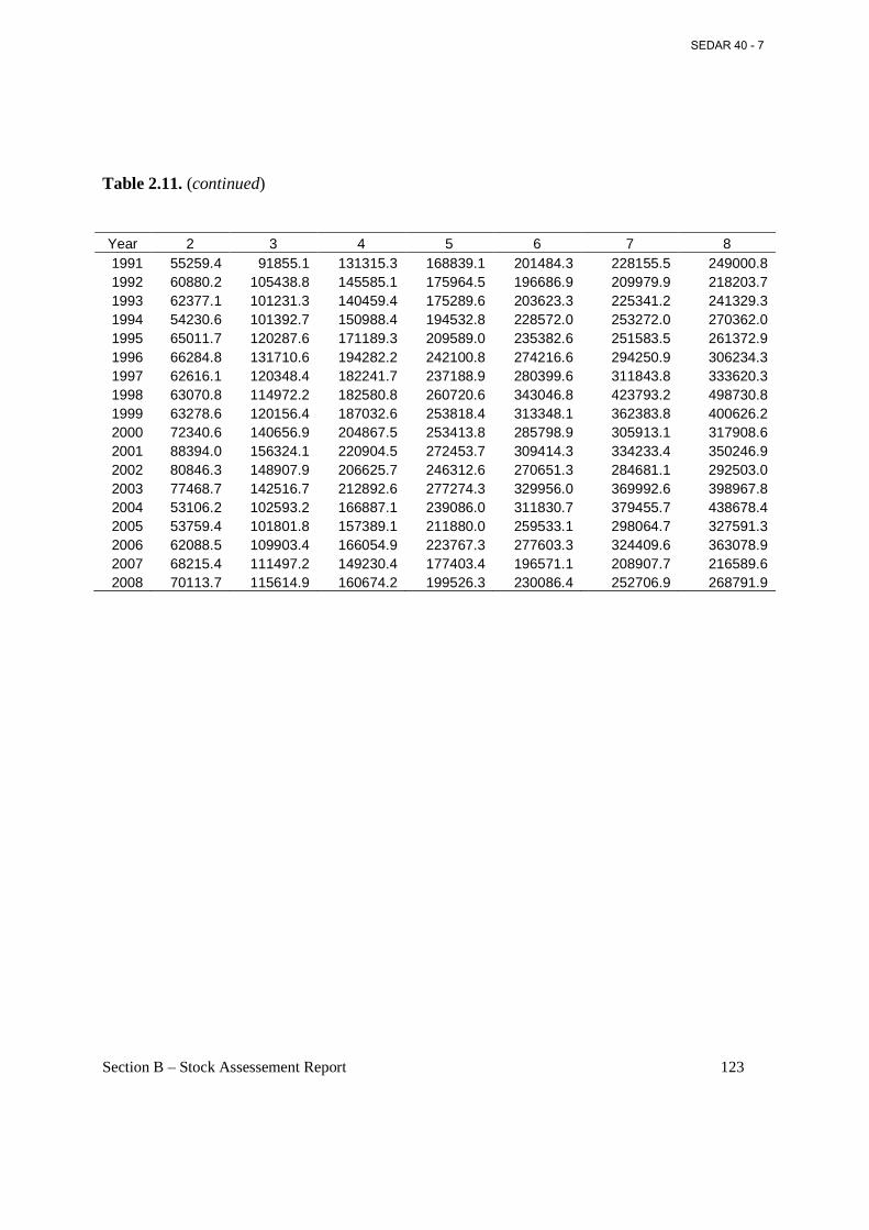
Section B – Stock Assessement Report 123
Table 2.11. (continued) Year 2 3 4 5 6 7 8 1991 55259.4 91855.1 131315.3 168839.1 201484.3 228155.5 249000.8 1992 60880.2 105438.8 145585.1 175964.5 196686.9 209979.9 218203.7 1993 62377.1 101231.3 140459.4 175289.6 203623.3 225341.2 241329.3 1994 54230.6 101392.7 150988.4 194532.8 228572.0 253272.0 270362.0 1995 65011.7 120287.6 171189.3 209589.0 235382.6 251583.5 261372.9 1996 66284.8 131710.6 194282.2 242100.8 274216.6 294250.9 306234.3 1997 62616.1 120348.4 182241.7 237188.9 280399.6 311843.8 333620.3 1998 63070.8 114972.2 182580.8 260720.6 343046.8 423793.2 498730.8 1999 63278.6 120156.4 187032.6 253818.4 313348.1 362383.8 400626.2 2000 72340.6 140656.9 204867.5 253413.8 285798.9 305913.1 317908.6 2001 88394.0 156324.1 220904.5 272453.7 309414.3 334233.4 350246.9 2002 80846.3 148907.9 206625.7 246312.6 270651.3 284681.1 292503.0 2003 77468.7 142516.7 212892.6 277274.3 329956.0 369992.6 398967.8 2004 53106.2 102593.2 166887.1 239086.0 311830.7 379455.7 438678.4 2005 53759.4 101801.8 157389.1 211880.0 259533.1 298064.7 327591.3 2006 62088.5 109903.4 166054.9 223767.3 277603.3 324409.6 363078.9 2007 68215.4 111497.2 149230.4 177403.4 196571.1 208907.7 216589.6 2008 70113.7 115614.9 160674.2 199526.3 230086.4 252706.9 268791.9
SEDAR 40 - 7
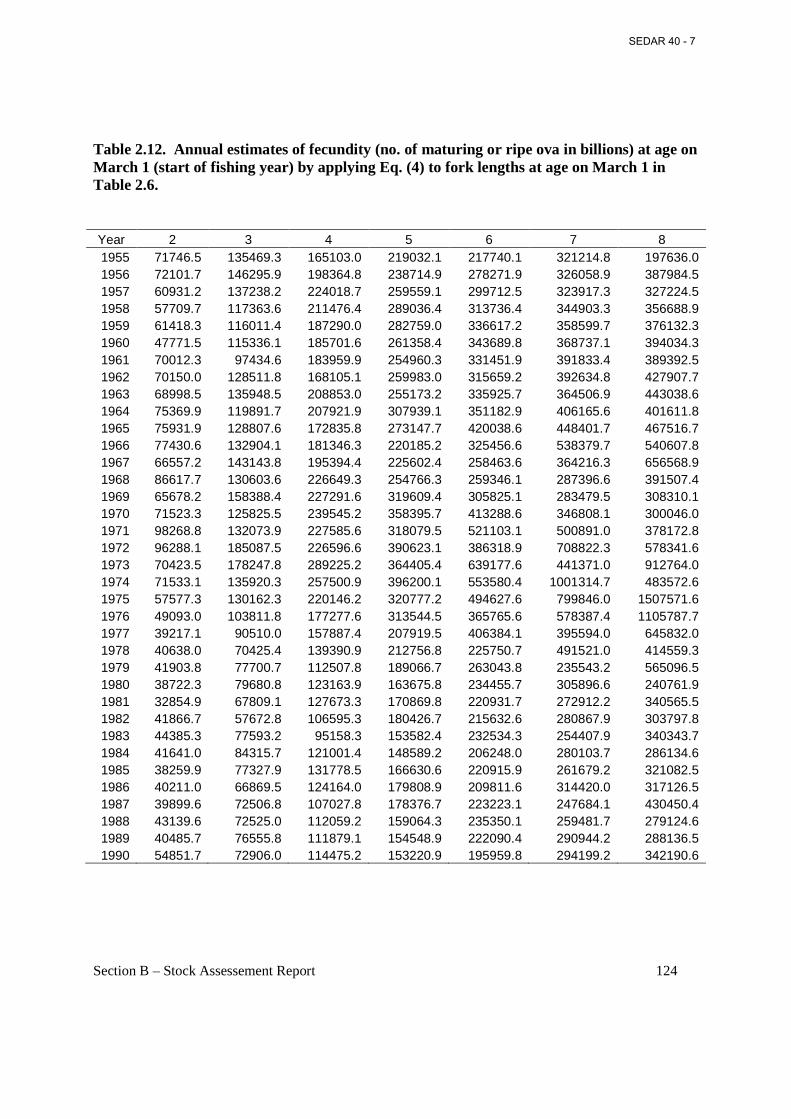
Section B – Stock Assessement Report 124
Table 2.12. Annual estimates of fecundity (no. of maturing or ripe ova in billions) at age on March 1 (start of fishing year) by applying Eq. (4) to fork lengths at age on March 1 in Table 2.6. Year 2 3 4 5 6 7 8 1955 71746.5 135469.3 165103.0 219032.1 217740.1 321214.8 197636.0 1956 72101.7 146295.9 198364.8 238714.9 278271.9 326058.9 387984.5 1957 60931.2 137238.2 224018.7 259559.1 299712.5 323917.3 327224.5 1958 57709.7 117363.6 211476.4 289036.4 313736.4 344903.3 356688.9 1959 61418.3 116011.4 187290.0 282759.0 336617.2 358599.7 376132.3 1960 47771.5 115336.1 185701.6 261358.4 343689.8 368737.1 394034.3 1961 70012.3 97434.6 183959.9 254960.3 331451.9 391833.4 389392.5 1962 70150.0 128511.8 168105.1 259983.0 315659.2 392634.8 427907.7 1963 68998.5 135948.5 208853.0 255173.2 335925.7 364506.9 443038.6 1964 75369.9 119891.7 207921.9 307939.1 351182.9 406165.6 401611.8 1965 75931.9 128807.6 172835.8 273147.7 420038.6 448401.7 467516.7 1966 77430.6 132904.1 181346.3 220185.2 325456.6 538379.7 540607.8 1967 66557.2 143143.8 195394.4 225602.4 258463.6 364216.3 656568.9 1968 86617.7 130603.6 226649.3 254766.3 259346.1 287396.6 391507.4 1969 65678.2 158388.4 227291.6 319609.4 305825.1 283479.5 308310.1 1970 71523.3 125825.5 239545.2 358395.7 413288.6 346808.1 300046.0 1971 98268.8 132073.9 227585.6 318079.5 521103.1 500891.0 378172.8 1972 96288.1 185087.5 226596.6 390623.1 386318.9 708822.3 578341.6 1973 70423.5 178247.8 289225.2 364405.4 639177.6 441371.0 912764.0 1974 71533.1 135920.3 257500.9 396200.1 553580.4 1001314.7 483572.6 1975 57577.3 130162.3 220146.2 320777.2 494627.6 799846.0 1507571.6 1976 49093.0 103811.8 177277.6 313544.5 365765.6 578387.4 1105787.7 1977 39217.1 90510.0 157887.4 207919.5 406384.1 395594.0 645832.0 1978 40638.0 70425.4 139390.9 212756.8 225750.7 491521.0 414559.3 1979 41903.8 77700.7 112507.8 189066.7 263043.8 235543.2 565096.5 1980 38722.3 79680.8 123163.9 163675.8 234455.7 305896.6 240761.9 1981 32854.9 67809.1 127673.3 170869.8 220931.7 272912.2 340565.5 1982 41866.7 57672.8 106595.3 180426.7 215632.6 280867.9 303797.8 1983 44385.3 77593.2 95158.3 153582.4 232534.3 254407.9 340343.7 1984 41641.0 84315.7 121001.4 148589.2 206248.0 280103.7 286134.6 1985 38259.9 77327.9 131778.5 166630.6 220915.9 261679.2 321082.5 1986 40211.0 66869.5 124164.0 179808.9 209811.6 314420.0 317126.5 1987 39899.6 72506.8 107027.8 178376.7 223223.1 247684.1 430450.4 1988 43139.6 72525.0 112059.2 159064.3 235350.1 259481.7 279124.6 1989 40485.7 76555.8 111879.1 154548.9 222090.4 290944.2 288136.5 1990 54851.7 72906.0 114475.2 153220.9 195959.8 294199.2 342190.6
SEDAR 40 - 7
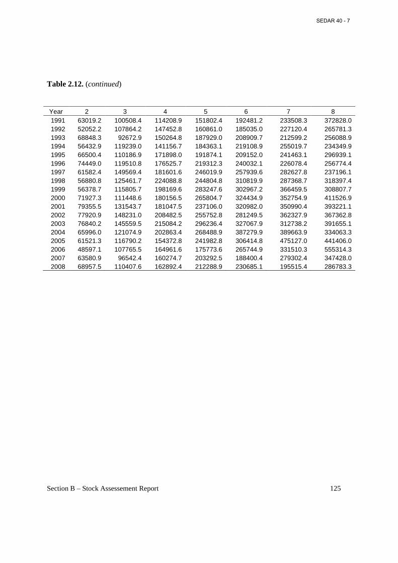
Section B – Stock Assessement Report 125
Table 2.12. (continued) Year 2 3 4 5 6 7 8 1991 63019.2 100508.4 114208.9 151802.4 192481.2 233508.3 372828.0 1992 52052.2 107864.2 147452.8 160861.0 185035.0 227120.4 265781.3 1993 68848.3 92672.9 150264.8 187929.0 208909.7 212599.2 256088.9 1994 56432.9 119239.0 141156.7 184363.1 219108.9 255019.7 234349.9 1995 66500.4 110186.9 171898.0 191874.1 209152.0 241463.1 296939.1 1996 74449.0 119510.8 176525.7 219312.3 240032.1 226078.4 256774.4 1997 61582.4 149569.4 181601.6 246019.9 257939.6 282627.8 237196.1 1998 56880.8 125461.7 224088.8 244804.8 310819.9 287368.7 318397.4 1999 56378.7 115805.7 198169.6 283247.6 302967.2 366459.5 308807.7 2000 71927.3 111448.6 180156.5 265804.7 324434.9 352754.9 411526.9 2001 79355.5 131543.7 181047.5 237106.0 320982.0 350990.4 393221.1 2002 77920.9 148231.0 208482.5 255752.8 281249.5 362327.9 367362.8 2003 76840.2 145559.5 215084.2 296236.4 327067.9 312738.2 391655.1 2004 65996.0 121074.9 202863.4 268488.9 387279.9 389663.9 334063.3 2005 61521.3 116790.2 154372.8 241982.8 306414.8 475127.0 441406.0 2006 48597.1 107765.5 164961.6 175773.6 265744.9 331510.3 555314.3 2007 63580.9 96542.4 160274.7 203292.5 188400.4 279302.4 347428.0 2008 68957.5 110407.6 162892.4 212288.9 230685.1 195515.4 286783.3
SEDAR 40 - 7
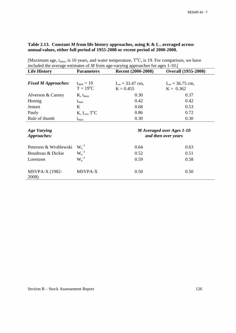
Section B – Stock Assessement Report 126
Table 2.13. Constant M from life history approaches, using K & L∞ averaged across annual values, either full period of 1955-2008 or recent period of 2000-2008. [Maximum age, tmax, is 10 years, and water temperature, ToC, is 19. For comparison, we have included the average estimates of M from age-varying approaches for ages 1-10.[ Life History Parameters Recent (2000-2008) Overall (1955-2008) Fixed M Approaches: tmax = 10
T = 19oC L∞ = 33.47 cm, K = 0.455
L∞ = 36.75 cm, K = 0.362
Alverson & Carney K, tmax 0.30 0.37 Hoenig tmax 0.42 0.42 Jensen K 0.68 0.53 Pauly K, L∞, ToC 0.86 0.72 Rule of thumb tmax 0.30 0.30 Age Varying Approaches:
M Averaged over Ages 1-10 and then over years
Peterson & Wroblewski Wa
-1 0.64 0.63 Boudreau & Dickie Wa
-1 0.52 0.51 Lorenzen Wa
-1 0.59 0.58 MSVPA-X (1982-2008)
MSVPA-X 0.50 0.50
SEDAR 40 - 7
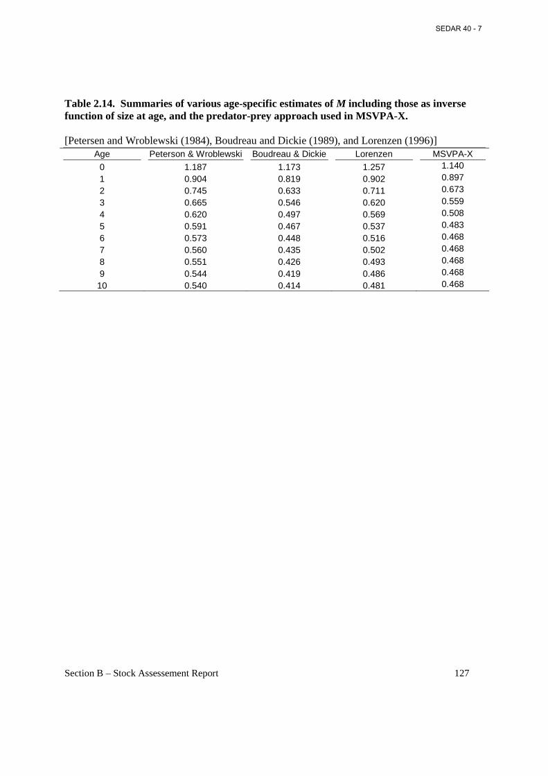
Section B – Stock Assessement Report 127
Table 2.14. Summaries of various age-specific estimates of M including those as inverse function of size at age, and the predator-prey approach used in MSVPA-X. [Petersen and Wroblewski (1984), Boudreau and Dickie (1989), and Lorenzen (1996)]
Age Peterson & Wroblewski Boudreau & Dickie Lorenzen MSVPA-X
0 1.187 1.173 1.257 1.140
1 0.904 0.819 0.902 0.897
2 0.745 0.633 0.711 0.673
3 0.665 0.546 0.620 0.559
4 0.620 0.497 0.569 0.508
5 0.591 0.467 0.537 0.483
6 0.573 0.448 0.516 0.468
7 0.560 0.435 0.502 0.468
8 0.551 0.426 0.493 0.468
9 0.544 0.419 0.486 0.468
10 0.540 0.414 0.481 0.468
SEDAR 40 - 7
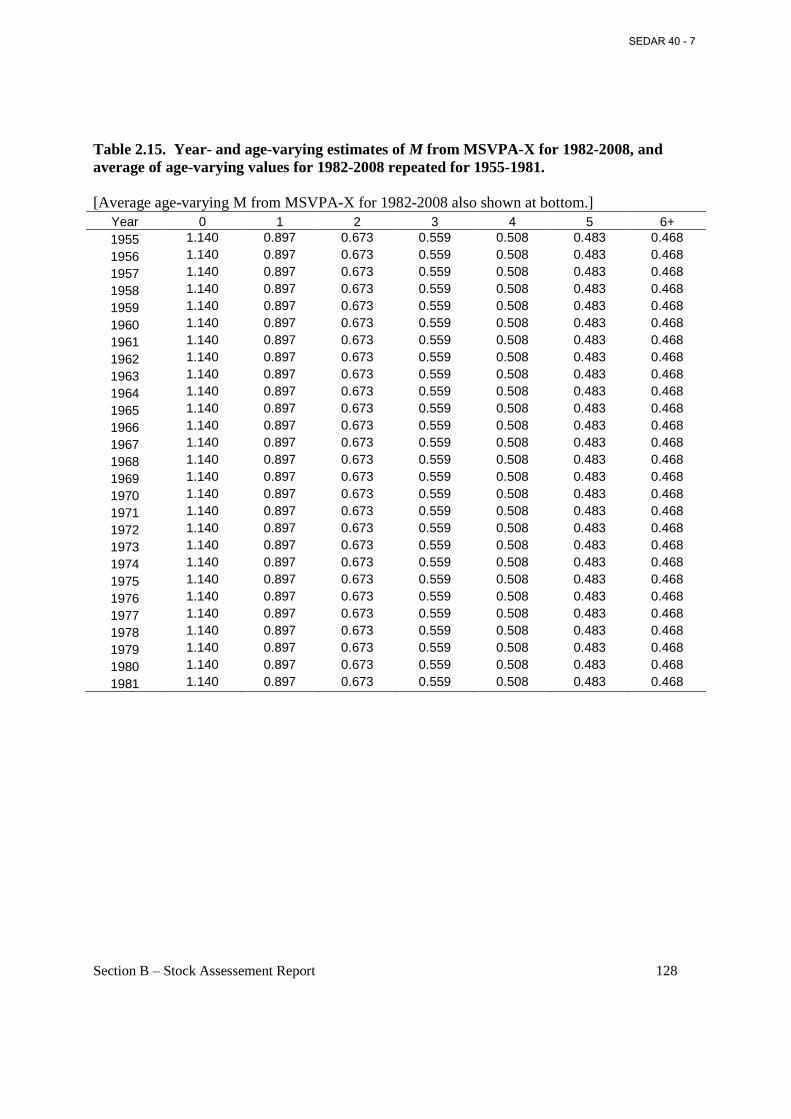
Section B – Stock Assessement Report 128
Table 2.15. Year- and age-varying estimates of M from MSVPA-X for 1982-2008, and average of age-varying values for 1982-2008 repeated for 1955-1981. [Average age-varying M from MSVPA-X for 1982-2008 also shown at bottom.]
Year 0 1 2 3 4 5 6+ 1955 1.140 0.897 0.673 0.559 0.508 0.483 0.468
1956 1.140 0.897 0.673 0.559 0.508 0.483 0.468
1957 1.140 0.897 0.673 0.559 0.508 0.483 0.468
1958 1.140 0.897 0.673 0.559 0.508 0.483 0.468
1959 1.140 0.897 0.673 0.559 0.508 0.483 0.468
1960 1.140 0.897 0.673 0.559 0.508 0.483 0.468
1961 1.140 0.897 0.673 0.559 0.508 0.483 0.468
1962 1.140 0.897 0.673 0.559 0.508 0.483 0.468
1963 1.140 0.897 0.673 0.559 0.508 0.483 0.468
1964 1.140 0.897 0.673 0.559 0.508 0.483 0.468
1965 1.140 0.897 0.673 0.559 0.508 0.483 0.468
1966 1.140 0.897 0.673 0.559 0.508 0.483 0.468
1967 1.140 0.897 0.673 0.559 0.508 0.483 0.468
1968 1.140 0.897 0.673 0.559 0.508 0.483 0.468
1969 1.140 0.897 0.673 0.559 0.508 0.483 0.468
1970 1.140 0.897 0.673 0.559 0.508 0.483 0.468
1971 1.140 0.897 0.673 0.559 0.508 0.483 0.468
1972 1.140 0.897 0.673 0.559 0.508 0.483 0.468
1973 1.140 0.897 0.673 0.559 0.508 0.483 0.468
1974 1.140 0.897 0.673 0.559 0.508 0.483 0.468
1975 1.140 0.897 0.673 0.559 0.508 0.483 0.468
1976 1.140 0.897 0.673 0.559 0.508 0.483 0.468
1977 1.140 0.897 0.673 0.559 0.508 0.483 0.468
1978 1.140 0.897 0.673 0.559 0.508 0.483 0.468
1979 1.140 0.897 0.673 0.559 0.508 0.483 0.468
1980 1.140 0.897 0.673 0.559 0.508 0.483 0.468
1981 1.140 0.897 0.673 0.559 0.508 0.483 0.468
SEDAR 40 - 7
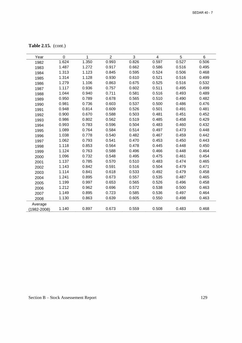
Section B – Stock Assessement Report 129
Table 2.15. (cont.)
Year 0 1 2 3 4 5 6 1982 1.624 1.350 0.993 0.826 0.597 0.527 0.506
1983 1.487 1.272 0.917 0.662 0.586 0.516 0.495
1984 1.313 1.123 0.845 0.595 0.524 0.506 0.468
1985 1.314 1.128 0.930 0.610 0.521 0.516 0.499
1986 1.279 1.106 0.863 0.675 0.525 0.516 0.532
1987 1.117 0.936 0.757 0.602 0.511 0.495 0.499
1988 1.044 0.940 0.711 0.581 0.516 0.493 0.489
1989 0.950 0.789 0.678 0.565 0.510 0.490 0.482
1990 0.981 0.736 0.603 0.537 0.500 0.486 0.476
1991 0.948 0.814 0.609 0.526 0.501 0.491 0.481
1992 0.900 0.670 0.588 0.503 0.481 0.451 0.452
1993 0.986 0.802 0.562 0.519 0.485 0.458 0.429
1994 0.993 0.783 0.596 0.504 0.483 0.460 0.432
1995 1.089 0.764 0.584 0.514 0.497 0.473 0.448
1996 1.038 0.778 0.540 0.482 0.467 0.459 0.442
1997 1.062 0.793 0.541 0.470 0.453 0.450 0.443
1998 1.118 0.853 0.564 0.478 0.445 0.448 0.450
1999 1.124 0.763 0.588 0.496 0.466 0.448 0.464
2000 1.096 0.732 0.548 0.495 0.475 0.461 0.454
2001 1.137 0.785 0.570 0.510 0.483 0.474 0.465
2002 1.143 0.842 0.591 0.516 0.504 0.479 0.471
2003 1.114 0.841 0.618 0.533 0.492 0.479 0.458
2004 1.241 0.895 0.673 0.557 0.535 0.487 0.465
2005 1.199 0.997 0.653 0.565 0.526 0.496 0.458
2006 1.212 0.962 0.696 0.572 0.538 0.500 0.463
2007 1.149 0.895 0.723 0.585 0.536 0.497 0.464
2008 1.130 0.863 0.639 0.605 0.550 0.498 0.463
Average (1982-2008) 1.140 0.897 0.673 0.559 0.508 0.483 0.468
SEDAR 40 - 7
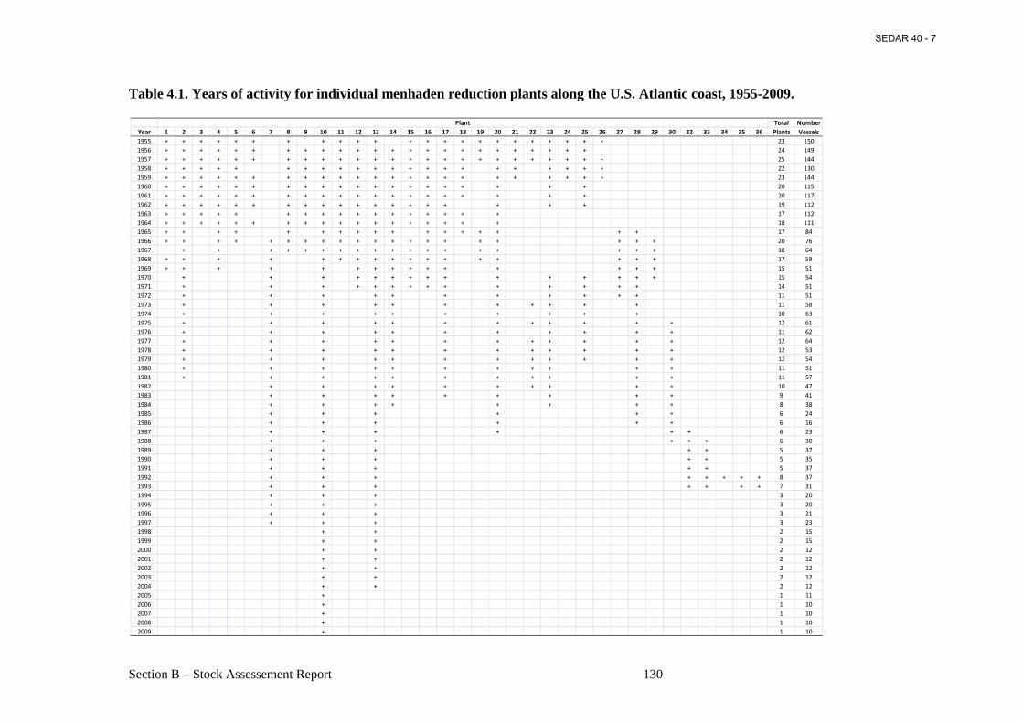
Section B – Stock Assessement Report 130
Table 4.1. Years of activity for individual menhaden reduction plants along the U.S. Atlantic coast, 1955-2009.
Total Number
Year 1 2 3 4 5 6 7 8 9 10 11 12 13 14 15 16 17 18 19 20 21 22 23 24 25 26 27 28 29 30 32 33 34 35 36 Plants Vessels
1955 + + + + + + + + + + + + + + + + + + + + + + + 23 150
1956 + + + + + + + + + + + + + + + + + + + + + + + + 24 149
1957 + + + + + + + + + + + + + + + + + + + + + + + + + 25 144
1958 + + + + + + + + + + + + + + + + + + + + + + 22 130
1959 + + + + + + + + + + + + + + + + + + + + + + + 23 144
1960 + + + + + + + + + + + + + + + + + + + + 20 115
1961 + + + + + + + + + + + + + + + + + + + + 20 117
1962 + + + + + + + + + + + + + + + + + + + 19 112
1963 + + + + + + + + + + + + + + + + + 17 112
1964 + + + + + + + + + + + + + + + + + + 18 111
1965 + + + + + + + + + + + + + + + + + 17 84
1966 + + + + + + + + + + + + + + + + + + + + 20 76
1967 + + + + + + + + + + + + + + + + + + 18 64
1968 + + + + + + + + + + + + + + + + + 17 59
1969 + + + + + + + + + + + + + + + 15 51
1970 + + + + + + + + + + + + + + + 15 54
1971 + + + + + + + + + + + + + + 14 51
1972 + + + + + + + + + + + 11 51
1973 + + + + + + + + + + + 11 58
1974 + + + + + + + + + + 10 63
1975 + + + + + + + + + + + + 12 61
1976 + + + + + + + + + + + 11 62
1977 + + + + + + + + + + + + 12 64
1978 + + + + + + + + + + + + 12 53
1979 + + + + + + + + + + + + 12 54
1980 + + + + + + + + + + + 11 51
1981 + + + + + + + + + + + 11 57
1982 + + + + + + + + + + 10 47
1983 + + + + + + + + + 9 41
1984 + + + + + + + + 8 38
1985 + + + + + + 6 24
1986 + + + + + + 6 16
1987 + + + + + + 6 23
1988 + + + + + + 6 30
1989 + + + + + 5 37
1990 + + + + + 5 35
1991 + + + + + 5 37
1992 + + + + + + + + 8 37
1993 + + + + + + + 7 31
1994 + + + 3 20
1995 + + + 3 20
1996 + + + 3 21
1997 + + + 3 23
1998 + + 2 15
1999 + + 2 15
2000 + + 2 12
2001 + + 2 12
2002 + + 2 12
2003 + + 2 12
2004 + + 2 12
2005 + 1 11
2006 + 1 10
2007 + 1 10
2008 + 1 10
2009 + 1 10
Plant
SEDAR 40 - 7
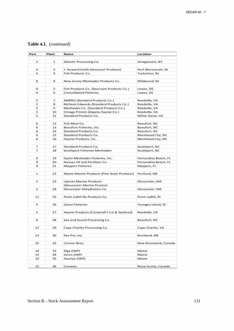
Section B – Stock Assessement Report 131
Table 4.1. (continued)
Port Plant Name Location
3 1 Atlantic Processing Co. Amagansett, NY
4 2 J. Howard Smith (Seacoast Products) Port Monmouth, NJ
4 3 Fish Products Co. Tuckerton, NJ
8 4 New Jersey Menhaden Products Co. Wildwood, NJ
0 5 Fish Products Co. (Seacoast Products Co.) Lewes, DE
0 6 Consolidated Fisheries Lewes, DE
5 7 AMPRO (Standard Products Co.) Reedville, VA
5 8 McNeal-Edwards (Standard Products Co.) Reedville, VA
5 9 Menhaden Co. (Standard Products Co.) Reedville, VA
5 10 Omega Protein (Zapata Haynie Co.) Reedville, VA
5 11 Standard Products Co. White Stone, VA
6 12 Fish Meal Co. Beaufort, NC
6 13 Beaufort Fisheries, Inc. Beaufort, NC
6 14 Standard Products Co. Beaufort, NC
6 15 Standard Products Co. Morehead City, NC
6 16 Haynie Products, Inc. Morehead City, NC
7 17 Standard Products Co. Southport, NC
7 18 Southport Fisheries Menhaden Southport, NC
9 19 Quinn Menhaden Fisheries, Inc. Fernandina Beach, FL
9 20 Nassau Oil and Fertilizer Co. Fernandina Beach, FL
9 21 Mayport Fisheries Mayport, FL
1 22 Maine Marine Products (Pine State Products) Portland, ME
2 23 Lipman Marine Products Gloucester, MA
(Gloucester Marine Protein)
2 24 Gloucester Dehydration Co. Gloucester, MA
11 25 Point Judith By Products Co. Point Judith, RI
9 26 Quinn Fisheries Younges Island, SC
5 27 Haynie Products (Cockerall's Ice & Seafood) Reedville, VA
6 28 Sea and Sound Processing Co. Beaufort, NC
12 29 Cape Charles Processing Co. Cape Charles, VA
13 30 Sea Pro, Inc. Rockland, ME
15 32 Connor Bros. New Brunswick, Canada
14 33 Riga (IWP) Maine
14 34 Vares (IWP) Maine
14 35 Dauriya (IWP) Maine
15 36 Comeau Nova Scotia, Canada
SEDAR 40 - 7
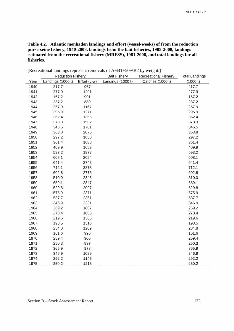
Section B – Stock Assessement Report 132
Table 4.2. Atlantic menhaden landings and effort (vessel-weeks) of from the reduction purse-seine fishery, 1940-2008, landings from the bait fisheries, 1985-2008, landings estimated from the recreational fishery (MRFSS), 1981-2008, and total landings for all fisheries. [Recreational landings represent removals of A+B1+50%B2 by weight.]
Reduction Fishery Bait Fishery Recreational Fishery Total Landings Year Landings (1000 t) Effort (v-w) Landings (1000 t) Catches (1000 t) (1000 t) 1940 217.7 967 217.7 1941 277.9 1291 277.9 1942 167.2 991 167.2 1943 237.2 889 237.2 1944 257.9 1167 257.9 1945 295.9 1271 295.9 1946 362.4 1365 362.4 1947 378.3 1582 378.3 1948 346.5 1781 346.5 1949 363.8 2076 363.8 1950 297.2 1650 297.2 1951 361.4 1686 361.4 1952 409.9 1653 409.9 1953 593.2 1972 593.2 1954 608.1 2094 608.1 1955 641.4 2748 641.4 1956 712.1 2878 712.1 1957 602.8 2775 602.8 1958 510.0 2343 510.0 1959 659.1 2847 659.1 1960 529.8 2097 529.8 1961 575.9 2371 575.9 1962 537.7 2351 537.7 1963 346.9 2331 346.9 1964 269.2 1807 269.2 1965 273.4 1805 273.4 1966 219.6 1386 219.6 1967 193.5 1316 193.5 1968 234.8 1209 234.8 1969 161.6 995 161.6 1970 259.4 906 259.4 1971 250.3 897 250.3 1972 365.9 973 365.9 1973 346.9 1099 346.9 1974 292.2 1145 292.2 1975 250.2 1218 250.2
SEDAR 40 - 7
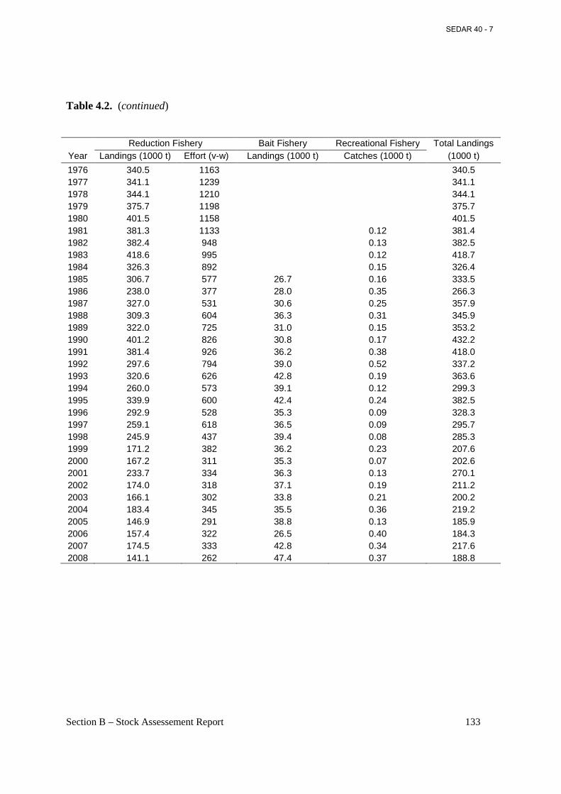
Section B – Stock Assessement Report 133
Table 4.2. (continued)
Reduction Fishery Bait Fishery Recreational Fishery Total Landings Year Landings (1000 t) Effort (v-w) Landings (1000 t) Catches (1000 t) (1000 t)
1976 340.5 1163 340.5 1977 341.1 1239 341.1 1978 344.1 1210 344.1 1979 375.7 1198 375.7 1980 401.5 1158 401.5 1981 381.3 1133 0.12 381.4 1982 382.4 948 0.13 382.5 1983 418.6 995 0.12 418.7 1984 326.3 892 0.15 326.4 1985 306.7 577 26.7 0.16 333.5 1986 238.0 377 28.0 0.35 266.3 1987 327.0 531 30.6 0.25 357.9 1988 309.3 604 36.3 0.31 345.9 1989 322.0 725 31.0 0.15 353.2 1990 401.2 826 30.8 0.17 432.2 1991 381.4 926 36.2 0.38 418.0 1992 297.6 794 39.0 0.52 337.2 1993 320.6 626 42.8 0.19 363.6 1994 260.0 573 39.1 0.12 299.3 1995 339.9 600 42.4 0.24 382.5 1996 292.9 528 35.3 0.09 328.3 1997 259.1 618 36.5 0.09 295.7 1998 245.9 437 39.4 0.08 285.3 1999 171.2 382 36.2 0.23 207.6 2000 167.2 311 35.3 0.07 202.6 2001 233.7 334 36.3 0.13 270.1 2002 174.0 318 37.1 0.19 211.2 2003 166.1 302 33.8 0.21 200.2 2004 183.4 345 35.5 0.36 219.2 2005 146.9 291 38.8 0.13 185.9 2006 157.4 322 26.5 0.40 184.3 2007 174.5 333 42.8 0.34 217.6 2008 141.1 262 47.4 0.37 188.8
SEDAR 40 - 7
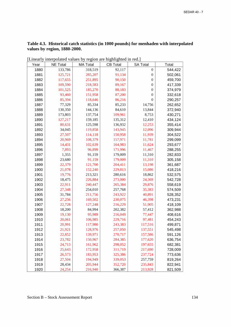
Section B – Stock Assessement Report 134
Table 4.3. Historical catch statistics (in 1000 pounds) for menhaden with interpolated values by region, 1880-2000. [Linearly interpolated values by region are highlighted in red.]
Year NE Total MA Total CB Total SA Total Total 1880 133,786 318,519 92,117 0 544,422 1881 125,721 285,207 91,134 0 502,061 1882 117,655 251,895 90,150 0 459,700 1883 109,590 218,583 89,167 0 417,339 1884 101,525 185,270 88,183 0 374,979 1885 93,460 151,958 87,200 0 332,618 1886 85,394 118,646 86,216 0 290,257 1887 77,329 85,334 85,233 14,756 262,652 1888 130,350 144,136 84,610 13,844 372,940 1889 173,803 137,754 109,961 8,753 430,271 1890 127,217 159,185 135,312 12,410 434,124 1891 80,631 125,598 136,932 12,253 355,414 1892 34,045 119,858 143,945 12,096 309,944 1893 27,507 114,118 150,958 11,939 304,522 1894 20,969 108,379 157,971 11,781 299,099 1895 14,431 102,639 164,983 11,624 293,677 1896 7,893 96,899 171,996 11,467 288,255 1897 1,355 91,159 179,009 11,310 282,833 1898 23,680 91,159 179,009 11,310 305,158 1899 22,379 121,700 204,411 13,198 361,687 1900 21,078 152,240 229,813 15,086 418,216 1901 19,776 213,321 280,616 18,862 532,575 1902 18,475 226,884 273,000 24,369 542,728 1903 22,911 240,447 265,384 29,876 558,619 1904 27,348 254,010 257,768 35,383 574,509 1905 31,784 211,756 243,922 40,891 528,352 1906 27,256 169,502 230,075 46,398 473,231 1907 22,728 127,248 216,229 51,905 418,109 1908 18,200 84,994 202,382 57,412 362,988 1909 19,130 95,989 216,049 77,447 408,616 1910 20,061 106,985 229,716 97,481 454,243 1911 20,991 117,980 243,383 117,516 499,871 1912 21,921 128,976 257,050 137,551 545,498 1913 22,852 139,971 270,717 157,586 591,126 1914 23,782 150,967 284,385 177,620 636,754 1915 24,713 161,962 298,052 197,655 682,381 1916 25,643 172,958 311,719 217,690 728,009 1917 26,573 183,953 325,386 237,724 773,636 1918 27,504 194,949 339,053 257,759 819,264 1919 28,434 205,944 352,720 235,843 822,941 1920 24,254 216,940 366,387 213,928 821,509
SEDAR 40 - 7
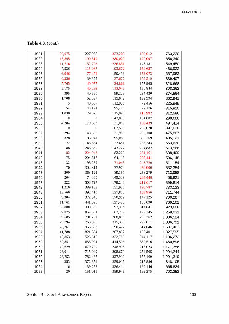
Section B – Stock Assessement Report 135
Table 4.3. (cont.)
1921 20,075 227,935 323,208 192,012 763,230 1922 15,895 190,319 280,029 170,097 656,340 1923 11,716 152,703 236,851 148,181 549,450 1924 7,536 115,087 193,672 150,627 466,922 1925 6,946 77,471 150,493 153,073 387,983 1926 6,356 39,855 137,677 155,519 339,407 1927 5,765 40,077 124,861 157,965 328,668 1928 5,175 40,298 112,045 150,844 308,362 1929 395 40,520 99,229 234,420 374,564 1930 1,708 52,397 115,842 192,994 362,941 1931 5 40,567 112,920 72,456 225,948 1932 54 43,194 195,486 77,176 315,910 1933 1,030 79,575 115,990 115,992 312,586 1934 0 0 143,879 154,807 298,686 1935 4,284 179,603 121,088 192,439 497,414 1936 0 0 167,558 230,070 397,628 1937 294 148,505 121,980 205,108 475,887 1938 328 86,941 95,083 302,769 485,121 1939 122 148,584 127,681 287,243 563,630 1940 88 245,369 143,227 224,882 613,566 1941 82 224,943 182,223 231,161 638,409 1942 75 204,517 64,115 237,441 506,148 1943 132 196,259 71,043 243,720 511,154 1944 70 304,314 77,970 250,000 632,354 1945 200 368,122 89,357 256,279 713,958 1946 204 74,830 149,339 234,448 458,821 1947 222 508,727 178,248 212,617 899,814 1948 1,216 389,188 151,932 190,787 733,123 1949 12,566 392,410 137,812 168,956 711,744 1950 9,304 372,946 170,912 147,125 700,287 1951 11,761 441,825 127,425 188,090 769,101 1952 36,088 480,305 92,374 314,841 923,608 1953 39,875 857,584 162,227 199,345 1,259,031 1954 59,685 781,761 288,816 206,262 1,336,524 1955 79,794 763,827 315,359 227,811 1,386,791 1956 78,767 953,568 190,422 314,646 1,537,403 1957 41,788 821,554 267,852 196,401 1,327,595 1958 13,853 525,516 322,786 244,117 1,106,272 1959 52,851 653,024 414,505 330,516 1,450,896 1960 42,629 670,799 248,905 215,023 1,177,356 1961 26,011 715,049 298,679 254,505 1,294,244 1962 23,753 782,487 327,910 157,169 1,291,319 1963 353 372,851 259,015 215,886 848,105 1964 6 139,258 336,414 190,146 665,824 1965 20 151,011 359,946 192,275 703,252
SEDAR 40 - 7
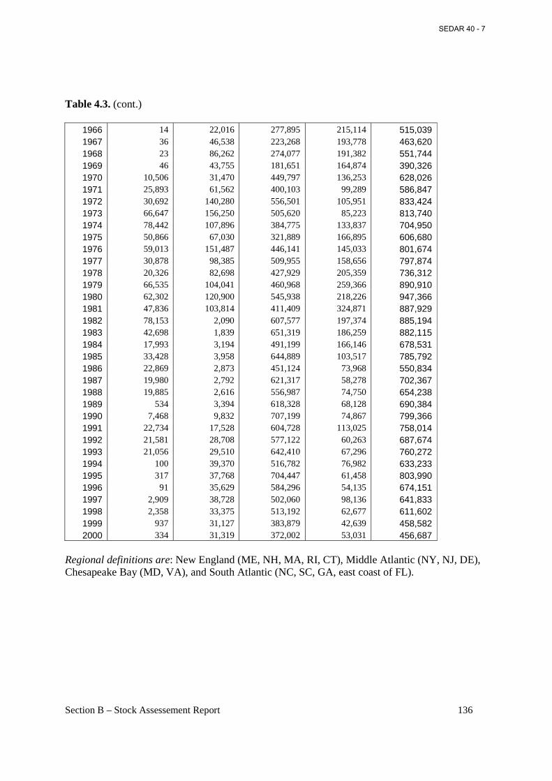
Section B – Stock Assessement Report 136
Table 4.3. (cont.)
1966 14 22,016 277,895 215,114 515,039 1967 36 46,538 223,268 193,778 463,620 1968 23 86,262 274,077 191,382 551,744 1969 46 43,755 181,651 164,874 390,326 1970 10,506 31,470 449,797 136,253 628,026 1971 25,893 61,562 400,103 99,289 586,847 1972 30,692 140,280 556,501 105,951 833,424 1973 66,647 156,250 505,620 85,223 813,740 1974 78,442 107,896 384,775 133,837 704,950 1975 50,866 67,030 321,889 166,895 606,680 1976 59,013 151,487 446,141 145,033 801,674 1977 30,878 98,385 509,955 158,656 797,874 1978 20,326 82,698 427,929 205,359 736,312 1979 66,535 104,041 460,968 259,366 890,910 1980 62,302 120,900 545,938 218,226 947,366 1981 47,836 103,814 411,409 324,871 887,929 1982 78,153 2,090 607,577 197,374 885,194 1983 42,698 1,839 651,319 186,259 882,115 1984 17,993 3,194 491,199 166,146 678,531 1985 33,428 3,958 644,889 103,517 785,792 1986 22,869 2,873 451,124 73,968 550,834 1987 19,980 2,792 621,317 58,278 702,367 1988 19,885 2,616 556,987 74,750 654,238 1989 534 3,394 618,328 68,128 690,384 1990 7,468 9,832 707,199 74,867 799,366 1991 22,734 17,528 604,728 113,025 758,014 1992 21,581 28,708 577,122 60,263 687,674 1993 21,056 29,510 642,410 67,296 760,272 1994 100 39,370 516,782 76,982 633,233 1995 317 37,768 704,447 61,458 803,990 1996 91 35,629 584,296 54,135 674,151 1997 2,909 38,728 502,060 98,136 641,833 1998 2,358 33,375 513,192 62,677 611,602 1999 937 31,127 383,879 42,639 458,582 2000 334 31,319 372,002 53,031 456,687
Regional definitions are: New England (ME, NH, MA, RI, CT), Middle Atlantic (NY, NJ, DE), Chesapeake Bay (MD, VA), and South Atlantic (NC, SC, GA, east coast of FL).
SEDAR 40 - 7
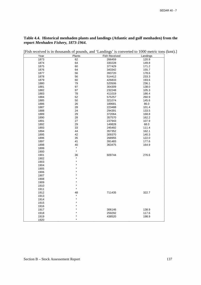
Section B – Stock Assessement Report 137
Table 4.4. Historical menhaden plants and landings (Atlantic and gulf menhaden) from the report Menhaden Fishery, 1873-1964. [Fish received is in thousands of pounds, and ‘Landings’ is converted to 1000 metric tons (kmt).]
Year Plants Fish Received Landings 1873 62 266459 120.9 1874 64 330228 149.8 1875 60 377429 171.2 1876 64 343342 155.7 1877 56 393720 178.6 1878 56 514412 233.3 1879 60 426833 193.6 1880 79 520506 236.1 1881 97 304309 138.0 1882 97 232248 105.3 1883 78 411019 186.4 1884 52 575257 260.9 1885 50 321074 145.6 1886 26 189681 86.0 1887 28 223488 101.4 1888 24 294391 133.5 1889 29 372064 168.8 1890 28 357570 162.2 1891 27 237943 107.9 1892 29 149828 68.0 1893 33 245492 111.4 1894 44 357352 162.1 1895 42 309370 140.3 1896 35 268955 122.0 1897 41 391483 177.6 1898 40 363475 164.9 1899 * 1900 * 1901 36 609744 276.6 1902 * 1903 * 1904 * 1905 * 1906 * 1907 * 1908 * 1909 * 1910 * 1911 * 1912 48 711435 322.7 1913 * 1914 * 1915 * 1916 * 1917 * 306146 138.9 1918 * 259292 117.6 1919 * 438520 198.9 1920 *
SEDAR 40 - 7
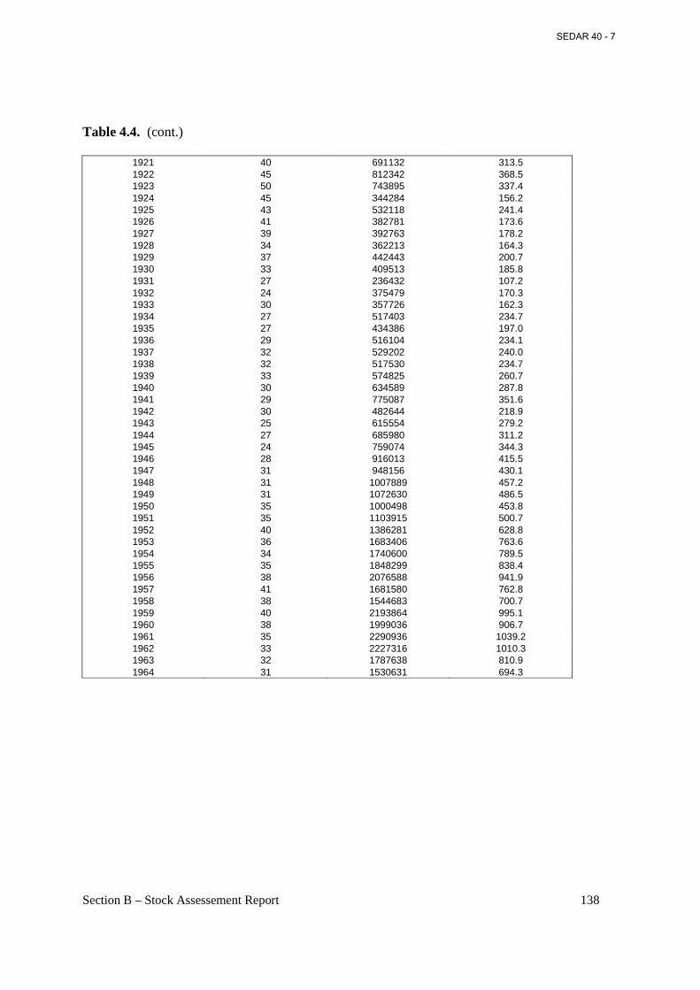
Section B – Stock Assessement Report 138
Table 4.4. (cont.)
1921 40 691132 313.5 1922 45 812342 368.5 1923 50 743895 337.4 1924 45 344284 156.2 1925 43 532118 241.4 1926 41 382781 173.6 1927 39 392763 178.2 1928 34 362213 164.3 1929 37 442443 200.7 1930 33 409513 185.8 1931 27 236432 107.2 1932 24 375479 170.3 1933 30 357726 162.3 1934 27 517403 234.7 1935 27 434386 197.0 1936 29 516104 234.1 1937 32 529202 240.0 1938 32 517530 234.7 1939 33 574825 260.7 1940 30 634589 287.8 1941 29 775087 351.6 1942 30 482644 218.9 1943 25 615554 279.2 1944 27 685980 311.2 1945 24 759074 344.3 1946 28 916013 415.5 1947 31 948156 430.1 1948 31 1007889 457.2 1949 31 1072630 486.5 1950 35 1000498 453.8 1951 35 1103915 500.7 1952 40 1386281 628.8 1953 36 1683406 763.6 1954 34 1740600 789.5 1955 35 1848299 838.4 1956 38 2076588 941.9 1957 41 1681580 762.8 1958 38 1544683 700.7 1959 40 2193864 995.1 1960 38 1999036 906.7 1961 35 2290936 1039.2 1962 33 2227316 1010.3 1963 32 1787638 810.9 1964 31 1530631 694.3
SEDAR 40 - 7
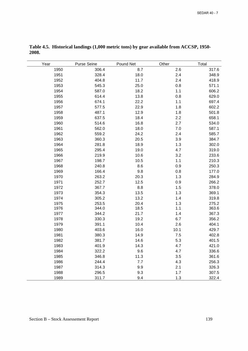
Section B – Stock Assessement Report 139
Table 4.5. Historical landings (1,000 metric tons) by gear available from ACCSP, 1950-2008.
Year Purse Seine Pound Net Other Total 1950 306.4 8.7 2.6 317.6 1951 328.4 18.0 2.4 348.9 1952 404.8 11.7 2.4 418.9 1953 545.3 25.0 0.8 571.1 1954 587.0 18.2 1.1 606.2 1955 614.4 13.8 0.8 629.0 1956 674.1 22.2 1.1 697.4 1957 577.5 22.9 1.8 602.2 1958 487.1 12.9 1.8 501.8 1959 637.5 18.4 2.2 658.1 1960 514.6 16.8 2.7 534.0 1961 562.0 18.0 7.0 587.1 1962 559.2 24.2 2.4 585.7 1963 360.3 20.5 3.9 384.7 1964 281.8 18.9 1.3 302.0 1965 295.4 19.0 4.7 319.0 1966 219.9 10.6 3.2 233.6 1967 198.7 10.5 1.1 210.3 1968 240.8 8.6 0.9 250.3 1969 166.4 9.8 0.8 177.0 1970 263.2 20.3 1.3 284.9 1971 252.7 12.5 0.9 266.2 1972 367.7 8.8 1.5 378.0 1973 354.3 13.5 1.3 369.1 1974 305.2 13.2 1.4 319.8 1975 253.5 20.4 1.3 275.2 1976 344.0 18.5 1.1 363.6 1977 344.2 21.7 1.4 367.3 1978 330.3 19.2 6.7 356.2 1979 391.1 10.4 2.6 404.1 1980 403.6 16.0 10.1 429.7 1981 380.3 14.9 7.5 402.8 1982 381.7 14.6 5.3 401.5 1983 401.9 14.3 4.7 421.0 1984 322.2 9.6 4.7 336.6 1985 346.8 11.3 3.5 361.6 1986 244.4 7.7 4.3 256.3 1987 314.3 9.9 2.1 326.3 1988 296.5 9.3 1.7 307.5 1989 311.7 9.4 1.3 322.4
SEDAR 40 - 7
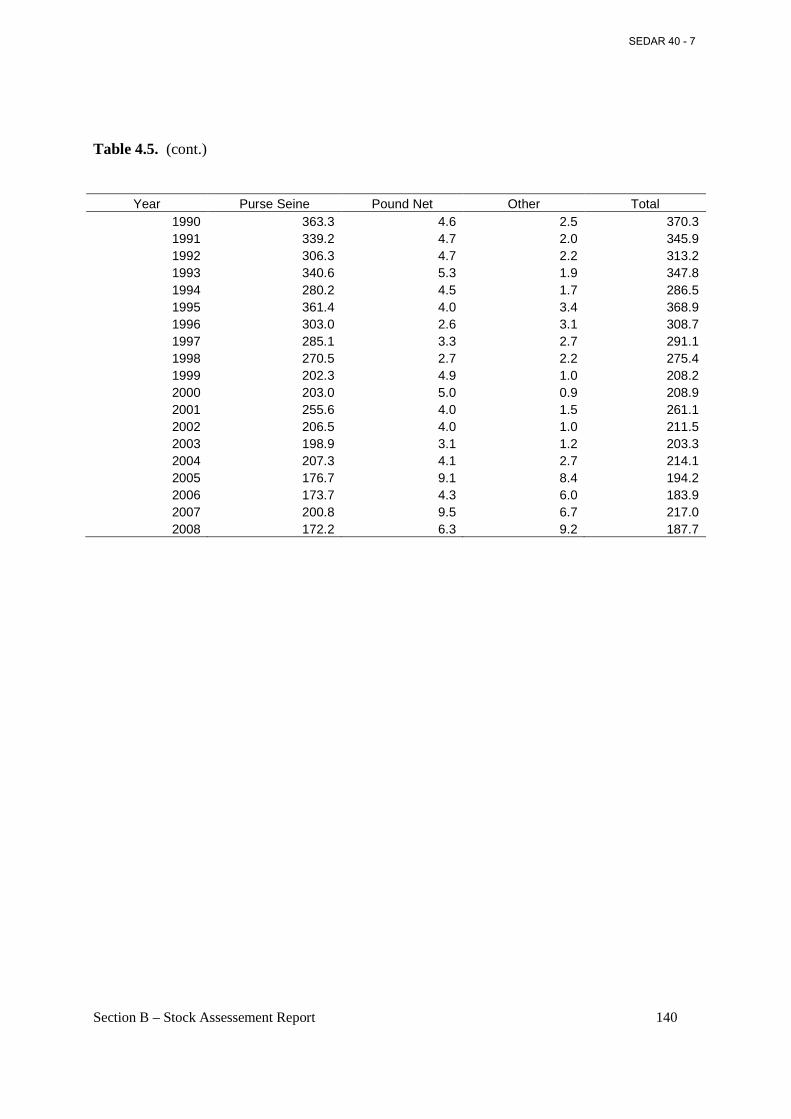
Section B – Stock Assessement Report 140
Table 4.5. (cont.)
Year Purse Seine Pound Net Other Total
1990 363.3 4.6 2.5 370.3 1991 339.2 4.7 2.0 345.9 1992 306.3 4.7 2.2 313.2 1993 340.6 5.3 1.9 347.8 1994 280.2 4.5 1.7 286.5 1995 361.4 4.0 3.4 368.9 1996 303.0 2.6 3.1 308.7 1997 285.1 3.3 2.7 291.1 1998 270.5 2.7 2.2 275.4 1999 202.3 4.9 1.0 208.2 2000 203.0 5.0 0.9 208.9 2001 255.6 4.0 1.5 261.1 2002 206.5 4.0 1.0 211.5 2003 198.9 3.1 1.2 203.3 2004 207.3 4.1 2.7 214.1 2005 176.7 9.1 8.4 194.2 2006 173.7 4.3 6.0 183.9 2007 200.8 9.5 6.7 217.0 2008 172.2 6.3 9.2 187.7
SEDAR 40 - 7
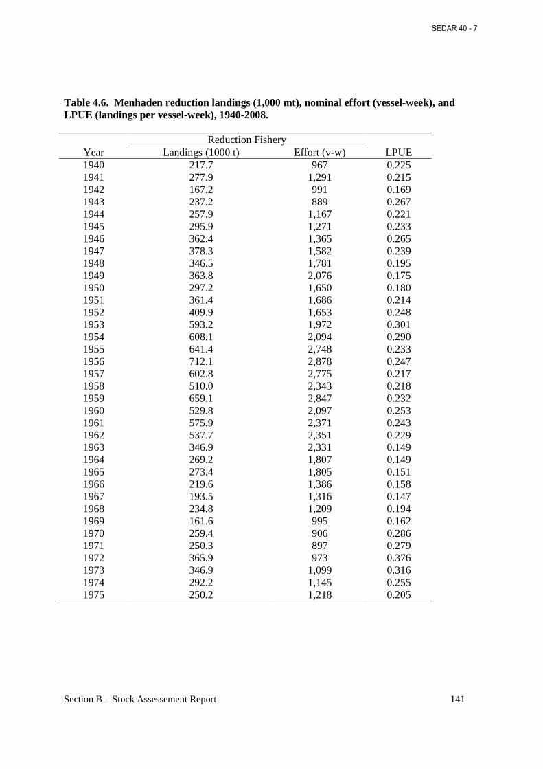
Section B – Stock Assessement Report 141
Table 4.6. Menhaden reduction landings (1,000 mt), nominal effort (vessel-week), and LPUE (landings per vessel-week), 1940-2008.
Reduction Fishery Year Landings (1000 t) Effort (v-w) LPUE 1940 217.7 967 0.225 1941 277.9 1,291 0.215 1942 167.2 991 0.169 1943 237.2 889 0.267 1944 257.9 1,167 0.221 1945 295.9 1,271 0.233 1946 362.4 1,365 0.265 1947 378.3 1,582 0.239 1948 346.5 1,781 0.195 1949 363.8 2,076 0.175 1950 297.2 1,650 0.180 1951 361.4 1,686 0.214 1952 409.9 1,653 0.248 1953 593.2 1,972 0.301 1954 608.1 2,094 0.290 1955 641.4 2,748 0.233 1956 712.1 2,878 0.247 1957 602.8 2,775 0.217 1958 510.0 2,343 0.218 1959 659.1 2,847 0.232 1960 529.8 2,097 0.253 1961 575.9 2,371 0.243 1962 537.7 2,351 0.229 1963 346.9 2,331 0.149 1964 269.2 1,807 0.149 1965 273.4 1,805 0.151 1966 219.6 1,386 0.158 1967 193.5 1,316 0.147 1968 234.8 1,209 0.194 1969 161.6 995 0.162 1970 259.4 906 0.286 1971 250.3 897 0.279 1972 365.9 973 0.376 1973 346.9 1,099 0.316 1974 292.2 1,145 0.255 1975 250.2 1,218 0.205
SEDAR 40 - 7
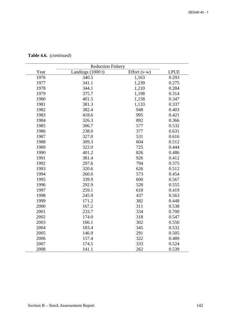
Section B – Stock Assessement Report 142
Table 4.6. (continued)
Reduction Fishery Year Landings (1000 t) Effort (v-w) LPUE 1976 340.5 1,163 0.293 1977 341.1 1,239 0.275 1978 344.1 1,210 0.284 1979 375.7 1,198 0.314 1980 401.5 1,158 0.347 1981 381.3 1,133 0.337 1982 382.4 948 0.403 1983 418.6 995 0.421 1984 326.3 892 0.366 1985 306.7 577 0.532 1986 238.0 377 0.631 1987 327.0 531 0.616 1988 309.3 604 0.512 1989 322.0 725 0.444 1990 401.2 826 0.486 1991 381.4 926 0.412 1992 297.6 794 0.375 1993 320.6 626 0.512 1994 260.0 573 0.454 1995 339.9 600 0.567 1996 292.9 528 0.555 1997 259.1 618 0.419 1998 245.9 437 0.563 1999 171.2 382 0.448 2000 167.2 311 0.538 2001 233.7 334 0.700 2002 174.0 318 0.547 2003 166.1 302 0.550 2004 183.4 345 0.532 2005 146.9 291 0.505 2006 157.4 322 0.489 2007 174.5 333 0.524 2008 141.1 262 0.539
SEDAR 40 - 7
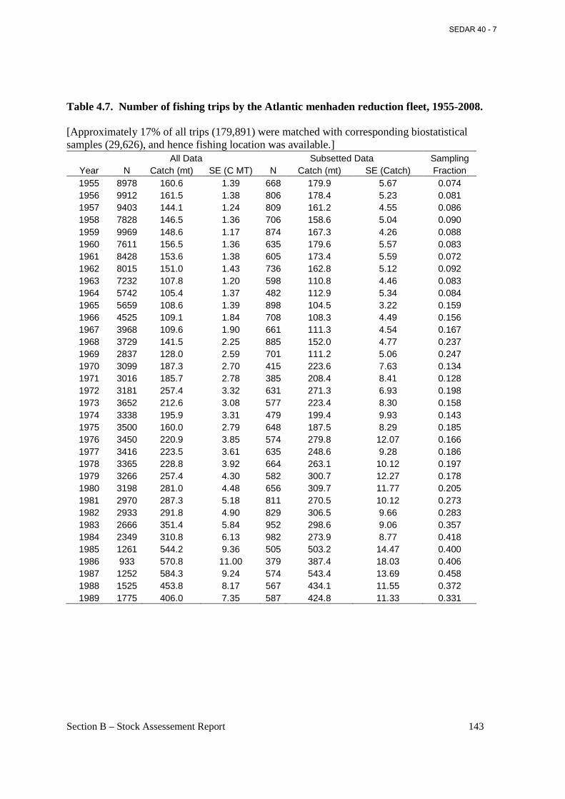
Section B – Stock Assessement Report 143
Table 4.7. Number of fishing trips by the Atlantic menhaden reduction fleet, 1955-2008. [Approximately 17% of all trips (179,891) were matched with corresponding biostatistical samples (29,626), and hence fishing location was available.]
All Data Subsetted Data Sampling Year N Catch (mt) SE (C MT) N Catch (mt) SE (Catch) Fraction 1955 8978 160.6 1.39 668 179.9 5.67 0.074 1956 9912 161.5 1.38 806 178.4 5.23 0.081 1957 9403 144.1 1.24 809 161.2 4.55 0.086 1958 7828 146.5 1.36 706 158.6 5.04 0.090 1959 9969 148.6 1.17 874 167.3 4.26 0.088 1960 7611 156.5 1.36 635 179.6 5.57 0.083 1961 8428 153.6 1.38 605 173.4 5.59 0.072 1962 8015 151.0 1.43 736 162.8 5.12 0.092 1963 7232 107.8 1.20 598 110.8 4.46 0.083 1964 5742 105.4 1.37 482 112.9 5.34 0.084 1965 5659 108.6 1.39 898 104.5 3.22 0.159 1966 4525 109.1 1.84 708 108.3 4.49 0.156 1967 3968 109.6 1.90 661 111.3 4.54 0.167 1968 3729 141.5 2.25 885 152.0 4.77 0.237 1969 2837 128.0 2.59 701 111.2 5.06 0.247 1970 3099 187.3 2.70 415 223.6 7.63 0.134 1971 3016 185.7 2.78 385 208.4 8.41 0.128 1972 3181 257.4 3.32 631 271.3 6.93 0.198 1973 3652 212.6 3.08 577 223.4 8.30 0.158 1974 3338 195.9 3.31 479 199.4 9.93 0.143 1975 3500 160.0 2.79 648 187.5 8.29 0.185 1976 3450 220.9 3.85 574 279.8 12.07 0.166 1977 3416 223.5 3.61 635 248.6 9.28 0.186 1978 3365 228.8 3.92 664 263.1 10.12 0.197 1979 3266 257.4 4.30 582 300.7 12.27 0.178 1980 3198 281.0 4.48 656 309.7 11.77 0.205 1981 2970 287.3 5.18 811 270.5 10.12 0.273 1982 2933 291.8 4.90 829 306.5 9.66 0.283 1983 2666 351.4 5.84 952 298.6 9.06 0.357 1984 2349 310.8 6.13 982 273.9 8.77 0.418 1985 1261 544.2 9.36 505 503.2 14.47 0.400 1986 933 570.8 11.00 379 387.4 18.03 0.406 1987 1252 584.3 9.24 574 543.4 13.69 0.458 1988 1525 453.8 8.17 567 434.1 11.55 0.372 1989 1775 406.0 7.35 587 424.8 11.33 0.331
SEDAR 40 - 7
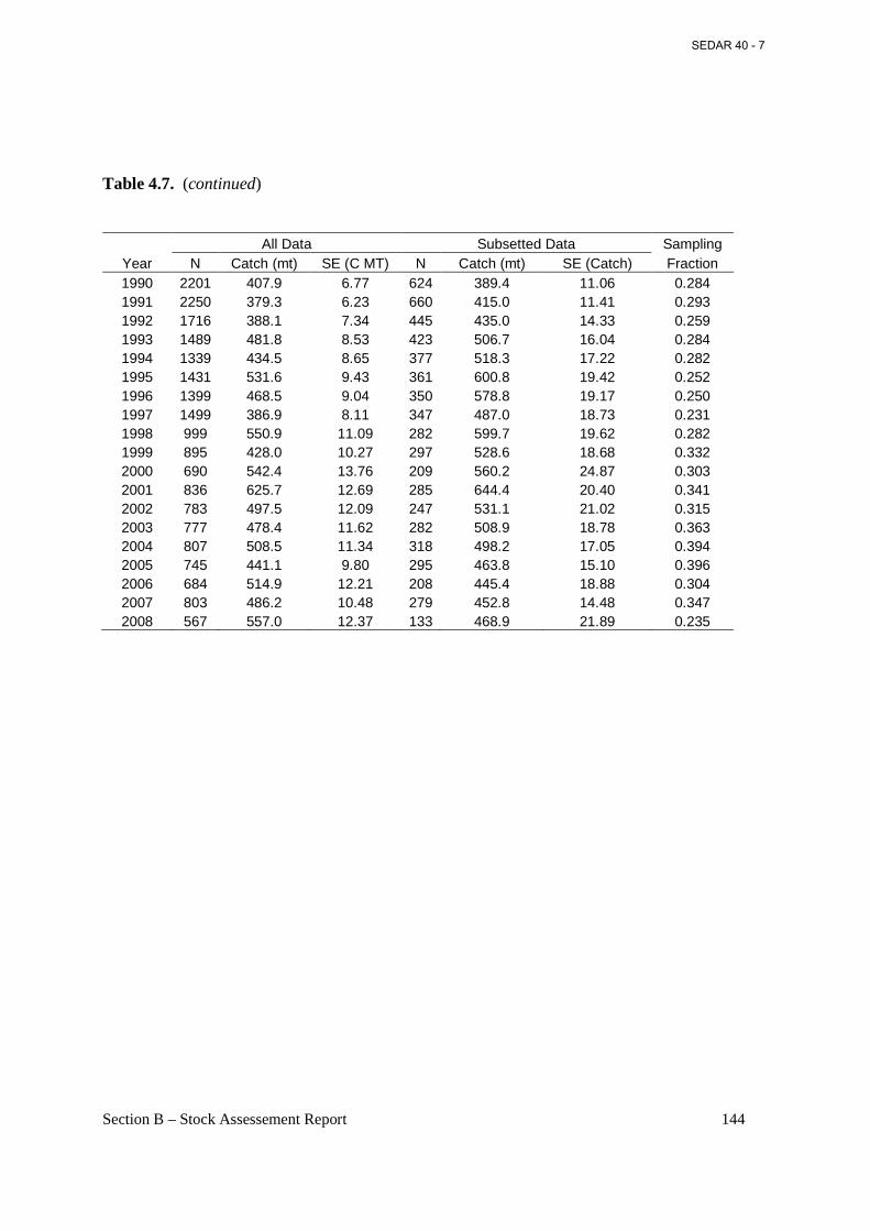
Section B – Stock Assessement Report 144
Table 4.7. (continued)
All Data Subsetted Data Sampling Year N Catch (mt) SE (C MT) N Catch (mt) SE (Catch) Fraction 1990 2201 407.9 6.77 624 389.4 11.06 0.284 1991 2250 379.3 6.23 660 415.0 11.41 0.293 1992 1716 388.1 7.34 445 435.0 14.33 0.259 1993 1489 481.8 8.53 423 506.7 16.04 0.284 1994 1339 434.5 8.65 377 518.3 17.22 0.282 1995 1431 531.6 9.43 361 600.8 19.42 0.252 1996 1399 468.5 9.04 350 578.8 19.17 0.250 1997 1499 386.9 8.11 347 487.0 18.73 0.231 1998 999 550.9 11.09 282 599.7 19.62 0.282 1999 895 428.0 10.27 297 528.6 18.68 0.332 2000 690 542.4 13.76 209 560.2 24.87 0.303 2001 836 625.7 12.69 285 644.4 20.40 0.341 2002 783 497.5 12.09 247 531.1 21.02 0.315 2003 777 478.4 11.62 282 508.9 18.78 0.363 2004 807 508.5 11.34 318 498.2 17.05 0.394 2005 745 441.1 9.80 295 463.8 15.10 0.396 2006 684 514.9 12.21 208 445.4 18.88 0.304 2007 803 486.2 10.48 279 452.8 14.48 0.347 2008 567 557.0 12.37 133 468.9 21.89 0.235
SEDAR 40 - 7
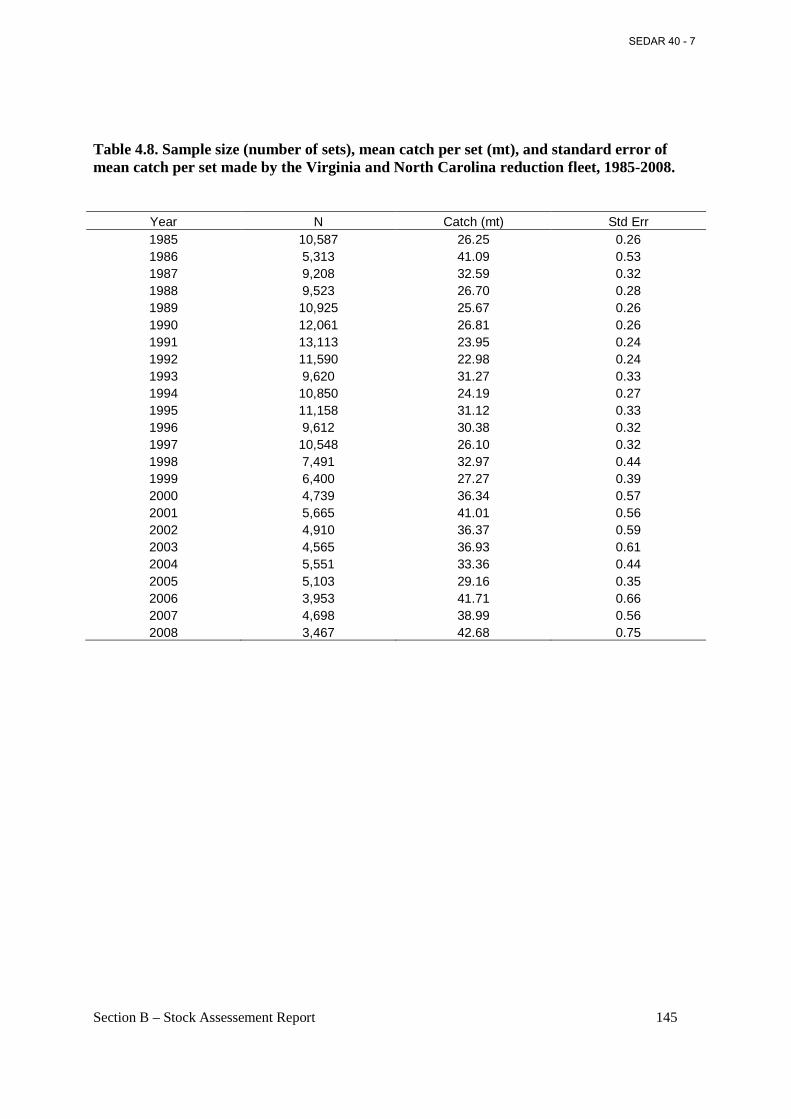
Section B – Stock Assessement Report 145
Table 4.8. Sample size (number of sets), mean catch per set (mt), and standard error of mean catch per set made by the Virginia and North Carolina reduction fleet, 1985-2008.
Year N Catch (mt) Std Err 1985 10,587 26.25 0.26 1986 5,313 41.09 0.53 1987 9,208 32.59 0.32 1988 9,523 26.70 0.28 1989 10,925 25.67 0.26 1990 12,061 26.81 0.26 1991 13,113 23.95 0.24 1992 11,590 22.98 0.24 1993 9,620 31.27 0.33 1994 10,850 24.19 0.27 1995 11,158 31.12 0.33 1996 9,612 30.38 0.32 1997 10,548 26.10 0.32 1998 7,491 32.97 0.44 1999 6,400 27.27 0.39 2000 4,739 36.34 0.57 2001 5,665 41.01 0.56 2002 4,910 36.37 0.59 2003 4,565 36.93 0.61 2004 5,551 33.36 0.44 2005 5,103 29.16 0.35 2006 3,953 41.71 0.66 2007 4,698 38.99 0.56 2008 3,467 42.68 0.75
SEDAR 40 - 7
Section B – Stock Assessement Report 146
Table 4.9. Sample size (n), landings in numbers of fish, landings in biomass (C), sampling ‘intensity’ (landings in metric tons per 100 fish measured), and mean weight of fish landed from the Atlantic menhaden reduction fishery, 1955-2005.
Year Sample Size
(n) Landings Intensity Mean
(millions) (1000 mt) (C/100n) Weight (g) 1955 16037 3118.4 641.4 3999.5 205.7 1956 19873 3564.8 712.1 3583.3 199.8 1957 19674 3511.7 602.8 3063.9 171.7 1958 15315 2719.2 510.0 3330.1 187.6 1959 17935 5353.6 659.1 3674.9 123.1 1960 13505 2775.1 529.8 3923.0 190.9 1961 13184 2598.3 575.9 4368.2 221.6 1962 15771 2099.9 537.7 3409.4 256.1 1963 13001 1764.5 346.9 2668.3 196.6 1964 10438 1729.1 269.2 2579.0 155.7 1965 19518 1519.5 273.4 1400.8 179.9 1966 15633 1340.6 219.6 1404.7 163.8 1967 15426 984.2 193.5 1254.4 196.6 1968 26830 1148.0 234.8 875.1 204.5 1969 15114 868.2 161.6 1069.2 186.1 1970 8426 1403.0 259.4 3078.6 184.9 1971 8269 969.1 250.3 3027.0 258.3 1972 6552 1713.9 365.9 5584.6 213.5 1973 6351 1843.4 346.9 5462.1 188.2 1974 5421 1990.6 292.2 5390.1 146.8 1975 7278 2162.3 250.2 3437.8 115.7 1976 6725 3283.5 340.5 5063.2 103.7 1977 7276 3673.7 341.1 4688.0 92.8 1978 7094 3085.2 344.1 4850.6 111.5 1979 6365 3870.1 375.7 5902.6 97.1 1980 7291 3332.3 401.5 5506.8 120.5 1981 9201 3984.0 381.3 4144.1 95.7 1982 9066 3175.7 382.4 4218.0 120.4 1983 11533 3942.1 418.6 3629.6 106.2 1984 11689 3548.0 326.3 2791.5 92.0 1985 8498 3025.3 306.7 3609.1 101.4 1986 5828 1912.4 238.0 4083.7 124.5 1987 7618 2315.2 327.0 4292.5 141.2 1988 7349 2158.0 309.3 4208.7 143.3 1989 7027 2630.5 322.0 4582.3 122.4
SEDAR 40 - 7
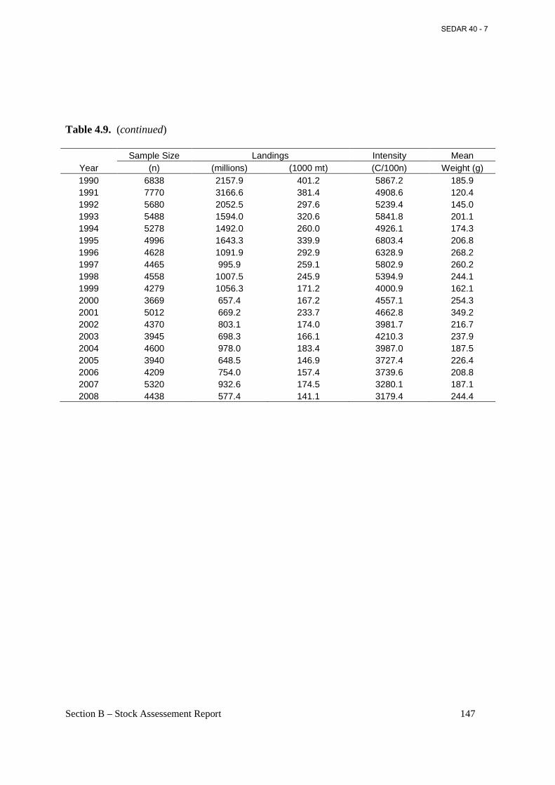
Section B – Stock Assessement Report 147
Table 4.9. (continued)
Year Sample Size Landings Intensity Mean
(n) (millions) (1000 mt) (C/100n) Weight (g) 1990 6838 2157.9 401.2 5867.2 185.9 1991 7770 3166.6 381.4 4908.6 120.4 1992 5680 2052.5 297.6 5239.4 145.0 1993 5488 1594.0 320.6 5841.8 201.1 1994 5278 1492.0 260.0 4926.1 174.3 1995 4996 1643.3 339.9 6803.4 206.8 1996 4628 1091.9 292.9 6328.9 268.2 1997 4465 995.9 259.1 5802.9 260.2 1998 4558 1007.5 245.9 5394.9 244.1 1999 4279 1056.3 171.2 4000.9 162.1 2000 3669 657.4 167.2 4557.1 254.3 2001 5012 669.2 233.7 4662.8 349.2 2002 4370 803.1 174.0 3981.7 216.7 2003 3945 698.3 166.1 4210.3 237.9 2004 4600 978.0 183.4 3987.0 187.5 2005 3940 648.5 146.9 3727.4 226.4 2006 4209 754.0 157.4 3739.6 208.8 2007 5320 932.6 174.5 3280.1 187.1 2008 4438 577.4 141.1 3179.4 244.4
SEDAR 40 - 7
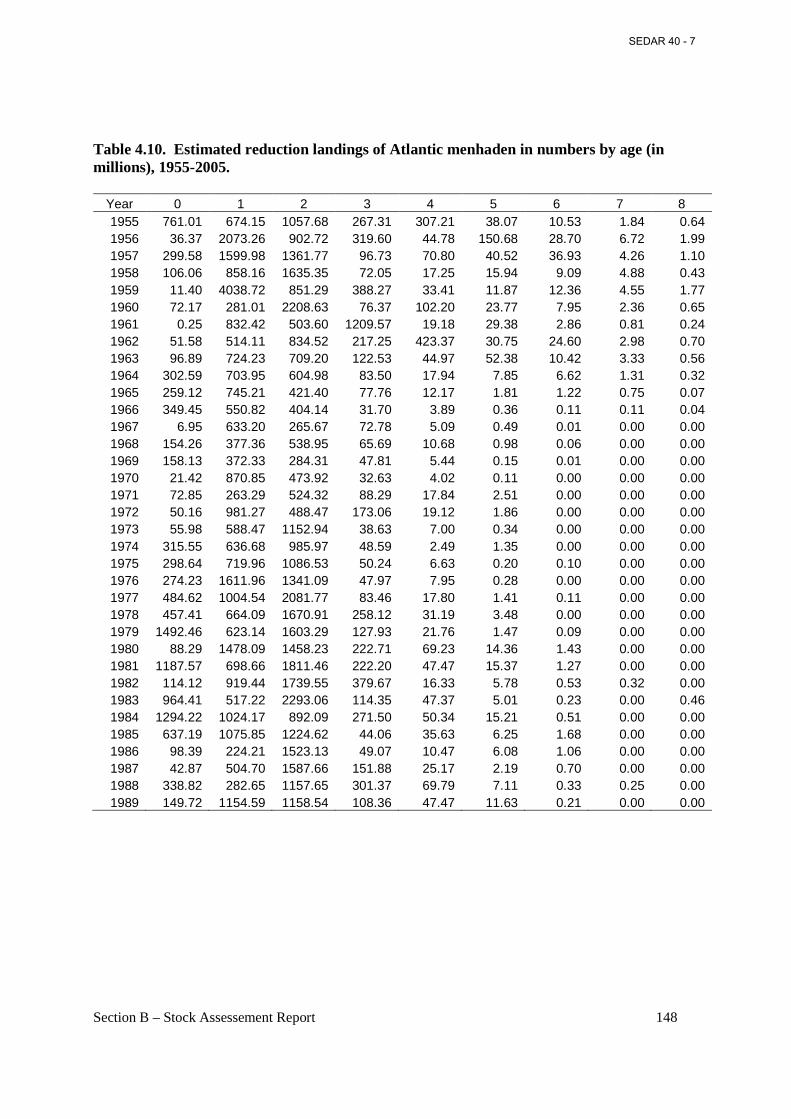
Section B – Stock Assessement Report 148
Table 4.10. Estimated reduction landings of Atlantic menhaden in numbers by age (in millions), 1955-2005.
Year 0 1 2 3 4 5 6 7 8 1955 761.01 674.15 1057.68 267.31 307.21 38.07 10.53 1.84 0.64 1956 36.37 2073.26 902.72 319.60 44.78 150.68 28.70 6.72 1.99 1957 299.58 1599.98 1361.77 96.73 70.80 40.52 36.93 4.26 1.10 1958 106.06 858.16 1635.35 72.05 17.25 15.94 9.09 4.88 0.43 1959 11.40 4038.72 851.29 388.27 33.41 11.87 12.36 4.55 1.77 1960 72.17 281.01 2208.63 76.37 102.20 23.77 7.95 2.36 0.65 1961 0.25 832.42 503.60 1209.57 19.18 29.38 2.86 0.81 0.24 1962 51.58 514.11 834.52 217.25 423.37 30.75 24.60 2.98 0.70 1963 96.89 724.23 709.20 122.53 44.97 52.38 10.42 3.33 0.56 1964 302.59 703.95 604.98 83.50 17.94 7.85 6.62 1.31 0.32 1965 259.12 745.21 421.40 77.76 12.17 1.81 1.22 0.75 0.07 1966 349.45 550.82 404.14 31.70 3.89 0.36 0.11 0.11 0.04 1967 6.95 633.20 265.67 72.78 5.09 0.49 0.01 0.00 0.00 1968 154.26 377.36 538.95 65.69 10.68 0.98 0.06 0.00 0.00 1969 158.13 372.33 284.31 47.81 5.44 0.15 0.01 0.00 0.00 1970 21.42 870.85 473.92 32.63 4.02 0.11 0.00 0.00 0.00 1971 72.85 263.29 524.32 88.29 17.84 2.51 0.00 0.00 0.00 1972 50.16 981.27 488.47 173.06 19.12 1.86 0.00 0.00 0.00 1973 55.98 588.47 1152.94 38.63 7.00 0.34 0.00 0.00 0.00 1974 315.55 636.68 985.97 48.59 2.49 1.35 0.00 0.00 0.00 1975 298.64 719.96 1086.53 50.24 6.63 0.20 0.10 0.00 0.00 1976 274.23 1611.96 1341.09 47.97 7.95 0.28 0.00 0.00 0.00 1977 484.62 1004.54 2081.77 83.46 17.80 1.41 0.11 0.00 0.00 1978 457.41 664.09 1670.91 258.12 31.19 3.48 0.00 0.00 0.00 1979 1492.46 623.14 1603.29 127.93 21.76 1.47 0.09 0.00 0.00 1980 88.29 1478.09 1458.23 222.71 69.23 14.36 1.43 0.00 0.00 1981 1187.57 698.66 1811.46 222.20 47.47 15.37 1.27 0.00 0.00 1982 114.12 919.44 1739.55 379.67 16.33 5.78 0.53 0.32 0.00 1983 964.41 517.22 2293.06 114.35 47.37 5.01 0.23 0.00 0.46 1984 1294.22 1024.17 892.09 271.50 50.34 15.21 0.51 0.00 0.00 1985 637.19 1075.85 1224.62 44.06 35.63 6.25 1.68 0.00 0.00 1986 98.39 224.21 1523.13 49.07 10.47 6.08 1.06 0.00 0.00 1987 42.87 504.70 1587.66 151.88 25.17 2.19 0.70 0.00 0.00 1988 338.82 282.65 1157.65 301.37 69.79 7.11 0.33 0.25 0.00 1989 149.72 1154.59 1158.54 108.36 47.47 11.63 0.21 0.00 0.00
SEDAR 40 - 7
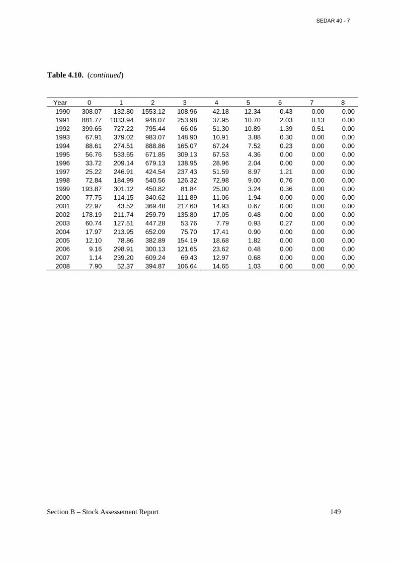
Section B – Stock Assessement Report 149
Table 4.10. (continued)
Year 0 1 2 3 4 5 6 7 8 1990 308.07 132.80 1553.12 108.96 42.18 12.34 0.43 0.00 0.00 1991 881.77 1033.94 946.07 253.98 37.95 10.70 2.03 0.13 0.00 1992 399.65 727.22 795.44 66.06 51.30 10.89 1.39 0.51 0.00 1993 67.91 379.02 983.07 148.90 10.91 3.88 0.30 0.00 0.00 1994 88.61 274.51 888.86 165.07 67.24 7.52 0.23 0.00 0.00 1995 56.76 533.65 671.85 309.13 67.53 4.36 0.00 0.00 0.00 1996 33.72 209.14 679.13 138.95 28.96 2.04 0.00 0.00 0.00 1997 25.22 246.91 424.54 237.43 51.59 8.97 1.21 0.00 0.00 1998 72.84 184.99 540.56 126.32 72.98 9.00 0.76 0.00 0.00 1999 193.87 301.12 450.82 81.84 25.00 3.24 0.36 0.00 0.00 2000 77.75 114.15 340.62 111.89 11.06 1.94 0.00 0.00 0.00 2001 22.97 43.52 369.48 217.60 14.93 0.67 0.00 0.00 0.00 2002 178.19 211.74 259.79 135.80 17.05 0.48 0.00 0.00 0.00 2003 60.74 127.51 447.28 53.76 7.79 0.93 0.27 0.00 0.00 2004 17.97 213.95 652.09 75.70 17.41 0.90 0.00 0.00 0.00 2005 12.10 78.86 382.89 154.19 18.68 1.82 0.00 0.00 0.00 2006 9.16 298.91 300.13 121.65 23.62 0.48 0.00 0.00 0.00 2007 1.14 239.20 609.24 69.43 12.97 0.68 0.00 0.00 0.00 2008 7.90 52.37 394.87 106.64 14.65 1.03 0.00 0.00 0.00
SEDAR 40 - 7
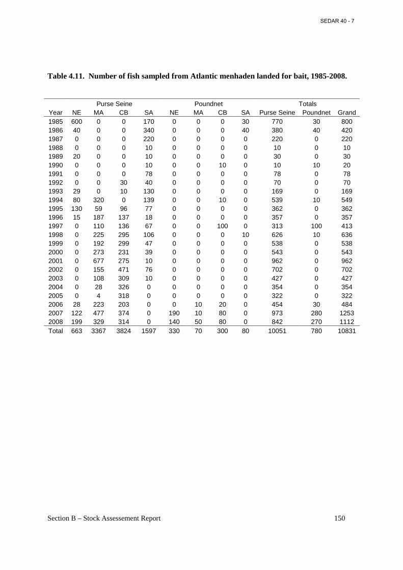
Section B – Stock Assessement Report 150
Table 4.11. Number of fish sampled from Atlantic menhaden landed for bait, 1985-2008.
Purse Seine Poundnet Totals Year NE MA CB SA NE MA CB SA Purse Seine Poundnet Grand 1985 600 0 0 170 0 0 0 30 770 30 800 1986 40 0 0 340 0 0 0 40 380 40 420 1987 0 0 0 220 0 0 0 0 220 0 220 1988 0 0 0 10 0 0 0 0 10 0 10 1989 20 0 0 10 0 0 0 0 30 0 30 1990 0 0 0 10 0 0 10 0 10 10 20 1991 0 0 0 78 0 0 0 0 78 0 78 1992 0 0 30 40 0 0 0 0 70 0 70 1993 29 0 10 130 0 0 0 0 169 0 169 1994 80 320 0 139 0 0 10 0 539 10 549 1995 130 59 96 77 0 0 0 0 362 0 362 1996 15 187 137 18 0 0 0 0 357 0 357 1997 0 110 136 67 0 0 100 0 313 100 413 1998 0 225 295 106 0 0 0 10 626 10 636 1999 0 192 299 47 0 0 0 0 538 0 538 2000 0 273 231 39 0 0 0 0 543 0 543 2001 0 677 275 10 0 0 0 0 962 0 962 2002 0 155 471 76 0 0 0 0 702 0 702 2003 0 108 309 10 0 0 0 0 427 0 427 2004 0 28 326 0 0 0 0 0 354 0 354 2005 0 4 318 0 0 0 0 0 322 0 322 2006 28 223 203 0 0 10 20 0 454 30 484 2007 122 477 374 0 190 10 80 0 973 280 1253 2008 199 329 314 0 140 50 80 0 842 270 1112 Total 663 3367 3824 1597 330 70 300 80 10051 780 10831
SEDAR 40 - 7
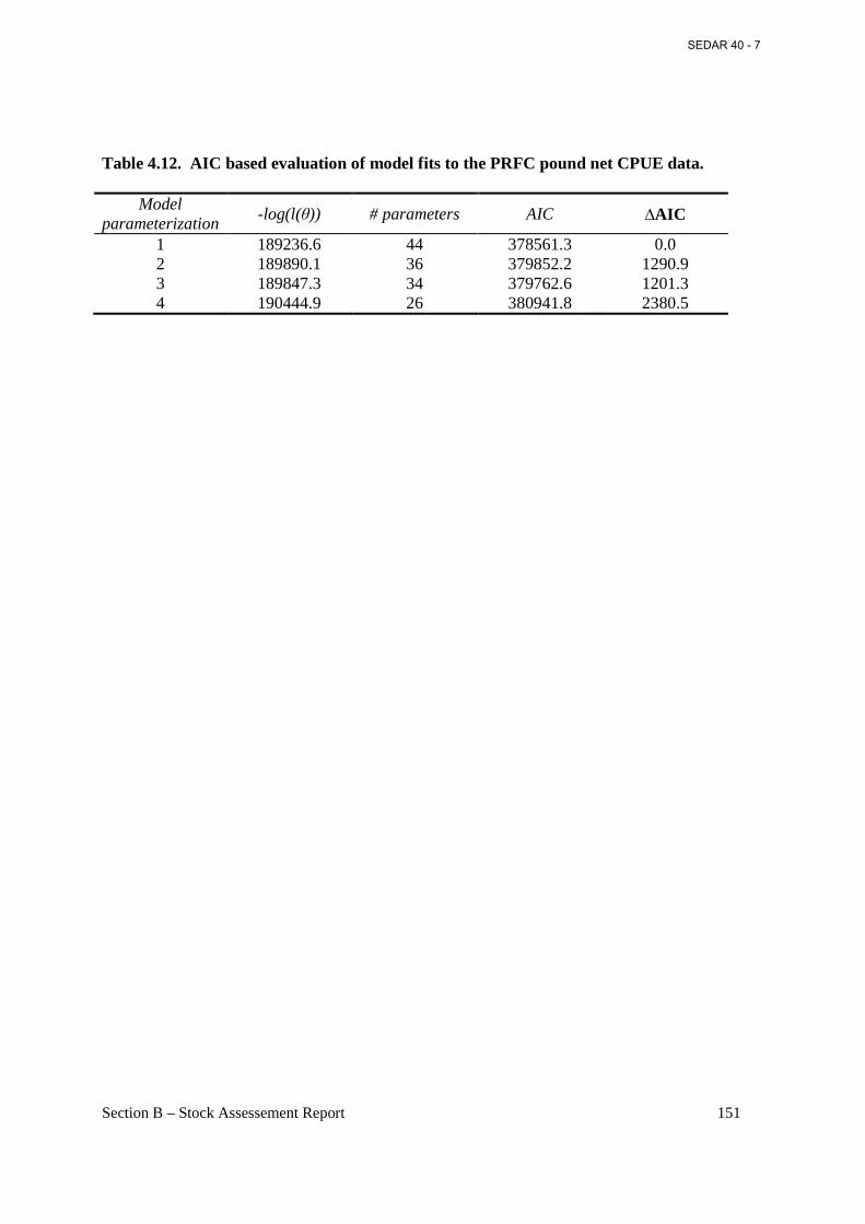
Section B – Stock Assessement Report 151
Table 4.12. AIC based evaluation of model fits to the PRFC pound net CPUE data.
Model parameterization
-log(l(θ)) # parameters AIC ∆AIC
1 189236.6 44 378561.3 0.0 2 189890.1 36 379852.2 1290.9 3 189847.3 34 379762.6 1201.3 4 190444.9 26 380941.8 2380.5
SEDAR 40 - 7
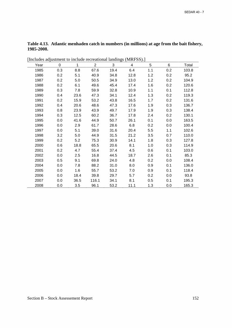
Section B – Stock Assessement Report 152
Table 4.13. Atlantic menhaden catch in numbers (in millions) at age from the bait fishery, 1985-2008. [Includes adjustment to include recreational landings (MRFSS).]
Year 0 1 2 3 4 5 6 Total 1985 0.3 8.8 67.6 19.4 6.4 1.1 0.2 103.8 1986 0.2 5.1 40.9 34.8 12.8 1.2 0.2 95.2 1987 0.2 5.0 50.5 34.9 13.0 1.2 0.2 104.9 1988 0.2 6.1 49.6 45.4 17.4 1.6 0.2 120.6 1989 0.3 7.8 59.9 32.8 10.9 1.1 0.1 112.8 1990 0.4 23.6 47.3 34.1 12.4 1.3 0.2 119.3 1991 0.2 15.9 53.2 43.8 16.5 1.7 0.2 131.6 1992 0.4 20.6 48.6 47.3 17.6 1.9 0.3 136.7 1993 0.8 23.9 43.9 49.7 17.9 1.9 0.3 138.4 1994 0.3 12.5 60.2 36.7 17.8 2.4 0.2 130.1 1995 0.0 41.6 44.9 50.7 26.1 0.1 0.0 163.5 1996 0.0 2.9 61.7 28.6 6.8 0.2 0.0 100.4 1997 0.0 5.1 39.0 31.6 20.4 5.5 1.1 102.6 1998 3.2 5.0 44.9 31.5 21.2 3.5 0.7 110.0 1999 0.2 5.2 75.3 30.9 14.1 1.8 0.3 127.8 2000 0.6 18.8 65.5 20.6 8.1 1.0 0.3 114.9 2001 0.2 4.7 55.4 37.4 4.5 0.6 0.1 103.0 2002 0.0 2.5 16.8 44.5 18.7 2.6 0.1 85.3 2003 0.5 9.1 69.8 24.0 4.8 0.2 0.0 108.4 2004 0.0 7.8 88.2 31.0 8.0 0.9 0.1 136.0 2005 0.0 1.6 55.7 53.2 7.0 0.9 0.1 118.4 2006 0.0 18.4 39.8 29.7 5.7 0.2 0.0 93.8 2007 0.0 36.5 116.1 34.1 8.1 0.5 0.1 195.3 2008 0.0 3.5 96.1 53.2 11.1 1.3 0.0 165.3
SEDAR 40 - 7
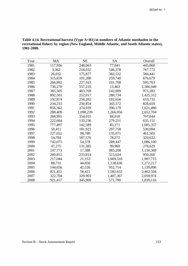
Section B – Stock Assessement Report 153
Table 4.14. Recreational harvest (Type A+B1) in numbers of Atlantic menhaden in the recreational fishery by region (New England, Middle Atlantic, and South Atlantic states), 1981-2008.
Year MA NE SA Overall 1981 117,956 248,063 77,841 443,860 1982 3,362 218,032 546,378 767,772 1983 26,032 175,877 382,532 584,441 1984 315,659 101,280 259,740 676,679 1985 266,892 227,163 101,708 595,763 1986 736,270 557,216 13,463 1,306,949 1987 365,505 463,769 142,009 971,283 1988 892,561 252,017 280,734 1,425,312 1989 192,874 258,202 182,656 633,732 1990 234,233 250,854 343,572 828,659 1991 856,362 374,939 390,179 1,621,480 1992 288,409 1,098,239 1,266,056 2,652,704 1993 268,991 354,035 84,018 707,044 1994 222,664 133,236 279,251 635,151 1995 777,497 142,589 85,271 1,005,357 1996 50,411 181,925 297,758 530,094 1997 227,652 98,780 135,071 461,503 1998 54,784 187,576 78,272 320,632 1999 742,075 54,578 289,447 1,086,100 2000 47,275 131,385 99,969 278,629 2001 147,773 17,388 985,208 1,150,369 2002 200,812 233,814 515,634 950,260 2003 217,044 21,153 1,669,518 1,907,715 2004 88,731 44,850 1,138,636 1,272,217 2005 144,656 42,526 952,714 1,139,896 2006 821,451 58,421 1,582,632 2,462,504 2007 322,704 329,903 1,407,367 2,059,974 2008 921,417 345,909 571,790 1,839,116
SEDAR 40 - 7
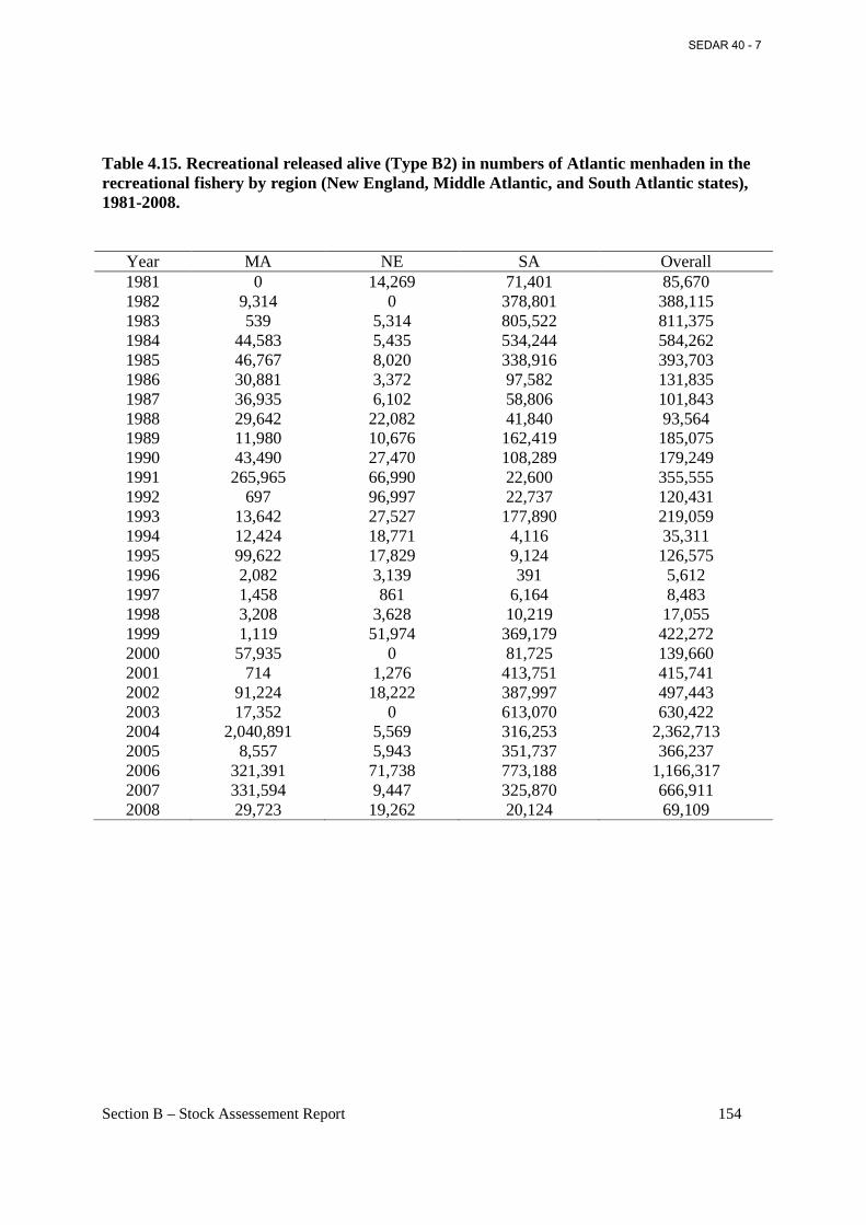
Section B – Stock Assessement Report 154
Table 4.15. Recreational released alive (Type B2) in numbers of Atlantic menhaden in the recreational fishery by region (New England, Middle Atlantic, and South Atlantic states), 1981-2008.
Year MA NE SA Overall 1981 0 14,269 71,401 85,670 1982 9,314 0 378,801 388,115 1983 539 5,314 805,522 811,375 1984 44,583 5,435 534,244 584,262 1985 46,767 8,020 338,916 393,703 1986 30,881 3,372 97,582 131,835 1987 36,935 6,102 58,806 101,843 1988 29,642 22,082 41,840 93,564 1989 11,980 10,676 162,419 185,075 1990 43,490 27,470 108,289 179,249 1991 265,965 66,990 22,600 355,555 1992 697 96,997 22,737 120,431 1993 13,642 27,527 177,890 219,059 1994 12,424 18,771 4,116 35,311 1995 99,622 17,829 9,124 126,575 1996 2,082 3,139 391 5,612 1997 1,458 861 6,164 8,483 1998 3,208 3,628 10,219 17,055 1999 1,119 51,974 369,179 422,272 2000 57,935 0 81,725 139,660 2001 714 1,276 413,751 415,741 2002 91,224 18,222 387,997 497,443 2003 17,352 0 613,070 630,422 2004 2,040,891 5,569 316,253 2,362,713 2005 8,557 5,943 351,737 366,237 2006 321,391 71,738 773,188 1,166,317 2007 331,594 9,447 325,870 666,911 2008 29,723 19,262 20,124 69,109
SEDAR 40 - 7
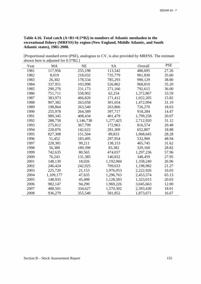
Section B – Stock Assessement Report 155
Table 4.16. Total catch (A+B1+0.5*B2) in numbers of Atlantic menhaden in the recreational fishery (MRFSS) by region (New England, Middle Atlantic, and South Atlantic states), 1981-2008. [Proportional standard error (PSE), analogous to CV, is also provided by MRFSS. The estimate shown here is adjusted for 0.5*B2.]
Year MA NE SA Overall PSE 1981 117,956 255,198 113,542 486,695 27.26 1982 8,019 218,032 735,779 961,830 35.60 1983 26,302 178,534 785,293 990,129 38.80 1984 337,951 103,998 526,862 968,810 35.20 1985 290,276 231,173 271,166 792,615 36.00 1986 751,711 558,902 62,254 1,372,867 33.59 1987 383,973 466,820 171,412 1,022,205 15.82 1988 907,382 263,058 301,654 1,472,094 31.19 1989 198,864 263,540 263,866 726,270 18.63 1990 255,978 264,589 397,717 918,284 14.47 1991 989,345 408,434 401,479 1,799,258 20.07 1992 288,758 1,146,738 1,277,425 2,712,920 31.12 1993 275,812 367,799 172,963 816,574 20.48 1994 228,876 142,622 281,309 652,807 18.88 1995 827,308 151,504 89,833 1,068,645 28.28 1996 51,452 183,495 297,954 532,900 48.94 1997 228,381 99,211 138,153 465,745 31.62 1998 56,388 189,390 83,382 329,160 28.82 1999 742,635 80,565 474,037 1,297,236 57.96 2000 76,243 131,385 140,832 348,459 27.95 2001 148,130 18,026 1,192,084 1,358,240 26.96 2002 246,424 242,925 709,633 1,198,982 21.27 2003 225,720 21,153 1,976,053 2,222,926 16.03 2004 1,109,177 47,635 1,296,763 2,453,574 65.13 2005 148,935 45,498 1,128,583 1,323,015 20.03 2006 982,147 94,290 1,969,226 3,045,663 12.00 2007 488,501 334,627 1,570,302 2,393,430 18.01 2008 936,279 355,540 581,852 1,873,671 16.67
SEDAR 40 - 7
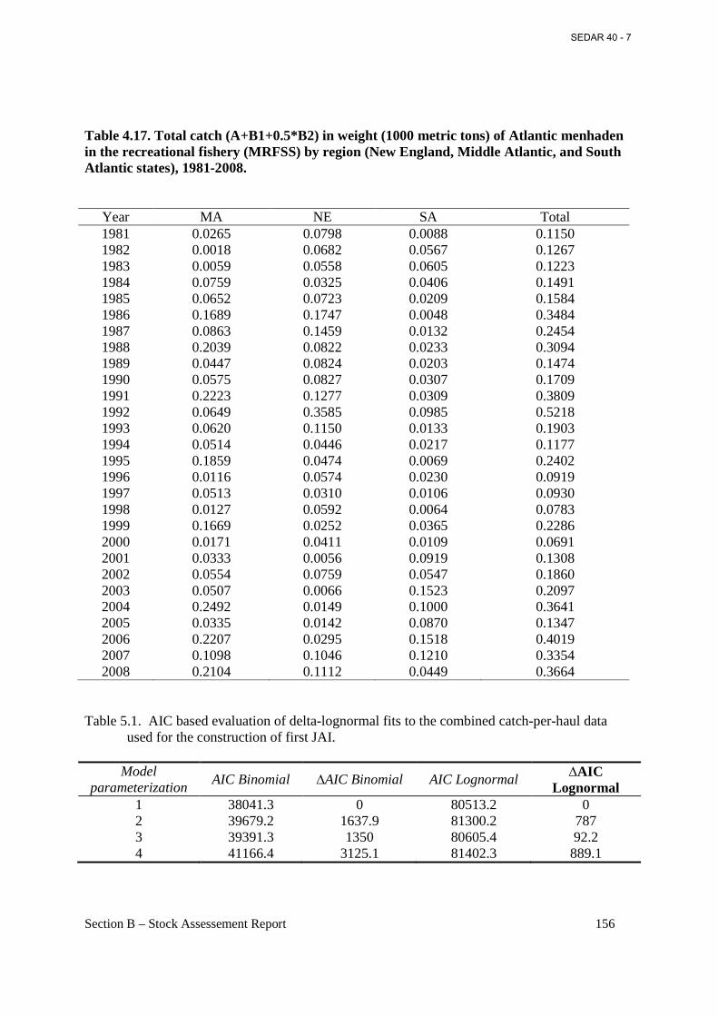
Section B – Stock Assessement Report 156
Table 4.17. Total catch (A+B1+0.5*B2) in weight (1000 metric tons) of Atlantic menhaden in the recreational fishery (MRFSS) by region (New England, Middle Atlantic, and South Atlantic states), 1981-2008.
Year MA NE SA Total 1981 0.0265 0.0798 0.0088 0.1150 1982 0.0018 0.0682 0.0567 0.1267 1983 0.0059 0.0558 0.0605 0.1223 1984 0.0759 0.0325 0.0406 0.1491 1985 0.0652 0.0723 0.0209 0.1584 1986 0.1689 0.1747 0.0048 0.3484 1987 0.0863 0.1459 0.0132 0.2454 1988 0.2039 0.0822 0.0233 0.3094 1989 0.0447 0.0824 0.0203 0.1474 1990 0.0575 0.0827 0.0307 0.1709 1991 0.2223 0.1277 0.0309 0.3809 1992 0.0649 0.3585 0.0985 0.5218 1993 0.0620 0.1150 0.0133 0.1903 1994 0.0514 0.0446 0.0217 0.1177 1995 0.1859 0.0474 0.0069 0.2402 1996 0.0116 0.0574 0.0230 0.0919 1997 0.0513 0.0310 0.0106 0.0930 1998 0.0127 0.0592 0.0064 0.0783 1999 0.1669 0.0252 0.0365 0.2286 2000 0.0171 0.0411 0.0109 0.0691 2001 0.0333 0.0056 0.0919 0.1308 2002 0.0554 0.0759 0.0547 0.1860 2003 0.0507 0.0066 0.1523 0.2097 2004 0.2492 0.0149 0.1000 0.3641 2005 0.0335 0.0142 0.0870 0.1347 2006 0.2207 0.0295 0.1518 0.4019 2007 0.1098 0.1046 0.1210 0.3354 2008 0.2104 0.1112 0.0449 0.3664
Table 5.1. AIC based evaluation of delta-lognormal fits to the combined catch-per-haul data
used for the construction of first JAI.
Model parameterization
AIC Binomial ∆AIC Binomial AIC Lognormal ∆AIC
Lognormal 1 38041.3 0 80513.2 0 2 39679.2 1637.9 81300.2 787 3 39391.3 1350 80605.4 92.2 4 41166.4 3125.1 81402.3 889.1
SEDAR 40 - 7
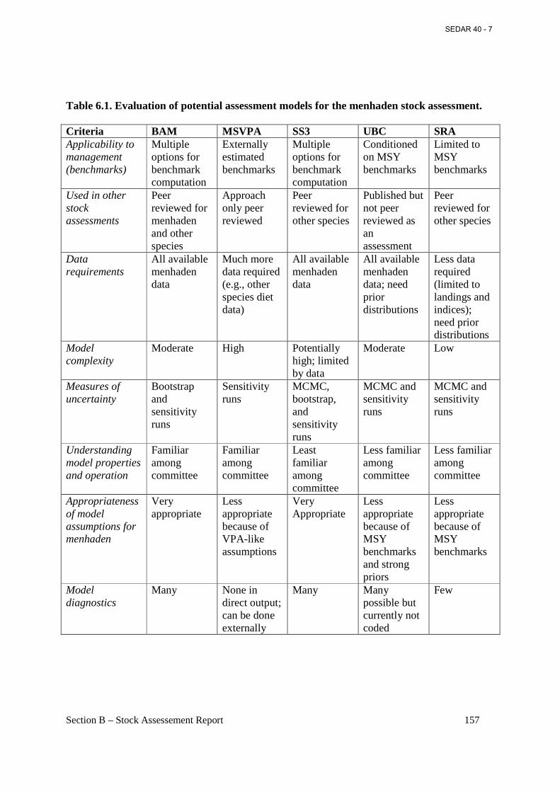
Section B – Stock Assessement Report 157
Table 6.1. Evaluation of potential assessment models for the menhaden stock assessment. Criteria BAM MSVPA SS3 UBC SRA Applicability to management (benchmarks)
Multiple options for benchmark computation
Externally estimated benchmarks
Multiple options for benchmark computation
Conditioned on MSY benchmarks
Limited to MSY benchmarks
Used in other stock assessments
Peer reviewed for menhaden and other species
Approach only peer reviewed
Peer reviewed for other species
Published but not peer reviewed as an assessment
Peer reviewed for other species
Data requirements
All available menhaden data
Much more data required (e.g., other species diet data)
All available menhaden data
All available menhaden data; need prior distributions
Less data required (limited to landings and indices); need prior distributions
Model complexity
Moderate High Potentially high; limited by data
Moderate Low
Measures of uncertainty
Bootstrap and sensitivity runs
Sensitivity runs
MCMC, bootstrap, and sensitivity runs
MCMC and sensitivity runs
MCMC and sensitivity runs
Understanding model properties and operation
Familiar among committee
Familiar among committee
Least familiar among committee
Less familiar among committee
Less familiar among committee
Appropriateness of model assumptions for menhaden
Very appropriate
Less appropriate because of VPA-like assumptions
Very Appropriate
Less appropriate because of MSY benchmarks and strong priors
Less appropriate because of MSY benchmarks
Model diagnostics
Many None in direct output; can be done externally
Many Many possible but currently not coded
Few
SEDAR 40 - 7
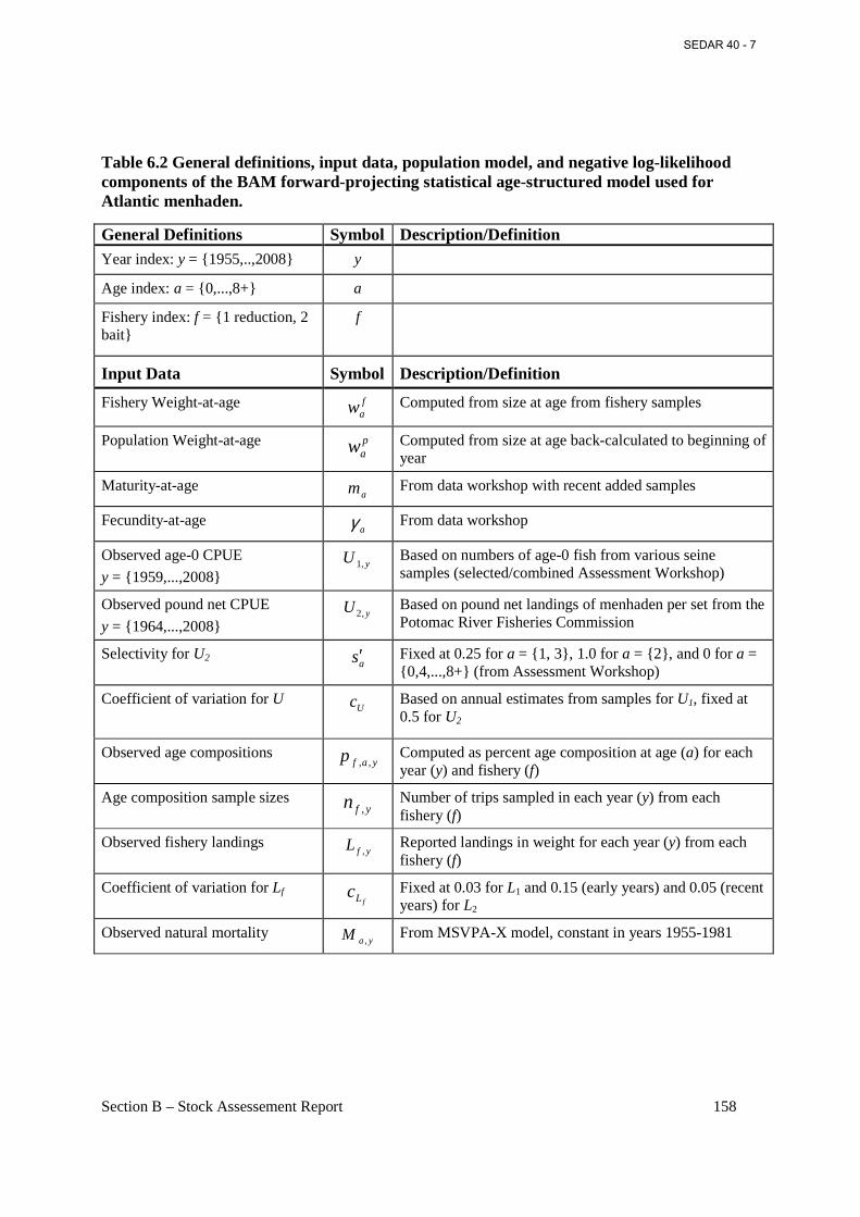
Section B – Stock Assessement Report 158
Table 6.2 General definitions, input data, population model, and negative log-likelihood components of the BAM forward-projecting statistical age-structured model used for Atlantic menhaden.
General Definitions Symbol Description/Definition Year index: y = {1955,..,2008} y
Age index: a = {0,...,8+} a
Fishery index: f = {1 reduction, 2 bait}
f
Input Data Symbol Description/Definition
Fishery Weight-at-age faw Computed from size at age from fishery samples
Population Weight-at-age paw Computed from size at age back-calculated to beginning of
year
Maturity-at-age am From data workshop with recent added samples
Fecundity-at-age aγ From data workshop
Observed age-0 CPUE y = {1959,...,2008}
yU ,1 Based on numbers of age-0 fish from various seine samples (selected/combined Assessment Workshop)
Observed pound net CPUE y = {1964,...,2008}
yU ,2 Based on pound net landings of menhaden per set from the Potomac River Fisheries Commission
Selectivity for U2 as′ Fixed at 0.25 for a = {1, 3}, 1.0 for a = {2}, and 0 for a =
{0,4,...,8+} (from Assessment Workshop)
Coefficient of variation for U Uc Based on annual estimates from samples for U1, fixed at
0.5 for U2
Observed age compositions yafp ,, Computed as percent age composition at age (a) for each
year (y) and fishery (f)
Age composition sample sizes yfn , Number of trips sampled in each year (y) from each
fishery (f)
Observed fishery landings yfL , Reported landings in weight for each year (y) from each
fishery (f)
Coefficient of variation for Lf fLc Fixed at 0.03 for L1 and 0.15 (early years) and 0.05 (recent
years) for L2
Observed natural mortality yaM , From MSVPA-X model, constant in years 1955-1981
SEDAR 40 - 7
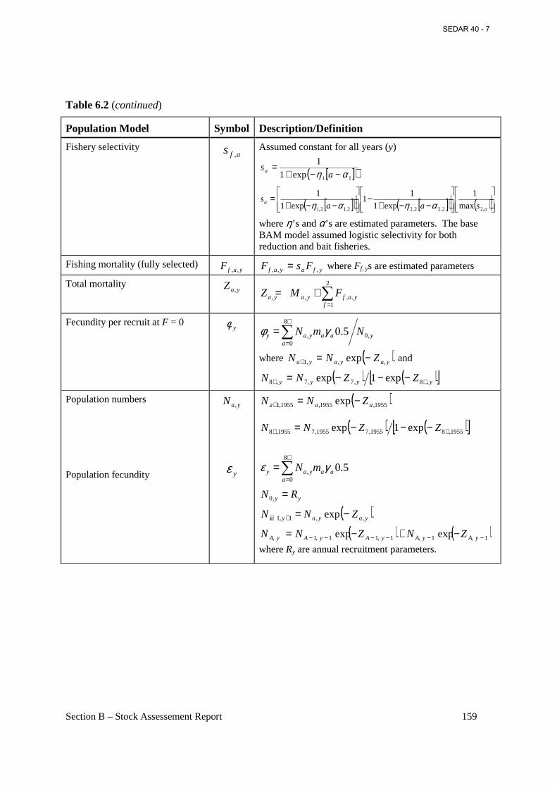
Section B – Stock Assessement Report 159
Table 6.2 (continued)
Population Model Symbol Description/Definition
Fishery selectivity afs , Assumed constant for all years (y)
[ ]( )11exp1
1
αη −−+=
asa
[ ]( ) [ ]( ) ( )
−−+−
−−+=
aa saa
s,22,22,22,12,1 max
1
exp1
11
exp1
1
αηαη
where η’s and α’s are estimated parameters. The base BAM model assumed logistic selectivity for both reduction and bait fisheries.
Fishing mortality (fully selected) yafF ,, yfayaf FsF ,,, = where Ff, ys are estimated parameters
Total mortality yaZ ,
∑=
+=2
1,,,,
fyafyaya FMZ
Fecundity per recruit at F = 0 yφ
yaa
ayay NmN ,0
8
0, 5.0γφ ∑
+
=
=
where ( )yayaya ZNN ,,,1 exp −=+ and
( ) ( )[ ]yyyy ZZNN ,8,7,7,8 exp1exp ++ −−−=
Population numbers
Population fecundity
yaN ,
yε
( )1955,1955,1955,1 exp aaa ZNN −=+
( ) ( )[ ]1955,81955,71955,71955,8 exp1exp ++ −−−= ZZNN
∑+
=
=8
0, 5.0
aaayay mN γε
yy RN =,0
( )yayaya ZNN ,,1,1 exp −=++
( ) ( )1,1,1,11,1, expexp −−−−−− −+−= yAyAyAyAyA ZNZNN
where Ry are annual recruitment parameters.
SEDAR 40 - 7

Section B – Stock Assessement Report 160
Table 6.2 (continued)
Population Model (cont.) Symbol Description/Definition Population biomass
yB ∑
+
=
=8
0,
a
payay wNB
Predicted catch-at-age yafC ,,
ˆ
( )[ ]yaya
ya
yafyaf ZN
Z
FC ,,
,
,,,, exp1ˆ −−=
Predicted landings yfL ,
ˆ ∑+
=
=8
0,,,
ˆˆa
fayafyf wCL
Predicted age composition yafp ,,ˆ
∑+
=
=8
0,,,,,,
ˆˆˆa
yafyafyaf CCp
Predicted age-0 CPUE yU ,1
ˆ 1,0,1ˆ qNU yy = where q1 is a catchability parameter
Predicted pound net CPUE yU ,2
ˆ ∑+
=
′=8
02,,2
ˆa
ayay qsNU where q2 is a catchability parameter
Negative Log-Likelihood Symbol Description/Definition
Multinomial age composition fΛ ( ) ( ) ( ) ( )xpxpxpxpn yafyafa
yafyafyfff ++−++−=Λ ∑+
=,,,,
8
0,,,,, logˆlogλ
where λf is a preset weighting factor and x is fixed at an arbitrary value of 0.001
Lognormal indices fΛ
( ) ( )[ ]
∑+−+
=Λy U
yfyfff c
xUxU2
2
,,
2
ˆloglogλ
where λf is a preset weighting factor and x is fixed at an arbitrary value of 0.001
Lognormal landings fΛ
( ) ( )[ ]
∑+−+
=Λy L
yfyfff
fc
xLxL2
2
,,
2
ˆloglogλ
where λf is a preset weighting factor and x is fixed at an arbitrary value of 0.001
SEDAR 40 - 7
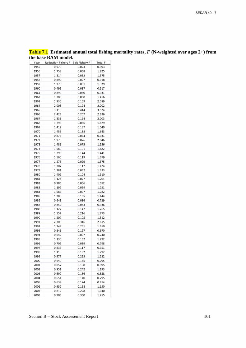
Section B – Stock Assessement Report 161
Table 7.1 Estimated annual total fishing mortality rates, F (N-weighted over ages 2+) from the base BAM model.
Year Reduction Fishery F Bait Fishery F Total F
1955 0.970 0.023 0.993
1956 1.758 0.068 1.825
1957 1.314 0.062 1.375
1958 0.890 0.027 0.918
1959 1.278 0.051 1.329
1960 0.499 0.017 0.517
1961 0.890 0.040 0.931
1962 1.388 0.068 1.456
1963 1.930 0.159 2.089
1964 2.008 0.194 2.202
1965 3.110 0.414 3.524
1966 2.429 0.207 2.636
1967 1.838 0.164 2.003
1968 1.793 0.086 1.879
1969 1.412 0.137 1.549
1970 1.456 0.188 1.643
1971 0.878 0.054 0.931
1972 1.970 0.076 2.046
1973 1.481 0.075 1.556
1974 1.580 0.101 1.682
1975 1.298 0.144 1.441
1976 1.560 0.119 1.679
1977 1.276 0.099 1.375
1978 1.307 0.117 1.424
1979 1.281 0.052 1.333
1980 1.406 0.104 1.510
1981 1.124 0.077 1.201
1982 0.986 0.066 1.052
1983 1.192 0.059 1.251
1984 1.685 0.097 1.782
1985 1.280 0.165 1.444
1986 0.643 0.086 0.729
1987 0.852 0.083 0.936
1988 1.122 0.142 1.265
1989 1.557 0.216 1.773
1990 1.207 0.105 1.312
1991 2.300 0.316 2.615
1992 1.349 0.261 1.610
1993 0.843 0.127 0.970
1994 0.642 0.097 0.740
1995 1.130 0.162 1.292
1996 0.709 0.089 0.798
1997 0.835 0.117 0.951
1998 1.110 0.182 1.292
1999 0.977 0.255 1.232
2000 0.640 0.155 0.795
2001 0.857 0.138 0.995
2002 0.951 0.242 1.193
2003 0.692 0.166 0.858
2004 0.654 0.140 0.795
2005 0.639 0.174 0.814
2006 0.952 0.198 1.150
2007 0.812 0.228 1.040
2008 0.906 0.350 1.255
SEDAR 40 - 7
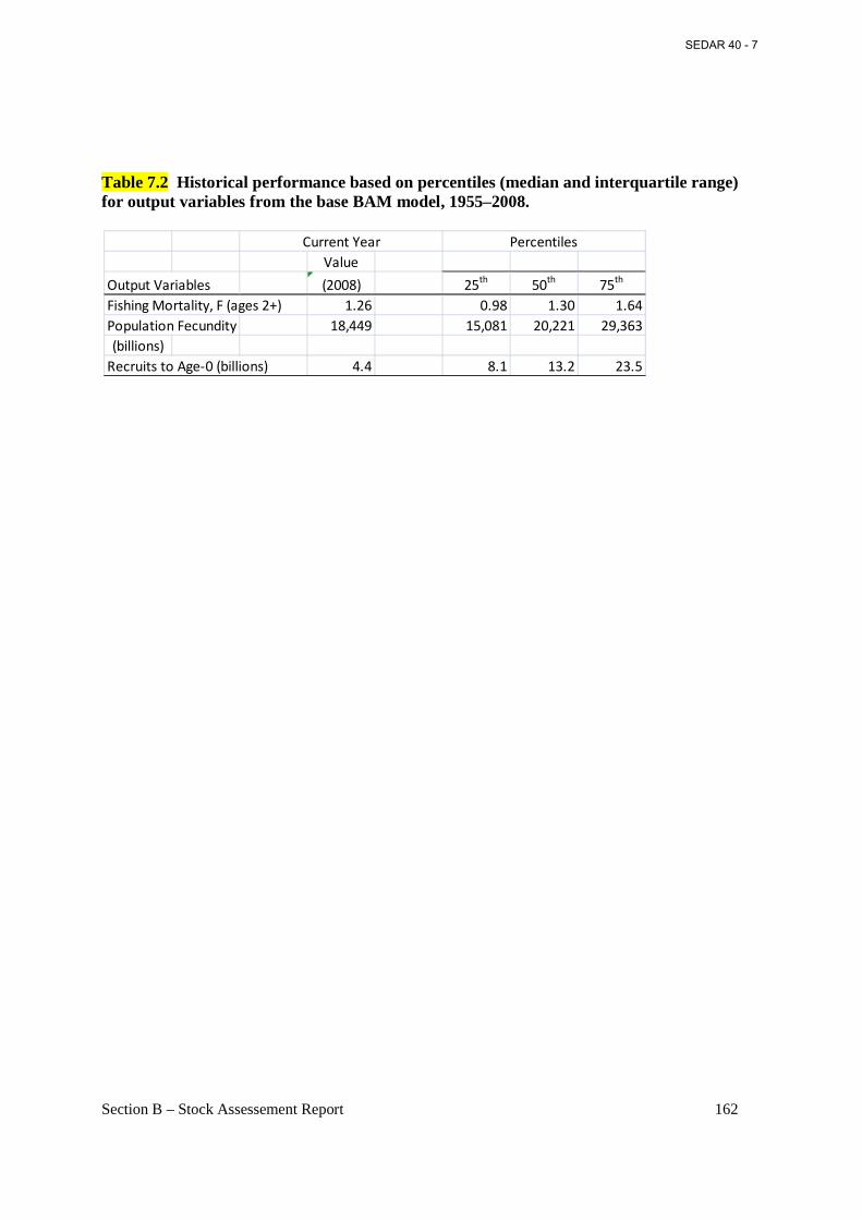
Section B – Stock Assessement Report 162
Table 7.2 Historical performance based on percentiles (median and interquartile range) for output variables from the base BAM model, 1955–2008.
Current Year
Value
Output Variables (2008) 25th
50th
75th
Fishing Mortality, F (ages 2+) 1.26 0.98 1.30 1.64
Population Fecundity 18,449 15,081 20,221 29,363
(billions)
Recruits to Age-0 (billions) 4.4 8.1 13.2 23.5
Percentiles
SEDAR 40 - 7
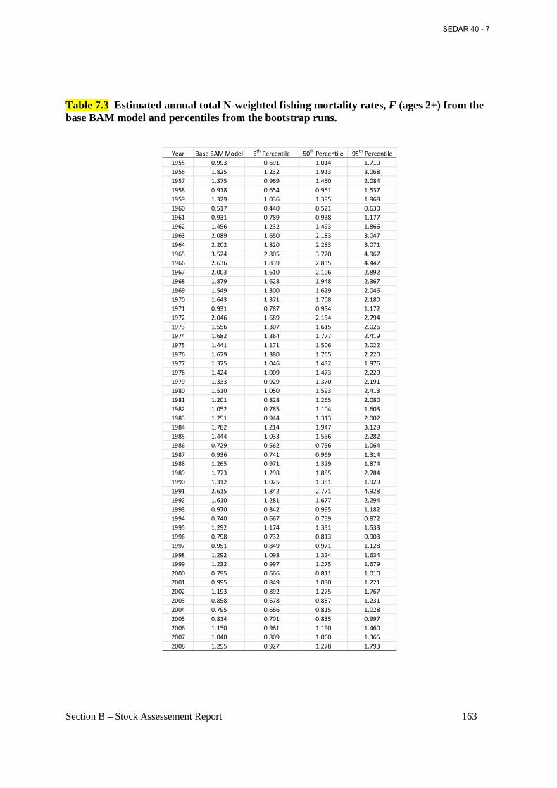
Section B – Stock Assessement Report 163
Table 7.3 Estimated annual total N-weighted fishing mortality rates, F (ages 2+) from the base BAM model and percentiles from the bootstrap runs.
Year Base BAM Model 5th
Percentile 50th
Percentile 95th
Percentile
1955 0.993 0.691 1.014 1.710
1956 1.825 1.232 1.913 3.068
1957 1.375 0.969 1.450 2.084
1958 0.918 0.654 0.951 1.537
1959 1.329 1.036 1.395 1.968
1960 0.517 0.440 0.521 0.630
1961 0.931 0.789 0.938 1.177
1962 1.456 1.232 1.493 1.866
1963 2.089 1.650 2.183 3.047
1964 2.202 1.820 2.283 3.071
1965 3.524 2.805 3.720 4.967
1966 2.636 1.839 2.835 4.447
1967 2.003 1.610 2.106 2.892
1968 1.879 1.628 1.948 2.367
1969 1.549 1.300 1.629 2.046
1970 1.643 1.371 1.708 2.180
1971 0.931 0.787 0.954 1.172
1972 2.046 1.689 2.154 2.794
1973 1.556 1.307 1.615 2.026
1974 1.682 1.364 1.777 2.419
1975 1.441 1.171 1.506 2.022
1976 1.679 1.380 1.765 2.220
1977 1.375 1.046 1.432 1.976
1978 1.424 1.009 1.473 2.229
1979 1.333 0.929 1.370 2.191
1980 1.510 1.050 1.593 2.413
1981 1.201 0.828 1.265 2.080
1982 1.052 0.785 1.104 1.603
1983 1.251 0.944 1.313 2.002
1984 1.782 1.214 1.947 3.129
1985 1.444 1.033 1.556 2.282
1986 0.729 0.562 0.756 1.064
1987 0.936 0.741 0.969 1.314
1988 1.265 0.971 1.329 1.874
1989 1.773 1.298 1.885 2.784
1990 1.312 1.025 1.351 1.929
1991 2.615 1.842 2.771 4.928
1992 1.610 1.281 1.677 2.294
1993 0.970 0.842 0.995 1.182
1994 0.740 0.667 0.759 0.872
1995 1.292 1.174 1.331 1.533
1996 0.798 0.732 0.813 0.903
1997 0.951 0.849 0.971 1.128
1998 1.292 1.098 1.324 1.634
1999 1.232 0.997 1.275 1.679
2000 0.795 0.666 0.811 1.010
2001 0.995 0.849 1.030 1.221
2002 1.193 0.892 1.275 1.767
2003 0.858 0.678 0.887 1.231
2004 0.795 0.666 0.815 1.028
2005 0.814 0.701 0.835 0.997
2006 1.150 0.961 1.190 1.460
2007 1.040 0.809 1.060 1.365
2008 1.255 0.927 1.278 1.793
SEDAR 40 - 7
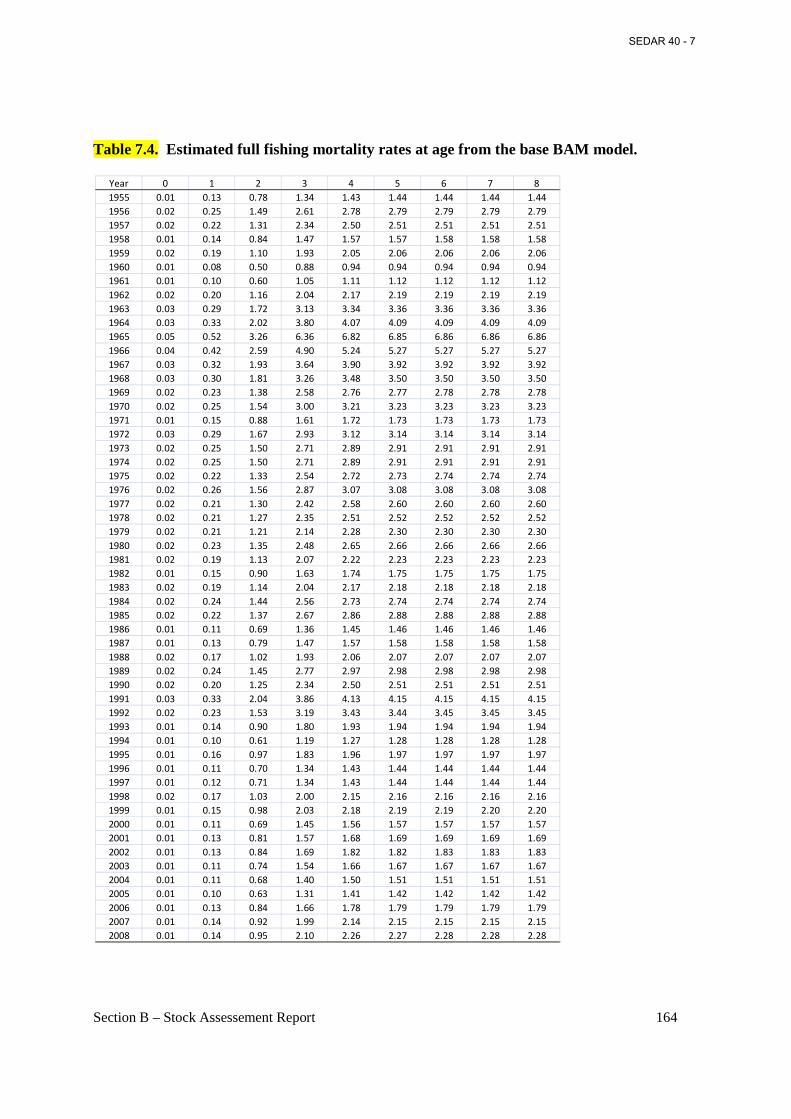
Section B – Stock Assessement Report 164
Table 7.4. Estimated full fishing mortality rates at age from the base BAM model.
Year 0 1 2 3 4 5 6 7 8
1955 0.01 0.13 0.78 1.34 1.43 1.44 1.44 1.44 1.44
1956 0.02 0.25 1.49 2.61 2.78 2.79 2.79 2.79 2.79
1957 0.02 0.22 1.31 2.34 2.50 2.51 2.51 2.51 2.51
1958 0.01 0.14 0.84 1.47 1.57 1.57 1.58 1.58 1.58
1959 0.02 0.19 1.10 1.93 2.05 2.06 2.06 2.06 2.06
1960 0.01 0.08 0.50 0.88 0.94 0.94 0.94 0.94 0.94
1961 0.01 0.10 0.60 1.05 1.11 1.12 1.12 1.12 1.12
1962 0.02 0.20 1.16 2.04 2.17 2.19 2.19 2.19 2.19
1963 0.03 0.29 1.72 3.13 3.34 3.36 3.36 3.36 3.36
1964 0.03 0.33 2.02 3.80 4.07 4.09 4.09 4.09 4.09
1965 0.05 0.52 3.26 6.36 6.82 6.85 6.86 6.86 6.86
1966 0.04 0.42 2.59 4.90 5.24 5.27 5.27 5.27 5.27
1967 0.03 0.32 1.93 3.64 3.90 3.92 3.92 3.92 3.92
1968 0.03 0.30 1.81 3.26 3.48 3.50 3.50 3.50 3.50
1969 0.02 0.23 1.38 2.58 2.76 2.77 2.78 2.78 2.78
1970 0.02 0.25 1.54 3.00 3.21 3.23 3.23 3.23 3.23
1971 0.01 0.15 0.88 1.61 1.72 1.73 1.73 1.73 1.73
1972 0.03 0.29 1.67 2.93 3.12 3.14 3.14 3.14 3.14
1973 0.02 0.25 1.50 2.71 2.89 2.91 2.91 2.91 2.91
1974 0.02 0.25 1.50 2.71 2.89 2.91 2.91 2.91 2.91
1975 0.02 0.22 1.33 2.54 2.72 2.73 2.74 2.74 2.74
1976 0.02 0.26 1.56 2.87 3.07 3.08 3.08 3.08 3.08
1977 0.02 0.21 1.30 2.42 2.58 2.60 2.60 2.60 2.60
1978 0.02 0.21 1.27 2.35 2.51 2.52 2.52 2.52 2.52
1979 0.02 0.21 1.21 2.14 2.28 2.30 2.30 2.30 2.30
1980 0.02 0.23 1.35 2.48 2.65 2.66 2.66 2.66 2.66
1981 0.02 0.19 1.13 2.07 2.22 2.23 2.23 2.23 2.23
1982 0.01 0.15 0.90 1.63 1.74 1.75 1.75 1.75 1.75
1983 0.02 0.19 1.14 2.04 2.17 2.18 2.18 2.18 2.18
1984 0.02 0.24 1.44 2.56 2.73 2.74 2.74 2.74 2.74
1985 0.02 0.22 1.37 2.67 2.86 2.88 2.88 2.88 2.88
1986 0.01 0.11 0.69 1.36 1.45 1.46 1.46 1.46 1.46
1987 0.01 0.13 0.79 1.47 1.57 1.58 1.58 1.58 1.58
1988 0.02 0.17 1.02 1.93 2.06 2.07 2.07 2.07 2.07
1989 0.02 0.24 1.45 2.77 2.97 2.98 2.98 2.98 2.98
1990 0.02 0.20 1.25 2.34 2.50 2.51 2.51 2.51 2.51
1991 0.03 0.33 2.04 3.86 4.13 4.15 4.15 4.15 4.15
1992 0.02 0.23 1.53 3.19 3.43 3.44 3.45 3.45 3.45
1993 0.01 0.14 0.90 1.80 1.93 1.94 1.94 1.94 1.94
1994 0.01 0.10 0.61 1.19 1.27 1.28 1.28 1.28 1.28
1995 0.01 0.16 0.97 1.83 1.96 1.97 1.97 1.97 1.97
1996 0.01 0.11 0.70 1.34 1.43 1.44 1.44 1.44 1.44
1997 0.01 0.12 0.71 1.34 1.43 1.44 1.44 1.44 1.44
1998 0.02 0.17 1.03 2.00 2.15 2.16 2.16 2.16 2.16
1999 0.01 0.15 0.98 2.03 2.18 2.19 2.19 2.20 2.20
2000 0.01 0.11 0.69 1.45 1.56 1.57 1.57 1.57 1.57
2001 0.01 0.13 0.81 1.57 1.68 1.69 1.69 1.69 1.69
2002 0.01 0.13 0.84 1.69 1.82 1.82 1.83 1.83 1.83
2003 0.01 0.11 0.74 1.54 1.66 1.67 1.67 1.67 1.67
2004 0.01 0.11 0.68 1.40 1.50 1.51 1.51 1.51 1.51
2005 0.01 0.10 0.63 1.31 1.41 1.42 1.42 1.42 1.42
2006 0.01 0.13 0.84 1.66 1.78 1.79 1.79 1.79 1.79
2007 0.01 0.14 0.92 1.99 2.14 2.15 2.15 2.15 2.15
2008 0.01 0.14 0.95 2.10 2.26 2.27 2.28 2.28 2.28
SEDAR 40 - 7
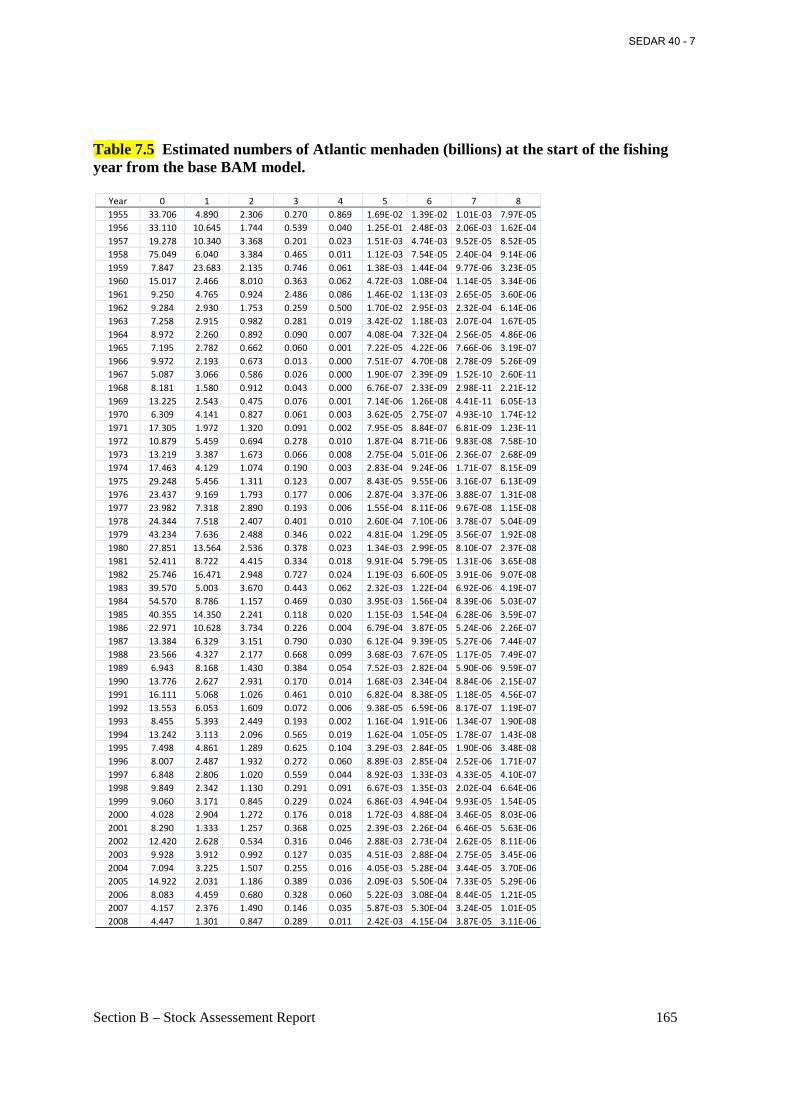
Section B – Stock Assessement Report 165
Table 7.5 Estimated numbers of Atlantic menhaden (billions) at the start of the fishing year from the base BAM model.
Year 0 1 2 3 4 5 6 7 8
1955 33.706 4.890 2.306 0.270 0.869 1.69E-02 1.39E-02 1.01E-03 7.97E-05
1956 33.110 10.645 1.744 0.539 0.040 1.25E-01 2.48E-03 2.06E-03 1.62E-04
1957 19.278 10.340 3.368 0.201 0.023 1.51E-03 4.74E-03 9.52E-05 8.52E-05
1958 75.049 6.040 3.384 0.465 0.011 1.12E-03 7.54E-05 2.40E-04 9.14E-06
1959 7.847 23.683 2.135 0.746 0.061 1.38E-03 1.44E-04 9.77E-06 3.23E-05
1960 15.017 2.466 8.010 0.363 0.062 4.72E-03 1.08E-04 1.14E-05 3.34E-06
1961 9.250 4.765 0.924 2.486 0.086 1.46E-02 1.13E-03 2.65E-05 3.60E-06
1962 9.284 2.930 1.753 0.259 0.500 1.70E-02 2.95E-03 2.32E-04 6.14E-06
1963 7.258 2.915 0.982 0.281 0.019 3.42E-02 1.18E-03 2.07E-04 1.67E-05
1964 8.972 2.260 0.892 0.090 0.007 4.08E-04 7.32E-04 2.56E-05 4.86E-06
1965 7.195 2.782 0.662 0.060 0.001 7.22E-05 4.22E-06 7.66E-06 3.19E-07
1966 9.972 2.193 0.673 0.013 0.000 7.51E-07 4.70E-08 2.78E-09 5.26E-09
1967 5.087 3.066 0.586 0.026 0.000 1.90E-07 2.39E-09 1.52E-10 2.60E-11
1968 8.181 1.580 0.912 0.043 0.000 6.76E-07 2.33E-09 2.98E-11 2.21E-12
1969 13.225 2.543 0.475 0.076 0.001 7.14E-06 1.26E-08 4.41E-11 6.05E-13
1970 6.309 4.141 0.827 0.061 0.003 3.62E-05 2.75E-07 4.93E-10 1.74E-12
1971 17.305 1.972 1.320 0.091 0.002 7.95E-05 8.84E-07 6.81E-09 1.23E-11
1972 10.879 5.459 0.694 0.278 0.010 1.87E-04 8.71E-06 9.83E-08 7.58E-10
1973 13.219 3.387 1.673 0.066 0.008 2.75E-04 5.01E-06 2.36E-07 2.68E-09
1974 17.463 4.129 1.074 0.190 0.003 2.83E-04 9.24E-06 1.71E-07 8.15E-09
1975 29.248 5.456 1.311 0.123 0.007 8.43E-05 9.55E-06 3.16E-07 6.13E-09
1976 23.437 9.169 1.793 0.177 0.006 2.87E-04 3.37E-06 3.88E-07 1.31E-08
1977 23.982 7.318 2.890 0.193 0.006 1.55E-04 8.11E-06 9.67E-08 1.15E-08
1978 24.344 7.518 2.407 0.401 0.010 2.60E-04 7.10E-06 3.78E-07 5.04E-09
1979 43.234 7.636 2.488 0.346 0.022 4.81E-04 1.29E-05 3.56E-07 1.92E-08
1980 27.851 13.564 2.536 0.378 0.023 1.34E-03 2.99E-05 8.10E-07 2.37E-08
1981 52.411 8.722 4.415 0.334 0.018 9.91E-04 5.79E-05 1.31E-06 3.65E-08
1982 25.746 16.471 2.948 0.727 0.024 1.19E-03 6.60E-05 3.91E-06 9.07E-08
1983 39.570 5.003 3.670 0.443 0.062 2.32E-03 1.22E-04 6.92E-06 4.19E-07
1984 54.570 8.786 1.157 0.469 0.030 3.95E-03 1.56E-04 8.39E-06 5.03E-07
1985 40.355 14.350 2.241 0.118 0.020 1.15E-03 1.54E-04 6.28E-06 3.59E-07
1986 22.971 10.628 3.734 0.226 0.004 6.79E-04 3.87E-05 5.24E-06 2.26E-07
1987 13.384 6.329 3.151 0.790 0.030 6.12E-04 9.39E-05 5.27E-06 7.44E-07
1988 23.566 4.327 2.177 0.668 0.099 3.68E-03 7.67E-05 1.17E-05 7.49E-07
1989 6.943 8.168 1.430 0.384 0.054 7.52E-03 2.82E-04 5.90E-06 9.59E-07
1990 13.776 2.627 2.931 0.170 0.014 1.68E-03 2.34E-04 8.84E-06 2.15E-07
1991 16.111 5.068 1.026 0.461 0.010 6.82E-04 8.38E-05 1.18E-05 4.56E-07
1992 13.553 6.053 1.609 0.072 0.006 9.38E-05 6.59E-06 8.17E-07 1.19E-07
1993 8.455 5.393 2.449 0.193 0.002 1.16E-04 1.91E-06 1.34E-07 1.90E-08
1994 13.242 3.113 2.096 0.565 0.019 1.62E-04 1.05E-05 1.78E-07 1.43E-08
1995 7.498 4.861 1.289 0.625 0.104 3.29E-03 2.84E-05 1.90E-06 3.48E-08
1996 8.007 2.487 1.932 0.272 0.060 8.89E-03 2.85E-04 2.52E-06 1.71E-07
1997 6.848 2.806 1.020 0.559 0.044 8.92E-03 1.33E-03 4.33E-05 4.10E-07
1998 9.849 2.342 1.130 0.291 0.091 6.67E-03 1.35E-03 2.02E-04 6.64E-06
1999 9.060 3.171 0.845 0.229 0.024 6.86E-03 4.94E-04 9.93E-05 1.54E-05
2000 4.028 2.904 1.272 0.176 0.018 1.72E-03 4.88E-04 3.46E-05 8.03E-06
2001 8.290 1.333 1.257 0.368 0.025 2.39E-03 2.26E-04 6.46E-05 5.63E-06
2002 12.420 2.628 0.534 0.316 0.046 2.88E-03 2.73E-04 2.62E-05 8.11E-06
2003 9.928 3.912 0.992 0.127 0.035 4.51E-03 2.88E-04 2.75E-05 3.45E-06
2004 7.094 3.225 1.507 0.255 0.016 4.05E-03 5.28E-04 3.44E-05 3.70E-06
2005 14.922 2.031 1.186 0.389 0.036 2.09E-03 5.50E-04 7.33E-05 5.29E-06
2006 8.083 4.459 0.680 0.328 0.060 5.22E-03 3.08E-04 8.44E-05 1.21E-05
2007 4.157 2.376 1.490 0.146 0.035 5.87E-03 5.30E-04 3.24E-05 1.01E-05
2008 4.447 1.301 0.847 0.289 0.011 2.42E-03 4.15E-04 3.87E-05 3.11E-06
SEDAR 40 - 7
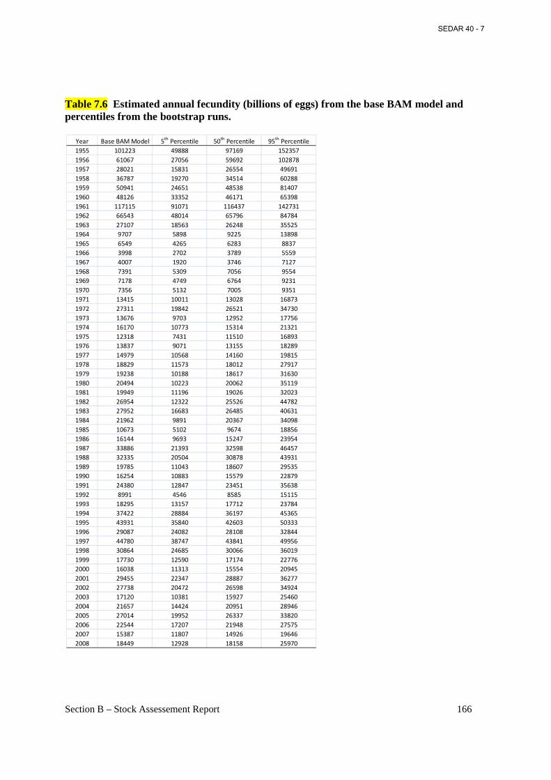
Section B – Stock Assessement Report 166
Table 7.6 Estimated annual fecundity (billions of eggs) from the base BAM model and percentiles from the bootstrap runs.
Year Base BAM Model 5th
Percentile 50th
Percentile 95th
Percentile
1955 101223 49888 97169 152357
1956 61067 27056 59692 102878
1957 28021 15831 26554 49691
1958 36787 19270 34514 60288
1959 50941 24651 48538 81407
1960 48126 33352 46171 65398
1961 117115 91071 116437 142731
1962 66543 48014 65796 84784
1963 27107 18563 26248 35525
1964 9707 5898 9225 13898
1965 6549 4265 6283 8837
1966 3998 2702 3789 5559
1967 4007 1920 3746 7127
1968 7391 5309 7056 9554
1969 7178 4749 6764 9231
1970 7356 5132 7005 9351
1971 13415 10011 13028 16873
1972 27311 19842 26521 34730
1973 13676 9703 12952 17756
1974 16170 10773 15314 21321
1975 12318 7431 11510 16893
1976 13837 9071 13155 18289
1977 14979 10568 14160 19815
1978 18829 11573 18012 27917
1979 19238 10188 18617 31630
1980 20494 10223 20062 35119
1981 19949 11196 19026 32023
1982 26954 12322 25526 44782
1983 27952 16683 26485 40631
1984 21962 9891 20367 34098
1985 10673 5102 9674 18856
1986 16144 9693 15247 23954
1987 33886 21393 32598 46457
1988 32335 20504 30878 43931
1989 19785 11043 18607 29535
1990 16254 10883 15579 22879
1991 24380 12847 23451 35638
1992 8991 4546 8585 15115
1993 18295 13157 17712 23784
1994 37422 28884 36197 45365
1995 43931 35840 42603 50333
1996 29087 24082 28108 32844
1997 44780 38747 43841 49956
1998 30864 24685 30066 36019
1999 17730 12590 17174 22776
2000 16038 11313 15554 20945
2001 29455 22347 28887 36277
2002 27738 20472 26598 34924
2003 17120 10381 15927 25460
2004 21657 14424 20951 28946
2005 27014 19952 26337 33820
2006 22544 17207 21948 27575
2007 15387 11807 14926 19646
2008 18449 12928 18158 25970
SEDAR 40 - 7
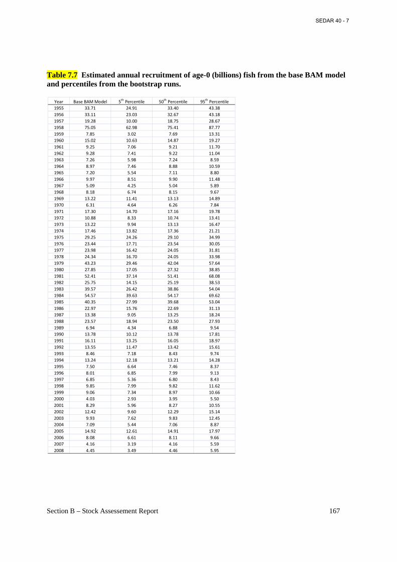
Section B – Stock Assessement Report 167
Table 7.7 Estimated annual recruitment of age-0 (billions) fish from the base BAM model and percentiles from the bootstrap runs.
Year Base BAM Model 5th
Percentile 50th
Percentile 95th
Percentile
1955 33.71 24.91 33.40 43.38
1956 33.11 23.03 32.67 43.18
1957 19.28 10.00 18.75 28.67
1958 75.05 62.98 75.41 87.77
1959 7.85 3.02 7.69 13.31
1960 15.02 10.63 14.87 19.27
1961 9.25 7.06 9.21 11.70
1962 9.28 7.41 9.22 11.04
1963 7.26 5.98 7.24 8.59
1964 8.97 7.46 8.88 10.59
1965 7.20 5.54 7.11 8.80
1966 9.97 8.51 9.90 11.48
1967 5.09 4.25 5.04 5.89
1968 8.18 6.74 8.15 9.67
1969 13.22 11.41 13.13 14.89
1970 6.31 4.64 6.26 7.84
1971 17.30 14.70 17.16 19.78
1972 10.88 8.33 10.74 13.41
1973 13.22 9.94 13.13 16.47
1974 17.46 13.82 17.36 21.21
1975 29.25 24.26 29.10 34.99
1976 23.44 17.71 23.54 30.05
1977 23.98 16.42 24.05 31.81
1978 24.34 16.70 24.05 33.98
1979 43.23 29.46 42.04 57.64
1980 27.85 17.05 27.32 38.85
1981 52.41 37.14 51.41 68.08
1982 25.75 14.15 25.19 38.53
1983 39.57 26.42 38.86 54.04
1984 54.57 39.63 54.17 69.62
1985 40.35 27.99 39.68 53.04
1986 22.97 15.76 22.69 31.13
1987 13.38 9.05 13.25 18.24
1988 23.57 18.94 23.50 27.93
1989 6.94 4.34 6.88 9.54
1990 13.78 10.12 13.78 17.81
1991 16.11 13.25 16.05 18.97
1992 13.55 11.47 13.42 15.61
1993 8.46 7.18 8.43 9.74
1994 13.24 12.18 13.21 14.28
1995 7.50 6.64 7.46 8.37
1996 8.01 6.85 7.99 9.13
1997 6.85 5.36 6.80 8.43
1998 9.85 7.99 9.82 11.62
1999 9.06 7.34 8.97 10.66
2000 4.03 2.93 3.95 5.50
2001 8.29 5.96 8.27 10.55
2002 12.42 9.60 12.29 15.14
2003 9.93 7.62 9.83 12.45
2004 7.09 5.44 7.06 8.87
2005 14.92 12.61 14.91 17.97
2006 8.08 6.61 8.11 9.66
2007 4.16 3.19 4.16 5.59
2008 4.45 3.49 4.46 5.95
SEDAR 40 - 7
Section B – Stock Assessement Report 168
Table 7.8 Results from base BAM model, sensitivity runs, and retrospective analysis. [Median recruitment to age-0 (billions) is labeled as R, total N-weighted fishing mortality (F) is for age 2+, and population fecundity (FEC) is in billions of mature ova.]
BAM Model Run Median R FMED Fta rget FECMED FECthres h F(2008)/FMED FEC(2008)/FECthres h
Base Run 13.2 1.25 0.61 18,628 9,314 1.00 1.98
Time invariant Natural Mortality (M) 13.1 1.29 0.62 17,549 8,775 0.91 2.22
Eight year average used for benchmark calculations 13.2 1.37 0.66 18,628 9,314 0.92 1.98
Pound net index coefficient of variation (CV)=0.2 13.2 1.25 0.62 18,609 9,305 0.80 2.31
Pound net index coefficient of variation (CV)=0.8 13.2 1.25 0.60 18,667 9,334 1.04 1.93
No ageing reading error 13.1 1.06 0.53 22,035 11,017 1.01 1.88
Four separate juvenile abundance indices (JAIs) with estimated weights 13.2 1.25 0.65 18,484 9,242 0.91 2.05
Dome-shaped selectivity in last period (1994-2008) for the reduction fishery 13.1 1.29 0.67 18,664 9,332 0.97 1.91
Start model in 1964 13.0 1.38 0.85 15,363 7,682 1.01 2.23
Three year average used for benchmark calculations 13.2 1.18 0.53 18,628 9,314 1.06 1.98
Random walk on pound net index catchability (q) 13.2 1.25 0.60 18,696 9,348 1.05 1.92
Leave out juvenile abundance index (JAI) 13.3 1.25 0.59 18,714 9,357 1.60 1.51
Leave out pound net (PN) index 13.2 1.25 0.60 18,692 9,346 1.08 1.90
GLM based on pound net (PN) index 13.2 1.25 0.61 18,641 9,320 0.99 2.00
Natural mortality (M) re-scaled +25% 22.9 1.08 0.46 20,547 10,274 1.10 1.88
Natural mortality (M) re-scaled -25% 7.6 1.42 0.75 16,719 8,359 0.92 2.12
Estimate natural mortality (M) scalar 70.3 0.76 0.19 25,697 12,849 1.35 1.69
Estimate MSY based on Beverton-Holt curve 13.2 1.25 0.61 18,627 9,313 1.00 1.98
Estimate MSY based on Ricker curve 13.2 1.25 0.69 18,633 9,317 1.02 1.95
Retrospective to 2007 13.2 1.26 0.60 18,377 9,189 1.30 1.29
Retrospective to 2006 13.2 1.24 0.63 18,813 9,407 1.13 2.23
Retrospective to 2005 13.3 1.25 0.65 18,606 9,303 0.44 3.97
Retrospective to 2004 13.3 1.25 0.64 18,643 9,322 0.62 2.42
Retrospective to 2003 13.3 1.30 0.63 17,823 8,912 0.58 2.21
Retrospective to 2002 13.5 1.27 0.62 18,243 9,122 0.79 3.52
Retrospective to 2001 13.6 1.33 0.63 17,301 8,651 0.33 6.04
SEDAR 40 - 7
Section B – Stock Assessement Report 169
Table 7.9 Summary of benchmarks and terminal year (2008) values estimated for the base BAM model (F are N-weighted for ages 2+).
Benchmarks and Base BAM Model Estimates
Terminal Year Values
Median Age-0 Recruits (billions) 13.2
Threshold (Limit): FMED 1.25
Target: Ftarget 0.61
F2008 1.26
F2008/FMED 1.00
F30% 0.41
F25% 0.50
F20% 0.62
Target: FECMED 18,628
Threshold (Limit): FECthreshold 9,314
FEC2008 18,449
FEC2008/FECthreshold 1.98
SEDAR 40 - 7
Section B – Stock Assessement Report 170
Table 8.1 Summary of benchmarks and terminal year value from previous stock assessments (ASMFC 2004, Table 9.1; and ASMFC 2006, Table 7.1). [Terminal years are 2002 and 2005, respectively; F is average for ages 2+, and eggs (fecundity) are mature ova in trillions.]
Benchmarks F-based Egg-based2003 Peer Review:Target 0.75 26.60
Limit 1.18 13.30Terminal 0.79 40.602006 Update:Target 0.55 26.35Limit 0.91 13.18Terminal 0.50 41.74
SEDAR 40 - 7

Section B – Stock Assessement Report
Figure 1.1 VPA historical retrospective on fishing mortality (F), both as (a) fishing mortality F for terminal years 1992year 2000 (1992-1999).
Stock Assessement Report
12.0 Figures
VPA historical retrospective on fishing mortality (F), both as (a) fishing mortality F for terminal years 1992-2001, and (b) as proportional deviations from terminal
171
VPA historical retrospective on fishing mortality (F), both as (a) fishing 2001, and (b) as proportional deviations from terminal
a
b
SEDAR 40 - 7

Section B – Stock Assessement Report
Figure 1.2 VPA historical rfor terminal years 1990, 19922000 (1992-1999).
Stock Assessement Report
historical r etrospective on spawning stock biomass (SSB), both for terminal years 1990, 1992-2001, and (b) as proportional deviations from
172
spawning stock biomass (SSB), both as (a) SSB proportional deviations from terminal year
a
b
SEDAR 40 - 7

Section B – Stock Assessement Report
Figure 1.3 VPA historical rterminal years 1990, 1992-2001, and (b) as (1992-1999).
Stock Assessement Report
historical r etrospective on recruits to age 1 (R1), both 2001, and (b) as proportional deviations from
173
), both as (a) R1 for proportional deviations from terminal year 2000
a
b
SEDAR 40 - 7

Section B – Stock Assessement Report
Figure 1.4 Comparison of fishing mortalitystatistical catch model for terminal years 2000 and 2001
Stock Assessement Report
fishing mortality , F, from “untuned” VPA with preliminary catch model for terminal years 2000 and 2001.
174
, from “untuned” VPA with preliminary
SEDAR 40 - 7

Section B – Stock Assessement Report
Figure 1.5 Comparison of spawning stock biomass, SSB, preliminary statistical catch model for terminal years 2000 and 2001
Stock Assessement Report
spawning stock biomass, SSB, from “untuned” VPA with preliminary statistical catch model for terminal years 2000 and 2001.
175
from “untuned” VPA with
SEDAR 40 - 7

Section B – Stock Assessement Report
Figure 1.6 Comparison of recruits to age 1, Rstatistical catch model for terminal years 2000 and 2001
Stock Assessement Report
recruits to age 1, R1, from “untuned” VPA with preliminary statistical catch model for terminal years 2000 and 2001.
176
from “untuned” VPA with preliminary
SEDAR 40 - 7

Section B – Stock Assessement Report
Figure 1.7 Comparison of fishing mortality(2003) and update (2006).
Stock Assessement Report
fishing mortality , F, from statistical catch model for peer review
177
, from statistical catch model for peer review
SEDAR 40 - 7

Section B – Stock Assessement Report
Figure 1.8 Comparison of spawnpeer review (2003) and update (2006)
Stock Assessement Report
spawning stock biomass, SSB, from statistical catch model for peer review (2003) and update (2006).
178
ing stock biomass, SSB, from statistical catch model for
SEDAR 40 - 7

Section B – Stock Assessement Report
Figure 1.9 Comparison of recruits to age 1, R(2003) and update (2006).
Stock Assessement Report
recruits to age 1, R1, from statistical catch model for peer review
179
, from statistical catch model for peer review
SEDAR 40 - 7
Section B – Stock Assessement Report 180
Figure 2.1. Matrix of paired age readings by scales for Atlantic menhaden from 2008. First reading age (in yrs)
2
9
6
4
4
90
111
9
1
157
821
115
9
6
59
1850
180
31
1
3
152
48
1
40
2
0 1 2 3 4 5
Second reading age (in yrs)
2
3
4
5
1
0
SEDAR 40 - 7
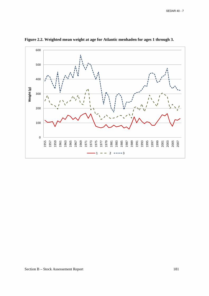
Section B – Stock Assessement Report 181
Figure 2.2. Weighted mean weight at age for Atlantic menhaden for ages 1 through 3.
0
100
200
300
400
500
600
19
55
19
57
19
59
19
61
19
63
19
65
19
67
19
69
19
71
19
73
19
75
19
77
19
79
19
81
19
83
19
85
19
87
19
89
19
91
19
93
19
95
19
97
19
99
20
01
20
03
20
05
20
07
We
igh
t (g
)
1 2 3
SEDAR 40 - 7
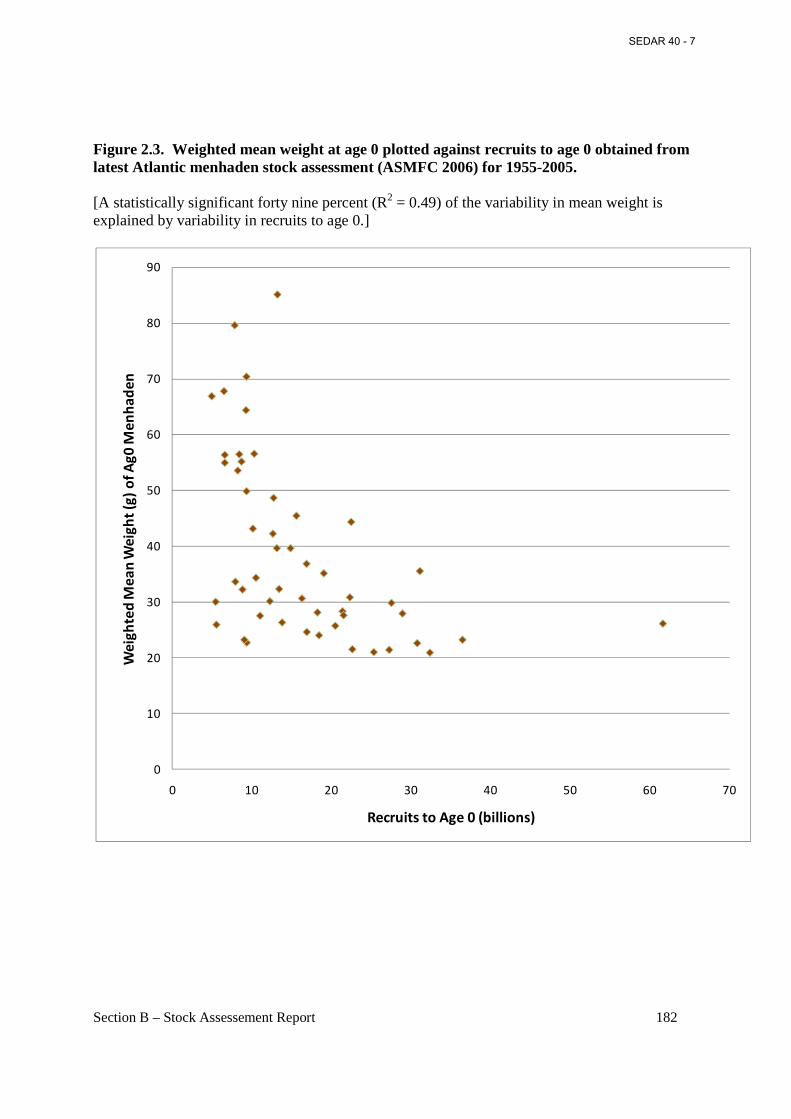
Section B – Stock Assessement Report 182
Figure 2.3. Weighted mean weight at age 0 plotted against recruits to age 0 obtained from latest Atlantic menhaden stock assessment (ASMFC 2006) for 1955-2005. [A statistically significant forty nine percent (R2 = 0.49) of the variability in mean weight is explained by variability in recruits to age 0.]
0
10
20
30
40
50
60
70
80
90
0 10 20 30 40 50 60 70
We
igh
ted
Me
an
We
igh
t (g
) o
f A
g0
Me
nh
ad
en
Recruits to Age 0 (billions)
SEDAR 40 - 7
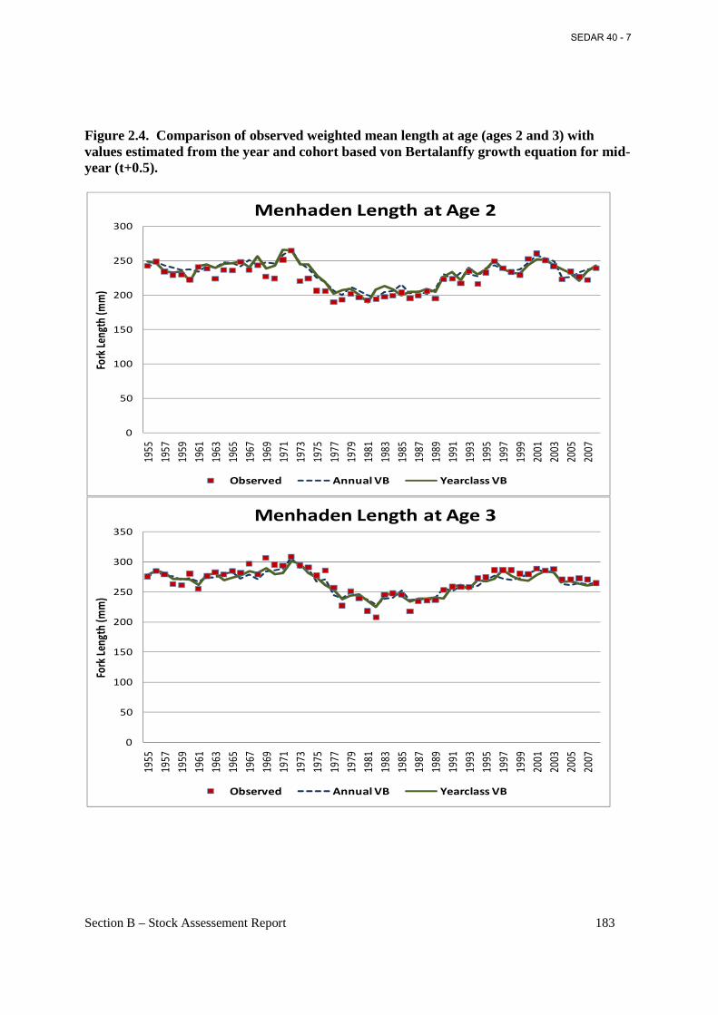
Section B – Stock Assessement Report 183
Figure 2.4. Comparison of observed weighted mean length at age (ages 2 and 3) with values estimated from the year and cohort based von Bertalanffy growth equation for mid-year (t+0.5).
0
50
100
150
200
250
300
1955
1957
1959
1961
1963
1965
1967
1969
1971
1973
1975
1977
1979
1981
1983
1985
1987
1989
1991
1993
1995
1997
1999
2001
2003
2005
2007
Fork
Len
gth
(mm
)
Menhaden Length at Age 2
Observed Annual VB Yearclass VB
0
50
100
150
200
250
300
350
1955
1957
1959
1961
1963
1965
1967
1969
1971
1973
1975
1977
1979
1981
1983
1985
1987
1989
1991
1993
1995
1997
1999
2001
2003
2005
2007
Fork
Len
gth
(m
m)
Menhaden Length at Age 3
Observed Annual VB Yearclass VB
SEDAR 40 - 7
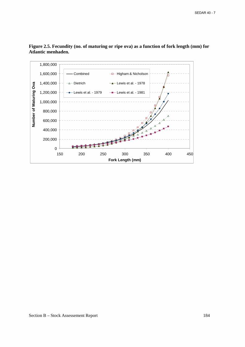
Section B – Stock Assessement Report 184
Figure 2.5. Fecundity (no. of maturing or ripe ova) as a function of fork length (mm) for Atlantic menhaden.
0
200,000
400,000
600,000
800,000
1,000,000
1,200,000
1,400,000
1,600,000
1,800,000
150 200 250 300 350 400 450
Fork Length (mm)
Num
ber
of M
atur
ing
Ova
Combined Higham & Nicholson
Dietrich Lewis et al. - 1978
Lewis et al. - 1979 Lewis et al. - 1981
SEDAR 40 - 7
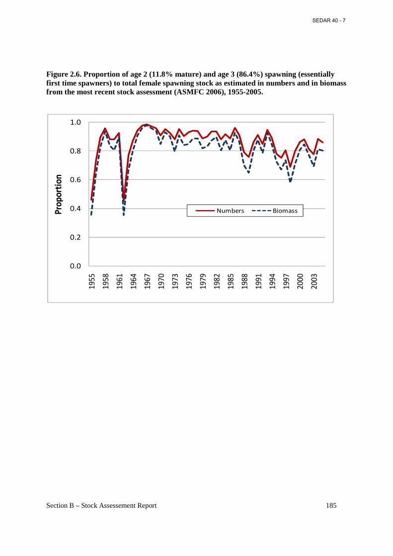
Section B – Stock Assessement Report 185
Figure 2.6. Proportion of age 2 (11.8% mature) and age 3 (86.4%) spawning (essentially first time spawners) to total female spawning stock as estimated in numbers and in biomass from the most recent stock assessment (ASMFC 2006), 1955-2005.
0.0
0.2
0.4
0.6
0.8
1.0
19
55
19
58
19
61
19
64
19
67
19
70
19
73
19
76
19
79
19
82
19
85
19
88
19
91
19
94
19
97
20
00
20
03
Pro
po
rtio
n
Numbers Biomass
SEDAR 40 - 7
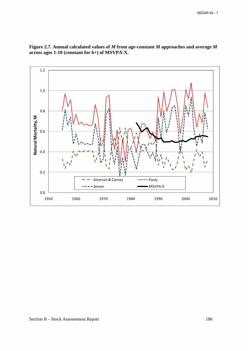
Section B – Stock Assessement Report 186
Figure 2.7. Annual calculated values of M from age-constant M approaches and average M across ages 1-10 (constant for 6+) of MSVPA-X.
0.0
0.2
0.4
0.6
0.8
1.0
1.2
1950 1960 1970 1980 1990 2000 2010
Na
tura
l Mo
rta
lity
, M
Alverson & Carney Pauly
Jensen MSVPA-X
SEDAR 40 - 7
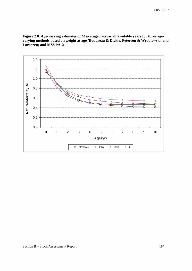
Section B – Stock Assessement Report 187
Figure 2.8. Age-varying estimates of M averaged across all available years for three age-varying methods based on weight at age (Boudreau & Dickie, Peterson & Wroblewski, and Lorenzen) and MSVPA-X.
0.0
0.2
0.4
0.6
0.8
1.0
1.2
1.4
0 1 2 3 4 5 6 7 8 9 10
Nat
ural
Mor
talit
y, M
Age (yr)
MSVPA-X P&W B&D L
SEDAR 40 - 7
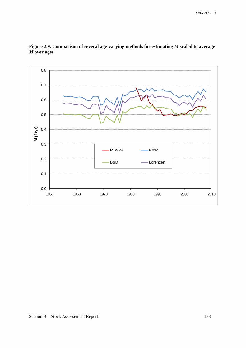
Section B – Stock Assessement Report 188
Figure 2.9. Comparison of several age-varying methods for estimating M scaled to average M over ages.
0.0
0.1
0.2
0.3
0.4
0.5
0.6
0.7
0.8
1950 1960 1970 1980 1990 2000 2010
M (1
/yr)
MSVPA P&W
B&D Lorenzen
SEDAR 40 - 7
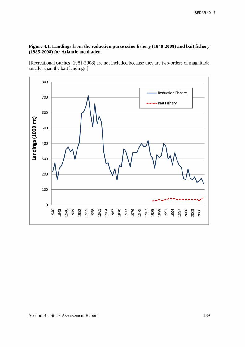
Section B – Stock Assessement Report 189
Figure 4.1. Landings from the reduction purse seine fishery (1940-2008) and bait fishery (1985-2008) for Atlantic menhaden. [Recreational catches (1981-2008) are not included because they are two-orders of magnitude smaller than the bait landings.]
0
100
200
300
400
500
600
700
800
19
40
19
43
19
46
19
49
19
52
19
55
19
58
19
61
19
64
19
67
19
70
19
73
19
76
19
79
19
82
19
85
19
88
19
91
19
94
19
97
20
00
20
03
20
06
Lan
din
gs
(10
00
mt)
Reduction Fishery
Bait Fishery
SEDAR 40 - 7
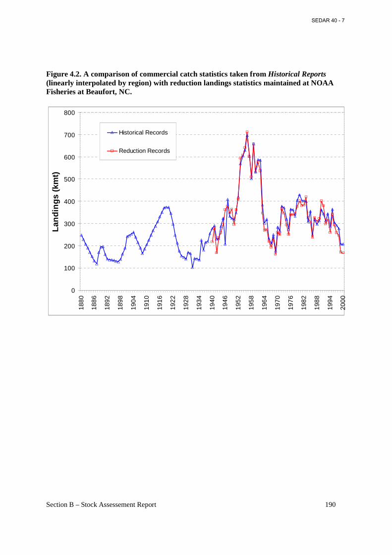
Section B – Stock Assessement Report 190
Figure 4.2. A comparison of commercial catch statistics taken from Historical Reports (linearly interpolated by region) with reduction landings statistics maintained at NOAA Fisheries at Beaufort, NC.
0
100
200
300
400
500
600
700
800
188
0
188
6
189
2
189
8
190
4
191
0
191
6
192
2
192
8
193
4
194
0
194
6
195
2
195
8
196
4
197
0
197
6
198
2
198
8
199
4
200
0
Land
ings
(km
t)
Historical Records
Reduction Records
SEDAR 40 - 7
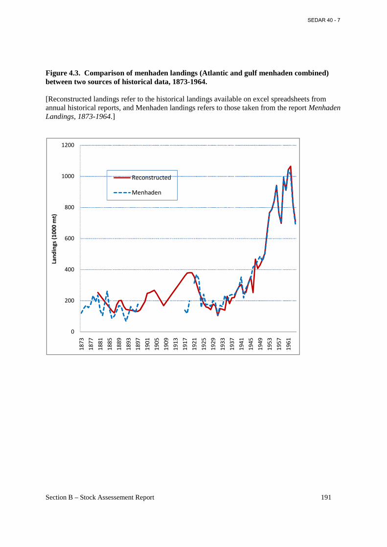
Section B – Stock Assessement Report 191
0
200
400
600
800
1000
1200
18
73
18
77
18
81
18
85
18
89
18
93
18
97
19
01
19
05
19
09
19
13
19
17
19
21
19
25
19
29
19
33
19
37
19
41
19
45
19
49
19
53
19
57
19
61
Lan
din
gs
(10
00
mt)
Reconstructed
Menhaden
Figure 4.3. Comparison of menhaden landings (Atlantic and gulf menhaden combined) between two sources of historical data, 1873-1964. [Reconstructed landings refer to the historical landings available on excel spreadsheets from annual historical reports, and Menhaden landings refers to those taken from the report Menhaden Landings, 1873-1964.]
SEDAR 40 - 7
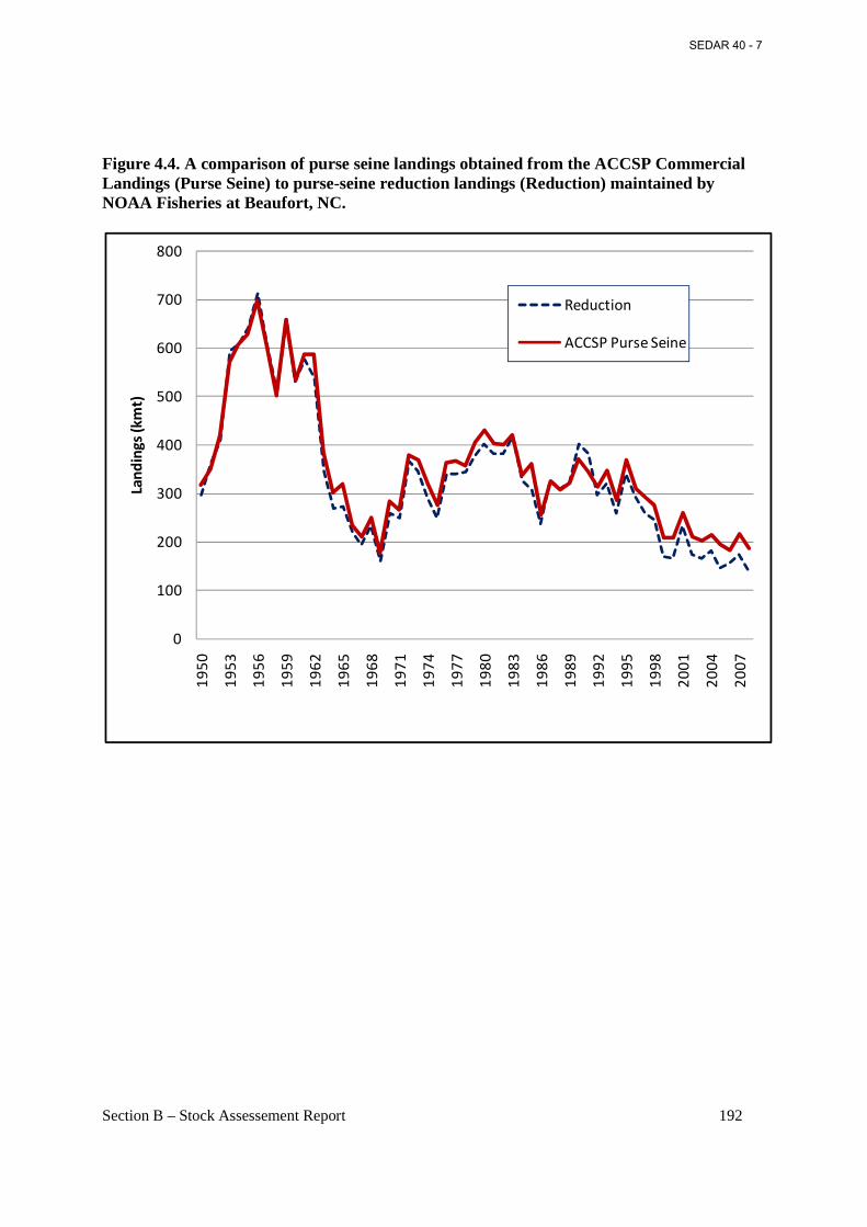
Section B – Stock Assessement Report 192
Figure 4.4. A comparison of purse seine landings obtained from the ACCSP Commercial Landings (Purse Seine) to purse-seine reduction landings (Reduction) maintained by NOAA Fisheries at Beaufort, NC.
0
100
200
300
400
500
600
700
800
19
50
19
53
19
56
19
59
19
62
19
65
19
68
19
71
19
74
19
77
19
80
19
83
19
86
19
89
19
92
19
95
19
98
20
01
20
04
20
07
Lan
din
gs
(km
t)
Reduction
ACCSP Purse Seine
SEDAR 40 - 7
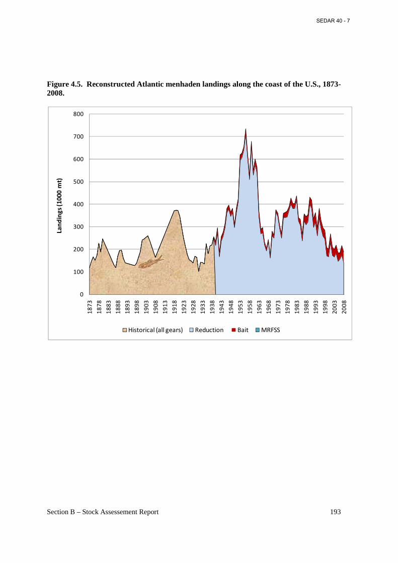
Section B – Stock Assessement Report 193
Figure 4.5. Reconstructed Atlantic menhaden landings along the coast of the U.S., 1873-2008.
0
100
200
300
400
500
600
700
800
18
73
18
78
18
83
18
88
18
93
18
98
19
03
19
08
19
13
19
18
19
23
19
28
19
33
19
38
19
43
19
48
19
53
19
58
19
63
19
68
19
73
19
78
19
83
19
88
19
93
19
98
20
03
20
08
Lan
din
gs
(10
00
mt)
Historical (all gears) Reduction Bait MRFSS
SEDAR 40 - 7
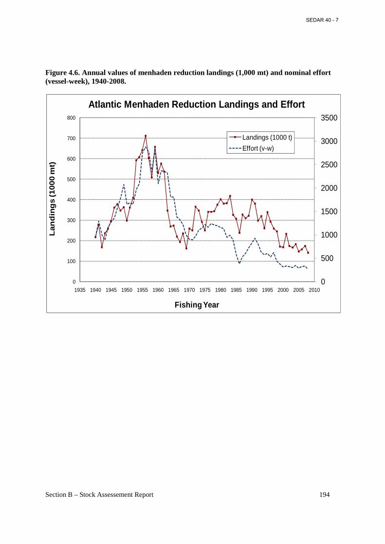
Section B – Stock Assessement Report 194
Figure 4.6. Annual values of menhaden reduction landings (1,000 mt) and nominal effort (vessel-week), 1940-2008.
0
500
1000
1500
2000
2500
3000
3500
0
100
200
300
400
500
600
700
800
1935 1940 1945 1950 1955 1960 1965 1970 1975 1980 1985 1990 1995 2000 2005 2010
Lan
din
gs
(1000 m
t)
Fishing Year
Atlantic Menhaden Reduction Landings and Effort
Landings (1000 t)
Effort (v-w)
SEDAR 40 - 7
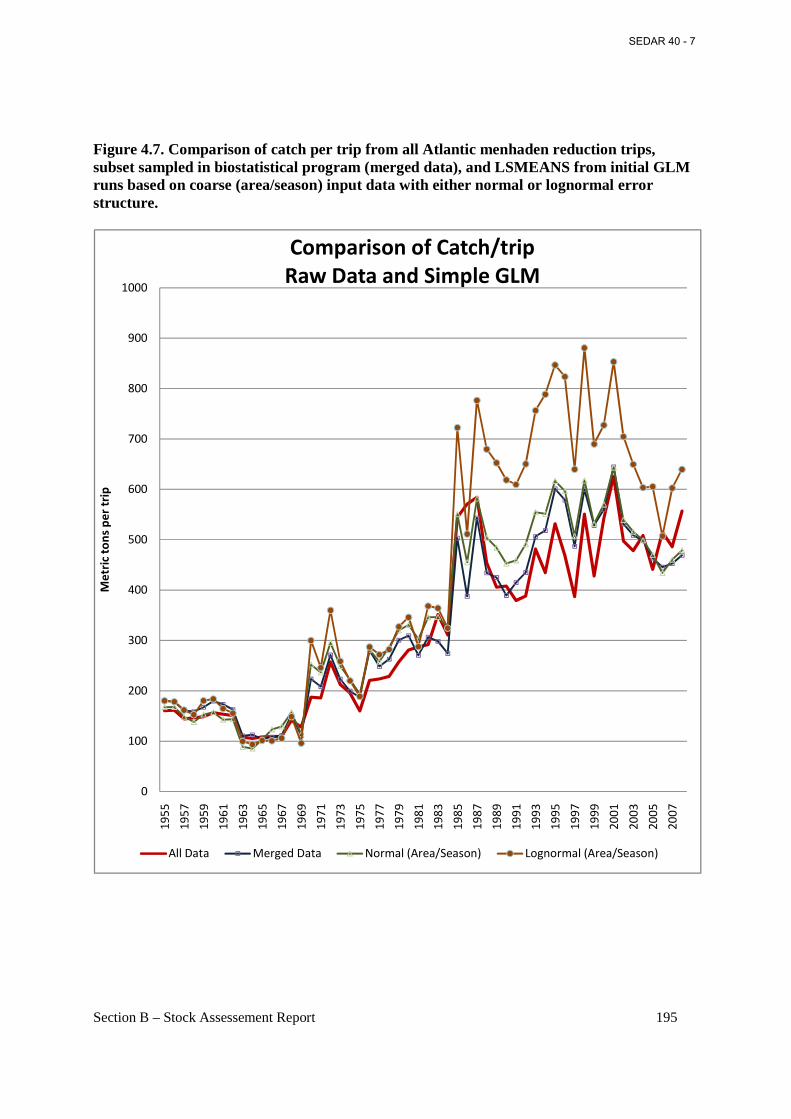
Section B – Stock Assessement Report 195
0
100
200
300
400
500
600
700
800
900
1000
19
55
19
57
19
59
19
61
19
63
19
65
19
67
19
69
19
71
19
73
19
75
19
77
19
79
19
81
19
83
19
85
19
87
19
89
19
91
19
93
19
95
19
97
19
99
20
01
20
03
20
05
20
07
Me
tric
to
ns
pe
r tr
ip
Comparison of Catch/trip
Raw Data and Simple GLM
All Data Merged Data Normal (Area/Season) Lognormal (Area/Season)
Figure 4.7. Comparison of catch per trip from all Atlantic menhaden reduction trips, subset sampled in biostatistical program (merged data), and LSMEANS from initial GLM runs based on coarse (area/season) input data with either normal or lognormal error structure.
SEDAR 40 - 7
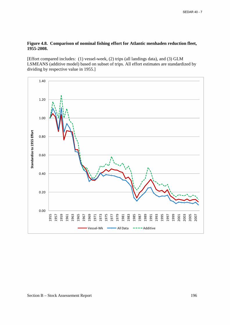
Section B – Stock Assessement Report 196
Figure 4.8. Comparison of nominal fishing effort for Atlantic menhaden reduction fleet, 1955-2008. [Effort compared includes: (1) vessel-week, (2) trips (all landings data), and (3) GLM LSMEANS (additive model) based on subset of trips. All effort estimates are standardized by dividing by respective value in 1955.]
0.00
0.20
0.40
0.60
0.80
1.00
1.20
1.40
19
55
19
57
19
59
19
61
19
63
19
65
19
67
19
69
19
71
19
73
19
75
19
77
19
79
19
81
19
83
19
85
19
87
19
89
19
91
19
93
19
95
19
97
19
99
20
01
20
03
20
05
20
07
Sta
nd
ard
ize
to
19
55
Eff
ort
Vessel-Wk All Data Additive
SEDAR 40 - 7
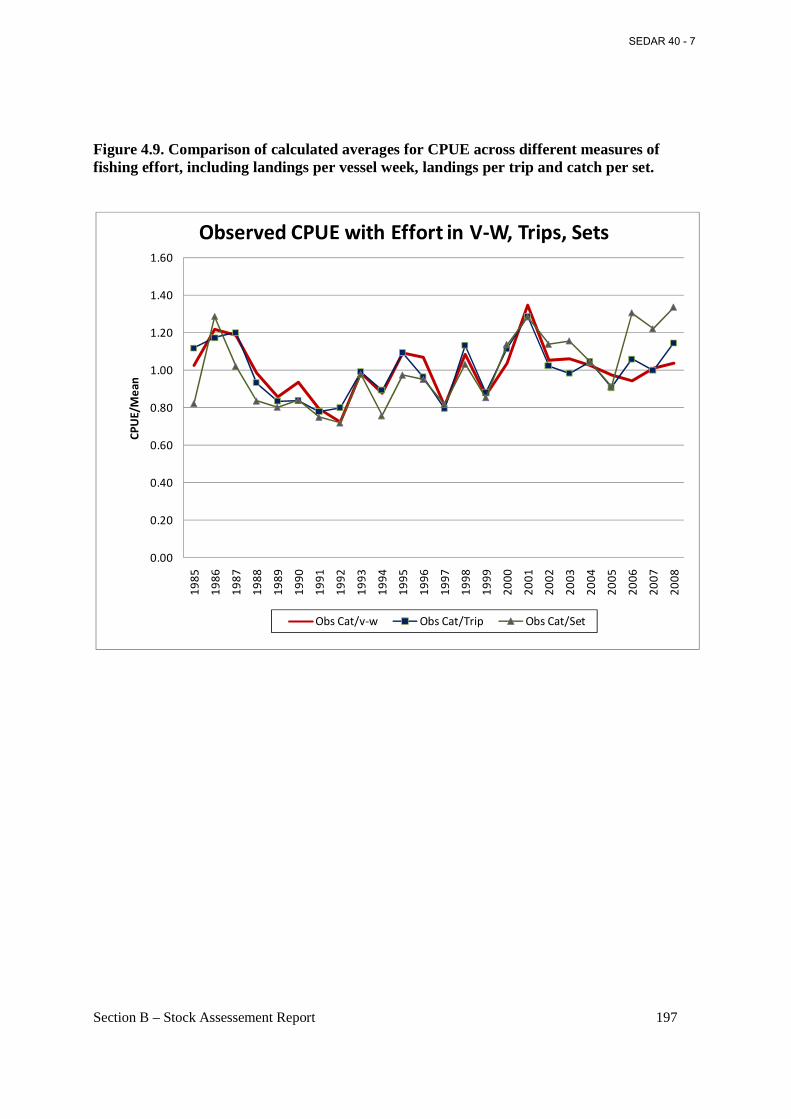
Section B – Stock Assessement Report 197
Figure 4.9. Comparison of calculated averages for CPUE across different measures of fishing effort, including landings per vessel week, landings per trip and catch per set.
0.00
0.20
0.40
0.60
0.80
1.00
1.20
1.40
1.60
19
85
19
86
19
87
19
88
19
89
19
90
19
91
19
92
19
93
19
94
19
95
19
96
19
97
19
98
19
99
20
00
20
01
20
02
20
03
20
04
20
05
20
06
20
07
20
08
CP
UE
/Me
an
Observed CPUE with Effort in V-W, Trips, Sets
Obs Cat/v-w Obs Cat/Trip Obs Cat/Set
SEDAR 40 - 7
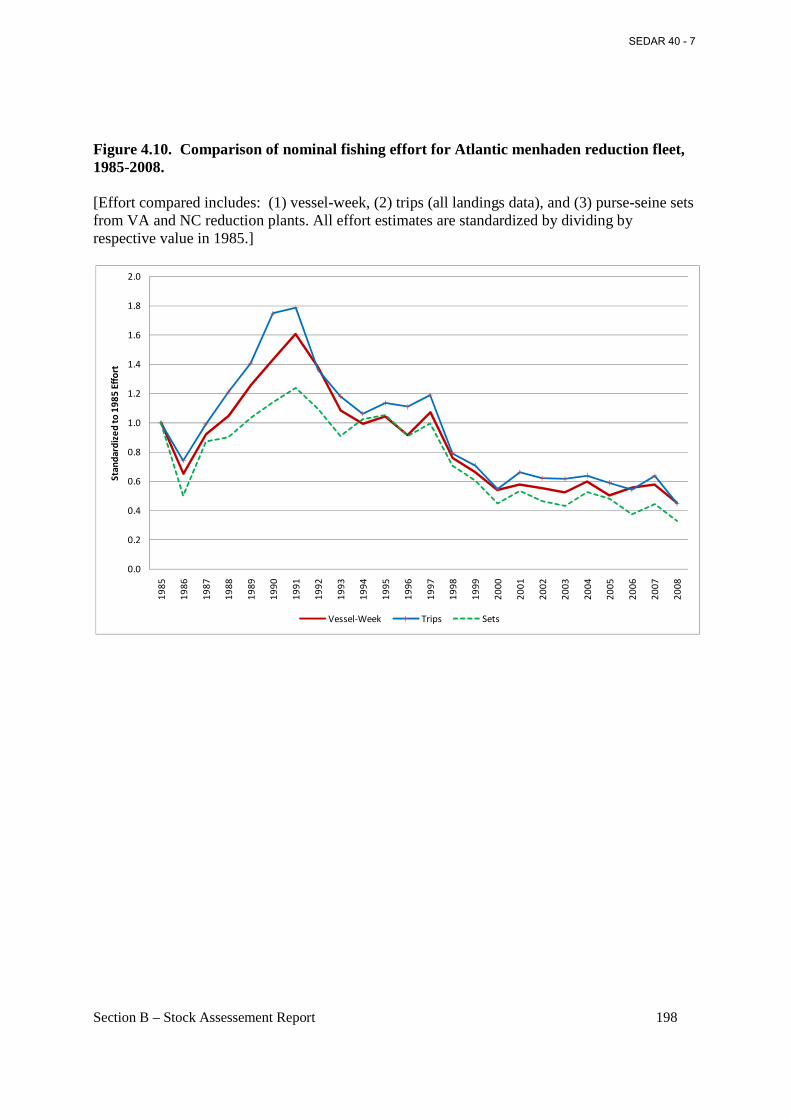
Section B – Stock Assessement Report 198
Figure 4.10. Comparison of nominal fishing effort for Atlantic menhaden reduction fleet, 1985-2008. [Effort compared includes: (1) vessel-week, (2) trips (all landings data), and (3) purse-seine sets from VA and NC reduction plants. All effort estimates are standardized by dividing by respective value in 1985.]
0.0
0.2
0.4
0.6
0.8
1.0
1.2
1.4
1.6
1.8
2.0
19
85
19
86
19
87
19
88
19
89
19
90
19
91
19
92
19
93
19
94
19
95
19
96
19
97
19
98
19
99
20
00
20
01
20
02
20
03
20
04
20
05
20
06
20
07
20
08
Sta
nd
ard
ize
d t
o 1
98
5 E
ffo
rt
Vessel-Week Trips Sets
SEDAR 40 - 7
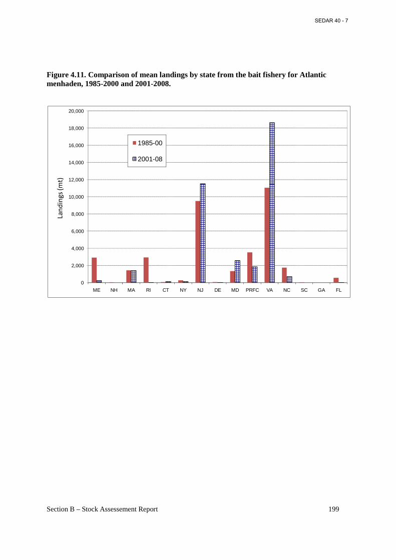
Section B – Stock Assessement Report 199
Figure 4.11. Comparison of mean landings by state from the bait fishery for Atlantic menhaden, 1985-2000 and 2001-2008.
0
2,000
4,000
6,000
8,000
10,000
12,000
14,000
16,000
18,000
20,000
ME NH MA RI CT NY NJ DE MD PRFC VA NC SC GA FL
1985-00
2001-08
Lan
din
gs
(mt)
SEDAR 40 - 7
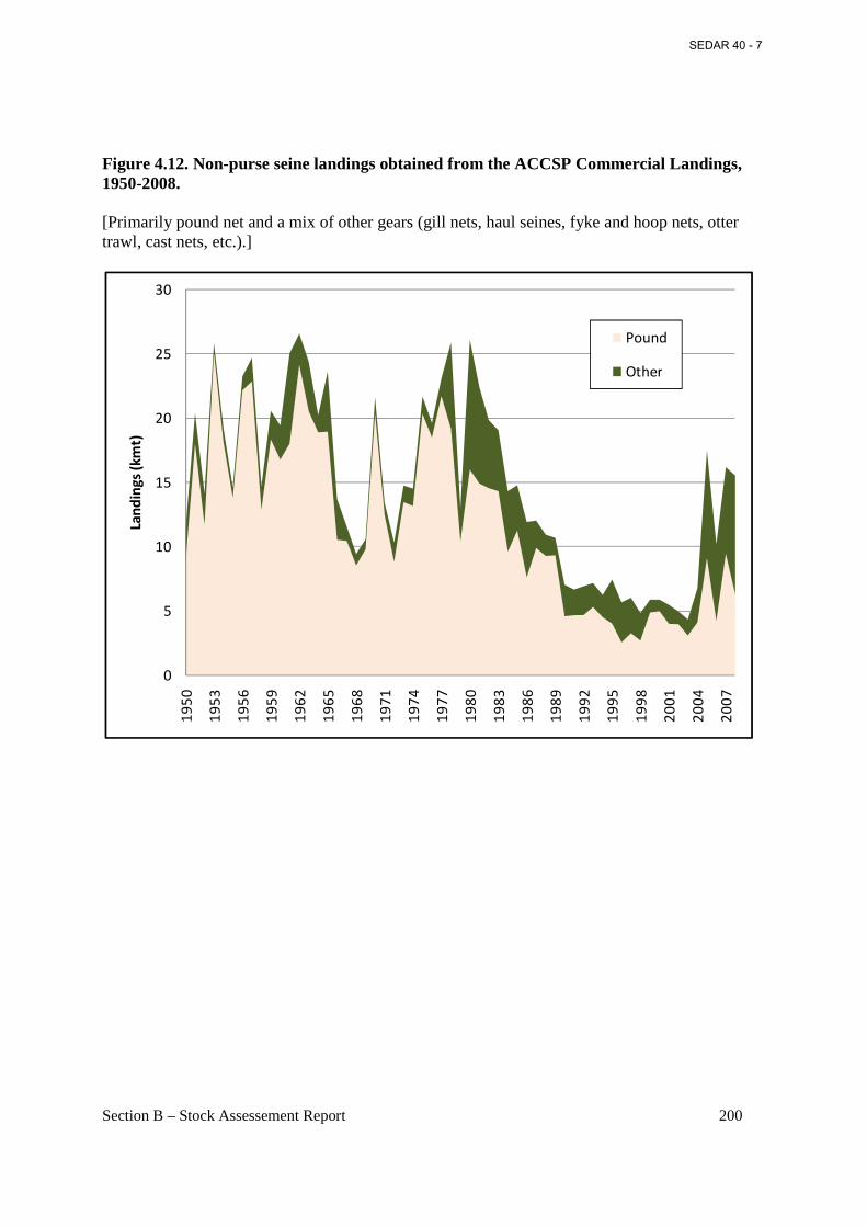
Section B – Stock Assessement Report 200
Figure 4.12. Non-purse seine landings obtained from the ACCSP Commercial Landings, 1950-2008. [Primarily pound net and a mix of other gears (gill nets, haul seines, fyke and hoop nets, otter trawl, cast nets, etc.).]
0
5
10
15
20
25
30
19
50
19
53
19
56
19
59
19
62
19
65
19
68
19
71
19
74
19
77
19
80
19
83
19
86
19
89
19
92
19
95
19
98
20
01
20
04
20
07
Lan
din
gs
(km
t)
Pound
Other
SEDAR 40 - 7
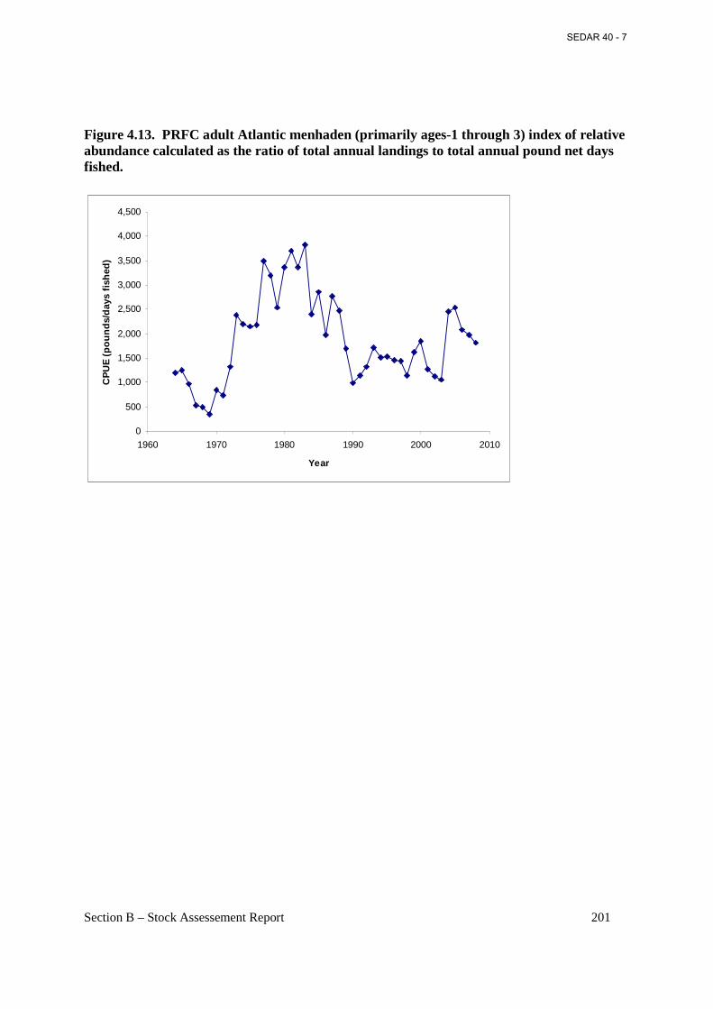
Section B – Stock Assessement Report 201
Figure 4.13. PRFC adult Atlantic menhaden (primarily ages-1 through 3) index of relative abundance calculated as the ratio of total annual landings to total annual pound net days fished.
0
500
1,000
1,500
2,000
2,500
3,000
3,500
4,000
4,500
1960 1970 1980 1990 2000 2010
Year
CP
UE
(po
unds
/day
s fis
hed)
SEDAR 40 - 7
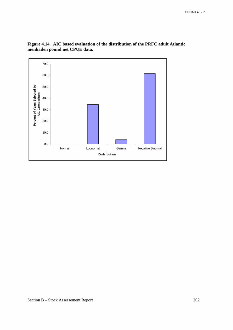
Section B – Stock Assessement Report 202
Figure 4.14. AIC based evaluation of the distribution of the PRFC adult Atlantic menhaden pound net CPUE data.
0.0
10.0
20.0
30.0
40.0
50.0
60.0
70.0
Normal Lognormal Gamma Negative Binomial
Distribution
Per
cent
of Y
ears
Sel
ecte
d by
A
IC C
ompa
rison
SEDAR 40 - 7
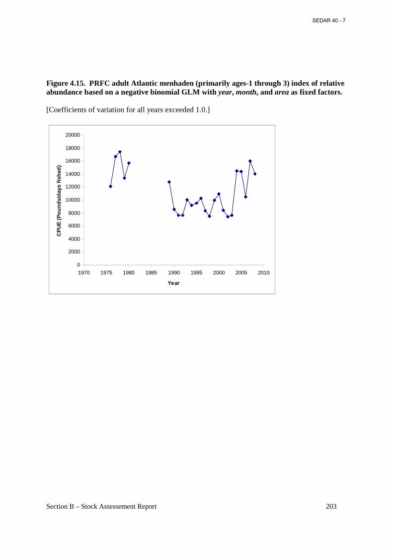
Section B – Stock Assessement Report 203
Figure 4.15. PRFC adult Atlantic menhaden (primarily ages-1 through 3) index of relative abundance based on a negative binomial GLM with year, month, and area as fixed factors. [Coefficients of variation for all years exceeded 1.0.]
0
2000
4000
6000
8000
10000
12000
14000
16000
18000
20000
1970 1975 1980 1985 1990 1995 2000 2005 2010
Year
CP
UE
(P
ound
s/da
ys fi
shed
)
SEDAR 40 - 7
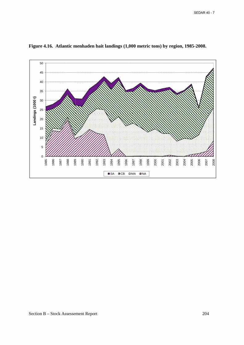
Section B – Stock Assessement Report 204
Figure 4.16. Atlantic menhaden bait landings (1,000 metric tons) by region, 1985-2008.
0
5
10
15
20
25
30
35
40
45
50
1985
1986
1987
1988
1989
1990
1991
1992
1993
1994
1995
1996
1997
1998
1999
2000
2001
2002
2003
2004
2005
2006
2007
2008
Land
ings
(10
00 t)
SA CB MA NA
SEDAR 40 - 7
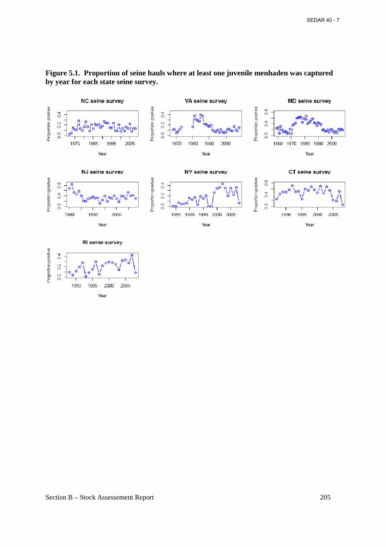
Section B – Stock Assessement Report 205
Figure 5.1. Proportion of seine hauls where at least one juvenile menhaden was captured by year for each state seine survey.
SEDAR 40 - 7
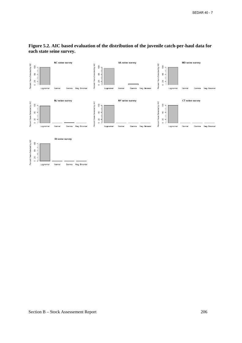
Section B – Stock Assessement Report 206
Figure 5.2. AIC based evaluation of the distribution of the juvenile catch-per-haul data for each state seine survey.
SEDAR 40 - 7
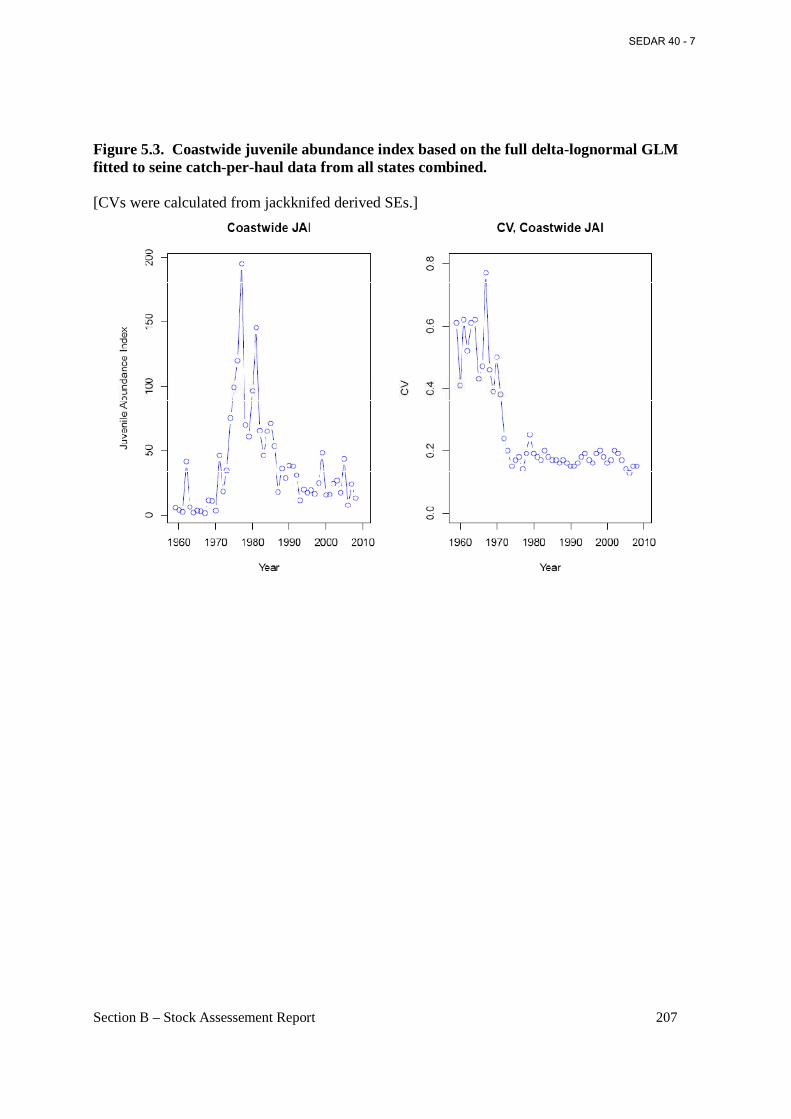
Section B – Stock Assessement Report 207
Figure 5.3. Coastwide juvenile abundance index based on the full delta-lognormal GLM fitted to seine catch-per-haul data from all states combined. [CVs were calculated from jackknifed derived SEs.]
SEDAR 40 - 7
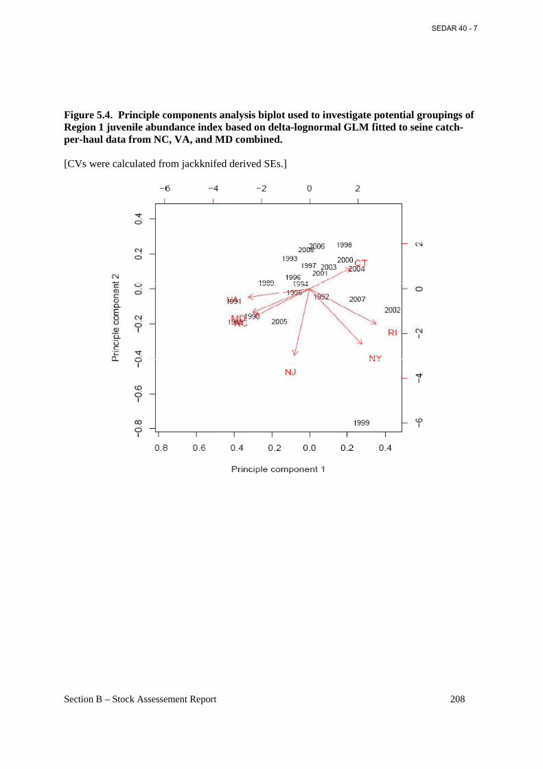
Section B – Stock Assessement Report 208
Figure 5.4. Principle components analysis biplot used to investigate potential groupings of Region 1 juvenile abundance index based on delta-lognormal GLM fitted to seine catch-per-haul data from NC, VA, and MD combined. [CVs were calculated from jackknifed derived SEs.]
SEDAR 40 - 7
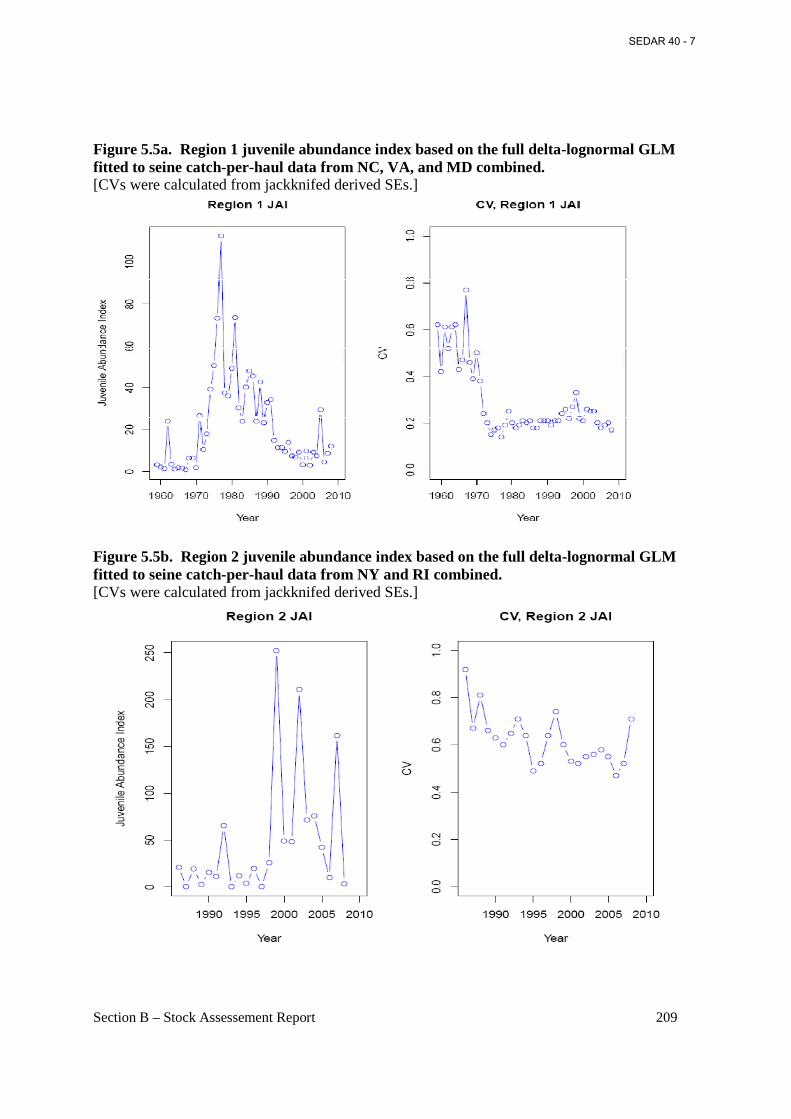
Section B – Stock Assessement Report 209
Figure 5.5a. Region 1 juvenile abundance index based on the full delta-lognormal GLM fitted to seine catch-per-haul data from NC, VA, and MD combined. [CVs were calculated from jackknifed derived SEs.]
Figure 5.5b. Region 2 juvenile abundance index based on the full delta-lognormal GLM fitted to seine catch-per-haul data from NY and RI combined. [CVs were calculated from jackknifed derived SEs.]
SEDAR 40 - 7
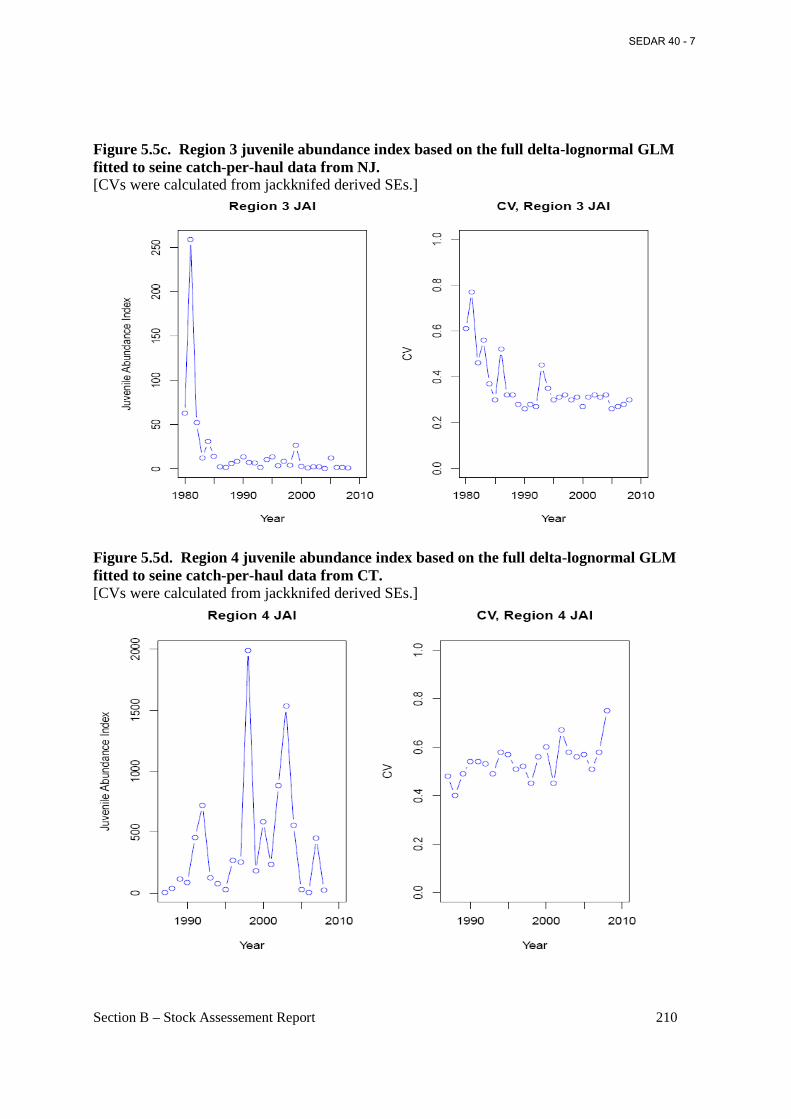
Section B – Stock Assessement Report 210
Figure 5.5c. Region 3 juvenile abundance index based on the full delta-lognormal GLM fitted to seine catch-per-haul data from NJ. [CVs were calculated from jackknifed derived SEs.]
Figure 5.5d. Region 4 juvenile abundance index based on the full delta-lognormal GLM fitted to seine catch-per-haul data from CT. [CVs were calculated from jackknifed derived SEs.]
SEDAR 40 - 7
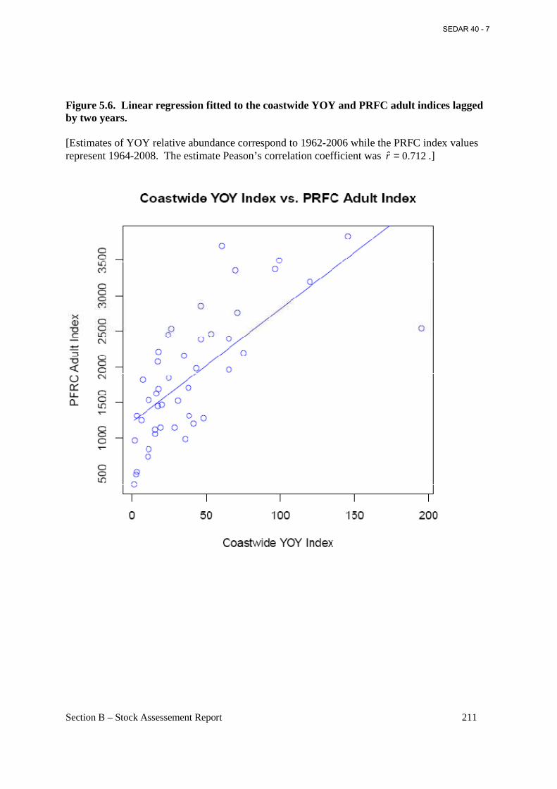
Section B – Stock Assessement Report 211
Figure 5.6. Linear regression fitted to the coastwide YOY and PRFC adult indices lagged by two years. [Estimates of YOY relative abundance correspond to 1962-2006 while the PRFC index values represent 1964-2008. The estimate Peason’s correlation coefficient was 712.0ˆ =r .]
SEDAR 40 - 7
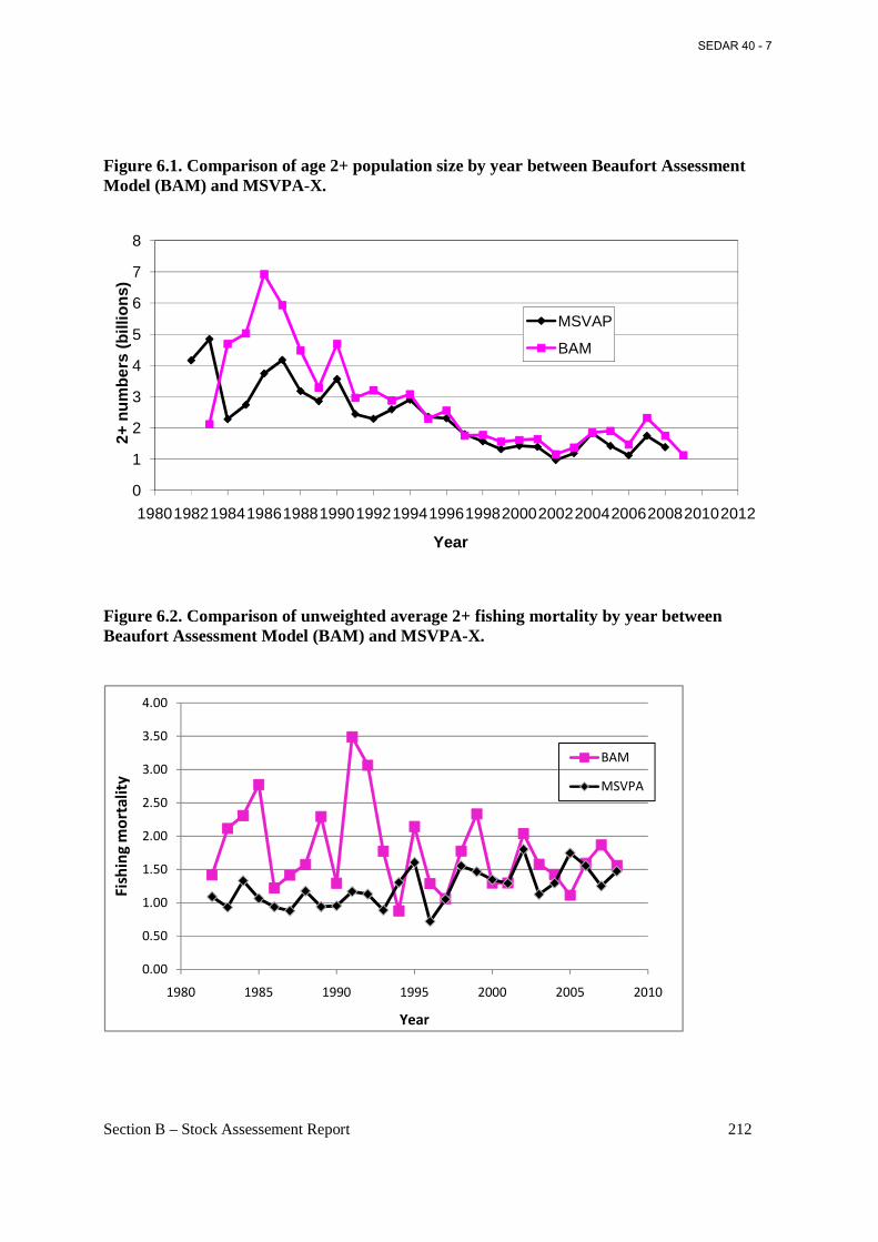
Section B – Stock Assessement Report 212
Figure 6.1. Comparison of age 2+ population size by year between Beaufort Assessment Model (BAM) and MSVPA-X.
Figure 6.2. Comparison of unweighted average 2+ fishing mortality by year between Beaufort Assessment Model (BAM) and MSVPA-X.
0
1
2
3
4
5
6
7
8
19801982198419861988199019921994199619982000200220042006200820102012
2+ n
umbe
rs (
billi
ons)
Year
MSVAP
BAM
0.00
0.50
1.00
1.50
2.00
2.50
3.00
3.50
4.00
1980 1985 1990 1995 2000 2005 2010
Fis
hin
g m
ort
ali
ty
Year
BAM
MSVPA
SEDAR 40 - 7
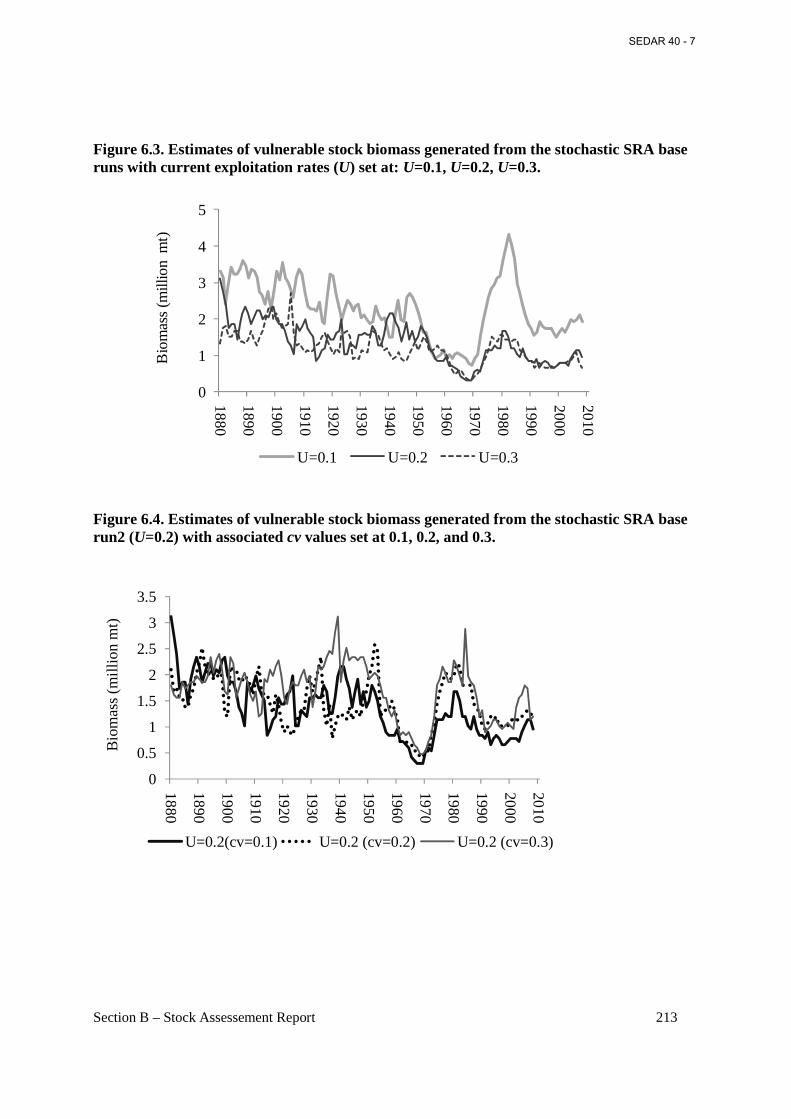
Section B – Stock Assessement Report 213
Figure 6.3. Estimates of vulnerable stock biomass generated from the stochastic SRA base runs with current exploitation rates (U) set at: U=0.1, U=0.2, U=0.3.
Figure 6.4. Estimates of vulnerable stock biomass generated from the stochastic SRA base run2 (U=0.2) with associated cv values set at 0.1, 0.2, and 0.3.
0
1
2
3
4
5
18
80
18
90
19
00
19
10
19
20
19
30
19
40
19
50
19
60
19
70
19
80
19
90
20
00
20
10
Bio
mas
s (m
illio
n m
t)
U=0.1 U=0.2 U=0.3
0
0.5
1
1.5
2
2.5
3
3.5
188
0
189
0
190
0
191
0
192
0
193
0
194
0
195
0
196
0
197
0
198
0
199
0
200
0
201
0
Bio
mas
s (m
illio
n m
t)
U=0.2(cv=0.1) U=0.2 (cv=0.2) U=0.2 (cv=0.3)
SEDAR 40 - 7
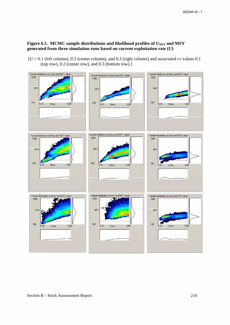
Section B – Stock Assessement Report 214
Figure 6.5. MCMC sample distributions and likelihood profiles of UMSY and MSY generated from three simulation runs based on current exploitation rate (U) [U = 0.1 (left column), 0.2 (center column), and 0.3 (right column) and associated cv values 0.1
(top row), 0.2 (center row), and 0.3 (bottom row).]
SEDAR 40 - 7
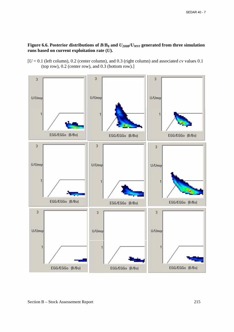
Section B – Stock Assessement Report 215
Figure 6.6. Posterior distributions of B/B0 and U2008/UMSY generated from three simulation runs based on current exploitation rate (U). [U = 0.1 (left column), 0.2 (center column), and 0.3 (right column) and associated cv values 0.1
(top row), 0.2 (center row), and 0.3 (bottom row).]
SEDAR 40 - 7
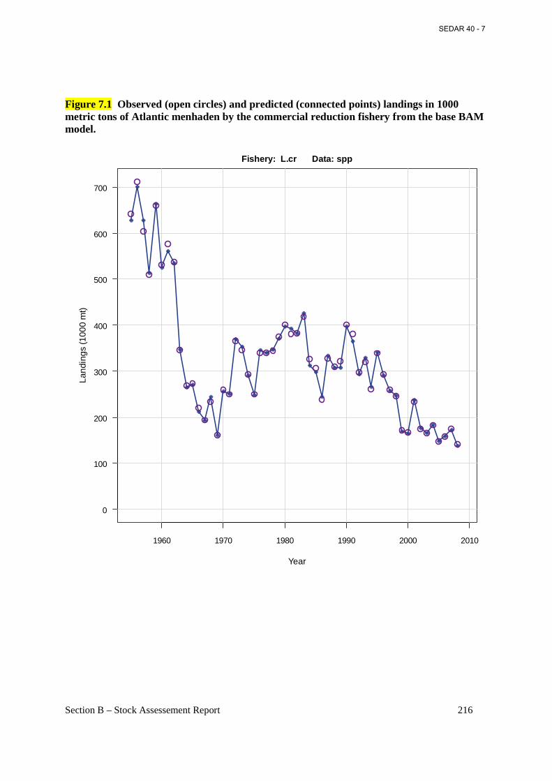
Section B – Stock Assessement Report 216
Figure 7.1 Observed (open circles) and predicted (connected points) landings in 1000 metric tons of Atlantic menhaden by the commercial reduction fishery from the base BAM model.
1960 1970 1980 1990 2000 2010
0
100
200
300
400
500
600
700
Fishery: L.cr Data: spp
Year
Land
ings
(100
0 m
t)
SEDAR 40 - 7
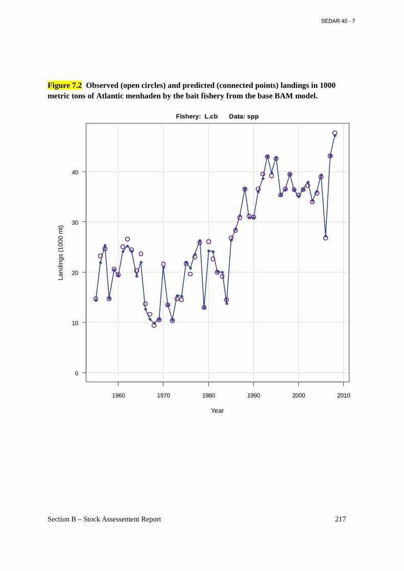
Section B – Stock Assessement Report 217
Figure 7.2 Observed (open circles) and predicted (connected points) landings in 1000 metric tons of Atlantic menhaden by the bait fishery from the base BAM model.
1960 1970 1980 1990 2000 2010
0
10
20
30
40
Fishery: L.cb Data: spp
Year
Land
ings
(100
0 m
t)
SEDAR 40 - 7
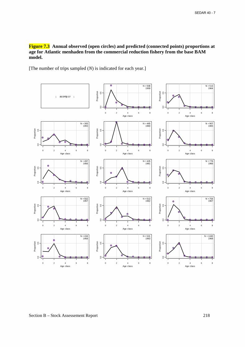
Section B – Stock Assessement Report 218
Figure 7.3 Annual observed (open circles) and predicted (connected points) proportions at age for Atlantic menhaden from the commercial reduction fishery from the base BAM model. [The number of trips sampled (N) is indicated for each year.]
↓ acomp.cr ↓
0 2 4 6 8
0.0
0.5
Age class
Pro
port
ion
N = 3051955
0 2 4 6 8
0.0
0.5
Age class
Pro
port
ion
N = 4971956
0 2 4 6 8
0.0
0.5
Age class
Pro
port
ion
N = 5021957
0 2 4 6 8
0.0
0.5
Age class
Pro
port
ion
N = 4341958
0 2 4 6 8
0.0
0.5
Age class
Pro
port
ion
N = 5081959
0 2 4 6 8
0.0
0.5
Age class
Pro
port
ion
N = 4651960
0 2 4 6 8
0.0
0.5
Age class
Pro
port
ion
N = 4251961
0 2 4 6 8
0.0
0.5
Age class
Pro
port
ion
N = 5131962
0 2 4 6 8
0.0
0.5
Age class
Pro
port
ion
N = 5311963
0 2 4 6 8
0.0
0.5
Age class
Pro
port
ion
N = 5131964
0 2 4 6 8
0.0
0.5
Age class
Pro
port
ion
N = 9071965
0 2 4 6 8
0.0
0.5
Age class
Pro
port
ion
N = 7761966
0 2 4 6 8
0.0
0.5
Age class
Pro
port
ion
N = 7541967
0 2 4 6 8
0.0
0.5
Age class
Pro
port
ion
N = 13401968
SEDAR 40 - 7
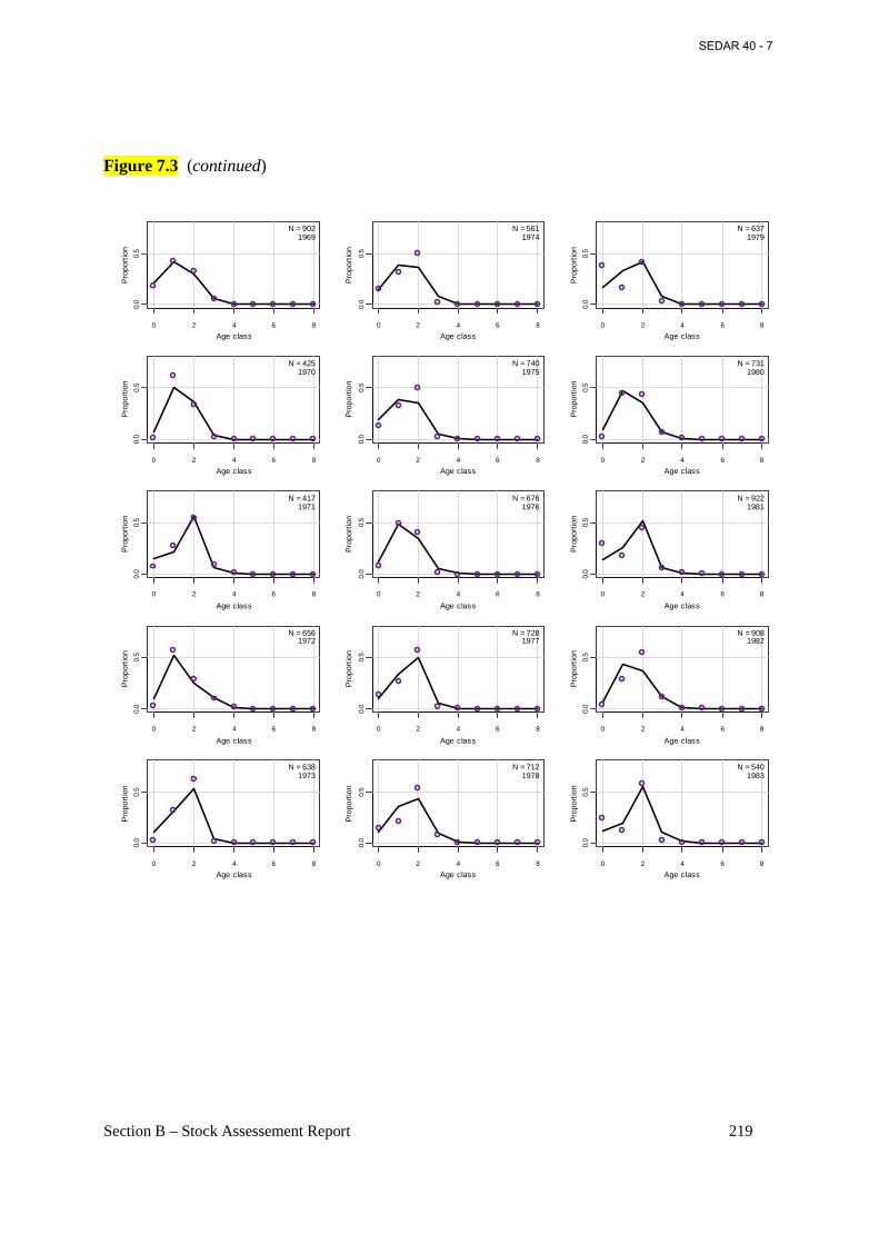
Section B – Stock Assessement Report 219
Figure 7.3 (continued)
0 2 4 6 8
0.0
0.5
Age class
Pro
port
ion
N = 9021969
0 2 4 6 8
0.0
0.5
Age class
Pro
port
ion
N = 4251970
0 2 4 6 8
0.0
0.5
Age class
Pro
port
ion
N = 4171971
0 2 4 6 8
0.0
0.5
Age class
Pro
port
ion
N = 6561972
0 2 4 6 8
0.0
0.5
Age class
Pro
port
ion
N = 6381973
0 2 4 6 8
0.0
0.5
Age class
Pro
port
ion
N = 5611974
0 2 4 6 8
0.0
0.5
Age class
Pro
port
ion
N = 7401975
0 2 4 6 8
0.0
0.5
Age class
Pro
port
ion
N = 6761976
0 2 4 6 8
0.0
0.5
Age class
Pro
port
ion
N = 7281977
0 2 4 6 8
0.0
0.5
Age class
Pro
port
ion
N = 7121978
0 2 4 6 8
0.0
0.5
Age class
Pro
port
ion
N = 6371979
0 2 4 6 8
0.0
0.5
Age class
Pro
port
ion
N = 7311980
0 2 4 6 80.
00.
5
Age class
Pro
port
ion
N = 9221981
0 2 4 6 8
0.0
0.5
Age class
Pro
port
ion
N = 9081982
0 2 4 6 8
0.0
0.5
Age class
Pro
port
ion
N = 5401983
SEDAR 40 - 7
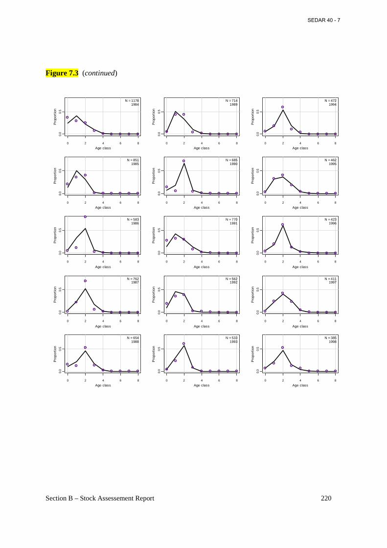
Section B – Stock Assessement Report 220
Figure 7.3 (continued)
0 2 4 6 8
0.0
0.5
Age class
Pro
port
ion
N = 11781984
0 2 4 6 8
0.0
0.5
Age class
Pro
port
ion
N = 8511985
0 2 4 6 8
0.0
0.5
Age class
Pro
port
ion
N = 5831986
0 2 4 6 8
0.0
0.5
Age class
Pro
port
ion
N = 7621987
0 2 4 6 8
0.0
0.5
Age class
Pro
port
ion
N = 6541988
0 2 4 6 8
0.0
0.5
Age class
Pro
port
ion
N = 7141989
0 2 4 6 8
0.0
0.5
Age class
Pro
port
ion
N = 6851990
0 2 4 6 8
0.0
0.5
Age class
Pro
port
ion
N = 7701991
0 2 4 6 8
0.0
0.5
Age class
Pro
port
ion
N = 5621992
0 2 4 6 8
0.0
0.5
Age class
Pro
port
ion
N = 5331993
0 2 4 6 8
0.0
0.5
Age class
Pro
port
ion
N = 4721994
0 2 4 6 8
0.0
0.5
Age class
Pro
port
ion
N = 4621995
0 2 4 6 80.
00.
5
Age class
Pro
port
ion
N = 4231996
0 2 4 6 8
0.0
0.5
Age class
Pro
port
ion
N = 4111997
0 2 4 6 8
0.0
0.5
Age class
Pro
port
ion
N = 3851998
SEDAR 40 - 7
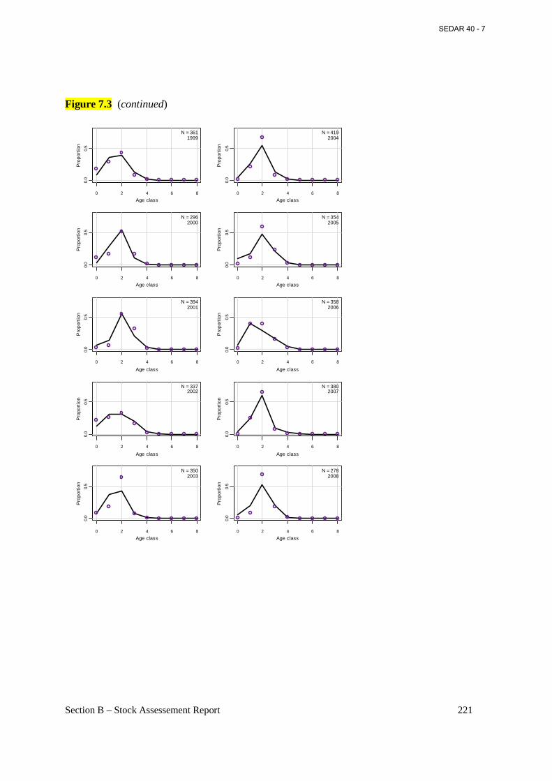
Section B – Stock Assessement Report 221
Figure 7.3 (continued)
0 2 4 6 8
0.0
0.5
Age class
Pro
port
ion
N = 3611999
0 2 4 6 8
0.0
0.5
Age class
Pro
port
ion
N = 2962000
0 2 4 6 8
0.0
0.5
Age class
Pro
port
ion
N = 3942001
0 2 4 6 8
0.0
0.5
Age class
Pro
port
ion
N = 3372002
0 2 4 6 8
0.0
0.5
Age class
Pro
port
ion
N = 3502003
0 2 4 6 8
0.0
0.5
Age class
Pro
port
ion
N = 4192004
0 2 4 6 8
0.0
0.5
Age class
Pro
port
ion
N = 3542005
0 2 4 6 8
0.0
0.5
Age class
Pro
port
ion
N = 3582006
0 2 4 6 8
0.0
0.5
Age class
Pro
port
ion
N = 3802007
0 2 4 6 8
0.0
0.5
Age class
Pro
port
ion
N = 2782008
SEDAR 40 - 7
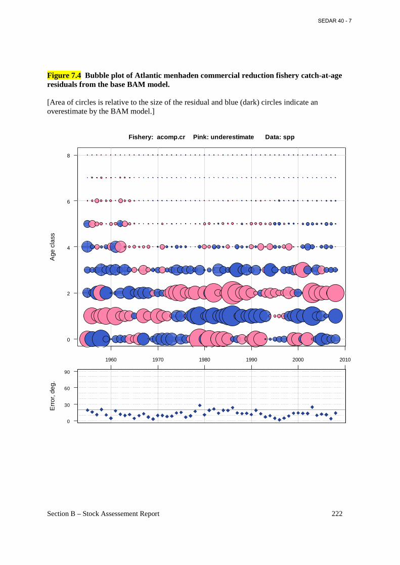
Section B – Stock Assessement Report 222
Figure 7.4 Bubble plot of Atlantic menhaden commercial reduction fishery catch-at-age residuals from the base BAM model. [Area of circles is relative to the size of the residual and blue (dark) circles indicate an overestimate by the BAM model.]
0
2
4
6
8
Age
cla
ssE
rror
, deg
.
0
30
60
90
1960 1970 1980 1990 2000 2010
Fishery: acomp.cr Pink: underestimate Data: spp
SEDAR 40 - 7
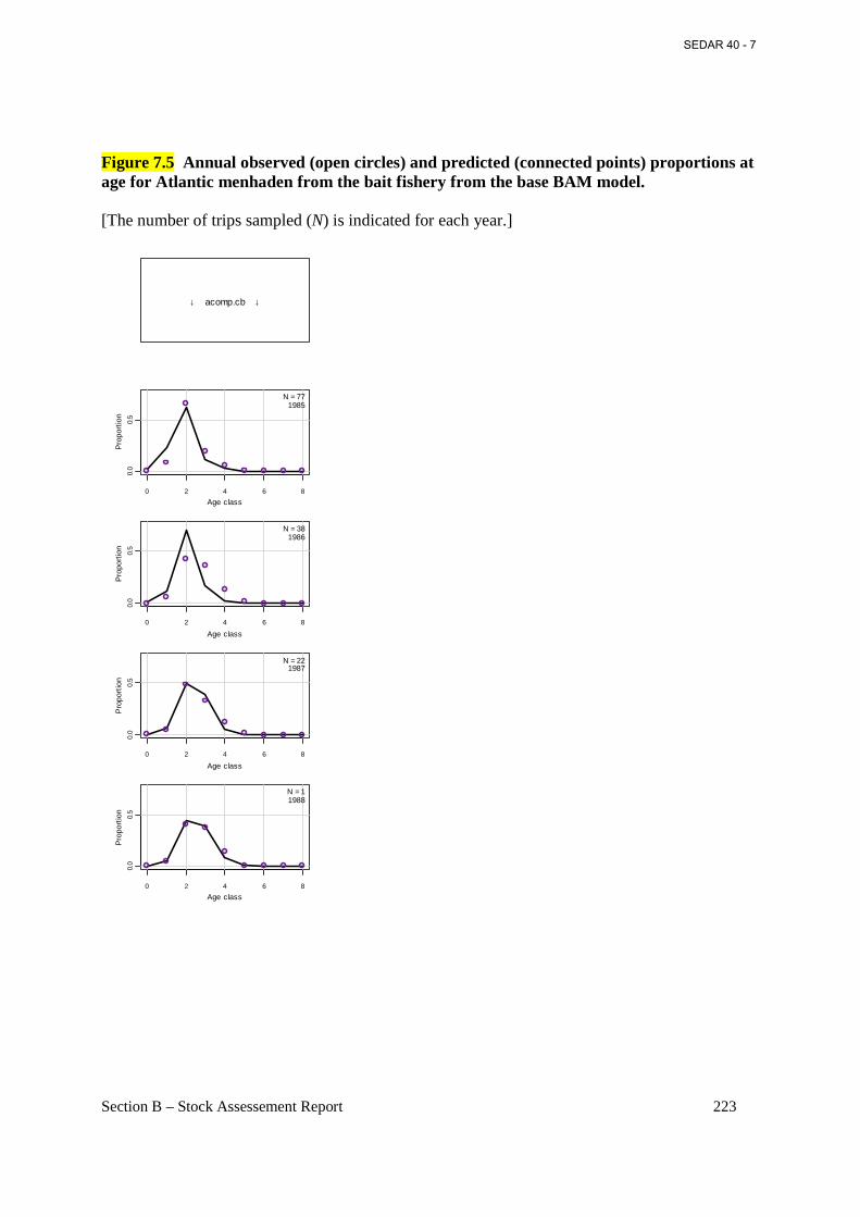
Section B – Stock Assessement Report 223
Figure 7.5 Annual observed (open circles) and predicted (connected points) proportions at age for Atlantic menhaden from the bait fishery from the base BAM model. [The number of trips sampled (N) is indicated for each year.]
↓ acomp.cb ↓
0 2 4 6 8
0.0
0.5
Age class
Pro
port
ion
N = 771985
0 2 4 6 8
0.0
0.5
Age class
Pro
port
ion
N = 381986
0 2 4 6 8
0.0
0.5
Age class
Pro
port
ion
N = 221987
0 2 4 6 8
0.0
0.5
Age class
Pro
port
ion
N = 11988
SEDAR 40 - 7
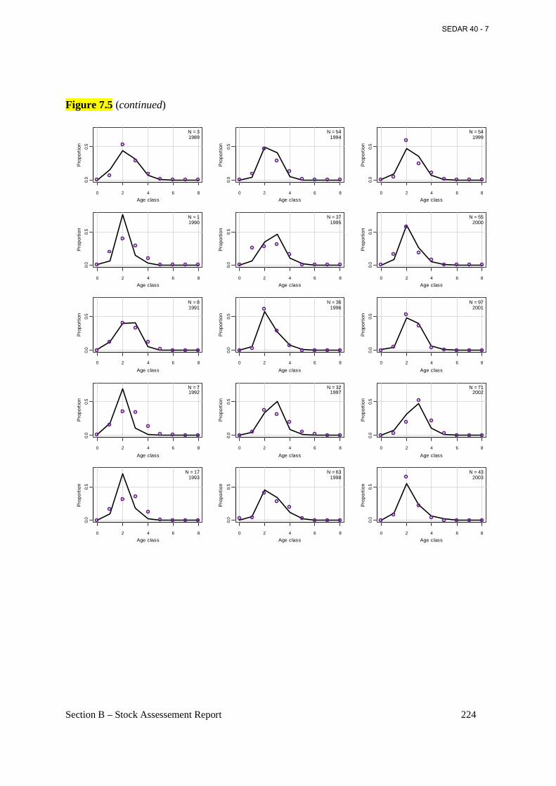
Section B – Stock Assessement Report 224
Figure 7.5 (continued)
0 2 4 6 8
0.0
0.5
Age class
Pro
port
ion
N = 31989
0 2 4 6 8
0.0
0.5
Age class
Pro
port
ion
N = 11990
0 2 4 6 8
0.0
0.5
Age class
Pro
port
ion
N = 81991
0 2 4 6 8
0.0
0.5
Age class
Pro
port
ion
N = 71992
0 2 4 6 8
0.0
0.5
Age class
Pro
port
ion
N = 171993
0 2 4 6 8
0.0
0.5
Age class
Pro
port
ion
N = 541994
0 2 4 6 8
0.0
0.5
Age class
Pro
port
ion
N = 371995
0 2 4 6 8
0.0
0.5
Age class
Pro
port
ion
N = 361996
0 2 4 6 8
0.0
0.5
Age class
Pro
port
ion
N = 321997
0 2 4 6 8
0.0
0.5
Age class
Pro
port
ion
N = 631998
0 2 4 6 8
0.0
0.5
Age class
Pro
port
ion
N = 541999
0 2 4 6 8
0.0
0.5
Age class
Pro
port
ion
N = 552000
0 2 4 6 8
0.0
0.5
Age class
Pro
port
ion
N = 972001
0 2 4 6 8
0.0
0.5
Age class
Pro
port
ion
N = 712002
0 2 4 6 8
0.0
0.5
Age class
Pro
port
ion
N = 432003
SEDAR 40 - 7
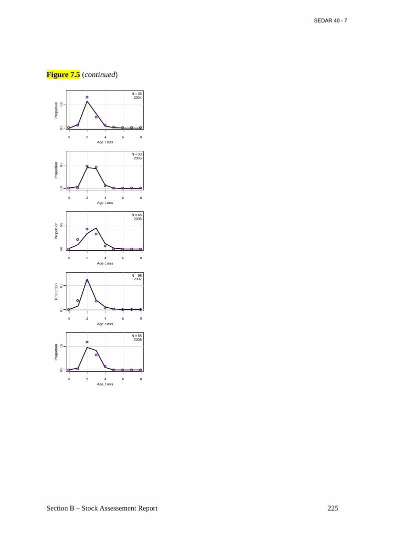
Section B – Stock Assessement Report 225
Figure 7.5 (continued)
0 2 4 6 8
0.0
0.5
Age class
Pro
port
ion
N = 362004
0 2 4 6 8
0.0
0.5
Age class
Pro
port
ion
N = 332005
0 2 4 6 8
0.0
0.5
Age class
Pro
port
ion
N = 462006
0 2 4 6 8
0.0
0.5
Age class
Pro
port
ion
N = 982007
0 2 4 6 8
0.0
0.5
Age class
Pro
port
ion
N = 852008
SEDAR 40 - 7
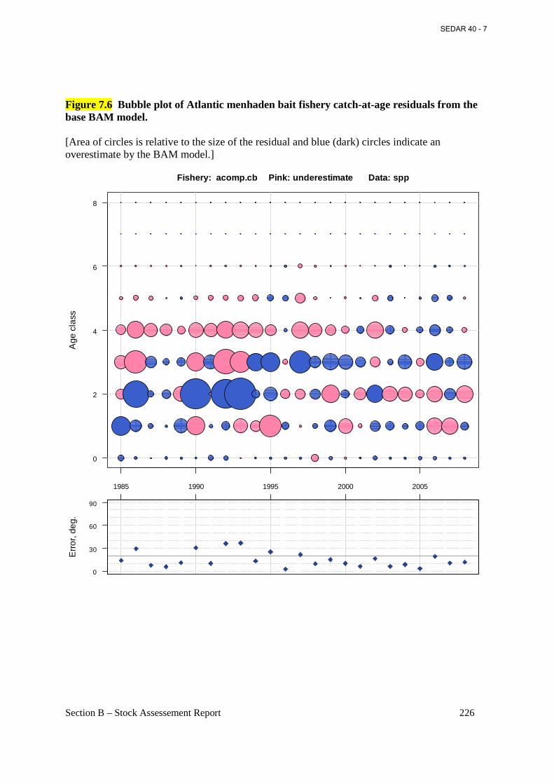
Section B – Stock Assessement Report 226
Figure 7.6 Bubble plot of Atlantic menhaden bait fishery catch-at-age residuals from the base BAM model. [Area of circles is relative to the size of the residual and blue (dark) circles indicate an overestimate by the BAM model.]
0
2
4
6
8
Age
cla
ssE
rror
, deg
.
0
30
60
90
1985 1990 1995 2000 2005
Fishery: acomp.cb Pink: underestimate Data: spp
SEDAR 40 - 7
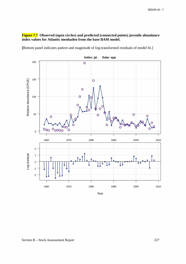
Section B – Stock Assessement Report 227
Figure 7.7 Observed (open circles) and predicted (connected points) juvenile abundance index values for Atlantic menhaden from the base BAM model. [Bottom panel indicates pattern and magnitude of log-transformed residuals of model fit.]
1960 1970 1980 1990 2000 2010
0
50
100
150
200
Index: jai Data: spp
Rel
ativ
e ab
unda
nce
(CP
UE
)
1960 1970 1980 1990 2000 2010
-2
-1
0
1
2
Year
Log
resi
dual
SEDAR 40 - 7
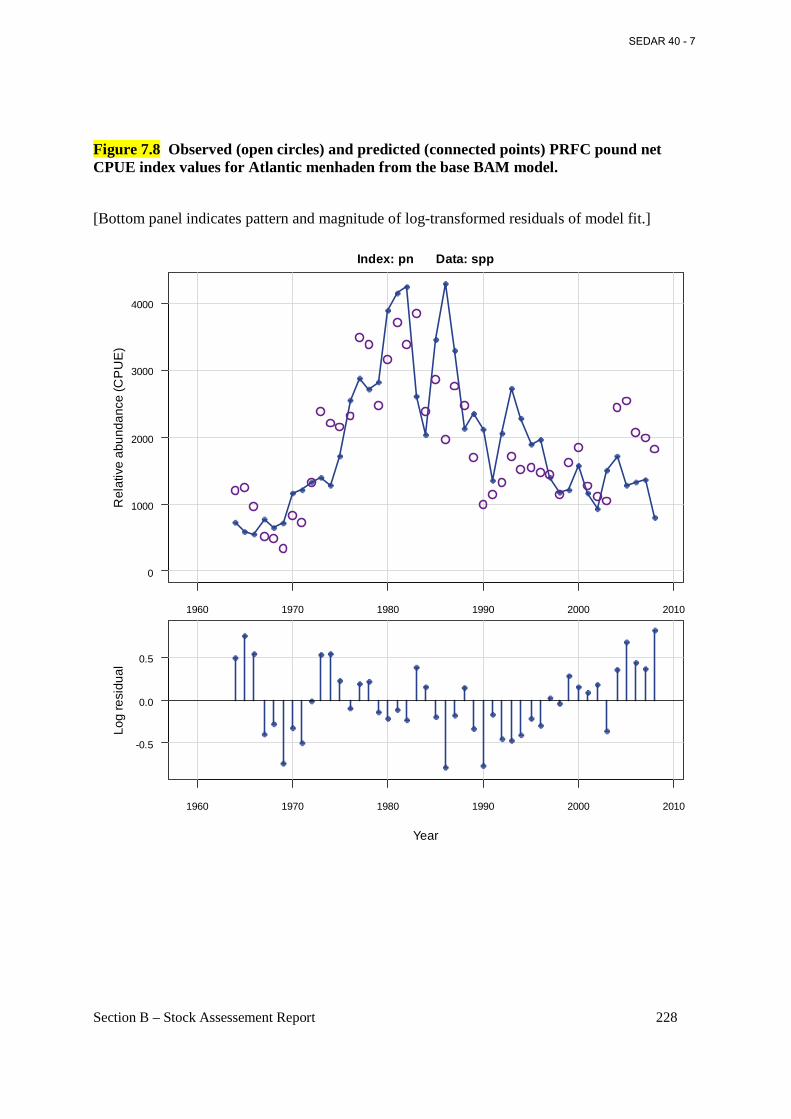
Section B – Stock Assessement Report 228
Figure 7.8 Observed (open circles) and predicted (connected points) PRFC pound net CPUE index values for Atlantic menhaden from the base BAM model.
[Bottom panel indicates pattern and magnitude of log-transformed residuals of model fit.]
1960 1970 1980 1990 2000 2010
0
1000
2000
3000
4000
Index: pn Data: spp
Rel
ativ
e ab
unda
nce
(CP
UE
)
1960 1970 1980 1990 2000 2010
-0.5
0.0
0.5
Year
Log
resi
dual
SEDAR 40 - 7
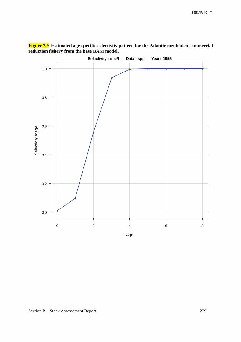
Section B – Stock Assessement Report 229
Figure 7.9 Estimated age-specific selectivity pattern for the Atlantic menhaden commercial reduction fishery from the base BAM model.
0 2 4 6 8
0.0
0.2
0.4
0.6
0.8
1.0
Selectivity in: cR Data: spp Year: 1955
Age
Sel
ectiv
ity a
t age
SEDAR 40 - 7
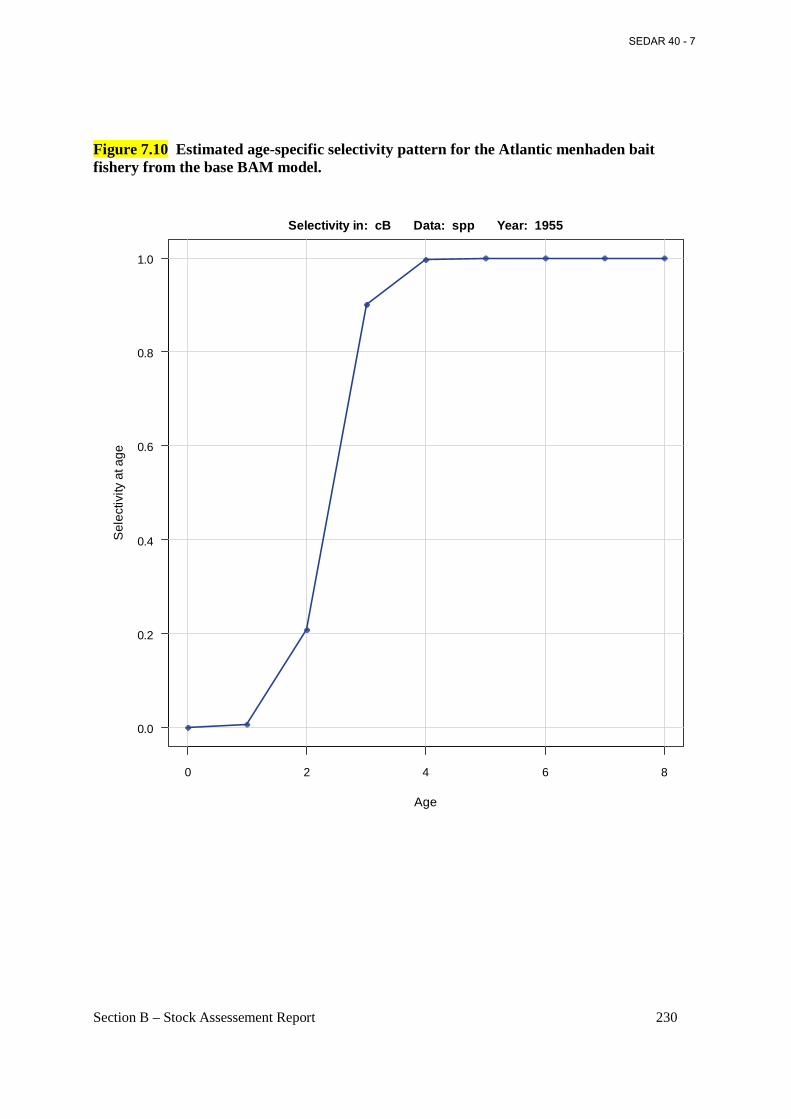
Section B – Stock Assessement Report 230
Figure 7.10 Estimated age-specific selectivity pattern for the Atlantic menhaden bait fishery from the base BAM model.
0 2 4 6 8
0.0
0.2
0.4
0.6
0.8
1.0
Selectivity in: cB Data: spp Year: 1955
Age
Sel
ectiv
ity a
t age
SEDAR 40 - 7
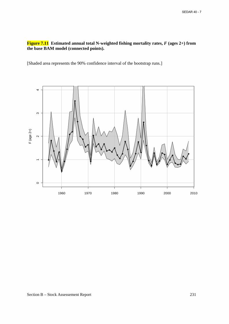
Section B – Stock Assessement Report 231
Figure 7.11 Estimated annual total N-weighted fishing mortality rates, F (ages 2+) from the base BAM model (connected points).
[Shaded area represents the 90% confidence interval of the bootstrap runs.]
1960 1970 1980 1990 2000 2010
01
23
4
F (a
ge 2
+)
SEDAR 40 - 7
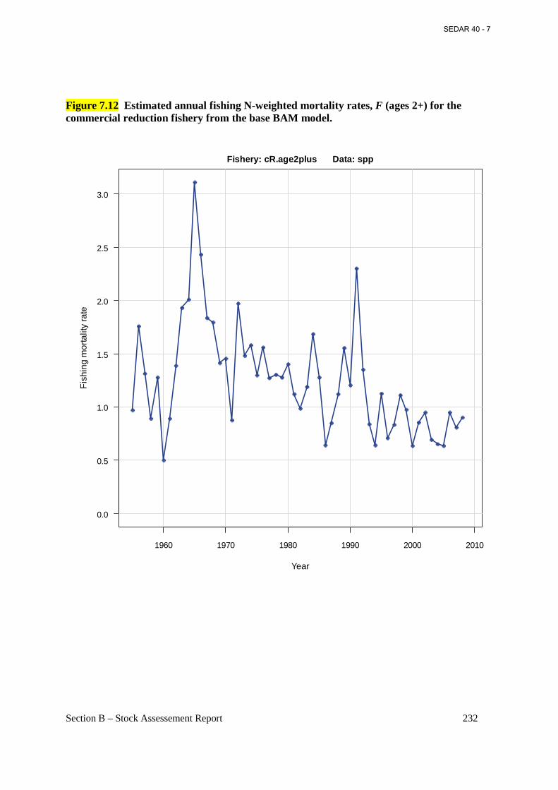
Section B – Stock Assessement Report 232
Figure 7.12 Estimated annual fishing N-weighted mortality rates, F (ages 2+) for the commercial reduction fishery from the base BAM model.
1960 1970 1980 1990 2000 2010
0.0
0.5
1.0
1.5
2.0
2.5
3.0
Fishery: cR.age2plus Data: spp
Year
Fis
hing
mor
talit
y ra
te
SEDAR 40 - 7
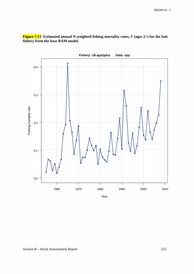
Section B – Stock Assessement Report 233
Figure 7.13 Estimated annual N-weighted fishing mortality rates, F (ages 2+) for the bait fishery from the base BAM model.
1960 1970 1980 1990 2000 2010
0.0
0.1
0.2
0.3
0.4
Fishery: cB.age2plus Data: spp
Year
Fis
hing
mor
talit
y ra
te
SEDAR 40 - 7
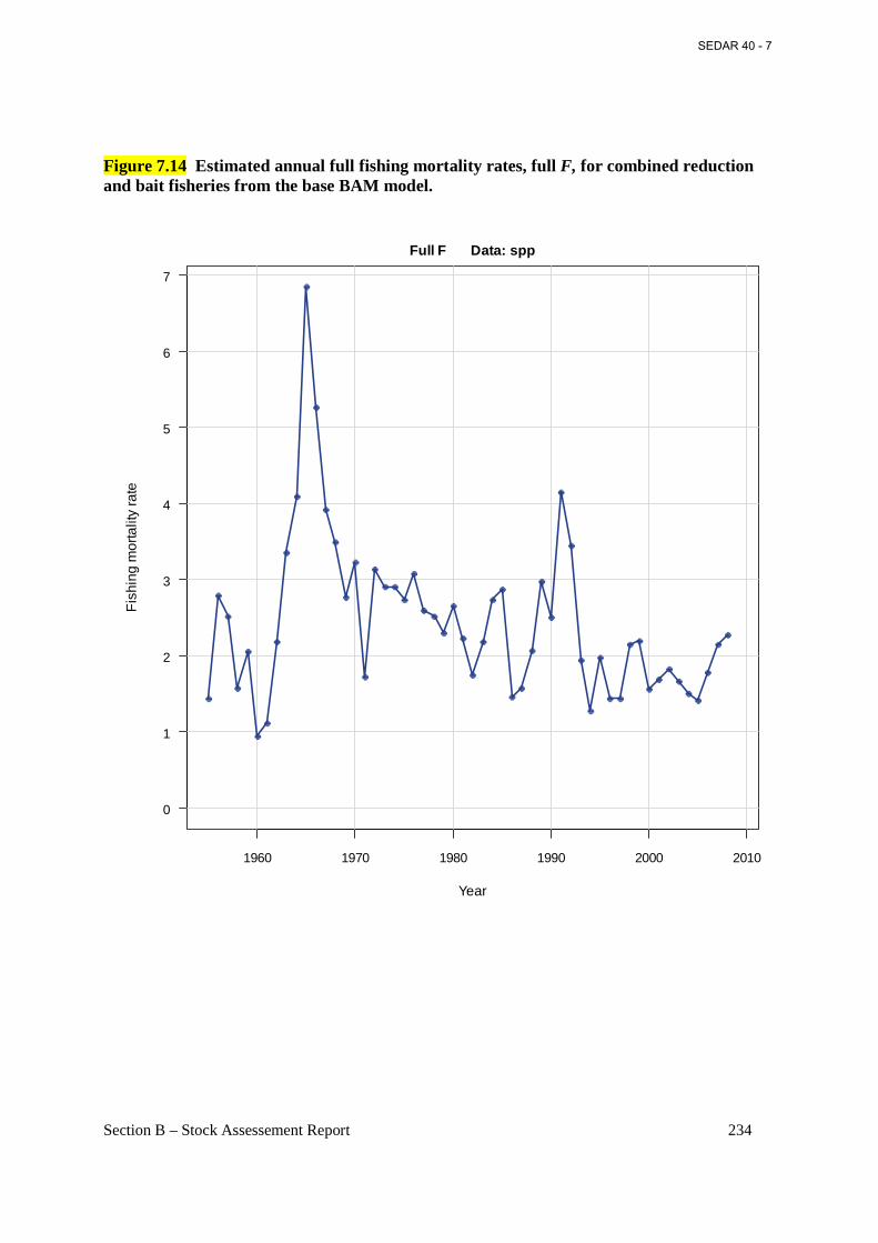
Section B – Stock Assessement Report 234
Figure 7.14 Estimated annual full fishing mortality rates, full F, for combined reduction and bait fisheries from the base BAM model.
1960 1970 1980 1990 2000 2010
0
1
2
3
4
5
6
7
Full F Data: spp
Year
Fis
hing
mor
talit
y ra
te
SEDAR 40 - 7
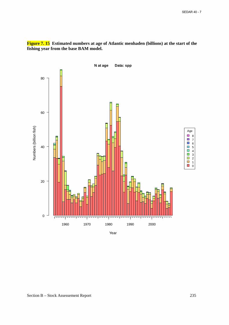
Section B – Stock Assessement Report 235
Figure 7. 15 Estimated numbers at age of Atlantic menhaden (billions) at the start of the fishing year from the base BAM model.
Year
Num
bers
(bill
ion
fish)
0
20
40
60
80
N at age Data: spp
1960 1970 1980 1990 2000
Age
876543210
SEDAR 40 - 7
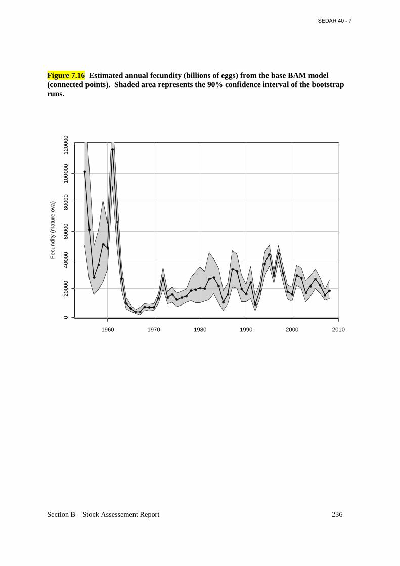
Section B – Stock Assessement Report 236
Figure 7.16 Estimated annual fecundity (billions of eggs) from the base BAM model (connected points). Shaded area represents the 90% confidence interval of the bootstrap runs.
1960 1970 1980 1990 2000 2010
020
000
4000
060
000
8000
010
0000
1200
00
Fec
undi
ty (m
atur
e ov
a)
SEDAR 40 - 7
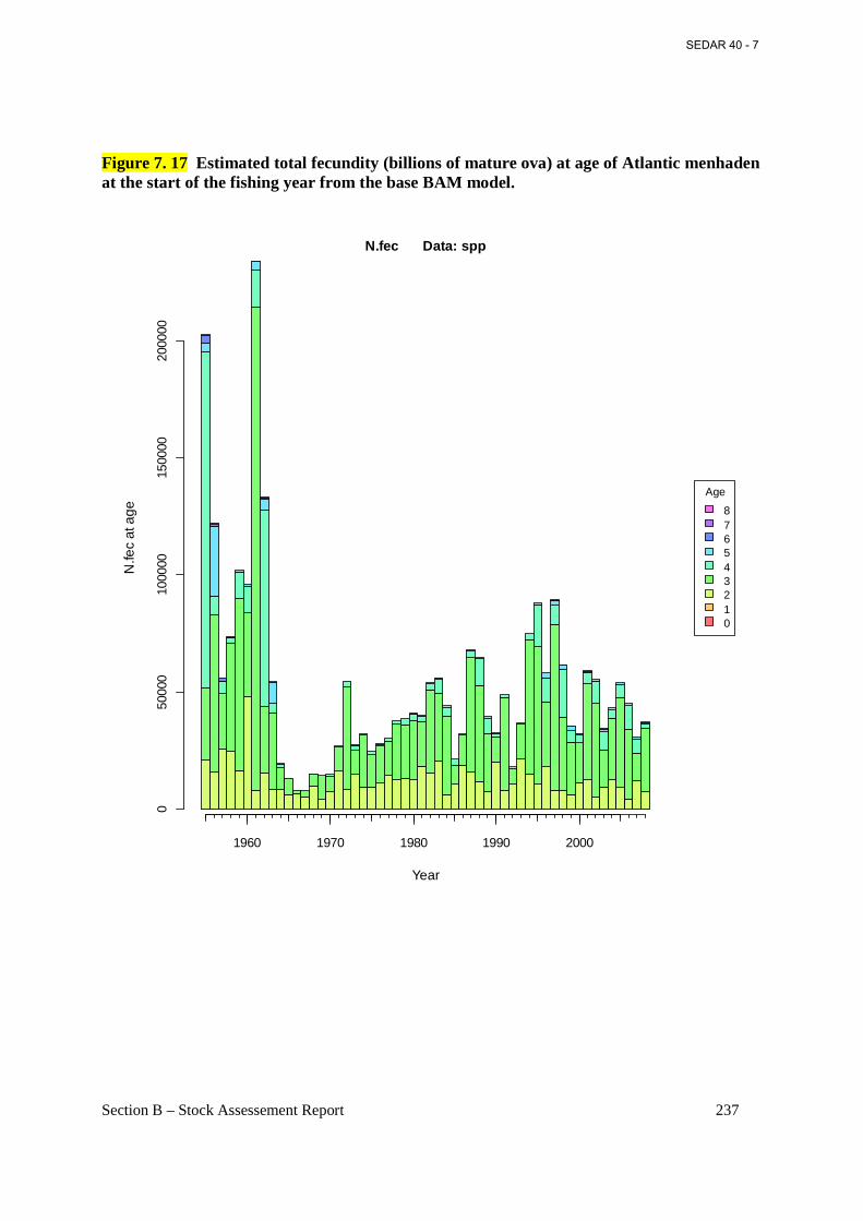
Section B – Stock Assessement Report 237
Figure 7. 17 Estimated total fecundity (billions of mature ova) at age of Atlantic menhaden at the start of the fishing year from the base BAM model.
Year
N.fe
c at
age
050
000
1000
0015
0000
2000
00
N.fec Data: spp
1960 1970 1980 1990 2000
Age
876543210
SEDAR 40 - 7
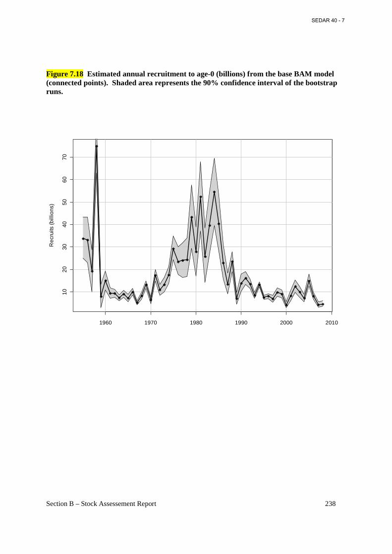
Section B – Stock Assessement Report 238
Figure 7.18 Estimated annual recruitment to age-0 (billions) from the base BAM model (connected points). Shaded area represents the 90% confidence interval of the bootstrap runs.
1960 1970 1980 1990 2000 2010
1020
3040
5060
70
Rec
ruits
(bill
ions
)
SEDAR 40 - 7
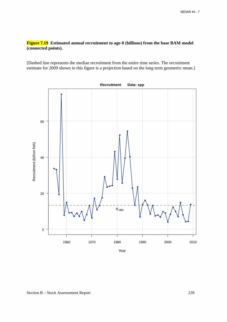
Section B – Stock Assessement Report 239
Figure 7.19 Estimated annual recruitment to age-0 (billions) from the base BAM model (connected points).
[Dashed line represents the median recruitment from the entire time series. The recruitment estimate for 2009 shown in this figure is a projection based on the long term geometric mean.]
1960 1970 1980 1990 2000 2010
0
20
40
60
Recruitment Data: spp
Year
Rec
ruitm
ent (
billi
on fi
sh)
R MED
SEDAR 40 - 7
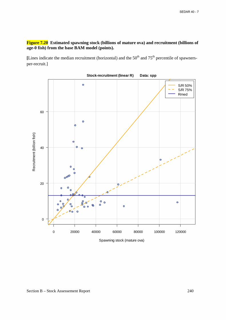
Section B – Stock Assessement Report 240
Figure 7.20 Estimated spawning stock (billions of mature ova) and recruitment (billions of age-0 fish) from the base BAM model (points). [Lines indicate the median recruitment (horizontal) and the 50th and 75th percentile of spawners-per-recruit.]
0 20000 40000 60000 80000 100000 120000
0
20
40
60
Stock-recruitment (linear R) Data: spp
Spawning stock (mature ova)
Rec
ruitm
ent (
billi
on fi
sh)
S/R 50%S/R 75%Rmed
SEDAR 40 - 7
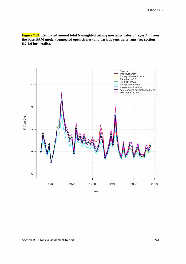
Section B – Stock Assessement Report 241
Figure 7.21 Estimated annual total N-weighted fishing mortality rates, F (ages 2+) from the base BAM model (connected open circles) and various sensitivity runs (see section 6.2.1.6 for details).
1960 1970 1980 1990 2000 2010
01
23
4
Year
F (A
ge 2
+)
Base runtime-invariant M8 yr avg per-recruit calcsPN index cv=0.2PN index cv=0.8No age reader error4 separate JAI indicesdome-shaped sel, last period of cRstart model in 1964
SEDAR 40 - 7

Section B – Stock Assessement Report 242
Figure 7.21 (continued)
1960 1970 1980 1990 2000 2010
010
020
030
040
050
060
070
0
Year
Rec
ruits
(bill
ions
)
Base run3 yr avg per-recruit calcsrandom walk on PN index qleave out JAI indexleave out PN indexGLM based PN indexM scaled up 25%M scaled down 25%M scalar estimated
SEDAR 40 - 7
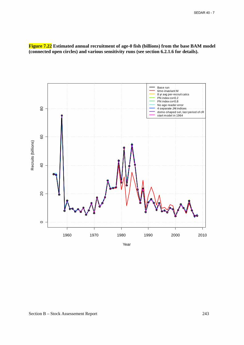
Section B – Stock Assessement Report 243
Figure 7.22 Estimated annual recruitment of age-0 fish (billions) from the base BAM model (connected open circles) and various sensitivity runs (see section 6.2.1.6 for details).
1960 1970 1980 1990 2000 2010
020
4060
80
Year
Rec
ruits
(bill
ions
)
Base runtime-invariant M8 yr avg per-recruit calcsPN index cv=0.2PN index cv=0.8No age reader error4 separate JAI indicesdome-shaped sel, last period of cRstart model in 1964
SEDAR 40 - 7
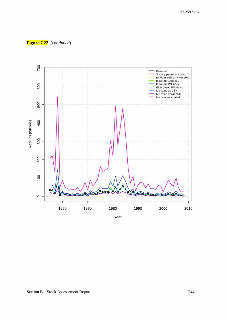
Section B – Stock Assessement Report 244
Figure 7.22 (continued)
1960 1970 1980 1990 2000 2010
010
020
030
040
050
060
070
0
Year
Rec
ruits
(bill
ions
)
Base run3 yr avg per-recruit calcsrandom walk on PN index qleave out JAI indexleave out PN indexGLM based PN indexM scaled up 25%M scaled down 25%M scalar estimated
SEDAR 40 - 7
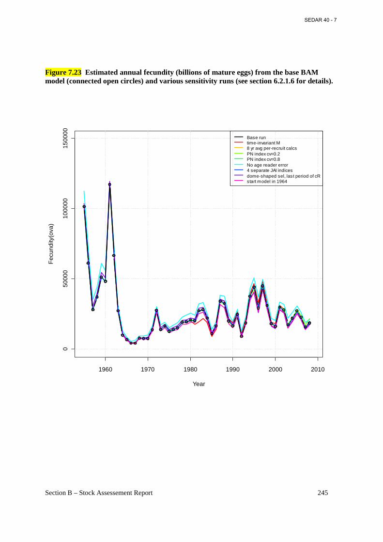
Section B – Stock Assessement Report 245
Figure 7.23 Estimated annual fecundity (billions of mature eggs) from the base BAM model (connected open circles) and various sensitivity runs (see section 6.2.1.6 for details).
1960 1970 1980 1990 2000 2010
050
000
1000
0015
0000
Year
Fec
undi
ty(o
va)
Base runtime-invariant M8 yr avg per-recruit calcsPN index cv=0.2PN index cv=0.8No age reader error4 separate JAI indicesdome-shaped sel, last period of cRstart model in 1964
SEDAR 40 - 7
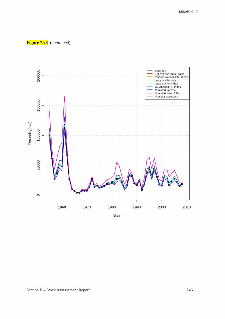
Section B – Stock Assessement Report 246
Figure 7.23 (continued)
1960 1970 1980 1990 2000 2010
050
000
1000
0015
0000
2000
00
Year
Fec
undi
ty(o
va)
Base run3 yr avg per-recruit calcsrandom walk on PN index qleave out JAI indexleave out PN indexGLM based PN indexM scaled up 25%M scaled down 25%M scalar estimated
SEDAR 40 - 7
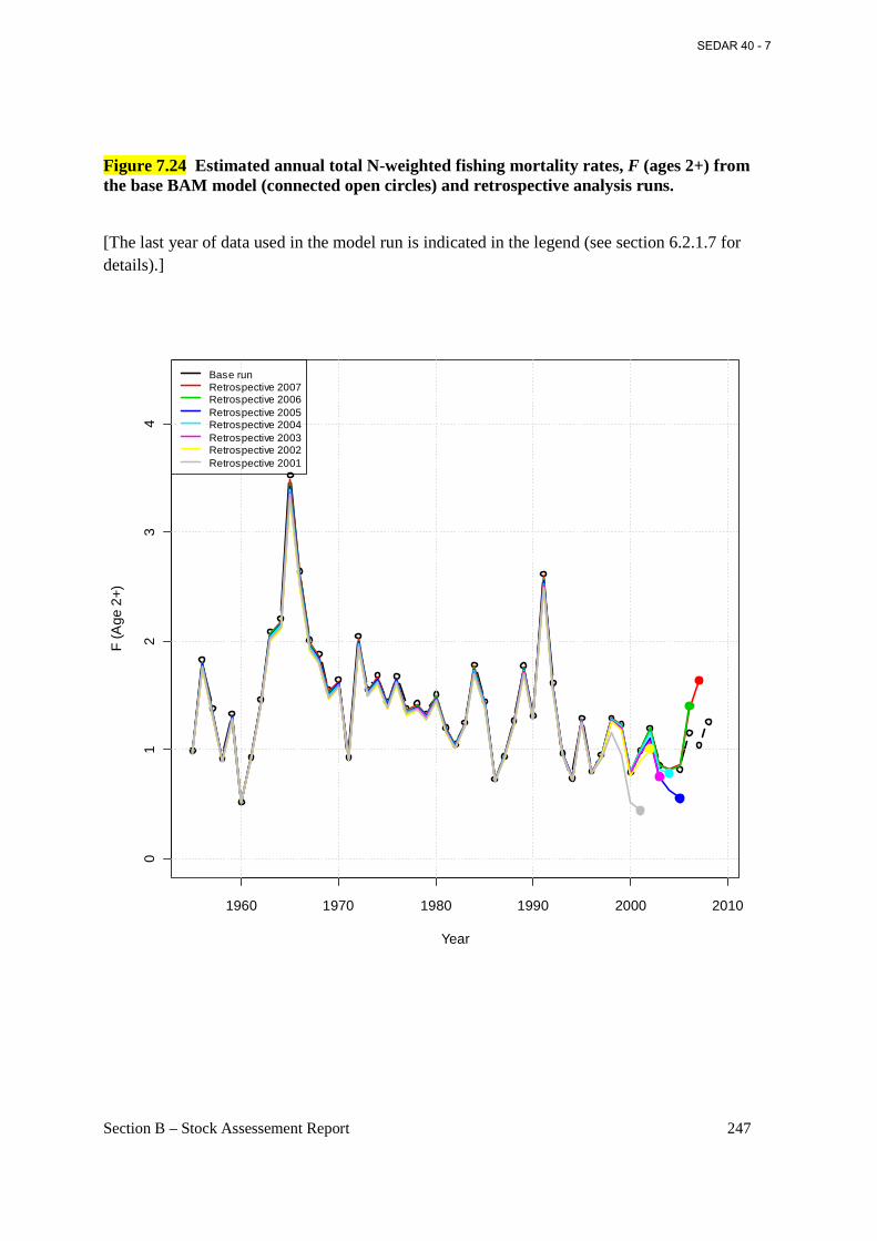
Section B – Stock Assessement Report 247
Figure 7.24 Estimated annual total N-weighted fishing mortality rates, F (ages 2+) from the base BAM model (connected open circles) and retrospective analysis runs.
[The last year of data used in the model run is indicated in the legend (see section 6.2.1.7 for details).]
1960 1970 1980 1990 2000 2010
01
23
4
Year
F (A
ge 2
+)
Base runRetrospective 2007Retrospective 2006Retrospective 2005Retrospective 2004Retrospective 2003Retrospective 2002Retrospective 2001
SEDAR 40 - 7
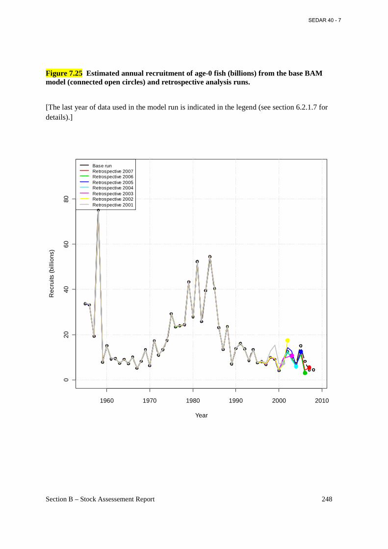
Section B – Stock Assessement Report 248
Figure 7.25 Estimated annual recruitment of age-0 fish (billions) from the base BAM model (connected open circles) and retrospective analysis runs.
[The last year of data used in the model run is indicated in the legend (see section 6.2.1.7 for details).]
1960 1970 1980 1990 2000 2010
020
4060
80
Year
Rec
ruits
(bill
ions
)
Base runRetrospective 2007Retrospective 2006Retrospective 2005Retrospective 2004Retrospective 2003Retrospective 2002Retrospective 2001
SEDAR 40 - 7
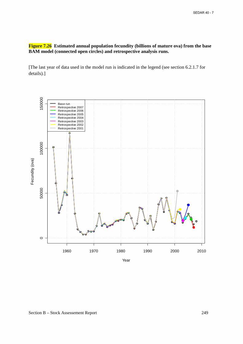
Section B – Stock Assessement Report 249
Figure 7.26 Estimated annual population fecundity (billions of mature ova) from the base BAM model (connected open circles) and retrospective analysis runs.
[The last year of data used in the model run is indicated in the legend (see section 6.2.1.7 for details).]
1960 1970 1980 1990 2000 2010
050
000
1000
0015
0000
Year
Fec
undi
ty (o
va)
Base runRetrospective 2007Retrospective 2006Retrospective 2005Retrospective 2004Retrospective 2003Retrospective 2002Retrospective 2001
SEDAR 40 - 7
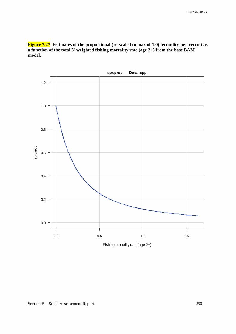
Section B – Stock Assessement Report 250
Figure 7.27 Estimates of the proportional (re-scaled to max of 1.0) fecundity-per-recruit as a function of the total N-weighted fishing mortality rate (age 2+) from the base BAM model.
0.0 0.5 1.0 1.5
0.0
0.2
0.4
0.6
0.8
1.0
1.2
spr.prop Data: spp
Fishing mortality rate (age 2+)
spr.p
rop
SEDAR 40 - 7
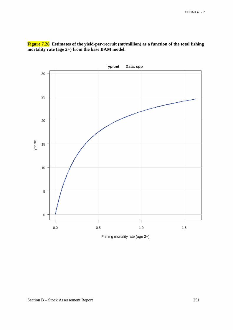
Section B – Stock Assessement Report 251
Figure 7.28 Estimates of the yield-per-recruit (mt/million) as a function of the total fishing mortality rate (age 2+) from the base BAM model.
0.0 0.5 1.0 1.5
0
5
10
15
20
25
30
ypr.mt Data: spp
Fishing mortality rate (age 2+)
ypr.m
t
SEDAR 40 - 7
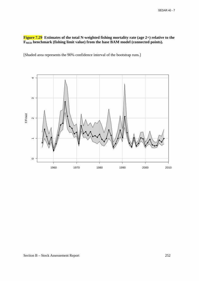
Section B – Stock Assessement Report 252
Figure 7.29 Estimates of the total N-weighted fishing mortality rate (age 2+) relative to the FMED benchmark (fishing limit value) from the base BAM model (connected points).
[Shaded area represents the 90% confidence interval of the bootstrap runs.]
1960 1970 1980 1990 2000 2010
01
23
4
F/F
med
SEDAR 40 - 7
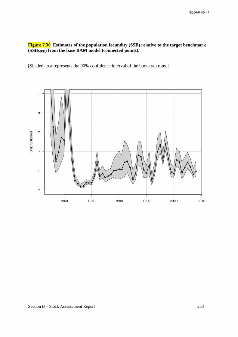
Section B – Stock Assessement Report 253
Figure 7.30 Estimates of the population fecundity (SSB) relative to the target benchmark (SSBMED) from the base BAM model (connected points).
[Shaded area represents the 90% confidence interval of the bootstrap runs.]
1960 1970 1980 1990 2000 2010
01
23
45
SS
B/S
SB
med
SEDAR 40 - 7
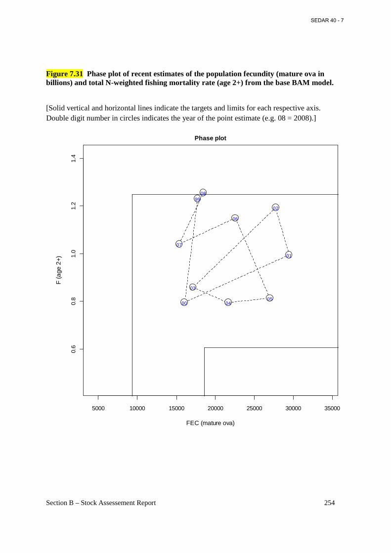
Section B – Stock Assessement Report 254
Figure 7.31 Phase plot of recent estimates of the population fecundity (mature ova in billions) and total N-weighted fishing mortality rate (age 2+) from the base BAM model.
[Solid vertical and horizontal lines indicate the targets and limits for each respective axis. Double digit number in circles indicates the year of the point estimate (e.g. 08 = 2008).]
5000 10000 15000 20000 25000 30000 35000
0.6
0.8
1.0
1.2
1.4
Phase plot
FEC (mature ova)
F (a
ge 2
+)
99
00
01
02
03
0405
06
07
08
SEDAR 40 - 7
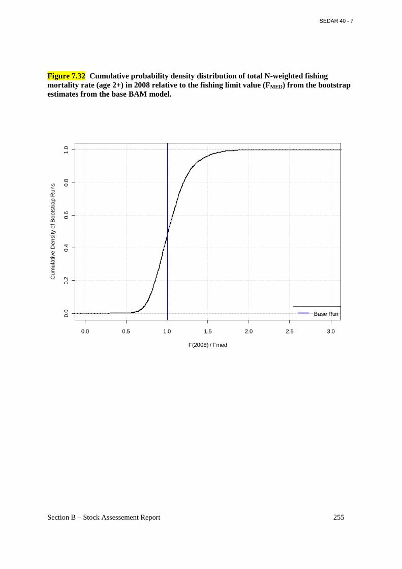
Section B – Stock Assessement Report 255
Figure 7.32 Cumulative probability density distribution of total N-weighted fishing mortality rate (age 2+) in 2008 relative to the fishing limit value (FMED) from the bootstrap estimates from the base BAM model.
0.0 0.5 1.0 1.5 2.0 2.5 3.0
0.0
0.2
0.4
0.6
0.8
1.0
F(2008) / Fmed
Cum
ulat
ive
Den
sity
of B
oots
trap
Run
s
Base Run
SEDAR 40 - 7
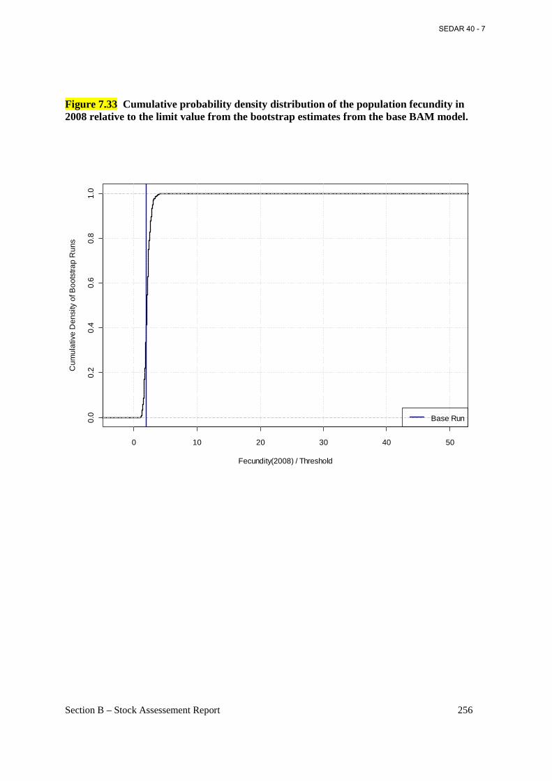
Section B – Stock Assessement Report 256
Figure 7.33 Cumulative probability density distribution of the population fecundity in 2008 relative to the limit value from the bootstrap estimates from the base BAM model.
0 10 20 30 40 50
0.0
0.2
0.4
0.6
0.8
1.0
Fecundity(2008) / Threshold
Cum
ulat
ive
Den
sity
of B
oots
trap
Run
s
Base Run
SEDAR 40 - 7
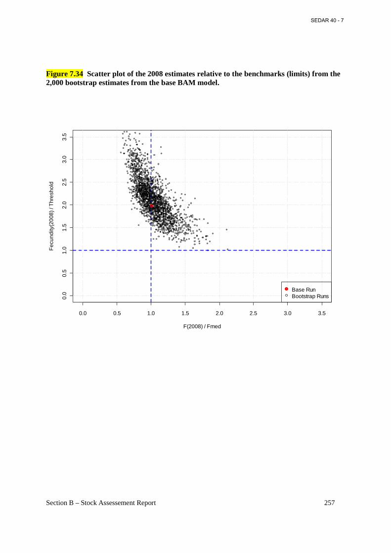
Section B – Stock Assessement Report 257
Figure 7.34 Scatter plot of the 2008 estimates relative to the benchmarks (limits) from the 2,000 bootstrap estimates from the base BAM model.
0.0 0.5 1.0 1.5 2.0 2.5 3.0 3.5
0.0
0.5
1.0
1.5
2.0
2.5
3.0
3.5
F(2008) / Fmed
Fec
undi
ty(2
008)
/ T
hres
hold
Base RunBootstrap Runs
SEDAR 40 - 7
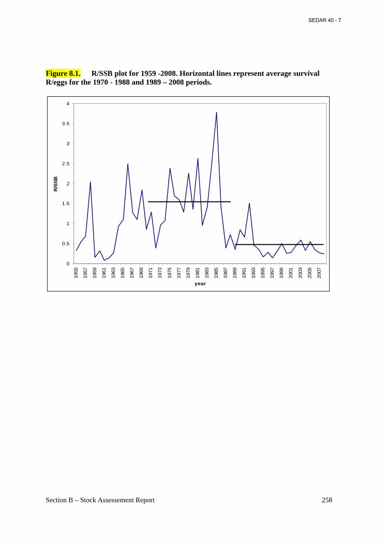
Section B – Stock Assessement Report 258
Figure 8.1. R/SSB plot for 1959 -2008. Horizontal lines represent average survival R/eggs for the 1970 - 1988 and 1989 – 2008 periods.
0
0.5
1
1.5
2
2.5
3
3.5
4
1955
1957
1959
1961
1963
1965
1967
1969
1971
1973
1975
1977
1979
1981
1983
1985
1987
1989
1991
1993
1995
1997
1999
2001
2003
2005
2007
year
R/S
SB
SEDAR 40 - 7
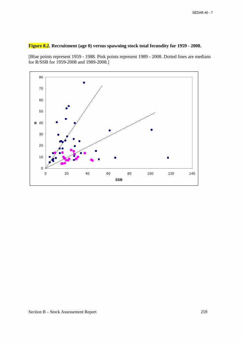
Section B – Stock Assessement Report 259
Figure 8.2. Recruitment (age 0) versus spawning stock total fecundity for 1959 - 2008. [Blue points represent 1959 - 1988. Pink points represent 1989 - 2008. Dotted lines are medians for R/SSB for 1959-2008 and 1989-2008.]
0
10
20
30
40
50
60
70
80
0 20 40 60 80 100 120 140
SSB
R
SEDAR 40 - 7
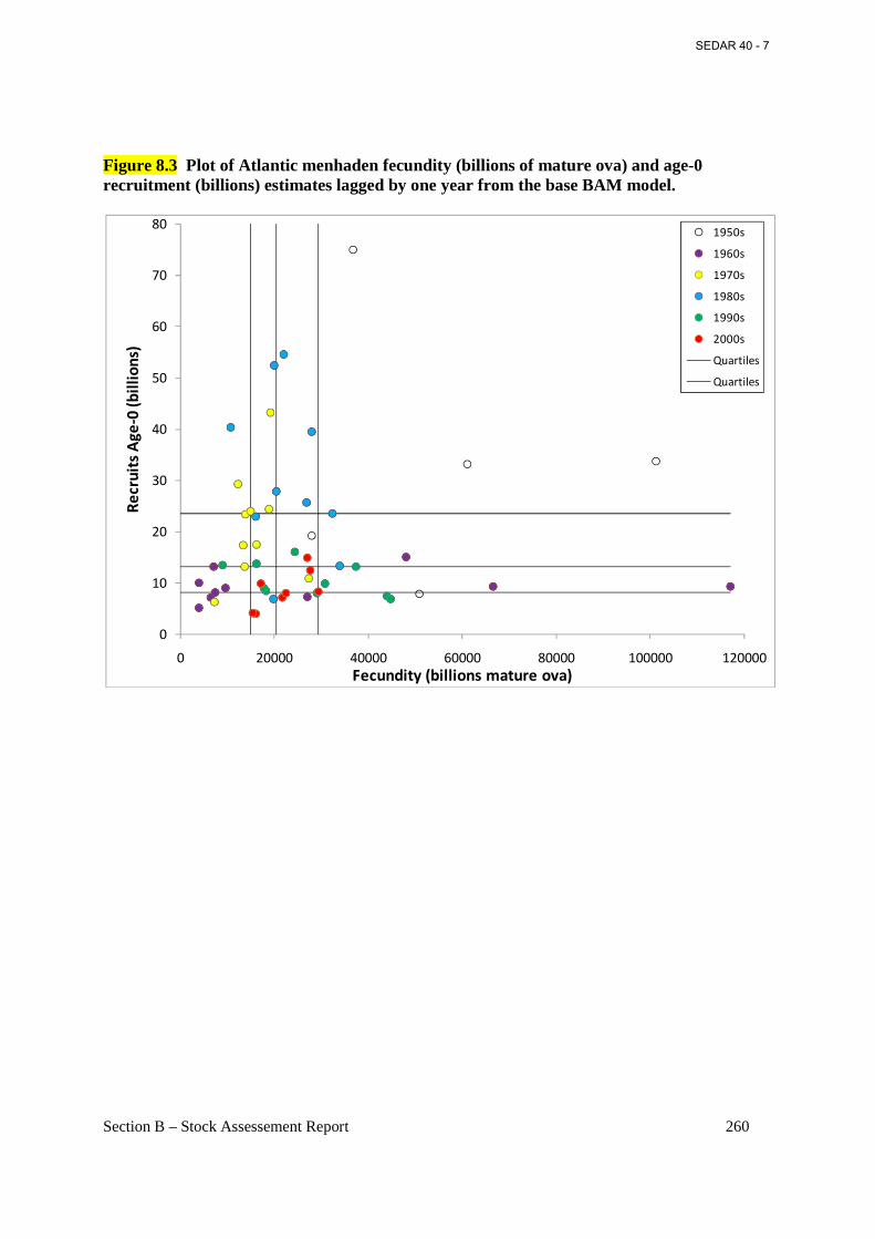
Section B – Stock Assessement Report 260
Figure 8.3 Plot of Atlantic menhaden fecundity (billions of mature ova) and age-0 recruitment (billions) estimates lagged by one year from the base BAM model.
0
10
20
30
40
50
60
70
80
0 20000 40000 60000 80000 100000 120000
Re
cru
its
Ag
e-0
(b
illi
on
s)
Fecundity (billions mature ova)
1950s
1960s
1970s
1980s
1990s
2000s
Quartiles
Quartiles
SEDAR 40 - 7
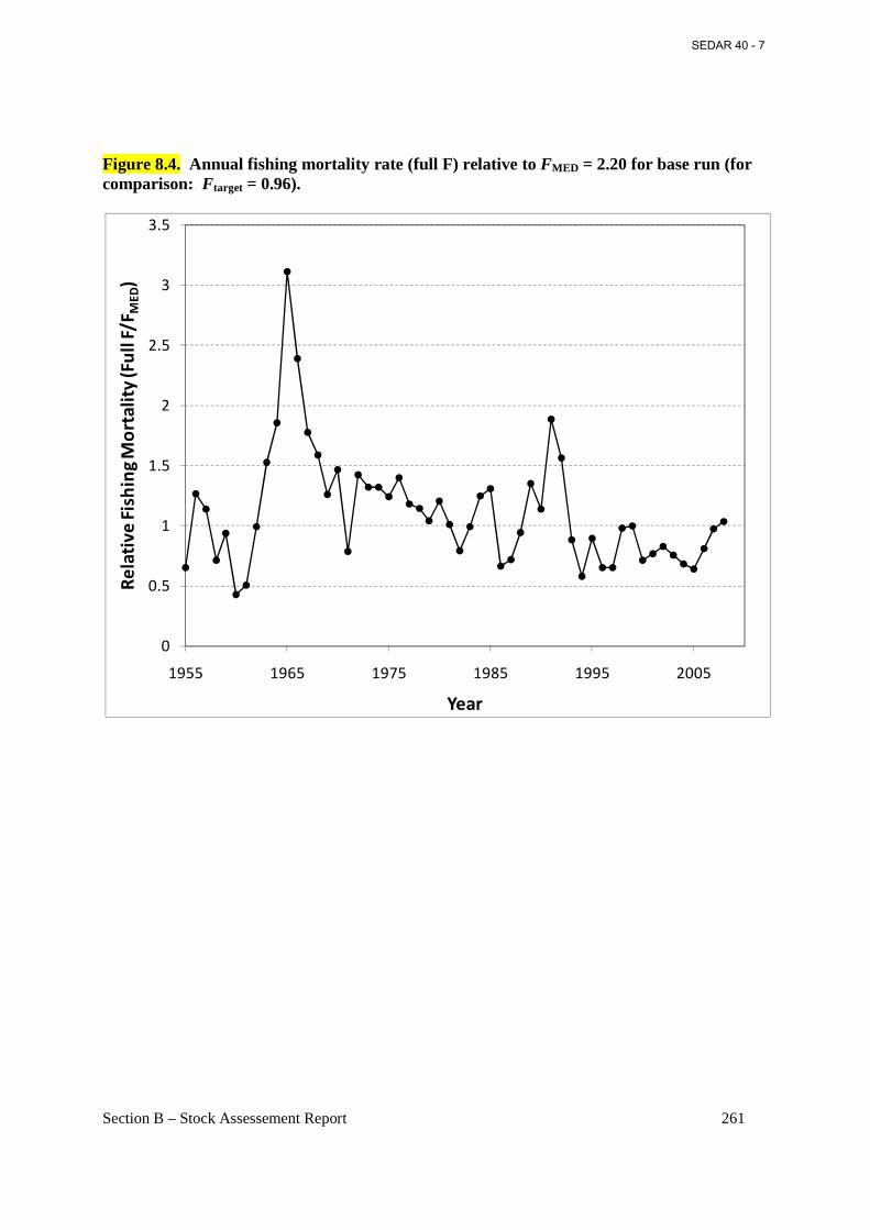
Section B – Stock Assessement Report 261
Figure 8.4. Annual fishing mortality rate (full F) relative to FMED = 2.20 for base run (for comparison: Ftarget = 0.96).
0
0.5
1
1.5
2
2.5
3
3.5
1955 1965 1975 1985 1995 2005
Re
lati
ve
Fis
hin
g M
ort
ali
ty (F
ull
F/F
ME
D)
Year
SEDAR 40 - 7
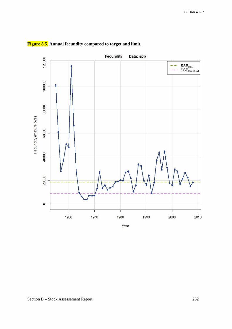
Section B – Stock Assessement Report 262
Figure 8.5. Annual fecundity compared to target and limit.
SEDAR 40 - 7

Section B – Stock Assessement Report 263
Appendices
A.1. Participants in Data and Assessment Workshops A.2. MSVPA-X comparison for striped bass and weakfish. A.3. BAM input file for base run A.4. BAM program file
SEDAR 40 - 7

Section B – Stock Assessement Report 264
Appendix A.1. Listing of Participants in Data and Assessment Workshops Data Workshop (May 12–13, 2009; Richmond, Virginia) Subcommittee members and participants in attendance:
Douglas Vaughan, Chair, NOAA Fisheries Beaufort NC Matt Cieri, ME DMR Jason McNamee, RI DEM Jeff Brust, NJ DEP Alexei Sharov, MD DNR Rob Latour, VIMS Behzad Mahmoudi, FL DEP Joseph Smith, NOAA Fisheries Beaufort NC Erik Williams, NOAA Fisheries Beaufort NC Julie Defilippi, ACCSP Brad Spear, ASMFC Genny Nesslage, ASMFC Jerry Benson, CCA-VA Ron Lukens, Omega Protein Patrick Lynch, VIMS grad student Bradley O’Bier, NOAA Fisheries Reedville VA Bill Windley, ASMFC Menhaden Advisory Panel Chair
Assessment Workshop (October 19-22, 2009; Beaufort, North Carolina) Stock Assessment Subcommittee Members:
Doug Vaughan (NOAA), Chair Joe Smith (NOAA) Erik Williams (NOAA) Alexei Sharov (MD) Matt Cieri (ME) Genny Nesslage (ASMFC) Jeff Brust (NJ) Jason McNamee (RI) Behzad Mahmoudi (FL) Rob Latour (VIMS) Brad Spear (ASMFC), Staff
Other Attendees:
Amy Schueller (NOAA) Kyle Shertzer (NOAA) Paul Conn (NOAA) Rob Cheshire (NOAA) Ron Lukens (Omega Protein) Jeff Kaelin (Lunds Seafood) Patrick Lynch (VIMS)
SEDAR 40 - 7

Section B – Stock Assessement Report
Appendix A.2. Comparison of abundaspecies assessments and MSVPA Figure A.1. Comparison of annual single species assessment and MSVPA
fishing mortality estimates for striped bass.
Stock Assessement Report
Comparison of abundance and fishing mortality estimates between single species assessments and MSVPA-X for striped bass and menhaden.
. Comparison of annual single species assessment and MSVPAfishing mortality estimates for striped bass.
265
nce and fishing mortality estimates between single
. Comparison of annual single species assessment and MSVPA-X abundance and
SEDAR 40 - 7

Section B – Stock Assessement Report
Figure A.2. Comparison of annual single species assessment and MSVPAfishing mortality estimates for weakfish.
Stock Assessement Report
Comparison of annual single species assessment and MSVPAfishing mortality estimates for weakfish.
266
Comparison of annual single species assessment and MSVPA-X abundance and
SEDAR 40 - 7
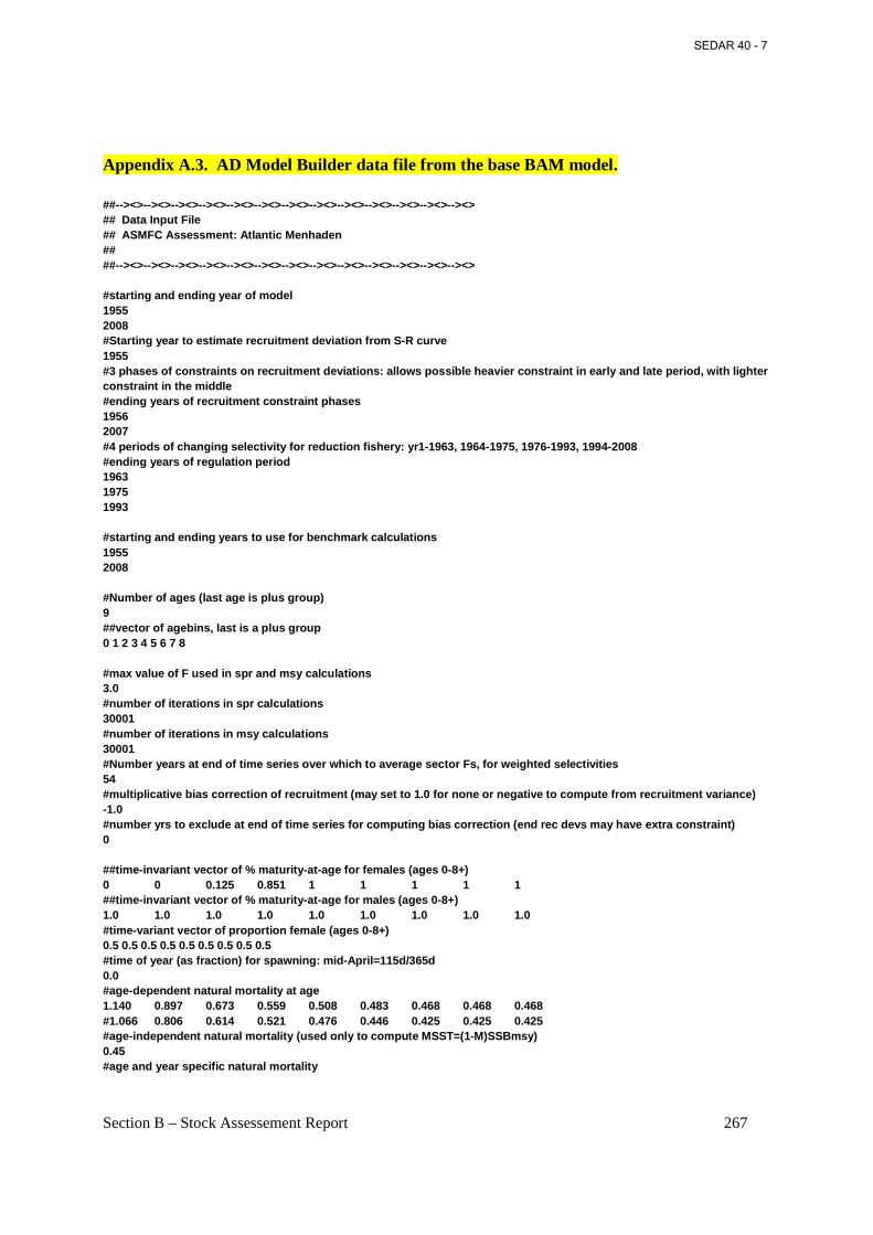
Section B – Stock Assessement Report 267
Appendix A.3. AD Model Builder data file from the base BAM model. ##--><>--><>--><>--><>--><>--><>--><>--><>--><>--><>--><>--><>--><> ## Data Input File ## ASMFC Assessment: Atlantic Menhaden ## ##--><>--><>--><>--><>--><>--><>--><>--><>--><>--><>--><>--><>--><> #starting and ending year of model 1955 2008 #Starting year to estimate recruitment deviation from S-R curve 1955 #3 phases of constraints on recruitment deviations: allows possible heavier constraint in early and late period, with lighter constraint in the middle #ending years of recruitment constraint phases 1956 2007 #4 periods of changing selectivity for reduction fishery: yr1-1963, 1964-1975, 1976-1993, 1994-2008 #ending years of regulation period 1963 1975 1993 #starting and ending years to use for benchmark calculations 1955 2008 #Number of ages (last age is plus group) 9 ##vector of agebins, last is a plus group 0 1 2 3 4 5 6 7 8 #max value of F used in spr and msy calculations 3.0 #number of iterations in spr calculations 30001 #number of iterations in msy calculations 30001 #Number years at end of time series over which to average sector Fs, for weighted selectivities 54 #multiplicative bias correction of recruitment (may set to 1.0 for none or negative to compute from recruitment variance) -1.0 #number yrs to exclude at end of time series for computing bias correction (end rec devs may have extra constraint) 0 ##time-invariant vector of % maturity-at-age for females (ages 0-8+) 0 0 0.125 0.851 1 1 1 1 1 ##time-invariant vector of % maturity-at-age for males (ages 0-8+) 1.0 1.0 1.0 1.0 1.0 1.0 1.0 1.0 1.0 #time-variant vector of proportion female (ages 0-8+) 0.5 0.5 0.5 0.5 0.5 0.5 0.5 0.5 0.5 #time of year (as fraction) for spawning: mid-April=115d/365d 0.0 #age-dependent natural mortality at age 1.140 0.897 0.673 0.559 0.508 0.483 0.468 0.468 0.468 #1.066 0.806 0.614 0.521 0.476 0.446 0.425 0.425 0.425 #age-independent natural mortality (used only to compute MSST=(1-M)SSBmsy) 0.45 #age and year specific natural mortality
SEDAR 40 - 7
Section B – Stock Assessement Report 268
1.140 0.897 0.673 0.559 0.508 0.483 0.468 0.468 0.468 1.140 0.897 0.673 0.559 0.508 0.483 0.468 0.468 0.468 1.140 0.897 0.673 0.559 0.508 0.483 0.468 0.468 0.468 1.140 0.897 0.673 0.559 0.508 0.483 0.468 0.468 0.468 1.140 0.897 0.673 0.559 0.508 0.483 0.468 0.468 0.468 1.140 0.897 0.673 0.559 0.508 0.483 0.468 0.468 0.468 1.140 0.897 0.673 0.559 0.508 0.483 0.468 0.468 0.468 1.140 0.897 0.673 0.559 0.508 0.483 0.468 0.468 0.468 1.140 0.897 0.673 0.559 0.508 0.483 0.468 0.468 0.468 1.140 0.897 0.673 0.559 0.508 0.483 0.468 0.468 0.468 1.140 0.897 0.673 0.559 0.508 0.483 0.468 0.468 0.468 1.140 0.897 0.673 0.559 0.508 0.483 0.468 0.468 0.468 1.140 0.897 0.673 0.559 0.508 0.483 0.468 0.468 0.468 1.140 0.897 0.673 0.559 0.508 0.483 0.468 0.468 0.468 1.140 0.897 0.673 0.559 0.508 0.483 0.468 0.468 0.468 1.140 0.897 0.673 0.559 0.508 0.483 0.468 0.468 0.468 1.140 0.897 0.673 0.559 0.508 0.483 0.468 0.468 0.468 1.140 0.897 0.673 0.559 0.508 0.483 0.468 0.468 0.468 1.140 0.897 0.673 0.559 0.508 0.483 0.468 0.468 0.468 1.140 0.897 0.673 0.559 0.508 0.483 0.468 0.468 0.468 1.140 0.897 0.673 0.559 0.508 0.483 0.468 0.468 0.468 1.140 0.897 0.673 0.559 0.508 0.483 0.468 0.468 0.468 1.140 0.897 0.673 0.559 0.508 0.483 0.468 0.468 0.468 1.140 0.897 0.673 0.559 0.508 0.483 0.468 0.468 0.468 1.140 0.897 0.673 0.559 0.508 0.483 0.468 0.468 0.468 1.140 0.897 0.673 0.559 0.508 0.483 0.468 0.468 0.468 1.140 0.897 0.673 0.559 0.508 0.483 0.468 0.468 0.468 1.624 1.350 0.993 0.826 0.597 0.527 0.506 0.506 0.506 1.487 1.272 0.917 0.662 0.586 0.516 0.495 0.495 0.495 1.313 1.123 0.845 0.595 0.524 0.506 0.468 0.468 0.468 1.314 1.128 0.930 0.610 0.521 0.516 0.499 0.499 0.499 1.279 1.106 0.863 0.675 0.525 0.516 0.532 0.532 0.532 1.117 0.936 0.757 0.602 0.511 0.495 0.499 0.499 0.499 1.044 0.940 0.711 0.581 0.516 0.493 0.489 0.489 0.489 0.950 0.789 0.678 0.565 0.510 0.490 0.482 0.482 0.482 0.981 0.736 0.603 0.537 0.500 0.486 0.476 0.476 0.476 0.948 0.814 0.609 0.526 0.501 0.491 0.481 0.481 0.481 0.900 0.670 0.588 0.503 0.481 0.451 0.452 0.452 0.452 0.986 0.802 0.562 0.519 0.485 0.458 0.429 0.429 0.429 0.993 0.783 0.596 0.504 0.483 0.460 0.432 0.432 0.432 1.089 0.764 0.584 0.514 0.497 0.473 0.448 0.448 0.448 1.038 0.778 0.540 0.482 0.467 0.459 0.442 0.442 0.442 1.062 0.793 0.541 0.470 0.453 0.450 0.443 0.443 0.443 1.118 0.853 0.564 0.478 0.445 0.448 0.450 0.450 0.450 1.124 0.763 0.588 0.496 0.466 0.448 0.464 0.464 0.464 1.096 0.732 0.548 0.495 0.475 0.461 0.454 0.454 0.454 1.137 0.785 0.570 0.510 0.483 0.474 0.465 0.465 0.465 1.143 0.842 0.591 0.516 0.504 0.479 0.471 0.471 0.471 1.114 0.841 0.618 0.533 0.492 0.479 0.458 0.458 0.458 1.241 0.895 0.673 0.557 0.535 0.487 0.465 0.465 0.465 1.199 0.997 0.653 0.565 0.526 0.496 0.458 0.458 0.458 1.212 0.962 0.696 0.572 0.538 0.500 0.463 0.463 0.463 1.149 0.895 0.723 0.585 0.536 0.497 0.464 0.464 0.464 1.130 0.863 0.639 0.605 0.550 0.498 0.463 0.463 0.463 ##Spawner-recruit parameters #switch for S-R function to use Ricker (1) or Beverton-Holt (2) 2 #steepness (fixed or initial guess) 0.99 #standard error of steepness (from meta-analysis)
SEDAR 40 - 7
Section B – Stock Assessement Report 269
0.2 #log_R0 - log virgin recruitment 2.7 # R autocorrelation 0.0 ##--><>--><>--><>-- Weight-at-age in the fishery (g) --><>--><>--><>--><>--><>--><>--><>--><> 36.2 124.3 274.3 390.3 451.5 523.3 610.8 681.9 674.8 25.2 105.1 267.1 428.1 498.1 558.8 601.7 633.0 710.4 41.2 91.3 230.8 413.4 553.1 595.6 645.8 668.9 649.8 22.8 109.9 231.7 382.2 555.5 655.8 686.9 719.8 728.9 60.5 75.2 231.4 373.5 507.5 643.9 697.1 726.6 739.2 32.2 129.6 189.6 375.4 513.3 636.2 738.3 752.7 789.3 48.3 116.0 258.4 336.7 512.9 618.3 727.6 789.9 771.3 60.1 131.0 267.1 394.1 466.5 591.0 644.3 731.1 754.8 63.5 145.6 257.7 424.9 567.3 635.0 727.1 742.6 835.6 67.1 150.4 281.1 380.3 550.2 721.1 767.2 811.7 786.5 53.0 145.8 275.5 386.3 462.2 621.2 835.8 853.3 852.3 66.8 121.9 278.1 387.7 455.6 509.7 648.2 899.7 887.3 62.1 157.6 252.4 434.2 507.2 535.7 581.5 722.8 1063.5 74.7 128.1 316.8 424.3 583.3 596.3 583.3 620.6 751.8 83.3 152.8 268.9 500.0 649.2 759.4 705.9 655.1 689.9 58.7 185.4 269.3 419.1 595.1 790.4 814.4 705.8 631.7 50.6 169.4 341.9 406.3 589.4 654.5 905.8 844.3 695.9 24.7 122.7 328.9 493.1 566.4 800.0 713.2 1048.6 897.8 43.1 121.1 263.3 475.2 636.9 752.9 1039.3 764.4 1175.1 28.7 103.4 263.0 408.7 582.0 764.0 968.3 1344.6 817.8 27.1 84.5 214.8 379.8 560.5 666.2 877.0 1204.4 1682.8 17.3 67.4 192.4 345.3 474.1 732.6 761.3 1023.0 1543.4 20.2 64.4 151.3 317.3 471.6 533.0 878.5 821.9 1126.2 28.4 68.7 163.2 252.6 420.4 556.1 543.8 944.0 817.6 24.8 68.7 168.8 279.1 366.8 516.4 638.4 562.1 1028.2 21.7 56.6 148.1 288.8 391.6 482.0 593.8 702.3 573.1 19.5 68.2 118.8 239.7 396.9 475.8 575.8 637.1 732.7 26.7 76.2 167.7 212.4 341.0 486.7 533.9 643.0 650.7 31.4 70.8 171.6 258.4 303.4 414.5 534.0 553.5 675.8 25.6 71.9 165.8 291.7 368.6 440.4 525.8 623.9 621.0 22.6 68.4 139.3 260.6 374.2 430.8 546.0 579.3 641.6 24.3 64.4 149.8 230.7 375.2 470.7 516.2 715.8 683.0 26.6 75.5 153.6 249.4 338.2 476.8 533.3 566.0 847.6 27.8 69.4 159.9 241.3 329.2 429.6 541.5 556.9 580.4 39.1 91.1 150.3 256.1 341.1 427.5 567.7 657.1 632.2 35.8 113.1 208.5 248.2 340.4 419.4 494.0 670.6 713.7 52.0 92.8 224.1 309.7 334.8 393.4 461.9 521.5 723.5 28.3 123.1 186.4 318.7 392.3 420.5 445.0 512.0 565.8 49.8 93.4 243.6 294.7 396.0 457.6 501.1 488.5 553.9 23.5 118.8 214.3 355.7 395.0 450.3 504.8 572.6 523.3 22.6 112.6 229.7 331.8 423.1 453.4 456.3 501.1 586.3 17.0 96.5 288.8 371.6 483.5 529.8 564.3 517.7 564.7 28.8 87.6 246.6 447.0 491.0 594.2 585.9 625.8 536.0 60.3 93.9 227.2 390.9 547.0 574.4 662.1 608.2 654.1 39.1 131.1 214.0 354.9 496.6 597.8 627.1 699.9 612.1 27.1 131.5 252.7 345.5 456.5 577.9 633.4 674.5 736.3 55.0 125.1 280.6 382.9 462.1 522.0 624.5 643.7 697.6 40.4 149.4 290.1 422.1 526.3 581.0 588.9 683.6 677.6 49.5 121.7 277.0 440.1 557.5 701.6 725.3 678.0 779.9 27.0 113.9 238.6 339.2 482.6 572.9 738.6 722.8 638.4 37.3 81.3 214.5 328.6 369.5 495.8 572.7 760.5 714.6 45.3 111.1 185.4 321.5 411.2 407.1 537.6 619.3 862.4 50.2 119.8 219.0 297.3 390.9 434.4 399.2 514.3 588.0 52.4 123.8 247.9 313.7 424.9 473.5 479.2 419.4 539.6
SEDAR 40 - 7
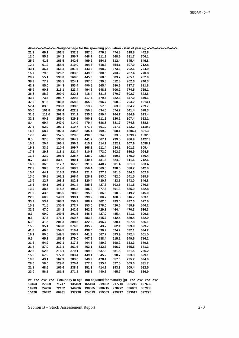
Section B – Stock Assessement Report 270
##--><>--><>--><>-- Weight-at-age for the spawning population - start of year (g) --><>--><>--><>--><> 21.2 66.1 191.5 332.3 387.5 476.8 474.8 618.8 442.8 12.0 55.8 194.2 356.7 448.7 511.9 568.6 631.7 706.1 25.9 41.6 163.5 342.6 499.2 554.5 612.4 645.4 649.8 12.4 61.2 158.6 310.0 494.6 618.3 654.1 697.0 712.8 43.1 36.4 166.3 301.5 443.6 598.2 673.6 702.6 724.9 15.7 79.6 126.2 303.5 449.5 580.6 703.2 737.4 770.8 29.7 55.1 190.0 260.8 445.3 568.6 683.7 765.1 762.0 38.3 77.2 193.1 324.1 397.6 539.8 612.8 702.6 740.3 42.1 85.0 194.3 353.4 490.5 565.4 680.6 717.7 811.8 45.9 90.8 215.1 323.4 494.2 648.1 706.2 774.5 769.1 36.5 88.2 209.0 332.1 418.4 581.6 770.7 802.7 823.6 43.5 73.5 208.7 329.8 417.4 479.5 622.8 847.0 849.1 47.0 91.6 180.8 358.2 455.9 506.7 558.3 704.2 1013.1 57.4 83.5 238.3 338.3 513.2 557.0 563.9 604.7 739.7 55.0 101.8 197.4 422.2 550.8 694.6 674.7 641.4 678.3 31.6 111.0 202.5 331.2 535.5 699.4 764.7 684.9 623.4 32.2 90.9 259.0 329.3 490.3 611.9 826.2 807.4 682.1 8.4 69.4 247.0 414.9 479.4 686.5 681.7 974.8 868.6 27.5 52.9 193.1 410.7 571.3 661.0 917.6 742.2 1110.9 16.5 58.7 192.3 334.8 535.4 709.2 868.1 1206.4 801.3 17.8 44.3 157.5 329.6 490.8 634.8 833.5 1099.7 1532.6 8.5 37.8 135.8 284.2 441.7 667.1 739.5 986.9 1427.3 10.8 29.4 106.1 256.9 415.2 514.2 822.2 807.9 1098.2 19.1 33.5 110.4 199.7 368.2 511.4 534.1 901.3 809.4 17.5 39.8 115.1 221.4 310.3 473.0 602.7 556.9 994.5 11.8 33.9 105.6 228.7 338.0 426.4 559.6 675.0 570.4 9.7 33.6 83.4 190.1 340.4 431.6 524.9 611.6 712.6 16.2 36.9 117.7 165.5 291.2 440.7 501.4 601.3 633.4 22.3 38.3 119.6 208.9 250.4 369.0 498.6 530.2 642.0 15.4 44.1 116.9 236.4 321.4 377.9 481.5 594.3 602.8 13.0 36.8 101.2 208.4 328.1 393.0 482.0 541.5 619.8 13.9 32.7 105.2 182.3 320.4 430.7 483.5 643.0 646.8 16.6 40.1 108.1 201.4 285.3 427.8 503.5 541.5 776.6 13.9 38.5 115.2 195.3 286.2 377.6 501.3 535.9 562.8 21.9 43.5 105.5 208.6 295.3 386.6 510.6 619.2 615.0 22.6 60.9 148.3 198.1 299.2 380.7 460.5 616.7 683.1 33.2 53.4 168.9 259.2 288.7 362.5 433.0 497.0 677.9 15.3 71.5 135.9 272.7 353.0 378.0 420.6 488.9 546.2 32.5 47.0 184.2 242.5 362.5 429.8 464.4 470.3 536.3 8.3 69.0 149.5 301.5 346.5 427.0 485.4 541.1 509.6 9.6 47.5 171.4 269.7 383.3 415.7 442.4 489.4 562.9 6.0 41.5 201.3 308.5 422.2 496.7 530.1 507.8 556.1 15.5 35.1 168.8 374.3 435.2 543.7 562.1 599.0 529.7 41.8 46.8 154.5 319.4 498.0 530.2 624.2 592.1 634.2 19.1 80.5 149.5 290.7 441.9 567.7 593.9 672.4 601.5 9.6 65.1 188.6 279.0 407.9 538.4 615.2 649.6 716.2 31.8 54.9 207.1 317.3 404.3 489.2 598.2 633.3 679.8 21.8 87.0 213.1 361.6 463.1 532.3 566.7 665.6 671.3 32.3 62.6 218.1 379.1 509.8 637.8 681.5 661.5 766.2 15.6 67.9 177.8 303.4 449.1 545.2 690.7 693.3 629.1 19.8 43.1 162.9 283.0 349.9 478.4 557.0 725.2 694.9 28.0 58.0 129.0 270.4 377.3 395.4 527.5 609.0 831.7 21.1 68.6 166.6 238.9 351.3 414.2 393.3 509.4 582.5 23.0 56.5 181.8 271.8 365.5 440.3 465.7 416.0 536.9 ##--><>--><>--><>-- Fecundity-at-age - not adjusted for maturity (g) --><>--><>--><>--><> 13463 27660 71747 135469 165103 219032 217740 321215 197636 10233 24296 72102 146296 198365 238715 278272 326059 387985 15428 20472 60931 137238 224019 259559 299712 323917 327225
SEDAR 40 - 7
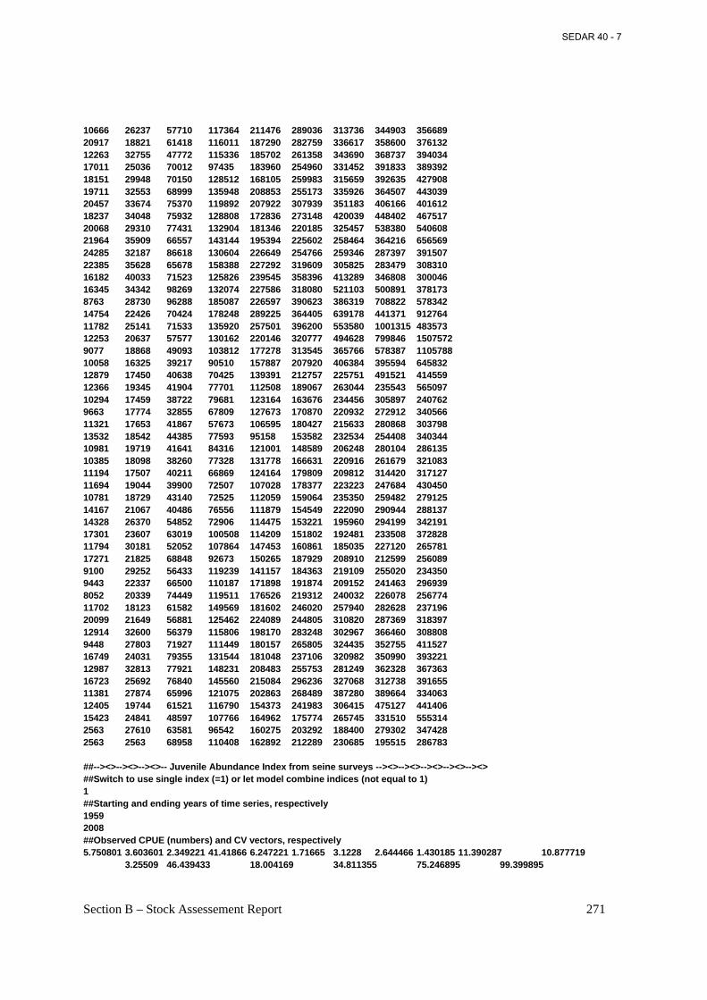
Section B – Stock Assessement Report 271
10666 26237 57710 117364 211476 289036 313736 344903 356689 20917 18821 61418 116011 187290 282759 336617 358600 376132 12263 32755 47772 115336 185702 261358 343690 368737 394034 17011 25036 70012 97435 183960 254960 331452 391833 389392 18151 29948 70150 128512 168105 259983 315659 392635 427908 19711 32553 68999 135948 208853 255173 335926 364507 443039 20457 33674 75370 119892 207922 307939 351183 406166 401612 18237 34048 75932 128808 172836 273148 420039 448402 467517 20068 29310 77431 132904 181346 220185 325457 538380 540608 21964 35909 66557 143144 195394 225602 258464 364216 656569 24285 32187 86618 130604 226649 254766 259346 287397 391507 22385 35628 65678 158388 227292 319609 305825 283479 308310 16182 40033 71523 125826 239545 358396 413289 346808 300046 16345 34342 98269 132074 227586 318080 521103 500891 378173 8763 28730 96288 185087 226597 390623 386319 708822 578342 14754 22426 70424 178248 289225 364405 639178 441371 912764 11782 25141 71533 135920 257501 396200 553580 1001315 483573 12253 20637 57577 130162 220146 320777 494628 799846 1507572 9077 18868 49093 103812 177278 313545 365766 578387 1105788 10058 16325 39217 90510 157887 207920 406384 395594 645832 12879 17450 40638 70425 139391 212757 225751 491521 414559 12366 19345 41904 77701 112508 189067 263044 235543 565097 10294 17459 38722 79681 123164 163676 234456 305897 240762 9663 17774 32855 67809 127673 170870 220932 272912 340566 11321 17653 41867 57673 106595 180427 215633 280868 303798 13532 18542 44385 77593 95158 153582 232534 254408 340344 10981 19719 41641 84316 121001 148589 206248 280104 286135 10385 18098 38260 77328 131778 166631 220916 261679 321083 11194 17507 40211 66869 124164 179809 209812 314420 317127 11694 19044 39900 72507 107028 178377 223223 247684 430450 10781 18729 43140 72525 112059 159064 235350 259482 279125 14167 21067 40486 76556 111879 154549 222090 290944 288137 14328 26370 54852 72906 114475 153221 195960 294199 342191 17301 23607 63019 100508 114209 151802 192481 233508 372828 11794 30181 52052 107864 147453 160861 185035 227120 265781 17271 21825 68848 92673 150265 187929 208910 212599 256089 9100 29252 56433 119239 141157 184363 219109 255020 234350 9443 22337 66500 110187 171898 191874 209152 241463 296939 8052 20339 74449 119511 176526 219312 240032 226078 256774 11702 18123 61582 149569 181602 246020 257940 282628 237196 20099 21649 56881 125462 224089 244805 310820 287369 318397 12914 32600 56379 115806 198170 283248 302967 366460 308808 9448 27803 71927 111449 180157 265805 324435 352755 411527 16749 24031 79355 131544 181048 237106 320982 350990 393221 12987 32813 77921 148231 208483 255753 281249 362328 367363 16723 25692 76840 145560 215084 296236 327068 312738 391655 11381 27874 65996 121075 202863 268489 387280 389664 334063 12405 19744 61521 116790 154373 241983 306415 475127 441406 15423 24841 48597 107766 164962 175774 265745 331510 555314 2563 27610 63581 96542 160275 203292 188400 279302 347428 2563 2563 68958 110408 162892 212289 230685 195515 286783 ##--><>--><>--><>-- Juvenile Abundance Index from seine surveys --><>--><>--><>--><>--><> ##Switch to use single index (=1) or let model combine indices (not equal to 1) 1 ##Starting and ending years of time series, respectively 1959 2008 ##Observed CPUE (numbers) and CV vectors, respectively 5.750801 3.603601 2.349221 41.41866 6.247221 1.71665 3.1228 2.644466 1.430185 11.390287 10.877719 3.25509 46.439433 18.004169 34.811355 75.246895 99.399895
SEDAR 40 - 7
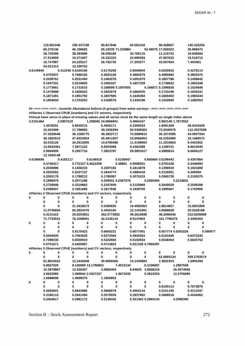
Section B – Stock Assessement Report 272
119.951046 195.337198 69.817846 60.591416 96.428657 145.325256 65.270146 46.196682 65.19235 71.233884 53.46075 17.926022 35.898472 28.725499 38.383986 38.008169 30.785115 11.215752 19.848584 17.514069 19.271607 16.332323 24.695283 47.967632 15.518712 15.747987 24.225217 26.762735 17.203377 43.507604 7.403461 24.021313 13.199752 0.6149945 0.412245 0.6160166 0.5175259 0.6059944 0.6200932 0.4278114 0.4703037 0.7686192 0.4633106 0.3882979 0.4985982 0.3803475 0.2439761 0.2031494 0.1462078 0.1691979 0.1807786 0.1408642 0.1947331 0.2519605 0.1905337 0.1827339 0.1738832 0.1962348 0.1773661 0.1731615 0.168699 0.1597693 0.166871 0.1596836 0.1524848 0.1479088 0.1606522 0.1832679 0.1860425 0.1733196 0.1620341 0.1871491 0.1951792 0.1807595 0.1645394 0.1669403 0.1965344 0.1854634 0.1703203 0.1428576 0.1330186 0.1542845 0.1482553 ##--><>--><>--><>-- Juvenile Abundance Indices (4 groups) from seine surveys --><>--><>--><>--><>--><> ##Series 1 Observed CPUE (numbers) and CV vectors, respectively ##must have zeros in place of missing values and all series must be the same length as single index above 3.2151464 2.0907619 1.296065 24.0666941 3.4964167 0.962149 1.7673552 1.4678251 0.8035215 6.4005171 6.2359334 1.8481459 26.5419328 10.423499 17.788682 39.1936394 50.5308363 73.2540075 112.3537838 37.3330648 36.1268775 49.2822717 73.5580815 30.3372085 24.0607934 40.1662515 47.8323004 45.4911007 23.9066903 42.5253985 23.1469572 33.018126 34.2912605 14.6780396 11.4196804 11.3316663 9.4401652 13.8334461 7.2871333 6.8303088 9.1563389 3.1189741 9.8610045 2.9694595 9.1957716 7.3823787 29.5901617 4.3980814 8.6606127 12.1693148 0.6196695 0.4182117 0.6146519 0.5190947 0.605684 0.6198442 0.4307864 0.4746417 0.772157 0.4622209 0.38851 0.5008351 0.3791538 0.2446993 0.2030896 0.1456319 0.1697192 0.1814878 0.1396919 0.1921808 0.2525552 0.2037137 0.1844774 0.1880418 0.2126051 0.200659 0.2053178 0.1788212 0.1780087 0.2075233 0.2065729 0.2109375 0.1895979 0.2071288 0.209001 0.2367578 0.2560394 0.2218841 0.2726946 0.3319883 0.2167609 0.2125969 0.2640029 0.2549398 0.2489007 0.1951689 0.1817646 0.1939705 0.1995067 0.1703956 ##Series 2 Observed CPUE (numbers) and CV vectors, respectively 0 0 0 0 0 0 0 0 0 0 0 0 0 0 0 0 0 0 0 0 0 0 0 0 0 0 0 21.3418573 0.5390835 19.4082953 2.8614657 15.6901809 11.0745694 65.3924476 0.4455194 12.1423391 3.9588828 20.0226198 0.4131422 25.6203651 252.5772802 49.2616698 48.2596546 210.6206898 71.7733531 76.1008091 42.2135115 9.9147803 161.7790276 3.3456304 0 0 0 0 0 0 0 0 0 0 0 0 0 0 0 0 0 0 0 0 0 0 0 0 0 0 0 0.9170423 0.6665231 0.8077591 0.657774 0.6303226 0.595977 0.6454505 0.7063529 0.6372563 0.4940303 0.5191645 0.6372243 0.7399235 0.6030919 0.5332693 0.5192834 0.5548404 0.5625752 0.5751671 0.5455987 0.4713823 0.521328 0.7065397 ##Series 3 Observed CPUE (numbers) and CV vectors, respectively 0 0 0 0 0 0 0 0 0 0 0 0 0 0 0 0 0 0 0 0 0 62.6893134 259.2783574 51.8810532 12.2443508 30.9959456 14.1435884 2.3832303 1.5905358 5.8567029 8.145969 13.1786803 7.4515134 6.3196687 1.2897558 10.3979867 13.436357 3.5883454 8.64925 3.8668316 26.4074946 2.6622985 1.089944 2.0327237 1.9672035 0.3815253 12.2755695 1.6988698 1.4698375 1.1856853 0 0 0 0 0 0 0 0 0 0 0 0 0 0 0 0 0 0 0 0 0 0.6100114 0.7673876 0.4563601 0.5643986 0.3666978 0.3004134 0.5151165 0.3213347 0.3180115 0.2841494 0.2579026 0.2837902 0.2688518 0.4544062 0.3454617 0.2981172 0.3135442 0.321363 0.2960134 0.3096394
SEDAR 40 - 7
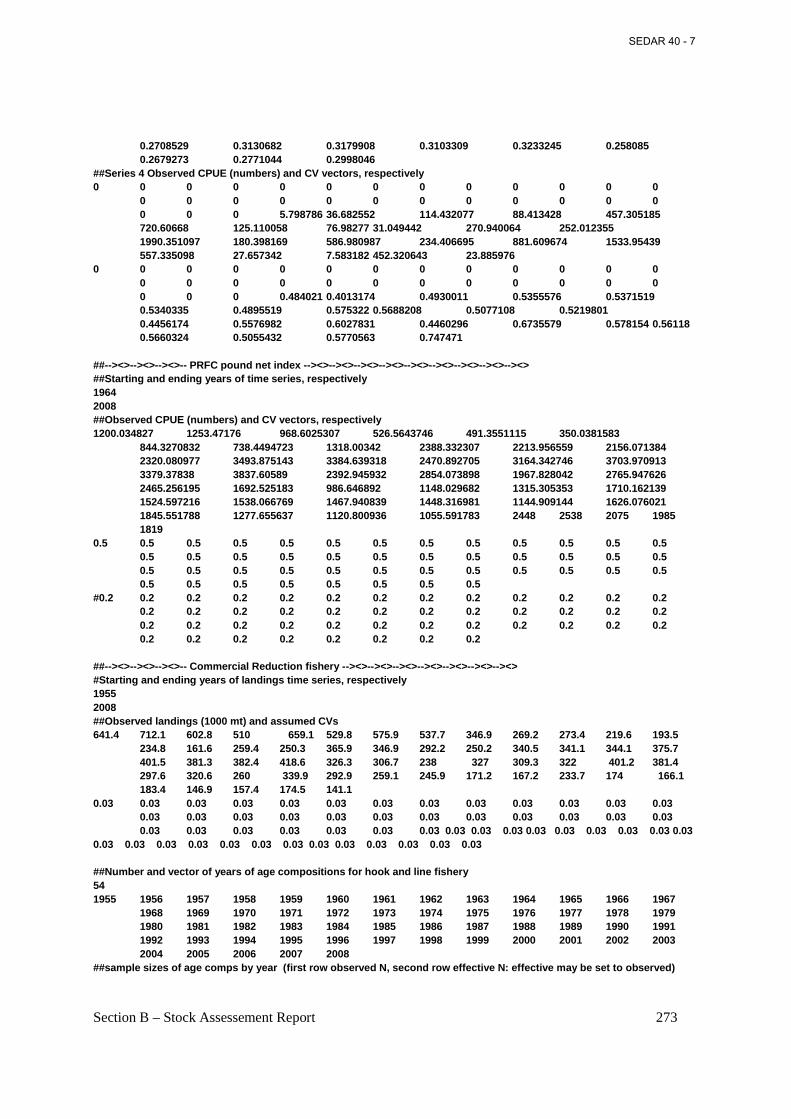
Section B – Stock Assessement Report 273
0.2708529 0.3130682 0.3179908 0.3103309 0.3233245 0.258085 0.2679273 0.2771044 0.2998046 ##Series 4 Observed CPUE (numbers) and CV vectors, respectively 0 0 0 0 0 0 0 0 0 0 0 0 0 0 0 0 0 0 0 0 0 0 0 0 0 0 0 0 5.798786 36.682552 114.432077 88.413428 457.305185 720.60668 125.110058 76.98277 31.049442 270.940064 252.012355 1990.351097 180.398169 586.980987 234.406695 881.609674 1533.95439 557.335098 27.657342 7.583182 452.320643 23.885976 0 0 0 0 0 0 0 0 0 0 0 0 0 0 0 0 0 0 0 0 0 0 0 0 0 0 0 0 0.484021 0.4013174 0.4930011 0.5355576 0.5371519 0.5340335 0.4895519 0.575322 0.5688208 0.5077108 0.5219801 0.4456174 0.5576982 0.6027831 0.4460296 0.6735579 0.578154 0.56118 0.5660324 0.5055432 0.5770563 0.747471 ##--><>--><>--><>-- PRFC pound net index --><>--><>--><>--><>--><>--><>--><>--><>--><> ##Starting and ending years of time series, respectively 1964 2008 ##Observed CPUE (numbers) and CV vectors, respectively 1200.034827 1253.47176 968.6025307 526.5643746 491.3551115 350.0381583 844.3270832 738.4494723 1318.00342 2388.332307 2213.956559 2156.071384 2320.080977 3493.875143 3384.639318 2470.892705 3164.342746 3703.970913 3379.37838 3837.60589 2392.945932 2854.073898 1967.828042 2765.947626 2465.256195 1692.525183 986.646892 1148.029682 1315.305353 1710.162139 1524.597216 1538.066769 1467.940839 1448.316981 1144.909144 1626.076021 1845.551788 1277.655637 1120.800936 1055.591783 2448 2538 2075 1985 1819 0.5 0.5 0.5 0.5 0.5 0.5 0.5 0.5 0.5 0.5 0.5 0.5 0.5 0.5 0.5 0.5 0.5 0.5 0.5 0.5 0.5 0.5 0.5 0.5 0.5 0.5 0.5 0.5 0.5 0.5 0.5 0.5 0.5 0.5 0.5 0.5 0.5 0.5 0.5 0.5 0.5 0.5 0.5 0.5 0.5 #0.2 0.2 0.2 0.2 0.2 0.2 0.2 0.2 0.2 0.2 0.2 0.2 0.2 0.2 0.2 0.2 0.2 0.2 0.2 0.2 0.2 0.2 0.2 0.2 0.2 0.2 0.2 0.2 0.2 0.2 0.2 0.2 0.2 0.2 0.2 0.2 0.2 0.2 0.2 0.2 0.2 0.2 0.2 0.2 0.2 ##--><>--><>--><>-- Commercial Reduction fishery --><>--><>--><>--><>--><>--><>--><> #Starting and ending years of landings time series, respectively 1955 2008 ##Observed landings (1000 mt) and assumed CVs 641.4 712.1 602.8 510 659.1 529.8 575.9 537.7 346.9 269.2 273.4 219.6 193.5 234.8 161.6 259.4 250.3 365.9 346.9 292.2 250.2 340.5 341.1 344.1 375.7 401.5 381.3 382.4 418.6 326.3 306.7 238 327 309.3 322 401.2 381.4 297.6 320.6 260 339.9 292.9 259.1 245.9 171.2 167.2 233.7 174 166.1 183.4 146.9 157.4 174.5 141.1 0.03 0.03 0.03 0.03 0.03 0.03 0.03 0.03 0.03 0.03 0.03 0.03 0.03 0.03 0.03 0.03 0.03 0.03 0.03 0.03 0.03 0.03 0.03 0.03 0.03 0.03 0.03 0.03 0.03 0.03 0.03 0.03 0.03 0.03 0.03 0.03 0.03 0.03 0.03 0.03 0.03 0.03 0.03 0.03 0.03 0.03 0.03 0.03 0.03 0.03 0.03 0.03 0.03 0.03 ##Number and vector of years of age compositions for hook and line fishery 54 1955 1956 1957 1958 1959 1960 1961 1962 1963 1964 1965 1966 1967 1968 1969 1970 1971 1972 1973 1974 1975 1976 1977 1978 1979 1980 1981 1982 1983 1984 1985 1986 1987 1988 1989 1990 1991 1992 1993 1994 1995 1996 1997 1998 1999 2000 2001 2002 2003 2004 2005 2006 2007 2008 ##sample sizes of age comps by year (first row observed N, second row effective N: effective may be set to observed)
SEDAR 40 - 7
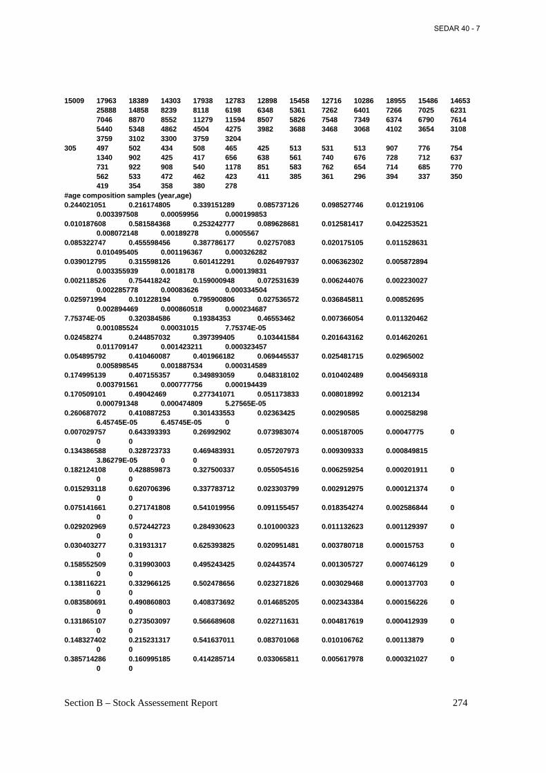
Section B – Stock Assessement Report 274
15009 17963 18389 14303 17938 12783 12898 15458 12716 10286 18955 15486 14653 25888 14858 8239 8118 6198 6348 5361 7262 6401 7266 7025 6231 7046 8870 8552 11279 11594 8507 5826 7548 7349 6374 6790 7614 5440 5348 4862 4504 4275 3982 3688 3468 3068 4102 3654 3108 3759 3102 3300 3759 3204 305 497 502 434 508 465 425 513 531 513 907 776 754 1340 902 425 417 656 638 561 740 676 728 712 637 731 922 908 540 1178 851 583 762 654 714 685 770 562 533 472 462 423 411 385 361 296 394 337 350 419 354 358 380 278 #age composition samples (year,age) 0.244021051 0.216174805 0.339151289 0.085737126 0.098527746 0.01219106 0.003397508 0.00059956 0.000199853 0.010187608 0.581584368 0.253242777 0.089628681 0.012581417 0.042253521 0.008072148 0.00189278 0.0005567 0.085322747 0.455598456 0.387786177 0.02757083 0.020175105 0.011528631 0.010495405 0.001196367 0.000326282 0.039012795 0.315598126 0.601412291 0.026497937 0.006362302 0.005872894 0.003355939 0.0018178 0.000139831 0.002118526 0.754418242 0.159000948 0.072531639 0.006244076 0.002230027 0.002285778 0.00083626 0.000334504 0.025971994 0.101228194 0.795900806 0.027536572 0.036845811 0.00852695 0.002894469 0.000860518 0.000234687 7.75374E-05 0.320384586 0.19384353 0.46553462 0.007366054 0.011320462 0.001085524 0.00031015 7.75374E-05 0.02458274 0.244857032 0.397399405 0.103441584 0.201643162 0.014620261 0.011709147 0.001423211 0.000323457 0.054895792 0.410460087 0.401966182 0.069445537 0.025481715 0.02965002 0.005898545 0.001887534 0.000314589 0.174995139 0.407155357 0.349893059 0.048318102 0.010402489 0.004569318 0.003791561 0.000777756 0.000194439 0.170509101 0.49042469 0.277341071 0.051173833 0.008018992 0.0012134 0.000791348 0.000474809 5.27565E-05 0.260687072 0.410887253 0.301433553 0.02363425 0.00290585 0.000258298 6.45745E-05 6.45745E-05 0 0.007029757 0.643393393 0.26992902 0.073983074 0.005187005 0.00047775 0 0 0 0.134386588 0.328723733 0.469483931 0.057207973 0.009309333 0.000849815 3.86279E-05 0 0 0.182124108 0.428859873 0.327500337 0.055054516 0.006259254 0.000201911 0 0 0 0.015293118 0.620706396 0.337783712 0.023303799 0.002912975 0.000121374 0 0 0 0.075141661 0.271741808 0.541019956 0.091155457 0.018354274 0.002586844 0 0 0 0.029202969 0.572442723 0.284930623 0.101000323 0.011132623 0.001129397 0 0 0 0.030403277 0.31931317 0.625393825 0.020951481 0.003780718 0.00015753 0 0 0 0.158552509 0.319903003 0.495243425 0.02443574 0.001305727 0.000746129 0 0 0 0.138116221 0.332966125 0.502478656 0.023271826 0.003029468 0.000137703 0 0 0 0.083580691 0.490860803 0.408373692 0.014685205 0.002343384 0.000156226 0 0 0 0.131865107 0.273503097 0.566689608 0.022711631 0.004817619 0.000412939 0 0 0 0.148327402 0.215231317 0.541637011 0.083701068 0.010106762 0.00113879 0 0 0 0.385714286 0.160995185 0.414285714 0.033065811 0.005617978 0.000321027 0 0 0
SEDAR 40 - 7
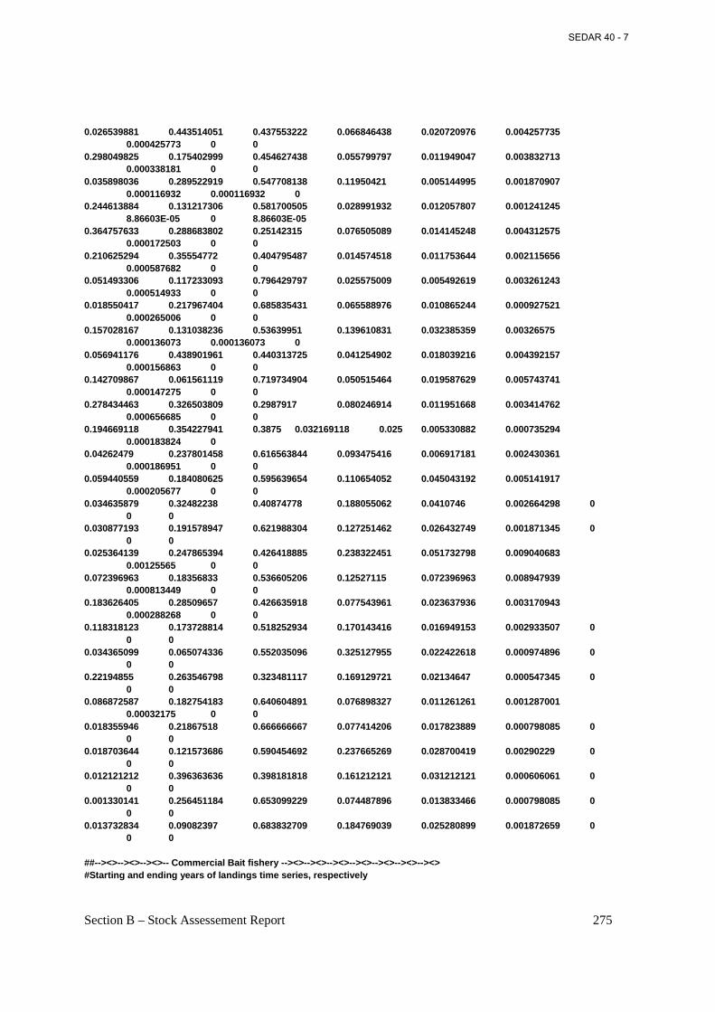
Section B – Stock Assessement Report 275
0.026539881 0.443514051 0.437553222 0.066846438 0.020720976 0.004257735 0.000425773 0 0 0.298049825 0.175402999 0.454627438 0.055799797 0.011949047 0.003832713 0.000338181 0 0 0.035898036 0.289522919 0.547708138 0.11950421 0.005144995 0.001870907 0.000116932 0.000116932 0 0.244613884 0.131217306 0.581700505 0.028991932 0.012057807 0.001241245 8.86603E-05 0 8.86603E-05 0.364757633 0.288683802 0.25142315 0.076505089 0.014145248 0.004312575 0.000172503 0 0 0.210625294 0.35554772 0.404795487 0.014574518 0.011753644 0.002115656 0.000587682 0 0 0.051493306 0.117233093 0.796429797 0.025575009 0.005492619 0.003261243 0.000514933 0 0 0.018550417 0.217967404 0.685835431 0.065588976 0.010865244 0.000927521 0.000265006 0 0 0.157028167 0.131038236 0.53639951 0.139610831 0.032385359 0.00326575 0.000136073 0.000136073 0 0.056941176 0.438901961 0.440313725 0.041254902 0.018039216 0.004392157 0.000156863 0 0 0.142709867 0.061561119 0.719734904 0.050515464 0.019587629 0.005743741 0.000147275 0 0 0.278434463 0.326503809 0.2987917 0.080246914 0.011951668 0.003414762 0.000656685 0 0 0.194669118 0.354227941 0.3875 0.032169118 0.025 0.005330882 0.000735294 0.000183824 0 0.04262479 0.237801458 0.616563844 0.093475416 0.006917181 0.002430361 0.000186951 0 0 0.059440559 0.184080625 0.595639654 0.110654052 0.045043192 0.005141917 0.000205677 0 0 0.034635879 0.32482238 0.40874778 0.188055062 0.0410746 0.002664298 0 0 0 0.030877193 0.191578947 0.621988304 0.127251462 0.026432749 0.001871345 0 0 0 0.025364139 0.247865394 0.426418885 0.238322451 0.051732798 0.009040683 0.00125565 0 0 0.072396963 0.18356833 0.536605206 0.12527115 0.072396963 0.008947939 0.000813449 0 0 0.183626405 0.28509657 0.426635918 0.077543961 0.023637936 0.003170943 0.000288268 0 0 0.118318123 0.173728814 0.518252934 0.170143416 0.016949153 0.002933507 0 0 0 0.034365099 0.065074336 0.552035096 0.325127955 0.022422618 0.000974896 0 0 0 0.22194855 0.263546798 0.323481117 0.169129721 0.02134647 0.000547345 0 0 0 0.086872587 0.182754183 0.640604891 0.076898327 0.011261261 0.001287001 0.00032175 0 0 0.018355946 0.21867518 0.666666667 0.077414206 0.017823889 0.000798085 0 0 0 0.018703644 0.121573686 0.590454692 0.237665269 0.028700419 0.00290229 0 0 0 0.012121212 0.396363636 0.398181818 0.161212121 0.031212121 0.000606061 0 0 0 0.001330141 0.256451184 0.653099229 0.074487896 0.013833466 0.000798085 0 0 0 0.013732834 0.09082397 0.683832709 0.184769039 0.025280899 0.001872659 0 0 0 ##--><>--><>--><>-- Commercial Bait fishery --><>--><>--><>--><>--><>--><>--><> #Starting and ending years of landings time series, respectively
SEDAR 40 - 7
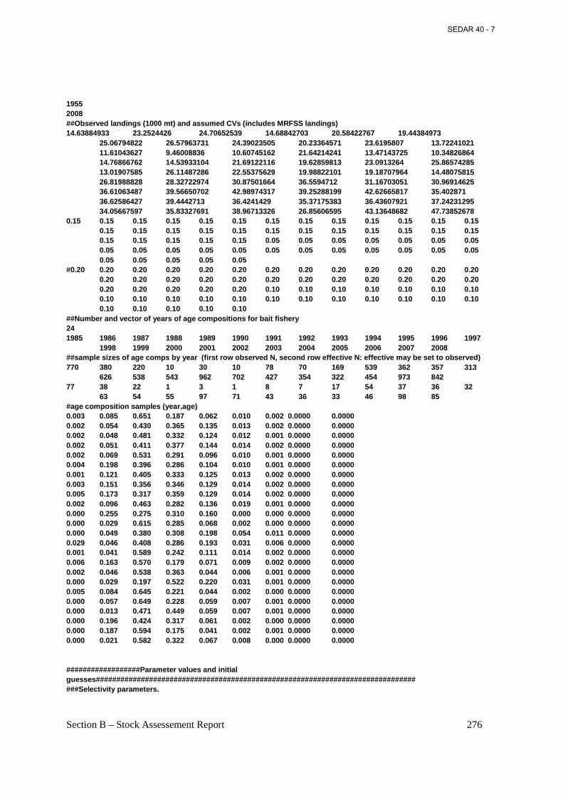
Section B – Stock Assessement Report 276
1955 2008 ##Observed landings (1000 mt) and assumed CVs (includes MRFSS landings) 14.63884933 23.2524426 24.70652539 14.68842703 20.58422767 19.44384973 25.06794822 26.57963731 24.39023505 20.23364571 23.6195807 13.72241021 11.61043627 9.46008836 10.60745162 21.64214241 13.47143725 10.34826864 14.76866762 14.53933104 21.69122116 19.62859813 23.0913264 25.86574285 13.01907585 26.11487286 22.55375629 19.98822101 19.18707964 14.48075815 26.81988828 28.32722974 30.87501664 36.5594712 31.16703051 30.96914625 36.61063487 39.56650702 42.98974317 39.25288199 42.62665817 35.402871 36.62586427 39.4442713 36.4241429 35.37175383 36.43607921 37.24231295 34.05667597 35.83327691 38.96713326 26.85606595 43.13648682 47.73852678 0.15 0.15 0.15 0.15 0.15 0.15 0.15 0.15 0.15 0.15 0.15 0.15 0.15 0.15 0.15 0.15 0.15 0.15 0.15 0.15 0.15 0.15 0.15 0.15 0.15 0.15 0.15 0.15 0.15 0.15 0.05 0.05 0.05 0.05 0.05 0.05 0.05 0.05 0.05 0.05 0.05 0.05 0.05 0.05 0.05 0.05 0.05 0.05 0.05 0.05 0.05 0.05 0.05 0.05 #0.20 0.20 0.20 0.20 0.20 0.20 0.20 0.20 0.20 0.20 0.20 0.20 0.20 0.20 0.20 0.20 0.20 0.20 0.20 0.20 0.20 0.20 0.20 0.20 0.20 0.20 0.20 0.20 0.20 0.20 0.10 0.10 0.10 0.10 0.10 0.10 0.10 0.10 0.10 0.10 0.10 0.10 0.10 0.10 0.10 0.10 0.10 0.10 0.10 0.10 0.10 0.10 0.10 0.10 ##Number and vector of years of age compositions for bait fishery 24 1985 1986 1987 1988 1989 1990 1991 1992 1993 1994 1995 1996 1997 1998 1999 2000 2001 2002 2003 2004 2005 2006 2007 2008 ##sample sizes of age comps by year (first row observed N, second row effective N: effective may be set to observed) 770 380 220 10 30 10 78 70 169 539 362 357 313 626 538 543 962 702 427 354 322 454 973 842 77 38 22 1 3 1 8 7 17 54 37 36 32 63 54 55 97 71 43 36 33 46 98 85 #age composition samples (year,age) 0.003 0.085 0.651 0.187 0.062 0.010 0.002 0.0000 0.0000 0.002 0.054 0.430 0.365 0.135 0.013 0.002 0.0000 0.0000 0.002 0.048 0.481 0.332 0.124 0.012 0.001 0.0000 0.0000 0.002 0.051 0.411 0.377 0.144 0.014 0.002 0.0000 0.0000 0.002 0.069 0.531 0.291 0.096 0.010 0.001 0.0000 0.0000 0.004 0.198 0.396 0.286 0.104 0.010 0.001 0.0000 0.0000 0.001 0.121 0.405 0.333 0.125 0.013 0.002 0.0000 0.0000 0.003 0.151 0.356 0.346 0.129 0.014 0.002 0.0000 0.0000 0.005 0.173 0.317 0.359 0.129 0.014 0.002 0.0000 0.0000 0.002 0.096 0.463 0.282 0.136 0.019 0.001 0.0000 0.0000 0.000 0.255 0.275 0.310 0.160 0.000 0.000 0.0000 0.0000 0.000 0.029 0.615 0.285 0.068 0.002 0.000 0.0000 0.0000 0.000 0.049 0.380 0.308 0.198 0.054 0.011 0.0000 0.0000 0.029 0.046 0.408 0.286 0.193 0.031 0.006 0.0000 0.0000 0.001 0.041 0.589 0.242 0.111 0.014 0.002 0.0000 0.0000 0.006 0.163 0.570 0.179 0.071 0.009 0.002 0.0000 0.0000 0.002 0.046 0.538 0.363 0.044 0.006 0.001 0.0000 0.0000 0.000 0.029 0.197 0.522 0.220 0.031 0.001 0.0000 0.0000 0.005 0.084 0.645 0.221 0.044 0.002 0.000 0.0000 0.0000 0.000 0.057 0.649 0.228 0.059 0.007 0.001 0.0000 0.0000 0.000 0.013 0.471 0.449 0.059 0.007 0.001 0.0000 0.0000 0.000 0.196 0.424 0.317 0.061 0.002 0.000 0.0000 0.0000 0.000 0.187 0.594 0.175 0.041 0.002 0.001 0.0000 0.0000 0.000 0.021 0.582 0.322 0.067 0.008 0.000 0.0000 0.0000 ##################Parameter values and initial guesses############################################################################## ###Selectivity parameters.
SEDAR 40 - 7
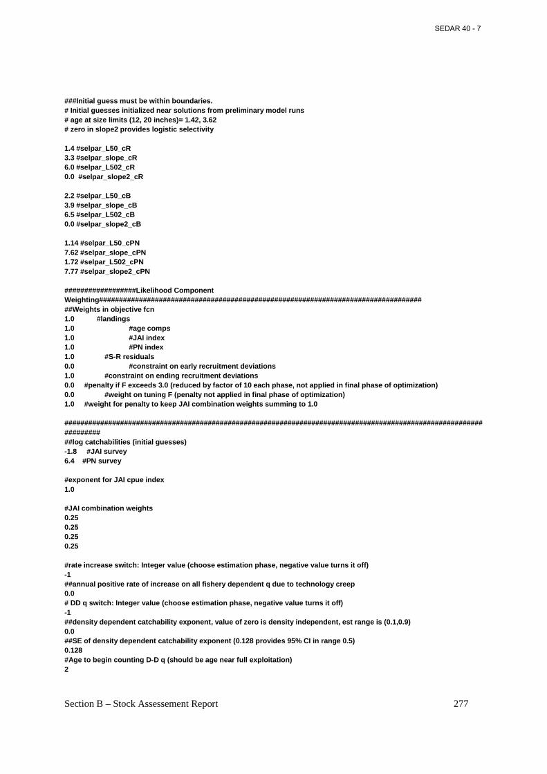
Section B – Stock Assessement Report 277
###Initial guess must be within boundaries. # Initial guesses initialized near solutions from preliminary model runs # age at size limits (12, 20 inches)= 1.42, 3.62 # zero in slope2 provides logistic selectivity 1.4 #selpar_L50_cR 3.3 #selpar_slope_cR 6.0 #selpar_L502_cR 0.0 #selpar_slope2_cR 2.2 #selpar_L50_cB 3.9 #selpar_slope_cB 6.5 #selpar_L502_cB 0.0 #selpar_slope2_cB 1.14 #selpar_L50_cPN 7.62 #selpar_slope_cPN 1.72 #selpar_L502_cPN 7.77 #selpar_slope2_cPN ##################Likelihood Component Weighting################################################################################# ##Weights in objective fcn 1.0 #landings 1.0 #age comps 1.0 #JAI index 1.0 #PN index 1.0 #S-R residuals 0.0 #constraint on early recruitment deviations 1.0 #constraint on ending recruitment deviations 0.0 #penalty if F exceeds 3.0 (reduced by factor of 10 each phase, not applied in final phase of optimization) 0.0 #weight on tuning F (penalty not applied in final phase of optimization) 1.0 #weight for penalty to keep JAI combination weights summing to 1.0 ################################################################################################################## ##log catchabilities (initial guesses) -1.8 #JAI survey 6.4 #PN survey #exponent for JAI cpue index 1.0 #JAI combination weights 0.25 0.25 0.25 0.25 #rate increase switch: Integer value (choose estimation phase, negative value turns it off) -1 ##annual positive rate of increase on all fishery dependent q due to technology creep 0.0 # DD q switch: Integer value (choose estimation phase, negative value turns it off) -1 ##density dependent catchability exponent, value of zero is density independent, est range is (0.1,0.9) 0.0 ##SE of density dependent catchability exponent (0.128 provides 95% CI in range 0.5) 0.128 #Age to begin counting D-D q (should be age near full exploitation) 2
SEDAR 40 - 7
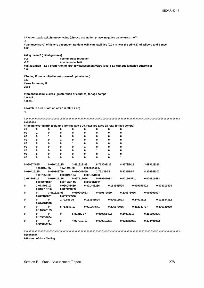
Section B – Stock Assessement Report 278
#Random walk switch:Integer value (choose estimation phase, negative value turns it off) -3 #Variance (sd^2) of fishery dependent random walk catchabilities (0.03 is near the sd=0.17 of Wilberg and Bence 0.03 ##log mean F (initial guesses) 0.2 #commercial reduction -1.2 #commercial bait #Initialization F as a proportion of first few assessment years (set to 1.0 without evidence otherwise) 1.0 #Tuning F (not applied in last phase of optimization) 1.5 #Year for tuning F 2008 #threshold sample sizes (greater than or equal to) for age comps 1.0 #cR 1.0 #cB #switch to turn priors on off (-1 = off, 1 = on) -1 ################################################################################################################# #Ageing error matrix (columns are true age 1-20, rows are ages as read for age comps) #1 0 0 0 0 0 0 0 0 #0 1 0 0 0 0 0 0 0 #0 0 1 0 0 0 0 0 0 #0 0 0 1 0 0 0 0 0 #0 0 0 0 1 0 0 0 0 #0 0 0 0 0 1 0 0 0 #0 0 0 0 0 0 1 0 0 #0 0 0 0 0 0 0 1 0 #0 0 0 0 0 0 0 0 1 0.989574885 0.010425115 3.41132E-08 8.71309E-12 4.9779E-12 3.69962E-10 1.06845E-07 1.57149E-05 0.000623385 0.010425115 0.979149769 0.036041469 2.7224E-05 5.8031E-07 8.37634E-07 1.08755E-05 0.000198104 0.001951093 2.07379E-12 0.010425115 0.927916994 0.089249633 0.001764541 0.000311433 0.000471017 0.001762145 0.006387882 0 2.07379E-12 0.036041469 0.821446286 0.163648594 0.019751402 0.008711424 0.010519756 0.017424063 0 0 3.41132E-08 0.089249633 0.669172569 0.226878066 0.069393527 0.042182061 0.039598326 0 0 0 2.7224E-05 0.163648594 0.506116523 0.24003818 0.113684332 0.074981978 0 0 0 8.71314E-12 0.001764541 0.226878066 0.362749737 0.206038939 0.118305185 0 0 0 0 5.8031E-07 0.019751402 0.24003818 0.251197896 0.155534864 0 0 0 0 4.97791E-12 0.000312271 0.078586951 0.374401052 0.585193224 ################################################################################################################## 999 #end of data file flag
SEDAR 40 - 7
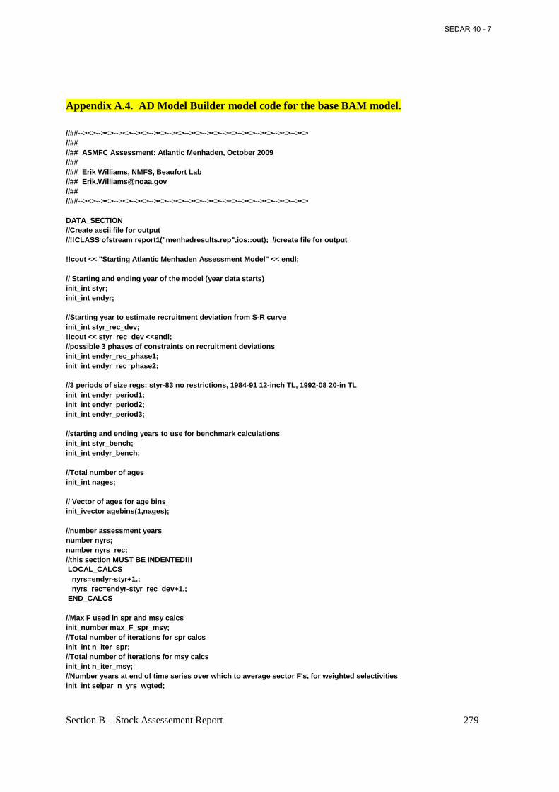
Section B – Stock Assessement Report 279
Appendix A.4. AD Model Builder model code for the base BAM model. //##--><>--><>--><>--><>--><>--><>--><>--><>--><>--><>--><>--><>--><> //## //## ASMFC Assessment: Atlantic Menhaden, October 2009 //## //## Erik Williams, NMFS, Beaufort Lab //## [email protected] //## //##--><>--><>--><>--><>--><>--><>--><>--><>--><>--><>--><>--><>--><> DATA_SECTION //Create ascii file for output //!!CLASS ofstream report1("menhadresults.rep",ios::out); //create file for output !!cout << "Starting Atlantic Menhaden Assessment Model" << endl; // Starting and ending year of the model (year data starts) init_int styr; init_int endyr; //Starting year to estimate recruitment deviation from S-R curve init_int styr_rec_dev; !!cout << styr_rec_dev <<endl; //possible 3 phases of constraints on recruitment deviations init_int endyr_rec_phase1; init_int endyr_rec_phase2; //3 periods of size regs: styr-83 no restrictions, 1984-91 12-inch TL, 1992-08 20-in TL init_int endyr_period1; init_int endyr_period2; init_int endyr_period3; //starting and ending years to use for benchmark calculations init_int styr_bench; init_int endyr_bench; //Total number of ages init_int nages; // Vector of ages for age bins init_ivector agebins(1,nages); //number assessment years number nyrs; number nyrs_rec; //this section MUST BE INDENTED!!! LOCAL_CALCS nyrs=endyr-styr+1.; nyrs_rec=endyr-styr_rec_dev+1.; END_CALCS //Max F used in spr and msy calcs init_number max_F_spr_msy; //Total number of iterations for spr calcs init_int n_iter_spr; //Total number of iterations for msy calcs init_int n_iter_msy; //Number years at end of time series over which to average sector F's, for weighted selectivities init_int selpar_n_yrs_wgted;
SEDAR 40 - 7
Section B – Stock Assessement Report 280
//bias correction (set to 1.0 for no bias correction or a negative value to compute from rec variance) init_number set_BiasCor; //exclude these years from end of time series for computing bias correction init_number BiasCor_exclude_yrs; //Female maturity and proportion female at age init_vector maturity_f_obs(1,nages); //proportion females mature at age init_vector maturity_m_obs(1,nages); //proportion males mature at age init_vector prop_f_obs(1,nages); //proportion female at age init_number spawn_time_frac; //time of year of peak spawning, as a fraction of the year // Natural mortality init_vector set_M(1,nages); //age-dependent: used in model init_number set_M_constant; //age-independent: used only for MSST init_matrix set_M_mat(styr,endyr,1,nages); //age and year specific M //Spawner-recruit parameters (Initial guesses or fixed values) init_number set_SR_switch; init_number set_steep; init_number set_steep_se; init_number set_log_R0; init_number set_R_autocorr; //--><>--><>--><>-- Weight-at-age in the fishery (g) --><>--><>--><>--><>--><>--><>--><>--><> init_matrix wgt_fish_g(styr,endyr,1,nages); //--><>--><>--><>-- Weight-at-age for the spawning population - start of year (g) --><>--><>--><>--><> init_matrix wgt_spawn_g(styr,endyr,1,nages); //--><>--><>--><>-- Fecundity-at-age - not adjusted for maturity (g) --><>--><>--><>--><> init_matrix fec_eggs(styr,endyr,1,nages); //--><>--><>--><>-- Juvenile Abundance Index from seine surveys --><>--><>--><>--><>--><> init_int JAI_cpue_switch; //CPUE init_int styr_JAI_cpue; init_int endyr_JAI_cpue; init_vector obs_JAI_cpue(styr_JAI_cpue,endyr_JAI_cpue); //Observed CPUE init_vector JAI_cpue_cv(styr_JAI_cpue,endyr_JAI_cpue); //CV of cpue //--><>--><>--><>-- Juvenile Abundance Indices from seine surveys --><>--><>--><>--><>--><> //CPUE, must have zeros in place of missing values init_vector obs_JAI1_cpue(styr_JAI_cpue,endyr_JAI_cpue); //Observed CPUE 1 init_vector JAI1_cpue_cv(styr_JAI_cpue,endyr_JAI_cpue); //CV of cpue 1 init_vector obs_JAI2_cpue(styr_JAI_cpue,endyr_JAI_cpue); //Observed CPUE 2 init_vector JAI2_cpue_cv(styr_JAI_cpue,endyr_JAI_cpue); //CV of cpue 2 init_vector obs_JAI3_cpue(styr_JAI_cpue,endyr_JAI_cpue); //Observed CPUE 3 init_vector JAI3_cpue_cv(styr_JAI_cpue,endyr_JAI_cpue); //CV of cpue 3 init_vector obs_JAI4_cpue(styr_JAI_cpue,endyr_JAI_cpue); //Observed CPUE 4 init_vector JAI4_cpue_cv(styr_JAI_cpue,endyr_JAI_cpue); //CV of cpue 4 //--><>--><>--><>-- PRFC pound net index --><>--><>--><>--><>--><>--><>--><>--><>--><> //CPUE init_int styr_PN_cpue; init_int endyr_PN_cpue; init_vector obs_PN_cpue(styr_PN_cpue,endyr_PN_cpue); //Observed CPUE init_vector PN_cpue_cv(styr_PN_cpue,endyr_PN_cpue); //cv of cpue //--><>--><>--><>-- Commercial Reduction fishery --><>--><>--><>--><>--><>--><>--><> // Landings (1000 mt) init_int styr_cR_L; init_int endyr_cR_L;
SEDAR 40 - 7
Section B – Stock Assessement Report 281
init_vector obs_cR_L(styr_cR_L,endyr_cR_L); //vector of observed landings by year init_vector cR_L_cv(styr_cR_L,endyr_cR_L); //vector of CV of landings by year // Age Compositions init_int nyr_cR_agec; init_ivector yrs_cR_agec(1,nyr_cR_agec); init_vector nsamp_cR_agec(1,nyr_cR_agec); init_vector neff_cR_agec(1,nyr_cR_agec); init_matrix obs_cR_agec(1,nyr_cR_agec,1,nages); //--><>--><>--><>-- Commercial Bait fishery --><>--><>--><>--><>--><>--><>--><>--><> // Landings (1000 mt) init_int styr_cB_L; init_int endyr_cB_L; init_vector obs_cB_L(styr_cB_L,endyr_cB_L); init_vector cB_L_cv(styr_cB_L,endyr_cB_L); //vector of CV of landings by year // Age compositions init_int nyr_cB_agec; init_ivector yrs_cB_agec(1,nyr_cB_agec); init_vector nsamp_cB_agec(1,nyr_cB_agec); init_vector neff_cB_agec(1,nyr_cB_agec); init_matrix obs_cB_agec(1,nyr_cB_agec,1,nages); //############################################################################# //##################Parameter values and initial guesses ################################# //Initial guesses of estimated selectivity parameters init_number set_selpar_L50_cR; init_number set_selpar_slope_cR; init_number set_selpar_L502_cR; init_number set_selpar_slope2_cR; init_number set_selpar_L50_cB; init_number set_selpar_slope_cB; init_number set_selpar_L502_cB; init_number set_selpar_slope2_cB; init_number set_selpar_L50_PN; init_number set_selpar_slope_PN; init_number set_selpar_L502_PN; init_number set_selpar_slope2_PN; //--weights for likelihood components------------------------------------------------------------------------------- init_number set_w_L; init_number set_w_ac; init_number set_w_I_JAI; init_number set_w_I_PN; init_number set_w_rec; //for fitting S-R curve init_number set_w_rec_early; //additional constraint on early years recruitment init_number set_w_rec_end; //additional constraint on ending years recruitment init_number set_w_fullF; //penalty for any Fapex>3(removed in final phase of optimization) init_number set_w_Ftune; //weight applied to tuning F (removed in final phase of optimization) init_number set_w_JAI_wgts; //weight for penalty to keep JAI combination weights summing to 1.0 ////--index catchability------------------------------------------------------------------------------------------------------------ init_number set_logq_JAI; //catchability coefficient (log) for MARMAP RVC init_number set_logq_PN; //catchability coefficient (log) for MARMAP CVT init_number set_JAI_exp; //exponent for cpue index //--JAI index combination weights------------------------------------------------------
SEDAR 40 - 7
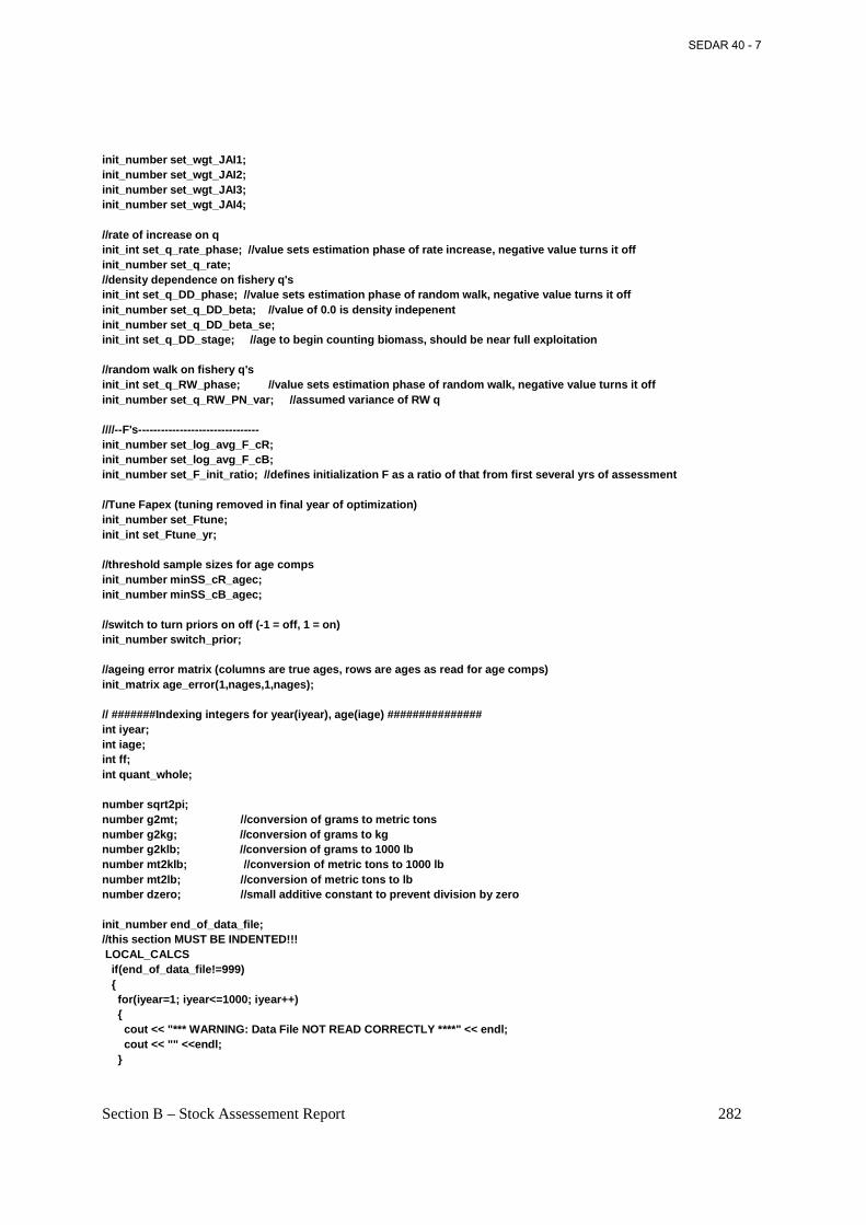
Section B – Stock Assessement Report 282
init_number set_wgt_JAI1; init_number set_wgt_JAI2; init_number set_wgt_JAI3; init_number set_wgt_JAI4; //rate of increase on q init_int set_q_rate_phase; //value sets estimation phase of rate increase, negative value turns it off init_number set_q_rate; //density dependence on fishery q's init_int set_q_DD_phase; //value sets estimation phase of random walk, negative value turns it off init_number set_q_DD_beta; //value of 0.0 is density indepenent init_number set_q_DD_beta_se; init_int set_q_DD_stage; //age to begin counting biomass, should be near full exploitation //random walk on fishery q's init_int set_q_RW_phase; //value sets estimation phase of random walk, negative value turns it off init_number set_q_RW_PN_var; //assumed variance of RW q ////--F's-------------------------------- init_number set_log_avg_F_cR; init_number set_log_avg_F_cB; init_number set_F_init_ratio; //defines initialization F as a ratio of that from first several yrs of assessment //Tune Fapex (tuning removed in final year of optimization) init_number set_Ftune; init_int set_Ftune_yr; //threshold sample sizes for age comps init_number minSS_cR_agec; init_number minSS_cB_agec; //switch to turn priors on off (-1 = off, 1 = on) init_number switch_prior; //ageing error matrix (columns are true ages, rows are ages as read for age comps) init_matrix age_error(1,nages,1,nages); // #######Indexing integers for year(iyear), age(iage) ############### int iyear; int iage; int ff; int quant_whole; number sqrt2pi; number g2mt; //conversion of grams to metric tons number g2kg; //conversion of grams to kg number g2klb; //conversion of grams to 1000 lb number mt2klb; //conversion of metric tons to 1000 lb number mt2lb; //conversion of metric tons to lb number dzero; //small additive constant to prevent division by zero init_number end_of_data_file; //this section MUST BE INDENTED!!! LOCAL_CALCS if(end_of_data_file!=999) { for(iyear=1; iyear<=1000; iyear++) { cout << "*** WARNING: Data File NOT READ CORRECTLY ****" << endl; cout << "" <<endl; }
SEDAR 40 - 7
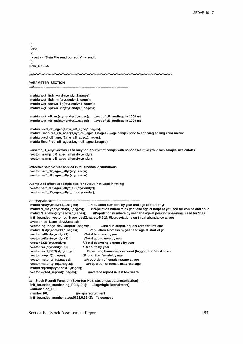
Section B – Stock Assessement Report 283
} else { cout << "Data File read correctly" << endl; } END_CALCS //##--><>--><>--><>--><>--><>--><>--><>--><>--><>--><>--><>--><>--><>--><>--><>--><>--><>--><> PARAMETER_SECTION //////----------------------------------------------------------------------------------------- matrix wgt_fish_kg(styr,endyr,1,nages); matrix wgt_fish_mt(styr,endyr,1,nages); matrix wgt_spawn_kg(styr,endyr,1,nages); matrix wgt_spawn_mt(styr,endyr,1,nages); matrix wgt_cR_mt(styr,endyr,1,nages); //wgt of cR landings in 1000 mt matrix wgt_cB_mt(styr,endyr,1,nages); //wgt of cB landings in 1000 mt matrix pred_cR_agec(1,nyr_cR_agec,1,nages); matrix ErrorFree_cR_agec(1,nyr_cR_agec,1,nages); //age comps prior to applying ageing error matrix matrix pred_cB_agec(1,nyr_cB_agec,1,nages); matrix ErrorFree_cB_agec(1,nyr_cB_agec,1,nages); //nsamp_X_allyr vectors used only for R output of comps with nonconsecutive yrs, given sample size cutoffs vector nsamp_cR_agec_allyr(styr,endyr); vector nsamp_cB_agec_allyr(styr,endyr); //effective sample size applied in multinomial distributions vector neff_cR_agec_allyr(styr,endyr); vector neff_cB_agec_allyr(styr,endyr); //Computed effective sample size for output (not used in fitting) vector neff_cR_agec_allyr_out(styr,endyr); vector neff_cB_agec_allyr_out(styr,endyr); //-----Population----------------------------------------------------------------------------------- matrix N(styr,endyr+1,1,nages); //Population numbers by year and age at start of yr matrix N_mdyr(styr,endyr,1,nages); //Population numbers by year and age at mdpt of yr: used for comps and cpue matrix N_spawn(styr,endyr,1,nages); //Population numbers by year and age at peaking spawning: used for SSB init_bounded_vector log_Nage_dev(2,nages,-5,5,1); //log deviations on initial abundance at age //vector log_Nage_dev(2,nages); vector log_Nage_dev_output(1,nages); //used in output. equals zero for first age matrix B(styr,endyr+1,1,nages); //Population biomass by year and age at start of yr vector totB(styr,endyr+1); //Total biomass by year vector totN(styr,endyr+1); //Total abundance by year vector SSB(styr,endyr); ///Total spawning biomass by year vector rec(styr,endyr+1); //Recruits by year vector pred_SPR(styr,endyr); //spawning biomass-per-recruit (lagged) for Fmed calcs vector prop_f(1,nages); //Proportion female by age vector maturity_f(1,nages); //Proportion of female mature at age vector maturity_m(1,nages); //Proportion of female mature at age matrix reprod(styr,endyr,1,nages); vector wgted_reprod(1,nages); //average reprod in last few years // ////---Stock-Recruit Function (Beverton-Holt, steepness parameterization)---------- init_bounded_number log_R0(1,10,1); //log(virgin Recruitment) //number log_R0; number R0; //virgin recruitment init_bounded_number steep(0.21,0.99,-3); //steepness
SEDAR 40 - 7
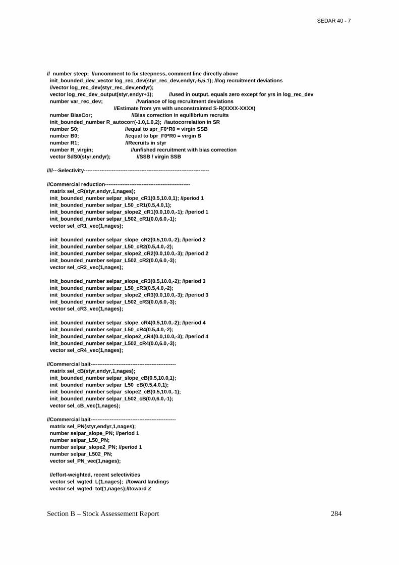
Section B – Stock Assessement Report 284
// number steep; //uncomment to fix steepness, comment line directly above init_bounded_dev_vector log_rec_dev(styr_rec_dev,endyr,-5,5,1); //log recruitment deviations //vector log_rec_dev(styr_rec_dev,endyr); vector log_rec_dev_output(styr,endyr+1); //used in output. equals zero except for yrs in log_rec_dev number var_rec_dev; //variance of log recruitment deviations //Estimate from yrs with unconstrainted S-R(XXXX-XXXX) number BiasCor; //Bias correction in equilibrium recruits init_bounded_number R_autocorr(-1.0,1.0,2); //autocorrelation in SR number S0; //equal to spr_F0*R0 = virgin SSB number B0; //equal to bpr_F0*R0 = virgin B number R1; //Recruits in styr number R_virgin; //unfished recruitment with bias correction vector SdS0(styr,endyr); //SSB / virgin SSB ////---Selectivity------------------------------------------------------------------------ //Commercial reduction------------------------------------------------- matrix sel_cR(styr,endyr,1,nages); init_bounded_number selpar_slope_cR1(0.5,10.0,1); //period 1 init_bounded_number selpar_L50_cR1(0.5,4.0,1); init_bounded_number selpar_slope2_cR1(0.0,10.0,-1); //period 1 init_bounded_number selpar_L502_cR1(0.0,6.0,-1); vector sel_cR1_vec(1,nages); init_bounded_number selpar_slope_cR2(0.5,10.0,-2); //period 2 init_bounded_number selpar_L50_cR2(0.5,4.0,-2); init_bounded_number selpar_slope2_cR2(0.0,10.0,-3); //period 2 init_bounded_number selpar_L502_cR2(0.0,6.0,-3); vector sel_cR2_vec(1,nages); init_bounded_number selpar_slope_cR3(0.5,10.0,-2); //period 3 init_bounded_number selpar_L50_cR3(0.5,4.0,-2); init_bounded_number selpar_slope2_cR3(0.0,10.0,-3); //period 3 init_bounded_number selpar_L502_cR3(0.0,6.0,-3); vector sel_cR3_vec(1,nages); init_bounded_number selpar_slope_cR4(0.5,10.0,-2); //period 4 init_bounded_number selpar_L50_cR4(0.5,4.0,-2); init_bounded_number selpar_slope2_cR4(0.0,10.0,-3); //period 4 init_bounded_number selpar_L502_cR4(0.0,6.0,-3); vector sel_cR4_vec(1,nages); //Commercial bait------------------------------------------------- matrix sel_cB(styr,endyr,1,nages); init_bounded_number selpar_slope_cB(0.5,10.0,1); init_bounded_number selpar_L50_cB(0.5,4.0,1); init_bounded_number selpar_slope2_cB(0.5,10.0,-1); init_bounded_number selpar_L502_cB(0.0,6.0,-1); vector sel_cB_vec(1,nages); //Commercial bait------------------------------------------------- matrix sel_PN(styr,endyr,1,nages); number selpar_slope_PN; //period 1 number selpar_L50_PN; number selpar_slope2_PN; //period 1 number selpar_L502_PN; vector sel_PN_vec(1,nages); //effort-weighted, recent selectivities vector sel_wgted_L(1,nages); //toward landings vector sel_wgted_tot(1,nages);//toward Z
SEDAR 40 - 7
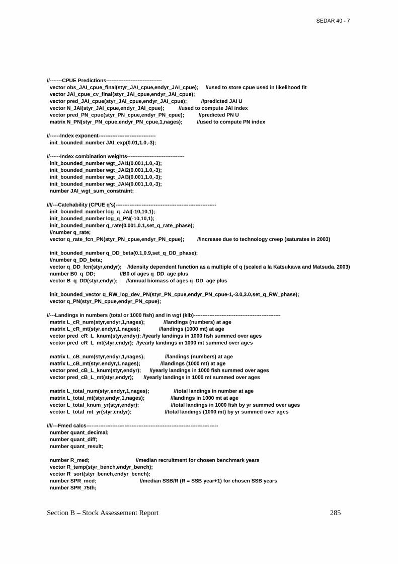
Section B – Stock Assessement Report 285
//-------CPUE Predictions-------------------------------- vector obs_JAI_cpue_final(styr_JAI_cpue,endyr_JAI_cpue); //used to store cpue used in likelihood fit vector JAI_cpue_cv_final(styr_JAI_cpue,endyr_JAI_cpue); vector pred_JAI_cpue(styr_JAI_cpue,endyr_JAI_cpue); //predicted JAI U vector N_JAI(styr_JAI_cpue,endyr_JAI_cpue); //used to compute JAI index vector pred_PN_cpue(styr_PN_cpue,endyr_PN_cpue); //predicted PN U matrix N_PN(styr_PN_cpue,endyr_PN_cpue,1,nages); //used to compute PN index //------Index exponent--------------------------------- init_bounded_number JAI_exp(0.01,1.0,-3); //------Index combination weights--------------------------------- init_bounded_number wgt_JAI1(0.001,1.0,-3); init_bounded_number wgt_JAI2(0.001,1.0,-3); init_bounded_number wgt_JAI3(0.001,1.0,-3); init_bounded_number wgt_JAI4(0.001,1.0,-3); number JAI_wgt_sum_constraint; ////---Catchability (CPUE q's)---------------------------------------------------------- init_bounded_number log_q_JAI(-10,10,1); init_bounded_number log_q_PN(-10,10,1); init_bounded_number q_rate(0.001,0.1,set_q_rate_phase); //number q_rate; vector q_rate_fcn_PN(styr_PN_cpue,endyr_PN_cpue); //increase due to technology creep (saturates in 2003) init_bounded_number q_DD_beta(0.1,0.9,set_q_DD_phase); //number q_DD_beta; vector q_DD_fcn(styr,endyr); //density dependent function as a multiple of q (scaled a la Katsukawa and Matsuda. 2003) number B0_q_DD; //B0 of ages q_DD_age plus vector B_q_DD(styr,endyr); //annual biomass of ages q_DD_age plus init_bounded_vector q_RW_log_dev_PN(styr_PN_cpue,endyr_PN_cpue-1,-3.0,3.0,set_q_RW_phase); vector q_PN(styr_PN_cpue,endyr_PN_cpue); //---Landings in numbers (total or 1000 fish) and in wgt (klb)-------------------------------------------------- matrix L_cR_num(styr,endyr,1,nages); //landings (numbers) at age matrix L_cR_mt(styr,endyr,1,nages); //landings (1000 mt) at age vector pred_cR_L_knum(styr,endyr); //yearly landings in 1000 fish summed over ages vector pred_cR_L_mt(styr,endyr); //yearly landings in 1000 mt summed over ages matrix L_cB_num(styr,endyr,1,nages); //landings (numbers) at age matrix L_cB_mt(styr,endyr,1,nages); //landings (1000 mt) at age vector pred_cB_L_knum(styr,endyr); //yearly landings in 1000 fish summed over ages vector pred_cB_L_mt(styr,endyr); //yearly landings in 1000 mt summed over ages matrix L_total_num(styr,endyr,1,nages); //total landings in number at age matrix L_total_mt(styr,endyr,1,nages); //landings in 1000 mt at age vector L_total_knum_yr(styr,endyr); //total landings in 1000 fish by yr summed over ages vector L_total_mt_yr(styr,endyr); //total landings (1000 mt) by yr summed over ages ////---Fmed calcs---------------------------------------------------------------------------- number quant_decimal; number quant_diff; number quant_result; number R_med; //median recruitment for chosen benchmark years vector R_temp(styr_bench,endyr_bench); vector R_sort(styr_bench,endyr_bench); number SPR_med; //median SSB/R (R = SSB year+1) for chosen SSB years number SPR_75th;
SEDAR 40 - 7
Section B – Stock Assessement Report 286
vector SPR_temp(styr_bench,endyr_bench); vector SPR_sort(styr_bench,endyr_bench); number SSB_med; //SSB corresponding to SSB/R median and R median number SSB_med_thresh; //SSB threshold vector SPR_diff(1,n_iter_spr); number SPR_diff_min; number F_med; //Fmed benchmark number F_med_target; number F_med_age2plus; //Fmed benchmark number F_med_target_age2plus; number L_med; ////---MSY calcs---------------------------------------------------------------------------- number F_cR_prop; //proportion of F_sum attributable to reduction, last X=selpar_n_yrs_wgted yrs, used for avg body weights number F_cB_prop; //proportion of F_sum attributable to bait, last X yrs number F_temp_sum; //sum of geom mean Fsum's in last X yrs, used to compute F_fishery_prop vector F_end(1,nages); vector F_end_L(1,nages); number F_end_apex; number SSB_msy_out; //SSB (total mature biomass) at msy number F_msy_out; //F at msy number msy_mt_out; //max sustainable yield (1000 mt) number msy_knum_out; //max sustainable yield (1000 fish) number B_msy_out; //total biomass at MSY number R_msy_out; //equilibrium recruitment at F=Fmsy number spr_msy_out; //spr at F=Fmsy vector N_age_msy(1,nages); //numbers at age for MSY calculations: beginning of yr vector N_age_msy_mdyr(1,nages); //numbers at age for MSY calculations: mdpt of yr vector L_age_msy(1,nages); //catch at age for MSY calculations vector Z_age_msy(1,nages); //total mortality at age for MSY calculations vector F_L_age_msy(1,nages); //fishing mortality landings (not discards) at age for MSY calculations vector F_msy(1,n_iter_msy); //values of full F to be used in equilibrium calculations vector spr_msy(1,n_iter_msy); //reproductive capacity-per-recruit values corresponding to F values in F_msy vector R_eq(1,n_iter_msy); //equilibrium recruitment values corresponding to F values in F_msy vector L_eq_mt(1,n_iter_msy); //equilibrium landings(1000 mt) values corresponding to F values in F_msy vector L_eq_knum(1,n_iter_msy); //equilibrium landings(1000 fish) values corresponding to F values in F_msy vector SSB_eq(1,n_iter_msy); //equilibrium reproductive capacity values corresponding to F values in F_msy vector B_eq(1,n_iter_msy); //equilibrium biomass values corresponding to F values in F_msy vector FdF_msy(styr,endyr); vector SdSSB_msy(styr,endyr); number SdSSB_msy_end; number FdF_msy_end; vector wgt_wgted_L_mt(1,nages); //fishery-weighted average weight at age of landings number wgt_wgted_L_denom; //used in intermediate calculations number iter_inc_msy; //increments used to compute msy, equals 1/(n_iter_msy-1) ////--------Mortality------------------------------------------------------------------ vector M(1,nages); //age-dependent natural mortality number M_constant; //age-indpendent: used only for MSST matrix M_mat(styr,endyr,1,nages); vector wgted_M(1,nages); //weighted M vector for last few years matrix F(styr,endyr,1,nages); vector Fsum(styr,endyr); //Full fishing mortality rate by year
SEDAR 40 - 7
Section B – Stock Assessement Report 287
vector Fapex(styr,endyr); //Max across ages, fishing mortality rate by year (may differ from Fsum bc of dome-shaped sel matrix Z(styr,endyr,1,nages); vector E(styr,endyr); //Exploitation rate vector F_age2plus(styr,endyr); //population weighted age 2+ F vector F_cR_age2plus(styr,endyr); //population weighted age 2+ F vector F_cB_age2plus(styr,endyr); //population weighted age 2+ F init_bounded_number log_avg_F_cR(-5,2.0,1); init_bounded_dev_vector log_F_dev_cR(styr_cR_L,endyr_cR_L,-10.0,5.0,2); matrix F_cR(styr,endyr,1,nages); vector F_cR_out(styr,endyr); //used for intermediate calculations in fcn get_mortality number log_F_dev_init_cR; number log_F_dev_end_cR; init_bounded_number log_avg_F_cB(-10,0.0,1); init_bounded_dev_vector log_F_dev_cB(styr_cB_L,endyr_cB_L,-10.0,5.0,2); matrix F_cB(styr,endyr,1,nages); vector F_cB_out(styr,endyr); //used for intermediate calculations in fcn get_mortality number log_F_dev_init_cB; number log_F_dev_end_cB; init_bounded_number F_init_ratio(0.05,2.0,-1); //---Per-recruit stuff---------------------------------------------------------------------------------- vector N_age_spr(1,nages); //numbers at age for SPR calculations: beginning of year vector N_age_spr_mdyr(1,nages); //numbers at age for SPR calculations: midyear vector L_age_spr(1,nages); //catch at age for SPR calculations vector Z_age_spr(1,nages); //total mortality at age for SPR calculations vector spr_static(styr,endyr); //vector of static SPR values by year vector F_L_age_spr(1,nages); //fishing mortality of landings (not discards) at age for SPR calculations vector F_spr(1,n_iter_spr); //values of full F to be used in per-recruit calculations vector F_spr_age2plus(1,n_iter_spr); //values of F age2+ to be used in per-recruit calculations vector spr_spr(1,n_iter_spr); //reproductive capacity-per-recruit values corresponding to F values in F_spr vector L_spr(1,n_iter_spr); //landings(mt)-per-recruit (ypr) values corresponding to F values in F_spr vector N_spr_F0(1,nages); //Used to compute spr at F=0: at time of peak spawning vector N_bpr_F0(1,nages); //Used to compute bpr at F=0: at start of year vector N_spr_initial(1,nages); //Initial spawners per recruit at age given initial F vector N_initial_eq(1,nages); //Initial equilibrium abundance at age vector F_initial(1,nages); //initial F at age vector Z_initial(1,nages); //initial Z at age number spr_initial; //initial spawners per recruit vector spr_F0(styr,endyr); //Spawning biomass per recruit at F=0 vector bpr_F0(styr,endyr); //Biomass per recruit at F=0 number wgted_spr_F0; number iter_inc_spr; //increments used to compute msy, equals max_F_spr_msy/(n_iter_spr-1) ////-------Objective function components----------------------------------------------------------------------------- number w_L; number w_ac; number w_I_JAI; number w_I_PN; number w_rec; number w_rec_early; number w_rec_end; number w_fullF; number w_Ftune;
SEDAR 40 - 7
Section B – Stock Assessement Report 288
number w_JAI_wgts; number f_JAI_cpue; number f_PN_cpue; number f_cR_L; number f_cB_L; number f_cR_agec; number f_cB_agec; number f_PN_RW_cpue; //random walk component of indices //Penalties and constraints. Not all are used. number f_rec_dev; //weight on recruitment deviations to fit S-R curve number f_rec_dev_early; //extra weight on deviations in first recruitment stanza number f_rec_dev_end; //extra weight on deviations in first recruitment stanza number f_Ftune; //penalty for tuning F in Ftune yr. Not applied in final optimization phase. number f_fullF_constraint; //penalty for Fapex>X number f_JAI_wgts; number f_priors; //prior information on parameters objective_function_value fval; number fval_unwgt; //--Dummy variables ---- number denom; //denominator used in some calculations number numer; //numerator used in some calculations vector temp_agevec(1,nages); number dum1; //##--><>--><>--><>--><>--><>--><>--><>--><>--><>--><>--><>--><>--><> //##--><>--><>--><>--><>--><>--><>--><>--><>--><>--><>--><>--><>--><> INITIALIZATION_SECTION //##--><>--><>--><>--><>--><>--><>--><>--><>--><>--><>--><>--><>--><> //##--><>--><>--><>--><>--><>--><>--><>--><>--><>--><>--><>--><>--><> GLOBALS_SECTION #include "admodel.h" // Include AD class definitions #include "admb2r.cpp" // Include S-compatible output functions (needs preceding) //##--><>--><>--><>--><>--><>--><>--><>--><>--><>--><>--><>--><>--><> RUNTIME_SECTION maximum_function_evaluations 1000, 4000,8000, 10000; convergence_criteria 1e-2, 1e-5,1e-6, 1e-7; //##--><>--><>--><>--><>--><>--><>--><>--><>--><>--><>--><>--><>--><> //##--><>--><>--><>--><>--><>--><>--><>--><>--><>--><>--><>--><>--><> PRELIMINARY_CALCS_SECTION // Set values of fixed parameters or set initial guess of estimated parameters M=set_M; M_constant=set_M_constant; M_mat=set_M_mat; steep=set_steep; R_autocorr=set_R_autocorr; log_q_JAI=set_logq_JAI; log_q_PN=set_logq_PN;
SEDAR 40 - 7
Section B – Stock Assessement Report 289
JAI_exp=set_JAI_exp; wgt_JAI1=set_wgt_JAI1; wgt_JAI2=set_wgt_JAI2; wgt_JAI3=set_wgt_JAI3; wgt_JAI4=set_wgt_JAI4; q_rate=set_q_rate; q_rate_fcn_PN=1.0; q_DD_beta=set_q_DD_beta; q_DD_fcn=1.0; q_RW_log_dev_PN.initialize(); if (set_q_rate_phase<0 & q_rate!=0.0) { for (iyear=styr_PN_cpue; iyear<=endyr_PN_cpue; iyear++) { if (iyear>styr_PN_cpue & iyear <=2003) {//q_rate_fcn_cL(iyear)=(1.0+q_rate)*q_rate_fcn_cL(iyear-1); //compound q_rate_fcn_PN(iyear)=(1.0+(iyear-styr_PN_cpue)*q_rate)*q_rate_fcn_PN(styr_PN_cpue); //linear } if (iyear>2003) {q_rate_fcn_PN(iyear)=q_rate_fcn_PN(iyear-1);} } } //end q_rate conditional w_L=set_w_L; w_ac=set_w_ac; w_I_JAI=set_w_I_JAI; w_I_PN=set_w_I_PN; w_rec=set_w_rec; w_fullF=set_w_fullF; w_rec_early=set_w_rec_early; w_rec_end=set_w_rec_end; w_Ftune=set_w_Ftune; w_JAI_wgts=set_w_JAI_wgts; log_avg_F_cR=set_log_avg_F_cR; log_avg_F_cB=set_log_avg_F_cB; F_init_ratio=set_F_init_ratio; log_R0=set_log_R0; selpar_L50_cR1=set_selpar_L50_cR; selpar_slope_cR1=set_selpar_slope_cR; selpar_L502_cR1=set_selpar_L502_cR; selpar_slope2_cR1=set_selpar_slope2_cR; selpar_L50_cR2=set_selpar_L50_cR; selpar_slope_cR2=set_selpar_slope_cR; selpar_L502_cR2=set_selpar_L502_cR; selpar_slope2_cR2=set_selpar_slope2_cR; selpar_L50_cR3=set_selpar_L50_cR; selpar_slope_cR3=set_selpar_slope_cR; selpar_L502_cR3=set_selpar_L502_cR; selpar_slope2_cR3=set_selpar_slope2_cR; selpar_L50_cR4=set_selpar_L50_cR; selpar_slope_cR4=set_selpar_slope_cR; selpar_L502_cR4=set_selpar_L502_cR; selpar_slope2_cR4=set_selpar_slope2_cR;
SEDAR 40 - 7
Section B – Stock Assessement Report 290
selpar_L50_cB=set_selpar_L50_cB; selpar_slope_cB=set_selpar_slope_cB; selpar_L502_cB=set_selpar_L502_cB; selpar_slope2_cB=set_selpar_slope2_cB; selpar_L50_PN=set_selpar_L50_PN; selpar_slope_PN=set_selpar_slope_PN; selpar_L502_PN=set_selpar_L502_PN; selpar_slope2_PN=set_selpar_slope2_PN; sqrt2pi=sqrt(2.*3.14159265); //g2mt=0.000001; //conversion of grams to metric tons g2mt=1.0; g2kg=0.001; //conversion of grams to kg mt2klb=2.20462; //conversion of metric tons to 1000 lb mt2lb=mt2klb*1000.0; //conversion of metric tons to lb g2klb=g2mt*mt2klb; //conversion of grams to 1000 lb dzero=0.00001; //additive constant to prevent division by zero SSB_msy_out=0.0; iter_inc_msy=max_F_spr_msy/(n_iter_msy-1); iter_inc_spr=max_F_spr_msy/(n_iter_spr-1); maturity_f=maturity_f_obs; maturity_m=maturity_m_obs; prop_f=prop_f_obs; //Fill in sample sizes of comps sampled in nonconsec yrs. //Used primarily for output in R object nsamp_cR_agec_allyr=missing; nsamp_cB_agec_allyr=missing; neff_cR_agec_allyr=missing; neff_cB_agec_allyr=missing; for (iyear=1; iyear<=nyr_cR_agec; iyear++) { if (nsamp_cR_agec(iyear)>=minSS_cR_agec) { nsamp_cR_agec_allyr(yrs_cR_agec(iyear))=nsamp_cR_agec(iyear); neff_cR_agec_allyr(yrs_cR_agec(iyear))=neff_cR_agec(iyear); } } for (iyear=1; iyear<=nyr_cB_agec; iyear++) { if (nsamp_cB_agec(iyear)>=minSS_cB_agec) { nsamp_cB_agec_allyr(yrs_cB_agec(iyear))=nsamp_cB_agec(iyear); neff_cB_agec_allyr(yrs_cB_agec(iyear))=neff_cB_agec(iyear); } } //fill in Fs for msy and per-recruit analyses F_msy(1)=0.0; for (ff=2;ff<=n_iter_msy;ff++) { F_msy(ff)=F_msy(ff-1)+iter_inc_msy; }
SEDAR 40 - 7
Section B – Stock Assessement Report 291
F_spr(1)=0.0; for (ff=2;ff<=n_iter_spr;ff++) { F_spr(ff)=F_spr(ff-1)+iter_inc_spr; } //fill in F's, Catch matrices, and log rec dev with zero's F_cR.initialize(); L_cR_num.initialize(); F_cB.initialize(); L_cB_num.initialize(); F_cR_out.initialize(); F_cB_out.initialize(); L_total_knum_yr.initialize(); L_total_mt_yr.initialize(); log_rec_dev_output.initialize(); log_Nage_dev_output.initialize(); log_rec_dev.initialize(); log_Nage_dev.initialize(); //##--><>--><>--><>--><>--><>--><>--><>--><>--><>--><>--><>--><>--><> //##--><>--><>--><>--><>--><>--><>--><>--><>--><>--><>--><>--><>--><> TOP_OF_MAIN_SECTION arrmblsize=20000000; gradient_structure::set_MAX_NVAR_OFFSET(1600); gradient_structure::set_GRADSTACK_BUFFER_SIZE(2000000); gradient_structure::set_CMPDIF_BUFFER_SIZE(2000000); gradient_structure::set_NUM_DEPENDENT_VARIABLES(500); //>--><>--><>--><>--><> //##--><>--><>--><>--><>--><>--><>--><>--><>--><>--><>--><>--><>--><> PROCEDURE_SECTION R0=mfexp(log_R0); //cout<<"start"<<endl; get_weight_at_age(); get_reprod(); get_weight_at_age_landings(); //cout<< "got weight at age of landings"<<endl; get_spr_F0(); //cout << "got F0 spr" << endl; get_selectivity(); //cout << "got selectivity" << endl; get_mortality(); //cout << "got mortalities" << endl; get_bias_corr(); //cout<< "got recruitment bias correction" << endl; get_numbers_at_age(); //cout << "got numbers at age" << endl; get_landings_numbers(); //cout << "got catch at age" << endl; get_landings_wgt(); //cout << "got landings" << endl; get_catchability_fcns(); //cout << "got catchability_fcns" << endl;
SEDAR 40 - 7

Section B – Stock Assessement Report 292
get_indices(); //cout << "got indices" << endl; get_age_comps(); //cout<< "got age comps"<< endl; evaluate_objective_function(); //cout << "objective function calculations complete" << endl; FUNCTION get_weight_at_age //compute mean length (mm) and weight (whole) at age wgt_fish_kg=g2kg*wgt_fish_g; //wgt in kilograms wgt_fish_mt=g2mt*wgt_fish_g; //mt of whole wgt: g2mt converts g to mt wgt_spawn_kg=g2kg*wgt_spawn_g; //wgt in kilograms wgt_spawn_mt=g2mt*wgt_spawn_g; //mt of whole wgt: g2mt converts g to mt FUNCTION get_reprod //product of stuff going into reproductive capacity calcs for (iyear=styr; iyear<=endyr; iyear++) { //reprod(iyear)=elem_prod((elem_prod(prop_f,maturity_f)+elem_prod((1.0-prop_f),maturity_m)),wgt_spawn_mt(iyear)); //reprod(iyear)=elem_prod((elem_prod(prop_f,maturity_f)+elem_prod((1.0-prop_f),maturity_m)),fec_eggs(iyear)); reprod(iyear)=elem_prod(elem_prod(prop_f,maturity_f),fec_eggs(iyear)); } //compute average natural mortality wgted_M=M_mat(endyr)*0.0; for(iyear=(endyr-selpar_n_yrs_wgted+1); iyear<=endyr; iyear++) { wgted_M+=M_mat(iyear); } wgted_M=wgted_M/selpar_n_yrs_wgted; //average reprod for last few years for eq calculations wgted_reprod=reprod(endyr)*0.0; for(iyear=(endyr-selpar_n_yrs_wgted+1); iyear<=endyr; iyear++) { wgted_reprod+=reprod(iyear); } wgted_reprod=wgted_reprod/selpar_n_yrs_wgted; FUNCTION get_weight_at_age_landings wgt_cR_mt=wgt_fish_mt; wgt_cB_mt=wgt_fish_mt; FUNCTION get_spr_F0 for (iyear=styr; iyear<=endyr; iyear++) { //at mdyr, apply half this yr's mortality, half next yr's N_spr_F0(1)=1.0*mfexp(-1.0*M_mat(iyear,1)*spawn_time_frac); //at peak spawning time N_bpr_F0(1)=1.0; //at start of year for (iage=2; iage<=nages; iage++) { //N_spr_F0(iage)=N_spr_F0(iage-1)*mfexp(-1.0*(M(iage-1))); dum1=M_mat(iyear,iage-1)*(1.0-spawn_time_frac) + M_mat(iyear,iage)*spawn_time_frac; N_spr_F0(iage)=N_spr_F0(iage-1)*mfexp(-1.0*(dum1)); N_bpr_F0(iage)=N_bpr_F0(iage-1)*mfexp(-1.0*(M_mat(iyear,iage-1))); } N_spr_F0(nages)=N_spr_F0(nages)/(1.0-mfexp(-1.0*M_mat(iyear,nages))); //plus group (sum of geometric series) N_bpr_F0(nages)=N_bpr_F0(nages)/(1.0-mfexp(-1.0*M_mat(iyear,nages)));
SEDAR 40 - 7
Section B – Stock Assessement Report 293
spr_F0(iyear)=sum(elem_prod(N_spr_F0,reprod(iyear))); bpr_F0(iyear)=sum(elem_prod(N_bpr_F0,wgt_spawn_mt(iyear))); } N_spr_F0(1)=1.0*mfexp(-1.0*wgted_M(1)*spawn_time_frac); //at peak spawning time for (iage=2; iage<=nages; iage++) { dum1=wgted_M(iage-1)*(1.0-spawn_time_frac) + wgted_M(iage)*spawn_time_frac; N_spr_F0(iage)=N_spr_F0(iage-1)*mfexp(-1.0*(dum1)); } N_spr_F0(nages)=N_spr_F0(nages)/(1.0-mfexp(-1.0*wgted_M(nages))); //plus group (sum of geometric series wgted_spr_F0=sum(elem_prod(N_spr_F0,wgted_reprod)); FUNCTION get_selectivity //// ------- compute landings selectivities by period for (iage=1; iage<=nages; iage++) { sel_cR1_vec(iage)=(1./(1.+mfexp(-1.*selpar_slope_cR1*(double(agebins(iage))- selpar_L50_cR1))))*(1.-(1./(1.+mfexp(-1.*selpar_slope2_cR1* (double(agebins(iage))-(selpar_L50_cR1+selpar_L502_cR1)))))); //double logistic sel_cR2_vec(iage)=(1./(1.+mfexp(-1.*selpar_slope_cR2*(double(agebins(iage))- selpar_L50_cR2))))*(1.-(1./(1.+mfexp(-1.*selpar_slope2_cR2* (double(agebins(iage))-(selpar_L50_cR2+selpar_L502_cR2)))))); //double logistic sel_cR3_vec(iage)=(1./(1.+mfexp(-1.*selpar_slope_cR3*(double(agebins(iage))- selpar_L50_cR3))))*(1.-(1./(1.+mfexp(-1.*selpar_slope2_cR3* (double(agebins(iage))-(selpar_L50_cR3+selpar_L502_cR3)))))); //double logistic sel_cR4_vec(iage)=(1./(1.+mfexp(-1.*selpar_slope_cR4*(double(agebins(iage))- selpar_L50_cR4))))*(1.-(1./(1.+mfexp(-1.*selpar_slope2_cR4* (double(agebins(iage))-(selpar_L50_cR4+selpar_L502_cR4)))))); //double logistic sel_cB_vec(iage)=(1./(1.+mfexp(-1.*selpar_slope_cB*(double(agebins(iage))- selpar_L50_cB))))*(1.-(1./(1.+mfexp(-1.*selpar_slope2_cB* (double(agebins(iage))-(selpar_L50_cB+selpar_L502_cB)))))); //double logistic sel_PN_vec(iage)=(1./(1.+mfexp(-1.*selpar_slope_PN*(double(agebins(iage))- selpar_L50_PN))))*(1.-(1./(1.+mfexp(-1.*selpar_slope2_PN* (double(agebins(iage))-(selpar_L50_PN+selpar_L502_PN)))))); //double logistic } sel_cR1_vec=sel_cR1_vec/max(sel_cR1_vec); //re-normalize double logistic sel_cR2_vec=sel_cR2_vec/max(sel_cR2_vec); //re-normalize double logistic sel_cR3_vec=sel_cR3_vec/max(sel_cR3_vec); //re-normalize double logistic sel_cR4_vec=sel_cR4_vec/max(sel_cR4_vec); //re-normalize double logistic sel_cB_vec=sel_cB_vec/max(sel_cB_vec); //re-normalize double logistic sel_PN_vec=sel_PN_vec/max(sel_PN_vec); //re-normalize double logistic //-----------fill in years-------------------------------------------- for (iyear=styr; iyear<=endyr; iyear++) { //time-invariant selectivities sel_cB(iyear)=sel_cB_vec; sel_PN(iyear)=sel_PN_vec; } //Period 1: for (iyear=styr; iyear<=endyr_period1; iyear++) {
SEDAR 40 - 7
Section B – Stock Assessement Report 294
sel_cR(iyear)=sel_cR1_vec; } //Period 2: for (iyear=endyr_period1+1; iyear<=endyr_period2; iyear++) { //sel_cR(iyear)=sel_cR2_vec; sel_cR(iyear)=sel_cR1_vec; } //Period 3 for (iyear=endyr_period2+1; iyear<=endyr_period3; iyear++) { //sel_cR(iyear)=sel_cR3_vec; sel_cR(iyear)=sel_cR1_vec; } //Period 4 for (iyear=endyr_period3+1; iyear<=endyr; iyear++) { //sel_cR(iyear)=sel_cR4_vec; sel_cR(iyear)=sel_cR1_vec; } FUNCTION get_mortality Fsum.initialize(); Fapex.initialize(); F.initialize(); ////initialization F is avg of first 3 yrs of observed landings log_F_dev_init_cR=sum(log_F_dev_cR(styr_cR_L,(styr_cR_L+2)))/3.0; log_F_dev_init_cB=sum(log_F_dev_cB(styr_cB_L,(styr_cB_L+2)))/3.0; for (iyear=styr; iyear<=endyr; iyear++) { //------------- if(iyear>=styr_cR_L & iyear<=endyr_cR_L) {F_cR_out(iyear)=mfexp(log_avg_F_cR+log_F_dev_cR(iyear));} if (iyear<styr_cR_L) {F_cR_out(iyear)=mfexp(log_avg_F_cR+log_F_dev_init_cR);} F_cR(iyear)=sel_cR(iyear)*F_cR_out(iyear); Fsum(iyear)+=F_cR_out(iyear); //------------- if(iyear>=styr_cB_L & iyear<=endyr_cB_L) {F_cB_out(iyear)=mfexp(log_avg_F_cB+log_F_dev_cB(iyear));} if (iyear<styr_cB_L) {F_cB_out(iyear)=mfexp(log_avg_F_cB+log_F_dev_init_cB);} F_cB(iyear)=sel_cB(iyear)*F_cB_out(iyear); Fsum(iyear)+=F_cB_out(iyear); //Total F at age F(iyear)=F_cR(iyear); //first in additive series (NO +=) F(iyear)+=F_cB(iyear); Fapex(iyear)=max(F(iyear)); Z(iyear)=M_mat(iyear)+F(iyear); } //end iyear FUNCTION get_bias_corr //may exclude last BiasCor_exclude_yrs yrs bc constrained or lack info to estimate var_rec_dev=norm2(log_rec_dev(styr_rec_dev,(endyr-BiasCor_exclude_yrs))-
SEDAR 40 - 7
Section B – Stock Assessement Report 295
sum(log_rec_dev(styr_rec_dev,(endyr-BiasCor_exclude_yrs))) /(nyrs_rec-BiasCor_exclude_yrs))/(nyrs_rec-BiasCor_exclude_yrs-1.0); if (set_BiasCor <= 0.0) {BiasCor=mfexp(var_rec_dev/2.0);} //bias correction else {BiasCor=set_BiasCor;} FUNCTION get_numbers_at_age //Initialization S0=spr_F0(styr)*R0; if(set_SR_switch>1) //Beverton-Holt { R_virgin=(R0/((5.0*steep-1.0)*spr_F0(styr)))* (BiasCor*4.0*steep*spr_F0(styr)-spr_F0(styr)*(1.0-steep)); } if(set_SR_switch<2) //Ricker { R_virgin=R0/spr_F0(styr)*(1+log(BiasCor*spr_F0(styr))/steep); } B0=bpr_F0(styr)*R_virgin; temp_agevec=wgt_fish_mt(styr); B0_q_DD=R_virgin*sum(elem_prod(N_bpr_F0(set_q_DD_stage,nages),temp_agevec(set_q_DD_stage,nages))); F_initial=sel_cR(styr)*mfexp(log_avg_F_cR+log_F_dev_init_cR)+ sel_cB(styr)*mfexp(log_avg_F_cB+log_F_dev_init_cB); Z_initial=M+F_init_ratio*F_initial; //Initial equilibrium age structure N_spr_initial(1)=1.0*mfexp(-1.0*Z_initial(1)*spawn_time_frac); //at peak spawning time; for (iage=2; iage<=nages; iage++) { N_spr_initial(iage)=N_spr_initial(iage-1)* mfexp(-1.0*(Z_initial(iage-1)*(1.0-spawn_time_frac) + Z_initial(iage)*spawn_time_frac)); } N_spr_initial(nages)=N_spr_initial(nages)/(1.0-mfexp(-1.0*Z_initial(nages))); //plus group // N_spr_F_init_mdyr(1,(nages-1))=elem_prod(N_spr_initial(1,(nages-1)), // mfexp((-1.*(M(nages-1)+ F_initial))/2.0)); spr_initial=sum(elem_prod(N_spr_initial,reprod(styr))); if(set_SR_switch>1) //Beverton-Holt { if (styr=styr_rec_dev) {R1=(R0/((5.0*steep-1.0)*spr_initial))* (4.0*steep*spr_initial-spr_F0(styr)*(1.0-steep));} //without bias correction (deviation added later) else {R1=(R0/((5.0*steep-1.0)*spr_initial))* (BiasCor*4.0*steep*spr_initial-spr_F0(styr)*(1.0-steep));} //with bias correction } if(set_SR_switch<2) //Ricker { if (styr=styr_rec_dev) {R1=R0/spr_initial*(1+log(BiasCor*spr_initial)/steep);} //without bias correction (deviation added later) else {R1=R0/spr_initial*(1+log(BiasCor*spr_initial)/steep);} //with bias correction } if(R1<0.0) {R1=1.0;} //Avoid negative popn sizes during search algorithm //Compute equilibrium age structure for first year N_initial_eq(1)=R1; for (iage=2; iage<=nages; iage++) {
SEDAR 40 - 7
Section B – Stock Assessement Report 296
N_initial_eq(iage)=N_initial_eq(iage-1)* mfexp(-1.0*(Z_initial(iage-1)*(1.0-spawn_time_frac) + Z_initial(iage)*spawn_time_frac)); } //plus group calculation N_initial_eq(nages)=N_initial_eq(nages)/(1.0-mfexp(-1.0*Z_initial(nages))); //plus group //Add deviations to initial equilibrium N N(styr)(2,nages)=elem_prod(N_initial_eq(2,nages),mfexp(log_Nage_dev)); if (styr=styr_rec_dev) {N(styr,1)=N_initial_eq(1)*mfexp(log_rec_dev(styr_rec_dev));} else {N(styr,1)=N_initial_eq(1);} N_mdyr(styr)(1,nages)=elem_prod(N(styr)(1,nages),(mfexp(-1.*(Z_initial(1,nages))*0.5))); //mid year N_spawn(styr)(1,nages)=elem_prod(N(styr)(1,nages),(mfexp(-1.*(Z_initial(1,nages))*spawn_time_frac))); //peak spawning time SSB(styr)=sum(elem_prod(N_spawn(styr),reprod(styr))); temp_agevec=wgt_fish_mt(styr); B_q_DD(styr)=sum(elem_prod(N(styr)(set_q_DD_stage,nages),temp_agevec(set_q_DD_stage,nages))); //Rest of years for (iyear=styr; iyear<endyr; iyear++) { if(iyear<(styr_rec_dev-1)) //recruitment follows S-R curve exactly { //add dzero to avoid log(zero) if(set_SR_switch>1) //Beverton-Holt { N(iyear+1,1)=BiasCor*mfexp(log(((0.8*R0*steep*SSB(iyear))/(0.2*R0*spr_F0(iyear)* (1.0-steep)+(steep-0.2)*SSB(iyear)))+dzero)); } if(set_SR_switch<2) //Ricker { N(iyear+1,1)=mfexp(log(BiasCor*SSB(iyear)/spr_F0(iyear)*mfexp(steep*(1-SSB(iyear)/(R0*spr_F0(iyear))))+dzero)); } N(iyear+1)(2,nages)=++elem_prod(N(iyear)(1,nages-1),(mfexp(-1.*Z(iyear)(1,nages-1)))); N(iyear+1,nages)+=N(iyear,nages)*mfexp(-1.*Z(iyear,nages));//plus group N_mdyr(iyear+1)(1,nages)=elem_prod(N(iyear+1)(1,nages),(mfexp(-1.*(Z(iyear+1)(1,nages))*0.5))); //mid year N_spawn(iyear+1)(1,nages)=elem_prod(N(iyear+1)(1,nages),(mfexp(-1.*(Z(iyear+1)(1,nages))*spawn_time_frac))); //peak spawning time SSB(iyear+1)=sum(elem_prod(N_spawn(iyear+1),reprod(iyear+1))); temp_agevec=wgt_fish_mt(iyear+1); B_q_DD(iyear+1)=sum(elem_prod(N(iyear+1)(set_q_DD_stage,nages),temp_agevec(set_q_DD_stage,nages))); } else //recruitment follows S-R curve with lognormal deviation { //add dzero to avoid log(zero) if(set_SR_switch>1) //Beverton-Holt { N(iyear+1,1)=mfexp(log(((0.8*R0*steep*SSB(iyear))/(0.2*R0*spr_F0(iyear)* (1.0-steep)+(steep-0.2)*SSB(iyear)))+dzero)+log_rec_dev(iyear+1)); } if(set_SR_switch<2) //Ricker { N(iyear+1,1)=mfexp(log(SSB(iyear)/spr_F0(iyear)*mfexp(steep*(1-SSB(iyear)/(R0*spr_F0(iyear))))+dzero)+log_rec_dev(iyear+1)); } N(iyear+1)(2,nages)=++elem_prod(N(iyear)(1,nages-1),(mfexp(-1.*Z(iyear)(1,nages-1)))); N(iyear+1,nages)+=N(iyear,nages)*mfexp(-1.*Z(iyear,nages));//plus group
SEDAR 40 - 7
Section B – Stock Assessement Report 297
N_mdyr(iyear+1)(1,nages)=elem_prod(N(iyear+1)(1,nages),(mfexp(-1.*(Z(iyear+1)(1,nages))*0.5))); //mid year N_spawn(iyear+1)(1,nages)=elem_prod(N(iyear+1)(1,nages),(mfexp(-1.*(Z(iyear+1)(1,nages))*spawn_time_frac))); //peak spawning time SSB(iyear+1)=sum(elem_prod(N_spawn(iyear+1),reprod(iyear+1))); temp_agevec=wgt_fish_mt(iyear+1); B_q_DD(iyear+1)=sum(elem_prod(N(iyear+1)(set_q_DD_stage,nages),temp_agevec(set_q_DD_stage,nages))); } } //last year (projection) has no recruitment variability if(set_SR_switch>1) //Beverton-Holt { N(endyr+1,1)=mfexp(log(((0.8*R0*steep*SSB(endyr))/(0.2*R0*spr_F0(endyr)* (1.0-steep)+(steep-0.2)*SSB(endyr)))+dzero)); } if(set_SR_switch<2) //Ricker { N(endyr+1,1)=mfexp(log(SSB(iyear)/spr_F0(iyear)*mfexp(steep*(1-SSB(iyear)/(R0*spr_F0(iyear))))+dzero)); } N(endyr+1)(2,nages)=++elem_prod(N(endyr)(1,nages-1),(mfexp(-1.*Z(endyr)(1,nages-1)))); N(endyr+1,nages)+=N(endyr,nages)*mfexp(-1.*Z(endyr,nages));//plus group //SSB(endyr+1)=sum(elem_prod(N(endyr+1),reprod)); //Time series of interest rec=column(N,1); SdS0=SSB/S0; for (iyear=styr; iyear<=endyr; iyear++) { pred_SPR(iyear)=SSB(iyear)/rec(iyear+1); } FUNCTION get_landings_numbers //Baranov catch eqn for (iyear=styr; iyear<=endyr; iyear++) { for (iage=1; iage<=nages; iage++) { L_cR_num(iyear,iage)=N(iyear,iage)*F_cR(iyear,iage)* (1.-mfexp(-1.*Z(iyear,iage)))/Z(iyear,iage); L_cB_num(iyear,iage)=N(iyear,iage)*F_cB(iyear,iage)* (1.-mfexp(-1.*Z(iyear,iage)))/Z(iyear,iage); } pred_cR_L_knum(iyear)=sum(L_cR_num(iyear)); pred_cB_L_knum(iyear)=sum(L_cB_num(iyear)); } FUNCTION get_landings_wgt ////---Predicted landings------------------------ for (iyear=styr; iyear<=endyr; iyear++) { L_cR_mt(iyear)=elem_prod(L_cR_num(iyear),wgt_cR_mt(iyear)); //in 1000 mt L_cB_mt(iyear)=elem_prod(L_cB_num(iyear),wgt_cB_mt(iyear)); //in 1000 mt pred_cR_L_mt(iyear)=sum(L_cR_mt(iyear)); pred_cB_L_mt(iyear)=sum(L_cB_mt(iyear)); } FUNCTION get_catchability_fcns
SEDAR 40 - 7
Section B – Stock Assessement Report 298
//Get rate increase if estimated, otherwise fixed above if (set_q_rate_phase>0.0) { for (iyear=styr_PN_cpue; iyear<=endyr_PN_cpue; iyear++) { if (iyear>styr_PN_cpue & iyear <=2003) {//q_rate_fcn_cL(iyear)=(1.0+q_rate)*q_rate_fcn_cL(iyear-1); //compound q_rate_fcn_PN(iyear)=(1.0+(iyear-styr_PN_cpue)*q_rate)*q_rate_fcn_PN(styr_PN_cpue); //linear } if (iyear>2003) {q_rate_fcn_PN(iyear)=q_rate_fcn_PN(iyear-1);} } } //end q_rate conditional //Get density dependence scalar (=1.0 if density independent model is used) if (q_DD_beta>0.0) { B_q_DD+=dzero; for (iyear=styr;iyear<=endyr;iyear++) {q_DD_fcn(iyear)=pow(B0_q_DD,q_DD_beta)*pow(B_q_DD(iyear),-q_DD_beta);} //{q_DD_fcn(iyear)=1.0+4.0/(1.0+mfexp(0.75*(B_q_DD(iyear)-0.1*B0_q_DD))); } } FUNCTION get_indices //---Predicted CPUEs------------------------ //combined JAI index if(JAI_cpue_switch==1) { obs_JAI_cpue_final=pow(obs_JAI_cpue,JAI_exp); JAI_cpue_cv_final=JAI_cpue_cv; } else { obs_JAI_cpue_final=(obs_JAI1_cpue*wgt_JAI1+obs_JAI2_cpue*wgt_JAI2+obs_JAI3_cpue*wgt_JAI3+obs_JAI4_cpue*wgt_JAI4) /(wgt_JAI1+wgt_JAI2+wgt_JAI3+wgt_JAI4); obs_JAI_cpue_final=pow(obs_JAI_cpue_final,JAI_exp); JAI_cpue_cv_final=(JAI1_cpue_cv*wgt_JAI1+JAI2_cpue_cv*wgt_JAI2+JAI3_cpue_cv*wgt_JAI3+JAI4_cpue_cv*wgt_JAI4) /(wgt_JAI1+wgt_JAI2+wgt_JAI3+wgt_JAI4); } //JAI survey for (iyear=styr_JAI_cpue; iyear<=endyr_JAI_cpue; iyear++) { //index in number units N_JAI(iyear)=N(iyear,1); pred_JAI_cpue(iyear)=mfexp(log_q_JAI)*N_JAI(iyear); } //PN index for (iyear=styr_PN_cpue; iyear<=endyr_PN_cpue; iyear++) { //index in number units N_PN(iyear)=elem_prod(N_mdyr(iyear),sel_PN(iyear)); pred_PN_cpue(iyear)=mfexp(log_q_PN)*sum(N_PN(iyear)); } FUNCTION get_age_comps //Commercial reduction for (iyear=1;iyear<=nyr_cR_agec;iyear++) { ErrorFree_cR_agec(iyear)=L_cR_num(yrs_cR_agec(iyear))/
SEDAR 40 - 7
Section B – Stock Assessement Report 299
sum(L_cR_num(yrs_cR_agec(iyear))); pred_cR_agec(iyear)=age_error*ErrorFree_cR_agec(iyear); } //Commercial bait for (iyear=1;iyear<=nyr_cB_agec;iyear++) { ErrorFree_cB_agec(iyear)=L_cB_num(yrs_cB_agec(iyear))/ sum(L_cB_num(yrs_cB_agec(iyear))); pred_cB_agec(iyear)=age_error*ErrorFree_cB_agec(iyear); } ////-------------------------------------------------------------------------------------------------------------------------------------------------------------------------------------------- FUNCTION get_weighted_current F_temp_sum=0.0; F_temp_sum+=mfexp((selpar_n_yrs_wgted*log_avg_F_cR+ sum(log_F_dev_cR((endyr-selpar_n_yrs_wgted+1),endyr)))/selpar_n_yrs_wgted); F_temp_sum+=mfexp((selpar_n_yrs_wgted*log_avg_F_cB+ sum(log_F_dev_cB((endyr-selpar_n_yrs_wgted+1),endyr)))/selpar_n_yrs_wgted); F_cR_prop=mfexp((selpar_n_yrs_wgted*log_avg_F_cR+ sum(log_F_dev_cR((endyr-selpar_n_yrs_wgted+1),endyr)))/selpar_n_yrs_wgted)/F_temp_sum; F_cB_prop=mfexp((selpar_n_yrs_wgted*log_avg_F_cB+ sum(log_F_dev_cB((endyr-selpar_n_yrs_wgted+1),endyr)))/selpar_n_yrs_wgted)/F_temp_sum; log_F_dev_end_cR=sum(log_F_dev_cR((endyr-selpar_n_yrs_wgted+1),endyr))/selpar_n_yrs_wgted; log_F_dev_end_cB=sum(log_F_dev_cB((endyr-selpar_n_yrs_wgted+1),endyr))/selpar_n_yrs_wgted; F_end_L=sel_cR(endyr)*mfexp(log_avg_F_cR+log_F_dev_end_cR)+ sel_cB(endyr)*mfexp(log_avg_F_cB+log_F_dev_end_cB); F_end=F_end_L; F_end_apex=max(F_end); sel_wgted_tot=F_end/F_end_apex; sel_wgted_L=elem_prod(sel_wgted_tot, elem_div(F_end_L,F_end)); wgt_wgted_L_denom=F_cR_prop+F_cB_prop; wgt_wgted_L_mt=F_cR_prop/wgt_wgted_L_denom*wgt_cR_mt(endyr)+ F_cB_prop/wgt_wgted_L_denom*wgt_cB_mt(endyr); FUNCTION get_msy //compute values as functions of F for(ff=1; ff<=n_iter_msy; ff++) { //uses fishery-weighted F's Z_age_msy=0.0; F_L_age_msy=0.0; F_L_age_msy=F_msy(ff)*sel_wgted_L; Z_age_msy=wgted_M+F_L_age_msy; N_age_msy(1)=1.0; for (iage=2; iage<=nages; iage++) { N_age_msy(iage)=N_age_msy(iage-1)*mfexp(-1.*Z_age_msy(iage-1)); } N_age_msy(nages)=N_age_msy(nages)/(1.0-mfexp(-1.*Z_age_msy(nages))); N_age_msy_mdyr(1,(nages-1))=elem_prod(N_age_msy(1,(nages-1)),
SEDAR 40 - 7
Section B – Stock Assessement Report 300
mfexp((-1.*Z_age_msy(1,(nages-1)))*spawn_time_frac)); N_age_msy_mdyr(nages)=(N_age_msy_mdyr(nages-1)* (mfexp(-1.*(Z_age_msy(nages-1)*(1.0-spawn_time_frac) + Z_age_msy(nages)*spawn_time_frac) ))) /(1.0-mfexp(-1.*Z_age_msy(nages))); spr_msy(ff)=sum(elem_prod(N_age_msy_mdyr,wgted_reprod)); //Compute equilibrium values of R (including bias correction), SSB and Yield at each F if(set_SR_switch>1) //Beverton-Holt { R_eq(ff)=(R0/((5.0*steep-1.0)*spr_msy(ff)))* (BiasCor*4.0*steep*spr_msy(ff)-wgted_spr_F0*(1.0-steep)); } if(set_SR_switch<2) //Ricker { R_eq(ff)=R0/spr_msy(ff)*(1+log(BiasCor*spr_msy(ff))/steep); } if (R_eq(ff)<dzero) {R_eq(ff)=dzero;} N_age_msy*=R_eq(ff); N_age_msy_mdyr*=R_eq(ff); for (iage=1; iage<=nages; iage++) { L_age_msy(iage)=N_age_msy(iage)*(F_L_age_msy(iage)/Z_age_msy(iage))* (1.-mfexp(-1.*Z_age_msy(iage))); } SSB_eq(ff)=sum(elem_prod(N_age_msy_mdyr,wgted_reprod)); B_eq(ff)=sum(elem_prod(N_age_msy,wgt_fish_mt(endyr))); L_eq_mt(ff)=sum(elem_prod(L_age_msy,wgt_wgted_L_mt)); L_eq_knum(ff)=sum(L_age_msy); } msy_mt_out=max(L_eq_mt); for(ff=1; ff<=n_iter_msy; ff++) { if(L_eq_mt(ff) == msy_mt_out) { SSB_msy_out=SSB_eq(ff); B_msy_out=B_eq(ff); R_msy_out=R_eq(ff); msy_knum_out=L_eq_knum(ff); F_msy_out=F_msy(ff); spr_msy_out=spr_msy(ff); } } //-------------------------------------------------------------------------------------------------------------------------------------------------------------------------------------------- FUNCTION get_miscellaneous_stuff //compute total landings- and discards-at-age in 1000 fish and klb L_total_num.initialize(); L_total_mt.initialize(); L_total_num=(L_cR_num+L_cB_num); //catch in number fish L_total_mt=L_cR_mt+L_cB_mt; //landings in klb whole weight
SEDAR 40 - 7
Section B – Stock Assessement Report 301
for(iyear=styr; iyear<=endyr; iyear++) { L_total_mt_yr(iyear)=sum(L_total_mt(iyear)); L_total_knum_yr(iyear)=sum(L_total_num(iyear)); B(iyear)=elem_prod(N(iyear),wgt_fish_mt(iyear)); totN(iyear)=sum(N(iyear)); totB(iyear)=sum(B(iyear)); } B(endyr+1)=elem_prod(N(endyr+1),wgt_fish_mt(endyr)); totN(endyr+1)=sum(N(endyr+1)); totB(endyr+1)=sum(B(endyr+1)); // steep_sd=steep; // fullF_sd=Fsum; if(F_msy_out>0) { FdF_msy=Fapex/F_msy_out; FdF_msy_end=FdF_msy(endyr); } if(SSB_msy_out>0) { SdSSB_msy=SSB/SSB_msy_out; SdSSB_msy_end=SdSSB_msy(endyr); } //fill in log recruitment deviations for yrs they are nonzero for(iyear=styr_rec_dev; iyear<=endyr; iyear++) { log_rec_dev_output(iyear)=log_rec_dev(iyear); } //fill in log Nage deviations for ages they are nonzero (ages2+) for(iage=2; iage<=nages; iage++) { log_Nage_dev_output(iage)=log_Nage_dev(iage); } //Compute the exploitation rate for ages 1+ and pop wgtd F for ages 2+ for(iyear=styr; iyear<=endyr; iyear++) { E(iyear)=sum(L_cR_num(iyear)(2,nages)+L_cB_num(iyear)(2,nages))/sum(N(iyear)(2,nages)); F_age2plus(iyear)=((F_cB(iyear)(3,nages)+F_cR(iyear)(3,nages))*N(iyear)(3,nages))/sum(N(iyear)(3,nages)); F_cR_age2plus(iyear)=(F_cR(iyear)(3,nages)*N(iyear)(3,nages))/sum(N(iyear)(3,nages)); F_cB_age2plus(iyear)=(F_cB(iyear)(3,nages)*N(iyear)(3,nages))/sum(N(iyear)(3,nages)); } //-------------------------------------------------------------------------------------------------------------------------------------------------------------------------------------------- FUNCTION get_per_recruit_stuff //static per-recruit stuff for(iyear=styr; iyear<=endyr; iyear++) { N_age_spr(1)=1.0; for(iage=2; iage<=nages; iage++) { N_age_spr(iage)=N_age_spr(iage-1)*mfexp(-1.*Z(iyear,iage-1));
SEDAR 40 - 7
Section B – Stock Assessement Report 302
} N_age_spr(nages)=N_age_spr(nages)/(1.0-mfexp(-1.*Z(iyear,nages))); N_age_spr_mdyr(1,(nages-1))=elem_prod(N_age_spr(1,(nages-1)), mfexp(-1.*Z(iyear)(1,(nages-1))*spawn_time_frac)); N_age_spr_mdyr(nages)=(N_age_spr_mdyr(nages-1)* (mfexp(-1.*(Z(iyear)(nages-1)*(1.0-spawn_time_frac) + Z(iyear)(nages)*spawn_time_frac) ))) /(1.0-mfexp(-1.*Z(iyear)(nages))); spr_static(iyear)=sum(elem_prod(N_age_spr_mdyr,reprod(iyear)))/spr_F0(iyear); } cout << "sel_wgted_L = " << sel_wgted_L << endl; cout << "wgted_M = " << wgted_M << endl; cout << "wgted_reprod = " << wgted_reprod << endl; cout << "wgt_wgted_L_mt = " << wgt_wgted_L_mt << endl; //compute SSB/R and YPR as functions of F for(ff=1; ff<=n_iter_spr; ff++) { //uses fishery-weighted F's, same as in MSY calculations Z_age_spr=0.0; F_L_age_spr=0.0; F_L_age_spr=F_spr(ff)*sel_wgted_L; Z_age_spr=wgted_M+F_L_age_spr; N_age_spr(1)=1.0; for (iage=2; iage<=nages; iage++) { N_age_spr(iage)=N_age_spr(iage-1)*mfexp(-1.*Z_age_spr(iage-1)); } N_age_spr(nages)=N_age_spr(nages)/(1-mfexp(-1.*Z_age_spr(nages))); N_age_spr_mdyr(1,(nages-1))=elem_prod(N_age_spr(1,(nages-1)), mfexp((-1.*Z_age_spr(1,(nages-1)))*spawn_time_frac)); N_age_spr_mdyr(nages)=(N_age_spr_mdyr(nages-1)* (mfexp(-1.*(Z_age_spr(nages-1)*(1.0-spawn_time_frac) + Z_age_spr(nages)*spawn_time_frac) ))) /(1.0-mfexp(-1.*Z_age_spr(nages))); F_spr_age2plus(ff)=F_L_age_spr(3,nages)*N_age_spr(3,nages)/sum(N_age_spr(3,nages)); spr_spr(ff)=sum(elem_prod(N_age_spr,wgted_reprod)); L_spr(ff)=0.0; for (iage=1; iage<=nages; iage++) { L_age_spr(iage)=N_age_spr(iage)*(F_L_age_spr(iage)/Z_age_spr(iage))* (1.-mfexp(-1.*Z_age_spr(iage))); L_spr(ff)+=L_age_spr(iage)*wgt_wgted_L_mt(iage); //in mt } } FUNCTION get_effective_sample_sizes neff_cR_agec_allyr_out=missing; neff_cB_agec_allyr_out=missing; for (iyear=1; iyear<=nyr_cR_agec; iyear++) {if (nsamp_cR_agec(iyear)>=minSS_cR_agec) { numer=sum( elem_prod(pred_cR_agec(iyear),(1.0-pred_cR_agec(iyear))) ); denom=sum( square(obs_cR_agec(iyear)-pred_cR_agec(iyear)) ); if (denom>0.0) {neff_cR_agec_allyr_out(yrs_cR_agec(iyear))=numer/denom;} else {neff_cR_agec_allyr_out(yrs_cR_agec(iyear))=-missing;} } else {neff_cR_agec_allyr_out(yrs_cR_agec(iyear))=-99;}
SEDAR 40 - 7
Section B – Stock Assessement Report 303
} for (iyear=1; iyear<=nyr_cB_agec; iyear++) {if (nsamp_cB_agec(iyear)>=minSS_cB_agec) { numer=sum( elem_prod(pred_cB_agec(iyear),(1.0-pred_cB_agec(iyear))) ); denom=sum( square(obs_cB_agec(iyear)-pred_cB_agec(iyear)) ); if (denom>0.0) {neff_cB_agec_allyr_out(yrs_cB_agec(iyear))=numer/denom;} else {neff_cB_agec_allyr_out(yrs_cB_agec(iyear))=-missing;} } else {neff_cB_agec_allyr_out(yrs_cB_agec(iyear))=-99;} } //-------------------------------------------------------------------------------------------------------------------------------------------------------------------------------------------- FUNCTION get_Fmed_benchmarks //sorting function for recruitment and SPR values (slow algorithm, but works) R_temp=rec(styr_bench,endyr_bench); SPR_temp=pred_SPR(styr_bench,endyr_bench); for(int jyear=endyr_bench; jyear>=styr_bench; jyear--) { R_sort(jyear)=max(R_temp); SPR_sort(jyear)=max(SPR_temp); for(iyear=styr_bench; iyear<=endyr_bench; iyear++) { if(R_temp(iyear)==R_sort(jyear)) { R_temp(iyear)=0.0; } if(SPR_temp(iyear)==SPR_sort(jyear)) { SPR_temp(iyear)=0.0; } } } // compute the quantile using quant_whole (declared in the data section) // which computes the floor integer of a decimal number //median quant_decimal=(endyr_bench-styr_bench)*0.5; quant_whole=(endyr_bench-styr_bench)*0.5; quant_diff=quant_decimal-quant_whole; R_med=R_sort(styr_bench+quant_whole)*(1-quant_diff)+R_sort(styr_bench+quant_whole+1)*(quant_diff); SPR_med=SPR_sort(styr_bench+quant_whole)*(1-quant_diff)+SPR_sort(styr_bench+quant_whole+1)*(quant_diff); //cout << "quant_decimal = " << quant_decimal << endl; //cout << "quant_whole = " << quant_whole << endl; //cout << "quant_diff = " << quant_diff << endl; //cout << "result = " << quant_whole*(1-quant_diff)+(quant_whole+1)*quant_diff << endl; //cout << "R_med = " << R_med << endl; //cout << "R_sort = " << R_sort << endl; //cout << "R = " << R_temp << endl; //75th quantile quant_decimal=(endyr_bench-styr_bench)*0.75; quant_whole=(endyr_bench-styr_bench)*0.75; quant_diff=quant_decimal-quant_whole; SPR_75th=SPR_sort(styr_bench+quant_whole)*(1-quant_diff)+SPR_sort(styr_bench+quant_whole+1)*(quant_diff); //cout << "quant_decimal = " << quant_decimal << endl; //cout << "quant_whole = " << quant_whole << endl; //cout << "quant_diff = " << quant_diff << endl; //cout << "result = " << quant_whole*(1-quant_diff)+(quant_whole+1)*quant_diff << endl;
SEDAR 40 - 7
Section B – Stock Assessement Report 304
//find F that matches SPR_med = F_med SPR_diff=square(spr_spr-SPR_med); SPR_diff_min=min(SPR_diff); for(ff=1; ff<=n_iter_spr; ff++) { if(SPR_diff(ff)==SPR_diff_min) { F_med=F_spr(ff); F_med_age2plus=F_spr_age2plus(ff); L_med=L_spr(ff)*R_med; } } SSB_med=SPR_med*R_med; SSB_med_thresh=SSB_med*0.5; //get the target that corresponds to Fmed, based on 75th quantile of SPR scatter SPR_diff=square(spr_spr-SPR_75th); SPR_diff_min=min(SPR_diff); for(ff=1; ff<=n_iter_spr; ff++) { if(SPR_diff(ff)==SPR_diff_min) { F_med_target=F_spr(ff); F_med_target_age2plus=F_spr_age2plus(ff); } } FUNCTION evaluate_objective_function fval=0.0; fval_unwgt=0.0; ////---likelihoods--------------------------- ////---Indices------------------------------- f_JAI_cpue=0.0; for (iyear=styr_JAI_cpue; iyear<=endyr_JAI_cpue; iyear++) { f_JAI_cpue+=square(log((pred_JAI_cpue(iyear)+dzero)/ (obs_JAI_cpue_final(iyear)+dzero)))/(2.0*log(1.0+square(JAI_cpue_cv_final(iyear)))); } fval+=w_I_JAI*f_JAI_cpue; fval_unwgt+=f_JAI_cpue; f_PN_cpue=0.0; for (iyear=styr_PN_cpue; iyear<=endyr_PN_cpue; iyear++) { f_PN_cpue+=square(log((pred_PN_cpue(iyear)+dzero)/ (obs_PN_cpue(iyear)+dzero)))/(2.0*log(1.0+square(PN_cpue_cv(iyear)))); } fval+=w_I_PN*f_PN_cpue; fval_unwgt+=f_PN_cpue; ////---Landings------------------------------- f_cR_L=0.0; //in 1000 mt for (iyear=styr_cR_L; iyear<=endyr_cR_L; iyear++) { f_cR_L+=square(log((pred_cR_L_mt(iyear)+dzero)/ (obs_cR_L(iyear)+dzero)))/(2.0*log(1.0+square(cR_L_cv(iyear)))); } fval+=w_L*f_cR_L;
SEDAR 40 - 7
Section B – Stock Assessement Report 305
fval_unwgt+=f_cR_L; f_cB_L=0.0; //in 1000 mt for (iyear=styr_cB_L; iyear<=endyr_cB_L; iyear++) { f_cB_L+=square(log((pred_cB_L_mt(iyear)+dzero)/ (obs_cB_L(iyear)+dzero)))/(2.0*log(1.0+square(cB_L_cv(iyear)))); } fval+=w_L*f_cB_L; fval_unwgt+=f_cB_L; //////---Age comps------------------------------- f_cR_agec=0.0; for (iyear=1; iyear<=nyr_cR_agec; iyear++) { if (nsamp_cR_agec(iyear)>=minSS_cR_agec) { f_cR_agec-=neff_cR_agec(iyear)* sum(elem_prod((obs_cR_agec(iyear)+dzero), log(elem_div((pred_cR_agec(iyear)+dzero), (obs_cR_agec(iyear)+dzero))))); } } fval+=w_ac*f_cR_agec; fval_unwgt+=f_cR_agec; f_cB_agec=0.0; for (iyear=1; iyear<=nyr_cB_agec; iyear++) { if (nsamp_cB_agec(iyear)>=minSS_cB_agec) { f_cB_agec-=neff_cB_agec(iyear)* sum(elem_prod((obs_cB_agec(iyear)+dzero), log(elem_div((pred_cB_agec(iyear)+dzero), (obs_cB_agec(iyear)+dzero))))); } } fval+=w_ac*f_cB_agec; fval_unwgt+=f_cB_agec; ////-----------Constraints and penalties-------------------------------- f_rec_dev=0.0; f_rec_dev=norm2(log_rec_dev); f_rec_dev=pow(log_rec_dev(styr_rec_dev),2); for(iyear=(styr_rec_dev+1); iyear<=endyr; iyear++) {f_rec_dev+=pow(log_rec_dev(iyear)-R_autocorr*log_rec_dev(iyear-1),2);} fval+=w_rec*f_rec_dev; f_rec_dev_early=0.0; //possible extra constraint on early rec deviations if (styr_rec_dev<endyr_rec_phase1) { f_rec_dev_early=pow(log_rec_dev(styr_rec_dev),2); for(iyear=(styr_rec_dev+1); iyear<=endyr_rec_phase1; iyear++) {f_rec_dev_early+=pow(log_rec_dev(iyear)-R_autocorr*log_rec_dev(iyear-1),2);} } fval+=w_rec_early*f_rec_dev_early; f_rec_dev_end=0.0; //possible extra constraint on ending rec deviations if (endyr_rec_phase2<endyr)
SEDAR 40 - 7
Section B – Stock Assessement Report 306
{ for(iyear=(endyr_rec_phase2+1); iyear<=endyr; iyear++) {f_rec_dev_end+=pow(log_rec_dev(iyear)-R_autocorr*log_rec_dev(iyear-1),2);} } fval+=w_rec_end*f_rec_dev_end; f_Ftune=0.0; if (!last_phase()) {f_Ftune=square(Fapex(set_Ftune_yr)-set_Ftune);} fval+=w_Ftune*f_Ftune; //code below contingent on four phases f_fullF_constraint=0.0; if (!last_phase()) {for (iyear=styr; iyear<=endyr; iyear++) {if (Fapex(iyear)>3.0){f_fullF_constraint+=mfexp(Fapex(iyear)-3.0);}} if (current_phase()==1) {w_fullF=set_w_fullF;} if (current_phase()==2) {w_fullF=set_w_fullF/10.0;} if (current_phase()==3) {w_fullF=set_w_fullF/100.0;} } fval+=w_fullF*f_fullF_constraint; //Random walk components of fishery dependent indices f_PN_RW_cpue=0.0; for (iyear=styr_PN_cpue; iyear<endyr_PN_cpue; iyear++) {f_PN_RW_cpue+=square(q_RW_log_dev_PN(iyear))/(2.0*set_q_RW_PN_var);} fval+=f_PN_RW_cpue; //JAI combination weights penalty to sum to 1.0 f_JAI_wgts=0.0; f_JAI_wgts=square(1.0-(wgt_JAI1+wgt_JAI2+wgt_JAI3+wgt_JAI4)); fval+=w_JAI_wgts*f_JAI_wgts; f_priors=0.0; f_priors=norm2(log_Nage_dev); f_priors+=square(steep-set_steep)/square(set_steep_se); f_priors+=square(R_autocorr-set_R_autocorr); f_priors+=square(q_DD_beta-set_q_DD_beta)/square(set_q_DD_beta_se); if(switch_prior==1) { fval+=f_priors; } //cout << "fval = " << fval << " fval_unwgt = " << fval_unwgt << endl; REPORT_SECTION //cout<<"start report"<<endl; get_weighted_current(); //cout<<"got weighted"<<endl; get_msy(); //cout<<"got msy"<<endl; get_miscellaneous_stuff(); //cout<<"got misc stuff"<<endl; get_per_recruit_stuff(); //cout<<"got per recruit"<<endl; get_effective_sample_sizes(); get_Fmed_benchmarks(); //><>--><>--><>--><>--><>--><>--><>--><>--><>--><>--><>--><>--><>--><>--><>--><>--><>--><>--><>--><>
SEDAR 40 - 7
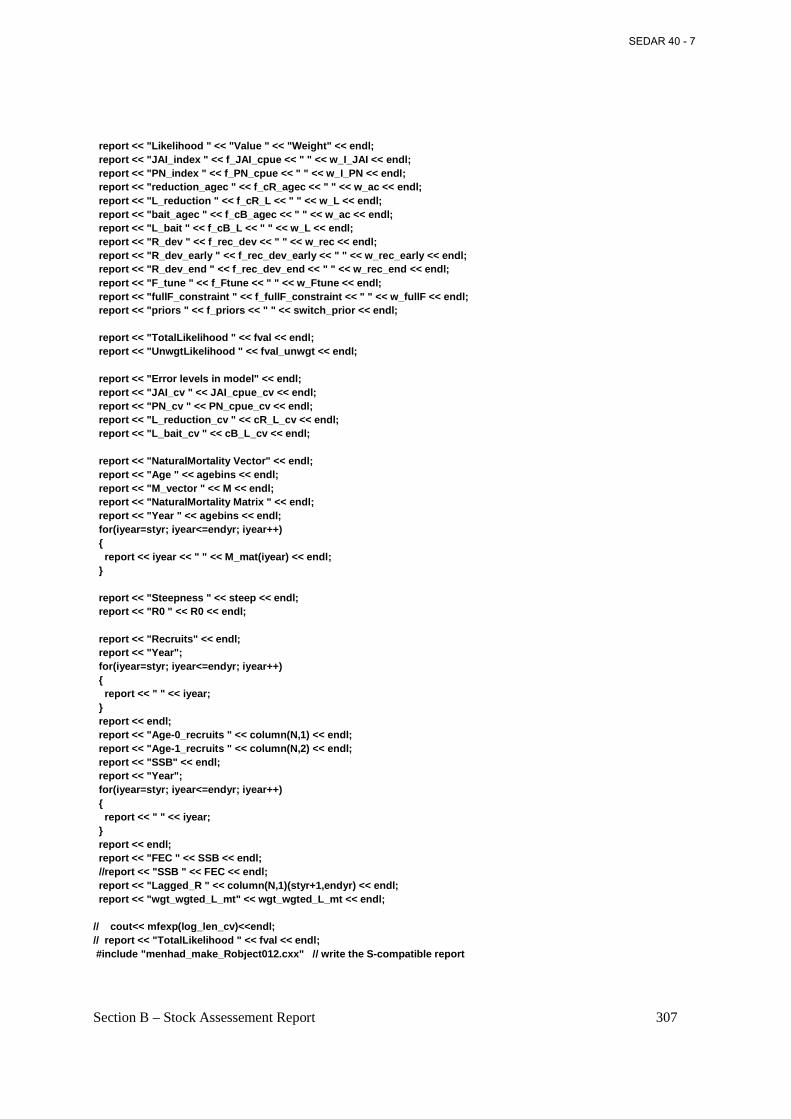
Section B – Stock Assessement Report 307
report << "Likelihood " << "Value " << "Weight" << endl; report << "JAI_index " << f_JAI_cpue << " " << w_I_JAI << endl; report << "PN_index " << f_PN_cpue << " " << w_I_PN << endl; report << "reduction_agec " << f_cR_agec << " " << w_ac << endl; report << "L_reduction " << f_cR_L << " " << w_L << endl; report << "bait_agec " << f_cB_agec << " " << w_ac << endl; report << "L_bait " << f_cB_L << " " << w_L << endl; report << "R_dev " << f_rec_dev << " " << w_rec << endl; report << "R_dev_early " << f_rec_dev_early << " " << w_rec_early << endl; report << "R_dev_end " << f_rec_dev_end << " " << w_rec_end << endl; report << "F_tune " << f_Ftune << " " << w_Ftune << endl; report << "fullF_constraint " << f_fullF_constraint << " " << w_fullF << endl; report << "priors " << f_priors << " " << switch_prior << endl; report << "TotalLikelihood " << fval << endl; report << "UnwgtLikelihood " << fval_unwgt << endl; report << "Error levels in model" << endl; report << "JAI_cv " << JAI_cpue_cv << endl; report << "PN_cv " << PN_cpue_cv << endl; report << "L_reduction_cv " << cR_L_cv << endl; report << "L_bait_cv " << cB_L_cv << endl; report << "NaturalMortality Vector" << endl; report << "Age " << agebins << endl; report << "M_vector " << M << endl; report << "NaturalMortality Matrix " << endl; report << "Year " << agebins << endl; for(iyear=styr; iyear<=endyr; iyear++) { report << iyear << " " << M_mat(iyear) << endl; } report << "Steepness " << steep << endl; report << "R0 " << R0 << endl; report << "Recruits" << endl; report << "Year"; for(iyear=styr; iyear<=endyr; iyear++) { report << " " << iyear; } report << endl; report << "Age-0_recruits " << column(N,1) << endl; report << "Age-1_recruits " << column(N,2) << endl; report << "SSB" << endl; report << "Year"; for(iyear=styr; iyear<=endyr; iyear++) { report << " " << iyear; } report << endl; report << "FEC " << SSB << endl; //report << "SSB " << FEC << endl; report << "Lagged_R " << column(N,1)(styr+1,endyr) << endl; report << "wgt_wgted_L_mt" << wgt_wgted_L_mt << endl; // cout<< mfexp(log_len_cv)<<endl; // report << "TotalLikelihood " << fval << endl; #include "menhad_make_Robject012.cxx" // write the S-compatible report
SEDAR 40 - 7
Section C – Review Panel Consensus Report 308
Section C - Consensus Review Panel Report for the 2010 Stock Assessment
Southeast Data, Assessment, and Review 20
Review Panel Consensus Report
Atlantic Menhaden
Members of the SEDAR 20 Review Panel Kim McKown (Panel Chair), New York State Department of Environmental Conservation
Dr. Tim Miller, NMFS Northeast Fisheries Science Center Patrick Cordue, Center for Independent Experts Dr. Chris Darby, Center for Independent Experts
Dr. Geoff Tingley, Center for Independent Experts
Prepared for the Atlantic Menhaden Management Board Workshop dates: March 8-12, 2010
Report date: April 14, 2010
SEDAR 40 - 7

Section C – Review Panel Consensus Report 309
Acknowledgments
The Panel thanks all of the individuals who contributed to the review of the Atlantic menhaden stock assessment report. The Panel thanks members of the Atlantic Menhaden Technical Committee (TC) and Stock Assessment Subcommittee (SAC) for preparation of these reports. In particular, the Panel thanks Brad Spear, Joe Smith, Doug Vaughan, Rob Latour, Matt Cieri and Erik Williams from the Atlantic Menhaden SAC for their informative presentations, for answering numerous questions and responding to additional analysis requests, and for participating in constructive discussions. The Panel also thanks Dale Theiling from SEDAR and Patrick Campfield from ASMFC for coordinating the peer review and preparation of this report.
SEDAR 40 - 7

Section C – Review Panel Consensus Report 310
Introduction The Review Workshop of the 2010 Atlantic Menhaden Assessment Report was held March 8 – 12, 2010 in Charleston, South Carolina. The Review Workshop provided a comprehensive and in-depth evaluation of this assessment. This report contains the Panel’s summary findings, detailed discussion of each TOR, and a summary of the results of analytical requests.
Summary of Findings
• The Panel is comfortable with the results from the menhaden base run. The model results and the status determination are robust.
• The 2008 point estimate of fishing mortality (F) was below the estimated F threshold, the status determination is that overfishing was not occurring and the 2008 point estimate of fecundity was above the fecundity threshold and target, the status determination is that the stock is not overfished.
• The Panel was concerned that the 2008 F estimate was very close to the threshold. If uncertainty in the estimate was considered there is a significant probability that overfishing occurred in 2008.
• The Panel was also concerned about the use of Fmed and the fecundity associated with it as reference points. The concern is that there is no information on the relationship of the target and threshold fecundity in relation to virgin fecundity levels. Projections were run to examine this, and the estimated annual fecundity since 1998 was only 5 to 10% of the virgin fecundity.
• The Panel recommends that a model specification similar to the Panel’s reference run be considered for future assessments. This includes capped effective sample size at 200, allow the gaps in the pound net index and bait fishery age composition where data are not available, modification of the reduction and bait fleets to northern and southern fleets, and time-varying domed selectivity for the southern region. This model specification combines information of the bait and reduction fisheries occurring together regionally because they are essentially using the same gear but fishing on different age components of the stock in the two areas. Removing the estimated age composition and indices for years where it is absent is desirable because the data from years where it is available is providing the correct amount of information, from a statistical perspective, to the assessment model. Allowing domed selectivity of the fisheries in the southern region allows for the lack of availability of older fish in that region when the fishery is occurring. The reduction of effective sample sizes is intended to better reflect the actual information content of the age composition data (the residuals in the base model were inconsistent with the large assumed effective sample sizes). Also, the time-varying selectivity in the southern region had the best AIC of comparable runs and reduced the undesirable pattern of residuals in the southern fishery.
SEDAR 40 - 7
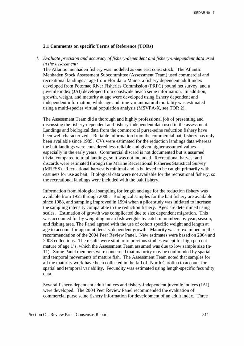
Section C – Review Panel Consensus Report 311
2.1 Comments on specific Terms of Reference (TORs)
1. Evaluate precision and accuracy of fishery-dependent and fishery-independent data used in the assessment: The Atlantic menhaden fishery was modeled as one east coast stock. The Atlantic Menhaden Stock Assessment Subcommittee (Assessment Team) used commercial and recreational landings at age from Florida to Maine, a fishery dependent adult index developed from Potomac River Fisheries Commission (PRFC) pound net survey, and a juvenile index (JAI) developed from coastwide beach seine information. In addition, growth, weight, and maturity at age were developed using fishery dependent and independent information, while age and time variant natural mortality was estimated using a multi-species virtual population analysis (MSVPA-X, see TOR 2). The Assessment Team did a thorough and highly professional job of presenting and discussing the fishery-dependent and fishery-independent data used in the assessment. Landings and biological data from the commercial purse-seine reduction fishery have been well characterized. Reliable information from the commercial bait fishery has only been available since 1985. CVs were estimated for the reduction landings data whereas the bait landings were considered less reliable and given higher assumed values – especially in the early years. Commercial discard is not documented but is assumed trivial compared to total landings, so it was not included. Recreational harvest and discards were estimated through the Marine Recreational Fisheries Statistical Survey (MRFSS). Recreational harvest is minimal and is believed to be caught primarily with cast nets for use as bait. Biological data were not available for the recreational fishery, so the recreational landings were included with the bait fishery. Information from biological sampling for length and age for the reduction fishery was available from 1955 through 2008. Biological samples for the bait fishery are available since 1988, and sampling improved in 1994 when a pilot study was initiated to increase the sampling intensity comparable to the reduction fishery. Ages are determined using scales. Estimation of growth was complicated due to size dependent migration. This was accounted for by weighting mean fish weights by catch in numbers by year, season, and fishing area. The Panel agreed with the use of cohort specific weight and length at age to account for apparent density-dependent growth. Maturity was re-examined on the recommendation of the 2004 Peer Review Panel. New estimates were based on 2004 and 2008 collections. The results were similar to previous studies except for high percent mature of age 1’s, which the Assessment Team assumed was due to low sample size (n-11). Some Panel members were concerned that maturity may be confounded by spatial and temporal movements of mature fish. The Assessment Team noted that samples for all the maturity work have been collected in the fall off North Carolina to account for spatial and temporal variability. Fecundity was estimated using length-specific fecundity data. Several fishery-dependent adult indices and fishery-independent juvenile indices (JAI) were developed. The 2004 Peer Review Panel recommended the evaluation of commercial purse seine fishery information for development of an adult index. Three
SEDAR 40 - 7
Section C – Review Panel Consensus Report 312
effort based time series were developed, but were not used due to concerns that they may not measure population abundance and effort. The Panel concurs with the decision not to include these indices in the model. Two adult relative abundance indices were developed from pound-net bait fishery landings collected by the Potomac River Fisheries Commission (PRFC). One was a catch-per-unit-effort (CPUE) index and the other was developed using a generalized linear model (GLM). There were years where the data were not collected, producing data gaps. Values were estimated to fill the gaps in the CPUE index. CVs were assumed constant for the index and sensitivities were run to test the assumption. The PRFC adult CPUE index was used in the model, including the estimated values to fill in data gaps. Since the model can handle missing data, the Panel recommended leaving the gaps in the data. Filling the gaps underestimates the uncertainty. Juvenile indices (JAI) were produced using two methods. The first approach calculates a single coastwide juvenile index. The Assessment Team used this coastwide juvenile index in the model, assuming that each survey represents a component of the coastal juvenile relative abundance. The second approach combined relative abundance data from groups of states according to the similarity of trends in the state-specific time series (additive approach). The Panel recommends this latter approach since these regional indices may capture spatial patterns of juvenile abundance. (see short term research recommendation e). CVs were calculated from jackknife-derived standard errors for the JAI.
Specific questions specified in TOR 1. are addressed below.
a. Discuss data strengths and weaknesses (e.g. temporal and spatial scale, gear
selectivities, aging accuracy, sampling intensity).
Strengths of the Fishery-dependent and fishery-independent data: • The reduction fishery landings and biological sampling information have been
collected since the 1950s in a consistent manner and represent one of the longest and most complete fisheries information series in the U.S.
• Daily logbooks (Captains Daily Fishing Reports) have been collected since 1985, and detail purse-seine set locations and estimated catch. Vessel compliance is 100%. This information is used to decrease “topping off” bias. Topping off is the practice of taking one more set to fill the hold at the end of a long trip. These added fish typically are smaller than fish in the rest of the hold.
• Scales have been used for ageing since the 1950s, and have been read by the same
person since 1969. A re-aging program was conducted in 2009 to determine precision of aging. The standard deviations associated with age estimates were used to provide the error associated with the age composition data. The error was assumed constant over time
SEDAR 40 - 7
Section C – Review Panel Consensus Report 313
Data weaknesses: • The Panel had some questions on the age structure and estimated selectivities of the
commercial reduction and bait fisheries by area. After inspection, it was revealed that the age structure of the landings was a result of the area harvested rather than the type of fishery. The Panel recommend the commercial fishery be modeled by area (north vs south) rather than by fishery (reduction vs bait) (see short term research recommendation a)
• A re-aging study was conducted to estimate precision (see above), but little age validation work has been conducted. An ongoing validation study at Old Dominion University has had good agreement between scale and otolith ages, but few age 2 and 3 fish have been processed, and fish >3 are not included.
• The Potomac River Fisheries Commission (PRFC) pound-net index had a number of years with missing data, which the Assessment Team filled in with estimated values. The Panel recommended leaving the data gaps, because inclusion of the estimated values would lower uncertainty estimates. (see short term research recommendation a)
• The Panel had some concerns about the appropriateness of the length-based cut offs
for age-0 juvenile menhaden for the state specific seine surveys which do not age menhaden. Raw data were not available at the Review to explore those concerns.
b. Report metrics of precision for data inputs and use them to inform the model as
appropriate. As mentioned above, a re-aging program was conducted in 2009 to determine precision of aging. The standard deviations associated with age estimates were used to provide the error associated with the age composition data. It was assumed constant over time. Error levels for the fishery catch at age were based on the number of sampling trips (effective sample size). The Panel thought the effective sample size on the age composition data was too high, and recommended capping at 200 (see short term research recommendation a).
c. Describe and justify index standardization methods. The Assessment Team developed several adult and juvenile (JAI) relative abundance indices for potential use in the model, including detailed methodology and justification. The Panel recommended using the alternative regional JAI (see discussion above). There was also discussion about developing an alternative coastwide adult index (see long term research recommendation a).
d. Justify weighting or elimination of available data sources.
As discussed above, the Assessment Team did several adjustments or weighting to account for size-variable migration (topping off adjustment, weighted mean
SEDAR 40 - 7
Section C – Review Panel Consensus Report 314
weights and length at age). The Panel agreed with the Assessment Team’s judgment not to include adult effort-based indices from the reduction fishery. For the PRFC adult index, the Panel recommended not to include estimated values, but to run the model with the data gaps (discussed in a).
2. Evaluate models used to estimate population parameters (e.g., F, biomass, abundance) and biological reference points.
The Beaufort Assessment Model (BAM) was the only model used to produce final assessment results. This is a statistical forward-projection model with separable selectivities using the Baranov catch equation. Catch histories, catch-at-age, juvenile and adult abundance indices were all fitted in the model assuming two fisheries (reduction and bait). Constant selectivities were estimated for the fisheries but fixed at assumed values for both the juvenile and adult indices. Catchability parameters were estimated for both indices. Lognormal likelihoods were assumed for the catch histories and indices, with multinomial likelihoods for the catch-at-age data. The MSVPA-X model was used to estimate age and year specific natural mortality from 1982-2008. The estimates were then assumed known in the base BAM run in those years with the average at-age estimates applied to the years 1955-1981. The MSVPA-X model was peer reviewed in 2005 and recommended for use in estimating natural mortality but not as a full assessment model. The Panel did not revisit this recommendation. There were mixed views within the Panel on the appropriateness of using these estimates in the base model. All members agreed that, in reality, natural mortality was age and year specific. However, there was some concern that the natural mortality estimates were unreliable because of the difficulties of modeling the complexity of the Atlantic ecosystem as it relates to menhaden mortality. However, it was noted that the assessment results are not sensitive to the choice between age-specific natural mortality or age-and-year specific natural mortality.
The base model has a number of strengths:
• well tested software, population dynamics equations, and likelihoods • based on a good understanding of stock structure and migration patterns • reasonable certainty in the catch history over an extended period • extensive catch-at-age data from the main fishery sampled in a consistent manner
over many years • defensible recruitment indices and an adult abundance time series (pound-net CPUE) • defensible estimates of age and year specific natural mortality.
However, there are also some potential weaknesses in the base model: • the definition of the fisheries in the model is based on the product produced rather
than the fishing method or other attribute of the fishery or stock • gaps in the catch-at-age data for the bait fishery and the pound-net CPUE indices
were “filled in” with unobserved data • the time series of juvenile and adult indices may not be representative of the whole
population (the pound-net CPUE is spatially very limited)
SEDAR 40 - 7
Section C – Review Panel Consensus Report 315
• the input variance assumptions, especially with regard to effective sample sizes, are inconsistent with the model residuals (the effective sample sizes are too high, and therefore uncertainty in model outputs is underestimated)
• there are strong residual patterns for the reduction fishery catch-at-age. Some of the problems with the base run were examined by the Panel in a number of sensitivity runs. A “reference run” was specified by the Panel:
• define two fisheries based on location (North – where the larger/older fish are typically caught; and South – where smaller/younger fish are typically caught; most catch in both areas is by purse-seine)
• reinstate the gaps in the data which were filled in with unobserved data • use a maximum effective sample size of 200 for catch-at-age data • allow the southern selectivity pattern to be domed
Sensitivities to this run included the use of time-blocked selectivities for the Southern fishery based on known changes in the fishery (three time blocks were used). This run had the lowest AIC amongst comparable runs, suggesting that the use of the additional parameters was justified by the improvement in fit. A visual examination of the catch-at-age residuals also showed some reduction in the extent of the residual patterns. The determination of stock status for the reference run and sensitivities was the same as in the base model. The Panel also evaluated the status of the stock relative to unfished fecundity. Two alternative “productivity periods” were considered. A “recent” period (1992-present) and the “full” period (1955-present); productivity in each period was determined by the mean and variance of the recruits, and the average natural mortality and mean weight-at-age over the period. Unfished fecundity for each period was determined by running the model forward, with stochastic recruitment, without fishing until stochastic equilibrium was established (the mean fecundity is then, by definition, the unfished fecundity; representing the “carrying capacity” of the population under the assumed productivity regime). For the base model, fecundity since 1998 was estimated at less than 10% of unfished fecundity for the full-regime and about 15% for the recent-regime. The results for the best-AIC model were similar, but higher (about 12% for the full-regime since 1998 and about 25% for the recent-regime), and also showed a slowly increasing trend since 1965 (the base model was fairly flat from 1965 to 2008). Specific questions specified in TOR 2. are addressed below.
a. Did the model have difficulty finding a stable solution?
The Panel requested that convergence be checked with some jittered starting values. Twenty five runs were performed and all runs converged to the same solution.
b. Were sensitivity analyses for starting parameter values, priors, etc. and other model diagnostics performed?
SEDAR 40 - 7
Section C – Review Panel Consensus Report 316
An extensive set of sensitivity runs were performed for the base model including higher and lower M, alternative weights on data sets, alternative selectivities, and an alternative start year. The only result of note was that leaving out the juvenile index (JAI) resulted in an over-fishing status in 2008. On investigation it was found that the JAI supported higher recruitment in the last three years than other data sets. Removal of the JAI was sufficient to move the point estimate of 2008 F just above the overfishing threshold.
c. Have the model strengths and limitations been clearly and thoroughly explained?
These were discussed in the assessment document and were also considered by the Panel (see above).
d. Have the models been used in other peer reviewed assessments? If not, has new model code been verified with simulated data?
BAM has been used in several other peer-reviewed assessments.
e. Compare and discuss differences among alternative models.
The Panel formulated an alternative BAM run which addressed the main problems identified with the base run. Given the other uncertainties, the differences in the assessment results between the two models are relatively minor (see above).
3. Evaluate the potential for conducting assessments at a sub-regional level (e.g.
Chesapeake Bay). All of the recent research results are consistent with a single Atlantic coast-wide menhaden stock. Although data are available to enable assessments at a sub-regional level, the results would be meaningless from a biological point of view (and would be of no use in making sensible management decisions). The issue of potential sub-regional quotas or fishing limits is outside the TOR for this review. However, the Panel notes that the implementation of such an approach could not sensibly be done by sub-regional assessment (and setting sub-regional quotas on the basis of the assessments). 4. State and evaluate assumptions made for all models and explain the likely effects of
assumption violations on model outputs. These were discussed under TOR 2. However, each point in the checklist is addressed below.
a. Calculation of M. Discussed under b.
b. Choice to incorporate constant or time-varying M and catchability.
SEDAR 40 - 7

Section C – Review Panel Consensus Report 317
Year and age-specific M were estimated in the MSVPA-X model and assumed known in the base BAM run. Sensitivity runs with higher and lower M and age-specific but time-invariant M did not change the status determination.
c. Choice of selectivity patterns. Fishery selectivities were estimated in the base run although domed-selectivities were not allowed. The potential impact of mis-specification was investigated by allowing domed-selectivities in some runs, but this did not change the status determination.
d. Choice of time steps in models. The model had a simple annual cycle and assumed that all fisheries were operating year-round. This is a significant departure from reality but it is unlikely to have a major impact on assessment results. Nevertheless, it would be better to model the timing of the fisheries more accurately, particularly as the timing of some of them has changed in recent years.
e. Error in the catch-at-age matrix. The catch at age data are assumed to follow a multinomial distribution in each year with effective sample sizes equal to the number of trips sampled. This is a mathematically convenient and commonly made assumption which is almost certainly violated. In this particular case, the effective sample sizes appear to be too high as the model residuals are much more variable than they should be given the assumed sample sizes. Also, there are obvious patterns in the residuals for the reduction fishery. Lower sample sizes and alternative splits of the fisheries, together with alternative selectivities alleviated these problems to some extent. Different point estimates were obtained but stock status determination was unaltered.
f. Choice of a plus group for age-structured species. A plus group was used at an appropriate age.
g. Constant ecosystem (abiotic and trophic) conditions. Ecosystem conditions are unlikely to have been constant over the period in which the stock was modeled. There are attempts in the model to deal with changing conditions in terms of year-specific natural mortality and cohort-specific growth. The reference points used assume that the time period modeled is representative of a single constant regime. This is a reasonable approach as without a full understanding of the processes involved it is not possible to know how long a “regime shift” might last (or even if it has occurred). There is some evidence of a “regime shift” in 1992 to lower productivity. This was considered by the Panel when calculating unfished fecundity (two alternatives: 1992-present or 1955-present).
SEDAR 40 - 7
Section C – Review Panel Consensus Report 318
h. Choice of stock-recruitment function. It is assumed that there is very little relationship between population fecundity and recruitment (i.e., steepness is close to 1). There is no evidence for a relationship in the model estimates of fecundity and recruitment. However, recruitment is quite variable and there could be a stock-recruit relationship which is not discernable for this reason. The current reference points are independent of steepness, so this assumption has no consequences for status determination.
i. Choice of reference points (e.g. equilibrium assumptions). The use of FMED based reference points is of concern. It appears that the stock has been at low levels of population fecundity for many years and yet the current reference points (and the FMED reference points of previous years) provide a determination of “not overfishing” and “not overfished”. The Panel recommends that alternative reference points be considered and chosen on the basis of providing better protection for SSB or population fecundity relative to the unfished level.
5. Evaluate uncertainty of model estimates and biological or empirical reference points.
Sensitivity runs were discussed under TOR 2.b. Almost all sensitivity runs gave the same stock status determination as the base run. However, from the bootstrap analysis of the base run, it is clear that there is considerable uncertainty with regard to the overfishing status of the stock in 2008 (with 37% of the runs indicating that overfishing was occurring). The Panel notes that uncertainty is underestimated in the bootstrap analysis as the assumed effective sample sizes are too high (see discussion of potential base-model weaknesses under TOR 2.) Specific questions specified in TOR 5. are addressed below.
a. Choice of weighting likelihood components.
The likelihood components were each given equal weight which, along with incorporated estimates or assumed CVs for each component, attempts to provide relative influence on the objective function that reflects knowledge about the quality of the inputs. However, correct weighting procedures seems to be an open question.
6. Perform retrospective analyses, assess magnitude and direction of retrospective patterns
detected, and discuss implications of any observed retrospective pattern for uncertainty in population parameters (e.g., F, SSB), reference points, and/or management measures.
A retrospective analysis was performed by the Assessment Team for the base model. There were no retrospective patterns of any consequence.
SEDAR 40 - 7
Section C – Review Panel Consensus Report 319
7. Recommend stock status as related to reference points. The Panel supports the recommendation of the Assessment Team that the stock status determination is “not overfished” and there is “no overfishing”, relative to the current reference points. Further, the Panel also agrees with the Assessment Team that the uncertainties in the assessment are such that there could have been overfishing in 2008 (removal of the JAI from the base model gave that determination and many bootstrap runs also fell in the overfishing zone). The Panel also notes that a strictly valid determination of the overfishing status requires comparison of full Fs and not number-weighted Fs. This is not a well-known result, but it is obvious once the problem is identified. Consider a population which is being fished at some reference level FREF (e.g., FMSY) with a constant selectivity pattern (e.g., domed or logistic). Suppose that recruitment is constant and that the population is at equilibrium. The number-weighted version of FREF, say F*REF, can be calculated from the equilibrium distribution of numbers-at-age and FREF. Now, consider what happens to the number-weighted version of F, say F*, when a large recruitment pulse is introduced into the population. As the pulse enters the first vulnerable age class (which is included in the calculation of F* and F*REF), there is a large increased weight on a partially selected age class, and hence F* is not equal to F*REF (it will probably be less than F*
REF, but this depends on the particular selectivity and population parameters). As the pulse travels through each age class, the value of F* changes, but it is unlikely to achieve equality with F*
REF at any age. When it reaches the first fully-recruited age class, it is likely that F* > F*REF.
In any case, in this example, F remains constant at FREF, but the number-weighted version of F varies – if used in an overfishing determination, it will give an incorrect status in most if not all years. This is an extreme example but, mathematically, it is sufficient to prove that the use of number-weighted F is not appropriate for overfishing status determination. In general, full F should be used.
8. Develop detailed short and long-term prioritized lists of recommendations for future research, data collection, and assessment methodology. Highlight improvements to be made by next benchmark review.
The Panel endorses the research recommendations in the menhaden assessment report and has additional short and long term research recommendations which are detailed below. The short and long term recommendations are in priority order. Short term (improvements for the next benchmark review)
a. The Panel recommends that model specifications similar to the Panel’s reference run be
considered for future assessments. This includes capped effective sample size at 200, allow the gaps in the pound net index and bait fishery age composition where data are not available, modification of the reduction and bait fleets to northern and southern fleets, and time-varying domed selectivity for the southern region.
SEDAR 40 - 7

Section C – Review Panel Consensus Report 320
This model specification combines information of the bait and reduction fisheries occurring together regionally because they are essentially using the same gear. Removing the estimated age composition and indices for years where it is absent is desirable because the data from years where it is available is providing the correct amount of information, from a statistical perspective, to the assessment model. Allowing domed selectivity in the southern region fishery allows for the lack of availability of older fish in that region when the fishery is occurring. The reduction of effective sample sizes is intended to better reflect the actual information content of the age composition data (the residuals in the base model were inconsistent with the large assumed effective sample sizes). Also, the time-varying selectivity in the southern region had the best AIC of comparable runs and reduced the undesirable pattern of residuals in the southern fishery. A reworking of the menhaden fishery into northern and southern fleets should be explored to support the assessment. This exploration should consider the spatial patterns of the stock and the fishery as the stock range and fishery have expanded and contracted over time, and may be expected to continue to do so in future and setting an appropriate fixed boundary (or fixed criteria to define a movable boundary) may be critical.
b. Fishing mortality should be calculated as full F. The N-weighted fishing mortalities relative to the N-weighted F-reference points do not provide correct interpretation with regard to overfishing.
c. The Panel has concerns about the use of FMED and the fecundity associated with it as reference points. The concern is that there was no information on the relationship of the target and threshold fecundity in relation to virgin fecundity levels. Projections were run to examine this, and the estimated fecundity since 1998 was less than 10% of the virgin fecundity for the base model. We recommend examination of alternative reference points which provide more protection to SSB or fecundity than FMED.
d. Examine weighting of datasets in the model. As a starting point, some experts assert that the input variance assumptions should be consistent with the estimated variance of residuals. Deviations from this weighting pattern may be desirable but the weightings ultimately used need to be justified. In the base model the effective sample sizes for catch-at-age data are far too high and consequently estimates of uncertainty are too low.
e. The Panel recommends the Assessment Team’s alternative use of the juvenile indices:
combining relative abundance data from groups of adjacent states according to the similarity of trends in the state-specific time series; and cumulatively-combining these indices within the model. This allows for different regional patterns of recruitment to provide a stock-wide recruitment pattern.
f. Examine the timing of fisheries and indices in the model. Many of the fisheries are
seasonal and need to be timed appropriately with the abundance indices. Incorrect timing may affect model fits.
SEDAR 40 - 7

Section C – Review Panel Consensus Report 321
Long Term a. Develop a coast-wide adult menhaden survey. Possible methodologies include an air-
spotter survey, a hydro-acoustic survey, or an industry-based survey with scientific observers on board collecting the data. In all cases, a sound statistical design is essential (involve statisticians in the development and review of the design; some pilot surveys may be necessary).
2.2 Summary results of analytical requests 1) Supply a time series of fully recruited Fs along with the traditional N-weighted Fs and
comparable F-reference points. Rationale: The N-weighted fishing mortalities relative to the N-weighted F-reference points
will not provide correct interpretation with regard to overfishing. Outcome: It was observed that the relationship of fully recruited Fs to the F-reference points
was different than that of the N-weighted Fs and F-reference points.
2) Present a map showing the age composition of the bait fishery catches in 2008 similar to the plot for the reduction fishery. Rationale: Understanding of the location and time of the fishery and index information will
be facilitated for reviewers not familiar with the locale. Outcome: Presentation of these maps helped the reviewers understand the location and
timing of the fisheries and indices.
3) Reverse prediction of recruits from adults. Rationale: A reviewer was interested in whether the same predictability of recruits from
adults is obtained as the reverse relationship. Outcome: It was shown that the predictability was also quite good in the reverse relationship.
4) Do base run with gaps in the adult fishery dependent index and with gaps in bait catch at age. Rationale: Removing the estimated age composition and indices for years where it is absent
is desirable because the data from years where it is available is providing the correct amount of information, from a statistical perspective, to the assessment model.
Outcome: These results were not noticeably different from the base run without gaps in the
index and catch at age.
SEDAR 40 - 7

Section C – Review Panel Consensus Report 322
5) Calculate standardized residuals for indices and catch-at-age and present standard deviation of standardized residuals with Q-Q plots. Rationale: These are diagnostics with regard to whether the statistical assumptions of the
model are satisfied or not. Outcome: The results showed that the juvenile abundance index was being fitted better
(standard deviation around 0.7) than other data components which had standard deviations substantially greater than 1. In particular, the results showed that the sample sizes of the catch-at-age data were too high. The Q-Q plots also showed that residuals departed from normality.
6) Run allowing dome-shaped selectivity in reduction and bait fishery.
Rationale: The reviewers were concerned about the availability of larger fish to these
fisheries and whether there was information in these age composition data to determine this.
Outcome: The assessment team presented these results which showed that there were
substantial drops in selectivity of older fish for both fisheries.
7) If time permits, do a run with fishery split between two regional “fleets” based on latitude. Rationale: This run combines information of the bait and reduction fisheries occurring
together regionally because they are essentially using the same gear while accounting for the availability of fish of different ages in the two regions.
Outcome: The Assessment Team were able to put this run together in time. It altered the
determination of over-fishing, compared to the base model, with current F estimated to be greater than FMED.
8) Likelihood profile across R0 and components for each data component and any penalties.
Rationale: The reviewers were interested in how the maximized likelihood components
change across R0, which provides information on the relative influence of the components on estimation of R0.
Outcome: Plots of scaled log-likelihood components were presented, but the Panel made a
follow-up request below (11). 9) The following reference run with specified data and sensitivities is requested.
a) northern and southern regional fisheries b) gaps in age composition and indices c) effective sample sizes truncated at 200 d) selectivity in the southern region allowed to be dome-shaped
SEDAR 40 - 7
Section C – Review Panel Consensus Report 323
Sensitivities: a) original effective sample sizes b) time-block-specific selectivities in the southern region c) logistic selectivity in the southern region d) age-specific and time-invariant natural mortality Provide total and component likelihood profiles for the run (not the sensitivities). Provide AIC values and standard deviations for standardized residuals for all runs and
sensitivities.
Rationale: The reference run combines information of the bait and reduction fisheries occurring together regionally because they are essentially using the same gear. Removing the estimated age composition and indices for years where it is absent is desirable because the data from years where it is available is providing the correct amount of information, from a statistical perspective, to the assessment model. Allowing domed-selectivity in the southern region allows for the lack of availability of older fish in that region when the fishery is occurring. Sensitivities (a-d) allow some idea of the influence of the respective model attributes on the results to be understood.
Outcome: For most runs and selectivities, the overfishing and overfished status were the
same as the base model. However, the sensitivity run of the reference model where logistic selectivity is assumed in the southern region estimated current fishing mortality to be greater than FMED.
10) Plots comparing output of the base run and the reference run and sensitivities.
Rationale: These plots will help the Panel understand the differences in results for the various runs.
Outcome: Comparison plots were presented by the Assessment Team for the base model, and
a number of the original sensitivities, the reference run and its sensitivities. 11) Provide profile log-likelihood components (across R0) for different data sources and
penalties with minima subtracted.
Rationale for Request: The change in the maximized log-likelihood values for each of the data components and penalties across fixed values of R0 is representative of the effect each has on the total log-likelihood. Outcome: The figure showed the trade-offs between the various components in the maximized log-likelihood components with respect to R0.
12) For the base model, stochastic projections of population without fishing to obtain mean
unfished fecundity. Future recruitments should be drawn from a log-normal distribution with mean and variance being empirical values from past recruitments. a) Use entire recruitment time series for projections
SEDAR 40 - 7
Section C – Review Panel Consensus Report 324
b) Use recruitments from low-productivity period (1992-2006). c) Provide standard deviation of the log-recruitment used for projections. d) Present estimated historical fecundity trajectories as a percentage of unfished fecundity.
Rationale: The Menhaden Technical Committee requested the Panel’s thoughts on reference
points for Menhaden. Some members of the Panel thought that it would be important to ensure that fecundity does not get lower than some critical value relative to the unfished fecundity. These projections allow the stochastic equilibrium unfished fecundity to be determined which can then be compared to estimates from the current assessment. The shorter time series of recruits were of interest because Wood and Austin (2009) found a change in productivity in the Chesapeake in 1992. Furthermore, a trend in higher natural mortality for menhaden occurred during this period also from the MSVPA-X model.
Outcome: Results were presented by the assessment team. Estimated fecundity since 1998
was between 5 and 10% of the unfished mean fecundity when the entire time series of historic recruitments were used and between 10 and 15% of the unfished mean fecundity when the shorter time series of recruitments were used.
13) As for (R12), but use the reference run with time-varying selectivity blocks in the south.
Rationale: These plots will help the Panel understand the differences in results for the two
runs. Outcome: Results were presented by the Assessment Team. Estimated current fecundity was
about 15% of unfished mean fecundity when the entire time series of historical recruitments were used and between 25 and 30% of the unfished mean fecundity when the shorter time series of recruitments were used.
14) Vary the starting values of parameters for the base model to check for convergence issues.
Rational: There is the possibility that the value of the maximized log-likelihood and resulting parameter estimates is sensitive to the starting values.
Outcome: Random restart analysis included catchability coefficients, selectivity parameters,
average fishing mortality, and R0. Results showed that virtually the same likelihood was achieved in all runs.
15) Determine reasons that the juvenile abundance index affects the overfishing status.
Rational: This index may be a poor measure of juvenile abundance and its impact on the overfishing status is of concern to the Panel.
Outcome: Estimated recruitments strengths are different between the runs in last three years
(2006-2008). The catch-at-age data and the juvenile index must be giving different signals on the strength of these year classes.
SEDAR 40 - 7
Section C – Review Panel Consensus Report 325
References Lorensen, K. 2005. Population dynamics and potential of fisheries stock enhancement: practical
theory for assessment and policy analysis. Philosophical Transactions of the Royal Society of London, Series B 360 (1453):171-189.
Stephens, A., and A. MacCall. 2004. A multispecies approach to subsetting logbook data for
purposes of estimating CPUE. Fisheries Research (Amsterdam) 70(2-3):299-310. Wigley, S. E., Rago, P. J., Sosebee, K. A. and Palka, D. L. 2006. The analytic component to the
standardized bycatch reporting methodology omnibus amendment: sampling design and estimation of precision and accuracy. NMFS/NEFSC, Reference Document 06-22.
Wood, R. J. and Austin, H.M. 2009. Synchronous multidecadal fish recruitment patterns in
Chesapeake Bay, USA. Can. J. Fish. Aquat. Sci. 66:496-508.
SEDAR 40 - 7
Related Documents