Asymptotically cylindrical Calabi–Yau 3–folds from weak Fano 3–folds ALESSIO CORTI MARK HASKINS JOHANNES NORDSTR ¨ OM TOMMASO P ACINI We prove the existence of asymptotically cylindrical (ACyl) Calabi–Yau 3–folds starting with (almost) any deformation family of smooth weak Fano 3–folds. This allow us to exhibit hundreds of thousands of new ACyl Calabi–Yau 3–folds; previously only a few hundred ACyl Calabi–Yau 3–folds were known. We pay particular attention to a subclass of weak Fano 3–folds that we call semi-Fano 3–folds. Semi-Fano 3–folds satisfy stronger cohomology vanishing theorems and enjoy certain topological properties not satisfied by general weak Fano 3–folds, but are far more numerous than genuine Fano 3–folds. Also, unlike Fanos they often contain P 1 s with normal bundle O(-1) ⊕O(-1), giving rise to compact rigid holomorphic curves in the associated ACyl Calabi–Yau 3–folds. We introduce some general methods to compute the basic topological invariants of ACyl Calabi–Yau 3–folds constructed from semi-Fano 3–folds, and study a small number of representative examples in detail. Similar methods allow the computation of the topology in many other examples. All the features of the ACyl Calabi–Yau 3–folds studied here find application in [17] where we construct many new compact G 2 –manifolds using Kovalev’s twisted connected sum construction. ACyl Calabi–Yau 3–folds constructed from semi-Fano 3–folds are particularly well-adapted for this purpose. 14J30, 53C29; 14E15, 14J28, 14J32, 14J45, 53C25 1 Introduction Compact Calabi–Yau manifolds have been studied intensively ever since Yau’s resolution of the Calabi conjecture [101] allowed algebraic geometers to produce them in abundance. Nevertheless, some fundamental questions about compact Calabi–Yau manifolds even in dimension three remain open. For example, are there finitely many or infinitely many topological types of nonsingular Calabi–Yau 3–fold? arXiv:1206.2277v3 [math.AG] 5 Aug 2013

Welcome message from author
This document is posted to help you gain knowledge. Please leave a comment to let me know what you think about it! Share it to your friends and learn new things together.
Transcript
Asymptotically cylindrical Calabi–Yau 3–folds from weakFano 3–folds
ALESSIO CORTI
MARK HASKINS
JOHANNES NORDSTROM
TOMMASO PACINI
We prove the existence of asymptotically cylindrical (ACyl) Calabi–Yau 3–foldsstarting with (almost) any deformation family of smooth weak Fano 3–folds. Thisallow us to exhibit hundreds of thousands of new ACyl Calabi–Yau 3–folds;previously only a few hundred ACyl Calabi–Yau 3–folds were known. We payparticular attention to a subclass of weak Fano 3–folds that we call semi-Fano3–folds. Semi-Fano 3–folds satisfy stronger cohomology vanishing theorems andenjoy certain topological properties not satisfied by general weak Fano 3–folds, butare far more numerous than genuine Fano 3–folds. Also, unlike Fanos they oftencontain P1 s with normal bundle O(−1) ⊕ O(−1), giving rise to compact rigidholomorphic curves in the associated ACyl Calabi–Yau 3–folds.
We introduce some general methods to compute the basic topological invariantsof ACyl Calabi–Yau 3–folds constructed from semi-Fano 3–folds, and study asmall number of representative examples in detail. Similar methods allow thecomputation of the topology in many other examples.
All the features of the ACyl Calabi–Yau 3–folds studied here find applicationin [17] where we construct many new compact G2 –manifolds using Kovalev’stwisted connected sum construction. ACyl Calabi–Yau 3–folds constructed fromsemi-Fano 3–folds are particularly well-adapted for this purpose.
14J30, 53C29; 14E15, 14J28, 14J32, 14J45, 53C25
1 Introduction
Compact Calabi–Yau manifolds have been studied intensively ever since Yau’s resolutionof the Calabi conjecture [101] allowed algebraic geometers to produce them in abundance.Nevertheless, some fundamental questions about compact Calabi–Yau manifolds evenin dimension three remain open. For example, are there finitely many or infinitely manytopological types of nonsingular Calabi–Yau 3–fold?
arX
iv:1
206.
2277
v3 [
mat
h.A
G]
5 A
ug 2
013
2 A Corti, M Haskins, J Nordstrom and T Pacini
There has also been important work on complete noncompact Kahler Ricci-flat (KRF)metrics by many authors: Calabi, Yau, Eguchi–Hansen, Gibbons–Hawking, Hitchin,Kronheimer, Anderson–Kronheimer–LeBrun, Atiyah–Hitchin, Tian–Yau, Joyce, Naka-jima, Biquard and Carron to name only a small selection. Nevertheless, compared tothe compact nonsingular case, current understanding of noncompact KRF metrics ismuch less complete and demands further study; several open questions in this area goback as far as Yau’s 1978 ICM address.
The simplest classes of noncompact KRF metrics are:
(a) those of maximal volume growth, that is, Euclidean volume growth;
(b) those of minimal volume growth, that is, linear volume growth.
The maximal volume growth case – especially the class of so-called ALE metrics – hasalready attracted considerable attention, for example, Kronheimer’s classification resultsfor ALE hyper-Kahler 4–manifolds [60] and Joyce’s higher dimensional existenceresults [44, Section 8]; part of the reason for the focus on the ALE case has been theintimate link to the theory of (noncollapsed) metric degenerations of compact Einsteinmanifolds with bounded diameter. Another obvious model for noncollapsed metricdegenerations of compact Einstein manifolds is provided by the development of long“almost cylindrical necks”. For this reason it is important to understand asymptoticallycylindrical (ACyl) Einstein metrics. The simplest class of such ACyl Einstein metricsare the asymptotically cylindrical Calabi–Yau metrics studied in the present paper; seealso Haskins–Hein–Nordstrom [33].
ACyl Calabi–Yau 3–folds play a distinguished role because they can also be usedas building blocks in Kovalev’s twisted connected sum construction of compactmanifolds with holonomy G2 : see Kovalev [57], Kovalev–Lee [58] and the morerecent developments in Corti–Haskins–Nordstrom–Pacini [17]. The twisted connectedsum construction – first developed in [57] – constituted a major advance in theunderstanding of compact G2 –manifolds; along with Joyce’s original orbifold resolutionconstruction [44, Sections 11 and 12] it remains one of only two methods available toproduce compact G2 –manifolds.
Given a pair of ACyl Calabi–Yau 3–folds V± the twisted connected sum constructiongives a way to combine the pair of noncompact ACyl 7–manifolds S1 × V± – bothof which have holonomy SU(3) ⊂ G2 – to construct a compact 7–manifold withholonomy the full group G2 . The twisted connected sum construction is possible onlywhen a certain compatibility between the cylindrical ends of V± can be arranged;studying this “matching” problem for pairs of ACyl Calabi–Yau 3–folds is thereforevery important for our applications to G2 –geometry in [17].
Asymptotically cylindrical Calabi–Yau 3–folds 3
While we know the existence of huge numbers of deformation classes of compactCalabi–Yau 3–folds, until the present paper only a couple of hundred families of ACylCalabi–Yau 3–folds were known. In the present paper we prove that it is possibleto construct deformation families of ACyl Calabi–Yau 3–folds from (almost) anydeformation family of smooth weak Fano 3–folds. As a consequence we prove thatthere are at least several hundred thousand deformation classes of ACyl Calabi–Yau3–folds.
A Fano 3–fold Y is a smooth projective variety for which −KY is ample or positive:complex projective space P3 , smooth quadrics, cubics and quartics in P4 being thesimplest examples. Fano 3–folds have been important objects in algebraic geometrysince Fano’s work in the 1930s and are still very much an active research area incontemporary algebraic geometry. A weak Fano 3–fold1 is a smooth projective 3–foldfor which −KY is big and nef (but not ample). Differential geometers are encouragedto think of a line bundle being big and nef as the algebraic–geometric formulation ofadmitting a hermitian metric whose curvature is sufficiently semi-positive. All weakFano 3–folds can be obtained by choosing suitable resolutions of mildly singular Fano3–folds.
A number of properties of Fano manifolds generalise without too much difficultyto weak Fanos; we replace applications of the Kodaira vanishing theorem with itsgeneralisation the Kawamata–Viehweg vanishing theorem. Kovalev [57] used Fano3–folds to construct ACyl Calabi–Yau 3–folds with ends asymptotic to C∗ × S whereS is a smooth K3 surface and suggested that other constructions of suitable ACylCalabi–Yau 3–folds might be possible [57, page 148]; we prove that starting onlywith a weak Fano 3–fold (satisfying one further very mild restriction which is alsoneeded even in the Fano case) we can still construct ACyl Calabi–Yau 3–folds withends asymptotic to C∗ × S . However, in order to solve the “matching” problem forpairs of ACyl Calabi–Yau 3–folds constructed from weak Fano 3–folds it turns out to beimportant to distinguish the subclass of semi-Fano 3–folds, that is, weak Fano 3–foldswhose anticanonical morphism is a semi-small map.2
There are two principal advantages in generalising from Fano to weak Fano or semi-Fano3–folds. It is well-known that there are exactly 105 deformation families of smooth
1some authors call this an almost Fano 3–fold.2There seems to be no established terminology for this particular subclass of weak Fano
3–folds, so the term semi-Fano is our invention; it is intended to suggest that a semi-Fano 3–foldhas semi-small anticanonical morphism. Warning: Chan et al [12] used the term semi-Fanomanifold to mean something even weaker than weak Fano, that is, a complex manifold forwhich −KY is nef (but not necessarily big).
4 A Corti, M Haskins, J Nordstrom and T Pacini
Fano 3–folds (see Iskovskih [36, 37], Mori–Mukai [67, 68, 69], Mukai–Umemura [72]and Takeuchi [94]): in the paper, we will refer to this result as the “Iskovskih–Mori–Mukai classification”. On the other hand, there are at least hundreds of thousands ofdeformation families of smooth weak Fano or semi-Fano 3–folds and their topologyis less restrictive than for Fano 3–folds; unlike the Fano case there is at present noclassification theory for weak Fano or semi-Fano 3–folds except under very specialgeometric assumptions. Thus generalising from Fano to weak Fano or semi-Fano3–folds allows us to construct a significantly larger number of ACyl Calabi–Yau 3–folds.
For applications to the twisted connected sum construction of compact G2 –manifoldsthe following feature is also important; whereas on any Fano 3–fold the anticanonicalclass satisfies −KY · C > 0 for any complex curve C , weak Fano 3–folds can containspecial complex curves C for which KY · C = 0 (the weakening of −KY being positiveto sufficiently semi-positive is crucial here). Moreover, in many cases C is a smoothrational curve with normal bundle O(−1)⊕O(−1) (where O(d) denotes OP1(d)). Inparticular, C is rigid, that is, it has no infinitesimal (holomorphic) deformations. Thesespecial K –trivial curves C in weak Fanos allow us to construct compact rigid curves inthe associated (noncompact) ACyl Calabi–Yau 3–folds. The fact that we can constructcompact holomorphic curves in our ACyl Calabi–Yau 3–folds and that these curveshave no infinitesimal deformations will be key to our construction of rigid associative3–folds in compact G2 –manifolds [17].
We also discuss the following topics in some detail (keeping in mind applications ofACyl Calabi–Yau 3–folds to the twisted connected sum construction of G2 –manifolds):
(i) the topology of ACyl Calabi–Yau 3–folds: see Section 5;
(ii) which hyper-Kahler K3 surfaces can appear as the ACyl limits of our ACylCalabi–Yau 3–folds: see Section 6;
(iii) some representative ACyl Calabi–Yau 3–folds obtained from semi-Fano 3–folds– including computations of the topology of these examples and the number ofrigid holomorphic curves they contain: see Section 7;
(iv) some general methods available for constructing (and in some cases classifying)weak Fano and semi-Fano 3–folds and some indication how the methods used in(iii) can be deployed in this more general context: see Section 8.
We now describe the structure of the rest of the paper.
Section 2 introduces (exponentially) ACyl Calabi–Yau manifolds and explains how toconstruct ACyl Calabi–Yau structures on certain types of quasiprojective manifold: seeTheorem 2.6. Underpinning Theorem 2.6 is an analytic existence theorem for ACyl
Asymptotically cylindrical Calabi–Yau 3–folds 5
Calabi–Yau manifolds recently proven by Haskins–Hein–Nordstrom [33, Theorem D];this result is related to previous work of Tian–Yau [95] and Kovalev [57]. Buildingon the previous work of Tian–Yau, Kovalev claimed to prove the existence of expo-nentially asymptotically cylindrical Calabi–Yau manifolds, improving substantially theasymptotics previously established by Tian–Yau. Unfortunately Kovalev’s proof of theimproved asymptotics contains an error (see the discussion following the statement ofTheorem 2.6 and also [33] for further details). Other errors in Kovalev [57] occur in theconstruction of hyper-Kahler rotations (especially Lemma 6.47 which is used in theproof of the main Theorem 6.44) while several other points are unclear. For this reason,in both this paper and in [17] we chose not to rely on arguments from [57], and to giveproofs or alternative references for the main results we need. To this end [33] gives ashort self-contained proof of the existence of exponentially asymptotically cylindricalCalabi–Yau metrics that also bypasses the difficult existence theory of Tian–Yau [95].
A significant fraction of this paper then concerns trying to find a large number ofquasiprojective 3–folds satisfying the hypotheses of Theorem 2.6. In Proposition 4.24we show that if we can find a closed Kahler 3–fold Y with an anticanonical pencilthat has some smooth member and whose base locus is a smooth curve, then blowingup that curve gives a 3–fold satisfying the hypotheses of Theorem 2.6, and hence anACyl Calabi–Yau 3–fold. In turn, almost any weak Fano 3–fold satisfies the hypothesesof Proposition 4.24. To prove this and to show the relative abundance of weak Fano3–folds requires a certain amount of algebro-geometric background; this background isdeveloped in Sections 3 and 4.
Section 3 contains some material from algebraic geometry needed for our discussion ofweak Fano 3–folds. We have included this algebro–geometric material in an attempt tomake the paper accessible to a wide readership. The first part of the section deals withvarious notions of weak positivity for line bundles on projective manifolds and relatedvanishing theorems; these vanishing theorems generalise the classical Kodaira vanishingtheorem (and its extension due to Akizuki–Nakano) for ample line bundles. The keyresults from this section are the Kawamata–Viehweg vanishing theorem for big andnef line bundles and the Sommese–Esnault–Viehweg vanishing result for l–ample linebundles. Also important for us is the Lefschetz theorem for semi-small morphisms; thisis a special case of Goresky–MacPherson’s vast generalization of the classical Lefschetzhyperplane theorem allowing a weaker positivity assumption on the line bundle thanampleness.
The second part of Section 3 contains material on mildly singular 3–folds and theircrepant and small resolutions. We are interested in Gorenstein terminal and canonical3–fold singularities; the anticanonical model of a smooth weak Fano 3–fold is a Fano
6 A Corti, M Haskins, J Nordstrom and T Pacini
3–fold with Gorenstein canonical singularities: see Remark 4.10. The simplest terminal3–fold singularity, the ordinary double point (ODP for short), or ordinary node, plays aparticularly important role throughout the paper. Conversely, given a mildly singularFano 3–fold we can often construct smooth weak Fano 3–folds by finding appropriateresolutions. In the terminal singularities case any crepant resolution is a so-calledsmall resolution, that is, the exceptional set contains no divisors. The existence of asmall resolution of a singular variety X forces it to be non–Q–factorial, that is, thereare Weil divisors on X no multiple of which are Cartier. We explain the intimate linkbetween small birational morphisms with target X and such Weil divisors on X . Animportant role is played by the defect of a Gorenstein canonical 3–fold X ; the defectquantifies the failure of X to be Q–factorial. We also recall some basic properties offlops in dimension three; for many weak Fano 3–folds we can use flops to produce manynon-isomorphic weak Fano 3–folds from a single weak Fano 3–fold. The final part ofthe section recalls some basic terminology and facts from Mori theory for 3–folds; thisis used only in Section 8 in our discussion of the classification scheme for weak Fano3–folds with Picard rank ρ = 2.
Section 4 defines weak Fano 3–folds and recalls a number of their basic properties.Foremost among these properties is Theorem 4.7 (due to Reid and Paoletti): a generalanticanonical divisor in a nonsingular weak Fano 3–fold is a nonsingular K3 surface;this is the fundamental property that allows us to construct ACyl Calabi–Yau 3–foldsout of weak Fano 3–folds. Propositions 4.24 and 4.25 show how one can obtainquasiprojective 3–folds on which we can construct ACyl Calabi–Yau structures byblowing up suitable curves in suitable Kahler 3–folds; the earlier material shows thatsuitable 3–folds include almost any weak Fano 3–fold. These results are central to thepaper.
As mentioned above, we also introduce an important subclass of weak Fano 3–foldswhich we call semi-Fano 3–folds: the anticanonical morphism of a semi-Fano 3–fold isa semi-small birational morphism, that is, it contracts no divisor to a point. Althoughweak Fano 3–folds suffice to construct ACyl Calabi–Yau 3–folds, for applications to theconstruction of compact G2 –manifolds using the twisted connected sum construction,we will often need to restrict to ACyl Calabi–Yau 3–folds obtained from semi-Fano3–folds. The basic advantage is the stronger cohomology vanishing theorems availablefor semi-Fano 3–folds.
Section 5 is concerned with computing the topology of ACyl Calabi–Yau 3–folds and inparticular the topology of the ACyl Calabi–Yau 3–folds we construct out of semi-Fano3–folds. We compute the full integral cohomology groups of our ACyl Calabi–Yau3–folds and note in particular that the only potential source of torsion comes from H3
Asymptotically cylindrical Calabi–Yau 3–folds 7
of the semi-Fano. We do not know any semi-Fano 3–folds for which H3 has torsion butwe have no general proof of its absence. We also establish simply-connectedness of ourACyl Calabi–Yau 3–folds and study the second Chern class c2 , particularly propertiesrelated to its divisibility. These results on the primary topological invariants of ACylCalabi–Yau 3–folds play an important role in [17]; there they are used to identify forthe first time the diffeomorphism type of many compact G2 –manifolds.
Section 6 studies anticanonical divisors in semi-Fano 3–folds in detail. By Theorem 4.7any general anticanonical divisor in a weak Fano 3–fold is a smooth K3 surface. Anatural geometric question about ACyl Calabi–Yau 3–folds constructed from a weakFano 3–fold is the following: which K3 surfaces can appear as asymptotic limits ofour ACyl Calabi–Yau 3–folds as we vary both the weak Fano 3–fold in its deformationclass and the chosen smooth anticanonical divisor? Addressing this question turns outto be crucial to the construction of so-called hyper-Kahler rotations between pairs ofACyl Calabi–Yau 3–folds and therefore to the construction of compact G2 –manifoldsvia the twisted connected sum construction.
To answer this question we need to develop some appropriate moduli/deformation theory.On the K3 side this requires recalling basic facts about lattice polarised K3 surfacesand versions of the Torelli theorem in this setting. We also need to extend Beauville’sresults [6] about the moduli stack parameterising pairs (Y, S) where Y belongs to a givendeformation family of smooth Fano 3–folds and S ∈ |−KY | is a smooth K3 section.The key observation – see Theorem 6.6 – is that the appropriate moduli stack is stillsmooth when Y is a semi-Fano 3–fold; here we use the stronger cohomology vanishingtheorems available for semi-Fano 3–folds. The immediate payoff is Theorem 6.8 whichgives us a good understanding of which K3 surfaces appear as smooth anticanonicaldivisors in a deformation class of semi-Fano 3–folds. It is likely that most of these factshold, with appropriate modification, for more general weak Fano 3–folds but we do notpursue this here; however see for instance the recent paper by Sano [88].
Section 7 constructs a handful of ACyl Calabi–Yau 3–folds from a carefully chosenselection of Fano and semi-Fano 3–folds and computes the topology of these ACylCalabi–Yau 3–folds in detail using the results from Section 5. In this section we onlyconstruct a very small number of typical examples making no attempt to be systematic.Similar methods can be used to produce many more ACyl Calabi–Yau 3–folds and tocompute their topology.
Section 8 gives many further examples of semi-Fano 3–folds from which one canconstruct many more ACyl Calabi–Yau 3–folds. Our basic aim is to back up ourassertion that there are many more weak Fano or semi-Fano 3–folds than Fano 3–folds.
8 A Corti, M Haskins, J Nordstrom and T Pacini
Unlike smooth Fano 3–folds, smooth weak Fano 3–folds are far from being classifiedand even in the longer-term such a classification may in practice be out of reach. Variousclasses of weak Fano 3–folds with special geometric or topological properties are muchcloser to being classified. We consider in some detail several such special classes: (a)weak Fano 3–folds with Picard rank ρ = 2, (b) toric weak Fano 3–folds and (c) weakFano 3–folds obtained by small resolutions of nodal cubics.
Thanks to recent work of various authors – including Arap–Cutrone–Marshburn [2],Blanc–Lamy [8], Cutrone–Marshburn [18], Jahnke–Peternell–Radloff [40, 41], Kalo-ghiros [45] and Takeuchi [93] – class (a) is known to consist of over 150 distinctdeformation classes of semi-Fano 3–folds; many of these can be obtained by blowing upan appropriate smooth irreducible curve in an appropriate smooth rank one Fano 3–fold.This makes it relatively straightforward to determine many of the basic topologicalproperties of such weak Fano 3–folds.
Class (b) gives rise to hundreds of thousands of distinct deformation classes of semi-Fano 3–folds (discussed in a forthcoming paper by Coates, Haskins, Kasprzyk andNordstrom [15]). Toric semi-Fano 3–folds can be understood completely in termsof the geometry of so-called reflexive polytopes of dimension three; such reflexivepolytopes were completely classified by Kreuzer–Skarke [59] and there are over fourthousand such reflexive polytopes. Moreover, the topology of toric semi-Fano 3–foldsis relatively simple and easily computed in terms of the reflexive polytope. This makestoric semi-Fano 3–folds a very convenient class for producing large numbers of ACylCalabi–Yau 3–folds and computing their topology.
Class (c) all consist of so-called weak del Pezzo3 3–folds, that is, weak Fano 3–folds forwhich −KY ∈ H2(Y;Z) is divisible by 2. There are very few smooth del Pezzo 3–folds,of which smooth cubics in P4 form one deformation family. Degenerating a smoothcubic 3–fold to a cubic 3–fold with only ordinary nodes and seeking projective smallresolutions of these singular del Pezzo 3–folds yields a method to produce numerousweak del Pezzo 3–folds – all of the same anticanonical degree but with increasing Picardrank – from a single deformation family of smooth del Pezzo 3–folds. This particularfamily of examples – studied in detail by Finkelnberg [24], Finkelnberg–Werner [26]and Werner [99] – illustrates a general principle that a single deformation family ofsmooth Fano 3–folds can spawn many different deformation families of smooth weakFano 3–folds; this helps to explain why weak Fano 3–folds can be expected to be sonumerous.
3some authors use almost del Pezzo

Asymptotically cylindrical Calabi–Yau 3–folds 9
Acknowledgements
The authors would like to thank Kevin Buzzard, Paolo Cascini, Tom Coates, IgorDolgachev, Simon Donaldson, Bert van Geemen, Anne-Sophie Kaloghiros, Al Kasprzykand Vyacheslav Nikulin. Computations related to toric semi-Fanos were performed incollaboration with Tom Coates and Al Kasprzyk and were carried out on the ImperialCollege mathematics cluster and the Imperial College High Performance ComputingService; we thank Simon Burbidge, Matt Harvey, and Andy Thomas for technicalassistance. Part of these computations were performed on hardware supported byAC’s EPSRC grant EP/I008128/1. MH would like to thank the EPSRC for theircontinuing support of his research under Leadership Fellowship EP/G007241/1, whichalso provided postdoctoral support for JN. JN also thanks the ERC for postdoctoralsupport provided by Grant 247331. TP gratefully acknowledges the financial supportprovided by a Marie Curie European Reintegration Grant. The authors would like tothank the referee for their careful reading of the paper and their detailed comments.
2 Asymptotically cylindrical Calabi–Yau 3–folds
By a Calabi–Yau manifold we mean a Kahler manifold (M2n, I, g, ω) with a parallelcomplex n–form Ω. Then the Riemannian holonomy of (M, g) is contained in SU(n) .(At this stage we do not insist that Hol(g) = SU(n) ; however, this will be the case forall the noncompact Calabi–Yau 3–folds constructed later in this paper.) We furtherimpose a normalisation condition that
(2–1)ωn
n!= in
22−nΩ ∧ Ω
(equivalently Ω has constant norm 2n ). The complex structure and metric can berecovered from the pair (ω,Ω), and we refer to this as a Calabi–Yau structure. Ω isholomorphic, so the canonical bundle of (M, I) is trivial. The well-known relationbetween the curvature of the canonical bundle and the Ricci curvature of a Kahler metricimplies that ω is Ricci-flat.
This relation implies also that if (M, I, ω) is a Ricci-flat Kahler manifold, then therestricted holonomy (that is, the group generated by parallel transport around contractibleclosed curves in M , or equivalently the identity component of Hol(M)) is contained inSU(n), but if M is not simply connected then there need not be any global holomorphicsection of KM . In other words, the canonical bundle need not be trivial, thoughthe real first Chern class c1(M) ∈ H2(M;R) must vanish. Conversely, Yau’s proof
10 A Corti, M Haskins, J Nordstrom and T Pacini
of the Calabi conjecture [101] shows that any compact Kahler manifold M withc1(M) = 0 ∈ H2(M;R) admits Ricci-flat Kahler metrics. More precisely, every Kahlerclass on M contains a unique Kahler Ricci-flat metric.
We now turn our attention to a special type of non-compact complete manifold calledasymptotically cylindrical.
Definition 2.2 We say that V2n∞ is a Calabi–Yau (half)cylinder if V∞ ∼= R+ × X2n−1
is equipped with an R+ –translation invariant Calabi–Yau structure (I∞, g∞, ω∞,Ω∞),such that g∞ is a product metric dt2 + g2
X and X is a smooth closed manifold called thecross-section of V∞ .
The only Calabi–Yau cylinders that will play any significant role in this paper havecross-section X = S1 × S for a Calabi–Yau (n−1)–fold (S2n−2, IS, gS, ωS,ΩS), andV∞ := R+× S1× S (biholomorphic to ∆∗× S where ∆∗ ⊂ C denotes the unit disc inC with the origin removed) has product structure
(2–3)I∞ := IC + IS, g∞ := dt2 + dϑ2 + gS,
ω∞ := dt ∧ dϑ+ ωS, Ω∞ := (dϑ− idt) ∧ ΩS,
where t and ϑ denote the standard variables on R+ and S1 . (The choice of phase forthe dϑ− idt factor makes no material difference, but helps some equations in [17] takea more pleasant form.)
Definition 2.4 Let (V, g, I, ω,Ω) be a complete Calabi–Yau manifold. We say that Vis an asymptotically cylindrical (or ACyl for short) Calabi–Yau manifold if there exist(i) a compact set K ⊂ V , (ii) a Calabi–Yau cylinder V∞ and (iii) a diffeomorphismη : V∞ → V\K such that for all k ≥ 0, for some λ > 0 and as t→∞,
η∗ω − ω∞ = d%, for some % such that |∇k%| = O(e−λt)
η∗Ω− Ω∞ = dς, for some ς such that |∇kς| = O(e−λt)
where ∇ and | · | are defined using the metric g∞ on V∞ . We will refer to V∞ as theasymptotic end of V .
Remark 2.5 Our definition demands that η∗ω be cohomologous to ω∞ on the endof V . However, as long as |η∗ω − ω∞| → 0, this is automatic. The main point of thedefinition is thus to impose the existence of specific % and ς with the stated rate ofdecay.
Asymptotically cylindrical Calabi–Yau 3–folds 11
Since the complex structures on both R+ × S1 × S and V are determined by thecorresponding complex volume forms, similar estimates also hold for |∇k(η∗I − I∞)|.The same is true for the metrics.
For the examples of this paper, we will be concerned with the case of complexdimension n = 3. Let us remark briefly on the relation between the holonomy of anACyl Calabi–Yau manifold V and its topology in this case.
• Hol(V) is exactly SU(3) if and only if π1(V) is finite.
• If Hol(V) = SU(3) and the asymptotic end is a product R+ × S1 × S , then S isa projective K3 surface.
• If the asymptotic end is a product R+ × S1 × S and S is a K3 surface, thenHol(V) = SU(3) unless V is a quotient of R× S1 × S by an involution; up todeformation there is a unique V of the latter kind.
For the proofs of these claims, and more general considerations of holonomy of ACylCalabi–Yau manifolds, see Haskins–Hein–Nordstrom [33, Section 2].
We now want to review a method for constructing ACyl Calabi–Yau manifolds. It isbased on the following ACyl version of the Calabi–Yau theorem. Note that if S is asmooth anticanonical divisor in a closed Kahler manifold Z , then the canonical bundleKS is trivial, so each Kahler class on S contains a Ricci-flat metric by Yau’s proof of theCalabi conjecture.
Theorem 2.6 Let Z be a closed Kahler manifold with a morphism f : Z → P1 , with asmooth connected reduced fibre S ∈ |−KZ|, and let V = Z \S . If ΩS is a non-vanishingholomorphic (n−1)–form on S , ωS a Ricci-flat Kahler metric on S satisfying thenormalisation condition (2–1), and [ωS] ∈ H1,1(S) is the restriction of a Kahler classon Z , then there is an ACyl Calabi–Yau structure (ω,Ω) on V whose asymptotic limithas the complex product form (2–3).
Closely related statements were made first by Tian–Yau in [95, Theorem 5.2] and laterby Kovalev in [57, Theorem 2.4]. Tian–Yau establish the existence of a Calabi–Yaustructure on V by solving a complex Monge–Ampere equation, but not that thisstructure is asymptotically cylindrical in the sense defined in Definition 2.4, that is,they do not prove that the metric they construct decays exponentially to the complexproduct form (2–3). The exponential decay is crucial for the gluing argument usedto construct compact G2 –manifolds from a pair of ACyl Calabi–Yau 3–folds via thetwisted connected sum construction. Kovalev used Tian–Yau’s work as a starting pointand then attempted to prove the exponential decay as a separate step. Unfortunately,
12 A Corti, M Haskins, J Nordstrom and T Pacini
Kovalev’s exponential decay argument [57, page 132] relies on an estimate establishedby Tian–Yau in their work on complete Kahler-Ricci-flat metrics with maximal volumegrowth [96, page 52] – but the estimate from [96] crucially relies on a Euclideantype Sobolev inequality that definitely fails for any volume growth rate less than themaximal one. Thus until very recently no complete proof of the existence of ACylCalabi–Yau manifolds existed in the literature. Haskins–Hein–Nordstrom [33] recentlyfilled this gap by giving a short, direct self-contained proof of an ACyl version of theCalabi conjecture [33, Theorem 4.1]; this proof avoids appealing to the more general(but technically more formidable and less precise) existence theory of Tian–Yau [95].Proving the existence of ACyl Calabi–Yau metrics is relatively straightforward giventhe ACyl Calabi conjecture: see [33, Theorem D]. Below we explain how to deduceTheorem 2.6 from [33, Theorem D].
Proof By assumption there is a meromorphic n–form Ω on Z with a simple polealong S . Its residue is a non-vanishing holomorphic (n−1)–form on S . Since this isunique up to multiplication by a complex scalar, we can choose Ω so that its residueis ΩS .
The restriction of Ω to V is a holomorphic volume form. Together with the exponentialmap R+ × S1 ∼= ∆∗ , a smooth local trivialisation ∆× S → Z for f yields a smoothmap η : R+× S1× S→ V that is a diffeomorphism onto the complement of a compactsubset, and η∗Ω has the asymptotic behaviour required in Definition 2.4.
Now [33, Theorem D] shows that, in the restriction to V of any Kahler class on Z , thereis a unique Ricci-flat Kahler metric ω such that (2–1) holds (implying that (ω,Ω) is aCalabi–Yau structure), and that ω is ACyl with respect to η . The asymptotic limit ofω has the form µdt ∧ dϑ+ ωS , where ωS is necessarily the unique Ricci-flat Kahlermetric in the restriction of the Kahler class from Z to S . Because (ωS,ΩS) satisfiesthe normalisation condition for Calabi–Yau structures we must have µ = 1. Thus theasymptotic limit of (ω,Ω) is precisely the product (2–3).
Remark Haskins–Hein–Nordstrom [33] also shows that the above construction isreversible in the following sense: If, as assumed in (2–3), V is an ACyl Calabi–Yaumanifold whose cross-section X splits as a Riemannian product S1×S for some smoothcompact Calabi–Yau (n−1)–fold S , then if V is simply-connected one can prove thatthere is a smooth closed Kahler (in fact projective) manifold Z with an anticanonicalfibration over P1 such that applying Theorem 2.6 recovers V . It is not always thecase that the asymptotic end of an ACyl Calabi–Yau manifold splits in this way:see [33, Example 1.5] for such a manifold. Provided that a simply-connected ACyl
Asymptotically cylindrical Calabi–Yau 3–folds 13
Calabi–Yau V has irreducible holonomy and dimC V > 2, then one can prove that aprojective compactification Z still exists even when the asymptotic end is not such aCalabi–Yau product; in this case Z may have orbifold singularities, but V can still berecovered from Z by a generalisation of Theorem 2.6: see [33, Theorems B and C].
Kovalev [57] applies Theorem 2.6 to certain blow-ups Z of Fano 3–folds. Since thereare 105 deformation classes of smooth Fano 3–folds this yields a similar numberof deformation classes of ACyl Calabi–Yau 3–folds. (Some Fano 3–folds Y can beblown up in several different ways to give different admissible Z , see, for example,Examples 7.8 and 7.9. This has not studied systematically, so it is difficult to be moreprecise with the enumeration here.) Kovalev–Lee [58] have also applied Theorem 2.6 to3–folds Z of a different kind, obtained from K3 surfaces with non-symplectic involution.There are 75 deformation classes of K3 surfaces with non-symplectic involution to whichtheir result applies; this gives another 75 deformation families of ACyl Calabi–Yau3–folds. Together these existing constructions yield at most a few hundred ACylCalabi–Yau 3–folds.
In Section 4 (for example, see Proposition 4.24 and the paragraph preceding it) we showthat the same procedure used by Kovalev in the case of Fano 3–folds can be appliedto the much larger class of weak Fano 3–folds: see Definition 4.1. Since, as we willexplain in detail later, there are hundreds of thousands of deformation classes of weakFano 3–folds this expands the number of known ACyl Calabi–Yau 3–folds from a fewhundred to at least several hundred thousand. The topology of these ACyl manifolds isdiscussed in Section 5. In particular we find that they are simply connected, so theirholonomy is exactly SU(3) .
3 Algebro–geometric preliminaries
We review briefly some definitions and results from algebraic geometry needed forour later discussion of weak Fano 3–folds; although these notions are well known toalgebraic geometers they seem to be unfamiliar to many differential geometers interestedin manifolds with special or exceptional holonomy. The reader should feel free toproceed to the section on weak Fano 3–folds, returning to this section as needed.
Convention 3.1 We always assume our varieties to be complex projective varietiesand morphisms to be projective unless specifically stated otherwise.

14 A Corti, M Haskins, J Nordstrom and T Pacini
Line bundles, weak positivity and vanishing theorems
We will need generalisations of the Kodaira–Akizuki–Nakano vanishing theorem andthe Lefschetz theorem for sections of ample line bundles; the generalisations we needreplace the ampleness/positivity of the line bundle with some condition of sufficientsemi-positivity of the line bundle. Depending on what semi-positivity assumption wemake on L we recover more or less of the cohomology vanishing results implied bythe Kodaira–Akizuki–Nakano vanishing theorem. We refer the reader to Lazarsfeld’sbook [62] for a comprehensive treatment of positivity for line bundles.
Definition 3.2 Let L be a line bundle on a projective algebraic variety Y ; we say that:
(i) L is very ample if the sections in H0(Y,L) define an embedding into projectivespace;
(ii) L is ample if for some integer m > 0 L⊗m is very ample;
(iii) L is semi-ample, or eventually free, if for some integer m > 0 the sections inH0(Y, L⊗m) define a morphism to projective space; equivalently, the linear system|L⊗m| is base point free;
(iv) L is nef if for every compact algebraic curve C ⊂ Y , deg L|C = c1(L) ∩ C ≥ 0;
(v) L is big if for some integer m > 0 the sections in H0(Y,L⊗m) define a rationalmap to projective space which is birational on its image.
By replacing ample in the definition of a Fano manifold with the weaker condition bigand nef we will obtain the definition of a weak Fano manifold: see Definition 4.1.
See also Definition 3.6 for the notion of an l–ample line bundle; this is intermediatebetween semi-ample and ample.
Remark It is well known that, if L is nef, then L is big if and only if
Ldim Y :=∫
Yc1(L)dim Y > 0.
Suppose that L is a semi-ample line bundle on a normal projective variety Y . Wedenote by M(Y,L) the sub-semigroup M(Y,L) = m ∈ N |L⊗m is base point free.We write e for the “exponent” of M(Y,L), that is, the largest natural number dividingevery element of M(Y,L); in particular L⊗ke is free for k 0. Given m ∈ M(Y,L),write Xm = ϕm(Y) for the image of the morphism ϕm = ϕL⊗m : Y → PH0(Y,L⊗m)∨ .
The following is a well-known result of Zariski: see Lazarsfeld [62, Theorem 2.1.27].
Asymptotically cylindrical Calabi–Yau 3–folds 15
Theorem 3.3 (Semi-ample fibrations) Let L be a semi-ample bundle on a normalprojective variety Y . Then there is an algebraic fibre space ϕ : Y −→ X having theproperty that for any sufficiently large integer k ∈ M(Y,L):
Xk = X and ϕk = ϕ.
Furthermore there is an ample line bundle A on X such that ϕ∗A = L⊗e , where e is theexponent of M(Y,L).
In other words, for m 0 the mappings ϕm stabilise to define a fibre space structureon Y (essentially characterised by the fact that L⊗e is trivial on the fibres).
Remark 3.4 A corollary of the previous theorem is the following fact: if L is asemiample line bundle then L is finitely generated, that is, R(Y, L) :=
⊕m≥0 H0(Y,mL)
is a finitely generated C–algebra: see [62, 2.1.30].
If L is ample (or positive) we have the famous cohomology vanishing theorem due toKodaira [52] and extended by Akizuki–Nakano [1]. If L is sufficiently semi-positivethen we can also obtain similar cohomology vanishing theorems as we now describe.
We begin with the Kawamata–Viehweg vanishing theorem; this requires the weakestpositivity assumption:
Theorem 3.5 (Kawamata–Viehweg vanishing) Let L be a nef and big line bundle ona non-singular projective variety Y . Then Hi(Y,KY ⊗ L) = (0) for i > 0. Equivalently,by Serre duality, Hi(Y,L∨) = (0) for 0 ≤ i < dim Y .
Remark We have stated a simplified form of the vanishing theorem of Kawamataand Viehweg that suffices for our purpose. The general statement – for example, seeKollar–Mori [56, Theorem 2.64] – and the proof of even the simplified form, requirethe use of fractional divisors.
In general the Akizuki–Nakano generalisation of Kodaira vanishing fails for big andnef line bundles: see Lazarsfeld [62, Example 4.3.4] for a big and nef line bundle Lon Y , the one point blowup of P3 , for which H1(Y, Ω1
Y ⊗ L∨) 6= 0. However, we dohave the following generalisation of the Akizuki–Nakano vanishing theorem, due toSommese and improved by Esnault–Viehweg [23, 6.6].
Definition 3.6 A semi-ample line bundle L on a non-singular projective variety Yis l–ample for some integer l ≥ 0 if the maximum dimension of any fibre of thesemi-ample fibration ϕ : Y → X is ≤ l.

16 A Corti, M Haskins, J Nordstrom and T Pacini
An ample line bundle is 0–ample. For l–ample line bundles we get Akizuki–Nakano-type vanishing results but for a restricted range of cohomology groups that dependson l.
Theorem 3.7 (Sommese–Esnault–Viehweg vanishing) Let L be an l–ample linebundle on a non-singular projective variety Y with semi-ample fibration ϕ : Y → X .Then
Hp(Y, ΩqY ⊗ L∨) = 0, for p + q < min dim X, dim Y − l + 1.
In particular, if L is also big then dim Y = dim X and so if l ≥ 1 vanishing holds whenp + q < dim Y − l + 1.
For ample line bundles L we have the Lefschetz hyperplane theorem that relates thetopology of sections of L to the topology of Y . For general big and nef line bundlesthe Lefschetz hyperplane theorem is false. However, there is a good generalisation ofthe Lefschetz hyperplane theorem to the case of a line bundle that defines a semi-smallmorphism, due – in its strongest and most general form – to Goresky and MacPherson.
We begin with the following, which we take from Goresky–MacPherson [32, page 151].
Definition 3.8 Let f : Y → X be a projective morphism of projective varieties (notnecessarily of the same dimension) and for any non-negative integer k write
Xk = x ∈ X | dim f−1(x) = k.
We say that f is semi-small if
dim Y − dim Xk ≥ 2k for every k ≥ 0.
Equivalently, f is semi-small if and only if there is no irreducible subvariety E ⊂ Ysuch that 2 dim E − dim f (E) > dim Y .
Remark 3.9 If L is a semi-ample line bundle on a non-singular projective 3–fold Yand the semi-ample fibration ϕ : Y → X is birational then L is semi-small if and onlyif L is 1–ample.
The following Lefschetz theorem for semi-small morphisms is a more-or-less immediateconsequence of Goresky–MacPherson’s “relative Lefschetz hyperplane theorem withlarge fibers” [32, Theorem 1.1, page 150].
Asymptotically cylindrical Calabi–Yau 3–folds 17
Proposition 3.10 Let Y be a non-singular projective variety of complex dimensionn = dimC Y , f : Y → PN a semi-small morphism, and S ∈ |f ?OPN (1)| a non-singularmember. Then, the restriction map
Hm(Y;Z)→ Hm(S;Z)
is an isomorphism for m < n− 1 and is primitive injective for m = n− 1.
Proof All statements follow from the fact that Hm(Y, S;Z) = (0) for m ≤ n− 1. Thisfact is an immediate consequence of [32, Theorem 1.1, page 150]. Here we are applyingthe statement with their (X,H) being our (Y, S). The assumptions are satisfied becausethe morphism Y → X is semi-small, see loc. cit. Remark (2), page 151. Note that byloc. cit. Remark (1), page 151, we are allowed to replace Hδ with H . In summary theconclusion is that the usual statement of the Lefschetz theorem holds in our case for thepair (Y, S).
We discuss in some further detail the statement of primitivity of the inclusion. Considerthe long exact sequence of cohomology of the pair (Y, S):
· · · → Hn−1(Y;Z)ρ→ Hn−1(S;Z) δ→ Hn(Y, S;Z)→ Hn(Y;Z)→ · · · .
Notice that Im(ρ) is primitive iff Coker(ρ) is torsion-free, which is equivalent to Im(δ)being torsion-free. It is thus enough to show that Hn(Y, S) is torsion-free. By theuniversal coefficient theorem, the torsion of this group is isomorphic to the torsion ofHn−1(Y, S), which is trivial by what we said.
Remark We will use Proposition 3.10 in the proof of Proposition 5.7(iii) (see alsoLemma 6.4) to show that anticanonical sections of a semi-Fano 3–fold Y are Pic Y –polarised K3 surfaces.
Weak Fano 3–folds via resolutions of singularities
We will see shortly that every smooth weak Fano 3–fold Y – one of the main objectsof interest in this paper – can be obtained as a special type of resolution of a mildlysingular Fano 3–fold: see Remark 4.10. For this reason even though we are interestedin constructing smooth weak Fano 3–folds we will need to deal with certain mildlysingular 3–folds. This forces us to address several issues that arise only on singularvarieties, for example, the fact that on a singular complex variety not every Weil divisorneed be Cartier plays an important role in this paper.
18 A Corti, M Haskins, J Nordstrom and T Pacini
Moreover, while resolutions of singularities exist very generally, the special sort ofresolutions required to produce smooth weak Fanos from singular Fanos impose severerestrictions on the type of singularities we should consider. This leads us to consider indetail Gorenstein canonical and terminal singularities and special types of resolution ofsuch singularities: so-called crepant and small resolutions. The existence of crepantand small resolutions is a delicate issue in general, as we will try to explain, but it iscentral to the construction of smooth weak Fano 3–folds from singular Fano 3–folds.
Divisors on singular varieties
We begin with some generalities about divisors on singular varieties; this issue comesup because we are forced to work with singular varieties.
We denote by Cl X , the class group of Weil divisors on X modulo linear equivalence,and by Pic X the Picard group of Cartier divisors on X modulo linear equivalence.A variety is factorial if every Weil divisor is Cartier or Q–factorial if some integermultiple of every Weil divisor is Cartier. Being Q–factorial is a local property in theZariski topology of X , not the analytic topology. On any normal complex varietywe can define the canonical divisor KX (by extension from the regular part using thenormality assumption) as a Weil divisor (unique up to linear equivalence). In generalKX is not a Cartier divisor; we say that X is Gorenstein (respectively Q–Gorenstein)if KX is Cartier (respectively there exists some j ∈ N so that jKX is Cartier) and X isCohen–Macaulay.
Convention 3.11 In the rest of the paper we assume all our varieties to be normaland Gorenstein, but many of the varieties we encounter will be neither factorial norQ–factorial.
Small projective birational morphisms and resolution of singularities
Let X and Y be normal complex algebraic varieties both of dimension n. Given aprojective birational morphism f : Y → X , define the f –exceptional set E := Ex(f ) tobe the closed subset where f is not a local isomorphism. f is surjective, E = f−1(f (E))and codimX f (E) ≥ 2.
Definition 3.12 We call a projective birational morphism f : Y → X small if theexceptional set E = Ex(f ) is of (complex) codimension at least 2.

Asymptotically cylindrical Calabi–Yau 3–folds 19
Small projective birational morphisms and particularly projective small resolutions(that is, when Y is non-singular: see Definition 3.19) play important roles in this paper.Example 3.22 gives the simplest – and for this paper the most important – example of asmall resolution.
Remark 3.13 If X is Q–factorial every irreducible component of E has codimension1 [19, Section 1.40]; in particular, if X is Q–factorial then a projective birationalmorphism f : Y → X is never small. In other words, if there exists any projectivebirational morphism f : Y → X which is small (but not an isomorphism) then X cannotbe Q–factorial; this forces us to deal with singular varieties that are not Q–factorial.
By Remark 3.13 if we are interested in small projective birational morphisms f : Y → Xthen X is forced to be non Q–factorial. We now want to explain in detail the intimate linkbetween non–Q–Cartier divisors D′ ∈ Cl(X) and small projective birational morphismsto X .
The following elementary lemma makes this connection precise: see, for example,Kawamata [49, Lemma 3.1] or Kollar’s survey [53, Proposition 6.1.2].
Lemma 3.14 Let f : Y → X be a small projective birational morphism which is notan isomorphism and let D be an f –ample (see Remark 3.15) Cartier divisor on Y . Thenthe following hold:
(i) mf∗D is not Cartier if m > 0;
(ii) f∗OY (mD) = OX(mf∗D) for m ≥ 0, and
(iii) R(X, f∗D) :=⊕
m≥0OX(mf∗D) is a finitely generated OX –algebra and Y isrecovered from R(X, f∗D) by taking Proj R(X, f∗D).
Conversely, let D′ be a Weil divisor on X which is not Q–Cartier and for which
R(X,D′) :=⊕m≥0
OX(mD′)
is a finitely generated OX –algebra. Then Y := Proj R(X,D′) is a normal projectivevariety, the projection map f : Y → X is a small projective birational morphism andf−1∗ D′ is f –ample (and Q–Cartier).
Remark 3.15 Given a projective morphism f : Y → X of varieties there is a generalnotion of f –ampleness or ampleness of a divisor relative to the morphism f : see,for example, Lazarsfeld [62, Section 1.7]. Rather than give the general definition werecall the relative version of the Nakai criterion: a divisor D is f –ample if and onlyif Ddim V · V > 0 for every irreducible subvariety V ⊂ Y of positive dimension whichmaps to a point under f .
20 A Corti, M Haskins, J Nordstrom and T Pacini
Remark Suppose that −D′ = Z ≥ 0 is effective; then OX(D′) = IZ ⊂ OX is theideal sheaf of Z ⊂ X , and then the m th symbolic power of IZ is I(m)
Z∼= O(mD′).
(For this reason the algebra R(X,D′) is called the symbolic power algebra of D′ .)If, in addition, we assume that the sheaf of algebras
⊕m≥0OX(mD′) is generated by
OX(D′) = IZ ⊂ OX , that is, generated in degree 1, then Y = BlIZ X is the blow up of theideal of Z . In other words, in this case we can get Y by blowing up the non–Q–Cartierdivisor Z ⊂ X . In fact, this will be the case in all the examples considered in this paper:see Section 7.
To motivate the construction, recall first the universal property of blowups. The blowupof X in a subvariety (or, more generally, closed subscheme) S ⊂ X with ideal IS ⊂ OX
is a morphism π : X′ → X such that the ideal π−1(IS) · OX′ ⊂ OX′ is a Cartier divisoron X′ and such that for any morphism f : Y → X with f−1(IS) · OY a Cartier divisoron Y there exists a unique morphism ρ : Y → X′ such that f = π ρ. Informally: theblowup of S ⊂ X is the “smallest” morphism to X that turns S into a Cartier divisor. Inparticular blowing up a Cartier divisor D ⊂ X can only induce an isomorphism of X .However, if X is not Q–factorial then blowing up a Weil divisor Z in X that is notQ–Cartier must induce a non-trivial birational morphism to X – because it convertsthe Weil divisor Z into a Cartier divisor in the blowup. Since Z is of codimension 1in X we expect that this birational morphism will not alter X too much; in fact, whenthe symbolic algebra of IZ is generated by IZ , Lemma 3.14 states that the inducedbirational morphism is small in the sense of Definition 3.12.
Remark To obtain a small projective birational morphism from a non–Q–Cartierdivisor D′ ∈ Cl(X) as above we need to know that the symbolic power algebra R(X,D′)is a finitely generated OX –algebra. This is not true in general. However, for 3–foldswith mild singularities Kawamata has shown that this is always true; we discuss this inmore detail below in Theorem 3.35, after we have introduced appropriate classes ofmildly singular 3–folds.
Remark 3.16 In general, blowing up different non–Q–Cartier divisors D′ ∈ Cl(X)as in Lemma 3.14 may give rise to the same small projective birational morphismf : Y → X .
In this paper given some mildly singular variety X we will be particularly interested inconstructing (special kinds of) projective birational morphisms f : Y → X where Y isnon-singular.
Definition 3.17 A resolution of singularities or desingularisation of X is a projectivebirational morphism f : Y → X where Y is non-singular.
Asymptotically cylindrical Calabi–Yau 3–folds 21
The so-called ramification formula for a resolution of singularities compares KY to thepullback f ∗KX and states that there exist unique integers ai ∈ Z (recall that we alwaysassume KX Cartier) so that
(3–18) KY − f ∗KX =∑
i
aiEi,
where Ei are the exceptional divisors of f , that is, the irreducible components of theexceptional set E of codimension 1. The divisor
∑i aiEi is sometimes called the
discrepancy of f . We say:
Definition 3.19 A resolution f : Y → X is crepant if KY = f ∗KX , that is, if all thecoefficients ai ∈ Z in (3–18) vanish.
A small resolution f : Y → X is a resolution of singularities in which the projectivebirational morphism f is small in the sense of Definition 3.12.
Remark
(i) If f : Y → X is a small resolution then the exceptional set E contains no divisorsand hence KY = f ∗KX ; so any small resolution is crepant.
(ii) In general a crepant resolution need not be small, however, see Remark 3.21(ii).
(iii) A resolution of singularities always exists (at least in characteristic 0) by Hironaka,whereas crepant or small resolutions exist only in very special circumstances. Wewill see below that the existence of a crepant or small resolution of X imposesstrong constraints on the singularities X may have (for example, see Remark 3.21).Moreover, even when X satisfies these constraints determining whether a given(mildly) singular variety X admits a projective crepant or small resolution can bevery delicate.
Terminal and canonical 3–fold Gorenstein singularities
One of the standard ways to define various classes of singularities is by assumptions onthe coefficients ai that appear in the ramification formula above. In this spirit we say:
Definition 3.20 A normal Gorenstein variety X has terminal (respectively canonical)singularities if for a given resolution of singularities f : Y → X all the coefficientsai ∈ Z in (3–18) are positive (respectively non-negative).
22 A Corti, M Haskins, J Nordstrom and T Pacini
One can show that this definition does not depend on the resolution f we chose.Numerous other equivalent definitions of terminal and canonical singularities can befound in Reid [86], which we recommend for an introduction to 3–fold terminal orcanonical singularities.
Remark 3.21
(i) If X admits a crepant resolution f then (3–18) holds with all coefficients ai = 0and hence X has canonical singularities. If X admits a small resolution f thensince the exceptional set contains no divisors, f vacuously satisfies the conditionin Definition 3.20 and so X has terminal singularities.
(ii) If X has terminal singularities then it follows immediately from (3–18) and thedefinitions that any crepant resolution must be small. In other words, if X hasterminal singularities then a resolution of X is crepant if and only if it is small.
(iii) If X is Q–factorial with terminal singularities then X admits no crepant (neces-sarily small by the previous remark) resolutions by Remark 3.13.
(iv) In dimension two terminal points are non-singular. Any canonical singularity ofa normal surface is (locally analytically) equivalent to a Du Val singularity, thatis, to a hypersurface singularity in C3 of type An , Dn (n ≥ 4), E6,E7 or E8 (seeReid [84, Table 0.2] for a list of defining polynomials); Du Val singularities arethe same as rational double points.
(v) A terminal normal 3–fold (respectively k–fold with k ≥ 3) has only isolatedsingularities (respectively at worst codimension 3 singularities); canonical 3–foldshave in general 1–dimensional singular loci.
(vi) One can prove that the notions of terminal and canonical singularities are(algebraically or analytically) local (see Matsuki [63, 4.1.2(iii)]); see alsoProposition 3.26 for a concrete local characterisation of Gorenstein terminal3–fold singularities.
The simplest example of a 3–fold Gorenstein terminal singularity is the ordinary doublepoint or ordinary node; this singularity will play a crucial role in the paper.
Example 3.22 (The 3–fold ordinary double point) Define a hypersurface X ⊂ C4 by
X := (z1, z2, z3, z4) ∈ C4 | z1z2 = z3z4 .
X is the affine cone over the quadric Q ' P1 × P1 ⊂ P3 . X is non-singular away fromthe origin 0 where it has an isolated singular point, called the ordinary double point(ODP for short) or ordinary node. Blowing up the origin yields a non-singular variety
Asymptotically cylindrical Calabi–Yau 3–folds 23
X and a resolution of singularities π : X → X whose exceptional set E is isomorphicto P1 × P1 , but π is not a crepant resolution. P1 × P1 has two rulings and we cancontract the fibres of either ruling; this yields two other resolutions π± : X± → Xwhose exceptional set E± is isomorphic to P1 with normal bundle O(−1)⊕O(−1).These two small resolutions of X can be realised concretely as complete intersectionsin C4 × P1 as follows
X+ = (z, [x1, x2]) ∈ C4 × P1 | z1x2 = z4x1, z3x2 = z2x1,(3–23a)
X− = (z, [y1, y2]) ∈ C4 × P1 | z1y2 = z3y1, z4y2 = z2y1,(3–23b)
where π± : X± → X are the restrictions of the obvious projection C4 × P1 → C4 .Since X admits small resolutions the origin is a (Gorenstein) terminal singularity.
Remark Affine cones over other del Pezzo surfaces give rise to canonical (non-terminal) 3–fold singularities. For example, take a non-singular del Pezzo surface Sin P8 isomorphic to the 1–point blowup of P2 . Then the vertex of the affine coneover S in C9 is an isolated canonical 3–fold singularity. This example illustrates that,unlike the ordinary double point (and Gorenstein terminal 3–fold singularities moregenerally see below), isolated Gorenstein canonical 3–fold singularities need not be ofhypersurface type.
Definition 3.24 We call a (normal Gorenstein) terminal projective 3–fold X a nodal3–fold if each of its singular points P ∈ X is (locally analytically) equivalent to theordinary double point of Example 3.22.
The Gorenstein terminal 3–fold singularities were classified by Reid [84]. To stateReid’s classification we recall the notion of a cDV singularity.
Definition 3.25 A 3–fold singularity P ∈ X is cDV – compound Du Val – if a generallocal analytic surface section P ∈ S ⊂ X has Du Val singularities. Equivalently, P ∈ Xis cDV if it is (locally analytically) equivalent to a hypersurface singularity given by
f + tg = 0,
where f ∈ C[x, y, z] defines a Du Val singularity and g ∈ C[x, y, z, t] is arbitrary. Notethat a general cDV singularity need not be isolated.
A cDV singularity P ∈ X is said to be of type cAn , cDn , cEn according to the Du Valsingularity type of a sufficiently general surface section S through P.

24 A Corti, M Haskins, J Nordstrom and T Pacini
Proposition 3.26 Every cDV singularity of a Gorenstein 3–fold is canonical and theGorenstein terminal 3–fold singularities are precisely the isolated cDV singularities; inparticular Gorenstein terminal 3–fold singularities are all hypersurface double pointsingularities.
Remark 3.27 Let (X, 0) (or just X ) be (the analytic germ of) an isolated Gorenstein3–fold singularity, and π : Y → X a small resolution. Write the exceptional set asE = π−1(0) = C =
⋃i Ci where each Ci is irreducible. It is known that the Ci are
non-singular rational curves meeting transversally and the normal bundle of Ci inY is of type (−1,−1) or (0,−2) or (1,−3): see Laufer [61, Theorem 4.1]. By theassumption that X admits a small resolution X has terminal singularities and thereforeby Proposition 3.26 has isolated cDV singularities. The converse question of whichisolated cDV singularities admit small resolutions is addressed by Katz–Morrison [48],Kawamata [50] and Pinkham [81]. For example, the cA2 singularity defined byx2 + y2 + z2 + t2n+1 = 0 is factorial and hence admits no small resolutions, butthis is not the case for the cA2 singularity x2 + y2 + z2 + t2n = 0; see Friedman[27, Remark 1.7].
3–fold flops
Flops will play an important role later in the paper; they allow one to produce new(possibly many) weak Fano 3–folds from an existing one. This is a phenomenon whichdoes not occur for smooth Fano 3–folds. We give only the basic definitions and statesome of the foundational results about 3–fold flops; we refer the reader to Kollar’ssurvey article [53] or to the book by Kollar–Mori [56] for much more comprehensivetreatments.
Definition 3.28 Let Y be a normal variety. A flopping contraction is a projectivebirational morphism f : Y → X to a normal variety X that is small and such that KY isnumerically f –trivial, that is, KY · C = 0 for any curve C contracted by f .
Let f : Y → X be a flopping contraction, and D be a Cartier divisor on Y that isf –antiample, that is, −D is f –ample (recall Remark 3.15). A projective birationalsmall morphism f + : Y+ → X is called the D–flop of f if D+ , the proper transform ofD on Y+ , is f + –ample.
Remark 3.29 The D–flop of f is unique if it exists.
Asymptotically cylindrical Calabi–Yau 3–folds 25
Theorem 3.30 (Kollar–Mori [56, Theorems 6.14–15]) Let D be a Cartier divisor ona projective threefold Y with terminal singularities. Then D–flops exist and preservethe analytic singularity type of Y . In particular, if Y is non-singular then so is anyflop Y+ .
There are always many similiarites between the 3–folds Y and Y+ , for example, see[53, Theorem 3.2.2], but typically are not isomorphic or even diffeomorphic varieties.
Remark 3.31 If Y is non-singular and has Picard rank ρ(Y) = 2, then the D–flop ofY does not depend on the choice of divisor D.
Remark 3.32 We explain very briefly how flops occur in the context of weak Fano3–folds; we will return to this point after we have developed the basic properties ofweak Fano 3–folds in Section 4.
For many weak Fano 3–folds Y the anticanonical morphism ϕAC : Y → X (seeDefinition 4.9) will be a flopping contraction in the sense of Definition 3.28. Bychoosing any ϕAC –antiample divisor D on Y we can perform the D–flop of ϕAC . Thisyields another weak Fano 3–fold Y+ and another projective small birational morphismϕ+ : Y+ → X ; X is again the anticanonical model of Y+ and Y+ is also smooth byTheorem 3.30. In general Y and Y+ are not isomorphic because the ring structure oncohomology is usually changed. Thus Y and Y+ are usually different projective smallresolutions of the same singular variety X ; X itself will turn out to be a mildly singularbut non–Q–factorial Fano variety: see Remark 4.10.
In general Y+ depends on the choice of the ϕAC –antiample divisor D. By Remark 3.31the D–flop of Y does not depend on D when ρ(Y) = 2; that is, in this case there willbe a unique flop of the rank two weak Fano 3–fold Y . However when ρ(Y) ≥ 3 thenY may admit many different flops depending on the choice of D and all of them aresmooth weak Fano 3–folds sharing many properties of Y . Remark 8.13(iii) exhibitsa smooth weak Fano 3–fold with ρ(Y) = 10 which admits over 80 non-isomorphicprojective small resolutions.
Defect, small Q–factorialisations and small resolutions
Recall from Remark 3.13 that if a singular variety X admits a small birational morphismf : Y → X then X cannot be Q–factorial. We now introduce a non-negative integerσ(X), the defect of X , which quantifies the failure of a singular 3–fold X to beQ–factorial; the defect also measures the failure of Poincare duality on the singularvariety X .

26 A Corti, M Haskins, J Nordstrom and T Pacini
Definition 3.33 The defect of a Gorenstein canonical projective 3–fold is
σ(X) = rk Cl(X)/Pic(X) = rk H4(X)− rk H2(X)
where Cl(X) denotes the class group of Weil divisors of X and Pic(X) the Picard groupof X .
Remark 3.34
(i) By definition the defect of X is zero if and only if X is Q–factorial. Hence anyGorenstein terminal 3–fold that admits a crepant (and hence small) resolutionmust have positive defect.
(ii) In fact the divisor class group Cl(X) of a terminal Gorenstein 3–fold X istorsion-free – see Kawamata [49, Lemma 5.1] who attributes the proof to Reidand Ue – so that X is Q–factorial if and only if it is factorial. In particular, thedefect σ(X) of a terminal Gorenstein 3–fold is zero if and only if X is factorial,that is, every Weil divisor is Cartier.
If X admits a projective small resolution f : Y → X then by the previous remark X musthave defect σ(X) > 0. We can therefore attempt to use the blowup construction fromLemma 3.14 to construct some small projective birational morphism to X by choosinga non–Q–Cartier divisor D′ ∈ Cl(X) and considering Proj R(X,D′). However, we mustverify that D′ satisfies the condition that R(X,D′) is a finitely generated OX –algebra.This is not true in general; however for 3–folds Kawamata [49, Theorem 6.1] provedthe following result.
Theorem 3.35 Let X be a Gorenstein canonical 3–fold and D′ ∈ Cl(X). Then R(X,D′)is finitely generated.
Kawamata’s proof uses the classification of Gorenstein terminal 3–fold singularitiesdescribed earlier in a fundamental way. An easy corollary of Theorem 3.35, also due toKawamata [49, Corollary 4.5] is the following.
Corollary 3.36 For any projective 3–fold X with canonical (respectively terminal)singularities there exists a small projective birational morphism f : Y → X such thatY is Q–factorial with at most canonical (respectively terminal) singularities. Themorphism f : Y → X is said to be a (small) Q–factorialisation of X .
Proof The proof is simple given Theorem 3.35. Set X = X0 and choose an arbitrarynon–Q–Cartier divisor D0 ∈ Cl(X0). Then by Theorem 3.35 and Lemma 3.14

Asymptotically cylindrical Calabi–Yau 3–folds 27
X1 := Proj R(X0,D0) is a normal projective variety and the natural projection to X givesa small projective birational morphism f1 : X1 → X0 . Clearly σ(X1) < σ(X0) <∞. IfX1 fails to be Q–factorial we repeat the process setting X2 = Proj R(X1,D1) etc. Thisprocess terminates after at most σ(X0) steps and yields Y = Xk a Q–factorial varietywith canonical (respectively terminal) singularities and a small projective birationalmorphism f : Y → X .
Remark If Y is any Q–factorialisation of X then the defect σ(X) can also be calculatedas
σ(X) = rk Pic(Y)− rk Pic(X).
Remark The existence of small Q–factorialisations is now known in all dimensionsas a consequence of the work of Birkar–Cascini–Hacon–McKernan [7]. One choosesan initial resolution of singularities and then runs an appropriate well-directed relativeminimal model program which contracts the exceptional divisors of the resolution andwhose output is the desired small Q–factorialisation. However, Kawamata’s result forcanonical 3–folds suffices for our purposes.
Remark 3.37
(i) Small Q–factorialisations are not unique but one can prove that any two differby a sequence of finitely many flops (see Kollar [53, 6.38]).
(ii) Suppose that X has only terminal singularities; if one small Q–factorialisationof X is singular, then because terminal flops preserve singularities (recallTheorem 3.30) all small Q–factorialisations are singular, and then X has nocrepant resolutions.
A natural question is whether there are only finitely many distinct small Q–factorialisa-tions of a given Gorenstein terminal 3–fold X . This follows from the following moregeneral finiteness result of Kawamata–Matsuki [51, Main Theorem].
Theorem 3.38 Let X be a projective 3–fold with canonical singularities. Then thereexist only finitely many projective birational crepant morphisms f : Y → X such that Yis a 3–fold with only canonical singularities.
Remark Generalising Definition 3.19, we say that a projective birational morphismf : Y → X is crepant if KY = f ∗KX .
28 A Corti, M Haskins, J Nordstrom and T Pacini
In particular as an immediate corollary of Theorem 3.38 there are only finitely manydifferent small Q–factorialisations of a given terminal 3–fold X .
We summarise our discussion above. Given any terminal 3–fold X we can always findsmall Q–factorialisations Y of X , but there are only finitely many of them and any twoof them are related by a sequence of flops. For a general X , all Q–factorialisationsof X will still be singular; in this case X admits no projective small resolutions. Inother words, for a general terminal 3–fold X it is quite rare that X admits a projectivesmall resolution. For many purposes in algebraic geometry the existence of a smallQ–factorialisation of X often suffices; however for our later purposes in constructingsmooth weak Fano 3–folds as projective small resolutions of terminal Fano 3–folds, itis crucial that the terminal Fano 3–fold admit a smooth small Q–factorialisation, that is,a projective small resolution.
It can therefore be very subtle to determine whether a 3–fold X with Gorensteinterminal (respectively canonical) singularities admits a projective small (respectivelycrepant) resolution. Even if we suppose X has only terminal and therefore isolatedcDV singularities and that locally (the analytic germ of) each singularity admits asmall resolution then there are global reasons why X may admit no projective smallresolutions. This occurs even in the simplest case where X is nodal, that is, has onlyordinary double points.
Projective small resolutions of nodal 3–folds
We now consider in more detail the projective small resolution problem for the specialcase of nodal 3–folds: recall Definition 3.24; projective small resolutions of nodal Fano3–folds will give rise to smooth weak Fano 3–folds containing special rigid holomorphiccurves. These special rigid curves will play a crucial role in [17] because they give riseto rigid associative 3–folds in twisted connected sum G2 –manifolds.
As we now explain, it is not a problem to find small resolutions of X if we are preparedto leave the projective world and work in the complex analytic category; the difficultyis to find projective (or Kahler) small resolutions of X . Suppose the 3–fold X hask ordinary nodes P1, . . . ,Pk as its only singular points. Let X denote the blowupof X in all its singular points; π : X → X is a non-singular projective 3–fold with kexceptional divisors E1, . . . ,Ek isomorphic to P1×P1 . There are two natural projectionsπ±i : Ei → P1 , (rulings of P1 × P1 ) corresponding to a choice of P1 factor. For eachexceptional divisor we make a choice of one of these two rulings; by Nakano [73, 28]the fibres of every π±i can be blown down to yield a non-singular Moishezon 3–fold X ,
Asymptotically cylindrical Calabi–Yau 3–folds 29
that is, a compact complex 3–fold with three algebraically independent meromorphicfunctions. Thus we obtain 2k Moishezon small resolutions X of the nodal 3–fold X inwhich each singular point Pi has been replaced by a non-singular rational curve Ci withnormal bundle O(−1)⊕O(−1). In general some of these 2k small resolutions may beisomorphic. This happens when the nodal 3–fold X admits automorphisms permutingthe nodes; such an automorphism will lift to an action on the set of all small resolutionsof X and thereby give rise to isomorphic small resolutions.
Since all the small resolutions are Moishezon, a small resolution X of X is projective ifand only if it is Kahler. (Recall that Moishezon [65] proved that a Moishezon manifoldis projective if and only if it is Kahler.) A natural but delicate question is therefore:given a nodal projective 3–fold X with k nodes how many of its 2k Moishezon smallresolutions are projective (Kahler)?
In general, even though our initial nodal 3–fold X is projective none of its 2k smallresolutions need be projective. In fact, from our previous results we have the following:all 2k Moishezon small resolutions of X are non-projective if and only if any (andtherefore all) projective small Q–factorialisation of X is singular. Thus answering thequestion above about how many of the small resolutions are projective is rather subtleand it is equivalent to the following two questions
(i) Does X admit a smooth projective small Q–factorialisation?
(ii) If so, how many different projective small Q–factorialisations does X admit?
The existence of projective small resolutions of nodal projective 3–folds has beenconsidered by various authors. To illustrate some of the issues in concrete cases – ofinterest later in this paper – we consider nodal cubics X ⊂ P4 with a small number ofnodes; for a systematic study of projective small resolutions of nodal cubics in P4 seeFinkelnberg [24], Finkelnberg–Werner [26] and Werner [99].
Small resolutions of nodal cubics and weak Fano 3–folds
Finkelnberg–Werner [26] proved that if a nodal cubic X ⊂ P4 has fewer than 4 nodesthen X itself is already Q–factorial irrespective of the position of its nodes; thereforeX admits no projective small resolutions. However, they showed that whether a nodalcubic X ⊂ P4 with 4 nodes is Q–factorial or not depends on the position of the 4nodes; X is Q–factorial if and only if the 4 nodes are not contained in some projectiveplane Π2 ⊂ P4 . If the 4 nodes do lie in some plane then this special surface Π gives usa Weil divisor D′ on X which is not Q–Cartier and one projective small resolution Y

30 A Corti, M Haskins, J Nordstrom and T Pacini
is then obtained by blowing up this plane, that is, by taking Y = Proj R(X,D′) as inLemma 3.14.
In fact, since the nodal cubic X is a mildly singular (Gorenstein terminal) Fano 3–foldit will turn out that the projective small resolution Y is a smooth weak Fano 3–foldcontaining 4 rigid rational curves with normal bundle O(−1)⊕O(−1): one from eachof the 4 nodes in X . We will return to nodal cubics in P4 in Section 8 where we willexplain how to obtain numerous smooth weak Fano 3–folds from such nodal cubics,generalising this example.
This example demonstrates clearly that the existence of projective small resolutions is aglobal question which depends on the location of singularities and not just the localanalytic singularity type or number of singularities. It also illustrates that if X does notcontain some relatively special surfaces (in this case the projective plane Π) then wehave no candidate Weil non–Q–Cartier divisors D′ which we can “blowup” to obtain anontrivial small birational morphism as in Lemma 3.14.
The number of small projective resolutions
We highlight another aspect of the subtlety of the projectivity of small resolutions.A cubic X with 4 nodes containing a plane Π as above has defect σ(X) = 1 (seeFinkelnberg–Werner [26, pages 190–191]) and hence the projective small resolutionϕ : Y → X obtained by blowing up the plane Π has Picard rank ρ(Y) = 2.4 Therefore,by Remark 3.31, ϕ : Y → X has a unique flop, ϕ+ : Y+ → X . Hence, by Remark 3.37,Y+ is the only other projective small resolution of X (moreover by [26, page 191] thesetwo projective small resolutions are not isomorphic). In other words, only 2 of the24 = 16 Moishezon small resolutions of X are projective.
More generally, we will see that nodal Fano 3–folds arising as the anticanonical modelsof non-singular weak Fano 3–folds of Picard rank 2 have exactly two projective smallresolutions (again because of the uniqueness of flops when the Picard rank ρ = 2).However, in Section 8 we will see that such rank 2 weak Fano 3–folds can have up to46 nodes in their anticanonical models and therefore admit up to 246 Moishezon smallresolutions!
4See also Example 7.3 where we prove similar statements for a quartic 3–fold that contains aplane.
Asymptotically cylindrical Calabi–Yau 3–folds 31
Small and crepant resolutions of toric Fano 3–folds
From the point of view of understanding small (respectively crepant) projective res-olutions one very nice class of Gorenstein terminal (respectively canonical) 3–foldsare the toric Gorenstein Fano 3–folds. Some particularly pleasant features of the toricGorenstein Fano world are:
(i) All singularities of toric terminal Gorenstein Fano 3–folds are ordinary doublepoints.
(ii) Toric terminal (respectively canonical) Gorenstein Fano 3–folds are completelyclassified.
(iii) Every toric terminal Gorenstein Fano 3–fold has at least one projective small res-olution, and moreover one can enumerate all possible projective small resolutionscombinatorially.
We will give a more detailed description of the class of toric Gorenstein terminal (andmore generally canonical) Fano 3–folds and small (respectively crepant) resolutionsthereof later in Section 8; this will show that there is a very plentiful supply of toricweak Fano 3–folds.
Rudiments of Mori theory
We recall some basic terminology from Mori theory: see Debarre’s book [19] for amore detailed introduction and Kollar–Mori’s book [56] for a complete treatment. Moritheory will be needed only in Section 8 when we discuss the classification scheme forweak Fano 3–folds with Picard rank ρ = 2 and so the rest of this section may be safelyignored until then.
Definition 3.39 A 1–cycle on a projective variety Y is a formal linear combinationof irreducible, reduced curves C =
∑i aiCi . C is effective if ai ≥ 0 for every i. Two
1–cycles C and C′ are numerically equivalent if they have the same intersection numberwith every Cartier divisor; we write C ∼ C′ . 1–cycles with real coefficients modulonumerical equivalence form a real vector space denoted N1(Y); the class of a 1–cycleC is denoted [C].
Inside N1(Y) sits the (convex) cone of curves NE (Y), the set of classes of effective1–cycles.
32 A Corti, M Haskins, J Nordstrom and T Pacini
Definition 3.40 The cone of curves NE (Y) is defined by
NE (Y) :=∑
ai[Ci]∣∣∣ Ci ⊂ X, 0 ≤ ai ∈ R
⊂ N1(Y),
where Ci are irreducible curves on Y . NE (Y) is defined to the closure of NE (Y)in N1(Y).
Let X and Y be projective varieties. Define the relative cone of a morphism π : Y → Xas the convex subcone NE (π) ⊂ NE (Y) generated by the classes of curves contractedby π . Since X is projective, an irreducible curve C is contracted by π if and only ifπ∗[C] = 0; in other words, being contracted is a numerical property. NE (π) has theadditional property that it is extremal.
Definition 3.41 Let V be a convex cone in Rn . A subcone W ⊂ V is extremal ifit is closed and convex and if any two elements of V whose sum lies in W are bothin W . Geometrically, this means that the cone V lies on one side of some hyperplanecontaining the extremal subcone W . An extremal cone of dimension 1 is called anextremal ray.
Lemma 3.42 (Debarre [19, Propositions 1.14 and 1.43–1.45]) Let π : Y → X be amorphism of projective varieties.
(i) The subcone NE (π) ⊂ NE (Y) is a closed convex subcone which is extremal.
(ii) If additionally we assume π∗OY ' OX then the morphism π is determined byNE (π) up to isomorphism.
Lemma 3.42 says that a morphism determines an extremal subcone of NE (Y) which,under the additional condition given in (ii), characterises that morphism. This motivatesthe following:
Definition 3.43 Let Y be a projective variety and F ⊂ NE (Y) an extremal face. Amorphism contF : Y → X to a projective variety X is called the contraction of F if
(i) contF(C) = pt , for an irreducible curve C if and only if [C] ∈ F ; and
(ii) (contF)∗OY = OX .
In general not every extremal face can be contracted. A central point in Mori theory isto find conditions guaranteeing the existence of contF . The main result in this directionis the following deep theorem often called the Contraction Theorem.

Asymptotically cylindrical Calabi–Yau 3–folds 33
Theorem 3.44 (Contraction Theorem) Let Y be a projective variety with at worstcanonical singularities and let F ⊂ NE (Y) be an extremal face on which KY is negative;then the contraction contF (as in Definition 3.43) exists.
Remark Kollar-Mori [56, Theorem 3.7.3] in fact proves a more general version of theContraction Theorem (for klt pairs).
From now on we focus on the case of contractions associated with extremal rays. Thefollowing result says that a contraction associated with an extremal ray comes in threebasic flavours: see [56, Proposition 2.5].
Proposition 3.45 Let Y be a normal projective variety that is Q–factorial. LetcontR : Y → X be the contraction of an extremal ray R ⊂ NE (Y). Then one of thefollowing holds:
(i) (fibre type contraction) dim Y > dim X ;
(ii) (divisorial contraction) f is birational and Ex(f ) is an irreducible divisor;
(iii) (small contraction) f is birational and Ex(f ) has codimension ≥ 2.
Mori [66] gave a description of all contractions of extremal rays on a non-singularprojective 3–fold.
Theorem 3.46 Let Y be a non-singular projective 3–fold and contR : Y → X be thecontraction of a KY –negative extremal ray R ⊂ NE (Y). The following is a completelist of possibilities for contR :
E (exceptional) dim X = 3, contR is birational and there are five types of localbehaviour near the contracted surface
E1 contR is the inverse of the blowup of a non-singular curve in the non-singularthreefold X
E2 contR is the inverse of the blowup of a non-singular point of the non-singularthreefold X
E3 contR is the inverse of the blowup of an ordinary double point of X
E4 contR is the inverse of the blowup of an isolated cDV point of X which islocally analytically given by the equation x2 + y2 + z2 + w3 = 0.
E5 contR contracts a non-singular P2 with normal bundle O(−2) to a pointon X which is locally analytically the quotient of C3 by the involution(x, y, z) 7→ −(x, y, z).
34 A Corti, M Haskins, J Nordstrom and T Pacini
C (conic bundle) dim X = 2, contR is a fibration whose fibres are plane conics.
D (del Pezzo) dim X = 1 and the general fibre of contR is a del Pezzo surface ofdegree d 6= 7.
F (Fano) dim X = 0, −KX is ample and hence X is a Fano variety.
Remark 3.47 Note that for non-singular projective threefolds there are no smallextremal contractions – type (iii) in Proposition 3.45.
4 Weak Fano 3–folds: basic theory
4.1 Weak Fano 3–folds and semi-Fano 3–folds
In this section, we review the definition and elementary properties of weak Fano 3–folds.We postpone any in-depth discussion of examples of weak Fano 3–folds until Sections 7and 8 giving only two of the simplest weak Fano 3–folds as Examples 4.15 and 4.16.
Definition 4.1 A weak Fano 3–fold is a non-singular projective complex 3–fold Ysuch that the anticanonical sheaf −KY is a nef and big line bundle (recall Definition 3.2for the definitions of big and nef). The index of a weak Fano 3–fold Y is the integerr = div c1(Y), that is, the greatest divisor of c1(Y) ∈ H2(Y;Z).
Remark 4.2 The index r(Y) of a weak Fano 3–fold belongs to 1, 2, 3, 4. Theonly weak Fano 3–fold with index 4 is P3 (which of course is Fano). Weak Fano3–folds with index 3 are classified; besides the quadric in P4 (which is Fano) there areonly two further weak Fano 3–folds of index 3, namely Examples 4.15 and 4.16: seeCasagrande–Jahnke–Radloff [11, Proposition 3.3] and Shin [89, Theorem 3.9]. WeakFano 3–folds with index 2 are called weak del Pezzo (or sometimes almost del Pezzo)3–folds. There are relatively few weak del Pezzo 3–folds: see Jahnke–Peternell [39]for a partial classification. However, note that a single deformation class of smooth delPezzo 3–folds may give rise to a fairly large number of different deformation classesof weak del Pezzo 3–folds: see the discussion of nodal cubics in Section 8 for a moreconcrete demonstration of this phenomenon. Nevertheless, the vast majority of weakFano 3–folds have index 1.
We construct a handful of examples of weak Fano 3–folds in Section 7 and discusspartial classification results and show the existence of many more examples in Section 8;
Asymptotically cylindrical Calabi–Yau 3–folds 35
the crucial point is that there are many more deformation families of weak Fano 3–foldsthan Fano 3–folds, though still only finitely many: see Theorem 4.13.
In the next several paragraphs, we summarise a few standard facts on weak Fano3–folds which play an important role in this paper. These are properties of Fano 3–foldswhich extend without much difficulty to the case when the anticanonical bundle isonly nef and big. Most of these follow by applying Kawamata–Viehweg vanishing(recall Theorem 3.5) wherever we would have used Kodaira vanishing in the Fano case.For an introduction to some of the basic properties of weak Fano 3–folds, see Reid[85, Section 4].
Corollary 4.3 For any weak Fano 3–fold Y we have
(i) All Hodge numbers hi,0 = h0,i = 0 for i > 0.
(ii) The natural homomorphism Pic Y → H2(Y;Z) is an isomorphism.
(iii) KY · c2(Y) = −24, where c2(Y) ∈ H4(Y;Z) denotes the second Chern class of Y .
(iv) The dimension of the space of holomorphic sections of −KY is given by
(4–4) h0(Y,−KY ) = g + 2 where − K3Y = 2g− 2.
Proof Part (i) follows immediately from Kawamata–Viehweg vanishing (Theorem 3.5)and Hodge theory. Part (ii) follows from the exponential short exact sequence0→ Z→ O → O∗ → 0 and h1(OY ) = h2(OY ) = 0. For part (iii) recall that Riemann–Roch in the case of a line bundle L on a non-singular 3–fold Y gives
(4–5) χ(Y,L) :=3∑
i=0
(−1)ihi(L) = 16 L3 − 1
4 L2KY + 112 L(K2
Y + c2)− 124 KY · c2(Y).
Using part (i) and setting L = 0 we obtain KY · c2(Y) = −24. For part (iv) we nowapply Kawamata–Viehweg vanishing with L = −2KY to yield
h0(Y,−KY ) = χ(Y,−KY ) = − 12 K3
Y + 3 = g + 2.
Definition 4.6 The invariant g in (4–4) is called the genus of Y ; the even integer(−KY )3 = 2g− 2 is called the anticanonical degree of Y .
The following facts about anticanonical sections of weak Fano 3–folds are well knownto algebraic geometers; they are central to the current paper.
It follows from the vanishing results in Corollary 4.3 together with adjunction that if amember S ∈ |−KY | is non-singular, then it is a K3 surface. For smooth Fano 3–folds
36 A Corti, M Haskins, J Nordstrom and T Pacini
the existence of a non-singular member S ∈ |−KY | is due to Shokurov [91]. For a weakFano 3–fold Y with at worst canonical Gorenstein singularities Reid [85, Theorem 0.5]proved that a general S ∈ |−KY | is an irreducible K3 with at worst rational double pointsingularities. Using Reid’s result Paoletti [79, Proposition 2.1] deduced the following:
Theorem 4.7 If Y is a non-singular weak Fano 3–fold then a general anticanonicalmember S ∈ |−KY | is a non-singular K3 surface.
To define the anticanonical morphism and the anticanonical model associated with anyweak Fano 3–fold we need the following:
Theorem 4.8 If Y is a weak Fano 3–fold, then −KY is semi-ample.
Proof The anticanonical divisor of Y is big and nef and hence by the Basepoint-freeTheorem (apply Reid [85, Theorem 0.0] with D = −KY and a = 1) the linear system|−nKY | is basepoint-free for n sufficiently large.
Since −KY is semi-ample, by Remark 3.4 −KY is finitely generated and the birationalmorphism ϕ : Y → Proj R(Y,−KY ) coincides with the algebraic fibre space ϕ : Y → Xgiven by Theorem 3.3.
Definition 4.9 If Y is a weak Fano 3–fold, we call the finitely generated ring
R(Y,−KY ) =⊕n≥0
H0(Y;−nKY )
the anticanonical ring of Y , the birational morphism ϕ : Y → X = Proj R(Y,−KY )attached to |−KY | the anticanonical morphism and X the anticanonical model of Y .
We will sometimes abbreviate anticanonical as AC and therefore refer to the ACmorphism or AC model of a weak Fano 3–fold Y .
Remark 4.10
(i) It is clear that Y is a resolution of singularities of the anticanonical model X . Itis more-or-less a tautology that
KY = ϕ∗KX, and R(Y,−KY ) = R(X,−KX).
Asymptotically cylindrical Calabi–Yau 3–folds 37
In particular, Y is a crepant resolution of X . It follows immediately that X hasGorenstein canonical singularities and that −KX is an ample line bundle; thusX is in its own right a singular Fano variety with at worst Gorenstein canonicalsingularities.
(ii) Conversely, given a Fano 3–fold X with Gorenstein canonical singularities onecan ask whether X admits a non-singular projective crepant resolution Y ; anysuch Y will be a non-singular weak Fano 3–fold with X as its anticanonicalmodel.
(iii) If |−KY | has two non-singular members S1, S2 intersecting transversally thenthe intersection S1 ∩ S2 is a canonically polarized curve C (that is, −KY|C = KC )of genus g.
(iv) In all examples we consider, the anticanonical ring R(Y,−KY ) is generated indegree 1; equivalently, −KX is very ample. In this case non-singular membersS1 , S2 always exist. The few Gorenstein canonical Fano 3–folds X for which−KX fails to be very ample are classified by Jahnke–Radloff [42, Theorem 1.1].
Now we define a subclass of weak Fano 3–folds that will play an important rolethroughout the rest of the paper and in our paper [17]. First recall the definitions ofsmall and semi-small projective birational morphisms from Definition 3.8.
Definition 4.11 Let Y be a weak Fano 3–fold and ϕ : Y → X its anticanonicalmorphism. If ϕ is semi-small, we call Y a semi-Fano 3–fold.
Remark 4.12
(i) The anticanonical morphism ϕ : Y → X of a semi-Fano 3–fold may contractdivisors to curves, or curves to points, but not divisors to points.
(ii) If the anticanonical morphism ϕ : Y → X of a semi-Fano 3–fold is small andnot just semi-small then it contracts only a finite number of curves to points.X is then a Fano 3–fold with Gorenstein terminal and therefore isolated cDVsingularities (recall Definition 3.25); the curves C ⊂ Y contracted by ϕ give riseto the isolated cDV points in X . In this case ϕ is a flopping contraction in thesense of Definition 3.28. Hence if D is any ϕ–antiample (recall Remark 3.15)Cartier divisor on Y by Theorem 3.30 we may perform the D–flop of ϕ. Thisyields another semi-Fano 3–fold Y+ whose anticanonical model ϕ+ : Y+ → Xis another small projective birational morphism, and where D+ is ϕ+ –ample.Thus each semi-Fano 3–fold Y with small anticanonical morphism gives rise to atleast one other semi-Fano 3–fold with small anticanonical morphism and the same

38 A Corti, M Haskins, J Nordstrom and T Pacini
anticanonical model X . (If ρ(Y/X) > 1, there can be several other semi-Fano3–folds with the same anticanonical model. For all Cartier divisors D on Y , thereis a sequence of flops Y 99K Y ′ , with anticanonical model ϕ′ : Y ′ → X , suchthat D′ is ϕ′–nef.)
(iii) In our construction of twisted connected sum G2 –manifolds in [17] we will beparticularly interested in semi-Fano 3–folds Y with nodal anticanonical model X ,that is, the only singular points of X are ordinary double points. In this specialcase of (ii) the curves contracted by ϕ are finitely many ‘rigid’ rational curveswith normal bundle O(−1)⊕O(−1). These curves are the exceptional curvesover the nodes of the anticanonical model X . As in the previous part we canflop ϕ : Y → X to obtain finitely many other semi-Fano 3–folds with the samenodal anticanonical model X . Each of these rigid rational curves C in Y willgive rise to a compact rigid holomorphic curve in any ACyl Calabi–Yau 3–foldV constructed from Y using Proposition 4.24. These compact rigid holomorphiccurves in our ACyl Calabi–Yau 3–folds will in turn be the source of compact rigidassociative 3–folds in the twisted connected sum G2 –manifolds we constructin [17] out of pairs of ACyl Calabi–Yau 3–folds.
For smooth Fano 3–folds we know there are precisely 105 deformation families. Forweak Fano 3–folds we still have:
Theorem 4.13 There are only finitely many deformation families of smooth weakFano 3–folds.
Proof The anticanonical model X of a weak Fano 3–fold is a Gorenstein canonicalFano 3–fold. Gorenstein canonical Fano 3–folds form a bounded family: see Kollar–Miyaoka–Mori–Takagi [55, Corollary 1.3] (which proves the same holds for all canonicalQ–Fano 3–folds). Applying Theorem 3.38 we see that each deformation family ofGorenstein canonical Fano 3–folds gives rise to only finitely many deformation familiesof weak Fano 3–folds.
We are not aware of another reference for Theorem 4.13 but it was surely known tovarious experts.
Remark 4.14
(i) The previous theorem does not yield any estimate on the number of deformationfamilies of weak Fano 3–folds. For this we would need an improvement ofTheorem 3.38 that gives a quantitative bound on the number of projective crepantresolutions of a given Gorenstein canonical Fano 3–fold.
Asymptotically cylindrical Calabi–Yau 3–folds 39
(ii) Even if we restrict to the toric world we will see in Section 8 that there are over4000 deformation families of toric Gorenstein canonical Fano 3–folds X . Eachsuch X has at least one and often a large number of projective crepant (toric)resolutions and therefore gives rise to potentially many deformation families oftoric weak Fano 3–folds with the same AC model X . Moreover, almost 900 ofthese toric Gorenstein canonical Fano 3–folds X give rise to semi-Fano 3–folds inthe sense of Definition 4.11. So even toric semi-Fano 3–folds are very plentiful.
To make the discussion more concrete we give two of the simplest examples of semi-Fano3–folds of different flavours; we will give many more examples of weak Fanos inSections 7 and 8. Examples 4.15 and 4.16 are the only two weak Fano 3–folds of indexthree (recall Remark 4.2) besides the quadric Q3 which of course is Fano.
Example 4.15 Let X ⊂ P4 be the projective cone over a smooth quadric surfaceQ ' P1 × P1 ⊂ P3 ; X is a Gorenstein terminal Fano 3–fold with Picard rank 1,defect 1, anticanonical degree 54, index 3 and 1 ODP at the apex of the cone. X hastwo small resolutions Y and Y+ both of which are projective and isomorphic toP(O ⊕O(−1)⊕O(−1)) (where O(d) denotes OP1(d)) which is a P2 –bundle over P1 .The anticanonical morphism ϕ : Y → X contracts the unique section C0 with normalbundle O(−1) ⊕O(−1). Y is the unique non-singular toric weak Fano 3–fold withnodal anticanonical model and Picard rank ρ = 2: see Remark 8.13.
Next we give a simple example of a semi-Fano 3–fold Y with ρ = 2 which is semi-smallbut not small, that is, for which the anticanonical morphism contracts a divisor to acurve; as in the previous example Y is a P2 –bundle over P1 and Y is toric.
Example 4.16 Y = P(O(−2)⊕O ⊕O) (where as above O(d) denotes OP1(d)) is anon-singular rank 2 toric weak Fano 3–fold. As in the previous example Y is a weakFano 3–fold of index 3 and anticanonical degree 54. However, in this case one canverify that the anticanonical morphism ϕ : Y → X contracts the divisor D = P(O⊕O)to a curve along which X has A1 singularities.
Remark If Y is a weak Fano 3–fold with index three then its anticanonical model Xis a Gorenstein Fano 3–fold of index three with at worst canonical singularities. Henceby Shin [89, Theorem 3.9] X is isomorphic to some hyperquadric in P4 .
40 A Corti, M Haskins, J Nordstrom and T Pacini
Smoothing terminal Fano 3–folds and semi-Fano 3–folds
A very useful result which yields some modest control over terminal Gorenstein Fano3–folds and hence over non-singular weak Fano 3–folds with small anticanonicalmorphism is Namikawa’s smoothing theorem for terminal Fano 3–folds: see Namikawa[74, Theorems 11 and 13] and also Namikawa–Steenbrink [75, Lemma 3.4].
Theorem 4.17 Let X be a Fano 3–fold X with Gorenstein terminal singularities.
(i) X is smoothable by a flat deformation, and hence is a degeneration of a non-singular Fano 3–fold Xt from the Iskovskih–Mori–Mukai classification. Inparticular, the anticanonical degrees, the Picard ranks and the Fano indices of Xand Xt are equal.
(ii) Suppose that a non-singular Fano 3–fold Xt degenerates to X by a flat deformation.Then we have
(4–18) e(X) +∑
p∈Sing(X)
µ(X, p) ≤ 21− 12χ(Xt) = h2,1(Xt) + 20− ρ(Xt),
where χ(Xt) is the topological Euler characteristic of Xt , e(X) is the number ofordinary double points of X and µ is the non-negative integer invariant of anisolated rational singularity defined in [74, Section 2] (µ vanishes for an ODPand is positive for other Gorenstein terminal singularities).
(iii) In the case considered in (ii) we have
Hi(X,Z) ∼= Hi(Xt,Z) for i 6= 3, 4,
and the defect of X satisfies
σ(X) = b3(X)− b3(Xt) +∑
P∈Sing(X)
mP,
where mP denotes the Milnor number of the isolated hypersurface singularityP ∈ X . In particular, the defect of a nodal Fano 3–fold X with e nodes and Fanosmoothing Xt satisfies
(4–19) σ(X) = b3(X)− b3(Xt) + e.
Remark Namikawa proves a slightly more general smoothing result than we havestated. His result generalises earlier work of Friedman [27, Corollary 4.2]. Theanticanonical degree of a Gorenstein canonical Fano 3–fold can be as large as 72; in
Asymptotically cylindrical Calabi–Yau 3–folds 41
particular, since the maximal anticanonical degree of a non-singular Fano 3–fold is64 (attained only by P3 ), there can be no general smoothing result for canonical Fano3–folds analogous to Theorem 4.17. A more fundamental reason is that smoothings ofcanonical singularities are much more subtle than smoothings of terminal singularities.
Remark 4.20
(i) Since we have only finitely many topological types of non-singular Fano 3–fold,χ(Xt) is bounded over all non-singular Fano 3–folds Xt and hence we get a boundon the maximum number of singular points (in particular ODPs) that any terminalGorenstein Fano 3–fold X can have. Consulting the Iskovskih–Mori–Mukaiclassification we find that
10 ≤ 21− 12χ(Xt) = h2,1(Xt) + 20− ρ(Xt) ≤ 71.
We can also consult the classification to compute χ(Xt) in any given case.
(ii) The term h2,1(Xt) on the RHS of (4–18) varies between 0 and 52. Only 11 Fano3–folds have h2,1 ≥ 5 and all such examples have relatively small anticanonicaldegree, for example, smooth quartics have h2,1 = 30 and anticanonical degree 4.On the other hand, ρ(Xt) varies only between 1 and 10, and exceeds 5 onlywhen the Fano 3–fold is the product of P1 with a del Pezzo surface. So themain contribution to the variation in the bound on the RHS of (4–18) comesfrom the variation of h2,1 . In particular only terminal Fano 3–folds whichsmooth to Fano 3–folds with large h2,1 (which from the classification have smallanticanonical degree) can have a large number of nodes. In [17] we constructcompact G2 –manifolds from a pair of ACyl Calabi–Yau 3–folds via the twistedconnected sum construction. When both ACyl Calabi–Yau 3–folds arise fromblowing up a generic AC pencil on a semi-Fano 3–fold with nodal AC modelX we can produce one rigid associative 3–fold with topology S1 × P1 for eachnode of X . Therefore bounds on the number of nodes of nodal Fano 3–foldsimply bounds on the number of rigid associative 3–folds we can exhibit in ourG2 –manifolds.
(iii) The maximum for 21− 12χ(Xt) of 71 is achieved only for sextic double solids.
The next highest value is 49 which is achieved only for quartics in P4 ; byde Jong–Shepherd-Barron–Van de Ven [43] a nodal quartic has at most 45 nodes(see Example 7.7 for such a quartic), so the bound from (4–18) is not sharp (butnot so far from sharp either).
(iv) If the singularity at P ∈ X is given by f (x, y, z, t) = 0 in local analyticcoordinates (recall Definition 3.25), for f a polynomial with an isolated critical
42 A Corti, M Haskins, J Nordstrom and T Pacini
point at the origin, then the Milnor fibre is f (x, y, z, t) = 1. It is homotopicto a bouquet of 3–spheres and hence its cohomology is supported in degrees 0and 3; the Milnor number mP is equal to the number of spheres in the bouquet.In particular, mP = 1 if and only if P is an ODP.
Let Y be a non-singular semi-Fano 3–fold with nodal anticanonical model X . We cancompute the third Betti number of Y in terms of the defect σ of X , the number of nodese and the third Betti number b of a Fano smoothing Xt of X as follows.
Lemma 4.21 Let Y be a non-singular semi-Fano 3–fold with nodal anticanonicalmodel X , and containing e exceptional (−1,−1) curves. Let σ be the defect of X andb = b3(Xt) the third Betti number of a Fano smoothing Xt of the nodal Fano 3–fold X .Then
(4–22) b3(Y) = b− 2e + 2σ.
Proof We will compare Y to X via the small resolution ϕ : Y → X and also X = X0
to a 1–parameter Fano smoothing Xt ; the existence of the Fano smoothing of X followsfrom Theorem 4.17.
In the computation of the cohomology of the small resolution, and elsewhere in this paper,we work in the derived category of sheaves with (Zariski) constructible cohomology.If X is an algebraic variety then ZX denotes the sheaf with constant fibre Z, that is, ifU ⊂ X is open and connected, then ZX(U) = Z. The sheaf cohomology groups of ZX
– calculated by taking an injective resolution ZX → I• – are isomorphic to the singularcohomology groups of X (with integer coefficients). If ϕ : Y → X is a morphism thenRϕ?ZY denotes the derived direct image: it is a complex of sheaves on X with theproperty that Hm(X,Rϕ?ZY ) = Hm(Y;Z).
We use the (nonsplit) exact triangle:
ZX → Rϕ?ZY →e⊕
i=1
ZPi[−2] +1−→
where Pi ∈ X are the e nodes, and ZPi the skyscraper sheaf at Pi . This gives rise to thelong exact sequence:
(0)→ H2(X)→ H2(Y)→ Ze → H3(X)→ H3(Y)→ (0)
and H4(X) ' H4(Y). The exact sequence shows that
(4–23) b3(Y) = b3(X)− e + b2(Y)− b2(X) = b3(X)− e + σ.
Asymptotically cylindrical Calabi–Yau 3–folds 43
From (4–19) we have b3(X) = b− e + σ . (4–22) follows immediately by substitutingfor b3(X) into (4–23).
We will use Lemma 4.21 repeatedly to compute b3 of the weak Fano 3–folds that arisein Section 7.
4.2 ACyl Calabi–Yau 3–folds from weak Fano 3–folds
We now explain how one can obtain a compact 3–fold Z , to which Theorem 2.6 can beapplied to construct ACyl Calabi–Yau manifolds, from almost any weak Fano 3–fold Y .Recall that Z needs to fibre over P1 with fibres in the anticanonical linear system, andsome smooth fibres. Since by Theorem 4.7 a generic anticanonical divisor on a weakFano 3–fold Y is a smooth K3 surface, it is natural to consider the 3–fold Z obtained byresolving the indeterminacies of a pencil in |−KY |. We will mostly consider pencilswith smooth base loci, so that we can perform the resolution by blowing it up. Asexplained in Remark 4.10(iv), this is the case for a generic anticanonical pencil onalmost any weak Fano; we assume this from now on.
Assumption The linear system |−KY | of the weak Fano 3–fold Y contains twonon-singular members S0, S∞ intersecting transversally.
Under this additional (mild) assumption on the weak Fano Y we can apply the followingProposition to obtain a compact projective 3–fold Z that satisfies the hypotheses of theACyl Calabi–Yau Theorem 2.6.
Proposition 4.24 Let Y be a closed Kahler (respectively projective) 3–fold, andsuppose that |S0, S∞| ⊂ |−KY | is a pencil with smooth (reduced) base locus C , andthat S ∈ |S0, S∞| is a smooth divisor. Then the blow-up π : Z → Y at C is a closedKahler (respectively projective) 3–fold with a fibration f : Z → P1 with anticanonicalfibres. The proper transform of S in Z is isomorphic to S , and the image in H1,1(S) ofthe Kahler cone of Z contains the image of the Kahler cone of Y .
Proof The proper transform of each element of |S0, S∞| is an anticanonical divisoron Z , and together they form a base-point-free pencil in |−KZ|, thus defining therequired fibration. If [ω0] ∈ H1,1(Y) is a Kahler class, then there is λ0 > 0 such thatπ∗[ω]− λ[E] is a Kahler class on Z for any Kahler class [ω] in a neighbourhood U of[ω0] and λ ≤ λ0 (where E is the exceptional divisor). The map from the Kahler coneof Y to the image of H1,1(Y) in H1,1(S) is open, so for sufficiently small λ > 0 there is
44 A Corti, M Haskins, J Nordstrom and T Pacini
some [ω] ∈ U such that [ω]S = [ω0]|S + λ[C]. Thus [ω0]|S lies in the image of theKahler cone of Z .
We will also consider some pencils where the base locus is reducible, but each componentCi is smooth and of multiplicity one. Blowing up C1 gives a new smooth Kahler3–fold Z1 with an anticanonical pencil whose base locus is the proper transform ofthe remaining components. We can thus obtain a suitable 3–fold Z by blowing upthe components in sequence; compare with the discussion preceding Example 2.7 inKovalev–Lee [58]. When the Ci meet transversely, this is equivalent to blowing up thebase locus and then making a projective small resolution of the ordinary double pointsresulting from the double points of the base locus.
Proposition 4.25 Let Y = Z0 be a closed Kahler 3–fold, and suppose that |S0, S∞| ⊂|−KY | is a pencil with base locus C1 ∪ · · · ∪ Ck so that Ci is smooth (and reduced) andsuppose S ∈ |S0, S∞| is a smooth divisor. Let Zi be the blow-up of Zi−1 at the propertransform of Ci . Then Z = Zk satisfies the conclusions of Proposition 4.24.
Proof The proof is a straightforward variation on the proof of Proposition 4.24. Thebase locus of the pencil |S0, S∞| is resolved by blowing up all of the curves Ci , in anyorder. Thus there is a fibration f : Z → P1 .
5 Topology
As explained in Theorem 2.6, we can obtain an ACyl Calabi–Yau manifold V = Z \ Sfrom a compact Kahler manifold Z fibred over P1 by a pencil of (generically smooth)anticanonical divisors where S is the smooth anticanonical divisor given by the fibre at∞. In this section, we collect some tools to compute basic topological invariants ofV and Z when the complex dimension is 3. The choice of topological invariants of Vand Z we compute is motivated in part by applications to the twisted connected sumconstruction of compact G2 –manifolds. To compute the integral cohomology of theresulting 7–manifolds in [17] and in many cases also the diffeomorphism type we needsufficient topological information about the topology of the building blocks used.
All homology and cohomology groups in this section are over Z unless explicitly statedotherwise.
Asymptotically cylindrical Calabi–Yau 3–folds 45
5.1 Cohomology of the ACyl manifolds
We begin by discussing how the topology of the ACyl manifold V = Z \ S is relatedto the compact manifolds Z and S . For convenience, we include some topologicalassumptions in our definition of such building blocks (see Definition 5.1), and restrictto the case of complex dimension 3. Proposition 5.7 provides a large class of buildingblocks (Z, f , S) satisfying the conditions imposed in Definition 5.1.
Definition 5.1 A building block is a non-singular projective 3–fold Z together with aprojective morphism f : Z → P1 satisfying the following four assumptions:
(i) The anticanonical class −KZ ∈ H2(Z) is primitive.
(ii) S = f ?(∞) is a non-singular K3 surface and S ∼ −KZ .
The fibration structure implies that S has trivial normal bundle in Z so c1(Z)2 ∼ S · S = 0.We denote by j : V = Z \ S → Z the open embedding of the complement and we stilldenote by f : V → C the restricted morphism. Since the normal bundle of S in Z istrivial, there is an inclusion S → V well-defined up to homotopy, and the restrictionmap Hm(Z) → Hm(S) factors through Hm(V), in the sense that it coincides with thecomposition
Hm(Z)→ Hm(V)→ Hm(S).
We write H = H2(V) and assume to have identified S with a “standard” K3 and H2(S)with the K3 lattice L , and set
• ρ : H → L the natural restriction map,
• K = ker(ρ), and
• N = ρ(H) ⊂ L .
(iii) The inclusion N → L is primitive, that is, L/N is torsion-free.
(iv) The group H3(Z) is torsion-free. This implies that H4(Z) is also torsion-free.
Remark In the case that, as in Proposition 4.24, the building block Z is obtained byblowing up the smooth (reduced) base locus C of an anticanonical pencil on a Kahler3–fold Y , then it will follow from Lemma 5.6 that H3(Z) is torsion-free if and only ifH3(Y) is. The possibility of torsion in H3(Y) is discussed in Remark 5.8 when Y isweak Fano.
Lemma 5.2 If (Z, S) is a building block then π1(Z) = π1(V) = (0).
46 A Corti, M Haskins, J Nordstrom and T Pacini
Remark Together with assumption (iv), this implies that H∗(Z) and H∗(Z) aretorsion-free.
Proof The critical values of the morphism f are discrete in P1 . The statementwill follow from the van Kampen theorem once we show that π1(V∆) = (0), whereV∆ = f−1(∆) for any disc ∆ ⊂ P1 containing at most 1 critical value x . To this end,write ∆× = ∆\x and V×∆ = f−1(∆×). Since V×∆ is a C∞ fiber bundle over ∆× withfibre a K3 surface, which is simply connected, we see from the long exact sequence ofhomotopy groups in a fibration that π1(V×∆) = π1(∆×) = Z. Now let f ∗(x) =
∑miFi
be the fibre at x , where Fi ⊂ V are the irreducible components and mi their multiplicities.Condition (i) in the definition of a building block implies gcd(mi) = 1. It is well knownand easy to see that the natural homomorphism j? : π1(V×∆)→ π1(V∆), induced by theinclusion j : V×∆ → V∆ , is surjective. Examining the image of a loop that loops oncearound the generic point of Fi , we see that mij?(1) = 0 in π1(V∆). Since, as we noted,gcd(mi) = 1, we conclude that j?(1) = 0, that is, π1(V∆) = 0 as was to be shown.
We regard N as a lattice with the quadratic form inherited from L via the primitiveinclusion N ⊂ L . In examples N is almost never unimodular, thus the natural inclusionN → N∗ is not an isomorphism. We write
T = l ∈ L | 〈l, n〉 = 0 ∀ n ∈ N.
T stands for “transcendental”; in examples, N and T are the Picard and transcendentallattices of a lattice polarized K3 surface. Notice that, unless N is unimodular, we cannotwrite L = N ⊕ T . However, since by (iii) N is primitive and L is unimodular thereexists a short exact sequence
0→ T → L→ N∗ → 0,
that is, L/T ' N∗ .
Lemma 5.3 Let (Z, f , S) be a building block and V := Z \ S . Then:
(i) H1(V) = (0);
(ii) the class [S] ∈ H2(Z) fits in a split exact sequence
(0)→ Z [S]−→ H2(Z)→ H2(V)→ (0),
hence H2(Z) ' Z[S]⊕ H2(V) and the restriction H2(Z)→ L maps onto N ;

Asymptotically cylindrical Calabi–Yau 3–folds 47
(iii) there is a split exact sequence
(0)→ H3(Z)→ H3(V)→ T → (0),
hence H3(V) ' H3(Z)⊕ T ;
(iv) there is a split exact sequence
(0)→ N∗ → H4(Z)→ H4(V)→ (0),
hence H4(Z) ' H4(V)⊕ N∗ ;
(v) H5(V) = (0).
In particular, H∗(V) is torsion-free.
Proof We use the triangle
ZS[−2]→ ZZ → Rj?ZV+1−→ .
The associated long exact sequence is isomorphic via Poincare duality to the long exactsequence for homology of the pair (Z, S). It starts out as
(0)→ H1(Z)→ H1(V)→ H0(S) → H2(Z)→ · · ·
We already know from Lemma 5.2 that the first two terms vanish (i). The exact sequencecontinues with
(0)→ H0(S) = Z[S]→ H2(Z)→ H2(V)→ (0) = H1(S).
The sequence splits because we assumed that [S] = −KZ is primitive (ii). The longexact sequence continues with:
(0)→ H3(Z)→ H3(V)→ L→ H4(Z)→ H4(V)→ (0).
The Poincare dual of L→ H4(Z) is H2(S)→ H2(Z). This dualizes to H2(Z)→ H2(S),which has image N . Identifying L ' L∗ , the image of the dual map coincides withthe orthogonal complement of the kernel of L → H4(Z); in other words, the kernelis T . This implies exactness of (iii), and exactness of (iv) follows since N∗ ∼= L/T .The sequence (iii) is split exact because T , being a subgroup of L , is torsion-free. Theinclusion N∗ → H4(Z) is primitive because the dual is surjective, so (iv) splits too.Finally, (v) is immediate from the last piece of the long exact sequence.
48 A Corti, M Haskins, J Nordstrom and T Pacini
Remark Apart from the conclusion that H∗(V) is torsion-free, the proof did not usethe condition that H3(Z) is torsion-free.
As a corollary of the proof we obtain the following description.
Corollary 5.4 Let (Z, f , S) be a building block and V := Z \ S . Since the normalbundle of S is trivial, we get a natural inclusion S× S1 ⊂ V . Denote by a0 ∈ H0(S1)and a1 ∈ H1(S1) the standard generators. The natural restriction homomorphisms:
βm : Hm(V)→ Hm(S× S1) = a0Hm(S)⊕ a1Hm−1(S)
are computed as follows:
(i) β1 = 0;
(ii) β2 : H2(V)→ H2(S× S1) = a0H2(S) is the homomorphism ρ : H → L;
(iii) β3 : H3(V)→ H3(S× S1) = a1H2(S) is the composition H3(V) T ⊂ L;
(iv) the natural restriction homomorphism H4(Z) → H4(S) = Z is surjective andfactors through β4 : H4(V) → H4(S × S1) = a0H4(S) = Z and, writingK = ker
[H → N
]as in Definition 5.1, there is a split exact sequence:
(0)→ K∗ → H4(V)β4
−→ H4(S)→ (0).
Proof Part (i) is trivial. Part (ii) uses only that pr1 βm : Hm(V) → Hm(S) is thenatural map specified in Definition 5.1.
For (iii), we use that the homomorphism Hm(V)→ Hm−1(S) in the long exact sequencein the proof of Lemma 5.3 is the “Griffiths tube map”, that is, it is the composition:
Hm(V)βm
−→ Hm(S× S1)pr2−→ a1Hm−1(S).
To see this, first note that the boundary map Hm(S× S1)→ Hm+1(S×∆, S× S1) ∼=Hm−1(S) is equivalent to pr2 (where S ×∆ is a tubular neighbourhood of S). Therestriction map Hm(Z \ S) → Hm(S ×∆×) is equivalent to βm while excision givesHm+1(Z, Z\S) ∼= Hm+1(S×∆, S×∆×). Therefore βm pr2 is the boundary map in thelong exact sequence for cohomology of the pair (Z, Z\S), which is Poincare dual to thelong exact sequence for homology of (Z, S).
The content of (iv) is to show that β4 is surjective and to determine its kernel. β4 fitsinto the long exact sequence for cohomology of V relative to its “boundary” S× S1 ,and surjectivity follows from H5(V, S × S1) ∼= H1(V) = 0. The cup product gives aperfect pairing between the free parts of kerβm and kerβ6−m for any m, so in particularkerβ4 ∼= (kerβ2)∗ = K∗ .
Asymptotically cylindrical Calabi–Yau 3–folds 49
Remark 5.5 We can also compute the homology groups of V as follows:
(i) H1(V) = 0;
(ii) 0→ H2(V)→ H2(Z)→ Z→ 0 split exact;
(iii) 0→ T∗ → H3(V)→ H3(Z)→ 0 split exact;
(iv) H4(V) ∼= K ;
(v) H5(V) = 0.
5.2 Building blocks from semi-Fano 3–folds
We now study the topology of the closed 3–folds Z produced in Proposition 4.24 byblowing up the base locus of a generic anticanonical pencil on a weak Fano 3–fold Y .
We will use the following simple lemma in numerous places in the rest of the paper.
Lemma 5.6 Let π : (E ⊂ Z)→ (C ⊂ Y) be the blow up of a non-singular curve in anon-singular 3–fold Y . Then Hm(Z) ' Hm(Y)⊕ Hm−2(C).
Proof The decomposition theorem holds over Z:
Rπ?ZZ ' ZY ⊕ ZC[−2];
hence Hm(Z) ' Hm(Y)⊕ Hm−2(C).
The following result proves that we can always obtain a building block (in the sense ofDefinition 5.1) by blowing up the base locus of a generic AC pencil (provided that this issmooth) on a semi-Fano 3–fold with torsion-free H3 ; see also Remark 5.8 for commentson the torsion-free assumption. We use the same notation as in Definition 5.1.
Proposition 5.7 Let Y be a weak Fano 3–fold, C the smooth base locus of a genericpencil in |−KY |, Z the blow-up of Y at C , and f : Z → P1 the fibration induced by thepencil.
(i) The anticanonical class −KZ ∈ H2(Z) is primitive.
(ii) Some fibre S = f ∗(∞) is a non-singular K3 surface and S ∼ −KZ .
(iii) The restriction maps from H2(Y), H2(Z) and H2(V) to H2(S) = L have the sameimage N . If Y is semi-Fano then K = 0 (that is, H2(V)→ H2(S) is injective)and the inclusion N → L is primitive.
50 A Corti, M Haskins, J Nordstrom and T Pacini
(iv) The group H3(Z) is torsion-free if and only if H3(Y) is.
Furthermore, π1(Z) = (0).
Proof (i) and (ii) follow from the well-known formula −KZ = π∗(−KY ) − E andTheorem 4.7. (iv) follows from Lemma 5.6. (i) and (ii) are the only hypotheses used inthe proof of Lemma 5.3(ii), which entails that H2(V) and H2(Z) have the same imagein L . The image of the class in H2(Z) of the exceptional divisor is [C] = −KY|S ∈ L ,so H2(Y) has the same image too.
To complete the proof of (iii) we need the following fact: if Y is a semi-Fano 3–foldand −KY ∼ S ⊂ Y is a non-singular K3 surface then H2(Y) → H2(S) is a primitiveinclusion. This follows from Proposition 3.10.
It was proved in Lemma 5.2 that (i) and (ii) imply π1(Z) = (0). This can also bededuced from some standard facts about weak Fano 3–folds. Recall that an algebraicvariety Y is rationally connected if given any two general points y1, y2 ∈ Y , there existsa morphism f : P1 → Y such that y1 and y2 are both in the image of f . Campana[10, Theorem 3.5] proved that rationally connected varieties are simply connected andKollar–Miyaoka–Mori [54, Corollary 3.11] established that any smooth weak Fano3–fold is rationally connected. Simple-connectivity of Z now follows from the fact thatπ1(Z) ∼= π1(Y) for the blow-up of Y in a smooth curve.
Remark 5.8
(i) The torsion subgroup T2 ⊂ H3(Y) is a birational invariant of a non-singularprojective variety Y of any dimension n. In particular, T2 = 0 if Y is rational,that is, Y is birational to Pn . Rationality of Fano 3–folds (including those withmild singularities) is somewhat subtle and still an area of current research activity.
(ii) It follows from the classification of non-singular Fano 3–folds that there is notorsion in H3(Y) for any non-singular Fano 3–fold; we are not aware of anyconceptual proof of this fact.
(iii) There is a well-known example due to Artin–Mumford of a singular Fano 3–foldwith torsion in H3 [4]. The Artin–Mumford example is a nodal quartic doublesolid with 10 nodes. Torsion in nodal double solids has been studied moresystematically by Endraß [22]. Nodal quartic double solids can have any numberof nodes e between 1 and 16; Endraß showed that for nodal double quarticsnon-zero torsion T2 can occur only when e = 10 [22, Theorem 3.6] (as in theArtin–Mumford example). Very recently, a nodal double sextic solid with 35nodes and non-zero torsion was constructed (see Iliev–Katzarkov–Przyjalkowski
Asymptotically cylindrical Calabi–Yau 3–folds 51
[34, Proposition 3.1]). However, since these examples do not admit any projectivesmall resolution they do not give rise to weak Fano 3–folds with torsion in H3 .
(iv) We can prove that H3(Y) is torsion-free for many semi-Fano 3–folds, in which caseby Proposition 5.7 Y gives rise to a building block in the sense of Definition 5.1.In fact we do not currently know of any weak Fano 3–fold Y with torsion inH3(Y).
For a Z obtained by a sequential blow-up as in Proposition 4.25, we replace part (iii) ofProposition 5.7 by a more limited claim.
Proposition 5.9 Let Y be a weak Fano 3–fold, C the base locus of a pencil in |−KY |such that each irreducible component C1, . . . ,Ck ⊆ C is smooth, and Z the blow-upof Y at the Ci in sequence. Then Z satisfies the conclusions (i), (ii) and (iv) ofProposition 5.7, and π1(Z) = (0).
H2(Z) and H2(V) have the same image N in L . Let K0 and N0 be the kernel and imageof H2(Y)→ L . Then rk N/N0 + rk K − rk K0 = k − 1.
Proof Parts (i), (ii), and (iv) are proved by repeated application of the proof ofProposition 5.7. Like there, it then follows that π1(Z) = (0) and that H2(Z) andH2(V) have equal image. The final claim is simply an application of rank-nullity, usingb2(V) = b2(Z)− 1 = b2(Y) + k − 1.
Examples 7.8, 7.9 and 7.11 consider in detail building blocks obtained from nongenericAC pencils on Fano or semi-Fano 3–folds. In the terminology of the previous propositionN = N0 in Examples 7.8 and 7.11. There the anticanonical pencil is spanned by ageneric K3 S and a sum of smooth divisors Di intersecting S transversely: then theimage of the exceptional divisor in H2(Z) over Ci = Di ∩ S is [Ci] ∈ H2(S), whichis already the image of [Di] ∈ H2(Y). On the other hand, if all the anticanonicaldivisors in the pencil are non-generic then H2(Z) can have bigger image than H2(Y).If, like in Example 7.9, we take a pencil of anticanonical divisors containing a specialcurve C1 , then [C1] ∈ H2(S) will be contained in the image of H2(Z), but not in theimage of H2(Y).
5.3 Chern classes
As in the previous subsection let f : Z → P1 be a building block in the sense ofDefinition 5.1, S be a smooth fibre of the morphism f and V = Z \ S . Let us first

52 A Corti, M Haskins, J Nordstrom and T Pacini
consider briefly the characteristic class c2(V) ∈ H4(V). When K = 0 (which byProposition 5.7 always holds when Z is a building block obtained from a generic ACpencil on a semi-Fano 3–fold with torsion-free H3 ), Corollary 5.4(iv) implies thatH4(V) ∼= H4(S) ∼= Z, and c2(V) is completely determined by the fact that the restrictionof c2(V) to S is c2(S) ∼= χ(S) = 24.
More generally, c2(V) is the restriction of c2(Z). By Lemma 5.3(iv) the restriction mapH4(Z)→ H4(V) has non-trivial kernel N∗ , so c2(Z) contains strictly more informationthan c2(V). In the twisted connected sum construction of compact G2 –manifoldsin [17], it turns out that in order to determine the characteristic class p1(M) for theresulting smooth 7–manifold one needs to understand c2(Z) of the building blocks.In order to apply classification results for smooth 2–connected 7–manifolds therewe are mainly concerned with determining the greatest divisors of these classes, see[17, Corollary 4.32]. We begin by observing:
Lemma 5.10 c2(Z) ∈ H4(Z) is even for any building block Z .
Proof Recall from Definition 5.1 following assumption (ii), that c1(Z)2 = 0 for anybuilding block Z . Consider the short exact sequence
0→ Z→ Z→ Z/2Z→ 0
and the induced “mod 2” maps Hi(Z;Z) → Hi(Z;Z/2Z). To prove the lemma itsuffices to prove that, for any complex 3–fold, c2(Z) mod 2 = c1(Z)2 mod 2. The proofrequires several facts about characteristic classes for which we refer to the book byMilnor and Stasheff [64].
Let wi(Z) ∈ Hi(Z;Z/2Z) denote the Stiefel–Whitney classes of Z . According to[64, Theorem 11.14], the classes wi(Z) can be written in terms of Steenrod squaresof the Wu classes vi(Z) in terms of the equation wk(Z) =
∑i+j=k Sqi(vj(Z)). As
in [64, page 171], w2i(Z) = ci(Z) mod 2 and w2i+1(Z) = 0. Using the basic propertiesof Steenrod squares, compare with [64, pages 90ff], it follows that v1(Z) = 0 andv2(Z) = w2(Z). Since w2(Z) = c1(Z) mod 2, the image of this class under theBockstein operator δ : H2(Z;Z/2Z) → H3(Z;Z) vanishes. On the other hand it isknown, compare with Steenrod–Epstein [92, page 2], that Sq1 is the Bockstein operatorH2(Z;Z/2Z)→ H3(Z;Z/2Z) defined by the short exact sequence
0→ Z/2Z→ Z/4Z→ Z/2Z→ 0.
Relating the above two sequences of coefficients via the obvious “mod” maps provesthat Sq1(w2(Z)) = δ(w2(Z)) mod 2 = 0. It follows that v3(Z) = 0. Also v4(Z) = 0

Asymptotically cylindrical Calabi–Yau 3–folds 53
because Wu classes in degree greater than half the dimension of the manifold vanish,compare with [64, page 132]. Hence w4(Z) = Sq2(v2(Z)) = w2(Z)2 .
The remainder of the section is devoted to providing tools to compute c2(Z) for theexamples of building blocks in this paper.
Proposition 5.11 Let Y be a compact complex 3–fold, S ⊂ Y a smooth anticanonicaldivisor and let π : Z → Y be obtained by blowing up, in sequence, smooth curvesC1, . . . ,Ck ⊂ S , such that −KY|S = [C1] + · · ·+ [Ck]. Then
(5–12) c2(Z) = π∗(c2(Y) + c1(Y)2) + K3Y [P1
1] +k−1∑i=1
K3Zi
([P1i+1]− [P1
i ]) ∈ H4(Z),
where P1i is a fibre in the exceptional set over Ci and Zi are the intermediate blow-ups
if k > 1.
Proof Since c1(Z)2 = 0, the result follows from the following claim by induction. LetY be a compact complex 3–fold, S a non-singular anticanonical divisor, and π : Z → Ythe blow-up of Y at a non-singular curve C ⊂ S . Then
(5–13) c2(Z) + c1(Z)2 = π∗(c2(Y) + c1(Y)2) + (−K3Z + K3
Y )[P1] ∈ H4(Z),
where [P1] is a fibre in the exceptional set E over C .
For d := c2(Z) + c1(Z)2 − π∗(c2(Y) + c1(Y)2) is 0 away from E , so it is Poincare dualto some class in H2(E). To show that d is a multiple of [P1] it suffices to show thatd · (E + S) = 0, where S is the proper transform of S . The line bundle correspondingto E + S is π∗(−KY ).
Because π : Z → Y is a blow-up in a smooth curve, Hk(Y,L) ∼= Hk(Z, π∗L) for anyline bundle L on Y and any k .5 In particular χ(Z, π∗L) = χ(Y,L). Applying this andthe Riemann–Roch formula (4–5) when L is trivial gives that c1(Z)c2(Z) = c1(Y)c2(Y).Applying it to L = −KY gives
π∗(−KY )(c2(Z) + c1(Z)2) = −KY (c2(Y) + c1(Y)2)
because all the other terms in the Riemann–Roch formula agree. The right-hand sideequals π∗(−KY )π∗(c2(Y) + c1(Y)2), so d · π∗(−KY ) = 0 as required.
To pin down the coefficient of [P1] we just evaluate on −KZ .5The projection formula states Rπ?(π?L) = L ⊗ Rπ?OZ ; here Rπ?OZ = OY ; so, finally
Hk(Z, π?(L)
)= Hk
(Y,Rπ?(π?L)
)= Hk
(Y,L
).
54 A Corti, M Haskins, J Nordstrom and T Pacini
Remark Fulton [30, Theorem 15.4] gives a general formula for the difference betweenthe Chern class of a blow-up and the pull-back of the Chern class of the base. Inaddition, Fulton’s Example 15.4.3 helpfully distills the formula for blow-ups in a smoothcodimension two variety. In our notation, it states
c2(Z)− π∗c2(Y) = π∗[C]− (π∗c1(Y))[E]
for a single step blow-up. We can use this to prove (5–13); however the ad hoc proof interms of Riemann–Roch makes it easier to identify the terms we want.
Recall that the index of a weak Fano Y is r = div(c1(Y)), the greatest divisor of c1(Y).
Corollary 5.14 Let Z be a building block obtained by blowing up the smooth baselocus of an AC pencil on a semi-Fano 3–fold Y with torsion-free H3 as in Proposition 5.7.Then
2 | div(c2(Z)) | gcd( 1
r (24 + K3Y ), 24
),
with equality on the right if k = 1 and Y has Picard rank 1. In particular, if r = 1 andK3
Y is not divisible by 3 or 4 then div(c2(Z)) = 2.
Proof c2(Z) is even for any building block Z according to Lemma 5.10.
div(c2(Y) + c1(Y)2) | 1
r
(c2(Y)c1(Y) + c1(Y)3) =
24 + K3Y
r
since 1r c1(Y) is integral. If Y has Picard rank 1 then Y is Fano so H3(Y) is torsion-free.
It follows that 1r c1(Y) spans H2(Y) and H4(Y) × H2(Y) → Z is a perfect pairing,
leading to equality. Thus, using Proposition 5.11,
div(c2(Z)) | gcd(c2(Y) + c1(Y)2,K3
Y)| gcd
( 1r (24 + K3
Y ),K3Y)
with equality on the left if k = 1 and equality on the right if Y has Picard rank 1.
If the Picard rank of the weak Fano Y is not 1 and the corollary does not forcediv c2(Z) = 2, then we can compute it by applying the lemma below to non-singulardivisors that together with −KY form a basis for H4(Y). In the examples considered inSection 7 there are obvious choices of such divisors.
Lemma 5.15 Let D be a non-singular divisor in a non-singular complex 3–fold Y .Then
(5–16) (c2(Y) + c1(Y)2)|D =
∫D
(c2(D)− c1(D)2) + D(−D− 2KY )(−KY ).
Asymptotically cylindrical Calabi–Yau 3–folds 55
Proof TY|D = TD + D|D implies that c2(Y)|D = c2(D) + c1(D)D|D and c1(D) =
(−D− KY )|D .
Remark 5.17 In examples where Y is a small resolution of a singular 3–fold X , takinga different small resolution Y+ (which is therefore related to Y by a finite sequence offlops) leaves the quadratic form on the Picard lattice unchanged, and hence also thelast term of (5–16). However, the divisors are transformed birationally, which changesthe first term of the RHS of (5–16). More precisely, observe that if D+ is the propertransform in Y+ of D, then
c1(D)2 − c1(D+)2 = D(D + KY )2 − D+(D+ + KY+)2 = D3 − (D+)3.
Since c2(D) + c1(D)2 is a birational invariant, it follows that c2(Y)|D − c2(Y+)|D+ =
−2(D3 − (D+)3). Hence it is easy to understand the change in div c2(Z) under a flop ifwe know the difference of the intersection numbers D3 − (D+)3 .
In the case when Z is obtained by blowing up a reducible base locus of an AC pencil,changing the order of the components also corresponds to a flop, and according to(5–12) div c2(Z) may depend on K3
Ziof the intermediate blow-ups.
In the fundamental case when the block Z is constructed from a weak Fano by asingle blow-up, viewing c2(Z) in a different basis can make it easier to determinethe greatest divisor of c2(Z) modulo certain subgroups of H4(Z); this is useful incertain applications of [17, Corollary 4.32] to compute characteristic classes of twistedconnected sum G2 –manifolds. (5–12) expresses c2(Z) in terms of the decompositionH4(Z) = π∗H4(Y)⊕ Z[P1], but we could also use the exactness of the sequence
0 = H3(S)→ H4cpt(V)→ H4(Z)→ H4(S)→ H5
cpt(V) = 0
to write H4(Z) = H4cpt(V) ⊕ Z[P1]. Composing π∗ : H4(Y) → H4(Z) with the
projection H4(Z)→ H4cpt(V) gives an isomorphism g : H4(Y)→ H4
cpt(V). Now (5–12)implies c2(Z) = g(c2(Y) + c1(Y)2) + 24[P1]. (This gives another way to phrase theproof of Corollary 5.14.)
There are natural maps iZ : L ∼= H2(S) → H2(Z) ∼= H4(Z) and iY : L → H4(Y).Because S has trivial self-intersection, the image of iZ is contained in H4
cpt(V), andg iY = iZ . Hence
Lemma 5.18 For any subgroup N′ ⊂ L ,
div(c2(Z) mod iZ(N′)) = gcd(c2(Y) + c1(Y)2 mod iY (N′), 24).
In turn, div(c2(Y) + c1(Y)2 mod iY (N′)) can be computed by using Lemma 5.15 toevaluate c2(Y) + c1(Y)2 on elements D ∈ H2(Y) such that i∗Y (D) is perpendicular to N′ .
56 A Corti, M Haskins, J Nordstrom and T Pacini
6 Anticanonical divisors in semi-Fano 3–folds
Almost any non-singular weak Fano 3–fold Y – recall both the standing Assumptionpreceding Proposition 4.24 and Remark 4.10(iv) – can be blown up as in Proposition 4.24to obtain a projective 3–fold Z with an anticanonical K3 divisor S , such that Theorem 2.6produces ACyl Calabi–Yau structures on V = Z \ S . The asymptotic limit is the productof the cylinder R+ × S1 and S as in (2–3). S is equipped with a non-vanishingholomorphic 2–form ΩS and a Kahler form ωS , and we can regard the pair (ΩS, ωS)as a hyper-Kahler structure. We now wish to understand better which hyper-Kahlerstructures on K3 occur as the asymptotic limits of ACyl Calabi–Yau 3–folds constructedthis way from a given family of weak Fanos. In Proposition 6.9 we show that when Yis a semi-Fano 3–fold then the subset of asymptotic limit hyper-Kahler structures on K3is “large” (as characterised by the de Rham cohomology classes of the 2–forms) in thespace of adapted hyper-Kahler structures, that is, those satisfying the a priori necessarypolarisation condition described below.
In view of Theorem 2.6, we are interested in which complex 2–forms on K3 areholomorphic with respect to some smooth embedding of K3 as an anticanonical divisorin an element Y of a family of weak Fano 3–folds, and which real 2–forms on K3 arerestrictions of Kahler forms on Y . We are therefore led to study the deformation theoryof pairs (Y, S) where Y is a weak Fano 3–fold and S is a non-singular anticanonicaldivisor.
If Y is a weak Fano 3–fold then by Theorem 4.7 a generic S ∈ |−KY | is a smooth K3surface. If moreover Y is semi-Fano then by Lemma 6.4 below, the natural restrictionhomomorphism Pic Y → Pic S is a primitive embedding. This implies that the K3surfaces appearing as anticanonical divisors in a given (deformation class of) semi-Fano3–fold are very special; we see only those K3 surfaces S that contain a primitivesublattice Pic Y ⊂ Pic S . Such K3 surfaces are called lattice polarised K3 surfaces andthe moduli theory of lattice polarised K3 surfaces is well understood; we recall it below.
In order to understand when a given lattice polarised K3 surface S appears as a smoothanticanonical divisor in a given deformation class of semi-Fano 3–folds, we also needto construct a sufficiently well-behaved moduli space (stack) parameterising pairsconsisting of a deformation class of semi-Fano 3–folds Y and the choice of a smoothanticanonical section S ∈ |−KY |: see Definition 6.5. The semi-Fano assumption on Yis used in our proof that the appropriate moduli stack parameterising such pairs is asmooth stack: see Theorem 6.6. The smoothness proof we give relies on the fact thatsemi-Fano 3–folds satisfy slightly better vanishing theorems (Theorem 3.7) than thestandard Kawamata–Viehweg vanishing (Theorem 3.5). (However, see also the Remark

Asymptotically cylindrical Calabi–Yau 3–folds 57
following Theorem 6.6 for the general weak Fano case). Most importantly of all, weneed to understand the forgetful map (Y, S) 7→ S from such pairs (Y, S) to the moduli(stack) of lattice polarised K3 surfaces: see Theorem 6.8 for the statement of such aresult.
Theorem 6.8 is a crucial ingredient in arguments in our paper [17, Section 6] that allowsus in many cases to solve the so-called “matching problem” for a pair of hyper-KahlerK3 surfaces and therefore construct many compact 7–manifolds with holonomy groupG2 using the twisted connected sum construction.
We now describe the relevant moduli theory first for lattice polarised K3 surfaces,secondly for pairs of semi-Fano 3–folds and smooth anticanonical sections and thenstudy the natural map between these two moduli spaces (stacks).
6.1 Lattice polarised K3 surfaces and the Torelli theorem
We recall some standard facts about moduli of lattice polarised K3 surfaces. Our purposeis to fix notation and recall just the facts that we need, not to give an introduction tomoduli of K3. The constructions here are described in greater detail for example inDolgachev [21, Sections 1 and 3].
We denote by L = 2E8(−1) ⊥ 3U an abstract copy of the K3 lattice. Fix a triple(N,A, j) of a lattice N of signature (1, ρ) (ρ = 0 is allowed), an element A ∈ N withA2 = 2g− 2 > 0, and a primitive lattice embedding j : N → L . (In general, there maybe several inequivalent such embeddings.)
Write ∆ = δ ∈ N | δ2 = −2. As we will see shortly, to specify the moduli space ofN –polarised K3 we need to choose a partition ∆ = ∆+ t∆− satisfying the properties:
(i) ∆− = −δ | δ ∈ ∆+,
(ii) if δ1, . . . , δk ∈ ∆+ and δ =∑λiδi ∈ ∆ with all λi ≥ 0 then also δ ∈ ∆+ , and
(iii) A ≥ 0 on ∆+ .
In what follows, we always (implicitly) assume that such a choice has been made.
Remark 6.1 In general, it is not easy to make explicit the choice of a partition of∆ = ∆+ t∆− as just discussed. In almost all cases of interest to us, it will be possibleto verify that for all δ ∈ ∆, A · δ 6= 0. When this is the case, property (iii) specifies that∆+ = δ ∈ ∆ | A · δ > 0.
58 A Corti, M Haskins, J Nordstrom and T Pacini
Let V+ ⊂ NR be the connected component of the cone V = ξ | ξ2 > 0 ⊂ NRcontaining A, and write
C+ = ξ ∈ V+ | ξ · δ > 0 for all δ ∈ ∆+.
Definition 6.2 The stack KN,A of (N,A, j)–polarised K3 surfaces (we often just sayN –polarised K3 surfaces) is the category whose objects are: families f : S → B of(non-singular) K3 surfaces, together with an isometry
N → Pic(S/B) ⊂ L = R2f?ZS
(where Pic(S/B) is the relative Picard group functor6) such that:
(i) for every b ∈ B, the embedding N ⊂ Lb is equivalent to j : N ⊂ L ,
(ii) C+ ∩ Amp(S/B) 6= ∅.
Morphisms in the category are Cartesian diagrams.
It is well known that KN,A is a smooth and connected Deligne–Mumford stack withquasi-projective coarse moduli space that we denote by KN,A . (Our only reason forworking with stacks, and not with spaces, is that, because of smoothness, we can usecertain infinitesimal arguments below. The reader who wishes to do so can pretend thatthe stack is in fact a smooth space, even though this is not, strictly speaking, true.)
Next we summarise the construction of the coarse moduli space from Hodge theory.
• Denote by D the Griffiths domain of oriented positive real 2–dimensional vectorsubspaces Π ⊂ N⊥R ⊂ LR . Recall that giving Π is equivalent to giving a polarisedHodge structure on L:
L⊗ C = H2,0 ⊕ H1,1 ⊕ H0,2
where Π⊗C = H2,0 ⊕H0,2 is the complex structure on Π where multiplicationby√−1 is achieved by the (positive) rotation by 90 degrees. Giving the real
2–plane Π ⊂ L⊗R is equivalent to giving the complex line H2,0 ∈ L⊗C. Theperiod point of a K3 surface S is the plane Π(S) corresponding to H2,0 = H2,0(S).
6That is, the sheaf on B for the faithfully flat topology associated to the presheaf (B′/B) 7→Pic(S ×B B′). This sheaf is representable by a group scheme over B that we also denote byPic(S/B).

Asymptotically cylindrical Calabi–Yau 3–folds 59
• The stack MN,A of marked (N,A, j)–polarised K3 surfaces is the category whoseobjects are: objects f : S→ B of KN,A , together with an isometry (marking)
h : R2f?ZS → L⊗ ZB
such that: (i) for every b ∈ B, the composition N ⊂ Lb = H2(Sb;Z) hb→ Lis j : N ⊂ L, and (ii) C+ ∩ Amp(S/B) 6= ∅. Morphisms in the category areCartesian diagrams.If δ ∈ N⊥ ⊂ L is a class with δ2 = −2, we denote by Hδ ⊂ D the hypersurfaceconsisting of Π ⊂ δ⊥ . Taking the union over all such δ , we write
(6–3) D0 = D \⋃
Hδ ⊂ D.
The period map is the morphism Π : MN,A → D0 that maps f : S→ B to thepolarised variation of Hodge structure on R2f?ZS – that is, it maps the surface Sto its period point Π(S). A variant of the Torelli theorem for K3 surfaces (seeDolgachev [21, Corollary 3.2]) states that Π is an isomorphism.
• It follows from the Torelli theorem just stated that
KN,A = [D0/Γ]
as stacks, and KN,A = D0/Γ as spaces, where Γ ⊂ O(L) is a discrete groupacting properly and discontinuously on D0 – see Dolgachev [20, 21] for details.For our purposes, we only need to know that Γ is commensurable with the set ofisometries of L which restrict to the identity on N . We do not need the precisedescription of Γ.
6.2 Semi-Fano 3–folds and their K3 sections
We now come to the key purpose of this section, which is to extend some of the notionsand results of Beauville [6] to the case of semi-Fano 3–folds.
Lemma 6.4 Let Y be a non-singular semi-Fano 3–fold, and let S ∈ |−KY | be a non-singular surface, necessarily a K3 surface. Then, the natural restriction homomorphismPic Y → Pic S is a primitive embedding.
Proof This was already shown in the proof of Proposition 5.7.
60 A Corti, M Haskins, J Nordstrom and T Pacini
Remark By Theorem 4.13 we know that the Picard rank ρ < c for all weak Fano3–folds, but in general we have no estimate of c. Lemma 6.4 implies that ρ(Y) :=rk Pic Y ≤ 20 for any non-singular semi-Fano 3–fold Y ; Example 7.7 gives a semi-Fano3–fold that has Picard rank ρ = 16 and a nodal AC model.
For a general non-singular weak Fano 3–fold this upper bound of 20 on the Picard rankis false; according to Remark 8.9 there exists a toric weak Fano 3–fold with ρ(Y) = 35.This is the maximal Picard rank that occurs for toric weak Fano 3–folds and is currentlythe largest Picard rank known for any non-singular weak Fano 3–fold.
If Y is a semi-Fano 3–fold, we regard Pic Y ∼= H2(Y,Z) as a lattice by means of thequadratic form (D1,D2) 7→ −D1 · D2 · KY ; this lattice has the distinguished elementA = −KY with A2 = 2g − 2. (Note that A is not a Kahler class on Y when Y issemi-Fano but not Fano.)
Definition 6.5 Fix now a lattice N of signature (1, ρ), with a distinguished element Awith A2 = 2g− 2. We also fix an embedding j : N ⊂ L in the K3 lattice. The stackFN,A is the category whose objects are families f : (S,Y)→ B, such that:
(i) for every geometric point b ∈ B, the fibre Yb is a non-singular semi-Fano 3–fold,and the fibre Sb ⊂ Yb is a non-singular K3 surface in the linear system |−KYb |,
together with an isometry N ∼= Pic(Y/B) sending A to −KY , such that:
(ii) for every geometric point b ∈ B, the composition N → Pic(Yb)→ H2(Sb;Z) isequivalent to j.
Theorem 6.6 The stack FN,A is a smooth algebraic stack.
Remark 6.7 The stack FN,A is often not connected: in examples, the connectedcomponents can often be understood in terms of flops relating different (partial)resolutions of singular Fano 3–folds.
Proof In the Fano case, Beauville [6] shows that FN,A is a smooth algebraic stack.The proof in [6] works word for word once we establish that H2(Y, TY ) = (0) – whichimplies that the stack FN,A is smooth. But H2(Y, TY ) = H2
(Y, Ω2
Y ⊗ (−KY ))
is Serredual to H1(Y, Ω1
Y ⊗ KY ), and this group vanishes for any semi-Fano 3–fold (but not fora general weak Fano) thanks to Theorem 3.7.
Asymptotically cylindrical Calabi–Yau 3–folds 61
Remark H2(Y, TY ) does not always vanish for a weak Fano Y (see [88, Example 2.7])and therefore Beauville’s proof of smoothness of FN,A does not work in the generalweak Fano setting. However, this does not necessarily mean that the stack FN,A
fails to be smooth. In fact, using Paoletti’s result (Theorem 4.7) that a generic anti-canonical member S ∈ |−KY | is a non-singular K3 surface, it follows from work of Ran[83, Corollary 3], using the so-called T1 –lifting method, that FN,A is still smooth forany (smooth) weak Fano 3–fold Y . (Very recently, Sano [88, Theorem 1.1] consideredthe extension of this result to weak Fano n–folds for n > 3 in which case it is no longertrue that a general S ∈ |−KY | need be smooth.)
The only reason that we use moduli stacks rather than spaces here is so we can useinfinitesimal arguments in the proof of Theorem 6.8 below: the stack is smooth evenwhen the space is not. As we already noted, for any semi-Fano 3–fold Y the restrictionhomomorphism Pic Y → Pic S ⊂ H2(S;Z) is a primitive embedding. Thus, we view Sas an (N,A)–polarised K3 surface. As above, let KN,A be the stack of (N,A)–polarisedK3 surfaces. There is an obvious forgetful morphism
sN,A : FN,A → KN,A.
The following is the key result of this section and lies at the core of the matchingargument in [17, Section 6].
Theorem 6.8 The morphism sN,A : FN,A → KN,A is smooth and generically surjective.More precisely, let F ⊂ FN,A be any connected component, and denote by s : F→ KN,A
the restriction of sN,A to F. Then s is smooth and generically surjective.
Proof Beauville’s proof in [6] works word for word.
Remark As already remarked above, Lemma 6.4 can definitely fail for general weakFano 3–folds. Hence, in the general weak Fano case it is not a priori clear what modulispace (stack) of lattice polarised K3 surfaces K should appear as the target of theforgetful morphism s above. An appropriate modification of Theorem 6.8 may stillhold in the general weak Fano case; we will not consider this issue further in this paper.
In order to show that the set of hyper-Kahler structures that appear in the limits of ourACyl Calabi–Yau manifolds is large in the sense we want, it remains to find a sufficientcondition for a class in LR to correspond to a restriction of a Kahler class from Y .

62 A Corti, M Haskins, J Nordstrom and T Pacini
Proposition 6.9 As in the previous theorem, let F ⊂ FN,A be any connected componentof the moduli stack FN,A of semi-Fano 3–folds, and s : F → KN,A the forgetfulmorphism. Recall that, according to the discussion in the previous section, KN,A =
[D0/Γ] where D0 ⊂ D is an open subset of the appropriate Griffiths domain of orientedpositive planes Π ⊂ N⊥R . Then there exist:
(1) a subset UF ⊆ D0 with complement a locally finite union of complex analyticsubmanifolds of positive codimension, and
(2) an open subcone AmpF ⊂ NR ,
with the following property: Fix any pair (Π, k) of Π ∈ UF and k ∈ AmpF ; denote by(S, h) the marked (N,A, j)–polarized K3 surface with period point Π(S, h) = Π (thismeans, in particular, that h : H2(S;Z)→ L is an isometry); then there is an embeddingS ⊂ Y in a semi-Fano 3–fold Y , and a Kahler class [ω] ∈ (Pic Y) ⊗ R such thath([ω|S]) = j(k) ∈ LR .
Proof By the following Lemma 6.10, there is a Zariski open subset F0 ⊂ F (the onlyopen stratum of the Zariski locally closed stratification in the statement of that lemma)such that the cone Amp Yb ⊂ NR is constant for b ∈ F0 . Let AmpF denote this constantcone: it is an open cone, because ampleness is an open property. By Theorem 6.8 therestriction of s to F0 is generically surjective. Therefore the image s(F0) contains aZariski open subset W ⊂ s(F0) ⊂ KN,A and, denoting by p : D0 → [D0/Γ] = KN,A thenatural projection, we take UF = p−1(W). Here (1) holds because Γ is a discrete groupand the action on D0 is properly discontinuous. We claim that the open UF and thecone AmpF just defined satisfy the conclusion.
Indeed, choose a pair (Π, k) with Π ∈ UF and k ∈ AmpF . By construction, p(Π) ∈W ⊂ s(F0): that is, S = p(Π) is part of a pair (S ⊂ Y) ∈ F0 where Y is a semi-Fano3–fold and k ∈ AmpF = Amp Y , so tautologically k corresponds to a Kahler class [ω]on Y under the identification N = Pic(Y) that is part of the data of the moduli problem.The statement that h([ω|S]) = j(k) is a tautology.
The proof of Lemma 6.10 used above rests on Paoletti’s study [79] of how the Kahlercone of a weak Fano (quasi-Fano in his terminology) 3–fold changes under deformation.It is well known that the Kahler cone of a non-singular Fano n–fold is locally constantunder deformation (see Wisniewski [100]). Paoletti’s main result [79, Theorem 1.1] isa characterisation of how the Kahler cone of a weak Fano 3–fold can fail to be locallyconstant under deformation. We don’t actually need the precise formulation of hisresult; we only need to know that, in an algebraic family, the cone is constant on a
Asymptotically cylindrical Calabi–Yau 3–folds 63
Zariski open subset. Also note loc. cit. Corollary 1.2 stating that the Kahler cone isconstant in a family of weak Fano 3–folds whose anticanonical morphism is small andin particular for any semi-Fano obtained as a (projective) small resolution of nodal Fano3–fold; this is the case for almost all of the examples we consider in detail in this paper.
Lemma 6.10 Let f : Y→ B be a flat algebraic family of semi-Fano 3–folds togetherwith an isometry N ∼= Pic(Y/B). There is a Zariski locally closed stratification∐
Bi = B of B such that for all i the ample cone Amp Yb ⊂ NR is constant in b ∈ Bi .
Proof The result follows easily from [79, Theorem 1.1]. Indeed consider the flatfamily X → B of anticanonical models of the family Y. For all b ∈ B, let Eb ⊂ Yb
be the exceptional set of the birational morphism Yb → Xb , with its reduced schemestructure. Let
∐Bi → B be a Zariski locally closed stratification of B such that for
all i:Ei =
⋃b∈Bi
Eb → Bi
is a flat family. Now [79, Theorem 1.1] immediately implies that Amp Yb ⊂ NR isconstant in b ∈ Bi . Indeed, if for some b0 ∈ Bi Eb0 contains a surface Fb ⊂ Yb
contracting to a curve Cb ⊂ Xb , then, by flatness, so does every b ∈ Bi .
Remark It is important to understand that AmpF is not the whole Kahler cone ofS , even generically. If Y is semi-Fano but not Fano, and the anticanonical morphismY → X is small, then −KY is not a Kahler class on Y but it is when restricted to ageneric S .
There is, however, an issue even in the strict Fano case when rank ≥ 2. For exampleconsider a tridegree (2, 2, 2) hypersurface S in Y = P1 × P1 × P1 . Then Amp Y|S is afundamental domain for the action of Aut S (a free group on the three involutions) onAmp S: see Oguiso [78].
Remark Different components F ⊂ FN,A have different AmpF , for example, inExample 7.3 where we consider a generic quartic containing a plane the AmpF of thetwo different small resolutions are the two components of Amp S \ 〈A〉.
Example 6.11 The restriction −KY|S is ample if and only if the anticanonical morphismY → X is small. The following examples further illustrate the statements of Theorem 6.8and Proposition 6.9:
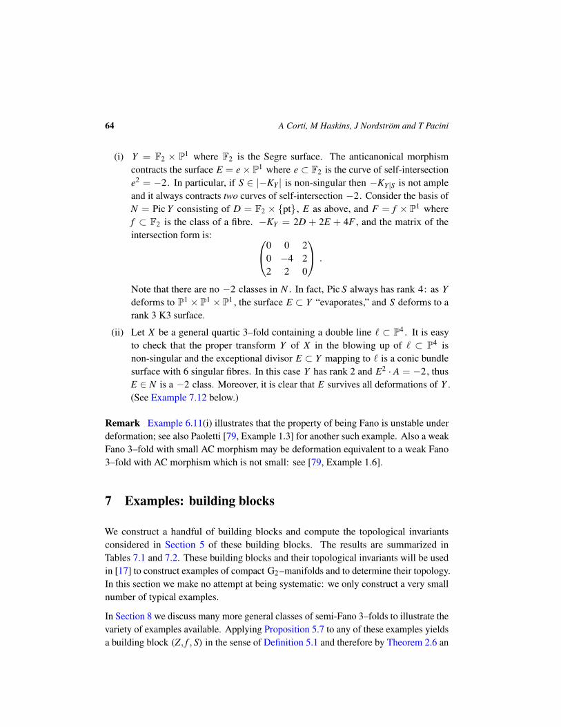
64 A Corti, M Haskins, J Nordstrom and T Pacini
(i) Y = F2 × P1 where F2 is the Segre surface. The anticanonical morphismcontracts the surface E = e× P1 where e ⊂ F2 is the curve of self-intersectione2 = −2. In particular, if S ∈ |−KY | is non-singular then −KY|S is not ampleand it always contracts two curves of self-intersection −2. Consider the basis ofN = Pic Y consisting of D = F2 × pt, E as above, and F = f × P1 wheref ⊂ F2 is the class of a fibre. −KY = 2D + 2E + 4F , and the matrix of theintersection form is: 0 0 2
0 −4 22 2 0
.
Note that there are no −2 classes in N . In fact, Pic S always has rank 4: as Ydeforms to P1 × P1 × P1 , the surface E ⊂ Y “evaporates,” and S deforms to arank 3 K3 surface.
(ii) Let X be a general quartic 3–fold containing a double line ` ⊂ P4 . It is easyto check that the proper transform Y of X in the blowing up of ` ⊂ P4 isnon-singular and the exceptional divisor E ⊂ Y mapping to ` is a conic bundlesurface with 6 singular fibres. In this case Y has rank 2 and E2 · A = −2, thusE ∈ N is a −2 class. Moreover, it is clear that E survives all deformations of Y .(See Example 7.12 below.)
Remark Example 6.11(i) illustrates that the property of being Fano is unstable underdeformation; see also Paoletti [79, Example 1.3] for another such example. Also a weakFano 3–fold with small AC morphism may be deformation equivalent to a weak Fano3–fold with AC morphism which is not small: see [79, Example 1.6].
7 Examples: building blocks
We construct a handful of building blocks and compute the topological invariantsconsidered in Section 5 of these building blocks. The results are summarized inTables 7.1 and 7.2. These building blocks and their topological invariants will be usedin [17] to construct examples of compact G2 –manifolds and to determine their topology.In this section we make no attempt at being systematic: we only construct a very smallnumber of typical examples.
In Section 8 we discuss many more general classes of semi-Fano 3–folds to illustrate thevariety of examples available. Applying Proposition 5.7 to any of these examples yieldsa building block (Z, f , S) in the sense of Definition 5.1 and therefore by Theorem 2.6 an

Asymptotically cylindrical Calabi–Yau 3–folds 65
ACyl Calabi–Yau structure on the quasiprojective 3–fold Z \S . Similar methods to thoseutilised in the present section would also allow the computation of the basic topologicalinvariants of the corresponding building blocks and ACyl Calabi–Yau 3–folds.
To construct the examples in this section typically we start with a singular Fano 3–foldX with only ordinary double points; resolve this to a non-singular semi-Fano Y andanticanonical morphism Y → X ; choose a K3 surface S and pencil in |−KY |, andresolve the indeterminacies to obtain S ⊂ Z → P1 where S is the fibre of ∞ ∈ P1 .According to Proposition 5.7, Z is a “building block” in the sense of Definition 5.1, andtherefore by Theorem 2.6, V = Z \ S admits ACyl Calabi–Yau metrics.
We compute the following topological invariants of the building blocks: the degree−K3
Y , the integral cohomology groups H2(Z) and H3(Z), the primitive sublattice N ⊂ Lof the K3 lattice, the kernel K of H2(V) → L, the greatest divisor of c2(Z), and thenumber e(Z) of (−1,−1)–curves. In examples involving small resolutions of 3–foldswith ordinary double points, all these invariants are independent of the choice of smallresolution, except possibly the greatest divisor of c2(Z) (recall Remark 5.17).
In the calculation of Hm(Z) we use Lemma 5.6; to compute b3(Y) we use Lemma 4.21;to compute c2(Z) we use Proposition 5.11. In all cases, except in Example 7.9 whichrequires some extra work, it is immediate from Proposition 5.7 that the sublattice N ⊂ Lis primitive.
Example 7.1 A class of examples, already considered in Kovalev [57], is to take Y tobe a Fano “of the first species”, that is, a member of one of the 17 deformation familiesof smooth Fano 3–folds with Picard rank 1, and let Z be the building block arising fromblowing up the (smooth) base locus of a generic transverse anticanonical pencil. Let rbe the index of Y , and d = (−1
r KY )3 the degree. Then by definition −KY = rH for Ha generator for Pic Y , and (−KY )H2 = rd . So the polarising lattice is N = 〈rd〉.
For these examples, Corollary 5.14 easily gives the greatest divisor of c2(Z). Con-sulting Iskovskih [37, Table 6.5] and Iskovskih–Prokhorov’s book [38, Table 12.2] wesummarise the values of b3(Z) and greatest divisor of c2(Z) in Table 7.1.
Example 7.2 We can also readily construct building blocks from the 36 rank 2 Fanosin the Mori–Mukai classification, but do not describe the examples in further detail here.
Examples 7.3 through 7.6 arise in a uniform way. We impose the condition that a quarticin P4 contain a special surface W : a projective plane Π, a quadric surface Q2
2 , a cubicscroll surface F and the complete intersection of two quadrics F2,2 respectively. Thegeneric such quartic X has only ODPs, the number e of which is determined by the

66 A Corti, M Haskins, J Nordstrom and T Pacini
Y r −K3Y b3(Y) b3(Z) div c2(Z)
P3 4 43 0 66 2Q2 ⊂ P4 3 33 · 2 0 56 2V1 → W4 2 23 42 52 8V2 → P3 2 23 · 2 20 38 4Q3 ⊂ P4 2 23 · 3 10 36 24V2·2 ⊂ P5 2 23 · 4 4 38 4V5 ⊂ P6 2 23 · 5 0 42 8V2 → P3 1 2 104 108 2Q4 ⊂ P4 1 4 60 66 4V2·3 ⊂ P5 1 6 40 48 6V2·2·2 ⊂ P6 1 8 28 38 8V10 ⊂ P7 1 10 20 32 2V12 ⊂ P8 1 12 14 28 12V14 ⊂ P9 1 14 10 26 2V16 ⊂ P10 1 16 6 24 8V18 ⊂ P11 1 18 4 24 6V22 ⊂ P13 1 22 0 24 2
Table 7.1: Building blocks Z from Fanos Y with Picard rank 1
special surface W imposed and all of which are contained in W . W gives us a Weildivisor on X which is not Q–Cartier; blowing up W ⊂ X as in Lemma 3.14 yields asmooth projective small resolution Y with anticanonical morphism ϕ : Y → X . Y isa smooth semi-Fano 3–fold with Picard rank ρ = 2 (so the defect σ(X) is 1) whoseintegral cohomology group H2(Y) is spanned by the anticanonical class A = −KY
and W , the proper transform of the special surface W ⊂ X . Since the anticanonicalmorphism ϕ : Y → X is small by Theorem 3.30 we can flop ϕ to obtain another smoothweak Fano Y+ with ρ(Y+) = 2; by Remark 3.31 there is a unique such flop of ϕ. Ingeneral the flop Y+ is not isomorphic to Y but shares the same topological invariantsexcept possibly for c2(Y) which we compute.
Example 7.3 (Generic AC pencil on a small resolution of a generic quartic containinga plane) The following semi-Fano also appears in work of Cheltsov [13, Lemma 25],Jahnke–Peternell–Radloff [41, 3.15] and Takeuchi [93, 2.9.6 and 6.6.6]. Fix a 2–planeΠ ⊂ P4 and let Π ⊂ X ⊂ P4 be a general quartic 3–fold containing Π. Choose

Asymptotically cylindrical Calabi–Yau 3–folds 67
homogeneous coordinates x0, . . . , x4 on P4 such that Π = (x0 = x1 = 0); thenX = (f4 = 0) is the zero locus of a homogeneous quartic in the ideal (x0, x1):
f4 = x0a3 + x1b3
where a3, b3 are degree 3 homogeneous in x0, . . . , x4 . To say that X is generalis to say that the forms a3, b3 are general; thus, X has 9 ordinary double pointsx0 = x1 = a3 = b3 = 0 – see also the remark at the end of this example. Blowing up Π
yields a non-singular semi-Fano 3–fold Y → X with e = 9 (−1,−1)–curves resolvingthe 9 ordinary double points of X on Π. We show that:
• H2(Y) = Z2 with basis Π (the proper transform of Π) and A = −KY , andquadratic form in this basis (
−2 11 4
);
• H3(Y) ' Z44 .
Below we discuss how to compute H2(Y) and H3(Y). The building block f : Z → P1
is obtained by blowing up the base locus of a pencil |S0, S∞| ⊂ |−KY | where S0, S∞are non-singular and meet transversely. The base locus is a non-singular curve C ofgenus 3 (naturally a plane quartic); hence, H3(Z) ' H3(Y)⊕ H1(C) ' Z44 ⊕ Z6 .
To calculate H2(Y) and H3(Y), we proceed as follows. First, Y is the proper transformof X in the blowup G→ P4 of the plane Π; this is the scroll with weight data
s0 s1 x2 x3 x4 x1 1 0 0 0 −10 0 1 1 1 1
with morphism to P4 given by x0 = s0x, x1 = s1x . Denoting by L the line bundle on Gwith sections s0, s1 and M the line bundle with sections x2, . . ., we see that the equationof Y ⊂ G is:
s0a3 + s1b3
that is Y ∈ |L + 3M|. Thus Y ⊂ G is an ample divisor; it then follows easily from theLefschetz theorems that the restriction H2(G)→ H2(Y) is an isomorphism and H3(Y)is torsion-free. To see this consider the long exact cohomology sequence of the pairG,Y :
· · · → Hm(G,Y)→ Hm(G)→ Hm(Y)→ Hm+1(G,Y)→ · · · ,
note that Hm(G,Y) = Hmcpt(G \ Y) = H8−m(G \ Y), and recall that the Lefschetz
homotopy dimension theorem states that G\Y has the homotopy type of a CW complex
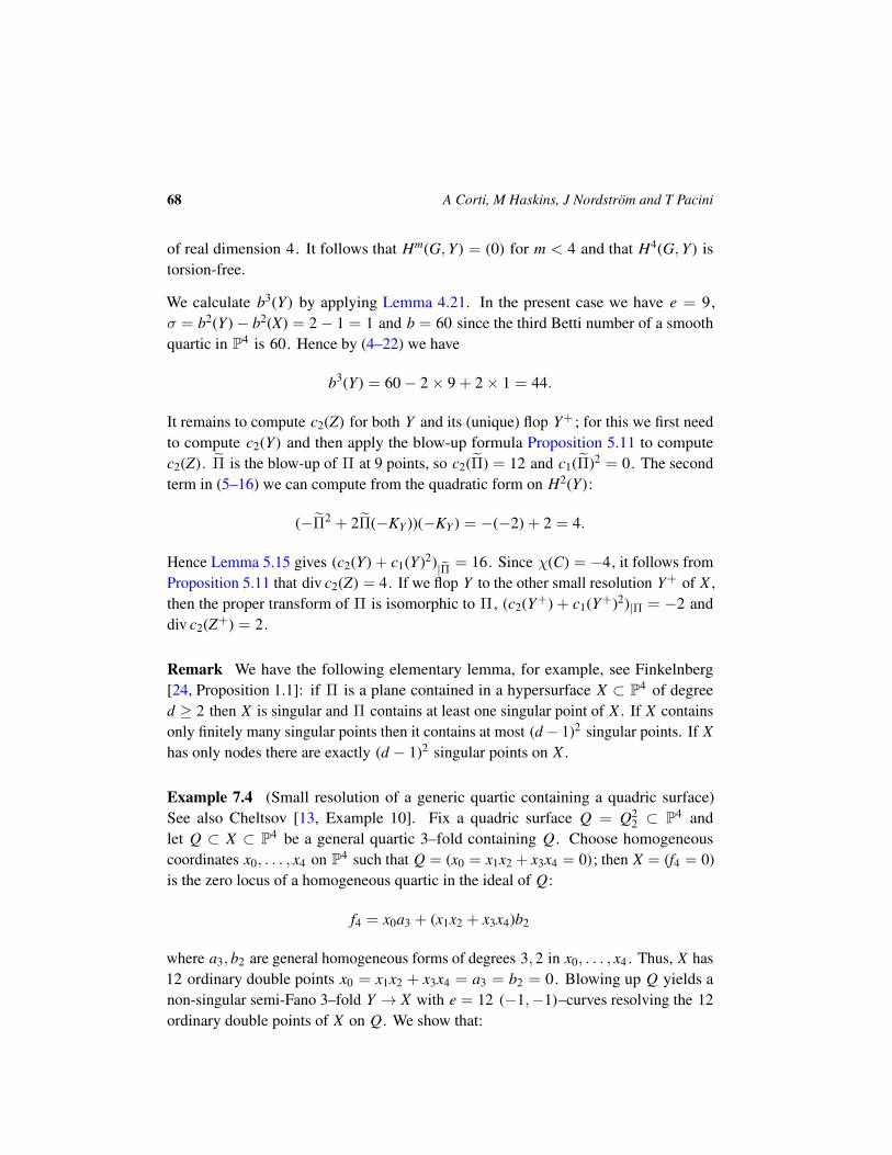
68 A Corti, M Haskins, J Nordstrom and T Pacini
of real dimension 4. It follows that Hm(G,Y) = (0) for m < 4 and that H4(G,Y) istorsion-free.
We calculate b3(Y) by applying Lemma 4.21. In the present case we have e = 9,σ = b2(Y)− b2(X) = 2− 1 = 1 and b = 60 since the third Betti number of a smoothquartic in P4 is 60. Hence by (4–22) we have
b3(Y) = 60− 2× 9 + 2× 1 = 44.
It remains to compute c2(Z) for both Y and its (unique) flop Y+ ; for this we first needto compute c2(Y) and then apply the blow-up formula Proposition 5.11 to computec2(Z). Π is the blow-up of Π at 9 points, so c2(Π) = 12 and c1(Π)2 = 0. The secondterm in (5–16) we can compute from the quadratic form on H2(Y):
(−Π2 + 2Π(−KY ))(−KY ) = −(−2) + 2 = 4.
Hence Lemma 5.15 gives (c2(Y) + c1(Y)2)|Π = 16. Since χ(C) = −4, it follows fromProposition 5.11 that div c2(Z) = 4. If we flop Y to the other small resolution Y+ of X ,then the proper transform of Π is isomorphic to Π, (c2(Y+) + c1(Y+)2)|Π = −2 anddiv c2(Z+) = 2.
Remark We have the following elementary lemma, for example, see Finkelnberg[24, Proposition 1.1]: if Π is a plane contained in a hypersurface X ⊂ P4 of degreed ≥ 2 then X is singular and Π contains at least one singular point of X . If X containsonly finitely many singular points then it contains at most (d− 1)2 singular points. If Xhas only nodes there are exactly (d − 1)2 singular points on X .
Example 7.4 (Small resolution of a generic quartic containing a quadric surface)See also Cheltsov [13, Example 10]. Fix a quadric surface Q = Q2
2 ⊂ P4 andlet Q ⊂ X ⊂ P4 be a general quartic 3–fold containing Q. Choose homogeneouscoordinates x0, . . . , x4 on P4 such that Q = (x0 = x1x2 + x3x4 = 0); then X = (f4 = 0)is the zero locus of a homogeneous quartic in the ideal of Q:
f4 = x0a3 + (x1x2 + x3x4)b2
where a3, b2 are general homogeneous forms of degrees 3, 2 in x0, . . . , x4 . Thus, X has12 ordinary double points x0 = x1x2 + x3x4 = a3 = b2 = 0. Blowing up Q yields anon-singular semi-Fano 3–fold Y → X with e = 12 (−1,−1)–curves resolving the 12ordinary double points of X on Q. We show that:
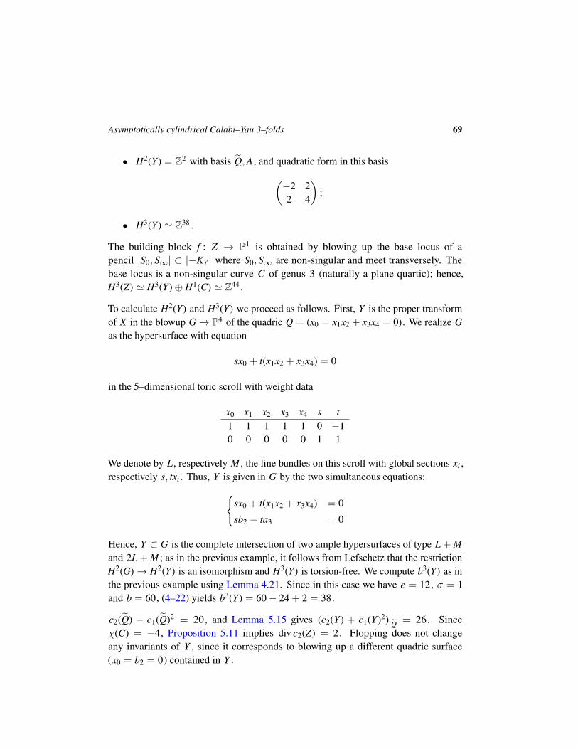
Asymptotically cylindrical Calabi–Yau 3–folds 69
• H2(Y) = Z2 with basis Q,A, and quadratic form in this basis(−2 22 4
);
• H3(Y) ' Z38 .
The building block f : Z → P1 is obtained by blowing up the base locus of apencil |S0, S∞| ⊂ |−KY | where S0, S∞ are non-singular and meet transversely. Thebase locus is a non-singular curve C of genus 3 (naturally a plane quartic); hence,H3(Z) ' H3(Y)⊕ H1(C) ' Z44 .
To calculate H2(Y) and H3(Y) we proceed as follows. First, Y is the proper transformof X in the blowup G→ P4 of the quadric Q = (x0 = x1x2 + x3x4 = 0). We realize Gas the hypersurface with equation
sx0 + t(x1x2 + x3x4) = 0
in the 5–dimensional toric scroll with weight data
x0 x1 x2 x3 x4 s t1 1 1 1 1 0 −10 0 0 0 0 1 1
We denote by L , respectively M , the line bundles on this scroll with global sections xi ,respectively s, txi . Thus, Y is given in G by the two simultaneous equations:
sx0 + t(x1x2 + x3x4) = 0
sb2 − ta3 = 0
Hence, Y ⊂ G is the complete intersection of two ample hypersurfaces of type L + Mand 2L + M ; as in the previous example, it follows from Lefschetz that the restrictionH2(G)→ H2(Y) is an isomorphism and H3(Y) is torsion-free. We compute b3(Y) as inthe previous example using Lemma 4.21. Since in this case we have e = 12, σ = 1and b = 60, (4–22) yields b3(Y) = 60− 24 + 2 = 38.
c2(Q) − c1(Q)2 = 20, and Lemma 5.15 gives (c2(Y) + c1(Y)2)|Q = 26. Sinceχ(C) = −4, Proposition 5.11 implies div c2(Z) = 2. Flopping does not changeany invariants of Y , since it corresponds to blowing up a different quadric surface(x0 = b2 = 0) contained in Y .
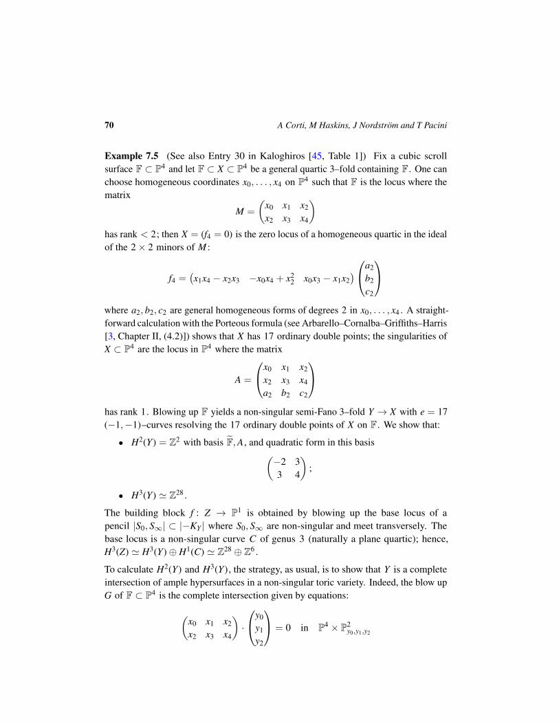
70 A Corti, M Haskins, J Nordstrom and T Pacini
Example 7.5 (See also Entry 30 in Kaloghiros [45, Table 1]) Fix a cubic scrollsurface F ⊂ P4 and let F ⊂ X ⊂ P4 be a general quartic 3–fold containing F. One canchoose homogeneous coordinates x0, . . . , x4 on P4 such that F is the locus where thematrix
M =
(x0 x1 x2
x2 x3 x4
)has rank < 2; then X = (f4 = 0) is the zero locus of a homogeneous quartic in the idealof the 2× 2 minors of M :
f4 =(x1x4 − x2x3 −x0x4 + x2
2 x0x3 − x1x2)a2
b2
c2
where a2, b2, c2 are general homogeneous forms of degrees 2 in x0, . . . , x4 . A straight-forward calculation with the Porteous formula (see Arbarello–Cornalba–Griffiths–Harris[3, Chapter II, (4.2)]) shows that X has 17 ordinary double points; the singularities ofX ⊂ P4 are the locus in P4 where the matrix
A =
x0 x1 x2
x2 x3 x4
a2 b2 c2
has rank 1. Blowing up F yields a non-singular semi-Fano 3–fold Y → X with e = 17(−1,−1)–curves resolving the 17 ordinary double points of X on F. We show that:
• H2(Y) = Z2 with basis F,A, and quadratic form in this basis(−2 33 4
);
• H3(Y) ' Z28 .
The building block f : Z → P1 is obtained by blowing up the base locus of apencil |S0, S∞| ⊂ |−KY | where S0, S∞ are non-singular and meet transversely. Thebase locus is a non-singular curve C of genus 3 (naturally a plane quartic); hence,H3(Z) ' H3(Y)⊕ H1(C) ' Z28 ⊕ Z6 .
To calculate H2(Y) and H3(Y), the strategy, as usual, is to show that Y is a completeintersection of ample hypersurfaces in a non-singular toric variety. Indeed, the blow upG of F ⊂ P4 is the complete intersection given by equations:(
x0 x1 x2
x2 x3 x4
)·
y0
y1
y2
= 0 in P4 × P2y0,y1,y2
Asymptotically cylindrical Calabi–Yau 3–folds 71
and Y is given in G by the equation:
a2y0 + b2y1 + c2y2 = 0.
Thus, Y is the complete intersection of 3 ample hypersurfaces in P4 × P2 . Everythingelse from now on proceeds as in the previous examples. Since e = 17, σ = 1 andb = 60, (4–22) yields b3(Y) = 60− 34 + 2 = 28.
F is P2 blown up in 1 point, and F is F blown up in 17 points. Lemma 5.15 gives(c2(Y) + c1(Y)2)|F = 38. Hence div c2(Z) = 2 by Proposition 5.11. In the othersmall resolution Y+ of X , the proper transform of F is isomorphic to F. There(c2(Y+) + c1(Y+)2)|F = 4 and div c2(Z+) = 4.
Example 7.6 (See also Cheltsov [13, Theorem 11, Lemma 21], Jahnke–Peternell–Radloff [41, 3.9.II.6.a], Kaloghiros [47, Example 3.9], and Takeuchi [93, 2.11.10].)Fix the complete intersection of two quadrics F = F2,2 ⊂ P4 (that is, a del Pezzosurface of degree 4) and let F ⊂ X ⊂ P4 be a general quartic 3–fold containing F .In homogeneous coordinates x0, . . . , x4 on P4 , F = (p2 = q2 = 0) where p2, q2 aregeneral homogeneous quadratic polynomials; then X = (f4 = 0) is the zero locus of ahomogeneous quartic in the ideal of F :
f4 = p2a2 + q2b2
where a2, b2 are general homogeneous quadratic forms in x0, . . . , x4 . Thus, X has 16ordinary double points p2 = q2 = a2 = b2 = 0. Blowing up F yields a non-singularsemi-Fano 3–fold Y → X with e = 16 (−1,−1)–curves resolving the 16 ordinarydouble points of X on F . By using the methods described in the previous examples, itis easy enough to show that:
• H2(Y) = Z2 with basis F,A, and quadratic form in this basis(0 44 4
);
• H3(Y) ' Z30 .
The building block f : Z → P1 is obtained by blowing up the base locus of apencil |S0, S∞| ⊂ |−KY | where S0, S∞ are non-singular and meet transversely. Thebase locus is a non-singular curve C of genus 3 (naturally a plane quartic); hence,H3(Z) ' H3(Y)⊕ H1(C) ' Z30 ⊕ Z6 .
Proposition 5.11 implies div c2(Z) = 4, using (c2(Y) + c1(Y)2)|F = 44. Flopping doesnot change any invariants of Y , since it corresponds to blowing up another completeintersection of quadrics (p2 = q2 = 0) contained in X .
72 A Corti, M Haskins, J Nordstrom and T Pacini
For the next example we again consider a weak Fano 3–fold Y whose AC model isa nodal quartic X ⊂ P4 but in this case with the maximal number of possible nodes(which is 45); such an X is unique up to projective equivalence. It is a classical factthat X admits projective small resolutions Y . Unlike the previous four examples inwhich ρ(Y) = 2 in this case we will show that ρ(Y) = 16 and hence X has defectσ = 15, that is, X contains many Weil divisors that are not Q–Cartier; by a result ofKaloghiros [46], 15 is also the maximal possible defect for any quartic in P4 with onlyterminal singularities. Because of the high Picard rank of Y the computation of thelattice structure on H2(Y) is considerably more involved in this case. As far as we knowthe number of distinct projective small resolutions of Y has not been computed in thiscase.
Example 7.7 The Burkhardt quartic 3–fold is the hypersurface
X =(x4
0 − x0(x31 + x3
2 + x33 + x3
4) + 3x1x2x3x4 = 0)⊂ P4.
It is well known (and one can verify by inspection), that: X contains 40 planes, has 45ordinary nodes as singularities, defect σ = 15, and several projective small resolutions.(See Finkelnberg’s thesis [25] for these and other facts on the Burkhardt quartic.)Below we take one such projective small resolution Y → X , and make a buildingblock f : Z → P1 by blowing up the (non-singular) base curve of a general pencil|S0, S∞| ⊂ |−KY |. In what follows, we establish the following facts about X , Y , and Z :
• Write N = H4(X) with the integral quadratic form
D1,D2 7→ q(D1,D2) = (−KX) · D1 · D2.
Then: N is a hyperbolic lattice of rank 16; N is 3–elementary; more precisely,the discriminant of N is (Z/3Z)5 (thus ` = 5); and, finally:
N ∼= E∗6(−3) ⊥ E8(−1) ⊥ U .
(Here U is the rank 2 hyperbolic lattice, while E∗6 is the dual lattice of thelattice E6 . In other words, if B is the intersection matrix for E6 , then B−1 isthe intersection matrix for E∗6 . In particular B−1 is not an integer matrix: ithas entries in 1
3Z; however, E∗6(−3) is an integral lattice. Since E6 has rank 6and discriminant Z/3Z, it immediately follows that E∗6(−3) has discriminant(Z/3Z)5 , which of course can also be checked by direct computation.)
• The embedding N ⊂ L in the K3 lattice L is unique, and N⊥ = T = A2(−1) ⊥2U(3), where A2(−1) and U(3) denote the rank 2 lattices with intersection forms(
−2 11 −2
)and
(0 33 0
).
Asymptotically cylindrical Calabi–Yau 3–folds 73
• All projective small resolutions Y → X have 45 (−1,−1)–curves, H2(Y) ∼= N ,and H3(Y) = (0).
• Let f : Z → Y be the blow up of the base locus of a pencil |S0, S∞| ⊂ |−KY |where S0 , S∞ are non-singular and meet transversely. Then Z is a building blockwith H2(Z) = Z17 , H3(Z) = Z6 .
We now prove all of these claims. Todd [97] gives an explicit birational map P3 99K X .Resolving this map by explicit blow ups, Finkelnberg [25] constructs a small resolutionY → X and a basis of H4(Y) consisting of planes. His notation for this basis is:
V, Ek1, Ek
2, Ek3, El
1, El2, El
3, Em1 , Em
2 , Em3 , F1
1, F12, F2
1, F22, F3
1, F32
Finkelnberg also makes a list of the curves contracted by Y → X ; using this information,it is not difficult (though tedious) to write down the matrix of the intersection form onH4(Y) in this basis:
−2 0 0 0 0 0 0 0 0 0 1 1 1 1 1 10 −2 0 0 1 0 0 0 0 1 0 1 0 0 0 0
−2 0 0 1 0 1 0 0 0 1 0 0 0 0−2 0 0 1 0 1 0 0 1 0 0 0 0
−2 0 0 1 0 0 0 0 0 1 0 0−2 0 0 1 0 0 0 0 1 0 0
−2 0 0 1 0 0 0 1 0 0−2 0 0 0 0 0 0 0 1
−2 0 0 0 0 0 0 1−2 0 0 0 0 0 1
−2 1 0 0 0 0−2 0 0 0 0
−2 1 0 0−2 0 0
−2 1−2
From this it is easy to compute (for example, by computer algebra) that the discriminantA ∼= (Z/3Z)5 . Recall that, for p prime, a lattice is said to be p–elementary if thediscriminant is of the form (Z/pZ)` : we have just shown that N is 3–elementarywith ` = 5. Rudakov and Shafarevich [87, Section 1, Theorem] prove that an even,hyperbolic (meaning it has signature (1, r − 1)), p–elementary for p 6= 2 prime, latticeof rank ≥ 3 is uniquely determined by its discriminant (that is, equivalently, the invariant`). This implies that
N ∼= E∗6(−3) ⊥ E8(−1) ⊥ U .
74 A Corti, M Haskins, J Nordstrom and T Pacini
The proof of [87, Section 1, Theorem] goes through, with the appropriate smallmodifications, for lattices of any indefinite signature. This implies that the transcendentallattice
T = N⊥ ∼= A2(−1) ⊥ 2U(3) ,
as this is the unique lattice with signature (2, 4) and discriminant (Z/3Z)5 . ByDolgachev [20, Theorem 1.4.8], the fact that rk T + `(T) + 2 ≤ rk L implies theprimitive embedding T ⊂ L is unique up to automorphisms, and so the same is true forthe embedding N ⊂ L (note that rk N + `(N) + 2 > rk L , so [20, Theorem 1.4.8] doesnot apply directly to N ).
All other assertions are straightforward.
We can compute div c2(Z) by evaluating it on the basis of planes. If the proper transformin Y of some plane remains a plane (that is, no points are blown up on the plane) then thatforces div c2(Z) = 2 like in Example 7.3. This is easy to arrange. For instance choosea plane Π ⊂ X and let Y ′ = Proj
(⊕n≥0OX(nΠ)
)→ X . Then the proper transform
Π′ ⊂ Y is relatively ample and isomorphic to Π and therefore Y ′ is non-singular in aneighbourhood of Π′ . Let next Y → Y ′ be a small resolution of Y ′ : this does not alterY ′ in a neighbourhood of Π′ , hence the proper transform of Π in Y is still isomorphicto P2 .
The next pair of examples consider building blocks slightly different from those above.They are obtained by blowing up the base locus of a nongeneric AC pencil on thesimplest smooth Fano 3–fold Y = P3 .
Example 7.8 (compare with Kovalev–Lee [58, Example 2.7]) Instead of a generictransverse pencil we consider the pencil |S0, S∞| ⊂ |O(4)|, where S0=(x0x1x2x3=0)is the sum of the four coordinate planes, and S∞ is a non-singular quartic surfacemeeting all coordinate planes transversely. The base curve of the pencil is the unionC =
∑3i=0 Γi of the four non-singular curves Γi = (xi = 0) ∩ S∞ . Let Z be obtained
from Y = P3 by blowing up the four base curves one at a time; Z is a non-singularbuilding block containing e = 6× 4 = 24 (−1,−1)–curves; the blow-up resolves thebase locus of the pencil, which then defines a (projective) morphism Z → P1 . It is clearthat H2(Z) ' H2(P3) ⊕
⊕3i=0H0(Γi) ' Z5 and, since each Γi is a curve of genus 3,
H3(Z) '⊕3
i=0H1(Γi) ' Z24 .
The image of H2(Z) in H2(S) equals the image of H2(P3), that is, it is generated bythe hyperplane class. This is because the image of each exceptional divisor is justthe hyperplane class, so they contribute only to the kernel K of H2(V) → H2(S),

Asymptotically cylindrical Calabi–Yau 3–folds 75
which is Z3 . Since c2(P3) + c1(P3)2 = 22H2 while −K3P3 = 64, it follows from
Proposition 5.11 that div c2(Z) = 2.
Example 7.9 We can also consider a pencil of anticanonical divisors in Y = P3 whereeach divisor is non-generic. Fix a pair of generic plane conics C1,C2 ⊂ P3 . It is easyto see that a generic quartic surface S containing both C1 and C2 is non-singular. Thecurves C1 , C2 and the hyperplane class generate a lattice N ⊂ H2(S) with intersectionform represented by −2 0 2
0 −2 22 2 4
.
We next argue that N ⊂ H2(S) is a primitive sublattice. Indeed consider the blow up Y ′
of P3 along C1tC2 . Since the union C1tC2 is cut out scheme theoretically by quartics,it follows that the anticanonical linear system |−KY′ | = |IC1tC2(4)| is base point freeon Y ′ and hence −KY′ is nef. A small calculation gives −K3
Y′ = 64 − 36 = 28 so−KY′ is also big and Y ′ is a weak Fano 3–fold. It is clear from the construction thatN is the image of H2(Y ′)→ H2(S), hence, in particular, H2(Y ′)→ H2(S) is injective(the matrix above is non-singular). This implies that Y ′ is a semi-Fano 3–fold (anycontracted divisor would lie in the kernel). The lattice N ⊂ H2(S) is therefore primitiveby Proposition 5.7.
Now take a generic pencil of quartic K3s containing both C1 and C2 . The base locusconsists of C1 , C2 and a degree 12 curve C3 (of genus 15) meeting each of C1 andC2 in 10 points. Let Z be obtained by blowing up the Ci in any order, and S theproper transform of a smooth element of the pencil. Then (Z, S) is a building block.H2(Z)→ L maps onto N , and H2(V)→ L is injective. Regardless of the order of theblow-ups, div c2(Z) = 2 like in the previous example.
By varying C1 , C2 and the pencils, we get three different families of blocks, dependingon whether we blow up C3 first, second or last. By Theorem 6.8, a generic N –polarisedK3 surface S can be embedded as an anticanonical divisor in a deformation of Y ′ , andhence as a quartic K3 in P3 containing a pair of conics. It will therefore occur as theK3 fibre of a building block in each of the three families.
The next pair of examples arise from blowing up AC pencils on a projective smallresolution Y of a very particular terminal Gorenstein toric Fano 3–fold X22 . X22 is asingular Fano 3–fold with Picard rank 1, AC degree 22 and 9 ODPs. Every Gorensteintoric Fano variety X has an associated combinatorial object called a reflexive polytopewhich determines X ; see Chapters 1 and 2 in the thesis of Nill [76] for a review of basic

76 A Corti, M Haskins, J Nordstrom and T Pacini
definitions and facts in toric Fano geometry. See also Section 8 for a brief overview ofbasic properties of toric weak Fano 3–folds in general.
All such 3d reflexive polytopes and hence all Gorenstein toric Fano 3–folds wereclassified by Kreuzer–Skarke [59]. The terminal toric Fano 3–folds are precisely thosereflexive polytopes whose facets are either standard triangles or standard parallelograms(see Lemma 8.10). Small resolutions of X are also toric and their projectivity can beseen in terms of the combinatorics of the associated reflexive polytope; in particularone can prove that any Gorenstein toric Fano 3–fold admits at least one projective smallresolution (see Proposition 8.7). For the toric Fano 3–fold X22 chosen in Examples 7.10and 7.11 one can prove that all 512 = 29 possible small resolutions of X are projective(this follows from the fact, shown below, that the defect σ(X) = 9 is equal to the numberof nodes of X ); using computer algebra one can show that these 512 projective smallresolutions consist of 84 distinct isomorphism classes of weak Fano 3–folds; see alsoRemark 8.13.
For any toric weak Fano 3–fold Y all odd cohomology groups vanish; in particularwe never have to worry about the possibility of torsion in H3(Y) for toric weak Fano3–folds. Toric semi-Fano 3–folds therefore give rise to a very large number of buildingblocks.
Example 7.10 Let X be the terminal Gorenstein toric Fano 3–fold with Fano polytopethe reflexive polytope in N = Hom(C×,T) with vertices 1 0 0 −1 1 1 −1 −1 −1 1 0 0 0
0 1 0 1 0 −1 1 0 0 −1 0 −1 −10 0 1 1 −1 0 0 1 0 −1 −1 0 −1
;
this is polytope 1942 in the Sage implementation of Kreuze–Skarke’s database of 4319reflexive polytopes in 3 dimensions. X has Picard rank 1 = rk H2(X) and 10 = rk H4(X).The polytope can be viewed in Sage (see also below). (Note, incidentally, that thepolytope is self-polar: thus, there is no point in wasting your efforts trying to determinewhether you are working in the fan picture or its dual: your conclusions will be correctin either case.) Direct inspection shows that X has a toric projective small semi-Fanoresolution Y → X with e = 9 (−1,−1)–curves resolving the ordinary nodes of X .Note that the defect σ = e = 9. Below we show that H2(Y) = Z10 and
N = E8(−1) ⊥ 〈8〉 ⊥ 〈−16〉
and H3(Y) = (0) since Y is a toric variety. The building block f : Z → P1 isobtained blowing up the base locus of a pencil |S0, S∞| ⊂ |−KY | where S0, S∞ are
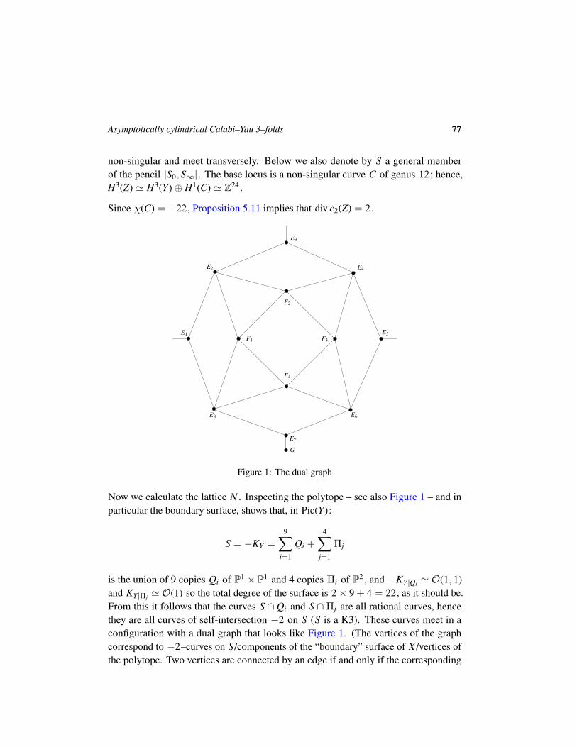
Asymptotically cylindrical Calabi–Yau 3–folds 77
non-singular and meet transversely. Below we also denote by S a general memberof the pencil |S0, S∞|. The base locus is a non-singular curve C of genus 12; hence,H3(Z) ' H3(Y)⊕ H1(C) ' Z24 .
Since χ(C) = −22, Proposition 5.11 implies that div c2(Z) = 2.
E4
F2
F4
E2
F3
E5
E7
G
E1
E8 E6
E3
F1
Figure 1: The dual graph
Now we calculate the lattice N . Inspecting the polytope – see also Figure 1 – and inparticular the boundary surface, shows that, in Pic(Y):
S = −KY =
9∑i=1
Qi +
4∑j=1
Πj
is the union of 9 copies Qi of P1 × P1 and 4 copies Πi of P2 , and −KY|Qi ' O(1, 1)and KY|Πj ' O(1) so the total degree of the surface is 2× 9 + 4 = 22, as it should be.From this it follows that the curves S ∩ Qi and S ∩ Πj are all rational curves, hencethey are all curves of self-intersection −2 on S (S is a K3). These curves meet in aconfiguration with a dual graph that looks like Figure 1. (The vertices of the graphcorrespond to −2–curves on S/components of the “boundary” surface of X /vertices ofthe polytope. Two vertices are connected by an edge if and only if the corresponding
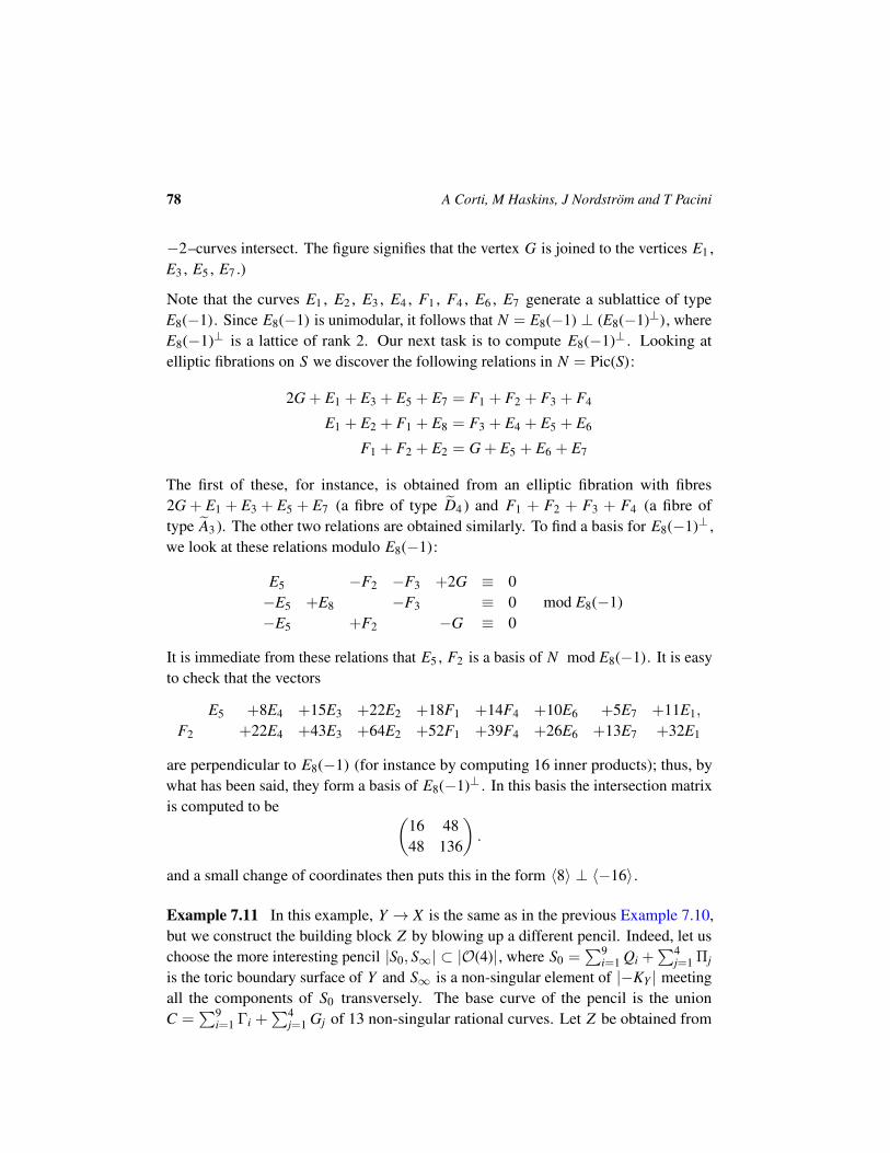
78 A Corti, M Haskins, J Nordstrom and T Pacini
−2–curves intersect. The figure signifies that the vertex G is joined to the vertices E1 ,E3 , E5 , E7 .)
Note that the curves E1 , E2 , E3 , E4 , F1 , F4 , E6 , E7 generate a sublattice of typeE8(−1). Since E8(−1) is unimodular, it follows that N = E8(−1) ⊥ (E8(−1)⊥), whereE8(−1)⊥ is a lattice of rank 2. Our next task is to compute E8(−1)⊥ . Looking atelliptic fibrations on S we discover the following relations in N = Pic(S):
2G + E1 + E3 + E5 + E7 = F1 + F2 + F3 + F4
E1 + E2 + F1 + E8 = F3 + E4 + E5 + E6
F1 + F2 + E2 = G + E5 + E6 + E7
The first of these, for instance, is obtained from an elliptic fibration with fibres2G + E1 + E3 + E5 + E7 (a fibre of type D4 ) and F1 + F2 + F3 + F4 (a fibre oftype A3 ). The other two relations are obtained similarly. To find a basis for E8(−1)⊥ ,we look at these relations modulo E8(−1):
E5 −F2 −F3 +2G ≡ 0−E5 +E8 −F3 ≡ 0−E5 +F2 −G ≡ 0
mod E8(−1)
It is immediate from these relations that E5 , F2 is a basis of N mod E8(−1). It is easyto check that the vectors
E5 +8E4 +15E3 +22E2 +18F1 +14F4 +10E6 +5E7 +11E1,
F2 +22E4 +43E3 +64E2 +52F1 +39F4 +26E6 +13E7 +32E1
are perpendicular to E8(−1) (for instance by computing 16 inner products); thus, bywhat has been said, they form a basis of E8(−1)⊥ . In this basis the intersection matrixis computed to be (
16 4848 136
).
and a small change of coordinates then puts this in the form 〈8〉 ⊥ 〈−16〉.
Example 7.11 In this example, Y → X is the same as in the previous Example 7.10,but we construct the building block Z by blowing up a different pencil. Indeed, let uschoose the more interesting pencil |S0, S∞| ⊂ |O(4)|, where S0 =
∑9i=1 Qi +
∑4j=1 Πj
is the toric boundary surface of Y and S∞ is a non-singular element of |−KY | meetingall the components of S0 transversely. The base curve of the pencil is the unionC =
∑9i=1 Γi +
∑4j=1 Gj of 13 non-singular rational curves. Let Z be obtained from

Asymptotically cylindrical Calabi–Yau 3–folds 79
Y by blowing up the 13 curves one at a time; Z is a non-singular building blockcontaining e = 9 + 24 = 33 (−1,−1)–curves: 9 that were present in Y , and 24 fromthe intersection points of C (corresponding to edges in Figure 1). The blow-up resolvesthe base locus of the pencil, which then defines a (projective) morphism Z → P1 . It isclear that H2(Z) ' H2(Y)⊕ Z13 ' Z23 and H3(Z) = (0).
From Proposition 5.11, div c2(Z) | (−K3Y ) = 22. Since also div c2(Z) | 24, it must be 2.
Example 7.12 Now we give an example using a semi-Fano 3–fold whose anticanonicalmorphism is not small, but contracts a divisor to a curve. Let X ⊂ P4 be defined by∑
0≤i≤j≤2
XiXjQij,
where Qij are homogeneous quadrics. This is the general form of a quartic “containinga double line” ` = X0 = X1 = X2 = 0. For generic Qij , the sextic polynomialdet(Qij) on ` has simple zeros, and the blow-up Y of X at ` is smooth, compare withConte–Murre [16, Lemma 1.15]. Then Y is a crepant resolution of X , and X is theanticanonical model of Y . In particular, Y is semi-Fano.
A generic hyperplane section S of Y is the resolution of a quartic K3 with a single node,so N = Pic S = 〈4〉 ⊥ 〈−2〉.
To understand more about the topology of Y , consider it as the proper transform of Xin G, the blow-up of P4 in `. Thinking of G as the union of all planes containing `identifies it with the total space of a P2 –bundle over P2 . To be precise, π : G→ P2 isthe projectivisation of V = 2O ⊕O(−1) on P2 . Let T be the associated tautologicalbundle on G, and F = π∗O(1). The exceptional divisor of G→ P4 is E = −T − F ,while the tautological bundle on P4 pulls back to T . Therefore Y is a section of−4T − 2E = −2T + 2F (so Y is a conic bundle over P2 ). This is an ample class(−T and F span the nef cone of G), so H3(Y) is torsion-free by the Lefschetz theorem,and we can apply Proposition 5.7 to get a building block Z .
To compute characteristic classes of Y , first note that as a complex vector bundleTG = TvertG ⊕ π∗TP2 , which is stably isomorphic to (T−1 ⊗ π∗V) ⊕ π∗(3O(1)) =
2T−1 ⊕ T−1F−1 ⊕ 3F . Therefore the total Chern class of Y is
c(Y) = (1− T)2(1− T − F)(1 + F)3 11− 2T + 2F
= 1− T + T2 − 5FT + T3 − 4FT2 + 7F2T,
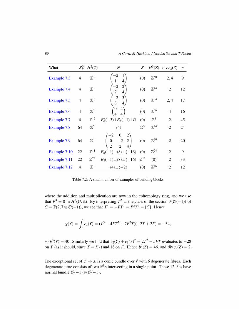
80 A Corti, M Haskins, J Nordstrom and T Pacini
What −K3Y H2(Z) N K H3(Z) div c2(Z) e
Example 7.3 4 Z3(−2 11 4
)(0) Z50 2, 4 9
Example 7.4 4 Z3(−2 22 4
)(0) Z44 2 12
Example 7.5 4 Z3(−2 33 4
)(0) Z34 2, 4 17
Example 7.6 4 Z3(
0 44 4
)(0) Z36 4 16
Example 7.7 4 Z17 E∗6(−3)⊥E8(−1)⊥U (0) Z6 2 45
Example 7.8 64 Z5 〈4〉 Z3 Z24 2 24
Example 7.9 64 Z4
−2 0 20 −2 22 2 4
(0) Z30 2 20
Example 7.10 22 Z11 E8(−1)⊥〈8〉⊥〈−16〉 (0) Z24 2 9
Example 7.11 22 Z23 E8(−1)⊥〈8〉⊥〈−16〉 Z12 (0) 2 33
Example 7.12 4 Z3 〈4〉⊥〈−2〉 (0) Z46 2 12
Table 7.2: A small number of examples of building blocks
where the addition and multiplication are now in the cohomology ring, and we usethat F3 = 0 in H6(G;Z). By interpreting T2 as the class of the section P(O(−1)) ofG = P(2O ⊕O(−1)), we see that T4 = −FT3 = F2T2 = [G]. Hence
χ(Y) =
∫Y
c3(Y) = (T3 − 4FT2 + 7F2T)(−2T + 2F) = −34,
so b3(Y) = 40. Similarly we find that c2(Y) + c1(Y)2 = 2T2 − 5FT evaluates to −28on T (as it should, since T = KY ) and 18 on F . Hence b3(Z) = 46, and div c2(Z) = 2.
The exceptional set of Y → X is a conic bundle over ` with 6 degenerate fibres. Eachdegenerate fibre consists of two P1 s intersecting in a single point. These 12 P1 s havenormal bundle O(−1)⊕O(−1).
Asymptotically cylindrical Calabi–Yau 3–folds 81
8 Weak Fano 3–folds: further examples and partial classifi-cation results
In this section we give some further examples of weak Fano 3–folds. Our aim is toback up our statement that there are many more non-singular weak Fano 3–folds thannon-singular Fano 3–folds. We will not be too systematic since weak Fano 3–folds arefar from being classified.
Any weak Fano Y for which −KY is big and nef but not ample has
ρ(Y) = rk Pic(Y) ≥ 2;
thus weak Fano 3–folds with ρ = 2 are the simplest class of weak Fano 3–folds that arenot actually Fano 3–folds.
Examples 7.3 to 7.6 already gave a small number of semi-Fano 3–folds with Picard rankρ = 2: all of anticanonical degree 4 obtained by a small resolution of a (sufficientlygeneric) quartic containing a special surface; Examples 4.15 and 4.16 are toric weakFano 3–folds with ρ = 2. As we will discuss below there are many other weak Fano3–folds that generalise both classes of examples: toric or ρ = 2.
For the purposes of the differential geometry of ACyl Calabi–Yau 3–folds, we are inter-ested in the classification of weak Fano 3–folds up to deformation. In Example 6.11(i)we considered how the semi-Fano F2 × P1 can deform to the rigid Fano P1 × P1 × P1 ;these are different varieties from the algebraic point of view as one is Fano and the otheris not, but the ACyl Calabi–Yau 3–folds we construct from them using Proposition 4.24are deformation-equivalent. We will not discuss the problem of classifying weak Fano3–folds up to deformation in depth. We use the deformation properties of extremalcontractions to distinguish between many of the rank two examples we describe. Forthe toric examples, we determine whether they are rigid (as complex manifolds) in orderto get a crude lower bound on the number of deformation classes.
Weak Fano 3–folds with Picard rank ρ = 2: classical examples
We now exhibit some further concrete examples of weak Fano 3–folds with Picardrank ρ = 2. These weak Fanos were studied initially because of their connection toso-called elementary rational maps between rank one Fano 3–folds, for example, seeIskovskih–Prokhorov’s book [38, Section 4.1] to which we refer the reader for furtherdetails and references. All these rank two weak Fano 3–folds arise as blowups in pointsor in low degree curves in rank one Fano 3–folds.
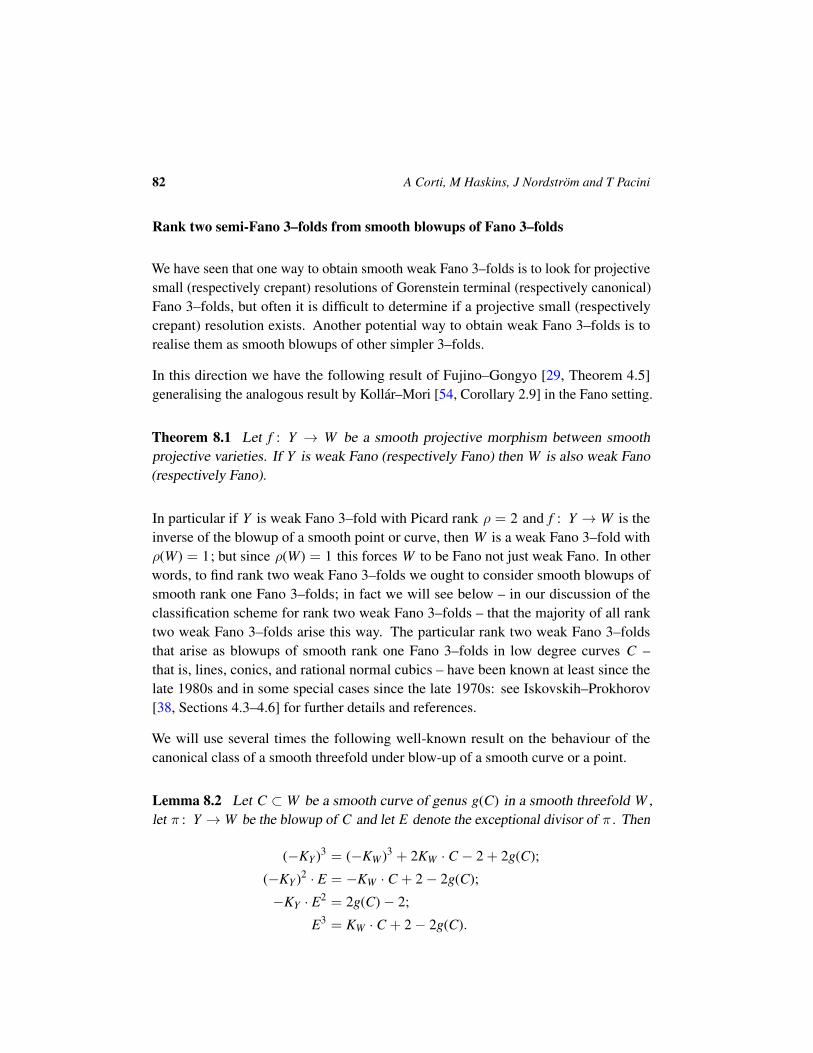
82 A Corti, M Haskins, J Nordstrom and T Pacini
Rank two semi-Fano 3–folds from smooth blowups of Fano 3–folds
We have seen that one way to obtain smooth weak Fano 3–folds is to look for projectivesmall (respectively crepant) resolutions of Gorenstein terminal (respectively canonical)Fano 3–folds, but often it is difficult to determine if a projective small (respectivelycrepant) resolution exists. Another potential way to obtain weak Fano 3–folds is torealise them as smooth blowups of other simpler 3–folds.
In this direction we have the following result of Fujino–Gongyo [29, Theorem 4.5]generalising the analogous result by Kollar–Mori [54, Corollary 2.9] in the Fano setting.
Theorem 8.1 Let f : Y → W be a smooth projective morphism between smoothprojective varieties. If Y is weak Fano (respectively Fano) then W is also weak Fano(respectively Fano).
In particular if Y is weak Fano 3–fold with Picard rank ρ = 2 and f : Y → W is theinverse of the blowup of a smooth point or curve, then W is a weak Fano 3–fold withρ(W) = 1; but since ρ(W) = 1 this forces W to be Fano not just weak Fano. In otherwords, to find rank two weak Fano 3–folds we ought to consider smooth blowups ofsmooth rank one Fano 3–folds; in fact we will see below – in our discussion of theclassification scheme for rank two weak Fano 3–folds – that the majority of all ranktwo weak Fano 3–folds arise this way. The particular rank two weak Fano 3–foldsthat arise as blowups of smooth rank one Fano 3–folds in low degree curves C –that is, lines, conics, and rational normal cubics – have been known at least since thelate 1980s and in some special cases since the late 1970s: see Iskovskih–Prokhorov[38, Sections 4.3–4.6] for further details and references.
We will use several times the following well-known result on the behaviour of thecanonical class of a smooth threefold under blow-up of a smooth curve or a point.
Lemma 8.2 Let C ⊂ W be a smooth curve of genus g(C) in a smooth threefold W ,let π : Y → W be the blowup of C and let E denote the exceptional divisor of π . Then
(−KY )3 = (−KW)3 + 2KW · C − 2 + 2g(C);
(−KY )2 · E = −KW · C + 2− 2g(C);
−KY · E2 = 2g(C)− 2;
E3 = KW · C + 2− 2g(C).
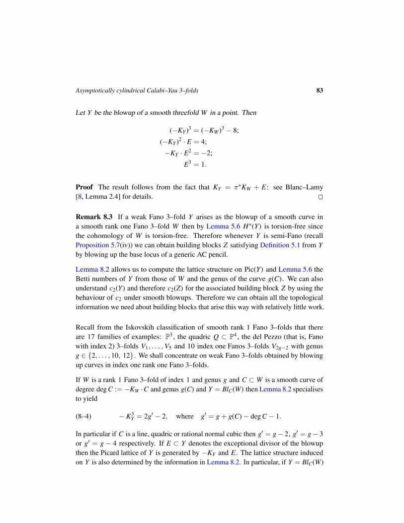
Asymptotically cylindrical Calabi–Yau 3–folds 83
Let Y be the blowup of a smooth threefold W in a point. Then
(−KY )3 = (−KW)3 − 8;
(−KY )2 · E = 4;
−KY · E2 = −2;
E3 = 1.
Proof The result follows from the fact that KY = π∗KW + E : see Blanc–Lamy[8, Lemma 2.4] for details.
Remark 8.3 If a weak Fano 3–fold Y arises as the blowup of a smooth curve ina smooth rank one Fano 3–fold W then by Lemma 5.6 H∗(Y) is torsion-free sincethe cohomology of W is torsion-free. Therefore whenever Y is semi-Fano (recallProposition 5.7(iv)) we can obtain building blocks Z satisfying Definition 5.1 from Yby blowing up the base locus of a generic AC pencil.
Lemma 8.2 allows us to compute the lattice structure on Pic(Y) and Lemma 5.6 theBetti numbers of Y from those of W and the genus of the curve g(C). We can alsounderstand c2(Y) and therefore c2(Z) for the associated building block Z by using thebehaviour of c2 under smooth blowups. Therefore we can obtain all the topologicalinformation we need about building blocks that arise this way with relatively little work.
Recall from the Iskovskih classification of smooth rank 1 Fano 3–folds that thereare 17 families of examples: P3 , the quadric Q ⊂ P4 , the del Pezzo (that is, Fanowith index 2) 3–folds V1, . . . ,V5 and 10 index one Fanos 3–folds V2g−2 with genusg ∈ 2, . . . , 10, 12. We shall concentrate on weak Fano 3–folds obtained by blowingup curves in index one rank one Fano 3–folds.
If W is a rank 1 Fano 3–fold of index 1 and genus g and C ⊂ W is a smooth curve ofdegree deg C := −KW ·C and genus g(C) and Y = BlC(W) then Lemma 8.2 specialisesto yield
(8–4) − K3Y = 2g′ − 2, where g′ = g + g(C)− deg C − 1.
In particular if C is a line, quadric or rational normal cubic then g′ = g− 2, g′ = g− 3or g′ = g − 4 respectively. If E ⊂ Y denotes the exceptional divisor of the blowupthen the Picard lattice of Y is generated by −KY and E . The lattice structure inducedon Y is also determined by the information in Lemma 8.2. In particular, if Y = BlC(W)
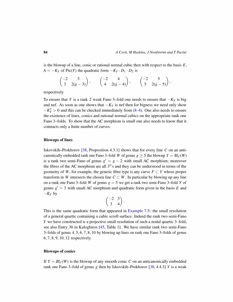
84 A Corti, M Haskins, J Nordstrom and T Pacini
is the blowup of a line, conic or rational normal cubic then with respect to the basis E ,A = −KY of Pic(Y) the quadratic form −KY · D1 · D2 is(
−2 33 2(g− 3)
),
(−2 44 2(g− 4)
),
(−2 55 2(g− 5)
),
respectively.
To ensure that Y is a rank 2 weak Fano 3–fold one needs to ensure that −KY is bigand nef. As soon as one shows that −KY is nef then for bigness we need only show−K3
Y > 0 and this can be checked immediately from (8–4). One also needs to ensurethe existence of lines, conics and rational normal cubics on the appropriate rank oneFano 3–folds. To show that the AC morphism is small one also needs to know that itcontracts only a finite number of curves.
Blowups of lines
Iskovskih–Prokhorov [38, Proposition 4.3.1] shows that for every line C on an anti-canonically embedded rank one Fano 3–fold W of genus g ≥ 5 the blowup Y = BlC(W)is a rank two semi-Fano of genus g′ = g − 2 with small AC morphism; moreoverthe fibres of the AC morphism are all P1 s and they can be understood in terms of thegeometry of W , for example, the generic fibre type is any curve F ⊂ Y whose propertransform in W intersects the chosen line C ⊂ W . In particular by blowing up any lineon a rank one Fano 3–fold W of genus g = 5 we get a rank two semi-Fano 3–fold Y ofgenus g′ = 3 with small AC morphism and quadratic form given in the basis E and−KY by (
−2 33 4
).
This is the same quadratic form that appeared in Example 7.5: the small resolutionof a general quartic containing a cubic scroll surface. Indeed the rank two semi-FanoY we have constructed is a projective small resolution of such a nodal quartic 3–fold;see also Entry 30 in Kaloghiros [45, Table 1]. We have similar rank two semi-Fano3–folds of genus 4, 5, 6, 7, 8, 10 by blowing up lines on rank one Fano 3–folds of genus6, 7, 8, 9, 10, 12 respectively.
Blowups of conics
If Y = BlC(W) is the blowup of any smooth conic C on an anticanonically embeddedrank one Fano 3–fold of genus g then by Iskovskih–Prokhorov [38, 4.4.3] Y is a weak

Asymptotically cylindrical Calabi–Yau 3–folds 85
Fano 3–fold of genus g′ = g − 3 for g ≥ 5. Furthermore, if g ≥ 7 then Y is asemi-Fano 3–fold with small AC morphism for any sufficiently generic conic in W andif g ≥ 9 the same holds for all conics. If we take g = 6 then Y is a weak Fano 3–foldof genus 3, that is, its AC model is a terminal quartic 3–fold: see also Kaloghiros[45, Table 1, number 25]. Its quadratic form in the basis E , −KY is(
−2 44 4
).
We have similar rank two semi-Fano 3–folds of genus 4, 5, 6, 7, 9 by blowing upsufficiently generic conics on rank one Fano 3–folds of genus 7, 8, 9, 10, 12 respectively.
Blowups of points
If Y = BlP(W) is the blowup of a point P not lying on a line in W (such points exist:see [38, 4.2.2]) on an anticanonically embedded rank one Fano 3–fold of genus g ≥ 6,then Y is a rank two weak Fano 3–fold of genus g′ = g− 4, moreover for a sufficientlygeneral point P the AC morphism of Y is small [38, 4.5.1]. If we take g = 7 then Y isa weak Fano 3–fold of genus 3, that is, its AC model is a terminal quartic 3–fold: seealso [45, Table 1, number 24]. Its quadratic form in the basis E , −KY is(
−2 44 4
)which is the same lattice which arose above by considering the blowup of a genus6 Fano 3–fold in a sufficiently generic conic. This pair of rank two weak Fano3–folds with the same Picard lattice structure are not deformation-equivalent – forinstance because they have extremal contractions of different types, compare with Mori[66, Theorem 3.47]. We have similar rank two semi-Fano 3–folds of genus 4, 5, 6, 10by blowing up sufficiently generic conics on rank one Fano 3–folds of genus 8, 9, 10, 12respectively.
Blowups of rational normal cubics
A rank one Fano 3–fold V2g−2 of g ≥ 5 which contains a line and a conic also containsa rational normal cubic [38, 4.6.1]. So we can also consider blowups along rationalnormal cubics. If Y = BlC(W) is the blowup of any (respectively a sufficiently general)rational normal cubic on a rank one Fano 3–fold of genus g ≥ 7 (respectively g ≥ 6),
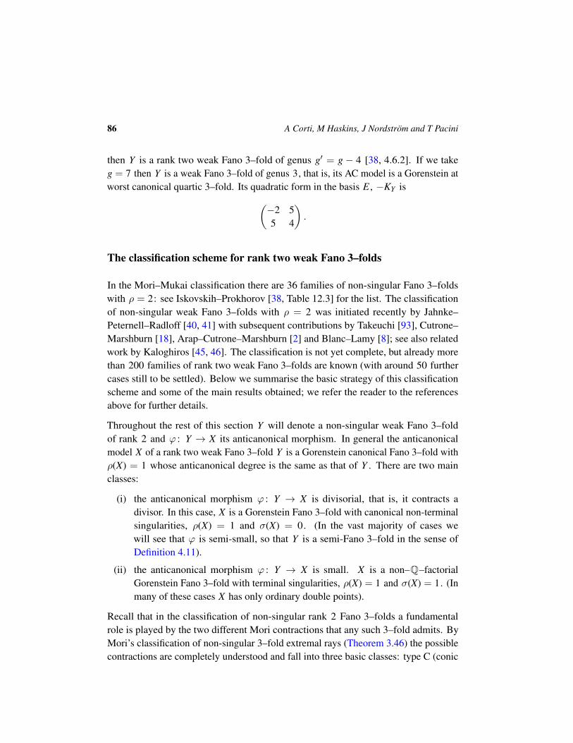
86 A Corti, M Haskins, J Nordstrom and T Pacini
then Y is a rank two weak Fano 3–fold of genus g′ = g − 4 [38, 4.6.2]. If we takeg = 7 then Y is a weak Fano 3–fold of genus 3, that is, its AC model is a Gorenstein atworst canonical quartic 3–fold. Its quadratic form in the basis E , −KY is(
−2 55 4
).
The classification scheme for rank two weak Fano 3–folds
In the Mori–Mukai classification there are 36 families of non-singular Fano 3–foldswith ρ = 2: see Iskovskih–Prokhorov [38, Table 12.3] for the list. The classificationof non-singular weak Fano 3–folds with ρ = 2 was initiated recently by Jahnke–Peternell–Radloff [40, 41] with subsequent contributions by Takeuchi [93], Cutrone–Marshburn [18], Arap–Cutrone–Marshburn [2] and Blanc–Lamy [8]; see also relatedwork by Kaloghiros [45, 46]. The classification is not yet complete, but already morethan 200 families of rank two weak Fano 3–folds are known (with around 50 furthercases still to be settled). Below we summarise the basic strategy of this classificationscheme and some of the main results obtained; we refer the reader to the referencesabove for further details.
Throughout the rest of this section Y will denote a non-singular weak Fano 3–foldof rank 2 and ϕ : Y → X its anticanonical morphism. In general the anticanonicalmodel X of a rank two weak Fano 3–fold Y is a Gorenstein canonical Fano 3–fold withρ(X) = 1 whose anticanonical degree is the same as that of Y . There are two mainclasses:
(i) the anticanonical morphism ϕ : Y → X is divisorial, that is, it contracts adivisor. In this case, X is a Gorenstein Fano 3–fold with canonical non-terminalsingularities, ρ(X) = 1 and σ(X) = 0. (In the vast majority of cases wewill see that ϕ is semi-small, so that Y is a semi-Fano 3–fold in the sense ofDefinition 4.11).
(ii) the anticanonical morphism ϕ : Y → X is small. X is a non–Q–factorialGorenstein Fano 3–fold with terminal singularities, ρ(X) = 1 and σ(X) = 1. (Inmany of these cases X has only ordinary double points).
Recall that in the classification of non-singular rank 2 Fano 3–folds a fundamentalrole is played by the two different Mori contractions that any such 3–fold admits. ByMori’s classification of non-singular 3–fold extremal rays (Theorem 3.46) the possiblecontractions are completely understood and fall into three basic classes: type C (conic
Asymptotically cylindrical Calabi–Yau 3–folds 87
bundle type), D (del Pezzo fibre type) and E (exceptional/divisorial) type. For example ifa Fano 3–fold with ρ = 2 admits an extremal contraction of type E1, that is, the inverseof the blowup of a non-singular curve in a smooth 3–fold W , then by Theorem 8.1W itself must be a smooth Fano 3–fold with ρ(W) = 1. In general the existence oftwo extremal rays of known type together with the condition of being Fano put severeconstraints on the 3–fold, enough to allow a complete classification.
For non-singular rank 2 weak Fano 3–folds there is only a single Mori contractionψ : Y → W . A substitute for the missing second extremal ray is provided by the ACmorphism ϕ : Y → X . When the anticanonical morphism contracts a divisor, an almostcomplete classification was given recently by Jahnke–Peternell–Radloff [40]. When theanticanonical morphism is small the analysis is more involved and the classification isnot yet close to complete. Nevertheless, as we will describe below, many examples areknown and there are classification results under additional assumptions.
Rank 2 weak Fanos with divisorial AC morphism
In [40], Jahnke, Peternell and Radloff classify rank two weak Fano 3–folds of type (i) –where the AC morphism ϕ is a divisorial contraction – according to the type of the Moricontraction ψ : Y → W ; see [40, Tables A.2–A.5, pages 627–630]. There are at most59 deformation families (the existence of two possible families A.2.7, A.2.8 remainsto be shown) with (even) anticanonical degrees −K3
Y between 2 and 72; because ofthe length and complexity of the classification we do not reproduce it here. A keytechnical role is played by Mukai’s classification [70] of all Gorenstein Fano threefoldswith canonical singularities such that the anticanonical divisor does not admit a movingdecomposition: see [40, 4.7].
One important fact to note from the classification is that rank two weak Fano 3–folds thatare not semi-Fano are extremely rare; when the extremal ray is of type D or E2–5 onecan show that Y is always semi-Fano [40, 2.3 and 5.2] and there is a single exceptionout of 25 cases with an extremal ray of type E1 [40, Section 4]. Altogether only infour (A.3.1, 3.9, 3.12 and 4.25 in [40]) out of the 59 families does the AC morphismcontract a divisor to a point. Hence we have 53(+2?) non-singular rank 2 semi-Fano3–folds for which the anticanonical morphism ϕ : Y → X contracts a divisor D to acurve B. In all such cases B ⊂ X is a non-singular curve of cDV singularities, Y is theblowup of X in the curve B and D is a conic bundle over B [40, 1.8].

88 A Corti, M Haskins, J Nordstrom and T Pacini
Rank 2 weak Fanos with small AC morphism
As mentioned above, the classification of rank two semi-Fano 3–folds whose ACmorphism ϕ is small is more involved and not yet complete, despite recent activity inthis direction by several authors. In this case the anticanonical model X is a non–Q–factorial Gorenstein Fano 3–fold with terminal singularities, which by Proposition 3.26are isolated cDV singularities; in many cases X has only ordinary double points.
By Namikawa’s smoothing result (Theorem 4.17) X admits a smoothing X → ∆ ⊂ Csuch that X0 ' X and Xt for t 6= 0 is a non-singular Fano 3–fold (this is not alwaystrue in the case of Gorenstein canonical singularities); moreover, the Picard groups(over Z) of X and the general Xt are isomorphic. Hence X and Xt have the same Fanoindex and Xt is a non-singular Fano 3–fold of Picard rank 1. The cases where X hasindex > 1 are relatively straightforward – see Jahnke–Peternell–Radloff [41, 2.12–3] –and the main case is when X has index 1. In this case the Iskovskih classification ofrank 1 non-singular Fano 3–folds (see [38, Table 12.2] for a convenient list or see ourTable 7.1 in Section 7) implies 2 ≤ −K3
Y ≤ 22 with −K3Y 6= 20 and, in fact, all such
possible anticanonical degrees actually occur.
The anticanonical morphism ϕ : Y → X is a flopping contraction (recall Definition 3.28)and thus it can be flopped (recall Theorem 3.30); that is, there is another non-singularrank 2 weak Fano 3–fold Y+ , whose (small) anticanonical morphism we denoteϕ+ : Y+ → X . Y+ has the same anticanonical degree as Y . For any divisor D on Ylet D+ denote the strict transform of D under the flop χ; the map D→ D+ induces anisomorphism between the Picard groups of Y and Y+ . Moreover, the lattice structuresinduced on the Picard lattices of Y and Y+ are isomorphic, that is, for any divisors D1
and D2 on Y we have
(8–5) − KY · D1 · D2 = −KY+ · D+1 · D
+2 .
Y+ also admits a (KY+ –negative) extremal contraction ψ+ : Y+ → W+ . Everythingfits into the following diagram:
(8–6) Yχ //
ψ
ϕ
Y+
ψ+
ϕ+
~~W X W+
The classification programme has two steps: a numerical classification stage andthe more delicate geometric realisability question. In the numerical classification
Asymptotically cylindrical Calabi–Yau 3–folds 89
stage one first writes down a system of Diophantine equations determined by therelations among various intersection numbers that any non-singular weak Fano 3–foldof rank 2 with small AC morphism would have to satisfy. The precise form of theseDiophantine equations depends on the pair of Mori contractions ψ and ψ+ ; as a resultthere are various subcases depending on the type of the pair of Mori contractions. SeeCutrone–Marshburn [18, Section 2.1] – particularly equations (2.6) and (2.7) therein –for the Diophantine equations in the case where both Mori contractions ψ and ψ+ areof type E1; in this latter case both Y and its flop Y+ arise as the blowups of smoothcurves C and C+ in rank one Fano 3–folds W and W+ . So rank two weak Fanos withlink type E1–E1 constitute a direct generalisation of the concrete rank two weak Fanosconstructed in the previous subsection as blowups of low degree curves in non-singularindex one rank one Fano 3–folds.
A solution of the numerical classification problem means a finite list of all possiblesolutions to these Diophantine equations. Each such solution is referred to as a numericallink. For some pairs of Mori contractions there are many numerical links while forothers there are relatively few. However, not every numerical link is realisable by aweak Fano 3–fold. For each numerical link further (often more delicate) argument isrequired either to find a weak Fano realising that numerical link or to prove that no suchweak Fano exists. This is the geometric realisability question.
Jahnke–Peternell–Radloff [41] give a complete list of numerical links in the case thatat most one of the Mori contractions ψ or ψ+ from (8–6) is of type E. Cutrone–Marshburn [18] completed the numerical classification when both Mori contractions areof type E. Takeuchi [93] considers the case where ψ is of type D and gives a completeclassification including the geometric realisability question when this del Pezzo fibrationhas degree different from 6; this augments (but also overlaps considerably with) thegeometric realisability studies contained in [41, Section 3]. Thus the classification ofrank two weak Fano 3–folds where at least one Mori contraction is not of type E isnow close to complete; the 6? entries in [41, Table 7.7] and the del Pezzo fibrations ofdegree 6 are still outstanding.
The classification of rank two weak Fano 3–folds where both Mori contractions areof type E is substantially less complete. Cutrone–Marshburn [18] gives a list of 111numerical links of type E1–E1: meaning both Mori contractions are of type E1, that is,both Y and Y+ arise as the blowup of smooth curves in rank one Fano 3–folds W andW+ . Of these 111 numerical links, they prove 11 to be geometrically realisable, 13 notto be geometrically realisable, and leave 87 numerical links unsettled: see [18, 5.1].Recall from Remark 8.3 that if Y is a rank two weak Fano 3–fold with link type E1–E1(or more generally E1–**) then H3Y is torsion-free. Hence we can always constructbuilding blocks in the sense of Definition 5.1 from any such weak Fano 3–fold.

90 A Corti, M Haskins, J Nordstrom and T Pacini
More recently Blanc–Lamy [8] settled the geometric realisability question when theweak Fano Y arises as the blowup of a space curve in P3 ; this gives the existence of 13further pairs (Y and its unique flop Y+ ) of rank two semi-Fano 3–folds with small ACmorphism. Very recently Arap–Cutrone–Marshburn [2] settled most of the geometricrealisability questions in the cases when the weak Fano Y arises as the blowup of acurve in: a smooth quadric in P4 , a pair of quadrics in P5 or a del Pezzo 3–fold ofdegree 5. These give another 8, 6 and 13 pairs of examples of rank two semi-Fano3–folds with small AC morphism respectively.
So geometric realisability currently remains open for approximately 50 of the 111numerical links of type E1–E1 listed in [18]. The situation for other numerical linksof type E–E is far more heavily constrained with only relatively few numerical linktypes; for most of these numerical links the geometric realisability question is alreadysolved [18, 5.2–5.7].
Rough enumeration of rank two weak Fano 3–folds with small AC morphism
Let us give a rough enumeration of the number of deformation types generated by therank two weak Fano 3–folds with small AC morphism currently known to exist.
If Y and Y ′ are smooth rank two weak Fano 3–folds belonging to the same deformationtype then by Mori’s deformation theory for extremal rays [66, Theorem 3.47] both Yand Y ′ admit extremal rays of the same type except possibly in the cases E3/E4 (thepoint being that E3 can degenerate to E4). In particular, if both Y and Y ′ have smallAC morphisms and different numerical links then Y and Y ′ do not belong to the samedeformation type.
Takeuchi [93, 2.2–2.13] gives a list of 33 families of del Pezzo fibred non-singular ranktwo Fano 3–folds with small AC morphism and shows that none of them are deformationequivalent [93, Theorem 2.15]. He also lists their anticanonical models X and theirflops Y+ ; in almost all cases the anticanonical model X has only ordinary double pointsand therefore both Y and Y+ have nodal AC model. The number of curves contractedby the anticanonical morphism ϕ varies between 1 and 46. In 19 cases Y+ is not itselfdel Pezzo fibred and is therefore not deformation equivalent to any of the rank twoweak Fanos in Takeuchi’s list of 33. Hence we obtain 52 distinct families of rank 2Fano 3–folds with small AC morphism from Takeuchi’s work, almost all of which havenodal AC model. When Y is a del Pezzo fibration of degree 6 [41, A.2–A.4] provides 5additional examples (plus their flops which are different) and leaves open a further 8possibilities for del Pezzo fibrations of degree 6. Finally [41, Tables 7.5–7.7] yields
Asymptotically cylindrical Calabi–Yau 3–folds 91
12 = 2 + 3 + 7 cases (plus their flops) where ψ is a conic bundle (with the geometricrealisability of 6 further numerical links left open).
In total this gives us 84 (that is, 52 + 2× 5 + 1× 2 + 2× 3 + 2× 7) currently knowndeformation types generated by rank 2 Fano 3–folds with small AC morphism for whichat least one of the Mori contractions ψ and ψ+ is not birational, and the majority ofthese have nodal AC model. In addition we have 26 cases from [18] where both Moricontractions ψ and ψ+ are birational and over 40 further examples of link type E1–E1from Arap–Cutrone–Marshburn [2] and Blanc–Lamy [8].
To summarise: we have at least 150 deformation types arising from known families ofrank two semi-Fano 3–folds for which the AC morphism is small (many of which havenodal AC model) in addition to the 36 deformation types of rank two genuine Fano3–folds. (There are additional deformation types which arise from the known rank twosemi-Fano 3–folds for which the AC morphism is only semi-small, but we must takesome care enumerating these because these may belong to the 150+ deformation typesabove or may be deformation equivalent to a rank two genuine Fano 3–fold.)
This abundance of rank two semi-Fanos will allow us to construct a large number ofnew compact G2 –holonomy manifolds in [17]. If we use at least one building blockbuilt from one of the many semi-Fano 3–folds with nodal AC model, then we will beable to construct G2 –holonomy manifolds containing a variety of different numbers ofrigid associative 3–folds.
Toric weak Fano 3–folds
In this section we give an overview of the results one can obtain for projective small(respectively crepant) resolutions of toric Gorenstein terminal (respectively canonical)Fano 3–folds. This will prove the existence of very many (hundreds of thousands of)non-singular toric weak Fano 3–folds. We will also see that the set of non-singular toricweak Fano 3–folds with nodal AC model is essentially disjoint from the many Picardrank 2 semi-Fanos discussed above. The building blocks in Examples 7.10 and 7.11both use one very particular toric semi-Fano with nodal AC model.
Although by Batyrev’s work [5] there are only 18 deformation classes of non-singulartoric Fano 3–fold (see also the table in [38, Appendix 12.8]), there are many deformationclasses of singular toric Fano 3–fold as soon as one allows even relatively mildsingularities. In the following whenever we refer to a toric Fano 3–fold we shallmean a Gorenstein toric Fano 3–fold; these automatically have at worst canonicalsingularities [5, 2.2.5].
92 A Corti, M Haskins, J Nordstrom and T Pacini
Toric Fano 3–folds correspond (uniquely up to isomorphism) to so-called reflexivepolytopes, see for example, Nill’s thesis [76, Chapters 1 and 2] for basic definitions intoric Fano geometry. Kreuzer–Skarke [59] developed an algorithm to classify reflexivepolyhedra in arbitrary dimensions; as an application of this algorithm they showed thatthere are 4319 3–dimensional reflexive polytopes, including the 18 that correspond tonon-singular toric Fano 3–folds.
A big advantage of Gorenstein toric Fano 3–folds compared to more general Gorensteincanonical Fano 3–folds (where often no projective crepant resolution exists, for example,any nodal quartic in P4 with fewer than 9 nodes) is that one can use toric geometry toprove that any toric Fano 3–fold admits a projective crepant resolution. Since every suchcrepant resolution is a non-singular toric weak Fano 3–fold this proves the existenceof at least 4301 deformation families of toric weak Fano 3–fold. In fact there aremany more such families because many singular toric Fano 3–folds admit numerousnon-isomorphic projective crepant resolutions; moreover, all the projective crepantresolutions are toric and can be enumerated purely combinatorially (see below). Thetopology of toric weak Fano 3–folds is also relatively straightforward: as smoothtoric varieties they have no cohomology in odd degree and their even cohomology istorsion-free. In particular we never have to worry about the condition H3(Y) beingtorsion-free. These features make toric weak Fano 3–folds a very rich class of exampleswhich nonetheless can be studied relatively easily.
Proposition 8.7 Any 3–dimensional Gorenstein toric Fano variety X admits at leastone projective crepant resolution Y ; Y is a non-singular toric weak Fano 3–fold whoseanticanonical model is X .
Remark 8.8
(i) This result is not true for higher-dimensional Gorenstein toric varieties X ; whatis true is that there is a projective birational morphism f : X′ → X , such thatf is crepant and X′ is toric with only Q–factorial terminal singularities [5,Theorem 2.2.24]. Batyrev calls f : X′ → X a maximal projective crepant partialdesingularisation of X or MPCP-desingularisation for short. Proposition 8.7is a special case of the existence of MPCP-desingularisations; since any 3–dimensional Gorenstein toric variety with Q–factorial terminal singularitiesmust in fact be non-singular, any 3–dimensional MPCP-desingularisation isnon-singular.
(ii) Crepant resolutions of a toric variety X correspond to fans ∆′ refining the originalfan ∆ defining X . The toric variety X′ associated to the fan ∆′ is in general not
Asymptotically cylindrical Calabi–Yau 3–folds 93
projective; when the toric variety associated to the fan ∆′ is again projective, thefan ∆′ is called a coherent crepant refinement of ∆.
(iii) Batyrev shows that any MPCP-desingularisation f : X′ → X defines a “maxi-mal projective triangulation” of the reflexive polytope P associated to X andconversely that any maximal projective triangulation of the reflexive polytopeP determines a MPCP-desingularisation of X . Since Gelfand, Kapranov andZelevinsky [31] already proved the existence of maximal projective triangulations(regular triangulations in their terminology) of any integral polyhedron P, theexistence of MPCP-desingularisations (and hence projective crepant resolutionsin the 3–dimensional case) then follows immediately.
(iv) One can use the correspondence between projective crepant resolutions of atoric Fano 3–fold and maximal projective triangulations of the correspondingreflexive polytope to enumerate all projective crepant resolutions of a giventoric Gorenstein Fano 3–fold. Together with Tom Coates and Al Kasprzykwe have used TOPCOM [82] in combination with PALP and Sage to find alltoric semi-Fano 3–folds up to isomorphism. A more detailed description of thiscomputation, the full data and a systematic treatment of G2 –manifolds arisingfrom them will appear elsewhere [15].
Many features of any crepant projective resolution of a toric Fano 3–fold can be readimmediately from the associated reflexive polytope. For example we have the following:
Remark 8.9 The Picard rank ρ of any crepant resolution of a toric Fano 3–fold equalsthe number of lattice points (including the origin) of the corresponding reflexive polytopeminus 4. Hence from Kreuzer–Skarke [59, Table 2] we have that for a non-singulartoric weak Fano 3–fold Y , ρ = b2(Y) can attain any value between 2 and 35 except 32and 33.
We can also recognise the various flavours of non-singular toric weak Fano Y fromthe geometry of the reflexive polytope associated with its (Gorenstein toric Fano)anticanonical model X .
For toric Fano 3–folds with small AC morphism we have:
Lemma 8.10 (Terminal toric Fano 3–folds)
(i) A toric Fano 3–fold X is terminal if and only if all facets of its reflexive polytopeare either standard triangles or standard parallelograms.
94 A Corti, M Haskins, J Nordstrom and T Pacini
(ii) The only singularities of a terminal toric Fano 3–fold are ordinary double pointsand the number of ODPs of X is equal to the number of parallelograms in itsreflexive polytope. In particular, every toric weak Fano 3–fold with small ACmorphism has nodal AC model.
(iii) Every terminal toric Fano 3–fold X admits at least one small projective resolutionY ; Y is a non-singular toric semi-Fano 3–fold. Conversely every non-singulartoric semi-Fano 3–fold Y with nodal AC model arises as a small projectiveresolution of a terminal (nodal) toric Fano 3–fold X .
Proof For (i) and (ii) see the thesis of Nill [76, 4.2.4 and 4.3.1–4.3.2]. (iii) is a specialcase of Proposition 8.7; see also the remark below.
Remark 8.11 In the special case of a terminal toric (and therefore nodal) Fano 3–foldX any “crepant refinement” of the reflexive polytope of X as in Remark 8.8 arisesas follows: for each parallelogram facet in the reflexive polytope pick one of its twodiagonals and make a new polytope by adding the chosen diagonals as additional edgesto the reflexive polytope. Clearly there are 2e such refinements where e is the numberof parallelograms (by Lemma 8.10(ii) parallelograms correspond to the nodes of X );each such refinement gives a (toric) small but not necessarily projective resolution of X .By Lemma 8.10(iii) at least one of these small resolutions is projective.
Corollary 8.12
(i) There are precisely 82 singular toric Fano 3–folds with terminal singularities.
(ii) The Picard rank ρ of a terminal toric Fano 3–fold X can be 1, 2, 3 or 4.
(iii) The Picard rank ρ of a toric semi-Fano 3–fold with nodal AC model takes allvalues between 2 and 11.
(iv) The genus g of a toric semi-Fano 3–fold with nodal AC model takes all values in11, . . . , 25 ∪ 28.
(v) The defect σ of a terminal toric Fano 3–fold takes all values in 1, . . . , 7 ∪ 9.
(vi) The number e of exceptional (−1,−1) curves of a toric semi-Fano 3–fold withnodal AC model takes all values in 1, . . . , 9 ∪ 12.
(vii) Every toric semi-Fano 3–fold Y with nodal AC model is rigid, that is,
H1(Y, TY ) = (0).
(viii) There are precisely 1009 deformation types of toric semi-Fano 3–fold with nodalAC model.
Asymptotically cylindrical Calabi–Yau 3–folds 95
Proof (i) follows either from Nill’s thesis [76] or from the Kreuzer–Skarke classificationof reflexive polytopes in three dimensions and the characterisation of the terminal onesfrom Lemma 8.10(i). (ii–vi) now follow from an examination of the 82 possible terminalreflexive polytopes, for example, see the list of terminal toric Fano 3–folds on the GradedRings database [9]. (vii) follows immediately from Ilten’s thesis [35, Corollary 4.2.6].For (viii) we first enumerate all projective small resolutions of the 82 terminal reflexivepolytopes. Next we identify projective small resolutions of a given terminal polytopewhich differ by a lattice automorphism. This yields the number of non-isomorphicprojective small resolutions for each polytope. The details of these calculations willappear in [15]. The total number of non-isomorphic projective small resolutions turnsout to be 1009: since by (vii) all these varieties are rigid the number of deformationtypes is also equal to 1009.
Remark 8.13 (Toric semi-Fano 3–folds with nodal AC model and near-extremalPicard rank)
(i) Let us a consider toric weak Fano 3–fold Y with the minimal possible Picardrank ρ = 2 (we assume Y is not already Fano so ρ ≥ 2). By Remark 8.9the reflexive polytope corresponding to its AC model X has exactly 6 latticepoints. Consulting the classification we find that among the 82 terminal reflexivepolytopes there is precisely one such polytope. The corresponding terminaltoric Fano 3–fold X ⊂ P4 is the projective cone over a non-singular quadricQ ' P1 × P1 ⊂ P3 and has two (isomorphic) projective small resolutions asdescribed in 4.15. Therefore up to isomorphism there is precisely one toricsemi-Fano 3–fold with ρ = 2 and nodal AC model; as remarked previously ithas index 3. In particular, only this toric semi-Fano 3–fold appears in our earliercount of over 150 semi-Fano 3–folds with ρ = 2 and small AC morphism.
(ii) By Corollary 8.12(iii) any toric semi-Fano 3–fold Y with nodal AC modelhas Picard rank at most 11. By counting lattice points again the classificationof terminal reflexive polytopes shows that if the Picard rank of Y equals 11then its anticanonical model X is the unique terminal toric Fano 3–fold X20
of degree 20; X20 has Picard rank 2 and defect 9. (We know X20 could nothave Picard rank 1 because there is no smooth rank 1 Fano of degree 20 whichcould degenerate to X20 .) X20 corresponds to polytope 2355 in the Sage list of3–dimensional reflexive polytopes; this polytope contains 12 parallelograms andhence X contains 12 nodes. Using TOPCOM to count regular triangulationsof the polytope we find that this polytope admits 3608 (out of all 212 = 4096possible small resolutions) projective small resolutions and that these lie in 125distinct isomorphism classes. Apart from these 125 isomorphism classes of
96 A Corti, M Haskins, J Nordstrom and T Pacini
toric semi-Fano 3–folds with nodal AC model and Picard rank 11, all other toricsemi-Fano 3–folds with nodal AC model have Picard rank between 2 and 10.
(iii) Similarly, any toric semi-Fano 3–fold with nodal AC model and Picard rankequal to 10 has anticanonical model the unique terminal toric Fano 3–fold X22 ofdegree 22; X22 has Picard rank 1 and defect 9. It corresponds to polytope 1942in the Sage list of 3–dimensional reflexive polytopes; this polytope contains 9parallelograms and hence X contains 9 nodes. Note that the number of nodes ofX is equal to its defect. Using TOPCOM to count regular triangulations of thepolytope we find that all 512 small resolutions of this polytope are projective andthese consist of 84 distinct isomorphism classes. Building blocks constructedfrom this particular polytope were discussed in detail in Examples 7.10 and 7.11.We selected this particular polytope because it has maximal defect σ = 9 andbecause the polytope is self-dual.
Similarly we can recognise more general toric semi-Fano 3–folds from the geometry ofthe associated reflexive polytope.
Lemma 8.14 (Toric semi-Fano 3–folds)
(i) A toric weak Fano 3–fold Y is semi-Fano if and only if the reflexive polytopecorresponding to the (toric Fano) anticanonical model X of Y has no facets thatcontain lattice points strictly in their interior, that is, every lattice point on anyfacet lies on an edge of the facet. In this case by a slight abuse of terminologywe will say that the reflexive polytope (or the singular toric Fano 3–fold X ) issemi-small.
(ii) Every semi-small toric Fano 3–fold X admits at least one projective crepantresolution Y ; Y is a non-singular toric semi-Fano 3–fold.
Proof (i) is obvious; (ii) is a special case of Proposition 8.7.
Corollary 8.15
(i) There are 799 semi-small 3–dimensional reflexive polytopes (excluding the100 = 18 + 82 corresponding to non-singular or terminal toric Fanos). These areprecisely the polytopes for which every facet contains no interior lattice points,but that contain at least one boundary lattice point that is not a vertex of thepolytope. 435 of these polytopes contain at least one standard parallelogram.
(ii) The Picard rank ρ of a semi-small toric Fano 3–fold X can be 1, 2, 3 or 4.

Asymptotically cylindrical Calabi–Yau 3–folds 97
(iii) The Picard rank ρ of a non-singular toric semi-Fano 3–fold Y can be any integerbetween 2 and 15.
(iv) The genus g of a toric semi-Fano 3–fold Y can be any integer between 7 and 29.
(v) The defect σ of a semi-small toric Fano 3–fold X is at least 1 and at most 13.
(vi) There are 526 130 isomorphism classes of non-singular toric semi-Fano 3–fold(including the 18 + 1009 corresponding to smooth toric Fanos and toric Fanoswith terminal AC model); 435 459 of these are rigid.
Proof (i) follows from the Kreuzer–Skarke explicit list of all 4319 reflexive polytopesand the characterisation given in Lemma 8.14(i). (ii–v) follow from computations basedon the explicit list of semi-small reflexive polytopes. The first part of (vi) follows byenumerating all projective crepant resolutions of the semi-small reflexive polytopesas described in the proof of Corollary 8.12(viii). It is not the case that every toricsemi-Fano 3–fold is rigid; Example 6.11(i) exhibits a toric semi-Fano 3–fold that isnot rigid. To determine which toric semi-Fano 3–folds are rigid first we computeh0 = dim H0(Y, TY ) by finding the number of Demazure roots of the associated fan,compare with Oda’s book [77, Corollary 3.13]. To compute h1 = dim H1(Y, TY ) weuse the fact that
h1 − h0 = −χ(Y, TY ) = 19− ρ− g + h2,1(Y)
where ρ and g are the Picard rank and genus respectively of the semi-Fano Y , comparewith Mukai [71, Section 4]. (In the toric case we always have h2,1 = 0). The detailedcalculations will appear in [15].
In particular, there are at least 435 459 deformation types of toric semi-Fano 3–folds(including the 1027 corresponding to smooth toric Fanos and toric semi-Fanos withterminal AC model). More effort would be needed to determine how many deformationtypes are realised by the remaining non-rigid toric semi-small Fano 3–folds.
Terminal Fano 3–folds via degenerations of non-singular Fano 3–folds
Given any non-singular semi-Fano 3–fold Y with small AC morphism, we can associatea deformation class of non-singular Fano 3–folds as follows. By Remark 4.12(ii), theanticanonical model X of Y is a terminal Gorenstein Fano 3–fold which thanks toNamikawa’s smoothing result (Theorem 4.17) is smoothable by a flat deformation to afamily of non-singular Fano 3–folds Xt . The anticanonical degrees and indexes of Y , X

98 A Corti, M Haskins, J Nordstrom and T Pacini
and Xt are all the same and ρ(X) = ρ(Xt) but ρ(Y) = ρ(X) + σ where σ is the defectof X . For instance in the case where Y is a rank 2 semi-Fano 3–fold with small ACmorphism (as considered earlier) this associates to Y one of the 17 deformation classesof non-singular rank 1 Fano 3–folds from the Iskovskih classification.
Semi-Fano 3–folds associated with degenerations of a cubic in P4 to a nodal cubic arecompletely understood; see below for a summary of these results. On the other handweak Fano 3–folds associated with say degenerations of a quartic in P4 are still very farfrom understood in general; see below for some further discussion of nodal quartics andtheir small resolutions.
Weak del Pezzo 3–folds from nodal cubics
From our earlier remarks about the behaviour of the index and degree under smoothingand small resolution, we see immediately that because a smooth cubic has index 2and degree 24, any semi-Fano 3–fold arising as the small resolution of a nodal cubicalso has index 2 and degree 24. In particular, they are all weak del Pezzo 3–folds.Finkelnberg–Werner [26] understood how many nodes can occur on a degeneration of asmooth cubic, what defects occur and in each case how many of the small resolutionsare projective. Their results demonstrate clearly how one single deformation class ofsmooth del Pezzo 3–folds can give rise to a much larger number of deformation classesof weak del Pezzo 3–folds.
Finkelnberg–Werner show that the number of nodes k can take any value up to 10 andthe defect any value up to 5. Table 8.1 lists the possible number of nodes e, the defect σ ,the number of projective small resolutions s, the number of planes P contained in thenodal cubic and b3(Y) denotes the third Betti number of any projective small resolutionof the nodal cubic (if any exists); the latter is computed using (4–22) and the fact thatb3 = 10 for a non-singular cubic 3–fold.
Remark 8.16
(i) A nodal cubic 3–fold X ⊂ P4 is nonrational if and only if it is smooth byClemens–Griffiths [14, Theorem 13.12]. Any projective small resolution Y of anodal cubic X therefore has no torsion in H3(Y) (recall Remark 5.8) and hencegives rise to a building block Z in the sense of Definition 5.1 via the constructionof Proposition 5.7.
(ii) All the examples in Table 8.1 with ρ(Y) > 2 have nodal AC model and are notalready included in any of the classes described earlier in the paper; to see this

Asymptotically cylindrical Calabi–Yau 3–folds 99
e σ s P ρ(Y) b3(Y)
0 0 0 0 1 10
1 0 0 0 − −
2 0 0 0 − −
3 0 0 0 − −
40 0 0 − −1 2 1 2 4
5 1 0 1 − −
61 0 1 − −1 2 0 2 02 6 2 3 2
72 6 2 3 02 0 3 − −
8 3 24 5 4 0
9 4 102 9 5 0
10 5 332 15 6 0
Table 8.1: The possible nodal degenerations of cubic 3–folds; e denotes the number of ODPs, σthe defect, s the number of projective small resolutions and P the number of planes contained inthe nodal cubic. ρ(Y) and b3(Y) denote the Picard rank and third Betti number of any projectivesmall resolution Y of the nodal cubic (when one exists).
we only need note the following: a non-singular cubic and hence any nodaldegeneration has Picard rank ρ = 1 and anticanonical degree 24, whereas theclassification of toric terminal Fano 3–folds shows none of the three degree 24examples has Picard rank 1.
(iii) (4–18) applied to a degeneration of a non-singular cubic yields e ≤ 5 + 20− 1 =
24, whereas in fact we have e ≤ 10. So in this case the bound from (4–18) isquite far from being sharp.
(iv) (4–22) and non-negativity of b3(Y) immediately implies e− σ ≤ 5; Table 8.1shows that there are 5 different possible combinations of e and σ realisinge− σ = 5 (which forces b3(Y) = 0).
100 A Corti, M Haskins, J Nordstrom and T Pacini
(v) From Table 8.1 we see that 3 ≤ e − σ ≤ 5 for any nodal cubic that admits aprojective small resolution.
(vi) In Table 8.1 some (sometimes many) of the s small projective resolutions of a givennodal cubic may give rise to projective varieties that are abstractly isomorphic;if the nodal cubic X admits a nontrivial discrete group of automorphisms thenthis group acts on the set of all small resolutions and different small resolutionsin the same orbit are isomorphic. For example, the unique (up to projectiveequivalence) nodal cubic with 10 nodes called the Segre cubic has automorphismgroup the symmetric group S6 . In [24] Finkelnberg showed that there are 13different orbits of S6 acting on the set of all 210 = 1024 small resolutions ofthe Segre cubic; 6 of these orbits consist of projective small resolutions while 7contain only non-projective small resolutions. In particular, we obtain 6 differentisomorphism classes of semi-Fano 3–fold with index 2 (weak del Pezzo 3–fold),degree 24, Picard rank 6 and nodal AC morphism. For other nodal cubics withclose to the maximal number of nodes the number of non-isomorphic projectivesmall resolutions does not seem to have been determined.
Semi-Fano 3–folds from nodal quartics
Examples 7.3 to 7.6 all give examples of defect 1 semi-Fano 3–folds arising fromprojective small resolutions of nodal quartics in P4 . Example 7.7 is a defect 15 weakFano 3–fold associated with a nodal quartic in P4 (with the maximal number of nodese = 45; moreover, 15 is the maximal possible defect for a terminal quartic 3–fold:see below). There currently does not seem to be a good understanding of semi-Fano3–folds associated with nodal quartics when the defect is not either 1 or close to themaximum 15. Even for the maximal defect σ = 15 it does not seem that the number ofprojective small resolutions of the Burkhardt quartic has been determined. (Recall ithas at least one projective small resolution and exactly 245 ' 3.5× 10¹³ Moishezonbut not necessarily projective small resolutions).
The following statement summarises some of the main known results about nodalquartics and their defects and projective small resolutions.
Theorem 8.17 Let X be a nodal quartic in P4 , let e denote the number of nodes of Xand σ(X) its defect.
(i) If e < 9 then σ = 0 and hence X admits no projective small resolutions.

Asymptotically cylindrical Calabi–Yau 3–folds 101
(ii) If e = 9 then σ = 0 if and only if X contains no planes Π. In particular, ageneral quartic with e = 9 admits no projective small resolutions. If e = 9 andX contains a plane Π then σ = 1 and blowing up Π in X yields a projectivesmall resolution as in Example 7.3.
(iii) If e < 12 and X contains no planes then σ = 0 and hence X admits no projectivesmall resolutions.
(iv) If e = 12 then σ = 0 unless X contains a quadric surface. A sufficiently generalquartic containing an irreducible quadric Q2
2 has precisely 12 nodes all containedin Q2
2 and has σ = 1. Blowing up Q22 yields a projective small resolution as in
Example 7.4.
(v) e ≤ 45 with equality if and only if X is projectively equivalent to the Burkhardtquartic as in Example 7.7.
(vi) σ ≤ 15 with equality if and only X is projectively equivalent to the Burkhardtquartic. Moreover, σ ≤ 10 if X contains no planes.
Proof (i) and (ii) are proved in Cheltsov [13, Theorems 2 and 5]. (iii) and (iv) areproved in Shramov [90, Theorem 1.3]. (v): e ≤ 45 was proved in Varchenko [98];the case of equality was treated in de Jong–Shepherd-Barron–Van de Ven [43]. (vi) isproved in Kaloghiros [46, Theorem 1.1]; see the erratum for a correction to the originalclaim of Theorem 1.1.(ii).
Remark 8.18 The special class of nodal determinantal quartics has been studied insome detail. A determinantal quartic is a hypersurface in P4 given as the zero-locus ofthe determinant of a 4×4 matrix of linear forms in [z0, . . . , z4]. A determinantal quarticis never smooth but generically has only nodes; this makes determinantal quartics agood source of nodal quartics. A nodal determinantal quartic has 20 ≤ e ≤ 45 and thegeneric one has e = 20. The Burkhardt quartic is determinantal. Every determinantalquartic is rational and hence any projective small resolution Y has no torsion in H3(Y).Pettersen’s thesis [80] used a particular rationalisation to study nodal determinantalquartics. He gave classification results for nodal determinantal quartics with e ≥ 42 andshowed any such quartic admits at least one projective small resolution. Such resolutionsare semi-Fano 3–folds with H3(Y) torsion-free and thus give rise to building blocksin the sense of Definition 5.1. Pettersen [80, Section 6.2] constructed determinantalquartics with e = 40 and σ = 10 which contain no plane; thus the defect bound fromTheorem 8.17(vi) is sharp.
102 A Corti, M Haskins, J Nordstrom and T Pacini
References
[1] Y Akizuki, S Nakano, Note on Kodaira–Spencer’s proof of Lefschetz theorems, Proc.Japan Acad. 30 (1954) 266–272 MR0066694
[2] M Arap, J W Cutrone, N A Marshburn, On the existence of certain weak Fanothreefolds of Picard number two arXiv:1112.2611
[3] E Arbarello, M Cornalba, P A Griffiths, J Harris, Geometry of algebraic curvesVol I, Grundl. Math. Wissen. 267, Springer, New York (1985) MR770932
[4] M Artin, D Mumford, Some elementary examples of unirational varieties which arenot rational, Proc. London Math. Soc. 25 (1972) 75–95 MR0321934
[5] V V Batyrev, Toric Fano threefolds, Izv. Akad. Nauk SSSR Ser. Mat. 45 (1981)704–717, 927 MR631434
[6] A Beauville, Fano threefolds and K3 surfaces, from: “The Fano Conference”, Univ.Torino, Turin (2004) 175–184 MR2112574
[7] C Birkar, P Cascini, C D Hacon, J McKernan, Existence of minimal models forvarieties of log general type, J. Amer. Math. Soc. 23 (2010) 405–468 MR2601039
[8] J Blanc, S Lamy, Weak Fano threefolds obtained by blowing-up a space curveand construction of Sarkisov links, Proc. Lond. Math. Soc. 105 (2012) 1047–1075MR2997046
[9] G Brown, A Kasprzyk, The graded rings database homepage Available athttp://grdb.lboro.ac.uk/
[10] F Campana, On twistor spaces of the class C , J. Differential Geom. 33 (1991) 541–549MR1094468
[11] C Casagrande, P Jahnke, I Radloff, On the Picard number of almost Fano threefoldswith pseudo-index > 1, Internat. J. Math. 19 (2008) 173–191 MR2384898
[12] K Chan, S-C Lau, N C Leung, H-H Tseng, Open Gromov–Witten invariants andmirror maps for semi-Fano toric manifolds arXiv:1112.0388
[13] I Cheltsov, Nonrational nodal quartic threefolds, Pacific J. Math. 226 (2006) 65–81MR2247856
[14] C H Clemens, P A Griffiths, The intermediate Jacobian of the cubic threefold, Ann.of Math. 95 (1972) 281–356 MR0302652
[15] T Coates, M Haskins, A M Kasprzyk, J Nordstrom, in preparation
[16] A Conte, J P Murre, On quartic threefolds with a double line I, Nederl. Akad. Wetensch.Proc. Ser. A 39 (1977) 145–160 MR0498594
[17] A Corti, M Haskins, J Nordstrom, T Pacini, G2 –manifolds and associative subman-ifolds via semi-Fano 3–folds arXiv:1207.4470
[18] J W Cutrone, N A Marshburn, Towards the classification of weak Fano threefoldswith ρ = 2 arXiv:1009.5036
Asymptotically cylindrical Calabi–Yau 3–folds 103
[19] O Debarre, Higher-dimensional algebraic geometry, Universitext, Springer, New York(2001) MR1841091
[20] I Dolgachev, Integral quadratic forms: applications to algebraic geometry (afterV Nikulin), from: “Bourbaki seminar, Vol. 1982/83”, Asterisque 105, Soc. Math. France,Paris (1983) 251–278 MR728992
[21] I V Dolgachev, Mirror symmetry for lattice polarized K3 surfaces, J. Math. Sci. 81(1996) 2599–2630 MR1420220
[22] S Endraß, On the divisor class group of double solids, Manuscripta Math. 99 (1999)341–358 MR1702593
[23] H Esnault, E Viehweg, Lectures on vanishing theorems, DMV Seminar 20, Birkhauser,Basel (1992) MR1193913
[24] H Finkelnberg, Small resolutions of the Segre cubic, Nederl. Akad. Wetensch. Indag.Math. 49 (1987) 261–277 MR914085
[25] H Finkelnberg, On the Geometry of the Burkhardt Quartic, PhD thesis, Leiden (1989)
[26] H Finkelnberg, J Werner, Small resolutions of nodal cubic threefolds, Nederl. Akad.Wetensch. Indag. Math. 51 (1989) 185–198 MR1005050
[27] R Friedman, Simultaneous resolution of threefold double points, Math. Ann. 274(1986) 671–689 MR848512
[28] A Fujiki, S Nakano, Supplement to “On the inverse of monoidal transformation”, Publ.Res. Inst. Math. Sci. 7 (1971/72) 637–644 MR0294712
[29] O Fujino, Y Gongyo, On images of weak Fano manifolds, Math. Z. 270 (2012) 531–544MR2875847
[30] W Fulton, Intersection theory, Ergeb. Math. Grenzgeb. 2, Springer, Berlin (1984)MR732620
[31] I M Gel’fand, A V Zelevinskiı, M M Kapranov, Hypergeometric functions and toricvarieties, Funktsional. Anal. i Prilozhen. 23 (1989) 12–26 MR1011353
[32] M Goresky, R MacPherson, Stratified Morse theory, Ergeb. Math. Grenzgeb. 14,Springer, Berlin (1988) MR932724
[33] M Haskins, H-J Hein, J Nordstrom, Asymptotically cylindrical Calabi–Yau manifoldsarXiv:1212.6929
[34] A Iliev, L Katzarkov, V Przyjalkowski, Double solids, categories and non-rationalityarXiv:1102.2130
[35] N O Ilten, Deformations of Rational Varieties with Codimension-One Torus Action,PhD thesis, Freie Universitat Berlin (2010)
[36] V A Iskovskih, Fano threefolds I, Izv. Akad. Nauk SSSR Ser. Mat. 41 (1977) 516–562,717 MR463151
[37] V A Iskovskih, Fano threefolds II, Izv. Akad. Nauk SSSR Ser. Mat. 42 (1978) 506–549MR503430
104 A Corti, M Haskins, J Nordstrom and T Pacini
[38] V A Iskovskikh, Y G Prokhorov, Fano varieties, from: “Algebraic geometry, V”,Encyclopaedia Math. Sci. 47, Springer, Berlin (1999) 1–247 MR1668579
[39] P Jahnke, T Peternell, Almost del Pezzo manifolds, Adv. Geom. 8 (2008) 387–411MR2427467
[40] P Jahnke, T Peternell, I Radloff, Threefolds with big and nef anticanonical bundles I,Math. Ann. 333 (2005) 569–631 MR2198800
[41] P Jahnke, T Peternell, I Radloff, Threefolds with big and nef anticanonical bundles II,Cent. Eur. J. Math. 9 (2011) 449–488 MR2784025
[42] P Jahnke, I Radloff, Gorenstein Fano threefolds with base points in the anticanonicalsystem, Compos. Math. 142 (2006) 422–432 MR2218903
[43] A J de Jong, N I Shepherd-Barron, A Van de Ven, On the Burkhardt quartic, Math.Ann. 286 (1990) 309–328 MR1032936
[44] D D Joyce, Compact manifolds with special holonomy, Oxford Mathematical Mono-graphs, Oxford University Press (2000) MR1787733
[45] A-S Kaloghiros, The topology of terminal quartic 3–folds arXiv:0707.1852
[46] A-S Kaloghiros, The defect of Fano 3–folds, J. Algebraic Geom. 20 (2011) 127–149MR2729277
[47] A-S Kaloghiros, A classification of terminal quartic 3–folds and applications torationality questions, Math. Ann. 354 (2012) 263–296 MR2957627
[48] S Katz, D R Morrison, Gorenstein threefold singularities with small resolutions viainvariant theory for Weyl groups, J. Algebraic Geom. 1 (1992) 449–530 MR1158626
[49] Y Kawamata, Crepant blowing-up of 3–dimensional canonical singularities and itsapplication to degenerations of surfaces, Ann. of Math. 127 (1988) 93–163 MR924674
[50] Y Kawamata, General hyperplane sections of nonsingular flops in dimension 3, Math.Res. Lett. 1 (1994) 49–52 MR1258489
[51] Y Kawamata, K Matsuki, The number of the minimal models for a 3–fold of generaltype is finite, Math. Ann. 276 (1987) 595–598 MR879538
[52] K Kodaira, On a differential-geometric method in the theory of analytic stacks, Proc.Nat. Acad. Sci. U. S. A. 39 (1953) 1268–1273 MR0066693
[53] J Kollar, Flips, flops, minimal models, etc, from: “Surveys in differential geometry(Cambridge, MA, 1990)”, Lehigh Univ., Bethlehem, PA (1991) 113–199 MR1144527
[54] J Kollar, Y Miyaoka, S Mori, Rationally connected varieties, J. Algebraic Geom. 1(1992) 429–448 MR1158625
[55] J Kollar, Y Miyaoka, S Mori, H Takagi, Boundedness of canonical Q–Fano 3–folds,Proc. Japan Acad. Ser. A Math. Sci. 76 (2000) 73–77 MR1771144
[56] J Kollar, S Mori, Birational geometry of algebraic varieties, Cambridge Tracts inMathematics 134, Cambridge Univ. Press (1998) MR1658959 With the collaborationof C H Clemens and A Corti. Translated from the 1998 Japanese original
Asymptotically cylindrical Calabi–Yau 3–folds 105
[57] A Kovalev, Twisted connected sums and special Riemannian holonomy, J. Reine Angew.Math. 565 (2003) 125–160 MR2024648
[58] A Kovalev, N-H Lee, K3 surfaces with non-symplectic involution and compactirreducible G2 –manifolds, Math. Proc. Cambridge Philos. Soc. 151 (2011) 193–218MR2823130
[59] M Kreuzer, H Skarke, Classification of reflexive polyhedra in three dimensions, Adv.Theor. Math. Phys. 2 (1998) 853–871 MR1663339
[60] P B Kronheimer, A Torelli-type theorem for gravitational instantons, J. DifferentialGeom. 29 (1989) 685–697 MR992335
[61] H B Laufer, On CP1 as an exceptional set, from: “Recent developments in severalcomplex variables (Proc. Conf., Princeton Univ., Princeton, N. J., 1979)”, Ann. of Math.Stud. 100, Princeton Univ. Press (1981) 261–275 MR627762
[62] R Lazarsfeld, Positivity in algebraic geometry I, Ergeb. Math. Grenzgeb. 48, Springer,Berlin (2004) MR2095471 Classical setting: line bundles and linear series
[63] K Matsuki, Introduction to the Mori program, Universitext, Springer, New York (2002)MR1875410
[64] J W Milnor, J D Stasheff, Characteristic classes, Annals of Mathematics Studies 76,Princeton Univ. Press (1974) MR0440554
[65] B G Moısezon, On n–dimensional compact complex manifolds having n algebraicallyindependent meromorphic functions I, Izv. Akad. Nauk SSSR Ser. Mat. 30 (1966)133–174 MR0216522
[66] S Mori, Threefolds whose canonical bundles are not numerically effective, Ann. ofMath. 116 (1982) 133–176 MR662120
[67] S Mori, S Mukai, Classification of Fano 3–folds with B2 ≥ 2, Manuscripta Math. 36(1981/82) 147–162 MR641971
[68] S Mori, S Mukai, Erratum: Classification of Fano 3–folds with B2 ≥ 2, ManuscriptaMath. 110 (2003) 407 MR641971
[69] S Mori, S Mukai, Extremal rays and Fano 3–folds, from: “The Fano Conference”,Univ. Torino, Turin (2004) 37–50 MR2112566
[70] S Mukai, New developments in Fano manifold theory related to the vector bundlemethod and moduli problems, Sugaku 47 (1995) 125–144 MR1364825
[71] S Mukai, Plane quartics and Fano threefolds of genus twelve, from: “The FanoConference”, Univ. Torino, Turin (2004) 563–572 MR2112592
[72] S Mukai, H Umemura, Minimal rational threefolds, from: “Algebraic geometry(Tokyo/Kyoto, 1982)”, Lecture Notes in Math. 1016, Springer, Berlin (1983) 490–518MR726439
[73] S Nakano, On the inverse of monoidal transformation, Publ. Res. Inst. Math. Sci. 6(1970/71) 483–502 MR0294710
106 A Corti, M Haskins, J Nordstrom and T Pacini
[74] Y Namikawa, Smoothing Fano 3–folds, J. Algebraic Geom. 6 (1997) 307–324MR1489117
[75] Y Namikawa, J H M Steenbrink, Global smoothing of Calabi–Yau threefolds, Invent.Math. 122 (1995) 403–419 MR1358982
[76] B Nill, Gorenstein toric Fano varieties, PhD thesis, Universitat Tubingen (2005)Available at http://tobias-lib.uni-tuebingen.de/volltexte/2005/1888
[77] T Oda, Convex bodies and algebraic geometry, Ergeb. Math. Grenzgeb. 15, Springer,Berlin (1988) MR922894 An introduction to the theory of toric varieties. Translatedfrom the Japanese
[78] K Oguiso, Birational automorphism groups and the movable cone theorem for Calabi–Yau manifolds of Wehler type via universal Coxeter groups arXiv:1107.5862
[79] R Paoletti, The Kahler cone in families of quasi–Fano threefolds, Math. Z. 227 (1998)45–68 MR1605373
[80] K Pettersen, On Nodal Determinantal Quartic Hypersurfaces in P4 , PhD thesis,University of Oslo (1998)
[81] H C Pinkham, Factorization of birational maps in dimension 3, from: “Singularities,Part 2 (Arcata, Calif., 1981)”, Proc. Sympos. Pure Math. 40, Amer. Math. Soc. (1983)343–371 MR713260
[82] J Rambau, TOPCOM: triangulations of point configurations and oriented matroids,from: “Mathematical software (Beijing, 2002)”, World Sci. Publ., River Edge, NJ(2002) 330–340 MR1932619
[83] Z Ran, Deformations of manifolds with torsion or negative canonical bundle, J.Algebraic Geom. 1 (1992) 279–291 MR1144440
[84] M Reid, Minimal models of canonical 3–folds, from: “Algebraic varieties and analyticvarieties (Tokyo, 1981)”, Adv. Stud. Pure Math. 1, North-Holland, Amsterdam (1983)131–180 MR715649
[85] M Reid, Projective morphisms according to Kawamata, Warwick preprint (1983)
[86] M Reid, Young person’s guide to canonical singularities, from: “Algebraic geometry,Bowdoin, 1985 (Brunswick, Maine, 1985)”, Proc. Sympos. Pure Math. 46, Amer. Math.Soc., Providence, RI (1987) 345–414 MR927963
[87] A N Rudakov, I R Shafarevich, Surfaces of type K3 over fields of finite characteristic,from: “Current problems in mathematics, Vol. 18”, Akad. Nauk SSSR, Vsesoyuz. Inst.Nauchn. i Tekhn. Informatsii, Moscow (1981) 115–207 MR633161
[88] T Sano, Unobstructedness of deformations of weak Fano manifolds, Int. Math. Res.Not. (to appear) arXiv:1302.0705
[89] K-H Shin, 3–dimensional Fano varieties with canonical singularities, Tokyo J. Math.12 (1989) 375–385 MR1030501
Asymptotically cylindrical Calabi–Yau 3–folds 107
[90] K A Shramov, Q–factorial quartic threefolds, Mat. Sb. 198 (2007) 103–114MR2355438
[91] V V Sokurov, Smoothness of a general anticanonical divisor on a Fano variety, Izv.Akad. Nauk SSSR Ser. Mat. 43 (1979) 430–441 MR534602
[92] N E Steenrod, Cohomology operations, Annals of Mathematics Studies 50, PrincetonUniv. Press (1962) MR0145525 Lectures by N E Steenrod written and revised byD B A Epstein
[93] K Takeuchi, Weak Fano threefolds with del Pezzo fibration arXiv:0910.2188
[94] K Takeuchi, Some birational maps of Fano 3–folds, Compositio Math. 71 (1989)265–283 MR1022045
[95] G Tian, S-T Yau, Complete Kahler manifolds with zero Ricci curvature. I, J. Amer.Math. Soc. 3 (1990) 579–609 MR1040196
[96] G Tian, S-T Yau, Complete Kahler manifolds with zero Ricci curvature. II, Invent.Math. 106 (1991) 27–60 MR1123371
[97] J A Todd, On a quartic primal with forty-five nodes, in space of four dimensions, Q. J.Math. 7 (1936) 168–174
[98] A N Varchenko, Semicontinuity of the spectrum and an upper bound for the numberof singular points of the projective hypersurface, Dokl. Akad. Nauk SSSR 270 (1983)1294–1297 MR712934
[99] J Werner, Kleine Auflosungen spezieller dreidimensionaler Varietaten, Bonner Mathe-matische Schriften 186, Universitat Bonn Mathematisches Institut (1987) MR930270
[100] J A Wisniewski, On deformation of nef values, Duke Math. J. 64 (1991) 325–332MR1136378
[101] S T Yau, On the Ricci curvature of a compact Kahler manifold and the complexMonge–Ampere equation I, Comm. Pure Appl. Math. 31 (1978) 339–411 MR480350
Department of Mathematics, Imperial College LondonLondon SW7 2AZ, UK
Scuola Normale SuperiorePiazza dei Cavalieri 7, 56126 Pisa, Italy
Related Documents