Asymptotic distribution of a simple linear estimator for ...dufourj/Web_Site/Dufour_Jouini_2003_LinearEst... · Asymptotic distribution of a simple linear estimator for VARMA models

Asymptotic distribution of a simple linear estimator forVARMA models in echelon form ∗

Jean-Marie Dufour † and Tarek Jouini ‡

Université de Montréal

First version: September 2000Revised: October 2003, March 2004

This version: July 18, 2004Compiled: July 18, 2004, 11:29pm

This paper is forthcoming in Statistical Modeling and Analysis for Complex Data Problems, editedby Pierre Duchesne and Bruno Rémillard, Kluwer, The Netherlands.

∗The authors thank Denis Pelletier, an anonymous referee, and the Editor Pierre Duchesne for several useful com-ments. This work was supported by the Canada Research Chair Program (Chair in Econometrics, Université de Mon-tréal), the Alexander-von-Humboldt Foundation (Germany), the Institut de Finance mathématique de Montréal (IFM2),the Canadian Network of Centres of Excellence [program on Mathematics of Information Technology and Complex Sys-tems (MITACS)], the Canada Council for the Arts (Killam Fellowship), the Natural Sciences and Engineering ResearchCouncil of Canada, the Social Sciences and Humanities Research Council of Canada, the Fonds de recherche sur lasociété et la culture (Québec), and the Fonds de recherche sur la nature et les technologies (Québec).

† Canada Research Chair Holder (Econometrics). Centre interuniversitaire de recherche en analyse des organisa-tions (CIRANO), Centre interuniversitaire de recherche en économie quantitative (CIREQ), and Département de scienceséconomiques, Université de Montréal. Mailing address: Département de sciences économiques, Université de Montréal,C.P. 6128 succursale Centre-ville, Montréal, Québec, Canada H3C 3J7. TEL: 1 514 343 2400; FAX: 1 514 343 5831;e-mail: [email protected] . Web page: http://www.fas.umontreal.ca/SCECO/Dufour

‡ CIRANO, CIREQ, and Département de sciences économiques, Université de Montréal. Mailing address: Départe-ment de sciences économiques, Université de Montréal, C.P. 6128 succursale Centre-ville, Montréal, Québec, CanadaH3C 3J7. TEL.: 1 (514) 343-6111, ext. 1814; FAX: 1 (514) 343 5831. E-mail: [email protected]

ABSTRACT

In this paper, we study the asymptotic distribution of a simple two-stage (Hannan-Rissanen-type)linear estimator for stationary invertible vector autoregressive moving average (VARMA) models inthe echelon form representation. General conditions for consistency and asymptotic normality aregiven. A consistent estimator of the asymptotic covariance matrix of the estimator is also provided,so that tests and confidence intervals can easily be constructed.

Keywords : Time series; VARMA; Stationary; Invertible; Echelon Form; Estimation; Asymptoticnormality; Bootstrap; Hannan-Rissanen.

i

Contents

List of assumptions, propositions and theorems ii

1. Introduction 1

2. Framework 22.1. Standard form . . . . . . . . . . . . . . . . . . . . . . . . . . . . . . . . . . . 32.2. Echelon form . . . . . . . . . . . . . . . . . . . . . . . . . . . . . . . . . . . 42.3. Regularity assumptions . . . . . . . . . . . . . . . . . . . . . . . . . . . . . . 8

3. Two-step linear estimation 9

4. Asymptotic distribution 12

5. Conclusion 15

A. Appendix: Proofs 16

List of assumptions, propositions and theorems

2.1 Assumption : Strong white noise innovations . . . . . . . . . . . . . . . . . . . . . 82.2 Assumption : Uniform boundedness of fourth moments . . . . . . . . . . . . . . . 82.3 Assumption : Autoregressive truncation lag of order less than T 1/2 . . . . . . . . . 82.4 Assumption : Decay rate of truncated autoregressive coefficients . . . . . . . . . . . 82.5 Assumption : Autoregressive truncation lag of order less than T 1/4 . . . . . . . . . 93.1 Proposition : Innovation covariance estimator consistency . . . . . . . . . . . . . . 114.1 Theorem : Consistency of second step HR estimates . . . . . . . . . . . . . . . . . 134.2 Proposition : Asymptotic equivalence . . . . . . . . . . . . . . . . . . . . . . . . 144.3 Theorem : Asymptotic distribution of two-stage estimator . . . . . . . . . . . . . . 14

Proof of Proposition 3.1 . . . . . . . . . . . . . . . . . . . . . . . . . . . . . . . . 16Proof of Proposition 4.1 . . . . . . . . . . . . . . . . . . . . . . . . . . . . . . . . 19Proof of Theorem 4.1 . . . . . . . . . . . . . . . . . . . . . . . . . . . . . . . . . 21Proof of Proposition 4.2 . . . . . . . . . . . . . . . . . . . . . . . . . . . . . . . . 27Proof of Theorem 4.3 . . . . . . . . . . . . . . . . . . . . . . . . . . . . . . . . . 27

ii

1. Introduction

Multivariate time series analysis is widely based on vector autoregressive models (VAR), especiallyin econometric studies [see Lütkepohl (1991, 2001) and Hamilton (1994, Chapter 11)]. One reasonfor this popularity is that VAR models are easy to estimate and can account for relatively complexdynamic phenomena. On the other hand, very large numbers of parameters are often required toobtain a good fit, and the class of VAR models is not robust to disaggregation: if a vector pro-cess satisfies a VAR scheme, its subvectors (such as individual components) do not follow VARprocesses. Instead, the subvectors of VAR processes follow vector autoregressive moving average(VARMA) processes. The latter class, indeed, includes VAR models as a special case, and canreproduce in a parsimonious way a much wider class of autocovariance structures. So they canlead to improvements in estimation and forecast precision. Further, VARMA modelling is theoreti-cally consistent, in the sense that the subvectors of a VARMA model also satisfy VARMA schemes(usually of different order). Similarly, the VARMA class of models is not affected by temporalaggregation, while a VAR model may cease to be a VAR after it has been aggregated over time [seeLütkepohl (1987)].

VARMA modelling has been proposed a long time ago [see Hillmer and Tiao (1979), Tiao andBox (1981), Lütkepohl (1991), Boudjellaba, Dufour and Roy (1992, 1994), Reinsel (1997)], buthas remained little used in practical work. Although the process of building VARMA models is, inprinciple, similar to the one associated with univariate ARMA modelling, the difficulties involvedare compounded by the multivariate nature of the data.

At the specification level, new identification issues (beyond the possible presence of commonfactors) arise and must be taken into account to ensure that unique parameter values can be as-sociated with a given autocovariance structure (compatible with a VARMA model); see Hannan(1969, 1970, 1976b, 1979), Deistler and Hannan (1981), Hannan and Deistler (1988, Chapter 2),Lütkepohl (1991, Chapter 7) and Reinsel (1997, Chapter 3). An important finding of this work isthe importance of the concepts of dynamic dimension and Kronecker indices in the formulation ofidentifiable VARMA structures. Further, specifying such models involves the selection of severalautoregressive and moving average orders: in view of achieving both identifiability and efficiency, itis important that a reasonably parsimonious model be formulated. Several methods for that purposehave been proposed. The main ones include: (1) techniques based on canonical variate analysis[Akaike (1976), Cooper and Wood (1982), Tiao and Tsay (1985, 1989), Tsay (1989a)]; (2) methodswhich specify an echelon form through the estimation of Kronecker indices [Hannan and Kavalieris(1984b), Tsay (1989b), Nsiri and Roy (1992, 1996), Poskitt (1992), Lütkepohl and Poskitt (1996),Bartel and Lütkepohl (1998)]; (3) scalar-component models [Tiao and Tsay (1989), Tsay (1991)].

At the estimation level, once an identifiable specification has been formulated, the most widelyproposed estimation method is maximum likelihood (ML) derived under the assumption of i.i.d.(independent and identically distributed) Gaussian innovations; see Hillmer and Tiao (1979), Tiaoand Box (1981), Shea (1989), Mauricio (2002), and the review of Mélard, Roy and Saidi (2002).This is mainly due to the presence of a moving average part in the model, which makes the latterfundamentally nonlinear. For example, in the Gaussian case, maximizing the likelihood function ofa VARMA(p, q) model is typically a burdensome numerical exercise, as soon as the model includes

1

a moving average part. Even numerical convergence may be problematic. Note also that, in thecase of weak white noise innovations, quasi-maximum likelihood estimates may not be consistent.These problems also show up (at a smaller scale) in the estimation of univariate ARMA models.

From the viewpoint of making VARMA modelling, it appears crucial to have estimation meth-ods that are both quick and simple to implement with standard statistical software, even if this mayinvolve an efficiency cost. Another reason for putting a premium on such estimation methods is thatlarge-sample distributional theory tends to be quite unreliable in high-dimensional dynamic models,so that tests and confidence sets based on asymptotic approximations are also unreliable (for exam-ple, the actual size of test procedures may be far larger than their nominal size). This suggests thatsimulation-based procedures – for example, bootstrap techniques – should be used, but simulationmay be impractical if calculation of the estimators involved is difficult or time consuming.

In the case of univariate ARMA models, a relatively simple estimation procedure was originallyproposed by Hannan and Rissanen (1982); see also Durbin (1960), Hannan and Kavalieris (1984a),Zhao-Guo (1985), Hannan, Kavalieris and Mackisack (1986), Poskitt (1987), Koreisha and Pukkila(1990a, 1990b, 1995), Pukkila, Koreisha and Kallinen (1990) and Galbraith and Zinde-Walsh (1994,1997). This approach is based on estimating (by least squares) the innovations of the process througha long autoregression; after that, the lagged innovations are replaced by the corresponding residualsin the ARMA equation, which may then be also estimated by least squares.

Extensions of this method to VARMA models have been studied by Hannan and Kavalieris(1984b, 1986), Hannan and Deistler (1988), Koreisha and Pukkila (1989), Huang and Guo (1990),Poskitt (1992), Poskitt and Lütkepohl (1995), Lütkepohl and Poskitt (1996), Lütkepohl and Claessen(1997) and Flores de Frutos and Serrano (2002). Work on VARMA estimation has focused onpreliminary use of such linear estimators for model selection purposes. It is then suggested thatother estimation procedures (such as ML) be used. Although consistency is proved, the asymptoticdistribution of the basic two-step estimator has not apparently been supplied.

In this paper, we consider the problem of estimating the parameters of stationary VARMA mod-els in echelon form using only linear least squares methods. The echelon form is selected becauseit tends to deliver relatively parsimonious parameterizations. In particular, we study a simple two-step estimator that can be implemented only through single equation linear regressions and thus isremarkably simple to apply. Such an estimator was previously considered in the above mentionedwork on linear VARMA estimation, but its asymptotic distribution has not apparently been estab-lished. Given the Kronecker indices of the VARMA process, we derive the asymptotic distributionof this estimator under standard regularity conditions. In particular, we show that the latter has anasymptotic normal distribution (which entails its consistency), and we provide a simple consistentestimator for its asymptotic covariance matrix, so that asymptotically valid tests and confidencetests can be built for the parameters of the model.

The paper is organized as follows. In section 2, we formulate the background model, wherethe echelon form VARMA representation is considered to ensure unique parametrization, and wedefine the assumptions which will be used in the rest of the paper. The two-step linear estimationprocedure studied in the paper is described in section 3, and we derive its asymptotic distributionin section 4. We conclude in section 5. The proofs of the propositions and theorems appear in theAppendix.

2

2. Framework

In this section, we describe the theoretical framework and the assumptions we will consider inthe sequel. We will first define the standard VARMA representation. As the latter may involveidentification problems, we will then define the echelon form on the VARMA model, which ensuresuniqueness of model parameters. Finally, we shall formulate the basic regularity assumptions weshall consider.

2.1. Standard form

A k-dimensional regular vector process {Yt : t ∈ Z} has a VARMA(p, q) representation if it satis-fies an equation of the form:

Yt =p∑

i=1

AiYt−i + ut +q∑

j=1

Bjut−j , (2.1)

for all t, where Yt = (Y1,t, . . . , Yk,t)′, p and q are non-negative integers (respectively, the autore-

gressive and moving average orders), Ai and Bj the k × k coefficient matrices, and {ut : t ∈ Z} isa (second order) white noise WN [0, Σu], where Σu is a k × k positive definite symmetric matrix.Under the stationary and invertibility conditions the coefficients Ai and Bj satisfy the constraints

det {A (z)} �= 0 and det {B (z)} �= 0 for all |z| ≤ 1 (2.2)

where z is a complex number, A (z) = Ik−∑p

i=1 Aizi and B (z) = Ik +

∑qj=1 Bjz

j . This processhas the following autoregressive and moving average representations:

Yt =∞∑

τ=1

ΠτYt−τ + ut , (2.3)

Yt = ut +∞∑

τ=1

Ψτut−τ , t = 1, . . . , T , (2.4)

where

Π (z) = B (z)−1 A (z) = Ik −∞∑

τ=1

Πτzτ , (2.5)

Ψ (z) = A (z)−1 B (z) = Ik +∞∑

τ=1

Ψτzτ , (2.6)

det {Π (z)} �= 0 and det {Ψ (z)} �= 0 , for all |z| ≤ 1 . (2.7)

Note also that we can find real constants C > 0 and ρ ∈ (0, 1) such that

‖Πτ‖ ≤ Cρτ and ‖Ψτ‖ ≤ Cρτ , (2.8)

3

hence ∞∑τ=1

‖Πτ‖ < ∞ ,

∞∑τ=1

‖Ψτ‖ < ∞ , (2.9)

where ‖.‖ is the Schur norm for a matrix [see Horn and Johnson (1985, section 5.6)], i.e.

‖M‖2 = tr(M ′M

). (2.10)

2.2. Echelon form

It is well known that the standard VARMA(p, q) representation given by (2.1) is not unique, in thesense that different sets of coefficients Ai and Bj may represent the same autocovariance struc-ture. To ensure a unique parameterization, we shall consider the stationary invertible VARMA(p, q)process in echelon form representation. Such a representation can be defined as follows:

Φ (L) Yt = Θ (L)ut , (2.11)

Φ (L) = Φ0 −p∑

i=1

ΦiLi , Θ (L) = Θ0 +

p∑j=1

ΘjLj , (2.12)

where L denotes the lag operator, Φi =[φlm,i

]l,m=1, ... , k

and Θj = [θlm,j ]l,m=1, ... , k , p =max (p, q), Θ0 = Φ0, and Φ0 is a lower-triangular matrix whose diagonal elements are all equalto one. The VARMA representation (2.11) has an echelon form if Φ (L) = [φlm (L)]l,m=1, ... , k andΘ (L) = [θlm (L)]l,m=1, ... , k satisfy the following conditions: given a vector of orders (p1, . . . , pk)called the Kronecker indices, the operators φlm (L) and θlm (L) on any given row l of Φ (L) andΘ (L) have the same degree pl (1 ≤ l ≤ k) and

φlm (L) = 1 −pl∑

i=1φll,iL

i if l = m ,

= −pl∑

i=pl−plm+1φlm,iL

i if l �= m ,(2.13)

θlm (L) =pl∑

j=0

θlm,jLj with Θ0 = Φ0 , (2.14)

for l, m = 1, . . . , k, where

plm = min (pl + 1, pm) for l ≥ m ,= min (pl, pm) for l < m .

(2.15)

Clearly, pll = pl is the order of the polynomial (i.e., the number of free coefficients) on the l-th di-agonal element of Φ (L) as well as the order of the polynomials on the corresponding row of Θ (L) ,while plm specifies the number of free coefficients in the operator φlm (L) for l �= m. The sum ofthe Kronecker indices

∑kl=1 pl is called the McMillan degree. The P matrix formed by the Kro-

4

necker indices associated with the model is P = [plm]l,m=1, ... , k . This leads to∑k

l=1

∑km=1 plm

autoregressive and k∑k

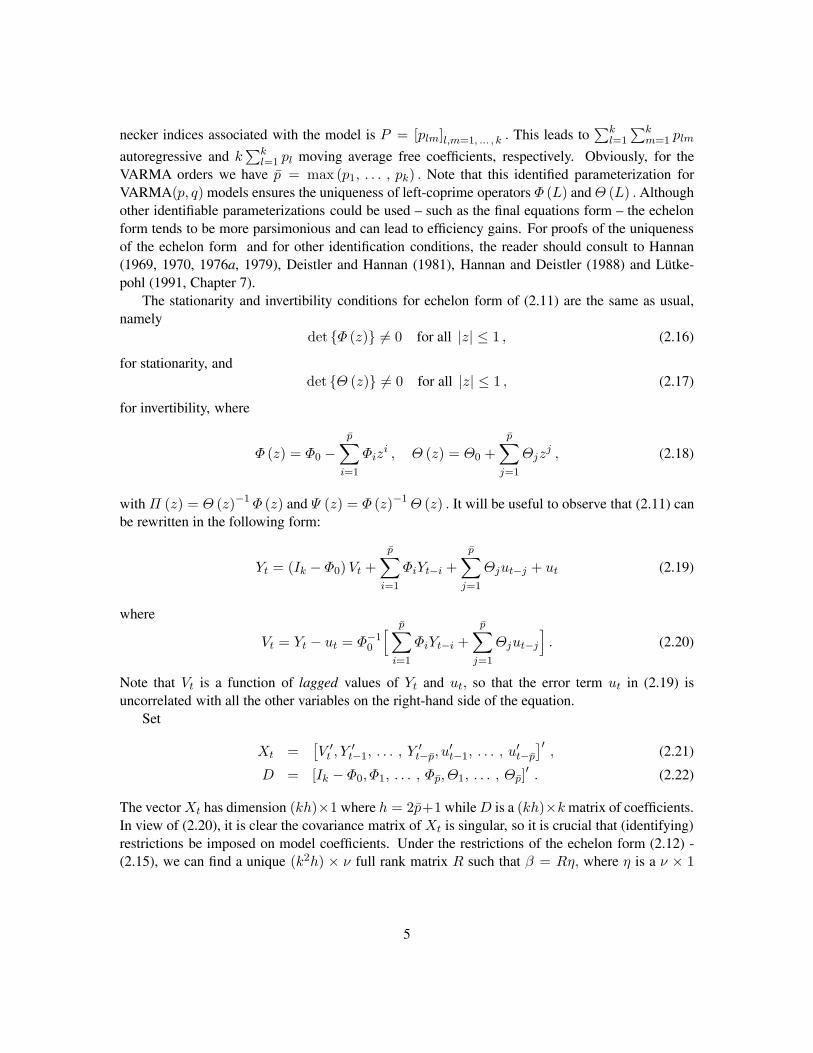
l=1 pl moving average free coefficients, respectively. Obviously, for theVARMA orders we have p = max (p1, . . . , pk) . Note that this identified parameterization forVARMA(p, q) models ensures the uniqueness of left-coprime operators Φ (L) and Θ (L) . Althoughother identifiable parameterizations could be used – such as the final equations form – the echelonform tends to be more parsimonious and can lead to efficiency gains. For proofs of the uniquenessof the echelon form and for other identification conditions, the reader should consult to Hannan(1969, 1970, 1976a, 1979), Deistler and Hannan (1981), Hannan and Deistler (1988) and Lütke-pohl (1991, Chapter 7).

The stationarity and invertibility conditions for echelon form of (2.11) are the same as usual,namely

det {Φ (z)} �= 0 for all |z| ≤ 1 , (2.16)

for stationarity, anddet {Θ (z)} �= 0 for all |z| ≤ 1 , (2.17)

for invertibility, where

Φ (z) = Φ0 −p∑

i=1

Φizi , Θ (z) = Θ0 +

p∑j=1

Θjzj , (2.18)

with Π (z) = Θ (z)−1 Φ (z) and Ψ (z) = Φ (z)−1 Θ (z) . It will be useful to observe that (2.11) canbe rewritten in the following form:

Yt = (Ik − Φ0) Vt +p∑

i=1

ΦiYt−i +p∑

j=1

Θjut−j + ut (2.19)

where

Vt = Yt − ut = Φ−10

[ p∑i=1

ΦiYt−i +p∑

j=1

Θjut−j

]. (2.20)

Note that Vt is a function of lagged values of Yt and ut, so that the error term ut in (2.19) isuncorrelated with all the other variables on the right-hand side of the equation.

Set

Xt =[V ′

t , Y ′t−1, . . . , Y ′

t−p, u′t−1, . . . , u′

t−p

]′, (2.21)

D = [Ik − Φ0, Φ1, . . . , Φp, Θ1, . . . , Θp]′ . (2.22)

The vector Xt has dimension (kh)×1 where h = 2p+1 while D is a (kh)×k matrix of coefficients.In view of (2.20), it is clear the covariance matrix of Xt is singular, so it is crucial that (identifying)restrictions be imposed on model coefficients. Under the restrictions of the echelon form (2.12) -(2.15), we can find a unique (k2h) × ν full rank matrix R such that β = Rη, where η is a ν × 1

5

vector of free coefficients and ν < k2h. Thus Yt in (2.19) can be expressed as

Yt = D′Xt + ut =(Ik ⊗ X ′

t

)Rη + ut . (2.23)

The structure of R is such that

β = vec(D) = Rη , (2.24)

R = diag(R1, . . . , Rk) =

⎡⎢⎢⎢⎢⎣

R1 0 · · · 0

0 R2 · · ·...

...... 0

0 0 · · · Rk

⎤⎥⎥⎥⎥⎦ , (2.25)

where Ri, i = 1, 2, . . . , k, are (kh)×νi full-rank selection (zero-one) matrices, each one of whichselects the non-zero elements of the corresponding equation, and νi is the number of freely varyingcoefficients present in the i-th equation. The structure of Ri is such that R′

iRi = Iνi and βi = Riηi

where βi and ηi are respectively a (kh) × 1 and νi × 1 vectors so that βi is the unconstrainedparameter vector in the i-th equation of (2.19) – on which zero restrictions are imposed – and ηi isthe corresponding vector of free parameters:

β =(β′

1, β′2, . . . , β′

k

)′, η =

(η′1, η′2, . . . , η′k

)′. (2.26)

Note also that successful identification entails that

rank{E[R′ (Ik ⊗ Xt)

(Ik ⊗ X ′

t

)R

]}= rank

{R′ (Ik ⊗ Γ )R

}= ν (2.27)

where Γ = E(XtX′t), or equivalently

rank{E[R′

iXtX′tRi

]}= rank

{R′

iΓRi

}= νi , i = 1, . . . , k . (2.28)

Setting

X(T ) = [X1, . . . , XT ]′ , (2.29)

Y (T ) = [Y1, . . . , YT ]′ = [y1(T ), . . . , yk(T )], (2.30)

U(T ) = [u1, . . . , uT ]′ = [U1(T ), . . . , Uk(T )] , (2.31)

y(T ) = vec[Y (T )] , u(T ) = vec[U(T )] , (2.32)

(2.23) can be put in any one of the two following matrix forms:

Y (T ) = X(T )D + U(T ) , (2.33)

y(T ) = [Ik ⊗ X(T )] Rη + u(T ) , (2.34)

6

where [Ik ⊗ X(T )] R is a (kT ) × ν matrix. In the sequel, we shall assume that

rank ([Ik ⊗ X(T )] R) = ν with probability 1. (2.35)

Under the assumption that the process is a regular process with continuous distribution, it is easythat the latter must hold.

To see better how the echelon restrictions should be written, consider the followingVARMA(2, 1) model in echelon form:

Y1,t = φ11,1Y1,t−1 + φ11,2Y1,t−2 + u1,t , (2.36)

Y2,t = φ21,0 (Y1,t − u1,t) + φ21,1Y1,t−1 + φ22,1Y2,t−1 + θ22,1u2,t−1 + u2,t . (2.37)

In this case, we have:

Φ (L) =[

1 − φ11,1L − φ11.2L2 −φ12,2L

2

−φ21,0 − φ21,1L 1 − φ22,1L

], (2.38)

Θ (L) =[

1 + θ11,1L + θ11,2L2 θ12,1L + θ12,2L

2

θ21,1L 1 + θ22,1L

], (2.39)

with φ12,2 = 0, θ11,1 = 0, θ11,2 = 0, θ12,1 = 0, θ12,2 = 0, θ21,1 = 0, so that the Kronecker indices

are p1 = p11 = 2, p2 = p22 = 1, p21 = 2 and p12 = 1. Setting Xt =[V ′

t , Y′t−1, Y

′t−2, u

′t−1

]′,

Vt = (V1,t, V2,t)′ , V1,t = (Y1,t − u1,t) and V2,t = (Y2,t − u2,t) , we can then write:[

Y1,t

Y2,t

]=

[0 0

φ21,0 0

] [V1,t

V2,t

]+

[φ11,1 0φ21,1 φ22,1

] [Y1,t−1

Y2,t−1

]

+[

φ11,2 00 0

] [Y1,t−2

Y2,t−2

]+

[0 00 θ22,1

] [u1,t−1

u2,t−1

]+

[u1,t

u2,t

]. (2.40)

Here we have:

β =(0, 0, φ11,1, 0, φ11,2, 0, 0, 0, φ21,0, 0, φ21,1, φ22,1, 0, 0, 0, θ22,1

)′, (2.41)

η =(φ11,1, φ11,2, φ21,0, φ21,1, φ22,1, θ22,1

)′, (2.42)

[Ik ⊗ X ′

t

]R =

[Y1,t−1 Y1,t−2 0 0 0 0

0 0 V1,t Y1,t−1 Y2,t−1 u2,t−1

], (2.43)

7

and

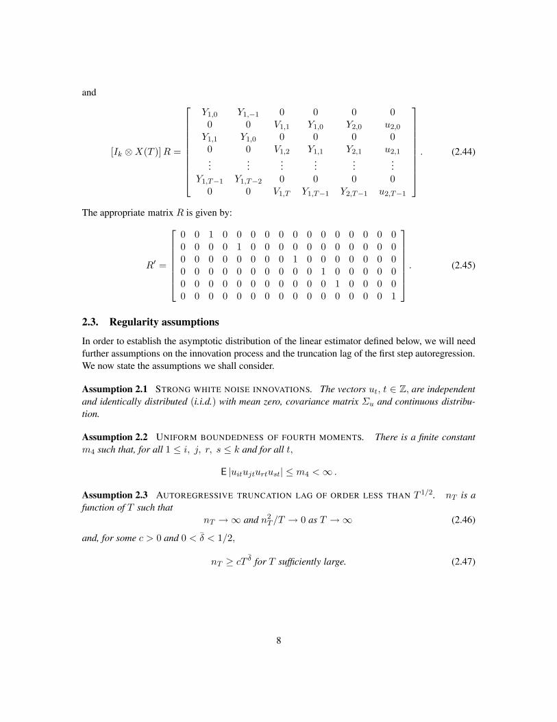
[Ik ⊗ X(T )] R =

⎡⎢⎢⎢⎢⎢⎢⎢⎢⎢⎣

Y1,0 Y1,−1 0 0 0 00 0 V1,1 Y1,0 Y2,0 u2,0

Y1,1 Y1,0 0 0 0 00 0 V1,2 Y1,1 Y2,1 u2,1...

......

......

...Y1,T−1 Y1,T−2 0 0 0 0

0 0 V1,T Y1,T−1 Y2,T−1 u2,T−1

⎤⎥⎥⎥⎥⎥⎥⎥⎥⎥⎦

. (2.44)

The appropriate matrix R is given by:

R′ =

⎡⎢⎢⎢⎢⎢⎢⎣

0 0 1 0 0 0 0 0 0 0 0 0 0 0 0 00 0 0 0 1 0 0 0 0 0 0 0 0 0 0 00 0 0 0 0 0 0 0 1 0 0 0 0 0 0 00 0 0 0 0 0 0 0 0 0 1 0 0 0 0 00 0 0 0 0 0 0 0 0 0 0 1 0 0 0 00 0 0 0 0 0 0 0 0 0 0 0 0 0 0 1

⎤⎥⎥⎥⎥⎥⎥⎦

. (2.45)

2.3. Regularity assumptions

In order to establish the asymptotic distribution of the linear estimator defined below, we will needfurther assumptions on the innovation process and the truncation lag of the first step autoregression.We now state the assumptions we shall consider.

Assumption 2.1 STRONG WHITE NOISE INNOVATIONS. The vectors ut, t ∈ Z, are independentand identically distributed (i.i.d.) with mean zero, covariance matrix Σu and continuous distribu-tion.

Assumption 2.2 UNIFORM BOUNDEDNESS OF FOURTH MOMENTS. There is a finite constantm4 such that, for all 1 ≤ i, j, r, s ≤ k and for all t,

E |uitujturtust| ≤ m4 < ∞ .

Assumption 2.3 AUTOREGRESSIVE TRUNCATION LAG OF ORDER LESS THAN T 1/2. nT is afunction of T such that

nT → ∞ and n2T /T → 0 as T → ∞ (2.46)

and, for some c > 0 and 0 < δ < 1/2,

nT ≥ cT δ for T sufficiently large. (2.47)

8

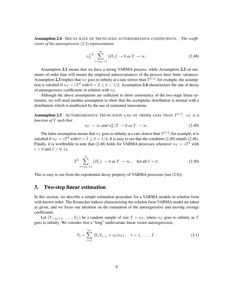
Assumption 2.4 DECAY RATE OF TRUNCATED AUTOREGRESSIVE COEFFICIENTS. The coeffi-cients of the autoregressive (2.3) representation

n1/2T

∞∑τ=nT +1

‖Πτ‖ → 0 as T → ∞ . (2.48)

Assumption 2.1 means that we have a strong VARMA process, while Assumption 2.2 on mo-ments of order four will ensure the empirical autocovariances of the process have finite variances.Assumption 2.3 implies that nT goes to infinity at a rate slower than T 1/2; for example, the assump-tion is satisfied if nT = cT δ with 0 < δ ≤ δ < 1/2. Assumption 2.4 characterizes the rate of decayof autoregressive coefficients in relation with nT .

Although the above assumptions are sufficient to show consistency of the two-stage linear es-timator, we will need another assumption to show that the asymptotic distribution is normal with adistribution which is unaffected by the use of estimated innovations.

Assumption 2.5 AUTOREGRESSIVE TRUNCATION LAG OF ORDER LESS THAN T 1/4. nT is afunction of T such that

nT → ∞ and n4T/T → 0 as T → ∞ . (2.49)

The latter assumption means that nT goes to infinity at a rate slower than T 1/4; for example, it issatisfied if nT = cT δ with 0 < δ ≤ δ < 1/4. It is easy to see that the condition (2.49) entails (2.46).Finally, it is worthwhile to note that (2.48) holds for VARMA processes whenever nT = cT δ withc > 0 and δ > 0, i.e.

T δ∞∑

τ=nT +1

‖Πτ‖ → 0 as T → ∞ , for all δ > 0 . (2.50)

This is easy to see from the exponential decay property of VARMA processes [see (2.8)].

3. Two-step linear estimation

In this section, we describe a simple estimation procedure for a VARMA models in echelon formwith known order. The Kronecker indices characterizing the echelon form VARMA model are takenas given, and we focus our attention on the estimation of the autoregressive and moving averagecoefficients.

Let (Y−nT +1, . . . , YT ) be a random sample of size T + nT , where nT goes to infinity as Tgoes to infinity. We consider first a “long” multivariate linear vector autoregression:

Yt =nT∑τ=1

ΠτYt−τ + ut(nT ) , t = 1, . . . , T , (3.1)

9

and the corresponding least squares estimates:

Π (nT ) =[Π1(nT ), . . . , ΠnT

(nT )]. (3.2)

Such an estimation can be performed by running k separate univariate linear regressions (one foreach variable in Yt). Yule-Walker estimates of the corresponding theoretical coefficients Πτ couldalso be considered. Then, under model (2.3) and the assumptions 2.1 to 2.4, it follows from theresults of Paparoditis (1996, Theorem 2.1) and Lewis and Reinsel (1985, proof of Theorem 1) that:

‖Π (nT ) − Π (nT ) ‖ = Op(n1/2T /T 1/2) (3.3)

whereΠ (nT ) =

[Π1, . . . , ΠnT

]. (3.4)

As usual, for any sequence of random variables ZT and positive numbers rT , T = 1, 2, . . . , thenotation ZT = Op(rT ) means that ZT /rT is asymptotically bounded in probability (as T → ∞),while ZT = op(rT ) means that ZT /rT converges to zero in probability. When Yt satisfies a VARMAscheme, the assumptions 2.3 and 2.4 are satisfied by any truncation lag of the form nT = cT δ withc > 0 and 0 < δ < 1/2. If, furthermore, the assumptions 2.3 and 2.4 are replaced by stronger ones,namely

nT → ∞ and n3T/T → 0 as T → ∞ , (3.5)

T 1/2∞∑

τ=nT +1

‖Πτ‖ → 0 as T → ∞ , (3.6)

then asymptotic normality also holds:

T 1/2 l (nT )′[π (nT ) − π (nT )

]−→

T→∞N

[0, l (nT )′ Q(nT )l (nT )

], (3.7)

where l (nT ) is a sequence of k2nT × 1 vectors such that 0 < M1 ≤ ‖l (nT )‖ ≤ M2 < ∞ fornT = 1, 2, . . . , and

π (nT ) − π (nT ) = vec[Π (nT ) − Π (nT )

], (3.8)

Q(nT ) = Γ (nT )−1 ⊗ Σu , Γ (nT ) = E[Yt(nT )Yt(nT )′] , (3.9)

Yt(nT ) =[Y ′

t−1, Y ′t−2, . . . , Y ′

t−nT

]′. (3.10)

Note that a possible choice for the sequence nT that satisfies both n3T/T → 0 and

T 1/2∑∞

τ=nT +1 ‖Πτ‖ → 0 is for example nT = T 1/ε with ε > 3. On the other hand nT = ln(ln T ),as suggested by Hannan and Kavalieris (1984b), is not a permissible choice because in generalT 1/2

∑∞τ=nT +1 ‖Πτ‖ does not approach zero as T → ∞.

10

Let

ut(nT ) = Yt −nT∑τ=1

Πτ (nT )Yt−τ = Yt − Π (nT )Yt(nT ) (3.11)

be the estimated residuals obtained from the first stage estimation procedure,

Σu(nT ) =1T

T∑t=1

ut(nT )ut(nT )′ (3.12)

the corresponding estimator of the innovation covariance matrix, and

ΣT =1T

T∑t=1

utu′t (3.13)

the covariance “estimator” based on the true innovations. Then, we have the following equivalencesand convergences.

Proposition 3.1 INNOVATION COVARIANCE ESTIMATOR CONSISTENCY. Let {Yt : t ∈ Z} bea k-dimensional stationary invertible stochastic process with the VARMA echelon representationgiven by (2.11) - (2.15). Then, under the assumptions 2.1 to 2.4, we have:

∥∥ 1T

T∑t=1

ut[ut(nT ) − ut]′∥∥ = Op(

nT

T) , (3.14)

1T

T∑t=1

‖ut(nT ) − ut‖2 = Op

(n2

T

T

), (3.15)

∥∥ 1T

T∑t=1

[ut(nT ) − ut][ut(nT ) − ut]′∥∥ = Op

(n2

T

T

), (3.16)

‖Σu(nT ) − ΣT ‖ = Op

(n2

T

T

), ‖Σu(nT ) − Σu‖ = Op

(n2

T

T

). (3.17)

The asymptotic equivalence between ut(nT ) and ut stated in the above proposition suggestswe may be able to consistently estimate the parameters of the VARMA model in (2.19) afterreplacing the unobserved lagged innovations ut−1, . . . , ut−p with the corresponding residualsut−1(nT ), . . . , ut−p(nT ) from the above long autoregression. So, in order to estimate the coef-ficients Φi and Θj of the VARMA process, we consider a linear regression of the form

Yt =p∑

i=1

ΦiYt−i +p∑

j=1

Θj ut−j(nT ) + et(nT ) (3.18)

11

imposing the (exclusion) restrictions associated with the echelon form. Setting

Vt(nT ) = Yt − ut(nT ) , (3.19)

this regression can also be put in a regression form similar to (2.19):

Yt = (Ik − Φ0) Vt(nT ) +p∑

i=1

ΦiYt−i +p∑

j=1

Θjut−j(nT ) + et(nT ) (3.20)

where

et(nT ) = ut(nT ) +p∑

j=0

Θj [ut−j − ut−j(nT )] . (3.21)

Note that (3.20) can be written as

Yt =[Ik ⊗ Xt(nT )′

]Rη + et(nT ) , t = 1, . . . , T , (3.22)

whereXt(nT ) =

[Vt(nT )′, Y ′

t−1, . . . , Y ′t−p, ut−1(nT )′, . . . , ut−p(nT )′

]′. (3.23)

Therefore the second step estimators η can be obtained by running least squares on the equations(3.22). Setting

X(nT ) =[X1(nT ), X2(nT ), . . . , XT (nT )

]′(3.24)

we get, after some manipulations,

η = {R′[Ik ⊗ X(nT )′X(nT )]R}−1R′[Ik ⊗ X(nT )′]y(T )

=(η′1, η

′2, . . . , η′k

)′(3.25)

whereηi = [R′

iX(nT )′X(nT )Ri]−1R′iX(nT )′yi(T ) . (3.26)

η can be easily obtained by stacking the single equation LS estimators ηi which are obtained byregressing yi on X(nT )Ri.

4. Asymptotic distribution

We will now study the asymptotic distribution of the linear estimator described in the previoussection. For that purpose, we note first that the estimator η in (3.25) can be expressed as

η = {R′[Ik ⊗ Γ (nT )]}R}−1{ 1

T

T∑t=1

R′[Ik ⊗ Xt(nT )]Yt

}(4.1)

12

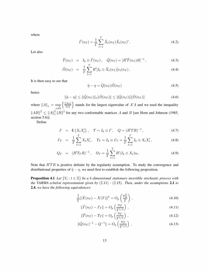
where

Γ (nT ) =1T

T∑t=1

Xt(nT )Xt(nT )′ . (4.2)

Let also

Υ (nT ) = Ik ⊗ Γ (nT ) , Q(nT ) = [R′Υ (nT )R]−1 , (4.3)

Ω(nT ) =1T

T∑t=1

R′[Ik ⊗ Xt(nT )]et(nT ) . (4.4)

It is then easy to see thatη − η = Q(nT )Ω(nT ) (4.5)

hence‖η − η‖ ≤ ‖Q(nT )‖1‖Ω(nT )‖ ≤ ‖Q(nT )‖‖Ω(nT )‖ (4.6)

where ‖A‖1 = supx �=0

{‖Ax‖‖x‖

}stands for the largest eigenvalue of A′A and we used the inequality

‖AB‖2 ≤ ‖A‖21 ‖B‖2 for any two conformable matrices A and B [see Horn and Johnson (1985,

section 5.6)].Define

Γ = E(XtX

′t

), Υ = Ik ⊗ Γ , Q = (R′ΥR)−1 , (4.7)

ΓT =1T

T∑t=1

XtX′t , ΥT = Ik ⊗ ΓT =

1T

T∑t=1

Ik ⊗ XtX′t , (4.8)

QT = (R′ΥT R)−1 , ΩT =1T

T∑t=1

R′(Ik ⊗ Xt)ut . (4.9)

Note that R′ΥR is positive definite by the regularity assumption. To study the convergence anddistributional properties of η − η, we need first to establish the following proposition.

Proposition 4.1 Let {Yt : t ∈ Z} be a k-dimensional stationary invertible stochastic process withthe VARMA echelon representation given by (2.11) - (2.15). Then, under the assumptions 2.1 to2.4, we have the following equivalences:

1T‖X(nT ) − X(T )‖2 = Op

(n2

T

T

), (4.10)

‖Γ (nT ) − ΓT ‖ = Op

( nT

T 1/2

), (4.11)

‖Υ (nT ) − ΥT ‖ = Op

( nT

T 1/2

), (4.12)

‖Q(nT )−1 − Q−1‖ = Op

( nT

T 1/2

), (4.13)

13

‖Q(nT ) − Q‖ = Op

( nT

T 1/2

). (4.14)

The latter proposition shows that the matrices Γ (nT ), Υ (nT ), Q(nT )−1 and Q(nT ) – based onapproximate innovations (estimated from a long autoregression) – are all asymptotically equivalentto the corresponding matrices based on true innovations, according to the rate nT/T 1/2. Similarlythe norm of the difference between the approximate regressor matrix X(nT ) and X(T ) has orderOp(nT /T 1/2). This suggests that η converges to η, and we give the appropriate rate of convergencein the following theorem.

Theorem 4.1 CONSISTENCY OF SECOND STEP HR ESTIMATES. Let {Yt : t ∈ Z} be a k-dimensional stationary invertible stochastic process with the VARMA echelon representation givenby (2.11) - (2.15). Then, under the assumptions 2.1 to 2.4, we have

‖ΩT ‖ = Op

(1

T 1/2

), ‖Ω(nT ) − ΩT ‖ = Op

(n2

T

T

), (4.15)

‖η − η‖ = Op

(1

T 1/2

)+ Op

(n2

T

T

). (4.16)

If, furthermore,n4

T/T → 0 as T → ∞ , (4.17)

then

‖η − η‖ = Op

(1

T 1/2

). (4.18)

The latter theorem shows that η is a consistent estimator. If furthermore, n4T /T → 0 as T → ∞,

then η converges at the rate T−1/2 which is typically expected to get asymptotic normality. In orderto derive an asymptotic distribution for η, we shall establish that the following random matrices

S(nT ) = T 1/2Q(nT )Ω(nT ) , ST = T 1/2QΩT , (4.19)

are asymptotically equivalent.

Proposition 4.2 ASYMPTOTIC EQUIVALENCE. Let {Yt : t ∈ Z} be a k-dimensional stationaryinvertible stochastic process with the VARMA echelon representation given by (2.11) - (2.15). Then,under the assumptions 2.1 to 2.4, the following equivalence holds

‖S(nT ) − ST‖ = Op

(n2

T

T 1/2

).

Finally, we can give the asymptotic distribution of√

T (η − η) .

Theorem 4.3 ASYMPTOTIC DISTRIBUTION OF TWO-STAGE ESTIMATOR. Let {Yt : t ∈ Z} bea k-dimensional stationary invertible stochastic process with the VARMA echelon representation

14

given by (2.11) - (2.15). If the assumptions 2.1 to 2.5 are satisfied, then the asymptotic distributionof the estimator η is the following:

√T

(η − η

)−→

T→∞N[0, Ση]

where

Ση = QΣXuQ′ , ΣXu = R′ [Σu ⊗ Γ ]R , (4.20)

Q = (R′ΥR)−1 , Υ = Ik ⊗ Γ , Γ = E(XtX

′t

), (4.21)

Xt =[V ′

t , Y ′t−1, . . . , Y ′

t−p, u′t−1, . . . , u′

t−p

]′and Vt = Yt − ut.

An important consequence of the above theorem is the fact that the asymptotic distributionof η is the same as in the case where the innovations u′

t−1, . . . , u′t−p are known rather than ap-

proximated by a long autoregression. Furthermore, the covariance matrix Ση can be consistentlyestimated by

Ση = Q(nT ){R′[Σu(nT ) ⊗ Γ (nT )]R}Q(nT )′ , (4.22)

where

Q(nT ) = [R′Υ (nT )R]−1, Υ (nT ) = Ik ⊗ Γ (nT ) , (4.23)

Γ (nT ) =1T

T∑t=1

Xt(nT )Xt(nT )′. (4.24)

Standard t and F -type tests may then be performed in the usual way.

5. Conclusion

In this paper, we have provided the asymptotic distribution of a simple two-stage estimator forVARMA models in echelon form. The estimator is consistent when the auxiliary long autoregres-sion used to generate first step estimates of model innovations has an order nT which increases toinfinity at a rate inferior to T δ with 0 < δ0 ≤ δ < 1/2. Further, it has an asymptotic normal distri-bution provided nT increases at a rate inferior to T δ with 0 < δ0 ≤ δ < 1/4. In the latter case, theasymptotic distribution is not affected by the fact that estimated lagged residuals are used.

The above results can be exploited in several ways. First, the two-stage estimates and the as-sociated distributional theory can be directly used for inference on the VARMA model. In partic-ular, they can be used for model selection purposes and to simplify the model (e.g., by eliminatinginsignificant coefficients). Second, two-stage estimates can be exploited to get more efficient esti-mators, such as ML estimators or estimators that are asymptotically to ML. This can be done, inparticular, to achieve efficiency with Gaussian innovations. Note, however, that such gains of ef-ficiency may not obtain if the innovations are not Gaussian. Thirdly, because of its simplicity, thetwo-stage linear estimator is especially well adapted for being used in the context of simulation-based inference procedures, such as bootstrap tests. Further, the asymptotic distribution provided

15

above can be useful in order to improve the validity of the bootstrap. Several of these issues will bestudied in a subsequent paper.

16

A. Appendix: Proofs

PROOF OF PROPOSITION 3.1 Let us write:

‖Σu(nT ) − Σu‖ = ‖Σu(nT ) − ΣT ‖ + ‖ΣT − Σu‖ (A.1)

where

ΣT − Σu =1T

T∑t=1

[utu′t − Σu] , (A.2)

Σu(nT ) − ΣT =1T

T∑t=1

{ut(nT )ut(nT )′ − utu

′t

}

=1T

T∑t=1

{[ut(nT ) − ut]ut(nT )

′+ ut[ut(nT ) − ut]

′}

=1T

T∑t=1

{[ut(nT ) − ut]u

′t + ut[ut(nT ) − ut]

′+ [ut(nT ) − ut][ut(nT ) − ut]

′}. (A.3)

By the assumptions 2.1 and 2.2,

ΣT − Σu =1T

T∑t=1

[utu′t − Σu] = Op

(1T

), (A.4)

1T

T∑t=1

‖ut‖ = Op (1) ,1T

T∑t=1

‖ut‖2 = Op (1) . (A.5)

Now

ut(nT ) − ut = [Π (nT ) − Π (nT )]Yt(nT ) +∞∑

τ=nT +1

ΠτYt−τ , (A.6)

hence1T

T∑t=1

[ut(nT ) − ut]u′t = [Π (nT ) − Π (nT )]CY u(nT ) + SY u(nT ) (A.7)

where Yt(nT ) =[Y ′

t−1, . . . , Y ′t−nT

]′, and

CY u(nT ) =1T

T∑t=1

Yt(nT )u′t = [CY u(1, T )′, . . . , CY u(nT , T )′]′ , (A.8)

CY u(τ , T ) =1T

T∑t=1

Yt−τu′t , (A.9)

17

SY u(nT ) =1T

T∑t=1

∞∑τ=nT +1

ΠτYt−τu′t . (A.10)

Using the fact that ut is independent of Xt, ut−1, . . . , u1, we see that

E‖CY u(τ , T )‖2 = E[CY u(τ , T )CY u(τ , T )′] =1T 2

T∑t=1

E[tr(Yt−τu′tutY

′t−τ )]

=1T 2

T∑t=1

tr[E(u′tut)E(Y ′

t−τYt−τ )] =1T

tr(Σu)tr[Γ (0)] , (A.11)

E[SY u(nT )] = 0 , (A.12)

where Γ (0) = E(YtY′t ), hence

E‖CY u(nT )‖2 = E[CY u(nT )′CY u(nT )] =nT∑τ=1

E‖CY u(τ , T )‖2

=nT

Ttr(Σu)tr[Γ (0)] , (A.13)

nT∑τ=1

‖CY u(τ , T )‖2 = Op

(nT

T

), (A.14)

and

‖[Π (nT ) − Π (nT )]CY u(nT )‖ ≤ ‖Π (nT ) − Π (nT ) ‖‖CY u(nT )‖ = Op

(nT

T

). (A.15)

Using the stationarity of Yt and (2.8), we have:

E[∥∥SY u(nT )

∥∥]≤ E

[ 1T

T∑t=1

( ∞∑τ=nT +1

‖Πτ‖ ‖Yt−τ‖ ‖ut‖)]

≤[E(‖Yt‖2

)]1/2[E(‖ut‖2

)]1/2 1T

T∑t=1

∞∑τ=nT +1

‖Πτ‖

≤[E(‖Yt‖2

)]1/2[E(‖ut‖2

)]1/2 C

T

T∑t=1

∞∑τ=nT +1

ρτ

≤[E(‖Yt‖2

)]1/2[E(‖ut‖2

)]1/2 C

T

T∑t=1

ρnT +1

1 − ρ

=[E(‖Yt‖2

)]1/2[E(‖ut‖2

)]1/2(

C ρ

1 − ρ

)ρnT = O(ρnT ) (A.16)

18

hence ∥∥SY u(nT )∥∥ = Op(ρnT ) . (A.17)

Consequently,

∥∥ 1T

T∑t=1

ut[ut(nT ) − ut]′∥∥ =

∥∥ 1T

T∑t=1

[ut(nT ) − ut]u′t

∥∥≤ ‖[Π (nT ) − Π (nT )]CY u(nT )‖ +

∥∥SY u(nT )∥∥

= Op

(nT

T

), (A.18)

and (3.14) is established. Finally,

∥∥ 1T

T∑t=1

[ut(nT ) − ut][ut(nT ) − ut]′∥∥ ≤ 1

T

T∑t=1

∥∥[ut(nT ) − ut][ut(nT ) − ut]′∥∥

≤ 1T

T∑t=1

∥∥ut(nT ) − ut

∥∥2(A.19)

where

1T

T∑t=1

‖ut(nT ) − ut‖2 ≤ 3T

T∑t=1

{‖Π (nT ) − Π (nT ) ‖2 ‖Yt(nT )‖2

+( ∞∑

τ=nT +1

‖Πτ‖ ‖Yt−τ‖)2}

≤ 3 ‖Π (nT ) − Π (nT ) ‖2 1T

T∑t=1

‖Yt(nT )‖2

+3T

T∑t=1

( ∞∑τ=nT +1

‖Πτ‖ ‖Yt−τ‖)2

. (A.20)

Since

E[ 1T

T∑t=1

‖Yt(nT )‖2]

= E[ 1T

T∑t=1

nT∑τ=1

‖Yt−τ‖2]

= nT E(‖Yt‖2 )

, (A.21)

we have1T

T∑t=1

‖Yt(nT )‖2 = Op(nT ) . (A.22)

19

Further,

E[ 1T

T∑t=1

( ∞∑τ=nT +1

‖Πτ‖ ‖Yt−τ‖)]

= E ‖Yt‖1T

T∑t=1

∞∑τ=nT +1

‖Πτ‖

≤ E ‖Yt‖C

T

T∑t=1

ρnT +1

1 − ρ=

(C E ‖Yt‖ ρ

1 − ρ

)ρnT

= O(ρnT ) , (A.23)

hence

1T

T∑t=1

( ∞∑τ=nT +1

‖Πτ‖ ‖Yt−τ‖)

= Op(ρnT ) , (A.24)

1T

T∑t=1

( ∞∑τ=nT +1

‖Πτ‖ ‖Yt−τ‖)2

≤ T[ 1T

T∑t=1

( ∞∑τ=nT +1

‖Πτ‖ ‖Yt−τ‖)]2

= Op(Tρ2nT ) . (A.25)

and

1T

T∑t=1

∥∥ut(nT ) − ut

∥∥2 ≤ Op

(nT

T

)Op(nT ) + Op(Tρ2nT ) = Op

(n2

T

T

), (A.26)

∥∥ 1T

T∑t=1

[ut(nT ) − ut][ut(nT ) − ut]′∥∥ = Op

(n2

T

T

). (A.27)

We can thus conclude that

‖Σu(nT ) − ΣT ‖ = Op(nT

T) + Op

(n2

T

T

)= Op

(n2

T

T

), (A.28)

‖Σu(nT ) − Σu‖ = Op

(n2

T

T

). (A.29)

PROOF OF PROPOSITION 4.1 Using (4.2) and (4.8), we see that

Γ (nT ) − ΓT =1T

T∑t=1

[Xt(nT )Xt(nT )′ − XtX

′t

]

=1T

T∑t=1

{[Xt(nT ) − Xt]X ′

t + Xt[Xt(nT ) − Xt]′}

+1T

T∑t=1

{[Xt(nT ) − Xt][Xt(nT ) − Xt]

′}(A.30)

20

hence, using the triangular and Cauchy-Schwarz inequalities,

‖Γ (nT ) − ΓT ‖ ≤ 2( 1

T

T∑t=1

‖Xt‖2)1/2( 1

T

T∑t=1

‖Xt(nT ) − Xt‖2)1/2

+1T

T∑t=1

‖Xt(nT ) − Xt‖2

= 2( 1

T‖X(T )‖2

)1/2( 1T‖X(nT ) − X(T )‖2

)1/2

+1T‖X(nT ) − X(T )‖2 (A.31)

where

Xt (nT ) − Xt =

⎡⎢⎢⎢⎢⎢⎢⎢⎢⎢⎢⎣

ut − ut (nT )0...0

ut−1 (nT ) − ut−1...

ut−p (nT ) − ut−p

⎤⎥⎥⎥⎥⎥⎥⎥⎥⎥⎥⎦

, (A.32)

1T‖X(nT ) − X(T )‖2 =

1T

T∑t=1

‖Xt(nT ) − Xt‖2

=p∑

j=0

[ 1T

T∑t=1

‖ut−j(nT ) − ut−j‖2]

= Op

(n2

T

T

)(A.33)

and, by the stationarity assumption,

1T‖X(T )‖2 =

1T

T∑t=1

‖Xt‖2 = Op (1) . (A.34)

It follows from the above orders that

‖Γ (nT ) − ΓT ‖ = Op

( nT

T 1/2

). (A.35)

Consequently, we have:

‖Υ (nT ) − ΥT ‖ = ‖Ik ⊗ Γ (nT ) − Ik ⊗ ΓT ‖= ‖Ik ⊗

(Γ (nT ) − ΓT

)‖

= k1/2‖Γ (nT ) − ΓT ‖ = Op

( nT

T 1/2

), (A.36)

21

‖Q(nT )−1 − Q−1T ‖ = ‖R′[Υ (nT ) − ΥT

]R‖

≤ ‖R‖2‖Υ (nT ) − ΥT ‖ = Op

( nT

T 1/2

). (A.37)

Further, since‖Q(nT )−1 − Q−1‖ ≤ ‖Q(nT )−1 − Q−1

T ‖ + ‖Q−1T − Q−1‖ (A.38)

and

‖Q−1T − Q−1‖ =

∥∥R′ (ΥT − Υ )R∥∥ ≤ ‖R‖2 ‖ΥT − Υ‖

≤ ‖R‖2 ‖Ik ⊗ (ΓT − Γ )‖ = k1/2 ‖R‖2 ‖ΓT − Γ‖

= k1/2 ‖R‖2∥∥∥ 1T

T∑t=1

XtX′t − E

(XtX

′t

) ∥∥∥ = Op

(1

T 1/2

), (A.39)

we have:‖Q(nT )−1 − Q−1‖ = Op

( nT

T 1/2

). (A.40)

Finally, using the triangular inequality, we get:

‖Q(nT )‖ ≤ ‖Q(nT ) − Q‖ + ‖Q‖ , (A.41)

‖Q(nT ) − Q‖ = ‖Q(nT )[Q(nT )−1 − Q−1

]Q‖

≤ ‖Q(nT )‖‖Q(nT )−1 − Q−1‖‖Q‖≤

[‖Q(nT ) − Q‖ + ‖Q‖

]‖Q(nT )−1 − Q−1‖‖Q‖ , (A.42)

hence, for ‖Q(nT )−1 − Q−1‖‖Q‖ < 1 (an event whose probability converges to 1 as T → ∞)

‖Q(nT ) − Q‖ ≤ ‖Q‖2‖Q(nT )−1 − Q−1‖1 − ‖Q(nT )−1 − Q−1‖‖Q‖

= Op

( nT

T 1/2

). (A.43)

PROOF OF THEOREM 4.1 Recall that η − η = Q(nT )Ω(nT ). Then, we have

‖η − η‖ ≤ ‖Q‖1 ‖ΩT ‖ + ‖Q(nT ) − Q‖1‖ΩT ‖ + ‖Q(nT )‖1‖Ω(nT ) − ΩT ‖≤ ‖Q‖ ‖ΩT ‖ + ‖Q(nT ) − Q‖‖ΩT ‖ + ‖Q(nT )‖‖Ω(nT ) − ΩT ‖ . (A.44)

By Proposition 4.1,

‖Q(nT ) − Q‖ = Op

( nT

T 1/2

), ‖Q(nT )‖ = Op (1) . (A.45)

22

Now

ΩT =1T

T∑t=1

R′ [Ik ⊗ Xt]ut = R′vec[ 1T

T∑t=1

Xtu′t

], (A.46)

so thatE ‖ΩT ‖2 ≤ ‖R‖2 E‖WT ‖2 (A.47)

where

WT =1T

T∑t=1

Xtu′t . (A.48)

Then, using the fact that ut is independent of Xt, ut−1, . . . , u1,

E ‖WT ‖2 = E[tr(WT W ′T )]

=1T 2

{ T∑t=1

E(tr

[Xtu

′tutX

′t

])+ 2

T−1∑t=1

T−l∑l=1

{E(tr

[Xtu

′tut+lX

′t+l

]) }

=1T 2

{ T∑t=1

E(tr

[u′

tutX′tXt

])+ 2

T−1∑t=1

T−l∑l=1

{E(tr

[ut+lX

′t+lXtu

′t

]) }

=1T 2

{ T∑t=1

tr[E(u′

tut)E(X ′tXt)

]+ 2

T−1∑t=1

T−l∑l=1

{E(tr

[E(ut+l)E(X ′

t+lXtu′t)

]) }

=1T 2

{ T∑t=1

tr[E

(utu

′t

)E

(X ′

tXt

)] }=

1T

tr(Σu)tr(Γ ) (A.49)

hence‖WT ‖ = Op

(T−1/2

), ‖ΩT ‖ = Op

(T−1/2

). (A.50)

Now, consider the term ‖Ω(nT ) − ΩT ‖. We have:

Ω(nT ) − ΩT =1T

R′T∑

t=1

{[Ik ⊗ Xt(nT )

]et(nT ) −

[Ik ⊗ Xt

]ut

}

= R′vec[ 1T

T∑t=1

{Xt(nT )et(nT )′ − Xtut

′}]= R′vec

{Ω1(nT ) + Ω2(nT )

}(A.51)

where

Ω1(nT ) =1T

T∑t=1

Xt [et(nT ) − ut]′ , (A.52)

23

Ω2(nT ) =1T

T∑t=1

[Xt(nT ) − Xt

]et(nT )

′, (A.53)

et (nT ) = ut (nT ) +p∑

j=0

Θj [ut−j − ut−j (nT )] . (A.54)

We can also write

et (nT ) − ut =p∑

j=0

Θj [ut−j (nT ) − ut−j ] (A.55)

where Θ0 = Ik − Θ0 and Θj = −Θj , j = 1, 2, . . . , p, and

ut (nT ) − ut =[Π (nT ) − Π (nT )

]Yt (nT ) +

∞∑τ=nT +1

ΠτYt−τ

=nT∑τ=1

[Πτ − Πτ (nT )

]Yt−τ +

∞∑τ=nT +1

ΠτYt−τ , (A.56)

hence

Ω1(nT ) =1T

T∑t=1

Xt [et(nT ) − ut]′

=p∑

j=0

{ 1T

T∑t=1

{ nT∑τ=1

XtY′t−j−τ

[Πτ − Πτ (nT )

]′ + ∞∑τ=nT +1

XtY′t−j−τΠ

′τ

}}Θ′

j

=p∑

j=0

{ nT∑τ=1

{ 1T

T∑t=1

XtY′t−j−τ

}[Πτ − Πτ (nT )

]′ + 1T

T∑t=1

∞∑τ=nT +1

XtY′t−j−τΠ

′τ

}Θ′

j

= Ω11(nT ) + Ω12(nT ) (A.57)

where

Ω11(nT ) =p∑

j=0

{ nT∑τ=1

Γj+τ (nT )[Πτ − Πτ (nT )

]′}Θ′

j , (A.58)

Γj+τ (nT ) =1T

T∑t=1

XtY′t−j−τ , (A.59)

Ω12(nT ) =p∑

j=0

{ 1T

T∑t=1

∞∑τ=nT +1

XtY′t−j−τΠ

′τ

}Θ′

j . (A.60)

24

Now, using the linearity and the VARMA structure of Yt, it is easy to see that

E‖Γj+τ (nT ) ‖2 ≤ 1T

C1ρj+τ1 (A.61)

for some constants C1 > 0 and 0 < ρ1 < 1, hence

E[ nT∑

τ=1

‖Γj+τ (nT ) ‖2]≤ 1

TC1

nT∑τ=1

ρj+τ1 ≤ 1

T

C1

1 − ρ1

= Op

(1T

). (A.62)

Thus

‖Ω11(nT )‖ ≤p∑

j=0

{ nT∑τ=1

‖Γj+τ (nT ) ‖‖Πτ − Πτ (nT )‖} ∥∥Θj

∥∥

≤p∑

j=0

{[ nT∑τ=1

‖Γj+τ (nT ) ‖2]1/2[ nT∑

τ=1

‖Πτ − Πτ (nT )‖2]1/2} ∥∥Θj

∥∥

≤p∑

j=0

{[ nT∑τ=1

‖Γj+τ (nT ) ‖2]1/2

‖Π (nT ) − Π (nT ) ‖} ∥∥Θj

∥∥

= Op

(n

1/2T

T

), (A.63)

while

E‖Ω12(nT )‖ ≤p∑

j=0

{E[ 1T

T∑t=1

∞∑τ=nT +1

‖Xt‖ ‖Yt−j−τ‖ ‖Πτ‖]} ∥∥Θj

∥∥

≤p∑

j=0

{ 1T

T∑t=1

∞∑τ=nT +1

‖Πτ‖E[‖Xt‖ ‖Yt−j−τ‖

]}∥∥Θj

∥∥

≤p∑

j=0

{[E(‖Xt‖2)E(‖Yt‖2)

]1/2 1T

T∑t=1

∞∑τ=nT +1

‖Πτ‖}∥∥Θj

∥∥= Op(ρnT ) , (A.64)

hence ‖Ω12(nT )‖ = Op(ρnT ) and

‖Ω1(nT )‖ ≤ ‖Ω11(nT )‖ + ‖Ω12(nT )‖ = Op

(n

1/2T

T

). (A.65)

Now, using (A.55), Ω2(nT ) can be decomposed as:

Ω2(nT ) = Ω21(nT ) + Ω22(nT ) (A.66)

25

where

Ω21(nT ) =1T

T∑t=1

[Xt(nT ) − Xt

]u

′t , (A.67)

Ω22(nT ) =p∑

j=0

{ 1T

T∑t=1

[Xt(nT ) − Xt

][ut−j (nT ) − ut−j ]

′}Θ′

j . (A.68)

Now, in view of (A.32), consider the variables:

Ci(nT ) =1T

T∑t=1

[ut−i (nT ) − ut−i]u′t

=nT∑τ=1

[Πτ − Πτ (nT )

]( 1T

T∑t=1

Yt−i−τu′t

)+

1T

T∑t=1

∞∑τ=nT +1

ΠτYt−i−τu′t , (A.69)

Cij(nT ) =1T

T∑t=1

[ut−i (nT ) − ut−i] [ut−j (nT ) − ut−j ]′ , (A.70)

for i = 0, 1, . . . , p. We have:

E‖ 1T

T∑t=1

Yt−i−τu′t‖2 =

1T 2

T∑t=1

Etr[Yt−i−τu′tutY

′t−i−τ ] =

1T 2

T∑t=1

tr[E(u′tut)E(Y ′

t−i−τYt−i−τ )]

=1T

tr(Σu)tr[Γ (0)] (A.71)

where Γ (0) = E(YtY′t ), hence

nT∑τ=1

E‖ 1T

T∑t=1

Yt−i−τu′t‖2 =

nT

Ttr(Σu)tr[Γ (0)] , (A.72)

nT∑τ=1

‖ 1T

T∑t=1

Yt−i−τu′t‖2 = Op

(nT

T

), (A.73)

and

‖Ci(nT )‖ ≤nT∑τ=1

‖Πτ − Πτ (nT )‖‖ 1T

T∑t=1

Yt−i−τu′t‖

+1T

T∑t=1

∞∑τ=nT +1

‖Πτ‖‖Yt−i−τ‖‖ut‖

26

≤[ nT∑

τ=1

‖Πτ − Πτ (nT )‖2]1/2[ nT∑

τ=1

‖ 1T

T∑t=1

Yt−i−τu′t‖2

]1/2

+1T

T∑t=1

∞∑τ=nT +1

‖Πτ‖‖Yt−i−τ‖‖ut‖

= ‖Π (nT ) − Π (nT ) ‖[ nT∑

τ=1

∥∥ 1T

T∑t=1

Yt−i−τu′t

∥∥2]1/2

+1T

T∑t=1

∞∑τ=nT +1

‖Πτ‖‖Yt−i−τ‖‖ut‖

= Op

(nT

T

). (A.74)

Further,

‖Cij(nT )‖ ≤ 1T

T∑t=1

‖ [ut−i (nT ) − ut−i] ‖‖ [ut−j (nT ) − ut−j ]′ ‖

≤[ 1T

T∑t=1

‖ut−i (nT ) − ut−i‖2]1/2[ 1

T

T∑t=1

‖ut−j (nT ) − ut−j‖2]1/2

= Op

(n2

T

T

). (A.75)

Thus

‖Ω21(nT )‖ = Op(nT /T ) , ‖Ω22(nT )‖ = Op

(n2

T

T

), (A.76)

hence

‖Ω2(nT )‖ ≤ ‖Ω21(nT )‖ + ‖Ω22(nT )‖ = Op

(n2

T

T

), (A.77)

‖Ω(nT ) − ΩT ‖ ≤ ‖R‖(‖Ω1(nT )‖ + ‖Ω2(nT )‖

)= Op

(n

1/2T

T

)+ Op

(n2

T

T

)= Op

(n2

T

T

). (A.78)

Consequently,

‖η − η‖ ≤ Op

(1

T 1/2

)+ Op

(nT

T

)+ Op

(n2

T

T

)

= Op

(1

T 1/2

)+ Op

(n2

T

T

)= op(1) . (A.79)

27

If furthermore n4T /T −→ 0 as T → ∞, the latter reduces to

‖η − η‖ = Op

(1

T 1/2

). (A.80)

PROOF OF PROPOSITION 4.2 We have:

‖S(nT ) − ST ‖ = T 1/2‖Q(nT )Ω(nT ) − QΩT ‖≤ T 1/2‖Q(nT )‖‖Ω(nT ) − ΩT ‖ + T 1/2‖Q(nT ) − Q‖‖ΩT ‖ . (A.81)

By Proposition 4.1 and Theorem 4.1, the following orders hold:

‖Q(nT ) − Q‖ = Op

( nT

T 1/2

), ‖Q(nT )‖ = Op (1) , (A.82)

‖Ω(nT ) − ΩT ‖ = Op

(n2

T

T

), ‖ΩT ‖ = Op

(1

T 1/2

). (A.83)

Therefore,

‖S(nT ) − ST‖ = Op

(n2

T

T 1/2

). (A.84)

PROOF OF THEOREM 4.3 By the standard central limit theorem for stationary processes [seeAnderson (1971, section 7.7), Lewis and Reinsel (1985, section 2)] and under the assumption ofindependence between ut and Xt, we have:

T 1/2ΩT =1

T 1/2

T∑t=1

R′(Ik ⊗ Xt)ut =1

T 1/2

T∑t=1

R′(ut ⊗ Xt) −→T→∞

N[0, ΣXu] (A.85)

where

ΣXu = E{R′(ut ⊗ Xt)(ut ⊗ Xt)′R

}= E

{R′ [utu

′t ⊗ XtX

′t

]R

}= R′ [E(utu

′t) ⊗ E(XtX

′t)

]R = R′ [Σu ⊗ Γ ]R . (A.86)

ThenST = T 1/2QΩT −→

T→∞N

[0, Ση

](A.87)

whereΣη = QΣXuQ′ . (A.88)

28

Finally, by Proposition 4.2, we can conclude that√

T (η − η) = S(nT ) −→T→∞

N[0, Ση

]. (A.89)

29

References

Akaike, H. (1976), Canonical correlation analysis of stochastic processes and its application to theanalysis of autoregressive moving average processes, in R. K. Mehra and D. G. Lainiotis, eds,‘System Identification: Advances in Case Studies’, Academic Press, New York, pp. 27–96.

Anderson, T. W. (1971), The Statistical Analysis of Time Series, John Wiley & Sons, New York.

Bartel, H. and Lütkepohl, H. (1998), ‘Estimating the Kronecker indices of cointegrated echelon-form VARMA models’, Econometrics Journal 1, C76–C99.

Boudjellaba, H., Dufour, J.-M. and Roy, R. (1992), ‘Testing causality between two vectors in multi-variate ARMA models’, Journal of the American Statistical Association 87(420), 1082–1090.

Boudjellaba, H., Dufour, J.-M. and Roy, R. (1994), ‘Simplified conditions for non-causality betweentwo vectors in multivariate ARMA models’, Journal of Econometrics 63, 271–287.

Cooper, D. M. and Wood, E. F. (1982), ‘Identifying multivariate time series models’, Journal ofTime Series Analysis 3(3), 153–164.

Deistler, M. and Hannan, E. J. (1981), ‘Some properties of the parameterization of ARMA systemswith unknown order’, Journal of Multivariate Analysis 11, 474–484.

Durbin, J. (1960), ‘The fitting of time series models’, Revue de l’Institut International de Statistique28, 233–244.

Flores de Frutos, R. and Serrano, G. R. (2002), ‘A generalized least squares estimation method forVARMA models’, Statistics 36(4), 303–316.

Galbraith, J. W. and Zinde-Walsh, V. (1994), ‘A simple, noniterative estimator for moving averagemodels’, Biometrika 81(1), 143–155.

Galbraith, J. W. and Zinde-Walsh, V. (1997), ‘On some simple, autoregression-based estimation andidentification techniques for ARMA models’, Biometrika 84(3), 685–696.

Hamilton, J. D. (1994), Time Series Analysis, Princeton University Press, Princeton, New Jersey.

Hannan, E. J. (1969), ‘The identification of vector mixed autoregressive- moving average systems’,Biometrika 57, 223–225.

Hannan, E. J. (1970), Multiple Time Series, John Wiley & Sons, New York.

Hannan, E. J. (1976a), ‘The asymptotic distribution of serial covariances’, The Annals of Statistics4(2), 396–399.

Hannan, E. J. (1976b), ‘The identification and parameterization of ARMAX and state space forms’,Econometrica 44(4), 713–723.

30

Hannan, E. J. (1979), The statistical theory of linear systems, in P. R. Krishnaiah, ed., ‘Develop-ments in Statistics’, Vol. 2, Academic Press, New York, pp. 83–121.

Hannan, E. J. and Deistler, M. (1988), The Statistical Theory of Linear Systems, John Wiley & Sons,New York.

Hannan, E. J. and Kavalieris, L. (1984a), ‘A method for autoregressive-moving average estimation’,Biometrika 71(2), 273–280.

Hannan, E. J. and Kavalieris, L. (1984b), ‘Multivariate linear time series models’, Advances inApplied Probability 16, 492–561.

Hannan, E. J. and Kavalieris, L. (1986), ‘Regression, autoregression models’, Journal of Time SeriesAnalysis 7(1), 27–49.

Hannan, E. J., Kavalieris, L. and Mackisack, M. (1986), ‘Recursive estimation of linear systems’,Biometrika 73(1), 119–133.

Hannan, E. J. and Rissanen, J. (1982), ‘Recursive estimation of mixed autoregressive-moving-average order’, Biometrika 69(1), 81–94. Errata 70 (1983), 303.

Hillmer, S. C. and Tiao, G. C. (1979), ‘Likelihood function of stationary multiple autoregressivemoving average models’, Journal of the American Statistical Association 74(367), 652–660.

Horn, R. G. and Johnson, C. A. (1985), Matrix Analysis, Cambridge University Press, Cambridge,U.K.

Huang, D. and Guo, L. (1990), ‘Estimation of nonstationary ARMAX models based on the Hannan-Rissanen method’, The Annals of Statistics 18(4), 1729–1756.

Koreisha, S. G. and Pukkila, T. M. (1989), ‘Fast linear estimation methods for vector autoregressivemoving-average models’, Journal of Time Series Analysis 10(4), 325–339.

Koreisha, S. G. and Pukkila, T. M. (1990a), ‘A generalized least-squares approach for estimation ofautoregressive-moving-average models’, Journal of Time Series Analysis 11(2), 139–151.

Koreisha, S. G. and Pukkila, T. M. (1990b), ‘Linear methods for estimating ARMA and regressionmodels with serial correlation’, Communications in Statistics, Part B -Simulation and Compu-tation 19(1), 71–102.

Koreisha, S. G. and Pukkila, T. M. (1995), ‘A comparison between different order-determinationcriteria for identification of ARIMA models’, Journal of Business and Economic Statistics13(1), 127–131.

Lewis, R. and Reinsel, G. C. (1985), ‘Prediction of multivariate time series by autoregressive modelfitting’, Journal of Multivariate Analysis 16, 393–411.

Lütkepohl, H. (1987), Forecasting Aggregated Vector ARMA Processes, Springer-Verlag, Berlin.

31

Lütkepohl, H. (1991), Introduction to Multiple Time Series Analysis, Springer-Verlag, Berlin.

Lütkepohl, H. (2001), Vector autoregressions, in B. Baltagi, ed., ‘Companion to Theoretical Econo-metrics’, Blackwell Companions to Contemporary Economics, Basil Blackwell, Oxford, U.K.,chapter 32, pp. 678–699.

Lütkepohl, H. and Claessen, H. (1997), ‘Analysis of cointegrated VARMA processes’, Journal ofEconometrics 80(2), 223–39.

Lütkepohl, H. and Poskitt, D. S. (1996), ‘Specification of echelon-form VARMA models’, Journalof Business and Economic Statistics 14(1), 69–79.

Mauricio, J. A. (2002), ‘An algorithm for the exact likelihood of a stationary vector autoregressive-moving average model’, Journal of Time Series Analysis 23(4), 473–486.

Mélard, G., Roy, R. and Saidi, A. (2002), Exact maximum likelihood estimation of structured orunit roots multivariate time series models, Technical report, Institut de Statistique, UniversitéLibre de Bruxelles, and Départment de mathématiques et statistique, Université de Montréal.

Nsiri, S. and Roy, R. (1992), ‘On the identification of ARMA echelon-form models’, CanadianJournal of Statistics 20(4), 369–386.

Nsiri, S. and Roy, R. (1996), ‘Identification of refined ARMA echelon form models for multivariatetime series’, Journal of Multivariate Analysis 56, 207–231.

Paparoditis, E. (1996), ‘Bootstrapping autoregressive and moving average parameter estimates ofinfinite order vector autoregressive processes’, Journal of Multivariate Analysis 57, 277–296.

Poskitt, D. S. (1987), ‘A modified Hannan-Rissanen strategy for mixed autoregressive-moving av-erage oder determination’, Biometrika 74(4), 781–790.

Poskitt, D. S. (1992), ‘Identification of echelon canonical forms for vector linear processes usingleast squares’, The Annals of Statistics 20(1), 195–215.

Poskitt, D. S. and Lütkepohl, H. (1995), Consistent specification of cointegrated autoregres-sive moving-average systems, Technical Report 54, Institut für Statistik und Ökonometrie,Humboldt-Universität zu Berlin.

Pukkila, T., Koreisha, S. and Kallinen, A. (1990), ‘The identification of ARMA models’, Biometrika77(3), 537–548.

Reinsel, G. C. (1997), Elements of Multivariate Time Series Analysis, second edn, Springer-Verlag,New York.

Shea, B. L. (1989), ‘The exact likelihood of a vector autoregressive moving average model’, Journalof the Royal Statistical Society Series C, Applied Statistics 38(1), 161–184.

32

Tiao, G. C. and Box, G. E. P. (1981), ‘Modeling multiple time series with applications’, Journal ofthe American Statistical Association 76(376), 802–816.

Tiao, G. C. and Tsay, R. S. (1985), A canonical correlation approach to modeling multivariatetime series, in ‘Proceedings of the Business and Economic Statistics Section of the AmericanStatistical Association’, Washington, D.C., pp. 112–120.

Tiao, G. C. and Tsay, R. S. (1989), ‘Model specification in multivariate time series’, Journal of theRoyal Statistical Society, Series B 51(2), 157–213.

Tsay, R. S. (1989a), ‘Identifying multivariate time series models’, Journal of Time Series Analysis10(4), 357–372.

Tsay, R. S. (1989b), ‘Parsimonious parameterization of vector autoregressive moving average mod-els’, Journal of Business and Economic Statistics 7(3), 327–341.

Tsay, R. S. (1991), ‘Two canonical forms for vector VARMA processes’, Statistica Sinica 1, 247–269.

Zhao-Guo, C. (1985), ‘The asymptotic efficiency of a linear procedure of estimation for ARMAmodels’, Journal of Time Series Analysis 6(1), 53–62.

33