© 2011 The Authors. Statistica Neerlandica © 2011 VVS. Published by Blackwell Publishing, 9600 Garsington Road, Oxford OX4 2DQ, UK and 350 Main Street, Malden, MA 02148, USA. doi:10.1111/j.1467-9574.2011.00495.x 462 Statistica Neerlandica (2011) Vol. 65, nr. 4, pp. 462–488 Asymptotic comparison at optimal levels of reduced-bias extreme value index estimators Frederico Caeiro* Universidade Nova de Lisboa, FCT and CMA M. Ivette Gomes† Universidade de Lisboa, DEIO, FCUL and CEAUL In this article we are interested in the asymptotic comparison, at opti- mal levels, of a set of semi-parametric reduced-bias extreme value (EV) index estimators, valid for a wide class of heavy-tailed models, underlying the available data. Again, as in the classical case, there is not any estimator that can always dominate the alternatives, but inter- esting clear-cut patterns are found. Consequently, and in practice, a suitable choice of a set of EV index estimators will jointly enable us to better estimate the EV index , the primary parameter of extreme events. Keywords and Phrases: statistics of extremes, semi-parametric esti- mation, bias estimation, heavy tails, optimal levels. 1 The estimators under study and scope of the article Let us consider a sample of size n of independent, identically distributed (i.i.d.) ran- dom variables (r.v.s), X 1 , X 2 , ... , X n , with a common distribution function (d.f.) F. Let us denote by X 1:n ≤ X 2:n ≤···≤ X n:n the associated ascending order statistics (o.s.) and let us assume that there exist sequences of real constants {a n > 0} and {b n ∈ R} such that the maximum, linearly normalized, that is, (X n:n − b n )/a n , converges in dis- tribution to a non-degenerate r.v. Then the limit distribution is necessarily of the type of the general extreme value (EV) d.f., given by EV (x) = exp(−(1 + x) −1/ ), 1 + x> 0 if = 0, exp(− exp(−x)), x ∈ R if = 0. (1) The d.f. F is said to belong to the max domain of attraction of EV , and we write F ∈D M (EV ). The parameter is the extreme value index (EVI), the primary para- meter of extreme events. This index measures the heaviness of the right tail function F := 1 − F , and the heavier the right tail, the larger the is. In this article, we shall work with heavy-tailed models, that is, Pareto-type underlying d.f.s, with a positive *[email protected] †[email protected]

Welcome message from author
This document is posted to help you gain knowledge. Please leave a comment to let me know what you think about it! Share it to your friends and learn new things together.
Transcript
© 2011 The Authors. Statistica Neerlandica © 2011 VVS.Published by Blackwell Publishing, 9600 Garsington Road, Oxford OX4 2DQ, UK and 350 Main Street, Malden, MA 02148, USA.
doi:10.1111/j.1467-9574.2011.00495.x
462
Statistica Neerlandica (2011) Vol. 65, nr. 4, pp. 462–488
Asymptotic comparison at optimal levels ofreduced-bias extreme value index estimators
Frederico Caeiro*
Universidade Nova de Lisboa, FCT and CMA
M. Ivette Gomes†
Universidade de Lisboa, DEIO, FCUL and CEAUL
In this article we are interested in the asymptotic comparison, at opti-mal levels, of a set of semi-parametric reduced-bias extreme value(EV) index estimators, valid for a wide class of heavy-tailed models,underlying the available data. Again, as in the classical case, there isnot any estimator that can always dominate the alternatives, but inter-esting clear-cut patterns are found. Consequently, and in practice, asuitable choice of a set of EV index estimators will jointly enable usto better estimate the EV index �, the primary parameter of extremeevents.
Keywords and Phrases: statistics of extremes, semi-parametric esti-mation, bias estimation, heavy tails, optimal levels.
1 The estimators under study and scope of the article
Let us consider a sample of size n of independent, identically distributed (i.i.d.) ran-dom variables (r.v.s), X1, X2, . . ., Xn, with a common distribution function (d.f.) F.Let us denote by X1:n≤X2:n≤· · ·≤Xn:n the associated ascending order statistics (o.s.)and let us assume that there exist sequences of real constants {an > 0} and {bn∈R}such that the maximum, linearly normalized, that is, (Xn:n−bn)/an, converges in dis-tribution to a non-degenerate r.v. Then the limit distribution is necessarily of thetype of the general extreme value (EV) d.f., given by
EV�(x)={
exp(−(1+ �x)−1/�), 1+ �x > 0 if � �=0,exp(− exp(−x)), x∈R if �=0.
(1)
The d.f. F is said to belong to the max domain of attraction of EV�, and we writeF ∈DM (EV�). The parameter � is the extreme value index (EVI), the primary para-meter of extreme events. This index measures the heaviness of the right tail functionF :=1−F , and the heavier the right tail, the larger the � is. In this article, we shallwork with heavy-tailed models, that is, Pareto-type underlying d.f.s, with a positive
Asymptotic comparison at optimal levels of EVI estimators 463
EVI. These heavy-tailed models are quite common in the most diversified areas ofapplication, such as computer science, telecommunications, insurance, finance, bib-liometrics and biostatistics, among others. Also very popular in insurance and fi-nance are all right tails of the type, F (x)=1−F (x)= exp{−H(x)}, H ∈RV1/�, � > 1,with RV� denoting the class of regularly varying functions at infinity, with an in-dex of regular variation equal to � (see Bingham, Goldie and Teugels, 1987). In acontext of extreme value theory we then have a null EVI, that is, �=0, in Equation1, but we are working with those tails in the domain of attraction for maxima ofEV0, which exhibit a penultimate behaviour (see Fisher and Tippett, 1928; Gomes,1984; and Diebolt and Guillou, 2005, among others), looking more similar toPareto-type tails than to exponential tails. These distributions belong to the classof sub-exponential models, another possible class of heavy-tailed models, and theestimators in this article can also be used under such a framework.
For heavy-tailed models in D+M ≡DM (EV�)�> 0, the classical EVI estimators are
the Hill (1975) estimators, which are the average of the scaled log-spacings as wellas of the log-excesses, given by
Ui := i{
lnXn−i +1:n
Xn−i:n
}and Vik := ln
Xn−i +1:n
Xn−k:n, 1≤ i≤k < n, (2)
respectively. We have
Hn(k)≡H(k)= 1k
k∑i =1
Ui = 1k
k∑i =1
Vik, 1≤k < n. (3)
But the EVI estimators in Equation 3 have often a strong asymptotic bias formoderate up to large values of k. Consequently, the adequate accommodation ofthe bias of Hill’s estimators has been extensively addressed in recent years by sev-eral authors. We mention the pioneering papers by Peng (1998), Beirlant et al.(1999), Feuerverger and Hall (1999) and Gomes, Martins and Neves (2000).In all these articles, authors are led to second-order reduced-bias EVI estimators,with asymptotic variances larger than or equal to (�(1−�)/�)2, the minimal asymp-totic variance of an ‘asymptotically unbiased’ estimator in Drees’ (1988) class offunctionals, where �< 0 is a ‘shape’ second-order parameter ruling the rate of con-vergence of the normalized sequence of maximum values towards the limiting lawEV�, in Equation 1. Recently, Caeiro, Gomes and Pestana (2005), Gomes, Martinsand Neves (2007a) and Gomes, de Haan and Henriques-Rodrigues (2008) consid-ered, in different ways, the problem of corrected-bias EVI estimation, being able toreduce the bias without increasing the asymptotic variance, which was shown to bekept at the value �2, the asymptotic variance of Hill’s estimator, the maximum like-lihood (ML) estimator of � for an underlying Pareto d.f., FP(x)=1− (x/C)−1/�, x≥C. Those estimators, called minimum variance reduced-bias (MVRB) EVI estimators,are all based on an adequate external estimation of a pair of second-order para-meters, (�, �)∈ (R, R−), done through estimators denoted (�, �), and outperform theclassical estimators for all k. Gomes et al. (2008) considered the first estimator of© 2011 The Authors. Statistica Neerlandica © 2011 VVS.
464 F. Caeiro and M. I. Gomes
this type, an EVI estimator based on a linear combination of the log-excesses Vik,in Equation 2, given by
WH�, �(k) := 1k
k∑i =1
e−�( n
k
)��ik (�)Vik, �ik(�)=�ik =− (i/k)−�−1
� ln(i/k), (4)
WH standing here for weighted Hill estimator. Caeiro et al. (2005) considered twoestimators of this same type, denoted here as:
CH�, �(k) :=H(k)
(1− �
1− �
( nk
)�)
(5)
and
CH�, �(k) :=H(k) exp
(− �
1− �
( nk
)�). (6)
A third class was introduced by Gomes et al. (2007a), and it has the functionalform
ML�,�(k) :=H(k)− �( n
k
)�(
1k
k∑i =1
(ik
)−�
Ui
), (7)
with Ui given in Equation 2. These authors also considered the estimator
ML�,�(k) := 1k
k∑i =1
e−�( n
i
)�
Ui , (8)
the estimator directly derived from the likelihood equation for �, with � and � fixed,based upon the exponential approximation Ui≈� exp(�(n/i)�)Ei , 1≤ i≤k, with {Ei}i≥1
denoting a sequence of independent, standard exponential r.v.s, being claimed abetter performance of the ML estimator, in Equation 7, compared with the ML esti-mator, in Equation 8, for a large class of models. This is the reason why we shall alsowork with a first-order approximation for the estimator WH�, �(k), in Equation 4,the bias-corrected Hill estimator
WH�, �(k) :=H(k)− �( n
k
)�(
1k
k∑i =1
�ik(�)Vik
). (9)
For the estimation of � it has been advised the use of the simplest class of estimatorsby Fraga Alves, Gomes and de Haan (2003), denoted now �(k), which are com-puted at k1 = [n1−ε], for any small value ε, like ε=0.01, where, as usual, [x] denotesthe integer part of x. In the notation of this article, and for the aforementionedEVI estimators, �= �(k1). The estimation of � has been performed through the useof a statistic dependent on a consistent estimator of �, denoted as �(k; �), intro-duced by Gomes and Martins (2002), and also computed at the same k1, that is,�= �(k1; �).© 2011 The Authors. Statistica Neerlandica © 2011 VVS.
Asymptotic comparison at optimal levels of EVI estimators 465
Apart from any of the aforementioned MVRB statistics, denoted generally asUH�, �(k), with UH standing for unbiased Hill, we shall also consider, similar towhat has been done in Beirlant et al. (1999) and Gomes and Martins (2002),among others, the statistics
UH*�(k) :=UH�(k;�), �(k), (10)
with an asymptotic variance that is no longer �2 but �2(1− �)2/�2 > �2 for every�. As mentioned before, in the UH�, �(k) and UH*
�(k) classes, (�, �) or �, respec-tively, need to be adequate consistent estimators of the second-order parameters, ifwe want to keep the same properties of UH�,�(k) or UH*
�(k), the associated r.v.s.For details on such a type of estimation see, for instance, Caeiro and Gomes (2008),Caeiro, Gomes and Henriques-Rodrigues, and Gomes, Pestana and Caeiro (2009),among others.
A third possibility is to estimate both the scale and shape second-order para-meters at the same level k, used for the estimation of �, like in Peng (1998),Feuerverger and Hall (1999) and Peng and Qi (2004), also among others. Wecould then work with statistics of the type, UH**(k) :=UH�(k;�(k)), �(k)(k), with anasymptotic variance surely larger than �2(1−�)2/�2, for every �. We shall here con-sider the estimator in Feuerverger and Hall (1999), as an illustration of estima-tors of this type. As mentioned before, and in Hall–Welsh’s class of models (Hall,1982; Hall and Welsh, 1985), the log-spacings Ui , 1≤ i ≤ k, in Equation 2, areapproximately exponential with mean value �i = �e�(i/n)−�
, 1≤ i≤k. Feuerverger andHall (1999) considered the joint maximization, in �, � and �, of the log-likelihoodof the scaled log-spacings,
ln L(�, �, �; Ui , 1≤ i≤k)=−k ln �−�k∑
i =1
(in
)−�
− 1�
k∑i =1
e−�(i/n)−�Ui .
Such a maximization leads to implicit estimators � and �, and to an explicit expres-sion for �, given by
FH**(k)≡FH�, �(k) := 1k
k∑i =1
e−�(i/n)−�Ui , (11)
which has the functional expression of the ML estimator, in Equation 8, but where(�, �) is computed at the same level k of the EVI estimator. More precisely,
(�, �) :=arg min(�, �)
{ln
(1k
k∑i =1
e−�(i/n)−�Ui
)+�
(1k
k∑i =1
(in
)−�)}
. (12)
In this article, we compare asymptotically, at optimal levels, the aforementionedMVRB statistics, in Equations 4–9, denoted generically as UH(k), the reduced-biasstatistics UH*(k), in Equation 10 (assuming thus that � and � are known oradequately estimated) and the FH**(k) statistics, in Equation 11, as illustrative ofreduced-bias EVI estimators associated with an ‘internal’ estimation of second-order© 2011 The Authors. Statistica Neerlandica © 2011 VVS.
466 F. Caeiro and M. I. Gomes
parameters. In section 2, we provide a brief review of the most common first-, sec-ond- and third-order frameworks for heavy-tailed models. In section 3, we derive, fora large class of models in D+
M , the asymptotic properties of UH(k) and UH*(k), and,in section 4, we obtain information about the dominant component of the asymp-totic bias of the EVI estimator in Equation 11, always working under an adequatethird-order framework. In section 5, we provide a full asymptotic comparison, atoptimal levels, of UH(k), UH*(k) and FH**(k) for UH=CH, ML and WH, draw-ing some concluding remarks. Finally, section 6 is dedicated to the proofs of resultsin sections 3 and 4.
2 A brief review of first-, second- and third-order conditions for heavy tails
In the most common frameworks in the area of statistics of extremes, a model F issaid to be heavy-tailed whenever the tail function F is a regularly varying functionwith a negative index of regular variation equal to −1/�, �> 0, or equivalently, thereciprocal quantile function U (t)=F←(1−1/t), t≥1, with F←(x)= inf{y : F (y)≥x},is of regular variation with index �, that is, for all x > 0,
limt→∞
F (tx)F (t)
=x−1/� ⇐⇒ limt→∞
U (tx)U (t)
=x� ⇐⇒ F ∈D+M . (13)
The second-order parameter � (≤ 0) rules the rate of convergence in the first-ordercondition 13, and it is the non-positive parameter appearing in the limiting relation
limt→∞
ln U (tx)− ln U (t)− � ln xA(t)
= x�−1�
, (14)
which is assumed to hold for every x > 0, and where |A | must then be of regularvariation with index � (Geluk and de Haan, 1987).
To obtain full information on the asymptotic bias of second-order reduced-biasEVI estimators, it is necessary to further assume a third-order condition, ruling therate of convergence in Equation 14, and which guarantees that, for all x > 0,
limt→∞
(ln U (tx)− ln U (t)− � ln x)/A(t)− (x�−1)/�B(t)
= x�+�′ −1�+�′
, (15)
where |B(t) | must then be of regular variation with index �′. There thus appearsthis extra non-positive third-order parameter �′ ≤ 0. Such a condition has alreadybeen used in Gomes, de Haan and Peng (2002) and Fraga Alves et al. (2003), forthe full derivation of the asymptotic behaviour of �-estimators, in Gomes, Caeiroand Figueiredo (2004), for the study of a reduced-bias EVI estimator and morerecently in Caeiro et al. (2009), for a comparison of some of the MVRB estimatorsin this article, where, similar to what has been done in Gomes et al. (2007a), weconsider a Pareto-type class of models, with a tail function
1−F (x)=Cx−1/�(1+D1x�/� +D2x2�/� +o(x2�/�)), (16)© 2011 The Authors. Statistica Neerlandica © 2011 VVS.
Asymptotic comparison at optimal levels of EVI estimators 467
as x→∞, with C > 0, D1, D2 /=0, �< 0. Note that to assume Equation 16 is equiv-alent to say that Equation 15 holds with �=�′< 0, and that we can there choose
A(t)=�t� =: ��t�, B(t)=�′t� = �′A(t)��
=:A(t)
�, �, �′ /=0, = �′
�, (17)
with � and �′ ‘scale’ second- and third-order parameters, respectively.
Remark 1. Several common heavy-tailed models belong to the class in Equation16. Among them we mention:
• the Fréchet model, with d.f. F (x)= exp(−x−1/�), x≥0, �> 0, for which �′=�=−1, �=0.5 and �′=5/6 (=10/6);
• the generalized Pareto (GP) model, with d.f. F (x)=1− (1+ �x)−1/�, x≥0, �> 0,for which �′=�=−� and �=�′=1 (=1);
• the Burr model, with d.f. F (x)=1− (1+x−�/�)1/�, x≥ 0, �> 0, �′=�< 0 and,as for the GP model, �=�′=1 (=1);• the Student’s t-model with degrees of freedom, with a probability density
function
ft (t)=�((+1)/2)(1+ t2/)−(+1)/2
√��(/2)
, t∈R (> 0),
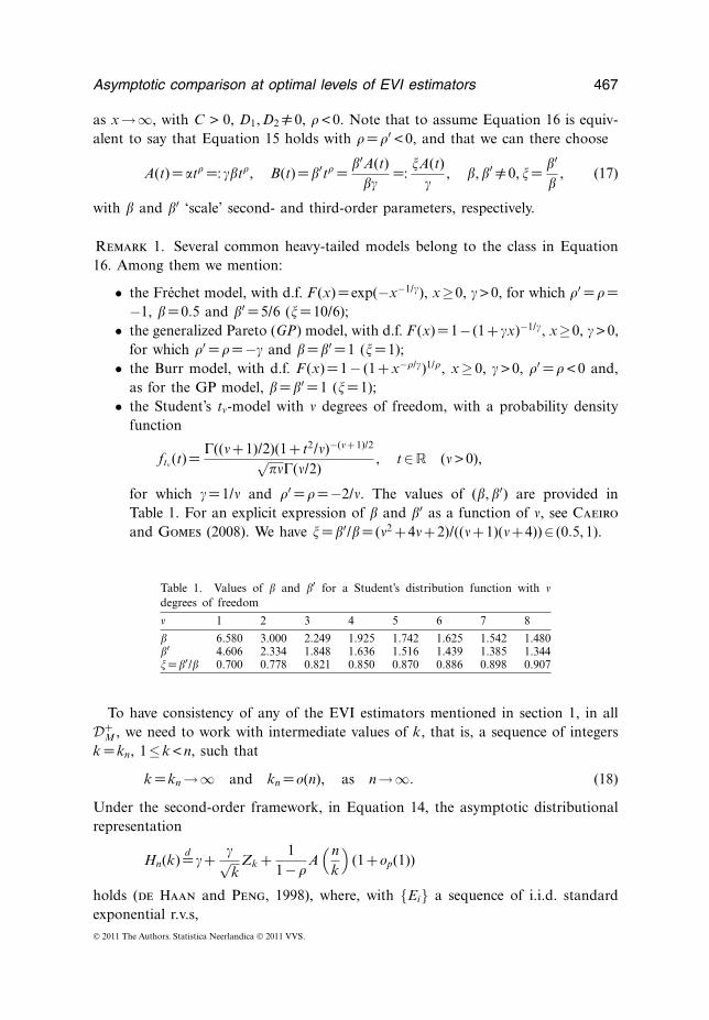
for which �=1/ and �′=�=−2/. The values of (�, �′) are provided inTable 1. For an explicit expression of � and �′ as a function of , see Caeiroand Gomes (2008). We have =�′/�= (2 +4+2)/((+1)(+4))∈ (0.5, 1).
Table 1. Values of � and �′ for a Student’s distribution function with degrees of freedom
1 2 3 4 5 6 7 8
� 6.580 3.000 2.249 1.925 1.742 1.625 1.542 1.480�′ 4.606 2.334 1.848 1.636 1.516 1.439 1.385 1.344=�′/� 0.700 0.778 0.821 0.850 0.870 0.886 0.898 0.907
To have consistency of any of the EVI estimators mentioned in section 1, in allD+
M , we need to work with intermediate values of k, that is, a sequence of integersk =kn, 1≤k < n, such that
k =kn→∞ and kn =o(n), as n→∞. (18)
Under the second-order framework, in Equation 14, the asymptotic distributionalrepresentation
Hn(k)d= �+ �√
kZk + 1
1−�A( n
k
)(1+op(1))
holds (de Haan and Peng, 1998), where, with {Ei} a sequence of i.i.d. standardexponential r.v.s,© 2011 The Authors. Statistica Neerlandica © 2011 VVS.
468 F. Caeiro and M. I. Gomes
Zk =√k
(1k
k∑i =1
Ei−1
)(19)
is an asymptotically standard normal r.v. Under adequate conditions on k, we get,for any of the aforementioned MVRB statistics, in Equations 4–9, denoted generallyas UH�, �(k), the validity of the asymptotic distributional representation
UH�, �(k)d= �+ �√
kZk +op
(A( n
k
)).
Under similar conditions, and for any of the reduced-bias statistics in Equation10, we get
UH*�(k)
d= �+ �(1−�)
|�|√kZ*
k +o*p
(A( n
k
)),
with Z*k an asymptotically standard normal r.v. For the reduced-bias statistics in
Equation 11 (Feuerverger and Hall, 1999),
FH**(k)d= �+ �(1−�)2
�2√
kZ**
k +o**p
(A( n
k
)),
with Z**k also an asymptotically standard normal r.v. Detailed information on the
remainder terms op(A(n/k)) and o*p(A(n/k)) will be given next, in section 3, whereas,
in section 4, we provide detailed information on o**p (A(n/k)).
3 The asymptotic behaviour of UH and UH*
We now state the following result, a particular case of theorems 3.1 and 3.2 inCaeiro et al. (2009), but with some additions related with the EVI estimators inEquations 4, 6 and 8.
Theorem 1. Under the third-order framework in Equation 16, with A(t) given in Equa-tion 17, Zk and Z*
k asymptotically standard normal r.v.s, and for intermediate k, thatis, if Equation 18 holds, we can write
UH�,�(k)d= �+ �Zk√
k+(
bUHA2( n
k
)+Op
(A(n/k)√
k
))(1+op(1)),
and
UH*�(k)
d= �+ �(1−�)Z*k
|� |√k+(
b*UHA2
( nk
)+Op
(A(n/k)√
k
))(1+op(1)),
where, with =�′/�,
bCH = 1�
(
1−2�− 1
(1−�)2
), bCH = 1
�
(
1−2�− 1
2(1−�)2
),
© 2011 The Authors. Statistica Neerlandica © 2011 VVS.
Asymptotic comparison at optimal levels of EVI estimators 469
bML = −1�(1−2�)
, bML = 2−12�(1−2�)
,
b*CH =− 1
�(1−3�)
((1−�)1−2�
− 2�2−�+1(1−�)2
),
b*CH
=− 1�(1−3�)
((1−�)1−2�
− 4�2−5�+32(1−�)2
),
b*ML =− (1−�)(−1)
�(1−2�)(1−3�), b*
ML=−2(1−�)− (3−5�)
2�(1−2�)(1−3�),
and with
a2(�)=− ln(1−2�)−2 ln(1−�)�2 ,
bWH = 1�
(
1−2�−a2(�)
), bWH = 1
�
(
1−2�− a2(�)
2
),
b*WH =− 1
�(1−3�)
((1−�)1−2�
−2+ (1−3�)a2(�))
,
b*WH
=− 1�(1−3�)
((1−�)1−2�
− 4− (1−3�)a2(�)2
).
Consequently, even if√
kA(n/k)→∞, with√
kA2(n/k)→�A , finite,√
k(UH�,�(k)− �) d−→n→∞ normal (�AbUH, UH = �) (20)
and√
k(UH*�(k)− �) d−→
n→∞normal(�Ab*UH, *
UH = �(1−�)/ |� | ). (21)
If√
kA2(n/k)→∞, both (UH�, �(k)− �) and (UH*�(k)− �) are Op(A2(n/k)).
Moreover, if we consistently estimate the vector (�, �) of second-order parametersthrough (�, �), with �− �=op(ln(n/k))/(
√kA(n/k)), Equations 20 and 21 still hold,
with UH�,�(k) and UH*�(k) replaced by UH�, �(k) and UH*
�(k), respectively.
Remark 2. For the adequate estimation of (�, �), see Gomes and Pestana (2007)and Caeiro et al. (2009), among others.
Remark 3. Note that bML =bML* =0 whenever =1(�′=�). This happens for impor-tant models like the Burr and the GP, and it is a point in favour of the ML statistic,as already mentioned in Gomes et al. (2007a).
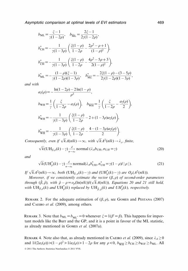
Remark 4. Note also that, as already mentioned in Caeiro et al. (2009), since �A≥0and 1/(2a2(�)) >(1−�)2 > 1/a2(�) > 1−2� for any �< 0, bWH≥bCH≥bWH ≥bML. All© 2011 The Authors. Statistica Neerlandica © 2011 VVS.
470 F. Caeiro and M. I. Gomes
depends then on the sign of the bias, but we expect the sample paths of WH to bealways above the sample paths of CH, which should be in turn above the samplepaths of WH, these ones above the ones of ML. The ML statistics are then prefer-able to the other ones whenever the bias are all positive. If the bias are all negative,WH is expected to outperform the other statistics.
4 The FH** estimators under a third-order framework
4.1 The estimators under play
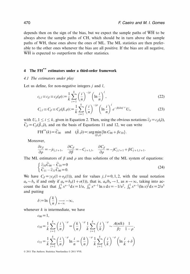
Let us define, for non-negative integers j and l,
cj,l ≡ cjl ≡ cjl(�) := 1k
k∑i =1
(in
)−j�(ln
in
)l
, (22)
Cj,l ≡Cjl ≡Cjl(�, �) := 1k
k∑i =1
(in
)−j�(ln
in
)l
e−�(i/n)−�Ui , (23)
with Ui , 1 ≤ i ≤ k, given in Equation 2. Then, using the obvious notations cjl = cjl(�),Cjl =Cjl(�, �), and on the basis of Equations 11 and 12, we can write
FH**(k)= C00 and (�, �)=: arg min(�,�){ln C00 +�c10}.
Moreover,
∂cjl
∂�=−jcj,l +1,
∂Cjl
∂�=−Cj +1,l ,
∂Cjl
∂�=−jCj,l +1 +�Cj +1,l +1.
The ML estimators of � and � are thus solutions of the ML system of equations:{c10C00− C10 =0C11− c11C00 =0.
(24)
We have Cjl = �cjl(1+op(1)), and for values j, l =0, 1, 2, with the usual notationan∼ bn if and only if an =bn(1+o(1)), that is, an/bn→ 1, as n→∞, taking into ac-count the fact that
∫ 10 x�−1dx =1/�,
∫ 10 x�−1 ln x dx =−1/�2,
∫ 10 x�−1(ln x)2dx =2/�3
and putting
� := ln(
kn
)−→n→∞−∞,
whenever k is intermediate, we have
c00 =1,
c10 = 1k
k∑i =1
(in
)−�
=(
kn
)−� 1k
k∑i =1
(ik
)−�
∼ A(n/k)��
11−�
,
c11 = 1k
k∑i =1
(in
)−�
lnin
=(
kn
)−� 1k
k∑i =1
(ik
)−�(ln
ik
+�
)© 2011 The Authors. Statistica Neerlandica © 2011 VVS.
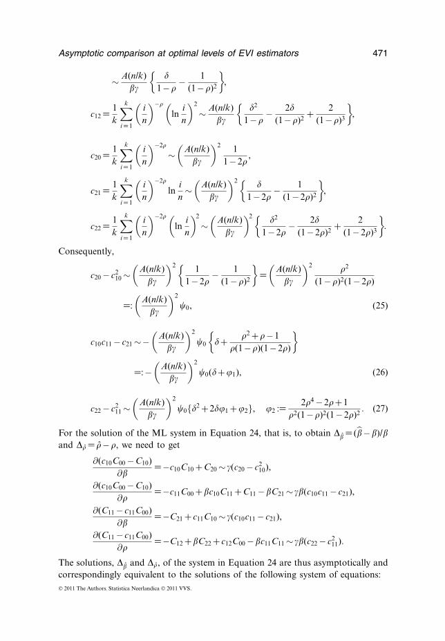
Asymptotic comparison at optimal levels of EVI estimators 471
∼ A(n/k)��
{�
1−�− 1
(1−�)2
},
c12 = 1k
k∑i =1
(in
)−�(ln
in
)2
∼ A(n/k)��
{�2
1−�− 2�
(1−�)2 + 2(1−�)3
},
c20 = 1k
k∑i =1
(in
)−2�
∼(
A(n/k)��
)2 11−2�
,
c21 = 1k
k∑i =1
(in
)−2�
lnin∼(
A(n/k)��
)2{ �1−2�
− 1(1−2�)2
},
c22 = 1k
k∑i =1
(in
)−2�(ln
in
)2
∼(
A(n/k)��
)2{ �2
1−2�− 2�
(1−2�)2 + 2(1−2�)3
}.
Consequently,
c20− c210∼
(A(n/k)
��
)2{ 11−2�
− 1(1−�)2
}=(
A(n/k)��
)2 �2
(1−�)2(1−2�)
=:(
A(n/k)��
)2
�0, (25)
c10c11− c21∼−(
A(n/k)��
)2
�0
{�+ �2 +�−1
�(1−�)(1−2�)
}
=:−(
A(n/k)��
)2
�0(�+�1), (26)
c22− c211∼
(A(n/k)
��
)2
�0{�2 +2��1 +�2}, �2 := 2�4−2�+1�2(1−�)2(1−2�)2 . (27)
For the solution of the ML system in Equation 24, that is, to obtain �� = (�−�)/�and �� = �−�, we need to get
∂(c10C00−C10)∂�
=−c10C10 +C20∼ �(c20− c210),
∂(c10C00−C10)∂�
=−c11C00 +�c10C11 +C11−�C21∼ ��(c10c11− c21),
∂(C11− c11C00)∂�
=−C21 + c11C10∼ �(c10c11− c21),
∂(C11− c11C00)∂�
=−C12 +�C22 + c12C00−�c11C11∼ ��(c22− c211).
The solutions, �� and ��, of the system in Equation 24 are thus asymptotically andcorrespondingly equivalent to the solutions of the following system of equations:© 2011 The Authors. Statistica Neerlandica © 2011 VVS.
472 F. Caeiro and M. I. Gomes⎧⎨⎩ 0≡ c10C00− C10 = c10C00−C10 +��(��(c20− c210)+��(c10c11− c21))
0≡ C11− c11C00 =C11− c11C00 +��(��(c11c10− c21)+��(c22− c211)).
With the notations introduced in Equations 25–27, for �0, �1 and �2, respectively,we can write[��
��
]= ��(1−�)2(1−2�)3
�2A2(n/k)
[�2 +2��1 +�2 �+�1
�+�1 1
][C10− c10C00
c11C00−C11
](1+op(1)).
(28)
After obtaining the asymptotic behaviour of � and �, the use of the �-method(Taylor’s expansion) enables us to write
FH�, �(k)≡ C00 =C00 + (�−�)∂C00
∂�(1+op(1))+ (�−�)
∂C00
∂�(1+op(1))
=C00−�(C10��−C11��)(1+op(1)).
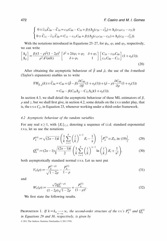
In section 4.3, we shall detail the asymptotic behaviour of these ML estimators of �,� and �, but we shall first give, in section 4.2, some details on the r.v.s under play, thatis, the r.v.s Cjl , in Equation 23, whenever working under a third-order framework.
4.2 Asymptotic behaviour of the random variables
For any real �≥1, with {Ei}i≥1 denoting a sequence of i.i.d. standard exponentialr.v.s, let us use the notations
P(�)k :=
√(2�−1)k
(1k
k∑i =1
(ik
)�−1
Ei− 1�
) [P(1)
k ≡Zk, in (19)], (29)
Q(�)k := (2�−1)
√(2�−1)k
2
(1k
k∑i =1
(ik
)�−1
ln(
ik
)Ei + 1
�2
), (30)
both asymptotically standard normal r.v.s. Let us next put
Vk(�) := P(1−�)k√1−2�
− P(1)k
1−�(31)
and
Wk(�) :=√
2Q(1−�)k
(1−2�)√
1−2�+ P(1)
k
(1−�)2 . (32)
We first state the following results.
Proposition 1. If k =kn −→n→∞∞, the second-order structure of the r.v.’s P(�)
k and Q(�)k
in Equations 29 and 30, respectively, is given by© 2011 The Authors. Statistica Neerlandica © 2011 VVS.
Asymptotic comparison at optimal levels of EVI estimators 473
cov(P(�)k , P(�)
k )∼√
(2�−1)(2�−1)�+�−1
and
cov(P(�)k , Q(�)
k )∼− (2�−1)√
(2�−1)(2�−1)√2(�+�−1)2
.
Trivial adaptations of the results in Gomes and Martins (2004), performed thereunder the second-order framework in Equation 14, enable us to state the followingresult, without the need of a proof.
Proposition 2. If k =kn is a sequence of intermediate positive integers, that is,Equation 18 holds, then for any real �≥1, the statistics
V�(k) := �k
k∑i =1
(ik
)�−1
Ui and W�(k) :=−�2
k
k∑i =1
(ik
)�−1
ln(
ik
)Ui
are consistent EVI estimators. Moreover, if the third-order condition in Equation 15holds, with A and B given in Equation 17, and up to levels k such that
√kA2(n/k) n→∞−→ �A,
finite, we can guarantee the asymptotic normality of the estimators, and the validityof the asymptotic distributional representations
V�(k)d= �+ �√
k
�P(�)k√
2�−1+ �A(n/k)
�−�+ �A2(n/k)
�(�−2�)(1+op(1)) (33)
and
W�(k)d= �− �√
k
√2�2Q(�)
k
(2�−1)√
2�−1+ �2A(n/k)
(�−�)2 + �2A2(n/k)�(�−2�)2 (1+op(1)), (34)
where P(�)k and Q(�)
k are the asymptotically standard normal r.v.s in Equations 29 and 30,respectively.
We shall now provide the asymptotic distributional properties of Cjl , in Equation 23,for j, l =0, 1. We obviously have Cjl = �cjl(1+op(1)), with cjl defined in Equation 22,and we also have the validity of the following asymptotic distributional representa-tions.
Theorem 2. If the third-order condition, in Equation 15, holds, with A and B given inEquation 17, if k =kn is a sequence of intermediate positive integers, that is, Equation18 holds, and up to levels such that
√kA2(n/k)→�A, finite,
C00 = �+ �√k
P(1)k + (2−1)A2(n/k)
2�(1−2�)(1+op(1)) (35)
=: �+ �√k
P(1)k +u00A2
( nk
), (36)
© 2011 The Authors. Statistica Neerlandica © 2011 VVS.
474 F. Caeiro and M. I. Gomes
C10 = A(n/k)��
{�
1−�+op(1)
}, (37)
and
C11 =�C10− A(n/k)��
(�
(1−�)2 +op(1)). (38)
Consequently, with Vk(�) and Wk(�) defined in Equations 31 and 32, respectively, andwith
u10 := (2−1)�2
�2(1−�)(1−2�)(1−3�), u11 :=− (2−1)�(1−2�−�2)
�2(1−�)2(1−2�)(1−3�)2 , (39)
we have
C10− c10C00 = A(n/k)
�√
k
(Vk(�)+u10
√kA2(n/k)(1+op(1))
)=:
A(n/k)
�√
kSk (40)
and
c11C00−C11 =−A(n/k)
�√
k
(�Sk +Wk(�)+u11
√kA2(n/k)(1+op(1))
)=:−A(n/k)
�√
k(�Sk +Tk).
(41)
4.3 Back to the ML system of equations
Let us go back to the ML system of equations in Equation 24, and its solution inEquation 28.
Theorem 3. Under the validity of the third-order framework in Equation 15, with Aand B given in Equation 17, and for k intermediate, such that
√kA(n/k)−→
n→∞∞, � is
consistent for the estimation of �. If we further have√
kA(n/k)ln(k/n) −→n→∞∞, � is consistent
for the estimation of �. We can more precisely say that
��
d= ln(k/n)√kA(n/k)
�(1−�)(1−2�)√
1−2��
Uk
+ (2−1)�(1−�)(1−2�)�(1−3�)2 ln
(kn
)A( n
k
)(1+op(1))
and
��d= 1√
kA(n/k)
�(1−�)(1−2�)√
1−2��
Uk
+ (2−1)�(1−�)(1−2�)�(1−3�)2 A
( nk
)(1+op(1)),
where Uk is a standard normal r.v.
Finally, for the EVI estimator in Equation 11 we obtain the following result.© 2011 The Authors. Statistica Neerlandica © 2011 VVS.
Asymptotic comparison at optimal levels of EVI estimators 475
Theorem 4. Under the third-order framework in Equation 15, with A and B given inEquation 17, and for intermediate k, the asymptotic distributional representation
FH**(k)d= �+ �
(1−�
�
)2 Z**k√k
+b**FHA2
( nk
)(1+op(1)) (42)
holds, where Z**k is an asymptotically standard normal r.v. and
b**FH := (2−1)(1−�)2
2�(1−2�)(1−3�)2 . (43)
Consequently, even if√
kA(n/k)→∞, with√
kA2(n/k)→�A, finite,
√k(FH**(k)− �) d−→
n→∞ normal(
�Ab**FH, **
FH = �(1−�)2
�2
).
Remark 5. Up to the scale �, the standard deviation (s.d.) of Feuerverger and Hall’sML EVI estimator is the square of the s.d. we obtain when we proceed to the exter-nal estimation of � and internal estimation of �. Indeed, with Feuerverger and Hall’snotation, we can compute the value in their Remark 5, obtaining exactly the re-sult obtained in our Theorem 4, as already noticed in Gomes and Martins (2002),among others. We have
�jk =∫ 1
0xj�1 (ln x)kdx = (−1)k �(k +1)
(1+ j�1)k +1
and �1 =−�. In the notation considered here, we have
�j0 = 11−�j
, �j1 =− 1(1−�j)2 , �j2 = 2
(1−�j)3 .
Then, we obtain
�0 = (�20−�210)(�22−�2
11)− (�21−�10�11)2 =(
�(1−�)(1−2�)
)4
,
�1 =�20�22−�221 = 1
(1−2�)4 , �2 =�11�21−�10�22 =− 1(1−�)2(1−2�)3 ,
�3 =�10�21−�11�20 =− �(1−�)2(1−2�)2
and, in the notation of Feuerverger and Hall (1999),
21 = 1
�20
∫ 1
0(�1 +�2x−� +�3x−� ln x)2dx =
(1−�
�
)4
.
5 Asymptotic comparison of EVI estimators at optimal levels
Following the comparison made in Gomes et al. (2007a) for the MVRB ML andML* estimators, we shall next proceed to the comparison of the estimators understudy at their optimal levels. This is again done in a way similar to the one used© 2011 The Authors. Statistica Neerlandica © 2011 VVS.
476 F. Caeiro and M. I. Gomes
in de Haan and Peng (1998), Gomes and Martins (2001), Gomes, Miranda andPereira (2005), Gomes, Miranda and Viseu (2007b), Gomes and Neves (2008) andGomes and Henriques-Rodrigues (2010) for the classical EVI estimators. Let usassume that �•n (k) denotes any arbitrary reduced-bias semi-parametric estimator ofthe EV index �, for which we have
�•n (k)= �+ •√k
Z •k +b•A2( n
k
)+op
(A2( n
k
)), (44)
for any intermediate sequence of integers k =kn, and where Z •k is asymptoticallystandard normal. Then,
√k(�•n (k)− �)→d N(�Ab•, 2
•) provided that k is such that√kA2(n/k)→ �A, finite, as n→∞. We then write bias∞(�•n(k)) :=b•A2(n/k) and
var∞(�•n (k)) := 2•/k. The so-called asymptotic mean square error (AMSE) is then given
by AMSE(�•n (k)) := 2•/k +b2
•A4(n/k). Regular variation theory (Bingham et al., 1997),
enables us to show that, whenever b• /=0, there exists a function �(n)=�(n, �, �), suchthat
limn→∞�(n)AMSE (�•n0)= ( 2
•)(−4�/(1−4�))(b2
•)1/(1−4�) =: LMSE(�•n0),
with LMSE standing for limiting mean square error, and where �•n0 := �•n, k•0 (n) andk•0(n) :=arg inf
kAMSE(�•n (k)).
It is then sensible to consider the following.
Definition 1. Given two biased estimators �(1)n (k) and �(2)
n (k), for which a distri-butional representation of the type of the one in Equation 44 holds, with constants( 1, b1) and ( 2, b2), b1, b2 /=0, respectively, both computed at their optimal levels,the asymptotic root efficiency (AREFF) of �(1)
n0 relative to �(2)n0 is:
AREFF1 |2≡AREFF�(1)n0 | �(2)
n0:=√√√√LMSE [�(2)
n0 ]
LMSE [�(1)n0 ]
=((
2
1
)−4� ∣∣∣∣b2
b1
∣∣∣∣)1/(1−4�)
.
(45)
Remark 6. Note that the AREFF indicator, in Equation 45, has been conceived sothat the highest the AREFF indicator is, the better is the first estimator.
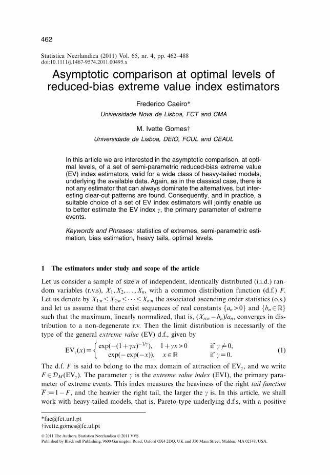
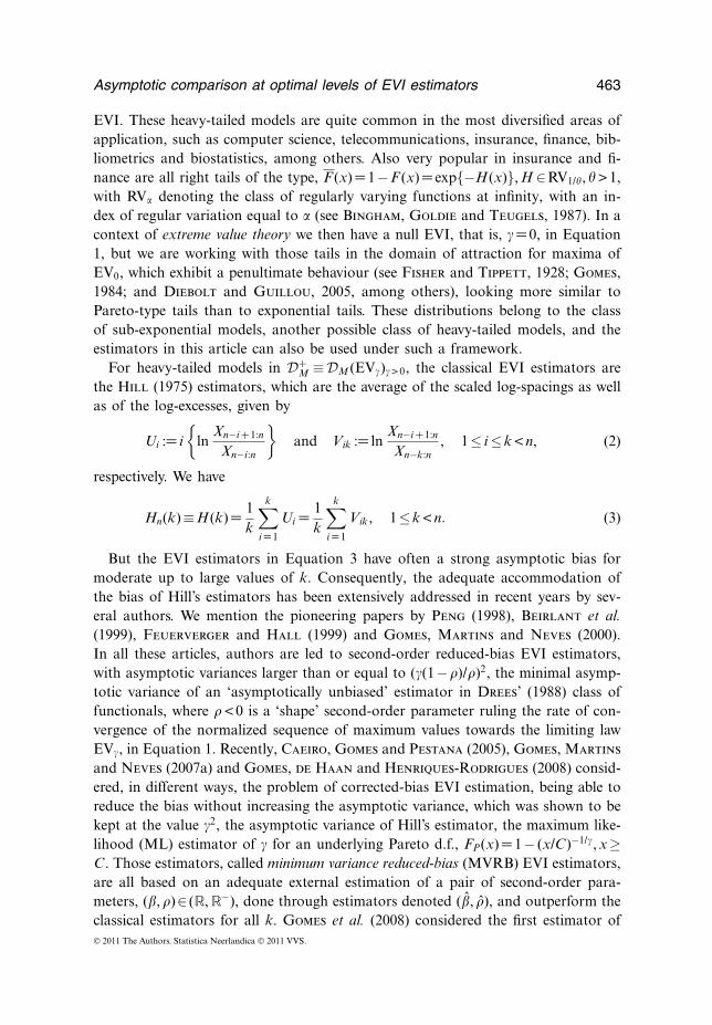
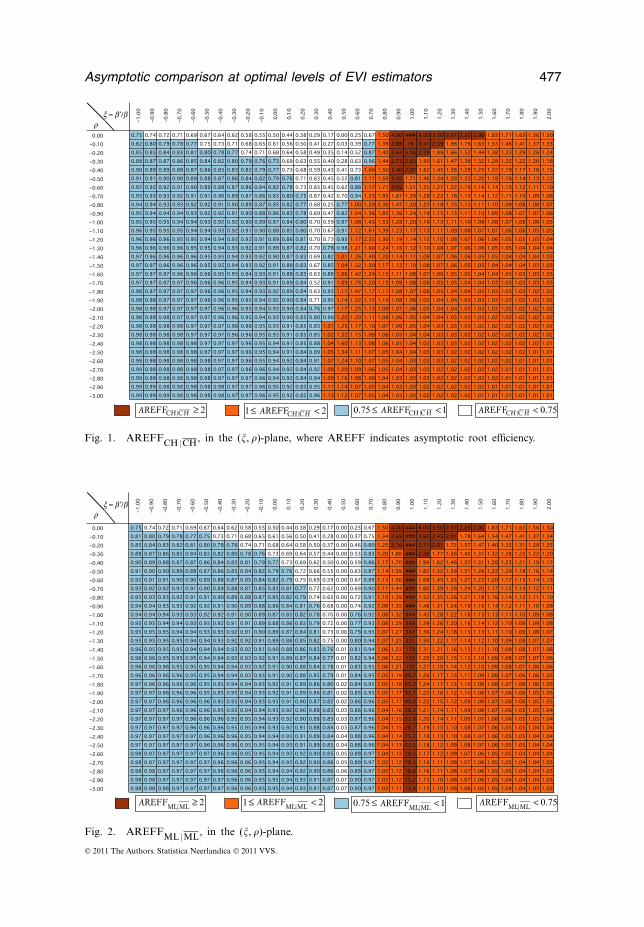
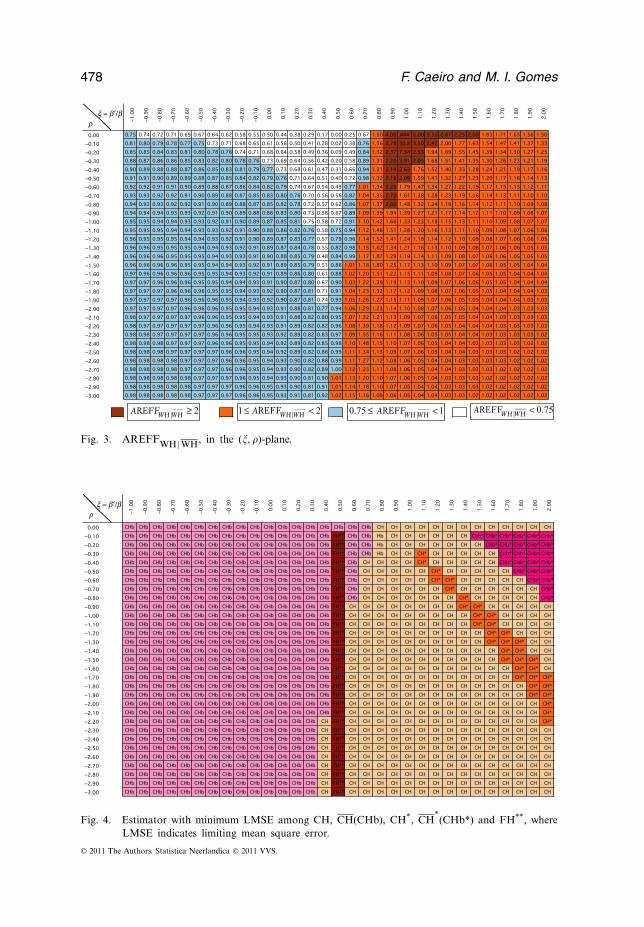
We first present in Figures 1–3, the measure AREFFUH |UH for UH=CH, ML,WH, respectively.
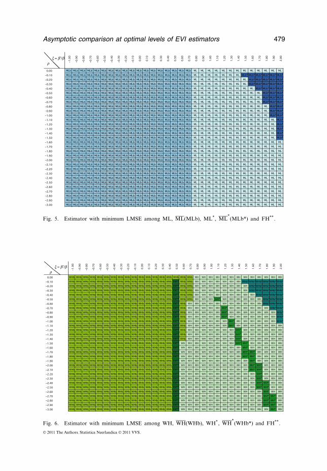
The general behaviour of UH, UH, UH* and UH*, again for UH=CH, ML,WH,
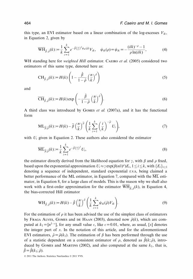
and jointly with the behaviour of FH**, is shown in Figures 4–6, respectively, wherewe register the estimator with the highest efficiency among the ones considered, thatis, the one with maximum AREFF, or equivalently, minimum LMSE. Note thatFH** is not present in Figure 5.
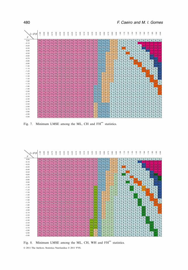
In Figure 7, we picture together all the CH, ML and FH statistics, and finally,in Figure 8, we put together all the CH, the ML, the WH and the FH statistics.© 2011 The Authors. Statistica Neerlandica © 2011 VVS.
Asymptotic comparison at optimal levels of EVI estimators 477
x = b ¢/br
Fig. 1. AREFFCH |CH, in the (, �)-plane, where AREFF indicates asymptotic root efficiency.
x = b ¢/br
Fig. 2. AREFFML |ML, in the (, �)-plane.
© 2011 The Authors. Statistica Neerlandica © 2011 VVS.
478 F. Caeiro and M. I. Gomes
x = b ¢/br
Fig. 3. AREFFWH |WH, in the (, �)-plane.
x = b ¢/br
Fig. 4. Estimator with minimum LMSE among CH, CH(CHb), CH*, CH*(CHb*) and FH**, where
LMSE indicates limiting mean square error.
© 2011 The Authors. Statistica Neerlandica © 2011 VVS.
Asymptotic comparison at optimal levels of EVI estimators 479
x = b ¢/br
Fig. 5. Estimator with minimum LMSE among ML, ML(MLb), ML*, ML*(MLb*) and FH**.
x = b ¢/br
Fig. 6. Estimator with minimum LMSE among WH, WH(WHb), WH*, WH*(WHb*) and FH**.
© 2011 The Authors. Statistica Neerlandica © 2011 VVS.
480 F. Caeiro and M. I. Gomes
x = b ¢/br
Fig. 7. Minimum LMSE among the ML, CH and FH** statistics.
x = b ¢/br
Fig. 8. Minimum LMSE among the ML, CH, WH and FH** statistics.
© 2011 The Authors. Statistica Neerlandica © 2011 VVS.
Asymptotic comparison at optimal levels of EVI estimators 481
5.1. Concluding remarks
1. From Figures 1–3, it is possible to see that, as expected, there is not a big differ-ence in the relative behaviour between UH and UH for UH=CH, ML and WH,but their simultaneous use will for sure enable us to better estimate �, the primaryparameter of extreme events.
2. As already proved in proposition 2.1 of Gomes et al. (2007a), ML beats ML*
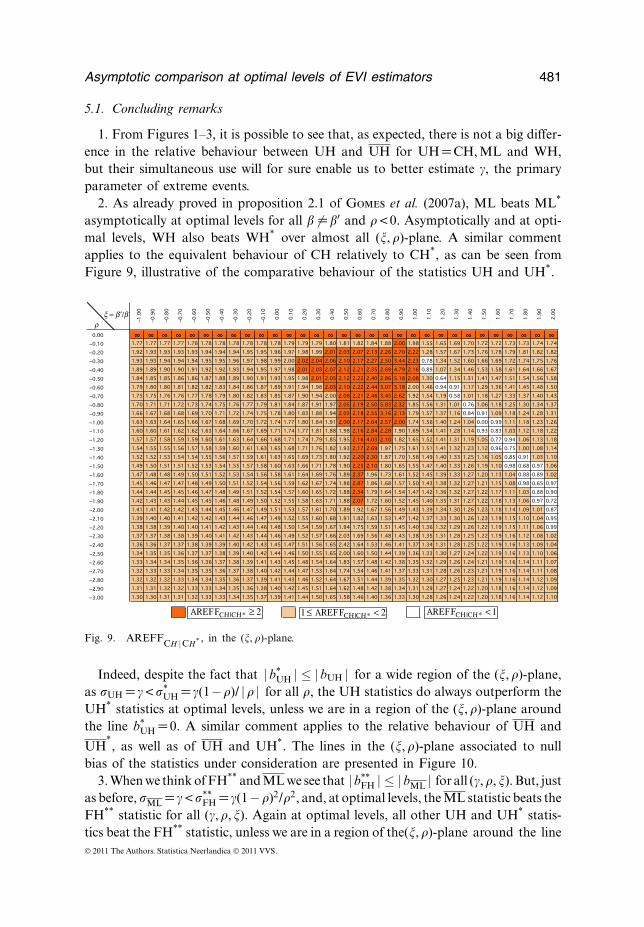
asymptotically at optimal levels for all � �=�′ and �< 0. Asymptotically and at opti-mal levels, WH also beats WH* over almost all (, �)-plane. A similar commentapplies to the equivalent behaviour of CH relatively to CH*, as can be seen fromFigure 9, illustrative of the comparative behaviour of the statistics UH and UH*.
x = b ¢/br
Fig. 9. AREFFCH |CH* , in the (, �)-plane.
Indeed, despite the fact that |b*UH | ≤ |bUH | for a wide region of the (, �)-plane,
as UH = �< *UH = �(1−�)/ |� | for all �, the UH statistics do always outperform the
UH* statistics at optimal levels, unless we are in a region of the (, �)-plane aroundthe line b*
UH =0. A similar comment applies to the relative behaviour of UH and
UH*, as well as of UH and UH*. The lines in the (, �)-plane associated to null
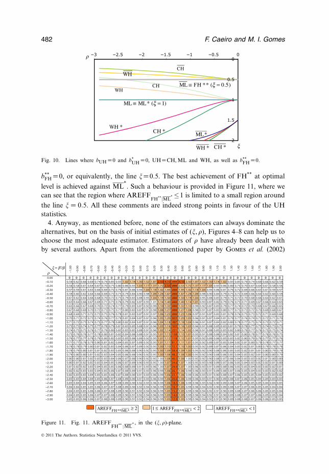
bias of the statistics under consideration are presented in Figure 10.3. When we think of FH** and ML we see that |b**
FH | ≤ |bML | for all (�, �, ). But, justas before, ML = �< **
FH = �(1−�)2/�2, and, at optimal levels, the ML statistic beats theFH** statistic for all (�, �, ). Again at optimal levels, all other UH and UH* statis-tics beat the FH** statistic, unless we are in a region of the(, �)-plane around the line© 2011 The Authors. Statistica Neerlandica © 2011 VVS.
482 F. Caeiro and M. I. Gomes
Fig. 10. Lines where bUH =0 and b*UH =0, UH=CH, ML and WH, as well as b**
FH =0.
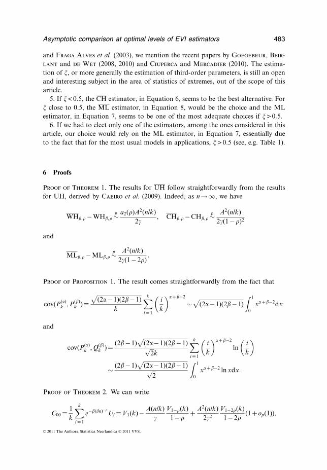
b**FH =0, or equivalently, the line =0.5. The best achievement of FH** at optimal
level is achieved against ML*. Such a behaviour is provided in Figure 11, where we
can see that the region where AREFFFH**|ML
*≤1 is limited to a small region around
the line = 0.5. All these comments are indeed strong points in favour of the UHstatistics.
4. Anyway, as mentioned before, none of the estimators can always dominate thealternatives, but on the basis of initial estimates of (, �), Figures 4–8 can help us tochoose the most adequate estimator. Estimators of � have already been dealt withby several authors. Apart from the aforementioned paper by Gomes et al. (2002)
x = b ¢/br
Figure 11. Fig. 11. AREFFFH** |ML
* , in the (, �)-plane.
© 2011 The Authors. Statistica Neerlandica © 2011 VVS.
Asymptotic comparison at optimal levels of EVI estimators 483
and Fraga Alves et al. (2003), we mention the recent papers by Goegebeur, Beir-lant and de Wet (2008, 2010) and Ciuperca and Mercadier (2010). The estima-tion of , or more generally the estimation of third-order parameters, is still an openand interesting subject in the area of statistics of extremes, out of the scope of thisarticle.
5. If < 0.5, the CH estimator, in Equation 6, seems to be the best alternative. For close to 0.5, the ML estimator, in Equation 8, would be the choice and the MLestimator, in Equation 7, seems to be one of the most adequate choices if > 0.5.
6. If we had to elect only one of the estimators, among the ones considered in thisarticle, our choice would rely on the ML estimator, in Equation 7, essentially dueto the fact that for the most usual models in applications, > 0.5 (see, e.g. Table 1).
6 Proofs
Proof of Theorem 1. The results for UH follow straightforwardly from the resultsfor UH, derived by Caeiro et al. (2009). Indeed, as n→∞, we have
WH�,�−WH�,�p∼ a2(�)A2(n/k)
2�, CH�,�−CH�,�
p∼ A2(n/k)2�(1−�)2
and
ML�,�−ML�,�p∼ A2(n/k)
2�(1−2�).
Proof of Proposition 1. The result comes straightforwardly from the fact that
cov(P(�)k , P(�)
k )=√
(2�−1)(2�−1)k
k∑i =1
(ik
)�+�−2
∼√
(2�−1)(2�−1)∫ 1
0x�+�−2dx
and
cov(P(�)k , Q(�)
k )= (2�−1)√
(2�−1)(2�−1)√2k
k∑i =1
(ik
)�+�−2
ln(
ik
)
∼ (2�−1)√
(2�−1)(2�−1)√2
∫ 1
0x�+�−2 ln xdx.
Proof of Theorem 2. We can write
C00 = 1k
k∑i =1
e−�(i/n)−�Ui =V1(k)− A(n/k)
�V1−�(k)
1−�+ A2(n/k)
2�2
V1−2�(k)1−2�
(1+op(1)),
© 2011 The Authors. Statistica Neerlandica © 2011 VVS.
484 F. Caeiro and M. I. Gomes
C10 = 1k
k∑i =1
(in
)−�
e−�(i/n)−�Ui = A(n/k)
��1k
k∑i =1
(ik
)−�
e−�(i/n)−�Ui
= A(n/k)��
(V1−�(k)
1−�− A(n/k)
�V1−2�(k)
1−2�+ A2(n/k)
2�2
V1−3�(k)1−3�
(1+op(1)))
,
and on the basis of Equation 33, the asymptotic results in Equations 35 and 36follow. We can further write
C00 = �+ �√k
P(1)k +Op
(A(n/k)√
k
)+ (2−1)A2(n/k)
2�(1−2�)(1+op(1)),
C10 = A(n/k)��
{�
1−�+ �√
k
P(1−�)k√1−2�
+Op
(A(n/k)√
k
)+ (2−1)A2(n/k)
2�(1−3�)(1+op(1))
}.
Next, with �= ln(k/n),
C11 = 1k
k∑i =1
(in
)−�
ln(
in
)e−�(i/n)−�
Ui = 1k
k∑i =1
(in
)−�(�+ ln
(ik
))e−�(i/n)−�
Ui
=�C10 + A(n/k)��
1k
k∑i =1
(ik
)−�
ln(
ik
)e−�(i/n)−�
Ui
=�C10 + A(n/k)��
(−W1−�(k)
(1−�)2 + A(n/k)�
W1−2�(k)(1−2�)2 −
A2(n/k)2�2
W1−3�(k)(1−3�)2 (1+op(1))
)and on the basis of Equation 34, the asymptotic distributional representation inEquation 38 follows, as well as the remaining of the theorem. Indeed,
C11d=�C10− A(n/k)
��
(�
(1−�)2 −�√k
√2Q(1−�)
k
(1−2�)√
1−2�+Op
(A(n/k)√
k
)(1+op(1))
+ (2−1)A2(n/k)2�(1−3�)2 (1+op(1))
),
c10C00−C10 =−A(n/k)��
(�Vk(�)√
k+Op
(A(n/k)√
k
)
+ (2−1)�2A2(n/k)�(1−�)(1−2�)(1−3�)
(1+op(1)))
and
c11C00−C11 =�(c10C00−C10)− c10C00
(1−�)− (C11−�C10)
=�(c10C00−C10)− A(n/k)��
(�Wk(�)√
k+Op
(A(n/k)√
k
)(1+op(1))
− (2−1)�(1−2�−�2)A2(n/k)�(1−�)2(1−2�)(1−3�)2 (1+op(1))
).
© 2011 The Authors. Statistica Neerlandica © 2011 VVS.
Asymptotic comparison at optimal levels of EVI estimators 485
Proof of Theorem 3. With the notations in Equations 40 and 41, we can write[����
]= ��(1−�)2(1−2�)3
�2A2(n/k)
[�2 +2��1 +�2 �+�1
�+�1 1
][C10− c10C00
c11C00−C11
]
= �(1−�)2(1−2�)3
�2√
kA(n/k)
[�(�1Sk−Tk)+ (�2Sk−�1Tk)
�1Sk−Tk
],
that is, we obtain, ��=Op(ln(k/n)/(
√kA(n/k))) and �� =Op(1/(
√kA(n/k))). We now
still need to get information on the dominant component of bias and on the asymp-totic distributional behaviour of the r.v.s {�1Vk(�)−Wk(�)}. After straightforwardcumbersome computations, we obtain
�1Vk(�)−Wk(�)= 1�(1−2�)
[P(1)
k + �2 +�−1
(1−�)√
1−2�P(1−�)
k −√
2�√1−2�
Q(1−�)k
],
and, with u10 and u11 given in Equation 39,
�1u10−u11 = (2−1)�3
�2(1−�)(1−2�)2(1−3�)2 .
We then get a dominant component of bias term ruled by
�(1−�)2(1−2�)3(�1u10−u11)�2
= (2−1)�(1−�)(1−2�)�(1−3�)2 .
Consequently, the theorem follows from the covariance structure in Proposition 1.
Proof of Theorem 4. We have
FH**(k)−C00 = ��(1−�)2(1−2�)3
�2√
kA(n/k)[−C10 C11 ]
[�(�1Sk−Tk)+ (�2Sk−�1Tk)
�1Sk−Tk
]and
−C10(�(�1Sk−Tk)+ (�2Sk−�1Tk))+ (�C10 + (C11−�C10))(�1Sk−Tk)
=−C10(�2Sk−�1Tk)+ (C11−�C10)(�1Sk−Tk)
=−A(n/k)�
(�2Sk−�1Tk
1−�+ �1Sk−Tk
(1−�)2 +op(1)).
Consequently, with �1, �2, u00, Sk and Tk given in Equations 25, 26, 36, 40 and 41,
FH**(k)= �+ �√k
P(1)k +u00A2(n/k)− �(1−2�)3
�2√
k((�1 + (1−�)�2)Sk
− (1+ (1−�)�1)Tk +op(1)).
Note first that
�1 + (1−�)�2 = (1−�)2
�2(1−2�)2 and 1+ (1−�)�1 =− (1−�)2
�(1−2�).
© 2011 The Authors. Statistica Neerlandica © 2011 VVS.
486 F. Caeiro and M. I. Gomes
The random part of FH**(k) is thus ruled by
�√k
P(1)k −
�(1−2�)3
�2√
k
((1−�)2
�2(1−2�)2
(P(1−�)
k√1−2�
− P(1)k
1−�
)
+ (1−�)2
�(1−2�)
( √2Q(1−�)
k
(1−2�)√
1−2�+ P(1)
k
(1−�)2
)),
which can be written as:
�√k
P(1)k −
�(1−�)2(1−2�)
�3√
k
(−1−2�+2�2
�(1−�)2 P(1)k + P(1−�)
k
�√
1−2�+√
2Q(1−�)k√
1−2�
)
= �(1−�)2
�4
((1−�)2P(1)
k −√
1−2�P(1−�)k −�
√2(1−2�)Q(1−�)
k
).
From the definition of P(�)k and Q(�)
k in Equations 29 and 30, respectively, the asymp-totic variance of FH**(k) follows. The dominant component of the bias, of the orderof A2(n/k), is ruled by
u00− �(1−2�)3
�2 {(�1u10 + (1−�)(�2u10−�1u11)}= (2−1)(1−�)2
2�(1−2�)(1−3�)2 ,
the value in Equation 43. Consequently, Equation 42 holds.
Acknowledgements
This research was partially supported by FCT/OE and PTDC/FEDER. The authorswould also like to thank a referee for valuable comments on a first version of thisarticle.
References
Beirlant, J., G. Dierckx, Y. Goegebeur, and G. Matthys, (1999), Tail index estimation andan exponential regression model. Extremes 2, 177–200.
Bingham, N., C. M. Goldie and J. L. Teugels (1987), Regular variation, Cambridge Univer-sity Press, Cambridge, UK.
Caeiro, F. and M. I. Gomes (2008), Minimum-variance reduced-bias tail index and high quan-tile estimation. Revstat 6, 1–20.
Caeiro, F., M. I. Gomes and D. D. Pestana (2005), Direct reduction of bias of the classicalHill estimator. Revstat 3, 111–136.
Caeiro, F., M. I. Gomes and L. Henriques-Rodrigues (2009), Reduced-bias tail index estima-tors under a third order framework. Communications in Statistics – Theory & Methods 38,1019–1040.
Ciuperca, G. and C. Mercadier (2010), Semi-parametric estimation for heavy tailed distribu-tions. Extremes 13, 55–87.
Diebolt, J. and A. Guillou (2005), Asymptotic behaviour of regular estimators. Revstat 3,19–44.
© 2011 The Authors. Statistica Neerlandica © 2011 VVS.
Asymptotic comparison at optimal levels of EVI estimators 487
Drees, H. (1998), A general class of estimators of the extreme value index. Journal of Statis-tical Planning and Inference 98, 95–112.
Feuerverger, A. and P. Hall (1999), Estimating a tail exponent by modelling departure froma Pareto distribution. Annals of Statistics 27, 760–781.
Fisher, R. A. and L. H. C. Tippett (1928), Limiting forms of the frequency distributions of thelargest or smallest member of a sample. Proceedings of the Cambridge Philosophical Society24, 180–190.
Fraga Alves, M. I., M. I. Gomes and L. de Haan (2003), A new class of semi-parametricestimators of the second order parameter. Portugaliae Mathematica 60, 193–213.
Geluk, J. and L. de Haan (1987), Regular variation, extensions and Tauberian theorems, CWITract 40, Center for Mathematics and Computer Science, Amsterdam, The Netherlands.
Goegebeur, Y., J. Beirlant and T. de wet (2008), Linking Pareto-tail kernel goodness-of-fitstatistics with tail index at optimal threshold and second order estimation. Revstat 6, 51–69.
Goegebeur, Y., J. Beirlant and T. de Wet (2010), Kernel estimators for the second orderparameter in extreme value statistics. Journal of Statistical Planning and Inference 140, 2632–2654.
Gomes, M. I. (1984), Penultimate limiting forms in extreme value theory. Annals of Institute ofStatistical Mathematics A 36, 71–85.
Gomes, M. I. and L. Henriques-Rodrigues (2010), Comparison at optimal levels of classicaltail index estimators: a challenge for reduced-bias estimation? Discussiones Mathematica:Probability and Statistics 30, 35–51.
Gomes, M. I. and M. J. Martins (2001), Generalizations of the Hill estimator – asymptoticversus finite sample behaviour. Journal of Statistical Planning and Inference 93, 161–180.
Gomes, M. I. and M. J. Martins (2002), “Asymptotically unbiased” estimators of the extremevalue index based on external estimation of the second order parameter. Extremes 5, 5–31.
Gomes, M. I. and M. J. Martins (2004), Bias reduction and explicit estimation of the extremevalue index. Journal of Statistical Planning and Inference 124, 361–378.
Gomes, M. I. and C. Neves (2008), Asymptotic comparison of the mixed moment and classicalextreme value index estimators. Statistics and Probability Letters 78, 643–653.
Gomes, M. I. and D. Pestana (2007), A simple second order reduced-bias extreme value indexestimator. Journal of Statistical Computation and Simulation 77, 487–504.
Gomes, M. I., M. J. Martins and M. M. Neves (2000), Alternatives to a semi-parametric esti-mator of parameters of rare events: the Jackknife methodology. Extremes 3, 207–229.
Gomes, M. I., L. de Haan and L. Peng (2002), Semi-parametric estimation of the second orderparameter – asymptotic and finite sample behaviour. Extremes 5, 387–414.
Gomes, M. I., F. Caeiro and F. Figueiredo (2004), Bias reduction of a extreme value indexestimator trough an external estimation of the second order parameter. Statistics 38, 497–510.
Gomes, M. I., H. Pereira and C. Miranda (2005), Revisiting the role of the Jackknife meth-odology in the estimation of a positive extreme value index. Communications in Statistics –Theory and Methods 34, 319–335.
Gomes, M. I., M. J. Martins and M. M. Neves (2007a), Improving second order reduced-biasextreme value index estimation. Revstat 5, 177–207.
Gomes, M. I., C. Miranda and C. Viseu (2007b), Reduced-bias tail index estimation and theJackknife methodology. Statistica Neerlandica 61, 243–270.
Gomes, M. I., L. de Haan and L. Henriques-Rodrigues (2008), Tail index estimation forheavy-tailed models: accommodation of bias in weighted log-excesses. Journal of Royal Sta-tistical Society B 70, 31–52.
Gomes, M. I., D. D. Pestana and F. Caeiro (2009), A note on the asymptotic variance atoptimal levels of a bias-corrected Hill estimator. Statistics and Probability Letters 79, 295–303.
de Haan, L. and L. Peng (1998), Comparison of extreme value index estimators. StatisticaNeerlandica 52, 60–70.
Hall, P. (1982), On some simple estimates of an exponent of regular variation. Journal ofRoyal Statistical Society B 44, 37–42.
© 2011 The Authors. Statistica Neerlandica © 2011 VVS.
488 F. Caeiro and M. I. Gomes
Hall, P. and A. W. Welsh (1985), Adaptive estimates of parameters of regular variation. An-nals of Statistics 13, 331–341.
Hill, B. M. (1975), A simple general approach to inference about the tail of a distribution.Annals of Statistics 3, 1163–1174.
Peng, L. (1998), Asymptotically unbiased estimator for the extreme-value index. Statistics andProbability Letters 38, 107–115.
Peng, L. and Y. Qi (2004), Estimating the first and second order parameters of a heavy taileddistribution. Australian and New Zealand Journal of Statistics 46, 305–312.
Received: September 2010. Revised: March 2011.
© 2011 The Authors. Statistica Neerlandica © 2011 VVS.
Related Documents