Astronomy and Astrophysics Observing the On-going Formation of Planets and its Effects on Their Parent Discs Mr Matthew Alexander Willson Submitted by Mr Matthew Alexander Willson to the University of Exeter as a thesis for the degree of Doctor of Philosophy in Physics, June, 2017. This thesis is available for Library use on the understanding that it is copyright material and that no quotation from the thesis may be published without proper acknowledgement. I certify that all material in this thesis which is not my own work has been identified and that no material has previously been submitted and approved for the award of a degree by this or any other University. Signed: ........................... M Willson Date: 07/09/2017

Welcome message from author
This document is posted to help you gain knowledge. Please leave a comment to let me know what you think about it! Share it to your friends and learn new things together.
Transcript

Astronomy and Astrophysics
Observing the On-going Formation of Planets and its Effects on Their Parent Discs
Mr Matthew Alexander Willson
Submitted by Mr Matthew Alexander Willson to the University of Exeter as a thesis for thedegree of Doctor of Philosophy in Physics, June, 2017.
This thesis is available for Library use on the understanding that it is copyright material andthat no quotation from the thesis may be published without proper acknowledgement.
I certify that all material in this thesis which is not my own work has been identified and thatno material has previously been submitted and approved for the award of a degree by this orany other University.
Signed: . . . . . . . . . . . . . . . . . . . . . . . . . . .M Willson
Date: 07/09/2017
Abstract
As the number of known exoplanetary systems has grown, it has become increasing ap-
parent that our current understanding of planet formation is insufficient to explain the broad but
distinct distributions of planets and planetary systems we observe. In particular, constructing a co-
herent model of planetary formation and migration within a circumstellar disc which is capable of
producing both hot Jupiters or Solar System-like planetary system is high challenging. Resolved
observations of where planets form and how they influence their parent discs provides essential
information for tackling this important question. A promising technique for detecting close-in
companions is Sparse Aperture Masking (SAM). The technique uses a mask to transform a single
aperture telescope into a compact interferometric array capable of reliably detecting point sources
at the diffraction limit or closer to a bright star with superior contrasts than extreme AO systems at
the cost of smaller fields of view. Applying image reconstruction techniques to the interferometric
information allows an observer to recover detailed structure in the circumstellar material.
In this thesis I present work on the interpretation of SAM interferometry data on protoplan-
etary discs through the simulation of a number of scenarios expected to be commonly seen, and
the application of this technique to a number of objects. Analysing data taken as part of a SAM
survey of transitional and pre-transitional discs using the Keck-II/NIRC2 instrument, I detected
three companion candidates within the discs of DM Tau, LkHα 330, and TW Hya, and resolved a
gap in the disc around FP Tau as indicated by flux from the disc rim. The location of all three of
the companions detected as part of the survey are positioned in interesting regions of their parent
discs. The candidate, LkHα 330 b is a potentially cavity opening companion due to its close radial
proximity to the inner rim of the outer disc. DM Tau b is located immediately outside of a ring
of dusty material largely responsible for the NIR comment of the disc SED, similar to TW Hya b
located in a shallow gap in the dust disc outside another ring of over-dense dusty material which
bounds a deep but narrow gap. Both of these companion candidates maybe migrating cores which
are feeding from the enriched ring of material.
I conducted a more extensive study of the pre-transitional disc, V1247 Ori, covering three
epochs and the H-, K- and L-wavebands. Complementary observations with VLT/SPHERE in
Hα and continuum plus SMA observations in CO (2-1) and continuum were performed. The
orientation and geometry of the outer disc was recovered with the SMA data and determine the
direction of rotation. We image the inner rim of the outer disc in L-band SAM data, recovering
the rim in all three epochs. Combining all three data sets together we form a detailed image of the
rim. In H- and K-band SAM data we observe the motion of a close-in companion candidate. This
motion was found to be too large to be adequately explained through a near-circular Keplerian
orbit within the plane of the disc around the central star. Hence an alternate hypothesis had to be
developed. I postulated that the fitted position of the companion maybe influenced by the emission
from the disc rim seen in the L-band SAM data. I constructed a suite of model SAM data sets of
a companion and a disc rim and found that under the right conditions the fitted separation of a
companion will be larger than the true separation. Under these conditions we find the motion of
2
the companion candidate to be consistent with a near-circular Keplerian orbit within the plane
of the disc at a semi-major axis of ∼6 au. The Hα data lack the necessary resolution to confirm
the companion as an accreting body, but through the high contrast sensitivities enabled by the
state of the art SPHERE instrument I was able to rule out any other accreting body within the
gap, unless deeply embedded by the sparse population of MIR emitting dust grains previously
inferred to reside within the gap. Through the combination of SAM and SMA data we constrain
the 3-D orientation of the disc, and through multi-wavelength SAM observation identify a close-
in companion potentially responsible for the gap clearing and asymmetric arm structures seen in
previous observations of this target.
During my PhD I have contributed to the field of planet formation through the identification
of four new candidate protoplanets observed in the discs of pre-main sequence stars. To do so I
have quantified the confidence levels of companion fits to SAM data sets and formed synthetic
data from models of asymmetric structures seen in these discs. I have described for the first time
the effects of extended sources of emission on the fitted results of companion searches within
interferometric data sets. I have combined SAM data sets from two separate telescopes with
different apertures and masks to produce reconstructed image of an illuminated disc rim with
superior uv-coverage. I have used the expertise I have developed in this field to contribute to a
number of other studies, including the study of the young star TYC 8241 2652 1, resulting in the
rejection of a sub-stellar companion as the cause of the rapid dispersal of the star‘s disc. The
companion candidates I have identified here should be followed up to confirm their presence and
nature as accreting protoplanets. Objects such as these will provide the opportunity for more
detailed study of the process of planet formation in the near future with the next generation of
instruments in the JWST and E-ELT.

Contents
1 Introduction 141.1 Background . . . . . . . . . . . . . . . . . . . . . . . . . . . . . . . . . . . . . 14
2 Star formation and disc evolution 172.1 Introduction . . . . . . . . . . . . . . . . . . . . . . . . . . . . . . . . . . . . . 17
2.2 Star formation paradigm . . . . . . . . . . . . . . . . . . . . . . . . . . . . . . 17
2.2.1 Initial collapse . . . . . . . . . . . . . . . . . . . . . . . . . . . . . . . 19
2.2.2 Formation of a protostar . . . . . . . . . . . . . . . . . . . . . . . . . . 20
2.2.3 Pre-main sequence evolution . . . . . . . . . . . . . . . . . . . . . . . . 21
2.2.4 Formation of the circumstellar disc . . . . . . . . . . . . . . . . . . . . 22
2.2.5 Angular momentum evolution . . . . . . . . . . . . . . . . . . . . . . . 22
2.3 Protoplanetary disks . . . . . . . . . . . . . . . . . . . . . . . . . . . . . . . . . 29
2.3.1 Classical . . . . . . . . . . . . . . . . . . . . . . . . . . . . . . . . . . 29
2.3.2 Transitional/Pre-transitional . . . . . . . . . . . . . . . . . . . . . . . . 31
2.4 Observational constraints on structure . . . . . . . . . . . . . . . . . . . . . . . 33
2.4.1 Spectral energy distribution model fitting . . . . . . . . . . . . . . . . . 33
2.4.2 Spectroscopic constraints . . . . . . . . . . . . . . . . . . . . . . . . . . 35
2.4.3 Sub-millimeter and radio continuum long baseline interferometry . . . . 36
2.4.4 Optical imaging . . . . . . . . . . . . . . . . . . . . . . . . . . . . . . . 37
2.4.5 Variability . . . . . . . . . . . . . . . . . . . . . . . . . . . . . . . . . . 42
2.4.6 Disc clearing mechanisms . . . . . . . . . . . . . . . . . . . . . . . . . 45
2.4.7 Non-dynamical disc clearing mechanisms . . . . . . . . . . . . . . . . . 45
2.4.8 Dynamical disc clearing mechanisms . . . . . . . . . . . . . . . . . . . 47
2.5 Chapter Summary . . . . . . . . . . . . . . . . . . . . . . . . . . . . . . . . . . 49
3 Planet formation and protoplanets 503.1 Introduction . . . . . . . . . . . . . . . . . . . . . . . . . . . . . . . . . . . . . 50
3.2 Planet formation theory . . . . . . . . . . . . . . . . . . . . . . . . . . . . . . . 50
3.2.1 From dust particles to pebbles . . . . . . . . . . . . . . . . . . . . . . . 51
3.2.2 From pebbles to planetesimals . . . . . . . . . . . . . . . . . . . . . . . 53
3.2.3 From planetesimals to planetary cores . . . . . . . . . . . . . . . . . . . 56
3.2.4 Giant planet formation . . . . . . . . . . . . . . . . . . . . . . . . . . . 61
3.3 Circumplanetary discs . . . . . . . . . . . . . . . . . . . . . . . . . . . . . . . 64
3
CONTENTS 4
3.4 Planet-disc dynamical interaction . . . . . . . . . . . . . . . . . . . . . . . . . . 67
3.5 Planet-planet dynamical interaction . . . . . . . . . . . . . . . . . . . . . . . . 70
3.6 Protoplanets . . . . . . . . . . . . . . . . . . . . . . . . . . . . . . . . . . . . . 72
3.6.1 Observational properties . . . . . . . . . . . . . . . . . . . . . . . . . . 72
3.6.2 Previous protoplanet observations . . . . . . . . . . . . . . . . . . . . . 73
3.7 Chapter summary . . . . . . . . . . . . . . . . . . . . . . . . . . . . . . . . . . 79
4 High angular resolution imaging techniques 824.1 Introduction . . . . . . . . . . . . . . . . . . . . . . . . . . . . . . . . . . . . . 82
4.2 Single-aperture imaging . . . . . . . . . . . . . . . . . . . . . . . . . . . . . . . 83
4.2.1 Principles of single aperture imaging . . . . . . . . . . . . . . . . . . . 83
4.2.2 Adaptive optics imaging . . . . . . . . . . . . . . . . . . . . . . . . . . 85
4.3 Interferometric Imaging . . . . . . . . . . . . . . . . . . . . . . . . . . . . . . . 87
4.3.1 Principles of Interferometry . . . . . . . . . . . . . . . . . . . . . . . . 87
4.3.2 Observables . . . . . . . . . . . . . . . . . . . . . . . . . . . . . . . . . 94
4.3.3 Calibrators . . . . . . . . . . . . . . . . . . . . . . . . . . . . . . . . . 97
4.3.4 Sparse Aperture Masking (SAM) . . . . . . . . . . . . . . . . . . . . . 98
4.4 Chapter summary . . . . . . . . . . . . . . . . . . . . . . . . . . . . . . . . . . 99
5 Image reconstruction algorithms 1015.1 Introduction . . . . . . . . . . . . . . . . . . . . . . . . . . . . . . . . . . . . . 101
5.2 Bayesian approach . . . . . . . . . . . . . . . . . . . . . . . . . . . . . . . . . 103
5.2.1 The likelihood function . . . . . . . . . . . . . . . . . . . . . . . . . . . 104
5.2.2 The regularisation function . . . . . . . . . . . . . . . . . . . . . . . . . 105
5.2.3 Regularisation weight parameter, µ . . . . . . . . . . . . . . . . . . . . 107
5.3 Separating star from environment . . . . . . . . . . . . . . . . . . . . . . . . . . 108
5.4 Employed image reconstruction algorithm . . . . . . . . . . . . . . . . . . . . . 109
5.5 Chapter summary . . . . . . . . . . . . . . . . . . . . . . . . . . . . . . . . . . 109
6 Simulation of aperture masking observables 1116.1 Introduction . . . . . . . . . . . . . . . . . . . . . . . . . . . . . . . . . . . . . 111
6.2 Generating synthetic observations . . . . . . . . . . . . . . . . . . . . . . . . . 111
6.2.1 Degeneracies between derived model parameters . . . . . . . . . . . . . 113
6.3 Numerical simulations of companion and disc scenarios . . . . . . . . . . . . . . 114
6.3.1 Small-separation/unresolved companion scenario . . . . . . . . . . . . . 114
6.3.2 Marginally resolved companion scenario . . . . . . . . . . . . . . . . . 115
6.3.3 Fully-resolved companion scenario . . . . . . . . . . . . . . . . . . . . 116
6.3.4 Asymmetries arising from a disc wall . . . . . . . . . . . . . . . . . . . 116
6.3.5 Asymmetries arising from disc inhomogeneities . . . . . . . . . . . . . . 119
6.3.6 The effect on the position of a companion in the presence of a disc . . . . 119
6.4 Summary . . . . . . . . . . . . . . . . . . . . . . . . . . . . . . . . . . . . . . 122
CONTENTS 5
7 Keck-II/NIRC2 Pre-Transitional Disk Survey 1237.1 Context . . . . . . . . . . . . . . . . . . . . . . . . . . . . . . . . . . . . . . . 123
7.2 Target selection . . . . . . . . . . . . . . . . . . . . . . . . . . . . . . . . . . . 124
7.3 Observations . . . . . . . . . . . . . . . . . . . . . . . . . . . . . . . . . . . . 124
7.4 Results . . . . . . . . . . . . . . . . . . . . . . . . . . . . . . . . . . . . . . . . 127
7.4.1 Detection statistics . . . . . . . . . . . . . . . . . . . . . . . . . . . . . 129
7.4.2 Degeneracies . . . . . . . . . . . . . . . . . . . . . . . . . . . . . . . . 132
7.4.3 DM Tau . . . . . . . . . . . . . . . . . . . . . . . . . . . . . . . . . . . 132
7.4.4 FP Tau . . . . . . . . . . . . . . . . . . . . . . . . . . . . . . . . . . . 137
7.4.5 LkHα 330 . . . . . . . . . . . . . . . . . . . . . . . . . . . . . . . . . . 138
7.4.6 RXJ1615.3-3255 . . . . . . . . . . . . . . . . . . . . . . . . . . . . . . 140
7.4.7 RXJ1842.9-3532 . . . . . . . . . . . . . . . . . . . . . . . . . . . . . . 141
7.4.8 TW Hya . . . . . . . . . . . . . . . . . . . . . . . . . . . . . . . . . . . 141
7.4.9 V2062 Oph . . . . . . . . . . . . . . . . . . . . . . . . . . . . . . . . . 146
7.4.10 V2246 Oph . . . . . . . . . . . . . . . . . . . . . . . . . . . . . . . . . 146
7.5 Alternate sources of asymmetry . . . . . . . . . . . . . . . . . . . . . . . . . . 146
7.6 Conclusion . . . . . . . . . . . . . . . . . . . . . . . . . . . . . . . . . . . . . 147
8 Multi-wavelength study of V1247 Ori 1498.1 Previous Observations and Context . . . . . . . . . . . . . . . . . . . . . . . . . 149
8.2 Observations . . . . . . . . . . . . . . . . . . . . . . . . . . . . . . . . . . . . 150
8.2.1 VLT/NACO + Keck-II/NIRC2 Sparse Aperture Masking Interferometry . 150
8.2.2 VLT/SPHERE Spectral Differential Imaging . . . . . . . . . . . . . . . 152
8.2.3 SMA Sub-millimetre Interferometry . . . . . . . . . . . . . . . . . . . . 153
8.3 Results . . . . . . . . . . . . . . . . . . . . . . . . . . . . . . . . . . . . . . . . 153
8.3.1 Disc Rim Detection in L’ Band . . . . . . . . . . . . . . . . . . . . . . . 153
8.3.2 Temporal evolution in H- and K-band . . . . . . . . . . . . . . . . . . . 155
8.3.3 Upper limits on companion accretion . . . . . . . . . . . . . . . . . . . 164
8.3.4 Geometry and dynamics of the outer disc . . . . . . . . . . . . . . . . . 167
8.4 Interpretation . . . . . . . . . . . . . . . . . . . . . . . . . . . . . . . . . . . . 168
8.5 Conclusions . . . . . . . . . . . . . . . . . . . . . . . . . . . . . . . . . . . . . 170
9 Discussion and future perspectives 1729.1 Introduction . . . . . . . . . . . . . . . . . . . . . . . . . . . . . . . . . . . . . 172
9.2 Comparing significance maps to reconstructed images . . . . . . . . . . . . . . . 172
9.3 Degenerating effects on the night of 09/06/2014 . . . . . . . . . . . . . . . . . . 173
9.4 First order estimations of the companion mass from stellar mass accretion rates . 174
9.5 Discussion . . . . . . . . . . . . . . . . . . . . . . . . . . . . . . . . . . . . . . 177
9.6 TYC 8241 2652 1 . . . . . . . . . . . . . . . . . . . . . . . . . . . . . . . . . . 178
9.7 Ongoing and future work . . . . . . . . . . . . . . . . . . . . . . . . . . . . . . 180

CONTENTS 6
10 Conclusions 18410.1 Introduction . . . . . . . . . . . . . . . . . . . . . . . . . . . . . . . . . . . . . 184
10.2 Observing A Previously Unseen Disc Wall in FP Tau . . . . . . . . . . . . . . . 184
10.3 Observing Companion Signals in Three Transitional Discs . . . . . . . . . . . . 184
10.4 Observing Structure in V1247 Ori . . . . . . . . . . . . . . . . . . . . . . . . . 185
11 Publications 187
List of Figures
1.1 Distribution of confirmed exoplanets by separation and planet mass . . . . . . . 16
2.1 Star formation paradigm . . . . . . . . . . . . . . . . . . . . . . . . . . . . . . 18
2.2 Distribution of pre-stellar cores in the Ophiuchus star forming region . . . . . . . 20
2.3 Formation of a circumstellar disc from a collapsing cloud . . . . . . . . . . . . . 23
2.4 Angular momentum transfer in a disc . . . . . . . . . . . . . . . . . . . . . . . 26
2.5 Schematic of the origin of radial drift of charged dust particles due to instabilities
arising from fossil magnetic fields . . . . . . . . . . . . . . . . . . . . . . . . . 28
2.6 Protoplanetary disc classification . . . . . . . . . . . . . . . . . . . . . . . . . . 32
2.7 Example pre-transitional disc SED . . . . . . . . . . . . . . . . . . . . . . . . . 34
2.8 Synthesised SMA 880 µm continuum emission from a selection of transitional disc
objects . . . . . . . . . . . . . . . . . . . . . . . . . . . . . . . . . . . . . . . . 38
2.9 Reconstructed images based on SAM closure phase data showing the environment
around the transitional disc, LkCa 15 . . . . . . . . . . . . . . . . . . . . . . . . 41
2.10 Sphere polarimetry observations of the planet-hosting transitional disc, HD 100546 43
2.11 Diagram displaying the strongest Lindblad resonances generated by a planet in orbit. 48
3.1 Dust grain evolution and inward radial drift within a dusty disc . . . . . . . . . . 52
3.2 Diagram displaying how a pressure maximum may trap inwardly drifting dust
particles. . . . . . . . . . . . . . . . . . . . . . . . . . . . . . . . . . . . . . . . 54
3.3 Schematic of the three most import types of collision between pebbles. . . . . . . 55
3.4 Diagram displaying how the gravitational field of a planetesimal will lead to a
greater collisional cross-section . . . . . . . . . . . . . . . . . . . . . . . . . . . 57
3.5 Diagram displaying the differences between “Drift-limited accretion” and “Hill-
limited accretion”. . . . . . . . . . . . . . . . . . . . . . . . . . . . . . . . . . . 60
3.6 Diagram displaying the key stages of the “Core accretion” model. . . . . . . . . 63
3.7 Schematic of the potential structure of a circumplanetary disc . . . . . . . . . . . 66
3.8 Forbidden zones in a restricted three body problem . . . . . . . . . . . . . . . . 70
3.9 Set-up for examining stability in a two planet system . . . . . . . . . . . . . . . 71
3.10 Results from MagAO, ADI observations of the transitional disc HD 142527 in Hα
and continuum . . . . . . . . . . . . . . . . . . . . . . . . . . . . . . . . . . . 74
3.11 H-band GPI image of HD 100546 resolving the companion, HD 100546 b . . . . 76
3.12 Companion candidate detection around LkCa 15 . . . . . . . . . . . . . . . . . . 80
7
LIST OF FIGURES 8
4.1 PSF of a circular aperture . . . . . . . . . . . . . . . . . . . . . . . . . . . . . . 83
4.2 Basic schematic of the operation of an AO system . . . . . . . . . . . . . . . . . 86
4.3 Schematic of a long baseline interferometer . . . . . . . . . . . . . . . . . . . . 87
4.4 Example of a set of fringes for an unresolved object within an Airy Disc . . . . . 89
4.5 Resultant fringe patterns formed from interference from two, three and four inter-
ferometric arrays . . . . . . . . . . . . . . . . . . . . . . . . . . . . . . . . . . 90
4.6 Model squared visibilities for an equal brightness binary. . . . . . . . . . . . . . 95
4.7 Set up for the calculation of closure phases . . . . . . . . . . . . . . . . . . . . . 97
4.8 9-hole Keck mask and resultant power spectrum . . . . . . . . . . . . . . . . . . 99
5.1 Reconstructed image of the sublimation radius of ring of material surrounding the
post-AGB binary system, IRAS 08544-4431, in H-band . . . . . . . . . . . . . . 102
5.2 Two example L-curves based on two PIONIER datasets of the variable object,
MWC 158 . . . . . . . . . . . . . . . . . . . . . . . . . . . . . . . . . . . . . . 108
6.1 Example significance map of the known binary, MWC 300 . . . . . . . . . . . . 112
6.2 Degeneracy plots of the detection in DM Tau. . . . . . . . . . . . . . . . . . . . 115
6.3 Significance map and degeneracy plot for an unresolved companion . . . . . . . 116
6.4 Significance map and degeneracy plot for a partially resolved companion . . . . . 117
6.5 Significance map and degeneracy plot for a fully resolved companion . . . . . . 117
6.6 Significance map and synthetic image of a model disc rim . . . . . . . . . . . . . 119
6.7 Significance maps of a model disc rim including forward scattering effects . . . . 120
6.8 Significance map and synthetic images of a disc asymmetry . . . . . . . . . . . . 121
7.1 K-band asymmetry signal within closure phase data of the calibrator target, HD
95105 . . . . . . . . . . . . . . . . . . . . . . . . . . . . . . . . . . . . . . . . 127
7.2 Calibrator statistics . . . . . . . . . . . . . . . . . . . . . . . . . . . . . . . . . 129
7.3 Exploring possible correlations within calibrator binary fits . . . . . . . . . . . . 130
7.4 Keck-II survey data sets where we see no significant emission . . . . . . . . . . 133
7.5 Keck-II survey data sets that were adversely affected by a technical problem and
therefore rejected . . . . . . . . . . . . . . . . . . . . . . . . . . . . . . . . . . 134
7.6 Potential candidate detections in Keck-II survey data . . . . . . . . . . . . . . . 135
7.7 Potential disc feature detections in Keck-II survey data . . . . . . . . . . . . . . 136
7.8 Schematic of the DM Tau system . . . . . . . . . . . . . . . . . . . . . . . . . . 137
7.9 Schematic diagram of the LkHα 330 system . . . . . . . . . . . . . . . . . . . . 139
7.10 ALMA image of the ring structure in the disc surrounding TW Hya in 880 µm
emission . . . . . . . . . . . . . . . . . . . . . . . . . . . . . . . . . . . . . . . 142
7.11 Schematic diagram of the TW Hya system . . . . . . . . . . . . . . . . . . . . . 143
7.12 Radial profile of the 880 µm emission from TW Hya . . . . . . . . . . . . . . . . 145
8.1 L’-band SAM observations of V1247 Ori . . . . . . . . . . . . . . . . . . . . . . 156
8.2 Combined L’-band SAM observations of V1247 Ori . . . . . . . . . . . . . . . . 156
LIST OF FIGURES 9
8.3 Figure showing H- and K- band SAM observations of V1247 Ori where we see
significant structure. . . . . . . . . . . . . . . . . . . . . . . . . . . . . . . . . . 159
8.4 A simple sketch of the scenario we propose for the V1247 Ori system . . . . . . 160
8.5 Simulated data sets to investigate the effect on the position and contrast of a close
companion in the presence of an outer disc rim . . . . . . . . . . . . . . . . . . 161
8.6 Figure showing a comparison of significance maps for a disc+companion simula-
tion and from the V1247 Ori SAM data . . . . . . . . . . . . . . . . . . . . . . 162
8.7 SPHERE/ZIMPOL images of V1247 Ori. . . . . . . . . . . . . . . . . . . . . . 165
8.8 5-σ detection limits derived from the SPHERE/ZIMPOL data . . . . . . . . . . 166
8.9 SMA images of the outer disc of V1247 Ori . . . . . . . . . . . . . . . . . . . . 169
8.10 V1247 Ori 880 µm SMA visibility data . . . . . . . . . . . . . . . . . . . . . . . 170
9.1 Calibrator statistics . . . . . . . . . . . . . . . . . . . . . . . . . . . . . . . . . 179

List of Tables
7.1 Log for our Keck/NIRC2 observations . . . . . . . . . . . . . . . . . . . . . . . 125
7.2 Target list . . . . . . . . . . . . . . . . . . . . . . . . . . . . . . . . . . . . . . 126
7.3 Phase variance, ω, for uncalibrated closures phases of reference targets. . . . . . 128
7.4 Companion candidates . . . . . . . . . . . . . . . . . . . . . . . . . . . . . . . 131
8.1 V1247 Ori Parameters . . . . . . . . . . . . . . . . . . . . . . . . . . . . . . . 150
8.2 Observation log . . . . . . . . . . . . . . . . . . . . . . . . . . . . . . . . . . . 151
8.3 Sparse Aperture Masking Binary Fit Results - H+K band . . . . . . . . . . . . . 154
8.4 Sparse Aperture Masking Binary Fit Results - L band . . . . . . . . . . . . . . . 154
8.5 Companion Candidate Properties . . . . . . . . . . . . . . . . . . . . . . . . . . 165
10

Declaration
The work presented was done wholly or mostly while a candidate for a research degree at the
University of Exeter.
Where any part of this thesis has been previously submitted as part of a degree or qualification
elsewhere, this has been indicated.
Work performed and published by other authors has been clearly attributed where used. All origi-
nal authors of illustrations have been attributed.
Where the work of other authors has been quoted, the source has been given. Aside from these
quotations, this thesis is entirely my own work.
I have acknowledged all main sources of assistance provided to me during my candidature.
Where work has been performed in collaboration with other, this has been clearly indicated.
The following chapters contains work previously published, or soon to be published:
Chapter 6 contains work published in Willson et al. (2016).
Chapter 7 contains work published in Willson et al. (2016).
Chapter 8 contains work soon to be published in Willson et al. (2017).
Chapter 9 contains work published in Gunther et al. (2017).
11
Acknowledgements
I would like to thank and acknowledge the support from and great patience shown by Prof Stefan
Kraus, Dr Jacques Kluska, Prof John Monnier, Prof Mike Ireland, and Dr Alex Kreplin. In par-
ticular I would like to thank Prof Stefan Kraus for providing the opportunity for me to pursue this
work, and the considerable time and effort he put into ensuring this project was a success.
I acknowledge the support from College of Engineering, Science and Physics, providing
the opportunity to study at the University of Exeter and to travel to conferences and workshops.
I would also like to acknowledge the opportunities provided to improve my skills in a number of
areas in the Researcher Development program.
I acknowledge the support from ESO and NASA in providing the resources to acquire data,
and travel to conferences and telescope facilities.
I acknowledge support from a Marie Sklodowska-Curie CIG grant (Ref. 618910). I wish to rec-
ognize and acknowledge the very significant cultural role and reverence that the summit of Mauna
Kea has always had within the indigenous Hawaiian community. I was most fortunate to have
the opportunity to conduct observations from this mountain and visit this beautiful island. Some
of the data presented herein were obtained at the W.M. Keck Observatory, which is operated as
a scientific partnership among the California Institute of Technology, the University of California
and the National Aeronautics and Space Administration. The Observatory was made possible by
the generous financial support of the W.M. Keck Foundation.
Thanks goes to Dr Claire Davies and Marie Krebs for their feedback and comments on this
thesis.
Special thanks goes to Prof Stewart Boogert and the rest of the group at Royal Holloway,
University of London for their valuable help and advice during my time there.
Matthew Willson
Exeter, U.K.
21th June 2017
12

LIST OF TABLES 13
“Cutangle: While I’m still confused and uncertain, it’s on
a much higher plane, d’you see, and at least I know I’m
bewildered about the really fundamental and important
facts of the universe.
Treatle: I hadn’t looked at it like that, but you’re absolutely
right. He’s really pushed back the boundaries of ignorance.
They both savoured the strange warm glow of being
much more ignorant than ordinary people, who were only
ignorant of ordinary things.”
Terry Pratchett, Equal Rites, A Discworld Novel
Chapter 1
Introduction
1.1 Background
One of the most enduring questions mankind has asked itself is, ”where did the world come from?”
Every culture developed its own ideas, creation myths wildly ranging from deities personifying
the Earth emerging from the void or raw chaos, the rising of solid ground from an endless sea,
the symbolic retreat of fire from ice, or ex nihilo creation. The discovery and measurement of
a spherical Earth and the discovery of material falling from the heavens were the earliest clues
towards a more empirical answer but without the development of the first rudimentary telescopes
during the Renaissance and the observation of other spherical worlds with their own moons, no
one would have been able to formulate the first hypotheses on the origin of the Solar System. The
knowledge that we reside on a body orbiting the Sun in a co-planar and co-rotational system of
worlds was the key piece of evidence to begin the scientific exploration of the origins of the Earth.
The earliest formulation of what would become the Nebula hypothesis came from Emanuel
Swedenborg in 1734 in his work Principia where he discussed his cosmology. This work was taken
up and developed further by Immanuel Kant, who was familiar with Swedenborg’s work, when he
published his own book, Allgemeine Naturgeschichte und Theorie des Himmels (Universal Natural
History and Theory of the Heavens). Kant postulated that the origin of the Solar System lay in
slowly rotating gaseous clouds which gradually contract and flatten out due to gravity (Woolfson
1993).
In 1796, Pierre-Simon Laplace independently developed a similar idea as to the formation
of the Solar System positing in Exposition du systeme du monde (The System of the World) that
planetary systems form from the material of an ever shrinking Sun. In the Laplacian model, the
Sun exists in a state of perpetual collapse, where the current centre of our solar system was once
a much larger and extended star. As the Sun contracted it would spin ever faster, throwing off
rings of material into the surrounding space to form the planar material from which the planets
would condense and form (Woolfson 1993). Here he sought to elegantly explain two long standing
astronomical problems within a single model, precisely the origin and formation of planets, and
the source of the energy which drove the Sun’s luminosity without exhaustion, for what was then
believed to be, thousands of years.
While broadly similar to Kant’s work, this model was on a smaller scale and more detailed
14

1.1. BACKGROUND 15
in its description of the exact mechanism. It also made the prediction that planets on larger orbital
separations would have formed from earlier ejections and so therefore must be older than the inner
planets and may represent a form of evolutionary track as one went further outwards.
While this model dominated theories of planet formation throughout the 19th century, it
was largely abandoned by the start of the 20th due to a number of fatal problems. In particular,
the model failed to account for the distribution of angular momentum in the Solar System. In
the Laplacian model the Sun should contain the majority of the angular momentum in the Solar
System but in actuality, the planets of the Solar System contain more than 99% of the total angular
momentum within the Solar System.
During the 20th century many theories arose to try and better explain the origin of the So-
lar System. Thomas Chamberlin and Forest Moulton developed the planetesimal theory in 1901
describing the coagulation of grains to kilometer sized planetary embryos based on the recent dis-
covery of spiral galaxies which were postulated at the time to be the discs around young stars
(Chamberlin 1901). Jeans published his tidal model in 1917 based on an old alternate idea to the
nebula model, wherein a portion of material was stripped from the Sun in a tidal interaction with a
second body on a close encounter. The second body was then ejected back into deep space. Many
theories involving a second or third stellar object were proposed but never gained signification
traction due to the improbability of such a close encounter with another star (Jeans 1917). Otto
Schmidt proposed the accretion model wherein the Sun passed through a dense interstellar cloud,
collecting around it the material which would form the planets. This solved the angular momen-
tum problem by separating the formation of the planets from the formation of the Sun but was
undermined by the work of Safronov who showed the timescale required for rocky bodies to form
from such diffuse material was longer than the lifetime of the Solar System. (Woolfson 1993)
It was Safronov who first described what can now be recognised as the widely-accepted
modern theory of planet formation. The Solar Nebula Disc Model (SNDM) wherein the Solar
System formed from the accretion disc surrounding the forming star as it evolves downwards to
join the Main Sequence (MS) (Woolfson 1993). Now, planet formation theories were being applied
to other stars and not just the Sun. Since the first publication of the SNDM, the number of known
planets in the galaxy has grown from nine to 2,950 as of 11 April 2017 with a further ∼ 2500
waiting to be confirmed according to the Exoplanet Data explorer (https://www.exoplanets.
org). The angular momentum problem was solved in the SNDM but many questions still remain,
in particular many systems resemble only loosely the familiar shape of our planetary system posing
strong challenges to our current understanding of planet formation.
While our knowledge of the exoplanetary population has exploded, many further questions
have been raised. The population of ’hot Jupiters’ has strongly tested our understanding migratory
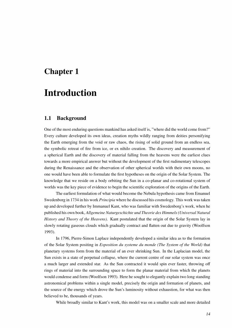
processes of young planets while the distinct populations (See Figure 1.1) rather than smooth
continuum of planet sizes and orbital radii has challenged formation theories themselves.
In the last few decades however technology has advanced such that we can now directly
resolve the disc where planets are expected to form and search directly for evidence of their birth
and the evolution of their system. In this thesis I will describe my contribution to that effort and
the progress I have made towards those ends.
1.1. BACKGROUND 16
Figure 1.1: Distribution of the population of confirmed planets by separation and planet mass(https://www.exoplanets.org). Red points mark planets detected through transit surveys,blue through radial velocity observations, green by gravitational lensing, and yellow by directimaging. Within the population of known exoplanets there are three distinct classes of objectwith fewer objects not fitting into one of these broad classes. Known rocky or terrestrial bodies(Super-Earths and smaller) occupy planet masses under 0.1 MJ and predominantly lie under anau from their parent star. ’Hot Jupiters’ are both larger and occupy a short period orbits. ’ColdJupiters’ are similar in mass but occupy larger orbital radii with few objects in between suggestingsome divergent mechanism creating the two different classes. This question is one of many whichchallenges modern planet formation theories.

Chapter 2
Star formation and disc evolution
2.1 Introduction
In this Chapter I describe the steps leading to the formation of a potentially planet hosting disc
around a young star. I start from the collapse of a giant molecular cloud into a protostar, and
the formation of a circumstellar disc. I then discuss the processes that drive the evolution of the
disc, the classification of the identified evolutionary steps and then summarise the current state of
observations of this discs. Finally I discuss potential mechanisms for clearing gaps in a disc.
2.2 Star formation paradigm
All stars form via the gravitational collapse of molecular clouds, advancing through a series of
evolutionary steps until the extreme temperatures and pressures achieved in the cores enables the
thermonuclear fusion of hydrogen into heavier elements. The energy generated arrests further col-
lapse and a state of hydrostatic equilibrium is achieved which lasts as long as there is sufficient
hydrogen fusion in the core to provide the necessary radiation pressure. These evolutionary steps
partially involve the shedding of excess angular momentum from the pro-stellar envelope, facili-
tating the continued accretion of material onto the central object as the proto-stellar core becomes
more and more compact. The accretion proceeds through interactions with a disc of material which
forms around the core and feeds it material until detached from the surrounding natal cloud. Ac-
cretion continues until the disc dissipated by the young star’s strong radiation field. Before the end
of a disc’s lifetime however, the disc is believed to provide the necessary conditions to form a plan-
etary system with properties similar to the Solar System or the thousands of systems discovered
by the Kepler space telescope. As such these objects are of prime importance for understanding
the planet formation process with larger implications for the prevalence of Earth-like planets.
In this chapter I discuss current theories on the formation of stars and the discs around
them, how these discs evolve and the mechanisms which potentially drive this evolution, and how
planets may form within the disc and their potential observational signatures.
17

2.2. STAR FORMATION PARADIGM 18
Figure 2.1: Simple schematic for the formation process of stars and their surrounding planetarysystems. For scale a unit length is shown. In this simplified picture, a gas cloud is disturbed fromits approximately static state and begins to collapse (top left). The result is the formation of aprotostar and a flared surrounding disc, formed as a result of angular momentum conservationand shocks within the collapsing material (top right). Fossil magnetic fields become trapped inthe proto-stellar core whose rotation drives a dynamo, which in turn generates a magnetic field.The rotating field lines clear the inner regions of the protostellar disc out to the co-rotation radius.Angular momentum transport within the protostellar disc leads to a dramatic reduction in thesurface density of the disc forming a “circumstellar” disc (bottom right). Coagulation of dustparticles leads to the growth of mm-cm sized dust grains which settle to the mid plane of thedisc. Processing of the dust grains through a number of mechanisms leads to the formation andevolution of a system of planetary-sized bodies. These planetary bodies aid the central star inclearing the remaining circumstellar disc except at large radii or in strong resonances (bottomleft) where primordial disc material remains.
2.2. STAR FORMATION PARADIGM 19
2.2.1 Initial collapse
Within the Milky Way, star formation is confined to the giant molecular clouds which inhabit the
spiral arms of the galaxy (Cohen et al. 1980; Dame et al. 1987). Such objects are predominantly
comprised of molecular hydrogen (H2) and are supported by the thermal motion of the molecules
against the clouds’ self gravity. These clouds are perturbed and mixed through internal turbulence
and interaction with other nearby objects such as collisions with other nearby molecular clouds or
propagating shock waves produced by supernovae (Cameron & Truran 1977; Boss 1995; Klessen
et al. 1998; Sato et al. 2000; Tan 2000; Preibisch et al. 2002; Bonnell et al. 2003). These perturba-
tions lead to local over densities within the cloud which can become gravitationally unstable. This
instability can be expressed as an inequality between the gravitational potential energy:
U = −αGM2
R, (2.1)
and the thermal energy, Etherm, assuming the gas behaves as an ideal gas:
Etherm =32RT Mµ
, (2.2)
where G is the gravitational constant, M is the mass of the over-dense region of radius, R, and
temperature, T , R is the ideal gas constant, and µ is the mean molecular weight. The dimensionless
factor, α, is a scaling constant which depends upon the mass distribution within the over-dense
region. The point at which an over-density becomes unstable can be represented in a few different
ways. Relating the two terms together via the Viral Theorem and rearranging for R provides the
Jeans radius, RJ:
RJ =α
3µGMRT
(2.3)
(Jeans 1902). This can further be modified to provide the mass for which a cloud of a given density
and temperature will collapse under its own gravity, known as the Jeans Mass, through defining
the density, ρ, as:
ρ =3M
4πR3J
, (2.4)
where the radius of the spherical initial cloud is given by RJ. This allows one to write the expres-
sion for the Jeans Mass as:
MJ =
(3
4πρ
)1/2(3RTαµG
)3/2
. (2.5)
Typical temperatures and number densities for a cloud dominated by H2 are around 100 K
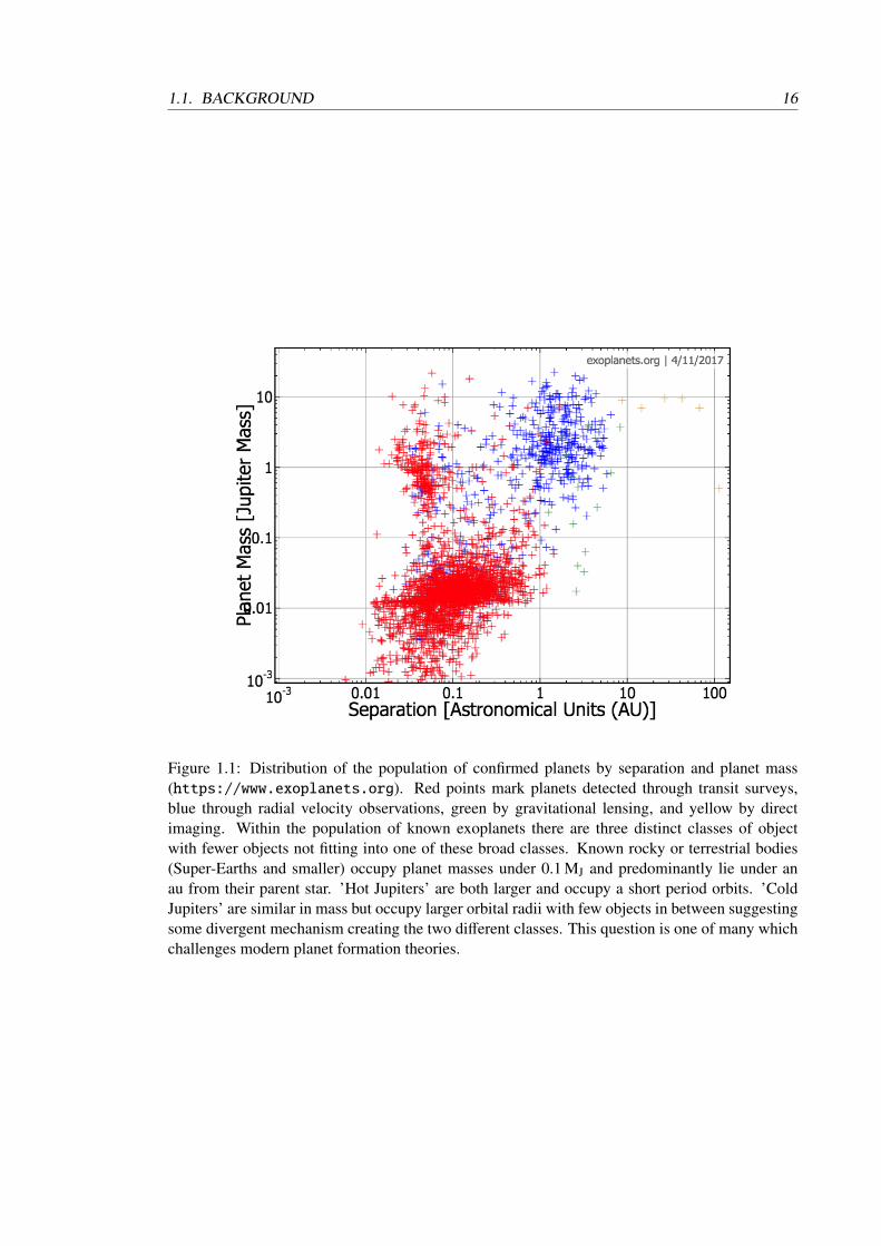
and 10 cm−3. Jeans mass for such a cloud is thus ∼104M. In practice, a collapsing cloud will frag-
ment into a larger number of loosely gravitationally bound cores (see Figure 2.2). For stars similar
in size to the Sun to form requires higher densities and lower temperatures than are typically found
in the bulk of the cloud.
Other forces exist to resist the collapse of a cloud, in particular the interaction between the
motion of the gas and the internal magnetic field (Kirby 2009). These effects tend to be weak
however and do not substantially effect the timescale of collapse for a perturbed gas cloud.
2.2. STAR FORMATION PARADIGM 20
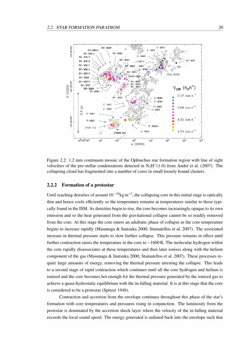
Figure 2.2: 1.2 mm continuum mosaic of the Ophiuchus star formation region with line of sightvelocities of the pre-stellar condensations detected in N2H+(1-0) from Andre et al. (2007). Thecollapsing cloud has fragmented into a number of cores in small loosely bound clusters.
2.2.2 Formation of a protostar
Until reaching densities of around 10 −10kg m−3, the collapsing core in this initial stage is optically
thin and hence cools efficiently so the temperature remains at temperatures similar to those typi-
cally found in the ISM. As densities begin to rise, the core becomes increasingly opaque to its own
emission and so the heat generated from the gravitational collapse cannot be so readily removed
from the core. At this stage the core enters an adiabatic phase of collapse as the core temperature
begins to increase rapidly (Masunaga & Inutsuka 2000; Stamatellos et al. 2007). The associated
increase in thermal pressure starts to slow further collapse. This pressure remains in effect until
further contraction raises the temperature in the core to ∼1600 K. The molecular hydrogen within
the core rapidly disassociates at these temperatures and then later ionises along with the helium
component of the gas (Masunaga & Inutsuka 2000; Stamatellos et al. 2007). These processes re-
quire large amounts of energy, removing the thermal pressure arresting the collapse. This leads
to a second stage of rapid contraction which continues until all the core hydrogen and helium is
ionised and the core becomes hot enough for the thermal pressure generated by the ionised gas to
achieve a quasi-hydrostatic equilibrium with the in-falling material. It is at this stage that the core
is considered to be a protostar (Spitzer 1948).
Contraction and accretion from the envelope continues throughout this phase of the star’s
formation with core temperatures and pressures rising in conjunction. The luminosity from the
protostar is dominated by the accretion shock layer where the velocity of the in-falling material
exceeds the local sound speed. The energy generated is radiated back into the envelope such that
2.2. STAR FORMATION PARADIGM 21
the luminosity of the protostar, Lproto, can be approximately expressed as:
Lproto ≈ Lacc =GMcoreM
Rcore, (2.6)
where M is the mass accretion rate onto the protostar while Mcore and Rcore represent the mass and
radius of the protostar.
The length of time a star remains in the proto-stellar stage of its lifetime is determined by the
rate of the circumstellar envelope’s collapse onto the protostar because the clearing of the envelope
marks the end of the “protostellar” phase. As the envelope remains approximately isothermal, the
time scale for the collapse is approximately given by the free fall timescale:
tff =
(3π
32Gρ
)1/2
. (2.7)
For low- to intermediate-mass stars (<9 M) this free-fall time is approximately the same and
roughly corresponds to 0.1 Myr.
2.2.3 Pre-main sequence evolution
For protostars over ∼8 M in mass, pressures and temperatures in the core rise rapidly enough for
thermonuclear reactions to begin within the core of the protostar before the proto-stellar envelope
is entirely dispersed with substantial accretion after the star enters the main sequence (MS). Low-
and intermediate-mass stars undergo an intermediate stage between the proto-stellar phase and
the MS. The period of continued contraction is labelled the pre-main sequence (PMS) stage. This
stage is formally defined to begin at the point the accretion luminosity has decreased sufficiently to
no longer dominate the luminosity from the protostar and the energy generated from gravitational
collapse is the dominant source of radiated energy. This represents a large drop-off in the amount
of material being accreted through the accretion shock layer, coinciding with the dispersal of much
of the natal envelope. This dispersal allows the object to be observed in the visible for the first
time.
During this stage of the star’s evolution the PMS star undergoes a period of slow quasi-
hydrostatic contraction. These objects follow evolutionary tracks on the Hertzsprung-Russell di-
agram (HRD). PMS stars evolving in this way follow an almost vertical path on the HRD (de-
scribed as the Hayashi tracks; Hayashi 1961). PMSs in the low- and intermediate-mass ranges
deviate from their Hayashi tracks after they develop radiative cores, moving onto their Henyey
tracks (Henyey et al. 1955). During this phase their luminosities remain approximately constant
while their radiative cores grows during continued contraction. This contraction continues until
temperatures and pressures rise sufficiency for nuclear fusion to begin. The region these objects
populate within the HRD at this point is referred to as the zero-age main sequence (ZAMS).
2.2. STAR FORMATION PARADIGM 22
2.2.4 Formation of the circumstellar disc
All giant molecular clouds contain some degree of large-scale rotation as a result of their large
extent and the differential rotation of the galaxy. Collapsing onto an effective point source the
angular momentum of the cloud cannot be effectively dissipated so remains conserved. The ulti-
mate result is the formation of a surrounding circumstellar disc through which the excess angular
momentum can be dissipated.
Considering the simplest case of a symmetrical sphere rotating as a solid body, parcels of
material located on the surface of the sphere experience the same gravitational pull from the center
of the sphere but differing centripetal accelerations dependent upon their latitude as their distance
from the rotation axis varies. Combining the two effects results in a net acceleration driving the
parcels towards the plane perpendicular to the rotation axis, forming a disc rotating in alignment
with the stellar rotation axis (see Figure 2.3; Terebey et al. 1984; Adams et al. 1987). The
initial size of the disc, ri, is determined by the total specific angular momentum of the collapsing
envelope, j, such:
ri =j2
GMcore. (2.8)
This is the initial radius of the disc. Evolution driven by the internal viscosity of the disc will cause
the radial extent to increase with time (Lynden-Bell & Pringle 1974; Pringle 1981).
The disc material remains in local hydrostatic equilibrium producing significant vertical
structure supported by the thermal motion of the material within the disc (Suttner & Yorke 2001).
The result is a flared structure with scale heights typically ranging ≤10% of the radial extent of the
disc.
2.2.5 Angular momentum evolution
Angular momentum transport occurs in massive discs as a result of “viscosity” within the disc
whose source is currently unknown with disc winds from the surface of the dis also playing an
important role. This viscosity enables material within the disc to simultaneous migrate inwards
and accrete onto the central star while transferring angular momentum to the outer disc. Here
it is dispersed through the spreading of the outer disc away from the star until the disc becomes
optically thin enough for material to be stripped away by the radiation of the star’s neighbours,
dissipating back into the ISM (O’dell & Wen 1994; Hollenbach et al. 1994; Johnstone et al. 1998).
To understand this process in more detail one can consider a geometrically thin disc with a
total mass, Mdisc M?, wherein a parcel of a mass, dm, at a distance from the star, r, orbits with
a Keplerian orbital velocity, ΩK:
ΩK =
(GM?
r3
)1/2
. (2.9)
One can define a surface density of an area of the disc, Σ, representing the amount of matter
contained within a column normal through the disc with unit surface area. Adopting cylindrical
coordinates (r, z, φ), one can calculate the surface density within the disc with vertical structure
via:
dΣ = ρ(z)dz. (2.10)
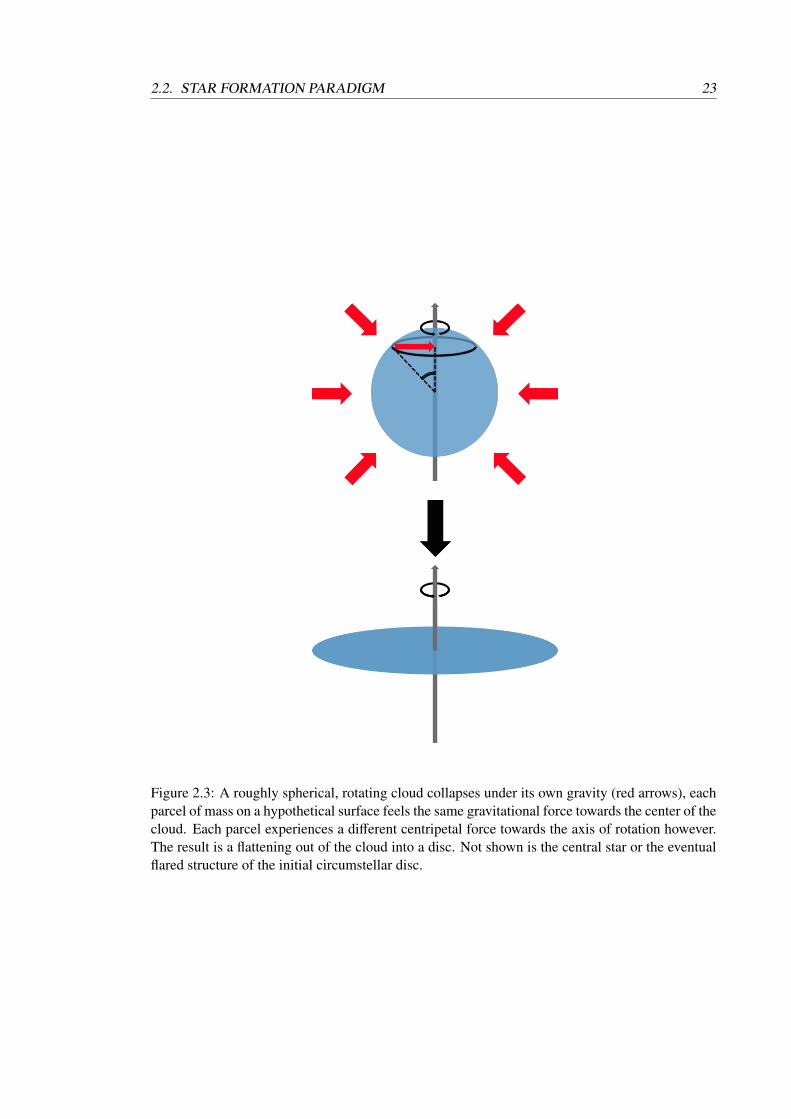
2.2. STAR FORMATION PARADIGM 23
Figure 2.3: A roughly spherical, rotating cloud collapses under its own gravity (red arrows), eachparcel of mass on a hypothetical surface feels the same gravitational force towards the center of thecloud. Each parcel experiences a different centripetal force towards the axis of rotation however.The result is a flattening out of the cloud into a disc. Not shown is the central star or the eventualflared structure of the initial circumstellar disc.

2.2. STAR FORMATION PARADIGM 24
This further enables one to calculate the mass, m, of a thin annulus at radius r from the central star
as:
dm = 2πrΣdr. (2.11)
Two annuli with radii r and r + dr will experience a velocity shear as a result of their differing
rates of rotation. Provided the disc is viscous this shear results in a frictional force between
neighbouring annuli. The magnitude of the frictional force per unit length, f , can be expressed as:
f (r) = νrΣ∂Ω
∂r. (2.12)
Here the parameter, ν, represents the viscosity coefficient. The net torque between two annuli is
then:
G(r) = 2πr2νΣ
(∂Ω
∂r
)(2.13)
For a disc rotating with a Keplerian rotation profile, ∂Ω/∂r < 0, and a constant value of ν, the
inner annulus transfers a portion of its angular momentum to the outer annulus. Thus a portion of
the material within the inner annulus moves inwards while a portion of the outer annulus moves
outwards. For a zero viscosity disc, there is no frictional force between the annuli and hence no
transfer of angular momentum.
For a viscous disc, the rate of angular momentum transfer is equal to the net torque;
J =DDt
jdm = −dr∂G
∂r= dm
D jDt, (2.14)
where the specific angular momentum is denoted by j and D / Dt is change with time. The right
side of Equation 2.14 can alternatively be represented by:
dmD jDt
= dm(∂ j∂t
+ v · ∇ j)
= dm(vd∂ j∂r
), (2.15)
where vd represents the radial drift velocity of material through the disc. Given that the rotation is
Keplerian (i.e. j = (GM?r)1/2) and that:
∂ j∂r
=12
ΩKr, (2.16)
it is possible to combine Equation 2.11 along with Equations 2.14 and 2.15 to show that:
2πrΣ
(vd∂ j∂r
)= −
∂G
∂r. (2.17)
This can be further combined with Equation 2.9 in order to produce an expression for the radial
drift, vd:
vd = −3
Σr1/2
∂
∂r(νΣr1/2) (2.18)
2.2. STAR FORMATION PARADIGM 25
Defining the mass continuity equation for the surface density as:
∂Σ
∂t+
1r∂
∂r(Σrvd) = 0, (2.19)
one can substitute Equation 2.18 into the above to obtain the expression which describes the evo-
lution of the surface density:∂Σ
∂t=
3r∂
∂r
[r1/2 ∂
∂r
(νΣr1/2
)](2.20)
(Lynden-Bell & Pringle 1974; Pringle 1981).
Starting from the the assumption that the viscosity term is related to the density of material
within an annulus and that higher densities will be found towards the central star, the viscosity can
be represented as a simple, positive, time-independent power law:
ν ∝ rγ. (2.21)
Equation 2.20 has a similarity solution (Lynden-Bell & Pringle 1974):
Σ(r) =C
3πν1Rγτ−(5/2−γ)/(2−γ)exp
[−
R(2−γ)
τ
](2.22)
(Hartmann et al. 1998). The constant, C, is a scaling constant. R is a radial scaling factor defined
such that:
R ≡rr1, (2.23)
while correspondingly:
ν1 ≡ ν(r1), (2.24)
τ is a non-dimensional time defined as:
τ =tts
+ 1, (2.25)
where ts is the viscous scaling time:
ts =1
3(2 − γ)2
r21
ν1. (2.26)
The mass flux through the disc is thus given by:
M(r, t) = Cτ−(5/2−γ)/(2−γ)[1 −
2(2 − γ)R(2−γ)
τ
]exp
[−
R(2−γ)
τ
]. (2.27)
The bulk motion of the inner disc is inwards and eventually leads to accretion onto the star while
the bulk motion of the outer disc is towards larger radii, increasing the radial extent of the disc.
This gradual spreading of the disc removes angular momentum from material which will eventu-
ally accrete onto the star and leads to lower surface densities (see Figure 2.4). From Equation 2.27
one can see from inspection that the radius at which there is no migration, representing the radius
2.2. STAR FORMATION PARADIGM 26
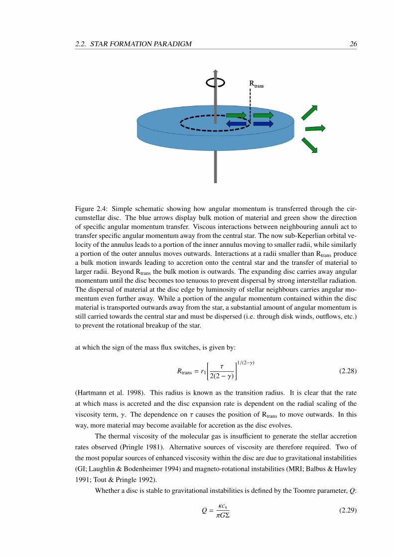
Figure 2.4: Simple schematic showing how angular momentum is transferred through the cir-cumstellar disc. The blue arrows display bulk motion of material and green show the directionof specific angular momentum transfer. Viscous interactions between neighbouring annuli act totransfer specific angular momentum away from the central star. The now sub-Keperlian orbital ve-locity of the annulus leads to a portion of the inner annulus moving to smaller radii, while similarlya portion of the outer annulus moves outwards. Interactions at a radii smaller than Rtrans producea bulk motion inwards leading to accretion onto the central star and the transfer of material tolarger radii. Beyond Rtrans the bulk motion is outwards. The expanding disc carries away angularmomentum until the disc becomes too tenuous to prevent dispersal by strong interstellar radiation.The dispersal of material at the disc edge by luminosity of stellar neighbours carries angular mo-mentum even further away. While a portion of the angular momentum contained within the discmaterial is transported outwards away from the star, a substantial amount of angular momentum isstill carried towards the central star and must be dispersed (i.e. through disk winds, outflows, etc.)to prevent the rotational breakup of the star.
at which the sign of the mass flux switches, is given by:
Rtrans = r1
[τ
2(2 − γ)
]1/(2−γ)
(2.28)
(Hartmann et al. 1998). This radius is known as the transition radius. It is clear that the rate
at which mass is accreted and the disc expansion rate is dependent on the radial scaling of the
viscosity term, γ. The dependence on τ causes the position of Rtrans to move outwards. In this
way, more material may become available for accretion as the disc evolves.
The thermal viscosity of the molecular gas is insufficient to generate the stellar accretion
rates observed (Pringle 1981). Alternative sources of viscosity are therefore required. Two of
the most popular sources of enhanced viscosity within the disc are due to gravitational instabilities
(GI; Laughlin & Bodenheimer 1994) and magneto-rotational instabilities (MRI; Balbus & Hawley
1991; Tout & Pringle 1992).
Whether a disc is stable to gravitational instabilities is defined by the Toomre parameter, Q:
Q =κcs
πGΣ(2.29)
2.2. STAR FORMATION PARADIGM 27
(Toomre 1964). cs represents the local sound speed within the disc and κ is the epicyclic frequency
of a particle within the disc:
κ =
[2Ω
rddr
(r2Ω)]1/2
. (2.30)
In the case of Keplerian rotation, κ = Ω.
The Toomre parameter represents the ability of the mean-free path of the particles in the
disc to resist the disc’s self gravity. For values of Q > 1.3, the non-axisymmetric spiral density
waves have been predicted to form due to the disc’s own gravity (Laughlin & Bodenheimer 1994).
These spiral waves efficiently transport angular momentum radially through the disc.
An often more useful quantity for determining the stability of a disc is through the mass
ratio, q = Mdisc/M? and the disc temperature, T . The mass terms enter through κ = [GM?/R3]1/2
and Σ ≈ Mdisc/[πR2], and the temperature through c2s = RT/µ. For a disc to be stable it must
satisfy the inequality:
q ≤cs
ΩR(2.31)
For typical disc values, a q value of > 0.1 is necessary for disc to be susceptible to GI and the
formation of angular momentum transporting spiral arms. Typical conditions observed around T-
Tauri wtars only produce value of q ≈ 0.01 (Andrews et al. 2013) and hence are likely to be stable
to GIs. During more massive phases of the disc’s evolution however, q values will be substantially
higher so may be a viable mechanism for angular momentum transport in younger discs.
The MRI originates in the interaction of the stellar or fossil magnetic field of the disc
threading through the inner or outer disc, respectively, and its interaction with charged particles
within the disc. The origin of this viscosity can be understood by considering two charged mass
elements m1 and m2 located at a distance, r, from the star and separated by a vertical distance
denoted by δz. The magnetic field lines thread vertically through the disc and the mass elements.
If a small radial displacement develops between the two elements such that the position of m1
becomes r − δr and m2 becomes r + δr (see Figure 2.5) then a tension develops in the threading
field line which acts to slow the inner parcel and accelerate the outer parcel. This removes angular
momentum from the inner parcel and transfers it to the outer such that the inner packet moves
further inwards and the outer packet outwards. The additional radial displacement enhances the
tension in the field line and leads to ever further radial drift between the charged particles.
Eventually this drift creates a radial component to the previously vertical field lines. Ad-
ditionally, as the mass packets undergo differing orbital speeds an azimuthal component is also
added to the field lines. This twists the magnetic field lines, reducing the relative vertical compo-
nent and generates magnetic hydrodynamic turbulence (Balbus et al. 1996).
Hence, for a disc to be susceptible to MRIs it must be at least partially ionised, initially
possess a magnetic field with a vertical component, rotate with an approximately Keplerian ro-
tation profile, and its thermal energy density must surpass the magnetic energy density to such
the initial perturbation of the ionised particles are not immediately stabalised by strong magnetic
forces(Gammie 1996; Turner et al. 2014). The ionisation of material in the disc can occur through
exposure to the intense radiation of the star leading to thermal ionisation in the inner disc or
through exposure to comic rays in the outer disc (Umebayashi & Nakano 1981).

2.2. STAR FORMATION PARADIGM 28
Figure 2.5: Schematic describing how angular momentum transport can occur within a chargeddisc threaded by a fossil magnetic field. Two charged particles at a radius, r, connected by afield line become displaced by a small amount in radius, δr. The tension in the field line willslow the inner particle while accelerating the outer particle such that one will trail the other. Thetension in the line then leads to a transfer of angular momentum from the inner particle to theouter by removing orbital energy from the inner to outer, further slowing the inner particle andaccelerating the outer particle, causing a further displacement as the inner moves further inwardsand the outer moves further outwards and increasing the degree of trailing between the particles.This further increases the tension in the field line, facilitating continued migration creating a stronginstability unless the initial magnetic field strength is sufficient to prevent the initial displacementfrom developing.

2.3. PROTOPLANETARY DISKS 29
At the furthest reaches of the disc the surface density drops off until the disc becomes
optically thin. Here, radiation from neighbouring stars and even the parent star launch photo-
evaporative winds as the gravitational binding energy here is weak enough that gas particles are
only tentatively bound to the protostar. These winds carry material and angular momentum away
from the system. Further this removes the protective shielding from any dust particles in this re-
gion, exposing them to sublimating radiation. Subsequently they too are evaporated away in the
disc wind leading to a steady erosion from the outside inwards (Johnstone et al. 1998). In particu-
lar, discs close to O and B type stars are subjected to strong radiation fields but also simultaneously
strong stellar winds containing substantial amounts of hot material. The impact of the winds from
O and B type stars can have a devastating effect on the local population of discs as evidenced by
the Orion Nebula cluster wherein discs within 0.03 pc of the massive O star, θ1 Ori C were signif-
icantly less massive than the discs around similar sized and aged stars at larger distances (Mann
et al. 2014). Disc winds may also play an important role is removing angular momentum from
the inner regions of the disc. Here the interaction between the central star’s intense radiation and
magnetic field lines threading through the disc leads to the launching of material from the surface
layer of the disc, forming a pair of collimated antiparallel jets (Blandford & Payne 1982).
Clearing of the disc appears to be rapid in comparison to the total lifetime of the disc
(See Section 2.3) as evidenced by the small fractional number of discs displaying clearing within
their SEDs. A possible explanation for such rapid dispersals could lie in the tidal interaction
between neighbouring stars within dense star forming regions, altering the dynamical nature of
the circumstellar material. Such an interaction could lead to the fragmentation of the disc and
inhibition of planet formation, as the planetesimals catastrophically collide within the excited disc
(Backman & Paresce 1993). In the case of some discs, the clearing can be extremely rapid with
a disc containing a substantial amount of material being nearing completely cleared on the time
scale of a few years (e.g. TYC 8241 2652 1; Melis et al. 2012; Gunther et al. 2017). Within such
short time frames, not even tidal interaction with a neighbour can clear the disc.
2.3 Protoplanetary disks
2.3.1 Classical
Theories regarding circumstellar discs which in turn give birth to planetary systems are reason-
ably old ideas having its origins in the Nebula Hypothesis developed by Kant in the 18th century
to explain the origin of the Solar System and its observable properties. Independently, Laplace
developed similar ideas which became the most widely accepted model (see Chapter 1). The or-
ganisation of the planets within the Solar System as a configuration confined to an approximate
plane, suggested a formation mechanism wherein the planets formed from an extended flattened
structure, such as a disc.
Surveys of potentially disc-hosting stars in the infrared were only made possible with the
advent of the Infrared Astronomical Satellite (IRAS; Strom et al. 1989). The gas dynamics of
protoplanetary discs were spatially resolved for the first time by sub-mm interferometers which
resolved the rotation of the discs (Sargent & Beckwith 1987). Undeniable evidence for the char-
2.3. PROTOPLANETARY DISKS 30
acteristic flattened morphology however had to wait until the first images from the Hubble Space
Telescope (HST). Imaged against the bright nebulosity of the Orion nebula, their profiles as flat-
tened discs could be clearly seen (O’dell & Wen 1994).
Two mass ranges of PMS stars are observed to frequently harbour circumstellar disc. In the
case of low-mass stars these are referred to as T Tauri stars (TTS), named for first object which
displayed the distinctive variability that characterises young, low mass stars (Joy 1945), while
intermediate mass parent stars are labelled as Herbig Ae/Be stars (Herbig 1960).
Of the total lifetime of the disc, the deeply embedded stages of Class-0 and Class-I objects
(central prostellar still embedded in an envelope of material, majority of material in the envelope
and in the protostar respectively) lasts a mere fraction, typically less than a Myr (Adams et al.
1987). Estimates for the typical lifetime of circumstellar discs are believed to lie in the region of
<10 Myr (Haisch et al. 2001), derived from the fraction of stars still hosting discs as a function of
their age. Determining the ages of young stars is a difficult task however, and estimates can differ
by more than a factor of two (Bell et al. 2013) affecting the disc lifetimes by the same amount.
By the time a protostar has began to evolve from Class-I to Class-II (pre-Main Sequenece
star surrounded by a massive disc, envelope dispersed), most of the material has either been ac-
creted onto the protostar or ejected through outflows so that the remaining material in the disc
contributes only a few percent to the total mass of the system with the vast majority confined
within the central object. This point marks when the disc is considered to be “protoplanetary” as
opposed to “protostellar” in the previous stage. This stage also represents the start of the system’s
isolation from the nursery core which birthed it as the feeding of material into the disc ceases.
The best method for determining the disc mass is to use (sub-)millimeter observations to
determine the dust mass and use an assumed gas to dust ratio to calculate the total disc mass. Here
the continuum emission is optically thin except in the inner regions of a full disc due to the high
densities. This allows the measurement of a surface density, Σ, representing the amount of mass
contained within a cylinder of unit area through the disc. This is formally defined as:
τν = κνΣ =
∫ρκνds, (2.32)
where τ is the optical depth along the line of sight, s, at frequency ν. The density of the disc is
represented by ρ and the dust opacity at ν by κν. This is commonly prescribed as:
τν = 0.1(
ν
1012Hz
)βcm2g−1 (2.33)
(Beckwith et al. 1990) under a number of assumptions such as the disc being optically thin at all
radii and that the gas-to-dust mass radio coresponds to a value of 100. The power law parameter,
β, and the absolute value are heavily reliant on the size distribution of the dust grains within the
disc and the exact composition of these dust grains (Ossenkopf & Henning 1994; Pollack et al.
1994).
To derive the mass of the disc one can consider the emission to directly rated to the total

2.3. PROTOPLANETARY DISKS 31
observed flux, Fν, as a result of the optically thin nature of the disc to mm wavelengths, such that,
M(gas + dust =Fνd2
κνBν(T )), (2.34)
where the distance to given object is given by d, and the Planck function, Bν(T ) ≈ 2ν2kT/c2
(Eisner et al. 2008). This is advantageous as the relation to the temperature of the dust is only
linear and not exponential.
2.3.2 Transitional/Pre-transitional
Within a small number of protoplanetary discs we observe strong drops in the mid and sometimes
near, infrared (Strom et al. 1989; Skrutskie et al. 1990) within their spectral energy distributions
(SEDs). Their SEDs within the NIR and MIR resemble those of a stellar photosphere of a young
stellar photosphere but then display strong excesses at wavelengths beyond ∼20µm similar to full
discs (Calvet et al. 2005). This is typically interpreted as being due to the opening of a gap in the
disc further from the star than can be explained by dust sublimation as a result of the strong stellar
radiation field or truncation by the stellar magnetic field. The rationale behind this lies in the vast
dynamical range seen with a circumstellar disc. The inner edge of a classical disc can be as close
as a few stellar radii while the outer disc can read distances of 100s au from the central star in the
most massive discs. Through SED modelling the highly irradiated inner rim was inferred to reach
close to the silicate sublimation temperature (∼1500 K; Espaillat et al. 2008) whilst the cold outer
edge rarely warms to above a few 10s of K. A useful property results in that most emission from
the disc over a narrow set of wavelengths will principally originate from within a narrow radial
region of the disc. Therefore a lack of mid infrared emission indicates a lack of emitting material
within intermediate radii of the disc. In particular, the gas component of the disc is expected to
be optically thin, whereas the dust is expected to be optically thick. Hence we observe a drop
in the density of small, typically sub-micron sized, dust grains. Performing spatially resolved
observations in the sub-mm of targets whose SEDs are characterised by a drop in both NIR and
MIR wavelengths revealed extended cavities in the distribution of the dusty disc supporting this
interpretation of the SEDs (Hughes et al. 2009; Brown et al. 2009; Andrews et al. 2011b).
Strom et al. (1989) and Skrutskie et al. (1990) additionally hypothesised that these repre-
sented a class of objects in transition from the previously identified Class II young stellar objects
(YSOs) to the later stage Class III YSOs.
For objects where the clearing has resulted in an inner disc cavity, the classification of
transitional discs is typically used (Strom et al. 1989), although other terms such as cold discs
(Brown et al. 2007) or weak-excess transitional discs (Muzerolle et al. 2010) have been used
to describe them. Gapped discs which still retain a significant dusty inner disc are meanwhile
typically referred to as pre-transitional discs (Espaillat et al. 2007) but are also referred to as
cold discs (Brown et al. 2007) or warm transitional discs (Muzerolle et al. 2010). Suggested
mechanisms for the clearing include grain growth (Brauer et al. 2008; Birnstiel et al. 2011), the
powerful stellar radiation field driving the photoevaporation of small dust grains (Hollenbach et al.
1994; Glassgold et al. 1997; Alexander et al. 2014), or the dynamical clearing of the orbital path of

2.3. PROTOPLANETARY DISKS 32
Figure 2.6: Left: Example synthetic SEDs of the three classes of protoplanetary disc discussedhere observed face-on (i = 0). The SEDs here were produced using the TORUS radiative transfercode (Pontefract et al. 2000; Harries 2014). The flux contribution from scattering effects are notshown separately but are included in the calculation of the total flux. Right: Schematic drawing ofthe structure responsible for each synthetic SED. Top: Classical or Full TTS disc Middle: Tran-sitional disc where the warmer inner portions of the disc have been removed, with their associatedNIR and MIR emission disappearing from the SED as well as the strong scattering componentfrom the inner disc leading to less NIR flux. Much of the NIR and MIR emission has its originin the puffed-up rim at the boundary between the disc and the cavity. Here the disc is exposed tomore radiation than in the classical case, heating the disc material. This results in more thermalemission from a larger surface area. Bottom: Pre-transitional disc where material from interme-diate radii has been removed. Here the hot inner disc remains intact, producing the NIR emission.However there is less material to emit in the MIR producing a sharp decrease in the MIR flux.Shadowing of the middle of the disc by a puffed up rim produces the dramatic drop in the MIRcompared to the transitional disc (middle) case.

2.4. OBSERVATIONAL CONSTRAINTS ON STRUCTURE 33
a forming giant planet through gravitational interactions. For a number of reasons listed in greater
detail below, both classes of transitional disc are believed to contain nascent planetary systems
still in the process of formation (Espaillat et al. 2014).
2.4 Observational constraints on structure
2.4.1 Spectral energy distribution model fitting
Detailed modelling of spatially unresolved spectral energy distribution (SED) data represents the
first efforts to determine the structure of transitional discs.
For objects observed to possess little NIR or MIR excess, models typically contain an op-
tically thick disc inwardly truncated at some orbital radii on the order of 10s of au, such as in
Calvet et al. (2002) and Rice et al. (2003b). This is modelled as black body emission of a given
temperature. This temperature represents the temperature of the inner edge of the disc where dusty
material is heated by stellar flux from the central star and dominates the majority of emission emit-
ted by the disc, in particular within the 20-30 µm. Conditions within the inner cavity vary wildly
with some objects containing cavities almost completely dust free (such as DM Tau) to many oth-
ers which contain strong line emission from optically thin dust populations such as the strong
10 µm silicate features in GM Aur shown by Calvet et al. (2005) or the polyaromatic hydrocarbon
lines (PAHs) displayed in a number of objects (Maaskant et al. 2014). For SEDs still containing
substantial amount of NIR emission, a second black body component is added. Beyond ∼40 µm
the SED is dominated by the outer disc.
In the case where there is still a non-negligible amount of NIR within the SED, models are
typically constructed using an outer disc similar to the one above with the addition of a second
smaller optically thick disc closer to the star. The two optically thick discs are then separated by
an optically thin annulus (Brown et al. 2007; Espaillat et al. 2007; Mulders et al. 2010; Dong et al.
2012) although this can too still contain an amount of optically thin dust. The inner disc casts a
shadow on the outer disc rim, reducing the emission in the 20-30 µm wavelength range. The inner
rim of the inner disc is located at the dust sublimation radius beyond which dust particles cannot
survive in significant quantities. The inner rim dominates the NIR flux contribution.
The usefulness of SED modelling is limited by the large number of degeneracies present
within the models. The shapes of model SEDs are highly dependent on a large number of parame-
ters which determine the exact disc geometry including large scale properties (i.e mass, dust grain
species, scale height, flaring, etc.) to small scale effects which cause large changes in the SED
(e.g. inner rim shape). Degeneracies also exist within the data. A popular and extensive source of
infrared data on stars in star forming regions comes from the Spitzer IRS. In a classical disc, the
majority of emission at 10 µm comes from within 1 au of the central star (> 80%, D’Alessio et al.
2006). Therefore Spitzer is most sensitive to a drop in the dust density between ∼0.1-0.5 au. A
gap within a pre-transitional disc with the outer edge of the inner disc outside 1 au would produce
only a small bump in the SED as measured with Spitzer and so would be mistakenly labelled as
a full disc. To find these objects, one would have to turn to latest sub-mm millimeter ground ob-
servations with instruments such as ALMA. This was the case with the discovery of gaps within
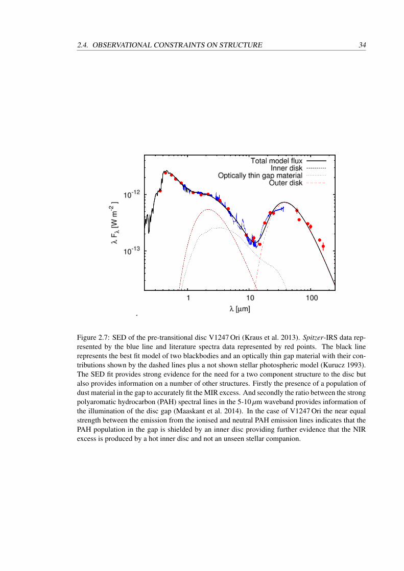
2.4. OBSERVATIONAL CONSTRAINTS ON STRUCTURE 34
Figure 2.7: SED of the pre-transitional disc V1247 Ori (Kraus et al. 2013). Spitzer-IRS data rep-resented by the blue line and literature spectra data represented by red points. The black linerepresents the best fit model of two blackbodies and an optically thin gap material with their con-tributions shown by the dashed lines plus a not shown stellar photospheric model (Kurucz 1993).The SED fit provides strong evidence for the need for a two component structure to the disc butalso provides information on a number of other structures. Firstly the presence of a population ofdust material in the gap to accurately fit the MIR excess. And secondly the ratio between the strongpolyaromatic hydrocarbon (PAH) spectral lines in the 5-10 µm waveband provides information ofthe illumination of the disc gap (Maaskant et al. 2014). In the case of V1247 Ori the near equalstrength between the emission from the ionised and neutral PAH emission lines indicates that thePAH population in the gap is shielded by an inner disc providing further evidence that the NIRexcess is produced by a hot inner disc and not an unseen stellar companion.

2.4. OBSERVATIONAL CONSTRAINTS ON STRUCTURE 35
HL Tau (ALMA Partnership et al. 2015, see Section 2.4.3).
2.4.2 Spectroscopic constraints
Much of the material within the disc is in the form of optically thin gas rather than dust. Much of
the processes which affect the dust, in particular dust migration and growth is dependent on the
presence of the gas disc so it is valuable to know something about its distribution within the disc,
its dynamics, and its relation to the dust disc. Additionally Najita et al. (2007) found that accretion
rates for pre- and transitional discs are typically an order of magnitude less than those of classical
TTS but remain substantial. Maintaining such accretion rates across extended and deep gaps in the
dust disc narrows down the number of mechanisms which can be responsible for the disc clearing
and understanding how the gas flows across the gap provides clues to the origin of the opening.
Observations at mm and sub-mm wavelengths have enabled the outer regions of many tran-
sitional and pre-transitional discs to be studied extensively (see Section 2.4.3). For some objects,
such as DM Tau, LkCa 15 and TW Hya, there exists rotationally excited CO at radii within the
cavity in the dust distribution (Pietu et al. 2007; Rosenfeld et al. 2012) although these observa-
tions do not at present constrain the distribution of the gas. On going accretion onto the central
star provides compelling evidence for the presence of substantial quantities of gas close to the
star along with observations of UV H2 emission (Ingleby et al. 2009; France et al. 2012), and
ro-vibrational CO emission (Najita et al. 2008, 2009; Salyk et al. 2009, 2011) coming from close
to the star where the gas has been heated by the strong stellar radiation field.
The molecular lines used to trace the gas disc around accreting, classical TTS within the
10-20µm Spitzer data are noticeably absent in transitional discs (Najita et al. 2010; Pontoppidan
et al. 2010). The cause of this discrepancy between the MIR and mm observations is not resolved.
These diagnostics probe orbital radii within a few au of the star so are perhaps suggestive of a gap
between the inner edge of the gas disc and the outer disc. Other possibilities include an abundant
gas disc but in a cold or atomic form.
While the ideal method for probing the radial structure of the gas disc is to use spatially
resolved imaging, resolution limits make this impossible for most targets. Instead, velocity re-
solved spectroscopy, in conjunction with an assumption of Keplerian rotation, can enable one to
investigate the radial structure of the gas (Najita et al. 2000). Calculating the centroid of spectrally
resolved line emission as a function of velocity can remove some of the ambiguities of this method
(Pontoppidan et al. 2008). The information these techniques provide are in detecting asymmetries
in the radial profile or sharp changes in the emission. These are interpreted to correspond to evi-
dence for a companion or vortices distorting the orbit of the disc and a cavity within the gas disc
respectively.
Studying the CO ro-vibrational emission from the evolved disc V836 Tau, Strom et al.
(1989) found tentative evidence for truncation of the inner gas disc. Supporting evidence of this
conclusion was found in the distinct double-peaked line profile in the V836 Tau CO emission.
This kind of profile is consistent with a truncated inner disc. Typically, CO profiles are singularly
peaked in other discs (Salyk et al. 2007, 2009; Najita et al. 2008, 2009). Additionally, such obser-
vations provide evidence for discrepancies between the dust and gas profiles. CO emission around

2.4. OBSERVATIONAL CONSTRAINTS ON STRUCTURE 36
the pre-transitional disc LkCa 15 is observed to cover a much broader range of velocities (Najita
et al. 2008) than V836 Tau implying a radial extent of <0.1 au out to a few au. SED modelling of
this object indicates an optically thin inner dust disc extending over a very narrow radial distance
(0.15-0.19 au; Espaillat et al. 2010).
In the context of the detection of otherwise unseen companions, the peculiar gaseous emis-
sion from the transitional disc HD 100546 indicated the first signs of the presence of a companion
possibly generating the observed cavity. Acke & van den Ancker (2006) used [O I] 6300 Å ob-
servations to identify a local minimum in the disc. Further evidence was found through the OH
emission which displayed a strong asymmetry consistent with emission from an eccentric inner
rim of e ≥ 0.18 (Liskowsky et al. 2012). Such asymmetries in the disc are believed to be the result
of the influence of a companion (e.g. Papaloizou et al. 2001; Kley & Dirksen 2006). Following
up these observations with high contrast imaging techniques, Quanz et al. (2015) and Currie et al.
(2015) detected and confirmed the presence of HD 100546 b with the VLT/NACO and Gemini
Planet Imager (GPI) respectively on an orbital radius of 53 au. In addition both groups observed
a tentative second companion at ∼13 au. HD 100546 b was found to be super-Jovian in size and
inferred to still be accreting significant material from a circumplanetary disc through measuring
the colour of the object and comparing to evolutionary models of sub-stellar objects (Currie et al.
2015). It should be noted that the formation of such a massive companion at such a large separation
from the central star challenges current planet formation theories.
2.4.3 Sub-millimeter and radio continuum long baseline interferometry
Observations in the radio and sub-millimeter possess many advantages for the observation of cool
material around hot stars with the only major drawback the need for large interferometric arrays
to reach similar angular resolutions as an ∼8 m research class telescope observing in the optical or
NIR. Such arrays are simple to construct however when compared to their optical equivalents and
have been in use for decades.
By observing with an interferometer in the radio regime one avoids the problems of issues
of contrast to the stellar photosphere as the emission from the star is negligible compared to the
dusty disc. Additionally the numerous spatial scales accessible through the use of interferometric
arrays now provides spatial resolutions of ∼1 au for stars at distances of ∼100 pc (Andrews et al.
2016) for the closest YSOs with the advent of ALMA. The emission in this regime is also believed
to be optically thin, providing the opportunity to directly measure masses and surface densities
due to the strong dependence on the distribution of mm- to cm-sized dust grains (Beckwith et al.
1990).
An interferometric array with a sufficient resolution and spatial frequency coverage, can
provide the ability to image transitional discs into ring structures with extended cavities (for more
details on this process, see Section 4.3.2). The observation of dust cavities around young stars has
demonstrated the problems of relying on SED modelling to identify discs containing cleared gaps.
Often the presence of the gap has not been indicated in the SED and only the object’s inclusion
in surveys to constrain the radial dust distribution of classical discs with high angular resolution
instruments such the Sub-millimeter Array (SMA) has revealed their presence (Andrews et al.

2.4. OBSERVATIONAL CONSTRAINTS ON STRUCTURE 37
2009).
This situation has become more extreme with the sub-100 mas imaging capabilities of
ALMA. There was little to no indication within the SED of HL Tau of an extended cavity of
any kind. ALMA however observed a series of narrow cleared rings within the disc in the now fa-
mous image. Further images of nearby disc revealed further ringed structures (TW Hya; Andrews
et al. 2016) where previously only cavities had been observed.
In the case of less resolved observations, such as the cavities observed in the sub-mm with
SMA, some radiative transfer modelling work is still required to derive the basic structure of the
disc. Typically such models are constructed such that the cavity is defined as a region where the
dust surface density is greatly reduced with a sharp transition to the full outer disc (e.g. Andrews
et al. 2011b; Cieza et al. 2012; Mathews et al. 2012). The results of such work indicate cavities
on scales of 15-75 au and density drops of 102-105 compared to a classical disc. The outer regions
are found to be comparable in radial extent and mass to classical discs so the mechanism for the
dust depletion appears to be limited to within the cavity. The depletion levels are not constrained
by the mm data however as the resolved images have only a limited dynamic range. Instead the
depletion levels have to be constrained using the infrared SED data. Additionally until ALMA
the only direct indication from the mm data about the nature of the boundary between the cavity
and the disc was that the density dropped off over a narrow radial region (<10 au). As such,
alternative modelling strategies where a smother density transition is imposed (e.g. Isella et al.
2010; Andrews et al. 2011a; Isella et al. 2012) reproduces the data equally well and as we now
know are indeed more physical thanks to the higher resolution ALMA images.
SMA and ALMA observations provided the first spatially resolved evidence for deviations
away from simple disc scenarios of centro-symmetric geometries and smooth surface density pro-
files. Evidence for strong azimuthal asymmetries within the emission rings have been found in
numerous objects and may even be a common feature (e.g. Brown et al. 2009; Tang et al. 2012;
Casassus et al. 2013; van der Marel et al. 2013; Isella et al. 2013).
2.4.4 Optical imaging
Free from the distorting effects of the Earth’s atmosphere, space-based infrared imaging instru-
ments have had some early success at observing the structure of a number of discs around bright
stars. For instance, Weinberger et al. (1999) used the Hubble Space Telescope (HST) to observe
ring-like structure around HD 141569 and Grady et al. (2001) observed pristine spiral arm struc-
ture around the Herbig star HD 100546. Both studies used a coronographic mask to block out the
bright central star, solving the contrast problem with the stellar photosphere in the process. Such
observations are limited however by the relatively small apertures of space telescopes compared to
ground based instruments, the costs associated with lifting a large object into space in conjunction
with the engineering problems associated with designing a collapsible mirror to survive the trauma
of leaving the Earth’s atmosphere and deploying reliably have limited the size of space telescopes.
The launch of the James Webb Space Telescope (JWST) will represent a significant advancement
in this regard, and its location well away from the contaminating effects of the Earth’s infrared
glow, variable gravitational field promises not just higher resolution data but substantially better

2.4. OBSERVATIONAL CONSTRAINTS ON STRUCTURE 38
Figure 2.8: Synthesised SMA 880 µm continuum emission from a selection of transitional discobjects presented by Andrews et al. (2011b). Each image has a 2.7 arcsecond field of view, beamsizes are shown in the bottom left of each panel, and an angular scale of 50 au is shown in thebottom right. Contours are shown at 3σ intervals. The inset images are synthesised with higherangular resolution and are shown on the same scale. Significant asymmetries can be seen withinthe resolved discs perhaps as a result of dust traps induced by the presence of a companion withinthe disc.

2.4. OBSERVATIONAL CONSTRAINTS ON STRUCTURE 39
quality data.
Complementary to these developments is the maturation of a number of high-resolution
imaging techniques for ground-based telescopes. Optical long baseline interferometric instru-
ments allow for larger arrays of telescopes, both in terms of the length of the baselines and the
number of telescopes as optical interferometers near the same capabilities as their radio equiv-
alents. These state of the art facilities provide visibility and phase data capable of forming the
first NIR images of the inner few au around pre-transitional discs, while MIR imaging will reveal
the extent and structure of the cavities of transitional discs. The re-emergence of sparse aperture
masking interferometry provides the high sensitivities and small inner working angles to search
for disc asymmetries or even direct companion detection probing complementary angular sizes to
both long baseline interferometers and conventional imaging techniques. Polarimetry meanwhile
allows one to probe dust distributions to within a few 10s of au of the central star. These techniques
are discussed in more detail below.
Long baseline interferometry
Facilities such as the Very Large Telescope Interferometer (VLTI) and the Center for High Angular
Resolution Astronomy (CHARA) array provide baselines >100 m with corresponding resolutions
on the scale of milliarcseconds (mas) in both the NIR and MIR, well beyond anything currently
capable with single aperture imaging techniques.
In a similar manner to how the interferometric visibility data in the radio can be used to
constrain the surface density distribution of mm-sized grains, IR visibility data can be used in con-
junction with radiative transfer models to constrain the physical parameters of the circumstellar
material such as the density distribution, grain composition and temperature. For NIR observa-
tions in the H- and K-band, this brightness distribution is dominated by the bright emission from
the inner disc wall of pre-transitional discs. Heated to close to the dust sublimation temperature
(∼1500 K), this region emits brightly in the IR with only small contributions in scattered light
(Olofsson et al. 2013) from more extended regions of the disc or optically thin material in the gap
(Kraus et al. 2013).
Observations in the MIR cover a larger proportion of the disc as they are more sensitive to
a larger range of temperatures and hence radial distance from the star in addition to potentially
shadowed regions of the disc.
Using these techniques in conjunction with radiative transfer modelling and longer wave-
length observations has produced some interesting results:
The SED interpretation of transitional discs containing an inner disc largely free of dust
and NIR and MIR emission was supported VLTI NIR+MIR through observations of both Herbig
Ae/Be stars, such as HD 100546 (Mulders et al. 2013) and TTS such as T Cha (Olofsson et al.
2011, 2013).
Numerous cases were also found however which require more sophisticated models than a
simply a gapped disc to explain the interferometric data. Of particular interest is the Herbig Ae
star, V1247 Ori. Within this pre-transitional disc a substantial population of optically thin dust
particles exist within the gap indicated by the SED, evident by the significant amount of MIR

2.4. OBSERVATIONAL CONSTRAINTS ON STRUCTURE 40
emission originating between the inner and outer discs (Kraus et al. 2013). The presence of this
material is not indicated within the SED and suggests that the clearing within the gap is incomplete
and that V1247 Ori may represent a class of objects between pre-transitional disc and transitional
discs. This also shows the need for spatially resolved observations to reveal the true physical
conditions in the disc that surround young stellar objects.
In the case of the transitional disc TW Hya, the innermost regions are found to contain
only optically thin material (Eisner et al. 2006; Ratzka et al. 2007; Akeson et al. 2011). This
cleared region is then bounded by an optically thick disc (Arnold et al. 2012) as predicted through
attempts to model the SED (Calvet et al. 2002) and through SMA sub-mm imaging (Hughes et al.
2007). However, as discussed in Section 2.4.3 the situation was found to be far more complicated
when resolved in sub-mm ALMA observations where a series of concentric rings and gaps were
observed. Cases such as this demonstrate how essential multi-wavelength observations at ever
higher resolutions are to our understanding of these objects.
Sparse aperture masking interferometry
The presence of companions, particularly planetary mass companions, has been most successfully
inferred indirectly through the influence of the companion on their parent star’s position and its
observed spectra. For stellar companions detection can be as simple as modelling high-resolution
spectra and discovering photospheric lines of two distinct components or direct measurement and
observation through high contrast imaging techniques. When observing disc-hosting stars however
the situation is more complex when an optically thick disc is present. High contrast imaging
techniques have had some success in detecting stellar mass companions such as the discovery of
a previously unknown companion around CoKu Tau/4 (Ireland & Kraus 2008). The clearing of
the inner disc is likely caused by the presence of this companion, as modelled by Artymowicz &
Lubow (1994); see Section 3.4 for further details. Such theoretical work has been backed up by
extensive observations of spectroscopic binaries around YSOs (Jensen & Mathieu 1997; White &
Ghez 2001) finding extensive cleared gaps in circumbinary discs.
Finding sub-stellar companions (<0.1 M) is more challenging. High contrasts are required
to detect a moderately accreting (10−8 Myr−1) protoplanet or older isolated planet (∆L′ = 5 mag
for 30 MJ) around a solar type star (Espaillat et al. 2014; Zhu 2015). Indirect methods such as
transit surveys or radial velocity measurements (RV), which have been the most successful meth-
ods in detecting and characterising exoplanets, rely on chance alignments with the observer and
are ambiguous in the case of young disc hosting stars as similar signals can be caused by stellar
spots or occultation by portions of the disc (Huelamo et al. 2008). Most protoplanetary compan-
ion candidates have instead been identified through sparse aperture masking interferometry (SAM)
observations which are highly sensitive to asymmetries within a given field of view through the
measurement of a quantity called the closure phase (See Section 4.3.2). Candidates include po-
tential protoplanets around LkCa 15 (see Figure 2.9, Kraus & Ireland 2012) and T Cha (Huelamo
et al. 2008). SAM also provides information on disc structures. For instance, evidence for forward
scattering from the rim of an inner disc has also been found in the case of FL Cha (Cieza et al.
2013), revealing a ring of dusty material within the disc cavity.

2.4. OBSERVATIONAL CONSTRAINTS ON STRUCTURE 41
Figure 2.9: Reconstructed images based on SAM closure phase data showing the environmentaround the transitional disc, LkCa 15 (Kraus & Ireland 2012). Epoch and waveband of each ob-servation are shown in the top left of each panel. The point source identified as the companioncandidate, LkCa 15 b can be seen to the north-west along with the extended structure which ispotentially linked to a further two objects in the gap of LkCa 15.
Follow up work to the tentative detections in T Cha and LkCa 15 reassigned the asymmetry
around T Cha as most likely to be due to forward scattering form the inner disc (Sallum et al.
2015a). Multi-epoch and multi-wavelength observations with instruments on the VLT and Magel-
lan telescopes were employed to improve the ability of SAM observations to distinguish between
the conflicting interpretations of the asymmetries around T Cha, providing evidence to support
some radial motion of the claimed companion but not enough to be consistent with a Keplerian
orbit unless the companion is on a highly eccentric, out of plane orbit. More probable is that the
emission originates from a disc rim either through forward scattering or thermal emission from
the far side of the disc. The case for the putative companion candidate LkCa 15 b was supported
in the SAM survey presented by Sallum et al. (2015b) who additionally found evidence for the
companion’s status as an active accretor through Hα emission (see Section 3.6.2 for details).
For more information on the SAM techniques, see Section 4.3.4.

2.4. OBSERVATIONAL CONSTRAINTS ON STRUCTURE 42
Polarimetry
NIR polarimetry is capable of tracing sub-micrometer-sized dust populations down to only a few
tens of au from the central star. Stellar light scattered from the very top most layers of the dust disc
is detected by the instrument while the unpolarized light from the stellar photosphere is effectively
removed. Free from the glare of the bright central source, fine detail in the inner regions of the
disc can be discerned down to the resolution of the telescope in use. Extensive surveys have been
carried out with this technique such as in the SEEDS survey (Strategic Explorations of Exoplan-
ets and Disks with Subaru; Tamura 2009) and the work done with the VLT/NACO instrument
presented by Quanz et al. (2011, 2012, 2013a,b) and Rameau et al. (2012). More recently the
VLT/SPHERE instrument has been used to explore the inner 10s of au around a number of nearby
YSOs such as the debris disc around HR4796A (Milli et al. 2017) revealing the entire dust ring,
and observing the complex azimuthal morphology around proposed planetary companion hosting
YSO HD 100546 (see Figure 2.10, Garufi et al. 2016).
The result of these surveys has revealed remarkable diversity within the surface profile of
transitional and pre-transitional discs. Some discs such as GM Aur (Andrews et al. 2011b; Oh et al.
2016) display clear cavities in the NIR polarized light while others show no cavity. The discs with
no observable cavity can be further distinguished into two further types of objects; those with a
smooth radial profile (e.g. SR 21, V2062 Oph) and those with a broken radial profile (e.g. TW Hya,
LkHα 330). An interpretation of these observations is that the distribution of different sized dust
is not necessarily the same. In the case of no observed cavity in the sub-micron dust particle
distribution there appears to still be a substantial population of smaller dust particles where the
larger mm and cm-sized particles have been cleared. One possible mechanism responsible could
be some form of dust filtration as proposed by Rice et al. (2006) or Zhu et al. (2012).
Observing the complex disc around V1247 Ori, Ohta et al. (2016) detected extreme, ex-
tended asymmetries unseen in earlier interferometric data. In polarized H-band light, a large arc-
like structure was found to extend to the south-east but with no matching feature to the north-west.
They were unable to distinguish between a disc rim or spiral arm without a low pitch angle. They
infer form their observations that a companion in the disc is the likely launching mechanism for
the arc.
2.4.5 Variability
Temporal spectroscopic variability is the norm for transitional and pre-transitional discs rather
than the exception. Ground based studies have long studied these short term evolutions to try and
determine their origins (e.g. Joy 1945; Rydgren et al. 1976; Carpenter et al. 2001). More recent
space-based telescopes have contributed to this effort, with the simultaneous MIR surveying capa-
bilities of the Spitzer instrument key in the discovery of large scale variability of pre-transitional
discs.
Of particular note is a form of variability seen in the IRS data where the flux in the NIR
and at longer wavelengths are seen to be anti-correlated. As the NIR flux increases, the mm flux
and beyond is observed to decrease and vice-versa (Muzerolle et al. 2009; Espaillat et al. 2011;
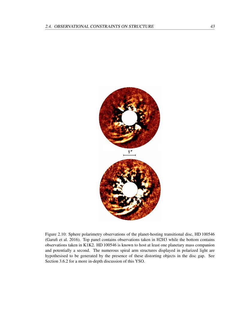
2.4. OBSERVATIONAL CONSTRAINTS ON STRUCTURE 43
Figure 2.10: Sphere polarimetry observations of the planet-hosting transitional disc, HD 100546(Garufi et al. 2016). Top panel contains observations taken in H2H3 while the bottom containsobservations taken in K1K2. HD 100546 is known to host at least one planetary mass companionand potentially a second. The numerous spiral arm structures displayed in polarized light arehypothesised to be generated by the presence of these distorting objects in the disc gap. SeeSection 3.6.2 for a more in-depth discussion of this YSO.

2.4. OBSERVATIONAL CONSTRAINTS ON STRUCTURE 44
Flaherty et al. 2012). MIR variability is observed within a number of transitional disc objects,
although this variability tends to be more limited to flux around the silicate feature such as in
GM Aur and LRLL 67 (Espaillat et al. 2011; Flaherty et al. 2012). The magnitude of the variability
between epochs is typically around 10% for most objects but in some extreme cases the flux can
vary by as much as 50%. This is sometimes referred to as ”seesaw” variability due to the coupled
rising and falling of the two flux contributions.
Variability is also observed in the spectral lines seen in the spectra of disc hosting stars.
Sitko et al. (2012) observed the transitional disc SAO 206462 in six gas emission lines (Brα, Brγ,
Paβ, Paγ, Paδ, Paη and 0.8446 µm O I line), and measured fluxes to vary by over a factor of two
over a time frame of months. They also found the continuum flux to vary by ∼30% but often
decreasing while gas emission line fluxes were increasing. They interpret this variability to be due
to changes in the structure of the inner disc.
As the SEDs of all circumstellar discs are known to be highly dependent on the structure of
the disc from radiative transfer modelling, the mechanism for producing photometric and spectro-
scopic variability is thought to lie in changes within the disc structure. This is a common interpre-
tation for variability in NIR emission from the inner rim of the inner disc of pre-transitional discs.
A change in the vertical height of the disc rim can result in substantially more or less emission.
This in turn leads to a shadow being cast across more extended, and hence colder, regions of the
disc. A smaller disc rim therefore results in less NIR flux but more MIR emission from the now
exposed outer disc. Variability produced in this manner provides strong evidence for the presence
of optically thick material in the innermost regions of pre-transitional discs (Espaillat et al. 2011).
In a similar manner, variability in transitional discs may be a result of low density, optically
thick material in the gap which casts a shadow on the outer disc. This material may even be com-
prised of large grains or highly limited in radial extent to a narrow ring, limiting its contribution
to the SED at wavelengths below 10µm. A possible mechanism to produce such a distribution is
the generation of accretion streams across the gap (Dodson-Robinson & Salyk 2011).
Other possible mechanisms struggle to explain the variability. Hot and cold spots on the
stellar surface have been used to adequately explain variability at shorter wavelengths (Carpenter
et al. 2001) and would affect the irradiance of the disc surface. It cannot however produce an
increase or decrease in the total flux, nor produce a seesaw variability. A dusty disc wind may
shadow the outer disc while supplementing the NIR flux but observations of objects displaying
strong variability, such as by Flaherty et al. (2011), show little to no evidence for strong winds.
A fluctuating magnetic field interacting with the inner disc (Goodson & Winglee 1999; Lai &
Zhang 2008) can distort the inner disc rim producing strong variability effects. The strength of
the magnetic field is unlikely to be strong enough to significantly distort the disc beyond the co-
rotation radius, which is within the dust sublimation radius. Therefore it is unlikely the magnetic
field could influence the dusty component of the disc (Flaherty et al. 2011). Accretion rates are
known to be variable but found to not be sufficient to reproduce the variability observed (Flaherty
et al. 2012). Powerful x-ray flares, known to exist in YSOs (Feigelson et al. 2007), can lead to
changes in the scale height of the disc while also ionising dust particles (Ke et al. 2012) but these
flares are not so prevalent however to explain the number of variables (Feigelson et al. 2007).

2.4. OBSERVATIONAL CONSTRAINTS ON STRUCTURE 45
The most probable source of the excitation required to alter the scale height of the disc is the
presence of a companion or turbulence within the disc. The gravitational field of a massive planet
is expected to launch and maintain spiral density waves in the disc. Such structures may already
have been seen in a number of objects (e.g. HD 100546, HD 142527, V1247 Ori; Boccaletti et al.
2013; Avenhaus et al. 2014; Currie et al. 2014; Ohta et al. 2016). An azimuthally asymmetric
structure in the disc such as this, particularly close to the companion, could excite the inner disc
while shadowing the outer hence generating the seesaw variability. If this were the case then the
timescale of the variability will be the same as the orbital period of the launching companion.
Typical timescales for the seesaw variability span on the order of days to 1-3 years. For a star
similar in mass to the Sun this corresponds to companion orbital radii of 0.05 au to a few au, well
in line with known, high mass hosting planetary systems (i.e. stars hosting hot Jupiters; Howard
et al. 2012).
Interactions between a turbulent disc and magnetic field lines threading through the disc
provide an additional mechanism for launching dusty material from the surface of the disc to where
it can shadow the outer regions of the disc (Turner et al. 2010; Hirose & Turner 2011). Simulations
of this mechanism find that the induced changes in scale height of the disc are sufficient to explain
the variability.
The exact cause of the variability seen is still unclear. Whether the variability is principally
driven by the warping effect of a companion within the disc remains a topic of intense research.
2.4.6 Disc clearing mechanisms
2.4.7 Non-dynamical disc clearing mechanisms
In the previous Section, I discussed the observational evidence for the presence of gaps in the disc
along with information as to the structure and nature of these gaps. Here I discuss a number of po-
tential clearing mechanisms and how feasible they may be in producing the previously described
structures seen in observations. There are a number of differing mechanisms for clearing dusty
particles from inner regions of a disc, each with their own observational signatures. The primary
focus of much work in the field is on the dynamical clearing of a gap through gravitational in-
teractions between a companion and the disc. This scenario will be looked at in more detail in
Section 3.4. Here I discuss possible alternate scenarios.
Radial drift
A natural avenue for the reduction of infrared flux from dusty material in the inner regions of the
disc is the removal of the dusty material itself. Inward drift of dust particles and eventual sub-
limation by the central star’s powerful radiation is thought to occur due to gas dust interaction.
This tendency for dust particles to migrate inwards is referred to as ”radial drift” and is caused
by thermal pressure causing the gas disc to orbit at sub-Keplerian velocities (Whipple 1972; Wei-
denschilling 1977; Birnstiel et al. 2012). The dust is less affected by the thermal pressure due
to its larger mass compared to gas molecules so continues to conform to Keplerian orbits. This
difference in orbital velocity leads to a drag force on the dust grains, which in turn causes them

2.4. OBSERVATIONAL CONSTRAINTS ON STRUCTURE 46
to drop into lower orbits (Whipple 1972; Weidenschilling 1977; Brauer et al. 2008). This contin-
ues until the particle accretes onto the star unless trapped by a ”pressure bump”. In this way the
vast majority of small dust grains (∼95%) can be removed from within a disc on the timescale of
1 Myr (Brauer et al. 2008). Small dust grains are observed however to persist in discs older than
1 Myr, even within gapped discs so radial drift is not expected to be the dominant cause of disc
clearing. The removal of dust grains from the inner regions can lead to a depletion of the emitting
particles large enough to cause a drop in the in IR SED however (Birnstiel et al. 2012) so cannot
be completely ignored but is not expected to be the dominant cause of gap clearing.
Grain growth
Another method for the removal of small dust grains from the inner disc is through their growth and
aggregation into larger dust grains. The density of dusty material remains the same in this scenario
but the particles become less efficient at emitting in the NIR and MIR (e.g. D’Alessio et al. 2001;
Draine 2006). Early models predicted the rapid growth of small particles to mm/cm sizes within
the inner disc where the dynamic timescales are short (Dullemond & Dominik 2005; Tanaka et al.
2005) resulting in a corresponding drop in IR from the inner disc. Including processes which
decrease the efficiency of this process such as dust fragmentation under high speed collisions in
more detailed models still results in short timescales for the removal of small dust grains from the
inner disc. Models such as these can reproduce the IR deficit in the SED while efficiently growing
particles to mm/cm from µm particles, however these particles can grow no further as the energy
of the collisions become catastrophically destructive, leading to a population of small, µm sized
fragmented particles which can emit efficiently in the IR again (Birnstiel et al. 2012). This washes
out the IR deficit due to grain growth.
While radial drift and grain growth provide plausible mechanisms for the reduction of IR
emission from the inner disc, fundamentally they are not capable of solely explaining the clearing
seen in transitional and pre-transitional discs as they fail to produce the cavities seen in mm data.
This is because in both scenarios there remains a substantial population of large dust grains which
still emit efficiently in the mm (D’Alessio et al. 2001; Birnstiel et al. 2012). They cannot be
completely discarded however as they may still remain important to the evolution of the disc.
Photoevaporation
To maintain the surface density of the inner disc, the material accreted onto the central star or lost
through disc winds must be replaced by material flowing inwards from larger radii. However to
reach the central star, dust particles must survive exposure to the powerful stellar radiation field.
As the disc evolves the reservoir of material is depleted and the rate of material flowing through
the disc drops off. If the rate of transport of dusty material through the disc is less than the rate
at which dust particles are destroyed at the inner edge of the dust disc, this inner edge will move
outwards away from the star producing an extended cavity. The stellar radiation field can be
powerful enough to drive substantial mass loss from the disc in the form of winds which further
amplifies this effect (Hollenbach et al. 1994; Clarke et al. 2001; Alexander et al. 2006; Alexander

2.4. OBSERVATIONAL CONSTRAINTS ON STRUCTURE 47
& Armitage 2007; Gorti & Hollenbach 2009; Gorti et al. 2009; Owen et al. 2010, 2011; Rosotti
et al. 2013).
While almost certainly important for the eventual dispersal of the disc as it nears the end of
its life (Clarke et al. 2001) photoevaporation alone struggles to explain a number of key features of
transitional and pre-transitional discs. In particular it cannot explain the tenuous but non-negligible
contents of the gap, substantial continued accretion onto the central star (Espaillat et al. 2014) and
the population of classical discs which show no indication of gaps or holes but have very small
accretion rates (Ingleby et al. 2012). Additionally work by Gorti & Hollenbach (2009) and Owen
et al. (2012) has indicated a strong dependence on the stellar x-ray luminosity, LX . Surveys of star
forming regions found that the population of disc hosting stars with gaps typically contained stars
with relatively low LX and no correlation between LX and gap sizes (Kim et al. 2013) implying
that extended cavities in the dust disc are unlikely to be caused by photoevaporation.
2.4.8 Dynamical disc clearing mechanisms
The development of a companion with a substantial gravitational field not only leads to clearing
within the companion’s immediate vicinity via accretion onto the body, it also leads to interactions
with the gas disc at other radii in the disc. A particle within a radii where the particle experiences
a periodic gravitational interaction with the protoplanet will have its orbit substantially altered,
becoming more eccentric until ejected from the gap through a scattering interaction within another
body in the disc. An identical process within the Solar System occurs between Jupiter and the
numerous bodies in the asteroid belt leading to a series of gaps known as the Kirkwood gaps.
Similarly, interactions been Saturn’s moon Mimas and icy particles in Saturn’s rings produce the
distinctive ringed structure around Saturn. Within the Kirkwood gaps, few if any particle survives
for long until the influence of Jupiter’s gravity deflects the particle inwards towards the inner Solar
System, on a highly eccentric orbit. The eventual fate of a deflected particle is typically the tidal
destruction and accretion of the particle onto the Sun or Jupiter, or ejection from the Solar System.
The result is a series of regions in the radial distribution of particles within the asteroid belt where
there is a substantial drop in the density of material. These gaps occur where the ratio between
the orbital periods of Jupiter and a particle in the disc are integer values. Hence these gaps are
sometimes described as related to orbital resonances, called Lindblad resonances (Lindblad 1961).
These are defined to occur when the angular frequency, Ω,
m(Ω −Ωp) = ±κ0, (2.35)
where m is an integer, κ0 is the epicyclic frequency, and Ω is the orbital frequencies of the particle
(Ωp is the orbital frequency of the planet). The epicyclic frequency is related to the stellar gravi-
tational potential. If one approximates that the gas orbits with a Keplerian velocity in all regions
of the disc, the position of the Lindblad torques generated by a planet in the disc is given by:
rL =
(1 ±
1m
)2/3
rp, (2.36)

2.4. OBSERVATIONAL CONSTRAINTS ON STRUCTURE 48
Figure 2.11: Diagram displaying the strongest Lindblad resonances generated by a planet in orbit.Shown are resonances corresponding to values of m of 1,2,3, and 4, both internal and external tothe planet. Higher values of m are not shown for clarity and also due to their gradually weakerstrength. A further co-orbital resonance is shown in black for m = 0. Gravitational interactionswith material at resonances paradoxically lead to the planet moving away from the resonance andmaterial in the resonance moving away from the planet.
where rp is the orbital radius of the planet. m = 0 represents the co-rotational resonance. The
position of the strongest resonances are shown in Figure 2.11.
The interaction with resonances exerts a torque on both the material within the resonance
and the perturbing companion (Ward 1997). The exact process by which this occurs is discussed
in more detail in Section 3.4, but the general result is to drive material within the resonance away
from the companion. For a resonance at a larger radii within the disc to the companion, this leads
not only to clearing, but also to generating a barrier against the radial drift of dusty material. At
resonances interior, material will be pushed closer to the central star with material drifting rapidly
across the resonances. Particles sufficiently perturbed from a circular orbit by the gravity of the
forming planet may cross the gap through streams of material, which connect the planet to the
outer and inner portions of the circumstellar disc (Lubow et al. 1999). Material can flow rapidly
across the gap in these streams, replenishing material lost through sublimation and radial drift.
The presence of massive planet in the disc acts as an effective remover of material from the
disc (see Section 3.4). This includes the solid material responsible for most of the flux both emitted
and scattered by the disc. Stellar flux which would have heated or scattered from surface layers
of the disc instead heat or scatter from the new disc rim at the outer edge of the gap, which now
dominates the resultant images of the disc and produce sharp drops in flux in the SEDs (Varniere
et al. 2006a).
2.5. CHAPTER SUMMARY 49
2.5 Chapter Summary
In this Chapter I described the current theories on the formation of gapped discs starting from the
collapse of a giant molecular cloud. From there I described the stages which lead to the formation
of a star through the several stages of collapse, quasi-static hydrodynamic equilibrium and further
contraction to protostars. I then described the subsequent formation of a circumstellar disc due to
the conservation of angular momentum and its role in the transport of material onto the protostar
and dispersal of angular momentum back into the ISM through viscosity within the disc itself. In
this manner a stellar object can continue to accrete material while spinning down through magnetic
breaking, preventing the rotational break up of the star.
From here I focused on the evolution of the protostellar disc into a protoplanetary disc,
including a summary of the current state of known observable traits of these objects and a brief
description of the techniques and their contributions to our body of knowledge on these objects. I
explained how identification of circumstellar discs and their rudimentary properties can be made
through the study of their SEDs and how more detailed structure can be determined through re-
solved interferometric observations in both the NIR+MIR and sub-mm.
I discussed in more detail the later stages of disc evolution in regards to the objects classified
as transitional or pre-transitional discs. In particular I described the reasoning and evidence for
their status as the nurseries of on-going planet formation, inferred from their simultaneous deep
gapped structure, the sharp or defined edges of their dusty rings, and high stellar accretion rates.

Chapter 3
Planet formation and protoplanets
3.1 Introduction
As discussed in Section 2.4.7 the effects of gas drag on the dust particles is to cause them to spiral
inwards and onto the parent star on a times scale of ∼1 Myr. In the most simplistic of mechanisms,
the dust grains therefore must grow from a population µm-sized to one of m-sized planetesimals
within 1 Myr, at which point the effect of the gas drag becomes negligible, or else be destroyed
and accreted. However, as also discussed in Section 2.4.7, growth beyond mm/cm-sized particles
becomes problematic as collisions between particles are too energetic and lead to the destruction
of larger particles. In such a scenario all the dust particles are accreted and no larger body is
formed within the disc before it is dispersed. For planets to form, which self-evidently must be the
case, alternative mechanisms must be invoked.
3.2 Planet formation theory
To better understand the processes involved in planet formation it can be useful to describe the
growth of the dust particles as transitioning through a number stages. In each of these stages, the
dust particle behave and interact with the disc in different ways and hence grow and evolve along
unique pathways.
Small particles of dust which range in size from the smallest solid particles of under a µm
in size to cm size are strongly coupled to the gas disc. They follow the gradual in-fall of the gas
disc, drifting radially and are vertically excited by turbulence and thermal properties. The growth
of small dust particles in the disc is determined by the rate of their collisions and the effectiveness
of their adhesion during those collision (Whipple 1972; Weidenschilling 1977).
Larger particles up to a meter in size are sometimes referred to as pebbles or rocks. These
particles have grown large enough in size to only be weakly interacting with the disc and have set-
tled to the mid-plane of the disc through dampening of their vertical oscillations via a combination
of the enhanced gravitational pull of the disc and gas drag (Weidenschilling 1977; Brauer et al.
2008). Their dynamics can be considered to be determined by approximately Keplerian orbits
with some small gas drag component.
50

3.2. PLANET FORMATION THEORY 51
Objects of a km in size or above are described as planetesimals and are comparable in size
to the objects which populate the asteroid and Kuiper belts in the Solar System. The gas disc
plays little role in the dynamics of these objects as the gas drag effects are negligible in perturbing
the orbit of objects this size. Typically, a large population of objects in this size range is used as
the initial conditions for N-body simulations of planet formation as they have now gained enough
mass to be held together by their self gravity and not weak electrostatic forces, making them more
cohesive objects and hence resistant to breaking up under collisions. Their gravitational fields also
allow them to interact with one another at greater distances and lower energies. Such conditions
allow larger particles to disrupt and accrete smaller particles through tidal interactions.
Once an object has achieved a mass of around that of the Earth, M⊕, its gravity is strong
enough to interact with the gas disc around it and so it again becomes coupled. The result of this
coupling is described in more detail in Section 3.4. The result of this coupling is a new phase of
inward migration which can be at a very rapid rate. The cores of growing gas giants likely rely on
the gas disc as a source of material for accretion and interact strongly with the disc (Mizuno 1980;
Bodenheimer & Pollack 1986).
Once the core of forming gas giant reaches around 10 M⊕, the core becomes massive
enough to transition from a quasi-hydrostatic core+gaseous envelope structure and into a regime
of accretion to the detriment of the accretion of another other nearby planetary cores. Such an ob-
ject will rapidly clear its orbital path and grow rapidly in a phase of ”oligarchic” growth (Kokubo
& Ida 1998).
3.2.1 From dust particles to pebbles
The growth and evolution of the smallest particles in the disc can be explained to first order through
the coagulation of particles to cm-sized grains which drift steadily inwards as a result of gas drag
(see Figure 3.1). Following a simple description of particle growth as laid out in works such
as Safronov (1969) and Dullemond & Dominik (2005), one can imagine a spherical particle of
radius a, and density ρdust settling towards the mid-plane with a velocity vsettle. This particle will
collide with and stick to smaller particles as it descends, gathering mass. Assuming all collisions
result in the particles sticking together with perfect efficiency, the rate at which mass is gained by
the particle is then defined by the amount of material within the volume defined by the particle’s
geometric cross-section and height above the mid-plane, z, such that:
dmdt
= πa2|vsettle| fρ(z(t)), (3.1)
where ρ(z) is the vertical density profile including gas and dust, and f is the gas to dust ratio of the
disc. Substituting the settling velocity for the settling time scale (which is derived through the ac-
celerating force of the disc’s gravity towards the mid-plane and the resistive gas drag component),
and the mass of the particle for the dust particle density (m = 4/3πa3ρdust) one finds:
dmdt
=34
Ω2 fv
zm, (3.2)

3.2. PLANET FORMATION THEORY 52
Figure 3.1: Dust grain (blue circle) evolution and inward radial drift (blue arrow) within a dustydisc. a) µm-sized dust particle starts high above the disc mid-plane with a substantial verticalmotion component within the disc. As the particle rises and falls in the disc due to turbulence andthermal motion, it collides with other particles, growing larger. b) As it becomes more massivethe gravitational pull of the disc (red arrow) becomes larger, dampening the vertical motion of theparticle. c) Once the particle is ∼cm-size it is approximately confined to the mid-plane. d) Furthergrowth is inhibited by fragmentation during high energy collisions with other cm-sized grains. e)Unless halted the gradual radial drift of the particle due to drag effects with the gas disc will resultin its sublimation and accretion onto the central star.
where Ω is the orbital rotation rate, and v is the mean thermal velocity of the gas. The expression
for the settling velocity, vsettle, is given by:
vsettle =Ω2
vρdust
ρ(z)az (3.3)
A rapid growth from µm to cm-sized grains occurs in all discs with realistic classical disc pa-
rameters in this description, and is the dominant mechanism by which dust particles settle to the
disc plane (Dullemond & Dominik 2005). Time scales derived using this simple model are on
the order of 103yr and even when compared to more sophisticated modelling regimes remain a
good approximation. The growth of grains in this manner is so efficient, explaining the observed
high NIR flux in the SEDs of classical and pre-transitional discs requires a feedback mechanism
to repopulate the µm to cm size range. Usually fragmentation during collisions, as mentioned in
Section 2.4.7 is invoked. The disruption of larger particles into a collection of smaller particles
repopulates the sub-mm sized dust particles which produces the NIR flux.
Until the particles grow large enough to become completely decoupled from the gas, the
lifetime of the dust particles is determined by the rate at which they drift inwards until they pass
through the inner rim of the dust disc and are exposed to the central star’s powerful radiation where
they are sublimated (Weidenschilling 1977). For small particles, the dust is well-coupled to the
gas and hence drifts inwards. In the case of pebble sized particles, they have largely decoupled but
3.2. PLANET FORMATION THEORY 53
now drift inwards due to gas drag. Taking the radial component of the momentum equation of the
gas disc as the start results in:
v2φ,gas(z = 0) =
GM∗r2 +
1ρ
dPdr
(3.4)
where P is the mid-plane gas pressure. One can define the pressure at a radius, r0:
P = P0
(rr0
)−η(3.5)
where P0 = ρ0c2s,0 (with cs,0 representing the sound speed at r0). Substituting, one finds,
vφ,gas = vK(1 − η)1/2 (3.6)
where vK is the velocity of the a particle in the disc as a result of a Keplerian orbit and η is a
constant representing nc2s/v
2K. The direction of drift is therefore entirely dependent on the sign of
n. For a pressure profile which decreases away from the central star, This fractional difference is
very small but at 1 au can amount to a headwinds on the order of 100 ms−1. This will sap their
angular velocity, resulting in a steady in-fall towards the central star (Weidenschilling 1977).
The radial velocity is size dependent and peaks for particles in the cm to m size range
(Weidenschilling 1977) and leads to short lifetimes for dust particles. Starting at a few au, a dust
particle is expected to survive on the order of 100s of years. This is far shorter than the disc
lifetime and presents a pressing problem. These time scales are based on the assumption that
the dust densities are negligible compared to the gas densities and hence no back reaction from
the dust disc occurs to slow the radial velocity. Even with these reactions considered however,
lifetimes do not match disc lifetimes (Nakagawa et al. 1986).
A possible solution to the problem is to consider a scenario where the pressure gradient
is at least locally reversed (negative values of n). Drift occurs towards higher pressure regions
so if there were a local pressure maximum within the disc, dust particles travelling inwards will
have their migration halted and will become trapped in the maximum (see Figure 3.2). Here dust
densities may rise sufficiently to facilitate further growth.
There are a number of physical processes which can produce local pressure maxima in
the disc. Some are persistent and long-lived such as at the inner edge of a magnetic dead zone
(Okuzumi & Ormel 2013), or can be transient as in the case of large-scale disc turbulence (Hasegawa
& Pudritz 2011). Gaps and warping of the disc surface density caused by the formation of a giant
core could also generate pressure bumps, facilitating further planet formation (Masset et al. 2006;
Hasegawa & Pudritz 2011).
3.2.2 From pebbles to planetesimals
The principle problem to be overcome in forming planetesimals is to form a km-sized body fast
enough to escape the steady spiralling path into the central star. A sensible starting point for the
growth of pebbles into planetesimals is to continue through the same process of steady aggrega-

3.2. PLANET FORMATION THEORY 54
Figure 3.2: Diagram displaying how a pressure maximum may trap inwardly drifting dust par-ticles. Small dust particles in the disc will travel towards regions of higher pressure. If a localmaxima is encountered, then further motion inwards will be arrested, trapping the dust particles.If no such maxima exists then the particles will continue inwards until sublimated.
tion through pairwise collisions. For this to be a viable mechanism, the material properties of the
colliding bodies must be such that collisions under a realistic velocity distribution results in more
aggregations than fragmentations or bouncing collisions (see Figure 3.3). Experiments under mi-
crogravity conditions indicate that silicon based grains of µm sized monomers will stick together
when impact velocities are under 1 ms−1 (Poppe et al. 2000). Similar experiments performed with
water-ice monomers of similar size indicated sticking velocities on the order of 10 ms−1 (Gund-
lach & Blum 2015) implying the location of the snow line within a disc, where conditions allow
the condensation of water-ice, is important for the rates of particle growth. This is intuitive as one
would expect such regions to contain enhanced dust to gas ratios and hence more material for par-
ticle growth compared to the inner regions of the disc, but the higher survivable impact velocities
will further aid rapid growth.
Beyond monomers, an object made up of a number of subunits can in principle be ”stronger”
than a monomer as the impact energy can be dissipated through the inner structure of the particle.
The electro-static binding between the subunits however is likely to be very weak. The result is
that there is no barrier to prevent grains growing to mm sizes interior to the snow-line, but the size
distribution of particles larger than ∼mm is determined by the interplay of the rate of coagulation
and fragmentation of the dust particles (Birnstiel et al. 2011). Growth beyond cm sizes is severely
limited due to the onset of particles bouncing rather than sticking during collisions (Zsom et al.
2010). Growth could continue beyond this size but fragmentation severely inhibits growth, hence
particles struggle to grow large enough to escape the radial drift problem.
Particles beyond the snow line benefit from the enhanced ability of ice particles to adhere
together and are likely to grow to larger sizes more efficiently. Rather than being limited by
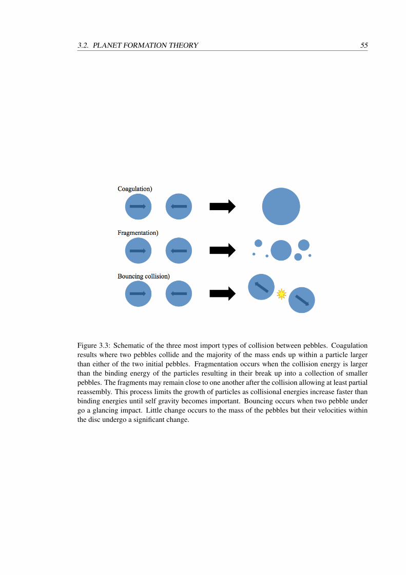
3.2. PLANET FORMATION THEORY 55
Figure 3.3: Schematic of the three most import types of collision between pebbles. Coagulationresults where two pebbles collide and the majority of the mass ends up within a particle largerthan either of the two initial pebbles. Fragmentation occurs when the collision energy is largerthan the binding energy of the particles resulting in their break up into a collection of smallerpebbles. The fragments may remain close to one another after the collision allowing at least partialreassembly. This process limits the growth of particles as collisional energies increase faster thanbinding energies until self gravity becomes important. Bouncing occurs when two pebble undergo a glancing impact. Little change occurs to the mass of the pebbles but their velocities withinthe disc undergo a significant change.
3.2. PLANET FORMATION THEORY 56
fragmentation, growth may instead be limited by the life span of the particle in the disc before
accretion onto the central star (Birnstiel et al. 2011). If even transient dust traps exist beyond the
snow-line, then dust particles could survive within the disc long enough to form planetesimals and
decouple from the gas disc (Pinilla et al. 2012). Further growth could be facilitated by condensa-
tion of vapour directly onto the particle, which could be important for growth in regions adjacent
to ice lines in the disc (Stevenson & Lunine 1988; Ros & Johansen 2013).
Alternate hypotheses for growing planetesimals invokes a local fragmentation of thedust
disc, fusing a dense clump of dust particles into a number of larger planetesimals. Phrased in its
simplest form, the dust settling process results in a dense layer in the mid-plane which could be
vulnerable to gravitational collapse (Goldreich & Ward 1973). For the sub-disc to be vulnerable
to collapse the density of dust particles must exceed that of the gas disc. After fragmentation of
the local disc, dense clusters of gravitationally bound pebbles dissipate internal energy through
collisions and steadily collapse to form planetesimals. This in practice is difficult to achieve as
shears and turbulence prevents the dust disc becoming dense enough to become unstable (Cuzzi
et al. 1993).
While forming a flat disc is problematic, a similar mechanism for growth invokes a ”stream-
ing instability” to concentrate dust grains such that the dust density exceeds the gas density trigger-
ing fragmentation and subsequent collapse into planetesimals. The term “Streaming instability”
is generally used to describe the instability between an aerodynamically coupled mixture of gas
and dust particles within a differentially rotating disc. Youdin & Goodman (2005) showed that
the radial drift of dust particles is unstable under a broad range of conditions and results in the
concentration of dust particles into weak asymmetric over densities which collapse on the radial
drift timescale. These over densities could seed the formation of a population of planetesimals.
3.2.3 From planetesimals to planetary cores
The growth of particles beyond a meter in size into planetesimals leads to a loose re-coupling of
the planetesimals to the gas disc. This re-coupling results in two opposing effects acting on the
planetesimal population’s orbital properties. Interactions with the gas disc will both dampen and
excite the orbital eccentricity of the planetesimals through aerodynamic drag and surface density
perturbations damping and exciting the eccentricity respectively (Laughlin et al. 2004; Nelson
2005; Okuzumi & Ormel 2013). While important when performing numerical simulations, further
dynamical interactions between the planetesimals and the gas disc are halted until they reach sizes
of approximately 103 km. Here they become massive enough for their gravitational interactions
with the gas disc to become significant. These interactions will be discussed in Section 3.4.
Further growth of planetesimals into planetary cores and protoplanets is believed to proceed
primarily through planetesimal-planetesimal and finally protoplanet-planetesimal collisions.
When considering the interactions of small particles and pebbles in the disc, the influence
of their gravity can be neglected. Planetesimals however have gathered enough mass to exert their
own gravitational field, albeit a weak field, diverting and focusing surrounding bodies towards the
planetesimals (see Figure 3.4). The effect is to increase the effective collisional cross section of

3.2. PLANET FORMATION THEORY 57
Figure 3.4: Diagram displaying how the gravitational field of a planetesimal will perturb the mo-tion of other particles in the disc (blue arrow) leading to a greater collisional cross-section, en-abling faster growth. Hence, more massive planetesimals will grow faster and at the expense ofsmaller planetesimals. The new effective radius, b, represents the larger effective radius giving riseto the in-turn larger collisional cross sectional, Γ, compared to the physical size of the planetesimalalone.
the planetesimal, accelerating growth. The cross section for collision, Γ, can be represented as:
Γ = πR2s
(1 +
v2esc
σ2
), (3.7)
where Rs is the sum of the radii of the two colliding objects, vesc is the escape velocity of the
planetesimal, and σ is the relative velocity of the two colliding bodies at infinity. The term within
the brackets is the enhancement of the cross-sectional area. If the parent disc is cold, so σ
vesc, the growth of planetesimals will be higher compared to a hot disc. Velocity dispersions are
therefore highly important for estimating the growth rate of planetesimals, with low dispersions
beneficial to planetesimal growth.
To derive an estimate for the growth rate we start from the assumption of a growing central
mass, M, and radius, Rs, with a surface escape velocity, vesc. This mass is assumed to be embedded
in a homogeneous ”swarm” of planetesimals with a local planetesimal surface density given by
Σp, velocity dispersion, σ, and scale height, hp. The plantesimal density within a unit volume of
the disc is given by:
ρp =Σp
2hp(3.8)
Under the further assumption that third body effects can be neglected, the material accreted onto

3.2. PLANET FORMATION THEORY 58
the central mass per unit time is given by:
dMdt
= ρpσπR2s
(1 +
v2esc
σ2
). (3.9)
Since hp ∼ σ/Ω, where Ω is the local angular velocity, we can substitute Equation 3.8 into Equa-
tion 3.9 to get the simplified form of the equation:
dMdt
=12
ΣpΩπR2s
(1 +
v2esc
σ2
). (3.10)
From this result comes a few important results. Firstly, the velocity dispersion of the planetesimal
swarm only appears in the growth rate in the gravitational focusing term. In an excited environ-
ment, this term can be high and restrict the rate of growth. Secondly, the growth rate is linearly
linked to the local surface density of the planetesimals, and thirdly that growth will be slower at
larger radii where both Ω and Σp are lower.
A simple analysis of how the growth rate evolves with time is not possible due to the feed-
back effects as a result of the changing gravitational field of a growing mass. As the planet grows,
its gravity will stir up the planetsimal swarm increasing the velocity dispersion and will later begin
to deplete the local planetesimal surface density. A simple first order approximation is to neglect
these effects, with the caveat that this approximation is only valid while the growing planet is still
too small to significantly affect the local surface density or excite the velocity dispersion. Taking
the gravitational focusing term, Fg as a start:
Fg =
(1 +
v2esc
σ2
). (3.11)
One can simplify this term down further to:
Fg ≈v2
esc
σ2 , (3.12)
in the case of low velocity dispersion where v2esc/σ
2 1. From here one can simplify further as
σ is taken to be a constant down to:
Fg ∝MRs. (3.13)
Putting this into Equation 3.10 produces the following relation:
dMdt
=∝ MRs. (3.14)
The consequence is that the growth rate scales with mass as the gravitational focusing term in-
creases, resulting in an oligarchic growth scheme where larger masses grow faster than their
smaller neighbours.
Another consequence is that rapid growth is dependent on the velocity dispersion remain-
ing low, or alternatively, the planetesimal swarm maintaining an approximately circular orbit in
the disc. Therefore there is a finite supply of accretable planetesimals for the growing planet to
3.2. PLANET FORMATION THEORY 59
gather. The isolation mass, Miso, is derived from the fact that as a planet grows, its feeding zone
expands as it exerts influence over a larger region of the disc. The mass of the new planetesimals
contained in the new feeding zone increases less than linearly and eventually results in the supply
of new material becoming exhausted and further growth ceases without the availability of a fresh
supply. Pollack et al. (1996) estimated this mass to be approximately 9 M⊕ for a planet growing
in conditions appropriate for the formation of a Jupiter-like planet. This estimate is appropriate
for the current best determinations of the mass of Jupiter’s core (Guillot 2005). Evaluating in a
similar manner the isolation mass for a planet at 1 au, Lissauer (1993) calculated Miso = 0.07 M⊕.
To form an Earth mass body in-situ clearly requires further accretion of embryos.
Previously we have only considered planetesimal-planetesimal accretion, smaller objects
are still expected to survive in the dust disc however. Further accretion of the remnant pebble or
dust disc, which is expected to be long lived based on SED observations of protoplanetary discs,
could also provide an important reservoir of material for the growth of planetesimals through
lower energy collisions. Such a process could alleviate the limited mass contained within the
feeding zone as more material drifts inwards from the outer disc into the growing planets region
of influence. Such a mode of continued accretion is referred to as pebble accretion and has been
developed by a number of groups (Ormel & Klahr 2010; Lambrechts & Johansen 2012). The
result of such work has been to define two phases of accretion (see Figure 3.5). In the case where
the mass of the growing planet is still small and tidal effects can be ignored, pebbles approach with
approximately the drift velocity and facilitates fast growth as there is little increase in the velocity
dispersion. Once the core has grown massive enough that tidal forces can no longer be ignored,
the approach velocity is dominated by the Keplerian shear velocity which limits the capture area
to the Hill sphere of the core. These phases are referred to as drift- and Hill-limited accretion
respectively. For a pebble interacting with the growing planet to be pulled from its radial drift, the
planet’s gravitational pull must be strong enough to accrete the pebble before it is lost to the inner
region of the disc where its radial drift will take it away from the forming planet. As the Keplerian
velocity shear can be larger for an extended Hill sphere, this leads to two rates of growth. For
drift-limited accretion, this results in a growth rate ∝ M, leading to exponential oligarchic growth.
For Hill limited accretion, the growth rate is ∝ M2/3, a slower rate of accretion but still more
rapid than smaller bodies (Ormel & Klahr 2010; Lambrechts & Johansen 2012). Local conditions
within the disc also affects the growth rate with higher surface densities leading to higher growth
rates.
The sum of these processes lead to a period of runaway growth where the largest planetes-
imals will grow rapidly, at ever faster rates until their source of material has been exhausted. This
phase of oligarchic growth results in the planetesimal swarm becoming stirred up, further limiting
the growth of smaller particles suppressing the formation of giant planets. The resultant mass
distribution will be dominated by a small number of large masses (Kokubo & Ida 1998; Thommes
et al. 2003). Such growth continues until the bodies become separated from the feeding material.
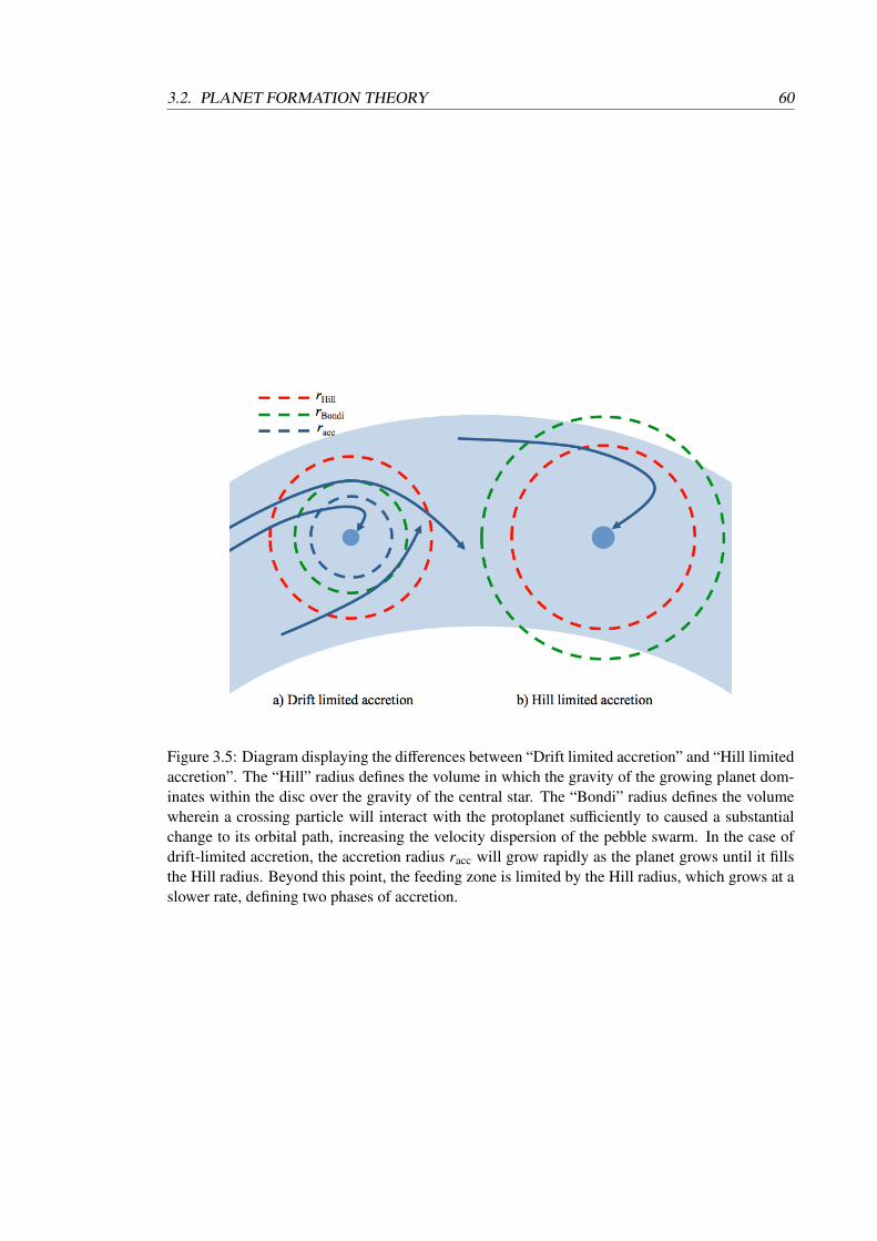
3.2. PLANET FORMATION THEORY 60
Figure 3.5: Diagram displaying the differences between “Drift limited accretion” and “Hill limitedaccretion”. The “Hill” radius defines the volume in which the gravity of the growing planet dom-inates within the disc over the gravity of the central star. The “Bondi” radius defines the volumewherein a crossing particle will interact with the protoplanet sufficiently to caused a substantialchange to its orbital path, increasing the velocity dispersion of the pebble swarm. In the case ofdrift-limited accretion, the accretion radius racc will grow rapidly as the planet grows until it fillsthe Hill radius. Beyond this point, the feeding zone is limited by the Hill radius, which grows at aslower rate, defining two phases of accretion.
3.2. PLANET FORMATION THEORY 61
3.2.4 Giant planet formation
For terrestrial planets of mass on the order of 10 Earth masses and below, the formation process
ends with the clearing away of the oligarchic growth of a planetesimal into a planetary embryo and
then protoplanet through collisions with other embryos to reach their final sizes. The atmospheres
of these planets contribute little in the way of the total mass and radial size, and their shallow
gravitational potentials are unlikely to be able to hold onto the volatile gases present in the gas disc
for a prolonged period of time as a result of atmospheric erosion through collisions with minor
and major planetesimals (Cameron 1983). The origins of any atmosphere around such planets are
more likely to be through chemical processing of the surface of the planet and out gassing from
the still molten core through volcanism. Such objects likely form after the majority of the gas disc
has been dispersed and any residual light elements in the atmosphere which are accreted readily
escape from the shallow gravity wells compared to gas giants.
The final stage of terrestrial planets growth up to their final size is likely through colli-
sions between the now isolated planetary embryos. Their orbital paths are likely perturbed by the
forming giant planets and mutual resonances into crossing (Chambers & Wetherill 1998). Such a
collision between a nascent Earth and a Mars-like protoplanet is believed to be the cause of the
formation of the Earth’s iron core, in addition to ejecting large amounts of material into a cicum-
planetary ring around the Earth to coagulate into the Moon (Canup 2004). Numerical simulations
find the assembly of terrestrial planets in a Solar System-like configuration takes on the order of
100 Myr with the final exact configuration being strongly dependent on the assumed initial plan-
etesimal and gas disc surface densities and the presence and evolution of giant planets in the outer
disc beyond the snow line (Kokubo et al. 2006; Levison & Agnor 2003; Raymond et al. 2005).
The important caveat to the validity of these models however is these simulations still fail to pro-
duce terrestrial planet configurations close to that of the inner Solar System, in particular failing
to match the mass and eccentricity of a Mars-like planet. It is clear therefore that some processes
remain missing in our current theories of planet formation (Raymond et al. 2009).
Cores which form while the gas disc is still present will have a far larger reservoir of mate-
rial to accrete from, so will likely form larger planet types from Mini-Neptunes to Jovian planets.
How these worlds form is explained in more detail below.
Gravitational instabilities
To collapse a gas envelope onto a core requires the efficient formation of a core on short enough
timescales to feed from a gas disc before it is dispersed in the later stages of a disc’s lifetime. In
the outer reaches of the disc where the surface densities are lower and the dust population is colder,
this is difficult to achieve. The presence of Uranus and Neptune within our own Solar System and
the population of gas giants on extended orbits in exoplanetary systems tells us planet formation
does take place here, or requires a substantial migration outwards. The majority of migrations
are inwards however (see Section 3.4) so the more probable is for a core to form here, perhaps
requiring an alternate formation mechanism. A potential avenue is through the fragmentation of
the outer disc through gravitational instabilities.
3.2. PLANET FORMATION THEORY 62
A cold or sufficiently massive disc is unstable to gravitational collapse under its own gravity
if its Toomre parameter, Q, is low enough. Formally this is:
Q ≡csΩ
πGΣ' 1 (3.15)
where cs is the local sound speed, Ω is the local angular velocity, and Σ is the local gas surface
density (Toomre 1964). From this equation it is clear that discs which possess small sound speeds
and low angular velocities favour instability along with high surface densities. Conversely the
opposite is true for stable discs. The dependence on high surface densities in particular makes
discs most vulnerable during their early stages of evolution. The typical size for a planet formed in
such a way is on the order of MJ but keeping such objects within the planetary mass range and not
develop into low-mass stellar objects or brown dwarfs in an accretion disc with a lifetime of Myr is
problematic (Kratter et al. 2010). Additionally, when the disc approaches low values of Q, rather
than fragment it produces a set of non-axisymmetric instabilities which heats up the disc through
angular momentum transfer in the shape of the production of spiral arms. This heating increases
the local sound speed supporting the disc against further collapse (Paczynski 1978). Furthermore
this angular momentum transfer leads to depletion of the local surface density, further pushing the
disc towards stability (Lin & Pringle 1990).
Hence for a disc to be gravitationally unstable the timescale for cooling must be shorter than
the heating of the disc as a result of the compression of the gas into spiral arms (Gammie 2001).
Global simulations of differentially rotating discs has supported this intuitive interpretation (Rice
et al. 2003a). The cooling is controlled within a real disc through a combination of local opacity
and vertical energy transfer. Modelling such effects allows one to estimate where in the disc
instabilities leading to fragmentation are likely to occur (Rafikov 2005; Clarke 2009). The result
of such work is that using standard opacities allows fragmentation into planets only at extended
radii from the central star of 50-100 au or more. Additionally the resultant objects are almost
always high mass/brown dwarf-type objects due to the large reservoir of material in the outer
disc (Stamatellos & Whitworth 2009). Simulations of the inner discs indicate that while the disc
can become gravitationally unstable, the instability saturates before fragmentation can occur and
leads instead to the formation of spiral arms and facilitates enhanced rates of angular momentum
transport.
Such models do not however contain all the physics which may be necessary to accurately
represent this formation mechanism. For instance, at radii beyond 50 au stellar irradiation can
no longer be neglected and will influence the fragmentation criteria (Rice et al. 2011). Further-
more the convergence problems (Meru & Bate 2011), sensitivity to stochastic effects Paardekooper
(2012), and the exact cooling treatment (Rice et al. 2014) all create divergent results. These effects
are not likely to be able to prevent fragmentation.
Core accretion
The most probable route to the formation of gas giant planets is through the core accretion model
(Mizuno 1980; Bodenheimer & Pollack 1986). The first complete description of the model ap-
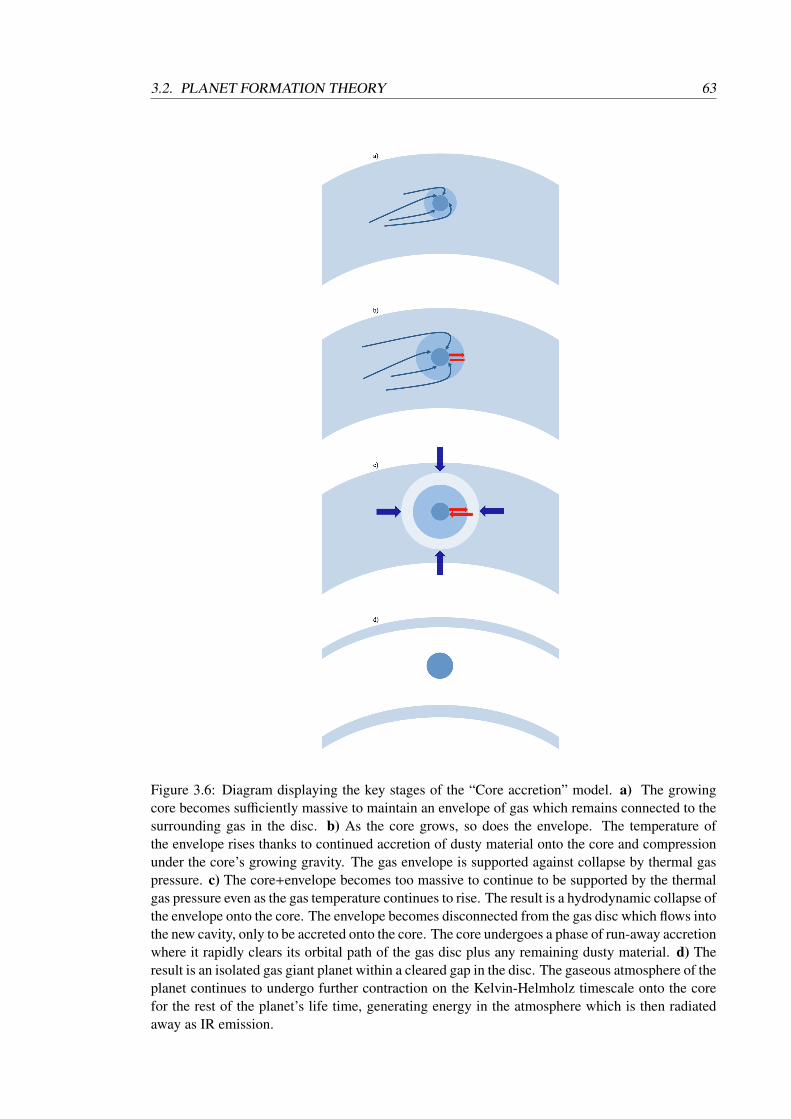
3.2. PLANET FORMATION THEORY 63
Figure 3.6: Diagram displaying the key stages of the “Core accretion” model. a) The growingcore becomes sufficiently massive to maintain an envelope of gas which remains connected to thesurrounding gas in the disc. b) As the core grows, so does the envelope. The temperature ofthe envelope rises thanks to continued accretion of dusty material onto the core and compressionunder the core’s growing gravity. The gas envelope is supported against collapse by thermal gaspressure. c) The core+envelope becomes too massive to continue to be supported by the thermalgas pressure even as the gas temperature continues to rise. The result is a hydrodynamic collapse ofthe envelope onto the core. The envelope becomes disconnected from the gas disc which flows intothe new cavity, only to be accreted onto the core. The core undergoes a phase of run-away accretionwhere it rapidly clears its orbital path of the gas disc plus any remaining dusty material. d) Theresult is an isolated gas giant planet within a cleared gap in the disc. The gaseous atmosphere of theplanet continues to undergo further contraction on the Kelvin-Helmholz timescale onto the corefor the rest of the planet’s life time, generating energy in the atmosphere which is then radiatedaway as IR emission.
3.3. CIRCUMPLANETARY DISCS 64
peared in the work of Pollack et al. (1996) after a long period of development. The basic idea
of this model is that after the formation of a massive, solid core with little to no atmosphere (the
shallow gravitational potential being insufficient to hold onto a significant amount of volatile gas)
in the presence of a substantial gas disc, it becomes massive enough to maintain a significant en-
velope onto which further gas accretion can occur. In its earliest stages this envelope is able to
support itself in a state of hydrostatic equilibrium with the gas pressure sufficient to resist col-
lapse under the core’s and the envelope’s combined gravity. At this stage the dominant driver for
luminosity of the protoplanet is the continued accretion of smaller bodies onto the core. Shocks
generated by in-falling material heats the surrounding gas envelope, increasing the gas pressure
and providing further support against collapse. Eventually however, the core and surrounding en-
velope become too massive for the thermal gas pressure to support against collapse. The envelope
begins to contract onto the core on its own Kelvin-Helmholtz time scale and continues to do so for
the rest of the planet’s lifetime. The rate of collapse and further gas accretion is then determined
by the rate at which the gravitational energy released by this collapse can be radiated away. This
triggers a phase of run-away growth as gas accretion can occur unrestricted onto the planet (see
Figure 3.6).
A number of models both numerical and analytical, have been produced to estimate what
this critical mass under which the collapse occurs may be such as in Mizuno (1980) and Papaloizou
& Terquem (1999). These studies show only weak dependencies to the local gas disc properties.
Sophisticated models which include more considered approaches to the thermodynamic properties
of the gas envelope such as convection produce values for this critical mass varying significantly
with distance to the central star (Rafikov 2006). Within an au, core masses of 5-20 M⊕ are required,
far too large for the in-situ formation of the hot Jupiter population observed with Kepler (Howard
et al. 2012). Forming a planet a few au from the central star in the gas giant mass range necessitates
core masses of 20-60 M⊕, placing a strong constraint on the timescale for planetary core formation
at these radii before the dissipation of the gas disc.
Values are highly dependent on the gas opacity however, and important effects such as core
migration in the disc are neglected. These introduced significant uncertainties into the critical mass
calculations. Models using lower opacities for the gas envelope find potential formation timescales
for Jovian planets as short as 1 Myr onto cores as small as 5 M⊕ (Hubickyj et al. 2005; Movshovitz
et al. 2010). Including radial drift of the cores has also been show to substantially influence the
critical mass (Papaloizou & Terquem 1999; Alibert et al. 2005) as the supply of material, both
gaseous and solid, is never exhausted until the disc is dispersed, preventing isolation.
In any case, once triggered the run-away growth of the giant planet is not halted until either
the planet is massive enough to carve a gap in the disc and isolate itself form the gas disc, or the
gas disc itself is dispersed as the circumstellar disc is disconnected from the natal cloud.
3.3 Circumplanetary discs
Within the Solar System there is obvious evidence for the existence of circumplanetary discs.
The regular moon systems of the giant planets and the prominent rings of small ice particles

3.3. CIRCUMPLANETARY DISCS 65
around Saturn and Uranus shepherded by their moon systems are possible remnants of primeval
circumplanetary discs and much of their properties seems to appear similar to those of planetary
systems formed from circumstellar discs. Caution should be exercised however when attempting
to apply scaling arguments between the two classes of discs as there are a number of fundamental
differences (Lissauer & Cuzzi 1985).
When the formation of such moon systems occurs is unclear, with a number of possible
mechanisms suggested. ’Satellitesimals’ could form from the amalgamation of dust in the cir-
cumplanetary disc in via comparable mechanisms to those involved in the formation of to plan-
etesimals in the circumstellar disc. Debris caused by the impacts between giant planets could
accumulate around the most massive planets, producing a wide distribution of particle sizes. Al-
ternatively planetesimals could have been captured from the wider circumstellar disc (Stevenson
et al. 1986; Coradini et al. 1989; Korycansky et al. 1991; Pollack et al. 1991). Each mechanism
predicts different distributions in the orbital properties of resultant moon and ring systems as well
as their mass distributions so could be potentially distinguishable from one another if observations
of exo-moon systems become sufficiently sophisticated. A different approach would be to detect
the circumplanetary disc in-situ around YSOs through high resolution imaging.
Some information can be obtained from the moon and ring systems present in the Solar Sys-
tem. The Jovian moons display a marked drop in density with distance from Jupiter, suggestive of
a radially decreasing temperature gradient in the early circum-jovian disc (Morrison & Cruikshank
1974). It is noted however than this distribution is dominated by the Galilean moons, of which the
innermost, Io and Europa are volcanically driven by their tidal interactions with Jupiter. Volatile
components may have therefore been lost early in their lives producing the observed enhanced
density compared to the outer moons. The moons of Saturn and Uranus are not found to display
any systematic trend with distance from their parent planet (Smith et al. 1982; Dermott & Thomas
1988; Campbell & Anderson 1989; Jacobson et al. 1992).
Ayliffe & Bate (2012) performed hydrodynamic simulations of the collapse of a gas enve-
lope onto a planetary core, and observed the formation of a circumplanetary disc. The gas density
around the core increases by more than an order of magnitude while the outer regions of the gas
envelope forms the initial circumplanetary disc. This process occurs over 100’s of orbits, during
which time the planet clears its orbital path of material. Further material enters the Hill sphere of
the planet through spiral arms generated by the planet’s distorting effect on the disc and through
radial drift of material into the gap. The majority of accreting material enters the disc from high
latitudes, while an outflow develops of material in the mid-plane of the protoplanetary disc disc
(Ayliffe & Bate 2012). This is in agreement with previous work studying gas accretion onto a
circumplanetary disc, where the outflowing material escapes from the planet’s Hill sphere through
the L1 and L2 Lagrange points back into the protoplanetary disc (Machida et al. 2008; Tanigawa
et al. 2012).
These simulations employ core radii values an order of magnitude larger or more than
expected from theory and observation due to resolution limitations. Hence, little information exists
to how far the planetary atmosphere extends and how close the inner edge of the circumplanetary
disc is to the outer edge of the atmosphere. The position of the the inner edge of the disc has a

3.3. CIRCUMPLANETARY DISCS 66
Figure 3.7: Schematic of the potential structure of a circumplanetary disc based on numericalsimulations carried out by Zhu et al. (2016). Material is fed onto and from the disc via two streamsof material from the outer disc and to the inner disc. This stream of material acts as a mechanismfor material to continue to cross the otherwise cleared gap, and also for maintaining the surfacedensity of the circumplanetary disc. This enables the central star to continue to accrete materialfrom the disc even in the presence of an otherwise extended cavity. Tidal interactions between thecentral star and the planet confines the disc to the Hill sphere and excites two spiral arms in thedisc. These spiral arms could potentially act as efficient carriers of angular momentum away fromthe planet preventing decretion.
3.4. PLANET-DISC DYNAMICAL INTERACTION 67
significant impact on the resultant NIR flux expected from the circumplanetary disc. Additional
unknowns include to what extent the magnetic field of the protoplanet may influence the structure
of the disc, and how that may affect accretion onto the planet.
Furthermore tidal interactions with the central star are likely to excite two spiral arm struc-
tures in the surface density of the disc leading to effective angular momentum transport through the
disc and episodic accretion onto the protoplanet (Zhu et al. 2016). See Figure 3.7 for a schematic
drawing of the structure of a circumplanetary disc based on such simulations.
Numerical simulation work has shown that actively accreting circumplanetary discs will
likely be many orders of magnitude brighter than their parent protoplanet (Zhu 2015). The ex-
tended nature of the disc in combination with the high temeperature generated by accretion onto
the disc drive this luminosity and will be the dominant source of emission for most companions
below ∼10 MJ.
3.4 Planet-disc dynamical interaction
As previously mentioned in Section 2.4.8, once a planetary core has formed and become mas-
sive enough to generate a significant gravitational field, it once again becomes coupled to the gas
disc, and even other growing planets, and begins to have its orbital dynamics substantially al-
tered. These interactions with the gas disc lead to considerable evolution in the final make up and
configuration of the planetary system as a whole.
The interaction with resonances exerts a torque on both the perturbing planet and the parti-
cle at the resonance. The low mass of the asteroid belt compared to the mass of Jupiter means the
change in angular momentum is negligible. Within a protoplanetary disc where the disc mass is
larger or comparable to the mass of a protoplanet, the torques exerted by the resonances can lead to
a considerable change in the angular momentum of the protoplanet resulting in migration through
the disc. The direction of the migration is determined by the strength of torques generated at res-
onances located inwards and outwards of the planet in the disc. Resonances inwards of the planet
increase the angular momentum of the protoplanet while resonances outwards generate torques
which decrease the angular momentum of the protoplanet. This results in migration outwards and
inwards respectively. If the torques are balanced, no net angular momentum transfer occurs and
the protoplanet does not migrate.
Calculating the net torque on a planet is highly technical and requires further treatment than
can be given here. For more details, see the reviews by Kley & Nelson (2012) and Baruteau et al.
(2014). Here the key results are given with their implications under the broad definition of Type-I
and Type-II migration schemes which are thought to dominate while a substantial gas disc still
exists:
Type-I migration
The two planetary migration regimes are broadly separated by the mass of the migrating planet.
For a reasonably low mass planet (Mp ∼ M⊕), any depletion of gas occurs at a substantially lower
rate than viscous evolution and radial gas drift within the disc. The surface density therefore

3.4. PLANET-DISC DYNAMICAL INTERACTION 68
remains approximately unchanged as the planet migrates. The net torque can then be calculated
through summing over all torques acting on the planet such that:
Tp = Tcorot +∑
Tinner +∑
Touter, (3.16)
where the planet loses angular momentum to torques generated in the outer disc, Touter, and gains
angular momentum from torques generated in the inner disc, Tinner. The corotational torque, Tcorot,
potential plays a contributing role as well. This regime is described as Type-I migration (Ward
1997).
If the gas disc truly orbits with a Keplerian velocity, one might expect the summations to
cancel and the net torque to be determined by the co-rotational torque. In practice however, the
pressure gradient in the disc causes the gas disc to orbit with a sub-Keplerian velocity, and hence
the inner torques are weaker than the outer torques such that inwards migration is the overwhelm-
ing norm for a protoplanet in the disc. Unless halted by interaction by a second protoplanet, as
in the Grand Tack model for explaining the growth and eventual orbital positions of Jupiter and
Saturn (Walsh et al. 2011), the inwards migration should result in the destruction of most proto-
planets. The problem is particularly accute when attempting to explain the origin of the population
of “Hot Jupiters”.
The strength of the torques is given by:
T (m) ∝ ΣM2p fc(ξ), (3.17)
where Σ is the surface density nominally dominated by the gas surface density, Mp is the planet
mass, and fc(ξ) is the torque cutoff function introduced to account for how the torques closer to
the planet contribute little to net torque (Artymowicz 1993). This term peaks at the radial location
where the r ≈ r ± h, where h is the scale height of the disc.
From the dependency to the square of the planet mass, one can estimate the migration
timescale:
τ ∝Mp
Tp∝ M−1
p . (3.18)
The timescale for Type-1 migration is therefore shortest for more massive planets until they be-
come large enough to begin to clear gaps at the resonances.
Following a full three dimensional treatment to account for dependence on the disc scale
height in the torque cutoff function, Tanaka et al. (2002) calculated that a 5 M⊕ planetary core
forming at 5 au in an isothermal disc with nominal parameters would accrete onto the central star
on a timescale of around 0.5 Myr, much shorter than the expected lifetime of the disc.
Type-II migration
Type-I migration ends once the migrating planet becomes massive enough to repel material away
from the resonances faster than radial drift and viscous evolution of the disc can replace it (Goldre-
ich & Tremaine 1980; Lin & Papaloizou 1980; Papaloizou & Lin 1984). Here gaps open up and
angular momentum transfer stops. This can be understood intuitively from Equation 3.17 when
3.4. PLANET-DISC DYNAMICAL INTERACTION 69
inserting a value of Σ of 0.
The second condition for the formation of a gap is that the volume in which the planet’s
gravity dominates and from which the protoplanet feeds (the Hill sphere or Roche radius) must be
comparable in size with the thickness of the disc:
rH =
(Mp
3M∗
)1/3
r & h, (3.19)
which necessitates a mass fraction, q = Mp/M∗:
q & 3(hr
)3
. (3.20)
For typical disc parameters, this inequality is satisfied for q values on the order of 5× 10⁻⁴, which
is similar to the mass fraction of Saturn to the Sun.
Once the gas has been cleared from the gap, the orbital evolution of the planet is no longer
dominated by Lindblad torques, but instead by its coupling to the viscous evolution of the gas. At
larger radii the bulk drift of the gas can be outward (Veras & Armitage 2004) but at smaller radii
the gas drift is invariably towards the central star. If the planet enforces a strict tidal barrier at the
outer edge of its Hill sphere, then the evolution of the disc inwards at shorter radii will drive the
planet inwards, on the condition that the local disc mass is comparable to the planet mass. This
implies that Type-II migration can occur in young discs where there is still a significant amount of
material in the disc. Under this regime migration timescales are similar to those under the Type-I
regime, resulting in rapid inward migration.
In older, depleted discs this condition no longer holds and the migration inwards slows and
the planet becomes a barrier to gas flow inwards from larger radii producing a ring of over dense
material and a pressure bump which halts inward radial drift of small dust particles. While this
pile-up would increase the torque acting on the planet, it also transfers angular momentum into the
disc, causing it to spread outwards, slowing the planet’s inward migration. Additionally the planet
does not act as a perfect barrier with most simulations showing that even gap-clearing planets
continue to accrete substantial amounts of material through streams of material linking the outer
and inner portions of the disc (Lubow et al. 1999). This decouples the orbital evolution of the
planet from the viscous evolution of the gas disc.
The effect of both migration regimes is to drive forming planetary companions inwards
and closer to their parent stars during the period in their lives where they are at their brightest.
We would therefore expect that to observe such objects would require high angular resolution
techniques. In addition, the build up of material external to an inwardly migrating protoplanet to
be an ideal site for further planet formation, perhaps even vulnerable to gravitational instabilities.
Both give us clues to where to search for on-going planet formation.

3.5. PLANET-PLANET DYNAMICAL INTERACTION 70
Figure 3.8: Figure showing the “forbidden zones” (red region) derived in the circular restricted3-body problem containing a very massive star, less massive planet, and test particle of negligiblemass. Any particle within the forbidden zone will be rapidly ejected. This defines three regionswhere a particle can exist in a stable state; orbiting around the star within the planet’s orbit, inorbit close to the planet, orbiting around the centre of mass of the planet-star system.
3.5 Planet-planet dynamical interaction
While a substantial gas disc remains, the effect of gas drag suppresses eccentricity in the orbits
of protoplanets in the disc. Once this disc has been cleared, unstable planetary configurations
may begin to interact leading to the population of eccentric orbits observed (Rasio & Ford 1996;
Weidenschilling & Marzari 1996; Lin & Ida 1997). This can also trigger a final phase of planetary
migration important in determining the eventual characteristics of a planetary system.
The general problem of a N-body interactions in orbital mechanics is well known to be un-
solvable analytically for a system containing more than two masses. One can consider a simplified
but useful treatment of the three-body problem, often called the circular restricted 3-body prob-
lem, where the motion of a “test particle” of negligible mass is considered in relation to two larger
masses, where the smaller of the two is taken to be in a perfectly circular orbit around the larger
(Murray & Dermott 1999). An analytical solution is still impossible but a set of zero-velocity sur-
faces can be derived which describe the bulk motion of small particles in the vicinity of a larger
mass in a planetary system, i.e. asteroids interacting with planets, particularly Jupiter, in the Solar
System and planetesimals close to a protoplanet. If a particle exists initially within a finite volume
bounded by a zero-velocity surface then it will be trapped and unable to leave.
The topology of the zero-velocity surfaces are shown in Figure 3.8. In the case of a planet
orbiting a far more massive star, the zero-velocity surfaces create three separate zones. One cor-
responds to close orbits around the planet where its gravity dominates over the star’s gravity. A
second zone exists closer to the star than the planet, defining orbits around only the star due to the
star’s gravity dominating over the planet’s. The final zone, corresponds to orbits external to the
position of the planet around a combined centre of gravity of the planet-star system.

3.5. PLANET-PLANET DYNAMICAL INTERACTION 71
Figure 3.9: Figure displaying the set-up for examining stability in a two planet system. The twoplanets are assumed to be in circular orbits.
The case of planet-planet scattering however requires the test particle in the case above to
no longer be negligible in mass. The simplified case is still applicable in a modified state however.
Determining if a planetary system is stable can be done using the setup shown in Figure 3.9, where
if any combination of two planets in a N-planet system are in an unstable configuration the whole
system can be treated as unstable. One can consider two planets with respective masses, m2 and
m3, around a star of mass, m1, on perfectly circular orbits from the star, a2 and a3. Intuitively, one
would expect the stability of the two planet system to depend on the separation of two planets, ∆,
a3 = a2(1 + ∆). (3.21)
∆ is a dimensionless quantity defining the separation between the two orbital radii. Further one
can define the dimensionless mass fraction for each of the planets compared to the central star as
µ2 = m2/m1 and µ3 = m3/m1. Gladman (1993) showed that for values of µ2 and µ3 1 that
the system will be stable under the condition that the value of ∆ is larger than a critical separation,
∆c expressed as,
∆c ≈ 2.4(µ2 + µ3)1/3. (3.22)
It is important to note however that fulfilling this criteria only guarantees stability, separations
smaller than ∆c do not imply instability as there exist configurations which can exist for long
periods of time (> 105 years). This prescription works well for two planet systems but there are
no known absolute stability limits for more complex systems containing N > 3 (Chambers et al.
1996).
The interaction of two planets in unstable configurations typically results in one of four
outcomes (Ford et al. 2001). The separations and eccentricities of the two planets increases until
the system reaches a stable configuration, as likely occurred in the case of Jupiter and Saturn
(Walsh et al. 2011). One of the two planets is ejected from the system in a close interaction
3.6. PROTOPLANETS 72
between the pair. The remaining planet typically has a non-zero eccentricity. If the evolution
of the orbital parameters leads to crossing orbits, then the planets may collide. The new body
typically has a low eccentricity. Such a collision is thought to have occurred early in the life of
the Earth (Canup 2004). Finally, one planet may develop an orbit eccentric enough to lead to a
collision with the central star or move into a close enough orbit for tidal interactions with the star
to become important.
Comprehensive studies using N-body simulations of planetary systems containing three
or more planets have resulted in eccentricity distributions closely matching those observed by
exoplanetary missions (Chatterjee et al. 2008; Juric & Tremaine 2008; Raymond et al. 2008). This
indicates that most if not all exoplanet systems undergo a phase of planet-planet scattering which
determines the eventual orbital parameters of the system.
3.6 Protoplanets
Current observations of planetary mass companions within protoplanetary discs are limited in
number compared to fully formed, older exoplanetary systems, and it is presently unclear how
protoplanets accrete to reach their final masses (see Section 3.3). Theoretical work however sug-
gests complex circumplanetary disc structures which could be substantially brighter in the infrared
than their parent protoplanets. Modelling the circumplanetary disc however could be even more
challenging than in the circumstellar case due to the way material enters the circumplanetary disc
system. In-falling circumstellar disc material can impact onto the circumplanetary disc from high
altitudes (Tanigawa et al. 2012; Szulagyi et al. 2014), the material can carry little to no angular
momentum into the circumplanetary disc (Canup & Ward 2002), the rate of in-fall can be variable
and episodic (Gressel et al. 2013), MRIs can develop within ionised regions of the circumplan-
etary disc (Fujii et al. 2011, 2014), magnetocentrifugal winds can develop and be influential on
the surface of circumplanetary discs (Gressel et al. 2013), Hall MHD can dominate in the disc
mid-plane (Keith & Wardle 2014), and emission from the disc could undergo outbursts (Lubow &
Martin 2012).
3.6.1 Observational properties
Determining which effects are most important for determining the late stage growth of a proto-
planet requires knowledge only obtainable through observation. The current capabilities of mod-
ern telescopes, both single aperture and in interferometric array, are not sufficient to resolve and
distinguish between these scenarios although there are plans to construct such instruments in the
future (Monnier et al. 2014; Kraus et al. 2014; Ireland & Monnier 2014). Some early work how-
ever can be performed through modelling the SEDs of such objects as they become available.
This mirrors the early work performed on circumstellar discs in determining their structure and
geometry before interferometric arrays allowed for resolved observations.
Current observations are sparse and the spectroscopic information broadband with large
uncertainties (see Section 3.6.2) hence lack the resolution to differentiate between more sophis-
ticated or nuanced models. First attempts to model circumplanetary discs, in work such as Zhu

3.6. PROTOPLANETS 73
(2015), where the disc is assumed to be heated principally through the viscous heating generated
by accretion (i.e. where the planet’s irradience of the disc is negligible compared to the accretion
luminosity) have shown however that a number of properties can be retrieved from limited infor-
mation such as this. These are firstly, and perhaps most importantly, the ability to differentiate
a circumplanetary disc from a Brown Dwarf or other sub-stellar companion through an infrared
excess in the SEDs into L-band and beyond compared to pure young planetary atmospheric mod-
els. Under the assumption of a flat, optically thin disc, information regarding the accretion rate
onto the disc could be determined from the absolute magnitude in the infrared without the need
to know anything about the protoplanetary atmosphere and its emissive qualities. The only pa-
rameters required to characterise the SED of an optically thick, steady accretion disc are simply
the product of the protoplanet’s mass and the disc accretion rate (MpM, hence MM) and the inner
radius of the circumplanetary disc (Rin). This enables one to begin to investigate a circumplanetary
disc, but must be caveated by acknowledging that these models only apply in the cases of a low
mass protoplanets (∼1MJ) with significant accretion (M ≥ 10−10Myr−1). Slower accreting large
protoplanets require a more complex model where the planet’s irradience of the disc must also be
considered.
3.6.2 Previous protoplanet observations
The number of previously observed protoplanetary companions is small in comparison to the
number of known exoplanetary systems. The most successful techniques for the detection of
exoplanets rely on surveys of large numbers of stars and chance alignments of orbital planes.
This is problematic for the application of these techniques to protoplanet detection campaigns.
The number of transitional discs observable form the Earth is limited to a small number of star
forming regions, while the extended, optically thick circumstellar disc prevents transit detections
and limits the sensitivity of radial velocity measurements. Protoplanet detections are therefore
limited to high resolution imaging campaigns. These are time consuming to perform on a sizable
number of stars and suffer from the traditional problems of imaging a faint object close in angular
separation to a much brighter object. A selection of the candidates so far reported are summerised
below.
CoKu Tau 4
CoKu Tau 4 is a transitional disc located within the Taurus star forming region, and young for a
gapped disc (145 pc, 1-2 Myr; Cohen & Kuhi 1979). Observations by the Spitzer Space Telescope
found strong MIR excesses but little to no excess at wavelengths <8µm (Forrest et al. 2004).
Subsequent modelling of the SED by D’Alessio et al. (2005) found that a cavity stretching to
∼ 10 au with little to no dusty material interior to the disc rim. They also noted the similarities
between the MIR spectrum of CoKu Tau 4 and the older disc, TW Hya. Unlike TW Hya however,
CoKu Tau 4 is a weak-line TTS, displaying little to no accretion or NIR flux from the innermost
regions of its disc. The authors posited this could be due to planet formation occurring on a more
rapid timescale than typically found and that giant planets may already be present in orbit.
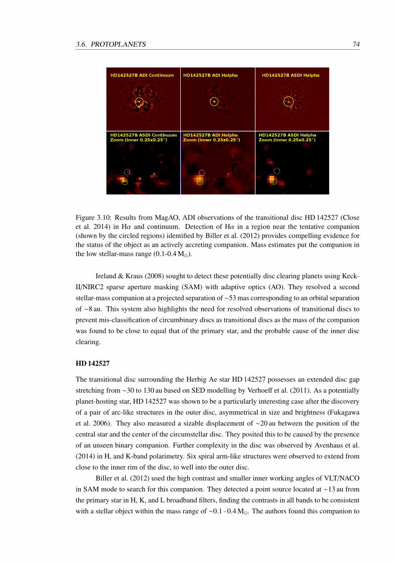
3.6. PROTOPLANETS 74
Figure 3.10: Results from MagAO, ADI observations of the transitional disc HD 142527 (Closeet al. 2014) in Hα and continuum. Detection of Hα in a region near the tentative companion(shown by the circled regions) identified by Biller et al. (2012) provides compelling evidence forthe status of the object as an actively accreting companion. Mass estimates put the companion inthe low stellar-mass range (0.1-0.4 M).
Ireland & Kraus (2008) sought to detect these potentially disc clearing planets using Keck-
II/NIRC2 sparse aperture masking (SAM) with adaptive optics (AO). They resolved a second
stellar-mass companion at a projected separation of ∼53 mas corresponding to an orbital separation
of ∼8 au. This system also highlights the need for resolved observations of transitional discs to
prevent mis-classification of circumbinary discs as transitional discs as the mass of the companion
was found to be close to equal that of the primary star, and the probable cause of the inner disc
clearing.
HD 142527
The transitional disc surrounding the Herbig Ae star HD 142527 possesses an extended disc gap
stretching from ∼30 to 130 au based on SED modelling by Verhoeff et al. (2011). As a potentially
planet-hosting star, HD 142527 was shown to be a particularly interesting case after the discovery
of a pair of arc-like structures in the outer disc, asymmetrical in size and brightness (Fukagawa
et al. 2006). They also measured a sizable displacement of ∼20 au between the position of the
central star and the center of the circumstellar disc. They posited this to be caused by the presence
of an unseen binary companion. Further complexity in the disc was observed by Avenhaus et al.
(2014) in H, and K-band polarimetry. Six spiral arm-like structures were observed to extend from
close to the inner rim of the disc, to well into the outer disc.
Biller et al. (2012) used the high contrast and smaller inner working angles of VLT/NACO
in SAM mode to search for this companion. They detected a point source located at ∼13 au from
the primary star in H, K, and L broadband filters, finding the contrasts in all bands to be consistent
with a stellar object within the mass range of ∼0.1 - 0.4 M. The authors found this companion to

3.6. PROTOPLANETS 75
be the likely source of the offset between the primary star and the center of the circumstellar disc
seen in Fukagawa et al. (2006). The wide radial extent of the inner cavity is not explained by the
presence of the secondary however, and so the existence of a further giant planet maybe necessary
to explain the enhanced clearing.
The enhanced L-band emission from the disc rim in comparison to the expected flux is
also discussed potentially as a result of either additional heating from the secondary, or through a
separate circumstellar disc surrounding the secondary. Some evidence is provided for the later in
MagAO observations carried about by Close et al. (2014) in Hα and continuum. The secondary
was recovered in both Hα and continuum, confirming the presence of the secondary (see Fig-
ure 3.10). From the equivalent width an accretion rate of 5.9 × 10⁻¹⁰Myr−1, assuming a mass of
0.25 M for the companion. An estimated accretion rate for a stellar companion was made at from
the equivalent Hα line width, indicating on-going accretion and hence the probable presence of an
accretion disc.
HD 100546
HD 100546 has long been studied as a possible location of on-going planet formation. Only
97±4 pc from the Earth (van Leeuwen 2007) and ∼3-10 Myr old (van den Ancker et al. 1997;
Manoj et al. 2006), it is both a reasonably close disc and a rather evolved disc in the final stages
of its life. SED modelling found little NIR emission, indicative of a tenuous inner disc, but a sub-
stantial outer disc emitting strongly in the MIR and at longer wavelengths. Fitting disc models to
the SED found an optically thick inner disc with a small radial extent within a few au of the central
star, separate from a more substantial and extended outer disc starting at ∼10 au (Bouwman et al.
2003). From sub-mm observations the disc mass was estimated to be 5× 10⁻⁴ M (Henning et al.
1998).
Studying the properties of the gas disc emission via high-resolution NIR spectroscopy of
CO and OH emission, Brittain et al. (2014), found the OH emission line shape to be asymmetric
and invariable with time, indicative of gas in an eccentric orbit close to the disc wall at approxi-
mately 13 au. In contrast, the CO emission was found to be variable in time and consistent with
the orbital motion of a companion. They additionally noted, that if the CO is optically thick, a
circumplanetary disc would produce a similar emitting area as that derived for the CO source. In
conjunction with earlier work (Liskowsky et al. 2012; Brittain et al. 2013) they concluded that
their work represented indirect evidence for the presence of a planetary companion responsible
for clearing the observed gap.
High contrast SAM observations of HD 100546 in L’-band with VLT/NACO were pre-
sented by Quanz et al. (2013a) and showed for the first time a clear indication of a compan-
ion within the disc. They detected a strong asymmetric signal consistent with a companion,
HD 100546 b, at 68±10 au from the central star, apparently embedded in the circumstellar disc.
They ruled out alternative sources for the L-band emission as a result of a local disc feature and
reason that the most likely scenario is a forming planet undergoing runaway accretion. Currie et al.
(2014) reobserved this L-band emission from HD 100546 b with Gemini/NICI, plus a previously
unseen disc feature resembling a spiral arm within the disc which they argue may be indirect evi-
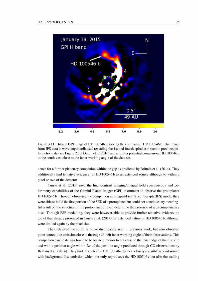
3.6. PROTOPLANETS 76
Figure 3.11: H-band GPI image of HD 100546 resolving the companion, HD 100546 b. The imagefrom IFS data is wavelength collapsed revealing the 1st and fourth spiral arm seen in previous po-larmetric data (see Figure 2.10; Garufi et al. 2016) and a further potential companion, HD 100546 cto the south-east close to the inner working angle of the data set.
dence for a further planetary companion within the gap as predicted by Brittain et al. (2014). They
additionally find tentative evidence for HD 100546 b as an extended source although to within a
pixel or two of the detector
Currie et al. (2015) used the high-contrast imaging/integral field spectroscopy and po-
larimetry capabilities of the Gemini Planet Imager (GPI) instrument to observe the protoplanet
HD 100546 b. Through observing the companion in Integral-Field Spectrograph (IFS) mode, they
were able to build the first portion of the SED of a protoplanet but could not conclude any meaning-
ful result on the structure of the protoplanet or even determine the presence of a circumplanetary
disc. Through PSF modelling, they were however able to provide further tentative evidence on
top of that already presented in Currie et al. (2014) for extended nature of HD 100546 b, although
were limited again by the pixel size.
They retrieved the spiral arm-like disc feature seen in previous work, but also observed
point source-like emission close to the edge of their inner working angle of their observations. This
companion candidate was found to be located interior to but close to the inner edge of the disc rim
and with a position angle within 2σ of the position angle predicted through CO observations by
Brittain et al. (2014). They find this potential HD 100546 c to most closely resemble a point source
with background disc emission which not only reproduces the HD 100546 c but also the trailing

3.6. PROTOPLANETS 77
structure previously interpreted to be perhaps a spiral arm. From the brightness of HD 100546 c
and comparison to models of newly formed planets (Baraffe et al. 2003; Spiegel & Burrows 2012),
they estimate a mass of between 10-20 MJ
HD 169142
HD 169142 is known to be a young disc-hosting Herbig Ae star. The circumstellar disc is com-
prised of three main components. Firstly a small, hot inner disc less than an au in extent from
the central star followed by an extended cavity to a second ring (∼25-40 au) observable in NIR
polarised and 9 mm emission (Quanz et al. 2013b; Osorio et al. 2014). A further gap extending
from 40 to 70 au separates the second ring from the cold outer disc. Further complexity is added
to the disc by the pronounced asymmetry of the ring in 7 mm emission. Osorio et al. (2014) pro-
posed this sub-structure to the ring as possibly the result of the presence of at least one companion
with further evidence for the presence of companions coming from the three annuli structure of
the disc.
Reggiani et al. (2014) observed HD 169142 in J and L’ wavebands utilising the high contrast
imaging capabilities of GPI and the VLT/NCO annular groove phase mask (AGPM) vector vortex
coronograph (Mawet et al. 2013). They observed a point source in L’-band at an angular separation
corresponding to an orbital distance of ∼23 au, immediately inside the rim of the second dusty
ring. From its observed L’-band magnitude of 12 mag and non-detection in J (> 14 mag), they
imply a companion mass in the range 28-32 MJ under the assumption that all emission from the
companion comes from a photosphere with no significant contribution from a circumplanetary
disc. They also note however that the low, but still substantial continued accretion onto the central
star (∼ 10−9 M yr−1; Grady et al. 2007) would imply that a companion located in the gap would
likely still be accreting. Therefore some of the emission would be due to accretion, hence implying
a lower companion mass. They also note a less massive companion would be more consistent for
the observed width and depth of the gap the companion lies in.
The presence of an asymmetry in L-band was also independently observed by Biller et al.
(2014). They used a similar observational setup as Reggiani et al. (2014), wherein they observed
in L’-band with the VLT/NCO AGPM vector vortex coronograph but replaced J-band GPI ob-
servations with H, Ks and 3.9µm observations with MagAO. While they close to simultaneously
observed the L’band asymmetry, they did not detect the potential companion in H or Ks, and their
3.9 µm observations were too shallow to retrieve the object. Their non-detections in the NIR rule
out the structure as being the result of emission from a sub-stellar object’s photosphere down to
masses in the ∼715 MJ range. They instead explored the possibility that the structure is the result
of a disc asymmetry. Performing radiative transfer modelling they find that a passively heated
clump of dust could not reach the necessary temperatures to be emitting as brightly in L-band as
the detected source. They instead tentatively suggest the source to be a locally heated portion of
the disc by an as yet unknown mechanism.
Further complicating matters, Momose et al. (2015) observed HD 169142 with the Sub-
aru/HiCIAO in H-band polarized light with a coronograph and observed a strong drop in polarized
image. The location of the minimum corresponded with the location of the proposed protoplanet

3.6. PROTOPLANETS 78
seen in the 7 mm data.
Recent GPI and MagAO observations presented by Follette et al. (2017) and Rameau et al.
(2017) provide more information on the system, but still offer no conclusive result.
Follette et al. (2017) observed HD 100546 in optical and near-infrared using the MagAO
and GPI instruments to form images in polarized and total light. To achieve higher sensitivi-
ties than in previous observation, the GPI data sets were processed with a variety of differential
imaging techniques, including polarimetry, differential angular imaging. They then attempted to
identify structures which remained consistent across the majority of employed processing tech-
niques. While the retrieval of the numerous spiral arm-like structures seen in previous studies was
accomplished, consistently detecting point source-like emission from the propounded compan-
ion, HD 100546 c was not and frequently appeared as a smooth continuous structure with similar
emissive properties to a disc feature.
They propose the number of spiral arms to be consistent with a two-armed spiral disc where
the additional features are due to the wrapping of the spiral arms around the disc.
Rameau et al. (2017) observed in H-band and Hα, focussing their analysis on the puta-
tive companion, HD 100546 b. Similar to the analysis of HD 100546 c, the morphology of the
emission from HD 100546 b is variable across different processing techniques. The morphology
appears point source-like in more “aggressive” data reductions but becomes part of the extended
outer disc structure in the majority of the remaining data reductions. Additionally, across the ∼ 5
years of data presented, the point source-like emission appears stationary and inconsistent with
a Keplarian orbit with a semi-major axis of 59 au. Further the spectrum of the H-band emission
is not compatible with a low-mass planetary atmosphere model or accreting circumplanetary disc
model. The authors conclude that the most likely origin for the H-band flux is in scattered light.
The H-band spectra from the structure was found to be consistent with the spectra of HD 100546
itself, providing strong evidence in favour of this interpretation. Combined with the non-detection
of co-located Hα emission, the structure is not likely to be caused by emission from an accreting
protoplanet, although the possibility of a deeply embedded companion is not ruled out.
LkCa 15
One of the most famous companion candidate detections is that of LkCa 15 b. A young solar
analogue, LkCa 15 is less than 5 Myr old and located in the Taurus-Auriga star-forming region
(Kraus & Hillenbrand 2009). Detailed SED modelling has shown the circumstellar disc to possess
an extended cavity (Espaillat et al. 2007) where NIR emission comes from a hot dusty disc within
an au of the central star while strong MIR and FIR emission comes from cold dust in an extended
outer disc that extended radially beyond ∼50 au.
A first detection of a companion candidate in the disc cavity was presented by Kraus &
Ireland (2012). They used the SAM capability of the Keck-II/NIRC2 instrument to achieve the
smallest possible inner working angle to search for a companion close to the star, observing across
three epochs in K’ and L’ prime. They observed a relatively blue point source (MK′ ≈ 9, K’ -
L’≈ 1, hence LkCa 15 b) with apparently co-orbital, surrounding dusty material which were more
extended and resolvable into two distinct structures. They were also found to be substantially

3.7. CHAPTER SUMMARY 79
redder in colour. The deprojected separations of the structures were found to be 16, 21, and 19 au.
This placed all three structures well within the cavity but too far from the disc wall to be the likely
cause of its presence. From hot-start planetary atmosphere models, an upper estimate for the mass
of the bluer point-source was made at 6 MJ, although the authors noted that the continued accretion
onto LkCa 15 and presence of the surrounding dusty material was likely evidence for continued
accretion onto the companion, and hence the mass of the companion was likely to be lower than
in this simplistic case.
Sallum et al. (2015b) detected both the point source and the co-orbital dusty material again
(see Figure 3.12). They used the SAM mode on the Large Binocular Telescope with the Ks
and L’ broadband filters, and reacquired the two previously observed structures seen in Kraus
& Ireland (2012); consistent with LkCa 15 b and hence LkCa 15 c. Additionally, they observe a
faint third structure, but only in L-band (LkCa 15 d). The motion of LkCa 15 b and c are found to
be consistent with Keplerian orbital motion between the two epochs. Analysis of the orbits with
the requirement of stable orbits puts upper limits on the mass of the two companion, with masses
above 5 MJ not permitted. If in a 2:1 resonance, the mass of the companions could potentially
be as high as 10MJ although the H-K colour of the LkCa 15 b would rule out a companion this
massive based on hot-start planetary atmosphere models.
Strong evidence for the nature of LkCa 15 b as an accreting protoplanet was found through
the detection of Hα emission through observations carried out with MagAO, with the measured
equivalent line corresponding to an accretion rate of 3× 10⁶ M2J yr−1. LkCa 15 c was not detected
in Hα which the authors suggest could be a result of higher extinction along its line of sight or a
lower accretion rate below the detection limit.
3.7 Chapter summary
In this Chapter I introduced the various mechanisms proposed to allow µm-sized dust particles to
coagulate and grow into the varied population of planetary bodies we observe in the Solar System
and beyond along with their strengths and weaknesses. I detailed the core accretion model and
gravitational instability models but focused on the core accertion model as the currently favoured
and currently best supported model, wherein planetesimals form through a combination of coag-
ulation and streaming instabilities to then merge to form protoplanetary cores or embryos. If the
largest of these form rapidly enough to still be in the presence of a gas disc when they reach these
sizes they can attract and maintain a sizable gaseous envelope. This envelope remains linked to the
gas disc until the growth of the core leads to the protoplanet’s gravity becoming too large for the
gas pressure to prevent collapse onto the core. Once this occurs a period of rapid growth ensues in
which the planet carves out a gap in both the gas and dust disc. Such a gap may trap more dusty
material triggering further planet formation.
I discussed this gap opening in more detail, focusing on the effects on the orbital properties
of the gap-opening body. While the planet may clear its orbital path leaving it isolated and unable
to accrete more material. The formation of gaps at resonances inside and outside the planet’s
location in the disc leads to a period of rapid migration for a giant planet. Such migration is

3.7. CHAPTER SUMMARY 80
Figure 3.12: Left: VLA 7 mm observations of LkCa 15 presented by Isella et al. (2014, ;greyscale). Natural weighting of the complex visibilities was adopted to maximise resolution.The illuminated rim of the outer disc can clearly be seen along with the extended inner cavity. Thecoloured portion of the image shows the Hα, Ks, and L’ LBT and Magellan observations (in blue,green and red respectively) presented by Sallum et al. (2015b) shown in the right panel but at thesame scale as the VLA observations. Right: Zoomed in image of the coloured portion of the leftpanel. The claimed companion detections are labelled ’b’, ’c’, and ’d’. The companion candidate,LkCa 15 b, is consistent with the point source identified by Kraus & Ireland (2012) in a Keplerianorbit within the plane of the outer disc. Similarly, the point source, LkCa 15 c is consistent withthe extended structure observed by Kraus & Ireland (2012). The co-located Hα emission fromLkCa 15 b provides strong evidence for on-going accretion onto the companion.

3.7. CHAPTER SUMMARY 81
used to explain the population of Hot Jupiters seen in extrasolar planetary systems and also as a
potential triggering mechanism for further growth of the planet and triggering of planet formation.
Finally I discussed the expected observational properties indicating the presence of a planet
within a disc. These are discussed in both the context of direct and indirect detection methods such
as through their influence on their parent discs. Indirect measurements focus on the generation
of structure within the surrounding disc which can be resolved with modern interferometric and
polarmetric instruments. The direct detection methods are dominated by observations in the NIR
using high contrast imaging techniques at these wavelengths where the protoplanet is expected to
have the most favourable contrast ratio to the parent star. The emission from the protoplanet is
expected to be dominated by the circumplanetary accretion disc which can be as bright a sub-solar
mass star even with moderate accretion rates due to its extended size.

Chapter 4
High angular resolution imagingtechniques
4.1 Introduction
The wave-nature of light imposes an absolute limit to the angular resolution attainable with an
aperture of a given diameter as a result of Fraunhofer diffraction. The problem is compounded
within the turbulent atmosphere of our planet where motion in the intervening atmosphere distorts
the wave front of any incoming light. Even in the stillest of conditions on the summits of the best
mountain-top observatories, this turbulence imposes strong limits to the angular resolution of an
instrument operating in the optical wavelength regime. Many of the solutions to the great number
of questions still facing astronomers have their solution in the ever higher resolution imaging of
distant objects. To find these solutions we therefore must overcome or mitigate these limits.
The diffraction limited angular resolution in radians (θ) of a telescope (given that the optical
elements are perfect) is defined by the Rayleigh criterion:
θ = 1.22λ
D, (4.1)
where λ and D represent the central wavelength of the collected light and the diameter of the light
collecting primary aperture (see Figure 4.1). This relation is derived through the approximate
radius of the first null in the Airy function, the description of diffraction pattern produced by a
point source, or the point spread function, when imaged with a circular aperture. The obvious
solution is therefore to construct larger telescopes, with larger effective diameters. Our ability
to do so however is limited greatly by the cost of building parabolic or spherical mirrors 10s
of metres across along with the housings to protect them from the elements and machinery to
operate them, but also by the previously mentioned atmospheric turbulence. When observing
at 1 µm under perfect seeing conditions, atmospheric turbulence may limit angular resolution to
the sub-arcsecond regime (∼0.6 ”) which makes constructing a diffraction-limited telescope with
a diameter beyond ∼1 m a futile exercise. To study planet formation within the 10s of au of
the central star, or any sub-arcsecond resolution imaging, therefore necessitates the development
of a set of instruments or techniques to correct for the turbulent effects of the atmosphere. For
82
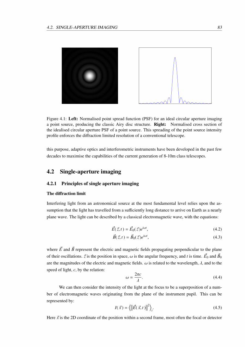
4.2. SINGLE-APERTURE IMAGING 83
Figure 4.1: Left: Normalised point spread function (PSF) for an ideal circular aperture imaginga point source, producing the classic Airy disc structure. Right: Normalised cross section ofthe idealised circular aperture PSF of a point source. This spreading of the point source intensityprofile enforces the diffraction limited resolution of a conventional telescope.
this purpose, adaptive optics and interferometric instruments have been developed in the past few
decades to maximise the capabilities of the current generation of 8-10m class telescopes.
4.2 Single-aperture imaging
4.2.1 Principles of single aperture imaging
The diffraction limit
Interfering light from an astronomical source at the most fundamental level relies upon the as-
sumption that the light has travelled from a sufficiently long distance to arrive on Earth as a nearly
plane wave. The light can be described by a classical electromagnetic wave, with the equations:
~E(~z, t ) = ~E0(~z )eiωt, (4.2)
~B(~z, t ) = ~B0(~z )eiωt, (4.3)
where ~E and ~B represent the electric and magnetic fields propagating perpendicular to the plane
of their oscillations. ~z is the position in space, ω is the angular frequency, and t is time. ~E0 and ~B0
are the magnitudes of the electric and magnetic fields. ω is related to the wavelength, λ, and to the
speed of light, c, by the relation:
ω =2πcλ. (4.4)
We can then consider the intensity of the light at the focus to be a superposition of a num-
ber of electromagnetic waves originating from the plane of the instrument pupil. This can be
represented by:
I( ~x ) =⟨∣∣∣∣∣∣~E( ~x, t )
∣∣∣∣∣∣2⟩t. (4.5)
Here ~x is the 2D coordinate of the position within a second frame, most often the focal or detector
4.2. SINGLE-APERTURE IMAGING 84
plane. In the case of a telescope bringing a light source to focus, this becomes:
I( ~x ) =
⟨∣∣∣∣∣∣∣∣∣∣∑i
~E( ~pi, t − τi )∣∣∣∣∣∣∣∣∣∣2⟩
t, (4.6)
where the index, t, represents the set of arbitrarily chosen points on the pupil plane of the instru-
ment, ~pi represents a set of points within the aperture plane and τi represents the delay in time for
waves travelling from different points to reach the focus.
If we consider the simplest case of a plane wave entering the front of the pupil (equivalent
to a distant point source) this expression can be integrated across the pupil instead, replacing the
sum in Equation 4.6. For a circular aperture the resultant pattern is an Airy disc as previously
mentioned in Section 4.1. For an aperture with a diameter, D, this can be expressed as:
I(r) =
(πD2
4
)2[ 2J1(πrD)πrD
]2
, (4.7)
where r represents the absolute magnitude of the 2D vector, ~x such that r = ||~x||. J1 is the 1st order
Bessel function (for a full derivation see: Born & Wolf 1999). The result is that, for example,
a pair of point sources imaged through an aperture will never appear as a pair of point sources.
Instead they will appear as the superposition of two point spread functions (PSFs), and the ability
to distinguish them apart is determined by the position of the first null of the PSF. This is the
source of the 1.22 factor in the Rayleigh Criterion (Equation 4.1). The spatial resolving power of
any given optical system is therefore determined by the diameter of the entrance pupil.
Atmospheric turbulence
Such a description ignores the practicalities of astronomy, particularly the distorting effects of
intervening material between the observer and the objects they wish to observe. For ground based
telescopes this material is the Earth’s turbulent atmosphere.
For example, the diffraction limit of the 8 m Unit Telescopes (UT) at the Very Large Tele-
scope (VLT) is 1.22λ/D = 0.066” when observing at λ = 2.2µm. The resolution is in practice
limited by the atmospheric turbulence which disrupts the planar shape of the incoming light. These
distortions induce small perturbations to the position of a point source which varies rapidly with
time in the optical. Over an exposure longer than the time scale of the turbulence, the new angular
resolution of the telescope is limited to λ/r0 ∼ 0.7”, where r0 is the Fried parameter, representing
the strength of the atmospheric turbulence. Without a strategy to get around the distorting effects
of the atmosphere, the construction of a telescope larger than D ≈1m provides no increase in
resolving power.
One method is to only take very short exposures over which time the atmosphere is frozen.
Over time scales smaller than this value, the atmosphere appears to be effectively still. Taking a
large number of images with short integrations might therefore result in a small number which
are only marginally effected by atmospheric turbulence (determined by their Strehl ratios) and one
might combine them together using a ”shift-and-add” approach. This is known as ”lucky imaging”
4.2. SINGLE-APERTURE IMAGING 85
(Mackay et al. 2004). For average seeing conditions, τ0 has a value typically of the order of ∼60 ms
when observing at 2.2 µm over which time the atmosphere can be considered static for the purposes
of lucky imaging. However, while larger telescopes provide improved light collecting capabilities,
photon counts will always be low for all but the brightest targets when limited to integrations under
100 ms, and as a result will be noisy as photon noises are ∝√
N, where N is the photon count.
Being limited to short integration times, the read noise of the detector is typically the dominant
and limiting noise source.
4.2.2 Adaptive optics imaging
An effective counter measure to the distorting effects of the atmosphere is to measure and correct
for the deformation of the wavefront (WF). The instruments which perform such a role on modern
telescopes are described as adaptive optics (AO). They consist of a wave front sensor (WFS) in
conjunction with a deformable mirror (DM). The WFS measures an incoming wavefront from a
point source-like reference star, passing the measurements to a real-time computer (RTC) which
calculates a correction which is applied to DM which the RTC controls. The DM is a thin plate
mirror the back of which is mounted on to a set of piezoelectric actuators which deform the mirror
into the desired shape to apply the correction to the incoming non-planar WF on timescales shorter
than the coherence time. A substantial reduction in the WF error can be achieved in this manner
allowing one to perform integrations of lengths of time much greater than the coherence time. The
new determining factor in how close an observation can get to the diffraction-limited resolution
will then be down to the accuracy of the AO correction and hence the quality of the resultant image
(see Figure 4.2).
For an AO system to be effective it must be able to ”close the loop”. This describes the
ability of the WFS and DM to measure and flatten the incoming WF, measure the residual er-
ror of the correction and reapply. If the atmospheric turbulence is too great, represented by a
short coherence time, then the AO fails and the loop opens, resulting in a dramatic drop in the
quality of the image. A good measure for this is the Strehl ratio (SR). The SR corresponds
to the amount of light contained with a region defined by the diffraction limit of the telescope
over the total amount of flux entering the optical system. An SR of 1.0 represents a perfect
instrument but in practice it is difficult to reach. What defines the difference between “Good”
and “Poor” SRs also differs between observing wavelengths where observing at shorter wave-
lengths typically produce smaller SRs, for example, a SR of ∼0.4 would be considered a “Bad”
AO correction when observing in H-band with the VLT/SPHERE instrument but the same SR
with the same instrument when observing in R-band would be considered a “Good” AO cor-
rection (e.g. SPHERE User Manual, 7th Release; https://www.eso.org/sci/facilities/
paranal/instruments/sphere/doc/VLT-MAN-SPH-14690-0430_v100.pdf).
A common form of WFS is the Shack-Hartmann screen such as the one fitted to the NAOS
instrument on the VLT (Rousset et al. 1998). This instrument is comprised of an array of lenslets
which sample the incoming WF in the pupil plane. Each of these lenslets forms a separate image
with a relative displacement dependent upon the slope of the WF where sampled by the lenslet.
Combining all these displacements together allows the reconstruction of the shape of the wavefront
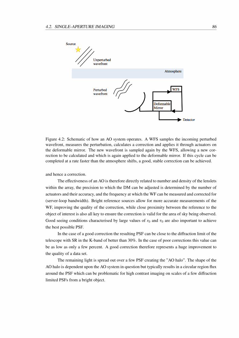
4.2. SINGLE-APERTURE IMAGING 86
Figure 4.2: Schematic of how an AO system operates. A WFS samples the incoming perturbedwavefront, measures the perturbation, calculates a correction and applies it through actuators onthe deformable mirror. The new wavefront is sampled again by the WFS, allowing a new cor-rection to be calculated and which is again applied to the deformable mirror. If this cycle can becompleted at a rate faster than the atmosphere shifts, a good, stable correction can be achieved.
and hence a correction.
The effectiveness of an AO is therefore directly related to number and density of the lenslets
within the array, the precision to which the DM can be adjusted is determined by the number of
actuators and their accuracy, and the frequency at which the WF can be measured and corrected for
(server-loop bandwidth). Bright reference sources allow for more accurate measurements of the
WF, improving the quality of the correction, while close proximity between the reference to the
object of interest is also all key to ensure the correction is valid for the area of sky being observed.
Good seeing conditions characterised by large values of r0 and τ0 are also important to achieve
the best possible PSF.
In the case of a good correction the resulting PSF can be close to the diffraction limit of the
telescope with SR in the K-band of better than 30%. In the case of poor corrections this value can
be as low as only a few percent. A good correction therefore represents a huge improvement to
the quality of a data set.
The remaining light is spread out over a few PSF creating the ”AO halo”. The shape of the
AO halo is dependent upon the AO system in question but typically results in a circular region flux
around the PSF which can be problematic for high contrast imaging on scales of a few diffraction
limited PSFs from a bright object.
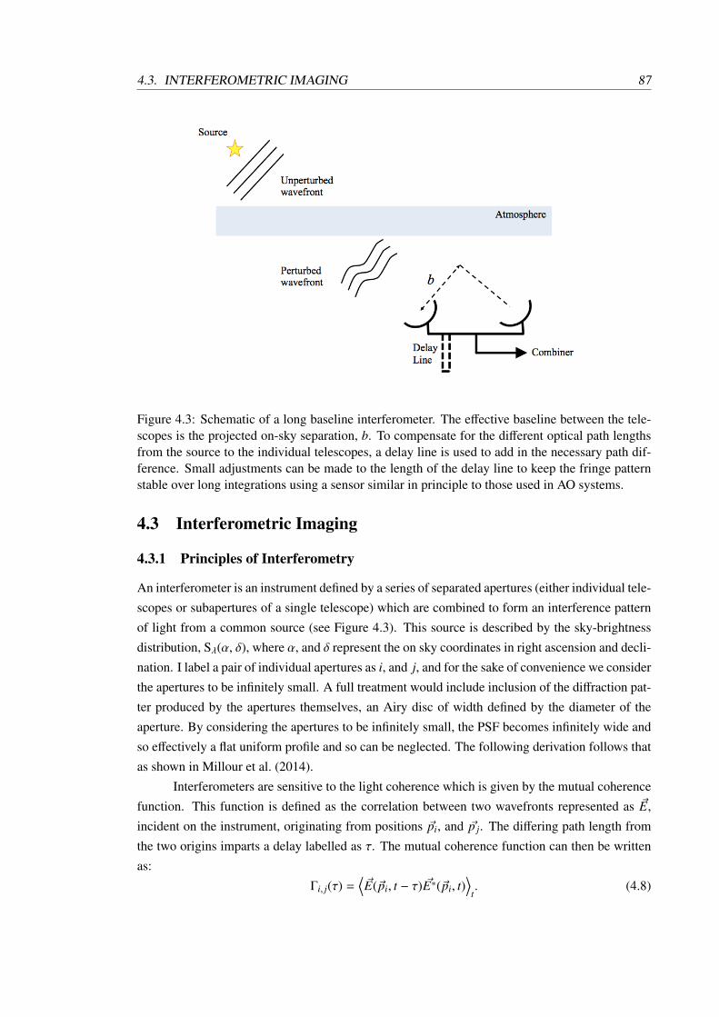
4.3. INTERFEROMETRIC IMAGING 87
Figure 4.3: Schematic of a long baseline interferometer. The effective baseline between the tele-scopes is the projected on-sky separation, b. To compensate for the different optical path lengthsfrom the source to the individual telescopes, a delay line is used to add in the necessary path dif-ference. Small adjustments can be made to the length of the delay line to keep the fringe patternstable over long integrations using a sensor similar in principle to those used in AO systems.
4.3 Interferometric Imaging
4.3.1 Principles of Interferometry
An interferometer is an instrument defined by a series of separated apertures (either individual tele-
scopes or subapertures of a single telescope) which are combined to form an interference pattern
of light from a common source (see Figure 4.3). This source is described by the sky-brightness
distribution, Sλ(α, δ), where α, and δ represent the on sky coordinates in right ascension and decli-
nation. I label a pair of individual apertures as i, and j, and for the sake of convenience we consider
the apertures to be infinitely small. A full treatment would include inclusion of the diffraction pat-
ter produced by the apertures themselves, an Airy disc of width defined by the diameter of the
aperture. By considering the apertures to be infinitely small, the PSF becomes infinitely wide and
so effectively a flat uniform profile and so can be neglected. The following derivation follows that
as shown in Millour et al. (2014).
Interferometers are sensitive to the light coherence which is given by the mutual coherence
function. This function is defined as the correlation between two wavefronts represented as ~E,
incident on the instrument, originating from positions ~pi, and ~p j. The differing path length from
the two origins imparts a delay labelled as τ. The mutual coherence function can then be written
as:
Γi, j(τ) =⟨~E(~pi, t − τ) ~E∗(~pi, t)
⟩t. (4.8)
4.3. INTERFEROMETRIC IMAGING 88
Utilising Equation 4.5, we can rewrite the light intensity as a function of Γ.
I( ~x ) =∑
i
Γi, j(0) +∑
i
(Γi, j(τ j − τi) + Γ∗i, j(τ j − τi)
). (4.9)
Here the Γi, j(0) terms merely represent the light intensity in the case of an unperturbed light source
(τ = 0 represents the case where the light originates from the same origin). The set of delays, τi,
are set by a function defined by the origin of the two wavefronts, the particulars of the optical set
up of the instrument and on the coordinates within the focal plane.
In the simplest case of a pair of apertures we can define τ j − τi as τ which allows us to
simplify Equation 4.9 to:
I( ~x ) = I1(~x) + I2(~x) + Γ1,2(τ) + Γ∗1,2(τ). (4.10)
Normalising by the total flux produces:
γ1,2(τ) =Γ1,2(τ)
Γ1,1(0) + Γ2,2(0), (4.11)
which defines γ1,2(τ), representing the complex coherence degree. Simplify the problem by con-
sidering the interference pattern in a single dimension, x, Equation 4.10 becomes:
I( ~x ) = [I1(~x) + I2(~x)][1 + Re(γ1,2(τ))] (4.12)
I( ~x ) = [I1(~x) + I2(~x)][1 + µ
obj1,2cos
(2πxλ
+ φobj1,2
)]. (4.13)
Here µobj1,2 is the modulus of γ1,2(0) while φ is the phase (i.e. γ1,2(0) = µeiφ). The distinctive
fringes associated with interferometric measurements are produced through the cosine term (see
Figures 4.4 and 4.5). Equation 4.13 is sometimes referred to as ”the interferometric equation” and
describes the interferogram (measured interference pattern) produced on the detector in the focal
plane. In turn, µ and φ are labelled as the ”visibility” and the ”phase” of the fringes respectively.
The dimension, x, becomes a length which represents the delay between two recombined beams.
Zernicke and van Cittert theorem
The Interferometry equation (Equation 4.13) is the basis to describe the well known Youngs
double-slit experiment. It is readily observed when shining a coherent light source through a
pair of slits that changing the size of the light source causes a change in the observed fringe pat-
tern. Increasing the size of the light source from a point source is seen to reduce the contrast of the
fringes until at certain sizes they can no longer be observed. Translating the position of the light
source in parallel to the slits will cause the fringes to shift in the opposite direction. The Zernicke
and van Cittert theorem (ZVC; van Cittert 1934; Zernike 1938) links these phenomena and en-
ables use to reconstruct the sky-brightness distribution in stellar interferometric observations from
the interferograms.
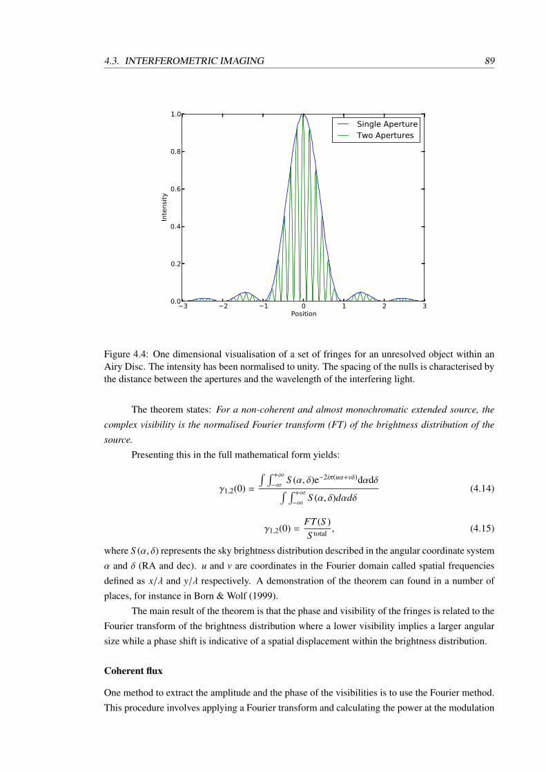
4.3. INTERFEROMETRIC IMAGING 89
3 2 1 0 1 2 3Position
0.0
0.2
0.4
0.6
0.8
1.0
Inte
nsi
ty
Single ApertureTwo Apertures
Figure 4.4: One dimensional visualisation of a set of fringes for an unresolved object within anAiry Disc. The intensity has been normalised to unity. The spacing of the nulls is characterised bythe distance between the apertures and the wavelength of the interfering light.
The theorem states: For a non-coherent and almost monochromatic extended source, the
complex visibility is the normalised Fourier transform (FT) of the brightness distribution of the
source.
Presenting this in the full mathematical form yields:
γ1,2(0) =
∫ ∫ +∞
−∞S (α, δ)e−2iπ(uα+vδ)dαdδ∫ ∫ +∞
−∞S (α, δ)dαdδ
(4.14)
γ1,2(0) =FT (S )S total , (4.15)
where S (α, δ) represents the sky brightness distribution described in the angular coordinate system
α and δ (RA and dec). u and v are coordinates in the Fourier domain called spatial frequencies
defined as x/λ and y/λ respectively. A demonstration of the theorem can found in a number of
places, for instance in Born & Wolf (1999).
The main result of the theorem is that the phase and visibility of the fringes is related to the
Fourier transform of the brightness distribution where a lower visibility implies a larger angular
size while a phase shift is indicative of a spatial displacement within the brightness distribution.
Coherent flux
One method to extract the amplitude and the phase of the visibilities is to use the Fourier method.
This procedure involves applying a Fourier transform and calculating the power at the modulation

4.3. INTERFEROMETRIC IMAGING 90
-10 -5 0 5 10 15Position in x [mm]
-10
-5
0
5
10
15
Posi
tion in y
[m
m]
-10 -5 0 5 10 15Position in x [mm]
-10
-5
0
5
10
15
Posi
tion in y
[m
m]
-10 -5 0 5 10 15Position in x [mm]
-10
-5
0
5
10
15
Posi
tion in y
[m
m]
Figure 4.5: Left: Theoretical apertures (white) and their geometry within a mask. Right: Resul-tant fringe pattern when observing a point source. Each unique baseline between any two holesproduces a fringe pattern which is superimposed on the others. This new fringe pattern modulatesthe Airy disc which characterises the size and shape of the apertures. Each addition of an extraaperture brings the resultant fringe pattern closer to an Airy disc characterising a circular apertureof diameter equal to the longest baseline.
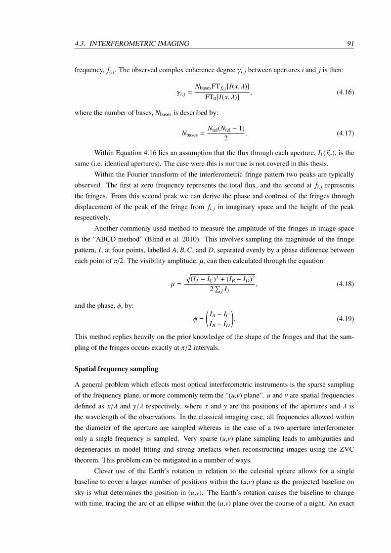
4.3. INTERFEROMETRIC IMAGING 91
frequency, fi, j. The observed complex coherence degree γi, j between apertures i and j is then:
γi, j =NbasesFT fi, j[I(x, λ)]
FT0[I(x, λ)], (4.16)
where the number of bases, Nbases is described by:
Nbases =Ntel(Ntel − 1)
2. (4.17)
Within Equation 4.16 lies an assumption that the flux through each aperture, I1(~xn), is the
same (i.e. identical apertures). The case were this is not true is not covered in this thesis.
Within the Fourier transform of the interferometric fringe pattern two peaks are typically
observed. The first at zero frequency represents the total flux, and the second at fi, j represents
the fringes. From this second peak we can derive the phase and contrast of the fringes through
displacement of the peak of the fringe from fi, j in imaginary space and the height of the peak
respectively.
Another commonly used method to measure the amplitude of the fringes in image space
is the ”ABCD method” (Blind et al. 2010). This involves sampling the magnitude of the fringe
pattern, I, at four points, labelled A, B,C, and D, separated evenly by a phase difference between
each point of π/2. The visibility amplitude, µ, can then calculated through the equation:
µ =
√(IA − IC)2 + (IB − ID)2
2∑
j I j, (4.18)
and the phase, φ, by:
φ =
(IA − IC
IB − ID
). (4.19)
This method replies heavily on the prior knowledge of the shape of the fringes and that the sam-
pling of the fringes occurs exactly at π/2 intervals.
Spatial frequency sampling
A general problem which effects most optical interferometric instruments is the sparse sampling
of the frequency plane, or more commonly term the “(u,v) plane”. u and v are spatial frequencies
defined as x/λ and y/λ respectively, where x and y are the positions of the apertures and λ is
the wavelength of the observations. In the classical imaging case, all frequencies allowed within
the diameter of the aperture are sampled whereas in the case of a two aperture interferometer
only a single frequency is sampled. Very sparse (u,v) plane sampling leads to ambiguities and
degeneracies in model fitting and strong artefacts when reconstructing images using the ZVC
theorem. This problem can be mitigated in a number of ways.
Clever use of the Earth’s rotation in relation to the celestial sphere allows for a single
baseline to cover a larger number of positions within the (u,v) plane as the projected baseline on
sky is what determines the position in (u,v). The Earth’s rotation causes the baseline to change
with time, tracing the arc of an ellipse within the (u,v) plane over the course of a night. An exact
4.3. INTERFEROMETRIC IMAGING 92
expression for these arcs is given in Segransan (2007). The shape and extension of these arcs is
determined by the position in the sky of the target and the latitude of the observatory.
The most obvious solution is the addition of further telescopes or apertures to the interfer-
ometric array. The number of baselines, hence points within the (u,v) plane is given by Equa-
tion 4.17 and scales approximately with the square of the number of telescopes. Every addition of
a further aperture results in a dramatic increase in the number of points in the (u,v) plane in the
case of radio interferometry. In this regime the telescopes, more commonly called antenna, are ca-
pable of directly measuring the complex visibility, storing the data and later amplifying this signal
for interfering with other antenna with little addition of noise. Arrays containing 10s of antenna
are possible with current technology, producing images with few and easily removed artefacts. In
the case of optical instruments however, the situation is more difficult as the light collected at each
aperture must be interfered directly at the time of observing. The addition of an additional tele-
scope therefore results in fewer photon counts within each interferogram. So additional telescopes
presents the problem of worsening SNRs and the need for more, expensive delay lines and optical
systems.
The spatial frequencies are dependent on wavelength in which the observation is performed.
Therefore performing dispersing the incoming light from a broadband channel into a set of narrow
band channels which are interfered separately will produce a spread of (u,v) plane points radially,
all sampling approximately the same regions of the object in question.
The phase problem
There exist a series of problems which adversely affect the measurement of the amplitude and
phase of the fringes.
The most damaging of all these effects is the addition of a phase term, φp, between tele-
scopes due to atmospheric turbulence. The atmosphere distorts the wavefront of an incoming
packet of coherent light, inducing optical path differences, δ(t), for the packet to reach different
telescopes beyond what would be expected as a result of their differing distances to the object.
This effect is sometimes referred to as the atmospheric piston. As a first approximation this ef-
fect can be described by φpλ = 2πδ(t)/λ. This also implies the atmosphere can be assumed to be
effectively static over certain time periods determined by the wavelength of the observations, with
the atmosphere remaining static over shorter periods at shorter wavelengths compared to longer
wavelengths.
The necessity for finite exposure times leads to further degrading effects. The turbulent
atmosphere with its turbulent timescales can be considered as a series of frames within which the
atmosphere is effectively still. Between each frames however the atmospheric piston imposes a
small phase difference between neighbouring frames. An exposure time over several atmospheric
timescales will therefore be a superposition of a number of fringe pattern each with a unique phase
shift. The net result is to blur out fringes, reducing their visibility. In long baseline interferometry
this problem can be solved or mitigated in two ways. For bright objects where SNR is not an
issue, taking a large number of very short exposures less than a single timescale in length and
combining the exposures into a single fringe pattern in the data reduction pipeline can be very

4.3. INTERFEROMETRIC IMAGING 93
effective in preventing the blurring of the fringe pattern. In cases where SNR is more important
and hence short integrations are not practical, longer integration times can be executed using a
fringe tracker. Similar in practice to an AO system, the fringe tracker samples incoming light,
measures the atmospheric piston and applies a small correction to the delay lines to keep the
fringes fixed in position on the detector of the beam combiner. This allows for longer integrations
and higher quality data. Neither technique is effective in sparse aperture masking however as much
of the light is lost, necessitating long integration times. Hence the visibilities measured with these
instruments almost always contain large uncertainties.
The fringes may also be smeared out due to ”chromatic longitudinal dispersion” (Tubbs
et al. 2004; Vannier et al. 2006). This refers to the width of a spectral bandwidth which is allowed
to impinge on the detector of a beam combiner. The light will interfere only with light of the same
wavelength so what develops on the detector is a superposition of every fringe pattern produced
by all of the wavelengths contained within the spectral channel allowed into the detector. Longer
wavelengths will produce more dispersed fringe patterns than the shorter wavelengths resulting in
smeared out fringes and lower visibilities. This can be mitigated by narrowing the bandwidth for
broadband observations or by increasing the spectral resolution in spectrally dispersed observa-
tions to limit the bandwidth smearing effect.
Optical beam combiners are complex instruments which contain a large number of optical
elements to control the path of the incoming beam. These include beam splitters and mirrors which
will split the light into the two polarisation states. Differing path lengths within the combiner
between the pair of polarisation states will induce a contrast variation, A(∆π), in the resultant
fringe pattern but this is largely corrected for in modern instruments (Lazareff et al. 2012).
Classical effects which effect all astronomical observations such as photon and detector
noise, σφ and σdet, can be grouped together into an additive noise term, b, which also need to be
considered. We can represent all these effects within the interferometric equation in the 1D case
thus:
I =
Ntel∑j=1
I j +
Ntel−1∑k=1
Ntel∑j=k+1
I jIkA(σpφ)A(∆π)A(δ)µobj
j,k cos(2πλ
(x + δ) + φobjj,k
)+ b, (4.20)
where the indices j, k represent the apertures in the array, x is the space coordinates, λ is the
wavelength of the incoming flux, µobjj,k , φ
objj,k are the visibility and phase respectively, δ is the optical
path difference induced by the atmospheric piston effect. A(σpφ) is and attenuation factor due to
the finite exposure time of each frame (Tatulli et al. 2007) and A(δ) is a further attenuation term
resulting from the spectral resolution of the instrument. The degree of attenuation due to the finite
exposure time is dependent on the atmospheric conditions and how that effects the fringe tracker
performance. A(∆π) is an attenuation factor dependent on the polarization state of the contributing
beams and b is the zero-mean noise contribution.
The result of these effects is a reduction in the accuracy of the amplitude measurements
while the atmospheric piston prevents the direct measurement of the phase. In the following
sections we will describe methods to work around these problems.
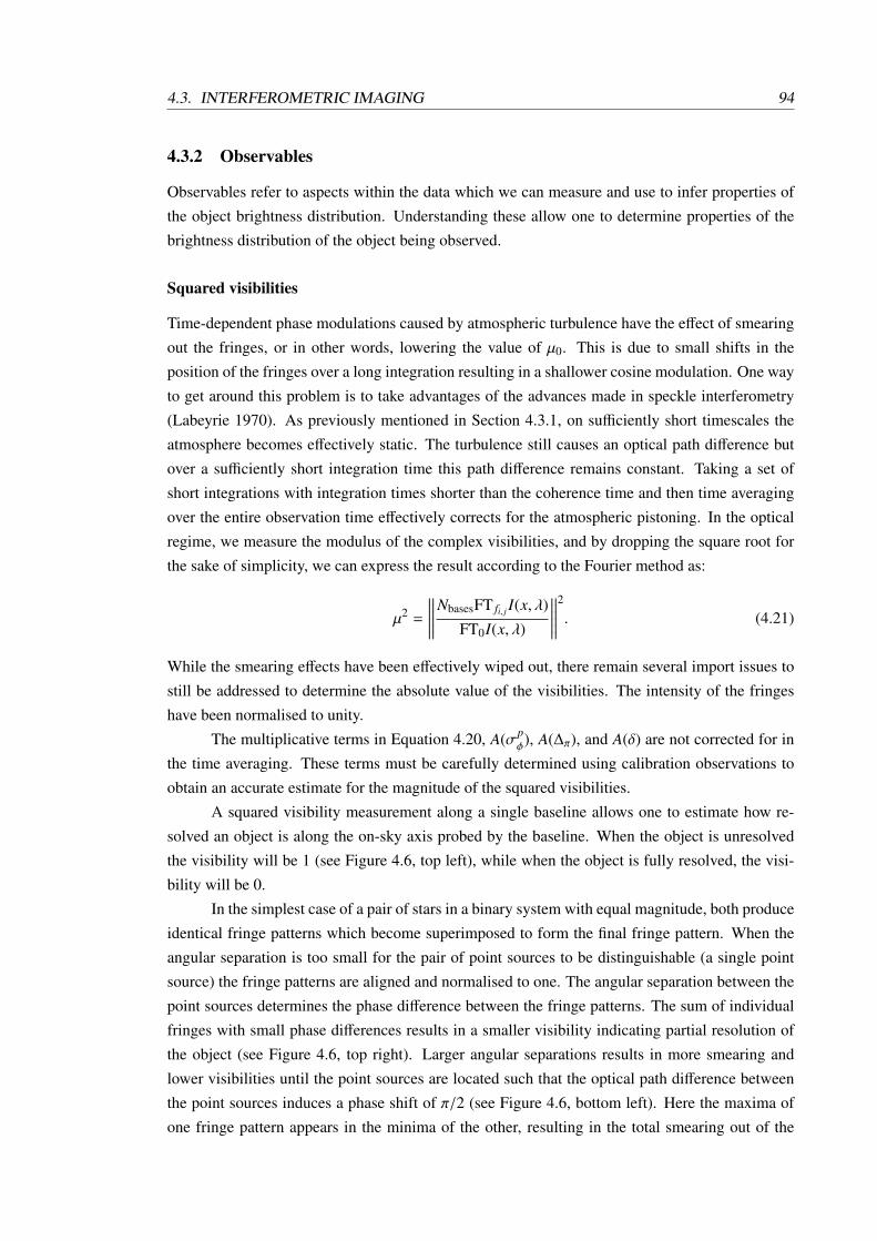
4.3. INTERFEROMETRIC IMAGING 94
4.3.2 Observables
Observables refer to aspects within the data which we can measure and use to infer properties of
the object brightness distribution. Understanding these allow one to determine properties of the
brightness distribution of the object being observed.
Squared visibilities
Time-dependent phase modulations caused by atmospheric turbulence have the effect of smearing
out the fringes, or in other words, lowering the value of µ0. This is due to small shifts in the
position of the fringes over a long integration resulting in a shallower cosine modulation. One way
to get around this problem is to take advantages of the advances made in speckle interferometry
(Labeyrie 1970). As previously mentioned in Section 4.3.1, on sufficiently short timescales the
atmosphere becomes effectively static. The turbulence still causes an optical path difference but
over a sufficiently short integration time this path difference remains constant. Taking a set of
short integrations with integration times shorter than the coherence time and then time averaging
over the entire observation time effectively corrects for the atmospheric pistoning. In the optical
regime, we measure the modulus of the complex visibilities, and by dropping the square root for
the sake of simplicity, we can express the result according to the Fourier method as:
µ2 =
∣∣∣∣∣∣∣∣∣∣∣∣NbasesFT fi, j I(x, λ)
FT0I(x, λ)
∣∣∣∣∣∣∣∣∣∣∣∣2. (4.21)
While the smearing effects have been effectively wiped out, there remain several import issues to
still be addressed to determine the absolute value of the visibilities. The intensity of the fringes
have been normalised to unity.
The multiplicative terms in Equation 4.20, A(σpφ), A(∆π), and A(δ) are not corrected for in
the time averaging. These terms must be carefully determined using calibration observations to
obtain an accurate estimate for the magnitude of the squared visibilities.
A squared visibility measurement along a single baseline allows one to estimate how re-
solved an object is along the on-sky axis probed by the baseline. When the object is unresolved
the visibility will be 1 (see Figure 4.6, top left), while when the object is fully resolved, the visi-
bility will be 0.
In the simplest case of a pair of stars in a binary system with equal magnitude, both produce
identical fringe patterns which become superimposed to form the final fringe pattern. When the
angular separation is too small for the pair of point sources to be distinguishable (a single point
source) the fringe patterns are aligned and normalised to one. The angular separation between the
point sources determines the phase difference between the fringe patterns. The sum of individual
fringes with small phase differences results in a smaller visibility indicating partial resolution of
the object (see Figure 4.6, top right). Larger angular separations results in more smearing and
lower visibilities until the point sources are located such that the optical path difference between
the point sources induces a phase shift of π/2 (see Figure 4.6, bottom left). Here the maxima of
one fringe pattern appears in the minima of the other, resulting in the total smearing out of the
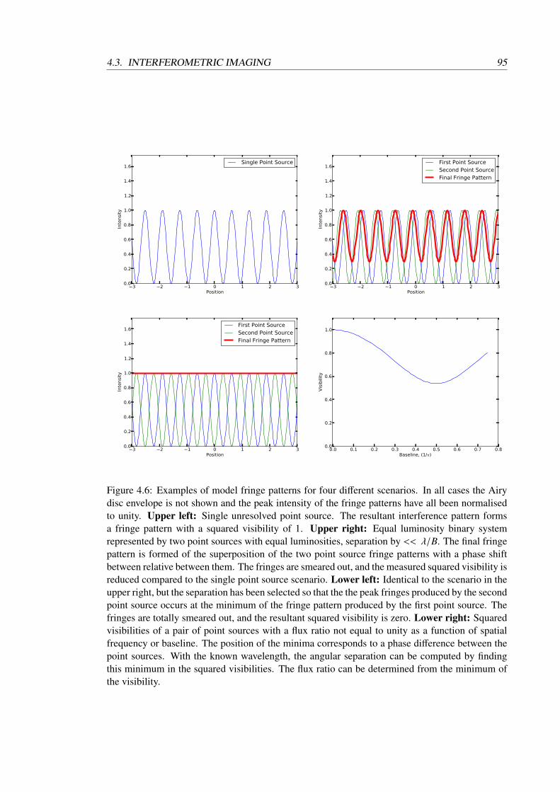
4.3. INTERFEROMETRIC IMAGING 95
3 2 1 0 1 2 3Position
0.0
0.2
0.4
0.6
0.8
1.0
1.2
1.4
1.6
Inte
nsi
ty
Single Point Source
3 2 1 0 1 2 3Position
0.0
0.2
0.4
0.6
0.8
1.0
1.2
1.4
1.6
Inte
nsi
ty
First Point SourceSecond Point SourceFinal Fringe Pattern
3 2 1 0 1 2 3Position
0.0
0.2
0.4
0.6
0.8
1.0
1.2
1.4
1.6
Inte
nsi
ty
First Point SourceSecond Point SourceFinal Fringe Pattern
0.0 0.1 0.2 0.3 0.4 0.5 0.6 0.7 0.8Baseline, (1/π)
0.0
0.2
0.4
0.6
0.8
1.0
Vis
ibili
ty
Figure 4.6: Examples of model fringe patterns for four different scenarios. In all cases the Airydisc envelope is not shown and the peak intensity of the fringe patterns have all been normalisedto unity. Upper left: Single unresolved point source. The resultant interference pattern formsa fringe pattern with a squared visibility of 1. Upper right: Equal luminosity binary systemrepresented by two point sources with equal luminosities, separation by << λ/B. The final fringepattern is formed of the superposition of the two point source fringe patterns with a phase shiftbetween relative between them. The fringes are smeared out, and the measured squared visibility isreduced compared to the single point source scenario. Lower left: Identical to the scenario in theupper right, but the separation has been selected so that the the peak fringes produced by the secondpoint source occurs at the minimum of the fringe pattern produced by the first point source. Thefringes are totally smeared out, and the resultant squared visibility is zero. Lower right: Squaredvisibilities of a pair of point sources with a flux ratio not equal to unity as a function of spatialfrequency or baseline. The position of the minima corresponds to a phase difference between thepoint sources. With the known wavelength, the angular separation can be computed by findingthis minimum in the squared visibilities. The flux ratio can be determined from the minimum ofthe visibility.

4.3. INTERFEROMETRIC IMAGING 96
fringes and a zero visibility. Sampling the resulting visibility modulation enables the accurate
measurement of the separation of binaries through measuring along multiple baselines differing in
magnitude and direction (see Figure 4.6, bottom right).
For more complex objects, sizes and radial profiles can be derived by fitting to the visibility
profile created through measuring the visibilities along multiple baselines. This allows one to
derive the shapes and orientations of a variety of extended objects.
Closure phases
As a result of the atmospheric piston, for a single baseline interferometric observation, the phase
information is essentially lost. The optical path difference induced is an unknown quantity and
time-dependent on milli-second timescales. Combining the phase information from three tele-
scopes enables one to measure a new quantity, namely the ”closure phase”, which possesses in-
teresting properties. The closure phase has the intriguing property that it cancels the atmospheric
disturbances and is a self-calibrating quantity, independent of atmospheric effects. First devel-
oped by Jennison (1958) in the use of radio interferometers, closure phases enable us to retrieve
otherwise lost phase information.
The closure phase is computed for a triangle of apertures, in the following denoted with
the indices 1, 2, and 3 (see Figure 4.7 for set-up). We label the object phase on the individual
baselines; φobj1,2, φobj
2,3, and φobj3,1. Each aperture affected by the atmospheric turbulence, inducing a
random phase term, φatm1 , φatm
2 , and φatm3 .
The phase measured on each baseline can thus be described as:
Φ1,2 = φobj1,2 + φatm
2 − φatm1 (4.22)
Φ2,3 = φobj2,3 + φatm
3 − φatm2 (4.23)
Φ3,1 = φobj3,1 + φatm
1 − φatm3 . (4.24)
Summing the three baselines together produces:
Ψ1,2,3 = φobj1,2 + φ
obj2,3 + φ
obj3,1 + φatm
1 − φatm1 + φatm
2 − φatm2 + φatm
3 − φatm3 , (4.25)
which cancels down simply to:
Ψ1,2,3 = φobj1,2 + φ
obj2,3 + φ
obj3,1. (4.26)
The closure phase extracted from individual interferograms might still be noisy as a result
of low photon counts which results in a distribution of the phases. Often it appears close to a
uniform distribution caused by phase wrapping, where phases of exceeding the range −π to π are
wrapped to fall within the normal range. One can avoid this problem by performing averaging in
the complex plane.
Therefore to compute it as an observable, one must compute the bispectrum of the inter-
ferogram directly, preserving the complex component and average across all frames. One then
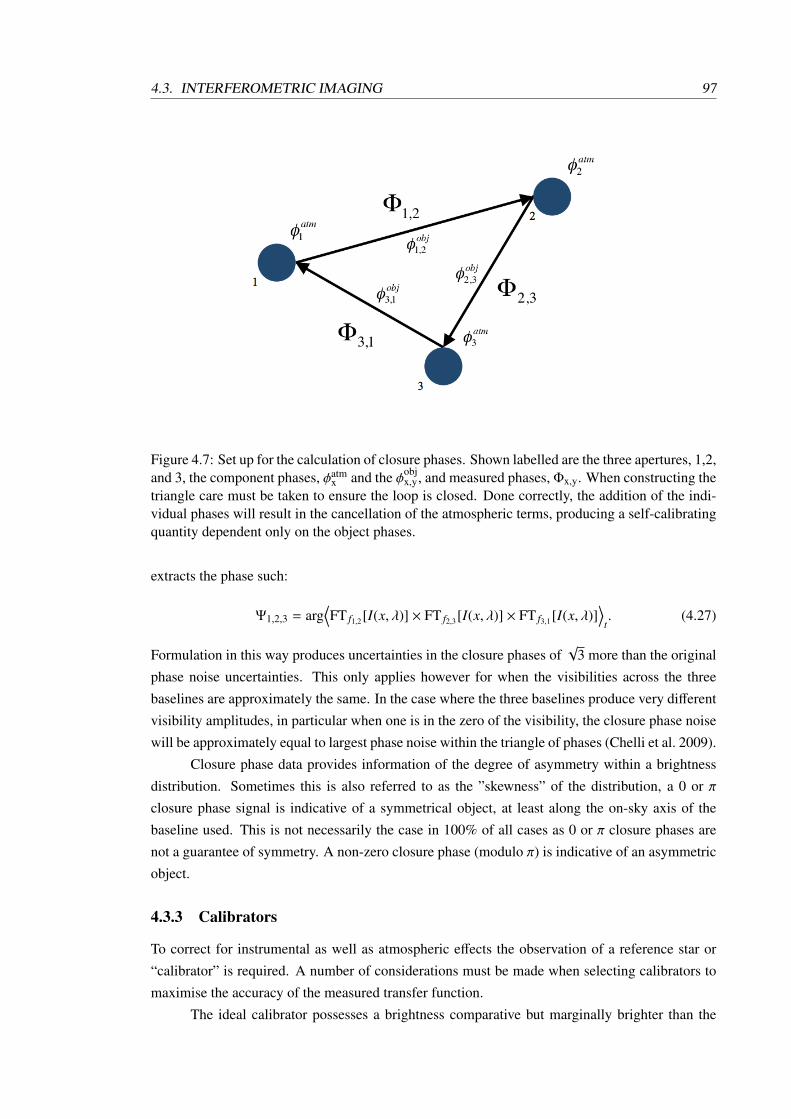
4.3. INTERFEROMETRIC IMAGING 97
Figure 4.7: Set up for the calculation of closure phases. Shown labelled are the three apertures, 1,2,and 3, the component phases, φatm
x and the φobjx,y, and measured phases, Φx,y. When constructing the
triangle care must be taken to ensure the loop is closed. Done correctly, the addition of the indi-vidual phases will result in the cancellation of the atmospheric terms, producing a self-calibratingquantity dependent only on the object phases.
extracts the phase such:
Ψ1,2,3 = arg⟨FT f1,2[I(x, λ)] × FT f2,3[I(x, λ)] × FT f3,1[I(x, λ)]
⟩t. (4.27)
Formulation in this way produces uncertainties in the closure phases of√
3 more than the original
phase noise uncertainties. This only applies however for when the visibilities across the three
baselines are approximately the same. In the case where the three baselines produce very different
visibility amplitudes, in particular when one is in the zero of the visibility, the closure phase noise
will be approximately equal to largest phase noise within the triangle of phases (Chelli et al. 2009).
Closure phase data provides information of the degree of asymmetry within a brightness
distribution. Sometimes this is also referred to as the ”skewness” of the distribution, a 0 or π
closure phase signal is indicative of a symmetrical object, at least along the on-sky axis of the
baseline used. This is not necessarily the case in 100% of all cases as 0 or π closure phases are
not a guarantee of symmetry. A non-zero closure phase (modulo π) is indicative of an asymmetric
object.
4.3.3 Calibrators
To correct for instrumental as well as atmospheric effects the observation of a reference star or
“calibrator” is required. A number of considerations must be made when selecting calibrators to
maximise the accuracy of the measured transfer function.
The ideal calibrator possesses a brightness comparative but marginally brighter than the

4.3. INTERFEROMETRIC IMAGING 98
science star, no bright companion, and a close angular proximity to the science star on sky. The
first condition can be relaxed in the case of a science target without an ideal calibrator within
approximately a few degrees. Following these conditions maximises the ability to calculate an
accurate transfer function to calibrate the measured science visibilities.
The requirement for the calibrator to be similar in magnitude to the science star is a result
of the need to maximise the performance of the fringe tracker. Similar magnitude calibrator and
science stars will produce similar SNRs on the fringe tracker and hence allow an observer to
optimise the settings of the tracker.
Additional constraints are applied depending on the type of interferometry being performed.
A favourable spectral type is particularly important for high spectral resolution interferometry
where O and B stars are preferred because of their simple spectra free of complex sets of ab-
sorption lines. This simplifies the calibration process as the need for a precise model of the stellar
atmosphere is not so stringent. For masking interferometry, broadband filters are used to maximise
throughput. Instead, earlier spectral types are avoided due to the higher proportion of binaries.
4.3.4 Sparse Aperture Masking (SAM)
Fitted to a number of single aperture instruments, sparse aperture masks allow an observer to reach
the diffraction limit of the conventional single aperture telescope in use and even beyond under
optimal conditions. The technique was pioneered in Baldwin et al. (1986) wherein fringes and
closure phases were observed and measured through a three holed mask placed in the re-imaged
aperture plane of the telescope. An example mask is shown in Figure 4.8. This optical set-up
has become a common configuration for SAM instruments (Haniff et al. 1987; Young et al. 2000;
Lacour et al. 2011). The mask in the re-imaged aperture plane blocks the majority of the incoming
light, only allowing flux to pass through a number of small holes.
This technique is also sometimes referred to as ”non-redundant aperture masking”, ref-
erencing the non-redundant spacing of any pair of holes. These spacings are analogous to the
baselines of long baseline interferometry. Each pair of holes samples a different spatial frequency
and produces a fringe pattern on the detector. A well designed mask will cover a range of base-
line lengths and orientations covering large, intermediate and short baselines, and also maximise
throughput. More numerous and larger holes will achieve both objectives but will also produce
fringe patterns which will tend to smear into one another even when using narrow band filters.
Mask design is therefore a trade off between maximising uv coverage and throughput and while
minimising smearing effects resulting in masks with fewer holes having large holes (and hence
higher throughput) and vice versa.
Performing a Fourier transform on the resultant fringe pattern from a mask allows the mea-
surement of visibilities and closure phases, although the long integration times required typically
results in a poor transfer function and hence large uncertainties on the squared visibility measure-
ments. Closure phases are more robust to atmospheric changes so are the principle observable
from SAM observations.
Combining SAM instruments with telescopes fitted with advanced AO systems greatly in-
creases both the photon counts attainable through the masks while also enhancing the stability of
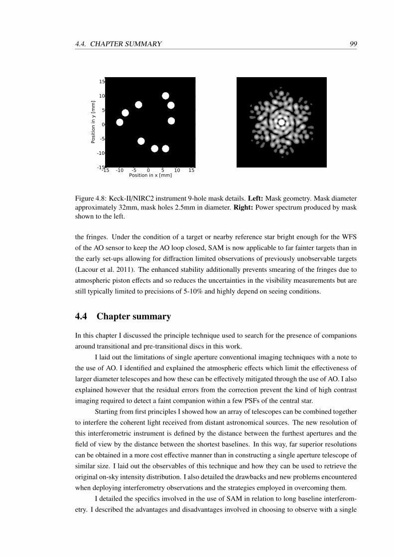
4.4. CHAPTER SUMMARY 99
-15 -10 -5 0 5 10 15Position in x [mm]
-15
-10
-5
0
5
10
15
Posi
tion in y
[m
m]
Figure 4.8: Keck-II/NIRC2 instrument 9-hole mask details. Left: Mask geometry. Mask diameterapproximately 32mm, mask holes 2.5mm in diameter. Right: Power spectrum produced by maskshown to the left.
the fringes. Under the condition of a target or nearby reference star bright enough for the WFS
of the AO sensor to keep the AO loop closed, SAM is now applicable to far fainter targets than in
the early set-ups allowing for diffraction limited observations of previously unobservable targets
(Lacour et al. 2011). The enhanced stability additionally prevents smearing of the fringes due to
atmospheric piston effects and so reduces the uncertainties in the visibility measurements but are
still typically limited to precisions of 5-10% and highly depend on seeing conditions.
4.4 Chapter summary
In this chapter I discussed the principle technique used to search for the presence of companions
around transitional and pre-transitional discs in this work.
I laid out the limitations of single aperture conventional imaging techniques with a note to
the use of AO. I identified and explained the atmospheric effects which limit the effectiveness of
larger diameter telescopes and how these can be effectively mitigated through the use of AO. I also
explained however that the residual errors from the correction prevent the kind of high contrast
imaging required to detect a faint companion within a few PSFs of the central star.
Starting from first principles I showed how an array of telescopes can be combined together
to interfere the coherent light received from distant astronomical sources. The new resolution of
this interferometric instrument is defined by the distance between the furthest apertures and the
field of view by the distance between the shortest baselines. In this way, far superior resolutions
can be obtained in a more cost effective manner than in constructing a single aperture telescope of
similar size. I laid out the observables of this technique and how they can be used to retrieve the
original on-sky intensity distribution. I also detailed the drawbacks and new problems encountered
when deploying interferometry observations and the strategies employed in overcoming them.
I detailed the specifics involved in the use of SAM in relation to long baseline interferom-
etry. I described the advantages and disadvantages involved in choosing to observe with a single

4.4. CHAPTER SUMMARY 100
telescope rather than with multiple telescopes.

Chapter 5
Image reconstruction algorithms
5.1 Introduction
Image reconstruction from interferometric measurements has a long and successful history in radio
interferometry. The specifics of optical interferometry make it a more difficult problem when
applied in the short wavelength regime however. In particular the loss of a large proportion of the
Fourier phase information in the optical and sparser sampling of the uv-plane results in any image
reconstruction algorithm having to fill in more information via a prioris. However, recovering the
initial intensity distribution in a model independent way allows one to reveal surprising details in
otherwise unresolved objects (see Figure 5.1).
The problem of sparse uv-coverage is largely solved when conducting sparse aperture
masking at the cost of much shorter baselines and a large drop in the collecting power of the
telescope. A nine hole mask will produce 36 visibility measurements and 28 closure phase mea-
surements per exposure. These form a single ”visit” and an object is typically ”visited” three to
four times within one observing sequence, where each visit to the science target is sandwiched
between observations of calibrator stars. The time between each visit to the science star allows for
a small amount of on-sky rotation which improves the overall uv-sampling of the science target.
In this way, a sample of 108 visibilities and 84 closure phase data points can be collected in a
three hour observational period. The squared visibilities tend to be a poorly calibrated quantity
due to the long exposures required for good SNR (see Section 4.3.3). The closure phases how-
ever are a self calibrating quantity and unaffected by atmospheric distortions (see Section 4.3.2).
These form the basis of a method to retrieve the brightness distribution of the observed objects in
a model-independent way. One can use image reconstruction techniques developed for infrared
long-baseline interferometry to retrieve images for calibrated closure phases and squared visibili-
ties recorded with SAM interferometry.
In the following sections I describe image reconstruction in the most general terms applying
to both radio and optical interferometry following the process laid out in Thiebaut (2008). I then
simplify to the optical interferometry case and the global equation we attempt to minimise.
101

5.1. INTRODUCTION 102
IRAS08544
−15−10−5 0 5 10 15
−15
−10
−5
0
5
10
15
∆α (mas)
∆δ
(mas
)
0
0.1
0.2
0.3
0.4
0.5
0.6
0.7
0.8
0.9
1
∆α (mas)
∆δ
(mas
)
N
E
Figure 5.1: Reconstructed image of the sublimation radius of ring of material surrounding thepost-AGB binary system, IRAS 08544-4431, in broadband H-band taken with the VLT/PIONIERinstrument (Hillen et al. 2016). The flux has been normalised. The reconstruction was performedusing the SPARCO software package, removing the flux from point of stellar objects in the centerto reveal remarkable structure in the surrounding disc reminiscent of a protoplanetary disc. Thispackage was used to perform all image reconstructions on SAM data in this thesis.
5.2. BAYESIAN APPROACH 103
5.2 Bayesian approach
The image estimation from the discrete points in the Fourier plane (the aperture masking measure-
ments) can be considered as an inverse problem. Given that there are more pixels within our final
image than there are measurements, the problem is ill-posed and solving it requires one to adopt
a Bayesian approach. From this viewpoint, the set of parameters (xtrue) which defines the original
brightness distribution can be chosen as the most probable ones given a data set (P(d)) where we
maximise the equation:
xtrue = P(xmodel|d) = P(d|xmodel)P(xmodel). (5.1)
This expression arises from Bayes’ Theorem (Papoulis 1984) where we have neglected the P(d)
term as it does not depends on the original brightness distribution parameters and is in many cases
impossible to calculate when the number of possible solutions is infinite. This is not the case when
comparing different methods of generating artificial data sets to perform this search and must be
calculated in these cases. However for our purposes we assume P(d) to be equal to unity.
Equation 5.1 is described as the maximum a priori solution and is sometimes written as:
xtrue = f (xmodel), (5.2)
where the penalty function is written as:
f (xmodel) = c0 − c1logP(xmodel|d) = c0 − c1logP(d|xmodel) − c1logP(xmodel), (5.3)
where the constants c0, andc1, are real, positive and non-zero. Their values are chosen for conve-
nience based on how one wishes to weight the reconstruction process. This changes on a case by
case basis.
Equation 5.3 can be considered a joint criterion where one has two distinct parts to min-
imise; a term which measures the agreement of the reconstructed image with the real data, fdata(xmodel),
and a second term which judges the likelihood of a given image based upon a prior, fprior(xmodel).
These terms are as follows:
fdata(xmodel) ∝ logP(d|xmodel), (5.4)
fprior(xmodel) ∝ logP(xmodel). (5.5)
Representing these terms as an equation to minimise we find
fcost = fdata + µ freg, (5.6)
where fdata is the likelihood function which dependents of the fit to the data and freg is the regular-
isation function which depends on the prior. The weighting between the two terms is given by the
dimensionless parameter, µ. Each of these terms are discussed in more detail below.
5.2. BAYESIAN APPROACH 104
5.2.1 The likelihood function
The penalty function, fdata(xmodel), is formally defined for our purposes as:
fdata(xmodel) = fv(xmodel) + fβ(xmodel), (5.7)
where vdata are the complex visibility measurements and the βdata are the closure phase data. In
this definition we assume that the visibilities and closure phases are uncorrelated.
Complex Visibilities
We assume that all the interferometric data are independent and that the errors are distributed
according to a Gaussian profile. In reality the data are correlated to some degree largely due to the
practice of calibrating the visibility data via a transfer function. We neglect such terms as they are
expected to not have a large effect on the resultant images.
The full equation for the penalty function when considering the time dependent complex
visibilities between apertures labelled k and l is written as:
fv(xmodel) =∑
t
∑k<l
Re(vresk,l (xmodel, t))
Im(vresk,l (xmodel, t))
T
·
W rrk,l(t) W ri
k,l(t)
W irk,l(t) W ii
k,l(t)
· Re(vresk,l (xmodel, t))
Im(vresk,l (xmodel, t))
, (5.8)
where the residuals are:
vresk,l (xmodel, t) = vres
k,l (xdata) − vsimk,l (xmodel, t), (5.9)
while the weights, W, are defined as:
W rrk,l(t) = [Crr
k,l(t)Ciik,l(t) −Cri
k,l(t)2(t)]−1 Cii
k,l(t), (5.10)
W rik,l(t) = [Crr
k,l(t)Ciik,l(t) −Cri
k,l(t)2(t)]−1 Cri
k,l(t), (5.11)
W iik,l(t) = [Crr
k,l(t)Ciik,l(t) −Crr
k,l(t)2(t)]−1 Cii
k,l(t), (5.12)
The covariances, C, are in turn calculated via:
Crrk,l(t) = Var[Re(vdata
k,l (t))], (5.13)
Crik,l(t) = Cov[Re(vdata
k,l (t)), Im(vdatak,l (t))], and (5.14)
Ciik,l(t) = Var[Im(vdata
k,l (t))]. (5.15)
Var and Cov are the variance and covariance.
The Goodman model is typically a good approximation for interferometric data complex
visibility errors. We can therefore take the real and imaginary parts of the complex visibility data
to be independent of one another. The covariance, Crik,l(t), is therefore approximated to be equal to
5.2. BAYESIAN APPROACH 105
zero and allows us to assume the variance of the real and imaginary parts are the same:
fv(xmodel) =∑
t
∑k<l
|vdatak,l (t) − vsim
k,l (t)|2
Var[vdatak,l (t)]
(5.16)
This results in a typical χ2 calculation. In practice, we measure squared visibilities when
working in optical interferometry, so sample only the real part of the complex visibilities. The
method outlined above however results in an expression free of a dependence on the unknown
imaginary component so we use the same expression for our squared visibility measurements.
Closure Phase Data
The closure phase data must be treated differently to the visibility data due to problems induced
by phase wrapping. All closure phase data is measured between –180 and +180 and so small
changes in the phase of a single baseline within the triplet can result in a large change in the closure
phase. This is problematic for minimisation algorithms as it produces large gradients in opposite
directions within a small parameter space. To remove this problem, some image reconstruction
algorithms treat the closure phases as complex phasors instead, formally defined as:
fv(xmodel) =∑
t
∑j<k<l
1Var[βdata
j,k,l(t)]|eiβdata
j,k,l (t) − eiβsimj,k,l(t)|2. (5.17)
This softens the strong gradients in the χ2 minimisation and so the problem of phase wrap-
ping. In the regime where the uncertainties in the phases are small, this expression simplifies to
the χ2 expression under the assumption of Gaussian noise statistics:
fv(xmodel) =∑
t
∑j<k<l
|βdataj,k,l(t) − β
simj,k,l(t)|
2
Var[βdataj,k,l(t)]
. (5.18)
Other methods have been proposed to deal with the phase wrapping problem but this is the
method utilised in the MiRa image reconstruction algorithm. The authors of this code adopt this
approach for reasons of computing efficiency and greater ease of convergence (Thiebaut 2008).
5.2.2 The regularisation function
The need to introduce a regularisation is driven by two principle reasons. First, the high number of
pixels in the reconstructed image in comparison to the number of interferometric data points results
in a set of equally likely solutions to fit the data. The second reason is it prevents the amplification
of the noise which can be caused by the large number of pixels. A good regularisation will enable
the determination of a unique solution which best adheres to a set of predetermined conditions.
This can be formally defined as minimising the expression:
xtrue = fprior(xmodel) such that fdata(xmodel) ≤ γ. (5.19)

5.2. BAYESIAN APPROACH 106
Here, the inequality enforces the requirement for the model to resemble the data. γ is a unit less
parameter which operates in a similar manner to χ2 where a smaller γ represents a model closer
to the data. Without this constraint the measurements are not taken into consideration during the
regularisation. This can be written as:
xtrue = fprior(xmodel) + ` fdata(xmodel), (5.20)
where ` is a Lagrange multiplier which is tuned such that fdata(xtrue) ' γ.
The problem of a high number of pixels is exasperated by ’holes’ in the uv-coverage that
are not sampled by the available data. Within the reconstructed images this results in regions
devoid of any data point to constrain the solution. For a regularisation to be effective, these gaps
must be filled in a way that selects the most likely solution from the infinite number of possible
solutions. This is typically done by using the regularisation to smooth the image via interpolation
between the measured spatial frequencies where the image is well constrained. This is typically
enforced with the use of a simple quadratic constraint or a maximum entropy method. We detail
both methods below.
Smoothness
The generic description for a quadratic regularisation which works by favouring reconstructed
images that maximises the ”smoothness” within the image is:
fprior(xmodel) = (Aprior · xmodel − bprior)T · Wprior.(Aprior · xmodel − bprior)), (5.21)
where any quadratic regularisation can be produced using the matrices, Wprior, Aprior, and bprior. To
produce a convex fprior requires a Wprior matrix which is simultaneously positive and symmetrical.
This enables the algorithm to converge correctly.
Taking a Bayesian approach to the problem and assuming Gaussian noise statistics produces
a quadratic regularisation which can be represented by:
µ fprior(xmodel) = (xmodel − xprior)T · C−1prior.(xmodel − xprior), (5.22)
where values of the covariance matrix, C−1prior and the expected value, xprior, are assumed to be
known.
A typical regularisation involves the following expression:
fprior(xmodel) = ||D · xmodel||2, (5.23)
where D is a finite difference operator. The difference operator enforces a minimisation of the
gradient between two pixels in the reconstructed image filling the gaps in the uv-coverage and
hence a smooth image.
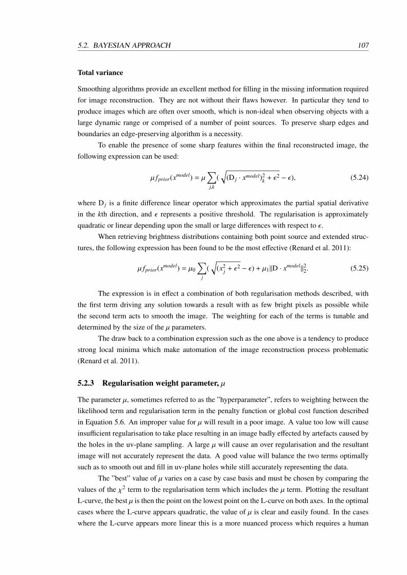
5.2. BAYESIAN APPROACH 107
Total variance
Smoothing algorithms provide an excellent method for filling in the missing information required
for image reconstruction. They are not without their flaws however. In particular they tend to
produce images which are often over smooth, which is non-ideal when observing objects with a
large dynamic range or comprised of a number of point sources. To preserve sharp edges and
boundaries an edge-preserving algorithm is a necessity.
To enable the presence of some sharp features within the final reconstructed image, the
following expression can be used:
µ fprior(xmodel) = µ∑
j,k
(√
(D j · xmodel)2k + ε2 − ε), (5.24)
where D j is a finite difference linear operator which approximates the partial spatial derivative
in the kth direction, and ε represents a positive threshold. The regularisation is approximately
quadratic or linear depending upon the small or large differences with respect to ε.
When retrieving brightness distributions containing both point source and extended struc-
tures, the following expression has been found to be the most effective (Renard et al. 2011):
µ fprior(xmodel) = µ0
∑j
(√
(x2j + ε2 − ε) + µ1||D · xmodel||22. (5.25)
The expression is in effect a combination of both regularisation methods described, with
the first term driving any solution towards a result with as few bright pixels as possible while
the second term acts to smooth the image. The weighting for each of the terms is tunable and
determined by the size of the µ parameters.
The draw back to a combination expression such as the one above is a tendency to produce
strong local minima which make automation of the image reconstruction process problematic
(Renard et al. 2011).
5.2.3 Regularisation weight parameter, µ
The parameter µ, sometimes referred to as the ”hyperparameter”, refers to weighting between the
likelihood term and regularisation term in the penalty function or global cost function described
in Equation 5.6. An improper value for µ will result in a poor image. A value too low will cause
insufficient regularisation to take place resulting in an image badly effected by artefacts caused by
the holes in the uv-plane sampling. A large µ will cause an over regularisation and the resultant
image will not accurately represent the data. A good value will balance the two terms optimally
such as to smooth out and fill in uv-plane holes while still accurately representing the data.
The ”best” value of µ varies on a case by case basis and must be chosen by comparing the
values of the χ2 term to the regularisation term which includes the µ term. Plotting the resultant
L-curve, the best µ is then the point on the lowest point on the L-curve on both axes. In the optimal
cases where the L-curve appears quadratic, the value of µ is clear and easily found. In the cases
where the L-curve appears more linear this is a more nuanced process which requires a human
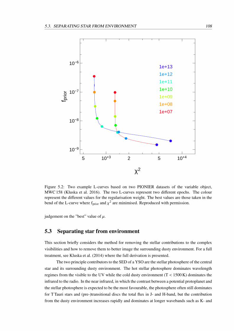
5.3. SEPARATING STAR FROM ENVIRONMENT 108
1e+07
1e+08
1e+09
1e+10
1e+11
1e+12
1e+13
10+3 10+425 5
10−9
10−8
10−7
10−6
χ2
f prio
r
Figure 5.2: Two example L-curves based on two PIONIER datasets of the variable object,MWC 158 (Kluska et al. 2016). The two L-curves represent two different epochs. The colourrepresent the different values for the regularisation weight. The best values are those taken in thebend of the L-curve where fprior and χ2 are minimised. Reproduced with permission.
judgement on the ”best” value of µ.
5.3 Separating star from environment
This section briefly considers the method for removing the stellar contributions to the complex
visibilities and how to remove them to better image the surrounding dusty environment. For a full
treatment, see Kluska et al. (2014) where the full derivation is presented.
The two principle contributors to the SED of a YSO are the stellar photosphere of the central
star and its surrounding dusty environment. The hot stellar photosphere dominates wavelength
regimes from the visible to the UV while the cold dusty environment (T < 1500 K) dominates the
infrared to the radio. In the near infrared, in which the contrast between a potential protoplanet and
the stellar photosphere is expected to be the most favourable, the photosphere often still dominates
for T Tauri stars and (pre-)transitional discs the total flux in J- and H-band, but the contribution
from the dusty environment increases rapidly and dominates at longer wavebands such as K- and

5.4. EMPLOYED IMAGE RECONSTRUCTION ALGORITHM 109
L-band. In reconstructed images therefore, the brightest pixels will be co-located with the star.
Accounting for this flux is useful if one is interested in examining the flux distribution of the
surrounding dusty material.
A useful property for separating the two components is that for even long baseline interfer-
ometry, the stellar surface remains unresolved in the NIR. For a star with a radius of 5R within
the Taurus star forming region (∼140 pc), the angular diameter of the star is 0.166 mas. Observing
this star on a 100 m long baseline in K-band yields a visibility of ≈0.998. This allows one to treat
the star as an unresolved component with visibilities equal to unity.
The only stellar contribution to the complex visibilities of the system is the total flux from
the star, f∗. For broadband observations this allows one to represent the total visibilities, Vtot, for
a given baseline, b, as:
Vtot(b) =f∗ + (1 − f∗)Venv(b)
f∗ + (1 − f∗)(5.26)
The environment visibilities, Venv, can then be retrieved by performing a Fourier transfer on the
image.
5.4 Employed image reconstruction algorithm
To perform our image reconstructions when working with sparse aperture masking data, we have
chosen the MiRA algorithm (Thiebaut 2008). This algorithm is minimising the cost function
( fcost) with a downhill gradient method. In our objects the central star is spatially unresolved. In
order to image its environment we have therefore modelled it as a point source and reconstruct an
image of the environment only, using the approach outlined in Kluska et al. (2014) and outlined in
Section 5.3.
The images are defined to have 128×128 pixels each. For the pixel size, we chose 5, 7
and 11 mas for H, K and L-bands respectively. We have chosen to use the quadratic smoothness
regularisation (Renard et al. 2011) as discussed in Section 5.2.2. We employed the L-curve method
(see Renard et al. 2011; Kluska et al. 2014, for more details) to determine the weight of the
regularisation for all data sets and then used the average weight of all the L-curves which was
found to be µ = 109.
To define the fraction of the stellar flux in the parametric model, we made a grid of re-
constructions with different flux ratios for the star. Because we are minimising the global cost
function fcost we should have chosen the images having the minimum fcost value. Because of the
regularisation effects, these images still have flux at the star position which is not physical. There-
fore we decided to keep the flux ratio for which the image has the smaller likelihood term ( fdata).
These images do not differ significantly from the images with smaller fcost except in correcting
this effect.
5.5 Chapter summary
In this chapter I presented a brief explanation to the theory and application of image reconstruction
techniques. In Section 5.2 I presented the fundamental equation used to form a χ2 minimisation on
5.5. CHAPTER SUMMARY 110
an interferometric data set, and described its practical application in more detail in Section 5.2.1
and Section 5.2.2. This in effect leads to a situation where one selects an appropriate value for the
”hyperparameter” µ (Section 5.2.3) and regularisation term. I briefly laid out the framework for the
subtraction of stellar flux from a reconstructed image in Section 5.3, allowing for better imaging of
the dusty environment around young stars. Within the work presented within this thesis, all image
reconstructions were performed using an adapted ’smoothness’ algorithm described in Section 5.4.
We avoided the use of a total variance algorithm, which are generally better at reproducing a wide
range of structures’ due to the tendency of such algorithms to produce strong local minima which
makes the automation of a large number of data sets problematic.
This is however a simplified case used for SAM data. Broadband filters are used to max-
imise signal to noise, and hence chromatic effects can be neglected. In long baseline observations,
utilising the interferometer as a simultaneous spectrograph, not only provides greater information
about the extended structure of an object but also provides more information for the purposes of
image reconstruction. In this case chromatic effects must be taken into effect.
Chapter 6
Simulation of aperture maskingobservables
This chapter contains work published in Willson et al. (2016).
6.1 Introduction
In this chapter I will discuss in detail the process by which we developed a set of geometric models
simulating different scenarios we might observe around transitional and pre-transitional discs. We
will use these in later chapters to identify different causes of asymmetric signal in the data sets I
analysed. The two key scenarios we investigated were the thermal emission and forward scattering
from an illuminated disc rim, and a faint companion on differing orbital separations. From the
companion simulations we also observed and characterised the known degeneracy between the
contrast and separation when fitting for a companion within the diffraction limit of the telescope.
We also briefly discuss other potential scenarios and also the combination of the companion and
disc rim scenarios.
6.2 Generating synthetic observations
We used the following equation to produce complex visibilities for theoretical binary models from
which we constructed model closure phases to fit to our measured closure phases:
V(u, v) =1 + f exp(2πi(uα + vβ))
1 + f. (6.1)
Here, f denotes the flux ratio of the model companion and the parent star, u and v are the Fourier
plane coordinates and α and β are the angular coordinates of the companion within the model.
This equation is also used to generate the significance maps we use to investigate these data sets.
To construct these maps, we build a grid of positions in RA (α) and DEC (β) with a resolution
of 1 mas, covering an area of 400×400 mas with the parent star located in the centre of the field.
At each position we fitted for the best contrast and convert the calculated χ2s into a significance
111

6.2. GENERATING SYNTHETIC OBSERVATIONS 112
200 100 0 -100 -200∆RA (mas)
-200
-100
0
100
200∆
Dec
(mas)
0
1
2
3
4
5
6
7
8
9
10
Figure 6.1: Example significance map of the known binary, MWC 300. The colour bar representsthe significance of a binary model across a 400 mas×400 mas grid of on-sky positions around thecentral star where the contrast is the only fitted parameter. The dashed (λ/D) and solid (λ/2D)white lines represent two regions where a degeneracy between the contrast and separation begin toadversely affect the uncertainties on any fit to a simple binary model. Inclusion of visibility datacan alleviate this problem but often contains too much noise in SAM data to adequately constrainthe position and contrast of a companion, particularly in high contrast cases. Weaker structuresare artefacts caused by the incomplete uv-coverage. In later significance maps, an upper limit of5σ is set on the colour bar. This is to allow greater clarity when examining high contrast cases.
to form a map which enabled us to make qualitative judgements about whether the detection
resembles likely a companion or a more complex brightness distribution. The significance was
estimated using:
σ =
√χ2
null − χ2, (6.2)
where the χ2null was calculated using Equation 6.1, taking the best χ2 value from a coarser 10×10 mas
grid. We enforced within our fits positive flux and flux ratios less than 1.0, physically representing
that the companion cannot be brighter than the parent star.
An example significance map formed from a real SAM dataset of the known binary system,
MWC 300 is shown in Figure 6.1. Observations were carried out the Keck-II/NIRC2 instrument in
K-band with the nine-hole mask on the night of 09/06/2014. The brighter, central star is not shown
in these maps, with a region corresponding to separations smaller than λ/2D set (solid white line)
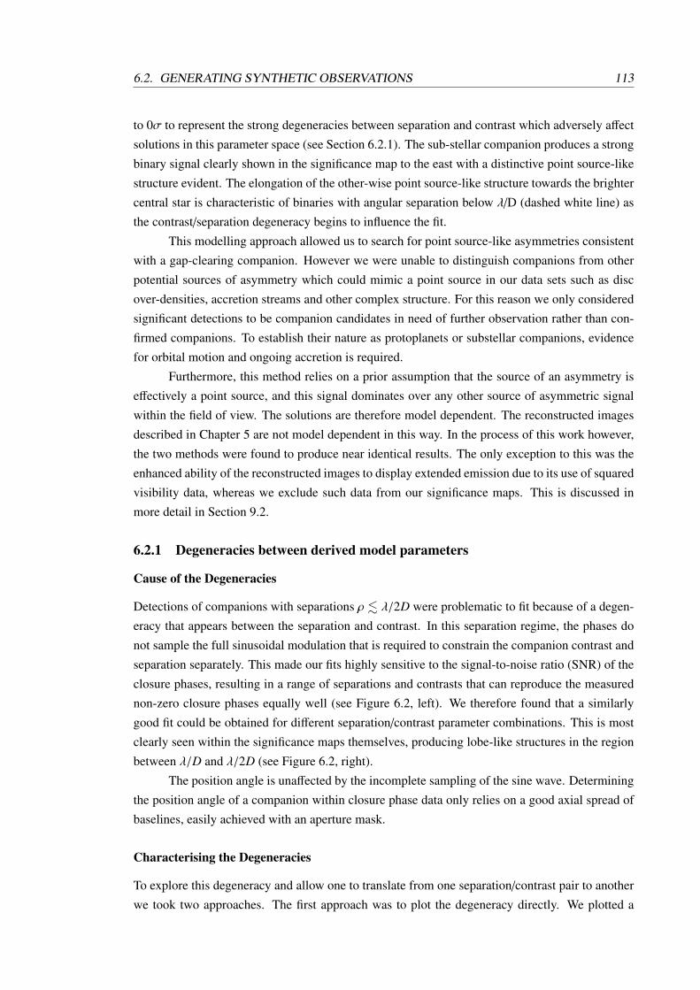
6.2. GENERATING SYNTHETIC OBSERVATIONS 113
to 0σ to represent the strong degeneracies between separation and contrast which adversely affect
solutions in this parameter space (see Section 6.2.1). The sub-stellar companion produces a strong
binary signal clearly shown in the significance map to the east with a distinctive point source-like
structure evident. The elongation of the other-wise point source-like structure towards the brighter
central star is characteristic of binaries with angular separation below λ/D (dashed white line) as
the contrast/separation degeneracy begins to influence the fit.
This modelling approach allowed us to search for point source-like asymmetries consistent
with a gap-clearing companion. However we were unable to distinguish companions from other
potential sources of asymmetry which could mimic a point source in our data sets such as disc
over-densities, accretion streams and other complex structure. For this reason we only considered
significant detections to be companion candidates in need of further observation rather than con-
firmed companions. To establish their nature as protoplanets or substellar companions, evidence
for orbital motion and ongoing accretion is required.
Furthermore, this method relies on a prior assumption that the source of an asymmetry is
effectively a point source, and this signal dominates over any other source of asymmetric signal
within the field of view. The solutions are therefore model dependent. The reconstructed images
described in Chapter 5 are not model dependent in this way. In the process of this work however,
the two methods were found to produce near identical results. The only exception to this was the
enhanced ability of the reconstructed images to display extended emission due to its use of squared
visibility data, whereas we exclude such data from our significance maps. This is discussed in
more detail in Section 9.2.
6.2.1 Degeneracies between derived model parameters
Cause of the Degeneracies
Detections of companions with separations ρ . λ/2D were problematic to fit because of a degen-
eracy that appears between the separation and contrast. In this separation regime, the phases do
not sample the full sinusoidal modulation that is required to constrain the companion contrast and
separation separately. This made our fits highly sensitive to the signal-to-noise ratio (SNR) of the
closure phases, resulting in a range of separations and contrasts that can reproduce the measured
non-zero closure phases equally well (see Figure 6.2, left). We therefore found that a similarly
good fit could be obtained for different separation/contrast parameter combinations. This is most
clearly seen within the significance maps themselves, producing lobe-like structures in the region
between λ/D and λ/2D (see Figure 6.2, right).
The position angle is unaffected by the incomplete sampling of the sine wave. Determining
the position angle of a companion within closure phase data only relies on a good axial spread of
baselines, easily achieved with an aperture mask.
Characterising the Degeneracies
To explore this degeneracy and allow one to translate from one separation/contrast pair to another
we took two approaches. The first approach was to plot the degeneracy directly. We plotted a
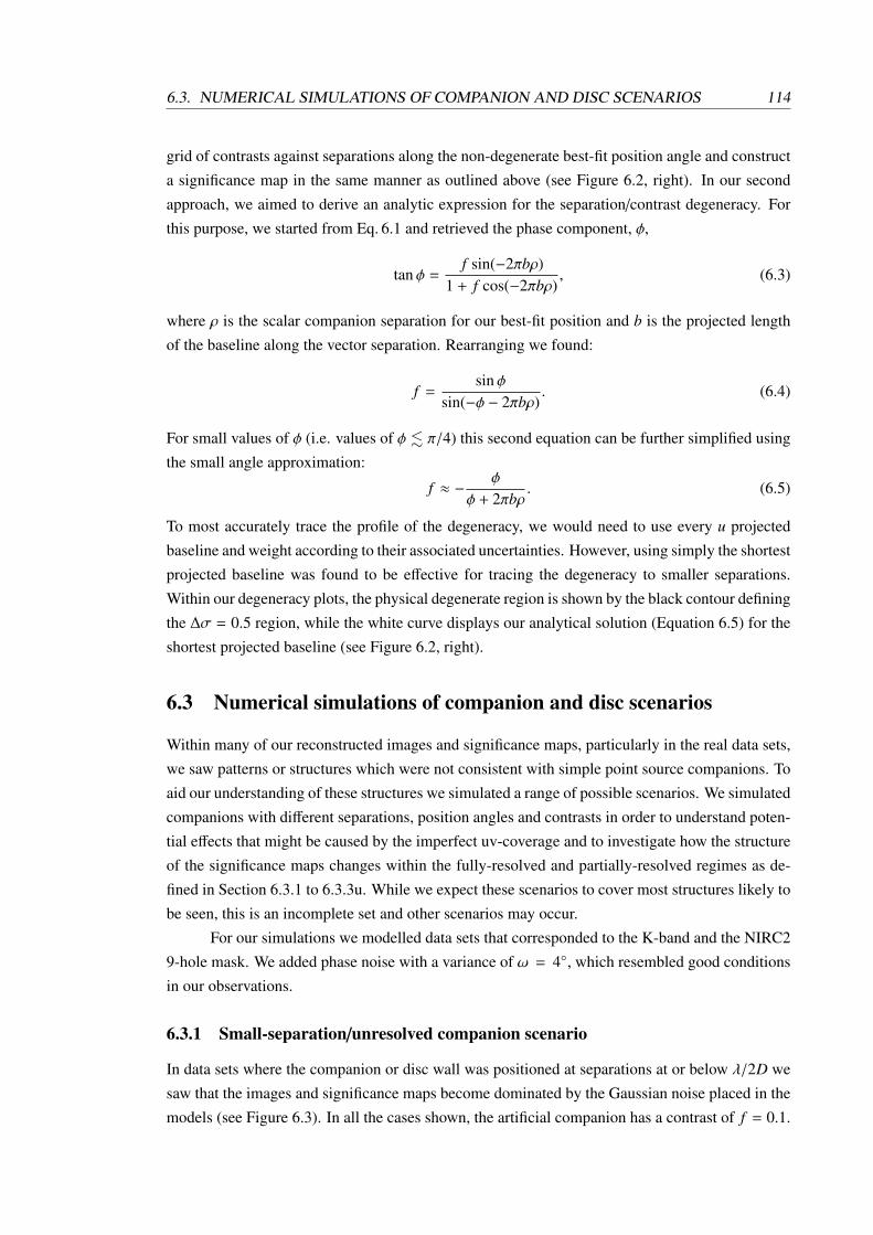
6.3. NUMERICAL SIMULATIONS OF COMPANION AND DISC SCENARIOS 114
grid of contrasts against separations along the non-degenerate best-fit position angle and construct
a significance map in the same manner as outlined above (see Figure 6.2, right). In our second
approach, we aimed to derive an analytic expression for the separation/contrast degeneracy. For
this purpose, we started from Eq. 6.1 and retrieved the phase component, φ,
tan φ =f sin(−2πbρ)
1 + f cos(−2πbρ), (6.3)
where ρ is the scalar companion separation for our best-fit position and b is the projected length
of the baseline along the vector separation. Rearranging we found:
f =sin φ
sin(−φ − 2πbρ). (6.4)
For small values of φ (i.e. values of φ . π/4) this second equation can be further simplified using
the small angle approximation:
f ≈ −φ
φ + 2πbρ. (6.5)
To most accurately trace the profile of the degeneracy, we would need to use every u projected
baseline and weight according to their associated uncertainties. However, using simply the shortest
projected baseline was found to be effective for tracing the degeneracy to smaller separations.
Within our degeneracy plots, the physical degenerate region is shown by the black contour defining
the ∆σ = 0.5 region, while the white curve displays our analytical solution (Equation 6.5) for the
shortest projected baseline (see Figure 6.2, right).
6.3 Numerical simulations of companion and disc scenarios
Within many of our reconstructed images and significance maps, particularly in the real data sets,
we saw patterns or structures which were not consistent with simple point source companions. To
aid our understanding of these structures we simulated a range of possible scenarios. We simulated
companions with different separations, position angles and contrasts in order to understand poten-
tial effects that might be caused by the imperfect uv-coverage and to investigate how the structure
of the significance maps changes within the fully-resolved and partially-resolved regimes as de-
fined in Section 6.3.1 to 6.3.3u. While we expect these scenarios to cover most structures likely to
be seen, this is an incomplete set and other scenarios may occur.
For our simulations we modelled data sets that corresponded to the K-band and the NIRC2
9-hole mask. We added phase noise with a variance of ω = 4, which resembled good conditions
in our observations.
6.3.1 Small-separation/unresolved companion scenario
In data sets where the companion or disc wall was positioned at separations at or below λ/2D we
saw that the images and significance maps become dominated by the Gaussian noise placed in the
models (see Figure 6.3). In all the cases shown, the artificial companion has a contrast of f = 0.1.
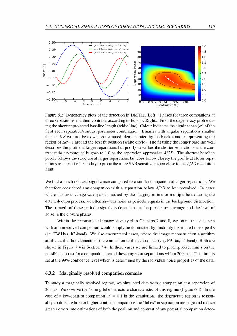
6.3. NUMERICAL SIMULATIONS OF COMPANION AND DISC SCENARIOS 115
8 6 4 2 0 2 4 6 8Baseline [m]
0.20
0.15
0.10
0.05
0.00
0.05
0.10
0.15
0.20Phase
[]
ρ = 26 mas, ∆MK = 6.3 mag
ρ = 39 mas, ∆MK = 6.7 mag
ρ = 52 mas, ∆MK = 7.0 mag
0.0 0.002 0.004 0.006 0.008Contrast (f2 /f1 )
0
10
20
30
40
50
60
70
80
90
Separa
tion (
mas)
0.0
0.5
1.0
1.5
2.0
2.5
3.0
3.5
4.0
4.5
5.0
Figure 6.2: Degeneracy plots of the detection in DM Tau. Left: Phases for three companions atthree separations and their contrasts according to Eq. 6.5. Right: Fit of the degeneracy profile us-ing the shortest projected baseline length (white line). Colour indicates the significance (σ) of thefit at each separation/contrast parameter combination. Binaries with angular separations smallerthan ∼ λ/B will not be as well constrained, demonstrated by the black contour representing theregion of ∆σ= 1 around the best fit position (white circle). The fit using the longer baseline welldescribes the profile at larger separations but poorly describes the shorter separations as the con-trast ratio asymptotically goes to 1.0 as the separation approaches λ/2D. The shortest baselinepoorly follows the structure at larger separations but does follow closely the profile at closer sepa-rations as a result of its ability to probe the more SNR sensitive region close to the λ/2D resolutionlimit.
We find a much reduced significance compared to a similar companion at larger separations. We
therefore considered any companion with a separation below λ/2D to be unresolved. In cases
where our uv-coverage was sparser, caused by the flagging of one or multiple holes during the
data reduction process, we often saw this noise as periodic signals in the background distribution.
The strength of these periodic signals is dependent on the precise uv-coverage and the level of
noise in the closure phases.
Within the reconstructed images displayed in Chapters 7 and 8, we found that data sets
with an unresolved companion would simply be dominated by randomly distributed noise peaks
(i.e. TW Hya, K’-band). We also encountered cases, where the image reconstruction algorithm
attributed the flux elements of the companion to the central star (e.g. FP Tau, L’-band). Both are
shown in Figure 7.4 in Section 7.4. In these cases we are limited to placing lower limits on the
possible contrast for a companion around these targets at separations within 200 mas. This limit is
set at the 99% confidence level which is determined by the individual noise properties of the data.
6.3.2 Marginally resolved companion scenario
To study a marginally resolved regime, we simulated data with a companion at a separation of
30 mas. We observe the ”strong lobe” structure characteristic of this regime (Figure 6.4). In the
case of a low-contrast companion ( f = 0.1 in the simulation), the degenerate region is reason-
ably confined, while for higher-contrast companions the ”lobes” in separation are large and induce
greater errors into estimations of both the position and contrast of any potential companion detec-
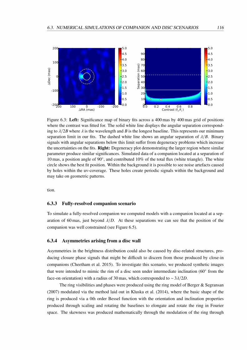
6.3. NUMERICAL SIMULATIONS OF COMPANION AND DISC SCENARIOS 116
200 100 0 -100 -200∆RA (mas)
-200
-100
0
100
200∆
Dec
(mas)
0.0
0.5
1.0
1.5
2.0
2.5
3.0
3.5
4.0
4.5
5.0
0.0 0.2 0.4 0.6 0.8Contrast (f2 /f1 )
0
10
20
30
40
50
60
70
80
90
Separa
tion (
mas)
0.0
0.5
1.0
1.5
2.0
2.5
3.0
3.5
4.0
4.5
5.0
Figure 6.3: Left: Significance map of binary fits across a 400 mas by 400 mas grid of positionswhere the contrast was fitted for. The solid white line displays the angular separation correspond-ing to λ/2B where λ is the wavelength and B is the longest baseline. This represents our minimumseparation limit in our fits. The dashed white line shows an angular separation of λ/B. Binarysignals with angular separations below this limit suffer from degeneracy problems which increasethe uncertainties on the fits. Right: Degeneracy plot demonstrating the larger region where similarparameter produce similar significances. Simulated data of a companion located at a separation of10 mas, a position angle of 90, and contributed 10% of the total flux (white triangle). The whitecircle shows the best fit position. Within the background it is possible to see noise artefacts causedby holes within the uv-coverage. These holes create periodic signals within the background andmay take on geometric patterns.
tion.
6.3.3 Fully-resolved companion scenario
To simulate a fully-resolved companion we computed models with a companion located at a sep-
aration of 60 mas, just beyond λ/D. At these separations we can see that the position of the
companion was well constrained (see Figure 6.5).
6.3.4 Asymmetries arising from a disc wall
Asymmetries in the brightness distribution could also be caused by disc-related structures, pro-
ducing closure phase signals that might be difficult to discern from those produced by close-in
companions (Cheetham et al. 2015). To investigate this scenario, we produced synthetic images
that were intended to mimic the rim of a disc seen under intermediate inclination (60 from the
face-on orientation) with a radius of 30 mas, which corresponded to ∼ 3λ/2D.
The ring visibilities and phases were produced using the ring model of Berger & Segransan
(2007) modulated via the method laid out in Kluska et al. (2014), where the basic shape of the
ring is produced via a 0th order Bessel function with the orientation and inclination properties
produced through scaling and rotating the baselines to elongate and rotate the ring in Fourier
space. The skewness was produced mathematically through the modulation of the ring through
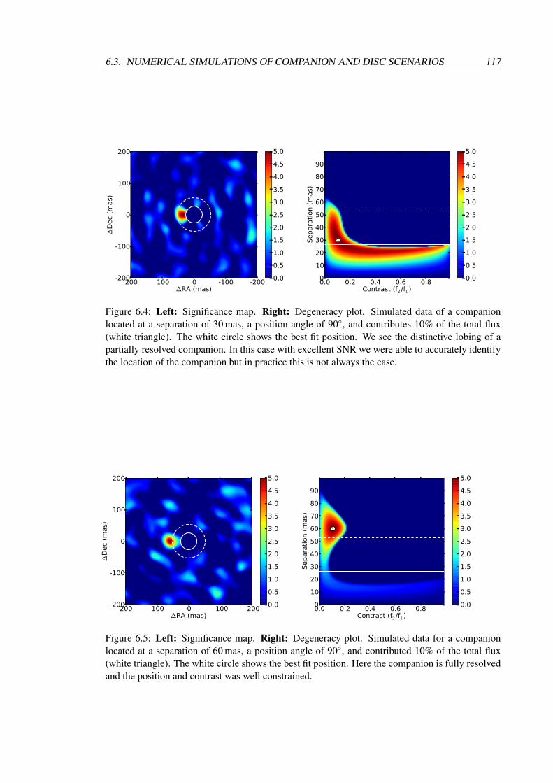
6.3. NUMERICAL SIMULATIONS OF COMPANION AND DISC SCENARIOS 117
200 100 0 -100 -200∆RA (mas)
-200
-100
0
100
200
∆D
ec
(mas)
0.0
0.5
1.0
1.5
2.0
2.5
3.0
3.5
4.0
4.5
5.0
0.0 0.2 0.4 0.6 0.8Contrast (f2 /f1 )
0
10
20
30
40
50
60
70
80
90
Separa
tion (
mas)
0.0
0.5
1.0
1.5
2.0
2.5
3.0
3.5
4.0
4.5
5.0
Figure 6.4: Left: Significance map. Right: Degeneracy plot. Simulated data of a companionlocated at a separation of 30 mas, a position angle of 90, and contributes 10% of the total flux(white triangle). The white circle shows the best fit position. We see the distinctive lobing of apartially resolved companion. In this case with excellent SNR we were able to accurately identifythe location of the companion but in practice this is not always the case.
200 100 0 -100 -200∆RA (mas)
-200
-100
0
100
200
∆D
ec
(mas)
0.0
0.5
1.0
1.5
2.0
2.5
3.0
3.5
4.0
4.5
5.0
0.0 0.2 0.4 0.6 0.8Contrast (f2 /f1 )
0
10
20
30
40
50
60
70
80
90
Separa
tion (
mas)
0.0
0.5
1.0
1.5
2.0
2.5
3.0
3.5
4.0
4.5
5.0
Figure 6.5: Left: Significance map. Right: Degeneracy plot. Simulated data for a companionlocated at a separation of 60 mas, a position angle of 90, and contributed 10% of the total flux(white triangle). The white circle shows the best fit position. Here the companion is fully resolvedand the position and contrast was well constrained.
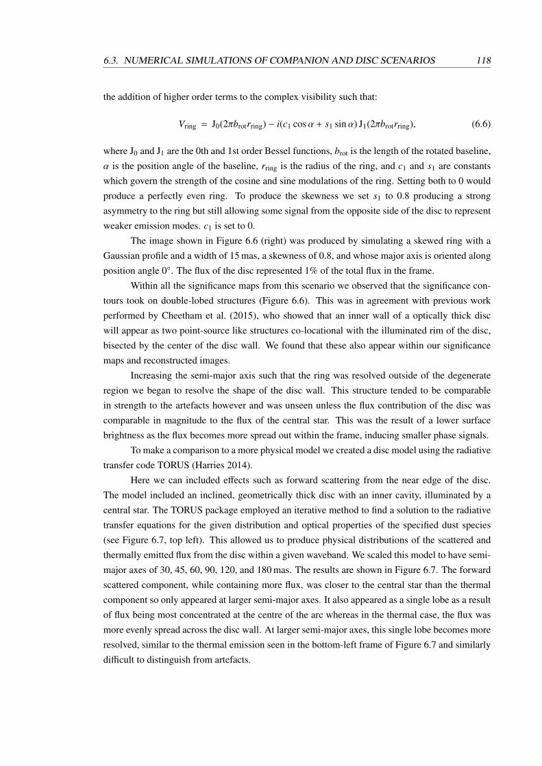
6.3. NUMERICAL SIMULATIONS OF COMPANION AND DISC SCENARIOS 118
the addition of higher order terms to the complex visibility such that:
Vring = J0(2πbrotrring) − i(c1 cosα + s1 sinα) J1(2πbrotrring), (6.6)
where J0 and J1 are the 0th and 1st order Bessel functions, brot is the length of the rotated baseline,
α is the position angle of the baseline, rring is the radius of the ring, and c1 and s1 are constants
which govern the strength of the cosine and sine modulations of the ring. Setting both to 0 would
produce a perfectly even ring. To produce the skewness we set s1 to 0.8 producing a strong
asymmetry to the ring but still allowing some signal from the opposite side of the disc to represent
weaker emission modes. c1 is set to 0.
The image shown in Figure 6.6 (right) was produced by simulating a skewed ring with a
Gaussian profile and a width of 15 mas, a skewness of 0.8, and whose major axis is oriented along
position angle 0. The flux of the disc represented 1% of the total flux in the frame.
Within all the significance maps from this scenario we observed that the significance con-
tours took on double-lobed structures (Figure 6.6). This was in agreement with previous work
performed by Cheetham et al. (2015), who showed that an inner wall of a optically thick disc
will appear as two point-source like structures co-locational with the illuminated rim of the disc,
bisected by the center of the disc wall. We found that these also appear within our significance
maps and reconstructed images.
Increasing the semi-major axis such that the ring was resolved outside of the degenerate
region we began to resolve the shape of the disc wall. This structure tended to be comparable
in strength to the artefacts however and was unseen unless the flux contribution of the disc was
comparable in magnitude to the flux of the central star. This was the result of a lower surface
brightness as the flux becomes more spread out within the frame, inducing smaller phase signals.
To make a comparison to a more physical model we created a disc model using the radiative
transfer code TORUS (Harries 2014).
Here we can included effects such as forward scattering from the near edge of the disc.
The model included an inclined, geometrically thick disc with an inner cavity, illuminated by a
central star. The TORUS package employed an iterative method to find a solution to the radiative
transfer equations for the given distribution and optical properties of the specified dust species
(see Figure 6.7, top left). This allowed us to produce physical distributions of the scattered and
thermally emitted flux from the disc within a given waveband. We scaled this model to have semi-
major axes of 30, 45, 60, 90, 120, and 180 mas. The results are shown in Figure 6.7. The forward
scattered component, while containing more flux, was closer to the central star than the thermal
component so only appeared at larger semi-major axes. It also appeared as a single lobe as a result
of flux being most concentrated at the centre of the arc whereas in the thermal case, the flux was
more evenly spread across the disc wall. At larger semi-major axes, this single lobe becomes more
resolved, similar to the thermal emission seen in the bottom-left frame of Figure 6.7 and similarly
difficult to distinguish from artefacts.
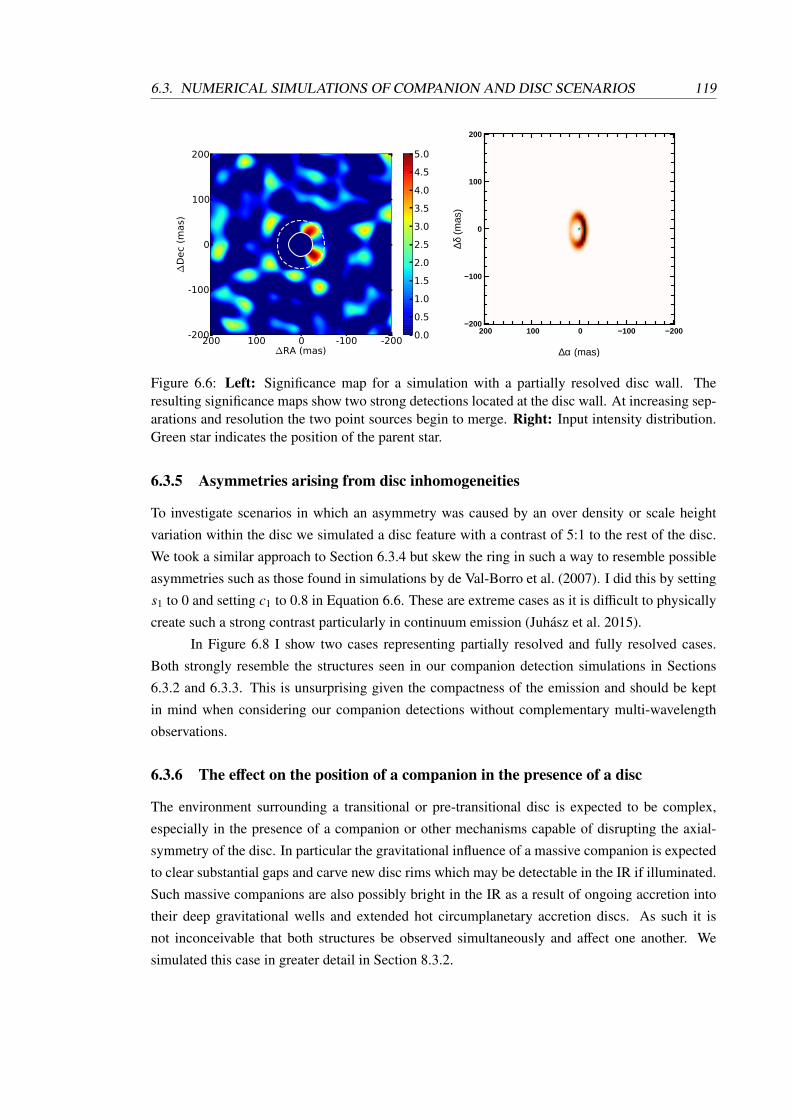
6.3. NUMERICAL SIMULATIONS OF COMPANION AND DISC SCENARIOS 119
200 100 0 -100 -200∆RA (mas)
-200
-100
0
100
200
∆D
ec
(mas)
0.0
0.5
1.0
1.5
2.0
2.5
3.0
3.5
4.0
4.5
5.0
−200−100 0 100 200−200
−100
0
100
200
∆α (mas)
∆δ (
mas
)
Figure 6.6: Left: Significance map for a simulation with a partially resolved disc wall. Theresulting significance maps show two strong detections located at the disc wall. At increasing sep-arations and resolution the two point sources begin to merge. Right: Input intensity distribution.Green star indicates the position of the parent star.
6.3.5 Asymmetries arising from disc inhomogeneities
To investigate scenarios in which an asymmetry was caused by an over density or scale height
variation within the disc we simulated a disc feature with a contrast of 5:1 to the rest of the disc.
We took a similar approach to Section 6.3.4 but skew the ring in such a way to resemble possible
asymmetries such as those found in simulations by de Val-Borro et al. (2007). I did this by setting
s1 to 0 and setting c1 to 0.8 in Equation 6.6. These are extreme cases as it is difficult to physically
create such a strong contrast particularly in continuum emission (Juhasz et al. 2015).
In Figure 6.8 I show two cases representing partially resolved and fully resolved cases.
Both strongly resemble the structures seen in our companion detection simulations in Sections
6.3.2 and 6.3.3. This is unsurprising given the compactness of the emission and should be kept
in mind when considering our companion detections without complementary multi-wavelength
observations.
6.3.6 The effect on the position of a companion in the presence of a disc
The environment surrounding a transitional or pre-transitional disc is expected to be complex,
especially in the presence of a companion or other mechanisms capable of disrupting the axial-
symmetry of the disc. In particular the gravitational influence of a massive companion is expected
to clear substantial gaps and carve new disc rims which may be detectable in the IR if illuminated.
Such massive companions are also possibly bright in the IR as a result of ongoing accretion into
their deep gravitational wells and extended hot circumplanetary accretion discs. As such it is
not inconceivable that both structures be observed simultaneously and affect one another. We
simulated this case in greater detail in Section 8.3.2.
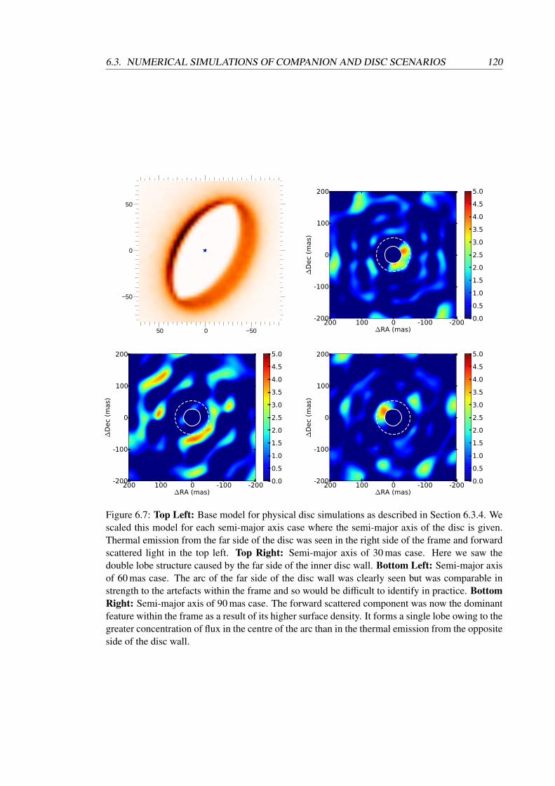
6.3. NUMERICAL SIMULATIONS OF COMPANION AND DISC SCENARIOS 120
−50 0 50
−50
0
50
200 100 0 -100 -200∆RA (mas)
-200
-100
0
100
200
∆D
ec
(mas)
0.0
0.5
1.0
1.5
2.0
2.5
3.0
3.5
4.0
4.5
5.0
200 100 0 -100 -200∆RA (mas)
-200
-100
0
100
200
∆D
ec
(mas)
0.0
0.5
1.0
1.5
2.0
2.5
3.0
3.5
4.0
4.5
5.0
200 100 0 -100 -200∆RA (mas)
-200
-100
0
100
200
∆D
ec
(mas)
0.0
0.5
1.0
1.5
2.0
2.5
3.0
3.5
4.0
4.5
5.0
Figure 6.7: Top Left: Base model for physical disc simulations as described in Section 6.3.4. Wescaled this model for each semi-major axis case where the semi-major axis of the disc is given.Thermal emission from the far side of the disc was seen in the right side of the frame and forwardscattered light in the top left. Top Right: Semi-major axis of 30 mas case. Here we saw thedouble lobe structure caused by the far side of the inner disc wall. Bottom Left: Semi-major axisof 60 mas case. The arc of the far side of the disc wall was clearly seen but was comparable instrength to the artefacts within the frame and so would be difficult to identify in practice. BottomRight: Semi-major axis of 90 mas case. The forward scattered component was now the dominantfeature within the frame as a result of its higher surface density. It forms a single lobe owing to thegreater concentration of flux in the centre of the arc than in the thermal emission from the oppositeside of the disc wall.
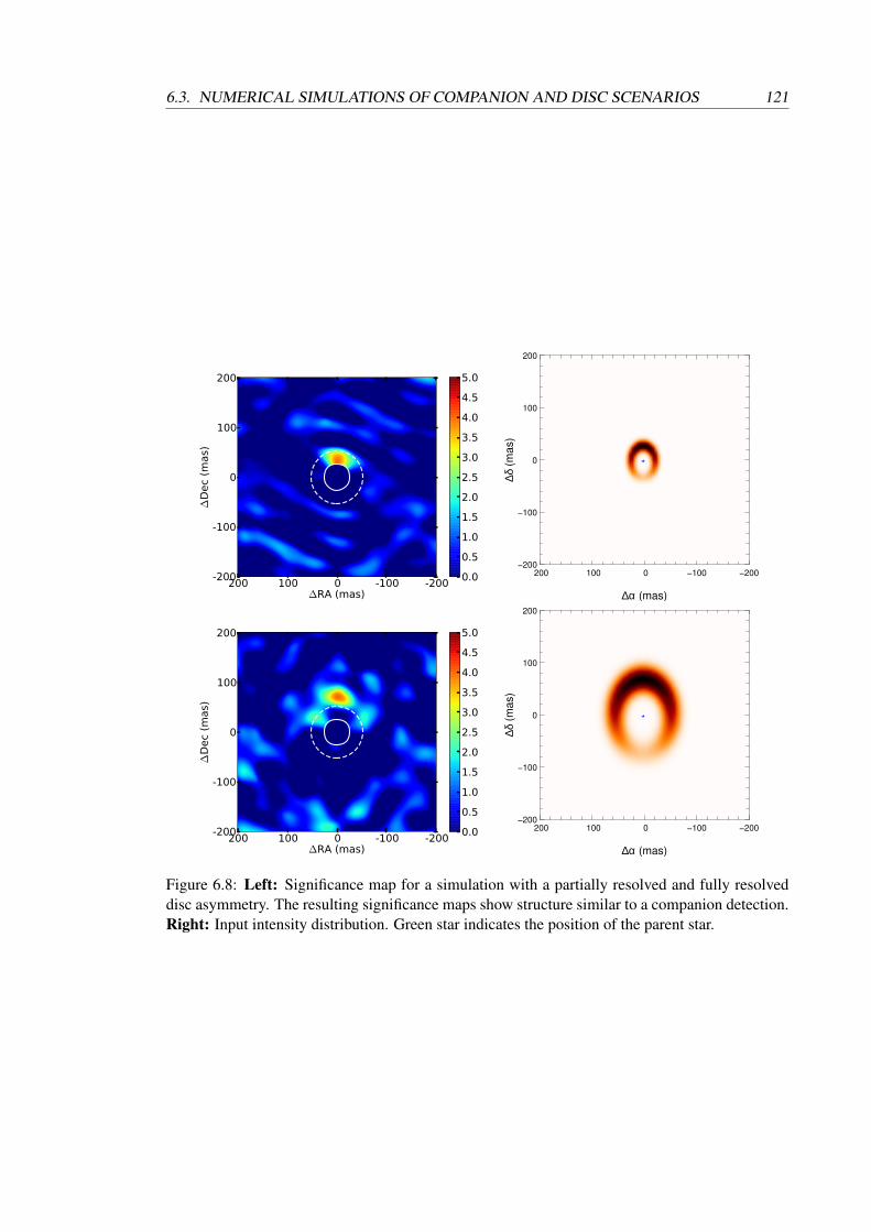
6.3. NUMERICAL SIMULATIONS OF COMPANION AND DISC SCENARIOS 121
200 100 0 -100 -200∆RA (mas)
-200
-100
0
100
200
∆D
ec
(mas)
0.0
0.5
1.0
1.5
2.0
2.5
3.0
3.5
4.0
4.5
5.0
−200−100 0 100 200−200
−100
0
100
200
∆α (mas)
∆δ (
ma
s)
200 100 0 -100 -200∆RA (mas)
-200
-100
0
100
200
∆D
ec
(mas)
0.0
0.5
1.0
1.5
2.0
2.5
3.0
3.5
4.0
4.5
5.0
−200−100 0 100 200−200
−100
0
100
200
∆α (mas)
∆δ (
ma
s)
Figure 6.8: Left: Significance map for a simulation with a partially resolved and fully resolveddisc asymmetry. The resulting significance maps show structure similar to a companion detection.Right: Input intensity distribution. Green star indicates the position of the parent star.

6.4. SUMMARY 122
6.4 Summary
In this Chapter I simulated and discussed a number of possible observable scenarios. These include
the case of a binary configurations with differing angular separations, both scattering and thermal
emission from a disc rim, and other disc asymmetries.
The results of simulating binary scenarios with differing angular separations in Sections 6.3.1,
6.3.2, and 6.3.3 primarily showed that a companion within the angular separation defined by the
conventional diffraction limit of the telescope as based on the Rayleigh criterion, ∼ λ/D, will
produce a distinctive lobed structure rather than appear more point source-like. The cause of this
effect was found to be the poor phase sampling of the sine wave signal produced by a companion.
The result was to produce a degeneracy where a range of angular separations and contrasts pro-
duce approximately equally good fits. An analytic description of this degeneracy was presented in
Section 6.2.1. The ability of the fitting algorithm to find the ’true’ angular separation and contrast
is then highly dependent on the SNR of the phases and is in effect the new resolution limit of the
SAM array. Already a moderate SNR allows one to reach below the formal resolution limit of a
conventional telescope of the same size, ∼ λ/D but uncertainties remain high due to the degener-
acy. In principle however detections below even this resolution limit are possible for a sufficiently
bright companion.
The results of our disc rim simulations (see Section 6.3.4) closely matched those of previous
work done on the subject where the extended emission from a thermally heated disc rim resembles
that of a pair of point sources (Cheetham et al. 2015). I used TORUS to simulate a physical disc rim
model which includes a scattered component as in Cieza et al. (2013) and study for the first time
systematically how the interferometric signal depends on the disc parameters. The scattered light
component was found to be more prominent in the resultant significance maps and reconstructed
images as the flux was more concentrated than in the predominantly thermal component from the
opposite side of the disc. This concentrated forward scattered component was found to mimic a
companion signal within the degenerate region between angular separations of ∼ λ/2D to ∼ λ/D.
Outside this region the more extended nature of the scattering was revealed as the ability to resolve
structure improves. The same was true for the thermal side of the disc although it was important
to remember that the closure phases are sensitive to asymmetric signals so a scenario where flux
is present on opposite sides will reduce the strength of the signal, producing a dependence on
inclination for detection. Observing a disc rim, either thermal or through scattering, likely requires
the observed disc to be moderately inclined, and so may be very challenging to observe in practice.
In a similar manner to how we made geometric models of the thermal emission from a far
disc rim, we model a disc inhomogeneity as a skewed ring. We found this to also resemble a
companion signal, even at larger angular separations. We found however that the amount of flux
within the inhomogeneity needs to be very high to be detectable therefore implying that only the
most extreme disc asymmetries are likely to be detectable in this way.

Chapter 7
Keck-II/NIRC2 Pre-Transitional DiskSurvey
This chapter contains work published in Willson et al. (2016).
7.1 Context
During the earliest stages of their lives, planetary cores are highly challenging to detect as they are
deeply embedded within the dusty material of their parent discs. However, once they have gained
sufficient mass to clear a gap (at the transitional or pre-transitional disc stage) they become acces-
sible to high resolution imaging observations. This phase likely coincides with the hydrodynamic
collapse and oligarchic growth of proto-Jupiters and proto-brown dwarfs and is likely associated
with the formation of an extended, hot circumplanetary disc that feeds material onto the accreting
core (Pollack et al. 1996; Ayliffe & Bate 2012). Once protoplanetary cores have cleared most
of their immediate disc environment, they can continue to accrete significant amounts of mass
from material flowing through the gap (10−9 Myr−1, Najita et al. 2007; Varniere et al. 2006b).
Therefore, it is expected that protoplanets would appear as strong NIR sources within cleared gap
regions.
Spatially resolving such systems proves a challenge due to the close angular separation
between the protoplanets and their parent stars and that the parent star is likely to be substantially
brighter than even a rapidly accreting protoplanet. Spatially resolved evidence for protoplanetary
companions could only be obtained for a small sample of objects so far: Coronagraphic imaging
has revealed ring-like and spiral-like structures on scales of 50-200 au (e.g. Subaru/SEEDS survey;
Hashimoto et al. 2011; Grady et al. 2013) and sparse aperture masking interferometry (SAM) has
resulted in the detection of small-scale asymmetries in the brightness distribution around young
stars that have been interpreted as low-mass companions (T Cha: Huelamo et al. 2011; LkCa 15:
Kraus & Ireland 2012; HD 142527: Biller et al. 2012) or as disc emission of a heated wall in
a centro-symmetric disc seen under intermediate inclination (FL Cha: Cieza et al. 2013; T Cha:
Olofsson et al. 2013). Only in the cases of LkCa 15 and HD 142527 has this continuum detection
been confirmed as an accreting companion, with subsequent observations using a combination of
123
7.2. TARGET SELECTION 124
SAM and Hα spectral differential imaging performed by Sallum et al. (2015b) to demonstrate for
the first time unambiguous evidence for the accreting nature of the companion.
Besides the emission associated with the protoplanets themselves and their associated cir-
cumplanetary discs, asymmetries can also be caused by dynamically-induced disc features such
as spiral arms, disc warps (Alencar et al. 2010; Muzerolle et al. 2009), or disc physics-related
processes such as gravitational instabilities, and density waves (Bouvier et al. 2007). Addition-
ally a highly inclined disc can induce strong asymmetries in an axial-symmetric disc owing to
forward-scattered light from the illuminated inner rim of disc (Olofsson et al. 2013; Cheetham
et al. 2015).
Most of the evidence for these larger-scale structures comes from photometric or spectro-
scopic monitoring investigations. For instance, it was found that the variability shows an anti-
correlated behaviour at NIR and MIR wavelengths. In order to explain both the timescale and
spectral behaviour of the variability, Espaillat et al. (2011) proposed shadowing effects from co-
rotating disc warps at the inner dust rim triggered by orbiting planets. Such warps are also pre-
dicted by hydrodynamic simulations of discs with embedded planets (e.g. Fouchet et al. 2010) and
would result in a highly asymmetric brightness distribution. The warp emission will be extended
and more complex in geometry than a companion point source.
In this Chapter I present the results of our survey of a number of transitional and pre-
transitional discs with the aim of detecting companions in their gaps or the distortion of the disc
due to the presence of a companion.
7.2 Target selection
The target sample was developed through searching the literature for known transitional and pre-
transitional discs. Highest priority was then given to the brightest objects. Amongst the remaining
target list were objects such as LkCa 15 which were already the subjects of SAM observing cam-
paigns of our collaborators so were excluded from our survey. The preference for bright objects is
motivated by the need for high throughput through the mask to achieve workable SNRs.
7.3 Observations
Our high-angular resolution observations were conducted using the NIRC2 instrument at the 10m
Keck-II telescope located on the summit of Mauna Kea on Hawaii (Table 7.1). We employed the
sparse aperture masking technique, which allows us to remove atmospheric phase noise through
the use of the closure phase technique (see Section 4.3.2). We employed the nine hole mask on
NIRC2 (see Figure 4.8), which offers a good compromise between sensitivity and uv-coverage.
The chosen wavebands were H, K’ and L’ band filters as we expect an accreting companion to
emit strongly in these bands. A list of our target stars can be found in Table 7.2.
Our data set was obtained during five nights between January 2012 and June 2014 (Table
7.1). The observations on the night of 09/06/14 was performed by myself and J. Monnier. Ob-
servations of most targets span a single epoch with the K’ filter (2.124±0.351µm) to search for

7.3. OBSERVATIONS 125
Table 7.1: Log for our Keck/NIRC2 observationsTarget Filter Date Nvisits On-Sky Rot Calibrator
[dd/mm/yy] []DM Tau K’ 08/01/12 3 1 HD 285938FP Tau K’ 20/10/13 3 24 HD 283420, HD 283477
L’ 20/10/13 2 63 HD 283420, HD 283477LkHα 330 CH4s 16/11/13 3 32 HD 22781, HD 281309
K’ 08/01/12 3 18 HD 22781, HD 2813092M034+3304, 2M0400+3311
RXJ1615.3-3255 K’ 09/06/14 4 15 HD 146569, HD 146593,HD 148806
RXJ1842.9-3532 K’ 09/06/14 5 13 HD 171450, HD 171574,HD 176999
TW Hya K’ 08/01/12 3 8 HD 94542, HD 95105K’ 10/01/12 3 11 HD 94542, HD 95105,
HD 97507V2062 Oph K’ 09/06/14 5 16 HD 147681, HD 148212,
HD 148562V2246 Oph K’ 09/06/14 1 2 HD 147742, HD 148352
direct emission from any close protoplanetary candidates. We observed FP Tau and LkHα 330
again during the same epoch but in additional wavebands, L’ (3.776±0.700µm) and H (CH4s;
1.633±0.330µm) respectively. We obtain an additional observation in the same epoch in the case
of TW Hya.
The NIRC2 data were reduced using the data reduction pipeline previous implemented in
Ireland & Kraus (2008), Kraus & Ireland (2012), and Kraus et al. (2013), providing calibrated
closure phases.
In order to record the instrument transfer function, we bracketed the science star obser-
vations with observations of unresolved calibrators. We aimed to alternate between two (ideally
three) different calibrator stars, which allows us to still calibrate our data even if a calibrator is
found to be a previously unknown binary. A calibrator with spatially resolved structure will in-
duce erroneous phase signals in our data, masking any companion signal or inducing a false signal.
We test for multiplicity in our calibrators by calibrating them against each other. In the cases where
we have three calibrators we can identify which calibrator is the binary, by fitting a binary model.
In this way we find a 5σ binary signal in HD 95105 during the observations of TW Hya
on 2012-01-10. The significance maps for the two observations are shown in Figure 7.1. We ad-
ditionally observed this calibrator on in the same epoch on 2012-01-08 and observed a potential
companion towards a similar position angle, although substantially weaker than during the first
night at 3.5σ. The position angle for both nights was found to be 219±2 while the fitted separa-
tions were 113±4 mas and 91±3 mas on the first and second night, and the contrasts were found to
vary between 5.4±0.3 mag and 3.0±0.2 mag over the first and second nights respectively. Includ-
ing HD 95105 in the data reduction produced a strong asymmetry in both TW Hya datasets at a
position angle of approximately ∆PA = 180 with an identical separation, leading to the conclusion
this was likely caused by the asymmetric signal in the calibrator.

7.3. OBSERVATIONS 126
Tabl
e7.
2:Ta
rget
list
Nam
eA
ssoc
iatio
nD
ista
nce
Spec
Type
Av
Tef
fM∗
L∗
R∗
Ref
eren
ces
[pc]
[K]
[M
][L
][R
]D
MTa
uTa
urus
140
M1
0.0
3705
0.47
0.37
1.3
6,8
FPTa
uTa
urus
140
M5
0.3
3125
0.22
0.62
2.5
6,8
LkHα
330
Pers
eus
250
G3
1.8
5830
1.25
2.78
1.5
2,5
RX
J161
5.3-
3255
Oph
185
K4
1.00
4590
1.28
1.01
1.59
11,1
3R
XJ1
842.
9-35
32C
rA13
6K
21.
149
001.
331.
291.
514
,15
TW
Hya
TW
Hya
56M
01.
038
500.
570.
641.
73,
12V
2062
Oph
Oph
125
K3
2.3
4730
1.4
1.3
1.7
1V
2246
Oph
Oph
121.
9K
06.
250
162.
220
.5—
10,1
,4,7
Col
umn
1:Ta
rget
;Col
umn
2:A
ssoc
iatio
n;C
olum
n3:
Dis
tanc
e;C
olum
n4:
Spec
tral
Type
;Col
umn
5:V
isua
lExt
inct
ion;
Col
umn
6:E
ffec
tive
Tem
pera
ture
;C
olum
n7:
Stel
larM
ass;
Col
umn
8:St
ella
rLum
inos
ity;C
olum
n9:
Stel
larR
adiu
s;C
olum
n10
:Lite
ratu
reR
efer
ence
s:(1
)Bou
vier
&A
ppen
zelle
r(19
92),
(2)B
row
net
al.(
2009
),(3
)Cal
vete
tal.
(200
4),(
4)C
hen
etal
.(19
95),
(5)F
erna
ndez
etal
.(19
95),
(6)F
urla
net
al.(
2006
),(7
)Jen
sen
etal
.(20
09),
(8)
Ken
yon
etal
.(19
98),
(9)K
raus
etal
.(20
13),
(10)
Loi
nard
etal
.(20
08),
(11)
Mer
ınet
al.(
2010
),(1
2)R
eipu
rth
etal
.(19
96),
(13)
And
rew
set
al.(
2011
b),
(14)
Silv
erst
one
etal
.(20
06),
(15)
Whi
teet
al.(
2007
)

7.4. RESULTS 127
200 100 0 -100 -200∆RA (mas)
-200
-100
0
100
200
∆D
ec
(mas)
0.0
0.5
1.0
1.5
2.0
2.5
3.0
3.5
4.0
4.5
5.0
200 100 0 -100 -200∆RA (mas)
-200
-100
0
100
200
∆D
ec
(mas)
0.0
0.5
1.0
1.5
2.0
2.5
3.0
3.5
4.0
4.5
5.0
Figure 7.1: Left: 08/01/2012 K-band observation of the calibrator target, HD 95105 Right:10/01/2012 K-band observation of the calibrator target, HD 95105. The asymmetry possessesconsistent position angles across the two night but displays significant radial motion (>3 standarddeviations). As a precaution this calibrator was removed from the data reduction process.
Therefore we remove this calibrator from the data reduction as a precaution. The result was
significant shift in the position of the best fit position in the binary fit.
Our observations represent ”snapshots” of the targets with often little field rotation. This
means that we are likely to suffer from hole aliasing problems creating strong artefacts in recon-
structed images and significance maps. For this reason we only consider the most significant fit
in the follow sections and do not discuss apparent additional asymmetric signals without comple-
mentary observations as in Chapter 8 when discussing the case of V1247 Ori.
As a diagnostic for identifying data sets adversely affected by degenerating factors such
as short coherence times and vibration in the optical system, we plotted histograms of the raw
closure phase measurements of the individual interferograms. We fit Gaussians to the closure
phase distribution and derive the variance ω. For the calibrator stars, ω provides a measure for the
residual phase noise as these point sources should not exhibit an intrinsic non-zero phase signal.
We list the measured variances in Table 7.3. The high variability seen in the L’-band observations
is related to the misalignment of the IR dichroic which has since been corrected (M. Ireland,
private communication).
We note consistently larger ω values for targets observed on 09/06/2014, and for the ob-
servation of TW Hya taken on 10/01/2012. These data sets were observed under adverse seeing
conditions as recorded by the telemetry from the nights, leading to lower sensitivities and erro-
neous structures as discussed in more detail in Section 7.4.
7.4 Results
We identify potential companion candidates through a combination of setting a threshold on the
significance of the binary fit and inspection of reconstructed images and significance maps. The
method for determining whether a detection is significant or not is described in Section 7.4.1. In
Table 7.4 we list data sets in which we find significant closure phase asymmetries excluding false
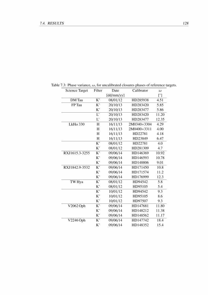
7.4. RESULTS 128
Table 7.3: Phase variance, ω, for uncalibrated closures phases of reference targets.Science Target Filter Date Calibrator ω
[dd/mm/yy] []DM Tau K’ 08/01/12 HD285938 4.51FP Tau K’ 20/10/13 HD283420 5.85
K’ 20/10/13 HD283477 5.86L’ 20/10/13 HD283420 11.20L’ 20/10/13 HD283477 12.35
LkHα 330 H 16/11/13 2M0340+3304 4.29H 16/11/13 2M0400+3311 4.00H 16/11/13 HD22781 4.18H 16/11/13 HD23849 6.47K’ 08/01/12 HD22781 4.0K’ 08/01/12 HD281309 4.7
RXJ1615.3-3255 K’ 09/06/14 HD146369 10.92K’ 09/06/14 HD146593 10.78K’ 09/06/14 HD148806 9.01
RXJ1842.9-3532 K’ 09/06/14 HD171450 10.8K’ 09/06/14 HD171574 11.2K’ 09/06/14 HD176999 12.3
TW Hya K’ 08/01/12 HD94542 5.8K’ 08/01/12 HD95105 5.4K’ 10/01/12 HD94542 9.3K’ 10/01/12 HD95105 8.6K’ 10/01/12 HD97507 9.3
V2062 Oph K’ 09/06/14 HD147681 11.80K’ 09/06/14 HD148212 11.38K’ 09/06/14 HD148562 11.17
V2246 Oph K’ 09/06/14 HD147742 18.4K’ 09/06/14 HD148352 15.4
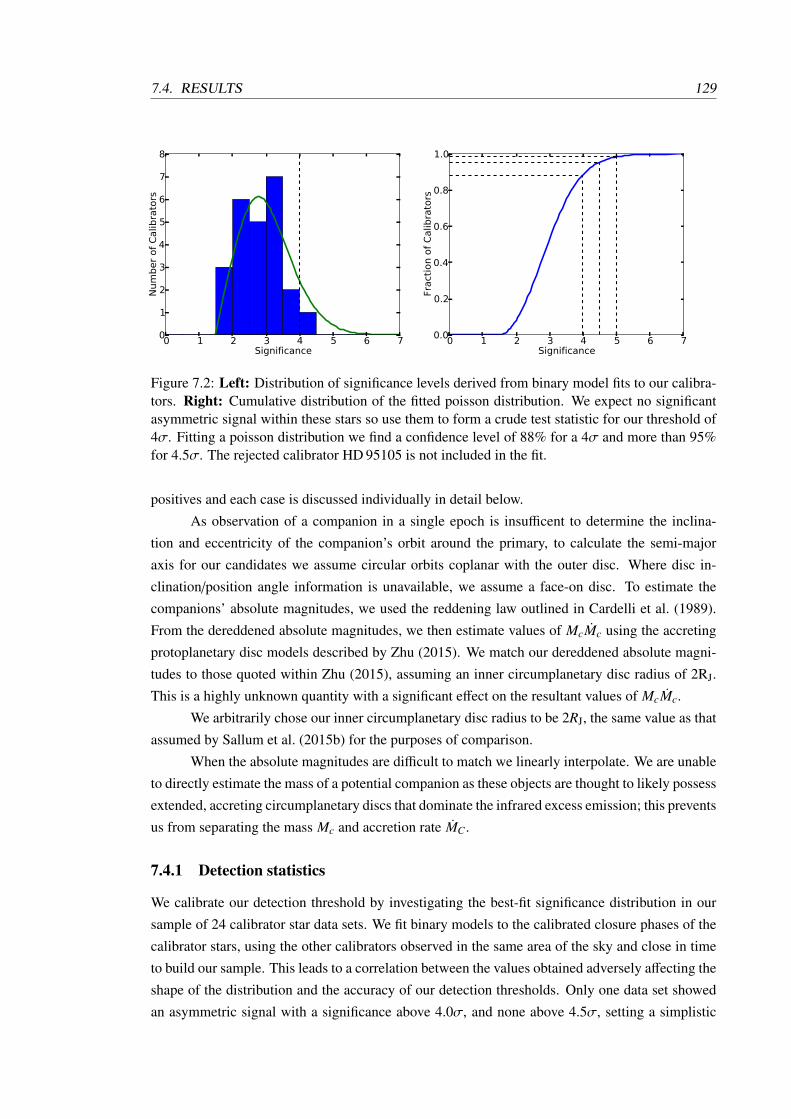
7.4. RESULTS 129
0 1 2 3 4 5 6 7Significance
0
1
2
3
4
5
6
7
8N
um
ber
of
Calib
rato
rs
0 1 2 3 4 5 6 7Significance
0.0
0.2
0.4
0.6
0.8
1.0
Fract
ion o
f C
alib
rato
rs
Figure 7.2: Left: Distribution of significance levels derived from binary model fits to our calibra-tors. Right: Cumulative distribution of the fitted poisson distribution. We expect no significantasymmetric signal within these stars so use them to form a crude test statistic for our threshold of4σ. Fitting a poisson distribution we find a confidence level of 88% for a 4σ and more than 95%for 4.5σ. The rejected calibrator HD 95105 is not included in the fit.
positives and each case is discussed individually in detail below.
As observation of a companion in a single epoch is insufficent to determine the inclina-
tion and eccentricity of the companion’s orbit around the primary, to calculate the semi-major
axis for our candidates we assume circular orbits coplanar with the outer disc. Where disc in-
clination/position angle information is unavailable, we assume a face-on disc. To estimate the
companions’ absolute magnitudes, we used the reddening law outlined in Cardelli et al. (1989).
From the dereddened absolute magnitudes, we then estimate values of McMc using the accreting
protoplanetary disc models described by Zhu (2015). We match our dereddened absolute magni-
tudes to those quoted within Zhu (2015), assuming an inner circumplanetary disc radius of 2RJ.
This is a highly unknown quantity with a significant effect on the resultant values of McMc.
We arbitrarily chose our inner circumplanetary disc radius to be 2RJ, the same value as that
assumed by Sallum et al. (2015b) for the purposes of comparison.
When the absolute magnitudes are difficult to match we linearly interpolate. We are unable
to directly estimate the mass of a potential companion as these objects are thought to likely possess
extended, accreting circumplanetary discs that dominate the infrared excess emission; this prevents
us from separating the mass Mc and accretion rate MC .
7.4.1 Detection statistics
We calibrate our detection threshold by investigating the best-fit significance distribution in our
sample of 24 calibrator star data sets. We fit binary models to the calibrated closure phases of the
calibrator stars, using the other calibrators observed in the same area of the sky and close in time
to build our sample. This leads to a correlation between the values obtained adversely affecting the
shape of the distribution and the accuracy of our detection thresholds. Only one data set showed
an asymmetric signal with a significance above 4.0σ, and none above 4.5σ, setting a simplistic

7.4. RESULTS 130
08/0
1/20
12
10/0
1/20
12
20/1
0/20
12
16/1
1/20
13
09/0
6/20
140
1
2
3
4
5
Sig
nific
ance
[σ]
7.5 8.0 8.5 9.0 9.5 10.0R magnitude [mag]
0
1
2
3
4
5
Sig
nific
ance
[σ]
Figure 7.3: Cross calibration of calibrator objects to search for potentially distorting asymmetricsignals in the closure phase and to test for correlations between observing conditions and AOeffectiveness. Only K-band calibrators are shown as too few calibrators were observed in L or H-band to test for wavelength dependent correlation. HD 95105, the rejected calibrator, is includedfor completeness. Left: Calibrators ordered by night observed to test for correlations as a result ofseeing conditions. Right: Calibrators ordered by R-band apparent magnitude. A higher R-bandmangitude allows for a more effective AO correction. The lack of a strong correlation in eitherseeing or AO effectiveness, allows us to assign more accurate confidence levels to the detectionsthrough fitting a poisson distribution to the sample of calibrators..
confidence level of greater than 95% for a significance of 4.0σ and 99% for significances above
4.5σ, shown in Figure 7.2, left. Fitting a poisson distribution to the data set, we find more sophis-
ticated confidence levels of 88.3% for 4.0σ and 95.4% for 4.5σ in agreement (Figure 7.2, right)
with our cruder approximation. Values ≥ 5.0σ represent confidence levels of greater than 98%.
This provides an intuitive interpretation for the meaning of the significance values we calculate
and quantifies our ability to differentiate from false positives. This method is inaccurate however
as the low number of targets within each bin and the cross calibration of pairs or triples of calibra-
tors results in values for the significance which are only semi-independent. We do not see strong
correlations between targets of similar R-band magnitudes (and hence similar AO-correction per-
formance) or within the same night (see Figure 7.3) however so the method remains reasonably
robust.
Additionally we considered the sample of 54 M-dwarfs observed with SAM as part of an
investigation into M dwarf multiplicity by Gaidos et al. (2016) using Keck-II/NIRC2. They found
approximately 25 % of science targets displayed asymmetric signals within their closure phases in
the 4-5σ range. Furthermore, 5 % were found to possess signals between 5-6σ. This places lower
confidence levels on our 4σ threshold but this sample of targets is likely to be strongly affected by
systematics caused by the observation strategy of a single visit and the use of the Laser Guide Star.
This will result in little on-sky rotation and inferior calibration so is not as applicable to our data
set, except in a cases where we too have little on-sky rotation (i.e. DM Tau). Computed on-sky
rotations are displayed in Table 7.1.

7.4. RESULTS 131
Tabl
e7.
4:C
ompa
nion
cand
idat
esId
entifi
erρ
PAC
ontr
ast(
∆m
K)
Sign
ifica
nce
Sem
i-M
ajor
Axi
sR
InM
KM
cMc
(a)
[mas
][
][m
ag]
[σ]
[AU
][A
U]
[mag
][1
0−6
M2 Jy
r−1 ]
DM
Tau
43±
712
1±6
6.8±
0.3
4.27
6.5±
1.7
(±1.
0)3/
19(b
)11
.0±
0.3
10L
kHα
330
132±
321
2.9±
1.4
5.6±
0.2
4.88
37±
4(±
0.8)
505.
3±0.
210
00T
WH
ya10
1±4
283±
25.
6±0.
24.
465.
5±0.
8(±
0.2)
49.
0±0.
210
Col
umns
are
orga
nise
dby
Iden
tifier
,ang
ular
sepa
ratio
n,ρ
,pos
ition
angl
e,PA
,sig
nific
ance
,orb
itals
epar
atio
nba
sed
onpr
evio
usob
serv
atio
nsof
the
disc
incl
inat
ion
and
posi
tion
angl
e(e
rror
whe
ndi
stan
ceer
rorn
egle
cted
),in
nerr
adiu
sof
optic
ally
thic
kdi
sc,R
In,a
bsol
ute
mag
nitu
deof
the
com
pani
onin
K-b
and,
MK
,and
the
prod
ucto
fthe
stel
lara
ccre
tion
rate
and
com
pani
onm
ass,
McM
c.D
ered
deni
ngw
aspe
rfor
med
asde
scri
bed
inC
arde
lliet
al.(
1989
)(a)
Val
ues
deriv
edfr
omZ
hu(2
015)
assu
min
gci
rcum
plan
etar
ydi
scra
diie
xten
ding
from
2R
Jou
twar
ds.(b
)Fi
rstv
alue
deriv
edfr
omfit
ting
IRsp
ectr
a,se
cond
from
fittin
gto
sub-
mm
data
.Dis
cR
Inre
fere
nces
;DM
Tau,
Cal
vete
tal.
(200
5),A
ndre
ws
etal
.(20
11b)
;LkHα
330,
Bro
wn
etal
.(20
07);
TW
Hya
,Cal
vet
etal
.(20
02).
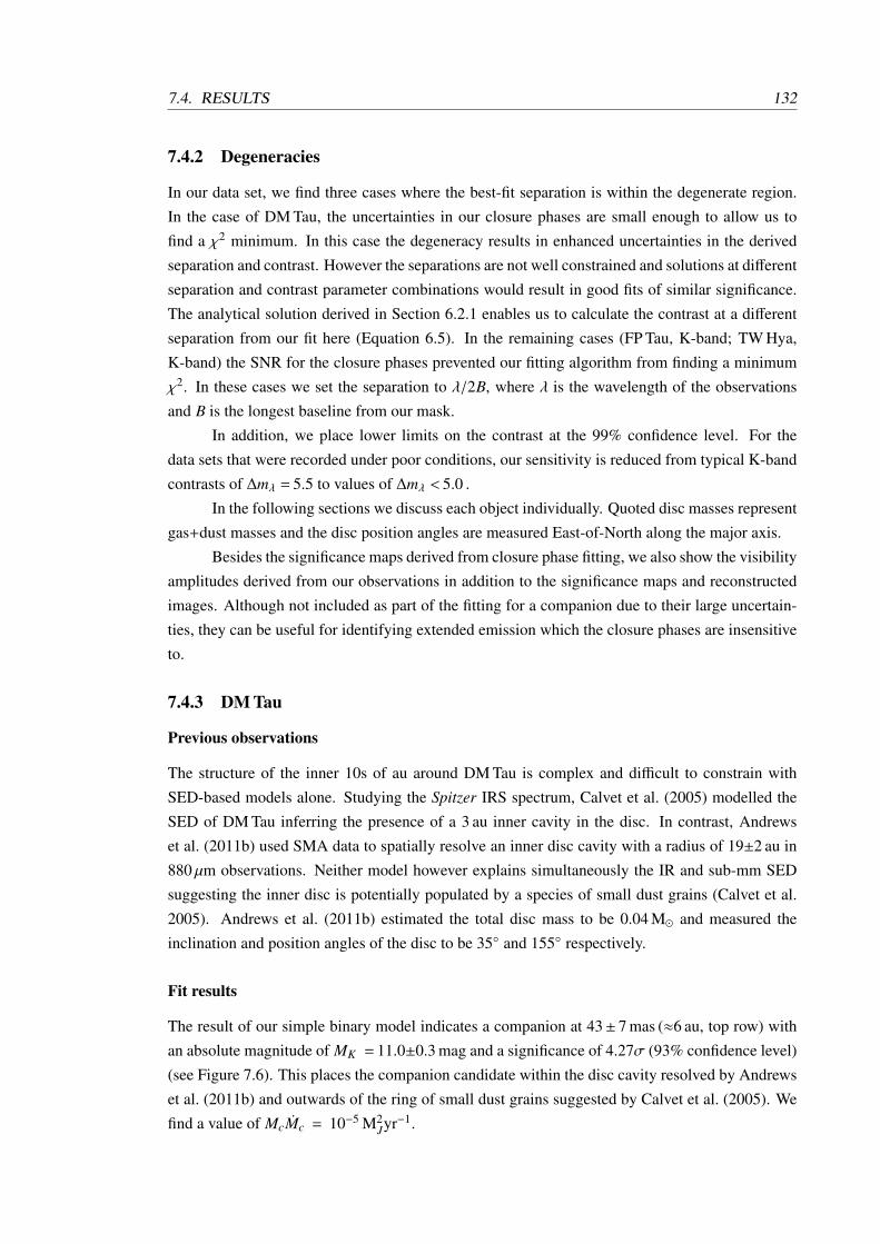
7.4. RESULTS 132
7.4.2 Degeneracies
In our data set, we find three cases where the best-fit separation is within the degenerate region.
In the case of DM Tau, the uncertainties in our closure phases are small enough to allow us to
find a χ2 minimum. In this case the degeneracy results in enhanced uncertainties in the derived
separation and contrast. However the separations are not well constrained and solutions at different
separation and contrast parameter combinations would result in good fits of similar significance.
The analytical solution derived in Section 6.2.1 enables us to calculate the contrast at a different
separation from our fit here (Equation 6.5). In the remaining cases (FP Tau, K-band; TW Hya,
K-band) the SNR for the closure phases prevented our fitting algorithm from finding a minimum
χ2. In these cases we set the separation to λ/2B, where λ is the wavelength of the observations
and B is the longest baseline from our mask.
In addition, we place lower limits on the contrast at the 99% confidence level. For the
data sets that were recorded under poor conditions, our sensitivity is reduced from typical K-band
contrasts of ∆mλ = 5.5 to values of ∆mλ < 5.0 .
In the following sections we discuss each object individually. Quoted disc masses represent
gas+dust masses and the disc position angles are measured East-of-North along the major axis.
Besides the significance maps derived from closure phase fitting, we also show the visibility
amplitudes derived from our observations in addition to the significance maps and reconstructed
images. Although not included as part of the fitting for a companion due to their large uncertain-
ties, they can be useful for identifying extended emission which the closure phases are insensitive
to.
7.4.3 DM Tau
Previous observations
The structure of the inner 10s of au around DM Tau is complex and difficult to constrain with
SED-based models alone. Studying the Spitzer IRS spectrum, Calvet et al. (2005) modelled the
SED of DM Tau inferring the presence of a 3 au inner cavity in the disc. In contrast, Andrews
et al. (2011b) used SMA data to spatially resolve an inner disc cavity with a radius of 19±2 au in
880 µm observations. Neither model however explains simultaneously the IR and sub-mm SED
suggesting the inner disc is potentially populated by a species of small dust grains (Calvet et al.
2005). Andrews et al. (2011b) estimated the total disc mass to be 0.04 M and measured the
inclination and position angles of the disc to be 35 and 155 respectively.
Fit results
The result of our simple binary model indicates a companion at 43± 7 mas (≈6 au, top row) with
an absolute magnitude of MK = 11.0±0.3 mag and a significance of 4.27σ (93% confidence level)
(see Figure 7.6). This places the companion candidate within the disc cavity resolved by Andrews
et al. (2011b) and outwards of the ring of small dust grains suggested by Calvet et al. (2005). We
find a value of McMc = 10−5 M2Jyr−1.
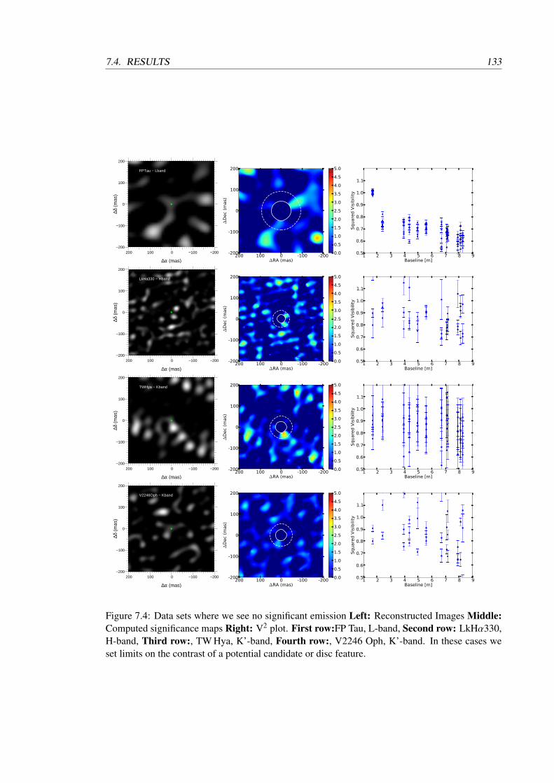
7.4. RESULTS 133
FPTau − Lband
−200−100 0 100 200−200
−100
0
100
200
0
0.1
0.2
0.3
0.4
0.5
0.6
0.7
0.8
0.9
1
∆α (mas)
∆δ (
mas
)
200 100 0 -100 -200∆RA (mas)
-200
-100
0
100
200
∆D
ec
(mas)
0.0
0.5
1.0
1.5
2.0
2.5
3.0
3.5
4.0
4.5
5.0
1 2 3 4 5 6 7 8 9Baseline [m]
0.5
0.6
0.7
0.8
0.9
1.0
1.1
Square
d V
isib
ility
LkHa330 − Hband
−200−100 0 100 200−200
−100
0
100
200
0
0.1
0.2
0.3
0.4
0.5
0.6
0.7
0.8
0.9
1
∆α (mas)
∆δ (
mas
)
200 100 0 -100 -200∆RA (mas)
-200
-100
0
100
200
∆D
ec
(mas)
0.0
0.5
1.0
1.5
2.0
2.5
3.0
3.5
4.0
4.5
5.0
1 2 3 4 5 6 7 8 9Baseline [m]
0.5
0.6
0.7
0.8
0.9
1.0
1.1
Square
d V
isib
ility
TWHya − Kband
−200−100 0 100 200−200
−100
0
100
200
0
0.1
0.2
0.3
0.4
0.5
0.6
0.7
0.8
0.9
1
∆α (mas)
∆δ (
mas
)
200 100 0 -100 -200∆RA (mas)
-200
-100
0
100
200
∆D
ec
(mas)
0.0
0.5
1.0
1.5
2.0
2.5
3.0
3.5
4.0
4.5
5.0
1 2 3 4 5 6 7 8 9Baseline [m]
0.5
0.6
0.7
0.8
0.9
1.0
1.1
Square
d V
isib
ility
V2246Oph − Kband
−200−100 0 100 200−200
−100
0
100
200
0
0.1
0.2
0.3
0.4
0.5
0.6
0.7
0.8
0.9
1
∆α (mas)
∆δ (
mas
)
200 100 0 -100 -200∆RA (mas)
-200
-100
0
100
200
∆D
ec
(mas)
0.0
0.5
1.0
1.5
2.0
2.5
3.0
3.5
4.0
4.5
5.0
1 2 3 4 5 6 7 8 9Baseline [m]
0.5
0.6
0.7
0.8
0.9
1.0
1.1
Square
d V
isib
ility
Figure 7.4: Data sets where we see no significant emission Left: Reconstructed Images Middle:Computed significance maps Right: V2 plot. First row:FP Tau, L-band, Second row: LkHα330,H-band, Third row:, TW Hya, K’-band, Fourth row:, V2246 Oph, K’-band. In these cases weset limits on the contrast of a potential candidate or disc feature.
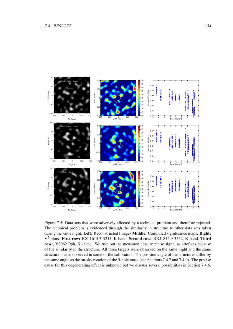
7.4. RESULTS 134
RXJ1615.3−3255 − Kband
−200−100 0 100 200−200
−100
0
100
200
0
0.1
0.2
0.3
0.4
0.5
0.6
0.7
0.8
0.9
1
∆α (mas)
∆δ (
mas
)
200 100 0 -100 -200∆RA (mas)
-200
-100
0
100
200
∆D
ec
(mas)
0.0
0.5
1.0
1.5
2.0
2.5
3.0
3.5
4.0
4.5
5.0
1 2 3 4 5 6 7 8 9Baseline [m]
0.5
0.6
0.7
0.8
0.9
1.0
1.1
Square
d V
isib
ility
RXJ1842.9−3532 − Kband
−200−100 0 100 200−200
−100
0
100
200
0
0.1
0.2
0.3
0.4
0.5
0.6
0.7
0.8
0.9
1
∆α (mas)
∆δ (
mas
)
200 100 0 -100 -200∆RA (mas)
-200
-100
0
100
200
∆D
ec
(mas)
0.0
0.5
1.0
1.5
2.0
2.5
3.0
3.5
4.0
4.5
5.0
1 2 3 4 5 6 7 8 9Baseline [m]
0.5
0.6
0.7
0.8
0.9
1.0
1.1
Square
d V
isib
ility
V2062Oph − Kband
−200−100 0 100 200−200
−100
0
100
200
0
0.1
0.2
0.3
0.4
0.5
0.6
0.7
0.8
0.9
1
∆α (mas)
∆δ (
mas
)
200 100 0 -100 -200∆RA (mas)
-200
-100
0
100
200
∆D
ec
(mas)
0.0
0.5
1.0
1.5
2.0
2.5
3.0
3.5
4.0
4.5
5.0
1 2 3 4 5 6 7 8 9Baseline [m]
0.5
0.6
0.7
0.8
0.9
1.0
1.1
Square
d V
isib
ility
Figure 7.5: Data sets that were adversely affected by a technical problem and therefore rejected.The technical problem is evidenced through the similarity in structure to other data sets takenduring the same night. Left: Reconstructed Images Middle: Computed significance maps. Right:V2 plots. First row: RXJ1615.3-3255, K-band, Second row: RXJ1842.9-3532, K-band, Thirdrow:, V2062 Oph, K’-band. We rule out the measured closure phase signal as artefacts becauseof the similarity in the structure. All three targets were observed on the same night and the samestructure is also observed in some of the calibrators. The position angle of the structures differ bythe same angle as the on-sky rotation of the 9-hole mask (see Sections 7.4.7 and 7.4.9). The precisecause for this degenerating effect is unknown but we discuss several possibilities in Section 7.4.6.
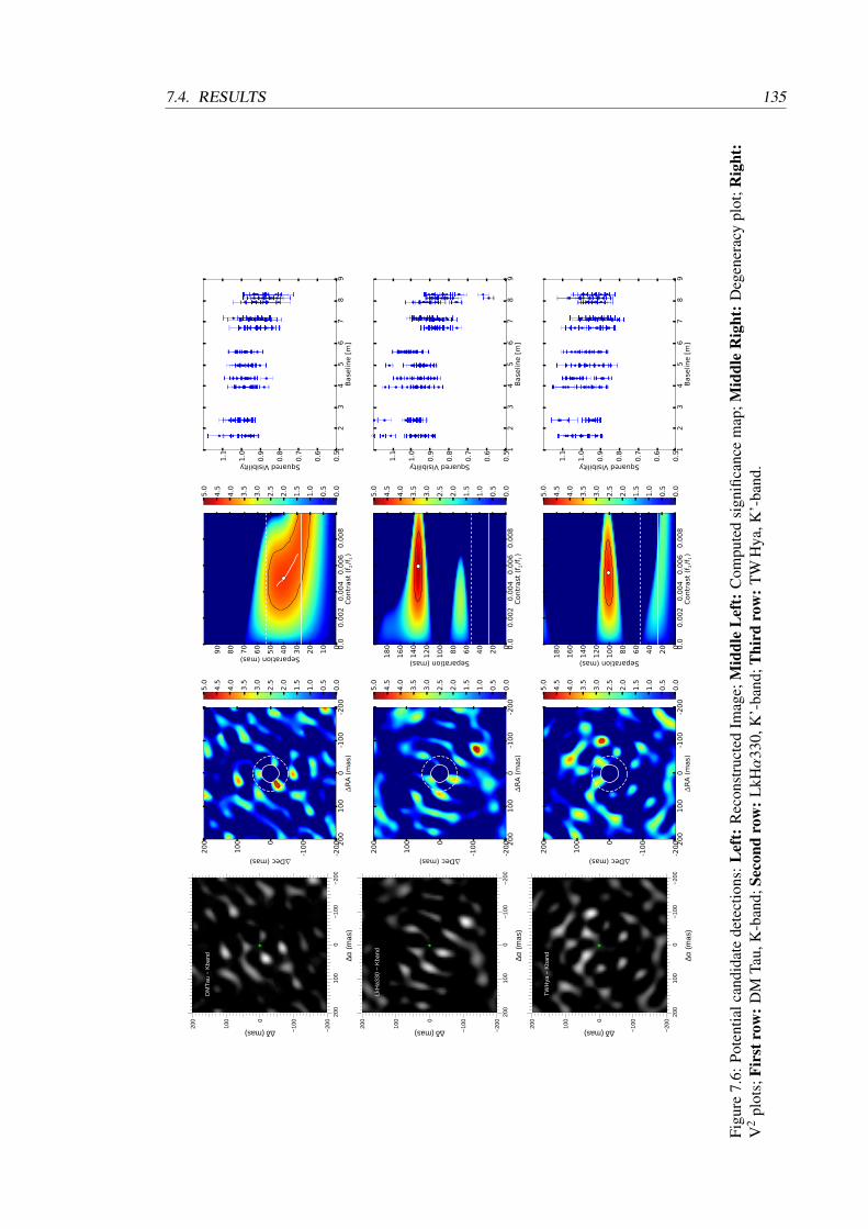
7.4. RESULTS 135
DM
Tau
− K
band
−20
0−
100
0 1
00 2
00−
200
−10
0 0
100
200
00.1
0.2
0.3
0.4
0.5
0.6
0.7
0.8
0.9
1
∆α (
mas
)
∆δ (mas)
200
100
0-1
00
-200
∆R
A (
mas)
-200
-1000
100
200
∆Dec (mas)
0.0
0.5
1.0
1.5
2.0
2.5
3.0
3.5
4.0
4.5
5.0
0.0
0.0
02
0.0
04
0.0
06
0.0
08
Contr
ast
(f 2
/f1)
0
10
20
30
40
50
60
70
80
90
Separation (mas)
0.0
0.5
1.0
1.5
2.0
2.5
3.0
3.5
4.0
4.5
5.0
12
34
56
78
9B
ase
line [
m]
0.5
0.6
0.7
0.8
0.9
1.0
1.1
Squared Visibility
LkH
a330
− K
band
−20
0−
100
0 1
00 2
00−
200
−10
0 0
100
200
00.1
0.2
0.3
0.4
0.5
0.6
0.7
0.8
0.9
1
∆α (
mas
)
∆δ (mas)
200
100
0-1
00
-200
∆R
A (
mas)
-200
-1000
100
200
∆Dec (mas)
0.0
0.5
1.0
1.5
2.0
2.5
3.0
3.5
4.0
4.5
5.0
0.0
0.0
02
0.0
04
0.0
06
0.0
08
Contr
ast
(f 2
/f1)
0
20
40
60
80
100
120
140
160
180
Separation (mas)
0.0
0.5
1.0
1.5
2.0
2.5
3.0
3.5
4.0
4.5
5.0
12
34
56
78
9B
ase
line [
m]
0.5
0.6
0.7
0.8
0.9
1.0
1.1
Squared Visibility
TW
Hya
− K
band
−20
0−
100
0 1
00 2
00−
200
−10
0 0
100
200
00.1
0.2
0.3
0.4
0.5
0.6
0.7
0.8
0.9
1
∆α (
mas
)
∆δ (mas)
200
100
0-1
00
-200
∆R
A (
mas)
-200
-1000
100
200
∆Dec (mas)
0.0
0.5
1.0
1.5
2.0
2.5
3.0
3.5
4.0
4.5
5.0
0.0
0.0
02
0.0
04
0.0
06
0.0
08
Contr
ast
(f 2
/f1)
0
20
40
60
80
100
120
140
160
180
Separation (mas)
0.0
0.5
1.0
1.5
2.0
2.5
3.0
3.5
4.0
4.5
5.0
12
34
56
78
9B
ase
line [
m]
0.5
0.6
0.7
0.8
0.9
1.0
1.1
Squared Visibility
Figu
re7.
6:Po
tent
ialc
andi
date
dete
ctio
ns:L
eft:
Rec
onst
ruct
edIm
age;
Mid
dle
Lef
t:C
ompu
ted
sign
ifica
nce
map
;Mid
dle
Rig
ht:
Deg
ener
acy
plot
;Rig
ht:
V2
plot
s;Fi
rstr
ow:D
MTa
u,K
-ban
d;Se
cond
row
:LkHα
330,
K’-
band
;Thi
rdro
w:T
WH
ya,K
’-ba
nd.
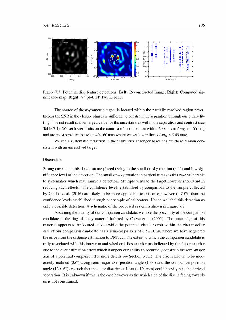
7.4. RESULTS 136
FPTau − Kband
−200−100 0 100 200−200
−100
0
100
200
0
0.1
0.2
0.3
0.4
0.5
0.6
0.7
0.8
0.9
1
∆α (mas)
∆δ (
mas
)
200 100 0 -100 -200∆RA (mas)
-200
-100
0
100
200
∆D
ec
(mas)
0.0
0.5
1.0
1.5
2.0
2.5
3.0
3.5
4.0
4.5
5.0
1 2 3 4 5 6 7 8 9Baseline [m]
0.5
0.6
0.7
0.8
0.9
1.0
1.1
Square
d V
isib
ility
Figure 7.7: Potential disc feature detections. Left: Reconstructed Image; Right: Computed sig-nificance map; Right: V2 plot. FP Tau, K-band.
The source of the asymmetric signal is located within the partially resolved region never-
theless the SNR in the closure phases is sufficient to constrain the separation through our binary fit-
ting. The net result is an enlarged value for the uncertainties within the separation and contrast (see
Table 7.4). We set lower limits on the contrast of a companion within 200 mas at ∆mK > 4.66 mag
and are most sensitive between 40-160 mas where we set lower limits ∆mK > 5.49 mag.
We see a systematic reduction in the visibilities at longer baselines but these remain con-
sistent with an unresolved target.
Discussion
Strong caveats on this detection are placed owing to the small on sky rotation (∼ 1) and low sig-
nificance level of the detection. The small on-sky rotation in particular makes this case vulnerable
to systematics which may mimic a detection. Multiple visits to the target however should aid in
reducing such effects. The confidence levels established by comparison to the sample collected
by Gaidos et al. (2016) are likely to be more applicable to this case however (∼ 70%) than the
confidence levels established through our sample of calibrators. Hence we label this detection as
only a possible detection. A schematic of the proposed system is shown in Figure 7.8
Assuming the fidelity of our companion candidate, we note the proximity of the companion
candidate to the ring of dusty material inferred by Calvet et al. (2005). The inner edge of this
material appears to be located at 3 au while the potential circular orbit within the circumstellar
disc of our companion candidate has a semi-major axis of 6.5±1.0 au, where we have neglected
the error from the distance estimation to DM Tau. The extent to which the companion candidate is
truly associated with this inner rim and whether it lies exterior (as indicated by the fit) or exterior
due to the over estimation effect which hampers our ability to accurately constrain the semi-major
axis of a potential companion (for more details see Section 6.2.1). The disc is known to be mod-
erately inclined (35) along semi-major axis position angle (155) and the companion position
angle (120±6) are such that the outer disc rim at 19 au (∼120 mas) could heavily bias the derived
separation. It is unknown if this is the case however as the which side of the disc is facing towards
us is not constrained.

7.4. RESULTS 137
Figure 7.8: Schematic of the DM Tau system based on our tentative detection of a companion inaddition to the previous observations of the outer disc in the sub-mm (Andrews et al. 2011b) andSED modelling of the inner disc in the NIR (Calvet et al. 2005). If confirmed the close proximityof the companion to the previously inferred ring of material at ∼3 au is of particular interest forunderstanding the formation of certain disc structures.
7.4.4 FP Tau
Previous observations
Furlan et al. (2005) classified FP Tau as a Class II object based on Spitzer mid-infrared spectra
and inferred the presence of an extended gap within the disc from the lack of near-infrared ex-
cess flux. This was further supported by later analysis by Currie & Sicilia-Aguilar (2011) but
neither characterised the spatial extent of the gap. They did however estimate the disc mass to
2.5×10⁻⁴ M.
Fits results
We see clear disc structures within FP Tau, with the K-band data set displaying both ”dual lobing”
in the significance map and dual point source-like emission in the image (Figure 7.7), which we
identified in Section 6.3.4 as likely indicators for disc-related asymmetries. From this we conclude
the inner edge of the outer disc of FP Tau to be likely moderately inclined and located between
26-52 mas. The SNR of the closure phase is insufficient to find an unambiguous solution for the
separation and we are forced to fix the separation to λ/2D within our fit. This corresponds to
∼26 mas or an inner disc edge located at 10.0±2.0 au where the unknown inclination dominates
the uncertainty. Values for the position of the inner rim of the disc can be as large as 20 au however
with an equally good fit to the data. Between 50-200 mas we set a lower limit on the contrast of a
companion at ∆mK > 5.0 mag.
The L-band data set on FP Tau does not show any significant asymmetries, as can be seen
within the significance map. No signal reaches the 4σ significance threshold, which is consistent
with the reconstructed images where we see little off-centre flux (see Figure 7.4). Between 50-
200 mas we set an lower limit on the contrast of a companion as ∆mL > 3.4 mag.
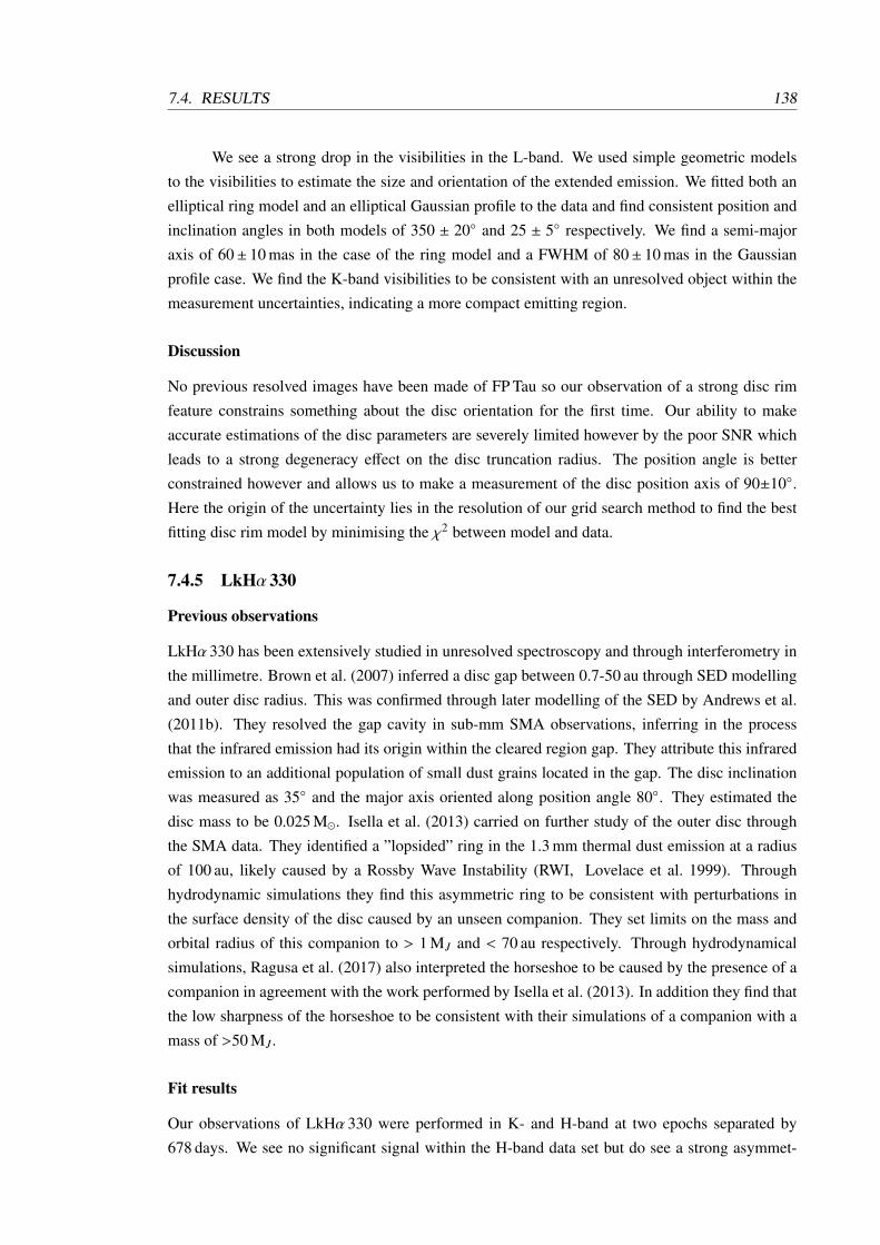
7.4. RESULTS 138
We see a strong drop in the visibilities in the L-band. We used simple geometric models
to the visibilities to estimate the size and orientation of the extended emission. We fitted both an
elliptical ring model and an elliptical Gaussian profile to the data and find consistent position and
inclination angles in both models of 350 ± 20 and 25 ± 5 respectively. We find a semi-major
axis of 60± 10 mas in the case of the ring model and a FWHM of 80± 10 mas in the Gaussian
profile case. We find the K-band visibilities to be consistent with an unresolved object within the
measurement uncertainties, indicating a more compact emitting region.
Discussion
No previous resolved images have been made of FP Tau so our observation of a strong disc rim
feature constrains something about the disc orientation for the first time. Our ability to make
accurate estimations of the disc parameters are severely limited however by the poor SNR which
leads to a strong degeneracy effect on the disc truncation radius. The position angle is better
constrained however and allows us to make a measurement of the disc position axis of 90±10.
Here the origin of the uncertainty lies in the resolution of our grid search method to find the best
fitting disc rim model by minimising the χ2 between model and data.
7.4.5 LkHα 330
Previous observations
LkHα 330 has been extensively studied in unresolved spectroscopy and through interferometry in
the millimetre. Brown et al. (2007) inferred a disc gap between 0.7-50 au through SED modelling
and outer disc radius. This was confirmed through later modelling of the SED by Andrews et al.
(2011b). They resolved the gap cavity in sub-mm SMA observations, inferring in the process
that the infrared emission had its origin within the cleared region gap. They attribute this infrared
emission to an additional population of small dust grains located in the gap. The disc inclination
was measured as 35 and the major axis oriented along position angle 80. They estimated the
disc mass to be 0.025 M. Isella et al. (2013) carried on further study of the outer disc through
the SMA data. They identified a ”lopsided” ring in the 1.3 mm thermal dust emission at a radius
of 100 au, likely caused by a Rossby Wave Instability (RWI, Lovelace et al. 1999). Through
hydrodynamic simulations they find this asymmetric ring to be consistent with perturbations in
the surface density of the disc caused by an unseen companion. They set limits on the mass and
orbital radius of this companion to > 1 MJ and < 70 au respectively. Through hydrodynamical
simulations, Ragusa et al. (2017) also interpreted the horseshoe to be caused by the presence of a
companion in agreement with the work performed by Isella et al. (2013). In addition they find that
the low sharpness of the horseshoe to be consistent with their simulations of a companion with a
mass of >50 MJ .
Fit results
Our observations of LkHα 330 were performed in K- and H-band at two epochs separated by
678 days. We see no significant signal within the H-band data set but do see a strong asymmet-
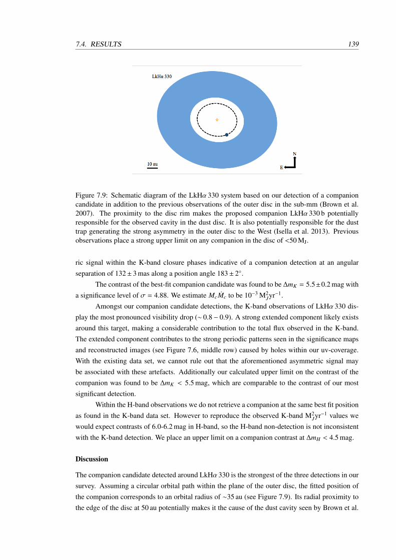
7.4. RESULTS 139
Figure 7.9: Schematic diagram of the LkHα 330 system based on our detection of a companioncandidate in addition to the previous observations of the outer disc in the sub-mm (Brown et al.2007). The proximity to the disc rim makes the proposed companion LkHα 330 b potentiallyresponsible for the observed cavity in the dust disc. It is also potentially responsible for the dusttrap generating the strong asymmetry in the outer disc to the West (Isella et al. 2013). Previousobservations place a strong upper limit on any companion in the disc of <50 MJ.
ric signal within the K-band closure phases indicative of a companion detection at an angular
separation of 132± 3 mas along a position angle 183± 2.
The contrast of the best-fit companion candidate was found to be ∆mK = 5.5±0.2 mag with
a significance level of σ = 4.88. We estimate McMc to be 10−3 M2Jyr−1.
Amongst our companion candidate detections, the K-band observations of LkHα 330 dis-
play the most pronounced visibility drop (∼ 0.8− 0.9). A strong extended component likely exists
around this target, making a considerable contribution to the total flux observed in the K-band.
The extended component contributes to the strong periodic patterns seen in the significance maps
and reconstructed images (see Figure 7.6, middle row) caused by holes within our uv-coverage.
With the existing data set, we cannot rule out that the aforementioned asymmetric signal may
be associated with these artefacts. Additionally our calculated upper limit on the contrast of the
companion was found to be ∆mK < 5.5 mag, which are comparable to the contrast of our most
significant detection.
Within the H-band observations we do not retrieve a companion at the same best fit position
as found in the K-band data set. However to reproduce the observed K-band M2Jyr−1 values we
would expect contrasts of 6.0-6.2 mag in H-band, so the H-band non-detection is not inconsistent
with the K-band detection. We place an upper limit on a companion contrast at ∆mH < 4.5 mag.
Discussion
The companion candidate detected around LkHα 330 is the strongest of the three detections in our
survey. Assuming a circular orbital path within the plane of the outer disc, the fitted position of
the companion corresponds to an orbital radius of ∼35 au (see Figure 7.9). Its radial proximity to
the edge of the disc at 50 au potentially makes it the cause of the dust cavity seen by Brown et al.
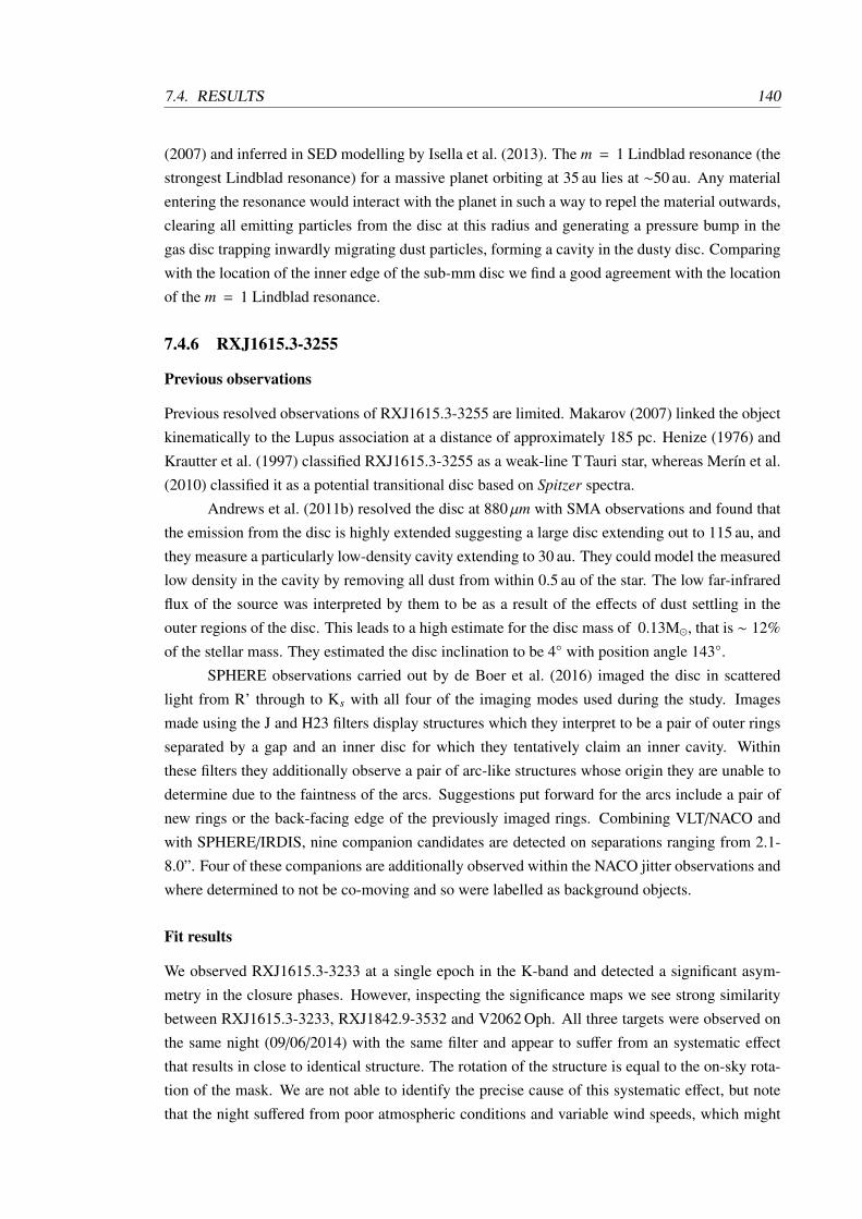
7.4. RESULTS 140
(2007) and inferred in SED modelling by Isella et al. (2013). The m = 1 Lindblad resonance (the
strongest Lindblad resonance) for a massive planet orbiting at 35 au lies at ∼50 au. Any material
entering the resonance would interact with the planet in such a way to repel the material outwards,
clearing all emitting particles from the disc at this radius and generating a pressure bump in the
gas disc trapping inwardly migrating dust particles, forming a cavity in the dusty disc. Comparing
with the location of the inner edge of the sub-mm disc we find a good agreement with the location
of the m = 1 Lindblad resonance.
7.4.6 RXJ1615.3-3255
Previous observations
Previous resolved observations of RXJ1615.3-3255 are limited. Makarov (2007) linked the object
kinematically to the Lupus association at a distance of approximately 185 pc. Henize (1976) and
Krautter et al. (1997) classified RXJ1615.3-3255 as a weak-line T Tauri star, whereas Merın et al.
(2010) classified it as a potential transitional disc based on Spitzer spectra.
Andrews et al. (2011b) resolved the disc at 880 µm with SMA observations and found that
the emission from the disc is highly extended suggesting a large disc extending out to 115 au, and
they measure a particularly low-density cavity extending to 30 au. They could model the measured
low density in the cavity by removing all dust from within 0.5 au of the star. The low far-infrared
flux of the source was interpreted by them to be as a result of the effects of dust settling in the
outer regions of the disc. This leads to a high estimate for the disc mass of 0.13M, that is ∼ 12%
of the stellar mass. They estimated the disc inclination to be 4 with position angle 143.
SPHERE observations carried out by de Boer et al. (2016) imaged the disc in scattered
light from R’ through to Ks with all four of the imaging modes used during the study. Images
made using the J and H23 filters display structures which they interpret to be a pair of outer rings
separated by a gap and an inner disc for which they tentatively claim an inner cavity. Within
these filters they additionally observe a pair of arc-like structures whose origin they are unable to
determine due to the faintness of the arcs. Suggestions put forward for the arcs include a pair of
new rings or the back-facing edge of the previously imaged rings. Combining VLT/NACO and
with SPHERE/IRDIS, nine companion candidates are detected on separations ranging from 2.1-
8.0”. Four of these companions are additionally observed within the NACO jitter observations and
where determined to not be co-moving and so were labelled as background objects.
Fit results
We observed RXJ1615.3-3233 at a single epoch in the K-band and detected a significant asym-
metry in the closure phases. However, inspecting the significance maps we see strong similarity
between RXJ1615.3-3233, RXJ1842.9-3532 and V2062 Oph. All three targets were observed on
the same night (09/06/2014) with the same filter and appear to suffer from an systematic effect
that results in close to identical structure. The rotation of the structure is equal to the on-sky rota-
tion of the mask. We are not able to identify the precise cause of this systematic effect, but note
that the night suffered from poor atmospheric conditions and variable wind speeds, which might
7.4. RESULTS 141
have induced vibrations and degraded the AO performance (these poor conditions also reflect in a
high variance in the individual uncalibrated closure phase; see Table 7.3). The visibilities are also
strongly affected by this systematic, showing similar strong drops and structure.
We set a lower limit for the contrast of a potential binary to ∆mK > 4.0 mag between 20-
40 mas and ∆mK > 4.6 mag between 40-200 mas (see Figure 7.6). The systematics previously
mentioned may affect adversely the accuracy of the limits we set in these cases.
7.4.7 RXJ1842.9-3532
Previous observations
Hughes et al. (2010) used a combination of resolved SMA observations and SED modelling to
infer the presence of an optically thin region inwards from 5 au with a narrow ring of optically
thick material at ∼ 0.01 − 0.2 au. Their models suggest little to no evidence for shadowing from
the inner on the outer disc. They estimate the disc mass to be 0.01 M and measure the inclination
to be 54 with a position angle of 32.
Fit results
We detect no significant asymmetric signal in the closure phases but see the same systematic
structure in the significance maps as in RXJ1615.3-3255 and V2062 Oph (see Section 7.4.6).
We set lower limits on the contrast of a companion at ∆mK >5.0 mag between 40-200 mas.
7.4.8 TW Hya
Previous observations
Estimates by Calvet et al. (2002) found that the optically-thick near and mid-IR disc of TW Hya
extends from 4 to 140 au, with a mass of 0.06 M for a 10 Myr old disc. They additionally found
that the inner region of the disc is not fully cleared. A population of 1 µm dust grains is required
within the optically-thin inner 4 au to properly fit the SED in agreement with observed continued
accretion onto TW Hya. This interpretation is supported by recent ALMA observations by An-
drews et al. (2016) which probed, through 870 µm emission, the distribution of millimeter-sized
grains to spatial scales on the order of an au. They observed ring structures suggestive of ongoing
planet formation, in particular an unresolved inner disc within 0.5 au and a bright ring at 2.4 au
separated by a dark annulus centred at 1 au (see Figure 7.10.
Radial velocity studies of this object performed by Setiawan et al. (2008) provided evidence
for the presence of a 9.8±3.3 MJ planet on an orbit with a semi-major axis of 0.041±0.002 au. This
body could be responsible for the clearing of the inner regions of the disc. This interpretation of
the RV data was disputed by Huelamo et al. (2008), who attributed the signal to the presence of a
cool stellar spot.
TW Hya was also observed as part of the AO imaging survey with Keck II by Brandeker
et al. (2003). They detected no companion in the H-band down to contrasts of ∼ 1 mag at 0′′.05,
increasing approximately linearly to 4 mag at 0′′.2, corresponding to distances of 2.75 to 11 au.
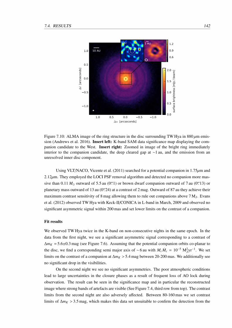
7.4. RESULTS 142
Figure 7.10: ALMA image of the ring structure in the disc surrounding TW Hya in 880 µm emis-sion (Andrews et al. 2016). Insert left: K-band SAM data significance map displaying the com-panion candidate to the West. Insert right: Zoomed in image of the bright ring immediatelyinterior to the companion candidate, the deep cleared gap at ∼1 au, and the emission from anunresolved inner disc component.
Using VLT/NACO, Vicente et al. (2011) searched for a potential companion in 1.75µm and
2.12µm. They employed the LOCI PSF removal algorithm and detected no companion more mas-
sive than 0.11 M outward of 5.5 au (0′′.1) or brown dwarf companion outward of 7 au (0′′.13) or
planetary mass outward of 13 au (0′′.24) at a contrast of 2 mag. Outward of 87 au they achieve their
maximum contrast sensitivity of 8 mag allowing them to rule out companions above 7 MJ . Evans
et al. (2012) observed TW Hya with Keck-II/CONICA in L-band in March, 2009 and observed no
significant asymmetric signal within 200 mas and set lower limits on the contrast of a companion.
Fit results
We observed TW Hya twice in the K-band on non-consecutive nights in the same epoch. In the
data from the first night, we see a significant asymmetric signal corresponding to a contrast of
∆mK = 5.6±0.3 mag (see Figure 7.6). Assuming that the potential companion orbits co-planar to
the disc, we find a corresponding semi major axis of ∼ 6 au with McMc = 10−5 M2Jyr−1. We set
limits on the contrast of a companion at ∆mK > 5.4 mag between 20-200 mas. We additionally see
no significant drop in the visibilities.
On the second night we see no significant asymmetries. The poor atmospheric conditions
lead to large uncertainties in the closure phases as a result of frequent loss of AO lock during
observation. The result can be seen in the significance map and in particular the reconstructed
image where strong bands of artefacts are visible (See Figure 7.4, third row from top). The contrast
limits from the second night are also adversely affected. Between 80-160 mas we set contrast
limits of ∆mK > 3.5 mag, which makes this data set unsuitable to confirm the detection from the

7.4. RESULTS 143
Figure 7.11: Schematic diagram of the TW Hya system based on our detection of a companioncandidate in addition to the previous observations of the disc with ALMA by Andrews et al. (2016)and Tsukagoshi et al. (2016). The proposed companion lies within the shallow gap identifiedby Tsukagoshi et al. (2016), immediately outside the bright ring of small particles observed byAndrews et al. (2016). The deep gap at ∼1 au is also shown along with the unseen companionwhich is the likely cause of the gap as well as the dust trapping which produced the bright ring.The deeper gaps at larger radii are not shown.
first night.
Discussion
Comparing our result from the first night to the limits in L-band set by Evans et al. (2012), we
use the circumplanetary disc models in Zhu (2015) to estimate the L-band absolute magnitude
an accreting companion of this absolute magnitude would display. We find the expected contrast
to be ∆mL ≈ 4 mag compared to the limit imposed by Evans et al. (2012) of ∆mL > 6 mag.
Assuming the scaling described within the circumplanetary disc models to be accurate, to account
for both observations the accretion rate onto the potential companion would be required to increase
by at least an order of magnitude during the three years separating the observations. The value
of M onto TW Hya is known to be highly variable with values fluctuating at least by an order of
magnitude (Alencar & Batalha 2002). This variation occurs on a time scale of years and we would
expect the accretion rate onto a companion to be related to the amount of material flowing through
the disc so we cannot rule out this companion candidate based on previous SAM observations.
Another possible cause for the origin of the detected companion-like asymmetry is not
protoplanetary in nature but instead from a another potential source of asymmetry such as an
accretion stream or disc asymmetry. ALMA observations carried out by Andrews et al. (2016) at
∼350GHz found no non-axisymmetric structures on these scales within the distribution of sub-mm
particles but this does not rule out a disc asymmetry in our data set as our K-band observations
probe the surface layer of the disc while their sub-mm observations probe the middle of the disc
(Juhasz et al. 2015). We lack the required signal to noise to be sensitive to any companion within
the 1 au gap seen in their sub-mm data but find no significant asymmetry in the bright ring at 2.4 au.
We additionally note that if confirmed, our companion candidate would be located immediately
7.4. RESULTS 144
outside the bright ring seen in the sub-mm data where the intensity distribution flattens out at ∼6 au
(see Figures 7.10, 7.11, and 7.12). ALMA observations taken in 138 and 230GHz (Tsukagoshi
et al. 2016) revealed a shallow drop in the surface density of a few percent centred at ∼6 au in
agreement with the location of our companion candidate. The location of our claimed companion
candidate is shown in Figure 7.11.
van Boekel et al. (2016) presented VLT/SPHERE scattered light images of TW Hya in
0.63, 0.79,1.24, and 1.62µm in polarimetric differential imaging mode (PDI) in addition to H2/H3
observations made using angular differential imaging (ADI). No significant point source was ob-
served within the H-band ADI observations but limits were set for a companion at 100 mas at
∼>8.0 ∆mH . Based on the Zhu (2015) circumplanetary disc models, we would expect our com-
panion candidate to have an absolute magnitude of 11.0 mH and so a contrast in H of ∼>7.5 ∆mH
placing our companion candidate on the limit of detectability in terms of both contrast sensitivity
and spatial resolution for the ADI measurements. In the scattered light images three shallow gaps
are observed in the radial profile of the disc approximately centered at ≤6, 21, and 85 au (with an
assumed distance to TW Hya of 56 au) in close agreement to the surface density drops observed in
previous ALMA sub-mm observations. Performing radiative transfer modelling of the gaps, van
Boekel et al. (2016) estimated the mass of an embedded planet required to partially open up the
observed density depression in the sub-mm radial profile. For the gap in which our companion
candidate potentially lies, they found a mass of 6 M⊕. The mass is highly sensitive to a number of
assumed disc parameters, in particular on the assumed value of the disc viscosity parameter. Ad-
ditionally, while the estimated mass well reproduces the depth of the depletion of the gas disc, the
gap profiles were found to be too shallow and wide to be caused by a companion in their models.
All scattered light observations indicate a largely azimuthally symmetric disc structure.
The combination of these three observations is suggestive of a potential scenario where a
low-mass core has become trapped close to, or indeed embedded-in, a region particularly rich in
material available for accretion onto the core. This accretion makes the core highly luminous but
the total mass accumulated onto the core is not yet sufficient to completely clear its orbital path.
The close proximity of a ring of over-dense material additionally suggests a possible scenario
for the origin of the core, wherein a planetary embryo has undergone migration through the disc
as a result of strong Lindblad torques overcoming the co-rotational torques. The embryo has
migrated inwards and gained mass until eventually encountering the dense ring of material located
at ∼4 au. This ring is likely to have been produced by material which has become trapped by the
gravitational influence of the massive indirectly inferred companion responsible for clearing the
deep gap seen centered at 1 au. Within the ring, the inward drift of the dusty particles has been
halted by torques generated by the closer-in companion. In encountering this sharp change in
density, the co-rotational torques which were previously too weak to counter the Linblad torques
are now strong enough to halt the inward motion. While this sharp radial structure exists, the core
seen within our observations is unlikely to be able to migrate further until it has become massive
enough to clear a gap itself, for example as shown in toy models presented by Coleman & Nelson
(2016).

7.4. RESULTS 145
Figure 7.12: Radial profile of the 880 µm emission from TW Hya. The dotted red line indicatesa full or classical disc. The blue dashed line displays the fitted orbital radius of the companioncandidate assuming a circular orbit within the plane of the disc. The PSF is show in the upperright. The companion candidate is located immediately outside the bright ring of dusty material,co-located with where the ring rejoins the more extended disc profile. Ruling out a shallow gapat the same orbital radii as the candidate is not possible as a result of the close proximity of thebright ring.
7.5. ALTERNATE SOURCES OF ASYMMETRY 146
7.4.9 V2062 Oph
Previous observations
Espaillat et al. (2010) modelled the Spitzer SED and deduced a disc cavity extending to 36 au
containing some optically thin dust consistent with other resolved observations of V2062 Oph.
Andrews et al. (2011b) resolved with SMA observations a cavity in the disc extending out to
30 au. They additionally constrained the inclination and position angle to 35 and 80 respectively
and they estimate the disc mass to be 0.007 M.
Fit results
We observed V2062 Oph in the K-band within a single epoch. Observing conditions were not
ideal, but we detect a significant asymmetry signal in the closure phases. As mentioned previ-
ously in Section 7.4.6, the produced structures are also reproduced within the RXJ1615.3-3255
and RXJ1842.9-3532 data sets leading to the conclusion that these are false positives along with
V2062 Oph.
We set lower limits on the contrast of a companion at ∆mK > 4.9 mag between 20-40 mas
and > 5.1 mag between 40-200 mas.
7.4.10 V2246 Oph
Previous observations
Mid-infrared 9-18 µm Gemini observations by Jensen et al. (2009) resolved V2246 Oph at subarc-
second resolution and found very little mid-infrared excess within 100 au. Beyond this region they
observed strongly extended and asymmetric emission out to 100s of au. The asymmetric emission
forms a half ring structure to the north west, at an angular separation of 1′′1.
Vicente et al. (2011) observed V2246 Oph as part of their VLT/NACO high resolution ob-
servations. They reached sensitivities of 15 MJ and 6 MJ past separations of 3 au and 192 au
respectively. They found no evidence for a companion within these limits.
Fit results
We observed V2246 Oph in the K-band in a single epoch. Poor observing conditions severely
limited the sensitivity of our observations. We place limits on the contrast of a potential companion
at ∆mK > 2.3 mag between 20-40 mas and > 3.1 mag between 40-200 mas.
7.5 Alternate sources of asymmetry
Care must be taken to not assume that the companion candidates detected here are the result of
the direct detection of a companion or circumplanetary disc. Instead, one must also consider that
a disc asymmetry such as an over density or dust trap may also be responsible. Naively, this may
seem improbable considering that each of the companion candidates detected here lie in the clear
gaps of their parent discs, but recent results from the ALMA telescope show ringed structures
7.6. CONCLUSION 147
in discs inferred to be full, classical discs (HL Tau, ALMA Partnership et al. 2015) and gapped
(TW Hya, Andrews et al. 2016; Tsukagoshi et al. 2016) from SED and previous interferometric
studies.
Such structures may themselves be indirect evidence for on-going planet formation. Dust
traps and spiral density waves which could appear in SAM data as point source-like structures are
believed to have their origin in the presence of planetary mass companions (see Chapter 2).
7.6 Conclusion
In this chapter we presented results of five nights of Keck sparse aperture masking observations on
eight targets in K-band, one in L-band (FP Tau), one in H-band (LkHα 330). Within this data set
we find significant non-zero closure phases for six targets, indicating asymmetries in the brightness
distribution on scales of few au. We however rule three of these to be false positives caused by a
systematic effect that affected one of our observing nights. The remaining detected asymmetries
indicate either the presence of complex disc structures and/or the presence of companions. We
conducted detailed simulations in order to understand the signature that these different scenarios
produce in our phase measurements and investigated the degeneracies that occur between the
derived separation and contrast parameters in the case of marginally resolved companions.
Using both modelling and image reconstruction methods, we investigated the likely origin
of the asymmetries for each target star. We estimate confidence levels for our companion de-
tections through fitting companion models to a sample of 24 calibrators stars known to be point
source-like. We use the resultant distribution to quantify our confidence levels. We report compan-
ion detections at a confidence level of > 99% (> 4.5σ) in LkHα 330 and detections in two further
stars (TW Hya and DM Tau) at the lower confidence level of > 95% (> 4.0σ). For the detections,
we derive McMc values of 10−3 M2Jyr−1 (LkHα330), 10−5 M2
Jyr−1 (DM Tau) and, 10−5 M2Jyr−1
(TW Hya). Additionally we infer through comparison to limits previously set on the contrast of a
companion in L-band that the origin of the asymmetry signal within the TW Hya data set would
require an increase in the accretion rate of an order of magnitude within a few years for it to be
consistent with an accreting protoplanet, the Zhu (2015) models predict accurately the K- to L-
band colour. Alencar & Batalha (2002) found TW Hya to be a highly variable disc however with
values of M varying by an order of magnitude over ∼years, supporting this scenario.
In LkHα 330 and DM Tau the gap properties have been characterised by earlier observa-
tions and we find the companion candidates to be located within the disc gaps, suggesting that
they are orbiting within the cleared regions of the disc. In the case of TW Hya we find the com-
panion candidate to be located on the outer edge of the bright annulus located at 2.4 au in recent
350GHz ALMA observations by Andrews et al. (2016). Furthermore we find that separation of
our companion candidate to be located within the shallow gap at 6 au observed by Tsukagoshi
et al. (2016) in 138 and 230GHz ALMA observations.
We interpret the asymmetries in FP Tau be to associated with disc emission, most likely a
disc wall between 20-40 mas, similar to the asymmetries seen in T Cha (Cheetham et al. 2015)
and FL Cha (Cieza et al. 2013). This is supported through strong drops in the K- and L-band

7.6. CONCLUSION 148
visibilities of this target. Fitting geometric disc models to the data sets we find find visibilities
consistent with a compact emitting region in K-band and an extended component in L-band with
a position angle of 350±20 and an inclination of 25±5. Finally, for the remaining data sets we
detect no significant asymmetries and set lower limits on the contrast of potential companions.
With the detection of significant asymmetries in four out of eight target stars, our detec-
tion frequency is relatively high (50%). This is higher than the detection rate that was found in
surveys of TTS (14%: Kraus et al. 2008; 20%: Kraus et al. 2011) conducted with Keck/NIRC2
SAM interferometry with a same observational setup and a similar data analysis scheme. This
demonstrates that transitional discs indeed trace a particularly interesting phase in disc evolution
and highlights the need for further studies on these object classes with the unique observational
window that SAM provides, both with the current-generation telescopes and the upcoming gener-
ation of Extremely Large Telescopes. Besides further continuum imaging, it is promising to image
these objects in accretion tracing spectral lines such as Hα, in order to confirm that these objects
are sites of continued accretion and to ultimately establish their classification as protoplanets.

Chapter 8
Multi-wavelength study of V1247 Ori
This chapter contains work soon to be published in Willson et al. (2017)
8.1 Previous Observations and Context
V1247 Orionis is part of the Orion OB1 b association (Guetter 1981) whose distance was estimated
to 385 ± 15 pc (Terrell et al. 2007; Caballero 2008). Caballero & Solano (2008) estimate the
age of the star to 5-10 Myr. Caballero (2010) observed two deep UX Ori-like occultation events
which were attributed to the obscuring effect of disc material passing in front of the star. They
additionally identified in the SED a substantial drop in the mid-infrared excess between 3-15µm,
marking V1247 Ori as a pre-transitional disc. Kraus et al. (2013) determined the spectral type to
F0V with HARPS spectroscopy. For a summary of the stellar parameters see Table 8.1
The pre-transitional disc of V1247 Ori is of particular interest due to previous interferomet-
ric observations that revealed complex structures within the disc gap extending from within an
au out to 37±5 au (Kraus et al. 2013). This study found that the unusually extended mid-infrared
emission around V1247 Ori could be explained with the presence of optically thin carbonaceous
dust grains located within the gap region, suggesting that the disc is still undergoing the process of
clearing its gap. Complementary single epoch Keck-II/NIRC2 SAM observations indicated small-
scale asymmetries across multiple wavebands which could not be fitted with a single point-source
companion model. These observations were interpreted as a potential spiral density wave in the
dust distribution within the gap.
Observations undertaken by Ohta et al. (2016) utilising Subaru/HiCIAO adaptive optics
polarimetry detected a strong spiral arm structure to the south of the object in scattered light. A
possible scenario for the single-armed nature they is “shadowing by the rim of the disc at 46 au,
although they note the radial decline in flux is not steep enough for a shadowed region. Other
potential explanations were proposed such as the trapping of small dust grains within a gas vortex
or a single spiral arm launched by a planetary companion.
In this Chapter I present new SAM observations of this target in H, K, and L’-band wave-
bands at two additional epochs to those presented by Kraus et al. (2013) and attempt to understand
the origin of the detected asymmetries. Our observations cover 678 days and make use of the
Keck-II/NIRC2 and VLT/NACO instruments. We attempt to directly detect accretion signatures
149
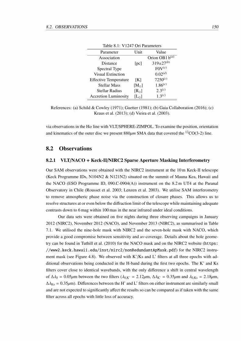
8.2. OBSERVATIONS 150
Table 8.1: V1247 Ori ParametersParameter Unit Value
Association Orion OB1 b(a)
Distance [pc] 319±27(b)
Spectral Type F0V(c)
Visual Extinction 0.02(d)
Effective Temperature [K] 7250(c)
Stellar Mass [M] 1.86(c)
Stellar Radius [R] 2.3(c)
Accretion Luminosity [L] 1.3(c)
References: (a) Schild & Cowley (1971); Guetter (1981); (b) Gaia Collaboration (2016); (c)Kraus et al. (2013); (d) Vieira et al. (2003).
via observations in the Hα line with VLT/SPHERE-ZIMPOL. To examine the position, orientation
and kinematics of the outer disc we present 880µm SMA data that covered the 12CO(3-2) line.
8.2 Observations
8.2.1 VLT/NACO + Keck-II/NIRC2 Sparse Aperture Masking Interferometry
Our SAM observations were obtained with the NIRC2 instrument at the 10 m Keck-II telescope
(Keck Programme IDs, N104N2 & N121N2) situated on the summit of Mauna Kea, Hawaii and
the NACO (ESO Programme ID, 090.C-0904(A)) instrument on the 8.2 m UT4 at the Paranal
Observatory in Chile (Rousset et al. 2003; Lenzen et al. 2003). We utilise SAM interferometry
to remove atmospheric phase noise via the construction of closure phases. This allows us to
resolve structures at or even below the diffraction limit of the telescope while maintaining adequate
contrasts down to 6 mag within 100 mas in the near infrared under ideal conditions.
Our data sets were obtained on five nights during three observing campaigns in January
2012 (NIRC2), November 2012 (NACO), and November 2013 (NIRC2), as summarised in Table
7.1. We utilised the nine-hole mask with NIRC2 and the seven-hole mask with NACO, which
provide a good compromise between sensitivity and uv-coverage. Details about the hole geome-
try can be found in Tuthill et al. (2010) for the NACO mask and on the NIRC2 website (https:
//www2.keck.hawaii.edu/inst/nirc2/nonRedundantApMask.pdf) for the NIRC2 instru-
ment mask (see Figure 4.8). We observed with K’/Ks and L’ filters at all three epochs with ad-
ditional observations being conducted in the H-band during the first two epochs. The K’ and Ks
filters cover close to identical wavebands, with the only difference a shift in central wavelength
of ∆λ0 = 0.05µm between the two filters (λ0,K’ = 2.12µm, ∆λK’ = 0.35µm and λ0,Ks = 2.18µm,
∆λKs = 0.35µm). Differences between the H’ and L’ filters on either instrument are similarly small
and are not expected to significantly affect the results so can be compared as if taken with the same
filter across all epochs with little loss of accuracy.
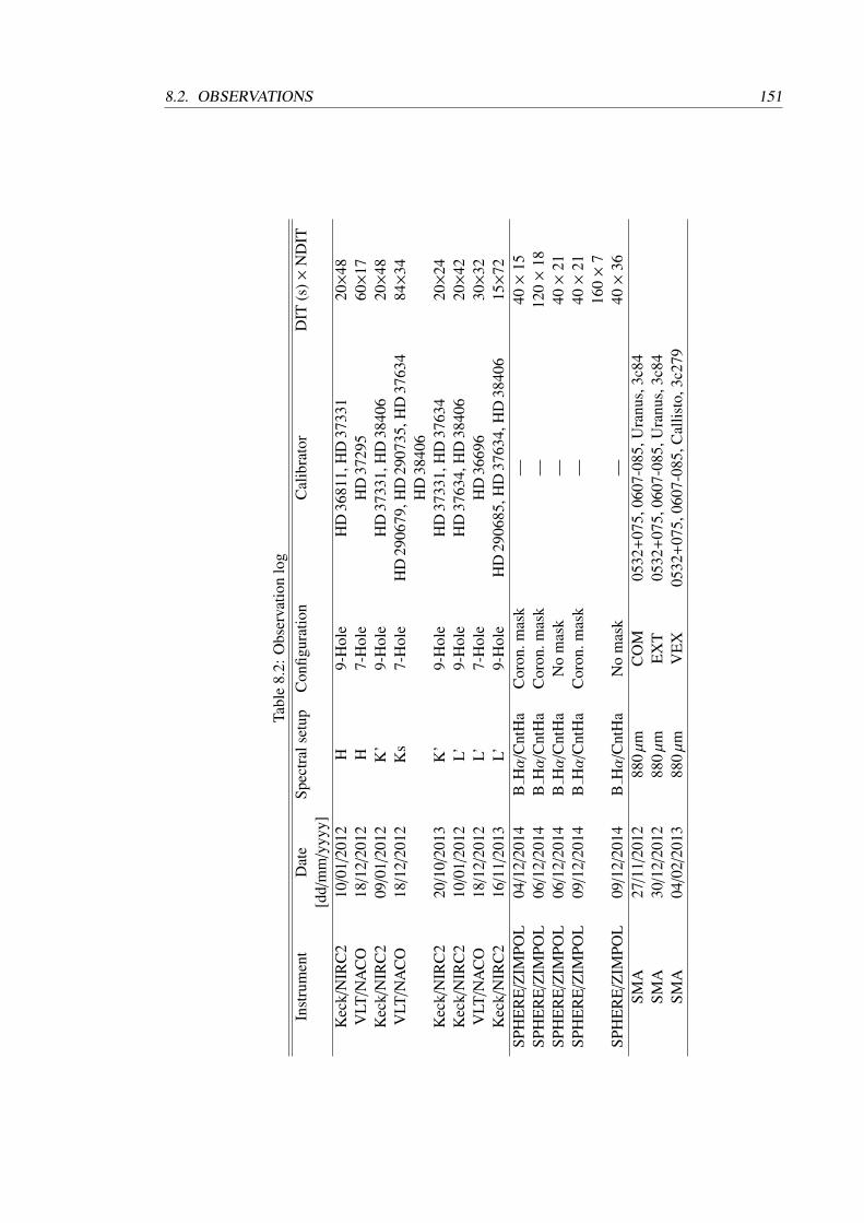
8.2. OBSERVATIONS 151
Tabl
e8.
2:O
bser
vatio
nlo
gIn
stru
men
tD
ate
Spec
tral
setu
pC
onfig
urat
ion
Cal
ibra
tor
DIT
(s)×
ND
IT[d
d/m
m/y
yyy]
Kec
k/N
IRC
210
/01/
2012
H9-
Hol
eH
D36
811,
HD
3733
120×
48V
LT/N
AC
O18
/12/
2012
H7-
Hol
eH
D37
295
60×
17K
eck/
NIR
C2
09/0
1/20
12K
’9-
Hol
eH
D37
331,
HD
3840
620×
48V
LT/N
AC
O18
/12/
2012
Ks
7-H
ole
HD
2906
79,H
D29
0735
,HD
3763
484×
34H
D38
406
Kec
k/N
IRC
220
/10/
2013
K’
9-H
ole
HD
3733
1,H
D37
634
20×
24K
eck/
NIR
C2
10/0
1/20
12L’
9-H
ole
HD
3763
4,H
D38
406
20×
42V
LT/N
AC
O18
/12/
2012
L’7-
Hol
eH
D36
696
30×
32K
eck/
NIR
C2
16/1
1/20
13L’
9-H
ole
HD
2906
85,H
D37
634,
HD
3840
615×
72SP
HE
RE
/ZIM
POL
04/1
2/20
14B
Hα
/Cnt
Ha
Cor
on.m
ask
—40×
15SP
HE
RE
/ZIM
POL
06/1
2/20
14B
Hα
/Cnt
Ha
Cor
on.m
ask
—12
0×
18SP
HE
RE
/ZIM
POL
06/1
2/20
14B
Hα
/Cnt
Ha
No
mas
k—
40×
21SP
HE
RE
/ZIM
POL
09/1
2/20
14B
Hα
/Cnt
Ha
Cor
on.m
ask
—40×
2116
0×
7SP
HE
RE
/ZIM
POL
09/1
2/20
14B
Hα
/Cnt
Ha
No
mas
k—
40×
36SM
A27
/11/
2012
880µ
mC
OM
0532
+07
5,06
07-0
85,U
ranu
s,3c
84SM
A30
/12/
2012
880µ
mE
XT
0532
+07
5,06
07-0
85,U
ranu
s,3c
84SM
A04
/02/
2013
880µ
mV
EX
0532
+07
5,06
07-0
85,C
allis
to,3
c279

8.2. OBSERVATIONS 152
To extract the visibility amplitudes and phases from the NIRC2 and NACO data, we use the
data reduction pipeline previously described in Ireland & Kraus (2008), Kraus et al. (2013) and
Chapter 7. SAM interferometry uses relatively long integration times compared to long baseline
interferometry, which results in a poor calibration of the transfer function for the visibility ampli-
tudes. To correct for this effect, we renormalise the visibilities by fixing the shortest baselines to a
squared visibility of 1.
In order to correct for atmospheric effects, we monitored the instrument transfer function by
bracketing our science observations with observations on unresolved calibrator stars. We observed
multiple calibrator stars, which allowed us to still calibrate our data even in the case when a
calibrator star is found to be resolved and needed to be rejected (i.e. due to a previously unknown
binary companion).
8.2.2 VLT/SPHERE Spectral Differential Imaging
We attempted to detect on-going accretion onto a potential companion through high resolution
imaging in Hαwith ZIMPOL (Roelfsema et al. 2010) from the VLT/SPHERE instrument mounted
on the 8 m UT4 at the Paranal Observatory, Chile. The observations were obtained as part of
SPHERE science verification (ESO programme ID 60.A-9356(A), PI S. Kraus) and spanned three
nights (2014-12-04, 2014-12-06, 2014-12-09) with the majority of data taken on 2014-12-09.
In order to detect accretion signatures we observed with ZIMPOL’s spectral differential imaging
(SDI) mode simultaneously in Hα and in the continuum around the line using the B Ha (λ0 =
656.6nm, ∆λ = 5.5nm) and CntHa (λ0 = 644.9nm, ∆λ = 4.1nm) filters. We observe V1247 Ori
in pupil-stabilised mode both with (8 of field rotation) and without a coronagraphic mask (18 of
field rotation). Coronagraphic images (with the V CLC M WF Lyot coronagraph; diameter 155 mas)
were taken on all three nights and AO-assisted images without mask were taken on the second and
third night (2014-12-06 and 2014-12-09). The dicroic beam-splitter was used.
We achieved the best seeing conditions on 2014-12-09 with an average seeing . 1′′.0.
Average seeing on the remaining two nights were between 1′′.0 and 2′′.0. We thus present here the
results on the best seeing night (i.e. 2014-12-09).
Our SPHERE images were reduced by Dr. Jacques Kluska using the Esorex SPHERE
pipeline v1.18 (Moller-Nilsson et al. 2010). After cleaning (bias, flat, bad pixels) and derotat-
ing each frame, we analysed the data using customised scripts separating the images with and
without the coronagraph. The Hα and continuum frames were stacked after de-rotating for sky
rotation (see Figure 8.7, top-left). Then, the Hα images were normalised to the continuum images
and subtracted. In the resulting image without coronagraph mask we found a negative point source
corresponding to a positive emission in the CntHa filter (Figure 8.7, bottom-left). The contrast of
this point source is about 103 and it is located at ∼110 mas from the central star (see Figure 8.7).
No such feature is present in the images with coronagraphic mask (see Figure 8.7, right). This
feature is likely to be a ghost and was already seen in other ZIMPOL observations (H. M. Schmid,
private communication).

8.3. RESULTS 153
8.2.3 SMA Sub-millimetre Interferometry
V1247 Ori was observed using the Submillimeter Array (SMA) interferometer at Mauna Kea,
Hawaii in the compact (2012-11-28), extended (2012-12-31), and very extended (2013-02-05)
configurations, with baseline lengths from 8–509 m (programme 2012B-S032; PI S. Kraus). The
correlator was configured to process two 2 GHz-wide IF (intermediate frequency) bands centered
at ±5 and 7 GHz from the LO (local oscillator) frequency of 340.8 GHz (880 µm). The CO J=3−2
transition at 345.796 GHz was centered in the upper sideband of the lower IF band, with a chan-
nel spacing of 0.35 km s−1. Observations of V1247 Ori were interleaved with regular visits to
J0532+075 and J0607-085 for use in gain calibration. Additional observations of the bright
quasars 3C 279 and 3C 84, as well as Uranus, Callisto, and Titan were made (depending on
availability and the array configuration) for bandpass and flux calibration (see Table 7.1).
The raw visibility data were reduced and calibrated by Prof. Sean Andrews using standard
procedures in the MIR software package (https://www.cfa.harvard.edu/˜cqi/mircook.
html). The calibrated visibilities were then Fourier inverted assuming natural weighting, de-
convolved with the clean algorithm (Hogbom 1974), and restored with the synthesised beam
(0′′.7 × 0′′.6 at PA = 45). The resulting continuum map has an RMS (root-mean squared) noise
level of 0.85 mJy beam−1; the CO channel maps have an RMS of 55 mJy beam−1 in each channel.
8.3 Results
To search for a companion in our SAM data, we reduce and fit to a star+companion model (Kraus
& Ireland 2012), where we treat the separation (ρ), positional angle (PA), and contrast ( f ) as free
parameters, identical to the treatment for the targets observed in Chapter 7. The best-fit parameters
for the H- and K’-band data sets are listed in Table 8.3 and the L-band are shown in Table 8.4.
In some cases we find the best-fit position to lie within the diffraction limit of the telescope.
Here we enter a regime where the phase signals of a companion become more difficult to constrain
due to degeneracies that can occur between different separation/contrast parameter combinations.
Hence we define this as the degenerate region. The ability to constrain the separation/contrast
parameter space, and hence the inner working angle, depends on the SNR of the closure phase data
recorded in a specific observation. We quantified and described this effect within Section 6.2.1 and
provided a method for deriving the profile of the degeneracy. Fortunately, the degeneracy affects
only the best-fit separation value, but not the position angle when determining the position of a
potential companion.
8.3.1 Disc Rim Detection in L’ Band
In the L’-band, we measure a similar brightness distribution at all three epochs and with a sim-
ilar significance level. Based on the pair-like morphology, the separation, and static nature, we
interpret these L’-band structures as a disc rim located to the north of the star (see Figure 8.1).
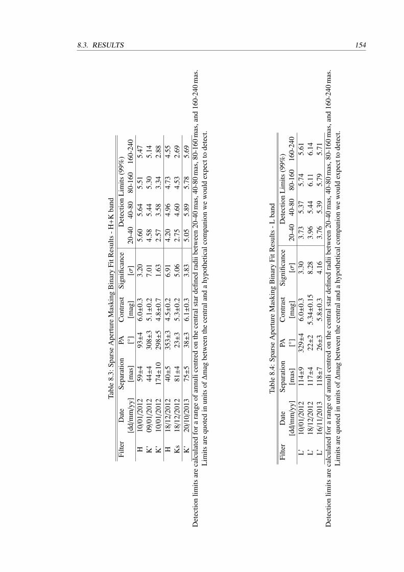
8.3. RESULTS 154
Tabl
e8.
3:Sp
arse
Ape
rtur
eM
aski
ngB
inar
yFi
tRes
ults
-H+
Kba
ndFi
lter
Dat
eSe
para
tion
PAC
ontr
ast
Sign
ifica
nce
Det
ectio
nL
imits
(99%
)[d
d/m
m/y
y][m
as]
[]
[mag
][σ
]20
-40
40-8
080
-160
160-
240
H10
/01/
2012
59±
493±
46.
0±0.
33.
205.
605.
645.
515.
47K
’09
/01/
2012
44±
430
8±3
5.1±
0.2
7.01
4.58
5.44
5.30
5.14
K’
10/0
1/20
1217
4±10
298±
54.
8±0.
71.
632.
573.
583.
342.
88H
18/1
2/20
1240±
535
3±3
4.5±
0.2
6.91
4.20
4.96
4.73
4.55
Ks
18/1
2/20
1281±
423±
35.
3±0.
25.
062.
754.
604.
532.
69K
’20
/10/
2013
75±
538±
36.
1±0.
33.
835.
055.
895.
785.
69D
etec
tion
limits
are
calc
ulat
edfo
rara
nge
ofan
nuli
cent
red
onth
ece
ntra
lsta
rdefi
ned
radi
ibet
wee
n20
-40
mas
,40-
80m
as,8
0-16
0m
as,a
nd16
0-24
0m
as.
Lim
itsar
equ
oted
inun
itsof
∆m
agbe
twee
nth
ece
ntra
land
ahy
poth
etic
alco
mpa
nion
we
wou
ldex
pect
tode
tect
.
Tabl
e8.
4:Sp
arse
Ape
rtur
eM
aski
ngB
inar
yFi
tRes
ults
-Lba
ndFi
lter
Dat
eSe
para
tion
PAC
ontr
ast
Sign
ifica
nce
Det
ectio
nL
imits
(99%
)[d
d/m
m/y
y][m
as]
[]
[mag
][σ
]20
-40
40-8
080
-160
160-
240
L’10
/01/
2012
114±
932
9±4
6.0±
0.3
3.30
3.73
5.37
5.74
5.61
L’18
/12/
2012
117±
422±
25.
34±
0.15
8.28
3.96
5.44
6.11
6.14
L’16
/11/
2013
118±
726±
35.
8±0.
34.
163.
765.
395.
795.
71D
etec
tion
limits
are
calc
ulat
edfo
rara
nge
ofan
nuli
cent
red
onth
ece
ntra
lsta
rdefi
ned
radi
ibet
wee
n20
-40
mas
,40-
80m
as,8
0-16
0m
as,a
nd16
0-24
0m
as.
Lim
itsar
equ
oted
inun
itsof
∆m
agbe
twee
nth
ece
ntra
land
ahy
poth
etic
alco
mpa
nion
we
wou
ldex
pect
tode
tect
.

8.3. RESULTS 155
As one would not expect the position and orientation of a disc rim to shift by a detectable ex-
tent over the time frame in which we observe V1247 Ori (assuming the dynamic timescale within a
disc possessing a roughly Keplerian rotation profile to be given to at least first order by the orbital
period), and as the position and orientation of the structures does not seem to vary substantially
between epochs, we combine the data sets from all three epochs to improve the uv-coverage for
our image reconstruction. The resulting image is shown in Figure 8.2 (left). We resolve the disc
as an arc with two regions of higher flux (to the north-east at a position angle of ∼30 and to
the north-west at a position angle ∼315). We model the disc rim as a skewed ring with a radial
Gaussian profile (see Section 6.3.4) and derive an inclination of i = 30± 10, a disc position angle
of 95 ± 10, and a disc major axis of 110±10 mas, which are consistent with the inner edge of the
outer disc deduced by Kraus et al. (2013) from N-band interferometry data. We define skewness
as the ratio between the amount of flux attributed to opposite sides of the ring along the minor
axis. We set this value to 0.8 and the disc width (50 mas) to represent radiative transfer effects
such as thermal emission or scattering from the opposite rim, but these parameters were found to
have only a marginal affect on the model closure phases. The resulting best-fit model is shown in
Figure 8.2 (right).
We determine the disc flux contribution based on the amount of resolved flux in the recon-
structed image of the combined data set and find that it contributes 5% of the total L’-band flux.
This value is determined through fitting to a grid of flux contributions and computing a χ2 for
each. We then select the best value.
8.3.2 Temporal evolution in H- and K-band
Companion Scenario
Within the shorter-wavelength (H and K-band) data sets we see phase signals that are more con-
sistent with point-source emission than the L’-band data and more moderate drops in the squared
visibilities. In this section we investigate the possibility of these signals being consistent with
an orbiting companion, assuming that there are no contributions due to disc emission, but intro-
duce and examine more complex scenarios in later subsections. In these sections we attempt to
explain the observed asymmetries with a disc rim model, as in Section 8.3.1, or through a com-
panion + disc rim model where the disc rim position and orientation matches that of the disc rim
seen in the L’-band observations.
We observe phase signals that are consistent with a companion at one K-band epoch (2012-
01-09) and at a second H-band epoch (see Figure 8.3; 2012-01-09 K-band, second row; 2012-
12-18 H-band, third row). The measured phase at the remaining two K-band epochs are not as
well reproduced by a single companion fit and appear to be more complex. In the 2012-12-18
K-band observations we see two close-in structures, where the inner one (∼40 mas) is displaced
from the source of the companion signal in the H-band observations taken on the same night by a
position angle of 11±6 as measured from the strongest points of both structures (see Figure 8.3;
2012-12-18 K-band, fourth row). Determining radial distance is more difficult as both structures
lie within the region in which the separation and contrast are not as well constrained. The second
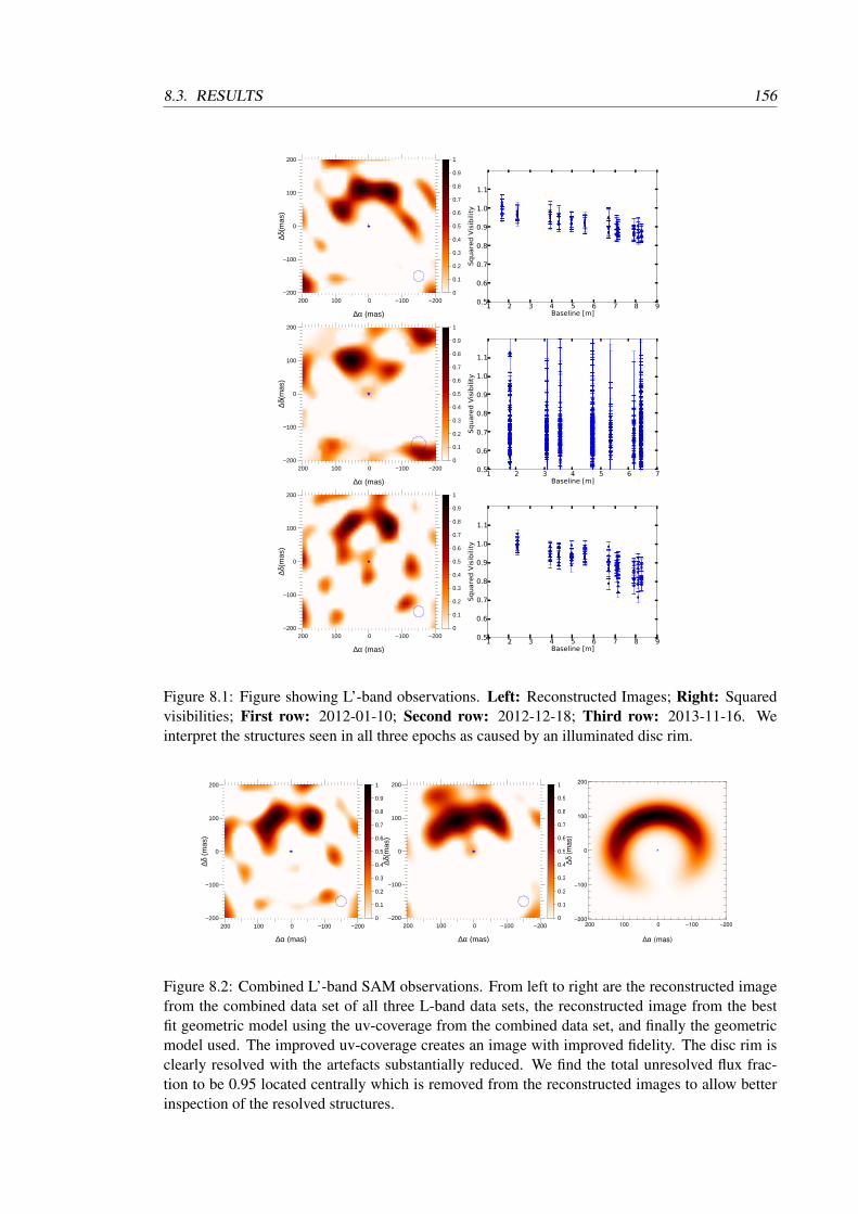
8.3. RESULTS 156
−200−100 0 100 200−200
−100
0
100
200
∆α (mas)
∆δ(m
as)
0
0.1
0.2
0.3
0.4
0.5
0.6
0.7
0.8
0.9
1
1 2 3 4 5 6 7 8 9Baseline [m]
0.5
0.6
0.7
0.8
0.9
1.0
1.1
Square
d V
isib
ility
−200−100 0 100 200−200
−100
0
100
200
∆α (mas)
∆δ(m
as)
0
0.1
0.2
0.3
0.4
0.5
0.6
0.7
0.8
0.9
1
1 2 3 4 5 6 7Baseline [m]
0.5
0.6
0.7
0.8
0.9
1.0
1.1
Square
d V
isib
ility
−200−100 0 100 200−200
−100
0
100
200
∆α (mas)
∆δ(m
as)
0
0.1
0.2
0.3
0.4
0.5
0.6
0.7
0.8
0.9
1
1 2 3 4 5 6 7 8 9Baseline [m]
0.5
0.6
0.7
0.8
0.9
1.0
1.1
Square
d V
isib
ility
Figure 8.1: Figure showing L’-band observations. Left: Reconstructed Images; Right: Squaredvisibilities; First row: 2012-01-10; Second row: 2012-12-18; Third row: 2013-11-16. Weinterpret the structures seen in all three epochs as caused by an illuminated disc rim.
V1247Ori
−200−100 0 100 200−200
−100
0
100
200
0
0.1
0.2
0.3
0.4
0.5
0.6
0.7
0.8
0.9
1
∆α (mas)
∆δ (
mas
)
−200−100 0 100 200−200
−100
0
100
200
∆α (mas)
∆δ(m
as)
0
0.1
0.2
0.3
0.4
0.5
0.6
0.7
0.8
0.9
1
−200−100 0 100 200−200
−100
0
100
200
∆α (mas)
∆δ (
ma
s)
Figure 8.2: Combined L’-band SAM observations. From left to right are the reconstructed imagefrom the combined data set of all three L-band data sets, the reconstructed image from the bestfit geometric model using the uv-coverage from the combined data set, and finally the geometricmodel used. The improved uv-coverage creates an image with improved fidelity. The disc rim isclearly resolved with the artefacts substantially reduced. We find the total unresolved flux frac-tion to be 0.95 located centrally which is removed from the reconstructed images to allow betterinspection of the resolved structures.

8.3. RESULTS 157
companion-like structure is located outside the degenerate region (indicated with a dashed circle
in Figure 8.3) and does not appear in the H-band observations. In the 2013-10-20 K-band data we
see again a single, weak, companion-like structure outside the degenerate region (see Figure 8.3;
2013-10-20 K-band, fifth row).
Based purely on the quality of the fit to the interferometric data, the strong detections (> 5σ)
in the H- and K-band are consistent with a companion at > 45 mas separation from the star. If we
de-redden the measured contrasts using the method outlined by Cardelli et al. (1989), we compute
absolute magnitudes of 5.1 in H-band and 4.3 in K-band. According to the circumplanetary disc
models by (Zhu 2015), the SED of an optically thick circumplanetary accretion disc is determined
by the parameters MM (the product of the planet mass and disc accretion rate) and the inner disc
radius. These magnitudes would imply a MM value of 10−3 M2Jyr−1 when assuming a circum-
planetary disc with an inner radius of 2RJup viewed under a similar inclination to the surrounding
circumstellar disc (∼30). The exact properties of the circumplanetary disc are unknown however
and hence such estimates should be treated with caution.
However, we find that the apparent motion between the two epochs is too large to be con-
sistent with a physical Keplerian orbit solution. Under the assumption of a co-planar, circular orbit
with the outer disc, a distance of ∼17 au between the central star and the companion is derived.
The change in position angle between the epochs however implies a distance ∼6 au which cannot
be reconciled with the fitted separation of the companion. Also, this scenario cannot explain why
the companion candidate was not detected in H-band during the first epoch and in the K-band
during the third epoch. Hence we find the probable cause of the strong asymmetries not to be a
single companion at ∼ 40-50 mas separation. We explore within the next two subsections alter-
native scenarios, namely a stationary disc rim at 40 mas and a bright companion on a close orbit
(∼20 mas) influenced by the presence of the disc rim observed in L’-band.
Disc Rim Scenario
Inspired by the detection of a disc rim in L’-band (Section 8.3.1), we test whether the asymme-
tries detected in H+K band (and their apparent temporal changes) might also be explained with
emission from a static disc structure, without invoking the presence of a companion. Previous
work (Cieza et al. 2013; Willson et al. 2016) has shown that the forward-scattered light of an
inclined disc rim can cause asymmetries in the brightness distribution that can mimic companion-
like phase signals in aperture masking observations (see Section 6.3.5). The presence of such a
disc rim with a similar position angle and inclination as the outer disc but with a semi-major axis
close to 40 mas, combined with the differing uv coverages between the epochs could produce a
point source-like asymmetry whose position appears to move. Cieza et al. (2013) found this to
be the case when investigating the asymmetry detected in the disc around FL Cha, where they too
observed apparently non-Keplerian motion.
To test this scenario we constructed a model similar in geometry and orientation to the one
described in Section 8.3.1 but leaving the radius of the ring as a free parameter (i.e. an inner
ring, co-planar to the ring seen in the L-band data). The ring radius which was found to produce
the lowest χ2 value to the data was selected. We then generated a synthetic data set from these

8.3. RESULTS 158
model images for our particular uv-coverage. The reconstructed images did not resemble those of
a point source nor the structures seen in our real data. In addition, our binary fits to the model data
sets found no significant change in the position angle of the the best fit positions between the two
epochs and uv-coverages.
Therefore we reject a this model of the disc but also models which are static over the time
frame of our observations. We do so as a static asymmetry as a result of structure in or of the disc
should also have resulted in a strong asymmetry signal in the third epoch (2013-10-20), where we
observe no significant signal in H or K.
Companion + Disc Scenario
The companion fits presented in Section 8.3.2 indicate companion separations of ∼ 45 mas, i.e.
near the λ/B resolution limit. In this regime, the determined parameters can suffer from a degener-
acy between separation and contrast (see Section 6.2.1). Also, the parameters could potentially be
affected by asymmetric emission from the disc wall that we detected in the L’-band data sets (see
Section 8.3.1), which could lead to an over-estimation of the fitted companion separation. There-
fore, we explore whether a companion+disc model could explain the temporal evolution that we
see in our aperture masking data between the different epochs.
A sketch of the proposed scenario is shown in Figure 8.4. The observed position of the
companion in the reconstructed images and in the binary fits is found to be at larger separations,
towards the location of a disc asymmetry along the same or similar position angle as the true
position angle of the companion. This is the case for first two epochs allowing the companion to
be observed as a strong asymmetry in the fits and reconstructed images. In the third, the orbital
motion of the companion alters the alignment between the companion and peak disc rim emission
such that the position angles between the two are no longer favourable. Here, no overestimation in
the fit to the separation occurs and hence the companion remains undetected explaining its absence
in the third epoch.
In order to test this scenario and to understand how the presence of a disc rim affects the
retrieved parameters in a companion fit, we construct a suite of models that contain a disc wall
similar to the one found in the L’-band observations (semi-major axis = 150 mas, semi-major axis
PA = 95, disc contrast ratio = 0.04) and with a bright companion similar in contrast and posi-
tion angle to the companion found within the 2012-01-09 K-band observations (see Table 8.3).
However, we place the companion at a separation that would be consistent with a Keplerian orbit
(ρ = 20 mas ≈ 6 au for a circular orbit within the plane of the outer disc) between the first and
second epoch in our new data set. We keep the companion position angle the same as the fitted
position angle, 308 We use the uv-coverage and noise from the 2012-01-09 K-band observations
to generate simulated data sets. We then vary within our models a single parameter of either the
disc or companion, namely either the disc major axis, major-axis position angle, disc inclination,
disc width, disc flux ratio, disc skewness, or companion flux ratio.
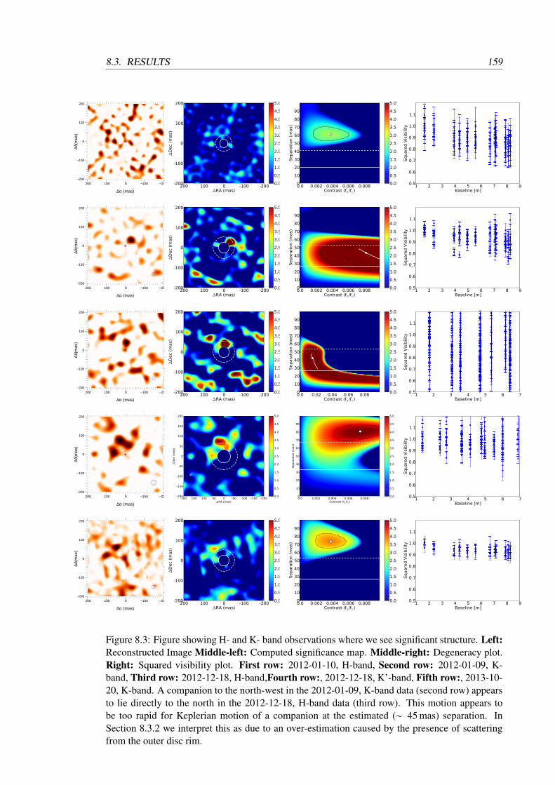
8.3. RESULTS 159
−200−100 0 100 200−200
−100
0
100
200
∆α (mas)
∆δ(m
as)
0
0.1
0.2
0.3
0.4
0.5
0.6
0.7
0.8
0.9
1
200 100 0 -100 -200∆RA (mas)
-200
-100
0
100
200
∆D
ec
(mas)
0.0
0.5
1.0
1.5
2.0
2.5
3.0
3.5
4.0
4.5
5.0
0.0 0.002 0.004 0.006 0.008Contrast (f2 /f1 )
0
10
20
30
40
50
60
70
80
90
Separa
tion (
mas)
0.0
0.5
1.0
1.5
2.0
2.5
3.0
3.5
4.0
4.5
5.0
1 2 3 4 5 6 7 8 9Baseline [m]
0.5
0.6
0.7
0.8
0.9
1.0
1.1
Square
d V
isib
ility
−200−100 0 100 200−200
−100
0
100
200
∆α (mas)
∆δ(m
as)
0
0.1
0.2
0.3
0.4
0.5
0.6
0.7
0.8
0.9
1
200 100 0 -100 -200∆RA (mas)
-200
-100
0
100
200
∆D
ec
(mas)
0.0
0.5
1.0
1.5
2.0
2.5
3.0
3.5
4.0
4.5
5.0
0.0 0.02 0.04 0.06 0.08Contrast (f2 /f1 )
0
10
20
30
40
50
60
70
80
90
Separa
tion (
mas)
0.0
0.5
1.0
1.5
2.0
2.5
3.0
3.5
4.0
4.5
5.0
1 2 3 4 5 6 7Baseline [m]
0.5
0.6
0.7
0.8
0.9
1.0
1.1
Square
d V
isib
ility
−200−100 0 100 200−200
−100
0
100
200
∆α (mas)
∆δ(m
as)
0
0.1
0.2
0.3
0.4
0.5
0.6
0.7
0.8
0.9
1
200 150 100 50 0 -50 -100 -150 -200∆RA (mas)
-200
-150
-100
-50
0
50
100
150
200
∆D
ec
(mas)
0.0
0.5
1.0
1.5
2.0
2.5
3.0
3.5
4.0
4.5
5.0
0.0 0.002 0.004 0.006 0.008Contrast (f2 /f1 )
0
10
20
30
40
50
60
70
80
90
Separa
tion (
mas)
0.0
0.5
1.0
1.5
2.0
2.5
3.0
3.5
4.0
4.5
5.0
1 2 3 4 5 6 7Baseline [m]
0.5
0.6
0.7
0.8
0.9
1.0
1.1
Square
d V
isib
ility
−200−100 0 100 200−200
−100
0
100
200
∆α (mas)
∆δ(m
as)
0
0.1
0.2
0.3
0.4
0.5
0.6
0.7
0.8
0.9
1
200 100 0 -100 -200∆RA (mas)
-200
-100
0
100
200
∆D
ec
(mas)
0.0
0.5
1.0
1.5
2.0
2.5
3.0
3.5
4.0
4.5
5.0
0.0 0.002 0.004 0.006 0.008Contrast (f2 /f1 )
0
10
20
30
40
50
60
70
80
90
Separa
tion (
mas)
0.0
0.5
1.0
1.5
2.0
2.5
3.0
3.5
4.0
4.5
5.0
1 2 3 4 5 6 7 8 9Baseline [m]
0.5
0.6
0.7
0.8
0.9
1.0
1.1
Square
d V
isib
ility
Figure 8.3: Figure showing H- and K- band observations where we see significant structure. Left:Reconstructed Image Middle-left: Computed significance map. Middle-right: Degeneracy plot.Right: Squared visibility plot. First row: 2012-01-10, H-band, Second row: 2012-01-09, K-band, Third row: 2012-12-18, H-band,Fourth row:, 2012-12-18, K’-band, Fifth row:, 2013-10-20, K-band. A companion to the north-west in the 2012-01-09, K-band data (second row) appearsto lie directly to the north in the 2012-12-18, H-band data (third row). This motion appears tobe too rapid for Keplerian motion of a companion at the estimated (∼ 45 mas) separation. InSection 8.3.2 we interpret this as due to an over-estimation caused by the presence of scatteringfrom the outer disc rim.
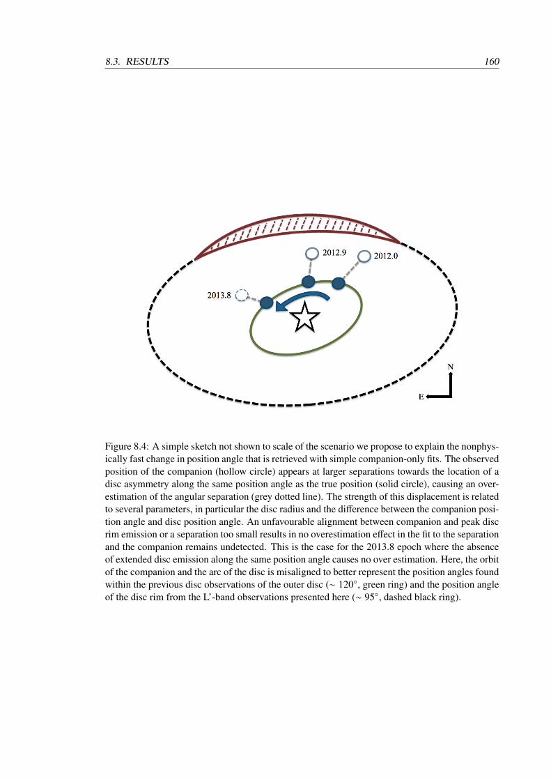
8.3. RESULTS 160
Figure 8.4: A simple sketch not shown to scale of the scenario we propose to explain the nonphys-ically fast change in position angle that is retrieved with simple companion-only fits. The observedposition of the companion (hollow circle) appears at larger separations towards the location of adisc asymmetry along the same position angle as the true position (solid circle), causing an over-estimation of the angular separation (grey dotted line). The strength of this displacement is relatedto several parameters, in particular the disc radius and the difference between the companion posi-tion angle and disc position angle. An unfavourable alignment between companion and peak discrim emission or a separation too small results in no overestimation effect in the fit to the separationand the companion remains undetected. This is the case for the 2013.8 epoch where the absenceof extended disc emission along the same position angle causes no over estimation. Here, the orbitof the companion and the arc of the disc is misaligned to better represent the position angles foundwithin the previous disc observations of the outer disc (∼ 120, green ring) and the position angleof the disc rim from the L’-band observations presented here (∼ 95, dashed black ring).
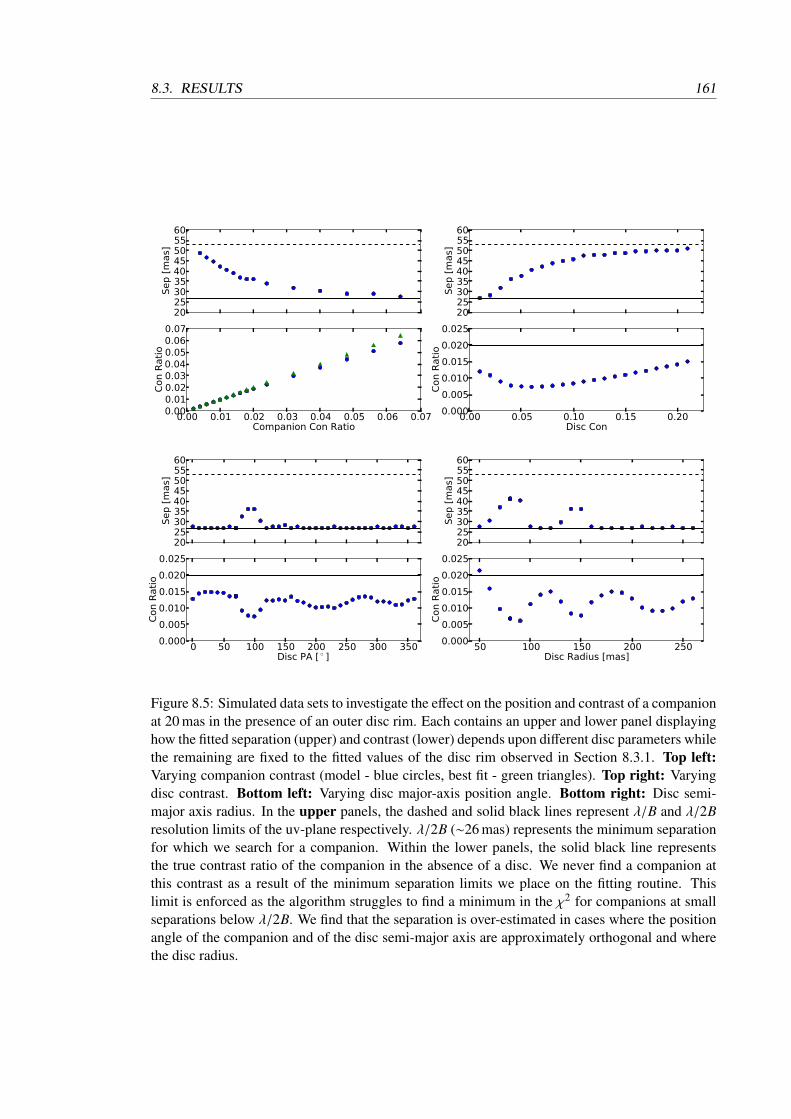
8.3. RESULTS 161
202530354045505560
Sep [
mas]
0.00 0.01 0.02 0.03 0.04 0.05 0.06 0.07Companion Con Ratio
0.000.010.020.030.040.050.060.07
Con R
ati
o
202530354045505560
Sep [
mas]
0.00 0.05 0.10 0.15 0.20Disc Con
0.000
0.005
0.010
0.015
0.020
0.025
Con R
ati
o
202530354045505560
Sep [
mas]
0 50 100 150 200 250 300 350Disc PA [ ]
0.000
0.005
0.010
0.015
0.020
0.025
Con R
ati
o
202530354045505560
Sep [
mas]
50 100 150 200 250Disc Radius [mas]
0.000
0.005
0.010
0.015
0.020
0.025
Con R
ati
o
Figure 8.5: Simulated data sets to investigate the effect on the position and contrast of a companionat 20 mas in the presence of an outer disc rim. Each contains an upper and lower panel displayinghow the fitted separation (upper) and contrast (lower) depends upon different disc parameters whilethe remaining are fixed to the fitted values of the disc rim observed in Section 8.3.1. Top left:Varying companion contrast (model - blue circles, best fit - green triangles). Top right: Varyingdisc contrast. Bottom left: Varying disc major-axis position angle. Bottom right: Disc semi-major axis radius. In the upper panels, the dashed and solid black lines represent λ/B and λ/2Bresolution limits of the uv-plane respectively. λ/2B (∼26 mas) represents the minimum separationfor which we search for a companion. Within the lower panels, the solid black line representsthe true contrast ratio of the companion in the absence of a disc. We never find a companion atthis contrast as a result of the minimum separation limits we place on the fitting routine. Thislimit is enforced as the algorithm struggles to find a minimum in the χ2 for companions at smallseparations below λ/2B. We find that the separation is over-estimated in cases where the positionangle of the companion and of the disc semi-major axis are approximately orthogonal and wherethe disc radius.
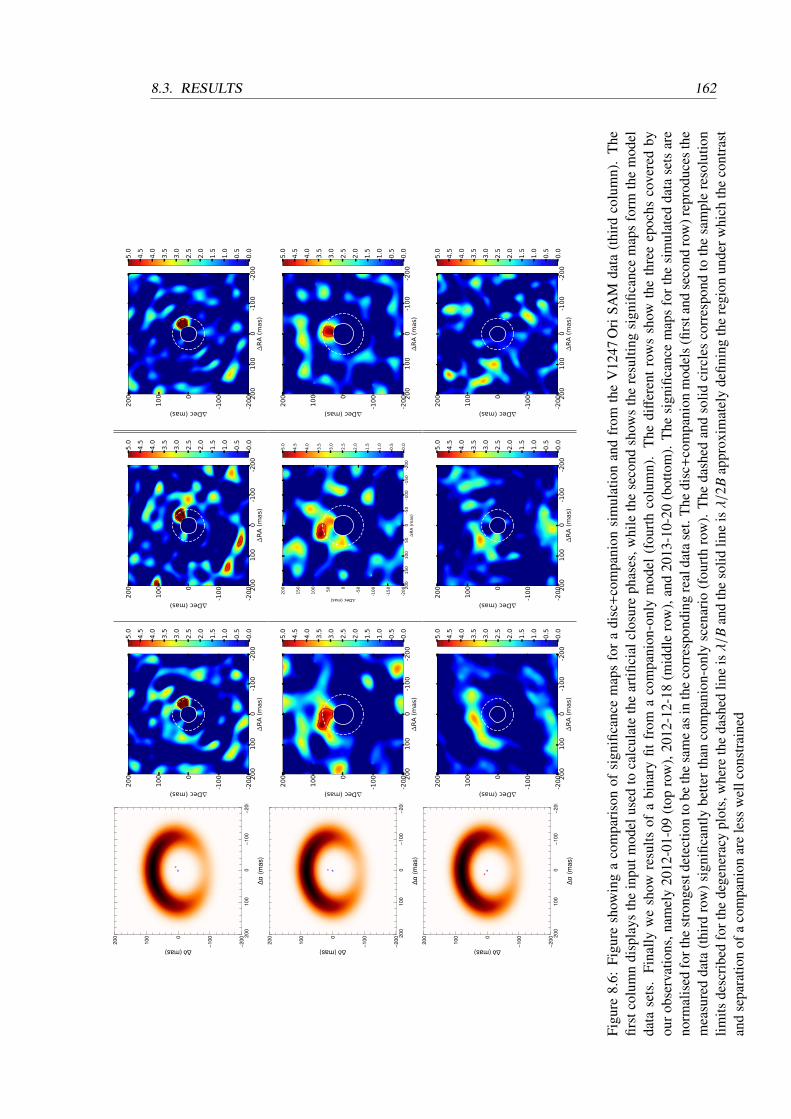
8.3. RESULTS 162
−200
−100
0 1
00
200
−200
−100 0
100
200
∆α (
ma
s)
∆δ (mas)
200
100
0-1
00
-200
∆R
A (
mas)
-200
-1000
100
200
∆Dec (mas)
0.0
0.5
1.0
1.5
2.0
2.5
3.0
3.5
4.0
4.5
5.0
200
100
0-1
00
-200
∆R
A (
mas)
-200
-1000
100
200
∆Dec (mas)
0.0
0.5
1.0
1.5
2.0
2.5
3.0
3.5
4.0
4.5
5.0
200
100
0-1
00
-200
∆R
A (
mas)
-200
-1000
100
200
∆Dec (mas)
0.0
0.5
1.0
1.5
2.0
2.5
3.0
3.5
4.0
4.5
5.0
−200
−100
0 1
00
200
−200
−100 0
100
200
∆α (
ma
s)
∆δ (mas)
200
100
0-1
00
-200
∆R
A (
mas)
-200
-1000
100
200
∆Dec (mas)
0.0
0.5
1.0
1.5
2.0
2.5
3.0
3.5
4.0
4.5
5.0
20
01
50
10
05
00
-50
-10
0-1
50
-20
0∆
RA
(m
as)
-20
0
-15
0
-10
0
-500
50
10
0
15
0
20
0
∆Dec (mas)
0.0
0.5
1.0
1.5
2.0
2.5
3.0
3.5
4.0
4.5
5.0
200
100
0-1
00
-200
∆R
A (
mas)
-200
-1000
100
200
∆Dec (mas)
0.0
0.5
1.0
1.5
2.0
2.5
3.0
3.5
4.0
4.5
5.0
−200
−100
0 1
00
200
−200
−100 0
100
200
∆α (
ma
s)
∆δ (mas)
200
100
0-1
00
-200
∆R
A (
mas)
-200
-1000
100
200
∆Dec (mas)
0.0
0.5
1.0
1.5
2.0
2.5
3.0
3.5
4.0
4.5
5.0
200
100
0-1
00
-200
∆R
A (
mas)
-200
-1000
100
200
∆Dec (mas)
0.0
0.5
1.0
1.5
2.0
2.5
3.0
3.5
4.0
4.5
5.0
200
100
0-1
00
-200
∆R
A (
mas)
-200
-1000
100
200
∆Dec (mas)
0.0
0.5
1.0
1.5
2.0
2.5
3.0
3.5
4.0
4.5
5.0
Figu
re8.
6:Fi
gure
show
ing
aco
mpa
riso
nof
sign
ifica
nce
map
sfo
ra
disc
+co
mpa
nion
sim
ulat
ion
and
from
the
V12
47O
riSA
Mda
ta(t
hird
colu
mn)
.T
hefir
stco
lum
ndi
spla
ysth
ein
putm
odel
used
toca
lcul
ate
the
artifi
cial
clos
ure
phas
es,w
hile
the
seco
ndsh
ows
the
resu
lting
sign
ifica
nce
map
sfo
rmth
em
odel
data
sets
.Fi
nally
we
show
resu
ltsof
abi
nary
fitfr
oma
com
pani
on-o
nly
mod
el(f
ourt
hco
lum
n).
The
diff
eren
tro
ws
show
the
thre
eep
ochs
cove
red
byou
rob
serv
atio
ns,n
amel
y20
12-0
1-09
(top
row
),20
12-1
2-18
(mid
dle
row
),an
d20
13-1
0-20
(bot
tom
).T
hesi
gnifi
canc
em
aps
for
the
sim
ulat
edda
tase
tsar
eno
rmal
ised
fort
hest
rong
estd
etec
tion
tobe
the
sam
eas
inth
eco
rres
pond
ing
real
data
set.
The
disc
+co
mpa
nion
mod
els
(firs
tand
seco
ndro
w)r
epro
duce
sth
em
easu
red
data
(thi
rdro
w)s
igni
fican
tlybe
ttert
han
com
pani
on-o
nly
scen
ario
(fou
rth
row
).T
heda
shed
and
solid
circ
les
corr
espo
ndto
the
sam
ple
reso
lutio
nlim
itsde
scri
bed
fort
hede
gene
racy
plot
s,w
here
the
dash
edlin
eisλ/B
and
the
solid
line
isλ/2
Bap
prox
imat
ely
defin
ing
the
regi
onun
derw
hich
the
cont
rast
and
sepa
ratio
nof
aco
mpa
nion
are
less
wel
lcon
stra
ined

8.3. RESULTS 163
The results of our simulations are shown in Figure 8.5. We find that the separation can
indeed be significantly over-estimated in the presence of the asymmetric disc emission, namely
the fitted separation of the companion can appear more than twice as far from the central star, if
the companion and the brightest point of emission from the disc rim are roughly aligned along a
similar position angle. This effect appears in both the image reconstructions and the binary fitting
to the closure phase data.
We find that the strength of the over-estimation in the fitted separation of the companion
is most sensitive to the disc radius, disc position angle and disc flux. We also find dimmer com-
panions to be more susceptible to larger shifts in their fitted separations compared to brighter
companions, but inversely the brighter companions’ contrasts are more affected by the presence of
a disc than the dimmer companions (Figure 8.5, top-left panel). When varying the disc flux contri-
bution (Figure 8.5, top-right panel) we do observe that the over-estimation effect does not shift the
fitted position of the companion outside of λ/B, except when the flux becomes large enough for the
disc asymmetries to dominate, and the best fit position becomes a point co-located on the disc rim.
Additionally we only observe a significant over estimation in the separation in a narrow window
of the position angle of the disc semi-major axis (Figure 8.5, lower left panel). For our particular
simulation setup, the strongest fitted separation over-estimation occurs for disc semi-major axis
position angles between 90-100, but some effects are present over the range from 70-120. The
relationship between disc radius and the over-estimation is rather complex (Figure 8.5, lower-right
panel), displaying a decaying sinusoidal relationship similar to a first order Bessel function with
the over-estimation fitted separation greatest between disc radii of 70-90 mas and weakest between
100-120 mas. This pattern repeats between 140-150 mas and out beyond 160 mas. This belies the
origin of the over-estimation as the Fourier transform of a skewed Gaussian ring is a Bessel func-
tion of the zeroth order. An alternative way to view the model is by considering the phases of the
disc+companion model, where the binary sine wave is modulated by the disc Bessel function. Ig-
noring the modulation and fitting with the simple sine function will therefore result in a bias in the
fit. The mean phase over all baselines determines the strength of the over estimation. Where the
disc phases pass through nulls is therefore determinant in how the strength of the over estimation
is modulated with changing disc radius. The effect on the phase at the shortest baselines is respon-
sible for producing the position angle relation between the companion and disc as these baselines
are the worst effected and require strong positive phases here to produce an over-estimation.
In our simulations with extended disc emission, we find that the companion contrast is al-
ways under-estimated compared to the true contrast. The difference between the simulated contrast
of the companion and the retrieved, best-fit contrast never exceeds more than a factor of three.
Following this parameter study on the influence of disc emission on companion fits, we
attempted to fit our specific five aperture masking data sets on V1247 Ori with this model. For
this purpose, we considered computing a full grid of all model parameters, but found that this
proved unfeasible due to the large number of involved free parameters. To simplify the problem
we therefore fixed the parameters of the disc rim to the values previously inferred from VLTI long-
baseline interferometry (disc semi-major axis = 110 mas, disc semi-major axis PA = 104; Kraus
et al. 2013). The flux contributions of the disc were fixed using the visibility data (fraction of
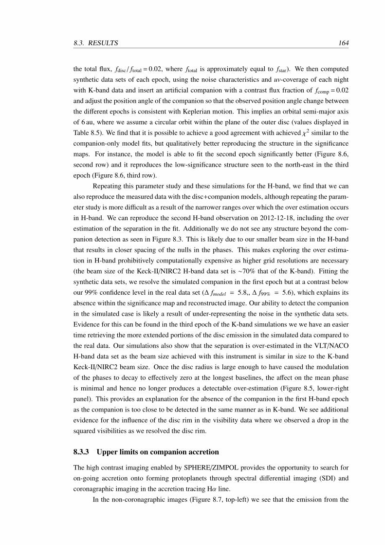
8.3. RESULTS 164
the total flux, fdisc/ ftotal = 0.02, where ftotal is approximately equal to fstar). We then computed
synthetic data sets of each epoch, using the noise characteristics and uv-coverage of each night
with K-band data and insert an artificial companion with a contrast flux fraction of fcomp = 0.02
and adjust the position angle of the companion so that the observed position angle change between
the different epochs is consistent with Keplerian motion. This implies an orbital semi-major axis
of 6 au, where we assume a circular orbit within the plane of the outer disc (values displayed in
Table 8.5). We find that it is possible to achieve a good agreement with achieved χ2 similar to the
companion-only model fits, but qualitatively better reproducing the structure in the significance
maps. For instance, the model is able to fit the second epoch significantly better (Figure 8.6,
second row) and it reproduces the low-significance structure seen to the north-east in the third
epoch (Figure 8.6, third row).
Repeating this parameter study and these simulations for the H-band, we find that we can
also reproduce the measured data with the disc+companion models, although repeating the param-
eter study is more difficult as a result of the narrower ranges over which the over estimation occurs
in H-band. We can reproduce the second H-band observation on 2012-12-18, including the over
estimation of the separation in the fit. Additionally we do not see any structure beyond the com-
panion detection as seen in Figure 8.3. This is likely due to our smaller beam size in the H-band
that results in closer spacing of the nulls in the phases. This makes exploring the over estima-
tion in H-band prohibitively computationally expensive as higher grid resolutions are necessary
(the beam size of the Keck-II/NIRC2 H-band data set is ∼70% that of the K-band). Fitting the
synthetic data sets, we resolve the simulated companion in the first epoch but at a contrast below
our 99% confidence level in the real data set (∆ fmodel = 5.8,, ∆ f99% = 5.6), which explains its
absence within the significance map and reconstructed image. Our ability to detect the companion
in the simulated case is likely a result of under-representing the noise in the synthetic data sets.
Evidence for this can be found in the third epoch of the K-band simulations we we have an easier
time retrieving the more extended portions of the disc emission in the simulated data compared to
the real data. Our simulations also show that the separation is over-estimated in the VLT/NACO
H-band data set as the beam size achieved with this instrument is similar in size to the K-band
Keck-II/NIRC2 beam size. Once the disc radius is large enough to have caused the modulation
of the phases to decay to effectively zero at the longest baselines, the affect on the mean phase
is minimal and hence no longer produces a detectable over-estimation (Figure 8.5, lower-right
panel). This provides an explanation for the absence of the companion in the first H-band epoch
as the companion is too close to be detected in the same manner as in K-band. We see additional
evidence for the influence of the disc rim in the visibility data where we observed a drop in the
squared visibilities as we resolved the disc rim.
8.3.3 Upper limits on companion accretion
The high contrast imaging enabled by SPHERE/ZIMPOL provides the opportunity to search for
on-going accretion onto forming protoplanets through spectral differential imaging (SDI) and
coronagraphic imaging in the accretion tracing Hα line.
In the non-coronagraphic images (Figure 8.7, top-left) we see that the emission from the
8.3. RESULTS 165
Table 8.5: Companion Candidate PropertiesModel Date ρ PA Sig a MH MK McMc
(a)
[dd/mm/yy] [mas] [] [σ] [AU] [mag] [mag] [10−6 M2Jyr−1]
Comp 09/01/2012 43±5 308±3 6.9 17 — 4.7±0.2 10−3
18/12/2012 40±5 353±3 7.0 17 4.8±0.2 — 10−3
Disc+Comp 09/01/2012 18 308 — 6 4.2 3.6 10−3
18/12/2012 15 353 — 6 4.2 3.6 10−3
20/10/2013 13 45 — 6 — 3.6 10−3
Columns are organised by model, date of observation, angular separation, ρ, position angle, PA,significance, orbital semi-major axis, a, based on previous observations of the disc inclination
and position angle, absolute magnitude of the companion in H-band, MH , absolute magnitude ofthe companion in K-band, MK , and the product of the accretion rate onto the companion and thecompanion mass, McMc. Dereddening was performed as described in Cardelli et al. (1989). Therows are are in chronological order with the second half detailing the model parameters used inFigure 8.6. (a) Values derived from Zhu (2015) assuming circumplanetary disc radii extending
from 2 RJ outwards.
−200 −100 0 100 200
−200
−100
0
100
200
−6.23
5.03e+03
1.01e+04
1.51e+04
2.02e+04
2.52e+04
3.02e+04
3.53e+04
4.03e+04
4.54e+04
5.04e+04
−200 −100 0 100 200
−200
−100
0
100
200
−100
−80
−60
−40
−20
0
20
40
60
80
100
Ghost
−400 −200 0 200 400
−400
−200
0
200
400
16.1
145
274
403
531
660
789
918
1.05e+03
1.18e+03
1.3e+03
−400 −200 0 200 400
−400
−200
0
200
400
−110
−91.6
−72.8
−54.1
−35.3
−16.5
2.26
21
39.8
58.6
77.4
100mas 100mas
100mas 100mas
Coronagraph
Spider arm
AO feature
N
E
N
E
N
E
N
E
Figure 8.7: SPHERE/ZIMPOL images of V1247 Ori in Hα and continuum. Top Left: Intensityimage of the target without coronagraph in continuum. We see an elongated structure to theSouth-East. Top Right: Intensity image in continuum with the coronagraph. The spider arms,chronograph, and AO feature are labelled. Bottom Left: SDI image without the coronagraph inHα and continuum. The ghost is located at ∼110mas from the central star and is labelled, seeSection 8.2.2 for details. Bottom right: Coronagraphic SDI image in Hα and continuum.

8.3. RESULTS 166
0 200 400 600
0
5
10
15
Detection limits at 5σ: Ha nocor Cnt nocor SDI nocor Ha cor Cnt cor SDI cor
Figure 8.8: 5-σ detection limits derived from the SPHERE/ZIMPOL data set and plotted as func-tion of the angular distance to the star with coronagraph (cor) and without coronagraph (nocor).The subtraction between the two filters allow a gain of 3 magnitudes in contrast.
immediate area around V1247 Ori on small separations (<100 mas) differs from a point source in
both filters, where the difference between the two filters is negligible. The emission is elongated
along a position angle of 108±10, which is consistent with the disc orientation. Possibly, we
see stellar light scattered from the surface of the disc. Without observations of a reference star
however, we are unable to determine with any reasonable confidence whether this elongation is
indeed due to scattered light from an inner disc component or an instrumentation effect.
Our SPHERE images do not reveal any point source in the inner region around V1247 Ori,
besides the instrumental ’ghost’ reflection outlined in Section 8.2.2 and shown in Figure 8.7.
Therefore, we derive detection upper limits from our images, where we avoid the area near the
reflection (’ghost’) in the continuum filter. These detection limits were calibrated on the flux of
the star using the image without the coronagraph. In the intensity images we derive upper limit
contrasts of ∼9.5 magnitudes at 200 mas without the coronagraph and ∼12.5 magnitudes with it
(Figure 8.8). Without the coronagraph mask we reach typical contrast limits of 3-8 magnitudes in
the Hα filter for separations between 25-100 mas. These values are consistent with the prediction
by the SPHERE/ZIMPOL exposure time calculator. Applying the SDI subtraction results in a gain
of ∼3 magnitudes on the detection limit. The SDI detection limits are derived with the assump-
tion that the companion flux ratio between the Hα and the continuum filters is high (fHα/fcont >5)
allowing a direct computation of the detection limit (Rameau et al. 2015).
We calculate upper limits from the Hα detection limits for the accretion rate onto a proto-
planet. Our method is identical to that outlined in Rigliaco et al. (2012) and Close et al. (2014)
after correcting for the stellar Hα contribution and assuming a companion mass of 1 MJ. Assum-
ing equal extinction for V1247 Ori A and a potential companion and that the accretion-luminosity

8.3. RESULTS 167
relation for low-mass T Tauri stars applies to the companion, we find this corresponds to a range of
MM values between 10−5-10−8 M2Jyr−1. With the coronagraph mask in place we achieve higher
contrast limits (9.5-12.5 magnitudes in Hα) which under the same assumptions corresponds to
MM values between 10−9-10−10 M2Jyr−1. These values are highly dependent on the value of ex-
tinction in R-band, AR, which is likely substantially higher within the disc gap than towards the
central star. To explore how much greater the extinction must be, one can assume an arbitrary but
not unreasonable value of AR of 10.0 mag (reasonable due to the known substantial population of
dusty material still resident within the gap of V1247 Ori Kraus et al. 2013), these limits become
100-10−3 M2Jyr−1 and 10−4-10−6 M2
Jyr−1 for between 25-100 mas and 100-600 mas. We there-
fore rule out a companion similar in Hα magnitude to LkCa 15 b between separations of 100 to
600 mas, or such a companion would need to be more deeply embedded in V1247 Ori than found
for LkCa 15 b.
To calculate the accretion luminosity of V1247 Ori, I used the the HARPS data presented
by Kraus et al. (2013) to measure and equivalent line width of the Hα emission, which was then
converted into a accretion rate using the method described by Rigliaco et al. (2012) and the stellar
mass derived by Kraus et al. (2013). This was found to be equivalent to a mass accretion rate of
∼10−8Myr−1 onto the primary star.
8.3.4 Geometry and dynamics of the outer disc
Our SMA sub-millimetre maps on V1247 Ori are shown in Figure 8.9. We reconstructed a 880 µm
continuum image with natural weighting from all baseline data (Figure 8.9, bottom). Here, once
beam shape has been accounted for, we resolve an elongated structure that is oriented along south-
east/north-west direction, roughly consistent with the disc position angle derived by our previous
infrared interferometric observations (Kraus et al. 2013). Fitting a uniform disc model to the
continuum visibilities yields a disc position angle of 142±5, shown in Figure 8.10. Our model
visibilities are shown in blue with the residuals displayed in the panel below. This position angle
differs slightly from our estimate derived from mid-infrared interferometry (104±15; Kraus et al.
2013), but still consistent to within 3σ. The estimated inclination value of 29±2 is in line with
our previous estimate (31.3 ± 7.5) within a single standard deviation. The integrated 880 µm flux
is 0.20±0.01 Jy.
The SMA data covers also the 12CO(3-2) line, where we detect a rotating disc profile (see
Figure 8.9, top). The position angle of the disc rotation axis (semi-minor axis along position angle
32±10) matches again the previous observations of the outer disc orientation (104 ± 15; Kraus
et al. 2013) and our own observations with SAM in L’-band (semi-minor axis along position angle
30±15).
Combining our constraints on the orbital motion of the companion candidate (Section 8.3.2)
with the disc rotation direction measurement in CO allows us also to draw conclusions to the 3-
dimensional orientation of the disc. Our aperture masking observations show that the companion
candidate moves from north-west to north-east in an anti-clockwise direction, i.e. with increasing
position angle in time (see Figure 8.4). However, this alone does not determine the orientation of
the disc with respect to the line-of-sight, as the northern arc of the orbit could face either towards
8.4. INTERPRETATION 168
us as observer, or away for us. This ambiguity is removed by our SMA disc rotation measurement,
where we see the approaching part of the disc being located north-west of the star, and the receding
disc part located south-east of the star. Assuming that the disc and the companion orbit in the same
direction, we conclude that the northern part of the orbit is facing towards us. Accordingly, we
also expect the near side of the rim to be located to the north-east of the star. This is consistent
with the strong disc rim feature that we resolve to the north-east in our L’-band SAM observations
and that also affects our H+K band observations. This emission is likely tracing forward-scattered
light from the near side of the rim.
8.4 Interpretation
Through invoking the presence of a close-in companion and a disc rim we can explain the un-
expectedly fast changes in position angle that are observed in our multi-epoch H- and K-band
aperture masking data. This scenario explains also the apparent disappearance of the companion
in the third epoch as the companion simultaneously moves too close to the central star as it orbits
within the same inclined plane as the outer disc derived from infrared long baseline interferom-
etry while also moving out of the small range in position angle where the fit to the separation is
overestimated. This replaces the previous interpretation of the asymmetries seen in Kraus et al.
(2013) of a single complex structure stretching across the gap, with two simple sources of asym-
metry within the intensity distribution. Evidence for the location and orientation of the disc rim
comes from previous observations but also from observations we have presented here including a
scattered-light detection in non-coronagraphic SPHERE imaging (Figure 8.7), the SMA 880 µm
continuum imaging (Figure 8.9, bottom) and the 12CO(3-2) moment map (Figure 8.9, top). The
strongest evidence shown here for the disc rim and its properties, in particular its location, comes
from the L’-band SAM observations. We see the static structure to the north-northeast in all three
epochs which combined into a single set produces a direct image of the rim (Figures 8.1 & 8.2).
Fitting to this data set we find a position angle of 95 ± 15 which is consistent with the previous
measurements of the disc reported by Kraus et al. (2013, 104±15).
The presence of the disc makes a direct fit to the separation of the companion ambiguous.
To constrain the separation between V1247 Ori and the companion candidate, we use the fitted
position angles from the two strong companion detections (K-band 2012-01-09: H-band 2012-12-
18) and the literature value for the mass of V1247 Ori. Assuming a circular orbit within the plane
of the disc we then derive an orbital separation of 6±1 au.
Our disk+companion simulations show that in the presence of extended disc emission the
flux of the companion is underestimated. The difference between the input and retrieved flux in
our simulations varies by up to a factor ∼ 2 (see Figure 8.5, bottom-left).
From the SPHERE observations we can rule out the presence of an accreting companion
at separations beyond 50 mas at MM values of 10−9 M2Jyr−1 out to 100 mas and 10−12 M2
Jyr−1
from 100 to 600 mas. These lower limits are heavily dependent upon the assumption that the
extinction within the disc is the same as towards the central star. However this is unlikely to be the
case, as earlier observations detected significant amount of optically-thin dust in the gap region

8.4. INTERPRETATION 169
Figure 8.9: (top): Synthesized maps of the CO J=3−2 integrated intensity (contours increase at150 mJy km s−1 beam−1 intervals) overlaid on the intensity-weighted velocities (color scale; toshow sense of rotation). (bottom) The synthesized 880 µm continuum map. Contours increaseat 4.25 mJy beam−1 intervals. The bottom left corners of each map show the synthesized beamdimensions.

8.5. CONCLUSIONS 170
0.00
0.05
0.10
0.15
0.20
Flux (
Jy)
0 100 200 300 400 500Baseline (kλ)
0.10
0.05
0.00
0.05
0.10
Resi
dual
Flux (
Jy)
Figure 8.10: 880 µm SMA visibility data with the best fit uniform disc profile visibilities overlaidin blue and the residual visibilities from the fit presented below.
(Kraus et al. 2013). Assuming a (still rather modest) visual extinction of AR = 10, we find limits
of MM = 10−3 M2Jyr−1 out to 100 mas and 10−6 M2
Jyr−1 from 100 to 600 mas, ruling out the
presence of a LkCa 15 b-like companion beyond 100 mas from V1247 Ori A. Accretion limits set
by NIR SAM observations are less affected by extinction. From 50 mas outward we are able to
rule out accreting companions of MM values of 10−3M2Jyr−1 through K-band detection limits and
accreting companions of 10−4M2Jyr−1 within 100-200 mas from the L’-band data sets.
8.5 Conclusions
We presented multi-wavelength, multi-epoch high-angular resolution observations of the pre-
transitional disc V1247 Ori, with the goal to identify the nature of the asymmetries that have
been detected around this object. Our SAM observations cover three epochs, with a total time
between the first and last epoch of 678 days. We observe with H-, K- and L’-band filters using
the Keck-II/NIRC2 instrument and the VLT/NACO instrument. SMA observations in the 880 µm
continuum and in the 12CO(3-2) line resolved the dust emission of the disc and its rotation profile
for the first time. Fitting 2-D Gaussian profiles to the continuum data allowed us to measure the
orientation and inclination of the disc, yielding values of 142±5 and 28±2 respectively.
Within our L’-band SAM observations we detect a structure consistent with a disc wall
across all three epochs. This disc wall is located at ∼ 54 au with a position angle and inclination in
agreement with the values found previously by Kraus et al. (2013). These values are in line with
the disc orientation and rotation observed within our SMA observations but is located towards a
position angle which differs by ∼15 compared to the long baseline observations.
We find strong evidence for a bright companion (∆ mH = 4.8 ± 0.2 mag,∆ mK = 4.7 ±
8.5. CONCLUSIONS 171
0.2 mag) at separation < 45 mas from V1247 Ori. We identify a new degeneracy that affects the
detection of close-in companions with aperture masking interferometry in the presence of extended
disc emission. We conducted detailed simulations to study this effect, where the position of the
companion was known and the parameters were then retrieved with standard interferometry fitting
routines. We conclude that the presence of the disc emission can lead to an overestimation of
the companion separation, in particular if the position angle of the companion and of the disc
asymmetry are aligned. For V1247 Ori, we have shown that the visibility and phase data measured
at three epochs are consistent with a companion located on a Keplerian orbit at a distance of
∼20 mas (=6 au) from the star. We estimate a value of MM = 10−3MJ yr−1.
Our SPHERE spectral differential imaging does not reach the small separation deduced for
the companion candidate detected with aperture masking (ρ = 20 mas), but it allowed us to search
for an accreting protoplanet at separations & 50 mas, which resulted in a non-detection.
V1247 Ori represents a highly interesting target due to the presence of the companion can-
didate and the complexity of its inner circumstellar environment. Further study of this target holds
the potential to answer many questions on the evolution of circumstellar discs and planet for-
mation. Future observations with extreme-AO instruments and AO-supported aperture masking
imaging on the E-ELT will remove much of the ambiguity discussed above, while additionally
holding the potential to probe scales of a few au for many nearby transitional disc targets.
Chapter 9
Discussion and future perspectives
This chapter contains work published in Gunther et al. (2017)
9.1 Introduction
In this chapter I discuss in more detail a number of results obtained in this thesis. I compare the
structures displayed in model dependent significance maps to those seen in model independent
reconstructed images. I examine the distorting effects seen in Keck-II/NIRC2 data taken on the
night of 09/06/2014 which produced an false asymmetric signal in the closure phases which we
were unable to remove through calibration. I discuss a potential method for estimating an approx-
imate mass range of a companion based on the observed stellar accretion rate and apply it to the
companion detections presented here and the companion candidate LkCa 15 b. Later I discuss each
target in which we observed a significant asymmetry and the consequences the confirmation of the
fitted scenarios on the structure of each disc system. As part of further work performed during
my candidature, I reduced and analysed a SAM data set on the unique object, TYC 8241 2652 1.
I discuss this work and examine some conclusions which can be drawn about this object. Finally
I discuss potential pathways open to confirming the companion candidates I have presented here
and how further science may be obtained with instruments set to be available in the next decade.
9.2 Comparing significance maps to reconstructed images
To form inspect the SAM data acquired during my PhD I utilised two methods to examine the
structure around the observed targets. The significance maps were employed to differentiate be-
tween a simple companion detection and disc rim scenarios, wherein multiple structures of ap-
proximate equal significance were interpreted as arising due to a disc rim. These maps were
highly model dependent however so image reconstruction algorithms were also employed to at-
tempt to observe further structure beyond a simple companion. An additional advantage to the
reconstructed images over the significance maps was that they made use of both the closure phase
and squared visibility data, while the significance maps used only the closure phase data. This
theoretically meant that the reconstructed images were more sensitive to extended and symmetric
structure compared to significance maps which were most sensitive to point source-like emission.
172
9.3. DEGENERATING EFFECTS ON THE NIGHT OF 09/06/2014 173
The most remarkable result of comparing the two methods of producing a pseudo-image
from the SAM data was the similarity between the two methods. The only major differences
between the two methods was found to be that the reconstructed images were less susceptible to
the contrast/separation degeneracy, likely due to a combination of the inclusion of the squared
visibility data and the regularisation method employed.
The result is surprising considering that they employ different data sets and that one is
strongly model dependent while the is other model independent. The probable cause is the domi-
nance of the closure phase data in the likelihood term of the image reconstruction algorithm. The
uncertainties in squared visibility data are much larger than those in the closure phase data due
to the poor transfer function that arises from the need for long exposures. The large uncertainties
in the squared visibilities diminishes their ability to constrain the flux in the reconstructed im-
ages, hence resulting in near identical structures between the significance maps and reconstructed
images.
9.3 Degenerating effects on the night of 09/06/2014
We observed similar structures across three science targets observed on the night of 09/06/2014
whose overall shape were identical but rotated relative to one another. The structures are shown
in Figure 7.5 in Section 7.4.6. We do not see the same structure in the V2246 Oph data set, but as
seen in Table 7.3 the poor quality of the data is the likely cause of the absence of any structure of
note. Performing a cross correlation on the calibrator targets taken on the same night, we see simi-
lar structures in a number of calibrators (HD 148806 - RXJ1615.3-3255, HD 171450 - RXJ1842.9-
3532, HD 148212 - V2062 Oph) and with the affected science targets spread approximately evenly
throughout the course of the night. Removing these affected calibrators from the calibration pro-
cess does not remove the effect in the science targets. Neither was it effective to only using these
calibrators to calibrate out the effect, resulting in little change between the differing calibrations.
The common features within the significance maps and reconstructed images are related to
the holes in the uv-coverage generated by the NIRC2 9-hole mask. The relative rotation of the
features from target to target are equal to the difference between the rotation of the mask between
the targets. The squared visibilities are also adversely affected (see Figure 7.5), demonstrating
strong drops at 4 m baselines to a squared visibility of V2 '0.9, rising to a peak at 6 m before
dropping again at 8 m (V2 '0.7).
Possible sources of the degenerating effect which were explored and ruled out include poor
flat or dark frames. Flat frames and dark frames taken on earlier nights where the degenerating
effect was not observed were substituted into the SAM data reduction pipeline. An inferior SNR
and correction for systematic effects was expected but the degenerating effect would be absent if
the dark or flat frames were responsible for inserting the erroneous signal into the closure phase
data. We found no significant difference between the results when performing the data reduction
with dark and flat frames taken on 09/06/2014 compared to those taken 08/01/2012 or 10/01/2012.
We do note that the weather conditions under which the data were taken on 09/06/2014 were
not ideal, including poor seeing and variable wind speeds. The result of such conditions were a

9.4. FIRST ORDER ESTIMATIONS OF THE COMPANION MASS FROM STELLAR MASSACCRETION RATES 174
degraded AO performance, reducing the level of light through the mask, and could also introduce
vibrations into the optical system. The enhanced spread of the uncalibrated closure phases of the
calibrator targets presented in Table 7.3 supports this hypothesis although we would expect a large
part of this effect to be calibrated out so we do not believe this to be the sole cause of the effect.
9.4 First order estimations of the companion mass from stellar massaccretion rates
Finding a reliable estimate for the mass of an accreting companion is currently impossible due
to the strong flux emanating from the hot, extended accretion disc which dominates over the flux
emanating from the hot protoplanetary atmosphere (Zhu 2015). Through models such as those
developed by Zhu (2015) we can derive the first estimates of the value of MM, the product of the
protoplanet mass and the accretion rate onto the circumplanetary disc (see Section 3.6.1), for a
measured absolute magnitude of a companion. Disentangling the accretion rate or the mass from
this parameter however requires previous knowledge of either the mass or the accretion rate onto
the disc, both of which are unknown. Without either, making inferences about the possible nature
of a companion is impossible.
To attempt to solve this problem, or at least provide a probable range of companion masses
through plausible upper and lower mass estimates, I looked to find a suitable proxy for the ac-
cretion rate onto the circumplanetary disc. A logical first step invokes the measured accretion
rate onto the stellar surface, measured through accretion line tracers such as Hα (Rigliaco et al.
2012). Taking the literature values for the stellar accretion rates listed in Manara et al. (2014)
for DM Tau (6×10⁻⁹Myr−1), LkHα 330 (2×10⁻⁹Myr−1) and, TW Hya (1×10⁻⁹yr−1) one can
begin to estimate the amount of material available for accretion onto a companion. Assuming a
one-to-one relationship between stellar and protoplanetary accretion along with the previously -
mentioned assumptions about the structure of the circumplanetary disc (inner circumplanetary disc
radius of 2RJ, the flux from disc dominates over the flux from the protoplanetary atmosphere, and
that the circumplanetary disc is aligned with the circumstellar disc), we find protoplanetary mass
estimates of 1.5 MJ (DM Tau b), 60 MJ (LkHα 330 b), and 8 MJ (TW Hya b). The LkHα 330 b
mass contradicts previous limits placed on a potential companion around LkHα 330 (Brown et al.
2009; Andrews et al. 2011b; Isella et al. 2013) which ruled out any companion Mc ≥50 MJ at sep-
arations Mc ≥10 au. In addition, in TW Hya we would expect a companion with a mass of 8 MJ to
clear a deep gap at ∼5.5 au in the disc which is not observed within either of the two observations
with ALMA.
If we drop the requirement for the circumplanetary disc to be truncated at 2 RJ and instead
choosing an inner disc radius of rinner = 1 RJ such that the disc is effectively in contact with
the planet surface, we find results more in line with the limits previously imposed. The new
protoplanetary masses, 0.9 MJ (DM Tau b), 30 MJ (LkHα 330 b), and 4 MJ (TW Hya b) represent
more reasonable estimates, although at the expense of a questionable assumption about the ability
of the disc to exist so close to the protoplanet surface.
The mass of the companion around TW Hya remains inconsistent however, with the only

9.4. FIRST ORDER ESTIMATIONS OF THE COMPANION MASS FROM STELLAR MASSACCRETION RATES 175
evidence for a shallow gap is a drop of a few percent in the spectral index (Tsukagoshi et al.
2016). A possible solution arises in the known variability of the accretion rate onto TW Hya
(Alencar & Batalha 2002). The accretion rate is known to vary temporally between 1× 10⁻⁹ –
1× 10⁻⁸ Myr−1. We previously invoked this variability in Section 7.4.8 to explain the absence
of the companion in previous SAM searches performed by Evans et al. (2012). Here we re-
quired the accretion onto the protoplanet to increase by an order of magnitude. If we use the
upper limit for the accretion rate onto TW Hya as our proxy for the protoplanetary accretion rate
(1× 10⁻⁸ Myr−1) instead, we find new protoplanetary masses of Mc = 0.5 MJ and, Mc = 1 MJ for
discs truncated at rinner = 1 RJ and, rinner = 2 RJ respectively. These values, in particular that of
the Rinner = 1 RJ case are more in line with the ALMA observations of TW Hya.
All of the above estimations have assumed the accretion onto the companion to be equal to
the accretion onto the star. This assumption is overly simplistic and is unlikely to hold however.
The opening of a gap in the disc is observed to be related to a drop in the stellar accretion rate of
an order of magnitude or more from typical values of 10−8Myr−1 – 10−8Myr−1 or lower (Najita
et al. 2007). Additionally hydrodynamic simulations have shown mass flows past a companion
to drop significantly interior to a companion, with simulations by Lubow & D’Angelo (2006)
indicating flows past a ∼1 MJ companion to be 10-25% of the flow through regions outside of the
companion. If one assumes the remaining material accretes onto the companion, accretion rates
onto the companion could be 3-10 times the accretion rate onto the star. This in turn leads to lower
estimates for the mass, driving the potential mass of the companion candidate around LkHα 330
down to 7 MJ and the candidates around DM Tau and TW Hya down to as low as ∼30M⊕. This
lower limit estimate for the companion mass in the case of TW Hya b agrees to within an order of
magnitude to the estimated mass derived through the radiative transfer modelling of the shallow
gap of TW Hya carried out by van Boekel et al. (2016).
Again however, the assumption that all the material ends up accreting onto the circumplan-
etary disc is complicated when examined in more detail. In particular, this would appear to be
problematic from angular momentum arguments. Any significant amount of material falling onto
an effective point in space which would require a highly efficient mechanism for dissipating the
angular momentum to prevent the rotational break up of the object. The simplest mechanism to
do so would be the loss of half the material away from the circumplanetary accretion disc back
into the gap to balance the accretion onto the protoplanet. This problem is further enhanced by
numerical simulations of embedded protoplanets in discs where the efficiency of accretion onto
protoplanet was found to be related to the mass of the planet (Lubow & D’Angelo 2006). Ra-
tios of material flowing past the planet, to material onto the protoplanet (Mi/Mp) were found to
vary for the smallest and largest planets (∼M⊕, ∼MJ) by a factor of ∼3 with the lowest ratio (and
hence, highest accretion onto the circumplanetary disc) found for intermediate mass protoplanets
(Mp = 0.5MJ , Mi/Mp = 0.08). This is reasonable as the weaker gravitational fields produced by
smaller protoplanets influences less of the disc, limiting their ability to intercept material flowing
across the region where the their gravity dominates, while larger protoplanets induce strong tidal
interactions with radially drifting material, producing new highly eccentric orbits which allows
material to cross the gap rapidly and suppressing accretion. These simulations included no cir-
9.4. FIRST ORDER ESTIMATIONS OF THE COMPANION MASS FROM STELLAR MASSACCRETION RATES 176
cumplanetary disc however so the ratio of Mi/Mp for larger companions maybe enhanced as a
result of a larger cross section produced by their thick circumplanetary discs. The overall result is
accretion efficiencies which are likely to be significantly lower.
The masses derived from the methods outlined above represent a first order approxima-
tion and are only useful at present for determining the class of low-mass objects the companion
candidates may eventually belong to at the end of their formation. In the cases of DM Tau b and
TW Hya b, the companion candidates appear to be young gas giants of around the same mass as
Jupiter or Saturn possibly undergoing run away gas accretion resulting in their high luminosities
as they clear a gap in the gas disc. This enhanced source of material to accrete from could drive
masses down further but most models suggest this process to be extremely rapid (Ayliffe & Bate
2012) so we are unlikely to be to be observing it here. They appear to be forming at similar orbital
radii as the current radial position of the gas giants in the Solar System.
LkHα 330 b appears to be significantly larger in mass, already several times the mass of
Jupiter, with a derived accretion rate of 50×10−6 M2Jyr−1. This at first glance suggests a proto-
brown dwarf caught in the process of formation, the large mass of the companion however would
be expected to generate strong tidal field generation which would prevent direct accretion onto the
protoplanet. We note the calculated absolute magnitude in K-band (4.3 mag) to be similar to that of
a 0.2 M sub-stellar companion at 2 Myr based on the evolutionary models by Baraffe et al. (1998).
Such a high mass companion however is ruled out by sub-millimeter observations as discussed
previously in Section 7.4.5. An alternative to both scenarios invokes a more massive companion,
likely a proto-brown dwarf with a mass in the region of 10-30 MJ , which possesses an extended
circumplanetary accretion disc but onto which the accretion rate is could be more than an order of
magnitude or more reduced, such that the accretion rate onto the star is of comparative magnitude
or more than the accretion onto the circumplanetary disc. In this regime, the assumption that the
flux from the surface of the planet is negligible compared to the flux from the circumplanetary
accretion disc may no longer be true.
The companion candidate around V1247 Ori is harder to allocate to a mass range with this
method due to its close angular separation to the central star and the influence of the outer disc
rim. Adding the further assumption that the H- and K-band contrasts found through the binary
fits are reliable, we found a probable value of MM = 10−3 M2J yr−1 for the companion. We used
the Hα to calculate a stellar accretion rate which was found to be ∼10−8Myr−1. We therefore
find a mass range for the companion of between 10-100 MJ placing this companion candidate in a
similar mass range as that found around LkHα 330.
Repeating the same procedure for the best supported protoplanetary candidate, LkCa 15 b
(Sallum et al. 2015b), we find a lower bound for the protoplanetary mass in the sub-Jovian regime
when estimating protoplanetary accretion rates as three times that of the stellar rate (M∗ = 4× 10⁻⁹ Myr−1,
Manara et al. 2014). Assuming an inner disc truncation radii of rinner = 1 RJ and, rinner = 2 RJ we
find protoplanetary masses of 0.5 MJ and 0.8 MJ placing it in a similar regime as DM Tau b and
TW Hya b although at a far greater orbital radii of 17.5 au, closer to that of Uranus within the Solar
system.
The companion candidates around LkHα 330 and V1247 Ori are more naturally comparable

9.5. DISCUSSION 177
to the companions detected around HD 100546 and HD 169142 (see Section 3.6.2). All four stars
are larger in mass than the Sun and are variably described Herbig stars. The higher mass of the
companions could therefore be potentially interpreted to be related to the higher mass of the host
star. An alternative hypothesis to explain the larger masses is down to a detection bias for higher
mass, and therefore brighter, companions around higher mass, and hence brighter stars.
9.5 Discussion
Of the nine objects observed during my PhD with the aim of identifying asymmetries within
their protoplanetary discs, we found significant asymmetrical signals in five. This represents a far
higher incidence than in previous SAM surveys on main sequence stars (14%: Kraus et al. 2008;
20%: Kraus et al. 2011). This is likely due to a combination of the abundance of bright material
surrounding pre-MS stars and the better understanding of the significance levels that we achieved
as part of my analysis of the phase distribution of calibrators.
I found searches in K-band to be more profitable for the detection of companion candidates
than L-band. Without a larger number of data sets of identical objects to which to compare, stating
that campaigns to find companions should given preference to K-band observations is premature.
The advantages however are obvious. The improved angular resolution achieved is in particular
useful for reaching as close to the parent star as possible. While the contrast between a young
companion and its parent star is greatest within the L-band the contrast remains comparable in K-
and even H-, especially when considering the probable presence of a substantial circumplanetary
disc (Zhu 2015). Here the lower resolution of L-band observations will confuse a simple binary
model and produce a low significance detection or hide a true companion or companion-like asym-
metry by injecting additional phase signals into the data. This problem is largely solved in the case
of H band observations due to lesser sensitivity to cold dust and the enhanced ability to resolve
out any extended thermal emission from a disc rim. It suffers however from lower SNR and more
systematics due to the faster atmospheric turbulence at shorter wavelengths. K-band provides a
compromise between the two.
The disc inclination and orientation effects, and small inhomogeneities within the disc, in-
ject additional noise into the phase measurements however, which cannot be accounted for through
the use of calibrators. These small asymmetric signals in the closure phases weaken any binary
fit detection through the χ2 measurements. Considering we are searching for faint companions on
the edge of the sensitivities of the instruments it is essential to maximise the ability of the fitting
routine to differentiate between an artefact and a real but weak binary signal. We fortunately have
a sample of ∼20 calibrators in pairs or triples which enable us to build a distribution of binary
detections significances on stars in which we expect to be effective point sources. We additionally
observed these calibrators multiple times over the course of a night so achieve decent on sky ro-
tation and found during our analysis no correlation between significance and target magnitude or
wavelength. This enabled us to assign more accurate confidence levels on our companion candi-
date detections than in previous surveys which relied on more anecdotal detection limits based on
surveys of spectral binary systems aimed at resolving their orbits and components.
9.6. TYC 8241 2652 1 178
An additional improvement to past observations involve the systematic simulation of a num-
ber of scenarios which may give rise to detectable asymmetries in the disc beyond a simple com-
panion. In particular, simulations of disc rims in both forward scattered and thermal scenarios has
enabled us to identify asymmetries which may have been discarded in the past as due to systemat-
ics.
9.6 TYC 8241 2652 1
During my PhD I have reduced and analysed SAM data sets on additional targets as part of wider
studies less related to the search for protoplanets within the gaps of transitional and pre-transitional
discs. Much of this work is unfinished so cannot be reproduced here, but one particularly inter-
esting case can be discussed. This is my contribution to the study of the star, TYC 8241 2652 1
(hence referred to as “TYC 8241”) which is a follow-up study on the Nature paper by Melis et al.
(2012), where the unique properties of the system were reported.
TYC 8241 was identified in a survey intended to flag main-sequence stars possessing signif-
icant mid- (MIR) and far-infrared (FIR) excesses but was observed to display previously unseen
behaviour (Melis et al. 2012, see Figure 9.1, left). TYC 8241 was first identified by comparing
the Tycho-2 catalogue (Høg et al. 2000) with the AKARI catalogue (Ishihara et al. 2010) and
the Wide-field Infrared Survey Explorer (Wright et al. 2010). These were supplemented with
additional observations using the Thermal-Region Camera Spectrograph mounted on the Gemini
South telescope (Telesco et al. 1998). The 11 µm excess was observed to drop from levels ∼30
times that of the stellar photosphere before 2009 to ∼13 times the stellar photosphere by mid-
2009. The WISE measurements taken in early and mid 2010, indicate little to no 11 µm excess.
Blackbody fits to the pre-2009 MIR spectral data indicated a temperature of ∼450 K, suggestive of
a substantial population of heated dust with a semi-major axis of 0.4 au from the star, reprocessing
approximately 11% of the total stellar flux. Within the span of a year, this flux appeared to have
been removed by some mechanism. Melis et al. (2012) discarded all likely models for remov-
ing this flux except through runaway accretion (Metzger et al. 2012) or a collisional avalanche
(Grigorieva et al. 2007) within the debris disc.
The disc of material surrounding TYC 8241 before 2009 is unlikely to be a full protoplan-
etary disc (i.e. large radial extended disc rich in gas and dust particles), more likely a result of
fragmentation of rocky bodies colliding and producing a debris disc of much smaller bodies. Ev-
idence for this interpretation comes from a number of sources. The age of the star was estimated
to be ∼10 Myr. The disc is likely to therefore be highly evolved, with the majority of the dust
and gas dispersed by this stage in the star‘s life (Haisch et al. 2001). This is further supported
by observations in the FIR where Herschel/PACS measurements rule out a substantial reservoir of
cold material in the region around TYC 8241. Finally, TYC 8241 is observed to possess no Hα
emission indicative of continuing accretion of hydrogen rich material onto the star. For the debris
disc to intercept 11% of the stellar flux requires a debris disc to be either geometrically thick, or to
be otherwise significantly deformed from a near flat shape. Fits to the post 2010 data allow only
for dust temperatures between 120-250 K, indicating a semi-major axis of ∼2 au. The deformed

9.6. TYC 8241 2652 1 179
200 100 0 -100 -200∆RA (mas)
-200
-100
0
100
200
∆D
ec
(mas)
0.0
0.5
1.0
1.5
2.0
2.5
3.0
3.5
4.0
4.5
5.0
Sig
nific
ance
[σ]
Figure 9.1: Left: SED of TYC 8241 2652 1 displaying its evolution since the first epoch of ob-servations in 2009 (Melis et al. 2012). Right: Significance map of the binary fit applied to theVLT/NACO L’-band SAM closure phases.
structure and rapid dispersal of dust particles was suggested by Melis et al. (2012) to likely be due
to the presence of an unseen sub-stellar companion.
As part of a study to examine this system, I attempted to identify a possible companion that
might be responsible for the observed dramatic drop in the infrared excess, either by triggering the
rapid disc dispersal or by obscuring the near-/mid-infrared-emitting material (e.g. with an edge-on
disk around the secondary, as observed in the Epsilon Aurigae system; Kloppenborg et al. 2010).
I reduced and analysed a L-band SAM observation of TYC 8241 using the NACO instrument
installed on the VLT, fitting identical models to those laid out in Section 7.4.
The NACO data was recorded on 2012-12-19 as part of program 090.C-0904(A) (Cure,
Kraus, Kanaan, Sitko, Ireland, Harries). We used NACOs 7-Hole mask and a near-infrared L’-
band (3.80±0.31 µm) filter. During our two pointings on TYC 8241, we recorded a total of 1110
interferograms with a detector integration time of 1 s. The on-source observations were interlayed
with observations on the calibrator star HD 105316 in order to calibrate instrumental closure phase
effects. The NACO data were reduced using the data reduction pipeline laid out in Ireland & Kraus
(2008), Kraus & Ireland (2012), and Kraus et al. (2013), providing absolute calibrated visibilities
and closure phases.
We estimate upper limits on the contrast of a companion within 200 mas, ruling out a com-
panion with a contrast of ∆L’< 1.9 mag between 20-40 mas, ∆L’< 3.6 mag between 40-80 mas,
and ∆L’< 4.4 mag in the 80-240 mas separation range.
From the model fit, I produced the significance map shown in Figure 9.1. The most signifi-
cant structure was found to the South-east, with a separation of 115±12 mas and a position angle
of 149±4. The fitted contrast was found to be ∆L’ = 4.5±0.3 mag at a significance level of ∼4.1σ.
Although similar in strength to the possible detection in the DM Tau b data set, I labeled this
detection as more likely a false positive. A high fitted contrast at the extreme of the instrument’s
detection capability and substantial amounts of nearby material emitting and scattering light, pro-
vided reasonable explanations for the low significance in the DM Tau b detection. This is not the
case for the fit results in TYC 8241. Here there is little in the way of optically thick material to
9.7. ONGOING AND FUTURE WORK 180
significantly deviate the system away from a simple binary scenario, as demonstrated by the SED,
and with a low contrast for a sub-stellar companion search, one would have expected the detection
to be far stronger than found here. Further support is lent to this interpretation by the lack of co-
located X-ray flux, which was also searched for during this study, indicative of a rapidly accreting
massive body, but also by the relative strength of the artefacts seen in the significance map where
numerous other structures are of similar strength compared to the strongest detection. Which of
these structures is the strongest within a given fit is highly sensitive to the data reduction process,
with minor choices in the reduction process producing drastically different results to the fit.
The non-detection in the L-band SAM data rules out the possibility of run away accretion
onto a sub-stellar companion, but does not confirm the run away accretion hypothesis for the
dispersal of the debris disc. Explaining the rapid dispersal of the disc remains unknown and a
subject of continued research.
9.7 Ongoing and future work
The work presented here not only represents a sample of new companion candidates and disc rim
observations, but also a number of new tools to better understand existing archival SAM data. Ap-
plying these methods on existing SAM data may reveal previously unseen or discarded companion
and disc rim detections in previous surveys. Sifting through the large amount of archival data to
identify previously ignored asymmetries is a priority, especially in conjuncture with the growing
number of high angular resolution images in the sub-mm which are revealing complex systems of
gaps and local over densities in dusty discs.
Continuing on with previous work, I wish to confirm and work towards characterising
the protoplanet candidates I have already identified here. Furthermore I seek to expand our
search to additional targets. My P99 ESO proposal has been granted time to observe the clos-
est and best studied transitional disc, TW Hya with NACO in H and K’ band with SAM. Re-
observation of the companion candidate around TW Hya would also be compelling evidence for
the techniques I have developed here and facilitate further study of promising targets. I would
continue to submit proposals with the aim of searching around further objects. The recent in-
stallation of a sparse aperture mask on the VLT/SPHERE instrument offers greater detection
abilities in which to explore these objects than the older NACO or the Keck-II/NIRC2 instru-
ment in K-band and in shorter wavebands. The next generation AO capability of the instru-
ment improves the contrast limits attainable for SAM observations from ∼5-6 mag in K-band
to ∼8-9 mag (SPHERE User Manual, 7th Release; https://www.eso.org/sci/facilities/
paranal/instruments/sphere/doc/VLT-MAN-SPH-14690-0430_v100.pdf). Similar im-
provements are found in H-band while a substantial suppression of the uncertainties of more than
an order of magnitude can be achieved when measuring the position of a companion. L-band
observations are not offered with SPHERE, but interesting opportunities are offered by the lim-
ited spectral dispersion offered by observing in IRDIFS mode. For the first time this opens an
avenue for SED characterisation of detected asymmetries in the NIR with spectrally dispersed
observations. I submitted a P100 proposal to study both TW Hya and LkHα 330 in this manner.

9.7. ONGOING AND FUTURE WORK 181
A particularly interesting case for follow up observations involves the target, LkHα 330
with a number of instruments in both optical and radio. The larger separation of the companion
detection draws parallels with the more well known case of HD 100546 b and c. The probable high
mass of the companion, in the 10s of Jupiter masses regime, could be affecting the surrounding
disc material sufficiently to be indirectly detectable with ALMA through its perturbing effects on
the local gas and large dust grain populations. It is also separated far enough from the central
star to be accessible with high contrast imaging techniques closer to traditional single telescope
imaging. Combining the two approaches would provide a broad range of dynamics to probe,
allowing a more comprehensive study of the influence of a forming planet has on its surrounding
disc than the smaller angular separation cases such as TW Hya or V1247 Ori.
A high priority is to confirm the companion candidates as active accretors. Detecting emis-
sion in accretion tracers such as Hα or Brγ is the most robust avenue for doing so. Performing
spectral differential imaging in continuum and an accretion tracing spectral line is therefore essen-
tial. This has so far been challenging as the inner working angles required present a considerable
challenge for modern high contrast imaging instruments. An additional potential problem is that
detecting Hα in the dusty environments of gapped discs are hampered by high extinctions within
the gaps. Searching for accretion in Hα is the most common mode as it provides the highest reso-
lution compared to other accretion tracers due to to its shorter wavelength. More success may be
achieved if alternate accretion tracing spectral lines at longer wavelengths were pursued instead,
such as in Br-γ, which are not as susceptible to extinction. To this end I am a part of propos-
als to search for signs for an accreting companion through measuring the photocenter of young
transitional disc systems in the accretion-tracing Brγ line using the GRAVITY interferometric in-
strument as part of an on-going collaboration with the Exeter interferometry group. Observed over
the course of a number of months, the shifting position of the photocenter could then be used to
identify the presence of additional flux from a close-in accreting companion. The field of view for
this method covers a complementary field of view to conventional imaging techniques and SAM,
namely 2 mas to ∼60 mas. A prime candidate for this approach could be the unseen companion in
TW Hya in the deep gap at 1 au (See Section 7.4.8).
Further science is still possible with the existing data sets presented here. To do so would
require overcoming the current limit of considering only the strongest asymmetric signal within
a given SAM data set reliably identifiable. The development of an algorithm similar to those
used in older radio interferometry data reduction pipelines for use with SAM data to create closer
to true images of complex systems with any artefacts removed or minimised would therefore
be transformative. Currently, fits to closure phase data are limited to only the most significant
asymmetry within the field of view unless large data sets are assembled covering substantial on-
sky rotation of the mask within a single night or across multiple nights. This limits the technique’s
ability to investigate more complex scenarios than simple companion or disc rim cases without a
huge investment of telescope time on a single or pair of objects with no guarantee of compelling
results. Breaking this requirement would open the technique to observing larger numbers of targets
with moderate or similar sensitivities. Treating the field as a combination of point sources would
enable an observer to remove the most significant asymmetric signal and perform further fits to
9.7. ONGOING AND FUTURE WORK 182
the residual data to identify weaker signals. If an artefact is removed by mistake, the result will
be to alter the noise in the closure phases but not alter any of the noise statistics as a result of the
Fourier nature of the phase data, while the ”real” asymmetric signal will remain unchanged. To test
the fidelity of this technique I would test any algorithm through the use of Monte Carlo methods
to produce a large number of artificial data sets upon which I can test the algorithm’s ability to
retrieve the positions and a contrasts of a disc rim and/or a random number of companions. If
successful I will then further apply this code to archival data to retrieve previously unseen weaker
signals.
Two future instruments provide the best opportunities for improving upon our existing
ability to observe the on-going formation of companions in dusty discs. These are the soon to
be launched James Webb Space Telescope (JWST) and the in-construction European-Extremely
Large Telescope (E-ELT). The JWST is installed with an interferometric mask for the purposes of
filtering redundant baselines and will operate in the NIR and MIR away from the contaminating
effects of the Earth’s warm atmosphere. Dimmer objects will become accessible while substantial
improvements in the achievable SNR in the closure phases on current targets will minimise de-
generacy problems for asymmetries within the diffraction limit of the telescope. Without a mask,
the effective number of baselines which build a point in the uv plane is so large to be indistin-
guishable to infinite. Each of these baselines takes a different optical path to the uv point with
each path possessing an associated noise and optical path error which add cumulatively for each
point. In the atmosphere these path errors are dominated by the atmospheric piston but for a space
telescope these errors arise principally from inaccuracies in the optical system. For a telescope
such as JWST with a segmented mirror, the optical system is not likely to be optimally phased.
Observations conducted with a mask will enable a user to separate these different noise contribu-
tions and calibrate for them which would be impossible for conventional observations. This would
result in significant improvement for the chances of detecting close-in companions requiring the
highest resolutions.
The cold pupil of the JWST and its L2 location provides the opportunity to collect simul-
taneous high SNR and high resolution MIR data with a single aperture for the first time. Spec-
troscopy of companions would allow the inference of a hot circumplanetary disc through an ex-
tended SED into the mid-infrared compared to hot-start models (Zhu 2015). The space telescope’s
ability to observe in infrared accretion-tracing lines such as Brγ, which are not as adversely af-
fected by extinction as visible line tracers, would enable the direct detection of accretion onto a
point source companion. Possible science is not limited to companion detection however, inves-
tigating gas tracers such as the PAH lines would enable the study of gas flows across gaps along
with more traditional imaging of structure of the environment in the circumstellar disc.
In the case of the E-ELT, the extreme adaptive optics instruments and ∼36 m aperture will
allow observations of even fainter targets and provide resolutions far superior to those currently
achievable even with SAM for ground or space based observations. No mask is currently planned
for installation on any instrument on the E-ELT at present however, so observations will be lim-
ited to extreme AO surveys under current proposals but these still promise to have the necessary
resolution and sensitivity to detect forming protoplanets.
9.7. ONGOING AND FUTURE WORK 183
I expect for the long term study of protoplanets to largely follow that of the study of their
parent discs. At present we are in the earliest phase of discovery were the objects are being
observed and identified for the first time. As more are discovered, the general characteristics and
populations will become more defined, for instance, are they steady accretors or episodic, are
they variable, etc. The next phase will involve the characterisation of their SEDs and modelling
efforts will be made to determine key questions about their structure, do they possess substantial
circumplanetary discs, how extended are their discs if they exist or what can be determined about
their photospheres. Finally, as next generation interferometric array are constructed, such as in the
proposed Planet Formation Imager (PFI) project (Monnier et al. 2014; Kraus et al. 2014; Ireland
& Monnier 2014), their structures will begin to be directly constrained and then imaged, as has
recently been the case with protoplanetary discs.

Chapter 10
Conclusions
10.1 Introduction
In this Chapter I summarise the key conclusions of this thesis. These include the observation of a
disc rim feature in the transitional disc, FP Tau, the detection of a companion signal in the closure
phases of DM Tau, LkHα 330, and TW Hya. Finally I conclude the multi-epoch, multi-wavelength
study of the pre-transitional disc, V1247 Ori, where a disc rim positioned in agreement with earlier
long baseline interferometry studies was imaged in L-band and a companion was detected on a
very close-in orbit, ∼20 mas.
10.2 Observing A Previously Unseen Disc Wall in FP Tau
We interpret the asymmetries in FP Tau be associated with disc emission, most likely a disc wall
between 20-40 mas, similar to the asymmetries seen in T Cha (Cheetham et al. 2015) and FL Cha
(Cieza et al. 2013). This is supported through strong drops in the visibilities in both the K- and
L-band observations of this target indicating that the disc rim has ben properly resolved. Fitting
geometric disc models to the data sets we find visibilities consistent with a compact emitting region
in K-Band and an extended component in L-band with a position angle of 350±20 and an incli-
nation of 25±5. Finally, for the remaining K-band data set we detect no significant asymmetries
and set lower limits on the contrast of a potential companion.
10.3 Observing Companion Signals in Three Transitional Discs
We report companion detections at a confidence level of > 99% (> 4.5σ) in LkHα 330 and detec-
tions in two further stars (TW Hya and DM Tau) at the lower confidence level of > 95% (> 4.0σ).
For the detections, we derive McMc values of 10−3 M2Jyr−1 (LkHα330), 10−5 M2
Jyr−1 (DM Tau)
and, 10−5 M2Jyr−1 (TW Hya). Additionally we infer through comparison to limits previously set on
the contrast of a companion in L-band that the origin of the asymmetry signal within the TW Hya
data set would require an increase in the accretion rate of an order of magnitude within a few years
for it to be consistent with an accreting protoplanet, assuming that the used models predict the
184
10.4. OBSERVING STRUCTURE IN V1247 ORI 185
K-L colour accurately. Observations by Alencar & Batalha (2002) indicate TW Hya to be a highly
variable disc with values of M varying by an order of magnitude over time scales of a year, adding
support to this scenario.
In LkHα 330 and DM Tau the gap properties have been characterised by earlier observations
and we find the companion candidates to be located within the disc gaps, suggesting that they are
orbiting within the cleared regions of the disc. In the case of TW Hya we find the companion
candidate to be located on the outer edge of the bright annulus located at 2.4 au in recent 350GHz
ALMA observations by Andrews et al. (2016). Furthermore, through the derived orbital semi-
major axis we find that our companion candidate orbits within the shallow gap at 6 au observed by
Tsukagoshi et al. (2016) in 138 and 230GHz ALMA observations.
10.4 Observing Structure in V1247 Ori
We presented multi-wavelength, multi-epoch high-angular resolution observations of the pre-
transitional disc V1247 Ori, with the goal to identify the nature of the asymmetries that have
been detected around this object. Our SAM observations cover three epochs, with a total time
between the first and last epoch of 678 days. We observe with H-, K- and L’-band filters using
the Keck-II/NIRC2 instrument and the VLT/NACO instrument. SMA observations in the 880 µm
continuum and in the 12CO(3-2) line resolved the dust emission of the disc and its rotation profile.
Fitting 2-D Gaussian profiles to the continuum data allowed us to measure the orientation and
inclination of the disc, yielding values of 142±5 and 28±2 respectively.
Our SPHERE spectral differential imaging does not reach the small separation deduced for
the companion candidate detected with aperture masking (ρ = 20 mas), but it allowed us to search
for an accreting protoplanet at separations & 50 mas, which resulted in a non-detection.
Within our L’-band SAM observations we detect a structure consistent with a disc wall
across all three epochs. This disc wall is located at ∼ 54 au with a position angle and inclination in
agreement with the values found previously by Kraus et al. (2013). These values are in line with
the disc orientation and rotation observed within our SMA observations but is located towards a
position angle which differs by ∼15 compared to the long baseline observations.
We find strong evidence for a bright companion (∆ mH = 4.8 ± 0.2 mag,∆ mK = 4.7 ±
0.2 mag) at separation < 45 mas from V1247 Ori. We identify a new degeneracy that affects the
detection of close-in companions with aperture masking interferometry in the presence of ex-
tended disc emission. We conducted detailed simulations to study this effect, where the position
of the companion was known and the parameters were then retrieved with standard interferometry
fitting routines. We conclude that the presence of the disc emission can lead to an overestimation
of the companion separation, in particular if the position angle of the companion and of the disc
asymmetry are aligned. For our V1247 Ori data set, we have shown that the visibility and phase
data measured at three epochs are consistent with a companion located on a Keplerian orbit at a
distance of ∼20 mas (=6 au) from the star. We estimate a value of MM = 10−3MJ yr−1, which
is substantially higher than the value found for the confirmed protoplanet LkCa 15 b and the pro-
toplanet candidates DM Tau b and TW Hya b (10−5 Myr−1, Sallum et al. 2015b; Willson et al.

10.4. OBSERVING STRUCTURE IN V1247 ORI 186
2016). The value found for V1247 Ori b is similar to the value found for the companion candidate
identified around LkHα 330.
Chapter 11
Publications
Imaging the orbital motion of a close-in companion candidate and disc features in the pre-transitional disc of V1247 Orionis, M. Willson, S. Kraus, J. Kluska, J. D. Monnier, M. Ireland,
A. Aarnio, M. L. Sitko, N. Calvet, C. Espaillat, and D. J. Wilner; Submitted, A&A
TYC 8241 2652 1 and the case of the disappearing disk: no smoking gun yet, H. M. Gunther,
S. Kraus, C. Melis, M. Cure, T. Harries, M. Ireland, S. Kanaan, K. Poppenhaeger, A. Rizzuto,
D. Rodriguez, C. P. Schneider, M. Sitko, G. Weigelt, M. Willson, and S. Wolk; 2016, A&A, 598,
A82
Sparse aperture masking interferometry survey of transitional discs, M. Willson, S. Kraus,
J. Kluska, J. D. Monnier, M. Ireland, A. Aarnio, M. L. Sitko, N. Calvet, C. Espaillat, and D. J. Wilner;
2016, A&A, 595, A9
Resolved astrometric orbits of ten O-type binaries, J. B. Le Bouquin, H. Sana, E. Gosset,
M. De Becker, G. Duvert, O. Absil, F. Anthonioz, J. P. Berger, S. Ertel, R. Grellmann, S. Guieu,
P. Kervella, M. Rabus, M. Willson; A&A, 601, A34
Observational calibration of the projection factor of Cepheids. I. The type II Cepheid κ
Pavonis, J. Breitfelder, P. Kervella, A. Mrand, A. Gallenne, L. Szabados, R. I. Anderson, M. Will-
son, J. B. Le Bouquin; 2016, A&A, 576, A64
187
Bibliography
Acke, B. & van den Ancker, M. E. 2006, A&A, 449, 267
Adams, F. C., Lada, C. J., & Shu, F. H. 1987, ApJ, 312, 788
Akeson, R. L., Millan-Gabet, R., Ciardi, D. R., et al. 2011, ApJ, 728, 96
Alencar, S. H. P. & Batalha, C. 2002, ApJ, 571, 378
Alencar, S. H. P., Teixeira, P. S., Guimaraes, M. M., et al. 2010, A&A, 519, A88
Alexander, R., Pascucci, I., Andrews, S., Armitage, P., & Cieza, L. 2014, Protostars and Planets
VI, 475
Alexander, R. D. & Armitage, P. J. 2007, MNRAS, 375, 500
Alexander, R. D., Clarke, C. J., & Pringle, J. E. 2006, MNRAS, 369, 229
Alibert, Y., Mordasini, C., Benz, W., & Winisdoerffer, C. 2005, A&A, 434, 343
ALMA Partnership, Brogan, C. L., Perez, L. M., et al. 2015, ApJL, 808, L3
Andre, P., Belloche, A., Motte, F., & Peretto, N. 2007, A&A, 472, 519
Andrews, S. M., Rosenfeld, K. A., Kraus, A. L., & Wilner, D. J. 2013, ApJ, 771, 129
Andrews, S. M., Rosenfeld, K. A., Wilner, D. J., & Bremer, M. 2011a, ApJL, 742, L5
Andrews, S. M., Wilner, D. J., Espaillat, C., et al. 2011b, ApJ, 732, 42
Andrews, S. M., Wilner, D. J., Hughes, A. M., Qi, C., & Dullemond, C. P. 2009, ApJ, 700, 1502
Andrews, S. M., Wilner, D. J., Zhu, Z., et al. 2016, ApJL, 820, L40
Arnold, T. J., Eisner, J. A., Monnier, J. D., & Tuthill, P. 2012, ApJ, 750, 119
Artymowicz, P. 1993, ApJ, 419, 155
Artymowicz, P. & Lubow, S. H. 1994, ApJ, 421, 651
Avenhaus, H., Quanz, S. P., Schmid, H. M., et al. 2014, ApJ, 781, 87
Ayliffe, B. A. & Bate, M. R. 2012, MNRAS, 427, 2597
188

BIBLIOGRAPHY 189
Backman, D. E. & Paresce, F. 1993, in Protostars and Planets III, ed. E. H. Levy & J. I. Lunine,
1253–1304
Balbus, S. A. & Hawley, J. F. 1991, ApJ, 376, 214
Balbus, S. A., Hawley, J. F., & Stone, J. M. 1996, ApJ, 467, 76
Baldwin, J. E., Haniff, C. A., Mackay, C. D., & Warner, P. J. 1986, Nature, 320, 595
Baraffe, I., Chabrier, G., Allard, F., & Hauschildt, P. H. 1998, A&A, 337, 403
Baraffe, I., Chabrier, G., Barman, T. S., Allard, F., & Hauschildt, P. H. 2003, A&A, 402, 701
Baruteau, C., Crida, A., Paardekooper, S.-J., et al. 2014, Protostars and Planets VI, 667
Beckwith, S. V. W., Sargent, A. I., Chini, R. S., & Guesten, R. 1990, AJ, 99, 924
Bell, C. P. M., Naylor, T., Mayne, N. J., Jeffries, R. D., & Littlefair, S. P. 2013, MNRAS, 434, 806
Berger, J. P. & Segransan, D. 2007, NewAR, 51, 576
Biller, B., Lacour, S., Juhasz, A., et al. 2012, ApJL, 753, L38
Biller, B. A., Males, J., Rodigas, T., et al. 2014, The Astrophysical Journal Letters, 792, L22
Birnstiel, T., Andrews, S. M., & Ercolano, B. 2012, A&A, 544, A79
Birnstiel, T., Ormel, C. W., & Dullemond, C. P. 2011, A&A, 525, A11
Blandford, R. D. & Payne, D. G. 1982, MNRAS, 199, 883
Blind, N., Le Bouquin, J.-B., Absil, O., et al. 2010, in Proc. SPIE, Vol. 7734, Optical and Infrared
Interferometry II, 773424
Boccaletti, A., Pantin, E., Lagrange, A.-M., et al. 2013, A&A, 560, A20
Bodenheimer, P. & Pollack, J. B. 1986, Icarus, 67, 391
Bonnell, I. A., Bate, M. R., & Vine, S. G. 2003, MNRAS, 343, 413
Born, M. & Wolf, E. 1999, Principles of Optics (UK: Cambridge University Press), 986
Boss, A. P. 1995, ApJ, 439, 224
Bouvier, J., Alencar, S. H. P., Boutelier, T., et al. 2007, A&A, 463, 1017
Bouvier, J. & Appenzeller, I. 1992, A&AS, 92, 481
Bouwman, J., de Koter, A., Dominik, C., & Waters, L. B. F. M. 2003, A&A, 401, 577
Brandeker, A., Jayawardhana, R., & Najita, J. 2003, AJ, 126, 2009
Brauer, F., Dullemond, C. P., & Henning, T. 2008, A&A, 480, 859

BIBLIOGRAPHY 190
Brittain, S. D., Carr, J. S., Najita, J. R., Quanz, S. P., & Meyer, M. R. 2014, ApJ, 791, 136
Brittain, S. D., Najita, J. R., Carr, J. S., et al. 2013, ApJ, 767, 159
Brown, J. M., Blake, G. A., Dullemond, C. P., et al. 2007, ApJL, 664, L107
Brown, J. M., Blake, G. A., Qi, C., et al. 2009, ApJ, 704, 496
Caballero, J. A. 2008, MNRAS, 383, 750
Caballero, J. A. 2010, A&A, 511, L9
Caballero, J. A. & Solano, E. 2008, A&A, 485, 931
Calvet, N., D’Alessio, P., Hartmann, L., et al. 2002, ApJ, 568, 1008
Calvet, N., D’Alessio, P., Watson, D. M., et al. 2005, ApJL, 630, L185
Calvet, N., Muzerolle, J., Briceno, C., et al. 2004, AJ, 128, 1294
Cameron, A. G. W. 1983, Icarus, 56, 195
Cameron, A. G. W. & Truran, J. W. 1977, Icarus, 30, 447
Campbell, J. K. & Anderson, J. D. 1989, AJ, 97, 1485
Canup, R. M. 2004, ARA&A, 42, 441
Canup, R. M. & Ward, W. R. 2002, AJ, 124, 3404
Cardelli, J. A., Clayton, G. C., & Mathis, J. S. 1989, ApJ, 345, 245
Carpenter, J. M., Hillenbrand, L. A., & Skrutskie, M. F. 2001, AJ, 121, 3160
Casassus, S., van der Plas, G., M, S. P., et al. 2013, Nature, 493, 191
Chamberlin, T. C. 1901, ApJ, 14, 17
Chambers, J. E. & Wetherill, G. W. 1998, Icarus, 136, 304
Chambers, J. E., Wetherill, G. W., & Boss, A. P. 1996, Icarus, 119, 261
Chatterjee, S., Ford, E. B., Matsumura, S., & Rasio, F. A. 2008, ApJ, 686, 580
Cheetham, A., Huelamo, N., Lacour, S., de Gregorio-Monsalvo, I., & Tuthill, P. 2015, MNRAS,
450, L1
Chelli, A., Duvert, G., Malbet, F., & Kern, P. 2009, A&A, 498, 321
Chen, H., Myers, P. C., Ladd, E. F., & Wood, D. O. S. 1995, ApJ, 445, 377
Cieza, L. A., Lacour, S., Schreiber, M. R., et al. 2013, ApJL, 762, L12
Cieza, L. A., Mathews, G. S., Williams, J. P., et al. 2012, ApJ, 752, 75
BIBLIOGRAPHY 191
Clarke, C. J. 2009, MNRAS, 396, 1066
Clarke, C. J., Gendrin, A., & Sotomayor, M. 2001, MNRAS, 328, 485
Close, L. M., Follette, K. B., Males, J. R., et al. 2014, ApJL, 781, L30
Cohen, M. & Kuhi, L. V. 1979, ApJS, 41, 743
Cohen, R. S., Cong, H., Dame, T. M., & Thaddeus, P. 1980, ApJL, 239, L53
Coleman, G. A. L. & Nelson, R. P. 2016, MNRAS, 460, 2779
Coradini, A., Cerroni, P., Magni, G., & Federico, C. 1989, Formation of the satellites of the outer
solar system - Sources of their atmospheres, ed. S. K. Atreya, J. B. Pollack, & M. S. Matthews,
723–762
Currie, T., Cloutier, R., Brittain, S., et al. 2015, ApJL, 814, L27
Currie, T., Muto, T., Kudo, T., et al. 2014, ApJL, 796, L30
Currie, T. & Sicilia-Aguilar, A. 2011, ApJ, 732, 24
Cuzzi, J. N., Dobrovolskis, A. R., & Champney, J. M. 1993, Icarus, 106, 102
D’Alessio, P., Calvet, N., & Hartmann, L. 2001, ApJ, 553, 321
D’Alessio, P., Calvet, N., Hartmann, L., Franco-Hernandez, R., & Servın, H. 2006, ApJ, 638, 314
D’Alessio, P., Hartmann, L., Calvet, N., et al. 2005, ApJ, 621, 461
Dame, T. M., Ungerechts, H., Cohen, R. S., et al. 1987, ApJ, 322, 706
de Boer, J., Salter, G., Benisty, M., et al. 2016, A&A, 595, A114
de Val-Borro, M., Artymowicz, P., D’Angelo, G., & Peplinski, A. 2007, A&A, 471, 1043
Dermott, S. F. & Thomas, P. C. 1988, Icarus, 73, 25
Dodson-Robinson, S. E. & Salyk, C. 2011, ApJ, 738, 131
Dong, R., Hashimoto, J., Rafikov, R., et al. 2012, ApJ, 760, 111
Draine, B. T. 2006, ApJ, 636, 1114
Dullemond, C. P. & Dominik, C. 2005, A&A, 434, 971
Eisner, J. A., Chiang, E. I., & Hillenbrand, L. A. 2006, ApJL, 637, L133
Eisner, J. A., Plambeck, R. L., Carpenter, J. M., et al. 2008, ApJ, 683, 304
Espaillat, C., Calvet, N., D’Alessio, P., et al. 2007, ApJL, 670, L135
Espaillat, C., Calvet, N., Luhman, K. L., Muzerolle, J., & D’Alessio, P. 2008, ApJL, 682, L125
BIBLIOGRAPHY 192
Espaillat, C., D’Alessio, P., Hernandez, J., et al. 2010, ApJ, 717, 441
Espaillat, C., Furlan, E., D’Alessio, P., et al. 2011, ApJ, 728, 49
Espaillat, C., Muzerolle, J., Najita, J., et al. 2014, Protostars and Planets VI, 497
Evans, T. M., Ireland, M. J., Kraus, A. L., et al. 2012, ApJ, 744, 120
Feigelson, E., Townsley, L., Gudel, M., & Stassun, K. 2007, Protostars and Planets V, 313
Fernandez, M., Ortiz, E., Eiroa, C., & Miranda, L. F. 1995, A&AS, 114, 439
Flaherty, K. M., Muzerolle, J., Rieke, G., et al. 2011, ApJ, 732, 83
Flaherty, K. M., Muzerolle, J., Rieke, G., et al. 2012, ApJ, 748, 71
Follette, K. B., Rameau, J., Dong, R., et al. 2017, AJ, 153, 264
Ford, E. B., Havlickova, M., & Rasio, F. A. 2001, Icarus, 150, 303
Forrest, W. J., Sargent, B., Furlan, E., et al. 2004, ApJS, 154, 443
Fouchet, L., Gonzalez, J.-F., & Maddison, S. T. 2010, A&A, 518, A16
France, K., Schindhelm, E., Herczeg, G. J., et al. 2012, ApJ, 756, 171
Fujii, Y. I., Okuzumi, S., & Inutsuka, S.-i. 2011, ApJ, 743, 53
Fujii, Y. I., Okuzumi, S., Tanigawa, T., & Inutsuka, S.-i. 2014, ApJ, 785, 101
Fukagawa, M., Tamura, M., Itoh, Y., et al. 2006, ApJL, 636, L153
Furlan, E., Calvet, N., D’Alessio, P., et al. 2005, ApJL, 628, L65
Furlan, E., Hartmann, L., Calvet, N., et al. 2006, ApJS, 165, 568
Gaia Collaboration. 2016, VizieR Online Data Catalog, 1337
Gaidos, E., Mann, A. W., Kraus, A. L., & Ireland, M. 2016, MNRAS, 457, 2877
Gammie, C. F. 1996, ApJ, 462, 725
Gammie, C. F. 2001, ApJ, 553, 174
Garufi, A., Quanz, S. P., Schmid, H. M., et al. 2016, A&A, 588, A8
Gladman, B. 1993, Icarus, 106, 247
Glassgold, A. E., Najita, J., & Igea, J. 1997, ApJ, 480, 344
Goldreich, P. & Tremaine, S. 1980, ApJ, 241, 425
Goldreich, P. & Ward, W. R. 1973, ApJ, 183, 1051
BIBLIOGRAPHY 193
Goodson, A. P. & Winglee, R. M. 1999, ApJ, 524, 159
Gorti, U., Dullemond, C. P., & Hollenbach, D. 2009, ApJ, 705, 1237
Gorti, U. & Hollenbach, D. 2009, ApJ, 690, 1539
Grady, C. A., Muto, T., Hashimoto, J., et al. 2013, ApJ, 762, 48
Grady, C. A., Polomski, E. F., Henning, T., et al. 2001, AJ, 122, 3396
Grady, C. A., Schneider, G., Hamaguchi, K., et al. 2007, ApJ, 665, 1391
Gressel, O., Nelson, R. P., Turner, N. J., & Ziegler, U. 2013, ApJ, 779, 59
Grigorieva, A., Artymowicz, P., & Thebault, P. 2007, A&A, 461, 537
Guetter, H. H. 1981, AJ, 86, 1057
Guillot, T. 2005, Annual Review of Earth and Planetary Sciences, 33, 493
Gundlach, B. & Blum, J. 2015, ApJ, 798, 34
Gunther, H. M., Kraus, S., Melis, C., et al. 2017, A&A, 598, A82
Haisch, Jr., K. E., Lada, E. A., & Lada, C. J. 2001, ApJL, 553, L153
Haniff, C. A., Mackay, C. D., Titterington, D. J., Sivia, D., & Baldwin, J. E. 1987, Nature, 328,
694
Harries, T. 2014, TORUS: Radiation transport and hydrodynamics code, Astrophysics Source
Code Library
Hartmann, L., Calvet, N., Gullbring, E., & D’Alessio, P. 1998, ApJ, 495, 385
Hasegawa, Y. & Pudritz, R. E. 2011, MNRAS, 417, 1236
Hashimoto, J., Tamura, M., Muto, T., et al. 2011, ApJL, 729, L17
Hayashi, C. 1961, PASJ, 13
Henize, K. G. 1976, ApJS, 30, 491
Henning, T., Burkert, A., Launhardt, R., Leinert, C., & Stecklum, B. 1998, A&A, 336, 565
Henyey, L. G., Lelevier, R., & Levee, R. D. 1955, PASP, 67, 154
Herbig, G. H. 1960, ApJS, 4, 337
Hillen, M., Kluska, J., Le Bouquin, J.-B., et al. 2016, A&A, 588, L1
Hirose, S. & Turner, N. J. 2011, ApJL, 732, L30
Høg, E., Fabricius, C., Makarov, V. V., et al. 2000, A&A, 355, L27
BIBLIOGRAPHY 194
Hogbom, J. A. 1974, A&AS, 15, 417
Hollenbach, D., Johnstone, D., Lizano, S., & Shu, F. 1994, ApJ, 428, 654
Howard, A. W., Marcy, G. W., Bryson, S. T., et al. 2012, ApJS, 201, 15
Hubickyj, O., Bodenheimer, P., & Lissauer, J. J. 2005, Icarus, 179, 415
Huelamo, N., Figueira, P., Bonfils, X., et al. 2008, A&A, 489, L9
Huelamo, N., Lacour, S., Tuthill, P., et al. 2011, A&A, 528, L7
Hughes, A. M., Andrews, S. M., Espaillat, C., et al. 2009, ApJ, 698, 131
Hughes, A. M., Andrews, S. M., Wilner, D. J., et al. 2010, AJ, 140, 887
Hughes, A. M., Wilner, D. J., Calvet, N., et al. 2007, ApJ, 664, 536
Ingleby, L., Calvet, N., Bergin, E., et al. 2009, ApJL, 703, L137
Ingleby, L., Calvet, N., Herczeg, G., & Briceno, C. 2012, ApJL, 752, L20
Ireland, M. J. & Kraus, A. L. 2008, ApJL, 678, L59
Ireland, M. J. & Monnier, J. D. 2014, in Proc. SPIE, Vol. 9146, Optical and Infrared Interferometry
IV, 914612
Isella, A., Chandler, C. J., Carpenter, J. M., Perez, L. M., & Ricci, L. 2014, ApJ, 788, 129
Isella, A., Natta, A., Wilner, D., Carpenter, J. M., & Testi, L. 2010, ApJ, 725, 1735
Isella, A., Perez, L. M., & Carpenter, J. M. 2012, ApJ, 747, 136
Isella, A., Perez, L. M., Carpenter, J. M., et al. 2013, ApJ, 775, 30
Ishihara, D., Onaka, T., Kataza, H., et al. 2010, A&A, 514, A1
Jacobson, R. A., Campbell, J. K., Taylor, A. H., & Synnott, S. P. 1992, AJ, 103, 2068
Jeans, J. H. 1902, Philosophical Transactions of the Royal Society of London Series A, 199, 1
Jeans, J. H. 1917, The Observatory, 40, 196
Jennison, R. C. 1958, MNRAS, 118, 276
Jensen, E. L. N., Cohen, D. H., & Gagne, M. 2009, ApJ, 703, 252
Jensen, E. L. N. & Mathieu, R. D. 1997, AJ, 114, 301
Johnstone, D., Hollenbach, D., & Bally, J. 1998, ApJ, 499, 758
Joy, A. H. 1945, ApJ, 102, 168
Juhasz, A., Benisty, M., Pohl, A., et al. 2015, MNRAS, 451, 1147
BIBLIOGRAPHY 195
Juric, M. & Tremaine, S. 2008, ApJ, 686, 603
Ke, T. T., Huang, H., & Lin, D. N. C. 2012, ApJ, 745, 60
Keith, S. L. & Wardle, M. 2014, MNRAS, 440, 89
Kenyon, S. J., Brown, D. I., Tout, C. A., & Berlind, P. 1998, AJ, 115, 2491
Kim, K. H., Watson, D. M., Manoj, P., et al. 2013, ApJ, 769, 149
Kirby, L. 2009, ApJ, 694, 1056
Klessen, R. S., Burkert, A., & Bate, M. R. 1998, ApJL, 501, L205
Kley, W. & Dirksen, G. 2006, A&A, 447, 369
Kley, W. & Nelson, R. P. 2012, ARA&A, 50, 211
Kloppenborg, B., Stencel, R., Monnier, J. D., et al. 2010, Nature, 464, 870
Kluska, J., Benisty, M., Soulez, F., et al. 2016, A&A, 591, A82
Kluska, J., Malbet, F., Berger, J.-P., et al. 2014, A&A, 564, A80
Kokubo, E. & Ida, S. 1998, Icarus, 131, 171
Kokubo, E., Kominami, J., & Ida, S. 2006, ApJ, 642, 1131
Korycansky, D. G., Pollack, J. B., & Bodenheimer, P. 1991, Icarus, 92, 234
Kratter, K. M., Murray-Clay, R. A., & Youdin, A. N. 2010, ApJ, 710, 1375
Kraus, A. L. & Hillenbrand, L. A. 2009, ApJ, 704, 531
Kraus, A. L. & Ireland, M. J. 2012, ApJ, 745, 5
Kraus, A. L., Ireland, M. J., Martinache, F., & Hillenbrand, L. A. 2011, ApJ, 731, 8
Kraus, A. L., Ireland, M. J., Martinache, F., & Lloyd, J. P. 2008, ApJ, 679, 762
Kraus, S., Ireland, M. J., Sitko, M. L., et al. 2013, ApJ, 768, 80
Kraus, S., Monnier, J., Harries, T., et al. 2014, in Proc. SPIE, Vol. 9146, Optical and Infrared
Interferometry IV, 914611
Krautter, J., Wichmann, R., Schmitt, J. H. M. M., et al. 1997, A&AS, 123, 329
Kurucz, R. 1993, SYNTHE Spectrum Synthesis Programs and Line Data. Kurucz CD-ROM
No. 18. Cambridge, Mass.: Smithsonian Astrophysical Observatory, 1993., 18
Labeyrie, A. 1970, A&A, 6, 85
Lacour, S., Tuthill, P., Ireland, M., Amico, P., & Girard, J. 2011, The Messenger, 146, 18
BIBLIOGRAPHY 196
Lai, D. & Zhang, H. 2008, ApJ, 683, 949
Lambrechts, M. & Johansen, A. 2012, A&A, 544, A32
Laughlin, G. & Bodenheimer, P. 1994, ApJ, 436, 335
Laughlin, G., Steinacker, A., & Adams, F. C. 2004, ApJ, 608, 489
Lazareff, B., Le Bouquin, J.-B., & Berger, J.-P. 2012, A&A, 543, A31
Lenzen, R., Hartung, M., Brandner, W., et al. 2003, in Proc. SPIE, Vol. 4841, Instrument De-
sign and Performance for Optical/Infrared Ground-based Telescopes, ed. M. Iye & A. F. M.
Moorwood, 944–952
Levison, H. F. & Agnor, C. 2003, AJ, 125, 2692
Lin, D. N. C. & Ida, S. 1997, ApJ, 477, 781
Lin, D. N. C. & Papaloizou, J. 1980, MNRAS, 191, 37
Lin, D. N. C. & Pringle, J. E. 1990, ApJ, 358, 515
Lindblad, P. O. 1961, AZh, 38, 507
Liskowsky, J. P., Brittain, S. D., Najita, J. R., et al. 2012, ApJ, 760, 153
Lissauer, J. J. 1993, ARA&A, 31, 129
Lissauer, J. J. & Cuzzi, J. N. 1985, in Protostars and Planets II, ed. D. C. Black & M. S. Matthews,
920–956
Loinard, L., Torres, R. M., Mioduszewski, A. J., & Rodrıguez, L. F. 2008, ApJL, 675, L29
Lovelace, R. V. E., Li, H., Colgate, S. A., & Nelson, A. F. 1999, ApJ, 513, 805
Lubow, S. H. & D’Angelo, G. 2006, ApJ, 641, 526
Lubow, S. H. & Martin, R. G. 2012, ApJL, 749, L37
Lubow, S. H., Seibert, M., & Artymowicz, P. 1999, ApJ, 526, 1001
Lynden-Bell, D. & Pringle, J. E. 1974, MNRAS, 168, 603
Maaskant, K. M., Min, M., Waters, L. B. F. M., & Tielens, A. G. G. M. 2014, A&A, 563, A78
Machida, M. N., Kokubo, E., Inutsuka, S.-i., & Matsumoto, T. 2008, ApJ, 685, 1220
Mackay, C. D., Baldwin, J., Law, N., & Warner, P. 2004, in Proc. SPIE, Vol. 5492, Ground-based
Instrumentation for Astronomy, ed. A. F. M. Moorwood & M. Iye, 128–135
Makarov, V. V. 2007, ApJ, 658, 480
Manara, C. F., Testi, L., Natta, A., et al. 2014, A&A, 568, A18
BIBLIOGRAPHY 197
Mann, R. K., Di Francesco, J., Johnstone, D., et al. 2014, ApJ, 784, 82
Manoj, P., Bhatt, H. C., Maheswar, G., & Muneer, S. 2006, ApJ, 653, 657
Masset, F. S., Morbidelli, A., Crida, A., & Ferreira, J. 2006, ApJ, 642, 478
Masunaga, H. & Inutsuka, S.-i. 2000, ApJ, 531, 350
Mathews, G. S., Williams, J. P., & Menard, F. 2012, ApJ, 753, 59
Mawet, D., Absil, O., Delacroix, C., et al. 2013, A&A, 552, L13
Melis, C., Zuckerman, B., Rhee, J. H., et al. 2012, Nature, 487, 74
Merın, B., Brown, J. M., Oliveira, I., et al. 2010, ApJ, 718, 1200
Meru, F. & Bate, M. R. 2011, MNRAS, 411, L1
Metzger, B. D., Rafikov, R. R., & Bochkarev, K. V. 2012, MNRAS, 423, 505
Milli, J., Vigan, A., Mouillet, D., et al. 2017, ArXiv e-prints
Millour, F., Chiavassa, L., Bigot, O., Meilland, A., & Ste, P. 2014, What the Highest Angular
Resolution Can Bring to Stellar Astrophysics (EAS, EDP Sciences 2015), 17–52
Mizuno, H. 1980, Progress of Theoretical Physics, 64, 544
Moller-Nilsson, O., Pavlov, A., & Feldt, M. 2010, in Proc. SPIE, Vol. 7740, Software and Cyber-
infrastructure for Astronomy, 774022
Momose, M., Morita, A., Fukagawa, M., et al. 2015, PASJ, 67, 83
Monnier, J. D., Kraus, S., Buscher, D., et al. 2014, in Proc. SPIE, Vol. 9146, Optical and Infrared
Interferometry IV, 914610
Morrison, D. & Cruikshank, D. P. 1974, Space Sci. Rev., 15, 641
Movshovitz, N., Bodenheimer, P., Podolak, M., & Lissauer, J. J. 2010, Icarus, 209, 616
Mulders, G. D., Dominik, C., & Min, M. 2010, A&A, 512, A11
Mulders, G. D., Paardekooper, S.-J., Panic, O., et al. 2013, A&A, 557, A68
Murray, C. D. & Dermott, S. F. 1999, Solar system dynamics
Muzerolle, J., Allen, L. E., Megeath, S. T., Hernandez, J., & Gutermuth, R. A. 2010, ApJ, 708,
1107
Muzerolle, J., Flaherty, K., Balog, Z., et al. 2009, ApJL, 704, L15
Najita, J. R., Carr, J. S., Strom, S. E., et al. 2010, ApJ, 712, 274
Najita, J. R., Crockett, N., & Carr, J. S. 2008, ApJ, 687, 1168

BIBLIOGRAPHY 198
Najita, J. R., Doppmann, G. W., Bitner, M. A., et al. 2009, ApJ, 697, 957
Najita, J. R., Edwards, S., Basri, G., & Carr, J. 2000, Protostars and Planets IV, 457
Najita, J. R., Strom, S. E., & Muzerolle, J. 2007, MNRAS, 378, 369
Nakagawa, Y., Sekiya, M., & Hayashi, C. 1986, Icarus, 67, 375
Nelson, R. P. 2005, A&A, 443, 1067
O’dell, C. R. & Wen, Z. 1994, ApJ, 436, 194
Oh, D., Hashimoto, J., Carson, J. C., et al. 2016, ApJL, 831, L7
Ohta, Y., Fukagawa, M., Sitko, M. L., et al. 2016, PASJ, 68, 53
Okuzumi, S. & Ormel, C. W. 2013, ApJ, 771, 43
Olofsson, J., Benisty, M., Augereau, J.-C., et al. 2011, A&A, 528, L6
Olofsson, J., Benisty, M., Le Bouquin, J.-B., et al. 2013, A&A, 552, A4
Ormel, C. W. & Klahr, H. H. 2010, A&A, 520, A43
Osorio, M., Anglada, G., Carrasco-Gonzalez, C., et al. 2014, ApJL, 791, L36
Ossenkopf, V. & Henning, T. 1994, A&A, 291, 943
Owen, J. E., Clarke, C. J., & Ercolano, B. 2012, MNRAS, 422, 1880
Owen, J. E., Ercolano, B., & Clarke, C. J. 2011, MNRAS, 412, 13
Owen, J. E., Ercolano, B., Clarke, C. J., & Alexander, R. D. 2010, MNRAS, 401, 1415
Paardekooper, S.-J. 2012, MNRAS, 421, 3286
Paczynski, B. 1978, ActaAstro, 28, 91
Papaloizou, J. & Lin, D. N. C. 1984, ApJ, 285, 818
Papaloizou, J. C. B., Nelson, R. P., & Masset, F. 2001, A&A, 366, 263
Papaloizou, J. C. B. & Terquem, C. 1999, ApJ, 521, 823
Papoulis, A. 1984, Bayes’ Theorem in Statistics” and ”Bayes’ Theorem in Statistics (Reexam-
ined). (New York: McGraw-Hill), 38–39, 78–81, and 112–114
Pietu, V., Dutrey, A., & Guilloteau, S. 2007, A&A, 467, 163
Pinilla, P., Birnstiel, T., Ricci, L., et al. 2012, A&A, 538, A114
Pollack, J. B., Hollenbach, D., Beckwith, S., et al. 1994, ApJ, 421, 615
Pollack, J. B., Hubickyj, O., Bodenheimer, P., et al. 1996, Icarus, 124, 62

BIBLIOGRAPHY 199
Pollack, J. B., Lunine, J. I., & Tittemore, W. C. 1991, Origin of the Uranian satellites, ed. J. T.
Bergstralh, E. D. Miner, & M. S. Matthews, 469–512
Pontefract, M., Drew, J. E., Harries, T. J., & Oudmaijer, R. D. 2000, MNRAS, 319, L19
Pontoppidan, K. M., Blake, G. A., van Dishoeck, E. F., et al. 2008, ApJ, 684, 1323
Pontoppidan, K. M., Salyk, C., Blake, G. A., et al. 2010, ApJ, 720, 887
Poppe, T., Blum, J., & Henning, T. 2000, ApJ, 533, 454
Preibisch, T., Brown, A. G. A., Bridges, T., Guenther, E., & Zinnecker, H. 2002, AJ, 124, 404
Pringle, J. E. 1981, ARA&A, 19, 137
Quanz, S. P., Amara, A., Meyer, M. R., et al. 2015, ApJ, 807, 64
Quanz, S. P., Amara, A., Meyer, M. R., et al. 2013a, ApJL, 766, L1
Quanz, S. P., Avenhaus, H., Buenzli, E., et al. 2013b, ApJL, 766, L2
Quanz, S. P., Birkmann, S. M., Apai, D., Wolf, S., & Henning, T. 2012, A&A, 538, A92
Quanz, S. P., Schmid, H. M., Geissler, K., et al. 2011, ApJ, 738, 23
Rafikov, R. R. 2005, ApJL, 621, L69
Rafikov, R. R. 2006, ApJ, 648, 666
Ragusa, E., Dipierro, G., Lodato, G., Laibe, G., & Price, D. J. 2017, MNRAS, 464, 1449
Rameau, J., Chauvin, G., Lagrange, A.-M., et al. 2015, A&A, 581, A80
Rameau, J., Chauvin, G., Lagrange, A.-M., et al. 2012, A&A, 546, A24
Rameau, J., Follette, K. B., Pueyo, L., et al. 2017, AJ, 153, 244
Rasio, F. A. & Ford, E. B. 1996, Science, 274, 954
Ratzka, T., Leinert, C., Henning, T., et al. 2007, A&A, 471, 173
Raymond, S. N., Armitage, P. J., & Gorelick, N. 2009, ApJL, 699, L88
Raymond, S. N., Barnes, R., Armitage, P. J., & Gorelick, N. 2008, ApJL, 687, L107
Raymond, S. N., Quinn, T., & Lunine, J. I. 2005, ApJ, 632, 670
Reggiani, M., Quanz, S. P., Meyer, M. R., et al. 2014, ApJL, 792, L23
Reipurth, B., Pedrosa, A., & Lago, M. T. V. T. 1996, A&AS, 120, 229
Renard, S., Thiebaut, E., & Malbet, F. 2011, A&A, 533, A64
Rice, W. K. M., Armitage, P. J., Bate, M. R., & Bonnell, I. A. 2003a, MNRAS, 339, 1025

BIBLIOGRAPHY 200
Rice, W. K. M., Armitage, P. J., Mamatsashvili, G. R., Lodato, G., & Clarke, C. J. 2011, MNRAS,
418, 1356
Rice, W. K. M., Armitage, P. J., Wood, K., & Lodato, G. 2006, MNRAS, 373, 1619
Rice, W. K. M., Paardekooper, S.-J., Forgan, D. H., & Armitage, P. J. 2014, MNRAS, 438, 1593
Rice, W. K. M., Wood, K., Armitage, P. J., Whitney, B. A., & Bjorkman, J. E. 2003b, MNRAS,
342, 79
Rigliaco, E., Natta, A., Testi, L., et al. 2012, A&A, 548, A56
Roelfsema, R., Schmid, H. M., Pragt, J., et al. 2010, in Proc. SPIE, Vol. 7735, Ground-based and
Airborne Instrumentation for Astronomy III, 77354B
Ros, K. & Johansen, A. 2013, A&A, 552, A137
Rosenfeld, K. A., Qi, C., Andrews, S. M., et al. 2012, ApJ, 757, 129
Rosotti, G. P., Ercolano, B., Owen, J. E., & Armitage, P. J. 2013, MNRAS, 430, 1392
Rousset, G., Lacombe, F., Puget, P., et al. 1998, in Proc. SPIE, Vol. 3353, Adaptive Optical System
Technologies, ed. D. Bonaccini & R. K. Tyson, 508–516
Rousset, G., Lacombe, F., Puget, P., et al. 2003, in Proc. SPIE, Vol. 4839, Adaptive Optical System
Technologies II, ed. P. L. Wizinowich & D. Bonaccini, 140–149
Rydgren, A. E., Strom, S. E., & Strom, K. M. 1976, ApJS, 30, 307
Safronov, V. S. 1969, Evolution of the protoplanetary cloud and formation of the earth and planets.
Sallum, S., Eisner, J. A., Close, L. M., et al. 2015a, ApJ, 801, 85
Sallum, S., Follette, K. B., Eisner, J. A., et al. 2015b, Nature, 527, 342
Salyk, C., Blake, G. A., Boogert, A. C. A., & Brown, J. M. 2007, ApJL, 655, L105
Salyk, C., Blake, G. A., Boogert, A. C. A., & Brown, J. M. 2009, ApJ, 699, 330
Salyk, C., Blake, G. A., Boogert, A. C. A., & Brown, J. M. 2011, ApJ, 743, 112
Sargent, A. I. & Beckwith, S. 1987, ApJ, 323, 294
Sato, F., Hasegawa, T., Whiteoak, J. B., & Miyawaki, R. 2000, ApJ, 535, 857
Schild, R. E. & Cowley, A. P. 1971, A&A, 14, 66
Segransan, D. 2007, NewAR, 51, 597
Setiawan, J., Henning, T., Launhardt, R., et al. 2008, Nature, 451, 38
Silverstone, M. D., Meyer, M. R., Mamajek, E. E., et al. 2006, ApJ, 639, 1138
BIBLIOGRAPHY 201
Sitko, M. L., Day, A. N., Kimes, R. L., et al. 2012, ApJ, 745, 29
Skrutskie, M. F., Dutkevitch, D., Strom, S. E., et al. 1990, AJ, 99, 1187
Smith, B. A., Soderblom, L., Batson, R. M., et al. 1982, Science, 215, 504
Spiegel, D. S. & Burrows, A. 2012, ApJ, 745, 174
Spitzer, Jr., L. 1948, Harvard Observatory Monographs, 7, 87
Stamatellos, D. & Whitworth, A. P. 2009, MNRAS, 392, 413
Stamatellos, D., Whitworth, A. P., Bisbas, T., & Goodwin, S. 2007, A&A, 475, 37
Stevenson, D. J., Harris, A. W., & Lunine, J. I. 1986, Origins of satellites, ed. J. A. Burns & M. S.
Matthews, 39–88
Stevenson, D. J. & Lunine, J. I. 1988, Icarus, 75, 146
Strom, K. M., Strom, S. E., Edwards, S., Cabrit, S., & Skrutskie, M. F. 1989, AJ, 97, 1451
Suttner, G. & Yorke, H. W. 2001, ApJ, 551, 461
Szulagyi, J., Morbidelli, A., Crida, A., & Masset, F. 2014, ApJ, 782, 65
Tamura, M. 2009, in American Institute of Physics Conference Series, Vol. 1158, American Insti-
tute of Physics Conference Series, ed. T. Usuda, M. Tamura, & M. Ishii, 11–16
Tan, J. C. 2000, ApJ, 536, 173
Tanaka, H., Himeno, Y., & Ida, S. 2005, ApJ, 625, 414
Tanaka, H., Takeuchi, T., & Ward, W. R. 2002, ApJ, 565, 1257
Tang, Y.-W., Guilloteau, S., Pietu, V., et al. 2012, A&A, 547, A84
Tanigawa, T., Ohtsuki, K., & Machida, M. N. 2012, ApJ, 747, 47
Tatulli, E., Millour, F., Chelli, A., et al. 2007, A&A, 464, 29
Telesco, C. M., Pina, R. K., Hanna, K. T., et al. 1998, in Proc. SPIE, Vol. 3354, Infrared Astro-
nomical Instrumentation, ed. A. M. Fowler, 534–544
Terebey, S., Shu, F. H., & Cassen, P. 1984, ApJ, 286, 529
Terrell, D., Munari, U., & Siviero, A. 2007, MNRAS, 374, 530
Thiebaut, E. 2008, in Society of Photo-Optical Instrumentation Engineers (SPIE) Conference Se-
ries, Vol. 7013, Society of Photo-Optical Instrumentation Engineers (SPIE) Conference Series,
1
Thommes, E. W., Duncan, M. J., & Levison, H. F. 2003, Icarus, 161, 431

BIBLIOGRAPHY 202
Toomre, A. 1964, ApJ, 139, 1217
Tout, C. A. & Pringle, J. E. 1992, MNRAS, 259, 604
Tsukagoshi, T., Nomura, H., Muto, T., et al. 2016, ApJL, 829, L35
Tubbs, R. N., Meisner, J. A., Bakker, E. J., & Albrecht, S. 2004, in Proc. SPIE, Vol. 5491, New
Frontiers in Stellar Interferometry, ed. W. A. Traub, 588
Turner, N. J., Carballido, A., & Sano, T. 2010, ApJ, 708, 188
Turner, N. J., Fromang, S., Gammie, C., et al. 2014, Protostars and Planets VI, 411
Tuthill, P., Lacour, S., Amico, P., et al. 2010, in Proc. SPIE, Vol. 7735, Ground-based and Airborne
Instrumentation for Astronomy III, 77351O
Umebayashi, T. & Nakano, T. 1981, PASJ, 33, 617
van Boekel, R., Henning, T., Menu, J., et al. 2016, ArXiv e-prints
van Cittert, P. H. 1934, Physica, 1, 201
van den Ancker, M. E., The, P. S., Tjin A Djie, H. R. E., et al. 1997, A&A, 324, L33
van der Marel, N., van Dishoeck, E. F., Bruderer, S., et al. 2013, Science, 340, 1199
van Leeuwen, F. 2007, A&A, 474, 653
Vannier, M., Petrov, R. G., Lopez, B., & Millour, F. 2006, MNRAS, 367, 825
Varniere, P., Bjorkman, J. E., Frank, A., et al. 2006a, ApJL, 637, L125
Varniere, P., Blackman, E. G., Frank, A., & Quillen, A. C. 2006b, ApJ, 640, 1110
Veras, D. & Armitage, P. J. 2004, MNRAS, 347, 613
Verhoeff, A. P., Min, M., Pantin, E., et al. 2011, A&A, 528, A91
Vicente, S., Merın, B., Hartung, M., et al. 2011, A&A, 533, A135
Vieira, S. L. A., Corradi, W. J. B., Alencar, S. H. P., et al. 2003, AJ, 126, 2971
Walsh, K. J., Morbidelli, A., Raymond, S. N., O’Brien, D. P., & Mandell, A. M. 2011, Nature,
475, 206
Ward, W. R. 1997, Icarus, 126, 261
Weidenschilling, S. J. 1977, MNRAS, 180, 57
Weidenschilling, S. J. & Marzari, F. 1996, Nature, 384, 619
Weinberger, A. J., Becklin, E. E., Schneider, G., et al. 1999, ApJL, 525, L53
BIBLIOGRAPHY 203
Whipple, F. L. 1972, in From Plasma to Planet, ed. A. Elvius, 211
White, R. J., Gabor, J. M., & Hillenbrand, L. A. 2007, AJ, 133, 2524
White, R. J. & Ghez, A. M. 2001, ApJ, 556, 265
Willson, M., Kraus, S., Kluska, J., et al. 2016, A&A, 595, A9
Woolfson, M. M. 1993, QJRAS, 34
Wright, E. L., Eisenhardt, P. R. M., Mainzer, A. K., et al. 2010, AJ, 140, 1868
Youdin, A. N. & Goodman, J. 2005, ApJ, 620, 459
Young, J. S., Baldwin, J. E., Boysen, R. C., et al. 2000, MNRAS, 315, 635
Zernike, F. 1938, Physica, 5, 785
Zhu, Z. 2015, ApJ, 799, 16
Zhu, Z., Ju, W., & Stone, J. M. 2016, ApJ, 832, 193
Zhu, Z., Nelson, R. P., Dong, R., Espaillat, C., & Hartmann, L. 2012, ApJ, 755, 6
Zsom, A., Ormel, C. W., Guttler, C., Blum, J., & Dullemond, C. P. 2010, A&A, 513, A57
Index
Artymowicz (1993), 68, 188
Biller et al. (2014), 77, 189
Boss (1995), 19, 189
Caballero (2008), 149, 190
Caballero (2010), 149, 190
Cameron (1983), 61, 190
Canup (2004), 61, 72, 190
Chamberlin (1901), 15, 190
Clarke (2009), 62, 190
Draine (2006), 46, 191
Gaia Collaboration (2016), 150, 192
Gammie (1996), 27, 192
Gammie (2001), 62, 192
Gladman (1993), 71, 192
Guetter (1981), 149, 150, 193
Guillot (2005), 59, 193
Harries (2014), 32, 118, 193
Hayashi (1961), 21, 193
Henize (1976), 140, 193
Herbig (1960), 30, 193
Hogbom (1974), 153, 193
Jeans (1902), 19, 194
Jeans (1917), 15, 194
Jennison (1958), 96, 194
Joy (1945), 30, 42, 194
Kirby (2009), 19, 195
Kurucz (1993), 34, 195
Labeyrie (1970), 94, 195
Lindblad (1961), 47, 196
Lissauer (1993), 59, 196
Makarov (2007), 140, 196
Mizuno (1980), 51, 62, 64, 197
Nelson (2005), 56, 198
Paardekooper (2012), 62, 198
Paczynski (1978), 62, 198
Papoulis (1984), 103, 198
Pringle (1981), 22, 25, 26, 199
Rafikov (2005), 62, 199
Rafikov (2006), 64, 199
Safronov (1969), 51, 200
Spitzer (1948), 20, 201
Segransan (2007), 92, 200
Tamura (2009), 42, 201
Tan (2000), 19, 201
Thiebaut (2008), 101, 105, 109, 201
Toomre (1964), 27, 62, 201
Ward (1997), 48, 68, 202
Weidenschilling (1977), 45, 46, 50, 52, 53, 202
Whipple (1972), 45, 46, 50, 202
Woolfson (1993), 14, 15, 203
Zernike (1938), 88, 203
Zhu (2015), 40, 67, 72, 129, 131, 143, 144, 147,
157, 165, 174, 177, 182, 203
van Cittert (1934), 88, 202
van Leeuwen (2007), 75, 202
ALMA Partnership et al. (2015), 35, 147, 188
Acke & van den Ancker (2006), 36, 188
Adams et al. (1987), 22, 30, 188
Akeson et al. (2011), 40, 188
Alencar & Batalha (2002), 143, 147, 175, 185,
188
Alencar et al. (2010), 124, 188
Alexander & Armitage (2007), 46, 188
Alexander et al. (2006), 46, 188
Alexander et al. (2014), 31, 188
Alibert et al. (2005), 64, 188
Andrews et al. (2009), 36, 188
Andrews et al. (2011a), 37, 188
Andrews et al. (2011b), 31, 37, 38, 42, 126, 131,
132, 137, 138, 140, 146, 174, 188
204

INDEX 205
Andrews et al. (2013), 27, 188
Andrews et al. (2016), 36, 37, 141–143, 147,
185, 188
Andre et al. (2007), 20, 188
Arnold et al. (2012), 40, 188
Artymowicz & Lubow (1994), 40, 188
Avenhaus et al. (2014), 45, 74, 188
Ayliffe & Bate (2012), 65, 123, 176, 188
Backman & Paresce (1993), 29, 188
Balbus & Hawley (1991), 26, 189
Balbus et al. (1996), 27, 189
Baldwin et al. (1986), 98, 189
Baraffe et al. (1998), 176, 189
Baraffe et al. (2003), 77, 189
Baruteau et al. (2014), 67, 189
Beckwith et al. (1990), 30, 36, 189
Bell et al. (2013), 30, 189
Berger & Segransan (2007), 116, 189
Biller et al. (2012), 74, 123, 189
Birnstiel et al. (2011), 31, 54, 56, 189
Birnstiel et al. (2012), 45, 46, 189
Blandford & Payne (1982), 29, 189
Blind et al. (2010), 91, 189
Boccaletti et al. (2013), 45, 189
Bodenheimer & Pollack (1986), 51, 62, 189
Bonnell et al. (2003), 19, 189
Born & Wolf (1999), 84, 89, 189
Bouvier & Appenzeller (1992), 126, 189
Bouvier et al. (2007), 124, 189
Bouwman et al. (2003), 75, 189
Brandeker et al. (2003), 141, 189
Brauer et al. (2008), 31, 46, 50, 189
Brittain et al. (2013), 75, 190
Brittain et al. (2014), 75, 76, 189
Brown et al. (2007), 31, 33, 131, 138, 139, 190
Brown et al. (2009), 31, 37, 126, 174, 190
Caballero & Solano (2008), 149, 190
Calvet et al. (2002), 33, 40, 131, 141, 190
Calvet et al. (2004), 126, 190
Calvet et al. (2005), 31, 33, 131, 132, 136, 137,
190
Cameron & Truran (1977), 19, 190
Campbell & Anderson (1989), 65, 190
Canup & Ward (2002), 72, 190
Cardelli et al. (1989), 129, 131, 157, 165, 190
Carpenter et al. (2001), 42, 44, 190
Casassus et al. (2013), 37, 190
Chambers & Wetherill (1998), 61, 190
Chambers et al. (1996), 71, 190
Chatterjee et al. (2008), 72, 190
Cheetham et al. (2015), 116, 118, 122, 124, 147,
184, 190
Chelli et al. (2009), 97, 190
Chen et al. (1995), 126, 190
Cieza et al. (2012), 37, 190
Cieza et al. (2013), 40, 122, 123, 147, 157, 184,
190
Clarke et al. (2001), 46, 47, 191
Close et al. (2014), 74, 75, 166, 191
Cohen & Kuhi (1979), 73, 191
Cohen et al. (1980), 19, 191
Coleman & Nelson (2016), 144, 191
Coradini et al. (1989), 65, 191
Currie & Sicilia-Aguilar (2011), 137, 191
Currie et al. (2014), 45, 75, 76, 191
Currie et al. (2015), 36, 76, 191
Cuzzi et al. (1993), 56, 191
D’Alessio et al. (2001), 46, 191
D’Alessio et al. (2005), 73, 191
D’Alessio et al. (2006), 33, 191
Dame et al. (1987), 19, 191
Dermott & Thomas (1988), 65, 191
Dodson-Robinson & Salyk (2011), 44, 191
Dong et al. (2012), 33, 191
Dullemond & Dominik (2005), 46, 51, 52, 191
Eisner et al. (2006), 40, 191
Eisner et al. (2008), 31, 191
Espaillat et al. (2007), 31, 33, 78, 191
Espaillat et al. (2008), 31, 191
Espaillat et al. (2010), 36, 146, 191
Espaillat et al. (2011), 42, 44, 124, 192
Espaillat et al. (2014), 33, 40, 47, 192
INDEX 206
Evans et al. (2012), 142, 143, 175, 192
Feigelson et al. (2007), 44, 192
Fernandez et al. (1995), 126, 192
Flaherty et al. (2011), 44, 192
Flaherty et al. (2012), 42, 44, 192
Follette et al. (2017), 78, 192
Ford et al. (2001), 71, 192
Forrest et al. (2004), 73, 192
Fouchet et al. (2010), 124, 192
France et al. (2012), 35, 192
Fujii et al. (2011), 72, 192
Fujii et al. (2014), 72, 192
Fukagawa et al. (2006), 74, 75, 192
Furlan et al. (2005), 137, 192
Furlan et al. (2006), 126, 192
Gaidos et al. (2016), 130, 136, 192
Garufi et al. (2016), 42, 43, 76, 192
Glassgold et al. (1997), 31, 192
Goldreich & Tremaine (1980), 68, 192
Goldreich & Ward (1973), 56, 192
Goodson & Winglee (1999), 44, 192
Gorti & Hollenbach (2009), 47, 193
Gorti et al. (2009), 47, 193
Grady et al. (2001), 37, 193
Grady et al. (2007), 77, 193
Grady et al. (2013), 123, 193
Gressel et al. (2013), 72, 193
Grigorieva et al. (2007), 178, 193
Gundlach & Blum (2015), 54, 193
Gunther et al. (2017), 11, 29, 172, 193
Haisch et al. (2001), 30, 178, 193
Haniff et al. (1987), 98, 193
Hartmann et al. (1998), 25, 26, 193
Hasegawa & Pudritz (2011), 53, 193
Hashimoto et al. (2011), 123, 193
Henning et al. (1998), 75, 193
Henyey et al. (1955), 21, 193
Hillen et al. (2016), 102, 193
Hirose & Turner (2011), 45, 193
Hollenbach et al. (1994), 22, 31, 46, 194
Howard et al. (2012), 45, 64, 194
Hubickyj et al. (2005), 64, 194
Hughes et al. (2007), 40, 194
Hughes et al. (2009), 31, 194
Hughes et al. (2010), 141, 194
Huelamo et al. (2008), 40, 141, 194
Huelamo et al. (2011), 123, 194
Høg et al. (2000), 178, 193
Ingleby et al. (2009), 35, 194
Ingleby et al. (2012), 47, 194
Ireland & Kraus (2008), 40, 73, 125, 152, 179,
194
Ireland & Monnier (2014), 72, 183, 194
Isella et al. (2010), 37, 194
Isella et al. (2012), 37, 194
Isella et al. (2013), 37, 138–140, 174, 194
Isella et al. (2014), 80, 194
Ishihara et al. (2010), 178, 194
Jacobson et al. (1992), 65, 194
Jensen & Mathieu (1997), 40, 194
Jensen et al. (2009), 126, 146, 194
Johnstone et al. (1998), 22, 29, 194
Juhasz et al. (2015), 119, 143, 194
Juric & Tremaine (2008), 72, 194
Keith & Wardle (2014), 72, 195
Kenyon et al. (1998), 126, 195
Ke et al. (2012), 44, 195
Kim et al. (2013), 47, 195
Klessen et al. (1998), 19, 195
Kley & Dirksen (2006), 36, 195
Kley & Nelson (2012), 67, 195
Kloppenborg et al. (2010), 179, 195
Kluska et al. (2014), 108, 109, 116, 195
Kluska et al. (2016), 108, 195
Kokubo & Ida (1998), 51, 59, 195
Kokubo et al. (2006), 61, 195
Korycansky et al. (1991), 65, 195
Kratter et al. (2010), 62, 195
Kraus & Hillenbrand (2009), 78, 195
Kraus & Ireland (2012), 40, 41, 78–80, 123,
125, 153, 179, 195
Kraus et al. (2008), 148, 177, 195

INDEX 207
Kraus et al. (2011), 148, 177, 195
Kraus et al. (2013), 34, 39, 40, 125, 126, 149,
150, 152, 155, 163, 167, 168, 170, 179,
185, 195
Kraus et al. (2014), 72, 183, 195
Krautter et al. (1997), 140, 195
Lacour et al. (2011), 98, 99, 195
Lai & Zhang (2008), 44, 195
Lambrechts & Johansen (2012), 59, 196
Laughlin & Bodenheimer (1994), 26, 27, 196
Laughlin et al. (2004), 56, 196
Lazareff et al. (2012), 93, 196
Lenzen et al. (2003), 150, 196
Levison & Agnor (2003), 61, 196
Lin & Ida (1997), 70, 196
Lin & Papaloizou (1980), 68, 196
Lin & Pringle (1990), 62, 196
Liskowsky et al. (2012), 36, 75, 196
Lissauer & Cuzzi (1985), 65, 196
Loinard et al. (2008), 126, 196
Lovelace et al. (1999), 138, 196
Lubow & D’Angelo (2006), 175, 196
Lubow & Martin (2012), 72, 196
Lubow et al. (1999), 48, 69, 196
Lynden-Bell & Pringle (1974), 22, 25, 196
Maaskant et al. (2014), 33, 34, 196
Machida et al. (2008), 65, 196
Mackay et al. (2004), 85, 196
Manara et al. (2014), 174, 176, 196
Mann et al. (2014), 29, 196
Manoj et al. (2006), 75, 197
Masset et al. (2006), 53, 197
Masunaga & Inutsuka (2000), 20, 197
Mathews et al. (2012), 37, 197
Mawet et al. (2013), 77, 197
Melis et al. (2012), 29, 178, 179, 197
Meru & Bate (2011), 62, 197
Merın et al. (2010), 126, 140, 197
Metzger et al. (2012), 178, 197
Milli et al. (2017), 42, 197
Millour et al. (2014), 87, 197
Momose et al. (2015), 77, 197
Monnier et al. (2014), 72, 183, 197
Morrison & Cruikshank (1974), 65, 197
Movshovitz et al. (2010), 64, 197
Mulders et al. (2010), 33, 197
Mulders et al. (2013), 39, 197
Murray & Dermott (1999), 70, 197
Muzerolle et al. (2009), 42, 124, 197
Muzerolle et al. (2010), 31, 197
Moller-Nilsson et al. (2010), 152, 197
Najita et al. (2000), 35, 198
Najita et al. (2007), 35, 123, 175, 198
Najita et al. (2008), 35, 36, 197
Najita et al. (2009), 35, 197
Najita et al. (2010), 35, 197
Nakagawa et al. (1986), 53, 198
O’dell & Wen (1994), 22, 30, 198
Ohta et al. (2016), 42, 45, 149, 198
Oh et al. (2016), 42, 198
Okuzumi & Ormel (2013), 53, 56, 198
Olofsson et al. (2011), 39, 198
Olofsson et al. (2013), 39, 123, 124, 198
Ormel & Klahr (2010), 59, 198
Osorio et al. (2014), 77, 198
Ossenkopf & Henning (1994), 30, 198
Owen et al. (2010), 47, 198
Owen et al. (2011), 47, 198
Owen et al. (2012), 47, 198
Papaloizou & Lin (1984), 68, 198
Papaloizou & Terquem (1999), 64, 198
Papaloizou et al. (2001), 36, 198
Pinilla et al. (2012), 56, 198
Pietu et al. (2007), 35, 198
Pollack et al. (1991), 65, 198
Pollack et al. (1994), 30, 198
Pollack et al. (1996), 59, 64, 123, 198
Pontefract et al. (2000), 32, 199
Pontoppidan et al. (2008), 35, 199
Pontoppidan et al. (2010), 35, 199
Poppe et al. (2000), 54, 199
Preibisch et al. (2002), 19, 199
INDEX 208
Quanz et al. (2011), 42, 199
Quanz et al. (2012), 42, 199
Quanz et al. (2013a), 42, 75, 199
Quanz et al. (2013b), 42, 77, 199
Quanz et al. (2015), 36, 199
Ragusa et al. (2017), 138, 199
Rameau et al. (2012), 42, 199
Rameau et al. (2015), 166, 199
Rameau et al. (2017), 78, 199
Rasio & Ford (1996), 70, 199
Ratzka et al. (2007), 40, 199
Raymond et al. (2005), 61, 199
Raymond et al. (2008), 72, 199
Raymond et al. (2009), 61, 199
Reggiani et al. (2014), 77, 199
Reipurth et al. (1996), 126, 199
Renard et al. (2011), 107, 109, 199
Rice et al. (2003a), 62, 199
Rice et al. (2003b), 33, 200
Rice et al. (2006), 42, 200
Rice et al. (2011), 62, 199
Rice et al. (2014), 62, 200
Rigliaco et al. (2012), 166, 167, 174, 200
Roelfsema et al. (2010), 152, 200
Rosenfeld et al. (2012), 35, 200
Rosotti et al. (2013), 47, 200
Ros & Johansen (2013), 56, 200
Rousset et al. (1998), 85, 200
Rousset et al. (2003), 150, 200
Rydgren et al. (1976), 42, 200
Sallum et al. (2015a), 41, 200
Sallum et al. (2015b), 41, 79, 80, 124, 129, 176,
185, 200
Salyk et al. (2007), 35, 200
Salyk et al. (2009), 35, 200
Salyk et al. (2011), 35, 200
Sargent & Beckwith (1987), 29, 200
Sato et al. (2000), 19, 200
Schild & Cowley (1971), 150, 200
Setiawan et al. (2008), 141, 200
Silverstone et al. (2006), 126, 200
Sitko et al. (2012), 44, 200
Skrutskie et al. (1990), 31, 201
Smith et al. (1982), 65, 201
Spiegel & Burrows (2012), 77, 201
Stamatellos & Whitworth (2009), 62, 201
Stamatellos et al. (2007), 20, 201
Stevenson & Lunine (1988), 56, 201
Stevenson et al. (1986), 65, 201
Strom et al. (1989), 29, 31, 35, 201
Suttner & Yorke (2001), 22, 201
Szulagyi et al. (2014), 72, 201
Tanaka et al. (2002), 68, 201
Tanaka et al. (2005), 46, 201
Tang et al. (2012), 37, 201
Tanigawa et al. (2012), 65, 72, 201
Tatulli et al. (2007), 93, 201
Telesco et al. (1998), 178, 201
Terebey et al. (1984), 22, 201
Terrell et al. (2007), 149, 201
Thommes et al. (2003), 59, 201
Tout & Pringle (1992), 26, 202
Tsukagoshi et al. (2016), 143, 144, 147, 175,
185, 202
Tubbs et al. (2004), 93, 202
Turner et al. (2010), 45, 202
Turner et al. (2014), 27, 202
Tuthill et al. (2010), 150, 202
Umebayashi & Nakano (1981), 27, 202
Vannier et al. (2006), 93, 202
Varniere et al. (2006a), 48, 202
Varniere et al. (2006b), 123, 202
Veras & Armitage (2004), 69, 202
Verhoeff et al. (2011), 74, 202
Vicente et al. (2011), 142, 146, 202
Vieira et al. (2003), 150, 202
Walsh et al. (2011), 68, 71, 202
Weidenschilling & Marzari (1996), 70, 202
Weinberger et al. (1999), 37, 202
White & Ghez (2001), 40, 203
White et al. (2007), 126, 203
Willson et al. (2016), 11, 111, 123, 157, 185,

INDEX 209
203
Wright et al. (2010), 178, 203
Youdin & Goodman (2005), 56, 203
Young et al. (2000), 98, 203
Zhu et al. (2012), 42, 203
Zhu et al. (2016), 66, 67, 203
Zsom et al. (2010), 54, 203
de Boer et al. (2016), 140, 191
de Val-Borro et al. (2007), 119, 191
van Boekel et al. (2016), 144, 175, 202
van den Ancker et al. (1997), 75, 202
van der Marel et al. (2013), 37, 202
Related Documents