ASSOCIAZIONE ITALIANA DI TELERILEVAMENTO

R,. -b-.\::;.' . - . . - ..

ASSOCIAZIONE ITALIANA DI TELERILEVAMENTO

Introduzione

Questo numero speciale della Rivista deii'Associazione Italiana di Telerilevamento contiene articoli che descrivono i lavori presentati nel corso di un Workshop promosso dall'AIT in collaborazione con il Centro di Telerilevamento a Microonde (CeTeM) che si e' tenuto a Firenze nel maggio 2002 presso il Dipartimento di Scienze della Terra dell'università di Firenze. I1 Workshop riguardava le tecniche e le applicazioni di telerilevamento che fanno uso di sensori (sia passivi che attivi) che operano nella regione spettrale delle microonde. Tale iniziativa e' alla sua seconda edizione; il primo Workshop sull'argomento si e' svolto a Roma presso la Facoltà di ingegneria dell'università La Sapienza nell'ottobre 1999. A quel tempo si era sentita l'esigenza, da parte del Comitato Direttivo AIT, di promuovere iniziative che ofissero occa- sioni di approfondimento in settori che per diversi motivi non trovavano uno spazio adeguato nella Conferenza ASITA. Mentre la conferenza affronta un'ampia panoramica di tematiche attinenti alle diverse Associazioni coinvolte, alcuni temi di sicuro interesse dei soci AIT dovevano necessariamente trovare uno spazio dedicato. Tra questi è stato individuato il telerilevamento a microonde, che coinvolge tematiche a volte molto specialistiche riguardanti le tecnologie dei sensori, le tecniche di elaborazione dei dati, i modelli interpretativi, e le cui applicazioni, potenzialmente importanti, sono in certi casi in fase di sviluppo e di validazione "sul campo". E' stata poi conseguente e quasi automatica la scelta di organizzare tale evento in collaborazione con un gruppo di ricercatori attivi in questo settore, associati nel CeTeM, che già usavano incon- trarsi periodicamente per illustrare le loro attività e che offrivano ali7AIT la possibilità di coinvolgere un più ampio spettro di specialisti nel settore, anche al di là della comunità della nostra Associazione. Entrambi gli eventi crediamo abbiano offerto una panoramica significativa delle attività che si svolgono in Italia nel campo del telerilevamento a microonde, sia per quanto riguarda le ricerche più specialistiche sulle tecniche e i modelli, sia per quanto riguarda interessanti casi applicativi a problemi ambientali e territoriali. Mentre la prima edizione del Workshop AIT ha lasciato alla storia solo una "volatile" raccolta delle presentazioni distri- buita ai partecipanti, siamo molto soddisfatti di essere riusciti a coinvolgere molti di coloro che hanno presentato dei lavori al secondo Workshop per realizzare gli articoli che compongono questo numero speciale della rivista AIT. Speriamo che esso possa fornire una visione, certo non del tutto completa, ma sufficientemente ampia, su quello che significa telerilevamento a microonde nella comunità nazionale. I lavori contenuti in questo numero possono in alcuni casi apparire singolari rispetto alla tradizione della rivista, affron- tando argomenti specialistici riguardanti modelli o algoritmi. In altri casi essi descrivono lavori in fase di sviluppo o offro- no una rassegna di risultati di gruppi di ricerca su temi specifici. Stante la premessa e le finalità informative dell'iniziativa ci siamo allineati alla tradizione di qualità e correttezza assicurate dall'accurata fase di revisione che caratterizza la nostra rivista. A tale proposito un particolare ringraziamento va' rivolto ai revisori che con i1 loro lavoro e le loro osservazioni hanno contribuito ad un miglioramento dei manoscritti presentati. Noi ci auguriamo che il lavoro degli autori, e magari anche di noi editori, venga apprezzato dai soci, specialmente tra coloro che hanno meno esperienza sul tema del telerilevamento a microonde cui questo numero è particolarmente rivolto.

Giovanni Macelloni

Istituto di Fisica Applicata "Nello Carrara", Consiglio Nazionale delle Ricerche, Firenze

Nazzareno Pierdicca

Dipartimento di Ingegneria Elettronica, Università ''La Sapienza", Roma

n" 26.27,28 - 2003 AITInJorma - RMsta Italiana di TELERILEVAMENTO

3

Microwave remote sensing of precipitable water vapour: integration of GPS and SSMII measurements

Patrizia Basili (l), Stefania Bonafoni (l), Vinia Mattioli (l),

Piero Ciotti (2), Nazzareno Pierdicca (3) and Luca Pulvirenti C3)

Abstract This paper concerns the remote sensing of atmospheric integrated precipitable water vapour (ZPVW) in the Mediterranean area using a Global Positioning System (GPS) network and the Special Sensor Microwave Imager (SSM/I) radiometer. An approach to integrate ZPWVestimates from GPS receivers over land and ZPWVretrieved fiom SSM/I images over sea is proposed. The resulting I P W maps produced over the Mediterranean area were qualitatively compared to Meteosat infrared images. A quantitative comparison with water vapour values computed from radiosonde observations at specific sites was also performed.

Riassunto In questo lavoro viene afiontato il telerilevamento a microonde del contenuto integrato di vapor d'acqua precipitabile (ZPV sull'area del Mediterraneo utilizzando una rete di ricevitori GPSposti a terra e il radiometro SSM/Z (Special Sensor Microwave Imager) posto su satellite. Vengono mostrati i risultati preliminari del processo di assimilazione dati ottenuto integrando I'ZPWV stimato da GPS su terra e quello stimato da SSM/I su mare. La attendibilità di tali mappe di vapore prodotte sul Mediterraneo è valutata efettuando un conjbnto qualitativo con contemporanee immagini Meteosat nell'infi.arosso e un confronto quantitativo con misure ottenute da radiosondaggi in corrispondenza di siti specz$ci.

Introduction Experimental measurements able to monitor the atmospheric water vapour are important to enable reliable climate studies and to characterise the influence of the atmosphere on microwave signal propagation. Water vapour continually cycles through evaporation and condensation, transporting heat energy around the Earth and between the surface and the atmosphere; such cycle is closely tied to the atmospheric circulation and temperature changes and pattems. Therefore, the amount of water vapour in the atmosphere requires to be quantified accurately and frequently sampled in time. The Integrated Precipitable Water Vapour (ZPWV) is usuaiiy obtained from ground-based or satellite-based microwave radiometers [Wu, 19791, from radiosonde observations (RAOB's) and fiom Global Positioning System (GPS) receivers.

(l) Dipartimento di Ingegneria Elettronica e deU'Informazione, Uni- versità degli Studi di Perugia, via Duranti 93 - 06125 Perugia, Italia e-mail: [email protected]

(2) Dipartimento di Ingegneria Elettrica - Centro di Eccellenza CETEMPS, Università dellYAquila - 67040 Monteluco di Roio, L'Aquila, Italia.

(3) Dipartimento di Ingegneria Elettronica, Universith "La Sapienza" di Roma, via Eudossiana 18 - 00184 Roma, Italia.

Recaived 15/10/2002 - Accepted 7/03/2003

Unfortunately, W B ' s produce accurate measurements of IPW with poor temporal and spatial resolution, while microwave radiometers have problems to measure ZPW in the presence of rainfall and over land for satellite-based sensors. On the contrary, GPS is able to quanti@ the IPWV accurately and with high time resolution [Bevis et al., 1992; Bevis et al., 1994, Crespi et al., 20001 in all-weather conditions, providing better spatial sampling as the nurnber of GPS receiver stations will continue to increase. Considering the lack of GPS stations in open sea, the integration of IPWV values retrieved by spaceborne radiometers over sea with those provided by a GPS network over land is very promising. As in many data fusion problems, the available data exhibit different characteristics in terms of spatial and temporal resolution: the ZPWV values provided by GPS receivers are available every fifieen minutes at specific locations, while those retrieved from microwave radiometers, such as the Special Sensor Microwave Imager (SSMA), are available few times a day in the region of interest with a spatial resolution of tens of kilometers. In this paper, comparisons of ZPWretrievals from the two different instruments have been preliminary performed over the Tyrrhenian Sea. Then, a data fusion process has been carried out by exploiting a geostatistical interpolation technique able to account for the actual distribution of the water vapour in the geographical area and to produce IPWV values on a regular grid. A qualitative comparison of these interpolated maps with Meteosat images (IR channel) has shown the ability of the map-

no 26,27,28 - 2003 AITinfonno - RIvisla Italiana di TELERILEVAMENTO

5

ping technique to reproduce the large scale patterns of water vapour. On the other hand, the availability of RAOB's has allowed us to quantitatively assess the interpolated IPWV at specific sites.

IPWV estimation using GPS As the GPS signals propagate from the GPS satellites to the receivers on ground, they are delayed by the atmosphere. While the dispersive ionospheric effects can be substantiaiiy removed by a linear combination of dual frequency data, the non-dispersive tropospheric effects cannot. The tropospheric delay consists of two components: the hydrostatic component (m) that is mainly dependent on the dry air gasses in the atmosphere (non polar molecules) and accounts for approximately 90% of the delay, and the wet component ( Z W ) that depends on the moisture content of the atmosphere and is highly varying both spatialiy and temporally. By processing the GPS observations (in this work we have used data processed by the GIPSY-OASIS I1 sohare package), it is possible to estimate the zenith total delay (Zm) affixting the GPS radio signals traveling through the troposphere, which is defined as:

ZTD = ZHD + ZWD = 10- jr N(')& [l]

where & has units of length, h (m) is the height of the GPS receiving antenna and N is the refractivity of moist air given by:

&ere P is the air pressure @a), T is the air temperature (K) and e is the partial pressure of water vapour (hPa). By using accurate measurements of the surface pressure, ZHD can be estimated through suitable atmospheric models [Saastamoinen, 19721 and removed from the total delay provided by the GPS as in [l]. Moreover, it is possible to transform ZWD values into IP WV ones by using the following relationship:

where factorp (-0.15) is dependent upon the mean temperature of the water vapour in the atmosphere [Bevis et al., 19961. Equation [3] assumes that the wet delay is entùely due to water vapour and that liquid water and ice do not contribute significantly to the wet delay at the operating frequency of GPS.

IP WV estimation from spaceborne microwave radiometric data The capability of spaceborne rnicrowave radiometers to retrieve atmospheric parameters, such as Liquid Water Content (LWQ and I P W over ocean, has been demonstrated in severa1 works [Alishouse et al., 1990; Schluessel and Emery, 19901. Even though some attempts have been made in order to retrieve water vapour over land [Pngent and Rossow, 19991, a good

accuracy can be achieved only over ocean surfaces, because of their low emissivity in the microwave spectrum that makes microwave radiometers very sensitive to changes in the emission of water vapour mativi and Migliorini, 20011. In this paper, we have considered the Special Sensor Microwave Imager (SSMO), instailed on board the Defence Meteorologica1 Satellite Program (DMSP) platforms. They fly on a near-polar sun-synchronous orbit at an aititude of about 830 km. SSM, is a multifrequency radiometer that measures the brightness temperature (TB) at 19.35,22.23,37.0 and 85.5 GHz. The 19,37 and 85 GHz channels operate in both vertical and horizontal polarisation, whilst the 22 GHz one senses the vertical polarisation only. The SSMO acquires data at an observation angle of 53. lo off-nadir and covers a swath of 1400 lan. The spatial resolution is 69x43 km at 19 GHz, 60x40 km at 22 GHz, 37x29 km at 37 GHz, 15x13 km at 85 GHz [Hollinger et al., 19901. At present, platforms F 13, F14 and F15 are operative. They pass two times per day over a given geographical area, thus preventing the possibility of inferring a temporal evolution of the estimated I P W . From the literature, many algorithrns that relate the SSMJI TB'S to IPWV are available, each considering different combinations of the SSMA channels [Alishouse et ai., 1990; Schluessel and Emery, 1990; Gerard and Eymard, 19981. h this work, we have chosen the algorithm proposed by Gerard and Eyrnard [1998], which is capable to retrieve both IPWV and LWC over sea, in the absence of min. The algorithm is based on a training dataset, which was derived using the profiles of atmospheric parameters extracted from a 36-hour forecast experiment performed by the European Centre for Medium-Range Weather Forecasts (ECMWF) model. For each profile, the values of IPWY LWC and the corresponding brightness temperatures, sirnulated by means of a radiative transfer model, were calculated. Subsequently, a multilinear regression analysis of the dataset was carried out, obtaining for the Integrated Precipitable Water Vapour the following estimator:

In this work, data from the DMSP platforms F 13 and F14 were acquired from the NOAA Satellite Active Archive (SAA). Al1 the considered SSMA images were calibrated and geometrically corrected. A preliminary quality contro1 of the data was performed, by rejecting those contaminated by the coast. For this purpose, we considered a 3x3-pixel moving window and we applied, sequentially, a median and a mean filter to the SSMA surface flag. In this way we obtained a widening of the coastal mask with respect to the SSMO one.

The integration approach The techniques described in the previous sections for estimating the water vapour content both from GPS receivers and from

Baslli i? et al.

microwave radiometers are becorning well consolidated. In particular, the IPWs given by GPS receivers have shown a good agreement with those provided by radiometers and RAOB's in the sites where the different instruments were simultaneously available [Basili et al., 200 1 a, 2001 b]. Actually, the computation fiom GPS data is basically an integration along the zenith direction above the receiver and the resulting IPW is therefore referred to a specific site only. In order to monitor the water vapour distribution in distribution in a wide area, it is needed to produce IPW maps Pasili et al., 20021. The method we considered in previous papers, knm as the Kriging interpolation procedure m g e , 1951; Isaaks and Shrivasiava, 1989; Cressie, 19931, is able to produce equally spaced samples of IPW from a non regular grid of observations available at each GPS site. However, the accuracy may defect in case of wide regions without observations, such as in open sea On the other hand, spaceborne radiometers sample the Earth surface according to their scanning geometry and resolution but, as already mentioned, only IPW values over sea are reliable. As a first step toward the definition of an integration procedure, a comparison over the Tyrrhenian Sea was performed between IPW from radiomeiric data and the corresponding values obtained fiom the interpolation technique applied to GPS measurements oniy. For this purpose, we used data from the SSM4 radiometer collected over the Mediterranean by platforms F 13 and F 14 in six days during years 2000 and 200 1, as reported in Table 1. The simultaneous IPW maps from GPS were obtained by interpolating data from five-available near shore receivers belonging to the Italian network (Genova, Elba, Cagliari, Reggio Calabria, and Larnpedusa). IPWvalues from SSM/I and GPS were sampled over the same grid of 0.2O~0.2~ in latitude and longitude, which corresponds to a mesh of about 20 krn, comparable to the ground resolution of the SSM/I higher frequency channels. In Figure 1 we show the scatterplot of IPWvalues from SSMA as function of I P W interpolated values from GPS, for al1 the selected days reported in Table 1.

Table 1 - Selected days.

2000 Sept 10: 2 passes 2000 Sept 14: 2 passes 2001 Jan 22: 2 passes 2001 Mar 12: 1 pass 2001 Apr 25: 1 pass 2001 Apr 27: 1 pass

A fairly good agreement between the two techniques can be noted, with a slight overestimation from S S W in case of highly moist air. As a further and independent source of reference data, we wnsidered RAOB's collected at the two near shore sites of Rome and Trapani.

Figare 1 - Satkqlot of ZPW values from SSM/I versus oom- sponding ZPWinterpolated values h m GPS o*.

Table 2 - M a ~ ~ e d I P W fiom GPS data comoared to RAOB' . . ZP~MAPPED - ~ ~ R A O B

Stations No samples Bias [cm] St. Dev [cm] Rome 9 0.14 029

The wmparison between ZPW interpolated values from GPS only and I P W s provided by RAOB's has lead to the bias and standard deviation of the differences shown in Table 2. In order to complement the two different sensors and to produce IPWV maps in a wider area including both land and sea, we attempted a combination of the two sources of information. To this aim, both SSMJI pixels over sea and IPWV's from the Italian GPS network were introduced into the Kriging interpolation procedure. The combined maps of IPW were produced with a spatial sampling of 20 krn, both in North-South and East-West directions, in correspondence of severa1 SSMiI passes over the Mediterranean Sea as close as possible to the synoptic hours. Severa1 days within a period of four months (January, April, July, and September) were selected in such a way to account for the IPWV seasonal variability, under atmospheric conditions including clear sky and non-precipitating clouds, but avoiding rainy events. An example of a combined IPWVmap is presented in Figure 2 (left panel) for the 29th of September 2001, at 06 GMT. A qualitative comparison with the corresponding Meteosat IR image is also presented in the same figure (right panel). From this comparison it can be noted that the meteorological situation depicted in the Meteosat image is in agreement - with the IPW distribution shown in the map. In particular, the cloud coverage in the Meteosat image resembles the pat-

no 26,27,28 - 2003 AITinfoma - Rivkrte Italiana di TELERILEVAMENTO

7

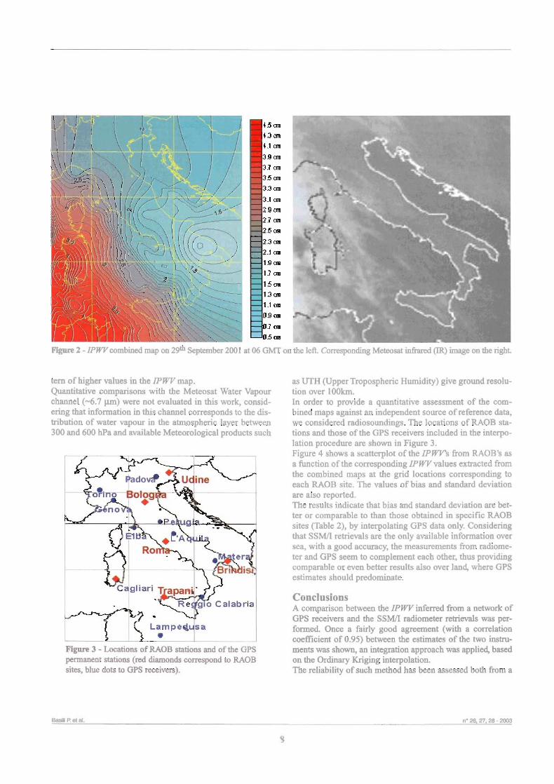
Figore 2 - IPWV combined m q on 2gth September 2001 at 06 GMT on the leR Comsponding Meteosat inhred (IR) irnage on the right.

tern of higher values in the IPWmap. as UTH (Upper Tropospheric Humidity) give ground resolu- Wt i t a t i ve camparisons with the Meteosat Water Vapour tion over 100krn. chanuel (-6.7 p) were not evaluated in this work, consid- In order to provide a quantitative assessment of the com- ering that information Ui this channel corresponds to the dis- bined maps against an independent source of reference data, tribution of water vapour in the atmospheric layer between we considered radiosoundings. The locations of RAOB sta- 300 and 600 hPa and available Meteorologica1 products such tions and those of the GPS receivers included in the interpo-

lation procedure are shown in Figure 3. Figure 4 shows a scatterplot of the I P W s fiom RAOB's as a function of the corresponding IPWvalues extracted from the combined maps at the grid locations corresponding to each RAOB site. The values of bias and standard deviation are also reported. The results indicate that bias and standard deviation are better or comparable to than those obtained in specific RAOB sites (Table 2), by interpolating GPS data only. Considering that SSMA retrievals are the only available information over sea, with a good accuracy, the measurements from radiometer and GPS seem to complement each other, thus providing cornparable or even better results also over land, where GPS estimates should predominate.

Figure 3 - Cocations of RAOB stations and of the C1PS permanmt stations (red diamonds correspond to RAOB sites, blue do@ t0 GPS receivers).

Conclusions A comparison between the IPW inferred fiom a network of GPS receivers and the SSMA radiometer retnevals was performed. Once a fairly good agreement (with a correlation coefficient of 0.95) between the estimates of the two insm- ments was shown, an integration approach was applied, based on the Ordinary Kriging interpolation. The reliability of such method has been assessed both from a

l h l i l? et al. ne 26,27,28 - 2003

8

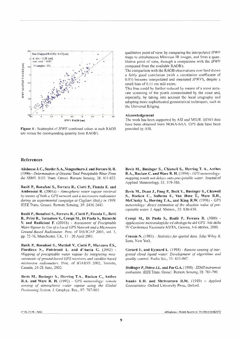
Figure 4 - Scatterplot of I P W combined vaiues at each RAOB site versus the corresponding quantity fkom W B ' s .

References

Alishouse J. C, Snyder S. A.,Vongsathorn J. and F e m R R (1 990) - Determination of Oceanic Total Precipituble Water From the SSMd. IEEE Trans. Geosci. Remote Sensing, 28: 81 1-822.

Basili P., Bonafoni S., Ferrara R, Ciotti P., Fionda E. and Ambrosini R. (2001a) - Atmospheric water vapour retrieval by means of both a GPS network and a microwave radiometer during un experimental campaign at Cagliari Qtaly) in 1999. IEEE Trans. Geosci. Remote Sensing, 39: 2436-2443.

Basili P., Bonafoni S., Ferrara R., Ciotti P., Fionda E., Betti B., Prini R., Tornatore i?, Crespi M., Di Paola S., Baiocchi V. and Radicioni E (2001b) - Assessment of Precipitable Water Vapour by Use of a Local GPS Ndwork and a Microwave Ground-Based Radiometer. Proc. of IEEACAP 2001, vol. 1, pp. 72-76, Manchester, UK, 17 - 20 Apri1200 1.

Basili P., Bonafoni S., Mattioli V., Ciotti P., Marzano F.S., Pierdicca N., Pulvirenti L. and d'Auria G. (2002) - Mapping of precipitable water vapour by integrating measurements of ground-based GPS receivers and satellite-based microwave radiometers. Proc. of IGARSS 2002, Toronto, Canada, 24-28 June, 2002.

Bevis M., Businger S., Herring T.A., Rocken C., Anthes R.A. and Ware R. H. (1992) - GPS meteorology: remote sensing of atmospheric water vapour using the Global Positioning System. J. Geophys. Res., 97: 787-801.

qualitative point of view, by comparing the interpolated IPWV maps to simultaneous Meteosat IR images, and fiom a quantitative point of view, through a comparison with the IPWV computed from the available RAOB's. The compasison with the RAOB observations over land shows a fairly good correlation (with a correlation coefficient of 0.93) between interpolated and measured I P W s , despite a small bias of 0.15 cm still exists. This bias could be further reduced by means of a more accurate screening of the pixels contarninated by the coast an4 especially, by taking into account the local orography and adopting more sophisticated geostatistical techniques, such as the Universal Kriging.

Aknowledgement The work has been supported by ASI and MIUR. SSMJI data have been obtained fiom NOAA-SAA. GPS data have been provided by ASI.

Bevis M., Businger S., Chiswell S., Herring T. A., Anthes R.A., Rocken C. and Ware R. H. (1994) - GPS meteorology: mapping zenith wet delays onto precipitable water. Journal of Applied Meteorology, 33: 379-386.

Bevis M., Duan J., Fang P., Bock Y., Businger S., Chiswell S., Rocken C., Solheim E, Van Hove T., Ware R.H., McClusky S., Herring T.A., and King R.W. (1996) - GPS meteorology: direct estimation of the absolute value of precipitable water. J. Appl. Meteor., 35: 830-838.

Crespi M., Di Paola S., Basili P,, Ferrara R (2000) - Applicazioni meteorologiche ed idrologiche del GPS. Atti della n/ Conferenza Nazionale ASITA, Genova, 3-6 ottobre, 2000.

Cressie N. (1993) - Statistics for spatial data. John Wiley L Sons, New York.

Gerard E. and Eymard L. (1998) - Remote sensing of integrated cloud liquid water: Development of algorithms and quali9 control. Radio Sci., 33: 433-447.

Hollinger P., Peirce J.L. and Poe G.A. (1990) - S S M instrument evaluation. EEE Trans. Geosci. Remote Sensing, 28: 78 1-790.

Isaaks E.H. and Shrivastava R.M. (1989) - Applied Geostatistics. Oxford University Press, Oxford.

Krige D.G. (195 1) - A statistica1 approach to some baic mine valuation pmblerns on the Witwatersmnd. J. of Chemical, Metallurgical and Mining Society of South Afnca, 52: 119-139.

Nativi S. and Migliorini M. (2001) - Pin-Part 11: Compamtive evaluation of SSML and TMI Precipitable Water Estimate for fhe Mediterraneun Sea. IEEE Trans. Geosci. Remote Sensing, 39: 2575-2586.

Pngent C. and Rossm W.R (1 999) - Retrieval of sudace and ahnospheric parameters over land from SSMI: Potential and limitations. Q. J. Royal Meteorol. Soc., 125: 2379-2400.

Saastamoinen J. (1972) - Atmospheric Correction for the Troposphere and Stratosphere in Radio Ranging of Satellites. The Use of Artificial Satellites for Geodesy, vol. 15, S.W. Henriksen et al., Eds., Geophysics Monograph Series, A.G.U., Washington, D.C.

Schluessel l? and Emery W.J. (1990) - Atmospheric water vapor over ocemfrom SSMB m e 4 S u m t s . Int. J. Rem. Sens., 1 1 : 753-766

Wu S.C. (1 979) - Optimumfiquencies of a passive microwave mdiometer for tropospheric path length correction. IEEE Trans. Antemas Propag., 27: 233-239.

Wii i? et al. n' 26,27,28 - 2003

10

Physical and empirical approaches to retrieve surface rain rate from the Special Sensor Microwave Imager: comparison with

rain-gauge measurements Luca Pulvirenti (l), Nazzareno Pierdicca (l), Giovanni d9Auria (l),

Piero Ciotti (2), Frank Silvio Manano (2) and Patrizia Basiii (3)

Abstract The different methods of estimating precipitation from spaceborne microwave radiometric data cari be divided in two categories: physical and empirical ones. In this work, an overview of different retrieval algorithms is given and their ability in detecting precipitation on a local scale is also evaluated. The assessment is carried out by means of a comparison with the rain rates measured by a rain-gauge network located along the Tiber nver basin, in Centra1 Italy. The considered radiometer is the Special Sensor Microwave Imager (SSMD).

Riassunto I diversi metodi di stima di precipitazione da dati radiometrici a microonde su satellite possono essere divisi in due categorie: fisici ed empirici. In questo lavoro viene fornita una panoramica su diversi algoritmi di stima e viene anche valutata la loro capacità di rilevare la precipitazione su scala locale. La venfica è efettuata tramite un conjkonto con le misure di una rete diplu- viometri situata lungo il bacino del fiume Tevere, in Italia Centrale. Il radiometro considerato è lo Special Sensor Microwave Imager (SSM/I).

Introduction In the last decades the capability of spacebome microwave radiometers to determine the properties of clouds, in particular the produced surface rain-rate, has been proved in severa1 works [Smith et ai., 1992; Kummerow et al., 1996; d'Auria et al., 19981. Such ability is due to the sensitivity of microwaves to the intemai structure of a cloud: the lowest frequencies are sensible mainly to the liquid hydrometeors, whilst the highest ones to the ice particles [Smith et al., 1992; dYAuria et al., 19981. The use of microwave radiometq as a technique to estimate precipitation has increased after the launch, in 1987, of the Defense Meteorologica1 Satellite Program @MSP) whose platforms carry the Special Sensor Microwave Imager (SSMD). More recently, the Microwave Irnager (TMI) operates with a radar sensor on board of the Tropical Rainfall Measuring

(1) Dipartimento di Ingegneria Elettronica, Università "La Sapienza" di Roma, via Eudossiana 18 - 00184 Roma, Italia +ma& [email protected]

(2) Dipartimento di Ingegneria Elettrica - Centro di Eccellenza CETEMPS, Università dell'Aqufla - 67040 Monteluco di Roio, L'Aquila, Italia.

(3) Dipartimento di Ingegneria Elettmnica e deii91nformazione, Uni- versità degli Studi di Perugia, via Duranti 93 - 06125 Pemgia, Italia.

Received 15/10/2002 - Accepted 4/01/2003

Mission (TRMM) to sound the precipitating cloud systems in the Tropical regions. In order to retrieve surface rain rate from microwave radiometric data, two different approaches cm be followed: physical or empirical ones. The former is generally based on a data set of simulated cloud vertical structures derived from a microphysical cloud model and on a radiative transfer model to associate to each structure a vector of multifiequency simuiated brightness temperatures. In the inversion procedure, one of the synthetic cloud vertical profiles cm be associated to the TB measurements through a Bayesian approach [Pierdicca et al., 1996; d7Auria et al., 1998; Manano et al., 19991. The physical method gives appreciable results only if the various parameters that have to be considered in the sirnulation process (such as temperature and humidity profiles, surface emissivity) are estimated with sufficient accuracy. Empirical approaches can be followed if a reliable data set of satellite measurements associated to ground-truth data (such as those of rain-gauges and weather radars) is available [Ferraro and Marks, 1995; Berg et al., 19981. They are generally simple to be implemented, but they are specific for only one sensor and cannot be easily extended to geographical areas different from the calibration one. The major limitation suffered by both techniques, over lan4 is their dependence on the depression of the 85 GHz TB caused by the scattering produced by the frozen hydrometeors [Petty, 1995; Conner and Petty, 19981. This means that only convective cloud systems, with ice at the top, can be easily reveaied by a

no 26,27,28 - 2003 AiTinfo~mn - RMsta Itallana di TELERILEVAMENTO

11

spaceborne microwave radiometer over land. If a cloud is forrned mainly by liquid particles, as in the case of a stratiform one, the sensor does not always detect it and the algorithms may fai1 to retrieve rainfall. In this paper, we give an overview of vanous algorithms for rain retrieval and we compare their performances by considering, as a reference, the precipitation data provided by a rain-gauge network placed along the Tiber river basin, in Centra1 Italy. The considered spaceborne radiometer is the Special Sensor Microwave Imager (SSM), which flies on a near-polar sun- synchronous orbit at an altitude of about 830 km. Presently three platforms carrying the SSM/i are in operation, providing a complete coverage of the earth, but with a still limited time sampling for many applications. SSMA measures TB at four ffequency bands (i. e., 19.35, 22.2, 37.0, 85.5 GHz) and at two linear polarizations (i.e., horizontal and vertical), apart from the 22.2 GHz channel, which operates only in the vertical polarization. During each conical scan, SSMA gathers data ;t an off- nadir obsewation angle of 53.1' with a swath of about 1400 h. The spatial resolution is 69x43 h, 60x40 h, 37x29 km and 15x13 lan for the 19,22,37 and 85 GHz channels, respectively [Hollinger et al., 19901. The comparison of the performances of the various methods has been carried out at basin leve1 (Le., by computing the mean value of rain rate within the basin) to overcome problems like the radiometer geo-location m r s .

Physical-Statistica1 approach Physical approaches permit an explicit consideration of the vertical distnbution of the hydrometeors and of the meteoro- logica1 variables (temperature, pressure and humidity) together with a rigorous theoretical treatment of the rainfall retrieval problem [Petty, 19951. The algorithm used in this work is based on the numerica1 outputs of a rnicrophysical cloud model used to statistically generate a database of cloud vertical profiles. We have adopted a model named University of Wisconsin - Non-hydrostatic Modeling System (UW-NMS), which is capable of explicitly describing the vertical distribution of four species of hydrometeors (i.e., cloud droplets, rain drops, graupel particles and ice particles) [Smith et al., 19921. From the origina1 vertical resolution of about 0.5 h, which determines 42 altitude levels, the number of cloud layers has been reduced to at most seven [Pierdicca et al., 19961. The cloud vertical stnictures have been classified into 9 classes following the World Meteorologica1 Organization (WMO) nomenclature [d'Auria et al., 19981. Each cloud is defined by a vector g whose elements are the equivalent water contents of the various hydrometeors. The major issue which have to be faced adopting the UW- NMS model is the discrepancy between the environmental conditions of the origina1 microphysical simulation, which is referred to a sumrner tropical storm, with respect to the climatology of the considered geographical zone in terms of meteorological variables (temperature, pressure and humidi-

ty). Such discrepancy may produce a bias in the simulated bnghtness temperatures with respect to the actual S S M measurements. We have used a set of radiosounding observations (RAOB's) collected in 1995 and relative to five Italian stations, in order to match the cloud simulations with the clirnat- ic conditions of the area of interest (i.e. the Mediterranea one). In particular, we have inferred the monthly mean profiles of temperature, pressure and water vapor density as well as the monthly mean values of the cloud top height. Details about the matching procedure can be found in Pulvirenti et al. [2002]. For the purpose of enlarging our cloud data set we have used a Monte Carlo statistica1 generation [Pierdicca et al., 19961 considenng al1 the hydrometeors as Gaussian variables with mean and standard deviation derived from the matching procedure mentioned above. The result of the whole simulation process consists of 12 data sets (one for each month) with 4500 vertical profiles (500 for each of the 9 classes). in order to associate to each cloud profile its spectral signature, we have used a plane-parallel radiative transfer model based on the Eddington solution [d'Auria et al., 19981. It is worth mentioning that the plane-parallel assumption does not permit to take into account the horizontal inhornogeneity of the clouds. This problem could affect rain retrieval especially for convective stnictures [Kummerow, 19981. To achieve a reliable simulation of the brightness temperature associated to a synthetic cloud stnicture, an accurate evaluation of the microwave emissivity of the surface is needed. We have generated monthly emissivity maps in terms of average values and correlation matrices among the SSMiI frequency channels [Pulvirenti et al., 20021. For this purpose we have considered SSMA data collected in the absence of scattering processes and we have calculated the surface emissivity by inverting the radiative transfer equation. To solve the inversion problem, we have used the Maximum A posteriori Probability (MAP) criterion. Details about MAP can be found in Pierdicca et al. [l9961 and in d'Auria et al. [1998]. The most probable profile gi of a cloud belonging to class i is inferred by searching in the database the cloud class i and the profile gi which minimize the following function:

where t(&) is the modeled TB vector (associated to the cloud vector gi in the training synthetic database), t, is the vector of S S M TB measurements, C, is the covariance matrix of the error affecting both the measured TB and the modeled one, mi and Ci are the mean vector and the covariance matrix of the g vectors within class i, det(.) indicates deterrninant and super- scripts "T" and "-1" indicate transposition and inversion of a matrix, respectively. The estirnated precipitation is related to the rain density of the lowest layer of the MAP selected cloud strutture through a formulation that accounts for gravity, atmospheric drag and the fa11 velocity mugnai et al., 19931.

Empirical approach As mentioned, an empirical approach to the rain retrieval problem requires the availability of a large training data set of ground-truth data associated to the SSMii méasurements. In our case these data have been collected throughout 9 years (1992-2000) by a rain-gauge network placed in Centra1 Italy. Each rain-gauge measures the cumulative precipitation every half an hour with a resolution of 0.2 mm. The number of active rain-gauge stations ranges from 46 in 1992 to 86 in 1995 and they cover an area of about 17000 km2. For each station, the closest SSMii pixel has been identified for both high resolution and low resolution channels, and the cumulated precipitation has been converted to rain intensity in mm/h. We have chosen a distance of 7 km, which is equal to about half the high resolution SSMD pixel size, as the maximum distance between rain- gauge location and the 85 GHz pixel center. When severa1 rain- gauges have fallen within one pixel, their precipitation intensities have been averaged. The resulting database consists of 6239 SSMii passes with about 30% of these related to a situation in which at least one rain-gauge detects min. We have considered three ernpirical techniques: a multivariate regression, an artificial Neural Network and the Maximurn Likelihood (ML) criterion. The regression technique assurnes that the relationship between the vector of predictors t, and the parameter RREG (estimated rain rate) is given by:

where b is the bias, CRt and Ct are the cross-covariance between R and t, and the auto-covariance of t,, respectively. We have considered a polynomial expansion to second order, that is the vector of predictors includes the muitihquency TBB and their square values, obtaining the following regressive estimator:

where ao, alk, a2k are coefficients computed as in Equation [2] and TBk is the measured brightness temperature of the radiometric channel k, being N the maximum number of channels (here N=7, that is al1 SSMD channels). As for the Neural Network method, we have used a feed-forward Network having seven input neurons (brightness temperature~), one hidden layer with 8 neurons and 1 output neuron (rain rate). The theoretical basis of such a choice is the universal approximation theorem which states that a multilayer feed- forward neural network having at least one hidden layer can approximate any non-linear function relating inputs to outputs. The training has been carried out by using the Levenberg- Marquardt algorithm and it has been performed by monitoring the error between the network outputs and the targets on the test set and stopping the process when a minimum of such error was found.

The last empirical criterion is the Maximum Likelihood one. The range of the rain-rate variability has been divided in L intervals, each equal to 0.4 mmh and for each interval the associated TB'S in the training data set have been averaged perraro and Marks, 19951. In this way the mean brightness temperature vector <t(i)> for each rain rate bin i has been found. Assuming a Gaussian distribution for t, around the mean value <t(i)> for the rain rate bin i, the ML criterion requires to find the interval (rain rate bin) i, which minimizes the following objective function:

where Cti is the covariance rnatrix of TB for the interval i, computed from the training data set and det(Cti) is its determinant.

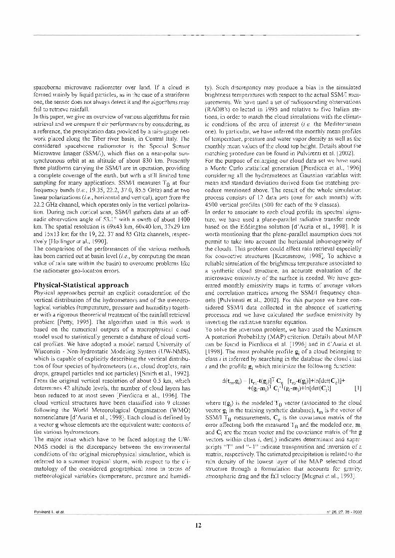
Comparison with rain-gauge data In order to veri% the capability of the considered procedures to estimate precipitation, we have performed a comparison with the measurements of the considered rain-gauge network. For this purpose, the rain-TB data set has been divided in training and validation sets. The former is composed by 33943 rain-TB pairs, the la* by 32250 samples. As mentioned, the comparison has been carried out considering the average of the rain rates in the basin. The results are summariz,ed in Table 1, fkom which it can be observed that the best resulis, in terms of both correlation between estimates and measurements and root mean square (RMS) estimation erm, are provided by the Neural Network.

Table 1 - Performances of the considered algorithms for the whole validation set.

Correlation RMS error Bias error coefficient (mmih) (mmh)

Regression (Rreg) 0.72 0.54 -0.07 Neural Network (Rnn) 0.76 0.49 -0.04 Maximum Likelihood (Rml) 0.67 0.76 O. 19 Physical MAF' (Rmap) 0.70 0.59 0.09

This result can be explained considering that the radiometer is sensible mainly to the frozen particles of a cloud and that the relationship between the density of these particles and the produced surface rain-rate is highly non-linear. The Neural Network is the method that better accounts for this non-linearity. However, the regressive estimator and the physical MAP approach give fairly good results as well. The worst resuits in terrns of correlation and RMS error are provided by the empirical ML approach. The comparison between estimates and measurements is illustrated in Figure 1. It can be noted that the

no 26,27,28 - 2003 AITinfoma - Rivista Italiana di TELERILEVAMENTO

13

Measured rain rate (mmlh) Measured rain rate (mmih)

a

Measured rain rate (mmlh) Measured rain rate (mmth)

Figure 1 - Comparison between measured and estimated rain rate at basin level for Regression (top left panel), Neural Network (top right panel), Maximum Likelihood (bottom left panel) and Physical MAP (bottom right panel). The comparison is relative to the whole validation set.

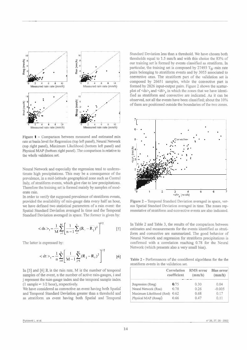
Neural Network and especiaily the regression tend to underes- timate high precipitations. This may be a consequence of the prevalence, in a mid-latitude geographical zone such as Centra1 Italy, of stratiform events, which give rise to low precipitations. Therefore the training set is formed mainly by samples of moderate rain. In order to veri6 the supposed prevalence of stratiform events, provided the availability of rain-gauge data every half an hour, we have defined two statistical parameters of a rain event: the Spatial Standard Deviation averaged in time and the Temporal Standard Deviation averaged in space. The former is given by:

The latter is expressed by:

in [5] and [6] R is the rain rate, M is the number of temporal samples of the event, n the number of active rain-gauges, i and j represent the rain-gauge index and the temporal sample index (1 sample = 112 hour), respectively. We have considered as convective an event having both Spatial and Temporal Standard Deviation greater than a threshold and as stratiform an event having both Spatial and Temporal

Standard Deviation less than a threshold. We have chosen both thresholds equa1 to 1.5 mm/h and with this choice the 83% of our training set is formed by events classified as stratiform. in particular, the training set is composed by 27493 T*-rain rate pairs belonging to stratiform events and by 3055 associated to convective ones. The stratiform part of the validation set is composed by 26651 samples, while the convective part is formed by 2826 input-output pairs. Figure 2 shows the scatterplot of <ds>, and <dos in which the zones that we have identified as stratiform and convective are indicated. As it can be obsewed, not al1 the events have been classified; about the 10% of them are positioned outside the boundaries of the two zones.

. . C o n v d i l .

e.'. t *...e e.*

e t *

,;** . .* * .

Figure 2 - Temporal Standard Deviation averaged in space, versus Spatial Standard Deviation averaged in time. The zones representative of stratiform and convective events are also indicated.

In Table 2 and Table 3, the results of the comparison between estimates and measurements for the events identified as stratiform and convective are sumrnarized. The good behavior of Neural Network and regression for stratiform precipitations is confirmed with a correlation reaching 0.78 for the Neural Network (which presents also a very small bias).

Table 2 - Performances of the considered algorithms for the the stratiform events in the validation set.

Correlation RMS error Bias error coefficient (mmh) (mmlh)

Regression (Rreg) 0.75 0.30 0.04 Neural Network (Rnn) 0.78 0.26 -0.005 Maximum Likelihood (Rmi) 0.62 0.68 0.17 Physical MAP (Rrnap) 0.66 0.47 0.1 1

PuMrentl L. e1 al. n' 26,27,28 - 2003

14

Correlation RMS error Bias error coefficient (mmlh) (mmh)

Regres~ion W&!) 0.63 1.43 -0.59 Neural Network (R.) 0.7 1 1.42 -0.48 Maximum LikeW1ood @ni) 0.74 1.35 -0.3 1 Physicai MAP (Rmap) 0.68 1.38 -0.10

Table 3 - Performances of the considered algonthms for the the convective events in the validation set.

. K K

O 0 2 4 6 8 1 0 O 0 2 4 6 8 1 0

Measured rain rate (rnmih) Measured rain rate (rnrnh)

F 4 ci Cm 0 2 4 8 8 1 0 Measured rain rate (rnmlh)

Measured rain rate (mmlh)

Measured rain rate (rndh)

Figure 4 - Comparison between measured and estimated rain rate 0 2 4 6 8 1 0 at basin leve1 for Regression (top left pane]), Neural Network (top

Measured rain rate (mmni) right panel), Maximum Likelihood (bottom lefi panel) and Physical MAP (bottom nght panel). The comparison is relative to

0 7 the convective events in the dataset.

Measured rain rate (rndh)

Figure 3 - Comparison between measured and estimated rain rate at basin level for Regression (top left panel), Neural Network (top nght panel), Maximum Likelihood (bottom left panel) and Physical MAP (bottom nght panel). The comparison is relative to the stratiform events in the dataset.

Therefore, the consideration of a large training set referred to a small geographicai area, has increased the capability of the radiometer to detect stratiform rain, at least according to our classification of stratiform events. On the other hand, for high convective rain, the physicai MAP and the empirical ML seem to give better perforrnances with respect to the other methods, especially in t e m of error bias. The comparisons between measurements and estirnates are shown in Figure 3 (stratiform) and in Figure 4 (convective). In the latter figure there are some points of very low rain intensity, even though they are representative of events classified as convective. These are cases in which the average precipitation in the area is low, since the convective cells cwer only a small part of the basin.

Conclusions An overview of the two different approaches (physical and empirical), which can be followed to retrieve surface precipi-

tation from spaceborne radiometric data, has been presented. The wrformances of the considered alnorithms have been - verified by means of a comparison between the estimated rain rates and the measurements of a rain-gauge network. The results of such comparison, that have been carried out considering the precipitation averaged over the area of interest, has shown that the Neural Network provides the best performances, especially for stratiform events. The regression gives also good results for moderate rain, while it tends to underes- timate high precipitations, probably because of the prevalence of sarnples of low rain in the training set. For convective rain both the empirical ML and the physical MAP present a fairly good behavior. It is worth mentioning that the physical approach, even though it gives performances that are slightly worse than the empirical ones on a local scale, can be easily extended to geographical areas different from the calibration one (provided the availability of some meteorologica1 data to match the simulations) and for sensors operating at frequencies that are different from those of the SSM/I.

Acknowledgments The rain-gauge data have been provided by the Dipartimento per i Servizi Tecnici Nazionali, Servizio Idrografico e Mareografico Nazionale, Ufficio di Roma. The SSMA data have been provided by NOAA/NESDIS, NOAAENMOC and GHRC.

n" 26,27,28 - 2003 AITinf~ma - RMsia Italiana di TELERILEVAMEMO

15

References

Berg W., Olson W., Ferraro R. Goodman S.J. and LaFontaine FJ. (1998) - An assessment of the First- and Second-Generation Navy operational and precipitation retrieval algorithms. J. Atmos. Sci., 55: 1558-1575.

Conner M.D. and Petty G.W. (1998) - Validation and inter- comparison of SSM/I min-rate retrieval methods over the con- tinental United States. J. Appl. Meteor. 37: 679-700.

d'Auria G., Marzano FS., Pierdicca N., Pinna Nossai R., Basiii P. and Ciotti P. (1998) - Remotely sensing cloudproper- ties j b m microwave radiometric observations by using a modeled cloud data base. Radio Sci., 33: 369-392.

Ferraro R.R and Marks G. F. (1995) - The development of SSM/I min-mte retrieval algorithrns using ground-based mdar measurements. J. Atmos. and Oceanic Techn., 12: 755-772.

Hoiiinger P., Peirce J.L. and Poe G.A. (1 990) - SSM/I instrument evaluation. IEEE Trans. Geosci. Remote Sensing, 28: 78 1-790.

Kummerow C., Olson W.S. and Giglio L. (1996) - A simplzjied scheme for obtaining precipitation and vertical hydrometeor profiles @m passive microwave sensors. IEEE Trans. Geosci. Remote Sensing, 34: 1213-1232.

Kummerow C. (1998) - Beamjìlling errors in passive microwave minfall retrievals. J. Appl. Meteor., 37: 356-370.

Manano F.S., Mugnai A., Panegrossi G., Pierdicca N., Smith E.A. and 'Liirk J. (1999) - Bayesian estimation ofpre- cipitating cloud pammeters j b m combined measurements of spacebome microwave mdiometer and mdar. IEEE Trans. Geosci. Remote Sensing, 37: 596-613.

Mugnai A., Smith E.A. and Tnpoli G.J. (1993) - Foundations for statistical-physical precipitation retrieval @m passive microwave satellite measurements. Part 17: Emission source and genemlized weightingfinction properties of a time-dependent cloud-radiation model. J. Appl. Meteor., 32: 17-39.

Petty G.W. (1995) - The status of satellite-based rainfall estimation over land. Rem. Sens. Environ., 51: 125-137.

Pierdicca N., Marzano F.S., d9Auria G., Basiii P., Ciotti P. and Mugnai A. (1996) - Precipitation retrievalhm spacebome microwave mdiometers using maximum a posteriori probability estimation. IEEE Trans. Geosci. Remote Sensing, 34: 83 1-846.

Pulvirenti L., Pierdicca N., Marzano ES., Castracane P. and d'Auria G. (2002)- A physical-statistica1 appmach to match passive microwave retrieval of minfall to Meditemnean clima- tologv. IEEE Trans. Geosci. Remote Sensing, 40: 227 1 -2284.

Smith E.A., Mugnai A,, Cooper H.J.,'Iiipoli G.J. and Xiang X. (1992) - Foundations for statistical-physical precipitation retrieval j b m passive microwave satellite measurements. Part I: Brightness-tempemture properties of a time-dependent cloud-radiation model. J. Appl. Meteor., 3 1 : 506-53 1 .

PuMrenii L. et al. n" 26.27,28 - XX)3

16

On the electromagnetic scattering of sea surfaces

Maurizio Migliaccio (l), Roberto Sabia (1) and Massimo Marrazzo (2)

Abstract In this paper we present a study on the electromagnetic scattering of sea surfaces based on the Integral Equation Method (IEM). Numerica1 results show that the sensitivity of different hydrologically water masses is very limited while greater importante is the dependence on the sea state. A detailed study on the anisotropic sea roughness spectnun is conducted in terms of classical oceanographic spectra. These latters are also approxirnated by means of a nove1 power-law spectrum which permits to extend the usual first-order IEM approach.

Riassunto In questo articolo si presenta uno studio dello scattering elettromagnetico da parte di una superficie marina basato sul modello IEM (Integra1 Equation Method). Gli esperimenti numerici mostrano che alle frequenze delle microonde masse d'acqua idro- logicamente molto dzfferenti presentano una variabilità limitata rispetto alla permittività mentre molto maggiore è la dipenden- za rispetto allo stato del mare. Quindi si è condotto uno studio dettagliato dell'influenza degli spettri oceanografici che si ritrovano in letteratura. Infine si è introdotta un 'approssimazione di questi spettri secondo una finzione di tipo potenza. Ciò ha permesso di estendere il tipico approccio al primo ordine dell'ZEM,

Introduction Global climate is dominated by sea-atmosphere physical processes and therefore it is a concern of humankind to observe and predict the sea surface wind field. Classica1 in situ techniques have always permitted very limited spatial and temporal measurements. By means of satellite remote sensing, it is now possible to solve such a problem. Microwave remote sensing allows conducting measurements in a way that is practically independent of the atmosphere. We note however that in remote sensing we always have an indirect measurement of the geophysical quantity of interest, i.e. the obse~ation is related to geophysical quantity in a cumbersome manner. In particular, the scatterometer, mounted on board of severa1 satellite missions, has shown its capability to perform measurements that can be properly inverteci to estimate the sea surface wind field.

(l) Laboratorio di Telerilevamento Ambientale, Istituto di Teoria e Tecnica delle Onde Elettromagnetiche, Università degli Studi di Napoli "Parthenope",Via Acton 38 - 80133 Napoli, Italia. email: [email protected]

(2) Dipartimento di Ingegneria Elettrica ed Elettronica, Universith degli Studi di Cagliari, Piazza d'Armi 19 - 09123 Cagliari, Italia.

Received W0/2002 - Accepted 19/02/2003

In this paper, we investigate the electromagnetic scattering of a sea surface making use the Integral Equation Methd OEM) model. We first characterize the sea surface in terms of its permittivity, then in terms of the anisotropic sea roughness spectrum. A set of meaningfil numericai experiments show that the normalized radar cross section @ has, as expected, a very limited sensitivity to sea water permittivity E and a significant dependence on sea roughness spectrum. Finally, a new study aimed at approxhating the classica1 oceanographic specfra (in the frequency range of interest) by means of a power-law analytical expression is accomplished. This allows us to consider not only the usual fmt-order IEM approximation but the M1 IEM approach. This part of the study is particularly important whenever the sea scattering process becomes even more involved, requiring the use of the improved IEM (I-EM) [Chen et al., 2000; Licheri et al., 20011. In order to properly appreciate the value of this work we must note that, due to the geophysical relevance of the sea environment, application of the E M to estimate the normalized radar cross section oO of sea surfaces is not at al1 original [Chen et al., 19921 but this paper contains some novelties that we shall sum- rnarize hereafter. Main novelties of this paper are the foilowing First, conversely to Fung [Chen et al., 19921, we emphasize that different sea spectra produce much different electromagnetic return Further, we show that it is possible to generalize the cus- tomary first-order IEM approach, once a proper approximation of the sea s p e c t m is achieved. This aspect is ori@ and is h- damental to considering any sea state.

The Integra1 Equation Method In this section we briefly summarize the scattering model that has been ernployed to perform this study. A proper, genera1 and reliable scattering model, used to evaluate the backscattering fiom random rough dielectnc surface, is the IEM model, which has been introduced by Fung and Pan in 1987 m g and Pan, 19871, and fùrther developed m g et al., 1992; Chen et al., 1992; Chen et al., 20001. The use of the IEM model is mainly justified by its capability to embody and extend the classica1 Kirchhoff and Small Perturbation Mode1 approaches b g , 19941. In brief, the Stratton-Chu scattering integra1 equation is written in the far-zone hypothesis which is obviously true in the satellite remote sensing case. Consequently, the electromagnetic field at the sensor can be determined once the rough surface tangential electromagnetic fields estimated. These surface tangential fields can be obtained (in principle) by solving a prop er set of coupled integrai-differential equations [Fung, 19941. In practice this is not at al1 an easy task and various approximate solutions have been considered in literature. In the IEM model the estirnate of the tangential surface fields is obtained by considering the Kirchhoff surface fields and the complementary ones. Hence, in the backscattering case, we have [Fung et al., 19921:

where p stands for the trasmitted and received field polarization, k is the electromagnetic wavenurnber, 8is incidence angle, kx = ksine, k, = kcose, o is the surface rms height and Wn (k,, k,) is the Fourier Transform (FT) of the n-power autocorrelation function. The function I;p is the following:

The fpp and Fpp terms are the Kirchhoff coefficient and the complementary field coefficient, respectively. These latter depend on the Fresnel reflection coefficient Rpp and therefore on the polarization. Their expressions are:

and:

2 s i n 2 ~ ( ~ + ~ , , , ) 2 [ [ :,) e,-sin2B-qcos2B F, = l-- + cose E cos2€J

2sin2 0(1+R,)2 -sin2 e-cos2 0 Fhh = -

cose l c0s2e

The interested reader can find a fully detailed mathematical and physical discussion on the IEM field decomposition in Fung, 19941. We note only that, as detailed in [Fung, 19941, this formulation is maneageable and therefore popularly employed but since it is based only on the single scattering term it is not capable of estimating the cross-polar t m s . Whenever a full-polarirnetric scattering model is requested, we must move to the I-IEM [Chen et al., 2000; Licheri et al., 20011. Unfortunately, in this latter case the oO expression becomes much less maneageable. The Fresnel reflection coefficients are:

Rw = E, cose -JT &rcose+J&zz '

'71

where E, is the seawater relative permittivity.

Sea scattering facts In this section, we summarize the fundamental facts that must be taken into account in order to characterize the IEM model to the sea surface scattering. In particular, we focus our attention on the seawater permittivity characterization and on the anisotropic (or directional) sea surface spectnun. With respect to the first point we have considered the model introduced by [Ellison et al., 19981. Obviously, the seawater permittivity is a function of the radar frequency, the seawater salinity and temperature. Once that the frequency is given, only the dependence on the other two parameters must be investigated. According to the Debye equation, we see that the seawater per- rnittivity is:

where f is the fiequency in Hertz, zis the relaxation time in seconds, P and Em are the static and high-fkequency seawater permittivity, E, i~ the free space permittivity and s is the ionic conductivity of the disolved salts in Siemenslm. According to [Ellison et al., 19981 we have:

s ( T 8 = c,(Q + s c2(T) 3

and aI(r) = 81.82 - 6.0503*10-2T- 3.1661-10-2P + + 3.1097*10-319 - 1.1791*1WT' + 1.4838*104F, [l41

M l g l W M. et al. no 26.27.28 - 2003

18

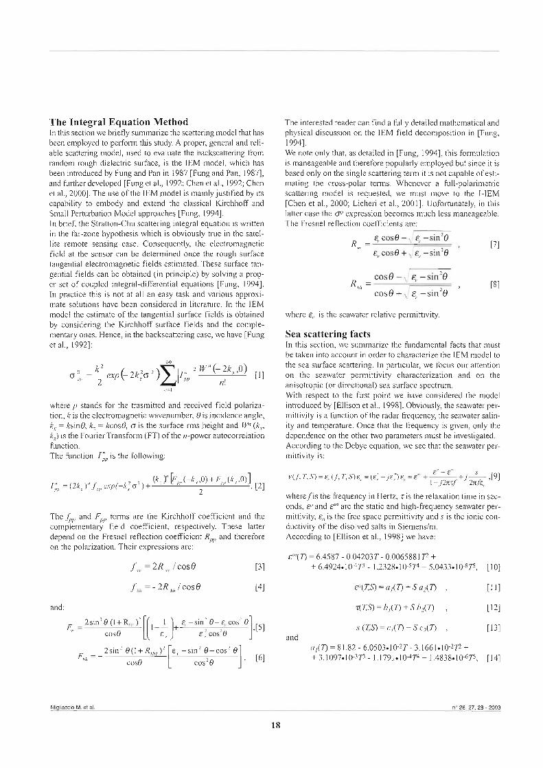
in which T is the seawater temperature in Celsius degree, and S is the seawater salinity in practical salinity units (psu). If we apply the Eqs. [l] to [l91 to the 5.3 GHz case we can plot the rea1 and imaginary seawater relative permittivity parts vs. T when S is set to 35%0, which is a typical value in an open sea. In this case, we note that, in the typical sea temperature range (O - 30" C) E' shows first an increase with T and then a decrease but with a minor slope and E" decreases with the increasing of temperature, see Figure 1.

Figure 1 - Relative seawater permittivity E, vs. temperature T. Frequency is equal to 5.3 GHz and the salinity is equal to 35%.

The relationship of E' and E" vs S, once T is set to 15' C and f to 5.3 GHz, in the range 20-40 psu, is linear with positive slope equal to 0.02% and 0.05%, respectively. Much greater variations of E' and E" are observed at variance of frequency. These figures are not shown in order to save space. Let us now consider the anisotropic sea spectrum characterization. In general the anisotropic sea spectrum W(K, @) is given by pElfouhaily, 1996; Guissard, 19931:

in which S(K) is the omnidirectional sea spectrum and D(K, #) is the spreading function. A pop&r spre&ng function is [Chen et al., 1992; Elfouhaily, 19961: 1

D(@)=-(l+dcos2@) , 2n r211

where d is wind-dependent and the azimuthal angle @ is equal

to zero when the wind blows in the upwind direction. In the following we consider D(@) in accordance to Eq. [21] at variance of S(K). First we consider the classical Phillips spectrum (PH) [Phillips, 19581, that is:

S(K)=PK4 2 1221 where p is the Phillips constant and is equal to 0.08. Since the Phillips spectrum does not show a relationship to the wind speed U, we also consider the modified Pierson- Moskowitz (PM) spectrum [Chen et al., 1992; Fung and Lee, 19821. hence:

where g is gravitational acceleration, KW is equal to 13.177 cm-2 and the wind dependence is taken into account by means of r, given by:

where u* is the fiction velocity. The wind speed U is related to u* as follows:

where z is anenomebric height, K is the von K m a n constant and

2, = 0.6841u8+ 4.28 10-5 u * ~ - 0.0443. [26]

Accordingly, in the IEM sea scattering studies only one term of Eq. [l] is considered [Wu et al., 20011. Although this approximation can be appropriate in the limited roughness case, this is untrue in the general case [Fung, 1994; Chen et al., 20001. The possibility to consider the full-term IEM approach is funda- menta1 when high wind states are to be considered. We note however that in this case we must consider the I-IEM [Chen et al., 2000; Licheri et al., 20011. Accordingly, we propose to consider the following p-power spectrum fùnctional form (PP) [Li et al., 20011:

where a, bp and Qp are fùnctions o f p [Li et al., 20011, and L is the surface correlation length. Eq. [27] is here employed to approximate the former oceanographic spectra. In fact, in order to apply the fu11 IEM approach, once that the pararneters of Eq. [27] have been determined, it is possible to replace the former oceanographic spectra with Eq. [27].

n" 26,27,28 - 2003 AiTIwfoma - RMsta Italiana di TELERILEVAMENTO

19

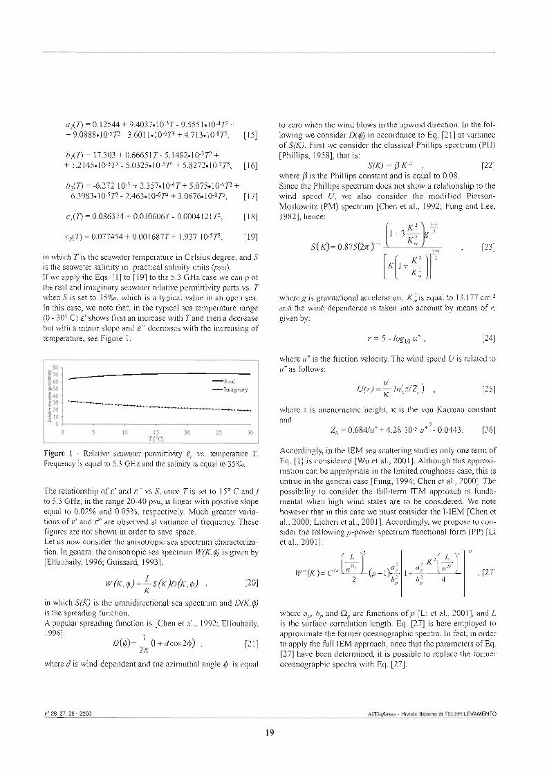
In Figure 2 we plot the normalized (to the rnaximum) PH and PM (V-7mis) and the PP one (p=1.5) spectra for the K range appropriate to the ESA scatterometer sensor p 5 . 3 Ghz and 8 ranging from 18' to 45'). We note that former sea surface spectra are not suitable once that the fu11 term iEM mode1 need to be considered. Figure 3 shows that is possible to tune the PP spectrum parameters in order to best fit the PH and PM spectra in range of interest. in particular, if we concentrate on the PM spectrurn once U is set to 7 mis we note that the most suitable p value of the PP spectrum is equal to 1.9. When al1 the PP spectrum parameters have been best tuned, it is possible to replace the PM spectrum with the PP one.

03 -PH spcctrum - PM spcctmm 0.6 -PP spectmm

0.2

o 70 80 90 100 110 120 130 140 150 160

K [radlm]

Figure 2 - Normalized W@) vs. K. The PM spectrum is relevant to U equal to 7 mis and PP spectrum is relevant top equal to 1.5.

1 -PM spechum

s +PP spectmm p=1.5 p 0.6 -PP spectmm p=1.9

4 0.4 +PP spectmm p=2.5 I z 0.2

o 70 80 90 100 110 120 130 140 150 160

K iradlm l

First we consider a frequency equal to 5.3 Ghz, W polarization and a wind speed equal to 7 d s blowing in the upwind direction. In Figure 4, oO vs. 8 is shown for the case in which the PH and the PM one (U=7 d s ) spectra are considered. A first-order IEM approach is ernployed. We note that very different results are obtained. Hence, the solution of the sea oceanic spectrum turns out to be critical. In Figure 5 we show oO vs. 8 once the PM spectrurn is characterized for different wind speeds. These results are congruent with specialized literature, e.g. [Moore and Fung, 19791.

-+ PM cas C (U=7mlr)

-30

-50

-7 O O 10 20 30 40 M 60 70 80

e ?)

Figure 4 - 8 vs. 8. The PH and PM spectra case are considered.

-PM case (U=7rnls)

+PM case (IT=14m/s)

-10 -20 -30 4 0

O 10 20 30 40 50 60 70 80

e 0

Figure 5 - & vs. 8. The PM spectnim is used and different wind speed cases are considered.

Let us finally consider the PP spectrum. We make reference to Figure 3 - Normalized W@) vs. K. The PM spectrum is relevant to the PM spectrum at U=7 d s . A matching procedure is accom- Uequal to 7 mis. PP spectra relevant top=1.5,1.9 and 2.5 are shown. plished and a p value equal to 1.9 is determined. A ko value

equal to 0.05 is achieved in the C-band case. in Figure 6 oO vs. 8 is shown once a single IEM term and 5 others are considered.

Migliamio M. et ai. no 28.27.28 - 2003

20

Numerica1 experiments in this section we show some meaningful numerica1 experiments. in these experiments the permittivity has been referred to 40°N latitude oceans mean conditions, i.e. S equal to 34.7%0 and T equal to 15' C [Pickard and Emery, 19901. Nevertheless, we underline that, as expected and previously pointed out, if we move to consider the mean Mediterranean hydrographic conditions (S=37.5% and T=22"), very s i d a r cP values are obtained. This confirms that at such microwave fiequencies the oO is o 10 20 30 40 50 60 70 80

practically invariant to different hydrologically water masses. em

Let us now concentrate on the dependence of oO to the sea Figure 6 - vs. 8 in the case of the PP spectrum for n=l and 5. state. ko = 0.05.

20 -PP case (n=I) +PP case (n=5)

a -20

-30

Figure 7 - aO vs. 8 in the case of the PP spectrum for n=l and 5. = 0.64.

Comparison of these results show a very limited difference. In Figure 7 we move to consider a similar case but pertinent to

References

Chen K.S., Fung A.K. and Weissman D.E. (1992) - A bachcattering model for ocean surface. IEEE Trans. Geosci. Remote Sensing, 30 (4): 811-817.

Chen K.S., Wu T.D., Tsay M.K. and Fung A.K. (2000) - A note on the multiple scattering in an IEM model. IEEE Trans. Geosci. Remote Sensing, 38 (1): 249-256.

Elfouahily T. (1996) - Physical modeling of eletromagnetic backscatter from the ocean surface; application to the retrieval of windfields and wind stress by remote sensing of the marine atmospheric boundary layer. Ph.D.Thesis, Université Denis Diderot, Paris.

Ellison W., Balana A., Delbos G., Lamkaouchi K., Eymard L., Guillou C. and Prigent C. (1998) - New permittivity measurements of seawater. Radio Sci., 33 (3): 639-648.

Fung A.K. (1994) - Microwave scattering and emission models and their application. Artech House, pp. 573.

Fung A.K. and Lee K.K. (1982) - A Semi-Empirical Sea- Spectrum Model for Scattering Coefficient Estimation. IEEE J. Oceanic Engineering, OE-7,4: 166- 176.

Fung A.K. and Pan G.W. (1987) - A scattering mode1 for pefectly conducting random su$ace: I. Model development. II. Range of validity. Int. J. Remote Sensing, 8 (1 1): 1579- 1605.

Fung A.K., Zongqian L. and Chen K.S. (1992) - Backscattering from a randomly rough dieletric surface. IEEE Trans. Geosci. Remote Sensing, 30 (2): 356-369.

U=14 d s in such that kois equa1 to 0.64. In this case the extension of the IEM single term approach is physically meaningful.

Conclusions A study regarding the sea surface scattering based on the IEM model has been conducted. It has been shown that, at the C-band ESA scatterometer frequency, the sensitivity to the sea salinity and temperature is quite limited, but is significant to the wind field. A generalized p-power spectrum functional form has been also employed to approximate the Phillips and the modified Pierson-Moskowitz spectra. Such a formulation is capable of determining the Fourier Transform (FT) of the n-power normalized autocorrelation function, fundamental in high wind regimes as shown in the numerica1 experiments.

Guissard A. (1993) - Directional spectrum of the sea surface and wind scatteromefry. Int. J. Remote Sensing, 14 (8): 161 5-1633.

Li Q., Shi J. and Chen K.S. (2001) - A Generalized Power Law Spectrum and its Applications to the Backscattering of Soil Surfaces Based on the Integra1 Equation Model. IEEE Trans. Geosci. Remote Sensing, 40 (2): 271-280.

Licheri M., Floury N., Borgeaud M and Migliaccio M. (2001) - On the Scattering from Natura1 Sufaces: the IEM and the Improved IEM. Proc. IGARSS '01, Sydney: 29 11-291 3.

Moore R.K. and Fung A.K. (1979) -Radar Determinations of Winds at Sea. Proc. IEEE, 67 (1 1): 1504-1521.

Phillips O.M. (1 958) - The equilibrium range in the spectrum of wind generated waves. J. Fluid Mech., 4: 426-434.

Pickard G.L. and Emery W.J. (1 990) - Descriptive Physical Oceanography: An introduction. 5th edition, Buttenvorth & Heinemann.

Wu T.D., Chen K.S., Shi J. and Fung A.K. (200 1) - A transition Model for the Rejlection Coeflcient in Surface Scattering. IEEE Trans. Geosci. Remote Sensing, 39 (9): 2040-2049.

n' 26.27,28 - XX)3 AITinforrna - Rivista IWiana di TELERILEVAMENTO

21

On the use of SAR image fractal analysis for sea surface roughness estimation

Fabrizio Berizzi, Enzo Dalle Mese and Marco Martorella (l)

Abstract Sea surface roughness is affected by many different phenomena such as wind falls, presence of oil slicks or natural films, etc. Both statistica1 and spectral analysis and image processing techniques are widely used to recognise sea surface anomalies, which often affect the sea surface roughness. A new definition of sea surface roughness is given by means of the sea surface fractal dimension. Due to the fact that the SAR image retains some of the characteristics of the sea surface roughness at large scales the authors aim to investigate whether the fractal dimension of the sea surface and its SAR image are related. The study is performed through the use of synoptic rea1 data collected by a buoy and by the ERS1-SAR system.

Riassunto La rugosità della superjìcie marina viene alterata da diversi fattori quali le cadute di vento, la presenza di oil slicks o di films naturali, ecc. Sia analisi statistiche e spettrali che tecniche di elaborazione dell'immagine sono largamente usate per riconoscere le anomalie della sup@cie marina, le quali spesso alterano la rugosità superjkiale. Una nuova definizione di rugosità della superficie marina viene data tramite la dimensione fmttale. Lo scopo degli autori è quello di verzficare che le dimensionifmttali della superficie marina e della immagine SAR siano correlate. L'analisi è condotta tramite l'uso di dati sinottici costituiti da misure efeteltuate da boe e da immagini ERSI-SAR.

Introduction As widely demonstrated in the literature [Mandelbrot, 1982; Barsnley, 19881, natural surfaces can be successfully modelled by the use of fractal geometry. The Weierstrass Function (WF) is largely used to develop fractal surface models. In Jaggard and Sun [1990], a one-dimensional fractal model based on the band-limited Weierstrass function is proposed. In Franceschetti et al. [1996], the authors use a two-dirnensional Weierstrass function to model the microscopic roughness of the single facets composing a resolution ce11 of a high resolution radar. The nurnber of sinusoidal components of the sea surface wave strutture is calculated on the basis of physical considerations by taking into account the facet size and the transmitted wavelength. In Chen et al. [l9961 the Pierson Moskowitz @M) spectrum is included in the Weierstrass function to obtain a one dirnensional(1D) model of the sea surface height. In Berizzi et al. [l9991 the authors propose a dynarnic 1D hc ta l model of the sea surface height, based on Weierstrass functions, which accounts for sea dispersion characteristics. Such a model also agrees with the solution of the Navier-Stokes differential equa-

(l) Dipartimento di Ingegneria dell'Informazione, Università di Pisa, Via Diotisalvi 2 - 56126 Pisa, Italia. e-mail: [email protected]

Received 111 012002 - Accepted 4/01/2003

tions [Apel, 19881 in iinear regime, hence ensuring its physical consistency. An extension of this model to include the realistic two-dimensional case is proposed in Berizzi and Dalle Mese [2001]. Because the sea surface height can be represented by a fractal set, we can expect that some associated phenomena retain their fractal properties. In Berizzi and Dalle Mese [2002] the authors demonstrate that in the case of ideal conditions, the graphs of the in-phase and quadrature components of the sea surface backscattering signal are fractal sets with fiactal dimension s = D,,-I, where D,, is the fractal dimension of the sea surface. As the sea backscattered signal can be represented by a fractal set, we can reasonably expect the SAR image to be a two-dimensional fractal function. In fact it is obtained by linearly and coherently processing the received signal. Moreover, a relationship between the sea surface and the relative sea SAR image fractal dimensions is expected. The idea of modelling the sea SAR image by means of a fractal set has been confirmed in the literature: fractal Brownian motions (fBm) are typically used to model sea surface SAR images [Ilow and Leung, 20011. The purpose of this paper is to investigate whether the fractal dimension of the sea SAR image is related to the fractal dimension of the relative sea surface, which in turn represents a measure of the sea roughness. Hence, the fractal dimension of the SAR image can represent an additional feature for sea surface anomalies recognition, such as oil spills, wind falls, ship wakes and others. Experimental data are used to perform this study. Two different

no 26, 27,28 - 2003 AITi~fom - Rivista Iiaiiana di TELERILEVAMENTO

23

types of measures are available: 1 - ERS 1 PRI geo-referred SAR images taken around Ponza Island in the Mediterranean sea. 2 - Omnidirectional sea wave spectra obtained by processing the data collected by a buoy of the ''Servizio Idmgrajco e Mareogmjìco Nazionale" in the same area and at the same time of the SAR image.

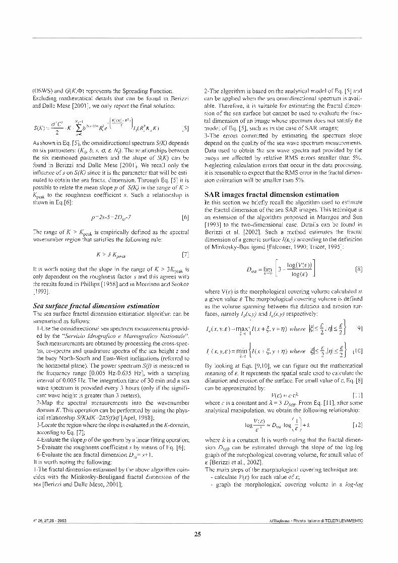
The two data types require iwo separate methods for the estimation of the fractal dimension. The sea surface fractal dimension is estimated by evaluating the slope p of the ornnidirectional sea wave spectrum beyond the spectrum peak. The value of the slope for the range of wavenumbers higher than the wavenumber in correspondence with the spectrum peak, namely Kpeak, is related to the sea fractal dimension D,, by means of the relationship: p=2D,-7 [Berizzi and Dalle Mese, 20011. The sea SAR image fracial dimension is estimated by using a two-dimensional extension of the morphological covenng method, originally proposed in Maragos and Sun 119931.

Sea surface fractal dimension estimation in this section we describe the method used for estimating the sea surface fractal dimension fiom the omnidirectional sea wave spectrum measured by means of the "in situ" buoy data. This method is based on the following theoretical key points:

1 - The sea surface can be represented by the fractal model defined in Berizzi and Dalle Mese [2001]; 2 - In the range of wavenumbers K > Kpeak, the slopep of the omnidirectional sea surface spectnim is related to the fractal dimension D,, through the relationship: p=2Dss-7.

in the next section we bnefiy recall the above theoretical results.

Sea Surface Fractal Mode1 Excluding al1 the mathematical details that led to the result, the analytical expression of the two-dimensional sea surface fiactal model is given in Eq. [l] [Berizzi and Dalle Mese, 20011:

where h is the sea surface height, (xy) are the spatial coordinates, t is the time coordinate, o is the standard deviation, C is a normalisation constant, b is the scale factor, Nfis the number of sinusoidal waves components, K, is the fundamental wavenumber, (V,, Vy) are the observer velocity components along the two spatial directions, P,,, Q,, and a, represent the propagation angular direction, the angular frequency and the phase of the n-th wave component, respectively. It is worth paying attention to the roughness factor s for the following two reasons: - it is related to Minkosky-Bouligand [Falconer, 1990; Tricot, 19951 sea surface fractal dimension D,,:

D,= s+l 121 - it acts on the sea wave spectral amplitude decay, generating more or less rough surfaces.

6eriz.a F. et al.

Larger values of s give rougher surfaces. As will be discussed later, the parameter s affects the shape of the sea spectnun in the range of K > +. It is worth clariwig useful mathematical and physical concepts. 1- For a given time instant t=t*:

a-The sea surface height h(x, y, t 3 is a Band Limited Generaiised Weierstrass (BLGW) surface with hctal dimension D,= s+l when Nf»l (verified in the case of sea surfaces); b-The sea surface height h@, I?, t?, written in polar coordinate~, represents, for a given value of +I?*, a one-dimensional BLGW (ID-BLGW) hc t ion . A 1D-BLGW function is a sum of Nf sinusoidal components with amplitudes ~,=oCb(s-~)n, which decrease when n decreases (note that b>l and I <s<2), and wavenurnber K,,=K@, which increases when n increases (wavelengths A,=A@ decrease when n increases).

2- The model of Eq. [l] agrees with the solution of Navier- Stokes differential equations in linear regime and it represents a wind-generated sea surface with infinite fetch and unimodal wind assurnptions [Apel, 19881.

Omnidìrectwnal sea wave Spectrum As shown in Berizzi and Dalle Mese [2001], it is possible to obtain a closed form expression of the directional sea wave spectrum directly fiom the analytical expression of the sea surface fractal model. Since the analytical manipulation is quite complex, we only report the final expression in Eq. [3].

Eq. [3] represents the directional sea wave spectrum in polar coordinates (K,@). Most of the parameters in Eq. [3] are the same as in the sea surface fractal model, but some others must be explained. The parameter R, represents the spatial correlation length, which is given by Rn=&An, with E a positive real number, Ik(x) is the modified Bessel function of k-th orda and

are the mean sea wave propagation directions. The quantities S,,(m) are the coefficients of the Fourier series of the probability density fimctions of P, considered as a 27r periodic function. To obtain the expression of the omnidirectional sea wave spectrum, W(K,@) can be written as the product of two fùnctions, according to the physical relationship expressed in Eq. [4]:

where S(K) identifies the Omnidirectional Sea Wave Spectrum

(OSWS) and G(KQ>) represents the Spreading Function. Excluding mathematical details that can be found in Berizzi and Dalle Mese [2001], we only report the finai solution:

As shown in Eq. [5], the omnidirectional spectrum S(K) depends on six parameters: (K& 6, s, o, E, N$. The relationships between the six mentioned parameters and the shape of S(K) can be found in Berizzi and Dalle Mese [2001]. We recai1 only the influente of s on S(K) since it is the parameter that will be estimated to obtain the sea fractal dimension. Through Eq. [5] it is possible to relate the mean slope p of S(K) in the range of K > Kpeak to the roughness coefficient S. Such a relationship is shown in Eq.[6]:

The range of K > Kw is empiricaiìy def"ined as the spectral wavenurnber region that satisfies the following rule:

It is worth noting that the slope in the range of K > 3% is only dependent on the roughness factor s and this agrees with the results found in Phillips [l9581 and in Morrison and Srokoz [1993].

Sea surface fractal dimension estimation The sea surface fractal dimension estimation algorithm can be summarised as foìlows:

1-Use the omnidirectional sea spectrum measurements provided by the "Servizio Idmgrafico e Mareogmfico Nazionale". Such measurements are obtained by processing the cross-speo tra, co-spectra and quadrature spectra of the sea height z and the buoy North-South and East-West inclinations (referred to the horizontal plane). The power spectnim S@ is measured in the frequency range [0.005 Hz-0.635 Hz], with a sarnpling interval of 0.005 Hz. The integration time of 30 rnin and a sea wave spectrum is provided every 3 hours (only if the significant wave height is greater than 3 meters); 2-Map the spectral measurements into the wavenumber domain K. This operation can be performed by using the physical relationship S(K)dK=2GV)df [Apel, 19881; 3-Locate the region where the slope is evaiuated in the Kdomain, according to Eq. [7]; 4Evaiuate ihe slopep of the spectrum by a linear fitting operation; 5-Evaluate the roughness coefficient s by means of Eq. [6]; 6-Evaluate the sea fractai dimension D,,= s+ l.

It is worth noting the following: l-The fractal dimension estimated by the above algorithm coincides with the Minkosky-Bouligand fractal dimension of the sea [Berizzi and Dalle Mese, 20011;

2-The algorithm is based on the analytical model of Eq. [5] and can be applied when the sea omnidirectional spectrum is available. Therefore, it is suitable for estimating the fractal dimension of the sea surface but cannot be used to evaluate the fractal dimension of an image whose spectrurn does not satisfy the model of Eq. [5], such as in the case of SAR images; 3-The errors committed by estimating the spectrum slope depend on the quality of the sea wave spectrum measurements. Data used to obtain the sea wave spectra and provided by the buoys are affected by relative RMS errors smder than 5%. Neglecting calculation errors that occur in the data processing, it is reasonable to expect that the RMS error in the fracial dirnension estimation will be smaller than 5%.

SAR images fractal dimension estimation In this section we briefly reca11 the algorithm used to estimate the fiactal dimension of the sea SAR images. This technique is an extension of the algorithm proposed in Maragos and Sun [l9931 to the twodimensional case. Details can be found in Berizzi et al. [2002]. Such a method estirnates the fractal dimension of a generic surface I(x,y) according to the definition of Minkosky-Bouligand palconer, 1990; Tnwt, 19951 :

where V(&) is the morphological covering volume calculated at a given value E. The morphological wvering volume is defined as the volume spanning between the dilation and erosion surfaces, namely Id(x,y) and I,(x,y) respectively:

& I(x+{,y+q) where 151<-< l? l<~} [lo]

5.11 2 2

By looking at Eqs. [9,10], we can figure out the mathematical meaning of E. It represents the spatial scale used to calculate the dilatation and erosion of the surface. For small value of E, Eq. [8] can be approximated by:

V(&) = CE^ [l l1 where c is a constant and A = 3-Dm From Eq. [ l l], &r some analytical manipulation, we obtain the following relationship:

where k is a constant. It is worih noting that the fiactal dimension DMB can be estimated through the slope of the log-log graph of the morphological covering volume, for small value of E merizzi et al., 20021. The main steps of the morphological covering technique are:

- calculate V(&) for each value of E;

- graph the morphological covering volume in a log-log

n' 26,27,28 - 2003 A r i I q f o m - Rivista Italiana di TELERILEVAMENTO

25

scaie(1og - , log7 ) for small values of q (:l a) - estimate the h t a l dirnension by evaluating the slope of log-log morphological covering volume graph.

To appiy the aigorithm to SAR irnages, which is a discrete surface with pixel size AmAy, the erosion and dilatation surfaces must be redef~ned in the discrete space domain:

Zd(x,, , y , , , .~ ' ) =@n ( ~ ( x , + A, y,,, + j ~ ) for ld s E: Ids E') 1.1

where E' is an integer number (discrete spatial scale), x,,=nA , y,=mA and N x Mis the image size. By comparing Eqs. [13,14] with Eqs. [9,10] we note that ~ 2 . 5 % and the rninimurn discrete scale is equa1 to 2A. The estimation of the fractal dirnension is still oblained by evaluating the slope of the log-log graph of the morphological cavering volume, caiculated at the discrete scale E'.

The morphological covering volume is then calculated by means of Eq. [l 51:

Through an extensive analysis of simulated fractal surfaces, we have calculated the fractal dimension estimation RMS error (of the order of 3%).

Sea surface and SAR image fractal dimensions In this section, we investigate the relationship between the fractal dimension of the sea surface and the fractal dimension of the relevant SAR image. Although the fractal dimension of the sea surface and of the SAR image are estimated by using different data and different methods we cm state that:

- both the proposed algorithms estimate the Minkosb- Bouligand fractal dimension of respectively the sea surface and the SAR image. These estimates have the same physical meaning and can be compared; - the algorithms have similar estimation errors (3-5%), which is sufficiently small.

In this paper we propose a numerica1 example obtained by using real data collected by a buoy and by the ERSl-SAR system. Accordiig to Figure 1, we sumrnarise the fractal analysis procedure:

l-use of the sea spectral measurements to estirnate the sea surface fractal dirnension D,,, according to the aigorithm presented in the section 'Sea surface fractal dimension estimation'; 2-use of the morphologicai covering algorithm as described in praious d o n t0 estimate the SAR image firictal dirnension Da,; 3- compare the two fractal dimensions and analyse the corre-

SAR mage

Conversion ta (K.S(K)) Sub-SAR unage seledon

Mo~phological wvenng fraaal dimensio~i estimator

Emtal hension wmpamon

Figure 1 - Block diagrarn of the W s i s procedure.

lation between the two estimates.

Data description The available data are:

a-two PRI ERSI geo-referred SAR images collected during two separate passages of the satellite over the area of Ponza Island (South of Italy), in the Mediterranea Sea. These images are narnely Ponzal and Ponza2; b-two synoptic omnidirectional sea wave spectra obtained by processing the data aquired by the buoy located near Ponza Island (Fig. 2 and Fig. 3).

Figure 4 shows the image frames and the buoy position. Acquisition date and time of the SAR images are reported in Table 1, whereas Table JI reports the main acquisition pararneters of buoy measurements. Far the f i image (F'onzal) the data acquisition tirne of the buoy (6 am.) is 4 hours ahead with respect to the satellite passage time. The subsequent data buoy acquisition at 9:00 am. was missing. This means that after 6 a.m. the sea wave height was lower than 3 meters, i.e. the sea state

K (dB rad m")

Figure 2 - Omnidirectional Sea Wave Spectrum of Ponzal .

Berlui F. et al. n" 28,27,28 - 2 W

26

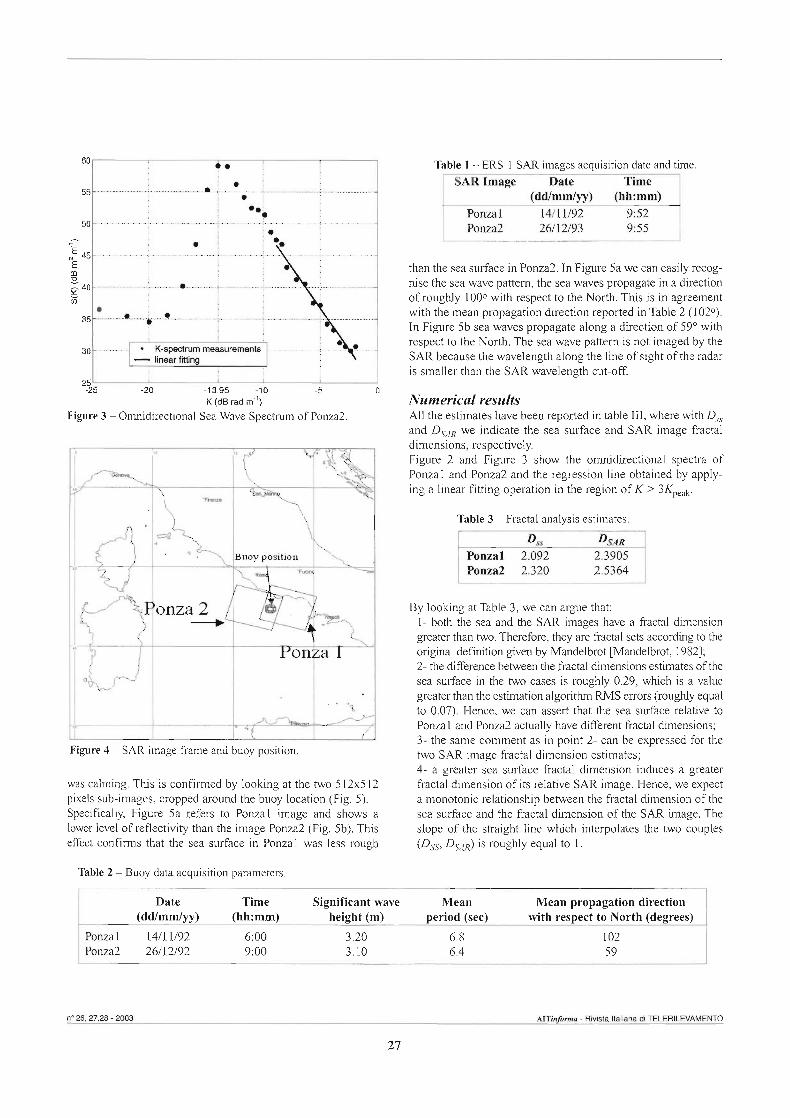
-- -25 -20 -13.95 -10 -5 O

K (dB rad m.')

Figure 3 - Ornnidirectional Sea Wave Spectrum of Ponza2.

Figure 4 - SAR image frame and buoy position.

was calrning. This is conf i ied by looking at the two 5 12x5 12 pixels sub-images, cropped mund the buoy location (Fig. 5). Specifically, Figure 5a refers to Ponzal image and shows a l m leve1 of reflectivity than the image Ponza2 (Fig. 5b). This effect c o n f m that the sea surface in Ponzal was less rough

Table 2 - Buoy data acquisition parameters.

Table 1 - ERS-l SAR images acquisition date and the . I SAR Image Date Time

than the sea surface in Ponza2. In Figure 5a we can easily recognise the sea wave pattern, the sea waves propagate in a direction of roughly 1000 with respect to the Norih. This is in agreement with the mean propagation direction reported in Table 2 (1020). In Figure 5b sea waves propagate along a direction of 59' with respect to the North. The sea wave pattern is not imaged by the SAR because the wavelength along the line of sight of the radar is smailer than the SAR wavelength cut-off.

Nurnerical results Al1 the estimates have been reported in table In, where with D,, and DuR we indicate the sea surface and SAR image fractal dimensions, respectively. Figure 2 and Figure 3 show the omnidirectional spectra of Ponzal and Ponza2 and the regression line obtained by applying a linear fitting operation in the region of K > 3K&.

Table 3 - Fractal analysis estimates.

By looking at Table 3, we can argue that: 1- both the sea and the SAR images have a fracial dimension greater than two. Therefore, they are fractal sets accarding to the originai definition given by Mandelbrot wandelbrot, 19821; 2- the differente between the fractal dimensions estimates of the sea surface in the two cases is roughly 0.29, which is a value greater than the estimation algorithm RMS errors (rougbiy equal to 0.07). Hence, we can assert that the sea surface relative to Ponzal and Ponza2 actually have different fracial dimensions; 3- the same cornment as in point 2- can be expressed for the two SAR image fractai dimension estimates; 4- a greater sea surface fractai dimension induces a greater fracial dimension of its relative SAR image. Hence, we expect a monotonic relationship between the fractai dimension of the sea surface and the £ractal dirnension of the SAR image. The slope of the straight line which interpolates the two couples (Dss, DSAR) is roughiy equal to 1.

Date Time Significant wave Mean Mean propagation direction (dd/mm/yy) ( h h : m ) height (m) period (sec) with respect to North (degrees)

Ponzal 1411 1/92 6:OO 3.20 6.8 102 Ponza2 26/12/92 9:OO 3.10 6.4 59

n' 26, 27,28 - 2003 AITiitforma - Rivista Italiana di TELERILEVAMENTO

27

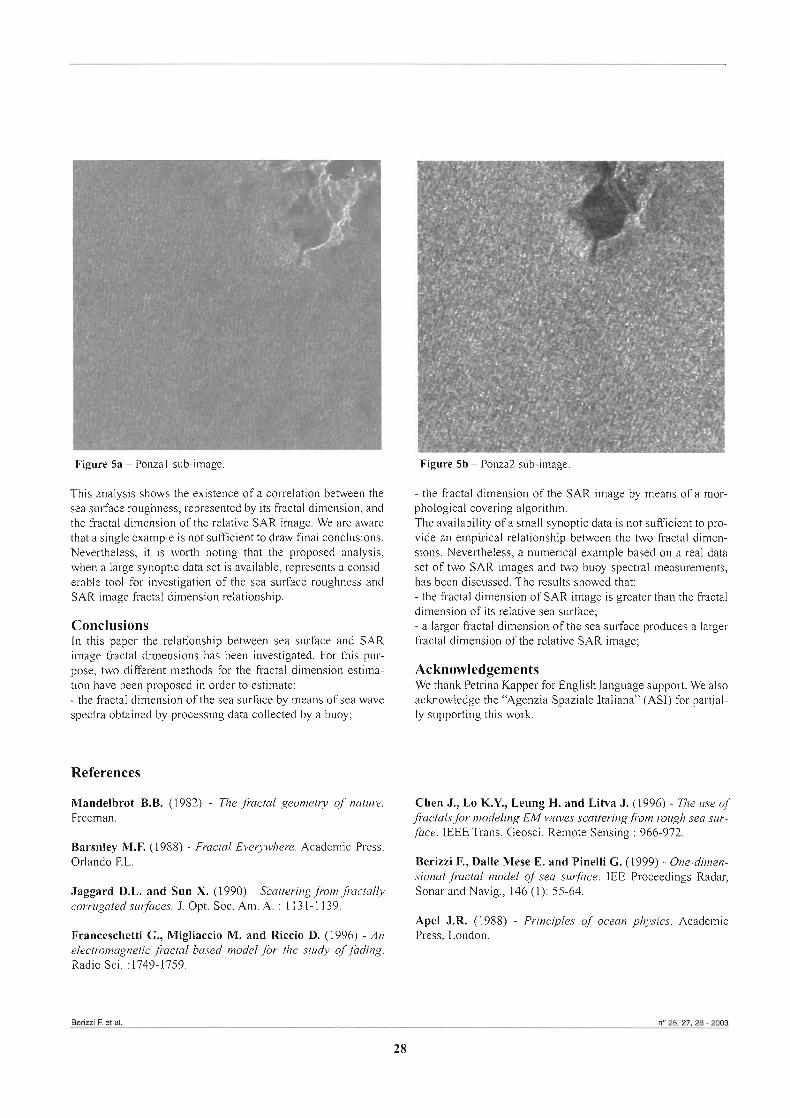
Figure 5a - Ponzal sub-image. Figure 5b - Ponza2 sub-image.

This analysis shows the existence of a correlation between the sea surface roughness, represented by its fractal dimension, and the fractal dimension of the relative SAR image. We are aware that a single example is not sufficient to draw final conclusions. Nevertheless, it is worth noting that the proposed analysis, when a large synoptic data set is available, represents a considerable t001 for investigation of the sea surface roughness and SAR image hc ta l dimension relationship.

Conclusions In this paper the relationship between sea surface and SAR image &tal dimensions has been investigated. For this purpose, two different methods for the fractal dimension estimation have been proposed in order to estimate: - the fractal dimension of the sea surface by means of sea wave spectra obtained by processing data collected by a buoy;

References

Mandelbrot B.B. (1982) - n e fmctal geomehy of nature. Freeman.

Barsnley M.F. (1988) - Fractal Everywhere. Academic Press. Orlando F.L.

Jaggard D.L. and Snn X. (1 990) - Scattering j b m fmctally comgated surfaces. J. Opt. Soc. Arn. A. : 1 13 1- 1 139.

Franceschetti G., Migliaccio M. and Riccio D. (1996) - An electmrnagnetic fractal-based model for the study of fading. Radio Sci. : 1749-1759.

- the fractal dimension of the SAR image by means of a morphological covering algorithrn. The availability of a small synoptic data is not sufficient to provide an empirical relationship between the two fiactal dimensions. Nevertheless, a numerica1 example based on a rea1 data set of two SAR images and two buoy spectral measurements, has been discussed. The results showed that: - the fractal dimension of SAR image is greater than the fractal dimension of its relative sea surface; - a larger fractal dimension of the sea surface produces a larger h c t a l dimension of the relative SAR image;

Acknowledgements We thank Petrina Kapper for English language support. We also acknowledge the "Agenzia Spaziale Italiana" (ASI) for partially supporting this work.

Chen J., Lo K.Y., Leung H. and Litva J. (1996) - n e use of fractals for modeling EM waves scatteringjbm mugh sea surface. E E E Trans. Geosci. Remote Sensing : 966-972.

Berizzi F., Daile Mese E. and Pineiii G. (1 999) - One-dimensional fractal model of sea surface. IEE Proceedings Radar, Sonar and Navig., 146 (1): 55-64.

Apel J.R. (1988) - Principles of ocean physics. Academic Press, London.

~erizzi E et ai. no 26. n. 28 - 2003

28

Berizzi F. and Daiie Mese E. (2001) - Sea-wavefiactal spectrum jÒr SAR remote sensing. IEE Proc. Radar, Sonar and Navig., 148 (2).

BeW F. and Daiie Mese E. (2002) - Scatteringfim a 2d-sea fiUctal surface: fiactal analysis of the scattered signal. IEEE Trans. Antemas and Propagation, 50 (7): 912-925.

now J. and Leung H. (2001) - Self-Similar Texture Modeling Using FARIMA Pmcesses with Applications to Satellite Images. IEEE Transaction on Image Processing, 10 (5), May.

Maragos P. and Sun EK. (1993) - Measuring the fiactal dirnension of signals: Morphological Covers and Itemtive Optimization. IEEE Trans. Signal Processing, 41 (4): 108- 12 1.

Falconer K. (1990) - Fractal Geometry: Mathernatical Foundations and Applications. Wiley.

Wcot C. (1995) - Curva and Fractal Dimension. Springer- Verlag.

Momson A.I. and Srokoz M.A. (1993) - Estimating thefmc- tal dimension of the sea surface: firsf attempt. AM. Geophysicae, 11: 648-658.

Philups O.M. (1958) - The Equilibrium Range in the Spectrum of Wind-generated waves. J. Fluid Mech., 4: 426-434.

Glazman RE. and Weichman P.B. (1989) - Statistica1 geom- eby of a s m l l surface path in a developed sea. J. Geophys. Res., 94: 4998-5010.

Berizzi E, Gamba P., Bertini G. and Del19Acqua E (2002) - Fractal behavior of sea SAR ERSI images. Proc. Int. Geosci. Remote Sensing System 2002 : 11 14-1 116.

n' 28,27,28 - 2003 AiTinforma - Rivista I t a l i a di TELERILEVAMENTO

29

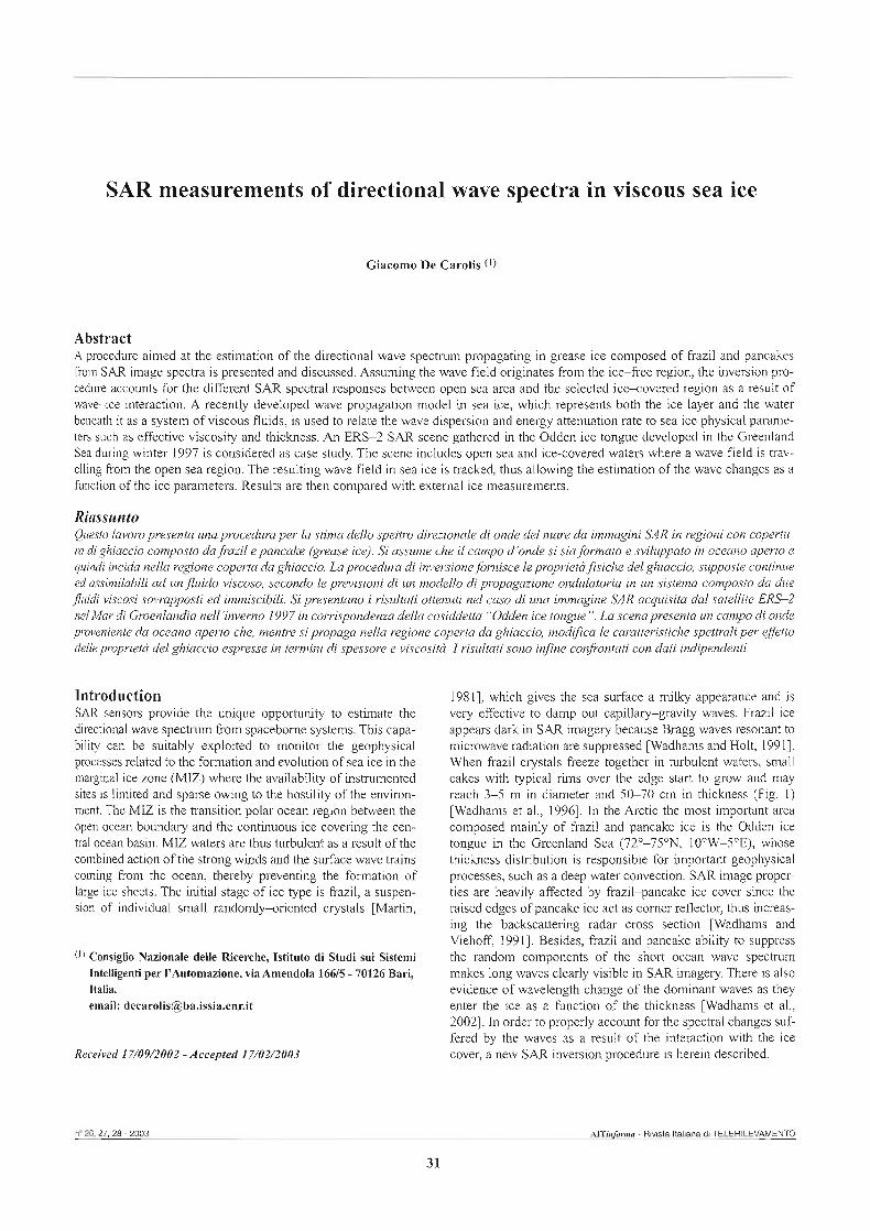
SAR measurements of directional wave spectra in viscous sea ice

Giacomo De Carolis (l)

Abstract A procedure aimed at the estimation of the directional wave spectrum propagating in grease ice composed of frazil and pancakes from SAR image spectra is presented and discussed. Assuming the wave field originates from the ice-free region, the inversion procedure accounts for the different SAR spectrai responses between open sea area and the selected ice-covered region as a result of wav+ice interaction. A recently developed wave propagation mode1 in sea ice, which represents both the ice layer and the water beneath it as a system of viscous fluids, is used to relate the wave dispersion and energy attenuation rate to sea ice physical parameters such as effective viscosity and thickness. An ERS-2 SAR scene gathered in the Odden ice tongue developed in the Greenland Sea during winter 1997 is considered as case study. The scene includes open sea and ice-covered waters where a wave field is travelling from the open sea region. The resulting wave field in sea ice is tracked, thus allowing the estimation of the wave changes as a function of the ice parameters. Results are then compared with external ice measurements.

Riassunto Questo lavoro presenta una procedura per la stima dello spetim direzionale di onde del mare da immagini SAR in regioni con copertura di ghiaccio composto dafrazll epancake ('rease ice). Si assume che il campo d'onde si sia formato e sviluppato in oceano aperto e quindi incida nella regione coperta da ghiaccio. La procedura di inversione fornisce le proprietà fisiche del ghiaccio, supposte continue ed assimilabili ad un fluido viscoso, secondo le previsioni di un modello di propagazione ondulatoria in un sistema composto da due fluidi viscosi sovmpposti ed immiscibili. Si presentano i risultati ottenuti nel caso di una immagine SAR acquisita dal satellite ERS-L nel Mar di Groenlandia nell'inverno 1997 in corrispondenza della cosiddetta 'Odden ice tongue 't La scena presenta un campo di onde proveniente da oceano aperto che, mentre si propaga nella regione coperta da ghiaccio, modifica le caratteristiche spettrali per efetto delle proprietà del ghiaccio espresse in termini di spessore e viscosità. I risultati sono infine confrontati con dati indipendenti.

Introduction SAR sensors provide the unique opportunity to estimate the directional wave spectnim fiom spacebome systems. This capability can be suitably exploited to monitor the geophysical processes related to the formation and evolution of sea ice in the margina1 ice zone (ME) where the availability of instrumented sites is limited and sparse owing to the hostility of the environment. The MIZ is the transition polar ocean region between the open ocean boundary and the continuous ice covering the cen- tra1 ocean basin. MIZ waters are thus turbulent as a result of the combined action of the strong winds and the surface wave trains coming from the ocean, thereby preventing the formation of large ice sheets. The initial stage of ice type is frazil, a suspen- sion of individua1 small randomiy-oriented crystals [Martiri,

(l) Consiglio Nazionale delle Ricerche, Istituto di Studi sui Sistemi Intelligenti per l'Automazione, via Amendola 16615 - 70126 Bari, Italia. email: [email protected]

Reeeived 17/09/2002 - Aceepted 17/02/2003

19811, which gives the sea surface a millcy appearance and is very effective to damp out capillary-gravity waves. Frazil ice appears dark in SAR imagery because Bragg waves resonant to microwave radiation are suppressed wadhams and Holt, 19911. When frazil crystals freeze together in turbulent waters, small cakes with typical rirns over the edge start to grow and may reach 3-5 m in diarneter and 5&70 cm in thickness (Fig. 1) [Wadhams et ai., 19961. In the Arctic the most important area composed mainly of frazil and pancake ice is the Odden ice tongue in the Greenland Sea (72"-75"N, 10°W-5"E), whose thickness distribution is responsible for important geophysical processes, such as a deep water convection. SAR image properties are heavily affected by frazil-pancake ice cover since the raised edges of pancake ice act as comer reflector, thus increasing the backscattering radar cross section [Wadhams and Viehoff, 19911. Besides, frazil and pancake ability to suppress the random components of the short ocean wave spectrum makes long waves clearly visible in SAR imagery. There is also evidence of wavelength change of the dominant waves as they enter the ice as a function of the thickness [Wadhams et al., 20021. In order to properly account for the spectral changes suffered by the waves as a resuit of the interaction with the ice cover, a new SAR inversion procedure is herein described.

n' 26, 27, 28 - 2003 AITlnfarma - Rivtsta Italiana di TELERILEVAMENTO

3 1

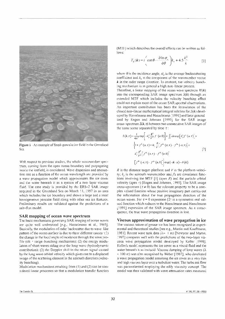
Figure 1 - An exarnple of frazii-pancake ice field in the Greenland Sea.

With respect to previous studies, the whole wavenurnber spectrum, coming iÌom the open ocean boundary and propagating inside the icefield, is considered. Wave dispersion and attenuation rate as a function of the ocean wavelength are provided by a wave propagation model which approximates the ice cover and the water beneath it as a system of a two-layer viscous fluid. The case study is provided by the ERS-2 SAR image acquired in the Greenland Sea on March 11, 1997 in an area which includes the ice boundary and shows a large and aimost homogeneous pancake field aiong with other sea ice features. Preliminaty results are vaiidated against the predictions of a sait-flux model.

SAR mapping of ocean wave spectrum The basic mechanisms goveming SAR imaging of ocean waves are quite well understood [e.g., Hasselmann et al., 19851. Basically, the modulation of radar backscatter due to wav+like pattem of the ocean surface is due to three different causes: (1) the change in the local angle of incidence through the wave profile (tilt + range-bunching mechanism); (2) the energy modulation of short waves riding over the long wave (hydrodynamic contribution); (3) the Doppler shift in the return signal caused by the long wave orbital velocity which gives rise to a displaced image of the scattering element in the azimuth direction (velocity bunchhg). Moddation mechanisms resdting fiom (l) and (2) can be considered linear processes so that a modulation transfer fùnction

k: $[fh (x. r) - f" (o. O)]

R is the distance target-platform and V is the platform velocity; k,, is the azimuth wavenumber mdfs are covariance functions involving the MTF [l] (apex R) and the particle orbital velocity (apex v) [Engen and Johnsen, 19951. The SAR image cross-spectsum (z + 0) has the relevant property to be a complex vaiued function whose positive imaginary part carries out the inforrnation about the true propagation direction of the ocean waves. For z = O expression [2] is a symmetric rea1 val- ued function which reduces to the Hasselmann and Hasselmann [l9911 expression of the SAR image spectrum. As a consequence, the tme wave propagation direction is lost.

Viscous approximation of wave propagation in ice The viscous nature of grease ice has been recognised in experi- menta1 and theoretical studies [see e.g., Martin and Kauiìhm, 198 l]. Recent wave tank data (h;. 1 m) [Newyear and Martin, 19971 compares well with the predictions of the twdayer viscous wave propagation model developed by Keller [1998]. Keller's model represents the ice cover as a viscid fluid and the water beneath it as inviscid. Viscous damping of long waves (h = 100 m) was also recognised by Weber [1987], who developed a wave propagation model assuming the ice cover as a very thin and high viscous layer over a turbdent water. The turbdent flow was parameterised emplaying the eddy viscosity concept. The model was then vaiidated with wave attenuation rates measured

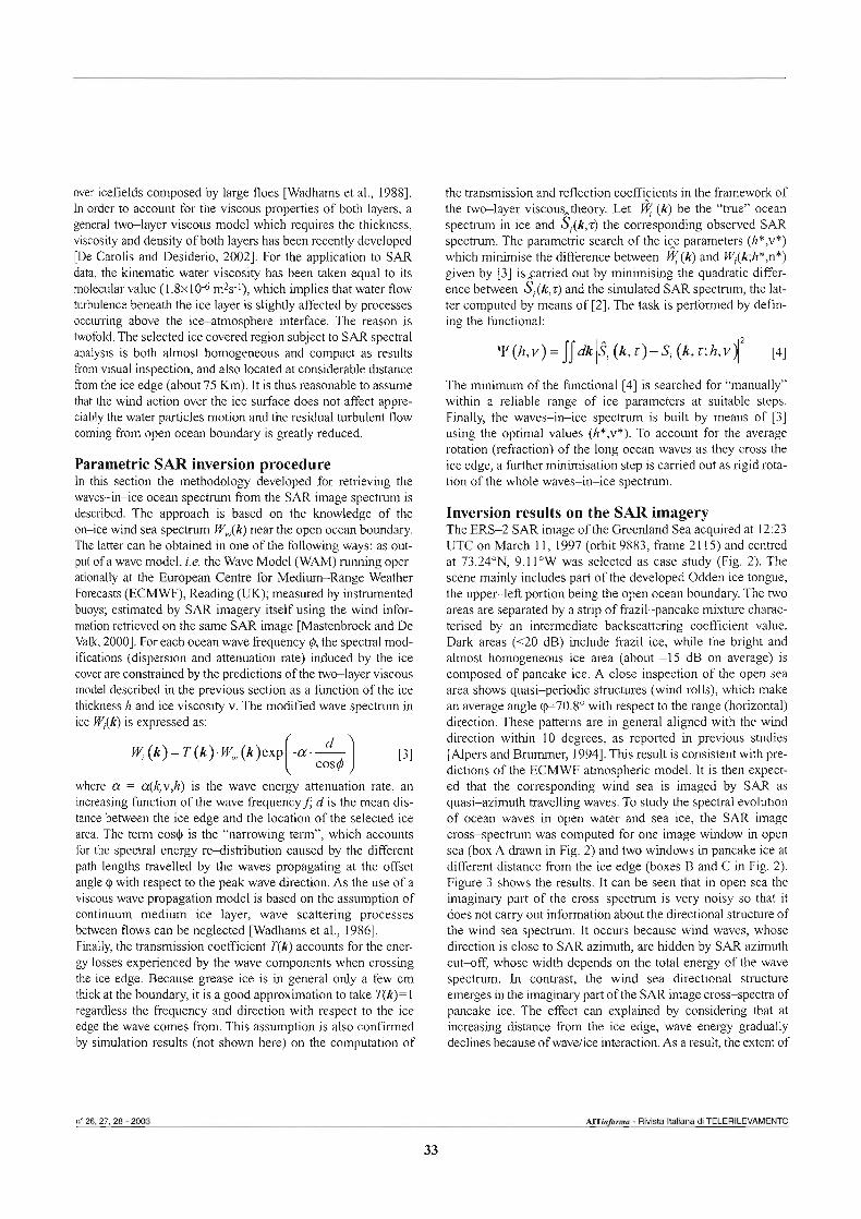
over icefields composed by large floes wadhams et al., 19881. In order to account for the viswus properties of both layers, a general two-layer viscous model which requires the thickness, viscosity and density of both layers has been recently developed [De Carolis and Desiderio, 20021. For the application to SAR data, the kinematic water viscosi@ has been taken equa1 to its molecuiar value (1.8~104 m%-'), which implies that water flow turbuience beneath the ice layer is slightly affected by processes occurring above the iceatmosphere interface. The reason is twofold The selected ice covered region subject to SAR spectral analysis is both almost homogeneous and compact as results from visual inspection, and also located at considerable distance fiom the ice edge (about 75 Km). It is thus reasonable to assume that the wind d o n over the ice surface does not affect appre- ciably the water particles motion and the residua1 turbulent flow coming h m open ocean boundary is greatly reduced.

Parametric SAR inversion procedure In this section the methodology developed for reirieving the waves-in-ice ocean spectnim from the SAR image spectrum is described. The approach is based on the knowledge of the on-ice wind sea spectrum W&) near the open ocean boundary, The latter can be obtained in one of the following ways: as output of a wave model, i.e. the Wave Mode1 (WAM) running oper- ationally at the Ewpean C e n e for Medium-Range Weather Forecasts (ECMWF), Reading (UK); measured by instrumented buoys; estimated by SAR imagev itself using the wind information retrieved on the same SAR image mastenbroek and De Valk, 20001. For each ocean wave fiwluency I), the spectral mod- ifications (dispersion and attenuation rate) induced by the ice w e r are constrahed by the predictions of the two-layer viscous model described in the previous section as a function of the ice thickness h and ice viscosity v. The m&ed wave spectrum in ice K{k) is expressed as:

where a = oa(k,v,h) is the wave energy aiìenuation rate, an increasing function of the wave frequencyj d d the mean dis- tante between the ice edge and the location of the selected ice area. The term cos$ is the "narrowing t m " , which accounts for the spectral energy re-distribution caused by the different path lengths travelled by the waves propagating at the offset angle $ with respect to the peak wave direction. As the use of a viscous wave propagation model is based on the assumption of continuum medium ice layer, wave scattering processes between flows can be neglected [Wadhams et al., 19861. Filly, the transrnission coefficient qk) accounts for the energy losses experienced by the wave components when crossing the ice edge. Because grease ice is in general only a few cm thick at the boundary, it is a good approxirnation to take T(k)= l regardless the frequency and direction with respect to the ice edge the wave comes from. This assumption is also confiied by simulation results (not shown here) on the computation of

the tmmmission and reflection coeffFients in the fiamework of the twdayer visc~us~theory. Let (k) be the "true" ocean spectrum in ice and St(k,z) the corresponding observed SAR spectrum. The pararnetric search of the ice parameters (h*,v*) which minimise the difference between y(k) and Wr<k;h*,n*) given by [3] issarried out by minimising the quadratic differente between Si(k,z) and the simulateci SAR spectrum, the latter computed by means of [2]. The task is performed by defining the functional:

The minimum of the functional [4] is searched for "manually" within a reliable m g e of ice parameters at suitable steps. Finally, the waves-in-ice spectrum is built by means of [3] using the optimal values (h*,v*). To account for the average rotation (refraction) of the long ocean waves as they cross the ice edge, a further minimisation step is carried out as sigid rotation of the whole waves-in-ice spectrum.

Inversion results on the SAR imagery The ERS-2 SAR image of the Greenland Sea acquired at 12:23 UTC on March 11, 1997 (orbit 9883, 21 15) and centred at 73.24"N, 9.1 1°W was selected as case study (Fig. 2). The scene mainly includes part of the developed Odden ice tongue, the upper-lefi portion being the open ocean boundary. The two areas are separated by a stnp of frazil-pancake mkture characterised by an intermediate backscattering coefficient value. Dark areas ( ~ 2 0 dB) include frazil ice, while the bright and almost homogeneous ice area (about -15 dB on average) is composed of pancake ice. A close inspection of the open sea area shows quasi-periodic structures (wind rolls), which make an average angle (p=70.8' with respect to the range (horizonial) direction. These patterns are in general aligned with the wind direction within 10 degrees, as reported in previous studies [Alpers and Brummer, 19941. This r e d t is consistent with predictions of the ECMWF atrnospheric model. It is then expected that the corresponding wind sea is irnaged by SAR as quasi-azimuth travelling waves. To study the spectral evolution of ocean waves in open water and sea ice, the SAR image cross-spectrum was computed for one image window in open sea (box A drawn in Fig. 2) and two windows in pancake ice at different distance from the ice edge (boxes B and C in Fig. 2). Figure 3 shows the results. It can be seen that in open sea the imaginary part of the cross-spectnun is very noisy so that it does not c a m out information about the directional structure of the wind sea spectrum. It occurs because wind waves, whose direction is close to SAR azimuth, are hidden by SAR azimuth cut-off, whose width depends on the total energy of the wave spectrum. In contrast, the wind sea directional structure emerges in the imaginary part of the SAR image cross-spectm of pancake ice. The effect can explained by considering that at increasing distance fiom the ice edge, wave energy grachialSl declines because of wavdice interaction. As a result, the extent of

n' 26.27,28 - 2003 AììInfiratu - RMsla Wlana di TELERILEVAMENTO

33

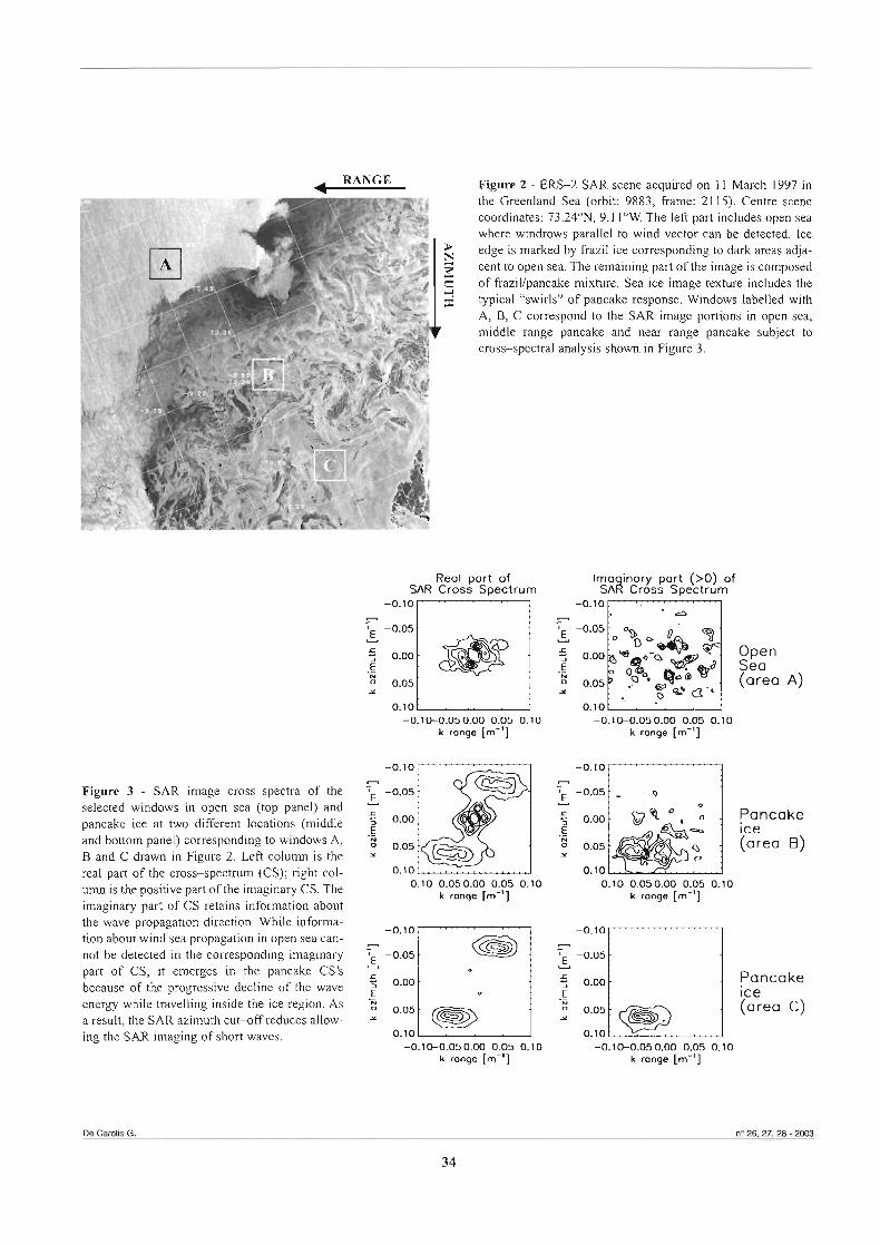
RANGE Figure 2 - ERS-2 SAR scene acquired on 11 March 1997 in the Greenland Sea (orbit: 9883, frame: 21 15). Centre scene coordinates: 73.24"N, 9.1 I0W. The left part includes open sea where windrows parallel to wind vector can be detected. Ice edge is marked by &il ice corresponding to dark area adjacent to open sea. The remaining part of the image is composed of frazil/pancake mixture. Sea ice image texture includes the 8 m a l c'swirlsy' of pancake response. Widows labelled with A, B, C correspond to the SAR image potions in open sea, middle range pancake and near range pancake subject to cross-spectral analysis shown in Figure 3.

Figure 3 - SAR image cross-spectra of the selected windows in open sea (top panel) and pancake ice at two different locations (middle and bottom panel) corresponding to windows A, B and C drawn in Figure 2. Left column is the real part of the cross-spectrum (CS); right col- urnn is the positive part of the imaginary CS. The imaginary part of CS retains information about the wave propagation direction. While information about wind sea propagation in open sea cannot be detected in the corresponding imaginary part of CS, it emerges in the pancake CS's because of the progressive decline of the wave energy while travelling inside the ice region. As a result, the SAR azimuth cut-off reduces aiiow- ing the SAR imaging of short waves.

Reol port of Imo inory port (>O) of SAR Cross Spectrum ~d Cross Spectrum

Y - p 0.10

-0.1 0-0.05 0.00 0.05 0.10 -0.10-0.05 0.00 0.05 0.1 O k range [m-'] k ronge [m-']

-0.10-0.05 0.00 0.05 0.10 k ronge [m-']

-0.1 0-0.05 0.00 0.05 0.1 k range [m-']

-0.1 0-0.05 0.00 0.05 0.1 O k ronge [m-']

(area C)

0.10 -0.10-0.05 0.00 0.05 0.1 0

k ronge [m-']

Input Open Sea wave spectrum Observed SAR spectrum - 0 . 1 5 7 j -0.15-j

-0.15-0.10-0.05-0.000.05 0.10 0.15 k ronge [m"]

-0.15-0.10-0.05-0.000.05 0.10 0.15 k ronge [m-']

Figure 4 - SAR inversion results in pancake ice. Upper left panel: ocean wave spectrum computed in open sea afier SAR spectral inversion assuming the wind vector estimated on SAR image. Bottom left panel: SAR retrieved wave spectrum in pancake ice according to the procedure described in the body of the paper. Upper right panel: observed ERS-2 SAR image spectrum in the selected pancake ice window. Bottom right: simulated SAR image spectrum from the ocean wave spectrum shown in the bottom left panel.

SAR azimuth cut-off reduces, thereby allawing the imaging of shorter waves. Assuming the wind sea spectrum direction is aligned with the wind direction, it can be wncluded that a regime of on-ice waves is being observed. Using the CMOD4 [Stoffelen and Andemn, 19971 and LMOD-FREMER [IFREMER, 19961 scatierometer model;, the wind speed at 10 m a.s.1. can also be estimated. Both models predict a value close to 11 ms-l. The SAR extracted wind vector was then used as input to estimate the wind sea spectnim according to the parameterisation of Donelan et ai. 119851, as done by Mastenbroek and De Vak [2000]. The retrieved wind wave spectrum resulted of significant waveheight of 2.4 m and dorninant wavelength equal to 89 m. To proceed with SAR analysis in pancake ice, a 5 12x5 12 pixels window corresponding to area C of Figure 2, located at about 75 Km fìom the ice edge and imaged at 21" incidente angle, was selected h m the Precision Image (J?RI) SAR product and the image .pectrum was computed to 128x128 pixels resolution. A prelim- i n q estimate of the RAR MTF was performed by selecting a S A R image stnp of homogeneous pancake area spanning 3" in the range dhction from 20.5". As the estimated backscatier (&O,/@ and tilting (cote) contributions to the RAR MTF were -8.10 and +2.6, respectively, the total MTF modulus resulted to be 10.7. This value is comparable with open ocean RAR MTF computed in the framework of the t w ~ c a l e approximation. The mversion scheme described in the previous section was then applied to retrieve the waves-kice spectrum and the results are

Retrieved Sea Ice wave spectrum Best fit SAR spectrum

shown in Figure 4. According to the results of the salt-flux model running at the Scott Polar Research Institute (SPRl), University of Carnbridge (UK), a mean ice thickness between 0.2 m and 0.7 m is m c t e d for the SAR imaged area [J. Wìllrinson, personal communication]. Using the two-layer viscous model [De Carolis and Desiderio, 20021 with the water viscosity value equa1 to the molecular viscosity 1.8~10-6 m2s-1, the optjmai ice parameters are (h*=0.57 m, v*+. 1 m%-l). As shown in Figure 4, there is a good agreement between the observed and simulated SAR spectrum. The SAR simulated peak wavelength and direction (107.6 m, 69.5") compare weil with the corresponding values of the observed SAR spectrum (93.6 m, 70.4"), while there is a slight underestimation of the simulated SAR spectral peak value (80.0 against 122.8). The ocean spectrum was retrieved with a considerable reduced waveheight (1 .O m) and dominant wavelength of 1 14.9 m. Fdy, it should be pointed out that the inversion result is quite insensitive to the numerica1 value of the RAR m. This can be explained since velocity bunching was the major mechanism responsible of wave visibility as the ocean waves were approximately azimuth travelling pachon et al., 19881.

Conclusions A new SAR inversion procedure of waves-Mce has been described and applied to an ERS SAR irnage case study. The inversion scheme requks the ocean wave spectrum originating h m the open ocean and entering the ice covered region The

F -0.10.

E -0.05 t - 0.00 z ,-

n926,27, 28 - 2M>3 ~ITimfomo - Rivista Italiana di TELERILEVAMEMO

F -0.10

L -0.05 ".m. .- z

- 0 . 1 5 ~ ' ' ~ ~ ' ' ~ ~ ~ " ' . . ' ' ' . . . . ' . . ' ' :

:

! I

t

-0.15~~~-~'.'~"~" ' . . . . ' . . . " " ' . j

:

1 @ !

; @ m . n - - - - s . . . . .

t 0.05

0.10

0.15. -0.15-0.10-0.05-0.000.05 0.10 0.15 -0.15-0.10-0.05-0.000.05 0.10 0.15

k ronge [m'] k ronge [m-']

: 2 0.05

' x 0.10

. . . . S . . . . . . . . . . . . . 0 . . . . t 1 0.15.

wave spectnim is tracked inside the icefield, allowing the esti- results were consistent with ice data obtained from the sal-flux mation of the wave spectral changes caused by the ice cover. model running at SPRI. The salt-flu model's adequacy depends Within the assurnption of homogeneous ice cover, a recently on its ability to account for ice thickness measurements per- developed two-layer viscous model is used to assess the ice formed during an oceanographic cruise in the Odden area on the thickness retsieval. The wave model accounts for the altered wave same day of SAR acquisition. Although in this case the described dispersion relation and energy attenuation rate as a function of SAR inversion method gives reliable results, it must be tested on the wave kquency. SSAR spectral infonnation of waves-kice other case studies in order to fully assess its capability. was used to estimate the corresponding wave spectrum. Inversion

References

Alpers W.R and Brummer B. (1994) - Atmospheric boundary Newyear K. and Martin S. (1997) - Comparison of labora- layer mlls observed by synthetic aperture radar aboard the tory data with a viscous two-layer mode1 of wavepropagation ERE1 satellite. J. Geophys. Res., 99: 12613-12621. in grease ice. J. Geophys. Res., 102: 25091-25099.

De Carolis G. and Desiderio D. (2002) - Dkpersion and atten- Stoffe1enA.C.M. and Anderson D.L.T. (1997) - Scattemmeter uation of gmviiy waves in ice: a twelayer viscousfluid mode1 data interpretation: estimation and validation of the transfer with experimental data validation. Phys. Leti. A, 305: 399412. function CMOD4. J. Geophys. Res., 102: 5767-5780.

Donelan M.A., Hamilton J. and Hui W.H. (1985) - Directional spectm of windgenemted waves. Philos. Trans. R. Soc. London, 315: 509-562.

Engen G. and Johnsen H. (1995) - SAR-ocean wave inversion using image cmss spectra. IEEE Trans. Geosci. Remote Sensing, 4: 1047-1056.

Hasselmann K., Raney R.K., Plant W.J., Alpers W., Shuchman R.A., Lyzenga D.R, Rufenach C.L. and Tucker M.J. (1985) - Theory of synthetic aperture mdar ocean imaging: a MAR5'EN vim. J. Geophys. Res., 90: 46594686.

Vachon P.W., Olsen R.B., Livingstone C.E. and Freeman N.G. (1988) - Airborne SAR imagery of ocean surface waves obtained during LEWEX: some initial results. IEEE Trans. Geosci. Remote Sensing, 26: 548-56 1.

Wadhams P., Squire MA., Ewing J.A. and Pasca1 RW. (1986) - Zhe effect of the marginal ice zone on the directional wave spectrum of the ocean. J. Phys. Oceanogt, 16: 358-376.

Wadhams P., Squire V.A., Goodman D.J., Cowan A.M. and Moore S.C. (1988) - The attenuation rates of ocean waves in the margina1 ice zone. J. Geophys. Res., 93: 6799-6818.

Hasselmann K. and Hasselmann S. (1991) - On the nonlinear Wadhams P. and Viehoff T. (1991) - The Odden ice tongue rnapping of un ocean wave spectrum into a synthetic aperture in the Greenland Sea: SAR imagery andjìeld obsewations of mdar image spectrum and its inversion. J. Geophys. Res., 96: its development in 1993. Proc. 2nd ERS-1 Symposium-Space 10713-10729. at the Service of our Environment. Harnburg. pp. 291-296.

IFREMER OfInstitut Francais de Recherche pour 1'Exploitation de la Mer) (1 996) - O$-ne wind scattemmeter ERS products. User manual. IFREMER-CERSAT, Ref. C2-MUT-W-01-lF, Version 2.0 IFREMER, BP70, 29280 Plouzane, France

Keller J. (1998) - Gmvity waves on ice-covered water: J. Geophys. Res., 103: 7663-7669.

Martin S. (1981) - Fmil ice in rivers and oceans. Ann. Rev. Fluid Mech., 13: 379-397.

Martin S. and Kauffmann P. (1981) - Ajìeld and laboratory study of wave damping by grease ice. J. Glaciol., 96: 283-3 13.

Mastenbroek C. and De Valk C.F. (2000) - A semiparamet- ric algorithm to retrieve ocean wave spectra from synthetic aperture radar J. Geophys. Res., 105: 3497-35 16.

Wadhams and Holt B. (1991) - Waves infrazil andpan- cake ice and their detection in Seasat synthetic aperture radar imagery. J. Geophys. Res., 96: 8835-8852.

Wadhams P., Comiso J.C., Prussen E., Wells S., Brandon M., Aldworth E., Viehoff T., Allegrino R. and Crane D.R. (1996) - The development of the Odden ice tongue in the Greenland Sea during winter 1993 Jiom remote sensing and jìeld obsewations. J. Geophys. Res., 101: 18213-18235.

Wadhams P., Parmiggiani F. and De Carolis G. (2002) - The use of SAR to measure ocean wave dispersion in frazil-pancake icefields. J. Phys. Oceanogt, 32: 172 1-1 746.

Weber J.E. (1987) - Wave attenuation and wave drift in the marginal ice zone. J. Phys. Oceanogr., 17: 2351-2361.

Marine surface slicks: theory, characterisation and detection by active microwave instruments

Walter Biamino (l), Cecilia De Vecchi (l), Francesco Nlrchio (2), Piero Pavese (3),

Roberto Ravera (1) and Paolo Trivero (1)

Abstract The a h of this paper is to show the use of in-situ and remote sensing microwave instruments in order to detect and classi@ pollu- tion phenomena on sea surface. Special attention is paid to spaceborne SAR data. The marine dynamics under influence of surface film has been well studied since the early 1970's from both theoretical and experimental point of view. Studies and measurements were carried out on soluble and insoluble, natura1 or artificial films as well as on oil slicks, evaluating the differences among the sea surface signgnatures left by different kinds of films. In later years an algorithm was developed and tested in order to detect automati- cally oil spills from other kinds of slicks using Synthetic Aperture Radar (SAR) images. The algorithm works using statistica1 information obtained from measurements of the Nonnalized Radar Cross-Section (NRCS) on SAR images, in particular on dark areas, and geometrica1 charactxistics for both oil spill and other features. The output is the probability for a dark area to be an oil slick. Our goal is to extend and generalise this algorithm in order to detect and classi@ the different kinds of slicks near the coast and in the open sea.

Riassunto In questo articolo verrà mostmto l'utilizzo di strumenti a microonde, tramite misure in-situ e telerilevate, per rilevare e classificare fenomeni di inquinamento sulla superficie marina. Sarà data particolare enfasi al1 'utilizzo dei dati SAR (Synthetic Aperture Radar). Fin dai primi anni 70 l'influenza difilm superficiali sulla dinamica del mare è stata profondamente studiata, sia nell'aspetto teori- co che mediante esperimenti. Sono stati condotti studi e misure su diferenti tipologie difilm: solubili ed insolubili, naturali ed arti- ficiali, così come sul mare ricoperto da petrolio, con lo scopo di valutare le dzferenze tm le diverse firme spettmli. In anni recenti è stato sviluppato e testato un algoritmo per il rilevamento automatico dei versamenti oleosi in mare ("oil spills'~ utilizzando dati SAR; esso distingue gli oil spills da altn' film superficiali. L'algoritmo utilizza informazioni statistiche ottenute misurando la saio- ne d'urto radar normalizzata (NRCS - Normalized Radar Cross-Section) sulle aree più scure delle immagini SAR, olfre che carane- ristzche di tipo geometrico delle suddette aree. Come risultato finale, si ottiene la probabilità che un 'area scura nel1 'immagine possa essere un film superficiale di petrolio. Il nostro scopo è di estendere e generalizzare la validità dell'algoritmo, alfine di classificare univocamente tutti i diversi tipi di film superficiali, sia presso la costa che in mare aperto.

Introduction Surfactant fiims or "sea-slicks" are responsible for wave damping and reflectivity modulation over a broad range of frequencies from the visible to the microwave regions of the spectrum. Theoretical considerations and experiments have shown that the presence of a monomolecular film on the water surface causes a resonant damping on ripples. The damping appears as

(l) Dipartimento di Scienze e Tecnologie Avanzate, Università del Piemonte Orientale "A. Avogadron, C.so Borsalino 54 - 15100 Alessandria, Itaiia. e-mail: [email protected] MI, Centro di Geodesia Spazble "G. Colombo", h. Terlecchia - - 75100 Matera, Italia.

(3) ISAC - CNR, C.so Fiume 4 - 10133 Torino, Italia.

Received 31/10/2002 - Accepfed 25/02/2003

a depression in the spectrum of wind waves in the 2 - 10 Hz band. The ratio between the clean water spectrum to the spectrum in presence of film reaches a maximum; the features of this maximum appear to depend entirely on properties of the substance fonning the film itself as shown in Figure 1. With the airn to measure the high frequencies sea spectrum component, and then to detect and characterise these substances, new microwave techniques have been developed: an interferential microwave probe and a multi-frequency radar system, and new applications about the use of Synihetic Aperture Radar (SAR) have also b e n suggested.

Theory The theory of rheology of air-water interfaces predicts a maximum in the frequency response of the ratio of the damping coefficient of short-gravity waves (2-10 Hz band) for water covered by an organic surface film to the coescient for a pure water surface. The concept of tensioelasticity developed by Lucassen-Reynders and Lucassen [l 9691 has been extended by

n" 26.27.28 - 2003 AiTbforna - Rivisia Itahana ch TELERILEVAMENTO

37

Figure 1 - Damping ratios for different slicks: 1) methyl palmitate, 2) oleic alcohol, 3) cethilic alcohol, 4) hexadecil-tri-metil ammo- nium bromide.

Cini and Lombardini [l9781 and complex solutions of the characteristic equation of Levich [1962], derived from Navier- Stokes equation for the case of small ripples at the air-water interface in presence of both soluble and insoluble films, have been obtained. The maximurn of damping ratio in presence of films is interpreted in terms of coupling of Marangoni (longitudinal) and Laplace (transversal) waves [Cini et al. 19871. The analytical form which describes the ratio between rea1 parts of the complex radian frequencies on a pure water to that for a water covered by slick (damping ratio) is given by:

where X, Y are functions of E,, = elasticity modulus wD = characteristic ftequency 7

and the + sign stands for soluble while the - sign stands for insoluble film respectively. Unfortunately, in the case of insoluble film, this equation cannot be solved algebraically and therefore in the last 30 years severa1 authors have proposed methods for getting a solution. Numerica1 methods can be used to solve the characteristic equation. We used the particularly simple and powerfid method of Newton-Fowier generalised to the complex plane [Fiscella et al., 19941. This method produces numerica1 solutions directly from the origina1 equation, with no need of algebraic approximations.

Microwave instrumentation Interferential microwave probe The sea spectrum c m be measured by gauging instantaneous surface elevation with a resolution of a few micrometers, by means of a rnicrowave self-calibrating wave meter [Fiscella et al., 1982; Fiscella et al., 19891. The basic element of this probe is a Teflon-coated wire held in a straight vertical position, the lower end of which is dipped in water, while the other end is fed by a microwave source. The microwave energy travels downward confined to a close proximity of the coated wire by surface wave effect [Goubau, 19691. The contact with the water acts as a short circuit, giving origin to a reflected wave. In conditions of good matching in the microwave system, the field in the transmission line has a standing-wave pattern, which is uniquely determined by the location of the water contact. The adopted circuit includes the rnicrowave source (10 mW, 10 GHz Gunn osciliator), which feeds the Goubau line via a 10 dB directional coupler and a femte circulator. The block diagram of the instrument is shown in Figure 2. A standard phase detec- tor circuit, composed of a ring hybrid and a 90" coupler, is used. The outputs of two mixers are low-pass filtered and are sine voltages in quadrature, namely V, and V,,. Displayed on an x - y scope, they will give origin to a point moving on a circle and having a phase linearly related to the water height. Changes in height of the water surface correspond to changes in phase angle between propagated and returning rnicrowaves. The relationship between phase @ and water height z is given by the formula:

0 = 47czIA [21 where h is the radio wavelength. Power specira are obtained by data segrnentation, Hanning win- dowing, FFT operation and subsequent power spectra averaging: 26 Hz may be considered the upper fiequency limit of the probe [Fiscella et al., 19821. In laboratory and clean water conditions the time series of the sea water elevation are affected by instrumenta1 errors of few micrometers and frequency spectra can be obtained without distortion up to 20 Hz. At this frequency a flat spectral noise at leve1 of 10-13 m2/Hz is reached. In open sea fiequency spectra can be obtained up to 15 Hz.

Figure 2 - Block diagram of microwave probe.

Biamino W. et ai. n' 26,27,28 - 2003

38

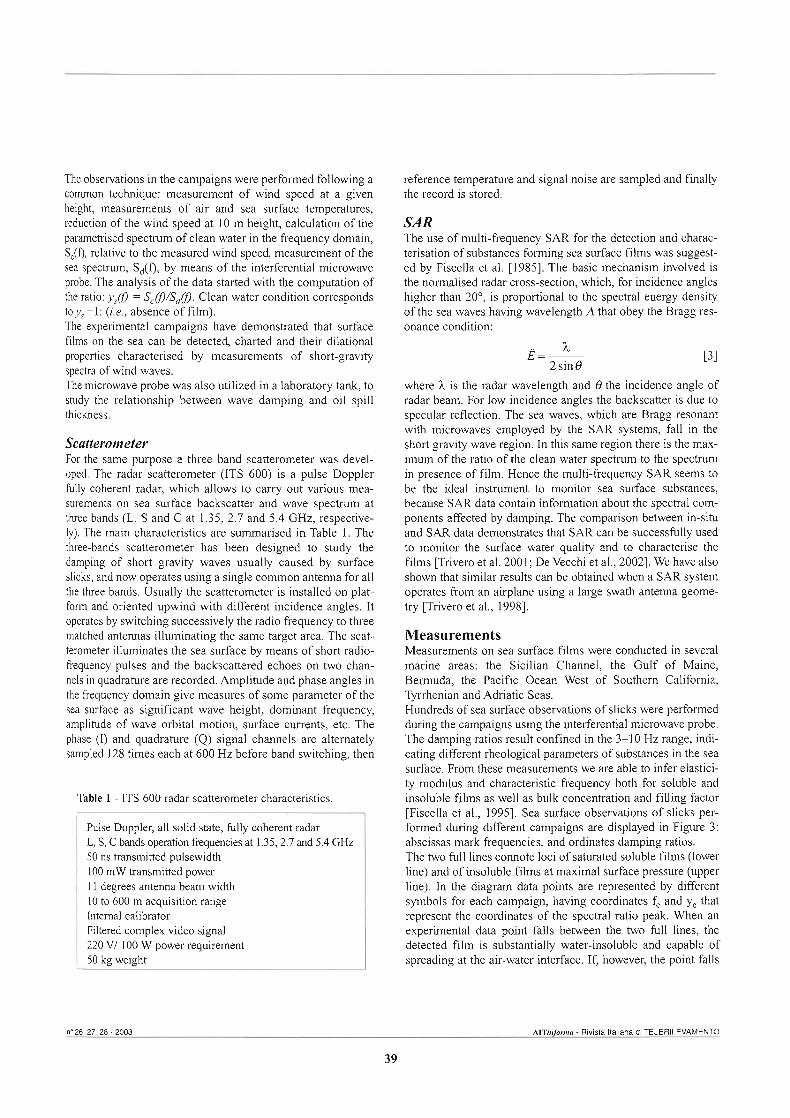
The observations in the campaigns were performed following a common technique: measurement of wind speed at a given height, measurements of air and sea surface temperatures, reduction of the wind speed at 10 m height, calculation of the parametrised spectnun of clean water in the frequency domain, S,(f), relative to the measured wind speed, measurement of the sea spectrum, Sd(f), by means of the interferential microwave probe. The analysis of the data started with the computation of the ratio: ys@ = Sc@/Sd@. Clean water condition corresponds to y, =l : (i.e., absence of film). The experimental campaigns have demonstrated that surface film on the sea can be detected, charted and their dilational properties characterised by measurements of short-gravity spectra of wind waves. The microwave probe was also utilized in a laboratory tank, to study the relationship between wave damping and oil spill thickness.

Scatterometer For the same purpose a three band scatterometer was developed. The radar scatterometer (ITS 600) is a pulse Doppler fully coherent radar, which allows to carry out various measurements on sea surface backscatter and wave spectnun at three bands (L, S and C at 1.35, 2.7 and 5.4 GHz, respectively). The main characteristics are summarised in Table 1. The three-bands scatterometer has been designed to study the damping of short gravity waves usually caused by surface slicks, and now operates using a single cornrnon antenna for al1 the three bands. Usually the scatterometer is installed on platform and oriented upwind with different incidence angles. It operates by switching successively the radio frequency to three matched antennas illuminating the same target area. The scatterometer illuminates the sea surface by means of short radio- hquency pulses and the backscattered echoes on two channels in quadrature are recorded. Amplitude and phase angles in the fiequency domain give measures of some parameter of the sea surface as significant wave height, dominant frequency, amplitude of wave orbita1 motion, surface currents, etc. The phase (I) and quadrature (Q) signal channels are alternately sampled 128 times each at 600 Hz before band switching, then

Table 1 - ITS 600 radar scatterometer characteristics.

Pulse Doppler, al1 solid state, fully coherent radar L, S, C bands opemtion fi-equencies at 1.35,2.7 and 5.4 GHz 50 ns transmitted pulsewidth 100 mW transmitted power 11 degrees antenna beam width 10 to 600 m acquisition range Intemal calibrator Filtered complex video signal 220 VI 100 W power requirement 50 kg weight

reference temperature and signal noise are sampled and finally the record is stored.

SAR The use of multi-frequency SAR for the detection and characterisation of substances forming sea surface films was suggested by Fiscella et al. [1985]. The basic mechanism involved is the normalised radar cross-section, which, for incidence angles higher than 20°, is proportional to the spectral energy density of the sea waves having wavelength A that obey the Bragg resonance condition:

h ,q=- 2 sin 8

i31

where h is the radar wavelength and 8 the incidence angle of radar beam. For low incidence angles the backscatter is due to specular reflection. The sea waves, which are Bragg resonant with microwaves employed by the SAR systems, fall in the short gravity wave region. In this same region there is the maximum of the ratio of the clean water spectrum to the spectrum in presence of film. Hence the multi-frequency SAR seems to be the idea1 instniment to monitor sea surface substances, because SAR data contain information about the svectral components affected by damping. The comparison between in-situ and SAR data demonstrates that SAR can be successfuliy used to monitor the surface water quality and to characterise the films [Trivero et al. 2001; De Vecchi et al., 20021. We have also shown that similar results can be obtained when a SAR system operates from an airplane using a large swath antenna geometry [Trivero et al., 19981.

Measurements Measurements on sea surface films were conducted in severa1 marine areas: the Sicilian Channel, the Gulf of Maine, Bermuda, the Pacific Ocean West of Southern California, Tyrrhenian and Adriatic Seas. Hundreds of sea surface observations of slicks were performed during the campaigns using the interferential microwave probe. The damping ratios result confined in the 3-1 0 I-iz range, indi- cating different rheological parameters of substances in the sea surface. From these measurements we are able to infer elasticity modulus and characteristic frequency both for soluble and insoluble films as well as bulk wncentration and fiiiing factor [Fiscella et al., 19951. Sea surface observations of slicks performed during different campaigns are displayed in Figure 3: abscissas mark frequencies, and ordinates damping ratios. The two fu11 lines connote loci of saturated soluble films (lower line) and of insoluble films at maxirnal surface pressure (upper line). In the diagram data points are represented by different syrnbols for each campaign, having coordinates fe and ye that represent the coordinates of the spectral ratio peak. When an experimental data point falls between the two fu11 lines, the detected film is substantially water-insoluble and capable of spreading at the air-water interface. If, however, the point falls

n' 26,27,28 - 2'003 AITlnfirma - Rivisia Italiana di TELERILEVAMENTO

39

l o O o 1 2 3 4 6 6 7 8 9 1 0 1 1

fi.Q.qneney

Figure 3 - Maxima of damping ratios and corresponding fkequen- cies observed in the Sicilian Channel (g), Maine (May (+) and September (e)), Bermuda 1s. (St. George) [o), and off San Diego (x). The fùii lines mark the theoretical damping of saturated soluble film (lower line), and of insoluble filrns at maximal surface pressure (upper line). The dotted iines are the diagrams of the formula (4) with fiiling factor F of 0.999,0.995,0.990 and 0.980 for insoluble films.

on or below the lower line, there is a good probability that the film is water-soluble and its molecules can absorb and desorb readily from the film. For soluble films we inferred a relationship between the bulk concentration and the wrresponding damping ratio [Cappa et al. 19941. This relation allows us to deduce the value of bulk concentration by measuring the offset of the experirnental point y, from the saturated theoretical vaiue yo. For insoluble substances, information on the surface coverage may be deduced by means of the so-called "fiilling factor" as defined by the formula:

l - l / y e F=- l - l / y o

L41

In Figure 3 the dotted lines show the damping ratio expected in the presence of different values of the filling factor (0.999, 0.995, 0.990, 0.980). Note that at 4 Hz, for instance, a drop of F as small as one-thousandth can lower the observable damping ratio by 1.5 dB. Consequently, it is very unlikely that an experimenta1 point will fa11 near the theoretical curve (upper line). We used the instments described in the previous paragraph during two SAR campaigns to investigate the backscatter damping produced by slicks of known characteristics, in order to extend the results to the interpretation of the SAR images. The first experirnent, organized and supported by the Italian Space Agency (ASI), took place in October 1990 in the northern Adriatic Sea, off the Venice coast in the area around the Italian National Research Council oceanographic platform. It was designed to study the characteristics of the radar backscatter fiom the sea surface and its attenuation in the presence of

films on the sea surface. A CONVAIR 580 aircraft, equipped with C and X band, W polarization SAR, carried out two orthogonal flights over the platforrn area. The platforrn measurements consisted of time series of the three bands radar backscatter of the sea surface elevation and of the wind vector, along with the bulk air and sea temperatura. The interferential rnicrowave probe was mounted upwind and some meters out- board to minimize the tower effects. During the experiment the mean wind speed was of 3.8 m s-1, the significant wave height 0.35 m and the wave ffequency 0.17 Hz. These conditions were ideai to make artificial spreading slicks and to measure backscatter fluctuations by remote-sensing systems and wave motion by gauge. Two small spots (- 104 m2 each) were produced on the sea surface upwind the oceanographic platforrn at approximate distances of 1 km and 100 m, respectively, using in al1 3.5 litres of oleyl alcohol. Canied by surface current, one of the spots crossed the tower permitting us to measure the wave damping by the three-fiequency scatterometer and by the wave gauge installed on board. As soon as the spot entered in the radar footprint, severe damp of the radar backscatter occurred. The SAR flight over the test site occurred approximately 30 minutes later. A portion of the C-band SAR image is shown in Figure 4. The ratios between the mean values of the Normalised Radar Cross Section (NRCS) at the various bands, outside the damp region and the minimum value inside, are compared with ratio between spectral data measured by microwave interferential probe, demonstrating a good agreement [Trivero et al., 20011. The second expenment took place in June 1991 in the Gulf of Genoa, when a . aircraft equipped with a three-fiequency SAR system observed a slicked sea area some days a h an oil- tanker accident [Tnvero et al., 19981. During the flight we per-

Figure 4 - A portion of the C band image acquired during the first SAR flight. The platform is visible as a small bright spot while the black spot is caused by artificial slicks of oleyc alcohol which dampes out the centimetric waves.

Birnino W. et al. n' 26,27, 28 - 2003

40

formed sea truth measurements both from shore as well as from a small boat. The SAR images display many slicks that were also directly observed from shore and boat. The intensity decreases regularly h m near to far range by about 10 dB. Ground-based measurements consisted of standard meteoro- logica1 observations. On boat measurements included wind observations and time series of high-resolution sea surface elevation with the microwave probe. For the SAR scenes we have three W polarization images respectively for the P-, L- and C- band. We elaborated each band of the images by excluding the regions showing land, radar interference and vessels tracks. By following the hypothesis that the Bragg mechanism is the main contribution to the radar backscatter and by associating to each range position the corresponding incidence angle 0, Equation [3] gives the wavelength of the water surface wave component responsible for backscatter. From each range position we explored the image along the azimuth direction and plotted the pixel intensities at the same Bragg fkquency. From the spectral shape analysis the upper points of the clusters show a continuous trend resembling the one obtained with the probe in rippled sea areas, while the bottom edge of the clusters almost match the damped sea waves spectnun. By plotting the ratio between upper and lower limit of clusters we obtain a spectral ratio very s idar to the one obtained by the gauge data.

Oil spiii detection Oil spills reduce water surface roughness and can be detected by the NRCS on SAR images where they appear as dark areas

[Calabresi et al., 19991. With the purpose of detecting oil slicks, in the recent years a probable method of distinguishing oil spills from other similar oceanic features in marine (SAR) images has been developed and tested [Fiscella et al., 20001. The method is based on a simple classifying algorithm that represents the last step of a researcb program in developing a completely automatic detection system, able to discriminate oil spills among al1 dark areas containing look-alike surface phenomena. The method uses statistical information obtained from previous measurements of physical and geometrica1 characteristics for both oil spill and natura1 features. The related operational activities are carried out at the Matera Geodesy Center where the Italian Space Agency Processing and Archiving Facility (PAF) for the European Remote Sensing (ERS) satellite sensor data and the Telespazio mobile acquisition facility are located. A sample image is evaluated using a procedure to determine the probability that it is an oil spill. The classification-algorithm performance was evaluated using a test dataset of SAR irnages containing hundreds of examples of oil spills and of features exhibiting characteristics similar to oil spills (look-alike) [Nirchio et al. 20021. The method is able to classi- fy correctly more then 90% of the samples. A new dataset con- f"nms the performance of this classi-g method even using images with different radiometric and geometric resolutions.

Water surface quality monitoring system Since November 1999 a satellite ground station has been operative in Matera (Italy) and is able to acquire data transmitted by

Oil Non oil

.+. s

Figure 5 - Comprehensive view of detected slicks from a sarnple dataset.

ri LO, LI. 28 - 2003 ~ITinfornra - Rivisia Italiana di TELERILEVAMENTO

41

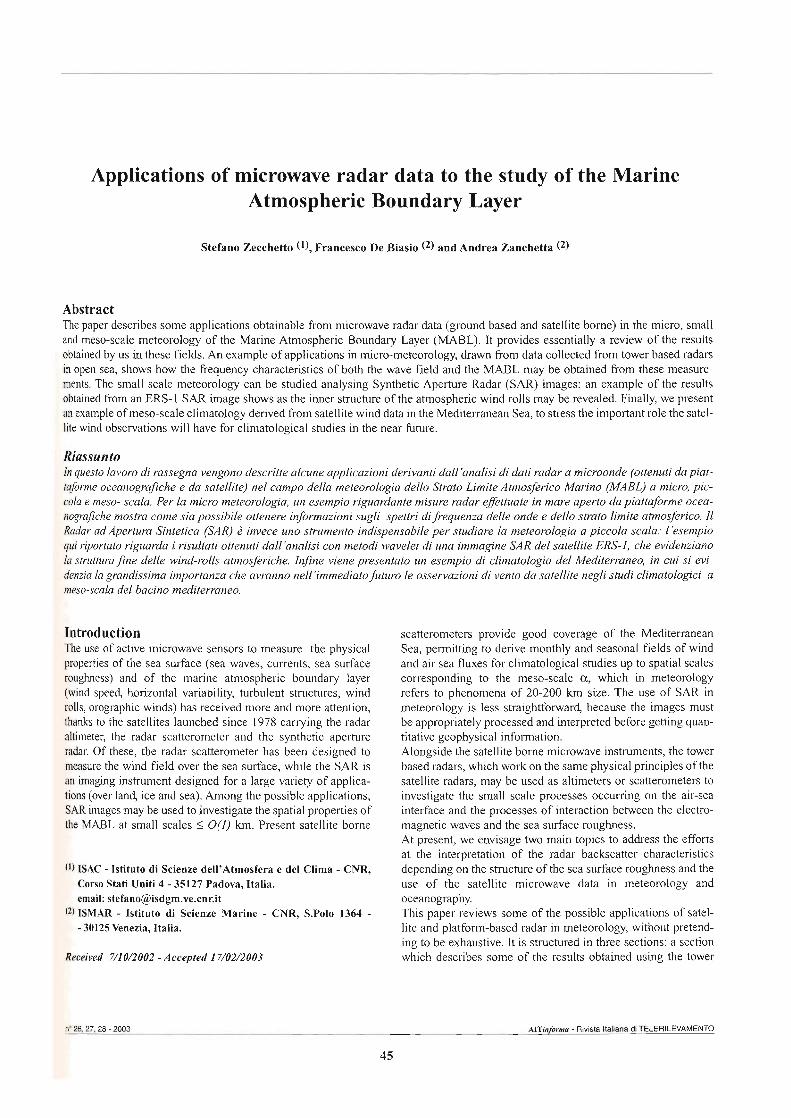
Applications of microwave radar data to the study of the Marine Atmospheric Boundary Layer

Stefano Zecchetto (l), Francesco De Biasio (2) and Andrea Zanchetta (2)

Abstract The paper describes some applications obtainable from microwave radar data (ground based and satellite borne) in the rnicro, small and meso-scale meteorology of the Marine Atmospheric Boundary Layer (MABL). It provides essentiaily a review of the results obtained by us in these fields. An example of applications in micro-meteorology, drawn from data collected from tower based radars in open sea, shows how the frequency characteristics of both the wave field and the MABL may be obtained from these measurements. The smail scale meteorology can be studied analysing Synthetic Aperture Radar (SAR) images: an example of the results obtained from an ERS-l SAR image shows as the inner structure of the atmosphenc wind rolls may be revealed. Finally, we present an example of meso-scale climatology derived from satellite wind data in the Mediterranean Sea, to stress the important role the satellite wind observations will have for climatologicai studies in the near future.

Riassunto In questo lavoro di rassegna vengono descritte alcune applicazioni derivanti dallanalisi di dati mdar a microonde (ottenuti da piattaforme oceanogmfiche e da satellite) nel campo della meteorologia dello Strato Limite Atmosferico Marino (UABL) a micro, piccola e mesoscala. Per la m i m meteorologia, un esempio riguardante misure radar eflettuate in mare aperto da piattaforme ocea- nogmjìche mostm come sia possibile ottenere informazioni sugli spettri di frequenza delle onde e dello strato limite atmosferico. Il Radar ad Apertura Sintetica (SAR) è invece uno strumento indispensabile per studiare la meteorologia a piccola scala: l'esempio qui riportato riguarda i risultati ottenuti dallanalisi con metodi wavelet di una immagine SAR del satellite ERS-I, che evidenziano la siruttam fine delle wind-rolls atmosfriche. Infine viene presentato un esempio di clirnatologia del Mediterraneo, in cui si evi- denzia la grandissima importanza che avranno nell'immediato futuro le osservazioni di vento da satellite negli studi climatologici a meso-scala del bacino mediterraneo.

Introduction The use of active microwave sensors to measure the physical properties of the sea surface (sea waves, currents, sea surface roughness) and of the marine atmospheric boundary layer (wind speed, horizontal variability, turbulent structures, wind rolls, orographic winds) has received more and more attention, thanks to the satellites launched since 1978 canying the radar altimeter, the radar scatterometer and the synthetic aperture radar. Of these, the radar scatterometer has been designed to measure the wind field over the sea surface, while the SAR is an imaging instrument designed for a large variety of applications (over land, ice and sea). Among the possible applications, SAR images may be used to investigate the spatial properties of the MABL at small scales L O(1) h. Present satellite bome

(l) ISAC - Istituto di Scienze deU'Atmosfera e del Clima - CNR, Corso Stati Uniti 4 - 35127 Padova, Italia. emaiì: [email protected]

(*) ISMAR - Istituto di Scienze Marine - CNR, S.Polo 1364 - - 30125 Venezia, Italia.


scatterometers provide good coverage of the Mediterranean Sea, permitting to derive monthly and seasonal fields of wind and air sea fluxes for climatologicai studies up to spatial scales corresponding to the meso-scale a, which in meteorology refers to phenomena of 20-200 km size. The use of SAR in meteorology is less straighdorward, because the images must be appropnately processed and interpreted before getting quantitative geophysical information. Alongside the satellite borne microwave instruments, the tower based radars, which work on the sarne physical principles of the satellite radars, may be used as altimeters or scatterometers to investigate the small scale processes occuning on the air-sea interfàce and the processes of interaction between the electromagnetic waves and the sea surface roughness. At present, we envisage two main topics to address the efforts at the interpretation of the radar backscatter characteristics depending on the structure of the sea surface roughness and the use of the satellite microwave data in meteorology and oceanography. Tbis paper reviews some of the possible applications of satellite and platform-based radar in meteorology, without pretend- ing to be exhaustive. It is stmctured in three sections: a section which describes some of the results obtained using the tower

~~2%,2?,28-2003 mhfima - Rivista Italiana di TELERILEVAMENTO

based radars, then foilowed by a section about the exploitation of SAR images in the s m d scale meteorology. The fina1 section is devoted to show an example of meso-scale climatology derived from satellite wind observations.

Radar appiications in micro-meteorology Tower based microwave radars may be used to investigate the Marine Atmosphenc Boundary Layer at micro-scale, i.e. at time scales O(I) s and spatial scales O(1) m. T i e series of radar backscatter, obtained using wherent and impulsive radar5 at C (5.4 GHz) and Ku (14.5 GHz) bands, W polarisation, have been taken during severa1 experiments on board of open sea platforms [Zecchetto et al., 1991; Fiscelia et al., 1991; De Biasio and Zecchetto, 20001, along with simultaneous measurements of wind components and sea surface elevation. A typical example of these tirne series is shown in Figure 1, which reports the radar cross section (top panel), the radar Doppler frequency (middle panel) and the wind speed (botbm panel). The radar Doppler frequencyfd has been derived fiom the radar complex output signal. As discussed in Zecchetb and Trivero [1992], h m such a time series the frequency characteristics of both the wave field and the MABL rnay be extracted. Figure 2 shows the power density spectra of the time series of Figure 1, in arbitrary uniis for comparison. While the fd spectrum (solid dotted line) describes the wave field (dominant waves near 0.22 Hz), the radar backscatter spectrum (solid line) is more complex presenting, besides a peak at the frequency of the gravity waves, another peak at lower tkequency (-0.02 Hz), which accounts for the frequency strutture of the MABL, also described here by the wind speed spectrum (dotted line). This spectral information, along with the retrieval of the significant

' l ' "'l " I I

wave height and the relationship between the radar backscatter and the wind speed (not shown here), permit to investigate the relationship between the bulk properties of the sea surface and the turbuient MABL, with the aim of a better estimate of the wave-induced effect on the drag coeff~cient and on the wind stress. Furthermore, thanks to the simultaneity of the time series, it has been possible to investigate the local properties (energy content as a function of time) of radar backscatter, wind and gravity waves [Zeccheao et al., 19991 and their mutua1 relationships. This aspect is particularly important in the study of the intennittencies in the air-sea interaction, or to understand the role of the different turbuient scales in the generation of the sea surface roughness. The analysis of backscatkr time series fiom ground based radars is also important because it rnay help the interpretation of SAR irnages (see next section), providing a complientary information (the frequency or tempra1 strutture of the sea surface roughness) with respect to that obtainable h m SAR images (the wave nurnber or spatial strucaire of the sea roughness).

SAR appiications in smaii scale meteorology Synthetic Aperture Radar images of the sea surface may be suc- cessfuily used to investigate the spatial properties of the MABL at spatial scales 2 100 m [Gerling, 1986; Alpers and Bnimmer, 1994; Sikora et al., 1995; Kratsov et al., 1996; Mourad, 1996; Young et al., 20001. Due to the relationship between the sea surface roughness, the radar backscatter and the wind (or the wind stress), it is possible to retrieve fiom SAR images information about the atmospheric stmctures in both convective and dynamical regimes. The evaluation of the geometric properties of these structures allows one to estimate some of the vertical

Figare 1 - Example of one-how time series of radar backscatter Figure 2 - Pwer spectra of the time series of Figure 1. Solid line: (top panel), radar Doppler frequency (middle panel) and wind radar cross section. Dotted-soiid line: radar Doppler fkquency. speed (bottorn panel). The radar data are at C band, W polarisa- Dotted line: wind speed The spectra have been normalised to one for tion and incidence angle 45 degrees. comparison.

Zecchetto S. ei al. n" 26,27,28 -m

46

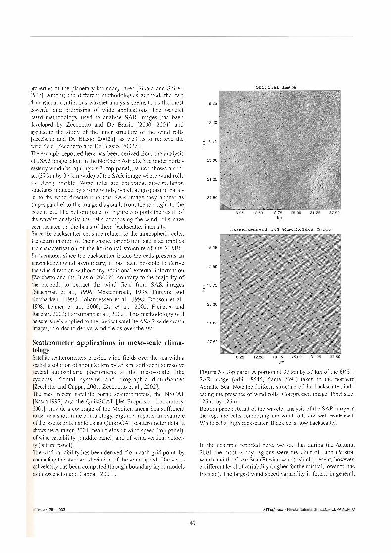
properties of the planetary boundary layer [Sikora and Shirer, 19971. Arnong the different methodologies adopted, the two dimensional continuous wavelet analysis seerns to us the most powerful and promising of wide applications. The wavelet based methodology used to analyse SAR images has been developed by Zecchetto and De Biasio [2000, 20011 and applied to the study of the inner structure of the wind rolls [Zecchetto and De Biasio, 2002a1, as weU as to retrieve the wind field [Zecchetto and De Biasio, 2002bl. The example reported here has been derived from the analysis of a S M image taken in the Northem Adriatic Sea under north- easterly wind (bora) (Figure 3, top panel), which shows a sub- set (37 krn by 37 km wide) of the SAR irnage where wind rolls are clearly visible. Wind rolls are helicoidal air-circulation structures induced by strong winds, which align quasi in paral- le1 to the wind direction: in this SAR image they appear as stripes parallel to the image diagonal, from the top right to the boaom left. The bottom panel of Figure 3 reports the result of the wavelet analysis: the cells composing the wind rolls have been isolated on the basis of their backscatter intensity. Since the backscatter cells are related to the atmospheric cells, the determination of their shape, orientation and size implies the characterisation of the horizontal structure of the MABL. Furthermore, since the backscatter inside the cells presents an upwind-downwind asymmetry, it has been possible to derive the wind direction without any additional extemal information [Zecchetto and De Biasio, 2002b1, contrary to the majority of the methods to extract the wind field from SAR images [Shuchman et al., 1996; Mastenbroek, 1998; Furevik and Korsbakken , 1998; Johannessen et al., 1998; Dobson et al., 1998; Lehner et al., 2000; Du et al., 2002; Fichaux and Ranchin, 2002; Horstmann et al., 20021. This methodology will be extensively applied to the Envisat satellite ASAR wide swath images, in order to derive wind fields over the sea.

Scatterometer applications in meso-scale climatology Satellite scatterometers provide wind fields over the sea with a spatial resolution of about 25 krn by 25 h, sufficient to resolve severa1 atmospheric phenomena at the meso-scale, like cyclones, frontal systems and orographic disturbances [Zecchetto and Cappa, 2001; Zecchetto et al., 20021. The most recent satellite borne scatterometers, the NSCAT [Nasda,1997] and the QuikSCAT [Jet Propulsion Laboratory, 20011, provide a coverage of the Mediterranean Sea sufficient to derive a short tirne clirnatology. Figure 4 reports an example of the results obtainable using QuikSCAT scatterometer data: it shows the Autumn 200 1 mean fields of wind speed (top panel), of wind variability (rniddle panel) and of wind vetical velocity (bottom panel). The wind variability has been derived, from each grid point, by computing the standard deviation of the wind speed. The vertical velocity has been computed through boundary layer models as in Zecchetto and Cappa, [2001].

Origina1 Image

km

Reconstructed and Threaholded Image

Figure 3 - Top panel: A portion of 37 km by 37 km of the ERS-l SAR image (orbit 18545, frame 2691) taken in the northern Adriatic Sea. Note the filiform structure of the backscatter, indi- cating the presence of wind rolls. Compressed image. Pixel size: 125 m by 125 m. Bottom panel: Result of the wavelet analysis of the SAR image at the top: the cells composing the wind rolls are well evidenced. White cells: high backscatter. Black cells: low backscatter.

In the example reported here, we see that during the Autumn 2001 the most windy regions were the Guif of Lion (Mistral wind) and the Crete Sea (Etesian wind) which present, however, a different leve1 of variability (hgher for the mistral, lawer for the Etesian). The largest wind speed variability is found, in general,

26,27,28 - 2003 ~ITinforma - RMsta italiana di TELERILEVAMENTO

47

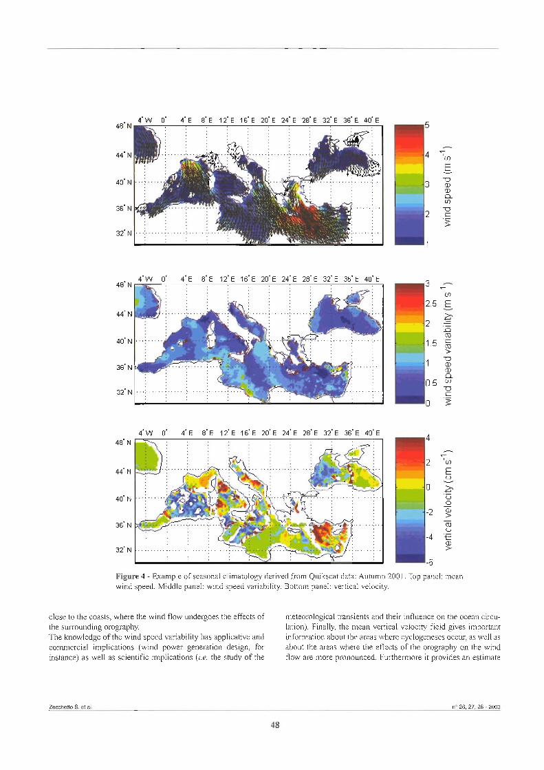
""I O' 48'Pde -

4 ' ~ 0' 4'E 8'E 1 2 ' ~ 1 6 ' ~ M ' E 2 4 ' ~ 2 8 ' ~ 3 2 ' ~ 36'E 4 0 ' ~ .m. .I l . . - 44 N _ : . n. .: .... .;. .... .:, .... .:.l h:.. - i A

. ,

M',,, ... : ...... .......... . I

. A m - ...... % ' N = - . f j.., . -

,'N ..........I...... : ..... :.. ... :., ............

Figure 4 - Example of seasonal climatology derived fiom Quikscat data: Autumn 2001. Top panel: mean wind speed. Middle panel: wind speed variability. Bottom panel: vertical velocity.

dose to the coasts, where the wind flow undergoes the effects of meteorological transients and their infiuence on the ocean circu- the surrounduig orography. lation). Finaliy, the mean vertical velocity field gives important The knowledge of the wind speed variability has applicative and informaiion about the areas &ere cyclogeneses occur, as weii as commercial implications (wind power generation design, for about the areas where the effects of the orogmphy on the wind iustance) as weil as scientific implications ( i . ~ fbe study of the flow are more pmounced. Furthermore it prcwides an &te

Zecchethi S. et al. no 26.27,28 -m

48

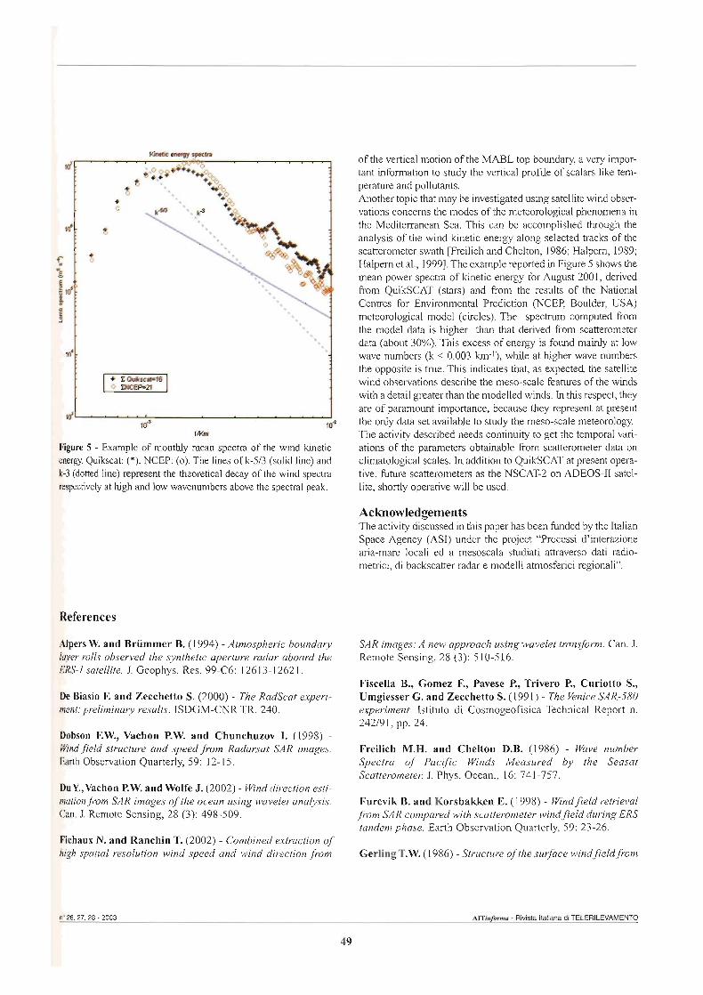
Figure 5 - Example of monthiy mean spectra of the wind kinetic energy. Quikscat: (*). NCEP: (o). The lines of k-513 (solid line) and k-3 (dotted lime) represent the theoretical decay of the wind spectm

at high and low wavenurnbers a b e the spectral peak

References

Alpers W. and Briimmer B. (1 994) - Atmospheric boundary layer rolls obsewed the synthetic aperture radar aboard the ERS-1 satellite. J. Geophys. Res. 99-C6: 126 13- 1262 1.

De Biasio F. and Zecchetto S. (2000) - The RadScat experiment: preliminary results. ISDGM-CNR TR. 240.

Dobson F.W., Vachon P.W. and Chunchuzov I. (1998) - WindJield strutture and speed@m Radarsat SAR images. Earth Observation Quarterly, 59: 12- 15.

DuY.,Vachon P.W. and Wolfe J. (2002) - Wnd direction estimation fivm SAR images of the ocean using wavelet analysis. Can. J. Remote Sensing, 28 (3): 498-509.

Fichaux N. and Ranchin T. (2002) - Combined extraction of high spatial resolution wind speed and wind direction jìvm

of the vertical motion of the MABL top boundary, a very irnportant inforrnation to study the vertical profile of scalars like temperature and pollutants. Another topic that rnay be investigateci using sateilite wind observations concems the modes of the meteorological phenomena in the Mediterranea Sea. This can be accomplished through the anaiysis of the wind kinetic energy along selected tracks of the scatterometer swath w l i c h and Chelton, 1986; Halpem, 1989; Halpern et al., 19991. The exarnple reported in Figure 5 shows the mean power spectra of kinetic energy for August 2001, derived from QuikSCAT (stars) and fmm the results of the National Centres for EnWonmental Prediction (NCEP, Boulder, USA) meteorological model (circles). The spectrum computed from the model data is higher than that derived from scatterometer data (about 30%). This excess of energy is found ma& at low wave nurnbers (k < 0.003 km-l), whiie at higher wave numbers the opposite is true. This indicates that, as expected, the satellite wind observations describe the meso-scale features of the winds with a detail greater than the modelled winds. In this respect, they are of paramount importante, because they represent at present the only data set available to study the meso-scale meteorology. The activity described needs continuity t0 get the tempra1 mi- ations of the parameten obtainable from scatterometer data on climatologi~ scales. In addition to QuikSCAT at present operative, future scatterometers as the NSCAT-2 on ADEOS-11 satellite, shortly operative will be used.

Acknowledgements The activity di&ussed in this papa has been funded by the Italian Space Agency (ASI) under the project "Processi d'interazione aria-mare locali ed a mesoscala studiati attraverso dati radiometrici, di backscatter radar e modelli atmosferici regionali".

SAR images: A new approach using wavelet transform. Can. J. Remote Sensing, 28 (3): 510-5 16.

Fiscella B., Gomez F., Pavese P., Trivero P., Curiotto S., Umgiesser G. and Zecchetto S. ( 1 99 1) - The Venice SAR-580 experiment. Istituto di Cosmogeofisica Technical Report n. 242191, pp. 24.

Freilich M.H. and Chelton D.B. (1986) - Wave number Spectra of Paclfic Winds Measured by the Seasat Scattemmetel: J. Phys. Ocean., 16: 741-757.

Furevik B. and Korsbakken E. (1998) - Mndfield retrieval fmm SAR compared with scatterometer windfield during ERS tandem phase. Earth Observation Quarterly, 59: 23-26.

Gerling T.W. (1 986) - Strutture of the suflace windfieldfrom

AITin/orm - Rlvlsta Italiana di TELERILEVAMEMTO

49

the Seasat SAR. J. Geophys. Res., 91: 2308-2320.

Halpern D. (1989) - Seasat A Satellite Scatterometer Measurements of Equatorial Suface Winds. J. Geophys. Res., 94, C4: 4829-4833.

Halpern D., Freilich M.H. and Weller R.A. (1999) - ECMWF and ERS-I Surface Winds over the Arabian Sea during July 1995. J. Phys. Ocean. - Notes and Correspondence, 29: 1619-1623.

Horstmann J., Koch W., Lehner S. and Tonboe R. (2002) - Ocean winds from RADARSAT-1 ScanSAR. Can. J. Remote Sensing, 28 (3): 524-533.

Johannessen O.M., Korsbakken E. and Johannessen J.A. (1998) - Coastal windfield retrievalfiom ERSsynthetic aperture radar images. J. Geophys. Res., 103: 7857-7874.

Jet Propulsion Laboratory (JPL) (2001) - QuikSCAT User S manual k 2.1. Apri1 2001, JPL, D- 18053.

retrieval using ERS-I synthetic aperture mdar imagery. IEEE Trans. Geosci. Remote Sensing, 34 (6): 1343-1352.

Young G.S., Sikora T.D. and Winstead N.S. (2000) - Inferring marine atmospheric boundary layerpropertiesfim spectral chamcteristics of satellite-borne SAR imagely. Mon. Weather Rev., 128: 1506-1 520.

Zecchetto S., Curiotto S. and Umgiesser G. (1991) - The VEERS-I group radar-air-sea experiment: description and preparatory activity. Istituto Dinamica Grandi Masse Technical Report n. 158. pp. 26.

Zecchetto S. and 'Iiivero l? (1992) - Experiment and Results of the Ztalian Activity in the Field of Ocean Microwave Backscattering. Proc. of the Conferente for Pacific Ocean Environrnents and Probing, Okinawa, Japan, 25-3 1 August 1992.

Zecchetto S., Trivero P., Fiscella B. and Pavese P. (1998) - Wind stress structure in the unstable marine surface layer detected by SAR. Boundary Layer Meteorology, 86: 1-28.

Kravtsov Y . k , Mityagina M.I., Pung V.G. and Yakovlev V.V. (1996) - Occurrence of convective processes in the boundary layer of he amsphere on radar images of the sea suface. Earth Obs. Remote Sens., 14: 1-15.

Lehner S., Tonboe R, Horstmann R. and Koch W. (2000) - Wind retrieval over the ocean using synthetic aperture radar with C-band hh polarization. IEEE Trans. Geosci. Remote Sensing, 38 (5): 21 22-21 3 1.

Mastenbroek K. (1 998) - High resolution wind jìelds j?om ERS SAR. Earth Observation Quarterly, 59: 20-22.

Mourad P.D. (1996) - Inferring multiscale structure in the atmospheric turbulence using satellite-based synthetic aperture radar imagery. J. Geophys. Res., 101, C8: 18433-1 8449.

NASDA (1997) - ADEOS Reference Handbook. Tokyo National Space Development Agency of Japan (NASDA).

Sikora T.D.,Young G.S., Beal R.C. and Edson J.B. (1995) - Use of spaceborne synthetic aperture radar imagery of the sea surface in detecting the presence and structure of the convective marine atmospheric boundary laye,: Mon. Weather Rev., 123 12: 3623-3632.

Sikora T.D. and Shirer H. N. (1997) - Estimating convective atmospheric boundary layer depth fiom microwave radar imagery of the sea surface. J. Appl. Meteor., 36: 833-845.

Shuchman RA., Johannessen A.J., Davidson K.L., Wackerman C.C. and Rufenhac C.L. (1996) - Wind vector

Zecchetto S., De Biasio F. and Trivero P. (1999) - Local proper ' s of mdar backscatter at C-band and off nadir angles.\ir-Sea Interaction Workshop, Sydney l l- I1 January 19

SAR images. SAR image Analysis, Modelling and Techniques 111, SPIE Proceedings Series, Vol. 4173, September 2000.

Zecchetto S. and Cappa C. (200 1) - The spatial structure of the Mediterranean Sea winds as revealed by the ERS-1 scat- teromete,: Int. J. Rem. Sens., 22 (1): 45-70.

Zecchetto S. and De Biasio F. (2001) - Wavelet analysis applied to SAR images to detect atmospheric sti-uctures. I1 Nuovo Cimento, 24 (1): 81-88.

Zecchetto S., De Biasio F., Music S., Nickovic S. and Pierdicca N. (2002) - Zntercomparison of satellite observations and atmospheric mode1 simulations of a meso-scale cyclone in the Mediterranean Sea. Cm. J. Remote Sensing, 28 (3): 1-1 1.

Zecchetto S. and De Biasio F. (2002a) - On shape, orientation and structure of atmosheric cells inside wind rolls in two SAR images. IEEE Trans. Geosci. Remote Sensing, 40 (10): 2257-2262.

Zecchetto S. and De Biasio F. (2002b) - Wind retrievalfrom SAR images using Continuous Wavelet Transform. Proc. IGARSS 2002, Toronto, Canada.

Zecchetto S. et al. n' 28, n. 28 - 2003

50

SAR intensity images in the study of coastal displacement

Marco Gatti (1)

Abstract This paper presents the results of a study evaluating the use of SAR intensity images to quantify the displacement in time of a coastline. First, it describes the preliminary tests to assess the accuracy of a coastline position obtained from SAR intensity images. Then, the displacements of the Ernilia-Romagna coastline (from the border with Marche to the Po River mouth) obtained by cartography and aerial photogrammetry are compared with those inferred from two SAR images. The preliminary tests show that the horizontal accuracy of the SAR intensity images is about 20 m, a value that coincides with the mean tidal excursion of the Emilia-Romagna coast. The comparison of the variations inferred by classical cartography, aerial photogrammetry and direct surveys with those calculated from the SAR images indicates similar speeds of the coastline erosions in rnany tracts of the Emilia-Romagna coast.

Riassunto Questo lavoro presenta i risultati di una verifica sperimentale sull'utilizzo deile immagini SAR per studiare e quantificare lo spostamen- to nel tempo di un litorale. Neila prima parte del lavoro vengono descritti i test preliminari di valutazione dell'accuratezza planimetrica di una linea di costa, fotointerpretata e restituita da un'immagine SAR. Successivamente vengono presentati i confronti sulle variazioni subi- te dal litorale Emiiiano-Romagnolo, dal &me con le Marche fino al Delta del Po, ottenuta da cartografia tecnica esistente, foto aeree e rilevamenti diretti sul terreno, con queiii ottenuti da due distinte immagini SAR. I test preliminari confermano che la linea di costa fotointerpretata e restituita da un'irnmagine SAR, ha una accuratezza planimetrica non inferiore ai 20 m; quest'ultimo valore non r id ia sor- prendentemente alto, se comparato con quella che 6 la variazione planimetrica della linea di costa prodotta dall'escursione di marea lungo il litorale Emiliano-Romagnolo. I confronti tra le variazioni denunciate dall'analisi del materiale topo-cartografico e quelle ottenute dalla fotointerpretazione e restituzione delle immagini SAR, indicano velocità di erosione e di avanzamento simili su molti tratti di litorale.

Introduction The advancement or the retreat of the coastline caused by flu- via1 deposition or marine erosion is a phenomenon very strong along the middle and upper Adriatic coast and produces areas of erosion and advancement in extensive coastal zones. The availability of SAR images (Henderson and Lewis, 1998), combined with new techniques of direct surveying, has greatly increased the potential applications of remote sensing in the study of this process. For this reason, the Department of Engineering, University of Ferrara, has developed a study to evaluate the use of photointerpreted SAR, ERSI and ERS2 intensity images to quantify in the time the coast displacements . This paper presents the preliminary results of the research. In particular, it descnbes the tests performed to assess the horizontal accuracy position of a coastline obtained from SAR intensity images. The variations of the Emilia-Romagna coast-

(l) Dipartimento di Ingegneria, via Saragat 1 - 44100 Ferrara, Italia. e-mail: [email protected]


line (from the border with Marche to the Po River mouth) obtained by cartography and aerial photography are then compared with those inferred from two SAR images. The preliminary tests show that the horizontal accuracy of the SAR intensity images is about 20 m, a value that coincides with the mean tidal excursion of the Emilia-Romagna coast. The comparison of the variations inferred by classical cartography, aerial photogrammetry and direct ground surveys with those calculated from the SAR images, indicates similar speeds of coastline advancement in many tracts of the Emilia-Romagna coast.

Definitions The aim of the survey is to define the horizontal position of the coastline. By comparing the horizontal positions of coastal tracts in successive epochs, it is possible to quanti@ their variation in time and to identify areas of erosion or advancement. The first problem is to define what is meant by "coastline". By definition, the "coastline" is the line of contact between the surface of the sea and the physical surface of the ground (Fig. la). However, for sandy beaches with very little slope, like those of Emilia-Romagna, there is more than one coastline: - the instantaneous coastline (Fig. lb), that one measured during the survey, either directly, by GPS or traditional topograph-

n" 26,27,28 - 2003 AiTkfom - Rivista italiana di TELERILEVAMENTO

51

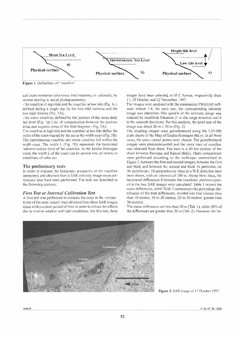
.\C .................... Mean Sea Leve1 "i ................m....... Instantaneous Sea Level

Physical Fb) surface

Figure 1. Definitions of "coastline".

ical instrurnentation (electronic total stations), or indirecily, by remote sensing or aerial photograrnmetry; - the coastline at high tide and the coastline at low tide (Fig. lc), defined during a single day by the two tidal maxima and the two tidal minima (Fig. 5A); - the mean coastline, defined by the position of the mean daily sea level (Fig. la) (line of compensation between the positive areas and negative area of the tidal diagram - Fig. 5A). The coastline at high tide and the coastline at low tide define the width of the coast washed by the sea or the width-coast (Fig. 5B). The insiantaneous coastline and mean coastline fa11 within the width-coast. The width L (Fig. 5B) represents the horizontal indetermination lirnit of the coastline. in the Emilia-Romagna coast, the width L of the coast can be severai tens of meters in conditions of calm sea.

The preliminary tests In order to evaluate the horizontal accuracies of the coastline interpreted and obtained from a SAR intensity image some preliminar~ tests have been performed. The tests are described in the following sections.

First Test or Interna1 Calibration Test A first test was performed to evaluate the error in the interpretation of the same coastal tract obtained fiom three SAR images taken within a short period of time in order to reduce the effects due to marine weather and tidal conditions. For this test, three

images have been seiected, in SLC format, respectively fiom 17, 18 October and 22 November 1997. The images were analysed with the commerciai PHASAR software release 1.4; for each one, the corresponding intensity image was identified. The speckle of the intensity irnage was reduced by multilook filtration (1 in the range direction and 4 in the azimuth direction). For this analysis, the pixel size of the image was about 20 m x 20 m (Fig. 2). The resulting images were georeferenced using the 1:25.000 scale sheets of the Map of Emilia-Romagna (italy). In all three cases, the same contro1 points were chosen. The georeferenced images were photointerpreted and the same tract of coastiine was obtained fiom them. The tract is a 40 km portion of the shore between Ravenna and Rimini (italy). Three comparisons were performed according to the technique summarized in Figure 3: betweenthe first and second images, between the fmt and third, and between the second and third. in particular, on the polylinears, 16 perpendicular lines in a W-E direction have been drawn, with an interaxis of 100 m. Along these lines, the horizontal differences 6 between the coastlines photointerpreted in the two SAR images were calculated. Table 1 reports the mean differences, while Table 2 surnmarizes the percentage distribution of the total differences, divided into four classes (less than 10 meters; 10 to 20 meters; 20 to 30 meters; greater than 30 meters). The mean differences are less than 20 m (Tab. l), while 40% of the differences are greater than 20 m (Tab. 2). However, the lat-

Figure 2. SAR image of 17 October 1997.

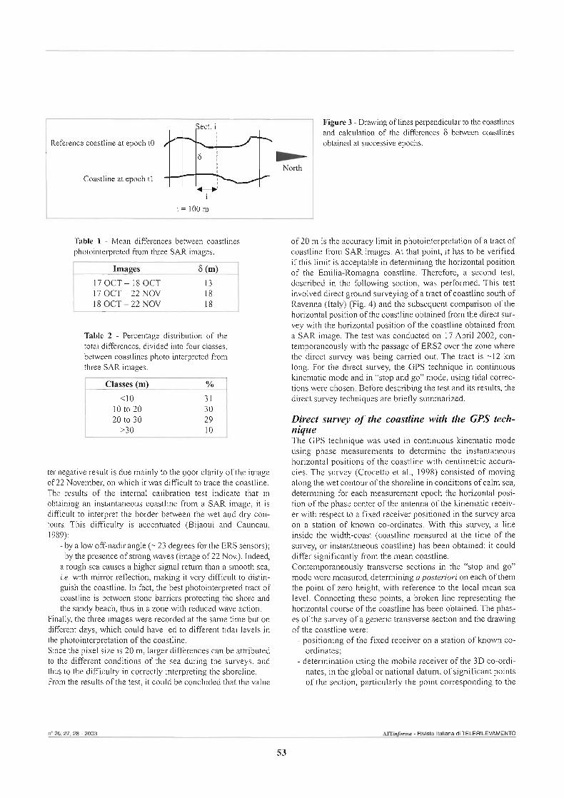
ect. i

Reference coastline at epoch t0 fi-s- I North

Coastline at epoch t1 t-+'

i i = 100m

Table 1 - Mean differences between coastlines photointerpreted from three SAR images.

Ima es

17 OCT - 18 OCT 17 OCT - 22 NOV 18 OCT-22 NOV

Table 2 - Percentage distnbution of the total differences, divided into four classes, between coastlines photo interpreted from three SAR images.

ter negative result is due mainly to the poor clarity of the image of 22 Nwember, on which it was difficult to trace the coastline. The results of the interna1 calibration test indicate that in obtaining an instantaneous coastline from a SAR image, it is dificult to interpret the border between the wet and dry con- tours. This difficulty is accentuated (Bijaoui and Cauneau, 1989):

- by a low off-nadir angle (- 23 degrees for the ERS sensors); - by the presence of strong waves (iage of 22 Nov.). Indeed, a rough sea causes a higher signal retum than a smooth sea, i.e. with mirror reflection, making it very difficult to distin- guish the coastline. In fact, the best photointerpreted tract of coastline is between stone barriers protecting &e shore and the sandy beach, thus in a zone with reduced wave action.

Filly, the three images were recorded at the sarne time but on different days, which could have led to different tidal levels jn the photointerpretation of the coastline. Since the pixel size is 20 m, larger differences can be attributed to the different conditions of the sea during the surveys, and thus to the difficulty in correctly interpreting the shoreline. From the results of the test, it could beconckded that the value

Figure 3 - Drawing of lines perpendicular to the coastiines and calculation of the diffmces 6 between coastlines obtained at successive epochs.

of 20 m is the accuracy lirnit in photointerpretation of a tract of coastline from SAR images. At that point, it has to be verified if this limit is acceptable in determining the horizontal position of the Ernilia-Romagna coastline. Therefore, a second test, described in the following section, was performed. This test involved direct ground surveying of a tract of coastline south of Ravenna (Italy) (Fig. 4) and the subsequent comparison of the horizontal position of the coastline obtained from the direct survey with the horizontal position of the coastline obtained fiom a SAR image. The test was conducted on 17 Apri1 2002, contemporaneously with the passage of ERS2 over the zone where the direct survey was being carried out. The tract is -12 km long. For the direct survey, the GPS technique in continuous kinematic mode and in "stop and go" mode, using tidal corrections were chosen. Before describing the test and its results, the direct survey techniques are briefly summarized.

Direct suwey of the coastline with the GPS technique The GPS technique was used in continuous kinematic mode using phase measurements to determine the instantaneous horizontal positions of the coastline with centimetric accuracies. The survey (Crocetto et al., 1998) consisted of moving along the wet contour of the shoreline in conditions of calm sea, determining for each measurement epoch the horizontal position of the phase center of the antenna of the kinematic receiver with respect to a fixed receiver positioned in the survey area on a station of laiown co-ordinates. With this survey, a line inside the width-coast (coastline measured at the time of the survey, or instantaneous coastline) has been obtained: it could deer significantly fi-om the mean coastline. Contemporaneously transverse sections in the "stop and go" mode were measured, determining aposteriori on each of them the point of zero height, with reference to the local mean sea level. Connecting these points, a broken line representing the horizontal course of the coastline has been obtained. The phases of the survey of a generic transverse section and the drawing of the coastline were: - positioning of the fixed receiver on a station of known co-

ordinate~; - determination using the mobile receiver of the 3D co-ordi-

nates, in the global or national datum, of significant points of the section, particularly the point corresponding to the

n" 26.27,28 - 2003 AI%fom - RMsta Italiana di TELERILEVAMENTO

53

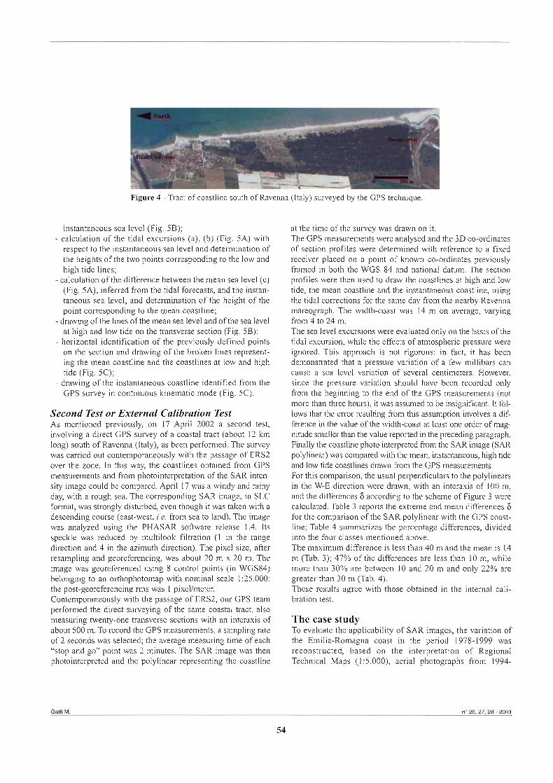
" - 1 t - l i- -,-=.m 'igure 4 - Tract of coastline south of Ravenna (Italy) surveyed by the GPS technique.

instantaneous sea level (Fig. 5B); - calculation of the tidai excursions (a), (b) (Fig. 5A) with

respect to the instantaneous sea level and determination of the heights of the two points corresponding to the low and high tide lines;

- calculation of the difference between the mean sea level (C) (Fig. 5A), inferred from the tidal forecasts, and the instantaneous sea level, and determination of the height of the point corresponding to the mean coastline;

- drawing of the lines of the mean sea level and of the sea level at high and low tide on the transverse section (Fig. 5B);

- horizontal identification of the previously defined points on the section and drawing of the broken lines representing the mean coastline and the coastlines at low and high tide (Fig. 5C);

- drawing of the instantaneous coastline identified from the GPS survey in continuous kinernatic mode (Fig. 5C).

Second Test or External Calibration Test As mentioned previously, on 17 April 2002 a sewnd test, involving a direct GPS survey of a coastal tract (about 12 km long) south of Ravenna (italy), as been performed. The survey was carried out contemporaneously with the passage of ERS2 over the zone. In this way, the wastlines obtained from GPS measurements and from photointerpretation of the SAR intensity image couid be compared. April 17 was a windy and rainy day, with a rough sea. The corresponding SAR image, in SLC format, was strongly disturbed, even though it was taken with a descending course (east-west, i.e. from sea to land). The image was analyzed using the PHASAR s o h a r e release 1.4. Its speckle was reduced by muitilook filtration (1 in the range direction and 4 in the azimuth direction). The pixel size, after resampling and georeferencing, was about 20 m x 20 m. The irnage was georeferenced using 8 contro1 points (in WGS84) belonging to an orthophotomap with nomind scale 1:25.000: the post-georeferencing nns was 1 pixewmeter. Contemporaneously with the passage of ERS2, our GPS team performed the direct surveying of the sarne coastal tract, also measuring twenty-one transverse sections with an interaxis of about 500 m. To record the GPS measurements, a sampling rate of 2 sewnds was selected; the average measuring time of each "stop and go" point was 2 minutes. The SAR image was then photointerpreted and the polylinear representing the coastline

at the time of the survey was drawn on it. The GPS measurements were analysed and the 3D co-ordinates of section profiles were determined with reference to a fixed receiver placed on a point of known co-ordinates previously -ed in both the WGS 84 and national daturn. The section profiles were then used to draw the wastlines at high and low tide, the mean coastline and the instantaneous coastline, using the tidal corrections for the same day from the nearby Ravenna mareograph. The width-coast was 14 m on average, varying from 4 to 24 m. The sea level excursions were evaluated only on the basis of the tidal excursion, while the effects of atmospheric pressure were ignored. This approach is not ngorous: in fact, it has been demonstrated that a pressure variation of a few rnillibars can cause a sea level variation of severa1 centimeters. However, since the pressure variation should have been recorded only from the beginning to the end of the GPS measurements (not more than three hours), it was assumed to be insignificant. It follows that the error resulting fkom this assumption involves a differente in the vdue of the width-coast at least one order of magnitude srnaller than the value reported in the preceding paragraph. Finally the coastline photo interpreteci from the SAR image (SAR polylinear) was compared with the mean, instantaneous, high tide and low tide wastlines drawn from the GPS measurements. For this comparison, the usual perpendiculars to the polylinears in the W-E direction were drawn, with an interaxis of 100 m, and the differences 6 according to the scheme of Figure 3 were calculated. Table 3 reports the extreme and mean differences 6 for the comparison of the SAR polylinear with the GPS coastline; Table 4 sumrnarizes the percentage differences, divided into the four classes mentioned above. The maximurn difference is less than 40 m and the mean is 14 m (Tab. 3); 47% of the differences are less than 10 m, while more than 30% are between 10 and 20 m and only 22% are greater than 30 m (Tab. 4). These results agree with those obtained in the interna1 calibration test.

The case study To evaluate the applicability of SAR images, the variation of the Emilia-Romagna coast in the period 1978-1999 was reconstructed, based on the interpretation of Regional Technical Maps (1:5.000), aerial photographs from 1994-

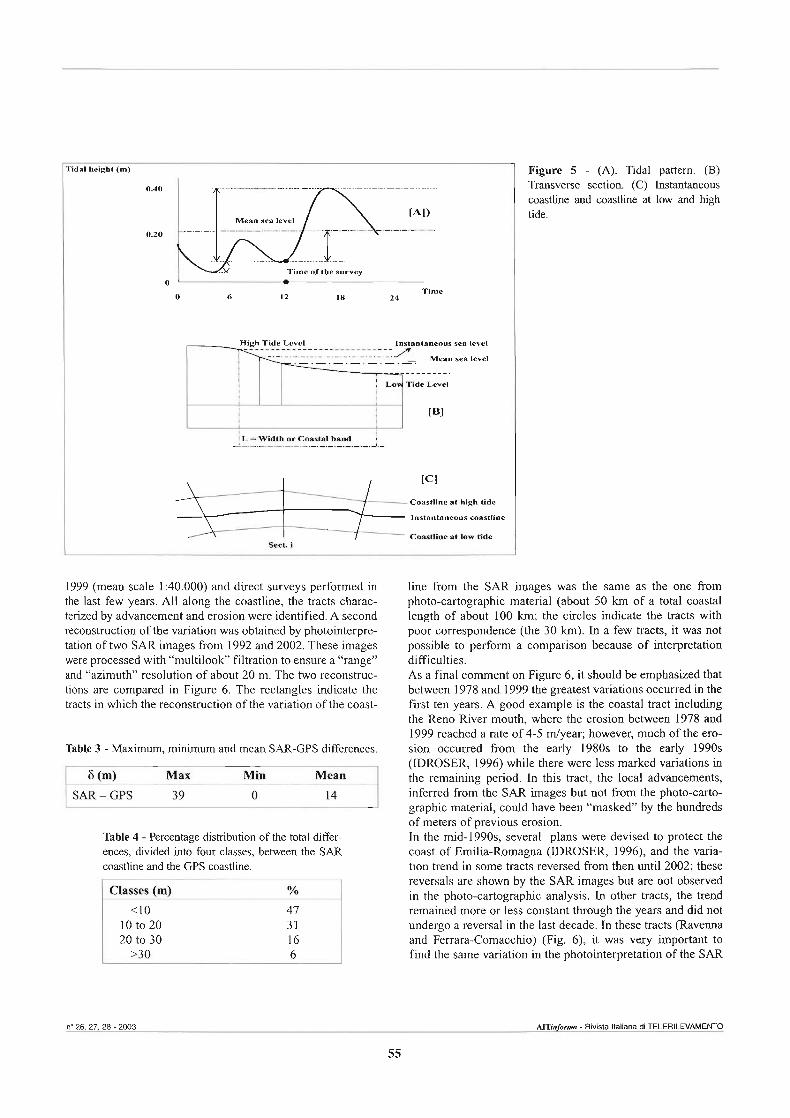
Figure 5 - (A). Tidal pattern. (B) Transverse section. (C) Instantaneous coastline and coastlllie at low and high tide.

'ildal height (m)

1999 (mean scale 1:40.000) and direct surveys performed in the last few years. AU along the coastline, the tracts characterized by advancement and erosion were identified. A second reconstruction of the variation was obtained by photointerpretation of two SAR images ftom 1992 and 2002. These images were processed with "multilook" filtration to ensure a "range" and "azimuth" resolution of about 20 m. The two reconstruc- tions are compared in Figure 6. The rectangles indicate the tracts in which the reconstruction of the variation of the coast-

OAO

Table 3 - Maxirnum, minimum and mean SAR-GPS differences.

, .-

I 6(m) Max Min Mean I

l,,.$-,

Mean sea level 1-41]

030

... , . ime of tbe survey

O

O 6 12 18 24 Time

Instantnneous sea level

- - - - - - - - .

I I IBI

i L = Width or Coastal band i

~ ~ w - . a, high iide

Instnntnneous masiiine

Coastline at low tide SeCL i

( SAR - GPS 39

Table 4 - Percentage distribution of the total differences, divided into four classes, between the SAR coastline and the GPS coastline.

line from the SAR images was the same as the one fiom photo-cartographic materia1 (about 50 km of a total coastal l e n a of about 100 km; the circles indicate the tracts with poor correspondence (the 30 h ) . In a f m tracts, it was not possible to perform a comparison because of interpretation difficulties. As a final cornrnent on Figure 6, it should be emphasized that between 1978 and 1999 the greatest variations occurred in the first ten years. A good exarnple is the coastal tract including the Reno River mouth, where the erosion between 1978 and 1999 reached a rate of 4-5 mlyear; however, much of the erosion occurred from the early 1980s to the early 1990s (IDROSER, 1996) while there were less marked variations in the remaining period. in this tract, the local advancements, inferred from the SAR images but not from the photo-cartographic material, could have been "masked by the hundreds of meters of previous erosion. In the mid-1990s, severa1 plans were devised to protect the coast of Ernilia-Romagna (IDROSER, 1996), and the variation trend in some tracts reversed fiom then unti1 2002; these reversals are shown by the SAR images but are not observed in the photo-cartographic analysis. In other tracts, the trend remained more or less constant through the years and did not undergo a reversal in the last decade. In these tracts (Ravenna and Ferrara-Comacchio) (Fig. 6), it was very important to fiid the same variation in the photointerpretation of the SAR

n' 26.27.28 - 2003 AITinfom - R i Italiana di TELERILEVAMENTO

55

Table 5 - Comparison of coastline advancement (speed and magnitude) at Ravenna and Ferrara-Comacchio obtained from photo- cartographic materia1 and from SAR images.

Anaiysis PhobGwbgmphic 1992-2002 SAR 1992-2002 Photo-cartographic 1992-2002 SAR 1992-2002

2-3 dyear 4 mlyear 4.5 dyear 5 dyear 20-30111

images as in the photo-cartographic analysis. in fact, the two types of analysis show approximately the same speed and magnitude of coastline advancement in the period 1992-2002 (Tab. 5).

Conclusions The results of the preliminary tests confirm that the horizontal accuracy of the SAR intensity images is about 20 m. This value is close to the mean tidal excursion of the Emilia- Romagna coast. The results of the comparison show that in many coastal tracts, especially those in advancement, the speeds of movement inferred from the maps and aerial pho- togramrnetry are comparable to those obtained from photointerpretation of the two SAR images. Within the limits of intrinsic precision of SAR intensity images (about 20 m) and where the sea level excursions involve horizontal coastline variations of the same value, the use of SAR in the study of coastline displacements is possible oniy to evaluate the displacement trend over a long time period (at least 10 years). in the case of variations in a shorter time period, direct surveyhg with correction of the sea level excursions due to the tide and atmospheric pressure seerns to be the only technique able to quanti@ submetnc displacements.

References

Bijaoui J., Cauneau F. (1989); - Sepamtion of sea and land in SAR images using texture classification - IEEE Trans Syst, 5: 522-526.

Crocetto N., Gatti M. and Russo P. (1998); - L'impiego del GPS nello studio della moi.fodinamica dei litorali - Atti della 2" Conferenza Nazionale delle Associazioni Scientifiche per le Informazioni Territoriali e Ambientali vol. 1, Bolzano, 24- 27 nov. 1998,535-540.

Deiia Rocca M.R. and Fortunato A. (2002); - Individuazione della linea di costa da immagine SAR mediante trasformata localizzata di mdon - Atti della 6" Conferenza Nazionale delle

CONFRONTO D E i A M O R W D I N AMICA (1NF.FOTOCART.- SAR)

I I

Figure 6 - Comparison of the variations found with the SAR images and with the photo-cartographic matenal.

Future studies will involve the refinement of SAR photointerpretation techniques using new filters to reduce the speckle or to identify the dry contour (Della Rocca and Fortunato, 2002).

Associazioni Scientifiche per le Informazioni Territoriali e Ambientali vol. 2, Perugia, 5-8 nar 2002, 101 1-1016.

Henderson Fioyd M. and Lewis J.A. (1998); - Manual of Remote Sensing, Principles and Applications of Zmaging Radar - Third Edition, vol. 2, John Wiley & Sons, inc.

IDROSER (1996) - Progetto di Piano per la dijèsa dal mare e la Riqualzjìcazione Ambientale del litorale della regione Emilia Romagna - Bologna, 1996.

An application of Artificial Neural Networks for the retrieval of soil moisture profiles by using microwave radiometers

Sionetta Paloscia, Giovanni Maceiioni, Emanuele Santi and Marco Tedesco (l)

Abstract In this paper the capability of multi-frequency microwave radiometers in retrieving soil moisture profiles was hvestigated by using both experimental data collected by IROE microwave radiometers and an electromagnetic model (IEM). The experimental data and the IEM results were used to train an Artificial Neural Network in order to invert the emissivity data and reproduce the soil moisture profiles

Riassunto La ricerca descritta in questo articolo indica come sia possibile ricavare il profilo di umidità del terreno attraverso un sistema di radiometri a microonde multi-frequenza. In questo caso si sono utilizzati i dati sperimentali, raccolti con i sensori a microonde IROE, e i risultati teorici, ottenuti per mezzo di un modello elettromagnetico per la descrizione dell'emissione da una superficie (IEM)), per allenare una Rete Neumle opportunamente conjìgurata.

Introduction The knowledge of the soil moisture content at various scales is important in several fields of applications as hydrology, meteorology, and climatology. However, the knowledge of the vertical profile of moisture is even more significant, shce the distribution of water in soil is highly dependent on the soil properties, climatic conditions, and vegetation cover situation. The trend of the soil moisture profile is therefore an indicator of the soil saturation and of its capability in absorbing further water, which. can be used in hydrological modeling for estimating the repartition of water in runoff, infiltration and evaporation or Evapotranspiration. This information is useful especially for flooding forecast and hydrological management. The sensitivity to soil moisture of microwave radiometers at low frequencies is well known and already studied in many research wks. However, the soil depth interested by the emission mainly depends on frequency and, whereas L-band is sensitive to the moisture of a relatively thick soil layer, higher frequencies are only sensitive to the moisture of soil layers closer to the surface [Shutko, 1982; Wang, 19871. This remark leads to the hypothesis that multi-frequency observations could be able to retrieve the soil moisture profile. In several experiments carried out both on agricultural fields and on samples of soil in a controlled environment, by using the IROE (Instrument of Radio-Observation of the Earth) multi-frequency microwave radiometers, the effect of moisture and surface roughness on

(l) CNR-IFAC, via Panciatichi 64 - 50127 Firenze, Italia. email: [email protected]

Received 14/10/2002 - Accepted 17/0U2003

different frequencies was studied paloscia et al. 19921. From these experiments, the capability of L-band (1.4 GHz) in measuring the moisture of a soil layer of several centimeters was confied, as well as the sensitivity to the moisture of the first centimeter layer at C- (6.4 GHz) and X- (10 GHz) bands, and the one of the very f i i t layer of smooth soil at Ka-band (37 GHz). In this study, by using an electromagnetic model (Integra1 Equation Model, EM) b g , 19941 the emissivities at 1.4,10, and 37 GHz were computed as a function of the incidence angle for different values of soil moisture and surface roughness and compared with measured values of microwave emission. Afkr this preliminary test, the data set generated by the IEM was used to train a neural network in order to reproduce the soil moisture at different depths.

Experimental results and comparison with the IEM model The IROE (Instrument of Radio-Observation of the Earth) sensor package, purposely designed for land studies, includes sev- era1 microwave radiometers at L (1.4 GHz, V or H polarisation), C (6.8 GHz, V and H pol.), X (1 0 GHz, V and H pol.), Ku (19 GHz, V, H and I45" pol) and Ka (37 GHz, V, H and I45" pol.) bands, and a thermal inflared sensor [Paloscia et al. 1992, Macelloni et al. 20001. Radiometric measurements of bare and vegetated soils were carried out in past years, by using the IROE sensors operating both from ground based platform and aircraft. In this paper the results obtained from accurate measurements of emission, at different incidence angles, from a soil sample (sand and sand + clay) placed in a tank of 120x120~70 cm3 are shown (Fig. 1). This approach gave the possibility of controlling some geophysical parameters and guaranteed greater precision.

n' 26,27.28 - 2003 -017~ - Rivisia Itaiiana di TELERILEVAMENTO

57

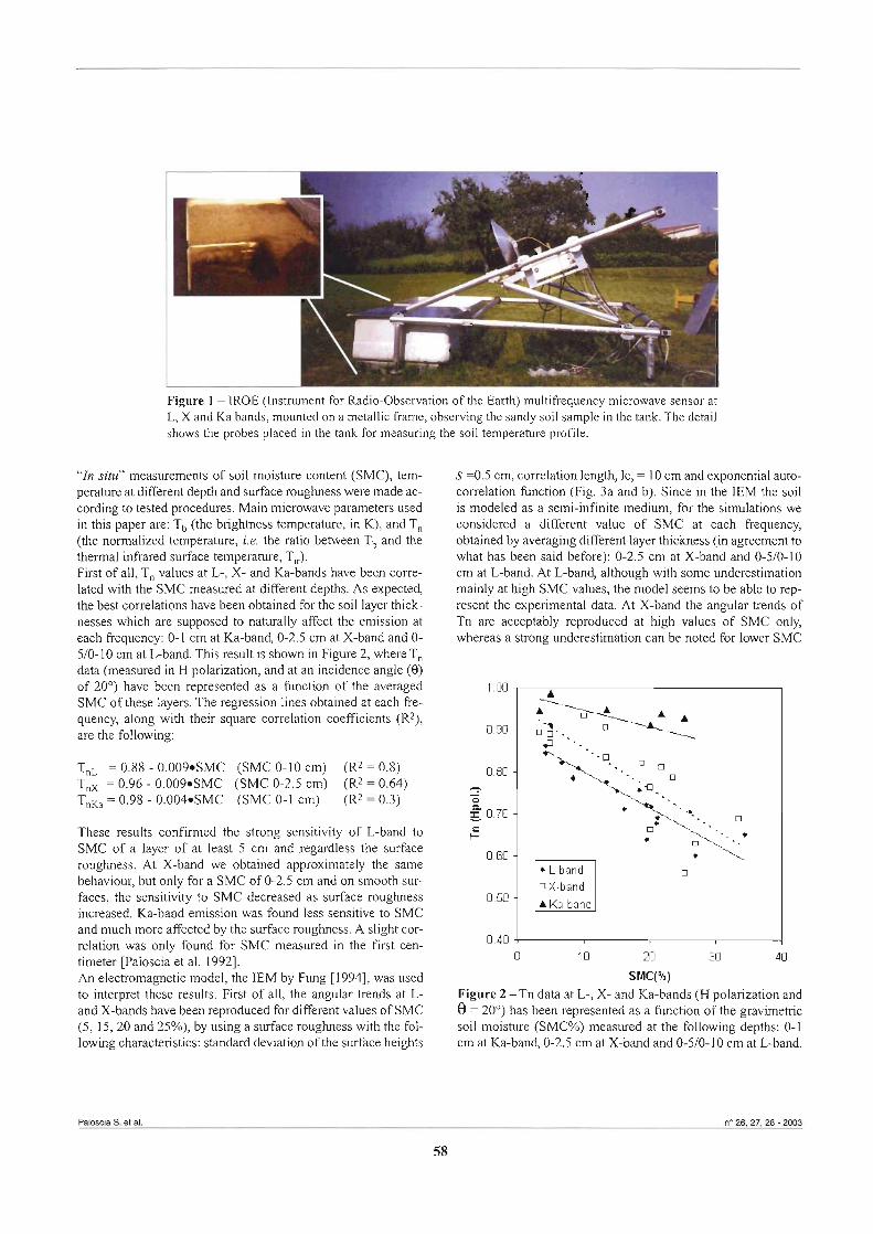
Figure 1 - IROE (Instrument for Radio-Observation of the Earth) multifrequency microwave sensor at L, X and Ka bands, mounted on a metallic fiame, obsewing the sandy soil sample in the tank. The detail shows the probes placed in the tank for measuring the soil temperature profile.

"In situ" measurements of soil moisture content (SMC), temperature at different depth and surface roughness were made according to tested procedures. Main rnicrowave parameters used in this paper are: Tb (the brightness temperature, in K), and T, (the normalized temperature, i.e. the ratio between Tb and the thermal inhred surface temperature, T"). First of ali, T,, d u e s at L-, X- and Ka-bands have been correlated with the SMC measured at different depths. As expected, the best correlations have been obtained for the soil layer thick- nesses which are supposed to naturally affect the emission at each frequency: 0-1 cm at Ka-band, 0-2.5 cm at X-band and 0- 510-10 cm at L-band. This result is shown in Figure 2, where T,, data (measured in H polarkation, and at an incidente angle (9) of 20") have been represented as a function of the averaged SMC of these layers. The regression lines obtained at each frequency, along with their square correlation coefficients @2), are the foiiowing:

T, = 0.88 - 0.009.SMC (SMC 0-10 cm) (R2 = 0.8) Tiix = 0.96 - 0.009.SMC (SMC 0-2.5 cm) (R2 = 0.64) T& = 0.98 - 0.004.SMC (SMC 0-1 cm) (R2 = 0.3)

These results confimed the strong sensitivity of L-band to SMC of a layer of at least 5 cm and regardless the surface roughness. At X-band we obtained approximately the same behaviour, but only for a SMC of 0-2.5 cm and on smooth surfaces, the sensitivity to SMC decreased as surface roughness increased. Ka-band emission was found less sensitive to SMC and much more aEected by the surface roughness. A slight correlation was only found for SMC measured in the f i t centimeter [Paloscia et al. 19921. An electromagnetic model, the IEM by Fung [1994], was used to interpret these results. First of all, the angular trends at L- and X-bands have been reproduced for different values of SMC (5, 15,20 and 25%), by using a surface roughness with the following chmcteristics: standard deviation of the surface heights

S =0.5 cm, correlation length, lc, = 10 cm and exponential autocorrelation function (Fig. 3a and b). Since in the IEM the soil is modeled as a semi-infinite medium, for the simulations we considered a different value of SMC at each frequency, obtained by averaging different layer thickness (in agreement to what has been said before): 0-2.5 cm at X-band and 0-510-10 cm at Lband. At L-band, although with some underestimation mainly at high SMC vaiues, the model seems to be able to represent the experimental data. At X-band the angular trends of Tn are acceptably reproduced at high values of SMC only, whereas a strong underestimation can be noted for lower SMC

0.40 1 q

O 10 20 30 40

SMC(%) Figure 2 - Tn data at L-, X- and Ka-bands (H polarization and e = 20") has been represented as a function of the gravimetric soil moisture (SMCOh) measured at the following depths: 0-1 cm at Ka-band, 0-2.5 cm at X-band and 0-510-10 cm at Lband.

Paioscia S. et al. no 26,27,28 - 2003

58

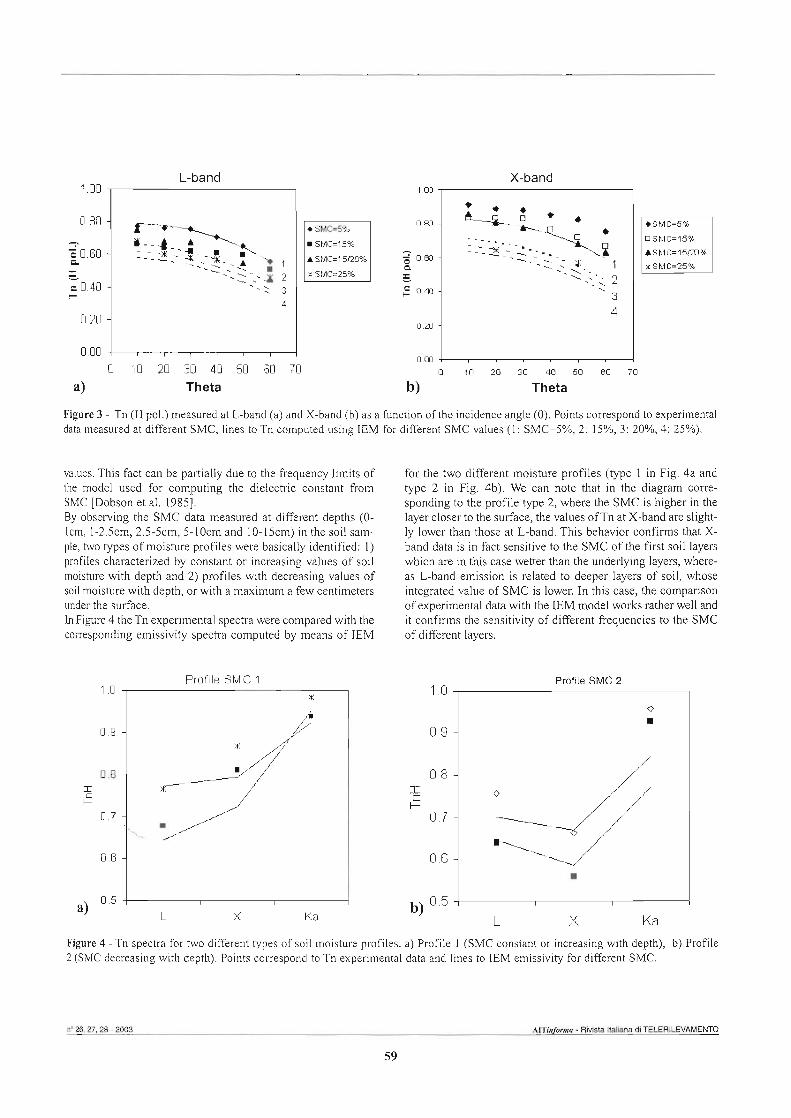
0.00 O 10 20 30 40 50 60 70

a) Theta

o .m O 10 20 30 40 50 BO 70

b) Theta

Figure 3 - Tn (H pol.) measured at L-band (a) and X-band (b) as a function of the incidence angle (9). Points correspond to experimental data measured at different SMC, lines to Tn computed using IEM for different SMC values (1: SMC=5%, 2: 15%, 3: 20%, 4: 25%).

values. This fact can be partially due to the fkquency limits of the model used for computing the dielectnc constant from SMC [Dobson et al. 19851. By observing the SMC data measured at different depths (0- lcm, 1-2.5cm, 2.5-Scm, 5-10cm and 10-15cm) in the soil sample, two types of moisture profiles were basically identified: 1) profiles characterized by constant or increasing values of soil moisture with depth and 2) profiles with decreasing values of soil moisture with depth, or with a maximurn a few centirneters under the surface. In Figure 4 the Tn experimental spectra were compared with the corresponding emissivity spectra computed by means of IEM

for the two different moisture profiles (type 1 in Fig. 4a and type 2 in Fig. 4b). We can note that in the diagram corresponding to the profile type 2, where the SMC is higher in the layer closer to the surface, the values ofTn at X-band are slightly lower than those at L-band. This behavior confirms that X- band data is in fact sensitive to the SMC of the first soil layers which are in this case wetter than the underlying layers, whereas L-band emission is related to deeper layers of soil, whose integrated value of SMC is lower. in this case, the comparison of experimental data with the LEM model works rather well and it confirms the sensitivity of different frequencies to the SMC of different layers.

Profile SMC 1 Profile SMC 2 1 .o

0.9 -

0.8 -

0 >7.;

0.6 -

0.5

Figure 4 - Tn spectra for two different types of soil moisture profiles. a) Profile 1 (SMC constant or increasing with depth), b) Profile 2 (SMC decreasing with depth). Points correspond to Tn experimental data and lines to IEM emissivity for different SMC.

m

'L.

1 I

n' 26,27,28 - 2003 AITinfia - R ' i t a Itallana W NERILEVAMENTO

59

L X Ka

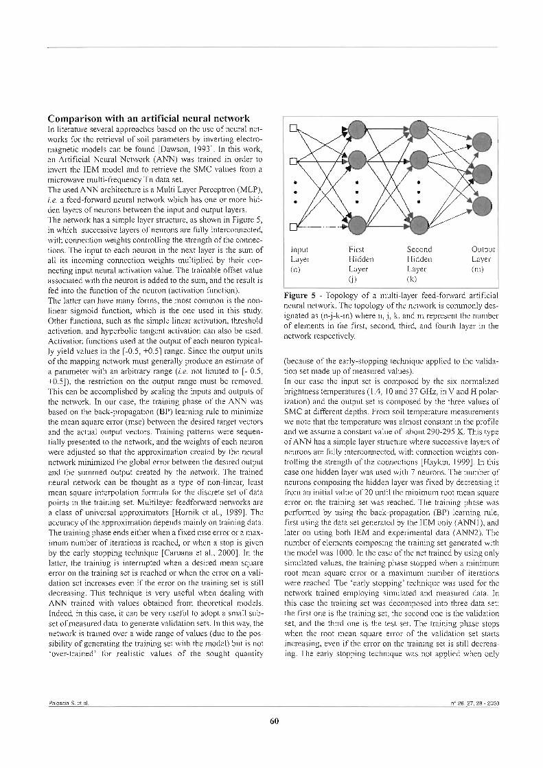
Comparison with an artificial neural network In literature severa1 approaches based on the use of neural networks for the retrieval of soil pararneters by inverting electromagnetic models can be found [Dawson, 19931. In this work, an Artificial Neural Network (ANN) was trained in order to invert the IEM model and to retrieve the SMC values from a microwave multi-frequency Tn data set. The used ANN architecture is a Multi Layer Perceptron (MLP), i.e. a feed-forward neural network which has one or more hidden layers of neurons between the input and output layers. The network has a simple layer smcture, as shown in Figure 5, in which successive layers of neurons are fully intercomected, with connection weights controlling the strength of the connections. The input to each neuron in the next layer is the sum of al1 its incoming comection weights multiplied by their connecting input neural activation value. The trainable offset value associated with the neuron is added to the sum, and the result is feci into the function of the neuron (activation function). The latter can have rnany forms, the most common is the non- linear sigmoid function, which is the one used in this study. Other functions, such as the simple linear activation, threshold activation, and hyperbolic tangent activation can also be used. Activation functions used at the output of each neuron typically yield values in the [-0.5, +0.5] range. Since the output units of the mapping network must generally produce an estimate of a parameter with an arbitrary range (i.e. not limited to [- 0.5, +0.5]), the restriction on the output range must be removed. This can be accomplished by scaling the inputs and outputs of the network. In our case, the training phase of the ANN was based on the back-propagation (BP) learning rule to minimize the mean square error (mse) between the desired target vectors and the actual output vectors. Training patterns were sequentially presented to the network, and the weights of each neuron were adjusted so that the approximation created by the neural network minimized the globai error between the desired output and the summed output created by the network. The trained neural network can be thought as a type of non-linear, least mean square interpolation formula for the discrete set of data points in the training set. Multilayer feedfonvard networks are a class of universal approximators [Hornik et al., 19891. The accuracy of the approxirnation depends mainly on training data. The training phase ends either when a fixed mse error or a maximum number of iterations is reached, or when a stop is given by the early stopping technique [Caruana et al., 20001. In the latter, the training is interrupted when a desired mean square error on the training set is reached or when the error on a validation set increases even if the error on the training set is still decreasing. This technique is very useful when dealing with ANN trained with vaiues obtained from theoretical models. Indeed, in this case, it can be very useful to adopt a small sub- set of measured data to generate validation sets. In this way, the network is trained over a wide range of values (due to the possibility of generating the training set with the model) but is not 'over-trained' for realistic values of the sought quantity

Figure 5 - Topology of a multi-layer feed-forward artificial neural network. The topology of the network is commonly des- ignated as (n-j-k-m) where n, j, k, and m represent the number of elements in the first, second, third, and fourth layer in the network respectively.

(because of the early-stopping technique applied to the validation set made up of measured values). In our case the input set is composed by the six normalized brightness temperatures (1.4, 10 and 37 GHz, in V and H polarization) and the output set is composed by the three values of SMC at different depths. From soil temperature measurements we note that the temperature was almost constant in the profile and we assume a constant value of about 290-295 K. This type of ANN has a simple layer smcture where successive layers of neurons are fully interconnected, with comection weights controlling the strength of the connections [Haykin, 19991. In this case one hidden layer was used with 7 neurons. The number of neurons cornposing the hidden layer was fixed by decreasing it from an initial value of 20 unti1 the minimum root mean square error on the training set was reached. The training phase was performed by using the back-propagation (BP) learning rule, first using the data set generated by the IEM only (ANNI), and later on using both IEM and experirnental data (ANN2). The number of elernents composing the training set generated with the model was 1000. In the case of the net trained by using only simulated values, the training phase stopped when a minimum root mean square error or a maximum number of iterations were reached. The 'early stopping' technique was used for the network trained employing simulated and measured data. In this case the training set was decomposed into three data set: the first one is the training set, the second one is the validation set, and the third one is the test set. The training phase stops when the root mean square error of the validation set starts increasing, even if the error on the training set is still decreasing. The early stopping technique was not applied when only

Faioscia S. et al. n" 26,27.28 - 2003

60

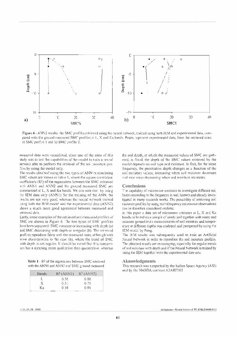
Figure 6 - ANN2 results: the SMC profiles retrieved using the neural network, trained using both IEM and experimental data, compared with the ground measured SMC profiles at L, X and Ka bands. Points represent experimental data, lines the retrieved ones. a) SMC profile 1 and b) SMC profile 2.

measured data were considered, since one of the aims of this study was to test the capabilities of the model to train a neural network able to perform the retrieval of the soil moisture profiles by using the model only. The results obtained using the two types of AM\1 in simulating SMC values are shown in Table 1, where the square correlation coeficients (R2) of the regressions between the SMC retrieved with ANNI and ANN2 and the ground measured SMC are summarized at L, X and Ka bands. We can note that by using the IEM data only (ANNI) for the training of the ANN, the results are not very good, whereas the neural network trained using both the IEM model and the experimental data (ANN2) shows a much more good agreement between measured and retrieved data. Lastly, some exarnples of the retrieved and measured profiles of SMC are shown in Figure 6. The two types of SMC profiles havebeen separate& SMC constant or increasing with depth (a) and SMC decreasing with depth or irregular (b). The retrieved profiles reproduce fairly well the measured ones, although with some discrepancies in the case (b), where the trend of SMC with depth is not regular. It should be noted that this comparison has a meaning more qualitative than quantitative: whereas

Table 1 - R2 of the regressions between SMC retrieved with the ANNI and AIW2 and SMC ground measured.

the soil depth, at which the measured values of SMC are gathered, is fiied, the depth of the SMC values retrieved by the model depends on soil type and moisture. In fact, for the sarne frequency, the penetration depth changes as a function of the soil moisture values, increasing when soil moisture decreases and vice versa decreasing when soil moisture increases.

Conclusions The capability of rnicrowave emission to investigate different soil layers according to the fkquency is weli known and already investigated in many research works. The possibility of retrieving soil moisture profiles by using mult&quency m i m v e o b s e d o n s can be therefore considered realistic. In this paper a data set of microwave emission at L, X and Ka bands collected on a sample of sandy soil together with many and accurate ground huth measurements of soil moisture and temperature at different depihs was adyzed and interpreted by using the IEM model by Fung. The IEM results was subsequently used to train an Amficial Neural Network in order to reproduce the soil moisture profdes. The obtained results are encouraging, especially for regular trends of soil moisture with depth and ifthe Neural Network is trained by using the IEM together with the experimental data sets.

Aknowledgments This research was supported by the Italian Space Agency (ASI) and by the NASDA contract A2ARF003.

n" 26.27,28 - 2 ~ ) 3 AlTlnfooraa - Rivista Italiana di TELERILEVAMENTO

6 1

References

Caruana R., Lawrence S. and Giles L. (2000) - Ovefitting in Neural Nets: backpropagation, conjugate gmdient, and early stopping. Todd K. Leen, Thomas G. Dietterich, Volker Tresp (Eds.): Advances in Neural Information Processing Systems 13, Papers from Neural Information Processing Systems (NIPS) 2000, Denver, CO, USA. MIT Press 2001.

Dawson M.S. (1993) - Surjàcepanmeter retrieval using fmt learning naaal netwoh. Remote Sensing Reviews, 7: 1-1 8.

Dobson C., Ulaby F., Hallikainen M. and El-Rayes M. (1985) - Microwave Dielectric behaviour of wet soil - Part 11: Four component dielectric mixing models. IEEE Trans. Geosci. Remote Sensing, 23 (4): 35-46.

Fung A.K. (1994) - Microwave scattering and emission models and their applications. Artech House, Norwood, MA.

Haykin S. (1999) - Neural Networks, A comprehensive foun- dation. I1 Edition, Prentice Hall, New Jersey.

Homik K., Stincombe M. and White H. (1989) - Multilayer feedforward networh are universal approximators. Neural Networks, 11: 359-366.

Macelloni G., Paloscia S., Pampaloni P., Ruisi R., Susini C. and Wigneron J.P. (2000) - Airbome passive microwave measurements on agricultural Jields. Microwave radiometry and remote sensing of the Earthh surface and atmosphere. P. Pampaloni and S. Paloscia Eds., VSP Press, Utrecht, The Netherlands, pp. 59-70.

Paloscia S., Pampaloni P., Chiarantini L., Coppo P., Gagliani S. and Luzi G. (1992) - Multzj?equency passive microwave remote sensing of soil moisture and roughness. Int. J. Remote Sensing, 14 (3): 467-483.

Shutko A. (1982) - Microwave radiometry of lands under natural and artijìcial moistening. IEEE Trans. Geosci. Remote Sensing, GE-20, 1, 18.

Wang J.R. (1987) - Microwave emission Ji.om smooth bare fields and soil moisture sampling depth. IEEE Trans. Geosci. Remote Sensing, GE-25,5: 616-622.

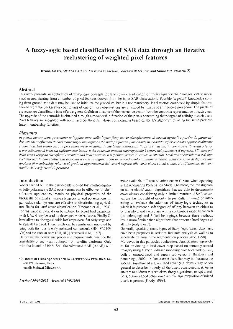
A fuzzy-logic based classification of SAR data through an iterative reclustering of weighted pixel features

Bruno Aiazzi, Stefano Baronti, Massimo Bianchini, Giovanni Macelloni and Simonetta Paloscia (1)

Abstract This work presents an application of fuzzy-logic concepts for land cover classification of multifrequency SAR images, either supervised or not, starting from a number of pixel features derived from the input SAR observations. Possible "a prion"' knowledge coming from ground truth data may be used to initialize the procedure, but it is not mandatory. Pixel vectors composed by simple features derived from the backscatter coefficients of one or more observations are clustered by means of an iterative procedure. The pixels of the scene are classified in base of a weighted Euclidean distance of the respective vector from the centroids representative of each class. The upgrade of the centroids is obtained through a membership function of the pixels concerning their degree of affinity to each class. Pixel features are weighted with optimized coeficients, whose computing is based on the LS algorithm by using the same previous fuzzy membership function.

Riassunto In questo lavoro viene presentata un 'applicazione della logica@zy per la classificazione di terreni agricoli a partire da pammetn derivati dai coejìcienti di bachcatiering di immagini SAR a multifrequenza, jùnzionante in modalità supervisionata oppure totalmente automatica. Nel primo caso la procedura viene inizializzata mediante conoscenza "a priori'" acquisita con misure di verità a terra. Il procedimento si basa sul mjìnamento itemtivo dei centroidi ottenuti raggruppando i vettori dei pammeni d'ingresso. Gli elementi della scena vengono classificati considemndo la distanza tra il rispettivo vettore e i centroidi ottenuti. La distanza considemta è di tipo euclideo pesata con coeflcienti associati a ciascun ingresso con un procedimento a minimi quadmti. Essa consente di definire una finzione di membership relativa al gmdo di appartenenza dei vettori rispetto alle varie classi su cui si basa il rajìnamento dei centroidi e dei coejìcienti di pesatum.

Introduction Works carried out in the past decade showed that multi-frequency fully polarirnetric SAR observations can be effective for classification applications, thanks to physical properties of the backscattered signal at various frequencies and polarizations. In particular, radar systems are effective in discrimjnating agriculture fields for land cover classification Freeman et al., 19941. For this purpose, P-band can be suitable for broad land cakgories, whiie Gband may be used for developed wide leafcrops. Finally, C- band dows to disijngush wide leaf crops even if at early stage and t0 sepamte bare soil. These d t s can be ~ i ~ c a n t i y improved by using both the four hearly polarized components (IM, V\! W VH) and the ckuiar ones (RR, RL) -li et al., 19971. Unfortunately, power and processing requirements preclude the availability of such data routinely ffom satellite p l a t f m . Only with the launch of ENVISAT the Advanced SAR (ASAR) will

(l) Istituto di Fisica Applicata ''Nello Carrara7',Via Panciatichi 64- - 50U7 Firenze, Italia. email: [email protected]


rnake available different polarizations in C-band when operating in the Altemating Polarization Mode. Therefore, the investigation on some classification algorithms that are able to discriminate cover classes considering only a limited number of SAR observations has the right of priori@ In particular, it would be interesting to evaluate the adoption of fuzzy-logic techniques in which it is present a sofi degree of affmity between an object to be classified and each class with a continuous range between O (no belonging) and 1 (M1 belonging), because these methods result more flexible than algorithms that present a hard degree of aff i ty (only O or I). Generally speaking, many types of fuzzy-logic based classifiers have been proposed in order to facilitate analysis as well as t0 accelerate training in the segmentation process [Abe, 19981. Moreover, in this particular application, classification approaches for producing a land cover map based on remotely sensed irnagery using fuzzy mie-based modeling have been widely used, both in unsupervised and supervised versions [Bardossy and Samaniego, 20021. In fact, a hard classifier may fai1 because the spectral signature of a given land cover (e.g. forest) may be too genera1 to describe properly al1 the pixels considered in it. As an attempt to address this criticism, fuzzy algorithms, or so3 classifiers, obtain a good behaviour even if a large proportion of mixed pixels is present [Foody, 19991.

n" 26,27,28 - 2003 AITlnfoma - Rivista ItaJiana di TELERILEVAMENTO

63

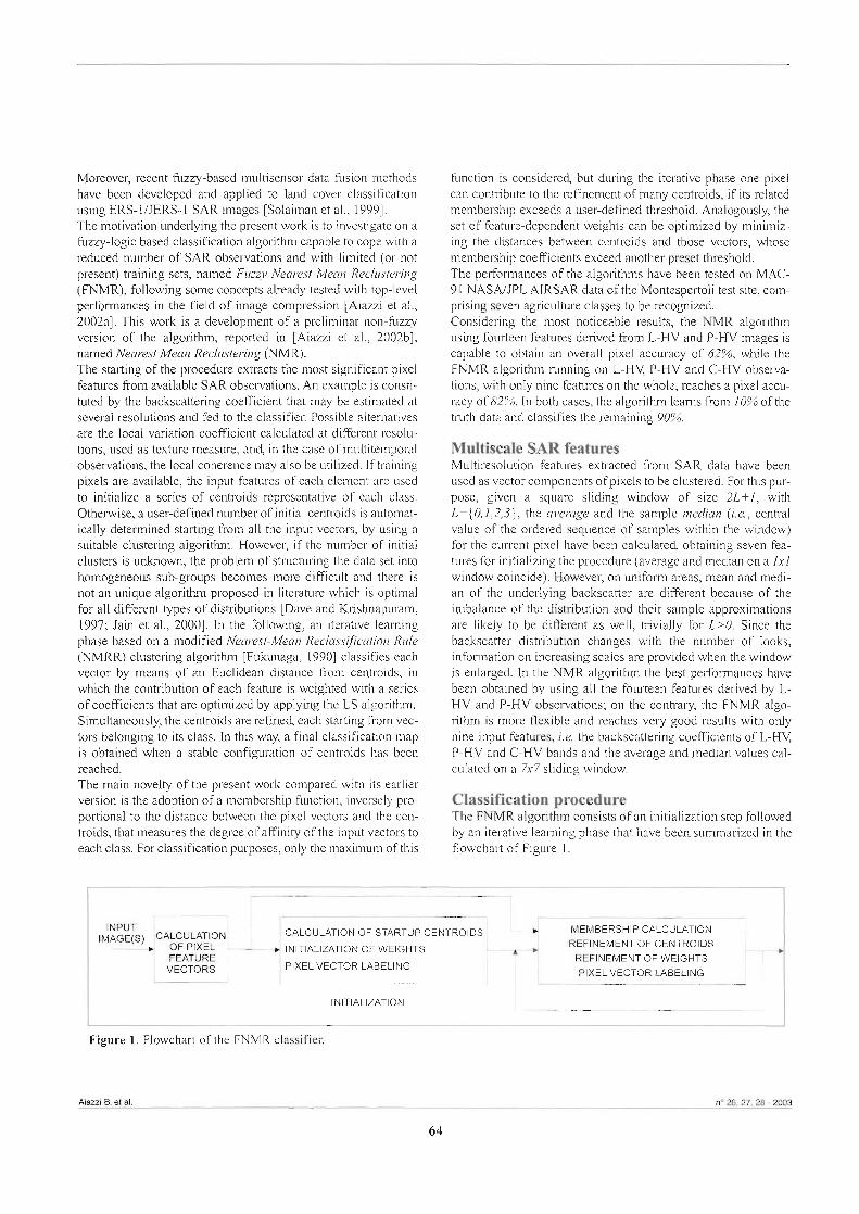
Moreover, recent fuzzy-based multisensor data fusion methods have been developed and applied to land cover classification using ERS-I JJERS- 1 SAR images [Solaiman et al., 19991. The motivation underlying the present work is to investigate on a fuzzy-logic based classification algorithm capable to cope with a reduced number of SAR observations and with lirnited (or not present) training sets, named Fuz~y Nearest Mean Reclustering (m), following some concepts already tested with top-leve1 performances in the field of irnage compression [Aiazzi et al., 2002al. This work is a development of a preliminar non-- version of the algorithm, reported in [Aiazzi et al., 2002b1, narned Nearest Mean Reclustering m). The starting of the procedure extracts the most significant pixel features from available SAR observations. An example is constituted by the backscattering coefficient that may be estimated at severa1 resolutions and fed to the classifier. Possible alternatives are the local variation coeficient calculated at different resolutions, used as texture measure, a d , in the case of multitemporal observations, the local coherence may also be utilized. If training pixels are available, the input features of each element are used to initialize a series of centroids representative of each class. Othenvise, a userdefined number of initial centroids is automat- ically determined starting from al1 the input vectors, by using a suitable c l u s t e ~ g algorithrn. However, if the number of initial clusters is unknown, the problem of structuring the data set into homogeneous sub-groups becomes more difficult and there is not an unique algorithrn proposed in literature which is optimal for al1 different types of distributions [Dave and Krishnapuram, 1997; Jain et al., 20001. In the following, an iterative learning phase based on a modified Nearest-Mean Reclassijìcation Rule (NMRR) clustering algorithm [Fukunaga, 19901 classifies each vector by means of an Euclidean distance fiom centroids, in which the contribution of each feature is weighted with a series of coeficients that are optimized by applying the LS algonthm. Simultaneously, the centroids are refined, each starting fiom vectors belonging to its class. In this way, a final classification map is obtained when a stable configuration of centroids has been reached. The main novelty of the present work compared with its earlier version is the adoption of a membership function, inversely proportional to the distance between the pixel vectors and the centroids, that measures the degree of a f f i t y of the input vectors to each class. For classification purposes, only the maximum of this

function is considereci, but during the iterative phase one pixel can contribute to the refinement of many centroids, if its related membership exceeds a user-defined threshold. Analogousiy, the set of feature-dependent weights can be optimized by rninimiz- ing the distances between centroids and those vectors, whose membership coefficients exceed another preset threshold. The performances of the algorithms have been tested on MAC- 9 1 NASNJPL AIRSAR data of the Montespertoli test site, comprising seven agriculture classes to be recognized. Considering the most noticeable results, the NMR algorithm using fourteen features derived from L-HV and P-HV images is capable to obtain an overall pixel accuracy of 62%, while the FNMR algorithm running on GHV, P-HV and C-HV observations, with only nine features on the whole, reaches a pixel accuracy of 82%. In both cases, the algorithm learns from IO% of the bxth data and classifies the remaining 90%.

Multiscale SAR features Multiresolution features extracted fiom SAR data have been used as vector components of pixels to be clustered. For this purpose, given a square sliding window of size 2L+I, with L={0.1,2,3), the avemge and the sample median (i.e., centra1 value of the ordered sequence of samples withii the window) for the current pixel have been calculated, obtaining seven features for initializing the procedure (average and median on a 1x1 window coincide). However, on uniform areas, mean and median of the underlying backscatter are different because of the imbalance of the distribution and their sample approximations are likely to be different as well, trivially for L>O. Since the backscatter distribution changes with the number of looks, information on increasing scales are provided when the window is enlarged. In the NMR algorithm the best performances have been obtained by using al1 the fourteen features derived by L- HV and P-HV observations; on the contrary, the FNMR algorithm is more flexible and reaches very good results with only nine input features, i.e. the backscattering coefficients of L-HV, P-HV and C-HV bands and the average and median values calculated on a 7x7 sliding window.

Classification procedure The FNMR algorithm consists of an initialization step followed by an iterative learning phase that have been sumrnarized in the flowchart of Figure 1.

I

INITIALIZATION OF WEIGHTS REFINEMENT OF CENTROIDS FEATURE

PIXEL VECTOR LABELING REFINEMENT OF WEIGHTS

VECTORS PIXEL VECTOR LABELING -

INITIALIZATION

Figure 1. Flowchart of the FNMR classifier.

ALani B. et al. n" 26,27,28 - 2003

64

The operations performed by single blocks can be explained by the following steps: - Step O (Initialization): M stamip centroids, {c(m), m = I, ...,M), are calculated from the K-dimensional pixel vectors, {x(n), n = I, ...,N), of the training set. The clustering procedure is based on a weighted Euclidean distance dZ,(n) between the nth pixel vector x(n) = {xk(n), k = I, ...,Q and the mth centroid c(m) = {ck(m), k = ],... ,a, defined as

d'.(n> = i%&+)-c , (m) l2 k=l

[l1

The procedure starts with al1 coefficients ak set to I/K. After the calcuiation of the startup centroids, the coefficients ak are computed by optirnizing the classification of the vectors belonging to training set through the minirnization of the distance [l] computed respect to the centroid of the same class. An initial classification can be obtained with the initial weights computing the average squared distance of the pixel from the initial centroids. - Step I (Memberhip Calculation): A membership function Um(n) providing the degree of a f f i ty between the pixel vector x(n) and the centroid c(m) is calculated as a function of the distance [l]

with p 0 and O<Um(n)ll. The dependence of U,(n) from dZm(n) is driven by the membership exponent y ruling the degree of fuzziness of the rnembership function. - Step 2 (Refnement of Centroids): The centroids {c(m), m = I,...,M) are refined by clustering a set of pixel vectors composed by three subsets: 1) training pixel (if available); 2) pixels that have been classified into the same class of the centroid at the previous iteration; 3) al1 the other pixels, provided their membership function exceeds an user-defined threshold pc The most noticeable novelty is that each pixel contributes to the refinement step depending on its membership function: the higher is the value of Um(n) [2] the more relevant is the contribution of the pixel vector x(n). A conventional Fuzq-C-Means (FCM) algorithm has been adopted in order to recalculate centroids at each iteration [Bezdek, 19811. - Step 3 (Refnement ofweights): The weights (ab k= I, ...,Q are recalculated by applying ihe Least Squam (LS) algorithm to [l] considering the new set of centroids. Pixels utilized in this step are: 1) training pixel (if available) belonging at the sarne class of the centroid; 2) pixels that have been labeled within the same class of the centroid in the previous iteration, as long as their mernbership function exceeds another user-defuled threshold p,,,. - Step 4 (Reclassification): Pixels are reclassified starting from the new sets of centroids and weights; the label of the centroid minimizing the distance [l] is assigned to pixel itself. In this way, pixels are moved from one class to another, thus reparti- tioning them into M new classes that are best matched by the current set of centroids. - Step 5: Check wnvergence; if found, stop; otherwise, go to Step I.

The convergence of this type of algorithms may be critical, due to resonance effects that cause the onset of oscillations having increasing amplitudes. In the present implementation, such oscillations are darnped by imposing that the modulus of the displacement of each centroid from the ith to (i+l)th iteration cannot exceed the minimum of those obtained in the previous iterations. This strategy was empirically validated on the ground tmth data: the percentage of correct classification monotonically converges to &e best attainable value, achieved when the rnagnitudes of al1 the displacement of the centroids are lower than a threshold value E.

Experimental results ~he-data set used in the experiments is constituted by a series of MAC-91 NASAIJPL AIRSAR data collected on June 22nd 1991 on the Montespertoli test site, located in Centra1 1%. In fact, the analysis of both remote sensing and ground truth data collected for many years, together with information concernuig climate, hydrologicai and geomorphologicai charactenstics, allowed to demonstrate the effectiveness of radar systems in discriminat- ing among classes of agricultural species paronti et al., 19951. A sarnple 512x300 area from the L-HV band is shown in Figure 2(a), with superimposed the map of polygons comprising those pixels whose ground truth is available. About IO% of the truth data is used for training, while the remaining 90% is used to assess the correct classification performance. The latter set of polygons is depicted in Figure 2(b), together with the percentage of each class compared with the total number of pixels of the test set. Seven agriculture classes are considered: forest, vheyard, wheat & alfalfa, sunfiower, bare soil, c o 4 and olive groves. Both FNMR and NMR algorithms were compared with a simple Box classifier considering the configuration that provides the best performances with the lowest number of input features. in particular, the FMMR and NMR methods have good performances even using only the HV polarization. On the contrary, the Box classifier uses multiple polarizations, but sliding windows have not been adopted in order to exploit spatial context [Ferrazzoli et al., 1997; Aiazzi et al., 2002bl. The respective configurations are the following:

- Box Classtjìer: three bands (C, L and P-band) with circular and linear polarizations for a total of nine inputs (C-RR, C-RL, C-W, L-RR, L-W, P-HH, P - W and P-HV); - NMR Classifier: two experiments, i.e. 1) Lband at HV polarization for a total of seven inputs (backscattering coefficient, average and median values on 3x3,5x5 and 7x7 sliding windows); 2) two bands (L. and P-band) at W polarization for a total of fourteen inputs (seven features for each band); - FNMR Classijìer: three bands (C, L and P-band) at HV polarization for a total of nine inputs (three features for each band: backscattering coefficient, average and median value on a 7x7 sliding window). The thresholds pc and U, have been found to be equa1 to 0.85 and 0.6 value, respectively.

no 28,27,28 - 2003 AITinfoorata - Rivista Italiana di TELERILEVAMENTO

65

Figure 2 - (a) 512x300 L-W band of Montespertoli with the rnap of polygons superimposed (10% used for training, 90% for classification); (b) ground truth of the seven classes (pixels used for classification), i.e. white: forest (16.8%), green: vineyard (22.4%), light blue: wheat & alfalfa (39.4%), dark gray: sunfiower (5.7%), brown: bare sd1(1.2%), purple: colza (1.8%), black olive groves (2.4%).

Figure 3 shows the classification maps achieved respectively by: (a) Box classifier; (b) NMR classifier in the experiment 1); (C) NMR classifier in the experiment 2); (d) FNMR classifier. Tables 1-4 report the relative confusion matrices. In these experiments, due to the extremely wide range in the population of the classes, the pararneters driving NMR and FNMR have been optimized in order to obtain the maximurn score relative to the comprehensive correct classification,

putting in background the partial scores of single classes. Following this approach, the NMR algorithm obtains percent- ages of correct classification of 54.8% in the configuration 1) and of 62.4% in the configuration 2), while the FNMR classifier reaches a percentage of 82.6%. Likewise, these parameters may be chosen with the aim to optimize the classification of the individua1 covers. Concerning the Box classifier, this attains 54.7% of correctly classified pixels; indicatively, the

/-""

Aiani B. et al. no 26, n, 28 - 2003

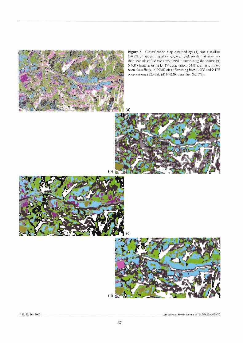
I ther been classified nor considered in computing the score); (b) NMR classifier using LHV observation (54.8%, al1 pixels have been classified); (C) NMR classifier using both L-HV and P-HV observations (62.4%); (d) F'NMR classifier (82.6%).

n' 26,27,28 - 2003 AFT~~ /oM - Rivkrta Italiana di TELERILEVAMENTO

67

Table 1 - Confusion matrix obtained by the Box classifier and eval- Table 2 - Confusion matrix obtained by the NMR classifier with uated on polygons of Figure 2. Notations: Y forest; V vineyard; a single L-HV observation, evaluated on polygons of Figure 2. MV: mixed vegetation (wheat & alfalfa); SF: sunflower; BS: bare soil; C: c o k , 0: olive groves.

Class Y V

MV SF BS C O

Table 3 - Confusion matrix obtained by the NMR classifier with Table 4 - Confusion matrix obtained by the FNMR classifier, both LHV and P-HV observations, evaluaied on polygons of Figure 2. evaluated on polygons of Figure 2.

Y V MV SF BS C O 87.7 11.1 0.4 0.1 - 0.4 0.3

1.0 35.3 18.1 7.5 31.0 1.9 5.2 0.5 2.7 55.0 9.3 9.8 13.4 9.3 - - 22.2 43.1 9.8 23.1 1.8 - 25.7 10.0 7.1 43.0 7.1 7.1 0.9 - 2.9 - - 96.2 -

11.6 27.9 8.1 21.8 0.7 21.8 8.1

Class Y V

MV SF BS C O

Y V MV SF BS C O 98.0 - 1.9 - O. 1 0.5 21.3 8.6 32.1 0.3 0.4 36.8 - 17.2 67.8 0.2 12.3 1.2 1.3 - 22.5 73.1 2.0 1.8 0.6 - - 27.1 2.9 - 31.4 12.9 25.7 5.7 - - 85.6 - 1.1 7.6 - 35.4 - 10.2 - 16.3 38.1

Class Y V

MV SF BS C O

Aiani B. e1 al. no 26,27,28 - 2003

68

Class Y V

MV SF BS C O

Y V MV SF BS C O 86.9 - - 13.1

- 63.1 4.8 11.5 6.2 4.5 9.9 - 3.4 67.2 - 21.4 8.0 - - 0.1 80.5 2.0 8.2 9.2 - - 38.6 5.7 - 34.2 21.5 - - - 90.5 - 9.5 - - 82.3 3.4 14.3

Y V MV SF BS C O 98.9 0.1 - 0.3 - - 0.7 0.2 62.1 14.7 3.5 0.4 - 19.1 - 0.1 95.8 0.2 3.0 - 0.9 - - 87.8 2.0 7.7 2.5 - - 41.4 4.3 - 54.3 - - - 100.0 - - 5.4 15.0 16.3 - 13.6 49.7

application of a 7x7 median to the output classification map of the Box classifier improves the correct classification to a value of about 65%. An analysis of the classification maps and the confusion matricies of NMR and FNMR algorithms shows a progressive increase of the correct classification of the classes, according with the physical characteristics of the backscattered signal. In particular, colza fields can be recognized only in C-band, while the relative high classification errors obtained for olive groves, vineyards and bare soil can be explained by the low density of this kind of plants and the presence of many pixels of bare soil within the olive groves and the vineyards. Furthermore, the bare soil can be well recognized in the C-RL and C-RR bands, i.e. the circular polarizations, that bave not been considered for the clustering algorithrns. The problems found in the recognition of sunflower fields present in the area derive from the incomplete development of the growing at the time of the flight (June 22nd), and this is the reason because the two automatic algorithms obtain a so low percentage of correct classification. Eventually, Figures 4(a) and (b) show the overall classification scores of NMR and FNMR algorithms plotted as a function of the number of iterations. As it appears, the convergence is not crucial and it is faster for FNMR.

References

Freeman A., Villasenor J., Klein J. D,, Hoogeboom P. and Groot J. (1994) - On the use of multrj?equency andpolarimet- ric radar bachcatter features for classijìcation of agricultural crops. Int. J. Remote Sensing, 15: 1799-1 812.

Ferrazzoli P., Paloscia S., Pampaloni P., Schiavon G., Sigismondi S. and Solimini D. (1 997) - The potential of multi- frequency polarimeiric SAR in assessing agricultural and arboreous biomass. IEEE Trans. Geosci. Remote Sensing, 35 (l): 5-17.

Abe S. (1998) - Dynamic cluster genemtion for afuzzy classifier with ellipsoidal regions. IEEE Trans. Syst. Man Cybern.-B, 28 (6): 869-876.

Bardossy A. and Samaniego L. (2002) - Fuzzy rule-based classification of remotely sensed imagery. IEEE Trans. Geosci. Remote Sensing, 40 (2): 362-374.

Foody G. M. (1999) - The continuum of classifzcationfuzziness in thematic mapping. Photogramm. Eng. Remote Sensing, 65 (4): 443-45 1.

Solaiman B., Pierce L. E. and Ulaby F. T. (1999) - Multisensor data jkion using fwzy concepts: application to land-cover classification using ERS-I/JERS-l SAR composi- ties. IEEE Trans. Geosci. Remote Sensing, 37 (3): 13 16-1326.

Conclusions and future developments This work has demonstmted the potential usefidness of fuzzy- logic based algorithms in classification applications, especialiy in the recognition of cova classes fkom SGR observations, whenever data diversity (time, frequency, polarhation, incidente angle) is available only in part, or definitively unavailable. Future works will concern on one side the utilization of more sophisticated multiscala features derived fiom backscatìered coeficients, on the other side the local optimization of the feature-dependent weights, in order to obtain the best performances for the individua1 classes. Further improvements that can be foreseen are the arrangement of the mernbership function, especially the membership exponent that adjusts the degree of fuzziness of the algorithm, and the adoption of new clustering meth- o& in the refinement of centroids along the iterative procedure.

Acknowledgments The authors are grateful to P. Parnpaloni for having encouraged the present work, as well as for a number of suggestions and useful discussion throughout. This work is supported in part by grants of the Italian Space Agency (AST).

Aiazzi B., Alparone L. and Baronti S. (2002a) - Fuzzy logic- based matching pursuits for lossless predictive coding of still images. IEEE Trans. Fuzzy Systerns, 10 (4): 473-483.

Aiazzi B., Alparone L., Baronti S., Bianchini M., Maceiloni G. and Paloscia S. (2002b) - Non pammetric classijìcation of SAR data based on a modrfied iterated nearest-mean reclustering ofpkelfeatures. In Remote Sensing: Integrating Our View of the Planet, vol. IV of Proc. IGARSS 2002, pp. 1947-1949.

Dave N. R and Krishnapuram R (1997) - Robust clustering methods: a unijìed viav. IEEE Trans. Fuzzy Systems, 5 (2): 270-293.

Jain A. K., Duin R P. W. and Mao J. (2000) - Statistica1 Pattern Recognition. IEEE Trans. Pattern Anal. Machine Intell., 22 (1): 4-7.

Fukunaga K. (1990) - Introduction to Statistica1 Pattern Recognition. Academic Press, Boston, MA, 2nd edition.

Bezdek J. C. (1981) - Pattem Recognition with Fuzs, Objective Function Algorithm. Plenum Press, NY.

Baronti S., Del Frate F., Ferrazzoli P., Paloscia S. and Pampaloni P. (1 995) - SAR polarimetric features of agricultural areas. Int. J. Remote Sensing, 16: 2639-2656.

n' 26,27,28 - 2003 ~lThfoonna - Rivista Italiana di TELERILEVAMENTO

69

Investigating radar configurations useful for crop identification and monitoring

Paolo Ferrazzoli (1)

Abstract The aim of this paper is to investigate the potential of various radar configurations for crop identification and monitoring. The paper is introduced with some short historical notes about the evolution of ground based, airborne and spacebome radar observations, and with some considerations about scattering modeling. Then, some important crop types are considered. For each crop type, radar configurations which prove to be suitable for identification and monitoring are described. The analysis is based on recent experimental results and electromagnetic considerations.

Riassunto Scopo di questo lavoro è quello di studiare le potenzialità di varie configurazioni radar nell'ident~~cazione e il monitoraggio di colture agricole. L'articolo è introdotto con brevi note storiche sull'evoluzione delle osservazioni radar con strumenti basati a terra, su aereo e su satellite, e con alcune considerazioni sulla modellistica dello scattering. Successivamente, vengono prese in considerazione alcune colture molto drfise. Per ciascuna di esse, vengono descritte le configurazioni radar che si mostrano utili per l'ident$cazione e il monibraggio. L'analisi si basa su recenti risultati sperimentali e considerazioni elettromagnetiche.

Introduction In the last decades, several efforts have been made forward at investigating a possible use of radar data for agricultural applications. A first extensive experimental data base was provided by several ground-based measurements carried out in the 70's and early 80's, mainly in the US, using calibrated scatterometers. Single fields of various crop types, e.g corn, soybeans, alfalfa, wheat, grass, etc., were monitored during their growth cycle. Observations over vegetated fields were mainly carried out in a frequency range between 4 and 18 GHz and in a linear copolar configuration (Le. at W and HH polarizations). Extensive results were published in several papers, e.g. [Ulaby, 19801, and summarized in important books m a b y et al., 1986; Ulaby and Dobson, 19891, In general, experimental results indicated that the radar backscatter coefficient o" is sensitive to vegetation parameters. Over some specific fields, a very nice correlation versus irnportant vegetation variables was observed, e.g. in Figure 21.53 of plaby et al., 19861. This f i s t activity gave a fundamental stirnulus to microwave remote sensing for agricultural applications.

(l) Universith Tor Vergata, Ingegneria, DISP,Via del Politecnico 1 - - 00133 Roma, Italia. e-mail: [email protected]


In the late 80's, some airborne campaigns made radar signatures available to a wide comrnunity of users [Churchill and Attema, 1992; Hoekman, 19921. The instruments, in this case, observed large agricultural areas including several fields. In order to monitor fields developments, the areas were observed 3-4 times during the Summer season. However, the temporal extension of the observations was more limited than in the case of ground based observations. The correlation between o' and ground parameters was investigated considering several fields observed simultaneously during lirnited time intervals. In general, correlations versus vegetation variables were not as good as with multitemporal single-field ground based observations. Soil properties and plant strutture were different arnong the various fields. Therefore, o" was not simply correlated to a single variable, but was influenced by complex interactions among soil scattering, vegetation attenuation and vegetation scattenng, as well as differences in geometry and permittivity of vegetation components (stem, leaf, petiole, ear, etc.). Moreover, the calibration problems were not yet completely solved, especially for airbome observations. In the late 80's and in the 90's important advances were achieved, opening prospects of a fu11 future utilization of SAR data for agricultural applications. First of all, significant improvements in calibration techniques were obtained using corner reflectors, extended targets and active calibrators [Freeman et al., 1990; van Zyl, 1990; Zebker and Lou, 19901. Moreover, fdly polarimetric instruments were realized. A lot of sites wmldwide were ovefflown by AIRSAR [Held et al., 19881

ne 26,27,28 - 2003 AITfnforfn8 - Rivlsta Italiana di TELERILEVAMENTO

71

and SIR-C [Stofan et al., 19951, thus allowing several scientists to get an insight into the problem of interaction between waves and natura1 media. Important activities were also carried out by means of EMISAR [Christensen et al., 19981. The launches of ERS-1, ERS-2, JERS-1 and RADARSAT made spaceborne multitemporal signatures available to many users for the first time. Finally, in parallel with the quantitative and qualitative improvements of experimental data bases, very important progresses were achieved in modeling, leading to a significant expansion of our capabilities in interpreting radar signatures. A simple "cloud" model gave a first key to understand o" dependence on main soil and vegetation variables m a b y and Attema, 19781. Important studies led to simulate o" using a discrete Radiative Transfer @T) model, with vegetation elements represented as discs and cylinders [Eom and Fung, 1984; Kararn and Fung, 19881. To summarize, tremendous efforts have been canied out, leading both to a significant expansion of experimental data bases available to us and to an important improvement of our capability to interpret the data. From the application point of view, the main objective is the reirieval of important agricultural variables such as Water Content (WC, kg/m2) and Leaf Area index (LAI, m2Im2). The work aimed at solving this problem may be subdived into three main steps. The first step consists in identi- e ing a convenient radar configuration, i.e. one or more combinations of frequency, incidence angle and polarization for which oO is sensitive to the variable to be retrieved. As a second step, a relationship between o" and al1 soil and vegetation variables by which it is influenced has to be established. The relationship must be reliable, in the sense that must be valid in different sites and under different operational conditions. Finding this relationship, which is constituted by a model, solves the direct problem. Finally, the inverse problem has to be solved, i.e. retrieving the variables of interest using data coliected in a convenient radar configuration and with the aid of a reliable direct model. This work is focused on the identification of convenient radar configurations.

Convenient radar configurations In order to retrieve a variable, the remote sensing system must be sensitive to the variable itself. In case of agricultural crops, since we are generally interested in variables associated to crop growing and crop senescence (i.e. WC and LAI), we need to identie combinations of frequency, incidence angle (19) and polarization for which the o" value is significantly influenced by the crop cycle. This is ensured by a high o" dynamic range between fidi growth and early stage and a gradual transition between the extreme values. Since the various crop types show different geornetries, the convenient radar configuration is not the same for al1 crops, but must be considered for any specific ty-pe. A systematic investigation on this topic would need very wide and detailed data sets, including signatures collected over long time intervals, covering the whole crop cycle, at various frequencies, polarizations and angles. Data sets with this com-

pleteness are achievable only in specific cases. If several crops are considered, such as in the case of this work, srvailable data may be only sufficient in identieing, for each crop, radar configurations leading to a high contrast with respect to bare soil and other crops. This is not yet sufficient to ensure a good capability for retrieving vegetation variables. However, it is a funda- menta1 first requirement fm monitoring. In most of the cases, the configurations with high contrast are also useful for crop identification. This section discusses convenient radar configurations based on recent studies. For sake of concreteness, a set of 7 crop types, i.e. potato, corn, sugarbeet, rape, wheat, barley and rice, has been selected. This set is limited, but statistically significant, in that it covers a high fraction of world crop area. For each of the seven crop types, diagrams or references to the literature are used to identiQ convenient radar configurations, on the basis of multitemporal trends or comparisons vs. o"s of bare soils and other crops. Most of the diagrams are plotted using o" data made available in the framework of the ERA-ORA Project, founded by the ECC. Results are interpreted by means of electromagnetic considerations based on previous model studies and validated by previous experiments [Ferrazzoli and Guerriero, 1994; Baronti et al., 1995; Bracaglia et al., 1995; Ferrazzoli et al., 1997; Ferrazzoli et al., 19991.

Potato crop At L band, HV polarization, higher angles, o"s of developed pota- to fields are clearly higher than o"s of other crops and bare soils. This configuration appears to be useful since it produces a high dynarnic range. Figure 1 shows results, obtained by AIRSAR, in an angular range 50"-55", over the Flevoland site in 1991, rnade available by the University of Wageningen W). Signatures collected in other experiments, shown by Ferrazzoli et al. [l 9991 and by Sknver et al. [1999], are in agreement with data of Figure 1. Stem density of potato is low (10-15 m-2). Crop strutture is ramified with large twigs (diameter > 4 mm). The feature of Figure 1 may be explained by the crosspolar scattering of twigs.

180 200 Dey of Year

l prr- other crops - I

Figure 1 - Multitemporal signatures cillected at Flevoland in 1991. L bancl, HV polarization, 6 = 50"- 55". Comparison between potato and other crops.

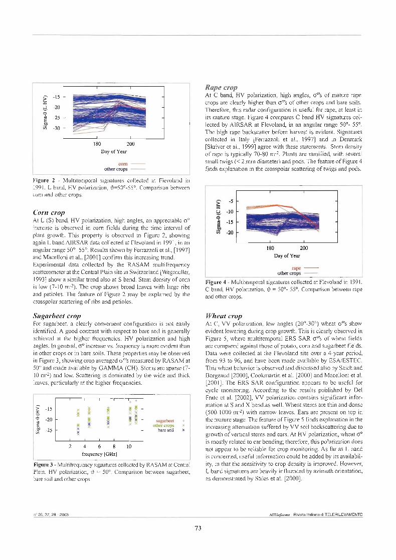
Figare 2 - Multitemporal signatures collected at Flevoland in 1991. L band, W polaxization, +5O0-55". Compatison between coni and other crops.

Rape crop At C band, W polarizaiion, high angies, 0"s of matm rape crops are clearly higher than 0"s of other crops and bare so&. Therefore, this radar configuration is useful for rape, at least in its mature stage. Figm 4 compares C band HV sigiaatures collected by AIRSAR at Flevoland, in an angdar range 50"- 55". The high rape backsatkr befm harvest is evident. Signatures collected in Italy [Ferrazzoli et ai., 19971 and in Denrnark [Skriver et al., 19991 agree with diese statiments. Stem density of rape is typ idy 70-80 m-2. Plants are ramified, with sevaal small twigs (< 2 mm diameter) md pods. The .feature of Figure 4 fmds explanation in the crosspolar imtkring of twigs and pods.

Corn crop At L (S) band, HV polarizaiion, high angles, an appreciable oO increase is observed in com fields during the time intenal of plant growth. This pqxrty is observed in F i 2, showing again L band ATRSAR data collected at flevoland in 1991, in an anguhr range SO0- 55". Results shown by Ferraimli et al., [l9971 and Maceiioni et ai., [2001] con f i i this increasing trend. Experimenta1 data collected by the RASAM multdkpency scatbmmeter at the Centrai Plain site in Switzerland [Wegmuller, 19931 show a sirnilar t m d also at S band. Stem density of com - Mdtitempral sm cou- at Flwoland in lwl. is low (7-10 m-2). The crop shows broad leaves with large ribs C b,4 w l ~ o n , 8 = 500- 550. rape and petioles. The feature of Figure 2 rnay be explained by the ,d o&a CTOps. cnmpolar ~08.tterhg of ribs and petioles.

Sugarbeet crop For sugarbeet, a clearìy convenient configuration is not eas& identified. A good contrast with respect to bare soil is generaiiy achieved at the higher fìquencies, HV polarization and high angles. In generai, o" increase vs. fìquency is more evident than in other crops or in bare soils. These properties may be observed in Figure 3, showing crop averagd oO"seamred by RASAM at 50" and ma& available by GAMMA (CH). Stems are sparse (7- 10 m-2) and low. Scattering is dominated by the wide and thick leaves, particuiariy at the higher freq[uencim.

FQum 3 - Mul-cy signatiires collected by RASAM at Central Plain. W polarization, 8 = 50°. Compatison between s-t, bare soil and ofher crops.

Wheat crop At C, W polarization, low angles (20"-30") wheat 0"s show evident lowering dunng crop growth. This is clearly observed in Figure 5, where multitemporal ERS SAR o"s of wheat fields are compared against those of potato, coni and sugarbeet fields. Data were collected at the Flevoland site wer a 4-year period, from 93 to 96, and have been made available by ESAlESTEC. This wheat behavior is observed and discussed aiso by Saich and Borgeaud [2000], Cookmartin et ai. [2000] and Maceiloni et ai. [2001]. The ERS SAR configuration appears to be useful for cycle monitoring. According t0 the d t s published by Del Frate et al. [2002], W polarizaton con& significaut information at S and X band.as well. Wheat stems are thin and dense (500-1000 m-2) with narraw leaves. Ears are present on top in the mature stage. The feature of Figure 5 finds explanation in the increasing attenuation suffered by W soil b a c W g due to growth of vertical stems and ears. At HV polarization, wheat oO is mostly related to ear bending; therefore, this polarization does not appear to be reliable for crop mnitoring. As far as L band is concemai, useful infbrmation could be added by its availability, in that the sensitivity to crop density is improved. However, L band signatuies are heavily infiuenced by azimuth onentation, as demonstrated by Stiles et al. [2000].

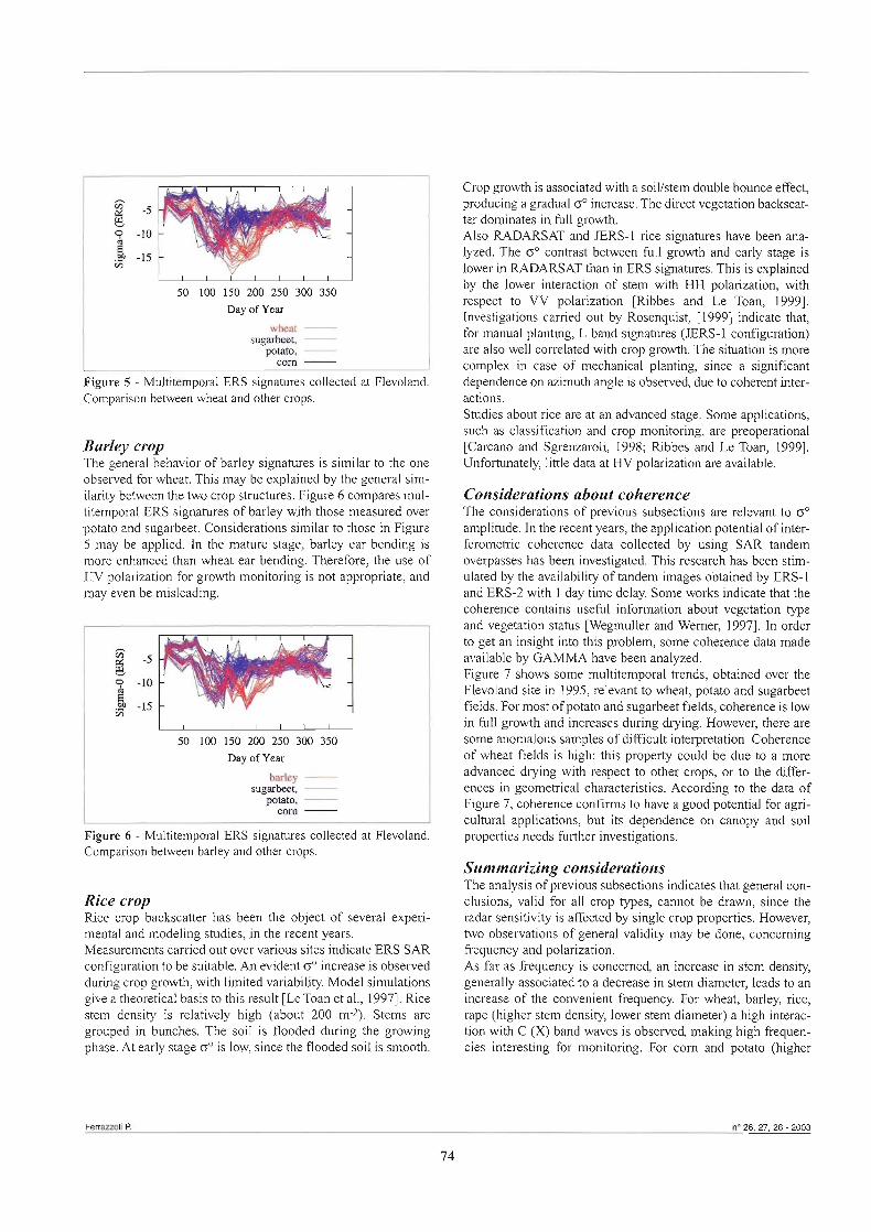
Day of Year

wheat -- sugarbeet, -

potato, - com -

Figure 5 - Multitemporal ERS signatures collected at Flevoland. Comparison between wheat and other crops.

Barley crop The general behavior of barley signatures is similar to the one observed for wheai. This may be explained by the general sim- ilarity between the two crop structures. Figure 6 compares multitemporal ERS signatures of barley with those measured over potato and sugarbeet. Considerations similar to those in Figure 5 may be applied. In the mature stage, barley ear bending is more enhanced than wheat ear bending. Therefore, the use of HV polarization for growth monitoring is not appropriate, and may even be misleading.

u 50 100 150 200 250 300 350

Day of Year

k l e y - sugarbeet, -

potato, - com -

Figure 6 - Multitemporal ERS signatures coiiected at Flevoland. Comparison between barley and other crops.

Rice crop Rice crop backscatter has been the object of severa1 experi- menta1 and modeling studies, in the recent years. Measurements carried out over various sites indicate ERS SAR configuration to be suitable. An evident o0 increase is observed during crop growth, with lirnited variability. Mode1 simulations give a theoretical basis to this result [Le Toan et al., 19971. Rice stem density is relatively high (about 200 m-*). Stems are grouped in bunches. The soil is flooded during the growing phase. At early stage o" is low, since the flooded soil is smooth.

Crop growth is associated with a soilistem double bounce effect, producing a gradua1 o0 increase. The direct vegetation backscatter dorninates in full growth. Also RADARSAT and JERS-1 rice signatures have been analyzed. The o" contrast between full growth and early stage is lower in RADARSAT than in ERS signatures. This is explained by the lower interaction of stem with HH polarization, with respect to W polarization [Ribbes and Le Toan, 19991. Investigations carried out by Rosenquist, [l9991 indicate that, for manual planting, L band signatures (JERS-1 configuration) are also well correlated with crop growth. The situation is more complex in case of mechanical planting, since a significant dependence on azimuth angie is observed, due to coherent interactions. Studies about rice are at an advanced stage. Some applications, such as classification and crop monitoring, are preoperational [Carcano and Sgrenzaroli, 1998; Ribbes and Le Toan, 19991. Unfortunately, little data at HV polarization are available.

Considerations about coherence The considerations of previous subsections are relevant to o0 arnplitude. In the recent years, the application potential of interferometric coherence data collected by using SAR tandem overpasses has been investigated. This research has been stim- ulated by the availability of tandem images obtained by ERS-1 and ERS-2 with 1 day time delay. Some works indicate that the coherence contains useful information about vegetation type and vegetation status [Wegmuller and Werner, 19971. In order to get an insight into this problem, some coherence data made available by GAMMA have been analyzed. Figure 7 shows some multitemporal trends, obtained over the Flevoland site in 1995, relevant to wheat, potato and sugarbeet fields. For most of potato and sugarbeet fields, coherence is low in M1 growth and increases during dryng. However, there are some anomalous samples of difficult interpretation. Coherence of wheat fields is high: this property could be due to a more advanced drying with respect to other crops, or to the differences in geometrica1 characteristics. According to the data of Figure 7, coherence confirms to have a good potential for agri- cultura1 applications, but its dependence on canopy and soil properties needs further investigations.

Summarizing considerations The analysis of previous subsections indicates that general conclusions, valid for al1 crop types, cannot be drawn, since the radar sensitivity is affected by single crop properties. However, two observations of general validity may be done, conceming frequency and polarization. As far as frequency is concemed, an increase in stem density, generally associated to a decrease in stem diameter, leads to an increase of the convenient frequency. For wheat, barley, nce, rape (higher stem density, lower stem diameter) a high interaction with C (X) band waves is observed, making high frequencies interesting for monitoring. For corn and potato (higher

50 100 150 24Xl 250 300 350 h y OfYcar

m- sugarbadt --

Potato -

Figure 7 - Multitemporal coherence data collected at Flevoland by ERS tandem overpasses. Comparison between potato, sugarbeet and wheat.

stem diameter, lower stem density) lower frequencies (L and S band) appear to be more convenient. As far as polarization is concerned, HV is particularly useful when crops are well rarnified, i.e. the relative weight of twigs, pods, petioles and leaf ribs becomes irnportant. It is the case of potato, coni and mature rape. For crops dorninated by vertical structures, such as wheat and barley, the most significant information is contained in the attenuation andlor double bounce effects produced at W polarization. The above considerations about frequency and polarization are

References

Baronti S., Del Frate F., Ferrazzoli P., Paloscia S., Pampaloni P. and Schiavon G. (1995) - SARpolarimetric features of agri- cultura1 areas. Int. J. Remote Sensing, 16: 2639-2656.

Bracaglia M., Ferrazzoli i? and Guerriero L. (1995) - Afully polarimetric multiple scattering model for cmps. Remote Sensing Environ., 54: 170-1 79.

Carcano G. and Sgrenzaroli M. (1998-99) - Telerilevamento da satellite con tecnologia SAR: individwzione delle risaie nel Sud-EstAsiatico. AIT Informa - Riv. It. Teleril., 14-15: 13-20.

Christensen E.L., Skou N., Dal1 J., Woelders K.W., Jorgensen J.H., Granholm J. and Madsen S. N. (1998) - EMISAR: an absoluteiy calibmtedpolarimeìric L- and C-band SAR. IEEE Trans. Geosci. Remote Sensing, 36: 1852- 1865.

Churchill P.N. and Attema E.P.W. (1992) - n e MAESTRO-I Eumpean airborne polarimetric Synthetic Aperture Radar campaign, MAESTRO- 11AGRISCATT Fina1 Workshop Proceedings, ESA wpp-3 1 : 1-1 1.

Cookmartin G., Saich P,, Quegan S., Cordey R, Burgess-

valid when scattering is dominated by cylindrical elements. Their applicability to sugarbeet, characterized by large leaves and very low sterns, is not straightfonvard. As a further information, it may be remembered that L band, HV polarization, has proved to be a convenient configuration also for sunflower [Ferrazzoli et al., 19971 and soybeans [De Roo et ai., 20011. From a system point of view, the forthcoming considerations ~ P P ~ Y . The configurations of present spaceborne SAR's, particularly ERS SAR, are interesting for some crops, such as rice, wheat and barley. ENVISAT ASAR signatures, provided ground resolution will be sufficient, will produce a significant improvement in monitoring, in that may contain HV polarization. A genera1 good potential in monitoring of the main crops could be achieved in the future by simultaneous availability of L and C band obse~ations. The analysis has been lirnited to linea. polarizations. Hawever, previous studies indicate that the availability of fully polarimetric data is very useful for classification perrazzoli et al., 1999; Skriver et al., 19991 and, to a lesser extent, for crop monitoring [Ferrazzoli et al., 1997; Skriver et al., 19991.

Acknowledgments The data collected at Flevoland and Centra1 Plain sites have been made available in the framework of the ERA-ORA Concerted Action, funded by ECC (Contract No. ENV4- CT97-0465).

AUen P. and Sowter A. (2000) - Modeling micmwave interactions with cmps and comparison with ERS-2 SAR observations. IEEE Trans. Geosci. Remote Sensing, 38: 658-670.

Del Frate F., Ferrazzoli P. , Guerriero L., Strozzi T., Wegmuller U., Cookmartin G. and Quegan S. (2002) - Monitoring cmp cycles by SAR using a neural network trained by a model. Proceedings of the Third International Symposium on Retrieval of bio- and geophysical parameters from SAR data for land applications, Sheffield (UK), September 2001, ESA SP 475: 239-244.

De Roo R.D., Du Y., Ulaby F.T. and Dobson M.C. (200 1) - A semiempirical baclrscattering model at L-band and C-band for a soybean canopy with soil moisture inversiun. IEEE Trans. Geosci. Remote Sensing, 39: 864-872.

Eom H.J. and Fung A.K. (1984) - A scatter model for vegetation up to Ku-band. Remote Sensing Environ., 19: 139-149.

Ferrazzoli P. and Guerriero L. (1994) - Interpretation and model analysis of MAESTRO-I Flevoland data. Int. J. Remote Sensing, 15 :2901-2915.

n" 26,27,28 - 2003 AITkrfonta - Rivista italiana di TELERILEVAMENTO

75

Fer rml i P., Schiavon G, Solimini D., Paioscia S., Pampaloni P. and Sigismondi S. (1997) - n e potential of mulhjkquens, polarwetric SAR in assessing agricultural and arboreous biomass. IEEE Trans. Geosci. Remote Sensing, 35: pp. 5-17.

Ferranoli P., Guerriera L. and Schiavon G. (1999) - Experimenta1 and model investigation on RADAR classification capabiliy. IEEE Trans. Geosci. Remote Sensing, 37: pp. 960-968.

Freeman A., Shen Y. and Wemer C.L. (1990) - Polarimetric SAR calibmtion experiment using active radar calibrators. IEEE Trans. Geosci. Remote Sensing, 28: 224-240.

Held D.H., Brown W.E., Freeman G., Klein J.D., Zebker H., Sato T., Nguyen Q. and Lou Y. (1988) - Z?ze NASA/JPL multzjirequency multipolarization airborne SAR system. IGARSS'88 Proceedings, Edinburgh (UK), 345-349.

Hoekman D. H. (1992) - Introduction to the Agriscatt'87 and '88 campaigns. MAESTRO-1IAGRISCATT Fina1 Workshop Proceedings, ESA wpp-3 1 : 13-2 1.

Karam M.A. and Fung A.K. (1988) - Electromagnetic scatteringfim a layer offnite length, mndomly oriented, dielectric, circular cylinders over a mugh interface with application to vegetation. Int. J. Remote Sens., 9: 1 109-1 134.

Le Toan T., Ribbes F., Wang L.-F., Fioury N., Ding K-H., Kong JA, Fujita M. and Kurosu T. (1997) - Rice crop mapping and monitoring using ERS-I data based on experiment and modeling results. EEE Trans. Geosci. Remote Sensing, 35: 41-56.

Macelioni G., Paioscia S., Pampaloni P., Marliani F. and Gai M. (2001) - The relationship between the bachcattering coeficient and the biomass of narmw and broad leaf cmps. IEEE Trans. Geosci. Remote Sensing, 39: 873-884.

Ribbes E and Le Toan T. (1999) - Ricefeld mapping and monitoring with RADARSATdata. Int. J. Remote Sensing, 20: 745-765. Rosenquist A. (1999) - Tempoml and spatial chamcteristics of imgated rice in JERS-I L-band SAR data. Int. J. Remote Sensing, 20: 1567-1587.

Saich P. and Borgeaud M. (2000) - Interpreting ERS SAR signatures of agricultuml cmps in Flevoland, 1993-1996. IEEE Trans. Geosci. Remote Sensing, 38: 65 1-657.

Skriver H., Svendsen M.T. and Thomsen A.G. (1999) - Multitemporal C- and Lbandpolarimeiric signatures of cmps. IEEE Trans. Geosci. Remote Sensing, 37: 2413-2429.

Stiles J.M., Sarabandi K. and Ulaby F.T. (2000) - Electromagnetic scattering f rom gmssland - part ZZ: measurement and modeling results. IEEE Trans. Geosci. Remote Sensing, 38: 349-356.

Stofan E.R., Evans D.L., Schmniiius C., Holt B., Plaut J.J., van Zyl J., Wali S.D. and Way J. (1995) - Ovewiew of results of spacebome imaging radar- C, X-band Synthetic Aperture Radar (SIR-c/X-SAR). IEEE Trans. Geosci. Remote Sensing, 33: 817-828.

Ulaby ET. and Attema E.P.W. (1978) - Vegetation modeled as a water cloud. Radio Science, 13: 357-364.

Ulaby F.T. (1980) - Vegetation clutter model. IEEE Trans. Antennas Propagat., 28: 538-545.

Ulaby F.T., Moore RK. and Fung A.K. (1986) - Microwave Remote Sensing. Active and Passive. Vol ZII. Artech House Ed.

Ulaby F.T. and Dobson M.C. (1989) - Handbook of Radar Scattering Statisticsfim Termin. Artech House Ed.

van Zyl J.J. (1990) - Calibration ofpolarimetric mdar images using only image pammeters and irihedml comer reflectors responses. EEE Trans. Geosci. Remote Sensing, 28: 337-347.

Wegmuller U. (1 993) - Signature research for cmp classz>cation by active andpassive micmwaves. Int. J. Remote Sensing, 14: 871-883.

Wegmuller U. and Wemer C. (1997) - Retrieval of vegetation pammeters with S A . inte$emmetry. EEE Trans. Geosci. Remote Sensing, 35: 18-24.

Zebker H. and Lon Y. (1990) - Phase calibmtion of imaging radar polarimeter Stokes matrices. IEEE Trans. Geosci. Remote Sensing, 28: 246-252.

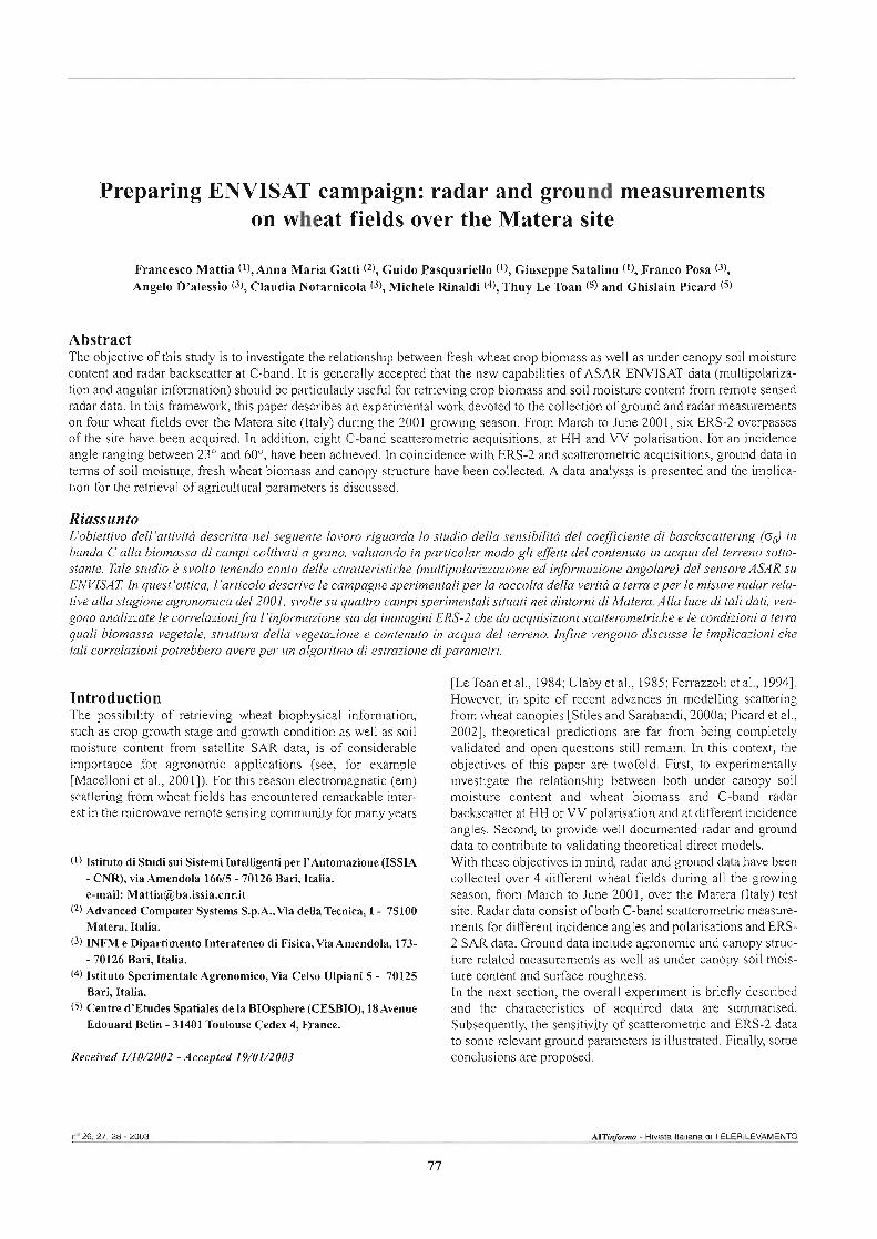
Preparing ENVISAT campaign: radar and ground measurements on wheat fields over the Matera site

Francesco Mattia (l), Anna Maria Gatti (*), Guido Pasquariello (l), Giuseppe Satalino (11, Franco Posa (3),

Angelo D'alessio (3), Claudia Notarnicola (3), Michele Rinaldi (4), Thuy Le Toan (5) and Ghislain Picard

Abstract The objective of this study is to investigate the relationship between fresh wheat crop biomass as well as under canopy soil moisture content and radar backscatter at C-band. It is generally accepted that the new capabilities of ASAR-ENVISAT data (multipolarization and angular information) should be particularly useful for retrieving crop biomass and soil moisture content from remote sensed radar data. In this framework, this paper describes an experimental work devoted to the collection of ground and radar measurements on four wheat fields over the Matera site (Italy) during the 200 1 growing season. From March to June 2001, six ERS-2 overpasses of the site have been acquired. In addition, eight C-band scatterometric acquisitions, at HH and W polarisation, for an incidence angle ranging between 23" and 60°, have been achieved. In coincidence with ERS-2 and scatterometric acquisitions, ground data in terms of soil moisture, fresh wheat biomass and canopy strutture have been coliected. A data analysis is presented and the implica- tion for the retrieval of agricultural parameters is discussed.

Riassunto L'obiettivo dell'attività descritta nel seguente lavoro riguarda lo studio della sensibilità del coejìciente di basckscattering ( ~ o ) in banda C alla biomassa di campi coltivati a gmno, valutando in particolar modo gli efletti del contenuto in acqua del terreno sotto- stante. Tale studio è svolto tenendo conto delle caratteristiche (multipolarizzazione ed informazione angolare) del sensore ASAR su ENVTSAT In quest'ottica, l'articolo descrive le campagne sperimentali per la mccolta della verità a terra eper le misure radar relative alla stagione agronomica del 2001, svolte su quattro campi sperimentali situati nei dintorni di Matera. Alla luce di tali dati, vengono analizzate le correlazioni fra l'informazione sia da immagini ERS-2 che da acquisizioni scatterometriche e le condizioni a terra quali biomassa vegetale, struttura della vegetazione e contenuto in acqua del terreno. Infine vengono discusse le implicazioni che tali correlazioni potrebbero avere per un algoritmo di estrazione di parametri.

Introduction The possibility of retrieving wheat biophysical information, such as crop growth stage and growth condition as well as soil moisture content from satellite SAR data, is of considerable importante for agronomic applications (see, for example [Macelloni et al., 20011). For this reason electromagnetic (em) scattering from wheat fields has encountered remarkable interest in the microwave remote sensing cornmunity for many years

(1) Istituto di Studi sui Sistemi Intelligenti per l'Automazione (ISSIA - CM), via Amendola 16615 - 70126 Bari, Itaiia. e-mail: [email protected]

(2) Advanced Computer Systems S.p.A.,Via deUaTecnica, 1 - 75100 Matera, Itaiia.

(3) INFM e Dipartimento Interateneo di Fisica,Via Amendola, 173- - 70126 Bari, Italia.

(4) Istituto Sperimentale Agronomico, Via Celso Ulpiani 5 - 70125 Bari, Italia.

(5) Centre d9Etudes Spatiales de la BIOsphere (CESBIO), 18Avenue Edouard Belin - 31401 Toulouse Cedex 4, h c e .


[LeToan et al., 1984; Ulaby et al., 1985; Fenazzoli et al., 19941. However, in spite of recent advances in modelling scattering from wheat canopies [Stiles and Sarabandi, 2000a; Picard et al., 20021, theoretical predictions are far from being completely validated and open questions still remain. In this context, the objectives of this paper are twofold. First, to experimentally investigate the relationship between both under canopy soil moisture content and wheat biomass and C-band radar backscatter at HH or W polarisation and at different incidence angles. Second, to provide well documented radar and ground data to contribute to validating theoretical direct models. With these objectives in rnind, radar and ground data have been collected over 4 different wheat fields during al1 the growing season, from March to June 2001, over the Matera (Itaiy) test site. Radar data consist of both C-band scatterometric measurements for different incidence angles and polarisations and ERS- 2 SAR data. Ground data include agronomic and canopy structure related measurements as well as under canopy soil moisture content and surface roughness. In the next section, the overall experiment is briefly described and the characteristics of acquired data are surnmarised. Subsequently, the sensitivity of scatterometric and ERS-2 data to some relevant ground parameters is illustrated. Finally, some conclusions are proposed.

no 26.27,28 - 2003 AiTinfonwr - Rhrita Itallana di TELERILEVAMENTO

77

Figure 1 - a) Landsat Tm image for a pictorial Test site location. b) Fd indicates the field used for scatterometric measurements (field 4 in the text); Fdl, Fd2 and Fd3 have been observed by ERS-2.

Experiment description The selected site is an area close to Matera, a town of the Basilicata Region, in the Southern Italy (Figure la gives a pictorial idea of the test site location, using a Landsat-Tm image whiie Figure lb is an ortophoto of the fields). This is a pre- dominantly agncultural area mainly devoted to wheat cultiva- tion. Four wheat fields, identified as field 1, 2, 3 and 4, were selected over a flat area: fields 1, 2 and 3 dimensions ranged between three and ten hectares, field 4 (Fd in red in Fig. lb) was smaller than one hectare. According to the local crop management practice, fields are usually sown at the end of December, wheat reaches its maximum growth at mid May and is harvested approximately at mid June depending on weather conditions. From March to June 2001, eight ground and scatterometric measurements were carried out over the field 4. In addition, ground measurements over other fields were conducted during six ERS-2 overpasses. Table 1 surnrnarises the dates for which ground and radar data (i.e. scatterometer andtor ERS-2) were acquired.

Table 1 - Ground and Satellite data time acquisition.

Ground data For each field, data including wheat phenological stage, wheat biomass, canopy strutture and soil measurements were collected. The following pararneters were measured: plant density, row spacing, stems per plant, leaves per stem, stem diameter and length, node position, leaf shape and thickness, flag leaf geometry, length, width and thickness of ears, wetfdry weight of stems, leaves and ears. Soil roughness profiles were acquired only once during the first ground campaign when wheat was at a very early stage, using a 4m long needle-like profiler to measure soil roughness along directions parallel, perpendicular and at 45O with respect to the row directions. Soil moisture content at 0.05 m for each field was measured using the gravimetric method. Over the area, the typical volurnetric soil moisture content is between 25 and 15% in March-April, whereas in May-June it may range between 15 and 10%. However, due to a few days of continuous raining, the maximurn soil moisture value (i.e. 27-30%) was reached on May 9. The majority of ground measurements were carried out on site within three hours from ERS-2 overpasses and during the Scatterometric acquisitions. Typically, for each field, three different locations have been selected to collect ground data. For each location, 30 measurements of plant geometry have been carried out on site. In addition, plant samples filling either 1 m or 0.5 m of rows (depending on the wheat growing stage) were collected, separated into stems, leaves and ears, and then weighted, within 1-2h, to obtain the fresh wheat biomass. The stems density (i. e. shoots/m*) was estimated too. Its mean value was approximately 400 shootsIm2 with a maximum spread of *200 shootsIm2. In addition, a second set of plants (i.e. typically 15) was collected in order to characterise finer geometrica1 details (Le. sterns radius at different heights, leaf thickness, etc.) during laboratory measurernents. Moreover, the components of these plants were scanned to permit an accurate characterisa-

Maffla F. et ai. no 26,27,28 - 2003

78

Graund meawir.

Date Sei= Day of Year

ERS-2 orbft

ERS-2 lrack

tion of shapes of stems, leaves and ears. Wheat water content was separately estimated for sterns, leaves and ears by drying the coiiected samples at 72" C for 24h.

Radar data The scatterometer sensor employed in this experiment has been realiseci and run by the team of the University of Bari [Sabatelli et al., 19991. The sensor is a C-band FM-CW radar which can measure backscattering coefficient between +lodi3 and -40dB, for target distances between 10 and 60m and for incidence angles ranging between 10" and 60". Table 2 reports the main sensor characteristics.

Table 2 - Scatterometer characteristics.

Pm?nneter Valiie cmta aequaicy 5.3CtE

insbunmt m d e l Lineer M - C W radar

Modulation band 300 MHz Moduiation agnal Triandar (6 O Hz)

Dymmic range 50 dB

Antuum lype H om antuum(dua1 antmm system) Antuum beamidthin Uie E 1 H plane 22'1 31"

Antenna gain 15 dB

P 0 k i ~ a t . i ~ modes VV. VH. HV, HH Range resolution 0.65m

Calibralion internai and extemai

Ueasunrnrnl aror f l m

A dedicated software allms the sensor control, data pmcessing and displaying. During the experiment, the sensor has been mounted on a truck platform at 15m above ground (Fig. 2). Measurements at HH and W polarisation for an incidence angle ranging between 23" and 60" were carried out. For each incidence angle, a large number of independent samples were acquired by azimuthally rotating the platform. Subsequently the independent samples were calibrated and then averaged in

order to estirnate the backscattering coeficient. Extemal calibration using a trihedral corner reflector was performed for each incidence angle at the beginning and at the end of the acquisition. The ERS-2 SAR images exploited in the study consist of six standard ESA PRI products. Al1 the images were acquired for descending orbits and along two adjacent tracks. In fact , the selected area is at the intersection between two ERS-2 swaths and for this reason an interval of approxirnately 20 days between two consecutive acquisitions has been obtained Data were calibrated and co-registered using the ESA TOOLBOX software package. For each field the number of pixels averaged to calculate the o. ranged between 100 and 400.

Data analysis As an example of acquired agronomic data, Figures 3 and 4 show the stems height and the total wheat fiesh biomass estimated during the campaign, respectively. As it can be seen, especially for the biomass values, there is a significant variability in the ground measurements collected over different fields.

O Field 2 Field 3

A Field 4

60 80 100 120 140 160 180 Day of Year

Figure 3 - Measured wheat stems height temporal profile.

60 80 100 120 140 160 180 Day of Year

Figure 2 - Scatterometer on test site F4. Figure 4 - Measured wheat fresh biomass temporal behaviour.

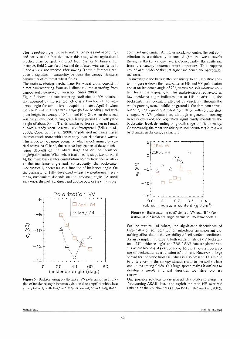
This is probably partly due to natura1 reasons (soil variability) and partly to the fact that, over this area, wheat agricultural practice may be quite different from farmer to farmer. For instance, field 2 was fertilised and disinfested whereas fields 1, 3 and 4 were not worked after sowing. These differences produce a significant variability between the canopy structure parameters of different wheat fields. The main scattering mechanisms for wheat crops consist of direct backscattering from soil, direct volume scattering from canopy and canopy-soil interaction [Stiles, 2000al. Figure 5 shows the backscattering coefficient at W polarisation acquired by the scatterometer, as a function of the incidente angle for two different acquisition dates: Apri1 4, when the wheat was in a vegetative stage (before heading) and with plant height in average of 0.4 m, and May 24, when the wheat was fuily developed, during grain filling period and with plant height of about 0.8 m. Trends similar to those shown in Figure 5 have already been observed and interpreteci [Stiles et al., 2000b; Cookmartin et al., 20001. V polarised incidence waves interact much more with the canopy than H polarised waves. This is due to the canopy geometry, which is determined by vertical stems. At C-band, the relative importance of these mechanisms depends on the wheat stage and on the incidence angie/polarisation. When wheat is at an early stage (i.e. on April 4), the main backscatter contribution comes from soil whatev- er the incidence angle and, consequently, the backscatter monotonically decreases as a function of incidence angle. On the contrary, for iùlly developed wheat the predominant scattering mechanism depends on the incidence angle. At small incidence, the soil (i.e. direct and double bounce) is still the pre-

Polarization W -6 1 . .

A n r i l

7 a n May 24

L

-

l , . . l . . . l . . .

dominant mechanism. At higher incidence angles, the soil contribution is considerably attenuated (i.e. the wave travels through a thicker canopy layer). Consequently, the scattering from the canopy becomes more important. This happens around 40' incidence then, at higher incidence, the backscatter increases. To investigate the backscatter sensitivity to soil moisture content, Figure 6 shows the backscatter at HH and W polarisation and at an incidence angle of 23", versus the soil moisture content for al1 the acquisitions. This multi-temporal behaviour at low incidence angle indicates that at HH polarisation, the backscatter is moderately affected by vegetation through the whole growing season while the ground is the dominant contribution giving a good qualitative correlation with soil moisture changes. At W polarisation, although a genera1 increasing trend is obsewed, the vegetation significantly modulates the backscatter level, depending on growth stage and field density. Consequently, the radar sensitivity to soil parameters is masked by changes in the canopy structure.

-14 O 20 40 60 80

incidence angle (deg.)

Figure 5 - Backscattering coeficient at W polarization as a function of incidence angle in two acquisition dates: April 4, with wheat at vegetative growth stage and May 24, during grain filling stage.

0.0 0.1 0.2 0.3 0.4 vol. soil moisture content (gr/cm3)

Figure 6 - Backscattering coeficients at W and HH polarization, at 23' incidence angle, versus soil moisture content.

For the retrieval of wheat, the significant dependence of backscatter on soil contribution introduces an important dis- turbing effect due to the variabiiity of soil surface conditions. As an example, in Figure 7, both scatterometric (W backscatter at 23O incidence angle) and ERS-2 SAR data are plotted versus wheat biomass. As can be seen, there is an overall decreasing of backscatter as a function of biomass. However, a large spread for the same biomass values is also present. This is due to differences in the canopy structure and in the soil surface conditions among fields. This large spread makes it dificult to develop a simple empirical algorithrn for wheat biomass retrieval. One possible solution to circumvent this problem, using the forthcoming ASAR data, is to exploit the ratio HH over W rather than the W channel as suggested in [Brown et al., 20021.

Mania F. el al. no 26,27,28 - 2003

80

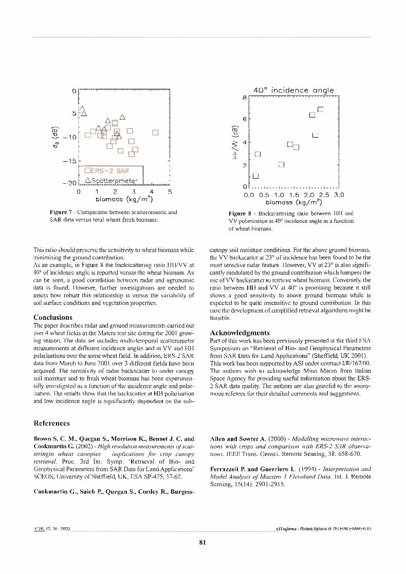
-20 0 1 2 3 4 5

biomass (kg/m2)

Figure 7 - Comparison between scatterometric and SAR data versus total wheat fiesh biomass.

This ratio should preserve the sensitivity to wheat biomass while minimising the ground contribution. As an exarnple, in Figure 8 the backscattering ratio HWW at 40" of incidence angle is reported versus the wheat biomass. As can be seen, a good correlation between radar and agronornic data is found. However, further investigations are needed to assess how robust this relationslup is versus the variability of soil surface conditions and vegetation properties.

Conclusions The paper describes radar and ground measurements carried out aver 4 wheat fields in the Matera test site during the 2001 growing season. The data set includes multi-temporal scatterometer measurements at different incidence angles and at W and HH polarisations over the same wheat field. in addition, ERS-2 SAR data kom March to June 2001 over 3 different fields have been acquired. The sensitivity of radar backscatter to under canopy soil moisture and to fresh wheat biomass has been experimentally investigated as a function of the incidence angle and polarisation. The results show that the backscatter at HH polarisation and low incidence angle is significantly dependent on the sub-

References

Brown S. C. M., Quegan S., Morrison K., Bennet J. C. and Cooùmartin G. (2002) - High resolution measurements of scat- teringin wheat canopies - implications for crop canopy retrieval. Proc. 3rd Int. Syrnp. 'Retrieval of Bio- and Geophysical Parameters fiom SAR Data for Land Applications' SCEOS, University of Sheffield, UK, ESA SP-475,57-62.

Cookmartin G., Saich P., Quegan S., Cordey R., Burgess-

40" incidence angle

m D

0- 0.0 0.5 1.0 1.5 2.0 2.5 3.0

biomass (kg/m2)

Figure 8 - Backscattering ratio between HH and W polarization at 40° incidence angle as a function of wheat biomass.

canopy soil moisture conditions. For the above ground biomass, the W backscatter at 23" of incidence has been found to be the most sensitive radar feature. However, W at 23" is also significantly modulated by the ground coniribution which hampers the use of W backscatter to retrieve wheat biomass. Conversely, the ratio between HH and W at 40" is promising because it still shows a good sensitivity to above p u n d biomass while is expected to be quite insensitive to ground conùibution. In this case the development of simplified reùieval algorithms might be feasible.

Acknowledgments Part of this work has been previously presented at the third ESA Symposium on "Retrieval of Bio- and Geophysical Pme te r s from SAR Data for Land Applications" (Sheffield, UK 200 1). This work has been supported by ASI under contsact W167100. The authors wish to aclmowledge Mino Marzo fiom Italian Space Agency for providing usefd information about the ERS- 2 SAR data quality. The authors are also gratefid to the anony- mous referees for their detailed comments and suggestions.

Aiien and Sowter A. (2000) - Modelling micmave interactions with crops and comparison with ERS-2 SAR observations. IEEE Trans. Geosci. Remote Sensing, 38: 658-670.

Ferrazzoli P. and Guerriero L. (1994) - Interpretation and Mode1 Analysis of Maestro 1 Flevoland Data. Int. J. Remote Sensing, 15(14): 2901-2915.

no 26,27.26 - 2003 AI~@WIW - R i Italiana di TELERILEVAMENTO

81

Maceiioni G., Paloscia S., Pampaloni P., F. Marliani F. and Gai M. (200 1) - The Relationship Between the Backscattering Coeflcient and the Biomass of N a m w and Broad Leaf Crops. IEEE Trans. Geosci. Remote Sensing, 39: 873-884.

Le Toan T., Lopes A. and Huet M. (1984) - On the relationships between mdar bacbcuttering coeficient and vegetation canopy cbhe t i s t i cs . Proc. IGARSS'84, ESA SP-215, 155-160.

Picard G., Le Toan T., Mattia E, Gatti A., Posa E, D'alessio A., Notamicola C. and Sabateiii V. (2002) -A backscattering modelfor wheat canopies. Proc. 3rd Int. Symp. 'Retrieval of Bio- and Geophysical Parameters from SAR Data for Land Applications', SCEOS, University of Sheffield, UK, ESA SP- 475,291-296.

Sabatelli V, Casarano D., Buono G., Paparella E and Posa E (1999) - An FM-CW Scatterometer radar: Design, Implementation and Use on Natura1 Surfaces. Alta Frequenza, 1 l(3): 48-51.

Stiles J. and Sarabandi K. (2000a) - Elecfromagnetic Scattering from Grassland-Part I: a Fully Phase Coherent Scattering Model. IEEE Trans. Geosci. Remote Sensing, 38: 339-348.

Stiles J., Sarabandi K. and Ulaby F. (2000b) - Electromagnetic Scattering from Grassland-Part II: Measurement and Modeling Results. EEE Trans. Geosci. Remote Sensing, 38: 349-356.

Ulaby F., Moore R and Fung A. K. (1985) - M' zcmave Remote Sensing: Active and Passive. Artech Hause, vol. m.

Mania F. ei al. no 26,27,28 - 2003

82

Recent studies on forest radiometry

Paolo Ferrazzoli and Leila Guerriero (1)

Abstract This paper presents a theoretical study of the emissivity of forested areas carried out by means of the electromagnetic model developed at Tor Vergata. The model, which simulates emissivity through the computation of bistatic scaltering fkom vegetation and applying the energy conservation, has been updated to improve the morphological representation of arboreous vegetation. The L-band theoretical results will be presented, separating the emissivity contributions from the various forest components. The results demostrate that the major emissivity contribution comes fi-om branches, while trunks which contain most of the biomass produce minor effects. The model has then been used to calibrate a simple zero-order radiative transfer model. Indeed, simple models have been recognized to be usefitl in retrieval applications at global scale, and can be used to evaluate the radiometric sensitivity to soil moisture.

Riassunto Questa memoria presenta uno studio di simulazione dell'emissività delle aree boschive efettuato mediante il modello elettromagnetico sviluppato a Tor Vergata. Il modello, che simula l'emissività attmverso il calcolo del coeflciente di scattering bistatico della vegetazione e applicando la conservazione dell'energia, è stato aggiornato per migliomre la rappresentazione morfologica della vegetazione arborea. Saranno perciò presentati i risultati teorici in banda L, sepamndo i contributi di emissione provenienti dai diversi elementi che compongono unajòresta. Questi risultati dimostmno che il principale conìributo di emissione proviene dai mmi, mentre i tronchi, che rappresentano la percentuale maggiore di biomassa, producono efetiì minori. Il modello è stato inoltre usato per cali- bmre un semplice modello di ordine zero del tmsjèrimento mdiativo. Infatti, i modelli semplici possono essere utili nelle inversioni a scala globale dei dati telerilevati, e possono essere utilizzati per valutare la sensibilità dei radiometn' al contenuto d'acqua del suolo.

Introduction Severa1 studies indicated that microwave emissivity of land is sensitive to soil moisture paloscia et al., 1993; Jackson and Schrnugge, 1989; Wigneron et al., 19981, especially at the lower frequencies, such as 1-1.5 GHz (L-band). Based on these results future satellite missions, such as SMOS [Ken et al., 200 l], have been planned. Since the resolution of spaceborne radiometers is of the order of some tens of kilometers, the objective of the missions is to generate large scale soil moisture maps. In the radiometric images, several pixels will be filled by forests, at various extents, so that a reliable characterization of forest emission is important. Moreover, since important progresses are being achieved in the ground resolution of spaceborne sensors, and also airborne systems may become operational, radiometers could be used in the future to monitor forest properties, such as biomass, moisture, etc.

(1) Università Tor Vergata, Ingegneria-DISP, Via del Politecnico - I- 00133 Roma, Italia. email: [email protected]


Indeed, in the more recent years the interest on radiometric forestry has been increasing: several experiments have been carried out over forests worldwide, with airborne systems, and some models have been developed. In 1994, the airborne radiometer PORTOS flew over Les Landes forest perfomiing multifrequency passive measurements which are thoroughly described in wigneron et al., 19971. In 1999, the ESTAR radiometer performed measurements over coniferous forests at L-band (1.4 GHz), horizontal polarization [Lang et al., 20001. In the same year, multifrequency radiometric measurements were carried out over Italian deciduous forests [Macelloni et al., 20001. Finally, the brightness temperatures of snow-covered forests with different biomass were measured in Finland in the framework of EMAC-95 campaign [Kruopis et al., 19991. Other important progresses in forest emissivity modeling have been made with results published Fenazzoli and Guemero, 1996; Karam, 19971. The model developed at Tor Vergata was described in [Ferrazzoli and Guerriero, 19961, where results of pararnetric investigations were shown and the performances of passive and active sensors were cornpared against each other. This paper describes recent advances in forest emission simulation. New developments are: i) an accurate representation of forest geometry, based on recent measurements [Wigneron et al., 19971,

n" 26,27,28 - 2003 ~ITUtfom - Rivista Italiana di TELERILEVAMENTO

83

ii) an investigation about the effects of single forest components (soil, trunk, branches, leaves), iii) the use of outputs generated by the physical model to calibrate a simple model. The last development is important for applications, in that it allows us to include the forest model into a general earth emission model. The latter, on its own, can be used to simulate the performance of Lband spaceborne radiometers, such as the SMOS one.

The model The microwave model developed at Tor Vergata is able to simulate both the backscattering coeficient and the emissivity of forests. Details can be found in [Ferrazzoli and Guerriero, 19961 and [Ferrazzoli and Guerriero, 19951, where the model has been described, respectively, in its passive and in its active version. In the following, a synthetic description of the Tor Vergata model, such as it has been used in this work, is reported. The simulations carried out in this paper are concerned with coniferous forests, which are subdivided into the following layers:

the crawn layer, made up by needles and branches modeled by means of dielectric oblate spheroids and cylinders, whose absortion and bistatic scattering cross sections are modeled by the Rayleigh-Gans and the infinite cylinder approximation, respectively; the trunk layer, modeled by means of dielectric cylinders whose electromagnetic properties are described by the infinite cylinder approximation; the soil, whose bistatic scattering cross section is simulated through the Integra1 Equation Model.

The various contributions are combined by means of the matrix doubling algorithm which yields the bistatic scattering coefficient of the forest canopy. The latter is finally used to simulate the emissivity, through the energy conservation law. The model needs as input a detailed description of the tree components [Ferrazzoli et al., 20021, many geometric parameters are required, such as tree and trunk height, diameter at breast height, primary and secondary branch dimensions, onentation, etc. In perrazzoli and Guerriero, 19961, the parameters were assigned making reasonable assumptions based on sparse data available in the literature at that time. In this paper, the allometric equations valid for Les Landes site, and reported in [Wigneron et al., 19971, are used. Some parameters, such as dimensions and density of primary and secondary branches, are not directly available, and have been derived as a fùnction of diameter at breast height (dbh) using relationships published in [Kasischke et al., 19941. The same Les Landes forest has been used as validation site. To this aim, radiometric and ground measurements carried out in 1994 using PORTOS radiometer wigneron et al., 19971, have been used. The results of the comparison between measured and simulated forest ernissivities are shown in [Ferrazzoli et al., 20021. A generally good correspondence is observed for both younger and older forests. Comparisons were done at C band.

Unfortunately, detailed experirnental data sets at lower frequencies (in particular, L band) are not yet available. Some experi- menta1 campaigns with L band radiometers are in progress and direct comparisons will be made as soon as results are available. For the time being, some L-band emissivity trends will be shown in next sections, and it will be observed that they are in general agreement with data published in the literature.

Model simulations Future satellite systems, aimed at monitoring soil moisture (and, in case, vegetation biomass) are planned to adopt L-band (i.e. 1.4 GHz), [Kerr et al., 20011. In this section, the model is used for a parametric study of Lband forest emissivity as a fùnction of forest age (or biomass) in various conditions, and the effects of the single forest components are afterwards investigated.

Parametric study As previously mentioned, the Tor Vergata model requires as input many geometrica1 parameters which vary with tree age. The ensemble of relationships between dimensions and density of leaves, branches and trunks with respect to tree age can be described by means of allometric equations. The allometric equations developed for Les Landes forest, as described in [Wigneron et al., 19971, have been used and they have been integrated with the growth parametrization described in [Kasischke et al., 19941. This procedure assumes that branch dimensions increase with forest age, while the percent of branch volume out of total volume decreases rapidly with forest age (due to self pruning) reaching a stable value around an age of 20. In order to simulate a number of rea1 situations, we have carried out a parametric study of emissivity vs. forest age varying the branch volume percent out of total wood volume of elderly trees between 10,20 and 30%. Figure 1 shows simulated trends of emissivity vs. age (which, on its turn, is related to biomass), for a percentage of branch volume equal to 30%, and an observation angle equal to 35". The curves show a gradua1 increase of emissivity with age, with saturation occurring at high age values. The simulations presented above make reference to the vegetation strutture of the arboreous canopy in Les Landes. However, similar emissivity behaviours can be reasonably expected for other forests with different characteristics. This is in agreement with some experimental data which were published lately, such as the ESTAR data [Lang et al., 20001, the radiometric data collected over a deciduous forest in Italy [Macelloni et al., 20001, and data of the EMAC-95 campaign [Kruopis et al., 19991.

Properties of single components Leaves, branches and trunks produce emission on their own, as well as scattering and absorption of the power emitted by other tree components; scattering and absorption determine the overall attenuation (extinction) of the power. In order to

Fenanoli P. et al.

I I I I I I I I I I

- - - - - ,,,_ ........ .. . . . . . . . . . . . . . - . . .

..I...

- ..., -

- ..

- - I I I I I I I I I I

O 5 10 15202530354045 Age [years]

Figure 1 - Sirnulated emissivity at L-band, 35" observation angle. Branch volume percent out of toiai wood volume: 30%. Polarization: Vertical (continous line); Horizontai (dotted line).

describe these effects, we have investigated the ernissivity and transmissivity of each forest component. In [Ferrazzoli et al., 20021, it is shown that branches give the main contribution both to emissivity and attenuation, while needles and tninks are minor contributors. We note that trunks, although containing most of the biomass, produce low effects; on the other hand, branches, which represent only a lirnited percent (10 to 30%) of total biomass, are the main responsible of wave attenuation and emission. In order to get an insight into this result, which is important for applications, we have computed, for both trunks and branches, the density (that is the number of branches and tninks per unit area in ha-l) and the average extinction cross section (in m2), which quantifies the attenuation due to both scattering and absorption (see Eq. [2] in the following section). Results are shown in Figure 2, where the density and the extinction cross- section are indicated in logarithrnic scale. As expected, the average extinction cross-section of tnuiks is much higher, by about two orders of magnitude, than the branch one. However, the branch density is about three orders of magnitude higher than the trunk one. When the two parameters (Le. extinction cross- section and density) are combined into the model, the overall attenuation and emission effects of branches are dominant.

Simplified Mode1 Future satellite systems, such as SMOS, are aimed at estirnat- ing soil moisture by L-band radiometric measurements at large scale, with a ground resolution of about 40 krn. At this extent, the earth surface is often covered by vegetation, thereby influ- encing the radiometric measurements, so that it is important to evaluate how the radiometric sensitivity to soil moisture is afTected by the presence of forests. In order to exploit the potential of radiometers in monitoring soil moisture, rough genera1 models are being developed, able to establish sirnple relationships between radiometer outputs

10 ' I I I I

10 20 30 40 50 Age (years)

I I I I I I 10 20 30 40 50

Age (years) Figure 2 - Density and average extinction cross section of tninks (continuous lines) and branches (dashed lines) vs forest age.

over various earth pixels and some properties of the observed surface, such as soil moisture and vegetation optical depth. To this aim, a simple zero order formulation, such as the one given in wigneron et al., 19951, may be usefui. Given multipolariza-

no 26,27,28 - 2003 AITh/onno - Ri ta Itallana di TELERILEVAMENTO

85

tion andlor multiangle measurements, simple models would also make the retrieval process simple and straightfonvard. Unfortunately, a direct application of the zero order model is not correct for forests [Ferrazzoli et al., 20021, due to multiple scattering effects. In this case, power scattered downward by branches can be absorbed by lower branches, and then re-emit- te4 thus raising the overall emissivity of the canopy. However, we will show that a simple formulation may be applied al1 the same, provided that the albedo and the optical depth are defined as equivalent pararneters, and calibrated by means of a theoretical multiple scattering model. A simplified solution of the radiative transfer equation leads to a zero order radiative transfer model, which is valid when scattering is negligible. Assuming the vegetation layer and the underlying soil at the same physical temperature, this model gives the emissivity of the vegetation-soil canopy as the sum of three contributions: ernissivity of the soil attenuated by the vegetation canopy ((I-TJT); emissivity of vegetation in the upward direction attenuated by the canopy itself ((l-T)(l-w)); emissivity of the canopy in the downward direction reflected by the soiì and attenuated again by the vegetation canopy ((1-g(1-w)TrJ).

where T, is the soil reflectivity, T is the vegetation transmissivity which is related to the vegetation optical depth T through T=exp(-z/cosO), with 8 as the observation angle. o is the vegetation single scattering albedo, which is defined as the ratio between the total scattering coefficient o, and the extinction coefficient o,=o,+o,, where o, is the absorption coefficient. Then:

We will now show that the simple formulation given by Equation [l] may still be applied to forests, but equivalent parameters need to be defined, that is the single scattering albedo and the optical depth pertaining to a non-scattering medium with the sarne emissivity of a forest. In order to obtain the equivalent parameters, a root mean square mini- mization procedure has been adopted. First of all, the Tor Vergata model has been used to simulate forest emissivity el in the foilowing configurations:

- Gravimetric soil moisture content: lo%, 20%, 30% - Observation angle 8: lo0, 20°, 30°, 40°, 50" - Polarization: Vertical and Horizontal

In this way, a set of N=30 emissivity values has been simulated. A soil with a height standard deviation equal to 1 cm has been considered. Then, the emissivity e2 of the same 30 cases has been modelled as in Equation [l]. The soil reflection coefficient T, has been simulated applying the formulation given in [Beckrnann and Spizzichino, 19631, with the same roughness parameters as those used by the Tor Vergata model.

Finally, the values of o, and zeq have been found by minimizing the following expression:

Note that o, and T, have been defined as independent of polarization. The best-fit equivalent parameters o, and T, have been computed for severa1 forest configurations, as indicated below:

- Forest age: 10,20,45 years; - Branch orientation angle: 35"<$<55" and 55°<B<750; - Branch volume percent out of total volume: lo%, 20%, 30%; - Woody moisture: 40%, 50%; - Presence and absence of understory.

The results obtained applying this procedure have been validated: as an example, Figure 3 compares the emissivities computed by the Tor Vergata model with the values obtained by the single scattenng model after optimization of equivalent 0, and T,~. The 3 plots are associated to 3 forest ages (10, 20 and 45 years-old, corresponding water content is about 20,50 and 110 tonslha). Soil moisture is 20% in al1 three cases. Three different pairs of oq and z are obtained for the 3 forest ages, and they

q. have been used to simulate the emissivity trend versus observation angle. The figures indicate that the equivalent W model shows a trend close to the one predicted by the electromagnetic model, provided the equivalent o, and zq parameters are adopted. As an application of the simplified model, we have finally considered in greater detail the dependence of zT and o, on total biomass and branch biomass. For each combmation o%age and branch volume percent, we have estimated zq and o,, and we have computed both the total water content WCT (kglm2) and the branch water content WCB using the empirical equations

where, for each tree component, Mg is the gravimetric water content forests [Fung and Ulaby, 19781, &/dw is the dry matter density over water density, V is the volume per unit area, pw is the water density equal to 1 gIcm3. As far as o, is concerned, values range between O and 0.2 for young forests, depending on understory and branch orientation, while they range between 0.1 and 0.15 for old forests. As far as zq is concerned, we have carried out a statistica1 computation, in order to evaluate the coeficients of linear relationships such as:

=e9 =aT+bTWCT

Ferrazzoii P. et al. no 26,27.28 - 2003

86

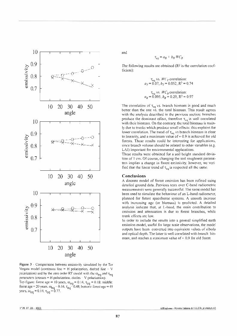
10 20 30 40 50 angle

10 20 30 40 50 angle

10 20 30 40 50 angle

Figure 3 - Comparisons between emissivity simulated by the Tor Vergata model (continuos line = H polht ion, dashed line = V polarkation) and by the zero order RT model with the o and zq e9 parameters (crosses = H polarization, circles =V polarization). Top figure: forest age = 10 years, mq = 0.14, zq = 0.18; middle: forest age = 20 years, W = 0.16, zq= 0.48; bottom: forest age = 45 years, oq=0.14, ~ ~ ~ 3 . 7 7 .

and

The following results are obtained (R2 is the correlation coefficient):

vs. WCT correlation: a, = 0.07, bT = 0.052, R2 = 0.74

VS. WCB correlation: a, = 0.095, b, = 0.29, R2 = 0.97

The correlation of vs. branch biomass is good and much better than the one vs. the total biomass. This resuit agrees with the analysis described in the previous section: branches produce the dominant effect, therefore is well correlated with their biomass. On the contrary, the total biomass is mainly due to trunks which produce small effects: this explains the lower correlation. The trend of zq vs branch biomass is close to linearity, and a maximum value of = 0.9 is achieved for old forests. These results could be interesting for applications, since branch volume shouid be related to other variables (e.g. LAI) important for environmental applications. These results were obtained for a soil height standard deviation of 1 cm. Of course, changing the soil roughness parameters implies a change in forest emissivity, however, we verified that the linea trend of zq is respected al1 the same.

Conclusions A discrete model of forest emission has been refined using detailed ground data. Previous tests over C-band radiometric measurements were generally successful. The same model has been used to simulate the behaviour of an L-band radiometer, planned for future spaceborne systems. A smooth increase with increasing age (or biomass) is predicted. A detailed analysis indicate that, at L-band, the main contribution to emission and attenuation is due to forest branches, while trunk effects are low. In order to include the results into a genera1 simplified earth emission model, useful for large scale observations, the model outputs have been converted into equivalent values of albedo and optical depth. The latter is well correlated with branch biomass, and reaches a maximum value of = 0.9 for old forest.

n' 28,27,28 - 2003 AITinforma - Rivista Italiane di TELERILEVAMENTO

87

References

Beckman P. and A. Spizzichino (1963) - The scattering of electromagnetic waves j b m rough sut$aces, Pergamon Press, Oxford.

Ferrazzoli P. and L. Guerriero (1995) - Radar sensifivity to tree geometry and woody volume: a mode1 analysis, IEEE Trans. Geosci. Remote Sensing, 33: 360-371.

Ferrazzoli P. and L. Guerriero (1996) - Passive microwave remote sensing of foresb: A mode1 investigation, IEEE Trans. Geosci. Remote Sensing, 34: 433-443.

Ferrazzoli P., L. Guerriero and J.-P. Wigneron (2002) - Simulating L-band emission of forests in view of future satellite applications, IEEE Trans. Geosci. Remote Sensing, 40: 2700-2708.

Fung A.K. and F.T. Ulaby (1978) - A scatter mode1 for leafj, vegetation, IEEE Trans. Geosci. electronics, 16: 28 1-285.

Jackson T.J. and T.J. Schmugge (1989) - Passive microwave sensing for soil moisture: some supporting research. IEEE Trans. Geosci. Remote Sensing, GE27: 225-235.

Karam M.A. (1 997) - A physical mode1 for microwave radiometry of vegetation, IEEE Trans. Geosci. Remote Sensing, 35: 1045-1058.

Kasischke E.S., N.L. Christensen and E.M. Haney (1994) - Modeling of geometric pmperties of loblolly pine tree stand characteristics for use in radar backscatter studies, IEEE Trans. Geosci. Remote Sensing, 32:800-822.

Kerr Y.H., Waldteufel P., Wigneron J.-P., Martinuzzi J.-M., Font J., and Berger M. (2001) - Soil moisture retrievalfrom space: the Soil Moisture and Ocean Salinity (SMOS) mmissn, IEEE Trans. Geosci. Remote Sensing, 39: 1729- 1735.

Kruopis N., J. Praks, A.N. Arslan, H.M. Alasalmi, J.T. Koskinen and M.T. Hallikainen (1999) - Passive microwave measurements of snow-covered forest areas in EMAC'95, IEEE Trans. Geosci. Remote Sensing, 37: 2699-2705.

Lang R.H., P. de Matthaeis, D.M. Levine, S. Bidweiì, M. Haken and N. Chauhan (2000) - L-band radiometer measurements of conferous forests, IGARSS 2000 Proceedings.

Macelloni G., S. Paloscia, P. Pampaloni, and R. Ruisi (2000) - Airborne mulh$-equency L- to Ka-band radiometric measurements over forests, IEEE Trans. Geosci. Remote Sensing, 39: 2507-25 13.

Wigneron J.-P., A. Chanzy, J.-C. Calvet and N. Bruguier (1 995) - A simple algorithm to retrieve soil moisture and vegetation biomass using passive microwave measurements over cropfields, Remote Sens. Environ., 51: 33 1-341.

Paloscia S., Pampaloni P., Chiarantini L., Coppo P., Gagliani S. and G. Luzi (1993) - Multiji-equency passive microwave remote sensing of soil moisture and roughness. int. J. Remote Sensing, 14: 467-483.

Wigneron J.-P., D. Guyon, J.-C. Calvet, G. Courrier and N. Bruguier (1 997) - Monitoring conifrous forest characteristics using a multifequency (5-90 GHz) microwave radiometer, Remote Sens. Environ., 60: 299-3 10.

Wigneron J.-P., Schmugge T., Chanzy A, Calvet J.-C. and Y. Kerr (1998) - Use of passive microwave remote sensing to monitor soil moisture. Agronomie, 18: 27-43.

Fenazrdi P. et al. no 26, n, 28 - m 88

Microwave remote sensing of snow melting

Anselmo Cagnati (l), Andrea Crepaz (f),Giovanni Macelloni (2), Simonetta Paloscia (2), Paolo Pampaloni Roberto Ranzi (34 Roberto Ruisi (2), Emanuele Santi (2), Marco Tedesco (2), Massimo Tomirotti (34 Mauro Valt (1) and Renato Zasso (1)

Abstract This work descnbes an experiment (MASMEX - Microwave Alpine Snow Melting Experiment) that was carried out in the spring of 2002 on the eastem Italian Alps which is aimed at studying the melting and refreezing cycles of snow by combining in-situ passive microwave measurements with conventional micrometeorological and snow data and modelling. The experiment pointed out the potential of microwave passive data (especially at 19 and 37 GHz) in detecting the melting refreezing-cycles of snow. Moreover, micrometeorological data has provided into the additional insight into the melting and refreezing processes in the snowpack and in the water percolation and heating of the soii. These data are needed in orda to simulate snowpack changes via a snowpack model that can provide some additional information (e.g. liquid water content, snow density and temperature) for interpretating radiometric data. They are especially in the application of remote sensing to the estimate of the areal water equivalent for water management and flood forecasting purposes in mountain basins, as well as for the prevention of avalanche hazards.

Riassunto In questo lavoro si presentano i primi risultati dell'esperimento MASMEX - Micmwave Alpine Snow Melting Experiment effettuato nella primavera del 2002 nelle Dolomiti con lo scopo di studiare il ciclo di furione e rigelo della neve combinando misure in-situ a micmonde con misure micmmeteorologiche, nivologiche e con un modello di simulazione del manto nevoso. L'esperimento ha posto in evidenza le potenzialità delle misure con sensori passivi allefiequenze delle micmonde (in particolare a 19 e 37 GHz) per il riconoscimento dei cicli di &ione-rigelo della neve. I dati micmmeteorologici mccolti hanno fornito delle indicazioni sui processi di tmsjèrimento di massa e calore nel manto nevoso e nel terreno. Questi dati sono necessariper definire le condizioni di flusso al con- forno del manto nevoso e consentire la simulazione di alcune variabili di stato (ad es. tempemhua, densità, contenuto d'acqua liqui- da della neve) che camtterizzano i suoi processi interni e consentono una migliore in tepaz ione dei dati mdiometrici. In pmspet- tiva si intuiscono applicazioni del telerilevamento a microonde con sensori atiivi e passivi per la gestione della risorsa idrica e la previsione di piena nei bacini montani e la prevenzione del rischio valanghivo.

Introduction Monitonng the areal snow water equivalent in mountain water- sheds and modeling the melting cycle of snow have a significant importante for the management of water resources, and for flood and avalanche forecasts. Moreover, a well tuned radiative model can be a useful t001 for interpreting remote sensing data collected in area where local measurements are not available or when remote sensing using optical sensors is inhibited by the presence of clouds.

(l) ARPAV - Centro Sperimentalevalanghe di ArabbqVia Pradat 5- - 320202 Arabba (BL), Italia. Istituto di Fisica Applicata, iFAC - CNR, via Panciatichi 64 - - 50127 Firenze, Italia. e-mail: [email protected]

(3) Dipartimento Ingegneria C i Università degli Studi di Brescia, Via Bnuize 38 - 25123 Brescia, Italia.


The abilitv of the microwave radiometer to monitor seasonal variations in snow cover, and in particular snow melting, has been the subject of severa1 experimental and theoretical investigations [e.g. Ulaby et al., 1986; Tsang et al., 20001. Measurements canied out between 3 GHz and 90 GHz have pointed out the sensitivity of rnicrowave emission to snow type and water equivalent. At the lower frequencies, emission fiom dry snow is mostly idluenced by the soii conditions and by snow layering. At the higher frequencies, however, the role played by volume scattering increases, and emissivity appears to be sensitive to the snow water equivalent u a b y et al., 19861. If snow melts, the presence of liquid water in the surface layer determines an increase in ernissivity, especially at high frequencies [Parnpaloni et al., 20011, due to the transition from volume to surface scattering. The average spectra of the brightness temperature Tb show that the Tb of dry and refiozen snow decrease; with frequency, whereas the Tb of wet spring snow increases [Macelloni et al., 20011. in some cases, the spectral behaviour of wet snow shows a slight increase with frequency; due to the increasing effect of surface roughness [Schanda et al., 19831.

n' 2627.28 - 2003 AITinfoma - Rivista Italiana di TELERILEVAMENTO

89

The physical and radiative properties of snow change extensively with the meteorologica1 and geographical conditions of the snowpack and the metarnorphism of ice crystals. The presente of liquid water within the snow pack causes rapid changes in the ice grains that compose the pack. During the melting process, typical grains of dry snow are transformed into big rounded grains that rapidly increase up to dimensions of 1-2 mm. During the night refreezing phase, which usually involves the first 10 cm of the snow cover, the crystals aggregate in a polycrystalline grain, fonning surface crusts of considerable hardness. This transformation impacts on the physical properties of snow which change in accordante with the daily melting-refreezing cycles and the fluxes of heat and moisture in the snowpack. This paper describes an experiment carried out on the Italian Alps, which was aimed at studying the melting cycle of snow by combining microwave remote sensing measurements with ground and micrometeorological data. In the first section, the snowpack heat balance that drives the internal changes of snow is presented. In the second, the experimental set-up is described. In the third one, the results are discussed with reference to two monitoring periods, the first in early spring and the last one, at the end of the snow melting.

Interaction between snowpack, atmosphere and terrain Since the conversion from ice to water requires the input of heat, the process of snowmelt is linked to the flow and storage of energy in the snowpack. The sources of energy that cause snowmelt include both short-wave and long-wave net radiation (H,, and H/,, respectively), convection from the air H, (sensible energy), vapor condensation HI (latent energy), and conduction to the ground Hg, as well as the advective heat of precipitation H,. These fluxes are measured as WJm*. The energy budget equation that describes the energy available for snowmelt, H,, can be written in the forrn [Male and Granger, 198 1 ; Ranzi and Rosso, 19911:

where H, denotes the rate of change in the internal energy stored in the snow per unit area of the snowpack. Radiative energy is the prime source of energy at the Earth's surface. Some of this energy is solar or short-wave radiation H,, and terrestrial or long-wave radiation H!,. These terms are generaily referred to as net radiation, H,. Short-wave radiation is the most irnportant source of energy for snowmelt. The amount of energy available for the snowpack from the incoming short-wave radiation, 4, is H,=(l-a) I, where a denotes the albedo. Values of arange from more than 80% for new-fallen snow to as little as 40% for melting, late-season, ripe snow. Some of the energy absorbed by the snowpack fiom solar radiation is radiated to the atrnosphere in the form of long-wave radiation according to the Stefan-Boltzmann law. In contrast to

this is the incoming long-wave radiation from the atmosphere, the surrounding terrain and forest c m r . Thus, net radiation heat flux H, can be expressed by the equation:

where E,, E , ~ , o T, and T,@ denote, respectively, the emissivity of the snow (E, = 0.99 for clean snow) and of the sky, the Stefan-Boltzmann constant and the temperature of the snow and the sky. Energy is also exchanged between the snowpack and atmosphere through the processes of convection (sensible heat) and condensation (latent heat). The relative importance of these processes differs widely, depending on the clirnatological and local weather conditions. For the spring period described in this paper, when the snow albedo decreases, the air temperature is just above O°C, and the relative humidity in low turbulent fluxes are of secondary importance, compared with radiation. The upward ground heat flux can be related to soil temperature gradients measured near the surface:

where z is the vertical coordinate (positive upward) and K in the thermal conductivity of the soil. When an isothermal temperature profile is established in the ground, as happens during the snowmelt period, heat conduction to the ground is a very small component in the overall energy budget, especially when compared with the radiation and the turbulent exchange at the airlsnow interface.

The Experiment The main purpose of this investigation was to study the melting-refreezing cycle of snow as well as the radiation budget and water balance after soil thawing. To this end, nivological, micrometeorological and microwave remote sensing me&ure- ments were carried out from March 20% 2002 to June 30", 2002. At the beginning of the experiment, the snow cover on the test site was about 35 cm deep; severa1 snowfails occurred in Apri1 and the terrain was snow covered unti1 May 10th. After May lo", the experiment dealt with the measurements of water balance and radiation budget. The experiment took place on the Mount Cherz plateau located at 2000 m a.s.1. in the basin of the Cordevole river (Fig. 1) in the eastern Italian Aivs. The main characteriskcs of the Cordevole area are summarized in Table 1. This site was selected for the study, due to its relatively smooth topography and the availability of historical data and a digital elevation model. The activities were managed by IFAC-CNR, Florence, Italy, for the microwave measurements; CVA- Centro Valanghe, Arabba, Italy, which contributed nivological and meteorologica1 data; and the Department of Civil Engineering of University of Brescia, Italy, khich carried out the micrometeorological measurements.

Cagnati A. et al. n"26.27.26-2003

90

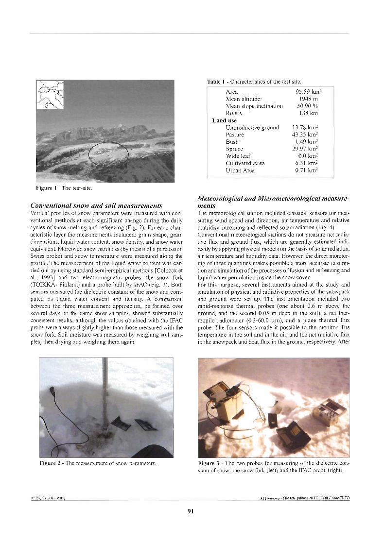
Figure 1 - The test-site.

Conventional snow and soil measurements Vertical profiles of snow parameters were measured with conventional methods at each significant change during the daily cycles of snow melting and refreezing (Fig. 2). For each characteristic layer the measurements included: grain shape, grain dirnensions, liquid water content, snow density, and snow water equivalent. Moreover, snow hardness (by means of a percussion Swiss probe) and snow temperature were measured along the profile. The measurement of the liquid water content was carried out by using standard semi-empirical methods [Colbeck et al., 19931 and two electromagnetic probes: the snow fork (TOiKKA- Finland) and a probe built by IFAC (Fig. 3). Both sensors measured the dielectric constant of the snow and computed its liquid water content and density. A comparison between the three measurement approaches, performed over several &ys on the same snow samples, showed substantially consistent results, aithough the values obtained with the IFAC probe were always slightly higher than those measured with the snow fork. Soil moisture was measured by weighing soil samples, then drymg and weighg them again.

Table 1 - Characteristics of the test site.

Area Mean altitude: Mean slope inclination Rivers

Land use Unproductive ground Pasture Bush Spruce Wide leaf Cultivated Area Urban Area

Meteorologica1 and Micrometeorological measurements The meteorologica1 station included classica1 sensors for measuring wind speed and direction, air temperature and relative humidity, incoming and reflected solar radiation (Fig. 4). Conventional meteorologicai stations do not measure net radiative flux and ground flux, which are genediy estirnated indi- rectly by applying physical models on the basis of sola radiation, air temperature and humidity data. However, the direct monitoring of these quantities makes possible a more accurate description and simulation of the pmcesses of fusion and refieezing and liquid water percolation inside the snow cover. For this purpose, several instniments airned at the study and simulation of physical and radiative properties of the snowpack and ground were set up. The instrumentation included two mpid-response thermal probes (one about 0.6 m above the ground, and the second 0.05 m deep in the soil), a net ther- mopile radiometer (0.3-60.0 p), and a plane thermal flux probe. The four sensors made it possible to the monitor. The temperature in the soil and in the air, and the net radiative flux in the snowpack and heat flux in the ground, respectively. After

Figure 2 - The measurement of snow parameters. Figure 3 - The two probes for measuring of the dielectric constant of snow: the snow fork (left) and the IFAC probe (right).

n' 26,27,28 - 2003 AiTinfoma - RIvIsia liallana di TELERILEVAMENTO

91

- The IFAC-ground based microwave radi ometers.

Table 2 - Characteristics of microwave radiometers.

kequency Polarization Incidente Angle Accuracy 1.4 GHz* Y H 6.8GHz Y H 550 fixed * 0.5 K

19 GHz** V, H, * 450 + 37 GHz Y H, * 450 300 -700 scaming

* after May 20th ** until May 10"

the snow had completly melted, (from the middle of May until the end of June), a tipping-bucket raingauge and TDR probe were installed at the Cherz site to monitor continuously aiso the soil moisture content, which is another variable that influences the rnicrowave radiative properties of the terrain.

Microwave measurements A set of rnicrowave and infrared radiometers was installed in a special container near to the meteorologicai station (Fig. 5). The main characteristics of the microwave radiometers are summarized in Table 2. The infrared sensor operated at 8-12 rnicron wavelengths. Multi-frequency radiometric data were coliected at C-band (6.8 GHz), Ku (19 GHz), and Ka-band (37 GHz) on snow-covered soils from March 20" 2002 to May 10th 2002, and at 1.4, 6.8 and 37 GHz on bare soil from May 20 to June 30" 2002. The sensors operated 24 hours Iday at an angle of 55O incidence. Angular scans between 30 and 70 degrees were car- ned out in specific conditions.

The Results Here, we report data obtained at two different time periods: One, between March 30" and April 5", when the snow cover, about 35 cm depth, was characterized by a reguiar succession

of melting and refreezing cycles, the other, between May 1st and May 20", was characterized by a sequence of rains and snowfall events, and also melting-refreezing cycles, with the progressive disappearance of the snow cover.

First period (March 30 - April 5) A progressive drop in the average daily air temperature, which after April 3rd changed from positive to negative values, characterized the first period (Fig. 6). During this transition phase, the minirnurn temperature was always negative during the night originating a series of melting and refreezing cycles of lower intensity in the night originating between April 2nd and 3d, when the sky was slightiy cloudy and the temperature remained close to 00 C (Fig. 7). The sky was clear for most of the day, with some cloudiness in the afternoon. On April 2nd, the snow was 30 cm deep with a temperature close to OOC and wetness between 0-3% and 3-8% (measured with conventional method). The grain shapes indicated an expansion of the melting process down to the base of the snow pack, where a basal layer composed of wet grains (classified as 6c according to the conventional snow-grain scale) mixed with various shapes of angular grains (4c) was present. This layer was separated from the overlaying layers by a small crust (9e), due to a melting-refreezing process. Crusts due to these processes were also present in the surface

Cagnaii A. el al. no 26,27,28 - 2003 92

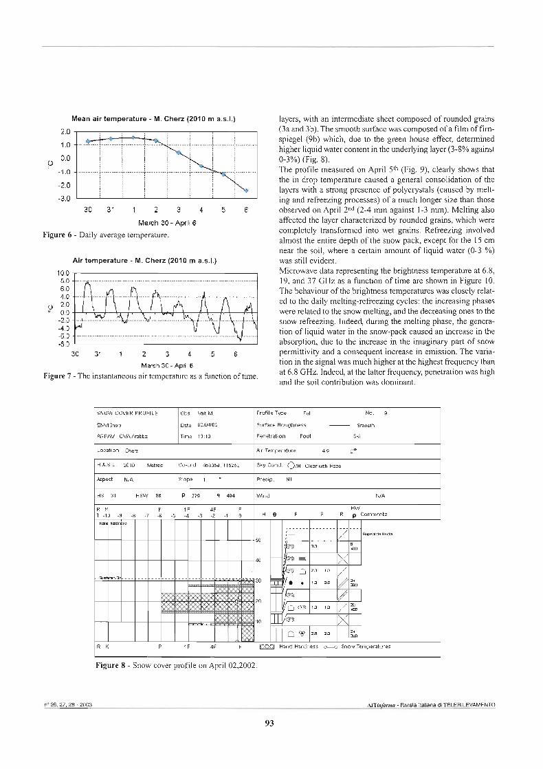
Mean air temperature - M. Chetz (2010 m a.s.1.)

2.0

1 .o 0.0 0 -1.0

-2.0

-3.0 3 0 3 1 1 2 3 4 5 6

March 30 - Aprll 6

Figure 6 - Daily average temperature.

Air temperature - M. Chetz (2010 m a d . )

3 0 3 ' 1 2 3 4 5 6 March 3C - Apdl6

Figure 7 - The instantaneous air temperature as a function of time.

layers, with an intermediate sheet composed of rounded grains (3a and 3b). The smooth surface was composed of a film of firn- spiegel (9b) which, due to the green house effect, determined higher liquid water content in the underlying layer (3-8% against O-3%) (Fig. 8). The profile measured on April 5" (Fig. 9), clearl'j shows that the in drop temperature caused a genera1 consolidation of the layers with a strong presence of polycrystals (caused by melting and refreezing processes) of a much longer size than those observed on April 2nd (2-4 mm against 1-3 rnm). Melting also affected the layer characterized by rounded grains, which were completely transformed into wet grains. Refkezing involved almost the entire depth of the snow pack, except for the 15 cm near the soil, where a ceriain amount of liquid water (0-3 %) was still evident. Microwave data representing the brightness temperature at 6.8, 19, and 37 GHz as a function of time are shown in Figure 10. The behaviour of the brightness temperatures was closely related to the daily melting-refreezing cycles: the increasing phases were related to the snow melting, and the decreasing ones to the snow refkezing. Indeed, during the melting phase, the generation of liquid water in the snow-pack caused an increase in the absorption, due to the increase in the imaginary part of snow permittivity and a consequent increase in emission. The variation in the signal was much higher at the highest frequency than at 6.8 GHz. Indeed, at the latter fkquency, penetration was high and the soil contribution was dominant.

Surfaoe Roughness - Srnooth

Figure 8 - Snow cover profile on April 02,2002.

n", 27,28 - 2003 m l i l f o m - Rivtsta Italiana di TELERILEVAMENTO

93

Figure 9 - Snow cover profile on Apnl05,2002.

Figure 10 - The brightness temperature at 6.8 GHz (top), 19 GH (medium) and 37 GHz (bottom) as a function of time between March 30 and Apri1 15,2002.

E 300 H 280 i.; l- 200 I:::

30W 31W Il4 W W4 U4 M 6M

Dato

E300 - 'g- 5 260 240

220

200

180

160 30/3 3113 IM W 3H U4 M 6/)

Dale

300

280 i :: 220

200

180

180 30W 31W 1H Y1 W U4 M W4

M e

Cagnati A. et ai. no 26.27,28 - 2003

94

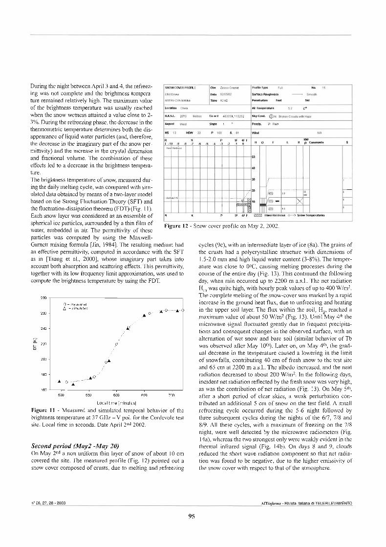
During the night between April 3 and 4, the refreezing was not complete and the brightness temperature remained relatively high. The maximum value of the brightness temperature was usually reached when the snow wetness attained a value close to 2- 3%. During the r e m g phase, the decrease in the thermometric temperature determines both the disappearance of liquid water particles ( a d , therefore, the decrease in the irnagimry part of the snow per- rnittivity) and the inmase in the crystal dimension and fractional volume. The wmbination of these effects led to a decrease in the brightness temperature. The brightness temperature of snow, measured during the daily melting cycle, was compared with simulated data obtained by means of a two-layer mode1 based on the Strong Fluctuation Theory (SFT) and the fluctuation-dissipation theorem (FDT) (Fig. 1 1). Each snow layer was considered as an ensemble of spherical ice particles, surrounded by a thin film of water, embedded in air. The permittivity of these

Figure 12 - Snow cover profile on May 2,2002.

particles was computed by using the Maxwell- Garnett mixing formula [ J i i 19841. The resulting medium had an effettive permittivity, computed in accordante with the SFT as in psang et al., 20001, whose imaghmy part takes into account both absorption and scattering effects. This pennittivity, together with its low fresuency lirnit approximation, was used to compute the brightness temperature by using the FDT.

Local time [tninutes]

Figure 11 - Measured and simulated temporal behavior of the brightness temperature at 37 GHz -V pol. for the Cordevole test site. Local time in seconds. Date April 2nd 2002.

Second period (May2 -May 20) On May 2nd a non uniform thin layer of snow of about 10 cm covered the site. The measured profile (Fig. 12) pointed out a snow cover composed of crusts, due to melting and refreezing

cycles (9c), with an intermediate layer of ice (8a). The grains of the crusts had a polycrystalline strutture with dimensions of 1.5-2.0 rnm and high liquid water content (3-8%). The temperature was close to OOC, causing melting processes during the course of the entire day (Fig. 13). This continued the following day, when rain occurred up to 2200 m a.s.1.. The net radiation H,,, was quite high, with hourly peak values of up to 400 WIm2. The complete melting of the snow-cover was marked by a rapid increase in the ground heat flux, due to unfreezing and heating in the upper soil layer. The flux within the soil, Hg, reached a maximum value of about 50 WIm2 (Fig. 13). Unti1 May 4" the microwave signal fluctuated greatly due to frequent precipitations and wnsequent changes in the observed surface, with an altemation of wet snow and bare soil (similar behavior of Tb was observed after May 1 0 ~ ) . Later on, on May 4", the gradual decrease in the temperature caused a lowering in the limit of snowfalls, contributing 40 cm of k s h snow to the test site and 65 cm at 2200 m a.s.1.. The albedo increased, and the neat radiation decreased to about 200 WIm2. In the following days, incident net radiation reflected by the fresh snow was very high, as was the contribution of net radiation (Fig. 13). On May 5", after a short penod of clear skies, a weak perturbation contributed an additional 5 cm of snow on the test field. A small refreezing cycle occurred during the 5-6 night followed by three subsequent cycles during the nights of the 617, 718 and 819. Al1 these cycles, with a maximum of freezing on the 718 night, were well detected by the microwave radiometers (Fig. 14a), whereas the two strongest only were weakly evident in the thermal infrared signal (Fig. 14b). On days 8 and 9, clouds reduced the short wave radiation component so that net radiation was found to be negative, due to the higher emissivity of the snow cover with respect to that of the atmosphere.

n' 26,27.28 - 2003 AiTinfom - Rlvista Italiana di TELERILR/AMENTO

95

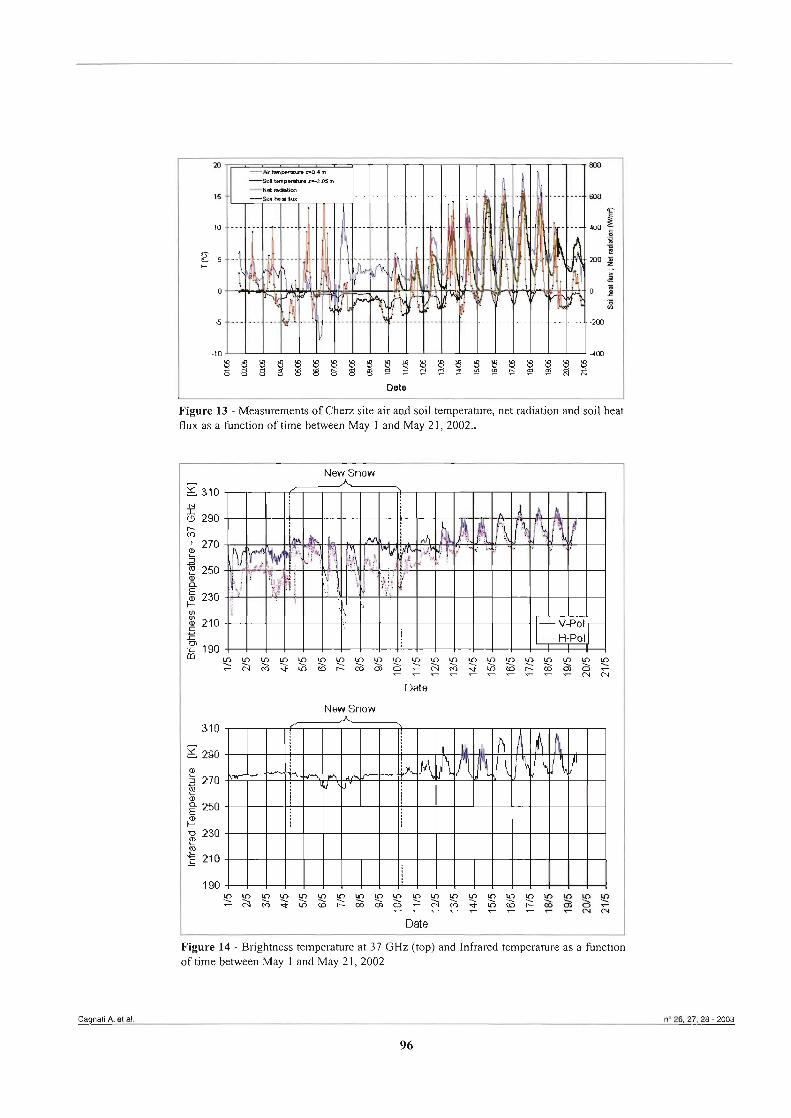
Figure 13 - Measurements of Chen site air and soil temperature, net radiation and soil heat flux as a function of time between May 1 and May 2 1,2002..

New Snow

E 310

g 290 m I 270

P 230 l- u, g 210

C 1, m m m m m m m m w m m m m m m m m m m m m m : h a 2 a h k a a ~ ~ s $ $ ~ ~ ~ ~ g g $

Date

310

Y 290

f! $ 270

E 250

P 'P 230 m

210 -

1 90 e m m q m m m w m m m m m m m m m m m m m - h a * h h 2 a a $ ~ $ $ ~ $ ~ ~ ~ $ Q $

Date

Figure 14 - Brightness temperature at 37 GHz (top) and Infrared temperature as a function of time between May 1 and May 2 1,2002

Cagnaii A. et al. no 26,27.28 - 2003

96

The ground heat flux also decreased, because a more homogeneous temperature profile was likely to be re-established in the ground. On May 10h the snow cover disappeared and the soil began to warm up definitely. Consequently, vertical temperature gradients built up and ground flux rapidly increased up to about 100 W/m2. A heating front propagated downward into the ground unti1 an equilibrium temperature profile was reached. A corresponding mean ground flux of about 30 Wim2 was recorded during the period May 16-18. During May 19-20 the decrease in solar radiation and air temperature marked a rainfall event with 17.6 and 8.6 rnrn, respectively. The mean ground flux increased, possibly because the percolated water changed the thermal behaviour of the upper soil layer.

Conclusions The experiment performed pointed out the potential of multisensor measurements in characterizing different states of snow cover. In particular, microwave radiometry was found to be very sensitive in detecting the melting refreezing-cycles of snow. High amplitude fluctuations of the brightness temperature at 19 an4 even more, 37 GHz were related to changes in the liquid water content and to the dirnension of snow crystals. These fluctuations were limited when the night refreezing was uncomplete in the upper snow layers. Data at 37 and 19 GHz were sensitive to the snow conditions in the upper

References

Colbeck S., Akitaya E., Armstrong R., Gubler H., Lafeuille J., Lied K., McClung D. and Morris E. (1990) - International Classzjìcation for Seasonal Snow on the Ground. International Com- mission for Snow and Ice (IAHS). World Data Center A for Glaciology, University of Colorado, Boulder, CO, USA.

Ji Y.-Q. (1984) - Wave appmach to brightness temperature from a bounded layer of random discrete scatterers. Electromagnetics, 4: 323-341.

Jin Y.-Q. and Kong J.A. (1984) - Stmngfluctuation theory of electmmagnetic wave scattering by a layer of random discrete scatterers. Journal of Applied Physics, 55: 1364-1 369.

Maceiioni G., Paloscia S., Pampaloni P. and Tedesco M. (2001) - Microwave Emissionfim Dry Snuw: A Comparison of Experimental and Model Result. IEEE Trans. Geosci. Remote Sensing, 39 (12): 2649-2656.

Male D. H. and Granger R. J. (198 1) - Snow Su$ace Energy Exchange. Water Resources Research, 17 (3): 609-627.

layers, while at 6.8 GHz penetration was high and the contribution of soil was dominant. Because of the influente of sev- era1 snow parameters on the microwave data, detailed information on the snowpack was needed for their interpretation. In the MASMEX 2002 experiment, severa1 snow profiles were collected from in-situ investigations. In non monitored sites, however, snowpack simulation seemed to be the only viable solution for this purpose. Micrometeorological data such as net radiation, soil temperature and heat flux provided additional insight on the melting and refreezing processes in the snowpack and in the water percolation and heating of the soil. These data could be used fmitfully to simulate snowpack changes, and to test the potential benefit provided by a physical snowpack mode1 based on meteorologica1 measurements for interpreting radiometric data. Within this perspective, the point measurements and their interpretation presented here could be extended to microwave data collected by passive and active (SAR) instruments air- and satellite-borne in order to make an estimate of the snow cover for hydrological purposes and to detect potential avalanches.

Acknowledgments This work was supported in part by the European Cornmission ENVISNOW project EVG2-2001-00018, by the Italian Space Agency and by GNDCI - CNR (U02.48).

Pampaloni P., Macelloni G., Paloscia S. and Tedesco M. (2001) - Multi-Frequency Micmwave EmissionJi.om Wet Snow. A Comparison of Experimental Results and Model Simulations. Proc. Int. Geosci. Remote Sensing Symp. (IGARSS 2001), Sydney: 810-812.

Ranzi R. and Rosso R. (1991) - A physically based approach to modelling distributed snowmelt in a small alpine catchment, in: Snow Hydrology and Forests in High Alpine Areas. Edited by H. Bergrnann, H. Lang, W. Frey, D. Issler & B. Salrn, IAHS Publ., 205: 141-150.

Schanda E., Matzler C. and Kunzi K. (1983) - Micmave Remote Sensing of Snow Covez Int. J. Remote Sensing, 4: 149-158.

Tsang L.J., Kong A. and Ding K.H. (2000) - Scattering of Electromagnetic waves. Wiley&Sons, New York.

Ulaby ET., Moore RK. and Fung A.K. (1986) - Microwave Remote sensing: Active and Passive. Vol m, Dedham, MA: Artech House.

n" 26,27.28 - 2003 AITinforma - Ri ta Italiana di TELERILEVAMENTO

97

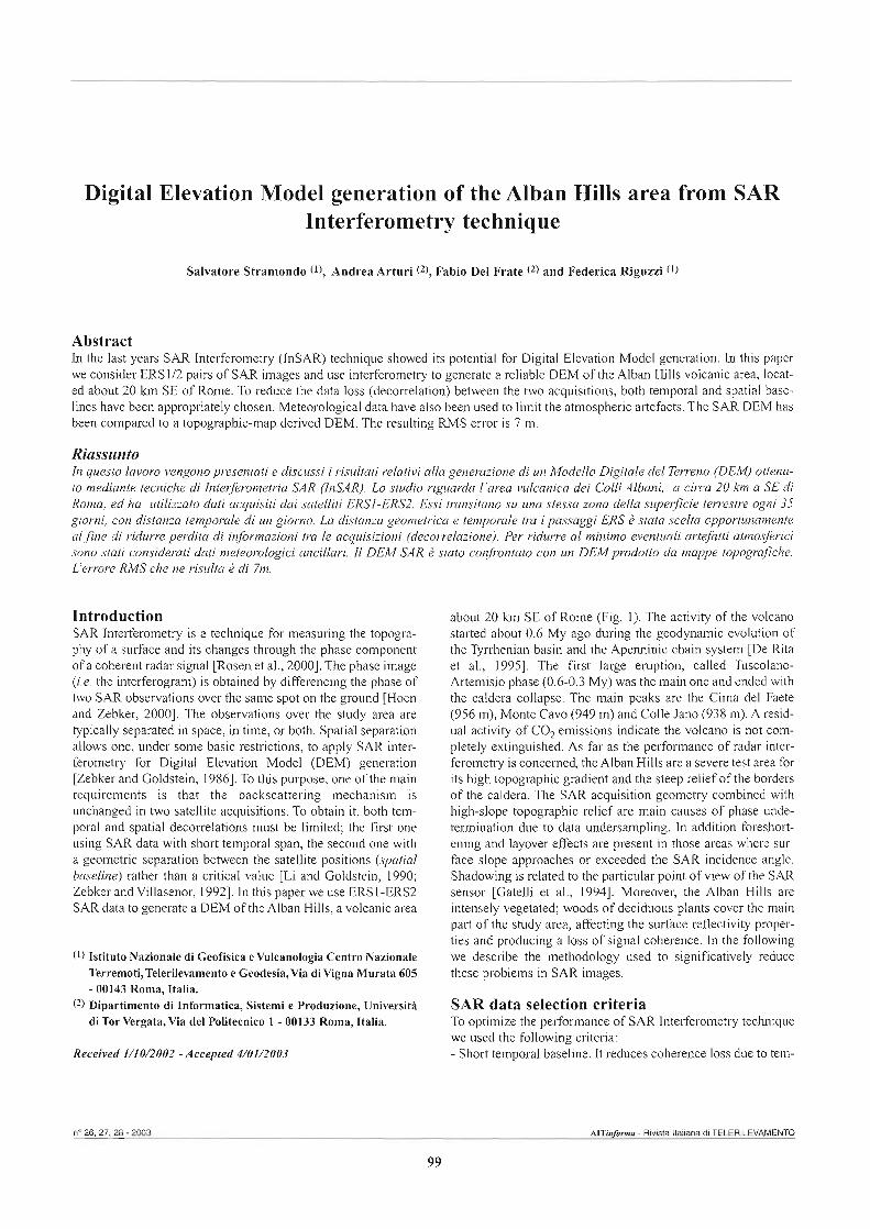
Digital Elevation Model generation of the Alban Hills area from SAR Interferometry technique

Salvatore Stramondo (l), Andrea Arturi (2), Fabio Del Frate (2) and Federica Riguzzi (l)

Abstract in the last years SAR Interferometry (InSAR) technique showed its potential for Digital Elevation Model generation. In this paper we consider ERSlI2 pairs of SAR images and use interferometry to generate a reliable DEM of the Alban Hills volcanic area, located about 20 km SE of Rome. To reduce the data loss (decorrelation) between the two acquisitions, both temporal and spatial base- lines have been appropriately chosen. Meteorological data have also been used to limit the atmosphenc artefacts. The SAR DEM has been compared to a topographic-map derived DEM. The resulting RMS error is 7 m.

Riassunto In questo lavoro vengono presentati e discussi i risultati relativi alla generazione di un Modello Digitale del Terreno (DEM, ottenu- to mediante tecniche di Inter$erometria SAR (InSAR). Lo studio riguarda l'area vulcanica dei Colli Albani, a circa 20 km a SE di Roma, ed ha utilizzato dati acquisiti dai satelliti ERSI-ERS2. Essi transitano su una stessa zona della supeficie terrestre ogni 35 giorni, con distanza temporale di un giorno. La distanza geometrica e temporale ira i passaggi ERS è stata scelta opportunamente alfine di ridurre perdita di informazioni tra le acquisizioni (decorrelazione). Per ridurre al minimo eventuali artefatti atmosferici sono stati considerati dati meteorologici ancillari. Il DEM SAR è stato confrontato con un DEMprodotto da mappe topograjìche. L'errore RMS che ne risulta è di 7m.

Introduction SAR Interferometry is a technique for measuring the topography of a surface and its changes through the phase component of a coherent radar signal [Rosen et al., 20001. The phase image (i.e. the interferogram) is obtained by differencing the phase of two SAR observations over the same spot on the ground [Hoen and Zebker, 20001. The observations over the study area are typicaily separated in space, in time, or both. Spatial separation aiiows one, under some basic restrictions, to apply SAR interferometry for Digital Elevation Model (DEM) generation [Zebker and Goldstein, 19861. To this purpose, one of the main requirements is that the backscattering mechanism is unchanged in two satellite acquisitions. To obtain it, both temporal and spatial decorrelations must be limited; the first one using SAR data with short temporal span, the second one with a geometric separation between the satellite positions (spatial baseline) rather than a critica1 value [Li and Goldstein, 1990; Zebker and Villasenor, 19921. In this paper we use ERS1-ERS2 SAR daia to generate a DEM of the Alban Hills, a volcanic area

(1) Istituto Nazionale di Geofisica evulcanologia Centro Nazionale Terremoti, Telerilevamento e Geodesia, Ma di Vigna Murata 605 - 00143 Roma, Italia.

(2) Dipartimento di Informatica, Sistemi e Produzione, Università di Tor Vergata, Via del Politecnico 1 - 00133 Roma, Italia.


about 20 krn SE of Rome (Fig. 1). The activity of the volcano starìed about 0.6 My ago during the geodynamic evolution of the Tyrrhenian basin and the Apenninic chain system [De Rita et al., 19951. The first large eruption, called Tuscolano- Artemisio phase (0.6-0.3 My) was the main one and ended with the caldera collapse. The main peaks are the Cima del Faete (956 m), Monte Cavo (949 m) and Colle Jano (938 m). A resid- ual activity of C02 emissions indicate the volcano is not completely extinguished. As far as the performance of radar interferometry is concerne4 the Alban Hills are a severe test area for its high topographic gradient and the steep relief of the borders of the caldera. The SAR acquisition geometry combined with high-slope topographic relief are main causes of phase undetermination due to data undersampling. In addition foreshort- ening and layover effects are present in those areas where surface slope approaches or exceeded the SAR incidence angle. Shadowing is related to the particular point of view of the SAR sensor [Gateiii et al., 19941. Moreover, the Alban Hills are intensely vegetated; woods of deciduous plants cover the main part of the study area, affecting the surface reflectivity properties and producing a loss of signal coherence. In the following we describe the methodology used to significatively reduce these problems in SAR images.

SAR data selection criteria To optimize the performance of SAR Interferometry technique we used the following criteria: - Short temporal baseline. It reduces coherence loss due to tem-

n' 28.27.28 - 2003 ~ITinfonna - RMsta Italiana di TELERILEVAMENTO

99

Figure 2 - Repeat-pass interferometry geometry: S, and S2 indicate the satellite positions, b1 is the baseline component perpendicular to r,, H the satellite altitude.

Figure 1 - SPOT image of the Alban Hills area. The position of this Table l - Meteorological Meteosat data relative to the dates of SAR area of Italy is shown by a white box in the left image. images acquisitions.

poral decorrelation; in particular we used two Tandem pairs (1- day delay between the SAR acquisitions). - Spatial baseline. The geometric separation of the two satellite positions produces signal decorrelation that increases the differences in the acquisition geometry. For DEM generation we must respect a compromise between two requirements: the sensitivity to the topography and the limitation due to the critical baseline. The first is ensured by a baseline large enough to obtain a small altitude of ambigui& (h,, i.e. the altitude variation producing a phase change of 2x) [Rosen et al., 20001:

where h is the wavelength (as for ERSI-ERS2 it is 5.6 cm, C- band), bl is the baseline component perpendicular to the satellite-surface line of sight, is the look angle and r, is the satellite- to-ground distance (Fig. 2). On the other side, phase unwrapping problems might arise for very large baseline values. Moreover, to avoid a complete decorrelation of the interferometric image pair, we must choose a baseline with a critical value less than b, [Zebker and Villasenor, 19921:

3L.q b, = with the SAR ground range resolution.

2r(, c0s2 8' - Meteorological data. To reduce the atmospheric effects, only SAR data characterized by low values of the most significant weather parameters (cloudness) as inferred from the Meteosat information (see Tab. 1) have been selected, where:

N: cloudness (0-8) DD: wind direction FF: wind speed (marine mile) TT: temperature Td: dew temperature U,.=[100 -(TT-Td).5%] relative umidity ww: recorded weather

values 0-39 = good weather 40-49 = fog 50-69 = rain 70-79 = snow 80-99 = storm

- Ascending and descending images. Due to the geometry of the study area, especially in the Alban Hills caldera, the use of two different viewpoints allows one to resolve some phase indeterminations. - According to the criteria described above we selected six SAR ERS I-ERS2 raw scenes (Tab. 2).

Table 2 - SAR ERS1-ERS2 raw data selected.

Satellite Acquis. Geom. Orbit 1378 1 05/03/94

Descending 13867 11/03/94 Ascending 24709 05/04/96

E2 Ascending 05036 06/04/96 E1 Ascending 43747 261 1 1 199 E2 Ascending 24074 2711 1/99

Track R a m e 22 2763 22 2763 172 0837 172 0837 172 0828 172 0828

Stramondo S. et al. n' 26,27.28 - 2M)3

100

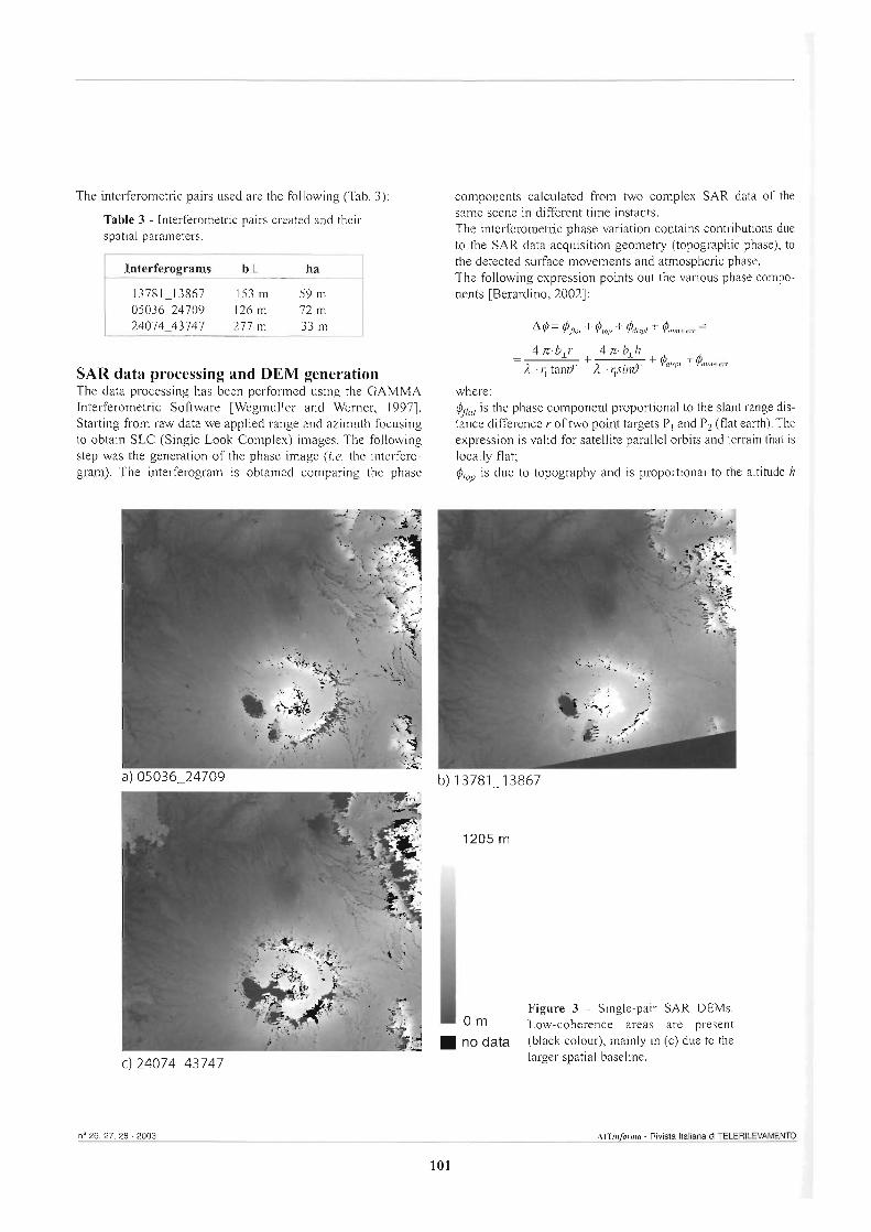
The interferometric pairs used are the following (Tab. 3):

Table 3 - Interferometric pairs created and their spatial parameters.

SAR data processing and DEM generation The data processing has been performed using the GAh4h4A Interferometric Software [Wegmuller and Werner, 19971. Starting from raw data we applied range and azimuth focusing to obtain SLC (Single Look Complex) images. The following step was the generation of the phase image (i.e. the interferogram). The interferogram is obtained comparing the phase

components calculated from two complex SAR data of the sarne scene in different time instants. The interferometric phase variation contains contributions due to the SAR data acquisition geometry (topographic phase), to the detected surface movements and atmospheric phase. The following expression points out the various phase components [Berardino, 20021:

where: @/r(I, is the phase component proportional to the slant range dis- tante differente r of two point targets P, and P2 (flat earth). The expression is valid for satellite parallel orbits and terrain that is locally flat;

is due to topography and is propdonal to the altitude h

1

no data (black colour), mainly in (C) due to the larger spatial baseline.

no 26,27,28 - XXM AIThfonne - Rivista italiana di TELERILNAMENR)

101

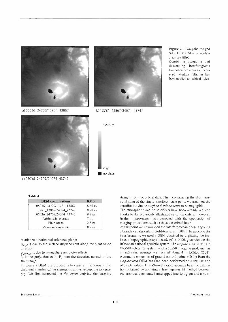
Table 4

i i no data

05036-2470911378 1-13867 8.60 m 1378 1-1 3867124074-43747 8.70 m 05036-24709124074-43747 9.7 m

Arithrnetic average 7 m Plain areas 2.6 m

Mountaneous areas 8.7 m

relative to a horizontal reference plane; is due to the surface displacement along the slant range

direction; &,+, is due to atmosphere and noise effects; h, is the projection of P,-P2 onto the direction norma1 to the slant range. To create a DEM our purpose is to erase al1 the terms in the right-end member of the expression above, except the topography. We f i t corrected the jlat earth deriving the baseline

Stramondo S. et ai.

Figure 4 - Two-pairs merged SAR DEMs. Most of nodata areas are filled. Combining ascending and descending interferograms low coherence areas are recov- ered. Median filtering has been applied to residua1 holes.

straight from the orbita1 data. Then, considering the short temporal span of the single interferomebic pairs, we assumed the contribution due to suflace displacements to be negligible. The atmospheric and noise effects have been already reduced thanks to the previously illustrated selection criteria; however, further improvernent was expected with the application of merging procedures such as those described later . At this point we unwrapped the interferometric phase applying a branch-cut algorithm [Goldstein et ai., 19881. To geocode the interferograms we used a DEM obtained by digitizing the iso- lines of topographic maps at scale of 1 : 10000, geocoded on the ROMA40 national geodetic system. The map-derived DEM is in WGS84 reference system, with a 50x50 m regular grid, and has an estimated average accuracy of about 4 m [Kolbl, 20011. Automatic extraction of ground contro1 points (GCP) from the map-derived DEM has then been performed on a regular grid of 32x32 values. This ailowed a more accurate baseline estirna- tion obtained by applying a least squares fit method between the previously generated unwrapped interferograrn and a num-

no data O m 1205 m

no data

Figure 5 - Comparison between mapderived DEM (a) and three-pairs-averaged SAR DEM (b). Figure (C) shows the map of differences: extreme differences (absolute value greater than RMS) are in white (positive differences) and black (negative differences) areas. In (4 the histogram of the distribution of RMS values is reported: x axis shows the residue (m), y axis the number of pixels.

n" 26,27,28 - 2003 AITbfom - Riisia Italiana di TELERILEVAMENTO

103

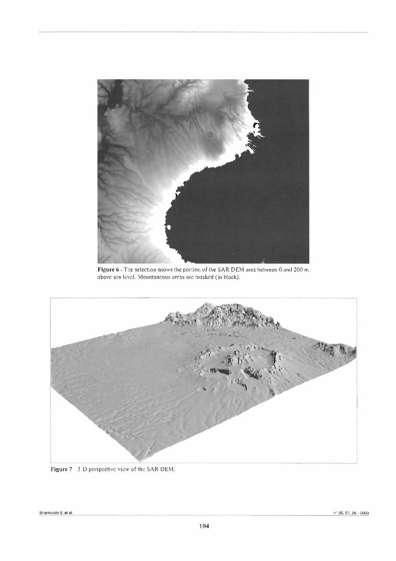
Figure 6 - The selection shows the portion of the SAR DEM area between O and 200 m above sea level. Mountaneous areas are masked (in black).

Stramondo S. ei ai. no 26.27,28 - 2003

104

ber of contro1 points in the grid [Wegmuller and Werner, 19971. The resulting more accurate baseline value was finally considered to optimise the conversion of the unwrapped interferometric phase to topographic heights. The so far descnbed methodology allowed to yield the three SAR DEMs shown in Figure 3. We see that each DEM is characterized by a number of black areas (no data areas). These are due to the phase undetermination factors described above, which caused the resulting DEMs to have some regions with very low coherence. The main part is located in and around the Alban Hills caldera, because of the high slope angles. In particular the DEM in Figure 3c, obtained by the 24074-43747 image pair, has a large spatial baseline that induces decorrelation. To reduce these low coherence effects, we merged the interferograrns two by two, obtaining three SAR DEMs (Tab. 4). More precisely, the merged interferograrn is obtained by considering for the no data areas in the first interferometric pair, the values yielded by the second pair. It has b e n observed that the combination of ascending and descending data succeeds in recovering most of the information (Fig. 4). We also applied a median filtering to the residua1 no-data areas of the image; it replaces each center pixel with the median value within the 3x3 pixel kernel-size. We compared these combinations with the map-derived DEM to evaluate their accuracy. To quantify the quality of the results we used the RMS parameter, where- by each SAR DEM is less than 10 m (Tab. 4). The RMS is sat-

References

Berardino P. (2002) - Tecniche di interfrometria Radar ad Apertura Sintetica (SAR) per lo studio dell'evoluzione delle deformazioni della superficie terrestre. Istituto Nazionale di Geofisica e Vulcanologia of Rome, ora1 presentation.

De Rita D., Faccenna C., Funiciello R. and Rosa C. (1 995) - Stratigraphy and volcano tectonics. In 'The volcano of the Alban Hills", ed. By Raffaello Trigila, pp. 33-71.

Franceschetti G. and Lanari R. ( 1 999) - Synthetic Aperture Radar Pmcessing. CRC Press.

Gatelli F., Monti Guamieri A., Parizzi E, Pasquali P,, Prati C. and Rocca F. (1994) - The Wavenumber Shijì in SAR Inteferometry. IEEE Trans. Geosci. Remote Sensing, 32 (4).

Goldstein R., Zebker H. and Werner C. (1988) - Satellite radar interferometry: Two dimensional phase unwrapping. Radio Sci., 23 (4): 713-720.

Hoen E. W. and Zebker H. A. (2000) - Penetration depths inferred from intefemmetric volume decorrelation observed over the Greenland ice sheet. IEEE Trans. Geosci. Remote Sensing, 38 (6).

isfactory, but we tried to improve it with an arithrnetical average of the two-pairs merged DEMs. The fina1 resulting SAR DEM (Fig. 5b and 7) is now with an RMS of 7 m. With respect to the previous SAR DEMs, the RMS decreases from 18.6 % up to 27.8 %. We also selected those areas of the obtained SAR DEM comprised in the range 0-200 m above sea level. The RMS of plain areas and mountaneous ones were then calculated separately. Results are presented in Table 4.

Conclusions SAR Interferometry technique allows to produce reliable DEMs also in areas with high topographic gradients. The comparison with a maps-derived DEM clearly shows the value of this methodology. Even if the obtained RMS (7 m) is quite good it may be still improved. In the near future attempt will be made to produce a more accurate SAR DEM by adding new SAR data. Further refinements can be obtained with the availability of more precise orbital data, which will allow better evaluation of the spatial baseline and further reduction of orbital fringes. The use of the GPS Alban Hills net can also be considered, in order to increase the accuracy of GCP selected for geocoding unwrapped interferograms. It should be noted that the importante of InSAR technique for DEM generation is also in the large earth surface coverage which characterizes ERS satellites.

Kolbl0. (200 1) - Technical Specfication for the Elaboration of Digital Elevation Models. Département de génie rural Institut de GéomatiquePhotogrammétrie, Version 161, fina1 Working Group Version.

Li F. and Goldstein RM. (1990) - Studies of multibaseline spaceborne interferometric synthetic aperture radars, IEEE Trans. Geosci. Remote Sensing, 28: 88-97.

Rosen P.A., Hensley S., Joughin I.R, Li EK., Madsen S.N., Rodriguez E. and Goldstein R.M. (2000) - Synthetic Aperture Radar Interfemmetry Proc. IEEE, 88 (3).

WegmulIer U. and Werner C.L. (1997) - GAMMA SAR processar and Interferometry Software. Proc. 3rd ERS Scientific Syrnp., Florence, Italy, 17-20 March 1997.

Zebker H. and Goldstein R. (1986) - Topographic mapping frorn intefemmetric SAR observations. J. Geophys. Res., 9 1, B5: 4993-4999.

Zebker A.H. and Villasenor J. (1992) - Decorrelation in interfrometric radar echoes. IEEE Trans. Geosci. Remote Sensing, 30: 950-959.

A time domain raw signal simulator for interferometric SAR

Alessandro Mori, Francesca De Vita and Mario Calamia (l)

Abstract A time domain raw signal simulator for single pass interferometic SAR is presented. We consider the case of a spacebome SAR, in stripmap, spotlight and hybrid modes. However the case of an airbome SAR can be also easily considered with the proposed model. The platform is descnbed as traveling on its nominal keplerian orbit, and the targets are located on an ellipsoidal Earth. Although it is computationally more expensive in comparison to a frequency domain simulator in the case of extended targets, a time domain approach allows to easily consider orbit perturbation, mechanical oscillations of the platform, etc. It represents a use- fu1 t001 for studying the effects due to moving away fkom nominal operational condition on the SAR impulse response and on images from targets with limited extension.

Riassunto Il lavoro proposto riguarda l'implementazione di un modello nel dominio del tempo per segnali grezziper un sistema SAR inter- ferometrico, operante in modalità stripmap, spotlight e ibrida. L'approccio nel dominio del tempo, pur rendendo il simulatore computazionalmente più oneroso rispetto a quelli operanti nel dominio dellaji-equenza, consente di modellare semplicemente eventuali variazioni rispetto alle condizioni nominali del sistema, quali la variabilità dei coeficienti di backscattering dei ber- sagli nel tempo di integrazione, perturbazioni orbitali e oscillazioni strutturali. In particolare nel presente lavoro sono stati ana- lizzati gli effetti prodotti da oscillazioni del supporto meccanico su cui è posta l'antenna slave di un sistema SAR interferometri- co in singolo passo.

.-...

Introduction In the framework of Synthetic Aperture Radar (SAR) remote sensing, development of classification algorithms or test performance of SAR processors takes advantage of having the signal returned from known targets. The simulation of the response from known targets, in operational conditions different from the nominal one, can also be used to predict how system perfomances change in the case of these anomalous conditions. It is also of interest to have interferometric signal pairs from known targets, considering the growing use of interferometric techniques in classification, in addition to high-resolution Digital Elevation Mode1 (DEM) generation. For example, during the Shuttle Radar Topography Mission, the mast carrying the slave antenna was subjected to oscillations that influenced the interferometric phase. Moreover the variability of the backscattering coefficients of the target during the SAR integration time could be of interest, especially for high-resolution systems (spotlight), characterised by a

(1) Dipartimento di Elettronica e Telecomunicazioni, Università degli Studi di Firenze,Via di Santa Marta, 3 - 50139 Firenze, Italia. e-mail: [email protected]


high integration time. Generation of the received SAR signals when both the platform and the targets characteristics are known is the aim of a SAR raw signal simulator. Severa1 works on SAR raw signal simulation have been published in recent years [Franceschetti et al., 1992; Nasr et a1.,1991]. Most of them concern SAR in stripmap mode, and use the hypothesis of straight line motion of the SAR platform. In such cases, the use of the SAR impulse response in the frequency domain (FD) leads to a computationally efficient simulator. This allows obtaining the raw signal from very extended targets with low CPU time. On the other hand, a time domain (TD) raw simulator, evaluating a coherent sum of the targets echo for each transmitted radar impulse, can easily consider the rea1 orbit of the platform, deviation from it, mechanical strutture oscillation, changes in the targets backscattering coefficient during the system integration time, and so on. The main drawback of a TD simulator is the very high computational complexity with respect to a FD approach. Therefore, if we are interested in a raw signal simulation from a very extended scene, with the platform operating in idea1 conditions, the FD approach is the best choice. On the contrary, if we are interested in a raw signal simulation fkom a geometrically limited target with the platform liable to mechanical oscillations, orbita1 deviations and so on, the TD approach is a good choice, keeping in mind the increasing

n" 26,27.28 - 2033 AITinfonnrr - &sta Italiana di TELERILEVAMENTO

107

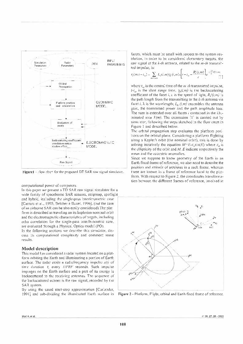
Mori A. et al. no 26,27,28 - 2003

108

_-- - facets, which must be small with respect to the system resolution, in order to be considered elementary targets, the

E,,,> raw signal at the k-th antenna, related to the m-th transmitted irnpulse, is:

-- R' (i m) rk(nst- t,,,) = L,(i,m)y, (i ,m)s t-', -L

i ~ v ( n ) [ C I a 111

where t, is the centra1 time of the m-th transmitted impulse, t-t,,, is the slant range time, yk(i,m) is the backscattering coefficient of the facet i, C is the speed of light, R$(i,m) is the path length from the transmitting to the k-th antenna via facet i, h is the wavelength; Lk @,m) ensembles the antenna gain, the transrnitted power and the path amplitude loss. The sum is extended over al1 facets i contained in the illuminated area V(m). The expression [l] is carried out by simulator, following the steps sketched in the flow chart in Figure 1 and described below. The orbital propagation step evaluates the platform positions on the orbital plane. Considering a platform flighting

ELECTROMAGNETIC along a Kepler's orbit (the nomina1 orbit), this is done by solving iteratively the equation M=E-&,sin(E) where E, is the ellipticity of the orbit and M, E indicate respectively the mean and the eccentric anomalies. Since we suppose to know geometq of the Earth in an

Raw SI& \-l') Earth fixed frame of reference, we also need to describe the

- position and attitude of antéiias in a such frame, whereas Figure1 - Flow chart for the proposeci DT SAR raw signal simulator.. these are known in a frame of reference local to the plat-

form. With respect to Figure 2, the coordinates transformation between the different frames of reference, involved in

computational power of computers. In this paper we present a TD SAR raw signal simulator for a wide farnily of spaceborne SAR sensors, stripmap, spotlight and hybrid, including the single-pass interferometric case [Carrara et al., 1995; Belcher e Baker, 19961, (but the case of an airborne SAR can be also easily considered).The platform is described as traveling on its keplerian nomina1 orbit and the electromagnetic characteristics of targets, including echo correlation for the single-pass interferometric case, are evaluated through a Physical Optics model (PO). In the following sections we describe this simulator, dis- cuss its computational complexity and comment some results.

Mode1 description This model has considered a radar system located on a platform orbiting the Earth and illuminating a portion of Earth surface. The radar emits a radiofrequency impulse s(i) of time duration T, every I/PRF seconds. Such impulse impinges on the Earth surface and a pa* of its energy is backscattered to the receiving antenna. The sequence of the backscattered echoes is the raw signal, recorded by the SAR system. By using the usual start-stop approximation [Curlander,

I

,,,,'' : --- -

. , , , , , *,'

.

19911 and sub-dividing the illuminated Earth surface in Figure 2 - Platform, Flight, orbital and Earth fixed frame of reference.

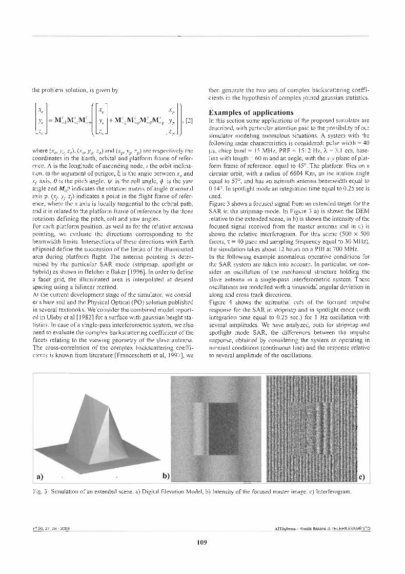
the problem solution, is given by

where (x, y,, z,), (x,, y, 2,) and (x,,, yp, zp) are respectively the coordinates in the Earth, orbital and platform frame of reference, A is the longitude of ascending node, i the orbit inclination, o the argument of perigee, 6 is the angle between x, and xf axis, 8 is the pitch angle, y is the roll angle, 4 is the yaw angle and M$ indicates the rotation matrix of angle a around axis p. (xj; y~ z/) indicates a point in the flight frame of reference, where the x axis is locally tangential to the orbital path, and it is related to the platform frame of reference by the three rotations defining the pitch, roll and yaw angles. For each platform position, as well as for the relative antenna pointing, we evaluate the directions corresponding to the bearnwidth limits. Intersections of these directions with Earth eilipsoid define the succession of the limits of the illuminated area during platform flight. The antenna pointing is determined by the particular SAR mode (stripmap, spotlight or hybrid) as shown in Belcher e Baker [1996]. In order to define a facet gri4 the illuminated area is interpolated at desired spacing using a bilinear method. At the current development stage of the simulator, we consider a bare soil and the Physical Optical (PO) solution published in severai textbooks. ~e.consider the combined mode1 reported in Ulaby et al [l9821 fora surface with gaussian height statistics. In case of a single-pass interferometric system, we also need to evaluate the complex backscattering coefficient of the facets relating to the viewing geometry of the slave antenna. The cross-correlation of the complex backscattering coefficients is known from literature [Franceschetti et al, 19971, we

then generate the two sets of complex backscattering coefficients in the hypothesis of complex joined gaussian statistics.

Examples of applications In this section some applications of the proposed simulator are described, with particular attention paid to the possibility of our simulator modeling anomalous situations. A system with the following radar characteristics is considered: pulse width = 40 ps, chirp band = 15 MHz, PRF = 1512 Hz, h = 3.1 cm, baseline with length = 60 m and an angle, with ihe x-y plane of platform frame of reference, equal to 45O. The platform flies on a circular orbit, with a radius of 6604 Km, an inclination angle equal to 57", and has an azimuth antenna beamwidth equal to 0.14". In spotlight mode an integration tirne equal to 0.25 sec is used. Figure 3 shows a focused signal from an extended target for the SAR in the stripmap mode. In Figure 3 a) is shown the DEM relative to the extended scene, in b) is shown the intensity of the focused signal received from the master antenna and in C) is shown the relative interferogram. For this scene (500 x 500 facets, z = 40 p e c and sampling frequency equal to 30 MHz), the simulation takes about 12 hours on a PII1 at 700 MHz. In the following exarnple anomalous operative conditions for the SAR system are taken into account. In particular, we consider an oscillation of the mechanical strutture holding the slave antenna in a single-pass interferometric system. These oscillations are modelled with a sinusoidal angular deviation in aiong and cross track directions. Figure 4 shows the azimuthal cuts of the focused impulse response for the SAR in stripmap and in spotlight mode (with integration tirne equal to 0.25 sec.) for 1 Hz oscillation with several amplitudes. We have analyzed, both for stripmap and spotlight mode SAR, the differences between the impulse response, obtained by considering the system as operating in nomina1 conditions (continuous line) and the response relative to several amplitude of the oscillations.

Fig. 3- Simulation of an extended scene. a) Digital Elevation Model, b) Intensity of the focused master image. C) Interferogram.

n" 26,27,28 - 2003 AiTinformu - R i t a Italiana di TELERILEVAMENTO

109

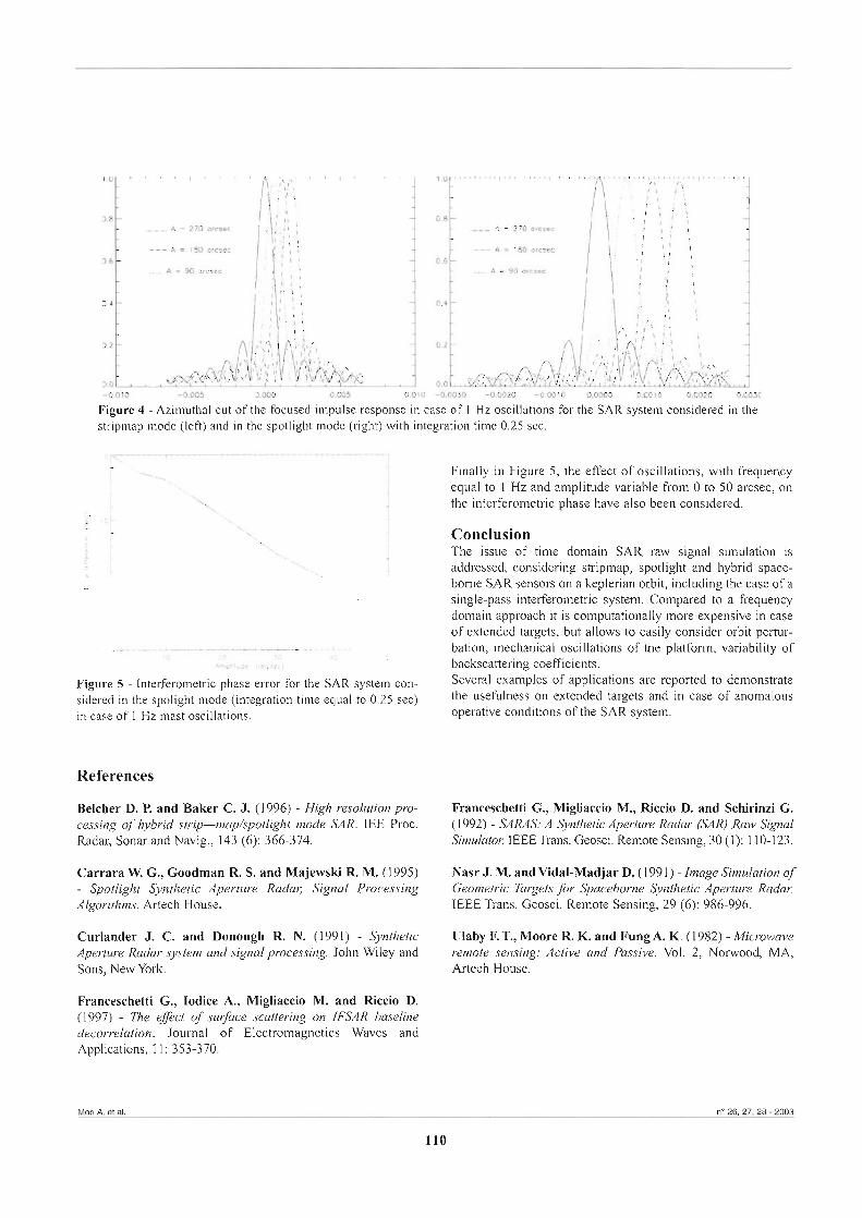
1.U ' , ,

3.8 - A - 270 arcsec

3.6 - - ..... A - 90 oresec

2.4 - -

3.2 - -

-0.010 -0.005 5.000 0.035 0.010

Figure 4 - Azimuthal cut of the fmused impulse response in case of 1 & oscillations for the SAFt system considered in the stnpmap mode (le@ and in the spotlight mode (right) with integration time 0.25 sec.

Finally in Figure 5, the effect of oscillations, with frequency equa1 to 1 Hz and arnplitude variable from O to 50 arcsec, on the interferometric phase have also been considered.

Conclusion The issue of time domain SAR raw signal simulation is addressed, considering striprnap, spotlight and hybrid spaceborne SAR sensors on a keplerian orbit, including the case of a single-pass interferometric system. Compared to a frequency domain approach it is computationally more expensive in case of extended targets, but allows to easily consider orbit pertur-

- ' 5 & . . . . . . . . S . . . . . . . , . , . . . . . . . I . ,, 0 10 20 30 50

bation, mechanical oscillations of the platform, variability of 40

~ ~ I ~ I ~ ~ ~ (arcsec) backscattering coeficients. ~i~ 5 - bterferometnc pbe far the SAR syskm Severa1 exarnples of applications are reported to demonstrate sidered in the spol*t mode (intemtiDn he qual t. 0.25 sec) the usefdness on extended targets and in case of anomalous in case of 1 Hz mast oscillations. operative conditions of the SAR system.

References

Belcher D. P. and Baker C. J. (1996) - High resolution processing of hybrid strip-mapispotlight mode SAR. IEE Proc. Radar, Sonar and Navig., 143 (6): 366-374.

Carrara W. G., Goodman R S. and Majewski R M. (1995) - Spotlight Synthetic Aperture Radar, Signal Processing Algorithms. Artech House.

Curlander J. C. and Donough R. N. (1991) - Synthetic Aperture Radar system and signal processing. John Wiley and Sons, New York.

Franceschetti G., Iodice A., Migliaccio M. and Riccio D. (1997) - ?%e efecf of swjibce scatiering on IFSAR baseline decorrelation. Journal of Electromagnetics Waves and Applications, 11: 353-370.

Franceschetti G., Migliaccio M., Riccio D. and Schirinzi G. (1 992) - SARAS: A Synthetic Aperture Radar (SAR) Raw Signal Simulator EEETrans. Geosci. Remote Sensing, 30 (1): 110-123.

Nasr J. M. and Vidal-Madjar D. (1991) - Image Simulatìon of Geometric Targets for Spaceborne Synthetic Aperture Radal: E E E Trans. Geosci. Remote Sensing, 29 (6): 986-996.

Ulaby E T., Moore R. K. and Fung A. K. (1 982) - Microwave remote sensing: Active and Passive. Vol. 2, Norwood, MA, Artech House.

Mori A. et ai. no 26,27,28 - 2003

110

A high frequency ground based SAR system for masonry investigation

Guido Luzi, Massimiliano Pieraccini, Daniele Mecatti, Linhsia Noferini and Carlo Atzeni (l)

Abstract Results of a test carried using a high-frequency large-bandwidth Synthetic Aperture Radar (SAR) for inspecting masonry structures are reported. The apparatus consists of a Continuous Wave Step Frequency (CW-SF) radar operating in a non-contact manner. The centre frequency is 10 GHz and the bandwidth is 4 GHz wide. The selected centre frequency makes it easily available a large bandwidth and hence a good resolution, of the order of few centimetres, along range direction. T h s value is better than these available from conventional GPR. Tri-dimensional images of the measurement scenario can be obtained by mechanicaily moving the antennas along two dimensions. Although penetration depth decreases dramatically with increasing frequency, a penetration depth up to sev- era1 tens of centimetres in masonry was observed: this can be considered satisfactory for a nurnber of applications.

Sommario In questo lavoro vengono descritti i risultati di una sperimentazione finalizzata all'introspezione muraria, effettuata con un radar ad apertura sintetica (SAR) ad alta frequenza ed a larga banda. L'apparato è costituito da un radar ad onda continua a passi di frequenza che opera non a contatto. La frequenza centrale è 10 GHz e la banda utilizzata di 4 GHz. La scelta di questa frequenza centrale consente di disporre facilmente di una larga banda e quindi di un'elevata risoluzione nella direzione di propagazione, dell'ordine di alcuni centimetri. Tale valore è migliore di quello ottenibile con GPR convenzionali. Con un movimento delle antenne lungo due direzioni si possono ottenere immagini tridimensionali dello scenario di misura. Benché lo spessore di penetrazione diminuisca forte- mente all'aumentare della frequenza, si è ottenuta una penetrazione nella muratura di alcune decine di centimetri, soddisfacente per numerose applicazioni.

Introduction Intra-wall radar inspection offers unique non invasive means for the diagnostics of buildings, wherby the assessment of the structural safety and durability depends on information regarding the interna1 stnicture and the location and size of voids and defects [Maierhofer and Leipold, 20011. In particular when the monitored object is considered an Historic Building, the non- destructive aspect of the technique is a great advantage. Nevertheless, penetrating radar systerns are mainly designed for ground inspection rather than for building diagnostics. A nurnber of works, both theoretical [Tsui and Matthews, 19971 and experimental [Mast et al., 1992; Binda et al., 19981 exist on this specific application, c l a W g for a high resolution, thus for a large bandwidth, as a key requirement. However, because a large bandwidth can be attained only through a correspondingly high operation centre frequency, resolution and penetration depth appear to be conflicting requirements. This drawback is critica1 in ground penetration applica-

(1) Laboratorio Tecnologie per i Beni Culturali, Dipartimento di Elettronica deii'Universith di Firenze, via Lombroso 6/11B - - 50134 Firenze, Italia. e-mail: [email protected]


tions that usually require penetration depths up to a few meters in strong attenuating media. Masonry investigation requirements are usually different under relevant respects: the required penetration depth rarely exceeds tens of centimetres, and the wall layers are rather dry and homogeneous. These characteristics rnake possible the use of radars operating at higher frequency and taking advantage of synthetic aperture near-field-focused processing techmques, to obtain higher spatial resolution and signal-to- noise ratio.

The radar system The ground based apparatus used in this experirnentation, shown in Figure 1, is composed of a Continuous Wave Step Frequency (CW-SF) Radar operating at 10 GHz centre frequency, with a bandwidth of 4 GHz and a mechanical digitally controlled frame which allows the radar sensor to scan along two perpendicular axes. The radar aperture is synthesized by mechanically moving the couple of transmitting and receiwig horn antennas along a horizontal rail and a vertical guide, in order to scan a plane bi-dimensional aperture up to 3 m in length and 1 m in height. An external synthesizer (HP 8672A) produces the radiated signal, and scans the required bandwidth in programmable frequency steps [Kong and By, 1995; Koppenjan et al., 2000; Stickley et al., 20001; the receiver is based on a simple homodyne architetture. The synthesizer, fol-

n" 26,27,28 - 2003 AITinforma - Rivista Italiana di TELERILEVAMENTO

111

Figure 1 - (a) Scheme of the radar sensor.(b) Photo of the iipparatus.

lowing a preliminary power amplification, feeds the antenna and provides a reference signal for the mker, which detects the in-phase component of the received signal. The demodulated signal is amplified and digitized before being sent to the acquisition board, which provides the digital samples to a portable persona1 computer. The system obtains radar images by range and cross-range syn- thesis: as the antennas scan a bi-dimensional surface, the received raw data provide three-dimensional information about the interna1 stnicture of the wall, i.e. bi-dimensional images on any plane crossing the target under investigation .

SAR algorythm The principle of Synthetic Aperture Radar is now strongly con- solidateci and is clearly explained in many papers and books, such as m a b y et al., 19821 or [Curlander and Donough, 199 1 ; Mensa, 199 l]. Synthetic aperture can be obtained both through impulse radar, commonly used on satellite sensors, and by using Continuous Wave Step Frequency Radar, sweeping a fkequency band and measuring the radar response in the frequency dominium over a finite bandwidth a "synthetic pulse" is generated. The value of the complex radar image at points identified by the index n is obtained by coherently adding al1 signal contributions, taking in to account their phase history as summarized by the following expression:

1 I =-- ~ E ~ ~ R : , ex{ jx (q , -4)) VI NpNf ik C

where Np is the number of the antenna positions, Nf the number of swept frequencies,f;: the i-th frequency, EiR i~ the in-phase component of the received signal atA fkequency and k-th anten-

na position, c the speed of light, RnSk the distance between the point n and the k-th antenna position. Direct computation of this expression is extremly time consuming but some algorithrns have been developed to overcome this shortcoming [Lopez-Sanchez and Fortuny-Guasch, 20001. Ro is a constant (dimensionally a distance) that takes into account the delay internally introduced by the RF wmponents of the system. In a quasi-monostatic radar arrangement, 2Rdc can be estimated by the antenna coupling delay, appearing in the time profile as a steady peak. This wnstant is used not for absolute calibration purpose but only for referring radar measurements to actual range values. Details on the algorithrn used in our case can be found in [Pieraccini et al., 20001. It should be cailed that the maximum resolution aiong the range direction, ARR is related to the swept RF band by the following expression:

When the area illuminated by the antenna is comparable to the cross-range scan length, the cross-range resolution depends on the position of the imaged point as well as on the antenna HPBW, and can be also affected by the defocusing due to propagation inside the wall. For the centra1 points of the wall an approxirnated value of some centimeters in air, can be calculated through the following expression:

h A&* = 2sin(8,,,, 12) 131

where h is the center wavelength and OWBW the Half Power Beam Width of the antenna. The focusing formula [l] does not take into account the changes of the propagation factor (speed of the electromagnet-

Luzl G. et al. n' ~6,27,28 - 2003

112

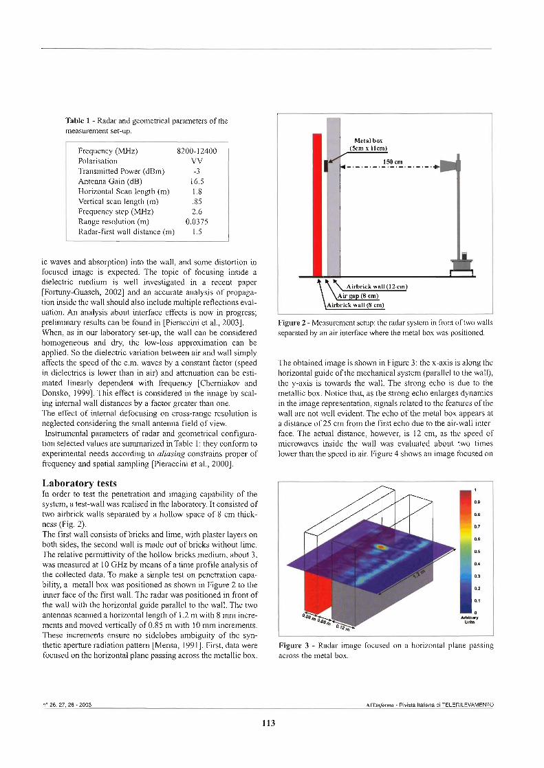
Table 1 - Radar and geometrica1 parametem of the measurement set-up.

Frequency W) 8200-12400 Polarisation W Transmitted Power (dBm) -3 Antenna Gain (dB) 16.5 Horizontal Scan le* (m) 1.8 Vertical scan lengtli (m) .85 Frequency step (MHz) 2.6 Range resolution (m) 0.0375 Radar-fit wall distance (m) 1.5

ic waves and absarption) in@ the waii, and some distortion in focused image is expected. The topic of focusing inside a dielectric m d u m is well investigated in a recent paper [portmy-Guasch, 20021 and an accurate W s i s of propagation inside the waU shouid also include d t i p l e reflectiom evai- uation An analysis about interfwe effects is now in progressi p r e h b r y results can be found in meraccini et al., 20031. When, as in our laboratory set-up, the wali can be considered homageneous and dry, the low-loss approximation oan be applied. So the dielectric variation between air and wali simply affects the speed of the e.m. waves by a constant factor (speed in dielectrics is l m than in air) and attenuation can be estimated iinearly dqendent with h p e n c y [Cherniakov and Donsko, 19991. Tbis effect is considered in the hage by scaling internai wail distanca by a factor greater than ane. The of intemal defocusing on cross-range resolution is n e g l W considering the small an- field of view. instrumental pmmeters of radar and geometrical conf~gura-

tion s e 1 W values are smmakd in Table 1: they conform to eqehen ta l needs aumding to aliasing constrains proper of ikcpency and spatiai sampiing mmccini et al., 29003.

Laboratory testti In orda to test the penetradon and imaging capability of the systm, a test-wail was r e a l i d h the laboratory. It conskted of two airbrick walls separated by a hoiiow space of 8 cm thickness (Fig. 2). The f i i wali consists of bricks and lime, with plaster layers on both si&, the seconci wail is made out of bricks witbout lime. The relative permìttMty of the hollow bricks medium, about 3, was meaJured at 10 GHz by m a m of a time profile analysis of the c o i l W data. To rnake a simple test on penetration capa- bìlity, a meta11 box was positioned as shown in Figure 2 to the imer face of the first wall. The radar was positioned in ftont of the wali with the horbntal guide parallel to the wali. The two aiitennas scanned a horizontal le@ of 1.2 m with 8 mm increments and maved ver t idy of 0.85 m with 10 mm increments. These increments ensure no sidelobes ambigui9 of the synthetic aperture radiation paaefn wensa, 19911. First, data were focused on the horizmtal plane passing across the metallic box.

Figure 2 - Measurement setup: the radar system in fiont of two walls sqianited by an air W a c e where the metal box was positioned.

The obtained image is shown in Figure 3 : the x-axis is along the horizontal guide of the mechanical systern (parallel to the wall), the y-axis is towards the wall. The strong echo is due to the metallic box. Notice that, as the strong echo enlarges dynamics in the image representation, signals related to the features of the waii are not well evident. The echo of the meta1 box appears at a distance of 25 cm from the first echo due to the air-waii interface. The actual distance, however, is 12 cm, as the speed of microwaves inside the wali was evaluated about two times lower than the speed in air. Figure 4 shows an image focused on

Figure 3 - Radar image focused on a horizontal plane passing across the meta1 box.

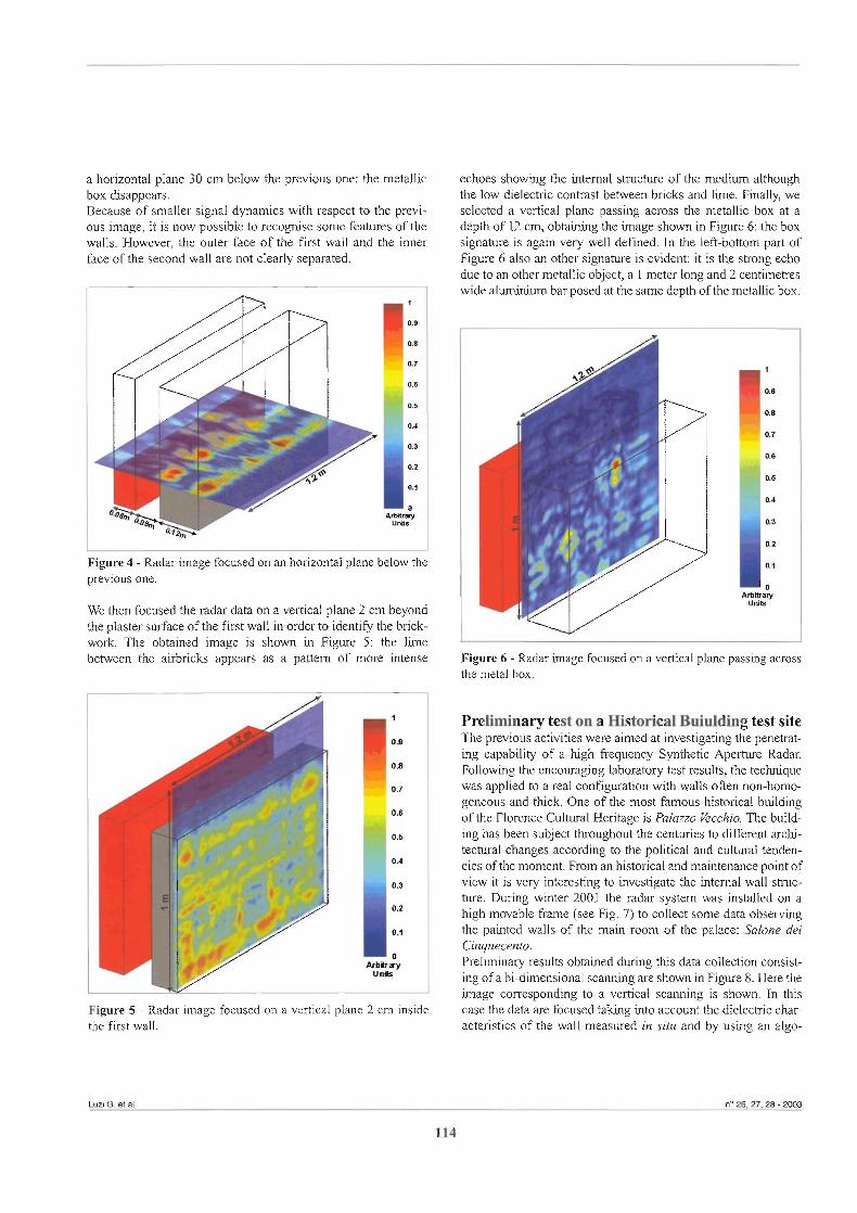
a horizontal plane 30 cm below the previous one: the metallic box disappears. Because of smaller signal dynamics with respect to the previous image, it is now possible to recognise some features of the walls. However, the outer face of the fust wall and the inner face of the second wall are not clearly separated.

Figure 4 - Radar image focused on an horizontal plane below the previous one.

We then focused the radar data on a vetical plane 2 cm beyond the plaster surface of the first wall in order to identifi the brick- work. The obtained image is shown in Figure 5: the lime between the airbricks appears as a pattem of more intense

echoes showing the intemai strutture of the medium although the low dielectric wntrast between bricks and lime. Fially, we selected a vertical plane passing across the metallic box at a depth of 12 cm, obtaining the image shown in Figure 6: the box signature is again very well defined. In the left-bottom part of Figure 6 also an other signature is evident: it is the strong echo due to an other metallic object, a 1 meter long and 2 centimetres wide aluminium bar posed at the same depth of the metallic box.

Figure 5 - Radar image focused on a vertical plane 2 cm inside the first wall.

Figure 6 - Radar image focused on a vertical plane passing across the meta1 box.

Preliminary test on a Historical Buiulding test site The previous activities were aimed at investigating the penetrating capability of a high frequency Synthetic Aperture Radar. Following the encouraging laboratory test results, the technique was applied to a rea1 configuration with waiis often non-homogeneous and thick. One of the most famous historical buiiding of the Florence Cultura1 Heritage is Palmo Vecchio. The building has been subject thoughout the centuries to different architectural changes according to the political and cultura1 tenden- cies of the moment. From an historical and maintenance point of view it is very interesting to investigate the intemal waii structure. During winter 2001 the radar system was instalied on a high mwable frame (see Fig. 7) to coilect some data observing the painted walls of the main room of the palace: Salone dei Cinquecento. Preliminary results obtained during this data coilection consist- ing of a bi-dimensional scanning are shown in Figure 8. Here the image wrresponding to a vertical scanning is shown. In this case the data are focused taking into account the dielectric characteristics of the wall measured in situ and by using an algo-

Luzi G. et ai. n" 26,27,28 - 2003

114

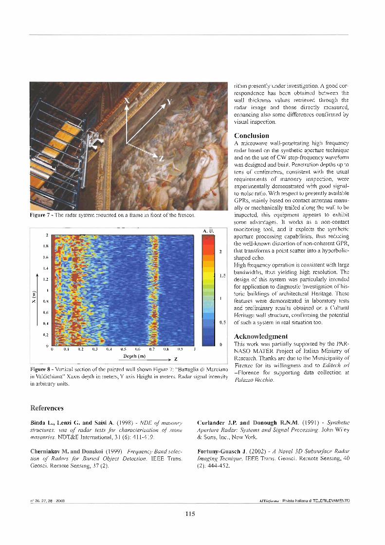
I Figure 7 - The radar system mounted on a fiame in front of the fiescos.

Figure 8 - Vertical section of the painted wall shown Figure 7: "Battagiia di Marciano in Valdichiana" Xaxis depth in meters, Y axis Height in meters. Radar signal intensity in arbitrary units.

rithm presently under investigation. A good correspondence has been obtained between the wall thickness values retrieved through the radar image and those directly measured, enhancing also some differences confi ied by visual inspection.

Conclusion A microwave wail-penetrating high frequency radar based on the synthetic aperture technique and on the use of CW step-fkequency waveform was designed and built. Penetration depths up to tens of centimetres, consistent wiih the usual requirements of masonry inspection, were experimentally demonstrated with good signal- to-noise ratio. With respect to presently available GPRs, mainly based on contact antennas manu- aily or mechanically trailed along the wall to be inspected, this equipment appears to exhibit some advantages. It works as a non-contact monitoring tool, and it exploits the synthetic aperture processing capabilities, thus reducing the weil-known distortion of non-coherent GPR, that transforms a point scatter into a hyperbolic- shaped echo. High ikequency operation is consistent with large bandwidths, thus yielding high resolution. The design of this system was particularly intended for application to diagnostic investigation of historic buildiigs of architectural Heritage. These features were demonstrated in laboratory tests and preliminary results obtained on a Cultura1 Heritage wall strutture, c o n f i i the potentiai of such a system in real situation too.

Acknowledgment This work was partially supported by the PAR- NASO MATER Project of Italian Ministry of Research. Thanks are due to the Municipality of Firenze for its willingness and to Editech srl -Florence for supporting data collection at Palazzo Vecchio.

References

Binda L, LenP G. and Sadsi A. (1998) - NDE of marronry Curlander J.P. and Donougb M . M . (1991) - Synthetic sbucium: use of redar tests jÒr charac&r&ation of stone Aperture Radar: Systems and Signai Processìng. John Wiley masonries. WT&E Inhmtional, 3 1 (6): 41 1419. & Sons, iuc., New York.

Cherniakov M. and Donskoi (1999) - Frequency Band selec- Fortuny-Guaseb J. (2002) - A Nove130 Subsu$ace Radar fion of Radms for Bwied Object Detection. 1EEE Trans. Imaging Tecnique. IEEE Trans. Geosci. Remote Sensing, 40 Gieosci. Remote Sensing, 37 (2). (2): 444-452.

n"2s,n.za-2009 AITInqh& - RMsta Italiana di TELERILNAMENTO

115

Lopez-Sanchez J.M. and Fortuny-Guash J. (2000) - 3-0 Radar Imaging Using Range Migration Tecniques. IEEE Trans. on Antennas and Propagation, 48 (5): 728-737.

Kong F.N. and By T. L. (1995) - Per$onnance of a GPR system which use step Jiequency signals. Journal of Applied Geophysics, 33: 15-26.

Koppenjan S.K.,Allen C.M., Gardner D,, Wong H. R., Lee H. and Lockwood S. J. (2000) - Multi-Ji-equency synthetic aperture imaging with lightweight gmund peneirating radar system. Journal of Applied Geophysics, 43: 25 1-258.

Maierhofer C. and Leipold S. (2001) - Radar investigatwn of masonry shuctures. NDT&E hkmational, 34: 139-147.

Mast J.E., Lee H. and Murtha J.P. (1992) - Application of Microwave Pulse-Echo Radar Imaging to the Nondesiructive Evaluation of Buildings. international Journal of Imaging Systems and Technology, 4: 164-169.

Mensa D.L. (1991) - High Resolution Radar Cross $ection Imaging. 2nd ed. Norwood, MA, Artech House.

Pieraccini 112, Luzi G. and Atzeni C. (2001) - Terrain mapping by ground-based [email protected] mdar. IEEE Trans. Geosci. Remote Sensing, 39 (10): 2176-21 81.

Pieraccini M., Luzi G., Noferini L., Mecatti D., Fratini M. and Aizeni C. (2003) - High Frequency Penetmting Radar Data Interpretation By Means Of Joint 7Tme Frequenq Amlysis. To be published in Proceedings of the Lnternational Workshop on Advanced Ground Penetrating Radar Delfi 14 - 16 May, 2003.

Stickley G.F, Noon D.A., Cherniakov M. and Longstaff I.D. (2000) - Gated stepped-fiequency ground penetmting radar. Journal of Applied Geophysics, 43: 259-269.

Tsui B.F. and Matthews S.L. (1997) - Analytical modelling of the dieleciric properties of concrete for subsurface mdar applications. Construction and Building Mataials, 1 1 (3): 149-161.

Ulaby F.T., Moore RK. Moore and Fung A.K. (1982) - Microwave remote Sensing: Active and Passive. Vol. 2, Reading Addison-Wesley.

iuzi G. ei al. no 26, n, 28 - 2003

116

Le missioni di Telerilevamento a microonde

A conclusione di questo numero speciale della rivista AIT, dedicata al convegno di telerilevamento a microonde che si è svolto a Firenze nel maggio 2002, ci sembrava utile passare in rassegna quelle che sono le principali missioni di telerilevamento a microonde operanti attualmente o nel prossimo futuro. Abbiamo diviso la descrizione fra sensori attivi (radar, scatterometri ed altimetri) e sensori passivi (radiometri) anche se è da osservare come molte missioni utilizzano simultaneamente i due diversi tipi di sensori riuscendo a smittarne le singole peculiarità per un utilizzo integrato. Oltre ad una descrizione dei sensori, dei dati disponibili e di alcune possibili applicazioni abbiamo indicato per ogni missione l'indirizzo aggiornato del sito web dove trovare ulteriori informazioni.

Sensori attivi La storia del telerilevamento radar dallo spazio è essenzialmente cronaca dell'ultimo ventennio. Dopo la breve missione SEASAT nel 1978 (SAR in banda L, scatterometro per il vento, radar altimetro), il satellite ERS-1 dell'Agenzia Spaziaie Europea (ESA) lanciato nel 1991 è stato il secondo a caricare a bordo un radar ad apertura sintetica (SAR) operante in banda C anche come scatterometro. La sua missione è continuata con il satellite ERS-2 che monta un sensore iden- tico e che è attualmente ancora operativo. Nel frattempo l'Agenzia Spaziale Canadese ha lanciato nel 1995 il satellite RADARSAT, pensato tra l'altro per il con- trollo dei ghiacci marini in ausilio alla navigazione. I1 sistema RADARSAT ha visto l'uso di una tecnologia di antenna in banda C che rende possibile una elevata flessibilità operativa nell'acquisizione delle immagini, le quali possono variare in risoluzione, copertura, angolo di incidenza. Al satellite RADARSAT-l si affiancherà, presumibilmente entro il 2005, il satellite RADARSAT-2 che presenta caratteristiche ancora più innovative. La flessibilità operativa di RADARSAT è ora disponibile anche con l'ultimo nato della famiglia ESA, owero il sistema ASAR a bordo della piattaforma ENVISAT lanciata con successo nello scorso marzo 2002 e che aggiunge la disponibilità di dati in banda C a diverse polarizzazioni. Nel frattempo anche l'Agenzia Spaziale Giapponese (NASDA) ha realizzato la missione J-ERS, lanciata nel 1992, con a bordo un radar che ricalcava, se pure in banda L, le caratteristiche di ERS- 1. Terminata la vita di J-ERS nell'ottobre 1998, la NASDA ha in programma nell'immediato futuro la missione ALOS, un satellite avente a bordo il radar PAL SAR con caratteristiche polarimetriche di grande interesse e potenzialità per le applicazioni. Non dobbiamo poi dimenticare che l'Italia è impegnata in un programma molto ambizione di realizzazione di una costellazione di satelliti che montano un radar in banda X con risoluzione f i o al metro e che verranno affiancate da piattaforme

con a bordo sensori ottici ad alta risoluzione (sistema COSMO-Skymed). Infine, il programma spaziale tedesco prevede lo sviluppo del sistema TerraSAR con un radar a due fiequenza e risoluzione al suolo fino al metro. In questo arco di tempo la NASA ha anche portato avanti un programma di missioni radar a bordo dello Space Shuttle (SIR-A, SIR-B, SIR-C, SRTM) anche in collaborazione con ASI e DLR (http://www.jpl.nasa.gov/missions/pasi/sir.html, http://'www.jpl.nasa.gov/srtm/). Sono stati sperimentati radar con diverse frequenze (bande L, C e X) e diverse modalità operative (angoli di incidenza, polarizzazioni, interferome- tria) che hanno fornito un enorme contributo aila ricerca in questo settore, ma anche informazioni significative sul nostro pianeta. Forniamo ora una descrizione sintetica dei sistemi qui citati rimandando alla documentazione delle agenzie e dei distribu- tori dei prodotti per ulteriori dettagli. I1 radar a bordo di ERS-2 (http://earth.esa.ini/ers/) è in realtà uno strumento con più funzioni denominato AMI (Active Microwave Instrument). Esso lavora alla frequenza di 5.33 GHz in polarizzazione verticale 0. Produce immagini standard con risoluzione geometrica di circa 30 metri. Per quanto riguarda i prodotti, oltre alle immagini standard a diversi look (e quindi con buona risoluzione radiometrica) ampie circa 100 km, sono disponibili immagini a piena risoluzione in cui ad ogni pixel è associato un numero complesso in ampiezza e fase, e immagini a livelli di elaborazione supe- riore con caratteristiche migliorate dal punto di vista geometrico (immagini geocodificate) (http://www.eurimage.com). A parte la particolare applicazione interferometrica, che richie- de necessariamente il dato di fase, molti utenti si rivolgono alla immagine standard, magari effettuando a loro carico le necessarie correzioni geometriche di precisione. I prodotti geocodificati sono invece caratterizzati da una migliore accuratezza nella localizzazione geografica di ogni

no 26.27.28 - 2003 AITbfonna - Rivista Italiana d TELERILEVAMENTO

117

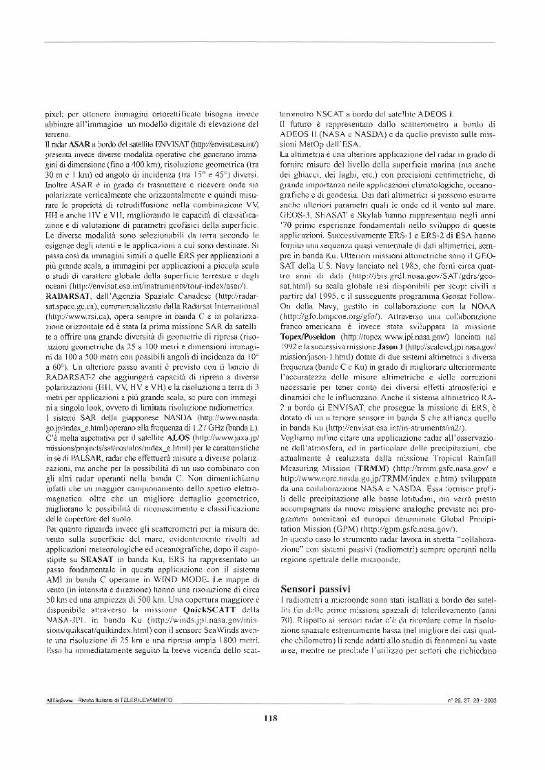
pixel; per ottenere immagini ortorettificate bisogna invece abbinare all'immagine un modello digitale di elevazione del terreno. ìi radar ASAR a bordo del satellite ENVISN @ t i p i / ~ ~ i n t / ) presenta invece diverse modalità operative che generano immagini di dimensione (fino a 400 km), risoluzione geometrica (tra 30 m e 1 km) ed angolo di incidenza (tra 15O e 45O) diversi. Inoltre ASAR è in grado di trasmettere e ricevere onde sia polarizzate verticalmente che orizzontalmente e quindi misu- &e le proprietà di retrodiffusione nella combinazione W, HH e anche H . e VH, migliorando le capacità di classificazione e di valutazione di parametri geofisici della superficie. Le diverse modalità sono selezionabili da terra secondo le esigenze degli utenti e le applicazioni a cui sono destinate. Si passa così da immagini simili a quelle ERS per applicazioni a più grande scala, a immagini per applicazioni a piccola scala o studi di carattere globale della superficie terrestre e degli oceani (http://envisat.esa.int/instniments/tour-index/asar~. RADARSAT, deU'Agenzia Spaziale Canadese (http://radarsat.space.gc.ca), commercialimato dalla Radarsat International (http://www.rsi.ca), opera sempre in banda C e in po1arkz.a- zione orizzontale ed è stata la prima missione SAR da satellite a 0fE-i~ una grande diversità di geometrie di ripresa (risoluzioni geometriche da 25 a 100 metri e dimensioni immagini da 100 a 500 metri con possibili angoli di incidenza da 10" a 60"). Un ulteriore passo avanti è previsto con il lancio di RADARSAT-2 che aggiungerà capacità di ripresa a diverse polarizzazioni (H., W, HV e VH) e la risoluzione a terra di 3 metri per applicazioni a più grande scala, se pure con immagini a singolo look, owero di limitata risoluzione radiometrica I sistemi SAR delia giapponese NASDA (http://www.nasda. go.jp/index-e.html) operano alla fkpenza di 1.27 GHz (banda L). C'è molta aspettativa per il satellite ALOS (http:lIwww.jaxa.jp/ missi~ns/~m~dsat/&dalodindex-e.h) per le caratteristiche in sé di PALSAR. radar che effettuerà misure a diverse volariz- zazioni, ma anche per la possibilità di un uso combinato con gli altri radar operanti nella banda C. Non dimentichiamo infatti che un maggior campionamento dello spettro elettromagnetico, oltre che un migliore dettaglio geometrico, migliorano le possibilità di riconoscimento e classificazione delle coperture del suolo. Per quanto riguarda invece gli scatterometri per la misura del vento sulla s u d i c i e del mare, evidentemente rivolti ad applicazioni meteorologiche ed oceanografiche, dopo il capo- stipite su SEASAT in banda Ku, ERS ha rappresentato un passo fondamentale in questa applicazione con il sistema AMI in banda C operante in WiND MODE. Le mappe di vento (in intensità e direzione) hanno una risoluzione di circa 50 km ed una ampiezza di 500 km. Una copertura maggiore è disponibile attraverso la missione QuickSCATT della NASA-JPL in banda Ku (http://winds.jpl.nasa.gov/missions/quikscai/quikindex.html) con il sensore SeaWids avente una risoluzione di 25 km e una ripresa ampia 1800 metri. Esso ha immediatamente seguito la breve vicenda dello scat-

terometro NSCAT a bordo del satellite ADEOS I. I1 futuro è rappresentato dallo scatterometro a bordo di ADEOS I1 (NASA e NASDA) e da quello previsto sulle missioni MetOp del17ESA. La altimetria è una ulteriore applicazione del radar in grado di fornire misure del livello della su~erficie marina (ma anche dei ghiacci, dei laghi, etc.) con precisioni centirnetriche, di grande importanza nelle applicazioni climatologiche, oceanografiche e di geodesia. Dai dati altimetrici si possono estrarre anche ulteriori parametri quali le onde ed il vento sul mare. GEOS-3, SEASAT e Skylab hanno rappresentato negli anni '70 prime esperienze fondamentali nello sviluppo di queste applicazioni. Successivamente ERS-l e ERS-2 di ESA hanno fornito una sequenza quasi ventennale di dati altimetrici, sempre in banda Ku. Ulteriori missioni altimetriche sono il GEO- SAT della U.S. Navy lanciato nel 1985, che fornì circa quattro anni di dati (http://ibis.grdl.noaa.gov/SAT/gdrs/geosat.html) su scala globale resi disponibili per scopi civili a partire dal 1995, e il susseguente programma Geosat Follow- On della Navy, gestito in collaborazione con la NOAA (http://gfo.bmpcoe.org/gfo/). Attraverso una collaborazione franco-americana è invece stata sviluppata la missione Topex/Poseidon (http://topex-wwwjpI.nasagov/) lanciata nel 1992 e la w&va missione Jason 1 (http://sealevel.jpl.nasagw/ rnissionJjason-l.html) dotate di due sistemi altimetrici a diversa frequenza (bande C e Ku) in grado di migliorare ulteriormente l'accuratezza delle misure altimetriche e delle correzioni necessarie per tener conto dei diversi effetti atmosferici e dinamici che le influenzano. Anche il sistema altimetrico RA- 2 a bordo di ENVISAT, che prosegue la missione di ERS, è dotato di un ulteriore sensore in banda S che affianca quello in banda Ku (http://envisat.esa.int/in-stniments/ra2/). Vogliamo infine citare una applicazione radar all'ossemazio- ne dell'atmosfera, ed in particolare delle precipitazioni, che attualmente è realizzata dalla missione Tropical Rainfall Measuring Mission (TRMM) (http://tnnm.gsfc.nasa.gov/ e http://www.eorc.nasda.go.jp~TRMM/index-e.htm) sviluppata da una collaborazione NASA e NASDA. Essa fornisce profili delle precipitazione alle basse latitudini, ma verrà presto accompagnata da nuove missione analoghe previste nei programmi americani ed europei denominate Global Precipi- tation Mission (GPM) (http://gpm.gsfc.nasa.gov/). In questo caso lo strumento radar lavora in stretta "collaborazione" con sistemi passivi (radiometri) sempre operanti nella regione spettrale delle microonde.

Sensori passivi I radiometri a microonde sono stati istallati a bordo dei satelliti fin delle prime missioni spaziali di telerilevamento (anni 70). Rispetto ai sensori radar c'è da ricordare come la risoluzione spaziale estremamente bassa (nel migliore dei casi qual- che chilometro) li rende adatti allo studio di fenomeni su vaste aree, mentre ne preclude l'utilizzo per settori che richiedano

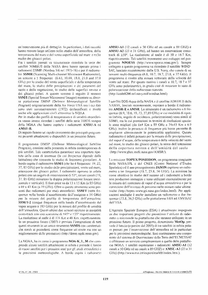
un'osservazione più di dettaglio. In particolare, i dati raccolti hanno trovato largo utilizzo nello studio dell'atmosfera, della temperatura del mare e del vento superficiale sul mare e nello studio dei ghiacci polari. Fra i satelliti passati va sicuramente ricordata la serie dei satelliti NIMBUS della NASA dove hanno operato prima i radiometri ESMR (Nimbus 516 nel 1975-76) e poi il radiometro SSMR (Scanning Multi-channel Microwave Radiometer), un sensore a 5 frequenze (6.63, 10.69, 18.0, 21.0 and 37.0 GHz) per lo studio del vento superficiale e della temperatura del mare, lo studio delle precipitazioni e dei parametri del suolo e della vegetazione, lo studio delle superfici nevose e dei ghiacci polari. A questo sensore è seguito il sensore SSIWI (Special Sensor Microwavel Imager) montato su diverse piattaforme DMSP (Defence Meteorological Satellite Program) originariamente della Air Force USA ma i cui dati sono stati successivamente (1972) declassificati e rivolti anche alle applicazioni civili attraverso la NOAA. Per lo studio dei profili di temperatura e di umidità atmosferi- ca vanno invece ricordati i satelliti della serie TIROS sempre della NOAA che hanno ospitato i radiometri AMSU-A ed AMSU-B. Di seguito faremo un rapido censimento dei principali programmi presenti attualmente o disponibili in un prossimo futuro.

I1 programma DMSP (Defense Meteorological Satellite Program), consiste nella presenza in orbita contemporanea di più satelliti. Tale caratteristica garantisce una copertura ripe- tuta della zona di interesse (la cui frequenza dipende dalla latitudine) che consente lo studio di fenomeni giornalieri. A bordo ospita il radiometro SSMII (che ha 4 frequenze: 19,22, 37'85 GHz) per lo studio delle precipitazioni, vento sul mare, estensione dei ghiacci polari. I radiometri operano in orbita polare con un angolo di osservazione di 53"; alcuni canali (1 9, 37, 85 GHz) misurano la doppia polarizzazione lineare (orizzontale e verticale). I1 foot-print va da 13 x 15 Km (a 85 GHz) a 69 x 43 Km (a 19 GHz). Oltre a questo strumento sono presenti due radiometri per studi atmosferici: SSMIT (sette frequenze nella banda d'assorbimento dell'ossigeno a 54 GHz) per la misura del profilo di temperatura dell'atmosfera; SSMJT-2 (cinque frequenze nella banda d'assorbimento del vapor acqueo a 183 GHz) per la misura del profilo di umidità dell'atmosfera. Questi ultimi due sensori operano in modalità cross-track con una scansione di k45" e i35" rispettivamente. La risoluzione al nadir è di 174 Km e 48 Km, rispettivamente. In un prossimo futuro (2007) è prevista l'integrazione di tutti questi strumenti in un unico strumento SSMIS con caratteristiche simili ai precedenti come frequenze utilizzate ma con un miglioramento delle prestazioni (http://dmsp.ngdc.noaa.gov).

La NOAA, ha in corso il programma NOA-K, L, M che com- prende alcuni satelliti attualmente in orbita e prevede il lancio di nuovi satelliti per i prossimi anni per gli studi atmosferici e le previsioni meteorologiche. A bordo ospita i radiometri

AMSU-A1 (12 canali a 50 GHz ed un canale a 89 GHZ) e AMSU-A2 (23 e 31 GHz), ed hanno un osservazione cross- track di +50°. La risoluzione al nadir è di 50 e 16.7 Km, rispettivamente. Tali satelliti troveranno uno sviluppo nel programma NPOESS (http://www.npoess.noaa.gov/). Sempre collegato a questo programma va ricordato il satellite WIND- SAT, lanciato recentemente dalla U.S. Navy, che consta di un sensore multi-frequenza (6.8, 10.7, 18.7, 23.8, e 37 GHz). Il programma è rivolto alla misura vettoriale della velocità del vento sul mare. Per questo motivo i canali a 10.7, 18.7 e 37 GHz sono polarimetrici, in grado cioè di misurare lo stato di polarizzazione della radiazione ricevuta. (http://code8200.nrl.navy.miVwindsat.htrni)

I satelliti EOS-Aqua della NASA e il satellite ADEOS 11 della NASDA, lanciati recentemente, ospitano a bordo il radiometro AMSR-E e AMSR. Lo strumento è un radiometro a 6 frequenze (6.9, 10.6, 19,23,37,89 GHz) le cui modalità di ripresa (orbita, angolo di incidenza, polarizzazione) sono simili al SSM/I, ma le cui prestazioni in termini di risoluzioni spaziale sono migliori (da 6x4 Km a 89 GHz a 74x43 Km a 6.9 GHz); inoltre la presenza di frequenze più basse permette di ampliarne ulteriormente le potenzialità applicative. Questo radiometro è infatti pensato per la misura delle precipitazioni, del vapor d'acqua, della temperatura e della velocità del vento sul mare, lo studio dei ghiacci polari, la stima dell'estensione della copertura nevosa e dell'umidità del suolo (http://www.ghcc.msfc.nasa.gov/AMSR~).

La missione TOPEXIPOSEIDON, un programma congiunto della NASA/JPL e del CNES (Centre National d'Etudes Spatiales) ed il suo proseguimento JASON ospitano un radiometro a tre frequenze (18.7, 23.8, 34 GHZ). La missione ha come obiettivo lo studio dell'oceano ed i radiometri a bordo non producono immagini e sono utilizzati essenzialmente per la misura del contenuto di vapor d'acqua atmosferico e per la correzione dell'eccesso di percorso nelle misure radar altimetriche (http://topex-www.jp1.nasa.govhdex.html). Per applicazioni analoghe è anche installato un radiometro a due frequenze (23.8,36,5 GHz) sulle piattaforme ERS ed ENVISAT del1 'ESA.

L'Agenzia Spaziale Europea (ESA) è attualmente impegnata su due importanti progetti che prevedono l'utilizzo di radiometri a microonde su piattaforme che saranno utilizzate in un prossimo futuro. Il primo progetto, denominato MetOp, prevede il lancio (a partire dal 2005) di ire sateliiti in orbita polare pensati per l'osservazione dell'atmosfera ed in particolare per le previsioni meteorologiche. Essi costituiranno una compo- nente del sistema di Osservazione delia Terra dell'EUMETSAT e ofkirawo un servizio complementare a queiio deiie piattaforme NOAA. I satelliti ospiteranno i radiometri AMSU-A1 (12 canali a 50 GHz ed un canale a 89 GHZ) e AMSU-A2 (23 e 3 1 GHz) (http://www.esa.int/export/esaME/index.hd).

I1 secondo progetto è SMOS, una missione dedicata allo studio della salinità del mare ed all'umidità del terreno che prevede l'utilizzo di un unico strumento: il radiometro in banda L MIRAS. I1 lancio è previsto nel 2007 e di particolare importanza è l'uso di un antenna a sintesi di apertura che per- metterà di ottenere una buona risoluzione spaziale a terra; inoltre, vi sarà la possibilità di osservare ad angoli di incidenza nell'intervallo 20"- 60" (h~://www.esa.int/export/esalP/ smos.htmi).

Fra i programmi futuri della NASA e della NASDA va sicuramente ricordato il GPM (Global F'recipitation Mission) che prevede una costellazione di satelliti per lo studio delle precipitazioni con a bordo un radiometro multi-fresuenza. Di particolare imporhnza l'obiettivo di poter avere dati ogni 3 ore, ottenendo un notevolmente miglioramento dei modelli previsionaii (hitp://gpm.gsfc.nasa.gov/). Anche 1' ESA sta valutando una sua partecipazione a questo programma attraverso la missione EGPM (European Global Precipitation Mission).

A B S T R A C T

Abstracts di lavori di Autori italiani pubblicati su riviste internazionali

a cura di Alba L'Astorina e-mail: [email protected]

Active and passive microwave measurements for the characterization of soils and crops

Maceiioni G.', S. Paloscial, P. Pampalonil, R. Ruisil, M. Dechambre2, R , Valentinz, A. Chanzy3, J.-P. Wigneron3 1 IFAC-CNR, via Panciatichi 64 - 50127 Firenze 2 CETPICNRS, 1 O- 12 avenue de l'Empe, 78140 Ve@ France 3 INRA Unité Climat, Sol et Environnement, Site Agroparc,

849 14 Avignon Cedex 9, France

Agronomie, 22 (6): 581-586,2002: EDP Sciences

In the framework of EC project ReSEDA, airborne and heli- copter-borne remote sensing campaigns were carried out to monitor soil and vegetation processes on an agricultural area located in South France. This paper discusses the sensitivity of active (scatterometer) and passive (radiometer) sensors to the surface characteristics of canopy-covered soils, and compares their performances in separating crops and in measuring soil moisture and vegetation biomass. Scatterometric and radiometric measurements, both carried out at C and X band, confirms the potentials of microwave sensors in detecting soil and vegetation features.

A summary of experimental results to assess the contribution of SAR for mapping vegetation biomass and soil moisture

Paloscia S.' 1 IFAC-CNR, via Panciatichi 64 - 50127 Firenze

Canadian Journal of Remote Sensing, 28 (2): 246-261,2002

This paper is an overview of the most recent results obtained by Italian groups involved in the SIR-CB[-SAR Hydrologicai experiment, by using multi-frequency and multi-polarization SAR data measured by JPLIAIRSAR, SIR-C, EMISAR, ERS- 1 and JERS-1 sensors. The sensitivity of backscattering coefficients to some geophysical parameters which play a significant role in hydrological processes - such as vegetation biomass, soil moisture and roughness - is discussed. Experimental results show that P-band appears to be suitable for the monitoring of forest biomass, whereas L-band is mainly sensitive to the

biomass of wide-leaf crops and C-band to narrow-leaf crops. Moreover, the L-band sensor gives the highest contribution in estimating soil moisture and surface roughness. The sensitivity of backscatter to soil moisture and surface roughness for indi- vidual agricultural fields is rather low, since both parameters affect the radar signal. However, by observing data collected at different dates and averaged over a relatively wide agncultural area, the correlation to soil moisture becomes considerable, since the effects of spatial roughness variations are smoothed. Lastly, retrievals of both soil moisture and surface roughness were performed using a semi-empirical model.

Modelling Radar Backscatter From Crops During The Growth Cycle 2

Maceiioni G.1, S. Paloscial, P. Pampalonii, R Ruisil, M. Dechambre2, R, Valentinz, A. Chanzyj, L. Prévot3 N. Bruguire3 1 IFAC-CNR, via Panciatichi 64 - 50127 Firenze 2 CETPICNRS, 10-12 avenue de l'Europe, 78140 Velizy, Fmnce 3 INRA Unité Climat, Sol et Envirotmement, Site Agroparc,

849 14 Avignon Cedex 9, France

Agronomie, 22 (6): 575-579,2002 ; EDP Sciences

A radiative transfer model that represents vegetation as a collection of randomly oriented disks and almost vertical cylinders on a rough surface has been implemented and used for interpreting radar backscattering from wheat and sunflowers fields. The model was used to simulate the growth cycle of wheat and sunflowers by using bio-physical data collected on the agricultural test site of RESEDA project as inputs. A comparison with experirnental data collected at two frequencies, two polarizations and two incidence angles from the ERSISAR and the French ERASME Scatterometer has been carried out. The comparison has shown that model simulations reproduce pretty well temporal trends and average values of experimental results, but in some cases some significant discrepancy exists between the absolute values. Moreover, the backscattering coefficient was found sensitive to geometrica1 characteristics of wheat and sunflowers. Indeed, as leaf area index increases, backscattering increases in the case of sunflowers and decreases in the case of wheat.

n" 28.27.28 - 2003 AITinforntn - Rivista Italiana di TELERILEVAMENTO

121

Analysis of the distorted Born approximation for subsurface reconstruction: truncation and uncertainties effects

Leone G.', Soldovieri F.1 1 DIMET, Univ. di Reggio Calabria, Italy

IEEE Transactions on Geoscience and Remote Sensing, 41 (1): 66- 74,2003; IEEE, Piscataway (NJ), USA

The problem of determining the dielectric permittivity profile of buried objects starting fiom the knowledge of the scattered field is considered in the two-dimensional geometry when incomplete near-zone data are collected at a single frequency under a multiview/multistatic measurement configuration. In particular, attention is paid to the practical issues of the trun- cated obse~ation domain and the presence of uncertainties on data. The problem is tackled with reference to the scalar polarization by linearization of the mathematical relationship between the unknown dielectric permittivity profile and the scattered field. A homogeneous, possibly lossy, half-space geometry for the subsurface modeling is adopted, thus leading to the so-called distorted Born approximation (DBA). A thor- ough investigation of the class of unknown functions that can be reliably retrieved is performed by dealing with singular value decomposition of the relevant linear operator. It results that even if sources and receivers are located at the interface, a very restricted set of profile variations can be reconstructed by a stable inversion algorithm. In particular, reduced vertical features of the buried objects with respect to the horizontal ones can be reconstnicted under DBA. Moreover, the bninca- tion of the obsewation domain further restricts this set, affecting mainly the vertical resolution. Numerica1 results confirm- ing the validity of the analysis are also provided.

Texture-based characterization of urban environments on satellite SAR images

Deli'Acqua F.1, P. Gamba1 1 Dipt. di Elettronica, Università di Pavia, Italy

IEEE Transactions on Geoscience and Remote Sensing, 41 (l): 153- 159,2003; IEEE, Piscataway (NJ), USA

We investigate the use of co-occurrence texture measures to provide information on different building densities inside a town strutture. We try to improve the pixel-by-pixel classification of an urban area by considering texture measures as a means for block analysis and classification. We find some interesting hints concerning the optimal dimension of the window to be considered for texture measures, as well as the most useful measures. Moreover, we show that it is possible to use medium-resolution readily available satellite synthetic

aperture radar images for a more refined urban analysis than previously shown.

Retrieving soil moisture and agricultural variables by microwave radiometry using neural networks

Del Frate F.', P. Ferrazzolil, G. Schiavonl 1 Università Tor Vergata - Dipartimento Informatica Sistemi e Produzione, via del Politecnico 1, 00 133 Roma, Italy

Remote Sensing of the Environment, 84 (2): 174-183, 2003; Elsevier, New York, USA

Two neural network algorithms trained by a physical vegetation mode1 are used to retrieve soil moisture and vegetation variables of wheat canopies during the whole crop cycle. The first algorithm retneves soil moisture using L-band, two polarizations and multiangular radiometric data, for each single date of radiometric acquisition. The algorithm includes roughness and vegetation effects, but does not require a priori knowledge of roughness and vegetation parameters for the specific field. The second algorithm retrieves vegetation variables using dual band, V polarization and multiangular radiometric data. This algorithm operates over the whole multitemporal data set. Previously retrieved soil moisture values are also used as a-priori information. The algorithms have been tested considering measurements carried out in 1993 and 1996 over wheat fields at the INRA Avignon test site.

The use of Meteosat and GMS imagery to detect bumed areas in tropical environments

Boschetti', P.A. Brivioz, J. M. Gregoirl

l Global Vegetation Monitoring Unit, Joint Research Centre Institute for Environment and Sustainability (JRC-IES), TP, 440 2 1020 Ispra (VA), Italy CNR-IREA, via Bassini 15,20133, Milano, Italy


This paper describes a methodology of using data acquired by the European Meteosat and the Japanese Geostationary Meteorologica1 Satellite (GMS) geostationary satellites to detect burned areas in different tropical environments. The methodology is based on a multiple threshold approach applied to the thermal radiance and to a spectral index specific for burned surfaces. The Simple Index for Burned Areas (SIBA), also developed in this study, makes use of the information contained in the visible and thermal InfraRed (IR) band available on the geostationary satellites, whose main advantages are the

~ ~ T i n f b r ~ t a - Rivisia Itaiiina di TELERILEVAMENTO n' 26,27,28 - 2M)3

122

high temporal resolution and the minima1 leve1 of pre-processing required. The results obtained with Meteosat data have been evaluated comparing them with NOAA-Advanced Very High Resolution Radiometer (AVHRR) data acquired over the Centra1 Africa forest-savannah areas. For GMS imagery, AVHRR data acquired over the woodland-savannah areas of Northern Territory in Australia have been used. Despite the very low spatial and spectral resolution of the data, accuracy assessment showed at a regional and continen- tal scale the resulting burned area maps could be a valuable source of information for the monitoring of the fire activity and for the assessment of fire impact on tropospheric chem- istry.

Efficient data compression for seismic-while- drilling applications

Bernasconi G.1, M. Vassallo1 Dipt. di Elettronica e Informazione, Politecnico di Milano, Milano, Italy

IEEE Transactions on Geoscience and Remote Sensing, 41 (3): 687- 696, 2003; TEEE, Piscataway (WJ), USA

Seismic-while-drilling services efficiently support drilling decisions. They use the vibrations produced by the drill-bit during perforation as a downhole seismic source. The seismic signai is recorded by sensors on the surface, and it is processed in order to obtaidupdate an image of the subsurface around the borehole. To improve the characterization of the source, some sensors have been experimentally installed also downhole, on the drill pipes in close proximity to the bit: data logged downhole have been able to give better quality information. Currently, the main drawback of downhole equipment is the absence of a high-bit-rate telemetry system to enable real-time activities. This problem may be solved by employing either an offline solution, with limited memory capacity up to few hundreds of megabytes, or an online solution with telemetry at a very low bit-rate (few bits per second). However, following the offline approach with standard acquisition parameters, the internal storage memory would be filled up in just a few hours at high acquisition rates. On the contrary, with the online solution, only a small portion of the acquired signals (or only a l m information about potentially dangerous events) can be transrnitted in reai time to the surface by using conventional mud-pulse telemetry. We present a lossy data compression algorithm based on a new representation of downhole data in angle domain, which is suitable for downhole irnplementation and may be successfully applied to both online and offline solutions. Nurnerical tests based on rea1 field data achieve compression ratios up to 112: 1 wiihout major loss of information. This allows a significant increase in downhole tirne acquisition and in real-time information that can be transmitted through mud-pulse telemetry.

Two years of operational use of Subpixel Auto- matic Navigation of AVHRR scheme: accuracy assessment and validation

Pergola N.1, V. Tramutoliz 1 CNR, Area di Ricerca di Potenza, Istituto di Metodologie per l'Analisi Ambientale, C.da, S. Loja, Tito Scalo (Pz) 85050, Italy

2 Dipartimento di Ingegneria e Fisica del1 'Ambiente, Università della Basilicata, Campus Macchia Romana, Potenza 85100, Italy


Automated techniques for satellite imagery navigation and co- location are especially required for environmental monitoring activities intensively using satellite data. In this work are presented the results obtained afier 2 years of operational use of the Subpixel Automatic Navigation of AVHRR (SANA) scheme. An automatic method for accuracy assessment of satellite navigation techniques, which pennits a preliminary evaiua- tion of their performances, dealing with a large collection of test images is aiso proposed. The navigation accuracy assessment, performed by using a selection of small islands as reference points, is discussed. Results achieved over more than 400 Advanced Very-High-Resolution Radiometer (AVHRR) scenes confirm that the SANA scheme is a very accurate one (computed mean navigation error is generally about one AVHRR pixel). Furthermore, because of its high processing speed, it can be considered a suitable t001 for intensive satellite data processing in multitemporal analyses, especially required for environmental studies as well as for operational monitoring purposes.

Three-dimensional focusing with multipass SAR data

Fornaro G.1, F. Serafino', E Soldovieril 1 REA-CNR, Napoli, Italy

IEEE Transactions on Geoscience and Remote Sensing, 41 (3): 507- 517,2003; IEEE, Piscataway (N), USA

Deals with the use of multipass synthetic aperture radar (SAR) data in order to achieve three-dimensional tomography reconstruction in presence of volumetric scattering. Starting from azimuth- and range-focused SAR data relative to the same area, neglecting any mutua1 interaction between the targets, and assuming the propagation in homogeneous media, we investigate the possibility to focus the data also in the elevation direction. The problem is formulated in the Eramework of linear inverse problem and the solution makes use of the singular value decomposition of the relevant operator. This ailows us to properly take into account nonuniform orbit separation and to exploit

AITinfoma - Rivista Italiana di TELERILEVAMENTO

123

a priori knowledge regarding the size of the volume interested by the scattering mechanism, thus leading to superresolution in the elevation direction. Results obtained on simulated data demonstrate the feasibility of the proposed processing technique.

Temporal analysis of a landslide by means of a ground-based SAR Interferometer

Leva D.1, G. Nicol, D. Tarchil, J. Fortuny-Guaschl, A.J. Sieberl 1 Institute for the Protection & Security of the Citizen, Joint Research Centre of the European Commission, Ispra, Italy


A ground-based synthetic aperture radar (GB-SAR) interferometer is used to retrieve the velocity field of a landslide. High- resolution images are obtained by means of a time domain SAR processar. An in-depth analysis of the sequence of SAR interferograms enables the recognition of a slowly deforming upper scarp in the scene, and a debris flow that feeds the accumula- tion zone of the landslide, where a fast change in terrain mor- phology is observed. The estimated deformation map is in agreement with the available measurements obtained by means of Global Positioning System receivers. Results show that GB- SAR interferometry is a cost-effective solution for the monitoring of landslides. The proposed method is shown to be a valid complement to space- and airborne SAR and to the traditional geodetic instruments.

Coupled magma chamber inflation and sector collapse slip observed with synthetic aperture radar interferometry on Mt. Etna volcano

Lundgren P.1, P. Berardino2, M. Coltellis, G. Fornaro2, R. LanarP, G. Puglisi3, E. Sansosti2, M. Tesauro2 1 Jet Propulsion Laboratory, California Institute of Technology, Pasadena, California, USA

2 IREA-CNR, via Diocleziano 328, 80124 Napoli, Italy 3 Istituto Nazionale di Geofisica e Vulcanologia, Catania, Italy

Journal of Geophysical Research, 108 (B5): ECV 4-1 to ECV 4-15,2003;

Volcanoes deform dynamically due to changes in both their magmatic system and instability of their edifice. Mt. Etna features vigorous and almost continuous eruptive activity from its surnrnit craters and periodic flank eruptions. Even though its shape is that of a large stratovolcano, its structure features two rift systems and a flank collapse structure similar to Hawaiian

shield volcanoes. We analyze European remote sensing (ERS) satellite differential interferometric synthetic aperture radar (InSAR) data (1993-1996) for Mt. Etna spanning its quiescence fiom 1993 through the initiation of renewed eruptive activity in late 1995. We use synthetic aperture radar (SAR) data fkom both ascending and descending ERS satellite tracks. Comparison of independent Interferograms covering the first 2 years of the infiationary period shows a pattern consistent with inflation of the volcano. Calcuiation of the tropospheric path delay based on meteorological data does not change this interpretation. Interferograms from late summer 1995- 1996 show no significant deformation. Joint inversion of interferograms fkom ascending and descending satellite tracks require both inflation fkom a spheroidal magrnatic source located beneath the surnrnit at 5 km below sea level, and displacement of the east flank of Etna along a basa1 decollement. Both sources of deformation were contemporaneous within the resolution of our data and suggest that inflation of the centra1 magma chamber acted to trigger slip of Etna's eastern flank. These results demonstrate that flank instability and recharge of a volcano's magma system must both be considered toward understanding how volcanoes work and in their hazard evaluation.

Pyramidal rain field decomposition using radia1 basis function neural networks for tracking and forecasting purposes

Del19Acqua F.1, P. Gamba1 1 Dipartimento di Elettronica, Università di Pavia, Italy


In this paper, we present how we used neural networks (NNs) and a pyramidal approach to mode1 the data obtained by a weather radar and to short-range forecast the rainfall behavior. Very short-range forecasting useful, for instance, for estimating the path attenuation in terrestrial point-to-point com- munications. Radia1 basis function NNs are used both to approximate the rain field and to forecast the parameters of this approximation in order to anticipate the movements and changes in geometric characteristics of significant meteoro- logica1 stmctures. The procedure is validated by applying it to actual weather radar data and comparing the outcome with a linear forecasting method, the steady-state method, and the persistence method. The same approach is probably useful also for predicting the behavior of other meteorological phenomena like clusters of clouds observed fiom satellites.

AITInforma - Rivista Italiana di TELERILEVAMENTO no 26, n, 28 - X X ) ~

124

An innovative real-time technique for buried object detection

Bermani E.', A. Boni', S. Caorsil, A. Massa1 'Dipartimento of Informatics & Communication Technology, Università of Trento, Italy

IEEE Transactions on Geoscience and Remote Sensing, 41 (4): 927- 93 1,2003; IEEE, Piscataway (NJ), USA

A new online inverse scattering methodology is proposed. The origina1 problem is recast into a regression estimation and successively solved by means of a support vector machine (SVM). Although the approach can be applied to various inverse scattering applications, it is very suitable for dealing with buried object detection. The application of SVMs to the solution of such problems is firstly illustrated. Then some exarnples, concerning the localization of a given object from scattered field data acquired at a number of measurement points, are presented. The effectiveness of the SVM method is evaluated in comparison with classica1 neural network based approaches.

SAR raw data compression by subband coding

Pascazio V.1, G. Schirinzil l Inst. di Teoria e Tecnica deiie Onde Elettromagnetiche, Università di Napoli "Parthenope", Napoli, Italy


A technique for compressing synthetic aperture radar raw data using multiresolution representations and subband coding is considered. In particular, we present the performance of a transform coding compression method using wavelet basis, coupled with a threshold quantizer optmiized for Gaussian statistics, as well as a proper subband bit allocation strategy. The performances achieved in terms of bit rate reduction and certain quality parameters computed on the images obtained by cornpressed data have been evaluated. These show an increased performance in the compression method with respect to conventionai methods, aibeit with a slightly increased complexity in the algorithm implementation.

Lossy predictive coding of SAR raw data

Magli E.1, G. Olmo1 1Dipt. di Elettronica, Politecnico di Torino, Italy

compression of synthetic aperture radar (SAR) raw data. We exploit the known result that a blockwise normalized SAR raw signal is a Gaussian stationary process in order to design an optimal decorrelator for this signal. We show that, due to the statistica1 properties of the SAR signal, an along-range linear predictor with few taps is able to effectively capture most of the raw signal correlation. The proposed predictive coding algorithm, which performs quantization of the prediction error, optionally followed by entropy coding, exhibits a number of advantages, and notably an interesting performance/complexity trade-off, with respect to other techniques such as flexible block adaptive quantization (FBAQ) or methods based on transform-coding; fractional output bit-rates can also be achieved in the entropy-constrained mode. Simulation results on real-world SUI-CB(-SAR as well as simulated raw and image data show that the proposed algorithm outperforms FBAQ as to SNR, at a computational cost compatible with modern SAR systems.

The effect of modified Markov random fields on the local minima occurrence in microwave imaging

Ferraiuolo G.', V. Pascazio1 1 Dipt. di Ingegneria Elettronica e delle Telecomunicazioni, Universita di Napoli "Federico 11", Naples, Italy


The application of a maximum a posteriori estimation method for rnicrowave imaging that makes use of a Markov random field (MRF) a priori statistical mode1 is presented. In particular, the R/LRF family adopted is generalized for complex profiles, characterized by a quadratic energy fimction and "modified" such to make it possible to statistically represent spatial interactions between rea1 and imaginary parts. Thanks to its pecu- liarities, the use of this approach simultaneously favors in many cases well posedness and robustness against local minima occurrence, as well as high quality in the reconstructed images. Numerica1 results show the performance of the method.

A new interpolation kernel for SAR interferometric registration

Migliaccio M.', E Bruno1 1 Inst. di Teoria e Tecnica delle Onde Elettromagnetiche, Univ. degli Studi di Napoli Parthenope, Italy

IEEE Transactions on Geoscience and Remote Sensing, 41 IEEE Transactions on Geoscience and Remote Sensing, 41 (5): 977- 987,2003; IEEE, Piscataway (NJ), USA (5): 1105- 1 110,2003; IEEE, Piscataway (NJ), USA

In this paper, we propose to employ predictive coding for lossy Estimation of digital elevation maps from electromagnetic

no 26,27.28 - 2003 AITinfornia - Rivista ItaJiana di TELERILEVAMENTO

125

signals received at an interferometric synthetic aperture radar thus promoting a retrieval-by-changes approach also in the (SAR) requires significant processing. In this framework, a monitoring of phenomena for which hard classifications are not key step is the interferometric registration, which can be sufficiently accurate nor complete. The data structure has been mathematically framed as an interpolation procedure. A new implemented in a system, which is also described, available interpolation kernel for SAR interferometric registration is today in a Windows version. It has been applied to the moni- presented and discussed in comparison with five classica1 toring of variations of Alpine glaciers. ones. It is based on the Knab sampling window that has been successfully employed in various electromagnetic problems and which has been proposed as capable of best preserving Global scale monitoring of soil and vegetation the stochastic information. The numerica1 experiments show using active and passive sensors the superiority of the new interpolation kernel.

Macelloni G.', S. Paloscia', P. Pampalonil, E. Santi1 IFAC-C%R, via Panciatichi 64 - 50127 Firenze

Time-based retrieval of soft maps for environ- menta1 change detection International Joumal of Remote Sensa'ng, 24 (1 2): 2409-2425,

2003: Taylor & Francis, London, UK Carraral P., G. Frestaz, A. Rampini' 1 IREA-CMI, via Bassini 15,20133 Milano, Italy The potential of SSMA data in monitoring land surface fea- 2 ISTI-CNR, Area della Ricerca, via M o M 1, I 56127 Pisa, Italy tures and global changes in synergy with the ERS Wind-

Scatterorneter was investigated. The backscattering coeffi- Infonnation Processing & Management, 39: 323-327, 2003, cient, the brightness temperature, and some related quantities, special issue on "Modelling vagueness and subjectivity in measured during a yearly cycle on a number of selected test information access", Elsevier sites in different climatic regions of the world, were related to

surface features obtained from ground information. The major This contribution aims to shortly describe a data strutture for characteristics of land surfaces were obtained from their ernis- creating and rnanaging archives of thematic maps derived by sivity spectra and polarization state, while a further classifi- classifymg remotely sensed irnages by soft techniques (soft cation of surfaces were carried out by means of multi-fre- maps). Unlike traditional models for managing spatial data, the quency, dual-polarized data. Vegetation biomass and snow main key feature for query formulation is time, thus improving cover were estimated frorn appropriate rnicrowave indexes the investigation on changes occurred in time ranges. The data and from spectra of brightness temperature. structure originally extends time-based models to soft maps,

AITInformo - RNista Iialiina di TELERILEVAMENTO n" 26.27,28 - 2003

126

Facoltà di Ingegneria deii'Università di Roma "La Sapienzan 24-27 febbraio 2004

Specialist Meeting on Microwave Radiometry and Remote Sensing Applications

Si tratta di un convegno internazionale alla sua ottava edizione che raccoglie gli specialisti nella radiometria a microonde, sia per quanto riguarda le diverse applicazioni (mare, atmosfera, suolo e vegetazione), che per quanto riguarda le tecnologie dei sensori (calibrazione, polarimetria, etc.). La radiometria a microonde sta acquisendo un ruolo sempre più significativo nelle applicazioni del telerilevamento a scala globale che riguardano la meteorologia (ad esempio le precipitazioni atmosferiche), il clima, I'idrologia (l'umidità del terreno), lo stato della vegetazione e molte altre. Le diverse edizioni sono state tenute alternativamente negli Stati Uniti ed in Italia, essendo l'iniziativa nata da un collaborazione scientifica di un gruppo di ricercatori di questi due paesi. In particolare, le precedenti edizioni sono state:

Rome, Italy March 1,2, 1983 (Univ. La Sapienza) Florence, Italy March 9,11,1988 (CNRIIROE) Boulder, Colorado January 14,16,1992 (NOAA) Rome, Italy February 14,17,1994 (Univ. Tor Vergata) Boston, Massachusetts November 4,6,1996 (MIT) Florence, Italy March 15,18,1999 (CNROROE) Boulder, Colorado November 200 1 (NOAA)

Esse hanno sempre visto 1'IEEE e I'URSI tra i patrocinatori dei Meeting e dato origine a numeri speciali di riviste (es. Radio Science) o pubblicazioni ad hoc.

La presente edizione si terrà anche sotto il patrocinio del17ASITA e dell'AIT.

Per avere maggiori notizie sul convegno, sottomettere lavori o iscriversi si può consultare il sito web dedicato all'indirizzo:

n", n, 28 - 2003 AITlnlornt~ - Rivista Italiana di TELERILEVAMENTO

127

ASSOCIAZIONE ITALIANA DI TELERILEVAMENTO

Documents