Assimilating concentration observations for transport and dispersion modeling in a meandering wind field

lable at ScienceDirect

Atmospheric Environment 43 (2009) 1329–1338

Contents lists avai

Atmospheric Environment

journal homepage: www.elsevier .com/locate/atmosenv

Assimilating concentration observations for transport and dispersionmodeling in a meandering wind field

Sue Ellen Haupt a,b,*, Anke Beyer-Lout b, Kerrie J. Long a, George S. Young b

a Applied Research Laboratory, The Pennsylvania State University, P.O. Box 30, State College, PA 16804, USAb Meteorology Department, The Pennsylvania State University, State College, PA 16804, USA

a r t i c l e i n f o

Article history:Received 1 July 2008Received in revised form24 November 2008Accepted 30 November 2008

Keywords:Data assimilationDispersion modelingGenetic algorithmGaussian puffGaussian plume

* Corresponding author. Applied Research LaboraUniversity, P.O. Box 30, State College, PA 16804, USA.

E-mail address: [email protected] (S.E. Haupt).

1352-2310/$ – see front matter � 2008 Elsevier Ltd.doi:10.1016/j.atmosenv.2008.11.043

a b s t r a c t

Assimilating concentration data into an atmospheric transport and dispersion model can provideinformation to improve downwind concentration forecasts. The forecast model is typically a one-waycoupled set of equations: the meteorological equations impact the concentration, but the concentrationdoes not generally affect the meteorological field. Thus, indirect methods of using concentration data toinfluence the meteorological variables are required. The problem studied here involves a simple windfield forcing Gaussian dispersion. Two methods of assimilating concentration data to infer the winddirection are demonstrated. The first method is Lagrangian in nature and treats the puff as an entityusing feature extraction coupled with nudging. The second method is an Eulerian field approach akin totraditional variational approaches, but minimizes the error by using a genetic algorithm (GA) to directlyoptimize the match between observations and predictions. Both methods show success at inferring thewind field. The GA-variational method, however, is more accurate but requires more computational time.Dynamic assimilation of a continuous release modeled by a Gaussian plume is also demonstrated usingthe genetic algorithm approach.

� 2008 Elsevier Ltd. All rights reserved.

1. Introduction

Most atmospheric transport and dispersion applications focuson modeling the statistics of the transport and dispersion. Such anapproach recognizes that it is impossible to accurately forecastthe details of a particular turbulent flow: atmospheric motion isgoverned by nonlinear physics that displays sensitivity to initialconditions, leading to unpredictable chaotic flow (Lorenz, 1963).Thus, only a stochastic approach is practical if one cannot deter-mine the flow details by other means. This approach predicts thestatistics of an ensemble of a large number of realizations, includingmeans, variances, and likely maximum concentrations. The statis-tical approach is appropriate for traditional regulatory purposesthat emphasize meeting standards over a long time period. Morerecently, however, some issues have arisen for which one mustinstead model the particular realization that is occurring. Anexample is a scenario where a toxic contaminant is released and itis necessary to predict its transport and dispersion in order toevacuate people at risk and to minimize the impact (NRC, 2003).Incorrect concentration predictions could lead to evacuating the

tory, The Pennsylvania StateTel.: þ1 814 863 7135.

All rights reserved.

wrong areas. In such cases, we need to determine the specificrealization from the available data so that the subsequent predic-tion is as accurate as possible. Although this objective soundsformidable, if there are field sensors to monitor contaminantconcentrations, one can use those data to (1) determine theturbulent scenario and (2) assimilate the concentration data intoa flow-aware transport and dispersion model.

The assimilation process is well documented in meteorologyapplications where a variety of data assimilation methods are usedoperationally to improve the quality of the Numerical WeatherPrediction (NWP) forecast (Daley, 1991; Ide et al., 1997; Kalnay,2003). Most of those methods formulated for NWP assimilateeither the same quantity as observed or ones that are easily derivedfrom the observed quantities. The situation is more complex forassimilating concentration data, however, due to the one-waycoupling. In contrast to numerical weather prediction (NWP)models, the system of equations used in the transport and disper-sion context is not fully coupled. Although, the wind field drives theconcentration field, the contaminant concentration field has nodirect influence on the wind field.1 Therefore, the goal is not only to

1 The simplification of one-way coupling assumes that the contaminant particlesare sufficiently small to neglect entrainment effects on the flow or gravitationalsettling, have noninertial initial conditions, and that it is nonreactive.

S.E. Haupt et al. / Atmospheric Environment 43 (2009) 1329–13381330

assimilate concentration data into the model to improve theconcentration forecast, but also to derive the time- dependent windfield from observations of the dispersed contaminant and assimi-late them as well. Thus, we need an indirect data assimilationmethod to infer the wind field from concentration observations.

Much of the uncertainty in atmospheric transport and disper-sion modeling is due to large- scale variations in the wind direction.Uncertainty in the wind direction is acknowledged as a source oferror when applying an atmospheric transport and dispersionsystem in an attempt to match measured field data (Chang et al.,2003) and even in experimental wind tunnel data (Krysta et al.,2006). In fact, even in wind tunnel studies, wind direction can varysufficiently that it becomes a large source of error in modelingdispersion (Zheng et al., 2007). Therefore, groups who are usingsensor concentration data to back-calculate source characteristicsare also finding it necessary to additionally back-calculate the windinformation (Krysta et al., 2006; Allen et al., 2007; Haupt et al.,2007; Long et al., submitted).

Deng et al. (2004), Davakis et al. (2007), and Lee et al.(submitted) showed that when meteorological data assimilation isincorporated into a numerical weather prediction model that forcesa transport and dispersion model, the concentration predictionsagree better with field monitored values. Several recent studiesadditionally used assimilation methods to incorporate observationsof a chemical species into a dispersion model (Cheng et al., 2007;Constantinescu et al., 2007; Reddy et al., 2007; Terejanu et al.,2007). Stuart et al. (2007) found that assimilating concentrationobservations into a simple model of sea breeze dynamics coupledwith a diffusion equation reduced errors in both the concentrationfield and in the meteorological fields.

Most of this previous work on assimilating concentration data todeduce a meteorological field assumed that the meteorologicalconditions are constant in time and space. If the wind field variesspatially or temporally, however, as is usually the case, one wouldinfer a wind that is not appropriate to the current time or locale.Then a dynamic data assimilation scheme is required to infera temporally evolving or spatially varying field. This current studydeals directly with this issue: we seek to analyze a wind that variesin time and space given measurements of concentration formultiple times and locations. We show how such an approach canmake a large improvement in predicted concentrations.

This work also addresses the issue that while the ensembleaverage predicted by Gaussian dispersion is an adequate grossrepresentation, such a model does not predict a specific realizationof the flow. By assimilating concentration observations, however,we can begin to use the time- dependent Gaussian puff model toestimate the time varying wind direction, and thus, force a disper-sion pattern towards the observed realization.

Gaussian dispersion in a meandering wind field is used asa testbed for our assimilation methods here. Such a configuration issimple, it varies smoothly in time and space, and it represents animportant realizable state of the atmosphere. Meandering windconditions are particularly common during nocturnal stableboundary layer conditions (Hanna, 1983; Mahrt, 1999; amongothers). It is also analogous to vertical plume meandering observedin unstable direct numerical simulations in the convectiveboundary layer (Liu and Leung, 2005).

Section 2 describes the general assimilation framework anddevelops the model of Gaussian dispersion in a meandering windfield. The data assimilation process for an instantaneous release ina time varying wind field is described for two different techniques:feature extraction combined with nudging (Section 3) and a three-dimensional variational technique solved with a genetic algorithm(Section 4). Section 5 discusses the issues involved in determiningthe minimum requirements of a sensor network to provide the data

necessary for the assimilation systems of Sections 3 and 4. Assim-ilation for a continuous release is described in Section 6. Section 7summarizes the results and their implication and discusses furtherresearch needs.

2. Formulation of the numerical experiment

2.1. Data assimilation for dispersion

The simplest way to pose the time rate of change of a dynamicalsystem (our transport and dispersion model in this case) is:

vxvt¼ Mx þ h (1)

where x represents the predictands (concentration and wind),vx=vt is their time rate of change or tendency, M is a linearizedoperator based on the potentially nonlinear dynamics, and h isa stochastic noise term representing the errors in the model and theunresolved subgrid processes.

One way to look at incorporating observations into the model is:

vxvt¼ Mx þ hþ G

�x0; xf

�(2)

where x0 is the observed value of the field and xf is the forecastfield. G is an adjustment function that specifies how the field is tobe ‘‘nudged’’ toward the observations. If G is applied sufficientlygradually, the dynamical system has a chance to adjust toward anequilibrium state that is consistent with the observations. Note theimplications if M is replaced or augmented by a nonlinear operatoras is the case for most fluid dynamics models. In that case,nonlinear dynamical systems theory applies, meaning that theremay be system behaviors such as bifurcations, multiple equilibria,and sensitivity to initial conditions.

Our goal is to define an optimal G for problems in transport anddispersion. There are numerous ways to do that. This is the problemthat both NWP assimilation techniques and sensor data fusiontechniques strive to solve. Our objectives are to: (1) define theessential dynamics, M, of Eq. (1) for this problem and (2) find waysof computing the functional operator G in Eq. (2). Implicit in thisprocess is evaluating the impact of uncertainty in both thedynamics and the measurements on the procedure and the results.

Forecasting the transport and dispersion of a contaminantrequires a set of coupled systems: a meteorological system thatincludes the wind equation and a concentration equation. This istypically a one-way coupled system: the transport equations forcethe dispersion equation but the dispersion equation does not affectthe meteorological transport. Thus, knowledge of the correctmeteorological conditions is essential to the accurate prediction ofthe path and spread of the contaminant plume.

Now consider how Eq. (2) can be dissected for the transport anddispersion problem. We can separate the problem into an equationfor the wind field and another for the concentration equation anddefine a separate G function for each. Both functions depend on themeteorological data forecasts and observations and also on theconcentration forecasts and observations. Thus, Eq. (2) can beseparated into:

v v!

vt¼ Mvð v!Þ v!þ hv þ Gv

�v!o; v!f ;Co;Cf

�(3)

vCvt¼ MCð v!ÞC þ hC þ GC

�v!o; v!f ;Co;Cf

�(4)

where v! denotes a continuous two- or three-dimensional windfield, and C is the two- or three-dimensional concentration field

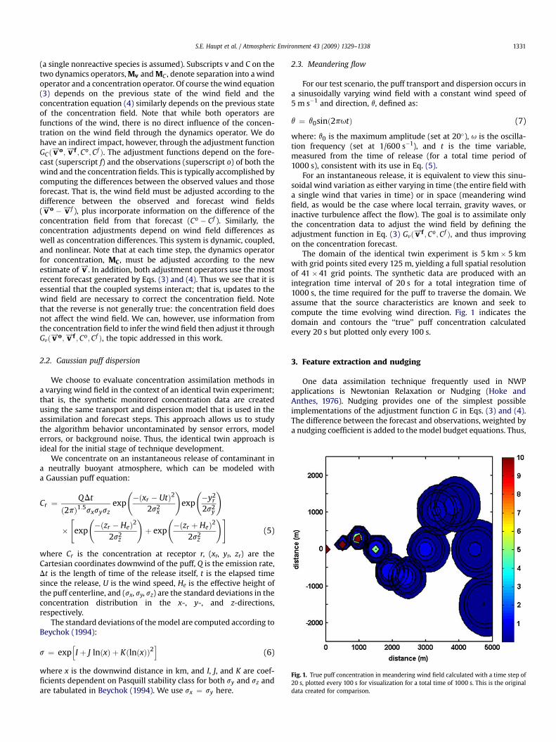
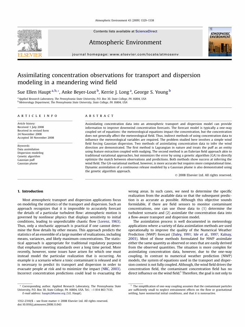
Fig. 1. True puff concentration in meandering wind field calculated with a time step of20 s, plotted every 100 s for visualization for a total time of 1000 s. This is the originaldata created for comparison.

S.E. Haupt et al. / Atmospheric Environment 43 (2009) 1329–1338 1331

(a single nonreactive species is assumed). Subscripts v and C on thetwo dynamics operators, Mv and MC , denote separation into a windoperator and a concentration operator. Of course the wind equation(3) depends on the previous state of the wind field and theconcentration equation (4) similarly depends on the previous stateof the concentration field. Note that while both operators arefunctions of the wind, there is no direct influence of the concen-tration on the wind field through the dynamics operator. We dohave an indirect impact, however, through the adjustment functionGCð v!o; v!f ;Co;Cf Þ. The adjustment functions depend on the fore-cast (superscript f) and the observations (superscript o) of both thewind and the concentration fields. This is typically accomplished bycomputing the differences between the observed values and thoseforecast. That is, the wind field must be adjusted according to thedifference between the observed and forecast wind fields( v!o � v!f ), plus incorporate information on the difference of theconcentration field from that forecast (Co � Cf ). Similarly, theconcentration adjustments depend on wind field differences aswell as concentration differences. This system is dynamic, coupled,and nonlinear. Note that at each time step, the dynamics operatorfor concentration, MC, must be adjusted according to the newestimate of v!. In addition, both adjustment operators use the mostrecent forecast generated by Eqs. (3) and (4). Thus we see that it isessential that the coupled systems interact; that is, updates to thewind field are necessary to correct the concentration field. Notethat the reverse is not generally true: the concentration field doesnot affect the wind field. We can, however, use information fromthe concentration field to infer the wind field then adjust it throughGvð v!o; v!f ;Co;Cf Þ, the topic addressed in this work.

2.2. Gaussian puff dispersion

We choose to evaluate concentration assimilation methods ina varying wind field in the context of an identical twin experiment;that is, the synthetic monitored concentration data are createdusing the same transport and dispersion model that is used in theassimilation and forecast steps. This approach allows us to studythe algorithm behavior uncontaminated by sensor errors, modelerrors, or background noise. Thus, the identical twin approach isideal for the initial stage of technique development.

We concentrate on an instantaneous release of contaminant ina neutrally buoyant atmosphere, which can be modeled witha Gaussian puff equation:

Cr ¼QDt

ð2pÞ1:5sxsyszexp

�ðxr � UtÞ2

2s2x

!exp

�y2

r

2s2y

!

�"

exp

�ðzr � HeÞ2

2s2z

!þ exp

�ðzr þ HeÞ2

2s2z

!#(5)

where Cr is the concentration at receptor r, (xr, yr, zr) are theCartesian coordinates downwind of the puff, Q is the emission rate,Dt is the length of time of the release itself, t is the elapsed timesince the release, U is the wind speed, He is the effective height ofthe puff centerline, and (sx, sy, sz) are the standard deviations in theconcentration distribution in the x-, y-, and z-directions,respectively.

The standard deviations of the model are computed according toBeychok (1994):

s ¼ exphI þ J lnðxÞ þ KðlnðxÞÞ2

i(6)

where x is the downwind distance in km, and I, J, and K are coef-ficients dependent on Pasquill stability class for both sy and sz andare tabulated in Beychok (1994). We use sx ¼ sy here.

2.3. Meandering flow

For our test scenario, the puff transport and dispersion occurs ina sinusoidally varying wind field with a constant wind speed of5 m s�1 and direction, q, defined as:

q ¼ q0sinð2putÞ (7)

where: q0 is the maximum amplitude (set at 20�), u is the oscilla-tion frequency (set at 1/600 s�1), and t is the time variable,measured from the time of release (for a total time period of1000 s), consistent with its use in Eq. (5).

For an instantaneous release, it is equivalent to view this sinu-soidal wind variation as either varying in time (the entire field witha single wind that varies in time) or in space (meandering windfield, as would be the case where local terrain, gravity waves, orinactive turbulence affect the flow). The goal is to assimilate onlythe concentration data to adjust the wind field by defining theadjustment function in Eq. (3) Gvð v!f ;Co;Cf Þ, and thus improvingon the concentration forecast.

The domain of the identical twin experiment is 5 km � 5 kmwith grid points sited every 125 m, yielding a full spatial resolutionof 41 � 41 grid points. The synthetic data are produced with anintegration time interval of 20 s for a total integration time of1000 s, the time required for the puff to traverse the domain. Weassume that the source characteristics are known and seek tocompute the time evolving wind direction. Fig. 1 indicates thedomain and contours the ‘‘true’’ puff concentration calculatedevery 20 s but plotted only every 100 s.

3. Feature extraction and nudging

One data assimilation technique frequently used in NWPapplications is Newtonian Relaxation or Nudging (Hoke andAnthes, 1976). Nudging provides one of the simplest possibleimplementations of the adjustment function G in Eqs. (3) and (4).The difference between the forecast and observations, weighted bya nudging coefficient is added to the model budget equations. Thus,

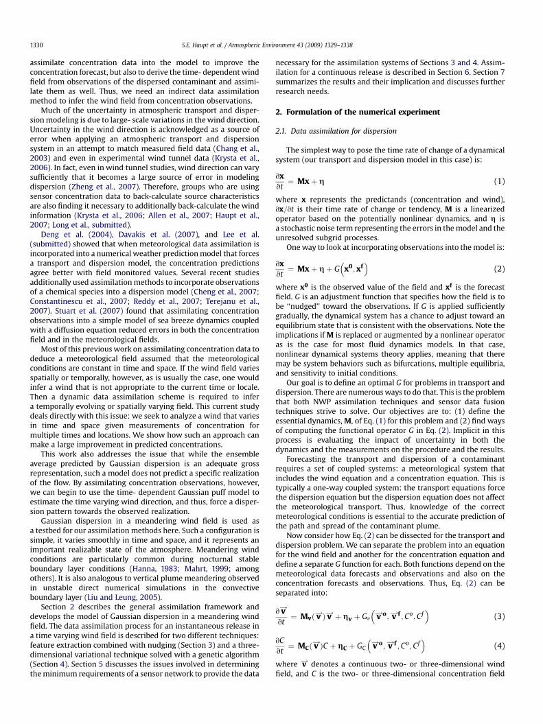
Fig. 2. FEWN sensitivity study: root mean squared error of the puff centroid locationfor multiple observational grids dependent on the nudging coefficient, Gnudge, usinga model time step of 20 s.

Fig. 3. Puff concentration predicted using feature extraction with nudging (FEWN)using a model time step of 20 s, plotted every 100 s.

S.E. Haupt et al. / Atmospheric Environment 43 (2009) 1329–13381332

observations are inserted directly into the model and the modelstate is slowly relaxed towards these observations.

Nudging is easily applied to those variables that are modeledexplicitly. It is a bit more difficult for our application, however,because concentration data is to be used to improve the wind field.Thus, we require a method to couple the concentration field back tothe wind field. Here this coupling is achieved by applying featureextraction to the concentration observations to infer errors in thewind field. As applied here, feature extraction assumes that theconcentration field can be represented by a single Gaussian puff.We must fit the location of the maximum concentration, themaximum concentration value, and the spread to the observedfield. The wind field error estimates are extracted by taking thedifference between the forecast and observed concentration field.The steepest gradient in this difference field provides a directionthat is used as the observation of the wind direction in the assim-ilation scheme. This feature extraction method is a crude, butnonetheless effective way to couple the concentration field to thewind field.

Combining Feature Extraction With Nudging (FEWN) providesa strategy that is both simple to implement and computationallyefficient. This single-puff analytic approach to feature extraction isnot applicable to every transport and dispersion situation.Numerical differencing and higher data densities would berequired for multi-puff or continuous field situations. However, fordemonstrating the approach with an identical twin experimentusing the Gaussian puff equation (5), the method is valid.

The wind forecast is nudged at each assimilation step by:

j v!jfs¼ j v!jfs�1 (8)

qfs ¼ qf

s�1 þ Gnudge

�qfs�1 � qo

�(9)

where the wind speed, j v!j, is assumed constant at every time steps. The forecast of the wind direction, qf

s , is based on the winddirection forecast of the previous time step, qf

s�1, and the adjust-ment functiond the weighted difference between the forecast,qfs�1, and the observation, qo, that is determined by feature

extraction. The relaxation timescale or nudging coefficient, Gnudge,which acts as a proportionality constant in the adjustment term, isalways positive and is chosen so that the nudging tendencies arerelatively small compared to the other terms in the prognosticequations (Stauffer and Seaman, 1993). In this study Gnudge is takento be fixed in space and time. A sensitivity study is conducted todetermine an appropriate value for the nudging coefficient. TheFEWN scheme is applied to the meandering puff scenario witha time step of 20 s and a variable grid of observation sensors(41 � 41, 21 � 21, 11 �11 and 5 � 5). Fig. 2 shows the dependence ofthe root mean squared error of the puff centroid location on thenudging coefficient Gnudge. It is evident that for all grid sizes studiedhere small values of Gnudge reduce the forecast errors significantly.Therefore, for the subsequent assimilation tests the nudging coef-ficient is fixed at a value of 0.1.

In the following test the FEWN method is applied to theconcentration puff model described in Section 2 using the samemodel time step (20 s) and the full observational grid (41 � 41). Puffconcentration predicted for the meandering puff using featureextraction with nudging is contoured every 100 s in Fig. 3. Fig. 4shows the true (solid black with Xs) and FEWN computed winddirection (dashed dot red) at each time step for the same assimi-lation setup. The wind diagnosed by feature extraction is relativelyclose to the truth and nudging keeps the wind direction in tandemwith the true wind direction. Fig. 5 shows the location of the puffcentroid plotted as a trajectory in time. Despite the minor

numerical oscillations about the truth, the puff centerline is trackedwell in the analysis. We conclude that the FEWN approach toassimilating concentration is successful, computationally fast, andshows promise in situations where we can define discrete featuresthat can be tracked.

4. Assimilation with a genetic algorithm

In the second assimilation method, we seek to directly optimizethe wind direction to produce a predicted concentration fieldclosest to that monitored. This method is most akin to the varia-tional approaches to assimilation (for example see Sasaki, 1970 orKalnay, 2003), but rather than using the variational formalism, itdirectly optimizes the match. We choose the continuous geneticalgorithm (GA) as our optimization tool. The GA is an artificialintelligence optimization method inspired by the biological

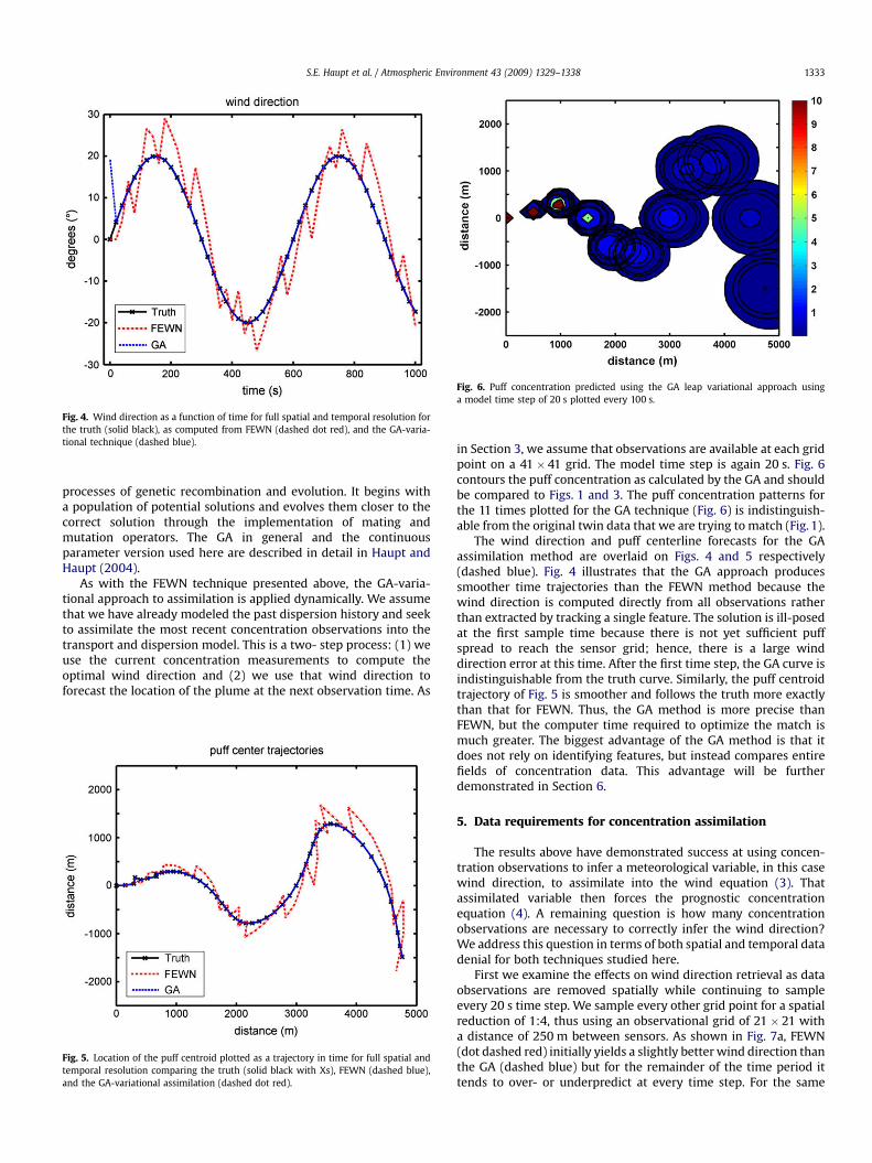
Fig. 4. Wind direction as a function of time for full spatial and temporal resolution forthe truth (solid black), as computed from FEWN (dashed dot red), and the GA-varia-tional technique (dashed blue).

Fig. 6. Puff concentration predicted using the GA leap variational approach usinga model time step of 20 s plotted every 100 s.

S.E. Haupt et al. / Atmospheric Environment 43 (2009) 1329–1338 1333

processes of genetic recombination and evolution. It begins witha population of potential solutions and evolves them closer to thecorrect solution through the implementation of mating andmutation operators. The GA in general and the continuousparameter version used here are described in detail in Haupt andHaupt (2004).

As with the FEWN technique presented above, the GA-varia-tional approach to assimilation is applied dynamically. We assumethat we have already modeled the past dispersion history and seekto assimilate the most recent concentration observations into thetransport and dispersion model. This is a two- step process: (1) weuse the current concentration measurements to compute theoptimal wind direction and (2) we use that wind direction toforecast the location of the plume at the next observation time. As

Fig. 5. Location of the puff centroid plotted as a trajectory in time for full spatial andtemporal resolution comparing the truth (solid black with Xs), FEWN (dashed blue),and the GA-variational assimilation (dashed dot red).

in Section 3, we assume that observations are available at each gridpoint on a 41 � 41 grid. The model time step is again 20 s. Fig. 6contours the puff concentration as calculated by the GA and shouldbe compared to Figs. 1 and 3. The puff concentration patterns forthe 11 times plotted for the GA technique (Fig. 6) is indistinguish-able from the original twin data that we are trying to match (Fig. 1).

The wind direction and puff centerline forecasts for the GAassimilation method are overlaid on Figs. 4 and 5 respectively(dashed blue). Fig. 4 illustrates that the GA approach producessmoother time trajectories than the FEWN method because thewind direction is computed directly from all observations ratherthan extracted by tracking a single feature. The solution is ill-posedat the first sample time because there is not yet sufficient puffspread to reach the sensor grid; hence, there is a large winddirection error at this time. After the first time step, the GA curve isindistinguishable from the truth curve. Similarly, the puff centroidtrajectory of Fig. 5 is smoother and follows the truth more exactlythan that for FEWN. Thus, the GA method is more precise thanFEWN, but the computer time required to optimize the match ismuch greater. The biggest advantage of the GA method is that itdoes not rely on identifying features, but instead compares entirefields of concentration data. This advantage will be furtherdemonstrated in Section 6.

5. Data requirements for concentration assimilation

The results above have demonstrated success at using concen-tration observations to infer a meteorological variable, in this casewind direction, to assimilate into the wind equation (3). Thatassimilated variable then forces the prognostic concentrationequation (4). A remaining question is how many concentrationobservations are necessary to correctly infer the wind direction?We address this question in terms of both spatial and temporal datadenial for both techniques studied here.

First we examine the effects on wind direction retrieval as dataobservations are removed spatially while continuing to sampleevery 20 s time step. We sample every other grid point for a spatialreduction of 1:4, thus using an observational grid of 21 � 21 witha distance of 250 m between sensors. As shown in Fig. 7a, FEWN(dot dashed red) initially yields a slightly better wind direction thanthe GA (dashed blue) but for the remainder of the time period ittends to over- or underpredict at every time step. For the same

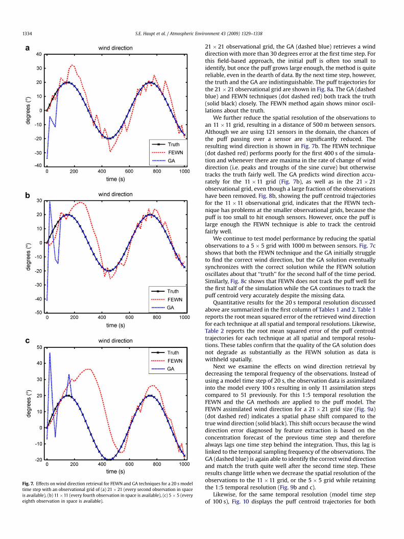
Fig. 7. Effects on wind direction retrieval for FEWN and GA techniques for a 20 s modeltime step with an observational grid of (a) 21 � 21 (every second observation in spaceis available), (b) 11 �11 (every fourth observation in space is available), (c) 5 � 5 (everyeighth observation in space is available).

S.E. Haupt et al. / Atmospheric Environment 43 (2009) 1329–13381334

21 � 21 observational grid, the GA (dashed blue) retrieves a winddirection with more than 30 degrees error at the first time step. Forthis field-based approach, the initial puff is often too small toidentify, but once the puff grows large enough, the method is quitereliable, even in the dearth of data. By the next time step, however,the truth and the GA are indistinguishable. The puff trajectories forthe 21 � 21 observational grid are shown in Fig. 8a. The GA (dashedblue) and FEWN techniques (dot dashed red) both track the truth(solid black) closely. The FEWN method again shows minor oscil-lations about the truth.

We further reduce the spatial resolution of the observations toan 11 �11 grid, resulting in a distance of 500 m between sensors.Although we are using 121 sensors in the domain, the chances ofthe puff passing over a sensor are significantly reduced. Theresulting wind direction is shown in Fig. 7b. The FEWN technique(dot dashed red) performs poorly for the first 400 s of the simula-tion and whenever there are maxima in the rate of change of winddirection (i.e. peaks and troughs of the sine curve) but otherwisetracks the truth fairly well. The GA predicts wind direction accu-rately for the 11 �11 grid (Fig. 7b), as well as in the 21 � 21observational grid, even though a large fraction of the observationshave been removed. Fig. 8b, showing the puff centroid trajectoriesfor the 11 �11 observational grid, indicates that the FEWN tech-nique has problems at the smaller observational grids, because thepuff is too small to hit enough sensors. However, once the puff islarge enough the FEWN technique is able to track the centroidfairly well.

We continue to test model performance by reducing the spatialobservations to a 5 � 5 grid with 1000 m between sensors. Fig. 7cshows that both the FEWN technique and the GA initially struggleto find the correct wind direction, but the GA solution eventuallysynchronizes with the correct solution while the FEWN solutionoscillates about that ‘‘truth’’ for the second half of the time period.Similarly, Fig. 8c shows that FEWN does not track the puff well forthe first half of the simulation while the GA continues to track thepuff centroid very accurately despite the missing data.

Quantitative results for the 20 s temporal resolution discussedabove are summarized in the first column of Tables 1 and 2. Table 1reports the root mean squared error of the retrieved wind directionfor each technique at all spatial and temporal resolutions. Likewise,Table 2 reports the root mean squared error of the puff centroidtrajectories for each technique at all spatial and temporal resolu-tions. These tables confirm that the quality of the GA solution doesnot degrade as substantially as the FEWN solution as data iswithheld spatially.

Next we examine the effects on wind direction retrieval bydecreasing the temporal frequency of the observations. Instead ofusing a model time step of 20 s, the observation data is assimilatedinto the model every 100 s resulting in only 11 assimilation stepscompared to 51 previously. For this 1:5 temporal resolution theFEWN and the GA methods are applied to the puff model. TheFEWN assimilated wind direction for a 21 � 21 grid size (Fig. 9a)(dot dashed red) indicates a spatial phase shift compared to thetrue wind direction (solid black). This shift occurs because the winddirection error diagnosed by feature extraction is based on theconcentration forecast of the previous time step and thereforealways lags one time step behind the integration. Thus, this lag islinked to the temporal sampling frequency of the observations. TheGA (dashed blue) is again able to identify the correct wind directionand match the truth quite well after the second time step. Theseresults change little when we decrease the spatial resolution of theobservations to the 11 �11 grid, or the 5 � 5 grid while retainingthe 1:5 temporal resolution (Fig. 9b and c).

Likewise, for the same temporal resolution (model time stepof 100 s), Fig. 10 displays the puff centroid trajectories for both

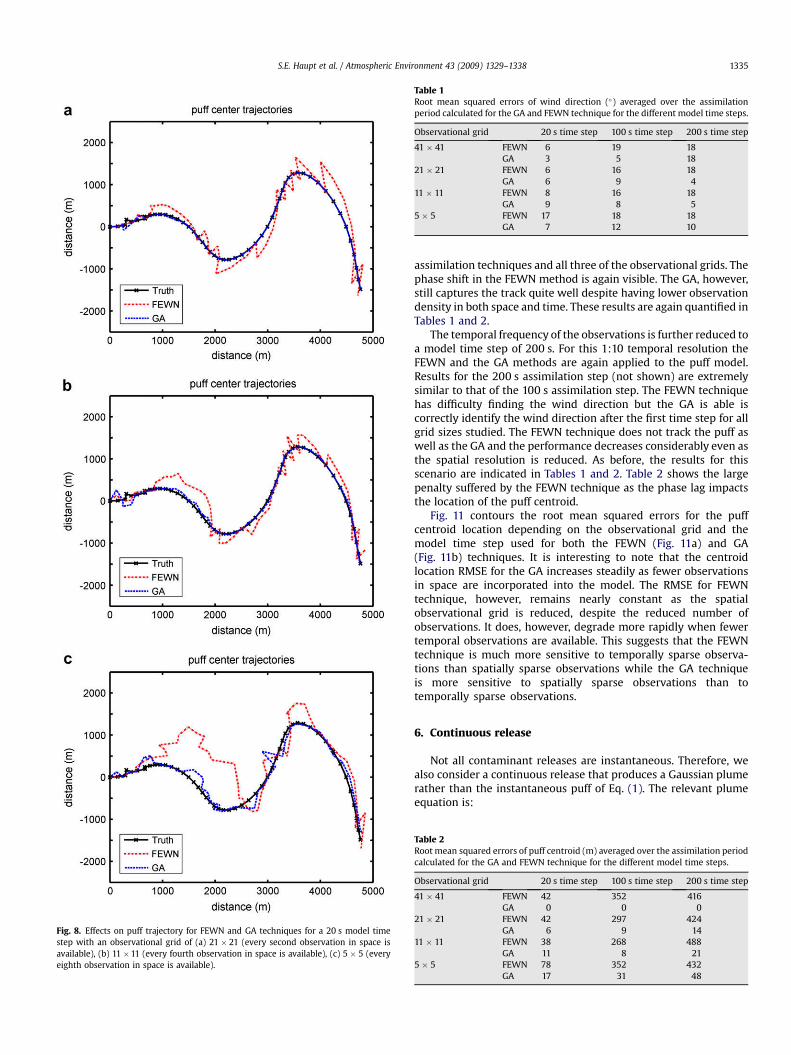
Table 1Root mean squared errors of wind direction (�) averaged over the assimilationperiod calculated for the GA and FEWN technique for the different model time steps.

Observational grid 20 s time step 100 s time step 200 s time step

41 � 41 FEWN 6 19 18GA 3 5 18

21 � 21 FEWN 6 16 18GA 6 9 4

11 � 11 FEWN 8 16 18GA 9 8 5

5 � 5 FEWN 17 18 18GA 7 12 10

Fig. 8. Effects on puff trajectory for FEWN and GA techniques for a 20 s model timestep with an observational grid of (a) 21 � 21 (every second observation in space isavailable), (b) 11 �11 (every fourth observation in space is available), (c) 5 � 5 (everyeighth observation in space is available).

S.E. Haupt et al. / Atmospheric Environment 43 (2009) 1329–1338 1335

assimilation techniques and all three of the observational grids. Thephase shift in the FEWN method is again visible. The GA, however,still captures the track quite well despite having lower observationdensity in both space and time. These results are again quantified inTables 1 and 2.

The temporal frequency of the observations is further reduced toa model time step of 200 s. For this 1:10 temporal resolution theFEWN and the GA methods are again applied to the puff model.Results for the 200 s assimilation step (not shown) are extremelysimilar to that of the 100 s assimilation step. The FEWN techniquehas difficulty finding the wind direction but the GA is able iscorrectly identify the wind direction after the first time step for allgrid sizes studied. The FEWN technique does not track the puff aswell as the GA and the performance decreases considerably even asthe spatial resolution is reduced. As before, the results for thisscenario are indicated in Tables 1 and 2. Table 2 shows the largepenalty suffered by the FEWN technique as the phase lag impactsthe location of the puff centroid.

Fig. 11 contours the root mean squared errors for the puffcentroid location depending on the observational grid and themodel time step used for both the FEWN (Fig. 11a) and GA(Fig. 11b) techniques. It is interesting to note that the centroidlocation RMSE for the GA increases steadily as fewer observationsin space are incorporated into the model. The RMSE for FEWNtechnique, however, remains nearly constant as the spatialobservational grid is reduced, despite the reduced number ofobservations. It does, however, degrade more rapidly when fewertemporal observations are available. This suggests that the FEWNtechnique is much more sensitive to temporally sparse observa-tions than spatially sparse observations while the GA techniqueis more sensitive to spatially sparse observations than totemporally sparse observations.

6. Continuous release

Not all contaminant releases are instantaneous. Therefore, wealso consider a continuous release that produces a Gaussian plumerather than the instantaneous puff of Eq. (1). The relevant plumeequation is:

Table 2Root mean squared errors of puff centroid (m) averaged over the assimilation periodcalculated for the GA and FEWN technique for the different model time steps.

Observational grid 20 s time step 100 s time step 200 s time step

41 � 41 FEWN 42 352 416GA 0 0 0

21 � 21 FEWN 42 297 424GA 6 9 14

11 � 11 FEWN 38 268 488GA 11 8 21

5 � 5 FEWN 78 352 432GA 17 31 48

Fig. 10. Effects on puff trajectory for FEWN and GA techniques for a 100 s model timestep with an observational grid of (a) 21 � 21 (every second observation in space isavailable), (b) 11 �11 (every fourth observation in space is available), (c) 5 � 5 (everyeighth observation in space is available).

Fig. 9. Effects on wind direction retrieval for FEWN and GA techniques for a 100 smodel time step with an observational grid of (a) 21 � 21 (every second observation inspace is available), (b) 11 �11 (every fourth observation in space is available), (c) 5 � 5(every eighth observation in space is available).

S.E. Haupt et al. / Atmospheric Environment 43 (2009) 1329–13381336

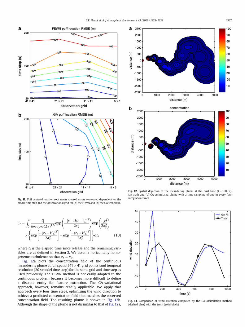
Fig. 11. Puff centroid location root mean squared errors contoured dependent on themodel time step and the observational grid for (a) the FEWN and (b) the GA technique.

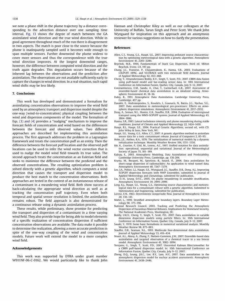
Fig. 12. Spatial depiction of the meandering plume at the final time (t ¼ 1000 s).(a) truth and (b) GA assimilated plume with a time sampling of one in every fourintegration times.

Fig. 13. Comparison of wind direction computed by the GA assimilation method(dashed blue) with the truth (solid black).

S.E. Haupt et al. / Atmospheric Environment 43 (2009) 1329–1338 1337

Cr ¼Z t

0

Q

usxsyszð2pÞ1:5exp

�½x�Uðt� tsÞ�2

2s2x

!exp

�y2

r

2s2y

!

�(

exp

"�ðzr�HeÞ2

2s2z

#þexp

"�ðzrþHeÞ2

2s2z

#)dts (10)

where ts is the elapsed time since release and the remaining vari-ables are as defined in Section 2. We assume horizontally homo-geneous turbulence so that sx ¼ sy.

Fig. 12a plots the concentration field of the continuousmeandering plume at full spatial (41 � 41 grid points) and temporalresolution (20 s model time step) for the same grid and time step asused previously. The FEWN method is not easily adapted to thecontinuous problem because it becomes more difficult to definea discrete entity for feature extraction. The GA-variationalapproach, however, remains readily applicable. We apply thatapproach every four time steps, optimizing the wind direction toachieve a predicted concentration field that matches the observedconcentration field. The resulting plume is shown in Fig. 12b.Although the shape of the plume is not dissimilar to that of Fig. 12a,

S.E. Haupt et al. / Atmospheric Environment 43 (2009) 1329–13381338

we note a phase shift in the plume trajectory by a distance corre-sponding to the advection distance over one sampling timeinterval. Fig. 13 shows the degree of match between the GAassimilated wind direction and the true wind direction. While ingood agreement throughout much of the run there is disagreementin two aspects. The match is poor close to the source because theplume is inadequately sampled until it becomes wide enough tospan multiple sensors. Further downwind the plume widens tocover more sensors and thus the correspondence with the truewind direction improves. At the longest downwind ranges,however, the difference between computed wind direction and thetruth again degrades. This degradation occurs because of theinherent lag between the observations and the prediction afterassimilation. The observations are not available sufficiently early tocapture the changes in wind direction. In a real situation, such rapidwind shifts may be less likely.

7. Conclusions

This work has developed and demonstrated a formalism forassimilating concentration observations to improve the wind fieldused by an atmospheric transport and dispersion model despite theone-way (wind-to-concentration) physical coupling between thewind and dispersion components of the model. The formalism ofEqs. (3) and (4) provides a ‘‘nudging’’ mechanism to improve theforecast fields of concentration and wind based on the differencesbetween the forecast and observed values. Two differentapproaches are described for implementing this assimilationprocess. The first approach addresses the problem in a Lagrangianframework and treats the concentration puff as an entity. Then thedifference between the forecast puff location and the observed pufflocations can be used to infer the wind vector correction that isused to nudge the model wind field towards its true value. Thesecond approach treats the concentration as an Eulerian field andseeks to minimize the difference between the predicted and theobserved concentrations. The resulting optimization problem issolved directly with a genetic algorithm, which computes a winddirection that causes the transport and dispersion model toproduce the best match to the concentration observations. Bothapproaches are tested in the context of an instantaneous release ofa contaminant in a meandering wind field. Both show success atback-calculating the appropriate wind direction as well as attracking the concentration puff trajectory. Even when bothtemporal and spatial sensor resolution is limited, the assimilationremains robust. The field approach is also demonstrated fora continuous release using a dynamic assimilation process.

These results, while preliminary, show promise for predictingthe transport and dispersion of a contaminant in a time varyingwind field. They also provide hope for being able to model elementsof a specific realization of concentration dispersion if sufficientconcentration observations are available. The data make it possibleto determine the realization, allowing a more accurate prediction inspite of the one-way coupling of the wind and concentrationmodels. Future work will extend the model to a more complexwind field.

Acknowledgements

This work was supported by DTRA under grant numberW911NF-06-C-0162. We would particularly like to thank John

Hannan and Christopher Kiley as well as our colleagues at theUniversity of Buffalo, Tarun Singh and Peter Scott. We thank JohnWyngaard for inspiration on this approach and an anonymousreviewer for various suggestions on how to clarify the presentation.

References

Allen, C.T., Young, G.S., Haupt, S.E., 2007. Improving pollutant source characteriza-tion by optimizing meteorological data with a genetic algorithm. AtmosphericEnvironment 41, 2283–2289.

Beychok, M.R., 1994. Fundamentals of Stack Gas Dispersion, third ed. MiltonBeychok, Irvine, CA, 193 pp.

Chang, J.C., Franzese, P., Chayantrakom, K., Hanna, S.R., 2003. Evaluations ofCALPUFF, HPAC, and VLSTRACK with two mesoscale field datasets. Journalof Applied Meteorology 42, 453–466.

Cheng, Y., Umanaheswara Reddy, K.V., Singh, T., Scott, P.D., 2007. CBRN data fusionusing puff-based model and bar-reading sensor data. In: 10th InternationalConference on Information Fusion, Quebec City, Canada, July 9–12, 2007.

Constantinescu, E.M., Sandu, A., Chai, T., Carmichael, G.R., 2007. Assessment ofensemble-based chemical data assimilation in an idealized setting. Atmo-spheric Environment 41, 18–36.

Daley, R., 1991. Atmospheric Data Assimilation. Cambridge University Press,Cambridge, 457 pp.

Davakis, E., Andronopoulos, S., Kovalets, I., Gounaris, N., Batzis, J.G., Nychas, S.G.,2007. Data assimilation in meteorological pre-processors: Effects on atmo-spheric dispersion simulations. Atmospheric Environment 41, 2917–2932.

Deng, A., Seman, N.L., Hunter, G.K., Stauffer, D.R., 2004. Evaluation of interregionaltransport using the MM5-SCIPUFF system. Journal of Applied Meteorology 43,1864–1886.

Hanna, S.R., 1983. Lateral turbulence intensity and plume meandering during stableconditions. Journal of Climate and Applied Meteorology 22, 1424–1430.

Haupt, R.L., Haupt, S.E., 2004. Practical Genetic Algorithms, second ed., with CD.John Wiley & Sons, New York, NY.

Haupt, S.E., Young, G.S., Allen, C.T., 2007. A genetic algorithm method to assimilatesensor data for a toxic contaminant release. Journal of Computers 2, 85–93.

Hoke, J.E., Anthes, R.A., 1976. The initialization of numerical models by a dynamicinitialization technique. Monthly Weather Review 104, 1551–1556.

Ide, K., Courtier, P., Ghil, M., Lorenc, A.C., 1997. Unified notation for data assimila-tion: operational, sequential and variational. Journal of the MeteorologicalSociety of Japan 75, 181–189.

Kalnay, E., 2003. Atmospheric Modeling, Data Assimilation and Predictability.Cambridge University Press, Cambridge, pp. 136-204.

Krysta, M., Bocquet, M., Sportisse, B., Isnard, O., 2006. Data assimilation forshort-range dispersion of radionuclides: An application to wind tunnel data.Atmospheric Environment 40, 7267–7279.

Lee, J.A., Peltier, L.J., Haupt, S.E., Wyngaard, J.C., Stauffer, D.R., Deng, A.J., ImprovingSCIPUFF dispersion forecasts with NWP Ensembles. submitted to Journal ofApplied Meteorology and Climatology. submitted for publication.

Liu, D.-H., Leung, D.Y.C., 2005. On plume meandering in unstable stratification.Atmospheric Environment 39, 2995–2999.

Long, K.J., Haupt, S.E., Young, G.S., Optimizing source characteristics and meteoro-logical data for a contaminant release with a genetic algorithm. Submitted toOptimization and Engineering. submitted for publication.

Lorenz, E.N., 1963. Deterministic nonperiodic flow. Journal of Atmospheric Science20, 130–141.

Mahrt, L., 1999. Stratified atmospheric boundary layers. Boundary Layer Meteo-rology 90, 375–396.

National Research Council, 2003. Tracking and Predicting the AtmosphericDispersion of Hazardous Material Releases. Implications for Homeland Security.The National Academies Press, Washington, DC.

Reddy, U.K.V., Cheng, Y., Singh, T., Scott, P.D., 2007. Data assimilation in variabledimension dispersion models using particle filters. In: 10th InternationalConference on Information Fusion, Quebec City, Canada, July 9–12, 2007.

Sasaki, Y., 1970. Some basic formalisms in numerical variational analysis. MonthlyWeather Review 98, 875–883.

Stauffer, D.R., Seaman, N.L., 1993. Multiscale four-dimensional data assimilation.Journal of Applied Meteorology 33, 416–434.

Stuart, A.L., Aksoy, A., Zhang, F., Nielsen-Gammon, J.W., 2007. Ensemble-based dataassimilation and targeted observation of a chemical tracer in a sea breezemodel. Atmospheric Environment 41, 3082–3094.

Terejanu, G., Singh, T., Scott, P.D., 2007. Unscented Kalman filter/smoother fora CBRN puff-based dispersion model. In: 10th International Conference onInformation Fusion, Quebec City, Canada, July 9–12, 2007.

Zheng, D.Q., Leung, J.K.C., Lee, B.Y., Lam, H.Y., 2007. Data assimilation in theatmospheric dispersion model for nuclear accident assessments. AtmosphericEnvironment 41, 2438–2446.